SABRE: a Sensitive Attribute Bucketization and REdistribution framework for t-closeness

Authors: Jianneng Cao, Panagiotis Karras, Panos Kalnis, Kian-Lee TanPublished in VLDB Journal 02/2011Presented by Hongwei Tian

2

Outline

• Privacy measure: t-closeness• Earth Movers’ Distance (EMD)• SABRE Algorithm– Bucketization– REdistribution

• Experiments

3

t-closeness

The published table still suffers other types of privacy attacks

4

t-closeness

• skewness attack– SA Particular Virus, overall SA distribution 99% negative

and 1% positive, SA distribution in one EC 50% negative and 50% positive

• similarity attack– SA values in one EC are distinct butsemantically similar

5

t-closeness

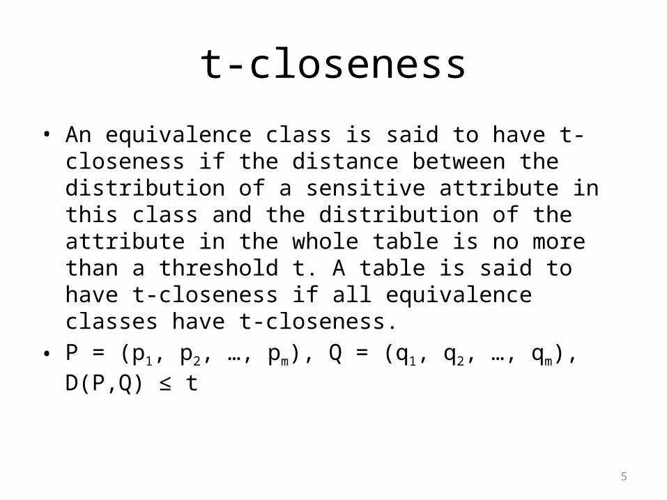
• An equivalence class is said to have t-closeness if the distance between the distribution of a sensitive attribute in this class and the distribution of the attribute in the whole table is no more than a threshold t. A table is said to have t-closeness if all equivalence classes have t-closeness.

• P = (p1, p2, …, pm), Q = (q1, q2, …, qm), D(P,Q) ≤ t

6

Earth Movers’ Distance (EMD)

• Intuitively, it views one distribution as a mass of earth piles spread over a space, and the other as a collection of holes, in which the mass fits, over the same space.

• The EMD between the two is defined as the minimum work needed to fill the holes with earth, thereby transforming one distribution to the other.

• P = (p1, p2, …, pm): distribution of “holes”

Q = (q1, q2, …, qm): distribution of “earth”

dij: ground distance of qi from pj

F=[fij], fij≥0: a flow of mass of earth moved from elements qi to pj

Minimize

7

Earth Movers’ Distance (EMD)

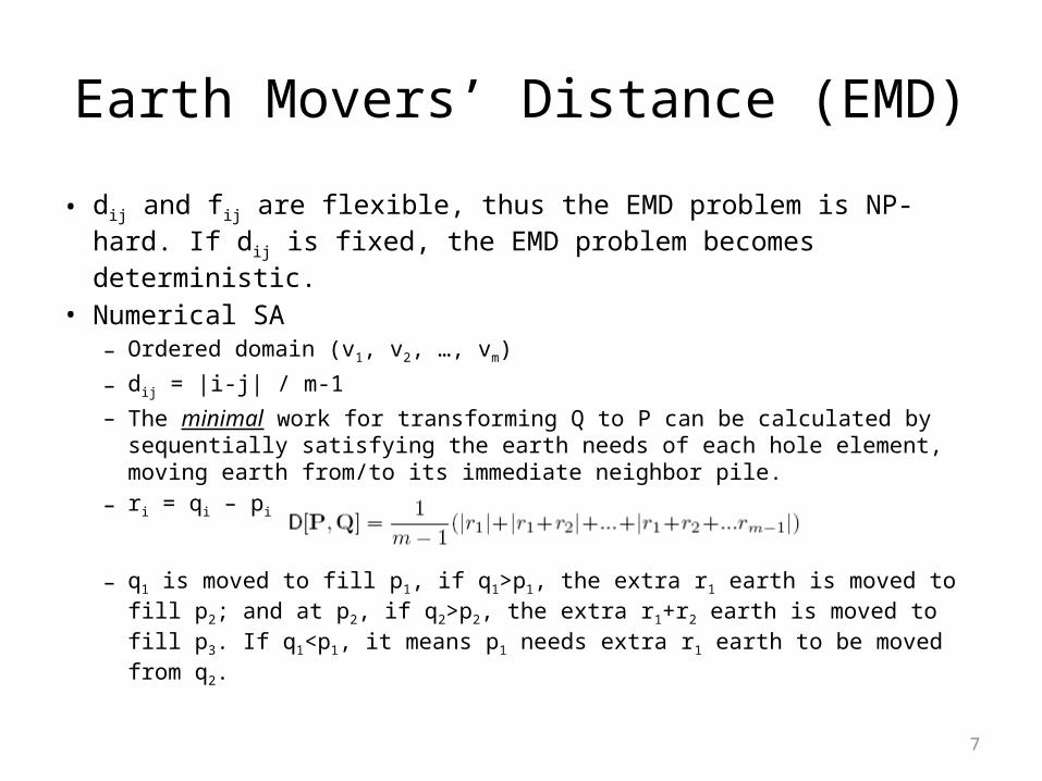
• dij and fij are flexible, thus the EMD problem is NP-hard. If dij is fixed, the EMD problem becomes deterministic.

• Numerical SA– Ordered domain (v1, v2, …, vm)

– dij = |i-j| / m-1– The minimal work for transforming Q to P can be calculated by sequentially

satisfying the earth needs of each hole element, moving earth from/to its immediate neighbor pile.

– ri = qi – pi

– q1 is moved to fill p1, if q1>p1, the extra r1 earth is moved to fill p2; and at p2, if q2>p2, the extra r1+r2 earth is moved to fill p3. If q1<p1, it means p1 needs extra r1 earth to be moved from q2.

8

Earth Movers’ Distance (EMD)

• Categorical SA– Generalization hierarchy H– dij = h(vi,vj)/h(H)

– h(vi,vj): height of least common ancestor of vi and vj

– The minimal work for transforming Q to P can be calculated by moving extra earth, as much as possible, from/to its sibling pile under least common ancestor in H.

– Extra earth to move out/in– For an internal node n

9

Earth Movers’ Distance (EMD)

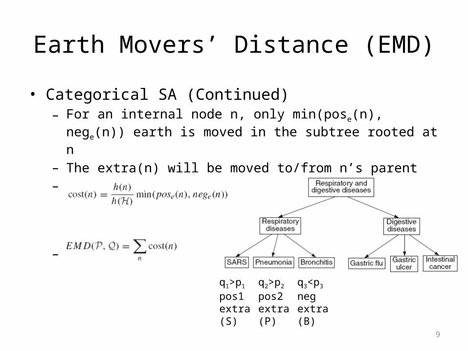
• Categorical SA (Continued)– For an internal node n, only min(pose(n), nege(n)) earth is moved in the

subtree rooted at n– The extra(n) will be moved to/from n’s parent– The cost of node n

– The total EMD

q1>p1

pos1 extra(S)

q2>p2

pos2 extra(P)

q3<p3

neg extra(B)

10

SABRE Algorithm

• SABRE consists of two phases:– Bucketization: partitions DB into a set of buckets,

such that each SA value appears in only one bucket

– Redistribution: reallocates tuples from buckets to ECs

11

SABRE - Bucketization

• Proportionality requirement– Given a table DB and a bucket partition ϕ, assume that an EC, G, is

formed with xi tuples from bucket Bi ϕ, i = 1, 2, …, |ϕ|.∈

– G satisfies the proportionality requirement with respect to ϕ, if and only if the sizes of xi are proportional to those of Bi , i.e., |x1| : |x2| : ··· : |x|ϕ|| = |B1| : |B2| : ··· : |B|ϕ||

– One bucket partition ϕ’=(B1,B2,…,Bm), each bucket Bi only contains tuples that have SA value vi. Select xi tuples from bucket Bi, to form an EC G following the proportionality requirement, then |x1| : |x2| : ··· : |xm| = |B1| : |B2| : ··· : |Bm| = N1 : N2 : ··· : Nm, thus G’s SA distribution is same as DB’s SA distribution, that is 0-closeness.

– A complete enforcement of 0-closeness for all ECs would severely degrade information quality.

12

SABRE - Bucketization

• Consider Buckets of more than one distinct SA value

– Less buckets– When pick xi tuples from a bucket Bi to EC following proportionality

requirement, SA values are not discriminated– And, it is usually not obeyed that |z1| : |z2| : ··· : |zm|= N1 : N2 : ··· : Nm

– Thus, this is not 0-closeness anymore, we need to consider EMD.

13

SABRE - Bucketization

• The questions– How should we partition SA values into buckets?– How many buckets should we generate to ensure

t-closeness?

14

SABRE - Bucketization

• Basic idea– SABRE partitions DB hierarchically, based on the SA values of its

tuples, forming a bucketization tree.– Each node of this tree denotes a bucket containing tuples having a

certain subset of SA values. (For categorical SA, the subset follows the SA domain hierarchy; For numerical SA, the subset is determined by the selected split)

– The leaf nodes of the tree are the buckets that correspond to the actual bucket partition of DB.

15

SABRE - Bucketization

• Basic idea (Continued)– The tree starts with a single node, the root, which corresponds to the

entire table with the whole domain of SA– Then the tree grows in a top-down manner by recursively splitting leaf

nodes.

16

SABRE - Bucketization

• Basic idea (Continued)– A node is not always valid to be split.

• Suppose we split a node to get new nodes/buckets. • Consider the new buckets (and all other leaves), if we form an EC

G to pick tuples from these buckets following proportionality requirement, the EC’s SA distribution Q = (q1, q2, …, qm).

• For one bucket B with distribution (p1, p2, …, pj), we need to transform (q1, q2, …, qj) to (p1, p2, …, pj), and the cost is CET(B,G).

• For other buckets with distribution like (pj+1, pj+2, …, pm), repeat the transformations.

• Then the Q=(q1, q2, …, qm) is transformed to P = (p1, p2, …, pm), and the total cost is ∑CET(B,G) for all B.

17

SABRE - Bucketization

• Basic idea (Continued)– A node is not always valid to be split.

• But, EC’s distribution is not known when splitting. Fortunately, we can describe the worst case (CET(B,G) maximized) for EC’s distribution. That is , Upper-bound cost in a bucket,

• If ≤ t, any EC selecting tuples from buckets following proportionality requirement satisfies t-closeness.

18

SABRE - Bucketization

• Basic idea (Continued)– In each iteration, we determine U as the summation of all upper

bounded cost. – In this way, we select the node that contributes to the largest

reduction of U as the node to be further split. – This process terminates when U becomes smaller than the closeness

threshold t.

19

SABRE - Redistribution

• The questions– How many ECs should we generate? • We need a plan to find number of ECs and size of each

EC.

– How should we choose tuples from each bucket to form an EC?

20

SABRE - Redistribution

• Basic idea– Consider the process of dynamically determining the size of an EC, or

deciding how many tuples to take out from each bucket to form an EC.– First, we consider all tuples of DB (i.e., all the buckets in ϕ) as a single

EC, r.– Then we split r into two ECs by dichotomizing Bi into Bi1 and Bi2, Bi1 and

Bi2 have approximately the same size.

– The left child c1 of r is composed of Bi1, and the right child c2 of r is composed of Bi2

21

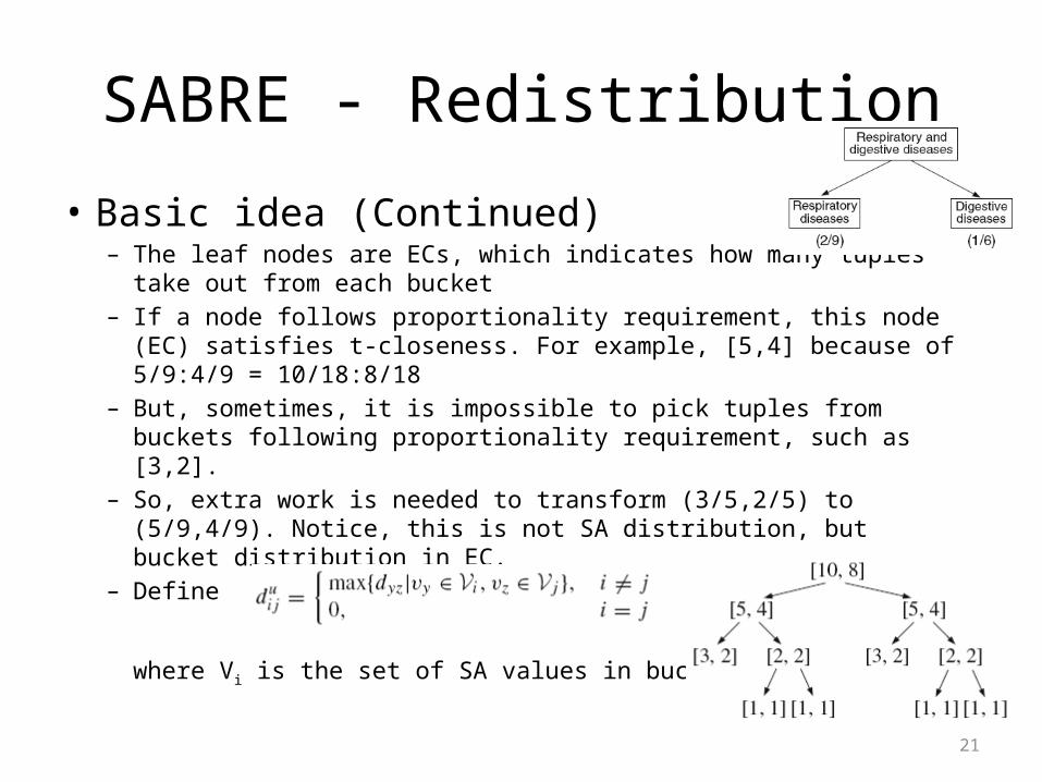
SABRE - Redistribution

• Basic idea (Continued)– The leaf nodes are ECs, which indicates how many tuples take out

from each bucket– If a node follows proportionality requirement, this node (EC) satisfies

t-closeness. For example, [5,4] because of 5/9:4/9 = 10/18:8/18– But, sometimes, it is impossible to pick tuples from buckets following

proportionality requirement, such as [3,2]. – So, extra work is needed to transform (3/5,2/5) to (5/9,4/9). Notice,

this is not SA distribution, but bucket distribution in EC.– Define

where Vi is the set of SA values in bucket Bi

22

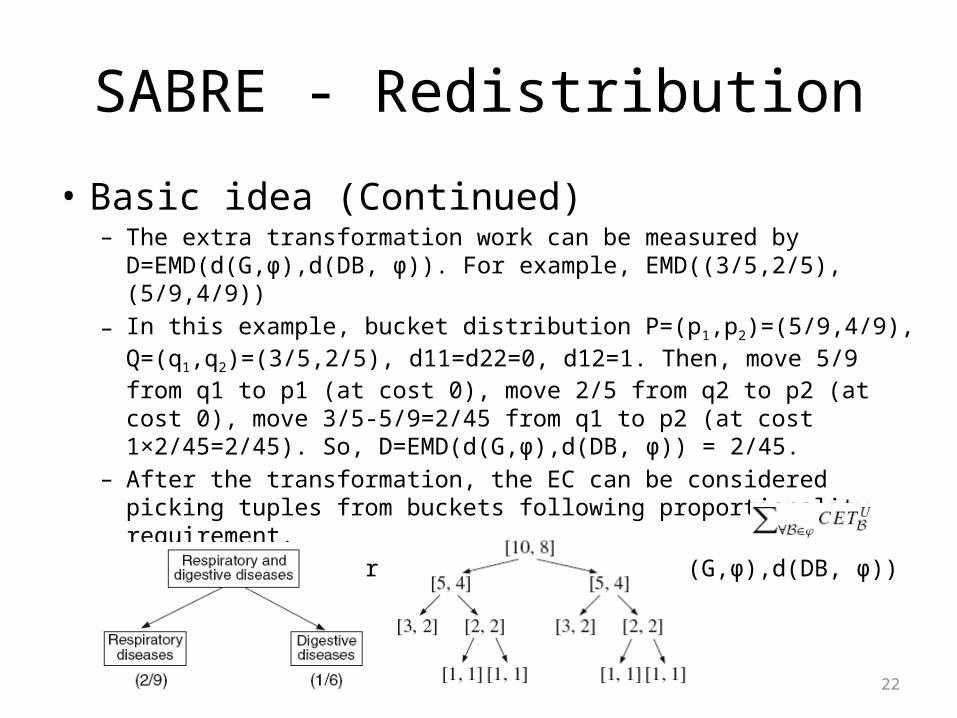
SABRE - Redistribution

• Basic idea (Continued)– The extra transformation work can be measured by D=EMD(d(G,φ),d(DB,

φ)). For example, EMD((3/5,2/5), (5/9,4/9))– In this example, bucket distribution P=(p1,p2)=(5/9,4/9),

Q=(q1,q2)=(3/5,2/5), d11=d22=0, d12=1. Then, move 5/9 from q1 to p1 (at cost 0), move 2/5 from q2 to p2 (at cost 0), move 3/5-5/9=2/45 from q1 to p2 (at cost 1×2/45=2/45). So, D=EMD(d(G,φ),d(DB, φ)) = 2/45.

– After the transformation, the EC can be considered picking tuples from buckets following proportionality requirement.

– The total cost for this EC is D+U= EMD(d(G,φ),d(DB, φ)) +

23

SABRE - Redistribution

• Basic idea (Continued)– A split is allowed only if both EMD(d(c1,φ),d(DB, φ)) + U ≤ t and

EMD(d(c2,φ),d(DB, φ)) + U ≤ t – The algorithm executes in a recursive way and terminates when no more

node can be split.– Finally, we get leaf nodes representing the size of possible ECs.

24

SABRE-TakeOut

• For each EC, pick real tuples from buckets according the ECs’ sizes [a1, a2, …, a| φ |].

• Consider the QI information quality– Select a random tuple x from a randomly selected bucket B– SABRE-KNN

• In each bucket Bi, find nearest ai neighbors of x and add them into G.

– SABRE-AK • Map multidimensional QI space to one-dimensional Hilbert values.

Each tuple has a Hilbert value.• Sort all tuples in each bucket in ascending order of their Hilbert

values• find x’s ai nearest neighbors in bucket Bi.

25

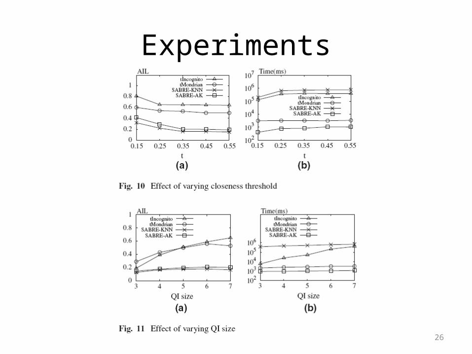
Experiments

• Compare SABRE-KNN, SABRE-AK with– tIncognito

• Sigmod 2005

– tMondrian• ICDE 2006

• CENSUS dataset containing 500,000 tuples and 8 attributes.

26

Experiments

27

Experiments

28

• Questions?

Thank you.