Near infrared analysis of sugarcane (Saccharum spp hybrid)

bud scales to predict resistance to

eldana stalk borer (Eldana saccharina Walker)

N.A. Coetzee BSc(Agric)

Submitted in partial fulfillment of the

requirements of the degree of

Masters of Science in Agriculture

Discipline of Genetics

Faculty of Science and Agriculture

University of Natal

Pietermaritzburg

December 2003

11

DECLARAnON

These studies represent original work by the author, which have not been submitted in any

form for any degree or diploma to any University. Where use was made of the work of

others it is duly acknowledged in the text.

NA Coetzee

I, the undersigned, confirm that I supervised the candidate, N Coetzee, in the reading of

this thesis.

P Shanahan

111

ABSTRACT

The eldana stalk borer (Eldana saccharina Walker) is the most serious pest of the Southern

African sugarcane industry, and it is imperative that effective control measures are

available to minimize economic damage. Because conventional control methods have had

limited success, cultivar resistance is seen as the most viable method of controlling

infestation. However, due to the space- and time-consuming nature of the present screening

methods, only small numbers of cultivars can be tested relatively late in the Plant Breeding

selection programme. Increased resistance in breeding and selection populations is

therefore slow.

Buds are a preferred entry point of eldana larvae as they are softer than the rind that is

present on the rest of the stalk surface. Preliminary results by other workers suggested that

near infrared spectroscopy (NIRS) could provide a rapid screening method for the

chemical profile in bud scales, the outer coating of buds and therefore the first contact

point of an invading larva. If feasible, analysis of samples using this method could be done

in the South African Sugar Experiment Station's (SASEX) stage two selection trials,

providing an early indication of eldana resistance on large numbers of cultivars, without

the necessity of separate trials. However, knowledge of how environments, position of bud

scales on the stalk and age affect NIRS is required in order to determine the feasibility of

the method. Planting of a trial with an identical set of genotypes across a range of

environments, sampled at a number of ages, would provide the necessary information on

environmental effects, whilst simultaneously providing the necessary range of samples to

develop a calibration between bud scale chemical profiles and eldana resistance ratings.

Inheritance patterns of the characteristics being measured is also required if they are to be

used in a breeding programme.

The original work by Rutherford (1993) was carried out on only five calibration sets (a set

of standard clones with relatively well-known eldana resistance ratings), and different sets

were not comparable due to what was assumed to be environmental differences between

calibration sets. One aspect of the current experiment was to examine more closely the

effect of genotype x environment interaction (G x E) on the performance of the NIRS

technique under a range of conditions. Two sites were chosen to represent the conditions

encountered in trials carried out by SASEX. The crops were sampled at three ages,

IV

representing the range of ages at which sugarcane is harvested in South Africa. Two

locations on the stalk were also examined, top and bottom, for removal of bud scales,

based on the assumption that aging of bud scales may affect chemical composition.

A new NIRSystems 6500 instrument was acquired during the course of this study. Data

from the new instrument indicated that there were no longer differences between the

different calibration sets, and therefore no longer differences between environments.

Spectra for different samples were very close, the differences being of the same scale as

those recorded with repeated measures of the same samples, or between the readings for

the standard solvent solution. This led to the conclusion that the differences observed on

the original NIRSystems 5000 instrument were due to instrument error, not environmental

differences. More importantly, the different calibration sets were not comparable despite

being similar to each other. Prediction from one calibration set to another was low.

These observations led to the conclusion that NIRS was not a suitable method for

determining chemical compounds associated with tolerance of sugarcane genotypes to

eldana borer. The original NIRS instrument was subject to error, and the small number of

calibration sets included in the study led to the erroneous conclusion that NIRS was

suitable for the prediction of varietal tolerance to eldana. With the acquisition of the new

instrument, the errors generated by the old instrument became apparent. With the increase

in number of calibration sets included in the study, it also became apparent that a global

calibration covering all environments was not possible.

An analysis of the heritability of the chemical compounds associated with eldana resistance

was also included in this study. A biparental progeny design of 24 crosses with 33

unselected offspring per cross was used. This trial would have been analysed once the

calibration had been developed using the environmental trial, and it would have provided

knowledge of the breeding behaviour of the chemical compounds associated with tolerance

to eldana. Because the NIRS technique proved to be unsuitable for detection of chemical

compounds associated with eldana resistance, the heritability of these chemical compounds

could not be studied.

As the NIRS study did not produce data, the G x E interaction analysis and determination

of heritability was applied to the bud scale mass data set. This study showed a relatively

v

low positive correlation between bud scale mass and resistance to eldana. The broad sense

heritability estimate for bud scale mass from the G x E interaction analysis was 0.45, and

the narrow sense heritability estimate from parent-offspring regression analysis was

approximately 0.27, suggesting a low degree of genetic determination in bud scale mass.

The G x E interaction analyses gave varying results depending on the method used. The

ANOVA analysis suggested that ages, sites and years had an effect on bud scale mass,

while deviation from maximum plot showed no significance for G x E interactions. The

number and choice of genotypes selected as unstable also varied with the method used to

determine the stability of individual genotypes. Regression analysis and rank order

analysis revealed a number of unstable genotypes, whilst stability variance and ecovalence,

which produced similar results, detected only two unstable genotypes. In the rank order

analysis correction of data to remove genotype effect, reduced the number of unstable

genotypes, suggesting that the G x E interaction effect was partially confounded with the

bud scale mass of the genotypes. This was a more reliable method than the uncorrected

rank order analysis, and would be the preferred analysis type of all those tried.

VI

PREFACE

The experimental work described in this dissertation was carried out at the South African

Sugar Association Experiment Station (SASEX), Mount Edgecombe, under the

supervision of Dr PE Shanahan and Prof PL Greenfield, of the Disciplines of Plant

Breeding and Crop Science respectively, in the Programme of Agricultural Plant Sciences.

These studies represent original work by the author that have not been submitted in any

form for any degree or diploma to any University. Where use was made of the work of

others it is duly acknowledged in the text.

TABLE OF CONTENTS

CHAPTER Page

Vll

DECLARATION II

ABSTRACT 111

PREFACE VI

TABLE OF CONTENTS Vll

LIST OF TABLES x

LIST OF FIGURES Xll

ACKNOWLEDGEMENTS XIV

LIST OF ABBREVIATIONS xv

LIST OF DEFINITIONS XVI

GENERAL INTRODUCTION XVll

1. LITERATURE REVIEW

1.1 A background to the South African sugar industry

and the South African Sugar Association Experiment

Station (SASEX)

1

1

1.2 Sugarcane genetics 2

1.3 History of the eldana borer in sugarcane 4

1.4 Current status of the eldana borer work at SASEX 6

1.4.1 Present screening methods for determining

eldana resistance 6

1.4.2 Control methods for eldana borer 7

1.5 Plant defence mechanisms 8

1.6 An overview of near infrared spectroscopy (NIRS) 12

1.6.1 Background ofNIRS technique 12

Vlll

1.6.2 NIRS calibration 13

1.6.3 Benefits and pitfalls ofNIRS 16

1.6.4 Previous applications ofNIRS technology

in sugarcane 20

1.7 Techniques for data analysis 22

1.7.1 Introduction 22

1.7.2 Genotype x environment interaction analysis 22

1.7.3 Heritability analysis 29

2. GENERAL MATERIALS AND METHODS 36

2.1

2.2

2.3

Bud scale removal

Preparation of samples

High performance liquid chromatography procedure

36

36

38

2.4 Rating system used for eldana resistance measurements . 39

2.5 Near infrared analysis 39

3. CALIBRATION TRIAL 44

3.1

3.2

3.3

Introduction

Materials and Methods

Data analysis - calibration

44

45

46

3.4 Data analysis - genotype x environment 47

3.4.1 Analysis of variance 47

3.4.2 Regression analysis 48

3.4.3 Qualitative or rank order analysis 49

3.4.4 Stability variance and ecovalence 50

3.4.5 Deviation of plot mean from maximum plot 51

IX

3.5 Results and Discussion - Calibration development 53

3.6 Results and Discussion - G X E interaction analyses 68

3.6.1 Analysis of variance 71

3.6.2 Regression analysis and variance 73

3.6.3 Qualitative or rank order analysis 75

3.6.4 Stability variance and ecovalence 78

3.6.5 Deviation of plot mean from maximum plot 78

3.6.6 Concluding remarks 80

4.

5.

HERITABILITY TRIAL

4.1 Introduction

4.2 Materials and Methods

4.3 Data analysis

4.4 Results and Discussion

CONCLUSION

82

82

83

83

85

92

REFERENCES

APPENDICES

96

121

LIST OF TABLES

Page

Table 3.1 Sample ANOVA table for G x E interaction

analysis, demonstrating the technique for estimating

Expected Mean Squares using first order interactions

(higher order interactions are included in the residual) .... 48

Table 3.2 Sample analysis of variance of the plot deviations from

the maximum response, for use in stability analysis 52

Table 3.3 Number of sugarcane clones that would be removed from

the population using different ratings on the 1-9 scale as

the cut-off value, for eldana predictions based on 400 nm

absorbance values 66

Table 3.4 Number of sugarcane clones that would be removed from

the population using different rating on the 1-9 scale as

the cut-off value, for eldana predictions based on

HPLC peak area 68

Table 3.5 Correlation of eldana ratings to bud scale mass of

sugarcane clones for plant crop of calibration study 69

Table 3.6 Correlation of eldana ratings to bud scale mass of

sugarcane clones for ratoon crop of calibration study 69

Table 3.7 Correlation of bud scale mass of sugarcane clones in

calibration study, between replications within sites and

ages 70

Table 3.8 Correlation of eldana ratings to bud scale mass of

sugarcane clones in calibration study, averaged over

replications 71

Table 3.9 ANOVA for bud scale mass of 60 sugarcane clones

evaluated for stability at two sites, three ages and in two

crops, including all interactions 72

Table 3.10 ANOVA for bud scale mass of 60 sugarcane clones

evaluated for stability at two sites, three ages and in

two crops, including only first order interactions for ease

of interpretation 73

x

Page

Table 3.11 Regression and variance data for sugarcane

genotypes evaluated for stability in two environments

at 12, 16 and 20 months at plant and ratoon stages . . . . . . . 74

Table 3.12 Stability parameters of bud scale mass of 60 sugarcane

clones over two environments, three ages and two

crops, based on qualitative or rank order analysis for

uncorrected sugarcane bud scale mass 76

Table 3.13 Stability parameters of bud scale mass of 60 sugarcane

clones over two environments, three ages and two

crops, based on qualitative or rank order analysis for

corrected bud scale mass 77

Table 3.14 Correlations between stability parameters of bud scale

mass of 60 sugarcane clones evaluated across two

environments, three ages and two crops, based on

qualitative or rank order analysis 78

Table 3.15 Stability variances and ecovalence parameters for bud

scale mass of 60 sugarcane clones evaluated across two

environments, three ages and two crops 79

Table 3.16 Deviation from maximum plot stability analysis for bud

scale mass of 60 sugarcane clones evaluated across two

environments, three ages and two crops 80

Table 4.1 Sample ANOVA table for cross analysis to determine

heritability 84

Table 4.2 Sample regression analysis of crosses for determination

of heritability 84

Table 4.3 Heritability estimates of bud scale mass of sugarcane

crosses calculated by variance and regression

analysis, including repeatability estimates 86

Table 4.4 Summary of regression analyses for heritability

study of bud scale mass of sugarcane crosses 87

Table 4.5 Summary of variance analyses for heritability study of

bud scale mass of sugarcane crosses 87

Xl

LIST OF FIGURES

Page

Figure 2.1 A sugarcane bud with an intact scale, located within the

root primordial band at a stalk node 37

Figure 2.2 The sugarcane bud scale removal process, with a bud

scale partially cut away and lifted to reveal the bud

underneath 37

Figure 2.3 A graphical representation of PCA H distances between

sample groups, for evaluation of the predictive potential

between groups, where calibrations developed in one group

cannot predict values in other groups that are spatially

separated. Prediction is theoretically possible between·

overlapping groups .43

Figure 3.1 Example ofNIRSystems 5000 spectra of extracted

sugarcane bud scale chemical components, showing

baseline shifts between samples within one sample set .... 54

Figure 3.2 Example ofNIRSystems 6500 spectra of extracted

sugarcane bud scale chemical components, showing small

differences between samples within one sample set. . . . .. 57

Figure 3.3 Enlargement of the graph area of the sugarcane

bud scale extract absorbance peak at 1460 nm 58

Figure 3.4 Enlargement of the graph area of the sugarcane

bud scale extract absorbance peak at1940 nm 59

Figure 3.5 Enlargement of the graph area of the sugarcane

bud scale extract absorbance peak at 2270 nm 60

Figure 3.6 Enlargement of the graph area of the sugarcane

bud scale extract absorbance peak at2490 nm 61

Figure 3.7 Breakdown of overall bud scale spectrum of a single

sugarcane genotype into individual peaks, in order to

estimate individual peak size and location 62

XlI

Page

Figure 3.8 Predicted vs actual eldana resistance ratings on sugarcane

for the sample set with the highest correlation with eldana

ratings (20 month plant crop), using 400 nm absorbance

peak values converted to a 1-9 scale for predicted values .. 64

Figure 3.9 Examples of HPLC profiles of resistant (a) and

susceptible (b) sugarcane clones (Rutherford and van

Staden, 1996) 66

Figure 3.10 Predicted vs actual eldana resistance ratings on sugarcane

for the sample set with the highest correlation with eldana

ratings (12 month plant crop), using HPLC peak area

converted to a 1-9 scale for predicted values 67

Figure 4.1 Residual plot of 24 crosses/21 offspring plant crop in

sugarcane heritability study of bud scale mass 88

Figure 4.2 Residual plot of 24 crosses/24 offspring plant crop in

sugarcane heritability study of bud scale mass 89

Figure 4.3 Residual plot of24 crosses/30 offspring plant crop in

sugarcane heritability study of bud scale mass 89

Figure 4.4 Residual plot of 24 crosses/21 offspring ratoon crop

in sugarcane heritability study of bud scale mass 90

Figure 4.5 Residual plot of24 crosses/21 offspring ratoon crop

in sugarcane heritability study of bud scale mass 90

Figure 4.6 Residual plot of24 crosses/21 offspring ratoon crop

in sugarcane heritability study of bud scale mass 91

Xlll

XIV

ACKNOWLEDGEMENTS

Dr Paul Shanahan and Prof Peter Greenfield for acting as supervisors.

Mr Karl Nuss of SASEX for the opportunity to carry out this study.

Dr Stuart Rutherford for initiating the work ofNIRS on bud scales.

Mr Mike Butlerfield for support and ideas.

Mrs Kerry Redshaw for assistance in planning of the trials.

Mr Albert Walton, Mr Otto de Haas and Mr Dave Stevenson for planting, maintaining and

sampling of the trials.

Mr Jan Meyer for his assistance with the NIRS work and for providing the equipment.

LIST OF ABBREVIATIONS

AMMI - additive main effects and multiplicative interaction

CV - coefficient of variation

FR - factorial regression

G x E - genotype x environment

H - Mahalanobis

HPLC - high performance liquid chromatography

MPLS - modified partial least squares

NIR - near infrared

NIRS - near infrared spectroscopy

PCA - principal component analysis

PLS - partial least squares

r2- coefficient of determination

REML - restricted! residual maximum likelihood

SEC - standard error of calibration

SECV - standard error of cross validation

SEP - standard error of prediction

SEV - standard error of validation

xv

XVI

LIST OF DEFINITIONS

Ratoon - The above ground components of the plant that regenerate from the root system

after harvesting.

Seedcane - Sugarcane is propagated from stalks of the sugarcane clone, rather than by the

more conventional method of true seed.

Tiller - Sugarcane forms many auxiliary stalks that are indistinguishable from the one

central stalk. These will be referred to as tillers in this thesis. Numbers may vary from a

few to over a hundred. Number of tillers has a large influence on yield.

XVll

GENERAL INTRODUCTION

Sugarcane (Saccharum spp hybrid) in South Africa is grown only in Kwazulu-Natal and

Mpumalanga (Nuss, 1998), on an area of over 420 000 ha. Approximately 320 000 ha are

harvested every year, producing on average 22 million tons of cane and 2.5 million tons of

sugar. Roughly 72 % of this crop is produced by about 2 000 large-scale commercial

growers, 15 % by 51 000 small-scale growers and 13 % by sugar milling companies. There

are 16 mills in the industry, owned by three milling companies and one grower co­

operative (Anon, 2002).

The eldana borer (Eldana saccharina Walker) is the most serious insect pest in the South

African sugar industry, resulting in a total loss to the industry of about R200 million every

year (Murray, 1997). Numerous methods of control have been attempted, from using

pesticides to biocontrol using natural predators, with little success. The only effective

method of controlling eldana populations that has been used to date is through limiting the

age at which the sugarcane crop is harvested (Camegie, 1974; Atkinson, 1984; Carnegie

and Leslie, 1990). Since there is a high prevalence of eldana in older cane, reducing the

time to harvest from approximately 18 months to about one year provides some protection

against high larval population development, as well as reducing potential losses from

excessive damage to the crop. However, this agronomic practice increases the long-term

maintenance costs involved in crop establishment, harvesting, weeding, etc., while

reducing the sucrose production per hectare per year. Genetic resistance is perceived as

being the most effective method of overcoming the current need for early harvest age.

Present eldana screening methods require the planting of additional trials separate from the

selection programme trials in which clones are evaluated for yield performance

characteristics. Numbers of genotypes that can be evaluated are low because of limited

space, so these trials can only be carried out at a late stage of the selection programme.

Because of the small size and artificial environment of the trials, results are not as accurate

as required for breeding and selection purposes, and the same clones must be tested a

number of times before a reasonable estimate of resistance potential can be made. As a

result, an alternative means of evaluating eldana resistance is needed. The ideal method

would be rapid, usable in the selection programme rather than in separate trials, reliable

and unaffected by environmental influences. Use of near infrared spectroscopy (NIRS)

XVlll

provides the possibility of fulfilling those criteria. If successful, it would be more rapid and

cost-effective than the establishment of separate trials, has the possibility of producing

consistent results regardless of the environment the trial was conducted in, and could be

done on a larger population than is done with the present screening method.

However, the use of NIRS in this regard is untried. While preliminary results suggested

that NIRS might be able to detect chemical components of bud scales that are related to

eldana resistance (Rutherford, 1993), the effects of environment, age of sugarcane, location

of bud scales up the stalk, and crop year on the chemical makeup of bud scales are not

fully known. The genetic control and inheritance of the chemical components that NIRS

detects is also unknown. This information is vital if the technique is to be used effectively,

not only as a screening method in trials, but also in the selection of parents in order to

establish a high level of eldana resistance in the breeding population.

The objectives of this study were therefore to determine whether NIRS was capable of

detecting the chemical components of bud scales associated with eldana resistance across a

range of environments. If so, the effect of environment on the eldana-related chemical

components would be studied, using the same trials that tested the NIRS technique. This

trial consisted of calibration sets of 60 genotypes with relatively well-defined eldana

resistance ratings, planted in three replications at two sites and sampled in plant and first

ratoon crops, in order to test the environmental influence on the bud scale chemical

components. In each crop, samples were taken at three ages, in order to determine whether

there was an optimal age at which to evaluate the bud scale chemical components.

Furthermore, samples from the bottom of the stalk were taken to determine whether

degradation of the bud scale chemical components was different for different genotypes,

and whether this contributed to the level of eldana resistance. A heritability study was also

set up in order to determine the inheritance of any bud scale chemical components that

could be linked to eldana resistance and detected by NIRS. The offspring of 24 crosses,

and the parents, were planted together with the calibration set for reference, to be used for

heritability estimation by parent-offspring regression analysis.

1

CHAPTER 1

LITERATURE REVIEW

1.1 A background to the South African sugar industry and the South African Sugar

Association Experiment Station (SASEX)

The subtropical conditions in the South African production areas limit the growth potential

of sugarcane, which is essentially a tropical crop. The South African Sugar Association

Experiment Station (SASEX) has succeeded in producing cultivars that are better adapted

to the less than ideal local conditions. Five research stations cover the regions found within

the South African sugar industry, namely high altitude Midlands, irrigated North, high

potential Coastal, low potential Coastal and Hinterland (Nuss, 1998). In the Midlands area,

growth is quite slow due to the colder conditions, and a cutting cycle of approximately two

years is necessary for economic viability. The Hinterland, having a climate affected by

both high altitude and coastal conditions, has a cutting cycle of approximately 18 months

(Nuss, 1998). The Coastal areas had a similar cutting cycle until the appearance of the stem

borer eldana, at which time a reduction to approximately one year became necessary

(Camegie, 1974; Atkinson, 1984; McCulloch, 1989; Camegie and Leslie, 1990). Because

of good soils, heat and plentiful water, the irrigated and high potential areas can produce

sufficient cane on the short one-year cycle in order for growers to remain profitable. On

more marginal lands, however, conditions are too poor for cane to grow sufficiently well in

the shorter cycle for optimal accumulation of sucrose.

The primary purpose of SASEX is to breed and select superior cultivars for release in the

industry. Fertile seed is difficult to obtain under South African conditions, due to cool

temperatures at flowering leading to male-infertile flowers, and incorrect photoperiod.

There is therefore a glasshouse and photoperiod house at SASEX to facilitate the

production of fertile flowers for the crossing program. These facilities allow the control of

temperature, humidity, light and other factors that affect flower production, pollination and

seed set, and are also used for manipulating the time of flowering so that flowering is

spread across a number of months (Brett, 1974; Brett and Harding, 1974; Brett et al., 1975;

Nuss, 1977; Berding and Skinner, 1980; Nuss, 1980; Berding, 1981; Nuss, 1982).

2

Superior parents are chosen each year, based on disease and yield characteristics, and are

grown in the glasshouse and photoperiod house. Flowering takes place between May and

August. Three times a week, open flowers are checked for pollen fertility and then crosses

are made according to potential positive combinations of disease and yield characteristics

of the parents (Nuss, 1982). Once the crossing season ends, seed selections are made from

the crosses that test positive for viable seed. Seedlings germinated from these crosses enter

the selection programme. This programme consists of five stages, with the top clones from

each stage being advanced to the next (Brett, 1954; Bond, 1988; Butterfield and Thomas,

1996). Of the 250 000 clones, derived from seed, that enter the programme each year, only

one or two may exhibit commercial potential and be released to the industry. Twelve to

fifteen years of testing are needed for each clone, depending on the cutting cycle of the

area that it is being tested in. A long testing phase is needed, not only because of variability

between years in both yield characteristics and disease trends, but also because initially

seed cane is in short supply and plots are small, resulting in imprecise trials.

Disease resistance measurements are not carried out until late in the selection programme,

although clones found with disease are discarded at all stages. Many cultivars are rejected

later in the selection programme because of a previously undiscovered susceptibility to a

commercially important disease. This represents a considerable waste of resources, which

would be more effectively used testing disease resistant cultivars for other important

agronomic traits (Butterfield and Thomas, 1996).

1.2 Sugarcane genetics

In the development of the modem commercial sugarcane hybrid, different Saccharum

species were used. The so-called noble sugarcane, S. officinarum, provided the high

sucrose content, while S. spontaneum, S. barberi and S. sinense provided good growing

habits such as high tiller numbers, good ratooning ability, vigour and disease resistance

(Panje, 1971; Irvine, 1977; Grisham et al., 1992; Burner et al., 1993). The dominant parent

was S. officinarum, which was used in backcrossing to achieve commercial standards of

sucrose as rapidly as possible. This process was accelerated by the tendency of S.

officinarum and its early generation offspring to transmit the somatic complement of

chromosomes rather than the customary reduced gametes, when used as the maternal

3

parent in a cross with the other species, S. spontaneum, S. barberi and S. sinense (Roach,

1968a; Roach, 1968b; Roach, 1971).

Genetically, sugarcane is a very complex crop. It is generally accepted that S. officinarum

is an octoploid, (Burner and Webster, 1994) and recent developments confirm that S.

spontaneum is a 5- to 16-ploid (as reviewed by Butterfield et al., 2001). Chromosome

numbers for both species range from 60 to 120 (Li and Price, 1965; Roach, 1968a),

although some clones may fall outside this range. Modern commercial sugarcane is also a

hybrid of different species with different chromosome numbers. While there is a certain

amount of chromosomal imbalance during cell division, because ofthe different ploidies of

the wild progenitors, most cell division is normal (Srivastava and Srivastava, 2001), and

the sugarcane clones tend to be very tolerant of irregularities such as aneuploidy, probably

because of the high copy number of each chromosome (Chen et al., 1983; Burner, 1991;

Burner and Legendre, 1993).

Even though the wild progenitors of sugarcane came from diverse sources, very few

genotypes within each species were used in the original hybridisations (Roach, 1971). The

genetic base is therefore very narrow, although inbreeding effects are negligible due to the

polyploidy. In recent years there has been a move to widen the genetic base in breeding

populations, primarily to search for new resistance genes and greater vigour in commercial

cultivars (Heinz, 1980; Roach, 1986; Legendre, 1989; Roach, 1989).

The genetic complexity of sugarcane clones makes it difficult for the plant breeder to

predict the outcome of different parent combinations. Inheritance patterns are difficult to

discern, particularly for quantitative traits, due to the multiple copies of chromosomes

present. Any trials undertaken to study inheritance must therefore be done with the

knowledge that some of the fundamental assumptions made in the calculation of

population statistics may be violated to an unknown degree. In particular, the underlying

theory of most statistical analyses is based on diploid genetics, whereas sugarcane is a

complex polyploid crop.

4

1.3 History of the eldana borer in sugarcane

Eldana (Eldana saccharina) is an indigenous pest in South Africa, and is usually found in

a range of weeds and grasses (Carnegie et al., 1976). Its true hosts are the larger

Cyperaceae (Atkinson, 1979, 1980), particularly Cyperus immensus, where it feeds

primarily in the inflorescence. It has been found in a number of crops, but because of its

preference for older, mature plants it does not cause significant loss in seed yield (for

example, the grain of maize), and is generally not regarded as a serious pest in other crops

(Cochereau, 1982).

Eldana was first found in sugarcane in South Africa in the 1940's (Dick, 1945; Carnegie,

1974; Atkinson et aI., 1981; Heathcote, 1984), but for unknown reasons the outbreak was

short-lived, and eldana was not subsequently seen in sugarcane until the 1970's (Carnegie,

1974; Smaill, 1978; Carnegie and Smaill, 1980; Atkinson et aI., 1981). The second

outbreak into sugarcane was permanent and ongoing, with eldana spreading from the first

outbreak in the Umfolozi area, to the rest of the coastal areas where sugarcane is grown.

The only region where numbers are limited in present times is the higher altitude Midlands

area, where the colder temperatures are believed to reduce the spread (Heathcote, 1984;

Way, 1994).

Eldana was also first recorded in Swaziland in the early 1970's, where it has become an

established pest in sugarcane (Carnegie et al., 1976; King, 1989). However, it has only

been found in sugarcane in Zimbabwe from the 1990's (Mazodze et aI., 1999). In the Ivory

Coast, sugarcane is damaged by both the eldana borer and a number of Sesamia species,

which also attack maize (Cochereau, 1982). Sesamia do more damage to maize than

eldana, because they attack the young plant and affect yield production, while eldana

attacks the mature plant. In sugarcane, Sesamia could cause as much damage as eldana if

infestation levels were the same, but at present it is not a serious pest. Differences in

biology and behaviour between eldana found in South Africa and west and east Africa

have been noticed, suggesting that there may be more than one biotype within the species

(Conlong, 1997). The borer tends to attack the upper portion of the stalk in west and east

Africa, unlike the borer in South Africa, which prefers the lower portion of the stalk,

although both share a preference for older cane.

5

Eldana has become the most serious insect pest in the South African sugarcane industry.

Excessive numbers can reduce yield substantially, by as much as 1.5% in recoverable

sugar for every 1% stalk bored (Smaill and Carnegie, 1979; Cochereau, 1982; King, 1989;

Leslie, 1994), resulting in a total loss to the industry of about R200 million every year

(Murray, 1997). Loss in yield is caused primarily by reduction of sucrose content due to

consumption by eldana larvae, although decreases in mass of stalk are also possible in

heavily infested cane. The biggest influence that eldana has had on the coastal production

regions is to reduce the age at which sugarcane is harvested (Camegie, 1974; Atkinson,

1984; Carnegie and Leslie, 1990). Because of its preference for older cane (Girling, 1971;

Carnegie and Smaill, 1980; Camegie, 1982; Paxton, 1982), eldana has caused a reduction

in the harvesting period from a two-year to an annual cycle. This affects sucrose yield as

sucrose accumulates preferentially in mature internodes, with little being stored in

immature intemodes. In younger cane, the immature internodes comprise a larger

proportion to the mature intemodes than in older cane, causing a lower sucrose yield on a

per month basis (McCulloch, 1989). Expenses are also increased substantially with more

frequent planting, maintenance and harvesting operations.

The size of the eldana population generally remains low due to harvesting at a young age.

Drought years can, however, cause a rapid increase in eldana numbers due to the higher

susceptibility of stressed cane to pest proliferation (Atkinson et al., 1981; Camegie, 1982;

Heathcote, 1984; Camegie and Leslie, 1990). Years with good yields also present a

problem, as a larger proportion of the crop cannot be processed during the milling season.

Some fields may be left for the next milling season (carry-over cane), and the increased

age results in high infestation levels the following milling season (Camegie, 1981;

McCulloch, 1989). Eldana therefore remains an ongoing problem with major detrimental

effects to the sugar industry, making the search for new control methods a top priority.

Eldana larval levels are monitored in the industry using two methods: eldana surveys and

light trapping. Eldana surveys consist of taking a destructive sample of a representative

number of stalks from the field, splitting them open and assessing the amount of damage,

either by measuring the proportion of damaged stalk or by counting the number of

damaged intemodes, as well as making counts of the number of larvae and pupae found

(Camegie et al., 1976; Smaill, 1978; Bond, 1988; King, 1989). This method is also used

when evaluating selection programme trials. The second method of predicting infestation

6

levels in fields uses light traps to catch moths. This is not as good a method of estimating

eldana damage as the survey method, as it is an indirect method of measuring eldana

numbers. Light traps are also not usually placed in-field, due to accessibility problems and

they are used mainly to determine when moth peaks occur in order to predict subsequent

rises in larval numbers (Atkinson, 1982; Camegie and Leslie, 1990).

1.4 Current status of the eldana borer work at SASEX

1.4.1 Present screening methods for determining eldana resistance

Two forms of trial assessment are used to measure eldana resistance levels in cultivars.

Yield trials from the selection programme that are planted in areas where naturally high

infestation levels can occur, are surveyed for eldana (Nuss and Atkinson, 1983). These

trials usually have high infestation variability, due to variability of soil, water availability,

etc. across the trial. The second type of assessment is conducted in pots (Nuss and

Atkinson, 1983; Nuss, 1991). Clones are planted in drums under shadecloth to prevent

natural infestation, together with reference cultivars with known responses to eldana. At

the age of eight months, the cane is stressed by water withdrawal and artificially inoculated

with eldana eggs. Infestation levels on all cultivars are then evaluated using amount of

stalk damage, and number and mass of larvae and pupae. Pot trials have correlated well

with field trials but are also subject to inconsistent results between trials due to unknown

factors (Nuss and Atkinson, 1983; Nuss, 1991), thereby requiring a fair number of

repetitions of trials in order to ensure accuracy of results. A further possible screening

method involved the hypothesis that eldana moths showed a preference for different clones

as oviposition sites, but this screening method was rejected as no discernible difference of

oviposition between clones was detected (Nuss and Atkinson, 1983).

Pot trials require several separate trials, with fairly limited numbers of clones, and are

therefore unsuitable for testing large numbers of clones from the early stages of the

selection programme. At these early stages, information on resistance ratings would give

the most selective gain (Nuss et aI., 1986; Bond, 1988). Only later stages, with lower

numbers of cultivars, can be tested, resulting in a loss of resources and time on cultivars

that are unsuited for release to the industry (Butterfield and Thomas, 1996).

7

1.4.2 Control methods for eldana borer

One of the most commonly used measures available for combating a pest is chemical

control. Whilst not desirable environmentally, insecticide usage usually provides a means

of controlling a variety of pests in many crops. Tests conducted by SASEX have shown

that eldana larvae have slower growth rates and higher mortality when fed on an artificial

medium containing insecticides (Heathcote, 1984). In the field, however, the effectiveness

of the same insecticides decreases (Camegie, 1982; Heathcote, 1984). Chemical control of

eldana is inconsistent, affected by method and number of applications (Leslie, 2001). The

inconsistent results may be caused by the rapidity with which the larvae bore into the stalk.

Compared to other borers, eldana larvae spend very little time feeding on the exposed areas

of the plant (Girling, 1971; Leslie, 1993). The eggs are also inserted under the leaf sheath,

where the insecticides do not penetrate (Camegie, 1974; Leslie, 1982).

A number of physical control measures have been attempted to control eldana numbers.

Due to the eldana moth's preference for dead leaf material as oviposition sites, it was

thought that the removal of dead leaves in a standing crop, a process known as pre­

trashing, would reduce eldana numbers (Camegie and Smaill, 1982; Leslie, 1994). Besides

having no effect on the level of infestation in the field, pre-trashing also appeared to reduce

yield. The killing of larvae in seedcane by chemical or hot water treatment of stalks has an

effect on numbers of eldana in the subsequent crop (Camegie et al., 1976; Heathcote,

1984), but also affects germination of the buds, requiring replanting in the gaps. Buming

before harvesting also helps control larvae levels in the following crop (Camegie et al.,

1976; Atkinson, 1984), but is no longer environmentally desirable. A method currently

under study is the use of indigenous plants as lures or repellents for eldana (Conlong and

Kasl, 2000 and 2001).

Natural parasites are a biological solution to the problem of control. Many parasites and

predators of eldana exist on the natural host plants of eldana, but there is a curious absence

of these insects in sugarcane fields (Camegie and Leslie, 1979; Camegie, 1982;

Cochereau, 1982; Leslie, 1982; Camegie et al., 1985). Differences between natural hosts

and sugarcane are thought to be the cause. Not only is the stalk of sugarcane much harder

than the natural hosts' to bore through, preventing parasites from reaching the eldana

8

(Camegie et al., 1985), but the sugarcane plant may also not carry the correct chemical

signals to attract the parasites (Conlong and Kasl, 2000; Conlong and Kasl, 2001).

Cultivar resistance is the most viable control method available to date (Girling, 1971;

Hensley et al., 1977; Klenke et al., 1986; Bond, 1988; Nuss, 1991). Resistance

mechanisms range from physical structure to chemical composition of stalk components.

Physical traits that act as deterrents include rind hardness and high fibre content. Both of

these factors have good heritability in sugarcane, and could be useful in combating eldana

infestation. However, both characteristics are undesirable to the grower and the miller

(Davidson, 1968; Skinner, 1974; Gravois and Milligan, 1992). Cane cutter output drops

drastically with hardness of stalks, and high fibre content is an unwanted complication in

the processing of sugarcane in the mill (Gravois and Milligan, 1992).

Transgenic maize (Zea mays) plants exhibiting resistance to borers have been produced,

and transgenic sugarcane plants are currently being studied for resistance to eldana. The

resistance genes commonly used are from Bacillus thuringiensis and code for insecticidal

proteins. The Bt genes have been used against insect pests of a number of crops, including

tomatoes (Lycopersicon esculentum), cotton (Gossypium hirsutum), potato (Solanum

tuberosum) and maize (Perlak et al., 1993; Armstrong et a!., 1995; Fitt, 2001), and

preliminary results with artificial medium have confirmed that the Bt gene is effective

against eldana (Cassim et al., 1999). The Biotechnology department at SASEX is currently

working on inserting the appropriate Bt gene into sugarcane cultivars, and testing the

expression of this gene through a number of ratoons (Cassim et a!., 1999). However, as

this gene is patented, there will be additional costs associated with its use in commercial

sugarcane production. Public opinion of transgenic crops is also not favourable and needs

to be taken into account before this approach is implemented. The testing phase is also

quite long, and the cultivar selected for transformation may no longer be commercially

popular when testing is complete.

1.5 Plant defence mechanisms

The chemical composition of the plant is perhaps the most important aspect of resistance to

insects. Exact mechanisms of resistance are unknown, and they may be too complex to

classify completely. Some aspects have, however, been studied.

9

In cotton, gossypol is a pigment that is known to be highly toxic to animals (Bi et aI.,

1999). Studies have suggested that gossypol may also be toxic to insects (Lukefahr and

Martin, 1966), and that there is a good indication that gossypol content is strongly heritable

(Lukefahr and Houghtaling, 1969), making it ideal in breeding for insect resistance. It may

even be possible to produce plants with high vegetative gossypol content with low

gossypol content seeds, so that the seeds can still be used as feed and extracted for their oil

content (Bi et al., 1999).

Others substances produced by the cotton plant, such as tannins, are also involved with the

natural defence mechanisms against insects (Klocke and Chan, 1982; Lege et aI., 1992).

Tannins are present in many plants, where they are considered the most important group of

defensive compounds (Lege et al., 1992; Bialczyk et al., 1999). Resistance mechanisms

are thought to be through unpleasant taste and inhibition of enzymatic activity in the

insect's digestive processes, thereby decreasing digestibility of certain nutrients (Klocke

and Chan, 1982; Lege et aI., 1992; Bialczyk et aI., 1999). Examination of various

lepidopteran larval growth and survival rates on artificial diets confirms this (Manuwoto

and Scriber, 1986). There is also the possibility that tannins have a direct toxic effect on

some insects (Karowe, 1989). However, tannins are strongly influenced by environment,

making them a less than ideal candidate in breeding programmes (Lege et al., 1992;

Bialczyk et al., 1999).

Hydroxamic acid in maize seems to provide protection from a range of pests (Long et aI.,

1977). It has a proven effect on the corn leaf aphid (Rhopalosiphum maidis) and, because

there seems to be a positive relationship between aphid infestation levels and attack by the

European corn borer (Ostrinia nubilalis), it probably works against the borer as well.

Hydroxamic acid also seems to be associated with levels of infestation of stalk rot

(Diplodia zeae) and Northern corn leaf blight (Helminthosporium turcicum), making it a

good candidate for all round protection. Wheat (Triticum spp) and its relatives also utilize

hydroxamic acid as a defence mechanism (Thackray et aI., 1990). Levels are highest in

young plants and in the emerging leaves of all ages, giving protection at the most

important development stage. Levels are, however, heavily influenced by environmental

factors such as water availability and light intensity, making it unreliable under all

conditions.

10

Lectins are present in a number of plant species, occurring primarily in the seeds. They

have a negative effect on insect growth, possibly by inhibiting absorption of nutrients

(Chrispeels and Raikhel, 1991). Tests using artificial diet confirm the deleterious effect of

lectins on insects (Czapla and Lang, 1990).

Proteinase inhibitors have been found in the roots, leaves and seeds of several plant genera

(Walker-Simmons and Ryan, 1977). They are wound induced, accumulating only when the

plant is damaged by insects or animals. They are not, however, restricted to the site of the

wound, and usually spread to undamaged parts of the plant as well (Green and Ryan,

1972).

It is also possible for a combination of compounds to work together to confer insect

resistance. In young sorghum (Sorghum hieolor), cyanide is produced to provide protection

for the most vulnerable stage of the plant's development. When the plant is older, and can

survive some damage, cyanide production drops, and phenolics become the primary

defence mechanism (Woodhead and Bernays, 1978). Interactions are not always

favourable, however. In lucerne (Medieago sativa), saponins provide the mechanism for

insect resistance, but only in the absence of sterols. Whilst not involved in plant defence,

high levels of sterols seriously compromise the protection given by the saponins, causing

plants with a resistant profile to be susceptible (Shany et al., 1970). Plant breeders need to

be aware of these types of interactions when trying to achieve resistant plant populations.

Some compounds are undesirable in a plant, as they attract insects rather than repelling

them. Sulphur-bearing chemicals in onions serve as attractants to the onion fly, Delia

antiqua (Soni and Finch, 1979), and rice (Oryza saliva) produces compounds that draw the

brown planthopper, Nilaparvata lugens (Saxena and Okesh, 1985). Some plants will

produce a chemical when wounded, attracting further attack by an insect pest, such as

carrot fly (Psila rosae) on carrots (Daueus earota) (Cole et aI., 1988). A problem for the

plant breeder is when a compound that confers resistance to one type of insect serves as an

attractant to another. An example of this is the tannins, which make a good protection

mechanism for many insects, but actually serve as a feeding stimulant to some (Manuwoto

and Scriber, 1986).

11

There is little information on the mechanisms of defence to insect damage in sugarcane.

Expression of several defensive proteins have been observed, but not examined in detail

(Falco and Silva-Falco, 2001). Rutherford (Rutherford, 1993; Rutherford et al., 1993)

studied a range of these substances to determine if they were related to eldana resistance.

These include tannins, lignin, bud flavonoids and surface waxes. Tannins and lignin seem

to have little effect on eldana resistance (Rutherford, 1993). Surface waxes are the first

chemicals that feeding larvae encounter, and they have been found to be a mechanism of

resistance in a number of other plant species (Woodhead, 1982; Woodhead and Taneja,

1987; Bodnaryk, 1992; Woodhead and Padgham, 1988). In sugarcane, larvae have shown

limited feeding on artificial diets containing surface waxes, suggesting that these may be a

mechanism for eldana resistance (Rutherford, 1993). Smut (Ustilago scitaminea) resistance

in sugarcane has been closely correlated to flavonoids found in bud scales, and there seems

to be an inverse relationship with eldana resistance. The bud is a common entry point for

eldana larvae (Atkinson, 1979), and therefore a good place to search for resistance factors.

However, tests using bud scale extracts in artificial diets were inconclusive, showing an

increase in feeding and survival on 'susceptible' diets, but no decrease in feeding or

survival on 'resistant' diets compared to the control diet (Rutherford, 1993). Initial work

by Rutherford (1993) did suggest correlations between chemical profiles of bud scales and

eldana resistance, however. These studies were done on a limited number of sample sets of

sugarcane genotypes grown in a limited number of environments, and it was therefore not

known how the chemical compounds found in the bud scales would change in different

conditions, and whether their detection by near infrared technology would remain reliable

in different environments. Furthermore, little is known about the inheritance of the

chemical composition of bud scales. Knowledge of heritability and environmental

interaction effects is important if this method of resistance is to be used successfully in

breeding and selecting resistant cultivars (Ladd et al., 1974; Schoonhoven, 1982; Thackray

et al., 1990; Lege et al., 1992). Evaluations of the inheritance of resistance to eldana in

sugarcane (Bond, 1988), and other borers in sugarcane and maize (Bastos et al., 1980)

using analysis of variance, have shown promising results.

An important aspect in determining the resistance of sugarcane to eldana is finding a quick,

easy method to identify the level of resistance, preferably without the confounding effect

of environment. If bud scales on sugarcane contribute significantly to eldana resistance,

and their chemical composition can be quickly and easily measured, then selection for a

12

specific chemical profile associated with eldana resistance would indirectly increase eldana

resistance. A technique such as near infrared spectroscopy (NIRS), which may measure

bud scale chemical profiles accurately enough for selection purposes, is ideal for this

purpose, as it provides a quick, easy method of analysis that can be added to existing trials,

precluding the need for separate trials (Rutherford et al., 1993; Rutherford and van Staden,

1996).

1.6 An overview of near infrared spectroscopy (NIRS)

1.6.1 Background ofNIRS technique

Absorption of light at a particular wavelength in the near infrared (NIR) region of the

spectrum indicates a particular molecular bond. The spectral information is usually

repeated a number of times within the NIR region, and since the absorbance bands

involved become weaker by an order of magnitude each time, they represent a built-in

dilution series. Wavelengths in the NIR region occur from 1100 to 2500 nm (Reeves,

1997; Givens and Deaville, 1999; Larrahondo et al., 2001).

There are a number of instrument models available for NIRS analysis and whilst they

differ in several respects, they all have the same basic components and method of

operation. A source of radiant energy produces a primary light beam that passes through a

device that provides wavelength discrimination. In older models, interference filters were

used to give a few fixed wavelengths, but these were very limiting as knowledge of the

relevant wavelengths was necessary prior to scanning. If unknown, a long, tedious process

would be involved to determine the wavelengths best suited to a particular sample. Newer

models with monochromators have the capacity to scan across the entire near infrared

range at every sampling, thereby producing useful information even on unknown samples.

The light from the wavelength discriminator is directed onto the sample. A photoelectric

detector collects the resultant absorbed or reflected radiant energy. Restriction of

wavelengths reaching the sample is necessary, as the detector responds to all wavelengths

and sensitivity decreases with an increase of wavelengths. Placing the detector close to the

sample minimizes loss of transmitted or reflected energy. Once the recording of reflection

values is complete, the information is converted to the log of the reciprocal (Starr et al.,

1981; Givens and DeaviIle, 1999). The amount of reflected light is inversely proportional

13

to the amount of light energy absorbed at a particular wavelength, which is proportional to

the concentration of the constituents that are optically active at that wavelength. Therefore

the concentration of the constituents can be derived if the relationship between amount of

reflected light and concentration is known. This knowledge is obtained by using a

calibration set of known concentrations.

There are three types of NIRS scanning options available: reflectance, transmittance and

transflectance. Reflectance is when the light beam is bounced off the surface of a solid,

opaque sample (Baer et al., 1983). For the majority of samples no preparation is required,

although in some cases such as grains it is necessary to grind the sample prior to analysis.

In transmittance, the absorption at different wavelengths as the light passes through a

transparent sample is measured. In transflectance, the sample is transparent, but the

instrument is set up for reflectance. In this case, the light passes through the sample and is

then reflected back through the sample, usually using a ceramic plate. The wavelength

absorption is then determined as for reflectance. In transflectance, all radiation is collected,

including that radiation reflected within the sample. Therefore, transflectance provides a

more reliable measure of absorbance of light scattering samples than transmittance, where

the back-scattered radiation is not measured. In all three cases, the sample is moved slowly

across the optics window and an averaged reading is obtained. This averaging is necessary,

particularly in solid samples, because uneven particle size plays a large role in the accuracy

of NIRS. New technology has made an additional piece of equipment available. Fibre

optics allows the sample to be scanned outside the instrument itself, even allowing

readings to be taken in the field. The fibre optic probe can scan solid, unprepared samples

(Givens and Deaville, 1999). Since the NIRS technique is sufficiently rapid for process

control, on-line sample presentation techniques have also been devised (Lee et al., 1997;

Givens and Deaville, 1999; Schaffler, 2001b).

1.6.2 NIRS calibration

NIRS instruments need calibration before they can be used for quantitative measurement.

Many other measuring techniques also require calibration, but NIRS is unusual because an

extensive set of calibrations must be carried out for the instrument to be of use (Shenk and

Westerhaus, 1993; Velasco and Becker, 1998; Givens and Deaville, 1999). For many of

the well-established applications, the manufacturers may supply instruments with

14

calibration equations in place, although even these require adjustments for instrument bias

and local conditions (Hymowitz et al., 1974; Osborne et al., 1982; Shenk and Westerhaus,

1991c). A number of calibration methods are available for overcoming the problems

inherent in NIRS. The main problems are the complex nature of NIRS spectra, where any

peak of interest is almost always overlapped by one or more interfering peaks (Osborne et

al., 1982; Lee et al., 1997; Givens and Deaville, 1999); and the strong interference caused

by the scattering properties of the sample, particularly of that related to particle size. No

one calibration method has proved to be superior in all applications, and the decision as to

which to use must be based on what each achieves for a particular purpose (Shenk and

Westerhaus, 1991a; Li et al., 1996; Smith et al., 1998). The calibration method must,

however, be able to handle the use of multiple wavelengths.

The method of least squares is one of the common methods to develop a calibration

equation. It is usually the practice in NIRS calibration to take the reference measurement

as the dependent variable. This has the advantage of being consistent with the way multiple

regression is used to fit equations involving several terms. Because it makes a difference

which way round the regression is performed it is important to be consistent when carrying

out any checks on the performance of the calibration.

Whatever mathematical solutions are used, the first step of the process is to perform a

calibration experiment. This involves collecting a set of calibration samples, which should

be representative of the population of samples that the procedure will eventually be used

on (Osborne et al., 1982; Wetherill and Murray, 1987; Shenk and Westerhaus, 1991a;

Shenk and Westerhaus, 1991b), and subjecting the samples to analysis by the reference

method for the constituent of interest, and by the NIRS instrument. From these data the

calibration method attempts to find a pattern for predicting the reference analysis results

from the spectral data. A minimum of 30 samples is usually needed for calibration.

The residual standard deviation and the correlation coefficient are usually used as measures

of the goodness of fit of the predictions (Shenk and Westerhaus, 1991b). The residual

standard deviation, or standard error of calibration (SEC), is a root mean square average of

the errors about the fitted line and represents a typical discrepancy from the prediction (Lee

et al., 1997). The SEC is usually an underestimate of errors that will occur in the prediction

of future samples (Lee et al., 1997). The main reason for this is that the equation used for

15

prediction is a line of best fit for the particular samples in the calibration set, not for the

population as a whole (Osborne et al., 1982; Shenk and Westerhaus, 1991b). A different

set of samples would produce different, although hopefully only slightly different, values.

This adds to the prediction errors, especially for samples near the extremes of the

calibration range. This problem is not serious so long as the calibration samples are

numerous enough, well distributed over the range and representative of the population to

be assessed, but even then SEC will be a little optimistic.

The coefficient of determination (r2) measures the extent to which the fitted straight-line

relationship explains the variability in the y-values (Griggs et al., 1999). In fact, r2, which

lies between 0 and 1, is the proportion of the total variance in the y-values explained by the

fitted line. It therefore depends on the spread of the y-values as much as it does on the

goodness of fit, and can only measure the predictive ability of the equation relative to the

range of y-values in the calibration. Therefore, by increasing the range, possibly outside

that of interest, an apparently impressive correlation can be created, although the prediction

errors actually get larger. In some circumstances, where the natural range is very wide and

the NIRS measurement quite accurate, even a poor calibration can have a high correlation.

In other situations calibrations with correlations far less than this may be perfectly

acceptable because the relationship between the natural range and the precision of the

reference method is quite different. The prediction error, of which SEP is the best

indicator, is therefore more important than the correlation coefficient, which is difficult to

interpret (Wetherill and Murray, 1987; Velasco and Becker, 1998; Velasco et ai, 1999a).

It is important to plot the data and inspect the plot for evidence of deviation from a straight

line, outlying observations and any other unusual features (Smith et al., 1998; Velasco et

al., 1999b). A check for skewness involves fitting a straight line, with the two variables

being the reference measurements as the observed, independent variable and NIRS

predictions as the predicted, dependent variables. The slope will be equal to one when

there is no skewness. Residual plots, i.e. observed minus predicted values, plotted against

predicted values, usually give the best indication of abnormalities. If any outliers, i.e.

observations suspiciously far from the line, are found then the data should be checked,

possibly even by repeating the measurements. If an outlier is not discarded it may unduly

influence the calibration (Lee et a!., 1997). However, if it is discarded, then a false, better

calibration fit may be obtained (Smith et al., 1998). The definition of an outlier is partly a

16

matter of statistics, but also partly a matter of judgement, but more than one or two per set

of fifty is excessive, and may indicate a problem.

Validation with a set of samples not included in the calibration is an important step in

calibration development. Samples that were not part of the original calibration must be

predicted using the calibration equation, and compared to the reference method values (Lee

et al., 1997). Statistics similar to those used for examining the accuracy of the calibration

fit, can be employed to check the accuracy of the prediction, with the advantage that

underestimation of prediction errors will not take place. If the samples used in validation

are from the calibration set, but were not used as part of the calibration development, the

relevant statistic is standard error of cross validation (SECV). If the samples are from an

independent set of samples, then the standard error of prediction (SEP) or standard error of

validation (SEV) is used (Shenk and Westerhaus, 1991b). Because the samples were not

part of the calibration set, the accuracy of the prediction will not be influenced by the link

between the calibration samples and the unique equation formed using those samples.

Errors will still be influenced by the set of validation samples used, but will be a better

indication of that found in the population as a whole.

1.6.3 Benefits and pitfalls ofNIRS

Conventional chemical analyses are usually time-consuming, expensive or hazardous, and

use a considerable amount of laboratory space, equipment and technical expertise.

However, NIRS can enable these determinations to be achieved with a single instrument

that is compact, cheap to run, simple once calibrated and safe (Starr et al., 1981; Givens

and Deaville, 1999; Larrahondo et al., 2001). Generally, NIRS gives a high signal to noise

ratio (Shenk and Westerhaus, 1991c), and can sometimes be more accurate than the

reference analysis method (Lee et al., 1997). However, because the accuracy of NIRS

depends partially on the reference method, the higher accuracy of the NIRS technique is

not always evident.

NIRS analysis has a distinct advantage over conventional analysis in many cases because

spectra can be obtained from intact, opaque, biological samples, thereby facilitating non­

destructive sampling. Sample preparation in general is minimal, contributing to the faster

speed and reduced chemical usage of the NIRS technique when compared to conventional

17

analyses. Care does, however, need to be taken that sufficient sample preparation is done

to ensure the necessary uniformity of material to give accurate results (Givens and

Deaville, 1999; Griggs et al., 1999; Velasco et al., 1999; Larrahondo et al., 2001; Lee et

al., 1997).

The benefit of being able to analyse samples with NIRS without complicated sample

preparation or separation into components, usually far outweighs the small loss in accuracy

that may be encountered when compared to standard analytical methods. Although a

relatively small amount of preparation work may be required, time-consuming separation

processes can be dispensed with. Therefore, NIRS has been explored for a variety of

purposes, including the study of both quality and quantity characteristics. The most

common examples seem to be in the determination of food quality, both for humans and

livestock (Starr et a!., 1981; Marten et al., 1984; Shenk and Westerhaus, 1993; Smith et

al., 1998; Fonseca et al., 1999; Griggs et al., 1999). The use of NIRS for most cases of

food analyses has met with success, but there are exceptions. Some components in a

multiple analysis seem to occasionally interfere with others. In the analysis of rapeseed for

oil and fatty acid content, for example, samples with low erucic acid must be analysed

separately from those with high erucic acid. Low erucic acid seeds show a range of values

under NIRS instead of low readings, and cause the combined calibration to consistently

overestimate erucic acid content in high erucic acid seeds (Velasco and Becker, 1998;

Velasco et al., 1999a). The structure of the samples also has an effect. Simultaneous

analysis of sugars in fruit juices also proved unsatisfactory because of the overlap of

absorption peaks for the different sugars (Lanza and Li, 1984).

The rapidity of NIRS over conventional analytical techniques is advantageous in ongoing

processes, where rapid information on the quality of each step is vital for a correct final

product. In cheese making, for example, the decision to move on to the next step in the

cheese-making process is usually based on the experience of the cheese-maker, as

conventional chemical analyses take too long to be viable. Cheese-makers found NIRS

useful, because of its speed and ease of use, in determining the moisture, fat and protein

levels in each step. The relative inaccuracy of the lactose content measurement, probably

due to particle size, is an acceptable trade-off for the benefit of receiving valuable

information on the other characteristics of interest (Lee et a!., 1997).

18

A disadvantage of NIRS is that it is an indirect method, relying on a calibration curve for

prediction (Givens and Deaville, 1999; Larrahondo et al., 2001). This requires samples

covering the range of possible values of the constituent of interest to be run through the

instrument, and a calibration equation devised using the known laboratory values of the

constituents (Shenk et al., 1993). New unknown samples can then be predicted using this

equation, with occasional checks to ensure that no bias is being introduced over time (Starr

et al., 1981). In certain cases, it is not possible to develop a calibration equation that covers

all possible samples. In the compositional analysis of whey powders, for example, a

universal calibration is not possible, and whey from different sources must be calibrated

and analysed separately (Baer et al., 1983).

Probably one of the most serious problems in NIRS is due to the use of too small a sample

size for the setup of the calibration equations. A calibration based on a small sample size

may incorrectly show a better fit between conventional analysis and NIRS than actually

exists, but will then be unable to accurately predict samples not included in the original

calibration (Shenk and Westerhaus, 1993). An example of this problem was seen in an

attempt to analyse sunflowers for oil quality characteristics in a breeding programme

(Velasco et al., 1999b). While the calibration performed well within the batch of samples

used to create it, prediction of new batches of sunflower were not as accurate, possibly due

to an environmental factor. However, because the requirement for the breeding programme .

was merely to provide enough accuracy to detect the lowest quality sunflowers, in order to

discard them from the breeding programme, the NIRS technique was still acceptable.

Generally, NIRS only detects organic substances, because it can change the energy levels

of the chemical bonds in organic molecules. Inorganic materials are not usually determined

by NIRS, unless they influence the spectra of other materials that do absorb in the NIR

region (Reeves, 1997). Low concentration levels of a particular constituent, even if

organic, are also usually difficult to quantify, as the discrimination of NIRS is not great

enough to detect low levels of elements in a sample (Albrecht et aI., 1987; Dumoulin et aI.,

1987; Huijbregts et al., 1996).

Accuracy of the NIRS technique is influenced by a number of factors in the sample.

Particle size determines scatter of light off the sample, and this light represents a loss in

absorption not directly related to the sample composition (Sverzut et al., 1987; Macnab

19

and Gagnon, 1996; Griggs et al., 1999; Larrahondo et a!., 2001). The problem of particle

size is difficult to overcome, and is influenced by the loading of the sample into the sample

holder as well as the actual particle size. The sample needs to be thoroughly mixed and

homogenized to ensure consistent particles sizes are presented to the instrument. A sample

that has been poured into the sample holder will be stratified and have an uneven

presentation to the instrument (Osborne et a!., 1982). Similarly, packing the sample down

influences the density of particles. Particle size is a lesser concern in liquid samples,

although dissolved matter may also refract light away from the receptor.

Water content plays a role in absorbance spectra because water absorbs in the near infrared

region. Samples containing too wide a range of water contents may not be predicted

accurately, especially if the samples used for calibration did not contain a similar range of

moisture variation (Shenk and Westerhaus, 1991b; Givens and Deaville, 1999; Griggs et

al., 1999). Difficulties will also be experienced if the absorption due to water is far greater

than that due to the constituent of interest (Dull and Giangiacomo, 1984; Lanza and Li,

1984; Dumoulin et al., 1987; Iizuka and Aishima, 1997). If the amount of water lost from

the sample during preparation varies, the spectra produced will have a random element that

will impact on prediction (Davies et al., 1985). In addition, the temperature of all samples

must be standardised as this affects the density of the samples, which will influence the

readings taken by the NIRS instrument (Hymowitz et al., 1974; Shenk and Westerhaus,

1991c; Schaffler, 2001a).

Variation due to instrument error can be a particular problem. Modem instruments tend to

suffer less from this random variation than older models (Shenk and Westerhaus, 1985;

Dalal and Henry, 1986). In one study of protein and moisture analysis in wheat, there was

a bias from year to year that made the use of NIRS impractical (Osborne et al., 1982).

Subsequent work on a later model instrument showed no such bias, providing a workable

alternative to conventional analysis (Osborne, 1983).

Often, more than one type of problem needs to be overcome for NIRS to be a viable

alternative to the reference analysis method. In analysis of herbage, dry ground samples

cost more to prepare, and there is an inconsistent alteration of the chemical composition of

the samples during the drying process. Fresh samples are less accurate, due to variable

moisture content, and more difficult to collect, but are cheaper and quicker to analyse. The

20

decision of which sample preparation to use would depend on the purpose of the sampling,

whether cost and speed were an issue, and whether compositional changes were acceptable

(Griggs et al., 1999).

In some cases, no matter what strategies are employed to overcome the drawbacks of

NIRS, the technique will be unable to provide a feasible alternative to conventional

analytical methods. In the NIRS analysis of haemoglobin in blood, for example, the light­

scattering nature of the samples is just too great to be overcome (Macnab and Gagnon,

1996). The analysis of inorganic substances, such as essential mineral concentrations in

turfgrass, also tends to be unsuccessful (Rodriguez and Miller, 2000).

1.6.4 Previous applications ofNIRS technology in sugarcane

Samples of cane stalks entering a mill need to be analysed quickly and accurately, as the

economic value of the rest of the delivery depends on the quality of the sampled cane.

Sucrose is the primary constituent that needs to be determined, but other factors affecting

mill performance are also important. These include non-sucrose components of the cane

juice, fibre and moisture. Use of NIRS technology is an ideal alternative to conventional

analysis as it is far quicker and requires less toxic chemicals. Many countries have

investigated the use of NIRS in the analysis of cane quality components, including

Columbia, South Africa, North America, France, Fiji and Australia. Earlier results with

less accurate instruments were disappointing (Ames et aI., 1989; Berding et al., 1989;

Schaffler et al., 1993), but the findings with new, more precise instruments are proving

satisfactory (Habib et al., 2001; Larrahondo et al., 2001). Some constituents, particularly

those that are inorganic or present in lower levels in sugarcane, do tend to have a poorer

prediction potential (Meyer and Wood, 1988; Schaffler, 2001a; Schaffler, 2001b).

The analysis of sugarcane samples is useful not only to the sugar manufacturing industry,

but to the sugarcane breeders as well. Early selection stages include large numbers of

clones under evaluation, and a limiting factor has always been the need to analyse a large

number of samples. Because of this, much work has been done to improve the predictive

ability of the NIRS technique with regards to determination of sucrose content. Shredded

cane has been the primary choice of sample, as it requires minimum preparation time.

Much progress has been made, aided by improvement in the instrument itself (Meyer and

21

Wood, 1988; Berding et al., 1989; Berding et al., 1991a; Berding et al., 1991b; Amaya et

al., 2001).

Fertiliser costs are one of the major expenses in sugarcane farming. Applying the exact

amounts of nutrients required potentially represent a considerable savings, as well as

having benefits to the environment. Estimation of nutrient quantities required by a crop is

best done with soil and leaf sample analysis. Soil sample data provide information on

organic matter content, nitrogen levels and nitrogen mineralisation potential, enabling

better nitrogen recommendations to be made (Meyer, 1989). Leaf sample data supply

information on the nutrient status of the crop, particularly nitrogen, enabling precise

quantities of fertiliser to be applied (Meyer, 1983; Larrahondo et aI., 2001). Both soil and

leaf samples need to be processed rapidly, in order that the grower receives the results

timeously. As NIRS is far more rapid than the conventional analyses, it has proved to be

ideal for this purpose.

Trials that test for the resistance of sugarcane to pests are resource intensive and tend to be

unreliable (Nuss and Atkinson, 1983; Nuss, 1991). A technique that can be applied within

existing trials and that is unaffected by environment would be greatly beneficial to the

plant breeding programme at SASEX. For this reason, NIRS was evaluated as a possible

technique for prediction of eldana resistance. Whilst resistance to eldana is conferred by

the interaction of a number of mechanisms, some unknown, the principle components

seem to be the fibre, lignin and tannin content of the stalk, the composition of the wax

layer on the exterior surface of the stalk, and the composition of the bud scales. Initial

studies have shown that NIRS has the potential to predict these components (Rutherford et

aI., 1993; Rutherford and van Staden, 1996), with the added benefits of sample-taking

from within existing trials and rapid prediction. However, very little is known about the

effect of environment on these factors, particularly the chemical composition of the waxes

and bud scales. In order for NIRS to be suitable, it must be usable across different

environments, crops and years. Knowledge of the changes that occur in the chemical

composition of the stalks would be beneficial in evaluating the effectiveness of NIRS.

Older stalks also show degradation of both the wax coating and the buds, particularly on

the lower part of the stalk. This needs to be examined in order to determine not only the

best sampling strategy for NIRS, but also to understand the effectiveness of these factors in

conferring eldana resistance. An important criterion for breeders is the inheritance of these

22

components of eldana resistance. In order to achieve maximum benefit in the breeding

programme, knowledge of inheritance patterns of these resistance mechanisms is required.

1.7 Techniques for data analysis

1.7.1 Introduction

If bud scale chemical composition contributes to eldana resistance, then the effect of the

environment on bud scale chemical profiles needs to be determined, not only to determine

if there are effects on the prediction accuracy of NIRS, but also to know whether the

resistance is consistent across all conditions. A resistance mechanism that is reduced

during low rainfall, for example, would be ineffective because that is when it is most

needed. In sugarcane, little is known about the inheritance of eldana resistance in general.

If the contribution of bud scale chemical composition to eldana resistance is significant,

then the heritability of this aspect of resistance also needs to be determined, in order to

fully utilise "bud scale resistance".

1.7.2 Genotype x environment interaction analysis

Selection programs are often complicated by the effect of different environments on

genotypes. Genotype x environment (G x E) interactions are important as they affect the

performance of genotypes across sites or years, and have an effect on the choice of

selection method for determination of top genotypes (Tai et al., 1982; Milligan et aI.,

1990; Tesemma et al., 1998). Significant deviations associated with environments and

G x E interactions have been detected using NIRS in other crops, so it is important to

investigate this possibility in sugarcane applications (Smith and Kearney, 2000).

Total varIance can be divided into that due to genotypes, environments, interaction

between genotypes and environments, and error. Environments can be further sub-divided

into sites and years, which can be of interest in determining whether it is more important to

have more trials in fewer years, less trials in more years, or some optimum balance of both

(Denis et al., 1997; Robert, 1997; Basford and Cooper, 1998). In sugarcane, an additional

complication is that ratoons are confounded with years (lones et al., 1993). Decline in

yield due to ratooning differs between genotypes, and may also confound G x E

23

interactions (Rice and Brown, 1985). The G x E interactions for yield characteristics have

been found to be significant in sugarcane (Kang et al., 1984).

Genotypes are generally evaluated on the basis of mean of performance, which may lead to

erroneous conclusions if G x E interactions are large (Kang and Martin, 1987; Pham and

Kang, 1988; Shafii et al., 1992). The G x E interaction properties of genotypes are specific

to those environments in which the genotypes were tested, and to that group of genotypes

that were tested (Dyke et al., 1995; Hohls, 1995), so the environments should be as

representative of the growing area of the crop as possible (Robert, 1997).

There are two types of G x E interactions (Hohls, 1995; Hohls et al., 1995; Wu and

Stettler, 1997; Basford and Cooper, 1998; Tesemma et al., 1998; Wagoire et aI., 1999).

Quantitative interactions change the absolute differences between genotypes without

changing the relative ranks between genotypes. These interactions are of less interest to the

plant breeder, as they do not affect the overall choice of which genotypes are superior.

Qualitative interactions are the changes that are important to the breeder as they alter the

relative ranks between genotypes across environments. These interactions require the

breeding of genotypes for specific environments rather than genotypes that perform well in

a number of environments. There are four main types of analysis for G x E interaction

analysis: the analysis of components of variance, stability analysis, multivariate methods

and qualitative analysis techniques (Hohls, 1995).

The design of trials for G x E interactions estimates must be carefully considered. Since

vanances are of interest rather than means alone, trial designs such as lattices, that

confound genetic and environmental differences among means, are not suitable. When

blocking is necessary to control environmental variation, the replications-in-blocks design

or a blocks-in-replication design is generally satisfactory (Dudley and Moll, 1969).

In the analysis of variance components, the effects of genotype, environment and G x E

interactions are estimated by comparing the observed and expected mean squares of the

analysis. While the relative importance of the G x E interactions can be estimated, the

causes and nature of the interactions cannot be determined (Shafii et al., 1992; Hohls,

1995). Even if fairly extensive environmental data is included in the study, all aspects of

24

the environment cannot be measured, and there will be some unknown factors influencing

the analysis.

Stability analysis uses the technique of joint regression analysis to elucidate the patterns of

response of genotypes to different environments. This widely used technique involves the

regression of genotype means on an environmental index (Powell et al., 1986; Westcott,

1986; Hohls, 1995; Hohls et al., 1995; Basford and Cooper, 1998), and has shown

significant interaction effects in sugarcane (Tai et al., 1982). However, this fonn of

stability analysis depends on a linear relationship between genotype and environments.

Deviations from the linear fonn can cause serious problems in the interpretation of results

if not detected (Powell et al., 1986; Hohls, 1995). The G x E interaction effect in sugarcane

seems to have a large non-linear component (Tai et al., 1982; Bissessur et aI., 2001a).

Another problem is the definition of the environmental index. The most commonly used

value is the mean of the genotypes grown in that environment. This causes a confounding

effect between the environmental index and the genotype means in the regression, as the

environmental index is based on particular genotypes (Dyke et al., 1995; Hohls, 1995).

This limits the interpretation of the data to only those environments and genotypes used in

the study. One alternative is to use a set of control genotypes at each site (Tan et aI., 1979).

However, because of limited resources an insufficient number of genotypes may be

included, giving an environmental index susceptible to error. Alternatively, commercial

fields in adjacent areas may be used as an indication of the potential trial site (Jones et al.,

1993). A further problem with joint regression analysis is the possibility of outliers

exerting a strong influence on the regression equation, and consequently on the G x E

interactions estimate (Westcott, 1986; Hohls, 1995). These outliers must therefore be

identified and removed from the analysis.

Multiple regreSSIOn on environmental variables may be useful in detennining the

underlying causes of differences between responses to environments (Saeed and Francis,

1984; Westcott, 1986; Denis et aI., 1997). They also provide an alternative to the

environmental index calculated from the genotype means. However, these weather

variables may be unpredictable and have different effects at different stages of the crop.

The definition of a stable genotype in regression analysis is a major problem in stability

analysis (Jalaluddin and Harrison, 1993; Dyke et aI., 1995; Hohls, 1995; Tesemma et al.,

25

1998). One definition is that a genotype that has low variance across environments is

stable. The advantage of this is that the measure of stability is not dependent on the other

genotypes in the analysis. However, this type of stability measure does not provide an

indication of the pattern of response of the genotype across different environments. Also,

stability of this kind gives no indication of mean performance of the genotype, and a

genotype may be stable but poor-yielding. An alternative measure of stability is to use the

interpretation of regression coefficients. A stable genotype has a slope parallel to the mean

response of all genotypes (Finlay and Wilkinson, 1963). A problem with this definition of

stability is that it is dependent on the genotypes and the environments used in the stability

tests. An alternative definition of stability, also calculated from the regression analysis, is

the residual mean squares from the regression model. A stable genotype is defined as one

with a low deviation from regression mean square. The main problem with this stability

measure is that it does not take into account the regression coefficient. Another argument

against it is that the regression coefficient is not predictive, as the environmental index is

dependent on the genotype means. Therefore, deviations mean squares should only be used

as a measure of goodness of fit of the linear regression equation. The use of control or

standard genotypes as a measure of stability has also been used, on the basis that new

genotypes should be more stable than known standards (Basford and Cooper, 1998).

Multivariate analysis is useful in stability measurements as the response to environment is

rarely univariate (Westcott, 1986; Hohls, 1995). Through multivariate analysis, genotypes

and environments with similar responses can be clustered, thereby summarising the data

more effectively, and allowing extrapolation to a much wider range of environments than

included in the experiment. Several clustering techniques are available, differing in the

way in which they measure similarity and the clustering strategy undertaken.

Unfortunately, these differences lead to different classifications of the same data,

depending on the options used. Also, a structure may be forced on the data where no

structure exists. Principal component analysis (PCA) has also been attempted for studying

G x E interactions. However, the results are difficult to interpret. Geometric methods,

including principal coordinate analysis, biplots and additive main effects and multiplicative

interaction (AMMI) model, have been tried in order to overcome the problems with

stability statistics. Biplots can be produced using various statistical options and are

particularly useful for visualising analytical results (Gauch and Furnas, 1991; Tai, 1999;

Yan et aI., 2000). One advantage of the clustering techniques is that one environment from

26

each cluster can be chosen to be representative of that cluster for future trial use, thereby

minimising the use of resources (Robert, 1997).

The AMMI model incorporates both additive and multiplicative components into the

analysis, which is an advantage, as main effects tend to be additive and interactions effects

are usually non-additive. Main effects are estimated with an analysis of variance, followed

by PCA on the residual portion in order to determine interaction effects (Gauch and

Furnas, 1991; Shafii et al., 1992; Hohls, 1995; Vargas et al., 1998). An alternative is to use

canonical variate analysis to estimate the multiplicative terms in the model (Tai, 1999).

The AMMI model seems to provide better accuracy in sugarcane trial analyses than other

statistical models (Bissessur et al., 2001a). Significance tests for the interaction effects are

complicated by the difficulty of assigning degrees of freedom to the multiplicative terms

(Tai, 1999). The AMMI model is also affected by unbalanced data, where genotypes are

not represented across all environments (Frensham et aI., 1998). Also, AMMI assumes that

genotypes and environments are fixed effects, and therefore that G x E interactions effects

are fixed. However, it is widely acknowledged that G x E interactions should be regarded

as random (Gogel et al., 1995; Frensham et al., 1998). Other examples of multiplicative

models include: the genotypes regression model, the sites regression model, the completely

multiplicative model, and the shifted multiplicative model (Cornelius and Crossa, 1999).

Mixed models overcome the fixed effects problem, by allowing the fixed and random

effects to be specified. They also allow the separation of G x E interactions from plot error

variance and can therefore accommodate heterogeneity of plot error variance. Mixed

models also allow the inclusion of genotype characteristics (e.g. plant type, maturity) and

environment (e.g. soil type, rainfall) information in the analysis, enabling causes of G x E

interactions to be studied (Frensham et al., 1998).

Partial least squares (PLS) and factorial regression (FR) are techniques that allow the use

of environmental and genotypic variables for studying G x E interactions (Balfourier et aI.,

1997; Vargas et al., 1998; Vargas et al., 1999). Factorial regression models are ordinary

linear models that explain G x E interactions by various environmental variables, and have

the advantage that these influences can be tested statistically. However, if there are many

explanatory variables, analysis and interpretation becomes difficult. The PLS regressions

are more useful for these cases. The PLS analyses create linear combinations of the

27

explanatory variables and there is no limit to the number of explanatory covariables that

can be used. The PLS regression models are not linear so the standard significance tests

cannot be used, but there are alternatives available.

Components of variance analysis, joint regression analysis and multivariate analysis cannot

distinguish between qualitative and quantitative interactions, so qualitative methods have

been tried (Hohls, 1995). These test the change of rank order in two-way tables, and are

particularly useful for comparing standard and new genotypes. Correlations can test for

consistency of ranking of genotypes across environments (Vogel et al., 1993). There are

also procedures that separate the G x E interaction component into a component due to

heterogeneity of variance and a component due to lack of correlation of genotype ranks

between environments. The second component is the one of interest, as it is likely to

complicate selection by causing changes of rank (Wu and Stettler, 1997; Basford and

Cooper, 1998).

Since G x E interactions that affect the rank are most often of interest, stability estimates

based entirely on rank may also be of interest (Huehn, 1990; Hohls et aI., 1995). If

genotypes were ranked within each environment, then a genotype would be considered

stable if it had similar ranks across different environments. Several statistical methods are

available for measuring similarity of ranks across environments. These include the mean of

the absolute rank differences of a genotype over several environments, variance of the

ranks, and sum of the absolute deviations of the ranks from the maximum stability (Huehn,

1990; Hohls et al., 1995). To remove the effect of genotypes from G x E interactions the

data may be adjusted before the ranks are calculated, using the difference between the

marginal mean of each genotype and the overall mean. The ranks will then reflect only the

interactions effects (and the mean error which is assumed to be zero). The confounding

effect of genotypes will be removed. These nonparametric measures of stability have some

advantages. They are not as heavily influenced by outliers, and there need be no

assumptions about the distribution of the data. The stability parameters are easy to use and

interpret, and repeatabilty, an important requirement for the breeder, may be higher. Also,

removal or addition of genotypes, or groups of genotypes, is not likely to cause great

variation in the estimates.

28

Methods that further partition G x E interaction variance into components assignable to

each genotype are useful to the breeder (Galvez, 1980; Kang and Miller, 1984; Kang and

Martin, 1987; Pham and Kang, 1988; Denis et al., 1997; Frensham et al., 1997). These

include ecovalence and stability-variance, where genotypes are considered stable if the

interaction component assignable to that genotype is significantly less than or equal to

experimental error.

An alternative for measuring stability in genotypes, particularly when the number of

genotypes is low and there are few replications, is to use the deviations of the plot means

from the maximum plot yield in that environment (Sumith and Abeysiriwardena, 2001).

Genotypes with the lowest mean deviation and non-significant variance in deviations are

deemed the most stable as they have the highest yield across environments. An analysis of

variance on the plot deviations from the maximum plot yield among all plots allows a test

of significance on the variance of deviations to be carried out, giving an indication of

specific adaptability.

Trials across multiple environments are usually non-orthogonal, and the restricted

maximum likelihood (REML) technique, also called the residual maximum likelihood,

provides a useful alternative for data analysis (Harville, 1977; Swallow and Monahan,

1984; Robinson, 1987; Gilmour et al., 1995; Gogel et al., 1995; Frensham et aI., 1997;

Basford and Cooper, 1998; Morrell, 1998). A REML analysis can handle unbalanced data

from large data sets. The REML method takes into account the loss of degrees of freedom

resulting from estimating fixed effects. It can also take into account heterogeneity of error

variances between environments.

For other methods of analysis, where the assumption is that error variances are equal for all

trials, the problem of unequal plot error variance may be overcome by the use of weighting

(Hohls et al., 1995; Frensham et aI., 1997; Frensham et aI., 1998), or by transforming the

data (Frensham et al., 1998).

A problem with genotype evaluation of disease resistance is to rank genotypes tested

across different environments on a common scale. Ranking within a trial is relatively

straightforward, provided the disease developed, but ranking between sites and seasons is

complicated by differing levels of the disease from environment to environment. One way

29

to overcome this is to use standard or control genotypes, with known disease ratings,

within each trial (Dyke et al., 1995).

An inappropriate statistical model may show non-significance for interaction effects while

a more suitable one may show important and significant interactions (Bissessur et a!.,

2001a). Also, the use of more than one technique may give a better result than the use of

one method only. For example, regression analysis can be used to determine the extent of

G x E interactions, i.e. quantitative, and then a suitable qualitative analysis can determine

the type of interactions present (Hohls, 1995). Alternatively, cluster analysis can classify

genotypes and environments, followed by AMMI to analyse the interactions (van

Oosterom et al., 1993).

Repeatabilty of stability statistics across different environments is very important to plant

breeders, and should be the primary determining factor in deciding which statistical

method to use (Sneller et al., 1997). Repeatability can be measured by calculating stability

in different subsets of the environments available, ranking the genotypes by these stability

estimators, and then correlating the rankings across the different subsets (Jalaluddin and

Harrison, 1993). Alternatively a repeatability measure can be estimated as a function of the

variance components and the number of locations and replications (Milligan, 1994),

allowing a plot of repeatability against number of locations to be used to determine the

optimum number of locations. However, in practice repeatability with all types of stability

measures tend to be low (Virk et al., 1985; Pham and Kang, 1988; lalaluddin and Harrison,

1993) because of temporal effects.

1.7.3 Heritability analysis

Heritability is important to the plant breeder as it provides information on the amount of

genetic progress that it is possible to make in the population under study. Knowledge of

the inheritance mechanisms of a character of interest allow the breeding and selection

strategies of a crop to be planned (Dudley and Moll, 1969; Talbert et al., 1983; Milligan et

al., 1990; Diz and Schank, 1995; Tancred et al., 1995; Gibson, 1996; Yin et al., 1996;

Rahman and Saad, 2000). Knowledge of covariances with other characters of interest is

also important in planning a breeding strategy as negative associations with other

characters can make improvements in both characters difficult (Milligan et al., 1990). An

30

ideal character would have high heritability and low environmental influence (Gravois and

Bemhardt, 2000). Improvement to a population also requires a high variability of the

character in the initial population (Hogarth, 1968; Hogarth et al., 1981; Vogel et al., 1993).

Heritability estimates are affected by various genetic and environmental influences. They

are dependent on the population used for the estimation, and it is therefore important that

the population be as representative as possible of the entire population under consideration.

This is particularly difficult when little is known about the characteristic and its incidence

in the population. Environmental variance will influence the measure of heritability as

well. Environmental influences mask the genetic effects, so it is important to have uniform

conditions within a heritability trial. Even with all conditions being ideal, the evaluations

of heritability must be made bearing in mind that the heritability only pertains to that

population under those conditions (Milligan et al., 1990; Rowe and Brink, 1993; Falconer

and Mackay, 1996; Wall and Corgan, 1999).

An important component of a heritability trial is the size of the population that needs to be

tested in order to give the results statistical significance, while minimising the use of

resources. Determination of the number of individuals is usually difficult because some

knowledge is needed of certain population parameters such as the variance of the

characteristic being measured, information that will not be available until the trial is

completed. However, it is usually possible to estimate these parameters based on certain

assumptions about the population, and then taking the worst-case estimate to ensure that

the required accuracy is achieved in the trial. When testing progeny in order to evaluate the

performance of a cultivar as a parent, there are two considerations. One is the total number

of offspring that will be tested, and the other is the number of crosses that will be included

in the test. If a high number of crosses are tested, the number of parents evaluated is high,

giving a better representation of the complete breeding population, but with decreased

accuracy of heritability estimate. If the number of crosses is low, the accuracy is increased,

but the number of genotypes evaluated is decreased (Wu et al., 1978).

One way in which to determine the optimum number of offspring needed to evaluate a

cross effectively, is to set up a once-off trial with a large number of individuals, and then

use different sample sizes of random individuals. Determining the optimum number of

individuals can then be done visually or statistically. The coefficient of variation (CV) for

31

different sample sizes will give an indication of optimum sample size for that particular

characteristic visually (Wu et al., 1978). Alternatively, the optimum sample size can be

determined statistically (Robertson, 1957; Wu et al., 1978; Cotterill and James, 1984),

which is less subjective, and is therefore preferable to a visual assessment. A separate trial,

however, still represents a drain on resources and a delay in setting up the actual trials.

Calculation of sample size from empirical or historical data would be preferable (Wu et al.,

1978).

The type of mating design depends on a number of factors, including mode of

reproduction, limitations imposed by the crop being studied, time, and the facilities

available. The biparental design has a disadvantage as no parent is used as both a male and

female, which means that maternal effects cannot be measured. It allows more parents to

be evaluated, but the information obtained is less precise. However, diallel crosses are

difficult to make with sugarcane due to incompatibility, male sterility, and inability to

emasculate male flowers (Hogarth, 1968; Hogarth, 1971).

Heritability is estimated from the degree of resemblance between relatives. When using a

biparental cross design, various methods can be used to calculate heritability. The most

common method is the regression of offspring on one parent or offspring on the average of

both parents (Vogel et al., 1980; Casler, 1982; Falconer and Mackay, 1996). The

covariance between one parent and its offspring, or mid-parent and offspring, is an

estimate of one-half of the additive variance in a population. The covariance between

offspring and parent is divided by the phenotypic variance of the parent to obtain the

regression coefficient. If the regression coefficient is calculated using offspring and one

parent, the regression coefficient is multiplied by two in order to obtain an estimate of

narrow sense heritability. If the mid-parent value is used, the regression coefficient is the

estimate of narrow sense heritability. The choice of which parent to use depends on the

population under study. Factors such as maternal effects and the chances of

misidentification of the male parent need to be taken into consideration (Casler, 1982). The

mean of several offspring is usually used as the offspring value, but each individual

offspring value can also be used, with parental value being repeated for all offspring. The

results from these two techniques seem to be similar (Tancred et a!., 1995).

32

It is also possible to calculate heritability based on the resemblance between full siblings,

but this is a more complicated case with bias due to dominance and epistatic effects, as

well as an environmental component that can be quite large and difficult to eliminate

(Casler, 1982; Falconer and Mackay, 1996). For this reason, full sibling analysis is rarely

used. However, if both methods are available, both may sometimes be obtained, and then a

pooled estimate calculated. This estimate has the potential to be more accurate than either

of the original estimates (Hill and Nicholas, 1974). Heritability can also be calculated

using variance component estimates (Vogel et al., 1981; Talbert et al., 1983; Swallow and

Monahan, 1984).

The different methods do not necessarily measure the same things. For example, variance

and regression methods only agree when all gene effects are additive. The type of sampling

unit, whether plant, plot, or the mean of several plots, also plays a part in the sampling

error and magnitude of the heritability estimate. Comparisons between heritability

estimates must bear this in mind (Johnson et al., 1955).

The estimation of heritability by these techniques depends on certain assumptions being

made about the population under study. These assumptions include diploidy, absence of

environmental correlation between relatives, linkage equilibrium, random mating, absence

of inbreeding and absence of dominance or epistatic effects (Dudley and Moll, 1969;

Vogel et aI., 1980; Tancred et aI., 1995). These assumptions are important so that the

heritability estimate will be unbiased. If these assumptions are violated, bias may be

introduced. Several of these assumptions may be and usually are violated in sugarcane.

Studies suggest that influence of these violations on estimates of heritability seem to be

small for some characteristics, but may cause large biases for others (Hogarth, 1977;

Hogarth et al., 1981).

The assumption of random mating usually does not apply in breeding programs as the

population has usually undergone some selection. However, if selection intensity has been

weak to moderate, and if a fairly large number of genotypes were used to form the

breeding material for the next generation, the bias caused by the use of selected material

would not be very great (Hogarth, 1968). Also, because the breeding population is the

population of interest, randomly chosen parents from this population should meet the

criteria of random matings (Hogarth, 1968). One difficulty with this selected population,

33

however, is that some of the parents may be closely related. Parent-offspring regression

has an advantage because the estimates obtained are valid both when the parents are

selected on some basis and when they are chosen at random from a population (Vogel et

al., 1980; Casler, 1982).

Sugarcane cultivars are complex polyploids, and inheritance follows a complicated pattern

even for characters that show simple Mendelian inheritance as in diploid species

(Natarajan et aI., 1967; Hogarth, 1968). The effect of variable numbers of chromosomes on

quantitative genetics theory must be taken into account when evaluating heritability in

sugarcane. A study of genetic relationships in sugarcane also seems to indicate the partial

preservation of original parental species associations (Brown et al., 1969). This is probably

due to the segregation of whole chromosomes from the wild species as intact units. This

type of transmission would be a major violation of the assumptions underlying genetic

theory, and would cause problems with the interpretation of heritability.

The assumption of no maternal effects is also probably invalid in sugarcane, as the effect

of both parents is quite noticeable is some studies (Natarajan et al., 1967). Other

researchers, however, believe that reciprocal differences in crosses are due to accidental

selfing, not maternal effects (Wu et al., 1980). Accidental self-pollination can cause a

serious bias when estimating variance components (Hogarth et aI., 1981). Either

alternative is a violation of the assumptions made for a population under heritability

studies. In some cases, maternal effects in sugarcane were determined to be negligible,

from whatever cause (Hogarth, 1977).

If inbreeding over a number of generations is present in the population under study,

heritability estimates may be biased upwards (Smith and Kinman, 1965; Fernandez and

Miller, 1985). Various adjustments are available, using measures of inbreeding in the

population (Fernandez and Miller, 1985; Gibson, 1996). Inbreeding in sugarcane does not,

however, seem to have a large effect on yield, possibly because of the polyploid nature of

the crop (Ethirajan et aI., 1977; Cassalett et al., 1996).

Heritability in the narrow sense deals with the additive portion of the genetic variance, as

this is the portion that has the most effect on selection efficiency. The presence of

dominance and epistatic effects makes the prediction of the heritability estimate less

34

accurate. Dominance and epistatic effects do seem to have an influence in some sugarcane

heritability studies (Hogarth, 1977), in some cases at least equal to the additive effects

(Hogarth et al., 1981). For certain characteristics, such as sucrose content, non-additive

effects vary in different studies from negligible to important, while for others, such as

yield, non-additive effects were repeatedly found to be significant. However, other studies

have found that additive effects were larger than non-additive effects for most

characteristics in sugarcane (Hogarth, 1971). Because of this uncertainty it is vital to

investigate the importance of non-additive effects in any new characteristics evaluated in

sugarcane heritability studies. A number of ways of measuring the effect of non-additive

effects have been proposed, including an alternative form of analysis using second order

regression equations in orthogonal bivariate polynomials (Gimelfarb, 1986), and a trial

design that includes selfed crosses in a biparental design (Smith et al., 1990).

Environmental influences can also affect the heritability estimate, either increasing or

decreasing it depending on whether the environmental effects increase or decrease the

covariances between parents and offspring. The interactions effect (G x E) can be reduced

to zero if the parents and offspring are randomised within the trial with respect to each

other (Vogel et al., 1980; Vogel et al., 1981), while the environmental bias can be

overcome by regressing progeny means from one environment onto parent means from

another environment (Casler, 1982; Talbert et al., 1983; Fernandez and Miller, 1985;

Tancred et al., 1995), or by analysing heritability under multiple years and locations

(Dudley and Moll, 1969; Vogel et al., 1981; Gibson, 1996). The analysis of heritability

across years and locations will also be beneficial if there is low repeatability of heritability

estimates across years and environments (Yin et aI., 1996). If all progeny from a cross are

not grown adjacent to one another, some protection against environmental correlations will

be possible (Tancred et aI., 1995). A covariance adjustment to remove the G x E

interaction is also possible (Casler, 1982). If variance among plants of a single genotype

can be measured, this can be equated with environmental variance and can be subtracted

from the variance among genotypes in order to remove some of the environmental effects

from the heritability estimates (Johnson et al., 1955; Bissessur et al., 2001b).

While environmental correlation may decrease within-family vanance, within-family

correlation may cause an overestimation of within-family variance, thereby masking the

differences between families (Hogarth, 1977; Talbert et al., 1983; Smith et al., 1990; De

35

Sousa-Vieira and Milligan, 1999). In sugarcane, competition between neighbouring plants

in a family can be important when calculating heritability estimates (Hogarth, 1971).

36

CHAPTER 2

GENERAL MATERIALS AND METHODS

2.1 Bud scale removal

AuxilIary buds occur at the nodes of sugarcane stalks, each with a band of root primordia

(Figure 2.1). Shoots germinate from these buds when the apical bud of the stalk is

damaged, or when the stalk is planted. Each bud is protected by a bud scale, which covers

the bud completely, and protects it from environmental damage. Bud scale shape varies

between genotypes, but there are generally two overlapping "ears" on each bud scale,

which may be joined at the base of the bud scale.

When removing the bud scale from the sugarcane stalk, only the bud scale must be

removed. No tissue from the bud or surrounding stalk area must be included in the sample.

All of the bud scale must be removed down to the base of the scale, where it connects to

the stalk (Figure 2.2).

2.2 Preparation of samples

The method for preparing bud scales for NIRS analysis was based on that developed by

Rutherford (1993). Quantities of extractants listed in the method were for 0.2 g samples,

and were adjusted according to fresh mass of sample. A number of solutions were

prepared:

Solution 1: methanol, chloroform and water in a ratio of 8:4:3.

Solution 2: chloroform and water in a ratio of 4: 1.

Solution 3: a buffer and methanol in a ratio of 3:2. The buffer consists of 50mM phosphate

buffer made up to a pH of 8 in water.

Three bud scales were removed from the top three nodes of each of seven fresh stalks of

sugarcane. These bud scales were then weighed to determine the fresh mass of the sample.

The bud scales were placed in a glass vial, to which 8 ml of Solution 1 was added, and then

stored in a freezer for two days. This ensured adequate time and conditions for release of

the extracts of interest.

37

Figure 2.1: A sugarcane bud with an intact scale, located within the root primordial

band at a stalk node

Figure 2.2: The sugarcane bud scale removal process, with a bud scale partially cut

away and lifted to reveal the bud underneath

38

After two days, the bud scale extracts were further processed, simultaneously

concentrating the extracts and preparing them for storage if necessary. To begin, 4 ml of

Solution 2 was added to each vial, followed by 2 ml of Solution 3. The resulting solution

was then mixed thoroughly. The layers were left to separate for an hour. The top layer

contains the chemicals of interest. Initially, 5 ml of the top layer were removed and

transferred to a test tube. A further 1 ml of Solution 3 was then added to the remaining

solution in the vial, thoroughly mixed, and the layers allowed to separate as before. A

further 3 ml of the top layer could then be removed and transferred to the same test tube as

in the first removal. The bottom layer in the vial could then be discarded. To each testtube

was added 20 III of 2 M hydrochloric acid, and the mixture was vortexed thoroughly. The

liquid was evaporated to dryness under a stream ofN2 gas at 60 QC in a water bath. The N2

gas prevented oxidation of the sample. Once dried, the samples could be stored in a freezer

until the NIR spectra could be read.

To prepare the samples for NIRS reading, the extracts in the test tubes were redissolved in

400 III methanol and 600 III water per 0.2 g fresh mass of bud scales. The methanol was

added first, as addition of water first caused damage to the sample. After each addition, the

test tube was vortexed to ensure that the sample was thoroughly dissolved and mixed. The

sample was then decanted into a 1.5 ml eppendorf tube and the particulates spun down. To

obtain the NIR spectrum, 750 III of the sample was placed in a 1 ml NIRS quartz cuvette

and placed in the sample holder in the NIRS instrument.

2.3 High performance liquid chromatography procedure

Once run through the NIRS instrument, some of the sample sets were run through HPLC to

obtain profiles to compare with the NIR spectra and eldana resistance ratings. The 12 and

16-month samples sets from the plant crop were run through the HPLC column.

For HPLC the extract was redissolved at the rate of 1 ml g-I in 60:40 HPLC eluents A:B

(given below) and particulates were spun down in microfuge tubes. HPLC conditions were

as follows:

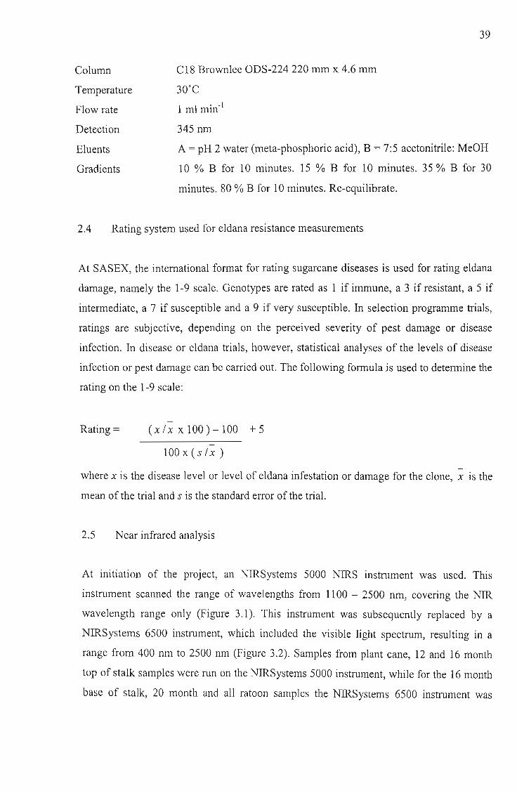
Column

Temperature

Flow rate

Detection

Eluents

Gradients

39

C18 Brownlee ODS-224 220 mm x 4.6 mm

30°C

1 ml min-1

345 nm

A = pH 2 water (meta-phosphoric acid), B = 7:5 acetonitrile: MeOH

10 % B for 10 minutes. 15 % B for 10 minutes. 35 % B for 30

minutes. 80 % B for 10 minutes. Re-equilibrate.

2.4 Rating system used for eldana resistance measurements

At SASEX, the international format for rating sugarcane diseases is used for rating eldana

damage, namely the 1-9 scale. Genotypes are rated as 1 if immune, a 3 if resistant, a 5 if

intermediate, a 7 if susceptible and a 9 if very susceptible. In selection programme trials,

ratings are subjective, depending on the perceived severity of pest damage or disease

infection. In disease or eldana trials, however, statistical analyses of the levels of disease

infection or pest damage can be carried out. The following formula is used to determine the

rating on the 1-9 scale:

Rating =-

( x / x x 100 ) - 100 + 5

100 x (s / x )

-where x is the disease level or level of eldana infestation or damage for the clone, x is the

mean of the trial and s is the standard error of the trial.

2.5 Near infrared analysis

At initiation of the project, an NIRSystems 5000 NIRS instrument was used. This

instrument scanned the range of wavelengths from 1100 - 2500 nm, covering the NIR

wavelength range only (Figure 3.1). This instrument was subsequently replaced by a

NIRSystems 6500 instrument, which included the visible light spectrum, resulting in a

range from 400 nm to 2500 nm (Figure 3.2). Samples from plant cane, 12 and 16 month

top of stalk samples were run on the NIRSystems 5000 instrument, while for the 16 month

base of stalk, 20 month and all ratoon samples the NIRSystems 6500 instrument was

40

available. All calibration development and results were therefore carried out on the more

accurate NIRSystems 6500 instrument.

The NIRS instruments worked on a transmittance analysis, with a quartz cuvette for

sample presentation. A total of 32 scans were run on each sample, and averaged to provide

a more accurate reading. Readings were treated with a log l/Transmittance transformation

before being presented to the instrument operator. The NIRS instruments came with their

own built-in software (listed below), capable of producing and verifying calibrations, as

well as providing various graphical options for visualising data.

Calibration development by the NIRSystems software (explanations provided from the

NIRS manual, © Infrasoft International, version 4.00, 1996) has a range of options

including stepwise regression, principal component regression and partial least squares

regression. Stepwise regression is the simplest option, where individual wavelengths are

added or subtracted to the model until a desirable level of accuracy is achieved. The

regression procedure begins with the calculation of correlations of predicted values with all

wavelengths available. The most highly correlated wavelengths are then added to the

equation. A number of iterations allows further highly correlated wavelengths to be added,

and wavelengths to be removed if their correlations subsequently decrease in the equation.

The statistic calculated to represent the accuracy of the equation is the standard error of

calibration (SEC). Overfitting is possible with this form of analysis. Overfitting may be

tested for by watching for an increase in the standard error of prediction (SEP), a statistic

that is obtained by attempting to predict samples not included in the calibration. A standard

error of validation (SEV) can also be calculated if a second set of samples is available. The

final equation form of a chemical component will be Y = a + b\X\ + b2X2 + ... + biXi

where Xi represents the absorbance value at a particular wavelength and bi is a weighting

factor for that wavelength. The value of each term in the equation can be evaluated from

the size of its variance ratio (partial F).

The principal component analysis (PCA) method is a data reduction method, reducing the

data points, in this case wavelengths, to a set of independent variables called principal

components or eigenvectors. Wavelength information is used to compute the eigenvectors

or loadings. Loadings are weights assigned to each wavelength and the weights are added

up to give a score. Terms are produced in an iterative process as information is extracted

41

from the sample scores. The first term represents the largest source of variation among the

scores.

Partial least squares (PLS) is another regression method that can be used to produce

calibration equations. PLS is similar to PCA except that when the loadings are calculated

they include information from all the X variables (absorbance readings at the different

wavelengths) as well as the Y variable (reference values from conventional determination

methods). The PLS is usually better than PCA because of the inclusion of the Y

information in the regression. A further improvement is offered in modified PLS (MPLS),

where the residuals, obtained after each factor is calculated, are standardised (divided by

the mean residual value) before calculating the next factor. Both PCA and PLS have the

benefit of being protected from overfitting by cross validation errors (SECV). Because

only independent sources of information are being fitted to absorption data rather than

coefficients and wavelengths, each sample in the calibration file can be tested for

prediction accuracy.

Within the calibration equation development system are a number of options available for

transformation of the data. Derivatives to various degrees are possible, as is a noise

adjustment.

The NIRS software provides a facility for testing the validation of calibration equations

with a separate set of samples, regardless of the mechanism used to produce the calibration

equation. This analysis provides the standard errors needed to verify the good performance

of a calibration equation, including SEP, SECV and bias. This step is important, as it is

possible to develop a calibration equation that is only useful for predicting the samples

within the set that was used to develop the calibration equation. Good prediction of an

entirely new set of samples is the best test for performance of the calibration equation.

The PCA can be used for a further application. A neighbourhood Mahalanobis (H) distance

can be produced from the principal components in order to determine the best samples to

be used for a local calibration. The H distance is a measure of the distance in

multidimensional space of each observation from the mean centre of the observations,

taking into account all the variables being considered (Manly, 1986). This is especially

useful if there are large differences between sample groups. A global library needs to be

42

created in order to cover all variations in sample groups and then local calibrations are

formed for each new sample group run, based on the samples that are most similar to the

ones being analysed.

The H distances can be used to graphically display the sample groups. A display of one

sample group on a three dimensional graph gives an indication of the variation within that

group, and can help determine whether some samples should be removed from a highly

represented area. In addition, graphs of histograms of H distances are available in order to

evaluate the scatter within a set of samples, and to earmark possible outliers. The greatest

benefit can be obtained, however, with the plotting of multiple sample groups on one

graph. This allows a visualisation of the amount of overlap between sample groups, even if

only in three dimensions, and an indication of the effective cover of a global library. An

example is shown in Figure 2.3. The sample group represented by the white crosses is

spatially separated from the red and blue sample groups. The white sample group cannot

therefore be used for predictions in the red and blue sample groups, or vice versa. The red

and blue sample groups, because they overlap, can be used to predict from one group to the

other. In the development of a global library for prediction purposes, the spaces between

the sample groups would need to be filled with other sample groups, until all new sample

groups fall into an area already covered by previously scanned samples.

NIRS software (© Infrasoft International, verSIOn 4.00, 1996) provides an additional

feature known as frequency space devolution, which breaks down the overall absorbance

into a series of peaks. It is assumed that these peaks exist, and that the combination of

absorbances of these peaks gives the overall outline of the absorbance, even though the

individual peaks are not differentiable. The software attempts to predict the presence and

size of these peaks iteratively in order to provide more information. Peak locations are

adjusted with the aid of the fourth derivative. If the estimated composite curve peaks do

not match the observed spectra, then the peak location is adjusted using the fourth

derivative rather than the peak of the observed spectra, as these may include the effects of

neighbouring peaks. Peak height and width are also adjusted using the fourth derivative.

43

o Sample group 1

mSample group 2

* Sample group 3

Figure 2.3: A graphical representation of peA H distances between sample groups,

for evaluation of the predictive potential between groups, where calibrations

developed in one group cannot predict values in other groups that are spatially

separated. Prediction is theoretically possible between overlapping groups

44

CHAPTER 3

CALIBRATION TRIAL

3.1 Introduction

Previous work (Rutherford, 1993; Rutherford et al., 1993) at SASEX suggested that NIRS

was a feasible method for predicting eldana resistance in sugarcane. Rutherford (1993)

used a sample set of 60 genotypes to establish the calibration. However, only a small

number of environments were included in Rutherford's evaluation, and prediction between

samples sets from different environments was poor.

There were two aspects to the current calibration trial. The first was to develop a global

library of samples to overcome environmental influences on the reading of samples. The

second was to evaluate the effect of environment on bud scale chemical profiles. The

sample set used in this study was the standard set of 60 clones used for the previous study

(Rutherford, 1993), each sample set being from a different environment or time. The

inability of a calibration set to predict eldana resistance ratings from one sample set to

another was assumed to be due to the environmental influence on the spectral readings.

This environmental influence is different from the environmental influence that may lead

to actual differences in chemical profiles of bud scales. It can be caused by differences in

sampling conditions, differing laboratory conditions at the time of reading the spectra,

different moisture levels in the samples, etc. This problem is usually overcome with the

use of a global set of samples representing all possible conditions that may be experienced

during sampling of bud scales. The global library is developed by taking samples from a

range of environments, at different times, until the full range of all possible samples is

included. This is achieved when any new samples that are subsequently added are similar

to ones already in the calibration. Similarity is based on PCA H distances, which reflect

whether samples are statistically similar to each other, regardless of what the actual

quantities of chemical constituents in the samples are. Part of the checks that are run on an

already developed calibration are to ensure that samples coming in for analysis are valid in

that there are similar types of samples already in the calibration. Once the global library is

developed, then the environmental impact on the chemical composition of the bud scales

can be evaluated, using the calibration to predict the amount of chemicals in the bud scales.

45

This second aspect of the calibration trial would determine if the resistance mechanism that

was being measured by NIR scanning of the chemical components of bud scales was

consistent over different environments. A clone that is resistant in all environments is

preferable to a clone that is only resistant part of the time. If the chemical profile of the bud

scales changed over different environments, then it would not be a worthwhile aspect of

eldana resistance to study, regardless of whether the NIRS calibration worked well or not.

If bud scale profiles prove to be an environmentally independent form of eldana resistance,

then the NIRS calibration can be used to discard clones from the breeding programme. In

this case, the aim is not to identify the clones with good eldana resistance, but just to have

sufficient accuracy to discard the clones that are susceptible. This would result in a savings

in resources, from not carrying poor clones forward in the selection programme.

The standard set of 60 genotypes used in the original work by Rutherford (1993) was

grown under a range of conditions, in order to both establish a global calibration and to test

the environmental impact on bud scale composition. Because previous work had only been

done on bud scales removed from the top section of the stalks, it was also relevant to

determine the levels of the compounds of interest in the lower section of the stalk. The

lower section of the stalk is the preferred entry site of the eldana larvae, and buds are

frequently damaged or degraded in this area, being older than those at the top of stalks.

Resistance of genotypes may be related to the degree of breakdown of chemicals in older

material more than the original composition of these chemicals.

3.2 Materials and Methods

A set of 60 cultivars with known eldana ratings was used for the calibration set. These

cultivars, together with their eldana ratings, are listed in Appendix 1. This set was planted

in December, 1996. It was planted at two sites, one on the Coast at Shakaskraal (Appendix

3), the other in the Midlands at Bruyns Hill (Appendix 4). These are two of the research

stations that were owned by SASEX at the time of the project. The trials were both planted

as a randomised block of three replications, with 1 m single row plots.

46

A bud scale sample was taken at each site at twelve, sixteen and twenty months. At the

sixteen and twenty month sampling dates, an additional sample was taken from the lower

portions of the stalks, in the same manner as the standard sample. A sample consisted of

taking seven representative stalks from each line, from different stools, excluding the end

stools. The two sites were then cut back and allowed to ratoon. Each site was sampled

again at the three different ages, in the same manner as in the first season.

3.3 Data analysis - calibration

A data analysis of the spectra was carried out with the NIRS software, in which

calibrations were developed between NIRS absorbance values and eldana ratings with the

various methods available, as outlined in section 2.4. Validations were carried out with the

NIRS software.

Additional analyses were carried out in Microsoft Excel. Data from the NIRS instrument

were imported. Each set of samples was standardised to have a mean of zero and a

standard error of one, using the transformation z = (x - x)ls where x is the mean of the

sample set and s the standard error of the sample set. Correlations between sample sets

were calculated.

Absorbance spectra were broken down into individual peaks using the frequency space

devolution methods available in the NIRS software. These peaks were imported into

Microsoft Excel. The locations of the peaks and their amplitudes were correlated with

eldana resistance estimates to determine if there was a relationship.

When comparing absorbance values of the NIRS instrument (or HPLC peak areas), with

the eldana ratings, the values of the absorbance values or peak areas were converted to the

1-9 scale, to be comparable to the eldana ratings. This was done using the following

formula:

Rating = (x - min ) / (( max - min ) / range) + offset

where x is the absorbance value or peak area, min is the minimum value for that sample

set, max is the maximum for that sample set, range is the range found in that sample set,

and offset is the amount by which the lowest value must be shifted from zero. So for the

disease ratings, the range is eight, i.e. 1-9, and the offset is one.

47

3.4 Data analysis - genotype x environment

3.4.1 Analysis of variance

In stability analysis, an analysis of variance gives an indication of the size and importance

of the various factors and their interactions. It is the first step in determining the behaviour

of a particular characteristic under different environmental conditions.

The analysis of variance for the calibration had the following model:

Yijklm = m + Gi + Sj + Yk + Al + (GS)ij + (GY)ik + (GA)il + (SY)jk + (SA)jl + (YA)kl +

GSYijk + GSAijl + SYAjkl + GSYAijkl + Eijklm

where Yijklm is the mth observation of the ith cultivar in the jth site in the kth year at the lth

age, and m is the mean. Gi, Sj, Yk and Al are the main effects of genotype, site, year and

age respectively. The six terms thereafter are the first order interactions. The next three

terms are the second order interactions, followed by one third order interaction. Eijklm is the

experimental error. The higher order interactions are grouped into the error term as they

are difficult to interpret, and may improve accuracy in the experiment.

The expected variance components for the different factors and their interactions can be

calculated according to the formulae in Table 3.1.

Significant interaction effects in the analysis of variance will indicate the need for further

analysis using other techniques, as mentioned below. The value of VG, obtained by

subtraction, provides an estimate of broad-sense heritability.

Variance components can also be analysed using a mixed model, where varieties are set as

fixed effects and environments as random effects. The REML model allows greater

efficiency in analysis as it takes into account the loss of degrees of freedom resulting from

estimating fixed effects. It can also take into account heterogeneity of error variances

between environments.

48

Table 3.1: Sample ANOVA table for G x E interaction analysis, demonstrating the

technique for estimating Expected Mean Squares using first order interactions

(higher order interactions are included in the residual)

Source df Expected mean squares

Genotypes (g-l) rsyaVo + ryaVos + rsaVOY + rsyVoA + VE

Sites (s-l) rgyaVs + ryaVos + rgaVsy + rgyVsA + VE

Years (y-l) rgsaVy + rsaVOY + rgaVsy + rgsVYA + VE

Ages (a-I) rgsyVA+ rsyVOA + rgyVSA + rgsVYA + VE

GxS (g-1 )(s-1) ryaVos + VE

GxY (g-I)(y-l) rsaVOY + VE

GxA (g-I)(a-1) rsyVoA + VE

SxY (s-1)(y-l ) rgaVSY + VE

SxA (s-I)(a-l) rgyVsA+ VE

YxA (y-l)(a-l) rgsVYA + VE

Residual gsya(r-l ) VE

3.4.2 Regression analysis

Regression analysis is still the most widely used technique for estimating individual

genotype effects across environments (Finlay and Wilkinson, 1963). The environmental

index in this trial would be the mean of all the genotypes. Various stability definitions

could be used to determine the performance of the clones. Low variance across

environments would indicate that the clone performs similarly across all sites. This

stability measure is independent of other genotypes, but it gives no indication of the pattern

of response of the clone. Examining the slope of the regression in relation to the mean

response of all clones would indicate if the clone has an above average performance in all

environments, but this only gives a stability indicator for those environments. Because of

the absence of standard or control genotypes for bud scale extract work, using the

definition of stability as being better than the control, could not be used in this trial.

49

3.4.3 Qualitative or rank order analysis

Because a clone should be resistant across all environments, it is important to test for

qualitative environmental influences. A change from resistant to susceptible under certain

conditions would make that particular characteristic undesirable to breeders. Tests that

determine rank-order changes would be beneficial in the calibration. In this case a

genotype is determined to be stable if its rank is similar over environments. The following

calculations were used (Huehn, 1990):

Xjj = phenotypic value of the ith genotype in the jth environment (i = 1,2, ... ,K; j =

1,2, ... ,N). In this two-way table with K rows (genotypes) and N columns (environments)

one ranks the K phenotypic values Xjj within each column, i.e. each environment separately

(lowest value = rank of 1 and highest value = rank of K). Let rij be the rank of genotype i in

environmentj. A number of stability estimates were calculated.

N-l N

(1) S/l) = 2 I I Irij - rij' Ij=l j'= j+\

N(N -1)

(Equation 1)

which is the mean of the absolute rank differences of a genotype i over the N

environments, where rij' is the rank in the (j+1) environment

N

(2) S (2) - '" - 2j - LJ (rjj - rj.)

j=l

N - 1

N

with ;. = ~ r··fNI. LJ IJ

j=l

(Equation 2)

-r j. can be interpreted to be the expectation of each rij under the hypothesis of

maximum stability (equal ranks)

N(3) _ ~ -

(3) Sj - LJ I rij - r j. Ij=l

(Equation 3)

which is the sum of the absolute deviations of the rjj's from mean stability, ; j.,

-expressed in r j. units

50

Since genotypes are ranked separately within each environment the environmental effects

have no influence on this type of stability. However, differences among genotypes would

have an effect on the stability measures and may lead to differences in stability· among

genotypes when there is no genotype-environment interaction. To avoid this the Xij values

were corrected using (Huehn, 1990):

. --Xij = Xij - ( Xi. - X •. )

where x i. is the marginal mean of genotype i and x .. is the overall mean.

(Equation 4)

The ranks can then be calculated usmg the corrected values. Approximate tests of

significance, based on the normal distribution, are available for the first two stability

parameters, sY) and Si(2) (Huehn, 1990):

(Equation 5)

would have an approximate chi-squared distribution with one degree of freedom.

The means E(Si(m)) and variances V(Si(m)) may be computed from the discrete uniform

distribution (1,2, ... ,K), using the following formulae:

V(sY)) = (K2- 1) [ (K2- 4)(N + 3) + 30 ] /45 K2N (N - 1)

V(S/2)) = (K2- 1) [ 2 (K2- 4) (N - 1) + 5 (K2- 1) ] /360 N (N - 1)

(Equations 6)

3.4.4 Stability variance and ecovalence

The stability-variance G x E technique (Kang and Miller, 1984) allows the partitioning of

G x E interactions into components assignable to each genotype, where genotypes are

51

considered stable if the interaction component assignable to that genotype is significantly

less than or equal to experimental error. Stability variances were calculated as follows:

a} = [1/(s-1)(t-l)(t-2)] x [t(t-l) L (,uij - Ji i.)2 - L L (,uij - Ji il]j j j

(Equation 7)

where flij = Yij - Y.j, J.1 i· = Lj

fli/S, s = number of locations, t = number of clones,

Yij = trait value of ith clone injth location, Y .j = mean of all clones injth location.

Another method of partitioning G x E interactions into components for each clone is

ecovalence (Kang and Miller, 1984), which was calculated as follows:

Wi = L (,uiji - 1 / S (Yi. - y../tij

where Yi. = sum ofthe ith clone over all s locations, and Y.. = grand sum.

(Equation 8)

Ecovalence sum of squares for each clone must be divided by (t-l )(s-1 )/t to obtain a mean

square, which allowed testing of its significance in the same manner as the stability

vanance.

3.4.5 Deviation of plot mean from maximum plot

Stability was also measured by using the deviations of the plot means from the maximum

plot yield in the environment (Sumith and Abeysiriwardena, 2001):

dijk = Ymaxj - Yijk (Equation 9)

where dijk is the yield deviation of the ilh clone in the klh replication in the /h environment

from the maximum plot yield recorded in that environment, Ymaxj is the maximum plot

yield recorded in the /h environment and Yijk is the yield of the jlh clone in the klh

replication in the /h environment.

The mean over replications for each clone in each environment was also calculated:

d·· =Ymax·- y ..IJ. J IJ. (Equation 10)

52

Mean deviation across environments for each clone, Dj, would estimate the average

superiority of that clone:

n _

D· = "d .. / n. 1 L-J 1J.

j=\

where n = number of environments.

(Equation 11)

An analysis of variance was carried out on the plot deviations based on Table 3.2:

Table 3.2: Sample analysis of variance of the plot deviations from the maximum

response, for use in stability analysis

Source

Total

Reps/Environment(E)

Clone(V)

E(V)

Variance ofvp(v/)

df

npq-I

n(q-I)

p-I

pen-I)

n-I

n-l

SS

n p q

L L L d\k-(d.. i/npqj=1 ;=1 k=l

p

L d2j .. - (d.. i/npq

;=1

n p p

LLd\. - L d2i..

j=1 ;=1 ;=1

n n

[L d\·-(L d1i/n]/qj=1 j=1

n n

[L d2pj.- (L dpi/n ]/qj=1 j=l

Pooled errorn p q n p

[p-I][n/(q-I)] I I I d\k - I I d\.-j=1 ;=\ k=\ j=\ ;=\

n q n

I I d2.jk - I d\

j=1 k=l j=1

where E is the environmental effect, V is the clonal effect and E(V) is the environmental

within clonal effect.

53

The variance of E(V) supplies a parameter that indicates the existence of differential

genotypic variances across environments, and is equivalent to the G x E interaction term in

the standard analysis of variance. The E(V) variance can be partitioned into components,

each of which corresponds to each clone. This Vi becomes the stability parameter for each

genotype.

Genotypes with the lowest mean deviation and non-significant variance in deviations are

the most stable as they have the highest yield across environments. An analysis of variance

on the plot deviations from the maximum plot yield among all plots allowed a test of

significance on the variance of deviations to be carried out, giving an indication of specific

adaptability.

3.5 Results and Discussion - Calibration development

The results obtained from the NIRSystems 5000 in the original studies (Rutherford et aI.,

1993; Rutherford and van Staden, 1996) indicated an inability to predict eldana resistance

in one sample set (the set of standard clones used for calibration development taken from

one particular environment) using a calibration developed from another sample set.

Analysis of the different sample sets indicated very little statistical overlap between sample

sets, based on PCA analysis with the NIRS instrument's software. Samples within a

sample set also showed wide differences in their base lines. It was assumed that

environment had a large effect on the sample sets, i.e. strong G x E interactions, and that a

global library, representing as many types of sample sets as possible, was needed in order

to produce a calibration that would be robust with regard to environment. Part of the

present study was to use the samples obtained to begin to develop a global library, and to

determine if it was possible to develop a complete global library that would be able to

evaluate any new samples on the basis of samples already in the calibration.

In the present study, wide differences were also observed between sample sets read on the

NIRSystems 5000, based on PCA H distances and graphic evaluation (Figure 3.1).

Calibration and validation between sample sets was not possible, with correlations being

extremely low (in the order of 0.001) for both PCA and stepwise regression calibrations.

The same genotypes were used in each sample set, so the effect of G x E interaction was

assumed to be large.

1.40 I I

1.20 I ,. "'" l

1.00C)c:"0j 080 1:~J~

"'- ~

I

-Clone1

~ -Clone 2

Clone3

-Clone 4o 0.60 -CloneSl/)

.Q

<0.40

0.20 I I

24002200200018001600140012000.00 I I I I

1000

Wavelength (nm)

Figure 3.1: Example of NIRSystems 5000 spectra of extracted sugarcane bud scale chemical components, showing baseline shifts between

samples within one sample set

Vl~

55

Examination of wavelengths selected for stepwise regressIOn calibration equations

highlighted another problem. Wavelengths chosen from each sample set differed from

those chosen from other sample sets, sometimes by only a few nm, other times having no

relationship with other sample sets. The wavelengths that differed only slightly could have

been caused by the baseline shifts that were observed even within sample sets, but the

wavelengths that had no commonality between sample sets were of concern as they

appeared to be random.

With the acquisition of the new NIRSystems 6500 instrument, the results were very

different. Samples within a sample set all had the same baseline, a necessity for

development of a good calibration equation. Analysis of the H distances between sample

sets showed that all sample sets overlapped coordinately, based on PCA analysis with the

NIRS instrument's software. This meant that all sample sets were comparable with each

other, and that environmental differences did not alter the spectra obtained from bud scale

extracts. It did not mean that the environment did not alter the amounts of the relevant

chemicals within the bud scales, which still had to be determined, but merely that the

ability of the NIRS instrument to detect bud scale profiles was not affected by the source

of the bud scales. It was therefore concluded that the differences between and within

sample sets on the NIRSystems 5000 instrument was due to instrument error, not

environmental differences, and that a global calibration would not be possible on this

instrument. The statistical overlap of sample sets on the NIRSystems 6500 instrument

eliminated the need for development of a global set of samples, covering all possible

sampling conditions, as all samples already overlapped as required.

However, the correlation between different sample sets was still low. None of the

calibration techniques available on the NIRS software provided a calibration equation that

could predict the values of another sample set. Use of derivatives and noise reduction did

not improve the situation. Wavelengths selected by stepwise regression also still differed

between sample sets despite the lack of baseline shifts on the new instrument. For this

reason, it was decided to further evaluate the data from the NIRSystems 6500 instrument in

Microsoft Excel.

In Microsoft Excel, the data was standardised, as in Chapter 3.3, to try to improve

correlations between the different sample sets. However, no improvements were observed.

56

A study of the areas of the spectra where differences between genotypes were visible,

showed that differences between spectra for different genotypes were very small. Figure

3.2 shows the spectra of four different genotypes and two blanks over the whole

wavelength range of the instrument. Figures 3.3 to 3.6 show enlargements ofthe regions of

the spectra where differences are most noticeable. The differences between genotype

spectra in Figures 3.3, 3.5 and 3.6 are all parallel and may only be a base shift, rather than

the presence of a peak. In Figure 3.4, however, there seems to be the presence of a small

peak superimposed on the larger background peak, possibly suggesting the detection of a

chemical bond that differs between samples. However, the differences between the spectra

are small compared to the background signal. More importantly is the behaviour of the

spectra of the blanks. The blanks contained the solvent mix of methanol and water in the

same ratio as for the bud scale samples, and were read in at the same time as the sample

sets to which they were compared. These blanks sometimes showed higher absorbances

than some of the spectra, something that should not be possible if absorbance was

increased on the basis of compounds in the samples. In Figure 3.4, the likeliest area for

evaluation, the spectrum of one of the blanks had one of the highest absorbances.

The areas where the largest peaks are visible in the spectra correspond to the absorbance

areas of methanol and water, the solvents used in the experiment (Figure 3.2). The

breakdown of the spectrum of each clone into individual peaks using the option available

in the NIRS software (Chapter 2.4), allowed the possibility of separation out of the peaks

caused by the chemicals of interest (Figure 3.7), as well as allowing for the removal of any

baseline shifts that may be present. Amplitude and position of peaks for each clone were

compared with other clones within a sample set to determine if there was any correlation

with eldana ratings of those clones, and then compared across sample sets. The exact

location of peaks was inconsistent across different spectra, suggesting that the process was

not precise enough for good results. However, the identification of peaks was

approximated manually, and reasonable consistency of peak identity was noted for

different clones. The sizes of these peaks were then compared to the eldana resistance

ratings for each clone. No relationship with the sizes of any peaks at any wavelength was

observed across sample sets.

With the original work on the NIRSystems 5000 instrument, it was assumed that the

differences between the spectra of different clones within a sample set were due to

Fig3.4

V

// Fig

3.6

/ ~ Fig

I3.5

7 \ 1\ /\ I \lrIPeaks due to~ F;93.3

water and

methanol 11\ '- V

1/~~~

4.5

4

3.5

0) 3t::ceu~ 2.5Cl)(.)t:eu

2.c...0111.c« 1.5

1

0.5

o400 900 1400

Wavelength (nm)

1900 2400

--Clone 1

--Blank2

Clone 2

-Blank 1

--Clone 3

Clone 4

Figure 3.2: Example of NIRSystems 6500 spectra of extracted sugarcane bud scale chemical components, showing small differences betweensamples within one sample set

VI-....)

1 r I

--Clone 1

--Blank 2

Clone 2

--Blank 1

--Clone 3

Clone 4

15401520150014801460144014200.4 I i i I I

1400

0.9 I n#7" ......~" I

0.5 +-11 ~

C) 0.8 -l-I-----~C:sCGG>

to;,. ""h I~ ~~u 07 I IIc .CG-eo

~ ~ I« 0.6 I I1

Wavelength (nm)

Figure 3.3: Enlargement of the graph area of the sugarcane bud scale extract absorbance peak at 1460 nm

VI00

4.5

4

3.5

C) 3c:::sCG

~ 2.5Q)CJc::CG

2€0III.Q

et 1.5

1

0.5

01850 1870 1890 1910 1930 1950 1970 1990

Wavelength (nm)

Figure 3.4: Enlargement of the graph area of the sugarcane bud scale extract absorbance peak at 1940 nm

--Clone 1

--Blank 2

Clone 2

--Blank 1

--Clone 3

- Clone 4

V'l'0

2 I I

1.8 I I

2300229022802270226022502240223022202210

1I.r I

0.8 F I I I

2200

C) 1.6c::s

C'CJ

~

--Clone 1

CU

--Blank 2

(.) 1.4c:C'CJ

Clone 2

€

--Blank 1

0III

--Clone 3

.c« 1.2

Clone 4

Wavelength (nm)

Figure 3.5: Enlargement of the graph area of the sugarcane bud scale extract absorbance peak at 2270 nm

0\o

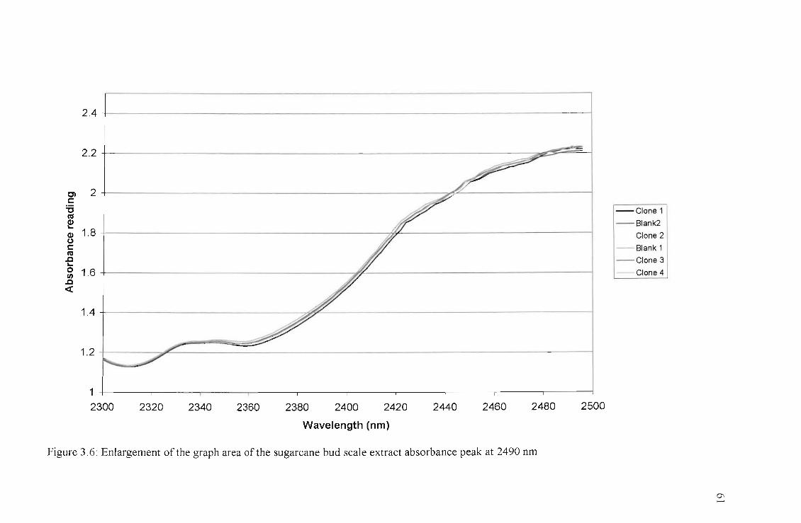
2.4 I I

25002480246024402420240023802360234023201 I i i I I I I

2300

2.21 ~I

1.2 I oar I

O'l 2c:::s"'

--Clone 1

eCl) 1.8

--Blank2

(JClone 2

c::

"'- Blank 1

.Q...0 1.6

--Clone 3

I/).Q

Clone 4

«

1.4

Wavelength (nm)

Figure 3.6: Enlargement of the graph area of the sugarcane bud scale extract absorbance peak at 2490 nm

0\

4 I I

3.5 I 1\ I

3

Cl

=25't' .C'Cl

~C1l

20c:C'Cl.c...0III 1.5

Overall spectrum

.cet

I I1

0.5 I I! \ '" JI

240019001400

Wavelength (nm)

900o-r':=400 I - ::::2%XL~ "- '" ' . /........ '- Lx.;:>....\. \ II

Figure 3.7: Breakdown of overall bud scale spectrum of a single sugarcane genotype into individual peaks, in order to estimate individual peak

size and location

0\IV

63

differences between chemical profiles of the bud scales. The inability of the calibration

equations to predict eldana resistance ratings from one sample set to another were assumed

to be due to the environmental influence on the spectral readings. With the subsequent data

from the NIRSystems 6500 instrument, it became clear that these differences were due to

error. Instrument error was high in the NIRSystems 5000 instrument, creating the false

impression that a global library was necessary. Due to the small number of samples that

were measured in the original experiment, false positives were obtained in the correlation

analysis. With the introduction of the more accurate NIRSystems 6500 instrument, it

became evident that incorrect assumptions had been made from the data from the

NIRSystems 5000 instrument. Increasing the number of samples also showed that the

correlations obtained in the original experiment were due to overfitting, and not to an

actual difference between samples. The non-overlap of the samples in the original

experiment also added to the erroneous conclusions drawn.

The new NIRS instrument included the wavelengths from the visible light spectrum, from

400 - 1100 nm. An additional peak was noted at the end of the instrument's range, namely

at 400 nm. This peak was investigated to determine if it contained any information on

eldana resistance. The correlation between samples sets for this peak was very promising,

both for the samples taken from the top stalk positions (0.63 - 0.74) and those taken from

the lower stalk positions (0.55 - 0.63). This suggested that the bud scale constituent that

the peak represented was not random or error, as was the case with the peaks in the NIR

region. However, the chemical component associated with this peak, as detected by NIRS,

does not appear to have a major influence on eldana resistance. Correlations between peak

amplitude and eldana resistance ratings were low (0.18 - 0.30 for the upper stalk position

and 0.03 to 0.12 for the lower stalk position).

More importantly, the relationship between the 400 nm peak and eldana resistance is

negligible. The plot of predicted eldana resistance ratings against eldana resistance ratings

(Figure 3.8), taken from the sample set with the highest correlation, shows that predictions

using the 400 nm peak would be inadequate for effective use in the breeding programme. If

the prediction of eldana resistance was accurate enough to remove a fair number of

susceptible clones without losing too many resistant clones, it would be useful. In the

example of the best sample set, choosing to discard those clones with a rating above a

••

• • • -.• •• •• - .

• y = 0.2524x + 3.6828

• • • • R2 = 0.0695

• • •• •• • •• •.... • •

• •• •• •• • •• •

• • • • •• • .-- • • ••

• •

10.00

9.00

8.00

fIi 7.00~

.5...."= 6.00.."=="=

5.00"0Q:j"0~....

4.00~:a~..~ 3.00

2.00

1.00

0.00

0

•2 3 4 5 6 7 8 9

Observed eldana ratings

Figure 3.8: Predicted vs actual eldana resistance ratings on sugarcane for the sample set with the highest correlation with eldana ratings (20

month plant crop), using 400 nm absorbance peak values converted to a 1-9 scale for predicted values

0\.p.

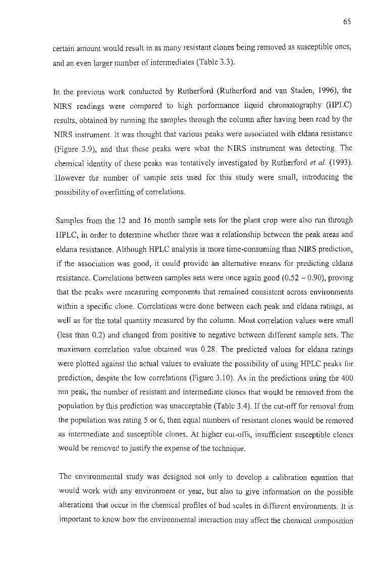
65

certain amount would result in as many resistant clones being removed as susceptible ones,

and an even larger number of intermediates (Table 3.3).

In the previous work conducted by Rutherford (Rutherford and van Staden, 1996), the

NIRS readings were compared to high performance liquid chromatography (HPLC)

results, obtained by running the samples through the column after having been read by the

NIRS instrument. It was thought that various peaks were associated with eldana resistance

(Figure 3.9), and that these peaks were what the NIRS instrument was detecting. The

chemical identity of these peaks was tentatively investigated by Rutherford et al. (1993).

However the number of sample sets used for this study were small, introducing the

possibility of overfitting of correlations.

Samples from the 12 and 16 month sample sets for the plant crop were also run through

HPLC, in order to determine whether there was a relationship between the peak areas and

eldana resistance. Although HPLC analysis is more time-consuming than NIRS prediction,

if the association was good, it could provide an alternative means for predicting eldana

resistance. Correlations between samples sets were once again good (0.52 - 0.90), proving

that the peaks were measuring components that remained consistent across environments

within a specific clone. Correlations were done between each peak and eldana ratings, as

well as for the total quantity measured by the column. Most correlation values were small

(less than 0.2) and changed from positive to negative between different sample sets. The

maximum correlation value obtained was 0.28. The predicted values for eldana ratings

were plotted against the actual values to evaluate the possibility of using HPLC peaks for

prediction, despite the low correlations (Figure 3.10). As in the predictions using the 400

nm peak, the number of resistant and intermediate clones that would be removed from the

population by this prediction was unacceptable (Table 3.4). If the cut-off for removal from

the population was rating 5 or 6, then equal numbers of resistant clones would be removed

as intermediate and susceptible clones. At higher cut-offs, insufficient susceptible clones

would be removed to justify the expense of the technique.

The environmental study was designed not only to develop a calibration equation that

would work with any environment or year, but also to give information on the possible

alterations that occur in the chemical profiles of bud scales in different environments. It is

important to know how the environmental interaction may affect the chemical composition

66

Table 3.3: Number of sugarcane clones that would be removed from the population

using different ratings on the 1-9 scale as the cut-off value, for eldana predictions

based on 400 nm absorbance values

Cut-off ratingNo of clones removed from category

Susceptible Intermediate Resistant9 0 1 08 0 2 07 3 6 16 4 8 45 6 12 6

0.4

E1::0.3lI)~M

cblorogenates

I I Total integrated area

a)

1.2 r---------;::==========:;::===:;----,flavonoids

b)

retention time (m ins) 60

Figure 3.9: Examples of HPLC profiles of bud scale extracts of resistant (a) and

susceptible (b) sugarcane clones (Rutherford and van Staden, 1996)

12

11

10

9I/)0)

8s:::;:;~

7n:ss::n:s

6"'CQ)

"'C5Q)-0:c4Q)

10..

a..3

2

1

0

••~

• • • ••• • •• • • y = 0.287x + 4.7015.

• R2 = 0.0629# -

• • -.•• • ••• • • •• •• •- •• • ••• • • • • • •• •• • •• • ••••

••

1 2 3 4 5

Observed eldana ratings

6 7 8 9

Figure 3.10: Predicted vs actual eldana resistance ratings on sugarcane for the sample set with the highest correlation with eldana ratings (12

month plant crop), using HPLC peak area converted to a 1-9 scale for predicted values

0'1-..l

68

of bud scales if the method is to be useful for breeding and selection purposes. It also

needs to be known if sampling has to be limited to a certain age of crop. It is important to

know if the chemical components break down on the older lower sections of the stalk, as

this will affect the usefulness of that method of resistance. However, because the NIRS

technique was unable to predict eldana resistance ratings, the environmental study could

not be carried out on the predictions of eldana resistance based on NIRS. Instead G x E

interaction analyses were conducted on bud scale mass, in order to test the selected

analyses on real data.

Table 3.4: Number of sugarcane clones that would be removed from the population

using different ratings on the 1-9 scale as the cut-off value, for eldana predictions

based on HPLC peak area

Cut-off ratingNo of clones removed from category

Susceptible Intermediate Resistant9 4 3 08 5 5 I7 7 6 36 10 11 105 10 13 12

3.6 Results and Discussion - G x E interaction analyses

The fresh mass of bud scales was measured after removal of the bud scales, in order to

calculate the quantities of chemicals to be added for the extraction process. These bud

scale masses were investigated for correlation to eldana resistance, and were used to test

the G x E interaction analyses that were to be used on the chemical profiles of the bud

scales. The average bud scale masses of the 60 cultivars in the calibration set are shown in

Appendix 1.

Correlation of bud scale mass (Tables 3.5 and 3.6) to eldana resistance ranged from -0.21

to 0.39 for top of stalk samples, showing inconsistency between different sample sets,

possibly due to moisture content. Negative correlations seemed to occur more in the

Coastal site for all ages in the plant crop, and more in the Midlands region for all ages in

the ratoon crop. This suggests that there is a seasonal and site influence on the relationship

between bud scale mass and eldana resistance. However, since none of the correlations

69

were very strong, interpretation was ineffectual. A maximum correlation of 0.39 was

obtained from a l6-month Coastal sample, and this was the only value out of 30 that

exceeded 0.2.

Table 3.5: Correlation of eldana ratings to bud scale mass of sugarcane clones for

plant crop of calibration study

Site Age of crop Replication Top of stalk Base of stalk1 -0.13 0.11

16 2 -0.11 0.06

Coastal3 -0.18 -0.141 -0.21 0.22

20 2 -0.05 -0.093 -0.10 0.081 0.13 0.17

16 2 0.14 0.15

Midlands3 0.15 0.311 0.07 0.19

20 2 0.02 0.093 0.13 0.26

Table 3.6: Correlation of eldana ratings to bud scale mass of sugarcane clones for

ratoon crop of calibration study

Site Age of crop Replication Top of stalk Base of stalk1 -0.10

12 2 -0.213 -0.051 0.39 0.26

Coastal 16 2 0.10 0.083 0.14 0.271 0.05 0.15

20 2 -0.01 0.243 0.10 0.17I -0.17

12 2 -0.023 0.071 0.06 0.25

Midlands 16 2 -0.03 0.153 0.19 0.281 0.06 0.11

20 2 -0.03 0.093 0.08 0.29

70

The correlation values for the bud scale mass from the lower section of the stalk to eldana

resistance were much better (Tables 3.5 and 3.6), having only two negative values (-0.14

and -0.08), with a maximum of 0.31. However, nine of the 24 values exceeded 0.2,

suggesting that there was a closer correlation between bud scale mass at the lower stalk

positions than at the top of the stalk. Eldana prefers the lower section of the stalk for entry,

and the buds here tend to decay or suffer damage over time. Since the mass, and therefore

size, of the bud scale is positively correlated with eldana resistance ratings, the implication

is that the less the buds degenerate with age the higher the susceptibility (a higher rating

value is given for susceptible clones). However, the relationship is not strong, and would

not be useful for predicting eldana resistance.

Correlation between replications within a site ranged from 0.28 to 0.70 (Table 3.7),

suggesting reasonable consistency of bud scale mass within one environment. The average

bud scale mass was lower for the base of the stalk at all sites and ages, except one. There

was no trend in average bud scale mass as age increased for the top of stalk buds, but older

bud scales at the base of the stalk tended to be lighter. Differences in average bud scale

mass between sites were not consistent across the different ages.

Table 3.7: Correlation of bud scale mass of sugarcane clones in calibration study,

between replications within sites and ages

Top of stalk Base of stalk

Crop SiteAge of Average Average

crop Correlation bud scale Correlation bud scalemass mass

Coastal16 0.68 0.228 0.48 0.172

Plant20 0.52 0.303 0.41 0.163

Midlands16 0.70 0.195 0.64 0.23820 0.54 0.251 0.48 0.20312 0.51 0.260

Coastal 16 0.36 0.232 0.33 0.166

Ratoon20 0.35 0.236 0.35 0.19812 0.59 0.260

Midlands 16 0.61 0.324 0.60 0.20220 0.53 0.260 0.28 0.146

71

Bud scale mass was averaged over replications, within sites and ages, before correlating to

eldana ratings. The results were similar to the correlations obtained on a per replication

basis (Table 3.8). None of the correlations exceeded 0.3.

Table 3.8: Correlation of eldana ratings to bud scale mass of sugarcane clones in

calibration study, averaged over replications

Crop Site Age of crop Top of stalk Base of stalk

Coastal16 -0.16 0.0220 -0.16 0.08

Plant16 0.16 0.24

Midlands20 0.08 0.2012 -0.14

Coastal 16 0.28 0.29

Ratoon20 0.08 0.2312 -0.05

Midlands 16 0.07 0.2620 0.04 0.23

Despite the low correlations between eldana resistance and bud scale mass, it was decided

to continue analysis of G x E interactions on bud scale mass, in order to study the

techniques available.

3.6.1 Analysis of variance

An analysis of variance was carried out for all possible interactions of treatment effects.

The results showed that all main effects were significant at the 1% level (Table 3.9). All

interactions were significant at the 1% level, except for the year.replication interaction

which was significant at the 5% level, and the site.age.replication and age.year.replication

interaction which were not significant. The standard error was 0.065 and the CV was

25.7%. This indicates the bud scale mass differs across sites, ages and years. More

importantly, there is an interaction at all levels between sites, ages and years, suggesting

that the effect of each of these is not consistent. Because the higher order interactions are

difficult to interpret, a further ANOVA was carried out for only the first order interactions

(Table 3.10). In this analysis, all main effects and interactions were significant at the 1%

level. The standard error was 0.0716 and the CV was 28.4%. This ANOVA was then used

to estimate VG, using subtraction in the formulae shown in Table 3.1. Adding together VG,

72

Table 3.9: ANOVA for bud scale mass of 60 sugarcane clones evaluated for stability

at two sites, three ages and in two crops, including all interactions

Source df MS

Genotypes (G) 59 0.1285**

Sites (S) 0.0740**

Years (Y) 0.1629**

Ages (A) 2 0.0641**

Rep (R) 2 0.0339**

GxS 59 0.0192**

GxA 118 0.0170**

SxA 2 0.3103**

GxY 59 0.0227**

SxY 1 1.4049**

AxY 1 (1) 0.7973**

GxR 118 0.0065**

SxR 2 0.0306**

AxR 4 0.0169**

YxR 2 0.0123*

GxSxA 118 0.0123**

GxSxY 59 0.0168**

GxAxY 59 (59) 0.0064**

SxAxY 1 (1) 0.0712**

GxSxR 118 0.0073**

GxAxR 236 0.0066**

SxAxR 4 0.0021

GxYxR 118 0.0092**

SxYxR 2 0.0276**

AxYxR 2 (2) 0.0090

Residual 629 (319) 0.0042

Total 1777 (382)

CV 25.7%

* Significant at 5% level

** Significant at 1% level

73

Table 3.10: ANOVA for bud scale mass of 60 sugarcane clones evaluated for stability

at two sites, three ages and in two crops, including only first order interactions for

ease of interpretation

Source df MS

Genotypes (G) 59 0.1281**

Sites (S) 1 0.0726**

Years (Y) 1 0.1677**

Ages (A) 2 0.0625**

GxS 59 0.0181**

GxY 59 0.0216**

GxA 118 0.0162**

SxY 1 1.4035**

SxA 2 0.3055**

YxA 1 (1) 0.8039**

Residual 1474 (381) 0.0051

Total 1777 (382)

CV 28.4%

** Significant at 1% level

VE (square of the standard error) and VG x E (the sum of the estimates of the first order

interactions) as the estimate ofVp, the broad-sense heritability for bud scale mass was then

calculated as 0.15. Since the interactions were all significant, further methods of G x E

interaction evaluation were employed.

3.6.2 Regression analysis and variance

A regression analysis was carried out on the bud scale mass data, using the mean of all

genotypes at a site as the environmental index. The definition that was used for a stable

genotype was one that had a slope parallel to the mean of all genotypes, i.e. a slope that did

not differ significantly from one. The variance of each genotype was also calculated, as

another measure of stability is low variance. The results are summarised in Table 3.11.

74

Examination of residual plots showed no non-linear trends or other problems (results not

shown).

Table 3.11: Regression and variance data for sugarcane genotypes evaluated for

stability in two environments at 12, 16 and 20 months at plant and ratoon stages

Clone Slope Var Clone Slope Var Clone Slope Var

1 1.199 0.02103 21 0.416 0.00458 41 1.168 0.00554

2 1.772* 0.00893 22 0.674 0.00664 42 1.704 0.01119

3 1.333 0.00817 23 0.509* 0.00266 43 1.043 0.00490

4 1.228 0.00836 24 0.466* 0.00282 44 0.726 0.00456

5 0.999 0.00399 25 2.125* 0.01837 45 2.053* 0.01124

6 0.653 0.00494 26 0.738 0.00474 46 1.365 0.00552

7 0.783 0.00238 27 0.092* 0.00316 47 0.683 0.00270

8 1.455* 0.00478 28 1.947* 0.01238 48 0.255* 0.00327

9 1.855 0.01289 29 1.282 0.00528 49 0.540 0.00735

10 1.183 0.01371 30 0.308* 0.00357 50 1.242 0.00707

11 0.327* 0.00335 31 1.437 0.00762 51 0.308* 0.00225

12 1.371 0.00615 32 2.195 0.02151 52 -0.019* 0.00278

13 0.734 0.01160 33 0.432 0.00498 53 0.771 0.00313

14 0.383* 0.00274 34 1.271 0.00895 54 0.621 0.00339

15 0.806 0.00791 35 0.935 0.00564 55 2.322* 0.01571

16 1.226 0.01162 36 1.786* 0.00844 56 0.525 0.00269

17 0.907 0.00447 37 1.413 0.00974 57 1.046 0.01457

18 1.439 0.00689 38 0.761 0.00367 58 0.850 0.00629

19 0.950 0.01153 39 0.553 0.00678 59 0.503* 0.00174

20 0.682 0.00322 40 1.058 0.00690 60 0.553 0.00445

* SIgnificant at 5% level

Results between the two methods are inconsistent. There are a number of genotypes that

are stable based on variance, but are unstable based on regression as they have a regression

slope significantly different from one. This is not unexpected as the two methods measure

different aspects of stability. These results do highlight the problem that stability depends

75

on the method used to define it. Those clones that rank well for both methods might be

classified as stable. One observation to note is that those clones with low variance and

significant slope tend to have a slope less than one, and that those clones with high

variance and significant slope tend to have a slope greater than one. This suggests that

clones with low variance across sites have low variability because of small bud sizes

across all sites, whilst those clones with high variance values have high variability because

of a greater than normal mass increase at sites that exhibit higher bud scale mass on

average. As eldana resistance is slightly associated with small buds, the low variance

clones with slopes less than one may be preferential to the stable clones.

3.6.3 Qualitative or rank order analysis

An evaluation of the stability of clones on a qualitative basis is important even in disease

evaluation. A change from resistant to susceptible under different environmental

conditions makes a particular clone undesirable, as the resistance is not stable. Therefore

the tests for measuring rank-order changes of genotypes between environments were

carried out on bud scale mass using the methods detailed in section 3.4.3 (Table 3.12). To

remove the effect of genotype on the stability analysis, corrected values were also

calculated (using Equation 4) and analysed for the stability parameter estimates (Table

3.13). Correlations between the different types of stability parameters are listed in Table

3.14.

There are a high number of unstable clones in the uncorrected data (78% for S(I) parameter

and 73% for S(2) parameter). This number drops drastically in the corrected data to 27% for

both parameters. The significances for the corrected data are considered more reliable as

they are independent of bud scale mass effects. Because of the drop in number of

significantly unstable clones from uncorrected to corrected data, there is a strong

possibility that genotype yield level has a major effect on perceived stability. The

correlation between S(I) and S(2) in the uncorrected data is good, but S(3) does not agree as

well with the other two parameters. Correlations between parameters of uncorrected and

corrected data are poor, and negative in the case of S(3). However, agreement between the

more reliable corrected parameters is high. This suggests that on corrected data the

calculation of only one stability parameter should be sufficient. Agreement with stability

estimators based on regression and variance are poor. However, these measure stability

76

Table 3.12: Stability parameters of bud scale mass of 60 sugarcane clones over two

environments, three ages and two crops, based on qualitative or rank order analysis

for uncorrected sugarcane bud scale mass

For defimtIOns of S ,S and S

see Section 3.4.3, equations 1-3

sIgmficant at 5 Yo level

** significant at 1% level

Clone Sllj S(2) StJ) Clone Sell S(2) S(3)

1 23.90* 420.7* 14.63 31 11.24** 94.3** 5.55

2 15.18** 179.6* 8.80 32 7.46** 50.4** 3.14

3 17.98 246.0 13.38 33 15.60* 194.7* 8.07

4 20.72 319.8 18.03 34 16.91 216.3 9.58

5 14.22** 156.5** 15.29 35 16.49* 201.1 17.13

6 15.51* 181.6* 11.23 36 18.03 244.5 12.16

7 9.92** 84.0** 21.19 37 20.11 297.3 14.46

8 14.59** 161.2** 12.40 38 13.02** 155.9** 16.88

9 11.23** 102.7** 4.92 39 16.57* 217.9 8.77

10 12.65** 160.0** 5.85 40 16.04* 194.0* 8.99

11 16.59 203.3 12.97 41 15.67* 183.8* 13.16

12 11.92** 109.6** 6.35 42 17.72 232.7 11.42

13 14.85** 170.8* 8.83 43 14.65** 165.6** 11.13

14 15.75* 190.2* 16.21 44 14.92** 171.2* 13.69

15 16.90 209.1 10.71 45 17.41 223.4 11.06

16 13.55** 176.9* 6.24 46 12.56** 125.2** 7.17

17 14.25** 151.6** 14.44 47 11.79** 105.5** 12.76

18 14.90** 167.2** 8.76 48 15.96* 189.1 * 15.14

19 20.34 307.5 15.38 49 17.10 215.4 11.21

20 14.31 ** 155.0** 11.20 50 18.18 245.0 14.81

21 18.36 255.1 16.60 51 15.92* 186.1 * 13.26

22 16.25* 202.0 10.98 52 11.49** 157.4** 31.67

23 11.23** 97.0** 19.08 53 10.16** 102.0** 24.71

24 12.33** 130.2** 16.96 54 14.52** 156.3** 13.35

25 5.42** 34.2** 2.09 55 12.08** 140.8** 5.40

26 14.08** 154.2** 8.84 56 11.68** 117.8** 18.99

27 15.86* 190.8* 8.77 57 23.55* 411.4* 15.30

28 6.68** 38.3** 2.66 58 13.82** 149.3** 7.40

29 12.11 ** 119.3** 7.58 59 10.65** 84.3** 12.70

30 15.33** 184.0* 16.59 60 15.92* 192.9* 19.20

* 0 .. ~(l) ,(2) ,(3)

77

Table 3.13: Stability parameters of bud scale mass of 60 sugarcane clones over two

environments, three ages and two crops, based on qualitative or rank order analysis

for corrected bud scale mass

For defimtIOns of S ,S and S

see Section 3.4.3, equations 1-3

SIgnIficant at 5 % level

** significant at 1% level

Clone S(l) S\l) S(3) Clone S\I) SW S(3)

1 26.94** 563.3** 22.06 31 19.56 283.2 14.77

2 18.71 262.2 13.72 32 25.22** 482.9** 21.66

3 22.06 378.8 18.99 33 20.48 307.7 13.56

4 23.56* 416.9* 18.88 34 21.44 335.9 15.06

5 16.61 204.1 11.06 35 19.94 292.1 13.91

6 18.70 263.4 11.86 36 21.07 326.4 15.39

7 14.03** 143.9** 9.42 37 22.57 376.4 17.95

8 15.63* 183.8* 11.64 38 15.67* 188.6* 10.67

9 22.03 358.2 16.97 39 22.15 359.1 15.53

10 24.67** 456.9** 18.55 40 20.19 309.3 14.77

11 19.67 287.9 13.24 41 17.48 228.1 13.00

12 18.03 240.2 12.83 42 22.24 376.1 18.89

13 18.97 265.6 15.63 43 18.56 257.3 11.90

14 18.49 253.4 12.55 44 18.77 265.2 12.93

15 21.14 329.3 16.28 45 21.70 352.7 18.09

16 22.56 376.8 16.05 46 18.34 246.9 12.96

17 18.13 245.3 11.52 47 15.21 ** 173.9* 9.84

18 20.64 313.9 15.48 48 19.83 291.4 13.96

19 23.48* 429.1* 20.91 49 22.78 383.3 17.37

20 16.99 214.0 12.00 50 20.86 319.7 16.08

21 20.60 317.7 15.89 51 18.40 248.6 12.02

22 19.40 279.6 14.86 52 18.40 250.9 13.83

23 17.07 215.4 11.21 53 16.20* 194.4* 11.21

24 16.69 203.6 10.76 54 18.25 243.2 12.35

25 25.01 ** 473.1** 22.04 55 25.02** 474.9** 21.39

26 17.78 235.1 12.30 56 17.10 215.3 11.34

27 21.28 334.0 14.49 57 26.05** 512.2** 16.75

28 23.41 * 407.3* 19.44 58 19.97 303.4 14.61

29 14.71 ** 167.8** 9.59 59 14.03** 147.5** 8.89

30 18.85 262.9 13.19 60 19.05 266.4 14.05

* 0 .. ~(l) ,(2) ,TJ)

78

Table 3.14: Correlations between stability parameters of bud scale mass of 60

sugarcane clones evaluated across two environments, three ages and two crops, based

on qualitative or rank order analysis

S(l) S(2) S(3) S(I) adj S(2) adj S(3) adjS(l) 1S\l) 0.97 1S(3) 0.24 0.26 1

S(I) adj 0.34 0.47 -0.38 1S(2) adj 0.33 0.47 -0.37 0.99 1S(3) adj 0.23 0.36 -0.37 0.94 0.94 1

ad] - data corrected for genotype

defined in a different way, and in terms of desirability of clones, may not reflect those that

are best for disease resistance. Environmental interactions that cause qualitative changes

are an important aspect to evaluate and the stability parameters calculated in this section

should be taken into account when determining the best clones for disease resistance.

3.6.4 Stability variance and ecovalence

The stability variance and ecovalence techniques (Equations 7 and 8) were applied to the

bud scale mass data (Table 3.15). These techniques allowed the partitioning of G x E

interaction variance into components for each genotype, thereby allowing individual clonal

determinations of stability. Approximate F distribution tests were applied to determine

whether the interaction variance attributable to each genotype was significant. Values for

stability variance and ecovalence were similar. Only two clones showed a variance

significantly different from the experimental error. This differs from previous techniques,

which showed a number of clones exhibiting unstable behaviour across environments.

3.6.5 Deviation of plot mean from maximum plot

An analysis of variance based on the deviation from maximum plot (Equations 9 to 11 and

Table 3.2) was carried out on the data. The deviation from maximum plot analysis allowed

a stability test for the trial, as well as for individual clones. Minimum bud scale mass was

used as the criteria rather than maximum bud scale mass, as minimum bud scale mass is

associated with eldana resistance. There was no significant effect for G x E interaction,

79

Table 3.15: Stability variances and ecovalence parameters for bud scale mass of 60

sugarcane clones evaluated across two environments, three ages and two crops

Clone Stability variance Ecovalence Clone Stability variance Ecova1ence

I 0.01836** 0.01809** 31 0.02514 0.00241

2 0.00263 0.00260 32 0.00472 0.00436

3 0.00340 0.00338 33 0.00223 0.00219

4 0.00429 0.00430 34 0.00435 0.00429

5 0.00028 0.00041 35 0.00300 0.00310

6 0.00130 0.00137 36 0.00178 0.00180

7 0.00058 0.00079 37 0.00212 0.00213

8 0.00085 0.00094 38 0.00109 0.00123

9 0.00442 0.04220 39 0.00290 0.00282

10 0.00507 0.00481 40 0.00311 0.03080

11 0.00220 0.00225 41 0.00137 0.00143

12 0.00213 0.00207 42 0.00519 0.00512

13 0.00597 0.00587 43 0.00202 0.00210

14 0.00200 0.02105 44 0.00223 0.00233

15 0.00228 0.00227 45 0.00501 0.00493

16 0.03735 0.00357 46 0.00067 0.00067

17 0.00195 0.02058 47 0.00127 0.00140

18 0.00177 0.00175 48 0.00177 0.00187

19 0.00395 0.00392 49 0.00277 0.00276

20 0.00164 0.00172 50 0.00264 0.00270

21 0.00178 0.00185 51 0.00163 0.00171

22 0.00434 0.00431 52 0.00328 0.00348

23 0.00101 0.00120 53 0.00078 0.00100

24 0.00806 0.00762 54 0.00126 0.00136

25 0.00117 0.00133 55 0.00487 0.00464

26 0.00087 0.00090 56 0.00108 0.00126

27 0.00287 0.00282 57 0.01558** 0.01542**

28 0.00408 0.00381 58 0.00232 0.00225

29 0.00112 0.00115 59 0.00080 0.00094

30 0.00266 0.00276 60 0.00356 0.00365

** sIgmficant at 1% level

80

E(V), or genotype, V (Table 3.16). The non-significant E(V) indicated that variances of

clonal deviations across environments were the same for all clones. A non-significant V

term indicated that none of the genotypes differed in tenns of bud scale mass. These results

were similar to those obtained for the stability variance and ecovalence parameters.

Because of the non-significance of the E(V) term, individual stability parameters were not

presented here, as they were all non-significant.

Table 3.16: Deviation from maximum plot stability analysis for bud scale mass of 60

sugarcane clones evaluated across two environments, three ages and two crops

Source df SS MS F ratio F prob

E 20 0.61 0.0304 0.758 0.77

V 59 2.00 0.0339 0.847 0.79

E(V) 540 19.85 0.0368 0.918 0.88

Pooled error 1180 47.26 0.0401

Total 1799 70.32

3.6.5 Concluding remarks

The analysis of variance provides an overall representation of the G x E interaction effects

present in the trial. If the interactions are significant, further analyses can be undertaken.

The variance of clones provides a simple measure of differences in performance between

environments, but shows nothing of the pattern of interactions. Regression shows how

clones tend to perform across good and poor environments, but the interpretation is

complicated by the definition of stability that is used. The results are also dependent on the

genotypes and environments used in the trial, rather than representing the general scenario.

Qualitative or rank order analysis proved useful in determining those clones that are

consistently better performing in terms of eldana resistance, in this case those with small

bud scale mass. The uncorrected data was subject to interference by the genotype effect

and should be regarded with suspicion. The corrected data with removed genotypic effect

provides more accurate information with greater agreement between the stability

parameters. It probably gave the best results for this trial. The correlations between

regression and the uncorrected stability parameters were negative (-0.17, -0.12 and -0.57

81

for S(1), S(2) and S(3) respectively) and between regreSSIOn and the corrected stability

parameters were positive (0.45, 0.47 and 0.57 respectively). Interestingly, the correlations

for S(3) were both high, although the signs were opposite, while corrected S(I) and S(2)

showed fair correlations.

The stability variance and ecovalence parameters showed only two unstable clones. Based

on the data from the other techniques, this is unlikely and it is evident that the technique is

not performing well. Replications were not considered in these techniques and this may

contribute to the lower differences noted between environments. The two parameters gave

very similar results.

The deviation of plot mean from maximum plot analysis showed no significance for clones

or G x E interactions. Once again, this does not agree with the majority of the other

techniques. This technique uses a very different classification of stability, which may

explain why it shows different results. For example, the regression analysis uses the

average as the stability comparison and this technique uses the maximum plot value.

The contrasting results from the various stability analyses demonstrate the problem with

stability analysis, in that there are many definitions of stability. In determining the best

option for use in a trial, other aspects should be considered. In disease resistance, the main

criteria is not to have a clone close to the average performance of the trial, but rather to

have a clone that performs well in all environments. Therefore regression is probably not

the best choice. The rank order analysis is perhaps a good choice as it provides an idea of

the relationship between the clones. Deviation from maximum plot may also be a good

way to find the most stable and best performing clone, but in this trial no differentiation

between clones was evident.

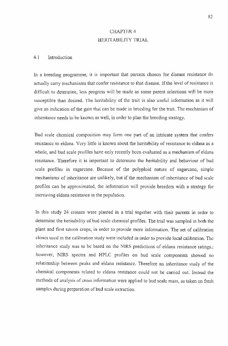
82

CHAPTER 4

HERITABILITY TRIAL

4.1 Introduction

In a breeding programme, it is important that parents chosen for disease resistance do

actually carry mechanisms that confer resistance to that disease. If the level of resistance is

difficult to determine, less progress will be made as some parent selections will be more

susceptible than desired. The heritability of the trait is also useful information as it will

give an indication of the gain that can be made in breeding for the trait. The mechanism of

inheritance needs to be known as well, in order to plan the breeding strategy.

Bud scale chemical composition may form one part of an intricate system that confers

resistance to eldana. Very little is known about the heritability of resistance to eldana as a

whole, and bud scale profiles have only recently been evaluated as a mechanism of eldana

resistance. Therefore it is important to determine the heritability and behaviour of bud

scale profiles in sugarcane. Because of the polyploid nature of sugarcane, simple

mechanisms of inheritance are unlikely, but if the mechanism of inheritance of bud scale

profiles can be approximated, the information will provide breeders with a strategy for

increasing eldana resistance in the population.

In this study 24 crosses were planted in a trial together with their parents in order to

determine the heritability of bud scale chemical profiles. The trial was sampled in both the

plant and first ratoon crops, in order to provide more information. The set of calibration

clones used in the calibration study were included in order to provide local calibration. The

inheritance study was to be based on the NIRS predictions of eldana resistance ratings.;

however, NIRS spectra and HPLC profiles on bud scale components showed no

relationship between peaks and eldana resistance. Therefore an inheritance study of the

chemical components related to eldana resistance could not be carried out. Instead the

methods of analysis of cross information were applied to bud scale mass, as taken on fresh

samples during preparation of bud scale extraction.

83

4.2 Materials and Methods

A biparental mating design of 24 pairs of parents was used, with no genotype being a

parent more than once. The crosses were chosen randomly from all available crosses,

excluding those with multiple possibilities of male parents in one female flower, or those

that could have undergone self-pollination. Eight crosses that were planted were lost due to

poor germination and assorted damage to young plants. The trial design was randomised

block. The list of 24 crosses and their parents are shown in Appendix 2, along with the

maximum number of offspring in each cross for those that were sampled.

The offspring were planted in three replications, with unique seedlings in each replication.

In other words, the seedlings were not replicated, but were divided into three groups. Each

offspring was represented by one stool. The parents were planted in an adjacent plot,

separate from the offspring, in order to prevent environmental correlation between parents

and offspring from affecting the heritability estimate. Each parent was planted in a 3 m

row. The calibration set was planted in three replications, between the parent rows and the

offspring plots. This was to provide a standard with which to compare the parents and

offspring. Each cultivar was planted in a 3 m row (Appendix 5).

The trial was planted in March 1996, cut back in February 1997, and sampled at 12

months. Each replication of the offspring was sampled at the same time as the adjoining

replication of the calibration set, in order to minimise time differences. The trial was then

cut back and allowed to ratoon. The ratoon crop was then sampled again at 12 months, in

the same way as the plant crop.

4.3 Data analysis

An analysis of variance can be used to determine heritability estimates if information on

individual offspring in each cross is available, where expected values of mean squares for

each type of variance are shown (Table 4.1).

84

Table 4.1: Sample ANOVA table for cross analysis to determine heritability

(Falconer and Mackay, 1996)

Source df Expected mean squares

Between crosses (n/2)-1 Vw + kVc

Within crosses (n/2)(k-l) Vw

Total (nk/2)-1

where n = number of parents, k = number of offspring within each cross, Vw = within cross

variance and Vc = between cross variance.

The following formulae can then be used:

Vw = Y2 VA + VE = Vp - Vc

Vc=Y2VA

where VA is an estimate of additive variance, Vp phenotypic vanance and VE error

variance. These formulae assume that dominance effects are zero. They allow heritability

to be calculated as VANp .

An intra-class correlation, rr, can also be calculated from these values, using the formulae

(Falconer and Mackay, 1996):

r\ = Vc / (Vc + Vw)

This correlation provides an estimate of repeatability. It represents the correlation between

repeated measures of the same cross, and therefore expresses the amount of variance in a

cross which is due to permanent differences between individuals in that cross.

A regression analysis can also be used to determine the heritability of a trait (Table 4.2),

using offspring as the dependent variable and parents as the independent variable. An F­

test will show whether the regression is significant or not.

Table 4.2: Sample regression analysis of crosses for determination of heritability

Source df

SS (due to regression) 1

SS(deviations from regression) n-2

T~~SS ~1

85

The regression coefficient, b, can be calculated from the sum of squares and sum of

products (Falconer and Mackay, 1996):

b = SP(xy)

SS(x)

where SP(xy) = ~xy - ( ~x~y / n ) and SS(x) = ~X2 - ( (~X)2 / n )

Because this is a biparental layout and the mid-parent value is being used in the regression

calculations, the regression coefficient is equal to the heritability estimate, h2.

Variance and regression methods will only agree if all gene effects are additive. Analyses

can also be carried out using only the male or female parent, with appropriate changes

made in the heritability calculations, in order to determine whether there are any parental

effects.

An important step is to examine the graph of the residuals of all analyses, in order to

determine whether there are any trends not accounted for by the linear analysis. Residual

graphs are plotted using (observed minus predicted values) as the y-axis values and the

predicted values as the x-axis values.

4.4 Results and Discussion

The heritability experiment contained both parents and offspring of a number of biparental

crosses. These were chosen on a random basis from the seed storage unit, therefore

representing a random sample of the breeding population. The field layout was designed so

that the parents were in a separate area from the offspring, therefore removing any

environmental covariance between parents and offspring that may come with field effects.

The calibration set was included in the same field to provide a sample set grown in the

same environment. Because of the small sample size of only seven stalks, individuals

could be sampled rather than a family mean. Parents had single seven-stalk samples taken

from them.

Not all the offspring that were planted survived in the field, due to poor growth and other

factors. The maximum number of offspring that were available for all of the 24 crosses was

86

21. For those crosses where additional offspring survived, samples were taken from all

available offspring, up to a total of 30. Analyses were carried out using different

combinations of numbers of crosses and offspring, in order to determine whether more

crosses with less offspring gave better information than less crosses with more offspring.

Appendix 2 gives the average bud scale mass for both parents and offspring from the 24

crosses.

The results for the heritability calculations are given in Table 4.3. The cross/offspring

column indicates the number of crosses and the number of offspring in each cross. The

24/24 and 24/30 options had missing values, due to some crosses having insufficient

offspring, but were included in the analysis for additional information. The analysis tables

are listed in Tables 4.4 and 4.5.

Table 4.3: Heritability estimates of bud scale mass of sugarcane crosses calculated by

variance and regression analysis, including repeatabilty estimates

Cross/offspringType of analysis

Repeatability CrI)Variance Regression

24/21 0.29** 0.28** 0.1524/24 0.28** 0.28** 0.14

Plant crop 24/30 0.26** 0.27** 0.1318/24 0.18** 0.10 0.0912/30 0.27** 0.17 0.1424/21 0.29** 0.30** 0.1524/24 0.25** 0.30** 0.13

Ratoon crop 24/30 0.22** 0.29** 0.1118/24 0.27** 0.29** 0.1412/30 0.31 ** 0.28* 0.16

** SIgnIficant at 1% level

* significant at 5% level

The heritability estimates determined by the two methods were similar, ranging from 0.18

to 0.31 in the cross analysis estimates, to 0.1 0 to 0.30 in the regression analysis estimates.

Narrow sense heritability seems to be low for the characteristic of bud scale mass while,

broad sense heritability, determined in the calibration analysis, seems to be even lower.

The crosses with higher number of crosses seemed to perform better than the crosses with

87

lower number of crosses and higher number of offspring. However, these results may be

misleading due to the relatively small differences between cross sizes, and the overall low

number of crosses that were available. In the analyses ofthe 24/24 and 24/30 cross options,

even with the large number of missing values, the results were significant.

Table 4.4: Summary of regression analyses for heritability study of bud scale mass of

sugarcane crosses

Crop Crosses OffspringMS MS

F ProbabilityRegression Residual

24 21 0.01033 0.00085 0.0021024 24 0.01010 0.00090 0.00290

Plant 24 30 0.00983 0.00092 0.0035018 24 0.00073 0.00080 0.3528712 30 0.00133 0.00100 0.2757924 21 0.01479 0.00102 0.0009024 24 0.01417 0.00086 0.00051

Ratoon 24 30 0.01380 0.00076 0.0003318 24 0.00989 0.00094 0.0050212 30 0.00714 0.00103 0.02479

Table 4.5: Summary of variance analyses for heritability study of bud scale mass of

sugarcane crosses

Crop Crosses Offspring MS Between MS Within F Probability24 21 0.02647 0.00577 3.91E -1124 24 0.02899 0.00592 2.58E -12

Plant 24 30 0.03214 0.00589 2.03E -1418 24 0.01903 0.00575 1.11E-0512 30 0.03083 0.00540 1.8E -0824 21 0.03386 0.00736 3.63E -1124 24 0.03325 0.00753 1. BE -10

Ratoon 24 30 0.03519 0.00754 1.17E -1118 24 0.03490 0.00731 2.46E -0912 30 0.04720 0.00717 5.41E -10

Repeatabilty of the heritability estimate, rI, was low, as expected, ranging from 0.09 to

0.16. No obvious pattern emerged in terms of which type of cross produced more

repeatable results, either those with higher numbers of crosses, or those with higher

numbers of offspring. The options with 24 crosses did, however, show a decrease in

repeatability with increase in number of offspring, i.e., with an increase in missing values.

88

This suggests that it may be better to use analyses that contain less crosses, if there are less

missing values in these crosses.

Examination of the residual plots is an important aspect of an analysis, in order to verify if

there are non-linear trends in the data, as well as other problems such as unequal variances.

The residual plots were drawn for the 24/21 (Figures 4.1 and 4.4), 24/24 (Figures 4.2 and

4.5) and 24/30 (Figures 4.3 and 4.6) options. They did not indicate any non-linear trends or

problems with unequal variances across the data.

Bud scale mass is correlated slightly with eldana, suggesting that bud size may be one

aspect of eldana resistance. Bud scale mass heritability estimates are significant, but fairly

low, suggesting that breeding for smaller bud size may be feasible, but difficult. Changes

in bud scale mass in the population would be slow, and, given the low correlation with

eldana resistance, would probably not improve eldana resistance to any great extent. It

would therefore not be feasible to introduce the screening of bud scale mass of clones to

the breeding programme and to attempt to breed for smaller bud size.

0.12

0.09 •0.06

•'"-; •="'0 0.03'{j; •~

~ •• •0 • •••• •• •• •• •-0.03 •••

-0.06

0 0.1 0.2 0.3 0.4 0.5

Predicted Y

Figure 4.1: Residual plot of 24 crosses/21 offspring plant crop in sugarcaneheritability study of bud scale mass

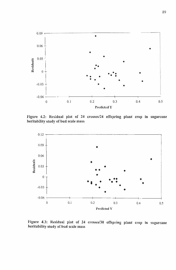
89

0.09•

0.06•

••

'" 0.03-; •="Q ••or;;+Q,l

~ 0 • +. •+ + • • •

+ + • +-0.03 • •

+

0.50.40.30.20.1

-0.06 -1-----+-----+-----+------+----­

oPredicted Y

Figure 4.2: Residual plot of 24 crosses/24 offspring plant crop in sugarcaneheritability study of bud scale mass

0.12

0.09 •0.06

•'" •-;="Q 0.03 •or;;

••Q,l •~

•0 •• •••• • • • •• •-0.03 • ••-0.06

0 0.1 0.2 0.3 0.4 0.5

Predicted Y

Figure 4.3: Residual plot of 24 crosses/30 offspring plant crop in sugarcaneheritability study of bud scale mass

90

0.09

•0.06

•• •0.03 •

'" • ••-; •• •::I"tl 0 •0(ii • •Q,l

~ • •• •• •-0.03 • •-0.06 •-0.09

0 0.1 0.2 0.3 0.4 0.5

Predicted Y

Figure 4.4: Residual plot of 24 crosses/2l offspring ratoon crop in sugarcaneheritability study of bud scale mass

0.09

•0.06

• •0.03

• • •'" • •-; ••::I::: 0 • ••'" •Q,l •~ • • •-0.03 • ,

•-0.06 •-0.09

0 0.1 0.2 0.3 0.4 0.5

Predicted Y

Figure 4.5: Residual plot of 24 crosses/24 offspring ratoon crop in sugarcaneheritability study of bud scale mass

91

O.09 ,... - -.- _ - _ _ _."··"·""1

•0.06

o

'" 0.03';

=:5!'"~

-0.03

•

•• •• • •• •• • •• •• • •• •

••

•

0.50.40.30.20.1

-0.06 +------j------+------+-----+-------I

oPredicted Y

Figure 4.6: Residual plot of 24 crosses/30 offspring ratoon crop in sugarcaneheritability study of bud scale mass

92

CHAPTERS

CONCLUSION

The original work carried out by Rutherford (Rutherford et al., 1993; Rutherford and van

Staden, 1996) suggested that there was a possibility of predicting eldana resistance in

sugarcane using the near infrared analysis of bud scale chemical profiles. However, this

work was carried out on a limited number of sample sets on an NIRS instrument that

exhibited baseshifts within sample sets and inconsistencies between sample sets. The

variation in NIRS readings between sample sets were thought to be due to environmental

effects, and that this could be overcome with the development of sufficient samples to

cover the range of conditions that influence the sampling of bud scale profiles.

The current study had two aims: to develop a global set so that accurate calibration

equations could be developed, and to study the environmental and genetic influences on

bud scale chemical profiles once the calibration was available. On the new NIRSystems

6500 instrument acquired during the study, various points came to note. Firstly, the

baseshifts between samples in the same sample set were no longer observed, suggesting

that the old NIRSystems 5000 instrument had a considerable error component even within

one session of sample scanning. Secondly, there were no longer differences between

sample sets, as the H distances indicated that all samples belonged to the same set.

However, the ability to calibrate from one sample set to another did not improve,

remaining negligible. The inability to predict samples from one sample set using the

calibration developed from another sample set on the old NIRS instrument was thought to

be due to the non-overlap of sample sets in multidimensional space, requiring a global

library to cover all types of sampling conditions in order to overcome the problem.

However, these differences were obviously caused by instrument error on the old NIRS

instrument as they were no longer evident on the new NIRS instrument.

Examination of spectra obtained on the new NIRS instrument revealed important details

that were not observable with the old instrument. The differences between spectra were

small, compared to the strength of the background signal caused by the solvents. These

differences were of the same order of magnitude as differences between spectra read

repeatedly on the same sample. Furthermore, spectra read on samples containing only the

solvents varied as widely as samples from different genotypes, and sometimes had

93

absorbance readings higher than those containing bud scale extracts. This suggested that if

there were differences between spectra from different genotypes they were being masked

by other factors, such as small differences between batches of solvents used, evaporation

rate of solvents from the solution during scanning, or temperature of the laboratory during

scanning. The NIRS technique was therefore not sensitive enough to detect valid

differences between samples.

Further study of the samples using HPLC revealed that the chemical profiles between

genotypes were different. Rutherford (Rutherford et al., 1993; Rutherford and van Staden,

1996) suggested that these chemical profiles were related to eldana resistance, but

correlations between eldana resistance ratings and chemical profiles in this study, as

determined by NIRS readings and HPLC, did not show this. It is possible that if the

chemicals represented by these peaks are associated with eldana resistance, that they are

not in the functional form needed to reflect this. Perhaps the preparation method destroys

the functional form of the chemical compounds, or some additional processing of the

chemical compounds takes place when damage by eldana larvae occurs. Nevertheless, the

results indicate that the method used here is insufficient to reveal differences in eldana

resistance between genotypes.

Bud scale mass has a relatively low correlation with eldana resistance, but G x E

interaction analyses and a heritability study were carried out on the bud scale fresh mass, in

order to evaluate the application of these techniques. The broad sense heritability estimate

from the G x E interaction analysis was 0.15, and the narrow sense heritability estimate

from the parent-offspring analysis was approximately 0.27, suggesting a slight relationship

between parent bud scale mass and offspring bud scale mass. The G x E interaction

analyses showed varying results depending on the method used. The ANOVA analysis

suggested that ages, sites and years had an effect on bud scale mass, while deviation from

maximum plot showed no significance for G x E interactions. The genotypes that were

selected as unstable were different depending on the method used to measure stability in

individual genotypes. The number of unstable genotypes also varied, with regression

analysis and rank order analysis revealing a number of unstable genotypes, while stability

variance and ecovalence, which produced similar results to one another, showed only two

unstable genotypes. In the rank order analysis, correction of data to remove genotype effect

reduced the number of unstable genotypes, suggesting that some of the G x E interaction

94

effect being measured came from the level of the character being studied. This was a more

reliable method than the uncorrected rank order analysis, and would be the preferred

analysis type of all those tried.

A number of problems were experienced in this study. Spectra from the old NIRS

instrument were misleading, suggesting legitimate differences between samples sets as the

reason for non-compatibility between sample sets. It is well-documented that calibration

development frequently needs a large number of samples to form a global set, to

incorporate all possible types of sampling conditions that may be encountered. These

conditions differ from the measurement of environmental effects on the characteristic

being studied. An example would be the differing moisture content of a sample affecting

the spectral detection of a chemical profile, even though moisture content is not of interest.

Samples containing all possible moisture contents in conjunction with the full range of the

characteristic being studied would have to be included in the calibration in order to

overcome the problem. The assumption was made that an effect of this type was involved

in making bud scale sample sets non-comparable. This assumption was proved incorrect

with the acquisition of the new NIRS instrument, as there were no such differences

between sample sets evident on the new instrument.

The baseshifts experienced on the old NIRS instrument were also cause for concern. The

effects were partially mitigated by the use of data transformations such as first and second

order derivatives, but the effects could not be removed completely. Baseshifts were not

merely a movement up or down on the y-axis, but also had a tilt effect where the baseshift

increased or decreased as wavelength increased. The new NIRS instrument fortunately did

not show any baseshifts, and the spectra showed great consistency of position between

sample sets as well as within sample sets. This suggested that the size of the error on the

old instrument was considerable.

Part of the reason for this study was to expand the number of samples available. The

original study consisted of a limited number of sample sets, which led to the false

impression that the chemicals being detected in the procedure were correlated with eldana

resistance. Based on knowledge of chemical interactions with insect pests, Rutherford

(Rutherford et al., 1993; Rutherford and van Staden, 1996) determined that the chemical

components he identified in the bud scale extracts could be connected to eldana resistance.

95

However, the chemical components, as detected by HPLC, showed no connection to

eldana resistance statistically. It is still possible that these chemicals do play a role in

eldana resistance, but they are not in the functional form for the important differences to be

detected. As bioassays seem to suggest a link with eldana feeding behaviour, this is a good

possibility (Rutherford, 1993).

The results obtained in this study, while not positive, are still important. It would have

meant an improvement to the breeding and selection programmes if a rapid screening

method for eldana resistance, unaffected by environment, could have been developed.

However, various results from this study suggest that eldana resistance is affected by the

environment, suggesting that whichever method is used to determine level of resistance,

trials would have to be repeated over a number of years to obtain an "average" eldana

resistance value. This conclusion is based on the HPLC results and the bud scale mass

differences between environments. Even though the HPLC profiles are not correlated with

eldana resistance, it is a possibility that the chemicals are associated with resistance in

other forms. Correlations between samples sets ranged from 0.52 to 0.90, suggesting that

some environments were quite similar with regard to HPLC profiles, and others could be

quite different. Similarly, the bud scale mass had a low correlation with eldana resistance,

but possibly has an effect on it. Bud scale mass correlations from different sites can be

almost zero, suggesting that results between sites differ widely. There is therefore a

possibility that eldana resistance itself is influenced by environment. This needs to be

investigated further as it would have a great impact on the determination of eldana

resistance in the future. Should eldana resistance vary with environment, it would have

disturbing implications for the performance of cultivars in the South African sugar

industry. Stability of resistance would then become as important a trait to breed and select

for as eldana resistance itself. At present, eldana resistance is evaluated by looking at the

average performance over a number of environments. This would have to be altered in

order to determine whether a genotype is consistently resistant over a number of

environments.

96

REFERENCES

Albrecht, K.A., Marten, G.C., Halgerson, J.L., and Wedin, W.F., 1987. Analysis of cell­

wall carbohydrates and starch in alfalfa by near infrared reflectance spectroscopy. Crop

Science 27: 586-588.

Amaya, A., Larrahondo, J., Oliveros, M., Rangel, H., Moreno, C., Viveros, e., Briceno, C.,

and Pena, W., 2001. A new proposal for clonal evaluation based on direct analysis and

NIR spectroscopy. Proc. International Society Sugar Cane Technologists 24: 524-526.

Ames, R.V., Norton, S.W., and Nguyen, H.H., 1989. Control of sugar polarization and

moisture using near infrared reflectance analysis. Proc. Australian Society Sugar Cane

Technologists 11: 246-252.

Anon, 2002. South African industry directory.

Arrnstrong, C.L., Parker, G.R, Pershing, lC., Brown, S.M., Sanders, P.R., Duncan, D.R.,

Stone, T., Dean, RA., DeBoer, D.L., Hart, J., Howe, A.R., Morrish, F.M., Pajeau, M.E.,

Peterson, W.L., Reich, BJ., Rodriguez, R., Santino, e.G., Sato, SJ., Schuler, W., Sims,

S.R., Stehling, S., Tarochione, LJ., and Fromme, M.E., 1995. Field evaluation of

European corn borer control in progeny of 173 transgenic corn events expressmg an

insecticidal protein from Bacillus thuringiensis. Crop Science 35: 550-557.

Atkinson, P.R., 1979. Distribution and natural hosts of Eldana saccharina Walker in Natal,

its oviposition sites, and feeding patterns. Proc. South African Sugar Technologists

Association 53: 111-115.

Atkinson, P.R., 1980. On the biology, distribution and natural host plants of Eldana

saccharina Walker (Lepidoptera: pyralidae). Journal Entomological Society SA 43: 171­

194.

Atkinson, P.R., 1982. Phenology of Eldana saccharina Walker in Natal and use of light

traps to monitor distribution and abundance. Proc. South African Sugar Technologists

Association 56: 90-94.

97

Atkinson, P.R., 1984. Seasonal cycle of eldana borer in relation to available control

measures. Proc. South African Sugar Technologists Association 58: 165-167.

Atkinson, P.R., Carnegie, AJ.M., and Smaill, RJ., 1981. A history of Eldana saccharina

Walker, in Natal. Proc. South African Sugar Technologists Association 55: 111-115.

Baer, RJ., Frank, J.F., Loewenstein, M., and Birth, G.S., 1983. Compositional analysis of

whey powders using near infrared diffuse reflectance spectroscopy. Journal Food Science

48: 959-961,989.

Ba1fourier, F., 01iveira, J.A., Charmet, G., and Arbones, E., 1997. Factorial regression

analysis of genotype by environment interaction in ryegrass populations, using both

isozyme and climatic data as covariates. Euphytica 98: 37-46.

Basford, K.E., and Cooper, M., 1998. Genotype x environment interactions and some

considerations of their implications for wheat breeding in Australia. Aust. J. Agric. Res.

49: 153-174.

Bastos, C.R., Pommer, C.V., and Nelli, EJ., 1980. Evaluation of sugarcane clones and its

relationships with their parents for resistance to stemborer. Proc. International Society

Sugar Cane Technologists 17: 1357-1364.

Berding, N., 1981. Improved flowering and pollen fertility in sugarcane under increased

night temperatures. Crop Science 21: 863-867.

Berding, N., Brotherton, G.A., LeBrocq, D.G., and Skinner, lC., 1989. Application of near

infrared reflectance (NIR) spectroscopy to the analysis of sugarcane in clonal evaluation

trials. Proc Australian Society Sugar Cane Technologists 11: 8-15.

Berding, N., Brotherton, G.A., LeBrocq, D.G., and Skinner, lC., 1991a. Near infrared

reflectance spectroscopy for analysis of sugarcane from clonal evaluation trials: 1. Fibrated

cane. Crop Science 31: 1017-1023.

98

Berding, N., Brotherton, G.A., LeBrocq, D.G., and Skinner, J.c., 1991b. Near infrared

reflectance spectroscopy for analysis of sugarcane from clonal evaluation trails: n.Expressed juice. Crop Science 31: 1024-1028.

Berding, N., and Skinner, J.c., 1980. Improvements of sugarcane fertility by modification

of cross-pollination environment. Crop Science 20: 463-467.

Bi, LV., Baudoin, J.P., Hau, B., and Mergeai, G., 1999. Development of high-gossypol

cotton plants with low-gossypol seeds using trispecies bridge crosses and in vitro culture of

seed embryos. Euphytica 106: 243-251.

Bialczyk, J., Lechowski, Z., and Libik, A., 1999. The protective action of tannins against

glasshouse whitefly in tomato seedlings. Journal Agricultural Science, Cambridge 133:

197-201.

Bissessur, D., Lim Shin Chong, L.C.Y., Ramnawaz, c., and Ramdoyal, K., 2001a.

Analysing G x E interaction in sugar cane using the Additive Main Effects and

Multiplicative Interaction (AMMI) model. Proc International Society Sugar Cane

Technologists 24: 506-511.

Bissessur, D., Tilney-Bassett, R.A.E., and Lim Shin Chong, L.c.Y., 200lb. Genetic

potential of sugarcane progenies grown in the extremely wet and dry environments in

Mauritius. Sugar Cane International: 5-10.

Bodnaryk, R.P., 1992. Leaf epicuticular wax, an antixenotic factor in Brassicaceae that

affects the rate and pattern of feeding of flea beetles, Phyllotreta cruciferae (Goeze).

Canadian Journal Plant Science 72: 1295-1303.

Bond, R.S., 1988. Progress in selecting for eldana resistance. Proc. South African Sugar

Technologists Association 62: 129-133.

Brett, P.G.C., 1954. The first ten years of sugarcane breeding in Natal. Proc. South African

Sugar Technologists Association 28: 141-145.

99

Brett, P.G.c., 1974. Early experiments on the artificial induction of flowering at Mount

Edgecombe. Proc. South African Sugar Technologists Association 48: 78-81.

Brett, P.G.C., and Harding, R.L., 1974. Artificial indu~tion of flowering in Natal. Proc.

International Society Sugar Cane Technologists 15: 55-66.

Brett, P.G.C., Harding, R.L., and Paxton, lC., 1975. Time and intensity of flowering as

influenced by certain temperatures and photoperiod treatments. Proc. South African Sugar

Technologists Association 49: 202-205.

Brown, A.H.D., Daniels, l, and Latter, B.D.H., 1969. Quantitative genetics of sugarcane.

n. Correlation analysis of continuous characters in relation to hybrid sugarcane breeding.

Theoretical and Applied Genetics 39: 1-10.

Burner, D.M., 1991. Cytogenetic analyses of sugarcane relatives (Andropogoneae:

Saccharinae). Euphytica 54: 125-133.

Burner, D.M., Grisham, M.P., and Legendre, B.L., 1993. Resistance of sugarcane relatives

injected with Ustilago scitaminea. Plant Disease 77: 1221-1223.

Burner, D.M., and Legendre, B.L., 1993. Chromosome transmission and meiotic stability

of sugarcane (Saccharum spp.) hybrid derivatives. Crop Science 33: 600-606.

Burner, D.M., and Webster, R.D., 1994. Cytological studies on North American species of

Saccharum (Poaceae: Andropogoneae). Sida 16(2): 233-244.

Butterfield, M.K., D'Hont, A., and Berding, N., 2001. The sugarcane genome: a synthesis

of current understanding, and lessons for breeding and technology. Proc. South African

Sugar Technologists Association 75: 1-5.

Butterfield, M.K., and Thomas, D.W., 1996. Sucrose, yield and disease resistance

characteristics of sugarcane varieties under test in the SASEX selection programme. Proc.

South African Sugar Technologists Association 70: 103-105.

100

Camegie, AJ.M., 1974. A recrudescence of the borer Eldana saccharina Walker

(Lepidoptera: pyralidae). Proc. South African Sugar Technologists Association 48: 107­

110.

Camegie, A.J.M., 1981. Combating Eldana saccharina Walker: a progress report. Proc.

South African Sugar Technologists Association 55: 116-119.

Camegie, AJ.M., 1982. Current research programme against Eldana saccharina Walker

(Lepidoptera: pyralidae). Proc. South African Sugar Technologists Association 56: 95-98.

Camegie, AJ.M., Conlong, D.E., and Graham, D.Y., 1985. Recent introductions of

parasitoids against Eldana saccharina Walker (Lepidoptera: pyralidae). Proc. South

African Sugar Technologists Association 59: 160-163.

Camegie, AJ.M., and Leslie, G.W., 1979. Attempts at the biological control of Eldana

saccharina Walker (Lepidoptera: pyralidae). Proc. South African Sugar Technologists

Association 53: 116-119.

Camegie, AJ.M., Leslie, G.W., and Hindley, M.E.G., 1976. Incidence and spread of the

borer Eldana saccharina Walker (Lepidoptera: pyralidae). Proc. South African Sugar

Technologists Association 50: 34-39.

Camegie, A.J.M., and Leslie, G.W., 1990. Eldana saccharina (Lepidoptera: pyralidae): ten

years oflight trapping. Proc. South African Sugar Technologists Association 64: 107-110.

Camegie, AJ.M., and Smaill, RJ., 1980. The incidence of moth borers in South African

sugarcane during the 1978/9 season. Proc. South African Sugar Technologists Association

54: 154-157.

Camegie, AJ.M., and Smaill, RJ., 1982. Pre-trashing of sugarcane as a means of

combating the borer Eldana saccharina Walker. Proc. South African Sugar Technologists

Association 56: 78-81.

101

Casler, M.D., 1982. Genotype x environment interaction bias to parent-offspring

regression heritability estimates. Crop Science 22:540-542.

Cassalett, C., Viveros, C.A., and Pizza, L.F., 1996. Self-pollination in sugarcane hybrids,

Saccharum sp. Proc International Society Sugar Cane Technologists 22: 312-315.

Cassim, T.N., Monosi, B.B., Meyer, G.M., Botha, F.C., Rutherford, R.S., and Huckett,

B.1., 1999. Transcriptional and translational expression of a wild type bacterial toxin gene

sequence in transgenic sugarcane. Proc. South African Sugar Technologists Association

73: 96-99.

Chen, W.H., Huang, Y.J., Shen, 1.S., and Shih, S.C., 1983. Utilisation of Miscanthus

germplasm in sugar cane breeding in Taiwan. Proc. International Society Sugar Cane

Technologists 18: 641-649.

Chrispeels, MJ., and Raikhel, N.V., 1991. Lectins, lectin genes, and their role in plant

defense. Plant Cell 3: 1-9.

Cochereau, P., 1982. Observations on the borer Eldana saccharina Walker (Lep.

Pyralidae) in maize and sugarcane in Ivory Coast. Proc. South African Sugar

Technologists Association 56: 82-84.

Cole, R.A., Phelps, K., Ellis, P.R., Hardman, lA., and Rollason, S.A., 1988. Further

studies relating chlorogenic acid concentration in carrots to carrot fly damage. Annals

Applied Biology 112: 13.

Conlong, D.E., 1997. Eldana saccharina (Lepidoptera: pyralidae) in Africa: are there

different biotypes? Proc South African Sugar Technologists Association 71: 83.

Conlong, D.E., and Kasl, B., 2000. Stimulo-deterrent diversion to decrease infestation in

sugarcane by Eldana saccharina (Lepidoptera: pyralidae). Proc South African Sugar

Technologists Association 74: 212-213.

102

Conlong, D.E., and Kasl, B., 2001. Stimulo-deterrent diversion of Eldana saccharina

(Lepidpotera: pyralidae) and Xanthopimpla stemmator (Hymenoptera: ichneumonidae) ­

preliminary results. Proc. South African Sugar Technologists Association 75: 180-182.

Cornelius, P.L., and Crossa, J., 1999. Prediction assessment of shrinkage estimators of

multiplicative models for multi-environment cultivar trials. Crop Science 39: 998-1009.

Cotterill, P.P., and James, lW., 1984. Number of offspring and plot sizes required for

progeny testing. Silvae Genetica 33: 203-209.

Czapla, T.H., and Lang, B.A., 1990. Effect of plant lectins on the larval development of

European corn borer (Lepidoptera: pyralidae) and Southern corn rootworm (Coleoptera:

chrysomelidae). Journal Economic Entomology 83: 2480-2485.

Dala1, R.C., and Henry, RJ., 1986. Simultaneous determination of moisture, orgamc

carbon, and total nitrogen by near infrared reflectance spectrophotometry. Soil Science

Society of America Journal 50: 120-123.

Davidson, L.G., 1968. Correlation of rind hardness and fibre III sugarcane. Proc.

International Society Sugar Cane Technologists 13: 1723-1728.

Davies, A.M.C., Coxon, D.T., Gavrel, G.M., and Wright, DJ., 1985. Determination of

starch and lipid in pea flour by near infrared reflectance analysis. The effect of pea

genotype on starch and lipid content. Journal Science and Food Agriculture 36: 49-54.

De Sousa-Vieira, 0., and Milligan, S.B., 1999. Intrarow plant spacing and family x

environment interaction effects on sugarcane family evaluation. Crop Science 39: 358-364.

Denis, J-B., Piepho, H-P., and van Eeuwijk, F.A., 1997. Modeling expectation and

variance for genotype by environment data. Heredity 79: 162-171.

Dick, l, 1945. Some data on the biology of the sugarcane borer. Proc. South African Sugar

Technologists Association 19: 75-79.

103

Diz, D.A., and Schank, S.C., 1995. Heritabilities, genetic parameters and response to

selection in pearl millet x elephantgrass hexaploid hybrids. Crop Science 35: 95-101.

Dudley, lW., and Moll, R.H., 1969. Interpretation and use of estimates of heritability and

genetic variances in plant breeding. Crop Science 9: 257-262.

Dull, G.G., and Giangiacomo, R., 1984. Determination of individual simple sugars in

aqueous solution by near infrared spectrophotometry. Journal Food Science 46: 1601­

1603.

Dumoulin, RD., Azais, B.P., and Guerain, J.T., 1987. Determination of sugar and ethanol

content in aqueous products of molasses distilleries by near infrared spectrophotometry.

Journal Food Science 52: 626-630.

Dyke, G.V., Lane, P.W., and Jenkyn, IF., 1995. Sensitivity (stability) analysis of multiple

variety trials, with specific reference to data expressed as proportions or percentages. Expl

Agric. 31: 75-87.

Ethirajan, A.S., Santhakumariamma, P.N., and Velayutham, N., 1977. Studies on

successive inbred generations of selected sugarcane cultivars. Proc. International Society

Sugar Cane Technologists 16: 269-273.

Falco, M.C., and Si1va-Falco, M.C., 2001. Searching for insect resistance genes III

sugarcane. Proc. International Society Sugar Cane Technologists 24: 547-550.

Falconer, D.S., and Mackay, T.F.C., 1996. Introduction to quantitative genetics. Fourth

Edition. Longman Scientific and Technical. Pp 160-181.

Fernandez, G.c.J., and Miller, J.C., 1985. Estimation of heritability by parent-offspring

regression. Theor Appl Genet 70: 650-654.

Finlay, K.W., and Wilkinson, G.N., 1963. The analysis of adaptation in a plant breeding

programme. Aust. l Agric. Res, 14: 742-754.

104

Fitt, G.P., 2001. Development and implementation of transgenic Bt cottons in Australia.

Proc. International Society Sugar Cane Technologists 24: 34-37.

Fonseca, C.E.L., Hansen, lL., Thomas, E.M., Pell, A.N., and Viands, D.R., 1999. Near

infrared reflectance spectroscopy prediction and heritability of neutral detergent-soluble

fiber in alfalfa. Crop Science 39: 1265-1270.

Frensham, A., Cullis, B., and Verbyla, A., 1997. Genotype by environment variance

heterogeneity in a two-stage analysis. Biometrics 53: 1373-1383.

Frensham, A.B., BaIT, A.R., Cullis, B.R., and Pelham, S.D., 1998. A mixed model analysis

of 10 years of oat evaluation data: use of agronomic information to explain genotype by

environment interaction. Euphytica 99: 43-56.

Galvez, G., 1980. The genotype-environment interaction III experiments of sugarcane

variety trials (Saccharum spp): comparison of three stability methods. Proc. International

Society Sugar Cane Technologists 17: 1152-1160.

Gauch, H.G., and Furnas, R.E., 1991. Statistical analysis of yield trials with MATMODEL.

Agronomy Journal 83: 916-920.

Gibson, P.T., 1996. Correcting for inbreeding in parent-offspring regression estimates of

heritability with non-additive and genotype x environment effects present. Crop Science

36: 594-600.

Gilmour, A.R., Thompson, R., and Cullis, B.R., 1995. Average information REML: an

efficient algorithm for variance parameter estimation in linear mixed models. Biometrics

51: 1440-1450.

Gimelfarb, A., 1986. Offspring-parent genotypic regression: how linear is it? Biometrics

42: 67-71.

Girling, DJ., 1971. Eldana saccharina Wlk (Lepidoptera: pyralidae), a pest of sugarcane

in East Africa. Proc. International Society Sugar Cane Technologists 14: 429-434.

105

Givens, DJ., and Deaville, E.R., 1999. The current and future role of near infrared

reflectance spectroscopy in animal nutrition: a review. Australian Journal Agricultural

Research 50: 1131-1145.

Gogel, BJ., Cullis, B.R., and Verbyla, A.P., 1995. REML estimation of multiplicative

effects in multi-environment variety trials. Biometrics 51: 744-749.

Gravois, K.A., and Bernhardt, 2000. Herita1:;>ility and genotype x environment interactions

for discolored rice kernels. Crop Science 40: 314-318.

Gravois, K.A., and Milligan, S.B., 1992. Genetic relationships between fiber and

sugarcane yield components. Crop Science 32: 62-67.

Green, T.R., and Ryan, C.A., 1972. Wound-induced proteinase inhibitor in plant leaves: a

possible defense mechanism against insects. Science 175: 776-777.

Griggs, T.C., Lobos, K.B., and Kingery, P.E., 1999. Digestibility analysis of undried,

unground and dry ground herbage by near-infrared reflectance spectroscopy. Crop Science

39: 1164-1170.

Grisham, M.P., Burner, D.M., and Legendre, B.L., 1992. Resistance to the H strain of

sugarcane mosaic virus among wild forms of sugarcane and relatives. Plant Disease 76:

360-362.

Habib, M., Bentley, G.A., Staunton, S., Atherton, P.G., and Henderson, C., 2001.

Application of NIR cane analysis technology to small consignments of cane in Fiji. Proc.

International Society Sugar Cane Technologists 24: 59-65.

Harville, D.A., 1977. Maximum likelihood approaches to variance component estimation

and to related problems. Journal of the American Statistical Association 72: 320-340.

Heathcote, RJ., 1984. Insecticide testing against Eldana saccharina Walker. Proc. South

African Sugar Technologists Association 58: 154-158.

106

Heinz, DJ., 1980. Thailand S spontaneum hybrid progeny as a new germplasm source in

Hawaii. Proc. International Society Sugar Cane Technologists 27: 1347-1356.

Hensley, S.D., Fanguy, H.P., and Giamalva, MJ., 1977. The role of varietal resistance in

control of the sugarcane borer, Diatraea saccharalis (Lepidoptera: pyralidae) in Louisiana.

Proc. International Society Sugar Cane Technologists 16: 517-522.

Hill, W.G., and Nicho1as, F.W., 1974. Estimation of heritability by both regression of

offspring on parent and intra-class correlation of sibs in one experiment. Biometrics 30:

447-468.

Hogarth, D.M., 1968. A review of quantitative genetics in plant breeding with particular

reference to sugarcane. Journal Australian Agricultural Science 34: 108-120.

Hogarth, D.M., 1971. Quantitative inheritance studies in sugarcane. 1. Estimation of

variance components. Australian Journal Agricultural Research 22: 93-102.

Hogarth, D.M., 1977. Quantitative inheritance studies. Ill. The effect of competition and

violation of genetic assumptions on estimates of genetic variance components. Australian

Journal Agricultural Research 28: 257-268.

Hogarth, D.M., Wu, K.K., and Heinz, DJ., 1981. Estimating genetic variance in sugarcane

using a factorial cross design. Crop Science 21: 21-25.

Hohls, T., 1995. Analysis of genotype-environment interactions. South African Journal of

Science 91: 121-124.

Hohls, T., Shanahan, P.E., Clarke, G.P., and Gevers, H.D., 1995. Genotype x environment

interactions in a 10 x 10 diallel cross of quality protein maize (Zea mays L.). Euphytica 84:

209-218.

Huehn, M., 1990. Nonparametric measures of phenotypic stability. Part I: theory.

Euphytica 47: 189-194.

107

Huijbregts, A.W.M., de Regt, A.H., and Gijssel, P.D., 1996. Determination of some quality

parameters in sugar beet by near infrared spectrometry (NIRS). Communications Soil

Science and Plant Analysis 27(5-8): 1549-1560.

Hymowitz, T., Dudley, lW., Collins, F.I., and Brown, C.M., 1974. Estimations of protein

and oil concentration in corn, soybean, and oat seed by near infrared light reflectance. Crop

Science 14: 713-716.

Iizuka, K., and Aishima, T., 1997. Soy sauce classification by geographic region based on

NIR spectra and chemometrics pattern recognition. Journal Food Science 62: 101-104.

Irvine, J.E., 1977. Identification of cold tolerance in Saccharum and related genera through

refrigerated freeze screening. Proc. International Society Sugar Cane Technologists 16:

147-156.

Jalaluddin, M., and Harrison, S.A., 1993. Repeatability of stability estimators for grain

yield in wheat. Crop Science 33: 720-725.

Johnson, H.W., Robinson, H.F., and Comstock, R.E., 1955. Estimates of genetic and

environmental variability in soybeans. Agronomy Journal 47: 314-318.

Jones, P.N., Ferraris, R., and Chapman, L.S., 1993. A technique for minimizing

confounding of genotype x year and genotype x crop type effects in sugarcane. Euphytica

67: 199-204.

Kang, M.S., and Martin, F.A., 1987. A reVIew of important aspects of genotype­

environmental interactions and practical suggestions for sugarcane breeders. Journal

American Society Sugar Cane Technologists 7: 36-38.

Kang, M.S., and Miller, J.D., 1984. Genotype x environment interactions for cane and

sugar yield and their implications in sugarcane breeding. Crop Science 24: 435-440.

108

Kang, M.S., Miller, lD., and Tai, P.Y.P., 1984. Clonal and individual repeatability of

agronomic traits in sugarcane. Journal American Society Sugar Cane Technologists 3: 22­

27.

Karowe, D.N., 1989. Differential effect of tannic acid on two tree-feeding Lepidoptera:

implications for theories of plant anti-herbivore chemistry. Oecologia 80: 507-512.

King, A.G., 1989. An assessment of the loss in sucrose yield caused by the stalk borer,

Eldana saccharina, in Swaziland. Proc. South African Sugar Technologists Association

63: 197-201.

Klenke, J.R., Russell, W.A., and Guthrie, W.D., 1986. Recurrent selection for resistance to

European corn borer in a corn synthetic and correlated effects on agronomic traits. Crop

Science 26: 864-868.

Klocke, lA., and Chan, E.G., 1982. Effects of cotton condensed tannin on feeding and

digestion in the cotton pest, Heliothis zea. Journal Insect Physiology 28: 911-915.

Ladd, S.L., Heinz, DJ., and Meyer, H.K., 1974. Control of sugarcane (Saccharum spp)

smut disease (Ustilago scitaminea) through breeding and selection of resistance clones.

Proc. International Society Sugar Cane Technologists 15: 36-45.

Lanza, E., and Li, W., 1984. Application for near infrared spectroscopy for predicting the

sugar content of fruit juices. Journal Food Science 49: 995-998.

Larrahondo, lE., Palau, F., Navarrete, A., and Ramirez, C., 2001. Applications of near

infrared spectroscopy in the sugarcane industry of Columbia. Proc. International Society

Sugar Cane Technologists 24: 163-165.

Lee, SJ., Jeon, 1.l, and Harbers, L.H., 1997. Near-infrared reflectance spectroscopy for

rapid analysis of curds during cheddar cheese making. Journal Food Science 62: 53-56.

Lege, K.E., Smith, C.W., and Cothren, IT., 1992. Genotypic and cultural effects on

condensed tannin concentration of cotton leaves. Crop Science 32: 1024-1028.

109

Legendre, B.L., 1989. Use of feral germplasm for sugarcane improvement in Louisiana.

Proc. International Society Sugar Cane Technologists 20: 883-891.

Leslie, G.W., 1982. A study of egg predators of Eldana saccharina Walker (Lepidoptera:

pyralidae). Proc. South African Sugar Technologists Association 56: 85-87.

Leslie, G.W., 1993. Dispersal behaviour of neonate larvae of the pyralid sugarcane borer

Eldana saccharina. Proc. South African Sugar Technologists Association 67: 122-126.

Leslie, G.W., 1994. Observations on crop damage and larval popu1ations of the pyralid

borer Eldana saccharina in sugarcane varieties NC0376 and NIL Proc. South African

Sugar Technologists Association 68: 12-15.

Leslie, G.W., 2001. Field-scale insecticide trials against the sugarcane borer Eldana

saccharina (Lepidoptera: pyralidae) in South Africa: a preliminary assessment. Proc.

International Society Sugar Cane Technologists 24: 395-397.

Li, W., Goovaerts, P., and Meurens, M., 1996. Quantitative analysis of individual sugars

and acids in orange juices by near-infrared spectroscopy of dry extract. Journal Agriculture

and Food Chemistry 44: 2252-2259.

Li, H.W., and Price, S., 1965. Chromosome numbers of some noble sugarcane clones.

Proc. International Society Sugar Cane Technologists 12: 884-886.

Long, BJ., Dunn, G.M., Bowman, lS., and Routly, D.G., 1977. Relationship of

hydroxamic acid content in corn and resistance to the corn leaf aphid. Crop Science 17: 55­

58.

Lukefahr, MJ., and Houghtaling, lE., 1969. Resistance of cotton strains with high

gossypol content to Heliothis spp. Journal Economic Entomology 62: 588-591.

Lukefahr, MJ., and Martin, D.F., 1966. Cotton-plant pigments as a source of resistance to

the bollworm and tobacco budworm. Journal Economic Entomology 59: 176-179.

110

Macnab, AJ., and Gagnon, R.E., 1996. Potential sources of discrepancies between living

tissue near infrared algorithms. Analytical Biochemistry 235: 375-377.

Manly, B.FJ., 1986. Multivariate statistical methods. Chapman and Hall, London, New

York. Ch 4: pp 42-58.

Manuwoto, S., and Scriber, lM., 1986. Effects of hydrolysable and condensed tannin on

growth and development of two species of polyphagous lepidoptera: Spodoptera eridania

and Callosamia promethean. Oecologia 69: 225-230.

Marten, G.C., Brink, G.E., Buxton, D.R., Halgerson, l1., and Homstein, lS., 1984. Near

infrared reflectance spectroscopy analysis of forage quality in four legume species. Crop

Science 24: 1179-1182.

Mazodze, R., Nyanhete, C., and Chidoma, S., 1999. First outbreak of Eldana saccharina

(Lepidoptera: pyralidae) in sugarcane in the South-East Lowveld of Zimbabwe. Proc.

South African Sugar Technologists Association 73: 107-111.

McCulloch, 1989. The feasibility of cutting rainfed cane at a younger age on the North

coast of Natal. Proc. South African Sugar Technologists Association 63: 206-208.

Meyer, lH., 1983. Rapid determination of nitrogen in cane leaves. Proc. South African

Sugar Technologists Association 57: 109-112.

Meyer, J.H., 1989. Rapid simultaneous rating of soil texture, organic matter, total nitrogen

and nitrogen mineralisation potential by near infrared reflectance. South African Journal

Plant and Soil 6: 59-63.

Meyer, J.H., and Wood, R.A., 1988. Rapid analysis of cane juice by near infrared

reflectance. Proc. South African Sugar Technologists Association 62: 203-207.

Milligan, S.B., 1994. Test site allocation within and among stages of a sugarcane breeding

program. Crop Science 34: 1184-1190.

111

Milligan, S.B., Gravois, K.A., Bischoff, K.P., and Martin, F.A., 1990. Crop effects on

broad-sense heritabilities and genetic variances of sugarcane yield components. Crop

Science 30: 344-349.

. Morrell, C.H., 1998. Likelihood ratio testing of variance components in the linear mixed­

effects model using restricted maximum likelihood. Biometrics 54: 1560-1568.

Murray, TJ., 1997. Chairman's Report. Pg 3. Annual Report, South African Sugar

Association Experiment Station.

Natarajan, RV., Krishnamurthy, T.N., and Thuljaram R., 1., 1967. Relative effects of

parents on some economic characters in sugarcane. Euphytica 16: 104-108.

Nuss, KJ., 1977. Synchronisation of flowering to implement a proven cross breeding

system in sugarcane. Proc. International Society Sugar Cane Technologists 16: 111-119.

Nuss, K.J., 1980. Effect of photoperiod and temperature on initiation and development of

flowers in sugarcane. Proc. International Society Sugar Cane Technologists 17: 486-493.

Nuss, KJ., 1982. Flowering of sugarcane in a photoperiod house from 1971 to 1981. Proc.

South African Sugar Technologists Association 56: 140-142.

Nuss, KJ., 1991. Screening sugarcane varieties for resistance to eldana borer. Proc. South

African Sugar Technologists Association 65: 92-95.

Nuss, K.J., 1998. Aspects considered in the search for new farms for the Experiment

Station. Proc. South African Sugar Technologists Association 72: 42-45.

Nuss, KJ., and Atkinson, P.R., 1983. Methods used to measure the susceptibility of

sugarcane varieties to attack by Eldana saccharina Walker. Proc. South African Sugar

Technologists Association 57: 92-94.

112

Nuss, KJ., Bond, R.S., and Atkinson, P.R., 1986. Susceptibility of sugarcane to the borer

Eldana saccharina Walker and selection for resistance. Proc. South African Sugar

Technologists Association 60: 153-155.

Osborne, B.G., 1983. Investigation of the perfonnance of an improved calibration for the

detennination of protein in UK home-grown wheat by near infrared reflectance analysis.

Journal Science and Food Agriculture 34: 1441-1443.

Osborne, B.G., Douglas, S., Fearn, T., and Willis, K.H., 1982. The development of

universal calibrations for measurement of protein and moisture in UK home-grown wheat

by near infrared reflectance analysis. Journal Science and Food Agriculture 33: 736-740.

Panje, R.R., 1971. The role of Saccharum spontaneum in sugarcane breeding. Proc.

International Society Sugar Cane Technologists 14: 217-223.

Paxton, R.H., 1982. Eldana borer (Eldana saccharina): the results of surveys. Proc. South

African Sugar Technologists Association 56: 99-103.

Perlak, F.J., Stone, T.B., Muskopf, Y.M., Peterson, L.l, Parker, G.B., McPherson, S.A.,

Wyman, l, Love, S., Reed, G., Biever, D., and Fischoff, D.A., 1993. Genetically improved

potatoes: protection from damage by Colorado potato beetles. Plant Molecular Biology 22:

313-321.

Pham, H.G., and Kang, M.S., 1988. Interrelationships among and repeatability of several

stability statistics estimated from international maize trials. Crop Science 28: 925-928.

Powell, W., Caligari, P.D.S., Phillips, M.S., and Jinks, lL., 1986. The measurement and

interpretation of genotype by environment interaction in spring barley (Hordeum vulgare).

Heredity 56: 255-262.

Rahman, M.A., and Saad, M.S., 2000. Estimation of additive, dominance and digenic

epistatic interaction effects for certain yield characters in Vigna sesquipedalis Fruw.

Euphytica 114: 61-66.

113

Reeves, lB., 1997. Concatenation of near- and mid-infrared spectra to improve

calibrations for determining forage composition. Journal Agricultural and Food Chemistry

45: 1711-1714.

Rice, lS., and Brown, R.B., 1985. Clonal interactions with harvests and years for quality

components in intermediate wheatgrass. Crop Science 25: 47-50.

Roach, B.T., 1968a. Cytological studies III Saccharum, chromosome transmission m

interspecific and intergeneric crosses. Proc. International Society Sugar Cane

Technologists 13: 901-920.

Roach, RT., 1968b. Quantitative effects of hybridisation in Saccharum officinarum x

Saccharum spontaneum crosses. Proc. International Society Sugar Cane Technologists 13:

939-954.

Roach, RT., 1971. Nobilisation of sugarcane. Proc. International Society Sugar Cane

Technologists 14: 206-216.

Roach, B.T., 1986. Evaluation and breeding use of sugarcane germplasm. Proc.

International Society Sugar Cane Technologists 19: 492-502.

Roach, RT., 1989. A programme for sugarcane improvement from genetic diversity:

background and preliminary results. Proc. International Society Sugar Cane Technologists

20: 900-909.

Robert, N., 1997. Structuring genotype x environment interaction for quality traits in bread

wheat, in two multi-location series of trials. Euphytica 97: 53-66.

Robertson, A., 1957. Optimum group SIze m progeny testing and family selection.

Biometrics 13: 442-450.

Robinson, D.L., 1987. Estimation and use of variance components. The Statistician 36: 3­

14.

114

Rodriguez, I.R., and Miller, G.L., 2000. Using near infrared reflectance spectroscopy to

schedule nitrogen applications on dwarf-type bermudagrasses. Agronomy Journal 92: 423­

427.

Rowe, D.E., and Brink, G.E., 1993. Heritabilities and genetic correlations of white clover

clones grown in three environments. Crop Science 33: 1149-1152.

Rutherford, R.S., 1993. Physiological and biochemical aspects of the interaction between

sugarcane and the larval borer Eldana saccharina Walker (Lepidoptera: Pyralidae). PhD

thesis, University of Natal.

Rutherford, R.S., Meyer, J.H., Smith, G.S., and van Staden, J., 1993. Resistance to Eldana

saccharina (Lepidoptera: pyralidae) in sugarcane and some phytochemical correlations.

Proc. South African Sugar Technologists Association 67: 82-87.

Rutherford, R.S., and van Staden, J., 1996. Towards a rapid near infrared technique for

prediction of resistance to sugarcane borer Eldana saccharina Walker (Lepidoptera:

pyralidae) using stalk surface wax. Journal Chemical Ecology 22: 681-694.

Saeed, M., and Francis, c.A., 1984. Association of weather variables with genotype x

environment interactions in grain sorghum. Crop Science 24: 13-16.

Saxena, KC., and Okech, S.H., 1985. Role of plant volatiles in resistance of selected rice

varieties to brown planthopper, Nilaparvata lugens (Stal) (Homoptera: delphacidae).

Journal Chemical Ecology 11: 1601-1616.

Schaffler, KJ., 2001 a. Automated routine analysis of quality parameters in sugarcane

juices and molasses by NIR. Proc. International Society Sugar Cane Technologists 24:

143-146.

Schaffler, 2001b. At-line analysis of shredded cane using a Foss direct-light NIR:

preliminary results prior to factory tests. Proc. International Society Sugar Cane

Technologists 24: 147-150.

115

Schaffler, KJ., Dunsmore, A.N., and Meyer, J.H., 1993. Rapid analysis of sugar products

by near infrared spectroscopy. Proc. South African Sugar Technologists Association 67:

222-229.

Schoonhoven, L.M., 1982. Biological aspects of antifeedants. Entomologia Experimentalis

and Applicata 31: 57-69.

Shafii, B., Mahler, K.A., Price, WJ., and Auld, D.L., 1992. Genotype x environment

interaction effects on winter rapeseed yield and oil content. Crop Science 32: 922-927.

Shany, S., Gestetner, B., Birk, Y., and Bondi, A., 1970. Effect of lucerne saponins on

larval growth and their detoxification by various sterols. Journal Science and Food

Agriculture 21: 508-510.

Shenk, J.S., Fales, S.L., and Westerhaus, M.O., 1993. Using near infrared reflectance

product library files to improve prediction accuracy and reduce calibration costs. Crop

Science 33: 578-581.

Shenk, J.S., and Westerhaus, M.O., 1985. Accuracy ofNIRS instruments to analyse forage

and grain. Crop Science 25: 1120-1122.

Shenk, J.S., and Westerhaus, M.O., 1991a. Population definition, sample selection, and

calibration procedures for near infrared reflectance spectroscopy. Crop Science 31: 469­

474.

Shenk, J.S., and Westerhaus, M.O., 1991 b. Population structuring of near infrared spectra

and modified partial least squares regression. Crop Science 31: 1548-1555.

Shenk, J.S., and Westerhaus, M.O., 1991c. New standardisation and calibration procedures

for NIRS analytical systems. Crop Science 31: 1694-1696.

Shenk, J.S., and Westerhaus, M.O., 1993. Near infrared reflectance analysis with single­

and multiproduct calibrations. Crop Science 33: 582-584.

116

Skinner, J.c., 1974. Rind hardness and fibre content. Proc. International Society Sugar

Cane Technologists 15: 153-167.

Smaill, RJ., 1978. Mill yard surveys of the lepidopterous cane borers Eldana saccharina

Walker and Sesamia calamistis. Proc. South African Sugar Technologists Association 52:

139-142.

Smaill, R.1., and Carnegie, A.1.M., 1979. The situation regarding Eldana borer (E

saccharina Walker) during 1978/9 and assessments of crop loss. Proc. South African

Sugar Technologists Association 53: 108-110.

Smith, M.C., Cornish, M.A., and Mackay, 1.1., 1990. An analysis of genetic variation in

sugar beet (Beta vulgaris L.) using an augmented biparental (ABIP) mating design. Ann.

AppI. BioI. 116: 583-590.

Smith, K.F., and Kearney, G.A., 2000. The distribution of errors associated with genotype

and environment during the prediction of the water-soluble carbohydrate concentration of

perennial ryegrass cultivars using near infrared reflectance spectroscopy. Aust. 1. Agric.

Res. 51: 481-486.

Smith, J.D., and Kinman, M.L., 1965. The use of parent-offspring regressIOn as an

estimator of heritability. Crop Science 5: 595-596.

Smith, K.F., Simpson, R.1., and Armstrong, R.D., 1998. Using near infrared reflectance

spectroscopy to estimate the nutritive value of senescing annual ryegrass (Lolium rigidum):

a comparison of calibration methods. Australian Journal Experimental Agriculture 38: 45­

54.

Sneller, C.H., Kilgore-Norquest, L., and Dombek, D., 1997. Repeatability of yield

statistics in soybean. Crop Science 37: 383-390.

Soni, S.K., and Finch, S., 1979. Laboratory evaluation of sulphur-bearing chemicals as

attractants for larvae of the onion fly, Delia antiqua (Meigen)(Diptera: Anthomyiidae).

Bulletin Entomological Research 69: 291-298.

117

Srivastava, S., and Srivastava, H.M., 2001. Genomic characterization of Saccharum

species hybrids of subtropical India: preferential chromosome pairing. Proc. International

Society Sugar Cane Technologists 24: 520-523.

Starr, C., Morgan, A.G., and Smith, D.B., 1981. An evaluation of near infrared reflectance

analysis in some plant breeding programmes. Journal Agricultural Science 97: 107-118.

Sumith, D., and Abeysiriwardena, Z., 2001. Statistical analysis of on-farm yield trials for

testing adaptability of rice. Euphytica 121: 215-222.

Sversat, e.B., Verma, L.R., and French, A.D., 1987. Sugarcane analysis usmg near

infrared spectroscopy. Transactions ASAE 30: 255-258.

Swallow, W.H., and Monahan, IF., 1984. Monte Carlo companson of ANOVA,

MNQUE, REML, and ML estimators of variance components. Technometrics 25: 47-57.

Tai, G.C.C., 1999. Canonical variate analysis of genotype x environment interactions. Can.

J. Plant Sci. 79: 427-431.

Tai, P.Y.P., Rice, E.R., Chew, V., and Miller, J.D., 1982. Phenotypic stability analyses of

sugarcane cultivar performance tests. Crop Science 22: 1179-1183.

Talbert, L.E., Timothy, D.H., Bums, le., Rawlings, lO., and Moll, R.H., 1983. Estimates

of genetic parameters in switchgrass. Crop Science 23: 725-728.

Tan, W.K., Tan, G.Y., and Walton, P.D., 1979. Regression analysis of genotype­

environment interaction in smooth bromegrass. Crop Science 19: 393-396.

Tancred, SJ., Zeppa, A.G., Cooper, M., and Stringer, lK., 1995. Heritability and patterns

of inheritance ofthe ripening date of apples. Hort Science 30: 325-328.

118

Tesemma, T., Tsegaye, S., Belay, G., Bechere, E., and Mitiku, D., 1998. Stability of

performance of tetraploid wheat landraces in the Ethiopian highland. Euphytica 102: 301­

308.

Thackray, DJ., Wratten, S.D., Edwards, PJ., and Niemeyer, H.M., 1990. Resistance to the

aphids Sitobion avenae and Rhopalosiphum padi in Gramineae in relation to hydroxamic

acid levels. Annals Applied Biology 116: 573-582.

Van Oosterom, EJ., Kleijn, D., Ceccarelli, S., and Nachit, M.M., 1993. Genotype-by­

environment interactions of barley in the Mediterranean region. Crop Science 33: 669-674.

Vargas, M., Crossa, J., van Eeuwijk, F.A., Ramirez, M.E., and Sayre, K., 1999. Using

partial least squares regression, factorial regression, and AMMI models for interpreting

genotype x environment interaction. Crop Science 39: 955-967.

Vargas, M., Crossa, J., Sayre, K., Reynolds, M., Ramirez, M.E., and Talbot, M., 1998.

Interpreting genotype x environment interaction in wheat by partial least squares

regression. Crop Science 38: 679-680.

Velasco, L., and Becker, H.c., 1998. Estimating the fatty acid composition of the oil in

intact-seed rapeseed (Brassica napus L.) by near-infrared reflectance spectroscopy.

Euphytica 101: 221-230.

Velasco, L., Mollers, c., and Becker, H.C., 1999a. Estimation of seed weight, oil content

and fatty acid composition in intact single seeds of rapeseed (Brassica napus L.) by near­

infrared reflectance spectroscopy. Euphytica 106: 79-85.

Velasco, L., Perez-Vich, B., and Femandez-Martinez, J.M., 1999b. Nondestructive

sampling for oleic and linoleic acid in single sunflower achenes by near-infrared

reflectance spectroscopy. Crop Science 39: 219-222.

Virk, D.S., Chahal, S.S., and Pooni, H.S., 1985. Repeatability of stability estimators for

downy mildew incidence in pearl millet. Theoretical and Applied Genetics 70: 102-106.

119

Vogel, K.P., Gorz, HJ., and Haskins, F.A., 1981. Heritability estimates for forage yield, in

vitro dry matter digestibility, crude protein and heading date in Indiangrass. Crop Science

21: 35-38.

Vogel, K.P., Haskins, F.A., and Gorz, H.J., 1980. Parent-progeny regreSSIOn In

Indiangrass: Inflation of heritability estimates by environmental covariances. Crop Science

20: 580-582.

Vogel, K.P., Reece, P.E., and Nichols, J.T., 1993. Genotype and genotype x environment

interaction effects on forage yield and quality of intermediate wheatgrass in swards. Crop

Science 33: 37-40.

Wagoire, W.W., Hill, J., Stolen, 0., and Ortiz, R., 1999. Impact of genotype-environment

interactions on the inheritance of wheat yield in low-yielding environments. Euphytica

105: 17-23.

Walker-Simmons, M., and Ryan, c.A., 1977. Wound-induced accumulation of trypsin

inhibitor activities in plant leaves. Plant Physiology 59: 437-439.

Wall, A.D., and Corgan, J.N., 1999. Heritability estimates and progeny testing of

phenotypic selections for soluble solids content in dehydrator onion. Euphytica 106: 7-13.

Way, M.J., 1994. A preliminary assessment of the effects of different constant

temperatures on the reproduction of Eldana saccharina (Lepidoptera: pyralidae). Proc.

South African Sugar Technologists Association 68: 16.

Westcott, 1986. Some methods of analysing genotype-environment interaction. Heredity

56: 243-253.

Wetherill, G.Z., and Murray, 1., 1987. The spread of the calibration set in near infrared

reflectance spectroscopy. Journal Agricultural Science 109: 539-544.

120

Woodhead, S., 1982. p-Hydroxybenza1dehyde in the surface wax of sorghum: its

importance in seedling resistance to acridids. Entomologia Experimentalis et Applicata 31:

296-302.

Woodhead, S., and Bemays, E.A., 1978. The chemical basis of resistance of Sorghum

hicolor to attack by Locusta migratoria. Entomologia Experimentalis et Applicata 24: 123­

144.

Woodhead, S., and Padgham, D.E., 1988. The effect of plant surface characteristics on

resistance to the brown planthopper, Nilaparvata lugens. Entomologia Experimentalis et

Applicata 47: 15-22.

Woodhead, S., and Taneja, S.L., 1987. The importance of the behaviour of young larvae in

sorghum resistance to Chilo partellus. Entomologia Experimentalis et Applicata 45: 47-54.

Wu, R., and Stettler, R.F., 1997. Quantitative genetics of growth and development in

Populus. n. The partitioning of genotype x environment interaction in stem growth.

Heredity 78: 124-134.

Wu, K.K., Heinz, DJ., Meyer, H.K., and Ladd, S.L., 1978. Minimum sample size for

estimating progeny mean and variance. Crop Science 18: 57-62.

Wu, K.K., Heinz, DJ., Meyer, H.K., and Ladd, S.L., 1980. Combining ability and parental

evaluation in five selected clones of sugarcane (Saccharum sp. Hybrids). Theoretical and

Applied Genetics 56: 241-244.

Yan, W., Hunt, L.A., Sheng, Q., and Szlavnics, Z., 2000. Cultivar evaluation and mega­

environment investigation based on the GGE biplot. Crop Science 40: 597-605.

Yin, Z., Hoy, J.W., and Milligan, S.B., 1996. Evaluation and heritability of resistance to

sugarcane red rot. Phytopathology 86: 662-667.

121

APPENDICES

Table of Contents

Appendix 1: List of the 60 sugarcane cultivars used for the standard sample set for

calibration of the NIRS instrument, including their eldana ratings (1 - resistant ... 9 ­

susceptible) and average bud scale mass

Appendix 2: List of eight sugarcane crosses and parents selected for heritability study of

NIRS-based eldana resistance, which were not included in the heritability analysis

Appendix 3: Field plan for Coastal (Shakaskraal) site calibration and G x E interaction

study, consisting of standard sample set of 60 sugarcane cultivars in a randomised block

design with three replications

Appendix 4: Field plan for Midlands (Bruyns Hill) site calibration and G x E interaction

study, consisting of standard sample set of 60 sugarcane cultivars in a randomised block

design with three replications

Appendix 5: Field plan for heritability trial of NIRS-based eldana resistance, planted at

Mount Edgecombe in a randomised block design with three replications, consisting of 24

sugarcane crosses and their parents in a separate block, with three randomised replications

of the calibration set planted for use as a reference

122

Appendix 1

List of the 60 sugarcane cultivars used for the standard sample set for calibration of the

NIRS instrument, including their eldana ratings (1- resistant ... 9 - susceptible) and

average bud scale mass

Clone Eldana rating Average bud scale mass (g)74M0659 3.3 0.289

75E0247 3.2 0.272

75L1157 3.0 0.260

75L1463 2.3 0.237

76F0879 3.0 0.206

76H0333 7.8 0.232

76MII01 1.8 0.163

76M1566 2.0 0.230

77F0637 3.5 0.346

77L1143 7.3 0.380

77L1720 3.6 0.232

77W1241 4.9 0.297

78F0909 6.3 0.280

78L0960 2.9 0.209

79H0181 6.8 0.268

79L0181 5.1 0.336

79M0955 5.2 0.203

80F2147 7.4 0.277

80L0432 7.3 0.262

80W1459 2.4 0.228

81L1308 6.3 0.227

81W0133 3.3 0.259

81W0447 4.4 0.171

82F0675 6.3 0.182

82F2907 4.9 0.443

83F0448 7.0 0.255

84F2753 7.2 0.281

84F3078 4.9 0.392

123

Clone Eldana rating Average bud scale mass (g)85F2805 5.3 0.254

87Wl198 4.1 0.205

88L1077 2.9 0.314

B42231 2.1 0.435

CB38/22 3.3 0.288

CB40/35 8.1 0.274

Co281 1.8 0.207

Co285 5.2 0.256

Co301 6.2 0.260

Co331 3.5 0.194

Co421 4.4 0.299

Co62175 3.4 0.272

159/3 8.0 0.234

NCo293 8.4 0.295

NCo376 5.1 0.197

NM214 7.6 0.198

N52/219 8.0 0.176

N8 2.4 0.244

Nll 7.1 0.277

N12 3.3 0.223

NB 5.8 0.210

N14 4.6 0.280

N16 5.4 0.276

N17 3.6 0.201

N18 5.9 0.215

N19 4.3 0.266

N20 2.7 0.230

N21 2.4 0.224

N22 4.9 0.144

N23 4.7 0.156

N24 6.8 0.214

N25 4.8 0.364

124

Appendix 2

List of24 sugarcane crosses and parents selected for heritability study ofNIRS-based

eldana resistance, the total number of offspring available in each cross and the average bud

scale mass of both parents and offspring

Cross Offspring Female parent Male Parent

Average Average Average

bud scale bud scale bud scale

No mass (g) mass (g) mass (g)

AA1213 21 0.34 N6 0.50 75L1463 0.41

BB0307 21 0.21 US82-42 0.24 C0312 0.36

BB0574 21 0.27 81W0133 0.31 83E0266 0.46

BB0890 24 0.26 79M0955 0.16 70E0517 0.29

BB1715 30 0.20 76MllOl 0.22 76F0879 0.19

CC0271 21 0.23 NC0376 0.24 C0285 0.22

DD0084 30 0.29 N16 0.31 84F3078 0.55

DD0451 30 0.26 75L1157 0.27 CP701l133 0.24

DD0926 30 0.24 84F2753 0.33 81E0892 0.13

DDI084 24 0.26 81W0050 0.35 77L1l43 0.37

DDI273 30 0.24 N17 0.22 N25 0.33

EEOO15 30 0.24 C0281 0.33 US1694 0.21

EE0085 30 0.22 N20 0.27 Kloet 0.12

EE0351 24 0.21 84H0192 0.25 78L0960 0.20

FF0546 24 0.24 N21 0.28 CP57/614 0.42

FF0879 21 0.22 77W0635 0.36 85F3710 0.21

V1175 21 0.25 76M1566 0.24 N18 0.30

V147 30 0.21 NC0310 0.39 IK76-86 0.11

V224 21 0.22 CP63/588 0.23 NiN2 0.15

V506 24 0.26 70E0457 0.32 NC0293 0.30

X55 30 0.23 N8 0.40 NM214 0.21

X84 30 0.32 NC0334 0.25 80El178

Y1475 30 0.28 70LI025 0.40 MZC741275 0.29

Y163 30 0.29 80M0214 0.40 70L1569 0.31

N8 87W1198 N21 81W0447 N18 80L0432 74M0659 B42231

83F0448 N24 82F0675 N25 Co62175 N52/219 76M1566 Co285

B42231 81L1308 77W1241 N52/219 80L0432 80F2147 Co421 N19

CB38/22 N17 79H0181 76M1101 87W1198 Co331 87W1198 R 88L1077

88L1077 84F3078 N23 Co285 76M1566 76M1101 81W0447 E N23

N25 78L0960 Co301 N23 Co331 84F3078 85F2805 P 80W1459

80F2147 77L1143 75L1157 N21 N8 75L1463 N22 82F2907

N13 78F0909 N22 78F0909 B42231 N16 79M0955 3 N18

75L1463 N52/219 Co62175 N22 N12 NCo376 75E0247 N13

82F2907 R N16 N12 R CB38/22 N20 84F2753 N17 Co281

80W1459 E 81W0133 CB40/35 E 81W0133 82F2907 75L1157 N14 N25

75E0247 P Co421 NCo376 P N24 CB40/35 76H0333 N20 81W0133

80L0432 85F2805 N19 85F2805 77F0637 N24 Co301

77F0637 1 N20 84F2753 2 75L1157 79H0181 NM214 78F0909

N19 77L1720 N16 83F0448 74M0659 81L1308 82F0675

Co285 79L0181 NCo293 Co301 80F2147 N21 CB40/35

N14 84F2753 Co421 N14 N11 Co62175 77L1143

76H0333 81W0447 N13 76H0333 81L1308 79L0181 J59/3

76M1101 J59/3 75L1463 84F3078 77W1241 N8 77L1720

79M0955 74M0659 78L0960 75E0247 J59/3 79H0181 N12

NCo293 N18 NM214 80W1459 76F0879 83F0448 77W1241

76M1566 Co281 Co281 79M0955 82F0675 76F0879 78L0960

N11 NM214 79L0181 NCo376 N17 77F0637 CB38/22

76F0879 Co331 88L1077 77L1143 77L1720 NCo293 N11

If) 0.0 coN .S co..... ...... .sen'UiC oB0u .~

~~'"Cl

.8 .-CI.len COC '"Cl

.~ ~...... uu 0cd .....~ ..0

I1co...... '"Cl

C coM.- en

~ .-S

i>< 0

d '"ClBc

'"Cl cd

C ~

Acd cd

M C C en N0 .- Ci>< .~

CI.l.~

~~ Kcd ......

~ .2: cdc ..0 uCO .- ...... .-0.. "@ ..... .....0.. ;:::3 0..

Gu u CO--< CO CO~

...... C U.-en cd,--.. U

A"@ ~

cdcd 0.0

R];a ;:::3CI.len

Dcd 0~ \0cd 4-<..0 0

(/) ......"--' CO"@ CI.l

...... COen .....cd 0..0 Su cd~ en

<8 '"ClH

C cdcd '"Cl.-. C0.. cd

'"Cl......CI.l

d) 4-<

~0

Guard

Guard

Guard

Guard

Guard

Guard

Guard

Guard

Guard

Guard

Guard

Guard

Guard

Guard

Guard

D

1

M

B

A

N

K

G

U

A

R

D Ien~cdcoH

..0

S.....'"Cl§S

NbI)

en .S~

......cd

0 E~

Sco......

If) ~

1

M

8

A

N

K

G

U

A

R

0 I 12roe,D

E......"0CroE

Nbl)

Ul C

~..........

0ro

I-< 5E .....V) ~

Guard

Guard

Guard

Guard

Guard

GuardGuard

Guard

Guard

Guard

Guard

Guard

Guard

Guard

Guard

Guard

Guard

Guard

75L1463 76M1566 NM214 79M0955 N21 78L0960 76M1566 C838/22 77L1143

N18 Co421 C840/35 Co421 82F2907 Co281 N52/219 79M0955 81L1308

77L1720 76F0879 78F0909 75E0247 80F2147 N24 77L1720 N19 Co421

80W1459 84F2753 75L1157 N18 Co301 N12 85F2805 Co62175 81W0447

C838/22 B42231 N25 77F0637 N22 76H0333 77F0637 76M1101 N25

N16 Co285 81W0447 79L0181 85F2805 N17 N17 77W1241 N16

82F0675 N23 81L1308 N25 84F3078 C838/22 J59/3 76F0879 N24

N8 R J59/3 N14 N52/219 N14 R 77L1720 84F3078 R N8 76H0333

N24 E 76H0333 75E0247 83F0448 NCo376 E 81W0447 82F2907 E N23 81W0133

Co331 P N17 N21 75L1463 84F2753 P 80W1459 N20 P 79L0181 N21

82F2907 Co62175 81W0133 NM214 N11 80L0432 Co281 N13 74M0659

88L1077 1 NCo376 Co281 N8 81W0133 2 Co331 78L0960 3 75L1463 87W1198

N13 79H0181 80F2147 81L1308 N19 Co62175 84F2753 75L1157 N14

N12 77F0637 87W1198 75L1157 82F0675 88L1077 N18 Co331 83F0448

77W1241 N11 79L0181 78F0909 Co285 NCo293 CB40/35 79H0181 Co285

N52/219 77L1143 76M1101 N16 79H0181 N20 N22 NCo376 842231

83F0448 80L0432 79M0955 N13 77W1241 76F0879 80W1459 N11 75E0247

N22 N19 84F3078 76M1566 N23 842231 82F0675 NCo293 N12

78L0960 74M0659 85F2805 87W1198 C840/35 76M1101 Co301 80F2147 78F0909

N20 Co301 NCo293 77L1143 J59/3 74M0659 80L0432 88L1077 NM214

\0

SoN......'Vi

~ d.>"0 "0B ..::.::Ul uC 0......0 ,D.- "0~

U d.>ro UlI-< .-d.> E~c 0.- "0~ c

I1>< ro

I-<

Cl ro M"0 C.-C Ulro I-<

C ro8:>- Ul0 ..... C..... ~

~ ...... 0 Aro ~ .-I-< U ~:-e roN':j'" d.> U

~ § .->< -~ u 0.. Ku d.>C d.> I-< I-<

~ rod.> ..... on d.>0.. Ul

~d.>

0.. :=-- Ul l= G-< - 0 ~.-::r: \0 .£J uUl 4-< .-C 0 ~ A~

.....d.>

I-< Ul Ro:l d.>'-" - 00..Ul E"0C roro Ul- "0"0

~I-<ro

"0I-< C

cB ro.....Ul

C 4-<ro 0-0.. on"0 .5Q) .....

Ul

~.....UlC0u

127

Appendix 5

Field plan for heritability trial ofNIRS-based eldana resistance, planted at Mount

Edgecombe in a randomised block design with three replications, consisting of 24

sugarcane crosses and their parents in a separate block, with three randomised replications

of the calibration set planted for use as a reference

Guard Guard

F F FI I IL L LL L L

W W WI I IT T TH H H

G G G

U U UA A AR R R0 0 0

N15 70L1025 CP57/614N21 83F0448 CP76/331

70L1569 84F2753 IK76-86N16 Co290 78L0960

80M0214 P Q96 81F182376F0879 a 86F2226 NCo37679M0955 r NCo310 Co62175

N25 e 82F1941 NCo29381W0050 n Co285 84H0192

J59/3 t 85F3710 M1025/7083E0266 s 81 E0892 81W0133US82-42 POJ2725 NiN2Co281 N8 70E0457

77L1143 NM214 75L146376M1566 MZC74/275 88L1077NCo334 N20 N6

N18 70E0517 76M1101CP70/1133 C0421 77W0635

84F3078 87F1322 75L1157N12 N17 US1694

Co312 CP63/588 KLOET

Red cane Red cane Red cane Red cane

Red cane Red cane Red cane Red cane

GUARo

GUARo

GUARo

Red cane Red cane

Red cane Red cane

Y1475 FF0879V224 H X55

BB0890 E 000926EE0351 R 000451AA1213 I 000009<p001084 T 001308<pBB1715 A Y163

V506 B EE0015FF0431 <p I X84001273 L FF0546

BB1281<p I CC1047<pBB0574 T 000084V1175 Y CC1001<pV147 CC0824<p

EE0085 2 BB0307EE0018<p CC0271

AA1213 EE0018<pEE0015 H 000451

CC0824<p E 000009<pFF0546 R FF0431<p

001308<p I Y163V224 T CC1047<p

001084 A BB0890EE0351 B 001273Y1475 I V506X55 L BB0574

FF0879 I EE0085000926 T CC0271BB0307 Y 000084

CC1001<p BB1715BB1281<p 3 V147

X84 V1175

CC1047<p X84

BB0307 H V506AA1213 E V147

Y163 R FF0431<p000451 I BB1715001084 T FF0879000084 A CC0824<p000926 B CC1001<pBB0890 I BB1281<pCC0271 L 001308<p001273 I V1175FF0546 T EE0351Y1475 Y X55V224 EE0015

000009<p 1 EE0018<pBB0574 EE0085

GuardGuardGuardGuard

83F0448 85F2805 80F2147 75L1157N19 84F2753 C 75L1463 77W1241

J59/3 76M1566 A N8 79H0181NM214 76H0333 L 74M0659 77F0637

77L1143 NCo293 I Co281 75E0247N23 NCo376 B N52/219 N24N20 B42231 R 87W1198 N18N13 CB40/35 A N14 81W0447

Co62175 77L1720 T 84F3078 C042180L0432 N12 I 80W1459 N1782F2907 78F0909 0 81W0133 76M1101Co301 82F0675 N N11 81L1308

78L0960 N25 Co285 N1679L0181 N21 3 CB38/22 Co331

N22 76F0879 79M0955 88L1077

84F2753 76M1101 N24 N14N12 Co281 C N16 N17

Co421 N22 A 76M1566 80L043280F2147 77F0637 L 79M0955 77L114378F0909 82F0675 I N21 81W044787W1198 88L1077 B 76F0879 CB40/3581W0133 84F3078 R 81L1308 B42231NM214 Co285 A 75L1463 Co301

77L1720 85F2805 T 82F2907 75E024778L0960 75L1157 I CB38/22 77W1241

N11 83F0448 0 N18 N8Co331 N13 N Co62175 N521219

79L0181 N25 N23 N20NCo376 NCo293 2 J59/3 74M0659

80W1459 N19 79H0181 76H0333

N17 Co62175 82F2907 NCo37685F2805 N23 C NM214 J59/3

N13 87W1198 A 77F0637 NCo29388L1077 77L1720 L Co331 75L1157Co285 N52/219 I 80L0432 Co421

79L0181 82F0675 B 75E0247 77L114377W1241 81L1308 R N20 N1478F0909 CB38/22 A 81W0133 N2476F0879 84F2753 T Co301 76M110176M1566 75L1463 I Co281 80W1459

N12 N25 0 80F2147 84F3078N22 76H0333 N 83F0448 N8

79H0181 N18 N19 74M0659N11 N16 1 79M0955 B42231

81W0447 N21 78L0960 CB40/35

GuardGuardGuard

d

9ua

with

F

Guard Guard Guard Guard Guard Guard

Parents and calibration = 3 m lines Offspring = 1 stool/genotype every metre for 20 m

q> cross did not survive to harvest, excluded from analysis