safety analysis of systems a dissertation...
TRANSCRIPT

SAFETY ANALYSIS OF SYSTEMS
A DISSERTATION
SUBMITTED TO THE DEPARTMENT OF COMPUTER SCIENCE
AND THE COMMITTEE ON GRADUATE STUDIES
OF STANFORD UNIVERSITY
IN PARTIAL FULFILLMENT OF THE REQUIREMENTS
FOR THE DEGREE OF
DOCTOR OF PHILOSOPHY
Aaron R. Bradley
May 2007

c© Copyright by Aaron R. Bradley 2007
All Rights Reserved
ii

I certify that I have read this dissertation and that, in my opinion, it is fully adequate
in scope and quality as a dissertation for the degree of Doctor of Philosophy.
(Zohar Manna) Principal Adviser
I certify that I have read this dissertation and that, in my opinion, it is fully adequate
in scope and quality as a dissertation for the degree of Doctor of Philosophy.
(Henny B. Sipma)
I certify that I have read this dissertation and that, in my opinion, it is fully adequate
in scope and quality as a dissertation for the degree of Doctor of Philosophy.
(David Dill)
Approved for the University Committee on Graduate Studies.
iii

Abstract
As the complexity of and the dependence on engineered systems rises, correctness becomes ever
more important. A system is correct with respect to its specification if all of its computations
satisfy the specification. When a system’s specification is provided in a formal language such as
first-order logic, one can attempt to verify or to disprove that the system meets its specification.
Safety specifications are among the most common forms of specification. A safety specification
asserts that every state of every computation of the system satisfies the given logical formula.
The inductive method is the fundamental technique for analyzing whether a system meets its
safety specification. An assertion is inductive if it holds on all initial states of the system and
if it is preserved when taking any transition of the system. These two conditions are called
verification conditions. If a system’s safety specification is inductive over that system, then
the system meets its specification. But most safety specifications are not inductive. In these
cases, the inductive method suggests finding a strengthening assertion that, conjoined with the
specification, is inductive. This process parallels mathematical induction: frequently, the theorem
must be strengthened for the inductive argument to succeed. The inductive method is relatively
complete for first-order safety specifications.
Two areas of research are crucial to making the inductive method practical. First, decision
procedures automate to some extent the task of proving the validity of the first-order verifica-
tion conditions. Second, invariant generation procedures generate auxiliary inductive assertions,
easing the burden on the system developer to discover the strengthening assertion. This thesis
presents progress in both areas.
First, this thesis focuses on decision procedures for a class of important non-recursive data
structures: arrays and array-like structures. Specifically, decision procedures are developed for
deciding satisfiability in fragments of first-order theories of arrays with uninterpreted indices,
of arrays with integer indices, and of hashtables. The fragments, called the array (hashtable)
property fragments, are larger than the quantifier-free fragments of the respective theories that
have been previously studied. Moreover, they are expressive enough to enable the encoding of
useful properties about the structures, for example, that two (sub)structures are equal, that all
(or a subset of) elements satisfy some property, or that an integer-indexed (sub)array is sorted.
iv

Some of these properties have been studied in isolation in the literature; this thesis unifies and
extends this previous work. The decision procedures complement the Nelson-Oppen combination
framework so that elements can be interpreted in another theory such as linear arithmetic or
recursive data structures. Additionally, undecidability results are proved that suggest that the
fragments to which the decision procedures apply are on the edge of decidability: satisfiability
in natural extensions to the fragments is undecidable.
The second part of the thesis turns to the problem of discovering strengthening assertions
through invariant generation procedures. This work focuses on property-directed incremental in-
variant generation procedures. Such procedures produce relatively weak inductive assertions at
relatively low computational cost; furthermore, the generated assertions are relevant for strength-
ening the safety specification. Two instances of this methodology are described. The first aug-
ments constraint-based generation of affine inequality invariants to be property-directed. In the
second instance, a procedure for generating minimal inductive clauses for analysis of finite-state
systems is developed and then made to generate the clauses in a property-directed fashion. Ex-
perimental evidence suggests that the implementation of the procedure indeed quickly discovers
inductive clauses that are useful for strengthening the specification.
v

Acknowledgment
I am grateful to a number of individuals for their contributions to this work. My parents invested
uncountable hours into my education. Andrew has patiently listened to and discussed my ideas.
I am grateful to my wife, Sarah, for her support and for many things that I won’t list here.
Zohar Manna and Henny Sipma have been generous in their academic and financial support.
They have fostered an environment that encourages meaningful research. I hope I have met, at
least partially, their expectations. David Dill suggested improvements and different perspectives
on several occassions. Tom Henzinger asked motivating questions about early versions of the
work on arrays. While they have contributed directly to the research presented in this thesis, all
errors and shortcomings are mine.
I thank the members of the STeP group for keeping things interesting. During my Ph.D.
studies, the group included Sriram Sankaranarayanan, Henny Sipma, Cesar Sanchez, Matteo
Slanina, Calogero Zarba, and Ting Zhang. Bernd Finkbeiner tolerated my undergraduate antics
but graduated before I became a Ph.D. student. Outside of the STeP group, Damon Mosk-
Aoyama has been a great office mate.
Finally, I would like to thank Dr. and Mrs. Sang Samuel Wang for their generous financial
support in the form of a Sang Samuel Wang Stanford Graduate Fellowship. Additional support
for this work includes NSF grants CCR-01-21403, CCR-02-20134, CCR-02-09237, CNS-0411363,
and CCF-0430102; ARO grant DAAD19-01-1-0723; and NAVY/ONR contract N00014-03-1-0939.
vi

Contents
Abstract iv
Acknowledgment vi
1 Introduction 1
1.1 A Simple Example . . . . . . . . . . . . . . . . . . . . . . . . . . . . . . . . . . . 2
1.2 Transition Systems . . . . . . . . . . . . . . . . . . . . . . . . . . . . . . . . . . . 4
1.3 The Inductive Method . . . . . . . . . . . . . . . . . . . . . . . . . . . . . . . . . 5
1.4 Decision Procedures . . . . . . . . . . . . . . . . . . . . . . . . . . . . . . . . . . 7
1.5 Further Reading . . . . . . . . . . . . . . . . . . . . . . . . . . . . . . . . . . . . 9
2 Reasoning About Arrays 10
2.1 The Theory of Arrays . . . . . . . . . . . . . . . . . . . . . . . . . . . . . . . . . 11
2.2 Arrays with Uninterpreted Indices . . . . . . . . . . . . . . . . . . . . . . . . . . 13
2.2.1 The Array Property Fragment . . . . . . . . . . . . . . . . . . . . . . . . 13
2.2.2 A Decision Procedure . . . . . . . . . . . . . . . . . . . . . . . . . . . . . 15
2.3 Integer-Indexed Arrays . . . . . . . . . . . . . . . . . . . . . . . . . . . . . . . . . 22
2.3.1 The Array Property Fragment . . . . . . . . . . . . . . . . . . . . . . . . 22
2.3.2 A Decision Procedure . . . . . . . . . . . . . . . . . . . . . . . . . . . . . 24
2.4 Negative Results . . . . . . . . . . . . . . . . . . . . . . . . . . . . . . . . . . . . 28
2.5 Hashtables . . . . . . . . . . . . . . . . . . . . . . . . . . . . . . . . . . . . . . . . 33
2.5.1 The Hashtable Property Fragment . . . . . . . . . . . . . . . . . . . . . . 34
2.5.2 A Decision Procedure . . . . . . . . . . . . . . . . . . . . . . . . . . . . . 35
2.6 Partial Arrays . . . . . . . . . . . . . . . . . . . . . . . . . . . . . . . . . . . . . . 38
2.6.1 The Guarded Fragment . . . . . . . . . . . . . . . . . . . . . . . . . . . . 38
2.6.2 Decision Procedures . . . . . . . . . . . . . . . . . . . . . . . . . . . . . . 40
2.6.3 Extensions . . . . . . . . . . . . . . . . . . . . . . . . . . . . . . . . . . . 43
2.7 Conclusion . . . . . . . . . . . . . . . . . . . . . . . . . . . . . . . . . . . . . . . 44
vii

3 Property-Directed Invariant Generation 45
3.1 Property-Directed Incremental Invariant Generation . . . . . . . . . . . . . . . . 46
3.1.1 Incremental Invariant Generation . . . . . . . . . . . . . . . . . . . . . . . 46
3.1.2 Property-Directed Incremental Invariant Generation . . . . . . . . . . . . 46
3.1.3 The Sampling Strategy . . . . . . . . . . . . . . . . . . . . . . . . . . . . 48
3.2 Inequality Invariants . . . . . . . . . . . . . . . . . . . . . . . . . . . . . . . . . . 48
3.2.1 Constraint-based Invariant Generation . . . . . . . . . . . . . . . . . . . . 48
3.2.2 Property-Directed Iterative Invariant Generation . . . . . . . . . . . . . . 52
3.2.3 Solving Bilinear Constraint Problems . . . . . . . . . . . . . . . . . . . . 57
3.3 Clausal Invariants . . . . . . . . . . . . . . . . . . . . . . . . . . . . . . . . . . . 57
3.3.1 Generating Minimal Inductive Subclauses . . . . . . . . . . . . . . . . . . 59
3.3.2 A Complete Analysis . . . . . . . . . . . . . . . . . . . . . . . . . . . . . . 65
3.3.3 The consequence Algorithm . . . . . . . . . . . . . . . . . . . . . . . . 66
3.3.4 Experiments . . . . . . . . . . . . . . . . . . . . . . . . . . . . . . . . . . 69
3.4 Related Work . . . . . . . . . . . . . . . . . . . . . . . . . . . . . . . . . . . . . . 71
3.4.1 Mathematical Programming-Based Analysis . . . . . . . . . . . . . . . . . 71
3.4.2 Safety Analysis of Hardware . . . . . . . . . . . . . . . . . . . . . . . . . . 72
3.5 Conclusion . . . . . . . . . . . . . . . . . . . . . . . . . . . . . . . . . . . . . . . 74
Bibliography 75
viii

List of Tables
3.1 Single-process analysis of benchmarks . . . . . . . . . . . . . . . . . . . . . . . . 70
3.2 Multi-process analysis of hard benchmarks . . . . . . . . . . . . . . . . . . . . . . 70
3.3 VIS benchmarks . . . . . . . . . . . . . . . . . . . . . . . . . . . . . . . . . . . . 71
3.4 Summary of comparison . . . . . . . . . . . . . . . . . . . . . . . . . . . . . . . . 73
ix

List of Figures
1.1 BubbleSort with function specification . . . . . . . . . . . . . . . . . . . . . . . . 2
1.2 BubbleSort with inductive annotations . . . . . . . . . . . . . . . . . . . . . . . . 3
1.3 One verification condition of BubbleSort . . . . . . . . . . . . . . . . . . . . . . . 4
3.1 Simple . . . . . . . . . . . . . . . . . . . . . . . . . . . . . . . . . . . . . . . . . . 50
3.2 Sqrt . . . . . . . . . . . . . . . . . . . . . . . . . . . . . . . . . . . . . . . . . . . 56
3.3 Finding a minimal subclause of c0 that is S-inductive relative to ψ . . . . . . . . 61
3.4 Finding the largest subclause of c0 that is S-inductive relative to ψ . . . . . . . . 61
3.5 An abstract interpretation on c0 . . . . . . . . . . . . . . . . . . . . . . . . . . . 63
3.6 Finding a minimal consequence of α in c . . . . . . . . . . . . . . . . . . . . . . . 64
3.7 Finite-state inductive strengthening of Π . . . . . . . . . . . . . . . . . . . . . . . 66
3.8 Finding a minimal satisfying subset . . . . . . . . . . . . . . . . . . . . . . . . . . 67
x
Chapter 1
Introduction
This thesis focuses on the safety analysis of systems. Informally, a system consists of state
variables and transitions. For our purposes, the execution of a system consists of moving at
discrete points in time from one state to another via a transition. A safety property is an
assertion that certain states cannot be reached during the execution of a system. A safety
analysis attempts to decide whether a system has a given safety property. These concepts are
formalized in Section 1.2.
The fundamental technique that underlies all safety analyses is induction over transitions. In
this induction principle, the base case, also known as initiation, asserts that all initial states of
the system obey the given safety property. The inductive step, also known as consecution, asserts
that every transition preserves the safety property: if a state satisfies the safety property, then
all states than can be reached by taking one transition from the state also satisfy the property.
Unfortunately, the inductive step fails on most safety properties. This situation, in which the
asserted property does not provide a strong enough hypothesis for the inductive step, is typical
when applying induction. When this failure occurs, one seeks a stronger property that is inductive
and that also implies the desired property. These concepts are formalized in Section 1.3.
The induction-based analysis presents two challenges. The first challenge is to prove the base
case and the inductive step. The second challenge is to strengthen the given property to be
inductive.
We address elements of each of these challenges. In Chapter 2, we consider theorem proving
in the presence of arrays. An array is a basic and ubiquitous data structure in software that
maps a subset of natural numbers to values in some domain. Our contribution is joint work with
Henny Sipma and Zohar Manna [BMS06].
In Chapter 3, we consider the procedural construction of strengthened inductive properties.
We describe an approach to the synthesis of weak inductive invariants that applies counterex-
amples to induction to focus the analysis. Our contribution to invariant generation of affine
1

CHAPTER 1. INTRODUCTION 2
@pre 0 ≤ u, ` < |a0|@post ∀i, j. ` ≤ i ≤ j ≤ u → rv [i] ≤ rv [j]
∧ |rv | = |a0|∧ ∀i. 0 ≤ i < ` → rv [i] = a0[i]∧ ∀i. u < i < |rv | → rv [i] = a0[i]
int[] BubbleSort(int[] a0, int `, int u) int[] a := a0;for @ >
(int m := u; m > `; m := m− 1)for @ >
(int n := `; n < m; n := n+ 1)if (a[n] > a[n+ 1]) int t := a[n];a[n] := a[n+ 1];a[n+ 1] := t;
return a;
Figure 1.1: BubbleSort with function specification
inequalities is joint work with Zohar Manna [BM06]. Our work on invariant generation of clauses
for hardware analysis has not been previously published.
1.1 A Simple Example
To motivate and unify the concepts introduced in this chapter, we verify a simple specified
program. BubbleSort, shown in Figure 1.1, should return (if it returns) an array whose elements
are sorted in the range [`, u], whose elements outside of the range [`, u] are as in the input
array, and whose multiset of elements are a permutation of the multiset of elements of the input
array. Figure 1.1 lists a function specification consisting of a function precondition and a function
postcondition. The precondition indicates the values of the formal parameters a0, `, u on which
BubbleSort is defined; the postcondition indicates the relation among the output value rv and
the formal parameters a0, `, u upon return.
Let us examine the specification. The function precondition asserts that u and ` ought to
be within the domain of a0. The first line of the function postcondition asserts that the output
array rv is sorted in the range [`, u]. The final two lines assert that the rest of rv equals the
input a0. This requirement is sometimes called a frame condition. Unlike the assertion that part
of the array is sorted, these frame conditions represent common specifications. One often needs
to indicate which parts of a data structure a function leaves unchanged.
Unfortunately, the decision procedure of Chapter 2 does not allow us to assert that the output

CHAPTER 1. INTRODUCTION 3
@pre 0 ≤ u, ` < |a0|@post ∀i, j. ` ≤ i ≤ j ≤ u → rv [i] ≤ rv [j]
∧ |rv | = |a0|∧ ∀i. 0 ≤ i < ` → rv [i] = a0[i]∧ ∀i. u < i < |rv | → rv [i] = a0[i]
int[] BubbleSort(int[] a0, int `, int u) int[] a := a0;for
@L1 :
m ≤ u ∧ |a| = |a0|∧ ∀i, j. m ≤ i ≤ j ≤ u → a[i] ≤ a[j]∧ ∀i, j. ` ≤ i ≤ m < j ≤ u → a[i] ≤ a[j]∧ ∀i. 0 ≤ i < ` → a[i] = a0[i]∧ ∀i. u < i < |a| → a[i] = a0[i]
(int m := u; m > `; m := m− 1)for
@L2 :
` < m ≤ u ∧ ` ≤ n ≤ m ∧ |a| = |a0|∧ ∀i, j. m ≤ i ≤ j ≤ u → a[i] ≤ a[j]∧ ∀i, j. ` ≤ i ≤ m < j ≤ u → a[i] ≤ a[j]∧ ∀i. ` ≤ i < n → a[i] ≤ a[n]∧ ∀i. 0 ≤ i < ` → a[i] = a0[i]∧ ∀i. u < i < |a| → a[i] = a0[i]
(int n := `; n < i; n := n+ 1)if (a[n] > a[n+ 1]) int t := a[n];a[n] := a[n+ 1];a[n+ 1] := t;
return a;
Figure 1.2: BubbleSort with inductive annotations
array is a permutation of the input array (for adding the ability to express permutation to the
studied fragment makes satisfiability undecidable). Therefore, the second line merely asserts
that the length of the output array is the same as the input array. Combined with the frame
conditions, only the elements within the range [`, u] cannot be accounted for (other than that
they are nondecreasing). Specifying properties within decidable fragments frequently requires
such compromises in practice.
This specification is a safety property. We prove that the implementation satisfies the specifi-
cation using the inductive method. Figure 1.2 lists BubbleSort with a strengthened specification.
Some of the additional annotations must be added manually, particularly those that assert facts
about the manipulated array. However, Chapter 3 discusses techniques that can discover the
numerical facts, such as the bounds on the loop variables, procedurally.

CHAPTER 1. INTRODUCTION 4
` < m ≤ u ∧ ` ≤ n ≤ m ∧ |a| = |a0|∧ ∀i, j. m ≤ i ≤ j ≤ u → a[i] ≤ a[j]∧ ∀i, j. ` ≤ i ≤ m < j ≤ u → a[i] ≤ a[j]∧ ∀i. ` ≤ i < n → a[i] ≤ a[n]∧ ∀i. 0 ≤ i < ` → a[i] = a0[i]∧ ∀i. u < i < |a| → a[i] = a0[i]∧ n < m ∧ a[n] > a[n+ 1]
⇒
` < m ≤ u ∧ ` ≤ n+ 1 ≤ m ∧ |a〈n / a[n+ 1]〉〈n+ 1 / a[n]〉| = |a0|∧ ∀i, j. m ≤ i ≤ j ≤ u
→ a〈n / a[n+ 1]〉〈n+ 1 / a[n]〉[i] ≤ a〈n / a[n+ 1]〉〈n+ 1 / a[n]〉[j]∧ ∀i, j. ` ≤ i ≤ m < j ≤ u
→ a〈n / a[n+ 1]〉〈n+ 1 / a[n]〉[i] ≤ a〈n / a[n+ 1]〉〈n+ 1 / a[n]〉[j]∧ ∀i. ` ≤ i < n
→ a〈n / a[n+ 1]〉〈n+ 1 / a[n]〉[i] ≤ a〈n / a[n+ 1]〉〈n+ 1 / a[n]〉[n]∧ ∀i. 0 ≤ i < ` → a〈n / a[n+ 1]〉〈n+ 1 / a[n]〉[i] = a0[i]∧ ∀i. u < i < |a| → a〈n / a[n+ 1]〉〈n+ 1 / a[n]〉[i] = a0[i]
Figure 1.3: One verification condition of BubbleSort
The remaining task is to prove the validity of the verification conditions that the fully an-
notated implementation induces. For example, the path through the inner loop L2 in which
two elements are swapped induces the verification condition of Figure 1.3. The symbols of this
formula lie in both the signatures ΣA and ΣZ, so its validity must be determined in the combi-
nation theory TA ∪ TZ. Chapter 2 discusses a decision procedure that proves the validity of this
formula and the other verification conditions, thus proving that BubbleSort meets its function
specification.
1.2 Transition Systems
Software and hardware are modeled in first-order logic via transition systems.
Definition 1.2.1 (Transition System) A transition system S : 〈x, θ, ρ〉 contains three compo-
nents:
• a set of program variables x = x1, . . . , xn,
• a formula θ[x] over variables x specifying the initial condition,
• and a formula ρ[x, x′] over variables x and x′ specifying the transition relation.
Primed variables x′ represent the next-state values of the variables x.

CHAPTER 1. INTRODUCTION 5
Example 1.2.1 The transition system
S1 : 〈x : Z︸ ︷︷ ︸
x
, x ≥ 0︸ ︷︷ ︸
θ
, x′ = 0 ∨ x′ > x︸ ︷︷ ︸
ρ
〉
describes a system consisting of one real variable x that is initially nonnegative. It evolves as
follows: in each step of the system, x is either reset to 0 (x′ = 0) or increased (x′ > x).
Several restricted forms of transition systems will be of interest in this thesis. In a Boolean
transition system, all variables x range over B : true, false. Boolean transition systems are
appropriate for modeling hardware. In a real-number transition system, all variables range over
R. A linear transition system is a real-number transition system in which the atoms of θ and
ρ are affine inequalities, while a polynomial transition system has polynomial inequality atoms.
Linear and polynomial transition systems are useful for analyzing programs that emphasize nu-
merical data (either explicitly or, for example, through size functions that map data structures
to integers). Although the variables of these systems range over R, every invariant (see Section
1.3) is also an invariant when considering the variables to range over Z.
The semantics of a transition system are defined in terms of states and computations.
Definition 1.2.2 (State & Computation) A state s of transition system S is an assignment
of values (of the proper type) to variables x. A computation σ : s0, s1, s2, . . . is an infinite
sequence of states such that
• s0 satisfies the initial condition: θ[s0], or s0 |= θ,
• and for each i ≥ 0, si and si+1 are related by ρ: ρ[si, si+1], or (si, si+1) |= ρ.
A state s is reachable by S if there exists a computation of S that contains s.
Example 1.2.2 〈x = 1〉 is a state of transition system S1. One possible computation of the
system is the following:
σ : 〈x = 1〉, 〈x = 2〉, 〈x = 0〉, 〈x = 11〉, . . . .
Each state of the computation is (obviously) reachable, while state 〈x = −1〉 is not reachable.
1.3 The Inductive Method
A safety property Π of a transition system S is a first-order formula over the variables x of S.
It asserts that at most the states s that satisfy Π (s |= Π) are reachable by S. Invariants and
inductive invariants are central to studying safety properties of transitions systems.

CHAPTER 1. INTRODUCTION 6
Definition 1.3.1 (Inductive Invariant) A formula ϕ is an invariant of S (or is S-invariant)
if for every computation σ : s0, s1, s2, . . ., for every i ≥ 0, si |= ϕ. Formula ϕ is S-inductive if
• it holds initially: ∀x. θ[x] → ϕ[x], (initiation)
• and it is preserved by ρ: ∀x, x′. ϕ[x] ∧ ρ[x, x′] → ϕ[x′]. (consecution)
These two requirements are sometimes referred to as verification conditions. If ϕ is S-inductive,
then it is S-invariant. When S is obvious from the context, we omit it from S-inductive and
S-invariant.
For convenience, we abbreviate formulae using entailment: ϕ ⇒ ψ abbreviates ∀y. ϕ → ψ,
where y are all variables of ϕ and ψ. Then initiation is θ ⇒ ϕ, and consecution is ϕ∧ ρ ⇒ ϕ′.
Example 1.3.1 The property Π : x ≥ 0 is S1-inductive. For the following verification conditions
are valid (in the theory of integers):
• x ≥ 0 ⇒ x ≥ 0 (initiation)
• x ≥ 0 ∧ (x′ = 0 ∨ x′ > x) ⇒ x′ ≥ 0 (consecution)
Hence Π is S-invariant.
The main problem that we consider is the following: Given transition system S : 〈x, θ, ρ〉
and specification Π[x], is Π S-invariant? Proving that Π is inductive answers the question
affirmatively. But frequently Π is invariant yet not inductive. The inductive method [MP95]
suggests finding a formula χ such that Π ∧ χ is inductive; χ is called a strengthening assertion.
Finding such a χ is the focus of Chapter 3.
Example 1.3.2 Consider the transition system
S2 : 〈x : Z, x = −1, x′ = −x〉 .
The property Π : x ≥ −1 is S2-invariant, for in no state of the only computation of S2,
σ : 〈x = −1〉, 〈x = 1〉, 〈x = −1〉, . . . ,
does x ever have value less than −1. But it is not S2-inductive:
• x = −1 ⇒ x ≥ −1 (initiation)
• x ≥ −1 ∧ (x′ = −x) ⇒ x′ ≥ −1 (consecution)

CHAPTER 1. INTRODUCTION 7
The (consecution) condition fails with, for example, a falsifying integer arithmetic interpretation
(see Section 1.4) in which x = 2.
The strengthening assertion χ : x ≤ 1 produces the inductive assertion Π ∧ χ : −1 ≤ x ≤ 1:
• x = −1 ⇒ −1 ≤ x ≤ 1 (initiation)
• −1 ≤ x ≤ 1 ∧ (x′ = −x) ⇒ −1 ≤ x′ ≤ 1 (consecution)
Now both verification conditions are valid in integer arithmetic. Hence, Π is S2-invariant.
If Π is not invariant, then we sometimes seek instead a counterexample trace.
Definition 1.3.2 (Counterexample Trace) A counterexample trace of system S and specifi-
cation Π is a finite sequence of states σ : s0, s1, s2, . . . , sk such that
• s0 satisfies the initial condition: s0 |= θ,
• for each i ∈ [0, k − 1], si and si+1 are related by ρ: (si, si+1) |= ρ,
• and sk violates Π: sk |= ¬Π.
Example 1.3.3 A counterexample trace to the proposed safety property Π : x ≤ 100 of S1 is
the following:
σ : 〈x = 3〉, 〈x = 13〉, 〈x = 0〉, 〈x = 16〉, 〈x = 1369〉 .
Hence, Π is not S1-invariant.
1.4 Decision Procedures
Proving the first-order verification conditions of Definition 1.3.1 requires a theorem prover. To
automate this task when possible, decision procedures are applied. Chapter 2 discusses decision
procedures to reason about arrays and array-like data structures. These data structures are
widely used in software and in hardware specifications. It also discusses more theoretical aspects
of several theories of arrays to determine bounds on decidability when reasoning about arrays.
We introduce the notation and concepts necessary for this study.
A first-order theory T is characterized by its signature Σ and a set of axioms. The signature
Σ is a set of constant, function, and predicate symbols; the function and predicate symbols have
fixed arity. A Σ-formula is a first-order formula whose constant, function, and predicate symbols
all appear in Σ. A term is a variable, constant symbol, or application of a function to a set of

CHAPTER 1. INTRODUCTION 8
terms. An atom is the application of a predicate symbol to a set of terms. A literal is an atom or
its negation. The axioms of T are a (countable) set of Σ-formulae. A T -interpretation I : 〈D,α〉
is a structure consisting of a domain D and an assignment α that assigns meaning to the symbols
of Σ: α assigns each constant symbol c a value αI [c] ∈ D; each n-ary function symbol f a function
αI [f ] : Dn → D; and each n-ary predicate symbol p a predicate αI [p] : Dn → B. Moreover, each
axiom of T evaluates to true on I according to first-order semantics; in other words, I satisfies
each axiom.
One of the main questions about a Σ-formula F is whether it is T -satisfiable: Does there
exist a T -interpretation that satisfies F ? A decision procedure for a theory is an algorithm that
decides whether a given Σ-formula is T -satisfiable.
A fragment of a theory T is a syntactically restricted set of Σ-formulae. For many theories,
the quantifier-free fragment is well-studied because satisfiability is often (efficiently) decidable
when it is undecidable or of high computational complexity for the full theory. One can view the
quantifier-free fragment of a theory T in two ways. If one extends the signature Σ to include a
countable set of constant symbols, then a quantifier-free Σ-formula F does not contain variables
but just symbols of the extended signature. Alternately, using the original signature Σ, every
variable of F is implicitly existentially quantified. Either perspective yields the same result for
considering T -satisfiability of F . When we say that a fragment of a theory is decidable we mean
that there exists a decision procedure for deciding satisfiability of formulae in that fragment.
We often drop T and Σ from T -satisfiable, T -interpretation, Σ-formula, etc., when they are
clear from the context.
Common theories include arithmetic without multiplication over integers TZ and rationals TQ,
equality in the presence of uninterpreted functions T=, recursive data structures like lists Tcons,
and arrays TA. Typically, only the quantifier-free fragments are widely used; indeed, satisfiability
in the full theories is undecidable except in the case of TZ and TQ.
Example 1.4.1 The signatures ΣZ and ΣQ of the linear arithmetic theories TZ and TQ, respec-
tively, include constant symbols 0 and 1 (and, in practice, 2, 3, 4, . . .), binary function symbol +
and unary function symbol −, and binary predicate symbols < and =. The formula
F : ∃x, y. 0 < x ∧ 0 < y ∧ 2x+ 3y < 5
is both a ΣZ-formula and a ΣQ-formula. Moreover, for satisfiability purposes, F is in the
quantifier-free fragments of both. While their signatures are similar, the axioms of TZ and TQ are
not: TZ-interpretations satisfy the same ΣZ-formulae as the structure Z, while TQ-interpretations
satisfy the same ΣQ-formulae as the structures Q and R. Hence, for example, F is TZ-unsatisfiable
but TQ-satisfiable.
The signature Σ= of T= includes the binary predicate = and every constant, function, and

CHAPTER 1. INTRODUCTION 9
predicate symbol. Its axioms force functions and predicates in T=-interpretations to behave as
expected under equality; for example, if x = y, then f(x) = f(y). The quantifier-free Σ=-formula
f(f(a)) = a ∧ f(f(f(a))) = a ∧ f(a) 6= a
is T=-unsatisfiable.
The signature Σcons of the theory of LISP-like lists Tcons includes binary function symbol cons,
unary function symbols car and cdr, and unary predicate atom. The Σcons-formula
¬atom(x) ∧ ¬atom(y) ∧ car(x) = car(y) ∧ cdr(x) = cdr(y) ∧ x 6= y
is Tcons-unsatisfiable.
The theory of arrays TA is discussed in detail in Chapter 2.
In practice, combination theories interest us. For a program does not typically have just one
data type but many, including integers, recursive data structures, and arrays. A combination
theory T = T1∪T2 is defined from two (or more) base theories T1 and T2. Its signature Σ = Σ1∪Σ2
is the union of the signatures Σ1 and Σ2, and its axioms consist of the union of the axioms
of T1 and T2. The Nelson-Oppen combination method [NO79] provides a generic method for
constructing a decision procedure for the quantifier-free fragment of a combination theory T
when decision procedures are available for the quantifier-free fragments of its base theories T1
and T2; when the base signatures share only the equality symbol, Σ1 ∩ Σ2 = =; and when T1
and T2 are stably infinite, a technical requirement that is not relevant to our discussion. For
example, the quantifier-free fragment of the combination theory TZ ∪ TA ∪ T= is decidable via
a Nelson-Oppen combination of decision procedures for the quantifier-free fragments of TZ, TA,
and T=.
1.5 Further Reading
This introductory chapter presents only the basic notations and concepts necessary for under-
standing this thesis. I invite the reader interested in a more comprehensive introduction to
first-order logic, verification, and decision procedures to read our textbook, The Calculus of
Computation [BM07]. For example, Chapter 5 of the book discusses the inductive method in
great depth. Chapters 2 and 3 cover first-order logic and first-order theories. Chapter 10 dis-
cusses the Nelson-Oppen method that allows us to apply our decision procedure for arrays to
interesting systems.

Chapter 2
Reasoning About Arrays
Arrays are a basic nonrecursive data type in imperative programming, so reasoning about them is
important. McCarthy first axiomatized arrays [McC62], and James King implemented a decision
procedure for the quantifier-free fragment for his dissertation [Kin69]. Several authors discuss
decision procedures for quantifier-free fragments of various augmented array theories that include
predicates useful for reasoning about the sorted aspect of sorting algorithms [Mat81, Jaf81]; and
for a restricted quantifier-free fragment of an augmented theory that includes a permutation
predicate but excludes arbitrary writes, instead allowing only swaps [SJ80]. Satisfiability in the
quantifier-free fragment of the extensional theory, in which two arrays are equal precisely when
their corresponding elements are equal, was shown to be decidable [SBDL01]. This chapter is
based on our study of arrays [BMS06].
We consider arrays with uninterpreted indices (TA, Section 2.2) and with integer indices (T ZA,
Section 2.3), and with elements interpreted in some theory T . In general, we are interested in
element theories T for which satisfiability in the quantifier-free fragments of the combination
theories TA ∪ T and T ZA∪ T is decidable, perhaps via a Nelson-Oppen combination [NO79]. In
each theory TA and T ZA, we address two questions:
1. Does there exist a fragment for which satisfiability is decidable and in which at least the
predicates of [SJ80, Mat81, Jaf81, SBDL01] can be expressed?
2. What is a (tight) upper bound on decidability?
Since the combination with element theories interests us, the questions should be phrased more
technically:
1. Does there exist a generic fragment of TA ∪ T (T ZA∪ T ) such that if satisfiability in the
quantifier-free fragment of TA∪T (T ZA∪T ) is decidable, then is it also decidable in the larger
fragment? Does this generic fragment (with the appropriate element theories) encompass
the predicates of [SJ80, Mat81, Jaf81, SBDL01]?
10

CHAPTER 2. REASONING ABOUT ARRAYS 11
2. Is this fragment an upper bound on decidability? That is, for every “natural” extension to
the fragment, does there exist an element theory T such that satisfiability in the quantifier-
free fragment of TA ∪ T (T ZA∪ T ) is decidable, but satisfiability in the extended fragment is
not decidable?
Addressing the first question, we describe the array property fragment of TA∪T (Section 2.2) and
of T ZA∪T (Section 2.3). This fragment expresses the definitions of the predicates of [SJ80, Mat81,
Jaf81, SBDL01] except the permutation predicate. Addressing the second question, we prove
negative results for several natural extensions to these array property fragments with integer
elements (Section 2.4). For example, adding the permutation predicate results in a fragment
for which satisfiability is undecidable. Permutation with equations among unaligned subarrays
was shown to be undecidable [Ros86]; however, allowing equations among unaligned subarrays
would already result in undecidability in our context because we allow array elements to be fully
interpreted in, for example, the theory of integers TZ.
Hashtables are another important data type. They are similar to arrays with uninterpreted
indices in that their indices, or keys, are uninterpreted. However, hashtables allow two new
interesting operations: first, a key/value pair can be removed; and second, a hashtable’s domain
— its set of keys that it maps to values — can be read. We formalize reasoning about hashtables
in the theory TH. Using the decision procedure of Section 2.2, Section 2.5 describes a decision
procedure for the hashtable property fragment of TH based on reducing ΣH-formulae to ΣA-
formulae in the array property fragment.
A variation on arrays in which elements may be undefined has been considered recently
[GNRZ06]; we call such arrays partial arrays. As in [SJ80, Mat81, Jaf81, SBDL01], the authors
augment the basic theory of arrays with several predicates and provide a decision procedure
for the quantifier-free fragment of the resulting theory. The two questions asked above of the
standard theories of arrays are relevant to partial arrays as well. We answer these questions and
show that the decision procedure for a fragment of partial arrays is a semi-decision procedure for
the corresponding fragment of the standard array theories (Section 2.6).
The main technique applied in all the decision procedures of this chapter is to instantiate
universally quantified indices over finite sets of index terms appearing in the formula; that is, to
convert universal quantification to finite conjunction. Surprisingly, this rather simple basis for
the decision procedures carries us essentially to the border of decidability.
2.1 The Theory of Arrays
The theory of arrays TA has signature
ΣA : ·[·], ·〈· / ·〉, = ,

CHAPTER 2. REASONING ABOUT ARRAYS 12
where
• a[i] is a binary function representing the read of array a at index i;
• a〈i / v〉 is a ternary function representing the write of value v to index i of array a;
• and = is a binary predicate.
The axioms of TA are the following:
• ∀x. x = x (reflexivity)
• ∀x, y. x = y → y = x (symmetry)
• ∀x, y, z. x = y ∧ y = z → x = z (transitivity)
• ∀a, i, j. i = j → a[i] = a[j] (array congruence)
• ∀a, v, i, j. i = j → a〈i / v〉[j] = v (read-over-write 1)
• ∀a, v, i, j. i 6= j → a〈i / v〉[j] = a[j] (read-over-write 2)
Satisfiability in the quantifier-free fragment of TA is easily seen to be decidable based on
this axiomatization [Kin69]. Given quantifier-free ΣA-formula F , perform the following recursive
steps:
1. If F does not contain any write terms a〈i / v〉, then
(a) associate array variables a with fresh function symbol fa, and replace read terms a[i]
with fa(i);
(b) and decide the T=-satisfiability of the resulting quantifier-free Σ=-formula [Ack57,
Sho78, NO80, DST80].
2. Otherwise, select some read-over-write term a〈i / v〉[j] (note that a may itself be a write
term) and split on two cases:
(a) According to (read-over-write 1), replace
F [a〈i / v〉[j]] with F1 : F [v] ∧ i = j ,
and recurse on F1. If F1 is found to be TA-satisfiable, return satisfiable.
(b) According to (read-over-write 2), replace
F [a〈i / v〉[j]] with F2 : F [a[j]] ∧ i 6= j ,
and recurse on F2. If F2 is found to be TA-satisfiable, return satisfiable.

CHAPTER 2. REASONING ABOUT ARRAYS 13
If both F1 and F2 are found to be TA-unsatisfiable, return unsatisfiable.
Reasoning about arrays with integer indices is often useful. The combination of TA and TZ
yields the theory T ZA
which is appropriate for reasoning about such arrays. Additionally, it is
almost always essential to reason about the elements of arrays. Again, combination theories are
appropriate; for example, integer-indexed arrays of list elements can be reasoned about in the
combined theory T ZA∪ Tcons. In all of our results, we keep such combinations in mind.
2.2 Arrays with Uninterpreted Indices
The quantifier-free fragment of TA essentially allows basic reasoning in the presence of arrays.
For verification purposes, it allows verifying properties of individual elements but not of entire
arrays. However, in practice, reasoning about properties such as equality between arrays is often
desired. Using combinations of theories, one would also like to reason about properties such as
that all integer elements of an array are positive.
2.2.1 The Array Property Fragment
In this section, we define a decidable fragment of TA that allows some quantification. This
fragment is called the array property fragment because it allows specifying basic properties of
arrays, not just properties of array elements. The principal characteristic of the array property
fragment is that array indices can be universally quantified with some restrictions.
Example 2.2.1 In the ΣA-formula
a[i] 6= v ∧ ∀j. a〈i / v〉[j] = a[j] ,
the second conjunct asserts that a〈i / v〉 and a are equal. This formula is TA-unsatisfiable.
Unfortunately, the use of universal quantification must be restricted to avoid undecidability
(see Section 2.4). An array property is a ΣA-formula of the form
∀i. F [i] → G[i] ,
where i is a list of variables and F [i] and G[i] are the index guard and the value constraint,
respectively. The index guard F [i] is any ΣA-formula that is syntactically constructed according
to the following grammar:
iguard → iguard ∧ iguard | iguard ∨ iguard | atom
atom → var = var | evar 6= var | var 6= evar | >
var → evar | uvar

CHAPTER 2. REASONING ABOUT ARRAYS 14
where uvar is any universally quantified index variable and evar is any constant or free variable.
Additionally, a universally quantified index can occur in a value constraint G[i] only in a read
a[i], where a is an array term. The read cannot be nested; for example, a[b[i]] is not allowed.
The array property fragment of TA then consists of formulae that are Boolean combinations
of quantifier-free ΣA-formulae and array properties.
Example 2.2.2 The antecedent of the implication in the ΣA-formula
F : ∀i. i 6= a[k] → a[i] = a[k]
is not a legal index guard since a[k] is not a variable (neither a uvar nor an evar); however, a
simple manipulation makes it conform:
F ′ : v = a[k] ∧ (∀i. i 6= v → a[i] = a[k])
Here, i 6= v is a legal index guard, and a[i] = a[k] is a legal value constraint. F and F ′ are
equisatisfiable.
However, no amount of manipulation can make the following formula conform:
G : ∀i. i 6= a[i] → a[i] = a[k] .
Thus, G is not in the array property fragment.
Example 2.2.3 The array property fragment allows expressing equality between arrays, a prop-
erty referred to as extensionality : two arrays are equal precisely when their corresponding ele-
ments are equal. For given formula
F : · · · ∧ a = b ∧ · · ·
with array terms a and b, rewrite F as
F ′ : · · · ∧ (∀i. a[i] = b[i]) ∧ · · · .
F and F ′ are equisatisfiable. Moreover, the index guard in the new subformula is just >, and the
value constraint a[i] = b[i] obeys the requirement that i appear only as an index in read terms.
Subsequently, when convenient, we write equality a = b between arrays to abbreviate ∀i. a[i] =
b[i].
When considering an element theory T with signature Σ we consider the array property
fragment of TA ∪T . Its definition extends naturally from TA because interaction with universally
CHAPTER 2. REASONING ABOUT ARRAYS 15
quantified index variables is already restricted: all quantifier-free constructs arising from Σ are
allowed.
Example 2.2.4 The array property fragment allows expressing universal properties of elements
of arrays. That is, given some quantifier-free T -formula F [x] with free variable x, the formula
∀i. F [a[i]]
is in the array property fragment of TA ∪ T , as is, for example,
∀i. i 6= j → F [a[i]] .
2.2.2 A Decision Procedure
The idea of the decision procedure for the array property fragment is to reduce universal quantifi-
cation to finite conjunction. That is, it constructs a finite set of index terms such that examining
only these positions of the arrays is sufficient.
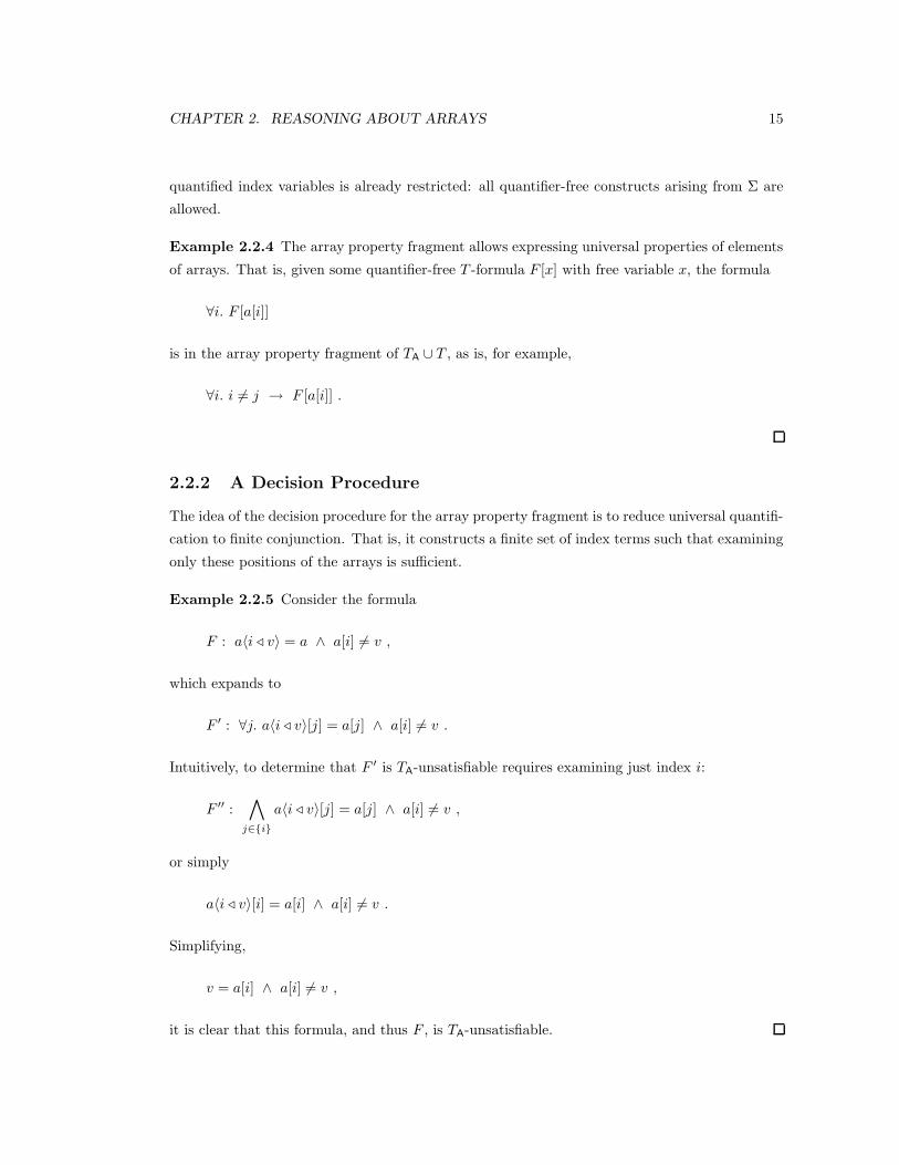
Example 2.2.5 Consider the formula
F : a〈i / v〉 = a ∧ a[i] 6= v ,
which expands to
F ′ : ∀j. a〈i / v〉[j] = a[j] ∧ a[i] 6= v .
Intuitively, to determine that F ′ is TA-unsatisfiable requires examining just index i:
F ′′ :∧
j∈i
a〈i / v〉[j] = a[j] ∧ a[i] 6= v ,
or simply
a〈i / v〉[i] = a[i] ∧ a[i] 6= v .
Simplifying,
v = a[i] ∧ a[i] 6= v ,
it is clear that this formula, and thus F , is TA-unsatisfiable.

CHAPTER 2. REASONING ABOUT ARRAYS 16
Given array property formula F , decide its TA-satisfiability by the following steps.
Step 1
Put F in positive normal form: push negations down to literals.
Step 2
Apply the following rule exhaustively to remove writes:
F [a〈i / v〉]
F [a′] ∧ a′[i] = v ∧ (∀j. j 6= i → a[j] = a′[j])for fresh a′ (write)
Rules should be read from top to bottom. For example, this rule states that given a formula F
containing an occurrence of a write term a〈i / v〉, substitute every occurrence of a〈i / v〉 with a
fresh variable a′ and conjoin additional constraints.
This step deconstructs write terms in a straightforward manner, essentially encoding the
(read-over-write) axioms into the new formula. After an application of the rule, the resulting
formula contains at least one fewer write terms than the given formula.
Step 3
Apply the following rule exhaustively to remove existential quantification:
F [∃i. G[i]]
F [G[j]]for fresh j (exists)
Existential quantification can arise during Step 1 if the given formula has a negated array prop-
erty.
Step 4
Steps 4-6 accomplish the reduction of universal quantification to finite conjunction. The main
idea is to select a set of symbolic index terms on which to instantiate all universal quantifiers.
The proof of Theorem 2.2.1 argues that the following set is sufficient for correctness.
From the output F3 of Step 3, construct the index set I:
I =
λ
∪ t : ·[t] ∈ F3 such that t is not a universally quantified variable
∪ t : t occurs as an evar in the parsing of index guards

CHAPTER 2. REASONING ABOUT ARRAYS 17
This index set is the finite set of indices that need to be examined. It includes all terms t that
occur in some read a[t] anywhere in F (unless it is a universally quantified variable) and all
terms t that are compared to a universally quantified variable in some index guard. λ is a fresh
constant that represents all other index positions that are not explicitly in I.
Step 5
Apply the following rule exhaustively to remove universal quantification:
H [∀i. F [i] → G[i]]
H
∧
i∈In
(F [i] → G[i]
)
(forall)
where n is the size of the list of quantified variables i. This is the key step. It replaces universal
quantification with finite conjunction over the index set.
Step 6
From the output F5 of Step 5, construct
F6 : F5 ∧∧
i ∈ I\λ
λ 6= i .
The new conjuncts assert that the variable λ introduced in Step 4 is indeed unique: it does not
equal any other index mentioned in F5.
Step 7
Decide the TA-satisfiability of F6 using the decision procedure for the quantifier-free fragment.
For deciding the (TA∪T )-satisfiability of an array property (ΣA∪Σ)-formula, use a combination
decision procedure for the quantifier-free fragment of TA ∪ T in Step 7. Thus, this procedure is
a decision procedure precisely when the quantifier-free fragment of TA ∪ T is decidable.
Theorem 2.2.1 (Sound & Complete) Given ΣA-formula F from the array property frag-
ment, the decision procedure returns satisfiable if F is TA-satisfiable; otherwise, it returns unsat-
isfiable.
Proof. Inspection proves the equivalence between the input and the output of Steps 1-3. The
crux of the proof is that the index set constructed in Step 4 is sufficient for producing a TA-
equisatisfiable quantifier-free formula.

CHAPTER 2. REASONING ABOUT ARRAYS 18
That satisfiability of F implies the satisfiability of F6 is straightforward: Step 5 weakens
universal quantification to finite conjunction. Moreover, the new conjuncts of Step 6 do not
affect the satisfiability of F6 since λ is a fresh constant.
The opposite direction is more complicated. Assume that TA-interpretation I is such that
I |= F6. We construct a TA-interpretation J such that J |= F .
First, define a projection function projI : ΣA-terms → I that maps ΣA-terms to terms of the
index set I:
projI(t) =
i if αI [t] = αI [i] for some i ∈ I
λ otherwise
Recall that αI assigns terms to values within the domain DI of interpretation I . Extend projI
to vectors of variables:
projI(i) = (projI(i1), . . . , projI(in)) .
Now, define J to be like I except for its arrays. Under J , let a[i] = a[projI(i)]. Technically,
we are specifying how αJ assigns values to terms of F and the array read function ·[·]; however,
we can think in terms of arrays.
To prove that J |= F , we focus on a particular subformula ∀i. F [i] → G[i]. Assume that
I |=∧
i∈In
(F [i] → G[i]
);
then also
J |=∧
i∈In
(F [i] → G[i]
)(2.1)
by construction of J . We need to prove that
J |= ∀i. F [i] → G[i] ; (2.2)
that is, that
J / i 7→ v |= F [i] → G[i]
for all v ∈ DnJ . Let K = J / i 7→ v.

CHAPTER 2. REASONING ABOUT ARRAYS 19
To do so, we prove the two implications represented by dashed arrows in the following diagram:
F [projK(i)] G[projK(i)]
K |=
F [i] G[i]
(1) (2)
?
The top implication holds under K by the assumption (2.1). If both implications (1) and (2) hold
under K, then the transitivity of implication implies that the bottom implication holds under K
as well.
For (1), we apply structural induction to the index guard F [i]. Atoms have the form i = e,
i 6= e, e 6= i, and i = j, for universally quantified variables i and j and existentially quantified
variable e. When such a literal is true under K, then so is the corresponding literal projK(i) = e,
projK(i) 6= e, e 6= projK(i), or projK(i) = projK(j), respectively, by definition of projK . For
example, if K |= i 6= e, then αK [i] is either equal to some αK [j] for some j ∈ I such that
αK [j] 6= αK [e] or equal to some other value v. In the latter case, projK(i) = λ; that λ 6= e is
asserted in F6 implies that projK(i) 6= e.
For the inductive case, consider that neither conjunction nor disjunction evaluates to true
when both arguments are false. Thus, (1) holds.
For (2), just note that αK [a[i]] = αK [a[projK(i)]] according to the construction of J .
Thus, the bottom implication holds under each variant K of J , so (2.2) holds.
Example 2.2.6 Consider the array property formula
F : a〈` / v〉[k] = b[k] ∧ b[k] 6= v ∧ a[k] = v ∧ (∀i. i 6= ` → a[i] = b[i]) .
It contains one array property,
∀i. i 6= ` → a[i] = b[i] ,
in which the index guard is i 6= ` and the value constraint is a[i] = b[i]. It is already in positive
normal form. According to Step 2, rewrite F as
F2 :a′[k] = b[k] ∧ b[k] 6= v ∧ a[k] = v ∧ (∀i. i 6= ` → a[i] = b[i])
∧ a′[`] = v ∧ (∀j. j 6= ` → a[j] = a′[j])

CHAPTER 2. REASONING ABOUT ARRAYS 20
F2 does not contain any existential quantifiers. Its index set is
I = λ ∪ k ∪ `
= λ, k, ` .
Thus, according to Step 5, replace universal quantification as follows:
F5 :
a′[k] = b[k] ∧ b[k] 6= v ∧ a[k] = v ∧∧
i ∈ I
(i 6= ` → a[i] = b[i])
∧ a′[`] = v ∧∧
j ∈ I
(j 6= ` → a[j] = a′[j])
Expanding produces
F ′5 :
a′[k] = b[k] ∧ b[k] 6= v ∧ a[k] = v ∧ (λ 6= ` → a[λ] = b[λ])
∧ (k 6= ` → a[k] = b[k]) ∧ (` 6= ` → a[`] = b[`])
∧ a′[`] = v ∧ (λ 6= ` → a[λ] = a′[λ])
∧ (k 6= ` → a[k] = a′[k]) ∧ (` 6= ` → a[`] = a′[`])
Simplifying produces
F ′′5 :
a′[k] = b[k] ∧ b[k] 6= v ∧ a[k] = v ∧ (λ 6= ` → a[λ] = b[λ])
∧ (k 6= ` → a[k] = b[k])
∧ a′[`] = v ∧ (λ 6= ` → a[λ] = a′[λ])
∧ (k 6= ` → a[k] = a′[k])
Step 6 distinguishes λ from other members of I:
F6 :
a′[k] = b[k] ∧ b[k] 6= v ∧ a[k] = v ∧ (λ 6= ` → a[λ] = b[λ])
∧ (k 6= ` → a[k] = b[k])
∧ a′[`] = v ∧ (λ 6= ` → a[λ] = a′[λ])
∧ (k 6= ` → a[k] = a′[k])
∧ λ 6= k ∧ λ 6= `
Simplifying, we have
F ′6 :
a′[k] = b[k] ∧ b[k] 6= v ∧ a[k] = v
∧ a[λ] = b[λ] ∧ (k 6= ` → a[k] = b[k])
∧ a′[`] = v ∧ a[λ] = a′[λ] ∧ (k 6= ` → a[k] = a′[k])
∧ λ 6= k ∧ λ 6= `

CHAPTER 2. REASONING ABOUT ARRAYS 21
TA-satisfiability of this quantifier-free ΣA-formula can be decided using the basic decision proce-
dure for the quantifier-free fragment of TA. But let us finish the example. There are two cases
to consider. If k = `, then a′[`] = v and a′[k] = b[k] imply b[k] = v, yet b[k] 6= v. If k 6= `,
then a[k] = v and a[k] = b[k] imply b[k] = v, but again b[k] 6= v. Hence, F ′6 is TA-unsatisfiable,
indicating that F is TA-unsatisfiable.
Theorem 2.2.2 (Complexity) For subfragments of the array property fragment consisting of
bounded-size blocks of quantifiers, TA-satisfiability is NP-complete.
Proof. NP-hardness follows from the NP-hardness of deciding satisfiability in the conjunctive
quantifier-free fragment of TA. We recall this well-known result.
Lemma 2.2.1 TA-satisfiability of quantifier-free conjunctive ΣA-formulae is NP-complete.
Proof. That the problem is in NP is simple: for a given formula F , guess a completion in which
for every instance of a read-over-write a〈i / v〉[j], either i = j or i 6= j is conjoined to the formula
F . Only a linear number of literals are added. Then check TA-satisfiability of this formula, using
the completion to simplify read-over-write occurrences to array reads.
To prove NP-hardness, we reduce from SAT (propositional satisfiability). Given a proposi-
tional formula F in CNF, assert
vP 6= v¬P
for each variable P in F ; vP and v¬P represent the values of P and ¬P , respectively. Introduce
a fresh constant •. Then consider the nth clause of F , say
(¬P ∨ Q ∨ ¬R) .
In this case, assert
a[jn] 6= • ∧ a〈iP / v¬P 〉〈iQ / vQ〉〈iR / v¬R〉[jn] = • .
Intuitively, jn must be equal to one of the introduced values at iP , iQ, or iR. Therefore, at cell
jn, the corresponding value (v¬P , vQ, or v¬R) must equal •. In this fashion, add an assertion for
each clause of F . Conjoin all assertions to form quantifier-free conjunctive ΣA-formula G. G is
equisatisfiable to F and of size polynomial in the size of F . Thus, deciding TA-satisfiability of G
decides propositional satisfiability of F , so TA-satisfiability is NP-complete.
That the problem is in NP follows easily from the procedure: instantiating a block of n
universal quantifiers quantifying subformula G over index set I produces |I|n new subformulae,

CHAPTER 2. REASONING ABOUT ARRAYS 22
each of length polynomial in the length of G. Hence, the output of Step 6 is of length only a
polynomial factor greater than the input to the procedure for fixed n.
This proof extends naturally to the case in which elements are defined by a theory T : the
problem is in NP precisely when satisfiability of the quantifier-free fragment of TA ∪ T is in NP.
Element theories that meet this requirement include TZ, TQ, Tcons, and T=.
We have considered only one-dimensional arrays for ease of presentation. However, the de-
cision procedures can be extended to the multi-dimensional case by considering, for example,
arrays of arrays.
2.3 Integer-Indexed Arrays
Software engineers usually think of arrays as integer-indexed segments of memory. Reasoning
about indices as integers provides the power of comparison via ≤, which enables reasoning about
subarrays and properties such as that a (sub)array is sorted or partitioned. In particular, rea-
soning about subarrays is essential for reasoning about programs that incrementally construct or
manipulate arrays.
The theory of integer-indexed arrays T ZA
is the combination theory TA ∪ TZ: its signature is
the union of the signatures of TA and TZ, and its axioms are the axioms of TA and TZ.
2.3.1 The Array Property Fragment
As in Section 2.2, we are interested in the array property fragment of T ZA. An array property is
again a ΣZA-formula of the form
∀i. F [i] → G[i] ,
where i is a list of integer variables, and F [i] and G[i] are the index guard and the value constraint,
respectively. The form of an index guard is constrained according to the following grammar:
iguard → iguard ∧ iguard | iguard ∨ iguard | atom
atom → expr ≤ expr | expr = expr
expr → uvar | pexpr
pexpr → pexpr′
pexpr′ → Z | Z · evar | pexpr′ + pexpr′
where uvar is any universally quantified integer variable, and evar is any existentially quantified
or free integer variable.
The form of a value constraint is also constrained. Any occurrence of a quantified index

CHAPTER 2. REASONING ABOUT ARRAYS 23
variable i must be as a read into an array, a[i], for array term a. Array reads may not be nested;
e.g., a[b[i]] is not allowed.
The array property fragment of T ZA
then consists of formulae that are Boolean combinations
of quantifier-free ΣZA-formulae and array properties.
Example 2.3.1 We list several interesting forms of properties and their definitions in the array
property fragment of T ZA:
• Array equality a = b:
∀i. a[i] = b[i]
• Bounded array equality beq(a, b, `, u):
∀i. ` ≤ i ≤ u → a[i] = b[i]
• Universal properties F [x]:
∀i. F [a[i]]
• Bounded universal properties F [x]:
∀i. ` ≤ i ≤ u → F [a[i]]
• Bounded and unbounded sortedness sorted(a, `, u):
∀i, j. ` ≤ i ≤ j ≤ u → a[i] ≤ a[j]
• Partitioned arrays partitioned(a, `1, u1, `2, u2):
∀i, j, `1 ≤ i ≤ u1 < `2 ≤ j ≤ u2 → a[i] ≤ a[j]
The last two predicates are necessary for reasoning about sorting algorithms, while the first
four forms of properties are useful in general. For example, bounded equality is essential for
summarizing the effects of a function on an array — in particular, what parts of the array are
unchanged.

CHAPTER 2. REASONING ABOUT ARRAYS 24
2.3.2 A Decision Procedure
As in Section 2.2, the idea of the decision procedure is to reduce universal quantification to finite
conjunction. Given F from the array property fragment of T ZA, decide its T Z
A-satisfiability as
follows:
Step 1
Put F in positive normal form.
Step 2
Apply the following rule exhaustively to remove writes:
F [a〈i / e〉]
F [a′] ∧ a′[i] = e ∧ (∀j. j 6= i → a[j] = a′[j])for fresh a′ (write)
To meet the syntactic requirements on an index guard, rewrite the third conjunct as
∀j. (j ≤ i− 1 ∨ i+ 1 ≤ j) → a[j] = a′[j] .
Step 3
Apply the following rule exhaustively to remove existential quantification:
F [∃i. G[i]]
F [G[j]]for fresh j (exists)
Existential quantification can arise during Step 1 if the given formula has a negated array prop-
erty.
Step 4
From the output of Step 3, F3, construct the index set I:
I =t : ·[t] ∈ F3 such that t is not a universally quantified variable
∪ t : t occurs as a pexpr in the parsing of index guards
If I = ∅, then let I = 0. The index set contains all relevant symbolic indices that occur in F3.
CHAPTER 2. REASONING ABOUT ARRAYS 25
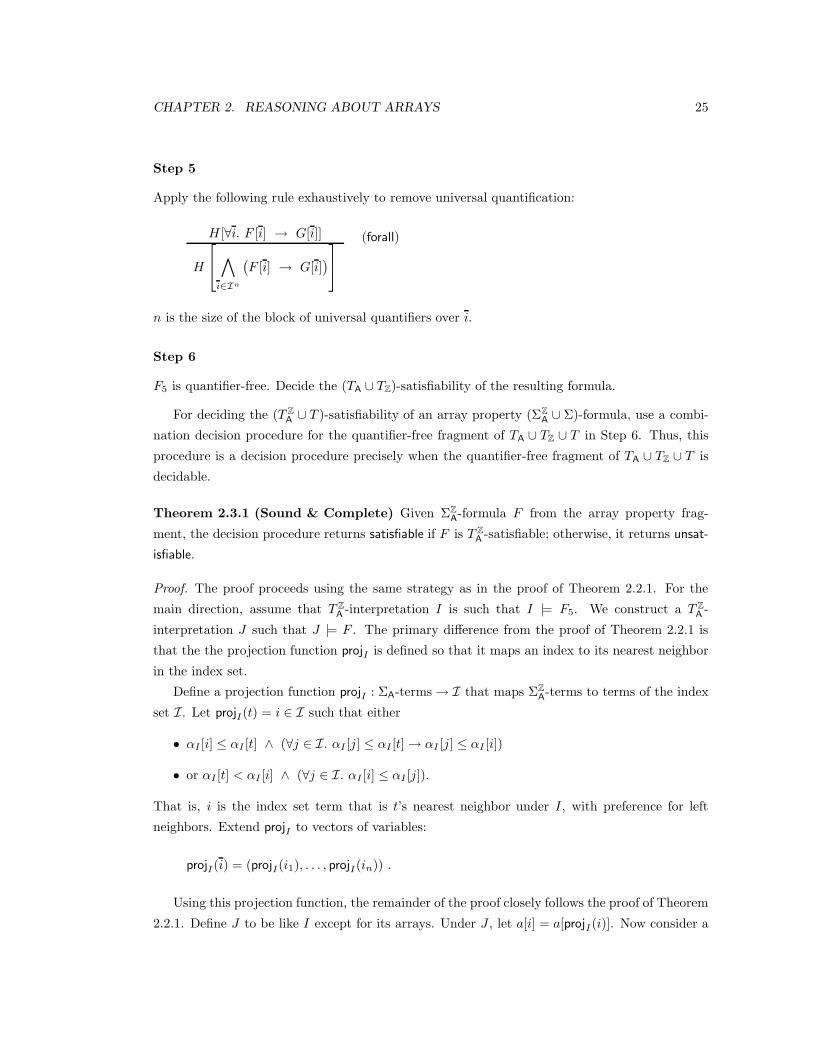
Step 5
Apply the following rule exhaustively to remove universal quantification:
H [∀i. F [i] → G[i]]
H
∧
i∈In
(F [i] → G[i]
)
(forall)
n is the size of the block of universal quantifiers over i.
Step 6
F5 is quantifier-free. Decide the (TA ∪ TZ)-satisfiability of the resulting formula.
For deciding the (T ZA∪ T )-satisfiability of an array property (ΣZ
A∪ Σ)-formula, use a combi-
nation decision procedure for the quantifier-free fragment of TA ∪ TZ ∪ T in Step 6. Thus, this
procedure is a decision procedure precisely when the quantifier-free fragment of TA ∪ TZ ∪ T is
decidable.
Theorem 2.3.1 (Sound & Complete) Given ΣZA-formula F from the array property frag-
ment, the decision procedure returns satisfiable if F is T ZA-satisfiable; otherwise, it returns unsat-
isfiable.
Proof. The proof proceeds using the same strategy as in the proof of Theorem 2.2.1. For the
main direction, assume that T ZA-interpretation I is such that I |= F5. We construct a T Z
A-
interpretation J such that J |= F . The primary difference from the proof of Theorem 2.2.1 is
that the the projection function projI is defined so that it maps an index to its nearest neighbor
in the index set.
Define a projection function projI : ΣA-terms → I that maps ΣZA-terms to terms of the index
set I. Let projI(t) = i ∈ I such that either
• αI [i] ≤ αI [t] ∧ (∀j ∈ I. αI [j] ≤ αI [t] → αI [j] ≤ αI [i])
• or αI [t] < αI [i] ∧ (∀j ∈ I. αI [i] ≤ αI [j]).
That is, i is the index set term that is t’s nearest neighbor under I , with preference for left
neighbors. Extend projI to vectors of variables:
projI(i) = (projI(i1), . . . , projI(in)) .
Using this projection function, the remainder of the proof closely follows the proof of Theorem
2.2.1. Define J to be like I except for its arrays. Under J , let a[i] = a[projI(i)]. Now consider a

CHAPTER 2. REASONING ABOUT ARRAYS 26
subformula ∀i. F [i] → G[i] and assume that
I |=∧
i∈In
(F [i] → G[i]
); (2.3)
immediately, we have
J |=∧
i∈In
(F [i] → G[i]
). (2.4)
We need to prove that
J |= ∀i. F [i] → G[i] ; (2.5)
that is, that
J / i 7→ v |= F [i] → G[i]
for all v ∈ DnJ . Let K = J / i 7→ v.
To do so, we prove the two implications represented by dashed arrows in the following diagram:
F [projK(i)] G[projK(i)]
K |=
F [i] G[i]
(1) (2)
?
The top implication holds under K by the assumption (2.4). If both implications (1) and (2) hold
under K, then the transitivity of implication implies that the bottom implication holds under K
as well.
For (1), we apply structural induction to the index guard F [i]. Consider an atom of the
form t1 ≤ t2; if it holds under K, then also projK(t1) ≤ projK(t2) holds under K because
projK is monotonic. Consider an atom of the form t1 = t2; if it holds under K, then also
projK(t1) = projK(t2) under K. For the inductive case, consider that neither conjunction nor
disjunction evaluates to true when both arguments are false. Thus, (1) holds.
For (2), just note that αK [a[i]] = αK [a[projK(i)]] according to the construction of J .
Thus, the bottom implication holds under each variant K of J , so (2.5) holds.

CHAPTER 2. REASONING ABOUT ARRAYS 27
Example 2.3.2 Consider the following ΣZA-formula:
F :(∀i. ` ≤ i ≤ u → a[i] = b[i])
∧ ¬(∀i. ` ≤ i ≤ u+ 1 → a〈u+ 1 / b[u+ 1]〉[i] = b[i])
In positive normal form, we have
F1 :(∀i. ` ≤ i ≤ u → a[i] = b[i])
∧ (∃i. ` ≤ i ≤ u+ 1 ∧ a〈u+ 1 / b[u+ 1]〉[i] 6= b[i])
Step 2 produces
F2 :
(∀i. ` ≤ i ≤ u → a[i] = b[i])
∧ (∃i. ` ≤ i ≤ u+ 1 ∧ a′[i] 6= b[i])
∧ a′[u+ 1] = b[u+ 1]
∧ (∀j. j ≤ u+ 1 − 1 ∨ u+ 1 + 1 ≤ j → a[j] = a′[j])
Step 3 removes the existential quantifier by introducing a fresh constant k:
F3 :
(∀i. ` ≤ i ≤ u → a[i] = b[i])
∧ ` ≤ k ≤ u+ 1 ∧ a′[k] 6= b[k]
∧ a′[u+ 1] = b[u+ 1]
∧ (∀j. j ≤ u+ 1 − 1 ∨ u+ 1 + 1 ≤ j → a[j] = a′[j])
Simplifying, we have
F ′3 :
(∀i. ` ≤ i ≤ u → a[i] = b[i])
∧ ` ≤ k ≤ u+ 1 ∧ a′[k] 6= b[k]
∧ a′[u+ 1] = b[u+ 1]
∧ (∀j. j ≤ u ∨ u+ 2 ≤ j → a[j] = a′[j])
The index set is thus
I = k, u+ 1 ∪ `, u, u+ 2 ,
which includes the read terms k and u + 1 and the terms `, u, and u + 2 that occur as pexprs
in the index guards. Then Step 5 rewrites universal quantification to finite conjunction over this

CHAPTER 2. REASONING ABOUT ARRAYS 28
set:
F5 :
∧
i ∈ I
(` ≤ i ≤ u → a[i] = b[i])
∧ ` ≤ k ≤ u+ 1 ∧ a′[k] 6= b[k]
∧ a′[u+ 1] = b[u+ 1]
∧∧
j ∈ I
(j ≤ u ∨ u+ 2 ≤ j → a[j] = a′[j])
Expanding the conjunctions according to the index set I and simplifying according to trivially
true or false antecedents (e.g., ` ≤ u+ 1 ≤ u simplifies to ⊥, while u ≤ u ∨ u+ 2 ≤ u simplifies
to >) produces:
F ′5 :
(` ≤ k ≤ u → a[k] = b[k]) ∧ (` ≤ u → a[`] = b[`] ∧ a[u] = b[u])
∧ ` ≤ k ≤ u+ 1 ∧ a′[k] 6= b[k]
∧ a′[u+ 1] = b[u+ 1]
∧ (k ≤ u ∨ u+ 2 ≤ k → a[k] = a′[k])
∧ (` ≤ u ∨ u+ 2 ≤ ` → a[`] = a′[`])
∧ a[u] = a′[u] ∧ a[u+ 2] = a′[u+ 2]
(TA ∪ TZ)-satisfiability of this quantifier-free (ΣA ∪ΣZ)-formula can be decided using the Nelson-
Oppen combination of the basic decision procedure for the quantifier-free fragment of TA with
a decision procedure for TZ. But let us finish the example. F ′5 is (TA ∪ TZ)-unsatisfiable. In
particular, note that k is restricted such that ` ≤ k ≤ u+ 1; that the first conjunct asserts that
for most of this range (k ∈ [`, u]), a[k] = b[k]; that the third-to-last conjunct asserts that for
k ≤ u, a[k] = a′[k], contradicting a[k] = a′[k] 6= b[k] when k ≤ u; and that even if k = u + 1,
a′[k] 6= b[k] = b[u + 1] = a′[u + 1] = a′[k] by the fourth and fifth conjuncts, a contradiction.
Hence, F is T ZA-unsatisfiable.
2.4 Negative Results
Theorem 2.4.1 Consider the following extensions to the array property fragment of TA:
• Permit an additional quantifier alternation.
• Permit nested reads (e.g., a[b[i]] when i is universally quantified).
• Permit array reads by a universally quantified variable in the index guard.
• Augment the theory with a permutation predicate.

CHAPTER 2. REASONING ABOUT ARRAYS 29
For each resulting fragment, there exists an element theory T such that satisfiability in the array
property fragment of TA ∪ T is decidable, yet satisfiability in the resulting fragment of TA ∪ T is
undecidable.
Proof. Our main proof technique is the following. Consider the problem of solving Diophantine
equations: Does a given polynomial p(x) have a nonnegative integer root? It has a root iff
there exists a finite path from the origin to that root, where each step of the path consists
of incrementing a variable xi by one. For each of the extensions, we show how to encode the
existence of such a path into a formula of the extended fragment of TA ∪ TZ. The undecidability
of the existence of integer roots then implies the undecidability of satisfiability in the fragment.
Consider a polynomial p(x), and let q(x) = p(x)2. q(x) is positive except at its roots (which
correspond to the roots of p(x)).
Since the element theory TZ does not have multiplication, the first task is to reason about
q(x) without multiplication. Suppose that the value of q(a) is known. To compute q’s value at
coordinate b in which bi = ai + 1 and bj = aj for j 6= i, compute its finite difference for the ith
dimension:
4xiq(x) = q(x1, . . . , xi + 1, . . . , xn) − q(x) .
Then q(b) = q(a) + (4xiq(x))(a). Higher-order finite differences are computed compositionally;
for example,
4xixjq(x) = 4xj
4xiq(x) .
Now construct the following tree from q(x), starting with q(x) as the root:
1. If node r(x) is simply a constant, then it is a leaf.
2. Otherwise, let the children of node r(x) be its n finite differences 4xir(x).
This construction terminates because q(x) is a polynomial.
Introduce at each non-leaf node r(x) of the tree a fresh variable vr(x). For notational conve-
nience, if node r(x) is a leaf, let vr(x) be its constant value. Let v be the vector of all of these
variables.
The following formula simulates the evaluation of q(x) at the origin 0:
Tq(0)[v] :∧
r(x)
vr(x) = r(0) ,
where the conjunction ranges over the non-leaf nodes of the tree. That is, each introduced variable
is equated to the value of the polynomial it represents at the origin. The following formula, a

CHAPTER 2. REASONING ABOUT ARRAYS 30
relation between the current values of the tree variables v and the next-state values of the tree
variables v′, simulates the incrementing of xi:
Txi+1[v, v′] :
∧
r(x)
v′r(x) = vr(x) + v4xir(x) ,
where v4xir(x) is the variable (or, using our convention, the constant) corresponding to the ith
child of node r(x), and the conjunction ranges over the non-leaf nodes of the tree. The formulae
Tq(0) and Txi+1 are ΣZ-formulae.
With these tools, we can now address decidability for the extended fragments. Consider first
allowing an additional quantifier alternation. Construct the following ΣA-formula:
∃v, s. ∀i. ∃j.
Tq(0)[v[0]]
∧(v[j] = v[i] ∨
∨
xiTxi+1[v[i], v[j]]
)
∧ s[j] = s[i] − vq(x)[i]
∧ s[i] > 0
(2.6)
This formula simulates a walk from the origin x = 0 in which each step consists of either staying
in place or moving one positive unit along one dimension xi. At each step, the current value of
the polynomial q(x) — which is maintained by vq(x) — is subtracted from s. To satisfy (2.6),
there must be some value of s[0] and some sequence of steps such that s never reaches 0. But
recall that vq(x) is always positive except at solutions. Hence, (2.6) is (TA ∪ TZ)-satisfiable only
when some finite path leads to a solution. Once the solution is reached, then each step consists
of remaining in place so that s is no longer decreased.
Consider permitting nested reads. In this case, an array can be used to skolemize the variable
j of (2.6):
∃v, s, j. ∀i.
Tq(0)[v[0]]
∧(v[j[i]] = v[i] ∨
∨
xiTxi+1[v[i], v[j[i]]]
)
∧ s[j[i]] = s[i] − vq(x)[i]
∧ s[i] > 0
(2.7)
Consider permitting array reads by a universally quantified variable in the index guard.
Then the skolem array of (2.7) can be extracted as follows (where it has been renamed to a for
convenience):
∃v, s, a. ∀i, j. j = a[i] →
Tq(0)[v[0]]
∧(v[j] = v[i] ∨
∨
xiTxi+1[v[i], v[j]]
)
∧ s[j] = s[i] − vq(x)[i]
∧ s[i] > 0
(2.8)
CHAPTER 2. REASONING ABOUT ARRAYS 31
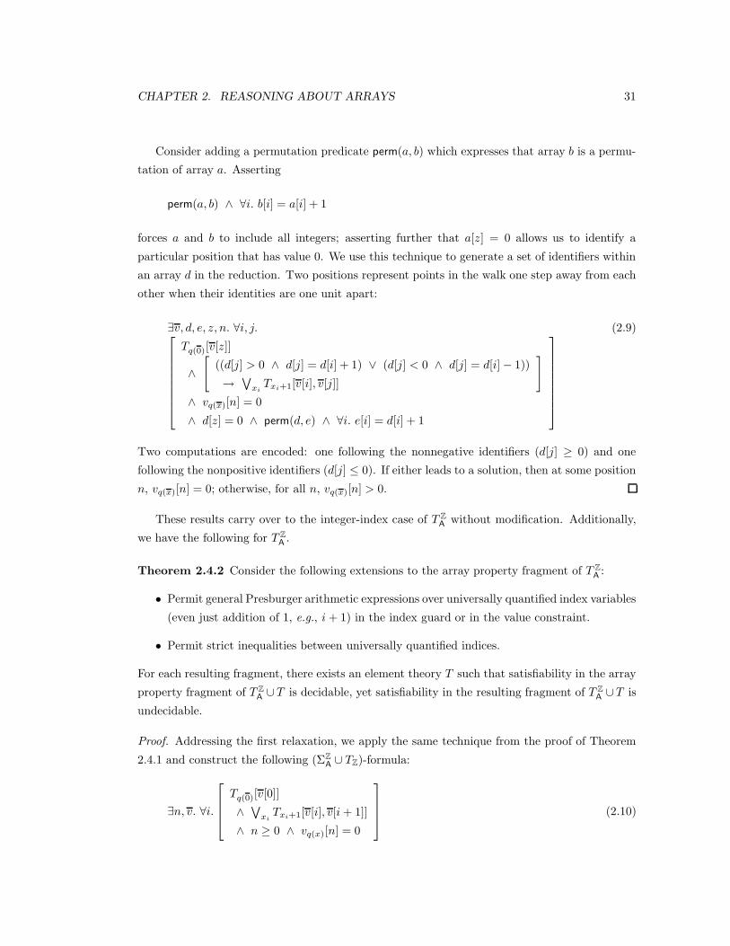
Consider adding a permutation predicate perm(a, b) which expresses that array b is a permu-
tation of array a. Asserting
perm(a, b) ∧ ∀i. b[i] = a[i] + 1
forces a and b to include all integers; asserting further that a[z] = 0 allows us to identify a
particular position that has value 0. We use this technique to generate a set of identifiers within
an array d in the reduction. Two positions represent points in the walk one step away from each
other when their identities are one unit apart:
∃v, d, e, z, n. ∀i, j.
Tq(0)[v[z]]
∧
[
((d[j] > 0 ∧ d[j] = d[i] + 1) ∨ (d[j] < 0 ∧ d[j] = d[i] − 1))
→∨
xiTxi+1[v[i], v[j]]
]
∧ vq(x)[n] = 0
∧ d[z] = 0 ∧ perm(d, e) ∧ ∀i. e[i] = d[i] + 1
(2.9)
Two computations are encoded: one following the nonnegative identifiers (d[j] ≥ 0) and one
following the nonpositive identifiers (d[j] ≤ 0). If either leads to a solution, then at some position
n, vq(x)[n] = 0; otherwise, for all n, vq(x)[n] > 0.
These results carry over to the integer-index case of T ZA
without modification. Additionally,
we have the following for T ZA.
Theorem 2.4.2 Consider the following extensions to the array property fragment of T ZA:
• Permit general Presburger arithmetic expressions over universally quantified index variables
(even just addition of 1, e.g., i+ 1) in the index guard or in the value constraint.
• Permit strict inequalities between universally quantified indices.
For each resulting fragment, there exists an element theory T such that satisfiability in the array
property fragment of T ZA∪ T is decidable, yet satisfiability in the resulting fragment of T Z
A∪ T is
undecidable.
Proof. Addressing the first relaxation, we apply the same technique from the proof of Theorem
2.4.1 and construct the following (ΣZA∪ TZ)-formula:
∃n, v. ∀i.
Tq(0)[v[0]]
∧∨
xiTxi+1[v[i], v[i+ 1]]
∧ n ≥ 0 ∧ vq(x)[n] = 0
(2.10)
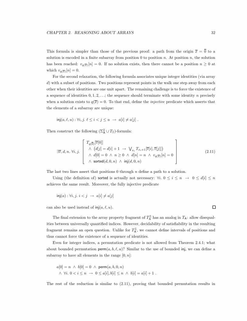
CHAPTER 2. REASONING ABOUT ARRAYS 32
This formula is simpler than those of the previous proof: a path from the origin x = 0 to a
solution is encoded in a finite subarray from position 0 to position n. At position n, the solution
has been reached: vq(x)[n] = 0. If no solution exists, then there cannot be a position n ≥ 0 at
which vq(x)[n] = 0.
For the second relaxation, the following formula associates unique integer identities (via array
d) with a subset of positions. Two positions represent points in the walk one step away from each
other when their identities are one unit apart. The remaining challenge is to force the existence of
a sequence of identities 0, 1, 2, . . .; the sequence should terminate with some identity n precisely
when a solution exists to q(x) = 0. To that end, define the injective predicate which asserts that
the elements of a subarray are unique:
inj(a, `, u) : ∀i, j. ` ≤ i < j ≤ u → a[i] 6= a[j] .
Then construct the following (ΣZA∪ TZ)-formula:
∃v, d, n. ∀i, j.
Tq(0)[v[0]]
∧(d[j] = d[i] + 1 →
∨
xiTxi+1[v[i], v[j]]
)
∧ d[0] = 0 ∧ n ≥ 0 ∧ d[n] = n ∧ vq(x)[n] = 0
∧ sorted(d, 0, n) ∧ inj(d, 0, n)
(2.11)
The last two lines assert that positions 0 through n define a path to a solution.
Using (the definition of) sorted is actually not necessary: ∀i. 0 ≤ i ≤ n → 0 ≤ d[i] ≤ n
achieves the same result. Moreover, the fully injective predicate
inj(a) : ∀i, j. i < j → a[i] 6= a[j]
can also be used instead of inj(a, `, u).
The final extension to the array property fragment of T ZA
has an analog in TA: allow disequal-
ities between universally quantified indices. However, decidability of satisfiability in the resulting
fragment remains an open question. Unlike for T ZA, we cannot define intervals of positions and
thus cannot force the existence of a sequence of identities.
Even for integer indices, a permutation predicate is not allowed from Theorem 2.4.1; what
about bounded permutation perm(a, b, `, u)? Similar to the use of bounded inj, we can define a
subarray to have all elements in the range [0, n]:
a[0] = n ∧ b[0] = 0 ∧ perm(a, b, 0, n)
∧ ∀i. 0 < i ≤ n → 0 ≤ a[i], b[i] ≤ n ∧ b[i] = a[i] + 1 .
The rest of the reduction is similar to (2.11), proving that bounded permutation results in
CHAPTER 2. REASONING ABOUT ARRAYS 33
undecidability as well.
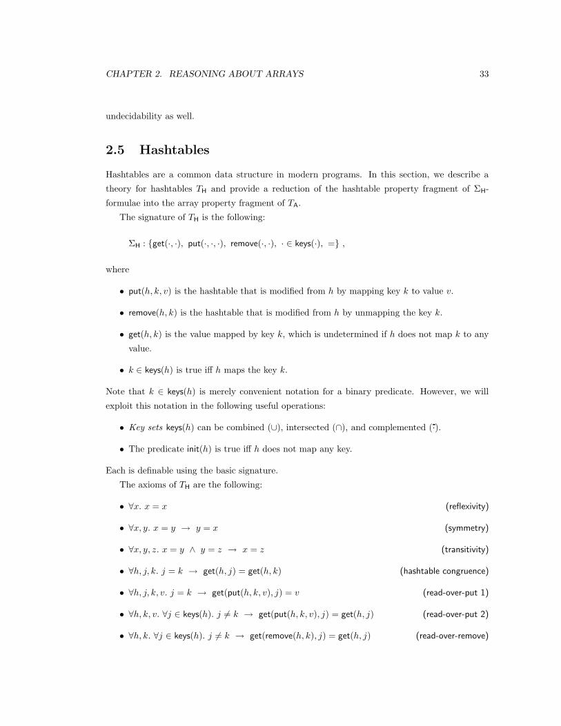
2.5 Hashtables
Hashtables are a common data structure in modern programs. In this section, we describe a
theory for hashtables TH and provide a reduction of the hashtable property fragment of ΣH-
formulae into the array property fragment of TA.
The signature of TH is the following:
ΣH : get(·, ·), put(·, ·, ·), remove(·, ·), · ∈ keys(·), = ,
where
• put(h, k, v) is the hashtable that is modified from h by mapping key k to value v.
• remove(h, k) is the hashtable that is modified from h by unmapping the key k.
• get(h, k) is the value mapped by key k, which is undetermined if h does not map k to any
value.
• k ∈ keys(h) is true iff h maps the key k.
Note that k ∈ keys(h) is merely convenient notation for a binary predicate. However, we will
exploit this notation in the following useful operations:
• Key sets keys(h) can be combined (∪), intersected (∩), and complemented (·).
• The predicate init(h) is true iff h does not map any key.
Each is definable using the basic signature.
The axioms of TH are the following:
• ∀x. x = x (reflexivity)
• ∀x, y. x = y → y = x (symmetry)
• ∀x, y, z. x = y ∧ y = z → x = z (transitivity)
• ∀h, j, k. j = k → get(h, j) = get(h, k) (hashtable congruence)
• ∀h, j, k, v. j = k → get(put(h, k, v), j) = v (read-over-put 1)
• ∀h, k, v. ∀j ∈ keys(h). j 6= k → get(put(h, k, v), j) = get(h, j) (read-over-put 2)
• ∀h, k. ∀j ∈ keys(h). j 6= k → get(remove(h, k), j) = get(h, j) (read-over-remove)

CHAPTER 2. REASONING ABOUT ARRAYS 34
• ∀h, k, v. k ∈ keys(put(h, k, v)) (keys-put)
• ∀h, k. k 6∈ keys(remove(h, k)) (keys-remove)
Note the similarity between the first six axioms of TH and those of TA. Key sets complicate
the (read-over-put 2) axiom compared to the (read-over-write 2) axiom, while keys sets and key
removal require three additional axioms.
2.5.1 The Hashtable Property Fragment
A hashtable property has the form
∀k. F [k] → G[k] ,
where F [k] is the key guard, and G[k] is the value constraint. Key guards are defined exactly as
index guards of the array property fragment of TA: they are positive Boolean combinations of
equations between universally quantified keys; and equations and disequalities between univer-
sally quantified keys k and other key terms. Value constraints can use universally quantified keys
k in hashtable reads get(h, k) and in key set membership checks. Finally, a hashtable property
does not contain any init literals.
ΣH-formulae that are Boolean combinations of quantifier-free ΣH-formulae and hashtable
properties comprise the hashtable property fragment of TH.
Example 2.5.1 Consider the following hashtable property formula:
F : ∀k ∈ keys(h). get(h, k) ≥ 0 .
Its key guard is trivial, while its value constraint is
k ∈ keys(h) → get(h, k) ≥ 0 .
Suppose that F annotates locations L1 and L2 in the following basic path (see Chapter 4 of
[BM07] for a discussion of basic paths in program verification):
@L1 : F
assume v ≥ 0;
put(h, s, v);
@L2 : F
We want to prove that if F holds at L1, then it holds at L2. The resulting verification condition

CHAPTER 2. REASONING ABOUT ARRAYS 35
is
∀h, s, v.
[
(∀k ∈ keys(h). get(h, k) ≥ 0) ∧ v ≥ 0
→ (∀k ∈ keys(put(h, s, v)). get(put(h, s, v), k) ≥ 0)
]
.
The key set keys(h) provides a mechanism for reasoning about the incremental modification of
hashtables.
Example 2.5.2 To express equality between key sets, keys(h1) = keys(h2), in TH, write for
example
∀k. k ∈ keys(h1) ↔ k ∈ keys(h2) ,
which has a trivial key guard. Then express equality between hashtables, h1 = h2, with the
following formula:
keys(h1) = keys(h2) ∧ ∀k ∈ keys(h1). get(h1, k) = get(h2, k) .
2.5.2 A Decision Procedure
Given F from the hashtable property fragment of TH, the decision procedure reduces TH-
satisfiability to TA-satisfiability of a formula in the array property fragment. The main idea
of the reduction is to represent hashtables h of the given ΣH-formula by two arrays in the ΣA-
formula: an array h for the elements and an array keysh that indicates if a key (an array index)
maps to an element. In particular, keysh[k] = indicates that k is not mapped by h, while
keysh[k] 6= (keysh[k] = •) indicates that h does map k to a value given by h[k].
Step 1
Construct F ∧ • 6= , for fresh constants • and .
Step 2
Rewrite F1 according to the following set of rules:
F [put(h, k, v)] =⇒ F [h′] ∧ h′ = h〈k / v〉 ∧ keysh′ = keysh〈k / •〉
F [remove(h, k)] =⇒ F [h′] ∧ (∀j ∈ keys(h′). h′[j] = h[j]) ∧ keysh′ = keysh〈k / 〉
for fresh variable h′.

CHAPTER 2. REASONING ABOUT ARRAYS 36
Step 3
Rewrite F2 according to the following set of rules:
F [get(h, k)] =⇒ F [h[k]]
F [k ∈ keys(h)] =⇒ F [keysh[k] 6= ]
F [k ∈ K1 ∪K2] =⇒ F [k ∈ K1 ∨ k ∈ K2]
F [k ∈ K1 ∩K2] =⇒ F [k ∈ K1 ∧ k ∈ K2]
F [k ∈ K] =⇒ F [¬(k ∈ K)]
F [init(h)] =⇒ F [∀k. ¬(k ∈ keys(h))]
where K, K1, and K2 are constructed from union, disjunction, and complementation of key set
membership atoms. The final four rules define auxiliary operations: the right-side of each is
expressible in the hashtable property fragment.
Step 4
Decide the TA-satisfiability of F3.
Step 2 relies on the defined predicate of equality between arrays, a = b, which is defined by
∀i. a[i] = b[i].
As in Sections 2.2 and 2.3, hashtable values may be interpreted in some theory T with
signature Σ. Then the above procedure is a decision procedure precisely when there is a decision
procedure for the array property fragment of TA ∪ T .
Theorem 2.5.1 (Sound & Complete) Given ΣH-formula F from the hashtable property frag-
ment, the decision procedure returns satisfiable iff F is TH-satisfiable; otherwise, it returns unsat-
isfiable.
Proof. Inspection shows that if F is a ΣH-formula from the hashtable property fragment, then
F3 is a ΣA-formula from the array property fragment. First, the rewrite system terminates: the
first rule of Step 2 and the first two rules of Step 3 remove instances of ΣH-literals and ΣH-terms
without introducing more, while the second rule of Step 2 introduces only one new ΣH-literal that
is addressed in Step 3; and the final four rules of Step 3 clearly terminate with a finite number
of applications of the first two rules of Step 3. Second, while three rules introduce (universal)
quantification, the definition of the hashtable property fragment guarantees that the quantified
subformulae occur outside of other quantifiers (except the topmost existential quantifiers). Hence,
Step 4 returns satisfiable or unsatisfiable.
We must show that F has a satisfying TH-interpretation precisely when F3 has a satisfying
TA-interpretation. Suppose that TH-interpretation I satisfies F . Construct the TA-interpretation
J satisfying F3 as follows:

CHAPTER 2. REASONING ABOUT ARRAYS 37
• if h maps k to v in I , set keysh[k] = • in J and h[k] = v;
• otherwise, set keysh[k] = and h[k] = v for some arbitrary value v.
This J satisfies the conjuncts added in Step 2; also, h[k] is the same value under J as get(h, k)
under I , and keysh[k] 6= under J iff k ∈ keys(h) under I , showing the correctness of the first
two rules of Step 3 (recall that the remaining rules are auxiliary and easily reduce to the first
two).
Similarly, a TA-interpretation J satisfying F3 induces a TH-interpretation I satisfying F .
Construct I as follows:
• if keysh[k] 6= and h[k] = v in J , assert get(h, k) = v and k ∈ keys(h) in I ;
• otherwise, assert ¬(h ∈ keys(h)) in I .
Again, the correspondence between the two sides of each rule is clear.
Example 2.5.3 Consider the following ΣH-formula:
G : ∀h, s, v.
[
(∀k ∈ keys(h). get(h, k) ≥ 0) ∧ v ≥ 0
→ (∀k ∈ keys(put(h, s, v)). get(put(h, s, v), k) ≥ 0)
]
To prove its TH-validity, prove the TH-satisfiability of the following:
F :(∀k ∈ keys(h). get(h, k) ≥ 0) ∧ v ≥ 0
∧ ¬(∀k ∈ keys(put(h, s, v)). get(put(h, s, v), k) ≥ 0)
Step 1 introduces • and :
F1 : F ∧ • 6= .
Step 2 reduces hashtable modifications to arrays:
F2 :
(∀k ∈ keys(h). get(h, k) ≥ 0) ∧ v ≥ 0
∧ ¬(∀k ∈ keys(h′). get(h′, k) ≥ 0)
∧ h′ = h〈s / v〉 ∧ keysh′ = keysh〈s / •〉
∧ • 6=
Step 3 completes the reduction:
F3 :
(∀k. keysh[k] 6= → h[k] ≥ 0) ∧ v ≥ 0
∧ ¬(∀k. keysh′ [k] 6= → h′[k] ≥ 0)
∧ h′ = h〈s / v〉 ∧ keysh′ = keysh〈s / •〉
∧ • 6=

CHAPTER 2. REASONING ABOUT ARRAYS 38
F3 is TA-unsatisfiable. In particular, keysh′ = keysh〈s / •〉 and h′ = h〈s / v〉, so that for all keys
of h (k such that keysh[k] 6= ), h′[k] = h[k] ≥ 0. For the one new key s of h′, we know that
h′[s] = h〈s / v〉[s] = v ≥ 0. Therefore, no key k of h′ exists at which h[k] < 0, a contradiction.
Hence, G is TH-valid.
The decision procedure of Section 2.2 would also prove the TA-unsatisfiability of F3.
2.6 Partial Arrays
A variation on arrays in which elements may be undefined has been considered recently [GNRZ06].
We apply the techniques developed for studying standard arrays to study the theory of partial
arrays.
The theory of read-only partial arrays T RO
Ahas signature
ΣRO
A = ·[·], =, ⊥ .
Its signature differs from ΣA in two ways: it does not have a function for constructing a modified
array; and it has a new constant symbol ⊥. Its axioms are just (reflexivity), (symmetry), (transi-
tivity), and (array congruence) of TA. Notice that ⊥ is undefined. It will play a role later when
we define an important fragment of T ROA
.
The theory of partial arrays T⊥A
has signature
Σ⊥A = ·[·], ·〈· / ·〉, =, ⊥
and includes all the axioms of TA.
2.6.1 The Guarded Fragment
Consider a ΣRO
A-formula F [a[i]] with subterm a[i] (possibly with multiple occurrences) in which
a and i are free; moreover, i does not appear in any other read term. The guarded universal
quantification of F [a[i]] is
∀i. a[i] 6= ⊥ → F [a[i]] .
Then a guarded ΣRO
A-formula is defined recursively as a quantifier-free ΣRO
A-formula, the guarded
universal quantification of a guarded ΣRO
A-formula, or the positive Boolean combination of
guarded ΣRO
A-formulae. Finally, the guarded fragment of T RO
Aconsists of Boolean combinations
of guarded ΣRO
A-formulae.
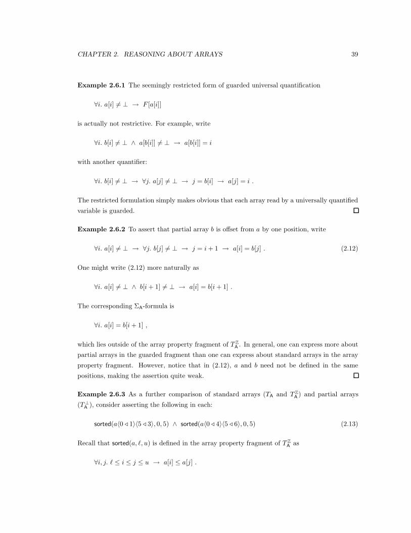
CHAPTER 2. REASONING ABOUT ARRAYS 39
Example 2.6.1 The seemingly restricted form of guarded universal quantification
∀i. a[i] 6= ⊥ → F [a[i]]
is actually not restrictive. For example, write
∀i. b[i] 6= ⊥ ∧ a[b[i]] 6= ⊥ → a[b[i]] = i
with another quantifier:
∀i. b[i] 6= ⊥ → ∀j. a[j] 6= ⊥ → j = b[i] → a[j] = i .
The restricted formulation simply makes obvious that each array read by a universally quantified
variable is guarded.
Example 2.6.2 To assert that partial array b is offset from a by one position, write
∀i. a[i] 6= ⊥ → ∀j. b[j] 6= ⊥ → j = i+ 1 → a[i] = b[j] . (2.12)
One might write (2.12) more naturally as
∀i. a[i] 6= ⊥ ∧ b[i+ 1] 6= ⊥ → a[i] = b[i+ 1] .
The corresponding ΣA-formula is
∀i. a[i] = b[i+ 1] ,
which lies outside of the array property fragment of T ZA. In general, one can express more about
partial arrays in the guarded fragment than one can express about standard arrays in the array
property fragment. However, notice that in (2.12), a and b need not be defined in the same
positions, making the assertion quite weak.
Example 2.6.3 As a further comparison of standard arrays (TA and T ZA) and partial arrays
(T⊥A
), consider asserting the following in each:
sorted(a〈0 / 1〉〈5 / 3〉, 0, 5) ∧ sorted(a〈0 / 4〉〈5 / 6〉, 0, 5) (2.13)
Recall that sorted(a, `, u) is defined in the array property fragment of T ZA
as
∀i, j. ` ≤ i ≤ j ≤ u → a[i] ≤ a[j] .

CHAPTER 2. REASONING ABOUT ARRAYS 40
In the guarded fragment of T⊥A
, it is defined as
∀i. a[i] 6= ⊥ → ∀j. a[j] 6= ⊥ → ` ≤ i ≤ j ≤ u → a[i] ≤ a[j] .
With these definitions, it is clear that (2.13) is T ZA-unsatisfiable: there is no way of filling in the
elements between positions 1 and 4 of a such that both modified arrays are sorted. However,
(2.13) is trivially T⊥A
-satisfiable: simply fill a with ⊥.
Example 2.6.4 As a final example comparing standard arrays (TA and T ZA) and partial arrays
(T⊥A
), consider asserting the following in each, where the arrays have integer elements:
a[0] = 0 ∧ a[5] = 4 ∧ sorted(a, 0, 5) ∧ inj(a, 0, 5) . (2.14)
In T ZA, inj(a, `, u) is defined as
∀i, j. ` ≤ i < j ≤ u → a[i] 6= a[j] ;
in T⊥A
, it is defined as
∀i. a[i] 6= ⊥ → ∀j. a[j] 6= ⊥ → ` ≤ i < j ≤ u → a[i] 6= a[j] .
From Theorem 2.4.2, we know that adding the power to express inj to the array property fragment
of T ZA
results in undecidability; however, it can be expressed in the guarded fragment of T⊥A
.
In any case, (2.14) is (T ZA∪TZ)-unsatisfiable: there are not enough distinct integers to fill the
positions between 1 and 4. However, (2.14) is (T⊥A
∪ TZ)-satisfiable: simply fill the interval with
⊥.
2.6.2 Decision Procedures
Satisfiability of ΣRO
A-formulae from the guarded fragment is decided by the following decision
procedure.
Step 1
Put F in positive normal form: push negations down to literals.

CHAPTER 2. REASONING ABOUT ARRAYS 41
Step 2
Apply the following rule exhaustively to remove existential quantification:
F [∃i. G[i]]
F [G[j]]for fresh j (exists)
Existential quantification can arise during Step 1 if the given formula has a negated guarded
ΣROA
-subformula.
Step 3
Steps 3-4 accomplish the reduction of universal quantification to finite conjunction. The main
idea is to select a set of symbolic index terms on which to instantiate all universal quantifiers.
The proof of Theorem 2.6.1 argues that the following set is sufficient for correctness.
From the output F2 of Step 2, construct the index set I:
I = t : ·[t] ∈ F2 such that t is not a universally quantified variable
This index set is the finite set of indices that need to be examined. It includes just the terms t
that contain only existentially quantified variables and that occur in some read a[t] somewhere
in F .
Step 4
Apply the following rule exhaustively to remove universal quantification:
H [∀i. a[i] 6= ⊥ → F [a[i]]]
H
∧
i∈In
(a[i] 6= ⊥ → F [a[i]])
(forall)
where n is the size of the list of quantified variables i. This is the key step. It replaces universal
quantification with finite conjunction over the index set.
Step 5
Decide the T RO
A-satisfiability of F4 using the decision procedure for the quantifier-free fragment.
Unlike in the case of standard arrays, this procedure works just as well on arrays with integer-
indexed arrays. While convenient, it also suggests the weakness of this theory.

CHAPTER 2. REASONING ABOUT ARRAYS 42
Theorem 2.6.1 (Sound & Complete) Given ΣROA
-formula F from the guarded fragment, the
decision procedure returns satisfiable if F is T RO
A-satisfiable; otherwise, it returns unsatisfiable.
Proof. As in the proof of Theorem 2.2.1, the crux of the proof is that the index set constructed
in Step 4 is sufficient for producing a T RO
A-equisatisfiable quantifier-free formula.
That satisfiability of F implies the satisfiability of F4 is straightforward: Step 4 weakens
universal quantification to finite conjunction.
For the opposite direction, assume that T ROA
-interpretation I is such that I |= F4. Then a
T RO
A-interpretation J such that J |= F is simple to construct: make it like I , but assign ⊥ to every
array position not referenced by some fixed position in I, which is the set I under interpretation
I .
To prove that J |= F , simply note that every instance of a guarded universal quantification
∀i. a[i] 6= ⊥ → F [a[i]]
is easily satisfied by J if the corresponding conjunction of F4 is satisfied by I . For it clearly holds
on positions in I; and in other positions, a[i] is ⊥ under J , falsifying the antecedent.
Let us now consider the case of arrays with writes, T⊥A
. In fact, all we need to do is to insert
the following step:
Step 1.5
Apply the following rule exhaustively to remove writes:
F [a〈i / v〉]
F [a′] ∧ a′[i] = v ∧ (∀j. j 6= i → a[j] = a′[j])for fresh a′ (write)
Oddly enough, this step introduces an unguarded formula (which is certainly required to
obtain true equality). The following theorem proves that the index set I of the procedure is still
sufficient.
Theorem 2.6.2 (Sound & Complete) Given Σ⊥A
-formula F from the guarded fragment, the
decision procedure returns satisfiable if F is T⊥A
-satisfiable; otherwise, it returns unsatisfiable.
Proof. The proof mirrors the proof of Theorem 2.6.1, except in considering the universally quan-
tified formulae introduced for array equality. For such a formula
∀j. j 6= i → a[j] = a′[j] ,
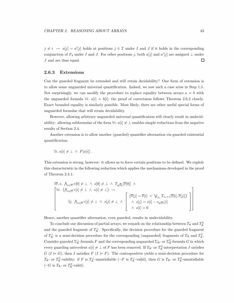
CHAPTER 2. REASONING ABOUT ARRAYS 43
j 6= i → a[j] = a′[j] holds at positions j ∈ I under I and J if it holds in the corresponding
conjunction of F4 under I and J . For other positions j, both a[j] and a′[j] are assigned ⊥ under
J and are thus equal.
2.6.3 Extensions
Can the guarded fragment be extended and still retain decidability? One form of extension is
to allow some unguarded universal quantification. Indeed, we saw such a case arise in Step 1.5.
Not surprisingly, we can modify the procedure to replace equality between arrays a = b with
the unguarded formula ∀i. a[i] = b[i]; the proof of correctness follows Theorem 2.6.2 closely.
Exact bounded equality is similarly possible. Most likely, there are other useful special forms of
unguarded formulae that will retain decidability.
However, allowing arbitrary unguarded universal quantification will clearly result in undecid-
ability: allowing subformulae of the form ∀i. a[i] 6= ⊥ enables simple reductions from the negative
results of Section 2.4.
Another extension is to allow another (guarded) quantifier alternation via guarded existential
quantification:
∃i. a[i] 6= ⊥ ∧ F [a[i]] .
This extension is strong, however: it allows us to force certain positions to be defined. We exploit
this characteristic in the following reduction which applies the mechanisms developed in the proof
of Theorem 2.4.1:
∃v, s.∧
v∈v v[0] 6= ⊥ ∧ s[0] 6= ⊥ ∧ Tq(0)[v[0]] ∧
∀i.(∧
v∈v v[i] 6= ⊥ ∧ s[i] 6= ⊥)
→
∃j.∧
v∈v v[j] 6= ⊥ ∧ s[j] 6= ⊥ ∧
(v[j] = v[i] ∨
∨
xiTxi+1[v[i], v[j]]
)
∧ s[j] = s[i] − vq(x)[i]
∧ s[i] > 0
Hence, another quantifier alternation, even guarded, results in undecidability.
To conclude our discussion of partial arrays, we remark on the relationship between TA and T ZA
and the guarded fragment of T⊥A
. Specifically, the decision procedure for the guarded fragment
of T⊥A
is a semi-decision procedure for the corresponding (unguarded) fragments of TA and T ZA.
Consider guarded Σ⊥A
-formula F and the corresponding unguarded ΣA- or ΣZA-formula G in which
every guarding antecedent a[i] 6= ⊥ of F has been removed. If TA- or T ZA-interpretation I satisfies
G (I |= G), then I satisfies F (I |= F ). The contrapositive yields a semi-decision procedure for
TA- or T ZA-validity: if F is T⊥
A-unsatisfiable (¬F is T⊥
A-valid), then G is TA- or T Z
A-unsatisfiable
(¬G is TA- or T ZA-valid).

CHAPTER 2. REASONING ABOUT ARRAYS 44
2.7 Conclusion
While there still exist interesting fragments for which decidability remains an open question
(specifically, adding the power to express injectivity in TA — but not in T ZA
— and adding
restricted use of unguarded universal quantification in T⊥A
), we have largely answered the moti-
vating two questions posed at the beginning of the chapter. The array property fragments of TA
and T ZA
capture many of the predicates previously examined separately, in particular predicates
for reasoning about sorting programs and for reasoning about extensionality. Furthermore, they
allow expressing many other interesting properties when array elements are interpreted in various
theories. Finally, the array property fragment is in some sense natural: simple extensions to the
fragment result in undecidability.
As a test of expressiveness and efficiency, we implemented the decision procedures of Sections
2.2 and 2.3 in our verifying compiler πVC and proved that the sorting algorithms BubbleSort,
InsertionSort, MergeSort, and QuickSort actually return sorted arrays. Besides requiring the pred-
icates sorted and partitioned, we found that bounded equality and general universal properties
were essential for proving the correctness of MergeSort and QuickSort. We expect that these lat-
ter properties will be of great value in verifying more general programs that manipulate arrays.
Finally, computation time was on the order of seconds.

Chapter 3
Property-Directed Invariant
Generation
The inductive method of proving a safety property Π of a transition system S : 〈x, θ, ρ〉 requires
finding an auxiliary assertion χ such that Π∧χ is inductive for the system [MP95]. This chapter
describes an invariant generation-based approach to finding auxiliary assertions for proving safety
properties of software and hardware systems.
An invariant generation procedure discovers auxiliary assertions. An abstract interpretation
based on forward propagation typically finds one large inductive assertion ϕ [CC77]. The dis-
covered assertion ϕ may or may not be a suitable auxiliary invariant for proving the invariance
of Π. Incremental invariant generation — for example of affine invariants [CSS03] — produces a
sequence of (relatively weak) inductive assertions ϕ1, . . . , ϕk; again, the conjunction of a subset
of these assertions may or may not be suitable for proving Π.
In [BM06], we suggested a method for making incremental invariant generation of affine and
polynomial inequality invariants property-directed so that each successive ϕi makes progress
toward building an auxiliary assertion χ such that Π∧χ is inductive. In this chapter, we extend
the approach to generating inductive clauses in a directed fashion for analyzing safety properties
of finite-state systems. We present both applications in a unified setting.
Section 3.1 presents the property-directed incremental methodology in an abstract setting.
Then Sections 3.2 and 3.3 develop instances of this methodology for generating inequality and
clausal invariants, respectively. Finally, Section 3.4 discusses related work and further directions
for research.
45

CHAPTER 3. PROPERTY-DIRECTED INVARIANT GENERATION 46
3.1 Property-Directed Incremental Invariant Generation
To prove that Π is an invariant of S : 〈x, θ, ρ〉, we attempt to find a strengthening assertion χ
such that Π ∧ χ is inductive. How do we find χ? This section describes several strategies of
incrementally generating χ. In all cases, it is assumed that θ ⇒ Π; otherwise, a counterexample
is easily found.
3.1.1 Incremental Invariant Generation
The first strategy ignores Π while iteratively building a sequence χi of ever stronger inductive
formulae. Let χ0def= true. Suppose that we have performed i iterations so far to produce an
inductive formula χi; that is, χi satisfies the (initiation) and (consecution) conditions:
θ ⇒ χi and χi ∧ ρ ⇒ χ′i . (3.1)
On iteration i+ 1, we seek a new formula γ that is inductive relative to χi:
θ ⇒ γ and χi ∧ γ ∧ ρ ⇒ γ′ . (3.2)
From (3.1) and (3.2), it follows that χi ∧ γ is inductive:
θ ⇒ χi ∧ γ and χi ∧ γ ∧ ρ ⇒ χ′i ∧ γ
′ .
To ensure that γ also provides new information, we require that it satisfy an additional condition
called (strengthening):
∃x. χi ∧ ¬γ .
This condition asserts that γ is not just a logical consequence of χi. Instead, χi ∧ γ is inductive
and is strictly stronger than χi: it eliminates more states than χi. This iteration ends by updating
the inductive information that is known: χi+1 := χi∧γ. χi+1 is inductive and is strictly stronger
than χi.
We call this strategy incremental invariant generation. Incremental invariant generation is
useful in practice for discovering information about a program in the absence of a specification.
3.1.2 Property-Directed Incremental Invariant Generation
The second strategy uses Π to guide the invariant generation and is thus called property-directed
incremental invariant generation. Again, let χ0def= true. Suppose that we have performed i

CHAPTER 3. PROPERTY-DIRECTED INVARIANT GENERATION 47
iterations so far to produce a formula χi that is inductive relative to Π:
θ ⇒ χi and Π ∧ χi ∧ ρ ⇒ χ′i . (3.3)
Note that χi is not necessarily inductive by itself but is inductive relative to Π. On iteration
i+ 1, we seek a new formula γ that is inductive relative to Π ∧ χi:
θ ⇒ γ and Π ∧ χi ∧ γ ∧ ρ ⇒ γ′ . (3.4)
From (3.3) and (3.4), it follows that χi ∧ γ is inductive relative to Π:
θ ⇒ χi ∧ γ and Π ∧ χi ∧ γ ∧ ρ ⇒ χ′i ∧ γ
′ .
As in incremental invariant generation, we want to ensure that γ provides new information.
We could apply the (strengthening) condition
∃x. χi ∧ ¬γ .
Alternately, consider when consecution fails:
Π ∧ χi ∧ ρ 6⇒ Π′ .
In this case, there is a counterexample to induction: a state s that can lead to a state s′ that
violates Π. We require that the new invariant γ eliminate such a state s:
∃x, x′. Π ∧ χi ∧ ρ ∧ ¬Π′ ∧ ¬γ . (3.5)
We refer to requirement (3.5) as the (Π-strengthening) verification condition. The invariant gen-
eration procedure should thus produce a new inductive formula that satisfies (initiation), (con-
secution), and (Π-strengthening). This iteration ends by conjoining the new inductive invariant
γ to the already known information: χi+1 := χi ∧ γ. χi+1 is strictly stronger than χi. By con-
struction, states excluded by χi+1 cannot be reached from a θ-state without first passing through
some other ¬Π-state.
The iterations continue until Π ∧ χi∗ is inductive on some iteration i∗. From (3.3), if the
following implication holds, then Π ∧ χi∗ is inductive:
Π ∧ χi∗ ∧ ρ ⇒ Π′ .
Notice that although Π is assumed to hold during the construction of each χi, the inductiveness
of Π ∧ χi∗ proves the invariance of Π as desired.

CHAPTER 3. PROPERTY-DIRECTED INVARIANT GENERATION 48
3.1.3 The Sampling Strategy
Implementing the strengthening conditions directly in a static analysis can be computationally
prohibitive. For example, in the application in Section 3.2, quantifier elimination could, in
principle, solve the initiation, consecution, and strengthening conditions exactly; however, the
analysis would not scale beyond a few variables.
Instead, the analyses of both Sections 3.2 and 3.3 decouple the initiation, consecution, and
strengthening conditions. Consider the case of applying (Π-strengthening). First, a state s is
selected that satisfies
∃x′. χi[s] ∧ Π[s] ∧ ρ[s, x′] ∧ ¬Π[x′] , (3.6)
so that it can lead in one step to a violation of Π. Then the incremental invariant generation
procedure constructs a new inductive assertion γ that satisfies
θ ⇒ χi ∧ γ and Π ∧ χi ∧ γ ∧ ρ ⇒ χ′i ∧ γ
′ and ¬γ[s] .
It is possible that for a given s, no single assertion γ exists that excludes s; in this case, a new
sample state s should be selected. To allow resampling, (3.6) should be solved with a randomized
constraint solver that, ideally, selects a satisfying state uniformly at random. In our experience,
we have found that randomized constraint solvers with no such guarantee are adequate.
3.2 Inequality Invariants
We now apply the property-directed invariant generation method to the problem of generating
polynomial inequality invariants of linear and polynomial transition systems. Section 3.2.1 re-
views the constraint-based method of inequality invariant generation. Then Section 3.2.2 uses
the resulting invariant generator in a property-directed procedure. The primary advantage of
using the property-directed method in this application is that it allows using generic constraint
solvers. We describe an incomplete but scalable constraint solver in Section 3.2.3.
3.2.1 Constraint-based Invariant Generation
To begin, we review the constraint-solving method based on Farkas’s Lemma [CSS03] or La-
grangian relaxation [Cou05]. Farkas’s Lemma relates a primal constraint system S (a conjunc-
tion of affine inequalities) over the program variables to a dual constraint system over a set of
introduced dual variables (Lagrangian multipliers) [Sch86]. Theorem 3.2.1 describes the case
when S consists of a conjunction of affine inequalities. Then Corollary 3.2.1 extends the result,
with loss of completeness, to the case when some constraints of S are polynomial inequalities.
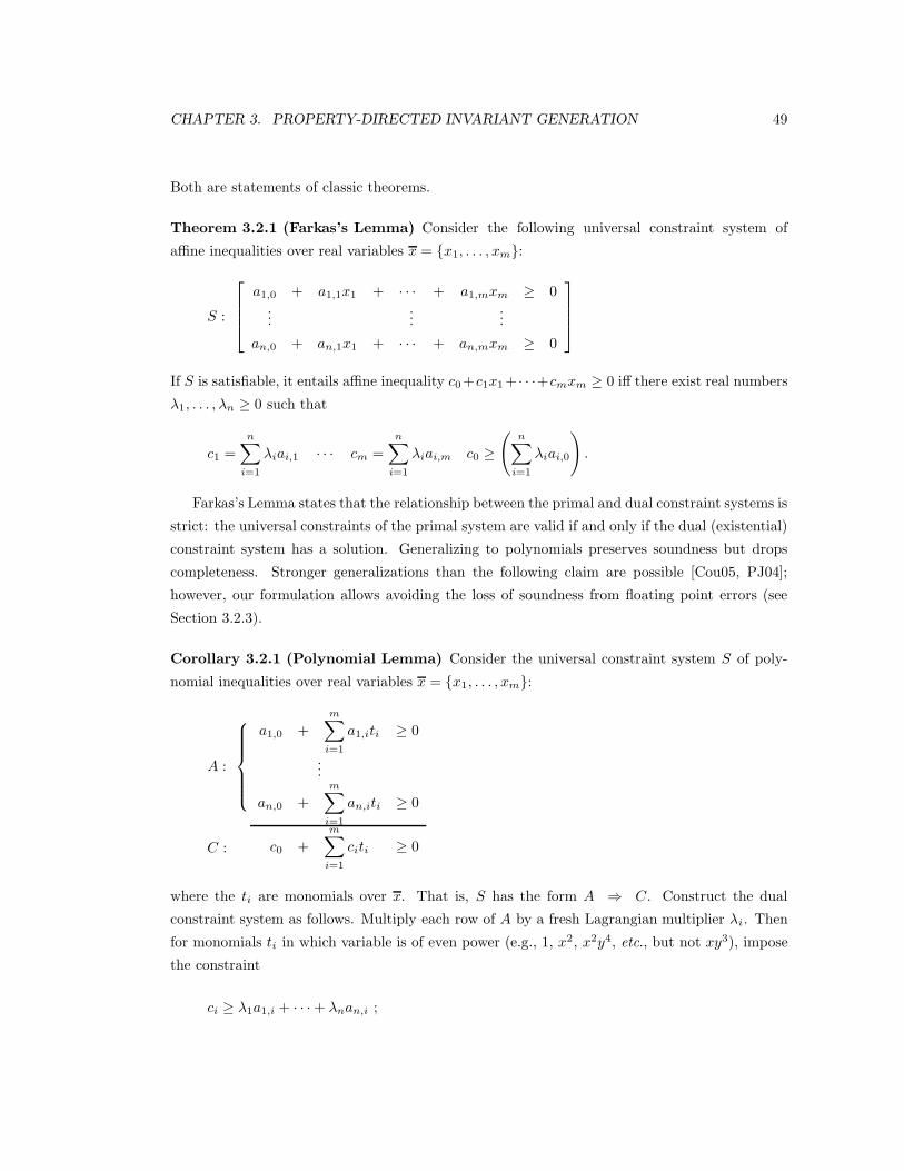
CHAPTER 3. PROPERTY-DIRECTED INVARIANT GENERATION 49
Both are statements of classic theorems.
Theorem 3.2.1 (Farkas’s Lemma) Consider the following universal constraint system of
affine inequalities over real variables x = x1, . . . , xm:
S :
a1,0 + a1,1x1 + · · · + a1,mxm ≥ 0...
......
an,0 + an,1x1 + · · · + an,mxm ≥ 0
If S is satisfiable, it entails affine inequality c0+c1x1 + · · ·+cmxm ≥ 0 iff there exist real numbers
λ1, . . . , λn ≥ 0 such that
c1 =
n∑
i=1
λiai,1 · · · cm =
n∑
i=1
λiai,m c0 ≥
(n∑
i=1
λiai,0
)
.
Farkas’s Lemma states that the relationship between the primal and dual constraint systems is
strict: the universal constraints of the primal system are valid if and only if the dual (existential)
constraint system has a solution. Generalizing to polynomials preserves soundness but drops
completeness. Stronger generalizations than the following claim are possible [Cou05, PJ04];
however, our formulation allows avoiding the loss of soundness from floating point errors (see
Section 3.2.3).
Corollary 3.2.1 (Polynomial Lemma) Consider the universal constraint system S of poly-
nomial inequalities over real variables x = x1, . . . , xm:
A :
C :
a1,0 +
m∑
i=1
a1,iti ≥ 0
...
an,0 +
m∑
i=1
an,iti ≥ 0
c0 +
m∑
i=1
citi ≥ 0
where the ti are monomials over x. That is, S has the form A ⇒ C. Construct the dual
constraint system as follows. Multiply each row of A by a fresh Lagrangian multiplier λi. Then
for monomials ti in which variable is of even power (e.g., 1, x2, x2y4, etc., but not xy3), impose
the constraint
ci ≥ λ1a1,i + · · · + λnan,i ;

CHAPTER 3. PROPERTY-DIRECTED INVARIANT GENERATION 50
int j, k;@ j = 2 ∧ k = 0while (· · · ) do
if (· · · )then j := j + 4;else j := j + 2;
k := k + 1;done
Figure 3.1: Simple
for all other terms, impose the constraint
ci = λ1a1,i + · · · + λnan,i .
Finally, require that all λi are nonnegative: λi ≥ 0. If the dual constraint system is satisfiable,
then the primal constraint system is valid.
Constraint-based linear invariant generation [CSS03] uses Farkas’s Lemma to generate affine
inequality invariants over linear transition systems. The method begins by proposing an affine
inequality template
c0 + c1x1 + · · · + cnxn ≥ 0 ,
where the ci are the template variables. It then imposes on the template the conditions (initiation)
θ ⇒ c0 + c1x1 + · · · + cnxn ≥ 0
and (consecution)
c0 + c1x1 + · · · + cnxn ≥ 0 ∧ ρ ⇒ c0 + c1x′1 + · · · + cnx
′n ≥ 0 .
Expressing θ and ρ in DNF reveals a finite set of parameterized linear constraint systems of the
form in Theorem 3.2.1, except for the presence of the parameters ci. Dualizing the constraint
systems according to Farkas’s Lemma and conjoining them produces a single large existential
conjunctive constraint system over the parameters ci and the introduced multipliers λ. The dual
system is a bilinear or a parameterized linear system: it is almost linear except for the presence
of the parameters ci. Each solution to this dual constraint system provides an instantiation of
the ci corresponding to an inductive inequality. Corollary 3.2.1 and the stronger versions in
[Cou05] provide the mechanism for extending this technique to polynomial inequality invariants
and analyzing polynomial transition systems.

CHAPTER 3. PROPERTY-DIRECTED INVARIANT GENERATION 51
Example 3.2.1 (Simple) Consider the loop Simple in Figure 3.1, which first appeared in
[CH78]. The · · · in Figure 3.1 indicates nondeterministic choice. The corresponding linear
transition system S is the following:
x : j, k
θ : j = 2 ∧ k = 0
ρ1 : j′ = j + 4 ∧ k′ = k
ρ2 : j′ = j + 2 ∧ k′ = k + 1
with ρ : ρ1 ∨ ρ2.
The constraint-based method seeks inductive instantiations of the template
p0 + p1j + p2k ≥ 0
with parameters pi. The (initiation) condition imposes the following constraint on the template:
j = 2 ∧ k = 0 ⇒ p0 + p1j + p2k ≥ 0 ,
or more simply,
p0 + 2p1 + 0p2 ≥ 0 . (3.7)
Treating each disjunct of ρ separately, the (consecution) condition imposes two constraints:
p0 + p1j + p2k ≥ 0 ∧ j′ = j + 4 ∧ k′ = k ⇒ p0 + p1j′ + p2k
′ ≥ 0 ,
or more simply
p0 + p1j + p2k ≥ 0 ⇒ (p0 + 4p1) + p1j + p2k ≥ 0 ; (3.8)
and
p0 + p1j + p2k ≥ 0 ⇒ (p0 + 2p1 + p2) + p1j + p2k ≥ 0 . (3.9)
All together, the (primal) constraint problem is thus
p0 + 2p1 + 0p2 ≥ 0
∧ p0 + p1j + p2k ≥ 0 ⇒ (p0 + 4p1) + p1j + p2k ≥ 0
∧ p0 + p1j + p2k ≥ 0 ⇒ (p0 + 2p1 + p2) + p1j + p2k ≥ 0
(3.10)

CHAPTER 3. PROPERTY-DIRECTED INVARIANT GENERATION 52
According to Theorem 3.2.1, we then have the following set of dual constraints:
p0 + 2p1 + 0p2 ≥ 0
from (3.7),
p1 = λ1p1 ∧ p2 = λ1p2 ∧ p0 + 4p1 ≥ λ1p0
from (3.8), and
p1 = λ2p1 ∧ p2 = λ2p2 ∧ p0 + 2p1 + p2 ≥ λ2p0
from (3.9). Conjoining them reveals the dual constraint system over the variables
p0, p1, p2, λ1, λ2.
In nontrivial solutions, λ1 = λ2 = 1. One solution is p0 = 0, p1 = 0, p2 = 1, corresponding
to the inductive invariant k ≥ 0. Section 3.2.3 describes an incomplete constraint solver that is
often fast in practice for solving such constraint systems.
3.2.2 Property-Directed Iterative Invariant Generation
In this section, we apply the constraint-based method to produce a procedure for property-
directed incremental invariant generation. Transitioning to incremental invariant generation is
not obvious. For example, applying a generic constraint solver to solve the dual constraint
problem arising from (3.10) will probably reveal the same solution again and again. The authors
of [CSS03] implemented a specialized solver described in [SSM04] to avoid this problem. In
contrast, the method of [Cou05] is essentially restricted to verification constraints in which a
single solution solves the problem (e.g., to prove termination by finding a ranking function; see
Section 3.4).
We describe two iterative procedures based on the sampling strategy of approximating addi-
tional (strengthening) or (Π-strengthening) conditions.
Incremental Invariant Generation
As in Section 3.1, suppose that we have generated so far the inductive invariant χi. We seek a
new invariant γ that is inductive relative to χi and, according to the (strengthening) condition,
such that γ excludes at least one state allowed by χi. Ideally, we would impose the conditions
(initiation), (consecution), and (strengthening) simultaneously. However, the resulting constraint
system would have both universally and existentially quantified variables and would thus not be
amenable to analysis via Theorem 3.2.1 or Corollary 3.2.1 (although the constraint system would
be solvable in principle at high computational cost [Tar51, Col75]). The following procedure

CHAPTER 3. PROPERTY-DIRECTED INVARIANT GENERATION 53
applies the sampling strategy of Section 3.1.3 to decouple the (strengthening) condition from the
others.
Let
p0 + p1x1 + · · · + pnxn︸ ︷︷ ︸
T
≥ 0
be the template. Perform the following steps:
1. Solve the existential constraint system χi. The solution is a state s.
2. Impose the conditions (initiation) and (consecution) on the template. For (initiation), impose
θ ⇒ p0 + p1x1 + · · · + pnxn ≥ 0 ;
for (consecution), use the known χi:
χi ∧ p0 + p1x1 + · · · + pnxn ≥ 0 ∧ ρ ⇒ p0 + p1x′1 + · · · + pnx
′n ≥ 0 .
Apply Theorem 3.2.1 or Corollary 3.2.1 to generate the dual constraint system ψ. Finally,
solve the existential constraint system
Tx 7→ s < 0 ∧ ψ , (3.11)
where Tx 7→ s represents the substitution of the state s for the variables x. A solution
that assigns q to p represents the inequality
q0 + q1x1 + · · · + qnxn ≥ 0
that is inductive relative to χi and that excludes the state s. If a solution is not found,
return to Step 1 to choose another state s.
3. Optimize the discovered solution q. Solve the following optimization problem:
minimize p0
subject to
(T ≥ 0 ∧ ψ)p1 7→ q1, . . . , pn 7→ qn
At most q0 from Step 2 is returned as the minimum of p0. Set q0 to the new solution.
4. Let χi+1def= χi ∧ Tp 7→ q ≥ 0.
Step 1 and condition (3.11) addresses the (strengthening) condition, while Steps 2 and 3 address

CHAPTER 3. PROPERTY-DIRECTED INVARIANT GENERATION 54
the (initiation) and (consecution) conditions.
The constraint problem of Step 1 can be solved in numerous ways, including using decision
procedures or numerical constraint solvers for solving linear and semi-algebraic constraint prob-
lems. It is best if these solvers can be randomized so that a wide selection of sample points is
possible. The constraint problem of Step 2 can be solved using a solver for bilinear constraint
problems (see Section 3.2.3).
Note that the strict inequality of Step 2 is easily handled by transforming the feasibility
problem into an optimization problem:
maximize ε
subject to
Tx 7→ s ≤ −ε ∧ ψ
The original system is feasible if and only if the maximum is positive.
Example 3.2.2 Consider again the linear transition system of Example 3.2.1. Let χ0def= true.
On the first iteration, let
p0 + p1j + p2k︸ ︷︷ ︸
T
≥ 0
be the template. Step 1 returns a point satisfying χ0, namely any point. Suppose that it is
s1 : (j : −1, k : −3). According to Step 2, impose (initiation) and (consecution) on T ≥ 0 and
let ψ be the dual constraint system. Because χ0 is true, the dual constraint system of Example
3.2.1 is ψ:
(p0 + 2p1 + 0p2 ≥ 0) ∧
p1 = λ1p1
∧ p2 = λ1p2
∧ p0 + 4p1 ≥ λ1p0
∧
p1 = λ2p1
∧ p2 = λ2p2
∧ p0 + 2p1 + p2 ≥ λ2p0
(3.12)
Then solve
Tj 7→ −1, k 7→ −3 < 0 ∧ ψ , i.e., p0 − p1 − 3p2 < 0 ∧ ψ ,
which is a constraint system over p0, p1, p2, λ1, λ2. One possible solution corresponds to the
inductive formula γ : k ≥ 0. Indeed, k ≥ 0 excludes s1 : (j : −1, k : −3) and is inductive. Step 3

CHAPTER 3. PROPERTY-DIRECTED INVARIANT GENERATION 55
attempts to improve upon k ≥ 0 by tightening the constant coefficient:
minimize p0
subject to
p0 + k ≥ 0 ∧ ψp1 7→ 0, p2 7→ 1
However, k ≥ 0 is already as strong as possible. Hence, χ1def= χ0 ∧ k ≥ 0. The assertion
χ1 : k ≥ 0 excludes the state s1 : (j : −1, k : −3) and any other state in which k < 0. Thus, no
future iteration can again discover k ≥ 0 (or any weaker assertion).
On the next iteration, Step 1 could find, for example, state s2 : (j : −1, k : 5), which satisfies
χ1 : k ≥ 0. Steps 2 and 3 would then discover inductive assertion j ≥ 0 to eliminate this point,
resulting in χ2 : k ≥ 0 ∧ j ≥ 0. A third or fourth iteration will probably yield the invariant
j ≥ 2k + 2: any sample point in which j < 2k + 2 (and k ≥ 0 ∧ j ≥ 0), such as (j : 5, k : 3),
reveals this invariant. Of the remaining points in the (j, k) plain, approximately half violate
j ≥ 2k + 2. Then
χ3 : k ≥ 0 ∧ j ≥ 0 ∧ j ≥ 2k + 2 ,
which is the strongest possible conjunctive affine invariant of the system.
Property-Directed Incremental Invariant Generation
Let
p0 + p1x1 + · · · + pnxn︸ ︷︷ ︸
T
≥ 0
be the template. Perform the following steps:
1. Solve the existential constraint system corresponding to the imposed strengthening condi-
tion:
• χi for (strengthening),
• Π ∧ χi ∧ ρ ∧ ¬Π′ for (Π-strengthening).
If the system for (Π-strengthening) does not have a solution, then declare that Π is S-
invariant. Otherwise, the solution is a state s.
Step 2-4 are like in incremental invariant generation with one difference. If a solution is not
found in Step 2 and a (Π-strengthening) condition was imposed in Step 1, possibly impose the
(strengthening) condition in the next attempt. For there may not currently exist an inductive
inequality that can exclude a state that leads to a violation of Π.

CHAPTER 3. PROPERTY-DIRECTED INVARIANT GENERATION 56
int u, w, x, z;@ x ≥ 1 ∧ u = 1 ∧ w = 1 ∧ z = 0while (w ≤ x) do
(z, u, w) := (z + 1, u+ 2, w + u+ 2);done
Figure 3.2: Sqrt
Example 3.2.3 (Integer Square-Root) The loop Sqrt in Figure 3.2 computes the integer
square-root z of a positive integer x. On exit, the following relation should hold between z and
x:
z2 ≤ x < (z + 1)2 .
Taking preconditions reveals that the following should be invariant at the top of the loop:
Π : (w ≤ x → (z + 1)2 ≤ x) ∧ (w > x → x < (z + 1)2) .
However, Π is not S-inductive. We apply the iterative procedure using condition (Π-
strengthening) for Step 1 to generate a χ such that χ ⇒ Π.
On each iteration, we use the template
Quadratic(u,w, x, z)︸ ︷︷ ︸
T
≥ 0 .
Quadratic forms the most general parameterized quadratic expression over the given variables;
e.g.,
Quadratic(x, y) = p0 + p1x+ p2y + p3xy + p4x2 + p5y
2 .
Because T is a polynomial template, we use Corollary 3.2.1 instead of Theorem 3.2.1.
One execution of the procedure constructs the following sequence of inductive assertions,
where each is inductive relative to the conjunction of the previous ones:
γ1 : −x+ ux− 2xz ≥ 0
γ2 : u ≥ 0
γ3 : u− u2 + 4uz − 4z2 ≥ 0
γ4 : 3u+ u2 − 4w ≥ 0
γ5 : x− ux+ 2xz ≥ 0
γ6 : 1 + 2u+ u2 − 4w ≥ 0
γ7 : −1 + u ≥ 0
γ8 : −2u− u2 + 4w ≥ 0
γ9 : −3 − u2 + 4w ≥ 0
γ10 : −5u− u2 + 6w ≥ 0
γ11 : −15 + 22u− 11u2 + 4uw ≥ 0
γ12 : −1 − 2u− u2 + 4w ≥ 0

CHAPTER 3. PROPERTY-DIRECTED INVARIANT GENERATION 57
Thus, χ12def= γ1 ∧ · · · ∧ γ12.
On the thirteenth iteration, it is discovered that no state satisfies χ12 ∧ ¬Π, proving that
Π ∧ χ12 is inductive and that Π is invariant. Specifically, γ1 and γ5 entail u = 1 + 2z, while γ6
and γ12 entail 4w = (u+ 1)2. Thus, w = (z + 1)2, entailing Π.
3.2.3 Solving Bilinear Constraint Problems
The constraint systems that arise in Step 2 of the procedures of Section 3.2.2 are bilinear con-
straint problems : quadratic terms are of the form λp, where λ and p are different variables.
Specifically, the variable λ is an introduced Lagrangian multiplier, while the variable p is a pa-
rameter (an unknown coefficient in the template). For example, the constraint problem (3.12) is
bilinear. While solvable via quantifier elimination [Tar51, Col75], this complete approach does
not scale. Instead, [SSM04, BMS05a, Cou05] suggest incomplete heuristic approaches, while
[SSM03] describes a complete and relatively efficient method for solving the constraint systems
that arise for a special class of transition systems.
We briefly describe one possible incomplete solver that has been found to work in practice.
Consider the bilinear constraint system ψ. Let each Lagrangian multiplier λ that appears in a
bilinear term λp range over a fixed set, say 0, 1 (this set 0, 1 is sufficient in some cases when
the disabled case is ignored [SSM03]). Then execute a search. Let ψi be the current constraint
system.
1. If the conjunction of the subset of linear constraints of ψi is unsatisfiable, then return
unsatisfiable.
2. Choose a multiplier λj that is unassigned and that appears bilinearly in ψi. If no such λj
exists, return satisfiable.
3. Try each value v in λj ’s possible solution set:
(a) Let ψi+1def= ψiλj 7→ v.
(b) Recurse on ψi+1, returning satisfiable if the recursive call returns satisfiable.
Step 1 offers an early detection of unsatisfiability.
For solving the intermediate linear constraint systems, our implementation uses a rational
solver [Avi98], thus avoiding the possible loss of soundness from floating point errors [Cou05].
3.3 Clausal Invariants
Scaling verification to large circuits requires some form of abstraction relative to the asserted
property. Many safety analyses of systems operate by abstracting a system’s transition relation

CHAPTER 3. PROPERTY-DIRECTED INVARIANT GENERATION 58
relative to the property [GS97, CGJ+03, HJMS02, MA03, McM03, McM05]. In contrast, we
describe a safety analysis of finite-state systems that operates on a system’s full transition re-
lation. The analysis incrementally strengthens the asserted property until it is inductive. Each
iteration produces one inductive clause. The construction of each inductive clause is guided by
a state that violates the inductiveness of the property. Therefore, the generated invariants are
relevant for proving the property. Because the analysis is property-directed, it scales to proving
properties that are local to submodules of relatively large circuits.
The analysis is just another instance of incremental invariant generation. However, let us
consider the analysis from the point of view of standard model checking [CE82]. Suppose that
an explicit-state backward model checker discovers a state s that leads to a violation of safety
property Π. A purely explicit-state algorithm would update Π to be Π ∧ ¬s and continue on
this new property. If the property holds, then an inductive strengthening of Π is eventually
discovered. Now consider computing the preimage of s to the fixpoint formula F : that is, F
represents precisely those states that can reach s. Then update Π to be Π ∧ ¬F . For efficiency,
one can under-approximate F . This computation converges to the same inductive assertion as
in the first algorithm.
Now consider our alternate approach. State s and its negation ¬s are described by a con-
junction of literals and a clause, respectively, say
s : x1 ∧ ¬x2 ∧ x3 ∧ · · ·
¬s : ¬x1 ∨ x2 ∨ ¬x3 ∨ · · ·
Any subclause c of ¬s that is inductive for the system is necessarily stronger than ¬F of the
preimage computation described above. Why? For c to be inductive, the represented set of
states cannot include any state that can lead to s. Moreover, c can be much stronger than ¬F
because reasoning based on an inductive argument allows us to eliminate states other than just
those that can lead to s. Finally, c can be much more efficient to compute; in practice, preimage
computations can be memory intensive, whereas a clause is small. A minimal inductive subclause
(MIC) of ¬s is an inductive subclause of ¬s that does not contain any strict subclauses that are
also inductive. When a (minimal) inductive subclause c of ¬s exists, update Π to be Π ∧ c;
otherwise, just update Π to be Π ∧ ¬s.
The success of our approach depends on two points. First, we need a fast way of finding
a minimal inductive subclause when one exists. We address this challenge in Section 3.3.1.
Second, small minimal inductive clauses must exist in practice. The empirical evidence of Section
3.3.4 suggests that they do. Our parallel implementation of our safety analysis solves all 20
PicoJava II benchmarks proposed by Ken McMillan [MA03, McM03, McM05], whereas proof-
based abstraction [MA03] and interpolation-based model checking [McM03, McM05] solve 18 and
19, respectively. Additionally, our implementation succeeds on several benchmarks from the VIS

CHAPTER 3. PROPERTY-DIRECTED INVARIANT GENERATION 59
distribution [VIS] that are difficult for analyses based on k-induction [AS06]. In Section 3.4, we
discuss related techniques and the potential for hybrid approaches.
First, we introduce some terminology and notation. A literal is a positive x or negative ¬x
occurrence of a program variable x ∈ x. A clause c is a disjunction of literals. Notationally, we
write a clause as a disjunction of literals c : `1 ∨ · · · ∨ `k. The size |c| of a clause c is the number
of literals it contains (the size of the empty clause, equivalent to false, is 0). A subclause d v c
is the disjunction of a subset of c’s literals. Using this terminology and that of Section 3.1, each
iteration of invariant generation produces a clause γ that is inductive relative to Π ∧ χi. Hence,
χi is a conjunction of i clauses.
3.3.1 Generating Minimal Inductive Subclauses
Consider the following problem. Given a Boolean transition system S : 〈x, θ, ρ〉 and a clause c0,
find a minimal inductive subclause c v c0 if one exists.
Definition 3.3.1 (Minimal Inductive Clause) A minimal inductive clause c is S-inductive
(possibly relative to some formula ψ, such as Π ∧ χi), and it does not contain any strict subclause
d @ c that is also S-inductive (again, possibly relative to ψ).
Shortly, we describe an algorithm for discovering a minimal inductive subclause (if one exists)
of a given clause c0. The idea of the algorithm is to traverse the lattice Lc0defined by the
subclauses of c0, where
• the elements are the subclauses of c0;
• comparison v is the weak subset relation between clauses’ literal sets;
• and join t and meet u are the union and the intersection, respectively, between the literal
sets of clauses.
Motivation: The Obvious Algorithm
Let us first consider the obvious approach to finding a minimal inductive subclause: execute
a backward abstract interpretation to discover the unique largest inductive subclause, which is
the greatest fixpoint d in Lc0of S. The algorithm is then applied recursively to each direct
descendant of d in the lattice. It terminates with clause e when the greatest fixpoint computed
for each of e’s direct descendants does not cover the initial condition of S; e is a minimal inductive
subclause of c0. There may be many minimal inductive subclauses of c0.
How does one compute the largest inductive subclause of c0? From abstract interpretation
theory [CC77], one computes the greatest fixpoint in the lattice Lc0by iteratively computing and
under-approximating preimages. The direct approach under-approximates the preimage wp. For

CHAPTER 3. PROPERTY-DIRECTED INVARIANT GENERATION 60
clause c, one seeks the unique largest subclause d v c such that d ⇒ wp(c, S). One computes
d by considering each literal ` of c in turn and testing whether ` ⇒ wp(c, S); ` is in d iff the
implication holds.
This approach has two problems. First, computing the greatest fixpoint is computationally
expensive. In lattice Lc0, it requires making O(|c0|) propositional satisfiability queries for each
of O(|c0|) rounds of under-approximation; hence, O(|c0|2) queries in total. Our solution exploits
the clause domain and requires solving only O(|c0|) queries.
Second, descending the lattice Lc0by finding successively stronger fixpoints can be slow. But
once a fixpoint d is discovered, one can execute a forward abstract interpretation in the lattice
Ld to discover, in practice, a relatively small fixpoint. By standard abstract interpretation
theory, one computes an over-approximation to a least fixpoint by iteratively computing and
over-approximating postimages. However, executing the forward abstract iteration naively also
requires solving O(|c0|2) queries. Our solution exploits a special property of monotonic queries
to require solving only O(m log |c0|) queries, where m is the size of the discovered clause.
Note that the forward abstract interpretation should only be executed within a lattice rooted
by an inductive subclause of c0; otherwise, it is likely that the discovered fixpoint is simply
true even if a better fixpoint exists. Why? First, there may be exponentially many best over-
approximations to a computed postimage because we are working with clauses. (Recall that the
conjunctive normal form (CNF) representation of a propositional formula may be exponentially
larger than the formula itself.) Second, each iteration of the forward abstract interpretation is
blind to the clauses that are available to it in the future when it makes its choice among the best
over-approximating clauses. Many choices may lead to paths in the lattice that do not contain
inductive clauses. Therefore, the backward abstract interpretation is necessary.
From this description of the obvious approach, we derive the following high-level view of the
problem and our proposed solution. First, the overall algorithm for finding a minimal inductive
subclause of c0 executes backward abstract interpretations to find successively smaller fixpoints
(which are inductive subclauses of c0). As an important optimization, it interleaves forward
abstract interpretations to “jump” far down the lattice. Second, implementing the backward
and forward abstract interpretations in a straightforward manner is computationally infeasible.
Therefore, the remainder of our work is to identify fast methods of computing greatest fixpoints
and over-approximations to least fixpoints.
Finding a Minimal Inductive Subclause
Figure 3.3 presents the algorithm mic for finding a minimal inductive subclause: mic(ψ, c0)
returns a minimal subclause c v c0 that is inductive relative to ψ if such a clause exists, and
true otherwise. It formalizes the proposed algorithm of the previous section. First, it computes
the greatest fixpoint c in the lattice Lc0with down. Second, it computes a (small, in practice)

CHAPTER 3. PROPERTY-DIRECTED INVARIANT GENERATION 61
let rec mic(ψ, c0) =Find largest inductive subclause of c0.let c = down(ψ, c0) inif c = truethen return true no inductive subclause of c0else Find “small” inductive subclause of c.
let d = up(ψ, c) inRecursively try each (|d| − 1)-subclause.foreach ` ∈ d do
let e = mic(ψ, d \ `) inif e 6= true then return e
done;Nothing smaller was found: return d as minimal.return d
Figure 3.3: Finding a minimal subclause of c0 that is S-inductive relative to ψ
let rec down(ψ, c0) =Check that initiation holds.if ¬(θ ⇒ c0)then return trueelse Check that consecution holds.
if ψ ∧ c0 ∧ ρ ⇒ c′0then return c0else Select a (¬c0)-predecessor.
let s = ∃x′. ψ ∧ c0 ∧ ρ ∧ ¬c′0 in
return down(ψ, (c0 u ¬s))
Figure 3.4: Finding the largest subclause of c0 that is S-inductive relative to ψ
fixpoint d in the lattice Lc with down. Finally, it recurses on each of the direct descendants of
d to attempt to find an even smaller clause than d.
In more detail, the algorithm down (Figure 3.4) moves down Lc0to find the largest inductive
subclause c of c0. If no such clauses exists, then mic returns the (weakest possible) inductive
invariant true. Otherwise, the discovered clause c is the top element of a sublattice Lc of Lc0. The
algorithm up (Figure 3.5) performs an abstract interpretation in Lc, climbing Lc and returning
an inductive element d v c. Since the root c of the lattice is an inductive clause, up returns c at
worst. As we are interested in a minimal inductive clause, mic then recurses on each immediate
subclause of d, returning a clause if one is found. Otherwise, it returns d.
Let us consider down(ψ, c0), which finds the greatest fixpoint in Lc0according to the seman-
tics given by the formula ψ and the transition relation ρ. If a subclause of c0 that is inductive
relative to ψ exists, the largest one is unique: it is the union of every inductive subclause of c0.
The downward traversal of the lattice Lc0progresses according to ψ and the transition relation

CHAPTER 3. PROPERTY-DIRECTED INVARIANT GENERATION 62
ρ. If it is currently at element d of the lattice, then one of two possibilities exists: either d is
inductive relative to ψ so that down has found the largest inductive subclause, or it is not. In
the latter case, there exists a state s that satisfies ψ ∧ d and that can transition to a state that
does not satisfy d. Formally, s satisfies the formula
∃x′. ψ ∧ d ∧ ρ ∧ ¬d′ .
Any inductive strengthening of d must exclude s. Viewing s as a conjunction of literals, the
weakest clause that excludes s is ¬s. Therefore, the strongest clause in the sublattice Ld of d
that also excludes s is d u ¬s.
Proposition 3.3.1 (Largest Inductive Subclause) If down(ψ, c0) is not true, then it is the
largest subclause of c0 that is S-inductive relative to ψ. This clause is unique. Moreover, it is
discovered in at most O(|c0|) SAT calls.
Proof. Let the output clause be c. From the structure of down, it is apparent that c is S-
inductive relative to ψ. We prove that every clause d v c0 that is S-inductive relative to ψ is a
subclause of the output clause c, proving that c is both the largest possible clause and unique:
for if another “largest” inductive subclause exists, then it must be a subset of c, a contradiction.
Suppose that d 6v c yet d v c0 and d is S-inductive relative to ψ. Without loss of generality,
suppose that d 6v c0 u ¬s — that is, the loss of some literal of d occurs at this level of recursion.
Decompose c0 as d∨ e and consider selecting state s: ∃x′. ψ∧ (d∨ e)∧ρ∧¬d′ ∧¬e′. Distributing
over disjunction, we find two possibilities: one of
∃x′. ψ ∧ d ∧ ρ ∧ ¬d′ ∧ ¬e′ (3.13)
∃x′. ψ ∧ e ∧ ¬d ∧ ρ ∧ ¬d′ ∧ ¬e′ (3.14)
is satisfiable. But (3.13) is unsatisfiable because d is S-inductive relative to ψ. Therefore, the
discovered state s satisfies e ∧ ¬d; and ¬s (and hence c0 u ¬s) contains d, contradicting our
assumption.
Regarding the complexity claim, it is easy to see that each level of recursion must either
terminate with an inductive subclause or remove at least one literal.
An effective optimization in mic and down is to cache the clauses c examined by down.
Caching these sets avoids applying down to a clause d when it has already been applied to
superclause c (d v c). For if c does not have an inductive subclause, then neither does d.
Let us turn to up (Figure 3.5). First, recall that up is unnecessary for the correctness of mic;
however, it is essential to a practical implementation of mic (improving performance by orders of
magnitude in our experiments). mic with only down progresses down the lattice of subclauses

CHAPTER 3. PROPERTY-DIRECTED INVARIANT GENERATION 63
Precondition: c0 is S-inductive relative to ψ.let up(ψ, c0) =
Initiation.c := consequence(θ, c0);Consecution.loop forever do
Compute successor clause. In practice, compute successors of new literals.let d = unprime(consequence(ψ ∧ c ∧ ρ, c′0)) inif d v c
then return c
else c := c t ddone
Figure 3.5: An abstract interpretation on c0
from one inductive clause to the next smaller one. Adding up accelerates the search by jumping
down the lattice to small inductive subclauses.
up(ψ, c0) performs a forward abstract interpretation [CC77] in the lattice Lc0defined by
subclauses of c0. Typical of an abstract interpretation, up first computes a smallest element
c of the lattice that approximates θ: θ ⇒ c. It then iteratively applies an abstract strongest
postcondition operator until a fixpoint is reached. Our abstract postcondition operator is
unprime(consequence(ψ ∧ c ∧ ρ, c′0)) .
To compute it, a smallest subclause of c′0 is chosen to over-approximate the logical consequence
of ψ∧ c∧ρ. Because c0 is inductive relative to ψ, this element is at most c′0. The returned clause
is then unprimed. The only technical aspect of this abstract interpretation is computing minimal
consequences efficiently in the abstract postcondition operator.
Definition 3.3.2 (Minimal Consequence) A clause c is a minimal consequence of α if it is
a logical consequence of α (α⇒ c), and there does not exist a strict subclause d @ c that is also
a consequence of α.
consequence(α, c) should return a minimal consequence d v c of α. Clausal consequences
can be computed similarly to blocking clauses [McM02], and minimal consequences can be com-
puted similarly to prime blocking clauses [JS05] (or prime implicates ; see Section 3.4 for further
discussion). One method of enforcing primality of the resulting clause requires solving a number
of propositional satisfiability queries linear in the number of literals of the original clause [JS05].
However, we discovered an algorithm that requires a number of calls linear in the number of lit-
erals in the discovered prime clause and only logarithmic in the number of literals in the original
clause.
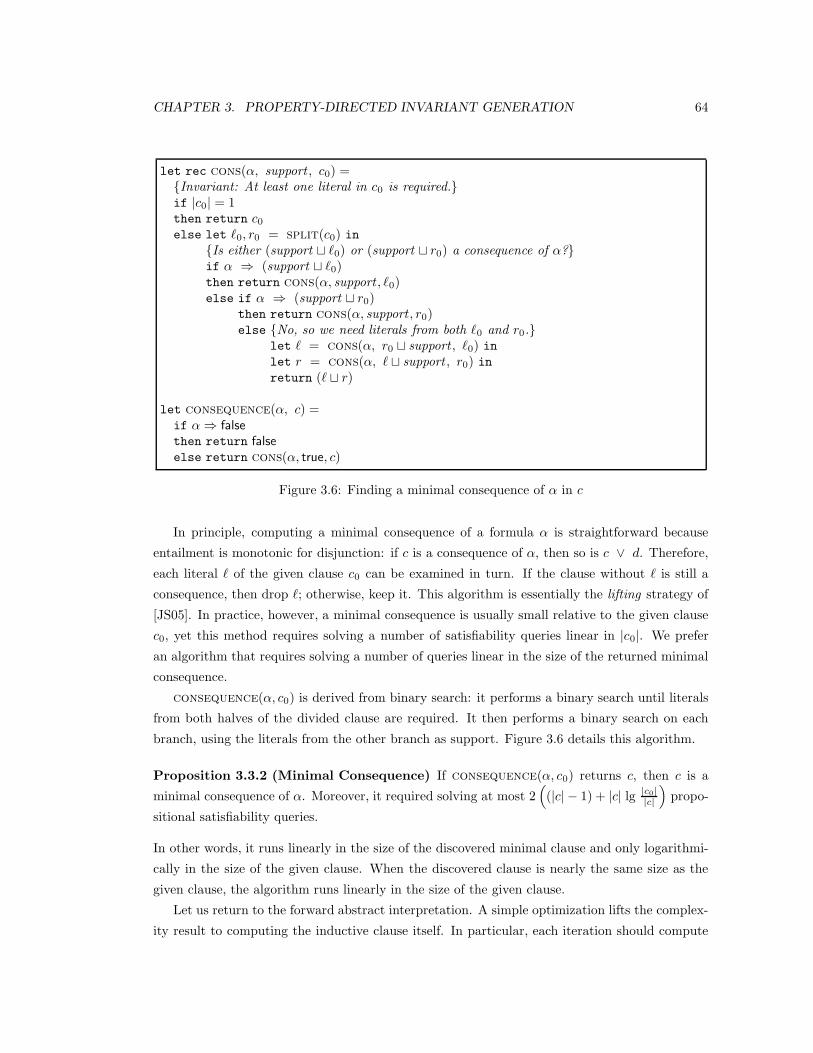
CHAPTER 3. PROPERTY-DIRECTED INVARIANT GENERATION 64
let rec cons(α, support , c0) =Invariant: At least one literal in c0 is required.if |c0| = 1then return c0else let `0, r0 = split(c0) in
Is either (support t `0) or (support t r0) a consequence of α?if α ⇒ (support t `0)then return cons(α, support , `0)else if α ⇒ (support t r0)
then return cons(α, support , r0)else No, so we need literals from both `0 and r0.
let ` = cons(α, r0 t support , `0) inlet r = cons(α, ` t support , r0) inreturn (` t r)
let consequence(α, c) =if α ⇒ falsethen return falseelse return cons(α, true, c)
Figure 3.6: Finding a minimal consequence of α in c
In principle, computing a minimal consequence of a formula α is straightforward because
entailment is monotonic for disjunction: if c is a consequence of α, then so is c ∨ d. Therefore,
each literal ` of the given clause c0 can be examined in turn. If the clause without ` is still a
consequence, then drop `; otherwise, keep it. This algorithm is essentially the lifting strategy of
[JS05]. In practice, however, a minimal consequence is usually small relative to the given clause
c0, yet this method requires solving a number of satisfiability queries linear in |c0|. We prefer
an algorithm that requires solving a number of queries linear in the size of the returned minimal
consequence.
consequence(α, c0) is derived from binary search: it performs a binary search until literals
from both halves of the divided clause are required. It then performs a binary search on each
branch, using the literals from the other branch as support. Figure 3.6 details this algorithm.
Proposition 3.3.2 (Minimal Consequence) If consequence(α, c0) returns c, then c is a
minimal consequence of α. Moreover, it required solving at most 2(
(|c| − 1) + |c| lg |c0||c|
)
propo-
sitional satisfiability queries.
In other words, it runs linearly in the size of the discovered minimal clause and only logarithmi-
cally in the size of the given clause. When the discovered clause is nearly the same size as the
given clause, the algorithm runs linearly in the size of the given clause.
Let us return to the forward abstract interpretation. A simple optimization lifts the complex-
ity result to computing the inductive clause itself. In particular, each iteration should compute

CHAPTER 3. PROPERTY-DIRECTED INVARIANT GENERATION 65
just the new literals that are necessary beyond the current ones: if c is the current clause and d
is c0 without any literal of c (so c0 = c ∨ d), then compute
unprime(consequence(ψ ∧ c ∧ ρ ∧ ¬c′, d′)) .
When each iteration of the abstract interpretation adds few literals relative to |c0|, each literal
of the inductive clause costs a number of queries logarithmic in |c0|. Thus, the final inductive
clause costs a number of queries logarithmic in |c0| and linear in its size.
As the consequence function has not been previously studied to our knowledge, we provide
a proof of correctness in Section 3.3.3 and a complexity analysis that shows that it is nearly
optimal in the number of satisfiability queries that it solves.
Proposition 3.3.3 (Minimal Inductive Subclause) If mic(ψ, c) is not true, then it is a min-
imal subclause of c that is S-inductive relative to ψ; otherwise, c does not have any subclauses
that are S-inductive relative to ψ.
Proof. Consider one level of recursion. From Proposition 3.3.1, c0 contains an inductive subclause
iff c = down(ψ, c0) is not true. In this case, d = up(ψ, c) is not true: up simply implements an
abstract interpretation on the lattice Lc, so that the correctness of consequence (see Theorem
3.3.2) implies its correctness. Hence, mic(ψ, c) returns an inductive subclause of c iff one exists.
Combining this argument with the loop of mic proves that d is minimal. For if mic(ψ, d\`)
is true for ` ∈ d, then d must be minimal.
A worst-case complexity analysis of mic suggests that O(|c|3) propositional queries are possi-
ble to find a minimal inductive clause: each descent step moves one step down Lc, costing O(1)
propositional queries and |c| recursive steps; at each recursive step, all but one direct descendant
does not have an inductive subclause, costing O(|c|) queries per descendant and hence O(|c|2)
queries overall for a recursive step. However, this cubic cost was not observed in our experiments.
3.3.2 A Complete Analysis
The mic algorithm is the basis for our safety analysis. If Π is an invariant of S, then a finite
number of (relatively) inductive clauses are discovered to comprise an assertion χ such that Π∧χ
is S-inductive. Otherwise, the algorithm finds a counterexample trace. We call the algorithm
finite-state inductive strengthening (FSIS).
FSIS is essentially a refinement of an explicit-state backward model checker [CE82]. It main-
tains a growing formula χ that is inductive relative to Π. When the explicit-state backward
analysis finds a state s that can lead to a violation of Π, mic is applied to ¬s to produce a
minimal inductive subclause of ¬s that excludes s, the states that can reach s, and many other
states as well. This clause is conjoined to χ. If ¬s does not have an inductive subclause, then

CHAPTER 3. PROPERTY-DIRECTED INVARIANT GENERATION 66
let fsis(S : 〈x, θ, ρ〉, Π) =χ := true;while Π ∧ χ ∧ ρ 6⇒ Π′ do
let s = ∃x′. Π ∧ χ ∧ ρ ∧ ¬Π′ in
if ∃x. θ ∧ s
then return falseelse let γ = mic(Π ∧ χ, ¬s) in
if γ = truethen Π := Π ∧ ¬selse χ := χ ∧ γ
done;return true
Figure 3.7: Finite-state inductive strengthening of Π
¬s is conjoined to Π: proving that s is unreachable is now a subgoal of proving the invariance of
Π. Figure 3.7 presents the algorithm.
Theorem 3.3.1 (Complete) fsis(S,Π) finds a formula χ such that Π ∧ χ is S-inductive and
returns true if and only if Π is S-invariant; otherwise, it returns false.
Completeness is theoretically trivial given that explicit-state model checking is already com-
plete. Section 3.3.4 presents preliminary experimental evidence of the practical value of fsis.
3.3.3 The consequence Algorithm
In this section, we continue our study of the consequence algorithm of Section 3.3.1. We
consider a more abstract problem: Given a finite set O and a predicate p : 2O → true, false
such that p(O) and
p(S0) ⇒ p(S1) when S0 ⊆ S1 ⊆ O ,
find a set M ⊆ O such that p(M) and, for N ⊂ M , ¬p(N). p is a monotonic predicate on the
set O. M is a minimal satisfying subset of O with respect to the predicate p. S may contain
multiple minimal satisfying subsets. Figure 3.8 presents the algorithm for this general case.
In the case of consequence(α, c), the literals of the clause c comprise O, and the predicate
p decides if a given clause is entailed by α. Calling p corresponds to solving one propositional
satisfiability query.
Theorem 3.3.2 (Correct) Suppose that O is nonempty, p(O), and ¬p(∅).
1. min(O, ∅, p) terminates.

CHAPTER 3. PROPERTY-DIRECTED INVARIANT GENERATION 67
let rec min(p, sup, S) =if |S| = 1then return S
else let `0, r0 = split(S) inif p(sup ∪ `0)then return min(p, sup, `0)else if p(sup ∪ r0)
then return min(p, sup, r0)else let ` = min(p, r0 ∪ sup, `0) in
let r = min(p, ` ∪ sup, r0) inreturn (` ∪ r)
let minimal(p, O) = return min(p, ∅, O)
Figure 3.8: Finding a minimal satisfying subset
2. Let M = min(O, ∅, p). Then p(M), and for each e ∈M , ¬p(M \ e).
Proof. The first claim is easy to prove: each level of recursion operates on a finite nonempty set
S that is smaller than the set in the calling context.
For the second claim, we prove first that p(M). We then prove that for each e ∈ M , ¬p(M \
e).
For the first part of the second claim, we prove that the following are invariants of min, letting
V be the return value:
1. the support sup ∪ S satisfies p: p(sup ∪ S)
2. the union of sup and the return value V satisfies p: p(sup ∪ V )
Invariants (1) and (2) are proved simultaneously. For the base case of (1), p(sup∪S), note that
p(∅ ∪ O) = p(O), which is true by assumption. For the inductive case, consider that p(sup ∪ `0)
and p(sup ∪ r0) are checked before the first two recursive calls; that sup ∪ r0 ∪ `0 = sup ∪ S for
the third recursive call; and that p(sup ∪ `∪ r0) = p(sup ∪ r0 ∪ `), which is true by invariant (2).
For the base case of invariant (2), we know at the first return of min that p(sup ∪ S) from
invariant (1), and V = S. For the inductive case, consider that the next two returns hold by
inductive hypothesis; and that for the fourth return, p(sup ∪ `∪ r) holds by inductive hypothesis
from the prior line.
In the first call to min in minimal, sup = ∅; hence, p(M) = p(∅∪M) = true by invariant (2).
To prove that M is minimal (i.e., that for each e ∈M , ¬p(M \ e)), consider the invariants
3. the return value is a subset of S: V ⊆ S
4. the support sup does not satisfy p: ¬p(sup)

CHAPTER 3. PROPERTY-DIRECTED INVARIANT GENERATION 68
5. the union of sup and the return value is minimal: ¬p(sup ∪ V \ e) for e ∈ V
For invariant (3), note for the base case that the first return of min returns V = S itself;
that the next two returns hold by inductive hypothesis; that ` ⊆ `0 and r ⊆ r0 by inductive
hypothesis; and, thus, that V = ` ∪ r ⊆ `0 ∪ r0 = S.
For the base case of invariant (4), consider that ¬p(∅) by assumption. For the inductive case,
consider that the first two recursive calls have the same sup; that at the third recursive call,
¬p(sup ∪ r0); and that at the fourth recursive call, it is known that ¬p(sup ∪ `0) and, from (3),
that ` ⊆ `0, so that ¬p(sup ∪ `) follows from monotonicity of p.
For the base case of invariant (5), consider that at the first return, ¬p(sup) by invariant (4).
Hence, the one element of S is necessary. The next two returns hold by the inductive hypothesis.
For the final return, we know by the inductive hypothesis that ¬p(sup ∪ ` ∪ r \ e) for e ∈ r;
hence, all of r is necessary. Additionally, from the inductive hypothesis, ¬p(sup ∪ r0 ∪ ` \ e)
for e ∈ `, and ¬p(sup ∪ r0 ∪ ` \ e) implies that ¬p(sup ∪ r ∪ ` \ e) by monotonicity of p and
because r ⊆ r0 by invariant (3); hence, all of ` is necessary.
In the first call to min at minimal, sup = ∅ and V = M ; hence, ¬p(M \ e) for e ∈M from
invariant (5).
Theorem 3.3.3 (Upper Bound) Let M = min(O, ∅, p). Discovering M required at most
2
(
(|M | − 1) + |M | lg|O|
|M |
)
queries to p.
Proof. Suppose that |M | = 2k and |O| = n2k for some k, n > 0. Each element of M induces one
divergence at some level in the recursion. At worst, these divergences occur evenly distributed
at the beginning, inducing |M | separate binary searches over sets of size |O||M | . Hence, |M | − 1
calls to min diverge, while |M | lg |O||M | calls behave like in a binary search. Noting that each call
results in at most 2 queries to p, we have the claimed upper bound in this special case, which is
also an upper bound for the general case.
For studying the lower bound on complexity of the problem, consider the following more
rigidly defined problem. For a parameterm, consider sets O with precisely one minimal satisfying
subset of size at most m. For such a set O, determine its minimal satisfying subset.
Theorem 3.3.4 (Lower Bound) Any algorithm for determining the minimal satisfying subset
of O (of size at most m) requires making Ω(m lg
(n−m
m
))queries to p when m n, and Ω(n)
queries when m is approximately n.
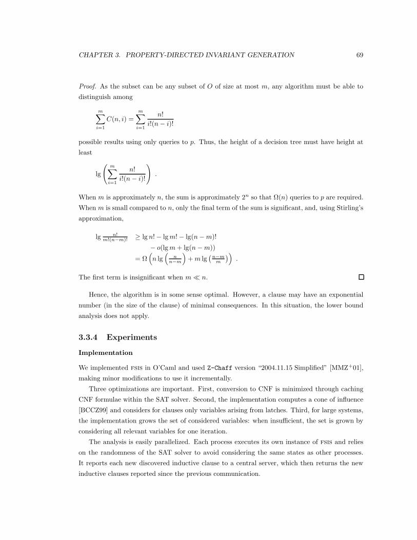
CHAPTER 3. PROPERTY-DIRECTED INVARIANT GENERATION 69
Proof. As the subset can be any subset of O of size at most m, any algorithm must be able to
distinguish among
m∑
i=1
C(n, i) =
m∑
i=1
n!
i!(n− i)!
possible results using only queries to p. Thus, the height of a decision tree must have height at
least
lg
(m∑
i=1
n!
i!(n− i)!
)
.
When m is approximately n, the sum is approximately 2n so that Ω(n) queries to p are required.
When m is small compared to n, only the final term of the sum is significant, and, using Stirling’s
approximation,
lg n!m!(n−m)! ≥ lg n! − lgm! − lg(n−m)!
− o(lgm+ lg(n−m))
= Ω(
n lg(
nn−m
)
+m lg(
n−mm
))
.
The first term is insignificant when m n.
Hence, the algorithm is in some sense optimal. However, a clause may have an exponential
number (in the size of the clause) of minimal consequences. In this situation, the lower bound
analysis does not apply.
3.3.4 Experiments
Implementation
We implemented fsis in O’Caml and used Z-Chaff version “2004.11.15 Simplified” [MMZ+01],
making minor modifications to use it incrementally.
Three optimizations are important. First, conversion to CNF is minimized through caching
CNF formulae within the SAT solver. Second, the implementation computes a cone of influence
[BCCZ99] and considers for clauses only variables arising from latches. Third, for large systems,
the implementation grows the set of considered variables: when insufficient, the set is grown by
considering all relevant variables for one iteration.
The analysis is easily parallelized. Each process executes its own instance of fsis and relies
on the randomness of the SAT solver to avoid considering the same states as other processes.
It reports each new discovered inductive clause to a central server, which then returns the new
inductive clauses reported since the previous communication.

CHAPTER 3. PROPERTY-DIRECTED INVARIANT GENERATION 70
Table 3.1: Single-process analysis of benchmarks
# Time (s) Clauses SAT COI Time (s) #2
2 48 11 450 306 403 31 4 120 306 505 84 194 17407 88 1146 2329 442 34188 318 25187 19 64 4379 67 168 29 72 4841 90 269 4 24 1022 46 6
10 6 7 281 54 713 235 20 810 352 23515 1270 195 15211 353 72816 929 209 14803 290 126517 57096 1718 501920 211 7632418 3460 436 62123 143 1283319 285 99 5765 52 334
Table 3.2: Multi-process analysis of hard benchmarks
2 4 8# Time Clauses Time Clauses Time Clauses
6 1278 500 945 586 502 59815 474 126 774 207 253 16016 562 234 665 316 297 34817 34860 1716 14419 1593 8304 187218 5369 1052 2111 734 1431 1093
Results
We studied two sets of benchmarks. The PicoJava II microprocessor benchmark set, previously
studied in [MA03, McM03, McM05], has the characteristic that the circuits are relatively large,
yet only small sections of the circuits are relevant for proving the properties. Standard BDD-
based model checking [BCM+92] fails, so abstracting the system or its state-space with respect to
the property is important. Of the 20 benchmarks, which are safety properties of the instruction
fetching and caching modules of the PicoJava II chip, proof-based abstraction solved 18 [MA03],
and interpolation-based model checking solved 19 [McM03, McM05]. Table 3.1 reports the per-
formance results for a single process. The Clauses, SAT, and COI columns list the number of
generated clauses, the number of SAT calls, and the number of active variables in the cone of
influence, respectively. Results can vary widely across runs, so we report times for a second run
in column Time (s) #2. Properties for benchmarks 0, 1, 4, 11, 12, and 14 are already inductive,

CHAPTER 3. PROPERTY-DIRECTED INVARIANT GENERATION 71
Table 3.3: VIS benchmarks
Name Time Clauses Name Time Clauses
Peterson 2 4 Heap 8605 2551PPC60X 2.1 71 3 PPC60X 2.2 69 3PPC60X 2.5 61 1 PPC60X 2.9 381 69
so results are not reported in the table. For the large benchmarks 2, 3, 6, 12, 15, and 16, we use
the growing-variable-set heuristic. Table 3.2 reports the performance results for analyzing the
hardest benchmarks with multiple processes.
The second set of benchmarks is from the VIS distribution [VIS]. We applied the analysis
to several valid properties of models that are difficult for standard k-induction (though easy for
standard BDD-based model checking) [AS06]. Table 3.3 reports the results. For comparison,
k-induction with strengthening fails on Peterson and Heap within 1800 seconds; but BDD-
based model checking requires at most a few seconds for each [AS06]. Peterson, Heap, and
the PPC60X 2 models have 16, 29, and 94 latches, respectively.
Our timing results were obtained using 3 GHz processors.
3.4 Related Work
3.4.1 Mathematical Programming-Based Analysis
For constructing witnesses to properties of systems in the form of polynomial functions, mathe-
matical programming was first applied to synthesize Lyapunov functions of continuous systems
[BY89] (see [PP02] for a more recent mathematical programming-based approach). Lyapunov
functions are a continuous analog of ranking functions of programs. A ranking function of a
program maps its states into a well-founded set, thus proving that the program always ter-
minates. Construction of affine and polynomial expressions for verification purposes was first
studied extensively in the context of ranking function synthesis. [KM75] discusses the generation
of constraint systems over loops with linear assertional guards and linear assignments for which
solutions are linear ranking functions. In [CS01, CS02], it is observed that duality of linear con-
straints achieves efficient synthesis. [PR04] proves that this duality-based method is complete
for single-path loops. [BMS05a] presents a complete method for the general case and shows how
lexicographic linear ranking functions can also be computed efficiently in practice. In [Cou05],
the approach is generalized by using semidefinite programming to approximate the polynomial
case.
Synthesizing invariant properties of systems is more complex because they are fixpoints of
the (initiation) and (consecution) conditions. Of course, invariants are often necessary for proving

CHAPTER 3. PROPERTY-DIRECTED INVARIANT GENERATION 72
termination, so that termination analysis can be just as complex; however, the synthesis of
ranking functions (or Lyapunov functions) alone does not require solving for a fixpoint. [CSS03]
proposes using Farkas’s Lemma and nonlinear constraint solving to generate affine invariants.
A solver for this method is described in [SSM04]. [SSM03] specializes the technique to Petri
nets, for which the problem is efficiently solvable. [BMS05c] proposes an idea for addressing the
case in which system variables must be treated as integers, for which duality is unknown. The
continuous analog of invariants, barrier certificates, was introduced in [PJ04]. They, too, apply
a method based on constraint solving.
Invariants are often necessary for proving termination: while the possible state-space may
not map into a well-founded domain, the reachable state-space may. One direction for future
research is to extend the directed approach to termination. While [BMS05a] presents a method
for constructing up to a fixed number of supporting invariants, a directed incremental approach
would allow the number to be unbounded.
3.4.2 Safety Analysis of Hardware
Qualitative Comparisons
We consider the characteristics of several related safety analyses: bounded model checking (BMC)
[BCCZ99], interpolation-based model checking (IMC) [McM03, McM05], k-induction (kI) [SSS00,
dMRS03, AFF+04, VH06, AS06], predicate abstraction with refinement (CEGAR) [CGJ+03],
and our analysis (FSIS). These analyses are similar in important ways: they are fundamentally
based on computing an inductive set that excludes all error states; they consider the property to
prove during the computation; and they use a SAT solver as the main computational resource.
Additionally, unlike standard model checking [CE82, BCM+90, McM02], they use both the initial
condition and the desired property to construct implicitly or explicitly an abstraction of some
kind.
We consider now their differences, defining several dimensions for comparison:
A. Abstraction: What is the mechanism for abstraction? Does it abstract the transition
relation (TR)? Or does it directly abstract the state space through induction (SS)?
B. Use of SAT solver : Does it pose a few difficult SAT problems (FD)? Or does it pose many
simple SAT problems (MS)?
C. Intermediate results : Are intermediate results transferable to other analyses (IT)? Or must
it run to convergence to provide useful information (IU)?
D. Parallelizable: Is it naturally and easily parallelized (P)? Or is it naturally serial (S)?
Table 3.4 summarizes the results. An analysis may not fit precisely at one end of each dimension;
however, this classification provides a first approximation.

CHAPTER 3. PROPERTY-DIRECTED INVARIANT GENERATION 73
Table 3.4: Summary of comparison
Analysis A B C D
BMC SS FD IU SIMC TR FD IT SkI SS FD IU SCEGAR TR MS IT SFSIS SS MS IT P
IMC and CEGAR compute successively finer approximations to the transition relation. Each
approximation causes a certain set of states to be deemed reachable. When this set includes an
error state, IMC increments the k associated with its postcondition operator, solving larger BMC
problems, while CEGAR learns a separating predicate. In contrast, BMC, kI, and FSIS operate
on the full transition relation. kI strengthens by requiring counterexamples to induction to be
ever longer paths. In a finite-state system, there exists a longest loop-free path that ends in an
error state. When kI’s k is longer than this path, k-induction succeeds. FSIS incrementally finds
invariants to slice off portions of the state space.
BMC, IMC, and kI pose relatively few difficult SAT problems in which the transition relation
is unrolled many times. In contrast, CEGAR and FSIS pose many simple SAT problems in which
the transition relation is not unrolled.
Each major iteration of IMC and CEGAR produces an inductive set that is informative even
when it is not strong enough to prove the property. Each successive iteration of FSIS produces
a stronger formula that excludes states that cannot be reached without previously violating the
property. Intermediate iterations of BMC and kI are not really useful. Exceptions include forms
of strengthening, which we discuss in greater depth below [dMRS03, AFF+04, VH06, AS06].
Finally, only FSIS is natural to parallelize. The difficulty of subproblems grows with successive
iterations in BMC, IMC, and kI so that parallelization across iterations is not useful. The
SAT solver itself would have to be parallelized. In CEGAR, each iteration is dependent on the
predicates just learned, though parallelization could occur at a finer level.
Related Work
SAT-based unbounded model checking for safety properties also generates clauses; at conver-
gence, their conjunction is inductive [McM02]. However, our approach differs fundamentally.
First, the semantics of clauses differ: in SAT-based model checking, each clause excludes a set
of states that lead to a violation; in our approach, each clause represents an inductive set of
states. Hence, the algorithms to compute the clauses differ markedly: in particular, our method
computes several approximations to fixpoints to generate a single clause, whereas SAT-based

CHAPTER 3. PROPERTY-DIRECTED INVARIANT GENERATION 74
model checking computes clausal representations of one-step preimages. Second, the different
semantics cause the behavior of the two approaches to differ: SAT-based model checking gener-
ates many clauses, each at low computational expense; our approach produces fewer clauses at
(relatively) higher expense. Finally, SAT-based unbounded model checking is an implementation
of CTL model checking with a clausal representation. It computes the fixpoint exactly, whereas
our method abstracts the state space relative to the initial condition and the property.
Not surprisingly, however, the two methods share a concept: blocking clauses are used in
SAT-based unbounded model checking [McM02]. Their discovery is refined in [JS05] to produce
prime blocking clauses, requiring at worst as many SAT calls as literals. The consequence
function of Section 3.3.1 requires asymptotically fewer SAT calls. An algorithm similar to the
consequence algorithm is described in [Zel99]. However, that algorithm can handle only sets
in which there exists precisely one minimal satisfying subset.
Strengthening based on under-approximating the states that can reach a violating state s
has been applied in the context of k-induction [dMRS03, AFF+04, VH06, AS06]. Quantifier-
elimination [dMRS03], ATPG-based computation of the n-level preimage of s [VH06], and SAT-
based backward model checking [AS06] have been used to perform the strengthening. Our induc-
tive basis for strengthening eliminates significantly more states in practice and at least as many
in theory. The first clause discovered by down already excludes all states that can reach s; in
practice, a much smaller clause is usually found. This stronger clause eliminates many states
from which s is not reachable.
An important direction for future research is to combine our incremental induction-based
strengthening with k-induction. This hybrid analysis would vary k in each parallel process
according to computational demands and to the success in finding MICs.
3.5 Conclusion
Incremental invariant generation procedures like the two described in this chapter characteristi-
cally synthesize relatively weak invariants at low computational cost. Typically, they share the
same problem as monolithic procedures like polyhedra-based abstract interpretation [CH78] and
symbolic model checking [BCM+90]: they produce too much information (at unnecessary com-
putational cost). We describe a general technique for directing incremental invariant generation
according to a given property and discuss two instances of the technique. The evidence of Section
3.3.4 suggests that incremental invariant generation can indeed be targeted to a property so that
relatively few invariants are actually generated.
Our work on safety analysis of hardware suggests an important direction for further research.
The analysis is motivated by a classically deductive approach to verification [MP95]. Can clas-
sically deductive techniques motivate fast analyses for other temporal properties as well?
Bibliography
[Ack57] W. Ackermann. Solvable cases of the decision problem. The Journal of Symbolic
Logic, 22(1):68–72, March 1957.
[AFF+04] R. Armoni, L. Fix, R. Fraer, S. Huddleston, N. Piterman, and M. Vardi. SAT-based
induction for temporal safety properties. In BMC, 2004.
[AS06] Mohammad Awedh and Fabio Somenzi. Automatic invariant strengthening to prove
properties in bounded model checking. In DAC, pages 1073–1076. ACM Press, 2006.
[Avi98] D. Avis. LRS: A revised implementation of the reverse search vertex enumeration
algorithm. Technical Report, McGill, 1998.
[BCCZ99] Armin Biere, Alessandro Cimatti, Edmund M. Clarke, and Yunshan Zhu. Sym-
bolic model checking without BDDs. In TACAS, pages 193–207, London, UK, 1999.
Springer-Verlag.
[BCM+90] Jerry R. Burch, Edmund M. Clarke, Ken L. McMillan, David L. Dill, and L.J. Hwang.
Symbolic model checking: 1020 states and beyond. In Proc. 5th IEEE Symp. Logic
in Comp. Sci., pages 428–439. IEEE Computer Society Press, June 1990.
[BCM+92] Jerry R. Burch, Edmund M. Clarke, Kenneth L. McMillan, David L. Dill, and L. J.
Hwang. Symbolic model checking: 10ˆ20 states and beyond. Inf. Comput., 98(2):142–
170, 1992.
[BM06] Aaron R. Bradley and Zohar Manna. Verification constraint problems with strength-
ening. In ICTAC, volume 3722 of LNCS. Springer-Verlag, 2006.
[BM07] Aaron R. Bradley and Zohar Manna. The Calculus of Computation: Decision Pro-
cedures with Applications to Verification. Springer, 2007.
[BMS05a] Aaron R. Bradley, Zohar Manna, and Henny B. Sipma. Linear ranking with reacha-
bility. In Kousha Etessami and Sriram K. Rajamani, editors, Proc. 17th Intl. Confer-
ence on Computer Aided Verification (CAV), volume 3576 of LNCS, pages 491–504.
Springer Verlag, July 2005.
75
BIBLIOGRAPHY 76
[BMS05b] Aaron R. Bradley, Zohar Manna, and Henny B. Sipma. The polyranking principle.
In International Colloquium on Automata, Languages, and Programming (ICALP),
volume 3580 of LNCS, pages 1349–1361. Springer Verlag, 2005.
[BMS05c] Aaron R. Bradley, Zohar Manna, and Henny B. Sipma. Termination analysis of
integer linear loops. In CONCUR, 2005.
[BMS05d] Aaron R. Bradley, Zohar Manna, and Henny B. Sipma. Termination of polynomial
programs. In Radhia Cousot, editor, Proc. of Verification, Model Checking and Ab-
stract Interpretation (VMCAI), volume 3385 of LNCS, Paris, France, January 2005.
Springer Verlag.
[BMS06] Aaron R. Bradley, Zohar Manna, and Henny B. Sipma. What’s decidable about
arrays? In Verification, Model Checking, and Abstract Interpretation: 7th Interna-
tional Conference, (VMCAI), volume 3855 of LNCS, pages 427–442, Charleston, SC,
January 2006. Springer Verlag.
[BY89] S. Boyd and Q. Yang. Structured and simultaneous Lyapunov functions for system
stability problems. Int. J. Control, 49(6):2215–2240, 1989.
[CC77] Patrick Cousot and Rhadia Cousot. Abstract interpretation: A unified lattice model
for static analysis of programs by construction or approximation of fixpoints. In 4th
ACM Symp. Princ. of Prog. Lang., pages 238–252. ACM Press, 1977.
[CE82] Edmund M. Clarke and E. Allen Emerson. Design and synthesis of synchronization
skeletons using branching-time temporal logic. In Logic of Programs, Workshop,
pages 52–71, London, UK, 1982. Springer-Verlag.
[CGJ+03] Edmund Clarke, Orna Grumberg, Somesh Jha, Yuan Lu, and Helmut Veith.
Counterexample-guided abstraction refinement for symbolic model checking. J. ACM,
50(5):752–794, 2003.
[CH78] Patrick Cousot and Nicholas Halbwachs. Automatic discovery of linear restraints
among the variables of a program. In 5th ACM Symp. Princ. of Prog. Lang., pages
84–97, January 1978.
[Col75] G.E. Collins. Quantifier elimination for real closed fields by cylindrical algebraic
decomposition. In H.Brakhage, editor, Automata Theory and Formal Languages,
volume 33 of LNCS, pages 134–183. Springer-Verlag, 1975.
[Cou05] P. Cousot. Proving program invariance and termination by parametric abstraction,
Lagrangian relaxation and semidefinite programming. In Proc. Verification, Model

BIBLIOGRAPHY 77
Checking, and Abstract Interpretation: 5th International Conference (VMCAI), pages
1–24, 2005.
[CS01] Michael Colon and Henny B. Sipma. Synthesis of linear ranking functions. In
Tiziana Margaria and Wang Yi, editors, 7th International Conference on Tools and
Algorithms for the Construction and Analysis of Systems (TACAS), volume 2031 of
LNCS, pages 67–81. Springer Verlag, April 2001.
[CS02] Michael Colon and Henny B. Sipma. Practical methods for proving program termi-
nation. In Proc. 14th Intl. Conference on Computer Aided Verification, volume 2404
of LNCS, pages 442–454. Springer Verlag, 2002.
[CSS03] Michael Colon, Sriram Sankaranarayanan, and Henny B. Sipma. Linear invariant
generation using non-linear constraint solving. In Computer Aided Verification, vol-
ume 2725 of LNCS, pages 420–433. Springer-Verlag, July 2003.
[dMRS03] L. de Moura, H. Ruess, and M. Sorea. Bounded model checking and induction: From
refutation to verification. In CAV, LNCS. Springer-Verlag, 2003.
[DST80] P. J. Downey, R. Sethi, and R. E. Tarjan. Variations on the common subexpressions
problem. Journal of the ACM, 27(4):758–771, 1980.
[GNRZ06] S. Ghilardi, E. Nicolini, S. Ranise, and D. Zucchelli. Deciding extensions of the theory
of arrays by integrating decision procedures and instantiation strategies. In JELIA.
Springer-Verlag, 2006.
[GS97] Susanne Graf and Hassen Saidi. Construction of abstract state graphs with PVS. In
Orna Grumberg, editor, Proc. 9th Intl. Conference on Computer Aided Verification,
volume 1254 of LNCS, pages 72–83. Springer-Verlag, June 1997.
[HJMS02] Thomas A. Henzinger, Ranjit Jhala, Rupak Majumdar, and Gregoire Sutre. Lazy
abstraction. In 29th ACM Symp. Princ. of Prog. Lang. (POPL), pages 58–70. ACM
Press, 2002.
[Jaf81] Joxan Jaffar. Presburger arithmetic with array segments. Inf. Processing Letters,
12(2), 1981.
[JS05] HoonSang Jin and Fabio Somenzi. Prime clauses for fast enumeration of satisfying
assignments to boolean circuits. In DAC, pages 750–753. ACM Press, 2005.
[Kin69] James King. A Program Verifier. PhD thesis, Carnegie Mellon University, September
1969.

BIBLIOGRAPHY 78
[KM75] Shmuel M. Katz and Zohar Manna. A closer look at termination. Acta Informatica,
5(4):333–352, 1975.
[MA03] Kenneth L. McMillan and Nina Amla. Automatic abstraction without counterexam-
ples. In TACAS, pages 2–17, 2003.
[Mat81] Prabhaker Mateti. A decision procedure for the correctness of a class of programs.
J. ACM, 28(2), 1981.
[McC62] John McCarthy. Towards a mathematical science of computation. In IFIP Congress
62, 1962.
[McM02] Kenneth L. McMillan. Applying SAT methods in unbounded symbolic model check-
ing. In CAV, volume 2404 of LNCS, pages 250–264. Springer-Verlag, 2002.
[McM03] Kenneth L. McMillan. Interpolation and SAT-based model checking. In CAV, volume
2725 of Lecture Notes in Computer Science, pages 1–13. Springer, 2003.
[McM05] Kenneth L. McMillan. Applications of Craig interpolants in model checking. In
TACAS, volume 3440 of Lecture Notes in Computer Science, pages 1–12. Springer,
2005.
[MMZ+01] Matthew W. Moskewicz, Conor F. Madigan, Ying Zhao, Lintao Zhang, and Sharad
Malik. Chaff: Engineering an Efficient SAT Solver. In DAC, 2001.
[MP95] Zohar Manna and Amir Pnueli. Temporal Verification of Reactive Systems: Safety.
Springer-Verlag, New York, 1995.
[NO79] Greg Nelson and Derek C. Oppen. Simplification by cooperating decision procedures.
ACM Trans. Prog. Lang. Sys., 1(2):245–257, October 1979.
[NO80] Greg Nelson and Derek C. Oppen. Fast decision procedures based on congruence
closure. Journal for the Association for Computing Machinery, 27(2):356–364, April
1980.
[PJ04] Stephen Prajna and Ali Jadbabaie. Safety verification of hybrid systems using barrier
certificates. In HSCC, volume 2993 of LNCS. Springer, 2004.
[PP02] A. Papachristodoulou and Stephen Prajna. On the construction of Lyapunov func-
tions using the sum of squares decomposition. In CDC, 2002.
[PR04] Andreas Podelski and Andrey Rybalchenko. A complete method for the synthesis of
linear ranking functions. In VMCAI, pages 239–251, 2004.

BIBLIOGRAPHY 79
[Ros86] L. E. Rosier. A note on Presburger arithmetic with array segments, permutation and
equality. Inf. Process. Lett., 22(1):33–35, 1986.
[SBDL01] Aaron Stump, Clark W. Barrett, David L. Dill, and Jeremy R. Levitt. A decision
procedure for an extensional theory of arrays. In Logic in Computer Science (LICS),
2001.
[Sch86] Alexander Schrijver. Theory of Linear and Integer Programming. Wiley, 1986.
[Sho78] Robert E. Shostak. An algorithm for reasoning about equality. Communications of
the ACM, 21(7):583–585, July 1978.
[SJ80] Norihisa Suzuki and David Jefferson. Verification decidability of Presburger array
programs. J. ACM, 27(1), 1980.
[SSM03] Sriram Sankaranarayanan, Henny B. Sipma, and Zohar Manna. Petri net analysis
using invariant generation. In Nachum Derschowitz, editor, Verification: Theory
and Practice, volume 2772 of LNCS, pages 682–701, Taurmina, Italy, 2003. Springer
Verlag.
[SSM04] Sriram Sankaranarayanan, Henny B. Sipma, and Zohar Manna. Constraint-based
linear relations analysis. In 11th Static Analysis Symposium (SAS’2004), volume
3148 of LNCS, pages 53–68. Springer-Verlag, 2004.
[SSS00] Mary Sheeran, Satnam Singh, and Gunnar Stalmarck. Checking safety properties
using induction and a SAT-solver. In FMCAD, volume 1954 of LNCS. Springer-
Verlag, 2000.
[Tar51] Alfred Tarski. A Decision Method for Elementary Algebra and Geometry. Univ. of
California Press, Berkeley, 2nd edition, 1951.
[VH06] Vishnu C. Vimjam and Michael S. Hsiao. Fast illegal state identification for improving
SAT-based induction. In DAC, pages 241–246. ACM Press, 2006.
[VIS] VIS. http://visi.colorado.edu/∼vis.
[Zel99] Andreas Zeller. Yesterday, my program worked. Today, it does not. Why? In ESEC
/ SIGSOFT FSE, pages 253–267, 1999.