safety first: perceived risk of street harassment and
TRANSCRIPT

Safety First: Perceived Risk of Street Harassment andEducational Choices of Women
Girija Borker*
30 October 2020
Abstract
This paper examines the impact of perceived risk of street harassment on women’s human
capital attainment. I combine survey data on students from the University of Delhi, a mapping
of potential travel routes to all colleges in the students’ choice set from Google Maps, and
crowdsourced mobile application safety data. Using a random utility framework, I estimate
that women are willing to choose a college in the bottom half of the quality distribution over
a college in the top quintile in order to travel by a route that is perceived to be one standard
deviation safer.
*The World Bank, 1818 H Street NW, Washington, DC 20433 USA. Tel: +1 (202) 473 1583 Email:[email protected]. Thanks to Andrew Foster for his invaluable guidance and continuous support, and to DanBjorkegren, Kaivan Munshi, Emily Oster, Jesse Shapiro, and Matthew Turner for their generous advice and insights. Iwould like to thank Kenneth Chay, John Friedman, Margarita Gafaro Gonzalez, Tarun Jain, Florence Kondylis, GabrielKreindler, Arianna Legovini, Akhil Lohia, Nancy Luke, Anja Sautmann, Simone Schaner, Bryce Steinberg, and Re-becca Thornton for their helpful conversations and comments, and the participants at various seminars and workshops.I am grateful to Inderjeet S. Bakshi, Harjender Singh Chaudhary, Rajiv Chopra, Sanjeev Grewal, Rabi Narayan Kar,Kawar Jit Kaur, Pravin Kumar, Amna Mirza, Shashi Nijhawan, Pragya, Rajendra Prasad, Savita Roy, Alka Sharma,Neetu Sharma, Malathi Subramaniam, Dinesh Yadav, Vimlendu for their support and to the team of dedicated surveyenumerators for their hard work and dedication during data collection at University of Delhi. I would like to thankAshish Basu and Kalpana Vishwanath for providing access to the SafetiPin mobile app data. This project was madepossible by the expertise of Michael Davlantes and the capable research assistance provided by Peeyush Kumar. Igratefully acknowledge financial support from Data2x, the Population Studies and Training Center, Global HealthInitiative, Brown India Initiative, Pembroke Center for Teaching and Research on Women, and the Department ofEconomics at Brown University. IRB approval #1511001373 for this project was granted by the Office of ResearchIntegrity at Brown University on December 22, 2015. The findings, interpretations, and conclusions expressed in thispaper are entirely those of the author. They do not necessarily represent the views of the World Bank and its affiliatedorganizations, or those of the Executive Directors of the World Bank or the governments they represent.
1

Gender-specific constraints may help explain the economic mobility differentials between men andwomen in developing countries. These constraints include laws that limit women’s access to andownership of productive assets (Rakodi 2014), poor access to credit (Asiedu et al. 2013), womenbearing disproportionate responsibility for household work (Ferrant, Pesando and Nowacka 2014),and persistent social norms based on the cultural context (Jayachandran 2015). In this paper, Iexamine an additional constraint that restricts women’s economic mobility – safety in public spaces.
Street harassment, or sexual harassment faced in public spaces, is a serious problem aroundthe world. In Delhi, where this study is based, 95 percent of women aged 16 to 49 report feelingunsafe in public spaces (ICRW 2013). Women incur significant psychological costs from sexualharassment (Langton and Truman 2014) and actively take precautions to avoid such confrontations(Pain 1997). For example, 84 percent of women aged 40 years or younger in India said that theyavoid an area in their city because of harassment or the fear of it (Livingston 2015).
In this paper, I document that women in Delhi choose to attend worse ranked colleges than men,both in absolute terms and conditional on their choice set. There can be several explanations for thisobservation. In a country where over 85 percent of marriages are arranged (Borker et al. 2020), itmay be that women do not care about college quality if an undergraduate degree only has signalingvalue in the marriage market. It could also be that women prefer to attend a local, lower qualityinstitution because of family obligations. Or that they do value high quality education but are unableto convince their parents of the same due to a low general sense of confidence (McKelway 2020).Another potential explanation could be that women do not like competitive environments, hencethey choose not to attend high quality colleges with high quality peers (Niederle and Vesterlund2007, Niederle and Vesterlund 2011, Buser, Niederle and Oosterbeek 2014). This paper positsanother explanation: in a context where the majority of students live at home and travel to collegeevery day, women choose to attend worse ranked colleges to avoid street harassment. Unrelated toindividual or family preferences that may result in optimal choices, street harassment imposes anexternal constraint on women’s behavior that could potentially lead to sub-optimal choices.
Choosing a worse ranked college has long-term consequences for students by affecting theiracademic training (Zhang 2005), network of peers (Winston and Zimmerman 2004), access to laboropportunities (Pascarella and Terenzini 2005), and lifetime earnings (Brewer, Eide and Ehrenberg1999; Eide, Brewer and Ehrenberg 1998). Recent evidence on returns to college quality in Indiashows that women experience improvements in their academic outcomes that are greater than thosefor men (Dasgupta et al. 2020) and a large and significant wage premium (Sekhri 2020) fromattending a higher quality college. A misallocation of students to colleges, where high achievingfemales sort to low quality colleges, not only affects women’s long-term outcomes but also hasconsequences for long-term economic growth through its effect on aggregate productivity (Hsiehet al. 2019).
2

This paper measures the extent to which perceived risk of street harassment can help explainwomen’s college choices in Delhi. For this, I evaluate the gender differential in trade-offs betweentravel safety, college quality, travel costs, and travel time in a model of college choice. The dif-ference in trade-offs captures the cost of street harassment for women, since men in Delhi do notface such harassment. I provide what to my knowledge is the first evidence of the effect that dailyharassment has on a durable human capital investment such as higher education. I also estimate thefirst revealed preference estimates of travel safety in terms of travel costs and travel time, augment-ing estimates based on women-only public transportation (Aguilar, Gutierrez and Soto Villagran2019, Kondylis et al. 2020).
The University of Delhi (DU) offers a unique setting to explore the tradeoff between collegequality and travel safety. DU is an umbrella entity that is composed of 77 colleges that are spreadacross Delhi. Each college has its own campus, classes, staff, and placements and operates inde-pendently. Critically, some colleges are more selective in admissions than others. Admissions inDU are strictly based on students’ high school exam scores: students submit one application formto all colleges in the university and are admitted to those colleges where their scores are higher thanthe “cutoff score” or the minimum percentage required to gain admission to a major in the college.This allows me to infer students’ comprehensive choice set of colleges within DU, based on a sur-vey of 3,800 students that I conducted at DU in 2016. Using Google Maps and an algorithm thatI developed, I map students’ travel routes by travel mode, including both the reported travel routeand the potential routes available to students for every college in their choice set. I combine this in-formation on travel routes with crowd-sourced safety data from two mobile applications. SafetiPin,which provides perceived spatial safety data in the form of safety audits conducted at various loca-tions across the Delhi National Capital Region (NCR); and Safecity, that provides analytical dataon harassment rates by travel mode recorded by users during their travel in the city. The area andmodal safety data together allow me to assign a safety score to each travel route.
To assess whether women face differential trade-offs between travel safety and college quality,travel costs, and travel time compared to men, I use two approaches. First, I take advantage of theDU’s admissions procedure to approximate a random allocation of college choice sets. I comparethe choices of each student with other students of the same gender who live in the same neigh-borhood, study the same major, and have the same admission year. Given the discrete cutoffs, achange in students’ relative exam scores also changes their choice set, relative to their neighbors.I find that while women’s choices seem to take into account both route safety and college quality,men’s choices only depend on quality and are consistent with a model in which preferences arelexicographic in college quality.
Second, I use a mixed logit model to estimate the magnitude of the student’s willingness topay for travel safety. In my benchmark specification, student’s indirect utility depends on college
3
quality, route safety, travel costs, and travel time, and I estimate the model for women and menseparately. The analysis uses spatial variation in students’ location, destination colleges, routechoices, mode choice and area safety. Identification is based on the assumption that the locationand attributes of the students, colleges, and possible routes are exogenous to the process of collegeand route choice.
I find that women are willing to choose a college that is in the bottom half of the quality distri-bution over a college in the top 20 percent for a route that is perceived to be one standard deviation(SD) safer. Men on the other hand are only willing to go from a top 20 percent college to a top30 percent college for an additional SD of perceived travel safety. Translating perceived safetyto actual safety, an additional SD of perceived safety while walking is equivalent to a 3.1 percentdecrease in the rapes reported annually. Using estimates from Sekhri (2019), on the labor-marketearnings advantage from attending a public college, women’s willingness to pay (WTP) for safetyin terms of college quality amounts to a 17 percent decline in the present discounted value of theirpost-college salaries. Based on the travel cost method, I am able to value harassment and I find thatwomen are willing to incur an additional expense of INR 17,500 (USD 250) per year to travel by aroute that is one SD safer. This is a significant sum of money, double the average annual tuition inDU and seven percent of the average annual per capita income in Delhi. Women’s WTP in termsof annual travel costs is much higher than men’s WTP of INR 9,950 (USD 140) for an additionalSD of perceived route safety.
This paper relates to several strands of literature: the economics literature on distortive effectsof fear, the psychology and criminology literature that provides qualitative evidence on the effectsof street harassment, the literature on the value of a statistical life that estimates individual’s WTPfor small reductions in mortality risks, the school choice literature that assesses the factors influ-encing choice of a school, and the literature on spatial frictions perpetuating gender disparities inacquisition of human capital. It has been shown that fear of imagined dangers affects individualbehavior (Becker and Rubinstein 2011). There is evidence that harassment by strangers strongly af-fects women’s perceptions of safety across social contexts (Macmillan, Nierobisz and Welsh 2000)and that women change their behavior in response (Keane 1998). Specifically, lack of safety hasbeen found to affect women’s mobility patterns (Hsu 2011, Porter et al. 2011) and is negatively cor-related with women’s labor force participation on the extensive margin (Chakraborty et al. 2018,Siddique 2018) and the intensive margin (Cook et al. Forthcoming). While there have been sev-eral studies that estimate value of a statistical life using implicit trade-offs between different risksand money (Viscusi and Aldy 2003), there has been no attempt, to my knowledge, to measure themisallocation effects associated with sexual harassment. The school choice literature examines theinstitutional attributes that families value. Families have been found to value high academic attain-ment, proximity, and certain composition of students in terms of race and socioeconomic status
4

(Gallego and Hernando 2009, Burgess et al. 2015, Hastings, Kane and Staiger 2009, Carneiro, Dasand Reis 2013). This is the first paper to consider travel safety in a model of college choice, afactor that is likely to be especially relevant for educational choices of women in rapidly urbaniz-ing developing countries. Access to schools and training centers through choice of their location,better roads or provision of transportation has been found to play a crucial role in women’s take-upof opportunities (Mukherjee 2012, Burde and Linden 2013, Muralidharan and Prakash 2017, Ja-coby and Mansuri 2015, Cheema et al. 2020). While most of this work alludes to women’s ownor their parents’ safety concerns as a potential mechanism in affecting women’s choices, this is thefirst paper to explicitly measure the extent to which safety affects women’s educational choices,conditional on travel time.
I Institutional Setting: College Choice and Harassment
A Structure of DU
DU is one of the top non-technical universities in India (BRICS University Rankings 2015). DUis composed of 77 colleges of which 58 offer general undergraduate majors in Humanities, Com-merce and Science.1Of the 58 general education undergraduate colleges, 17 colleges are womenonly and eight colleges are evening colleges.2 There are over 180,000 undergraduate students atDU (University of Delhi Annual Report 2013-14), that represent around 8 percent of all studentswho passed the Class 12 qualifying exams in India.3 DU is also the main public central universityin Delhi that offers liberal arts education. Other public universities offering general undergradu-ate degrees are either significantly smaller in comparison or have limited overlap with the majorsoffered by DU.4 Another option for students in Delhi are the private universities. However, theseprivate institutions not only offer limited number of majors but are also considerably more expen-sive than DU. For example, one of the biggest private universities in Delhi charges on average 9 to18 times DU’s average annual tuition.5
Colleges in DU are spread across Delhi. Figure 1 shows the spread of colleges in Delhi. Col-leges vary in the size of their student population; on average, a college has about 2,800 students.
1Other colleges offer professional degrees like law and medicine.2Evening colleges offer classes after 2 pm.3This is equal to 6.6 percent of all students who appeared for the Class 12 qualifying exam in India.4These general public universities in Delhi are Dr. B. R. Ambedkar University of Delhi, Jamia Millia Islamia Uni-
versity, Jawahar Lal Nehru University, and Guru Gobind Singh Indraprastha University. In 2015, Dr. B. R. AmbedkarUniversity had 1.1 percent of DU’s annual undergraduate intake and Jamia Milia had less than 14 percent of DU’sannual undergraduate intake of which up to 50 percent is reserved for Muslim students. Jawahar Lal Nehru Universityoffers undergraduate programs only in foreign languages. Guru Gobind Singh Indraprastha University only offers onecourse that is offered by DU’s general undergraduate colleges.
5Based on the comparison of 2016-17 fees for general undergraduate courses.
5

Undergraduate studies at DU are for three years,6 and each college offers multiple majors. On av-erage a college offers about 12 majors with most colleges having a large overlap in the majors theyoffer.7 Each college has its own campus, staff, classes, and placements.8 All teaching is conductedwithin the colleges while the curriculum is identical across colleges. Students within a major acrosscolleges take a common university-wide exam at the end of each academic year. This exam on av-erage accounts for 75 percent of the student’s final grades. The remaining 25 percent of the finalgrade is based on an internal college evaluation of the student.
A distinguishing feature of DU is that the admission to colleges is strictly based on a student’shigh school exam scores. Each college specifies a cutoff score or the minimum percentage requiredto gain admission to a major. Based on a single application form, that is used for admission to allcolleges in the university, every student who scores above this cutoff score in their high school-leaving exams is guaranteed admission to the college. In line with previous studies (Black andSmith 2004), I use selectivity in admissions as an indicator of college quality, measured by a col-lege’s cutoff score. Based on these cutoff scores I am able to rank each college in absolute termsand within a student’s choice set, where a higher rank indicates a lower cutoff score and henceworse quality. The absolute rank rates colleges within a major and admission year using cutoffscores from the the first cutoff list released by each college. Rank within a student’s choice setorders the colleges to which the student was admitted to by their cutoff score for the student’s ma-jor and admission year. Figures 2a and 2b show the cumulative distribution function (CDF) of theabsolute rank of a college and the CDF of rank within a student’s choice set, respectively. We cansee that women’s CDF lies below the CDF for men, indicating that women choose worse rankedcolleges than men across the distribution. This implies that women choose worse ranked collegesthan men in absolute terms for the most part of distribution, and they choose worse quality collegesfrom the ones that they were eligible to attend for the entire distribution.9 This is despite womenscoring higher than men on exams at the end of high school, as shown in Figure A1.
Another feature of DU is that majority of the students (72 percent) enrolled at the Universityare residents of the Delhi NCR. Of the students who are residents of Delhi, 99.1 percent live withtheir parents and travel to college every day. This is primarily because of the social norm of living
6In 2013, DU attempted to move to a four-year undergraduate program (FYUP). However, this decision was metwith widespread protests and was embroiled in controversy since its implementation. The FYUP was rolled back in2014 and the University returned to its three-year undergraduate program.
7Only few colleges offer additional specialized courses such as Bachelors in Journalism and Bachelors in Elemen-tary Education.
8While there is a Central Placement Cell that is open to all students enrolled in the University, the majority of theplacements take place at the individual colleges. A Right to Information appeal revealed that the Central PlacementCell has placed only 5,800 students in past five years, equal to 13 percent of the total number of students who reg-istered with the Cell (Ghosh, Sushmita. 2017. “DU cell shows dismal placement record”. The Asian Age, May 5,http://www.asianage.com/metros/delhi/du-cell-shows-dismal-placement-record, (last accessed: May 25, 2020).
9We can see from Figure 2b that 64 percent of men and 40 percent of women choose one of the top three collegesin their choice set.
6
with parents and also because of lack of residential facilities at the University. About 18 percent ofcolleges have on-campus residence facilities that can accommodate about five percent of studentsenrolled in the University.10 The students travel to college by either public or private transport. Inmy sample, 83 percent of students use some form of public transport to travel to college every day.By focusing on Delhi residents who live with their parents and travel to college every day, I havea sample of students that does not sort on the basis of college location. It is unlikely that parentschoice of residence is influenced by their children’s future choice of college given the uncertaintyabout the college they will be eligible to attend. I also do not find evidence of students and theirparents moving in response to their college admissions with 98.7 percent of the students who livein Delhi and travel to college everyday residing in the same location while enrolled in college asthey did when they were in high school. The low rate of movement may be explained in part by thehigh rates of home ownership rates in the sample of Delhi residents with 82 percent the studentsowning the homes that they reside in, indicative of the high costs associated with changing theirplace of residence.
B Street Harassment
Gender-based street harassment is defined as “unwanted comments, gestures, and actions forced ona stranger in a public place and is directed at them because of their actual or perceived sex” (StopStreet Harassment 2015). According to a nationally representative survey in the US, 65 percent ofwomen have experienced street harassment (Stop Street Harassment 2014). Similarly, 86 percentof women living in cities in Thailand and 86 percent in Brazil have been subjected to harassment inpublic (Three in Four Women Experience Harassment and Violence in UK and Global Cities ActionAid 2016). Delhi, infamously known as the “rape capital” of India, is notorious for both verbal andphysical harassment in public transportation.11 In my sample, 89 percent of female college studentshave faced some form of harassment while traveling in Delhi. In particular, 64 percent of femalestudents have experienced unwanted staring, 50 percent have received inappropriate comments,33 percent have been touched, groped or grabbed, and 26 percent have been followed. Manywomen take precautions to avoid harassment, for example, in my sample 71 percent of femalestudents report avoiding an unsafe area, 67 percent avoid going out after dark, 30 percent moveaway from the harasser, and only 3 percent of women report taking no action to avoid harassmentwhile traveling in Delhi.
This paper focuses on women enrolled in college as they are vulnerable to sexual attacks due to
10Press Trust of India. 2015. “With Hostel Shortage in Delhi University, Students Demand Implementation ofRent Act”. NDTV, June 14, https://www.ndtv.com/delhi-news/not-enough-hostel-seats-in-delhi-university-students,(last accessed: May 25, 2020).
11Thomson Reuters Foundation News. 2014. “Most dangerous transport systems for women”. October, 31.http://news.trust.org/spotlight/most-dangerous-transport-systems-for-women, (last accessed: May 25, 2020).
7

their age (17-21 years) and lack of experience in dealing with harassment. A survey of women 18years and older in Chennai, another major city in India, found that 75 percent of women had theirfirst encounter with sexual harassment between 14 to 21 years of age (Mitra-Sarkar and Partheeban2011). For a majority of children in Delhi, both girls and boys, the main mode of transport toand from school is the official school bus. Once they finish high school, they are expected to takeresponsibility for their travel, as colleges neither officially provide transport nor are there standard-ized times for classes. Next, I present a simple stylized model of college choice to characterize howwomen may face trade-offs between travel safety and college quality.
II Stylized Model of College Choice
This simple stylized model of college choice explicitly captures how women might have to chooseworse quality colleges in order to avoid travel by unsafe routes. In the 2×2 matrix shown in Figure3a, the high-scoring students are in the first row (high school exam score = H) and low-scoringstudents are in the second row (high school exam score = L). In the columns, there is a low quality“Not-so-good college” (cutoff score = n) and a high quality “Good college” (cutoff score = g) withg > n. In between these two colleges there is a “danger” area that is unsafe, a travel route becomesunsafe if it passes through this unsafe area. There is an equal number of high and low-scoringmales and females located in each college’s neighborhood. A high scoring student is eligible toattend both the good and the not-so-good colleges given that their high school exam score is abovethe cutoff for both colleges (H > g > n). A low-scoring student, on the other hand, is only eligibleto attend the not-so-good college given that their high school exam score is below the cutoff for thegood college (g > L > n). In this model, I assume that women have two options when choosingtheir travel routes: they can either avoid unsafe areas or travel by a safer but more expensive modeof transport and women prefer the former.
Figure 3b and 3c show the choices made by high-scoring and low-scoring males respectively.Both high-scoring males attend the good college and both low-scoring males attend the not-so-goodcollege. Given the set-up, this means that 1
2 of the males travel by unsafe routes, denoted by thearrows, and a male student on average attends a college with quality = g+n
2 . Figure 3d shows thechoices of women who do not face a safety-quality trade-off. The high-scoring female choosesthe good college and the low-scoring female chooses the not-so-good college. In Figure 3e, wecan see the choice of a high-scoring female who would have to take an unsafe route i.e. cross theunsafe area if she were to choose the good college. By assumption, she avoids the unsafe area andchooses the lower quality not-so-good college. Finally, Figure 3f shows the decision of the lowscoring woman who would have to cross the unsafe area to attend the only college she is eligible toattend. She chooses a safe but more expensive route to travel to the not-so-good-college, denoted
8
by the dashed green arrow. With this a female student on average attends a college with quality= g+3n
4 < g+n2 . Another case is where the woman who can only attend the not-so-good-college by
traveling through the unsafe area could have chosen to not attend college at all, as denoted by thethick arrow. This is beyond the scope of my study since I examine the choices of students currentlyenrolled in DU and am unable to evaluate the effects of safety on the decision to attend college.However, if selection into college is similar to the selection into high and low quality colleges, thenmy estimates provide a lower bound of the effects of travel safety. This is because there might be ahost of women who choose to not attend college at all in order to avoid harassment.
Based on this stylized example, for the students who decide to attend college, we can see that theembedded quality-safety trade-off manifests itself in all women traveling by safer routes vs. onlyhalf of the men, women attending lower quality colleges relative to men, and women incurringhigher travel costs than men.
There are three main challenges in estimating these trade-offs in practice, outside a 2×2 set-up.There are many colleges that a student can choose from, many routes that a student can take to eachof the colleges in their choice set, and each route can have a different level of safety. I address eachof these challenges in the following data section.
III Data
I use three main types of data – student information from DU, travel routes from Google Maps,and mobile application safety data. This data enables me to address the aforementioned challenges.Using students’ exam scores and DU’s admissions information, I create students’ complete choiceset of colleges. Using Google Maps, I map students’ reported and potential travel routes to eachcollege in their choice set. Finally, I combine the mapped routes with mobile app safety data tocompute the perceived safety of each travel route. Section A describes the student data, Section Bdescribes the admissions procedure at DU. Section C explains how the choice sets are created foreach student. Section D describes the route creation using Google Maps, and Section E outlinesthe mobile app safety data.
A Student Data
I have student information from three main sources: a sample of students from eight colleges inDU where a detailed survey was conducted, confidential administrative data on the entire studentpopulation of these eight colleges, and a sample of students from 32 other colleges in DU wherea shorter survey was conducted. The main analysis is based on the full survey data, that I explain
9
here.12
I use detailed data on students in eight colleges at DU from a survey conducted in January - April2016. As part of the survey, data was collected on 3,948 male and female students across 19majors. The paper survey was conducted in class at a time that was previously scheduled withthe professors.13 On average, students took about 25 minutes to complete the survey. From thefull survey, I have information on students’ current and permanent residential locations, exact dailytravel route as a sequence of landmarks, modes of travel and time of departure, high school examscores by subject, parental and household characteristics, and measures of exposure to harassmentfor female students.
The eight colleges were purposefully chosen based on their geographic location and quality.We can see from Figure 1 that the colleges are spread out across the city. Two colleges in sampleare women only and one college is an evening college. The colleges in the full survey sample arefairly evenly distributed across the quality distribution, as shown in Figure 5 where each coloredbar represents a college in the full survey sample.Figure 4 shows the students in the full survey sample. From the figure, we can see that studentstravel to college from most parts of the Delhi NCR. Based on the full survey data, I have a sample of3,744 students with complete information and geocoded travel routes. Of these, 2,713 students (72percent) are residents of Delhi who live with their families and travel to college every day. Studentsin the full survey sample are also representative of the wider student body in the eight colleges andthe University.14
Panel A in Table 1 shows descriptive statistics for Delhi residents who live at home and travelto college and Panel B shows characteristics of the colleges they chose to attend. In this sampleof students, 65 percent of the students are female. Relative to men, women on average comefrom households with a higher socioeconomic status.15 In terms of college choice, women choosecolleges that have more than a one percentage point lower cutoff score than men’s chosen collegesand attend colleges that are on average ranked 5th within their choice set, compared to men who
12Please refer to the Online Data Appendix Section 1 for a description of the other datasets and a comparison of thefull survey data with students from the other datasets.
13There was 100 percent response rate for the surveys but 204 students (5.2 percent) did not complete the surveywith missing information on residential location and/or high school exam scores.
14Table A1 compares the characteristics in the full survey sample, the short survey sample and the administrativedata. Test statistic for two sample t-tests comparing the sample means of the full survey data with the short survey dataand administrative data are also reported. Based on the t-tests, I am unable to reject the null hypothesis of equality ofsample means between the short survey sample and the full survey sample in a majority of the admission categories ofstudents and their high school exam scores.
15Students’ socioeconomic status is measured by an index variable created using principal component analysis. Theindex is based on whether a student lives in rented or owned house, owns a laptop, computer, or both, the number ofcars, scooters and motorcycles owned by household, price of most expensive car owned by household, “pocket money”or money spent per month excluding travel expenses, indicator for whether the student attended private school, mother’sand father’s years of education.
10

attend their 3rd or 4th ranked college. The chosen college is equally far for both men and women.Women seem to choose colleges that have a larger student population, offer more majors, and aremore likely to have boarding facilities. In this sample, 44 percent of women attend women onlycolleges.16
B Admissions in DU
To gain admission in DU, students have to complete the Common Pre-admission Form. This is asingle application form that is used for admission to all colleges in the university. A student has tospecify the major(s) they wish to apply for. Following the submission of the application form, eachcollege releases the first list of cutoff scores. The cutoff score is the minimum average percentagescore a student needs in high school to gain admission into a college.17 The high school scoresare based on the national Senior School Certificate Examinations.18 There is a different cutoffscore for each major on the basis of the seats available in a college, the number of applicants, thehigh school scores of applicants, and the cutoff score in previous years (Delhi University StandingCommittee on Admissions 2015).19 The cutoffs vary by social category, disability status, subjectsstudied in Class 12 and in some cases by gender of the student.20 Following the release of the cutofflist, students have about three days to register at a college of their choice. Students are required tosubmit their original degree certificate and pay the first year’s fees at the time of admission. Thecolleges are obligated to admit every student who approaches the college with a score above thereleased cutoff score.21 After three days if there are seats available in a college then the collegerevises its cutoffs downward and releases a second cutoff list. The same process is repeated untilall seats in every college are filled. In 2015, DU released 12 cutoff lists. Based on these objective
16Table A4 describes the sample of non-Delhi residents.17The average for each student is calculated on a “best of four” basis or using scores of four of the five or six
subjects that a student wrote exams for. Most colleges require students to include at least one language in this average.18The majority of schools in India come under the purview of the Central Board for Secondary Education (CBSE),
a board of education that conducts the Senior School Certificate Examination. The only other national board is theIndian Certificate of Secondary Education. There are other boards of education at the state level. In our sample over96 percent of students’ board of examination was the CBSE.
19Kohli, Gauri. 2015. “Want to join DU? Check out how cutoffs are calculated”. The Hindustan Times, June30, https://www.hindustantimes.com/education/want-to-join-du-check-out-how-cutoffs-are-calculated, (last accessed:May 25, 2020).
20In minority colleges, cutoffs are lower for students belonging to the minority religion. A few colleges also takeinto account the subjects studied in Class 10, most often for undergraduate courses in language. A sample cutoff list isshown in Table ??. In this cutoff list, the cutoff scores are listed by college major (rows) and students’ social categories(columns). We can see that the minimum score required by a general category male student to gain admission inEconomics is 95 percent, for female students the cutoff score is 1 percentage point lower at 94 percent.
21There are some instances where colleges have claimed to run out of registration forms to prevent students fromregistering once the college had reached its sanctioned limit (Joshi, Mallica. 2013. “Some colleges flouting norms, ad-mits DU”. Hindustan Times, July, 4. http://www.hindustantimes.com/education/some-colleges-flouting-norms-admits-du, last accessed: May 25, 2020).
11
cutoffs it is possible to construct the choice set of colleges for each student conditional on choiceof major.22
C Choice Set Creation
I construct student’s choice set conditional on major choice using students’ high school scores bysubject and each college’s publicly available cutoff lists. For every student in the sample, I computean aggregate score following detailed guidelines specified by each college in DU. If the student’saggregate score percentage is greater than the cutoff specified by a college, then that college is inthe student’s choice set. The cutoff that is applicable for each student based on their social category,gender, religion and high school subjects is used. I construct the choice sets cumulatively using allthe cutoff lists released by every college, which is equivalent to using the lowest cutoff score acrosscutoff lists. As mentioned previously, in 2015 DU had 12 cutoff lists.23,24 On average, a studenthas 22 colleges in their choice set. As expected, the number of colleges in a student’s choice set ispositively correlated with their high school exam score and the cutoff score of their chosen college,as shown in Figure A2.25
Accurate choice sets are crucial for my analysis. Most importantly, there should not be anysystematic errors in choice sets by gender. Since the choice sets are created based on students’reported high school exam scores, I test if there is any systematic misreporting of exam scores bygender. For this, I match students from the full survey sample to the college administrative data atthe one college for which the administrative data has information on students’ high school examscores. The students are matched on the basis of their residential location, gender, social categoryand parental occupation.26 I find that on average students report 0.75 to 1 percentage point higherscores in the survey data, but there is no gender differential in this misreporting.
22In principle, only a student with scores above the cutoff can be granted admission. However, in my data I findabout 10 percent of the students enrolled in a college where the cutoff score is above their high school exam score.This could be because of misreporting of the high school exam score, patronage or if the student was admitted undera different category than stated. For example, a small number of seats in every college are reserved for students whohave excelled in sports and extra-curricular activities, and the cutoffs for these students are not made public by all thecolleges.
23The number of colleges accepting students decreases steeply across cutoff lists. For example, while all collegeswere open for enrollment in History honors in 2015 in the first cutoff list, 62.5 percent colleges were open for enroll-ment in the second cutoff list and only 37.5 percent colleges had seats remaining in the third cutoff list.
24Two colleges are excluded from the analysis because they followed a different procedure for admissions.25There positive gap between the number of colleges in female and male students’ choice set represents the women
only colleges which only apprear in the choice sets for females.26I was able to match 78 percent of the Delhi residents in my full survey sample to the administrative data for the
one college, without any conflicts.
12
D Route Mapping using Google Maps
Students’ reported and potential travel routes are mapped using an algorithm I develop in GoogleMaps. I map students’ reported travel routes as a sequence of landmarks and travel modes, takinginto account the departure times. The travel information collected as part of the full survey and itsmapping in Google Maps fills a major data gap in India, since there are no detailed travel surveysin the country. The existing data on daily travel from the Census of India is aggregated at thedistrict level making it impossible to study travel choices by individual attributes.27 To create astudent’s potential routes to the chosen college and the colleges in their choice set, up to fourroutes are extracted per Google Maps based travel option, i.e., driving only, walking only andpublic transit, giving a total of up to 12 travel routes for every student to each college in theirchoice set.28 The public transit routes are then broken into separate legs based on travel modes.Allowing for variation in departure times, the reported travel route is one of the options suggestedby Google Maps between the origin and destination for over 90 percent of the students in sample.29
Ultimately, for every student I have their reported travel route and potential travel routes to thecollege they chose and the potential travel routes they could have taken to each college in theirchoice set.30
An example of route mapping is given in Figure A3. Figure A3a shows a student and the collegehe chose to attend. Figure A3b shows the actual route he travels by every day where he steps out ofhis house and takes a rickshaw to the closest metro station, he then takes a bus to a bus stop near hiscollege and then walks to college. Figure A3c shows potential route options to the chosen college,as suggested by Google Maps and Figure A3d shows the potential route options to each of the 32colleges in this student’s choice set. Section 2 in the Online Data Appendix provides additionaldetails of the algorithm.
E Safety Data
The final piece of data I use is safety data from two popular mobile applications in Delhi – areasafety data from the SafetiPin mobile app and safety by travel mode from the Safecity mobile app.
Safetipin mobile application data: area safety27One exception to this is the travel survey conducted by Bansal et al. (2016) in three major cities in India. However,
the focus of their travel survey is vehicle ownership with a few questions on average travel patterns, as opposed todetails of exact daily travel routes by mode, which I collect.
28The algorithm allows for extraction of four routes since a maximum of three routes per mode are suggested byGoogle maps in interactive mode.
29These checks were conducted on a 15 percent random sample of the data, stratified by travel mode.30To my knowledge, Google Maps does not factor in travel safety in their route suggestion algorithm. Given that
the observed routes and hypothetical routes highly overlap, under the null of zero safety effect, the routes created usingGoogle Maps seem to perform well as choice set routes for the students.
13
SafetiPin is a mobile app that allows its contributors to conduct “safety audits” of a location. Thesesafety audits enable the user to characterize the safety of a location based on nine parameters.The nine parameters are openness of spaces, visibility or “eyes on the street”, presence of securitypersonnel, the condition of the walking path, presence of people specifically women and childrenon the street, access to public transport, extent of lighting, and the overall feeling of safety. Thecontributors can rate a location by assigning a score from 0 (low safety) to 3 (high safety) on eachof the nine parameters. Details of each parameter and a description of the audit rubric are givenin Table A3. For my benchmark specification, I use a composite area safety index of the nineparameters computed using principal component analysis based on the assumption that each of theparameters capture factors that contribute to both men and women’s perceived safety of an area. Icheck for robustness by dropping one safety parameter from the safety index each time.
SafetiPin was launched in November 2013 in Delhi, and the app is now available in 28 citiesacross 10 countries. The SafetiPin data is partially crowdsourced and in part collected by trainedauditors. The latter enables SafetiPin to have a wider and more representative coverage of the city(Viswanath and Basu 2015). I have data on over 26,500 audits from November 2013 to January2016, as shown in Figure 6a. In this sample, 98 percent of the contributors are 39 years or youngerand 70 percent of the users are female.31 I interpolate these audits to create a safety surface usingInverse Distance Weighting, this base level of area safety is shown in Figure 6b. Each pixel is 300meters×300 meters.
To better understand the meaning of one additional SD of travel safety, I translate perceivedsafety to actual safety using district level rape data from the National Crime Record Bureau (NCRB).Figure A7 in the Online Appendix shows the correlation of area safety with crimes against womenrecorded by the NCRB that could potentially take place in public spaces. As we can see, area safetyis negatively correlated with all reported crimes against women except assaults against women, forwhich it is close to zero.
Safecity mobile application data: safety data by mode of travel
SafetiPin audits do not capture the safety of a travel mode. I use data on safety of a travel modefrom analytical data based on another safety mobile app called Safecity. Safecity allows its users torecord personal stories of harassment and abuse in public spaces. In these stories, the users mentionthe mode of transport they were using when they experienced harassment. The data I use is basedon 11,500 crowdsourced reports of harassment. This information is used to weight area safety bythe travel mode, while computing the safety of a travel route. Table 2 provides information on
31Contributor characteristics are available for 80 percent of the data.
14
mode usage by gender in the full survey data and proportion of harassment reports by mode fromSafecity’s analytical data. Students use a variety of modes to travel to college, with 38 percentof students traveling by a public or private bus for some portion of their daily route. Men aresignificantly more likely to travel by bus than women. The metro is the most popular mode oftransport for all college students with over 42 percent students traveling by the metro for some partof their daily travel route and is more popular among women compared to men by a significantmargin. Of the women who travel by the metro, 80 percent reported exclusively traveling in theladies-only compartment. A large proportion of both men and women are likely to walk for somepart of their travel route, with men being more likely than women to walk for part of their route.17.5 percent of students always travel to college accompanied by someone else. While both menand women are equally likely to always travel with someone, women are significantly more likelyto travel with a family member like a parent or a sibling. From the last column of Table 2, we cansee that, in line with anecdotal evidence, buses are the most unsafe mode of transport with about40 percent of the harassment incidents involving a bus. This is followed by the metro which ismentioned in case of about 16 percent of the incidents.
F Calculating Route Safety
I assign a safety score to the reported and potential travel routes by computing a weighted average ofthe area safety for the travel route, where the weights are the proportion of the route and harassmentby travel mode (m) in each safety pixel (p). Specifically, the safety score for a route, such as theone shown in Figure 7 is calculated as:
Sa f ety o f travel route = ΣmΣp
[Area sa f etyp×Route lengthmp
Total route length× (1−Harassmentmp)
](1)
Here the area safety is from the SafetiPin data, route length in a safety pixel divided by the totalroute length gives the proportion of route in pixel p, and the final term is to take into accountharassment based on mode m used in pixel p. I use (1−Harassment) since Safecity data is aboutharassment while the SafetiPin area safety data is about the feeling of safety such that a higher valueindicates higher perceived safety. For example, Harassmentm=walk = 0 while Harassmentm=bus =
0.4, using the above formula this means that in the same area and with equal length routes, routesafety in a bus is 40 percent lower than the route safety while walking. This is my benchmarkroute safety measure.32,33 The underlying assumption here is that routes with a low safety scoreare perceived to be more risky by both women and men. It may be that while traveling on a route
3269.6 percent of the variation in the safety score comes from variation in area safety and the remaining 30.4 percentof variation in harassment across modes.
33I check for robustness by using alternative safety measures.
15
with a low safety score women feel more at risk than men or that both women and men feel equallyat risk but only women change their behavior in response. Given the data and construction of thesafety score, I am unable to estimate how much perceptions and behaviors contribute separatelyto the observed choices. The difference between the response of women and men is assumed tocapture the incremental risk posed by harassment that affects women exclusively.
Table 1, Panel C reports summary statistics of the reported travel routes. Relative to menwomen choose routes that are safer, more expensive, and have a shorter travel time. The descriptivestatistics from Panel A, B and C are in line with the outcomes from the stylized example in SectionII.
IV Descriptive Evidence: Response to Changes in Choice Set
We could get an insight into a student’s preferences if we observed their response to differentchoice sets. The ideal experiment for this exercise would require evaluating student’s responses toa random allocation of college choice sets. I exploit DU’s admissions process to approximate thisideal experimental design. I use the fact that a student’s high school exam scores combined withcolleges’ cutoff scores completely determine their choice set.
I compare the choices made by males and females relative to other students of the same genderfrom their neighborhood, with the same admission year and studying the same major as their rela-tive exam scores change. Given the discrete cutoffs, a change in the student’s relative exam score,or score gap, also changes their relative choice set. A student with a higher exam score faces a su-perior choice set in terms of college quality and a larger, though not necessarily superior, choice setin terms of route attributes compared to a neighbor with a lower exam score. A neighborhood is de-fined as a 1.5kms radius around the index student.34 I have 1,228 unique pairs that use informationon 1,232 students in my sample.
To better understand how analyzing student’s choices to a change in their relative choice sethelps deduce their underlying preferences, consider two extreme cases. First, if students havelexicographic preferences in terms of quality, then we would observe that the relative quality ofthe college chosen by the index student would increase with the index student’s score relative toher neighbors, while the relative route safety could move in any direction. Relative travel time andtravel cost could also change in any direction with an increase in the index student’s score gap. Inthe other extreme case, if students have lexicographic preferences in terms of safety then we wouldobserve no change or an increase in the safety of the index student’s chosen route relative to her
34This is based on the observation that the average area of a ward in Delhi is 5.4 kms2, which implies a radius of1.3kms.
16

neighbor’s chosen route with an increase in the score gap.35 The relative college quality of thechosen college, the relative travel time, and cost could move in any direction with a increase in thescore gap.Figure 8 plots the binned scatter plots of difference in safety, quality, time, and cost between theindex student and their neighbors’ choice against the difference between the index student’s highschool exam score and their neighbor’s, separately for males and females. The score bins are of atwo-point absolute score difference. In the student-neighbor pair, the index student is the studentwho has a greater high school exam score. In these figures, a greater score gap implies that the indexstudent faces a larger choice set in terms of both colleges and travel routes relative to their neighbor.I find that women choose higher quality colleges that lie on safer travel routes that are longer andmarginally more expensive with an expansion in their choice set. Men also choose higher qualitycolleges and routes that are marginally more expensive but they do not respond in terms of safetyor time. From Figure 8a, we can see that there is a positive relation between safety difference andthe score gap for females while there is a no such systematic relation for males. This means thatwhile females choose safer routes relative to their neighbors as their college choice set and hencetheir route choice set expands, this is not the case for males whose choice of relative route safetyis almost flat across the score differences. From Figure 8b, the positive relation between qualitydifference and the score gap for both males and females signifies that an increase in the indexstudent’s score relative to their neighbor’s is associated with an increase in relative college qualityfor both men and women. Figure 8c shows that women choose significantly longer routes with anincrease in their relative scores, compared to men. Both women and men choose more expensiveroutes as their choice set expands, as shown in Figure 8d. The equivalent linear regression resultsare reported in Table A7.36
It is important to note that the binned scatter plots show the total or unconditional effects, asopposed to partial effects, associated with the expansion of a student’s choice set. Based on thesetotal effects, I find that women value safety differently compared to men. And while women’schoices seem to take into account both route safety and college quality, men’s choices only dependon quality and are in fact fairly consistent with the hypothesized preferences that are lexicographicin quality. These results are suggestive of important differences between men and women’s pref-erences for safety and quality. However, it is unlikely that students consider each attribute inisolation, hence we need to compute partial effects or the effect of each choice attribute conditionalon other attributes. Additionally, based on this evidence we also cannot ascertain the magnitudeof the trade-offs. I address both these issues in the utility model of college choice presented in thenext section.
35The safety difference would remain constant with an increase in the score gap in the special case when the collegewith the safest travel route has a lower cutoff score than all students’ high school exam scores in every neighborhood.
36Figure A5 shows the robustness of these results, by using different radii to define a neighborhood.
17

V Model of College Choice
A Estimating the Trade-off between Route Safety and College Quality
To estimate the partial effects and measure student’s willingness to pay for different choice at-tributes, I use an additive random utility framework with a rational, utility maximizing student i
(McFadden et al. 1977, McFadden 1978). In this framework, each student i faces a choice of Ni
mutually exclusive colleges denoted by Ci = {Ci1,Ci2, . . . ,CiNi} and travel routes to each collegein her choice set r1
i1, . . . ,r1iR1
, . . . ,rNii1 , . . . ,r
NiiRNi
where rciR is the Rth route that student i can take to
college c.I assume that each student i maximizes an indirect utility function of the form:
Ucir = β ′i Xc
ir + εcir
= βiq Qci +βis Sc
ir +βit T cir +βip Pc
ir + εcir
(2)
where r and c denote the travel route and college respectively, Qci is quality of college c, Sc
ir issafety of the travel route to college, T c
ir is the travel time to college, Pcir is the travel cost to college,
and the respective, βi represent the weight student i places on the respective attribute. εcir is the
unobserved part of utility that captures the effect of unmeasured variables, personal idiosyncrasies,maximization error, etc. Student i chooses college c and route r (dc
ir = 1) such that the choicemaximizes his or her utility over all possible colleges and routes in their choice set:
dcir = 1 i f and only i f Uc
ir >Ubis ∀b 6= c ∀r 6= s
dcir = 0 otherwise
The main variable of interest is the trade-off between route safety and college quality, as measuredby the marginal rate of substitution representing the college quality a student is willing to give upfor an additional unit of perceived safety while traveling to college. This trade-off can be denotedby
MRSQSi ≡
4Qci
4Scir=
βis
βiq(3)
I estimate this model in a mixed logit framework with random coefficients to estimate variationin preference across the population and recover the full distribution of the MRSQS for male andfemale students. The mixed logit model is appropriate in this setting for several reasons. First, itallows relaxation of the Independence of Irrelevant Alternatives (IIA) assumption that is imposedby logit and generalized extreme value (GEV) models and allows for flexible substitution patterns.The IIA assumption is potentially problematic in this case since there are several routes to everycollege in the student’s choice set. The IIA assumption implies that the relative odds of choosing
18

between two routes to a college remains constant when a new route option is introduced, say witha mode composition similar to one of the existing routes. Second, logit and GEV models assumethat all agents in the population have the same preferences whereas mixed logit allows for randomtaste variation and enables explicit estimation of parameter heterogeneity. This is relevant sincethe weight students place on college quality and route safety may vary idiosyncratically and withobservable student characteristics such as socioeconomic status and high school academic achieve-ment. The weight students place on college quality may vary for two reasons. First, some studentsmay simply place an inherently high value on institutional quality. Second, even if all studentsplace high importance on college quality, some students may face high decision making costs, dueto individual or household constraints, leading them to place lower expressed weight on qualitywhen determining their expected utility and selecting a college (Hastings, Kane and Staiger 2009).Similarly, the weight students place on route safety may vary because some students are inherentlyaverse to harassment while others may also dislike harassment but due to differential exposure toharassment in their lifetime are less sensitive to it. These different sources of heterogeneity can-not be separately identified in this analysis because they result in observationally equivalent choicebehavior.
The mixed logit model can approximate any random utility model, given appropriate mixingdistributions and explanatory variables (Train 2003). I assume that εc
ir is distributed i.i.d. extremevalue and that the idiosyncratic portions of preferences are drawn from a triangular mixing dis-tribution, i.e.,β ∼ f (β |b,s), where b and s denote the mean and spread parameters. Given theseassumptions, the probability that student i chooses route r to college c is:
Pcir =
∫ ( exp(β ′Xcir)
ΣNic=1Σr∈Ccexp(β ′Xc
ir)
)f (β |b,s) dβ
where Xcir is as defined before, and f (·) is the mixing distribution. These probabilities form the
log-likelihood function:LL(X ,b,s) = ∑
i∑c
∑r
dcir log{Pc
ir}
I use the triangular distribution as the mixing distribution f (·) for the route safety and collegequality coefficients, and the restricted triangular distribution for the travel time and cost coefficientso that all students dislike longer commute time and we have a negative price coefficient. Thetriangular and restricted triangular distributions have bounded support and are hence less sensitive
19

to outliers.37,38 I estimate the model separately for men and women. Since the log-likelihoodfunction does not have a closed form solution, simulation methods are used to generate draws of β
from f (·) to numerically integrate over the distribution of β . Estimation is done by the method ofmaximum simulated likelihood.
B Empirical Specification
In the empirical estimation, Qci is quality of college c, measured by the cutoff score of college c to
capture the selectivity of the college. I use the cutoffs for general category male students for co-educational colleges and for general category female students for women only colleges. I use thesecutoffs for two reasons, first to ensure comparability across colleges since general category cutoffsare available for all colleges while some other social category cutoffs are not,39,40 and second,using cutoffs for female students would, by construction, lower the quality of colleges that givean advantage to female students. Figure A4 shows the correlation between the cutoff score andproportion of accepted students who enrolled in a college, separately for male and female students.As expected we see a strong positive relationship. Sc
ir is the safety of the travel route to collegemeasured in standard deviations (SD) from the mean. The safety score for each route is computedas explained previously in Section III F. Pc
ir is the monthly travel cost to college in thousands ofRupees (Rs.), its calculation is explained in Section 3 of the Online Data Appendix. T c
ir is the dailytravel time to college in minutes as computed by Google Maps. I use monthly costs here to replicatethe monthly payments students make for bus travel and how they receive travel allowances fromtheir parents, it also lends a more relevant interpretation to the time coefficient, i.e., the marginalutility from a unit increase in daily travel time keeping the total monthly travel cost fixed. Theuse of travel time improves on previous estimations using travel distance to proxy for duration oftravel. Student’s choice variable is an indicator equal to 1 for the reported daily travel route totheir chosen college, and 0 otherwise. The ratio of the coefficient estimate on route safety to thecoefficient estimate on college quality is the marginal rate of substitution between safety and quality(MRSQS
i ). This gives the value of safety in terms of percentage points of the cutoff score. I alsocompute the marginal rate of substitution between safety and travel time (MRST S
i ) and marginal
37Online Appendix Figure A6 presents an example of a triangular distribution which has positive density that startsat b− s, rises linearly to b, and then drops linearly to b+ s, taking the form of a tent or triangle. The mean b and spreads is estimated. By constraining s = b, we can ensure that the coefficients have the same sign for all decision-makers(Train 2003). Kremer et al. (2011) and León and Miguel (2017) also use a restricted triangular mixing distribution intheir analysis.
38Estimation of the mixed logit models was carried out using Matlab code developed by Kenneth Train; seehttp://eml.berkeley.edu/Software/abstracts/train, (last accessed on 19 June 2020).
39For example, colleges that are recognized as Sikh minority institutions do not release a separate cutoff for studentsbelonging to the OBC social category.
40The results do not change if I use cutoffs for other social categories (not shown).
20

rate of substitution between safety and travel costs (MRSPSi ) to highlight the potential costs women
incur both in the short-term and long-term, from the lack of travel safety.I expect the distribution of MRSQS for women to lie to the left of the distribution for men.
In other words, I expect women to be willing to forego a higher level of college quality for anadditional SD of travel safety, compared to men. Similarly, I also expect the distribution of MRST S
and MRSPS for women to lie to the right to that of men, such that women have a higher willingnessto pay for an additional unit of safety in terms of travel time and travel costs.The identifying assumption is that the location and attributes of the students, colleges, and possibleroutes are exogenous to the process of college and route choice. Several aspects of the context anddata help to identify the parameters in the model of college choice. First, as mentioned previously,in addition to the lack of on-campus housing at DU, it is the norm that students live at homewith their parents. With college admissions based purely on student’s uncertain high school examscores, parents are unlikely to base their residential choices on the location of their children’s futurepreferred colleges. Moreover, only 1.3 percent of the Delhi residents in our sample have movedsince high school, indicative of a lack of response to college admissions. The low rate of movementmay be explained by high rates of home ownership rate among the Delhi residents with 82 percentstudents living in owned houses.41The “fixed” location of the Delhi residents helps to identifyvalues placed on travel times and travel safety separately from residential sorting .
Second, colleges in DU are spread out across the city and are located in neighborhoods withvarying characteristics, with students of both genders across socioeconomic groups. Each studentfaces a host of college and route choices only determined by the student’s high school exam scoreand the college’s cutoff score. Figure 9 shows the characteristics of students and the area aroundeach college. Each bar represents a college and the colleges are in ascending order of quality.42
Figure 9a and Figure 9b show that students with all levels of high school scores and both genderslive close to colleges across quality levels. There is also no sorting of colleges by quality accordingto the socioeconomic status of students living in their neighborhood or by the safety of neighbor-hoods they are located in, as can be seen from Figure 9c and 10d. There is also no correlationbetween college quality and how safe it is to reach them from various points in Delhi as shown inFigure 9e. Hence, I have wide variation in both college and student locations, providing variationin route safety for students of both genders and colleges of all quality.
Third, college cutoff scores do not seem to take into account women’s safety concerns. If travelsafety affects the pool of students who enroll in a college, such that the number of high achievingfemale students who enroll is less than what a college anticipated, it maybe that the cutoff scoresfor women decrease or the advantage given to them increases the following year. This could bias
41Another five percent of Delhi residents live in houses allotted to either parent by the parent’s employer and theremaining students live in rental properties.
42Based on the cutoff score for Bachelors in Political Science, as shown in Figure 5(a).
21
the safety estimate. However, I find that observable characteristics of a college are unable to predictthe advantage given to women, as shown in Table A5.
VI Results
Table 3 presents the main mixed logit model results. I regress the college route choice indicatoron the safety score of the travel route (in SD from the mean), cutoff score that captures selectivityof the college as a measure of its quality (in percent), daily travel time (in minutes), and monthlytravel cost (in ’000 Rs). The model is estimated separately for female and male students. I assumethat the random coefficients associated with route safety and college quality follow a triangulardistribution and the time and cost coefficients follow a restricted triangular distribution, such thatthey are always non-positive.
In the benchmark specification, shown in columns (1) and (3), both men and women preferroutes that are quicker and cheaper. The mean coefficient on route safety is positive for both menand women, additionally all men and women in the sample have a positive coefficient on safety.The positive safety coefficient for men most likely captures the amenity value of a safe route, i.e.,better lighting, better access to transport etc. The mean coefficient on college selectivity is alsopositive for both men and women indicative of a preference for more selective colleges. However,23 percent of women and 5 percent of men have a negative coefficient of quality, suggestive ofdecision making costs faced by some students. Following equation 3, I use the coefficient estimateson the route safety and college selectivity to estimate women and men’s willingness to pay for travelsafety in terms of college quality, averaging this across the sample gives me the average valuationof safety in terms of college quality by gender. I find that women are willing to attend a college thatis 8.8 percentage points lower in quality for an additional SD of safety within their choice set. Thisis equivalent to choosing a college that is 5.8 ranks lower.43 In terms of actual crime, I estimate thatone additional SD of route safety while walking is equivalent to a 3.1 percent decrease in the rapesreported annually based on crime data from the NCRB.44,45 Men on the other hand are willing toattend a college that is only 2.1 percentage points (or 1.4 ranks) lower in quality for an additionalSD of safety. This means that women are willing to give up four times more in terms of collegequality than men for an additional SD of perceived travel safety. Women are also willing to travelan additional 27 minutes daily or 40 percent more than their daily travel time for a route that is
43Conversion to rank is based on the regression of absolute rank on cutoff score for all general education under-graduate colleges in DU for the three years. The regression includes major and year fixed effects (not shown).
44This estimate is based on a district level regression of log of rapes in 2013 on average area safety and log of thenumber of the 15 to 34 year old females (not shown). Correlation of area safety with other crimes against women areshown in Figure A7 in the Online Appendix.
45Rape is the most feared crime by women younger than 35 years of age. Additionally, for women, the perceivedseriousness of a rape is approximately equal to the perceived seriousness of murder (Fairchild and Rudman 2008).
22
one SD safer. Men are willing to increase their daily travel time by 21 minutes or by 30 percentfor an additional SD of safety. In terms of travel costs, women are willing to travel by a route thatcosts Rs. 17,500 (USD 250) more per year as long as it is one SD safer. Men are willing to spendan additional Rs. 9,950 (USD 140). This shows that women are willing to spend 75 percent morethan men in terms of travel costs for an additional unit of safety. The difference of Rs. 7,500 isequal to over 70 percent of the average annual tuition at DU and is 5 times the average monthlytravel costs in this context. All of the aforementioned safety valuations are measured in terms ofthe SD of route safety across the predicted route alternatives within a students’ choice set. Thisis since the variation in safety that matters is across routes in the students’ choice set as opposedthe overall variation in safety across students and routes. The within choice set variation is 38.1percent lower than the overall SD in route safety for male students and 47.4 percent lower forfemale students.46,47
The key assumption in the specification above is that there are not other attributes of a collegeor route that are systematically correlated with safety, time or cost that determine choice differentlyfor men and women. For example, women may not like to travel with crowds, since travelingwith a crowd has implications for safety, time and cost, a dislike for crowds while traveling can bemisinterpreted as a preference for safety. To control for other factors that may influence studentscollege and route choice I include additional college level and route level variables, in columns (2)and (4). At the college level, I include attributes that may attract students, in addition to qualityof the college. These include, for every college, the area safety within a 1.5km radius around thecollege to account for how safe a student feels around their college campus, the total number ofstudents enrolled which is highly correlated with college amenities and an indicator for whether thecollege is women’s only, to control for the gender composition and concomitant safety concernswithin the college. I also include an indicator for whether the majority of the travel route usespublic transport (bus, train or metro) i.e. modes that are characterized by group travel and fixedschedules which has implications for travel cost (cheaper), travel time (longer) and perceived safety(considered unsafe). Addition of these controls increases in magnitude the average willingness topay for safety in terms of college quality for both women and men, with women willing to payalmost five times men’s willingness to pay for safety in terms of college quality. The additionalcollege and route attributes are all statistically significant.
46Based on the mixed logit estimates, the utility maximizing route is predicted for each student and college in theirchoice set. Assuming that the predicted route is chosen for each college, the utility maxmizing college is predicted.The SD of route safety across colleges in a student’s choice is calculated.
47For example, Average MRSQS = (1−0.381)×Average(
βsβq
)for male students.
23
A Robustness Checks for the Choice Model
How we define the safety of a travel route based on the area safety and modal safety data dependson how we think men and women interact with and interpret the physical space they are travelingin. Table 4 presents the results from the mixed logit model using alternative measures of routesafety. In columns (1) and (2), the harassment data from Safecity is normalized by mode usage.The Safecity data while informative of the safety of different modes, does not take into accounttravel volumes. For example, of the incidents reported in Safecity, 40 percent mention a bus, aco-passenger or the conductor however the percentage of incidents maybe high simply becausethe buses are the most popular mode of transport and not because they are the least safe. Usingmode usage48 information from the full survey data, the proportion of women that report facingharassment while traveling in Delhi and assuming independence of harassment across modes, Iam able to calculate a harassment rate per trip for each mode, as shown in Table A10. Busesremain the least safe mode of transport but metro replaces the train as the most safe mode oftransport once mode usage is taken into account. The usage normalization does not affect thesafety-quality trade-off in both absolute terms and relative to mean. Women’s willingness to payfor an additional SD of route safety remaining almost four times that of men, similar to the resultsfrom the benchmark regression. The usage normalization does increase women’s willingness to payfor safety in terms of travel costs, potentially arising from the increase in route safety scores forboth buses (the cheapest and least safe mode of public transport) and the metro (the most expensiveand most safe49 mode of public transport) which are used by over 80 percent of the students inthe sample. The greater increase in the safety score for buses than metro, means that students nowhave to pay more for each additional SD of safety. Since women use the metro significant moreand buses significantly less than men, we see a larger change in their willingness to pay.
The safety score of each route is calculated as a weighted average of area safety where theweights are the distance in each area safety pixel and harassment by mode. In columns (3) and(4), the safety score of a route is defined as the minimum of the area safety-harassment by modecombination that a student experiences. This construction aims to capture the idea that a route is assafe as its least safe section in it or that a student is trying to minimize the probability of an extremebad event when calculating the safety score of a route. Similarly, columns (5) and (6), report themodal safety score across the route capturing how safe a student feels most often. In both cases thesafety-quality trade-off for women is almost triple relative to men.The area safety index is constructed using principal component analysis, with the nine parametersin SafetiPin as inputs. Column (7) onward, I drop one parameter each time and reconstruct the area
48I calculate the dominant modes for each student, defined as the mode used for the longest distance of the trip, incase of a multi-modal route from the full survey data.
49In terms of harassment per trip.
24

safety index. I find that the results do not change significantly across these different area safetyindices. For example, in columns (7) and (8), the area safety index excludes the light parameter,removing the evening and night time light evaluation of an area. In columns (9) and (10), theindex excludes the openness parameter which measure the extent of the line of sight in an area.Columns (13) and (14) are based on an area safety index excluding the crowd parameter, which is ameasure of the number of people an auditor observes in the public space and has been found to havean inverse-U relationship with perceived safety with completely deserted areas and very crowdedspaces being perceived as highly unsafe. The estimates with these alternative measures of safetyfor the benchmark specification are similar to the benchmark regression. There is a robust positivecoefficient on travel safety for women across specifications. Women’s willingness to pay for routesafety in terms of college quality varies between two to 4.2 times that of men’s. Similarly, women’swillingness to pay for safety in terms of travel time and costs, relative to men, varies between oneto 1.5 times and 1.7 to 5.9 times, respectively.It could be that students’ jointly consider college and major choice. The benchmark analysis isconditional on major choice but it maybe that the choice of major is affected by students’ safetyconsideration. From the full survey data I know the majors that each student considered at the timeof application. I find that students apply for up to five majors, with majority of students submittingeither one (33 percent) or two (30 percent) majors. The distribution is shown in TableA6. I find thatthere is significant overlap in related majors which students tend to consider together, at the timeof application. As shown in Table A6, the overlap in choice sets varies between 76 percent to ashigh as 96 percent. This implies that the choice across related majors is unlikely to greatly changethe students consideration set of colleges.
VII Conclusion
Street harassment is a serious problem around the world especially in rapidly urbanizing develop-ing countries. While there is qualitative evidence on the negative effects of street harassment onwomen’s economic mobility, this is the first study to quantitatively assess the long term economicconsequences of street harassment. By combining unique data that I collected from the Universityof Delhi, with route mapping from Google Maps, and mobile app safety data, I study the trade-offs women face between college quality and travel safety, relative to men. I find that women facesignificant trade-offs and are willing to attend a college that is nine percentage points lower in thequality distribution for a route that is perceived to be one SD safer. Men are only willing to attenda college that is two percentage points lower in the quality distribution for a route that is one SDsafer. Using estimates from Sekhri (2020), on the labor-market earnings advantage from attendinga public college, I estimate that women’s willingness to pay for safety translates to a 17 percent de-
25
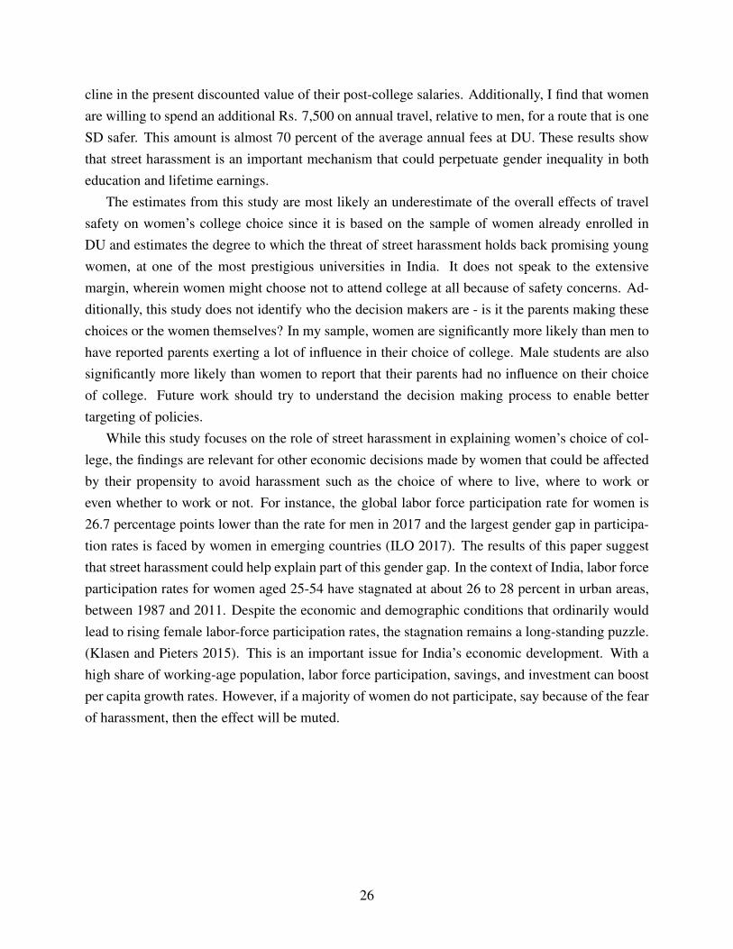
cline in the present discounted value of their post-college salaries. Additionally, I find that womenare willing to spend an additional Rs. 7,500 on annual travel, relative to men, for a route that is oneSD safer. This amount is almost 70 percent of the average annual fees at DU. These results showthat street harassment is an important mechanism that could perpetuate gender inequality in botheducation and lifetime earnings.
The estimates from this study are most likely an underestimate of the overall effects of travelsafety on women’s college choice since it is based on the sample of women already enrolled inDU and estimates the degree to which the threat of street harassment holds back promising youngwomen, at one of the most prestigious universities in India. It does not speak to the extensivemargin, wherein women might choose not to attend college at all because of safety concerns. Ad-ditionally, this study does not identify who the decision makers are - is it the parents making thesechoices or the women themselves? In my sample, women are significantly more likely than men tohave reported parents exerting a lot of influence in their choice of college. Male students are alsosignificantly more likely than women to report that their parents had no influence on their choiceof college. Future work should try to understand the decision making process to enable bettertargeting of policies.
While this study focuses on the role of street harassment in explaining women’s choice of col-lege, the findings are relevant for other economic decisions made by women that could be affectedby their propensity to avoid harassment such as the choice of where to live, where to work oreven whether to work or not. For instance, the global labor force participation rate for women is26.7 percentage points lower than the rate for men in 2017 and the largest gender gap in participa-tion rates is faced by women in emerging countries (ILO 2017). The results of this paper suggestthat street harassment could help explain part of this gender gap. In the context of India, labor forceparticipation rates for women aged 25-54 have stagnated at about 26 to 28 percent in urban areas,between 1987 and 2011. Despite the economic and demographic conditions that ordinarily wouldlead to rising female labor-force participation rates, the stagnation remains a long-standing puzzle.(Klasen and Pieters 2015). This is an important issue for India’s economic development. With ahigh share of working-age population, labor force participation, savings, and investment can boostper capita growth rates. However, if a majority of women do not participate, say because of the fearof harassment, then the effect will be muted.
26

References
Aguilar, Arturo, Emilio Gutierrez and Paula Soto Villagran. 2019. “Benefits and Unintended Con-sequences of Gender Segregation in Public Transportation: Evidence from Mexico City’s Sub-way System.” Economic Development and Cultural Change .
Asiedu, Elizabeth, Isaac Kalonda-Kanyama, Leonce Ndikumana and Akwasi Nti-Addae. 2013.“Access to credit by firms in Sub-Saharan Africa: How relevant is gender?” The American
Economic Review 103(3):293–297.
Azevedo, Eduardo M and Jacob D Leshno. 2016. “A supply and demand framework for two-sidedmatching markets.” Journal of Political Economy 124(5):1235–1268.
Bansal, Prateek, Kara M Kockelman, Will Schievelbein and Scott Schauer-West. 2016. “IndianVehicle Ownership and Travel Behaviors: A Case Study of Bangalore, Delhi and Kolkata.”.
Becker, Gary and Yona Rubinstein. 2011. Fear and the Response to Terrorism: An EconomicAnalysis. Technical report Centre for Economic Performance, LSE.
Black, Dan A and Jeffrey A Smith. 2004. “How robust is the evidence on the effects of collegequality? Evidence from matching.” Journal of Econometrics 121(1):99–124.
Borker, Girija, Jan Eeckhout, Nancy Luke, Shantidani Minz, Kaivan Munshi and Soumya Swami-nathan. 2020. “Wealth, Marriage, and Sex Selection.” Working Paper .
Börsch-Supan, Axel. 1990. “On the compatibility of nested logit models with utility maximization.”Journal of Econometrics 43(3):373–388.
Brewer, Dominic J, Eric R Eide and Ronald G Ehrenberg. 1999. “Does it pay to attend an eliteprivate college? Cross-cohort evidence on the effects of college type on earnings.” Journal of
Human Resources pp. 104–123.
Burde, Dana and Leigh L Linden. 2013. “Bringing education to Afghan girls: A randomized con-trolled trial of village-based schools.” American Economic Journal: Applied Economics 5(3):27–40.
Burgess, Simon, Ellen Greaves, Anna Vignoles and Deborah Wilson. 2015. “What parents want:School preferences and school choice.” The Economic Journal 125(587):1262–1289.
27
Buser, Thomas, Muriel Niederle and Hessel Oosterbeek. 2014. “Gender, competitiveness, andcareer choices.” The Quarterly Journal of Economics 129(3):1409–1447.
Buss, Christian, Jeffrey Parker and Jon Rivenburg. 2004. “Cost, quality and enrollment demand atliberal arts colleges.” Economics of Education Review 23(1):57–65.
Card, David and Alan B Krueger. 1992. “Does school quality matter? Returns to education and thecharacteristics of public schools in the United States.” Journal of Political Economy 100(1):1–40.
Carneiro, Pedro, Jishnu Das and Hugo Reis. 2013. “Parental Valuation of SchoolAttributes in Developing Countries: Evidence from Pakistan.” London, UK
http://ipl.econ.duke.edu/bread/papers/1013conf/carneiro.pdf .
Cattaneo, Matias D, Rocío Titiunik, Gonzalo Vazquez-Bare and Luke Keele. 2016. “Interpretingregression discontinuity designs with multiple cutoffs.” The Journal of Politics 78(4):1229–1248.
Chakraborty, T., A. Mukherjee, S. R. Rachapalli and S. Saha. 2018. “Stigma of Sexual Violenceand Women’s Decision to Work.” World Development 103:226–238.
Cheema, Ali, Asim I Khwaja, Farooq Naseer and Jacob N Shapiro. 2020. “Glass Walls: Experi-mental Evidence on Access Constraints Faced by Women.”.
Cook, Cody, Rebecca Diamond, Jonathan Hall, John A List and Paul Oyer. Forthcoming. “TheGender Earnings Gap in the Gig Economy: Evidence from over a Million Rideshare Drivers.”Review of Economic Studies .
Daly, Andrew and Stanley Zachary. 1978. “Improved multiple choice models.” Determinants of
travel choice 335:357.
Dasgupta, Utteeyo, Subha Mani, Smriti Sharma and Saurabh Singhal. 2020. “Effects of Peers andRank on Cognition, Preferences, and Personality.” Review of Economics and Statistics pp. 1–47.
Definitions of Street Harassment. 2015.URL: http://www.stopstreetharassment.org/resources/definitions/
Eide, Eric, Dominic J Brewer and Ronald G Ehrenberg. 1998. “Does it pay to attend an eliteprivate college? Evidence on the effects of undergraduate college quality on graduate schoolattendance.” Economics of Education Review 17(4):371–376.
Fairchild, Kimberly and Laurie A Rudman. 2008. “Everyday stranger harassment and women’sobjectification.” Social Justice Research 21(3):338–357.
28

Ferrant, Gaëlle, Luca Maria Pesando and Keiko Nowacka. 2014. “Unpaid Care Work: The missinglink in the analysis of gender gaps in labor outcomes.”.
Gallego, Francisco A and Andrés Hernando. 2009. “School Choice in Chile: Looking at the De-mand Side.”.
Hastings, Justine S, Thomas J Kane and Douglas O Staiger. 2009. Heterogenous Preferences andthe Efficacy of Public School Choice. Technical report National Bureau of Economic Research.
Herriges, Joseph A and Catherine L Kling. 1996. “Testing the consistency of nested logit modelswith utility maximization.” Economics Letters 50(1):33–39.
Horsman, Jenny. 2013. Too scared to learn: Women, violence, and education. Routledge.
Hsieh, Chang-Tai, Erik Hurst, Charles I Jones and Peter J Klenow. 2019. “The Allocation of Talentand U.S. Economic Growth.” Econometrica 87(5):1439–1474.
Hsu, Hsin-Ping. 2011. “How Does Fear of Sexual Harassment on Transit Affect Women’s Use ofTransit?” Women’s Issues in Transportation .
ICRW, UN Women &. 2013. Unsafe: An Epidemic of Sexual Violence in Delhi’s Public Spaces:
Baseline Findings from the Safe Cities Delhi Programme.
ILO. 2017. “World Employment Social Outlook - Trends for Women.”.
Jacoby, Hanan G and Ghazala Mansuri. 2015. “Crossing boundaries: How social hierarchy impedeseconomic mobility.” Journal of Economic Behavior & Organization 117:135–154.
Jayachandran, Seema. 2015. “The Roots of Gender Inequality in Developing Countries.” Annual
Review of Economics 7:63–88.
Keane, Carl. 1998. “Evaluating the influence of fear of crime as an environmental mobility restric-tor on women’s routine activities.” Environment and Behavior 30(1):60–74.
Klasen, Stephan and Janneke Pieters. 2015. “What Explains the Stagnation of Female Labor ForceParticipation in Urban India?” The World Bank Economic Review 29(3):449–478.
Kling, Catherine L and Joseph A Herriges. 1995. “An empirical investigation of the consistencyof nested logit models with utility maximization.” American Journal of Agricultural Economics
77(4):875–884.
Kondylis, Florence, Arianna Legovini, Kate Vyborny, Astrid Zwager and Luiza Andrade. 2020.“Demand for "Safe Spaces": Avoiding Harassment and Stigma.” Working Paper .
29

Kremer, Michael, Jessica Leino, Edward Miguel and Alix Peterson Zwane. 2011. “Spring clean-ing: Rural water impacts, valuation, and property rights institutions.” The Quarterly Journal of
Economics 126(1):145–205.
Langton, Lynn and Jennifer L Truman. 2014. Socio-emotional impact of violent crime. US Depart-ment of Justice, Office of Justice Programs, Bureau of Justice Statistics.
León, Gianmarco and Edward Miguel. 2017. “Risky Transportation Choices and the Value of aStatistical Life.” American Economic Journal: Applied Economics 9(1):202–28.
Livingston, Beth. 2015. “Hollaback! International Street Harassment Survey Project.”.URL: https://www.ihollaback.org/cornell-international-survey-on-street-harassment/
Macmillan, Ross, Annette Nierobisz and Sandy Welsh. 2000. “Experiencing the streets: Harass-ment and perceptions of safety among women.” Journal of Research in Crime and Delinquency
37(3):306–322.
McFadden, Daniel. 1978. “Modeling the choice of residential location.” Transportation Research
Record (673).
McFadden, Daniel and Kenneth Train. 2000. “Mixed MNL Models for Discrete Response.” Journal
of applied Econometrics pp. 447–470.
McFadden, Daniel et al. 1977. Quantitative methods for analyzing travel behavior of individuals:
some recent developments. Institute of Transportation Studies, University of California.
McKelway, Madeline. 2020. Women’s Employment in India: Intra-Household and Intra-PersonalConstraints. Technical report Working paper.
Mitra-Sarkar, Sheila and P Partheeban. 2011. “Abandon All Hope, Ye Who Enter Here: Under-standing the Problem of "Eve Teasing" in Chennai, India.” 2(46).
Most dangerous transport systems for women. 2014.URL: http://news.trust.org//spotlight/most-dangerous-transport-systems-for-women/
Mukherjee, Mukta. 2012. “Do Better Roads Increase School Enrollment? Evidence from a UniqueRoad Policy in India.” Evidence from a Unique Road Policy in India (August 28, 2012) .
Muralidharan, Karthik and Nishith Prakash. 2017. “Cycling to School: Increasing SecondarySchool Enrolment for Girls in India.” American Economic Journal: Applied Economics
29(3):321–350.
30

Neill, Christine. 2009. “Tuition fees and the demand for university places.” Economics of Education
Review 28(5):561–570.
Niederle, Muriel and Lise Vesterlund. 2007. “Do women shy away from competition? Do mencompete too much?” The Quarterly Journal of Economics 122(3):1067–1101.
Niederle, Muriel and Lise Vesterlund. 2011. “Gender and competition.” Annual Review of Eco-
nomics 3(1):601–630.
Pain, Rachel H. 1997. “Social geographies of women’s fear of crime.” Transactions of the Institute
of British geographers pp. 231–244.
Pascarella, Ernest T and Patrick T Terenzini. 2005. How college affects students. Vol. 2 Jossey-BassSan Francisco, CA.
Porter, Gina, Kate Hampshire, Albert Abane, Augustine Tanle, Alister Munthali, Elsbeth Robson,Mac Mashiri, Goodhope Maponya and S Dube. 2011. “Young people’s transport and mobility insub-Saharan Africa: the gendered journey to school.” Documents d’analisi geografica 57(1):61–79.
Rakodi, Carole. 2014. “Expanding Women’s Access to Land and Housing in Urban Areas.”.
Rubinstein, Yona and Sheetal Sekhri. 2013. “Value-Added versus Positive Sorting In Higher Edu-cation: Evidence from General Education Sector in India.” Working Paper .
Sanders, Nicholas J. 2012. “What doesn’t kill you makes you weaker prenatal pollution exposureand educational outcomes.” Journal of Human Resources 47(3):826–850.
Satija, Shivani and Amrita Datta. 2015. “Crime against Women and Children in Delhi.” Economic
& Political Weekly 50(9).
Schneider, Mark and Jack Buckley. 2002. “What do parents want from schools? Evidence fromthe Internet.” Educational evaluation and policy analysis 24(2):133–144.
Sekhri, Sheetal. 2020. “Prestige Matters: Wage Premium and Value Addition in Elite Colleges.”American Economic Journal : Applied Economics 12(3).
Siddique, Zahra. 2018. “Violence and Female Labor Supply.” IZA Discussion Paper .
Some Colleges Flouting Norms, Admits DU. 2013.URL: http://www.hindustantimes.com/education/some-colleges-flouting-norms-admits-
du/story-wl80DrnA8aDOLMj9VDyQxH.html
31
Sudarshan, Ratna M and Shrayana Bhattacharya. 2009. “Through the magnifying glass: Women’swork and labour force participation in urban Delhi.” Economic and Political Weekly pp. 59–66.
The Annual Report of the University of Delhi 2013-14. 2014. Technical report.
The Times Higher Education BRICS and Emerging Economies Rankings. 2015.URL: https://www.timeshighereducation.com/world-university-rankings/2015
Three in Four Women Experience Harassment and Violence in UK and Global Cities. 2016.URL: https://www.actionaid.org.uk/latest-news/three-in-four-women-experience-harassment-
and-violence
Train, Kenneth. 2003. Discrete Choice Methods with Simulation. Cambridge: Cambridge Univer-sity Press.
Viscusi, W Kip and Joseph E Aldy. 2003. “The Value of a Statistical Life: a Critical Review ofMarket Estimates Throughout the World.” Journal of Risk and Uncertainty 27(1):5–76.
Viswanath, Kalpana and Ashish Basu. 2015. “SafetiPin: an innovative mobile app to collect dataon women’s safety in Indian cities.” Gender & Development 23(1):45–60.
Warr, Mark. 1985. “Fear of rape among urban women.” Social problems 32(3):238–250.
Winston, Gordon and David Zimmerman. 2004. Peer effects in higher education. In College
choices: The economics of where to go, when to go, and how to pay for it. University of ChicagoPress pp. 395–424.
Zhang, Liang. 2005. “Advance to graduate education: The effect of college quality and undergrad-uate majors.” The Review of Higher Education 28(3):313–338.
32
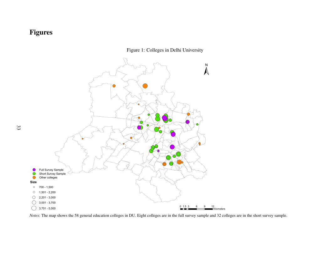
Figures
Figure 1: Colleges in Delhi University
±
0 3 6 9 121.5Kilometers
Size700 - 1,500
1,501 - 2,200
2,201 - 3,000
3,001 - 3,700
3,701 - 5,000
Full Survey SampleShort Survey SampleOther colleges
Notes: The map shows the 58 general education colleges in DU. Eight colleges are in the full survey sample and 32 colleges are in the short survey sample.
33

Figure 2: Cumulative Distribution Function of Rank for Female and Male Students
(a) Absolute rank
0.2
.4.6
.81
Cum
ulat
ive
prob
abilit
y
0 5 10 15 20 25Absolute Rank
Female Male
(b) Rank within choice set
.2.4
.6.8
1C
umul
ativ
e pr
obab
ility
0 5 10 15Rank in choice set
Female Male
Notes: Rank is based on cutoff scores of a college for the student’s major and admission year from the first cutoff listfor general category male students. A higher rank indicates a lower cutoff score or worse quality. The absolute rankin Panel (a) ranks college within a major and admission year using the first cutoff list for that year. Rank within astudent’s choice set in Panel (b) ranks the colleges that the student was eligible to attend, by their cutoff score for thestudent’s major and admission year. The CDF is for colleges chosen by students in the full survey sample and shortsurvey sample who are Delhi residents that live at home, and travel to college everyday.
34

Figure 3: Stylized Example
(a) The set-up
H
L
Not so good college Good college
M F
M F
M F
M F
D
A
N
G
E
R
(b) High-scoring males
L M F M F
Not so good college Good college
H M F M F
D
A
N
G
E
R
(c) Low-scoring males
L M F M F
Not so good college Good college
H M F M F
D
A
N
G
E
R
(d) Females who do not face a safety-quality trade-off
L M F M F
Not so good college Good college
H M F M F
D
A
N
G
E
R
(e) High-scoring female chooses lower quality college
L M F M F
Not so good college Good college
H M F M F
D
A
N
G
E
R
(f) Female uses more expensive mode of transport
L M F M F
Not so good college Good college
H M F M F
D
A
N
G
E
R
Notes: This figure shows the college and route choice of students by gender and high school exam scores. M and F denotea male and female student respectively. H and L denote students’ high school exam scores. The thin arrows denote a travelroute. A route is considered unsafe if it crosses the red "danger" area. The green dashed arrow denotes a route using a moreexpensive mode of transport. The thick grey arrow denotes the choice of not attending college at all.
35

Figure 4: Students in Full Survey Sample
#
#
##
#
#
#
#
#
#
#
#
#
#
#
#
#
#
##
#
###
#
#
#
###
#
##
#
#
#
#
##
#
#
#
#
#
#
#
#
#
#
#
#
#
#
#
# ##
##
##
#
#
#
#
#
#
##
#
#
#
#
#
#
#
#
#
#
#
#
#
#
##
#
#
#
##
#
#
#
#
#
#
#
#
#
# #
#
#
# #
#
#
#
#
##
#
#
#
#
# ##
##
#
#
#
#
#
#
#
##
##
#
##
#
#
#
#
#
#
#
#
#
#
#
#
# ##
#
#
#
#
#
#
#
#
#
#
#
#
##
#
#
#
#
#
#
#
#
#
# ##
#
#
##
##
##
#
#
#
##
#
#
## #
#
#
#
##
##
#
#
#
##
#
#
#
#
#
#
#
#
#
#
#
#
#
#
#
#
#
##
#
#
#
#
# #
##
#
#
##
#
#
#
###
#
#
#
#
#
#
#
#
#
#
#
#
#
##
#
#
#
#
#
#
#
#
#
##
#
#
#
#
#
#
#
#
##
##
#
#
#
#
#
#
#
#
#
#
##
#
#
##
#
##
#
#
#
#
#
#
#
#
#
#
#
#
#
#
#
#
##
#
## #
#
#
#
#
#
#
#
#
#
#
#
#
##
#
#
#
#
#
#
#
#
#
#
#
#
#
#
##
###
#
#
#
#
#
#
#
#
#
#
#
#
#
#
#
#
#
#
#
#
##
#
#
#
#
#
#
#
#
#
#
#
#
#
#
#
#
#
#
#
#
#
#
#
#
#
##
#
#
#
#
##
#
#
#
#
#
#
#
#
#
#
#
#
#
#
#
#
#
#
#
#
#
#
##
#
#
#
# #
#
#
#
#
#
#
#
#
#
#
#
#
#
#
#
#
#
#
#
##
#
#
#
#
#
#
#
#
#
#
#
#
#
#
#
##
#
#
#
#
#
#
#
#
#
#
#
#
#
#
#
#
#
#
#
#
#
#
#
#
##
#
#
#
#
#
#
#
#
#
#
#
#
#
#
#
#
#
#
#
#
#
#
#
#
#
# #
#
#
#
#
#
#
#
#
#
#
#
#
##
#
#
#
#
#
#
#
#
#
#
#
#
#
#
#
#
#
#
#
#
#
#
#
#
#
#
#
#
#
#
#
#
#
#
#
#
#
#
##
#
#
#
#
##
#
#
#
#
#
#
#
#
#
#
#
#
#
##
#
#
#
#
#
#
#
#
#
#
##
#
#
#
#
#
#
#
#
#
#
#
#
#
#
##
#
#
#
#
#
#
#
#
#
#
##
#
# #
##
#
#
#
#
#
#
#
#
#
#
#
#
#
#
#
#
#
#
#
#
#
#
#
#
#
#
#
#
#
#
#
#
#
#
#
#
##
#
#
#
#
##
#
##
#
##
#
#
#
#
#
#
#
#
#
#
#
#
#
#
#
#
#
##
#
#
#
#
#
#
##
##
#
#
#
#
#
#
#
#
#
#
#
#
#
#
#
#
#
#
#
#
#
#
#
#
#
#
#
#
#
#
#
##
#
#
#
#
#
##
#
#
##
##
#
#
#
##
#
##
##
#
##
#
#
#
##
#
#
#
#
#
#
#
#
#
#
#
#
#
##
#
#
#
#
#
#
#
#
#
#
#
#
##
#
#
#
#
#
#
#
#
#
#
#
#
#
#
#
#
#
#
#
#
#
#
##
#
#
#
#
# #
#
#
#
#
#
#
#
#
#
#
#
#
#
#
#
#
#
##
#
#
#
#
#
#
#
#
#
#
# #
#
##
##
#
#
#
#
#
#
#
#
#
#
#
#
#
#
#
#
#
#
#
#
#
#
#
#
#
#
#
#
#
#
#
#
#
#
#
# #
#
# #
#
#
#
##
#
#
#
#
#
#
^
^^
^
^^
^̂
0 4 8 12 162Kilometers
±
^ Sample college# Males
Females
Notes: This map shows the residential location of students who are Delhi residents from the full survey sample that live at home and travel to college everyday.
36

Figure 5: Variation in Quality of the Full Survey Sample Colleges
(a) Political Science
74
79
84
89
94
99
54 77 38 7 64 39 50 46 36 19 17 51 56 62 3 12 29 70 26 41 52 34
2015
-16
C
utof
f %
College codes
Political Science (Hons.) (b) History
74
79
84
89
94
99
64 43 35 39 75 28 50 48 62 76 17 14 20 4 12 29 69 31 52 22
2015
-16
C
uto
ff %
College codes
History (Hons.)
Notes: This figure shows the cutoff scores for male, general category students from the first cutoff list in 2015-16. Panel (a) shows the cutoffs for Bachelor of Artsin Political Science and Panel (b) shows the cutoffs for Bachelor of Arts in History. Alternate bars are labelled with college codes.
37
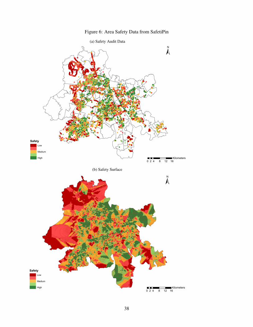
Figure 6: Area Safety Data from SafetiPin
(a) Safety Audit Data
0 4 8 12 162Kilometers
Medium
±
SafetyLow
High
(b) Safety Surface
0 4 8 12 162Kilometers
Medium
±
SafetyLow
High
38
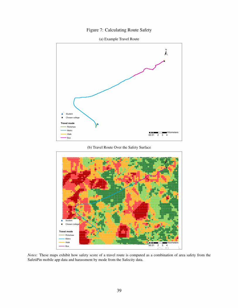
Figure 7: Calculating Route Safety
(a) Example Travel Route
^
#
0 1 2 3 40.5Kilometers
±
# Student
^ Chosen college
Travel modeRickshaw
Metro
Walk
Bus
(b) Travel Route Over the Safety Surface
^
#
0 1 2 3 40.5Kilometers
±
# Student
^ Chosen college
Travel modeRickshaw
Metro
Walk
Bus
Notes: These maps exhibit how safety score of a travel route is computed as a combination of area safety from theSafetiPin mobile app data and harassment by mode from the Safecity data.
39

Figure 8: Choice Relative to Neighbors
(a) Safety difference-1
01
2Sa
fety
Diff
eren
ce
0 10 20 30Score gap
Females Males
(b) Quality difference
05
1015
Qua
lity
Diff
eren
ce
0 10 20 30Score gap
Females Males
(c) Time difference
-30
-10
1030
Tim
e D
iffer
ence
0 10 20 30Score gap
Females Males
(d) Cost difference
-10
12
3C
ost D
iffer
ence
0 10 20 30Score gap
Females Males
A5Notes: The figure plot binned scatter plots of difference in travel safety (SD), college quality (percentage), daily traveltime (minutes), and monthly travel cost (thousand INR) between the index student and their neighbor’s choice. Indexstudent is the student who scores higher. Score gap bin is the two point bin of high school score difference between theindex student and the neighbor. A neighbor is defined as a student living within a 1.5kms radius of the index studentand has the same gender, major, and admission year. Table A7 shows the equivalent regressions. Figure A5 in theOnline Appendix shows robustness of these results to different neighborhood radii.
40

Figure 9: Variation of Student and Area Characteristics Around Colleges
(a) Average high school exam score by gender
7075
8085
9095
Exam
sco
reFemales
7075
8085
9095
Exam
sco
re
5447
7728
3865
735
3943
4850
6446
6357
3619
7576
1718
5153
5660
6268
34
1214
2920
7026
4269
2441
5222
3431
Males
(b) Proportion of female students
.2.4
.6.8
1Pr
opor
tion
5447
7728
3865
735
3943
4850
6446
6357
3619
7576
1718
5153
5660
6268
34
1214
2920
7026
4269
2441
5222
3431
Notes: The figures show the average high school score (%) of students by gender and the proportion of female studentsliving within a 1.5kms radius around each general education college in DU that offers a Bachelor of Arts in PoliticalScience. Each bar represents a college. The colleges are in ascending order of quality. The quality measure used hereis the cutoff scores for Bachelor of Arts in Political Science applicable for male, general category students from thefirst cutoff list in 2015-16, as shown in Figure 5(a). Alternate bars are labeled.
41
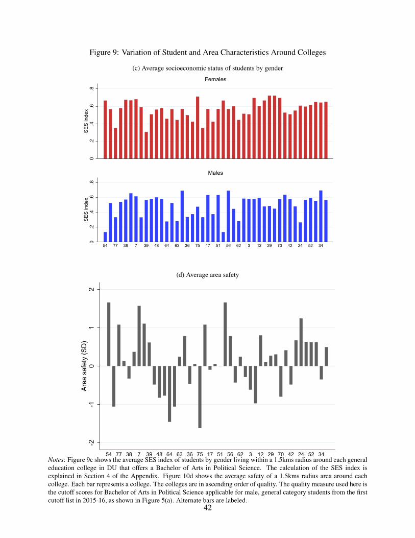
Figure 9: Variation of Student and Area Characteristics Around Colleges
(c) Average socioeconomic status of students by gender
0.2
.4.6
.8SE
S in
dex
Females
0.2
.4.6
.8SE
S in
dex
5447
7728
3865
735
3943
4850
6446
6357
3619
7576
1718
5153
5660
6268
34
1214
2920
7026
4269
2441
5222
3431
Males
(d) Average area safety
-2-1
01
2Ar
ea s
afet
y (S
D)
5447
7728
3865
735
3943
4850
6446
6357
3619
7576
1718
5153
5660
6268
34
1214
2920
7026
4269
2441
5222
3431Notes: Figure 9c shows the average SES index of students by gender living within a 1.5kms radius around each general
education college in DU that offers a Bachelor of Arts in Political Science. The calculation of the SES index isexplained in Section 4 of the Appendix. Figure 10d shows the average safety of a 1.5kms radius area around eachcollege. Each bar represents a college. The colleges are in ascending order of quality. The quality measure used here isthe cutoff scores for Bachelor of Arts in Political Science applicable for male, general category students from the firstcutoff list in 2015-16, as shown in Figure 5(a). Alternate bars are labeled.
42

Figure 9: Variation of Student and Area Characteristics Around Colleges
(e) Average route safety
-.6-.4
-.20
.2.4
Aver
age
rout
e sa
fety
5447
7728
3865
735
3943
4850
6446
6357
3619
7576
1718
5153
5660
6268
34
1214
2920
7026
4269
2441
5222
3431
Notes: The figure shows the average route safety from 25 randomly chosen locations in Delhi to each general educationcollege in DU that offers a Bachelor of Arts in Political Science. Each bar represents a college. The colleges are inascending order of quality. The quality measure used here is the cutoff scores for Bachelor of Arts in Political Scienceapplicable for male, general category students from the first cutoff list in 2015-16, as shown in Figure 5(a). Alternatebars are labeled.
43

Tables
Table 1: Summary Statistics
Total Female Male Female - MaleN = 2,713 N = 1,767 N = 946
Mean SD Mean SD Mean SD Mean Diff. SEA. Student Characteristics
Proportion surveyed 0.72 0.76 0.67Proportion of Delhi residents 0.99 0.99 0.99Female 0.65High school exam score (%) 83.88 [9.08] 84.52 [8.85] 82.68 [9.39] -1.84 (0.36)Socio-economic status 0.47 [0.29] 0.50 [0.28] 0.40 [0.30] -0.10 (0.01)
B. College Characteristics
First cutoff score 87.96 [8.82] 87.57 [9.20] 88.70 [8.00] 1.13 (0.35)Absolute rank 10.87 [5.51] 11.15 [5.31] 10.34 [5.83] -0.81 (0.22)Rank in choice set 4.53 [3.23] 5.02 [3.35] 3.60 [2.75] -1.42 (0.13)Distance (km.) 13.05 [9.66] 13.06 [9.54] 13.05 [9.88] -0.01 (0.39)Annual Tuition (’000 Rs.) 10.57 [3.22] 10.86 [3.07] 10.02 [3.43] -0.85 (0.13)Size of college 3,566.14 [942.36] 3,761.39 [798.86] 3,201.44 [1,073.08] -559.94 (36.42)Number of majors 13.68 [4.20] 14.11 [3.66] 12.88 [4.96] -1.23 (0.17)Boarding college 0.21 [0.41] 0.26 [0.44] 0.12 [0.32] -0.14 (0.02)Women only college 0.44 0.50
C. Route Characteristics
Route safety (SD) 0.36 [1.09] 0.45 [1.04] 0.17 [1.15] -0.28 (0.04)Monthly travel cost (’000 Rs.) 1.59 [2.00] 1.78 [2.14] 1.24 1.66 -0.55 (0.08)Travel time (minutes) 67.27 [35.71] 66.26 [34.42] 69.16 [37.95] 2.90 (1.44)
Notes: Based on sample of Delhi residents from the full survey who live at home. The socio-economic status is an index thatcaptures the student relative wealth, its construction is explained in Section 4 of the Appendix. First cutoff score is for malestudents of general category. College characteristics describe the college chosen by the student. The absolute rank rates collegeswithin a major and admission year using cutoff scores from the the first cutoff list. Rank in choice set ranks the colleges to whichthe student was admitted to by their cutoff score for the students’ major and admission year. Distance is the shortest distance fromstudent’s residence to their chosen college. Annual tuition is for 2016. Size of college is the number of students enrolled in thecollege.
44
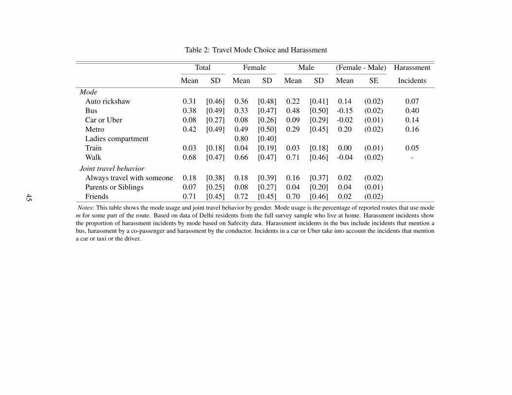
Table 2: Travel Mode Choice and Harassment
Total Female Male (Female - Male) Harassment
Mean SD Mean SD Mean SD Mean SE IncidentsMode
Auto rickshaw 0.31 [0.46] 0.36 [0.48] 0.22 [0.41] 0.14 (0.02) 0.07Bus 0.38 [0.49] 0.33 [0.47] 0.48 [0.50] -0.15 (0.02) 0.40Car or Uber 0.08 [0.27] 0.08 [0.26] 0.09 [0.29] -0.02 (0.01) 0.14Metro 0.42 [0.49] 0.49 [0.50] 0.29 [0.45] 0.20 (0.02) 0.16Ladies compartment 0.80 [0.40]Train 0.03 [0.18] 0.04 [0.19] 0.03 [0.18] 0.00 (0.01) 0.05Walk 0.68 [0.47] 0.66 [0.47] 0.71 [0.46] -0.04 (0.02) -
Joint travel behaviorAlways travel with someone 0.18 [0.38] 0.18 [0.39] 0.16 [0.37] 0.02 (0.02)Parents or Siblings 0.07 [0.25] 0.08 [0.27] 0.04 [0.20] 0.04 (0.01)Friends 0.71 [0.45] 0.72 [0.45] 0.70 [0.46] 0.02 (0.02)
Notes: This table shows the mode usage and joint travel behavior by gender. Mode usage is the percentage of reported routes that use modem for some part of the route. Based on data of Delhi residents from the full survey sample who live at home. Harassment incidents showthe proportion of harassment incidents by mode based on Safecity data. Harassment incidents in the bus include incidents that mention abus, harassment by a co-passenger and harassment by the conductor. Incidents in a car or Uber take into account the incidents that mentiona car or taxi or the driver.
45

Table 3: Trade-off between Route Safety and College Quality: Mixed Logit Estimates
Female Male
(1) (2) (3) (4)Random coefficientsRoute safety 0.705 1.010 0.468 0.570
(0.025) (0.033) (0.034) (0.043)Cutoff score 0.065 0.045 0.143 0.162
(0.007) (0.007) (0.012) (0.014)Daily travel time -0.014 -0.023 -0.014 -0.019
(0.001) (0.002) (0.002) (0.002)Monthly travel cost -0.256 -0.115 -0.352 -0.303
(0.015) (0.018) (0.026) (0.029)Fixed coefficientsCollege neighborhood safety 0.159 0.088
(0.037) (0.042)Size of college 0.001 0.001
(0.000) (0.000)Women’s only college 0.591 -
(0.056)Public transport mode 1.581 0.601
(0.077) (0.109)Number of students 1,767 1,767 946 946Observations 289,121 298,121 112,958 112,958Log-likelihood -7985.66 -6825.76 -3901.95 -3807.22
Mean MRS (Safety, Score)(pp per SD of safety) -8.798 -13.518 -2.112 -2.932
2.5 percentile -39.048 -28.790 -3.299 -12.20497.5 percentile -3.152 -7.694 -1.556 -1.189
Mean MRS (Safety, Time)(minutes per SD of safety) 26.773 22.698 20.798 18.135
2.5 percentile 24.630 19.698 19.022 16.10897.5 percentile 30.468 27.744 24.409 22.622
Mean MRS (Safety, Cost)(’000 Rs. per SD of safety) 1.453 4.473 0.829 1.127
2.5 percentile 1.329 4.279 0.760 1.04297.5 percentile 1.749 4.857 1.052 1.392
Notes: This table reports the mixed logit estimates from the student’s model ofcollege choice. Each observation is a unique student-route pair. The dependentvariable is an indicator equal to one for the route reported by the student. The randomcoefficients associated with route safety, cutoff score are estimated using a triangulardistribution and the daily travel time and monthly route cost coefficients are estimatedusing a restricted triangular distribution, which are both assumed to be non-positive.The other coefficients are assumed to be fixed. The MRS is the negative ratio of thecoefficient estimates on route safety over score or cost or time, and its standard erroris estimated using the delta method. MRS are measured in terms of the SD of routesafety across the predicted route alternatives within a students’ choice set.
46
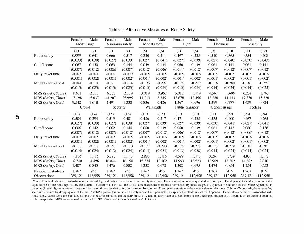
Table 4: Alternative Measures of Route Safety
Female Male Female Male Female Male Female Male Female Male Female MaleMode usage Minimum safety Modal safety Light Openness Visibility
(1) (2) (3) (4) (5) (6) (7) (8) (9) (10) (11) (12)Route safety 0.999 0.641 0.666 0.517 0.320 0.211 0.497 0.325 0.510 0.365 0.554 0.408
(0.033) (0.038) (0.027) (0.039) (0.027) (0.041) (0.027) (0.039) (0.027) (0.040) (0.030) (0.043)Cutoff score 0.067 0.150 0.063 0.144 0.059 0.134 0.060 0.139 0.061 0.141 0.061 0.141
(0.007) (0.012) (0.006) (0.007) (0.012) (0.006) (0.011) (0.012) (0.007) (0.012) (0.007) (0.012)Daily travel time -0.025 -0.021 -0.007 -0.009 -0.015 -0.015 -0.015 -0.016 -0.015 -0.015 -0.015 -0.016
(0.001) (0.002) (0.001) (0.002) (0.001) (0.002) (0.001) (0.002) (0.001) (0.002) (0.001) (0.002)Monthly travel cost -0.044 -0.194 -0.128 -0.234 -0.196 -0.297 -0.175 -0.279 -0.176 -0.280 -0.187 -0.293
(0.013) (0.023) (0.013) (0.023) (0.013) (0.024) (0.013) (0.024) (0.014) (0.024) (0.014) (0.025)MRS (Safety, Score) -8.621 -2.272 -6.333 -2.229 -3.019 -0.962 -5.012 -1.449 -4.567 -1.606 -6.238 -1.763MRS (Safety, Time) 17.198 15.037 44.207 35.995 11.213 8.345 15.678 12.456 16.280 14.133 17.570 15.320MRS (Safety, Cost) 9.542 1.618 2.491 1.330 0.836 0.426 1.367 0.696 1.399 0.777 1.439 0.824
Crowd Security Walk path Public transport Gender usage Feeling
(13) (14) (15) (16) (17) (18) (19) (20) (21) (22) (23) (24)Route safety 0.504 0.394 0.519 0.401 0.486 0.317 0.471 0.325 0.535 0.400 0.467 0.265
(0.027) (0.039) (0.027) (0.038) (0.027) (0.039) (0.027) (0.039) (0.030) (0.041) (0.027) (0.041)Cutoff score 0.006 0.142 0.062 0.144 0.060 0.139 0.060 0.139 0.061 0.143 0.060 0.138
(0.007) (0.012) (0.007) (0.012) (0.007) (0.012) (0.006) (0.012) (0.007) (0.012) (0.006) (0.012)Daily travel time -0.015 -0.015 -0.015 -0.015 -0.015 -0.016 -0.015 -0.016 -0.015 -0.015 -0.016 -0.016
(0.001) (0.002) (0.001) (0.002) (0.001) (0.002) (0.001) (0.002) (0.001) (0.002) (0.001) (0.002)Monthly travel cost -0.173 -0.278 -0.167 -0.270 -0.177 -0.280 -0.175 -0.278 -0.173 -0.279 -0.181 -0.284
(0.014) (0.024) (0.013) (0.024) (0.014) (0.024) (0.013) (0.028) (0.014) (0.024) (0.014) (0.024)MRS (Safety, Score) -4.806 -1.716 -5.382 -1.745 -2.835 -1.416 -4.588 -1.445 -3.267 -1.739 -4.937 -1.173MRS (Safety, Time) 16.740 14.496 16.844 16.150 15.334 12.162 14.993 12.523 16.909 15.502 14.262 9.810MRS (Safety, Cost) 1.407 0.845 1.476 0.882 1.332 0.678 1.302 0.695 1.474 0.854 1.254 0.553Number of students 1,767 946 1,767 946 1,767 946 1,767 946 1,767 946 1,767 946Observations 289,121 112,958 289,121 112,958 289,121 112,958 289,121 112,958 289,121 112,958 289,121 112,958
Notes: This table shows the robustness of the mixed logit estimates to alternative route safety measures. Each observation is a unique student-route pair. The dependent variable is an indicatorequal to one for the route reported by the student. In columns (1) and (2), the safety score uses harassment rates normalized by mode usage, as explained in Section 5 of the Online Appendix. Incolumns (3) and (4), route safety is measured by the minimum level of safety on the route. In columns (5) and (6) route safety is the modal safety on the route. Column (7) onwards, the route safetyscore is calculated by dropping one of the nine SafetiPin parameters in the area safety index. Each parameter is explained in Table A3, of the Appendix. The random coefficients associated withroute safety, cutoff score are estimated using a triangular distribution and the daily travel time and monthly route cost coefficients using a restricted triangular distribution, which are both assumedto be non-positive. MRS are measured in terms of the SD of route safety within a students’ choice set.
47

Online AppendixSafety First: Perceived Risk of Street Harassment and Educa-tional Choices of Women
A Additional Figures
Figure A1: High School Exam Scores for Female and Male Students
0.0
1.0
2.0
3.0
4Pr
obab
ility
50 60 70 80 90 100High school exam score
Female Male
Notes: The figure shows the probability distribution function of school-leaving exam scores for students in the fullsurvey sample and short survey sample who are Delhi residents that live at home and travel to college everyday.
48
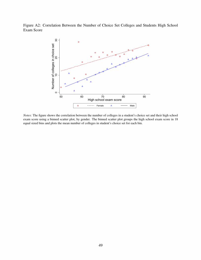
Figure A2: Correlation Between the Number of Choice Set Colleges and Students High SchoolExam Score
010
2030
Num
ber o
f col
lege
s in
cho
ice
set
50 60 70 80 90High school exam score
Female Male
Notes: The figure shows the correlation between the number of colleges in a student’s choice set and their high schoolexam score using a binned scatter plot, by gender. The binned scatter plot groups the high school exam score in 18equal sized bins and plots the mean number of colleges in student’s choice set for each bin.
49

Figure A3: An example of route mapping
(a) Student and chosen college
^
#
0 4 8 12 162Kilometers
±
# Student^ Chosen college
(b) Reported route to chosen college
^
#
0 4 8 12 162Kilometers
±
# Student^ Chosen college
Travel modeBusDrivingMetroWalking
Notes: Panel (a) shows a male student in our sample and his chosen college. Panel (b) shows his reported daily travelroute, where he walks from his home to the closest metro station, takes the metro to Moti Nagar metro station fromwhere he take a bus to a bus stop close to college and then walks to college.
50
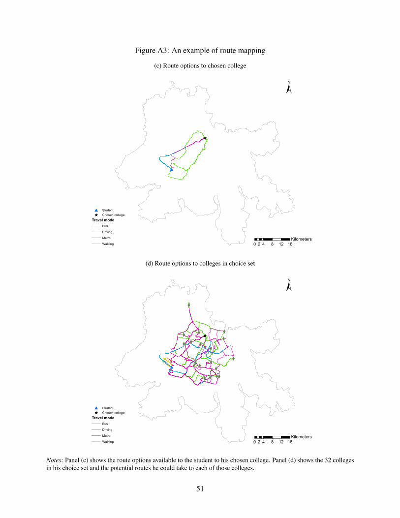
Figure A3: An example of route mapping
(c) Route options to chosen college
^
#
0 4 8 12 162Kilometers
±
# Student^ Chosen college
Travel modeBusDrivingMetroWalking
(d) Route options to colleges in choice set
XW
XW
XW
XW
XW
XW
XW
XWXW
XW XW
XW
XWXWXWXW
XW
XW
XW
XWXWXW
XWXW
XWXWXW
XWXW
XW
XW
XW
XWXW
^
#
0 4 8 12 162Kilometers
±
# Student^ Chosen college
Travel modeBusDrivingMetroWalking
Notes: Panel (c) shows the route options available to the student to his chosen college. Panel (d) shows the 32 collegesin his choice set and the potential routes he could take to each of those colleges.
51
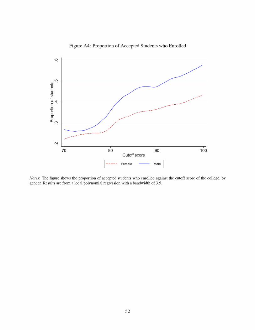
Figure A4: Proportion of Accepted Students who Enrolled
.2.3
.4.5
.6Pr
opor
tion
of s
tude
nts
70 80 90 100Cutoff score
Female Male
Notes: The figure shows the proportion of accepted students who enrolled against the cutoff score of the college, bygender. Results are from a local polynomial regression with a bandwidth of 3.5.
52

Figure A5: Robustness of Choice Relative to Neighbors
-10
12
Safe
ty D
iffer
ence
0 10 20 30
1 km
-10
12
0 10 20 30
1.5 kms
-10
12
0 10 20 30
2 kms
-10
12
0 10 20 30
2.5 kms
05
1015
Qua
lity
Diff
eren
ce
0 10 20 30
05
1015
0 10 20 30
05
1015
0 10 20 30
05
1015
0 10 20 30
-30
-10
1030
Tim
e D
iffer
ence
0 10 20 30
-30
-10
1030
0 10 20 30
-30
-10
1030
0 10 20 30
-30
-10
1030
0 10 20 30
-10
12
3C
ost D
iffer
ence
0 10 20 30Score gap
-10
12
3
0 10 20 30Score gap
-10
12
3
0 10 20 30Score gap
-10
12
3
0 10 20 30Score gap
Unique pairs = 815Students = 946
Unique pairs = 1,228Students = 1,232
Unique pairs = 2,462Students = 1,708
Unique pairs = 3,503Students = 1,934
Female Male
Notes: The figures plot binned scatter plots of difference in travel safety (SD), college quality (percentage), daily travel time (minutes), and monthly travel cost(thousand INR) between the index student and their neighbor’s choice. Index student is the student who scores higher. Score gap bin is the two point bin of highschool score difference between the index student and the neighbor. A neighbor is defined as a student living within a 1km, 1.5km, 2km and 2.5km radius of theindex student and has the same gender, major, and admission year.
53
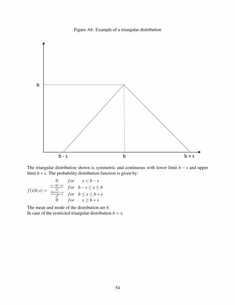
Figure A6: Example of a triangular distribution
b - s b + sb
b
The triangular distribution shown is symmetric and continuous with lower limit b− s and upperlimit b+ s. The probability distribution function is given by:
f (x|b,s) =
0 f or x < b− sx−(b−s)
s2 f or b− s≤ x≤ b(b+s)−x
s2 f or b≤ x≤ b+ s0 f or x≥ b+ s
The mean and mode of the distribution are b.In case of the restricted triangular distribution b = s.
54

Figure A7: Reported Crime and Perceived Safety
-.15 -.1 -.05 0Crime equivalent to +1 SD of perceived safety
Rape
Kidnapping and abduction
Insult to modesty
Assault on women
Notes: The figure shows the coefficient from a district level regression of log of rapes in 2013 on average area safetyand log of the number of the 15 to 34 year old females. Data on crimes is from the National Crime Records Bureau.The four types of crime against women that could potentially take place in public spaces are shown here.
55

B Additional Tables
Table A1: Comparison of Student Characteristics
Data Female Male
Full Survey Short Survey Admin. Data Full Survey Short Survey Admin. DataDelhi residents 1,767 459 11,450 946 171 8,288Proportion of surveyed 0.74 0.82 0.80 0.67 0.62 0.68
Social CategoryGeneral 0.75 0.70 0.73 0.56 0.59 0.50
[2.19] [2.25] [0.81] [-3.05]SC 0.12 0.11 0.14 0.20 0.14 0.19
[-0.39] [2.39] [-1.91] [-0.79]ST 0.01 0.01 0.02 0.02 0.02 0.03
[-1.07] [1.80] [-0.22] [2.07]OBC 0.11 0.18 0.11 0.22 0.25 0.27
[3.69] [-0.94] [0.97] [3.34]High school exam score (%) 84.88 83.90 - 82.70 82.03 -
[-2.05] [-0.84]Distance to college (kms.) 13.06 11.98 13.34 13.05 15.63 14.30
[-2.14] [1.28] [2.87] [3.68]Distance to center (kms.) 15.42 12.11 15.05 15.99 15.93 16.49
[-7.96] [-1.92] [-0.09] [1.65]Notes: Distance to college is the shortest travel distance to the chosen college calculated by Google Maps. Distance to city center is the shortest
distance to India Gate, a central landmark in Delhi. Test statistic for two sample t-tests is reported in brackets where sample mean for each data setis compared with sample mean of full survey data. Social categories refers to the officially designated groups of historically disadvantaged peoplein India. These categories are used for the purposes of affirmative action. The categories are General category, Scheduled Castes (SC), ScheduledTribes (ST), and Other Backward Castes (OBC). General is the unreserved category, SC were formerly referred to as "untouchables", ST are theindigenous people, and OBC is the collective term used by the Government to classify castes which are socially and educationally disadvantagedbut not SC.
56

Table A2: Sample Cutoff List
Notes: This is scanned copy of a sample cutoff list from a college in DU for 2015-16. The rows specify the major, and the columns show the category of admission.Each cell has the relevant cutoff score. The remarks specify additional conditions.
57
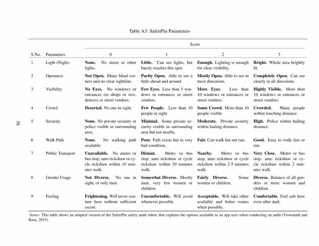
Table A3: SafetiPin Parameters
Score
S.No. Parameters 0 1 2 3
1 Light (Night) None. No street or otherlights.
Little. Can see lights, butbarely reaches this spot.
Enough. Lighting is enoughfor clear visibility.
Bright. Whole area brightlylit.
2 Openness Not Open. Many blind cor-ners and no clear sightline.
Partly Open. Able to see alittle ahead and around.
Mostly Open. Able to see inmost directions.
Completely Open. Can seeclearly in all directions.
3 Visibility No Eyes. No windows orentrances (to shops or resi-dences) or street vendors.
Few Eyes. Less than 5 win-dows or entrances or streetvendors.
More Eyes. Less than10 windows or entrances orstreet vendors.
Highly Visible. More than10 windows or entrances orstreet vendors.
4 Crowd Deserted. No one in sight. Few People. Less than 10people in sight.
Some Crowd. More than 10people visible.
Crowded. Many peoplewithin touching distance.
5 Security None. No private security orpolice visible in surroundingarea.
Minimal. Some private se-curity visible in surroundingarea but not nearby.
Moderate. Private securitywithin hailing distance.
High. Police within hailingdistance.
6 Walk Path None. No walking pathavailable.
Poor. Path exists but in verybad condition.
Fair. Can walk but not run. Good. Easy to walk fast orrun.
7 Public Transport Unavailable. No metro orbus stop, auto rickshaw or cy-cle rickshaw within 10 min-utes walk.
Distant. Metro or busstop, auto rickshaw or cyclerickshaw within 10 minuteswalk.
Nearby. Metro or busstop, auto rickshaw or cyclerickshaw within 2-5 minuteswalk.
Very Close. Metro or busstop, auto rickshaw or cy-cle rickshaw within 2 min-utes walk.
8 Gender Usage Not Diverse. No one insight, or only men.
Somewhat Diverse. Mostlymen, very few women orchildren.
Fairly Diverse. Somewomen or children.
Diverse. Balance of all gen-ders or more women andchildren.
9 Feeling Frightening. Will never ven-ture here without sufficientescort.
Uncomfortable. Will avoidwhenever possible.
Acceptable. Will take otheravailable and better routeswhen possible.
Comfortable. Feel safe hereeven after dark.
Notes: This table shows an adapted version of the SafetiPin safety audit rubric that explains the options available to an app user when conducting an audit (Viswanath andBasu, 2015).
58

Table A4: Summary Statistics for non-Delhi residents
Total Female Male Female - MaleN = 1,031 N = 564 N = 467
Mean SD Mean SD Mean SD Mean Diff. SEA. Student Characteristics
Female 0.55
High school exam score (%) 89.15 [7.37] 90.57 [6.33] 87.44 [8.14] -3.13 (0.45)SES index 0.56 [0.26] 0.64 [0.24] 0.47 [0.26] -0.17 (0.02)
B. College Characteristics
First cutoff score 92.22 [6.53] 92.69 [6.06] 91.66 [7.02] -1.03 (0.41)Absolute rank 7.35 [4.58] 7.46 [4.16] 7.21 [5.03] -0.25 (0.29)Rank in choice set 3.69 [2.61] 4.27 [2.72] 2.99 [2.28] -1.28 (0.16)Distance (km.) 5.48 [7.30] 4.17 [6.67] 7.07 [7.71] 2.90 (0.45)Annual Tuition (’000 Rs.) 11.08 [3.66] 11.89 [3.37] 10.11 [3.76] -1.78 (0.22)Size of college 3,972.54 [1,003.85] 4,215.60 [737.73] 3,678.99 [1,188.27] -536.62 (60.57)Number of majors 15.15 [3.81] 15.96 [2.81] 14.18 [4.56] -1.79 (0.23)Boarding college 0.51 [0.50] 0.64 [0.48] 0.35 [0.48] -0.29 (0.03)Women only college 0.48 [0.50]
C. Route Characteristics
Route safety (SD) 1.17 [1.26] 1.41 [1.14] 0.87 [1.34] -0.54 (0.08)Monthly travel cost (’000 Rs.) 0.81 [1.39] 0.78 [1.43] 0.84 [1.34] 0.05 (0.09)Travel time (minutes) 36.46 [38.52] 30.18 [39.43] 44.03 [36.00] 13.85 (2.37)
Notes: Based on sample of students who are not residents of Delhi from the full survey. The socio-economic status is an index that captures the studentrelative wealth, its construction is explained in the Appendix Section 4. First cutoff score is for male students of general category. College characteristicsdescribe the college chosen by the student. The absolute rank rates colleges within a major and admission year using cutoff scores from the the firstcutoff list. Rank in choice set ranks the colleges to which the student was admitted to by their cutoff score for the students’ major and admission year.Distance is the shortest distance from student’s residence to their chosen college. Annual tuition is for 2016. Size of college is the number of studentsenrolled in the college.
59
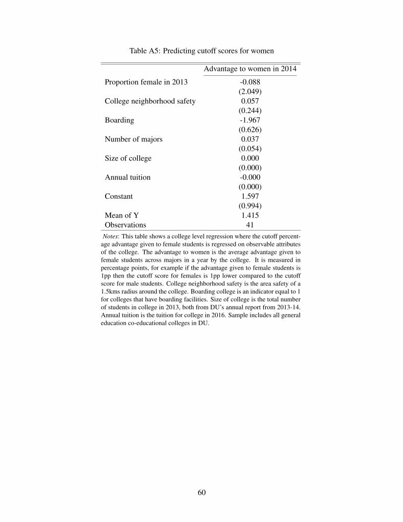
Table A5: Predicting cutoff scores for women
Advantage to women in 2014
Proportion female in 2013 -0.088(2.049)
College neighborhood safety 0.057(0.244)
Boarding -1.967(0.626)
Number of majors 0.037(0.054)
Size of college 0.000(0.000)
Annual tuition -0.000(0.000)
Constant 1.597(0.994)
Mean of Y 1.415Observations 41
Notes: This table shows a college level regression where the cutoff percent-age advantage given to female students is regressed on observable attributesof the college. The advantage to women is the average advantage given tofemale students across majors in a year by the college. It is measured inpercentage points, for example if the advantage given to female students is1pp then the cutoff score for females is 1pp lower compared to the cutoffscore for male students. College neighborhood safety is the area safety of a1.5kms radius around the college. Boarding college is an indicator equal to 1for colleges that have boarding facilities. Size of college is the total numberof students in college in 2013, both from DU’s annual report from 2013-14.Annual tuition is the tuition for college in 2016. Sample includes all generaleducation co-educational colleges in DU.
60
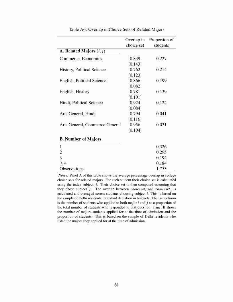
Table A6: Overlap in Choice Sets of Related Majors
Overlap in Proportion ofchoice set students
A. Related Majors (i, j)
Commerce, Economics 0.839 0.227[0.143]
History, Political Science 0.762 0.214[0.123]
English, Political Science 0.866 0.199[0.082]
English, History 0.781 0.139[0.101]
Hindi, Political Science 0.924 0.124[0.084]
Arts General, Hindi 0.794 0.041[0.116]
Arts General, Commerce General 0.956 0.031[0.104]
B. Number of Majors
1 0.3262 0.2953 0.194≥ 4 0.184Observations 1,753
Notes: Panel A of this table shows the average percentage overlap in collegechoice sets for related majors. For each student their choice set is calculatedusing the index subject, i. Their choice set is then computed assuming thatthey chose subject j. The overlap between choiceset i and choiceset j iscalculated and averaged across students choosing subject i. This is based onthe sample of Delhi residents. Standard deviation in brackets. The last columnis the number of students who applied to both major i and j as a proportion ofthe total number of students who responded to that question. Panel B showsthe number of majors students applied for at the time of admission and theproportion of students. This is based on the sample of Delhi residents wholisted the majors they applied for at the time of admission.
61
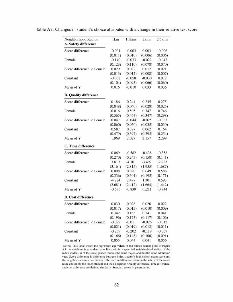
Table A7: Changes in student’s choice attributes with a change in their relative test score
Neighborhood Radius 1km 1.5kms 2kms 2.5kmsA. Safety difference
Score difference -0.001 -0.003 0.003 -0.006(0.011) (0.010) (0.006) (0.006)
Female -0.140 -0.033 -0.022 -0.043(0.123) (0.110) (0.078) (0.070)
Score difference × Female 0.029 0.022 0.012 0.021(0.013) (0.012) (0.008) (0.007)
Constant -0.002 -0.058 -0.030 0.012(0.104) (0.095) (0.066) (0.060)
Mean of Y 0.016 -0.010 0.033 0.036
B. Quality difference
Score difference 0.186 0.244 0.245 0.275(0.048) (0.040) (0.028) (0.025)
Female 0.016 0.505 0.747 0.746(0.565) (0.464) (0.347) (0.298)
Score difference × Female 0.047 -0.044 -0.025 -0.063(0.060) (0.050) (0.035) (0.030)
Constant 0.587 0.327 0.062 0.164(0.479) (0.397) (0.295) (0.254)
Mean of Y 1.969 2.027 2.157 2.299
C. Time difference
Score difference 0.069 -0.582 -0.438 -0.358(0.270) (0.243) (0.158) (0.141)
Female 3.819 -4.701 -3.497 -2.225(3.164) (2.815) (1.955) (1.687)
Score difference × Female 0.098 0.890 0.649 0.586(0.336) (0.301) (0.195) (0.171)
Constant -4.224 2.477 1.301 0.593(2.681) (2.412) (1.664) (1.442)
Mean of Y -0.636 -0.839 -1.211 -0.744
D. Cost difference
Score difference 0.030 0.028 0.026 0.022(0.017) (0.015) (0.010) (0.009)
Female 0.342 0.163 0.141 0.041(0.196) (0.173) (0.117) (0.106)
Score difference × Female -0.029 -0.011 -0.026 -0.012(0.021) (0.019) (0.012) (0.011)
Constant -0.259 -0.202 -0.119 -0.067(0.166) (0.148) (0.100) (0.091)
Mean of Y 0.055 0.044 0.041 0.056Notes: This table shows the regression equivalent of the binned scatter plots in Figure
A5. A neighbor is a student who lives within a specified neighborhood radius of theindex student, is of the same gender, studies the same major, and has the same admissionyear. Score difference is difference between index student’s high school exam score andthe neighbor’s exam score. Safety difference is difference between the safety of the travelroute chosen by the index student and their neighbor. Quality difference, time difference,and cost difference are defined similarly. Standard errors in parentheses.
62

C Data
1 Additional student data
I have student information from three main sources: a sample of students from eight colleges inDU where a detailed survey was conducted, confidential administrative data on the entire studentpopulation of these eight colleges, and a sample of students from 32 other colleges in DU where ashorter survey was conducted. The main analysis is based on the full survey sample. For the eightcolleges in the full survey sample, I have confidential administrative data on all students enrolledin the colleges. I have information on student’s gender, current and permanent residential location,course of study and social category. For one of the colleges, I also have student’s aggregate highschool score and parental occupation.I also conducted a combination of online and intercept short surveys across 32 other colleges in DUto be able to compare students in my sample to students in other colleges. Data on 799 male andfemale students was collected through a combination of online (34 percent) and intercept (66 per-cent) surveys. For the online survey, the staff and/or students in the 32 colleges were contacted. Forthe intercept survey, the students were approached outside their college campuses by enumeratorsand requested to fill the survey form.From this survey, I have information on student’s current and permanent residential location andhigh school exam scores by subject. In the short survey data, 630 students (79 percent) live in Delhiwith their family and travel to college every day and comprise 99.5 percent of the Delhi residentswho were surveyed.
2 Route mapping
Students reported their travel routes as a combination of n landmarks and n−1 modes of transportwith the first landmark being the student’s home address and final landmark being the collegelocation. The route is split into “legs” by landmarks, in the data a maximum number of four legsare reported by any student. All routes are mapped using Google Maps API. The student reportedroutes are mapped as a sequence of legs. The routes take into account student’s reported departuretime. For the reported routes where student’s travel by a rickshaw, the travel times are mapped aswalking routes and the travel time is then adjusted to be 60 percent of the walking travel time.For the potential travel routes, up to four routes are extracted per routing option available in GoogleMaps, these are the top suggested routes by Google. The routing options in Google Maps aredriving, walking and public transit. The driving and walking routes are unimodal. The publictransit routing options in Google Maps includes bus, subway, train, tram and rail. If this was tobe done interactively in Google Maps then you would search for directions from origin (student’s
63
home) to destination (choice set college) and then record the different route options provided byGoogle Maps by each Google Maps routing option. The potential travel routes also take intoaccount the student’s departure time, the departure time to choice set colleges is assumed to be thesame as the reported departure time to their chosen college if the chosen college and the choiceset college are both morning/afternoon colleges. If not then for morning colleges in the choice set,the departure time is assumed to be 9am and for afternoon colleges it is assumed to be 2pm. Forthe potential travel routes, a date in the future has to be set for the student to travel to college, thisis set to the Wednesday following the date the script is run. Thus if the script is run on Tuesday,the student will be modeled as traveling at their designated time the following day. Setting such atime in the future ensures consistency across choice set routes. Wednesday was chosen because it’sthe day least likely to be affected by any holidays or metro maintenance, but it could be any dayof the week that you’d like. All travel times take into account traffic conditions (as opposed to atraffic-free journey).
3 Travel cost
Below I specify how the travel cost is calculated by travel mode, where Ci = cost in INR for modei, d = distance in kilometers and t = time in minutes.
• Auto: Ca = 25+8(d−2), where Rs. 25 is charged at hire for the first two kilometers and Rs.8 for every subsequent kilometer.
• Car: Cc =d13 ×60, assuming an average mileage of 13km/liter and Rs. 60/liter as the cost of
fuel, which was the average price of petrol in Delhi from September 2015 to August 2016.
• Carpool: Ccp =d13 ×60× 1
3 , assuming that three people on average travel by carpool.
• Bus: Rs. 115 per month for the monthly student pass.
• Metro: The following fares are used, which are the official metro fares that were effectivefrom November 13, 2009 to May 10, 2017.50
50As given here: http://www.delhimetrorail.com, (last accessed: May 28, 2020).
64

Table A8: Metro fares
Distance Zones (Kms.) Fare (Rs.)0-2 82-4 104-6 126-9 15
9-12 1612-15 1815-18 1918-21 2121-24 2224-27 2327-31 2531-35 2735-39 2839-44 29> 44 30
Notes: These fares were effective from November 13,2009 to May 10, 2017. Source: Delhi Metro Rail Cor-poration. http://www.delhimetrorail.com/ (last accessed:May 28, 2020)
• Rickshaw: A flat rate of Rs. 10 per rickshaw ride as per the rate charged by E-rickshaws inDelhi.
• Motorcycle: Cm = d50 × 60, assuming an average mileage of 50km/liter and Rs. 60/liter as
the cost of fuel.
• Scooter: Cs =d40×60, assuming an average mileage of 40km/liter and Rs. 60/liter as the cost
of fuel.
• Taxi/Uber: Cu = 40+ t +6d based on UberGo fares.
• Walking: Rs. 0
• Train: The fares for monthly train passes are shown below, such a pass enables travel bysecond class. Following the official guidelines a 50 percent discount is applied for all generalcategory students and 75 percent discount for SC and ST students. Students are also assumedto purchase a quarterly train pass which gives them an additional discount of 10 percent onthe fare.51
51As given here: https://nfr.indianrailways.gov.in,(last accessed: May 28, 2020).
65

Table A9: Train fares for a monthly travel pass
Distance (Kms.) Fare (INR)1-10 6011-15 7516-20 9021-30 10531-35 12036-40 13541-45 15046-50 16551-55 18056-60 19561-65 19566-70 21071-75 22576-80 24081-85 23586-95 270
96-100 285101-110 300111-115 315116-125 330126-135 345136-140 360141-150 375
Notes: These are monthly fares for Secondclass travel by a general category adult. Sea-son ticket for general category students are at adiscount of 50 percent and at a discount of 75percent for SC/ST students. Quarterly tickets of-fer an additional discount of 10 percent.Source:https://nfr.indianrailways.gov.in, (last accessed:May 28, 2020)
4 Wealth index
An index of the student’s socioeconomic status is created in two steps. First using principal com-ponent analysis a wealth index is created, the variables included are: dummy for residing in anowned house, dummy for owning a laptop and/or computer, amount of money spent every month,excluding travel expenses and rent), in INR, dummy for private school attended in Class 12, yearsof education completed by father, years of education completed by mother, number of cars ownedby student’s permanent household, number of scooters owned by student’s permanent household,and price of the most expensive car owned by student’s permanent household.52 Next, a continuous
52The students’ were asked to list the “type/make and model” of all the cars owned by their permanent household,the price was extracted from https://www.carwale.com on June 25, 2017.
66
measure of the student’s relative wealth is created by ranking them according to this wealth index,from 0 (poorest) to 1 (wealthiest).
5 Harassment per trip
To calculate the probability of harassment per trip for a mode, I normalize the harassment per mode,as available from the Safecity data, by volume of usage observed in my survey data. Number ofharassment incidents per trip for a mode multiplied by the trips per mode in a year gives us the totalnumber of harassment incidents for the mode for the year.
hm×Tm = Hm
where hmis the harassment per trip in mode m, Tm are the total number of trips taken by mode in ayear m and Hm is the total number of harassment incidents for mode m in a year. Taking the ratioof harassment incidents in a year for mode m and n, we have:
hm×Tm
hn×Tn=
Hm
Hn
Dividing both the numerator and denominator by the total number of harassment incidents and bythe total number of trips enables us to express the ratio in probabilities and proportion of modeusage:
pm× tmpn× tn
=Pm
Pn=⇒ pm =
Pm
Pn× pn× tn
tmwhere pm is the probability of harassment per trip for mode m, Pm is the probability of harassmentper mode in a year and tm is the proportion of all trips by mode m. This allows us to expressprobabilities for all modes m in terms of pn. To calculate pn, assuming independence of harass-ment across modes, we can sum the probability of harassment per trip across modes to give us theprobability of being ever harassed:
∑m
pm = P(ever harassed)
Table A10 shows all the variables used to compute the probability of harassment per trip. Theseprobabilities are then used in lieu of Harassmentm in equation 1 to calculate the mode usage ad-justed safety score. Results from using this safety score are shown in columns (1) and (2) of Table4.
67
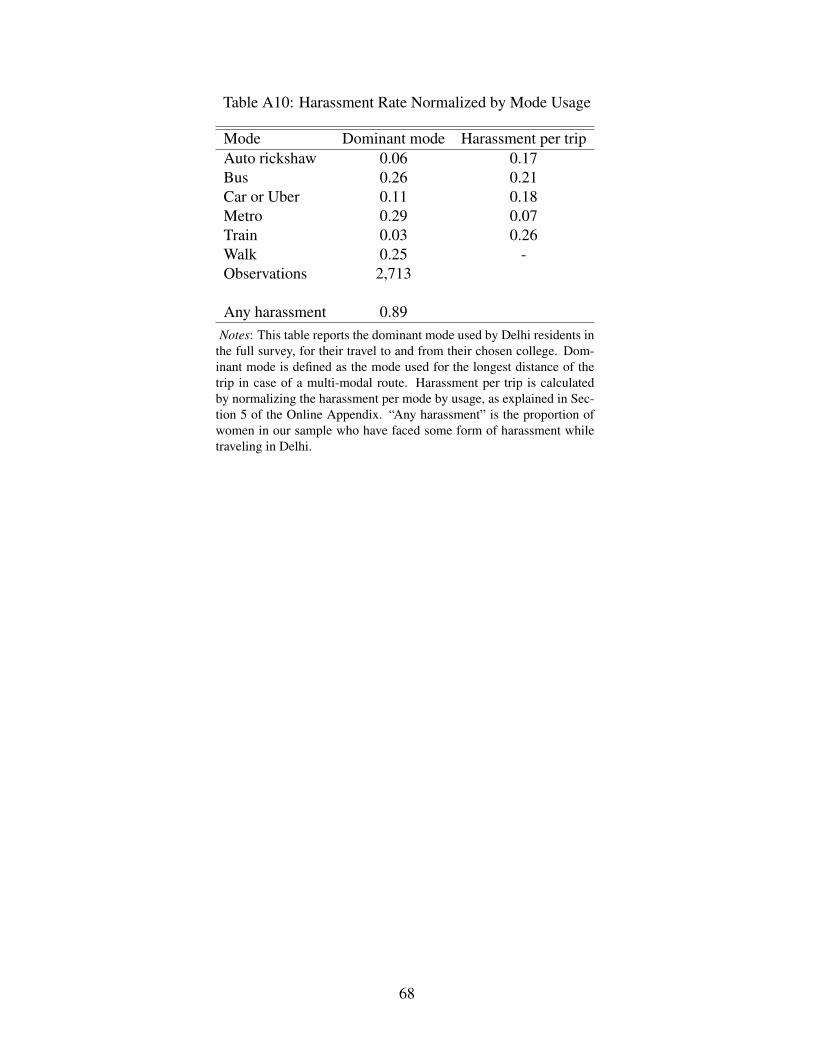
Table A10: Harassment Rate Normalized by Mode Usage
Mode Dominant mode Harassment per tripAuto rickshaw 0.06 0.17Bus 0.26 0.21Car or Uber 0.11 0.18Metro 0.29 0.07Train 0.03 0.26Walk 0.25 -Observations 2,713
Any harassment 0.89Notes: This table reports the dominant mode used by Delhi residents in
the full survey, for their travel to and from their chosen college. Dom-inant mode is defined as the mode used for the longest distance of thetrip in case of a multi-modal route. Harassment per trip is calculatedby normalizing the harassment per mode by usage, as explained in Sec-tion 5 of the Online Appendix. “Any harassment” is the proportion ofwomen in our sample who have faced some form of harassment whiletraveling in Delhi.
68