sage reference manual: matrices and spaces of...
TRANSCRIPT
Sage Reference Manual: Matrices andSpaces of Matrices
Release 9.0
The Sage Development Team
Jan 01, 2020

CONTENTS
1 Matrix Spaces 3
2 General matrix Constructor 17
3 Constructors for special matrices 25
4 Helpers for creating matrices 63
5 Matrices over an arbitrary ring 735.1 Indexing . . . . . . . . . . . . . . . . . . . . . . . . . . . . . . . . . . . . . . . . . . . . . . . . . 74
6 Base class for matrices, part 0 81
7 Base class for matrices, part 1 119
8 Base class for matrices, part 2 139
9 Generic Asymptotically Fast Strassen Algorithms 297
10 Minimal Polynomials of Linear Recurrence Sequences 301
11 Base class for dense matrices 303
12 Base class for sparse matrices 305
13 Dense Matrices over a general ring 311
14 Sparse Matrices over a general ring 313
15 Dense matrices over the integer ring 317
16 Sparse integer matrices. 345
17 Modular algorithm to compute Hermite normal forms of integer matrices. 351
18 Saturation over ZZ 363
19 Dense matrices over the rational field 367
20 Sparse rational matrices. 379
21 Dense matrices using a NumPy backend. 383
i
22 Dense matrices over the Real Double Field using NumPy 421
23 Dense matrices over GF(2) using the M4RI library. 423
24 Dense matrices over F2𝑒 for 2 <= 𝑒 <= 10 using the M4RIE library. 433
25 Dense matrices over Z/𝑛Z for 𝑛 < 223 using LinBox’s Modular<double> 443
26 Dense matrices over Z/𝑛Z for 𝑛 < 211 using LinBox’s Modular<float> 457
27 Sparse matrices over Z/𝑛Z for 𝑛 small 471
28 Symbolic matrices 475
29 Dense matrices over the Complex Double Field using NumPy 487
30 Arbitrary precision complex ball matrices using Arb 489
31 Dense matrices over univariate polynomials over fields 493
32 Dense matrices over multivariate polynomials over fields 513
33 Matrices over Cyclotomic Fields 517
34 Operation Tables 523
35 Actions used by the coercion model for matrix and vector multiplications 531
36 Functions for changing the base ring of matrices quickly. 535
37 Echelon matrices over finite fields. 537
38 Miscellaneous matrix functions 539
39 Matrix windows 543
40 Misc matrix algorithms 545
41 Calculate symplectic bases for matrices over fields and the integers. 549
42 𝐽-ideals of matrices 55542.1 Classes and Methods . . . . . . . . . . . . . . . . . . . . . . . . . . . . . . . . . . . . . . . . . . . 556
43 Benchmarks for matrices 565
44 Indices and Tables 575
Python Module Index 577
Index 579
ii
Sage Reference Manual: Matrices and Spaces of Matrices, Release 9.0
Sage provides native support for working with matrices over any commutative or noncommutative ring. The parentobject for a matrix is a matrix space MatrixSpace(R, n, m) of all 𝑛×𝑚 matrices over a ring 𝑅.
To create a matrix, either use the matrix(...) function or create a matrix space using the MatrixSpace com-mand and coerce an object into it.
Matrices also act on row vectors, which you create using the vector(...) command or by making aVectorSpace and coercing lists into it. The natural action of matrices on row vectors is from the right. Sagecurrently does not have a column vector class (on which matrices would act from the left), but this is planned.
In addition to native Sage matrices, Sage also includes the following additional ways to compute with matrices:
• Several math software systems included with Sage have their own native matrix support, which can be usedfrom Sage. E.g., PARI, GAP, Maxima, and Singular all have a notion of matrices.
• The GSL C-library is included with Sage, and can be used via Cython.
• The scipy module provides support for sparse numerical linear algebra, among many other things.
• The numpy module, which you load by typing import numpy is included standard with Sage. It contains avery sophisticated and well developed array class, plus optimized support for numerical linear algebra. Sage’smatrices over RDF and CDF (native floating-point real and complex numbers) use numpy.
Finally, this module contains some data-structures for matrix-like objects like operation tables (e.g. the multiplicationtable of a group).
CONTENTS 1

Sage Reference Manual: Matrices and Spaces of Matrices, Release 9.0
2 CONTENTS
CHAPTER
ONE
MATRIX SPACES
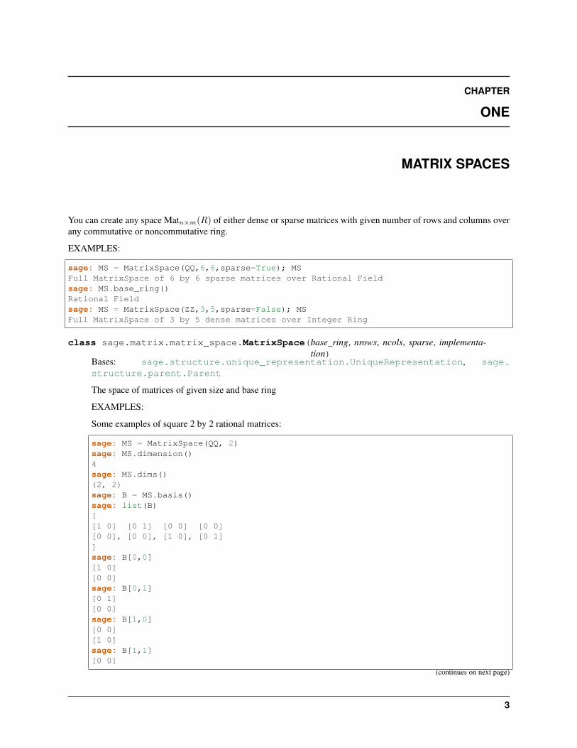
You can create any space Mat𝑛×𝑚(𝑅) of either dense or sparse matrices with given number of rows and columns overany commutative or noncommutative ring.
EXAMPLES:
sage: MS = MatrixSpace(QQ,6,6,sparse=True); MSFull MatrixSpace of 6 by 6 sparse matrices over Rational Fieldsage: MS.base_ring()Rational Fieldsage: MS = MatrixSpace(ZZ,3,5,sparse=False); MSFull MatrixSpace of 3 by 5 dense matrices over Integer Ring
class sage.matrix.matrix_space.MatrixSpace(base_ring, nrows, ncols, sparse, implementa-tion)
Bases: sage.structure.unique_representation.UniqueRepresentation, sage.structure.parent.Parent
The space of matrices of given size and base ring
EXAMPLES:
Some examples of square 2 by 2 rational matrices:
sage: MS = MatrixSpace(QQ, 2)sage: MS.dimension()4sage: MS.dims()(2, 2)sage: B = MS.basis()sage: list(B)[[1 0] [0 1] [0 0] [0 0][0 0], [0 0], [1 0], [0 1]]sage: B[0,0][1 0][0 0]sage: B[0,1][0 1][0 0]sage: B[1,0][0 0][1 0]sage: B[1,1][0 0]
(continues on next page)
3
Sage Reference Manual: Matrices and Spaces of Matrices, Release 9.0
(continued from previous page)
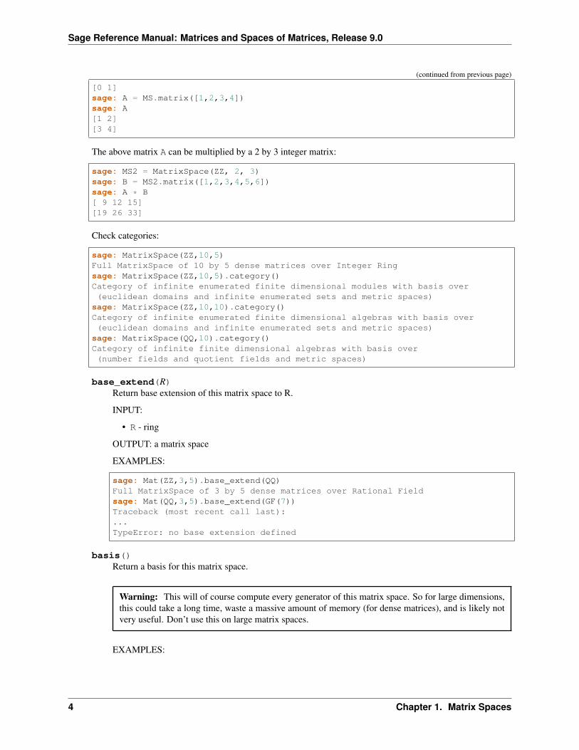
[0 1]sage: A = MS.matrix([1,2,3,4])sage: A[1 2][3 4]
The above matrix A can be multiplied by a 2 by 3 integer matrix:
sage: MS2 = MatrixSpace(ZZ, 2, 3)sage: B = MS2.matrix([1,2,3,4,5,6])sage: A * B[ 9 12 15][19 26 33]
Check categories:
sage: MatrixSpace(ZZ,10,5)Full MatrixSpace of 10 by 5 dense matrices over Integer Ringsage: MatrixSpace(ZZ,10,5).category()Category of infinite enumerated finite dimensional modules with basis over(euclidean domains and infinite enumerated sets and metric spaces)sage: MatrixSpace(ZZ,10,10).category()Category of infinite enumerated finite dimensional algebras with basis over(euclidean domains and infinite enumerated sets and metric spaces)sage: MatrixSpace(QQ,10).category()Category of infinite finite dimensional algebras with basis over(number fields and quotient fields and metric spaces)
base_extend(R)Return base extension of this matrix space to R.
INPUT:
• R - ring
OUTPUT: a matrix space
EXAMPLES:
sage: Mat(ZZ,3,5).base_extend(QQ)Full MatrixSpace of 3 by 5 dense matrices over Rational Fieldsage: Mat(QQ,3,5).base_extend(GF(7))Traceback (most recent call last):...TypeError: no base extension defined
basis()Return a basis for this matrix space.
Warning: This will of course compute every generator of this matrix space. So for large dimensions,this could take a long time, waste a massive amount of memory (for dense matrices), and is likely notvery useful. Don’t use this on large matrix spaces.
EXAMPLES:
4 Chapter 1. Matrix Spaces
Sage Reference Manual: Matrices and Spaces of Matrices, Release 9.0
sage: list(Mat(ZZ,2,2).basis())[[1 0] [0 1] [0 0] [0 0][0 0], [0 0], [1 0], [0 1]]
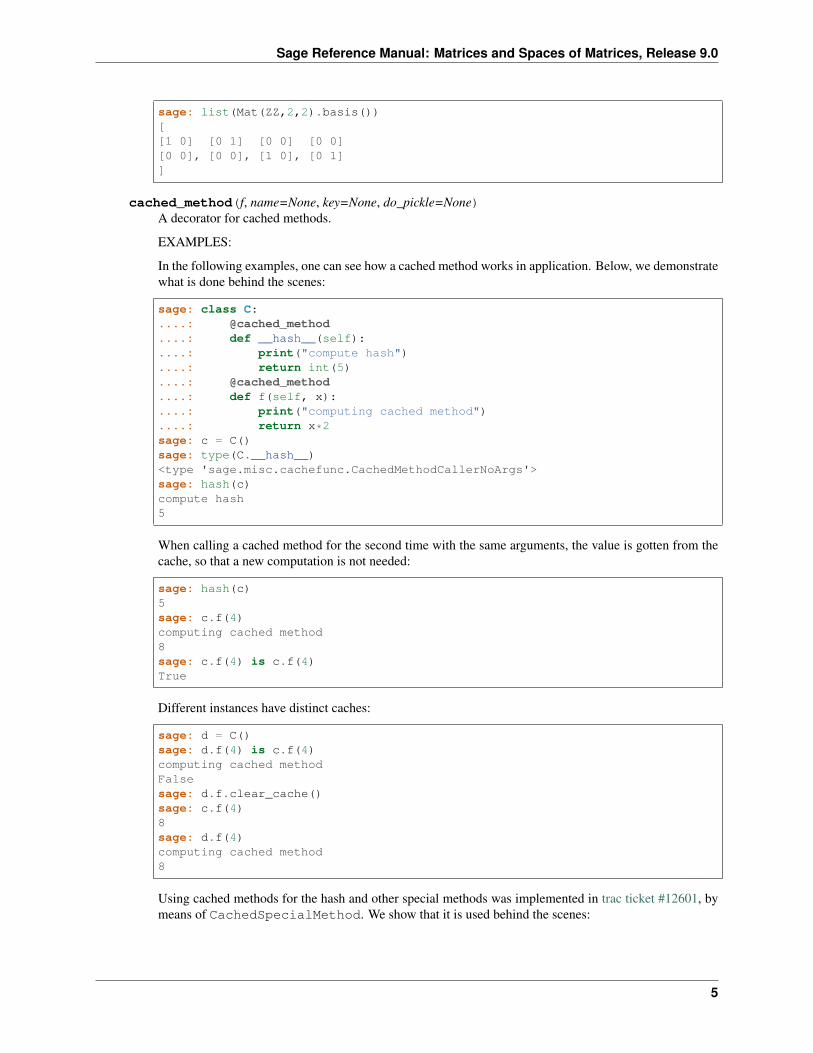
cached_method(f, name=None, key=None, do_pickle=None)A decorator for cached methods.
EXAMPLES:
In the following examples, one can see how a cached method works in application. Below, we demonstratewhat is done behind the scenes:
sage: class C:....: @cached_method....: def __hash__(self):....: print("compute hash")....: return int(5)....: @cached_method....: def f(self, x):....: print("computing cached method")....: return x*2sage: c = C()sage: type(C.__hash__)<type 'sage.misc.cachefunc.CachedMethodCallerNoArgs'>sage: hash(c)compute hash5
When calling a cached method for the second time with the same arguments, the value is gotten from thecache, so that a new computation is not needed:
sage: hash(c)5sage: c.f(4)computing cached method8sage: c.f(4) is c.f(4)True
Different instances have distinct caches:
sage: d = C()sage: d.f(4) is c.f(4)computing cached methodFalsesage: d.f.clear_cache()sage: c.f(4)8sage: d.f(4)computing cached method8
Using cached methods for the hash and other special methods was implemented in trac ticket #12601, bymeans of CachedSpecialMethod. We show that it is used behind the scenes:
5
Sage Reference Manual: Matrices and Spaces of Matrices, Release 9.0
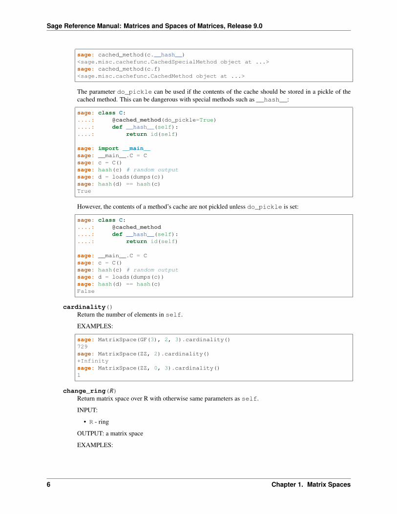
sage: cached_method(c.__hash__)<sage.misc.cachefunc.CachedSpecialMethod object at ...>sage: cached_method(c.f)<sage.misc.cachefunc.CachedMethod object at ...>
The parameter do_pickle can be used if the contents of the cache should be stored in a pickle of thecached method. This can be dangerous with special methods such as __hash__:
sage: class C:....: @cached_method(do_pickle=True)....: def __hash__(self):....: return id(self)
sage: import __main__sage: __main__.C = Csage: c = C()sage: hash(c) # random outputsage: d = loads(dumps(c))sage: hash(d) == hash(c)True
However, the contents of a method’s cache are not pickled unless do_pickle is set:
sage: class C:....: @cached_method....: def __hash__(self):....: return id(self)
sage: __main__.C = Csage: c = C()sage: hash(c) # random outputsage: d = loads(dumps(c))sage: hash(d) == hash(c)False
cardinality()Return the number of elements in self.
EXAMPLES:
sage: MatrixSpace(GF(3), 2, 3).cardinality()729sage: MatrixSpace(ZZ, 2).cardinality()+Infinitysage: MatrixSpace(ZZ, 0, 3).cardinality()1
change_ring(R)Return matrix space over R with otherwise same parameters as self.
INPUT:
• R - ring
OUTPUT: a matrix space
EXAMPLES:
6 Chapter 1. Matrix Spaces
Sage Reference Manual: Matrices and Spaces of Matrices, Release 9.0
sage: Mat(QQ,3,5).change_ring(GF(7))Full MatrixSpace of 3 by 5 dense matrices over Finite Field of size 7
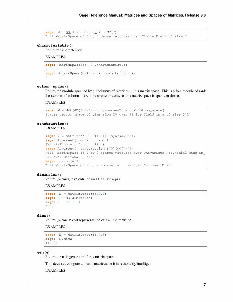
characteristic()Return the characteristic.
EXAMPLES:
sage: MatrixSpace(ZZ, 2).characteristic()0sage: MatrixSpace(GF(9), 0).characteristic()3
column_space()Return the module spanned by all columns of matrices in this matrix space. This is a free module of rankthe number of columns. It will be sparse or dense as this matrix space is sparse or dense.
EXAMPLES:
sage: M = Mat(GF(9,'a'),20,5,sparse=True); M.column_space()Sparse vector space of dimension 20 over Finite Field in a of size 3^2
construction()EXAMPLES:
sage: A = matrix(ZZ, 2, [1..4], sparse=True)sage: A.parent().construction()(MatrixFunctor, Integer Ring)sage: A.parent().construction()[0](QQ['x'])Full MatrixSpace of 2 by 2 sparse matrices over Univariate Polynomial Ring in→˓x over Rational Fieldsage: parent(A/2)Full MatrixSpace of 2 by 2 sparse matrices over Rational Field
dimension()Return (m rows) * (n cols) of self as Integer.
EXAMPLES:
sage: MS = MatrixSpace(ZZ,4,6)sage: u = MS.dimension()sage: u - 24 == 0True
dims()Return (m row, n col) representation of self dimension.
EXAMPLES:
sage: MS = MatrixSpace(ZZ,4,6)sage: MS.dims()(4, 6)
gen(n)Return the n-th generator of this matrix space.
This does not compute all basis matrices, so it is reasonably intelligent.
EXAMPLES:
7
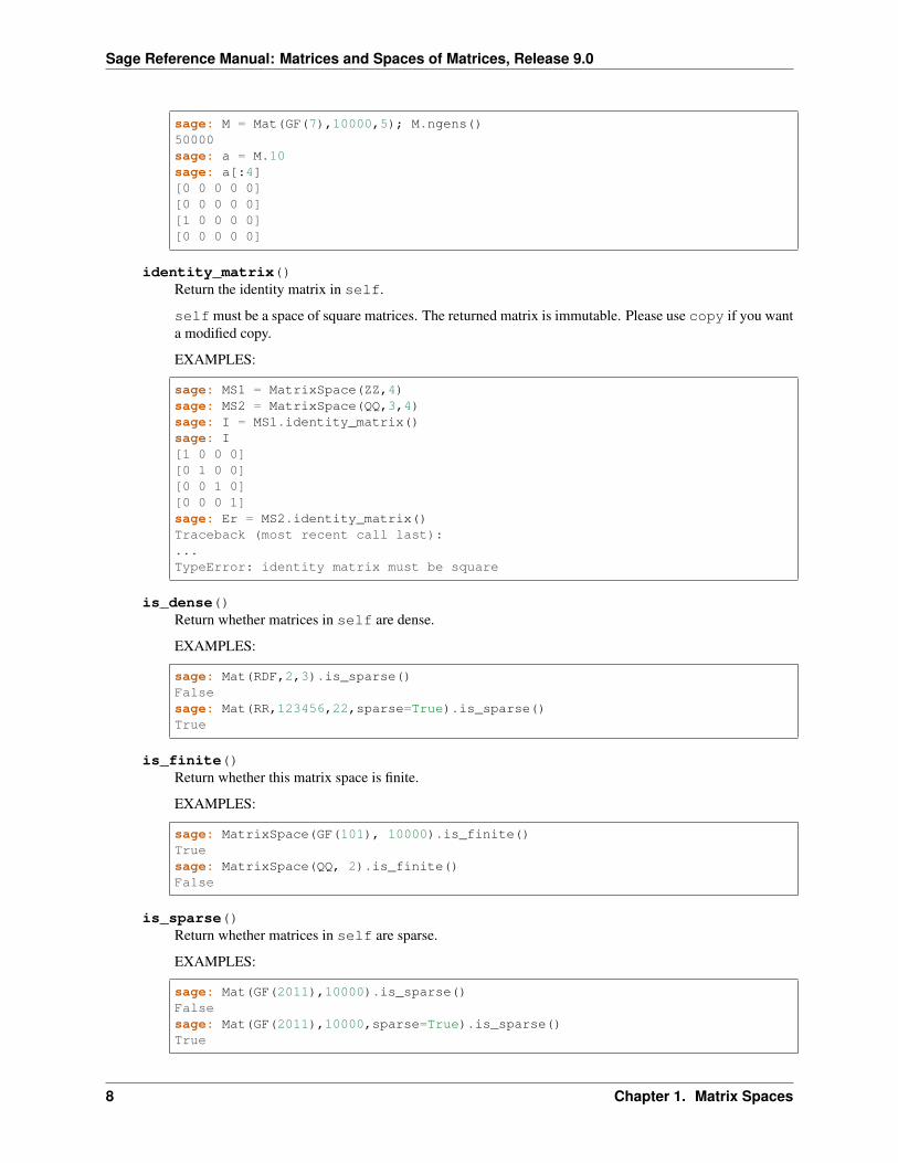
Sage Reference Manual: Matrices and Spaces of Matrices, Release 9.0
sage: M = Mat(GF(7),10000,5); M.ngens()50000sage: a = M.10sage: a[:4][0 0 0 0 0][0 0 0 0 0][1 0 0 0 0][0 0 0 0 0]
identity_matrix()Return the identity matrix in self.
self must be a space of square matrices. The returned matrix is immutable. Please use copy if you wanta modified copy.
EXAMPLES:
sage: MS1 = MatrixSpace(ZZ,4)sage: MS2 = MatrixSpace(QQ,3,4)sage: I = MS1.identity_matrix()sage: I[1 0 0 0][0 1 0 0][0 0 1 0][0 0 0 1]sage: Er = MS2.identity_matrix()Traceback (most recent call last):...TypeError: identity matrix must be square
is_dense()Return whether matrices in self are dense.
EXAMPLES:
sage: Mat(RDF,2,3).is_sparse()Falsesage: Mat(RR,123456,22,sparse=True).is_sparse()True
is_finite()Return whether this matrix space is finite.
EXAMPLES:
sage: MatrixSpace(GF(101), 10000).is_finite()Truesage: MatrixSpace(QQ, 2).is_finite()False
is_sparse()Return whether matrices in self are sparse.
EXAMPLES:
sage: Mat(GF(2011),10000).is_sparse()Falsesage: Mat(GF(2011),10000,sparse=True).is_sparse()True
8 Chapter 1. Matrix Spaces
Sage Reference Manual: Matrices and Spaces of Matrices, Release 9.0
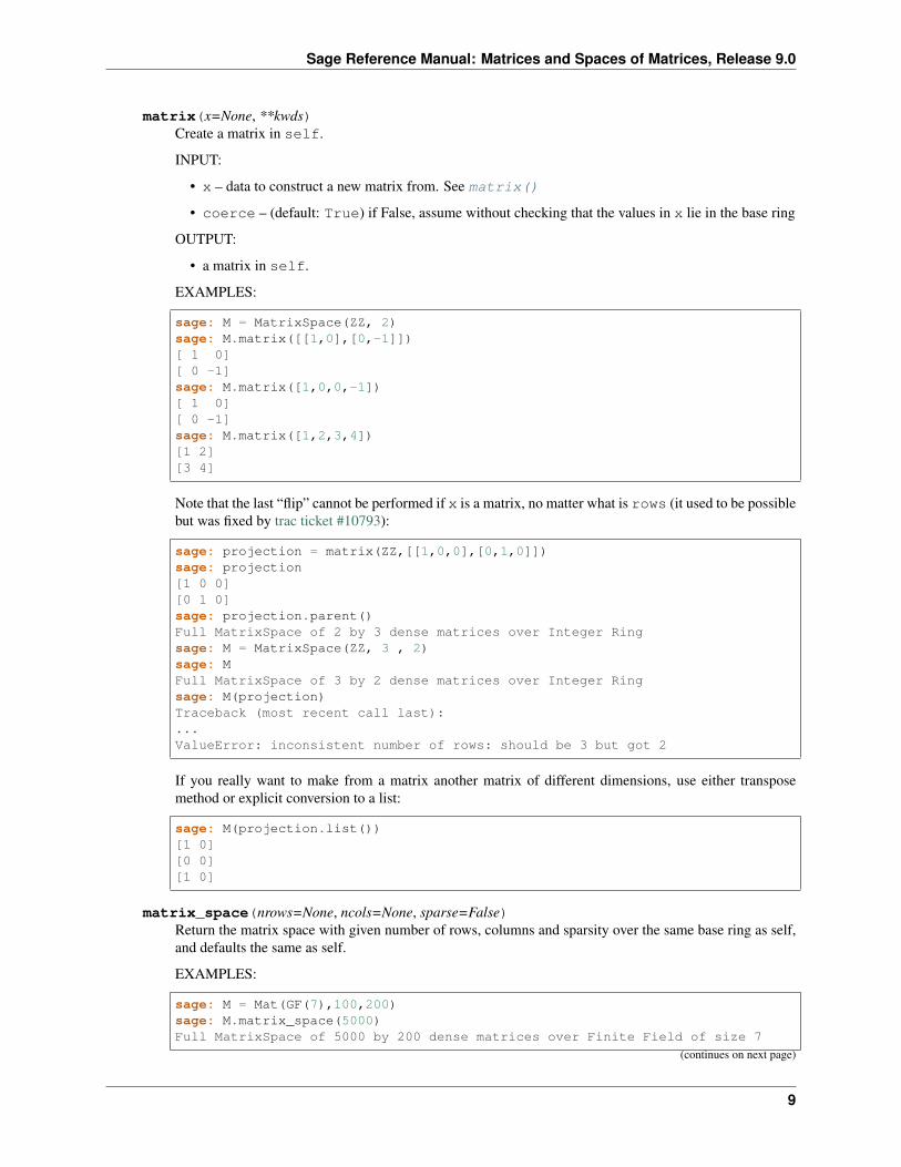
matrix(x=None, **kwds)Create a matrix in self.
INPUT:
• x – data to construct a new matrix from. See matrix()
• coerce – (default: True) if False, assume without checking that the values in x lie in the base ring
OUTPUT:
• a matrix in self.
EXAMPLES:
sage: M = MatrixSpace(ZZ, 2)sage: M.matrix([[1,0],[0,-1]])[ 1 0][ 0 -1]sage: M.matrix([1,0,0,-1])[ 1 0][ 0 -1]sage: M.matrix([1,2,3,4])[1 2][3 4]
Note that the last “flip” cannot be performed if x is a matrix, no matter what is rows (it used to be possiblebut was fixed by trac ticket #10793):
sage: projection = matrix(ZZ,[[1,0,0],[0,1,0]])sage: projection[1 0 0][0 1 0]sage: projection.parent()Full MatrixSpace of 2 by 3 dense matrices over Integer Ringsage: M = MatrixSpace(ZZ, 3 , 2)sage: MFull MatrixSpace of 3 by 2 dense matrices over Integer Ringsage: M(projection)Traceback (most recent call last):...ValueError: inconsistent number of rows: should be 3 but got 2
If you really want to make from a matrix another matrix of different dimensions, use either transposemethod or explicit conversion to a list:
sage: M(projection.list())[1 0][0 0][1 0]
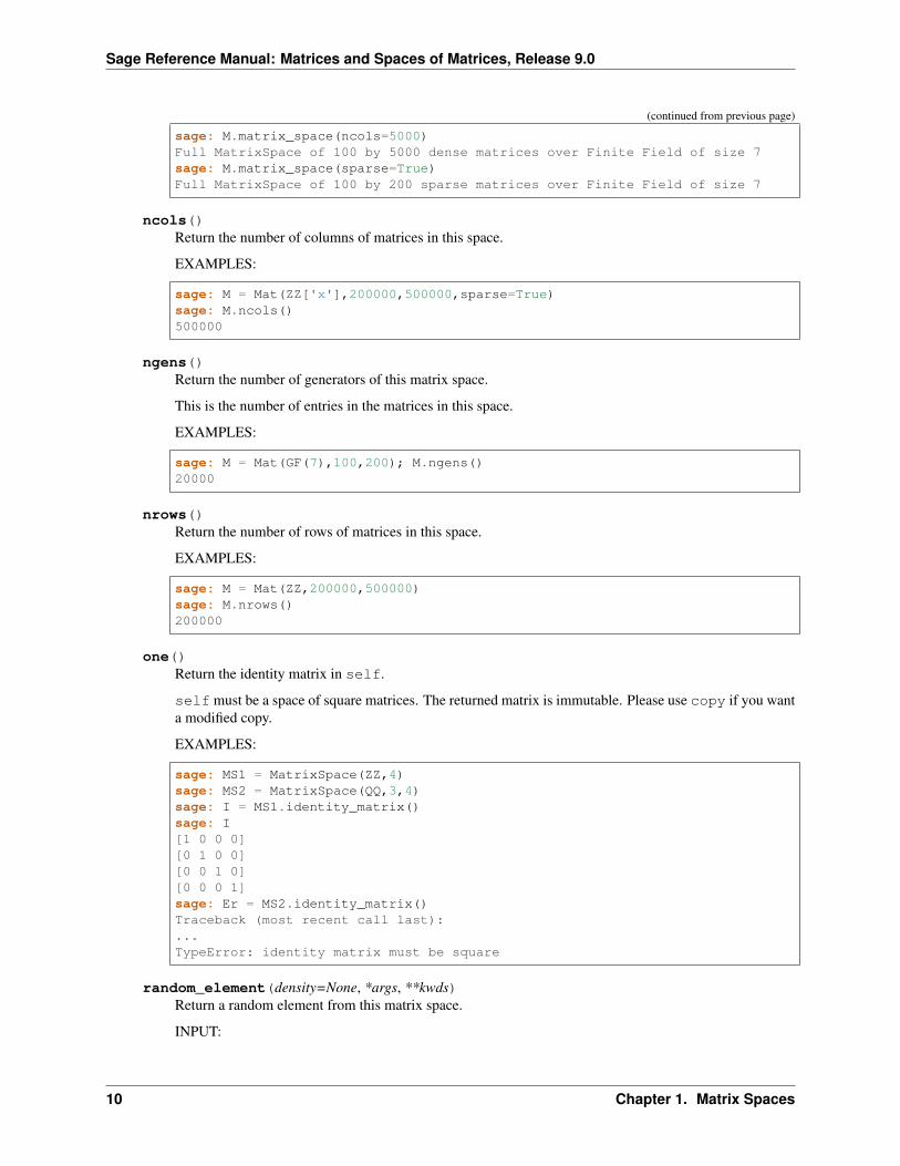
matrix_space(nrows=None, ncols=None, sparse=False)Return the matrix space with given number of rows, columns and sparsity over the same base ring as self,and defaults the same as self.
EXAMPLES:
sage: M = Mat(GF(7),100,200)sage: M.matrix_space(5000)Full MatrixSpace of 5000 by 200 dense matrices over Finite Field of size 7
(continues on next page)
9
Sage Reference Manual: Matrices and Spaces of Matrices, Release 9.0
(continued from previous page)
sage: M.matrix_space(ncols=5000)Full MatrixSpace of 100 by 5000 dense matrices over Finite Field of size 7sage: M.matrix_space(sparse=True)Full MatrixSpace of 100 by 200 sparse matrices over Finite Field of size 7
ncols()Return the number of columns of matrices in this space.
EXAMPLES:
sage: M = Mat(ZZ['x'],200000,500000,sparse=True)sage: M.ncols()500000
ngens()Return the number of generators of this matrix space.
This is the number of entries in the matrices in this space.
EXAMPLES:
sage: M = Mat(GF(7),100,200); M.ngens()20000
nrows()Return the number of rows of matrices in this space.
EXAMPLES:
sage: M = Mat(ZZ,200000,500000)sage: M.nrows()200000
one()Return the identity matrix in self.
self must be a space of square matrices. The returned matrix is immutable. Please use copy if you wanta modified copy.
EXAMPLES:
sage: MS1 = MatrixSpace(ZZ,4)sage: MS2 = MatrixSpace(QQ,3,4)sage: I = MS1.identity_matrix()sage: I[1 0 0 0][0 1 0 0][0 0 1 0][0 0 0 1]sage: Er = MS2.identity_matrix()Traceback (most recent call last):...TypeError: identity matrix must be square
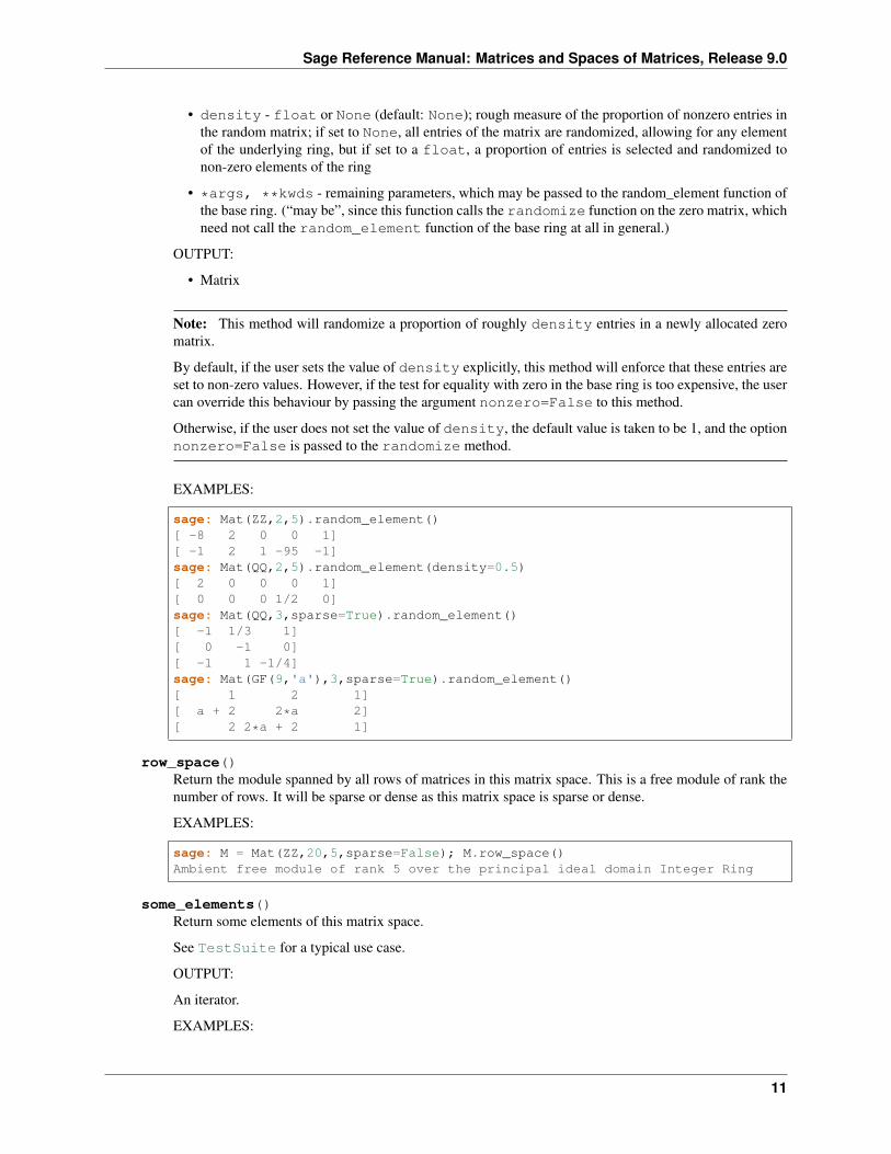
random_element(density=None, *args, **kwds)Return a random element from this matrix space.
INPUT:
10 Chapter 1. Matrix Spaces
Sage Reference Manual: Matrices and Spaces of Matrices, Release 9.0
• density - float or None (default: None); rough measure of the proportion of nonzero entries inthe random matrix; if set to None, all entries of the matrix are randomized, allowing for any elementof the underlying ring, but if set to a float, a proportion of entries is selected and randomized tonon-zero elements of the ring
• *args, **kwds - remaining parameters, which may be passed to the random_element function ofthe base ring. (“may be”, since this function calls the randomize function on the zero matrix, whichneed not call the random_element function of the base ring at all in general.)
OUTPUT:
• Matrix
Note: This method will randomize a proportion of roughly density entries in a newly allocated zeromatrix.
By default, if the user sets the value of density explicitly, this method will enforce that these entries areset to non-zero values. However, if the test for equality with zero in the base ring is too expensive, the usercan override this behaviour by passing the argument nonzero=False to this method.
Otherwise, if the user does not set the value of density, the default value is taken to be 1, and the optionnonzero=False is passed to the randomize method.
EXAMPLES:
sage: Mat(ZZ,2,5).random_element()[ -8 2 0 0 1][ -1 2 1 -95 -1]sage: Mat(QQ,2,5).random_element(density=0.5)[ 2 0 0 0 1][ 0 0 0 1/2 0]sage: Mat(QQ,3,sparse=True).random_element()[ -1 1/3 1][ 0 -1 0][ -1 1 -1/4]sage: Mat(GF(9,'a'),3,sparse=True).random_element()[ 1 2 1][ a + 2 2*a 2][ 2 2*a + 2 1]
row_space()Return the module spanned by all rows of matrices in this matrix space. This is a free module of rank thenumber of rows. It will be sparse or dense as this matrix space is sparse or dense.
EXAMPLES:
sage: M = Mat(ZZ,20,5,sparse=False); M.row_space()Ambient free module of rank 5 over the principal ideal domain Integer Ring
some_elements()Return some elements of this matrix space.
See TestSuite for a typical use case.
OUTPUT:
An iterator.
EXAMPLES:
11
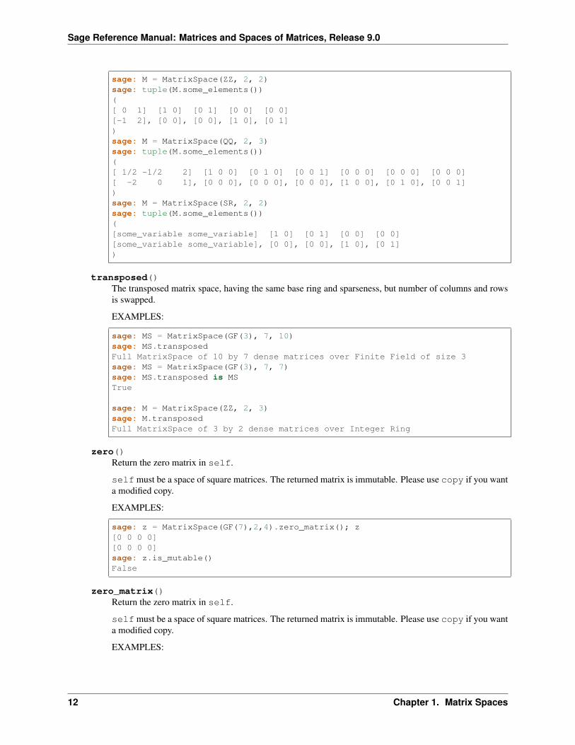
Sage Reference Manual: Matrices and Spaces of Matrices, Release 9.0
sage: M = MatrixSpace(ZZ, 2, 2)sage: tuple(M.some_elements())([ 0 1] [1 0] [0 1] [0 0] [0 0][-1 2], [0 0], [0 0], [1 0], [0 1])sage: M = MatrixSpace(QQ, 2, 3)sage: tuple(M.some_elements())([ 1/2 -1/2 2] [1 0 0] [0 1 0] [0 0 1] [0 0 0] [0 0 0] [0 0 0][ -2 0 1], [0 0 0], [0 0 0], [0 0 0], [1 0 0], [0 1 0], [0 0 1])sage: M = MatrixSpace(SR, 2, 2)sage: tuple(M.some_elements())([some_variable some_variable] [1 0] [0 1] [0 0] [0 0][some_variable some_variable], [0 0], [0 0], [1 0], [0 1])
transposed()The transposed matrix space, having the same base ring and sparseness, but number of columns and rowsis swapped.
EXAMPLES:
sage: MS = MatrixSpace(GF(3), 7, 10)sage: MS.transposedFull MatrixSpace of 10 by 7 dense matrices over Finite Field of size 3sage: MS = MatrixSpace(GF(3), 7, 7)sage: MS.transposed is MSTrue
sage: M = MatrixSpace(ZZ, 2, 3)sage: M.transposedFull MatrixSpace of 3 by 2 dense matrices over Integer Ring
zero()Return the zero matrix in self.
self must be a space of square matrices. The returned matrix is immutable. Please use copy if you wanta modified copy.
EXAMPLES:
sage: z = MatrixSpace(GF(7),2,4).zero_matrix(); z[0 0 0 0][0 0 0 0]sage: z.is_mutable()False
zero_matrix()Return the zero matrix in self.
self must be a space of square matrices. The returned matrix is immutable. Please use copy if you wanta modified copy.
EXAMPLES:
12 Chapter 1. Matrix Spaces
Sage Reference Manual: Matrices and Spaces of Matrices, Release 9.0
sage: z = MatrixSpace(GF(7),2,4).zero_matrix(); z[0 0 0 0][0 0 0 0]sage: z.is_mutable()False
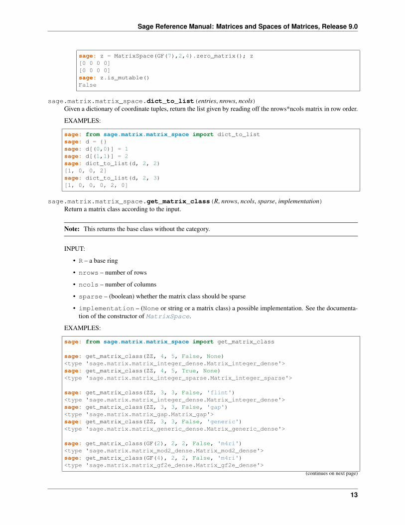
sage.matrix.matrix_space.dict_to_list(entries, nrows, ncols)Given a dictionary of coordinate tuples, return the list given by reading off the nrows*ncols matrix in row order.
EXAMPLES:
sage: from sage.matrix.matrix_space import dict_to_listsage: d = {}sage: d[(0,0)] = 1sage: d[(1,1)] = 2sage: dict_to_list(d, 2, 2)[1, 0, 0, 2]sage: dict_to_list(d, 2, 3)[1, 0, 0, 0, 2, 0]
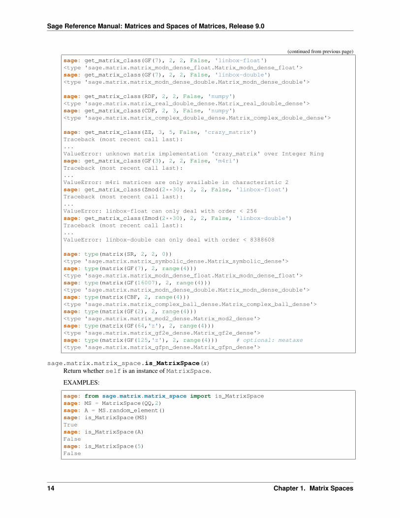
sage.matrix.matrix_space.get_matrix_class(R, nrows, ncols, sparse, implementation)Return a matrix class according to the input.
Note: This returns the base class without the category.
INPUT:
• R – a base ring
• nrows – number of rows
• ncols – number of columns
• sparse – (boolean) whether the matrix class should be sparse
• implementation – (None or string or a matrix class) a possible implementation. See the documenta-tion of the constructor of MatrixSpace.
EXAMPLES:
sage: from sage.matrix.matrix_space import get_matrix_class
sage: get_matrix_class(ZZ, 4, 5, False, None)<type 'sage.matrix.matrix_integer_dense.Matrix_integer_dense'>sage: get_matrix_class(ZZ, 4, 5, True, None)<type 'sage.matrix.matrix_integer_sparse.Matrix_integer_sparse'>
sage: get_matrix_class(ZZ, 3, 3, False, 'flint')<type 'sage.matrix.matrix_integer_dense.Matrix_integer_dense'>sage: get_matrix_class(ZZ, 3, 3, False, 'gap')<type 'sage.matrix.matrix_gap.Matrix_gap'>sage: get_matrix_class(ZZ, 3, 3, False, 'generic')<type 'sage.matrix.matrix_generic_dense.Matrix_generic_dense'>
sage: get_matrix_class(GF(2), 2, 2, False, 'm4ri')<type 'sage.matrix.matrix_mod2_dense.Matrix_mod2_dense'>sage: get_matrix_class(GF(4), 2, 2, False, 'm4ri')<type 'sage.matrix.matrix_gf2e_dense.Matrix_gf2e_dense'>
(continues on next page)
13
Sage Reference Manual: Matrices and Spaces of Matrices, Release 9.0
(continued from previous page)
sage: get_matrix_class(GF(7), 2, 2, False, 'linbox-float')<type 'sage.matrix.matrix_modn_dense_float.Matrix_modn_dense_float'>sage: get_matrix_class(GF(7), 2, 2, False, 'linbox-double')<type 'sage.matrix.matrix_modn_dense_double.Matrix_modn_dense_double'>
sage: get_matrix_class(RDF, 2, 2, False, 'numpy')<type 'sage.matrix.matrix_real_double_dense.Matrix_real_double_dense'>sage: get_matrix_class(CDF, 2, 3, False, 'numpy')<type 'sage.matrix.matrix_complex_double_dense.Matrix_complex_double_dense'>
sage: get_matrix_class(ZZ, 3, 5, False, 'crazy_matrix')Traceback (most recent call last):...ValueError: unknown matrix implementation 'crazy_matrix' over Integer Ringsage: get_matrix_class(GF(3), 2, 2, False, 'm4ri')Traceback (most recent call last):...ValueError: m4ri matrices are only available in characteristic 2sage: get_matrix_class(Zmod(2**30), 2, 2, False, 'linbox-float')Traceback (most recent call last):...ValueError: linbox-float can only deal with order < 256sage: get_matrix_class(Zmod(2**30), 2, 2, False, 'linbox-double')Traceback (most recent call last):...ValueError: linbox-double can only deal with order < 8388608
sage: type(matrix(SR, 2, 2, 0))<type 'sage.matrix.matrix_symbolic_dense.Matrix_symbolic_dense'>sage: type(matrix(GF(7), 2, range(4)))<type 'sage.matrix.matrix_modn_dense_float.Matrix_modn_dense_float'>sage: type(matrix(GF(16007), 2, range(4)))<type 'sage.matrix.matrix_modn_dense_double.Matrix_modn_dense_double'>sage: type(matrix(CBF, 2, range(4)))<type 'sage.matrix.matrix_complex_ball_dense.Matrix_complex_ball_dense'>sage: type(matrix(GF(2), 2, range(4)))<type 'sage.matrix.matrix_mod2_dense.Matrix_mod2_dense'>sage: type(matrix(GF(64,'z'), 2, range(4)))<type 'sage.matrix.matrix_gf2e_dense.Matrix_gf2e_dense'>sage: type(matrix(GF(125,'z'), 2, range(4))) # optional: meataxe<type 'sage.matrix.matrix_gfpn_dense.Matrix_gfpn_dense'>
sage.matrix.matrix_space.is_MatrixSpace(x)Return whether self is an instance of MatrixSpace.
EXAMPLES:
sage: from sage.matrix.matrix_space import is_MatrixSpacesage: MS = MatrixSpace(QQ,2)sage: A = MS.random_element()sage: is_MatrixSpace(MS)Truesage: is_MatrixSpace(A)Falsesage: is_MatrixSpace(5)False
14 Chapter 1. Matrix Spaces
Sage Reference Manual: Matrices and Spaces of Matrices, Release 9.0
sage.matrix.matrix_space.test_trivial_matrices_inverse(ring, sparse=True, imple-mentation=None, check-rank=True)
Tests inversion, determinant and is_invertible for trivial matrices.
This function is a helper to check that the inversion of trivial matrices (of size 0x0, nx0, 0xn or 1x1) is handledconsistently by the various implementation of matrices. The coherency is checked through a bunch of assertions.If an inconsistency is found, an AssertionError is raised which should make clear what is the problem.
INPUT:
• ring - a ring
• sparse - a boolean
• checkrank - a boolean
OUTPUT:
• nothing if everything is correct, otherwise raise an AssertionError
The methods determinant, is_invertible, rank and inverse are checked for
• the 0x0 empty identity matrix
• the 0x3 and 3x0 matrices
• the 1x1 null matrix [0]
• the 1x1 identity matrix [1]
If checkrank is False then the rank is not checked. This is used the check matrix over ring where echelonform is not implemented.
Todo: This must be adapted to category check framework when ready (see trac ticket #5274).
15

Sage Reference Manual: Matrices and Spaces of Matrices, Release 9.0
16 Chapter 1. Matrix Spaces
CHAPTER
TWO
GENERAL MATRIX CONSTRUCTOR
sage.matrix.constructor.Matrix(*args, **kwds)Create a matrix.
This implements the matrix constructor:
sage: matrix([[1,2],[3,4]])[1 2][3 4]
It also contains methods to create special types of matrices, see matrix.[tab] for more options. For exam-ple:
sage: matrix.identity(2)[1 0][0 1]
INPUT:
The matrix command takes the entries of a matrix, optionally preceded by a ring and the dimensions of thematrix, and returns a matrix.
The entries of a matrix can be specified as a flat list of elements, a list of lists (i.e., a list of rows), a list ofSage vectors, a callable object, or a dictionary having positions as keys and matrix entries as values (see theexamples). If you pass in a callable object, then you must specify the number of rows and columns. You cancreate a matrix of zeros by passing an empty list or the integer zero for the entries. To construct a multiple of theidentity (𝑐𝐼), you can specify square dimensions and pass in 𝑐. Calling matrix() with a Sage object may returnsomething that makes sense. Calling matrix() with a NumPy array will convert the array to a matrix.
All arguments (even the positional) are optional.
Positional and keyword arguments:
• ring – parent of the entries of the matrix (despite the name, this is not a priori required to be a ring). Bydefault, determine this from the given entries, falling back to ZZ if no entries are given.
• nrows – the number of rows in the matrix.
• ncols – the number of columns in the matrix.
• entries – see examples below.
If either nrows or ncols is given as keyword argument, then no positional arguments nrows and ncolsmay be given.
Keyword-only arguments:
• sparse – (boolean) create a sparse matrix. This defaults to True when the entries are given as a dictio-nary, otherwise defaults to False.
17
Sage Reference Manual: Matrices and Spaces of Matrices, Release 9.0
• space – matrix space which will be the parent of the output matrix. This determines ring, nrows,ncols and sparse.
OUTPUT:
a matrix
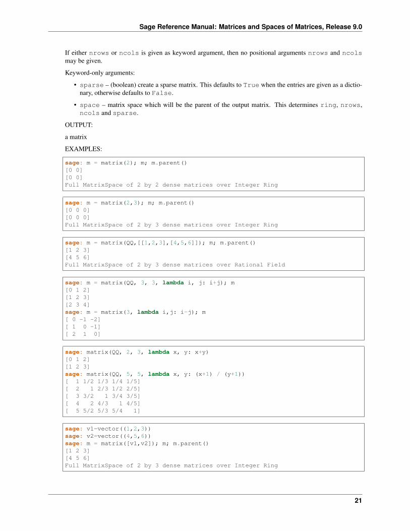
EXAMPLES:
sage: m = matrix(2); m; m.parent()[0 0][0 0]Full MatrixSpace of 2 by 2 dense matrices over Integer Ring
sage: m = matrix(2,3); m; m.parent()[0 0 0][0 0 0]Full MatrixSpace of 2 by 3 dense matrices over Integer Ring
sage: m = matrix(QQ,[[1,2,3],[4,5,6]]); m; m.parent()[1 2 3][4 5 6]Full MatrixSpace of 2 by 3 dense matrices over Rational Field
sage: m = matrix(QQ, 3, 3, lambda i, j: i+j); m[0 1 2][1 2 3][2 3 4]sage: m = matrix(3, lambda i,j: i-j); m[ 0 -1 -2][ 1 0 -1][ 2 1 0]
sage: matrix(QQ, 2, 3, lambda x, y: x+y)[0 1 2][1 2 3]sage: matrix(QQ, 5, 5, lambda x, y: (x+1) / (y+1))[ 1 1/2 1/3 1/4 1/5][ 2 1 2/3 1/2 2/5][ 3 3/2 1 3/4 3/5][ 4 2 4/3 1 4/5][ 5 5/2 5/3 5/4 1]
sage: v1=vector((1,2,3))sage: v2=vector((4,5,6))sage: m = matrix([v1,v2]); m; m.parent()[1 2 3][4 5 6]Full MatrixSpace of 2 by 3 dense matrices over Integer Ring
sage: m = matrix(QQ,2,[1,2,3,4,5,6]); m; m.parent()[1 2 3][4 5 6]Full MatrixSpace of 2 by 3 dense matrices over Rational Field
18 Chapter 2. General matrix Constructor
Sage Reference Manual: Matrices and Spaces of Matrices, Release 9.0
sage: m = matrix(QQ,2,3,[1,2,3,4,5,6]); m; m.parent()[1 2 3][4 5 6]Full MatrixSpace of 2 by 3 dense matrices over Rational Field
sage: m = matrix({(0,1): 2, (1,1):2/5}); m; m.parent()[ 0 2][ 0 2/5]Full MatrixSpace of 2 by 2 sparse matrices over Rational Field
sage: m = matrix(QQ,2,3,{(1,1): 2}); m; m.parent()[0 0 0][0 2 0]Full MatrixSpace of 2 by 3 sparse matrices over Rational Field
sage: import numpysage: n = numpy.array([[1,2],[3,4]],float)sage: m = matrix(n); m; m.parent()[1.0 2.0][3.0 4.0]Full MatrixSpace of 2 by 2 dense matrices over Real Double Field
sage: v = vector(ZZ, [1, 10, 100])sage: m = matrix(v); m; m.parent()[ 1 10 100]Full MatrixSpace of 1 by 3 dense matrices over Integer Ringsage: m = matrix(GF(7), v); m; m.parent()[1 3 2]Full MatrixSpace of 1 by 3 dense matrices over Finite Field of size 7sage: m = matrix(GF(7), 3, 1, v); m; m.parent()[1][3][2]Full MatrixSpace of 3 by 1 dense matrices over Finite Field of size 7
sage: matrix(pari.mathilbert(3))[ 1 1/2 1/3][1/2 1/3 1/4][1/3 1/4 1/5]
sage: g = graphs.PetersenGraph()sage: m = matrix(g); m; m.parent()[0 1 0 0 1 1 0 0 0 0][1 0 1 0 0 0 1 0 0 0][0 1 0 1 0 0 0 1 0 0][0 0 1 0 1 0 0 0 1 0][1 0 0 1 0 0 0 0 0 1][1 0 0 0 0 0 0 1 1 0][0 1 0 0 0 0 0 0 1 1][0 0 1 0 0 1 0 0 0 1][0 0 0 1 0 1 1 0 0 0][0 0 0 0 1 0 1 1 0 0]Full MatrixSpace of 10 by 10 dense matrices over Integer Ring
19

Sage Reference Manual: Matrices and Spaces of Matrices, Release 9.0
sage: matrix(ZZ, 10, 10, range(100), sparse=True).parent()Full MatrixSpace of 10 by 10 sparse matrices over Integer Ring
sage: R = PolynomialRing(QQ, 9, 'x')sage: A = matrix(R, 3, 3, R.gens()); A[x0 x1 x2][x3 x4 x5][x6 x7 x8]sage: det(A)-x2*x4*x6 + x1*x5*x6 + x2*x3*x7 - x0*x5*x7 - x1*x3*x8 + x0*x4*x8
AUTHORS:
• William Stein: Initial implementation
• Jason Grout (2008-03): almost a complete rewrite, with bits and pieces from the original implementation
• Jeroen Demeyer (2016-02-05): major clean up, see trac ticket #20015 and trac ticket #20016
• Jeroen Demeyer (2018-02-20): completely rewritten using MatrixArgs, see trac ticket #24742
sage.matrix.constructor.matrix(*args, **kwds)Create a matrix.
This implements the matrix constructor:
sage: matrix([[1,2],[3,4]])[1 2][3 4]
It also contains methods to create special types of matrices, see matrix.[tab] for more options. For exam-ple:
sage: matrix.identity(2)[1 0][0 1]
INPUT:
The matrix command takes the entries of a matrix, optionally preceded by a ring and the dimensions of thematrix, and returns a matrix.
The entries of a matrix can be specified as a flat list of elements, a list of lists (i.e., a list of rows), a list ofSage vectors, a callable object, or a dictionary having positions as keys and matrix entries as values (see theexamples). If you pass in a callable object, then you must specify the number of rows and columns. You cancreate a matrix of zeros by passing an empty list or the integer zero for the entries. To construct a multiple of theidentity (𝑐𝐼), you can specify square dimensions and pass in 𝑐. Calling matrix() with a Sage object may returnsomething that makes sense. Calling matrix() with a NumPy array will convert the array to a matrix.
All arguments (even the positional) are optional.
Positional and keyword arguments:
• ring – parent of the entries of the matrix (despite the name, this is not a priori required to be a ring). Bydefault, determine this from the given entries, falling back to ZZ if no entries are given.
• nrows – the number of rows in the matrix.
• ncols – the number of columns in the matrix.
• entries – see examples below.
20 Chapter 2. General matrix Constructor
Sage Reference Manual: Matrices and Spaces of Matrices, Release 9.0
If either nrows or ncols is given as keyword argument, then no positional arguments nrows and ncolsmay be given.
Keyword-only arguments:
• sparse – (boolean) create a sparse matrix. This defaults to True when the entries are given as a dictio-nary, otherwise defaults to False.
• space – matrix space which will be the parent of the output matrix. This determines ring, nrows,ncols and sparse.
OUTPUT:
a matrix
EXAMPLES:
sage: m = matrix(2); m; m.parent()[0 0][0 0]Full MatrixSpace of 2 by 2 dense matrices over Integer Ring
sage: m = matrix(2,3); m; m.parent()[0 0 0][0 0 0]Full MatrixSpace of 2 by 3 dense matrices over Integer Ring
sage: m = matrix(QQ,[[1,2,3],[4,5,6]]); m; m.parent()[1 2 3][4 5 6]Full MatrixSpace of 2 by 3 dense matrices over Rational Field
sage: m = matrix(QQ, 3, 3, lambda i, j: i+j); m[0 1 2][1 2 3][2 3 4]sage: m = matrix(3, lambda i,j: i-j); m[ 0 -1 -2][ 1 0 -1][ 2 1 0]
sage: matrix(QQ, 2, 3, lambda x, y: x+y)[0 1 2][1 2 3]sage: matrix(QQ, 5, 5, lambda x, y: (x+1) / (y+1))[ 1 1/2 1/3 1/4 1/5][ 2 1 2/3 1/2 2/5][ 3 3/2 1 3/4 3/5][ 4 2 4/3 1 4/5][ 5 5/2 5/3 5/4 1]
sage: v1=vector((1,2,3))sage: v2=vector((4,5,6))sage: m = matrix([v1,v2]); m; m.parent()[1 2 3][4 5 6]Full MatrixSpace of 2 by 3 dense matrices over Integer Ring
21
Sage Reference Manual: Matrices and Spaces of Matrices, Release 9.0
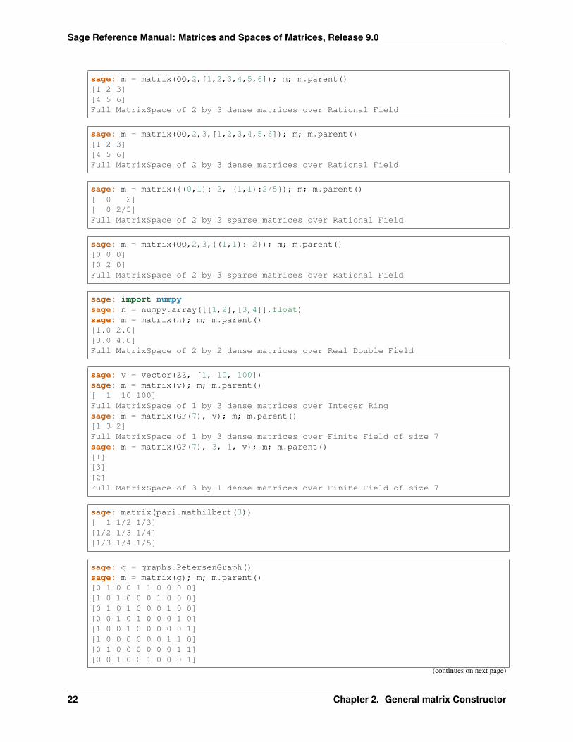
sage: m = matrix(QQ,2,[1,2,3,4,5,6]); m; m.parent()[1 2 3][4 5 6]Full MatrixSpace of 2 by 3 dense matrices over Rational Field
sage: m = matrix(QQ,2,3,[1,2,3,4,5,6]); m; m.parent()[1 2 3][4 5 6]Full MatrixSpace of 2 by 3 dense matrices over Rational Field
sage: m = matrix({(0,1): 2, (1,1):2/5}); m; m.parent()[ 0 2][ 0 2/5]Full MatrixSpace of 2 by 2 sparse matrices over Rational Field
sage: m = matrix(QQ,2,3,{(1,1): 2}); m; m.parent()[0 0 0][0 2 0]Full MatrixSpace of 2 by 3 sparse matrices over Rational Field
sage: import numpysage: n = numpy.array([[1,2],[3,4]],float)sage: m = matrix(n); m; m.parent()[1.0 2.0][3.0 4.0]Full MatrixSpace of 2 by 2 dense matrices over Real Double Field
sage: v = vector(ZZ, [1, 10, 100])sage: m = matrix(v); m; m.parent()[ 1 10 100]Full MatrixSpace of 1 by 3 dense matrices over Integer Ringsage: m = matrix(GF(7), v); m; m.parent()[1 3 2]Full MatrixSpace of 1 by 3 dense matrices over Finite Field of size 7sage: m = matrix(GF(7), 3, 1, v); m; m.parent()[1][3][2]Full MatrixSpace of 3 by 1 dense matrices over Finite Field of size 7
sage: matrix(pari.mathilbert(3))[ 1 1/2 1/3][1/2 1/3 1/4][1/3 1/4 1/5]
sage: g = graphs.PetersenGraph()sage: m = matrix(g); m; m.parent()[0 1 0 0 1 1 0 0 0 0][1 0 1 0 0 0 1 0 0 0][0 1 0 1 0 0 0 1 0 0][0 0 1 0 1 0 0 0 1 0][1 0 0 1 0 0 0 0 0 1][1 0 0 0 0 0 0 1 1 0][0 1 0 0 0 0 0 0 1 1][0 0 1 0 0 1 0 0 0 1]
(continues on next page)
22 Chapter 2. General matrix Constructor
Sage Reference Manual: Matrices and Spaces of Matrices, Release 9.0
(continued from previous page)
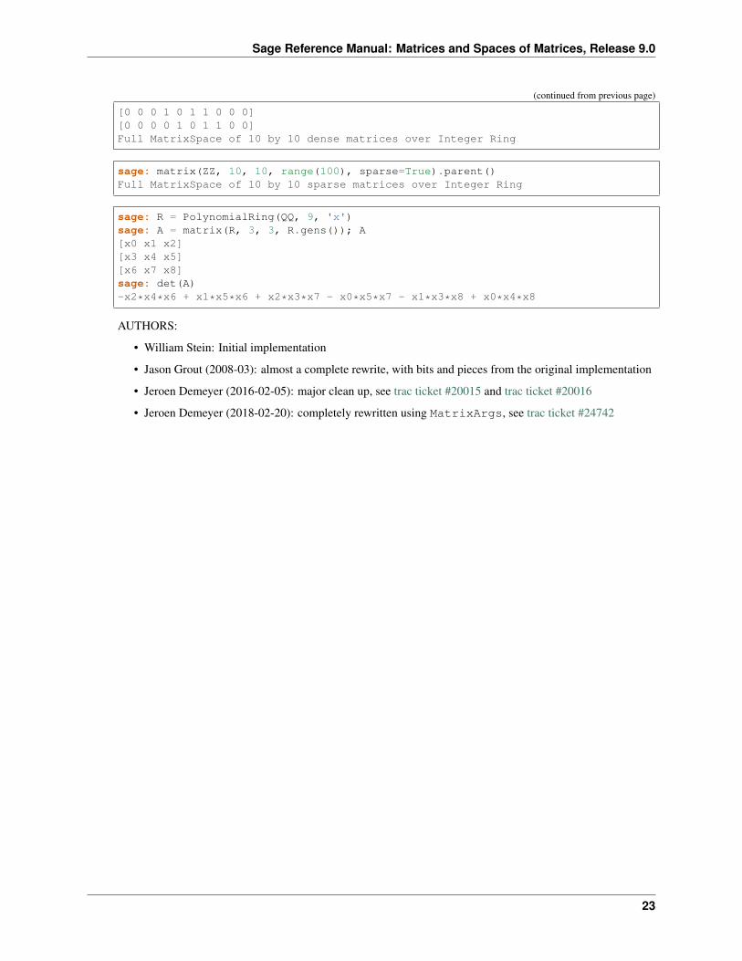
[0 0 0 1 0 1 1 0 0 0][0 0 0 0 1 0 1 1 0 0]Full MatrixSpace of 10 by 10 dense matrices over Integer Ring
sage: matrix(ZZ, 10, 10, range(100), sparse=True).parent()Full MatrixSpace of 10 by 10 sparse matrices over Integer Ring
sage: R = PolynomialRing(QQ, 9, 'x')sage: A = matrix(R, 3, 3, R.gens()); A[x0 x1 x2][x3 x4 x5][x6 x7 x8]sage: det(A)-x2*x4*x6 + x1*x5*x6 + x2*x3*x7 - x0*x5*x7 - x1*x3*x8 + x0*x4*x8
AUTHORS:
• William Stein: Initial implementation
• Jason Grout (2008-03): almost a complete rewrite, with bits and pieces from the original implementation
• Jeroen Demeyer (2016-02-05): major clean up, see trac ticket #20015 and trac ticket #20016
• Jeroen Demeyer (2018-02-20): completely rewritten using MatrixArgs, see trac ticket #24742
23

Sage Reference Manual: Matrices and Spaces of Matrices, Release 9.0
24 Chapter 2. General matrix Constructor
CHAPTER
THREE
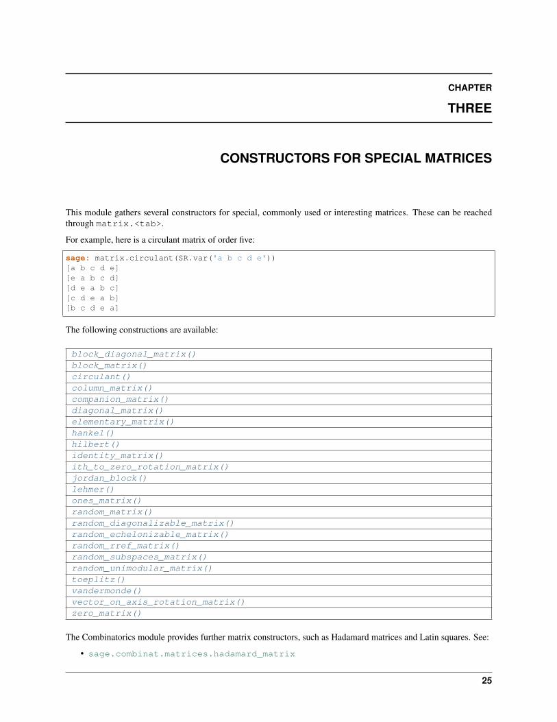
CONSTRUCTORS FOR SPECIAL MATRICES
This module gathers several constructors for special, commonly used or interesting matrices. These can be reachedthrough matrix.<tab>.
For example, here is a circulant matrix of order five:
sage: matrix.circulant(SR.var('a b c d e'))[a b c d e][e a b c d][d e a b c][c d e a b][b c d e a]
The following constructions are available:
block_diagonal_matrix()block_matrix()circulant()column_matrix()companion_matrix()diagonal_matrix()elementary_matrix()hankel()hilbert()identity_matrix()ith_to_zero_rotation_matrix()jordan_block()lehmer()ones_matrix()random_matrix()random_diagonalizable_matrix()random_echelonizable_matrix()random_rref_matrix()random_subspaces_matrix()random_unimodular_matrix()toeplitz()vandermonde()vector_on_axis_rotation_matrix()zero_matrix()
The Combinatorics module provides further matrix constructors, such as Hadamard matrices and Latin squares. See:
• sage.combinat.matrices.hadamard_matrix
25
Sage Reference Manual: Matrices and Spaces of Matrices, Release 9.0
• sage.combinat.matrices.latin
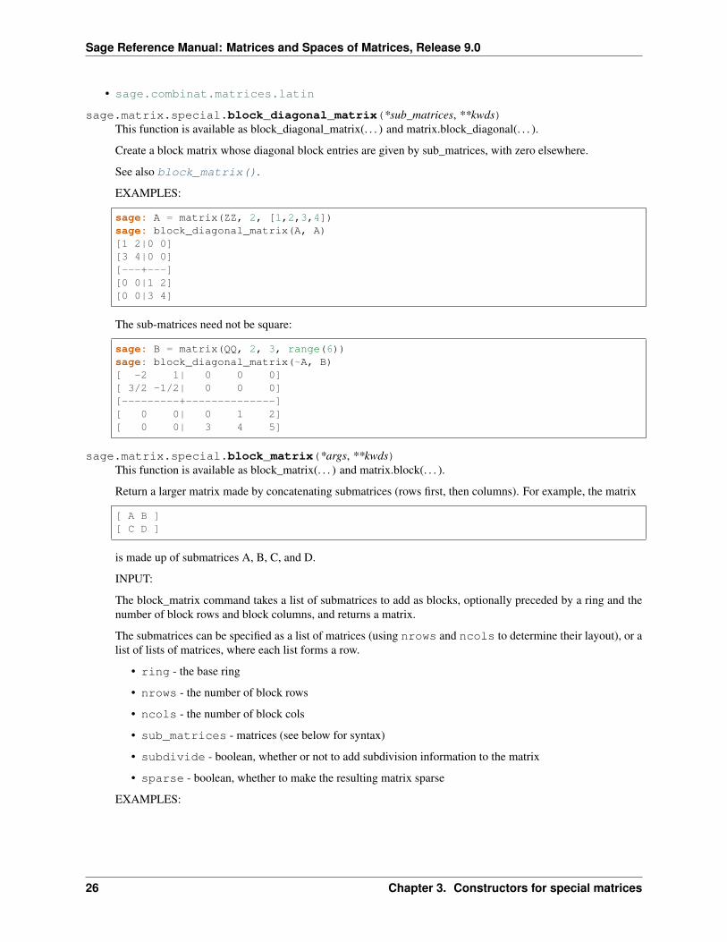
sage.matrix.special.block_diagonal_matrix(*sub_matrices, **kwds)This function is available as block_diagonal_matrix(. . . ) and matrix.block_diagonal(. . . ).
Create a block matrix whose diagonal block entries are given by sub_matrices, with zero elsewhere.
See also block_matrix().
EXAMPLES:
sage: A = matrix(ZZ, 2, [1,2,3,4])sage: block_diagonal_matrix(A, A)[1 2|0 0][3 4|0 0][---+---][0 0|1 2][0 0|3 4]
The sub-matrices need not be square:
sage: B = matrix(QQ, 2, 3, range(6))sage: block_diagonal_matrix(~A, B)[ -2 1| 0 0 0][ 3/2 -1/2| 0 0 0][---------+--------------][ 0 0| 0 1 2][ 0 0| 3 4 5]
sage.matrix.special.block_matrix(*args, **kwds)This function is available as block_matrix(. . . ) and matrix.block(. . . ).
Return a larger matrix made by concatenating submatrices (rows first, then columns). For example, the matrix
[ A B ][ C D ]
is made up of submatrices A, B, C, and D.
INPUT:
The block_matrix command takes a list of submatrices to add as blocks, optionally preceded by a ring and thenumber of block rows and block columns, and returns a matrix.
The submatrices can be specified as a list of matrices (using nrows and ncols to determine their layout), or alist of lists of matrices, where each list forms a row.
• ring - the base ring
• nrows - the number of block rows
• ncols - the number of block cols
• sub_matrices - matrices (see below for syntax)
• subdivide - boolean, whether or not to add subdivision information to the matrix
• sparse - boolean, whether to make the resulting matrix sparse
EXAMPLES:
26 Chapter 3. Constructors for special matrices
Sage Reference Manual: Matrices and Spaces of Matrices, Release 9.0
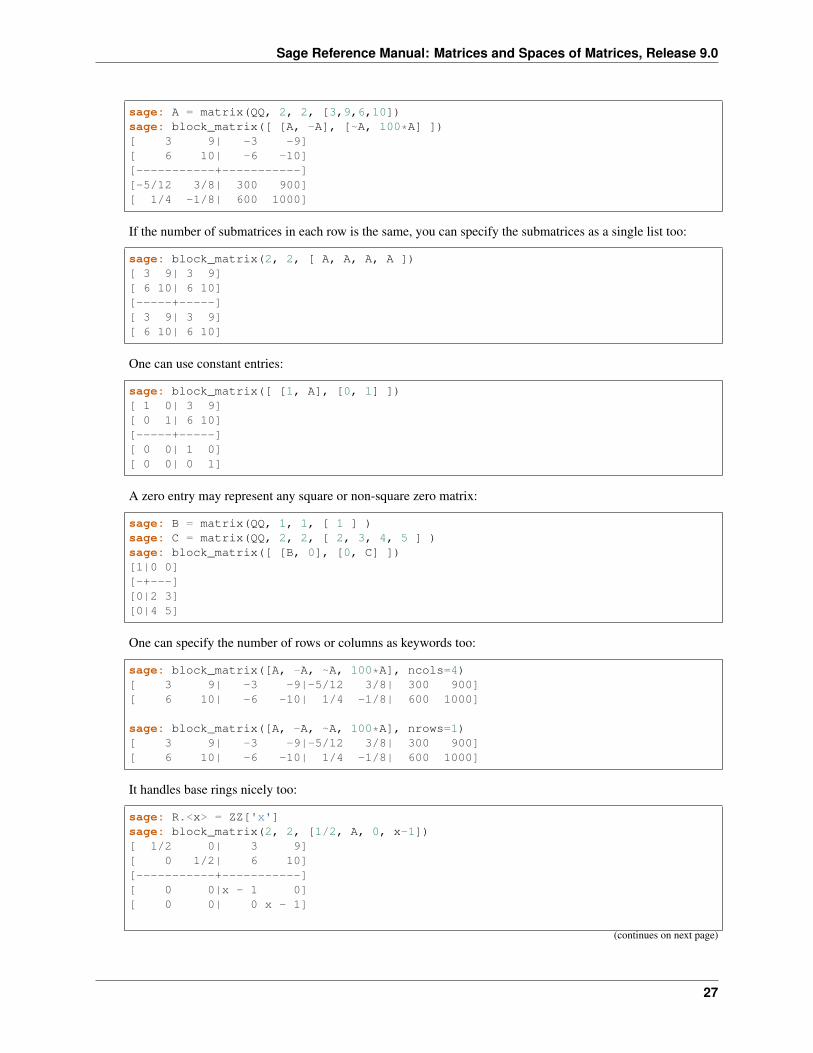
sage: A = matrix(QQ, 2, 2, [3,9,6,10])sage: block_matrix([ [A, -A], [~A, 100*A] ])[ 3 9| -3 -9][ 6 10| -6 -10][-----------+-----------][-5/12 3/8| 300 900][ 1/4 -1/8| 600 1000]
If the number of submatrices in each row is the same, you can specify the submatrices as a single list too:
sage: block_matrix(2, 2, [ A, A, A, A ])[ 3 9| 3 9][ 6 10| 6 10][-----+-----][ 3 9| 3 9][ 6 10| 6 10]
One can use constant entries:
sage: block_matrix([ [1, A], [0, 1] ])[ 1 0| 3 9][ 0 1| 6 10][-----+-----][ 0 0| 1 0][ 0 0| 0 1]
A zero entry may represent any square or non-square zero matrix:
sage: B = matrix(QQ, 1, 1, [ 1 ] )sage: C = matrix(QQ, 2, 2, [ 2, 3, 4, 5 ] )sage: block_matrix([ [B, 0], [0, C] ])[1|0 0][-+---][0|2 3][0|4 5]
One can specify the number of rows or columns as keywords too:
sage: block_matrix([A, -A, ~A, 100*A], ncols=4)[ 3 9| -3 -9|-5/12 3/8| 300 900][ 6 10| -6 -10| 1/4 -1/8| 600 1000]
sage: block_matrix([A, -A, ~A, 100*A], nrows=1)[ 3 9| -3 -9|-5/12 3/8| 300 900][ 6 10| -6 -10| 1/4 -1/8| 600 1000]
It handles base rings nicely too:
sage: R.<x> = ZZ['x']sage: block_matrix(2, 2, [1/2, A, 0, x-1])[ 1/2 0| 3 9][ 0 1/2| 6 10][-----------+-----------][ 0 0|x - 1 0][ 0 0| 0 x - 1]
(continues on next page)
27
Sage Reference Manual: Matrices and Spaces of Matrices, Release 9.0
(continued from previous page)
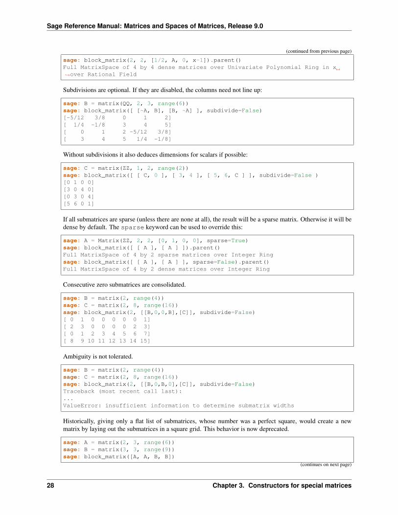
sage: block_matrix(2, 2, [1/2, A, 0, x-1]).parent()Full MatrixSpace of 4 by 4 dense matrices over Univariate Polynomial Ring in x→˓over Rational Field
Subdivisions are optional. If they are disabled, the columns need not line up:
sage: B = matrix(QQ, 2, 3, range(6))sage: block_matrix([ [~A, B], [B, ~A] ], subdivide=False)[-5/12 3/8 0 1 2][ 1/4 -1/8 3 4 5][ 0 1 2 -5/12 3/8][ 3 4 5 1/4 -1/8]
Without subdivisions it also deduces dimensions for scalars if possible:
sage: C = matrix(ZZ, 1, 2, range(2))sage: block_matrix([ [ C, 0 ], [ 3, 4 ], [ 5, 6, C ] ], subdivide=False )[0 1 0 0][3 0 4 0][0 3 0 4][5 6 0 1]
If all submatrices are sparse (unless there are none at all), the result will be a sparse matrix. Otherwise it will bedense by default. The sparse keyword can be used to override this:
sage: A = Matrix(ZZ, 2, 2, [0, 1, 0, 0], sparse=True)sage: block_matrix([ [ A ], [ A ] ]).parent()Full MatrixSpace of 4 by 2 sparse matrices over Integer Ringsage: block_matrix([ [ A ], [ A ] ], sparse=False).parent()Full MatrixSpace of 4 by 2 dense matrices over Integer Ring
Consecutive zero submatrices are consolidated.
sage: B = matrix(2, range(4))sage: C = matrix(2, 8, range(16))sage: block_matrix(2, [[B,0,0,B],[C]], subdivide=False)[ 0 1 0 0 0 0 0 1][ 2 3 0 0 0 0 2 3][ 0 1 2 3 4 5 6 7][ 8 9 10 11 12 13 14 15]
Ambiguity is not tolerated.
sage: B = matrix(2, range(4))sage: C = matrix(2, 8, range(16))sage: block_matrix(2, [[B,0,B,0],[C]], subdivide=False)Traceback (most recent call last):...ValueError: insufficient information to determine submatrix widths
Historically, giving only a flat list of submatrices, whose number was a perfect square, would create a newmatrix by laying out the submatrices in a square grid. This behavior is now deprecated.
sage: A = matrix(2, 3, range(6))sage: B = matrix(3, 3, range(9))sage: block_matrix([A, A, B, B])
(continues on next page)
28 Chapter 3. Constructors for special matrices
Sage Reference Manual: Matrices and Spaces of Matrices, Release 9.0
(continued from previous page)
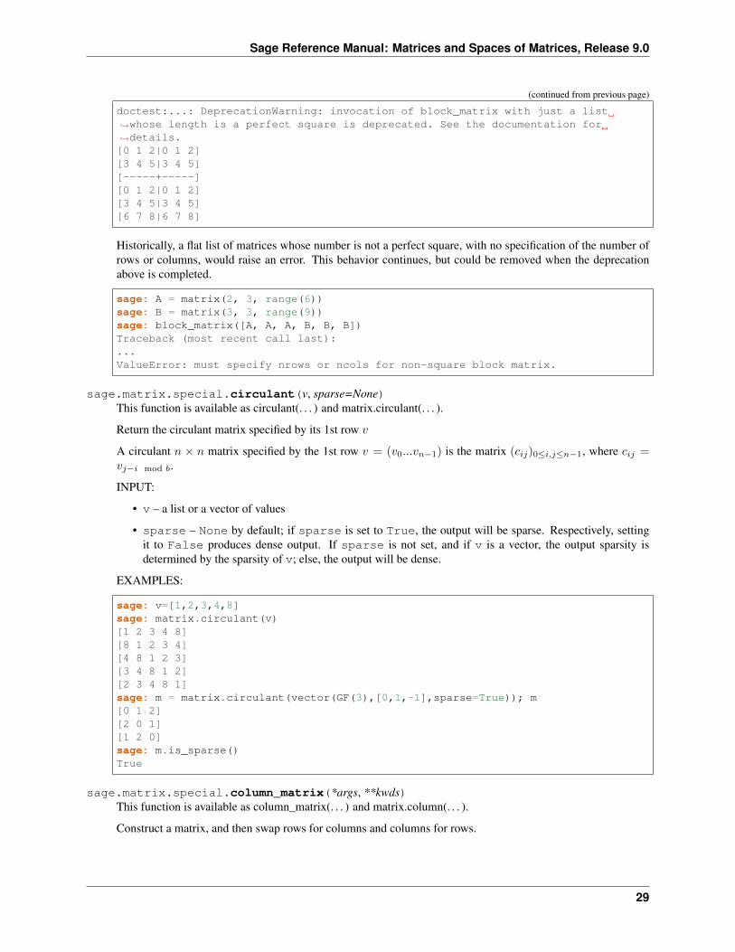
doctest:...: DeprecationWarning: invocation of block_matrix with just a list→˓whose length is a perfect square is deprecated. See the documentation for→˓details.[0 1 2|0 1 2][3 4 5|3 4 5][-----+-----][0 1 2|0 1 2][3 4 5|3 4 5][6 7 8|6 7 8]
Historically, a flat list of matrices whose number is not a perfect square, with no specification of the number ofrows or columns, would raise an error. This behavior continues, but could be removed when the deprecationabove is completed.
sage: A = matrix(2, 3, range(6))sage: B = matrix(3, 3, range(9))sage: block_matrix([A, A, A, B, B, B])Traceback (most recent call last):...ValueError: must specify nrows or ncols for non-square block matrix.
sage.matrix.special.circulant(v, sparse=None)This function is available as circulant(. . . ) and matrix.circulant(. . . ).
Return the circulant matrix specified by its 1st row 𝑣
A circulant 𝑛 × 𝑛 matrix specified by the 1st row 𝑣 = (𝑣0...𝑣𝑛−1) is the matrix (𝑐𝑖𝑗)0≤𝑖,𝑗≤𝑛−1, where 𝑐𝑖𝑗 =𝑣𝑗−𝑖 mod 𝑏.
INPUT:
• v – a list or a vector of values
• sparse – None by default; if sparse is set to True, the output will be sparse. Respectively, settingit to False produces dense output. If sparse is not set, and if v is a vector, the output sparsity isdetermined by the sparsity of v; else, the output will be dense.
EXAMPLES:
sage: v=[1,2,3,4,8]sage: matrix.circulant(v)[1 2 3 4 8][8 1 2 3 4][4 8 1 2 3][3 4 8 1 2][2 3 4 8 1]sage: m = matrix.circulant(vector(GF(3),[0,1,-1],sparse=True)); m[0 1 2][2 0 1][1 2 0]sage: m.is_sparse()True
sage.matrix.special.column_matrix(*args, **kwds)This function is available as column_matrix(. . . ) and matrix.column(. . . ).
Construct a matrix, and then swap rows for columns and columns for rows.
29

Sage Reference Manual: Matrices and Spaces of Matrices, Release 9.0
Note: Linear algebra in Sage favors rows over columns. So, generally, when creating a matrix, input vectorsand lists are treated as rows. This function is a convenience that turns around this convention when creating amatrix. If you are not familiar with the usual matrix() constructor, you might want to consider it first.
INPUT:
Inputs are almost exactly the same as for the matrix() constructor, which are documented there. But seeexamples below for how dimensions are handled.
OUTPUT:
Output is exactly the transpose of what the matrix() constructor would return. In other words, the matrixconstructor builds a matrix and then this function exchanges rows for columns, and columns for rows.
EXAMPLES:
The most compelling use of this function is when you have a collection of lists or vectors that you would liketo become the columns of a matrix. In almost any other situation, the matrix`() constructor can probably dothe job just as easily, or easier.
sage: col_1 = [1,2,3]sage: col_2 = [4,5,6]sage: column_matrix([col_1, col_2])[1 4][2 5][3 6]
sage: v1 = vector(QQ, [10, 20])sage: v2 = vector(QQ, [30, 40])sage: column_matrix(QQ, [v1, v2])[10 30][20 40]
If you only specify one dimension along with a flat list of entries, then it will be the number of columns in theresult (which is different from the behavior of the matrix constructor).
sage: column_matrix(ZZ, 8, range(24))[ 0 3 6 9 12 15 18 21][ 1 4 7 10 13 16 19 22][ 2 5 8 11 14 17 20 23]
And when you specify two dimensions, then they should be number of columns first, then the number of rows,which is the reverse of how they would be specified for the matrix constructor.
sage: column_matrix(QQ, 5, 3, range(15))[ 0 3 6 9 12][ 1 4 7 10 13][ 2 5 8 11 14]
And a few unproductive, but illustrative, examples.
sage: A = matrix(ZZ, 3, 4, range(12))sage: B = column_matrix(ZZ, 3, 4, range(12))sage: A == B.transpose()True
sage: A = matrix(QQ, 7, 12, range(84))
(continues on next page)
30 Chapter 3. Constructors for special matrices
Sage Reference Manual: Matrices and Spaces of Matrices, Release 9.0
(continued from previous page)
sage: A == column_matrix(A.columns())True
sage: A = column_matrix(QQ, matrix(ZZ, 3, 2, range(6)) )sage: A[0 2 4][1 3 5]sage: A.parent()Full MatrixSpace of 2 by 3 dense matrices over Rational Field
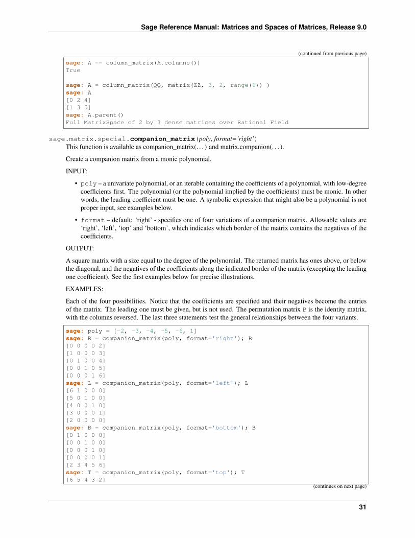
sage.matrix.special.companion_matrix(poly, format=’right’)This function is available as companion_matrix(. . . ) and matrix.companion(. . . ).
Create a companion matrix from a monic polynomial.
INPUT:
• poly – a univariate polynomial, or an iterable containing the coefficients of a polynomial, with low-degreecoefficients first. The polynomial (or the polynomial implied by the coefficients) must be monic. In otherwords, the leading coefficient must be one. A symbolic expression that might also be a polynomial is notproper input, see examples below.
• format – default: ‘right’ - specifies one of four variations of a companion matrix. Allowable values are‘right’, ‘left’, ‘top’ and ‘bottom’, which indicates which border of the matrix contains the negatives of thecoefficients.
OUTPUT:
A square matrix with a size equal to the degree of the polynomial. The returned matrix has ones above, or belowthe diagonal, and the negatives of the coefficients along the indicated border of the matrix (excepting the leadingone coefficient). See the first examples below for precise illustrations.
EXAMPLES:
Each of the four possibilities. Notice that the coefficients are specified and their negatives become the entriesof the matrix. The leading one must be given, but is not used. The permutation matrix P is the identity matrix,with the columns reversed. The last three statements test the general relationships between the four variants.
sage: poly = [-2, -3, -4, -5, -6, 1]sage: R = companion_matrix(poly, format='right'); R[0 0 0 0 2][1 0 0 0 3][0 1 0 0 4][0 0 1 0 5][0 0 0 1 6]sage: L = companion_matrix(poly, format='left'); L[6 1 0 0 0][5 0 1 0 0][4 0 0 1 0][3 0 0 0 1][2 0 0 0 0]sage: B = companion_matrix(poly, format='bottom'); B[0 1 0 0 0][0 0 1 0 0][0 0 0 1 0][0 0 0 0 1][2 3 4 5 6]sage: T = companion_matrix(poly, format='top'); T[6 5 4 3 2]
(continues on next page)
31
Sage Reference Manual: Matrices and Spaces of Matrices, Release 9.0
(continued from previous page)
[1 0 0 0 0][0 1 0 0 0][0 0 1 0 0][0 0 0 1 0]
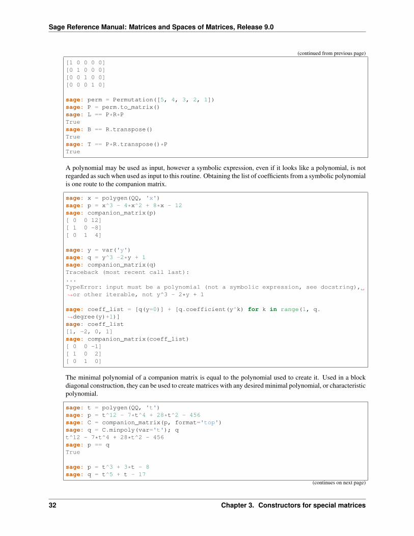
sage: perm = Permutation([5, 4, 3, 2, 1])sage: P = perm.to_matrix()sage: L == P*R*PTruesage: B == R.transpose()Truesage: T == P*R.transpose()*PTrue
A polynomial may be used as input, however a symbolic expression, even if it looks like a polynomial, is notregarded as such when used as input to this routine. Obtaining the list of coefficients from a symbolic polynomialis one route to the companion matrix.
sage: x = polygen(QQ, 'x')sage: p = x^3 - 4*x^2 + 8*x - 12sage: companion_matrix(p)[ 0 0 12][ 1 0 -8][ 0 1 4]
sage: y = var('y')sage: q = y^3 -2*y + 1sage: companion_matrix(q)Traceback (most recent call last):...TypeError: input must be a polynomial (not a symbolic expression, see docstring),→˓or other iterable, not y^3 - 2*y + 1
sage: coeff_list = [q(y=0)] + [q.coefficient(y^k) for k in range(1, q.→˓degree(y)+1)]sage: coeff_list[1, -2, 0, 1]sage: companion_matrix(coeff_list)[ 0 0 -1][ 1 0 2][ 0 1 0]
The minimal polynomial of a companion matrix is equal to the polynomial used to create it. Used in a blockdiagonal construction, they can be used to create matrices with any desired minimal polynomial, or characteristicpolynomial.
sage: t = polygen(QQ, 't')sage: p = t^12 - 7*t^4 + 28*t^2 - 456sage: C = companion_matrix(p, format='top')sage: q = C.minpoly(var='t'); qt^12 - 7*t^4 + 28*t^2 - 456sage: p == qTrue
sage: p = t^3 + 3*t - 8sage: q = t^5 + t - 17
(continues on next page)
32 Chapter 3. Constructors for special matrices
Sage Reference Manual: Matrices and Spaces of Matrices, Release 9.0
(continued from previous page)
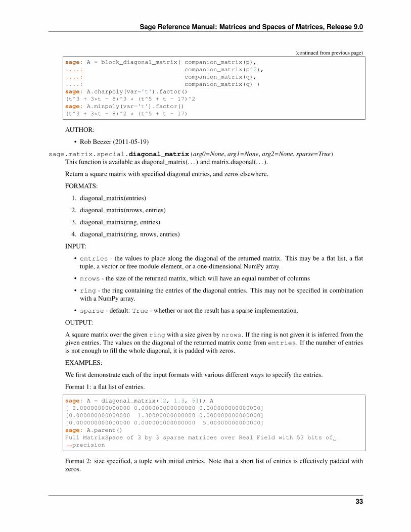
sage: A = block_diagonal_matrix( companion_matrix(p),....: companion_matrix(p^2),....: companion_matrix(q),....: companion_matrix(q) )sage: A.charpoly(var='t').factor()(t^3 + 3*t - 8)^3 * (t^5 + t - 17)^2sage: A.minpoly(var='t').factor()(t^3 + 3*t - 8)^2 * (t^5 + t - 17)
AUTHOR:
• Rob Beezer (2011-05-19)
sage.matrix.special.diagonal_matrix(arg0=None, arg1=None, arg2=None, sparse=True)This function is available as diagonal_matrix(. . . ) and matrix.diagonal(. . . ).
Return a square matrix with specified diagonal entries, and zeros elsewhere.
FORMATS:
1. diagonal_matrix(entries)
2. diagonal_matrix(nrows, entries)
3. diagonal_matrix(ring, entries)
4. diagonal_matrix(ring, nrows, entries)
INPUT:
• entries - the values to place along the diagonal of the returned matrix. This may be a flat list, a flattuple, a vector or free module element, or a one-dimensional NumPy array.
• nrows - the size of the returned matrix, which will have an equal number of columns
• ring - the ring containing the entries of the diagonal entries. This may not be specified in combinationwith a NumPy array.
• sparse - default: True - whether or not the result has a sparse implementation.
OUTPUT:
A square matrix over the given ring with a size given by nrows. If the ring is not given it is inferred from thegiven entries. The values on the diagonal of the returned matrix come from entries. If the number of entriesis not enough to fill the whole diagonal, it is padded with zeros.
EXAMPLES:
We first demonstrate each of the input formats with various different ways to specify the entries.
Format 1: a flat list of entries.
sage: A = diagonal_matrix([2, 1.3, 5]); A[ 2.00000000000000 0.000000000000000 0.000000000000000][0.000000000000000 1.30000000000000 0.000000000000000][0.000000000000000 0.000000000000000 5.00000000000000]sage: A.parent()Full MatrixSpace of 3 by 3 sparse matrices over Real Field with 53 bits of→˓precision
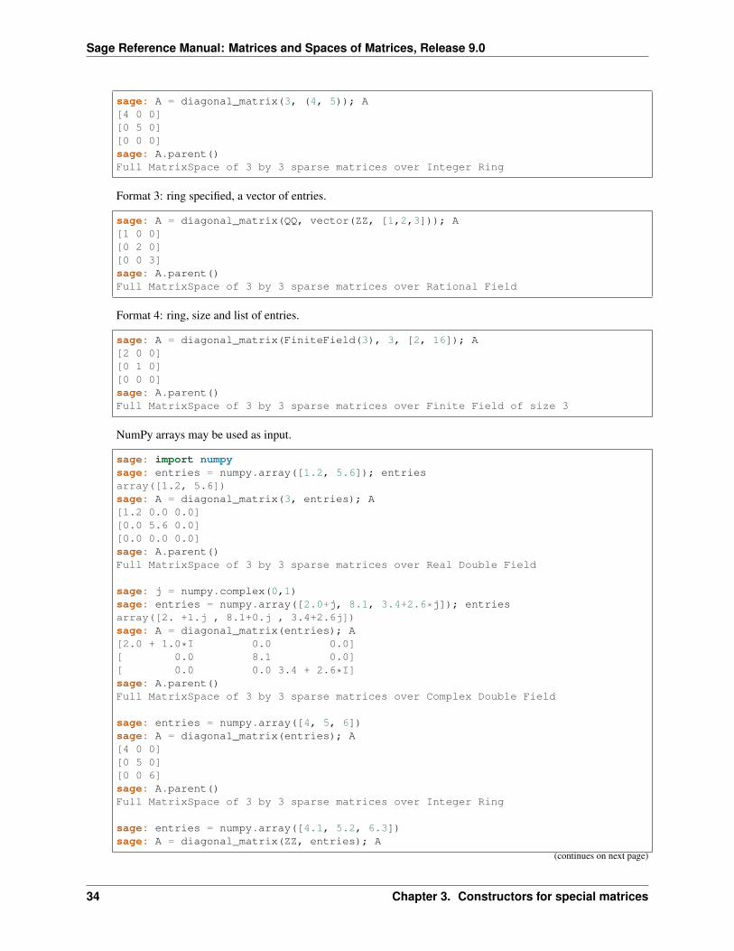
Format 2: size specified, a tuple with initial entries. Note that a short list of entries is effectively padded withzeros.
33
Sage Reference Manual: Matrices and Spaces of Matrices, Release 9.0
sage: A = diagonal_matrix(3, (4, 5)); A[4 0 0][0 5 0][0 0 0]sage: A.parent()Full MatrixSpace of 3 by 3 sparse matrices over Integer Ring
Format 3: ring specified, a vector of entries.
sage: A = diagonal_matrix(QQ, vector(ZZ, [1,2,3])); A[1 0 0][0 2 0][0 0 3]sage: A.parent()Full MatrixSpace of 3 by 3 sparse matrices over Rational Field
Format 4: ring, size and list of entries.
sage: A = diagonal_matrix(FiniteField(3), 3, [2, 16]); A[2 0 0][0 1 0][0 0 0]sage: A.parent()Full MatrixSpace of 3 by 3 sparse matrices over Finite Field of size 3
NumPy arrays may be used as input.
sage: import numpysage: entries = numpy.array([1.2, 5.6]); entriesarray([1.2, 5.6])sage: A = diagonal_matrix(3, entries); A[1.2 0.0 0.0][0.0 5.6 0.0][0.0 0.0 0.0]sage: A.parent()Full MatrixSpace of 3 by 3 sparse matrices over Real Double Field
sage: j = numpy.complex(0,1)sage: entries = numpy.array([2.0+j, 8.1, 3.4+2.6*j]); entriesarray([2. +1.j , 8.1+0.j , 3.4+2.6j])sage: A = diagonal_matrix(entries); A[2.0 + 1.0*I 0.0 0.0][ 0.0 8.1 0.0][ 0.0 0.0 3.4 + 2.6*I]sage: A.parent()Full MatrixSpace of 3 by 3 sparse matrices over Complex Double Field
sage: entries = numpy.array([4, 5, 6])sage: A = diagonal_matrix(entries); A[4 0 0][0 5 0][0 0 6]sage: A.parent()Full MatrixSpace of 3 by 3 sparse matrices over Integer Ring
sage: entries = numpy.array([4.1, 5.2, 6.3])sage: A = diagonal_matrix(ZZ, entries); A
(continues on next page)
34 Chapter 3. Constructors for special matrices
Sage Reference Manual: Matrices and Spaces of Matrices, Release 9.0
(continued from previous page)
Traceback (most recent call last):...TypeError: unable to convert 4.1 to an element of Integer Ring
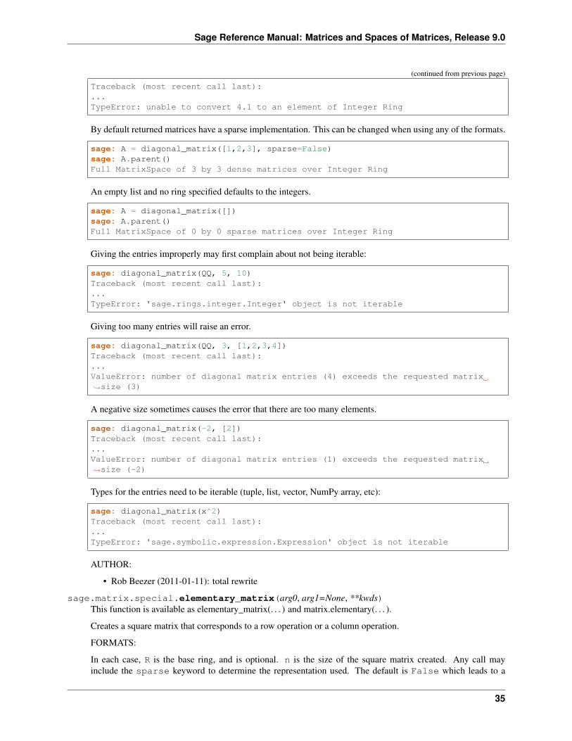
By default returned matrices have a sparse implementation. This can be changed when using any of the formats.
sage: A = diagonal_matrix([1,2,3], sparse=False)sage: A.parent()Full MatrixSpace of 3 by 3 dense matrices over Integer Ring
An empty list and no ring specified defaults to the integers.
sage: A = diagonal_matrix([])sage: A.parent()Full MatrixSpace of 0 by 0 sparse matrices over Integer Ring
Giving the entries improperly may first complain about not being iterable:
sage: diagonal_matrix(QQ, 5, 10)Traceback (most recent call last):...TypeError: 'sage.rings.integer.Integer' object is not iterable
Giving too many entries will raise an error.
sage: diagonal_matrix(QQ, 3, [1,2,3,4])Traceback (most recent call last):...ValueError: number of diagonal matrix entries (4) exceeds the requested matrix→˓size (3)
A negative size sometimes causes the error that there are too many elements.
sage: diagonal_matrix(-2, [2])Traceback (most recent call last):...ValueError: number of diagonal matrix entries (1) exceeds the requested matrix→˓size (-2)
Types for the entries need to be iterable (tuple, list, vector, NumPy array, etc):
sage: diagonal_matrix(x^2)Traceback (most recent call last):...TypeError: 'sage.symbolic.expression.Expression' object is not iterable
AUTHOR:
• Rob Beezer (2011-01-11): total rewrite
sage.matrix.special.elementary_matrix(arg0, arg1=None, **kwds)This function is available as elementary_matrix(. . . ) and matrix.elementary(. . . ).
Creates a square matrix that corresponds to a row operation or a column operation.
FORMATS:
In each case, R is the base ring, and is optional. n is the size of the square matrix created. Any call mayinclude the sparse keyword to determine the representation used. The default is False which leads to a
35
Sage Reference Manual: Matrices and Spaces of Matrices, Release 9.0
dense representation. We describe the matrices by their associated row operation, see the output description formore.
• elementary_matrix(R, n, row1=i, row2=j)
The matrix which swaps rows i and j.
• elementary_matrix(R, n, row1=i, scale=s)
The matrix which multiplies row i by s.
• elementary_matrix(R, n, row1=i, row2=j, scale=s)
The matrix which multiplies row j by s and adds it to row i.
Elementary matrices representing column operations are created in an entirely analogous way, replacing row1by col1 and replacing row2 by col2.
Specifying the ring for entries of the matrix is optional. If it is not given, and a scale parameter is provided, thena ring containing the value of scale will be used. Otherwise, the ring defaults to the integers.
OUTPUT:
An elementary matrix is a square matrix that is very close to being an identity matrix. If E is an elementarymatrix and A is any matrix with the same number of rows, then E*A is the result of applying a row operationto A. This is how the three types created by this function are described. Similarly, an elementary matrix canbe associated with a column operation, so if E has the same number of columns as A then A*E is the result ofperforming a column operation on A.
An elementary matrix representing a row operation is created if row1 is specified, while an elementary matrixrepresenting a column operation is created if col1 is specified.
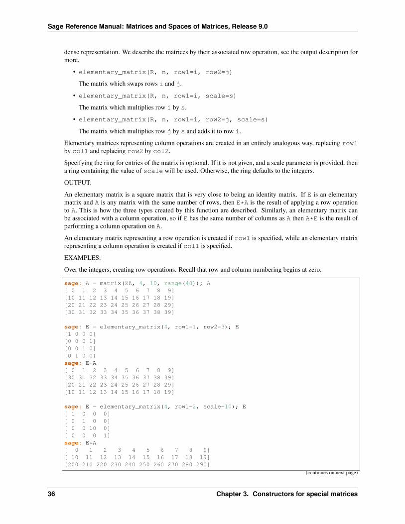
EXAMPLES:
Over the integers, creating row operations. Recall that row and column numbering begins at zero.
sage: A = matrix(ZZ, 4, 10, range(40)); A[ 0 1 2 3 4 5 6 7 8 9][10 11 12 13 14 15 16 17 18 19][20 21 22 23 24 25 26 27 28 29][30 31 32 33 34 35 36 37 38 39]
sage: E = elementary_matrix(4, row1=1, row2=3); E[1 0 0 0][0 0 0 1][0 0 1 0][0 1 0 0]sage: E*A[ 0 1 2 3 4 5 6 7 8 9][30 31 32 33 34 35 36 37 38 39][20 21 22 23 24 25 26 27 28 29][10 11 12 13 14 15 16 17 18 19]
sage: E = elementary_matrix(4, row1=2, scale=10); E[ 1 0 0 0][ 0 1 0 0][ 0 0 10 0][ 0 0 0 1]sage: E*A[ 0 1 2 3 4 5 6 7 8 9][ 10 11 12 13 14 15 16 17 18 19][200 210 220 230 240 250 260 270 280 290]
(continues on next page)
36 Chapter 3. Constructors for special matrices
Sage Reference Manual: Matrices and Spaces of Matrices, Release 9.0
(continued from previous page)
[ 30 31 32 33 34 35 36 37 38 39]
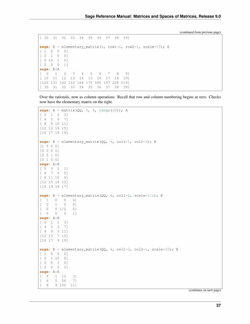
sage: E = elementary_matrix(4, row1=2, row2=1, scale=10); E[ 1 0 0 0][ 0 1 0 0][ 0 10 1 0][ 0 0 0 1]sage: E*A[ 0 1 2 3 4 5 6 7 8 9][ 10 11 12 13 14 15 16 17 18 19][120 131 142 153 164 175 186 197 208 219][ 30 31 32 33 34 35 36 37 38 39]
Over the rationals, now as column operations. Recall that row and column numbering begins at zero. Checksnow have the elementary matrix on the right.
sage: A = matrix(QQ, 5, 4, range(20)); A[ 0 1 2 3][ 4 5 6 7][ 8 9 10 11][12 13 14 15][16 17 18 19]
sage: E = elementary_matrix(QQ, 4, col1=1, col2=3); E[1 0 0 0][0 0 0 1][0 0 1 0][0 1 0 0]sage: A*E[ 0 3 2 1][ 4 7 6 5][ 8 11 10 9][12 15 14 13][16 19 18 17]
sage: E = elementary_matrix(QQ, 4, col1=2, scale=1/2); E[ 1 0 0 0][ 0 1 0 0][ 0 0 1/2 0][ 0 0 0 1]sage: A*E[ 0 1 1 3][ 4 5 3 7][ 8 9 5 11][12 13 7 15][16 17 9 19]
sage: E = elementary_matrix(QQ, 4, col1=2, col2=1, scale=10); E[ 1 0 0 0][ 0 1 10 0][ 0 0 1 0][ 0 0 0 1]sage: A*E[ 0 1 12 3][ 4 5 56 7][ 8 9 100 11]
(continues on next page)
37
Sage Reference Manual: Matrices and Spaces of Matrices, Release 9.0
(continued from previous page)
[ 12 13 144 15][ 16 17 188 19]
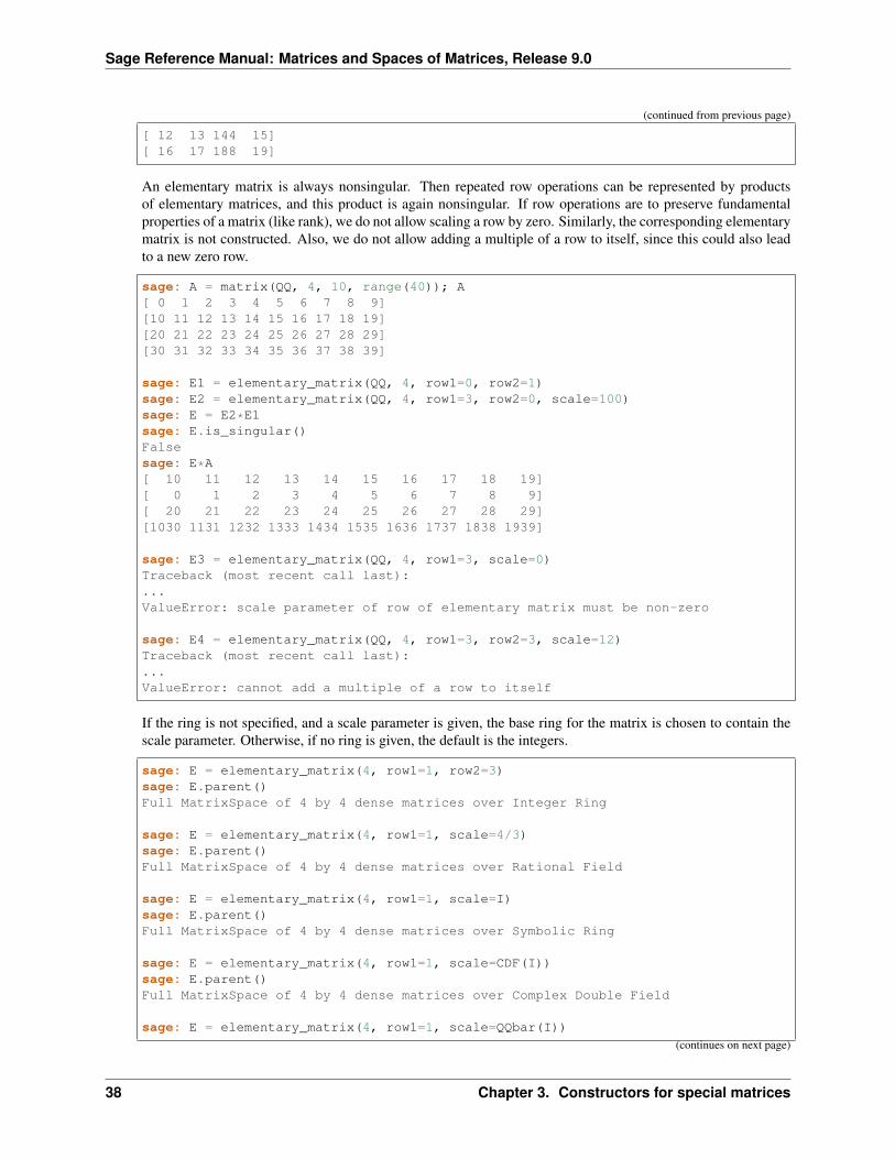
An elementary matrix is always nonsingular. Then repeated row operations can be represented by productsof elementary matrices, and this product is again nonsingular. If row operations are to preserve fundamentalproperties of a matrix (like rank), we do not allow scaling a row by zero. Similarly, the corresponding elementarymatrix is not constructed. Also, we do not allow adding a multiple of a row to itself, since this could also leadto a new zero row.
sage: A = matrix(QQ, 4, 10, range(40)); A[ 0 1 2 3 4 5 6 7 8 9][10 11 12 13 14 15 16 17 18 19][20 21 22 23 24 25 26 27 28 29][30 31 32 33 34 35 36 37 38 39]
sage: E1 = elementary_matrix(QQ, 4, row1=0, row2=1)sage: E2 = elementary_matrix(QQ, 4, row1=3, row2=0, scale=100)sage: E = E2*E1sage: E.is_singular()Falsesage: E*A[ 10 11 12 13 14 15 16 17 18 19][ 0 1 2 3 4 5 6 7 8 9][ 20 21 22 23 24 25 26 27 28 29][1030 1131 1232 1333 1434 1535 1636 1737 1838 1939]
sage: E3 = elementary_matrix(QQ, 4, row1=3, scale=0)Traceback (most recent call last):...ValueError: scale parameter of row of elementary matrix must be non-zero
sage: E4 = elementary_matrix(QQ, 4, row1=3, row2=3, scale=12)Traceback (most recent call last):...ValueError: cannot add a multiple of a row to itself
If the ring is not specified, and a scale parameter is given, the base ring for the matrix is chosen to contain thescale parameter. Otherwise, if no ring is given, the default is the integers.
sage: E = elementary_matrix(4, row1=1, row2=3)sage: E.parent()Full MatrixSpace of 4 by 4 dense matrices over Integer Ring
sage: E = elementary_matrix(4, row1=1, scale=4/3)sage: E.parent()Full MatrixSpace of 4 by 4 dense matrices over Rational Field
sage: E = elementary_matrix(4, row1=1, scale=I)sage: E.parent()Full MatrixSpace of 4 by 4 dense matrices over Symbolic Ring
sage: E = elementary_matrix(4, row1=1, scale=CDF(I))sage: E.parent()Full MatrixSpace of 4 by 4 dense matrices over Complex Double Field
sage: E = elementary_matrix(4, row1=1, scale=QQbar(I))
(continues on next page)
38 Chapter 3. Constructors for special matrices
Sage Reference Manual: Matrices and Spaces of Matrices, Release 9.0
(continued from previous page)
sage: E.parent()Full MatrixSpace of 4 by 4 dense matrices over Algebraic Field
Returned matrices have a dense implementation by default, but a sparse implementation may be requested.
sage: E = elementary_matrix(4, row1=0, row2=1)sage: E.is_dense()True
sage: E = elementary_matrix(4, row1=0, row2=1, sparse=True)sage: E.is_sparse()True
And the ridiculously small cases. The zero-row matrix cannot be built since then there are no rows to manipulate.
sage: elementary_matrix(QQ, 1, row1=0, row2=0)[1]sage: elementary_matrix(QQ, 0, row1=0, row2=0)Traceback (most recent call last):...ValueError: size of elementary matrix must be 1 or greater, not 0
AUTHOR:
• Rob Beezer (2011-03-04)
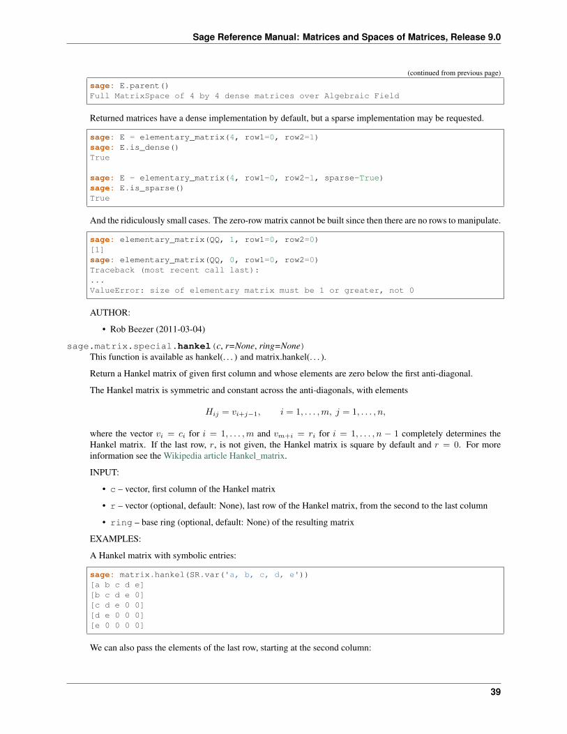
sage.matrix.special.hankel(c, r=None, ring=None)This function is available as hankel(. . . ) and matrix.hankel(. . . ).
Return a Hankel matrix of given first column and whose elements are zero below the first anti-diagonal.
The Hankel matrix is symmetric and constant across the anti-diagonals, with elements
𝐻𝑖𝑗 = 𝑣𝑖+𝑗−1, 𝑖 = 1, . . . ,𝑚, 𝑗 = 1, . . . , 𝑛,
where the vector 𝑣𝑖 = 𝑐𝑖 for 𝑖 = 1, . . . ,𝑚 and 𝑣𝑚+𝑖 = 𝑟𝑖 for 𝑖 = 1, . . . , 𝑛 − 1 completely determines theHankel matrix. If the last row, 𝑟, is not given, the Hankel matrix is square by default and 𝑟 = 0. For moreinformation see the Wikipedia article Hankel_matrix.
INPUT:
• c – vector, first column of the Hankel matrix
• r – vector (optional, default: None), last row of the Hankel matrix, from the second to the last column
• ring – base ring (optional, default: None) of the resulting matrix
EXAMPLES:
A Hankel matrix with symbolic entries:
sage: matrix.hankel(SR.var('a, b, c, d, e'))[a b c d e][b c d e 0][c d e 0 0][d e 0 0 0][e 0 0 0 0]
We can also pass the elements of the last row, starting at the second column:
39
Sage Reference Manual: Matrices and Spaces of Matrices, Release 9.0
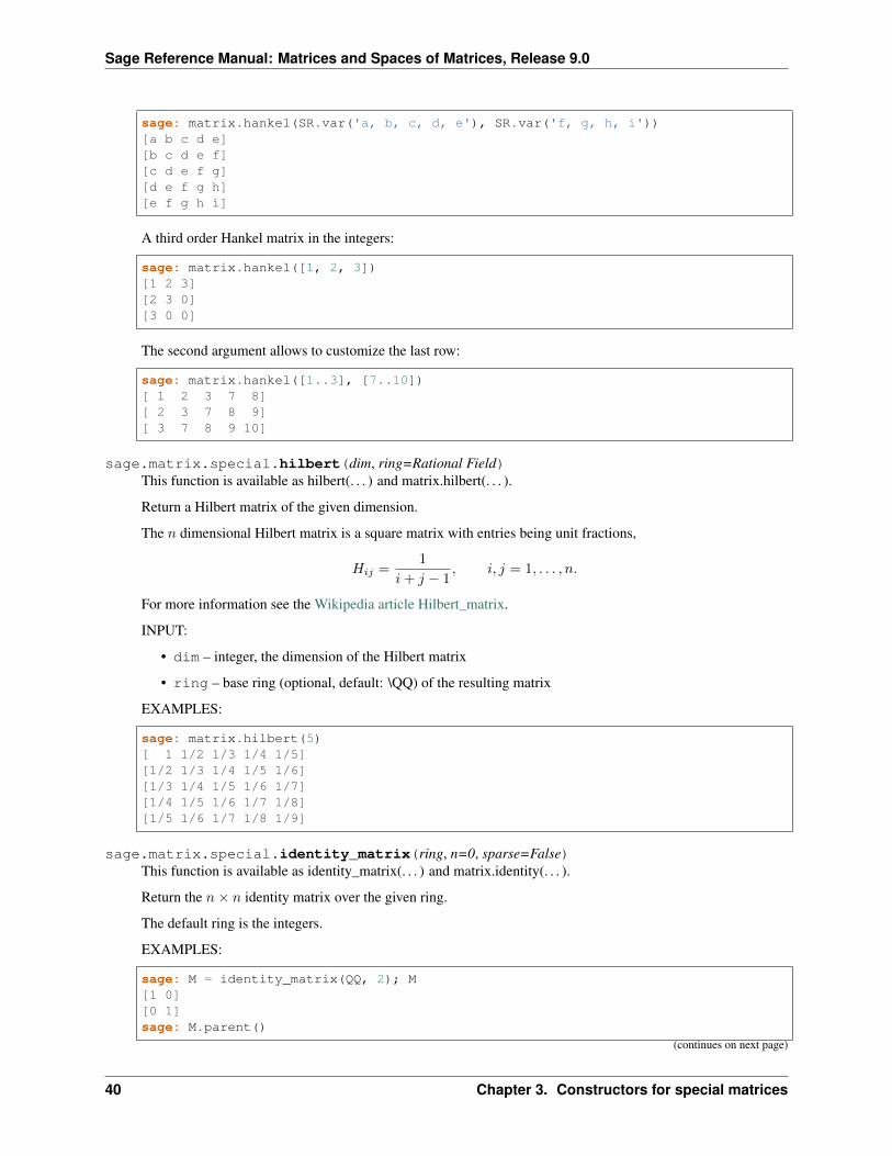
sage: matrix.hankel(SR.var('a, b, c, d, e'), SR.var('f, g, h, i'))[a b c d e][b c d e f][c d e f g][d e f g h][e f g h i]
A third order Hankel matrix in the integers:
sage: matrix.hankel([1, 2, 3])[1 2 3][2 3 0][3 0 0]
The second argument allows to customize the last row:
sage: matrix.hankel([1..3], [7..10])[ 1 2 3 7 8][ 2 3 7 8 9][ 3 7 8 9 10]
sage.matrix.special.hilbert(dim, ring=Rational Field)This function is available as hilbert(. . . ) and matrix.hilbert(. . . ).
Return a Hilbert matrix of the given dimension.
The 𝑛 dimensional Hilbert matrix is a square matrix with entries being unit fractions,
𝐻𝑖𝑗 =1
𝑖+ 𝑗 − 1, 𝑖, 𝑗 = 1, . . . , 𝑛.
For more information see the Wikipedia article Hilbert_matrix.
INPUT:
• dim – integer, the dimension of the Hilbert matrix
• ring – base ring (optional, default: \QQ) of the resulting matrix
EXAMPLES:
sage: matrix.hilbert(5)[ 1 1/2 1/3 1/4 1/5][1/2 1/3 1/4 1/5 1/6][1/3 1/4 1/5 1/6 1/7][1/4 1/5 1/6 1/7 1/8][1/5 1/6 1/7 1/8 1/9]
sage.matrix.special.identity_matrix(ring, n=0, sparse=False)This function is available as identity_matrix(. . . ) and matrix.identity(. . . ).
Return the 𝑛× 𝑛 identity matrix over the given ring.
The default ring is the integers.
EXAMPLES:
sage: M = identity_matrix(QQ, 2); M[1 0][0 1]sage: M.parent()
(continues on next page)
40 Chapter 3. Constructors for special matrices
Sage Reference Manual: Matrices and Spaces of Matrices, Release 9.0
(continued from previous page)
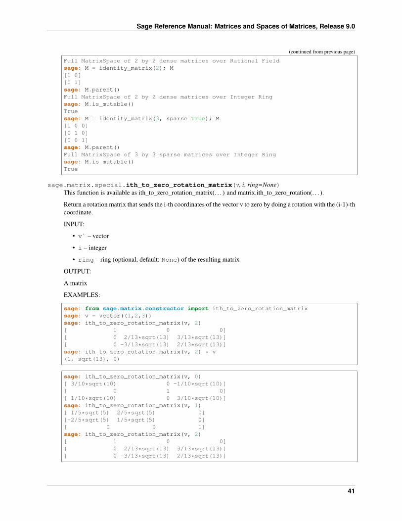
Full MatrixSpace of 2 by 2 dense matrices over Rational Fieldsage: M = identity_matrix(2); M[1 0][0 1]sage: M.parent()Full MatrixSpace of 2 by 2 dense matrices over Integer Ringsage: M.is_mutable()Truesage: M = identity_matrix(3, sparse=True); M[1 0 0][0 1 0][0 0 1]sage: M.parent()Full MatrixSpace of 3 by 3 sparse matrices over Integer Ringsage: M.is_mutable()True
sage.matrix.special.ith_to_zero_rotation_matrix(v, i, ring=None)This function is available as ith_to_zero_rotation_matrix(. . . ) and matrix.ith_to_zero_rotation(. . . ).
Return a rotation matrix that sends the i-th coordinates of the vector v to zero by doing a rotation with the (i-1)-thcoordinate.
INPUT:
• v` – vector
• i – integer
• ring – ring (optional, default: None) of the resulting matrix
OUTPUT:
A matrix
EXAMPLES:
sage: from sage.matrix.constructor import ith_to_zero_rotation_matrixsage: v = vector((1,2,3))sage: ith_to_zero_rotation_matrix(v, 2)[ 1 0 0][ 0 2/13*sqrt(13) 3/13*sqrt(13)][ 0 -3/13*sqrt(13) 2/13*sqrt(13)]sage: ith_to_zero_rotation_matrix(v, 2) * v(1, sqrt(13), 0)
sage: ith_to_zero_rotation_matrix(v, 0)[ 3/10*sqrt(10) 0 -1/10*sqrt(10)][ 0 1 0][ 1/10*sqrt(10) 0 3/10*sqrt(10)]sage: ith_to_zero_rotation_matrix(v, 1)[ 1/5*sqrt(5) 2/5*sqrt(5) 0][-2/5*sqrt(5) 1/5*sqrt(5) 0][ 0 0 1]sage: ith_to_zero_rotation_matrix(v, 2)[ 1 0 0][ 0 2/13*sqrt(13) 3/13*sqrt(13)][ 0 -3/13*sqrt(13) 2/13*sqrt(13)]
41
Sage Reference Manual: Matrices and Spaces of Matrices, Release 9.0
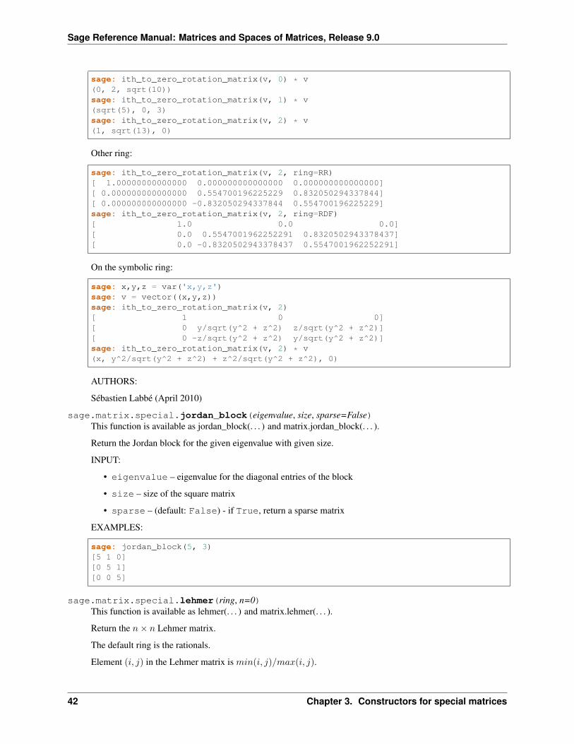
sage: ith_to_zero_rotation_matrix(v, 0) * v(0, 2, sqrt(10))sage: ith_to_zero_rotation_matrix(v, 1) * v(sqrt(5), 0, 3)sage: ith_to_zero_rotation_matrix(v, 2) * v(1, sqrt(13), 0)
Other ring:
sage: ith_to_zero_rotation_matrix(v, 2, ring=RR)[ 1.00000000000000 0.000000000000000 0.000000000000000][ 0.000000000000000 0.554700196225229 0.832050294337844][ 0.000000000000000 -0.832050294337844 0.554700196225229]sage: ith_to_zero_rotation_matrix(v, 2, ring=RDF)[ 1.0 0.0 0.0][ 0.0 0.5547001962252291 0.8320502943378437][ 0.0 -0.8320502943378437 0.5547001962252291]
On the symbolic ring:
sage: x,y,z = var('x,y,z')sage: v = vector((x,y,z))sage: ith_to_zero_rotation_matrix(v, 2)[ 1 0 0][ 0 y/sqrt(y^2 + z^2) z/sqrt(y^2 + z^2)][ 0 -z/sqrt(y^2 + z^2) y/sqrt(y^2 + z^2)]sage: ith_to_zero_rotation_matrix(v, 2) * v(x, y^2/sqrt(y^2 + z^2) + z^2/sqrt(y^2 + z^2), 0)
AUTHORS:
Sébastien Labbé (April 2010)
sage.matrix.special.jordan_block(eigenvalue, size, sparse=False)This function is available as jordan_block(. . . ) and matrix.jordan_block(. . . ).
Return the Jordan block for the given eigenvalue with given size.
INPUT:
• eigenvalue – eigenvalue for the diagonal entries of the block
• size – size of the square matrix
• sparse – (default: False) - if True, return a sparse matrix
EXAMPLES:
sage: jordan_block(5, 3)[5 1 0][0 5 1][0 0 5]
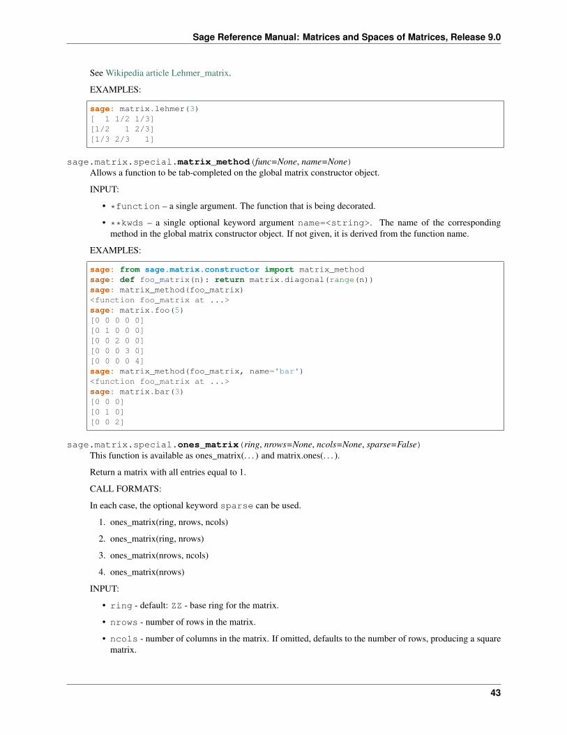
sage.matrix.special.lehmer(ring, n=0)This function is available as lehmer(. . . ) and matrix.lehmer(. . . ).
Return the 𝑛× 𝑛 Lehmer matrix.
The default ring is the rationals.
Element (𝑖, 𝑗) in the Lehmer matrix is 𝑚𝑖𝑛(𝑖, 𝑗)/𝑚𝑎𝑥(𝑖, 𝑗).
42 Chapter 3. Constructors for special matrices
Sage Reference Manual: Matrices and Spaces of Matrices, Release 9.0
See Wikipedia article Lehmer_matrix.
EXAMPLES:
sage: matrix.lehmer(3)[ 1 1/2 1/3][1/2 1 2/3][1/3 2/3 1]
sage.matrix.special.matrix_method(func=None, name=None)Allows a function to be tab-completed on the global matrix constructor object.
INPUT:
• *function – a single argument. The function that is being decorated.
• **kwds – a single optional keyword argument name=<string>. The name of the correspondingmethod in the global matrix constructor object. If not given, it is derived from the function name.
EXAMPLES:
sage: from sage.matrix.constructor import matrix_methodsage: def foo_matrix(n): return matrix.diagonal(range(n))sage: matrix_method(foo_matrix)<function foo_matrix at ...>sage: matrix.foo(5)[0 0 0 0 0][0 1 0 0 0][0 0 2 0 0][0 0 0 3 0][0 0 0 0 4]sage: matrix_method(foo_matrix, name='bar')<function foo_matrix at ...>sage: matrix.bar(3)[0 0 0][0 1 0][0 0 2]
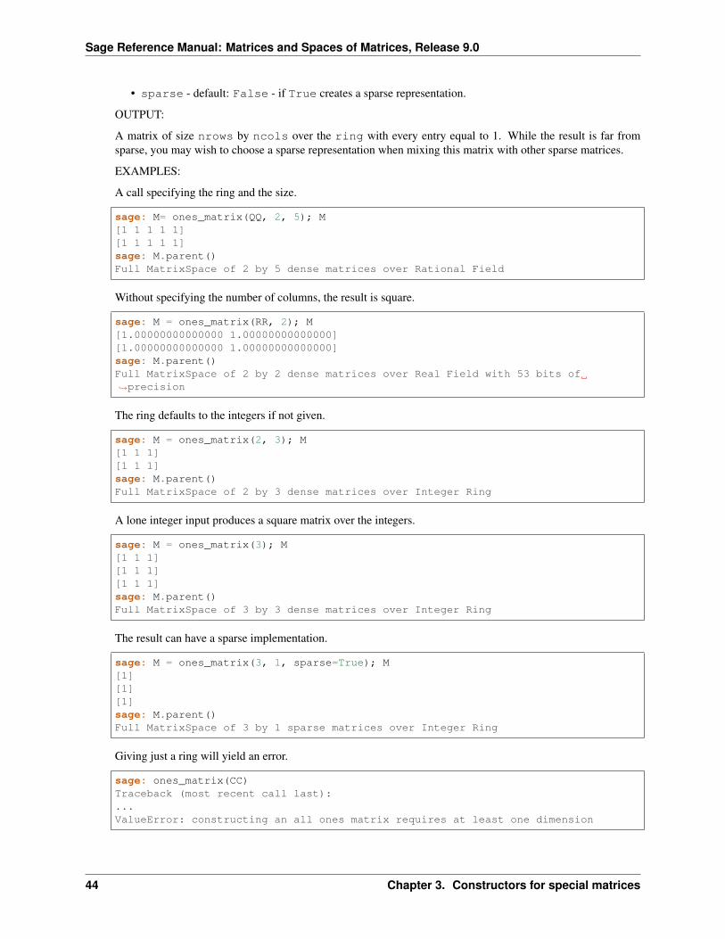
sage.matrix.special.ones_matrix(ring, nrows=None, ncols=None, sparse=False)This function is available as ones_matrix(. . . ) and matrix.ones(. . . ).
Return a matrix with all entries equal to 1.
CALL FORMATS:
In each case, the optional keyword sparse can be used.
1. ones_matrix(ring, nrows, ncols)
2. ones_matrix(ring, nrows)
3. ones_matrix(nrows, ncols)
4. ones_matrix(nrows)
INPUT:
• ring - default: ZZ - base ring for the matrix.
• nrows - number of rows in the matrix.
• ncols - number of columns in the matrix. If omitted, defaults to the number of rows, producing a squarematrix.
43
Sage Reference Manual: Matrices and Spaces of Matrices, Release 9.0
• sparse - default: False - if True creates a sparse representation.
OUTPUT:
A matrix of size nrows by ncols over the ring with every entry equal to 1. While the result is far fromsparse, you may wish to choose a sparse representation when mixing this matrix with other sparse matrices.
EXAMPLES:
A call specifying the ring and the size.
sage: M= ones_matrix(QQ, 2, 5); M[1 1 1 1 1][1 1 1 1 1]sage: M.parent()Full MatrixSpace of 2 by 5 dense matrices over Rational Field
Without specifying the number of columns, the result is square.
sage: M = ones_matrix(RR, 2); M[1.00000000000000 1.00000000000000][1.00000000000000 1.00000000000000]sage: M.parent()Full MatrixSpace of 2 by 2 dense matrices over Real Field with 53 bits of→˓precision
The ring defaults to the integers if not given.
sage: M = ones_matrix(2, 3); M[1 1 1][1 1 1]sage: M.parent()Full MatrixSpace of 2 by 3 dense matrices over Integer Ring
A lone integer input produces a square matrix over the integers.
sage: M = ones_matrix(3); M[1 1 1][1 1 1][1 1 1]sage: M.parent()Full MatrixSpace of 3 by 3 dense matrices over Integer Ring
The result can have a sparse implementation.
sage: M = ones_matrix(3, 1, sparse=True); M[1][1][1]sage: M.parent()Full MatrixSpace of 3 by 1 sparse matrices over Integer Ring
Giving just a ring will yield an error.
sage: ones_matrix(CC)Traceback (most recent call last):...ValueError: constructing an all ones matrix requires at least one dimension
44 Chapter 3. Constructors for special matrices
Sage Reference Manual: Matrices and Spaces of Matrices, Release 9.0
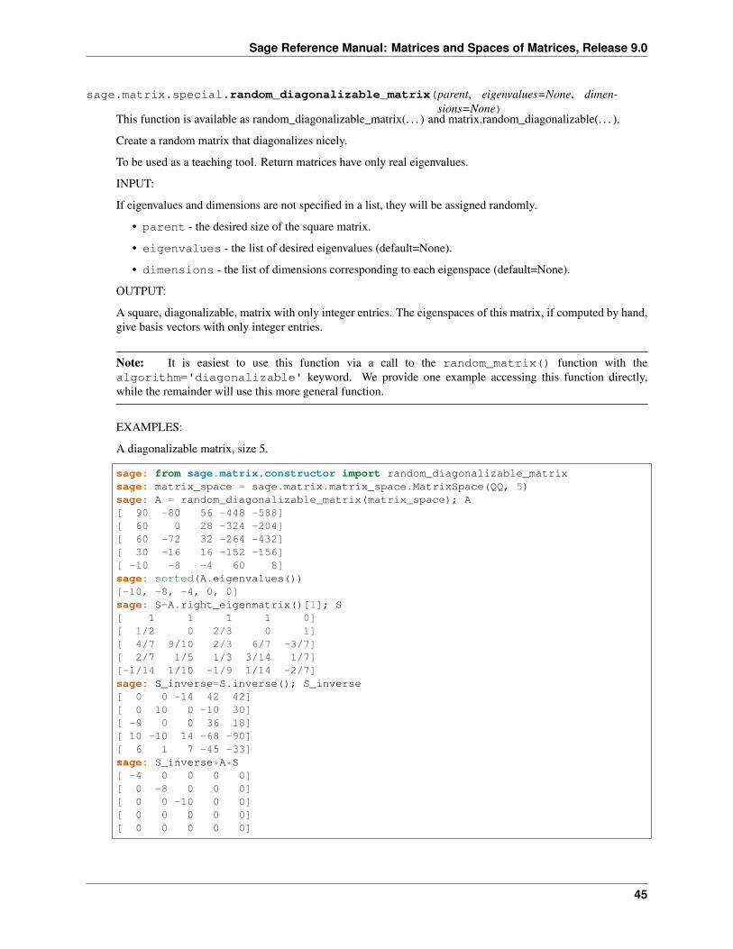
sage.matrix.special.random_diagonalizable_matrix(parent, eigenvalues=None, dimen-sions=None)
This function is available as random_diagonalizable_matrix(. . . ) and matrix.random_diagonalizable(. . . ).
Create a random matrix that diagonalizes nicely.
To be used as a teaching tool. Return matrices have only real eigenvalues.
INPUT:
If eigenvalues and dimensions are not specified in a list, they will be assigned randomly.
• parent - the desired size of the square matrix.
• eigenvalues - the list of desired eigenvalues (default=None).
• dimensions - the list of dimensions corresponding to each eigenspace (default=None).
OUTPUT:
A square, diagonalizable, matrix with only integer entries. The eigenspaces of this matrix, if computed by hand,give basis vectors with only integer entries.
Note: It is easiest to use this function via a call to the random_matrix() function with thealgorithm='diagonalizable' keyword. We provide one example accessing this function directly,while the remainder will use this more general function.
EXAMPLES:
A diagonalizable matrix, size 5.
sage: from sage.matrix.constructor import random_diagonalizable_matrixsage: matrix_space = sage.matrix.matrix_space.MatrixSpace(QQ, 5)sage: A = random_diagonalizable_matrix(matrix_space); A[ 90 -80 56 -448 -588][ 60 0 28 -324 -204][ 60 -72 32 -264 -432][ 30 -16 16 -152 -156][ -10 -8 -4 60 8]sage: sorted(A.eigenvalues())[-10, -8, -4, 0, 0]sage: S=A.right_eigenmatrix()[1]; S[ 1 1 1 1 0][ 1/2 0 2/3 0 1][ 4/7 9/10 2/3 6/7 -3/7][ 2/7 1/5 1/3 3/14 1/7][-1/14 1/10 -1/9 1/14 -2/7]sage: S_inverse=S.inverse(); S_inverse[ 0 0 -14 42 42][ 0 10 0 -10 30][ -9 0 0 36 18][ 10 -10 14 -68 -90][ 6 1 7 -45 -33]sage: S_inverse*A*S[ -4 0 0 0 0][ 0 -8 0 0 0][ 0 0 -10 0 0][ 0 0 0 0 0][ 0 0 0 0 0]
45
Sage Reference Manual: Matrices and Spaces of Matrices, Release 9.0
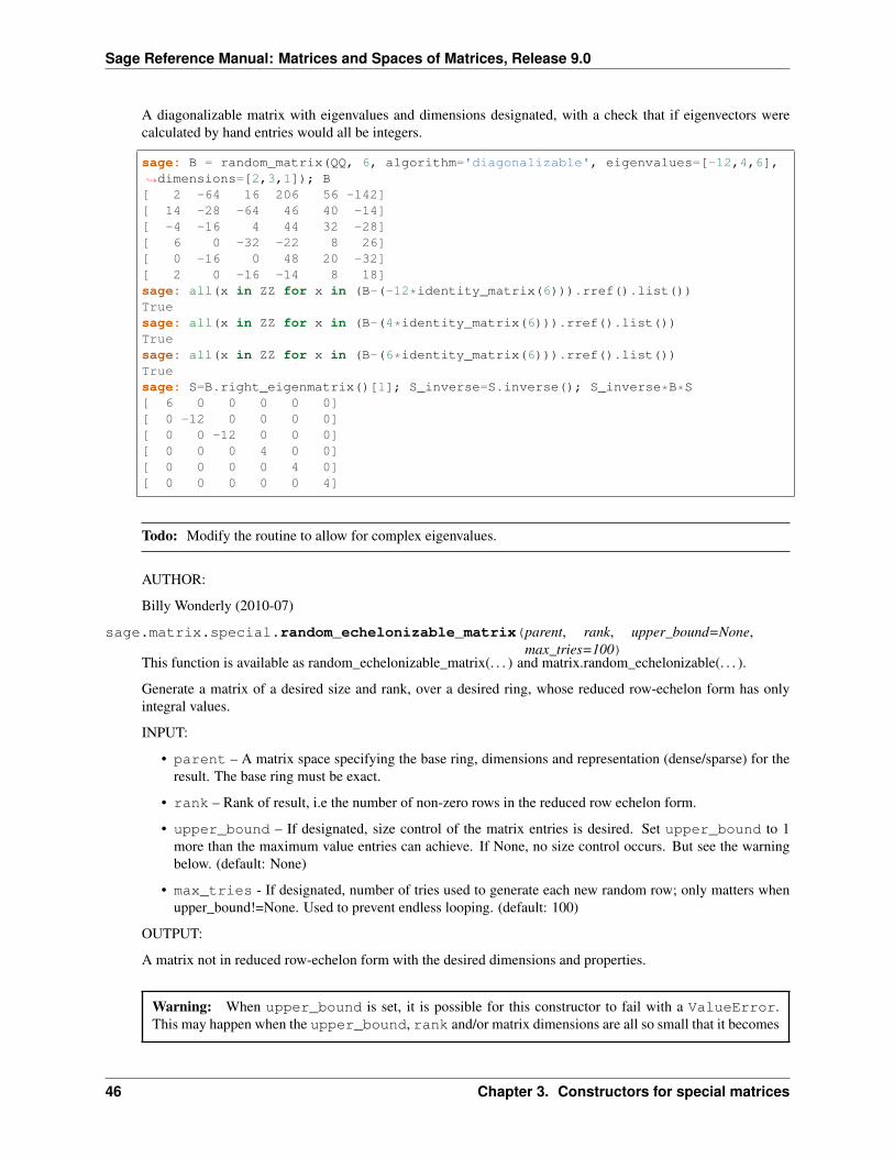
A diagonalizable matrix with eigenvalues and dimensions designated, with a check that if eigenvectors werecalculated by hand entries would all be integers.
sage: B = random_matrix(QQ, 6, algorithm='diagonalizable', eigenvalues=[-12,4,6],→˓dimensions=[2,3,1]); B[ 2 -64 16 206 56 -142][ 14 -28 -64 46 40 -14][ -4 -16 4 44 32 -28][ 6 0 -32 -22 8 26][ 0 -16 0 48 20 -32][ 2 0 -16 -14 8 18]sage: all(x in ZZ for x in (B-(-12*identity_matrix(6))).rref().list())Truesage: all(x in ZZ for x in (B-(4*identity_matrix(6))).rref().list())Truesage: all(x in ZZ for x in (B-(6*identity_matrix(6))).rref().list())Truesage: S=B.right_eigenmatrix()[1]; S_inverse=S.inverse(); S_inverse*B*S[ 6 0 0 0 0 0][ 0 -12 0 0 0 0][ 0 0 -12 0 0 0][ 0 0 0 4 0 0][ 0 0 0 0 4 0][ 0 0 0 0 0 4]
Todo: Modify the routine to allow for complex eigenvalues.
AUTHOR:
Billy Wonderly (2010-07)
sage.matrix.special.random_echelonizable_matrix(parent, rank, upper_bound=None,max_tries=100)
This function is available as random_echelonizable_matrix(. . . ) and matrix.random_echelonizable(. . . ).
Generate a matrix of a desired size and rank, over a desired ring, whose reduced row-echelon form has onlyintegral values.
INPUT:
• parent – A matrix space specifying the base ring, dimensions and representation (dense/sparse) for theresult. The base ring must be exact.
• rank – Rank of result, i.e the number of non-zero rows in the reduced row echelon form.
• upper_bound – If designated, size control of the matrix entries is desired. Set upper_bound to 1more than the maximum value entries can achieve. If None, no size control occurs. But see the warningbelow. (default: None)
• max_tries - If designated, number of tries used to generate each new random row; only matters whenupper_bound!=None. Used to prevent endless looping. (default: 100)
OUTPUT:
A matrix not in reduced row-echelon form with the desired dimensions and properties.
Warning: When upper_bound is set, it is possible for this constructor to fail with a ValueError.This may happen when the upper_bound, rank and/or matrix dimensions are all so small that it becomes
46 Chapter 3. Constructors for special matrices
Sage Reference Manual: Matrices and Spaces of Matrices, Release 9.0
infeasible or unlikely to create the requested matrix. If you must have this routine return successfully, do notset upper_bound.
Note: It is easiest to use this function via a call to the random_matrix() function with thealgorithm='echelonizable' keyword. We provide one example accessing this function directly, whilethe remainder will use this more general function.
EXAMPLES:
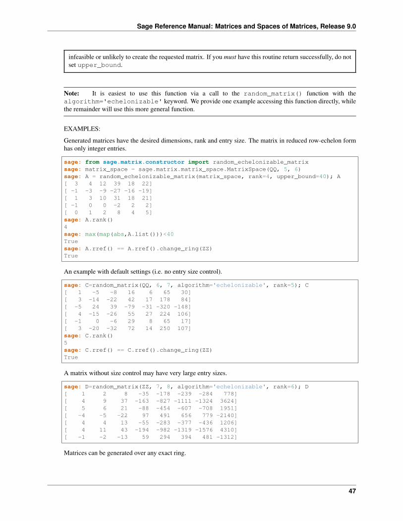
Generated matrices have the desired dimensions, rank and entry size. The matrix in reduced row-echelon formhas only integer entries.
sage: from sage.matrix.constructor import random_echelonizable_matrixsage: matrix_space = sage.matrix.matrix_space.MatrixSpace(QQ, 5, 6)sage: A = random_echelonizable_matrix(matrix_space, rank=4, upper_bound=40); A[ 3 4 12 39 18 22][ -1 -3 -9 -27 -16 -19][ 1 3 10 31 18 21][ -1 0 0 -2 2 2][ 0 1 2 8 4 5]sage: A.rank()4sage: max(map(abs,A.list()))<40Truesage: A.rref() == A.rref().change_ring(ZZ)True
An example with default settings (i.e. no entry size control).
sage: C=random_matrix(QQ, 6, 7, algorithm='echelonizable', rank=5); C[ 1 -5 -8 16 6 65 30][ 3 -14 -22 42 17 178 84][ -5 24 39 -79 -31 -320 -148][ 4 -15 -26 55 27 224 106][ -1 0 -6 29 8 65 17][ 3 -20 -32 72 14 250 107]sage: C.rank()5sage: C.rref() == C.rref().change_ring(ZZ)True
A matrix without size control may have very large entry sizes.
sage: D=random_matrix(ZZ, 7, 8, algorithm='echelonizable', rank=6); D[ 1 2 8 -35 -178 -239 -284 778][ 4 9 37 -163 -827 -1111 -1324 3624][ 5 6 21 -88 -454 -607 -708 1951][ -4 -5 -22 97 491 656 779 -2140][ 4 4 13 -55 -283 -377 -436 1206][ 4 11 43 -194 -982 -1319 -1576 4310][ -1 -2 -13 59 294 394 481 -1312]
Matrices can be generated over any exact ring.
47
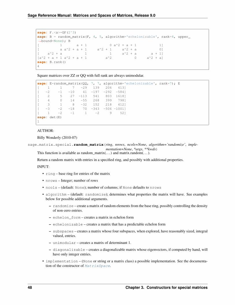
Sage Reference Manual: Matrices and Spaces of Matrices, Release 9.0
sage: F.<a>=GF(2^3)sage: B = random_matrix(F, 4, 5, algorithm='echelonizable', rank=4, upper_→˓bound=None); B[ 1 a + 1 0 a^2 + a + 1 1][ a a^2 + a + 1 a^2 + 1 a^2 + a 0][ a^2 + a 1 1 a^2 + a a + 1][a^2 + a + 1 a^2 + a + 1 a^2 0 a^2 + a]sage: B.rank()4
Square matrices over ZZ or QQ with full rank are always unimodular.
sage: E=random_matrix(QQ, 7, 7, algorithm='echelonizable', rank=7); E[ 1 1 7 -29 139 206 413][ -2 -1 -10 41 -197 -292 -584][ 2 5 27 -113 541 803 1618][ 4 0 14 -55 268 399 798][ 3 1 8 -32 152 218 412][ -3 -2 -18 70 -343 -506 -1001][ 1 -2 -1 1 -2 9 52]sage: det(E)1
AUTHOR:
Billy Wonderly (2010-07)
sage.matrix.special.random_matrix(ring, nrows, ncols=None, algorithm=’randomize’, imple-mentation=None, *args, **kwds)
This function is available as random_matrix(. . . ) and matrix.random(. . . ).
Return a random matrix with entries in a specified ring, and possibly with additional properties.
INPUT:
• ring – base ring for entries of the matrix
• nrows – Integer; number of rows
• ncols – (default: None); number of columns; if None defaults to nrows
• algorithm – (default: randomize); determines what properties the matrix will have. See examplesbelow for possible additional arguments.
– randomize – create a matrix of random elements from the base ring, possibly controlling the densityof non-zero entries.
– echelon_form – creates a matrix in echelon form
– echelonizable – creates a matrix that has a predictable echelon form
– subspaces – creates a matrix whose four subspaces, when explored, have reasonably sized, integralvalued, entries.
– unimodular – creates a matrix of determinant 1.
– diagonalizable – creates a diagonalizable matrix whose eigenvectors, if computed by hand, willhave only integer entries.
• implementation – (None or string or a matrix class) a possible implementation. See the documenta-tion of the constructor of MatrixSpace.
48 Chapter 3. Constructors for special matrices
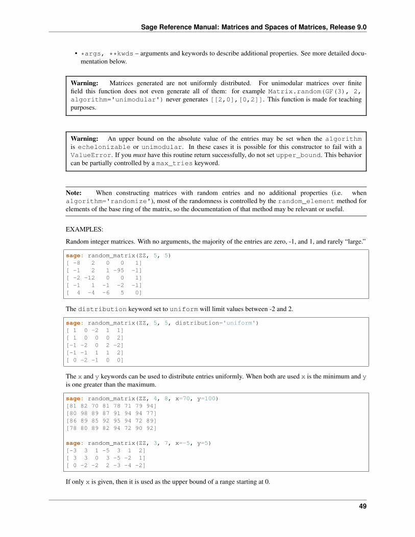
Sage Reference Manual: Matrices and Spaces of Matrices, Release 9.0
• *args, **kwds – arguments and keywords to describe additional properties. See more detailed docu-mentation below.
Warning: Matrices generated are not uniformly distributed. For unimodular matrices over finitefield this function does not even generate all of them: for example Matrix.random(GF(3), 2,algorithm='unimodular') never generates [[2,0],[0,2]]. This function is made for teachingpurposes.
Warning: An upper bound on the absolute value of the entries may be set when the algorithmis echelonizable or unimodular. In these cases it is possible for this constructor to fail with aValueError. If you must have this routine return successfully, do not set upper_bound. This behaviorcan be partially controlled by a max_tries keyword.
Note: When constructing matrices with random entries and no additional properties (i.e. whenalgorithm='randomize'), most of the randomness is controlled by the random_element method forelements of the base ring of the matrix, so the documentation of that method may be relevant or useful.
EXAMPLES:
Random integer matrices. With no arguments, the majority of the entries are zero, -1, and 1, and rarely “large.”
sage: random_matrix(ZZ, 5, 5)[ -8 2 0 0 1][ -1 2 1 -95 -1][ -2 -12 0 0 1][ -1 1 -1 -2 -1][ 4 -4 -6 5 0]
The distribution keyword set to uniform will limit values between -2 and 2.
sage: random_matrix(ZZ, 5, 5, distribution='uniform')[ 1 0 -2 1 1][ 1 0 0 0 2][-1 -2 0 2 -2][-1 -1 1 1 2][ 0 -2 -1 0 0]
The x and y keywords can be used to distribute entries uniformly. When both are used x is the minimum and yis one greater than the maximum.
sage: random_matrix(ZZ, 4, 8, x=70, y=100)[81 82 70 81 78 71 79 94][80 98 89 87 91 94 94 77][86 89 85 92 95 94 72 89][78 80 89 82 94 72 90 92]
sage: random_matrix(ZZ, 3, 7, x=-5, y=5)[-3 3 1 -5 3 1 2][ 3 3 0 3 -5 -2 1][ 0 -2 -2 2 -3 -4 -2]
If only x is given, then it is used as the upper bound of a range starting at 0.
49
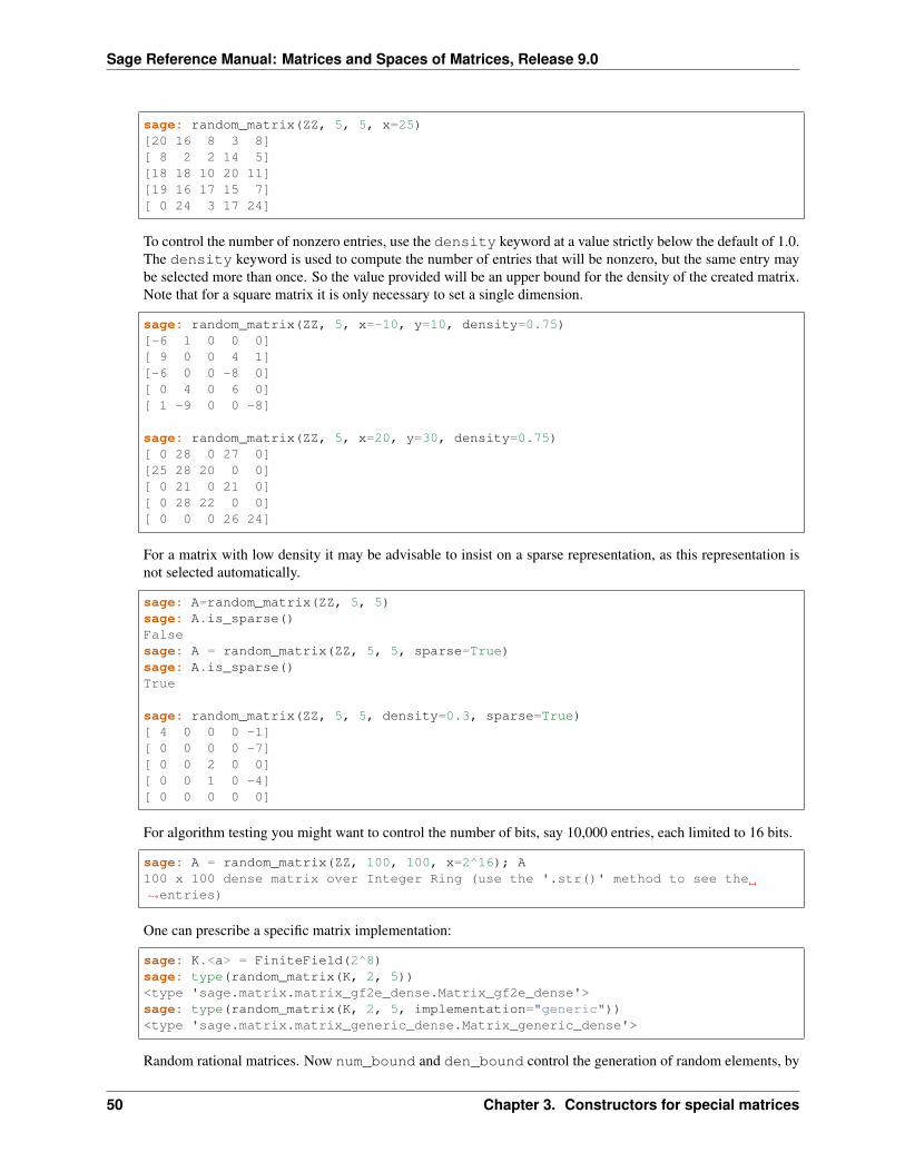
Sage Reference Manual: Matrices and Spaces of Matrices, Release 9.0
sage: random_matrix(ZZ, 5, 5, x=25)[20 16 8 3 8][ 8 2 2 14 5][18 18 10 20 11][19 16 17 15 7][ 0 24 3 17 24]
To control the number of nonzero entries, use the density keyword at a value strictly below the default of 1.0.The density keyword is used to compute the number of entries that will be nonzero, but the same entry maybe selected more than once. So the value provided will be an upper bound for the density of the created matrix.Note that for a square matrix it is only necessary to set a single dimension.
sage: random_matrix(ZZ, 5, x=-10, y=10, density=0.75)[-6 1 0 0 0][ 9 0 0 4 1][-6 0 0 -8 0][ 0 4 0 6 0][ 1 -9 0 0 -8]
sage: random_matrix(ZZ, 5, x=20, y=30, density=0.75)[ 0 28 0 27 0][25 28 20 0 0][ 0 21 0 21 0][ 0 28 22 0 0][ 0 0 0 26 24]
For a matrix with low density it may be advisable to insist on a sparse representation, as this representation isnot selected automatically.
sage: A=random_matrix(ZZ, 5, 5)sage: A.is_sparse()Falsesage: A = random_matrix(ZZ, 5, 5, sparse=True)sage: A.is_sparse()True
sage: random_matrix(ZZ, 5, 5, density=0.3, sparse=True)[ 4 0 0 0 -1][ 0 0 0 0 -7][ 0 0 2 0 0][ 0 0 1 0 -4][ 0 0 0 0 0]
For algorithm testing you might want to control the number of bits, say 10,000 entries, each limited to 16 bits.
sage: A = random_matrix(ZZ, 100, 100, x=2^16); A100 x 100 dense matrix over Integer Ring (use the '.str()' method to see the→˓entries)
One can prescribe a specific matrix implementation:
sage: K.<a> = FiniteField(2^8)sage: type(random_matrix(K, 2, 5))<type 'sage.matrix.matrix_gf2e_dense.Matrix_gf2e_dense'>sage: type(random_matrix(K, 2, 5, implementation="generic"))<type 'sage.matrix.matrix_generic_dense.Matrix_generic_dense'>
Random rational matrices. Now num_bound and den_bound control the generation of random elements, by
50 Chapter 3. Constructors for special matrices
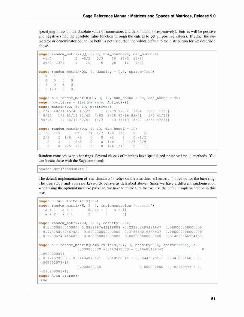
Sage Reference Manual: Matrices and Spaces of Matrices, Release 9.0
specifying limits on the absolute value of numerators and denominators (respectively). Entries will be positiveand negative (map the absolute value function through the entries to get all positive values). If either the nu-merator or denominator bound (or both) is not used, then the values default to the distribution for ZZ describedabove.
sage: random_matrix(QQ, 2, 8, num_bound=20, den_bound=4)[ -1/4 5 5 -9/2 5/3 19 15/2 19/2][ 20/3 -13/4 0 16 -5 -20 -11 -7/3]
sage: random_matrix(QQ, 4, density = 0.5, sparse=True)[ 0 1 0 -1][ 0 0 0 0][ 6 0 3 0][ 1 1/3 0 0]
sage: A = random_matrix(QQ, 3, 10, num_bound = 99, den_bound = 99)sage: positives = list(map(abs, A.list()))sage: matrix(QQ, 3, 10, positives)[ 2/45 40/21 45/46 17/22 1 70/79 97/71 7/24 12/5 13/8][ 8/25 1/3 61/14 92/45 4/85 3/38 95/16 82/71 1/5 41/16][55/76 19 28/41 52/51 14/3 43 76/13 8/77 13/38 37/21]
sage: random_matrix(QQ, 4, 10, den_bound = 10)[ 1/9 1/5 -1 2/9 1/4 -1/7 1/8 -1/9 0 2][ 2/3 2 1/8 -2 0 0 -2 2 0 -1/2][ 0 2 1 -2/3 0 0 1/6 0 -1/3 -2/9][ 0 0 2/5 1/9 0 0 1/6 1/10 0 1]
Random matrices over other rings. Several classes of matrices have specialized randomize() methods. Youcan locate these with the Sage command:
search_def('randomize')
The default implementation of randomize() relies on the random_element() method for the base ring.The density and sparse keywords behave as described above. Since we have a different randomisationwhen using the optional meataxe package, we have to make sure that we use the default implementation in thistest:
sage: K.<a>=FiniteField(3^2)sage: random_matrix(K, 2, 5, implementation='generic')[ a + 1 a + 1 0 2*a + 2 a + 1][ a + 2 a + 1 2 0 0]
sage: random_matrix(RR, 3, 4, density=0.66)[ 0.000000000000000 0.0869697644118808 -0.232952499486647 0.000000000000000][-0.793158962467820 0.000000000000000 0.318853016385637 0.000000000000000][-0.220342454156035 0.000000000000000 0.000000000000000 0.914890766754157]
sage: A = random_matrix(ComplexField(32), 3, density=0.8, sparse=True); A[ 0.000000000 -0.443499553 - 0.406854867*I 0.→˓000000000][ 0.171578609 + 0.644048756*I 0.518523841 + 0.794429291*I -0.341030168 - 0.→˓507791873*I][ 0.000000000 0.000000000 0.782759943 + 0.→˓236288982*I]sage: A.is_sparse()True
51
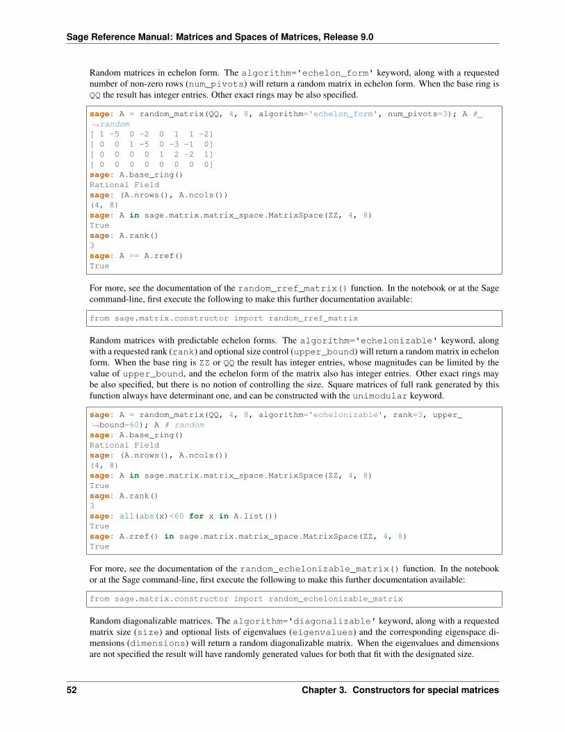
Sage Reference Manual: Matrices and Spaces of Matrices, Release 9.0
Random matrices in echelon form. The algorithm='echelon_form' keyword, along with a requestednumber of non-zero rows (num_pivots) will return a random matrix in echelon form. When the base ring isQQ the result has integer entries. Other exact rings may be also specified.
sage: A = random_matrix(QQ, 4, 8, algorithm='echelon_form', num_pivots=3); A #→˓random[ 1 -5 0 -2 0 1 1 -2][ 0 0 1 -5 0 -3 -1 0][ 0 0 0 0 1 2 -2 1][ 0 0 0 0 0 0 0 0]sage: A.base_ring()Rational Fieldsage: (A.nrows(), A.ncols())(4, 8)sage: A in sage.matrix.matrix_space.MatrixSpace(ZZ, 4, 8)Truesage: A.rank()3sage: A == A.rref()True
For more, see the documentation of the random_rref_matrix() function. In the notebook or at the Sagecommand-line, first execute the following to make this further documentation available:
from sage.matrix.constructor import random_rref_matrix
Random matrices with predictable echelon forms. The algorithm='echelonizable' keyword, alongwith a requested rank (rank) and optional size control (upper_bound) will return a random matrix in echelonform. When the base ring is ZZ or QQ the result has integer entries, whose magnitudes can be limited by thevalue of upper_bound, and the echelon form of the matrix also has integer entries. Other exact rings maybe also specified, but there is no notion of controlling the size. Square matrices of full rank generated by thisfunction always have determinant one, and can be constructed with the unimodular keyword.
sage: A = random_matrix(QQ, 4, 8, algorithm='echelonizable', rank=3, upper_→˓bound=60); A # randomsage: A.base_ring()Rational Fieldsage: (A.nrows(), A.ncols())(4, 8)sage: A in sage.matrix.matrix_space.MatrixSpace(ZZ, 4, 8)Truesage: A.rank()3sage: all(abs(x)<60 for x in A.list())Truesage: A.rref() in sage.matrix.matrix_space.MatrixSpace(ZZ, 4, 8)True
For more, see the documentation of the random_echelonizable_matrix() function. In the notebookor at the Sage command-line, first execute the following to make this further documentation available:
from sage.matrix.constructor import random_echelonizable_matrix
Random diagonalizable matrices. The algorithm='diagonalizable' keyword, along with a requestedmatrix size (size) and optional lists of eigenvalues (eigenvalues) and the corresponding eigenspace di-mensions (dimensions) will return a random diagonalizable matrix. When the eigenvalues and dimensionsare not specified the result will have randomly generated values for both that fit with the designated size.
52 Chapter 3. Constructors for special matrices
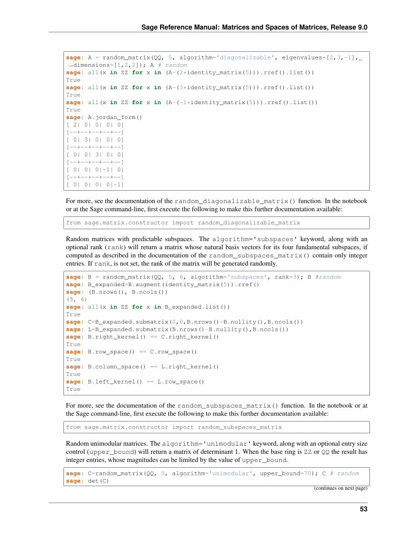
Sage Reference Manual: Matrices and Spaces of Matrices, Release 9.0
sage: A = random_matrix(QQ, 5, algorithm='diagonalizable', eigenvalues=[2,3,-1],→˓dimensions=[1,2,2]); A # randomsage: all(x in ZZ for x in (A-(2*identity_matrix(5))).rref().list())Truesage: all(x in ZZ for x in (A-(3*identity_matrix(5))).rref().list())Truesage: all(x in ZZ for x in (A-(-1*identity_matrix(5))).rref().list())Truesage: A.jordan_form()[ 2| 0| 0| 0| 0][--+--+--+--+--][ 0| 3| 0| 0| 0][--+--+--+--+--][ 0| 0| 3| 0| 0][--+--+--+--+--][ 0| 0| 0|-1| 0][--+--+--+--+--][ 0| 0| 0| 0|-1]
For more, see the documentation of the random_diagonalizable_matrix() function. In the notebookor at the Sage command-line, first execute the following to make this further documentation available:
from sage.matrix.constructor import random_diagonalizable_matrix
Random matrices with predictable subspaces. The algorithm='subspaces' keyword, along with anoptional rank (rank) will return a matrix whose natural basis vectors for its four fundamental subspaces, ifcomputed as described in the documentation of the random_subspaces_matrix() contain only integerentries. If rank, is not set, the rank of the matrix will be generated randomly.
sage: B = random_matrix(QQ, 5, 6, algorithm='subspaces', rank=3); B #randomsage: B_expanded=B.augment(identity_matrix(5)).rref()sage: (B.nrows(), B.ncols())(5, 6)sage: all(x in ZZ for x in B_expanded.list())Truesage: C=B_expanded.submatrix(0,0,B.nrows()-B.nullity(),B.ncols())sage: L=B_expanded.submatrix(B.nrows()-B.nullity(),B.ncols())sage: B.right_kernel() == C.right_kernel()Truesage: B.row_space() == C.row_space()Truesage: B.column_space() == L.right_kernel()Truesage: B.left_kernel() == L.row_space()True
For more, see the documentation of the random_subspaces_matrix() function. In the notebook or atthe Sage command-line, first execute the following to make this further documentation available:
from sage.matrix.constructor import random_subspaces_matrix
Random unimodular matrices. The algorithm='unimodular' keyword, along with an optional entry sizecontrol (upper_bound) will return a matrix of determinant 1. When the base ring is ZZ or QQ the result hasinteger entries, whose magnitudes can be limited by the value of upper_bound.
sage: C=random_matrix(QQ, 5, algorithm='unimodular', upper_bound=70); C # randomsage: det(C)
(continues on next page)
53
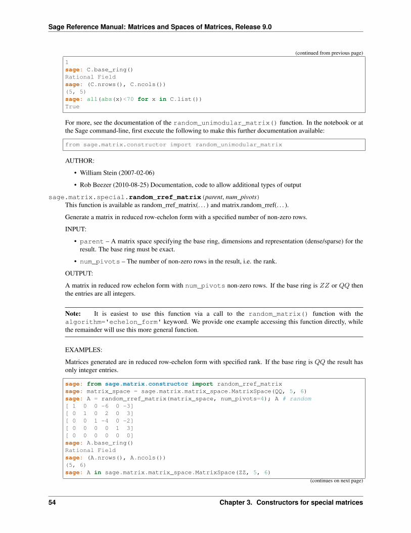
Sage Reference Manual: Matrices and Spaces of Matrices, Release 9.0
(continued from previous page)
1sage: C.base_ring()Rational Fieldsage: (C.nrows(), C.ncols())(5, 5)sage: all(abs(x)<70 for x in C.list())True
For more, see the documentation of the random_unimodular_matrix() function. In the notebook or atthe Sage command-line, first execute the following to make this further documentation available:
from sage.matrix.constructor import random_unimodular_matrix
AUTHOR:
• William Stein (2007-02-06)
• Rob Beezer (2010-08-25) Documentation, code to allow additional types of output
sage.matrix.special.random_rref_matrix(parent, num_pivots)This function is available as random_rref_matrix(. . . ) and matrix.random_rref(. . . ).
Generate a matrix in reduced row-echelon form with a specified number of non-zero rows.
INPUT:
• parent – A matrix space specifying the base ring, dimensions and representation (dense/sparse) for theresult. The base ring must be exact.
• num_pivots – The number of non-zero rows in the result, i.e. the rank.
OUTPUT:
A matrix in reduced row echelon form with num_pivots non-zero rows. If the base ring is 𝑍𝑍 or 𝑄𝑄 thenthe entries are all integers.
Note: It is easiest to use this function via a call to the random_matrix() function with thealgorithm='echelon_form' keyword. We provide one example accessing this function directly, whilethe remainder will use this more general function.
EXAMPLES:
Matrices generated are in reduced row-echelon form with specified rank. If the base ring is 𝑄𝑄 the result hasonly integer entries.
sage: from sage.matrix.constructor import random_rref_matrixsage: matrix_space = sage.matrix.matrix_space.MatrixSpace(QQ, 5, 6)sage: A = random_rref_matrix(matrix_space, num_pivots=4); A # random[ 1 0 0 -6 0 -3][ 0 1 0 2 0 3][ 0 0 1 -4 0 -2][ 0 0 0 0 1 3][ 0 0 0 0 0 0]sage: A.base_ring()Rational Fieldsage: (A.nrows(), A.ncols())(5, 6)sage: A in sage.matrix.matrix_space.MatrixSpace(ZZ, 5, 6)
(continues on next page)
54 Chapter 3. Constructors for special matrices
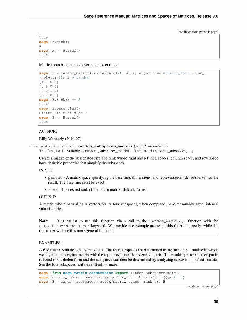
Sage Reference Manual: Matrices and Spaces of Matrices, Release 9.0
(continued from previous page)
Truesage: A.rank()4sage: A == A.rref()True
Matrices can be generated over other exact rings.
sage: B = random_matrix(FiniteField(7), 4, 4, algorithm='echelon_form', num_→˓pivots=3); B # random[1 0 0 0][0 1 0 6][0 0 1 4][0 0 0 0]sage: B.rank() == 3Truesage: B.base_ring()Finite Field of size 7sage: B == B.rref()True
AUTHOR:
Billy Wonderly (2010-07)
sage.matrix.special.random_subspaces_matrix(parent, rank=None)This function is available as random_subspaces_matrix(. . . ) and matrix.random_subspaces(. . . ).
Create a matrix of the designated size and rank whose right and left null spaces, column space, and row spacehave desirable properties that simplify the subspaces.
INPUT:
• parent - A matrix space specifying the base ring, dimensions, and representation (dense/sparse) for theresult. The base ring must be exact.
• rank - The desired rank of the return matrix (default: None).
OUTPUT:
A matrix whose natural basis vectors for its four subspaces, when computed, have reasonably sized, integralvalued, entries.
Note: It is easiest to use this function via a call to the random_matrix() function with thealgorithm='subspaces' keyword. We provide one example accessing this function directly, while theremainder will use this more general function.
EXAMPLES:
A 6x8 matrix with designated rank of 3. The four subspaces are determined using one simple routine in whichwe augment the original matrix with the equal row dimension identity matrix. The resulting matrix is then put inreduced row-echelon form and the subspaces can then be determined by analyzing subdivisions of this matrix.See the four subspaces routine in [Bee] for more.
sage: from sage.matrix.constructor import random_subspaces_matrixsage: matrix_space = sage.matrix.matrix_space.MatrixSpace(QQ, 6, 8)sage: B = random_subspaces_matrix(matrix_space, rank=3); B
(continues on next page)
55
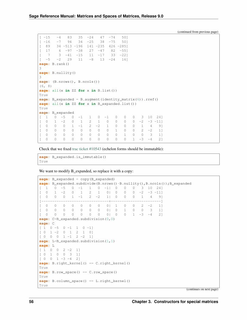
Sage Reference Manual: Matrices and Spaces of Matrices, Release 9.0
(continued from previous page)
[ -15 -4 83 35 -24 47 -74 50][ -16 -7 94 34 -25 38 -75 50][ 89 34 -513 -196 141 -235 426 -285][ 17 6 -97 -38 27 -47 82 -55][ 7 3 -41 -15 11 -17 33 -22][ -5 -2 29 11 -8 13 -24 16]sage: B.rank()3sage: B.nullity()3sage: (B.nrows(), B.ncols())(6, 8)sage: all(x in ZZ for x in B.list())Truesage: B_expanded = B.augment(identity_matrix(6)).rref()sage: all(x in ZZ for x in B_expanded.list())Truesage: B_expanded[ 1 0 -5 0 -1 1 0 -1 0 0 0 3 10 24][ 0 1 -2 0 1 2 1 0 0 0 0 -2 -3 -11][ 0 0 0 1 -1 2 -2 1 0 0 0 1 4 9][ 0 0 0 0 0 0 0 0 1 0 0 2 -2 1][ 0 0 0 0 0 0 0 0 0 1 0 0 3 1][ 0 0 0 0 0 0 0 0 0 0 1 -3 -4 2]
Check that we fixed trac ticket #10543 (echelon forms should be immutable):
sage: B_expanded.is_immutable()True
We want to modify B_expanded, so replace it with a copy:
sage: B_expanded = copy(B_expanded)sage: B_expanded.subdivide(B.nrows()-B.nullity(),B.ncols());B_expanded[ 1 0 -5 0 -1 1 0 -1| 0 0 0 3 10 24][ 0 1 -2 0 1 2 1 0| 0 0 0 -2 -3 -11][ 0 0 0 1 -1 2 -2 1| 0 0 0 1 4 9][-------------------------------+-----------------------][ 0 0 0 0 0 0 0 0| 1 0 0 2 -2 1][ 0 0 0 0 0 0 0 0| 0 1 0 0 3 1][ 0 0 0 0 0 0 0 0| 0 0 1 -3 -4 2]sage: C=B_expanded.subdivision(0,0)sage: C[ 1 0 -5 0 -1 1 0 -1][ 0 1 -2 0 1 2 1 0][ 0 0 0 1 -1 2 -2 1]sage: L=B_expanded.subdivision(1,1)sage: L[ 1 0 0 2 -2 1][ 0 1 0 0 3 1][ 0 0 1 -3 -4 2]sage: B.right_kernel() == C.right_kernel()Truesage: B.row_space() == C.row_space()Truesage: B.column_space() == L.right_kernel()True
(continues on next page)
56 Chapter 3. Constructors for special matrices
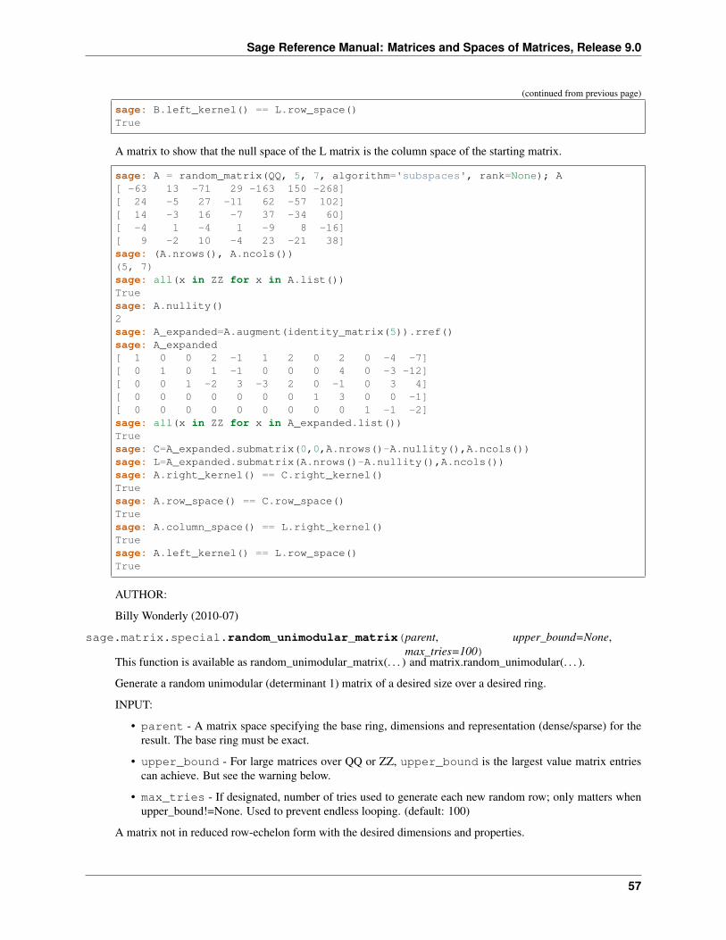
Sage Reference Manual: Matrices and Spaces of Matrices, Release 9.0
(continued from previous page)
sage: B.left_kernel() == L.row_space()True
A matrix to show that the null space of the L matrix is the column space of the starting matrix.
sage: A = random_matrix(QQ, 5, 7, algorithm='subspaces', rank=None); A[ -63 13 -71 29 -163 150 -268][ 24 -5 27 -11 62 -57 102][ 14 -3 16 -7 37 -34 60][ -4 1 -4 1 -9 8 -16][ 9 -2 10 -4 23 -21 38]sage: (A.nrows(), A.ncols())(5, 7)sage: all(x in ZZ for x in A.list())Truesage: A.nullity()2sage: A_expanded=A.augment(identity_matrix(5)).rref()sage: A_expanded[ 1 0 0 2 -1 1 2 0 2 0 -4 -7][ 0 1 0 1 -1 0 0 0 4 0 -3 -12][ 0 0 1 -2 3 -3 2 0 -1 0 3 4][ 0 0 0 0 0 0 0 1 3 0 0 -1][ 0 0 0 0 0 0 0 0 0 1 -1 -2]sage: all(x in ZZ for x in A_expanded.list())Truesage: C=A_expanded.submatrix(0,0,A.nrows()-A.nullity(),A.ncols())sage: L=A_expanded.submatrix(A.nrows()-A.nullity(),A.ncols())sage: A.right_kernel() == C.right_kernel()Truesage: A.row_space() == C.row_space()Truesage: A.column_space() == L.right_kernel()Truesage: A.left_kernel() == L.row_space()True
AUTHOR:
Billy Wonderly (2010-07)
sage.matrix.special.random_unimodular_matrix(parent, upper_bound=None,max_tries=100)
This function is available as random_unimodular_matrix(. . . ) and matrix.random_unimodular(. . . ).
Generate a random unimodular (determinant 1) matrix of a desired size over a desired ring.
INPUT:
• parent - A matrix space specifying the base ring, dimensions and representation (dense/sparse) for theresult. The base ring must be exact.
• upper_bound - For large matrices over QQ or ZZ, upper_bound is the largest value matrix entriescan achieve. But see the warning below.
• max_tries - If designated, number of tries used to generate each new random row; only matters whenupper_bound!=None. Used to prevent endless looping. (default: 100)
A matrix not in reduced row-echelon form with the desired dimensions and properties.
57
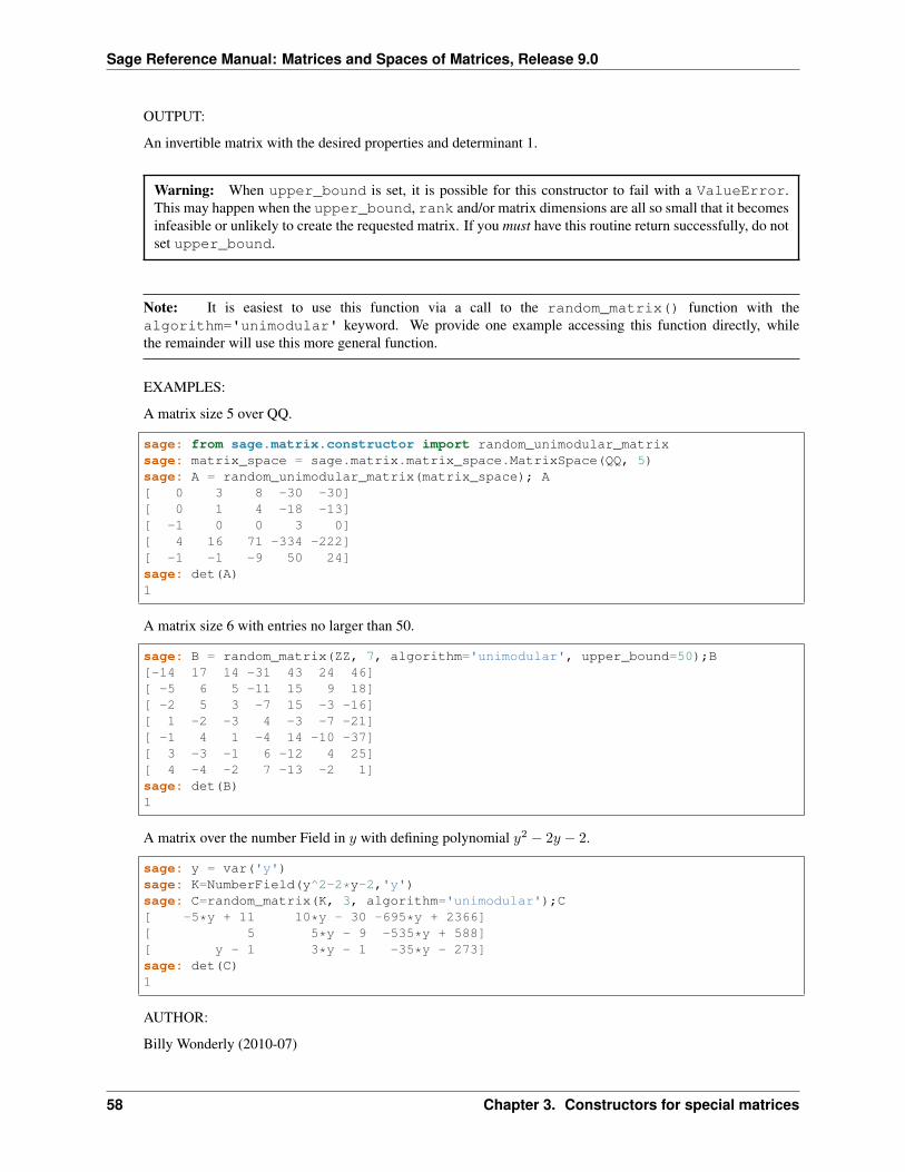
Sage Reference Manual: Matrices and Spaces of Matrices, Release 9.0
OUTPUT:
An invertible matrix with the desired properties and determinant 1.
Warning: When upper_bound is set, it is possible for this constructor to fail with a ValueError.This may happen when the upper_bound, rank and/or matrix dimensions are all so small that it becomesinfeasible or unlikely to create the requested matrix. If you must have this routine return successfully, do notset upper_bound.
Note: It is easiest to use this function via a call to the random_matrix() function with thealgorithm='unimodular' keyword. We provide one example accessing this function directly, whilethe remainder will use this more general function.
EXAMPLES:
A matrix size 5 over QQ.
sage: from sage.matrix.constructor import random_unimodular_matrixsage: matrix_space = sage.matrix.matrix_space.MatrixSpace(QQ, 5)sage: A = random_unimodular_matrix(matrix_space); A[ 0 3 8 -30 -30][ 0 1 4 -18 -13][ -1 0 0 3 0][ 4 16 71 -334 -222][ -1 -1 -9 50 24]sage: det(A)1
A matrix size 6 with entries no larger than 50.
sage: B = random_matrix(ZZ, 7, algorithm='unimodular', upper_bound=50);B[-14 17 14 -31 43 24 46][ -5 6 5 -11 15 9 18][ -2 5 3 -7 15 -3 -16][ 1 -2 -3 4 -3 -7 -21][ -1 4 1 -4 14 -10 -37][ 3 -3 -1 6 -12 4 25][ 4 -4 -2 7 -13 -2 1]sage: det(B)1
A matrix over the number Field in 𝑦 with defining polynomial 𝑦2 − 2𝑦 − 2.
sage: y = var('y')sage: K=NumberField(y^2-2*y-2,'y')sage: C=random_matrix(K, 3, algorithm='unimodular');C[ -5*y + 11 10*y - 30 -695*y + 2366][ 5 5*y - 9 -535*y + 588][ y - 1 3*y - 1 -35*y - 273]sage: det(C)1
AUTHOR:
Billy Wonderly (2010-07)
58 Chapter 3. Constructors for special matrices
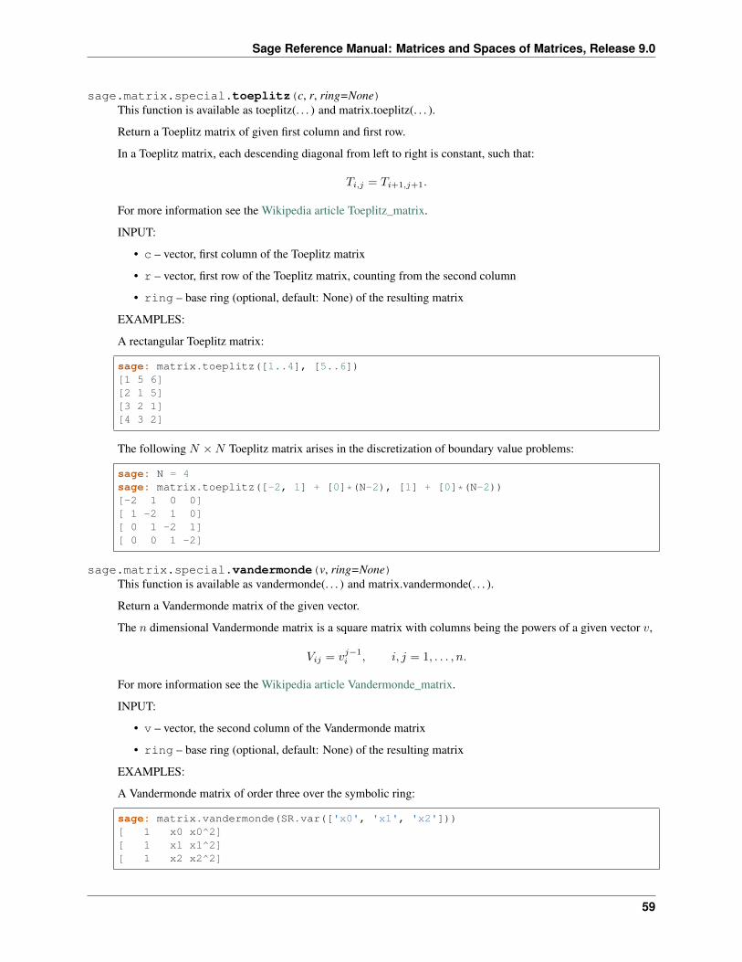
Sage Reference Manual: Matrices and Spaces of Matrices, Release 9.0
sage.matrix.special.toeplitz(c, r, ring=None)This function is available as toeplitz(. . . ) and matrix.toeplitz(. . . ).
Return a Toeplitz matrix of given first column and first row.
In a Toeplitz matrix, each descending diagonal from left to right is constant, such that:
𝑇𝑖,𝑗 = 𝑇𝑖+1,𝑗+1.
For more information see the Wikipedia article Toeplitz_matrix.
INPUT:
• c – vector, first column of the Toeplitz matrix
• r – vector, first row of the Toeplitz matrix, counting from the second column
• ring – base ring (optional, default: None) of the resulting matrix
EXAMPLES:
A rectangular Toeplitz matrix:
sage: matrix.toeplitz([1..4], [5..6])[1 5 6][2 1 5][3 2 1][4 3 2]
The following 𝑁 ×𝑁 Toeplitz matrix arises in the discretization of boundary value problems:
sage: N = 4sage: matrix.toeplitz([-2, 1] + [0]*(N-2), [1] + [0]*(N-2))[-2 1 0 0][ 1 -2 1 0][ 0 1 -2 1][ 0 0 1 -2]
sage.matrix.special.vandermonde(v, ring=None)This function is available as vandermonde(. . . ) and matrix.vandermonde(. . . ).
Return a Vandermonde matrix of the given vector.
The 𝑛 dimensional Vandermonde matrix is a square matrix with columns being the powers of a given vector 𝑣,
𝑉𝑖𝑗 = 𝑣𝑗−1𝑖 , 𝑖, 𝑗 = 1, . . . , 𝑛.
For more information see the Wikipedia article Vandermonde_matrix.
INPUT:
• v – vector, the second column of the Vandermonde matrix
• ring – base ring (optional, default: None) of the resulting matrix
EXAMPLES:
A Vandermonde matrix of order three over the symbolic ring:
sage: matrix.vandermonde(SR.var(['x0', 'x1', 'x2']))[ 1 x0 x0^2][ 1 x1 x1^2][ 1 x2 x2^2]
59
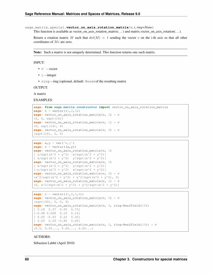
Sage Reference Manual: Matrices and Spaces of Matrices, Release 9.0
sage.matrix.special.vector_on_axis_rotation_matrix(v, i, ring=None)This function is available as vector_on_axis_rotation_matrix(. . . ) and matrix.vector_on_axis_rotation(. . . ).
Return a rotation matrix 𝑀 such that 𝑑𝑒𝑡(𝑀) = 1 sending the vector 𝑣 on the i-th axis so that all othercoordinates of 𝑀𝑣 are zero.
Note: Such a matrix is not uniquely determined. This function returns one such matrix.
INPUT:
• v` – vector
• i – integer
• ring – ring (optional, default: None) of the resulting matrix
OUTPUT:
A matrix
EXAMPLES:
sage: from sage.matrix.constructor import vector_on_axis_rotation_matrixsage: v = vector((1,2,3))sage: vector_on_axis_rotation_matrix(v, 2) * v(0, 0, sqrt(14))sage: vector_on_axis_rotation_matrix(v, 1) * v(0, sqrt(14), 0)sage: vector_on_axis_rotation_matrix(v, 0) * v(sqrt(14), 0, 0)
sage: x,y = var('x,y')sage: v = vector((x,y))sage: vector_on_axis_rotation_matrix(v, 1)[ y/sqrt(x^2 + y^2) -x/sqrt(x^2 + y^2)][ x/sqrt(x^2 + y^2) y/sqrt(x^2 + y^2)]sage: vector_on_axis_rotation_matrix(v, 0)[ x/sqrt(x^2 + y^2) y/sqrt(x^2 + y^2)][-y/sqrt(x^2 + y^2) x/sqrt(x^2 + y^2)]sage: vector_on_axis_rotation_matrix(v, 0) * v(x^2/sqrt(x^2 + y^2) + y^2/sqrt(x^2 + y^2), 0)sage: vector_on_axis_rotation_matrix(v, 1) * v(0, x^2/sqrt(x^2 + y^2) + y^2/sqrt(x^2 + y^2))
sage: v = vector((1,2,3,4))sage: vector_on_axis_rotation_matrix(v, 0) * v(sqrt(30), 0, 0, 0)sage: vector_on_axis_rotation_matrix(v, 0, ring=RealField(10))[ 0.18 0.37 0.55 0.73][-0.98 0.068 0.10 0.14][ 0.00 -0.93 0.22 0.30][ 0.00 0.00 -0.80 0.60]sage: vector_on_axis_rotation_matrix(v, 0, ring=RealField(10)) * v(5.5, 0.00..., 0.00..., 0.00...)
AUTHORS:
Sébastien Labbé (April 2010)
60 Chapter 3. Constructors for special matrices
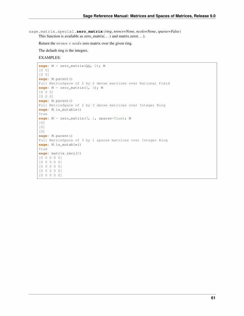
Sage Reference Manual: Matrices and Spaces of Matrices, Release 9.0
sage.matrix.special.zero_matrix(ring, nrows=None, ncols=None, sparse=False)This function is available as zero_matrix(. . . ) and matrix.zero(. . . ).
Return the 𝑛𝑟𝑜𝑤𝑠× 𝑛𝑐𝑜𝑙𝑠 zero matrix over the given ring.
The default ring is the integers.
EXAMPLES:
sage: M = zero_matrix(QQ, 2); M[0 0][0 0]sage: M.parent()Full MatrixSpace of 2 by 2 dense matrices over Rational Fieldsage: M = zero_matrix(2, 3); M[0 0 0][0 0 0]sage: M.parent()Full MatrixSpace of 2 by 3 dense matrices over Integer Ringsage: M.is_mutable()Truesage: M = zero_matrix(3, 1, sparse=True); M[0][0][0]sage: M.parent()Full MatrixSpace of 3 by 1 sparse matrices over Integer Ringsage: M.is_mutable()Truesage: matrix.zero(5)[0 0 0 0 0][0 0 0 0 0][0 0 0 0 0][0 0 0 0 0][0 0 0 0 0]
61

Sage Reference Manual: Matrices and Spaces of Matrices, Release 9.0
62 Chapter 3. Constructors for special matrices
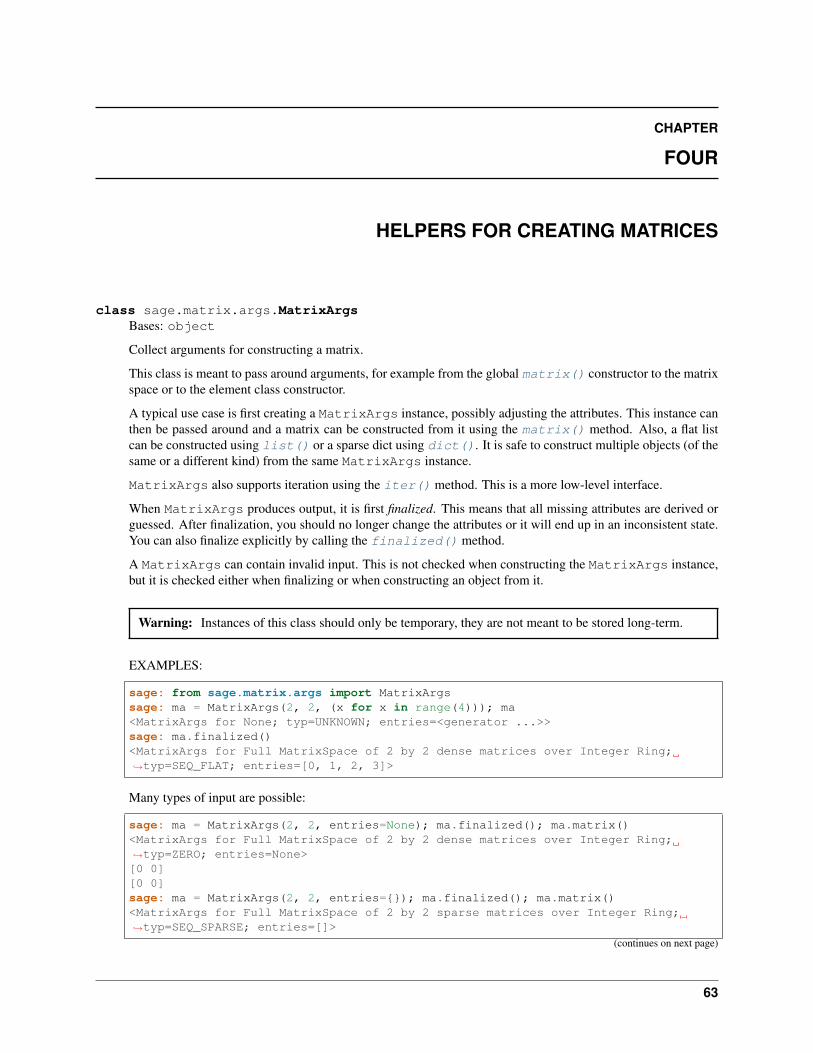
CHAPTER
FOUR
HELPERS FOR CREATING MATRICES
class sage.matrix.args.MatrixArgsBases: object
Collect arguments for constructing a matrix.
This class is meant to pass around arguments, for example from the global matrix() constructor to the matrixspace or to the element class constructor.
A typical use case is first creating a MatrixArgs instance, possibly adjusting the attributes. This instance canthen be passed around and a matrix can be constructed from it using the matrix() method. Also, a flat listcan be constructed using list() or a sparse dict using dict(). It is safe to construct multiple objects (of thesame or a different kind) from the same MatrixArgs instance.
MatrixArgs also supports iteration using the iter() method. This is a more low-level interface.
When MatrixArgs produces output, it is first finalized. This means that all missing attributes are derived orguessed. After finalization, you should no longer change the attributes or it will end up in an inconsistent state.You can also finalize explicitly by calling the finalized() method.
A MatrixArgs can contain invalid input. This is not checked when constructing the MatrixArgs instance,but it is checked either when finalizing or when constructing an object from it.
Warning: Instances of this class should only be temporary, they are not meant to be stored long-term.
EXAMPLES:
sage: from sage.matrix.args import MatrixArgssage: ma = MatrixArgs(2, 2, (x for x in range(4))); ma<MatrixArgs for None; typ=UNKNOWN; entries=<generator ...>>sage: ma.finalized()<MatrixArgs for Full MatrixSpace of 2 by 2 dense matrices over Integer Ring;→˓typ=SEQ_FLAT; entries=[0, 1, 2, 3]>
Many types of input are possible:
sage: ma = MatrixArgs(2, 2, entries=None); ma.finalized(); ma.matrix()<MatrixArgs for Full MatrixSpace of 2 by 2 dense matrices over Integer Ring;→˓typ=ZERO; entries=None>[0 0][0 0]sage: ma = MatrixArgs(2, 2, entries={}); ma.finalized(); ma.matrix()<MatrixArgs for Full MatrixSpace of 2 by 2 sparse matrices over Integer Ring;→˓typ=SEQ_SPARSE; entries=[]>
(continues on next page)
63
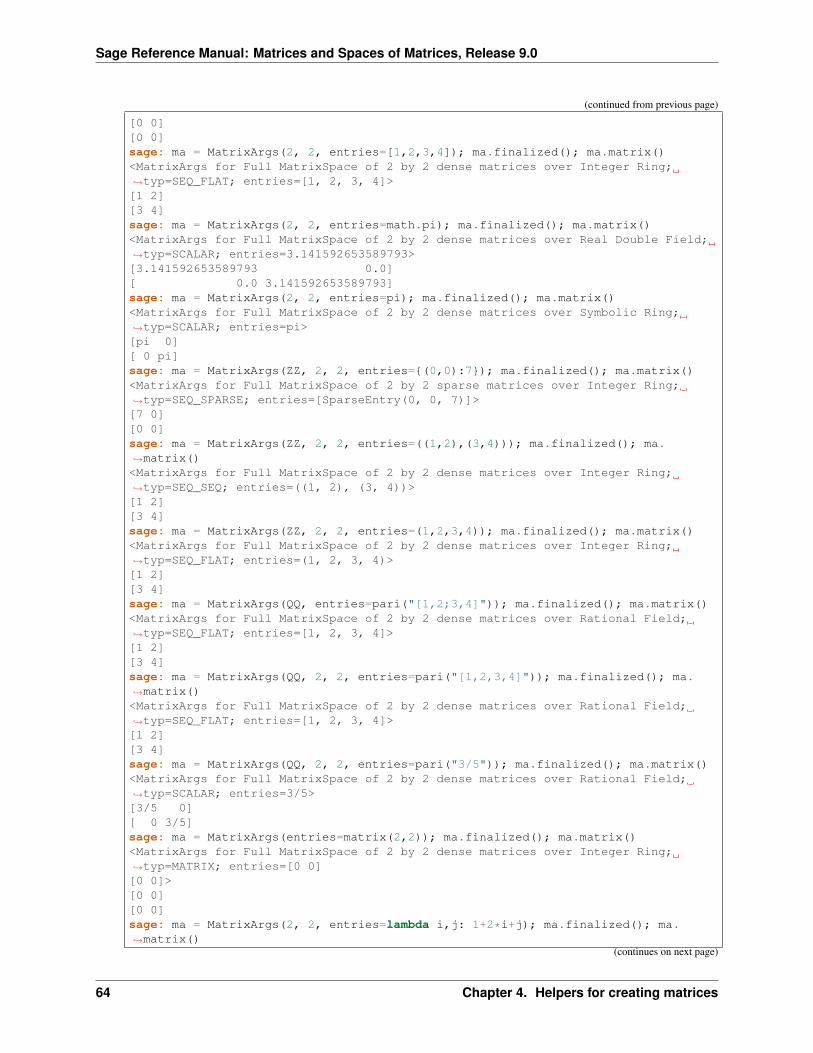
Sage Reference Manual: Matrices and Spaces of Matrices, Release 9.0
(continued from previous page)
[0 0][0 0]sage: ma = MatrixArgs(2, 2, entries=[1,2,3,4]); ma.finalized(); ma.matrix()<MatrixArgs for Full MatrixSpace of 2 by 2 dense matrices over Integer Ring;→˓typ=SEQ_FLAT; entries=[1, 2, 3, 4]>[1 2][3 4]sage: ma = MatrixArgs(2, 2, entries=math.pi); ma.finalized(); ma.matrix()<MatrixArgs for Full MatrixSpace of 2 by 2 dense matrices over Real Double Field;→˓typ=SCALAR; entries=3.141592653589793>[3.141592653589793 0.0][ 0.0 3.141592653589793]sage: ma = MatrixArgs(2, 2, entries=pi); ma.finalized(); ma.matrix()<MatrixArgs for Full MatrixSpace of 2 by 2 dense matrices over Symbolic Ring;→˓typ=SCALAR; entries=pi>[pi 0][ 0 pi]sage: ma = MatrixArgs(ZZ, 2, 2, entries={(0,0):7}); ma.finalized(); ma.matrix()<MatrixArgs for Full MatrixSpace of 2 by 2 sparse matrices over Integer Ring;→˓typ=SEQ_SPARSE; entries=[SparseEntry(0, 0, 7)]>[7 0][0 0]sage: ma = MatrixArgs(ZZ, 2, 2, entries=((1,2),(3,4))); ma.finalized(); ma.→˓matrix()<MatrixArgs for Full MatrixSpace of 2 by 2 dense matrices over Integer Ring;→˓typ=SEQ_SEQ; entries=((1, 2), (3, 4))>[1 2][3 4]sage: ma = MatrixArgs(ZZ, 2, 2, entries=(1,2,3,4)); ma.finalized(); ma.matrix()<MatrixArgs for Full MatrixSpace of 2 by 2 dense matrices over Integer Ring;→˓typ=SEQ_FLAT; entries=(1, 2, 3, 4)>[1 2][3 4]sage: ma = MatrixArgs(QQ, entries=pari("[1,2;3,4]")); ma.finalized(); ma.matrix()<MatrixArgs for Full MatrixSpace of 2 by 2 dense matrices over Rational Field;→˓typ=SEQ_FLAT; entries=[1, 2, 3, 4]>[1 2][3 4]sage: ma = MatrixArgs(QQ, 2, 2, entries=pari("[1,2,3,4]")); ma.finalized(); ma.→˓matrix()<MatrixArgs for Full MatrixSpace of 2 by 2 dense matrices over Rational Field;→˓typ=SEQ_FLAT; entries=[1, 2, 3, 4]>[1 2][3 4]sage: ma = MatrixArgs(QQ, 2, 2, entries=pari("3/5")); ma.finalized(); ma.matrix()<MatrixArgs for Full MatrixSpace of 2 by 2 dense matrices over Rational Field;→˓typ=SCALAR; entries=3/5>[3/5 0][ 0 3/5]sage: ma = MatrixArgs(entries=matrix(2,2)); ma.finalized(); ma.matrix()<MatrixArgs for Full MatrixSpace of 2 by 2 dense matrices over Integer Ring;→˓typ=MATRIX; entries=[0 0][0 0]>[0 0][0 0]sage: ma = MatrixArgs(2, 2, entries=lambda i,j: 1+2*i+j); ma.finalized(); ma.→˓matrix()
(continues on next page)
64 Chapter 4. Helpers for creating matrices

Sage Reference Manual: Matrices and Spaces of Matrices, Release 9.0
(continued from previous page)
<MatrixArgs for Full MatrixSpace of 2 by 2 dense matrices over Integer Ring;→˓typ=SEQ_FLAT; entries=[1, 2, 3, 4]>[1 2][3 4]sage: ma = MatrixArgs(ZZ, 2, 2, entries=lambda i,j: 1+2*i+j); ma.finalized(); ma.→˓matrix()<MatrixArgs for Full MatrixSpace of 2 by 2 dense matrices over Integer Ring;→˓typ=CALLABLE; entries=<function ...>>[1 2][3 4]sage: from numpy import arraysage: ma = MatrixArgs(array([[1,2],[3,4]])); ma.finalized(); ma.matrix()<MatrixArgs for Full MatrixSpace of 2 by 2 dense matrices over Integer Ring;→˓typ=SEQ_SEQ; entries=array([[1, 2],
[3, 4]])>[1 2][3 4]sage: ma = MatrixArgs(array([[1.,2.],[3.,4.]])); ma.finalized(); ma.matrix()<MatrixArgs for Full MatrixSpace of 2 by 2 dense matrices over Real Double Field;→˓typ=MATRIX; entries=[1.0 2.0][3.0 4.0]>[1.0 2.0][3.0 4.0]sage: ma = MatrixArgs(RealField(20), array([[1.,2.],[3.,4.]])); ma.finalized();→˓ma.matrix()<MatrixArgs for Full MatrixSpace of 2 by 2 dense matrices over Real Field with 20→˓bits of precision; typ=MATRIX; entries=[1.0 2.0][3.0 4.0]>[1.0000 2.0000][3.0000 4.0000]sage: ma = MatrixArgs(graphs.CycleGraph(3)); ma.finalized(); ma.matrix()<MatrixArgs for Full MatrixSpace of 3 by 3 dense matrices over Integer Ring;→˓typ=MATRIX; entries=[0 1 1][1 0 1][1 1 0]>[0 1 1][1 0 1][1 1 0]
sage: ma = MatrixArgs([vector([0,1], sparse=True), vector([0,0], sparse=True)],→˓sparse=True)sage: ma.finalized(); ma.matrix()<MatrixArgs for Full MatrixSpace of 2 by 2 sparse matrices over Integer Ring;→˓typ=SEQ_SPARSE; entries=[SparseEntry(0, 1, 1)]>[0 1][0 0]
Test invalid input:
sage: MatrixArgs(ZZ, 2, 2, entries="abcd").finalized()Traceback (most recent call last):...TypeError: unable to convert 'abcd' to a matrixsage: MatrixArgs(ZZ, 2, 2, entries=MatrixArgs()).finalized()Traceback (most recent call last):...TypeError: unable to convert <MatrixArgs for None; typ=UNKNOWN; entries=None> to→˓a matrix (continues on next page)
65
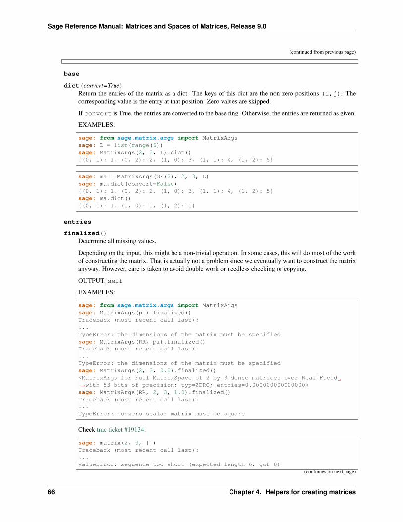
Sage Reference Manual: Matrices and Spaces of Matrices, Release 9.0
(continued from previous page)
base
dict(convert=True)Return the entries of the matrix as a dict. The keys of this dict are the non-zero positions (i,j). Thecorresponding value is the entry at that position. Zero values are skipped.
If convert is True, the entries are converted to the base ring. Otherwise, the entries are returned as given.
EXAMPLES:
sage: from sage.matrix.args import MatrixArgssage: L = list(range(6))sage: MatrixArgs(2, 3, L).dict(){(0, 1): 1, (0, 2): 2, (1, 0): 3, (1, 1): 4, (1, 2): 5}
sage: ma = MatrixArgs(GF(2), 2, 3, L)sage: ma.dict(convert=False){(0, 1): 1, (0, 2): 2, (1, 0): 3, (1, 1): 4, (1, 2): 5}sage: ma.dict(){(0, 1): 1, (1, 0): 1, (1, 2): 1}
entries
finalized()Determine all missing values.
Depending on the input, this might be a non-trivial operation. In some cases, this will do most of the workof constructing the matrix. That is actually not a problem since we eventually want to construct the matrixanyway. However, care is taken to avoid double work or needless checking or copying.
OUTPUT: self
EXAMPLES:
sage: from sage.matrix.args import MatrixArgssage: MatrixArgs(pi).finalized()Traceback (most recent call last):...TypeError: the dimensions of the matrix must be specifiedsage: MatrixArgs(RR, pi).finalized()Traceback (most recent call last):...TypeError: the dimensions of the matrix must be specifiedsage: MatrixArgs(2, 3, 0.0).finalized()<MatrixArgs for Full MatrixSpace of 2 by 3 dense matrices over Real Field→˓with 53 bits of precision; typ=ZERO; entries=0.000000000000000>sage: MatrixArgs(RR, 2, 3, 1.0).finalized()Traceback (most recent call last):...TypeError: nonzero scalar matrix must be square
Check trac ticket #19134:
sage: matrix(2, 3, [])Traceback (most recent call last):...ValueError: sequence too short (expected length 6, got 0)
(continues on next page)
66 Chapter 4. Helpers for creating matrices
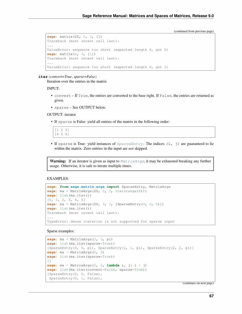
Sage Reference Manual: Matrices and Spaces of Matrices, Release 9.0
(continued from previous page)
sage: matrix(ZZ, 2, 3, [])Traceback (most recent call last):...ValueError: sequence too short (expected length 6, got 0)sage: matrix(2, 3, [1])Traceback (most recent call last):...ValueError: sequence too short (expected length 6, got 1)
iter(convert=True, sparse=False)Iteration over the entries in the matrix
INPUT:
• convert – If True, the entries are converted to the base right. If False, the entries are returned asgiven.
• sparse – See OUTPUT below.
OUTPUT: iterator
• If sparse is False: yield all entries of the matrix in the following order:
[1 2 3][4 5 6]
• If sparse is True: yield instances of SparseEntry . The indices (i, j) are guaranteed to liewithin the matrix. Zero entries in the input are not skipped.
Warning: If an iterator is given as input to MatrixArgs, it may be exhausted breaking any furtherusage. Otherwise, it is safe to iterate multiple times.
EXAMPLES:
sage: from sage.matrix.args import SparseEntry, MatrixArgssage: ma = MatrixArgs(ZZ, 2, 3, iter(range(6)))sage: list(ma.iter())[0, 1, 2, 3, 4, 5]sage: ma = MatrixArgs(ZZ, 3, 3, [SparseEntry(0, 0, 0)])sage: list(ma.iter())Traceback (most recent call last):...TypeError: dense iteration is not supported for sparse input
Sparse examples:
sage: ma = MatrixArgs(3, 3, pi)sage: list(ma.iter(sparse=True))[SparseEntry(0, 0, pi), SparseEntry(1, 1, pi), SparseEntry(2, 2, pi)]sage: ma = MatrixArgs(2, 3)sage: list(ma.iter(sparse=True))[]sage: ma = MatrixArgs(2, 2, lambda i, j: i > j)sage: list(ma.iter(convert=False, sparse=True))[SparseEntry(0, 0, False),SparseEntry(0, 1, False),
(continues on next page)
67
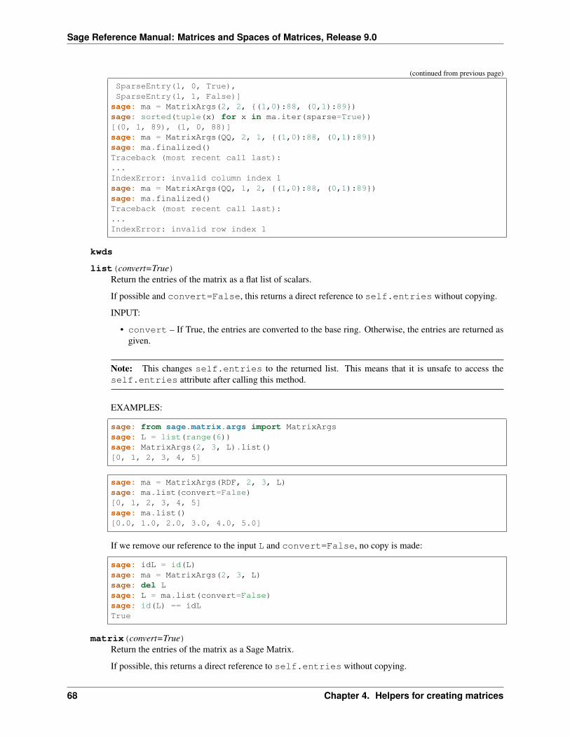
Sage Reference Manual: Matrices and Spaces of Matrices, Release 9.0
(continued from previous page)
SparseEntry(1, 0, True),SparseEntry(1, 1, False)]
sage: ma = MatrixArgs(2, 2, {(1,0):88, (0,1):89})sage: sorted(tuple(x) for x in ma.iter(sparse=True))[(0, 1, 89), (1, 0, 88)]sage: ma = MatrixArgs(QQ, 2, 1, {(1,0):88, (0,1):89})sage: ma.finalized()Traceback (most recent call last):...IndexError: invalid column index 1sage: ma = MatrixArgs(QQ, 1, 2, {(1,0):88, (0,1):89})sage: ma.finalized()Traceback (most recent call last):...IndexError: invalid row index 1
kwds
list(convert=True)Return the entries of the matrix as a flat list of scalars.
If possible and convert=False, this returns a direct reference to self.entries without copying.
INPUT:
• convert – If True, the entries are converted to the base ring. Otherwise, the entries are returned asgiven.
Note: This changes self.entries to the returned list. This means that it is unsafe to access theself.entries attribute after calling this method.
EXAMPLES:
sage: from sage.matrix.args import MatrixArgssage: L = list(range(6))sage: MatrixArgs(2, 3, L).list()[0, 1, 2, 3, 4, 5]
sage: ma = MatrixArgs(RDF, 2, 3, L)sage: ma.list(convert=False)[0, 1, 2, 3, 4, 5]sage: ma.list()[0.0, 1.0, 2.0, 3.0, 4.0, 5.0]
If we remove our reference to the input L and convert=False, no copy is made:
sage: idL = id(L)sage: ma = MatrixArgs(2, 3, L)sage: del Lsage: L = ma.list(convert=False)sage: id(L) == idLTrue
matrix(convert=True)Return the entries of the matrix as a Sage Matrix.
If possible, this returns a direct reference to self.entries without copying.
68 Chapter 4. Helpers for creating matrices

Sage Reference Manual: Matrices and Spaces of Matrices, Release 9.0
INPUT:
• convert – if True, the matrix is guaranteed to have the correct parent matrix space. If False, theinput matrix may be returned even if it lies in the wrong space.
Note: This changes self.entries to the returned matrix. This means that it is unsafe to access theself.entries attribute after calling this method.
EXAMPLES:
sage: from sage.matrix.args import MatrixArgssage: M = matrix(2, 3, range(6), sparse=True)
sage: ma = MatrixArgs(M); ma.finalized()<MatrixArgs for Full MatrixSpace of 2 by 3 sparse matrices over Integer Ring;→˓typ=MATRIX; entries=[0 1 2][3 4 5]>sage: ma.matrix()[0 1 2][3 4 5]
sage: ma = MatrixArgs(M, sparse=False); ma.finalized()<MatrixArgs for Full MatrixSpace of 2 by 3 dense matrices over Integer Ring;→˓typ=MATRIX; entries=[0 1 2][3 4 5]>sage: ma.matrix()[0 1 2][3 4 5]
sage: ma = MatrixArgs(RDF, M); ma.finalized()<MatrixArgs for Full MatrixSpace of 2 by 3 sparse matrices over Real Double→˓Field; typ=MATRIX; entries=[0 1 2][3 4 5]>sage: ma.matrix(convert=False)[0 1 2][3 4 5]sage: ma.matrix()[0.0 1.0 2.0][3.0 4.0 5.0]
If we remove our reference to the input M, no copy is made:
sage: idM = id(M)sage: ma = MatrixArgs(M)sage: del Msage: M = ma.matrix()sage: id(M) == idMTrue
Immutable matrices are never copied:
sage: M.set_immutable()sage: matrix(M) is MTrue
ncols
69
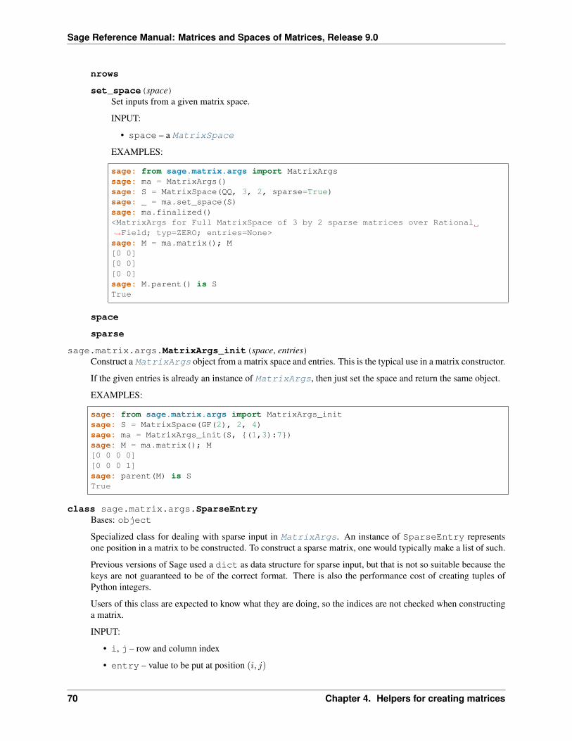
Sage Reference Manual: Matrices and Spaces of Matrices, Release 9.0
nrows
set_space(space)Set inputs from a given matrix space.
INPUT:
• space – a MatrixSpace
EXAMPLES:
sage: from sage.matrix.args import MatrixArgssage: ma = MatrixArgs()sage: S = MatrixSpace(QQ, 3, 2, sparse=True)sage: _ = ma.set_space(S)sage: ma.finalized()<MatrixArgs for Full MatrixSpace of 3 by 2 sparse matrices over Rational→˓Field; typ=ZERO; entries=None>sage: M = ma.matrix(); M[0 0][0 0][0 0]sage: M.parent() is STrue
space
sparse
sage.matrix.args.MatrixArgs_init(space, entries)Construct a MatrixArgs object from a matrix space and entries. This is the typical use in a matrix constructor.
If the given entries is already an instance of MatrixArgs, then just set the space and return the same object.
EXAMPLES:
sage: from sage.matrix.args import MatrixArgs_initsage: S = MatrixSpace(GF(2), 2, 4)sage: ma = MatrixArgs_init(S, {(1,3):7})sage: M = ma.matrix(); M[0 0 0 0][0 0 0 1]sage: parent(M) is STrue
class sage.matrix.args.SparseEntryBases: object
Specialized class for dealing with sparse input in MatrixArgs. An instance of SparseEntry representsone position in a matrix to be constructed. To construct a sparse matrix, one would typically make a list of such.
Previous versions of Sage used a dict as data structure for sparse input, but that is not so suitable because thekeys are not guaranteed to be of the correct format. There is also the performance cost of creating tuples ofPython integers.
Users of this class are expected to know what they are doing, so the indices are not checked when constructinga matrix.
INPUT:
• i, j – row and column index
• entry – value to be put at position (𝑖, 𝑗)
70 Chapter 4. Helpers for creating matrices
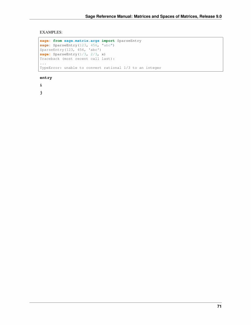
Sage Reference Manual: Matrices and Spaces of Matrices, Release 9.0
EXAMPLES:
sage: from sage.matrix.args import SparseEntrysage: SparseEntry(123, 456, "abc")SparseEntry(123, 456, 'abc')sage: SparseEntry(1/3, 2/3, x)Traceback (most recent call last):...TypeError: unable to convert rational 1/3 to an integer
entry
i
j
71

Sage Reference Manual: Matrices and Spaces of Matrices, Release 9.0
72 Chapter 4. Helpers for creating matrices
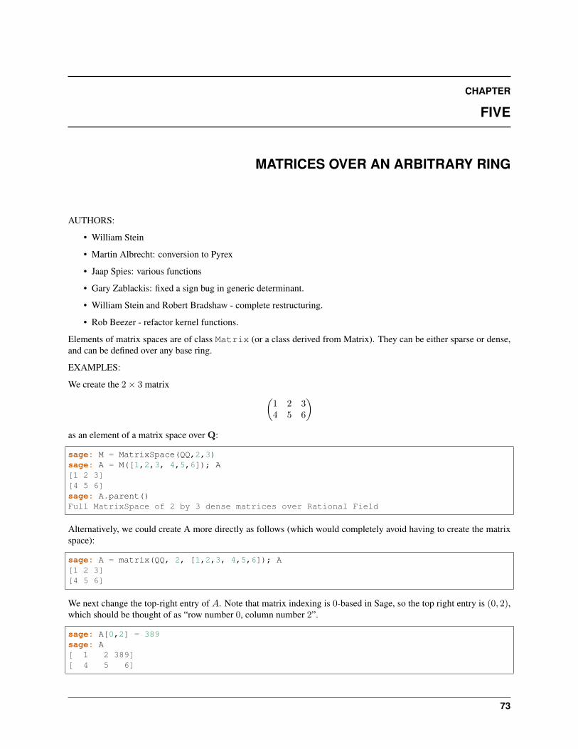
CHAPTER
FIVE
MATRICES OVER AN ARBITRARY RING
AUTHORS:
• William Stein
• Martin Albrecht: conversion to Pyrex
• Jaap Spies: various functions
• Gary Zablackis: fixed a sign bug in generic determinant.
• William Stein and Robert Bradshaw - complete restructuring.
• Rob Beezer - refactor kernel functions.
Elements of matrix spaces are of class Matrix (or a class derived from Matrix). They can be either sparse or dense,and can be defined over any base ring.
EXAMPLES:
We create the 2× 3 matrix (︂1 2 34 5 6
)︂as an element of a matrix space over Q:
sage: M = MatrixSpace(QQ,2,3)sage: A = M([1,2,3, 4,5,6]); A[1 2 3][4 5 6]sage: A.parent()Full MatrixSpace of 2 by 3 dense matrices over Rational Field
Alternatively, we could create A more directly as follows (which would completely avoid having to create the matrixspace):
sage: A = matrix(QQ, 2, [1,2,3, 4,5,6]); A[1 2 3][4 5 6]
We next change the top-right entry of 𝐴. Note that matrix indexing is 0-based in Sage, so the top right entry is (0, 2),which should be thought of as “row number 0, column number 2”.
sage: A[0,2] = 389sage: A[ 1 2 389][ 4 5 6]
73
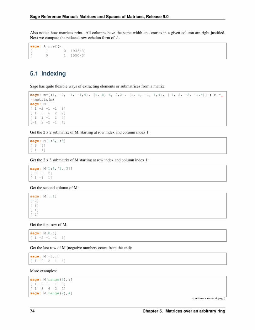
Sage Reference Manual: Matrices and Spaces of Matrices, Release 9.0
Also notice how matrices print. All columns have the same width and entries in a given column are right justified.Next we compute the reduced row echelon form of 𝐴.
sage: A.rref()[ 1 0 -1933/3][ 0 1 1550/3]
5.1 Indexing
Sage has quite flexible ways of extracting elements or submatrices from a matrix:
sage: m=[(1, -2, -1, -1,9), (1, 8, 6, 2,2), (1, 1, -1, 1,4), (-1, 2, -2, -1,4)] ; M =→˓matrix(m)sage: M[ 1 -2 -1 -1 9][ 1 8 6 2 2][ 1 1 -1 1 4][-1 2 -2 -1 4]
Get the 2 x 2 submatrix of M, starting at row index and column index 1:
sage: M[1:3,1:3][ 8 6][ 1 -1]
Get the 2 x 3 submatrix of M starting at row index and column index 1:
sage: M[1:3,[1..3]][ 8 6 2][ 1 -1 1]
Get the second column of M:
sage: M[:,1][-2][ 8][ 1][ 2]
Get the first row of M:
sage: M[0,:][ 1 -2 -1 -1 9]
Get the last row of M (negative numbers count from the end):
sage: M[-1,:][-1 2 -2 -1 4]
More examples:
sage: M[range(2),:][ 1 -2 -1 -1 9][ 1 8 6 2 2]sage: M[range(2),4]
(continues on next page)
74 Chapter 5. Matrices over an arbitrary ring
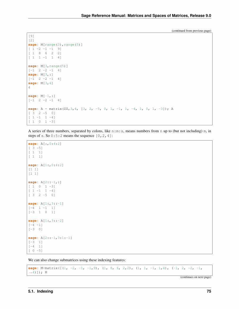
Sage Reference Manual: Matrices and Spaces of Matrices, Release 9.0
(continued from previous page)
[9][2]sage: M[range(3),range(5)][ 1 -2 -1 -1 9][ 1 8 6 2 2][ 1 1 -1 1 4]
sage: M[3,range(5)][-1 2 -2 -1 4]sage: M[3,:][-1 2 -2 -1 4]sage: M[3,4]4
sage: M[-1,:][-1 2 -2 -1 4]
sage: A = matrix(ZZ,3,4, [3, 2, -5, 0, 1, -1, 1, -4, 1, 0, 1, -3]); A[ 3 2 -5 0][ 1 -1 1 -4][ 1 0 1 -3]
A series of three numbers, separated by colons, like n:m:s, means numbers from n up to (but not including) m, insteps of s. So 0:5:2 means the sequence [0,2,4]:
sage: A[:,0:4:2][ 3 -5][ 1 1][ 1 1]
sage: A[1:,0:4:2][1 1][1 1]
sage: A[2::-1,:][ 1 0 1 -3][ 1 -1 1 -4][ 3 2 -5 0]
sage: A[1:,3::-1][-4 1 -1 1][-3 1 0 1]
sage: A[1:,3::-2][-4 -1][-3 0]
sage: A[2::-1,3:1:-1][-3 1][-4 1][ 0 -5]
We can also change submatrices using these indexing features:
sage: M=matrix([(1, -2, -1, -1,9), (1, 8, 6, 2,2), (1, 1, -1, 1,4), (-1, 2, -2, -1,→˓4)]); M
(continues on next page)
5.1. Indexing 75
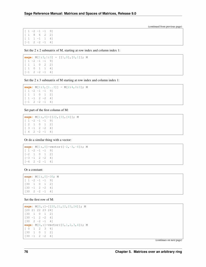
Sage Reference Manual: Matrices and Spaces of Matrices, Release 9.0
(continued from previous page)
[ 1 -2 -1 -1 9][ 1 8 6 2 2][ 1 1 -1 1 4][-1 2 -2 -1 4]
Set the 2 x 2 submatrix of M, starting at row index and column index 1:
sage: M[1:3,1:3] = [[1,0],[0,1]]; M[ 1 -2 -1 -1 9][ 1 1 0 2 2][ 1 0 1 1 4][-1 2 -2 -1 4]
Set the 2 x 3 submatrix of M starting at row index and column index 1:
sage: M[1:3,[1..3]] = M[2:4,0:3]; M[ 1 -2 -1 -1 9][ 1 1 0 1 2][ 1 -1 2 -2 4][-1 2 -2 -1 4]
Set part of the first column of M:
sage: M[1:,0]=[[2],[3],[4]]; M[ 1 -2 -1 -1 9][ 2 1 0 1 2][ 3 -1 2 -2 4][ 4 2 -2 -1 4]
Or do a similar thing with a vector:
sage: M[1:,0]=vector([-2,-3,-4]); M[ 1 -2 -1 -1 9][-2 1 0 1 2][-3 -1 2 -2 4][-4 2 -2 -1 4]
Or a constant:
sage: M[1:,0]=30; M[ 1 -2 -1 -1 9][30 1 0 1 2][30 -1 2 -2 4][30 2 -2 -1 4]
Set the first row of M:
sage: M[0,:]=[[20,21,22,23,24]]; M[20 21 22 23 24][30 1 0 1 2][30 -1 2 -2 4][30 2 -2 -1 4]sage: M[0,:]=vector([0,1,2,3,4]); M[ 0 1 2 3 4][30 1 0 1 2][30 -1 2 -2 4]
(continues on next page)
76 Chapter 5. Matrices over an arbitrary ring
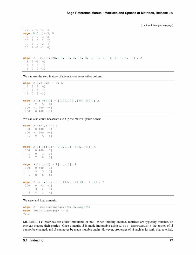
Sage Reference Manual: Matrices and Spaces of Matrices, Release 9.0
(continued from previous page)
[30 2 -2 -1 4]sage: M[0,:]=-3; M[-3 -3 -3 -3 -3][30 1 0 1 2][30 -1 2 -2 4][30 2 -2 -1 4]
sage: A = matrix(ZZ,3,4, [3, 2, -5, 0, 1, -1, 1, -4, 1, 0, 1, -3]); A[ 3 2 -5 0][ 1 -1 1 -4][ 1 0 1 -3]
We can use the step feature of slices to set every other column:
sage: A[:,0:3:2] = 5; A[ 5 2 5 0][ 5 -1 5 -4][ 5 0 5 -3]
sage: A[1:,0:4:2] = [[100,200],[300,400]]; A[ 5 2 5 0][100 -1 200 -4][300 0 400 -3]
We can also count backwards to flip the matrix upside down:
sage: A[::-1,:]=A; A[300 0 400 -3][100 -1 200 -4][ 5 2 5 0]
sage: A[1:,3::-1]=[[2,3,0,1],[9,8,7,6]]; A[300 0 400 -3][ 1 0 3 2][ 6 7 8 9]
sage: A[1:,::-2] = A[1:,::2]; A[300 0 400 -3][ 1 3 3 1][ 6 8 8 6]
sage: A[::-1,3:1:-1] = [[4,3],[1,2],[-1,-2]]; A[300 0 -2 -1][ 1 3 2 1][ 6 8 3 4]
We save and load a matrix:
sage: A = matrix(Integers(8),3,range(9))sage: loads(dumps(A)) == ATrue
MUTABILITY: Matrices are either immutable or not. When initially created, matrices are typically mutable, soone can change their entries. Once a matrix 𝐴 is made immutable using A.set_immutable() the entries of 𝐴cannot be changed, and 𝐴 can never be made mutable again. However, properties of 𝐴 such as its rank, characteristic
5.1. Indexing 77
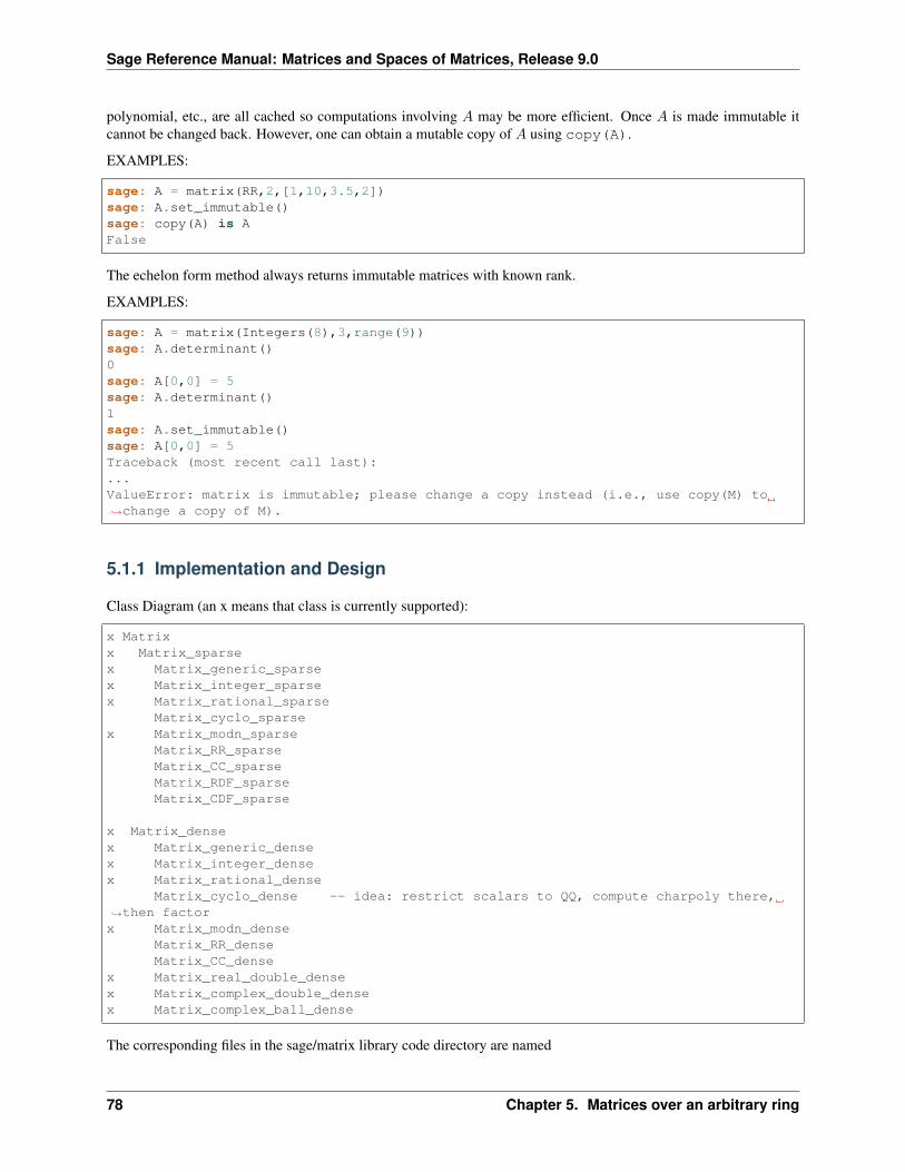
Sage Reference Manual: Matrices and Spaces of Matrices, Release 9.0
polynomial, etc., are all cached so computations involving 𝐴 may be more efficient. Once 𝐴 is made immutable itcannot be changed back. However, one can obtain a mutable copy of 𝐴 using copy(A).
EXAMPLES:
sage: A = matrix(RR,2,[1,10,3.5,2])sage: A.set_immutable()sage: copy(A) is AFalse
The echelon form method always returns immutable matrices with known rank.
EXAMPLES:
sage: A = matrix(Integers(8),3,range(9))sage: A.determinant()0sage: A[0,0] = 5sage: A.determinant()1sage: A.set_immutable()sage: A[0,0] = 5Traceback (most recent call last):...ValueError: matrix is immutable; please change a copy instead (i.e., use copy(M) to→˓change a copy of M).
5.1.1 Implementation and Design
Class Diagram (an x means that class is currently supported):
x Matrixx Matrix_sparsex Matrix_generic_sparsex Matrix_integer_sparsex Matrix_rational_sparse
Matrix_cyclo_sparsex Matrix_modn_sparse
Matrix_RR_sparseMatrix_CC_sparseMatrix_RDF_sparseMatrix_CDF_sparse
x Matrix_densex Matrix_generic_densex Matrix_integer_densex Matrix_rational_dense
Matrix_cyclo_dense -- idea: restrict scalars to QQ, compute charpoly there,→˓then factorx Matrix_modn_dense
Matrix_RR_denseMatrix_CC_dense
x Matrix_real_double_densex Matrix_complex_double_densex Matrix_complex_ball_dense
The corresponding files in the sage/matrix library code directory are named
78 Chapter 5. Matrices over an arbitrary ring
Sage Reference Manual: Matrices and Spaces of Matrices, Release 9.0
[matrix] [base ring] [dense or sparse].
New matrices types can only be implemented in Cython.
*********** LEVEL 1 **********NON-OPTIONALFor each base field it is *absolutely* essential to completelyimplement the following functionality for that base ring:
* __cinit__ -- should use check_allocarray from cysignals.memory(only needed if allocate memory)
* __init__ -- this signature: 'def __init__(self, parent, entries, copy,→˓coerce)'
* __dealloc__ -- use sig_free (only needed if allocate memory)
* set_unsafe(self, size_t i, size_t j, x) -- doesn't do bounds or any other checks;→˓ assumes x is in self._base_ring
* get_unsafe(self, size_t i, size_t j) -- doesn't do checks
* __richcmp__ -- always the same (I don't know why its needed -- bug in PYREX).
Note that the __init__ function must construct the all zero matrix if ``entries ==→˓None``.
*********** LEVEL 2 **********
IMPORTANT (and *highly* recommended):
After getting the special class with all level 1 functionality towork, implement all of the following (they should not changefunctionality, except speed (always faster!) in any way):
* def _pickle(self):return data, version
* def _unpickle(self, data, int version)reconstruct matrix from given data and version; may assume _parent, _nrows,
→˓and _ncols are set.Use version numbers >= 0 so if you change the pickle strategy thenold objects still unpickle.
* cdef _list -- list of underlying elements (need not be a copy)
* cdef _dict -- sparse dictionary of underlying elements
* cdef _add_ -- add two matrices with identical parents
* _matrix_times_matrix_c_impl -- multiply two matrices with compatible dimensions→˓and
identical base rings (both sparse or both dense)
* cpdef _richcmp_ -- compare two matrices with identical parents
* cdef _lmul_c_impl -- multiply this matrix on the right by a scalar, i.e., self *→˓scalar
* cdef _rmul_c_impl -- multiply this matrix on the left by a scalar, i.e., scalar→˓* self
* __copy__
* __neg__
The list and dict returned by _list and _dict will *not* be changedby any internal algorithms and are not accessible to the user.
*********** LEVEL 3 **********OPTIONAL:
(continues on next page)
5.1. Indexing 79
Sage Reference Manual: Matrices and Spaces of Matrices, Release 9.0
(continued from previous page)
* cdef _sub_
* __invert__
* _multiply_classical
* __deepcopy__
Further special support:
* Matrix windows -- to support Strassen multiplication for a given base ring.
* Other functions, e.g., transpose, for which knowing thespecific representation can be helpful.
.. note::
- For caching, use self.fetch and self.cache.
- Any method that can change the matrix should call``check_mutability()`` first. There are also many fast cdef'd bounds checking
→˓methods.
- Kernels of matricesImplement only a left_kernel() or right_kernel() method, whichever requiresthe least overhead (usually meaning little or no transposing). Let themethods in the matrix2 class handle left, right, generic kernel distinctions.
80 Chapter 5. Matrices over an arbitrary ring
CHAPTER
SIX
BASE CLASS FOR MATRICES, PART 0
Note: For design documentation see matrix/docs.py.
EXAMPLES:
sage: matrix(2,[1,2,3,4])[1 2][3 4]
class sage.matrix.matrix0.MatrixBases: sage.structure.element.Matrix
A generic matrix.
The Matrix class is the base class for all matrix classes. To create a Matrix, first create a MatrixSpace,then coerce a list of elements into the MatrixSpace. See the documentation of MatrixSpace for moredetails.
EXAMPLES:
We illustrate matrices and matrix spaces. Note that no actual matrix that you make should have class Matrix;the class should always be derived from Matrix.
sage: M = MatrixSpace(CDF,2,3); MFull MatrixSpace of 2 by 3 dense matrices over Complex Double Fieldsage: a = M([1,2,3, 4,5,6]); a[1.0 2.0 3.0][4.0 5.0 6.0]sage: type(a)<type 'sage.matrix.matrix_complex_double_dense.Matrix_complex_double_dense'>sage: parent(a)Full MatrixSpace of 2 by 3 dense matrices over Complex Double Field
sage: matrix(CDF, 2,3, [1,2,3, 4,5,6])[1.0 2.0 3.0][4.0 5.0 6.0]sage: Mat(CDF,2,3)(range(1,7))[1.0 2.0 3.0][4.0 5.0 6.0]
sage: Q.<i,j,k> = QuaternionAlgebra(QQ, -1,-1)sage: matrix(Q,2,1,[1,2])[1][2]
81
Sage Reference Manual: Matrices and Spaces of Matrices, Release 9.0
act_on_polynomial(f)Returns the polynomial f(self*x).
INPUT:
• self - an nxn matrix
• f - a polynomial in n variables x=(x1,. . . ,xn)
OUTPUT: The polynomial f(self*x).
EXAMPLES:
sage: R.<x,y> = QQ[]sage: x, y = R.gens()sage: f = x**2 - y**2sage: M = MatrixSpace(QQ, 2)sage: A = M([1,2,3,4])sage: A.act_on_polynomial(f)-8*x^2 - 20*x*y - 12*y^2
add_multiple_of_column(i, j, s, start_row=0)Add s times column j to column i.
EXAMPLES: We add -1 times the third column to the second column of an integer matrix, rememberingto start numbering cols at zero:
sage: a = matrix(ZZ,2,3,range(6)); a[0 1 2][3 4 5]sage: a.add_multiple_of_column(1,2,-1)sage: a[ 0 -1 2][ 3 -1 5]
To add a rational multiple, we first need to change the base ring:
sage: a = a.change_ring(QQ)sage: a.add_multiple_of_column(1,0,1/3)sage: a[ 0 -1 2][ 3 0 5]
If not, we get an error message:
sage: a.add_multiple_of_column(1,0,i)Traceback (most recent call last):...TypeError: Multiplying column by Symbolic Ring element cannot be done over→˓Rational Field, use change_ring or with_added_multiple_of_column instead.
add_multiple_of_row(i, j, s, start_col=0)Add s times row j to row i.
EXAMPLES: We add -3 times the first row to the second row of an integer matrix, remembering to startnumbering rows at zero:
sage: a = matrix(ZZ,2,3,range(6)); a[0 1 2][3 4 5]
(continues on next page)
82 Chapter 6. Base class for matrices, part 0
Sage Reference Manual: Matrices and Spaces of Matrices, Release 9.0
(continued from previous page)
sage: a.add_multiple_of_row(1,0,-3)sage: a[ 0 1 2][ 3 1 -1]
To add a rational multiple, we first need to change the base ring:
sage: a = a.change_ring(QQ)sage: a.add_multiple_of_row(1,0,1/3)sage: a[ 0 1 2][ 3 4/3 -1/3]
If not, we get an error message:
sage: a.add_multiple_of_row(1,0,i)Traceback (most recent call last):...TypeError: Multiplying row by Symbolic Ring element cannot be done over→˓Rational Field, use change_ring or with_added_multiple_of_row instead.
add_to_entry(i, j, elt)Add elt to the entry at position (i, j).
EXAMPLES:
sage: m = matrix(QQ['x,y'], 2, 2)sage: m.add_to_entry(0, 1, 2)sage: m[0 2][0 0]
anticommutator(other)Return the anticommutator self and other.
The anticommutator of two 𝑛× 𝑛 matrices 𝐴 and 𝐵 is defined as {𝐴,𝐵} := 𝐴𝐵 + 𝐵𝐴 (sometimes thisis written as [𝐴,𝐵]+).
EXAMPLES:
sage: A = Matrix(ZZ, 2, 2, range(4))sage: B = Matrix(ZZ, 2, 2, [0, 1, 0, 0])sage: A.anticommutator(B)[2 3][0 2]sage: A.anticommutator(B) == B.anticommutator(A)Truesage: A.commutator(B) + B.anticommutator(A) == 2*A*BTrue
base_ring()Returns the base ring of the matrix.
EXAMPLES:
sage: m=matrix(QQ,2,[1,2,3,4])sage: m.base_ring()Rational Field
83
Sage Reference Manual: Matrices and Spaces of Matrices, Release 9.0
change_ring(ring)Return the matrix obtained by coercing the entries of this matrix into the given ring.
Always returns a copy (unless self is immutable, in which case returns self).
EXAMPLES:
sage: A = Matrix(QQ, 2, 2, [1/2, 1/3, 1/3, 1/4])sage: A.parent()Full MatrixSpace of 2 by 2 dense matrices over Rational Field
sage: A.change_ring(GF(25,'a'))[3 2][2 4]sage: A.change_ring(GF(25,'a')).parent()Full MatrixSpace of 2 by 2 dense matrices over Finite Field in a of size 5^2
sage: A.change_ring(ZZ)Traceback (most recent call last):...TypeError: matrix has denominators so can't change to ZZ.
Changing rings preserves subdivisions:
sage: A.subdivide([1], []); A[1/2 1/3][-------][1/3 1/4]sage: A.change_ring(GF(25,'a'))[3 2][---][2 4]
commutator(other)Return the commutator self*other - other*self.
EXAMPLES:
sage: A = Matrix(ZZ, 2, 2, range(4))sage: B = Matrix(ZZ, 2, 2, [0, 1, 0, 0])sage: A.commutator(B)[-2 -3][ 0 2]sage: A.commutator(B) == -B.commutator(A)True
dict(copy=True)Dictionary of the elements of self with keys pairs (i,j) and values the nonzero entries of self.
INPUT:
• copy – (default: True) make a copy of the dict corresponding to self
If copy=True, then is safe to change the returned dictionary. Otherwise, this can cause undesired behav-ior by mutating the dict.
EXAMPLES:
sage: R.<x,y> = QQ[]sage: a = matrix(R,2,[x,y,0, 0,0,2*x+y]); a[ x y 0][ 0 0 2*x + y]
(continues on next page)
84 Chapter 6. Base class for matrices, part 0
Sage Reference Manual: Matrices and Spaces of Matrices, Release 9.0
(continued from previous page)
sage: d = a.dict(); d{(0, 0): x, (0, 1): y, (1, 2): 2*x + y}
Notice that changing the returned list does not change a (the list is a copy):
sage: d[0,0] = 25sage: a[ x y 0][ 0 0 2*x + y]
dimensions()Returns the dimensions of this matrix as the tuple (nrows, ncols).
EXAMPLES:
sage: M = matrix([[1,2,3],[4,5,6]])sage: N = M.transpose()sage: M.dimensions()(2, 3)sage: N.dimensions()(3, 2)
AUTHORS:
• Benjamin Lundell (2012-02-09): examples
inverse_of_unit(algorithm=None)Return the inverse of this matrix in the same matrix space.
The matrix must be invertible on the base ring. Otherwise, an ArithmeticError is raised.
The computation goes through the matrix of cofactors and avoids division. In particular the base ring doesnot need to have a fraction field.
INPUT:
• algorithm – (default: None) either None or "df" (for division free)
EXAMPLES:
sage: R.<a,b,c,d> = ZZ[]sage: RR = R.quotient(a*d-b*c-1)sage: a,b,c,d = RR.gens()sage: m = matrix(2, [a,b,c,d])sage: n = m.inverse_of_unit()sage: m * n[1 0][0 1]
sage: matrix(RR, 2, 1, [a,b]).inverse_of_unit()Traceback (most recent call last):...ArithmeticError: self must be a square matrixsage: matrix(RR, 1, 1, [2]).inverse_of_unit()Traceback (most recent call last):...NotImplementedError
sage: R = ZZ.cartesian_product(ZZ)
(continues on next page)
85
Sage Reference Manual: Matrices and Spaces of Matrices, Release 9.0
(continued from previous page)
sage: m = matrix(R, 2, [R((2,1)), R((1,1)), R((1,1)), R((1,2))])sage: m * m.inverse_of_unit()[(1, 1) (0, 0)][(0, 0) (1, 1)]
Tests for trac ticket #28570:
sage: P = posets.TamariLattice(7)sage: M = P._hasse_diagram._leq_matrixsage: M.inverse_of_unit() # this was very slow, now 1s429 x 429 sparse matrix over Integer Ring...
sage: m = matrix(Zmod(2**2), 1, 1, [1], sparse=True)sage: mi = ~m; mi[1]sage: mi.parent()Full MatrixSpace of 1 by 1 sparse matrices over Ring of integers modulo 4
is_alternating()Return True if self is an alternating matrix.
Here, “alternating matrix” means a square matrix 𝐴 satisfying 𝐴𝑇 = −𝐴 and such that the diagonalentries of 𝐴 are 0. Notice that the condition that the diagonal entries be 0 is not redundant for matricesover arbitrary ground rings (but it is redundant when 2 is invertible in the ground ring). A square matrix𝐴 only required to satisfy 𝐴𝑇 = −𝐴 is said to be “skew-symmetric”, and this property is checked by theis_skew_symmetric() method.
EXAMPLES:
sage: m = matrix(QQ, [[0,2], [-2,0]])sage: m.is_alternating()Truesage: m = matrix(QQ, [[1,2], [2,1]])sage: m.is_alternating()False
In contrast to the property of being skew-symmetric, the property of being alternating does not toleratenonzero entries on the diagonal even if they are their own negatives:
sage: n = matrix(Zmod(4), [[0, 1], [-1, 2]])sage: n.is_alternating()False
is_dense()Returns True if this is a dense matrix.
In Sage, being dense is a property of the underlying representation, not the number of nonzero entries.
EXAMPLES:
sage: matrix(QQ,2,2,range(4)).is_dense()Truesage: matrix(QQ,2,2,range(4),sparse=True).is_dense()False
is_hermitian()Returns True if the matrix is equal to its conjugate-transpose.
86 Chapter 6. Base class for matrices, part 0
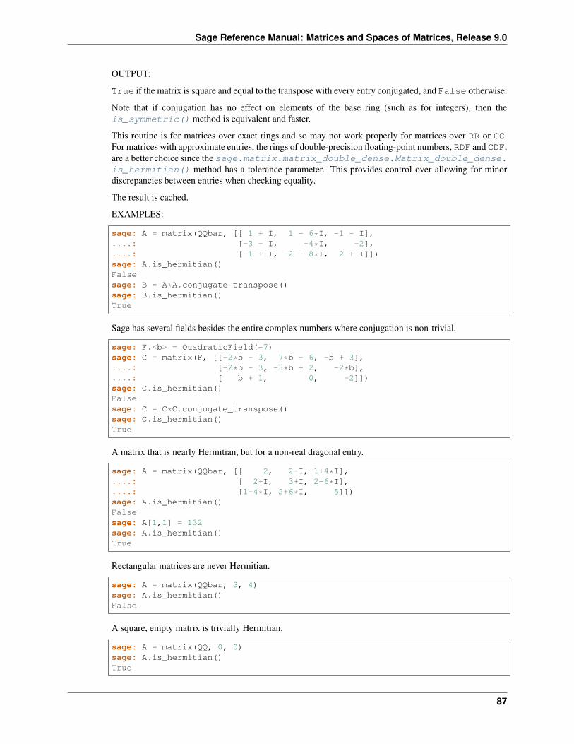
Sage Reference Manual: Matrices and Spaces of Matrices, Release 9.0
OUTPUT:
True if the matrix is square and equal to the transpose with every entry conjugated, and False otherwise.
Note that if conjugation has no effect on elements of the base ring (such as for integers), then theis_symmetric() method is equivalent and faster.
This routine is for matrices over exact rings and so may not work properly for matrices over RR or CC.For matrices with approximate entries, the rings of double-precision floating-point numbers, RDF and CDF,are a better choice since the sage.matrix.matrix_double_dense.Matrix_double_dense.is_hermitian() method has a tolerance parameter. This provides control over allowing for minordiscrepancies between entries when checking equality.
The result is cached.
EXAMPLES:
sage: A = matrix(QQbar, [[ 1 + I, 1 - 6*I, -1 - I],....: [-3 - I, -4*I, -2],....: [-1 + I, -2 - 8*I, 2 + I]])sage: A.is_hermitian()Falsesage: B = A*A.conjugate_transpose()sage: B.is_hermitian()True
Sage has several fields besides the entire complex numbers where conjugation is non-trivial.
sage: F.<b> = QuadraticField(-7)sage: C = matrix(F, [[-2*b - 3, 7*b - 6, -b + 3],....: [-2*b - 3, -3*b + 2, -2*b],....: [ b + 1, 0, -2]])sage: C.is_hermitian()Falsesage: C = C*C.conjugate_transpose()sage: C.is_hermitian()True
A matrix that is nearly Hermitian, but for a non-real diagonal entry.
sage: A = matrix(QQbar, [[ 2, 2-I, 1+4*I],....: [ 2+I, 3+I, 2-6*I],....: [1-4*I, 2+6*I, 5]])sage: A.is_hermitian()Falsesage: A[1,1] = 132sage: A.is_hermitian()True
Rectangular matrices are never Hermitian.
sage: A = matrix(QQbar, 3, 4)sage: A.is_hermitian()False
A square, empty matrix is trivially Hermitian.
sage: A = matrix(QQ, 0, 0)sage: A.is_hermitian()True
87
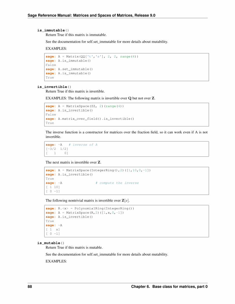
Sage Reference Manual: Matrices and Spaces of Matrices, Release 9.0
is_immutable()Return True if this matrix is immutable.
See the documentation for self.set_immutable for more details about mutability.
EXAMPLES:
sage: A = Matrix(QQ['t','s'], 2, 2, range(4))sage: A.is_immutable()Falsesage: A.set_immutable()sage: A.is_immutable()True
is_invertible()Return True if this matrix is invertible.
EXAMPLES: The following matrix is invertible over Q but not over Z.
sage: A = MatrixSpace(ZZ, 2)(range(4))sage: A.is_invertible()Falsesage: A.matrix_over_field().is_invertible()True
The inverse function is a constructor for matrices over the fraction field, so it can work even if A is notinvertible.
sage: ~A # inverse of A[-3/2 1/2][ 1 0]
The next matrix is invertible over Z.
sage: A = MatrixSpace(IntegerRing(),2)([1,10,0,-1])sage: A.is_invertible()Truesage: ~A # compute the inverse[ 1 10][ 0 -1]
The following nontrivial matrix is invertible over Z[𝑥].
sage: R.<x> = PolynomialRing(IntegerRing())sage: A = MatrixSpace(R,2)([1,x,0,-1])sage: A.is_invertible()Truesage: ~A[ 1 x][ 0 -1]
is_mutable()Return True if this matrix is mutable.
See the documentation for self.set_immutable for more details about mutability.
EXAMPLES:
88 Chapter 6. Base class for matrices, part 0
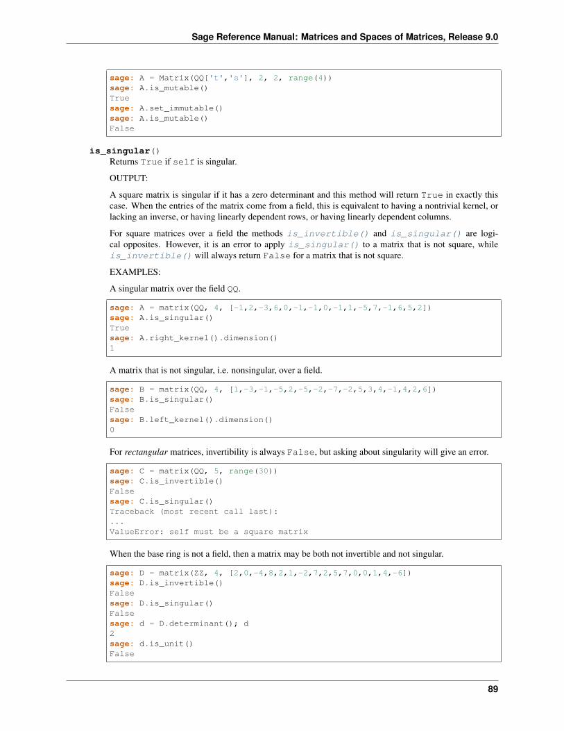
Sage Reference Manual: Matrices and Spaces of Matrices, Release 9.0
sage: A = Matrix(QQ['t','s'], 2, 2, range(4))sage: A.is_mutable()Truesage: A.set_immutable()sage: A.is_mutable()False
is_singular()Returns True if self is singular.
OUTPUT:
A square matrix is singular if it has a zero determinant and this method will return True in exactly thiscase. When the entries of the matrix come from a field, this is equivalent to having a nontrivial kernel, orlacking an inverse, or having linearly dependent rows, or having linearly dependent columns.
For square matrices over a field the methods is_invertible() and is_singular() are logi-cal opposites. However, it is an error to apply is_singular() to a matrix that is not square, whileis_invertible() will always return False for a matrix that is not square.
EXAMPLES:
A singular matrix over the field QQ.
sage: A = matrix(QQ, 4, [-1,2,-3,6,0,-1,-1,0,-1,1,-5,7,-1,6,5,2])sage: A.is_singular()Truesage: A.right_kernel().dimension()1
A matrix that is not singular, i.e. nonsingular, over a field.
sage: B = matrix(QQ, 4, [1,-3,-1,-5,2,-5,-2,-7,-2,5,3,4,-1,4,2,6])sage: B.is_singular()Falsesage: B.left_kernel().dimension()0
For rectangular matrices, invertibility is always False, but asking about singularity will give an error.
sage: C = matrix(QQ, 5, range(30))sage: C.is_invertible()Falsesage: C.is_singular()Traceback (most recent call last):...ValueError: self must be a square matrix
When the base ring is not a field, then a matrix may be both not invertible and not singular.
sage: D = matrix(ZZ, 4, [2,0,-4,8,2,1,-2,7,2,5,7,0,0,1,4,-6])sage: D.is_invertible()Falsesage: D.is_singular()Falsesage: d = D.determinant(); d2sage: d.is_unit()False
89
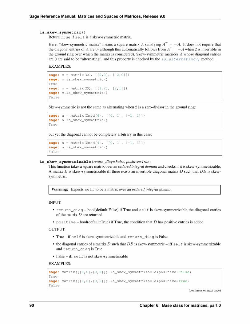
Sage Reference Manual: Matrices and Spaces of Matrices, Release 9.0
is_skew_symmetric()Return True if self is a skew-symmetric matrix.
Here, “skew-symmetric matrix” means a square matrix 𝐴 satisfying 𝐴𝑇 = −𝐴. It does not require thatthe diagonal entries of 𝐴 are 0 (although this automatically follows from 𝐴𝑇 = −𝐴 when 2 is invertible inthe ground ring over which the matrix is considered). Skew-symmetric matrices 𝐴 whose diagonal entriesare 0 are said to be “alternating”, and this property is checked by the is_alternating() method.
EXAMPLES:
sage: m = matrix(QQ, [[0,2], [-2,0]])sage: m.is_skew_symmetric()Truesage: m = matrix(QQ, [[1,2], [2,1]])sage: m.is_skew_symmetric()False
Skew-symmetric is not the same as alternating when 2 is a zero-divisor in the ground ring:
sage: n = matrix(Zmod(4), [[0, 1], [-1, 2]])sage: n.is_skew_symmetric()True
but yet the diagonal cannot be completely arbitrary in this case:
sage: n = matrix(Zmod(4), [[0, 1], [-1, 3]])sage: n.is_skew_symmetric()False
is_skew_symmetrizable(return_diag=False, positive=True)This function takes a square matrix over an ordered integral domain and checks if it is skew-symmetrizable.A matrix 𝐵 is skew-symmetrizable iff there exists an invertible diagonal matrix 𝐷 such that 𝐷𝐵 is skew-symmetric.
Warning: Expects self to be a matrix over an ordered integral domain.
INPUT:
• return_diag – bool(default:False) if True and self is skew-symmetrizable the diagonal entriesof the matrix 𝐷 are returned.
• positive – bool(default:True) if True, the condition that 𝐷 has positive entries is added.
OUTPUT:
• True – if self is skew-symmetrizable and return_diag is False
• the diagonal entries of a matrix 𝐷 such that 𝐷𝐵 is skew-symmetric – iff self is skew-symmetrizableand return_diag is True
• False – iff self is not skew-symmetrizable
EXAMPLES:
sage: matrix([[0,6],[3,0]]).is_skew_symmetrizable(positive=False)Truesage: matrix([[0,6],[3,0]]).is_skew_symmetrizable(positive=True)False
(continues on next page)
90 Chapter 6. Base class for matrices, part 0
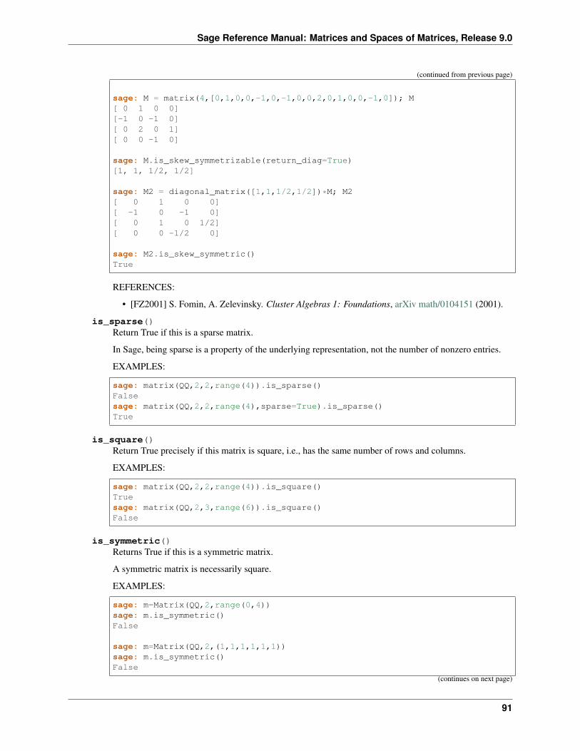
Sage Reference Manual: Matrices and Spaces of Matrices, Release 9.0
(continued from previous page)
sage: M = matrix(4,[0,1,0,0,-1,0,-1,0,0,2,0,1,0,0,-1,0]); M[ 0 1 0 0][-1 0 -1 0][ 0 2 0 1][ 0 0 -1 0]
sage: M.is_skew_symmetrizable(return_diag=True)[1, 1, 1/2, 1/2]
sage: M2 = diagonal_matrix([1,1,1/2,1/2])*M; M2[ 0 1 0 0][ -1 0 -1 0][ 0 1 0 1/2][ 0 0 -1/2 0]
sage: M2.is_skew_symmetric()True
REFERENCES:
• [FZ2001] S. Fomin, A. Zelevinsky. Cluster Algebras 1: Foundations, arXiv math/0104151 (2001).
is_sparse()Return True if this is a sparse matrix.
In Sage, being sparse is a property of the underlying representation, not the number of nonzero entries.
EXAMPLES:
sage: matrix(QQ,2,2,range(4)).is_sparse()Falsesage: matrix(QQ,2,2,range(4),sparse=True).is_sparse()True
is_square()Return True precisely if this matrix is square, i.e., has the same number of rows and columns.
EXAMPLES:
sage: matrix(QQ,2,2,range(4)).is_square()Truesage: matrix(QQ,2,3,range(6)).is_square()False
is_symmetric()Returns True if this is a symmetric matrix.
A symmetric matrix is necessarily square.
EXAMPLES:
sage: m=Matrix(QQ,2,range(0,4))sage: m.is_symmetric()False
sage: m=Matrix(QQ,2,(1,1,1,1,1,1))sage: m.is_symmetric()False
(continues on next page)
91
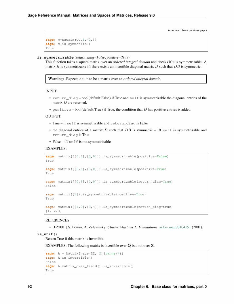
Sage Reference Manual: Matrices and Spaces of Matrices, Release 9.0
(continued from previous page)
sage: m=Matrix(QQ,1,(2,))sage: m.is_symmetric()True
is_symmetrizable(return_diag=False, positive=True)This function takes a square matrix over an ordered integral domain and checks if it is symmetrizable. Amatrix 𝐵 is symmetrizable iff there exists an invertible diagonal matrix 𝐷 such that 𝐷𝐵 is symmetric.
Warning: Expects self to be a matrix over an ordered integral domain.
INPUT:
• return_diag – bool(default:False) if True and self is symmetrizable the diagonal entries of thematrix 𝐷 are returned.
• positive – bool(default:True) if True, the condition that 𝐷 has positive entries is added.
OUTPUT:
• True – if self is symmetrizable and return_diag is False
• the diagonal entries of a matrix 𝐷 such that 𝐷𝐵 is symmetric – iff self is symmetrizable andreturn_diag is True
• False – iff self is not symmetrizable
EXAMPLES:
sage: matrix([[0,6],[3,0]]).is_symmetrizable(positive=False)True
sage: matrix([[0,6],[3,0]]).is_symmetrizable(positive=True)True
sage: matrix([[0,6],[0,0]]).is_symmetrizable(return_diag=True)False
sage: matrix([2]).is_symmetrizable(positive=True)True
sage: matrix([[1,2],[3,4]]).is_symmetrizable(return_diag=true)[1, 2/3]
REFERENCES:
• [FZ2001] S. Fomin, A. Zelevinsky. Cluster Algebras 1: Foundations, arXiv math/0104151 (2001).
is_unit()Return True if this matrix is invertible.
EXAMPLES: The following matrix is invertible over Q but not over Z.
sage: A = MatrixSpace(ZZ, 2)(range(4))sage: A.is_invertible()Falsesage: A.matrix_over_field().is_invertible()True
92 Chapter 6. Base class for matrices, part 0
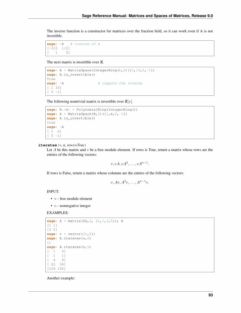
Sage Reference Manual: Matrices and Spaces of Matrices, Release 9.0
The inverse function is a constructor for matrices over the fraction field, so it can work even if A is notinvertible.
sage: ~A # inverse of A[-3/2 1/2][ 1 0]
The next matrix is invertible over Z.
sage: A = MatrixSpace(IntegerRing(),2)([1,10,0,-1])sage: A.is_invertible()Truesage: ~A # compute the inverse[ 1 10][ 0 -1]
The following nontrivial matrix is invertible over Z[𝑥].
sage: R.<x> = PolynomialRing(IntegerRing())sage: A = MatrixSpace(R,2)([1,x,0,-1])sage: A.is_invertible()Truesage: ~A[ 1 x][ 0 -1]
iterates(v, n, rows=True)Let 𝐴 be this matrix and 𝑣 be a free module element. If rows is True, return a matrix whose rows are theentries of the following vectors:
𝑣, 𝑣𝐴, 𝑣𝐴2, . . . , 𝑣𝐴𝑛−1.
If rows is False, return a matrix whose columns are the entries of the following vectors:
𝑣,𝐴𝑣,𝐴2𝑣, . . . , 𝐴𝑛−1𝑣.
INPUT:
• v - free module element
• n - nonnegative integer
EXAMPLES:
sage: A = matrix(ZZ,2, [1,1,3,5]); A[1 1][3 5]sage: v = vector([1,0])sage: A.iterates(v,0)[]sage: A.iterates(v,5)[ 1 0][ 1 1][ 4 6][ 22 34][124 192]
Another example:
93
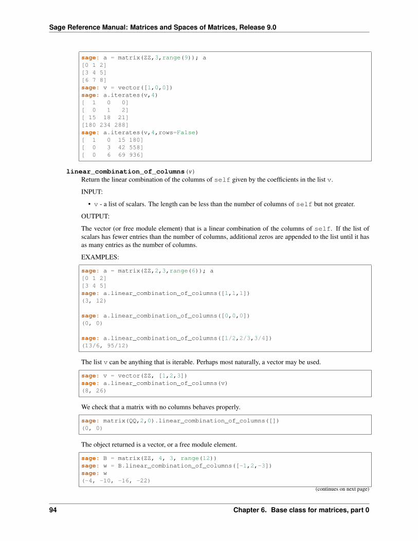
Sage Reference Manual: Matrices and Spaces of Matrices, Release 9.0
sage: a = matrix(ZZ,3,range(9)); a[0 1 2][3 4 5][6 7 8]sage: v = vector([1,0,0])sage: a.iterates(v,4)[ 1 0 0][ 0 1 2][ 15 18 21][180 234 288]sage: a.iterates(v,4,rows=False)[ 1 0 15 180][ 0 3 42 558][ 0 6 69 936]
linear_combination_of_columns(v)Return the linear combination of the columns of self given by the coefficients in the list v.
INPUT:
• v - a list of scalars. The length can be less than the number of columns of self but not greater.
OUTPUT:
The vector (or free module element) that is a linear combination of the columns of self. If the list ofscalars has fewer entries than the number of columns, additional zeros are appended to the list until it hasas many entries as the number of columns.
EXAMPLES:
sage: a = matrix(ZZ,2,3,range(6)); a[0 1 2][3 4 5]sage: a.linear_combination_of_columns([1,1,1])(3, 12)
sage: a.linear_combination_of_columns([0,0,0])(0, 0)
sage: a.linear_combination_of_columns([1/2,2/3,3/4])(13/6, 95/12)
The list v can be anything that is iterable. Perhaps most naturally, a vector may be used.
sage: v = vector(ZZ, [1,2,3])sage: a.linear_combination_of_columns(v)(8, 26)
We check that a matrix with no columns behaves properly.
sage: matrix(QQ,2,0).linear_combination_of_columns([])(0, 0)
The object returned is a vector, or a free module element.
sage: B = matrix(ZZ, 4, 3, range(12))sage: w = B.linear_combination_of_columns([-1,2,-3])sage: w(-4, -10, -16, -22)
(continues on next page)
94 Chapter 6. Base class for matrices, part 0
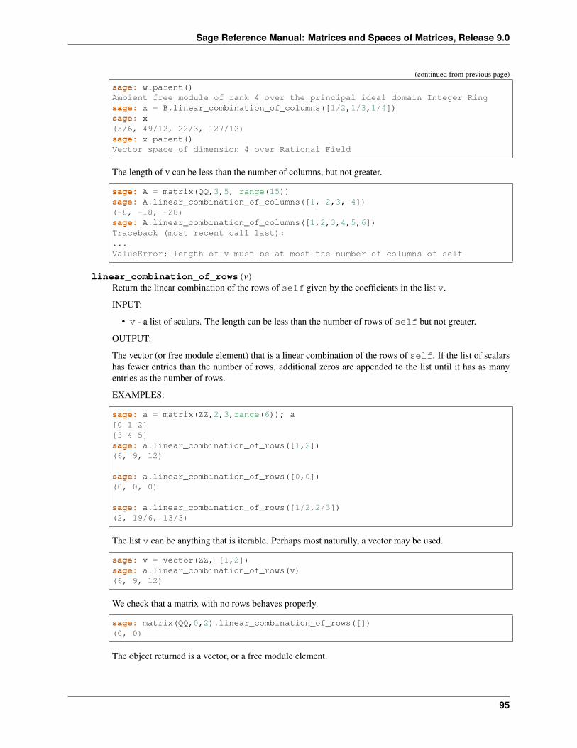
Sage Reference Manual: Matrices and Spaces of Matrices, Release 9.0
(continued from previous page)
sage: w.parent()Ambient free module of rank 4 over the principal ideal domain Integer Ringsage: x = B.linear_combination_of_columns([1/2,1/3,1/4])sage: x(5/6, 49/12, 22/3, 127/12)sage: x.parent()Vector space of dimension 4 over Rational Field
The length of v can be less than the number of columns, but not greater.
sage: A = matrix(QQ,3,5, range(15))sage: A.linear_combination_of_columns([1,-2,3,-4])(-8, -18, -28)sage: A.linear_combination_of_columns([1,2,3,4,5,6])Traceback (most recent call last):...ValueError: length of v must be at most the number of columns of self
linear_combination_of_rows(v)Return the linear combination of the rows of self given by the coefficients in the list v.
INPUT:
• v - a list of scalars. The length can be less than the number of rows of self but not greater.
OUTPUT:
The vector (or free module element) that is a linear combination of the rows of self. If the list of scalarshas fewer entries than the number of rows, additional zeros are appended to the list until it has as manyentries as the number of rows.
EXAMPLES:
sage: a = matrix(ZZ,2,3,range(6)); a[0 1 2][3 4 5]sage: a.linear_combination_of_rows([1,2])(6, 9, 12)
sage: a.linear_combination_of_rows([0,0])(0, 0, 0)
sage: a.linear_combination_of_rows([1/2,2/3])(2, 19/6, 13/3)
The list v can be anything that is iterable. Perhaps most naturally, a vector may be used.
sage: v = vector(ZZ, [1,2])sage: a.linear_combination_of_rows(v)(6, 9, 12)
We check that a matrix with no rows behaves properly.
sage: matrix(QQ,0,2).linear_combination_of_rows([])(0, 0)
The object returned is a vector, or a free module element.
95
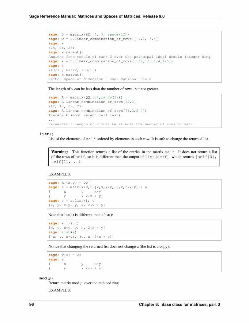
Sage Reference Manual: Matrices and Spaces of Matrices, Release 9.0
sage: B = matrix(ZZ, 4, 3, range(12))sage: w = B.linear_combination_of_rows([-1,2,-3,4])sage: w(24, 26, 28)sage: w.parent()Ambient free module of rank 3 over the principal ideal domain Integer Ringsage: x = B.linear_combination_of_rows([1/2,1/3,1/4,1/5])sage: x(43/10, 67/12, 103/15)sage: x.parent()Vector space of dimension 3 over Rational Field
The length of v can be less than the number of rows, but not greater.
sage: A = matrix(QQ,3,4,range(12))sage: A.linear_combination_of_rows([2,3])(12, 17, 22, 27)sage: A.linear_combination_of_rows([1,2,3,4])Traceback (most recent call last):...ValueError: length of v must be at most the number of rows of self
list()List of the elements of self ordered by elements in each row. It is safe to change the returned list.
Warning: This function returns a list of the entries in the matrix self. It does not return a listof the rows of self, so it is different than the output of list(self), which returns [self[0],self[1],...].
EXAMPLES:
sage: R.<x,y> = QQ[]sage: a = matrix(R,2,[x,y,x*y, y,x,2*x+y]); a[ x y x*y][ y x 2*x + y]sage: v = a.list(); v[x, y, x*y, y, x, 2*x + y]
Note that list(a) is different than a.list():
sage: a.list()[x, y, x*y, y, x, 2*x + y]sage: list(a)[(x, y, x*y), (y, x, 2*x + y)]
Notice that changing the returned list does not change a (the list is a copy):
sage: v[0] = 25sage: a[ x y x*y][ y x 2*x + y]
mod(p)Return matrix mod 𝑝, over the reduced ring.
EXAMPLES:
96 Chapter 6. Base class for matrices, part 0
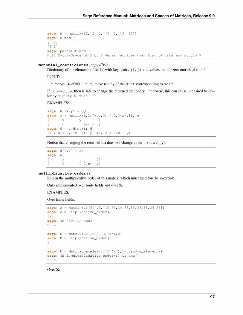
Sage Reference Manual: Matrices and Spaces of Matrices, Release 9.0
sage: M = matrix(ZZ, 2, 2, [5, 9, 13, 15])sage: M.mod(7)[5 2][6 1]sage: parent(M.mod(7))Full MatrixSpace of 2 by 2 dense matrices over Ring of integers modulo 7
monomial_coefficients(copy=True)Dictionary of the elements of self with keys pairs (i,j) and values the nonzero entries of self.
INPUT:
• copy – (default: True) make a copy of the dict corresponding to self
If copy=True, then is safe to change the returned dictionary. Otherwise, this can cause undesired behav-ior by mutating the dict.
EXAMPLES:
sage: R.<x,y> = QQ[]sage: a = matrix(R,2,[x,y,0, 0,0,2*x+y]); a[ x y 0][ 0 0 2*x + y]sage: d = a.dict(); d{(0, 0): x, (0, 1): y, (1, 2): 2*x + y}
Notice that changing the returned list does not change a (the list is a copy):
sage: d[0,0] = 25sage: a[ x y 0][ 0 0 2*x + y]
multiplicative_order()Return the multiplicative order of this matrix, which must therefore be invertible.
Only implemented over finite fields and over Z.
EXAMPLES:
Over finite fields:
sage: A = matrix(GF(59),3,[10,56,39,53,56,33,58,24,55])sage: A.multiplicative_order()580sage: (A^580).is_one()True
sage: B = matrix(GF(10007^3,'b'),0)sage: B.multiplicative_order()1
sage: E = MatrixSpace(GF(11^2,'e'),5).random_element()sage: (E^E.multiplicative_order()).is_one()True
Over Z:
97
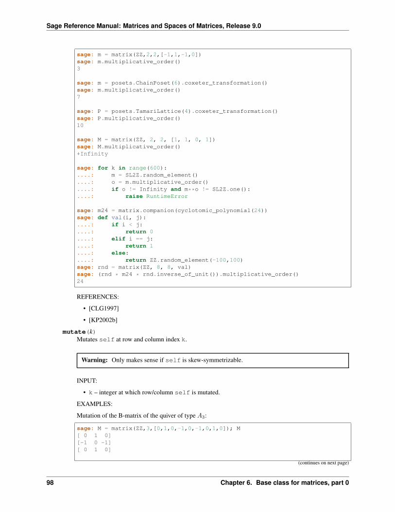
Sage Reference Manual: Matrices and Spaces of Matrices, Release 9.0
sage: m = matrix(ZZ,2,2,[-1,1,-1,0])sage: m.multiplicative_order()3
sage: m = posets.ChainPoset(6).coxeter_transformation()sage: m.multiplicative_order()7
sage: P = posets.TamariLattice(4).coxeter_transformation()sage: P.multiplicative_order()10
sage: M = matrix(ZZ, 2, 2, [1, 1, 0, 1])sage: M.multiplicative_order()+Infinity
sage: for k in range(600):....: m = SL2Z.random_element()....: o = m.multiplicative_order()....: if o != Infinity and m**o != SL2Z.one():....: raise RuntimeError
sage: m24 = matrix.companion(cyclotomic_polynomial(24))sage: def val(i, j):....: if i < j:....: return 0....: elif i == j:....: return 1....: else:....: return ZZ.random_element(-100,100)sage: rnd = matrix(ZZ, 8, 8, val)sage: (rnd * m24 * rnd.inverse_of_unit()).multiplicative_order()24
REFERENCES:
• [CLG1997]
• [KP2002b]
mutate(k)Mutates self at row and column index k.
Warning: Only makes sense if self is skew-symmetrizable.
INPUT:
• k – integer at which row/column self is mutated.
EXAMPLES:
Mutation of the B-matrix of the quiver of type 𝐴3:
sage: M = matrix(ZZ,3,[0,1,0,-1,0,-1,0,1,0]); M[ 0 1 0][-1 0 -1][ 0 1 0]
(continues on next page)
98 Chapter 6. Base class for matrices, part 0
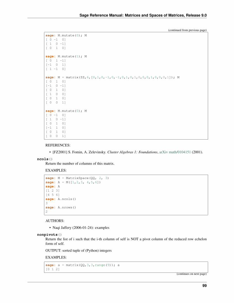
Sage Reference Manual: Matrices and Spaces of Matrices, Release 9.0
(continued from previous page)
sage: M.mutate(0); M[ 0 -1 0][ 1 0 -1][ 0 1 0]
sage: M.mutate(1); M[ 0 1 -1][-1 0 1][ 1 -1 0]
sage: M = matrix(ZZ,6,[0,1,0,-1,0,-1,0,1,0,1,0,0,0,1,0,0,0,1]); M[ 0 1 0][-1 0 -1][ 0 1 0][ 1 0 0][ 0 1 0][ 0 0 1]
sage: M.mutate(0); M[ 0 -1 0][ 1 0 -1][ 0 1 0][-1 1 0][ 0 1 0][ 0 0 1]
REFERENCES:
• [FZ2001] S. Fomin, A. Zelevinsky. Cluster Algebras 1: Foundations, arXiv math/0104151 (2001).
ncols()Return the number of columns of this matrix.
EXAMPLES:
sage: M = MatrixSpace(QQ, 2, 3)sage: A = M([1,2,3, 4,5,6])sage: A[1 2 3][4 5 6]sage: A.ncols()3sage: A.nrows()2
AUTHORS:
• Naqi Jaffery (2006-01-24): examples
nonpivots()Return the list of i such that the i-th column of self is NOT a pivot column of the reduced row echelonform of self.
OUTPUT: sorted tuple of (Python) integers
EXAMPLES:
sage: a = matrix(QQ,3,3,range(9)); a[0 1 2]
(continues on next page)
99
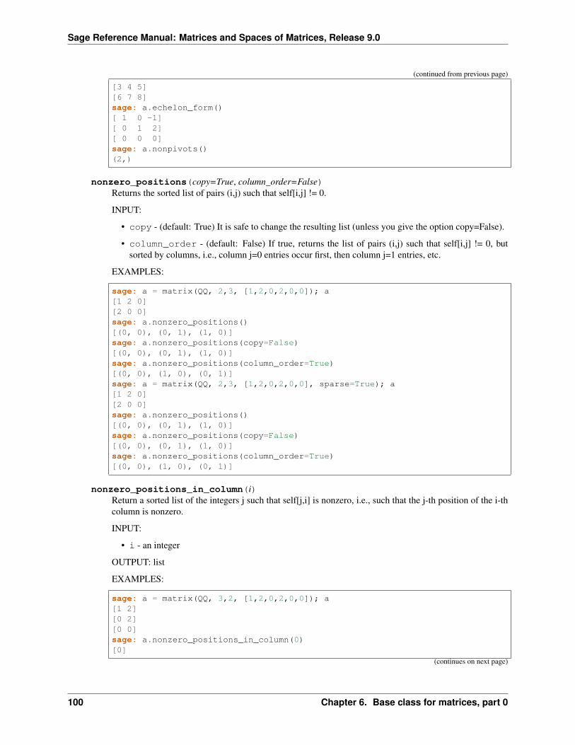
Sage Reference Manual: Matrices and Spaces of Matrices, Release 9.0
(continued from previous page)
[3 4 5][6 7 8]sage: a.echelon_form()[ 1 0 -1][ 0 1 2][ 0 0 0]sage: a.nonpivots()(2,)
nonzero_positions(copy=True, column_order=False)Returns the sorted list of pairs (i,j) such that self[i,j] != 0.
INPUT:
• copy - (default: True) It is safe to change the resulting list (unless you give the option copy=False).
• column_order - (default: False) If true, returns the list of pairs (i,j) such that self[i,j] != 0, butsorted by columns, i.e., column j=0 entries occur first, then column j=1 entries, etc.
EXAMPLES:
sage: a = matrix(QQ, 2,3, [1,2,0,2,0,0]); a[1 2 0][2 0 0]sage: a.nonzero_positions()[(0, 0), (0, 1), (1, 0)]sage: a.nonzero_positions(copy=False)[(0, 0), (0, 1), (1, 0)]sage: a.nonzero_positions(column_order=True)[(0, 0), (1, 0), (0, 1)]sage: a = matrix(QQ, 2,3, [1,2,0,2,0,0], sparse=True); a[1 2 0][2 0 0]sage: a.nonzero_positions()[(0, 0), (0, 1), (1, 0)]sage: a.nonzero_positions(copy=False)[(0, 0), (0, 1), (1, 0)]sage: a.nonzero_positions(column_order=True)[(0, 0), (1, 0), (0, 1)]
nonzero_positions_in_column(i)Return a sorted list of the integers j such that self[j,i] is nonzero, i.e., such that the j-th position of the i-thcolumn is nonzero.
INPUT:
• i - an integer
OUTPUT: list
EXAMPLES:
sage: a = matrix(QQ, 3,2, [1,2,0,2,0,0]); a[1 2][0 2][0 0]sage: a.nonzero_positions_in_column(0)[0]
(continues on next page)
100 Chapter 6. Base class for matrices, part 0

Sage Reference Manual: Matrices and Spaces of Matrices, Release 9.0
(continued from previous page)
sage: a.nonzero_positions_in_column(1)[0, 1]
You’ll get an IndexError, if you select an invalid column:
sage: a.nonzero_positions_in_column(2)Traceback (most recent call last):...IndexError: matrix column index out of range
nonzero_positions_in_row(i)Return the integers j such that self[i,j] is nonzero, i.e., such that the j-th position of the i-th row is nonzero.
INPUT:
• i - an integer
OUTPUT: list
EXAMPLES:
sage: a = matrix(QQ, 3,2, [1,2,0,2,0,0]); a[1 2][0 2][0 0]sage: a.nonzero_positions_in_row(0)[0, 1]sage: a.nonzero_positions_in_row(1)[1]sage: a.nonzero_positions_in_row(2)[]
nrows()Return the number of rows of this matrix.
EXAMPLES:
sage: M = MatrixSpace(QQ,6,7)sage: A = M([1,2,3,4,5,6,7, 22,3/4,34,11,7,5,3, 99,65,1/2,2/3,3/5,4/5,5/6, 9,→˓8/9, 9/8,7/6,6/7,76,4, 0,9,8,7,6,5,4, 123,99,91,28,6,1024,1])sage: A[ 1 2 3 4 5 6 7][ 22 3/4 34 11 7 5 3][ 99 65 1/2 2/3 3/5 4/5 5/6][ 9 8/9 9/8 7/6 6/7 76 4][ 0 9 8 7 6 5 4][ 123 99 91 28 6 1024 1]sage: A.ncols()7sage: A.nrows()6
AUTHORS:
• Naqi Jaffery (2006-01-24): examples
permute_columns(permutation)Permute the columns of self by applying the permutation group element permutation.
101
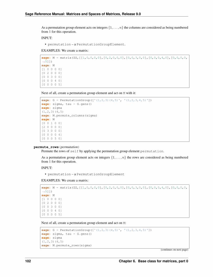
Sage Reference Manual: Matrices and Spaces of Matrices, Release 9.0
As a permutation group element acts on integers {1, . . . , 𝑛} the columns are considered as being numberedfrom 1 for this operation.
INPUT:
• permutation – a PermutationGroupElement.
EXAMPLES: We create a matrix:
sage: M = matrix(ZZ,[[1,0,0,0,0],[0,2,0,0,0],[0,0,3,0,0],[0,0,0,4,0],[0,0,0,0,→˓5]])sage: M[1 0 0 0 0][0 2 0 0 0][0 0 3 0 0][0 0 0 4 0][0 0 0 0 5]
Next of all, create a permutation group element and act on M with it:
sage: G = PermutationGroup(['(1,2,3)(4,5)', '(1,2,3,4,5)'])sage: sigma, tau = G.gens()sage: sigma(1,2,3)(4,5)sage: M.permute_columns(sigma)sage: M[0 0 1 0 0][2 0 0 0 0][0 3 0 0 0][0 0 0 0 4][0 0 0 5 0]
permute_rows(permutation)Permute the rows of self by applying the permutation group element permutation.
As a permutation group element acts on integers {1, . . . , 𝑛} the rows are considered as being numberedfrom 1 for this operation.
INPUT:
• permutation – a PermutationGroupElement
EXAMPLES: We create a matrix:
sage: M = matrix(ZZ,[[1,0,0,0,0],[0,2,0,0,0],[0,0,3,0,0],[0,0,0,4,0],[0,0,0,0,→˓5]])sage: M[1 0 0 0 0][0 2 0 0 0][0 0 3 0 0][0 0 0 4 0][0 0 0 0 5]
Next of all, create a permutation group element and act on M:
sage: G = PermutationGroup(['(1,2,3)(4,5)', '(1,2,3,4,5)'])sage: sigma, tau = G.gens()sage: sigma(1,2,3)(4,5)sage: M.permute_rows(sigma)
(continues on next page)
102 Chapter 6. Base class for matrices, part 0
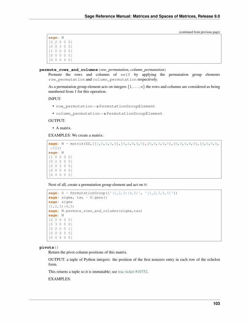
Sage Reference Manual: Matrices and Spaces of Matrices, Release 9.0
(continued from previous page)
sage: M[0 2 0 0 0][0 0 3 0 0][1 0 0 0 0][0 0 0 0 5][0 0 0 4 0]
permute_rows_and_columns(row_permutation, column_permutation)Permute the rows and columns of self by applying the permutation group elementsrow_permutation and column_permutation respectively.
As a permutation group element acts on integers {1, . . . , 𝑛} the rows and columns are considered as beingnumbered from 1 for this operation.
INPUT:
• row_permutation – a PermutationGroupElement
• column_permutation – a PermutationGroupElement
OUTPUT:
• A matrix.
EXAMPLES: We create a matrix:
sage: M = matrix(ZZ,[[1,0,0,0,0],[0,2,0,0,0],[0,0,3,0,0],[0,0,0,4,0],[0,0,0,0,→˓5]])sage: M[1 0 0 0 0][0 2 0 0 0][0 0 3 0 0][0 0 0 4 0][0 0 0 0 5]
Next of all, create a permutation group element and act on M:
sage: G = PermutationGroup(['(1,2,3)(4,5)', '(1,2,3,4,5)'])sage: sigma, tau = G.gens()sage: sigma(1,2,3)(4,5)sage: M.permute_rows_and_columns(sigma,tau)sage: M[2 0 0 0 0][0 3 0 0 0][0 0 0 0 1][0 0 0 5 0][0 0 4 0 0]
pivots()Return the pivot column positions of this matrix.
OUTPUT: a tuple of Python integers: the position of the first nonzero entry in each row of the echelonform.
This returns a tuple so it is immutable; see trac ticket #10752.
EXAMPLES:
103
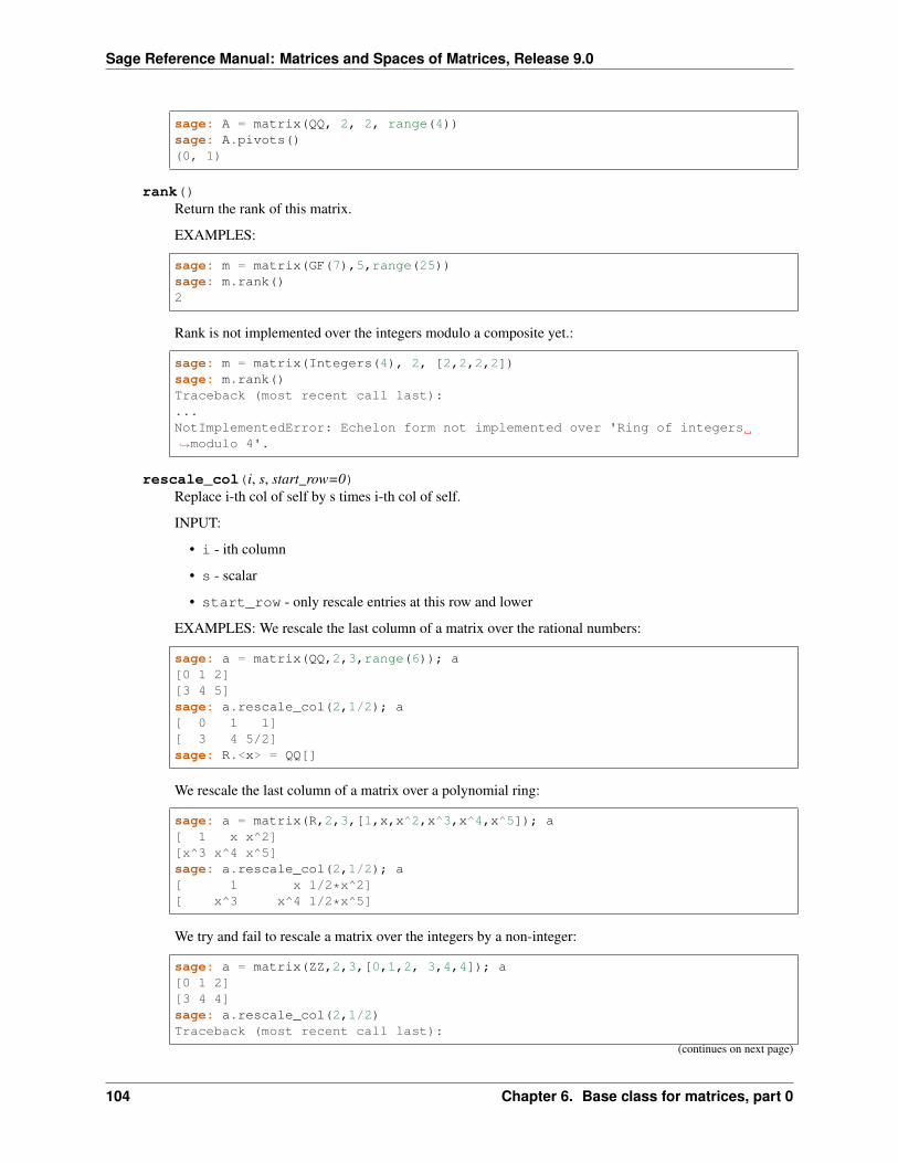
Sage Reference Manual: Matrices and Spaces of Matrices, Release 9.0
sage: A = matrix(QQ, 2, 2, range(4))sage: A.pivots()(0, 1)
rank()Return the rank of this matrix.
EXAMPLES:
sage: m = matrix(GF(7),5,range(25))sage: m.rank()2
Rank is not implemented over the integers modulo a composite yet.:
sage: m = matrix(Integers(4), 2, [2,2,2,2])sage: m.rank()Traceback (most recent call last):...NotImplementedError: Echelon form not implemented over 'Ring of integers→˓modulo 4'.
rescale_col(i, s, start_row=0)Replace i-th col of self by s times i-th col of self.
INPUT:
• i - ith column
• s - scalar
• start_row - only rescale entries at this row and lower
EXAMPLES: We rescale the last column of a matrix over the rational numbers:
sage: a = matrix(QQ,2,3,range(6)); a[0 1 2][3 4 5]sage: a.rescale_col(2,1/2); a[ 0 1 1][ 3 4 5/2]sage: R.<x> = QQ[]
We rescale the last column of a matrix over a polynomial ring:
sage: a = matrix(R,2,3,[1,x,x^2,x^3,x^4,x^5]); a[ 1 x x^2][x^3 x^4 x^5]sage: a.rescale_col(2,1/2); a[ 1 x 1/2*x^2][ x^3 x^4 1/2*x^5]
We try and fail to rescale a matrix over the integers by a non-integer:
sage: a = matrix(ZZ,2,3,[0,1,2, 3,4,4]); a[0 1 2][3 4 4]sage: a.rescale_col(2,1/2)Traceback (most recent call last):
(continues on next page)
104 Chapter 6. Base class for matrices, part 0
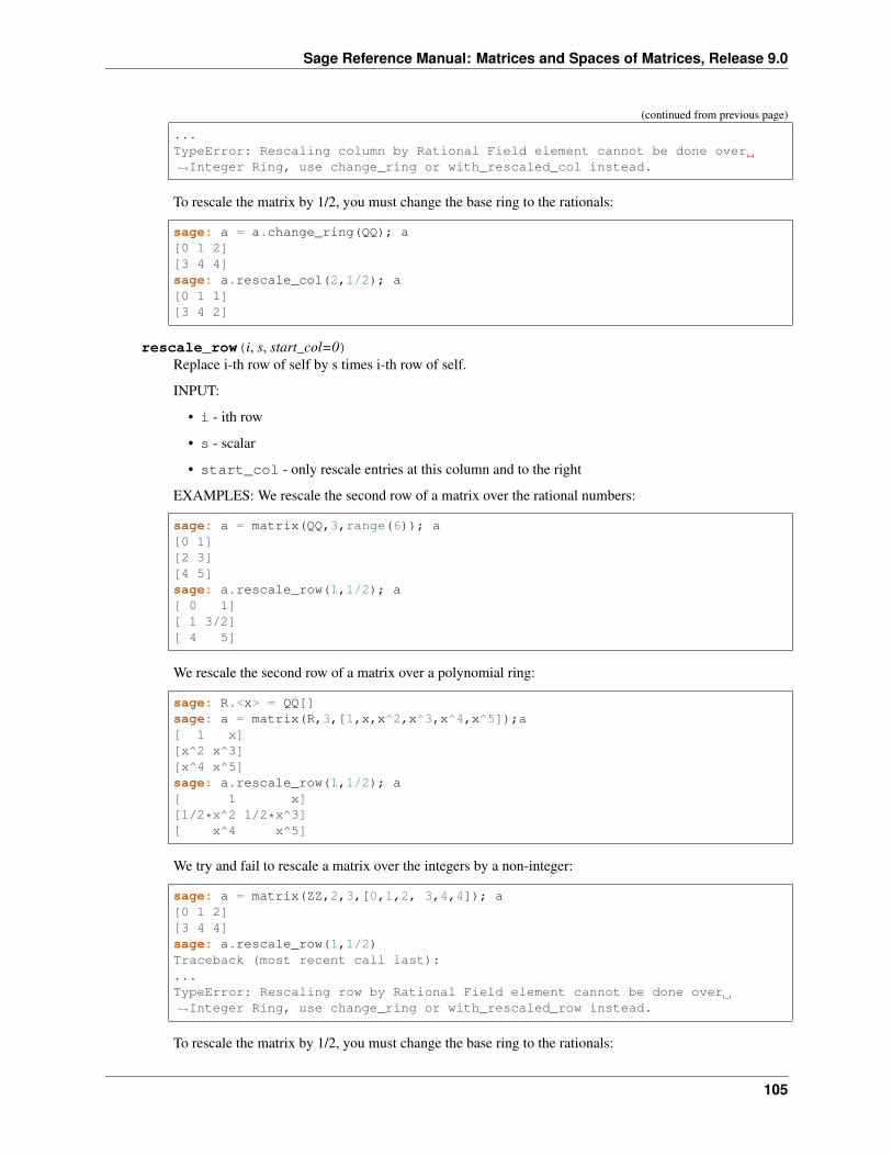
Sage Reference Manual: Matrices and Spaces of Matrices, Release 9.0
(continued from previous page)
...TypeError: Rescaling column by Rational Field element cannot be done over→˓Integer Ring, use change_ring or with_rescaled_col instead.
To rescale the matrix by 1/2, you must change the base ring to the rationals:
sage: a = a.change_ring(QQ); a[0 1 2][3 4 4]sage: a.rescale_col(2,1/2); a[0 1 1][3 4 2]
rescale_row(i, s, start_col=0)Replace i-th row of self by s times i-th row of self.
INPUT:
• i - ith row
• s - scalar
• start_col - only rescale entries at this column and to the right
EXAMPLES: We rescale the second row of a matrix over the rational numbers:
sage: a = matrix(QQ,3,range(6)); a[0 1][2 3][4 5]sage: a.rescale_row(1,1/2); a[ 0 1][ 1 3/2][ 4 5]
We rescale the second row of a matrix over a polynomial ring:
sage: R.<x> = QQ[]sage: a = matrix(R,3,[1,x,x^2,x^3,x^4,x^5]);a[ 1 x][x^2 x^3][x^4 x^5]sage: a.rescale_row(1,1/2); a[ 1 x][1/2*x^2 1/2*x^3][ x^4 x^5]
We try and fail to rescale a matrix over the integers by a non-integer:
sage: a = matrix(ZZ,2,3,[0,1,2, 3,4,4]); a[0 1 2][3 4 4]sage: a.rescale_row(1,1/2)Traceback (most recent call last):...TypeError: Rescaling row by Rational Field element cannot be done over→˓Integer Ring, use change_ring or with_rescaled_row instead.
To rescale the matrix by 1/2, you must change the base ring to the rationals:
105
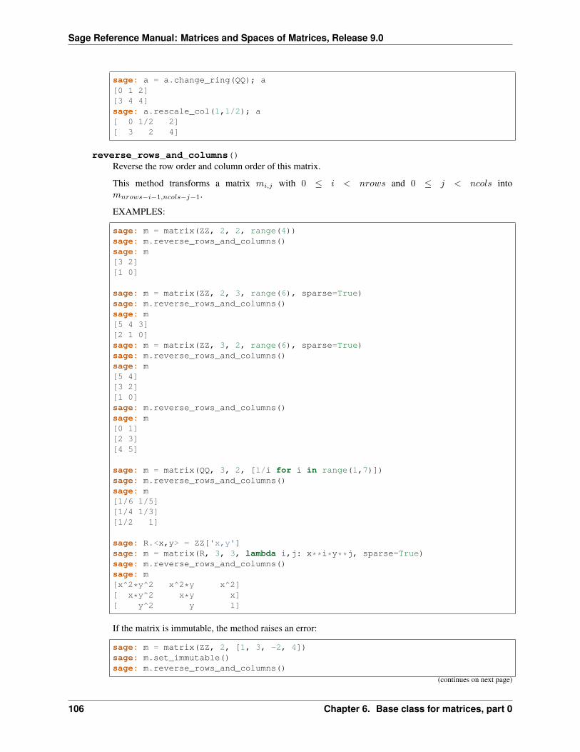
Sage Reference Manual: Matrices and Spaces of Matrices, Release 9.0
sage: a = a.change_ring(QQ); a[0 1 2][3 4 4]sage: a.rescale_col(1,1/2); a[ 0 1/2 2][ 3 2 4]
reverse_rows_and_columns()Reverse the row order and column order of this matrix.
This method transforms a matrix 𝑚𝑖,𝑗 with 0 ≤ 𝑖 < 𝑛𝑟𝑜𝑤𝑠 and 0 ≤ 𝑗 < 𝑛𝑐𝑜𝑙𝑠 into𝑚𝑛𝑟𝑜𝑤𝑠−𝑖−1,𝑛𝑐𝑜𝑙𝑠−𝑗−1.
EXAMPLES:
sage: m = matrix(ZZ, 2, 2, range(4))sage: m.reverse_rows_and_columns()sage: m[3 2][1 0]
sage: m = matrix(ZZ, 2, 3, range(6), sparse=True)sage: m.reverse_rows_and_columns()sage: m[5 4 3][2 1 0]sage: m = matrix(ZZ, 3, 2, range(6), sparse=True)sage: m.reverse_rows_and_columns()sage: m[5 4][3 2][1 0]sage: m.reverse_rows_and_columns()sage: m[0 1][2 3][4 5]
sage: m = matrix(QQ, 3, 2, [1/i for i in range(1,7)])sage: m.reverse_rows_and_columns()sage: m[1/6 1/5][1/4 1/3][1/2 1]
sage: R.<x,y> = ZZ['x,y']sage: m = matrix(R, 3, 3, lambda i,j: x**i*y**j, sparse=True)sage: m.reverse_rows_and_columns()sage: m[x^2*y^2 x^2*y x^2][ x*y^2 x*y x][ y^2 y 1]
If the matrix is immutable, the method raises an error:
sage: m = matrix(ZZ, 2, [1, 3, -2, 4])sage: m.set_immutable()sage: m.reverse_rows_and_columns()
(continues on next page)
106 Chapter 6. Base class for matrices, part 0
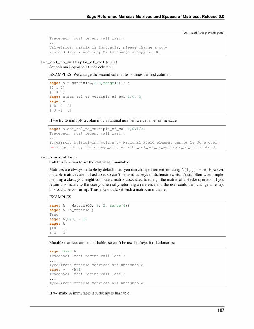
Sage Reference Manual: Matrices and Spaces of Matrices, Release 9.0
(continued from previous page)
Traceback (most recent call last):...ValueError: matrix is immutable; please change a copyinstead (i.e., use copy(M) to change a copy of M).
set_col_to_multiple_of_col(i, j, s)Set column i equal to s times column j.
EXAMPLES: We change the second column to -3 times the first column.
sage: a = matrix(ZZ,2,3,range(6)); a[0 1 2][3 4 5]sage: a.set_col_to_multiple_of_col(1,0,-3)sage: a[ 0 0 2][ 3 -9 5]
If we try to multiply a column by a rational number, we get an error message:
sage: a.set_col_to_multiple_of_col(1,0,1/2)Traceback (most recent call last):...TypeError: Multiplying column by Rational Field element cannot be done over→˓Integer Ring, use change_ring or with_col_set_to_multiple_of_col instead.
set_immutable()Call this function to set the matrix as immutable.
Matrices are always mutable by default, i.e., you can change their entries using A[i,j] = x. However,mutable matrices aren’t hashable, so can’t be used as keys in dictionaries, etc. Also, often when imple-menting a class, you might compute a matrix associated to it, e.g., the matrix of a Hecke operator. If youreturn this matrix to the user you’re really returning a reference and the user could then change an entry;this could be confusing. Thus you should set such a matrix immutable.
EXAMPLES:
sage: A = Matrix(QQ, 2, 2, range(4))sage: A.is_mutable()Truesage: A[0,0] = 10sage: A[10 1][ 2 3]
Mutable matrices are not hashable, so can’t be used as keys for dictionaries:
sage: hash(A)Traceback (most recent call last):...TypeError: mutable matrices are unhashablesage: v = {A:1}Traceback (most recent call last):...TypeError: mutable matrices are unhashable
If we make A immutable it suddenly is hashable.
107
Sage Reference Manual: Matrices and Spaces of Matrices, Release 9.0
sage: A.set_immutable()sage: A.is_mutable()Falsesage: A[0,0] = 10Traceback (most recent call last):...ValueError: matrix is immutable; please change a copy instead (i.e., use→˓copy(M) to change a copy of M).sage: hash(A) #random12sage: v = {A:1}; v{[10 1][ 2 3]: 1}
set_row_to_multiple_of_row(i, j, s)Set row i equal to s times row j.
EXAMPLES: We change the second row to -3 times the first row:
sage: a = matrix(ZZ,2,3,range(6)); a[0 1 2][3 4 5]sage: a.set_row_to_multiple_of_row(1,0,-3)sage: a[ 0 1 2][ 0 -3 -6]
If we try to multiply a row by a rational number, we get an error message:
sage: a.set_row_to_multiple_of_row(1,0,1/2)Traceback (most recent call last):...TypeError: Multiplying row by Rational Field element cannot be done over→˓Integer Ring, use change_ring or with_row_set_to_multiple_of_row instead.
str(rep_mapping=None, zero=None, plus_one=None, minus_one=None, unicode=False,shape=None)Return a nice string representation of the matrix.
INPUT:
• rep_mapping - a dictionary or callable used to override the usual representation of elements.
If rep_mapping is a dictionary then keys should be elements of the base ring and values the desiredstring representation. Values sent in via the other keyword arguments will override values in thedictionary. Use of a dictionary can potentially take a very long time due to the need to hash entries ofthe matrix. Matrices with entries from QQbar are one example.
If rep_mapping is callable then it will be called with elements of the matrix and must return astring. Simply call repr() on elements which should have the default representation.
• zero - string (default: None); if not None use the value of zero as the representation of the zeroelement.
• plus_one - string (default: None); if not None use the value of plus_one as the representationof the one element.
• minus_one - string (default: None); if not None use the value of minus_one as the representationof the negative of the one element.
108 Chapter 6. Base class for matrices, part 0
Sage Reference Manual: Matrices and Spaces of Matrices, Release 9.0
• unicode - boolean (default: False). Whether to use Unicode symbols instead of ASCII symbolsfor brackets and subdivision lines.
• shape - one of "square" or "round" (default: None). Switches between round and squarebrackets. The default depends on the setting of the unicode keyword argument. For Unicode sym-bols, the default is round brackets in accordance with the TeX rendering, while the ASCII renderingdefaults to square brackets.
EXAMPLES:
sage: R = PolynomialRing(QQ,6,'z')sage: a = matrix(2,3, R.gens())sage: a.__repr__()'[z0 z1 z2]\n[z3 z4 z5]'
sage: M = matrix([[1,0],[2,-1]])sage: M.str()'[ 1 0]\n[ 2 -1]'sage: M.str(plus_one='+',minus_one='-',zero='.')'[+ .]\n[2 -]'sage: M.str({1:"not this one",2:"II"},minus_one="*",plus_one="I")'[ I 0]\n[II *]'
sage: def print_entry(x):....: if x>0:....: return '+'....: elif x<0:....: return '-'....: else: return '.'...sage: M.str(print_entry)'[+ .]\n[+ -]'sage: M.str(repr)'[ 1 0]\n[ 2 -1]'
sage: M = matrix([[1,2,3],[4,5,6],[7,8,9]])sage: M.subdivide(None, 2)sage: print(M.str(unicode=True))⎛1 2 3
⎞⎜4 5 6
⎟⎝7 8 9
⎠sage: M.subdivide([0,1,1,3], [0,2,3,3])sage: print(M.str(unicode=True, shape="square"))⎡+ + ++
⎤⎢1 2 3
⎥⎢+ + ++
⎥⎢+ + ++
⎥⎢4 5 6
⎥⎢7 8 9
⎥⎣+ + ++
⎦swap_columns(c1, c2)
Swap columns c1 and c2 of self.
EXAMPLES: We create a rational matrix:
109
Sage Reference Manual: Matrices and Spaces of Matrices, Release 9.0
sage: M = MatrixSpace(QQ,3,3)sage: A = M([1,9,-7,4/5,4,3,6,4,3])sage: A[ 1 9 -7][4/5 4 3][ 6 4 3]
Since the first column is numbered zero, this swaps the second and third columns:
sage: A.swap_columns(1,2); A[ 1 -7 9][4/5 3 4][ 6 3 4]
swap_rows(r1, r2)Swap rows r1 and r2 of self.
EXAMPLES: We create a rational matrix:
sage: M = MatrixSpace(QQ,3,3)sage: A = M([1,9,-7,4/5,4,3,6,4,3])sage: A[ 1 9 -7][4/5 4 3][ 6 4 3]
Since the first row is numbered zero, this swaps the first and third rows:
sage: A.swap_rows(0,2); A[ 6 4 3][4/5 4 3][ 1 9 -7]
with_added_multiple_of_column(i, j, s, start_row=0)Add s times column j to column i, returning new matrix.
EXAMPLES: We add -1 times the third column to the second column of an integer matrix, rememberingto start numbering cols at zero:
sage: a = matrix(ZZ,2,3,range(6)); a[0 1 2][3 4 5]sage: b = a.with_added_multiple_of_column(1,2,-1); b[ 0 -1 2][ 3 -1 5]
The original matrix is unchanged:
sage: a[0 1 2][3 4 5]
Adding a rational multiple is okay, and reassigning a variable is okay:
sage: a = a.with_added_multiple_of_column(0,1,1/3); a[ 1/3 1 2][13/3 4 5]
110 Chapter 6. Base class for matrices, part 0
Sage Reference Manual: Matrices and Spaces of Matrices, Release 9.0
with_added_multiple_of_row(i, j, s, start_col=0)Add s times row j to row i, returning new matrix.
EXAMPLES: We add -3 times the first row to the second row of an integer matrix, remembering to startnumbering rows at zero:
sage: a = matrix(ZZ,2,3,range(6)); a[0 1 2][3 4 5]sage: b = a.with_added_multiple_of_row(1,0,-3); b[ 0 1 2][ 3 1 -1]
The original matrix is unchanged:
sage: a[0 1 2][3 4 5]
Adding a rational multiple is okay, and reassigning a variable is okay:
sage: a = a.with_added_multiple_of_row(0,1,1/3); a[ 1 7/3 11/3][ 3 4 5]
with_col_set_to_multiple_of_col(i, j, s)Set column i equal to s times column j, returning a new matrix.
EXAMPLES: We change the second column to -3 times the first column.
sage: a = matrix(ZZ,2,3,range(6)); a[0 1 2][3 4 5]sage: b = a.with_col_set_to_multiple_of_col(1,0,-3); b[ 0 0 2][ 3 -9 5]
Note that the original matrix is unchanged:
sage: a[0 1 2][3 4 5]
Adding a rational multiple is okay, and reassigning a variable is okay:
sage: a = a.with_col_set_to_multiple_of_col(1,0,1/2); a[ 0 0 2][ 3 3/2 5]
with_permuted_columns(permutation)Return the matrix obtained from permuting the columns of self by applying the permutation groupelement permutation.
As a permutation group element acts on integers {1, . . . , 𝑛} the columns are considered as being numberedfrom 1 for this operation.
INPUT:
• permutation, a PermutationGroupElement
111
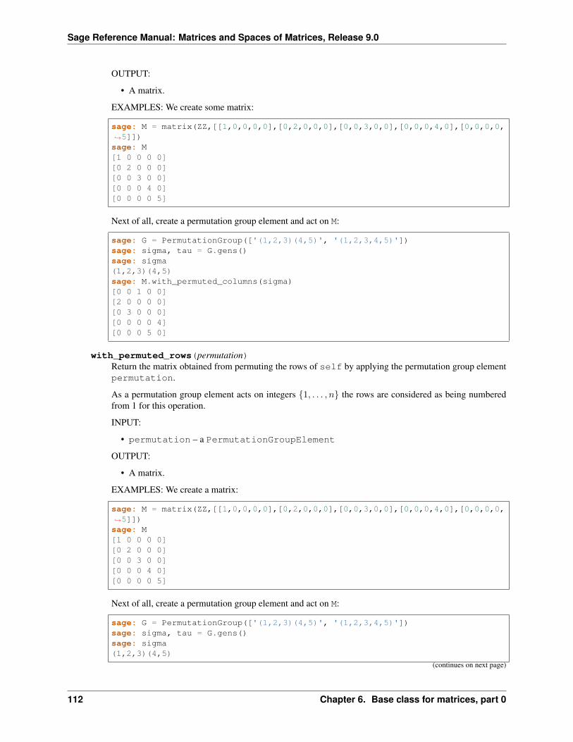
Sage Reference Manual: Matrices and Spaces of Matrices, Release 9.0
OUTPUT:
• A matrix.
EXAMPLES: We create some matrix:
sage: M = matrix(ZZ,[[1,0,0,0,0],[0,2,0,0,0],[0,0,3,0,0],[0,0,0,4,0],[0,0,0,0,→˓5]])sage: M[1 0 0 0 0][0 2 0 0 0][0 0 3 0 0][0 0 0 4 0][0 0 0 0 5]
Next of all, create a permutation group element and act on M:
sage: G = PermutationGroup(['(1,2,3)(4,5)', '(1,2,3,4,5)'])sage: sigma, tau = G.gens()sage: sigma(1,2,3)(4,5)sage: M.with_permuted_columns(sigma)[0 0 1 0 0][2 0 0 0 0][0 3 0 0 0][0 0 0 0 4][0 0 0 5 0]
with_permuted_rows(permutation)Return the matrix obtained from permuting the rows of self by applying the permutation group elementpermutation.
As a permutation group element acts on integers {1, . . . , 𝑛} the rows are considered as being numberedfrom 1 for this operation.
INPUT:
• permutation – a PermutationGroupElement
OUTPUT:
• A matrix.
EXAMPLES: We create a matrix:
sage: M = matrix(ZZ,[[1,0,0,0,0],[0,2,0,0,0],[0,0,3,0,0],[0,0,0,4,0],[0,0,0,0,→˓5]])sage: M[1 0 0 0 0][0 2 0 0 0][0 0 3 0 0][0 0 0 4 0][0 0 0 0 5]
Next of all, create a permutation group element and act on M:
sage: G = PermutationGroup(['(1,2,3)(4,5)', '(1,2,3,4,5)'])sage: sigma, tau = G.gens()sage: sigma(1,2,3)(4,5)
(continues on next page)
112 Chapter 6. Base class for matrices, part 0
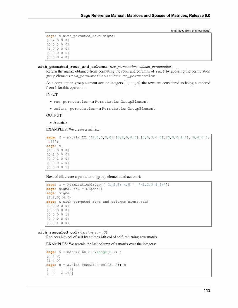
Sage Reference Manual: Matrices and Spaces of Matrices, Release 9.0
(continued from previous page)
sage: M.with_permuted_rows(sigma)[0 2 0 0 0][0 0 3 0 0][1 0 0 0 0][0 0 0 0 5][0 0 0 4 0]
with_permuted_rows_and_columns(row_permutation, column_permutation)Return the matrix obtained from permuting the rows and columns of self by applying the permutationgroup elements row_permutation and column_permutation.
As a permutation group element acts on integers {1, . . . , 𝑛} the rows are considered as being numberedfrom 1 for this operation.
INPUT:
• row_permutation – a PermutationGroupElement
• column_permutation – a PermutationGroupElement
OUTPUT:
• A matrix.
EXAMPLES: We create a matrix:
sage: M = matrix(ZZ,[[1,0,0,0,0],[0,2,0,0,0],[0,0,3,0,0],[0,0,0,4,0],[0,0,0,0,→˓5]])sage: M[1 0 0 0 0][0 2 0 0 0][0 0 3 0 0][0 0 0 4 0][0 0 0 0 5]
Next of all, create a permutation group element and act on M:
sage: G = PermutationGroup(['(1,2,3)(4,5)', '(1,2,3,4,5)'])sage: sigma, tau = G.gens()sage: sigma(1,2,3)(4,5)sage: M.with_permuted_rows_and_columns(sigma,tau)[2 0 0 0 0][0 3 0 0 0][0 0 0 0 1][0 0 0 5 0][0 0 4 0 0]
with_rescaled_col(i, s, start_row=0)Replaces i-th col of self by s times i-th col of self, returning new matrix.
EXAMPLES: We rescale the last column of a matrix over the integers:
sage: a = matrix(ZZ,2,3,range(6)); a[0 1 2][3 4 5]sage: b = a.with_rescaled_col(2,-2); b[ 0 1 -4][ 3 4 -10]
113
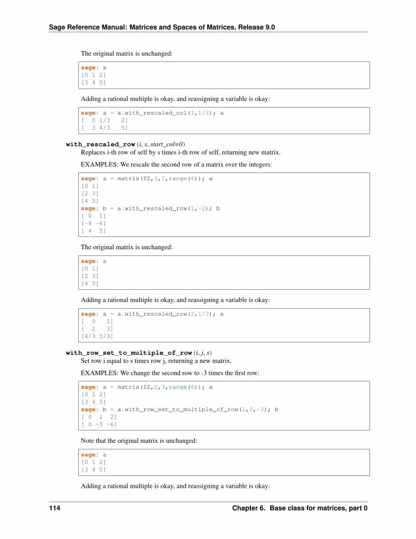
Sage Reference Manual: Matrices and Spaces of Matrices, Release 9.0
The original matrix is unchanged:
sage: a[0 1 2][3 4 5]
Adding a rational multiple is okay, and reassigning a variable is okay:
sage: a = a.with_rescaled_col(1,1/3); a[ 0 1/3 2][ 3 4/3 5]
with_rescaled_row(i, s, start_col=0)Replaces i-th row of self by s times i-th row of self, returning new matrix.
EXAMPLES: We rescale the second row of a matrix over the integers:
sage: a = matrix(ZZ,3,2,range(6)); a[0 1][2 3][4 5]sage: b = a.with_rescaled_row(1,-2); b[ 0 1][-4 -6][ 4 5]
The original matrix is unchanged:
sage: a[0 1][2 3][4 5]
Adding a rational multiple is okay, and reassigning a variable is okay:
sage: a = a.with_rescaled_row(2,1/3); a[ 0 1][ 2 3][4/3 5/3]
with_row_set_to_multiple_of_row(i, j, s)Set row i equal to s times row j, returning a new matrix.
EXAMPLES: We change the second row to -3 times the first row:
sage: a = matrix(ZZ,2,3,range(6)); a[0 1 2][3 4 5]sage: b = a.with_row_set_to_multiple_of_row(1,0,-3); b[ 0 1 2][ 0 -3 -6]
Note that the original matrix is unchanged:
sage: a[0 1 2][3 4 5]
Adding a rational multiple is okay, and reassigning a variable is okay:
114 Chapter 6. Base class for matrices, part 0
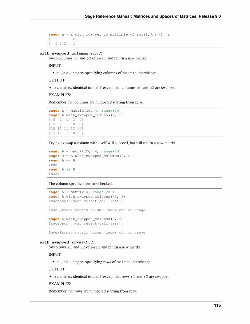
Sage Reference Manual: Matrices and Spaces of Matrices, Release 9.0
sage: a = a.with_row_set_to_multiple_of_row(1,0,1/2); a[ 0 1 2][ 0 1/2 1]
with_swapped_columns(c1, c2)Swap columns c1 and c2 of self and return a new matrix.
INPUT:
• c1, c2 - integers specifying columns of self to interchange
OUTPUT:
A new matrix, identical to self except that columns c1 and c2 are swapped.
EXAMPLES:
Remember that columns are numbered starting from zero.
sage: A = matrix(QQ, 4, range(20))sage: A.with_swapped_columns(1, 2)[ 0 2 1 3 4][ 5 7 6 8 9][10 12 11 13 14][15 17 16 18 19]
Trying to swap a column with itself will succeed, but still return a new matrix.
sage: A = matrix(QQ, 4, range(20))sage: B = A.with_swapped_columns(2, 2)sage: A == BTruesage: A is BFalse
The column specifications are checked.
sage: A = matrix(4, range(20))sage: A.with_swapped_columns(-1, 2)Traceback (most recent call last):...IndexError: matrix column index out of range
sage: A.with_swapped_columns(2, 5)Traceback (most recent call last):...IndexError: matrix column index out of range
with_swapped_rows(r1, r2)Swap rows r1 and r2 of self and return a new matrix.
INPUT:
• r1, r2 - integers specifying rows of self to interchange
OUTPUT:
A new matrix, identical to self except that rows r1 and r2 are swapped.
EXAMPLES:
Remember that rows are numbered starting from zero.
115
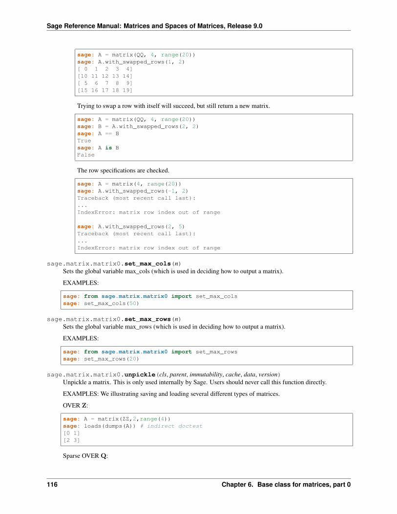
Sage Reference Manual: Matrices and Spaces of Matrices, Release 9.0
sage: A = matrix(QQ, 4, range(20))sage: A.with_swapped_rows(1, 2)[ 0 1 2 3 4][10 11 12 13 14][ 5 6 7 8 9][15 16 17 18 19]
Trying to swap a row with itself will succeed, but still return a new matrix.
sage: A = matrix(QQ, 4, range(20))sage: B = A.with_swapped_rows(2, 2)sage: A == BTruesage: A is BFalse
The row specifications are checked.
sage: A = matrix(4, range(20))sage: A.with_swapped_rows(-1, 2)Traceback (most recent call last):...IndexError: matrix row index out of range
sage: A.with_swapped_rows(2, 5)Traceback (most recent call last):...IndexError: matrix row index out of range
sage.matrix.matrix0.set_max_cols(n)Sets the global variable max_cols (which is used in deciding how to output a matrix).
EXAMPLES:
sage: from sage.matrix.matrix0 import set_max_colssage: set_max_cols(50)
sage.matrix.matrix0.set_max_rows(n)Sets the global variable max_rows (which is used in deciding how to output a matrix).
EXAMPLES:
sage: from sage.matrix.matrix0 import set_max_rowssage: set_max_rows(20)
sage.matrix.matrix0.unpickle(cls, parent, immutability, cache, data, version)Unpickle a matrix. This is only used internally by Sage. Users should never call this function directly.
EXAMPLES: We illustrating saving and loading several different types of matrices.
OVER Z:
sage: A = matrix(ZZ,2,range(4))sage: loads(dumps(A)) # indirect doctest[0 1][2 3]
Sparse OVER Q:
116 Chapter 6. Base class for matrices, part 0

Sage Reference Manual: Matrices and Spaces of Matrices, Release 9.0
Dense over Q[𝑥, 𝑦]:
Dense over finite field.
117

Sage Reference Manual: Matrices and Spaces of Matrices, Release 9.0
118 Chapter 6. Base class for matrices, part 0
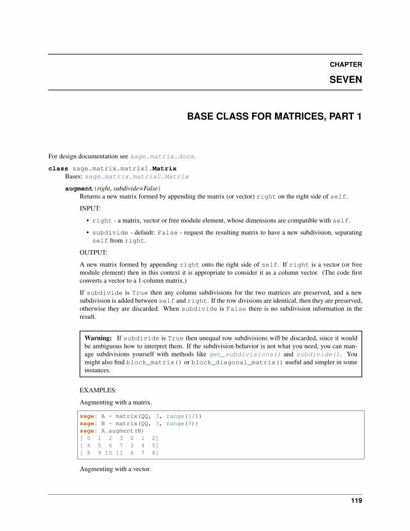
CHAPTER
SEVEN
BASE CLASS FOR MATRICES, PART 1
For design documentation see sage.matrix.docs.
class sage.matrix.matrix1.MatrixBases: sage.matrix.matrix0.Matrix
augment(right, subdivide=False)Returns a new matrix formed by appending the matrix (or vector) right on the right side of self.
INPUT:
• right - a matrix, vector or free module element, whose dimensions are compatible with self.
• subdivide - default: False - request the resulting matrix to have a new subdivision, separatingself from right.
OUTPUT:
A new matrix formed by appending right onto the right side of self. If right is a vector (or freemodule element) then in this context it is appropriate to consider it as a column vector. (The code firstconverts a vector to a 1-column matrix.)
If subdivide is True then any column subdivisions for the two matrices are preserved, and a newsubdivision is added between self and right. If the row divisions are identical, then they are preserved,otherwise they are discarded. When subdivide is False there is no subdivision information in theresult.
Warning: If subdivide is True then unequal row subdivisions will be discarded, since it wouldbe ambiguous how to interpret them. If the subdivision behavior is not what you need, you can man-age subdivisions yourself with methods like get_subdivisions() and subdivide(). Youmight also find block_matrix() or block_diagonal_matrix() useful and simpler in someinstances.
EXAMPLES:
Augmenting with a matrix.
sage: A = matrix(QQ, 3, range(12))sage: B = matrix(QQ, 3, range(9))sage: A.augment(B)[ 0 1 2 3 0 1 2][ 4 5 6 7 3 4 5][ 8 9 10 11 6 7 8]
Augmenting with a vector.
119
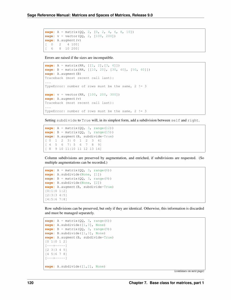
Sage Reference Manual: Matrices and Spaces of Matrices, Release 9.0
sage: A = matrix(QQ, 2, [0, 2, 4, 6, 8, 10])sage: v = vector(QQ, 2, [100, 200])sage: A.augment(v)[ 0 2 4 100][ 6 8 10 200]
Errors are raised if the sizes are incompatible.
sage: A = matrix(RR, [[1, 2],[3, 4]])sage: B = matrix(RR, [[10, 20], [30, 40], [50, 60]])sage: A.augment(B)Traceback (most recent call last):...TypeError: number of rows must be the same, 2 != 3
sage: v = vector(RR, [100, 200, 300])sage: A.augment(v)Traceback (most recent call last):...TypeError: number of rows must be the same, 2 != 3
Setting subdivide to True will, in its simplest form, add a subdivision between self and right.
sage: A = matrix(QQ, 3, range(12))sage: B = matrix(QQ, 3, range(15))sage: A.augment(B, subdivide=True)[ 0 1 2 3| 0 1 2 3 4][ 4 5 6 7| 5 6 7 8 9][ 8 9 10 11|10 11 12 13 14]
Column subdivisions are preserved by augmentation, and enriched, if subdivisions are requested. (Somultiple augmentations can be recorded.)
sage: A = matrix(QQ, 3, range(6))sage: A.subdivide(None, [1])sage: B = matrix(QQ, 3, range(9))sage: B.subdivide(None, [2])sage: A.augment(B, subdivide=True)[0|1|0 1|2][2|3|3 4|5][4|5|6 7|8]
Row subdivisions can be preserved, but only if they are identical. Otherwise, this information is discardedand must be managed separately.
sage: A = matrix(QQ, 3, range(6))sage: A.subdivide([1,3], None)sage: B = matrix(QQ, 3, range(9))sage: B.subdivide([1,3], None)sage: A.augment(B, subdivide=True)[0 1|0 1 2][---+-----][2 3|3 4 5][4 5|6 7 8][---+-----]
sage: A.subdivide([1,2], None)
(continues on next page)
120 Chapter 7. Base class for matrices, part 1
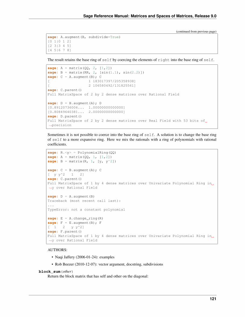
Sage Reference Manual: Matrices and Spaces of Matrices, Release 9.0
(continued from previous page)
sage: A.augment(B, subdivide=True)[0 1|0 1 2][2 3|3 4 5][4 5|6 7 8]
The result retains the base ring of self by coercing the elements of right into the base ring of self.
sage: A = matrix(QQ, 2, [1,2])sage: B = matrix(RR, 2, [sin(1.1), sin(2.2)])sage: C = A.augment(B); C[ 1 183017397/205358938][ 2 106580492/131825561]sage: C.parent()Full MatrixSpace of 2 by 2 dense matrices over Rational Field
sage: D = B.augment(A); D[0.89120736006... 1.00000000000000][0.80849640381... 2.00000000000000]sage: D.parent()Full MatrixSpace of 2 by 2 dense matrices over Real Field with 53 bits of→˓precision
Sometimes it is not possible to coerce into the base ring of self. A solution is to change the base ringof self to a more expansive ring. Here we mix the rationals with a ring of polynomials with rationalcoefficients.
sage: R.<y> = PolynomialRing(QQ)sage: A = matrix(QQ, 1, [1,2])sage: B = matrix(R, 1, [y, y^2])
sage: C = B.augment(A); C[ y y^2 1 2]sage: C.parent()Full MatrixSpace of 1 by 4 dense matrices over Univariate Polynomial Ring in→˓y over Rational Field
sage: D = A.augment(B)Traceback (most recent call last):...TypeError: not a constant polynomial
sage: E = A.change_ring(R)sage: F = E.augment(B); F[ 1 2 y y^2]sage: F.parent()Full MatrixSpace of 1 by 4 dense matrices over Univariate Polynomial Ring in→˓y over Rational Field
AUTHORS:
• Naqi Jaffery (2006-01-24): examples
• Rob Beezer (2010-12-07): vector argument, docstring, subdivisions
block_sum(other)Return the block matrix that has self and other on the diagonal:
121
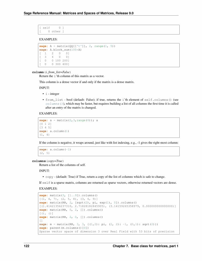
Sage Reference Manual: Matrices and Spaces of Matrices, Release 9.0
[ self 0 ][ 0 other ]
EXAMPLES:
sage: A = matrix(QQ[['t']], 2, range(1, 5))sage: A.block_sum(100*A)[ 1 2 0 0][ 3 4 0 0][ 0 0 100 200][ 0 0 300 400]
column(i, from_list=False)Return the i’th column of this matrix as a vector.
This column is a dense vector if and only if the matrix is a dense matrix.
INPUT:
• i - integer
• from_list - bool (default: False); if true, returns the i’th element of self.columns() (seecolumns()), which may be faster, but requires building a list of all columns the first time it is calledafter an entry of the matrix is changed.
EXAMPLES:
sage: a = matrix(2,3,range(6)); a[0 1 2][3 4 5]sage: a.column(1)(1, 4)
If the column is negative, it wraps around, just like with list indexing, e.g., -1 gives the right-most column:
sage: a.column(-1)(2, 5)
columns(copy=True)Return a list of the columns of self.
INPUT:
• copy - (default: True) if True, return a copy of the list of columns which is safe to change.
If self is a sparse matrix, columns are returned as sparse vectors, otherwise returned vectors are dense.
EXAMPLES:
sage: matrix(3, [1..9]).columns()[(1, 4, 7), (2, 5, 8), (3, 6, 9)]sage: matrix(RR, 2, [sqrt(2), pi, exp(1), 0]).columns()[(1.41421356237310, 2.71828182845905), (3.14159265358979, 0.000000000000000)]sage: matrix(RR, 0, 2, []).columns()[(), ()]sage: matrix(RR, 2, 0, []).columns()[]sage: m = matrix(RR, 3, 3, {(1,2): pi, (2, 2): -1, (0,1): sqrt(2)})sage: parent(m.columns()[0])Sparse vector space of dimension 3 over Real Field with 53 bits of precision
122 Chapter 7. Base class for matrices, part 1
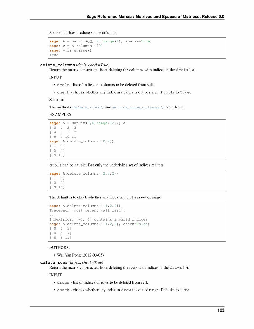
Sage Reference Manual: Matrices and Spaces of Matrices, Release 9.0
Sparse matrices produce sparse columns.
sage: A = matrix(QQ, 2, range(4), sparse=True)sage: v = A.columns()[0]sage: v.is_sparse()True
delete_columns(dcols, check=True)Return the matrix constructed from deleting the columns with indices in the dcols list.
INPUT:
• dcols - list of indices of columns to be deleted from self.
• check - checks whether any index in dcols is out of range. Defaults to True.
See also:
The methods delete_rows() and matrix_from_columns() are related.
EXAMPLES:
sage: A = Matrix(3,4,range(12)); A[ 0 1 2 3][ 4 5 6 7][ 8 9 10 11]sage: A.delete_columns([0,2])[ 1 3][ 5 7][ 9 11]
dcols can be a tuple. But only the underlying set of indices matters.
sage: A.delete_columns((2,0,2))[ 1 3][ 5 7][ 9 11]
The default is to check whether any index in dcols is out of range.
sage: A.delete_columns([-1,2,4])Traceback (most recent call last):...IndexError: [-1, 4] contains invalid indicessage: A.delete_columns([-1,2,4], check=False)[ 0 1 3][ 4 5 7][ 8 9 11]
AUTHORS:
• Wai Yan Pong (2012-03-05)
delete_rows(drows, check=True)Return the matrix constructed from deleting the rows with indices in the drows list.
INPUT:
• drows - list of indices of rows to be deleted from self.
• check - checks whether any index in drows is out of range. Defaults to True.
123
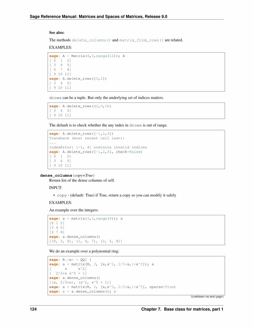
Sage Reference Manual: Matrices and Spaces of Matrices, Release 9.0
See also:
The methods delete_columns() and matrix_from_rows() are related.
EXAMPLES:
sage: A = Matrix(4,3,range(12)); A[ 0 1 2][ 3 4 5][ 6 7 8][ 9 10 11]sage: A.delete_rows([0,2])[ 3 4 5][ 9 10 11]
drows can be a tuple. But only the underlying set of indices matters.
sage: A.delete_rows((2,0,2))[ 3 4 5][ 9 10 11]
The default is to check whether the any index in drows is out of range.
sage: A.delete_rows([-1,2,4])Traceback (most recent call last):...IndexError: [-1, 4] contains invalid indicessage: A.delete_rows([-1,2,4], check=False)[ 0 1 2][ 3 4 5][ 9 10 11]
dense_columns(copy=True)Return list of the dense columns of self.
INPUT:
• copy - (default: True) if True, return a copy so you can modify it safely
EXAMPLES:
An example over the integers:
sage: a = matrix(3,3,range(9)); a[0 1 2][3 4 5][6 7 8]sage: a.dense_columns()[(0, 3, 6), (1, 4, 7), (2, 5, 8)]
We do an example over a polynomial ring:
sage: R.<x> = QQ[ ]sage: a = matrix(R, 2, [x,x^2, 2/3*x,1+x^5]); a[ x x^2][ 2/3*x x^5 + 1]sage: a.dense_columns()[(x, 2/3*x), (x^2, x^5 + 1)]sage: a = matrix(R, 2, [x,x^2, 2/3*x,1+x^5], sparse=True)sage: c = a.dense_columns(); c
(continues on next page)
124 Chapter 7. Base class for matrices, part 1
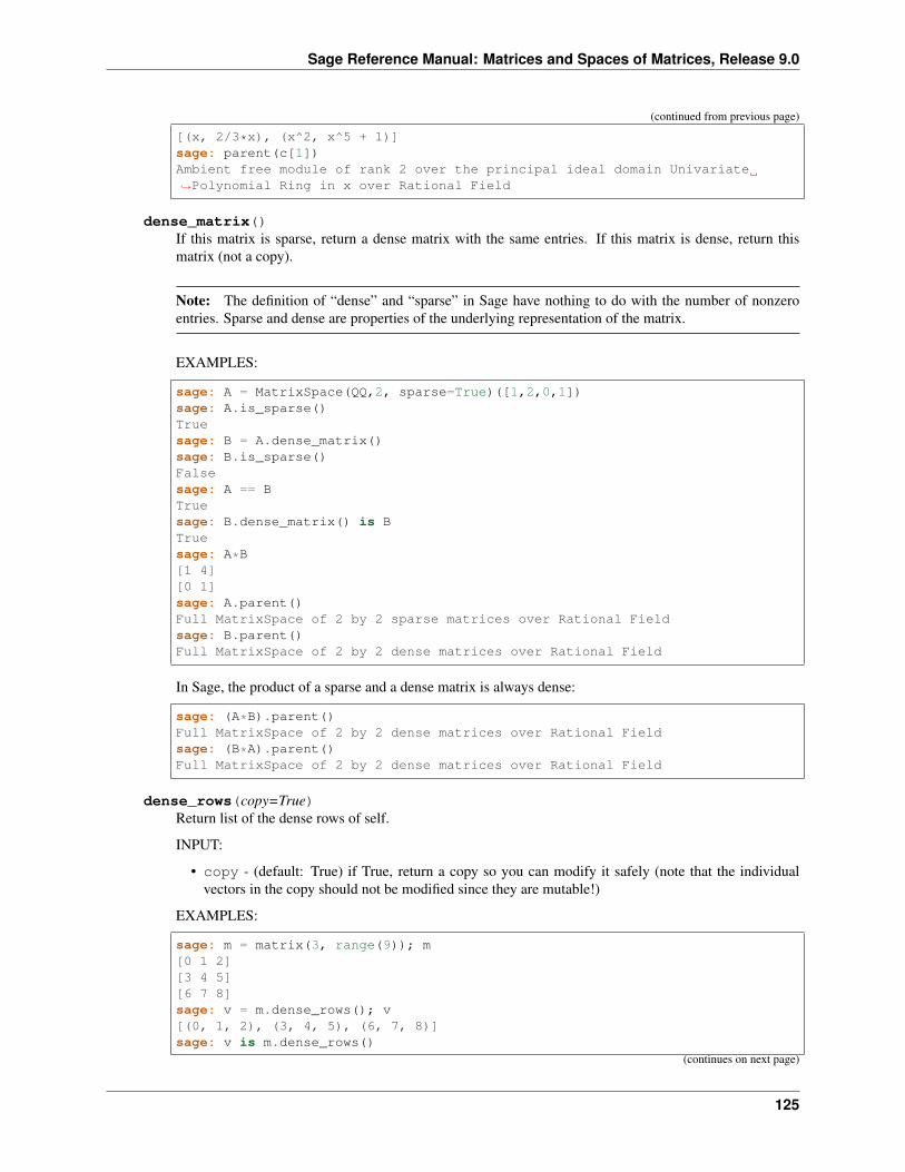
Sage Reference Manual: Matrices and Spaces of Matrices, Release 9.0
(continued from previous page)
[(x, 2/3*x), (x^2, x^5 + 1)]sage: parent(c[1])Ambient free module of rank 2 over the principal ideal domain Univariate→˓Polynomial Ring in x over Rational Field
dense_matrix()If this matrix is sparse, return a dense matrix with the same entries. If this matrix is dense, return thismatrix (not a copy).
Note: The definition of “dense” and “sparse” in Sage have nothing to do with the number of nonzeroentries. Sparse and dense are properties of the underlying representation of the matrix.
EXAMPLES:
sage: A = MatrixSpace(QQ,2, sparse=True)([1,2,0,1])sage: A.is_sparse()Truesage: B = A.dense_matrix()sage: B.is_sparse()Falsesage: A == BTruesage: B.dense_matrix() is BTruesage: A*B[1 4][0 1]sage: A.parent()Full MatrixSpace of 2 by 2 sparse matrices over Rational Fieldsage: B.parent()Full MatrixSpace of 2 by 2 dense matrices over Rational Field
In Sage, the product of a sparse and a dense matrix is always dense:
sage: (A*B).parent()Full MatrixSpace of 2 by 2 dense matrices over Rational Fieldsage: (B*A).parent()Full MatrixSpace of 2 by 2 dense matrices over Rational Field
dense_rows(copy=True)Return list of the dense rows of self.
INPUT:
• copy - (default: True) if True, return a copy so you can modify it safely (note that the individualvectors in the copy should not be modified since they are mutable!)
EXAMPLES:
sage: m = matrix(3, range(9)); m[0 1 2][3 4 5][6 7 8]sage: v = m.dense_rows(); v[(0, 1, 2), (3, 4, 5), (6, 7, 8)]sage: v is m.dense_rows()
(continues on next page)
125
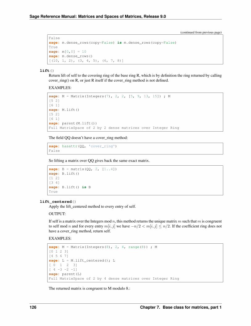
Sage Reference Manual: Matrices and Spaces of Matrices, Release 9.0
(continued from previous page)
Falsesage: m.dense_rows(copy=False) is m.dense_rows(copy=False)Truesage: m[0,0] = 10sage: m.dense_rows()[(10, 1, 2), (3, 4, 5), (6, 7, 8)]
lift()Return lift of self to the covering ring of the base ring R, which is by definition the ring returned by callingcover_ring() on R, or just R itself if the cover_ring method is not defined.
EXAMPLES:
sage: M = Matrix(Integers(7), 2, 2, [5, 9, 13, 15]) ; M[5 2][6 1]sage: M.lift()[5 2][6 1]sage: parent(M.lift())Full MatrixSpace of 2 by 2 dense matrices over Integer Ring
The field QQ doesn’t have a cover_ring method:
sage: hasattr(QQ, 'cover_ring')False
So lifting a matrix over QQ gives back the same exact matrix.
sage: B = matrix(QQ, 2, [1..4])sage: B.lift()[1 2][3 4]sage: B.lift() is BTrue
lift_centered()Apply the lift_centered method to every entry of self.
OUTPUT:
If self is a matrix over the Integers mod 𝑛, this method returns the unique matrix 𝑚 such that 𝑚 is congruentto self mod 𝑛 and for every entry 𝑚[𝑖, 𝑗] we have −𝑛/2 < 𝑚[𝑖, 𝑗] ≤ 𝑛/2. If the coefficient ring does nothave a cover_ring method, return self.
EXAMPLES:
sage: M = Matrix(Integers(8), 2, 4, range(8)) ; M[0 1 2 3][4 5 6 7]sage: L = M.lift_centered(); L[ 0 1 2 3][ 4 -3 -2 -1]sage: parent(L)Full MatrixSpace of 2 by 4 dense matrices over Integer Ring
The returned matrix is congruent to M modulo 8.:
126 Chapter 7. Base class for matrices, part 1
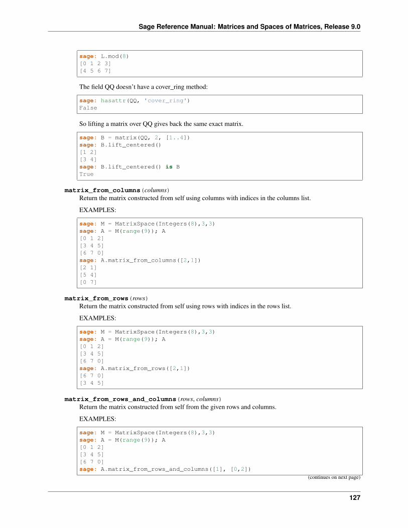
Sage Reference Manual: Matrices and Spaces of Matrices, Release 9.0
sage: L.mod(8)[0 1 2 3][4 5 6 7]
The field QQ doesn’t have a cover_ring method:
sage: hasattr(QQ, 'cover_ring')False
So lifting a matrix over QQ gives back the same exact matrix.
sage: B = matrix(QQ, 2, [1..4])sage: B.lift_centered()[1 2][3 4]sage: B.lift_centered() is BTrue
matrix_from_columns(columns)Return the matrix constructed from self using columns with indices in the columns list.
EXAMPLES:
sage: M = MatrixSpace(Integers(8),3,3)sage: A = M(range(9)); A[0 1 2][3 4 5][6 7 0]sage: A.matrix_from_columns([2,1])[2 1][5 4][0 7]
matrix_from_rows(rows)Return the matrix constructed from self using rows with indices in the rows list.
EXAMPLES:
sage: M = MatrixSpace(Integers(8),3,3)sage: A = M(range(9)); A[0 1 2][3 4 5][6 7 0]sage: A.matrix_from_rows([2,1])[6 7 0][3 4 5]
matrix_from_rows_and_columns(rows, columns)Return the matrix constructed from self from the given rows and columns.
EXAMPLES:
sage: M = MatrixSpace(Integers(8),3,3)sage: A = M(range(9)); A[0 1 2][3 4 5][6 7 0]sage: A.matrix_from_rows_and_columns([1], [0,2])
(continues on next page)
127
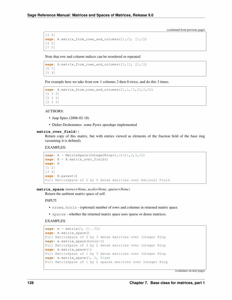
Sage Reference Manual: Matrices and Spaces of Matrices, Release 9.0
(continued from previous page)
[3 5]sage: A.matrix_from_rows_and_columns([1,2], [1,2])[4 5][7 0]
Note that row and column indices can be reordered or repeated:
sage: A.matrix_from_rows_and_columns([2,1], [2,1])[0 7][5 4]
For example here we take from row 1 columns 2 then 0 twice, and do this 3 times.
sage: A.matrix_from_rows_and_columns([1,1,1],[2,0,0])[5 3 3][5 3 3][5 3 3]
AUTHORS:
• Jaap Spies (2006-02-18)
• Didier Deshommes: some Pyrex speedups implemented
matrix_over_field()Return copy of this matrix, but with entries viewed as elements of the fraction field of the base ring(assuming it is defined).
EXAMPLES:
sage: A = MatrixSpace(IntegerRing(),2)([1,2,3,4])sage: B = A.matrix_over_field()sage: B[1 2][3 4]sage: B.parent()Full MatrixSpace of 2 by 2 dense matrices over Rational Field
matrix_space(nrows=None, ncols=None, sparse=None)Return the ambient matrix space of self.
INPUT:
• nrows, ncols - (optional) number of rows and columns in returned matrix space.
• sparse - whether the returned matrix space uses sparse or dense matrices.
EXAMPLES:
sage: m = matrix(3, [1..9])sage: m.matrix_space()Full MatrixSpace of 3 by 3 dense matrices over Integer Ringsage: m.matrix_space(ncols=2)Full MatrixSpace of 3 by 2 dense matrices over Integer Ringsage: m.matrix_space(1)Full MatrixSpace of 1 by 3 dense matrices over Integer Ringsage: m.matrix_space(1, 2, True)Full MatrixSpace of 1 by 2 sparse matrices over Integer Ring
(continues on next page)
128 Chapter 7. Base class for matrices, part 1
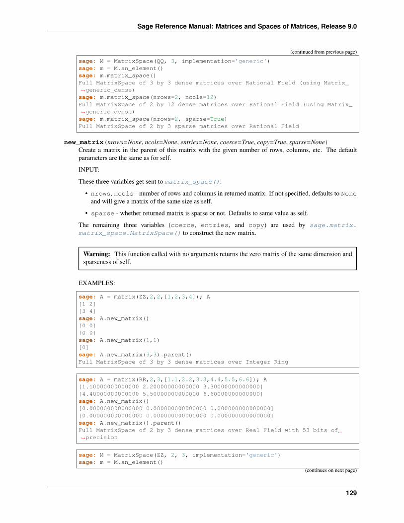
Sage Reference Manual: Matrices and Spaces of Matrices, Release 9.0
(continued from previous page)
sage: M = MatrixSpace(QQ, 3, implementation='generic')sage: m = M.an_element()sage: m.matrix_space()Full MatrixSpace of 3 by 3 dense matrices over Rational Field (using Matrix_→˓generic_dense)sage: m.matrix_space(nrows=2, ncols=12)Full MatrixSpace of 2 by 12 dense matrices over Rational Field (using Matrix_→˓generic_dense)sage: m.matrix_space(nrows=2, sparse=True)Full MatrixSpace of 2 by 3 sparse matrices over Rational Field
new_matrix(nrows=None, ncols=None, entries=None, coerce=True, copy=True, sparse=None)Create a matrix in the parent of this matrix with the given number of rows, columns, etc. The defaultparameters are the same as for self.
INPUT:
These three variables get sent to matrix_space():
• nrows, ncols - number of rows and columns in returned matrix. If not specified, defaults to Noneand will give a matrix of the same size as self.
• sparse - whether returned matrix is sparse or not. Defaults to same value as self.
The remaining three variables (coerce, entries, and copy) are used by sage.matrix.matrix_space.MatrixSpace() to construct the new matrix.
Warning: This function called with no arguments returns the zero matrix of the same dimension andsparseness of self.
EXAMPLES:
sage: A = matrix(ZZ,2,2,[1,2,3,4]); A[1 2][3 4]sage: A.new_matrix()[0 0][0 0]sage: A.new_matrix(1,1)[0]sage: A.new_matrix(3,3).parent()Full MatrixSpace of 3 by 3 dense matrices over Integer Ring
sage: A = matrix(RR,2,3,[1.1,2.2,3.3,4.4,5.5,6.6]); A[1.10000000000000 2.20000000000000 3.30000000000000][4.40000000000000 5.50000000000000 6.60000000000000]sage: A.new_matrix()[0.000000000000000 0.000000000000000 0.000000000000000][0.000000000000000 0.000000000000000 0.000000000000000]sage: A.new_matrix().parent()Full MatrixSpace of 2 by 3 dense matrices over Real Field with 53 bits of→˓precision
sage: M = MatrixSpace(ZZ, 2, 3, implementation='generic')sage: m = M.an_element()
(continues on next page)
129
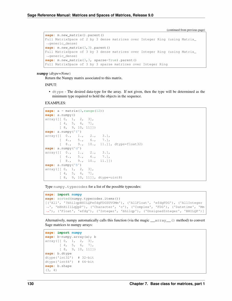
Sage Reference Manual: Matrices and Spaces of Matrices, Release 9.0
(continued from previous page)
sage: m.new_matrix().parent()Full MatrixSpace of 2 by 3 dense matrices over Integer Ring (using Matrix_→˓generic_dense)sage: m.new_matrix(3,3).parent()Full MatrixSpace of 3 by 3 dense matrices over Integer Ring (using Matrix_→˓generic_dense)sage: m.new_matrix(3,3, sparse=True).parent()Full MatrixSpace of 3 by 3 sparse matrices over Integer Ring
numpy(dtype=None)Return the Numpy matrix associated to this matrix.
INPUT:
• dtype - The desired data-type for the array. If not given, then the type will be determined as theminimum type required to hold the objects in the sequence.
EXAMPLES:
sage: a = matrix(3,range(12))sage: a.numpy()array([[ 0, 1, 2, 3],
[ 4, 5, 6, 7],[ 8, 9, 10, 11]])
sage: a.numpy('f')array([[ 0., 1., 2., 3.],
[ 4., 5., 6., 7.],[ 8., 9., 10., 11.]], dtype=float32)
sage: a.numpy('d')array([[ 0., 1., 2., 3.],
[ 4., 5., 6., 7.],[ 8., 9., 10., 11.]])
sage: a.numpy('B')array([[ 0, 1, 2, 3],
[ 4, 5, 6, 7],[ 8, 9, 10, 11]], dtype=uint8)
Type numpy.typecodes for a list of the possible typecodes:
sage: import numpysage: sorted(numpy.typecodes.items())[('All', '?bhilqpBHILQPefdgFDGSUVOMm'), ('AllFloat', 'efdgFDG'), ('AllInteger→˓', 'bBhHiIlLqQpP'), ('Character', 'c'), ('Complex', 'FDG'), ('Datetime', 'Mm→˓'), ('Float', 'efdg'), ('Integer', 'bhilqp'), ('UnsignedInteger', 'BHILQP')]
Alternatively, numpy automatically calls this function (via the magic __array__() method) to convertSage matrices to numpy arrays:
sage: import numpysage: b=numpy.array(a); barray([[ 0, 1, 2, 3],
[ 4, 5, 6, 7],[ 8, 9, 10, 11]])
sage: b.dtypedtype('int32') # 32-bitdtype('int64') # 64-bitsage: b.shape(3, 4)
130 Chapter 7. Base class for matrices, part 1
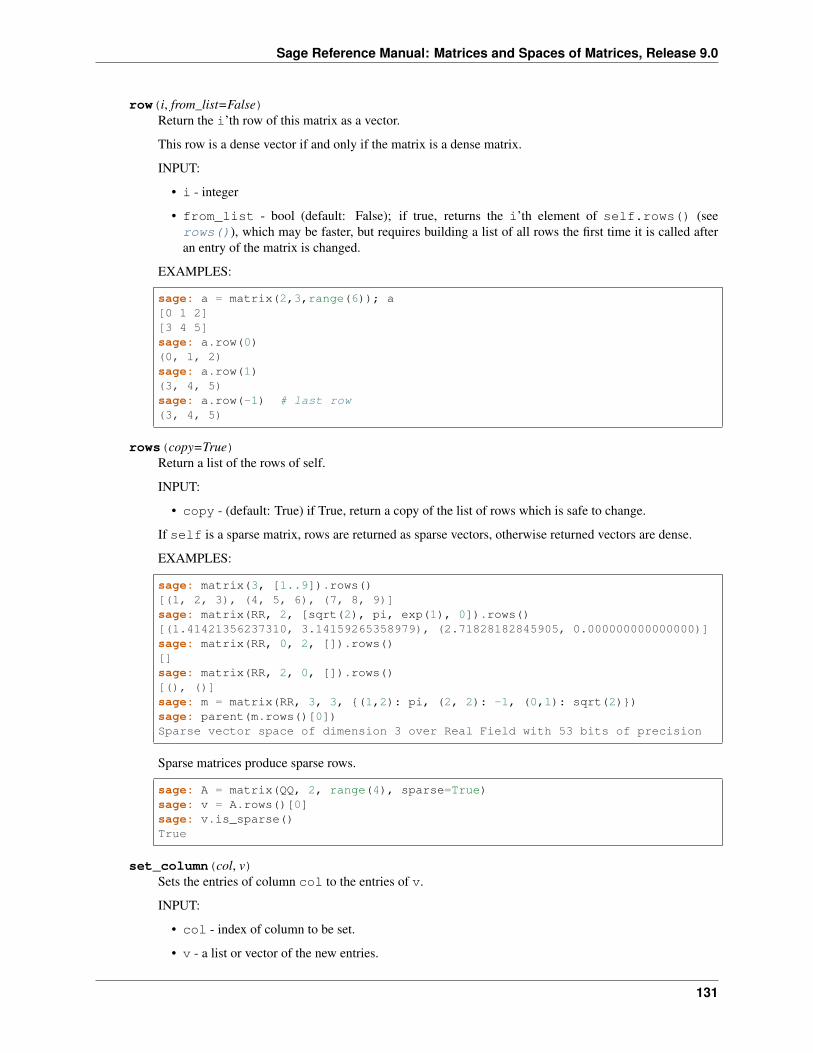
Sage Reference Manual: Matrices and Spaces of Matrices, Release 9.0
row(i, from_list=False)Return the i’th row of this matrix as a vector.
This row is a dense vector if and only if the matrix is a dense matrix.
INPUT:
• i - integer
• from_list - bool (default: False); if true, returns the i’th element of self.rows() (seerows()), which may be faster, but requires building a list of all rows the first time it is called afteran entry of the matrix is changed.
EXAMPLES:
sage: a = matrix(2,3,range(6)); a[0 1 2][3 4 5]sage: a.row(0)(0, 1, 2)sage: a.row(1)(3, 4, 5)sage: a.row(-1) # last row(3, 4, 5)
rows(copy=True)Return a list of the rows of self.
INPUT:
• copy - (default: True) if True, return a copy of the list of rows which is safe to change.
If self is a sparse matrix, rows are returned as sparse vectors, otherwise returned vectors are dense.
EXAMPLES:
sage: matrix(3, [1..9]).rows()[(1, 2, 3), (4, 5, 6), (7, 8, 9)]sage: matrix(RR, 2, [sqrt(2), pi, exp(1), 0]).rows()[(1.41421356237310, 3.14159265358979), (2.71828182845905, 0.000000000000000)]sage: matrix(RR, 0, 2, []).rows()[]sage: matrix(RR, 2, 0, []).rows()[(), ()]sage: m = matrix(RR, 3, 3, {(1,2): pi, (2, 2): -1, (0,1): sqrt(2)})sage: parent(m.rows()[0])Sparse vector space of dimension 3 over Real Field with 53 bits of precision
Sparse matrices produce sparse rows.
sage: A = matrix(QQ, 2, range(4), sparse=True)sage: v = A.rows()[0]sage: v.is_sparse()True
set_column(col, v)Sets the entries of column col to the entries of v.
INPUT:
• col - index of column to be set.
• v - a list or vector of the new entries.
131
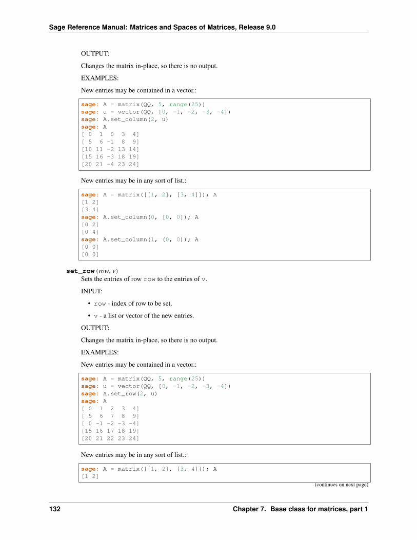
Sage Reference Manual: Matrices and Spaces of Matrices, Release 9.0
OUTPUT:
Changes the matrix in-place, so there is no output.
EXAMPLES:
New entries may be contained in a vector.:
sage: A = matrix(QQ, 5, range(25))sage: u = vector(QQ, [0, -1, -2, -3, -4])sage: A.set_column(2, u)sage: A[ 0 1 0 3 4][ 5 6 -1 8 9][10 11 -2 13 14][15 16 -3 18 19][20 21 -4 23 24]
New entries may be in any sort of list.:
sage: A = matrix([[1, 2], [3, 4]]); A[1 2][3 4]sage: A.set_column(0, [0, 0]); A[0 2][0 4]sage: A.set_column(1, (0, 0)); A[0 0][0 0]
set_row(row, v)Sets the entries of row row to the entries of v.
INPUT:
• row - index of row to be set.
• v - a list or vector of the new entries.
OUTPUT:
Changes the matrix in-place, so there is no output.
EXAMPLES:
New entries may be contained in a vector.:
sage: A = matrix(QQ, 5, range(25))sage: u = vector(QQ, [0, -1, -2, -3, -4])sage: A.set_row(2, u)sage: A[ 0 1 2 3 4][ 5 6 7 8 9][ 0 -1 -2 -3 -4][15 16 17 18 19][20 21 22 23 24]
New entries may be in any sort of list.:
sage: A = matrix([[1, 2], [3, 4]]); A[1 2]
(continues on next page)
132 Chapter 7. Base class for matrices, part 1
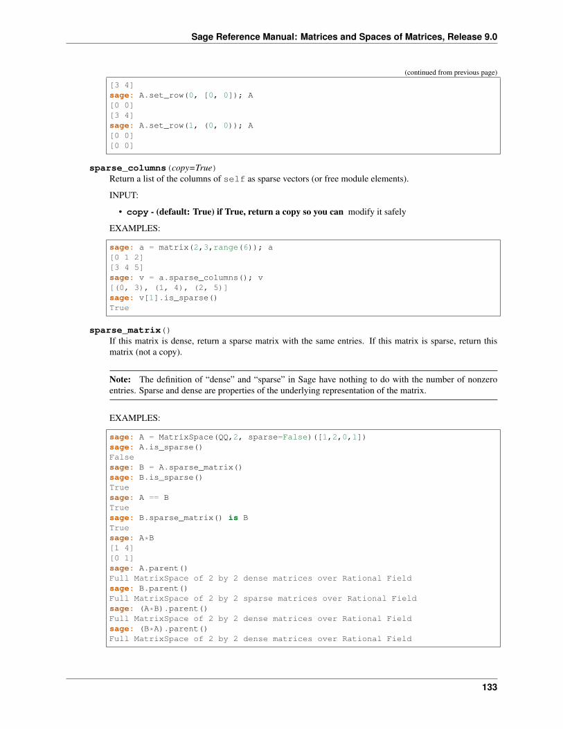
Sage Reference Manual: Matrices and Spaces of Matrices, Release 9.0
(continued from previous page)
[3 4]sage: A.set_row(0, [0, 0]); A[0 0][3 4]sage: A.set_row(1, (0, 0)); A[0 0][0 0]
sparse_columns(copy=True)Return a list of the columns of self as sparse vectors (or free module elements).
INPUT:
• copy - (default: True) if True, return a copy so you can modify it safely
EXAMPLES:
sage: a = matrix(2,3,range(6)); a[0 1 2][3 4 5]sage: v = a.sparse_columns(); v[(0, 3), (1, 4), (2, 5)]sage: v[1].is_sparse()True
sparse_matrix()If this matrix is dense, return a sparse matrix with the same entries. If this matrix is sparse, return thismatrix (not a copy).
Note: The definition of “dense” and “sparse” in Sage have nothing to do with the number of nonzeroentries. Sparse and dense are properties of the underlying representation of the matrix.
EXAMPLES:
sage: A = MatrixSpace(QQ,2, sparse=False)([1,2,0,1])sage: A.is_sparse()Falsesage: B = A.sparse_matrix()sage: B.is_sparse()Truesage: A == BTruesage: B.sparse_matrix() is BTruesage: A*B[1 4][0 1]sage: A.parent()Full MatrixSpace of 2 by 2 dense matrices over Rational Fieldsage: B.parent()Full MatrixSpace of 2 by 2 sparse matrices over Rational Fieldsage: (A*B).parent()Full MatrixSpace of 2 by 2 dense matrices over Rational Fieldsage: (B*A).parent()Full MatrixSpace of 2 by 2 dense matrices over Rational Field
133
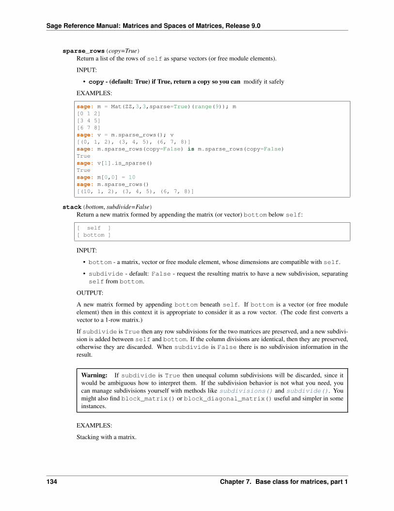
Sage Reference Manual: Matrices and Spaces of Matrices, Release 9.0
sparse_rows(copy=True)Return a list of the rows of self as sparse vectors (or free module elements).
INPUT:
• copy - (default: True) if True, return a copy so you can modify it safely
EXAMPLES:
sage: m = Mat(ZZ,3,3,sparse=True)(range(9)); m[0 1 2][3 4 5][6 7 8]sage: v = m.sparse_rows(); v[(0, 1, 2), (3, 4, 5), (6, 7, 8)]sage: m.sparse_rows(copy=False) is m.sparse_rows(copy=False)Truesage: v[1].is_sparse()Truesage: m[0,0] = 10sage: m.sparse_rows()[(10, 1, 2), (3, 4, 5), (6, 7, 8)]
stack(bottom, subdivide=False)Return a new matrix formed by appending the matrix (or vector) bottom below self:
[ self ][ bottom ]
INPUT:
• bottom - a matrix, vector or free module element, whose dimensions are compatible with self.
• subdivide - default: False - request the resulting matrix to have a new subdivision, separatingself from bottom.
OUTPUT:
A new matrix formed by appending bottom beneath self. If bottom is a vector (or free moduleelement) then in this context it is appropriate to consider it as a row vector. (The code first converts avector to a 1-row matrix.)
If subdivide is True then any row subdivisions for the two matrices are preserved, and a new subdivi-sion is added between self and bottom. If the column divisions are identical, then they are preserved,otherwise they are discarded. When subdivide is False there is no subdivision information in theresult.
Warning: If subdivide is True then unequal column subdivisions will be discarded, since itwould be ambiguous how to interpret them. If the subdivision behavior is not what you need, youcan manage subdivisions yourself with methods like subdivisions() and subdivide(). Youmight also find block_matrix() or block_diagonal_matrix() useful and simpler in someinstances.
EXAMPLES:
Stacking with a matrix.
134 Chapter 7. Base class for matrices, part 1
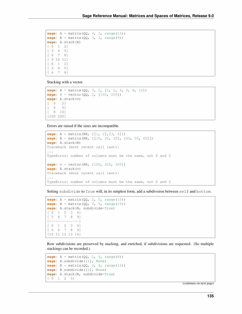
Sage Reference Manual: Matrices and Spaces of Matrices, Release 9.0
sage: A = matrix(QQ, 4, 3, range(12))sage: B = matrix(QQ, 3, 3, range(9))sage: A.stack(B)[ 0 1 2][ 3 4 5][ 6 7 8][ 9 10 11][ 0 1 2][ 3 4 5][ 6 7 8]
Stacking with a vector.
sage: A = matrix(QQ, 3, 2, [0, 2, 4, 6, 8, 10])sage: v = vector(QQ, 2, [100, 200])sage: A.stack(v)[ 0 2][ 4 6][ 8 10][100 200]
Errors are raised if the sizes are incompatible.
sage: A = matrix(RR, [[1, 2],[3, 4]])sage: B = matrix(RR, [[10, 20, 30], [40, 50, 60]])sage: A.stack(B)Traceback (most recent call last):...TypeError: number of columns must be the same, not 2 and 3
sage: v = vector(RR, [100, 200, 300])sage: A.stack(v)Traceback (most recent call last):...TypeError: number of columns must be the same, not 2 and 3
Setting subdivide to True will, in its simplest form, add a subdivision between self and bottom.
sage: A = matrix(QQ, 2, 5, range(10))sage: B = matrix(QQ, 3, 5, range(15))sage: A.stack(B, subdivide=True)[ 0 1 2 3 4][ 5 6 7 8 9][--------------][ 0 1 2 3 4][ 5 6 7 8 9][10 11 12 13 14]
Row subdivisions are preserved by stacking, and enriched, if subdivisions are requested. (So multiplestackings can be recorded.)
sage: A = matrix(QQ, 2, 4, range(8))sage: A.subdivide([1], None)sage: B = matrix(QQ, 3, 4, range(12))sage: B.subdivide([2], None)sage: A.stack(B, subdivide=True)[ 0 1 2 3]
(continues on next page)
135
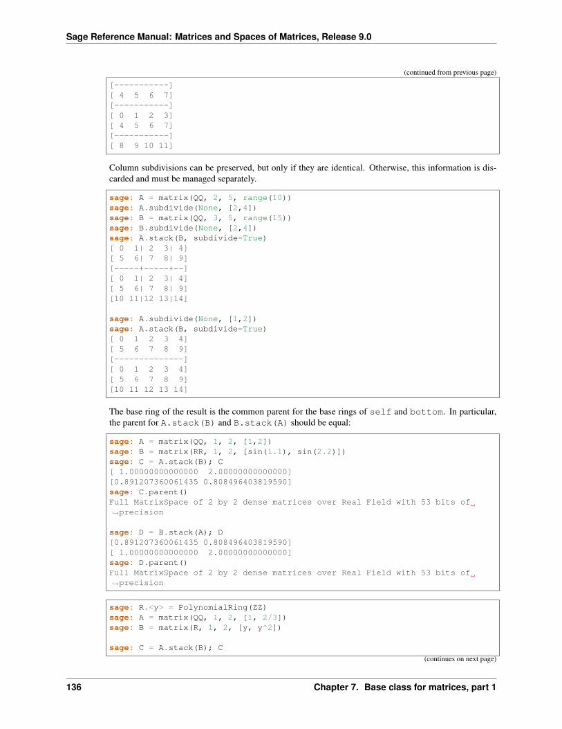
Sage Reference Manual: Matrices and Spaces of Matrices, Release 9.0
(continued from previous page)
[-----------][ 4 5 6 7][-----------][ 0 1 2 3][ 4 5 6 7][-----------][ 8 9 10 11]
Column subdivisions can be preserved, but only if they are identical. Otherwise, this information is dis-carded and must be managed separately.
sage: A = matrix(QQ, 2, 5, range(10))sage: A.subdivide(None, [2,4])sage: B = matrix(QQ, 3, 5, range(15))sage: B.subdivide(None, [2,4])sage: A.stack(B, subdivide=True)[ 0 1| 2 3| 4][ 5 6| 7 8| 9][-----+-----+--][ 0 1| 2 3| 4][ 5 6| 7 8| 9][10 11|12 13|14]
sage: A.subdivide(None, [1,2])sage: A.stack(B, subdivide=True)[ 0 1 2 3 4][ 5 6 7 8 9][--------------][ 0 1 2 3 4][ 5 6 7 8 9][10 11 12 13 14]
The base ring of the result is the common parent for the base rings of self and bottom. In particular,the parent for A.stack(B) and B.stack(A) should be equal:
sage: A = matrix(QQ, 1, 2, [1,2])sage: B = matrix(RR, 1, 2, [sin(1.1), sin(2.2)])sage: C = A.stack(B); C[ 1.00000000000000 2.00000000000000][0.891207360061435 0.808496403819590]sage: C.parent()Full MatrixSpace of 2 by 2 dense matrices over Real Field with 53 bits of→˓precision
sage: D = B.stack(A); D[0.891207360061435 0.808496403819590][ 1.00000000000000 2.00000000000000]sage: D.parent()Full MatrixSpace of 2 by 2 dense matrices over Real Field with 53 bits of→˓precision
sage: R.<y> = PolynomialRing(ZZ)sage: A = matrix(QQ, 1, 2, [1, 2/3])sage: B = matrix(R, 1, 2, [y, y^2])
sage: C = A.stack(B); C
(continues on next page)
136 Chapter 7. Base class for matrices, part 1

Sage Reference Manual: Matrices and Spaces of Matrices, Release 9.0
(continued from previous page)
[ 1 2/3][ y y^2]sage: C.parent()Full MatrixSpace of 2 by 2 dense matrices over Univariate Polynomial Ring in→˓y over Rational Field
Stacking a dense matrix atop a sparse one returns a sparse matrix:
sage: M = Matrix(ZZ, 2, 3, range(6), sparse=False)sage: N = diagonal_matrix([10,11,12], sparse=True)sage: P = M.stack(N); P[ 0 1 2][ 3 4 5][10 0 0][ 0 11 0][ 0 0 12]sage: P.is_sparse()Truesage: P = N.stack(M); P[10 0 0][ 0 11 0][ 0 0 12][ 0 1 2][ 3 4 5]sage: P.is_sparse()True
One can stack matrices over different rings (trac ticket #16399).
sage: M = Matrix(ZZ, 2, 3, range(6))sage: N = Matrix(QQ, 1, 3, [10,11,12])sage: M.stack(N)[ 0 1 2][ 3 4 5][10 11 12]sage: N.stack(M)[10 11 12][ 0 1 2][ 3 4 5]
AUTHORS:
• Rob Beezer (2011-03-19): rewritten to mirror code for augment()
• Jeroen Demeyer (2015-01-06): refactor, see trac ticket #16399. Put all boilerplate in one place (here)and put the actual type-dependent implementation in _stack_impl.
submatrix(row=0, col=0, nrows=-1, ncols=-1)Return the matrix constructed from self using the specified range of rows and columns.
INPUT:
• row, col - index of the starting row and column. Indices start at zero.
• nrows, ncols - (optional) number of rows and columns to take. If not provided, take all rows belowand all columns to the right of the starting entry.
See also:
137
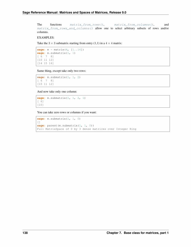
Sage Reference Manual: Matrices and Spaces of Matrices, Release 9.0
The functions matrix_from_rows(), matrix_from_columns(), andmatrix_from_rows_and_columns() allow one to select arbitrary subsets of rows and/orcolumns.
EXAMPLES:
Take the 3× 3 submatrix starting from entry (1,1) in a 4× 4 matrix:
sage: m = matrix(4, [1..16])sage: m.submatrix(1, 1)[ 6 7 8][10 11 12][14 15 16]
Same thing, except take only two rows:
sage: m.submatrix(1, 1, 2)[ 6 7 8][10 11 12]
And now take only one column:
sage: m.submatrix(1, 1, 2, 1)[ 6][10]
You can take zero rows or columns if you want:
sage: m.submatrix(1, 1, 0)[]sage: parent(m.submatrix(1, 1, 0))Full MatrixSpace of 0 by 3 dense matrices over Integer Ring
138 Chapter 7. Base class for matrices, part 1
CHAPTER
EIGHT
BASE CLASS FOR MATRICES, PART 2
For design documentation see matrix/docs.py.
AUTHORS:
• William Stein: initial version
• Jaap Spies (2006-02-24): added prod_of_row_sums, permanent, permanental_minor,rook_vector methods
• Robert Bradshaw (2007-06-14): added subdivide method
• Jaap Spies (2007-11-14): implemented _binomial, _choose auxiliary functions
• William Stein (2007-11-18): added _gram_schmidt_noscale method
• David Loeffler (2008-12-05): added smith_form method
• David Loeffler (2009-06-01): added _echelon_form_PID method
• Sebastian Pancratz (2009-06-25): implemented adjoint and charpoly methods; fixed adjoint reflectingthe change that _adjoint is now implemented in Matrix; used the division-free algorithm for charpoly
• Rob Beezer (2009-07-13): added elementwise_product method
• Miguel Marco (2010-06-19): modified eigenvalues and eigenvectors functions to allow the optionextend=False
• Thierry Monteil (2010-10-05): bugfix for trac ticket #10063, so that the determinant is computed even for ringsfor which the is_field method is not implemented.
• Rob Beezer (2010-12-13): added conjugate_transpose method
• Rob Beezer (2011-02-05): refactored all of the matrix kernel routines; added extended_echelon_form,right_kernel_matrix, QR, _gram_schmidt_noscale, is_similar methods
• Moritz Minzlaff (2011-03-17): corrected _echelon_form_PID method for matrices of one row, fixed in tracticket #9053
• Rob Beezer (2011-06-09): added is_normal, is_diagonalizable, LU, cyclic_subspace,zigzag_form, rational_form methods
• Rob Beezer (2012-05-27): added indefinite_factorization, is_positive_definite,cholesky methods
• Darij Grinberg (2013-10-01): added first (slow) pfaffian implementation
• Mario Pernici (2014-07-01): modified rook_vector method
• Rob Beezer (2015-05-25): modified is_similar method
139
Sage Reference Manual: Matrices and Spaces of Matrices, Release 9.0
class sage.matrix.matrix2.MatrixBases: sage.matrix.matrix1.Matrix
Base class for matrices, part 2
CReturns the conjugate matrix.
EXAMPLES:
sage: A = matrix(QQbar, [[ -3, 5 - 3*I, 7 - 4*I],....: [7 + 3*I, -1 + 6*I, 3 + 5*I],....: [3 + 3*I, -3 + 6*I, 5 + I]])sage: A.C[ -3 5 + 3*I 7 + 4*I][ 7 - 3*I -1 - 6*I 3 - 5*I][ 3 - 3*I -3 - 6*I 5 - 1*I]
HReturns the conjugate-transpose (Hermitian) matrix.
EXAMPLES:
sage: A = matrix(QQbar, [[ -3, 5 - 3*I, 7 - 4*I],....: [7 + 3*I, -1 + 6*I, 3 + 5*I],....: [3 + 3*I, -3 + 6*I, 5 + I]])sage: A.H[ -3 7 - 3*I 3 - 3*I][ 5 + 3*I -1 - 6*I -3 - 6*I][ 7 + 4*I 3 - 5*I 5 - 1*I]
LU(pivot=None, format=’plu’)Finds a decomposition into a lower-triangular matrix and an upper-triangular matrix.
INPUT:
• pivot - pivoting strategy
– ‘auto’ (default) - see if the matrix entries are ordered (i.e. if they have an absolute value method),and if so, use a the partial pivoting strategy. Otherwise, fall back to the nonzero strategy. This isthe best choice for general routines that may call this for matrix entries of a variety of types.
– ‘partial’ - each column is examined for the element with the largest absolute value and the rowcontaining this element is swapped into place.
– ‘nonzero’ - the first nonzero element in a column is located and the row with this element is used.
• format - contents of output, see more discussion below about output.
– ‘plu’ (default) - a triple; matrices P, L and U such that A = P*L*U.
– ‘compact’ - a pair; row permutation as a tuple, and the matrices L and U combined into onematrix.
OUTPUT:
Suppose that 𝐴 is an 𝑚× 𝑛 matrix, then an LU decomposition is a lower-triangular 𝑚×𝑚 matrix 𝐿 withevery diagonal element equal to 1, and an upper-triangular 𝑚 × 𝑛 matrix, 𝑈 such that the product 𝐿𝑈 ,after a permutation of the rows, is then equal to 𝐴. For the ‘plu’ format the permutation is returned as an𝑚×𝑚 permutation matrix 𝑃 such that
𝐴 = 𝑃𝐿𝑈
140 Chapter 8. Base class for matrices, part 2

Sage Reference Manual: Matrices and Spaces of Matrices, Release 9.0
It is more common to place the permutation matrix just to the left of 𝐴. If you desire this version, then usethe inverse of 𝑃 which is computed most efficiently as its transpose.
If the ‘partial’ pivoting strategy is used, then the non-diagonal entries of 𝐿 will be less than or equal to 1 inabsolute value. The ‘nonzero’ pivot strategy may be faster, but the growth of data structures for elementsof the decomposition might counteract the advantage.
By necessity, returned matrices have a base ring equal to the fraction field of the base ring of the originalmatrix.
In the ‘compact’ format, the first returned value is a tuple that is a permutation of the rows of 𝐿𝑈 thatyields 𝐴. See the doctest for how you might employ this permutation. Then the matrices 𝐿 and 𝑈 aremerged into one matrix – remove the diagonal of ones in 𝐿 and the remaining nonzero entries can replacethe entries of 𝑈 beneath the diagonal.
The results are cached, only in the compact format, separately for each pivot strategy called. Repeatedrequests for the ‘plu’ format will require just a small amount of overhead in each call to bust out thecompact format to the three matrices. Since only the compact format is cached, the components of thecompact format are immutable, while the components of the ‘plu’ format are regenerated, and hence aremutable.
Notice that while 𝑈 is similar to row-echelon form and the rows of 𝑈 span the row space of 𝐴, the rows of𝑈 are not generally linearly independent. Nor are the pivot columns (or rank) immediately obvious. How-ever for rings without specialized echelon form routines, this method is about twice as fast as the genericechelon form routine since it only acts “below the diagonal”, as would be predicted from a theoreticalanalysis of the algorithms.
Note: This is an exact computation, so limited to exact rings. If you need numerical results, convert thebase ring to the field of real double numbers, RDF or the field of complex double numbers, CDF, whichwill use a faster routine that is careful about numerical subtleties.
ALGORITHM:
“Gaussian Elimination with Partial Pivoting,” Algorithm 21.1 of [TB1997].
EXAMPLES:
Notice the difference in the 𝐿 matrix as a result of different pivoting strategies. With partial pivoting, everyentry of 𝐿 has absolute value 1 or less.
sage: A = matrix(QQ, [[1, -1, 0, 2, 4, 7, -1],....: [2, -1, 0, 6, 4, 8, -2],....: [2, 0, 1, 4, 2, 6, 0],....: [1, 0, -1, 8, -1, -1, -3],....: [1, 1, 2, -2, -1, 1, 3]])sage: P, L, U = A.LU(pivot='partial')sage: P[0 0 0 0 1][1 0 0 0 0][0 0 0 1 0][0 0 1 0 0][0 1 0 0 0]sage: L[ 1 0 0 0 0][ 1/2 1 0 0 0][ 1/2 1/3 1 0 0][ 1 2/3 1/5 1 0][ 1/2 -1/3 -2/5 0 1]
(continues on next page)
141
Sage Reference Manual: Matrices and Spaces of Matrices, Release 9.0
(continued from previous page)
sage: U[ 2 -1 0 6 4 8 -2][ 0 3/2 2 -5 -3 -3 4][ 0 0 -5/3 20/3 -2 -4 -10/3][ 0 0 0 0 2/5 4/5 0][ 0 0 0 0 1/5 2/5 0]sage: A == P*L*UTruesage: P, L, U = A.LU(pivot='nonzero')sage: P[1 0 0 0 0][0 1 0 0 0][0 0 1 0 0][0 0 0 1 0][0 0 0 0 1]sage: L[ 1 0 0 0 0][ 2 1 0 0 0][ 2 2 1 0 0][ 1 1 -1 1 0][ 1 2 2 0 1]sage: U[ 1 -1 0 2 4 7 -1][ 0 1 0 2 -4 -6 0][ 0 0 1 -4 2 4 2][ 0 0 0 0 1 2 0][ 0 0 0 0 -1 -2 0]sage: A == P*L*UTrue
An example of the compact format.
sage: B = matrix(QQ, [[ 1, 3, 5, 5],....: [ 1, 4, 7, 8],....: [-1, -4, -6, -6],....: [ 0, -2, -5, -8],....: [-2, -6, -6, -2]])sage: perm, M = B.LU(format='compact')sage: perm(4, 3, 0, 1, 2)sage: M[ -2 -6 -6 -2][ 0 -2 -5 -8][-1/2 0 2 4][-1/2 -1/2 3/4 0][ 1/2 1/2 -1/4 0]
We can easily illustrate the relationships between the two formats with a square matrix.
sage: C = matrix(QQ, [[-2, 3, -2, -5],....: [ 1, -2, 1, 3],....: [-4, 7, -3, -8],....: [-3, 8, -1, -5]])sage: P, L, U = C.LU(format='plu')sage: perm, M = C.LU(format='compact')sage: (L - identity_matrix(4)) + U == MTrue
(continues on next page)
142 Chapter 8. Base class for matrices, part 2
Sage Reference Manual: Matrices and Spaces of Matrices, Release 9.0
(continued from previous page)
sage: p = [perm[i]+1 for i in range(len(perm))]sage: PP = Permutation(p).to_matrix()sage: PP == PTrue
For a nonsingular matrix, and the ‘nonzero’ pivot strategy there is no need to permute rows, so the permu-tation matrix will be the identity. Furthermore, it can be shown that then the 𝐿 and 𝑈 matrices are uniquelydetermined by requiring 𝐿 to have ones on the diagonal.
sage: D = matrix(QQ, [[ 1, 0, 2, 0, -2, -1],....: [ 3, -2, 3, -1, 0, 6],....: [-4, 2, -3, 1, -1, -8],....: [-2, 2, -3, 2, 1, 0],....: [ 0, -1, -1, 0, 2, 5],....: [-1, 2, -4, -1, 5, -3]])sage: P, L, U = D.LU(pivot='nonzero')sage: P[1 0 0 0 0 0][0 1 0 0 0 0][0 0 1 0 0 0][0 0 0 1 0 0][0 0 0 0 1 0][0 0 0 0 0 1]sage: L[ 1 0 0 0 0 0][ 3 1 0 0 0 0][ -4 -1 1 0 0 0][ -2 -1 -1 1 0 0][ 0 1/2 1/4 1/2 1 0][ -1 -1 -5/2 -2 -6 1]sage: U[ 1 0 2 0 -2 -1][ 0 -2 -3 -1 6 9][ 0 0 2 0 -3 -3][ 0 0 0 1 0 4][ 0 0 0 0 -1/4 -3/4][ 0 0 0 0 0 1]sage: D == L*UTrue
The base ring of the matrix may be any field, or a ring which has a fraction field implemented in Sage. Thering needs to be exact (there is a numerical LU decomposition for matrices over RDF and CDF). Matricesreturned are over the original field, or the fraction field of the ring. If the field is not ordered (i.e. theabsolute value function is not implemented), then the pivot strategy needs to be ‘nonzero’.
sage: A = matrix(RealField(100), 3, 3, range(9))sage: P, L, U = A.LU()Traceback (most recent call last):...TypeError: base ring of the matrix must be exact, not Real Field with 100→˓bits of precision
sage: A = matrix(Integers(6), 3, 2, range(6))sage: A.LU()Traceback (most recent call last):...
(continues on next page)
143
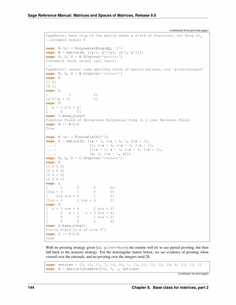
Sage Reference Manual: Matrices and Spaces of Matrices, Release 9.0
(continued from previous page)
TypeError: base ring of the matrix needs a field of fractions, not Ring of→˓integers modulo 6
sage: R.<y> = PolynomialRing(QQ, 'y')sage: B = matrix(R, [[y+1, y^2+y], [y^2, y^3]])sage: P, L, U = B.LU(pivot='partial')Traceback (most recent call last):...TypeError: cannot take absolute value of matrix entries, try 'pivot=nonzero'sage: P, L, U = B.LU(pivot='nonzero')sage: P[1 0][0 1]sage: L[ 1 0][y^2/(y + 1) 1]sage: U[ y + 1 y^2 + y][ 0 0]sage: L.base_ring()Fraction Field of Univariate Polynomial Ring in y over Rational Fieldsage: B == P*L*UTrue
sage: F.<a> = FiniteField(5^2)sage: C = matrix(F, [[a + 3, 4*a + 4, 2, 4*a + 2],....: [3, 2*a + 4, 2*a + 4, 2*a + 1],....: [3*a + 1, a + 3, 2*a + 4, 4*a + 3],....: [a, 3, 3*a + 1, a]])sage: P, L, U = C.LU(pivot='nonzero')sage: P[1 0 0 0][0 1 0 0][0 0 1 0][0 0 0 1]sage: L[ 1 0 0 0][3*a + 3 1 0 0][ 2*a 4*a + 2 1 0][2*a + 3 2 2*a + 4 1]sage: U[ a + 3 4*a + 4 2 4*a + 2][ 0 a + 1 a + 3 2*a + 4][ 0 0 1 4*a + 2][ 0 0 0 0]sage: L.base_ring()Finite Field in a of size 5^2sage: C == P*L*UTrue
With no pivoting strategy given (i.e. pivot=None) the routine will try to use partial pivoting, but thenfall back to the nonzero strategy. For the nonsingular matrix below, we see evidence of pivoting whenviewed over the rationals, and no pivoting over the integers mod 29.
sage: entries = [3, 20, 11, 7, 16, 28, 5, 15, 21, 23, 22, 18, 8, 23, 15, 2]sage: A = matrix(Integers(29), 4, 4, entries)
(continues on next page)
144 Chapter 8. Base class for matrices, part 2
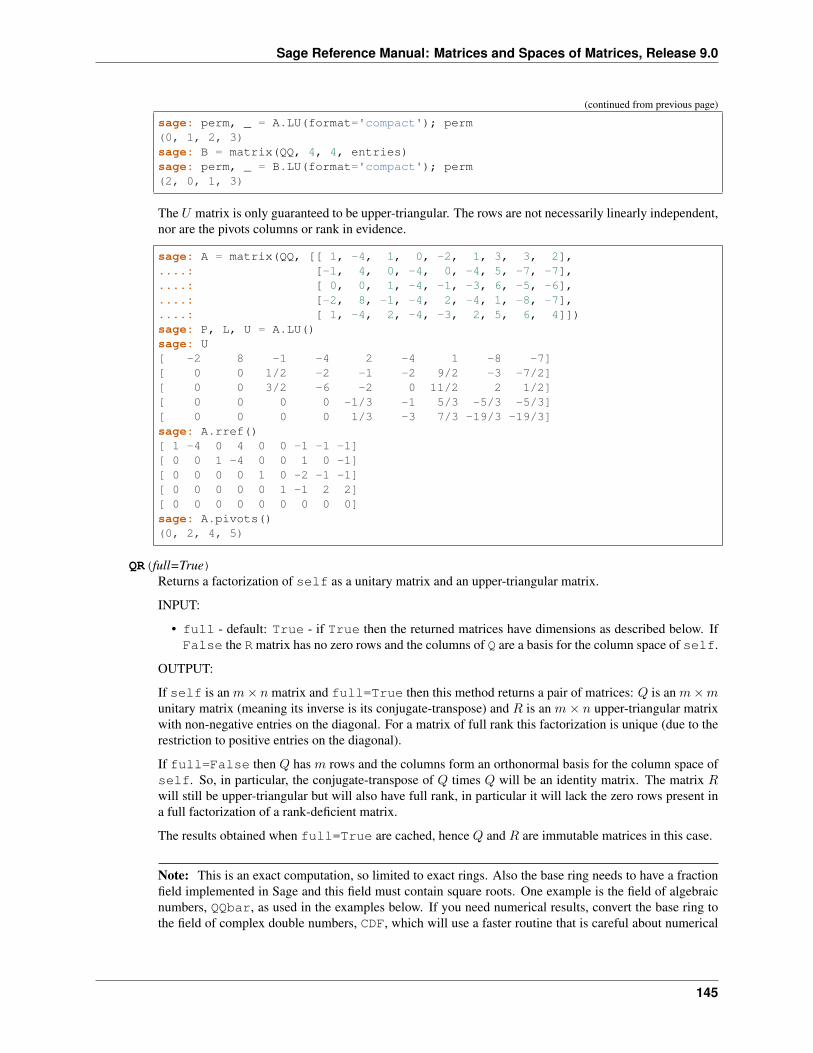
Sage Reference Manual: Matrices and Spaces of Matrices, Release 9.0
(continued from previous page)
sage: perm, _ = A.LU(format='compact'); perm(0, 1, 2, 3)sage: B = matrix(QQ, 4, 4, entries)sage: perm, _ = B.LU(format='compact'); perm(2, 0, 1, 3)
The 𝑈 matrix is only guaranteed to be upper-triangular. The rows are not necessarily linearly independent,nor are the pivots columns or rank in evidence.
sage: A = matrix(QQ, [[ 1, -4, 1, 0, -2, 1, 3, 3, 2],....: [-1, 4, 0, -4, 0, -4, 5, -7, -7],....: [ 0, 0, 1, -4, -1, -3, 6, -5, -6],....: [-2, 8, -1, -4, 2, -4, 1, -8, -7],....: [ 1, -4, 2, -4, -3, 2, 5, 6, 4]])sage: P, L, U = A.LU()sage: U[ -2 8 -1 -4 2 -4 1 -8 -7][ 0 0 1/2 -2 -1 -2 9/2 -3 -7/2][ 0 0 3/2 -6 -2 0 11/2 2 1/2][ 0 0 0 0 -1/3 -1 5/3 -5/3 -5/3][ 0 0 0 0 1/3 -3 7/3 -19/3 -19/3]sage: A.rref()[ 1 -4 0 4 0 0 -1 -1 -1][ 0 0 1 -4 0 0 1 0 -1][ 0 0 0 0 1 0 -2 -1 -1][ 0 0 0 0 0 1 -1 2 2][ 0 0 0 0 0 0 0 0 0]sage: A.pivots()(0, 2, 4, 5)
QR(full=True)Returns a factorization of self as a unitary matrix and an upper-triangular matrix.
INPUT:
• full - default: True - if True then the returned matrices have dimensions as described below. IfFalse the R matrix has no zero rows and the columns of Q are a basis for the column space of self.
OUTPUT:
If self is an 𝑚× 𝑛 matrix and full=True then this method returns a pair of matrices: 𝑄 is an 𝑚×𝑚unitary matrix (meaning its inverse is its conjugate-transpose) and 𝑅 is an 𝑚× 𝑛 upper-triangular matrixwith non-negative entries on the diagonal. For a matrix of full rank this factorization is unique (due to therestriction to positive entries on the diagonal).
If full=False then 𝑄 has 𝑚 rows and the columns form an orthonormal basis for the column space ofself. So, in particular, the conjugate-transpose of 𝑄 times 𝑄 will be an identity matrix. The matrix 𝑅will still be upper-triangular but will also have full rank, in particular it will lack the zero rows present ina full factorization of a rank-deficient matrix.
The results obtained when full=True are cached, hence 𝑄 and 𝑅 are immutable matrices in this case.
Note: This is an exact computation, so limited to exact rings. Also the base ring needs to have a fractionfield implemented in Sage and this field must contain square roots. One example is the field of algebraicnumbers, QQbar, as used in the examples below. If you need numerical results, convert the base ring tothe field of complex double numbers, CDF, which will use a faster routine that is careful about numerical
145
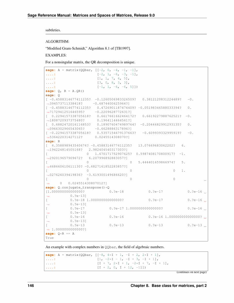
Sage Reference Manual: Matrices and Spaces of Matrices, Release 9.0
subtleties.
ALGORITHM:
“Modified Gram-Schmidt,” Algorithm 8.1 of [TB1997].
EXAMPLES:
For a nonsingular matrix, the QR decomposition is unique.
sage: A = matrix(QQbar, [[-2, 0, -4, -1, -1],....: [-2, 1, -6, -3, -1],....: [1, 1, 7, 4, 5],....: [3, 0, 8, 3, 3],....: [-1, 1, -6, -6, 5]])sage: Q, R = A.QR()sage: Q[ -0.4588314677411235? -0.1260506983326509? 0.3812120831224489? -0.→˓394573711338418? -0.6874400625964?][ -0.4588314677411235? 0.4726901187474409? -0.05198346588033394? 0.→˓7172941251646595? -0.2209628772631?][ 0.2294157338705618? 0.6617661662464172? 0.6619227988762521? -0.→˓1808720937375480? 0.1964114464561?][ 0.6882472016116853? 0.1890760474989764? -0.2044682991293135? 0.→˓0966302966543065? -0.6628886317894?][ -0.2294157338705618? 0.5357154679137663? -0.609939332995919? -0.→˓536422031427112? 0.0245514308070?]sage: R[ 4.358898943540674? -0.4588314677411235? 13.07669683062202? 6.→˓194224814505168? 2.982404540317303?][ 0 1.670171752907625? 0.5987408170800917? -1.→˓292019657909672? 6.207996892883057?][ 0 0 5.444401659866974? 5.→˓468660610611130? -0.6827161852283857?][ 0 0 0 1.→˓027626039419836? -3.619300149686620?][ 0 0 0→˓ 0 0.024551430807012?]sage: Q.conjugate_transpose()*Q[1.000000000000000? 0.?e-18 0.?e-17 0.?e-16→˓ 0.?e-13][ 0.?e-18 1.000000000000000? 0.?e-17 0.?e-16→˓ 0.?e-13][ 0.?e-17 0.?e-17 1.000000000000000? 0.?e-16→˓ 0.?e-13][ 0.?e-16 0.?e-16 0.?e-16 1.000000000000000?→˓ 0.?e-13][ 0.?e-13 0.?e-13 0.?e-13 0.?e-13→˓ 1.0000000000000?]sage: Q*R == ATrue
An example with complex numbers in QQbar, the field of algebraic numbers.
sage: A = matrix(QQbar, [[-8, 4*I + 1, -I + 2, 2*I + 1],....: [1, -2*I - 1, -I + 3, -I + 1],....: [I + 7, 2*I + 1, -2*I + 7, -I + 1],....: [I + 2, 0, I + 12, -1]])
(continues on next page)
146 Chapter 8. Base class for matrices, part 2
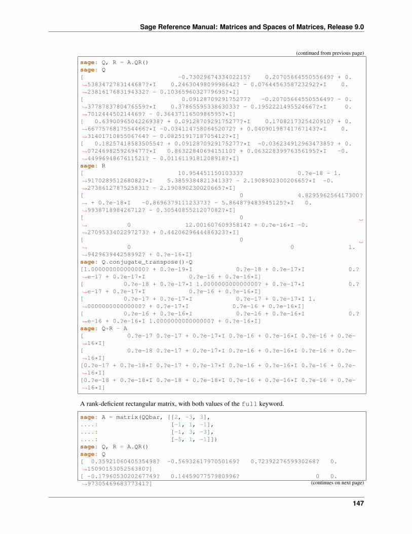
Sage Reference Manual: Matrices and Spaces of Matrices, Release 9.0
(continued from previous page)
sage: Q, R = A.QR()sage: Q[ -0.7302967433402215? 0.2070566455055649? + 0.→˓5383472783144687?*I 0.2463049809998642? - 0.0764456358723292?*I 0.→˓2381617683194332? - 0.1036596032779695?*I][ 0.0912870929175277? -0.2070566455055649? - 0.→˓3778783780476559?*I 0.3786559533863033? - 0.1952221495524667?*I 0.→˓701244450214469? - 0.3643711650986595?*I][ 0.6390096504226938? + 0.0912870929175277?*I 0.1708217325420910? + 0.→˓6677576817554466?*I -0.03411475806452072? + 0.04090198741767143?*I 0.→˓3140171085506764? - 0.0825191718705412?*I][ 0.1825741858350554? + 0.0912870929175277?*I -0.03623491296347385? + 0.→˓0724698259269477?*I 0.8632284069415110? + 0.06322839976356195?*I -0.→˓4499694867611521? - 0.0116119181208918?*I]sage: R[ 10.95445115010333? 0.?e-18 - 1.→˓917028951268082?*I 5.385938482134133? - 2.190890230020665?*I -0.→˓2738612787525831? - 2.190890230020665?*I][ 0 4.829596256417300?→˓ + 0.?e-18*I -0.869637911123373? - 5.864879483945125?*I 0.→˓993871898426712? - 0.3054085521207082?*I][ 0→˓ 0 12.00160760935814? + 0.?e-16*I -0.→˓2709533402297273? + 0.4420629644486323?*I][ 0→˓ 0 0 1.→˓942963944258992? + 0.?e-16*I]sage: Q.conjugate_transpose()*Q[1.000000000000000? + 0.?e-19*I 0.?e-18 + 0.?e-17*I 0.?→˓e-17 + 0.?e-17*I 0.?e-16 + 0.?e-16*I][ 0.?e-18 + 0.?e-17*I 1.000000000000000? + 0.?e-17*I 0.?→˓e-17 + 0.?e-17*I 0.?e-16 + 0.?e-16*I][ 0.?e-17 + 0.?e-17*I 0.?e-17 + 0.?e-17*I 1.→˓000000000000000? + 0.?e-17*I 0.?e-16 + 0.?e-16*I][ 0.?e-16 + 0.?e-16*I 0.?e-16 + 0.?e-16*I 0.?→˓e-16 + 0.?e-16*I 1.000000000000000? + 0.?e-16*I]sage: Q*R - A[ 0.?e-17 0.?e-17 + 0.?e-17*I 0.?e-16 + 0.?e-16*I 0.?e-16 + 0.?e-→˓16*I][ 0.?e-18 0.?e-17 + 0.?e-17*I 0.?e-16 + 0.?e-16*I 0.?e-16 + 0.?e-→˓16*I][0.?e-17 + 0.?e-18*I 0.?e-17 + 0.?e-17*I 0.?e-16 + 0.?e-16*I 0.?e-16 + 0.?e-→˓16*I][0.?e-18 + 0.?e-18*I 0.?e-18 + 0.?e-18*I 0.?e-16 + 0.?e-16*I 0.?e-16 + 0.?e-→˓16*I]
A rank-deficient rectangular matrix, with both values of the full keyword.
sage: A = matrix(QQbar, [[2, -3, 3],....: [-1, 1, -1],....: [-1, 3, -3],....: [-5, 1, -1]])sage: Q, R = A.QR()sage: Q[ 0.3592106040535498? -0.5693261797050169? 0.7239227659930268? 0.→˓1509015305256380?][ -0.1796053020267749? 0.1445907757980996? 0 0.→˓9730546968377341?] (continues on next page)
147
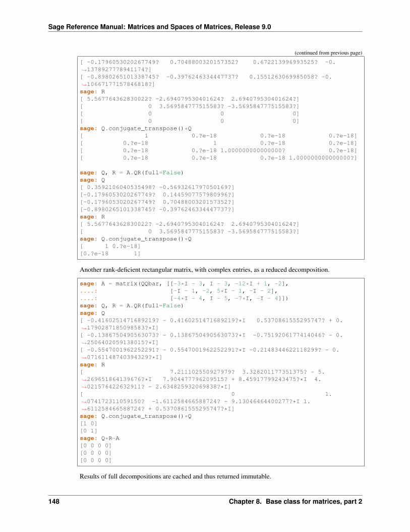
Sage Reference Manual: Matrices and Spaces of Matrices, Release 9.0
(continued from previous page)
[ -0.1796053020267749? 0.7048800320157352? 0.672213996993525? -0.→˓1378927778941174?][ -0.8980265101338745? -0.3976246334447737? 0.1551263069985058? -0.→˓10667177157846818?]sage: R[ 5.567764362830022? -2.694079530401624? 2.694079530401624?][ 0 3.569584777515583? -3.569584777515583?][ 0 0 0][ 0 0 0]sage: Q.conjugate_transpose()*Q[ 1 0.?e-18 0.?e-18 0.?e-18][ 0.?e-18 1 0.?e-18 0.?e-18][ 0.?e-18 0.?e-18 1.000000000000000? 0.?e-18][ 0.?e-18 0.?e-18 0.?e-18 1.000000000000000?]
sage: Q, R = A.QR(full=False)sage: Q[ 0.3592106040535498? -0.5693261797050169?][-0.1796053020267749? 0.1445907757980996?][-0.1796053020267749? 0.7048800320157352?][-0.8980265101338745? -0.3976246334447737?]sage: R[ 5.567764362830022? -2.694079530401624? 2.694079530401624?][ 0 3.569584777515583? -3.569584777515583?]sage: Q.conjugate_transpose()*Q[ 1 0.?e-18][0.?e-18 1]
Another rank-deficient rectangular matrix, with complex entries, as a reduced decomposition.
sage: A = matrix(QQbar, [[-3*I - 3, I - 3, -12*I + 1, -2],....: [-I - 1, -2, 5*I - 1, -I - 2],....: [-4*I - 4, I - 5, -7*I, -I - 4]])sage: Q, R = A.QR(full=False)sage: Q[ -0.4160251471689219? - 0.4160251471689219?*I 0.5370861555295747? + 0.→˓1790287185098583?*I][ -0.1386750490563073? - 0.1386750490563073?*I -0.7519206177414046? - 0.→˓2506402059138015?*I][ -0.5547001962252291? - 0.5547001962252291?*I -0.2148344622118299? - 0.→˓07161148740394329?*I]sage: R[ 7.211102550927979? 3.328201177351375? - 5.→˓269651864139676?*I 7.904477796209515? + 8.45917799243475?*I 4.→˓021576422632911? - 2.634825932069838?*I][ 0 1.→˓074172311059150? -1.611258466588724? - 9.13046464400277?*I 1.→˓611258466588724? + 0.5370861555295747?*I]sage: Q.conjugate_transpose()*Q[1 0][0 1]sage: Q*R-A[0 0 0 0][0 0 0 0][0 0 0 0]
Results of full decompositions are cached and thus returned immutable.
148 Chapter 8. Base class for matrices, part 2
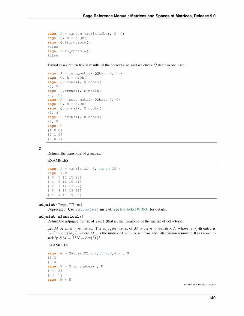
Sage Reference Manual: Matrices and Spaces of Matrices, Release 9.0
sage: A = random_matrix(QQbar, 2, 2)sage: Q, R = A.QR()sage: Q.is_mutable()Falsesage: R.is_mutable()False
Trivial cases return trivial results of the correct size, and we check 𝑄 itself in one case.
sage: A = zero_matrix(QQbar, 0, 10)sage: Q, R = A.QR()sage: Q.nrows(), Q.ncols()(0, 0)sage: R.nrows(), R.ncols()(0, 10)sage: A = zero_matrix(QQbar, 3, 0)sage: Q, R = A.QR()sage: Q.nrows(), Q.ncols()(3, 3)sage: R.nrows(), R.ncols()(3, 0)sage: Q[1 0 0][0 1 0][0 0 1]
TReturns the transpose of a matrix.
EXAMPLES:
sage: A = matrix(QQ, 5, range(25))sage: A.T[ 0 5 10 15 20][ 1 6 11 16 21][ 2 7 12 17 22][ 3 8 13 18 23][ 4 9 14 19 24]
adjoint(*args, **kwds)Deprecated: Use adjugate() instead. See trac ticket #10501 for details.
adjoint_classical()Return the adjugate matrix of self (that is, the transpose of the matrix of cofactors).
Let 𝑀 be an 𝑛 × 𝑛-matrix. The adjugate matrix of 𝑀 is the 𝑛 × 𝑛-matrix 𝑁 whose (𝑖, 𝑗)-th entry is(−1)𝑖+𝑗 det(𝑀𝑗,𝑖), where 𝑀𝑗,𝑖 is the matrix 𝑀 with its 𝑗-th row and 𝑖-th column removed. It is known tosatisfy 𝑁𝑀 = 𝑀𝑁 = det(𝑀)𝐼 .
EXAMPLES:
sage: M = Matrix(ZZ,2,2,[5,2,3,4]) ; M[5 2][3 4]sage: N = M.adjugate() ; N[ 4 -2][-3 5]sage: M * N
(continues on next page)
149

Sage Reference Manual: Matrices and Spaces of Matrices, Release 9.0
(continued from previous page)
[14 0][ 0 14]sage: N * M[14 0][ 0 14]sage: M = Matrix(QQ,2,2,[5/3,2/56,33/13,41/10]) ; M[ 5/3 1/28][33/13 41/10]sage: N = M.adjugate() ; N[ 41/10 -1/28][-33/13 5/3]sage: M * N[7363/1092 0][ 0 7363/1092]
An alias is adjoint_classical(), which replaces the deprecated adjoint() method:
sage: M.adjoint()...: DeprecationWarning: adjoint is deprecated. Please use adjugate instead.See http://trac.sagemath.org/10501 for details.[ 41/10 -1/28][-33/13 5/3]sage: M.adjoint_classical()[ 41/10 -1/28][-33/13 5/3]
ALGORITHM:
Use PARI whenever the method self._adjugate is included to do so in an inheriting class. Otherwise,use a generic division-free algorithm that computes the adjugate matrix from the characteristic polynomial.
The result is cached.
adjugate()Return the adjugate matrix of self (that is, the transpose of the matrix of cofactors).
Let 𝑀 be an 𝑛 × 𝑛-matrix. The adjugate matrix of 𝑀 is the 𝑛 × 𝑛-matrix 𝑁 whose (𝑖, 𝑗)-th entry is(−1)𝑖+𝑗 det(𝑀𝑗,𝑖), where 𝑀𝑗,𝑖 is the matrix 𝑀 with its 𝑗-th row and 𝑖-th column removed. It is known tosatisfy 𝑁𝑀 = 𝑀𝑁 = det(𝑀)𝐼 .
EXAMPLES:
sage: M = Matrix(ZZ,2,2,[5,2,3,4]) ; M[5 2][3 4]sage: N = M.adjugate() ; N[ 4 -2][-3 5]sage: M * N[14 0][ 0 14]sage: N * M[14 0][ 0 14]sage: M = Matrix(QQ,2,2,[5/3,2/56,33/13,41/10]) ; M[ 5/3 1/28][33/13 41/10]sage: N = M.adjugate() ; N
(continues on next page)
150 Chapter 8. Base class for matrices, part 2
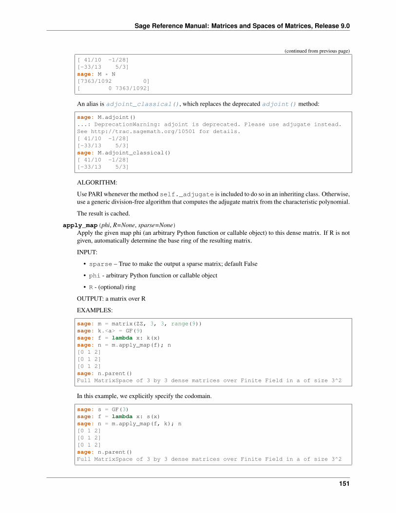
Sage Reference Manual: Matrices and Spaces of Matrices, Release 9.0
(continued from previous page)
[ 41/10 -1/28][-33/13 5/3]sage: M * N[7363/1092 0][ 0 7363/1092]
An alias is adjoint_classical(), which replaces the deprecated adjoint() method:
sage: M.adjoint()...: DeprecationWarning: adjoint is deprecated. Please use adjugate instead.See http://trac.sagemath.org/10501 for details.[ 41/10 -1/28][-33/13 5/3]sage: M.adjoint_classical()[ 41/10 -1/28][-33/13 5/3]
ALGORITHM:
Use PARI whenever the method self._adjugate is included to do so in an inheriting class. Otherwise,use a generic division-free algorithm that computes the adjugate matrix from the characteristic polynomial.
The result is cached.
apply_map(phi, R=None, sparse=None)Apply the given map phi (an arbitrary Python function or callable object) to this dense matrix. If R is notgiven, automatically determine the base ring of the resulting matrix.
INPUT:
• sparse – True to make the output a sparse matrix; default False
• phi - arbitrary Python function or callable object
• R - (optional) ring
OUTPUT: a matrix over R
EXAMPLES:
sage: m = matrix(ZZ, 3, 3, range(9))sage: k.<a> = GF(9)sage: f = lambda x: k(x)sage: n = m.apply_map(f); n[0 1 2][0 1 2][0 1 2]sage: n.parent()Full MatrixSpace of 3 by 3 dense matrices over Finite Field in a of size 3^2
In this example, we explicitly specify the codomain.
sage: s = GF(3)sage: f = lambda x: s(x)sage: n = m.apply_map(f, k); n[0 1 2][0 1 2][0 1 2]sage: n.parent()Full MatrixSpace of 3 by 3 dense matrices over Finite Field in a of size 3^2
151
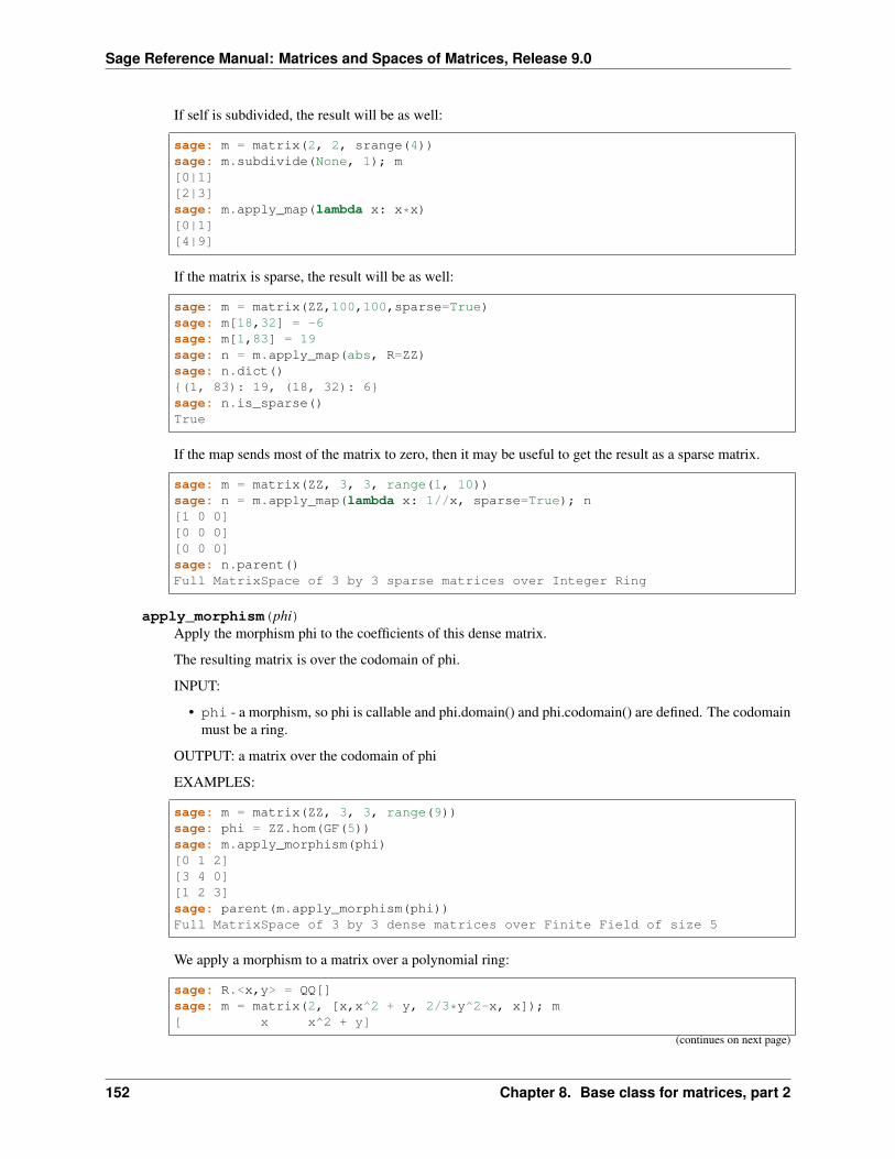
Sage Reference Manual: Matrices and Spaces of Matrices, Release 9.0
If self is subdivided, the result will be as well:
sage: m = matrix(2, 2, srange(4))sage: m.subdivide(None, 1); m[0|1][2|3]sage: m.apply_map(lambda x: x*x)[0|1][4|9]
If the matrix is sparse, the result will be as well:
sage: m = matrix(ZZ,100,100,sparse=True)sage: m[18,32] = -6sage: m[1,83] = 19sage: n = m.apply_map(abs, R=ZZ)sage: n.dict(){(1, 83): 19, (18, 32): 6}sage: n.is_sparse()True
If the map sends most of the matrix to zero, then it may be useful to get the result as a sparse matrix.
sage: m = matrix(ZZ, 3, 3, range(1, 10))sage: n = m.apply_map(lambda x: 1//x, sparse=True); n[1 0 0][0 0 0][0 0 0]sage: n.parent()Full MatrixSpace of 3 by 3 sparse matrices over Integer Ring
apply_morphism(phi)Apply the morphism phi to the coefficients of this dense matrix.
The resulting matrix is over the codomain of phi.
INPUT:
• phi - a morphism, so phi is callable and phi.domain() and phi.codomain() are defined. The codomainmust be a ring.
OUTPUT: a matrix over the codomain of phi
EXAMPLES:
sage: m = matrix(ZZ, 3, 3, range(9))sage: phi = ZZ.hom(GF(5))sage: m.apply_morphism(phi)[0 1 2][3 4 0][1 2 3]sage: parent(m.apply_morphism(phi))Full MatrixSpace of 3 by 3 dense matrices over Finite Field of size 5
We apply a morphism to a matrix over a polynomial ring:
sage: R.<x,y> = QQ[]sage: m = matrix(2, [x,x^2 + y, 2/3*y^2-x, x]); m[ x x^2 + y]
(continues on next page)
152 Chapter 8. Base class for matrices, part 2
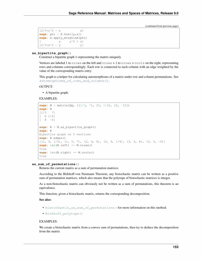
Sage Reference Manual: Matrices and Spaces of Matrices, Release 9.0
(continued from previous page)
[2/3*y^2 - x x]sage: phi = R.hom([y,x])sage: m.apply_morphism(phi)[ y y^2 + x][2/3*x^2 - y y]
as_bipartite_graph()Construct a bipartite graph B representing the matrix uniquely.
Vertices are labeled 1 to nrows on the left and nrows + 1 to nrows + ncols on the right, representingrows and columns correspondingly. Each row is connected to each column with an edge weighted by thevalue of the corresponding matrix entry.
This graph is a helper for calculating automorphisms of a matrix under row and column permutations. Seeautomorphisms_of_rows_and_columns().
OUTPUT:
• A bipartite graph.
EXAMPLES:
sage: M = matrix(QQ, [[1/3, 7], [6, 1/4], [8, -5]])sage: M[1/3 7][ 6 1/4][ 8 -5]
sage: B = M.as_bipartite_graph()sage: BBipartite graph on 5 verticessage: B.edges()[(1, 4, 1/3), (1, 5, 7), (2, 4, 6), (2, 5, 1/4), (3, 4, 8), (3, 5, -5)]sage: len(B.left) == M.nrows()Truesage: len(B.right) == M.ncols()True
as_sum_of_permutations()Returns the current matrix as a sum of permutation matrices
According to the Birkhoff-von Neumann Theorem, any bistochastic matrix can be written as a positivesum of permutation matrices, which also means that the polytope of bistochastic matrices is integer.
As a non-bistochastic matrix can obviously not be written as a sum of permutations, this theorem is anequivalence.
This function, given a bistochastic matrix, returns the corresponding decomposition.
See also:
• bistochastic_as_sum_of_permutations – for more information on this method.
• Birkhoff_polytope()
EXAMPLES:
We create a bistochastic matrix from a convex sum of permutations, then try to deduce the decompositionfrom the matrix
153
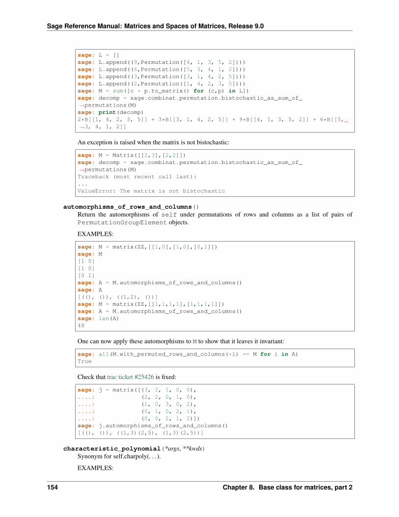
Sage Reference Manual: Matrices and Spaces of Matrices, Release 9.0
sage: L = []sage: L.append((9,Permutation([4, 1, 3, 5, 2])))sage: L.append((6,Permutation([5, 3, 4, 1, 2])))sage: L.append((3,Permutation([3, 1, 4, 2, 5])))sage: L.append((2,Permutation([1, 4, 2, 3, 5])))sage: M = sum([c * p.to_matrix() for (c,p) in L])sage: decomp = sage.combinat.permutation.bistochastic_as_sum_of_→˓permutations(M)sage: print(decomp)2*B[[1, 4, 2, 3, 5]] + 3*B[[3, 1, 4, 2, 5]] + 9*B[[4, 1, 3, 5, 2]] + 6*B[[5,→˓3, 4, 1, 2]]
An exception is raised when the matrix is not bistochastic:
sage: M = Matrix([[2,3],[2,2]])sage: decomp = sage.combinat.permutation.bistochastic_as_sum_of_→˓permutations(M)Traceback (most recent call last):...ValueError: The matrix is not bistochastic
automorphisms_of_rows_and_columns()Return the automorphisms of self under permutations of rows and columns as a list of pairs ofPermutationGroupElement objects.
EXAMPLES:
sage: M = matrix(ZZ,[[1,0],[1,0],[0,1]])sage: M[1 0][1 0][0 1]sage: A = M.automorphisms_of_rows_and_columns()sage: A[((), ()), ((1,2), ())]sage: M = matrix(ZZ,[[1,1,1,1],[1,1,1,1]])sage: A = M.automorphisms_of_rows_and_columns()sage: len(A)48
One can now apply these automorphisms to M to show that it leaves it invariant:
sage: all(M.with_permuted_rows_and_columns(*i) == M for i in A)True
Check that trac ticket #25426 is fixed:
sage: j = matrix([(3, 2, 1, 0, 0),....: (2, 2, 0, 1, 0),....: (1, 0, 3, 0, 2),....: (0, 1, 0, 2, 1),....: (0, 0, 2, 1, 2)])sage: j.automorphisms_of_rows_and_columns()[((), ()), ((1,3)(2,5), (1,3)(2,5))]
characteristic_polynomial(*args, **kwds)Synonym for self.charpoly(. . . ).
EXAMPLES:
154 Chapter 8. Base class for matrices, part 2
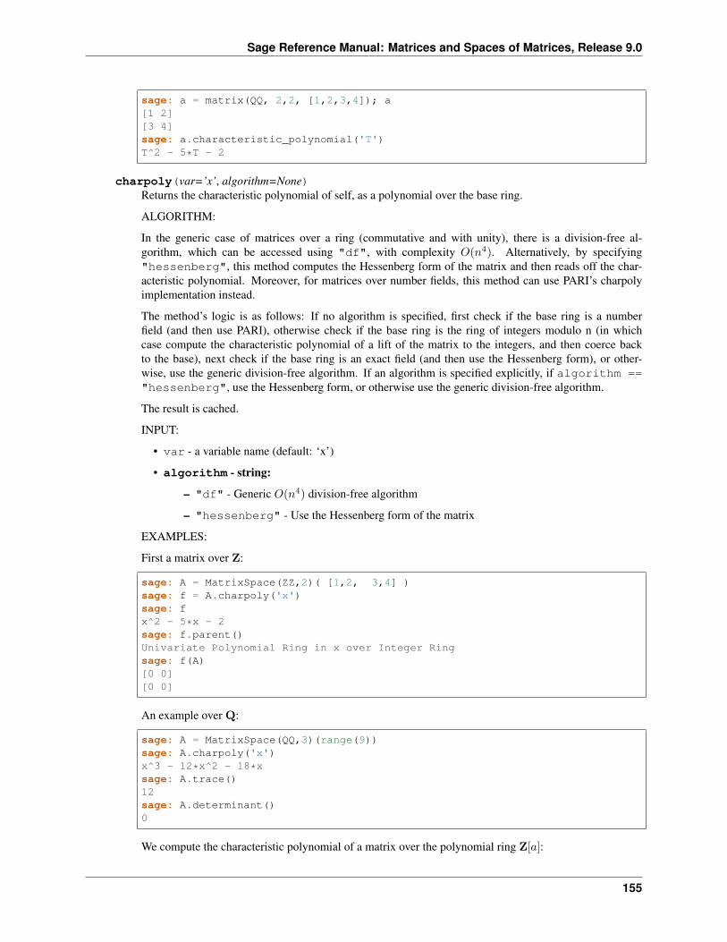
Sage Reference Manual: Matrices and Spaces of Matrices, Release 9.0
sage: a = matrix(QQ, 2,2, [1,2,3,4]); a[1 2][3 4]sage: a.characteristic_polynomial('T')T^2 - 5*T - 2
charpoly(var=’x’, algorithm=None)Returns the characteristic polynomial of self, as a polynomial over the base ring.
ALGORITHM:
In the generic case of matrices over a ring (commutative and with unity), there is a division-free al-gorithm, which can be accessed using "df", with complexity 𝑂(𝑛4). Alternatively, by specifying"hessenberg", this method computes the Hessenberg form of the matrix and then reads off the char-acteristic polynomial. Moreover, for matrices over number fields, this method can use PARI’s charpolyimplementation instead.
The method’s logic is as follows: If no algorithm is specified, first check if the base ring is a numberfield (and then use PARI), otherwise check if the base ring is the ring of integers modulo n (in whichcase compute the characteristic polynomial of a lift of the matrix to the integers, and then coerce backto the base), next check if the base ring is an exact field (and then use the Hessenberg form), or other-wise, use the generic division-free algorithm. If an algorithm is specified explicitly, if algorithm =="hessenberg", use the Hessenberg form, or otherwise use the generic division-free algorithm.
The result is cached.
INPUT:
• var - a variable name (default: ‘x’)
• algorithm - string:
– "df" - Generic 𝑂(𝑛4) division-free algorithm
– "hessenberg" - Use the Hessenberg form of the matrix
EXAMPLES:
First a matrix over Z:
sage: A = MatrixSpace(ZZ,2)( [1,2, 3,4] )sage: f = A.charpoly('x')sage: fx^2 - 5*x - 2sage: f.parent()Univariate Polynomial Ring in x over Integer Ringsage: f(A)[0 0][0 0]
An example over Q:
sage: A = MatrixSpace(QQ,3)(range(9))sage: A.charpoly('x')x^3 - 12*x^2 - 18*xsage: A.trace()12sage: A.determinant()0
We compute the characteristic polynomial of a matrix over the polynomial ring Z[𝑎]:
155
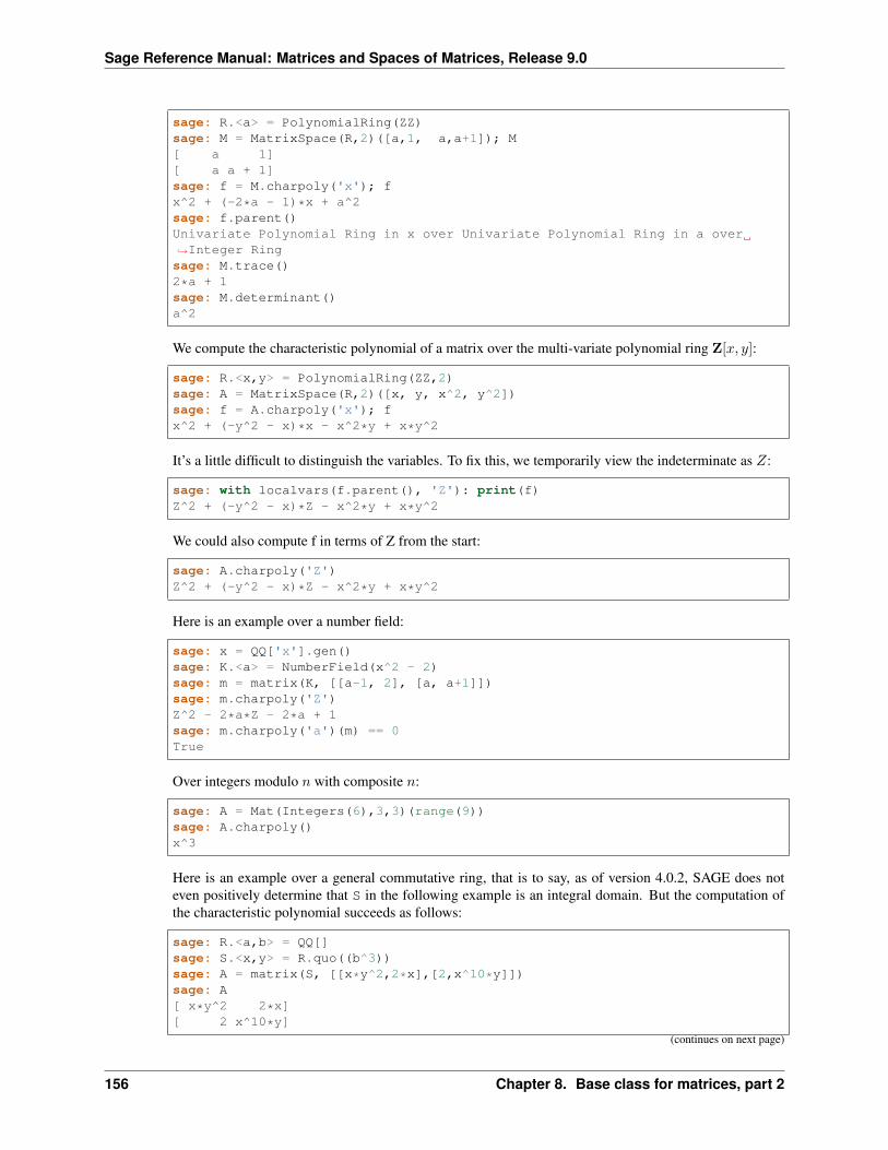
Sage Reference Manual: Matrices and Spaces of Matrices, Release 9.0
sage: R.<a> = PolynomialRing(ZZ)sage: M = MatrixSpace(R,2)([a,1, a,a+1]); M[ a 1][ a a + 1]sage: f = M.charpoly('x'); fx^2 + (-2*a - 1)*x + a^2sage: f.parent()Univariate Polynomial Ring in x over Univariate Polynomial Ring in a over→˓Integer Ringsage: M.trace()2*a + 1sage: M.determinant()a^2
We compute the characteristic polynomial of a matrix over the multi-variate polynomial ring Z[𝑥, 𝑦]:
sage: R.<x,y> = PolynomialRing(ZZ,2)sage: A = MatrixSpace(R,2)([x, y, x^2, y^2])sage: f = A.charpoly('x'); fx^2 + (-y^2 - x)*x - x^2*y + x*y^2
It’s a little difficult to distinguish the variables. To fix this, we temporarily view the indeterminate as 𝑍:
sage: with localvars(f.parent(), 'Z'): print(f)Z^2 + (-y^2 - x)*Z - x^2*y + x*y^2
We could also compute f in terms of Z from the start:
sage: A.charpoly('Z')Z^2 + (-y^2 - x)*Z - x^2*y + x*y^2
Here is an example over a number field:
sage: x = QQ['x'].gen()sage: K.<a> = NumberField(x^2 - 2)sage: m = matrix(K, [[a-1, 2], [a, a+1]])sage: m.charpoly('Z')Z^2 - 2*a*Z - 2*a + 1sage: m.charpoly('a')(m) == 0True
Over integers modulo 𝑛 with composite 𝑛:
sage: A = Mat(Integers(6),3,3)(range(9))sage: A.charpoly()x^3
Here is an example over a general commutative ring, that is to say, as of version 4.0.2, SAGE does noteven positively determine that S in the following example is an integral domain. But the computation ofthe characteristic polynomial succeeds as follows:
sage: R.<a,b> = QQ[]sage: S.<x,y> = R.quo((b^3))sage: A = matrix(S, [[x*y^2,2*x],[2,x^10*y]])sage: A[ x*y^2 2*x][ 2 x^10*y]
(continues on next page)
156 Chapter 8. Base class for matrices, part 2
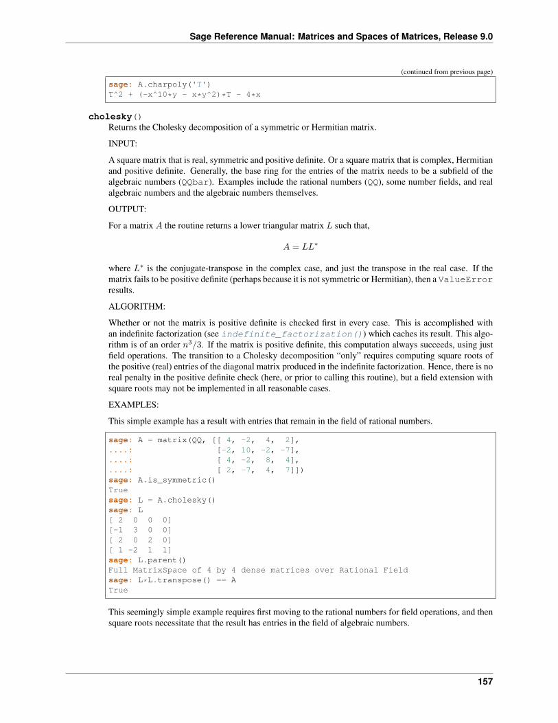
Sage Reference Manual: Matrices and Spaces of Matrices, Release 9.0
(continued from previous page)
sage: A.charpoly('T')T^2 + (-x^10*y - x*y^2)*T - 4*x
cholesky()Returns the Cholesky decomposition of a symmetric or Hermitian matrix.
INPUT:
A square matrix that is real, symmetric and positive definite. Or a square matrix that is complex, Hermitianand positive definite. Generally, the base ring for the entries of the matrix needs to be a subfield of thealgebraic numbers (QQbar). Examples include the rational numbers (QQ), some number fields, and realalgebraic numbers and the algebraic numbers themselves.
OUTPUT:
For a matrix 𝐴 the routine returns a lower triangular matrix 𝐿 such that,
𝐴 = 𝐿𝐿*
where 𝐿* is the conjugate-transpose in the complex case, and just the transpose in the real case. If thematrix fails to be positive definite (perhaps because it is not symmetric or Hermitian), then a ValueErrorresults.
ALGORITHM:
Whether or not the matrix is positive definite is checked first in every case. This is accomplished withan indefinite factorization (see indefinite_factorization()) which caches its result. This algo-rithm is of an order 𝑛3/3. If the matrix is positive definite, this computation always succeeds, using justfield operations. The transition to a Cholesky decomposition “only” requires computing square roots ofthe positive (real) entries of the diagonal matrix produced in the indefinite factorization. Hence, there is noreal penalty in the positive definite check (here, or prior to calling this routine), but a field extension withsquare roots may not be implemented in all reasonable cases.
EXAMPLES:
This simple example has a result with entries that remain in the field of rational numbers.
sage: A = matrix(QQ, [[ 4, -2, 4, 2],....: [-2, 10, -2, -7],....: [ 4, -2, 8, 4],....: [ 2, -7, 4, 7]])sage: A.is_symmetric()Truesage: L = A.cholesky()sage: L[ 2 0 0 0][-1 3 0 0][ 2 0 2 0][ 1 -2 1 1]sage: L.parent()Full MatrixSpace of 4 by 4 dense matrices over Rational Fieldsage: L*L.transpose() == ATrue
This seemingly simple example requires first moving to the rational numbers for field operations, and thensquare roots necessitate that the result has entries in the field of algebraic numbers.
157
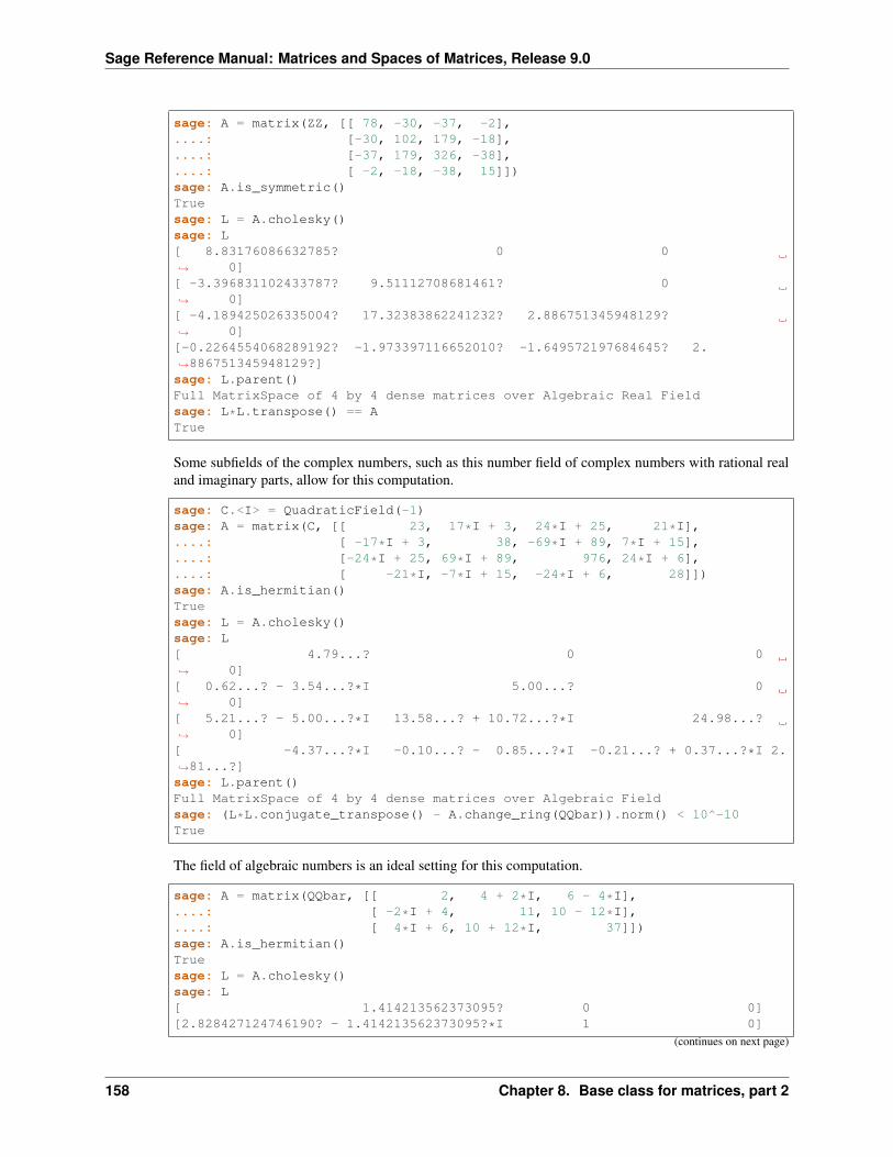
Sage Reference Manual: Matrices and Spaces of Matrices, Release 9.0
sage: A = matrix(ZZ, [[ 78, -30, -37, -2],....: [-30, 102, 179, -18],....: [-37, 179, 326, -38],....: [ -2, -18, -38, 15]])sage: A.is_symmetric()Truesage: L = A.cholesky()sage: L[ 8.83176086632785? 0 0→˓ 0][ -3.396831102433787? 9.51112708681461? 0→˓ 0][ -4.189425026335004? 17.32383862241232? 2.886751345948129?→˓ 0][-0.2264554068289192? -1.973397116652010? -1.649572197684645? 2.→˓886751345948129?]sage: L.parent()Full MatrixSpace of 4 by 4 dense matrices over Algebraic Real Fieldsage: L*L.transpose() == ATrue
Some subfields of the complex numbers, such as this number field of complex numbers with rational realand imaginary parts, allow for this computation.
sage: C.<I> = QuadraticField(-1)sage: A = matrix(C, [[ 23, 17*I + 3, 24*I + 25, 21*I],....: [ -17*I + 3, 38, -69*I + 89, 7*I + 15],....: [-24*I + 25, 69*I + 89, 976, 24*I + 6],....: [ -21*I, -7*I + 15, -24*I + 6, 28]])sage: A.is_hermitian()Truesage: L = A.cholesky()sage: L[ 4.79...? 0 0→˓ 0][ 0.62...? - 3.54...?*I 5.00...? 0→˓ 0][ 5.21...? - 5.00...?*I 13.58...? + 10.72...?*I 24.98...?→˓ 0][ -4.37...?*I -0.10...? - 0.85...?*I -0.21...? + 0.37...?*I 2.→˓81...?]sage: L.parent()Full MatrixSpace of 4 by 4 dense matrices over Algebraic Fieldsage: (L*L.conjugate_transpose() - A.change_ring(QQbar)).norm() < 10^-10True
The field of algebraic numbers is an ideal setting for this computation.
sage: A = matrix(QQbar, [[ 2, 4 + 2*I, 6 - 4*I],....: [ -2*I + 4, 11, 10 - 12*I],....: [ 4*I + 6, 10 + 12*I, 37]])sage: A.is_hermitian()Truesage: L = A.cholesky()sage: L[ 1.414213562373095? 0 0][2.828427124746190? - 1.414213562373095?*I 1 0]
(continues on next page)
158 Chapter 8. Base class for matrices, part 2
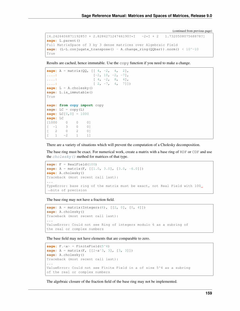
Sage Reference Manual: Matrices and Spaces of Matrices, Release 9.0
(continued from previous page)
[4.242640687119285? + 2.828427124746190?*I -2*I + 2 1.732050807568878?]sage: L.parent()Full MatrixSpace of 3 by 3 dense matrices over Algebraic Fieldsage: (L*L.conjugate_transpose() - A.change_ring(QQbar)).norm() < 10^-10True
Results are cached, hence immutable. Use the copy function if you need to make a change.
sage: A = matrix(QQ, [[ 4, -2, 4, 2],....: [-2, 10, -2, -7],....: [ 4, -2, 8, 4],....: [ 2, -7, 4, 7]])sage: L = A.cholesky()sage: L.is_immutable()True
sage: from copy import copysage: LC = copy(L)sage: LC[0,0] = 1000sage: LC[1000 0 0 0][ -1 3 0 0][ 2 0 2 0][ 1 -2 1 1]
There are a variety of situations which will prevent the computation of a Cholesky decomposition.
The base ring must be exact. For numerical work, create a matrix with a base ring of RDF or CDF and usethe cholesky() method for matrices of that type.
sage: F = RealField(100)sage: A = matrix(F, [[1.0, 3.0], [3.0, -6.0]])sage: A.cholesky()Traceback (most recent call last):...TypeError: base ring of the matrix must be exact, not Real Field with 100→˓bits of precision
The base ring may not have a fraction field.
sage: A = matrix(Integers(6), [[2, 0], [0, 4]])sage: A.cholesky()Traceback (most recent call last):...ValueError: Could not see Ring of integers modulo 6 as a subring ofthe real or complex numbers
The base field may not have elements that are comparable to zero.
sage: F.<a> = FiniteField(5^4)sage: A = matrix(F, [[2+a^3, 3], [3, 3]])sage: A.cholesky()Traceback (most recent call last):...ValueError: Could not see Finite Field in a of size 5^4 as a subringof the real or complex numbers
The algebraic closure of the fraction field of the base ring may not be implemented.
159
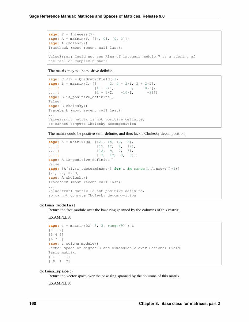
Sage Reference Manual: Matrices and Spaces of Matrices, Release 9.0
sage: F = Integers(7)sage: A = matrix(F, [[4, 0], [0, 3]])sage: A.cholesky()Traceback (most recent call last):...ValueError: Could not see Ring of integers modulo 7 as a subring ofthe real or complex numbers
The matrix may not be positive definite.
sage: C.<I> = QuadraticField(-1)sage: B = matrix(C, [[ 2, 4 - 2*I, 2 + 2*I],....: [4 + 2*I, 8, 10*I],....: [2 - 2*I, -10*I, -3]])sage: B.is_positive_definite()Falsesage: B.cholesky()Traceback (most recent call last):...ValueError: matrix is not positive definite,so cannot compute Cholesky decomposition
The matrix could be positive semi-definite, and thus lack a Cholesky decomposition.
sage: A = matrix(QQ, [[21, 15, 12, -3],....: [15, 12, 9, 12],....: [12, 9, 7, 3],....: [-3, 12, 3, 8]])sage: A.is_positive_definite()Falsesage: [A[:i,:i].determinant() for i in range(1,A.nrows()+1)][21, 27, 0, 0]sage: A.cholesky()Traceback (most recent call last):...ValueError: matrix is not positive definite,so cannot compute Cholesky decomposition
column_module()Return the free module over the base ring spanned by the columns of this matrix.
EXAMPLES:
sage: t = matrix(QQ, 3, 3, range(9)); t[0 1 2][3 4 5][6 7 8]sage: t.column_module()Vector space of degree 3 and dimension 2 over Rational FieldBasis matrix:[ 1 0 -1][ 0 1 2]
column_space()Return the vector space over the base ring spanned by the columns of this matrix.
EXAMPLES:
160 Chapter 8. Base class for matrices, part 2
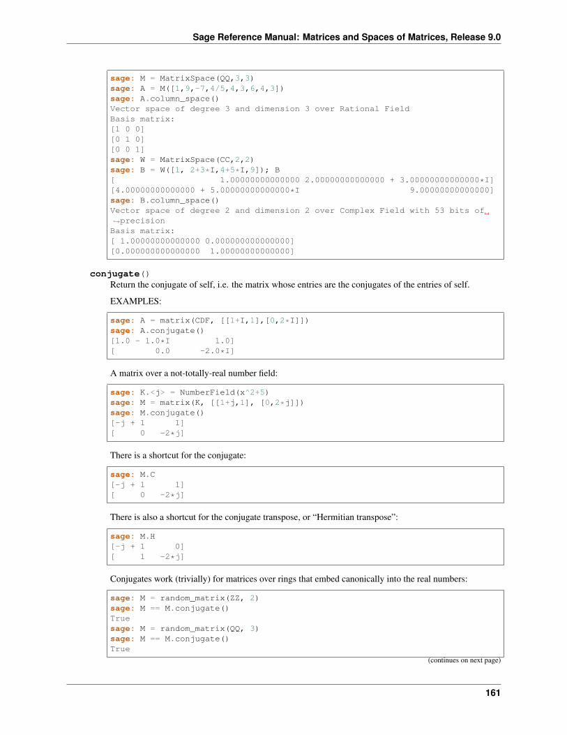
Sage Reference Manual: Matrices and Spaces of Matrices, Release 9.0
sage: M = MatrixSpace(QQ,3,3)sage: A = M([1,9,-7,4/5,4,3,6,4,3])sage: A.column_space()Vector space of degree 3 and dimension 3 over Rational FieldBasis matrix:[1 0 0][0 1 0][0 0 1]sage: W = MatrixSpace(CC,2,2)sage: B = W([1, 2+3*I,4+5*I,9]); B[ 1.00000000000000 2.00000000000000 + 3.00000000000000*I][4.00000000000000 + 5.00000000000000*I 9.00000000000000]sage: B.column_space()Vector space of degree 2 and dimension 2 over Complex Field with 53 bits of→˓precisionBasis matrix:[ 1.00000000000000 0.000000000000000][0.000000000000000 1.00000000000000]
conjugate()Return the conjugate of self, i.e. the matrix whose entries are the conjugates of the entries of self.
EXAMPLES:
sage: A = matrix(CDF, [[1+I,1],[0,2*I]])sage: A.conjugate()[1.0 - 1.0*I 1.0][ 0.0 -2.0*I]
A matrix over a not-totally-real number field:
sage: K.<j> = NumberField(x^2+5)sage: M = matrix(K, [[1+j,1], [0,2*j]])sage: M.conjugate()[-j + 1 1][ 0 -2*j]
There is a shortcut for the conjugate:
sage: M.C[-j + 1 1][ 0 -2*j]
There is also a shortcut for the conjugate transpose, or “Hermitian transpose”:
sage: M.H[-j + 1 0][ 1 -2*j]
Conjugates work (trivially) for matrices over rings that embed canonically into the real numbers:
sage: M = random_matrix(ZZ, 2)sage: M == M.conjugate()Truesage: M = random_matrix(QQ, 3)sage: M == M.conjugate()True
(continues on next page)
161
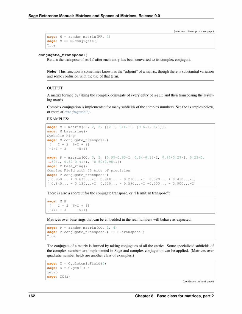
Sage Reference Manual: Matrices and Spaces of Matrices, Release 9.0
(continued from previous page)
sage: M = random_matrix(RR, 2)sage: M == M.conjugate()True
conjugate_transpose()Return the transpose of self after each entry has been converted to its complex conjugate.
Note: This function is sometimes known as the “adjoint” of a matrix, though there is substantial variationand some confusion with the use of that term.
OUTPUT:
A matrix formed by taking the complex conjugate of every entry of self and then transposing the result-ing matrix.
Complex conjugation is implemented for many subfields of the complex numbers. See the examples below,or more at conjugate().
EXAMPLES:
sage: M = matrix(SR, 2, 2, [[2-I, 3+4*I], [9-6*I, 5*I]])sage: M.base_ring()Symbolic Ringsage: M.conjugate_transpose()[ I + 2 6*I + 9]
[-4*I + 3 -5*I]
sage: P = matrix(CC, 3, 2, [0.95-0.63*I, 0.84+0.13*I, 0.94+0.23*I, 0.23+0.→˓59*I, 0.52-0.41*I, -0.50+0.90*I])sage: P.base_ring()Complex Field with 53 bits of precisionsage: P.conjugate_transpose()[ 0.950... + 0.630...*I 0.940... - 0.230...*I 0.520... + 0.410...*I][ 0.840... - 0.130...*I 0.230... - 0.590...*I -0.500... - 0.900...*I]
There is also a shortcut for the conjugate transpose, or “Hermitian transpose”:
sage: M.H[ I + 2 6*I + 9]
[-4*I + 3 -5*I]
Matrices over base rings that can be embedded in the real numbers will behave as expected.
sage: P = random_matrix(QQ, 3, 4)sage: P.conjugate_transpose() == P.transpose()True
The conjugate of a matrix is formed by taking conjugates of all the entries. Some specialized subfields ofthe complex numbers are implemented in Sage and complex conjugation can be applied. (Matrices overquadratic number fields are another class of examples.)
sage: C = CyclotomicField(5)sage: a = C.gen(); azeta5sage: CC(a)
(continues on next page)
162 Chapter 8. Base class for matrices, part 2
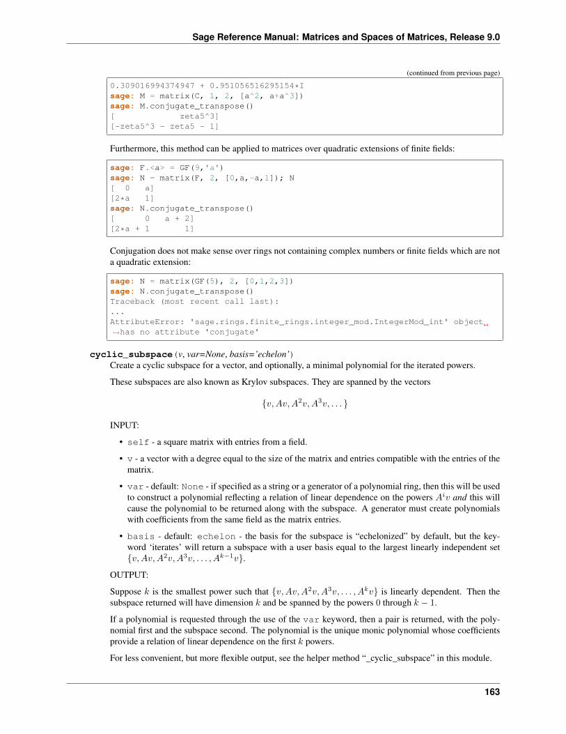
Sage Reference Manual: Matrices and Spaces of Matrices, Release 9.0
(continued from previous page)
0.309016994374947 + 0.951056516295154*Isage: M = matrix(C, 1, 2, [a^2, a+a^3])sage: M.conjugate_transpose()[ zeta5^3][-zeta5^3 - zeta5 - 1]
Furthermore, this method can be applied to matrices over quadratic extensions of finite fields:
sage: F.<a> = GF(9,'a')sage: N = matrix(F, 2, [0,a,-a,1]); N[ 0 a][2*a 1]sage: N.conjugate_transpose()[ 0 a + 2][2*a + 1 1]
Conjugation does not make sense over rings not containing complex numbers or finite fields which are nota quadratic extension:
sage: N = matrix(GF(5), 2, [0,1,2,3])sage: N.conjugate_transpose()Traceback (most recent call last):...AttributeError: 'sage.rings.finite_rings.integer_mod.IntegerMod_int' object→˓has no attribute 'conjugate'
cyclic_subspace(v, var=None, basis=’echelon’)Create a cyclic subspace for a vector, and optionally, a minimal polynomial for the iterated powers.
These subspaces are also known as Krylov subspaces. They are spanned by the vectors
{𝑣,𝐴𝑣,𝐴2𝑣,𝐴3𝑣, . . . }
INPUT:
• self - a square matrix with entries from a field.
• v - a vector with a degree equal to the size of the matrix and entries compatible with the entries of thematrix.
• var - default: None - if specified as a string or a generator of a polynomial ring, then this will be usedto construct a polynomial reflecting a relation of linear dependence on the powers 𝐴𝑖𝑣 and this willcause the polynomial to be returned along with the subspace. A generator must create polynomialswith coefficients from the same field as the matrix entries.
• basis - default: echelon - the basis for the subspace is “echelonized” by default, but the key-word ‘iterates’ will return a subspace with a user basis equal to the largest linearly independent set{𝑣,𝐴𝑣,𝐴2𝑣,𝐴3𝑣, . . . , 𝐴𝑘−1𝑣}.
OUTPUT:
Suppose 𝑘 is the smallest power such that {𝑣,𝐴𝑣,𝐴2𝑣,𝐴3𝑣, . . . , 𝐴𝑘𝑣} is linearly dependent. Then thesubspace returned will have dimension 𝑘 and be spanned by the powers 0 through 𝑘 − 1.
If a polynomial is requested through the use of the var keyword, then a pair is returned, with the poly-nomial first and the subspace second. The polynomial is the unique monic polynomial whose coefficientsprovide a relation of linear dependence on the first 𝑘 powers.
For less convenient, but more flexible output, see the helper method “_cyclic_subspace” in this module.
163
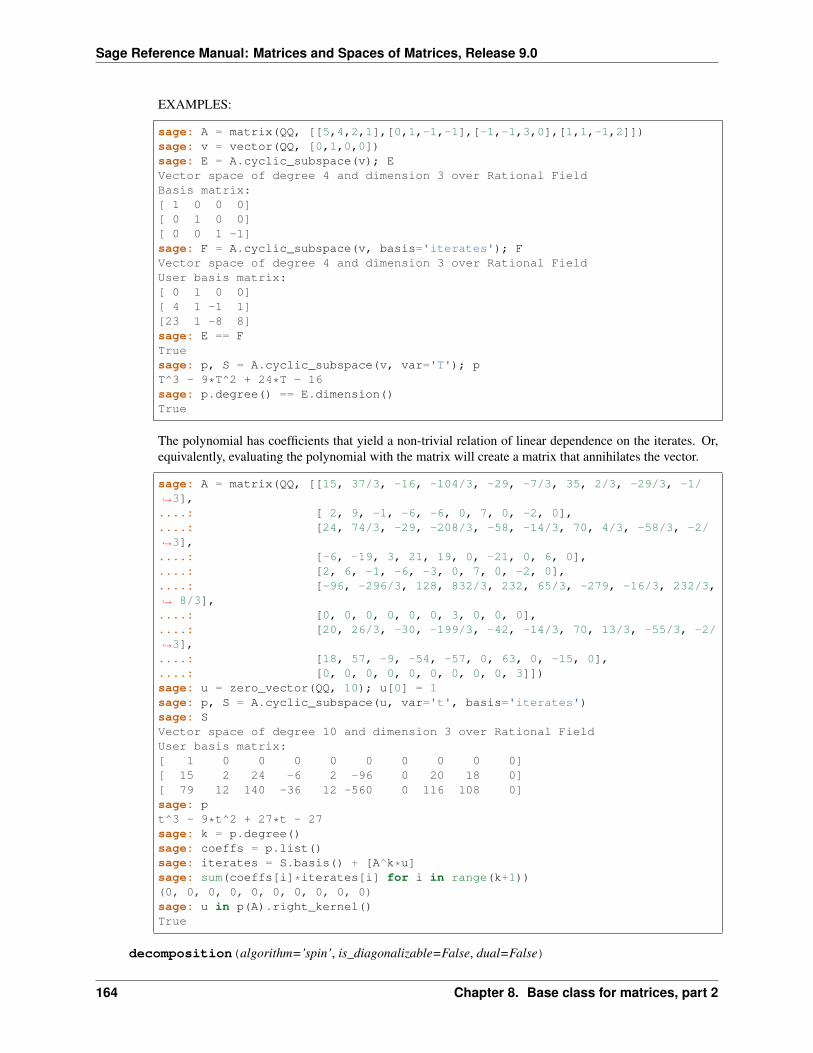
Sage Reference Manual: Matrices and Spaces of Matrices, Release 9.0
EXAMPLES:
sage: A = matrix(QQ, [[5,4,2,1],[0,1,-1,-1],[-1,-1,3,0],[1,1,-1,2]])sage: v = vector(QQ, [0,1,0,0])sage: E = A.cyclic_subspace(v); EVector space of degree 4 and dimension 3 over Rational FieldBasis matrix:[ 1 0 0 0][ 0 1 0 0][ 0 0 1 -1]sage: F = A.cyclic_subspace(v, basis='iterates'); FVector space of degree 4 and dimension 3 over Rational FieldUser basis matrix:[ 0 1 0 0][ 4 1 -1 1][23 1 -8 8]sage: E == FTruesage: p, S = A.cyclic_subspace(v, var='T'); pT^3 - 9*T^2 + 24*T - 16sage: p.degree() == E.dimension()True
The polynomial has coefficients that yield a non-trivial relation of linear dependence on the iterates. Or,equivalently, evaluating the polynomial with the matrix will create a matrix that annihilates the vector.
sage: A = matrix(QQ, [[15, 37/3, -16, -104/3, -29, -7/3, 35, 2/3, -29/3, -1/→˓3],....: [ 2, 9, -1, -6, -6, 0, 7, 0, -2, 0],....: [24, 74/3, -29, -208/3, -58, -14/3, 70, 4/3, -58/3, -2/→˓3],....: [-6, -19, 3, 21, 19, 0, -21, 0, 6, 0],....: [2, 6, -1, -6, -3, 0, 7, 0, -2, 0],....: [-96, -296/3, 128, 832/3, 232, 65/3, -279, -16/3, 232/3,→˓ 8/3],....: [0, 0, 0, 0, 0, 0, 3, 0, 0, 0],....: [20, 26/3, -30, -199/3, -42, -14/3, 70, 13/3, -55/3, -2/→˓3],....: [18, 57, -9, -54, -57, 0, 63, 0, -15, 0],....: [0, 0, 0, 0, 0, 0, 0, 0, 0, 3]])sage: u = zero_vector(QQ, 10); u[0] = 1sage: p, S = A.cyclic_subspace(u, var='t', basis='iterates')sage: SVector space of degree 10 and dimension 3 over Rational FieldUser basis matrix:[ 1 0 0 0 0 0 0 0 0 0][ 15 2 24 -6 2 -96 0 20 18 0][ 79 12 140 -36 12 -560 0 116 108 0]sage: pt^3 - 9*t^2 + 27*t - 27sage: k = p.degree()sage: coeffs = p.list()sage: iterates = S.basis() + [A^k*u]sage: sum(coeffs[i]*iterates[i] for i in range(k+1))(0, 0, 0, 0, 0, 0, 0, 0, 0, 0)sage: u in p(A).right_kernel()True
decomposition(algorithm=’spin’, is_diagonalizable=False, dual=False)
164 Chapter 8. Base class for matrices, part 2
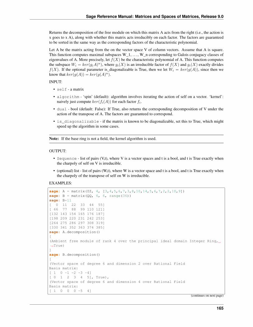
Sage Reference Manual: Matrices and Spaces of Matrices, Release 9.0
Returns the decomposition of the free module on which this matrix A acts from the right (i.e., the action isx goes to x A), along with whether this matrix acts irreducibly on each factor. The factors are guaranteedto be sorted in the same way as the corresponding factors of the characteristic polynomial.
Let A be the matrix acting from the on the vector space V of column vectors. Assume that A is square.This function computes maximal subspaces W_1, . . . , W_n corresponding to Galois conjugacy classes ofeigenvalues of A. More precisely, let 𝑓(𝑋) be the characteristic polynomial of A. This function computesthe subspace 𝑊𝑖 = 𝑘𝑒𝑟(𝑔(𝐴)𝑛), where 𝑔𝑖(𝑋) is an irreducible factor of 𝑓(𝑋) and 𝑔𝑖(𝑋) exactly divides𝑓(𝑋). If the optional parameter is_diagonalizable is True, then we let 𝑊𝑖 = 𝑘𝑒𝑟(𝑔(𝐴)), since then weknow that 𝑘𝑒𝑟(𝑔(𝐴)) = 𝑘𝑒𝑟(𝑔(𝐴)𝑛).
INPUT:
• self - a matrix
• algorithm - ‘spin’ (default): algorithm involves iterating the action of self on a vector. ‘kernel’:naively just compute 𝑘𝑒𝑟(𝑓𝑖(𝐴)) for each factor 𝑓𝑖.
• dual - bool (default: False): If True, also returns the corresponding decomposition of V under theaction of the transpose of A. The factors are guaranteed to correspond.
• is_diagonalizable - if the matrix is known to be diagonalizable, set this to True, which mightspeed up the algorithm in some cases.
Note: If the base ring is not a field, the kernel algorithm is used.
OUTPUT:
• Sequence - list of pairs (V,t), where V is a vector spaces and t is a bool, and t is True exactly whenthe charpoly of self on V is irreducible.
• (optional) list - list of pairs (W,t), where W is a vector space and t is a bool, and t is True exactly whenthe charpoly of the transpose of self on W is irreducible.
EXAMPLES:
sage: A = matrix(ZZ, 4, [3,4,5,6,7,3,8,10,14,5,6,7,2,2,10,9])sage: B = matrix(QQ, 6, 6, range(36))sage: B*11[ 0 11 22 33 44 55][ 66 77 88 99 110 121][132 143 154 165 176 187][198 209 220 231 242 253][264 275 286 297 308 319][330 341 352 363 374 385]sage: A.decomposition()[(Ambient free module of rank 4 over the principal ideal domain Integer Ring,→˓True)]sage: B.decomposition()[(Vector space of degree 6 and dimension 2 over Rational FieldBasis matrix:[ 1 0 -1 -2 -3 -4][ 0 1 2 3 4 5], True),(Vector space of degree 6 and dimension 4 over Rational FieldBasis matrix:[ 1 0 0 0 -5 4]
(continues on next page)
165
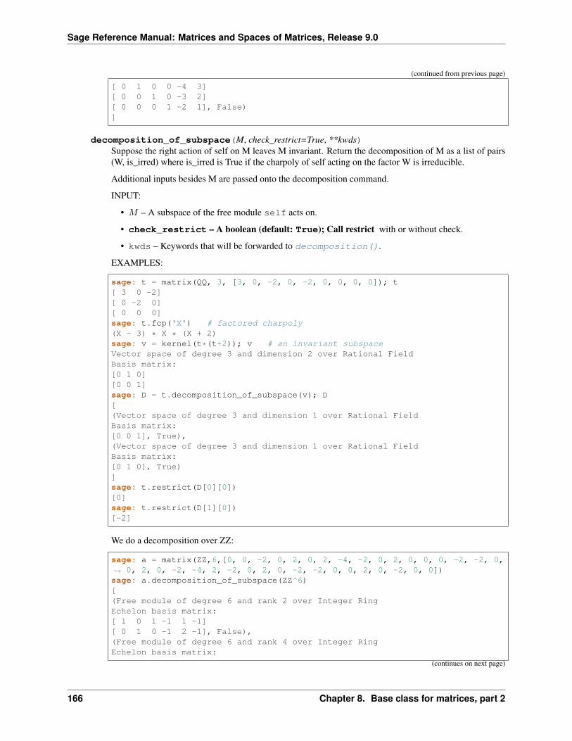
Sage Reference Manual: Matrices and Spaces of Matrices, Release 9.0
(continued from previous page)
[ 0 1 0 0 -4 3][ 0 0 1 0 -3 2][ 0 0 0 1 -2 1], False)]
decomposition_of_subspace(M, check_restrict=True, **kwds)Suppose the right action of self on M leaves M invariant. Return the decomposition of M as a list of pairs(W, is_irred) where is_irred is True if the charpoly of self acting on the factor W is irreducible.
Additional inputs besides M are passed onto the decomposition command.
INPUT:
• 𝑀 – A subspace of the free module self acts on.
• check_restrict – A boolean (default: True); Call restrict with or without check.
• kwds – Keywords that will be forwarded to decomposition().
EXAMPLES:
sage: t = matrix(QQ, 3, [3, 0, -2, 0, -2, 0, 0, 0, 0]); t[ 3 0 -2][ 0 -2 0][ 0 0 0]sage: t.fcp('X') # factored charpoly(X - 3) * X * (X + 2)sage: v = kernel(t*(t+2)); v # an invariant subspaceVector space of degree 3 and dimension 2 over Rational FieldBasis matrix:[0 1 0][0 0 1]sage: D = t.decomposition_of_subspace(v); D[(Vector space of degree 3 and dimension 1 over Rational FieldBasis matrix:[0 0 1], True),(Vector space of degree 3 and dimension 1 over Rational FieldBasis matrix:[0 1 0], True)]sage: t.restrict(D[0][0])[0]sage: t.restrict(D[1][0])[-2]
We do a decomposition over ZZ:
sage: a = matrix(ZZ,6,[0, 0, -2, 0, 2, 0, 2, -4, -2, 0, 2, 0, 0, 0, -2, -2, 0,→˓ 0, 2, 0, -2, -4, 2, -2, 0, 2, 0, -2, -2, 0, 0, 2, 0, -2, 0, 0])sage: a.decomposition_of_subspace(ZZ^6)[(Free module of degree 6 and rank 2 over Integer RingEchelon basis matrix:[ 1 0 1 -1 1 -1][ 0 1 0 -1 2 -1], False),(Free module of degree 6 and rank 4 over Integer RingEchelon basis matrix:
(continues on next page)
166 Chapter 8. Base class for matrices, part 2
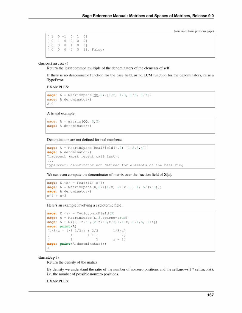
Sage Reference Manual: Matrices and Spaces of Matrices, Release 9.0
(continued from previous page)
[ 1 0 -1 0 1 0][ 0 1 0 0 0 0][ 0 0 0 1 0 0][ 0 0 0 0 0 1], False)]
denominator()Return the least common multiple of the denominators of the elements of self.
If there is no denominator function for the base field, or no LCM function for the denominators, raise aTypeError.
EXAMPLES:
sage: A = MatrixSpace(QQ,2)([1/2, 1/3, 1/5, 1/7])sage: A.denominator()210
A trivial example:
sage: A = matrix(QQ, 0,2)sage: A.denominator()1
Denominators are not defined for real numbers:
sage: A = MatrixSpace(RealField(),2)([1,2,3,4])sage: A.denominator()Traceback (most recent call last):...TypeError: denominator not defined for elements of the base ring
We can even compute the denominator of matrix over the fraction field of Z[𝑥].
sage: K.<x> = Frac(ZZ['x'])sage: A = MatrixSpace(K,2)([1/x, 2/(x+1), 1, 5/(x^3)])sage: A.denominator()x^4 + x^3
Here’s an example involving a cyclotomic field:
sage: K.<z> = CyclotomicField(3)sage: M = MatrixSpace(K,3,sparse=True)sage: A = M([(1+z)/3,(2+z)/3,z/3,1,1+z,-2,1,5,-1+z])sage: print(A)[1/3*z + 1/3 1/3*z + 2/3 1/3*z][ 1 z + 1 -2][ 1 5 z - 1]sage: print(A.denominator())3
density()Return the density of the matrix.
By density we understand the ratio of the number of nonzero positions and the self.nrows() * self.ncols(),i.e. the number of possible nonzero positions.
EXAMPLES:
167
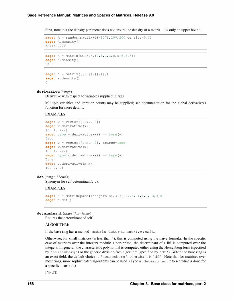
Sage Reference Manual: Matrices and Spaces of Matrices, Release 9.0
First, note that the density parameter does not ensure the density of a matrix, it is only an upper bound.
sage: A = random_matrix(GF(127),200,200,density=0.3)sage: A.density()5211/20000
sage: A = matrix(QQ,3,3,[0,1,2,3,0,0,6,7,8])sage: A.density()2/3
sage: a = matrix([[],[],[],[]])sage: a.density()0
derivative(*args)Derivative with respect to variables supplied in args.
Multiple variables and iteration counts may be supplied; see documentation for the global derivative()function for more details.
EXAMPLES:
sage: v = vector([1,x,x^2])sage: v.derivative(x)(0, 1, 2*x)sage: type(v.derivative(x)) == type(v)Truesage: v = vector([1,x,x^2], sparse=True)sage: v.derivative(x)(0, 1, 2*x)sage: type(v.derivative(x)) == type(v)Truesage: v.derivative(x,x)(0, 0, 2)
det(*args, **kwds)Synonym for self.determinant(. . . ).
EXAMPLES:
sage: A = MatrixSpace(Integers(8),3)([1,7,3, 1,1,1, 3,4,5])sage: A.det()6
determinant(algorithm=None)Returns the determinant of self.
ALGORITHM:
If the base ring has a method _matrix_determinant(), we call it.
Otherwise, for small matrices (n less than 4), this is computed using the naive formula. In the specificcase of matrices over the integers modulo a non-prime, the determinant of a lift is computed over theintegers. In general, the characteristic polynomial is computed either using the Hessenberg form (specifiedby "hessenberg") or the generic division-free algorithm (specified by "df"). When the base ring isan exact field, the default choice is "hessenberg", otherwise it is "df". Note that for matrices overmost rings, more sophisticated algorithms can be used. (Type A.determinant? to see what is done fora specific matrix A.)
INPUT:
168 Chapter 8. Base class for matrices, part 2
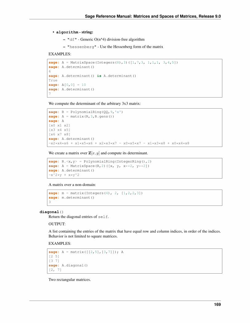
Sage Reference Manual: Matrices and Spaces of Matrices, Release 9.0
• algorithm - string:
– "df" - Generic O(n^4) division-free algorithm
– "hessenberg" - Use the Hessenberg form of the matrix
EXAMPLES:
sage: A = MatrixSpace(Integers(8),3)([1,7,3, 1,1,1, 3,4,5])sage: A.determinant()6sage: A.determinant() is A.determinant()Truesage: A[0,0] = 10sage: A.determinant()7
We compute the determinant of the arbitrary 3x3 matrix:
sage: R = PolynomialRing(QQ,9,'x')sage: A = matrix(R,3,R.gens())sage: A[x0 x1 x2][x3 x4 x5][x6 x7 x8]sage: A.determinant()-x2*x4*x6 + x1*x5*x6 + x2*x3*x7 - x0*x5*x7 - x1*x3*x8 + x0*x4*x8
We create a matrix over Z[𝑥, 𝑦] and compute its determinant.
sage: R.<x,y> = PolynomialRing(IntegerRing(),2)sage: A = MatrixSpace(R,2)([x, y, x**2, y**2])sage: A.determinant()-x^2*y + x*y^2
A matrix over a non-domain:
sage: m = matrix(Integers(4), 2, [1,2,2,3])sage: m.determinant()3
diagonal()Return the diagonal entries of self.
OUTPUT:
A list containing the entries of the matrix that have equal row and column indices, in order of the indices.Behavior is not limited to square matrices.
EXAMPLES:
sage: A = matrix([[2,5],[3,7]]); A[2 5][3 7]sage: A.diagonal()[2, 7]
Two rectangular matrices.
169
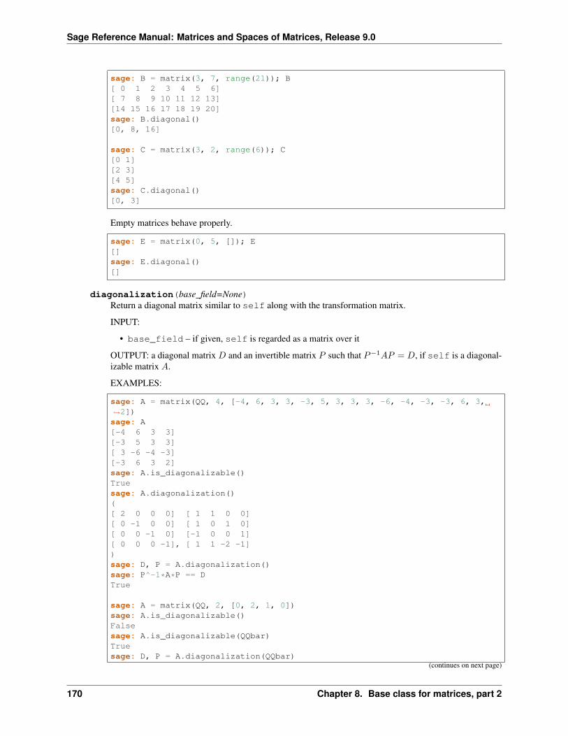
Sage Reference Manual: Matrices and Spaces of Matrices, Release 9.0
sage: B = matrix(3, 7, range(21)); B[ 0 1 2 3 4 5 6][ 7 8 9 10 11 12 13][14 15 16 17 18 19 20]sage: B.diagonal()[0, 8, 16]
sage: C = matrix(3, 2, range(6)); C[0 1][2 3][4 5]sage: C.diagonal()[0, 3]
Empty matrices behave properly.
sage: E = matrix(0, 5, []); E[]sage: E.diagonal()[]
diagonalization(base_field=None)Return a diagonal matrix similar to self along with the transformation matrix.
INPUT:
• base_field – if given, self is regarded as a matrix over it
OUTPUT: a diagonal matrix 𝐷 and an invertible matrix 𝑃 such that 𝑃−1𝐴𝑃 = 𝐷, if self is a diagonal-izable matrix 𝐴.
EXAMPLES:
sage: A = matrix(QQ, 4, [-4, 6, 3, 3, -3, 5, 3, 3, 3, -6, -4, -3, -3, 6, 3,→˓2])sage: A[-4 6 3 3][-3 5 3 3][ 3 -6 -4 -3][-3 6 3 2]sage: A.is_diagonalizable()Truesage: A.diagonalization()([ 2 0 0 0] [ 1 1 0 0][ 0 -1 0 0] [ 1 0 1 0][ 0 0 -1 0] [-1 0 0 1][ 0 0 0 -1], [ 1 1 -2 -1])sage: D, P = A.diagonalization()sage: P^-1*A*P == DTrue
sage: A = matrix(QQ, 2, [0, 2, 1, 0])sage: A.is_diagonalizable()Falsesage: A.is_diagonalizable(QQbar)Truesage: D, P = A.diagonalization(QQbar)
(continues on next page)
170 Chapter 8. Base class for matrices, part 2
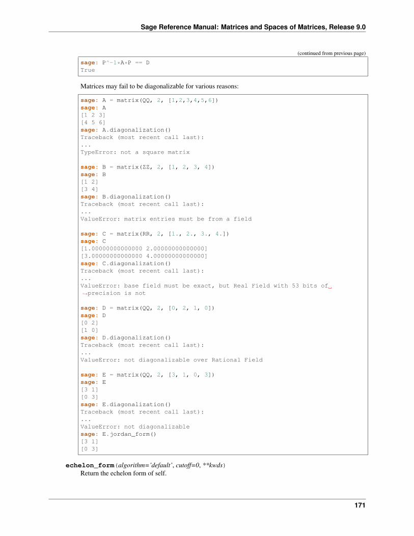
Sage Reference Manual: Matrices and Spaces of Matrices, Release 9.0
(continued from previous page)
sage: P^-1*A*P == DTrue
Matrices may fail to be diagonalizable for various reasons:
sage: A = matrix(QQ, 2, [1,2,3,4,5,6])sage: A[1 2 3][4 5 6]sage: A.diagonalization()Traceback (most recent call last):...TypeError: not a square matrix
sage: B = matrix(ZZ, 2, [1, 2, 3, 4])sage: B[1 2][3 4]sage: B.diagonalization()Traceback (most recent call last):...ValueError: matrix entries must be from a field
sage: C = matrix(RR, 2, [1., 2., 3., 4.])sage: C[1.00000000000000 2.00000000000000][3.00000000000000 4.00000000000000]sage: C.diagonalization()Traceback (most recent call last):...ValueError: base field must be exact, but Real Field with 53 bits of→˓precision is not
sage: D = matrix(QQ, 2, [0, 2, 1, 0])sage: D[0 2][1 0]sage: D.diagonalization()Traceback (most recent call last):...ValueError: not diagonalizable over Rational Field
sage: E = matrix(QQ, 2, [3, 1, 0, 3])sage: E[3 1][0 3]sage: E.diagonalization()Traceback (most recent call last):...ValueError: not diagonalizablesage: E.jordan_form()[3 1][0 3]
echelon_form(algorithm=’default’, cutoff=0, **kwds)Return the echelon form of self.
171
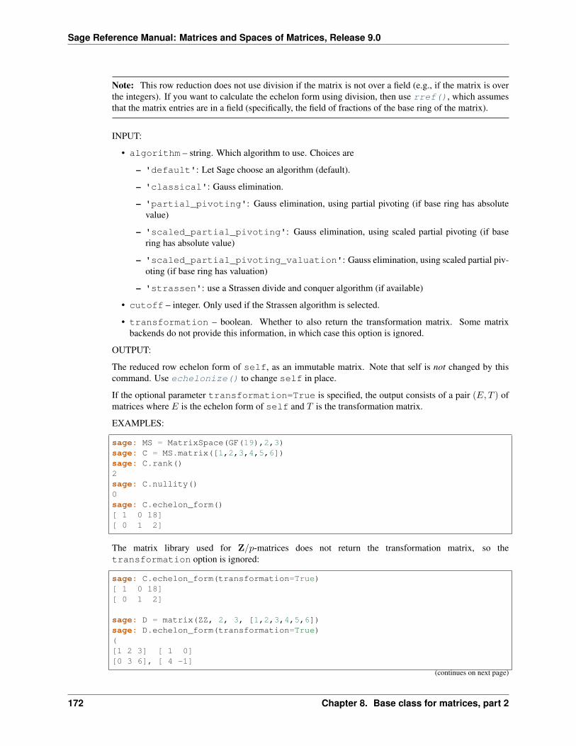
Sage Reference Manual: Matrices and Spaces of Matrices, Release 9.0
Note: This row reduction does not use division if the matrix is not over a field (e.g., if the matrix is overthe integers). If you want to calculate the echelon form using division, then use rref(), which assumesthat the matrix entries are in a field (specifically, the field of fractions of the base ring of the matrix).
INPUT:
• algorithm – string. Which algorithm to use. Choices are
– 'default': Let Sage choose an algorithm (default).
– 'classical': Gauss elimination.
– 'partial_pivoting': Gauss elimination, using partial pivoting (if base ring has absolutevalue)
– 'scaled_partial_pivoting': Gauss elimination, using scaled partial pivoting (if basering has absolute value)
– 'scaled_partial_pivoting_valuation': Gauss elimination, using scaled partial piv-oting (if base ring has valuation)
– 'strassen': use a Strassen divide and conquer algorithm (if available)
• cutoff – integer. Only used if the Strassen algorithm is selected.
• transformation – boolean. Whether to also return the transformation matrix. Some matrixbackends do not provide this information, in which case this option is ignored.
OUTPUT:
The reduced row echelon form of self, as an immutable matrix. Note that self is not changed by thiscommand. Use echelonize() to change self in place.
If the optional parameter transformation=True is specified, the output consists of a pair (𝐸, 𝑇 ) ofmatrices where 𝐸 is the echelon form of self and 𝑇 is the transformation matrix.
EXAMPLES:
sage: MS = MatrixSpace(GF(19),2,3)sage: C = MS.matrix([1,2,3,4,5,6])sage: C.rank()2sage: C.nullity()0sage: C.echelon_form()[ 1 0 18][ 0 1 2]
The matrix library used for Z/𝑝-matrices does not return the transformation matrix, so thetransformation option is ignored:
sage: C.echelon_form(transformation=True)[ 1 0 18][ 0 1 2]
sage: D = matrix(ZZ, 2, 3, [1,2,3,4,5,6])sage: D.echelon_form(transformation=True)([1 2 3] [ 1 0][0 3 6], [ 4 -1]
(continues on next page)
172 Chapter 8. Base class for matrices, part 2
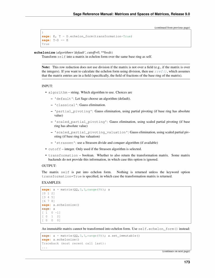
Sage Reference Manual: Matrices and Spaces of Matrices, Release 9.0
(continued from previous page)
)sage: E, T = D.echelon_form(transformation=True)sage: T*D == ETrue
echelonize(algorithm=’default’, cutoff=0, **kwds)Transform self into a matrix in echelon form over the same base ring as self.
Note: This row reduction does not use division if the matrix is not over a field (e.g., if the matrix is overthe integers). If you want to calculate the echelon form using division, then use rref(), which assumesthat the matrix entries are in a field (specifically, the field of fractions of the base ring of the matrix).
INPUT:
• algorithm – string. Which algorithm to use. Choices are
– 'default': Let Sage choose an algorithm (default).
– 'classical': Gauss elimination.
– 'partial_pivoting': Gauss elimination, using partial pivoting (if base ring has absolutevalue)
– 'scaled_partial_pivoting': Gauss elimination, using scaled partial pivoting (if basering has absolute value)
– 'scaled_partial_pivoting_valuation': Gauss elimination, using scaled partial piv-oting (if base ring has valuation)
– 'strassen': use a Strassen divide and conquer algorithm (if available)
• cutoff – integer. Only used if the Strassen algorithm is selected.
• transformation – boolean. Whether to also return the transformation matrix. Some matrixbackends do not provide this information, in which case this option is ignored.
OUTPUT:
The matrix self is put into echelon form. Nothing is returned unless the keyword optiontransformation=True is specified, in which case the transformation matrix is returned.
EXAMPLES:
sage: a = matrix(QQ,3,3,range(9)); a[0 1 2][3 4 5][6 7 8]sage: a.echelonize()sage: a[ 1 0 -1][ 0 1 2][ 0 0 0]
An immutable matrix cannot be transformed into echelon form. Use self.echelon_form() instead:
sage: a = matrix(QQ,3,3,range(9)); a.set_immutable()sage: a.echelonize()Traceback (most recent call last):...
(continues on next page)
173
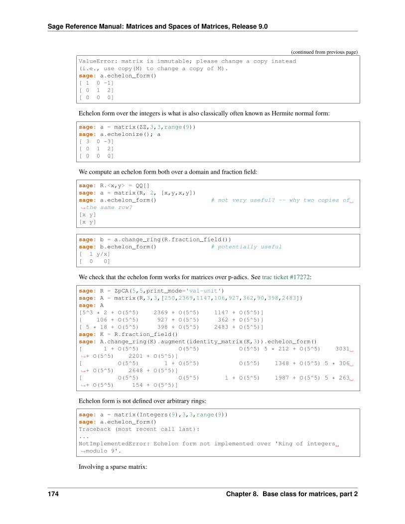
Sage Reference Manual: Matrices and Spaces of Matrices, Release 9.0
(continued from previous page)
ValueError: matrix is immutable; please change a copy instead(i.e., use copy(M) to change a copy of M).sage: a.echelon_form()[ 1 0 -1][ 0 1 2][ 0 0 0]
Echelon form over the integers is what is also classically often known as Hermite normal form:
sage: a = matrix(ZZ,3,3,range(9))sage: a.echelonize(); a[ 3 0 -3][ 0 1 2][ 0 0 0]
We compute an echelon form both over a domain and fraction field:
sage: R.<x,y> = QQ[]sage: a = matrix(R, 2, [x,y,x,y])sage: a.echelon_form() # not very useful? -- why two copies of→˓the same row?[x y][x y]
sage: b = a.change_ring(R.fraction_field())sage: b.echelon_form() # potentially useful[ 1 y/x][ 0 0]
We check that the echelon form works for matrices over p-adics. See trac ticket #17272:
sage: R = ZpCA(5,5,print_mode='val-unit')sage: A = matrix(R,3,3,[250,2369,1147,106,927,362,90,398,2483])sage: A[5^3 * 2 + O(5^5) 2369 + O(5^5) 1147 + O(5^5)][ 106 + O(5^5) 927 + O(5^5) 362 + O(5^5)][ 5 * 18 + O(5^5) 398 + O(5^5) 2483 + O(5^5)]sage: K = R.fraction_field()sage: A.change_ring(K).augment(identity_matrix(K,3)).echelon_form()[ 1 + O(5^5) O(5^5) O(5^5) 5 * 212 + O(5^5) 3031→˓+ O(5^5) 2201 + O(5^5)][ O(5^5) 1 + O(5^5) O(5^5) 1348 + O(5^5) 5 * 306→˓+ O(5^5) 2648 + O(5^5)][ O(5^5) O(5^5) 1 + O(5^5) 1987 + O(5^5) 5 * 263→˓+ O(5^5) 154 + O(5^5)]
Echelon form is not defined over arbitrary rings:
sage: a = matrix(Integers(9),3,3,range(9))sage: a.echelon_form()Traceback (most recent call last):...NotImplementedError: Echelon form not implemented over 'Ring of integers→˓modulo 9'.
Involving a sparse matrix:
174 Chapter 8. Base class for matrices, part 2
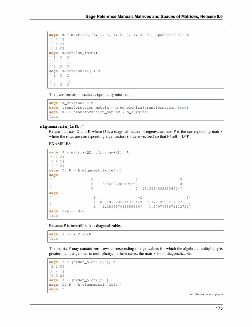
Sage Reference Manual: Matrices and Spaces of Matrices, Release 9.0
sage: m = matrix(3,[1, 1, 1, 1, 0, 2, 1, 2, 0], sparse=True); m[1 1 1][1 0 2][1 2 0]sage: m.echelon_form()[ 1 0 2][ 0 1 -1][ 0 0 0]sage: m.echelonize(); m[ 1 0 2][ 0 1 -1][ 0 0 0]
The transformation matrix is optionally returned:
sage: m_original = msage: transformation_matrix = m.echelonize(transformation=True)sage: m == transformation_matrix * m_originalTrue
eigenmatrix_left()Return matrices D and P, where D is a diagonal matrix of eigenvalues and P is the corresponding matrixwhere the rows are corresponding eigenvectors (or zero vectors) so that P*self = D*P.
EXAMPLES:
sage: A = matrix(QQ,3,3,range(9)); A[0 1 2][3 4 5][6 7 8]sage: D, P = A.eigenmatrix_left()sage: D[ 0 0 0][ 0 -1.348469228349535? 0][ 0 0 13.34846922834954?]sage: P[ 1 -2 1][ 1 0.3101020514433644? -0.3797958971132713?][ 1 1.289897948556636? 1.579795897113272?]sage: P*A == D*PTrue
Because P is invertible, A is diagonalizable.
sage: A == (~P)*D*PTrue
The matrix P may contain zero rows corresponding to eigenvalues for which the algebraic multiplicity isgreater than the geometric multiplicity. In these cases, the matrix is not diagonalizable.
sage: A = jordan_block(2,3); A[2 1 0][0 2 1][0 0 2]sage: A = jordan_block(2,3)sage: D, P = A.eigenmatrix_left()sage: D
(continues on next page)
175
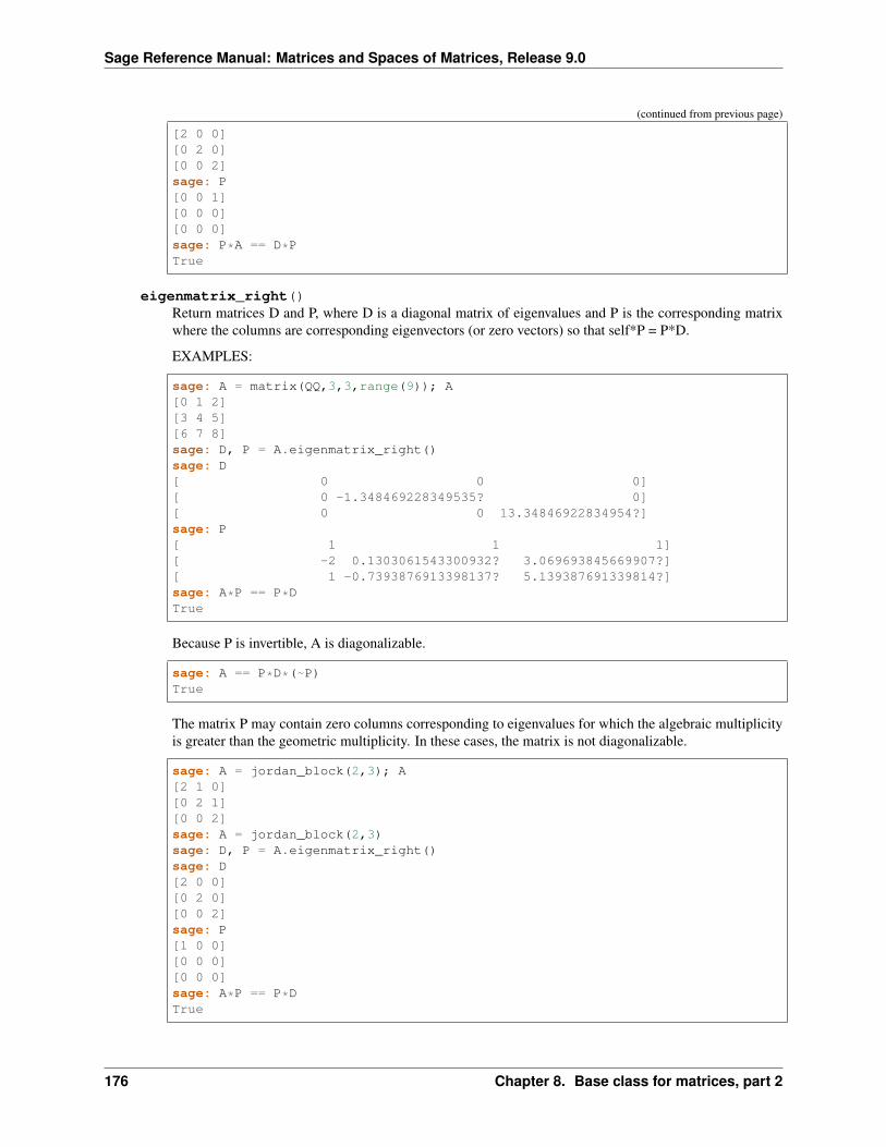
Sage Reference Manual: Matrices and Spaces of Matrices, Release 9.0
(continued from previous page)
[2 0 0][0 2 0][0 0 2]sage: P[0 0 1][0 0 0][0 0 0]sage: P*A == D*PTrue
eigenmatrix_right()Return matrices D and P, where D is a diagonal matrix of eigenvalues and P is the corresponding matrixwhere the columns are corresponding eigenvectors (or zero vectors) so that self*P = P*D.
EXAMPLES:
sage: A = matrix(QQ,3,3,range(9)); A[0 1 2][3 4 5][6 7 8]sage: D, P = A.eigenmatrix_right()sage: D[ 0 0 0][ 0 -1.348469228349535? 0][ 0 0 13.34846922834954?]sage: P[ 1 1 1][ -2 0.1303061543300932? 3.069693845669907?][ 1 -0.7393876913398137? 5.139387691339814?]sage: A*P == P*DTrue
Because P is invertible, A is diagonalizable.
sage: A == P*D*(~P)True
The matrix P may contain zero columns corresponding to eigenvalues for which the algebraic multiplicityis greater than the geometric multiplicity. In these cases, the matrix is not diagonalizable.
sage: A = jordan_block(2,3); A[2 1 0][0 2 1][0 0 2]sage: A = jordan_block(2,3)sage: D, P = A.eigenmatrix_right()sage: D[2 0 0][0 2 0][0 0 2]sage: P[1 0 0][0 0 0][0 0 0]sage: A*P == P*DTrue
176 Chapter 8. Base class for matrices, part 2
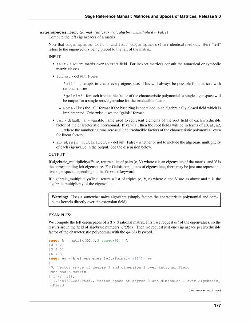
Sage Reference Manual: Matrices and Spaces of Matrices, Release 9.0
eigenspaces_left(format=’all’, var=’a’, algebraic_multiplicity=False)Compute the left eigenspaces of a matrix.
Note that eigenspaces_left() and left_eigenspaces() are identical methods. Here “left”refers to the eigenvectors being placed to the left of the matrix.
INPUT:
• self - a square matrix over an exact field. For inexact matrices consult the numerical or symbolicmatrix classes.
• format - default: None
– 'all' - attempts to create every eigenspace. This will always be possible for matrices withrational entries.
– 'galois' - for each irreducible factor of the characteristic polynomial, a single eigenspace willbe output for a single root/eigenvalue for the irreducible factor.
– None - Uses the ‘all’ format if the base ring is contained in an algebraically closed field which isimplemented. Otherwise, uses the ‘galois’ format.
• var - default: ‘a’ - variable name used to represent elements of the root field of each irreduciblefactor of the characteristic polynomial. If var=’a’, then the root fields will be in terms of a0, a1, a2,. . . ., where the numbering runs across all the irreducible factors of the characteristic polynomial, evenfor linear factors.
• algebraic_multiplicity - default: False - whether or not to include the algebraic multiplicityof each eigenvalue in the output. See the discussion below.
OUTPUT:
If algebraic_multiplicity=False, return a list of pairs (e, V) where e is an eigenvalue of the matrix, and V isthe corresponding left eigenspace. For Galois conjugates of eigenvalues, there may be just one representa-tive eigenspace, depending on the format keyword.
If algebraic_multiplicity=True, return a list of triples (e, V, n) where e and V are as above and n is thealgebraic multiplicity of the eigenvalue.
Warning: Uses a somewhat naive algorithm (simply factors the characteristic polynomial and com-putes kernels directly over the extension field).
EXAMPLES:
We compute the left eigenspaces of a 3× 3 rational matrix. First, we request 𝑎𝑙𝑙 of the eigenvalues, so theresults are in the field of algebraic numbers, 𝑄𝑄𝑏𝑎𝑟. Then we request just one eigenspace per irreduciblefactor of the characteristic polynomial with the 𝑔𝑎𝑙𝑜𝑖𝑠 keyword.
sage: A = matrix(QQ,3,3,range(9)); A[0 1 2][3 4 5][6 7 8]sage: es = A.eigenspaces_left(format='all'); es[(0, Vector space of degree 3 and dimension 1 over Rational FieldUser basis matrix:[ 1 -2 1]),(-1.348469228349535?, Vector space of degree 3 and dimension 1 over Algebraic→˓Field
(continues on next page)
177
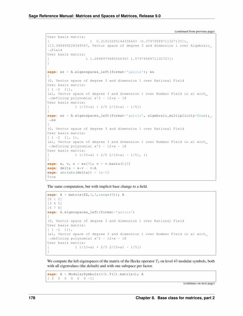
Sage Reference Manual: Matrices and Spaces of Matrices, Release 9.0
(continued from previous page)
User basis matrix:[ 1 0.3101020514433644? -0.3797958971132713?]),(13.34846922834954?, Vector space of degree 3 and dimension 1 over Algebraic→˓FieldUser basis matrix:[ 1 1.289897948556636? 1.579795897113272?])]
sage: es = A.eigenspaces_left(format='galois'); es[(0, Vector space of degree 3 and dimension 1 over Rational FieldUser basis matrix:[ 1 -2 1]),(a1, Vector space of degree 3 and dimension 1 over Number Field in a1 with→˓defining polynomial x^2 - 12*x - 18User basis matrix:[ 1 1/15*a1 + 2/5 2/15*a1 - 1/5])]sage: es = A.eigenspaces_left(format='galois', algebraic_multiplicity=True);→˓es[(0, Vector space of degree 3 and dimension 1 over Rational FieldUser basis matrix:[ 1 -2 1], 1),(a1, Vector space of degree 3 and dimension 1 over Number Field in a1 with→˓defining polynomial x^2 - 12*x - 18User basis matrix:[ 1 1/15*a1 + 2/5 2/15*a1 - 1/5], 1)]sage: e, v, n = es[0]; v = v.basis()[0]sage: delta = e*v - v*Asage: abs(abs(delta)) < 1e-10True
The same computation, but with implicit base change to a field.
sage: A = matrix(ZZ,3,3,range(9)); A[0 1 2][3 4 5][6 7 8]sage: A.eigenspaces_left(format='galois')[(0, Vector space of degree 3 and dimension 1 over Rational FieldUser basis matrix:[ 1 -2 1]),(a1, Vector space of degree 3 and dimension 1 over Number Field in a1 with→˓defining polynomial x^2 - 12*x - 18User basis matrix:[ 1 1/15*a1 + 2/5 2/15*a1 - 1/5])]
We compute the left eigenspaces of the matrix of the Hecke operator 𝑇2 on level 43 modular symbols, bothwith all eigenvalues (the default) and with one subspace per factor.
sage: A = ModularSymbols(43).T(2).matrix(); A[ 3 0 0 0 0 0 -1]
(continues on next page)
178 Chapter 8. Base class for matrices, part 2
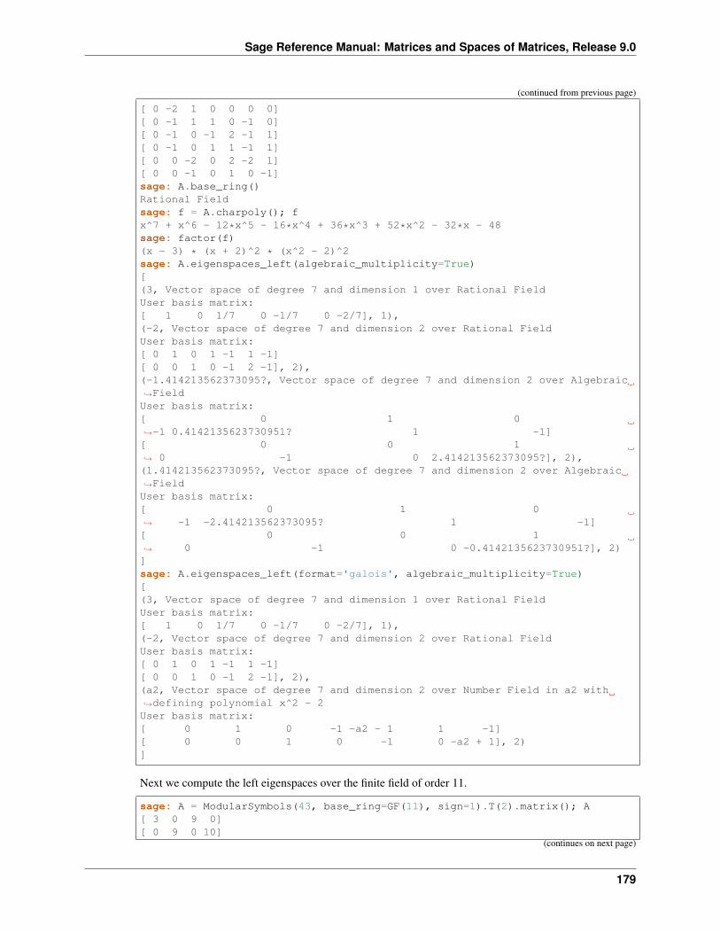
Sage Reference Manual: Matrices and Spaces of Matrices, Release 9.0
(continued from previous page)
[ 0 -2 1 0 0 0 0][ 0 -1 1 1 0 -1 0][ 0 -1 0 -1 2 -1 1][ 0 -1 0 1 1 -1 1][ 0 0 -2 0 2 -2 1][ 0 0 -1 0 1 0 -1]sage: A.base_ring()Rational Fieldsage: f = A.charpoly(); fx^7 + x^6 - 12*x^5 - 16*x^4 + 36*x^3 + 52*x^2 - 32*x - 48sage: factor(f)(x - 3) * (x + 2)^2 * (x^2 - 2)^2sage: A.eigenspaces_left(algebraic_multiplicity=True)[(3, Vector space of degree 7 and dimension 1 over Rational FieldUser basis matrix:[ 1 0 1/7 0 -1/7 0 -2/7], 1),(-2, Vector space of degree 7 and dimension 2 over Rational FieldUser basis matrix:[ 0 1 0 1 -1 1 -1][ 0 0 1 0 -1 2 -1], 2),(-1.414213562373095?, Vector space of degree 7 and dimension 2 over Algebraic→˓FieldUser basis matrix:[ 0 1 0→˓-1 0.4142135623730951? 1 -1][ 0 0 1→˓ 0 -1 0 2.414213562373095?], 2),(1.414213562373095?, Vector space of degree 7 and dimension 2 over Algebraic→˓FieldUser basis matrix:[ 0 1 0→˓ -1 -2.414213562373095? 1 -1][ 0 0 1→˓ 0 -1 0 -0.4142135623730951?], 2)]sage: A.eigenspaces_left(format='galois', algebraic_multiplicity=True)[(3, Vector space of degree 7 and dimension 1 over Rational FieldUser basis matrix:[ 1 0 1/7 0 -1/7 0 -2/7], 1),(-2, Vector space of degree 7 and dimension 2 over Rational FieldUser basis matrix:[ 0 1 0 1 -1 1 -1][ 0 0 1 0 -1 2 -1], 2),(a2, Vector space of degree 7 and dimension 2 over Number Field in a2 with→˓defining polynomial x^2 - 2User basis matrix:[ 0 1 0 -1 -a2 - 1 1 -1][ 0 0 1 0 -1 0 -a2 + 1], 2)]
Next we compute the left eigenspaces over the finite field of order 11.
sage: A = ModularSymbols(43, base_ring=GF(11), sign=1).T(2).matrix(); A[ 3 0 9 0][ 0 9 0 10]
(continues on next page)
179
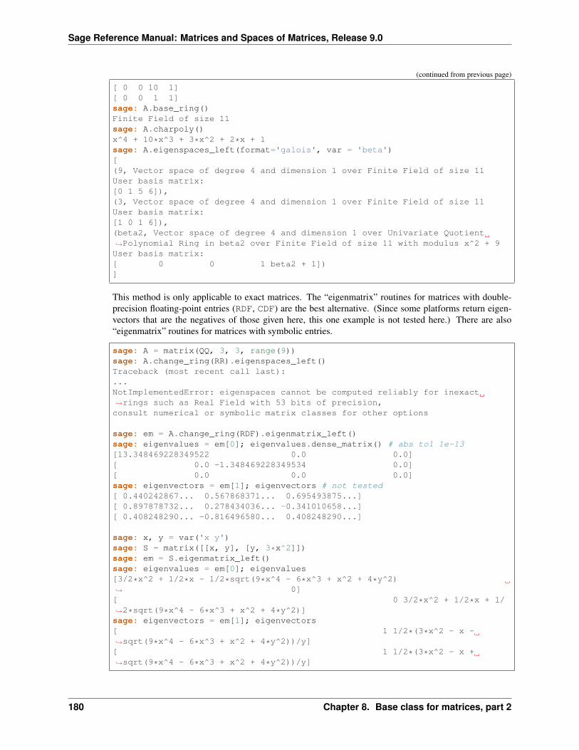
Sage Reference Manual: Matrices and Spaces of Matrices, Release 9.0
(continued from previous page)
[ 0 0 10 1][ 0 0 1 1]sage: A.base_ring()Finite Field of size 11sage: A.charpoly()x^4 + 10*x^3 + 3*x^2 + 2*x + 1sage: A.eigenspaces_left(format='galois', var = 'beta')[(9, Vector space of degree 4 and dimension 1 over Finite Field of size 11User basis matrix:[0 1 5 6]),(3, Vector space of degree 4 and dimension 1 over Finite Field of size 11User basis matrix:[1 0 1 6]),(beta2, Vector space of degree 4 and dimension 1 over Univariate Quotient→˓Polynomial Ring in beta2 over Finite Field of size 11 with modulus x^2 + 9User basis matrix:[ 0 0 1 beta2 + 1])]
This method is only applicable to exact matrices. The “eigenmatrix” routines for matrices with double-precision floating-point entries (RDF, CDF) are the best alternative. (Since some platforms return eigen-vectors that are the negatives of those given here, this one example is not tested here.) There are also“eigenmatrix” routines for matrices with symbolic entries.
sage: A = matrix(QQ, 3, 3, range(9))sage: A.change_ring(RR).eigenspaces_left()Traceback (most recent call last):...NotImplementedError: eigenspaces cannot be computed reliably for inexact→˓rings such as Real Field with 53 bits of precision,consult numerical or symbolic matrix classes for other options
sage: em = A.change_ring(RDF).eigenmatrix_left()sage: eigenvalues = em[0]; eigenvalues.dense_matrix() # abs tol 1e-13[13.348469228349522 0.0 0.0][ 0.0 -1.348469228349534 0.0][ 0.0 0.0 0.0]sage: eigenvectors = em[1]; eigenvectors # not tested[ 0.440242867... 0.567868371... 0.695493875...][ 0.897878732... 0.278434036... -0.341010658...][ 0.408248290... -0.816496580... 0.408248290...]
sage: x, y = var('x y')sage: S = matrix([[x, y], [y, 3*x^2]])sage: em = S.eigenmatrix_left()sage: eigenvalues = em[0]; eigenvalues[3/2*x^2 + 1/2*x - 1/2*sqrt(9*x^4 - 6*x^3 + x^2 + 4*y^2)→˓ 0][ 0 3/2*x^2 + 1/2*x + 1/→˓2*sqrt(9*x^4 - 6*x^3 + x^2 + 4*y^2)]sage: eigenvectors = em[1]; eigenvectors[ 1 1/2*(3*x^2 - x -→˓sqrt(9*x^4 - 6*x^3 + x^2 + 4*y^2))/y][ 1 1/2*(3*x^2 - x +→˓sqrt(9*x^4 - 6*x^3 + x^2 + 4*y^2))/y]
180 Chapter 8. Base class for matrices, part 2
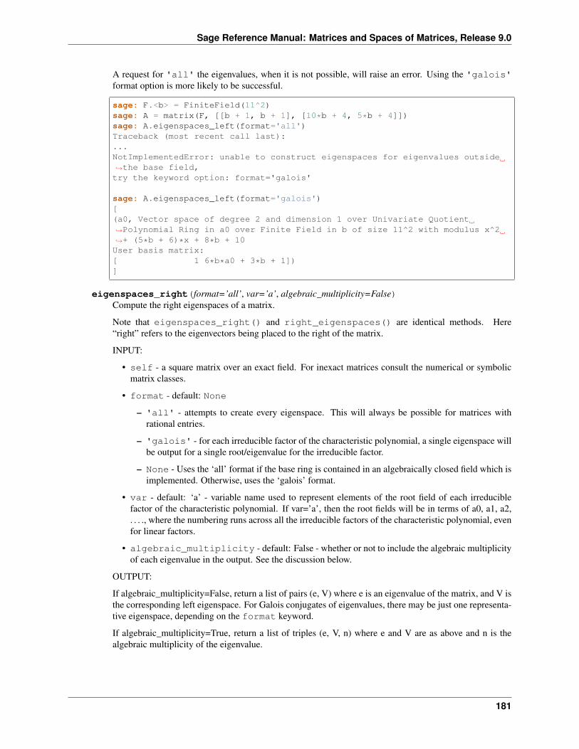
Sage Reference Manual: Matrices and Spaces of Matrices, Release 9.0
A request for 'all' the eigenvalues, when it is not possible, will raise an error. Using the 'galois'format option is more likely to be successful.
sage: F.<b> = FiniteField(11^2)sage: A = matrix(F, [[b + 1, b + 1], [10*b + 4, 5*b + 4]])sage: A.eigenspaces_left(format='all')Traceback (most recent call last):...NotImplementedError: unable to construct eigenspaces for eigenvalues outside→˓the base field,try the keyword option: format='galois'
sage: A.eigenspaces_left(format='galois')[(a0, Vector space of degree 2 and dimension 1 over Univariate Quotient→˓Polynomial Ring in a0 over Finite Field in b of size 11^2 with modulus x^2→˓+ (5*b + 6)*x + 8*b + 10User basis matrix:[ 1 6*b*a0 + 3*b + 1])]
eigenspaces_right(format=’all’, var=’a’, algebraic_multiplicity=False)Compute the right eigenspaces of a matrix.
Note that eigenspaces_right() and right_eigenspaces() are identical methods. Here“right” refers to the eigenvectors being placed to the right of the matrix.
INPUT:
• self - a square matrix over an exact field. For inexact matrices consult the numerical or symbolicmatrix classes.
• format - default: None
– 'all' - attempts to create every eigenspace. This will always be possible for matrices withrational entries.
– 'galois' - for each irreducible factor of the characteristic polynomial, a single eigenspace willbe output for a single root/eigenvalue for the irreducible factor.
– None - Uses the ‘all’ format if the base ring is contained in an algebraically closed field which isimplemented. Otherwise, uses the ‘galois’ format.
• var - default: ‘a’ - variable name used to represent elements of the root field of each irreduciblefactor of the characteristic polynomial. If var=’a’, then the root fields will be in terms of a0, a1, a2,. . . ., where the numbering runs across all the irreducible factors of the characteristic polynomial, evenfor linear factors.
• algebraic_multiplicity - default: False - whether or not to include the algebraic multiplicityof each eigenvalue in the output. See the discussion below.
OUTPUT:
If algebraic_multiplicity=False, return a list of pairs (e, V) where e is an eigenvalue of the matrix, and V isthe corresponding left eigenspace. For Galois conjugates of eigenvalues, there may be just one representa-tive eigenspace, depending on the format keyword.
If algebraic_multiplicity=True, return a list of triples (e, V, n) where e and V are as above and n is thealgebraic multiplicity of the eigenvalue.
181
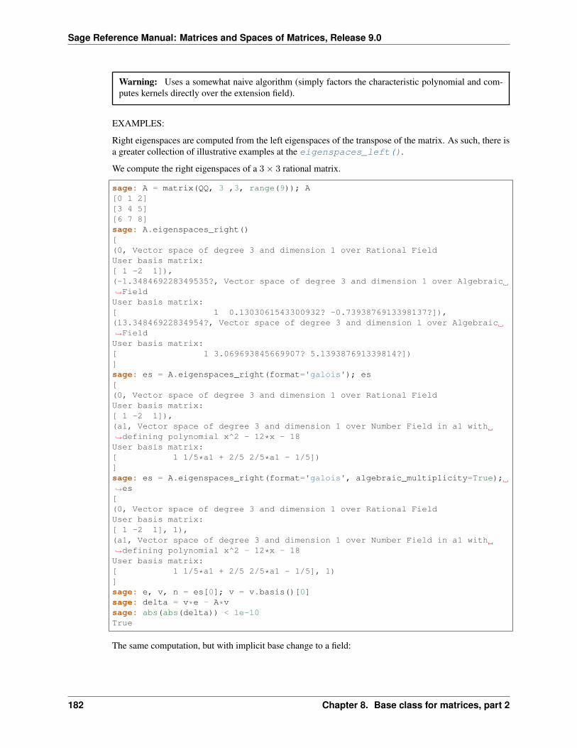
Sage Reference Manual: Matrices and Spaces of Matrices, Release 9.0
Warning: Uses a somewhat naive algorithm (simply factors the characteristic polynomial and com-putes kernels directly over the extension field).
EXAMPLES:
Right eigenspaces are computed from the left eigenspaces of the transpose of the matrix. As such, there isa greater collection of illustrative examples at the eigenspaces_left().
We compute the right eigenspaces of a 3× 3 rational matrix.
sage: A = matrix(QQ, 3 ,3, range(9)); A[0 1 2][3 4 5][6 7 8]sage: A.eigenspaces_right()[(0, Vector space of degree 3 and dimension 1 over Rational FieldUser basis matrix:[ 1 -2 1]),(-1.348469228349535?, Vector space of degree 3 and dimension 1 over Algebraic→˓FieldUser basis matrix:[ 1 0.1303061543300932? -0.7393876913398137?]),(13.34846922834954?, Vector space of degree 3 and dimension 1 over Algebraic→˓FieldUser basis matrix:[ 1 3.069693845669907? 5.139387691339814?])]sage: es = A.eigenspaces_right(format='galois'); es[(0, Vector space of degree 3 and dimension 1 over Rational FieldUser basis matrix:[ 1 -2 1]),(a1, Vector space of degree 3 and dimension 1 over Number Field in a1 with→˓defining polynomial x^2 - 12*x - 18User basis matrix:[ 1 1/5*a1 + 2/5 2/5*a1 - 1/5])]sage: es = A.eigenspaces_right(format='galois', algebraic_multiplicity=True);→˓es[(0, Vector space of degree 3 and dimension 1 over Rational FieldUser basis matrix:[ 1 -2 1], 1),(a1, Vector space of degree 3 and dimension 1 over Number Field in a1 with→˓defining polynomial x^2 - 12*x - 18User basis matrix:[ 1 1/5*a1 + 2/5 2/5*a1 - 1/5], 1)]sage: e, v, n = es[0]; v = v.basis()[0]sage: delta = v*e - A*vsage: abs(abs(delta)) < 1e-10True
The same computation, but with implicit base change to a field:
182 Chapter 8. Base class for matrices, part 2
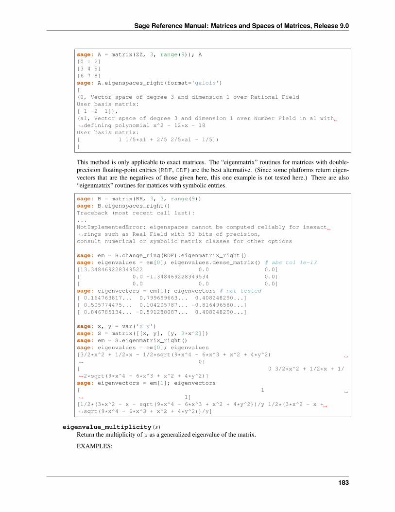
Sage Reference Manual: Matrices and Spaces of Matrices, Release 9.0
sage: A = matrix(ZZ, 3, range(9)); A[0 1 2][3 4 5][6 7 8]sage: A.eigenspaces_right(format='galois')[(0, Vector space of degree 3 and dimension 1 over Rational FieldUser basis matrix:[ 1 -2 1]),(a1, Vector space of degree 3 and dimension 1 over Number Field in a1 with→˓defining polynomial x^2 - 12*x - 18User basis matrix:[ 1 1/5*a1 + 2/5 2/5*a1 - 1/5])]
This method is only applicable to exact matrices. The “eigenmatrix” routines for matrices with double-precision floating-point entries (RDF, CDF) are the best alternative. (Since some platforms return eigen-vectors that are the negatives of those given here, this one example is not tested here.) There are also“eigenmatrix” routines for matrices with symbolic entries.
sage: B = matrix(RR, 3, 3, range(9))sage: B.eigenspaces_right()Traceback (most recent call last):...NotImplementedError: eigenspaces cannot be computed reliably for inexact→˓rings such as Real Field with 53 bits of precision,consult numerical or symbolic matrix classes for other options
sage: em = B.change_ring(RDF).eigenmatrix_right()sage: eigenvalues = em[0]; eigenvalues.dense_matrix() # abs tol 1e-13[13.348469228349522 0.0 0.0][ 0.0 -1.348469228349534 0.0][ 0.0 0.0 0.0]sage: eigenvectors = em[1]; eigenvectors # not tested[ 0.164763817... 0.799699663... 0.408248290...][ 0.505774475... 0.104205787... -0.816496580...][ 0.846785134... -0.591288087... 0.408248290...]
sage: x, y = var('x y')sage: S = matrix([[x, y], [y, 3*x^2]])sage: em = S.eigenmatrix_right()sage: eigenvalues = em[0]; eigenvalues[3/2*x^2 + 1/2*x - 1/2*sqrt(9*x^4 - 6*x^3 + x^2 + 4*y^2)→˓ 0][ 0 3/2*x^2 + 1/2*x + 1/→˓2*sqrt(9*x^4 - 6*x^3 + x^2 + 4*y^2)]sage: eigenvectors = em[1]; eigenvectors[ 1→˓ 1][1/2*(3*x^2 - x - sqrt(9*x^4 - 6*x^3 + x^2 + 4*y^2))/y 1/2*(3*x^2 - x +→˓sqrt(9*x^4 - 6*x^3 + x^2 + 4*y^2))/y]
eigenvalue_multiplicity(s)Return the multiplicity of s as a generalized eigenvalue of the matrix.
EXAMPLES:
183
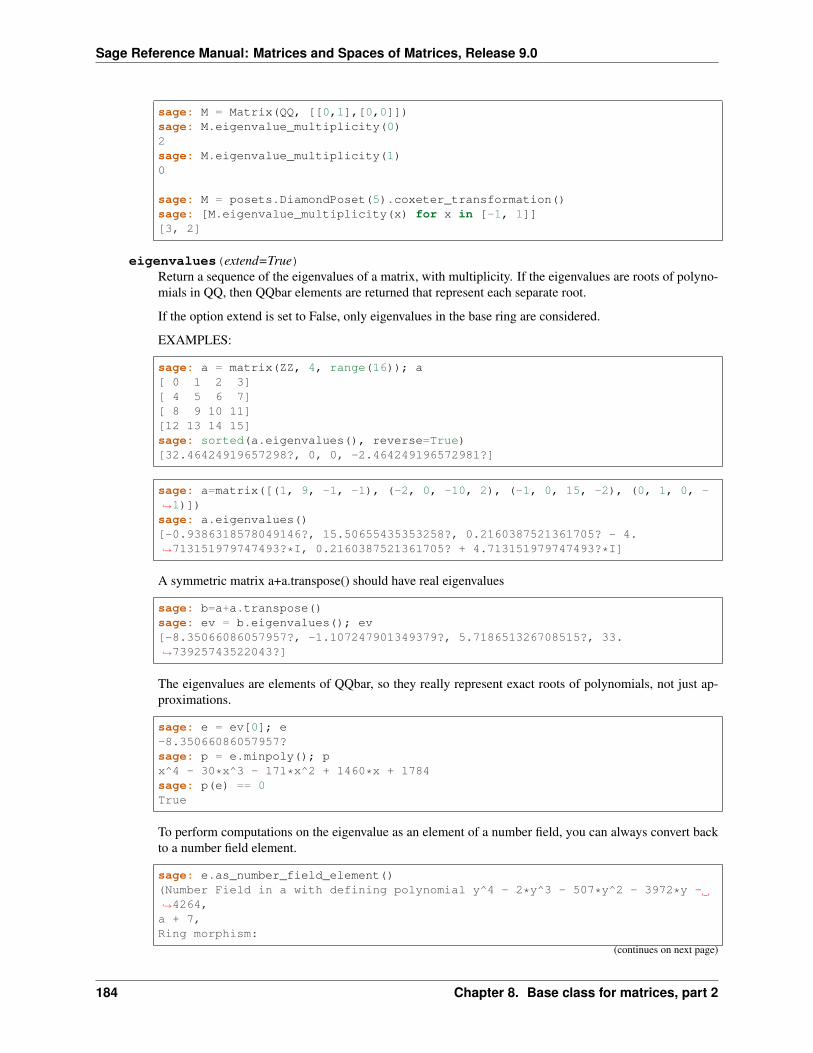
Sage Reference Manual: Matrices and Spaces of Matrices, Release 9.0
sage: M = Matrix(QQ, [[0,1],[0,0]])sage: M.eigenvalue_multiplicity(0)2sage: M.eigenvalue_multiplicity(1)0
sage: M = posets.DiamondPoset(5).coxeter_transformation()sage: [M.eigenvalue_multiplicity(x) for x in [-1, 1]][3, 2]
eigenvalues(extend=True)Return a sequence of the eigenvalues of a matrix, with multiplicity. If the eigenvalues are roots of polyno-mials in QQ, then QQbar elements are returned that represent each separate root.
If the option extend is set to False, only eigenvalues in the base ring are considered.
EXAMPLES:
sage: a = matrix(ZZ, 4, range(16)); a[ 0 1 2 3][ 4 5 6 7][ 8 9 10 11][12 13 14 15]sage: sorted(a.eigenvalues(), reverse=True)[32.46424919657298?, 0, 0, -2.464249196572981?]
sage: a=matrix([(1, 9, -1, -1), (-2, 0, -10, 2), (-1, 0, 15, -2), (0, 1, 0, -→˓1)])sage: a.eigenvalues()[-0.9386318578049146?, 15.50655435353258?, 0.2160387521361705? - 4.→˓713151979747493?*I, 0.2160387521361705? + 4.713151979747493?*I]
A symmetric matrix a+a.transpose() should have real eigenvalues
sage: b=a+a.transpose()sage: ev = b.eigenvalues(); ev[-8.35066086057957?, -1.107247901349379?, 5.718651326708515?, 33.→˓73925743522043?]
The eigenvalues are elements of QQbar, so they really represent exact roots of polynomials, not just ap-proximations.
sage: e = ev[0]; e-8.35066086057957?sage: p = e.minpoly(); px^4 - 30*x^3 - 171*x^2 + 1460*x + 1784sage: p(e) == 0True
To perform computations on the eigenvalue as an element of a number field, you can always convert backto a number field element.
sage: e.as_number_field_element()(Number Field in a with defining polynomial y^4 - 2*y^3 - 507*y^2 - 3972*y -→˓4264,a + 7,Ring morphism:
(continues on next page)
184 Chapter 8. Base class for matrices, part 2
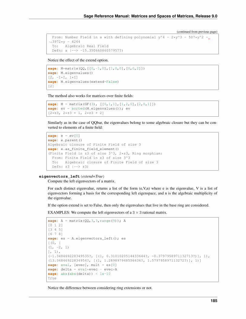
Sage Reference Manual: Matrices and Spaces of Matrices, Release 9.0
(continued from previous page)
From: Number Field in a with defining polynomial y^4 - 2*y^3 - 507*y^2 -→˓3972*y - 4264To: Algebraic Real FieldDefn: a |--> -15.35066086057957?)
Notice the effect of the extend option.
sage: M=matrix(QQ,[[0,-1,0],[1,0,0],[0,0,2]])sage: M.eigenvalues()[2, -1*I, 1*I]sage: M.eigenvalues(extend=False)[2]
The method also works for matrices over finite fields:
sage: M = matrix(GF(3), [[0,1,1],[1,2,0],[2,0,1]])sage: ev = sorted(M.eigenvalues()); ev[2*z3, 2*z3 + 1, 2*z3 + 2]
Similarly as in the case of QQbar, the eigenvalues belong to some algebraic closure but they can be con-verted to elements of a finite field:
sage: e = ev[0]sage: e.parent()Algebraic closure of Finite Field of size 3sage: e.as_finite_field_element()(Finite Field in z3 of size 3^3, 2*z3, Ring morphism:
From: Finite Field in z3 of size 3^3To: Algebraic closure of Finite Field of size 3Defn: z3 |--> z3)
eigenvectors_left(extend=True)Compute the left eigenvectors of a matrix.
For each distinct eigenvalue, returns a list of the form (e,V,n) where e is the eigenvalue, V is a list ofeigenvectors forming a basis for the corresponding left eigenspace, and n is the algebraic multiplicity ofthe eigenvalue.
If the option extend is set to False, then only the eigenvalues that live in the base ring are considered.
EXAMPLES: We compute the left eigenvectors of a 3× 3 rational matrix.
sage: A = matrix(QQ,3,3,range(9)); A[0 1 2][3 4 5][6 7 8]sage: es = A.eigenvectors_left(); es[(0, [(1, -2, 1)], 1),(-1.348469228349535?, [(1, 0.3101020514433644?, -0.3797958971132713?)], 1),(13.34846922834954?, [(1, 1.289897948556636?, 1.579795897113272?)], 1)]sage: eval, [evec], mult = es[0]sage: delta = eval*evec - evec*Asage: abs(abs(delta)) < 1e-10True
Notice the difference between considering ring extensions or not.
185
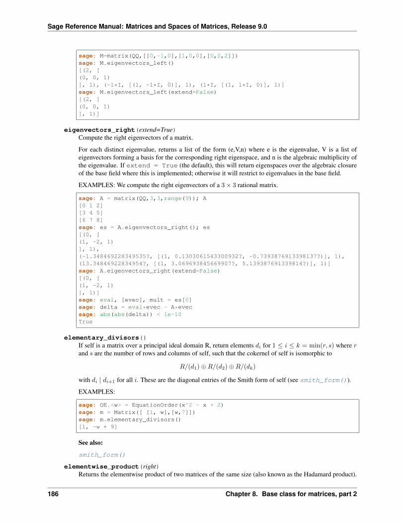
Sage Reference Manual: Matrices and Spaces of Matrices, Release 9.0
sage: M=matrix(QQ,[[0,-1,0],[1,0,0],[0,0,2]])sage: M.eigenvectors_left()[(2, [(0, 0, 1)], 1), (-1*I, [(1, -1*I, 0)], 1), (1*I, [(1, 1*I, 0)], 1)]sage: M.eigenvectors_left(extend=False)[(2, [(0, 0, 1)], 1)]
eigenvectors_right(extend=True)Compute the right eigenvectors of a matrix.
For each distinct eigenvalue, returns a list of the form (e,V,n) where e is the eigenvalue, V is a list ofeigenvectors forming a basis for the corresponding right eigenspace, and n is the algebraic multiplicity ofthe eigenvalue. If extend = True (the default), this will return eigenspaces over the algebraic closureof the base field where this is implemented; otherwise it will restrict to eigenvalues in the base field.
EXAMPLES: We compute the right eigenvectors of a 3× 3 rational matrix.
sage: A = matrix(QQ,3,3,range(9)); A[0 1 2][3 4 5][6 7 8]sage: es = A.eigenvectors_right(); es[(0, [(1, -2, 1)], 1),(-1.348469228349535?, [(1, 0.1303061543300932?, -0.7393876913398137?)], 1),(13.34846922834954?, [(1, 3.069693845669907?, 5.139387691339814?)], 1)]sage: A.eigenvectors_right(extend=False)[(0, [(1, -2, 1)], 1)]sage: eval, [evec], mult = es[0]sage: delta = eval*evec - A*evecsage: abs(abs(delta)) < 1e-10True
elementary_divisors()If self is a matrix over a principal ideal domain R, return elements 𝑑𝑖 for 1 ≤ 𝑖 ≤ 𝑘 = min(𝑟, 𝑠) where 𝑟and 𝑠 are the number of rows and columns of self, such that the cokernel of self is isomorphic to
𝑅/(𝑑1)⊕𝑅/(𝑑2)⊕𝑅/(𝑑𝑘)
with 𝑑𝑖 | 𝑑𝑖+1 for all 𝑖. These are the diagonal entries of the Smith form of self (see smith_form()).
EXAMPLES:
sage: OE.<w> = EquationOrder(x^2 - x + 2)sage: m = Matrix([ [1, w],[w,7]])sage: m.elementary_divisors()[1, -w + 9]
See also:
smith_form()
elementwise_product(right)Returns the elementwise product of two matrices of the same size (also known as the Hadamard product).
186 Chapter 8. Base class for matrices, part 2
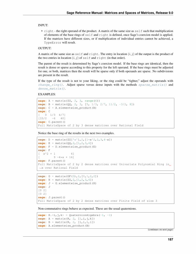
Sage Reference Manual: Matrices and Spaces of Matrices, Release 9.0
INPUT:
• right - the right operand of the product. A matrix of the same size as self such that multiplicationof elements of the base rings of self and right is defined, once Sage’s coercion model is applied.If the matrices have different sizes, or if multiplication of individual entries cannot be achieved, aTypeError will result.
OUTPUT:
A matrix of the same size as self and right. The entry in location (𝑖, 𝑗) of the output is the product ofthe two entries in location (𝑖, 𝑗) of self and right (in that order).
The parent of the result is determined by Sage’s coercion model. If the base rings are identical, then theresult is dense or sparse according to this property for the left operand. If the base rings must be adjustedfor one, or both, matrices then the result will be sparse only if both operands are sparse. No subdivisionsare present in the result.
If the type of the result is not to your liking, or the ring could be “tighter,” adjust the operands withchange_ring(). Adjust sparse versus dense inputs with the methods sparse_matrix() anddense_matrix().
EXAMPLES:
sage: A = matrix(ZZ, 2, 3, range(6))sage: B = matrix(QQ, 2, 3, [5, 1/3, 2/7, 11/2, -3/2, 8])sage: C = A.elementwise_product(B)sage: C[ 0 1/3 4/7][33/2 -6 40]sage: C.parent()Full MatrixSpace of 2 by 3 dense matrices over Rational Field
Notice the base ring of the results in the next two examples.
sage: D = matrix(ZZ['x'],2,[1+x^2,2,3,4-x])sage: E = matrix(QQ,2,[1,2,3,4])sage: F = D.elementwise_product(E)sage: F[ x^2 + 1 4][ 9 -4*x + 16]sage: F.parent()Full MatrixSpace of 2 by 2 dense matrices over Univariate Polynomial Ring in→˓x over Rational Field
sage: G = matrix(GF(3),2,[0,1,2,2])sage: H = matrix(ZZ,2,[1,2,3,4])sage: J = G.elementwise_product(H)sage: J[0 2][0 2]sage: J.parent()Full MatrixSpace of 2 by 2 dense matrices over Finite Field of size 3
Non-commutative rings behave as expected. These are the usual quaternions.
sage: R.<i,j,k> = QuaternionAlgebra(-1, -1)sage: A = matrix(R, 2, [1,i,j,k])sage: B = matrix(R, 2, [i,i,i,i])sage: A.elementwise_product(B)
(continues on next page)
187
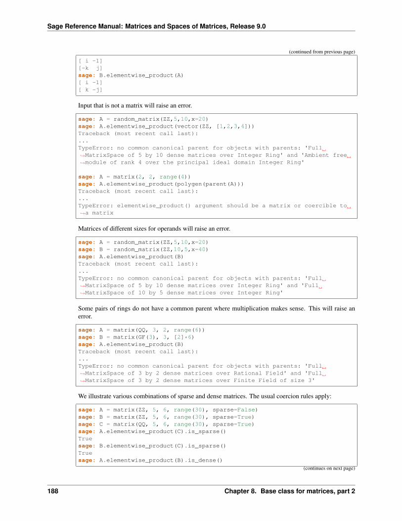
Sage Reference Manual: Matrices and Spaces of Matrices, Release 9.0
(continued from previous page)
[ i -1][-k j]sage: B.elementwise_product(A)[ i -1][ k -j]
Input that is not a matrix will raise an error.
sage: A = random_matrix(ZZ,5,10,x=20)sage: A.elementwise_product(vector(ZZ, [1,2,3,4]))Traceback (most recent call last):...TypeError: no common canonical parent for objects with parents: 'Full→˓MatrixSpace of 5 by 10 dense matrices over Integer Ring' and 'Ambient free→˓module of rank 4 over the principal ideal domain Integer Ring'
sage: A = matrix(2, 2, range(4))sage: A.elementwise_product(polygen(parent(A)))Traceback (most recent call last):...TypeError: elementwise_product() argument should be a matrix or coercible to→˓a matrix
Matrices of different sizes for operands will raise an error.
sage: A = random_matrix(ZZ,5,10,x=20)sage: B = random_matrix(ZZ,10,5,x=40)sage: A.elementwise_product(B)Traceback (most recent call last):...TypeError: no common canonical parent for objects with parents: 'Full→˓MatrixSpace of 5 by 10 dense matrices over Integer Ring' and 'Full→˓MatrixSpace of 10 by 5 dense matrices over Integer Ring'
Some pairs of rings do not have a common parent where multiplication makes sense. This will raise anerror.
sage: A = matrix(QQ, 3, 2, range(6))sage: B = matrix(GF(3), 3, [2]*6)sage: A.elementwise_product(B)Traceback (most recent call last):...TypeError: no common canonical parent for objects with parents: 'Full→˓MatrixSpace of 3 by 2 dense matrices over Rational Field' and 'Full→˓MatrixSpace of 3 by 2 dense matrices over Finite Field of size 3'
We illustrate various combinations of sparse and dense matrices. The usual coercion rules apply:
sage: A = matrix(ZZ, 5, 6, range(30), sparse=False)sage: B = matrix(ZZ, 5, 6, range(30), sparse=True)sage: C = matrix(QQ, 5, 6, range(30), sparse=True)sage: A.elementwise_product(C).is_sparse()Truesage: B.elementwise_product(C).is_sparse()Truesage: A.elementwise_product(B).is_dense()
(continues on next page)
188 Chapter 8. Base class for matrices, part 2
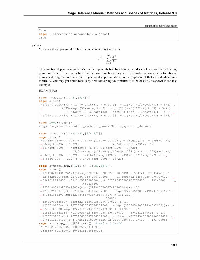
Sage Reference Manual: Matrices and Spaces of Matrices, Release 9.0
(continued from previous page)
Truesage: B.elementwise_product(A).is_dense()True
exp()Calculate the exponential of this matrix X, which is the matrix
𝑒𝑋 =
∞∑︁𝑘=0
𝑋𝑘
𝑘!.
This function depends on maxima’s matrix exponentiation function, which does not deal well with floatingpoint numbers. If the matrix has floating point numbers, they will be rounded automatically to rationalnumbers during the computation. If you want approximations to the exponential that are calculated nu-merically, you may get better results by first converting your matrix to RDF or CDF, as shown in the lastexample.
EXAMPLES:
sage: a=matrix([[1,2],[3,4]])sage: a.exp()[-1/22*((sqrt(33) - 11)*e^sqrt(33) - sqrt(33) - 11)*e^(-1/2*sqrt(33) + 5/2)→˓ 2/33*(sqrt(33)*e^sqrt(33) - sqrt(33))*e^(-1/2*sqrt(33) + 5/2)][ 1/11*(sqrt(33)*e^sqrt(33) - sqrt(33))*e^(-1/2*sqrt(33) + 5/2)→˓1/22*((sqrt(33) + 11)*e^sqrt(33) - sqrt(33) + 11)*e^(-1/2*sqrt(33) + 5/2)]
sage: type(a.exp())<type 'sage.matrix.matrix_symbolic_dense.Matrix_symbolic_dense'>
sage: a=matrix([[1/2,2/3],[3/4,4/5]])sage: a.exp()[-1/418*((3*sqrt(209) - 209)*e^(1/10*sqrt(209)) - 3*sqrt(209) - 209)*e^(-1/→˓20*sqrt(209) + 13/20) 20/627*(sqrt(209)*e^(1/→˓10*sqrt(209)) - sqrt(209))*e^(-1/20*sqrt(209) + 13/20)][ 15/418*(sqrt(209)*e^(1/10*sqrt(209)) - sqrt(209))*e^(-1/→˓20*sqrt(209) + 13/20) 1/418*((3*sqrt(209) + 209)*e^(1/10*sqrt(209)) -→˓3*sqrt(209) + 209)*e^(-1/20*sqrt(209) + 13/20)]
sage: a=matrix(RR,[[1,pi.n()],[1e2,1e-2]])sage: a.exp()[ 1/11882424341266*((11*sqrt(227345670387496707609) + 5941212170633)*e^(3/→˓1275529100*sqrt(227345670387496707609)) - 11*sqrt(227345670387496707609) +→˓5941212170633)*e^(-3/2551058200*sqrt(227345670387496707609) + 101/200)→˓ 445243650/→˓75781890129165569203*(sqrt(227345670387496707609)*e^(3/→˓1275529100*sqrt(227345670387496707609)) - sqrt(227345670387496707609))*e^(-→˓3/2551058200*sqrt(227345670387496707609) + 101/200)][ 10000/→˓53470909535697*(sqrt(227345670387496707609)*e^(3/→˓1275529100*sqrt(227345670387496707609)) - sqrt(227345670387496707609))*e^(-→˓3/2551058200*sqrt(227345670387496707609) + 101/200) -1/→˓11882424341266*((11*sqrt(227345670387496707609) - 5941212170633)*e^(3/→˓1275529100*sqrt(227345670387496707609)) - 11*sqrt(227345670387496707609) -→˓5941212170633)*e^(-3/2551058200*sqrt(227345670387496707609) + 101/200)]sage: a.change_ring(RDF).exp() # rel tol 1e-14[42748127.31532951 7368259.244159399][234538976.1381042 40426191.45156228]
189
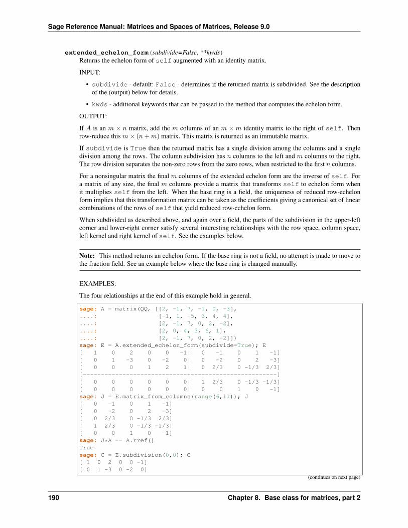
Sage Reference Manual: Matrices and Spaces of Matrices, Release 9.0
extended_echelon_form(subdivide=False, **kwds)Returns the echelon form of self augmented with an identity matrix.
INPUT:
• subdivide - default: False - determines if the returned matrix is subdivided. See the descriptionof the (output) below for details.
• kwds - additional keywords that can be passed to the method that computes the echelon form.
OUTPUT:
If 𝐴 is an 𝑚 × 𝑛 matrix, add the 𝑚 columns of an 𝑚 × 𝑚 identity matrix to the right of self. Thenrow-reduce this 𝑚× (𝑛+𝑚) matrix. This matrix is returned as an immutable matrix.
If subdivide is True then the returned matrix has a single division among the columns and a singledivision among the rows. The column subdivision has 𝑛 columns to the left and 𝑚 columns to the right.The row division separates the non-zero rows from the zero rows, when restricted to the first 𝑛 columns.
For a nonsingular matrix the final 𝑚 columns of the extended echelon form are the inverse of self. Fora matrix of any size, the final 𝑚 columns provide a matrix that transforms self to echelon form whenit multiplies self from the left. When the base ring is a field, the uniqueness of reduced row-echelonform implies that this transformation matrix can be taken as the coefficients giving a canonical set of linearcombinations of the rows of self that yield reduced row-echelon form.
When subdivided as described above, and again over a field, the parts of the subdivision in the upper-leftcorner and lower-right corner satisfy several interesting relationships with the row space, column space,left kernel and right kernel of self. See the examples below.
Note: This method returns an echelon form. If the base ring is not a field, no attempt is made to move tothe fraction field. See an example below where the base ring is changed manually.
EXAMPLES:
The four relationships at the end of this example hold in general.
sage: A = matrix(QQ, [[2, -1, 7, -1, 0, -3],....: [-1, 1, -5, 3, 4, 4],....: [2, -1, 7, 0, 2, -2],....: [2, 0, 4, 3, 6, 1],....: [2, -1, 7, 0, 2, -2]])sage: E = A.extended_echelon_form(subdivide=True); E[ 1 0 2 0 0 -1| 0 -1 0 1 -1][ 0 1 -3 0 -2 0| 0 -2 0 2 -3][ 0 0 0 1 2 1| 0 2/3 0 -1/3 2/3][-----------------------------+------------------------][ 0 0 0 0 0 0| 1 2/3 0 -1/3 -1/3][ 0 0 0 0 0 0| 0 0 1 0 -1]sage: J = E.matrix_from_columns(range(6,11)); J[ 0 -1 0 1 -1][ 0 -2 0 2 -3][ 0 2/3 0 -1/3 2/3][ 1 2/3 0 -1/3 -1/3][ 0 0 1 0 -1]sage: J*A == A.rref()Truesage: C = E.subdivision(0,0); C[ 1 0 2 0 0 -1][ 0 1 -3 0 -2 0]
(continues on next page)
190 Chapter 8. Base class for matrices, part 2
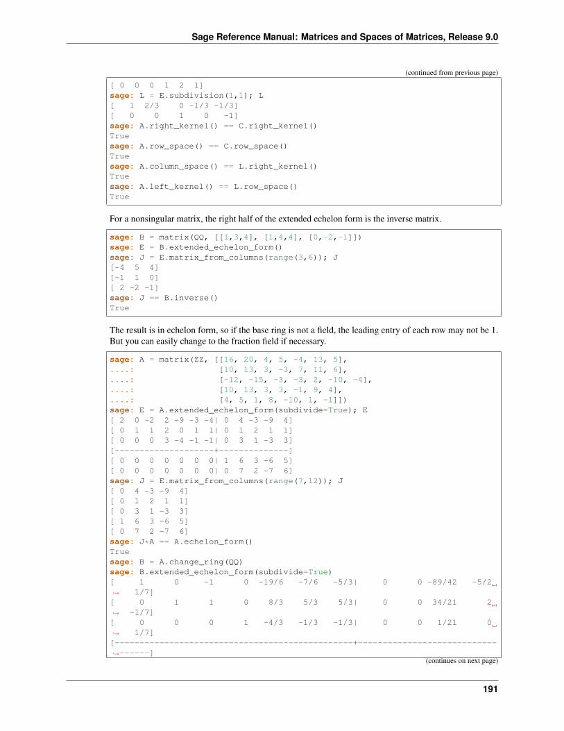
Sage Reference Manual: Matrices and Spaces of Matrices, Release 9.0
(continued from previous page)
[ 0 0 0 1 2 1]sage: L = E.subdivision(1,1); L[ 1 2/3 0 -1/3 -1/3][ 0 0 1 0 -1]sage: A.right_kernel() == C.right_kernel()Truesage: A.row_space() == C.row_space()Truesage: A.column_space() == L.right_kernel()Truesage: A.left_kernel() == L.row_space()True
For a nonsingular matrix, the right half of the extended echelon form is the inverse matrix.
sage: B = matrix(QQ, [[1,3,4], [1,4,4], [0,-2,-1]])sage: E = B.extended_echelon_form()sage: J = E.matrix_from_columns(range(3,6)); J[-4 5 4][-1 1 0][ 2 -2 -1]sage: J == B.inverse()True
The result is in echelon form, so if the base ring is not a field, the leading entry of each row may not be 1.But you can easily change to the fraction field if necessary.
sage: A = matrix(ZZ, [[16, 20, 4, 5, -4, 13, 5],....: [10, 13, 3, -3, 7, 11, 6],....: [-12, -15, -3, -3, 2, -10, -4],....: [10, 13, 3, 3, -1, 9, 4],....: [4, 5, 1, 8, -10, 1, -1]])sage: E = A.extended_echelon_form(subdivide=True); E[ 2 0 -2 2 -9 -3 -4| 0 4 -3 -9 4][ 0 1 1 2 0 1 1| 0 1 2 1 1][ 0 0 0 3 -4 -1 -1| 0 3 1 -3 3][--------------------+--------------][ 0 0 0 0 0 0 0| 1 6 3 -6 5][ 0 0 0 0 0 0 0| 0 7 2 -7 6]sage: J = E.matrix_from_columns(range(7,12)); J[ 0 4 -3 -9 4][ 0 1 2 1 1][ 0 3 1 -3 3][ 1 6 3 -6 5][ 0 7 2 -7 6]sage: J*A == A.echelon_form()Truesage: B = A.change_ring(QQ)sage: B.extended_echelon_form(subdivide=True)[ 1 0 -1 0 -19/6 -7/6 -5/3| 0 0 -89/42 -5/2→˓ 1/7][ 0 1 1 0 8/3 5/3 5/3| 0 0 34/21 2→˓ -1/7][ 0 0 0 1 -4/3 -1/3 -1/3| 0 0 1/21 0→˓ 1/7][------------------------------------------------+----------------------------→˓------]
(continues on next page)
191
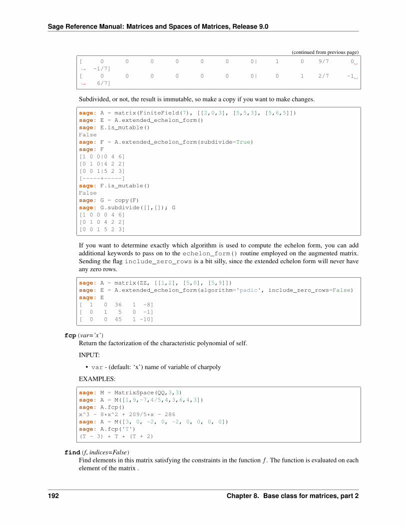
Sage Reference Manual: Matrices and Spaces of Matrices, Release 9.0
(continued from previous page)
[ 0 0 0 0 0 0 0| 1 0 9/7 0→˓ -1/7][ 0 0 0 0 0 0 0| 0 1 2/7 -1→˓ 6/7]
Subdivided, or not, the result is immutable, so make a copy if you want to make changes.
sage: A = matrix(FiniteField(7), [[2,0,3], [5,5,3], [5,6,5]])sage: E = A.extended_echelon_form()sage: E.is_mutable()Falsesage: F = A.extended_echelon_form(subdivide=True)sage: F[1 0 0|0 4 6][0 1 0|4 2 2][0 0 1|5 2 3][-----+-----]sage: F.is_mutable()Falsesage: G = copy(F)sage: G.subdivide([],[]); G[1 0 0 0 4 6][0 1 0 4 2 2][0 0 1 5 2 3]
If you want to determine exactly which algorithm is used to compute the echelon form, you can addadditional keywords to pass on to the echelon_form() routine employed on the augmented matrix.Sending the flag include_zero_rows is a bit silly, since the extended echelon form will never haveany zero rows.
sage: A = matrix(ZZ, [[1,2], [5,0], [5,9]])sage: E = A.extended_echelon_form(algorithm='padic', include_zero_rows=False)sage: E[ 1 0 36 1 -8][ 0 1 5 0 -1][ 0 0 45 1 -10]
fcp(var=’x’)Return the factorization of the characteristic polynomial of self.
INPUT:
• var - (default: ‘x’) name of variable of charpoly
EXAMPLES:
sage: M = MatrixSpace(QQ,3,3)sage: A = M([1,9,-7,4/5,4,3,6,4,3])sage: A.fcp()x^3 - 8*x^2 + 209/5*x - 286sage: A = M([3, 0, -2, 0, -2, 0, 0, 0, 0])sage: A.fcp('T')(T - 3) * T * (T + 2)
find(f, indices=False)Find elements in this matrix satisfying the constraints in the function 𝑓 . The function is evaluated on eachelement of the matrix .
192 Chapter 8. Base class for matrices, part 2
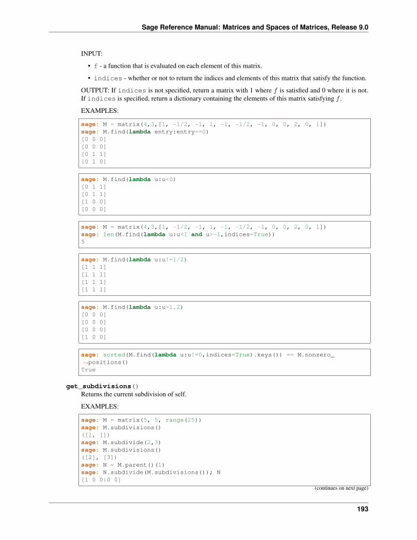
Sage Reference Manual: Matrices and Spaces of Matrices, Release 9.0
INPUT:
• f - a function that is evaluated on each element of this matrix.
• indices - whether or not to return the indices and elements of this matrix that satisfy the function.
OUTPUT: If indices is not specified, return a matrix with 1 where 𝑓 is satisfied and 0 where it is not.If indices is specified, return a dictionary containing the elements of this matrix satisfying 𝑓 .
EXAMPLES:
sage: M = matrix(4,3,[1, -1/2, -1, 1, -1, -1/2, -1, 0, 0, 2, 0, 1])sage: M.find(lambda entry:entry==0)[0 0 0][0 0 0][0 1 1][0 1 0]
sage: M.find(lambda u:u<0)[0 1 1][0 1 1][1 0 0][0 0 0]
sage: M = matrix(4,3,[1, -1/2, -1, 1, -1, -1/2, -1, 0, 0, 2, 0, 1])sage: len(M.find(lambda u:u<1 and u>-1,indices=True))5
sage: M.find(lambda u:u!=1/2)[1 1 1][1 1 1][1 1 1][1 1 1]
sage: M.find(lambda u:u>1.2)[0 0 0][0 0 0][0 0 0][1 0 0]
sage: sorted(M.find(lambda u:u!=0,indices=True).keys()) == M.nonzero_→˓positions()True
get_subdivisions()Returns the current subdivision of self.
EXAMPLES:
sage: M = matrix(5, 5, range(25))sage: M.subdivisions()([], [])sage: M.subdivide(2,3)sage: M.subdivisions()([2], [3])sage: N = M.parent()(1)sage: N.subdivide(M.subdivisions()); N[1 0 0|0 0]
(continues on next page)
193
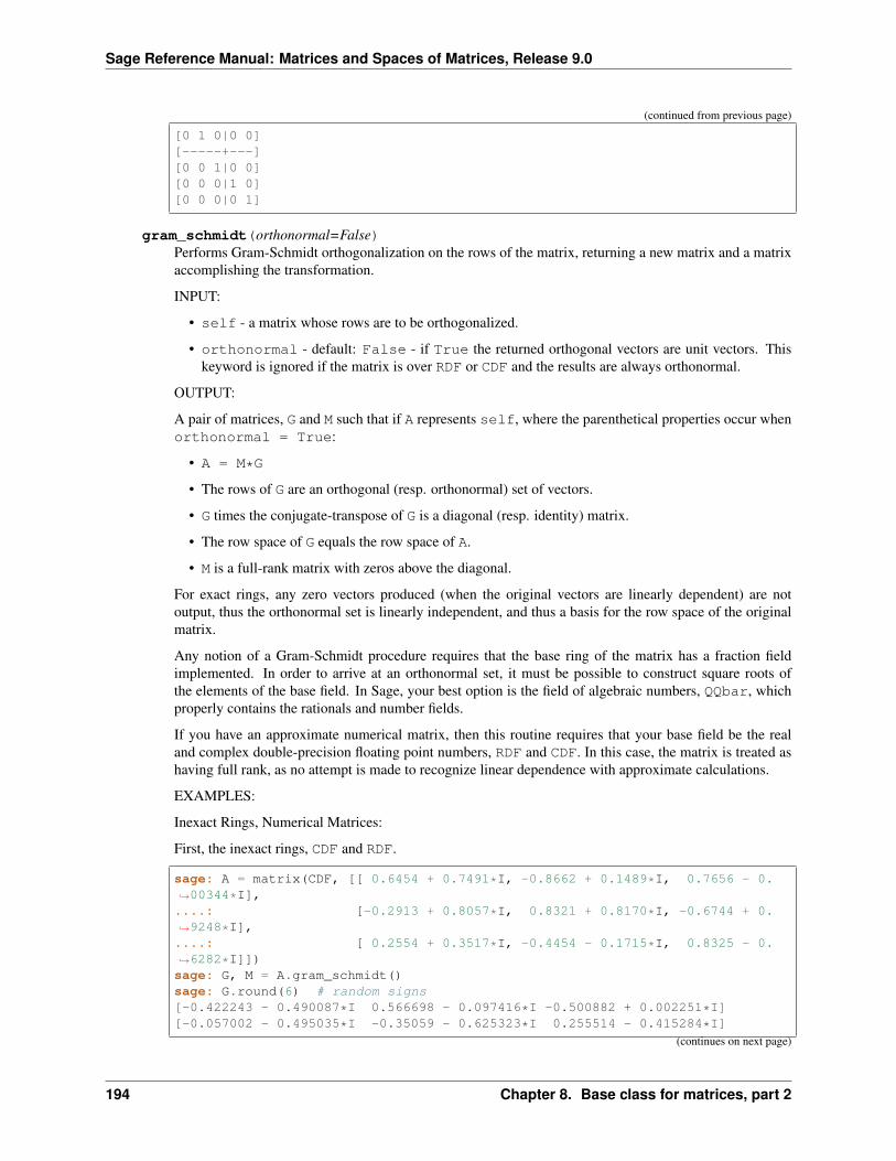
Sage Reference Manual: Matrices and Spaces of Matrices, Release 9.0
(continued from previous page)
[0 1 0|0 0][-----+---][0 0 1|0 0][0 0 0|1 0][0 0 0|0 1]
gram_schmidt(orthonormal=False)Performs Gram-Schmidt orthogonalization on the rows of the matrix, returning a new matrix and a matrixaccomplishing the transformation.
INPUT:
• self - a matrix whose rows are to be orthogonalized.
• orthonormal - default: False - if True the returned orthogonal vectors are unit vectors. Thiskeyword is ignored if the matrix is over RDF or CDF and the results are always orthonormal.
OUTPUT:
A pair of matrices, G and M such that if A represents self, where the parenthetical properties occur whenorthonormal = True:
• A = M*G
• The rows of G are an orthogonal (resp. orthonormal) set of vectors.
• G times the conjugate-transpose of G is a diagonal (resp. identity) matrix.
• The row space of G equals the row space of A.
• M is a full-rank matrix with zeros above the diagonal.
For exact rings, any zero vectors produced (when the original vectors are linearly dependent) are notoutput, thus the orthonormal set is linearly independent, and thus a basis for the row space of the originalmatrix.
Any notion of a Gram-Schmidt procedure requires that the base ring of the matrix has a fraction fieldimplemented. In order to arrive at an orthonormal set, it must be possible to construct square roots ofthe elements of the base field. In Sage, your best option is the field of algebraic numbers, QQbar, whichproperly contains the rationals and number fields.
If you have an approximate numerical matrix, then this routine requires that your base field be the realand complex double-precision floating point numbers, RDF and CDF. In this case, the matrix is treated ashaving full rank, as no attempt is made to recognize linear dependence with approximate calculations.
EXAMPLES:
Inexact Rings, Numerical Matrices:
First, the inexact rings, CDF and RDF.
sage: A = matrix(CDF, [[ 0.6454 + 0.7491*I, -0.8662 + 0.1489*I, 0.7656 - 0.→˓00344*I],....: [-0.2913 + 0.8057*I, 0.8321 + 0.8170*I, -0.6744 + 0.→˓9248*I],....: [ 0.2554 + 0.3517*I, -0.4454 - 0.1715*I, 0.8325 - 0.→˓6282*I]])sage: G, M = A.gram_schmidt()sage: G.round(6) # random signs[-0.422243 - 0.490087*I 0.566698 - 0.097416*I -0.500882 + 0.002251*I][-0.057002 - 0.495035*I -0.35059 - 0.625323*I 0.255514 - 0.415284*I]
(continues on next page)
194 Chapter 8. Base class for matrices, part 2
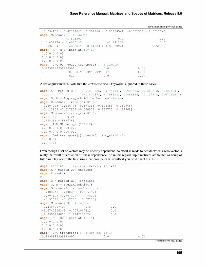
Sage Reference Manual: Matrices and Spaces of Matrices, Release 9.0
(continued from previous page)
[ 0.394105 - 0.421778*I -0.392266 - 0.039345*I -0.352905 + 0.62195*I]sage: M.round(6) # random[ -1.528503 0.0 0.0][ 0.459974 - 0.40061*I -1.741233 0.0][-0.934304 + 0.148868*I 0.54833 + 0.073202*I -0.550725]sage: (A - M*G).zero_at(10^-12)[0.0 0.0 0.0][0.0 0.0 0.0][0.0 0.0 0.0]sage: (G*G.conjugate_transpose()) # random[0.9999999999999999 0.0 0.0][ 0.0 0.9999999999999997 0.0][ 0.0 0.0 1.0]
A rectangular matrix. Note that the orthonormal keyword is ignored in these cases.
sage: A = matrix(RDF, [[-0.978325, -0.751994, 0.925305, -0.200512, 0.420458],....: [-0.474877, -0.983403, 0.089836, 0.132218, 0.672965]])sage: G, M = A.gram_schmidt(orthonormal=False)sage: G.round(6).zero_at(10^-6)[-0.607223 -0.466745 0.574315 -0.124453 0.260968][ 0.123203 -0.617909 -0.530578 0.289773 0.487368]sage: M.round(6).zero_at(10^-6)[1.611147 0.0][0.958116 0.867778]sage: (A-M*G).zero_at(10^-12)[0.0 0.0 0.0 0.0 0.0][0.0 0.0 0.0 0.0 0.0]sage: (G*G.transpose()).round(6).zero_at(10^-6)[1.0 0.0][0.0 1.0]
Even though a set of vectors may be linearly dependent, no effort is made to decide when a zero vector isreally the result of a relation of linear dependence. So in this regard, input matrices are treated as being offull rank. Try one of the base rings that provide exact results if you need exact results.
sage: entries = [[1,1,2], [2,1,3], [3,1,4]]sage: A = matrix(QQ, entries)sage: A.rank()2sage: B = matrix(RDF, entries)sage: G, M = B.gram_schmidt()sage: G.round(6) # random signs[-0.408248 -0.408248 -0.816497][ 0.707107 -0.707107 -0.0][ -0.57735 -0.57735 0.57735]sage: M.round(10) # random[-2.4494897428 0.0 0.0][-3.6742346142 0.7071067812 0.0][-4.8989794856 1.4142135624 0.0]sage: (A - M*G).zero_at(1e-14)[0.0 0.0 0.0][0.0 0.0 0.0][0.0 0.0 0.0]sage: (G*G.transpose()) # abs tol 1e-14[0.9999999999999997 0.0 0.0]
(continues on next page)
195
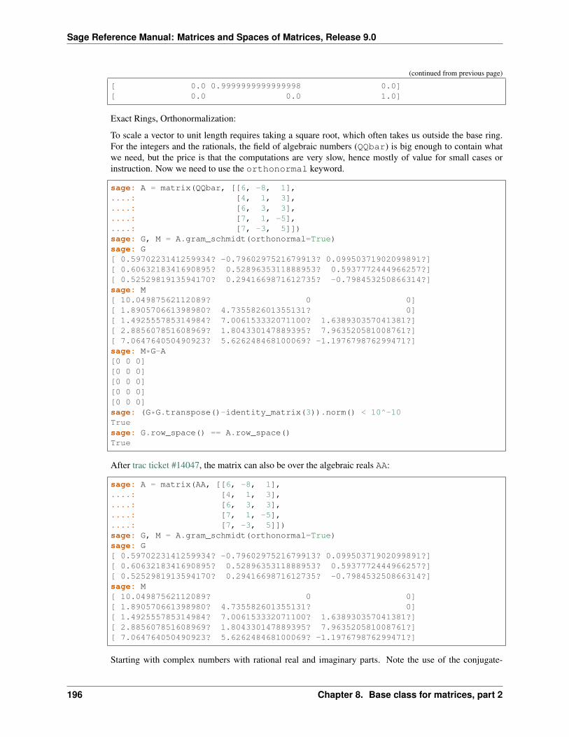
Sage Reference Manual: Matrices and Spaces of Matrices, Release 9.0
(continued from previous page)
[ 0.0 0.9999999999999998 0.0][ 0.0 0.0 1.0]
Exact Rings, Orthonormalization:
To scale a vector to unit length requires taking a square root, which often takes us outside the base ring.For the integers and the rationals, the field of algebraic numbers (QQbar) is big enough to contain whatwe need, but the price is that the computations are very slow, hence mostly of value for small cases orinstruction. Now we need to use the orthonormal keyword.
sage: A = matrix(QQbar, [[6, -8, 1],....: [4, 1, 3],....: [6, 3, 3],....: [7, 1, -5],....: [7, -3, 5]])sage: G, M = A.gram_schmidt(orthonormal=True)sage: G[ 0.5970223141259934? -0.7960297521679913? 0.09950371902099891?][ 0.6063218341690895? 0.5289635311888953? 0.5937772444966257?][ 0.5252981913594170? 0.2941669871612735? -0.798453250866314?]sage: M[ 10.04987562112089? 0 0][ 1.890570661398980? 4.735582601355131? 0][ 1.492555785314984? 7.006153332071100? 1.638930357041381?][ 2.885607851608969? 1.804330147889395? 7.963520581008761?][ 7.064764050490923? 5.626248468100069? -1.197679876299471?]sage: M*G-A[0 0 0][0 0 0][0 0 0][0 0 0][0 0 0]sage: (G*G.transpose()-identity_matrix(3)).norm() < 10^-10Truesage: G.row_space() == A.row_space()True
After trac ticket #14047, the matrix can also be over the algebraic reals AA:
sage: A = matrix(AA, [[6, -8, 1],....: [4, 1, 3],....: [6, 3, 3],....: [7, 1, -5],....: [7, -3, 5]])sage: G, M = A.gram_schmidt(orthonormal=True)sage: G[ 0.5970223141259934? -0.7960297521679913? 0.09950371902099891?][ 0.6063218341690895? 0.5289635311888953? 0.5937772444966257?][ 0.5252981913594170? 0.2941669871612735? -0.798453250866314?]sage: M[ 10.04987562112089? 0 0][ 1.890570661398980? 4.735582601355131? 0][ 1.492555785314984? 7.006153332071100? 1.638930357041381?][ 2.885607851608969? 1.804330147889395? 7.963520581008761?][ 7.064764050490923? 5.626248468100069? -1.197679876299471?]
Starting with complex numbers with rational real and imaginary parts. Note the use of the conjugate-
196 Chapter 8. Base class for matrices, part 2
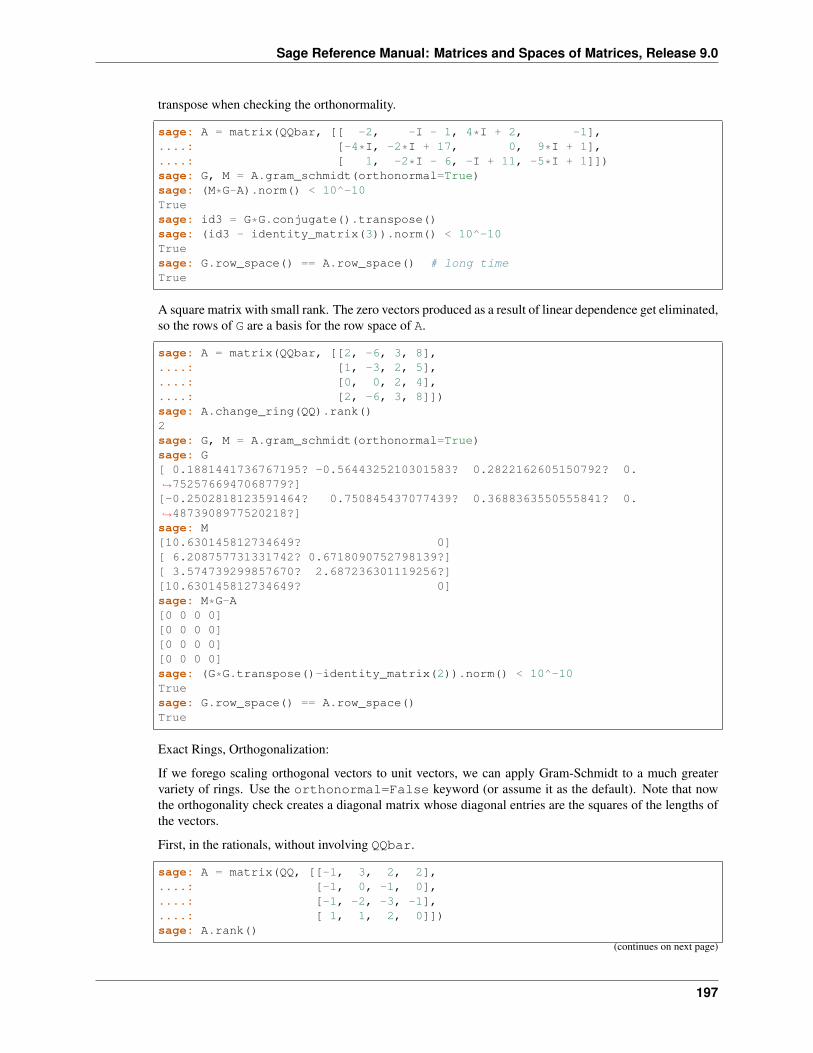
Sage Reference Manual: Matrices and Spaces of Matrices, Release 9.0
transpose when checking the orthonormality.
sage: A = matrix(QQbar, [[ -2, -I - 1, 4*I + 2, -1],....: [-4*I, -2*I + 17, 0, 9*I + 1],....: [ 1, -2*I - 6, -I + 11, -5*I + 1]])sage: G, M = A.gram_schmidt(orthonormal=True)sage: (M*G-A).norm() < 10^-10Truesage: id3 = G*G.conjugate().transpose()sage: (id3 - identity_matrix(3)).norm() < 10^-10Truesage: G.row_space() == A.row_space() # long timeTrue
A square matrix with small rank. The zero vectors produced as a result of linear dependence get eliminated,so the rows of G are a basis for the row space of A.
sage: A = matrix(QQbar, [[2, -6, 3, 8],....: [1, -3, 2, 5],....: [0, 0, 2, 4],....: [2, -6, 3, 8]])sage: A.change_ring(QQ).rank()2sage: G, M = A.gram_schmidt(orthonormal=True)sage: G[ 0.1881441736767195? -0.5644325210301583? 0.2822162605150792? 0.→˓7525766947068779?][-0.2502818123591464? 0.750845437077439? 0.3688363550555841? 0.→˓4873908977520218?]sage: M[10.630145812734649? 0][ 6.208757731331742? 0.6718090752798139?][ 3.574739299857670? 2.687236301119256?][10.630145812734649? 0]sage: M*G-A[0 0 0 0][0 0 0 0][0 0 0 0][0 0 0 0]sage: (G*G.transpose()-identity_matrix(2)).norm() < 10^-10Truesage: G.row_space() == A.row_space()True
Exact Rings, Orthogonalization:
If we forego scaling orthogonal vectors to unit vectors, we can apply Gram-Schmidt to a much greatervariety of rings. Use the orthonormal=False keyword (or assume it as the default). Note that nowthe orthogonality check creates a diagonal matrix whose diagonal entries are the squares of the lengths ofthe vectors.
First, in the rationals, without involving QQbar.
sage: A = matrix(QQ, [[-1, 3, 2, 2],....: [-1, 0, -1, 0],....: [-1, -2, -3, -1],....: [ 1, 1, 2, 0]])sage: A.rank()
(continues on next page)
197
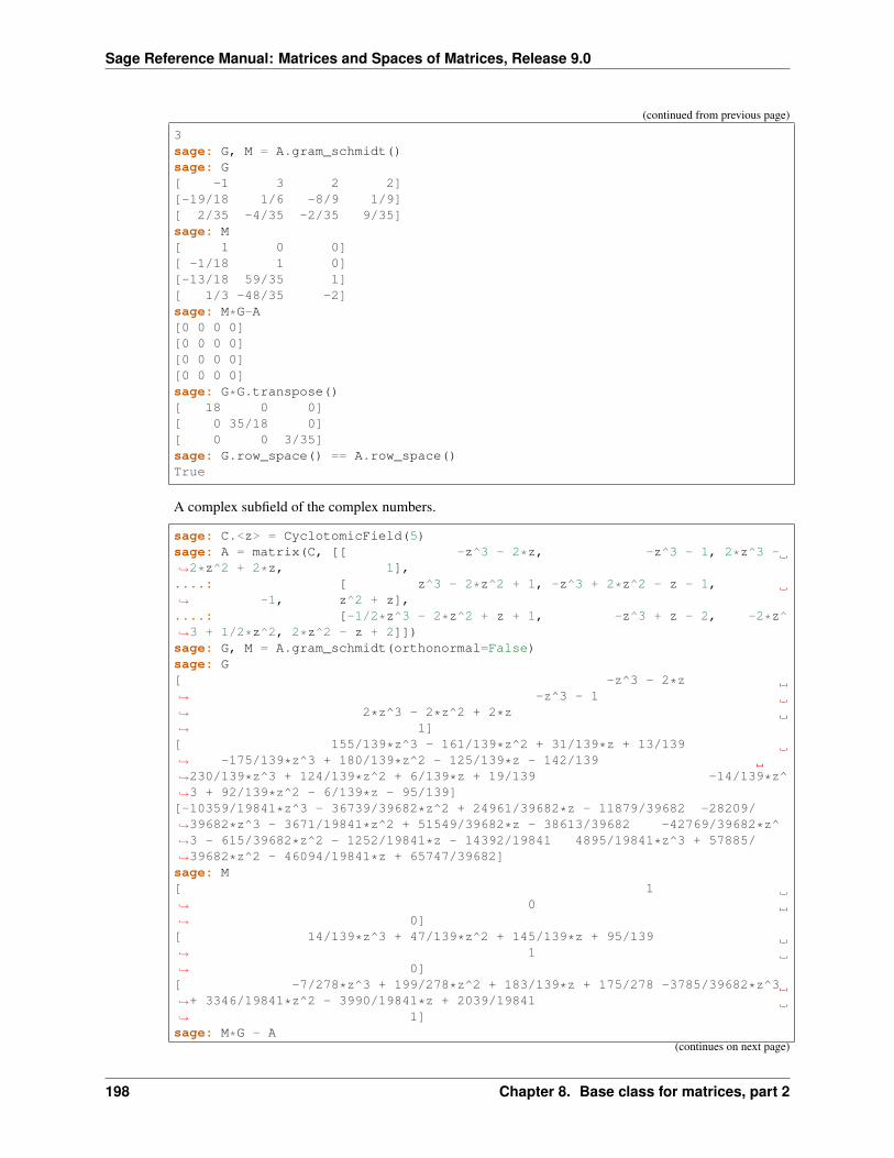
Sage Reference Manual: Matrices and Spaces of Matrices, Release 9.0
(continued from previous page)
3sage: G, M = A.gram_schmidt()sage: G[ -1 3 2 2][-19/18 1/6 -8/9 1/9][ 2/35 -4/35 -2/35 9/35]sage: M[ 1 0 0][ -1/18 1 0][-13/18 59/35 1][ 1/3 -48/35 -2]sage: M*G-A[0 0 0 0][0 0 0 0][0 0 0 0][0 0 0 0]sage: G*G.transpose()[ 18 0 0][ 0 35/18 0][ 0 0 3/35]sage: G.row_space() == A.row_space()True
A complex subfield of the complex numbers.
sage: C.<z> = CyclotomicField(5)sage: A = matrix(C, [[ -z^3 - 2*z, -z^3 - 1, 2*z^3 -→˓2*z^2 + 2*z, 1],....: [ z^3 - 2*z^2 + 1, -z^3 + 2*z^2 - z - 1,→˓ -1, z^2 + z],....: [-1/2*z^3 - 2*z^2 + z + 1, -z^3 + z - 2, -2*z^→˓3 + 1/2*z^2, 2*z^2 - z + 2]])sage: G, M = A.gram_schmidt(orthonormal=False)sage: G[ -z^3 - 2*z→˓ -z^3 - 1→˓ 2*z^3 - 2*z^2 + 2*z→˓ 1][ 155/139*z^3 - 161/139*z^2 + 31/139*z + 13/139→˓ -175/139*z^3 + 180/139*z^2 - 125/139*z - 142/139→˓230/139*z^3 + 124/139*z^2 + 6/139*z + 19/139 -14/139*z^→˓3 + 92/139*z^2 - 6/139*z - 95/139][-10359/19841*z^3 - 36739/39682*z^2 + 24961/39682*z - 11879/39682 -28209/→˓39682*z^3 - 3671/19841*z^2 + 51549/39682*z - 38613/39682 -42769/39682*z^→˓3 - 615/39682*z^2 - 1252/19841*z - 14392/19841 4895/19841*z^3 + 57885/→˓39682*z^2 - 46094/19841*z + 65747/39682]sage: M[ 1→˓ 0→˓ 0][ 14/139*z^3 + 47/139*z^2 + 145/139*z + 95/139→˓ 1→˓ 0][ -7/278*z^3 + 199/278*z^2 + 183/139*z + 175/278 -3785/39682*z^3→˓+ 3346/19841*z^2 - 3990/19841*z + 2039/19841→˓ 1]sage: M*G - A
(continues on next page)
198 Chapter 8. Base class for matrices, part 2
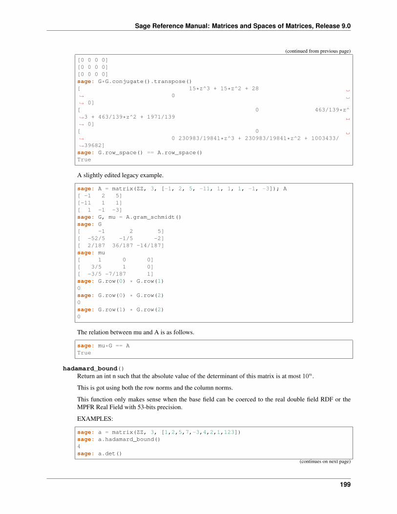
Sage Reference Manual: Matrices and Spaces of Matrices, Release 9.0
(continued from previous page)
[0 0 0 0][0 0 0 0][0 0 0 0]sage: G*G.conjugate().transpose()[ 15*z^3 + 15*z^2 + 28→˓ 0→˓ 0][ 0 463/139*z^→˓3 + 463/139*z^2 + 1971/139→˓ 0][ 0→˓ 0 230983/19841*z^3 + 230983/19841*z^2 + 1003433/→˓39682]sage: G.row_space() == A.row_space()True
A slightly edited legacy example.
sage: A = matrix(ZZ, 3, [-1, 2, 5, -11, 1, 1, 1, -1, -3]); A[ -1 2 5][-11 1 1][ 1 -1 -3]sage: G, mu = A.gram_schmidt()sage: G[ -1 2 5][ -52/5 -1/5 -2][ 2/187 36/187 -14/187]sage: mu[ 1 0 0][ 3/5 1 0][ -3/5 -7/187 1]sage: G.row(0) * G.row(1)0sage: G.row(0) * G.row(2)0sage: G.row(1) * G.row(2)0
The relation between mu and A is as follows.
sage: mu*G == ATrue
hadamard_bound()Return an int n such that the absolute value of the determinant of this matrix is at most 10𝑛.
This is got using both the row norms and the column norms.
This function only makes sense when the base field can be coerced to the real double field RDF or theMPFR Real Field with 53-bits precision.
EXAMPLES:
sage: a = matrix(ZZ, 3, [1,2,5,7,-3,4,2,1,123])sage: a.hadamard_bound()4sage: a.det()
(continues on next page)
199

Sage Reference Manual: Matrices and Spaces of Matrices, Release 9.0
(continued from previous page)
-2014sage: 10^410000
In this example the Hadamard bound has to be computed (automatically) using MPFR instead of doubles,since doubles overflow:
sage: a = matrix(ZZ, 2, [2^10000,3^10000,2^50,3^19292])sage: a.hadamard_bound()12215sage: len(str(a.det()))12215
hermite_form(include_zero_rows=True, transformation=False)Return the Hermite form of self, if it is defined.
INPUT:
• include_zero_rows – bool (default: True); if False the zero rows in the output matrix are deleted.
• transformation – bool (default: False) a matrix U such that U*self == H.
OUTPUT:
• matrix H
• (optional) transformation matrix U such that U*self == H, possibly with zero rows deleted. . .
EXAMPLES:
sage: M = FunctionField(GF(7),'x').maximal_order()sage: K.<x> = FunctionField(GF(7)); M = K.maximal_order()sage: A = matrix(M, 2, 3, [x, 1, 2*x, x, 1+x, 2])sage: A.hermite_form()[ x 1 2*x][ 0 x 5*x + 2]sage: A.hermite_form(transformation=True)([ x 1 2*x] [1 0][ 0 x 5*x + 2], [6 1])sage: A = matrix(M, 2, 3, [x, 1, 2*x, 2*x, 2, 4*x])sage: A.hermite_form(transformation=True, include_zero_rows=False)([ x 1 2*x], [1 0])sage: H, U = A.hermite_form(transformation=True, include_zero_rows=True); H, U([ x 1 2*x] [1 0][ 0 0 0], [5 1])sage: U*A == HTruesage: H, U = A.hermite_form(transformation=True, include_zero_rows=False)sage: U*A[ x 1 2*x]sage: U*A == HTrue
hessenberg_form()Return Hessenberg form of self.
200 Chapter 8. Base class for matrices, part 2
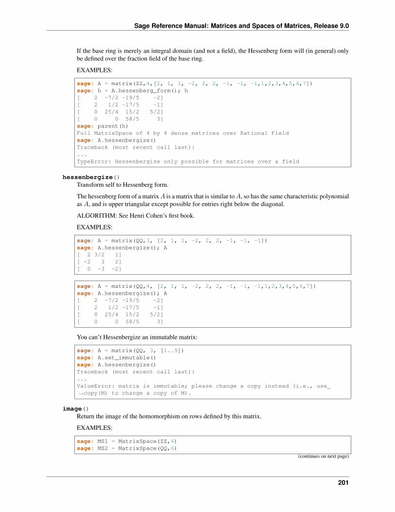
Sage Reference Manual: Matrices and Spaces of Matrices, Release 9.0
If the base ring is merely an integral domain (and not a field), the Hessenberg form will (in general) onlybe defined over the fraction field of the base ring.
EXAMPLES:
sage: A = matrix(ZZ,4,[2, 1, 1, -2, 2, 2, -1, -1, -1,1,2,3,4,5,6,7])sage: h = A.hessenberg_form(); h[ 2 -7/2 -19/5 -2][ 2 1/2 -17/5 -1][ 0 25/4 15/2 5/2][ 0 0 58/5 3]sage: parent(h)Full MatrixSpace of 4 by 4 dense matrices over Rational Fieldsage: A.hessenbergize()Traceback (most recent call last):...TypeError: Hessenbergize only possible for matrices over a field
hessenbergize()Transform self to Hessenberg form.
The hessenberg form of a matrix 𝐴 is a matrix that is similar to 𝐴, so has the same characteristic polynomialas 𝐴, and is upper triangular except possible for entries right below the diagonal.
ALGORITHM: See Henri Cohen’s first book.
EXAMPLES:
sage: A = matrix(QQ,3, [2, 1, 1, -2, 2, 2, -1, -1, -1])sage: A.hessenbergize(); A[ 2 3/2 1][ -2 3 2][ 0 -3 -2]
sage: A = matrix(QQ,4, [2, 1, 1, -2, 2, 2, -1, -1, -1,1,2,3,4,5,6,7])sage: A.hessenbergize(); A[ 2 -7/2 -19/5 -2][ 2 1/2 -17/5 -1][ 0 25/4 15/2 5/2][ 0 0 58/5 3]
You can’t Hessenbergize an immutable matrix:
sage: A = matrix(QQ, 3, [1..9])sage: A.set_immutable()sage: A.hessenbergize()Traceback (most recent call last):...ValueError: matrix is immutable; please change a copy instead (i.e., use→˓copy(M) to change a copy of M).
image()Return the image of the homomorphism on rows defined by this matrix.
EXAMPLES:
sage: MS1 = MatrixSpace(ZZ,4)sage: MS2 = MatrixSpace(QQ,6)
(continues on next page)
201
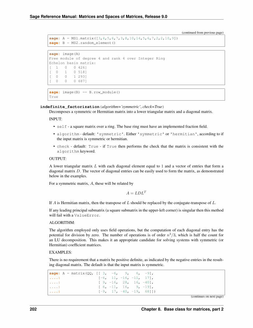
Sage Reference Manual: Matrices and Spaces of Matrices, Release 9.0
(continued from previous page)
sage: A = MS1.matrix([3,4,5,6,7,3,8,10,14,5,6,7,2,2,10,9])sage: B = MS2.random_element()
sage: image(A)Free module of degree 4 and rank 4 over Integer RingEchelon basis matrix:[ 1 0 0 426][ 0 1 0 518][ 0 0 1 293][ 0 0 0 687]
sage: image(B) == B.row_module()True
indefinite_factorization(algorithm=’symmetric’, check=True)Decomposes a symmetric or Hermitian matrix into a lower triangular matrix and a diagonal matrix.
INPUT:
• self - a square matrix over a ring. The base ring must have an implemented fraction field.
• algorithm - default: 'symmetric'. Either 'symmetric' or 'hermitian', according to ifthe input matrix is symmetric or hermitian.
• check - default: True - if True then performs the check that the matrix is consistent with thealgorithm keyword.
OUTPUT:
A lower triangular matrix 𝐿 with each diagonal element equal to 1 and a vector of entries that form adiagonal matrix 𝐷. The vector of diagonal entries can be easily used to form the matrix, as demonstratedbelow in the examples.
For a symmetric matrix, 𝐴, these will be related by
𝐴 = 𝐿𝐷𝐿𝑇
If 𝐴 is Hermitian matrix, then the transpose of 𝐿 should be replaced by the conjugate-transpose of 𝐿.
If any leading principal submatrix (a square submatrix in the upper-left corner) is singular then this methodwill fail with a ValueError.
ALGORITHM:
The algorithm employed only uses field operations, but the computation of each diagonal entry has thepotential for division by zero. The number of operations is of order 𝑛3/3, which is half the count foran LU decomposition. This makes it an appropriate candidate for solving systems with symmetric (orHermitian) coefficient matrices.
EXAMPLES:
There is no requirement that a matrix be positive definite, as indicated by the negative entries in the result-ing diagonal matrix. The default is that the input matrix is symmetric.
sage: A = matrix(QQ, [[ 3, -6, 9, 6, -9],....: [-6, 11, -16, -11, 17],....: [ 9, -16, 28, 16, -40],....: [ 6, -11, 16, 9, -19],....: [-9, 17, -40, -19, 68]])
(continues on next page)
202 Chapter 8. Base class for matrices, part 2
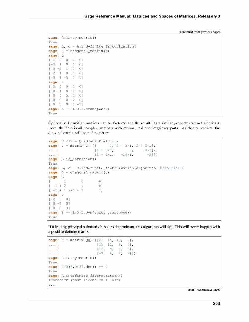
Sage Reference Manual: Matrices and Spaces of Matrices, Release 9.0
(continued from previous page)
sage: A.is_symmetric()Truesage: L, d = A.indefinite_factorization()sage: D = diagonal_matrix(d)sage: L[ 1 0 0 0 0][-2 1 0 0 0][ 3 -2 1 0 0][ 2 -1 0 1 0][-3 1 -3 1 1]sage: D[ 3 0 0 0 0][ 0 -1 0 0 0][ 0 0 5 0 0][ 0 0 0 -2 0][ 0 0 0 0 -1]sage: A == L*D*L.transpose()True
Optionally, Hermitian matrices can be factored and the result has a similar property (but not identical).Here, the field is all complex numbers with rational real and imaginary parts. As theory predicts, thediagonal entries will be real numbers.
sage: C.<I> = QuadraticField(-1)sage: B = matrix(C, [[ 2, 4 - 2*I, 2 + 2*I],....: [4 + 2*I, 8, 10*I],....: [2 - 2*I, -10*I, -3]])sage: B.is_hermitian()Truesage: L, d = B.indefinite_factorization(algorithm='hermitian')sage: D = diagonal_matrix(d)sage: L[ 1 0 0][ I + 2 1 0][ -I + 1 2*I + 1 1]sage: D[ 2 0 0][ 0 -2 0][ 0 0 3]sage: B == L*D*L.conjugate_transpose()True
If a leading principal submatrix has zero determinant, this algorithm will fail. This will never happen witha positive definite matrix.
sage: A = matrix(QQ, [[21, 15, 12, -2],....: [15, 12, 9, 6],....: [12, 9, 7, 3],....: [-2, 6, 3, 8]])sage: A.is_symmetric()Truesage: A[0:3,0:3].det() == 0Truesage: A.indefinite_factorization()Traceback (most recent call last):...
(continues on next page)
203
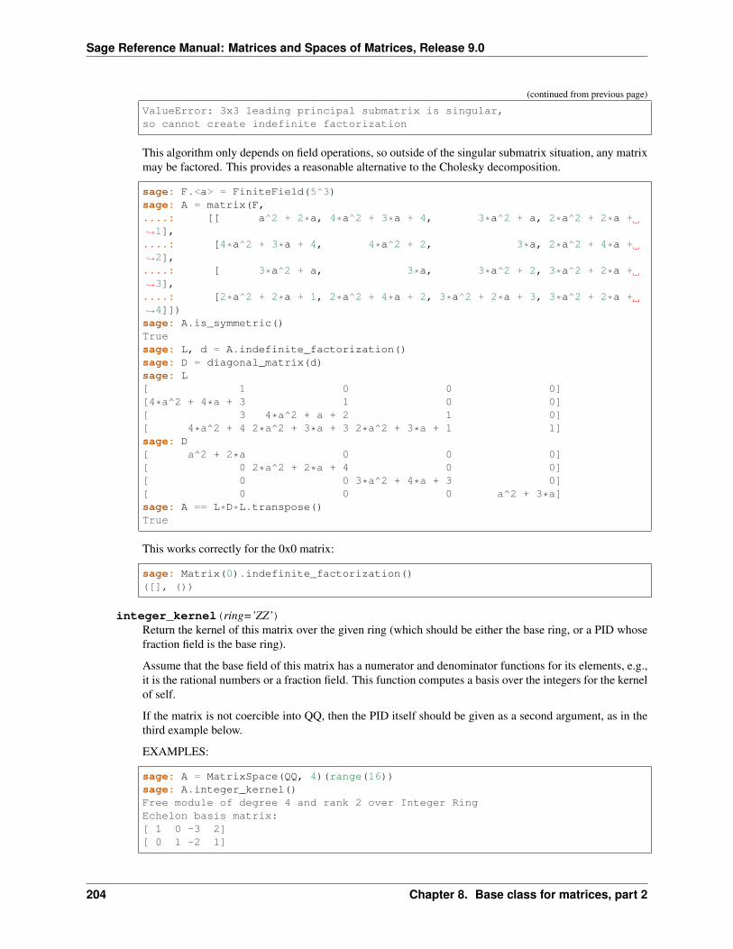
Sage Reference Manual: Matrices and Spaces of Matrices, Release 9.0
(continued from previous page)
ValueError: 3x3 leading principal submatrix is singular,so cannot create indefinite factorization
This algorithm only depends on field operations, so outside of the singular submatrix situation, any matrixmay be factored. This provides a reasonable alternative to the Cholesky decomposition.
sage: F.<a> = FiniteField(5^3)sage: A = matrix(F,....: [[ a^2 + 2*a, 4*a^2 + 3*a + 4, 3*a^2 + a, 2*a^2 + 2*a +→˓1],....: [4*a^2 + 3*a + 4, 4*a^2 + 2, 3*a, 2*a^2 + 4*a +→˓2],....: [ 3*a^2 + a, 3*a, 3*a^2 + 2, 3*a^2 + 2*a +→˓3],....: [2*a^2 + 2*a + 1, 2*a^2 + 4*a + 2, 3*a^2 + 2*a + 3, 3*a^2 + 2*a +→˓4]])sage: A.is_symmetric()Truesage: L, d = A.indefinite_factorization()sage: D = diagonal_matrix(d)sage: L[ 1 0 0 0][4*a^2 + 4*a + 3 1 0 0][ 3 4*a^2 + a + 2 1 0][ 4*a^2 + 4 2*a^2 + 3*a + 3 2*a^2 + 3*a + 1 1]sage: D[ a^2 + 2*a 0 0 0][ 0 2*a^2 + 2*a + 4 0 0][ 0 0 3*a^2 + 4*a + 3 0][ 0 0 0 a^2 + 3*a]sage: A == L*D*L.transpose()True
This works correctly for the 0x0 matrix:
sage: Matrix(0).indefinite_factorization()([], ())
integer_kernel(ring=’ZZ’)Return the kernel of this matrix over the given ring (which should be either the base ring, or a PID whosefraction field is the base ring).
Assume that the base field of this matrix has a numerator and denominator functions for its elements, e.g.,it is the rational numbers or a fraction field. This function computes a basis over the integers for the kernelof self.
If the matrix is not coercible into QQ, then the PID itself should be given as a second argument, as in thethird example below.
EXAMPLES:
sage: A = MatrixSpace(QQ, 4)(range(16))sage: A.integer_kernel()Free module of degree 4 and rank 2 over Integer RingEchelon basis matrix:[ 1 0 -3 2][ 0 1 -2 1]
204 Chapter 8. Base class for matrices, part 2
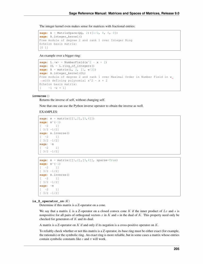
Sage Reference Manual: Matrices and Spaces of Matrices, Release 9.0
The integer kernel even makes sense for matrices with fractional entries:
sage: A = MatrixSpace(QQ, 2)([1/2, 0, 0, 0])sage: A.integer_kernel()Free module of degree 2 and rank 1 over Integer RingEchelon basis matrix:[0 1]
An example over a bigger ring:
sage: L.<w> = NumberField(x^2 - x + 2)sage: OL = L.ring_of_integers()sage: A = matrix(L, 2, [1, w/2])sage: A.integer_kernel(OL)Free module of degree 2 and rank 1 over Maximal Order in Number Field in w→˓with defining polynomial x^2 - x + 2Echelon basis matrix:[ -1 -w + 1]
inverse()Returns the inverse of self, without changing self.
Note that one can use the Python inverse operator to obtain the inverse as well.
EXAMPLES:
sage: m = matrix([[1,2],[3,4]])sage: m^(-1)[ -2 1][ 3/2 -1/2]sage: m.inverse()[ -2 1][ 3/2 -1/2]sage: ~m[ -2 1][ 3/2 -1/2]
sage: m = matrix([[1,2],[3,4]], sparse=True)sage: m^(-1)[ -2 1][ 3/2 -1/2]sage: m.inverse()[ -2 1][ 3/2 -1/2]sage: ~m[ -2 1][ 3/2 -1/2]
is_Z_operator_on(K)Determine if this matrix is a Z-operator on a cone.
We say that a matrix 𝐿 is a Z-operator on a closed convex cone 𝐾 if the inner product of 𝐿𝑥 and 𝑠 isnonpositive for all pairs of orthogonal vectors 𝑥 in 𝐾 and 𝑠 in the dual of 𝐾. This property need only bechecked for generators of 𝐾 and its dual.
A matrix is a Z-operator on 𝐾 if and only if its negation is a cross-positive operator on 𝐾.
To reliably check whether or not this matrix is a Z operator, its base ring must be either exact (for example,the rationals) or the symbolic ring. An exact ring is more reliable, but in some cases a matrix whose entriescontain symbolic constants like 𝑒 and 𝜋 will work.
205
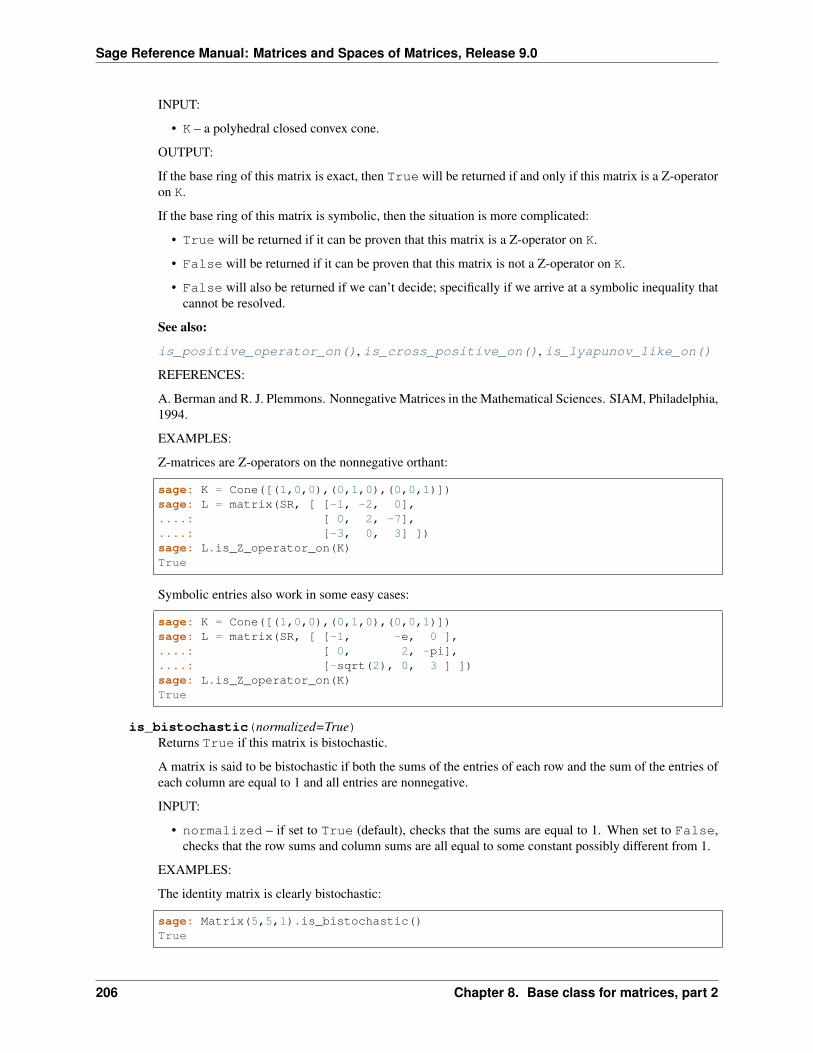
Sage Reference Manual: Matrices and Spaces of Matrices, Release 9.0
INPUT:
• K – a polyhedral closed convex cone.
OUTPUT:
If the base ring of this matrix is exact, then True will be returned if and only if this matrix is a Z-operatoron K.
If the base ring of this matrix is symbolic, then the situation is more complicated:
• True will be returned if it can be proven that this matrix is a Z-operator on K.
• False will be returned if it can be proven that this matrix is not a Z-operator on K.
• False will also be returned if we can’t decide; specifically if we arrive at a symbolic inequality thatcannot be resolved.
See also:
is_positive_operator_on(), is_cross_positive_on(), is_lyapunov_like_on()
REFERENCES:
A. Berman and R. J. Plemmons. Nonnegative Matrices in the Mathematical Sciences. SIAM, Philadelphia,1994.
EXAMPLES:
Z-matrices are Z-operators on the nonnegative orthant:
sage: K = Cone([(1,0,0),(0,1,0),(0,0,1)])sage: L = matrix(SR, [ [-1, -2, 0],....: [ 0, 2, -7],....: [-3, 0, 3] ])sage: L.is_Z_operator_on(K)True
Symbolic entries also work in some easy cases:
sage: K = Cone([(1,0,0),(0,1,0),(0,0,1)])sage: L = matrix(SR, [ [-1, -e, 0 ],....: [ 0, 2, -pi],....: [-sqrt(2), 0, 3 ] ])sage: L.is_Z_operator_on(K)True
is_bistochastic(normalized=True)Returns True if this matrix is bistochastic.
A matrix is said to be bistochastic if both the sums of the entries of each row and the sum of the entries ofeach column are equal to 1 and all entries are nonnegative.
INPUT:
• normalized – if set to True (default), checks that the sums are equal to 1. When set to False,checks that the row sums and column sums are all equal to some constant possibly different from 1.
EXAMPLES:
The identity matrix is clearly bistochastic:
sage: Matrix(5,5,1).is_bistochastic()True
206 Chapter 8. Base class for matrices, part 2
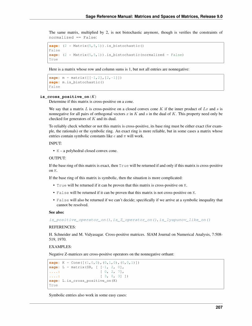
Sage Reference Manual: Matrices and Spaces of Matrices, Release 9.0
The same matrix, multiplied by 2, is not bistochastic anymore, though is verifies the constraints ofnormalized == False:
sage: (2 * Matrix(5,5,1)).is_bistochastic()Falsesage: (2 * Matrix(5,5,1)).is_bistochastic(normalized = False)True
Here is a matrix whose row and column sums is 1, but not all entries are nonnegative:
sage: m = matrix([[-1,2],[2,-1]])sage: m.is_bistochastic()False
is_cross_positive_on(K)Determine if this matrix is cross-positive on a cone.
We say that a matrix 𝐿 is cross-positive on a closed convex cone 𝐾 if the inner product of 𝐿𝑥 and 𝑠 isnonnegative for all pairs of orthogonal vectors 𝑥 in 𝐾 and 𝑠 in the dual of 𝐾. This property need only bechecked for generators of 𝐾 and its dual.
To reliably check whether or not this matrix is cross-positive, its base ring must be either exact (for exam-ple, the rationals) or the symbolic ring. An exact ring is more reliable, but in some cases a matrix whoseentries contain symbolic constants like 𝑒 and 𝜋 will work.
INPUT:
• K – a polyhedral closed convex cone.
OUTPUT:
If the base ring of this matrix is exact, then Truewill be returned if and only if this matrix is cross-positiveon K.
If the base ring of this matrix is symbolic, then the situation is more complicated:
• True will be returned if it can be proven that this matrix is cross-positive on K.
• False will be returned if it can be proven that this matrix is not cross-positive on K.
• False will also be returned if we can’t decide; specifically if we arrive at a symbolic inequality thatcannot be resolved.
See also:
is_positive_operator_on(), is_Z_operator_on(), is_lyapunov_like_on()
REFERENCES:
H. Schneider and M. Vidyasagar. Cross-positive matrices. SIAM Journal on Numerical Analysis, 7:508-519, 1970.
EXAMPLES:
Negative Z-matrices are cross-positive operators on the nonnegative orthant:
sage: K = Cone([(1,0,0),(0,1,0),(0,0,1)])sage: L = matrix(SR, [ [-1, 2, 0],....: [ 0, 2, 7],....: [ 3, 0, 3] ])sage: L.is_cross_positive_on(K)True
Symbolic entries also work in some easy cases:
207

Sage Reference Manual: Matrices and Spaces of Matrices, Release 9.0
sage: K = Cone([(1,0,0),(0,1,0),(0,0,1)])sage: L = matrix(SR, [ [-1, e, 0 ],....: [ 0, 2, pi],....: [ sqrt(2), 0, 3 ] ])sage: L.is_cross_positive_on(K)True
is_diagonalizable(base_field=None)Determine if the matrix is similar to a diagonal matrix.
INPUT:
• base_field - a new field to use for entries of the matrix.
OUTPUT:
If self is the matrix 𝐴, then it is diagonalizable if there is an invertible matrix 𝑃 and a diagonal matrix𝐷 such that
𝑃−1𝐴𝑃 = 𝐷
This routine returns True if self is diagonalizable. The diagonal entries of the matrix 𝐷 are the eigen-values of 𝐴.
A matrix not diagonalizable over the base field may become diagonalizable by extending the base field tocontain all of the eigenvalues. Over the rationals, the field of algebraic numbers, sage.rings.qqbaris a good choice.
To obtain the matrices 𝐷 and 𝑃 , use the diagonalization() method.
ALGORITHM:
For each eigenvalue, this routine checks that the algebraic multiplicity (number of occurrences as a root ofthe characteristic polynomial) is equal to the geometric multiplicity (dimension of the eigenspace), whichis sufficient to ensure a basis of eigenvectors for the columns of 𝑃 .
EXAMPLES:
A matrix that is diagonalizable over the rationals:
sage: A = matrix(QQ, [[-7, 16, 12, 0, 6],....: [-9, 15, 0, 12, -27],....: [ 9, -8, 11, -12, 51],....: [ 3, -4, 0, -1, 9],....: [-1, 0, -4, 4, -12]])sage: A.is_diagonalizable()Truesage: A.diagonalization()([ 2 0 0 0 0] [ 1 1 0 1 0][ 0 3 0 0 0] [ 1/2 0 1 0 1][ 0 0 3 0 0] [ 1/6 1 -3/2 2/3 -14/9][ 0 0 0 -1 0] [ -1/6 0 -1/4 0 -1/3][ 0 0 0 0 -1], [ -1/6 -1/3 1/3 -1/3 4/9])
This is a matrix not diagonalizable over the rationals, but you can still get its Jordan form.
sage: A = matrix(QQ, [[-3, -14, 2, -1, 15],....: [4, 6, -2, 3, -8],
(continues on next page)
208 Chapter 8. Base class for matrices, part 2
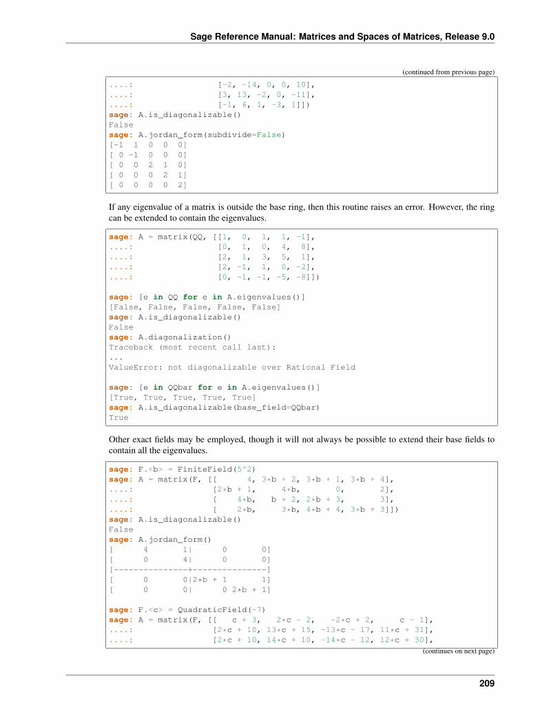
Sage Reference Manual: Matrices and Spaces of Matrices, Release 9.0
(continued from previous page)
....: [-2, -14, 0, 0, 10],
....: [3, 13, -2, 0, -11],
....: [-1, 6, 1, -3, 1]])sage: A.is_diagonalizable()Falsesage: A.jordan_form(subdivide=False)[-1 1 0 0 0][ 0 -1 0 0 0][ 0 0 2 1 0][ 0 0 0 2 1][ 0 0 0 0 2]
If any eigenvalue of a matrix is outside the base ring, then this routine raises an error. However, the ringcan be extended to contain the eigenvalues.
sage: A = matrix(QQ, [[1, 0, 1, 1, -1],....: [0, 1, 0, 4, 8],....: [2, 1, 3, 5, 1],....: [2, -1, 1, 0, -2],....: [0, -1, -1, -5, -8]])
sage: [e in QQ for e in A.eigenvalues()][False, False, False, False, False]sage: A.is_diagonalizable()Falsesage: A.diagonalization()Traceback (most recent call last):...ValueError: not diagonalizable over Rational Field
sage: [e in QQbar for e in A.eigenvalues()][True, True, True, True, True]sage: A.is_diagonalizable(base_field=QQbar)True
Other exact fields may be employed, though it will not always be possible to extend their base fields tocontain all the eigenvalues.
sage: F.<b> = FiniteField(5^2)sage: A = matrix(F, [[ 4, 3*b + 2, 3*b + 1, 3*b + 4],....: [2*b + 1, 4*b, 0, 2],....: [ 4*b, b + 2, 2*b + 3, 3],....: [ 2*b, 3*b, 4*b + 4, 3*b + 3]])sage: A.is_diagonalizable()Falsesage: A.jordan_form()[ 4 1| 0 0][ 0 4| 0 0][---------------+---------------][ 0 0|2*b + 1 1][ 0 0| 0 2*b + 1]
sage: F.<c> = QuadraticField(-7)sage: A = matrix(F, [[ c + 3, 2*c - 2, -2*c + 2, c - 1],....: [2*c + 10, 13*c + 15, -13*c - 17, 11*c + 31],....: [2*c + 10, 14*c + 10, -14*c - 12, 12*c + 30],
(continues on next page)
209
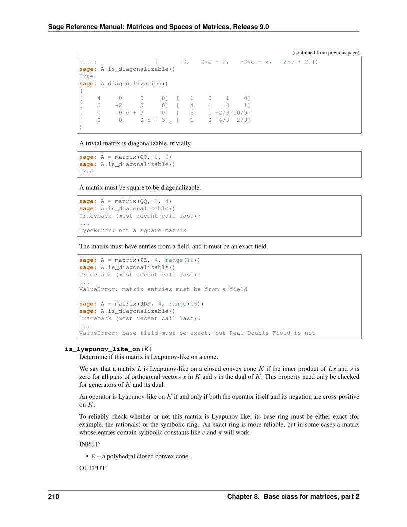
Sage Reference Manual: Matrices and Spaces of Matrices, Release 9.0
(continued from previous page)
....: [ 0, 2*c - 2, -2*c + 2, 2*c + 2]])sage: A.is_diagonalizable()Truesage: A.diagonalization()([ 4 0 0 0] [ 1 0 1 0][ 0 -2 0 0] [ 4 1 0 1][ 0 0 c + 3 0] [ 5 1 -2/9 10/9][ 0 0 0 c + 3], [ 1 0 -4/9 2/9])
A trivial matrix is diagonalizable, trivially.
sage: A = matrix(QQ, 0, 0)sage: A.is_diagonalizable()True
A matrix must be square to be diagonalizable.
sage: A = matrix(QQ, 3, 4)sage: A.is_diagonalizable()Traceback (most recent call last):...TypeError: not a square matrix
The matrix must have entries from a field, and it must be an exact field.
sage: A = matrix(ZZ, 4, range(16))sage: A.is_diagonalizable()Traceback (most recent call last):...ValueError: matrix entries must be from a field
sage: A = matrix(RDF, 4, range(16))sage: A.is_diagonalizable()Traceback (most recent call last):...ValueError: base field must be exact, but Real Double Field is not
is_lyapunov_like_on(K)Determine if this matrix is Lyapunov-like on a cone.
We say that a matrix 𝐿 is Lyapunov-like on a closed convex cone 𝐾 if the inner product of 𝐿𝑥 and 𝑠 iszero for all pairs of orthogonal vectors 𝑥 in 𝐾 and 𝑠 in the dual of 𝐾. This property need only be checkedfor generators of 𝐾 and its dual.
An operator is Lyapunov-like on 𝐾 if and only if both the operator itself and its negation are cross-positiveon 𝐾.
To reliably check whether or not this matrix is Lyapunov-like, its base ring must be either exact (forexample, the rationals) or the symbolic ring. An exact ring is more reliable, but in some cases a matrixwhose entries contain symbolic constants like 𝑒 and 𝜋 will work.
INPUT:
• K – a polyhedral closed convex cone.
OUTPUT:
210 Chapter 8. Base class for matrices, part 2
Sage Reference Manual: Matrices and Spaces of Matrices, Release 9.0
If the base ring of this matrix is exact, then Truewill be returned if and only if this matrix is Lyapunov-likeon K.
If the base ring of this matrix is symbolic, then the situation is more complicated:
• True will be returned if it can be proven that this matrix is Lyapunov-like on K.
• False will be returned if it can be proven that this matrix is not Lyapunov-like on K.
• False will also be returned if we can’t decide; specifically if we arrive at a symbolic inequality thatcannot be resolved.
See also:
is_positive_operator_on(), is_cross_positive_on(), is_Z_operator_on()
REFERENCES:
• [Or2017]
EXAMPLES:
Diagonal matrices are Lyapunov-like operators on the nonnegative orthant:
sage: set_random_seed()sage: K = Cone([(1,0,0),(0,1,0),(0,0,1)])sage: L = diagonal_matrix(random_vector(QQ,3))sage: L.is_lyapunov_like_on(K)True
Symbolic entries also work in some easy cases:
sage: K = Cone([(1,0,0),(0,1,0),(0,0,1)])sage: L = matrix(SR, [ [e, 0, 0 ],....: [0, pi, 0 ],....: [0, 0, sqrt(2)] ])sage: L.is_lyapunov_like_on(K)True
is_normal()Returns True if the matrix commutes with its conjugate-transpose.
OUTPUT:
True if the matrix is square and commutes with its conjugate-transpose, and False otherwise.
Normal matrices are precisely those that can be diagonalized by a unitary matrix.
This routine is for matrices over exact rings and so may not work properly for matrices over RR or CC.For matrices with approximate entries, the rings of double-precision floating-point numbers, RDF and CDF,are a better choice since the sage.matrix.matrix_double_dense.Matrix_double_dense.is_normal() method has a tolerance parameter. This provides control over allowing for minor discrep-ancies between entries when checking equality.
The result is cached.
EXAMPLES:
Hermitian matrices are normal.
sage: A = matrix(QQ, 5, 5, range(25)) + I*matrix(QQ, 5, 5, range(0, 50, 2))sage: B = A*A.conjugate_transpose()sage: B.is_hermitian()
(continues on next page)
211
Sage Reference Manual: Matrices and Spaces of Matrices, Release 9.0
(continued from previous page)
Truesage: B.is_normal()True
Circulant matrices are normal.
sage: G = graphs.CirculantGraph(20, [3, 7])sage: D = digraphs.Circuit(20)sage: A = 3*D.adjacency_matrix() - 5*G.adjacency_matrix()sage: A.is_normal()True
Skew-symmetric matrices are normal.
sage: A = matrix(QQ, 5, 5, range(25))sage: B = A - A.transpose()sage: B.is_skew_symmetric()Truesage: B.is_normal()True
A small matrix that does not fit into any of the usual categories of normal matrices.
sage: A = matrix(ZZ, [[1, -1],....: [1, 1]])sage: A.is_normal()Truesage: not A.is_hermitian() and not A.is_skew_symmetric()True
Sage has several fields besides the entire complex numbers where conjugation is non-trivial.
sage: F.<b> = QuadraticField(-7)sage: C = matrix(F, [[-2*b - 3, 7*b - 6, -b + 3],....: [-2*b - 3, -3*b + 2, -2*b],....: [ b + 1, 0, -2]])sage: C = C*C.conjugate_transpose()sage: C.is_normal()True
A matrix that is nearly normal, but for a non-real diagonal entry.
sage: A = matrix(QQbar, [[ 2, 2-I, 1+4*I],....: [ 2+I, 3+I, 2-6*I],....: [1-4*I, 2+6*I, 5]])sage: A.is_normal()Falsesage: A[1,1] = 132sage: A.is_normal()True
Rectangular matrices are never normal.
sage: A = matrix(QQbar, 3, 4)sage: A.is_normal()False
212 Chapter 8. Base class for matrices, part 2
Sage Reference Manual: Matrices and Spaces of Matrices, Release 9.0
A square, empty matrix is trivially normal.
sage: A = matrix(QQ, 0, 0)sage: A.is_normal()True
is_one()Return True if this matrix is the identity matrix.
EXAMPLES:
sage: m = matrix(QQ,2,2,range(4))sage: m.is_one()Falsesage: m = matrix(QQ,2,[5,0,0,5])sage: m.is_one()Falsesage: m = matrix(QQ,2,[1,0,0,1])sage: m.is_one()Truesage: m = matrix(QQ,2,[1,1,1,1])sage: m.is_one()False
is_permutation_of(N, check=False)Return True if there exists a permutation of rows and columns sending self to N and False otherwise.
INPUT:
• N – a matrix.
• check – boolean (default: False). If False return Boolean indicating whether there exists apermutation of rows and columns sending self to N and False otherwise. If True return a tupleof a Boolean and a permutation mapping self to N if such a permutation exists, and (False,None) if it does not.
OUTPUT:
A Boolean or a tuple of a Boolean and a permutation.
EXAMPLES:
sage: M = matrix(ZZ,[[1,2,3],[3,5,3],[2,6,4]])sage: M[1 2 3][3 5 3][2 6 4]sage: N = matrix(ZZ,[[1,2,3],[2,6,4],[3,5,3]])sage: N[1 2 3][2 6 4][3 5 3]sage: M.is_permutation_of(N)True
Some examples that are not permutations of each other:
sage: N = matrix(ZZ,[[1,2,3],[4,5,6],[7,8,9]])sage: N[1 2 3]
(continues on next page)
213
Sage Reference Manual: Matrices and Spaces of Matrices, Release 9.0
(continued from previous page)
[4 5 6][7 8 9]sage: M.is_permutation_of(N)Falsesage: N = matrix(ZZ,[[1,2],[3,4]])sage: N[1 2][3 4]sage: M.is_permutation_of(N)False
And for when check is True:
sage: N = matrix(ZZ,[[3,5,3],[2,6,4],[1,2,3]])sage: N[3 5 3][2 6 4][1 2 3]sage: r = M.is_permutation_of(N, check=True)sage: r(True, ((1,2,3), ()))sage: p = r[1]sage: M.with_permuted_rows_and_columns(*p) == NTrue
is_positive_definite(certificate=False)Determines if a real or symmetric matrix is positive definite.
A square matrix 𝐴 is positive definite if it is symmetric with real entries or Hermitian with complex entries,and for every non-zero vector �⃗�
�⃗�*𝐴�⃗� > 0.
Here �⃗�* is the conjugate-transpose, which can be simplified to just the transpose in the real case.
ALGORITHM:
A matrix is positive definite if and only if the diagonal entries from the indefinite factorization are all posi-tive (see indefinite_factorization()). So this algorithm is of order n^3/3 and may be appliedto matrices with elements of any ring that has a fraction field contained within the reals or complexes.
INPUT:
Any square matrix.
• certificate – (default: False) return the decomposition from the indefinite factorization ifpossible
OUTPUT:
This routine will return True if the matrix is square, symmetric or Hermitian, and meets the conditionabove for the quadratic form.
The base ring for the elements of the matrix needs to have a fraction field implemented and the computa-tions that result from the indefinite factorization must be convertible to real numbers that are comparableto zero.
EXAMPLES:
A real symmetric matrix that is positive definite, as evidenced by the positive entries for the diagonalmatrix of the indefinite factorization and the positive determinants of the leading principal submatrices.
214 Chapter 8. Base class for matrices, part 2
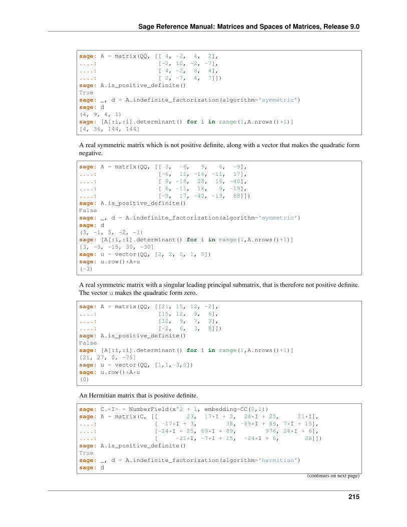
Sage Reference Manual: Matrices and Spaces of Matrices, Release 9.0
sage: A = matrix(QQ, [[ 4, -2, 4, 2],....: [-2, 10, -2, -7],....: [ 4, -2, 8, 4],....: [ 2, -7, 4, 7]])sage: A.is_positive_definite()Truesage: _, d = A.indefinite_factorization(algorithm='symmetric')sage: d(4, 9, 4, 1)sage: [A[:i,:i].determinant() for i in range(1,A.nrows()+1)][4, 36, 144, 144]
A real symmetric matrix which is not positive definite, along with a vector that makes the quadratic formnegative.
sage: A = matrix(QQ, [[ 3, -6, 9, 6, -9],....: [-6, 11, -16, -11, 17],....: [ 9, -16, 28, 16, -40],....: [ 6, -11, 16, 9, -19],....: [-9, 17, -40, -19, 68]])sage: A.is_positive_definite()Falsesage: _, d = A.indefinite_factorization(algorithm='symmetric')sage: d(3, -1, 5, -2, -1)sage: [A[:i,:i].determinant() for i in range(1,A.nrows()+1)][3, -3, -15, 30, -30]sage: u = vector(QQ, [2, 2, 0, 1, 0])sage: u.row()*A*u(-3)
A real symmetric matrix with a singular leading principal submatrix, that is therefore not positive definite.The vector u makes the quadratic form zero.
sage: A = matrix(QQ, [[21, 15, 12, -2],....: [15, 12, 9, 6],....: [12, 9, 7, 3],....: [-2, 6, 3, 8]])sage: A.is_positive_definite()Falsesage: [A[:i,:i].determinant() for i in range(1,A.nrows()+1)][21, 27, 0, -75]sage: u = vector(QQ, [1,1,-3,0])sage: u.row()*A*u(0)
An Hermitian matrix that is positive definite.
sage: C.<I> = NumberField(x^2 + 1, embedding=CC(0,1))sage: A = matrix(C, [[ 23, 17*I + 3, 24*I + 25, 21*I],....: [ -17*I + 3, 38, -69*I + 89, 7*I + 15],....: [-24*I + 25, 69*I + 89, 976, 24*I + 6],....: [ -21*I, -7*I + 15, -24*I + 6, 28]])sage: A.is_positive_definite()Truesage: _, d = A.indefinite_factorization(algorithm='hermitian')sage: d
(continues on next page)
215
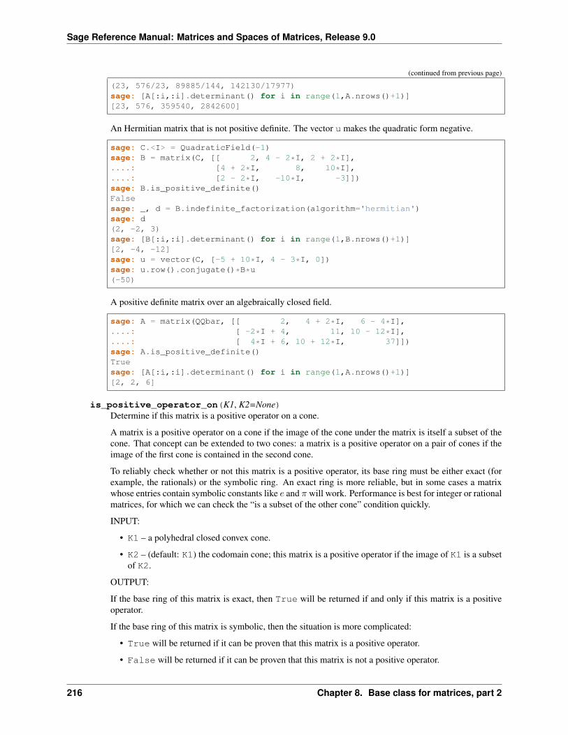
Sage Reference Manual: Matrices and Spaces of Matrices, Release 9.0
(continued from previous page)
(23, 576/23, 89885/144, 142130/17977)sage: [A[:i,:i].determinant() for i in range(1,A.nrows()+1)][23, 576, 359540, 2842600]
An Hermitian matrix that is not positive definite. The vector u makes the quadratic form negative.
sage: C.<I> = QuadraticField(-1)sage: B = matrix(C, [[ 2, 4 - 2*I, 2 + 2*I],....: [4 + 2*I, 8, 10*I],....: [2 - 2*I, -10*I, -3]])sage: B.is_positive_definite()Falsesage: _, d = B.indefinite_factorization(algorithm='hermitian')sage: d(2, -2, 3)sage: [B[:i,:i].determinant() for i in range(1,B.nrows()+1)][2, -4, -12]sage: u = vector(C, [-5 + 10*I, 4 - 3*I, 0])sage: u.row().conjugate()*B*u(-50)
A positive definite matrix over an algebraically closed field.
sage: A = matrix(QQbar, [[ 2, 4 + 2*I, 6 - 4*I],....: [ -2*I + 4, 11, 10 - 12*I],....: [ 4*I + 6, 10 + 12*I, 37]])sage: A.is_positive_definite()Truesage: [A[:i,:i].determinant() for i in range(1,A.nrows()+1)][2, 2, 6]
is_positive_operator_on(K1, K2=None)Determine if this matrix is a positive operator on a cone.
A matrix is a positive operator on a cone if the image of the cone under the matrix is itself a subset of thecone. That concept can be extended to two cones: a matrix is a positive operator on a pair of cones if theimage of the first cone is contained in the second cone.
To reliably check whether or not this matrix is a positive operator, its base ring must be either exact (forexample, the rationals) or the symbolic ring. An exact ring is more reliable, but in some cases a matrixwhose entries contain symbolic constants like 𝑒 and 𝜋 will work. Performance is best for integer or rationalmatrices, for which we can check the “is a subset of the other cone” condition quickly.
INPUT:
• K1 – a polyhedral closed convex cone.
• K2 – (default: K1) the codomain cone; this matrix is a positive operator if the image of K1 is a subsetof K2.
OUTPUT:
If the base ring of this matrix is exact, then True will be returned if and only if this matrix is a positiveoperator.
If the base ring of this matrix is symbolic, then the situation is more complicated:
• True will be returned if it can be proven that this matrix is a positive operator.
• False will be returned if it can be proven that this matrix is not a positive operator.
216 Chapter 8. Base class for matrices, part 2
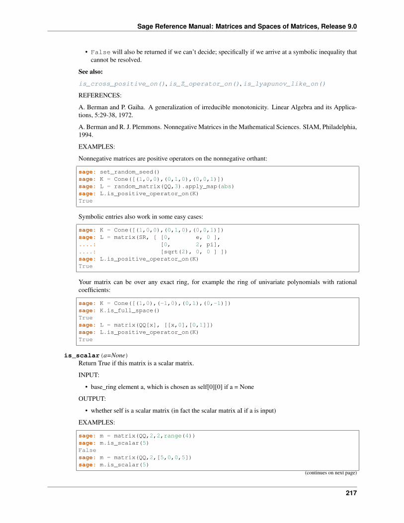
Sage Reference Manual: Matrices and Spaces of Matrices, Release 9.0
• False will also be returned if we can’t decide; specifically if we arrive at a symbolic inequality thatcannot be resolved.
See also:
is_cross_positive_on(), is_Z_operator_on(), is_lyapunov_like_on()
REFERENCES:
A. Berman and P. Gaiha. A generalization of irreducible monotonicity. Linear Algebra and its Applica-tions, 5:29-38, 1972.
A. Berman and R. J. Plemmons. Nonnegative Matrices in the Mathematical Sciences. SIAM, Philadelphia,1994.
EXAMPLES:
Nonnegative matrices are positive operators on the nonnegative orthant:
sage: set_random_seed()sage: K = Cone([(1,0,0),(0,1,0),(0,0,1)])sage: L = random_matrix(QQ,3).apply_map(abs)sage: L.is_positive_operator_on(K)True
Symbolic entries also work in some easy cases:
sage: K = Cone([(1,0,0),(0,1,0),(0,0,1)])sage: L = matrix(SR, [ [0, e, 0 ],....: [0, 2, pi],....: [sqrt(2), 0, 0 ] ])sage: L.is_positive_operator_on(K)True
Your matrix can be over any exact ring, for example the ring of univariate polynomials with rationalcoefficients:
sage: K = Cone([(1,0),(-1,0),(0,1),(0,-1)])sage: K.is_full_space()Truesage: L = matrix(QQ[x], [[x,0],[0,1]])sage: L.is_positive_operator_on(K)True
is_scalar(a=None)Return True if this matrix is a scalar matrix.
INPUT:
• base_ring element a, which is chosen as self[0][0] if a = None
OUTPUT:
• whether self is a scalar matrix (in fact the scalar matrix aI if a is input)
EXAMPLES:
sage: m = matrix(QQ,2,2,range(4))sage: m.is_scalar(5)Falsesage: m = matrix(QQ,2,[5,0,0,5])sage: m.is_scalar(5)
(continues on next page)
217
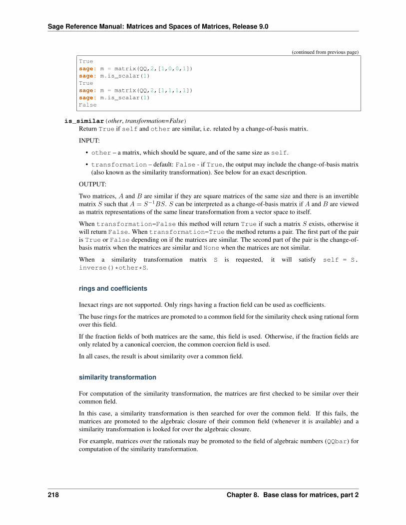
Sage Reference Manual: Matrices and Spaces of Matrices, Release 9.0
(continued from previous page)
Truesage: m = matrix(QQ,2,[1,0,0,1])sage: m.is_scalar(1)Truesage: m = matrix(QQ,2,[1,1,1,1])sage: m.is_scalar(1)False
is_similar(other, transformation=False)Return True if self and other are similar, i.e. related by a change-of-basis matrix.
INPUT:
• other – a matrix, which should be square, and of the same size as self.
• transformation – default: False - if True, the output may include the change-of-basis matrix(also known as the similarity transformation). See below for an exact description.
OUTPUT:
Two matrices, 𝐴 and 𝐵 are similar if they are square matrices of the same size and there is an invertiblematrix 𝑆 such that 𝐴 = 𝑆−1𝐵𝑆. 𝑆 can be interpreted as a change-of-basis matrix if 𝐴 and 𝐵 are viewedas matrix representations of the same linear transformation from a vector space to itself.
When transformation=False this method will return True if such a matrix 𝑆 exists, otherwise itwill return False. When transformation=True the method returns a pair. The first part of the pairis True or False depending on if the matrices are similar. The second part of the pair is the change-of-basis matrix when the matrices are similar and None when the matrices are not similar.
When a similarity transformation matrix S is requested, it will satisfy self = S.inverse()*other*S.
rings and coefficients
Inexact rings are not supported. Only rings having a fraction field can be used as coefficients.
The base rings for the matrices are promoted to a common field for the similarity check using rational formover this field.
If the fraction fields of both matrices are the same, this field is used. Otherwise, if the fraction fields areonly related by a canonical coercion, the common coercion field is used.
In all cases, the result is about similarity over a common field.
similarity transformation
For computation of the similarity transformation, the matrices are first checked to be similar over theircommon field.
In this case, a similarity transformation is then searched for over the common field. If this fails, thematrices are promoted to the algebraic closure of their common field (whenever it is available) and asimilarity transformation is looked for over the algebraic closure.
For example, matrices over the rationals may be promoted to the field of algebraic numbers (QQbar) forcomputation of the similarity transformation.
218 Chapter 8. Base class for matrices, part 2
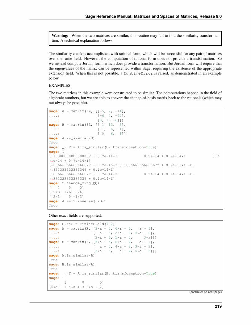
Sage Reference Manual: Matrices and Spaces of Matrices, Release 9.0
Warning: When the two matrices are similar, this routine may fail to find the similarity transforma-tion. A technical explanation follows.
The similarity check is accomplished with rational form, which will be successful for any pair of matricesover the same field. However, the computation of rational form does not provide a transformation. Sowe instead compute Jordan form, which does provide a transformation. But Jordan form will require thatthe eigenvalues of the matrix can be represented within Sage, requiring the existence of the appropriateextension field. When this is not possible, a RuntimeError is raised, as demonstrated in an examplebelow.
EXAMPLES:
The two matrices in this example were constructed to be similar. The computations happen in the field ofalgebraic numbers, but we are able to convert the change-of-basis matrix back to the rationals (which maynot always be possible).
sage: A = matrix(ZZ, [[-5, 2, -11],....: [-6, 7, -42],....: [0, 1, -6]])sage: B = matrix(ZZ, [[ 1, 12, 3],....: [-1, -6, -1],....: [ 0, 6, 1]])sage: A.is_similar(B)Truesage: _, T = A.is_similar(B, transformation=True)sage: T[ 1.00000000000000? + 0.?e-14*I 0.?e-14 + 0.?e-14*I 0.?→˓e-14 + 0.?e-14*I][-0.66666666666667? + 0.?e-15*I 0.166666666666667? + 0.?e-15*I -0.→˓83333333333334? + 0.?e-14*I][ 0.66666666666667? + 0.?e-14*I 0.?e-14 + 0.?e-14*I -0.→˓33333333333333? + 0.?e-14*I]sage: T.change_ring(QQ)[ 1 0 0][-2/3 1/6 -5/6][ 2/3 0 -1/3]sage: A == T.inverse()*B*TTrue
Other exact fields are supported.
sage: F.<a> = FiniteField(7^2)sage: A = matrix(F,[[2*a + 5, 6*a + 6, a + 3],....: [ a + 3, 2*a + 2, 4*a + 2],....: [2*a + 6, 5*a + 5, 3*a]])sage: B = matrix(F,[[5*a + 5, 6*a + 4, a + 1],....: [ a + 5, 4*a + 3, 3*a + 3],....: [3*a + 5, a + 4, 5*a + 6]])sage: A.is_similar(B)Truesage: B.is_similar(A)Truesage: _, T = A.is_similar(B, transformation=True)sage: T[ 1 0 0][6*a + 1 4*a + 3 4*a + 2]
(continues on next page)
219
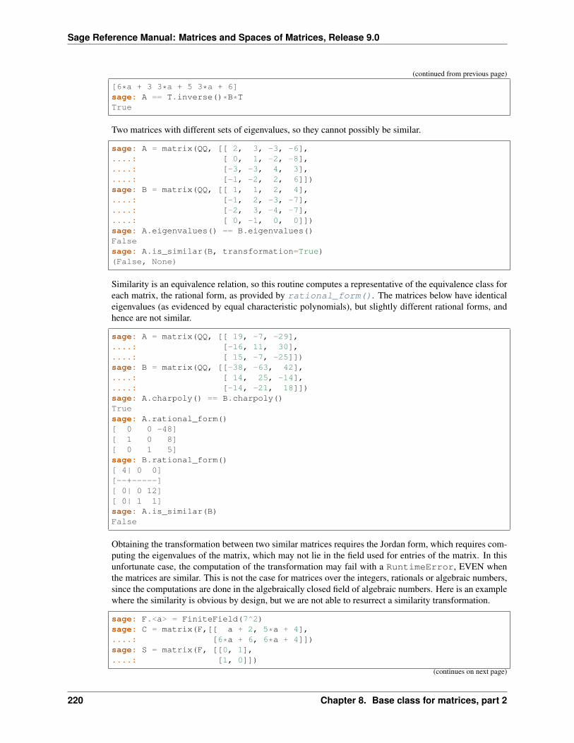
Sage Reference Manual: Matrices and Spaces of Matrices, Release 9.0
(continued from previous page)
[6*a + 3 3*a + 5 3*a + 6]sage: A == T.inverse()*B*TTrue
Two matrices with different sets of eigenvalues, so they cannot possibly be similar.
sage: A = matrix(QQ, [[ 2, 3, -3, -6],....: [ 0, 1, -2, -8],....: [-3, -3, 4, 3],....: [-1, -2, 2, 6]])sage: B = matrix(QQ, [[ 1, 1, 2, 4],....: [-1, 2, -3, -7],....: [-2, 3, -4, -7],....: [ 0, -1, 0, 0]])sage: A.eigenvalues() == B.eigenvalues()Falsesage: A.is_similar(B, transformation=True)(False, None)
Similarity is an equivalence relation, so this routine computes a representative of the equivalence class foreach matrix, the rational form, as provided by rational_form(). The matrices below have identicaleigenvalues (as evidenced by equal characteristic polynomials), but slightly different rational forms, andhence are not similar.
sage: A = matrix(QQ, [[ 19, -7, -29],....: [-16, 11, 30],....: [ 15, -7, -25]])sage: B = matrix(QQ, [[-38, -63, 42],....: [ 14, 25, -14],....: [-14, -21, 18]])sage: A.charpoly() == B.charpoly()Truesage: A.rational_form()[ 0 0 -48][ 1 0 8][ 0 1 5]sage: B.rational_form()[ 4| 0 0][--+-----][ 0| 0 12][ 0| 1 1]sage: A.is_similar(B)False
Obtaining the transformation between two similar matrices requires the Jordan form, which requires com-puting the eigenvalues of the matrix, which may not lie in the field used for entries of the matrix. In thisunfortunate case, the computation of the transformation may fail with a RuntimeError, EVEN whenthe matrices are similar. This is not the case for matrices over the integers, rationals or algebraic numbers,since the computations are done in the algebraically closed field of algebraic numbers. Here is an examplewhere the similarity is obvious by design, but we are not able to resurrect a similarity transformation.
sage: F.<a> = FiniteField(7^2)sage: C = matrix(F,[[ a + 2, 5*a + 4],....: [6*a + 6, 6*a + 4]])sage: S = matrix(F, [[0, 1],....: [1, 0]])
(continues on next page)
220 Chapter 8. Base class for matrices, part 2
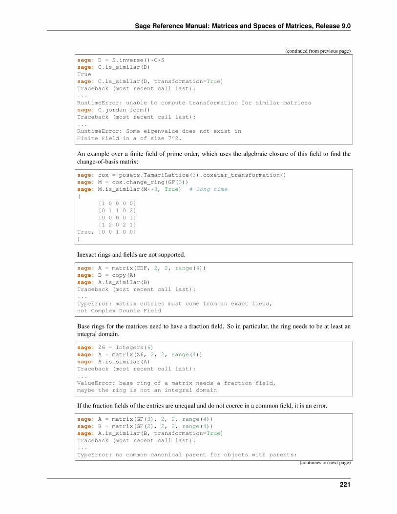
Sage Reference Manual: Matrices and Spaces of Matrices, Release 9.0
(continued from previous page)
sage: D = S.inverse()*C*Ssage: C.is_similar(D)Truesage: C.is_similar(D, transformation=True)Traceback (most recent call last):...RuntimeError: unable to compute transformation for similar matricessage: C.jordan_form()Traceback (most recent call last):...RuntimeError: Some eigenvalue does not exist inFinite Field in a of size 7^2.
An example over a finite field of prime order, which uses the algebraic closure of this field to find thechange-of-basis matrix:
sage: cox = posets.TamariLattice(3).coxeter_transformation()sage: M = cox.change_ring(GF(3))sage: M.is_similar(M**3, True) # long time(
[1 0 0 0 0][0 1 1 0 2][0 0 0 0 1][1 2 0 2 1]
True, [0 0 1 0 0])
Inexact rings and fields are not supported.
sage: A = matrix(CDF, 2, 2, range(4))sage: B = copy(A)sage: A.is_similar(B)Traceback (most recent call last):...TypeError: matrix entries must come from an exact field,not Complex Double Field
Base rings for the matrices need to have a fraction field. So in particular, the ring needs to be at least anintegral domain.
sage: Z6 = Integers(6)sage: A = matrix(Z6, 2, 2, range(4))sage: A.is_similar(A)Traceback (most recent call last):...ValueError: base ring of a matrix needs a fraction field,maybe the ring is not an integral domain
If the fraction fields of the entries are unequal and do not coerce in a common field, it is an error.
sage: A = matrix(GF(3), 2, 2, range(4))sage: B = matrix(GF(2), 2, 2, range(4))sage: A.is_similar(B, transformation=True)Traceback (most recent call last):...TypeError: no common canonical parent for objects with parents:
(continues on next page)
221
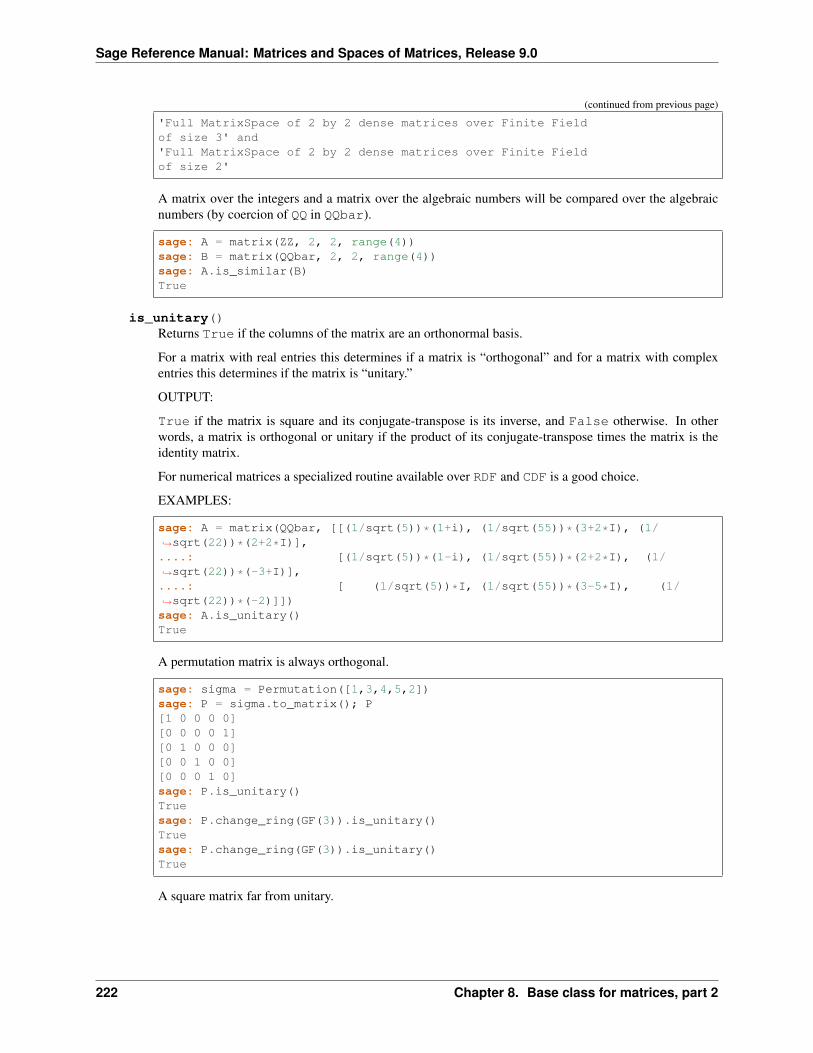
Sage Reference Manual: Matrices and Spaces of Matrices, Release 9.0
(continued from previous page)
'Full MatrixSpace of 2 by 2 dense matrices over Finite Fieldof size 3' and'Full MatrixSpace of 2 by 2 dense matrices over Finite Fieldof size 2'
A matrix over the integers and a matrix over the algebraic numbers will be compared over the algebraicnumbers (by coercion of QQ in QQbar).
sage: A = matrix(ZZ, 2, 2, range(4))sage: B = matrix(QQbar, 2, 2, range(4))sage: A.is_similar(B)True
is_unitary()Returns True if the columns of the matrix are an orthonormal basis.
For a matrix with real entries this determines if a matrix is “orthogonal” and for a matrix with complexentries this determines if the matrix is “unitary.”
OUTPUT:
True if the matrix is square and its conjugate-transpose is its inverse, and False otherwise. In otherwords, a matrix is orthogonal or unitary if the product of its conjugate-transpose times the matrix is theidentity matrix.
For numerical matrices a specialized routine available over RDF and CDF is a good choice.
EXAMPLES:
sage: A = matrix(QQbar, [[(1/sqrt(5))*(1+i), (1/sqrt(55))*(3+2*I), (1/→˓sqrt(22))*(2+2*I)],....: [(1/sqrt(5))*(1-i), (1/sqrt(55))*(2+2*I), (1/→˓sqrt(22))*(-3+I)],....: [ (1/sqrt(5))*I, (1/sqrt(55))*(3-5*I), (1/→˓sqrt(22))*(-2)]])sage: A.is_unitary()True
A permutation matrix is always orthogonal.
sage: sigma = Permutation([1,3,4,5,2])sage: P = sigma.to_matrix(); P[1 0 0 0 0][0 0 0 0 1][0 1 0 0 0][0 0 1 0 0][0 0 0 1 0]sage: P.is_unitary()Truesage: P.change_ring(GF(3)).is_unitary()Truesage: P.change_ring(GF(3)).is_unitary()True
A square matrix far from unitary.
222 Chapter 8. Base class for matrices, part 2
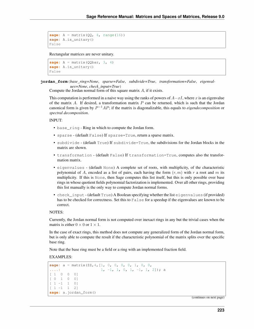
Sage Reference Manual: Matrices and Spaces of Matrices, Release 9.0
sage: A = matrix(QQ, 4, range(16))sage: A.is_unitary()False
Rectangular matrices are never unitary.
sage: A = matrix(QQbar, 3, 4)sage: A.is_unitary()False
jordan_form(base_ring=None, sparse=False, subdivide=True, transformation=False, eigenval-ues=None, check_input=True)
Compute the Jordan normal form of this square matrix 𝐴, if it exists.
This computation is performed in a naive way using the ranks of powers of 𝐴−𝑥𝐼 , where 𝑥 is an eigenvalueof the matrix 𝐴. If desired, a transformation matrix 𝑃 can be returned, which is such that the Jordancanonical form is given by 𝑃−1𝐴𝑃 ; if the matrix is diagonalizable, this equals to eigendecomposition orspectral decomposition.
INPUT:
• base_ring - Ring in which to compute the Jordan form.
• sparse - (default False) If sparse=True, return a sparse matrix.
• subdivide - (default True) If subdivide=True, the subdivisions for the Jordan blocks in thematrix are shown.
• transformation - (default False) If transformation=True, computes also the transfor-mation matrix.
• eigenvalues - (default None) A complete set of roots, with multiplicity, of the characteristicpolynomial of 𝐴, encoded as a list of pairs, each having the form (𝑟,𝑚) with 𝑟 a root and 𝑚 itsmultiplicity. If this is None, then Sage computes this list itself, but this is only possible over baserings in whose quotient fields polynomial factorization is implemented. Over all other rings, providingthis list manually is the only way to compute Jordan normal forms.
• check_input - (default True) A Boolean specifying whether the list eigenvalues (if provided)has to be checked for correctness. Set this to False for a speedup if the eigenvalues are known to becorrect.
NOTES:
Currently, the Jordan normal form is not computed over inexact rings in any but the trivial cases when thematrix is either 0× 0 or 1× 1.
In the case of exact rings, this method does not compute any generalized form of the Jordan normal form,but is only able to compute the result if the characteristic polynomial of the matrix splits over the specificbase ring.
Note that the base ring must be a field or a ring with an implemented fraction field.
EXAMPLES:
sage: a = matrix(ZZ,4,[1, 0, 0, 0, 0, 1, 0, 0,....: 1, -1, 1, 0, 1, -1, 1, 2]); a[ 1 0 0 0][ 0 1 0 0][ 1 -1 1 0][ 1 -1 1 2]sage: a.jordan_form()
(continues on next page)
223
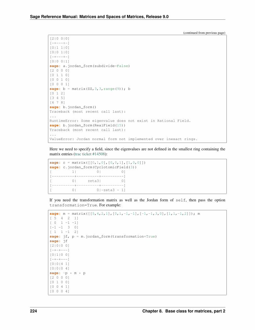
Sage Reference Manual: Matrices and Spaces of Matrices, Release 9.0
(continued from previous page)
[2|0 0|0][-+---+-][0|1 1|0][0|0 1|0][-+---+-][0|0 0|1]sage: a.jordan_form(subdivide=False)[2 0 0 0][0 1 1 0][0 0 1 0][0 0 0 1]sage: b = matrix(ZZ,3,3,range(9)); b[0 1 2][3 4 5][6 7 8]sage: b.jordan_form()Traceback (most recent call last):...RuntimeError: Some eigenvalue does not exist in Rational Field.sage: b.jordan_form(RealField(15))Traceback (most recent call last):...ValueError: Jordan normal form not implemented over inexact rings.
Here we need to specify a field, since the eigenvalues are not defined in the smallest ring containing thematrix entries (trac ticket #14508):
sage: c = matrix([[0,1,0],[0,0,1],[1,0,0]])sage: c.jordan_form(CyclotomicField(3))[ 1| 0| 0][----------+----------+----------][ 0| zeta3| 0][----------+----------+----------][ 0| 0|-zeta3 - 1]
If you need the transformation matrix as well as the Jordan form of self, then pass the optiontransformation=True. For example:
sage: m = matrix([[5,4,2,1],[0,1,-1,-1],[-1,-1,3,0],[1,1,-1,2]]); m[ 5 4 2 1][ 0 1 -1 -1][-1 -1 3 0][ 1 1 -1 2]sage: jf, p = m.jordan_form(transformation=True)sage: jf[2|0|0 0][-+-+---][0|1|0 0][-+-+---][0|0|4 1][0|0|0 4]sage: ~p * m * p[2 0 0 0][0 1 0 0][0 0 4 1][0 0 0 4]
224 Chapter 8. Base class for matrices, part 2
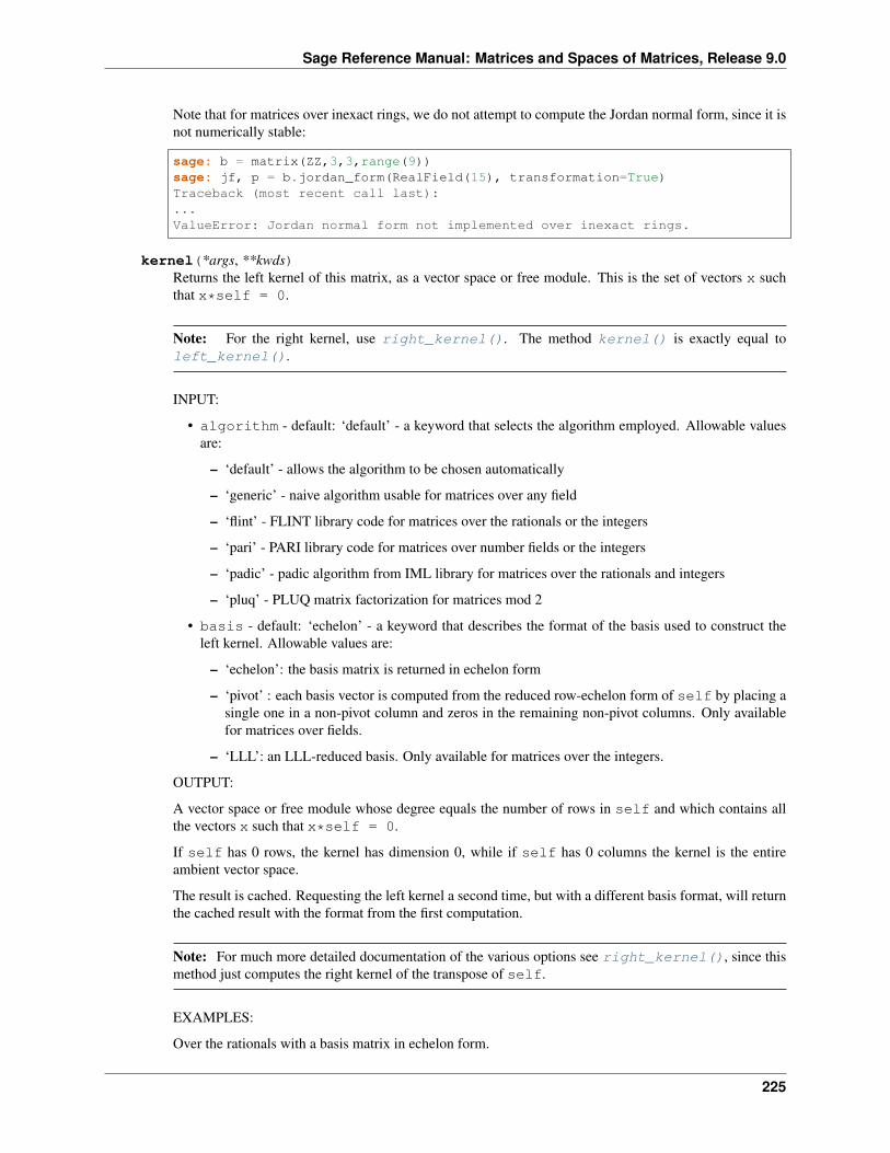
Sage Reference Manual: Matrices and Spaces of Matrices, Release 9.0
Note that for matrices over inexact rings, we do not attempt to compute the Jordan normal form, since it isnot numerically stable:
sage: b = matrix(ZZ,3,3,range(9))sage: jf, p = b.jordan_form(RealField(15), transformation=True)Traceback (most recent call last):...ValueError: Jordan normal form not implemented over inexact rings.
kernel(*args, **kwds)Returns the left kernel of this matrix, as a vector space or free module. This is the set of vectors x suchthat x*self = 0.
Note: For the right kernel, use right_kernel(). The method kernel() is exactly equal toleft_kernel().
INPUT:
• algorithm - default: ‘default’ - a keyword that selects the algorithm employed. Allowable valuesare:
– ‘default’ - allows the algorithm to be chosen automatically
– ‘generic’ - naive algorithm usable for matrices over any field
– ‘flint’ - FLINT library code for matrices over the rationals or the integers
– ‘pari’ - PARI library code for matrices over number fields or the integers
– ‘padic’ - padic algorithm from IML library for matrices over the rationals and integers
– ‘pluq’ - PLUQ matrix factorization for matrices mod 2
• basis - default: ‘echelon’ - a keyword that describes the format of the basis used to construct theleft kernel. Allowable values are:
– ‘echelon’: the basis matrix is returned in echelon form
– ‘pivot’ : each basis vector is computed from the reduced row-echelon form of self by placing asingle one in a non-pivot column and zeros in the remaining non-pivot columns. Only availablefor matrices over fields.
– ‘LLL’: an LLL-reduced basis. Only available for matrices over the integers.
OUTPUT:
A vector space or free module whose degree equals the number of rows in self and which contains allthe vectors x such that x*self = 0.
If self has 0 rows, the kernel has dimension 0, while if self has 0 columns the kernel is the entireambient vector space.
The result is cached. Requesting the left kernel a second time, but with a different basis format, will returnthe cached result with the format from the first computation.
Note: For much more detailed documentation of the various options see right_kernel(), since thismethod just computes the right kernel of the transpose of self.
EXAMPLES:
Over the rationals with a basis matrix in echelon form.
225
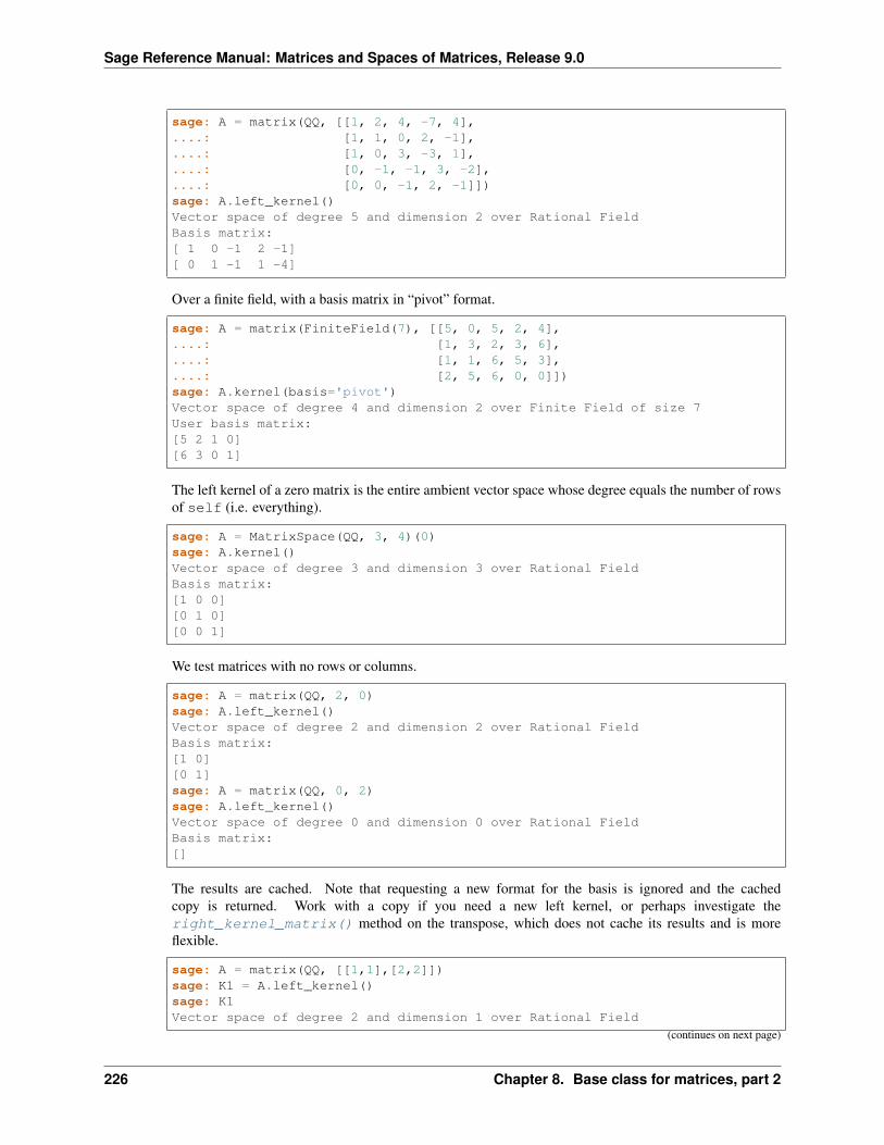
Sage Reference Manual: Matrices and Spaces of Matrices, Release 9.0
sage: A = matrix(QQ, [[1, 2, 4, -7, 4],....: [1, 1, 0, 2, -1],....: [1, 0, 3, -3, 1],....: [0, -1, -1, 3, -2],....: [0, 0, -1, 2, -1]])sage: A.left_kernel()Vector space of degree 5 and dimension 2 over Rational FieldBasis matrix:[ 1 0 -1 2 -1][ 0 1 -1 1 -4]
Over a finite field, with a basis matrix in “pivot” format.
sage: A = matrix(FiniteField(7), [[5, 0, 5, 2, 4],....: [1, 3, 2, 3, 6],....: [1, 1, 6, 5, 3],....: [2, 5, 6, 0, 0]])sage: A.kernel(basis='pivot')Vector space of degree 4 and dimension 2 over Finite Field of size 7User basis matrix:[5 2 1 0][6 3 0 1]
The left kernel of a zero matrix is the entire ambient vector space whose degree equals the number of rowsof self (i.e. everything).
sage: A = MatrixSpace(QQ, 3, 4)(0)sage: A.kernel()Vector space of degree 3 and dimension 3 over Rational FieldBasis matrix:[1 0 0][0 1 0][0 0 1]
We test matrices with no rows or columns.
sage: A = matrix(QQ, 2, 0)sage: A.left_kernel()Vector space of degree 2 and dimension 2 over Rational FieldBasis matrix:[1 0][0 1]sage: A = matrix(QQ, 0, 2)sage: A.left_kernel()Vector space of degree 0 and dimension 0 over Rational FieldBasis matrix:[]
The results are cached. Note that requesting a new format for the basis is ignored and the cachedcopy is returned. Work with a copy if you need a new left kernel, or perhaps investigate theright_kernel_matrix() method on the transpose, which does not cache its results and is moreflexible.
sage: A = matrix(QQ, [[1,1],[2,2]])sage: K1 = A.left_kernel()sage: K1Vector space of degree 2 and dimension 1 over Rational Field
(continues on next page)
226 Chapter 8. Base class for matrices, part 2
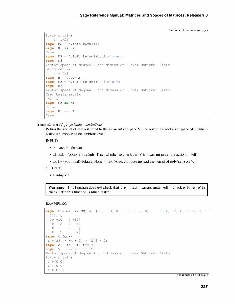
Sage Reference Manual: Matrices and Spaces of Matrices, Release 9.0
(continued from previous page)
Basis matrix:[ 1 -1/2]sage: K2 = A.left_kernel()sage: K1 is K2Truesage: K3 = A.left_kernel(basis='pivot')sage: K3Vector space of degree 2 and dimension 1 over Rational FieldBasis matrix:[ 1 -1/2]sage: B = copy(A)sage: K3 = B.left_kernel(basis='pivot')sage: K3Vector space of degree 2 and dimension 1 over Rational FieldUser basis matrix:[-2 1]sage: K3 is K1Falsesage: K3 == K1True
kernel_on(V, poly=None, check=True)Return the kernel of self restricted to the invariant subspace V. The result is a vector subspace of V, whichis also a subspace of the ambient space.
INPUT:
• V - vector subspace
• check - (optional) default: True; whether to check that V is invariant under the action of self.
• poly - (optional) default: None; if not None, compute instead the kernel of poly(self) on V.
OUTPUT:
• a subspace
Warning: This function does not check that V is in fact invariant under self if check is False. Withcheck False this function is much faster.
EXAMPLES:
sage: t = matrix(QQ, 4, [39, -10, 0, -12, 0, 2, 0, -1, 0, 1, -2, 0, 0, 2, 0, -→˓2]); t[ 39 -10 0 -12][ 0 2 0 -1][ 0 1 -2 0][ 0 2 0 -2]sage: t.fcp()(x - 39) * (x + 2) * (x^2 - 2)sage: s = (t-39)*(t^2-2)sage: V = s.kernel(); VVector space of degree 4 and dimension 3 over Rational FieldBasis matrix:[1 0 0 0][0 1 0 0][0 0 0 1]
(continues on next page)
227
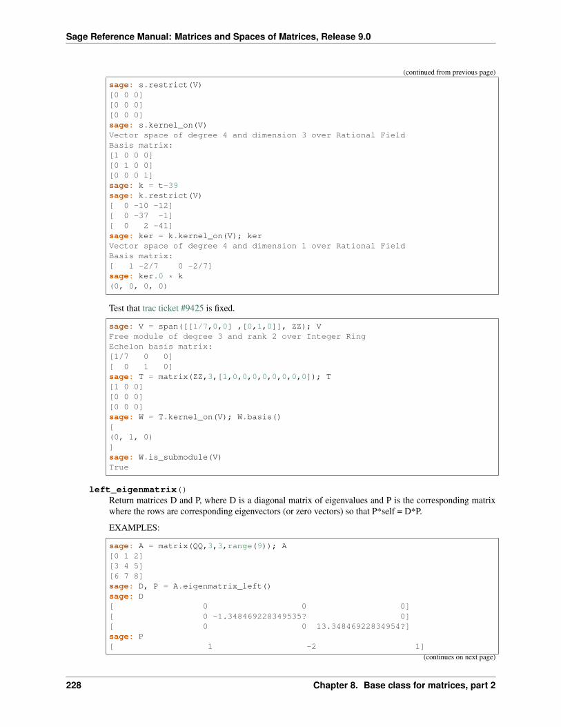
Sage Reference Manual: Matrices and Spaces of Matrices, Release 9.0
(continued from previous page)
sage: s.restrict(V)[0 0 0][0 0 0][0 0 0]sage: s.kernel_on(V)Vector space of degree 4 and dimension 3 over Rational FieldBasis matrix:[1 0 0 0][0 1 0 0][0 0 0 1]sage: k = t-39sage: k.restrict(V)[ 0 -10 -12][ 0 -37 -1][ 0 2 -41]sage: ker = k.kernel_on(V); kerVector space of degree 4 and dimension 1 over Rational FieldBasis matrix:[ 1 -2/7 0 -2/7]sage: ker.0 * k(0, 0, 0, 0)
Test that trac ticket #9425 is fixed.
sage: V = span([[1/7,0,0] ,[0,1,0]], ZZ); VFree module of degree 3 and rank 2 over Integer RingEchelon basis matrix:[1/7 0 0][ 0 1 0]sage: T = matrix(ZZ,3,[1,0,0,0,0,0,0,0,0]); T[1 0 0][0 0 0][0 0 0]sage: W = T.kernel_on(V); W.basis()[(0, 1, 0)]sage: W.is_submodule(V)True
left_eigenmatrix()Return matrices D and P, where D is a diagonal matrix of eigenvalues and P is the corresponding matrixwhere the rows are corresponding eigenvectors (or zero vectors) so that P*self = D*P.
EXAMPLES:
sage: A = matrix(QQ,3,3,range(9)); A[0 1 2][3 4 5][6 7 8]sage: D, P = A.eigenmatrix_left()sage: D[ 0 0 0][ 0 -1.348469228349535? 0][ 0 0 13.34846922834954?]sage: P[ 1 -2 1]
(continues on next page)
228 Chapter 8. Base class for matrices, part 2
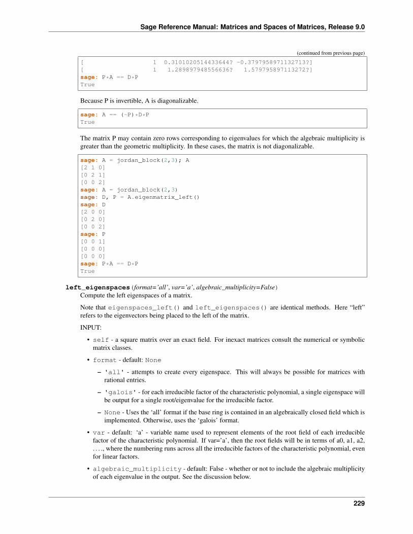
Sage Reference Manual: Matrices and Spaces of Matrices, Release 9.0
(continued from previous page)
[ 1 0.3101020514433644? -0.3797958971132713?][ 1 1.289897948556636? 1.579795897113272?]sage: P*A == D*PTrue
Because P is invertible, A is diagonalizable.
sage: A == (~P)*D*PTrue
The matrix P may contain zero rows corresponding to eigenvalues for which the algebraic multiplicity isgreater than the geometric multiplicity. In these cases, the matrix is not diagonalizable.
sage: A = jordan_block(2,3); A[2 1 0][0 2 1][0 0 2]sage: A = jordan_block(2,3)sage: D, P = A.eigenmatrix_left()sage: D[2 0 0][0 2 0][0 0 2]sage: P[0 0 1][0 0 0][0 0 0]sage: P*A == D*PTrue
left_eigenspaces(format=’all’, var=’a’, algebraic_multiplicity=False)Compute the left eigenspaces of a matrix.
Note that eigenspaces_left() and left_eigenspaces() are identical methods. Here “left”refers to the eigenvectors being placed to the left of the matrix.
INPUT:
• self - a square matrix over an exact field. For inexact matrices consult the numerical or symbolicmatrix classes.
• format - default: None
– 'all' - attempts to create every eigenspace. This will always be possible for matrices withrational entries.
– 'galois' - for each irreducible factor of the characteristic polynomial, a single eigenspace willbe output for a single root/eigenvalue for the irreducible factor.
– None - Uses the ‘all’ format if the base ring is contained in an algebraically closed field which isimplemented. Otherwise, uses the ‘galois’ format.
• var - default: ‘a’ - variable name used to represent elements of the root field of each irreduciblefactor of the characteristic polynomial. If var=’a’, then the root fields will be in terms of a0, a1, a2,. . . ., where the numbering runs across all the irreducible factors of the characteristic polynomial, evenfor linear factors.
• algebraic_multiplicity - default: False - whether or not to include the algebraic multiplicityof each eigenvalue in the output. See the discussion below.
229
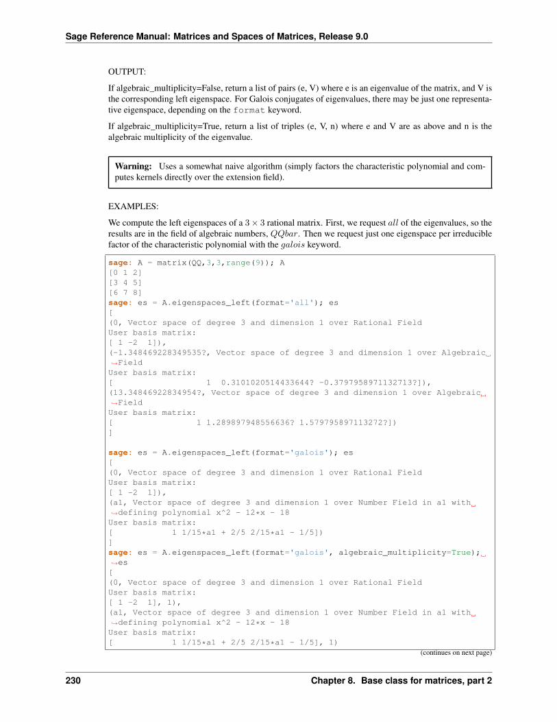
Sage Reference Manual: Matrices and Spaces of Matrices, Release 9.0
OUTPUT:
If algebraic_multiplicity=False, return a list of pairs (e, V) where e is an eigenvalue of the matrix, and V isthe corresponding left eigenspace. For Galois conjugates of eigenvalues, there may be just one representa-tive eigenspace, depending on the format keyword.
If algebraic_multiplicity=True, return a list of triples (e, V, n) where e and V are as above and n is thealgebraic multiplicity of the eigenvalue.
Warning: Uses a somewhat naive algorithm (simply factors the characteristic polynomial and com-putes kernels directly over the extension field).
EXAMPLES:
We compute the left eigenspaces of a 3× 3 rational matrix. First, we request 𝑎𝑙𝑙 of the eigenvalues, so theresults are in the field of algebraic numbers, 𝑄𝑄𝑏𝑎𝑟. Then we request just one eigenspace per irreduciblefactor of the characteristic polynomial with the 𝑔𝑎𝑙𝑜𝑖𝑠 keyword.
sage: A = matrix(QQ,3,3,range(9)); A[0 1 2][3 4 5][6 7 8]sage: es = A.eigenspaces_left(format='all'); es[(0, Vector space of degree 3 and dimension 1 over Rational FieldUser basis matrix:[ 1 -2 1]),(-1.348469228349535?, Vector space of degree 3 and dimension 1 over Algebraic→˓FieldUser basis matrix:[ 1 0.3101020514433644? -0.3797958971132713?]),(13.34846922834954?, Vector space of degree 3 and dimension 1 over Algebraic→˓FieldUser basis matrix:[ 1 1.289897948556636? 1.579795897113272?])]
sage: es = A.eigenspaces_left(format='galois'); es[(0, Vector space of degree 3 and dimension 1 over Rational FieldUser basis matrix:[ 1 -2 1]),(a1, Vector space of degree 3 and dimension 1 over Number Field in a1 with→˓defining polynomial x^2 - 12*x - 18User basis matrix:[ 1 1/15*a1 + 2/5 2/15*a1 - 1/5])]sage: es = A.eigenspaces_left(format='galois', algebraic_multiplicity=True);→˓es[(0, Vector space of degree 3 and dimension 1 over Rational FieldUser basis matrix:[ 1 -2 1], 1),(a1, Vector space of degree 3 and dimension 1 over Number Field in a1 with→˓defining polynomial x^2 - 12*x - 18User basis matrix:[ 1 1/15*a1 + 2/5 2/15*a1 - 1/5], 1)
(continues on next page)
230 Chapter 8. Base class for matrices, part 2
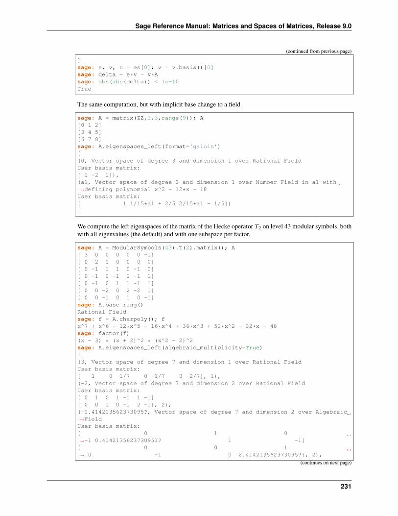
Sage Reference Manual: Matrices and Spaces of Matrices, Release 9.0
(continued from previous page)
]sage: e, v, n = es[0]; v = v.basis()[0]sage: delta = e*v - v*Asage: abs(abs(delta)) < 1e-10True
The same computation, but with implicit base change to a field.
sage: A = matrix(ZZ,3,3,range(9)); A[0 1 2][3 4 5][6 7 8]sage: A.eigenspaces_left(format='galois')[(0, Vector space of degree 3 and dimension 1 over Rational FieldUser basis matrix:[ 1 -2 1]),(a1, Vector space of degree 3 and dimension 1 over Number Field in a1 with→˓defining polynomial x^2 - 12*x - 18User basis matrix:[ 1 1/15*a1 + 2/5 2/15*a1 - 1/5])]
We compute the left eigenspaces of the matrix of the Hecke operator 𝑇2 on level 43 modular symbols, bothwith all eigenvalues (the default) and with one subspace per factor.
sage: A = ModularSymbols(43).T(2).matrix(); A[ 3 0 0 0 0 0 -1][ 0 -2 1 0 0 0 0][ 0 -1 1 1 0 -1 0][ 0 -1 0 -1 2 -1 1][ 0 -1 0 1 1 -1 1][ 0 0 -2 0 2 -2 1][ 0 0 -1 0 1 0 -1]sage: A.base_ring()Rational Fieldsage: f = A.charpoly(); fx^7 + x^6 - 12*x^5 - 16*x^4 + 36*x^3 + 52*x^2 - 32*x - 48sage: factor(f)(x - 3) * (x + 2)^2 * (x^2 - 2)^2sage: A.eigenspaces_left(algebraic_multiplicity=True)[(3, Vector space of degree 7 and dimension 1 over Rational FieldUser basis matrix:[ 1 0 1/7 0 -1/7 0 -2/7], 1),(-2, Vector space of degree 7 and dimension 2 over Rational FieldUser basis matrix:[ 0 1 0 1 -1 1 -1][ 0 0 1 0 -1 2 -1], 2),(-1.414213562373095?, Vector space of degree 7 and dimension 2 over Algebraic→˓FieldUser basis matrix:[ 0 1 0→˓-1 0.4142135623730951? 1 -1][ 0 0 1→˓ 0 -1 0 2.414213562373095?], 2),
(continues on next page)
231
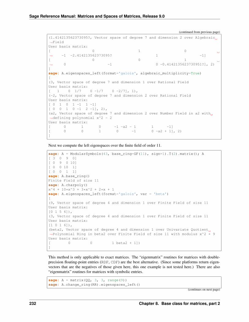
Sage Reference Manual: Matrices and Spaces of Matrices, Release 9.0
(continued from previous page)
(1.414213562373095?, Vector space of degree 7 and dimension 2 over Algebraic→˓FieldUser basis matrix:[ 0 1 0→˓ -1 -2.414213562373095? 1 -1][ 0 0 1→˓ 0 -1 0 -0.4142135623730951?], 2)]sage: A.eigenspaces_left(format='galois', algebraic_multiplicity=True)[(3, Vector space of degree 7 and dimension 1 over Rational FieldUser basis matrix:[ 1 0 1/7 0 -1/7 0 -2/7], 1),(-2, Vector space of degree 7 and dimension 2 over Rational FieldUser basis matrix:[ 0 1 0 1 -1 1 -1][ 0 0 1 0 -1 2 -1], 2),(a2, Vector space of degree 7 and dimension 2 over Number Field in a2 with→˓defining polynomial x^2 - 2User basis matrix:[ 0 1 0 -1 -a2 - 1 1 -1][ 0 0 1 0 -1 0 -a2 + 1], 2)]
Next we compute the left eigenspaces over the finite field of order 11.
sage: A = ModularSymbols(43, base_ring=GF(11), sign=1).T(2).matrix(); A[ 3 0 9 0][ 0 9 0 10][ 0 0 10 1][ 0 0 1 1]sage: A.base_ring()Finite Field of size 11sage: A.charpoly()x^4 + 10*x^3 + 3*x^2 + 2*x + 1sage: A.eigenspaces_left(format='galois', var = 'beta')[(9, Vector space of degree 4 and dimension 1 over Finite Field of size 11User basis matrix:[0 1 5 6]),(3, Vector space of degree 4 and dimension 1 over Finite Field of size 11User basis matrix:[1 0 1 6]),(beta2, Vector space of degree 4 and dimension 1 over Univariate Quotient→˓Polynomial Ring in beta2 over Finite Field of size 11 with modulus x^2 + 9User basis matrix:[ 0 0 1 beta2 + 1])]
This method is only applicable to exact matrices. The “eigenmatrix” routines for matrices with double-precision floating-point entries (RDF, CDF) are the best alternative. (Since some platforms return eigen-vectors that are the negatives of those given here, this one example is not tested here.) There are also“eigenmatrix” routines for matrices with symbolic entries.
sage: A = matrix(QQ, 3, 3, range(9))sage: A.change_ring(RR).eigenspaces_left()
(continues on next page)
232 Chapter 8. Base class for matrices, part 2
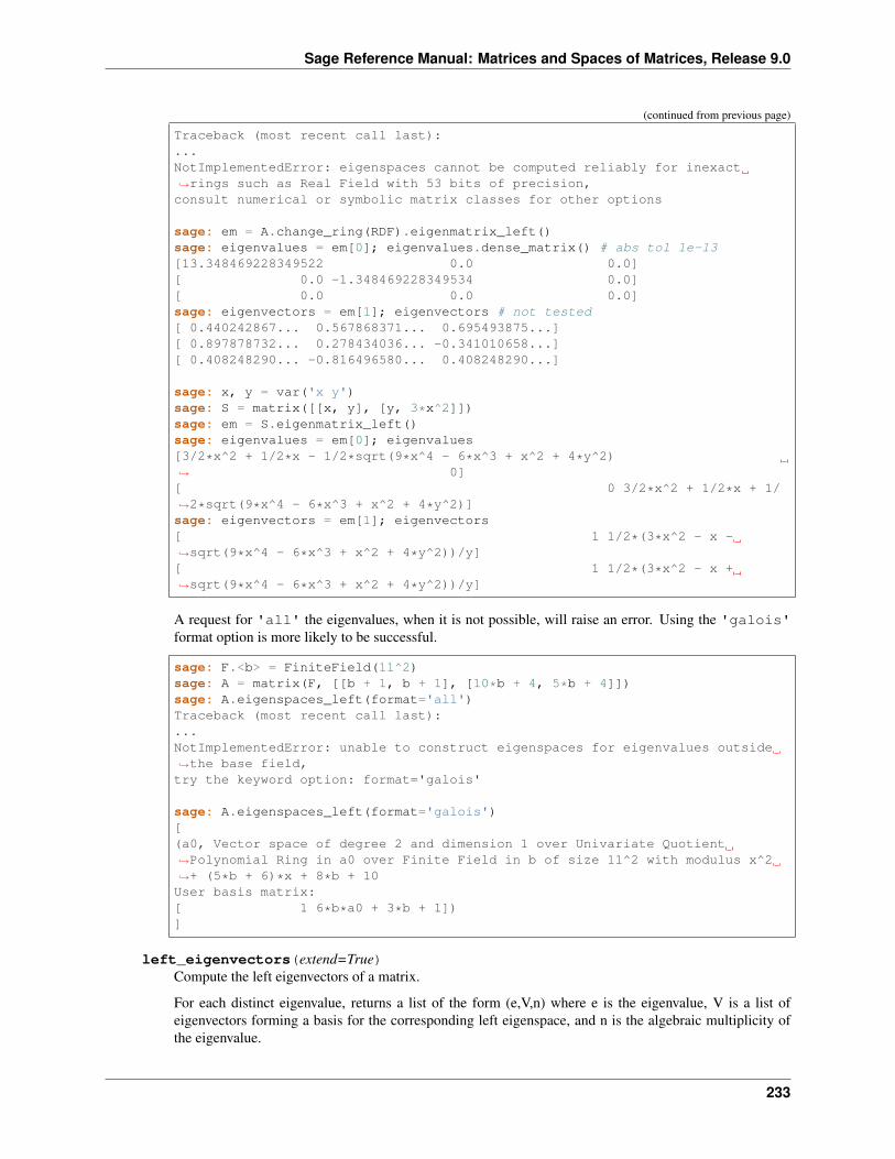
Sage Reference Manual: Matrices and Spaces of Matrices, Release 9.0
(continued from previous page)
Traceback (most recent call last):...NotImplementedError: eigenspaces cannot be computed reliably for inexact→˓rings such as Real Field with 53 bits of precision,consult numerical or symbolic matrix classes for other options
sage: em = A.change_ring(RDF).eigenmatrix_left()sage: eigenvalues = em[0]; eigenvalues.dense_matrix() # abs tol 1e-13[13.348469228349522 0.0 0.0][ 0.0 -1.348469228349534 0.0][ 0.0 0.0 0.0]sage: eigenvectors = em[1]; eigenvectors # not tested[ 0.440242867... 0.567868371... 0.695493875...][ 0.897878732... 0.278434036... -0.341010658...][ 0.408248290... -0.816496580... 0.408248290...]
sage: x, y = var('x y')sage: S = matrix([[x, y], [y, 3*x^2]])sage: em = S.eigenmatrix_left()sage: eigenvalues = em[0]; eigenvalues[3/2*x^2 + 1/2*x - 1/2*sqrt(9*x^4 - 6*x^3 + x^2 + 4*y^2)→˓ 0][ 0 3/2*x^2 + 1/2*x + 1/→˓2*sqrt(9*x^4 - 6*x^3 + x^2 + 4*y^2)]sage: eigenvectors = em[1]; eigenvectors[ 1 1/2*(3*x^2 - x -→˓sqrt(9*x^4 - 6*x^3 + x^2 + 4*y^2))/y][ 1 1/2*(3*x^2 - x +→˓sqrt(9*x^4 - 6*x^3 + x^2 + 4*y^2))/y]
A request for 'all' the eigenvalues, when it is not possible, will raise an error. Using the 'galois'format option is more likely to be successful.
sage: F.<b> = FiniteField(11^2)sage: A = matrix(F, [[b + 1, b + 1], [10*b + 4, 5*b + 4]])sage: A.eigenspaces_left(format='all')Traceback (most recent call last):...NotImplementedError: unable to construct eigenspaces for eigenvalues outside→˓the base field,try the keyword option: format='galois'
sage: A.eigenspaces_left(format='galois')[(a0, Vector space of degree 2 and dimension 1 over Univariate Quotient→˓Polynomial Ring in a0 over Finite Field in b of size 11^2 with modulus x^2→˓+ (5*b + 6)*x + 8*b + 10User basis matrix:[ 1 6*b*a0 + 3*b + 1])]
left_eigenvectors(extend=True)Compute the left eigenvectors of a matrix.
For each distinct eigenvalue, returns a list of the form (e,V,n) where e is the eigenvalue, V is a list ofeigenvectors forming a basis for the corresponding left eigenspace, and n is the algebraic multiplicity ofthe eigenvalue.
233
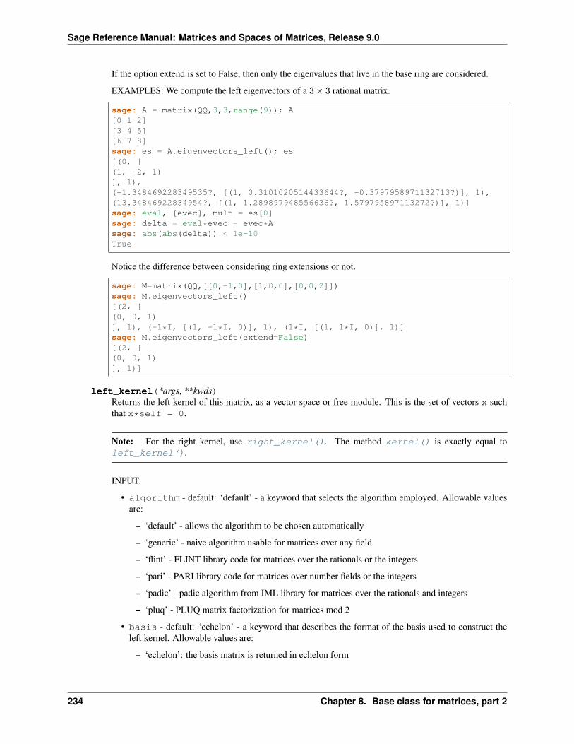
Sage Reference Manual: Matrices and Spaces of Matrices, Release 9.0
If the option extend is set to False, then only the eigenvalues that live in the base ring are considered.
EXAMPLES: We compute the left eigenvectors of a 3× 3 rational matrix.
sage: A = matrix(QQ,3,3,range(9)); A[0 1 2][3 4 5][6 7 8]sage: es = A.eigenvectors_left(); es[(0, [(1, -2, 1)], 1),(-1.348469228349535?, [(1, 0.3101020514433644?, -0.3797958971132713?)], 1),(13.34846922834954?, [(1, 1.289897948556636?, 1.579795897113272?)], 1)]sage: eval, [evec], mult = es[0]sage: delta = eval*evec - evec*Asage: abs(abs(delta)) < 1e-10True
Notice the difference between considering ring extensions or not.
sage: M=matrix(QQ,[[0,-1,0],[1,0,0],[0,0,2]])sage: M.eigenvectors_left()[(2, [(0, 0, 1)], 1), (-1*I, [(1, -1*I, 0)], 1), (1*I, [(1, 1*I, 0)], 1)]sage: M.eigenvectors_left(extend=False)[(2, [(0, 0, 1)], 1)]
left_kernel(*args, **kwds)Returns the left kernel of this matrix, as a vector space or free module. This is the set of vectors x suchthat x*self = 0.
Note: For the right kernel, use right_kernel(). The method kernel() is exactly equal toleft_kernel().
INPUT:
• algorithm - default: ‘default’ - a keyword that selects the algorithm employed. Allowable valuesare:
– ‘default’ - allows the algorithm to be chosen automatically
– ‘generic’ - naive algorithm usable for matrices over any field
– ‘flint’ - FLINT library code for matrices over the rationals or the integers
– ‘pari’ - PARI library code for matrices over number fields or the integers
– ‘padic’ - padic algorithm from IML library for matrices over the rationals and integers
– ‘pluq’ - PLUQ matrix factorization for matrices mod 2
• basis - default: ‘echelon’ - a keyword that describes the format of the basis used to construct theleft kernel. Allowable values are:
– ‘echelon’: the basis matrix is returned in echelon form
234 Chapter 8. Base class for matrices, part 2
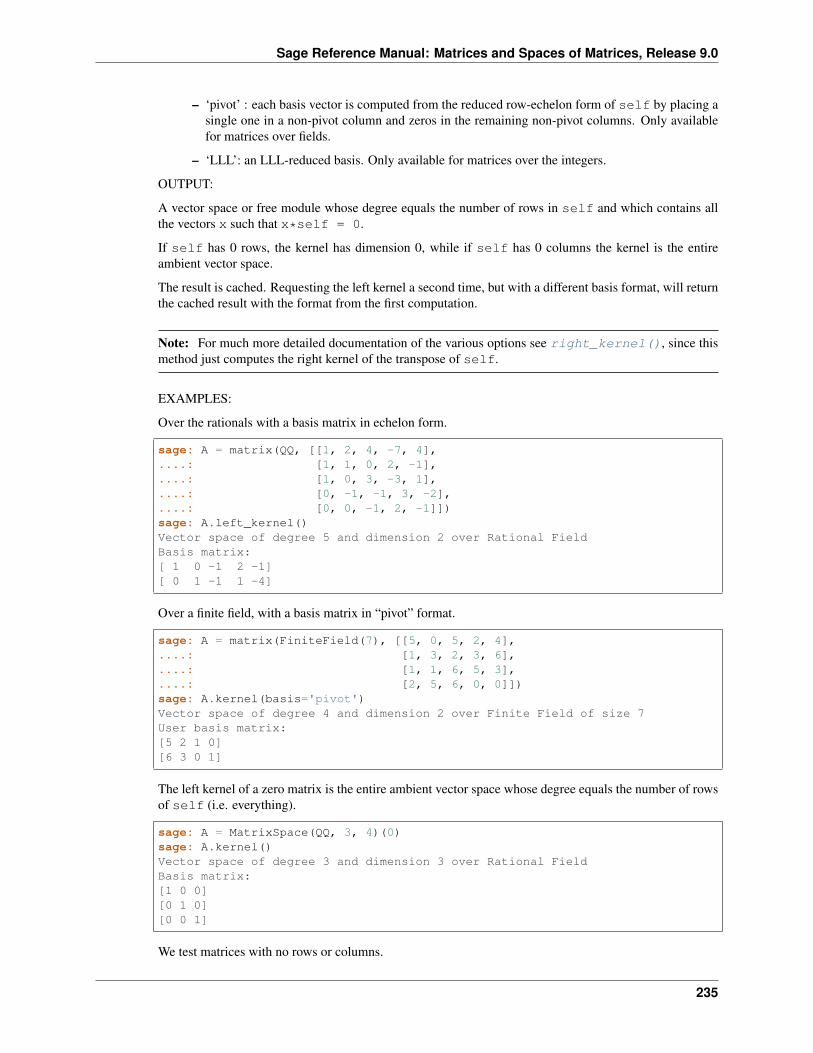
Sage Reference Manual: Matrices and Spaces of Matrices, Release 9.0
– ‘pivot’ : each basis vector is computed from the reduced row-echelon form of self by placing asingle one in a non-pivot column and zeros in the remaining non-pivot columns. Only availablefor matrices over fields.
– ‘LLL’: an LLL-reduced basis. Only available for matrices over the integers.
OUTPUT:
A vector space or free module whose degree equals the number of rows in self and which contains allthe vectors x such that x*self = 0.
If self has 0 rows, the kernel has dimension 0, while if self has 0 columns the kernel is the entireambient vector space.
The result is cached. Requesting the left kernel a second time, but with a different basis format, will returnthe cached result with the format from the first computation.
Note: For much more detailed documentation of the various options see right_kernel(), since thismethod just computes the right kernel of the transpose of self.
EXAMPLES:
Over the rationals with a basis matrix in echelon form.
sage: A = matrix(QQ, [[1, 2, 4, -7, 4],....: [1, 1, 0, 2, -1],....: [1, 0, 3, -3, 1],....: [0, -1, -1, 3, -2],....: [0, 0, -1, 2, -1]])sage: A.left_kernel()Vector space of degree 5 and dimension 2 over Rational FieldBasis matrix:[ 1 0 -1 2 -1][ 0 1 -1 1 -4]
Over a finite field, with a basis matrix in “pivot” format.
sage: A = matrix(FiniteField(7), [[5, 0, 5, 2, 4],....: [1, 3, 2, 3, 6],....: [1, 1, 6, 5, 3],....: [2, 5, 6, 0, 0]])sage: A.kernel(basis='pivot')Vector space of degree 4 and dimension 2 over Finite Field of size 7User basis matrix:[5 2 1 0][6 3 0 1]
The left kernel of a zero matrix is the entire ambient vector space whose degree equals the number of rowsof self (i.e. everything).
sage: A = MatrixSpace(QQ, 3, 4)(0)sage: A.kernel()Vector space of degree 3 and dimension 3 over Rational FieldBasis matrix:[1 0 0][0 1 0][0 0 1]
We test matrices with no rows or columns.
235

Sage Reference Manual: Matrices and Spaces of Matrices, Release 9.0
sage: A = matrix(QQ, 2, 0)sage: A.left_kernel()Vector space of degree 2 and dimension 2 over Rational FieldBasis matrix:[1 0][0 1]sage: A = matrix(QQ, 0, 2)sage: A.left_kernel()Vector space of degree 0 and dimension 0 over Rational FieldBasis matrix:[]
The results are cached. Note that requesting a new format for the basis is ignored and the cachedcopy is returned. Work with a copy if you need a new left kernel, or perhaps investigate theright_kernel_matrix() method on the transpose, which does not cache its results and is moreflexible.
sage: A = matrix(QQ, [[1,1],[2,2]])sage: K1 = A.left_kernel()sage: K1Vector space of degree 2 and dimension 1 over Rational FieldBasis matrix:[ 1 -1/2]sage: K2 = A.left_kernel()sage: K1 is K2Truesage: K3 = A.left_kernel(basis='pivot')sage: K3Vector space of degree 2 and dimension 1 over Rational FieldBasis matrix:[ 1 -1/2]sage: B = copy(A)sage: K3 = B.left_kernel(basis='pivot')sage: K3Vector space of degree 2 and dimension 1 over Rational FieldUser basis matrix:[-2 1]sage: K3 is K1Falsesage: K3 == K1True
left_nullity()Return the (left) nullity of this matrix, which is the dimension of the (left) kernel of this matrix acting fromthe right on row vectors.
EXAMPLES:
sage: M = Matrix(QQ,[[1,0,0,1],[0,1,1,0],[1,1,1,0]])sage: M.nullity()0sage: M.left_nullity()0
sage: A = M.transpose()sage: A.nullity()1
(continues on next page)
236 Chapter 8. Base class for matrices, part 2
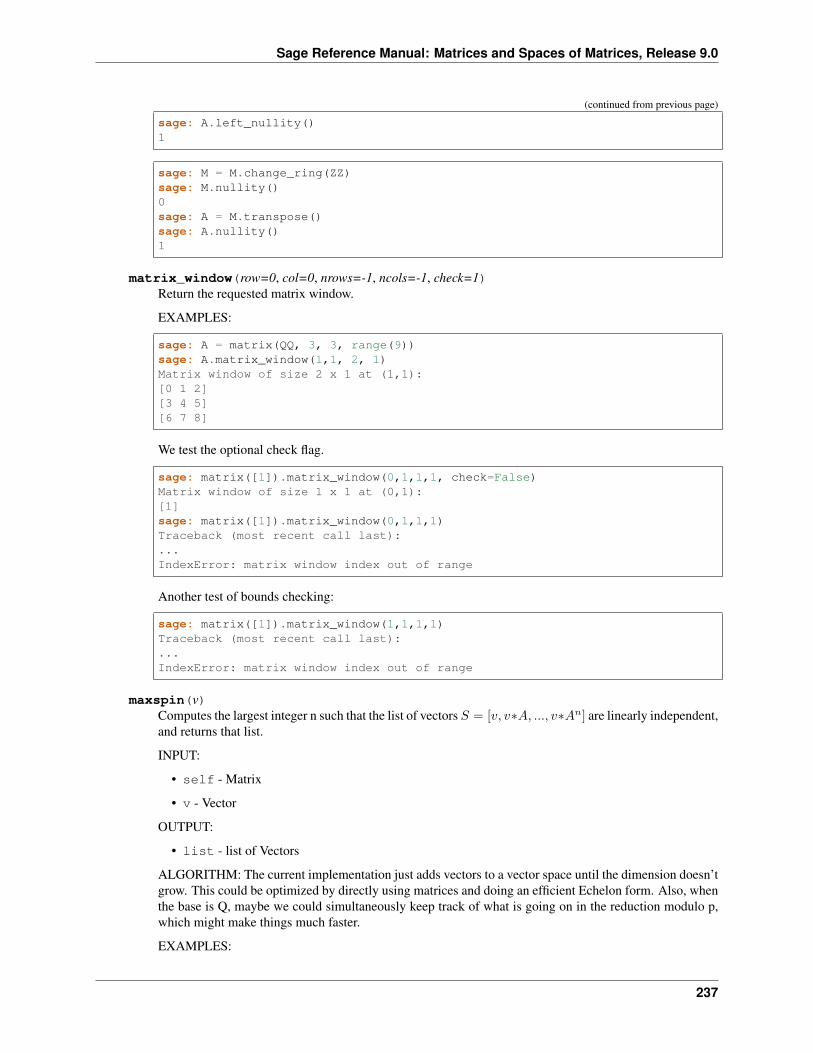
Sage Reference Manual: Matrices and Spaces of Matrices, Release 9.0
(continued from previous page)
sage: A.left_nullity()1
sage: M = M.change_ring(ZZ)sage: M.nullity()0sage: A = M.transpose()sage: A.nullity()1
matrix_window(row=0, col=0, nrows=-1, ncols=-1, check=1)Return the requested matrix window.
EXAMPLES:
sage: A = matrix(QQ, 3, 3, range(9))sage: A.matrix_window(1,1, 2, 1)Matrix window of size 2 x 1 at (1,1):[0 1 2][3 4 5][6 7 8]
We test the optional check flag.
sage: matrix([1]).matrix_window(0,1,1,1, check=False)Matrix window of size 1 x 1 at (0,1):[1]sage: matrix([1]).matrix_window(0,1,1,1)Traceback (most recent call last):...IndexError: matrix window index out of range
Another test of bounds checking:
sage: matrix([1]).matrix_window(1,1,1,1)Traceback (most recent call last):...IndexError: matrix window index out of range
maxspin(v)Computes the largest integer n such that the list of vectors 𝑆 = [𝑣, 𝑣*𝐴, ..., 𝑣*𝐴𝑛] are linearly independent,and returns that list.
INPUT:
• self - Matrix
• v - Vector
OUTPUT:
• list - list of Vectors
ALGORITHM: The current implementation just adds vectors to a vector space until the dimension doesn’tgrow. This could be optimized by directly using matrices and doing an efficient Echelon form. Also, whenthe base is Q, maybe we could simultaneously keep track of what is going on in the reduction modulo p,which might make things much faster.
EXAMPLES:
237
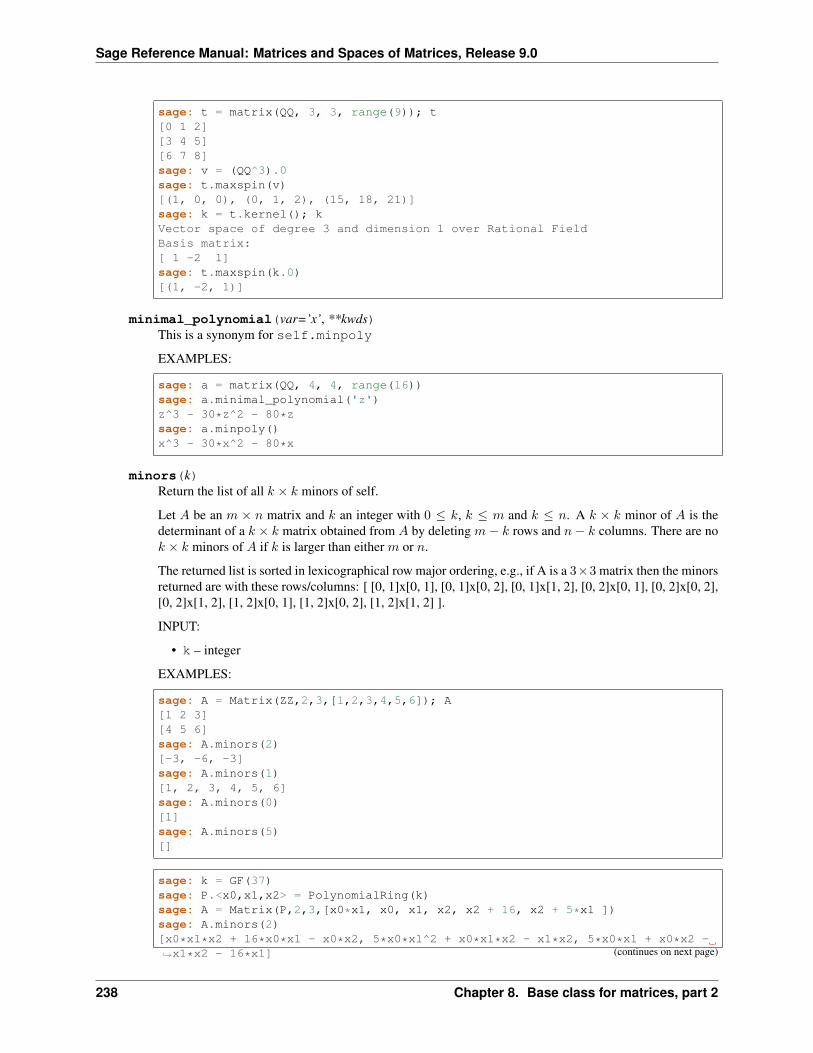
Sage Reference Manual: Matrices and Spaces of Matrices, Release 9.0
sage: t = matrix(QQ, 3, 3, range(9)); t[0 1 2][3 4 5][6 7 8]sage: v = (QQ^3).0sage: t.maxspin(v)[(1, 0, 0), (0, 1, 2), (15, 18, 21)]sage: k = t.kernel(); kVector space of degree 3 and dimension 1 over Rational FieldBasis matrix:[ 1 -2 1]sage: t.maxspin(k.0)[(1, -2, 1)]
minimal_polynomial(var=’x’, **kwds)This is a synonym for self.minpoly
EXAMPLES:
sage: a = matrix(QQ, 4, 4, range(16))sage: a.minimal_polynomial('z')z^3 - 30*z^2 - 80*zsage: a.minpoly()x^3 - 30*x^2 - 80*x
minors(k)Return the list of all 𝑘 × 𝑘 minors of self.
Let 𝐴 be an 𝑚 × 𝑛 matrix and 𝑘 an integer with 0 ≤ 𝑘, 𝑘 ≤ 𝑚 and 𝑘 ≤ 𝑛. A 𝑘 × 𝑘 minor of 𝐴 is thedeterminant of a 𝑘 × 𝑘 matrix obtained from 𝐴 by deleting 𝑚− 𝑘 rows and 𝑛− 𝑘 columns. There are no𝑘 × 𝑘 minors of 𝐴 if 𝑘 is larger than either 𝑚 or 𝑛.
The returned list is sorted in lexicographical row major ordering, e.g., if A is a 3×3 matrix then the minorsreturned are with these rows/columns: [ [0, 1]x[0, 1], [0, 1]x[0, 2], [0, 1]x[1, 2], [0, 2]x[0, 1], [0, 2]x[0, 2],[0, 2]x[1, 2], [1, 2]x[0, 1], [1, 2]x[0, 2], [1, 2]x[1, 2] ].
INPUT:
• k – integer
EXAMPLES:
sage: A = Matrix(ZZ,2,3,[1,2,3,4,5,6]); A[1 2 3][4 5 6]sage: A.minors(2)[-3, -6, -3]sage: A.minors(1)[1, 2, 3, 4, 5, 6]sage: A.minors(0)[1]sage: A.minors(5)[]
sage: k = GF(37)sage: P.<x0,x1,x2> = PolynomialRing(k)sage: A = Matrix(P,2,3,[x0*x1, x0, x1, x2, x2 + 16, x2 + 5*x1 ])sage: A.minors(2)[x0*x1*x2 + 16*x0*x1 - x0*x2, 5*x0*x1^2 + x0*x1*x2 - x1*x2, 5*x0*x1 + x0*x2 -→˓x1*x2 - 16*x1] (continues on next page)
238 Chapter 8. Base class for matrices, part 2
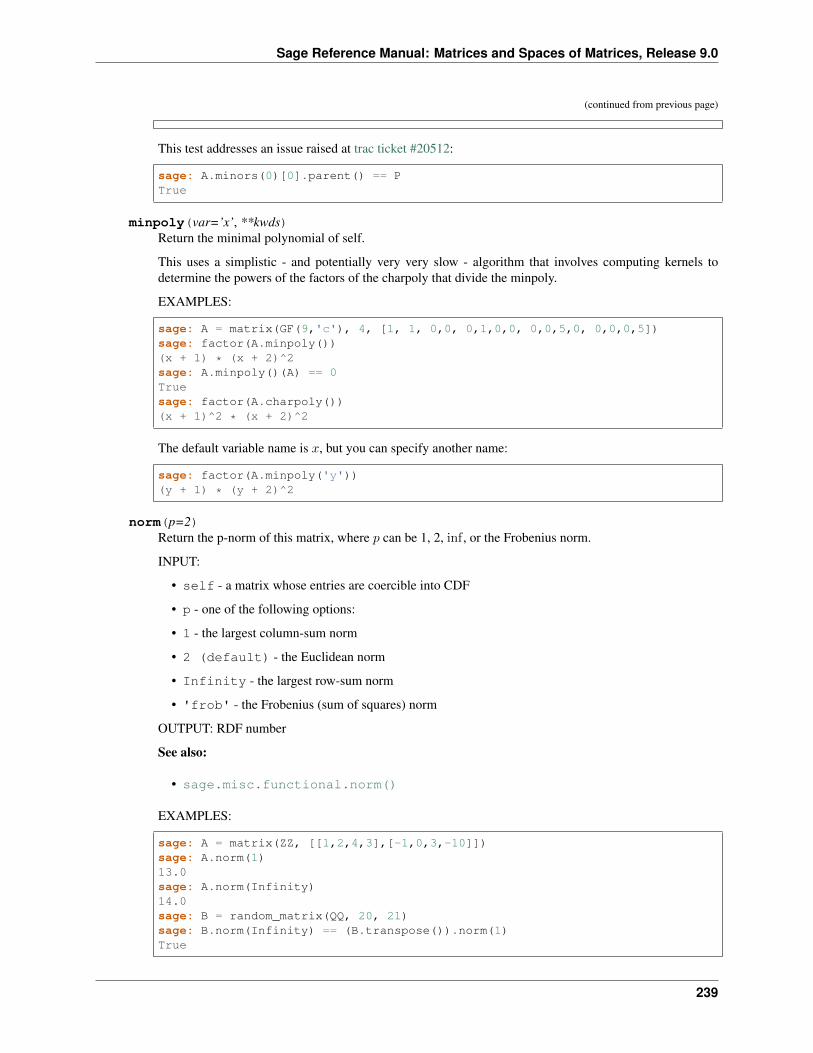
Sage Reference Manual: Matrices and Spaces of Matrices, Release 9.0
(continued from previous page)
This test addresses an issue raised at trac ticket #20512:
sage: A.minors(0)[0].parent() == PTrue
minpoly(var=’x’, **kwds)Return the minimal polynomial of self.
This uses a simplistic - and potentially very very slow - algorithm that involves computing kernels todetermine the powers of the factors of the charpoly that divide the minpoly.
EXAMPLES:
sage: A = matrix(GF(9,'c'), 4, [1, 1, 0,0, 0,1,0,0, 0,0,5,0, 0,0,0,5])sage: factor(A.minpoly())(x + 1) * (x + 2)^2sage: A.minpoly()(A) == 0Truesage: factor(A.charpoly())(x + 1)^2 * (x + 2)^2
The default variable name is 𝑥, but you can specify another name:
sage: factor(A.minpoly('y'))(y + 1) * (y + 2)^2
norm(p=2)Return the p-norm of this matrix, where 𝑝 can be 1, 2, inf , or the Frobenius norm.
INPUT:
• self - a matrix whose entries are coercible into CDF
• p - one of the following options:
• 1 - the largest column-sum norm
• 2 (default) - the Euclidean norm
• Infinity - the largest row-sum norm
• 'frob' - the Frobenius (sum of squares) norm
OUTPUT: RDF number
See also:
• sage.misc.functional.norm()
EXAMPLES:
sage: A = matrix(ZZ, [[1,2,4,3],[-1,0,3,-10]])sage: A.norm(1)13.0sage: A.norm(Infinity)14.0sage: B = random_matrix(QQ, 20, 21)sage: B.norm(Infinity) == (B.transpose()).norm(1)True
239
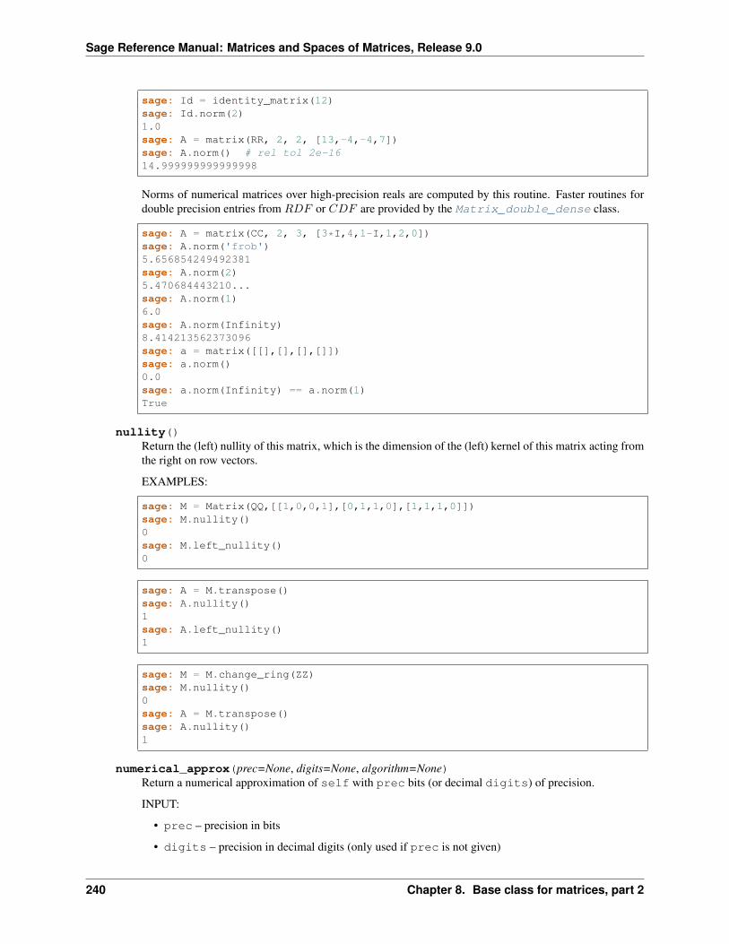
Sage Reference Manual: Matrices and Spaces of Matrices, Release 9.0
sage: Id = identity_matrix(12)sage: Id.norm(2)1.0sage: A = matrix(RR, 2, 2, [13,-4,-4,7])sage: A.norm() # rel tol 2e-1614.999999999999998
Norms of numerical matrices over high-precision reals are computed by this routine. Faster routines fordouble precision entries from 𝑅𝐷𝐹 or 𝐶𝐷𝐹 are provided by the Matrix_double_dense class.
sage: A = matrix(CC, 2, 3, [3*I,4,1-I,1,2,0])sage: A.norm('frob')5.656854249492381sage: A.norm(2)5.470684443210...sage: A.norm(1)6.0sage: A.norm(Infinity)8.414213562373096sage: a = matrix([[],[],[],[]])sage: a.norm()0.0sage: a.norm(Infinity) == a.norm(1)True
nullity()Return the (left) nullity of this matrix, which is the dimension of the (left) kernel of this matrix acting fromthe right on row vectors.
EXAMPLES:
sage: M = Matrix(QQ,[[1,0,0,1],[0,1,1,0],[1,1,1,0]])sage: M.nullity()0sage: M.left_nullity()0
sage: A = M.transpose()sage: A.nullity()1sage: A.left_nullity()1
sage: M = M.change_ring(ZZ)sage: M.nullity()0sage: A = M.transpose()sage: A.nullity()1
numerical_approx(prec=None, digits=None, algorithm=None)Return a numerical approximation of self with prec bits (or decimal digits) of precision.
INPUT:
• prec – precision in bits
• digits – precision in decimal digits (only used if prec is not given)
240 Chapter 8. Base class for matrices, part 2
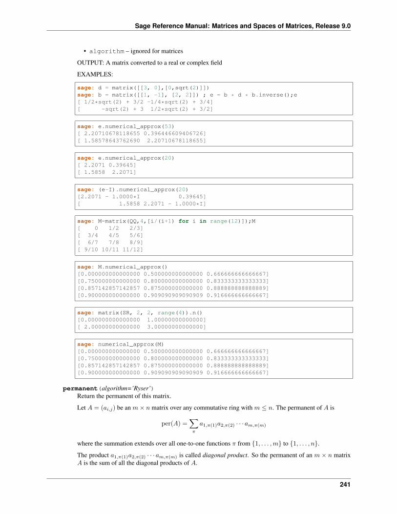
Sage Reference Manual: Matrices and Spaces of Matrices, Release 9.0
• algorithm – ignored for matrices
OUTPUT: A matrix converted to a real or complex field
EXAMPLES:
sage: d = matrix([[3, 0],[0,sqrt(2)]])sage: b = matrix([[1, -1], [2, 2]]) ; e = b * d * b.inverse();e[ 1/2*sqrt(2) + 3/2 -1/4*sqrt(2) + 3/4][ -sqrt(2) + 3 1/2*sqrt(2) + 3/2]
sage: e.numerical_approx(53)[ 2.20710678118655 0.396446609406726][ 1.58578643762690 2.20710678118655]
sage: e.numerical_approx(20)[ 2.2071 0.39645][ 1.5858 2.2071]
sage: (e-I).numerical_approx(20)[2.2071 - 1.0000*I 0.39645][ 1.5858 2.2071 - 1.0000*I]
sage: M=matrix(QQ,4,[i/(i+1) for i in range(12)]);M[ 0 1/2 2/3][ 3/4 4/5 5/6][ 6/7 7/8 8/9][ 9/10 10/11 11/12]
sage: M.numerical_approx()[0.000000000000000 0.500000000000000 0.666666666666667][0.750000000000000 0.800000000000000 0.833333333333333][0.857142857142857 0.875000000000000 0.888888888888889][0.900000000000000 0.909090909090909 0.916666666666667]
sage: matrix(SR, 2, 2, range(4)).n()[0.000000000000000 1.00000000000000][ 2.00000000000000 3.00000000000000]
sage: numerical_approx(M)[0.000000000000000 0.500000000000000 0.666666666666667][0.750000000000000 0.800000000000000 0.833333333333333][0.857142857142857 0.875000000000000 0.888888888888889][0.900000000000000 0.909090909090909 0.916666666666667]
permanent(algorithm=’Ryser’)Return the permanent of this matrix.
Let 𝐴 = (𝑎𝑖,𝑗) be an 𝑚× 𝑛 matrix over any commutative ring with 𝑚 ≤ 𝑛. The permanent of 𝐴 is
per(𝐴) =∑︁𝜋
𝑎1,𝜋(1)𝑎2,𝜋(2) · · · 𝑎𝑚,𝜋(𝑚)
where the summation extends over all one-to-one functions 𝜋 from {1, . . . ,𝑚} to {1, . . . , 𝑛}.
The product 𝑎1,𝜋(1)𝑎2,𝜋(2) · · · 𝑎𝑚,𝜋(𝑚) is called diagonal product. So the permanent of an 𝑚 × 𝑛 matrix𝐴 is the sum of all the diagonal products of 𝐴.
241
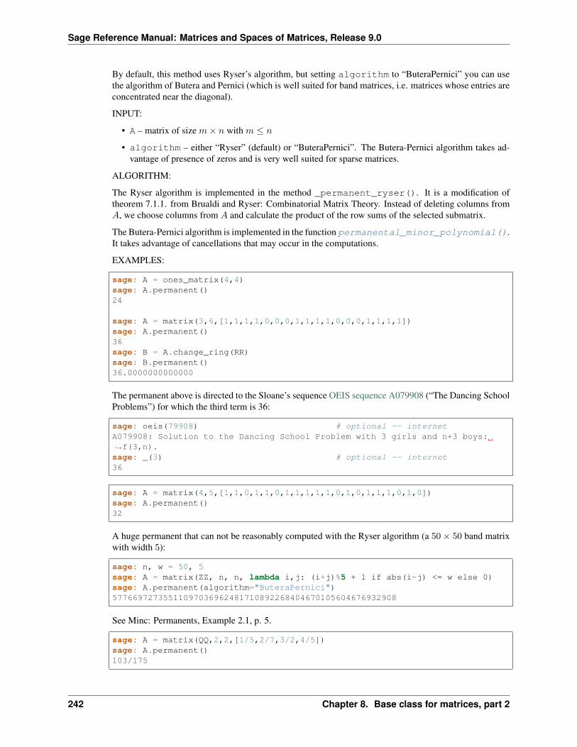
Sage Reference Manual: Matrices and Spaces of Matrices, Release 9.0
By default, this method uses Ryser’s algorithm, but setting algorithm to “ButeraPernici” you can usethe algorithm of Butera and Pernici (which is well suited for band matrices, i.e. matrices whose entries areconcentrated near the diagonal).
INPUT:
• A – matrix of size 𝑚× 𝑛 with 𝑚 ≤ 𝑛
• algorithm – either “Ryser” (default) or “ButeraPernici”. The Butera-Pernici algorithm takes ad-vantage of presence of zeros and is very well suited for sparse matrices.
ALGORITHM:
The Ryser algorithm is implemented in the method _permanent_ryser(). It is a modification oftheorem 7.1.1. from Brualdi and Ryser: Combinatorial Matrix Theory. Instead of deleting columns from𝐴, we choose columns from 𝐴 and calculate the product of the row sums of the selected submatrix.
The Butera-Pernici algorithm is implemented in the function permanental_minor_polynomial().It takes advantage of cancellations that may occur in the computations.
EXAMPLES:
sage: A = ones_matrix(4,4)sage: A.permanent()24
sage: A = matrix(3,6,[1,1,1,1,0,0,0,1,1,1,1,0,0,0,1,1,1,1])sage: A.permanent()36sage: B = A.change_ring(RR)sage: B.permanent()36.0000000000000
The permanent above is directed to the Sloane’s sequence OEIS sequence A079908 (“The Dancing SchoolProblems”) for which the third term is 36:
sage: oeis(79908) # optional -- internetA079908: Solution to the Dancing School Problem with 3 girls and n+3 boys:→˓f(3,n).sage: _(3) # optional -- internet36
sage: A = matrix(4,5,[1,1,0,1,1,0,1,1,1,1,1,0,1,0,1,1,1,0,1,0])sage: A.permanent()32
A huge permanent that can not be reasonably computed with the Ryser algorithm (a 50× 50 band matrixwith width 5):
sage: n, w = 50, 5sage: A = matrix(ZZ, n, n, lambda i,j: (i+j)%5 + 1 if abs(i-j) <= w else 0)sage: A.permanent(algorithm="ButeraPernici")57766972735511097036962481710892268404670105604676932908
See Minc: Permanents, Example 2.1, p. 5.
sage: A = matrix(QQ,2,2,[1/5,2/7,3/2,4/5])sage: A.permanent()103/175
242 Chapter 8. Base class for matrices, part 2
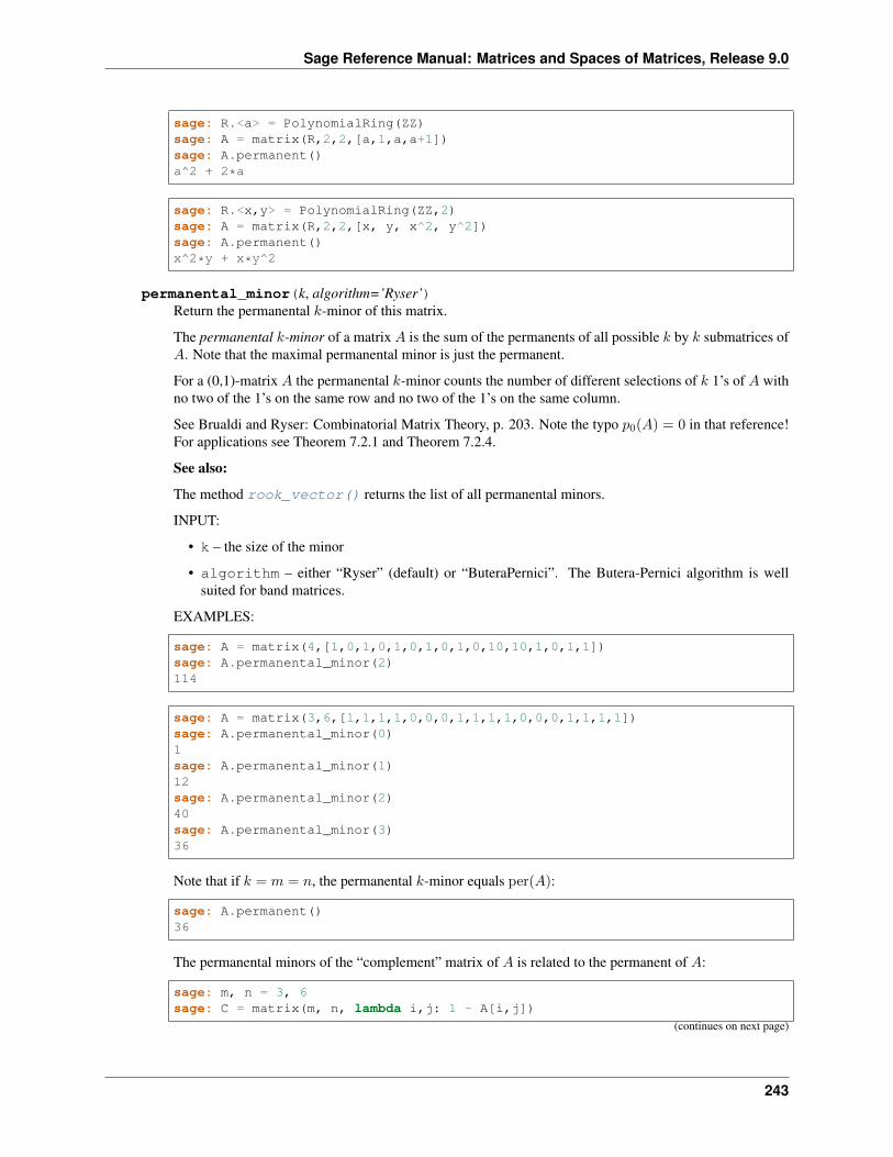
Sage Reference Manual: Matrices and Spaces of Matrices, Release 9.0
sage: R.<a> = PolynomialRing(ZZ)sage: A = matrix(R,2,2,[a,1,a,a+1])sage: A.permanent()a^2 + 2*a
sage: R.<x,y> = PolynomialRing(ZZ,2)sage: A = matrix(R,2,2,[x, y, x^2, y^2])sage: A.permanent()x^2*y + x*y^2
permanental_minor(k, algorithm=’Ryser’)Return the permanental 𝑘-minor of this matrix.
The permanental 𝑘-minor of a matrix 𝐴 is the sum of the permanents of all possible 𝑘 by 𝑘 submatrices of𝐴. Note that the maximal permanental minor is just the permanent.
For a (0,1)-matrix 𝐴 the permanental 𝑘-minor counts the number of different selections of 𝑘 1’s of 𝐴 withno two of the 1’s on the same row and no two of the 1’s on the same column.
See Brualdi and Ryser: Combinatorial Matrix Theory, p. 203. Note the typo 𝑝0(𝐴) = 0 in that reference!For applications see Theorem 7.2.1 and Theorem 7.2.4.
See also:
The method rook_vector() returns the list of all permanental minors.
INPUT:
• k – the size of the minor
• algorithm – either “Ryser” (default) or “ButeraPernici”. The Butera-Pernici algorithm is wellsuited for band matrices.
EXAMPLES:
sage: A = matrix(4,[1,0,1,0,1,0,1,0,1,0,10,10,1,0,1,1])sage: A.permanental_minor(2)114
sage: A = matrix(3,6,[1,1,1,1,0,0,0,1,1,1,1,0,0,0,1,1,1,1])sage: A.permanental_minor(0)1sage: A.permanental_minor(1)12sage: A.permanental_minor(2)40sage: A.permanental_minor(3)36
Note that if 𝑘 = 𝑚 = 𝑛, the permanental 𝑘-minor equals per(𝐴):
sage: A.permanent()36
The permanental minors of the “complement” matrix of 𝐴 is related to the permanent of 𝐴:
sage: m, n = 3, 6sage: C = matrix(m, n, lambda i,j: 1 - A[i,j])
(continues on next page)
243
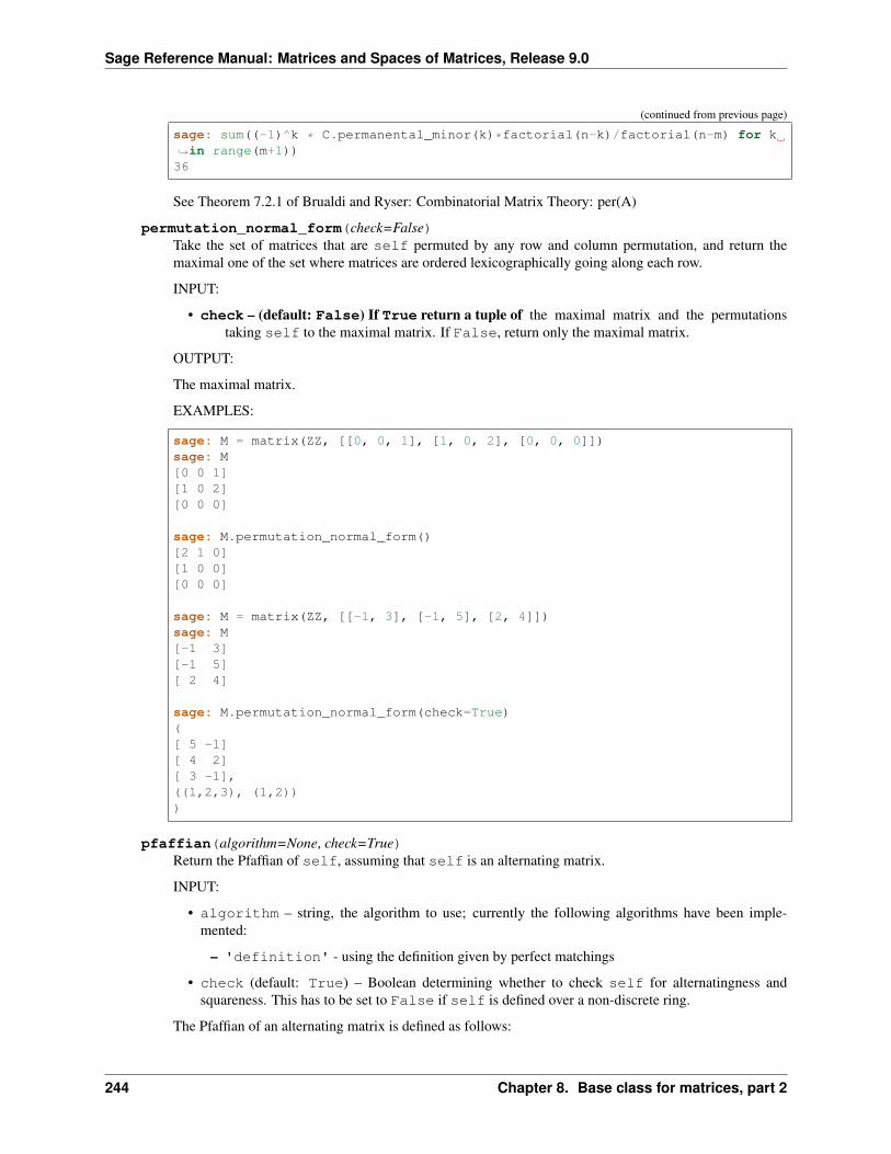
Sage Reference Manual: Matrices and Spaces of Matrices, Release 9.0
(continued from previous page)
sage: sum((-1)^k * C.permanental_minor(k)*factorial(n-k)/factorial(n-m) for k→˓in range(m+1))36
See Theorem 7.2.1 of Brualdi and Ryser: Combinatorial Matrix Theory: per(A)
permutation_normal_form(check=False)Take the set of matrices that are self permuted by any row and column permutation, and return themaximal one of the set where matrices are ordered lexicographically going along each row.
INPUT:
• check – (default: False) If True return a tuple of the maximal matrix and the permutationstaking self to the maximal matrix. If False, return only the maximal matrix.
OUTPUT:
The maximal matrix.
EXAMPLES:
sage: M = matrix(ZZ, [[0, 0, 1], [1, 0, 2], [0, 0, 0]])sage: M[0 0 1][1 0 2][0 0 0]
sage: M.permutation_normal_form()[2 1 0][1 0 0][0 0 0]
sage: M = matrix(ZZ, [[-1, 3], [-1, 5], [2, 4]])sage: M[-1 3][-1 5][ 2 4]
sage: M.permutation_normal_form(check=True)([ 5 -1][ 4 2][ 3 -1],((1,2,3), (1,2)))
pfaffian(algorithm=None, check=True)Return the Pfaffian of self, assuming that self is an alternating matrix.
INPUT:
• algorithm – string, the algorithm to use; currently the following algorithms have been imple-mented:
– 'definition' - using the definition given by perfect matchings
• check (default: True) – Boolean determining whether to check self for alternatingness andsquareness. This has to be set to False if self is defined over a non-discrete ring.
The Pfaffian of an alternating matrix is defined as follows:
244 Chapter 8. Base class for matrices, part 2
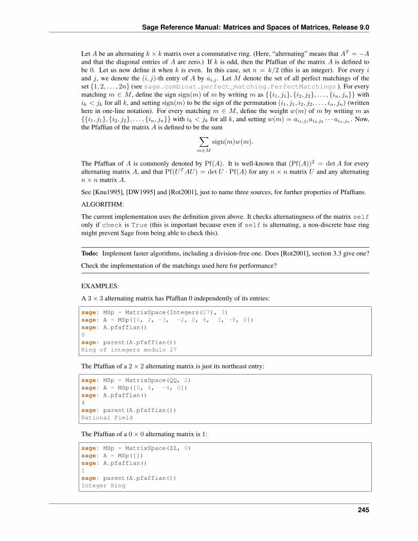
Sage Reference Manual: Matrices and Spaces of Matrices, Release 9.0
Let 𝐴 be an alternating 𝑘 × 𝑘 matrix over a commutative ring. (Here, “alternating” means that 𝐴𝑇 = −𝐴and that the diagonal entries of 𝐴 are zero.) If 𝑘 is odd, then the Pfaffian of the matrix 𝐴 is defined tobe 0. Let us now define it when 𝑘 is even. In this case, set 𝑛 = 𝑘/2 (this is an integer). For every 𝑖and 𝑗, we denote the (𝑖, 𝑗)-th entry of 𝐴 by 𝑎𝑖,𝑗 . Let 𝑀 denote the set of all perfect matchings of theset {1, 2, . . . , 2𝑛} (see sage.combinat.perfect_matching.PerfectMatchings ). For everymatching 𝑚 ∈ 𝑀 , define the sign sign(𝑚) of 𝑚 by writing 𝑚 as {{𝑖1, 𝑗1}, {𝑖2, 𝑗2}, . . . , {𝑖𝑛, 𝑗𝑛}} with𝑖𝑘 < 𝑗𝑘 for all 𝑘, and setting sign(𝑚) to be the sign of the permutation (𝑖1, 𝑗1, 𝑖2, 𝑗2, . . . , 𝑖𝑛, 𝑗𝑛) (writtenhere in one-line notation). For every matching 𝑚 ∈ 𝑀 , define the weight 𝑤(𝑚) of 𝑚 by writing 𝑚 as{{𝑖1, 𝑗1}, {𝑖2, 𝑗2}, . . . , {𝑖𝑛, 𝑗𝑛}} with 𝑖𝑘 < 𝑗𝑘 for all 𝑘, and setting 𝑤(𝑚) = 𝑎𝑖1,𝑗1𝑎𝑖2,𝑗2 · · · 𝑎𝑖𝑛,𝑗𝑛 . Now,the Pfaffian of the matrix 𝐴 is defined to be the sum∑︁
𝑚∈𝑀
sign(𝑚)𝑤(𝑚).
The Pfaffian of 𝐴 is commonly denoted by Pf(𝐴). It is well-known that (Pf(𝐴))2 = det𝐴 for everyalternating matrix 𝐴, and that Pf(𝑈𝑇𝐴𝑈) = det𝑈 · Pf(𝐴) for any 𝑛 × 𝑛 matrix 𝑈 and any alternating𝑛× 𝑛 matrix 𝐴.
See [Knu1995], [DW1995] and [Rot2001], just to name three sources, for further properties of Pfaffians.
ALGORITHM:
The current implementation uses the definition given above. It checks alternatingness of the matrix selfonly if check is True (this is important because even if self is alternating, a non-discrete base ringmight prevent Sage from being able to check this).
Todo: Implement faster algorithms, including a division-free one. Does [Rot2001], section 3.3 give one?
Check the implementation of the matchings used here for performance?
EXAMPLES:
A 3× 3 alternating matrix has Pfaffian 0 independently of its entries:
sage: MSp = MatrixSpace(Integers(27), 3)sage: A = MSp([0, 2, -3, -2, 0, 8, 3, -8, 0])sage: A.pfaffian()0sage: parent(A.pfaffian())Ring of integers modulo 27
The Pfaffian of a 2× 2 alternating matrix is just its northeast entry:
sage: MSp = MatrixSpace(QQ, 2)sage: A = MSp([0, 4, -4, 0])sage: A.pfaffian()4sage: parent(A.pfaffian())Rational Field
The Pfaffian of a 0× 0 alternating matrix is 1:
sage: MSp = MatrixSpace(ZZ, 0)sage: A = MSp([])sage: A.pfaffian()1sage: parent(A.pfaffian())Integer Ring
245
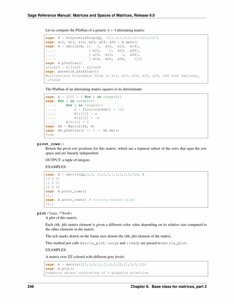
Sage Reference Manual: Matrices and Spaces of Matrices, Release 9.0
Let us compute the Pfaffian of a generic 4× 4 alternating matrix:
sage: R = PolynomialRing(QQ, 'x12,x13,x14,x23,x24,x34')sage: x12, x13, x14, x23, x24, x34 = R.gens()sage: A = matrix(R, [[ 0, x12, x13, x14],....: [-x12, 0, x23, x24],....: [-x13, -x23, 0, x34],....: [-x14, -x24, -x34, 0]])sage: A.pfaffian()x14*x23 - x13*x24 + x12*x34sage: parent(A.pfaffian())Multivariate Polynomial Ring in x12, x13, x14, x23, x24, x34 over Rational→˓Field
The Pfaffian of an alternating matrix squares to its determinant:
sage: A = [[0] * 6 for i in range(6)]sage: for i in range(6):....: for j in range(i):....: u = floor(random() * 10)....: A[i][j] = u....: A[j][i] = -u....: A[i][i] = 0sage: AA = Matrix(ZZ, A)sage: AA.pfaffian() ** 2 == AA.det()True
pivot_rows()Return the pivot row positions for this matrix, which are a topmost subset of the rows that span the rowspace and are linearly independent.
OUTPUT: a tuple of integers
EXAMPLES:
sage: A = matrix(QQ,3,3, [0,0,0,1,2,3,2,4,6]); A[0 0 0][1 2 3][2 4 6]sage: A.pivot_rows()(1,)sage: A.pivot_rows() # testing cached value(1,)
plot(*args, **kwds)A plot of this matrix.
Each (ith, jth) matrix element is given a different color value depending on its relative size compared tothe other elements in the matrix.
The tick marks drawn on the frame axes denote the (ith, jth) element of the matrix.
This method just calls matrix_plot. *args and **kwds are passed to matrix_plot.
EXAMPLES:
A matrix over ZZ colored with different grey levels:
sage: A = matrix([[1,3,5,1],[2,4,5,6],[1,3,5,7]])sage: A.plot()Graphics object consisting of 1 graphics primitive
246 Chapter 8. Base class for matrices, part 2
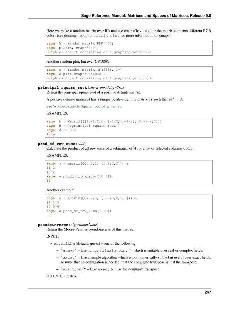
Sage Reference Manual: Matrices and Spaces of Matrices, Release 9.0
Here we make a random matrix over RR and use cmap=’hsv’ to color the matrix elements different RGBcolors (see documentation for matrix_plot for more information on cmaps):
sage: A = random_matrix(RDF, 50)sage: plot(A, cmap='hsv')Graphics object consisting of 1 graphics primitive
Another random plot, but over GF(389):
sage: A = random_matrix(GF(389), 10)sage: A.plot(cmap='Oranges')Graphics object consisting of 1 graphics primitive
principal_square_root(check_positivity=True)Return the principal square root of a positive definite matrix.
A positive definite matrix 𝐴 has a unique positive definite matrix 𝑀 such that 𝑀2 = 𝐴.
See Wikipedia article Square_root_of_a_matrix.
EXAMPLES:
sage: A = Matrix([[1,-1/2,0],[-1/2,1,-1/2],[0,-1/2,1]])sage: B = A.principal_square_root()sage: A == B^2True
prod_of_row_sums(cols)Calculate the product of all row sums of a submatrix of 𝐴 for a list of selected columns cols.
EXAMPLES:
sage: a = matrix(QQ, 2,2, [1,2,3,2]); a[1 2][3 2]sage: a.prod_of_row_sums([0,1])15
Another example:
sage: a = matrix(QQ, 2,3, [1,2,3,2,5,6]); a[1 2 3][2 5 6]sage: a.prod_of_row_sums([1,2])55
pseudoinverse(algorithm=None)Return the Moore-Penrose pseudoinverse of this matrix.
INPUT:
• algorithm (default: guess) – one of the following:
– "numpy" – Use numpy’s linalg.pinv() which is suitable over real or complex fields.
– "exact" – Use a simple algorithm which is not numerically stable but useful over exact fields.Assume that no conjugation is needed, that the conjugate transpose is just the transpose.
– "exactconj" – Like exact but use the conjugate transpose.
OUTPUT: a matrix
247
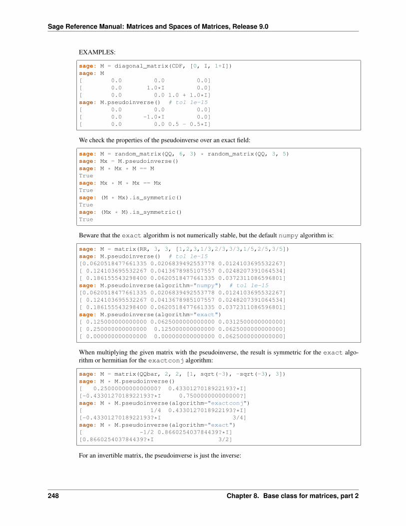
Sage Reference Manual: Matrices and Spaces of Matrices, Release 9.0
EXAMPLES:
sage: M = diagonal_matrix(CDF, [0, I, 1+I])sage: M[ 0.0 0.0 0.0][ 0.0 1.0*I 0.0][ 0.0 0.0 1.0 + 1.0*I]sage: M.pseudoinverse() # tol 1e-15[ 0.0 0.0 0.0][ 0.0 -1.0*I 0.0][ 0.0 0.0 0.5 - 0.5*I]
We check the properties of the pseudoinverse over an exact field:
sage: M = random_matrix(QQ, 6, 3) * random_matrix(QQ, 3, 5)sage: Mx = M.pseudoinverse()sage: M * Mx * M == MTruesage: Mx * M * Mx == MxTruesage: (M * Mx).is_symmetric()Truesage: (Mx * M).is_symmetric()True
Beware that the exact algorithm is not numerically stable, but the default numpy algorithm is:
sage: M = matrix(RR, 3, 3, [1,2,3,1/3,2/3,3/3,1/5,2/5,3/5])sage: M.pseudoinverse() # tol 1e-15[0.0620518477661335 0.0206839492553778 0.0124103695532267][ 0.124103695532267 0.0413678985107557 0.0248207391064534][ 0.186155543298400 0.0620518477661335 0.0372311086596801]sage: M.pseudoinverse(algorithm="numpy") # tol 1e-15[0.0620518477661335 0.0206839492553778 0.0124103695532267][ 0.124103695532267 0.0413678985107557 0.0248207391064534][ 0.186155543298400 0.0620518477661335 0.0372311086596801]sage: M.pseudoinverse(algorithm="exact")[ 0.125000000000000 0.0625000000000000 0.0312500000000000][ 0.250000000000000 0.125000000000000 0.0625000000000000][ 0.000000000000000 0.000000000000000 0.0625000000000000]
When multiplying the given matrix with the pseudoinverse, the result is symmetric for the exact algo-rithm or hermitian for the exactconj algorithm:
sage: M = matrix(QQbar, 2, 2, [1, sqrt(-3), -sqrt(-3), 3])sage: M * M.pseudoinverse()[ 0.2500000000000000? 0.4330127018922193?*I][-0.4330127018922193?*I 0.750000000000000?]sage: M * M.pseudoinverse(algorithm="exactconj")[ 1/4 0.4330127018922193?*I][-0.4330127018922193?*I 3/4]sage: M * M.pseudoinverse(algorithm="exact")[ -1/2 0.866025403784439?*I][0.866025403784439?*I 3/2]
For an invertible matrix, the pseudoinverse is just the inverse:
248 Chapter 8. Base class for matrices, part 2
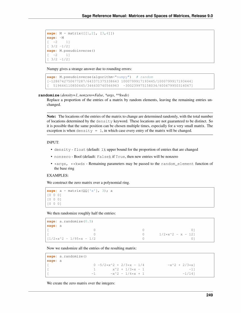
Sage Reference Manual: Matrices and Spaces of Matrices, Release 9.0
sage: M = matrix([[1,2], [3,4]])sage: ~M[ -2 1][ 3/2 -1/2]sage: M.pseudoinverse()[ -2 1][ 3/2 -1/2]
Numpy gives a strange answer due to rounding errors:
sage: M.pseudoinverse(algorithm="numpy") # random[-1286742750677287/643371375338643 1000799917193445/1000799917193444][ 519646110850445/346430740566963 -300239975158034/600479950316067]
randomize(density=1, nonzero=False, *args, **kwds)Replace a proportion of the entries of a matrix by random elements, leaving the remaining entries un-changed.
Note: The locations of the entries of the matrix to change are determined randomly, with the total numberof locations determined by the density keyword. These locations are not guaranteed to be distinct. Soit is possible that the same position can be chosen multiple times, especially for a very small matrix. Theexception is when density = 1, in which case every entry of the matrix will be changed.
INPUT:
• density - float (default: 1); upper bound for the proportion of entries that are changed
• nonzero - Bool (default: False); if True, then new entries will be nonzero
• *args, **kwds - Remaining parameters may be passed to the random_element function ofthe base ring
EXAMPLES:
We construct the zero matrix over a polynomial ring.
sage: a = matrix(QQ['x'], 3); a[0 0 0][0 0 0][0 0 0]
We then randomize roughly half the entries:
sage: a.randomize(0.5)sage: a[ 0 0 0][ 0 0 1/2*x^2 - x - 12][1/2*x^2 - 1/95*x - 1/2 0 0]
Now we randomize all the entries of the resulting matrix:
sage: a.randomize()sage: a[ 0 -5/2*x^2 + 2/3*x - 1/4 -x^2 + 2/3*x][ 1 x^2 + 1/3*x - 1 -1][ -1 -x^2 - 1/4*x + 1 -1/14]
We create the zero matrix over the integers:
249
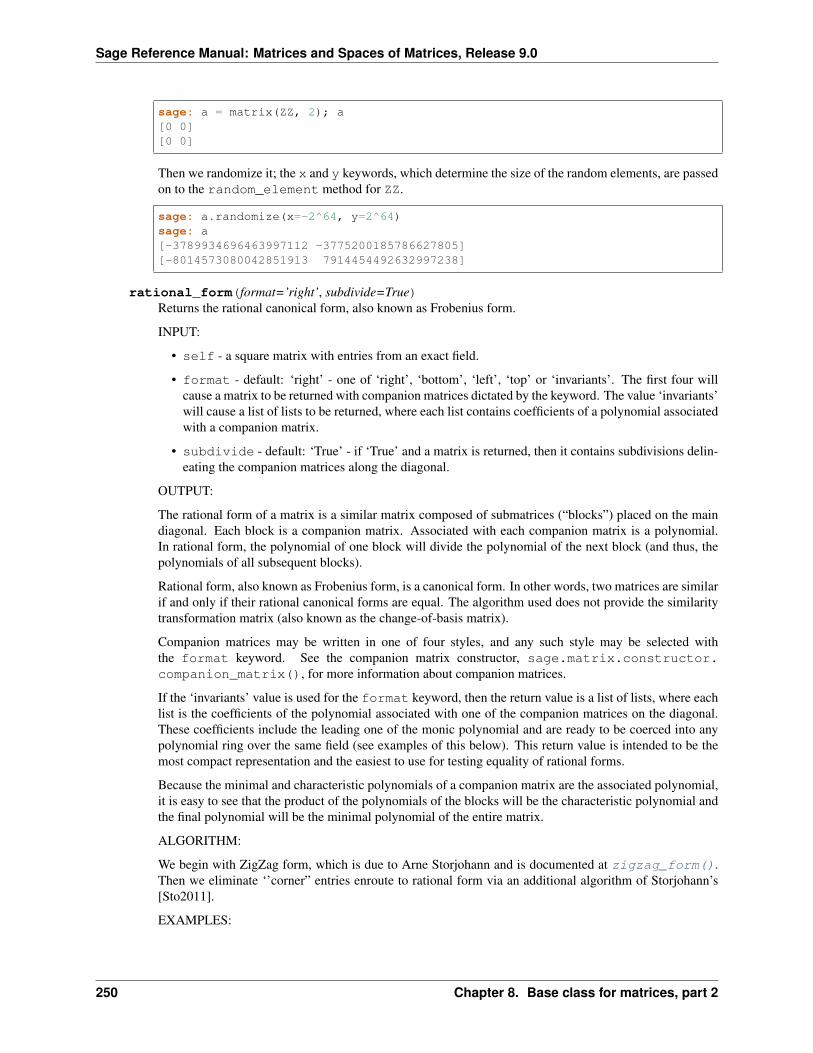
Sage Reference Manual: Matrices and Spaces of Matrices, Release 9.0
sage: a = matrix(ZZ, 2); a[0 0][0 0]
Then we randomize it; the x and y keywords, which determine the size of the random elements, are passedon to the random_element method for ZZ.
sage: a.randomize(x=-2^64, y=2^64)sage: a[-3789934696463997112 -3775200185786627805][-8014573080042851913 7914454492632997238]
rational_form(format=’right’, subdivide=True)Returns the rational canonical form, also known as Frobenius form.
INPUT:
• self - a square matrix with entries from an exact field.
• format - default: ‘right’ - one of ‘right’, ‘bottom’, ‘left’, ‘top’ or ‘invariants’. The first four willcause a matrix to be returned with companion matrices dictated by the keyword. The value ‘invariants’will cause a list of lists to be returned, where each list contains coefficients of a polynomial associatedwith a companion matrix.
• subdivide - default: ‘True’ - if ‘True’ and a matrix is returned, then it contains subdivisions delin-eating the companion matrices along the diagonal.
OUTPUT:
The rational form of a matrix is a similar matrix composed of submatrices (“blocks”) placed on the maindiagonal. Each block is a companion matrix. Associated with each companion matrix is a polynomial.In rational form, the polynomial of one block will divide the polynomial of the next block (and thus, thepolynomials of all subsequent blocks).
Rational form, also known as Frobenius form, is a canonical form. In other words, two matrices are similarif and only if their rational canonical forms are equal. The algorithm used does not provide the similaritytransformation matrix (also known as the change-of-basis matrix).
Companion matrices may be written in one of four styles, and any such style may be selected withthe format keyword. See the companion matrix constructor, sage.matrix.constructor.companion_matrix(), for more information about companion matrices.
If the ‘invariants’ value is used for the format keyword, then the return value is a list of lists, where eachlist is the coefficients of the polynomial associated with one of the companion matrices on the diagonal.These coefficients include the leading one of the monic polynomial and are ready to be coerced into anypolynomial ring over the same field (see examples of this below). This return value is intended to be themost compact representation and the easiest to use for testing equality of rational forms.
Because the minimal and characteristic polynomials of a companion matrix are the associated polynomial,it is easy to see that the product of the polynomials of the blocks will be the characteristic polynomial andthe final polynomial will be the minimal polynomial of the entire matrix.
ALGORITHM:
We begin with ZigZag form, which is due to Arne Storjohann and is documented at zigzag_form().Then we eliminate ‘’corner” entries enroute to rational form via an additional algorithm of Storjohann’s[Sto2011].
EXAMPLES:
250 Chapter 8. Base class for matrices, part 2
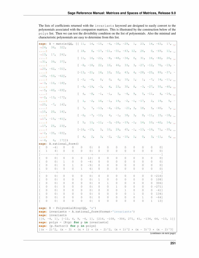
Sage Reference Manual: Matrices and Spaces of Matrices, Release 9.0
The lists of coefficients returned with the invariants keyword are designed to easily convert to thepolynomials associated with the companion matrices. This is illustrated by the construction below of thepolys list. Then we can test the divisibility condition on the list of polynomials. Also the minimal andcharacteristic polynomials are easy to determine from this list.
sage: A = matrix(QQ, [[ 11, 14, -15, -4, -38, -29, 1, 23, 14, -63, 17,→˓24, 36, 32],....: [ 18, 6, -17, -11, -31, -43, 12, 26, 0, -69, 11,→˓13, 17, 24],....: [ 11, 16, -22, -8, -48, -34, 0, 31, 16, -82, 26,→˓31, 39, 37],....: [ -8, -18, 22, 10, 46, 33, 3, -27, -12, 70, -19, -→˓20, -42, -31],....: [-13, -21, 16, 10, 52, 43, 4, -28, -25, 89, -37, -→˓20, -53, -62],....: [ -2, -6, 0, 0, 6, 10, 1, 1, -7, 14, -11,→˓-3, -10, -18],....: [ -9, -19, -3, 4, 23, 30, 8, -3, -27, 55, -40,→˓-5, -40, -69],....: [ 4, -8, -1, -1, 5, -4, 9, 5, -11, 4, -14,→˓-2, -13, -17],....: [ 1, -2, 16, -1, 19, -2, -1, -17, 2, 19, 5, -→˓25, -7, 14],....: [ 7, 7, -13, -4, -26, -21, 3, 18, 5, -40, 7,→˓15, 20, 14],....: [ -6, -7, -12, 4, -1, 18, 3, 8, -11, 15, -18,→˓17, -15, -41],....: [ 5, 11, -11, -3, -26, -19, -1, 14, 10, -42, 14,→˓17, 25, 23],....: [-16, -15, 3, 10, 29, 45, -1, -13, -19, 71, -35,→˓-2, -35, -65],....: [ 4, 2, 3, -2, -2, -10, 1, 0, 3, -11, 6,→˓-4, 6, 17]])sage: A.rational_form()[ 0 -4| 0 0 0 0| 0 0 0 0 0 0 0 0][ 1 4| 0 0 0 0| 0 0 0 0 0 0 0 0][---------+-------------------+---------------------------------------][ 0 0| 0 0 0 12| 0 0 0 0 0 0 0 0][ 0 0| 1 0 0 -4| 0 0 0 0 0 0 0 0][ 0 0| 0 1 0 -9| 0 0 0 0 0 0 0 0][ 0 0| 0 0 1 6| 0 0 0 0 0 0 0 0][---------+-------------------+---------------------------------------][ 0 0| 0 0 0 0| 0 0 0 0 0 0 0 -216][ 0 0| 0 0 0 0| 1 0 0 0 0 0 0 108][ 0 0| 0 0 0 0| 0 1 0 0 0 0 0 306][ 0 0| 0 0 0 0| 0 0 1 0 0 0 0 -271][ 0 0| 0 0 0 0| 0 0 0 1 0 0 0 -41][ 0 0| 0 0 0 0| 0 0 0 0 1 0 0 134][ 0 0| 0 0 0 0| 0 0 0 0 0 1 0 -64][ 0 0| 0 0 0 0| 0 0 0 0 0 0 1 13]
sage: R = PolynomialRing(QQ, 'x')sage: invariants = A.rational_form(format='invariants')sage: invariants[[4, -4, 1], [-12, 4, 9, -6, 1], [216, -108, -306, 271, 41, -134, 64, -13, 1]]sage: polys = [R(p) for p in invariants]sage: [p.factor() for p in polys][(x - 2)^2, (x - 3) * (x + 1) * (x - 2)^2, (x + 1)^2 * (x - 3)^3 * (x - 2)^3]
(continues on next page)
251
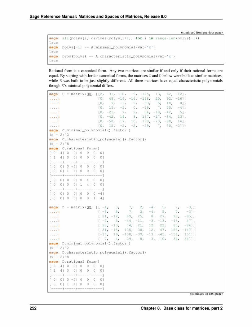
Sage Reference Manual: Matrices and Spaces of Matrices, Release 9.0
(continued from previous page)
sage: all(polys[i].divides(polys[i+1]) for i in range(len(polys)-1))Truesage: polys[-1] == A.minimal_polynomial(var='x')Truesage: prod(polys) == A.characteristic_polynomial(var='x')True
Rational form is a canonical form. Any two matrices are similar if and only if their rational forms areequal. By starting with Jordan canonical forms, the matrices C and D below were built as similar matrices,while E was built to be just slightly different. All three matrices have equal characteristic polynomialsthough E’s minimal polynomial differs.
sage: C = matrix(QQ, [[2, 31, -10, -9, -125, 13, 62, -12],....: [0, 48, -16, -16, -188, 20, 92, -16],....: [0, 9, -1, 2, -33, 5, 18, 0],....: [0, 15, -5, 0, -59, 7, 30, -4],....: [0, -21, 7, 2, 84, -10, -42, 5],....: [0, -42, 14, 8, 167, -17, -84, 13],....: [0, -50, 17, 10, 199, -23, -98, 14],....: [0, 15, -5, -2, -59, 7, 30, -2]])sage: C.minimal_polynomial().factor()(x - 2)^2sage: C.characteristic_polynomial().factor()(x - 2)^8sage: C.rational_form()[ 0 -4| 0 0| 0 0| 0 0][ 1 4| 0 0| 0 0| 0 0][-----+-----+-----+-----][ 0 0| 0 -4| 0 0| 0 0][ 0 0| 1 4| 0 0| 0 0][-----+-----+-----+-----][ 0 0| 0 0| 0 -4| 0 0][ 0 0| 0 0| 1 4| 0 0][-----+-----+-----+-----][ 0 0| 0 0| 0 0| 0 -4][ 0 0| 0 0| 0 0| 1 4]
sage: D = matrix(QQ, [[ -4, 3, 7, 2, -4, 5, 7, -3],....: [ -6, 5, 7, 2, -4, 5, 7, -3],....: [ 21, -12, 89, 25, 8, 27, 98, -95],....: [ -9, 5, -44, -11, -3, -13, -48, 47],....: [ 23, -13, 74, 21, 12, 22, 85, -84],....: [ 31, -18, 135, 38, 12, 47, 155, -147],....: [-33, 19, -138, -39, -13, -45, -156, 151],....: [ -7, 4, -29, -8, -3, -10, -34, 34]])sage: D.minimal_polynomial().factor()(x - 2)^2sage: D.characteristic_polynomial().factor()(x - 2)^8sage: D.rational_form()[ 0 -4| 0 0| 0 0| 0 0][ 1 4| 0 0| 0 0| 0 0][-----+-----+-----+-----][ 0 0| 0 -4| 0 0| 0 0][ 0 0| 1 4| 0 0| 0 0][-----+-----+-----+-----]
(continues on next page)
252 Chapter 8. Base class for matrices, part 2
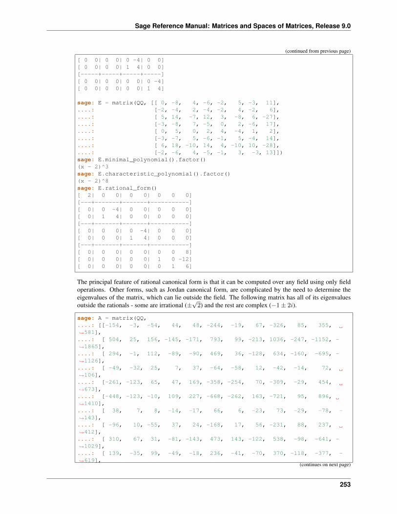
Sage Reference Manual: Matrices and Spaces of Matrices, Release 9.0
(continued from previous page)
[ 0 0| 0 0| 0 -4| 0 0][ 0 0| 0 0| 1 4| 0 0][-----+-----+-----+-----][ 0 0| 0 0| 0 0| 0 -4][ 0 0| 0 0| 0 0| 1 4]
sage: E = matrix(QQ, [[ 0, -8, 4, -6, -2, 5, -3, 11],....: [-2, -4, 2, -4, -2, 4, -2, 6],....: [ 5, 14, -7, 12, 3, -8, 6, -27],....: [-3, -8, 7, -5, 0, 2, -6, 17],....: [ 0, 5, 0, 2, 4, -4, 1, 2],....: [-3, -7, 5, -6, -1, 5, -4, 14],....: [ 6, 18, -10, 14, 4, -10, 10, -28],....: [-2, -6, 4, -5, -1, 3, -3, 13]])sage: E.minimal_polynomial().factor()(x - 2)^3sage: E.characteristic_polynomial().factor()(x - 2)^8sage: E.rational_form()[ 2| 0 0| 0 0| 0 0 0][---+-------+-------+-----------][ 0| 0 -4| 0 0| 0 0 0][ 0| 1 4| 0 0| 0 0 0][---+-------+-------+-----------][ 0| 0 0| 0 -4| 0 0 0][ 0| 0 0| 1 4| 0 0 0][---+-------+-------+-----------][ 0| 0 0| 0 0| 0 0 8][ 0| 0 0| 0 0| 1 0 -12][ 0| 0 0| 0 0| 0 1 6]
The principal feature of rational canonical form is that it can be computed over any field using only fieldoperations. Other forms, such as Jordan canonical form, are complicated by the need to determine theeigenvalues of the matrix, which can lie outside the field. The following matrix has all of its eigenvaluesoutside the rationals - some are irrational (±
√2) and the rest are complex (−1± 2𝑖).
sage: A = matrix(QQ,....: [[-154, -3, -54, 44, 48, -244, -19, 67, -326, 85, 355,→˓581],....: [ 504, 25, 156, -145, -171, 793, 99, -213, 1036, -247, -1152, -→˓1865],....: [ 294, -1, 112, -89, -90, 469, 36, -128, 634, -160, -695, -→˓1126],....: [ -49, -32, 25, 7, 37, -64, -58, 12, -42, -14, 72,→˓106],....: [-261, -123, 65, 47, 169, -358, -254, 70, -309, -29, 454,→˓673],....: [-448, -123, -10, 109, 227, -668, -262, 163, -721, 95, 896,→˓1410],....: [ 38, 7, 8, -14, -17, 66, 6, -23, 73, -29, -78, -→˓143],....: [ -96, 10, -55, 37, 24, -168, 17, 56, -231, 88, 237,→˓412],....: [ 310, 67, 31, -81, -143, 473, 143, -122, 538, -98, -641, -→˓1029],....: [ 139, -35, 99, -49, -18, 236, -41, -70, 370, -118, -377, -→˓619],
(continues on next page)
253
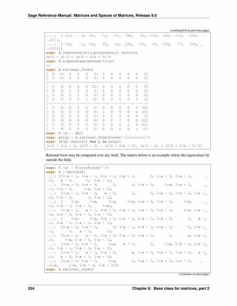
Sage Reference Manual: Matrices and Spaces of Matrices, Release 9.0
(continued from previous page)
....: [ 243, 9, 81, -72, -81, 386, 43, -105, 508, -124, -564, -→˓911],....: [-155, -3, -55, 45, 50, -245, -27, 65, -328, 77, 365,→˓583]])sage: A.characteristic_polynomial().factor()(x^2 - 2)^2 * (x^2 + 2*x + 5)^4sage: A.eigenvalues(extend=False)[]sage: A.rational_form()[ 0 -5| 0 0 0 0| 0 0 0 0 0 0][ 1 -2| 0 0 0 0| 0 0 0 0 0 0][-------+---------------+-----------------------][ 0 0| 0 0 0 10| 0 0 0 0 0 0][ 0 0| 1 0 0 4| 0 0 0 0 0 0][ 0 0| 0 1 0 -3| 0 0 0 0 0 0][ 0 0| 0 0 1 -2| 0 0 0 0 0 0][-------+---------------+-----------------------][ 0 0| 0 0 0 0| 0 0 0 0 0 50][ 0 0| 0 0 0 0| 1 0 0 0 0 40][ 0 0| 0 0 0 0| 0 1 0 0 0 3][ 0 0| 0 0 0 0| 0 0 1 0 0 -12][ 0 0| 0 0 0 0| 0 0 0 1 0 -12][ 0 0| 0 0 0 0| 0 0 0 0 1 -4]sage: F.<x> = QQ[]sage: polys = A.rational_form(format='invariants')sage: [F(p).factor() for p in polys][x^2 + 2*x + 5, (x^2 - 2) * (x^2 + 2*x + 5), (x^2 - 2) * (x^2 + 2*x + 5)^2]
Rational form may be computed over any field. The matrix below is an example where the eigenvalues lieoutside the field.
sage: F.<a> = FiniteField(7^2)sage: A = matrix(F,....: [[5*a + 3, 4*a + 1, 6*a + 2, 2*a + 5, 6, 4*a + 5, 4*a + 5,→˓5, a + 6, 5, 4*a + 4],....: [6*a + 3, 2*a + 4, 0, 6, 5*a + 5, 2*a, 5*a + 1,→˓1, 5*a + 2, 4*a, 5*a + 6],....: [3*a + 1, 6*a + 6, a + 6, 2, 0, 3*a + 6, 5*a + 4, 5*a +→˓6, 5*a + 2, 3, 4*a + 2],....: [ 3*a, 6*a, 3*a, 4*a, 4*a + 4, 3*a + 6, 6*a,→˓4, 3*a + 4, 6*a + 2, 4*a],....: [4*a + 5, a + 1, 4*a + 3, 6*a + 5, 5*a + 2, 5*a + 2, 6*a, 4*a +→˓6, 6*a + 4, 5*a + 3, 3*a + 1],....: [ 3*a, 6*a, 4*a + 1, 6*a + 2, 2*a + 5, 4*a + 6, 2, a +→˓5, 2*a + 4, 2*a + 1, 2*a + 1],....: [4*a + 5, 3*a + 3, 6, 4*a + 1, 4*a + 3, 6*a + 3, 6, 3*a +→˓3, 3, a + 3, 0],....: [6*a + 6, a + 4, 2*a + 6, 3*a + 5, 4*a + 3, 2, a, 3*a +→˓4, 5*a, 2*a + 5, 4*a + 3],....: [3*a + 5, 6*a + 2, 4*a, a + 5, 0, 5*a, 6*a + 5, 2*a +→˓1, 3*a + 1, 3*a + 5, 4*a + 2],....: [3*a + 2, a + 3, 3*a + 6, a, 3*a + 5, 5*a + 1, 3*a + 2, a +→˓3, a + 2, 6*a + 1, 3*a + 3],....: [6*a + 6, 5*a + 1, 4*a, 2, 5*a + 5, 3*a + 5, 3*a + 1,→˓2*a, 2*a, 2*a + 4, 4*a + 2]])sage: A.rational_form()
(continues on next page)
254 Chapter 8. Base class for matrices, part 2
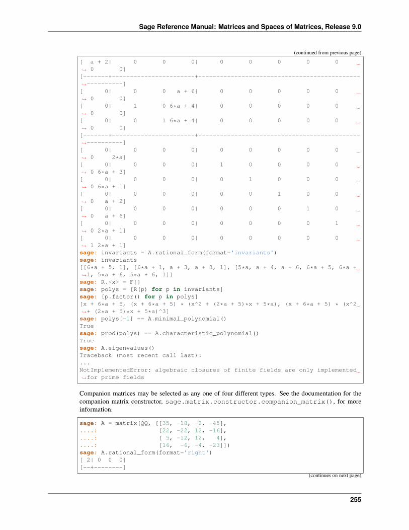
Sage Reference Manual: Matrices and Spaces of Matrices, Release 9.0
(continued from previous page)
[ a + 2| 0 0 0| 0 0 0 0 0→˓ 0 0][-------+-----------------------+---------------------------------------------→˓----------][ 0| 0 0 a + 6| 0 0 0 0 0→˓ 0 0][ 0| 1 0 6*a + 4| 0 0 0 0 0→˓ 0 0][ 0| 0 1 6*a + 4| 0 0 0 0 0→˓ 0 0][-------+-----------------------+---------------------------------------------→˓----------][ 0| 0 0 0| 0 0 0 0 0→˓ 0 2*a][ 0| 0 0 0| 1 0 0 0 0→˓ 0 6*a + 3][ 0| 0 0 0| 0 1 0 0 0→˓ 0 6*a + 1][ 0| 0 0 0| 0 0 1 0 0→˓ 0 a + 2][ 0| 0 0 0| 0 0 0 1 0→˓ 0 a + 6][ 0| 0 0 0| 0 0 0 0 1→˓ 0 2*a + 1][ 0| 0 0 0| 0 0 0 0 0→˓ 1 2*a + 1]sage: invariants = A.rational_form(format='invariants')sage: invariants[[6*a + 5, 1], [6*a + 1, a + 3, a + 3, 1], [5*a, a + 4, a + 6, 6*a + 5, 6*a +→˓1, 5*a + 6, 5*a + 6, 1]]sage: R.<x> = F[]sage: polys = [R(p) for p in invariants]sage: [p.factor() for p in polys][x + 6*a + 5, (x + 6*a + 5) * (x^2 + (2*a + 5)*x + 5*a), (x + 6*a + 5) * (x^2→˓+ (2*a + 5)*x + 5*a)^3]sage: polys[-1] == A.minimal_polynomial()Truesage: prod(polys) == A.characteristic_polynomial()Truesage: A.eigenvalues()Traceback (most recent call last):...NotImplementedError: algebraic closures of finite fields are only implemented→˓for prime fields
Companion matrices may be selected as any one of four different types. See the documentation for thecompanion matrix constructor, sage.matrix.constructor.companion_matrix(), for moreinformation.
sage: A = matrix(QQ, [[35, -18, -2, -45],....: [22, -22, 12, -16],....: [ 5, -12, 12, 4],....: [16, -6, -4, -23]])sage: A.rational_form(format='right')[ 2| 0 0 0][--+--------]
(continues on next page)
255
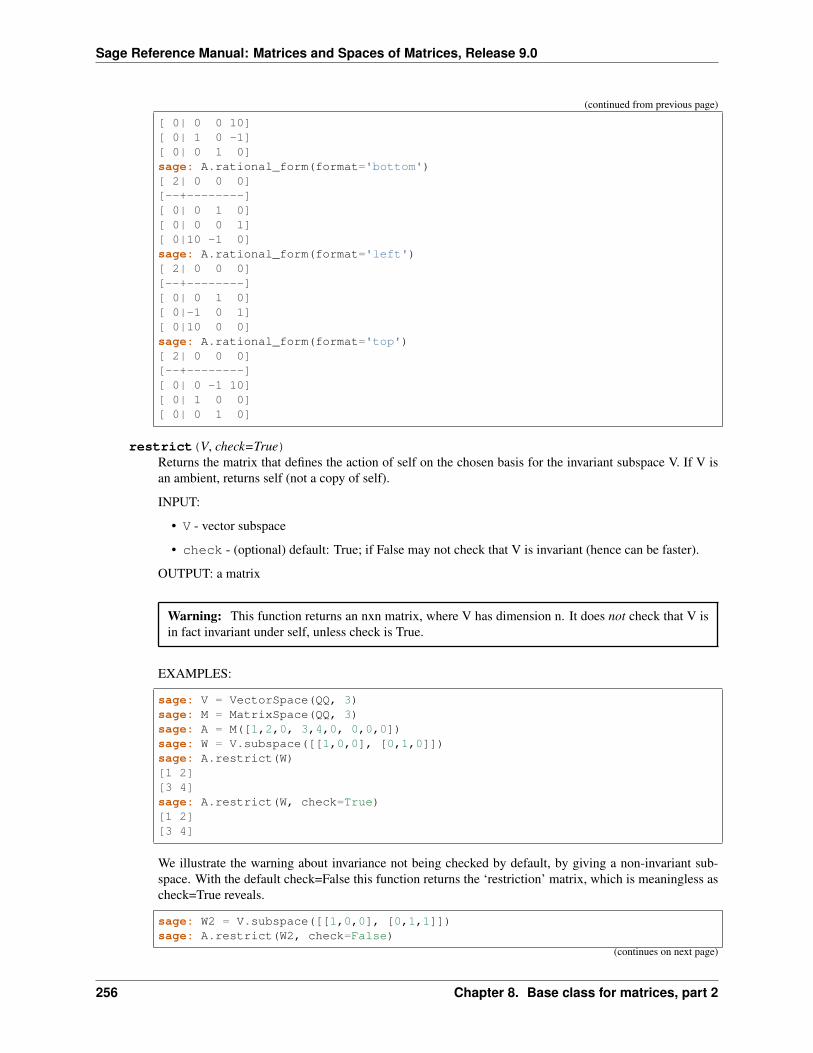
Sage Reference Manual: Matrices and Spaces of Matrices, Release 9.0
(continued from previous page)
[ 0| 0 0 10][ 0| 1 0 -1][ 0| 0 1 0]sage: A.rational_form(format='bottom')[ 2| 0 0 0][--+--------][ 0| 0 1 0][ 0| 0 0 1][ 0|10 -1 0]sage: A.rational_form(format='left')[ 2| 0 0 0][--+--------][ 0| 0 1 0][ 0|-1 0 1][ 0|10 0 0]sage: A.rational_form(format='top')[ 2| 0 0 0][--+--------][ 0| 0 -1 10][ 0| 1 0 0][ 0| 0 1 0]
restrict(V, check=True)Returns the matrix that defines the action of self on the chosen basis for the invariant subspace V. If V isan ambient, returns self (not a copy of self).
INPUT:
• V - vector subspace
• check - (optional) default: True; if False may not check that V is invariant (hence can be faster).
OUTPUT: a matrix
Warning: This function returns an nxn matrix, where V has dimension n. It does not check that V isin fact invariant under self, unless check is True.
EXAMPLES:
sage: V = VectorSpace(QQ, 3)sage: M = MatrixSpace(QQ, 3)sage: A = M([1,2,0, 3,4,0, 0,0,0])sage: W = V.subspace([[1,0,0], [0,1,0]])sage: A.restrict(W)[1 2][3 4]sage: A.restrict(W, check=True)[1 2][3 4]
We illustrate the warning about invariance not being checked by default, by giving a non-invariant sub-space. With the default check=False this function returns the ‘restriction’ matrix, which is meaningless ascheck=True reveals.
sage: W2 = V.subspace([[1,0,0], [0,1,1]])sage: A.restrict(W2, check=False)
(continues on next page)
256 Chapter 8. Base class for matrices, part 2
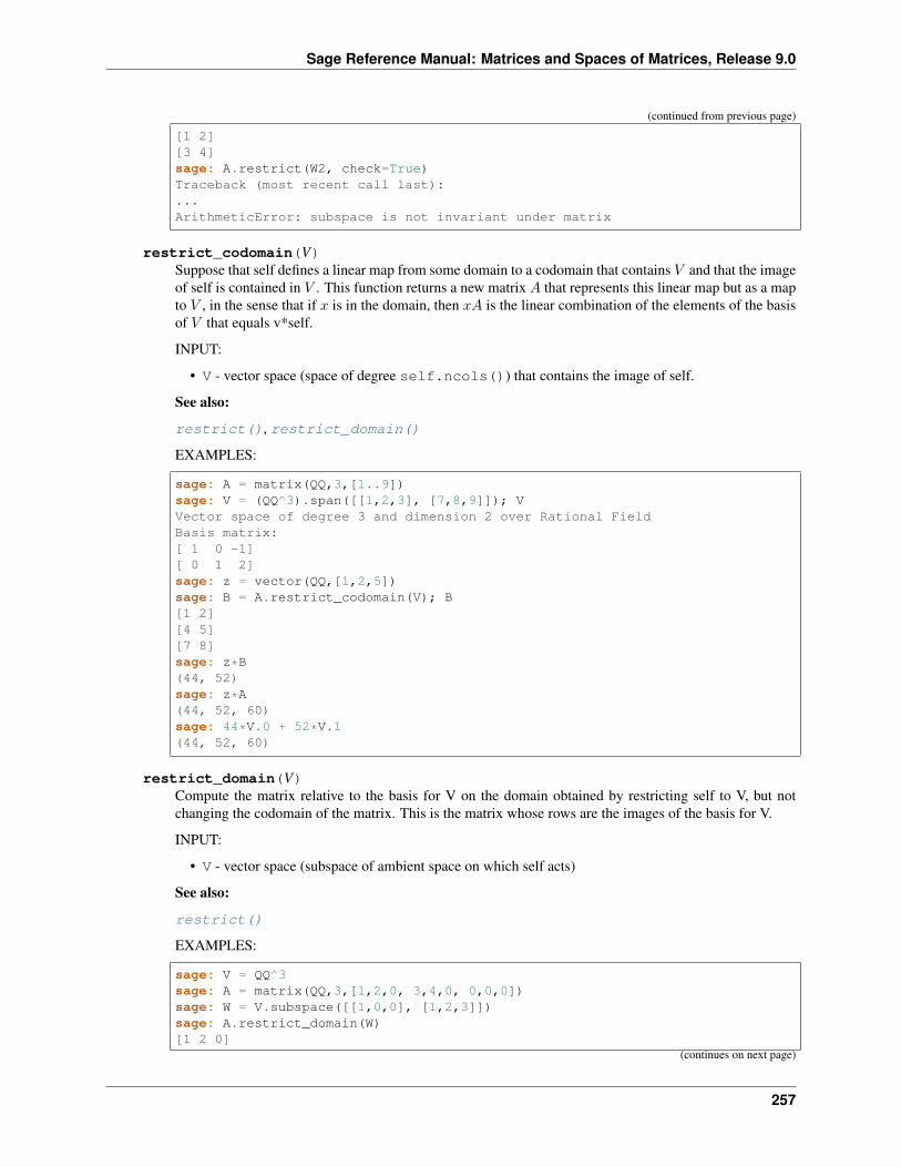
Sage Reference Manual: Matrices and Spaces of Matrices, Release 9.0
(continued from previous page)
[1 2][3 4]sage: A.restrict(W2, check=True)Traceback (most recent call last):...ArithmeticError: subspace is not invariant under matrix
restrict_codomain(V)Suppose that self defines a linear map from some domain to a codomain that contains 𝑉 and that the imageof self is contained in 𝑉 . This function returns a new matrix 𝐴 that represents this linear map but as a mapto 𝑉 , in the sense that if 𝑥 is in the domain, then 𝑥𝐴 is the linear combination of the elements of the basisof 𝑉 that equals v*self.
INPUT:
• V - vector space (space of degree self.ncols()) that contains the image of self.
See also:
restrict(), restrict_domain()
EXAMPLES:
sage: A = matrix(QQ,3,[1..9])sage: V = (QQ^3).span([[1,2,3], [7,8,9]]); VVector space of degree 3 and dimension 2 over Rational FieldBasis matrix:[ 1 0 -1][ 0 1 2]sage: z = vector(QQ,[1,2,5])sage: B = A.restrict_codomain(V); B[1 2][4 5][7 8]sage: z*B(44, 52)sage: z*A(44, 52, 60)sage: 44*V.0 + 52*V.1(44, 52, 60)
restrict_domain(V)Compute the matrix relative to the basis for V on the domain obtained by restricting self to V, but notchanging the codomain of the matrix. This is the matrix whose rows are the images of the basis for V.
INPUT:
• V - vector space (subspace of ambient space on which self acts)
See also:
restrict()
EXAMPLES:
sage: V = QQ^3sage: A = matrix(QQ,3,[1,2,0, 3,4,0, 0,0,0])sage: W = V.subspace([[1,0,0], [1,2,3]])sage: A.restrict_domain(W)[1 2 0]
(continues on next page)
257
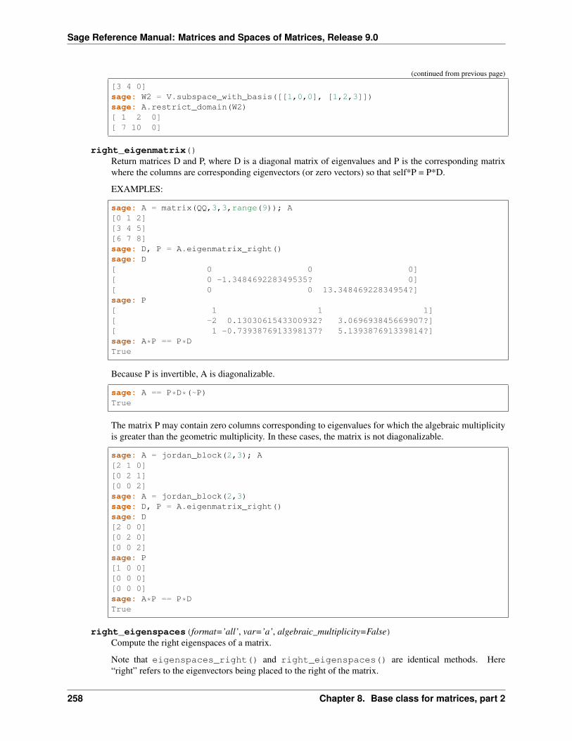
Sage Reference Manual: Matrices and Spaces of Matrices, Release 9.0
(continued from previous page)
[3 4 0]sage: W2 = V.subspace_with_basis([[1,0,0], [1,2,3]])sage: A.restrict_domain(W2)[ 1 2 0][ 7 10 0]
right_eigenmatrix()Return matrices D and P, where D is a diagonal matrix of eigenvalues and P is the corresponding matrixwhere the columns are corresponding eigenvectors (or zero vectors) so that self*P = P*D.
EXAMPLES:
sage: A = matrix(QQ,3,3,range(9)); A[0 1 2][3 4 5][6 7 8]sage: D, P = A.eigenmatrix_right()sage: D[ 0 0 0][ 0 -1.348469228349535? 0][ 0 0 13.34846922834954?]sage: P[ 1 1 1][ -2 0.1303061543300932? 3.069693845669907?][ 1 -0.7393876913398137? 5.139387691339814?]sage: A*P == P*DTrue
Because P is invertible, A is diagonalizable.
sage: A == P*D*(~P)True
The matrix P may contain zero columns corresponding to eigenvalues for which the algebraic multiplicityis greater than the geometric multiplicity. In these cases, the matrix is not diagonalizable.
sage: A = jordan_block(2,3); A[2 1 0][0 2 1][0 0 2]sage: A = jordan_block(2,3)sage: D, P = A.eigenmatrix_right()sage: D[2 0 0][0 2 0][0 0 2]sage: P[1 0 0][0 0 0][0 0 0]sage: A*P == P*DTrue
right_eigenspaces(format=’all’, var=’a’, algebraic_multiplicity=False)Compute the right eigenspaces of a matrix.
Note that eigenspaces_right() and right_eigenspaces() are identical methods. Here“right” refers to the eigenvectors being placed to the right of the matrix.
258 Chapter 8. Base class for matrices, part 2
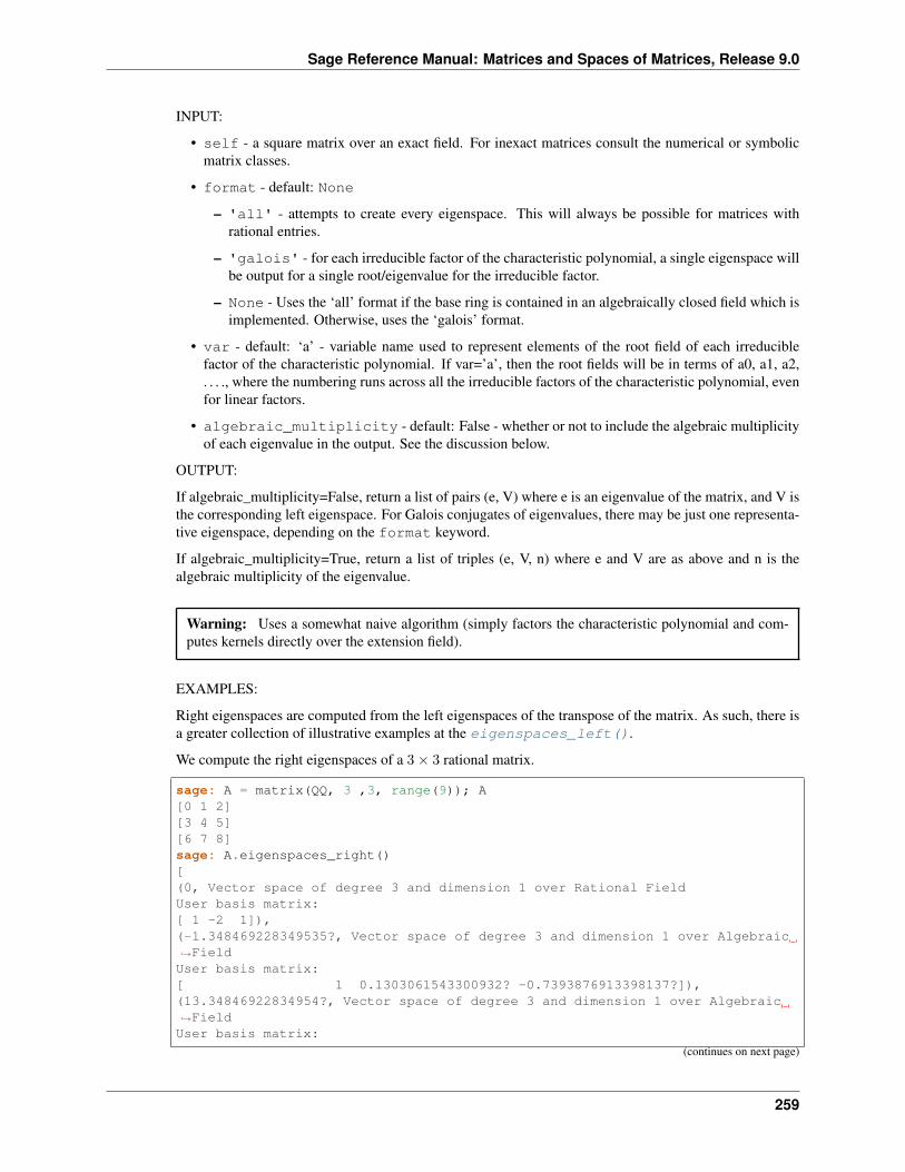
Sage Reference Manual: Matrices and Spaces of Matrices, Release 9.0
INPUT:
• self - a square matrix over an exact field. For inexact matrices consult the numerical or symbolicmatrix classes.
• format - default: None
– 'all' - attempts to create every eigenspace. This will always be possible for matrices withrational entries.
– 'galois' - for each irreducible factor of the characteristic polynomial, a single eigenspace willbe output for a single root/eigenvalue for the irreducible factor.
– None - Uses the ‘all’ format if the base ring is contained in an algebraically closed field which isimplemented. Otherwise, uses the ‘galois’ format.
• var - default: ‘a’ - variable name used to represent elements of the root field of each irreduciblefactor of the characteristic polynomial. If var=’a’, then the root fields will be in terms of a0, a1, a2,. . . ., where the numbering runs across all the irreducible factors of the characteristic polynomial, evenfor linear factors.
• algebraic_multiplicity - default: False - whether or not to include the algebraic multiplicityof each eigenvalue in the output. See the discussion below.
OUTPUT:
If algebraic_multiplicity=False, return a list of pairs (e, V) where e is an eigenvalue of the matrix, and V isthe corresponding left eigenspace. For Galois conjugates of eigenvalues, there may be just one representa-tive eigenspace, depending on the format keyword.
If algebraic_multiplicity=True, return a list of triples (e, V, n) where e and V are as above and n is thealgebraic multiplicity of the eigenvalue.
Warning: Uses a somewhat naive algorithm (simply factors the characteristic polynomial and com-putes kernels directly over the extension field).
EXAMPLES:
Right eigenspaces are computed from the left eigenspaces of the transpose of the matrix. As such, there isa greater collection of illustrative examples at the eigenspaces_left().
We compute the right eigenspaces of a 3× 3 rational matrix.
sage: A = matrix(QQ, 3 ,3, range(9)); A[0 1 2][3 4 5][6 7 8]sage: A.eigenspaces_right()[(0, Vector space of degree 3 and dimension 1 over Rational FieldUser basis matrix:[ 1 -2 1]),(-1.348469228349535?, Vector space of degree 3 and dimension 1 over Algebraic→˓FieldUser basis matrix:[ 1 0.1303061543300932? -0.7393876913398137?]),(13.34846922834954?, Vector space of degree 3 and dimension 1 over Algebraic→˓FieldUser basis matrix:
(continues on next page)
259
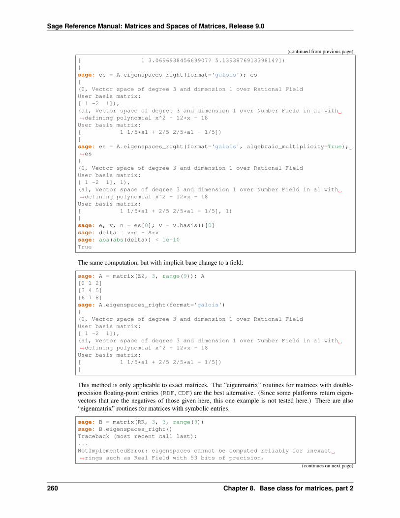
Sage Reference Manual: Matrices and Spaces of Matrices, Release 9.0
(continued from previous page)
[ 1 3.069693845669907? 5.139387691339814?])]sage: es = A.eigenspaces_right(format='galois'); es[(0, Vector space of degree 3 and dimension 1 over Rational FieldUser basis matrix:[ 1 -2 1]),(a1, Vector space of degree 3 and dimension 1 over Number Field in a1 with→˓defining polynomial x^2 - 12*x - 18User basis matrix:[ 1 1/5*a1 + 2/5 2/5*a1 - 1/5])]sage: es = A.eigenspaces_right(format='galois', algebraic_multiplicity=True);→˓es[(0, Vector space of degree 3 and dimension 1 over Rational FieldUser basis matrix:[ 1 -2 1], 1),(a1, Vector space of degree 3 and dimension 1 over Number Field in a1 with→˓defining polynomial x^2 - 12*x - 18User basis matrix:[ 1 1/5*a1 + 2/5 2/5*a1 - 1/5], 1)]sage: e, v, n = es[0]; v = v.basis()[0]sage: delta = v*e - A*vsage: abs(abs(delta)) < 1e-10True
The same computation, but with implicit base change to a field:
sage: A = matrix(ZZ, 3, range(9)); A[0 1 2][3 4 5][6 7 8]sage: A.eigenspaces_right(format='galois')[(0, Vector space of degree 3 and dimension 1 over Rational FieldUser basis matrix:[ 1 -2 1]),(a1, Vector space of degree 3 and dimension 1 over Number Field in a1 with→˓defining polynomial x^2 - 12*x - 18User basis matrix:[ 1 1/5*a1 + 2/5 2/5*a1 - 1/5])]
This method is only applicable to exact matrices. The “eigenmatrix” routines for matrices with double-precision floating-point entries (RDF, CDF) are the best alternative. (Since some platforms return eigen-vectors that are the negatives of those given here, this one example is not tested here.) There are also“eigenmatrix” routines for matrices with symbolic entries.
sage: B = matrix(RR, 3, 3, range(9))sage: B.eigenspaces_right()Traceback (most recent call last):...NotImplementedError: eigenspaces cannot be computed reliably for inexact→˓rings such as Real Field with 53 bits of precision,
(continues on next page)
260 Chapter 8. Base class for matrices, part 2
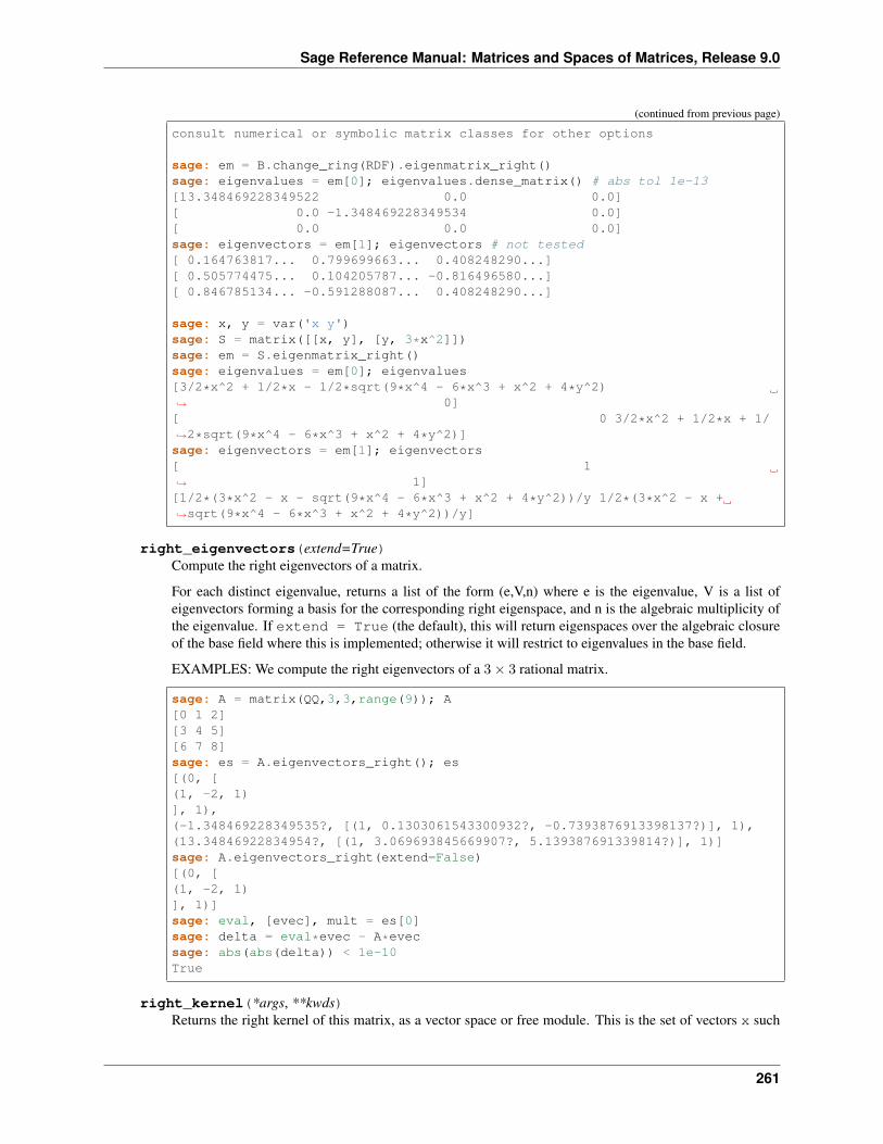
Sage Reference Manual: Matrices and Spaces of Matrices, Release 9.0
(continued from previous page)
consult numerical or symbolic matrix classes for other options
sage: em = B.change_ring(RDF).eigenmatrix_right()sage: eigenvalues = em[0]; eigenvalues.dense_matrix() # abs tol 1e-13[13.348469228349522 0.0 0.0][ 0.0 -1.348469228349534 0.0][ 0.0 0.0 0.0]sage: eigenvectors = em[1]; eigenvectors # not tested[ 0.164763817... 0.799699663... 0.408248290...][ 0.505774475... 0.104205787... -0.816496580...][ 0.846785134... -0.591288087... 0.408248290...]
sage: x, y = var('x y')sage: S = matrix([[x, y], [y, 3*x^2]])sage: em = S.eigenmatrix_right()sage: eigenvalues = em[0]; eigenvalues[3/2*x^2 + 1/2*x - 1/2*sqrt(9*x^4 - 6*x^3 + x^2 + 4*y^2)→˓ 0][ 0 3/2*x^2 + 1/2*x + 1/→˓2*sqrt(9*x^4 - 6*x^3 + x^2 + 4*y^2)]sage: eigenvectors = em[1]; eigenvectors[ 1→˓ 1][1/2*(3*x^2 - x - sqrt(9*x^4 - 6*x^3 + x^2 + 4*y^2))/y 1/2*(3*x^2 - x +→˓sqrt(9*x^4 - 6*x^3 + x^2 + 4*y^2))/y]
right_eigenvectors(extend=True)Compute the right eigenvectors of a matrix.
For each distinct eigenvalue, returns a list of the form (e,V,n) where e is the eigenvalue, V is a list ofeigenvectors forming a basis for the corresponding right eigenspace, and n is the algebraic multiplicity ofthe eigenvalue. If extend = True (the default), this will return eigenspaces over the algebraic closureof the base field where this is implemented; otherwise it will restrict to eigenvalues in the base field.
EXAMPLES: We compute the right eigenvectors of a 3× 3 rational matrix.
sage: A = matrix(QQ,3,3,range(9)); A[0 1 2][3 4 5][6 7 8]sage: es = A.eigenvectors_right(); es[(0, [(1, -2, 1)], 1),(-1.348469228349535?, [(1, 0.1303061543300932?, -0.7393876913398137?)], 1),(13.34846922834954?, [(1, 3.069693845669907?, 5.139387691339814?)], 1)]sage: A.eigenvectors_right(extend=False)[(0, [(1, -2, 1)], 1)]sage: eval, [evec], mult = es[0]sage: delta = eval*evec - A*evecsage: abs(abs(delta)) < 1e-10True
right_kernel(*args, **kwds)Returns the right kernel of this matrix, as a vector space or free module. This is the set of vectors x such
261
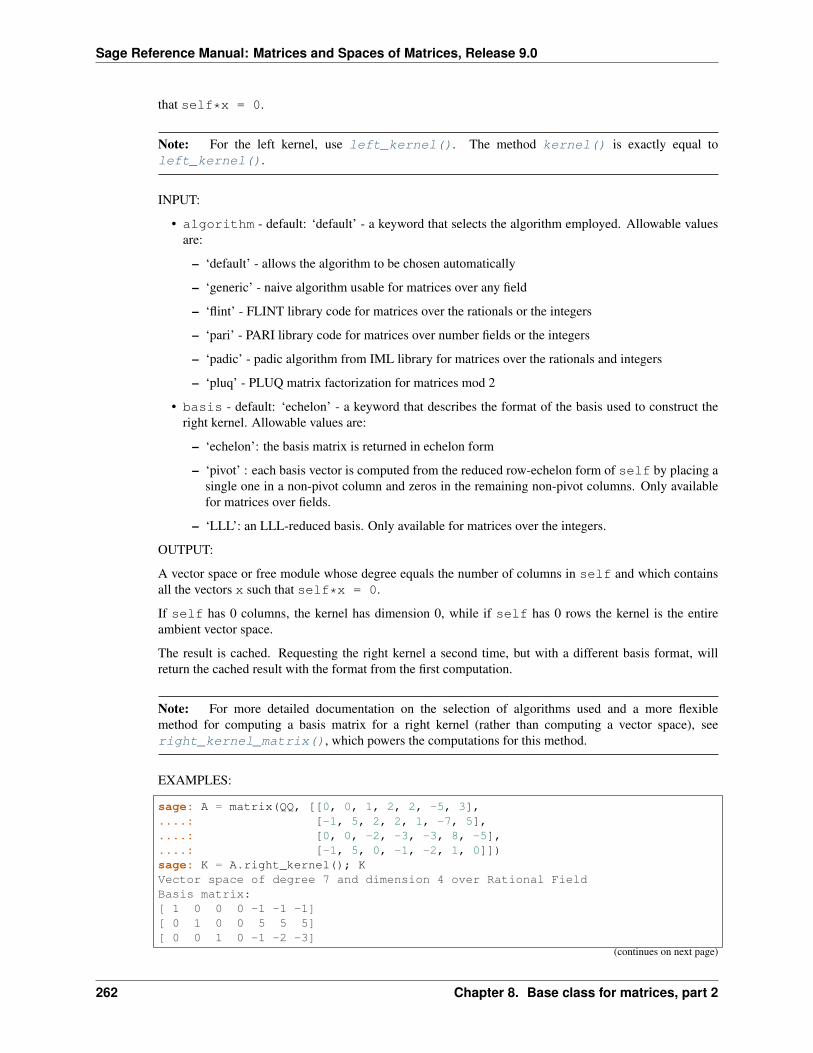
Sage Reference Manual: Matrices and Spaces of Matrices, Release 9.0
that self*x = 0.
Note: For the left kernel, use left_kernel(). The method kernel() is exactly equal toleft_kernel().
INPUT:
• algorithm - default: ‘default’ - a keyword that selects the algorithm employed. Allowable valuesare:
– ‘default’ - allows the algorithm to be chosen automatically
– ‘generic’ - naive algorithm usable for matrices over any field
– ‘flint’ - FLINT library code for matrices over the rationals or the integers
– ‘pari’ - PARI library code for matrices over number fields or the integers
– ‘padic’ - padic algorithm from IML library for matrices over the rationals and integers
– ‘pluq’ - PLUQ matrix factorization for matrices mod 2
• basis - default: ‘echelon’ - a keyword that describes the format of the basis used to construct theright kernel. Allowable values are:
– ‘echelon’: the basis matrix is returned in echelon form
– ‘pivot’ : each basis vector is computed from the reduced row-echelon form of self by placing asingle one in a non-pivot column and zeros in the remaining non-pivot columns. Only availablefor matrices over fields.
– ‘LLL’: an LLL-reduced basis. Only available for matrices over the integers.
OUTPUT:
A vector space or free module whose degree equals the number of columns in self and which containsall the vectors x such that self*x = 0.
If self has 0 columns, the kernel has dimension 0, while if self has 0 rows the kernel is the entireambient vector space.
The result is cached. Requesting the right kernel a second time, but with a different basis format, willreturn the cached result with the format from the first computation.
Note: For more detailed documentation on the selection of algorithms used and a more flexiblemethod for computing a basis matrix for a right kernel (rather than computing a vector space), seeright_kernel_matrix(), which powers the computations for this method.
EXAMPLES:
sage: A = matrix(QQ, [[0, 0, 1, 2, 2, -5, 3],....: [-1, 5, 2, 2, 1, -7, 5],....: [0, 0, -2, -3, -3, 8, -5],....: [-1, 5, 0, -1, -2, 1, 0]])sage: K = A.right_kernel(); KVector space of degree 7 and dimension 4 over Rational FieldBasis matrix:[ 1 0 0 0 -1 -1 -1][ 0 1 0 0 5 5 5][ 0 0 1 0 -1 -2 -3]
(continues on next page)
262 Chapter 8. Base class for matrices, part 2
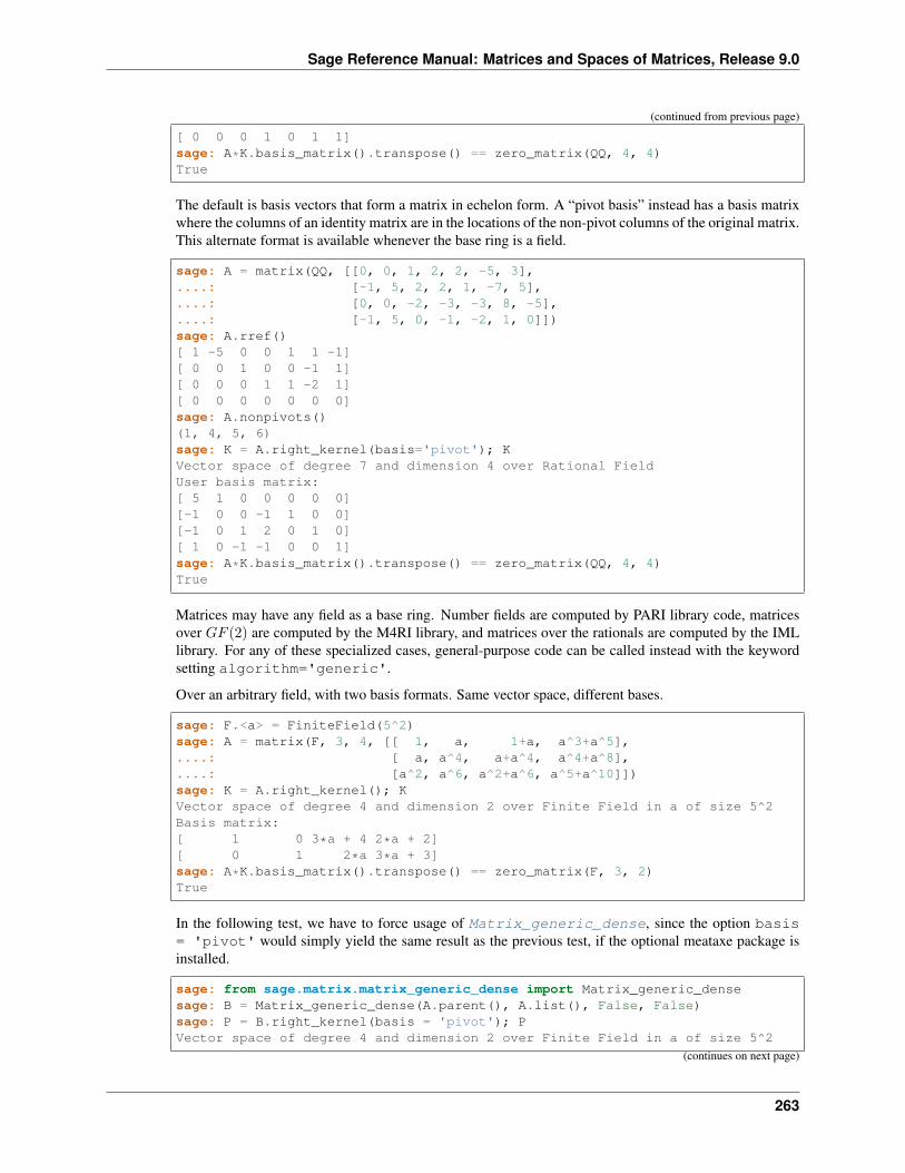
Sage Reference Manual: Matrices and Spaces of Matrices, Release 9.0
(continued from previous page)
[ 0 0 0 1 0 1 1]sage: A*K.basis_matrix().transpose() == zero_matrix(QQ, 4, 4)True
The default is basis vectors that form a matrix in echelon form. A “pivot basis” instead has a basis matrixwhere the columns of an identity matrix are in the locations of the non-pivot columns of the original matrix.This alternate format is available whenever the base ring is a field.
sage: A = matrix(QQ, [[0, 0, 1, 2, 2, -5, 3],....: [-1, 5, 2, 2, 1, -7, 5],....: [0, 0, -2, -3, -3, 8, -5],....: [-1, 5, 0, -1, -2, 1, 0]])sage: A.rref()[ 1 -5 0 0 1 1 -1][ 0 0 1 0 0 -1 1][ 0 0 0 1 1 -2 1][ 0 0 0 0 0 0 0]sage: A.nonpivots()(1, 4, 5, 6)sage: K = A.right_kernel(basis='pivot'); KVector space of degree 7 and dimension 4 over Rational FieldUser basis matrix:[ 5 1 0 0 0 0 0][-1 0 0 -1 1 0 0][-1 0 1 2 0 1 0][ 1 0 -1 -1 0 0 1]sage: A*K.basis_matrix().transpose() == zero_matrix(QQ, 4, 4)True
Matrices may have any field as a base ring. Number fields are computed by PARI library code, matricesover 𝐺𝐹 (2) are computed by the M4RI library, and matrices over the rationals are computed by the IMLlibrary. For any of these specialized cases, general-purpose code can be called instead with the keywordsetting algorithm='generic'.
Over an arbitrary field, with two basis formats. Same vector space, different bases.
sage: F.<a> = FiniteField(5^2)sage: A = matrix(F, 3, 4, [[ 1, a, 1+a, a^3+a^5],....: [ a, a^4, a+a^4, a^4+a^8],....: [a^2, a^6, a^2+a^6, a^5+a^10]])sage: K = A.right_kernel(); KVector space of degree 4 and dimension 2 over Finite Field in a of size 5^2Basis matrix:[ 1 0 3*a + 4 2*a + 2][ 0 1 2*a 3*a + 3]sage: A*K.basis_matrix().transpose() == zero_matrix(F, 3, 2)True
In the following test, we have to force usage of Matrix_generic_dense, since the option basis= 'pivot' would simply yield the same result as the previous test, if the optional meataxe package isinstalled.
sage: from sage.matrix.matrix_generic_dense import Matrix_generic_densesage: B = Matrix_generic_dense(A.parent(), A.list(), False, False)sage: P = B.right_kernel(basis = 'pivot'); PVector space of degree 4 and dimension 2 over Finite Field in a of size 5^2
(continues on next page)
263
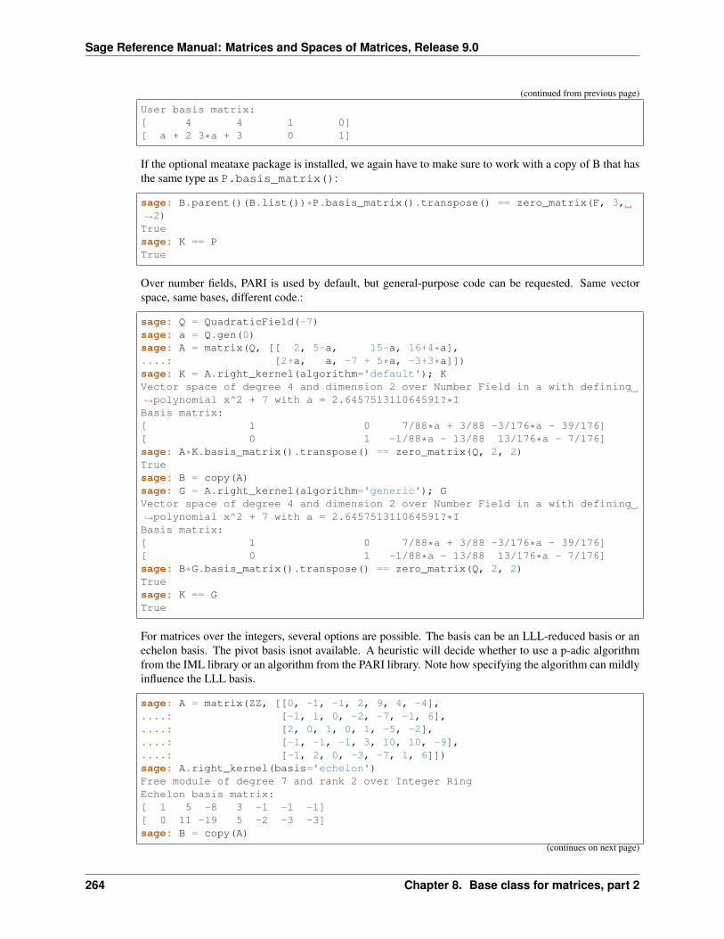
Sage Reference Manual: Matrices and Spaces of Matrices, Release 9.0
(continued from previous page)
User basis matrix:[ 4 4 1 0][ a + 2 3*a + 3 0 1]
If the optional meataxe package is installed, we again have to make sure to work with a copy of B that hasthe same type as P.basis_matrix():
sage: B.parent()(B.list())*P.basis_matrix().transpose() == zero_matrix(F, 3,→˓2)Truesage: K == PTrue
Over number fields, PARI is used by default, but general-purpose code can be requested. Same vectorspace, same bases, different code.:
sage: Q = QuadraticField(-7)sage: a = Q.gen(0)sage: A = matrix(Q, [[ 2, 5-a, 15-a, 16+4*a],....: [2+a, a, -7 + 5*a, -3+3*a]])sage: K = A.right_kernel(algorithm='default'); KVector space of degree 4 and dimension 2 over Number Field in a with defining→˓polynomial x^2 + 7 with a = 2.645751311064591?*IBasis matrix:[ 1 0 7/88*a + 3/88 -3/176*a - 39/176][ 0 1 -1/88*a - 13/88 13/176*a - 7/176]sage: A*K.basis_matrix().transpose() == zero_matrix(Q, 2, 2)Truesage: B = copy(A)sage: G = A.right_kernel(algorithm='generic'); GVector space of degree 4 and dimension 2 over Number Field in a with defining→˓polynomial x^2 + 7 with a = 2.645751311064591?*IBasis matrix:[ 1 0 7/88*a + 3/88 -3/176*a - 39/176][ 0 1 -1/88*a - 13/88 13/176*a - 7/176]sage: B*G.basis_matrix().transpose() == zero_matrix(Q, 2, 2)Truesage: K == GTrue
For matrices over the integers, several options are possible. The basis can be an LLL-reduced basis or anechelon basis. The pivot basis isnot available. A heuristic will decide whether to use a p-adic algorithmfrom the IML library or an algorithm from the PARI library. Note how specifying the algorithm can mildlyinfluence the LLL basis.
sage: A = matrix(ZZ, [[0, -1, -1, 2, 9, 4, -4],....: [-1, 1, 0, -2, -7, -1, 6],....: [2, 0, 1, 0, 1, -5, -2],....: [-1, -1, -1, 3, 10, 10, -9],....: [-1, 2, 0, -3, -7, 1, 6]])sage: A.right_kernel(basis='echelon')Free module of degree 7 and rank 2 over Integer RingEchelon basis matrix:[ 1 5 -8 3 -1 -1 -1][ 0 11 -19 5 -2 -3 -3]sage: B = copy(A)
(continues on next page)
264 Chapter 8. Base class for matrices, part 2
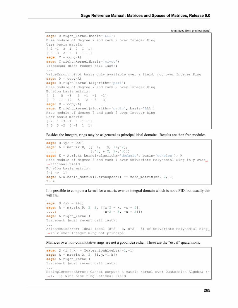
Sage Reference Manual: Matrices and Spaces of Matrices, Release 9.0
(continued from previous page)
sage: B.right_kernel(basis='LLL')Free module of degree 7 and rank 2 over Integer RingUser basis matrix:[ 2 -1 3 1 0 1 1][-5 -3 2 -5 1 -1 -1]sage: C = copy(A)sage: C.right_kernel(basis='pivot')Traceback (most recent call last):...ValueError: pivot basis only available over a field, not over Integer Ringsage: D = copy(A)sage: D.right_kernel(algorithm='pari')Free module of degree 7 and rank 2 over Integer RingEchelon basis matrix:[ 1 5 -8 3 -1 -1 -1][ 0 11 -19 5 -2 -3 -3]sage: E = copy(A)sage: E.right_kernel(algorithm='padic', basis='LLL')Free module of degree 7 and rank 2 over Integer RingUser basis matrix:[-2 1 -3 -1 0 -1 -1][ 5 3 -2 5 -1 1 1]
Besides the integers, rings may be as general as principal ideal domains. Results are then free modules.
sage: R.<y> = QQ[]sage: A = matrix(R, [[ 1, y, 1+y^2],....: [y^3, y^2, 2*y^3]])sage: K = A.right_kernel(algorithm='default', basis='echelon'); KFree module of degree 3 and rank 1 over Univariate Polynomial Ring in y over→˓Rational FieldEchelon basis matrix:[-1 -y 1]sage: A*K.basis_matrix().transpose() == zero_matrix(ZZ, 2, 1)True
It is possible to compute a kernel for a matrix over an integral domain which is not a PID, but usually thiswill fail.
sage: D.<x> = ZZ[]sage: A = matrix(D, 2, 2, [[x^2 - x, -x + 5],....: [x^2 - 8, -x + 2]])sage: A.right_kernel()Traceback (most recent call last):...ArithmeticError: Ideal Ideal (x^2 - x, x^2 - 8) of Univariate Polynomial Ring→˓in x over Integer Ring not principal
Matrices over non-commutative rings are not a good idea either. These are the “usual” quaternions.
sage: Q.<i,j,k> = QuaternionAlgebra(-1,-1)sage: A = matrix(Q, 2, [i,j,-1,k])sage: A.right_kernel()Traceback (most recent call last):...NotImplementedError: Cannot compute a matrix kernel over Quaternion Algebra (-→˓1, -1) with base ring Rational Field
265
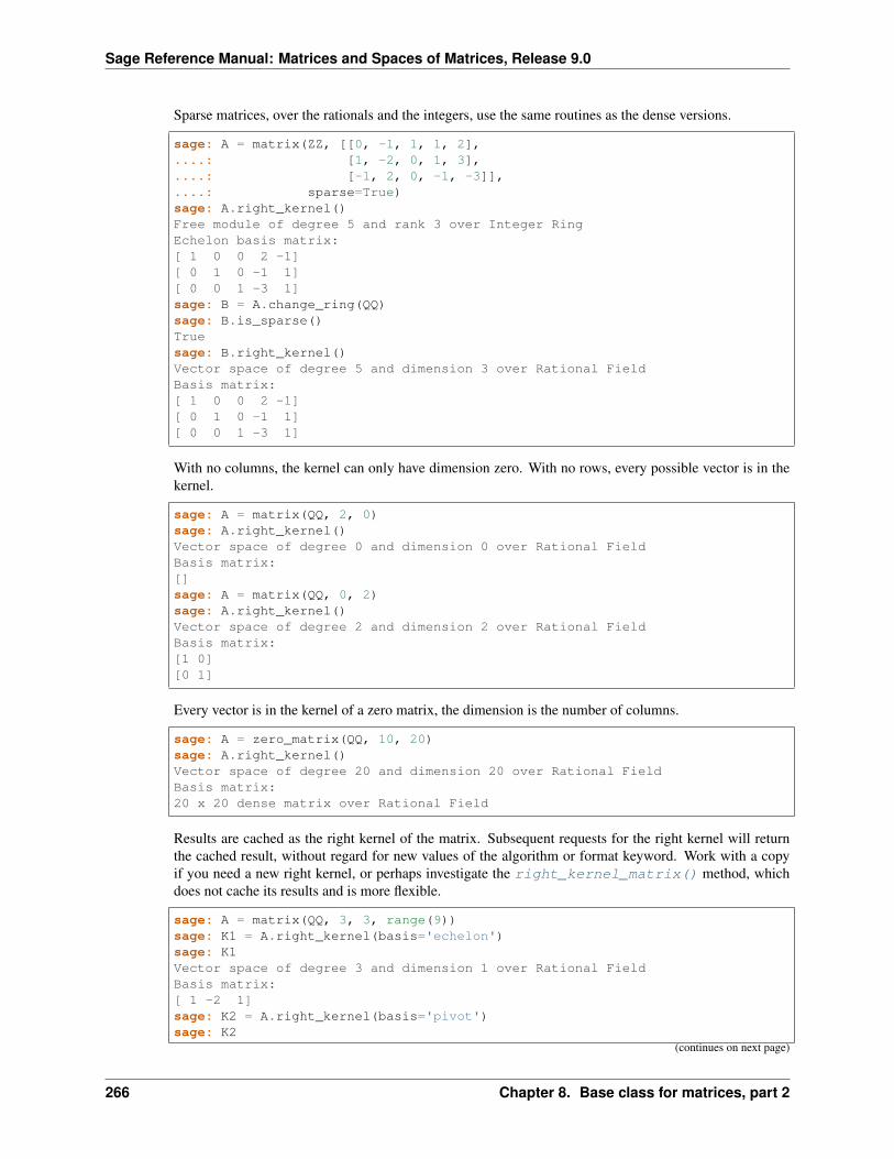
Sage Reference Manual: Matrices and Spaces of Matrices, Release 9.0
Sparse matrices, over the rationals and the integers, use the same routines as the dense versions.
sage: A = matrix(ZZ, [[0, -1, 1, 1, 2],....: [1, -2, 0, 1, 3],....: [-1, 2, 0, -1, -3]],....: sparse=True)sage: A.right_kernel()Free module of degree 5 and rank 3 over Integer RingEchelon basis matrix:[ 1 0 0 2 -1][ 0 1 0 -1 1][ 0 0 1 -3 1]sage: B = A.change_ring(QQ)sage: B.is_sparse()Truesage: B.right_kernel()Vector space of degree 5 and dimension 3 over Rational FieldBasis matrix:[ 1 0 0 2 -1][ 0 1 0 -1 1][ 0 0 1 -3 1]
With no columns, the kernel can only have dimension zero. With no rows, every possible vector is in thekernel.
sage: A = matrix(QQ, 2, 0)sage: A.right_kernel()Vector space of degree 0 and dimension 0 over Rational FieldBasis matrix:[]sage: A = matrix(QQ, 0, 2)sage: A.right_kernel()Vector space of degree 2 and dimension 2 over Rational FieldBasis matrix:[1 0][0 1]
Every vector is in the kernel of a zero matrix, the dimension is the number of columns.
sage: A = zero_matrix(QQ, 10, 20)sage: A.right_kernel()Vector space of degree 20 and dimension 20 over Rational FieldBasis matrix:20 x 20 dense matrix over Rational Field
Results are cached as the right kernel of the matrix. Subsequent requests for the right kernel will returnthe cached result, without regard for new values of the algorithm or format keyword. Work with a copyif you need a new right kernel, or perhaps investigate the right_kernel_matrix() method, whichdoes not cache its results and is more flexible.
sage: A = matrix(QQ, 3, 3, range(9))sage: K1 = A.right_kernel(basis='echelon')sage: K1Vector space of degree 3 and dimension 1 over Rational FieldBasis matrix:[ 1 -2 1]sage: K2 = A.right_kernel(basis='pivot')sage: K2
(continues on next page)
266 Chapter 8. Base class for matrices, part 2

Sage Reference Manual: Matrices and Spaces of Matrices, Release 9.0
(continued from previous page)
Vector space of degree 3 and dimension 1 over Rational FieldBasis matrix:[ 1 -2 1]sage: K1 is K2Truesage: B = copy(A)sage: K3 = B.kernel(basis='pivot')sage: K3Vector space of degree 3 and dimension 1 over Rational FieldUser basis matrix:[ 1 -2 1]sage: K3 is K1Falsesage: K3 == K1True
right_kernel_matrix(*args, **kwds)Returns a matrix whose rows form a basis for the right kernel of self.
INPUT:
• algorithm - default: ‘default’ - a keyword that selects the algorithm employed. Allowable valuesare:
– ‘default’ - allows the algorithm to be chosen automatically
– ‘generic’ - naive algorithm usable for matrices over any field
– ‘flint’ - FLINT library code for matrices over the rationals or the integers
– ‘pari’ - PARI library code for matrices over number fields or the integers
– ‘padic’ - padic algorithm from IML library for matrices over the rationals and integers
– ‘pluq’ - PLUQ matrix factorization for matrices mod 2
• basis - default: ‘echelon’ - a keyword that describes the format of the basis returned. Allowablevalues are:
– ‘echelon’: the basis matrix is returned in echelon form
– ‘pivot’ : each basis vector is computed from the reduced row-echelon form of self by placing asingle one in a non-pivot column and zeros in the remaining non-pivot columns. Only availablefor matrices over fields.
– ‘LLL’: an LLL-reduced basis. Only available for matrices over the integers.
– ‘computed’: no work is done to transform the basis, it is returned exactly as provided bywhichever routine actually computed the basis. Request this for the least possible computationpossible, but with no guarantees about the format of the basis.
OUTPUT:
A matrix X whose rows are an independent set spanning the right kernel of self. So self*X.transpose() is a zero matrix.
The output varies depending on the choice of algorithm and the format chosen by basis.
The results of this routine are not cached, so you can call it again with different options to get possiblydifferent output (like the basis format). Conversely, repeated calls on the same matrix will always startfrom scratch.
267

Sage Reference Manual: Matrices and Spaces of Matrices, Release 9.0
Note: If you want to get the most basic description of a kernel, with a minimum of overhead, then ask forthe right kernel matrix with the basis format requested as ‘computed’. You are then free to work with theoutput for whatever purpose. For a left kernel, call this method on the transpose of your matrix.
For greater convenience, plus cached results, request an actual vector space or free module withright_kernel() or left_kernel().
EXAMPLES:
Over the Rational Numbers:
Kernels are computed by the IML library in _right_kernel_matrix(). Setting the 𝑎𝑙𝑔𝑜𝑟𝑖𝑡ℎ𝑚keyword to ‘default’, ‘padic’ or unspecified will yield the same result, as there is no optional behavior.The ‘computed’ format of the basis vectors are exactly the negatives of the vectors in the ‘pivot’ format.
sage: A = matrix(QQ, [[1, 0, 1, -3, 1],....: [-5, 1, 0, 7, -3],....: [0, -1, -4, 6, -2],....: [4, -1, 0, -6, 2]])sage: C = A.right_kernel_matrix(algorithm='default', basis='computed'); C[-1 2 -2 -1 0][ 1 2 0 0 -1]sage: A*C.transpose() == zero_matrix(QQ, 4, 2)Truesage: P = A.right_kernel_matrix(algorithm='padic', basis='pivot'); P[ 1 -2 2 1 0][-1 -2 0 0 1]sage: A*P.transpose() == zero_matrix(QQ, 4, 2)Truesage: C == -PTruesage: E = A.right_kernel_matrix(algorithm='default', basis='echelon'); E[ 1 0 1 1/2 -1/2][ 0 1 -1/2 -1/4 -1/4]sage: A*E.transpose() == zero_matrix(QQ, 4, 2)True
Since the rationals are a field, we can call the general code available for any field by using the ‘generic’keyword.
sage: A = matrix(QQ, [[1, 0, 1, -3, 1],....: [-5, 1, 0, 7, -3],....: [0, -1, -4, 6, -2],....: [4, -1, 0, -6, 2]])sage: G = A.right_kernel_matrix(algorithm='generic', basis='echelon'); G[ 1 0 1 1/2 -1/2][ 0 1 -1/2 -1/4 -1/4]sage: A*G.transpose() == zero_matrix(QQ, 4, 2)True
We verify that the rational matrix code is called for both dense and sparse rational matrices, with equalresult.
sage: A = matrix(QQ, [[1, 0, 1, -3, 1],....: [-5, 1, 0, 7, -3],....: [0, -1, -4, 6, -2],....: [4, -1, 0, -6, 2]],
(continues on next page)
268 Chapter 8. Base class for matrices, part 2
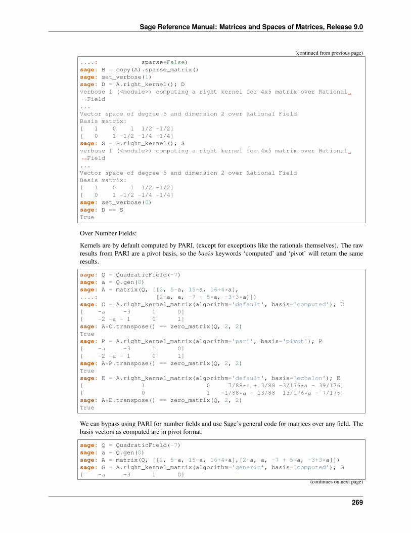
Sage Reference Manual: Matrices and Spaces of Matrices, Release 9.0
(continued from previous page)
....: sparse=False)sage: B = copy(A).sparse_matrix()sage: set_verbose(1)sage: D = A.right_kernel(); Dverbose 1 (<module>) computing a right kernel for 4x5 matrix over Rational→˓Field...Vector space of degree 5 and dimension 2 over Rational FieldBasis matrix:[ 1 0 1 1/2 -1/2][ 0 1 -1/2 -1/4 -1/4]sage: S = B.right_kernel(); Sverbose 1 (<module>) computing a right kernel for 4x5 matrix over Rational→˓Field...Vector space of degree 5 and dimension 2 over Rational FieldBasis matrix:[ 1 0 1 1/2 -1/2][ 0 1 -1/2 -1/4 -1/4]sage: set_verbose(0)sage: D == STrue
Over Number Fields:
Kernels are by default computed by PARI, (except for exceptions like the rationals themselves). The rawresults from PARI are a pivot basis, so the 𝑏𝑎𝑠𝑖𝑠 keywords ‘computed’ and ‘pivot’ will return the sameresults.
sage: Q = QuadraticField(-7)sage: a = Q.gen(0)sage: A = matrix(Q, [[2, 5-a, 15-a, 16+4*a],....: [2+a, a, -7 + 5*a, -3+3*a]])sage: C = A.right_kernel_matrix(algorithm='default', basis='computed'); C[ -a -3 1 0][ -2 -a - 1 0 1]sage: A*C.transpose() == zero_matrix(Q, 2, 2)Truesage: P = A.right_kernel_matrix(algorithm='pari', basis='pivot'); P[ -a -3 1 0][ -2 -a - 1 0 1]sage: A*P.transpose() == zero_matrix(Q, 2, 2)Truesage: E = A.right_kernel_matrix(algorithm='default', basis='echelon'); E[ 1 0 7/88*a + 3/88 -3/176*a - 39/176][ 0 1 -1/88*a - 13/88 13/176*a - 7/176]sage: A*E.transpose() == zero_matrix(Q, 2, 2)True
We can bypass using PARI for number fields and use Sage’s general code for matrices over any field. Thebasis vectors as computed are in pivot format.
sage: Q = QuadraticField(-7)sage: a = Q.gen(0)sage: A = matrix(Q, [[2, 5-a, 15-a, 16+4*a],[2+a, a, -7 + 5*a, -3+3*a]])sage: G = A.right_kernel_matrix(algorithm='generic', basis='computed'); G[ -a -3 1 0]
(continues on next page)
269

Sage Reference Manual: Matrices and Spaces of Matrices, Release 9.0
(continued from previous page)
[ -2 -a - 1 0 1]sage: A*G.transpose() == zero_matrix(Q, 2, 2)True
We check that number fields are handled by the right routine as part of typical right kernel computation.
sage: Q = QuadraticField(-7)sage: a = Q.gen(0)sage: A = matrix(Q, [[2, 5-a, 15-a, 16+4*a],[2+a, a, -7 + 5*a, -3+3*a]])sage: set_verbose(1)sage: A.right_kernel(algorithm='default')verbose ...verbose 1 (<module>) computing right kernel matrix over a number field for→˓2x4 matrixverbose 1 (<module>) done computing right kernel matrix over a number field→˓for 2x4 matrix...Vector space of degree 4 and dimension 2 over Number Field in a with defining→˓polynomial x^2 + 7 with a = 2.645751311064591?*IBasis matrix:[ 1 0 7/88*a + 3/88 -3/176*a - 39/176][ 0 1 -1/88*a - 13/88 13/176*a - 7/176]sage: set_verbose(0)
Over the Finite Field of Order 2:
Kernels are computed by the M4RI library using PLUQ matrix decomposition in the_right_kernel_matrix() method. There are no options for the algorithm used.
sage: A = matrix(GF(2),[[0, 1, 1, 0, 0, 0],....: [1, 0, 0, 0, 1, 1,],....: [1, 0, 0, 0, 1, 1]])sage: E = A.right_kernel_matrix(algorithm='default', format='echelon'); E[1 0 0 0 0 1][0 1 1 0 0 0][0 0 0 1 0 0][0 0 0 0 1 1]sage: A*E.transpose() == zero_matrix(GF(2), 3, 4)True
Since GF(2) is a field we can route this computation to the generic code and obtain the ‘pivot’ form of thebasis. The algorithm keywords, ‘pluq’, ‘default’ and unspecified, all have the same effect as there isno optional behavior.
sage: A = matrix(GF(2),[[0, 1, 1, 0, 0, 0],....: [1, 0, 0, 0, 1, 1,],....: [1, 0, 0, 0, 1, 1]])sage: P = A.right_kernel_matrix(algorithm='generic', basis='pivot'); P[0 1 1 0 0 0][0 0 0 1 0 0][1 0 0 0 1 0][1 0 0 0 0 1]sage: A*P.transpose() == zero_matrix(GF(2), 3, 4)Truesage: DP = A.right_kernel_matrix(algorithm='default', basis='pivot'); DP[0 1 1 0 0 0][0 0 0 1 0 0]
(continues on next page)
270 Chapter 8. Base class for matrices, part 2
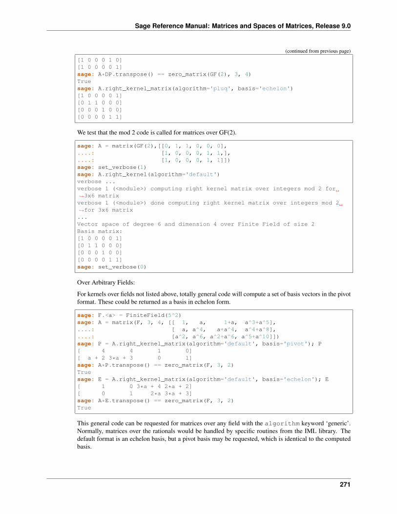
Sage Reference Manual: Matrices and Spaces of Matrices, Release 9.0
(continued from previous page)
[1 0 0 0 1 0][1 0 0 0 0 1]sage: A*DP.transpose() == zero_matrix(GF(2), 3, 4)Truesage: A.right_kernel_matrix(algorithm='pluq', basis='echelon')[1 0 0 0 0 1][0 1 1 0 0 0][0 0 0 1 0 0][0 0 0 0 1 1]
We test that the mod 2 code is called for matrices over GF(2).
sage: A = matrix(GF(2),[[0, 1, 1, 0, 0, 0],....: [1, 0, 0, 0, 1, 1,],....: [1, 0, 0, 0, 1, 1]])sage: set_verbose(1)sage: A.right_kernel(algorithm='default')verbose ...verbose 1 (<module>) computing right kernel matrix over integers mod 2 for→˓3x6 matrixverbose 1 (<module>) done computing right kernel matrix over integers mod 2→˓for 3x6 matrix...Vector space of degree 6 and dimension 4 over Finite Field of size 2Basis matrix:[1 0 0 0 0 1][0 1 1 0 0 0][0 0 0 1 0 0][0 0 0 0 1 1]sage: set_verbose(0)
Over Arbitrary Fields:
For kernels over fields not listed above, totally general code will compute a set of basis vectors in the pivotformat. These could be returned as a basis in echelon form.
sage: F.<a> = FiniteField(5^2)sage: A = matrix(F, 3, 4, [[ 1, a, 1+a, a^3+a^5],....: [ a, a^4, a+a^4, a^4+a^8],....: [a^2, a^6, a^2+a^6, a^5+a^10]])sage: P = A.right_kernel_matrix(algorithm='default', basis='pivot'); P[ 4 4 1 0][ a + 2 3*a + 3 0 1]sage: A*P.transpose() == zero_matrix(F, 3, 2)Truesage: E = A.right_kernel_matrix(algorithm='default', basis='echelon'); E[ 1 0 3*a + 4 2*a + 2][ 0 1 2*a 3*a + 3]sage: A*E.transpose() == zero_matrix(F, 3, 2)True
This general code can be requested for matrices over any field with the algorithm keyword ‘generic’.Normally, matrices over the rationals would be handled by specific routines from the IML library. Thedefault format is an echelon basis, but a pivot basis may be requested, which is identical to the computedbasis.
271
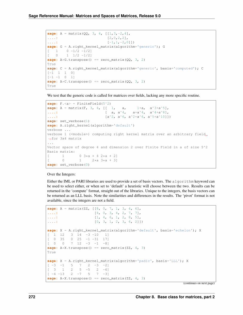
Sage Reference Manual: Matrices and Spaces of Matrices, Release 9.0
sage: A = matrix(QQ, 3, 4, [[1,3,-2,4],....: [2,0,2,2],....: [-1,1,-2,0]])sage: G = A.right_kernel_matrix(algorithm='generic'); G[ 1 0 -1/2 -1/2][ 0 1 1/2 -1/2]sage: A*G.transpose() == zero_matrix(QQ, 3, 2)Truesage: C = A.right_kernel_matrix(algorithm='generic', basis='computed'); C[-1 1 1 0][-1 -1 0 1]sage: A*C.transpose() == zero_matrix(QQ, 3, 2)True
We test that the generic code is called for matrices over fields, lacking any more specific routine.
sage: F.<a> = FiniteField(5^2)sage: A = matrix(F, 3, 4, [[ 1, a, 1+a, a^3+a^5],....: [ a, a^4, a+a^4, a^4+a^8],....: [a^2, a^6, a^2+a^6, a^5+a^10]])sage: set_verbose(1)sage: A.right_kernel(algorithm='default')verbose ...verbose 1 (<module>) computing right kernel matrix over an arbitrary field→˓for 3x4 matrix...Vector space of degree 4 and dimension 2 over Finite Field in a of size 5^2Basis matrix:[ 1 0 3*a + 4 2*a + 2][ 0 1 2*a 3*a + 3]sage: set_verbose(0)
Over the Integers:
Either the IML or PARI libraries are used to provide a set of basis vectors. The algorithm keyword canbe used to select either, or when set to ‘default’ a heuristic will choose between the two. Results can bereturned in the ‘compute’ format, straight out of the libraries. Unique to the integers, the basis vectors canbe returned as an LLL basis. Note the similarities and differences in the results. The ‘pivot’ format is notavailable, since the integers are not a field.
sage: A = matrix(ZZ, [[8, 0, 7, 1, 3, 4, 6],....: [4, 0, 3, 4, 2, 7, 7],....: [1, 4, 6, 1, 2, 8, 5],....: [0, 3, 1, 2, 3, 6, 2]])
sage: X = A.right_kernel_matrix(algorithm='default', basis='echelon'); X[ 1 12 3 14 -3 -10 1][ 0 35 0 25 -1 -31 17][ 0 0 7 12 -3 -1 -8]sage: A*X.transpose() == zero_matrix(ZZ, 4, 3)True
sage: X = A.right_kernel_matrix(algorithm='padic', basis='LLL'); X[ -3 -1 5 7 2 -3 -2][ 3 1 2 5 -5 2 -6][ -4 -13 2 -7 5 7 -3]sage: A*X.transpose() == zero_matrix(ZZ, 4, 3)
(continues on next page)
272 Chapter 8. Base class for matrices, part 2
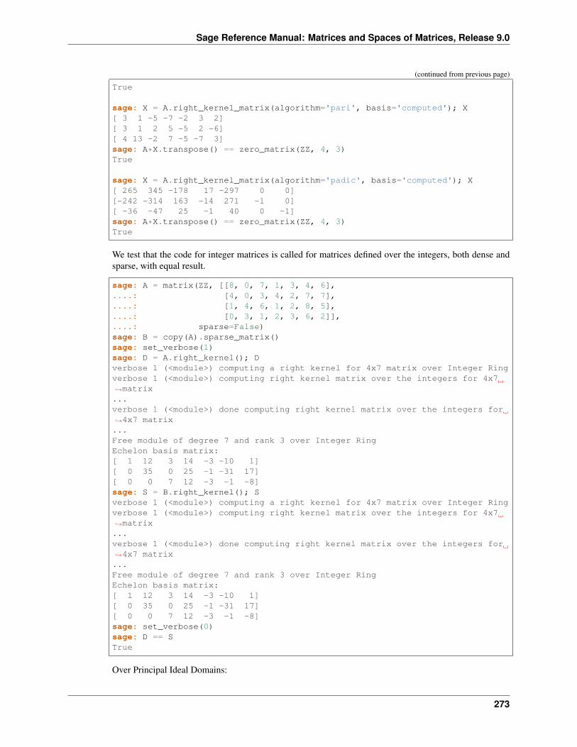
Sage Reference Manual: Matrices and Spaces of Matrices, Release 9.0
(continued from previous page)
True
sage: X = A.right_kernel_matrix(algorithm='pari', basis='computed'); X[ 3 1 -5 -7 -2 3 2][ 3 1 2 5 -5 2 -6][ 4 13 -2 7 -5 -7 3]sage: A*X.transpose() == zero_matrix(ZZ, 4, 3)True
sage: X = A.right_kernel_matrix(algorithm='padic', basis='computed'); X[ 265 345 -178 17 -297 0 0][-242 -314 163 -14 271 -1 0][ -36 -47 25 -1 40 0 -1]sage: A*X.transpose() == zero_matrix(ZZ, 4, 3)True
We test that the code for integer matrices is called for matrices defined over the integers, both dense andsparse, with equal result.
sage: A = matrix(ZZ, [[8, 0, 7, 1, 3, 4, 6],....: [4, 0, 3, 4, 2, 7, 7],....: [1, 4, 6, 1, 2, 8, 5],....: [0, 3, 1, 2, 3, 6, 2]],....: sparse=False)sage: B = copy(A).sparse_matrix()sage: set_verbose(1)sage: D = A.right_kernel(); Dverbose 1 (<module>) computing a right kernel for 4x7 matrix over Integer Ringverbose 1 (<module>) computing right kernel matrix over the integers for 4x7→˓matrix...verbose 1 (<module>) done computing right kernel matrix over the integers for→˓4x7 matrix...Free module of degree 7 and rank 3 over Integer RingEchelon basis matrix:[ 1 12 3 14 -3 -10 1][ 0 35 0 25 -1 -31 17][ 0 0 7 12 -3 -1 -8]sage: S = B.right_kernel(); Sverbose 1 (<module>) computing a right kernel for 4x7 matrix over Integer Ringverbose 1 (<module>) computing right kernel matrix over the integers for 4x7→˓matrix...verbose 1 (<module>) done computing right kernel matrix over the integers for→˓4x7 matrix...Free module of degree 7 and rank 3 over Integer RingEchelon basis matrix:[ 1 12 3 14 -3 -10 1][ 0 35 0 25 -1 -31 17][ 0 0 7 12 -3 -1 -8]sage: set_verbose(0)sage: D == STrue
Over Principal Ideal Domains:
273
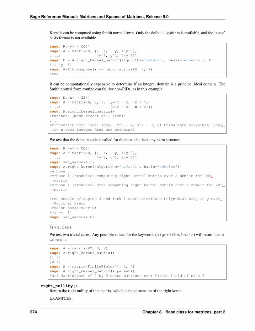
Sage Reference Manual: Matrices and Spaces of Matrices, Release 9.0
Kernels can be computed using Smith normal form. Only the default algorithm is available, and the ‘pivot’basis format is not available.
sage: R.<y> = QQ[]sage: A = matrix(R, [[ 1, y, 1+y^2],....: [y^3, y^2, 2*y^3]])sage: E = A.right_kernel_matrix(algorithm='default', basis='echelon'); E[-1 -y 1]sage: A*E.transpose() == zero_matrix(ZZ, 2, 1)True
It can be computationally expensive to determine if an integral domain is a principal ideal domain. TheSmith normal form routine can fail for non-PIDs, as in this example.
sage: D.<x> = ZZ[]sage: A = matrix(D, 2, 2, [[x^2 - x, -x + 5],....: [x^2 - 8, -x + 2]])sage: A.right_kernel_matrix()Traceback (most recent call last):...ArithmeticError: Ideal Ideal (x^2 - x, x^2 - 8) of Univariate Polynomial Ring→˓in x over Integer Ring not principal
We test that the domain code is called for domains that lack any extra structure.
sage: R.<y> = QQ[]sage: A = matrix(R, [[ 1, y, 1+y^2],....: [y^3, y^2, 2*y^3]])sage: set_verbose(1)sage: A.right_kernel(algorithm='default', basis='echelon')verbose ...verbose 1 (<module>) computing right kernel matrix over a domain for 2x3→˓matrixverbose 1 (<module>) done computing right kernel matrix over a domain for 2x3→˓matrix...Free module of degree 3 and rank 1 over Univariate Polynomial Ring in y over→˓Rational FieldEchelon basis matrix:[-1 -y 1]sage: set_verbose(0)
Trivial Cases:
We test two trivial cases. Any possible values for the keywords (algorithm, basis) will return identi-cal results.
sage: A = matrix(ZZ, 0, 2)sage: A.right_kernel_matrix()[1 0][0 1]sage: A = matrix(FiniteField(7), 2, 0)sage: A.right_kernel_matrix().parent()Full MatrixSpace of 0 by 0 dense matrices over Finite Field of size 7
right_nullity()Return the right nullity of this matrix, which is the dimension of the right kernel.
EXAMPLES:
274 Chapter 8. Base class for matrices, part 2
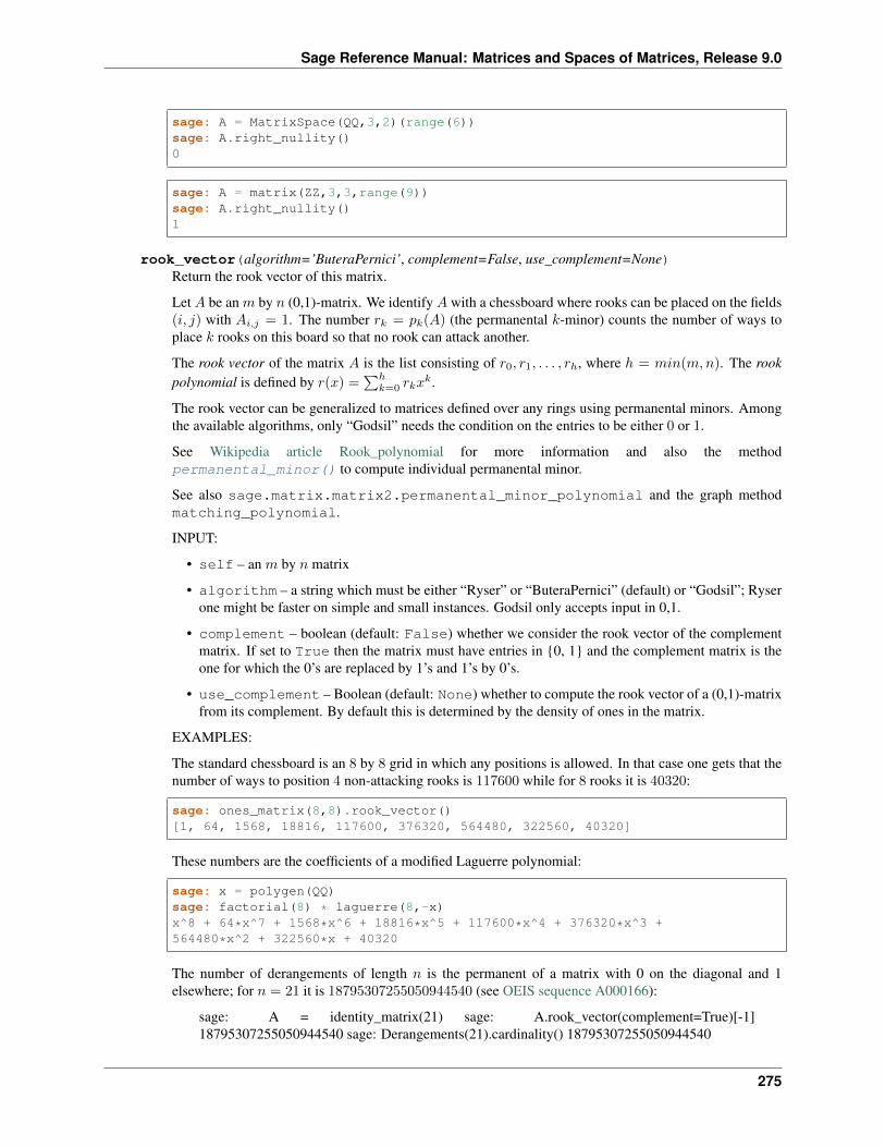
Sage Reference Manual: Matrices and Spaces of Matrices, Release 9.0
sage: A = MatrixSpace(QQ,3,2)(range(6))sage: A.right_nullity()0
sage: A = matrix(ZZ,3,3,range(9))sage: A.right_nullity()1
rook_vector(algorithm=’ButeraPernici’, complement=False, use_complement=None)Return the rook vector of this matrix.
Let 𝐴 be an 𝑚 by 𝑛 (0,1)-matrix. We identify 𝐴 with a chessboard where rooks can be placed on the fields(𝑖, 𝑗) with 𝐴𝑖,𝑗 = 1. The number 𝑟𝑘 = 𝑝𝑘(𝐴) (the permanental 𝑘-minor) counts the number of ways toplace 𝑘 rooks on this board so that no rook can attack another.
The rook vector of the matrix 𝐴 is the list consisting of 𝑟0, 𝑟1, . . . , 𝑟ℎ, where ℎ = 𝑚𝑖𝑛(𝑚,𝑛). The rookpolynomial is defined by 𝑟(𝑥) =
∑︀ℎ𝑘=0 𝑟𝑘𝑥
𝑘.
The rook vector can be generalized to matrices defined over any rings using permanental minors. Amongthe available algorithms, only “Godsil” needs the condition on the entries to be either 0 or 1.
See Wikipedia article Rook_polynomial for more information and also the methodpermanental_minor() to compute individual permanental minor.
See also sage.matrix.matrix2.permanental_minor_polynomial and the graph methodmatching_polynomial.
INPUT:
• self – an 𝑚 by 𝑛 matrix
• algorithm – a string which must be either “Ryser” or “ButeraPernici” (default) or “Godsil”; Ryserone might be faster on simple and small instances. Godsil only accepts input in 0,1.
• complement – boolean (default: False) whether we consider the rook vector of the complementmatrix. If set to True then the matrix must have entries in {0, 1} and the complement matrix is theone for which the 0’s are replaced by 1’s and 1’s by 0’s.
• use_complement – Boolean (default: None) whether to compute the rook vector of a (0,1)-matrixfrom its complement. By default this is determined by the density of ones in the matrix.
EXAMPLES:
The standard chessboard is an 8 by 8 grid in which any positions is allowed. In that case one gets that thenumber of ways to position 4 non-attacking rooks is 117600 while for 8 rooks it is 40320:
sage: ones_matrix(8,8).rook_vector()[1, 64, 1568, 18816, 117600, 376320, 564480, 322560, 40320]
These numbers are the coefficients of a modified Laguerre polynomial:
sage: x = polygen(QQ)sage: factorial(8) * laguerre(8,-x)x^8 + 64*x^7 + 1568*x^6 + 18816*x^5 + 117600*x^4 + 376320*x^3 +564480*x^2 + 322560*x + 40320
The number of derangements of length 𝑛 is the permanent of a matrix with 0 on the diagonal and 1elsewhere; for 𝑛 = 21 it is 18795307255050944540 (see OEIS sequence A000166):
sage: A = identity_matrix(21) sage: A.rook_vector(complement=True)[-1]18795307255050944540 sage: Derangements(21).cardinality() 18795307255050944540
275

Sage Reference Manual: Matrices and Spaces of Matrices, Release 9.0
An other example that we convert into a rook polynomial:
sage: A = matrix(3,6, [1,1,1,1,0,0,0,1,1,1,1,0,0,0,1,1,1,1])sage: A[1 1 1 1 0 0][0 1 1 1 1 0][0 0 1 1 1 1]sage: A.rook_vector()[1, 12, 40, 36]
sage: R = PolynomialRing(ZZ, 'x')sage: R(A.rook_vector())36*x^3 + 40*x^2 + 12*x + 1
Different algorithms are available:
sage: A = matrix([[1,0,0,1],[0,1,1,0],[0,1,1,0],[1,0,0,1]])sage: A.rook_vector(algorithm="ButeraPernici")[1, 8, 20, 16, 4]sage: A.rook_vector(algorithm="Ryser")[1, 8, 20, 16, 4]sage: A.rook_vector(algorithm="Godsil")[1, 8, 20, 16, 4]
When the matrix 𝐴 has more ones then zeroes it is usually faster to compute the rook polynomial ofthe complementary matrix, with zeroes and ones interchanged, and use the inclusion-exclusion theorem,giving for a 𝑚× 𝑛 matrix 𝐴 with complementary matrix 𝐵
𝑟𝑘(𝐴) =
𝑘∑︁𝑗=0
(−1)𝑗(︂𝑚− 𝑗
𝑘 − 𝑗
)︂(︂𝑛− 𝑗
𝑘 − 𝑗
)︂(𝑘 − 𝑗)!𝑟𝑗(𝐵)
see [Rio1958] or the introductory text [AS2011]. This can be done setting the argumentuse_complement to True.
An example with an exotic matrix (for which only Butera-Pernici and Ryser algorithms are available):
sage: R.<x,y> = PolynomialRing(GF(5))sage: A = matrix(R,[[1,x,y],[x*y,x**2+y,0]])sage: A.rook_vector(algorithm="ButeraPernici")[1, x^2 + x*y + x + 2*y + 1, 2*x^2*y + x*y^2 + x^2 + y^2 + y]sage: A.rook_vector(algorithm="Ryser")[1, x^2 + x*y + x + 2*y + 1, 2*x^2*y + x*y^2 + x^2 + y^2 + y]sage: A.rook_vector(algorithm="Godsil")Traceback (most recent call last):...ValueError: coefficients must be zero or one, but we have 'x' in position (0,→˓1).sage: B = A.transpose()sage: B.rook_vector(algorithm="ButeraPernici")[1, x^2 + x*y + x + 2*y + 1, 2*x^2*y + x*y^2 + x^2 + y^2 + y]sage: B.rook_vector(algorithm="Ryser")[1, x^2 + x*y + x + 2*y + 1, 2*x^2*y + x*y^2 + x^2 + y^2 + y]
row_module(base_ring=None)Return the free module over the base ring spanned by the rows of self.
EXAMPLES:
276 Chapter 8. Base class for matrices, part 2

Sage Reference Manual: Matrices and Spaces of Matrices, Release 9.0
sage: A = MatrixSpace(IntegerRing(), 2)([1,2,3,4])sage: A.row_module()Free module of degree 2 and rank 2 over Integer RingEchelon basis matrix:[1 0][0 2]
row_space(base_ring=None)Return the row space of this matrix. (Synonym for self.row_module().)
EXAMPLES:
sage: t = matrix(QQ, 3, 3, range(9)); t[0 1 2][3 4 5][6 7 8]sage: t.row_space()Vector space of degree 3 and dimension 2 over Rational FieldBasis matrix:[ 1 0 -1][ 0 1 2]
sage: m = Matrix(Integers(5),2,2,[2,2,2,2])sage: m.row_space()Vector space of degree 2 and dimension 1 over Ring of integers modulo 5Basis matrix:[1 1]
rref(*args, **kwds)Return the reduced row echelon form of the matrix, considered as a matrix over a field.
If the matrix is over a ring, then an equivalent matrix is constructed over the fraction field, and then rowreduced.
All arguments are passed on to echelon_form().
Note: Because the matrix is viewed as a matrix over a field, every leading coefficient of the returnedmatrix will be one and will be the only nonzero entry in its column.
EXAMPLES:
sage: A=matrix(3,range(9)); A[0 1 2][3 4 5][6 7 8]sage: A.rref()[ 1 0 -1][ 0 1 2][ 0 0 0]
Note that there is a difference between rref() and echelon_form() when the matrix is not over afield (in this case, the integers instead of the rational numbers):
sage: A.base_ring()Integer Ringsage: A.echelon_form()
(continues on next page)
277
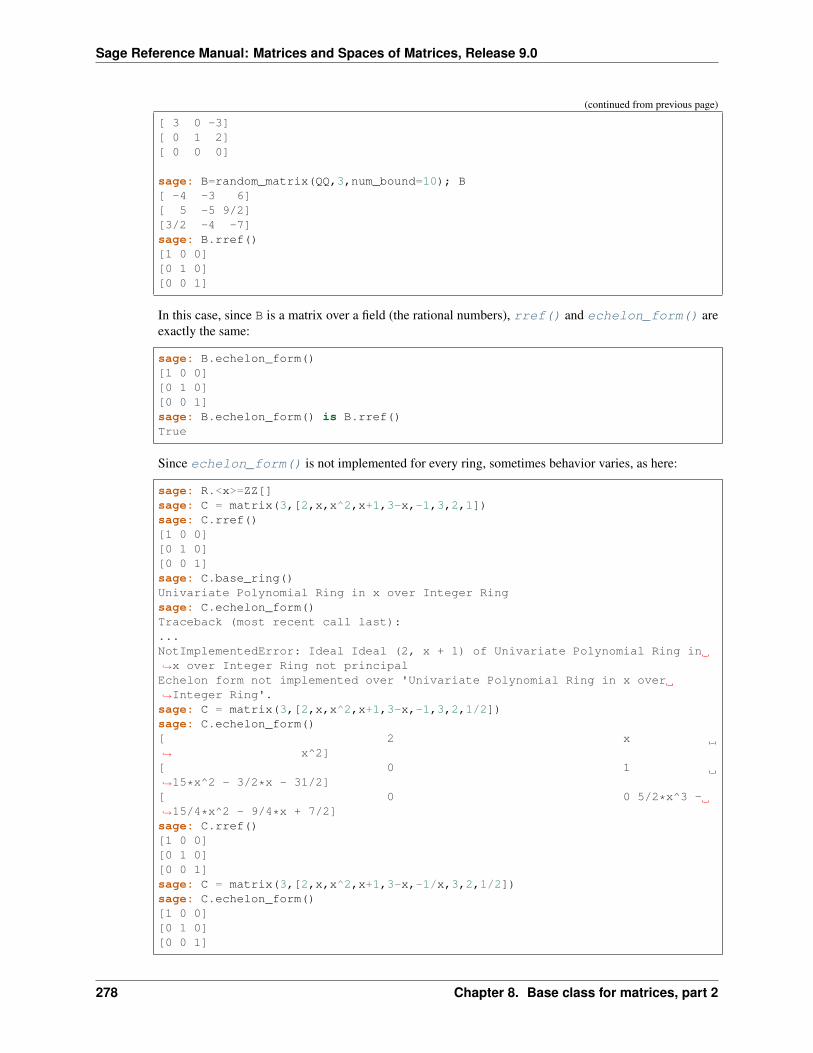
Sage Reference Manual: Matrices and Spaces of Matrices, Release 9.0
(continued from previous page)
[ 3 0 -3][ 0 1 2][ 0 0 0]
sage: B=random_matrix(QQ,3,num_bound=10); B[ -4 -3 6][ 5 -5 9/2][3/2 -4 -7]sage: B.rref()[1 0 0][0 1 0][0 0 1]
In this case, since B is a matrix over a field (the rational numbers), rref() and echelon_form() areexactly the same:
sage: B.echelon_form()[1 0 0][0 1 0][0 0 1]sage: B.echelon_form() is B.rref()True
Since echelon_form() is not implemented for every ring, sometimes behavior varies, as here:
sage: R.<x>=ZZ[]sage: C = matrix(3,[2,x,x^2,x+1,3-x,-1,3,2,1])sage: C.rref()[1 0 0][0 1 0][0 0 1]sage: C.base_ring()Univariate Polynomial Ring in x over Integer Ringsage: C.echelon_form()Traceback (most recent call last):...NotImplementedError: Ideal Ideal (2, x + 1) of Univariate Polynomial Ring in→˓x over Integer Ring not principalEchelon form not implemented over 'Univariate Polynomial Ring in x over→˓Integer Ring'.sage: C = matrix(3,[2,x,x^2,x+1,3-x,-1,3,2,1/2])sage: C.echelon_form()[ 2 x→˓ x^2][ 0 1→˓15*x^2 - 3/2*x - 31/2][ 0 0 5/2*x^3 -→˓15/4*x^2 - 9/4*x + 7/2]sage: C.rref()[1 0 0][0 1 0][0 0 1]sage: C = matrix(3,[2,x,x^2,x+1,3-x,-1/x,3,2,1/2])sage: C.echelon_form()[1 0 0][0 1 0][0 0 1]
278 Chapter 8. Base class for matrices, part 2
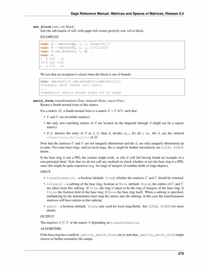
Sage Reference Manual: Matrices and Spaces of Matrices, Release 9.0
set_block(row, col, block)Sets the sub-matrix of self, with upper left corner given by row, col to block.
EXAMPLES:
sage: A = matrix(QQ, 3, 3, range(9))/2sage: B = matrix(ZZ, 2, 1, [100,200])sage: A.set_block(0, 1, B)sage: A[ 0 100 1][3/2 200 5/2][ 3 7/2 4]
We test that an exception is raised when the block is out of bounds:
sage: matrix([1]).set_block(0,1,matrix([1]))Traceback (most recent call last):...IndexError: matrix window index out of range
smith_form(transformation=True, integral=None, exact=True)Return a Smith normal form of this matrix.
For a matrix 𝑀 , a Smith normal form is a matrix 𝑆 = 𝑈𝑀𝑉 such that:
• 𝑈 and 𝑉 are invertible matrices
• the only non-vanishing entries of 𝑆 are located on the diagonal (though 𝑆 might not be a squarematrix)
• if 𝑑𝑖 denotes the entry of 𝑆 at (𝑖, 𝑖), then 𝑑𝑖 divides 𝑑𝑖+1 for all 𝑖, i.e., the 𝑑𝑖 are the orderedelementary_divisors() of 𝑀
Note that the matrices 𝑈 and 𝑉 are not uniquely determined and the 𝑑𝑖 are only uniquely determined upto units. For some base rings, such as local rings, the 𝑑𝑖 might be further normalized, see LOCAL RINGSbelow.
If the base ring is not a PID, the routine might work, or else it will fail having found an example of anon-principal ideal. Note that we do not call any methods to check whether or not the base ring is a PID,since this might be quite expensive (e.g. for rings of integers of number fields of large degree).
INPUT:
• transformation – a boolean (default: True); whether the matrices 𝑈 and 𝑉 should be returned
• integral – a subring of the base ring, boolean or None (default: None); the entries of 𝑈 and 𝑉are taken from this subring. If True, the ring is taken to be the ring of integers of the base ring; ifFalse the fraction field of the base ring; if None the base ring itself. When a subring is specified,multiplying by the denominator must map the entries into the subring; in this case the transformationmatrices will have entries in this subring.
• exact – a boolean (default: True), only used for local rings/fields. See LOCAL RINGS for moredetails.
OUTPUT:
The matrices 𝑆,𝑈, 𝑉 or the matrix 𝑆 depending on transformation.
ALGORITHM:
If the base ring has a method _matrix_smith_form, use it; note that _matrix_smith_formmightchoose to further normalize the output.
279

Sage Reference Manual: Matrices and Spaces of Matrices, Release 9.0
Otherwise, use the algorithm from Wikipedia article Smith_normal_form.
LOCAL RINGS:
Over local rings, we normalize 𝑆 to only contain powers of the uniformizer.
In order to simplify the precision handling, we truncate the absolute precision of the input matrix to theminimum absolute precision of any of its entries. As long as all of the elementary divisors are nonzeromodulo this precision, they can be determined exactly since they are defined to be powers of the uni-formizer. In this case, which is specified by the keyword exact=True, one of the transformation ma-trices will be inexact: 𝑈 in the case that the number of rows is at least the number of columns, and 𝑉otherwise.
If exact=False, we instead return an inexact Smith form. Now the transformation matrices are exactand we can deal gracefully with elementary divisors that are zero modulo the working precision. How-ever, the off-diagonal entries of the smith form carry a precision that can affect the precision of futurecalculations.
See _matrix_smith_form on the base ring for more detail.
EXAMPLES:
An example over the ring of integers of a number field (of class number 1):
sage: OE.<w> = EquationOrder(x^2 - x + 2)sage: m = Matrix([ [1, w],[w,7]])sage: d, u, v = m.smith_form()sage: (d, u, v)([ 1 0] [ 1 0] [ 1 -w][ 0 -w + 9], [-w 1], [ 0 1])sage: u * m * v == dTruesage: u.base_ring() == v.base_ring() == d.base_ring() == OETruesage: u.det().is_unit() and v.det().is_unit()True
An example over the polynomial ring QQ[x]:
sage: R.<x> = QQ[]; m=x*matrix(R,2,2,1) - matrix(R, 2,2,[3,-4,1,-1]); m.smith_→˓form()([ 1 0] [ 0 -1] [ 1 x + 1][ 0 x^2 - 2*x + 1], [ 1 x - 3], [ 0 1])
An example over a field:
sage: m = matrix( GF(17), 3, 3, [11,5,1,3,6,8,1,16,0]); d,u,v = m.smith_form()sage: d[1 0 0][0 1 0][0 0 0]sage: u*m*v == dTrue
When the base ring has a ring_of_integers method and supports denominators, you can get anintegral version of the smith form:
280 Chapter 8. Base class for matrices, part 2
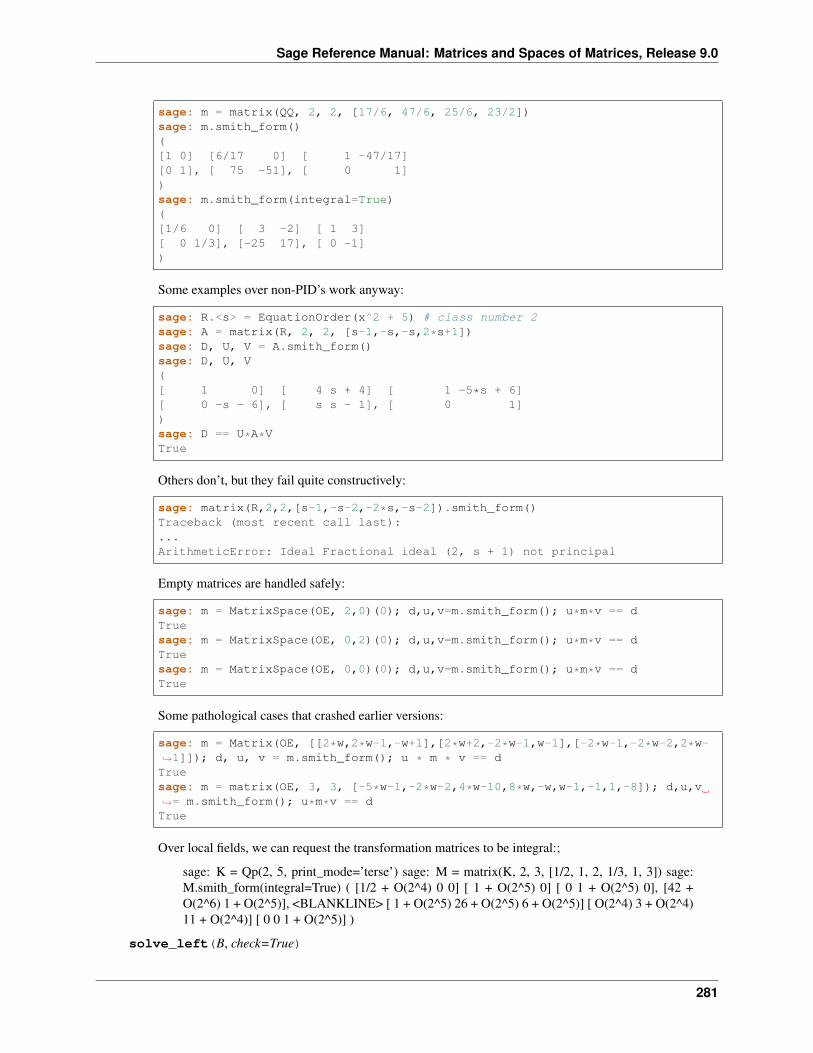
Sage Reference Manual: Matrices and Spaces of Matrices, Release 9.0
sage: m = matrix(QQ, 2, 2, [17/6, 47/6, 25/6, 23/2])sage: m.smith_form()([1 0] [6/17 0] [ 1 -47/17][0 1], [ 75 -51], [ 0 1])sage: m.smith_form(integral=True)([1/6 0] [ 3 -2] [ 1 3][ 0 1/3], [-25 17], [ 0 -1])
Some examples over non-PID’s work anyway:
sage: R.<s> = EquationOrder(x^2 + 5) # class number 2sage: A = matrix(R, 2, 2, [s-1,-s,-s,2*s+1])sage: D, U, V = A.smith_form()sage: D, U, V([ 1 0] [ 4 s + 4] [ 1 -5*s + 6][ 0 -s - 6], [ s s - 1], [ 0 1])sage: D == U*A*VTrue
Others don’t, but they fail quite constructively:
sage: matrix(R,2,2,[s-1,-s-2,-2*s,-s-2]).smith_form()Traceback (most recent call last):...ArithmeticError: Ideal Fractional ideal (2, s + 1) not principal
Empty matrices are handled safely:
sage: m = MatrixSpace(OE, 2,0)(0); d,u,v=m.smith_form(); u*m*v == dTruesage: m = MatrixSpace(OE, 0,2)(0); d,u,v=m.smith_form(); u*m*v == dTruesage: m = MatrixSpace(OE, 0,0)(0); d,u,v=m.smith_form(); u*m*v == dTrue
Some pathological cases that crashed earlier versions:
sage: m = Matrix(OE, [[2*w,2*w-1,-w+1],[2*w+2,-2*w-1,w-1],[-2*w-1,-2*w-2,2*w-→˓1]]); d, u, v = m.smith_form(); u * m * v == dTruesage: m = matrix(OE, 3, 3, [-5*w-1,-2*w-2,4*w-10,8*w,-w,w-1,-1,1,-8]); d,u,v→˓= m.smith_form(); u*m*v == dTrue
Over local fields, we can request the transformation matrices to be integral:;
sage: K = Qp(2, 5, print_mode=’terse’) sage: M = matrix(K, 2, 3, [1/2, 1, 2, 1/3, 1, 3]) sage:M.smith_form(integral=True) ( [1/2 + O(2^4) 0 0] [ 1 + O(2^5) 0] [ 0 1 + O(2^5) 0], [42 +O(2^6) 1 + O(2^5)], <BLANKLINE> [ 1 + O(2^5) 26 + O(2^5) 6 + O(2^5)] [ O(2^4) 3 + O(2^4)11 + O(2^4)] [ 0 0 1 + O(2^5)] )
solve_left(B, check=True)
281
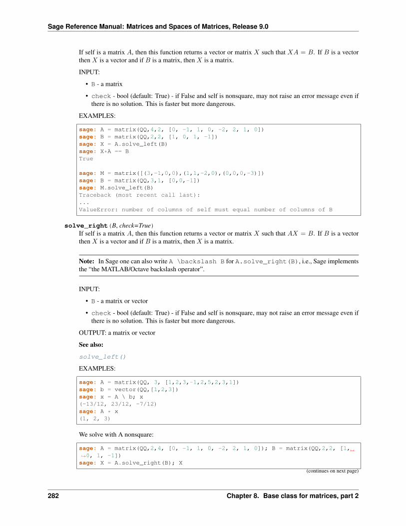
Sage Reference Manual: Matrices and Spaces of Matrices, Release 9.0
If self is a matrix 𝐴, then this function returns a vector or matrix 𝑋 such that 𝑋𝐴 = 𝐵. If 𝐵 is a vectorthen 𝑋 is a vector and if 𝐵 is a matrix, then 𝑋 is a matrix.
INPUT:
• B - a matrix
• check - bool (default: True) - if False and self is nonsquare, may not raise an error message even ifthere is no solution. This is faster but more dangerous.
EXAMPLES:
sage: A = matrix(QQ,4,2, [0, -1, 1, 0, -2, 2, 1, 0])sage: B = matrix(QQ,2,2, [1, 0, 1, -1])sage: X = A.solve_left(B)sage: X*A == BTrue
sage: M = matrix([(3,-1,0,0),(1,1,-2,0),(0,0,0,-3)])sage: B = matrix(QQ,3,1, [0,0,-1])sage: M.solve_left(B)Traceback (most recent call last):...ValueError: number of columns of self must equal number of columns of B
solve_right(B, check=True)If self is a matrix 𝐴, then this function returns a vector or matrix 𝑋 such that 𝐴𝑋 = 𝐵. If 𝐵 is a vectorthen 𝑋 is a vector and if 𝐵 is a matrix, then 𝑋 is a matrix.
Note: In Sage one can also write A \backslash B for A.solve_right(B), i.e., Sage implementsthe “the MATLAB/Octave backslash operator”.
INPUT:
• B - a matrix or vector
• check - bool (default: True) - if False and self is nonsquare, may not raise an error message even ifthere is no solution. This is faster but more dangerous.
OUTPUT: a matrix or vector
See also:
solve_left()
EXAMPLES:
sage: A = matrix(QQ, 3, [1,2,3,-1,2,5,2,3,1])sage: b = vector(QQ,[1,2,3])sage: x = A \ b; x(-13/12, 23/12, -7/12)sage: A * x(1, 2, 3)
We solve with A nonsquare:
sage: A = matrix(QQ,2,4, [0, -1, 1, 0, -2, 2, 1, 0]); B = matrix(QQ,2,2, [1,→˓0, 1, -1])sage: X = A.solve_right(B); X
(continues on next page)
282 Chapter 8. Base class for matrices, part 2
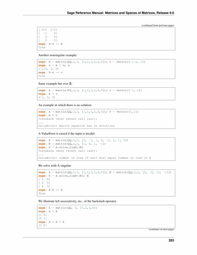
Sage Reference Manual: Matrices and Spaces of Matrices, Release 9.0
(continued from previous page)
[-3/2 1/2][ -1 0][ 0 0][ 0 0]sage: A*X == BTrue
Another nonsingular example:
sage: A = matrix(QQ,2,3, [1,2,3,2,4,6]); v = vector([-1/2,-1])sage: x = A \ v; x(-1/2, 0, 0)sage: A*x == vTrue
Same example but over Z:
sage: A = matrix(ZZ,2,3, [1,2,3,2,4,6]); v = vector([-1,-2])sage: A \ v(-1, 0, 0)
An example in which there is no solution:
sage: A = matrix(QQ,2,3, [1,2,3,2,4,6]); v = vector([1,1])sage: A \ vTraceback (most recent call last):...ValueError: matrix equation has no solutions
A ValueError is raised if the input is invalid:
sage: A = matrix(QQ,4,2, [0, -1, 1, 0, -2, 2, 1, 0])sage: B = matrix(QQ,2,2, [1, 0, 1, -1])sage: X = A.solve_right(B)Traceback (most recent call last):...ValueError: number of rows of self must equal number of rows of B
We solve with A singular:
sage: A = matrix(QQ,2,3, [1,2,3,2,4,6]); B = matrix(QQ,2,2, [6, -6, 12, -12])sage: X = A.solve_right(B); X[ 6 -6][ 0 0][ 0 0]sage: A*X == BTrue
We illustrate left associativity, etc., of the backslash operator.
sage: A = matrix(QQ, 2, [1,2,3,4])sage: A \ A[1 0][0 1]sage: A \ A \ A[1 2]
(continues on next page)
283
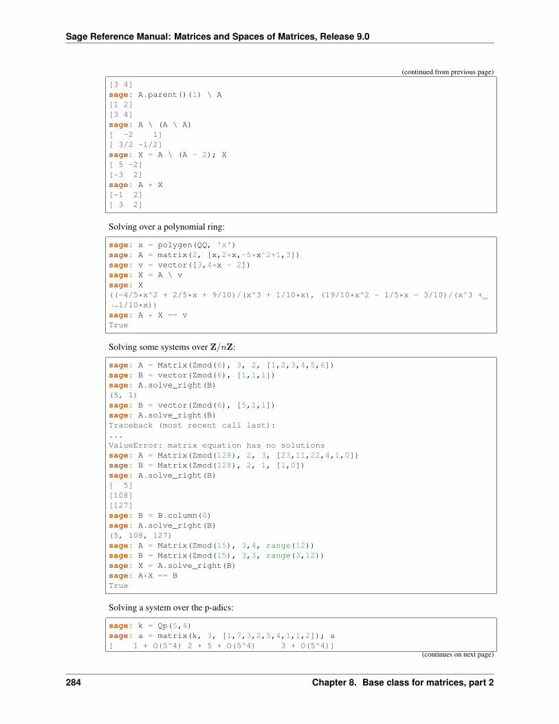
Sage Reference Manual: Matrices and Spaces of Matrices, Release 9.0
(continued from previous page)
[3 4]sage: A.parent()(1) \ A[1 2][3 4]sage: A \ (A \ A)[ -2 1][ 3/2 -1/2]sage: X = A \ (A - 2); X[ 5 -2][-3 2]sage: A * X[-1 2][ 3 2]
Solving over a polynomial ring:
sage: x = polygen(QQ, 'x')sage: A = matrix(2, [x,2*x,-5*x^2+1,3])sage: v = vector([3,4*x - 2])sage: X = A \ vsage: X((-4/5*x^2 + 2/5*x + 9/10)/(x^3 + 1/10*x), (19/10*x^2 - 1/5*x - 3/10)/(x^3 +→˓1/10*x))sage: A * X == vTrue
Solving some systems over Z/𝑛Z:
sage: A = Matrix(Zmod(6), 3, 2, [1,2,3,4,5,6])sage: B = vector(Zmod(6), [1,1,1])sage: A.solve_right(B)(5, 1)sage: B = vector(Zmod(6), [5,1,1])sage: A.solve_right(B)Traceback (most recent call last):...ValueError: matrix equation has no solutionssage: A = Matrix(Zmod(128), 2, 3, [23,11,22,4,1,0])sage: B = Matrix(Zmod(128), 2, 1, [1,0])sage: A.solve_right(B)[ 5][108][127]sage: B = B.column(0)sage: A.solve_right(B)(5, 108, 127)sage: A = Matrix(Zmod(15), 3,4, range(12))sage: B = Matrix(Zmod(15), 3,3, range(3,12))sage: X = A.solve_right(B)sage: A*X == BTrue
Solving a system over the p-adics:
sage: k = Qp(5,4)sage: a = matrix(k, 3, [1,7,3,2,5,4,1,1,2]); a[ 1 + O(5^4) 2 + 5 + O(5^4) 3 + O(5^4)]
(continues on next page)
284 Chapter 8. Base class for matrices, part 2
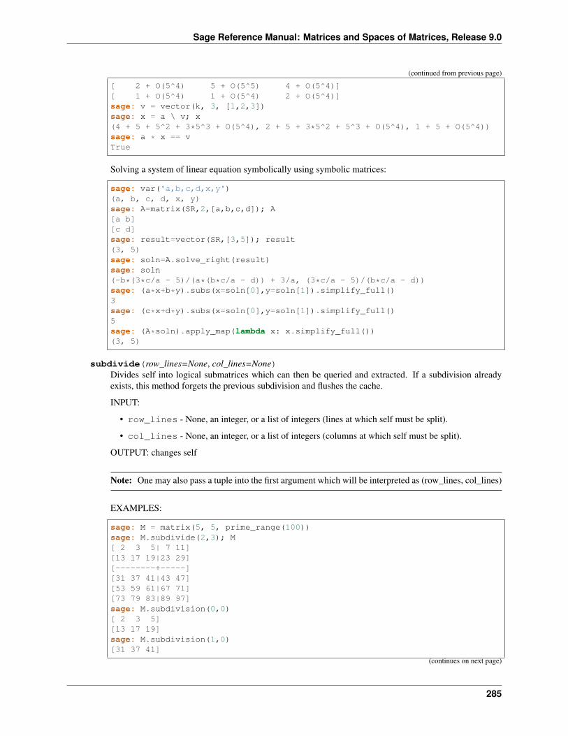
Sage Reference Manual: Matrices and Spaces of Matrices, Release 9.0
(continued from previous page)
[ 2 + O(5^4) 5 + O(5^5) 4 + O(5^4)][ 1 + O(5^4) 1 + O(5^4) 2 + O(5^4)]sage: v = vector(k, 3, [1,2,3])sage: x = a \ v; x(4 + 5 + 5^2 + 3*5^3 + O(5^4), 2 + 5 + 3*5^2 + 5^3 + O(5^4), 1 + 5 + O(5^4))sage: a * x == vTrue
Solving a system of linear equation symbolically using symbolic matrices:
sage: var('a,b,c,d,x,y')(a, b, c, d, x, y)sage: A=matrix(SR,2,[a,b,c,d]); A[a b][c d]sage: result=vector(SR,[3,5]); result(3, 5)sage: soln=A.solve_right(result)sage: soln(-b*(3*c/a - 5)/(a*(b*c/a - d)) + 3/a, (3*c/a - 5)/(b*c/a - d))sage: (a*x+b*y).subs(x=soln[0],y=soln[1]).simplify_full()3sage: (c*x+d*y).subs(x=soln[0],y=soln[1]).simplify_full()5sage: (A*soln).apply_map(lambda x: x.simplify_full())(3, 5)
subdivide(row_lines=None, col_lines=None)Divides self into logical submatrices which can then be queried and extracted. If a subdivision alreadyexists, this method forgets the previous subdivision and flushes the cache.
INPUT:
• row_lines - None, an integer, or a list of integers (lines at which self must be split).
• col_lines - None, an integer, or a list of integers (columns at which self must be split).
OUTPUT: changes self
Note: One may also pass a tuple into the first argument which will be interpreted as (row_lines, col_lines)
EXAMPLES:
sage: M = matrix(5, 5, prime_range(100))sage: M.subdivide(2,3); M[ 2 3 5| 7 11][13 17 19|23 29][--------+-----][31 37 41|43 47][53 59 61|67 71][73 79 83|89 97]sage: M.subdivision(0,0)[ 2 3 5][13 17 19]sage: M.subdivision(1,0)[31 37 41]
(continues on next page)
285
Sage Reference Manual: Matrices and Spaces of Matrices, Release 9.0
(continued from previous page)
[53 59 61][73 79 83]sage: M.subdivision_entry(1,0,0,0)31sage: M.subdivisions()([2], [3])sage: M.subdivide(None, [1,3]); M[ 2| 3 5| 7 11][13|17 19|23 29][31|37 41|43 47][53|59 61|67 71][73|79 83|89 97]
Degenerate cases work too:
sage: M.subdivide([2,5], [0,1,3]); M[| 2| 3 5| 7 11][|13|17 19|23 29][+--+-----+-----][|31|37 41|43 47][|53|59 61|67 71][|73|79 83|89 97][+--+-----+-----]sage: M.subdivision(0,0)[]sage: M.subdivision(0,1)[ 2][13]sage: M.subdivide([2,2,3], [0,0,1,1]); M[|| 2|| 3 5 7 11][||13||17 19 23 29][++--++-----------][++--++-----------][||31||37 41 43 47][++--++-----------][||53||59 61 67 71][||73||79 83 89 97]sage: M.subdivision(0,0)[]sage: M.subdivision(2,4)[37 41 43 47]
Indices do not need to be in the right order (trac ticket #14064):
sage: M.subdivide([4, 2], [3, 1]); M[ 2| 3 5| 7 11][13|17 19|23 29][--+-----+-----][31|37 41|43 47][53|59 61|67 71][--+-----+-----][73|79 83|89 97]
subdivision(i, j)Returns an immutable copy of the (i,j)th submatrix of self, according to a previously set subdivision.
Before a subdivision is set, the only valid arguments are (0,0) which returns self.
286 Chapter 8. Base class for matrices, part 2
Sage Reference Manual: Matrices and Spaces of Matrices, Release 9.0
EXAMPLES:
sage: M = matrix(3, 4, range(12))sage: M.subdivide(1,2); M[ 0 1| 2 3][-----+-----][ 4 5| 6 7][ 8 9|10 11]sage: M.subdivision(0,0)[0 1]sage: M.subdivision(0,1)[2 3]sage: M.subdivision(1,0)[4 5][8 9]
It handles size-zero subdivisions as well.
sage: M = matrix(3, 4, range(12))sage: M.subdivide([0],[0,2,2,4]); M[+-----++-----+][| 0 1|| 2 3|][| 4 5|| 6 7|][| 8 9||10 11|]sage: M.subdivision(0,0)[]sage: M.subdivision(1,1)[0 1][4 5][8 9]sage: M.subdivision(1,2)[]sage: M.subdivision(1,0)[]sage: M.subdivision(0,1)[]
subdivision_entry(i, j, x, y)Returns the x,y entry of the i,j submatrix of self.
EXAMPLES:
sage: M = matrix(5, 5, range(25))sage: M.subdivide(3,3); M[ 0 1 2| 3 4][ 5 6 7| 8 9][10 11 12|13 14][--------+-----][15 16 17|18 19][20 21 22|23 24]sage: M.subdivision_entry(0,0,1,2)7sage: M.subdivision(0,0)[1,2]7sage: M.subdivision_entry(0,1,0,0)3sage: M.subdivision_entry(1,0,0,0)15
(continues on next page)
287
Sage Reference Manual: Matrices and Spaces of Matrices, Release 9.0
(continued from previous page)
sage: M.subdivision_entry(1,1,1,1)24
Even though this entry exists in the matrix, the index is invalid for the submatrix.
sage: M.subdivision_entry(0,0,4,0)Traceback (most recent call last):...IndexError: Submatrix 0,0 has no entry 4,0
subdivisions()Returns the current subdivision of self.
EXAMPLES:
sage: M = matrix(5, 5, range(25))sage: M.subdivisions()([], [])sage: M.subdivide(2,3)sage: M.subdivisions()([2], [3])sage: N = M.parent()(1)sage: N.subdivide(M.subdivisions()); N[1 0 0|0 0][0 1 0|0 0][-----+---][0 0 1|0 0][0 0 0|1 0][0 0 0|0 1]
subs(*args, **kwds)Substitute values to the variables in that matrix.
All the arguments are transmitted unchanged to the method subs of the coefficients.
EXAMPLES:
sage: var('a,b,d,e')(a, b, d, e)sage: m = matrix([[a,b], [d,e]])sage: m.substitute(a=1)[1 b][d e]sage: m.subs(a=b, b=d)[b d][d e]sage: m.subs({a: 3, b:2, d:1, e:-1})[ 3 2][ 1 -1]
The parent of the newly created matrix might be different from the initial one. It depends on what themethod .subs does on coefficients (see trac ticket #19045):
sage: x = polygen(ZZ)sage: m = matrix([[x]])sage: m2 = m.subs(x=2)sage: m2.parent()
(continues on next page)
288 Chapter 8. Base class for matrices, part 2
Sage Reference Manual: Matrices and Spaces of Matrices, Release 9.0
(continued from previous page)
Full MatrixSpace of 1 by 1 dense matrices over Integer Ringsage: m1 = m.subs(x=RDF(1))sage: m1.parent()Full MatrixSpace of 1 by 1 dense matrices over Real Double Field
However, sparse matrices remain sparse:
sage: m = matrix({(3,2): -x, (59,38): x^2+2}, nrows=1000, ncols=1000)sage: m1 = m.subs(x=1)sage: m1.is_sparse()True
symplectic_form()Find a symplectic form for self if self is an anti-symmetric, alternating matrix defined over a field.
Returns a pair (F, C) such that the rows of C form a symplectic basis for self and F = C * self *C.transpose().
Raises a ValueError if not over a field, or self is not anti-symmetric, or self is not alternating.
Anti-symmetric means that 𝑀 = −𝑀 𝑡. Alternating means that the diagonal of 𝑀 is identically zero.
A symplectic basis is a basis of the form 𝑒1, . . . , 𝑒𝑗 , 𝑓1, . . . 𝑓𝑗 , 𝑧1, . . . , 𝑧𝑘 such that
• 𝑧𝑖𝑀𝑣𝑡 = 0 for all vectors 𝑣
• 𝑒𝑖𝑀𝑒𝑗𝑡 = 0 for all 𝑖, 𝑗
• 𝑓𝑖𝑀𝑓𝑗𝑡 = 0 for all 𝑖, 𝑗
• 𝑒𝑖𝑀𝑓𝑖𝑡 = 1 for all 𝑖
• 𝑒𝑖𝑀𝑓𝑗𝑡 = 0 for all 𝑖 not equal 𝑗.
See the example for a pictorial description of such a basis.
EXAMPLES:
sage: E = matrix(QQ, 8, 8, [0, -1/2, -2, 1/2, 2, 0, -2, 1, 1/2, 0, -1, -3, 0,→˓2, 5/2, -3, 2, 1, 0, 3/2, -1, 0, -1, -2, -1/2, 3, -3/2, 0, 1, 3/2, -1/2, -1/→˓2, -2, 0, 1, -1, 0, 0, 1, -1, 0, -2, 0, -3/2, 0, 0, 1/2, -2, 2, -5/2, 1, 1/→˓2, -1, -1/2, 0, -1, -1, 3, 2, 1/2, 1, 2, 1, 0]); E[ 0 -1/2 -2 1/2 2 0 -2 1][ 1/2 0 -1 -3 0 2 5/2 -3][ 2 1 0 3/2 -1 0 -1 -2][-1/2 3 -3/2 0 1 3/2 -1/2 -1/2][ -2 0 1 -1 0 0 1 -1][ 0 -2 0 -3/2 0 0 1/2 -2][ 2 -5/2 1 1/2 -1 -1/2 0 -1][ -1 3 2 1/2 1 2 1 0]sage: F, C = E.symplectic_form(); F[ 0 0 0 0 1 0 0 0][ 0 0 0 0 0 1 0 0][ 0 0 0 0 0 0 1 0][ 0 0 0 0 0 0 0 1][-1 0 0 0 0 0 0 0][ 0 -1 0 0 0 0 0 0][ 0 0 -1 0 0 0 0 0][ 0 0 0 -1 0 0 0 0]sage: F == C * E * C.transpose()True
289
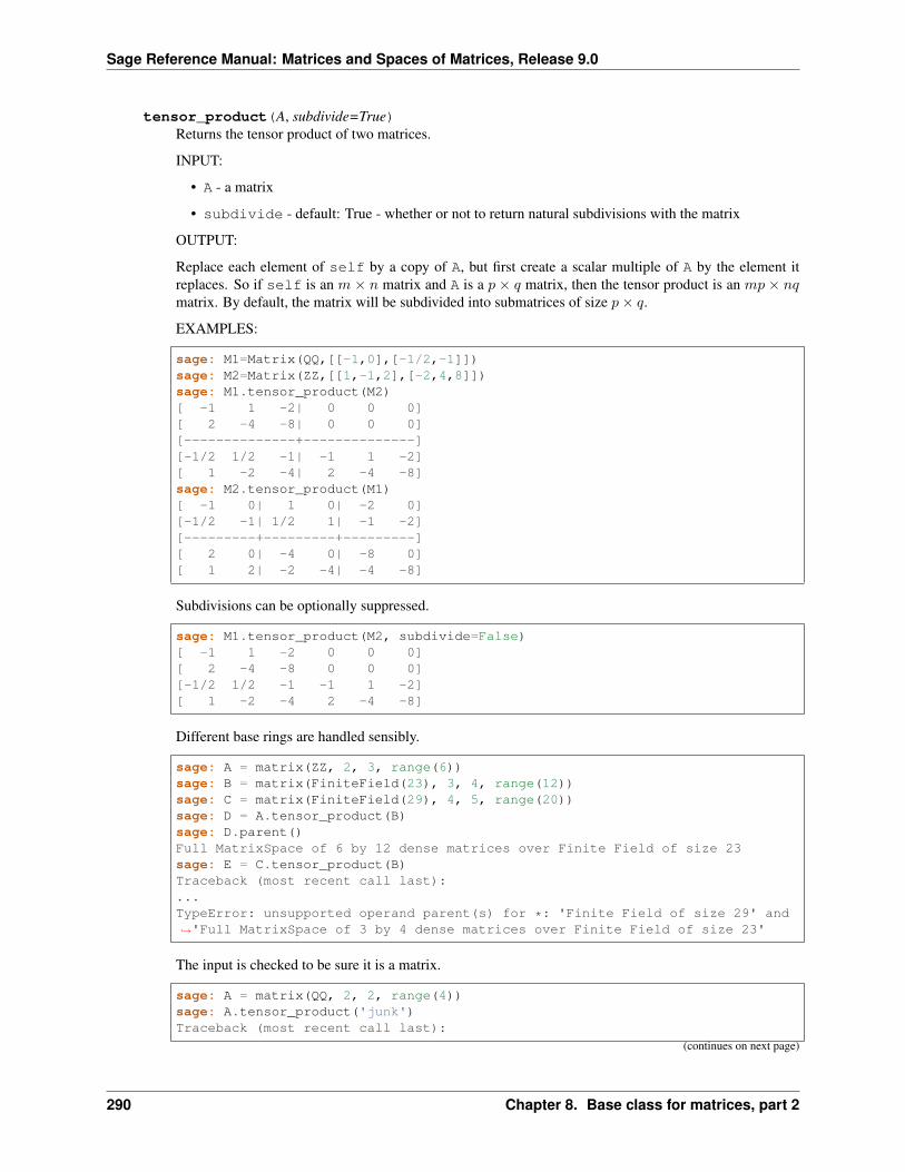
Sage Reference Manual: Matrices and Spaces of Matrices, Release 9.0
tensor_product(A, subdivide=True)Returns the tensor product of two matrices.
INPUT:
• A - a matrix
• subdivide - default: True - whether or not to return natural subdivisions with the matrix
OUTPUT:
Replace each element of self by a copy of A, but first create a scalar multiple of A by the element itreplaces. So if self is an 𝑚 × 𝑛 matrix and A is a 𝑝 × 𝑞 matrix, then the tensor product is an 𝑚𝑝 × 𝑛𝑞matrix. By default, the matrix will be subdivided into submatrices of size 𝑝× 𝑞.
EXAMPLES:
sage: M1=Matrix(QQ,[[-1,0],[-1/2,-1]])sage: M2=Matrix(ZZ,[[1,-1,2],[-2,4,8]])sage: M1.tensor_product(M2)[ -1 1 -2| 0 0 0][ 2 -4 -8| 0 0 0][--------------+--------------][-1/2 1/2 -1| -1 1 -2][ 1 -2 -4| 2 -4 -8]sage: M2.tensor_product(M1)[ -1 0| 1 0| -2 0][-1/2 -1| 1/2 1| -1 -2][---------+---------+---------][ 2 0| -4 0| -8 0][ 1 2| -2 -4| -4 -8]
Subdivisions can be optionally suppressed.
sage: M1.tensor_product(M2, subdivide=False)[ -1 1 -2 0 0 0][ 2 -4 -8 0 0 0][-1/2 1/2 -1 -1 1 -2][ 1 -2 -4 2 -4 -8]
Different base rings are handled sensibly.
sage: A = matrix(ZZ, 2, 3, range(6))sage: B = matrix(FiniteField(23), 3, 4, range(12))sage: C = matrix(FiniteField(29), 4, 5, range(20))sage: D = A.tensor_product(B)sage: D.parent()Full MatrixSpace of 6 by 12 dense matrices over Finite Field of size 23sage: E = C.tensor_product(B)Traceback (most recent call last):...TypeError: unsupported operand parent(s) for *: 'Finite Field of size 29' and→˓'Full MatrixSpace of 3 by 4 dense matrices over Finite Field of size 23'
The input is checked to be sure it is a matrix.
sage: A = matrix(QQ, 2, 2, range(4))sage: A.tensor_product('junk')Traceback (most recent call last):
(continues on next page)
290 Chapter 8. Base class for matrices, part 2

Sage Reference Manual: Matrices and Spaces of Matrices, Release 9.0
(continued from previous page)
...TypeError: tensor product requires a second matrix, not junk
trace()Return the trace of self, which is the sum of the diagonal entries of self.
INPUT:
• self - a square matrix
OUTPUT: element of the base ring of self
EXAMPLES:
sage: a = matrix(3,3,range(9)); a[0 1 2][3 4 5][6 7 8]sage: a.trace()12sage: a = matrix({(1,1):10, (2,1):-3, (2,2):4/3}); a[ 0 0 0][ 0 10 0][ 0 -3 4/3]sage: a.trace()34/3
trace_of_product(other)Returns the trace of self * other without computing the entire product.
EXAMPLES:
sage: M = random_matrix(ZZ, 10, 20)sage: N = random_matrix(ZZ, 20, 10)sage: M.trace_of_product(N)-1629sage: (M*N).trace()-1629
visualize_structure(maxsize=512)Visualize the non-zero entries
White pixels are put at positions with zero entries. If ‘maxsize’ is given, then the maximal dimension ineither x or y direction is set to ‘maxsize’ depending on which is bigger. If the image is scaled, the darknessof the pixel reflects how many of the represented entries are nonzero. So if e.g. one image pixel actuallyrepresents a 2x2 submatrix, the dot is darker the more of the four values are nonzero.
INPUT:
• maxsize - integer (default: 512). Maximal dimension in either x or y direction of the resultingimage. If None or a maxsize larger than max(self.nrows(),self.ncols()) is given theimage will have the same pixelsize as the matrix dimensions.
OUTPUT:
Bitmap image as an instance of Image.
EXAMPLES:
291
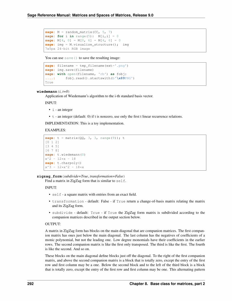
Sage Reference Manual: Matrices and Spaces of Matrices, Release 9.0
sage: M = random_matrix(CC, 5, 7)sage: for i in range(5): M[i,i] = 0sage: M[4, 0] = M[0, 6] = M[4, 6] = 0sage: img = M.visualize_structure(); img7x5px 24-bit RGB image
You can use save() to save the resulting image:
sage: filename = tmp_filename(ext='.png')sage: img.save(filename)sage: with open(filename, 'rb') as fobj:....: fobj.read().startswith(b'\x89PNG')True
wiedemann(i, t=0)Application of Wiedemann’s algorithm to the i-th standard basis vector.
INPUT:
• i - an integer
• t - an integer (default: 0) if t is nonzero, use only the first t linear recurrence relations.
IMPLEMENTATION: This is a toy implementation.
EXAMPLES:
sage: t = matrix(QQ, 3, 3, range(9)); t[0 1 2][3 4 5][6 7 8]sage: t.wiedemann(0)x^2 - 12*x - 18sage: t.charpoly()x^3 - 12*x^2 - 18*x
zigzag_form(subdivide=True, transformation=False)Find a matrix in ZigZag form that is similar to self.
INPUT:
• self - a square matrix with entries from an exact field.
• transformation - default: False - if True return a change-of-basis matrix relating the matrixand its ZigZag form.
• subdivide - default: True - if True the ZigZag form matrix is subdivided according to thecompanion matrices described in the output section below.
OUTPUT:
A matrix in ZigZag form has blocks on the main diagonal that are companion matrices. The first compan-ion matrix has ones just below the main diagonal. The last column has the negatives of coefficients of amonic polynomial, but not the leading one. Low degree monomials have their coefficients in the earlierrows. The second companion matrix is like the first only transposed. The third is like the first. The fourthis like the second. And so on.
These blocks on the main diagonal define blocks just off the diagonal. To the right of the first companionmatrix, and above the second companion matrix is a block that is totally zero, except the entry of the firstrow and first column may be a one. Below the second block and to the left of the third block is a blockthat is totally zero, except the entry of the first row and first column may be one. This alternating pattern
292 Chapter 8. Base class for matrices, part 2
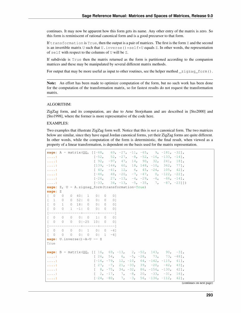
Sage Reference Manual: Matrices and Spaces of Matrices, Release 9.0
continues. It may now be apparent how this form gets its name. Any other entry of the matrix is zero. Sothis form is reminiscent of rational canonical form and is a good precursor to that form.
If transformation is True, then the output is a pair of matrices. The first is the form Z and the secondis an invertible matrix U such that U.inverse()*self*U equals Z. In other words, the representationof self with respect to the columns of U will be Z.
If subdivide is True then the matrix returned as the form is partitioned according to the companionmatrices and these may be manipulated by several different matrix methods.
For output that may be more useful as input to other routines, see the helper method _zigzag_form().
Note: An effort has been made to optimize computation of the form, but no such work has been donefor the computation of the transformation matrix, so for fastest results do not request the transformationmatrix.
ALGORITHM:
ZigZag form, and its computation, are due to Arne Storjohann and are described in [Sto2000] and[Sto1998], where the former is more representative of the code here.
EXAMPLES:
Two examples that illustrate ZigZag form well. Notice that this is not a canonical form. The two matricesbelow are similar, since they have equal Jordan canonical forms, yet their ZigZag forms are quite different.In other words, while the computation of the form is deterministic, the final result, when viewed as aproperty of a linear transformation, is dependent on the basis used for the matrix representation.
sage: A = matrix(QQ, [[-68, 69, -27, -11, -65, 9, -181, -32],....: [-52, 52, -27, -8, -52, -16, -133, -14],....: [ 92, -97, 47, 14, 90, 32, 241, 18],....: [139, -144, 60, 18, 148, -10, 362, 77],....: [ 40, -41, 12, 6, 45, -24, 105, 42],....: [-46, 48, -20, -7, -47, 0, -122, -22],....: [-26, 27, -13, -4, -29, -6, -66, -14],....: [-33, 34, -13, -5, -35, 7, -87, -23]])sage: Z, U = A.zigzag_form(transformation=True)sage: Z[ 0 0 0 40| 1 0| 0 0][ 1 0 0 52| 0 0| 0 0][ 0 1 0 18| 0 0| 0 0][ 0 0 1 -1| 0 0| 0 0][---------------+-------+-------][ 0 0 0 0| 0 1| 0 0][ 0 0 0 0|-25 10| 0 0][---------------+-------+-------][ 0 0 0 0| 1 0| 0 -4][ 0 0 0 0| 0 0| 1 -4]sage: U.inverse()*A*U == ZTrue
sage: B = matrix(QQ, [[ 16, 69, -13, 2, -52, 143, 90, -3],....: [ 26, 54, 6, -5, -28, 73, 73, -48],....: [-16, -79, 12, -10, 64, -142, -115, 41],....: [ 27, -7, 21, -33, 39, -20, -42, 43],....: [ 8, -75, 34, -32, 86, -156, -130, 42],....: [ 2, -17, 7, -8, 20, -33, -31, 16],....: [-24, -80, 7, -3, 56, -136, -112, 42],
(continues on next page)
293
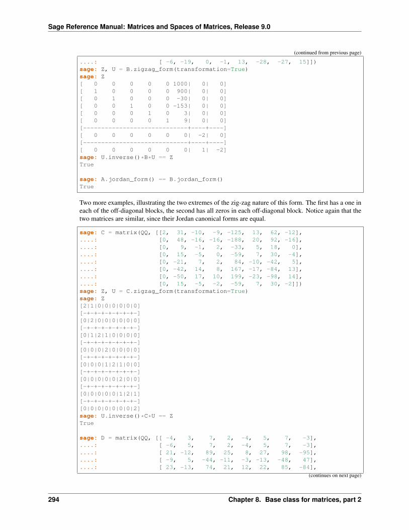
Sage Reference Manual: Matrices and Spaces of Matrices, Release 9.0
(continued from previous page)
....: [ -6, -19, 0, -1, 13, -28, -27, 15]])sage: Z, U = B.zigzag_form(transformation=True)sage: Z[ 0 0 0 0 0 1000| 0| 0][ 1 0 0 0 0 900| 0| 0][ 0 1 0 0 0 -30| 0| 0][ 0 0 1 0 0 -153| 0| 0][ 0 0 0 1 0 3| 0| 0][ 0 0 0 0 1 9| 0| 0][-----------------------------+----+----][ 0 0 0 0 0 0| -2| 0][-----------------------------+----+----][ 0 0 0 0 0 0| 1| -2]sage: U.inverse()*B*U == ZTrue
sage: A.jordan_form() == B.jordan_form()True
Two more examples, illustrating the two extremes of the zig-zag nature of this form. The first has a one ineach of the off-diagonal blocks, the second has all zeros in each off-diagonal block. Notice again that thetwo matrices are similar, since their Jordan canonical forms are equal.
sage: C = matrix(QQ, [[2, 31, -10, -9, -125, 13, 62, -12],....: [0, 48, -16, -16, -188, 20, 92, -16],....: [0, 9, -1, 2, -33, 5, 18, 0],....: [0, 15, -5, 0, -59, 7, 30, -4],....: [0, -21, 7, 2, 84, -10, -42, 5],....: [0, -42, 14, 8, 167, -17, -84, 13],....: [0, -50, 17, 10, 199, -23, -98, 14],....: [0, 15, -5, -2, -59, 7, 30, -2]])sage: Z, U = C.zigzag_form(transformation=True)sage: Z[2|1|0|0|0|0|0|0][-+-+-+-+-+-+-+-][0|2|0|0|0|0|0|0][-+-+-+-+-+-+-+-][0|1|2|1|0|0|0|0][-+-+-+-+-+-+-+-][0|0|0|2|0|0|0|0][-+-+-+-+-+-+-+-][0|0|0|1|2|1|0|0][-+-+-+-+-+-+-+-][0|0|0|0|0|2|0|0][-+-+-+-+-+-+-+-][0|0|0|0|0|1|2|1][-+-+-+-+-+-+-+-][0|0|0|0|0|0|0|2]sage: U.inverse()*C*U == ZTrue
sage: D = matrix(QQ, [[ -4, 3, 7, 2, -4, 5, 7, -3],....: [ -6, 5, 7, 2, -4, 5, 7, -3],....: [ 21, -12, 89, 25, 8, 27, 98, -95],....: [ -9, 5, -44, -11, -3, -13, -48, 47],....: [ 23, -13, 74, 21, 12, 22, 85, -84],
(continues on next page)
294 Chapter 8. Base class for matrices, part 2
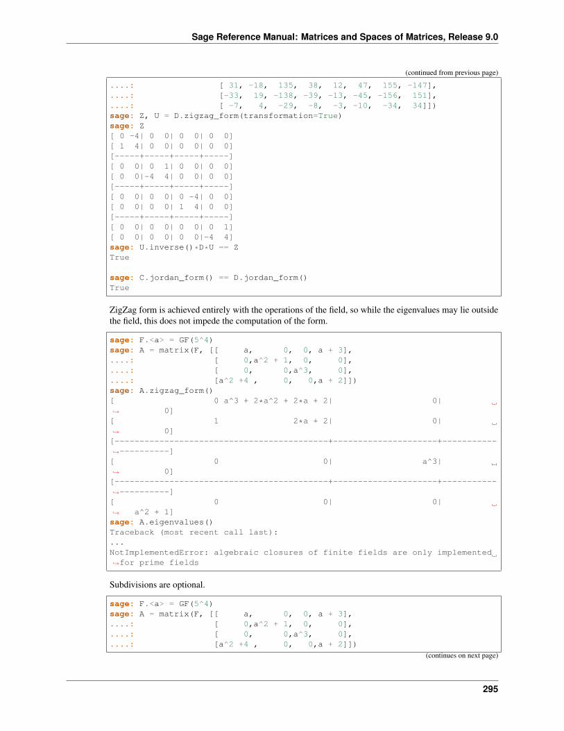
Sage Reference Manual: Matrices and Spaces of Matrices, Release 9.0
(continued from previous page)
....: [ 31, -18, 135, 38, 12, 47, 155, -147],
....: [-33, 19, -138, -39, -13, -45, -156, 151],
....: [ -7, 4, -29, -8, -3, -10, -34, 34]])sage: Z, U = D.zigzag_form(transformation=True)sage: Z[ 0 -4| 0 0| 0 0| 0 0][ 1 4| 0 0| 0 0| 0 0][-----+-----+-----+-----][ 0 0| 0 1| 0 0| 0 0][ 0 0|-4 4| 0 0| 0 0][-----+-----+-----+-----][ 0 0| 0 0| 0 -4| 0 0][ 0 0| 0 0| 1 4| 0 0][-----+-----+-----+-----][ 0 0| 0 0| 0 0| 0 1][ 0 0| 0 0| 0 0|-4 4]sage: U.inverse()*D*U == ZTrue
sage: C.jordan_form() == D.jordan_form()True
ZigZag form is achieved entirely with the operations of the field, so while the eigenvalues may lie outsidethe field, this does not impede the computation of the form.
sage: F.<a> = GF(5^4)sage: A = matrix(F, [[ a, 0, 0, a + 3],....: [ 0,a^2 + 1, 0, 0],....: [ 0, 0,a^3, 0],....: [a^2 +4 , 0, 0,a + 2]])sage: A.zigzag_form()[ 0 a^3 + 2*a^2 + 2*a + 2| 0|→˓ 0][ 1 2*a + 2| 0|→˓ 0][-------------------------------------------+---------------------+-----------→˓----------][ 0 0| a^3|→˓ 0][-------------------------------------------+---------------------+-----------→˓----------][ 0 0| 0|→˓ a^2 + 1]sage: A.eigenvalues()Traceback (most recent call last):...NotImplementedError: algebraic closures of finite fields are only implemented→˓for prime fields
Subdivisions are optional.
sage: F.<a> = GF(5^4)sage: A = matrix(F, [[ a, 0, 0, a + 3],....: [ 0,a^2 + 1, 0, 0],....: [ 0, 0,a^3, 0],....: [a^2 +4 , 0, 0,a + 2]])
(continues on next page)
295
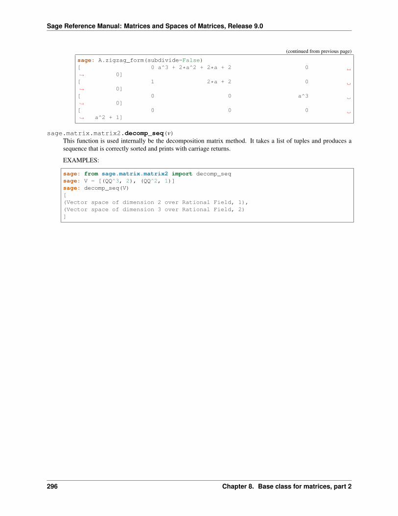
Sage Reference Manual: Matrices and Spaces of Matrices, Release 9.0
(continued from previous page)
sage: A.zigzag_form(subdivide=False)[ 0 a^3 + 2*a^2 + 2*a + 2 0→˓ 0][ 1 2*a + 2 0→˓ 0][ 0 0 a^3→˓ 0][ 0 0 0→˓ a^2 + 1]
sage.matrix.matrix2.decomp_seq(v)This function is used internally be the decomposition matrix method. It takes a list of tuples and produces asequence that is correctly sorted and prints with carriage returns.
EXAMPLES:
sage: from sage.matrix.matrix2 import decomp_seqsage: V = [(QQ^3, 2), (QQ^2, 1)]sage: decomp_seq(V)[(Vector space of dimension 2 over Rational Field, 1),(Vector space of dimension 3 over Rational Field, 2)]
296 Chapter 8. Base class for matrices, part 2
CHAPTER
NINE
GENERIC ASYMPTOTICALLY FAST STRASSEN ALGORITHMS
Sage implements asymptotically fast echelon form and matrix multiplication algorithms.
class sage.matrix.strassen.int_range(indices=None, range=None)Bases: object
Represent a list of integers as a list of integer intervals.
Note: Repetitions are not considered.
Useful class for dealing with pivots in the strassen echelon, could have much more general application
INPUT:
It can be one of the following:
• indices - integer, start of the unique interval
• range - integer, length of the unique interval
OR
• indices - list of integers, the integers to wrap into intervals
OR
• indices - None (default), shortcut for an empty list
OUTPUT:
An instance of int_range, i.e. a list of pairs (start, length).
EXAMPLES:
From a pair of integers:
sage: from sage.matrix.strassen import int_rangesage: int_range(2, 4)[(2, 4)]
Default:
sage: int_range()[]
From a list of integers:
297
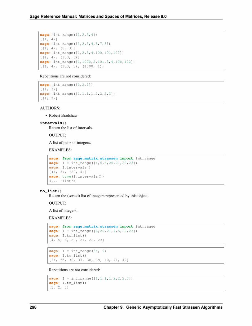
Sage Reference Manual: Matrices and Spaces of Matrices, Release 9.0
sage: int_range([1,2,3,4])[(1, 4)]sage: int_range([1,2,3,4,6,7,8])[(1, 4), (6, 3)]sage: int_range([1,2,3,4,100,101,102])[(1, 4), (100, 3)]sage: int_range([1,1000,2,101,3,4,100,102])[(1, 4), (100, 3), (1000, 1)]
Repetitions are not considered:
sage: int_range([1,2,3])[(1, 3)]sage: int_range([1,1,1,1,2,2,2,3])[(1, 3)]
AUTHORS:
• Robert Bradshaw
intervals()Return the list of intervals.
OUTPUT:
A list of pairs of integers.
EXAMPLES:
sage: from sage.matrix.strassen import int_rangesage: I = int_range([4,5,6,20,21,22,23])sage: I.intervals()[(4, 3), (20, 4)]sage: type(I.intervals())<... 'list'>
to_list()Return the (sorted) list of integers represented by this object.
OUTPUT:
A list of integers.
EXAMPLES:
sage: from sage.matrix.strassen import int_rangesage: I = int_range([6,20,21,4,5,22,23])sage: I.to_list()[4, 5, 6, 20, 21, 22, 23]
sage: I = int_range(34, 9)sage: I.to_list()[34, 35, 36, 37, 38, 39, 40, 41, 42]
Repetitions are not considered:
sage: I = int_range([1,1,1,1,2,2,2,3])sage: I.to_list()[1, 2, 3]
298 Chapter 9. Generic Asymptotically Fast Strassen Algorithms
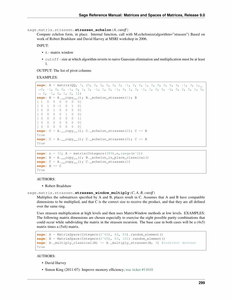
Sage Reference Manual: Matrices and Spaces of Matrices, Release 9.0
sage.matrix.strassen.strassen_echelon(A, cutoff)Compute echelon form, in place. Internal function, call with M.echelonize(algorithm=”strassen”) Based onwork of Robert Bradshaw and David Harvey at MSRI workshop in 2006.
INPUT:
• A - matrix window
• cutoff - size at which algorithm reverts to naive Gaussian elimination and multiplication must be at least1.
OUTPUT: The list of pivot columns
EXAMPLES:
sage: A = matrix(QQ, 7, [5, 0, 0, 0, 0, 0, -1, 0, 0, 1, 0, 0, 0, 0, 0, -1, 3, 1,→˓0, -1, 0, 0, -1, 0, 1, 2, -1, 1, 0, -1, 0, 1, 3, -1, 1, 0, 0, -2, 0, 2, 0, 1, 0,→˓ 0, -1, 0, 1, 0, 1])sage: B = A.__copy__(); B._echelon_strassen(1); B[ 1 0 0 0 0 0 0][ 0 1 0 -1 0 1 0][ 0 0 1 0 0 0 0][ 0 0 0 0 1 0 0][ 0 0 0 0 0 0 1][ 0 0 0 0 0 0 0][ 0 0 0 0 0 0 0]sage: C = A.__copy__(); C._echelon_strassen(2); C == BTruesage: C = A.__copy__(); C._echelon_strassen(4); C == BTrue
sage: n = 32; A = matrix(Integers(389),n,range(n^2))sage: B = A.__copy__(); B._echelon_in_place_classical()sage: C = A.__copy__(); C._echelon_strassen(2)sage: B == CTrue
AUTHORS:
• Robert Bradshaw
sage.matrix.strassen.strassen_window_multiply(C, A, B, cutoff)Multiplies the submatrices specified by A and B, places result in C. Assumes that A and B have compatibledimensions to be multiplied, and that C is the correct size to receive the product, and that they are all definedover the same ring.
Uses strassen multiplication at high levels and then uses MatrixWindow methods at low levels. EXAMPLES:The following matrix dimensions are chosen especially to exercise the eight possible parity combinations thatcould occur while subdividing the matrix in the strassen recursion. The base case in both cases will be a (4x5)matrix times a (5x6) matrix.
sage: A = MatrixSpace(Integers(2^65), 64, 83).random_element()sage: B = MatrixSpace(Integers(2^65), 83, 101).random_element()sage: A._multiply_classical(B) == A._multiply_strassen(B, 3) #indirect doctestTrue
AUTHORS:
• David Harvey
• Simon King (2011-07): Improve memory efficiency; trac ticket #11610
299
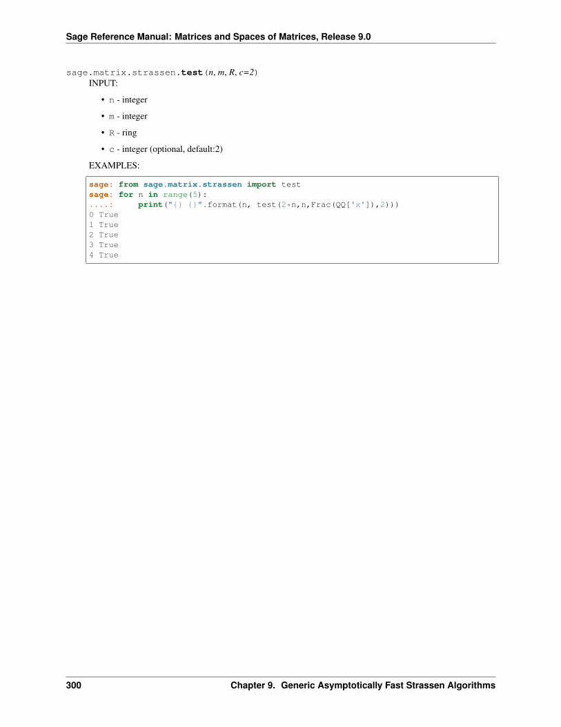
Sage Reference Manual: Matrices and Spaces of Matrices, Release 9.0
sage.matrix.strassen.test(n, m, R, c=2)INPUT:
• n - integer
• m - integer
• R - ring
• c - integer (optional, default:2)
EXAMPLES:
sage: from sage.matrix.strassen import testsage: for n in range(5):....: print("{} {}".format(n, test(2*n,n,Frac(QQ['x']),2)))0 True1 True2 True3 True4 True
300 Chapter 9. Generic Asymptotically Fast Strassen Algorithms
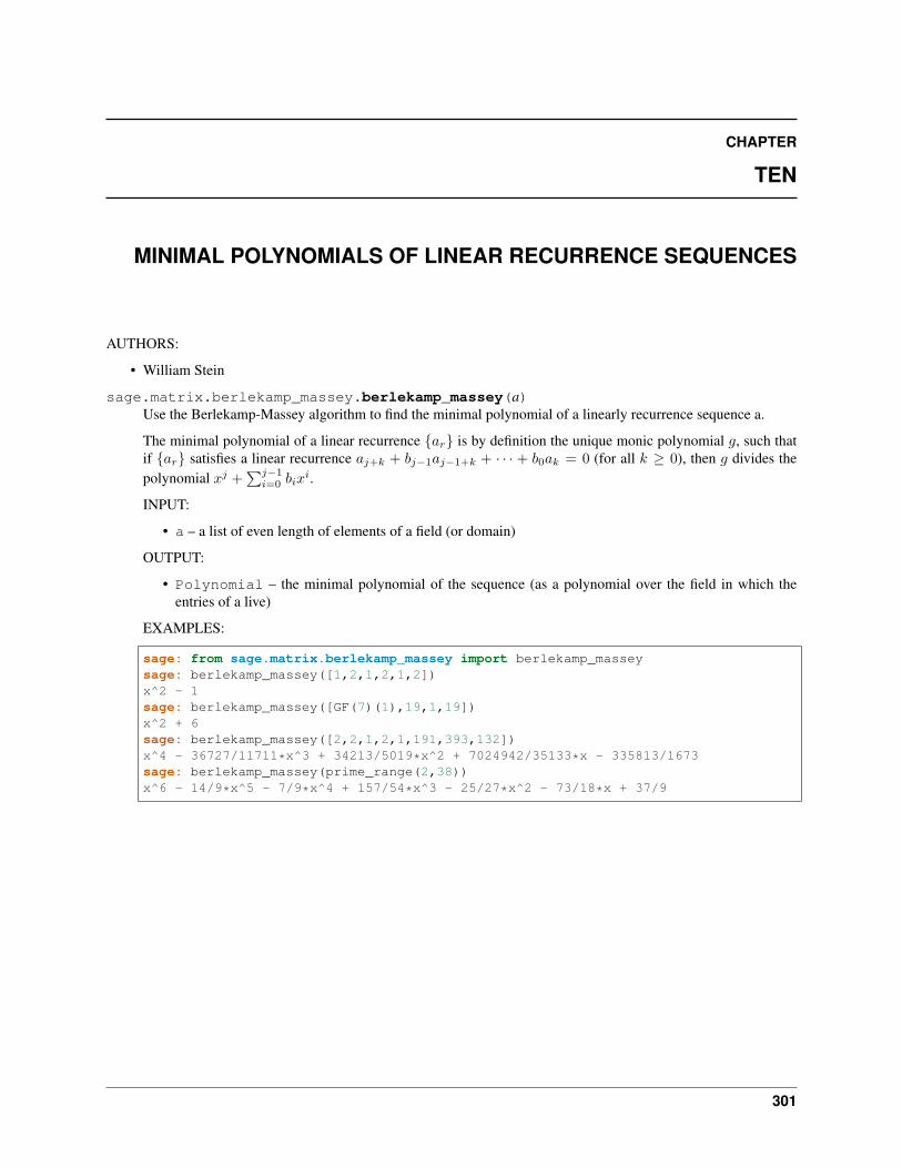
CHAPTER
TEN
MINIMAL POLYNOMIALS OF LINEAR RECURRENCE SEQUENCES
AUTHORS:
• William Stein
sage.matrix.berlekamp_massey.berlekamp_massey(a)Use the Berlekamp-Massey algorithm to find the minimal polynomial of a linearly recurrence sequence a.
The minimal polynomial of a linear recurrence {𝑎𝑟} is by definition the unique monic polynomial 𝑔, such thatif {𝑎𝑟} satisfies a linear recurrence 𝑎𝑗+𝑘 + 𝑏𝑗−1𝑎𝑗−1+𝑘 + · · · + 𝑏0𝑎𝑘 = 0 (for all 𝑘 ≥ 0), then 𝑔 divides thepolynomial 𝑥𝑗 +
∑︀𝑗−1𝑖=0 𝑏𝑖𝑥
𝑖.
INPUT:
• a – a list of even length of elements of a field (or domain)
OUTPUT:
• Polynomial – the minimal polynomial of the sequence (as a polynomial over the field in which theentries of a live)
EXAMPLES:
sage: from sage.matrix.berlekamp_massey import berlekamp_masseysage: berlekamp_massey([1,2,1,2,1,2])x^2 - 1sage: berlekamp_massey([GF(7)(1),19,1,19])x^2 + 6sage: berlekamp_massey([2,2,1,2,1,191,393,132])x^4 - 36727/11711*x^3 + 34213/5019*x^2 + 7024942/35133*x - 335813/1673sage: berlekamp_massey(prime_range(2,38))x^6 - 14/9*x^5 - 7/9*x^4 + 157/54*x^3 - 25/27*x^2 - 73/18*x + 37/9
301
Sage Reference Manual: Matrices and Spaces of Matrices, Release 9.0
302 Chapter 10. Minimal Polynomials of Linear Recurrence Sequences
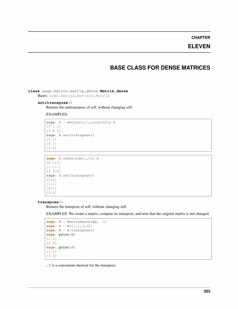
CHAPTER
ELEVEN
BASE CLASS FOR DENSE MATRICES
class sage.matrix.matrix_dense.Matrix_denseBases: sage.matrix.matrix2.Matrix
antitranspose()Returns the antitranspose of self, without changing self.
EXAMPLES:
sage: A = matrix(2,3,range(6)); A[0 1 2][3 4 5]sage: A.antitranspose()[5 2][4 1][3 0]
sage: A.subdivide(1,2); A[0 1|2][---+-][3 4|5]sage: A.antitranspose()[5|2][-+-][4|1][3|0]
transpose()Returns the transpose of self, without changing self.
EXAMPLES: We create a matrix, compute its transpose, and note that the original matrix is not changed.
sage: M = MatrixSpace(QQ, 2)sage: A = M([1,2,3,4])sage: B = A.transpose()sage: print(B)[1 3][2 4]sage: print(A)[1 2][3 4]
.T is a convenient shortcut for the transpose:
303
Sage Reference Manual: Matrices and Spaces of Matrices, Release 9.0
sage: A.T[1 3][2 4]
sage: A.subdivide(None, 1); A[1|2][3|4]sage: A.transpose()[1 3][---][2 4]
304 Chapter 11. Base class for dense matrices

CHAPTER
TWELVE
BASE CLASS FOR SPARSE MATRICES
class sage.matrix.matrix_sparse.Matrix_sparseBases: sage.matrix.matrix2.Matrix
antitranspose()Return the antitranspose of self, without changing self.
This is the mirror image along the other diagonal.
EXAMPLES:
sage: M = MatrixSpace(QQ, 2, sparse=True)sage: A = M([1,2,3,4]); A[1 2][3 4]sage: A.antitranspose()[4 2][3 1]
See also:
transpose()
apply_map(phi, R=None, sparse=True)Apply the given map phi (an arbitrary Python function or callable object) to this matrix.
If R is not given, automatically determine the base ring of the resulting matrix.
INPUT:
• phi – arbitrary Python function or callable object
• R – (optional) ring
• sparse – (optional, default True) whether to return a sparse or a dense matrix
OUTPUT: a matrix over R
EXAMPLES:
sage: m = matrix(ZZ, 10000, {(1,2): 17}, sparse=True)sage: k.<a> = GF(9)sage: f = lambda x: k(x)sage: n = m.apply_map(f)sage: n.parent()Full MatrixSpace of 10000 by 10000 sparse matrices over Finite Field in a of→˓size 3^2sage: n[1,2]2
305
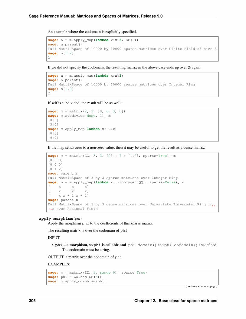
Sage Reference Manual: Matrices and Spaces of Matrices, Release 9.0
An example where the codomain is explicitly specified.
sage: n = m.apply_map(lambda x:x%3, GF(3))sage: n.parent()Full MatrixSpace of 10000 by 10000 sparse matrices over Finite Field of size 3sage: n[1,2]2
If we did not specify the codomain, the resulting matrix in the above case ends up over Z again:
sage: n = m.apply_map(lambda x:x%3)sage: n.parent()Full MatrixSpace of 10000 by 10000 sparse matrices over Integer Ringsage: n[1,2]2
If self is subdivided, the result will be as well:
sage: m = matrix(2, 2, [0, 0, 3, 0])sage: m.subdivide(None, 1); m[0|0][3|0]sage: m.apply_map(lambda x: x*x)[0|0][9|0]
If the map sends zero to a non-zero value, then it may be useful to get the result as a dense matrix.
sage: m = matrix(ZZ, 3, 3, [0] * 7 + [1,2], sparse=True); m[0 0 0][0 0 0][0 1 2]sage: parent(m)Full MatrixSpace of 3 by 3 sparse matrices over Integer Ringsage: n = m.apply_map(lambda x: x+polygen(QQ), sparse=False); n[ x x x][ x x x][ x x + 1 x + 2]sage: parent(n)Full MatrixSpace of 3 by 3 dense matrices over Univariate Polynomial Ring in→˓x over Rational Field
apply_morphism(phi)Apply the morphism phi to the coefficients of this sparse matrix.
The resulting matrix is over the codomain of phi.
INPUT:
• phi – a morphism, so phi is callable and phi.domain() and phi.codomain() are defined.The codomain must be a ring.
OUTPUT: a matrix over the codomain of phi
EXAMPLES:
sage: m = matrix(ZZ, 3, range(9), sparse=True)sage: phi = ZZ.hom(GF(5))sage: m.apply_morphism(phi)
(continues on next page)
306 Chapter 12. Base class for sparse matrices
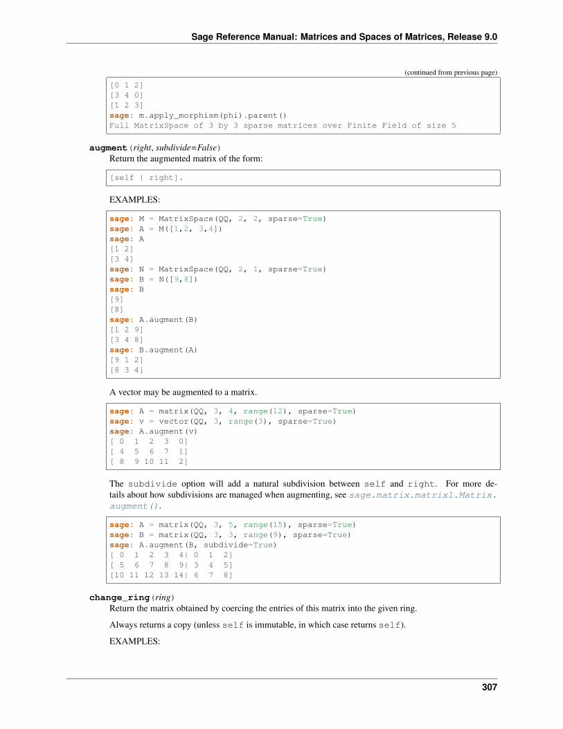
Sage Reference Manual: Matrices and Spaces of Matrices, Release 9.0
(continued from previous page)
[0 1 2][3 4 0][1 2 3]sage: m.apply_morphism(phi).parent()Full MatrixSpace of 3 by 3 sparse matrices over Finite Field of size 5
augment(right, subdivide=False)Return the augmented matrix of the form:
[self | right].
EXAMPLES:
sage: M = MatrixSpace(QQ, 2, 2, sparse=True)sage: A = M([1,2, 3,4])sage: A[1 2][3 4]sage: N = MatrixSpace(QQ, 2, 1, sparse=True)sage: B = N([9,8])sage: B[9][8]sage: A.augment(B)[1 2 9][3 4 8]sage: B.augment(A)[9 1 2][8 3 4]
A vector may be augmented to a matrix.
sage: A = matrix(QQ, 3, 4, range(12), sparse=True)sage: v = vector(QQ, 3, range(3), sparse=True)sage: A.augment(v)[ 0 1 2 3 0][ 4 5 6 7 1][ 8 9 10 11 2]
The subdivide option will add a natural subdivision between self and right. For more de-tails about how subdivisions are managed when augmenting, see sage.matrix.matrix1.Matrix.augment().
sage: A = matrix(QQ, 3, 5, range(15), sparse=True)sage: B = matrix(QQ, 3, 3, range(9), sparse=True)sage: A.augment(B, subdivide=True)[ 0 1 2 3 4| 0 1 2][ 5 6 7 8 9| 3 4 5][10 11 12 13 14| 6 7 8]
change_ring(ring)Return the matrix obtained by coercing the entries of this matrix into the given ring.
Always returns a copy (unless self is immutable, in which case returns self).
EXAMPLES:
307
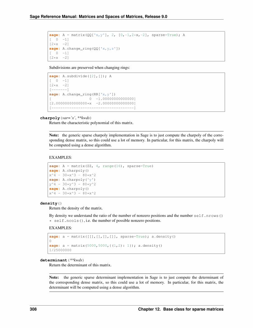
Sage Reference Manual: Matrices and Spaces of Matrices, Release 9.0
sage: A = matrix(QQ['x,y'], 2, [0,-1,2*x,-2], sparse=True); A[ 0 -1][2*x -2]sage: A.change_ring(QQ['x,y,z'])[ 0 -1][2*x -2]
Subdivisions are preserved when changing rings:
sage: A.subdivide([2],[]); A[ 0 -1][2*x -2][-------]sage: A.change_ring(RR['x,y'])[ 0 -1.00000000000000][2.00000000000000*x -2.00000000000000][-------------------------------------]
charpoly(var=’x’, **kwds)Return the characteristic polynomial of this matrix.
Note: the generic sparse charpoly implementation in Sage is to just compute the charpoly of the corre-sponding dense matrix, so this could use a lot of memory. In particular, for this matrix, the charpoly willbe computed using a dense algorithm.
EXAMPLES:
sage: A = matrix(ZZ, 4, range(16), sparse=True)sage: A.charpoly()x^4 - 30*x^3 - 80*x^2sage: A.charpoly('y')y^4 - 30*y^3 - 80*y^2sage: A.charpoly()x^4 - 30*x^3 - 80*x^2
density()Return the density of the matrix.
By density we understand the ratio of the number of nonzero positions and the number self.nrows()* self.ncols(), i.e. the number of possible nonzero positions.
EXAMPLES:
sage: a = matrix([[],[],[],[]], sparse=True); a.density()0sage: a = matrix(5000,5000,{(1,2): 1}); a.density()1/25000000
determinant(**kwds)Return the determinant of this matrix.
Note: the generic sparse determinant implementation in Sage is to just compute the determinant ofthe corresponding dense matrix, so this could use a lot of memory. In particular, for this matrix, thedeterminant will be computed using a dense algorithm.
308 Chapter 12. Base class for sparse matrices
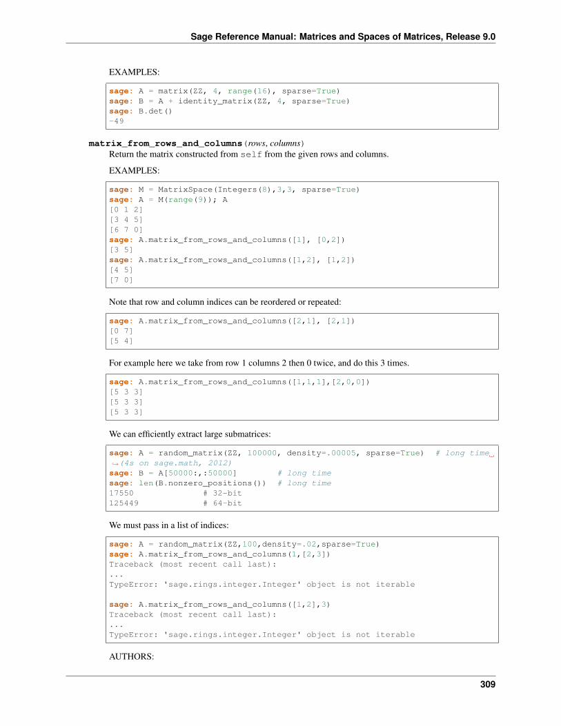
Sage Reference Manual: Matrices and Spaces of Matrices, Release 9.0
EXAMPLES:
sage: A = matrix(ZZ, 4, range(16), sparse=True)sage: B = A + identity_matrix(ZZ, 4, sparse=True)sage: B.det()-49
matrix_from_rows_and_columns(rows, columns)Return the matrix constructed from self from the given rows and columns.
EXAMPLES:
sage: M = MatrixSpace(Integers(8),3,3, sparse=True)sage: A = M(range(9)); A[0 1 2][3 4 5][6 7 0]sage: A.matrix_from_rows_and_columns([1], [0,2])[3 5]sage: A.matrix_from_rows_and_columns([1,2], [1,2])[4 5][7 0]
Note that row and column indices can be reordered or repeated:
sage: A.matrix_from_rows_and_columns([2,1], [2,1])[0 7][5 4]
For example here we take from row 1 columns 2 then 0 twice, and do this 3 times.
sage: A.matrix_from_rows_and_columns([1,1,1],[2,0,0])[5 3 3][5 3 3][5 3 3]
We can efficiently extract large submatrices:
sage: A = random_matrix(ZZ, 100000, density=.00005, sparse=True) # long time→˓(4s on sage.math, 2012)sage: B = A[50000:,:50000] # long timesage: len(B.nonzero_positions()) # long time17550 # 32-bit125449 # 64-bit
We must pass in a list of indices:
sage: A = random_matrix(ZZ,100,density=.02,sparse=True)sage: A.matrix_from_rows_and_columns(1,[2,3])Traceback (most recent call last):...TypeError: 'sage.rings.integer.Integer' object is not iterable
sage: A.matrix_from_rows_and_columns([1,2],3)Traceback (most recent call last):...TypeError: 'sage.rings.integer.Integer' object is not iterable
AUTHORS:
309
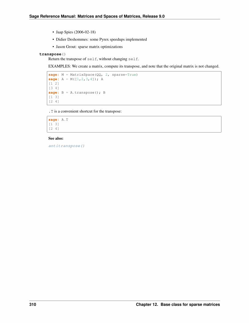
Sage Reference Manual: Matrices and Spaces of Matrices, Release 9.0
• Jaap Spies (2006-02-18)
• Didier Deshommes: some Pyrex speedups implemented
• Jason Grout: sparse matrix optimizations
transpose()Return the transpose of self, without changing self.
EXAMPLES: We create a matrix, compute its transpose, and note that the original matrix is not changed.
sage: M = MatrixSpace(QQ, 2, sparse=True)sage: A = M([1,2,3,4]); A[1 2][3 4]sage: B = A.transpose(); B[1 3][2 4]
.T is a convenient shortcut for the transpose:
sage: A.T[1 3][2 4]
See also:
antitranspose()
310 Chapter 12. Base class for sparse matrices
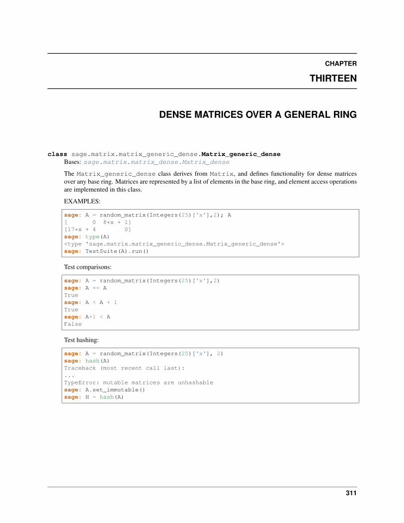
CHAPTER
THIRTEEN
DENSE MATRICES OVER A GENERAL RING
class sage.matrix.matrix_generic_dense.Matrix_generic_denseBases: sage.matrix.matrix_dense.Matrix_dense
The Matrix_generic_dense class derives from Matrix, and defines functionality for dense matricesover any base ring. Matrices are represented by a list of elements in the base ring, and element access operationsare implemented in this class.
EXAMPLES:
sage: A = random_matrix(Integers(25)['x'],2); A[ 0 8*x + 1][17*x + 4 0]sage: type(A)<type 'sage.matrix.matrix_generic_dense.Matrix_generic_dense'>sage: TestSuite(A).run()
Test comparisons:
sage: A = random_matrix(Integers(25)['x'],2)sage: A == ATruesage: A < A + 1Truesage: A+1 < AFalse
Test hashing:
sage: A = random_matrix(Integers(25)['x'], 2)sage: hash(A)Traceback (most recent call last):...TypeError: mutable matrices are unhashablesage: A.set_immutable()sage: H = hash(A)
311
Sage Reference Manual: Matrices and Spaces of Matrices, Release 9.0
312 Chapter 13. Dense Matrices over a general ring
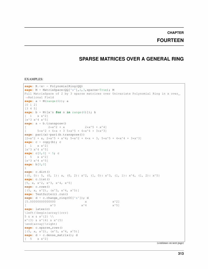
CHAPTER
FOURTEEN
SPARSE MATRICES OVER A GENERAL RING
EXAMPLES:
sage: R.<x> = PolynomialRing(QQ)sage: M = MatrixSpace(QQ['x'],2,3,sparse=True); MFull MatrixSpace of 2 by 3 sparse matrices over Univariate Polynomial Ring in x over→˓Rational Fieldsage: a = M(range(6)); a[0 1 2][3 4 5]sage: b = M([x^n for n in range(6)]); b[ 1 x x^2][x^3 x^4 x^5]sage: a * b.transpose()[ 2*x^2 + x 2*x^5 + x^4][ 5*x^2 + 4*x + 3 5*x^5 + 4*x^4 + 3*x^3]sage: pari(a)*pari(b.transpose())[2*x^2 + x, 2*x^5 + x^4; 5*x^2 + 4*x + 3, 5*x^5 + 4*x^4 + 3*x^3]sage: c = copy(b); c[ 1 x x^2][x^3 x^4 x^5]sage: c[0,0] = 5; c[ 5 x x^2][x^3 x^4 x^5]sage: b[0,0]1sage: c.dict(){(0, 0): 5, (0, 1): x, (0, 2): x^2, (1, 0): x^3, (1, 1): x^4, (1, 2): x^5}sage: c.list()[5, x, x^2, x^3, x^4, x^5]sage: c.rows()[(5, x, x^2), (x^3, x^4, x^5)]sage: TestSuite(c).run()sage: d = c.change_ring(CC['x']); d[5.00000000000000 x x^2][ x^3 x^4 x^5]sage: latex(c)\left(\begin{array}{rrr}5 & x & x^{2} \\x^{3} & x^{4} & x^{5}\end{array}\right)sage: c.sparse_rows()[(5, x, x^2), (x^3, x^4, x^5)]sage: d = c.dense_matrix(); d[ 5 x x^2]
(continues on next page)
313
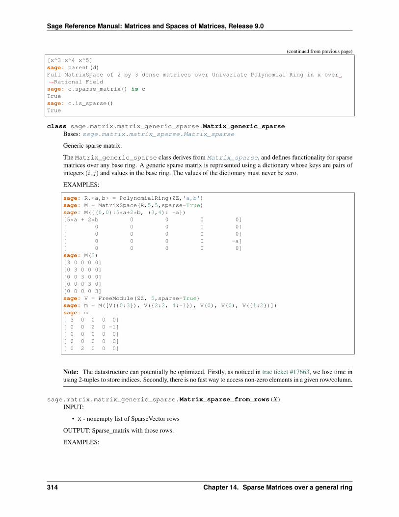
Sage Reference Manual: Matrices and Spaces of Matrices, Release 9.0
(continued from previous page)
[x^3 x^4 x^5]sage: parent(d)Full MatrixSpace of 2 by 3 dense matrices over Univariate Polynomial Ring in x over→˓Rational Fieldsage: c.sparse_matrix() is cTruesage: c.is_sparse()True
class sage.matrix.matrix_generic_sparse.Matrix_generic_sparseBases: sage.matrix.matrix_sparse.Matrix_sparse
Generic sparse matrix.
The Matrix_generic_sparse class derives from Matrix_sparse, and defines functionality for sparsematrices over any base ring. A generic sparse matrix is represented using a dictionary whose keys are pairs ofintegers (𝑖, 𝑗) and values in the base ring. The values of the dictionary must never be zero.
EXAMPLES:
sage: R.<a,b> = PolynomialRing(ZZ,'a,b')sage: M = MatrixSpace(R,5,5,sparse=True)sage: M({(0,0):5*a+2*b, (3,4): -a})[5*a + 2*b 0 0 0 0][ 0 0 0 0 0][ 0 0 0 0 0][ 0 0 0 0 -a][ 0 0 0 0 0]sage: M(3)[3 0 0 0 0][0 3 0 0 0][0 0 3 0 0][0 0 0 3 0][0 0 0 0 3]sage: V = FreeModule(ZZ, 5,sparse=True)sage: m = M([V({0:3}), V({2:2, 4:-1}), V(0), V(0), V({1:2})])sage: m[ 3 0 0 0 0][ 0 0 2 0 -1][ 0 0 0 0 0][ 0 0 0 0 0][ 0 2 0 0 0]
Note: The datastructure can potentially be optimized. Firstly, as noticed in trac ticket #17663, we lose time inusing 2-tuples to store indices. Secondly, there is no fast way to access non-zero elements in a given row/column.
sage.matrix.matrix_generic_sparse.Matrix_sparse_from_rows(X)INPUT:
• X - nonempty list of SparseVector rows
OUTPUT: Sparse_matrix with those rows.
EXAMPLES:
314 Chapter 14. Sparse Matrices over a general ring
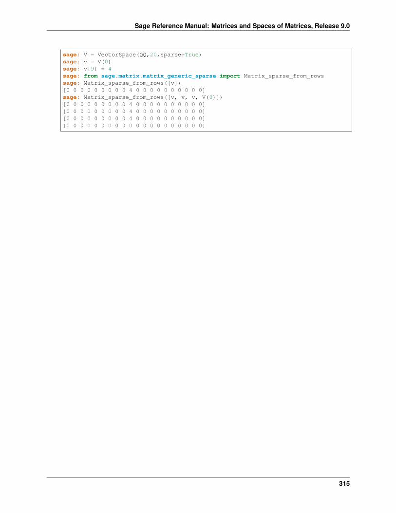
Sage Reference Manual: Matrices and Spaces of Matrices, Release 9.0
sage: V = VectorSpace(QQ,20,sparse=True)sage: v = V(0)sage: v[9] = 4sage: from sage.matrix.matrix_generic_sparse import Matrix_sparse_from_rowssage: Matrix_sparse_from_rows([v])[0 0 0 0 0 0 0 0 0 4 0 0 0 0 0 0 0 0 0 0]sage: Matrix_sparse_from_rows([v, v, v, V(0)])[0 0 0 0 0 0 0 0 0 4 0 0 0 0 0 0 0 0 0 0][0 0 0 0 0 0 0 0 0 4 0 0 0 0 0 0 0 0 0 0][0 0 0 0 0 0 0 0 0 4 0 0 0 0 0 0 0 0 0 0][0 0 0 0 0 0 0 0 0 0 0 0 0 0 0 0 0 0 0 0]
315

Sage Reference Manual: Matrices and Spaces of Matrices, Release 9.0
316 Chapter 14. Sparse Matrices over a general ring
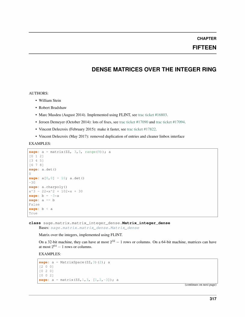
CHAPTER
FIFTEEN
DENSE MATRICES OVER THE INTEGER RING
AUTHORS:
• William Stein
• Robert Bradshaw
• Marc Masdeu (August 2014). Implemented using FLINT, see trac ticket #16803.
• Jeroen Demeyer (October 2014): lots of fixes, see trac ticket #17090 and trac ticket #17094.
• Vincent Delecroix (February 2015): make it faster, see trac ticket #17822.
• Vincent Delecroix (May 2017): removed duplication of entries and cleaner linbox interface
EXAMPLES:
sage: a = matrix(ZZ, 3,3, range(9)); a[0 1 2][3 4 5][6 7 8]sage: a.det()0sage: a[0,0] = 10; a.det()-30sage: a.charpoly()x^3 - 22*x^2 + 102*x + 30sage: b = -3*asage: a == bFalsesage: b < aTrue
class sage.matrix.matrix_integer_dense.Matrix_integer_denseBases: sage.matrix.matrix_dense.Matrix_dense
Matrix over the integers, implemented using FLINT.
On a 32-bit machine, they can have at most 232 − 1 rows or columns. On a 64-bit machine, matrices can haveat most 264 − 1 rows or columns.
EXAMPLES:
sage: a = MatrixSpace(ZZ,3)(2); a[2 0 0][0 2 0][0 0 2]sage: a = matrix(ZZ,1,3, [1,2,-3]); a
(continues on next page)
317
Sage Reference Manual: Matrices and Spaces of Matrices, Release 9.0
(continued from previous page)
[ 1 2 -3]sage: a = MatrixSpace(ZZ,2,4)(2); aTraceback (most recent call last):...TypeError: nonzero scalar matrix must be square
BKZ(delta=None, algorithm=’fpLLL’, fp=None, block_size=10, prune=0, use_givens=False, preci-sion=0, proof=None, **kwds)Block Korkin-Zolotarev reduction.
INPUT:
• delta – (default: 0.99) LLL parameter
• algorithm – (default: "fpLLL") "fpLLL" or "NTL"
• fp – floating point number implementation
– None – NTL’s exact reduction or fpLLL’s wrapper (default)
– 'fp' – double precision: NTL’s FP or fpLLL’s double
– 'ld' – long doubles (fpLLL only)
– 'qd' – NTL’s QP
-'qd1' – quad doubles: Uses quad_float precision to compute Gram-Schmidt, butuses double precision in the search phase of the block reduction algorithm. This seemsadequate for most purposes, and is faster than 'qd', which uses quad_float precision uni-formly throughout (NTL only).
– 'xd' – extended exponent: NTL’s XD or fpLLL’s dpe
– 'rr' – arbitrary precision: NTL’RR or fpLLL’s MPFR
• block_size – (default: 10) Specifies the size of the blocks in the reduction. High valuesyield shorter vectors, but the running time increases double exponentially with block_size.block_size should be between 2 and the number of rows of self.
• proof – (default: same as proof.linear_algebra()) Insist on full BKZ reduction. If disabledand fplll is called, reduction is much faster but the result is not fully BKZ reduced.
NTL SPECIFIC INPUT:
• prune – (default: 0) The optional parameter prune can be set to any positive number to invokethe Volume Heuristic from [SH1995]. This can significantly reduce the running time, and henceallow much bigger block size, but the quality of the reduction is of course not as good in general.Higher values of prune mean better quality, and slower running time. When prune is 0, pruning isdisabled. Recommended usage: for block_size==30, set 10 <= prune <=15.
• use_givens – Use Givens orthogonalization. Only applies to approximate reduction using NTL.This is a bit slower, but generally much more stable, and is really the preferred orthogonalizationstrategy. For a nice description of this, see Chapter 5 of [GL1996].
fpLLL SPECIFIC INPUT:
• precision – (default: 0 for automatic choice) bit precision to use if fp='rr' is set
• **kwds – keywords to be passed to fpylll. See fpylll.BKZ.Param for details.
318 Chapter 15. Dense matrices over the integer ring
Sage Reference Manual: Matrices and Spaces of Matrices, Release 9.0
Also, if the verbose level is at least 2, some output is printed during the computation.
EXAMPLES:
sage: A = Matrix(ZZ,3,3,range(1,10))sage: A.BKZ()[ 0 0 0][ 2 1 0][-1 1 3]
sage: A = Matrix(ZZ,3,3,range(1,10))sage: A.BKZ(use_givens=True)[ 0 0 0][ 2 1 0][-1 1 3]
sage: A = Matrix(ZZ,3,3,range(1,10))sage: A.BKZ(fp="fp")[ 0 0 0][ 2 1 0][-1 1 3]
ALGORITHM:
Calls either NTL or fpLLL.
LLL(delta=None, eta=None, algorithm=’fpLLL:wrapper’, fp=None, prec=0, early_red=False,use_givens=False, use_siegel=False, **kwds)Return LLL reduced or approximated LLL reduced lattice 𝑅 for this matrix interpreted as a lattice.
A lattice (𝑏1, 𝑏2, ..., 𝑏𝑑) is (𝛿, 𝜂)-LLL-reduced if the two following conditions hold:
• For any 𝑖 > 𝑗, we have |𝜇𝑖,𝑗 | ≤ 𝜂.
• For any 𝑖 < 𝑑, we have 𝛿|𝑏*𝑖 |2 ≤ |𝑏*𝑖+1 + 𝜇𝑖+1,𝑖𝑏*𝑖 |2,
where 𝜇𝑖,𝑗 = ⟨𝑏𝑖, 𝑏*𝑗 ⟩/⟨𝑏*𝑗 , 𝑏*𝑗 ⟩ and 𝑏*𝑖 is the 𝑖-th vector of the Gram-Schmidt orthogonalisation of(𝑏1, 𝑏2, ..., 𝑏𝑑).
The default reduction parameters are 𝛿 = 0.99 and 𝜂 = 0.501. The parameters 𝛿 and 𝜂 must satisfy0.25 < 𝛿 ≤ 1.0 and 0.5 ≤ 𝜂 <
√𝛿. Polynomial time complexity is only guaranteed for 𝛿 < 1. Not every
algorithm admits the case 𝛿 = 1.
The lattice is returned as a matrix. Also the rank (and the determinant) of self are cached if thoseare computed during the reduction. Note that in general this only happens when self.rank() ==self.ncols() and the exact algorithm is used.
INPUT:
• delta – (default: 0.99) 𝛿 parameter as described above
• eta – (default: 0.501) 𝜂 parameter as described above, ignored by NTL
• algorithm – string; one of the algorithms listed below (default: "fpLLL:wrapper").
• fp – floating point number implementation:
– None – NTL’s exact reduction or fpLLL’s wrapper
– 'fp' – double precision: NTL’s FP or fpLLL’s double
– 'ld' – long doubles (fpLLL only)
– 'qd' – NTL’s QP
319
Sage Reference Manual: Matrices and Spaces of Matrices, Release 9.0
– 'xd' – extended exponent: NTL’s XD or fpLLL’s dpe
– 'rr' – arbitrary precision: NTL’s RR or fpLLL’s MPFR
• prec – (default: auto choose) precision, ignored by NTL
• early_red – (default: False) perform early reduction, ignored by NTL
• use_givens – (default: False) use Givens orthogonalization. Only applies to approximate reduc-tion using NTL. This is slower but generally more stable.
• use_siegel – (default: False) use Siegel’s condition instead of Lovász’s condition, ignored byNTL
• **kwds – keywords to be passed to fpylll. See fpylll.LLL.reduction() for details.
Also, if the verbose level is at least 2, some output is printed during the computation.
AVAILABLE ALGORITHMS:
• 'NTL:LLL' - NTL’s LLL + choice of fp.
• 'fpLLL:heuristic' - fpLLL’s heuristic + choice of fp.
• 'fpLLL:fast' - fpLLL’s fast + choice of fp.
• 'fpLLL:proved' - fpLLL’s proved + choice of fp.
• 'fpLLL:wrapper' - fpLLL’s automatic choice (default).
OUTPUT:
A matrix over the integers.
EXAMPLES:
sage: A = Matrix(ZZ,3,3,range(1,10))sage: A.LLL()[ 0 0 0][ 2 1 0][-1 1 3]
We compute the extended GCD of a list of integers using LLL, this example is from the Magma handbook:
sage: Q = [ 67015143, 248934363018, 109210, 25590011055, 74631449,....: 10230248, 709487, 68965012139, 972065, 864972271 ]sage: n = len(Q)sage: S = 100sage: X = Matrix(ZZ, n, n + 1)sage: for i in range(n):....: X[i, i + 1] = 1sage: for i in range(n):....: X[i, 0] = S * Q[i]sage: L = X.LLL()sage: M = L.row(n-1).list()[1:]sage: M[-3, -1, 13, -1, -4, 2, 3, 4, 5, -1]sage: add(Q[i]*M[i] for i in range(n))-1
The case 𝛿 = 1 is not always supported:
320 Chapter 15. Dense matrices over the integer ring
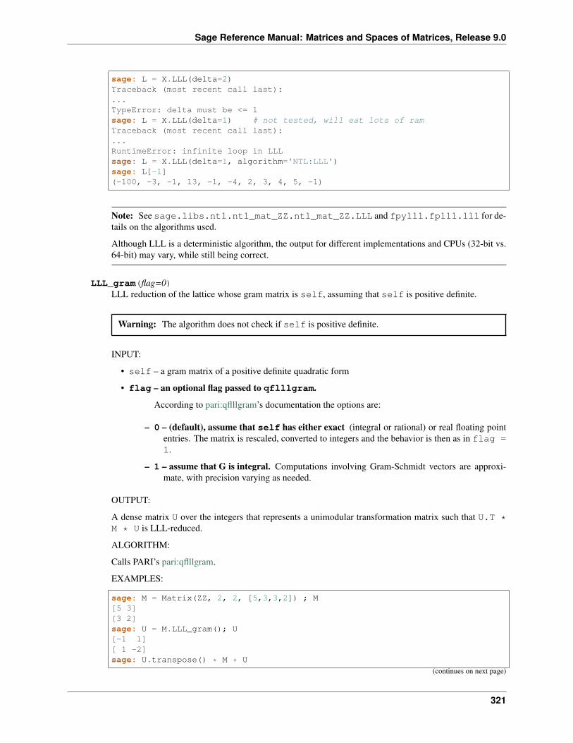
Sage Reference Manual: Matrices and Spaces of Matrices, Release 9.0
sage: L = X.LLL(delta=2)Traceback (most recent call last):...TypeError: delta must be <= 1sage: L = X.LLL(delta=1) # not tested, will eat lots of ramTraceback (most recent call last):...RuntimeError: infinite loop in LLLsage: L = X.LLL(delta=1, algorithm='NTL:LLL')sage: L[-1](-100, -3, -1, 13, -1, -4, 2, 3, 4, 5, -1)
Note: See sage.libs.ntl.ntl_mat_ZZ.ntl_mat_ZZ.LLL and fpylll.fplll.lll for de-tails on the algorithms used.
Although LLL is a deterministic algorithm, the output for different implementations and CPUs (32-bit vs.64-bit) may vary, while still being correct.
LLL_gram(flag=0)LLL reduction of the lattice whose gram matrix is self, assuming that self is positive definite.
Warning: The algorithm does not check if self is positive definite.
INPUT:
• self – a gram matrix of a positive definite quadratic form
• flag – an optional flag passed to qflllgram.
According to pari:qflllgram’s documentation the options are:
– 0 – (default), assume that self has either exact (integral or rational) or real floating pointentries. The matrix is rescaled, converted to integers and the behavior is then as in flag =1.
– 1 – assume that G is integral. Computations involving Gram-Schmidt vectors are approxi-mate, with precision varying as needed.
OUTPUT:
A dense matrix U over the integers that represents a unimodular transformation matrix such that U.T *M * U is LLL-reduced.
ALGORITHM:
Calls PARI’s pari:qflllgram.
EXAMPLES:
sage: M = Matrix(ZZ, 2, 2, [5,3,3,2]) ; M[5 3][3 2]sage: U = M.LLL_gram(); U[-1 1][ 1 -2]sage: U.transpose() * M * U
(continues on next page)
321
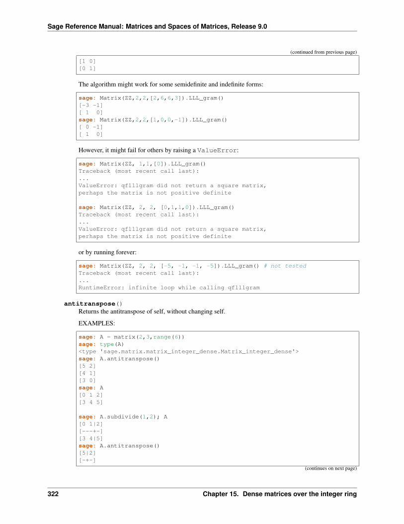
Sage Reference Manual: Matrices and Spaces of Matrices, Release 9.0
(continued from previous page)
[1 0][0 1]
The algorithm might work for some semidefinite and indefinite forms:
sage: Matrix(ZZ,2,2,[2,6,6,3]).LLL_gram()[-3 -1][ 1 0]sage: Matrix(ZZ,2,2,[1,0,0,-1]).LLL_gram()[ 0 -1][ 1 0]
However, it might fail for others by raising a ValueError:
sage: Matrix(ZZ, 1,1,[0]).LLL_gram()Traceback (most recent call last):...ValueError: qflllgram did not return a square matrix,perhaps the matrix is not positive definite
sage: Matrix(ZZ, 2, 2, [0,1,1,0]).LLL_gram()Traceback (most recent call last):...ValueError: qflllgram did not return a square matrix,perhaps the matrix is not positive definite
or by running forever:
sage: Matrix(ZZ, 2, 2, [-5, -1, -1, -5]).LLL_gram() # not testedTraceback (most recent call last):...RuntimeError: infinite loop while calling qflllgram
antitranspose()Returns the antitranspose of self, without changing self.
EXAMPLES:
sage: A = matrix(2,3,range(6))sage: type(A)<type 'sage.matrix.matrix_integer_dense.Matrix_integer_dense'>sage: A.antitranspose()[5 2][4 1][3 0]sage: A[0 1 2][3 4 5]
sage: A.subdivide(1,2); A[0 1|2][---+-][3 4|5]sage: A.antitranspose()[5|2][-+-]
(continues on next page)
322 Chapter 15. Dense matrices over the integer ring
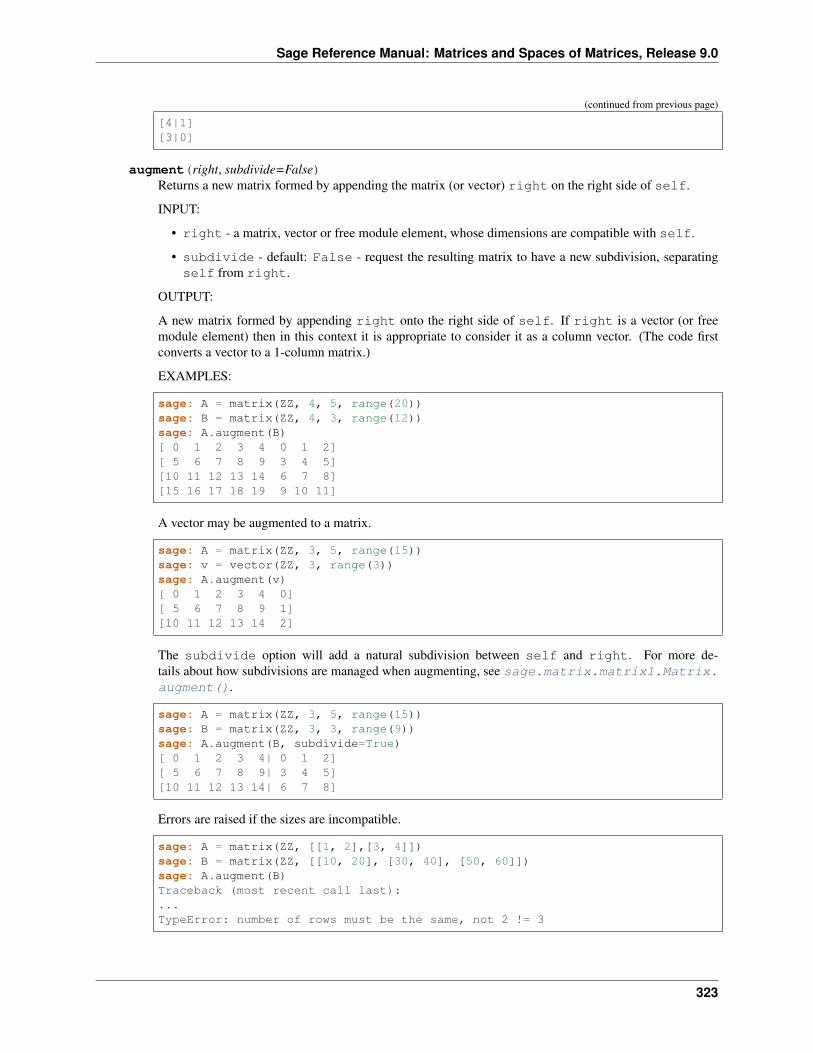
Sage Reference Manual: Matrices and Spaces of Matrices, Release 9.0
(continued from previous page)
[4|1][3|0]
augment(right, subdivide=False)Returns a new matrix formed by appending the matrix (or vector) right on the right side of self.
INPUT:
• right - a matrix, vector or free module element, whose dimensions are compatible with self.
• subdivide - default: False - request the resulting matrix to have a new subdivision, separatingself from right.
OUTPUT:
A new matrix formed by appending right onto the right side of self. If right is a vector (or freemodule element) then in this context it is appropriate to consider it as a column vector. (The code firstconverts a vector to a 1-column matrix.)
EXAMPLES:
sage: A = matrix(ZZ, 4, 5, range(20))sage: B = matrix(ZZ, 4, 3, range(12))sage: A.augment(B)[ 0 1 2 3 4 0 1 2][ 5 6 7 8 9 3 4 5][10 11 12 13 14 6 7 8][15 16 17 18 19 9 10 11]
A vector may be augmented to a matrix.
sage: A = matrix(ZZ, 3, 5, range(15))sage: v = vector(ZZ, 3, range(3))sage: A.augment(v)[ 0 1 2 3 4 0][ 5 6 7 8 9 1][10 11 12 13 14 2]
The subdivide option will add a natural subdivision between self and right. For more de-tails about how subdivisions are managed when augmenting, see sage.matrix.matrix1.Matrix.augment().
sage: A = matrix(ZZ, 3, 5, range(15))sage: B = matrix(ZZ, 3, 3, range(9))sage: A.augment(B, subdivide=True)[ 0 1 2 3 4| 0 1 2][ 5 6 7 8 9| 3 4 5][10 11 12 13 14| 6 7 8]
Errors are raised if the sizes are incompatible.
sage: A = matrix(ZZ, [[1, 2],[3, 4]])sage: B = matrix(ZZ, [[10, 20], [30, 40], [50, 60]])sage: A.augment(B)Traceback (most recent call last):...TypeError: number of rows must be the same, not 2 != 3
323
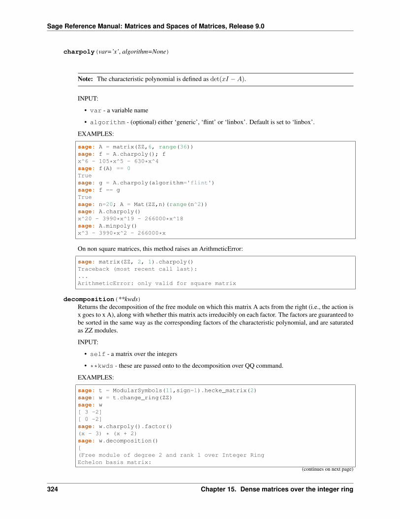
Sage Reference Manual: Matrices and Spaces of Matrices, Release 9.0
charpoly(var=’x’, algorithm=None)
Note: The characteristic polynomial is defined as det(𝑥𝐼 −𝐴).
INPUT:
• var - a variable name
• algorithm - (optional) either ‘generic’, ‘flint’ or ‘linbox’. Default is set to ‘linbox’.
EXAMPLES:
sage: A = matrix(ZZ,6, range(36))sage: f = A.charpoly(); fx^6 - 105*x^5 - 630*x^4sage: f(A) == 0Truesage: g = A.charpoly(algorithm='flint')sage: f == gTruesage: n=20; A = Mat(ZZ,n)(range(n^2))sage: A.charpoly()x^20 - 3990*x^19 - 266000*x^18sage: A.minpoly()x^3 - 3990*x^2 - 266000*x
On non square matrices, this method raises an ArithmeticError:
sage: matrix(ZZ, 2, 1).charpoly()Traceback (most recent call last):...ArithmeticError: only valid for square matrix
decomposition(**kwds)Returns the decomposition of the free module on which this matrix A acts from the right (i.e., the action isx goes to x A), along with whether this matrix acts irreducibly on each factor. The factors are guaranteed tobe sorted in the same way as the corresponding factors of the characteristic polynomial, and are saturatedas ZZ modules.
INPUT:
• self - a matrix over the integers
• **kwds - these are passed onto to the decomposition over QQ command.
EXAMPLES:
sage: t = ModularSymbols(11,sign=1).hecke_matrix(2)sage: w = t.change_ring(ZZ)sage: w[ 3 -2][ 0 -2]sage: w.charpoly().factor()(x - 3) * (x + 2)sage: w.decomposition()[(Free module of degree 2 and rank 1 over Integer RingEchelon basis matrix:
(continues on next page)
324 Chapter 15. Dense matrices over the integer ring
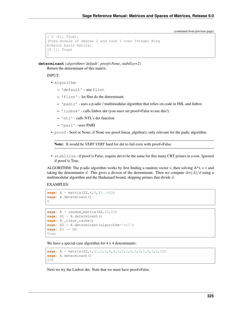
Sage Reference Manual: Matrices and Spaces of Matrices, Release 9.0
(continued from previous page)
[ 5 -2], True),(Free module of degree 2 and rank 1 over Integer RingEchelon basis matrix:[0 1], True)]
determinant(algorithm=’default’, proof=None, stabilize=2)Return the determinant of this matrix.
INPUT:
• algorithm
– 'default' – use flint
– 'flint' – let flint do the determinant
– 'padic' - uses a p-adic / multimodular algorithm that relies on code in IML and linbox
– 'linbox' - calls linbox det (you must set proof=False to use this!)
– 'ntl' - calls NTL’s det function
– 'pari' - uses PARI
• proof - bool or None; if None use proof.linear_algebra(); only relevant for the padic algorithm.
Note: It would be VERY VERY hard for det to fail even with proof=False.
• stabilize - if proof is False, require det to be the same for this many CRT primes in a row. Ignoredif proof is True.
ALGORITHM: The p-adic algorithm works by first finding a random vector v, then solving A*x = v andtaking the denominator 𝑑. This gives a divisor of the determinant. Then we compute det(𝐴)/𝑑 using amultimodular algorithm and the Hadamard bound, skipping primes that divide 𝑑.
EXAMPLES:
sage: A = matrix(ZZ,8,8,[3..66])sage: A.determinant()0
sage: A = random_matrix(ZZ,20,20)sage: D1 = A.determinant()sage: A._clear_cache()sage: D2 = A.determinant(algorithm='ntl')sage: D1 == D2True
We have a special-case algorithm for 4 x 4 determinants:
sage: A = matrix(ZZ,4,[1,2,3,4,4,3,2,1,0,5,0,1,9,1,2,3])sage: A.determinant()270
Next we try the Linbox det. Note that we must have proof=False.
325
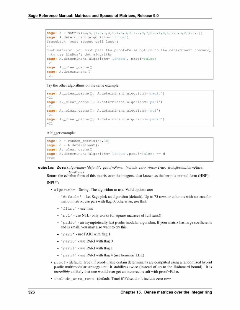
Sage Reference Manual: Matrices and Spaces of Matrices, Release 9.0
sage: A = matrix(ZZ,5,[1,2,3,4,5,4,6,3,2,1,7,9,7,5,2,1,4,6,7,8,3,2,4,6,7])sage: A.determinant(algorithm='linbox')Traceback (most recent call last):...RuntimeError: you must pass the proof=False option to the determinant command→˓to use LinBox's det algorithmsage: A.determinant(algorithm='linbox', proof=False)-21sage: A._clear_cache()sage: A.determinant()-21
Try the other algorithms on the same example:
sage: A._clear_cache(); A.determinant(algorithm='padic')-21sage: A._clear_cache(); A.determinant(algorithm='pari')-21sage: A._clear_cache(); A.determinant(algorithm='ntl')-21sage: A._clear_cache(); A.determinant(algorithm='padic')-21
A bigger example:
sage: A = random_matrix(ZZ,30)sage: d = A.determinant()sage: A._clear_cache()sage: A.determinant(algorithm='linbox',proof=False) == dTrue
echelon_form(algorithm=’default’, proof=None, include_zero_rows=True, transformation=False,D=None)
Return the echelon form of this matrix over the integers, also known as the hermite normal form (HNF).
INPUT:
• algorithm – String. The algorithm to use. Valid options are:
– 'default' – Let Sage pick an algorithm (default). Up to 75 rows or columns with no transfor-mation matrix, use pari with flag 0; otherwise, use flint.
– 'flint' - use flint
– 'ntl' - use NTL (only works for square matrices of full rank!)
– 'padic' - an asymptotically fast p-adic modular algorithm, If your matrix has large coefficientsand is small, you may also want to try this.
– 'pari' - use PARI with flag 1
– 'pari0' - use PARI with flag 0
– 'pari1' - use PARI with flag 1
– 'pari4' - use PARI with flag 4 (use heuristic LLL)
• proof - (default: True); if proof=False certain determinants are computed using a randomized hybridp-adic multimodular strategy until it stabilizes twice (instead of up to the Hadamard bound). It isincredibly unlikely that one would ever get an incorrect result with proof=False.
• include_zero_rows - (default: True) if False, don’t include zero rows
326 Chapter 15. Dense matrices over the integer ring
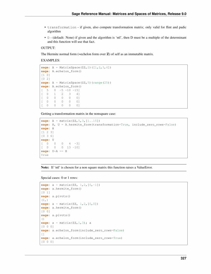
Sage Reference Manual: Matrices and Spaces of Matrices, Release 9.0
• transformation - if given, also compute transformation matrix; only valid for flint and padicalgorithm
• D - (default: None) if given and the algorithm is ‘ntl’, then D must be a multiple of the determinantand this function will use that fact.
OUTPUT:
The Hermite normal form (=echelon form over Z) of self as an immutable matrix.
EXAMPLES:
sage: A = MatrixSpace(ZZ,2)([1,2,3,4])sage: A.echelon_form()[1 0][0 2]sage: A = MatrixSpace(ZZ,5)(range(25))sage: A.echelon_form()[ 5 0 -5 -10 -15][ 0 1 2 3 4][ 0 0 0 0 0][ 0 0 0 0 0][ 0 0 0 0 0]
Getting a transformation matrix in the nonsquare case:
sage: A = matrix(ZZ,5,3,[1..15])sage: H, U = A.hermite_form(transformation=True, include_zero_rows=False)sage: H[1 2 3][0 3 6]sage: U[ 0 0 0 4 -3][ 0 0 0 13 -10]sage: U*A == HTrue
Note: If ‘ntl’ is chosen for a non square matrix this function raises a ValueError.
Special cases: 0 or 1 rows:
sage: a = matrix(ZZ, 1,2,[0,-1])sage: a.hermite_form()[0 1]sage: a.pivots()(1,)sage: a = matrix(ZZ, 1,2,[0,0])sage: a.hermite_form()[0 0]sage: a.pivots()()sage: a = matrix(ZZ,1,3); a[0 0 0]sage: a.echelon_form(include_zero_rows=False)[]sage: a.echelon_form(include_zero_rows=True)[0 0 0]
327
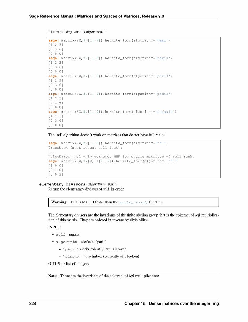
Sage Reference Manual: Matrices and Spaces of Matrices, Release 9.0
Illustrate using various algorithms.:
sage: matrix(ZZ,3,[1..9]).hermite_form(algorithm='pari')[1 2 3][0 3 6][0 0 0]sage: matrix(ZZ,3,[1..9]).hermite_form(algorithm='pari0')[1 2 3][0 3 6][0 0 0]sage: matrix(ZZ,3,[1..9]).hermite_form(algorithm='pari4')[1 2 3][0 3 6][0 0 0]sage: matrix(ZZ,3,[1..9]).hermite_form(algorithm='padic')[1 2 3][0 3 6][0 0 0]sage: matrix(ZZ,3,[1..9]).hermite_form(algorithm='default')[1 2 3][0 3 6][0 0 0]
The ‘ntl’ algorithm doesn’t work on matrices that do not have full rank.:
sage: matrix(ZZ,3,[1..9]).hermite_form(algorithm='ntl')Traceback (most recent call last):...ValueError: ntl only computes HNF for square matrices of full rank.sage: matrix(ZZ,3,[0] +[2..9]).hermite_form(algorithm='ntl')[1 0 0][0 1 0][0 0 3]
elementary_divisors(algorithm=’pari’)Return the elementary divisors of self, in order.
Warning: This is MUCH faster than the smith_form() function.
The elementary divisors are the invariants of the finite abelian group that is the cokernel of left multiplica-tion of this matrix. They are ordered in reverse by divisibility.
INPUT:
• self - matrix
• algorithm - (default: ‘pari’)
– 'pari': works robustly, but is slower.
– 'linbox' - use linbox (currently off, broken)
OUTPUT: list of integers
Note: These are the invariants of the cokernel of left multiplication:
328 Chapter 15. Dense matrices over the integer ring
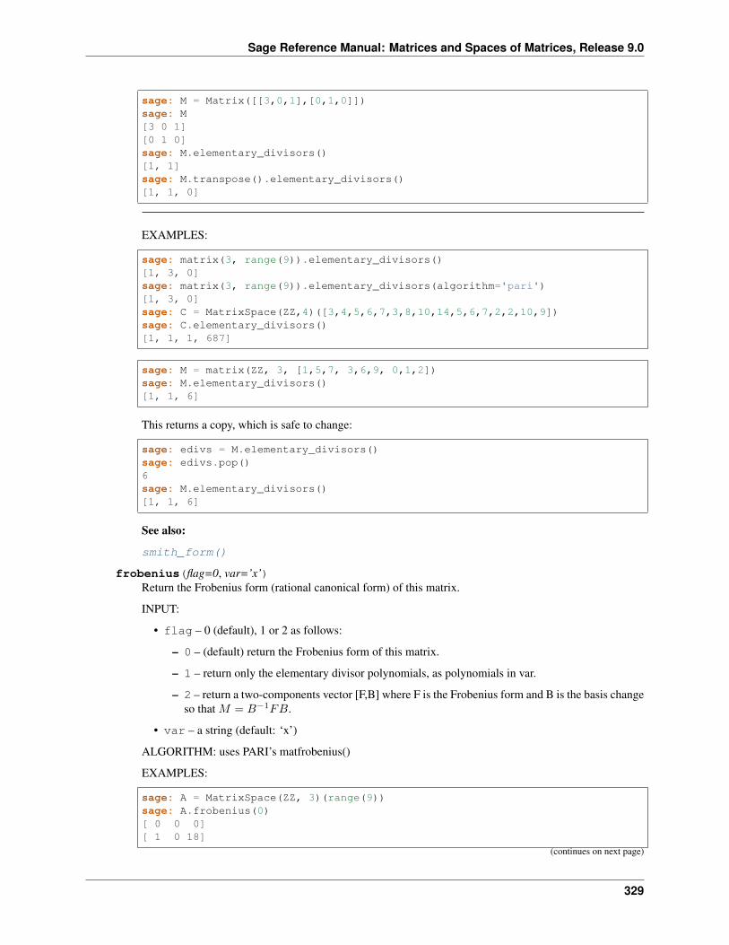
Sage Reference Manual: Matrices and Spaces of Matrices, Release 9.0
sage: M = Matrix([[3,0,1],[0,1,0]])sage: M[3 0 1][0 1 0]sage: M.elementary_divisors()[1, 1]sage: M.transpose().elementary_divisors()[1, 1, 0]
EXAMPLES:
sage: matrix(3, range(9)).elementary_divisors()[1, 3, 0]sage: matrix(3, range(9)).elementary_divisors(algorithm='pari')[1, 3, 0]sage: C = MatrixSpace(ZZ,4)([3,4,5,6,7,3,8,10,14,5,6,7,2,2,10,9])sage: C.elementary_divisors()[1, 1, 1, 687]
sage: M = matrix(ZZ, 3, [1,5,7, 3,6,9, 0,1,2])sage: M.elementary_divisors()[1, 1, 6]
This returns a copy, which is safe to change:
sage: edivs = M.elementary_divisors()sage: edivs.pop()6sage: M.elementary_divisors()[1, 1, 6]
See also:
smith_form()
frobenius(flag=0, var=’x’)Return the Frobenius form (rational canonical form) of this matrix.
INPUT:
• flag – 0 (default), 1 or 2 as follows:
– 0 – (default) return the Frobenius form of this matrix.
– 1 – return only the elementary divisor polynomials, as polynomials in var.
– 2 – return a two-components vector [F,B] where F is the Frobenius form and B is the basis changeso that 𝑀 = 𝐵−1𝐹𝐵.
• var – a string (default: ‘x’)
ALGORITHM: uses PARI’s matfrobenius()
EXAMPLES:
sage: A = MatrixSpace(ZZ, 3)(range(9))sage: A.frobenius(0)[ 0 0 0][ 1 0 18]
(continues on next page)
329
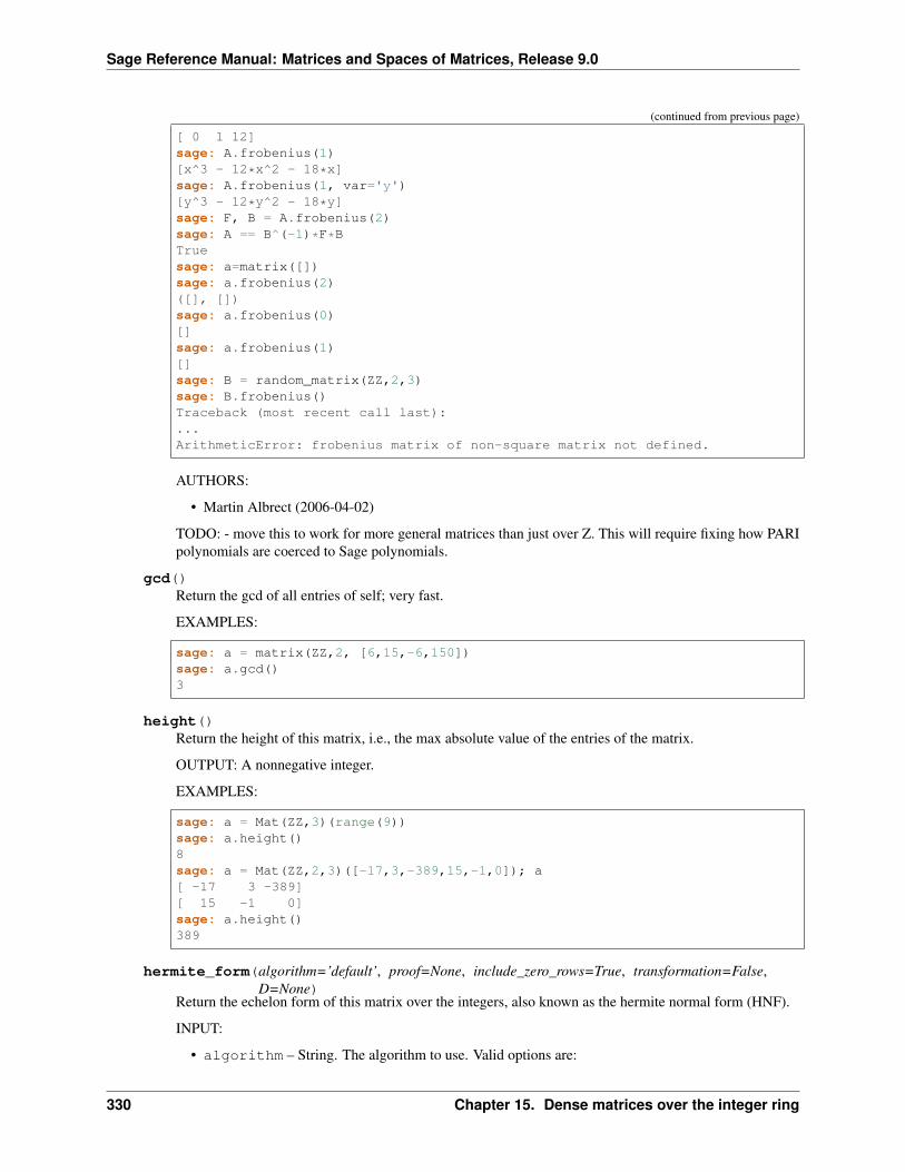
Sage Reference Manual: Matrices and Spaces of Matrices, Release 9.0
(continued from previous page)
[ 0 1 12]sage: A.frobenius(1)[x^3 - 12*x^2 - 18*x]sage: A.frobenius(1, var='y')[y^3 - 12*y^2 - 18*y]sage: F, B = A.frobenius(2)sage: A == B^(-1)*F*BTruesage: a=matrix([])sage: a.frobenius(2)([], [])sage: a.frobenius(0)[]sage: a.frobenius(1)[]sage: B = random_matrix(ZZ,2,3)sage: B.frobenius()Traceback (most recent call last):...ArithmeticError: frobenius matrix of non-square matrix not defined.
AUTHORS:
• Martin Albrect (2006-04-02)
TODO: - move this to work for more general matrices than just over Z. This will require fixing how PARIpolynomials are coerced to Sage polynomials.
gcd()Return the gcd of all entries of self; very fast.
EXAMPLES:
sage: a = matrix(ZZ,2, [6,15,-6,150])sage: a.gcd()3
height()Return the height of this matrix, i.e., the max absolute value of the entries of the matrix.
OUTPUT: A nonnegative integer.
EXAMPLES:
sage: a = Mat(ZZ,3)(range(9))sage: a.height()8sage: a = Mat(ZZ,2,3)([-17,3,-389,15,-1,0]); a[ -17 3 -389][ 15 -1 0]sage: a.height()389
hermite_form(algorithm=’default’, proof=None, include_zero_rows=True, transformation=False,D=None)
Return the echelon form of this matrix over the integers, also known as the hermite normal form (HNF).
INPUT:
• algorithm – String. The algorithm to use. Valid options are:
330 Chapter 15. Dense matrices over the integer ring
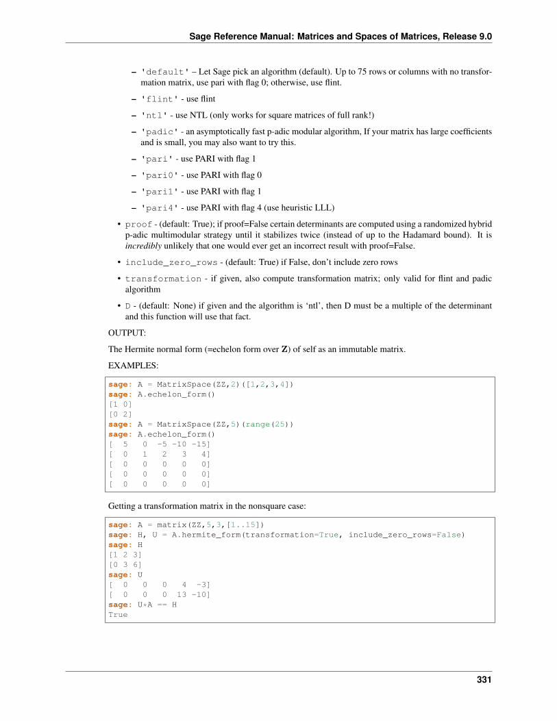
Sage Reference Manual: Matrices and Spaces of Matrices, Release 9.0
– 'default' – Let Sage pick an algorithm (default). Up to 75 rows or columns with no transfor-mation matrix, use pari with flag 0; otherwise, use flint.
– 'flint' - use flint
– 'ntl' - use NTL (only works for square matrices of full rank!)
– 'padic' - an asymptotically fast p-adic modular algorithm, If your matrix has large coefficientsand is small, you may also want to try this.
– 'pari' - use PARI with flag 1
– 'pari0' - use PARI with flag 0
– 'pari1' - use PARI with flag 1
– 'pari4' - use PARI with flag 4 (use heuristic LLL)
• proof - (default: True); if proof=False certain determinants are computed using a randomized hybridp-adic multimodular strategy until it stabilizes twice (instead of up to the Hadamard bound). It isincredibly unlikely that one would ever get an incorrect result with proof=False.
• include_zero_rows - (default: True) if False, don’t include zero rows
• transformation - if given, also compute transformation matrix; only valid for flint and padicalgorithm
• D - (default: None) if given and the algorithm is ‘ntl’, then D must be a multiple of the determinantand this function will use that fact.
OUTPUT:
The Hermite normal form (=echelon form over Z) of self as an immutable matrix.
EXAMPLES:
sage: A = MatrixSpace(ZZ,2)([1,2,3,4])sage: A.echelon_form()[1 0][0 2]sage: A = MatrixSpace(ZZ,5)(range(25))sage: A.echelon_form()[ 5 0 -5 -10 -15][ 0 1 2 3 4][ 0 0 0 0 0][ 0 0 0 0 0][ 0 0 0 0 0]
Getting a transformation matrix in the nonsquare case:
sage: A = matrix(ZZ,5,3,[1..15])sage: H, U = A.hermite_form(transformation=True, include_zero_rows=False)sage: H[1 2 3][0 3 6]sage: U[ 0 0 0 4 -3][ 0 0 0 13 -10]sage: U*A == HTrue
331
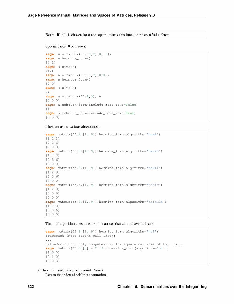
Sage Reference Manual: Matrices and Spaces of Matrices, Release 9.0
Note: If ‘ntl’ is chosen for a non square matrix this function raises a ValueError.
Special cases: 0 or 1 rows:
sage: a = matrix(ZZ, 1,2,[0,-1])sage: a.hermite_form()[0 1]sage: a.pivots()(1,)sage: a = matrix(ZZ, 1,2,[0,0])sage: a.hermite_form()[0 0]sage: a.pivots()()sage: a = matrix(ZZ,1,3); a[0 0 0]sage: a.echelon_form(include_zero_rows=False)[]sage: a.echelon_form(include_zero_rows=True)[0 0 0]
Illustrate using various algorithms.:
sage: matrix(ZZ,3,[1..9]).hermite_form(algorithm='pari')[1 2 3][0 3 6][0 0 0]sage: matrix(ZZ,3,[1..9]).hermite_form(algorithm='pari0')[1 2 3][0 3 6][0 0 0]sage: matrix(ZZ,3,[1..9]).hermite_form(algorithm='pari4')[1 2 3][0 3 6][0 0 0]sage: matrix(ZZ,3,[1..9]).hermite_form(algorithm='padic')[1 2 3][0 3 6][0 0 0]sage: matrix(ZZ,3,[1..9]).hermite_form(algorithm='default')[1 2 3][0 3 6][0 0 0]
The ‘ntl’ algorithm doesn’t work on matrices that do not have full rank.:
sage: matrix(ZZ,3,[1..9]).hermite_form(algorithm='ntl')Traceback (most recent call last):...ValueError: ntl only computes HNF for square matrices of full rank.sage: matrix(ZZ,3,[0] +[2..9]).hermite_form(algorithm='ntl')[1 0 0][0 1 0][0 0 3]
index_in_saturation(proof=None)Return the index of self in its saturation.
332 Chapter 15. Dense matrices over the integer ring
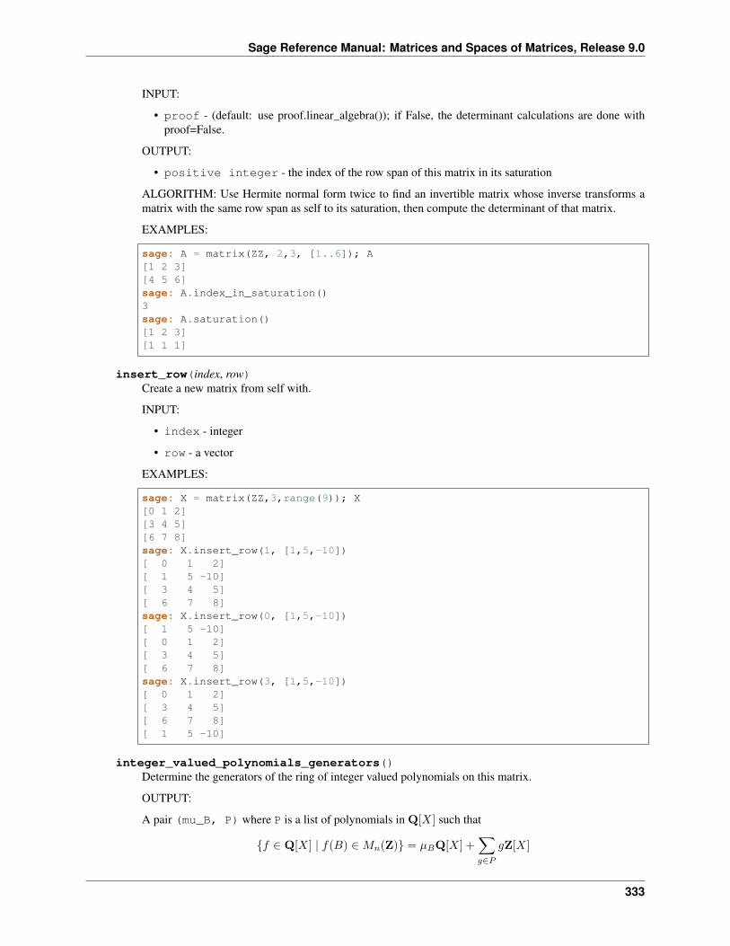
Sage Reference Manual: Matrices and Spaces of Matrices, Release 9.0
INPUT:
• proof - (default: use proof.linear_algebra()); if False, the determinant calculations are done withproof=False.
OUTPUT:
• positive integer - the index of the row span of this matrix in its saturation
ALGORITHM: Use Hermite normal form twice to find an invertible matrix whose inverse transforms amatrix with the same row span as self to its saturation, then compute the determinant of that matrix.
EXAMPLES:
sage: A = matrix(ZZ, 2,3, [1..6]); A[1 2 3][4 5 6]sage: A.index_in_saturation()3sage: A.saturation()[1 2 3][1 1 1]
insert_row(index, row)Create a new matrix from self with.
INPUT:
• index - integer
• row - a vector
EXAMPLES:
sage: X = matrix(ZZ,3,range(9)); X[0 1 2][3 4 5][6 7 8]sage: X.insert_row(1, [1,5,-10])[ 0 1 2][ 1 5 -10][ 3 4 5][ 6 7 8]sage: X.insert_row(0, [1,5,-10])[ 1 5 -10][ 0 1 2][ 3 4 5][ 6 7 8]sage: X.insert_row(3, [1,5,-10])[ 0 1 2][ 3 4 5][ 6 7 8][ 1 5 -10]
integer_valued_polynomials_generators()Determine the generators of the ring of integer valued polynomials on this matrix.
OUTPUT:
A pair (mu_B, P) where P is a list of polynomials in Q[𝑋] such that
{𝑓 ∈ Q[𝑋] | 𝑓(𝐵) ∈ 𝑀𝑛(Z)} = 𝜇𝐵Q[𝑋] +∑︁𝑔∈𝑃
𝑔Z[𝑋]
333
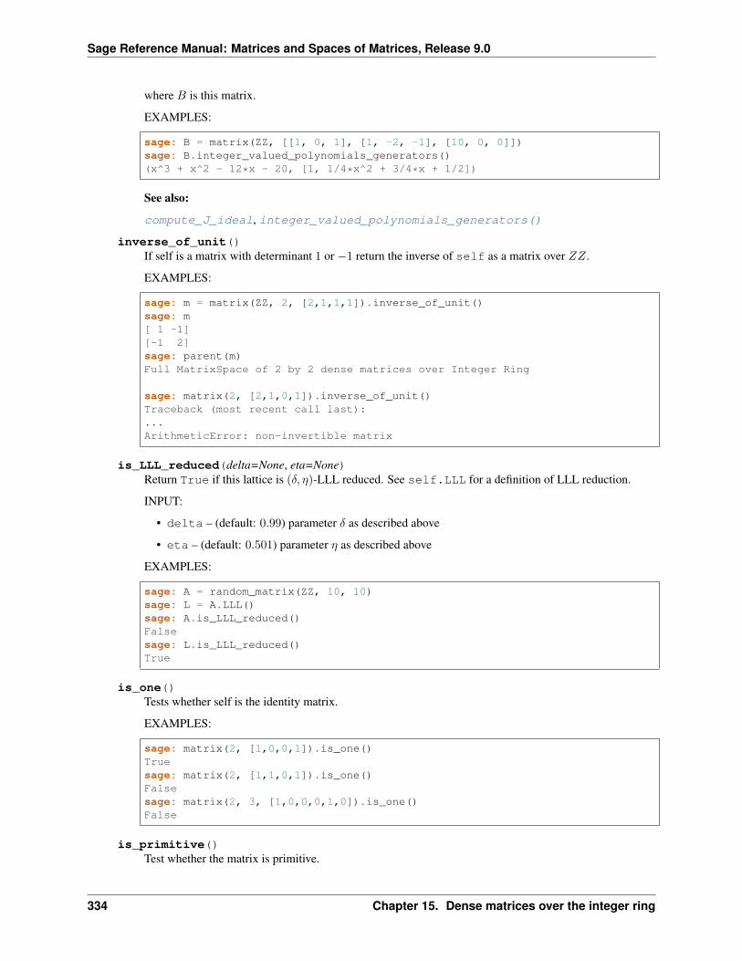
Sage Reference Manual: Matrices and Spaces of Matrices, Release 9.0
where 𝐵 is this matrix.
EXAMPLES:
sage: B = matrix(ZZ, [[1, 0, 1], [1, -2, -1], [10, 0, 0]])sage: B.integer_valued_polynomials_generators()(x^3 + x^2 - 12*x - 20, [1, 1/4*x^2 + 3/4*x + 1/2])
See also:
compute_J_ideal, integer_valued_polynomials_generators()
inverse_of_unit()If self is a matrix with determinant 1 or −1 return the inverse of self as a matrix over 𝑍𝑍.
EXAMPLES:
sage: m = matrix(ZZ, 2, [2,1,1,1]).inverse_of_unit()sage: m[ 1 -1][-1 2]sage: parent(m)Full MatrixSpace of 2 by 2 dense matrices over Integer Ring
sage: matrix(2, [2,1,0,1]).inverse_of_unit()Traceback (most recent call last):...ArithmeticError: non-invertible matrix
is_LLL_reduced(delta=None, eta=None)Return True if this lattice is (𝛿, 𝜂)-LLL reduced. See self.LLL for a definition of LLL reduction.
INPUT:
• delta – (default: 0.99) parameter 𝛿 as described above
• eta – (default: 0.501) parameter 𝜂 as described above
EXAMPLES:
sage: A = random_matrix(ZZ, 10, 10)sage: L = A.LLL()sage: A.is_LLL_reduced()Falsesage: L.is_LLL_reduced()True
is_one()Tests whether self is the identity matrix.
EXAMPLES:
sage: matrix(2, [1,0,0,1]).is_one()Truesage: matrix(2, [1,1,0,1]).is_one()Falsesage: matrix(2, 3, [1,0,0,0,1,0]).is_one()False
is_primitive()Test whether the matrix is primitive.
334 Chapter 15. Dense matrices over the integer ring
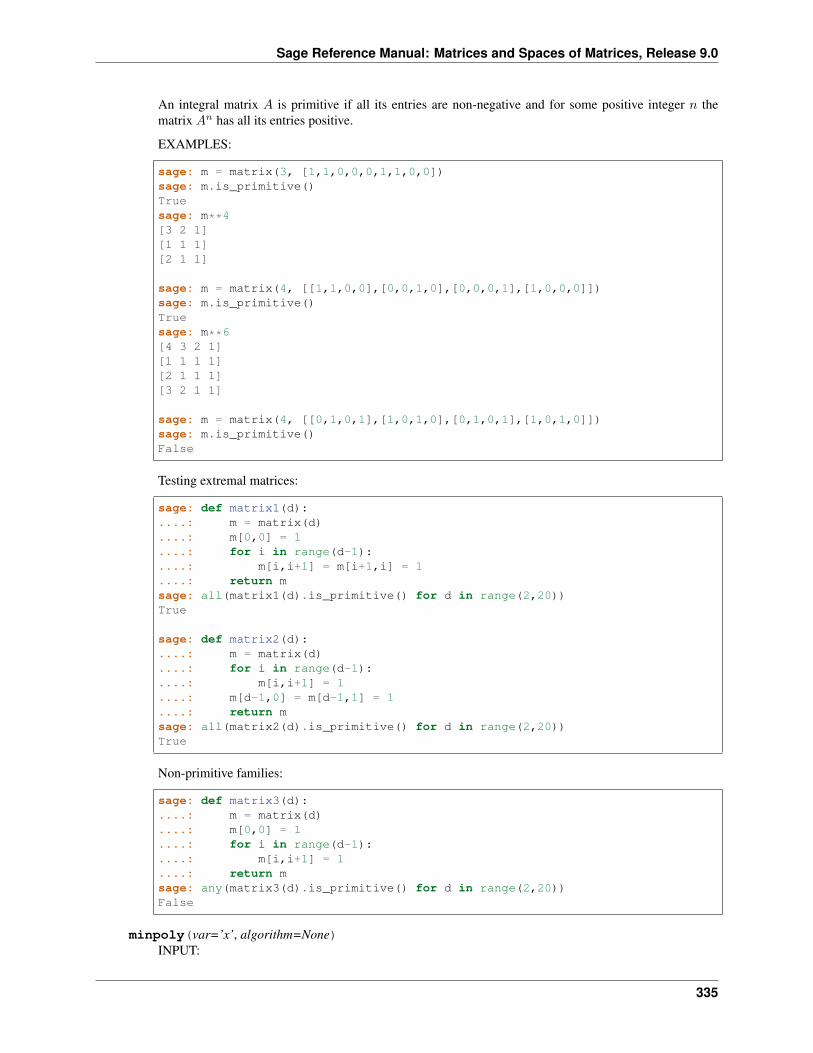
Sage Reference Manual: Matrices and Spaces of Matrices, Release 9.0
An integral matrix 𝐴 is primitive if all its entries are non-negative and for some positive integer 𝑛 thematrix 𝐴𝑛 has all its entries positive.
EXAMPLES:
sage: m = matrix(3, [1,1,0,0,0,1,1,0,0])sage: m.is_primitive()Truesage: m**4[3 2 1][1 1 1][2 1 1]
sage: m = matrix(4, [[1,1,0,0],[0,0,1,0],[0,0,0,1],[1,0,0,0]])sage: m.is_primitive()Truesage: m**6[4 3 2 1][1 1 1 1][2 1 1 1][3 2 1 1]
sage: m = matrix(4, [[0,1,0,1],[1,0,1,0],[0,1,0,1],[1,0,1,0]])sage: m.is_primitive()False
Testing extremal matrices:
sage: def matrix1(d):....: m = matrix(d)....: m[0,0] = 1....: for i in range(d-1):....: m[i,i+1] = m[i+1,i] = 1....: return msage: all(matrix1(d).is_primitive() for d in range(2,20))True
sage: def matrix2(d):....: m = matrix(d)....: for i in range(d-1):....: m[i,i+1] = 1....: m[d-1,0] = m[d-1,1] = 1....: return msage: all(matrix2(d).is_primitive() for d in range(2,20))True
Non-primitive families:
sage: def matrix3(d):....: m = matrix(d)....: m[0,0] = 1....: for i in range(d-1):....: m[i,i+1] = 1....: return msage: any(matrix3(d).is_primitive() for d in range(2,20))False
minpoly(var=’x’, algorithm=None)INPUT:
335
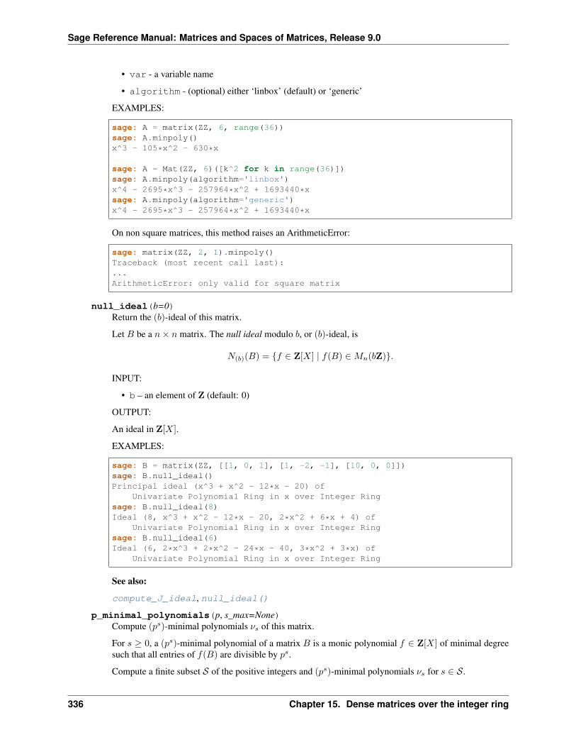
Sage Reference Manual: Matrices and Spaces of Matrices, Release 9.0
• var - a variable name
• algorithm - (optional) either ‘linbox’ (default) or ‘generic’
EXAMPLES:
sage: A = matrix(ZZ, 6, range(36))sage: A.minpoly()x^3 - 105*x^2 - 630*x
sage: A = Mat(ZZ, 6)([k^2 for k in range(36)])sage: A.minpoly(algorithm='linbox')x^4 - 2695*x^3 - 257964*x^2 + 1693440*xsage: A.minpoly(algorithm='generic')x^4 - 2695*x^3 - 257964*x^2 + 1693440*x
On non square matrices, this method raises an ArithmeticError:
sage: matrix(ZZ, 2, 1).minpoly()Traceback (most recent call last):...ArithmeticError: only valid for square matrix
null_ideal(b=0)Return the (𝑏)-ideal of this matrix.
Let 𝐵 be a 𝑛× 𝑛 matrix. The null ideal modulo 𝑏, or (𝑏)-ideal, is
𝑁(𝑏)(𝐵) = {𝑓 ∈ Z[𝑋] | 𝑓(𝐵) ∈ 𝑀𝑛(𝑏Z)}.
INPUT:
• b – an element of Z (default: 0)
OUTPUT:
An ideal in Z[𝑋].
EXAMPLES:
sage: B = matrix(ZZ, [[1, 0, 1], [1, -2, -1], [10, 0, 0]])sage: B.null_ideal()Principal ideal (x^3 + x^2 - 12*x - 20) of
Univariate Polynomial Ring in x over Integer Ringsage: B.null_ideal(8)Ideal (8, x^3 + x^2 - 12*x - 20, 2*x^2 + 6*x + 4) of
Univariate Polynomial Ring in x over Integer Ringsage: B.null_ideal(6)Ideal (6, 2*x^3 + 2*x^2 - 24*x - 40, 3*x^2 + 3*x) of
Univariate Polynomial Ring in x over Integer Ring
See also:
compute_J_ideal, null_ideal()
p_minimal_polynomials(p, s_max=None)Compute (𝑝𝑠)-minimal polynomials 𝜈𝑠 of this matrix.
For 𝑠 ≥ 0, a (𝑝𝑠)-minimal polynomial of a matrix 𝐵 is a monic polynomial 𝑓 ∈ Z[𝑋] of minimal degreesuch that all entries of 𝑓(𝐵) are divisible by 𝑝𝑠.
Compute a finite subset 𝒮 of the positive integers and (𝑝𝑠)-minimal polynomials 𝜈𝑠 for 𝑠 ∈ 𝒮.
336 Chapter 15. Dense matrices over the integer ring
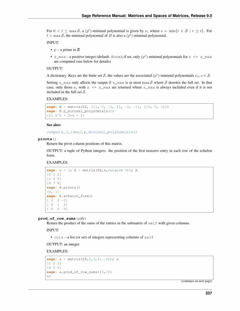
Sage Reference Manual: Matrices and Spaces of Matrices, Release 9.0
For 0 < 𝑡 ≤ max𝒮, a (𝑝𝑡)-minimal polynomial is given by 𝜈𝑠 where 𝑠 = min{𝑟 ∈ 𝒮 | 𝑟 ≥ 𝑡}. For𝑡 > max𝒮 , the minimal polynomial of 𝐵 is also a (𝑝𝑡)-minimal polynomial.
INPUT:
• p – a prime in Z
• s_max – a positive integer (default: None); if set, only (𝑝𝑠)-minimal polynomials for s <= s_maxare computed (see below for details)
OUTPUT:
A dictionary. Keys are the finite set 𝒮, the values are the associated (𝑝𝑠)-minimal polynomials 𝜈𝑠, 𝑠 ∈ 𝒮.
Setting s_max only affects the output if s_max is at most max𝒮 where 𝒮 denotes the full set. In thatcase, only those 𝜈𝑠 with s <= s_max are returned where s_max is always included even if it is notincluded in the full set 𝒮.
EXAMPLES:
sage: B = matrix(ZZ, [[1, 0, 1], [1, -2, -1], [10, 0, 0]])sage: B.p_minimal_polynomials(2){2: x^2 + 3*x + 2}
See also:
compute_J_ideal, p_minimal_polynomials()
pivots()Return the pivot column positions of this matrix.
OUTPUT: a tuple of Python integers: the position of the first nonzero entry in each row of the echelonform.
EXAMPLES:
sage: n = 3; A = matrix(ZZ,n,range(n^2)); A[0 1 2][3 4 5][6 7 8]sage: A.pivots()(0, 1)sage: A.echelon_form()[ 3 0 -3][ 0 1 2][ 0 0 0]
prod_of_row_sums(cols)Return the product of the sums of the entries in the submatrix of self with given columns.
INPUT:
• cols – a list (or set) of integers representing columns of self
OUTPUT: an integer
EXAMPLES:
sage: a = matrix(ZZ,2,3,[1..6]); a[1 2 3][4 5 6]sage: a.prod_of_row_sums([0,2])40
(continues on next page)
337
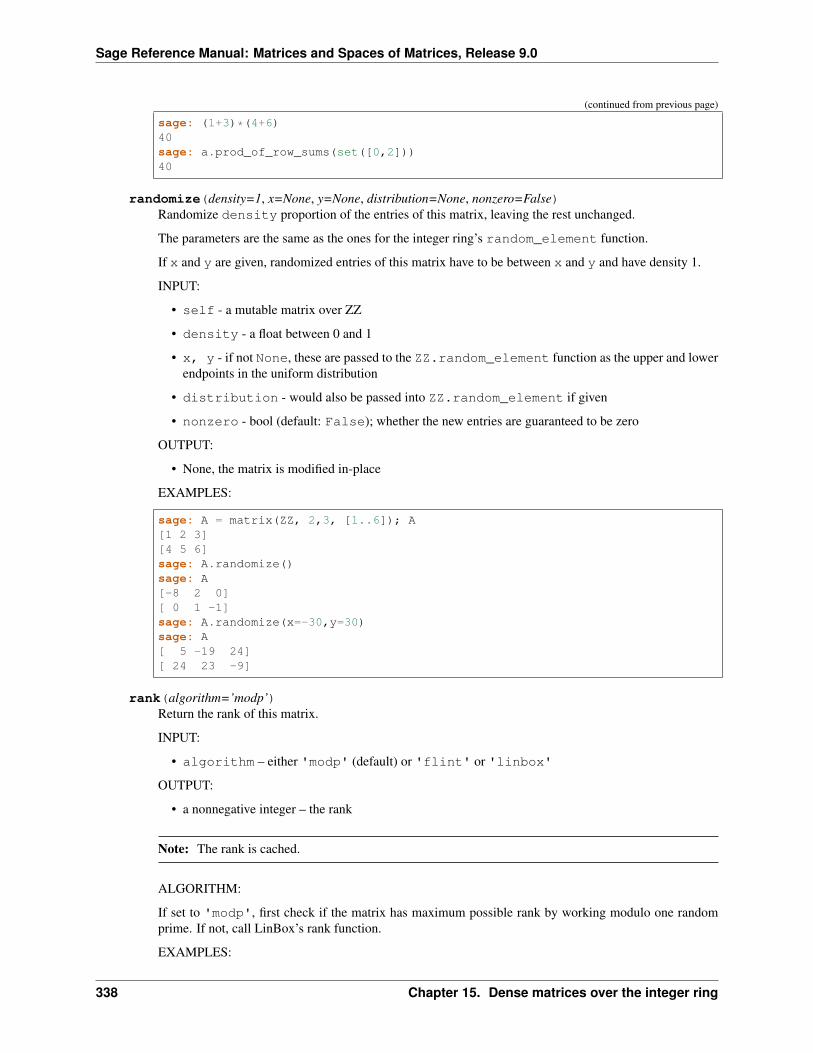
Sage Reference Manual: Matrices and Spaces of Matrices, Release 9.0
(continued from previous page)
sage: (1+3)*(4+6)40sage: a.prod_of_row_sums(set([0,2]))40
randomize(density=1, x=None, y=None, distribution=None, nonzero=False)Randomize density proportion of the entries of this matrix, leaving the rest unchanged.
The parameters are the same as the ones for the integer ring’s random_element function.
If x and y are given, randomized entries of this matrix have to be between x and y and have density 1.
INPUT:
• self - a mutable matrix over ZZ
• density - a float between 0 and 1
• x, y - if not None, these are passed to the ZZ.random_element function as the upper and lowerendpoints in the uniform distribution
• distribution - would also be passed into ZZ.random_element if given
• nonzero - bool (default: False); whether the new entries are guaranteed to be zero
OUTPUT:
• None, the matrix is modified in-place
EXAMPLES:
sage: A = matrix(ZZ, 2,3, [1..6]); A[1 2 3][4 5 6]sage: A.randomize()sage: A[-8 2 0][ 0 1 -1]sage: A.randomize(x=-30,y=30)sage: A[ 5 -19 24][ 24 23 -9]
rank(algorithm=’modp’)Return the rank of this matrix.
INPUT:
• algorithm – either 'modp' (default) or 'flint' or 'linbox'
OUTPUT:
• a nonnegative integer – the rank
Note: The rank is cached.
ALGORITHM:
If set to 'modp', first check if the matrix has maximum possible rank by working modulo one randomprime. If not, call LinBox’s rank function.
EXAMPLES:
338 Chapter 15. Dense matrices over the integer ring
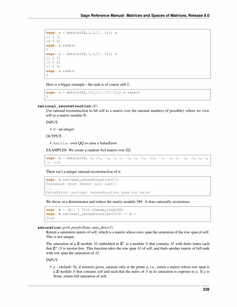
Sage Reference Manual: Matrices and Spaces of Matrices, Release 9.0
sage: a = matrix(ZZ,2,3,[1..6]); a[1 2 3][4 5 6]sage: a.rank()2sage: a = matrix(ZZ,3,3,[1..9]); a[1 2 3][4 5 6][7 8 9]sage: a.rank()2
Here is a bigger example - the rank is of course still 2:
sage: a = matrix(ZZ,100,[1..100^2]); a.rank()2
rational_reconstruction(N)Use rational reconstruction to lift self to a matrix over the rational numbers (if possible), where we viewself as a matrix modulo N.
INPUT:
• N - an integer
OUTPUT:
• matrix - over QQ or raise a ValueError
EXAMPLES: We create a random 4x4 matrix over ZZ.
sage: A = matrix(ZZ, 4, [4, -4, 7, 1, -1, 1, -1, -12, -1, -1, 1, -1, -3, 1, 5,→˓ -1])
There isn’t a unique rational reconstruction of it:
sage: A.rational_reconstruction(11)Traceback (most recent call last):...ValueError: rational reconstruction does not exist
We throw in a denominator and reduce the matrix modulo 389 - it does rationally reconstruct.
sage: B = (A/3 % 389).change_ring(ZZ)sage: B.rational_reconstruction(389) == A/3True
saturation(p=0, proof=None, max_dets=5)Return a saturation matrix of self, which is a matrix whose rows span the saturation of the row span of self.This is not unique.
The saturation of a Z module 𝑀 embedded in Z𝑛 is a module 𝑆 that contains 𝑀 with finite index suchthat Z𝑛/𝑆 is torsion free. This function takes the row span 𝑀 of self, and finds another matrix of full rankwith row span the saturation of 𝑀 .
INPUT:
• p - (default: 0); if nonzero given, saturate only at the prime 𝑝, i.e., return a matrix whose row span isa Z-module 𝑆 that contains self and such that the index of 𝑆 in its saturation is coprime to 𝑝. If 𝑝 isNone, return full saturation of self.
339
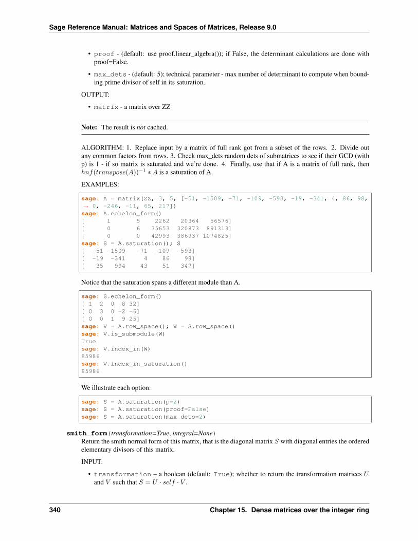
Sage Reference Manual: Matrices and Spaces of Matrices, Release 9.0
• proof - (default: use proof.linear_algebra()); if False, the determinant calculations are done withproof=False.
• max_dets - (default: 5); technical parameter - max number of determinant to compute when bound-ing prime divisor of self in its saturation.
OUTPUT:
• matrix - a matrix over ZZ
Note: The result is not cached.
ALGORITHM: 1. Replace input by a matrix of full rank got from a subset of the rows. 2. Divide outany common factors from rows. 3. Check max_dets random dets of submatrices to see if their GCD (withp) is 1 - if so matrix is saturated and we’re done. 4. Finally, use that if A is a matrix of full rank, thenℎ𝑛𝑓(𝑡𝑟𝑎𝑛𝑠𝑝𝑜𝑠𝑒(𝐴))−1 *𝐴 is a saturation of A.
EXAMPLES:
sage: A = matrix(ZZ, 3, 5, [-51, -1509, -71, -109, -593, -19, -341, 4, 86, 98,→˓ 0, -246, -11, 65, 217])sage: A.echelon_form()[ 1 5 2262 20364 56576][ 0 6 35653 320873 891313][ 0 0 42993 386937 1074825]sage: S = A.saturation(); S[ -51 -1509 -71 -109 -593][ -19 -341 4 86 98][ 35 994 43 51 347]
Notice that the saturation spans a different module than A.
sage: S.echelon_form()[ 1 2 0 8 32][ 0 3 0 -2 -6][ 0 0 1 9 25]sage: V = A.row_space(); W = S.row_space()sage: V.is_submodule(W)Truesage: V.index_in(W)85986sage: V.index_in_saturation()85986
We illustrate each option:
sage: S = A.saturation(p=2)sage: S = A.saturation(proof=False)sage: S = A.saturation(max_dets=2)
smith_form(transformation=True, integral=None)Return the smith normal form of this matrix, that is the diagonal matrix 𝑆 with diagonal entries the orderedelementary divisors of this matrix.
INPUT:
• transformation – a boolean (default: True); whether to return the transformation matrices 𝑈and 𝑉 such that 𝑆 = 𝑈 · 𝑠𝑒𝑙𝑓 · 𝑉 .
340 Chapter 15. Dense matrices over the integer ring
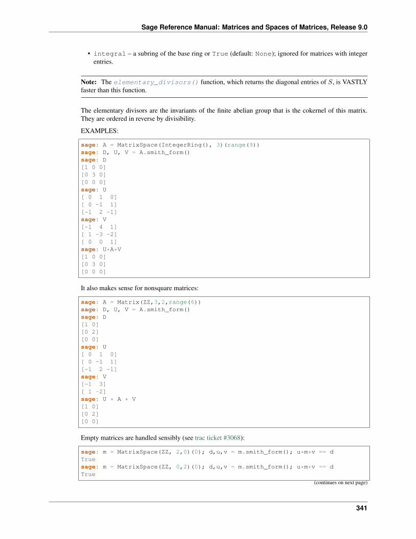
Sage Reference Manual: Matrices and Spaces of Matrices, Release 9.0
• integral – a subring of the base ring or True (default: None); ignored for matrices with integerentries.
Note: The elementary_divisors() function, which returns the diagonal entries of 𝑆, is VASTLYfaster than this function.
The elementary divisors are the invariants of the finite abelian group that is the cokernel of this matrix.They are ordered in reverse by divisibility.
EXAMPLES:
sage: A = MatrixSpace(IntegerRing(), 3)(range(9))sage: D, U, V = A.smith_form()sage: D[1 0 0][0 3 0][0 0 0]sage: U[ 0 1 0][ 0 -1 1][-1 2 -1]sage: V[-1 4 1][ 1 -3 -2][ 0 0 1]sage: U*A*V[1 0 0][0 3 0][0 0 0]
It also makes sense for nonsquare matrices:
sage: A = Matrix(ZZ,3,2,range(6))sage: D, U, V = A.smith_form()sage: D[1 0][0 2][0 0]sage: U[ 0 1 0][ 0 -1 1][-1 2 -1]sage: V[-1 3][ 1 -2]sage: U * A * V[1 0][0 2][0 0]
Empty matrices are handled sensibly (see trac ticket #3068):
sage: m = MatrixSpace(ZZ, 2,0)(0); d,u,v = m.smith_form(); u*m*v == dTruesage: m = MatrixSpace(ZZ, 0,2)(0); d,u,v = m.smith_form(); u*m*v == dTrue
(continues on next page)
341
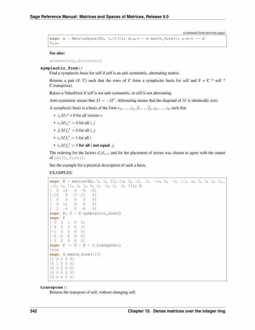
Sage Reference Manual: Matrices and Spaces of Matrices, Release 9.0
(continued from previous page)
sage: m = MatrixSpace(ZZ, 0,0)(0); d,u,v = m.smith_form(); u*m*v == dTrue
See also:
elementary_divisors()
symplectic_form()Find a symplectic basis for self if self is an anti-symmetric, alternating matrix.
Returns a pair (F, C) such that the rows of C form a symplectic basis for self and F = C * self *C.transpose().
Raises a ValueError if self is not anti-symmetric, or self is not alternating.
Anti-symmetric means that 𝑀 = −𝑀 𝑡. Alternating means that the diagonal of 𝑀 is identically zero.
A symplectic basis is a basis of the form 𝑒1, . . . , 𝑒𝑗 , 𝑓1, . . . 𝑓𝑗 , 𝑧1, . . . , 𝑧𝑘 such that
• 𝑧𝑖𝑀𝑣𝑡 = 0 for all vectors 𝑣
• 𝑒𝑖𝑀𝑒𝑗𝑡 = 0 for all 𝑖, 𝑗
• 𝑓𝑖𝑀𝑓𝑗𝑡 = 0 for all 𝑖, 𝑗
• 𝑒𝑖𝑀𝑓𝑖𝑡 = 1 for all 𝑖
• 𝑒𝑖𝑀𝑓𝑗𝑡 = 0 for all 𝑖 not equal 𝑗.
The ordering for the factors 𝑑𝑖|𝑑𝑖+1 and for the placement of zeroes was chosen to agree with the outputof smith_form().
See the example for a pictorial description of such a basis.
EXAMPLES:
sage: E = matrix(ZZ, 5, 5, [0, 14, 0, -8, -2, -14, 0, -3, -11, 4, 0, 3, 0, 0,→˓0, 8, 11, 0, 0, 8, 2, -4, 0, -8, 0]); E[ 0 14 0 -8 -2][-14 0 -3 -11 4][ 0 3 0 0 0][ 8 11 0 0 8][ 2 -4 0 -8 0]sage: F, C = E.symplectic_form()sage: F[ 0 0 1 0 0][ 0 0 0 2 0][-1 0 0 0 0][ 0 -2 0 0 0][ 0 0 0 0 0]sage: F == C * E * C.transpose()Truesage: E.smith_form()[0][1 0 0 0 0][0 1 0 0 0][0 0 2 0 0][0 0 0 2 0][0 0 0 0 0]
transpose()Returns the transpose of self, without changing self.
342 Chapter 15. Dense matrices over the integer ring
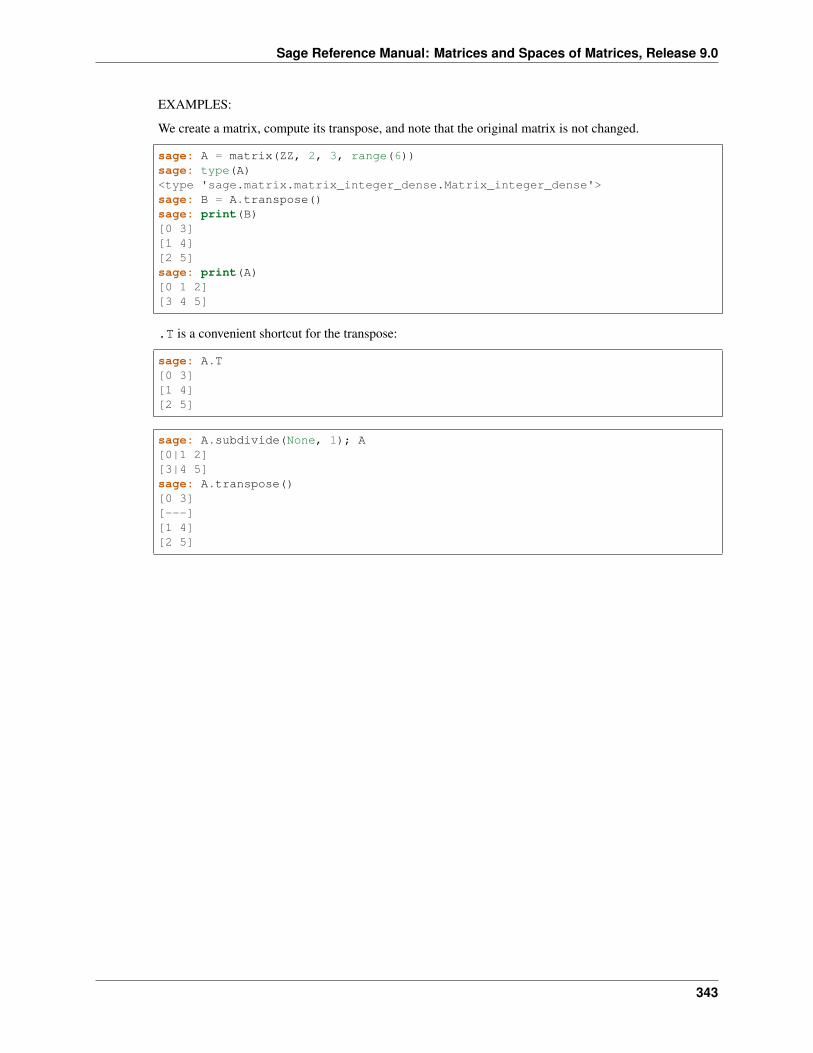
Sage Reference Manual: Matrices and Spaces of Matrices, Release 9.0
EXAMPLES:
We create a matrix, compute its transpose, and note that the original matrix is not changed.
sage: A = matrix(ZZ, 2, 3, range(6))sage: type(A)<type 'sage.matrix.matrix_integer_dense.Matrix_integer_dense'>sage: B = A.transpose()sage: print(B)[0 3][1 4][2 5]sage: print(A)[0 1 2][3 4 5]
.T is a convenient shortcut for the transpose:
sage: A.T[0 3][1 4][2 5]
sage: A.subdivide(None, 1); A[0|1 2][3|4 5]sage: A.transpose()[0 3][---][1 4][2 5]
343

Sage Reference Manual: Matrices and Spaces of Matrices, Release 9.0
344 Chapter 15. Dense matrices over the integer ring
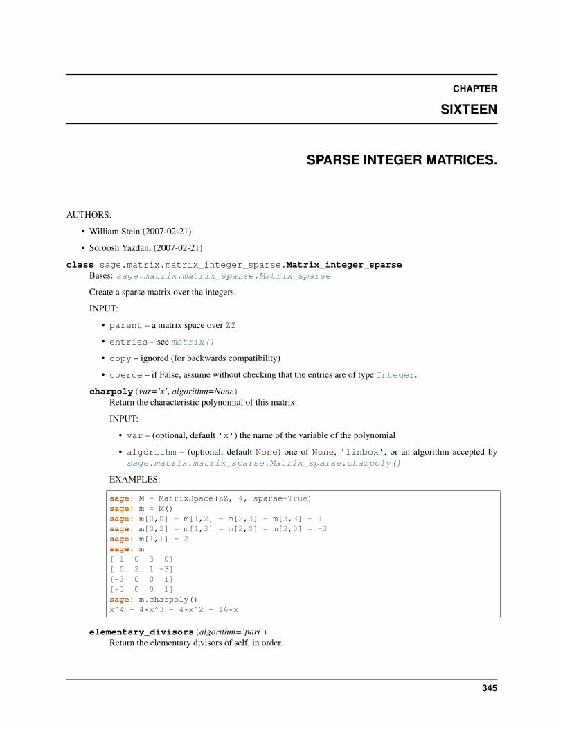
CHAPTER
SIXTEEN
SPARSE INTEGER MATRICES.
AUTHORS:
• William Stein (2007-02-21)
• Soroosh Yazdani (2007-02-21)
class sage.matrix.matrix_integer_sparse.Matrix_integer_sparseBases: sage.matrix.matrix_sparse.Matrix_sparse
Create a sparse matrix over the integers.
INPUT:
• parent – a matrix space over ZZ
• entries – see matrix()
• copy – ignored (for backwards compatibility)
• coerce – if False, assume without checking that the entries are of type Integer.
charpoly(var=’x’, algorithm=None)Return the characteristic polynomial of this matrix.
INPUT:
• var – (optional, default 'x') the name of the variable of the polynomial
• algorithm – (optional, default None) one of None, 'linbox', or an algorithm accepted bysage.matrix.matrix_sparse.Matrix_sparse.charpoly()
EXAMPLES:
sage: M = MatrixSpace(ZZ, 4, sparse=True)sage: m = M()sage: m[0,0] = m[1,2] = m[2,3] = m[3,3] = 1sage: m[0,2] = m[1,3] = m[2,0] = m[3,0] = -3sage: m[1,1] = 2sage: m[ 1 0 -3 0][ 0 2 1 -3][-3 0 0 1][-3 0 0 1]sage: m.charpoly()x^4 - 4*x^3 - 4*x^2 + 16*x
elementary_divisors(algorithm=’pari’)Return the elementary divisors of self, in order.
345
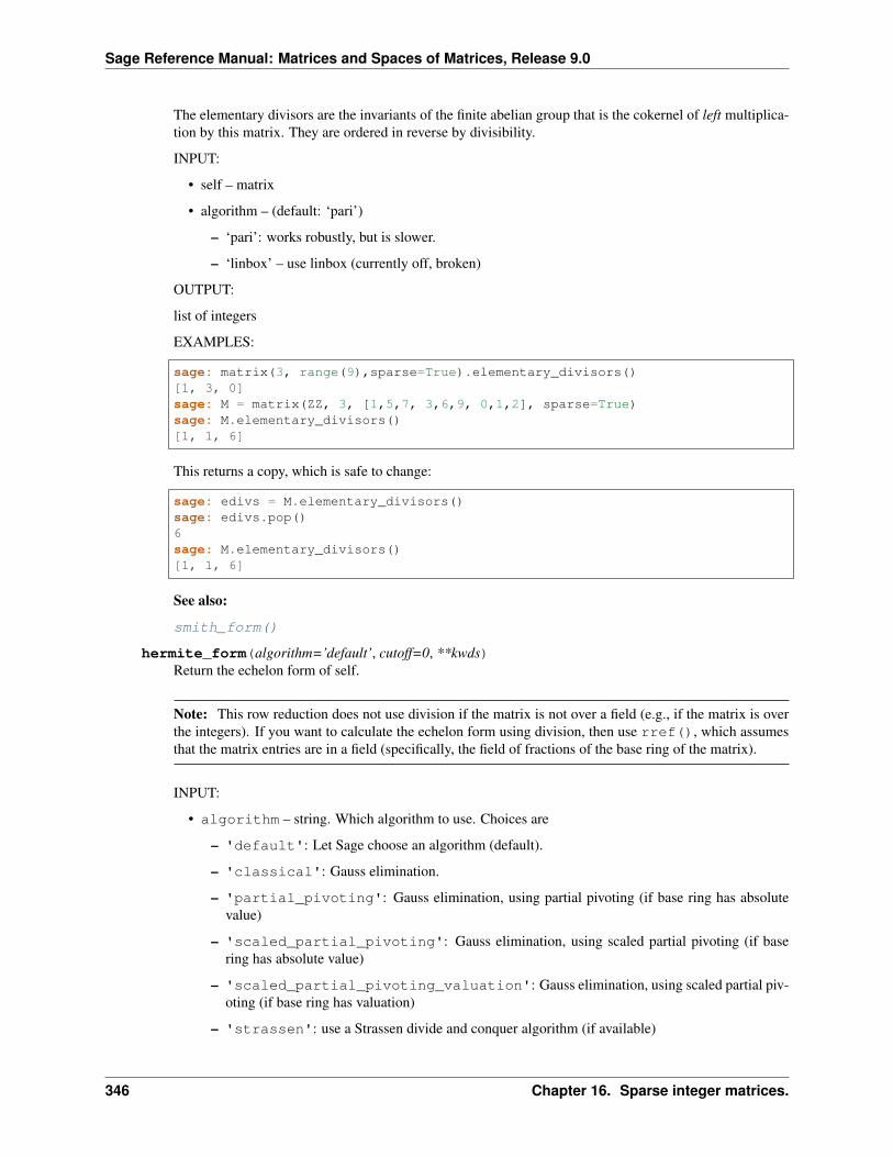
Sage Reference Manual: Matrices and Spaces of Matrices, Release 9.0
The elementary divisors are the invariants of the finite abelian group that is the cokernel of left multiplica-tion by this matrix. They are ordered in reverse by divisibility.
INPUT:
• self – matrix
• algorithm – (default: ‘pari’)
– ‘pari’: works robustly, but is slower.
– ‘linbox’ – use linbox (currently off, broken)
OUTPUT:
list of integers
EXAMPLES:
sage: matrix(3, range(9),sparse=True).elementary_divisors()[1, 3, 0]sage: M = matrix(ZZ, 3, [1,5,7, 3,6,9, 0,1,2], sparse=True)sage: M.elementary_divisors()[1, 1, 6]
This returns a copy, which is safe to change:
sage: edivs = M.elementary_divisors()sage: edivs.pop()6sage: M.elementary_divisors()[1, 1, 6]
See also:
smith_form()
hermite_form(algorithm=’default’, cutoff=0, **kwds)Return the echelon form of self.
Note: This row reduction does not use division if the matrix is not over a field (e.g., if the matrix is overthe integers). If you want to calculate the echelon form using division, then use rref(), which assumesthat the matrix entries are in a field (specifically, the field of fractions of the base ring of the matrix).
INPUT:
• algorithm – string. Which algorithm to use. Choices are
– 'default': Let Sage choose an algorithm (default).
– 'classical': Gauss elimination.
– 'partial_pivoting': Gauss elimination, using partial pivoting (if base ring has absolutevalue)
– 'scaled_partial_pivoting': Gauss elimination, using scaled partial pivoting (if basering has absolute value)
– 'scaled_partial_pivoting_valuation': Gauss elimination, using scaled partial piv-oting (if base ring has valuation)
– 'strassen': use a Strassen divide and conquer algorithm (if available)
346 Chapter 16. Sparse integer matrices.
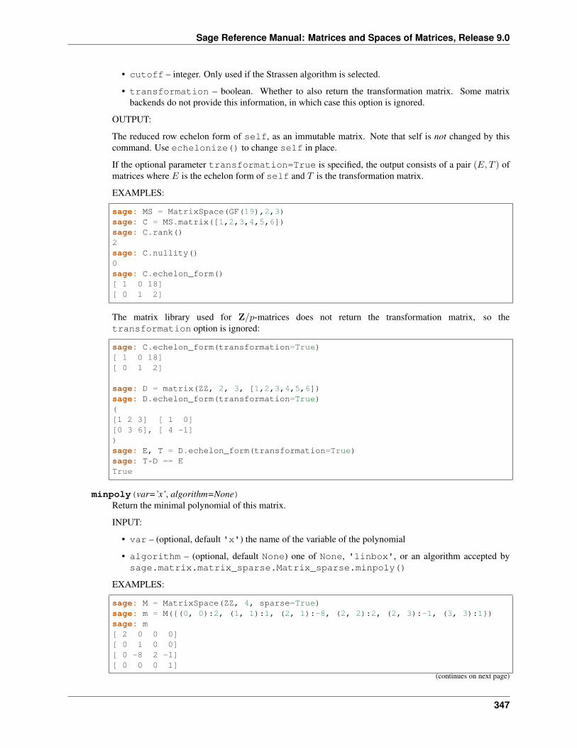
Sage Reference Manual: Matrices and Spaces of Matrices, Release 9.0
• cutoff – integer. Only used if the Strassen algorithm is selected.
• transformation – boolean. Whether to also return the transformation matrix. Some matrixbackends do not provide this information, in which case this option is ignored.
OUTPUT:
The reduced row echelon form of self, as an immutable matrix. Note that self is not changed by thiscommand. Use echelonize() to change self in place.
If the optional parameter transformation=True is specified, the output consists of a pair (𝐸, 𝑇 ) ofmatrices where 𝐸 is the echelon form of self and 𝑇 is the transformation matrix.
EXAMPLES:
sage: MS = MatrixSpace(GF(19),2,3)sage: C = MS.matrix([1,2,3,4,5,6])sage: C.rank()2sage: C.nullity()0sage: C.echelon_form()[ 1 0 18][ 0 1 2]
The matrix library used for Z/𝑝-matrices does not return the transformation matrix, so thetransformation option is ignored:
sage: C.echelon_form(transformation=True)[ 1 0 18][ 0 1 2]
sage: D = matrix(ZZ, 2, 3, [1,2,3,4,5,6])sage: D.echelon_form(transformation=True)([1 2 3] [ 1 0][0 3 6], [ 4 -1])sage: E, T = D.echelon_form(transformation=True)sage: T*D == ETrue
minpoly(var=’x’, algorithm=None)Return the minimal polynomial of this matrix.
INPUT:
• var – (optional, default 'x') the name of the variable of the polynomial
• algorithm – (optional, default None) one of None, 'linbox', or an algorithm accepted bysage.matrix.matrix_sparse.Matrix_sparse.minpoly()
EXAMPLES:
sage: M = MatrixSpace(ZZ, 4, sparse=True)sage: m = M({(0, 0):2, (1, 1):1, (2, 1):-8, (2, 2):2, (2, 3):-1, (3, 3):1})sage: m[ 2 0 0 0][ 0 1 0 0][ 0 -8 2 -1][ 0 0 0 1]
(continues on next page)
347
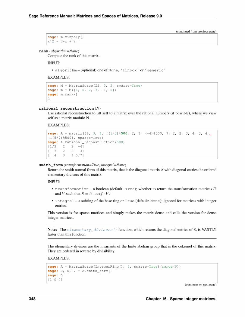
Sage Reference Manual: Matrices and Spaces of Matrices, Release 9.0
(continued from previous page)
sage: m.minpoly()x^2 - 3*x + 2
rank(algorithm=None)Compute the rank of this matrix.
INPUT:
• algorithm – (optional) one of None, 'linbox' or 'generic'
EXAMPLES:
sage: M = MatrixSpace(ZZ, 3, 2, sparse=True)sage: m = M([1, 0, 2, 3, -1, 0])sage: m.rank()2
rational_reconstruction(N)Use rational reconstruction to lift self to a matrix over the rational numbers (if possible), where we viewself as a matrix modulo N.
EXAMPLES:
sage: A = matrix(ZZ, 3, 4, [(1/3)%500, 2, 3, (-4)%500, 7, 2, 2, 3, 4, 3, 4,→˓(5/7)%500], sparse=True)sage: A.rational_reconstruction(500)[1/3 2 3 -4][ 7 2 2 3][ 4 3 4 5/7]
smith_form(transformation=True, integral=None)Return the smith normal form of this matrix, that is the diagonal matrix 𝑆 with diagonal entries the orderedelementary divisors of this matrix.
INPUT:
• transformation – a boolean (default: True); whether to return the transformation matrices 𝑈and 𝑉 such that 𝑆 = 𝑈 · 𝑠𝑒𝑙𝑓 · 𝑉 .
• integral – a subring of the base ring or True (default: None); ignored for matrices with integerentries.
This version is for sparse matrices and simply makes the matrix dense and calls the version for denseinteger matrices.
Note: The elementary_divisors() function, which returns the diagonal entries of S, is VASTLYfaster than this function.
The elementary divisors are the invariants of the finite abelian group that is the cokernel of this matrix.They are ordered in reverse by divisibility.
EXAMPLES:
sage: A = MatrixSpace(IntegerRing(), 3, sparse=True)(range(9))sage: D, U, V = A.smith_form()sage: D[1 0 0]
(continues on next page)
348 Chapter 16. Sparse integer matrices.
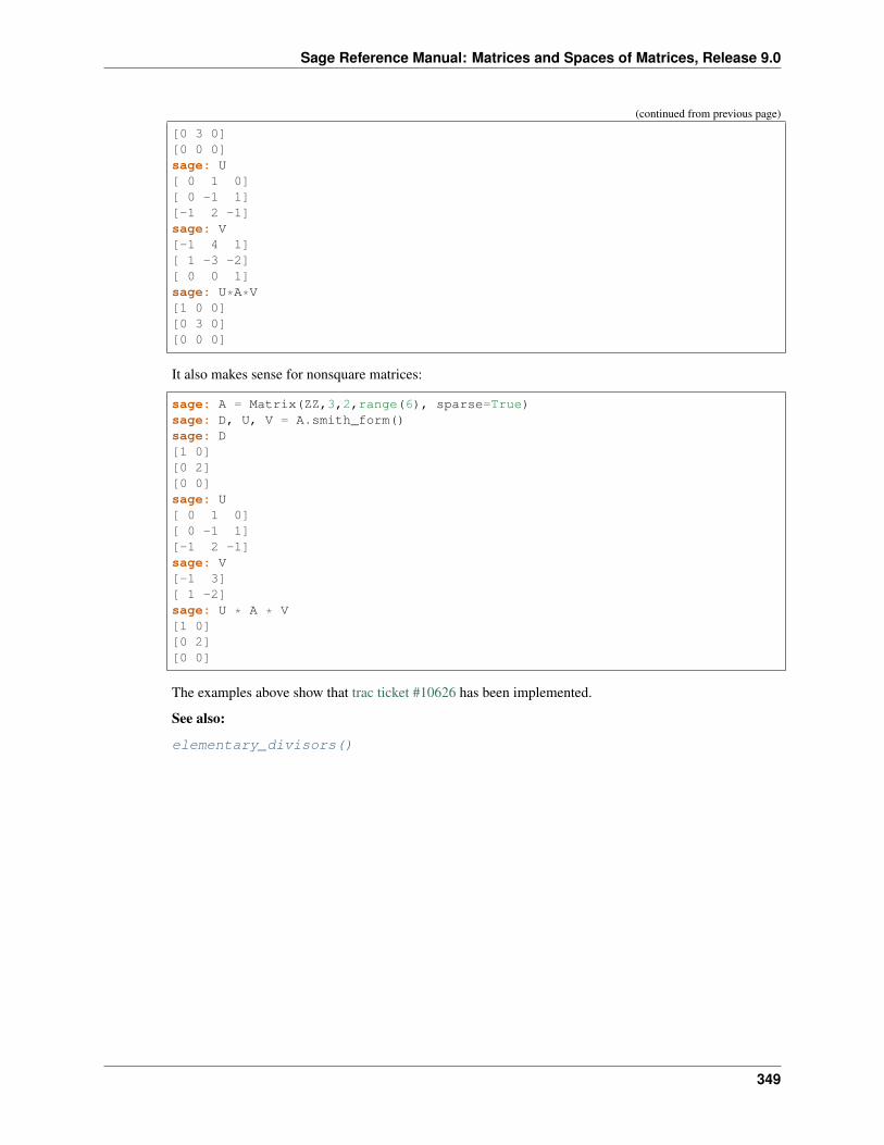
Sage Reference Manual: Matrices and Spaces of Matrices, Release 9.0
(continued from previous page)
[0 3 0][0 0 0]sage: U[ 0 1 0][ 0 -1 1][-1 2 -1]sage: V[-1 4 1][ 1 -3 -2][ 0 0 1]sage: U*A*V[1 0 0][0 3 0][0 0 0]
It also makes sense for nonsquare matrices:
sage: A = Matrix(ZZ,3,2,range(6), sparse=True)sage: D, U, V = A.smith_form()sage: D[1 0][0 2][0 0]sage: U[ 0 1 0][ 0 -1 1][-1 2 -1]sage: V[-1 3][ 1 -2]sage: U * A * V[1 0][0 2][0 0]
The examples above show that trac ticket #10626 has been implemented.
See also:
elementary_divisors()
349

Sage Reference Manual: Matrices and Spaces of Matrices, Release 9.0
350 Chapter 16. Sparse integer matrices.
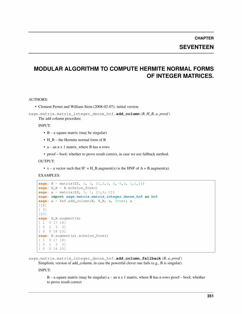
CHAPTER
SEVENTEEN
MODULAR ALGORITHM TO COMPUTE HERMITE NORMAL FORMSOF INTEGER MATRICES.
AUTHORS:
• Clement Pernet and William Stein (2008-02-07): initial version
sage.matrix.matrix_integer_dense_hnf.add_column(B, H_B, a, proof)The add column procedure.
INPUT:
• B – a square matrix (may be singular)
• H_B – the Hermite normal form of B
• a – an n x 1 matrix, where B has n rows
• proof – bool; whether to prove result correct, in case we use fallback method.
OUTPUT:
• x – a vector such that H’ = H_B.augment(x) is the HNF of A = B.augment(a).
EXAMPLES:
sage: B = matrix(ZZ, 3, 3, [1,2,5, 0,-5,3, 1,1,2])sage: H_B = B.echelon_form()sage: a = matrix(ZZ, 3, 1, [1,8,-2])sage: import sage.matrix.matrix_integer_dense_hnf as hnfsage: x = hnf.add_column(B, H_B, a, True); x[18][ 3][23]sage: H_B.augment(x)[ 1 0 17 18][ 0 1 3 3][ 0 0 18 23]sage: B.augment(a).echelon_form()[ 1 0 17 18][ 0 1 3 3][ 0 0 18 23]
sage.matrix.matrix_integer_dense_hnf.add_column_fallback(B, a, proof)Simplistic version of add_column, in case the powerful clever one fails (e.g., B is singular).
INPUT:
B – a square matrix (may be singular) a – an n x 1 matrix, where B has n rows proof – bool; whetherto prove result correct
351
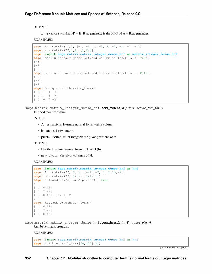
Sage Reference Manual: Matrices and Spaces of Matrices, Release 9.0
OUTPUT:
x – a vector such that H’ = H_B.augment(x) is the HNF of A = B.augment(a).
EXAMPLES:
sage: B = matrix(ZZ,3, [-1, -1, 1, -3, 8, -2, -1, -1, -1])sage: a = matrix(ZZ,3,1, [1,2,3])sage: import sage.matrix.matrix_integer_dense_hnf as matrix_integer_dense_hnfsage: matrix_integer_dense_hnf.add_column_fallback(B, a, True)[-3][-7][-2]sage: matrix_integer_dense_hnf.add_column_fallback(B, a, False)[-3][-7][-2]sage: B.augment(a).hermite_form()[ 1 1 1 -3][ 0 11 1 -7][ 0 0 2 -2]
sage.matrix.matrix_integer_dense_hnf.add_row(A, b, pivots, include_zero_rows)The add row procedure.
INPUT:
• A – a matrix in Hermite normal form with n column
• b – an n x 1 row matrix
• pivots – sorted list of integers; the pivot positions of A.
OUTPUT:
• H – the Hermite normal form of A.stack(b).
• new_pivots – the pivot columns of H.
EXAMPLES:
sage: import sage.matrix.matrix_integer_dense_hnf as hnfsage: A = matrix(ZZ, 2, 3, [-21, -7, 5, 1,20,-7])sage: b = matrix(ZZ, 1,3, [-1,1,-1])sage: hnf.add_row(A, b, A.pivots(), True)([ 1 6 29][ 0 7 28][ 0 0 46], [0, 1, 2])sage: A.stack(b).echelon_form()[ 1 6 29][ 0 7 28][ 0 0 46]
sage.matrix.matrix_integer_dense_hnf.benchmark_hnf(nrange, bits=4)Run benchmark program.
EXAMPLES:
sage: import sage.matrix.matrix_integer_dense_hnf as hnfsage: hnf.benchmark_hnf([50,100],32)
(continues on next page)
352 Chapter 17. Modular algorithm to compute Hermite normal forms of integer matrices.
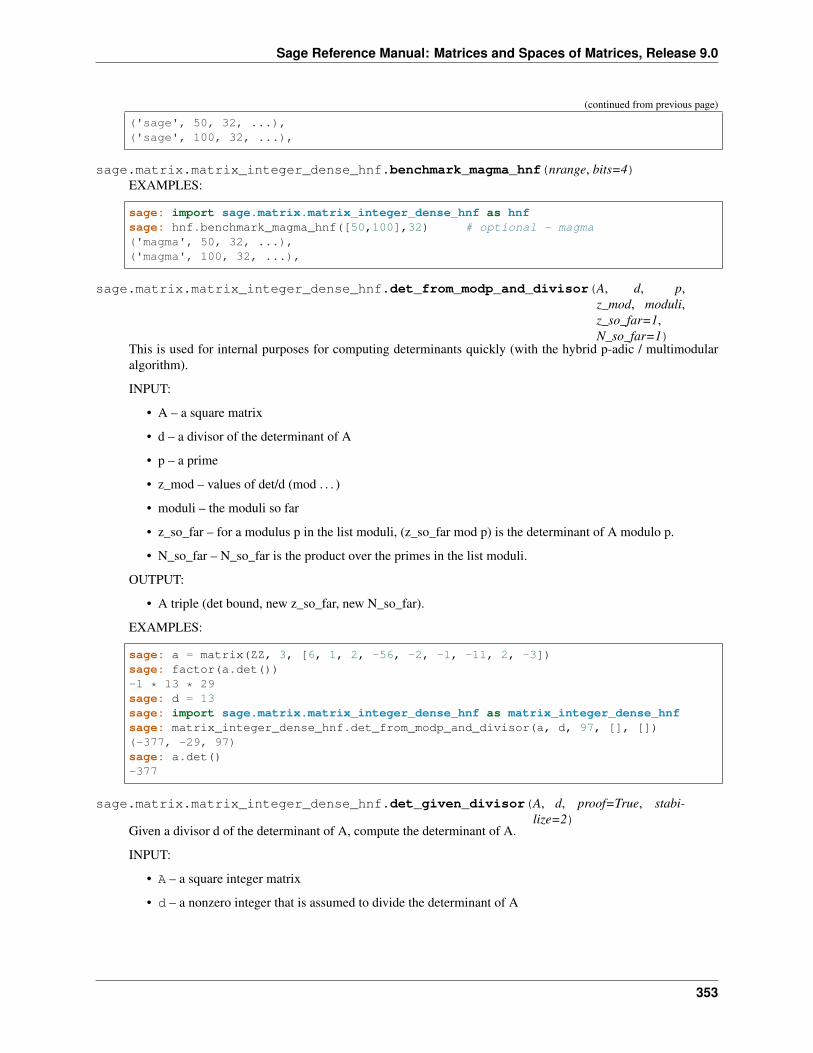
Sage Reference Manual: Matrices and Spaces of Matrices, Release 9.0
(continued from previous page)
('sage', 50, 32, ...),('sage', 100, 32, ...),
sage.matrix.matrix_integer_dense_hnf.benchmark_magma_hnf(nrange, bits=4)EXAMPLES:
sage: import sage.matrix.matrix_integer_dense_hnf as hnfsage: hnf.benchmark_magma_hnf([50,100],32) # optional - magma('magma', 50, 32, ...),('magma', 100, 32, ...),
sage.matrix.matrix_integer_dense_hnf.det_from_modp_and_divisor(A, d, p,z_mod, moduli,z_so_far=1,N_so_far=1)
This is used for internal purposes for computing determinants quickly (with the hybrid p-adic / multimodularalgorithm).
INPUT:
• A – a square matrix
• d – a divisor of the determinant of A
• p – a prime
• z_mod – values of det/d (mod . . . )
• moduli – the moduli so far
• z_so_far – for a modulus p in the list moduli, (z_so_far mod p) is the determinant of A modulo p.
• N_so_far – N_so_far is the product over the primes in the list moduli.
OUTPUT:
• A triple (det bound, new z_so_far, new N_so_far).
EXAMPLES:
sage: a = matrix(ZZ, 3, [6, 1, 2, -56, -2, -1, -11, 2, -3])sage: factor(a.det())-1 * 13 * 29sage: d = 13sage: import sage.matrix.matrix_integer_dense_hnf as matrix_integer_dense_hnfsage: matrix_integer_dense_hnf.det_from_modp_and_divisor(a, d, 97, [], [])(-377, -29, 97)sage: a.det()-377
sage.matrix.matrix_integer_dense_hnf.det_given_divisor(A, d, proof=True, stabi-lize=2)
Given a divisor d of the determinant of A, compute the determinant of A.
INPUT:
• A – a square integer matrix
• d – a nonzero integer that is assumed to divide the determinant of A
353
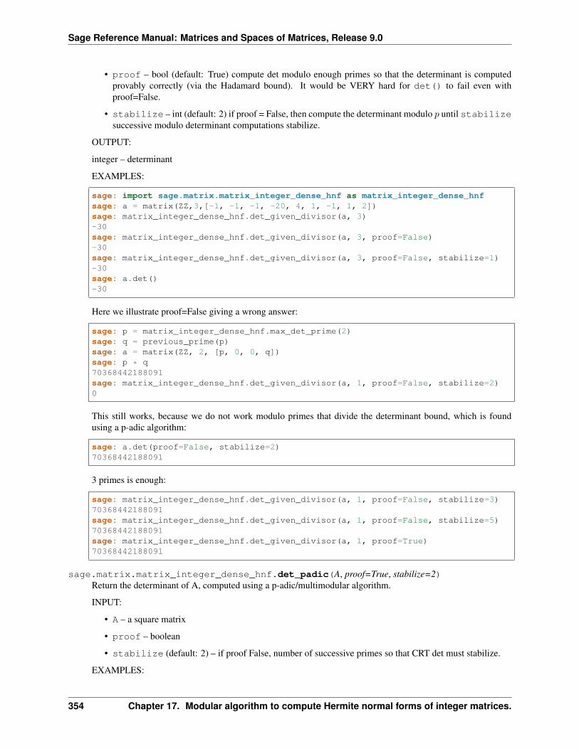
Sage Reference Manual: Matrices and Spaces of Matrices, Release 9.0
• proof – bool (default: True) compute det modulo enough primes so that the determinant is computedprovably correctly (via the Hadamard bound). It would be VERY hard for det() to fail even withproof=False.
• stabilize – int (default: 2) if proof = False, then compute the determinant modulo 𝑝 until stabilizesuccessive modulo determinant computations stabilize.
OUTPUT:
integer – determinant
EXAMPLES:
sage: import sage.matrix.matrix_integer_dense_hnf as matrix_integer_dense_hnfsage: a = matrix(ZZ,3,[-1, -1, -1, -20, 4, 1, -1, 1, 2])sage: matrix_integer_dense_hnf.det_given_divisor(a, 3)-30sage: matrix_integer_dense_hnf.det_given_divisor(a, 3, proof=False)-30sage: matrix_integer_dense_hnf.det_given_divisor(a, 3, proof=False, stabilize=1)-30sage: a.det()-30
Here we illustrate proof=False giving a wrong answer:
sage: p = matrix_integer_dense_hnf.max_det_prime(2)sage: q = previous_prime(p)sage: a = matrix(ZZ, 2, [p, 0, 0, q])sage: p * q70368442188091sage: matrix_integer_dense_hnf.det_given_divisor(a, 1, proof=False, stabilize=2)0
This still works, because we do not work modulo primes that divide the determinant bound, which is foundusing a p-adic algorithm:
sage: a.det(proof=False, stabilize=2)70368442188091
3 primes is enough:
sage: matrix_integer_dense_hnf.det_given_divisor(a, 1, proof=False, stabilize=3)70368442188091sage: matrix_integer_dense_hnf.det_given_divisor(a, 1, proof=False, stabilize=5)70368442188091sage: matrix_integer_dense_hnf.det_given_divisor(a, 1, proof=True)70368442188091
sage.matrix.matrix_integer_dense_hnf.det_padic(A, proof=True, stabilize=2)Return the determinant of A, computed using a p-adic/multimodular algorithm.
INPUT:
• A – a square matrix
• proof – boolean
• stabilize (default: 2) – if proof False, number of successive primes so that CRT det must stabilize.
EXAMPLES:
354 Chapter 17. Modular algorithm to compute Hermite normal forms of integer matrices.
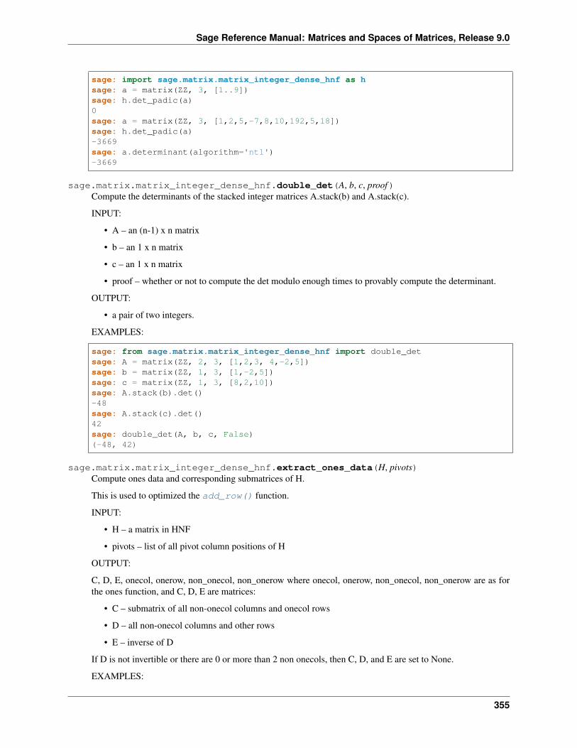
Sage Reference Manual: Matrices and Spaces of Matrices, Release 9.0
sage: import sage.matrix.matrix_integer_dense_hnf as hsage: a = matrix(ZZ, 3, [1..9])sage: h.det_padic(a)0sage: a = matrix(ZZ, 3, [1,2,5,-7,8,10,192,5,18])sage: h.det_padic(a)-3669sage: a.determinant(algorithm='ntl')-3669
sage.matrix.matrix_integer_dense_hnf.double_det(A, b, c, proof)Compute the determinants of the stacked integer matrices A.stack(b) and A.stack(c).
INPUT:
• A – an (n-1) x n matrix
• b – an 1 x n matrix
• c – an 1 x n matrix
• proof – whether or not to compute the det modulo enough times to provably compute the determinant.
OUTPUT:
• a pair of two integers.
EXAMPLES:
sage: from sage.matrix.matrix_integer_dense_hnf import double_detsage: A = matrix(ZZ, 2, 3, [1,2,3, 4,-2,5])sage: b = matrix(ZZ, 1, 3, [1,-2,5])sage: c = matrix(ZZ, 1, 3, [8,2,10])sage: A.stack(b).det()-48sage: A.stack(c).det()42sage: double_det(A, b, c, False)(-48, 42)
sage.matrix.matrix_integer_dense_hnf.extract_ones_data(H, pivots)Compute ones data and corresponding submatrices of H.
This is used to optimized the add_row() function.
INPUT:
• H – a matrix in HNF
• pivots – list of all pivot column positions of H
OUTPUT:
C, D, E, onecol, onerow, non_onecol, non_onerow where onecol, onerow, non_onecol, non_onerow are as forthe ones function, and C, D, E are matrices:
• C – submatrix of all non-onecol columns and onecol rows
• D – all non-onecol columns and other rows
• E – inverse of D
If D is not invertible or there are 0 or more than 2 non onecols, then C, D, and E are set to None.
EXAMPLES:
355
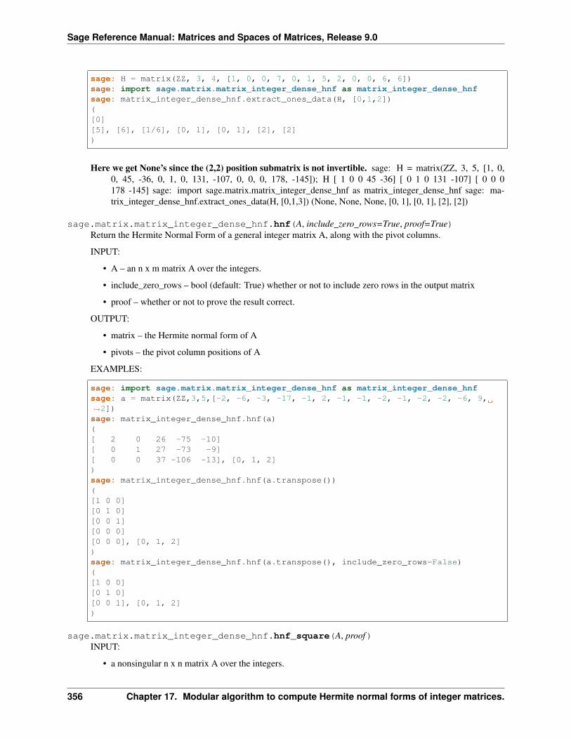
Sage Reference Manual: Matrices and Spaces of Matrices, Release 9.0
sage: H = matrix(ZZ, 3, 4, [1, 0, 0, 7, 0, 1, 5, 2, 0, 0, 6, 6])sage: import sage.matrix.matrix_integer_dense_hnf as matrix_integer_dense_hnfsage: matrix_integer_dense_hnf.extract_ones_data(H, [0,1,2])([0][5], [6], [1/6], [0, 1], [0, 1], [2], [2])
Here we get None’s since the (2,2) position submatrix is not invertible. sage: H = matrix(ZZ, 3, 5, [1, 0,0, 45, -36, 0, 1, 0, 131, -107, 0, 0, 0, 178, -145]); H [ 1 0 0 45 -36] [ 0 1 0 131 -107] [ 0 0 0178 -145] sage: import sage.matrix.matrix_integer_dense_hnf as matrix_integer_dense_hnf sage: ma-trix_integer_dense_hnf.extract_ones_data(H, [0,1,3]) (None, None, None, [0, 1], [0, 1], [2], [2])
sage.matrix.matrix_integer_dense_hnf.hnf(A, include_zero_rows=True, proof=True)Return the Hermite Normal Form of a general integer matrix A, along with the pivot columns.
INPUT:
• A – an n x m matrix A over the integers.
• include_zero_rows – bool (default: True) whether or not to include zero rows in the output matrix
• proof – whether or not to prove the result correct.
OUTPUT:
• matrix – the Hermite normal form of A
• pivots – the pivot column positions of A
EXAMPLES:
sage: import sage.matrix.matrix_integer_dense_hnf as matrix_integer_dense_hnfsage: a = matrix(ZZ,3,5,[-2, -6, -3, -17, -1, 2, -1, -1, -2, -1, -2, -2, -6, 9,→˓2])sage: matrix_integer_dense_hnf.hnf(a)([ 2 0 26 -75 -10][ 0 1 27 -73 -9][ 0 0 37 -106 -13], [0, 1, 2])sage: matrix_integer_dense_hnf.hnf(a.transpose())([1 0 0][0 1 0][0 0 1][0 0 0][0 0 0], [0, 1, 2])sage: matrix_integer_dense_hnf.hnf(a.transpose(), include_zero_rows=False)([1 0 0][0 1 0][0 0 1], [0, 1, 2])
sage.matrix.matrix_integer_dense_hnf.hnf_square(A, proof)INPUT:
• a nonsingular n x n matrix A over the integers.
356 Chapter 17. Modular algorithm to compute Hermite normal forms of integer matrices.
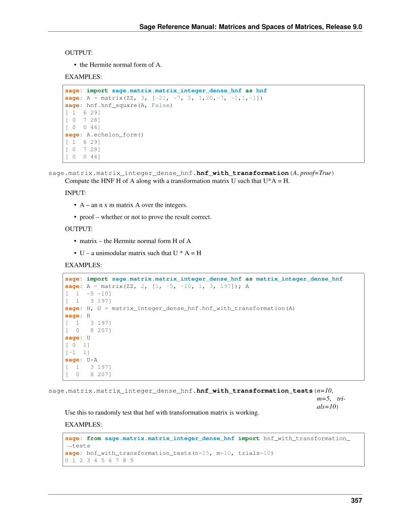
Sage Reference Manual: Matrices and Spaces of Matrices, Release 9.0
OUTPUT:
• the Hermite normal form of A.
EXAMPLES:
sage: import sage.matrix.matrix_integer_dense_hnf as hnfsage: A = matrix(ZZ, 3, [-21, -7, 5, 1,20,-7, -1,1,-1])sage: hnf.hnf_square(A, False)[ 1 6 29][ 0 7 28][ 0 0 46]sage: A.echelon_form()[ 1 6 29][ 0 7 28][ 0 0 46]
sage.matrix.matrix_integer_dense_hnf.hnf_with_transformation(A, proof=True)Compute the HNF H of A along with a transformation matrix U such that U*A = H.
INPUT:
• A – an n x m matrix A over the integers.
• proof – whether or not to prove the result correct.
OUTPUT:
• matrix – the Hermite normal form H of A
• U – a unimodular matrix such that U * A = H
EXAMPLES:
sage: import sage.matrix.matrix_integer_dense_hnf as matrix_integer_dense_hnfsage: A = matrix(ZZ, 2, [1, -5, -10, 1, 3, 197]); A[ 1 -5 -10][ 1 3 197]sage: H, U = matrix_integer_dense_hnf.hnf_with_transformation(A)sage: H[ 1 3 197][ 0 8 207]sage: U[ 0 1][-1 1]sage: U*A[ 1 3 197][ 0 8 207]
sage.matrix.matrix_integer_dense_hnf.hnf_with_transformation_tests(n=10,m=5, tri-als=10)
Use this to randomly test that hnf with transformation matrix is working.
EXAMPLES:
sage: from sage.matrix.matrix_integer_dense_hnf import hnf_with_transformation_→˓testssage: hnf_with_transformation_tests(n=15, m=10, trials=10)0 1 2 3 4 5 6 7 8 9
357
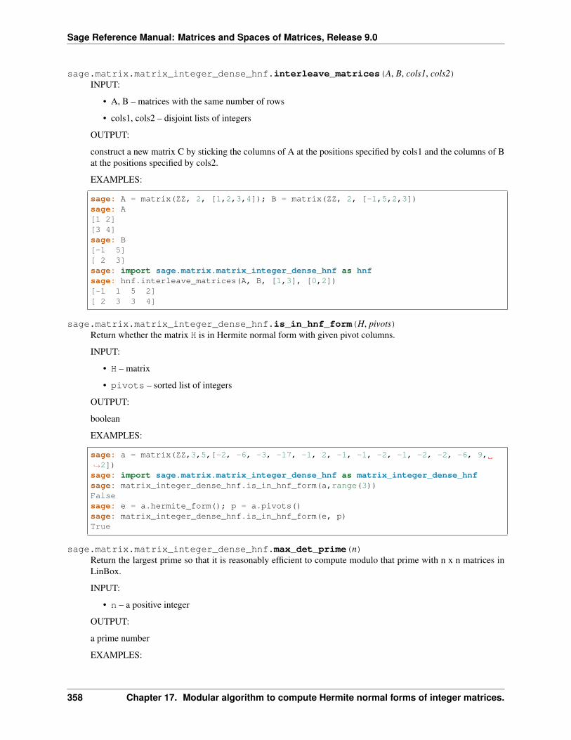
Sage Reference Manual: Matrices and Spaces of Matrices, Release 9.0
sage.matrix.matrix_integer_dense_hnf.interleave_matrices(A, B, cols1, cols2)INPUT:
• A, B – matrices with the same number of rows
• cols1, cols2 – disjoint lists of integers
OUTPUT:
construct a new matrix C by sticking the columns of A at the positions specified by cols1 and the columns of Bat the positions specified by cols2.
EXAMPLES:
sage: A = matrix(ZZ, 2, [1,2,3,4]); B = matrix(ZZ, 2, [-1,5,2,3])sage: A[1 2][3 4]sage: B[-1 5][ 2 3]sage: import sage.matrix.matrix_integer_dense_hnf as hnfsage: hnf.interleave_matrices(A, B, [1,3], [0,2])[-1 1 5 2][ 2 3 3 4]
sage.matrix.matrix_integer_dense_hnf.is_in_hnf_form(H, pivots)Return whether the matrix H is in Hermite normal form with given pivot columns.
INPUT:
• H – matrix
• pivots – sorted list of integers
OUTPUT:
boolean
EXAMPLES:
sage: a = matrix(ZZ,3,5,[-2, -6, -3, -17, -1, 2, -1, -1, -2, -1, -2, -2, -6, 9,→˓2])sage: import sage.matrix.matrix_integer_dense_hnf as matrix_integer_dense_hnfsage: matrix_integer_dense_hnf.is_in_hnf_form(a,range(3))Falsesage: e = a.hermite_form(); p = a.pivots()sage: matrix_integer_dense_hnf.is_in_hnf_form(e, p)True
sage.matrix.matrix_integer_dense_hnf.max_det_prime(n)Return the largest prime so that it is reasonably efficient to compute modulo that prime with n x n matrices inLinBox.
INPUT:
• n – a positive integer
OUTPUT:
a prime number
EXAMPLES:
358 Chapter 17. Modular algorithm to compute Hermite normal forms of integer matrices.
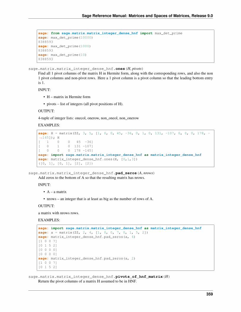
Sage Reference Manual: Matrices and Spaces of Matrices, Release 9.0
sage: from sage.matrix.matrix_integer_dense_hnf import max_det_primesage: max_det_prime(10000)8388593sage: max_det_prime(1000)8388593sage: max_det_prime(10)8388593
sage.matrix.matrix_integer_dense_hnf.ones(H, pivots)Find all 1 pivot columns of the matrix H in Hermite form, along with the corresponding rows, and also the non1 pivot columns and non-pivot rows. Here a 1 pivot column is a pivot column so that the leading bottom entryis 1.
INPUT:
• H – matrix in Hermite form
• pivots – list of integers (all pivot positions of H).
OUTPUT:
4-tuple of integer lists: onecol, onerow, non_oneol, non_onerow
EXAMPLES:
sage: H = matrix(ZZ, 3, 5, [1, 0, 0, 45, -36, 0, 1, 0, 131, -107, 0, 0, 0, 178, -→˓145]); H[ 1 0 0 45 -36][ 0 1 0 131 -107][ 0 0 0 178 -145]sage: import sage.matrix.matrix_integer_dense_hnf as matrix_integer_dense_hnfsage: matrix_integer_dense_hnf.ones(H, [0,1,3])([0, 1], [0, 1], [2], [2])
sage.matrix.matrix_integer_dense_hnf.pad_zeros(A, nrows)Add zeros to the bottom of A so that the resulting matrix has nrows.
INPUT:
• A – a matrix
• nrows – an integer that is at least as big as the number of rows of A.
OUTPUT:
a matrix with nrows rows.
EXAMPLES:
sage: import sage.matrix.matrix_integer_dense_hnf as matrix_integer_dense_hnfsage: a = matrix(ZZ, 2, 4, [1, 0, 0, 7, 0, 1, 5, 2])sage: matrix_integer_dense_hnf.pad_zeros(a, 4)[1 0 0 7][0 1 5 2][0 0 0 0][0 0 0 0]sage: matrix_integer_dense_hnf.pad_zeros(a, 2)[1 0 0 7][0 1 5 2]
sage.matrix.matrix_integer_dense_hnf.pivots_of_hnf_matrix(H)Return the pivot columns of a matrix H assumed to be in HNF.
359
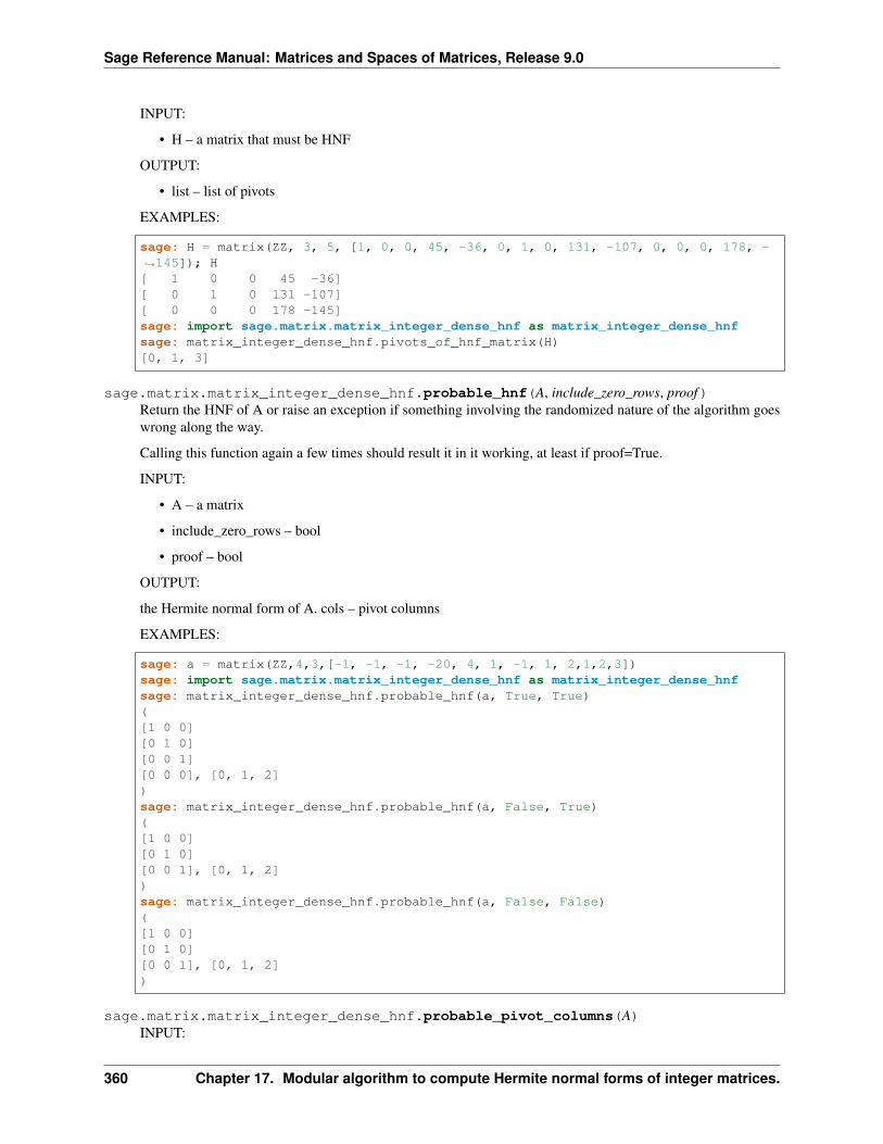
Sage Reference Manual: Matrices and Spaces of Matrices, Release 9.0
INPUT:
• H – a matrix that must be HNF
OUTPUT:
• list – list of pivots
EXAMPLES:
sage: H = matrix(ZZ, 3, 5, [1, 0, 0, 45, -36, 0, 1, 0, 131, -107, 0, 0, 0, 178, -→˓145]); H[ 1 0 0 45 -36][ 0 1 0 131 -107][ 0 0 0 178 -145]sage: import sage.matrix.matrix_integer_dense_hnf as matrix_integer_dense_hnfsage: matrix_integer_dense_hnf.pivots_of_hnf_matrix(H)[0, 1, 3]
sage.matrix.matrix_integer_dense_hnf.probable_hnf(A, include_zero_rows, proof)Return the HNF of A or raise an exception if something involving the randomized nature of the algorithm goeswrong along the way.
Calling this function again a few times should result it in it working, at least if proof=True.
INPUT:
• A – a matrix
• include_zero_rows – bool
• proof – bool
OUTPUT:
the Hermite normal form of A. cols – pivot columns
EXAMPLES:
sage: a = matrix(ZZ,4,3,[-1, -1, -1, -20, 4, 1, -1, 1, 2,1,2,3])sage: import sage.matrix.matrix_integer_dense_hnf as matrix_integer_dense_hnfsage: matrix_integer_dense_hnf.probable_hnf(a, True, True)([1 0 0][0 1 0][0 0 1][0 0 0], [0, 1, 2])sage: matrix_integer_dense_hnf.probable_hnf(a, False, True)([1 0 0][0 1 0][0 0 1], [0, 1, 2])sage: matrix_integer_dense_hnf.probable_hnf(a, False, False)([1 0 0][0 1 0][0 0 1], [0, 1, 2])
sage.matrix.matrix_integer_dense_hnf.probable_pivot_columns(A)INPUT:
360 Chapter 17. Modular algorithm to compute Hermite normal forms of integer matrices.
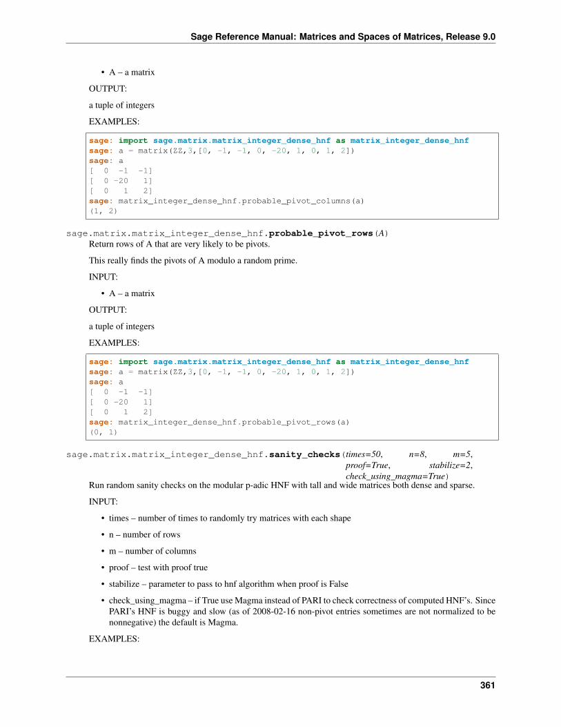
Sage Reference Manual: Matrices and Spaces of Matrices, Release 9.0
• A – a matrix
OUTPUT:
a tuple of integers
EXAMPLES:
sage: import sage.matrix.matrix_integer_dense_hnf as matrix_integer_dense_hnfsage: a = matrix(ZZ,3,[0, -1, -1, 0, -20, 1, 0, 1, 2])sage: a[ 0 -1 -1][ 0 -20 1][ 0 1 2]sage: matrix_integer_dense_hnf.probable_pivot_columns(a)(1, 2)
sage.matrix.matrix_integer_dense_hnf.probable_pivot_rows(A)Return rows of A that are very likely to be pivots.
This really finds the pivots of A modulo a random prime.
INPUT:
• A – a matrix
OUTPUT:
a tuple of integers
EXAMPLES:
sage: import sage.matrix.matrix_integer_dense_hnf as matrix_integer_dense_hnfsage: a = matrix(ZZ,3,[0, -1, -1, 0, -20, 1, 0, 1, 2])sage: a[ 0 -1 -1][ 0 -20 1][ 0 1 2]sage: matrix_integer_dense_hnf.probable_pivot_rows(a)(0, 1)
sage.matrix.matrix_integer_dense_hnf.sanity_checks(times=50, n=8, m=5,proof=True, stabilize=2,check_using_magma=True)
Run random sanity checks on the modular p-adic HNF with tall and wide matrices both dense and sparse.
INPUT:
• times – number of times to randomly try matrices with each shape
• n – number of rows
• m – number of columns
• proof – test with proof true
• stabilize – parameter to pass to hnf algorithm when proof is False
• check_using_magma – if True use Magma instead of PARI to check correctness of computed HNF’s. SincePARI’s HNF is buggy and slow (as of 2008-02-16 non-pivot entries sometimes are not normalized to benonnegative) the default is Magma.
EXAMPLES:
361
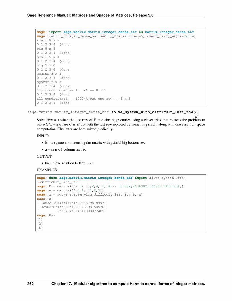
Sage Reference Manual: Matrices and Spaces of Matrices, Release 9.0
sage: import sage.matrix.matrix_integer_dense_hnf as matrix_integer_dense_hnfsage: matrix_integer_dense_hnf.sanity_checks(times=5, check_using_magma=False)small 8 x 50 1 2 3 4 (done)big 8 x 50 1 2 3 4 (done)small 5 x 80 1 2 3 4 (done)big 5 x 80 1 2 3 4 (done)sparse 8 x 50 1 2 3 4 (done)sparse 5 x 80 1 2 3 4 (done)ill conditioned -- 1000*A -- 8 x 50 1 2 3 4 (done)ill conditioned -- 1000*A but one row -- 8 x 50 1 2 3 4 (done)
sage.matrix.matrix_integer_dense_hnf.solve_system_with_difficult_last_row(B,a)
Solve B*x = a when the last row of 𝐵 contains huge entries using a clever trick that reduces the problem tosolve C*x = a where 𝐶 is 𝐵 but with the last row replaced by something small, along with one easy null spacecomputation. The latter are both solved 𝑝-adically.
INPUT:
• B – a square n x n nonsingular matrix with painful big bottom row.
• a – an n x 1 column matrix
OUTPUT:
• the unique solution to B*x = a.
EXAMPLES:
sage: from sage.matrix.matrix_integer_dense_hnf import solve_system_with_→˓difficult_last_rowsage: B = matrix(ZZ, 3, [1,2,4, 3,-4,7, 939082,2930982,132902384098234])sage: a = matrix(ZZ,3,1, [1,2,5])sage: z = solve_system_with_difficult_last_row(B, a)sage: z[ 106321906985474/132902379815497][132902385037291/1329023798154970][ -5221794/664511899077485]sage: B*z[1][2][5]
362 Chapter 17. Modular algorithm to compute Hermite normal forms of integer matrices.
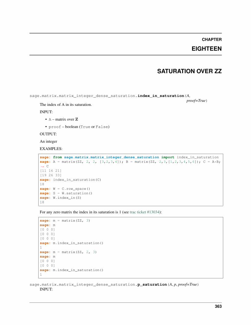
CHAPTER
EIGHTEEN
SATURATION OVER ZZ
sage.matrix.matrix_integer_dense_saturation.index_in_saturation(A,proof=True)
The index of A in its saturation.
INPUT:
• A – matrix over Z
• proof – boolean (True or False)
OUTPUT:
An integer
EXAMPLES:
sage: from sage.matrix.matrix_integer_dense_saturation import index_in_saturationsage: A = matrix(ZZ, 2, 2, [3,2,3,4]); B = matrix(ZZ, 2,3,[1,2,3,4,5,6]); C = A*B;→˓ C[11 16 21][19 26 33]sage: index_in_saturation(C)18sage: W = C.row_space()sage: S = W.saturation()sage: W.index_in(S)18
For any zero matrix the index in its saturation is 1 (see trac ticket #13034):
sage: m = matrix(ZZ, 3)sage: m[0 0 0][0 0 0][0 0 0]sage: m.index_in_saturation()1sage: m = matrix(ZZ, 2, 3)sage: m[0 0 0][0 0 0]sage: m.index_in_saturation()1
sage.matrix.matrix_integer_dense_saturation.p_saturation(A, p, proof=True)INPUT:
363
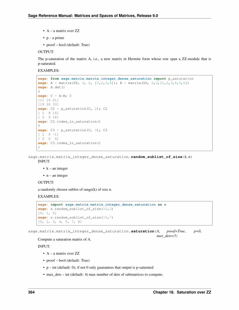
Sage Reference Manual: Matrices and Spaces of Matrices, Release 9.0
• A – a matrix over ZZ
• p – a prime
• proof – bool (default: True)
OUTPUT:
The p-saturation of the matrix A, i.e., a new matrix in Hermite form whose row span a ZZ-module that isp-saturated.
EXAMPLES:
sage: from sage.matrix.matrix_integer_dense_saturation import p_saturationsage: A = matrix(ZZ, 2, 2, [3,2,3,4]); B = matrix(ZZ, 2,3,[1,2,3,4,5,6])sage: A.det()6sage: C = A*B; C[11 16 21][19 26 33]sage: C2 = p_saturation(C, 2); C2[ 1 8 15][ 0 9 18]sage: C2.index_in_saturation()9sage: C3 = p_saturation(C, 3); C3[ 1 0 -1][ 0 2 4]sage: C3.index_in_saturation()2
sage.matrix.matrix_integer_dense_saturation.random_sublist_of_size(k, n)INPUT:
• k – an integer
• n – an integer
OUTPUT:
a randomly chosen sublist of range(k) of size n.
EXAMPLES:
sage: import sage.matrix.matrix_integer_dense_saturation as ssage: s.random_sublist_of_size(10,3)[0, 1, 5]sage: s.random_sublist_of_size(10,7)[0, 1, 3, 4, 5, 7, 8]
sage.matrix.matrix_integer_dense_saturation.saturation(A, proof=True, p=0,max_dets=5)
Compute a saturation matrix of A.
INPUT:
• A – a matrix over ZZ
• proof – bool (default: True)
• p – int (default: 0); if not 0 only guarantees that output is p-saturated
• max_dets – int (default: 4) max number of dets of submatrices to compute.
364 Chapter 18. Saturation over ZZ
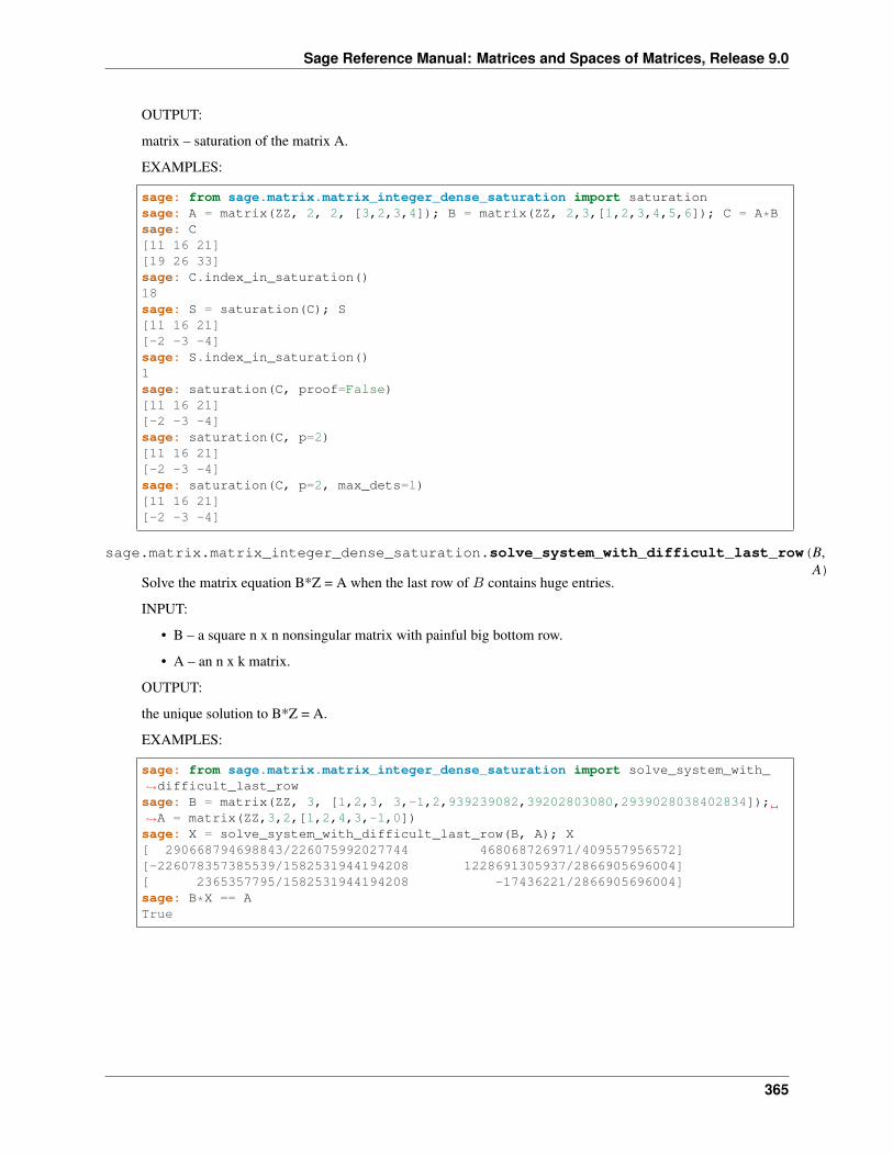
Sage Reference Manual: Matrices and Spaces of Matrices, Release 9.0
OUTPUT:
matrix – saturation of the matrix A.
EXAMPLES:
sage: from sage.matrix.matrix_integer_dense_saturation import saturationsage: A = matrix(ZZ, 2, 2, [3,2,3,4]); B = matrix(ZZ, 2,3,[1,2,3,4,5,6]); C = A*Bsage: C[11 16 21][19 26 33]sage: C.index_in_saturation()18sage: S = saturation(C); S[11 16 21][-2 -3 -4]sage: S.index_in_saturation()1sage: saturation(C, proof=False)[11 16 21][-2 -3 -4]sage: saturation(C, p=2)[11 16 21][-2 -3 -4]sage: saturation(C, p=2, max_dets=1)[11 16 21][-2 -3 -4]
sage.matrix.matrix_integer_dense_saturation.solve_system_with_difficult_last_row(B,A)
Solve the matrix equation B*Z = A when the last row of 𝐵 contains huge entries.
INPUT:
• B – a square n x n nonsingular matrix with painful big bottom row.
• A – an n x k matrix.
OUTPUT:
the unique solution to B*Z = A.
EXAMPLES:
sage: from sage.matrix.matrix_integer_dense_saturation import solve_system_with_→˓difficult_last_rowsage: B = matrix(ZZ, 3, [1,2,3, 3,-1,2,939239082,39202803080,2939028038402834]);→˓A = matrix(ZZ,3,2,[1,2,4,3,-1,0])sage: X = solve_system_with_difficult_last_row(B, A); X[ 290668794698843/226075992027744 468068726971/409557956572][-226078357385539/1582531944194208 1228691305937/2866905696004][ 2365357795/1582531944194208 -17436221/2866905696004]sage: B*X == ATrue
365

Sage Reference Manual: Matrices and Spaces of Matrices, Release 9.0
366 Chapter 18. Saturation over ZZ
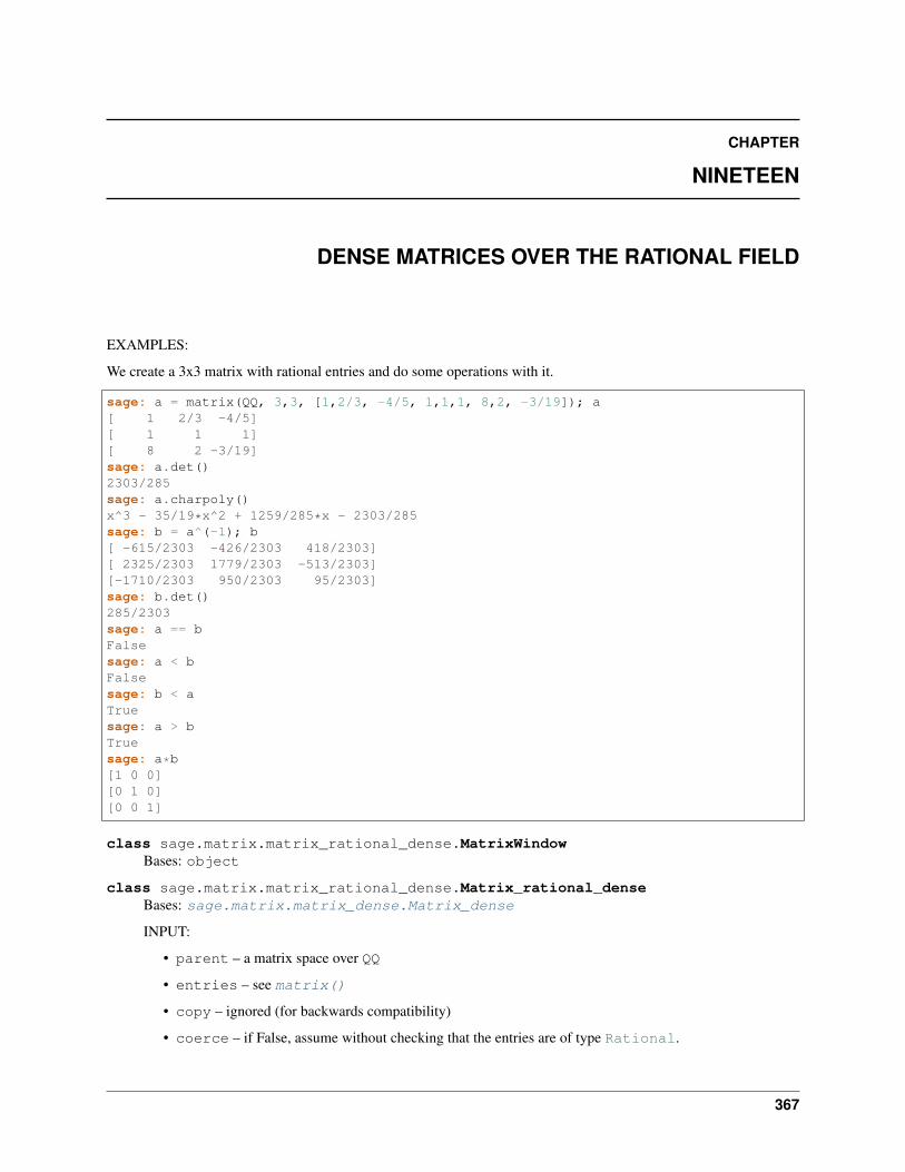
CHAPTER
NINETEEN
DENSE MATRICES OVER THE RATIONAL FIELD
EXAMPLES:
We create a 3x3 matrix with rational entries and do some operations with it.
sage: a = matrix(QQ, 3,3, [1,2/3, -4/5, 1,1,1, 8,2, -3/19]); a[ 1 2/3 -4/5][ 1 1 1][ 8 2 -3/19]sage: a.det()2303/285sage: a.charpoly()x^3 - 35/19*x^2 + 1259/285*x - 2303/285sage: b = a^(-1); b[ -615/2303 -426/2303 418/2303][ 2325/2303 1779/2303 -513/2303][-1710/2303 950/2303 95/2303]sage: b.det()285/2303sage: a == bFalsesage: a < bFalsesage: b < aTruesage: a > bTruesage: a*b[1 0 0][0 1 0][0 0 1]
class sage.matrix.matrix_rational_dense.MatrixWindowBases: object
class sage.matrix.matrix_rational_dense.Matrix_rational_denseBases: sage.matrix.matrix_dense.Matrix_dense
INPUT:
• parent – a matrix space over QQ
• entries – see matrix()
• copy – ignored (for backwards compatibility)
• coerce – if False, assume without checking that the entries are of type Rational.
367
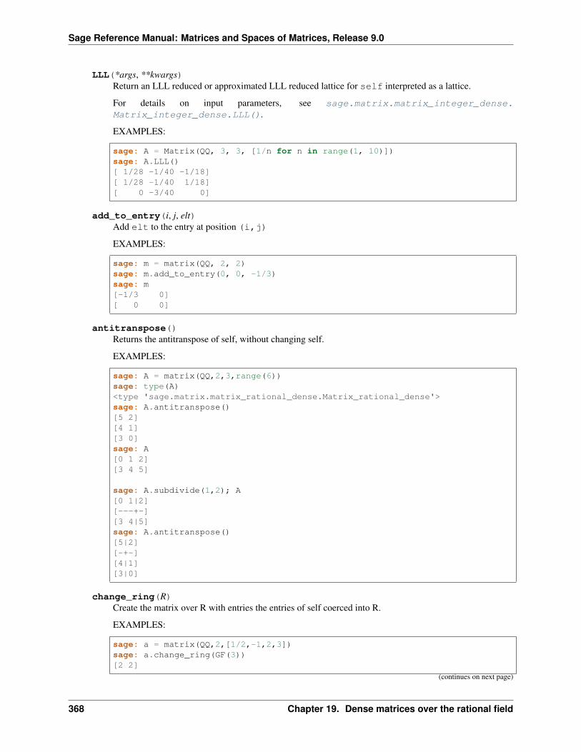
Sage Reference Manual: Matrices and Spaces of Matrices, Release 9.0
LLL(*args, **kwargs)Return an LLL reduced or approximated LLL reduced lattice for self interpreted as a lattice.
For details on input parameters, see sage.matrix.matrix_integer_dense.Matrix_integer_dense.LLL().
EXAMPLES:
sage: A = Matrix(QQ, 3, 3, [1/n for n in range(1, 10)])sage: A.LLL()[ 1/28 -1/40 -1/18][ 1/28 -1/40 1/18][ 0 -3/40 0]
add_to_entry(i, j, elt)Add elt to the entry at position (i,j)
EXAMPLES:
sage: m = matrix(QQ, 2, 2)sage: m.add_to_entry(0, 0, -1/3)sage: m[-1/3 0][ 0 0]
antitranspose()Returns the antitranspose of self, without changing self.
EXAMPLES:
sage: A = matrix(QQ,2,3,range(6))sage: type(A)<type 'sage.matrix.matrix_rational_dense.Matrix_rational_dense'>sage: A.antitranspose()[5 2][4 1][3 0]sage: A[0 1 2][3 4 5]
sage: A.subdivide(1,2); A[0 1|2][---+-][3 4|5]sage: A.antitranspose()[5|2][-+-][4|1][3|0]
change_ring(R)Create the matrix over R with entries the entries of self coerced into R.
EXAMPLES:
sage: a = matrix(QQ,2,[1/2,-1,2,3])sage: a.change_ring(GF(3))[2 2]
(continues on next page)
368 Chapter 19. Dense matrices over the rational field
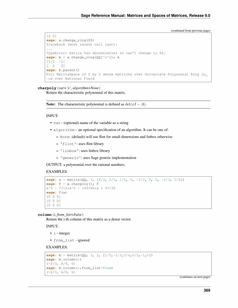
Sage Reference Manual: Matrices and Spaces of Matrices, Release 9.0
(continued from previous page)
[2 0]sage: a.change_ring(ZZ)Traceback (most recent call last):...TypeError: matrix has denominators so can't change to ZZ.sage: b = a.change_ring(QQ['x']); b[1/2 -1][ 2 3]sage: b.parent()Full MatrixSpace of 2 by 2 dense matrices over Univariate Polynomial Ring in→˓x over Rational Field
charpoly(var=’x’, algorithm=None)Return the characteristic polynomial of this matrix.
Note: The characteristic polynomial is defined as det(𝑥𝐼 −𝐴).
INPUT:
• var - (optional) name of the variable as a string
• algorithm – an optional specification of an algorithm. It can be one of:
– None: (default) will use flint for small dimensions and linbox otherwise
– 'flint': uses flint library
– 'linbox': uses linbox library
– 'generic': uses Sage generic implementation
OUTPUT: a polynomial over the rational numbers.
EXAMPLES:
sage: a = matrix(QQ, 3, [4/3, 2/5, 1/5, 4, -3/2, 0, 0, -2/3, 3/4])sage: f = a.charpoly(); fx^3 - 7/12*x^2 - 149/40*x + 97/30sage: f(a)[0 0 0][0 0 0][0 0 0]
column(i, from_list=False)Return the i-th column of this matrix as a dense vector.
INPUT:
• i - integer
• from_list - ignored
EXAMPLES:
sage: m = matrix(QQ, 3, 2, [1/5,-2/3,3/4,4/9,-1,0])sage: m.column(1)(-2/3, 4/9, 0)sage: m.column(1,from_list=True)(-2/3, 4/9, 0)
(continues on next page)
369
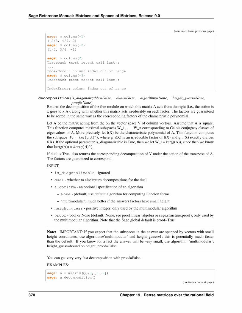
Sage Reference Manual: Matrices and Spaces of Matrices, Release 9.0
(continued from previous page)
sage: m.column(-1)(-2/3, 4/9, 0)sage: m.column(-2)(1/5, 3/4, -1)
sage: m.column(2)Traceback (most recent call last):...IndexError: column index out of rangesage: m.column(-3)Traceback (most recent call last):...IndexError: column index out of range
decomposition(is_diagonalizable=False, dual=False, algorithm=None, height_guess=None,proof=None)
Returns the decomposition of the free module on which this matrix A acts from the right (i.e., the action isx goes to x A), along with whether this matrix acts irreducibly on each factor. The factors are guaranteedto be sorted in the same way as the corresponding factors of the characteristic polynomial.
Let A be the matrix acting from the on the vector space V of column vectors. Assume that A is square.This function computes maximal subspaces W_1, . . . , W_n corresponding to Galois conjugacy classes ofeigenvalues of A. More precisely, let f(X) be the characteristic polynomial of A. This function computesthe subspace 𝑊𝑖 = 𝑘𝑒𝑟(𝑔(𝐴)𝑛), where g_i(X) is an irreducible factor of f(X) and g_i(X) exactly dividesf(X). If the optional parameter is_diagonalizable is True, then we let W_i = ker(g(A)), since then we knowthat ker(g(A)) = 𝑘𝑒𝑟(𝑔(𝐴)𝑛).
If dual is True, also returns the corresponding decomposition of V under the action of the transpose of A.The factors are guaranteed to correspond.
INPUT:
• is_diagonalizable - ignored
• dual - whether to also return decompositions for the dual
• algorithm - an optional specification of an algorithm
– None - (default) use default algorithm for computing Echelon forms
– ‘multimodular’: much better if the answers factors have small height
• height_guess - positive integer; only used by the multimodular algorithm
• proof - bool or None (default: None, see proof.linear_algebra or sage.structure.proof); only used bythe multimodular algorithm. Note that the Sage global default is proof=True.
Note: IMPORTANT: If you expect that the subspaces in the answer are spanned by vectors with smallheight coordinates, use algorithm=’multimodular’ and height_guess=1; this is potentially much fasterthan the default. If you know for a fact the answer will be very small, use algorithm=’multimodular’,height_guess=bound on height, proof=False.
You can get very very fast decomposition with proof=False.
EXAMPLES:
sage: a = matrix(QQ,3,[1..9])sage: a.decomposition()
(continues on next page)
370 Chapter 19. Dense matrices over the rational field
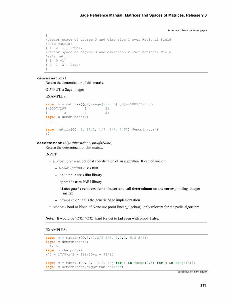
Sage Reference Manual: Matrices and Spaces of Matrices, Release 9.0
(continued from previous page)
[(Vector space of degree 3 and dimension 1 over Rational FieldBasis matrix:[ 1 -2 1], True),(Vector space of degree 3 and dimension 2 over Rational FieldBasis matrix:[ 1 0 -1][ 0 1 2], True)]
denominator()Return the denominator of this matrix.
OUTPUT: a Sage Integer
EXAMPLES:
sage: b = matrix(QQ,2,range(6)); b[0,0]=-5007/293; b[-5007/293 1 2][ 3 4 5]sage: b.denominator()293
sage: matrix(QQ, 2, [1/2, 1/3, 1/4, 1/5]).denominator()60
determinant(algorithm=None, proof=None)Return the determinant of this matrix.
INPUT:
• algorithm – an optional specification of an algorithm. It can be one of
– None: (default) uses flint
– 'flint': uses flint library
– 'pari': uses PARI library
– 'integer': removes denominator and call determinant on the corresponding integermatrix
– 'generic': calls the generic Sage implementation
• proof - bool or None; if None use proof.linear_algebra(); only relevant for the padic algorithm.
Note: It would be VERY VERY hard for det to fail even with proof=False.
EXAMPLES:
sage: m = matrix(QQ,3,[1,2/3,4/5, 2,2,2, 5,3,2/5])sage: m.determinant()-34/15sage: m.charpoly()x^3 - 17/5*x^2 - 122/15*x + 34/15
sage: m = matrix(QQ, 3, [(1/i)**j for i in range(2,5) for j in range(3)])sage: m.determinant(algorithm="flint")
(continues on next page)
371
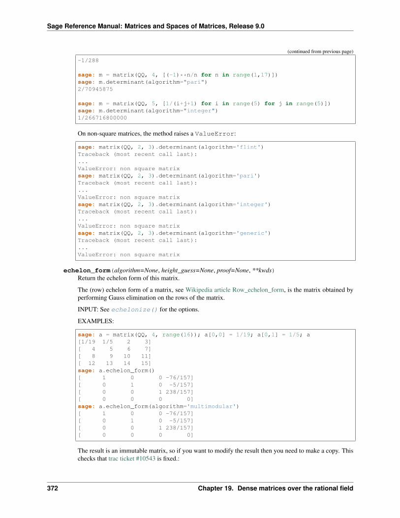
Sage Reference Manual: Matrices and Spaces of Matrices, Release 9.0
(continued from previous page)
-1/288
sage: m = matrix(QQ, 4, [(-1)**n/n for n in range(1,17)])sage: m.determinant(algorithm="pari")2/70945875
sage: m = matrix(QQ, 5, [1/(i+j+1) for i in range(5) for j in range(5)])sage: m.determinant(algorithm="integer")1/266716800000
On non-square matrices, the method raises a ValueError:
sage: matrix(QQ, 2, 3).determinant(algorithm='flint')Traceback (most recent call last):...ValueError: non square matrixsage: matrix(QQ, 2, 3).determinant(algorithm='pari')Traceback (most recent call last):...ValueError: non square matrixsage: matrix(QQ, 2, 3).determinant(algorithm='integer')Traceback (most recent call last):...ValueError: non square matrixsage: matrix(QQ, 2, 3).determinant(algorithm='generic')Traceback (most recent call last):...ValueError: non square matrix
echelon_form(algorithm=None, height_guess=None, proof=None, **kwds)Return the echelon form of this matrix.
The (row) echelon form of a matrix, see Wikipedia article Row_echelon_form, is the matrix obtained byperforming Gauss elimination on the rows of the matrix.
INPUT: See echelonize() for the options.
EXAMPLES:
sage: a = matrix(QQ, 4, range(16)); a[0,0] = 1/19; a[0,1] = 1/5; a[1/19 1/5 2 3][ 4 5 6 7][ 8 9 10 11][ 12 13 14 15]sage: a.echelon_form()[ 1 0 0 -76/157][ 0 1 0 -5/157][ 0 0 1 238/157][ 0 0 0 0]sage: a.echelon_form(algorithm='multimodular')[ 1 0 0 -76/157][ 0 1 0 -5/157][ 0 0 1 238/157][ 0 0 0 0]
The result is an immutable matrix, so if you want to modify the result then you need to make a copy. Thischecks that trac ticket #10543 is fixed.:
372 Chapter 19. Dense matrices over the rational field
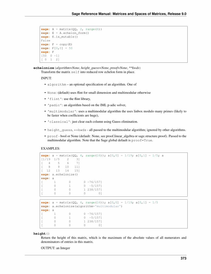
Sage Reference Manual: Matrices and Spaces of Matrices, Release 9.0
sage: A = matrix(QQ, 2, range(6))sage: E = A.echelon_form()sage: E.is_mutable()Falsesage: F = copy(E)sage: F[0,0] = 50sage: F[50 0 -1][ 0 1 2]
echelonize(algorithm=None, height_guess=None, proof=None, **kwds)Transform the matrix self into reduced row echelon form in place.
INPUT:
• algorithm – an optional specification of an algorithm. One of
• None: (default) uses flint for small dimension and multimodular otherwise
• 'flint': use the flint library,
• 'padic': an algorithm based on the IML p-adic solver,
• 'multimodular': uses a multimodular algorithm the uses linbox modulo many primes (likely tobe faster when coefficients are huge),
• 'classical': just clear each column using Gauss elimination.
• height_guess, **kwds - all passed to the multimodular algorithm; ignored by other algorithms.
• proof - bool or None (default: None, see proof.linear_algebra or sage.structure.proof). Passed to themultimodular algorithm. Note that the Sage global default is proof=True.
EXAMPLES:
sage: a = matrix(QQ, 4, range(16)); a[0,0] = 1/19; a[0,1] = 1/5; a[1/19 1/5 2 3][ 4 5 6 7][ 8 9 10 11][ 12 13 14 15]sage: a.echelonize()sage: a[ 1 0 0 -76/157][ 0 1 0 -5/157][ 0 0 1 238/157][ 0 0 0 0]
sage: a = matrix(QQ, 4, range(16)); a[0,0] = 1/19; a[0,1] = 1/5sage: a.echelonize(algorithm='multimodular')sage: a[ 1 0 0 -76/157][ 0 1 0 -5/157][ 0 0 1 238/157][ 0 0 0 0]
height()Return the height of this matrix, which is the maximum of the absolute values of all numerators anddenominators of entries in this matrix.
OUTPUT: an Integer
373
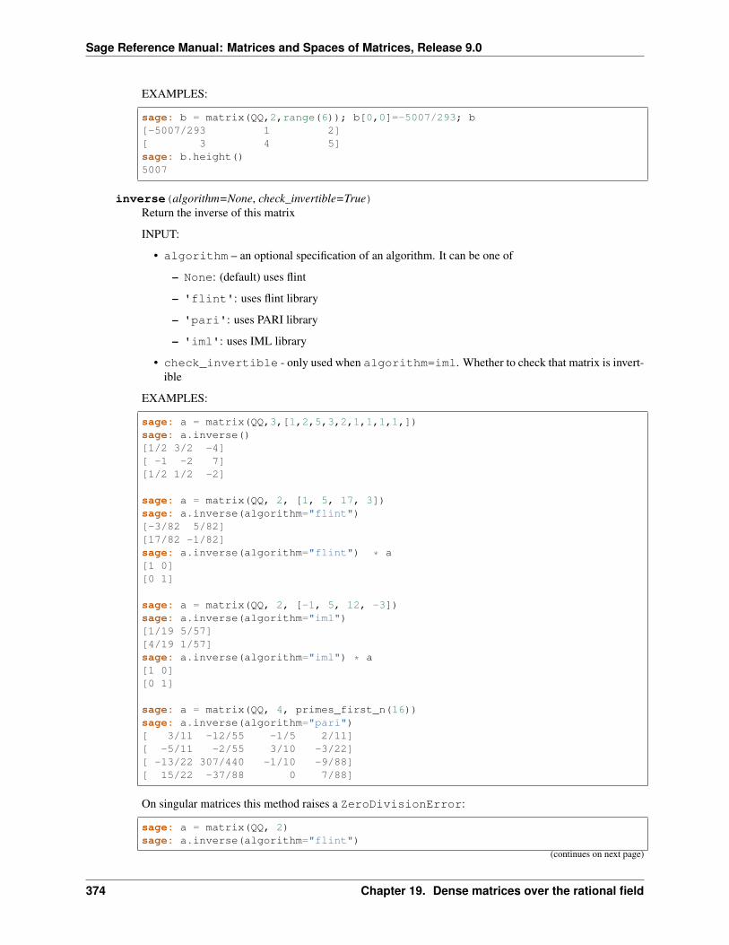
Sage Reference Manual: Matrices and Spaces of Matrices, Release 9.0
EXAMPLES:
sage: b = matrix(QQ,2,range(6)); b[0,0]=-5007/293; b[-5007/293 1 2][ 3 4 5]sage: b.height()5007
inverse(algorithm=None, check_invertible=True)Return the inverse of this matrix
INPUT:
• algorithm – an optional specification of an algorithm. It can be one of
– None: (default) uses flint
– 'flint': uses flint library
– 'pari': uses PARI library
– 'iml': uses IML library
• check_invertible - only used when algorithm=iml. Whether to check that matrix is invert-ible
EXAMPLES:
sage: a = matrix(QQ,3,[1,2,5,3,2,1,1,1,1,])sage: a.inverse()[1/2 3/2 -4][ -1 -2 7][1/2 1/2 -2]
sage: a = matrix(QQ, 2, [1, 5, 17, 3])sage: a.inverse(algorithm="flint")[-3/82 5/82][17/82 -1/82]sage: a.inverse(algorithm="flint") * a[1 0][0 1]
sage: a = matrix(QQ, 2, [-1, 5, 12, -3])sage: a.inverse(algorithm="iml")[1/19 5/57][4/19 1/57]sage: a.inverse(algorithm="iml") * a[1 0][0 1]
sage: a = matrix(QQ, 4, primes_first_n(16))sage: a.inverse(algorithm="pari")[ 3/11 -12/55 -1/5 2/11][ -5/11 -2/55 3/10 -3/22][ -13/22 307/440 -1/10 -9/88][ 15/22 -37/88 0 7/88]
On singular matrices this method raises a ZeroDivisionError:
sage: a = matrix(QQ, 2)sage: a.inverse(algorithm="flint")
(continues on next page)
374 Chapter 19. Dense matrices over the rational field
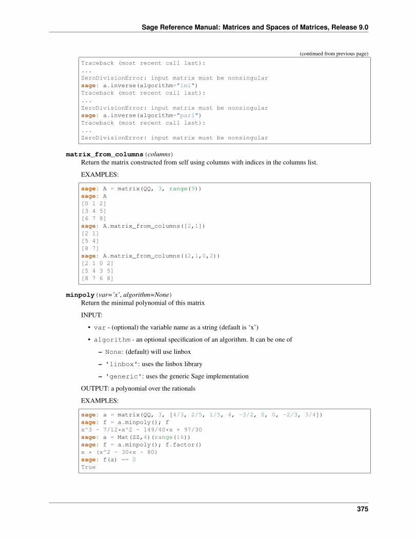
Sage Reference Manual: Matrices and Spaces of Matrices, Release 9.0
(continued from previous page)
Traceback (most recent call last):...ZeroDivisionError: input matrix must be nonsingularsage: a.inverse(algorithm="iml")Traceback (most recent call last):...ZeroDivisionError: input matrix must be nonsingularsage: a.inverse(algorithm="pari")Traceback (most recent call last):...ZeroDivisionError: input matrix must be nonsingular
matrix_from_columns(columns)Return the matrix constructed from self using columns with indices in the columns list.
EXAMPLES:
sage: A = matrix(QQ, 3, range(9))sage: A[0 1 2][3 4 5][6 7 8]sage: A.matrix_from_columns([2,1])[2 1][5 4][8 7]sage: A.matrix_from_columns((2,1,0,2))[2 1 0 2][5 4 3 5][8 7 6 8]
minpoly(var=’x’, algorithm=None)Return the minimal polynomial of this matrix
INPUT:
• var - (optional) the variable name as a string (default is ‘x’)
• algorithm - an optional specification of an algorithm. It can be one of
– None: (default) will use linbox
– 'linbox': uses the linbox library
– 'generic': uses the generic Sage implementation
OUTPUT: a polynomial over the rationals
EXAMPLES:
sage: a = matrix(QQ, 3, [4/3, 2/5, 1/5, 4, -3/2, 0, 0, -2/3, 3/4])sage: f = a.minpoly(); fx^3 - 7/12*x^2 - 149/40*x + 97/30sage: a = Mat(ZZ,4)(range(16))sage: f = a.minpoly(); f.factor()x * (x^2 - 30*x - 80)sage: f(a) == 0True
375
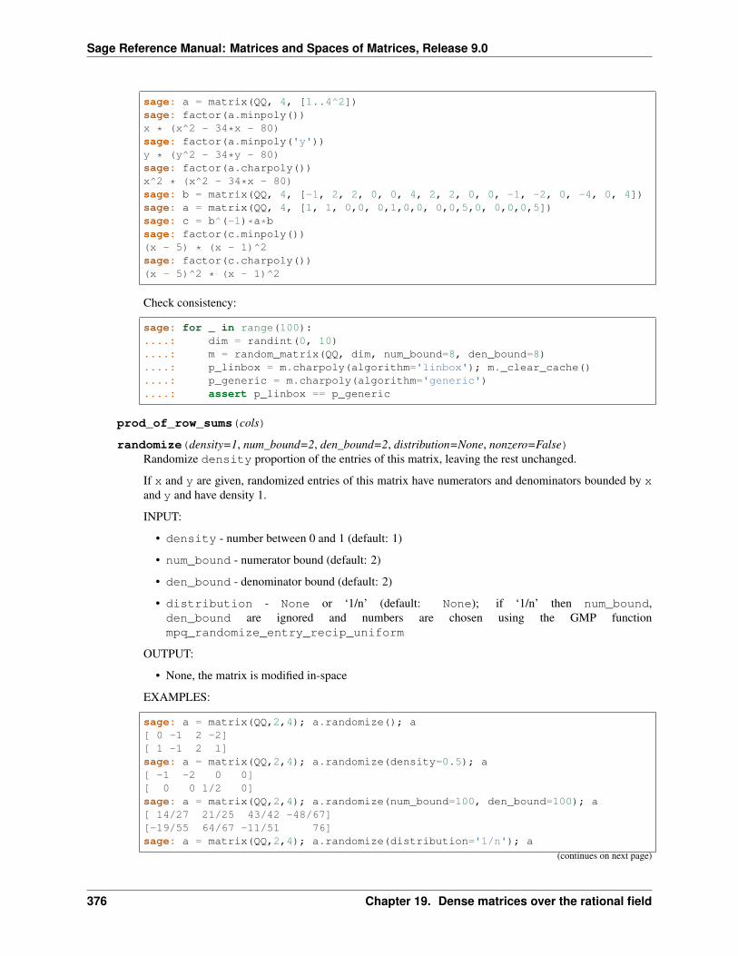
Sage Reference Manual: Matrices and Spaces of Matrices, Release 9.0
sage: a = matrix(QQ, 4, [1..4^2])sage: factor(a.minpoly())x * (x^2 - 34*x - 80)sage: factor(a.minpoly('y'))y * (y^2 - 34*y - 80)sage: factor(a.charpoly())x^2 * (x^2 - 34*x - 80)sage: b = matrix(QQ, 4, [-1, 2, 2, 0, 0, 4, 2, 2, 0, 0, -1, -2, 0, -4, 0, 4])sage: a = matrix(QQ, 4, [1, 1, 0,0, 0,1,0,0, 0,0,5,0, 0,0,0,5])sage: c = b^(-1)*a*bsage: factor(c.minpoly())(x - 5) * (x - 1)^2sage: factor(c.charpoly())(x - 5)^2 * (x - 1)^2
Check consistency:
sage: for _ in range(100):....: dim = randint(0, 10)....: m = random_matrix(QQ, dim, num_bound=8, den_bound=8)....: p_linbox = m.charpoly(algorithm='linbox'); m._clear_cache()....: p_generic = m.charpoly(algorithm='generic')....: assert p_linbox == p_generic
prod_of_row_sums(cols)
randomize(density=1, num_bound=2, den_bound=2, distribution=None, nonzero=False)Randomize density proportion of the entries of this matrix, leaving the rest unchanged.
If x and y are given, randomized entries of this matrix have numerators and denominators bounded by xand y and have density 1.
INPUT:
• density - number between 0 and 1 (default: 1)
• num_bound - numerator bound (default: 2)
• den_bound - denominator bound (default: 2)
• distribution - None or ‘1/n’ (default: None); if ‘1/n’ then num_bound,den_bound are ignored and numbers are chosen using the GMP functionmpq_randomize_entry_recip_uniform
OUTPUT:
• None, the matrix is modified in-space
EXAMPLES:
sage: a = matrix(QQ,2,4); a.randomize(); a[ 0 -1 2 -2][ 1 -1 2 1]sage: a = matrix(QQ,2,4); a.randomize(density=0.5); a[ -1 -2 0 0][ 0 0 1/2 0]sage: a = matrix(QQ,2,4); a.randomize(num_bound=100, den_bound=100); a[ 14/27 21/25 43/42 -48/67][-19/55 64/67 -11/51 76]sage: a = matrix(QQ,2,4); a.randomize(distribution='1/n'); a
(continues on next page)
376 Chapter 19. Dense matrices over the rational field

Sage Reference Manual: Matrices and Spaces of Matrices, Release 9.0
(continued from previous page)
[ 3 1/9 1/2 1/4][ 1 1/39 2 -1955/2]
rank(algorithm=None)Return the rank of this matrix.
INPUT:
• algorithm - an optional specification of an algorithm. One of
– None: (default) will use flint
– 'flint': uses the flint library
– 'pari': uses the PARI library
– 'integer': eliminate denominators and calls the rank function on the corresponding integermatrix
EXAMPLES:
sage: matrix(QQ,3,[1..9]).rank()2sage: matrix(QQ,100,[1..100^2]).rank()2
row(i, from_list=False)Return the i-th row of this matrix as a dense vector.
INPUT:
• i - integer
• from_list - ignored
EXAMPLES:
sage: m = matrix(QQ, 2, [1/5, -2/3, 3/4, 4/9])sage: m.row(0)(1/5, -2/3)sage: m.row(1)(3/4, 4/9)sage: m.row(1, from_list=True)(3/4, 4/9)sage: m.row(-2)(1/5, -2/3)
sage: m.row(2)Traceback (most recent call last):...IndexError: row index out of rangesage: m.row(-3)Traceback (most recent call last):...IndexError: row index out of range
set_row_to_multiple_of_row(i, j, s)Set row i equal to s times row j.
EXAMPLES:
377
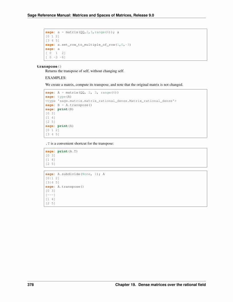
Sage Reference Manual: Matrices and Spaces of Matrices, Release 9.0
sage: a = matrix(QQ,2,3,range(6)); a[0 1 2][3 4 5]sage: a.set_row_to_multiple_of_row(1,0,-3)sage: a[ 0 1 2][ 0 -3 -6]
transpose()Returns the transpose of self, without changing self.
EXAMPLES:
We create a matrix, compute its transpose, and note that the original matrix is not changed.
sage: A = matrix(QQ, 2, 3, range(6))sage: type(A)<type 'sage.matrix.matrix_rational_dense.Matrix_rational_dense'>sage: B = A.transpose()sage: print(B)[0 3][1 4][2 5]sage: print(A)[0 1 2][3 4 5]
.T is a convenient shortcut for the transpose:
sage: print(A.T)[0 3][1 4][2 5]
sage: A.subdivide(None, 1); A[0|1 2][3|4 5]sage: A.transpose()[0 3][---][1 4][2 5]
378 Chapter 19. Dense matrices over the rational field
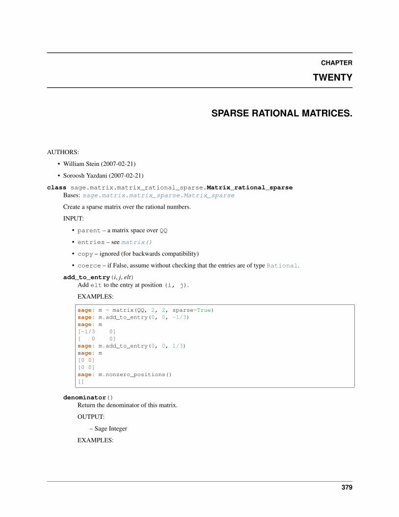
CHAPTER
TWENTY
SPARSE RATIONAL MATRICES.
AUTHORS:
• William Stein (2007-02-21)
• Soroosh Yazdani (2007-02-21)
class sage.matrix.matrix_rational_sparse.Matrix_rational_sparseBases: sage.matrix.matrix_sparse.Matrix_sparse
Create a sparse matrix over the rational numbers.
INPUT:
• parent – a matrix space over QQ
• entries – see matrix()
• copy – ignored (for backwards compatibility)
• coerce – if False, assume without checking that the entries are of type Rational.
add_to_entry(i, j, elt)Add elt to the entry at position (i, j).
EXAMPLES:
sage: m = matrix(QQ, 2, 2, sparse=True)sage: m.add_to_entry(0, 0, -1/3)sage: m[-1/3 0][ 0 0]sage: m.add_to_entry(0, 0, 1/3)sage: m[0 0][0 0]sage: m.nonzero_positions()[]
denominator()Return the denominator of this matrix.
OUTPUT:
– Sage Integer
EXAMPLES:
379

Sage Reference Manual: Matrices and Spaces of Matrices, Release 9.0
sage: b = matrix(QQ,2,range(6)); b[0,0]=-5007/293; b[-5007/293 1 2][ 3 4 5]sage: b.denominator()293
dense_matrix()Return dense version of this matrix.
EXAMPLES:
sage: a = matrix(QQ,2,[1..4],sparse=True); type(a)<type 'sage.matrix.matrix_rational_sparse.Matrix_rational_sparse'>sage: type(a.dense_matrix())<type 'sage.matrix.matrix_rational_dense.Matrix_rational_dense'>sage: a.dense_matrix()[1 2][3 4]
Check that subdivisions are preserved when converting between dense and sparse matrices:
sage: a.subdivide([1,1], [2])sage: b = a.dense_matrix().sparse_matrix().dense_matrix()sage: b.subdivisions() == a.subdivisions()True
echelon_form(algorithm=’default’, height_guess=None, proof=True, **kwds)INPUT:
height_guess, proof, **kwds – all passed to the multimodular algorithm; ignored by the p-adicalgorithm.
OUTPUT:
self is no in reduced row echelon form.
EXAMPLES:
sage: a = matrix(QQ, 4, range(16), sparse=True); a[0,0] = 1/19; a[0,1] = 1/5;→˓a[1/19 1/5 2 3][ 4 5 6 7][ 8 9 10 11][ 12 13 14 15]sage: a.echelon_form()[ 1 0 0 -76/157][ 0 1 0 -5/157][ 0 0 1 238/157][ 0 0 0 0]
echelonize(height_guess=None, proof=True, **kwds)Transform the matrix self into reduced row echelon form in place.
INPUT:
height_guess, proof, **kwds – all passed to the multimodular algorithm; ignored by the p-adicalgorithm.
OUTPUT:
Nothing. The matrix self is transformed into reduced row echelon form in place.
380 Chapter 20. Sparse rational matrices.
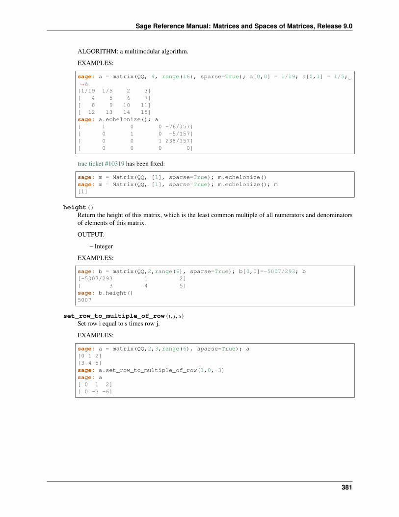
Sage Reference Manual: Matrices and Spaces of Matrices, Release 9.0
ALGORITHM: a multimodular algorithm.
EXAMPLES:
sage: a = matrix(QQ, 4, range(16), sparse=True); a[0,0] = 1/19; a[0,1] = 1/5;→˓a[1/19 1/5 2 3][ 4 5 6 7][ 8 9 10 11][ 12 13 14 15]sage: a.echelonize(); a[ 1 0 0 -76/157][ 0 1 0 -5/157][ 0 0 1 238/157][ 0 0 0 0]
trac ticket #10319 has been fixed:
sage: m = Matrix(QQ, [1], sparse=True); m.echelonize()sage: m = Matrix(QQ, [1], sparse=True); m.echelonize(); m[1]
height()Return the height of this matrix, which is the least common multiple of all numerators and denominatorsof elements of this matrix.
OUTPUT:
– Integer
EXAMPLES:
sage: b = matrix(QQ,2,range(6), sparse=True); b[0,0]=-5007/293; b[-5007/293 1 2][ 3 4 5]sage: b.height()5007
set_row_to_multiple_of_row(i, j, s)Set row i equal to s times row j.
EXAMPLES:
sage: a = matrix(QQ,2,3,range(6), sparse=True); a[0 1 2][3 4 5]sage: a.set_row_to_multiple_of_row(1,0,-3)sage: a[ 0 1 2][ 0 -3 -6]
381

Sage Reference Manual: Matrices and Spaces of Matrices, Release 9.0
382 Chapter 20. Sparse rational matrices.
CHAPTER
TWENTYONE
DENSE MATRICES USING A NUMPY BACKEND.
This serves as a base class for dense matrices over Real Double Field and Complex Double Field.
AUTHORS:
• Jason Grout, Sep 2008: switch to NumPy backend, factored out the Matrix_double_dense class
• Josh Kantor
• William Stein: many bug fixes and touch ups.
EXAMPLES:
sage: b = Mat(RDF,2,3).basis()sage: b[0,0][1.0 0.0 0.0][0.0 0.0 0.0]
We deal with the case of zero rows or zero columns:
sage: m = MatrixSpace(RDF,0,3)sage: m.zero_matrix()[]
class sage.matrix.matrix_double_dense.Matrix_double_denseBases: sage.matrix.matrix_dense.Matrix_dense
Base class for matrices over the Real Double Field and the Complex Double Field. These are supposed tobe fast matrix operations using C doubles. Most operations are implemented using numpy which will call theunderlying BLAS on the system.
This class cannot be instantiated on its own. The numpy matrix creation depends on several variables that areset in the subclasses.
EXAMPLES:
sage: m = Matrix(RDF, [[1,2],[3,4]])sage: m**2[ 7.0 10.0][15.0 22.0]sage: m^(-1) # rel tol 1e-15[-1.9999999999999996 0.9999999999999998][ 1.4999999999999998 -0.4999999999999999]
LU()Return a decomposition of the (row-permuted) matrix as a product of a lower-triangular matrix (“L”) andan upper-triangular matrix (“U”).
383
Sage Reference Manual: Matrices and Spaces of Matrices, Release 9.0
OUTPUT:
For an 𝑚× 𝑛 matrix A this method returns a triple of immutable matrices P, L, U such that
• P*A = L*U
• P is a square permutation matrix, of size 𝑚×𝑚, so is all zeroes, but with exactly a single one in eachrow and each column.
• L is lower-triangular, square of size 𝑚×𝑚, with every diagonal entry equal to one.
• U is upper-triangular with size 𝑚× 𝑛, i.e. entries below the “diagonal” are all zero.
The computed decomposition is cached and returned on subsequent calls, thus requiring the results to beimmutable.
Effectively, P permutes the rows of A. Then L can be viewed as a sequence of row operations on thismatrix, where each operation is adding a multiple of a row to a subsequent row. There is no scaling (thus1’s on the diagonal of L) and no row-swapping (P does that). As a result U is close to being the result ofGaussian-elimination. However, round-off errors can make it hard to determine the zero entries of U.
Note: Sometimes this decomposition is written as A=P*L*U, where P represents the inverse permutationand is the matrix inverse of the P returned by this method. The computation of this matrix inverse can beaccomplished quickly with just a transpose as the matrix is orthogonal/unitary.
EXAMPLES:
sage: m = matrix(RDF,4,range(16))sage: P,L,U = m.LU()sage: P*m[12.0 13.0 14.0 15.0][ 0.0 1.0 2.0 3.0][ 8.0 9.0 10.0 11.0][ 4.0 5.0 6.0 7.0]sage: L*U # rel tol 2e-16[12.0 13.0 14.0 15.0][ 0.0 1.0 2.0 3.0][ 8.0 9.0 10.0 11.0][ 4.0 5.0 6.0 7.0]
trac ticket #10839 made this routine available for rectangular matrices.
sage: A = matrix(RDF, 5, 6, range(30)); A[ 0.0 1.0 2.0 3.0 4.0 5.0][ 6.0 7.0 8.0 9.0 10.0 11.0][12.0 13.0 14.0 15.0 16.0 17.0][18.0 19.0 20.0 21.0 22.0 23.0][24.0 25.0 26.0 27.0 28.0 29.0]sage: P, L, U = A.LU()sage: P[0.0 0.0 0.0 0.0 1.0][1.0 0.0 0.0 0.0 0.0][0.0 0.0 1.0 0.0 0.0][0.0 0.0 0.0 1.0 0.0][0.0 1.0 0.0 0.0 0.0]sage: L.zero_at(0) # Use zero_at(0) to get rid of signed zeros[ 1.0 0.0 0.0 0.0 0.0][ 0.0 1.0 0.0 0.0 0.0]
(continues on next page)
384 Chapter 21. Dense matrices using a NumPy backend.
Sage Reference Manual: Matrices and Spaces of Matrices, Release 9.0
(continued from previous page)
[ 0.5 0.5 1.0 0.0 0.0][0.75 0.25 0.0 1.0 0.0][0.25 0.75 0.0 0.0 1.0]sage: U.zero_at(0) # Use zero_at(0) to get rid of signed zeros[24.0 25.0 26.0 27.0 28.0 29.0][ 0.0 1.0 2.0 3.0 4.0 5.0][ 0.0 0.0 0.0 0.0 0.0 0.0][ 0.0 0.0 0.0 0.0 0.0 0.0][ 0.0 0.0 0.0 0.0 0.0 0.0]sage: P*A-L*U[0.0 0.0 0.0 0.0 0.0 0.0][0.0 0.0 0.0 0.0 0.0 0.0][0.0 0.0 0.0 0.0 0.0 0.0][0.0 0.0 0.0 0.0 0.0 0.0][0.0 0.0 0.0 0.0 0.0 0.0]sage: P.transpose()*L*U[ 0.0 1.0 2.0 3.0 4.0 5.0][ 6.0 7.0 8.0 9.0 10.0 11.0][12.0 13.0 14.0 15.0 16.0 17.0][18.0 19.0 20.0 21.0 22.0 23.0][24.0 25.0 26.0 27.0 28.0 29.0]
Trivial cases return matrices of the right size and characteristics.
sage: A = matrix(RDF, 5, 0)sage: P, L, U = A.LU()sage: P.parent()Full MatrixSpace of 5 by 5 dense matrices over Real Double Fieldsage: L.parent()Full MatrixSpace of 5 by 5 dense matrices over Real Double Fieldsage: U.parent()Full MatrixSpace of 5 by 0 dense matrices over Real Double Fieldsage: P*A-L*U[]
The results are immutable since they are cached.
sage: P, L, U = matrix(RDF, 2, 2, range(4)).LU()sage: L[0,0] = 0Traceback (most recent call last):
...ValueError: matrix is immutable; please change a copy instead (i.e., use→˓copy(M) to change a copy of M).sage: P[0,0] = 0Traceback (most recent call last):
...ValueError: matrix is immutable; please change a copy instead (i.e., use→˓copy(M) to change a copy of M).sage: U[0,0] = 0Traceback (most recent call last):
...ValueError: matrix is immutable; please change a copy instead (i.e., use→˓copy(M) to change a copy of M).
LU_valid()Return True if the LU form of this matrix has already been computed.
EXAMPLES:
385
Sage Reference Manual: Matrices and Spaces of Matrices, Release 9.0
sage: A = random_matrix(RDF,3) ; A.LU_valid()Falsesage: P, L, U = A.LU()sage: A.LU_valid()True
QR()Return a factorization into a unitary matrix and an upper-triangular matrix.
INPUT:
Any matrix over RDF or CDF.
OUTPUT:
Q, R – a pair of matrices such that if 𝐴 is the original matrix, then
𝐴 = 𝑄𝑅, 𝑄*𝑄 = 𝐼
where 𝑅 is upper-triangular. 𝑄* is the conjugate-transpose in the complex case, and just the transposein the real case. So 𝑄 is a unitary matrix (or rather, orthogonal, in the real case), or equivalently 𝑄 hasorthogonal columns. For a matrix of full rank this factorization is unique up to adjustments via multiplesof rows and columns by multiples with scalars having modulus 1. So in the full-rank case, 𝑅 is unique ifthe diagonal entries are required to be positive real numbers.
The resulting decomposition is cached.
ALGORITHM:
Calls “linalg.qr” from SciPy, which is in turn an interface to LAPACK routines.
EXAMPLES:
Over the reals, the inverse of Q is its transpose, since including a conjugate has no effect. In the real case,we say Q is orthogonal.
sage: A = matrix(RDF, [[-2, 0, -4, -1, -1],....: [-2, 1, -6, -3, -1],....: [1, 1, 7, 4, 5],....: [3, 0, 8, 3, 3],....: [-1, 1, -6, -6, 5]])sage: Q, R = A.QR()
At this point, Q is only well-defined up to the signs of its columns, and similarly for R and its rows, so wenormalize them:
sage: Qnorm = Q._normalize_columns()sage: Rnorm = R._normalize_rows()sage: Qnorm.round(6).zero_at(10^-6)[ 0.458831 0.126051 0.381212 0.394574 0.68744][ 0.458831 -0.47269 -0.051983 -0.717294 0.220963][-0.229416 -0.661766 0.661923 0.180872 -0.196411][-0.688247 -0.189076 -0.204468 -0.09663 0.662889][ 0.229416 -0.535715 -0.609939 0.536422 -0.024551]sage: Rnorm.round(6).zero_at(10^-6)[ 4.358899 -0.458831 13.076697 6.194225 2.982405][ 0.0 1.670172 0.598741 -1.29202 6.207997][ 0.0 0.0 5.444402 5.468661 -0.682716][ 0.0 0.0 0.0 1.027626 -3.6193][ 0.0 0.0 0.0 0.0 0.024551]
(continues on next page)
386 Chapter 21. Dense matrices using a NumPy backend.
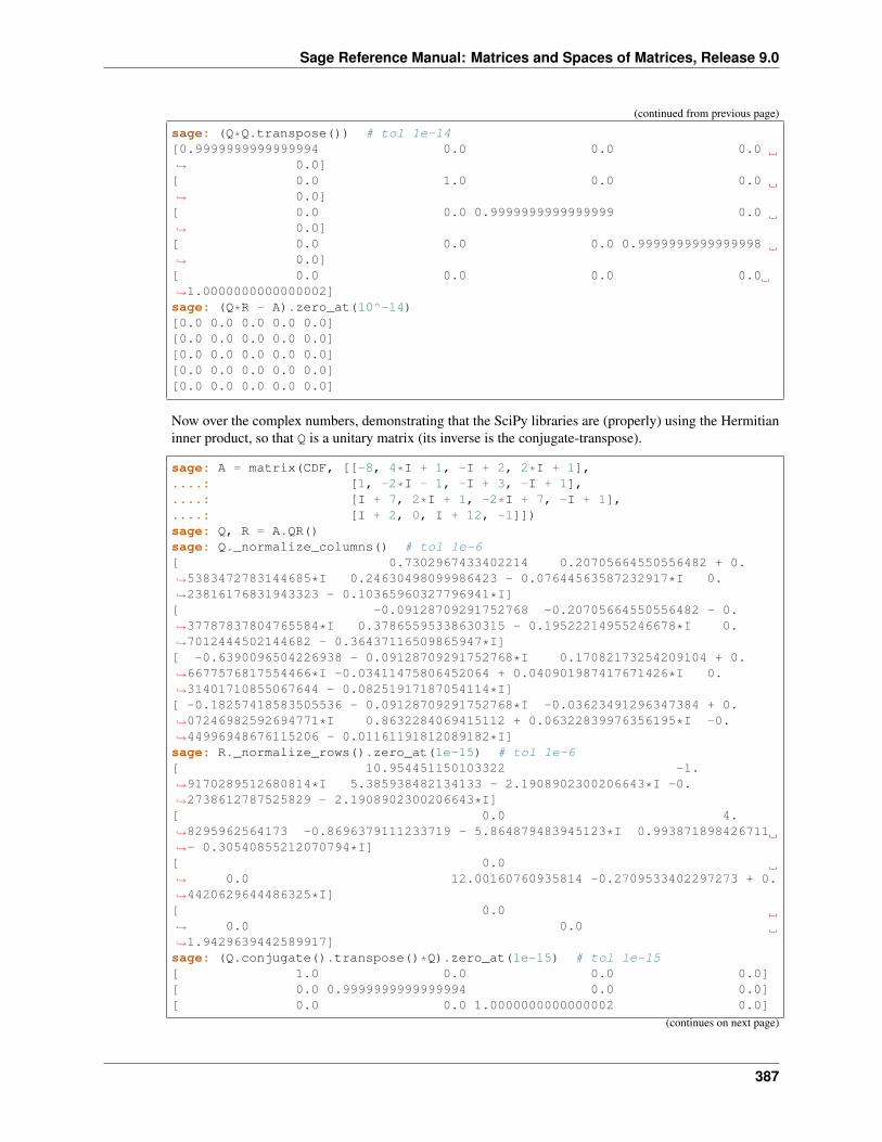
Sage Reference Manual: Matrices and Spaces of Matrices, Release 9.0
(continued from previous page)
sage: (Q*Q.transpose()) # tol 1e-14[0.9999999999999994 0.0 0.0 0.0→˓ 0.0][ 0.0 1.0 0.0 0.0→˓ 0.0][ 0.0 0.0 0.9999999999999999 0.0→˓ 0.0][ 0.0 0.0 0.0 0.9999999999999998→˓ 0.0][ 0.0 0.0 0.0 0.0→˓1.0000000000000002]sage: (Q*R - A).zero_at(10^-14)[0.0 0.0 0.0 0.0 0.0][0.0 0.0 0.0 0.0 0.0][0.0 0.0 0.0 0.0 0.0][0.0 0.0 0.0 0.0 0.0][0.0 0.0 0.0 0.0 0.0]
Now over the complex numbers, demonstrating that the SciPy libraries are (properly) using the Hermitianinner product, so that Q is a unitary matrix (its inverse is the conjugate-transpose).
sage: A = matrix(CDF, [[-8, 4*I + 1, -I + 2, 2*I + 1],....: [1, -2*I - 1, -I + 3, -I + 1],....: [I + 7, 2*I + 1, -2*I + 7, -I + 1],....: [I + 2, 0, I + 12, -1]])sage: Q, R = A.QR()sage: Q._normalize_columns() # tol 1e-6[ 0.7302967433402214 0.20705664550556482 + 0.→˓5383472783144685*I 0.24630498099986423 - 0.07644563587232917*I 0.→˓23816176831943323 - 0.10365960327796941*I][ -0.09128709291752768 -0.20705664550556482 - 0.→˓37787837804765584*I 0.37865595338630315 - 0.19522214955246678*I 0.→˓7012444502144682 - 0.36437116509865947*I][ -0.6390096504226938 - 0.09128709291752768*I 0.17082173254209104 + 0.→˓6677576817554466*I -0.03411475806452064 + 0.040901987417671426*I 0.→˓31401710855067644 - 0.08251917187054114*I][ -0.18257418583505536 - 0.09128709291752768*I -0.03623491296347384 + 0.→˓07246982592694771*I 0.8632284069415112 + 0.06322839976356195*I -0.→˓44996948676115206 - 0.01161191812089182*I]sage: R._normalize_rows().zero_at(1e-15) # tol 1e-6[ 10.954451150103322 -1.→˓9170289512680814*I 5.385938482134133 - 2.1908902300206643*I -0.→˓2738612787525829 - 2.1908902300206643*I][ 0.0 4.→˓8295962564173 -0.8696379111233719 - 5.864879483945123*I 0.993871898426711→˓- 0.30540855212070794*I][ 0.0→˓ 0.0 12.00160760935814 -0.2709533402297273 + 0.→˓4420629644486325*I][ 0.0→˓ 0.0 0.0→˓1.9429639442589917]sage: (Q.conjugate().transpose()*Q).zero_at(1e-15) # tol 1e-15[ 1.0 0.0 0.0 0.0][ 0.0 0.9999999999999994 0.0 0.0][ 0.0 0.0 1.0000000000000002 0.0]
(continues on next page)
387
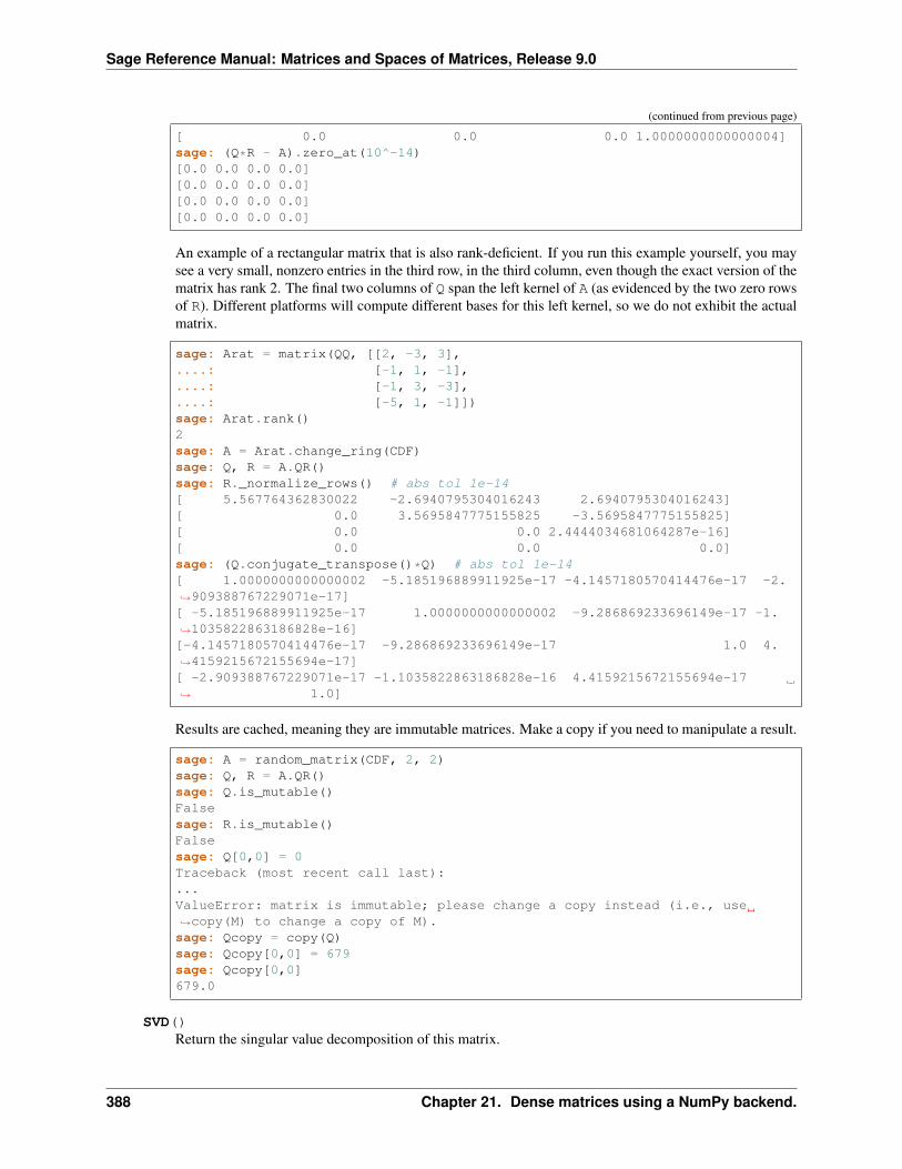
Sage Reference Manual: Matrices and Spaces of Matrices, Release 9.0
(continued from previous page)
[ 0.0 0.0 0.0 1.0000000000000004]sage: (Q*R - A).zero_at(10^-14)[0.0 0.0 0.0 0.0][0.0 0.0 0.0 0.0][0.0 0.0 0.0 0.0][0.0 0.0 0.0 0.0]
An example of a rectangular matrix that is also rank-deficient. If you run this example yourself, you maysee a very small, nonzero entries in the third row, in the third column, even though the exact version of thematrix has rank 2. The final two columns of Q span the left kernel of A (as evidenced by the two zero rowsof R). Different platforms will compute different bases for this left kernel, so we do not exhibit the actualmatrix.
sage: Arat = matrix(QQ, [[2, -3, 3],....: [-1, 1, -1],....: [-1, 3, -3],....: [-5, 1, -1]])sage: Arat.rank()2sage: A = Arat.change_ring(CDF)sage: Q, R = A.QR()sage: R._normalize_rows() # abs tol 1e-14[ 5.567764362830022 -2.6940795304016243 2.6940795304016243][ 0.0 3.5695847775155825 -3.5695847775155825][ 0.0 0.0 2.4444034681064287e-16][ 0.0 0.0 0.0]sage: (Q.conjugate_transpose()*Q) # abs tol 1e-14[ 1.0000000000000002 -5.185196889911925e-17 -4.1457180570414476e-17 -2.→˓909388767229071e-17][ -5.185196889911925e-17 1.0000000000000002 -9.286869233696149e-17 -1.→˓1035822863186828e-16][-4.1457180570414476e-17 -9.286869233696149e-17 1.0 4.→˓4159215672155694e-17][ -2.909388767229071e-17 -1.1035822863186828e-16 4.4159215672155694e-17→˓ 1.0]
Results are cached, meaning they are immutable matrices. Make a copy if you need to manipulate a result.
sage: A = random_matrix(CDF, 2, 2)sage: Q, R = A.QR()sage: Q.is_mutable()Falsesage: R.is_mutable()Falsesage: Q[0,0] = 0Traceback (most recent call last):...ValueError: matrix is immutable; please change a copy instead (i.e., use→˓copy(M) to change a copy of M).sage: Qcopy = copy(Q)sage: Qcopy[0,0] = 679sage: Qcopy[0,0]679.0
SVD()Return the singular value decomposition of this matrix.
388 Chapter 21. Dense matrices using a NumPy backend.
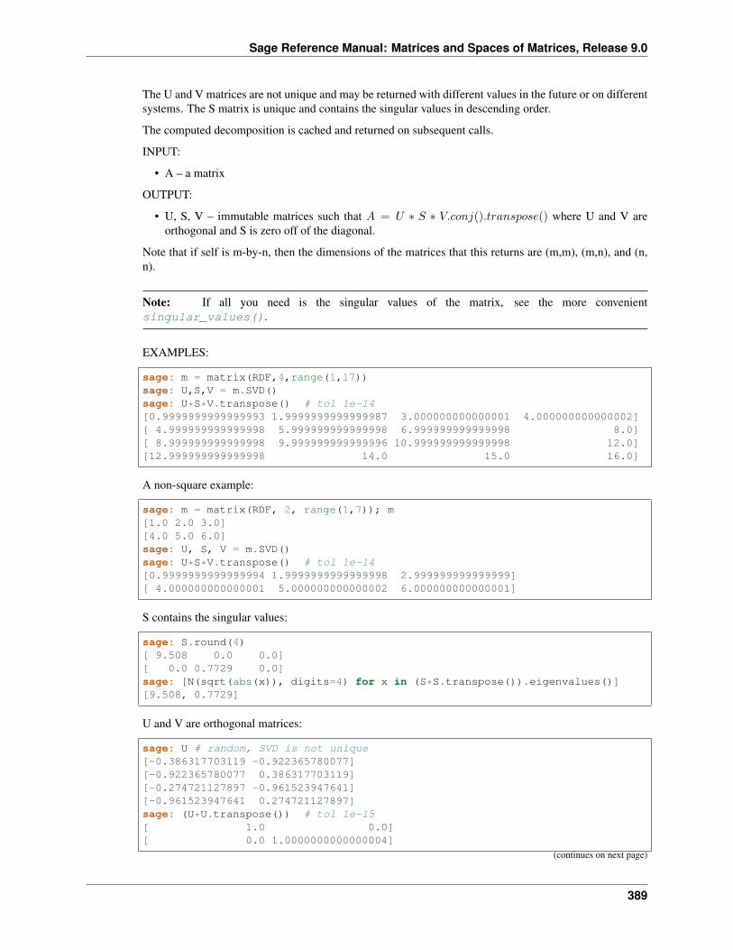
Sage Reference Manual: Matrices and Spaces of Matrices, Release 9.0
The U and V matrices are not unique and may be returned with different values in the future or on differentsystems. The S matrix is unique and contains the singular values in descending order.
The computed decomposition is cached and returned on subsequent calls.
INPUT:
• A – a matrix
OUTPUT:
• U, S, V – immutable matrices such that 𝐴 = 𝑈 * 𝑆 * 𝑉.𝑐𝑜𝑛𝑗().𝑡𝑟𝑎𝑛𝑠𝑝𝑜𝑠𝑒() where U and V areorthogonal and S is zero off of the diagonal.
Note that if self is m-by-n, then the dimensions of the matrices that this returns are (m,m), (m,n), and (n,n).
Note: If all you need is the singular values of the matrix, see the more convenientsingular_values().
EXAMPLES:
sage: m = matrix(RDF,4,range(1,17))sage: U,S,V = m.SVD()sage: U*S*V.transpose() # tol 1e-14[0.9999999999999993 1.9999999999999987 3.000000000000001 4.000000000000002][ 4.999999999999998 5.999999999999998 6.999999999999998 8.0][ 8.999999999999998 9.999999999999996 10.999999999999998 12.0][12.999999999999998 14.0 15.0 16.0]
A non-square example:
sage: m = matrix(RDF, 2, range(1,7)); m[1.0 2.0 3.0][4.0 5.0 6.0]sage: U, S, V = m.SVD()sage: U*S*V.transpose() # tol 1e-14[0.9999999999999994 1.9999999999999998 2.999999999999999][ 4.000000000000001 5.000000000000002 6.000000000000001]
S contains the singular values:
sage: S.round(4)[ 9.508 0.0 0.0][ 0.0 0.7729 0.0]sage: [N(sqrt(abs(x)), digits=4) for x in (S*S.transpose()).eigenvalues()][9.508, 0.7729]
U and V are orthogonal matrices:
sage: U # random, SVD is not unique[-0.386317703119 -0.922365780077][-0.922365780077 0.386317703119][-0.274721127897 -0.961523947641][-0.961523947641 0.274721127897]sage: (U*U.transpose()) # tol 1e-15[ 1.0 0.0][ 0.0 1.0000000000000004]
(continues on next page)
389
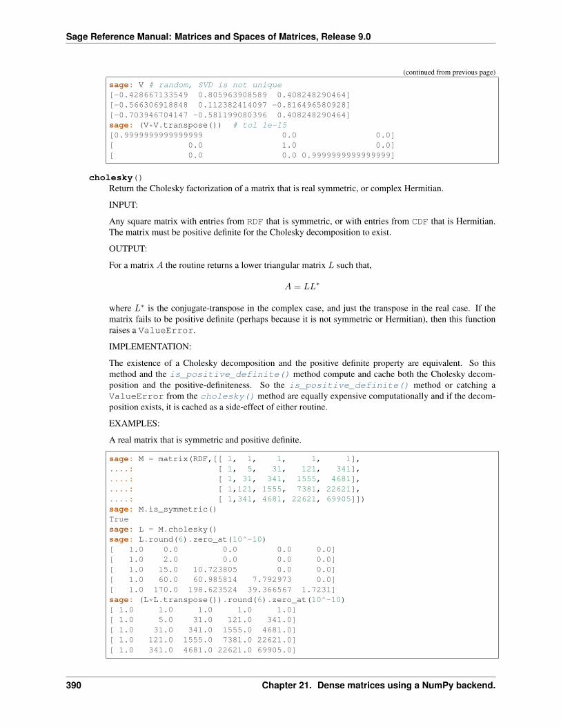
Sage Reference Manual: Matrices and Spaces of Matrices, Release 9.0
(continued from previous page)
sage: V # random, SVD is not unique[-0.428667133549 0.805963908589 0.408248290464][-0.566306918848 0.112382414097 -0.816496580928][-0.703946704147 -0.581199080396 0.408248290464]sage: (V*V.transpose()) # tol 1e-15[0.9999999999999999 0.0 0.0][ 0.0 1.0 0.0][ 0.0 0.0 0.9999999999999999]
cholesky()Return the Cholesky factorization of a matrix that is real symmetric, or complex Hermitian.
INPUT:
Any square matrix with entries from RDF that is symmetric, or with entries from CDF that is Hermitian.The matrix must be positive definite for the Cholesky decomposition to exist.
OUTPUT:
For a matrix 𝐴 the routine returns a lower triangular matrix 𝐿 such that,
𝐴 = 𝐿𝐿*
where 𝐿* is the conjugate-transpose in the complex case, and just the transpose in the real case. If thematrix fails to be positive definite (perhaps because it is not symmetric or Hermitian), then this functionraises a ValueError.
IMPLEMENTATION:
The existence of a Cholesky decomposition and the positive definite property are equivalent. So thismethod and the is_positive_definite() method compute and cache both the Cholesky decom-position and the positive-definiteness. So the is_positive_definite() method or catching aValueError from the cholesky() method are equally expensive computationally and if the decom-position exists, it is cached as a side-effect of either routine.
EXAMPLES:
A real matrix that is symmetric and positive definite.
sage: M = matrix(RDF,[[ 1, 1, 1, 1, 1],....: [ 1, 5, 31, 121, 341],....: [ 1, 31, 341, 1555, 4681],....: [ 1,121, 1555, 7381, 22621],....: [ 1,341, 4681, 22621, 69905]])sage: M.is_symmetric()Truesage: L = M.cholesky()sage: L.round(6).zero_at(10^-10)[ 1.0 0.0 0.0 0.0 0.0][ 1.0 2.0 0.0 0.0 0.0][ 1.0 15.0 10.723805 0.0 0.0][ 1.0 60.0 60.985814 7.792973 0.0][ 1.0 170.0 198.623524 39.366567 1.7231]sage: (L*L.transpose()).round(6).zero_at(10^-10)[ 1.0 1.0 1.0 1.0 1.0][ 1.0 5.0 31.0 121.0 341.0][ 1.0 31.0 341.0 1555.0 4681.0][ 1.0 121.0 1555.0 7381.0 22621.0][ 1.0 341.0 4681.0 22621.0 69905.0]
390 Chapter 21. Dense matrices using a NumPy backend.
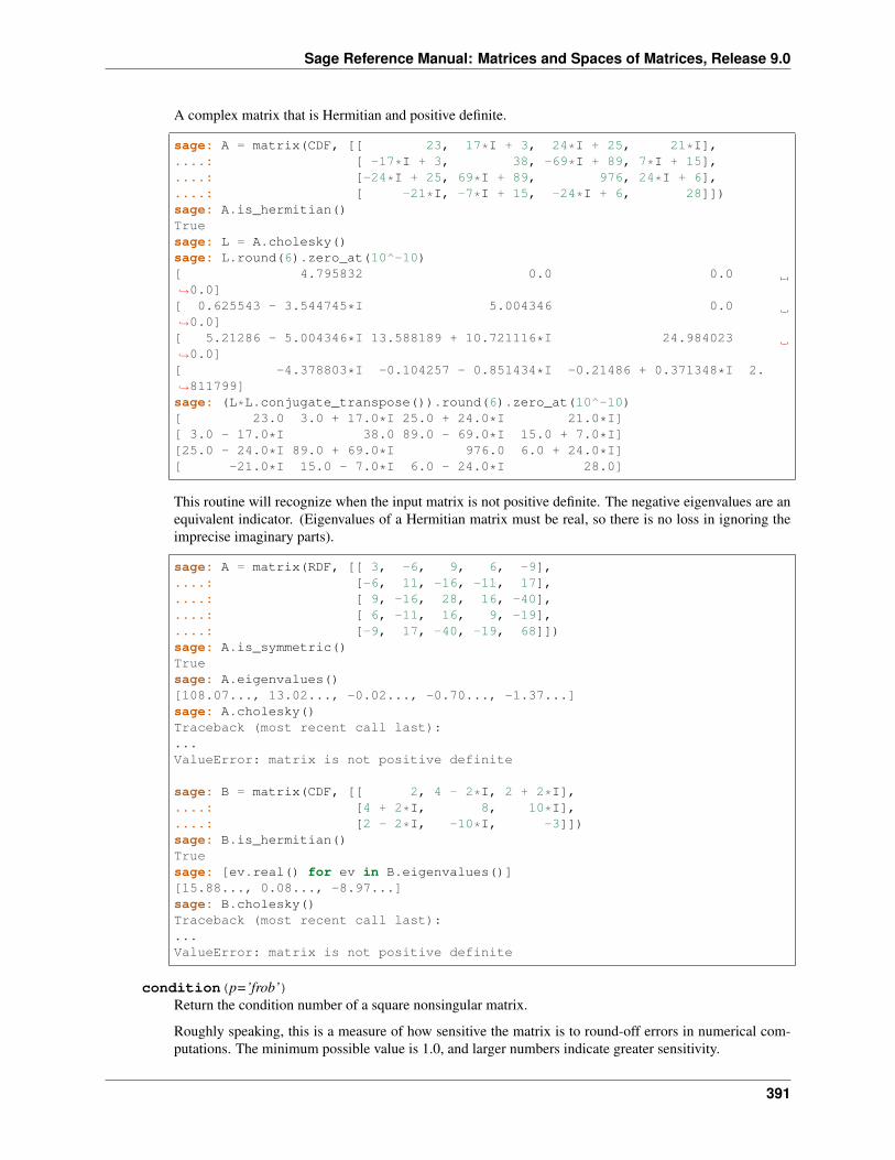
Sage Reference Manual: Matrices and Spaces of Matrices, Release 9.0
A complex matrix that is Hermitian and positive definite.
sage: A = matrix(CDF, [[ 23, 17*I + 3, 24*I + 25, 21*I],....: [ -17*I + 3, 38, -69*I + 89, 7*I + 15],....: [-24*I + 25, 69*I + 89, 976, 24*I + 6],....: [ -21*I, -7*I + 15, -24*I + 6, 28]])sage: A.is_hermitian()Truesage: L = A.cholesky()sage: L.round(6).zero_at(10^-10)[ 4.795832 0.0 0.0→˓0.0][ 0.625543 - 3.544745*I 5.004346 0.0→˓0.0][ 5.21286 - 5.004346*I 13.588189 + 10.721116*I 24.984023→˓0.0][ -4.378803*I -0.104257 - 0.851434*I -0.21486 + 0.371348*I 2.→˓811799]sage: (L*L.conjugate_transpose()).round(6).zero_at(10^-10)[ 23.0 3.0 + 17.0*I 25.0 + 24.0*I 21.0*I][ 3.0 - 17.0*I 38.0 89.0 - 69.0*I 15.0 + 7.0*I][25.0 - 24.0*I 89.0 + 69.0*I 976.0 6.0 + 24.0*I][ -21.0*I 15.0 - 7.0*I 6.0 - 24.0*I 28.0]
This routine will recognize when the input matrix is not positive definite. The negative eigenvalues are anequivalent indicator. (Eigenvalues of a Hermitian matrix must be real, so there is no loss in ignoring theimprecise imaginary parts).
sage: A = matrix(RDF, [[ 3, -6, 9, 6, -9],....: [-6, 11, -16, -11, 17],....: [ 9, -16, 28, 16, -40],....: [ 6, -11, 16, 9, -19],....: [-9, 17, -40, -19, 68]])sage: A.is_symmetric()Truesage: A.eigenvalues()[108.07..., 13.02..., -0.02..., -0.70..., -1.37...]sage: A.cholesky()Traceback (most recent call last):...ValueError: matrix is not positive definite
sage: B = matrix(CDF, [[ 2, 4 - 2*I, 2 + 2*I],....: [4 + 2*I, 8, 10*I],....: [2 - 2*I, -10*I, -3]])sage: B.is_hermitian()Truesage: [ev.real() for ev in B.eigenvalues()][15.88..., 0.08..., -8.97...]sage: B.cholesky()Traceback (most recent call last):...ValueError: matrix is not positive definite
condition(p=’frob’)Return the condition number of a square nonsingular matrix.
Roughly speaking, this is a measure of how sensitive the matrix is to round-off errors in numerical com-putations. The minimum possible value is 1.0, and larger numbers indicate greater sensitivity.
391
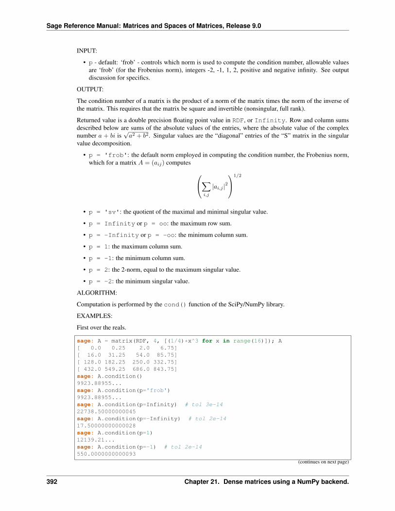
Sage Reference Manual: Matrices and Spaces of Matrices, Release 9.0
INPUT:
• p - default: ‘frob’ - controls which norm is used to compute the condition number, allowable valuesare ‘frob’ (for the Frobenius norm), integers -2, -1, 1, 2, positive and negative infinity. See outputdiscussion for specifics.
OUTPUT:
The condition number of a matrix is the product of a norm of the matrix times the norm of the inverse ofthe matrix. This requires that the matrix be square and invertible (nonsingular, full rank).
Returned value is a double precision floating point value in RDF, or Infinity. Row and column sumsdescribed below are sums of the absolute values of the entries, where the absolute value of the complexnumber 𝑎 + 𝑏𝑖 is
√𝑎2 + 𝑏2. Singular values are the “diagonal” entries of the “S” matrix in the singular
value decomposition.
• p = 'frob': the default norm employed in computing the condition number, the Frobenius norm,which for a matrix 𝐴 = (𝑎𝑖𝑗) computes ⎛⎝∑︁
𝑖,𝑗
|𝑎𝑖,𝑗 |2⎞⎠1/2
• p = 'sv': the quotient of the maximal and minimal singular value.
• p = Infinity or p = oo: the maximum row sum.
• p = -Infinity or p = -oo: the minimum column sum.
• p = 1: the maximum column sum.
• p = -1: the minimum column sum.
• p = 2: the 2-norm, equal to the maximum singular value.
• p = -2: the minimum singular value.
ALGORITHM:
Computation is performed by the cond() function of the SciPy/NumPy library.
EXAMPLES:
First over the reals.
sage: A = matrix(RDF, 4, [(1/4)*x^3 for x in range(16)]); A[ 0.0 0.25 2.0 6.75][ 16.0 31.25 54.0 85.75][ 128.0 182.25 250.0 332.75][ 432.0 549.25 686.0 843.75]sage: A.condition()9923.88955...sage: A.condition(p='frob')9923.88955...sage: A.condition(p=Infinity) # tol 3e-1422738.50000000045sage: A.condition(p=-Infinity) # tol 2e-1417.50000000000028sage: A.condition(p=1)12139.21...sage: A.condition(p=-1) # tol 2e-14550.0000000000093
(continues on next page)
392 Chapter 21. Dense matrices using a NumPy backend.

Sage Reference Manual: Matrices and Spaces of Matrices, Release 9.0
(continued from previous page)
sage: A.condition(p=2)9897.8088...sage: A.condition(p=-2)0.000101032462...
And over the complex numbers.
sage: B = matrix(CDF, 3, [x + x^2*I for x in range(9)]); B[ 0.0 1.0 + 1.0*I 2.0 + 4.0*I][ 3.0 + 9.0*I 4.0 + 16.0*I 5.0 + 25.0*I][6.0 + 36.0*I 7.0 + 49.0*I 8.0 + 64.0*I]sage: B.condition()doctest:warning......ComplexWarning: Casting complex values to real discards the imaginary part203.851798...sage: B.condition(p='frob')203.851798...sage: B.condition(p=Infinity)369.55630...sage: B.condition(p=-Infinity)5.46112969...sage: B.condition(p=1)289.251481...sage: B.condition(p=-1)20.4566639...sage: B.condition(p=2)202.653543...sage: B.condition(p=-2)0.00493453005...
Hilbert matrices are famously ill-conditioned, while an identity matrix can hit the minimum with the rightnorm.
sage: A = matrix(RDF, 10, [1/(i+j+1) for i in range(10) for j in range(10)])sage: A.condition() # tol 2e-416332197709146.014sage: id = identity_matrix(CDF, 10)sage: id.condition(p=1)1.0
Return values are in 𝑅𝐷𝐹 .
sage: A = matrix(CDF, 2, range(1,5))sage: A.condition() in RDFTrue
Rectangular and singular matrices raise errors if p is not ‘sv’.
sage: A = matrix(RDF, 2, 3, range(6))sage: A.condition()Traceback (most recent call last):...TypeError: matrix must be square if p is not 'sv', not 2 x 3
sage: A.condition('sv')
(continues on next page)
393

Sage Reference Manual: Matrices and Spaces of Matrices, Release 9.0
(continued from previous page)
7.34...
sage: A = matrix(QQ, 5, range(25))sage: A.is_singular()Truesage: B = A.change_ring(CDF)sage: B.condition()+Infinity
Improper values of p are caught.
sage: A = matrix(CDF, 2, range(1,5))sage: A.condition(p='bogus')Traceback (most recent call last):...ValueError: condition number 'p' must be +/- infinity, 'frob', 'sv' or an→˓integer, not bogussage: A.condition(p=632)Traceback (most recent call last):...ValueError: condition number integer values of 'p' must be -2, -1, 1 or 2,→˓not 632
determinant()Return the determinant of self.
ALGORITHM:
Use numpy
EXAMPLES:
sage: m = matrix(RDF,2,range(4)); m.det()-2.0sage: m = matrix(RDF,0,[]); m.det()1.0sage: m = matrix(RDF, 2, range(6)); m.det()Traceback (most recent call last):...ValueError: self must be a square matrix
eigenvalues(algorithm=’default’, tol=None)Return a list of eigenvalues.
INPUT:
• self - a square matrix
• algorithm - default: 'default'
– 'default' - applicable to any matrix with double-precision floating point entries. Uses theeigvals() method from SciPy.
– 'symmetric' - converts the matrix into a real matrix (i.e. with entries from RDF), then ap-plies the algorithm for Hermitian matrices. This algorithm can be significantly faster than the'default' algorithm.
– 'hermitian' - uses the eigh() method from SciPy, which applies only to real symmetricor complex Hermitian matrices. Since Hermitian is defined as a matrix equaling its conjugate-
394 Chapter 21. Dense matrices using a NumPy backend.
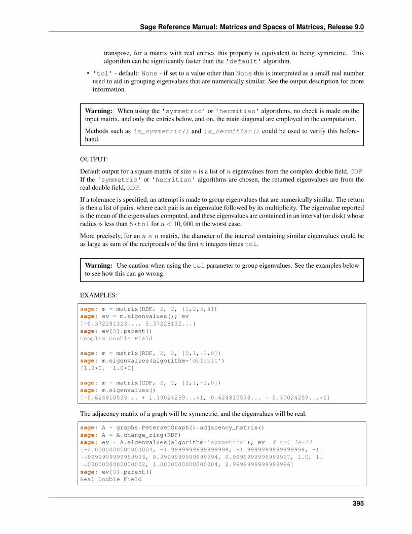
Sage Reference Manual: Matrices and Spaces of Matrices, Release 9.0
transpose, for a matrix with real entries this property is equivalent to being symmetric. Thisalgorithm can be significantly faster than the 'default' algorithm.
• 'tol' - default: None - if set to a value other than None this is interpreted as a small real numberused to aid in grouping eigenvalues that are numerically similar. See the output description for moreinformation.
Warning: When using the 'symmetric' or 'hermitian' algorithms, no check is made on theinput matrix, and only the entries below, and on, the main diagonal are employed in the computation.
Methods such as is_symmetric() and is_hermitian() could be used to verify this before-hand.
OUTPUT:
Default output for a square matrix of size 𝑛 is a list of 𝑛 eigenvalues from the complex double field, CDF.If the 'symmetric' or 'hermitian' algorithms are chosen, the returned eigenvalues are from thereal double field, RDF.
If a tolerance is specified, an attempt is made to group eigenvalues that are numerically similar. The returnis then a list of pairs, where each pair is an eigenvalue followed by its multiplicity. The eigenvalue reportedis the mean of the eigenvalues computed, and these eigenvalues are contained in an interval (or disk) whoseradius is less than 5*tol for 𝑛 < 10, 000 in the worst case.
More precisely, for an 𝑛 × 𝑛 matrix, the diameter of the interval containing similar eigenvalues could beas large as sum of the reciprocals of the first 𝑛 integers times tol.
Warning: Use caution when using the tol parameter to group eigenvalues. See the examples belowto see how this can go wrong.
EXAMPLES:
sage: m = matrix(RDF, 2, 2, [1,2,3,4])sage: ev = m.eigenvalues(); ev[-0.372281323..., 5.37228132...]sage: ev[0].parent()Complex Double Field
sage: m = matrix(RDF, 2, 2, [0,1,-1,0])sage: m.eigenvalues(algorithm='default')[1.0*I, -1.0*I]
sage: m = matrix(CDF, 2, 2, [I,1,-I,0])sage: m.eigenvalues()[-0.624810533... + 1.30024259...*I, 0.624810533... - 0.30024259...*I]
The adjacency matrix of a graph will be symmetric, and the eigenvalues will be real.
sage: A = graphs.PetersenGraph().adjacency_matrix()sage: A = A.change_ring(RDF)sage: ev = A.eigenvalues(algorithm='symmetric'); ev # tol 1e-14[-2.0000000000000004, -1.9999999999999998, -1.9999999999999998, -1.→˓9999999999999993, 0.9999999999999994, 0.9999999999999997, 1.0, 1.→˓0000000000000002, 1.0000000000000004, 2.9999999999999996]sage: ev[0].parent()Real Double Field
395
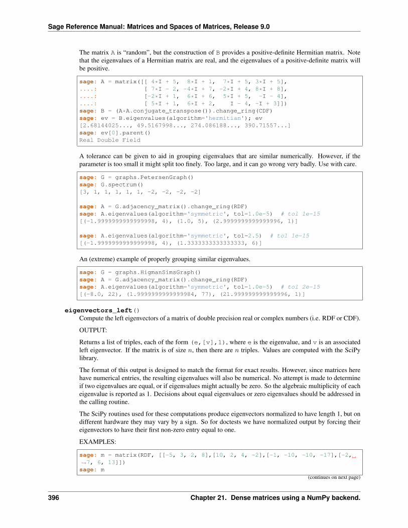
Sage Reference Manual: Matrices and Spaces of Matrices, Release 9.0
The matrix A is “random”, but the construction of B provides a positive-definite Hermitian matrix. Notethat the eigenvalues of a Hermitian matrix are real, and the eigenvalues of a positive-definite matrix willbe positive.
sage: A = matrix([[ 4*I + 5, 8*I + 1, 7*I + 5, 3*I + 5],....: [ 7*I - 2, -4*I + 7, -2*I + 4, 8*I + 8],....: [-2*I + 1, 6*I + 6, 5*I + 5, -I - 4],....: [ 5*I + 1, 6*I + 2, I - 4, -I + 3]])sage: B = (A*A.conjugate_transpose()).change_ring(CDF)sage: ev = B.eigenvalues(algorithm='hermitian'); ev[2.68144025..., 49.5167998..., 274.086188..., 390.71557...]sage: ev[0].parent()Real Double Field
A tolerance can be given to aid in grouping eigenvalues that are similar numerically. However, if theparameter is too small it might split too finely. Too large, and it can go wrong very badly. Use with care.
sage: G = graphs.PetersenGraph()sage: G.spectrum()[3, 1, 1, 1, 1, 1, -2, -2, -2, -2]
sage: A = G.adjacency_matrix().change_ring(RDF)sage: A.eigenvalues(algorithm='symmetric', tol=1.0e-5) # tol 1e-15[(-1.9999999999999998, 4), (1.0, 5), (2.9999999999999996, 1)]
sage: A.eigenvalues(algorithm='symmetric', tol=2.5) # tol 1e-15[(-1.9999999999999998, 4), (1.3333333333333333, 6)]
An (extreme) example of properly grouping similar eigenvalues.
sage: G = graphs.HigmanSimsGraph()sage: A = G.adjacency_matrix().change_ring(RDF)sage: A.eigenvalues(algorithm='symmetric', tol=1.0e-5) # tol 2e-15[(-8.0, 22), (1.9999999999999984, 77), (21.999999999999996, 1)]
eigenvectors_left()Compute the left eigenvectors of a matrix of double precision real or complex numbers (i.e. RDF or CDF).
OUTPUT:
Returns a list of triples, each of the form (e,[v],1), where e is the eigenvalue, and v is an associatedleft eigenvector. If the matrix is of size 𝑛, then there are 𝑛 triples. Values are computed with the SciPylibrary.
The format of this output is designed to match the format for exact results. However, since matrices herehave numerical entries, the resulting eigenvalues will also be numerical. No attempt is made to determineif two eigenvalues are equal, or if eigenvalues might actually be zero. So the algebraic multiplicity of eacheigenvalue is reported as 1. Decisions about equal eigenvalues or zero eigenvalues should be addressed inthe calling routine.
The SciPy routines used for these computations produce eigenvectors normalized to have length 1, but ondifferent hardware they may vary by a sign. So for doctests we have normalized output by forcing theireigenvectors to have their first non-zero entry equal to one.
EXAMPLES:
sage: m = matrix(RDF, [[-5, 3, 2, 8],[10, 2, 4, -2],[-1, -10, -10, -17],[-2,→˓7, 6, 13]])sage: m
(continues on next page)
396 Chapter 21. Dense matrices using a NumPy backend.
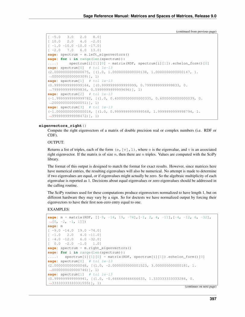
Sage Reference Manual: Matrices and Spaces of Matrices, Release 9.0
(continued from previous page)
[ -5.0 3.0 2.0 8.0][ 10.0 2.0 4.0 -2.0][ -1.0 -10.0 -10.0 -17.0][ -2.0 7.0 6.0 13.0]sage: spectrum = m.left_eigenvectors()sage: for i in range(len(spectrum)):....: spectrum[i][1][0] = matrix(RDF, spectrum[i][1]).echelon_form()[0]sage: spectrum[0] # tol 1e-13(2.0000000000000675, [(1.0, 1.0000000000000138, 1.0000000000000147, 1.→˓0000000000000309)], 1)sage: spectrum[1] # tol 1e-13(0.9999999999999164, [(0.9999999999999999, 0.7999999999999833, 0.→˓7999999999999836, 0.5999999999999696)], 1)sage: spectrum[2] # tol 1e-13(-1.9999999999999782, [(1.0, 0.40000000000000335, 0.6000000000000039, 0.→˓2000000000000051)], 1)sage: spectrum[3] # tol 1e-13(-1.0000000000000018, [(1.0, 0.9999999999999568, 1.9999999999998794, 1.→˓9999999999998472)], 1)
eigenvectors_right()Compute the right eigenvectors of a matrix of double precision real or complex numbers (i.e. RDF orCDF).
OUTPUT:
Returns a list of triples, each of the form (e,[v],1), where e is the eigenvalue, and v is an associatedright eigenvector. If the matrix is of size 𝑛, then there are 𝑛 triples. Values are computed with the SciPylibrary.
The format of this output is designed to match the format for exact results. However, since matrices herehave numerical entries, the resulting eigenvalues will also be numerical. No attempt is made to determineif two eigenvalues are equal, or if eigenvalues might actually be zero. So the algebraic multiplicity of eacheigenvalue is reported as 1. Decisions about equal eigenvalues or zero eigenvalues should be addressed inthe calling routine.
The SciPy routines used for these computations produce eigenvectors normalized to have length 1, but ondifferent hardware they may vary by a sign. So for doctests we have normalized output by forcing theireigenvectors to have their first non-zero entry equal to one.
EXAMPLES:
sage: m = matrix(RDF, [[-9, -14, 19, -74],[-1, 2, 4, -11],[-4, -12, 6, -32],→˓[0, -2, -1, 1]])sage: m[ -9.0 -14.0 19.0 -74.0][ -1.0 2.0 4.0 -11.0][ -4.0 -12.0 6.0 -32.0][ 0.0 -2.0 -1.0 1.0]sage: spectrum = m.right_eigenvectors()sage: for i in range(len(spectrum)):....: spectrum[i][1][0] = matrix(RDF, spectrum[i][1]).echelon_form()[0]sage: spectrum[0] # tol 1e-13(2.000000000000048, [(1.0, -2.0000000000001523, 3.000000000000181, 1.→˓0000000000000746)], 1)sage: spectrum[1] # tol 1e-13(0.999999999999941, [(1.0, -0.666666666666633, 1.333333333333286, 0.→˓33333333333331555)], 1)
(continues on next page)
397
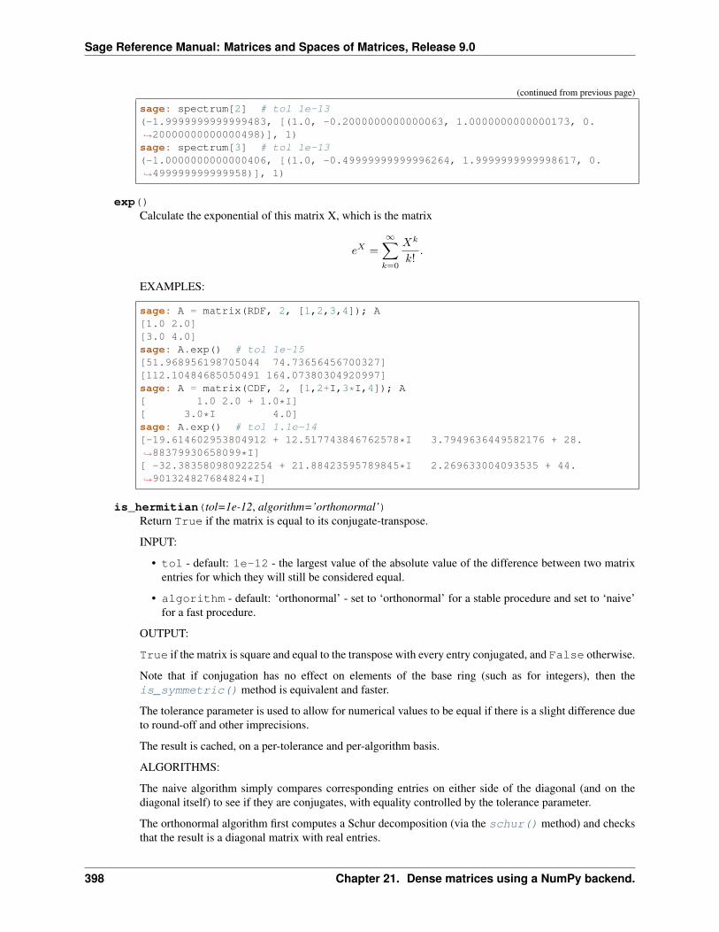
Sage Reference Manual: Matrices and Spaces of Matrices, Release 9.0
(continued from previous page)
sage: spectrum[2] # tol 1e-13(-1.9999999999999483, [(1.0, -0.2000000000000063, 1.0000000000000173, 0.→˓20000000000000498)], 1)sage: spectrum[3] # tol 1e-13(-1.0000000000000406, [(1.0, -0.49999999999996264, 1.9999999999998617, 0.→˓499999999999958)], 1)
exp()Calculate the exponential of this matrix X, which is the matrix
𝑒𝑋 =
∞∑︁𝑘=0
𝑋𝑘
𝑘!.
EXAMPLES:
sage: A = matrix(RDF, 2, [1,2,3,4]); A[1.0 2.0][3.0 4.0]sage: A.exp() # tol 1e-15[51.968956198705044 74.73656456700327][112.10484685050491 164.07380304920997]sage: A = matrix(CDF, 2, [1,2+I,3*I,4]); A[ 1.0 2.0 + 1.0*I][ 3.0*I 4.0]sage: A.exp() # tol 1.1e-14[-19.614602953804912 + 12.517743846762578*I 3.7949636449582176 + 28.→˓88379930658099*I][ -32.383580980922254 + 21.88423595789845*I 2.269633004093535 + 44.→˓901324827684824*I]
is_hermitian(tol=1e-12, algorithm=’orthonormal’)Return True if the matrix is equal to its conjugate-transpose.
INPUT:
• tol - default: 1e-12 - the largest value of the absolute value of the difference between two matrixentries for which they will still be considered equal.
• algorithm - default: ‘orthonormal’ - set to ‘orthonormal’ for a stable procedure and set to ‘naive’for a fast procedure.
OUTPUT:
True if the matrix is square and equal to the transpose with every entry conjugated, and False otherwise.
Note that if conjugation has no effect on elements of the base ring (such as for integers), then theis_symmetric() method is equivalent and faster.
The tolerance parameter is used to allow for numerical values to be equal if there is a slight difference dueto round-off and other imprecisions.
The result is cached, on a per-tolerance and per-algorithm basis.
ALGORITHMS:
The naive algorithm simply compares corresponding entries on either side of the diagonal (and on thediagonal itself) to see if they are conjugates, with equality controlled by the tolerance parameter.
The orthonormal algorithm first computes a Schur decomposition (via the schur() method) and checksthat the result is a diagonal matrix with real entries.
398 Chapter 21. Dense matrices using a NumPy backend.
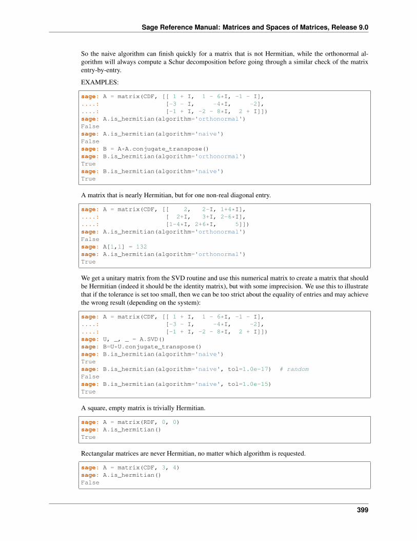
Sage Reference Manual: Matrices and Spaces of Matrices, Release 9.0
So the naive algorithm can finish quickly for a matrix that is not Hermitian, while the orthonormal al-gorithm will always compute a Schur decomposition before going through a similar check of the matrixentry-by-entry.
EXAMPLES:
sage: A = matrix(CDF, [[ 1 + I, 1 - 6*I, -1 - I],....: [-3 - I, -4*I, -2],....: [-1 + I, -2 - 8*I, 2 + I]])sage: A.is_hermitian(algorithm='orthonormal')Falsesage: A.is_hermitian(algorithm='naive')Falsesage: B = A*A.conjugate_transpose()sage: B.is_hermitian(algorithm='orthonormal')Truesage: B.is_hermitian(algorithm='naive')True
A matrix that is nearly Hermitian, but for one non-real diagonal entry.
sage: A = matrix(CDF, [[ 2, 2-I, 1+4*I],....: [ 2+I, 3+I, 2-6*I],....: [1-4*I, 2+6*I, 5]])sage: A.is_hermitian(algorithm='orthonormal')Falsesage: A[1,1] = 132sage: A.is_hermitian(algorithm='orthonormal')True
We get a unitary matrix from the SVD routine and use this numerical matrix to create a matrix that shouldbe Hermitian (indeed it should be the identity matrix), but with some imprecision. We use this to illustratethat if the tolerance is set too small, then we can be too strict about the equality of entries and may achievethe wrong result (depending on the system):
sage: A = matrix(CDF, [[ 1 + I, 1 - 6*I, -1 - I],....: [-3 - I, -4*I, -2],....: [-1 + I, -2 - 8*I, 2 + I]])sage: U, _, _ = A.SVD()sage: B=U*U.conjugate_transpose()sage: B.is_hermitian(algorithm='naive')Truesage: B.is_hermitian(algorithm='naive', tol=1.0e-17) # randomFalsesage: B.is_hermitian(algorithm='naive', tol=1.0e-15)True
A square, empty matrix is trivially Hermitian.
sage: A = matrix(RDF, 0, 0)sage: A.is_hermitian()True
Rectangular matrices are never Hermitian, no matter which algorithm is requested.
sage: A = matrix(CDF, 3, 4)sage: A.is_hermitian()False
399
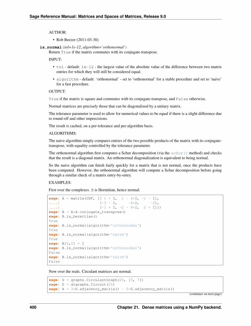
Sage Reference Manual: Matrices and Spaces of Matrices, Release 9.0
AUTHOR:
• Rob Beezer (2011-03-30)
is_normal(tol=1e-12, algorithm=’orthonormal’)Return True if the matrix commutes with its conjugate-transpose.
INPUT:
• tol - default: 1e-12 - the largest value of the absolute value of the difference between two matrixentries for which they will still be considered equal.
• algorithm - default: ‘orthonormal’ - set to ‘orthonormal’ for a stable procedure and set to ‘naive’for a fast procedure.
OUTPUT:
True if the matrix is square and commutes with its conjugate-transpose, and False otherwise.
Normal matrices are precisely those that can be diagonalized by a unitary matrix.
The tolerance parameter is used to allow for numerical values to be equal if there is a slight difference dueto round-off and other imprecisions.
The result is cached, on a per-tolerance and per-algorithm basis.
ALGORITHMS:
The naive algorithm simply compares entries of the two possible products of the matrix with its conjugate-transpose, with equality controlled by the tolerance parameter.
The orthonormal algorithm first computes a Schur decomposition (via the schur() method) and checksthat the result is a diagonal matrix. An orthonormal diagonalization is equivalent to being normal.
So the naive algorithm can finish fairly quickly for a matrix that is not normal, once the products havebeen computed. However, the orthonormal algorithm will compute a Schur decomposition before goingthrough a similar check of a matrix entry-by-entry.
EXAMPLES:
First over the complexes. B is Hermitian, hence normal.
sage: A = matrix(CDF, [[ 1 + I, 1 - 6*I, -1 - I],....: [-3 - I, -4*I, -2],....: [-1 + I, -2 - 8*I, 2 + I]])sage: B = A*A.conjugate_transpose()sage: B.is_hermitian()Truesage: B.is_normal(algorithm='orthonormal')Truesage: B.is_normal(algorithm='naive')Truesage: B[0,0] = Isage: B.is_normal(algorithm='orthonormal')Falsesage: B.is_normal(algorithm='naive')False
Now over the reals. Circulant matrices are normal.
sage: G = graphs.CirculantGraph(20, [3, 7])sage: D = digraphs.Circuit(20)sage: A = 3*D.adjacency_matrix() - 5*G.adjacency_matrix()
(continues on next page)
400 Chapter 21. Dense matrices using a NumPy backend.
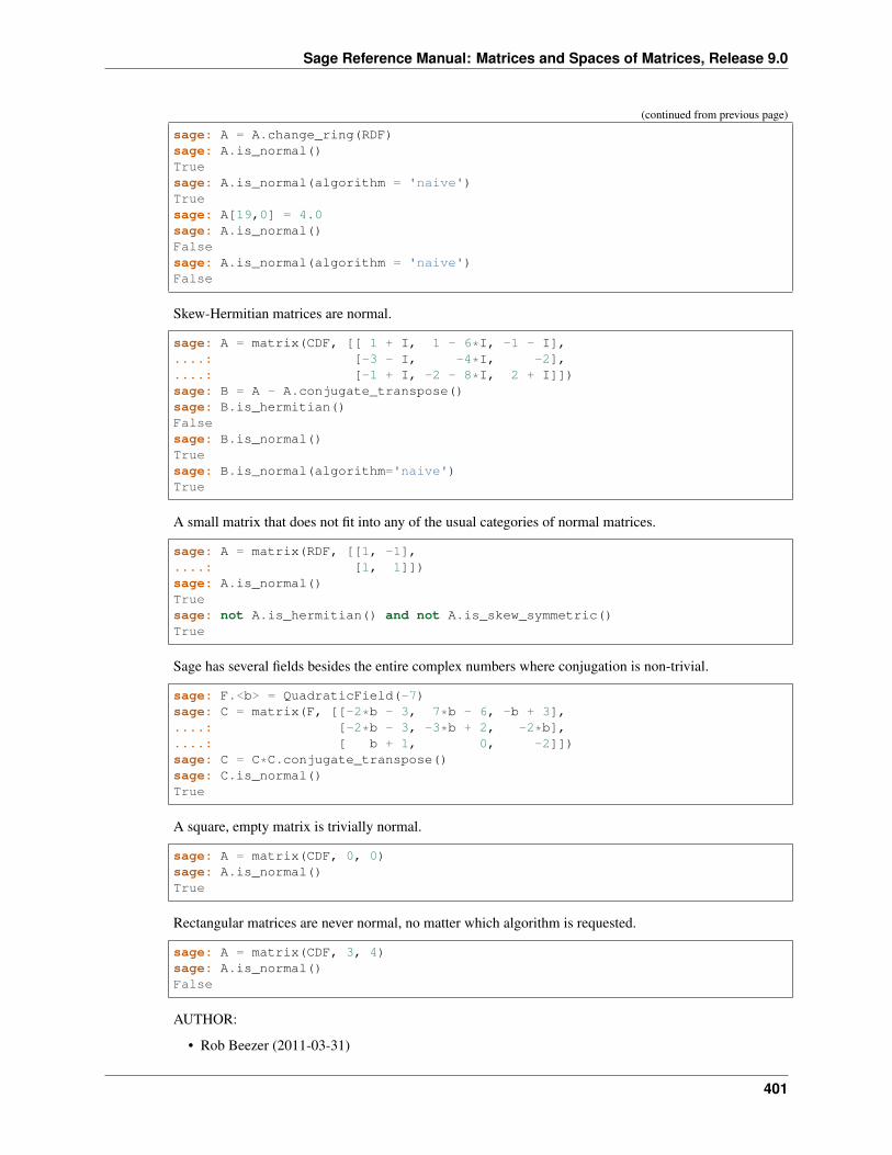
Sage Reference Manual: Matrices and Spaces of Matrices, Release 9.0
(continued from previous page)
sage: A = A.change_ring(RDF)sage: A.is_normal()Truesage: A.is_normal(algorithm = 'naive')Truesage: A[19,0] = 4.0sage: A.is_normal()Falsesage: A.is_normal(algorithm = 'naive')False
Skew-Hermitian matrices are normal.
sage: A = matrix(CDF, [[ 1 + I, 1 - 6*I, -1 - I],....: [-3 - I, -4*I, -2],....: [-1 + I, -2 - 8*I, 2 + I]])sage: B = A - A.conjugate_transpose()sage: B.is_hermitian()Falsesage: B.is_normal()Truesage: B.is_normal(algorithm='naive')True
A small matrix that does not fit into any of the usual categories of normal matrices.
sage: A = matrix(RDF, [[1, -1],....: [1, 1]])sage: A.is_normal()Truesage: not A.is_hermitian() and not A.is_skew_symmetric()True
Sage has several fields besides the entire complex numbers where conjugation is non-trivial.
sage: F.<b> = QuadraticField(-7)sage: C = matrix(F, [[-2*b - 3, 7*b - 6, -b + 3],....: [-2*b - 3, -3*b + 2, -2*b],....: [ b + 1, 0, -2]])sage: C = C*C.conjugate_transpose()sage: C.is_normal()True
A square, empty matrix is trivially normal.
sage: A = matrix(CDF, 0, 0)sage: A.is_normal()True
Rectangular matrices are never normal, no matter which algorithm is requested.
sage: A = matrix(CDF, 3, 4)sage: A.is_normal()False
AUTHOR:
• Rob Beezer (2011-03-31)
401
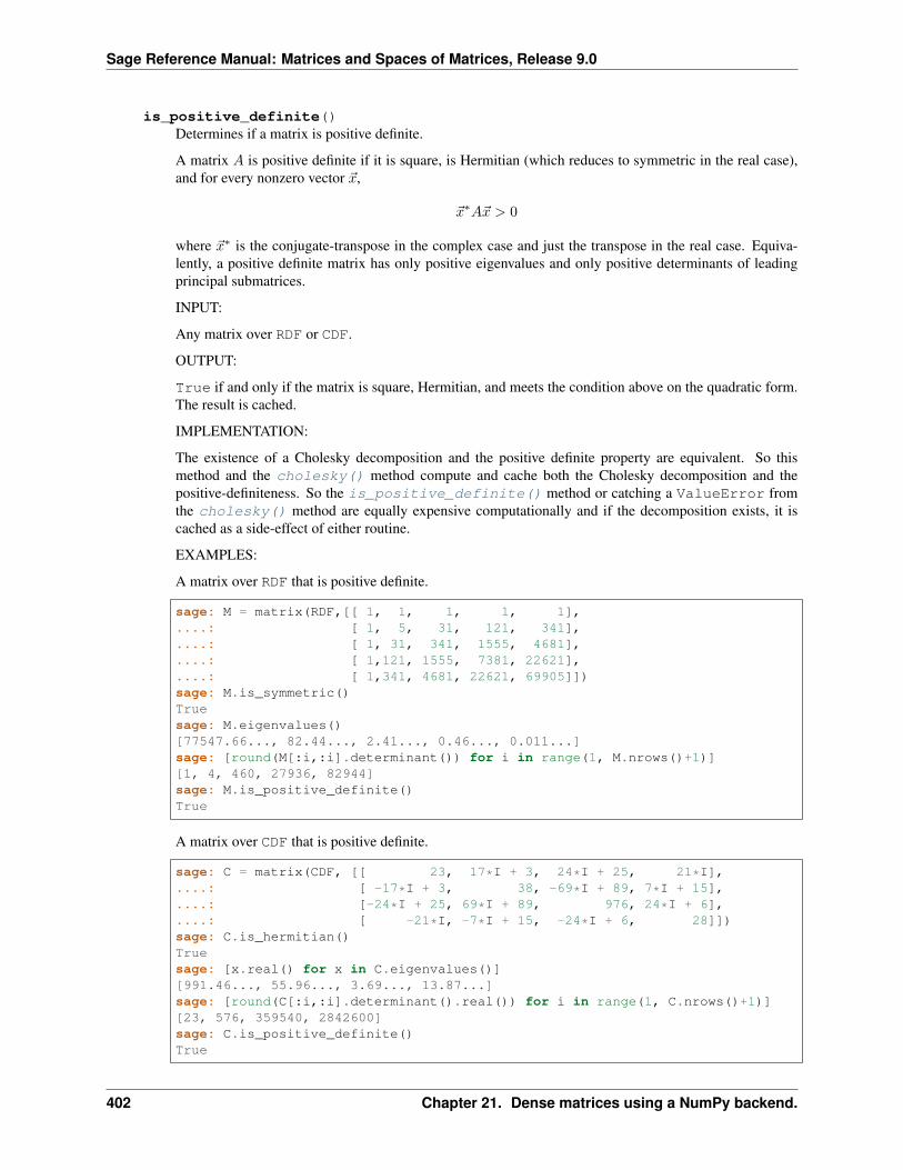
Sage Reference Manual: Matrices and Spaces of Matrices, Release 9.0
is_positive_definite()Determines if a matrix is positive definite.
A matrix 𝐴 is positive definite if it is square, is Hermitian (which reduces to symmetric in the real case),and for every nonzero vector �⃗�,
�⃗�*𝐴�⃗� > 0
where �⃗�* is the conjugate-transpose in the complex case and just the transpose in the real case. Equiva-lently, a positive definite matrix has only positive eigenvalues and only positive determinants of leadingprincipal submatrices.
INPUT:
Any matrix over RDF or CDF.
OUTPUT:
True if and only if the matrix is square, Hermitian, and meets the condition above on the quadratic form.The result is cached.
IMPLEMENTATION:
The existence of a Cholesky decomposition and the positive definite property are equivalent. So thismethod and the cholesky() method compute and cache both the Cholesky decomposition and thepositive-definiteness. So the is_positive_definite() method or catching a ValueError fromthe cholesky() method are equally expensive computationally and if the decomposition exists, it iscached as a side-effect of either routine.
EXAMPLES:
A matrix over RDF that is positive definite.
sage: M = matrix(RDF,[[ 1, 1, 1, 1, 1],....: [ 1, 5, 31, 121, 341],....: [ 1, 31, 341, 1555, 4681],....: [ 1,121, 1555, 7381, 22621],....: [ 1,341, 4681, 22621, 69905]])sage: M.is_symmetric()Truesage: M.eigenvalues()[77547.66..., 82.44..., 2.41..., 0.46..., 0.011...]sage: [round(M[:i,:i].determinant()) for i in range(1, M.nrows()+1)][1, 4, 460, 27936, 82944]sage: M.is_positive_definite()True
A matrix over CDF that is positive definite.
sage: C = matrix(CDF, [[ 23, 17*I + 3, 24*I + 25, 21*I],....: [ -17*I + 3, 38, -69*I + 89, 7*I + 15],....: [-24*I + 25, 69*I + 89, 976, 24*I + 6],....: [ -21*I, -7*I + 15, -24*I + 6, 28]])sage: C.is_hermitian()Truesage: [x.real() for x in C.eigenvalues()][991.46..., 55.96..., 3.69..., 13.87...]sage: [round(C[:i,:i].determinant().real()) for i in range(1, C.nrows()+1)][23, 576, 359540, 2842600]sage: C.is_positive_definite()True
402 Chapter 21. Dense matrices using a NumPy backend.
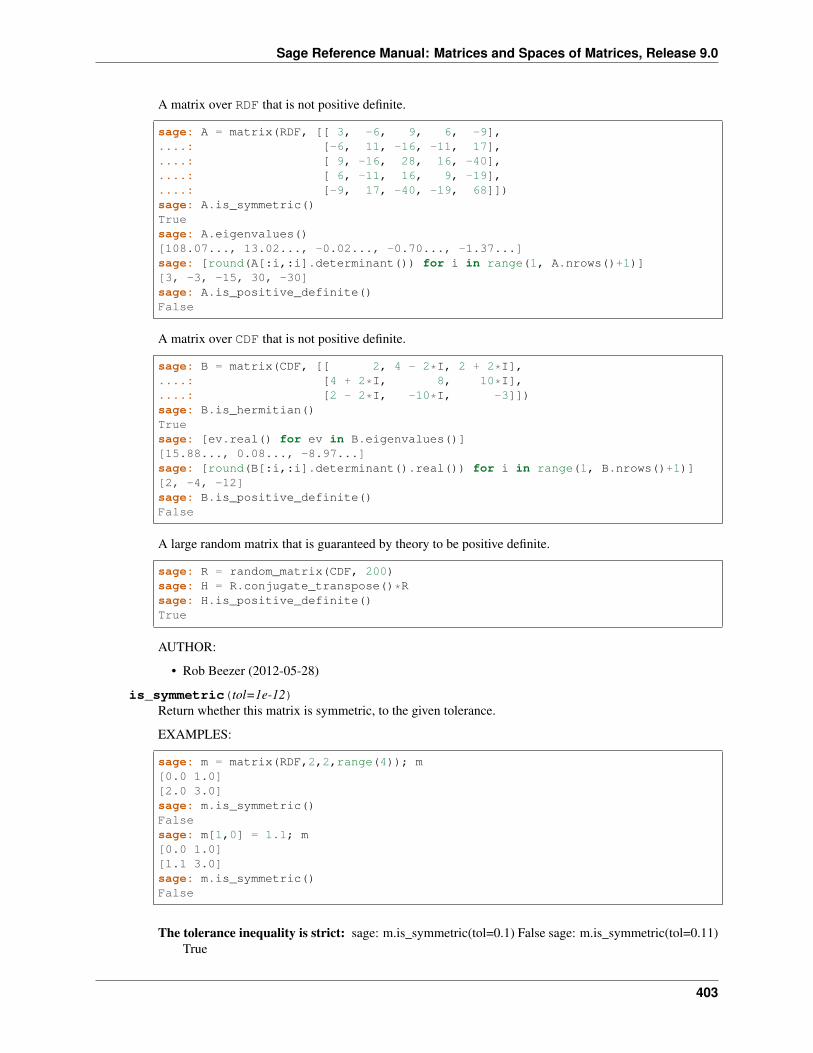
Sage Reference Manual: Matrices and Spaces of Matrices, Release 9.0
A matrix over RDF that is not positive definite.
sage: A = matrix(RDF, [[ 3, -6, 9, 6, -9],....: [-6, 11, -16, -11, 17],....: [ 9, -16, 28, 16, -40],....: [ 6, -11, 16, 9, -19],....: [-9, 17, -40, -19, 68]])sage: A.is_symmetric()Truesage: A.eigenvalues()[108.07..., 13.02..., -0.02..., -0.70..., -1.37...]sage: [round(A[:i,:i].determinant()) for i in range(1, A.nrows()+1)][3, -3, -15, 30, -30]sage: A.is_positive_definite()False
A matrix over CDF that is not positive definite.
sage: B = matrix(CDF, [[ 2, 4 - 2*I, 2 + 2*I],....: [4 + 2*I, 8, 10*I],....: [2 - 2*I, -10*I, -3]])sage: B.is_hermitian()Truesage: [ev.real() for ev in B.eigenvalues()][15.88..., 0.08..., -8.97...]sage: [round(B[:i,:i].determinant().real()) for i in range(1, B.nrows()+1)][2, -4, -12]sage: B.is_positive_definite()False
A large random matrix that is guaranteed by theory to be positive definite.
sage: R = random_matrix(CDF, 200)sage: H = R.conjugate_transpose()*Rsage: H.is_positive_definite()True
AUTHOR:
• Rob Beezer (2012-05-28)
is_symmetric(tol=1e-12)Return whether this matrix is symmetric, to the given tolerance.
EXAMPLES:
sage: m = matrix(RDF,2,2,range(4)); m[0.0 1.0][2.0 3.0]sage: m.is_symmetric()Falsesage: m[1,0] = 1.1; m[0.0 1.0][1.1 3.0]sage: m.is_symmetric()False
The tolerance inequality is strict: sage: m.is_symmetric(tol=0.1) False sage: m.is_symmetric(tol=0.11)True
403
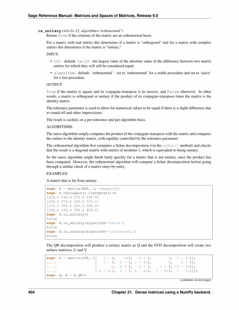
Sage Reference Manual: Matrices and Spaces of Matrices, Release 9.0
is_unitary(tol=1e-12, algorithm=’orthonormal’)Return True if the columns of the matrix are an orthonormal basis.
For a matrix with real entries this determines if a matrix is “orthogonal” and for a matrix with complexentries this determines if the matrix is “unitary.”
INPUT:
• tol - default: 1e-12 - the largest value of the absolute value of the difference between two matrixentries for which they will still be considered equal.
• algorithm - default: ‘orthonormal’ - set to ‘orthonormal’ for a stable procedure and set to ‘naive’for a fast procedure.
OUTPUT:
True if the matrix is square and its conjugate-transpose is its inverse, and False otherwise. In otherwords, a matrix is orthogonal or unitary if the product of its conjugate-transpose times the matrix is theidentity matrix.
The tolerance parameter is used to allow for numerical values to be equal if there is a slight difference dueto round-off and other imprecisions.
The result is cached, on a per-tolerance and per-algorithm basis.
ALGORITHMS:
The naive algorithm simply computes the product of the conjugate-transpose with the matrix and comparesthe entries to the identity matrix, with equality controlled by the tolerance parameter.
The orthonormal algorithm first computes a Schur decomposition (via the schur() method) and checksthat the result is a diagonal matrix with entries of modulus 1, which is equivalent to being unitary.
So the naive algorithm might finish fairly quickly for a matrix that is not unitary, once the product hasbeen computed. However, the orthonormal algorithm will compute a Schur decomposition before goingthrough a similar check of a matrix entry-by-entry.
EXAMPLES:
A matrix that is far from unitary.
sage: A = matrix(RDF, 4, range(16))sage: A.conjugate().transpose()*A[224.0 248.0 272.0 296.0][248.0 276.0 304.0 332.0][272.0 304.0 336.0 368.0][296.0 332.0 368.0 404.0]sage: A.is_unitary()Falsesage: A.is_unitary(algorithm='naive')Falsesage: A.is_unitary(algorithm='orthonormal')False
The QR decomposition will produce a unitary matrix as Q and the SVD decomposition will create twounitary matrices, U and V.
sage: A = matrix(CDF, [[ 1 - I, -3*I, -2 + I, 1, -2 + 3*I],....: [ 1 - I, -2 + I, 1 + 4*I, 0, 2 + I],....: [ -1, -5 + I, -2 + I, 1 + I, -5 - 4*I],....: [-2 + 4*I, 2 - I, 8 - 4*I, 1 - 8*I, 3 - 2*I]])sage: Q, R = A.QR()
(continues on next page)
404 Chapter 21. Dense matrices using a NumPy backend.
Sage Reference Manual: Matrices and Spaces of Matrices, Release 9.0
(continued from previous page)
sage: Q.is_unitary()Truesage: U, S, V = A.SVD()sage: U.is_unitary(algorithm='naive')Truesage: U.is_unitary(algorithm='orthonormal')Truesage: V.is_unitary(algorithm='naive')True
If we make the tolerance too strict we can get misleading results.
sage: A = matrix(RDF, 10, 10, [1/(i+j+1) for i in range(10) for j in→˓range(10)])sage: Q, R = A.QR()sage: Q.is_unitary(algorithm='naive', tol=1e-16)Falsesage: Q.is_unitary(algorithm='orthonormal', tol=1e-17)False
Rectangular matrices are not unitary/orthogonal, even if their columns form an orthonormal set.
sage: A = matrix(CDF, [[1,0], [0,0], [0,1]])sage: A.is_unitary()False
The smallest cases. The Schur decomposition used by the orthonormal algorithm will fail on a matrix ofsize zero.
sage: P = matrix(CDF, 0, 0)sage: P.is_unitary(algorithm='naive')True
sage: P = matrix(CDF, 1, 1, [1])sage: P.is_unitary(algorithm='orthonormal')True
sage: P = matrix(CDF, 0, 0,)sage: P.is_unitary(algorithm='orthonormal')Traceback (most recent call last):...error: ((lwork==-1)||(lwork >= MAX(1,2*n))) failed for 3rd keyword lwork:→˓zgees:lwork=0
AUTHOR:
• Rob Beezer (2011-05-04)
left_eigenvectors()Compute the left eigenvectors of a matrix of double precision real or complex numbers (i.e. RDF or CDF).
OUTPUT:
Returns a list of triples, each of the form (e,[v],1), where e is the eigenvalue, and v is an associatedleft eigenvector. If the matrix is of size 𝑛, then there are 𝑛 triples. Values are computed with the SciPylibrary.
The format of this output is designed to match the format for exact results. However, since matrices herehave numerical entries, the resulting eigenvalues will also be numerical. No attempt is made to determine
405
Sage Reference Manual: Matrices and Spaces of Matrices, Release 9.0
if two eigenvalues are equal, or if eigenvalues might actually be zero. So the algebraic multiplicity of eacheigenvalue is reported as 1. Decisions about equal eigenvalues or zero eigenvalues should be addressed inthe calling routine.
The SciPy routines used for these computations produce eigenvectors normalized to have length 1, but ondifferent hardware they may vary by a sign. So for doctests we have normalized output by forcing theireigenvectors to have their first non-zero entry equal to one.
EXAMPLES:
sage: m = matrix(RDF, [[-5, 3, 2, 8],[10, 2, 4, -2],[-1, -10, -10, -17],[-2,→˓7, 6, 13]])sage: m[ -5.0 3.0 2.0 8.0][ 10.0 2.0 4.0 -2.0][ -1.0 -10.0 -10.0 -17.0][ -2.0 7.0 6.0 13.0]sage: spectrum = m.left_eigenvectors()sage: for i in range(len(spectrum)):....: spectrum[i][1][0] = matrix(RDF, spectrum[i][1]).echelon_form()[0]sage: spectrum[0] # tol 1e-13(2.0000000000000675, [(1.0, 1.0000000000000138, 1.0000000000000147, 1.→˓0000000000000309)], 1)sage: spectrum[1] # tol 1e-13(0.9999999999999164, [(0.9999999999999999, 0.7999999999999833, 0.→˓7999999999999836, 0.5999999999999696)], 1)sage: spectrum[2] # tol 1e-13(-1.9999999999999782, [(1.0, 0.40000000000000335, 0.6000000000000039, 0.→˓2000000000000051)], 1)sage: spectrum[3] # tol 1e-13(-1.0000000000000018, [(1.0, 0.9999999999999568, 1.9999999999998794, 1.→˓9999999999998472)], 1)
log_determinant()Compute the log of the absolute value of the determinant using LU decomposition.
Note: This is useful if the usual determinant overflows.
EXAMPLES:
sage: m = matrix(RDF,2,2,range(4)); m[0.0 1.0][2.0 3.0]sage: RDF(log(abs(m.determinant())))0.6931471805599453sage: m.log_determinant()0.6931471805599453sage: m = matrix(RDF,0,0,[]); m[]sage: m.log_determinant()0.0sage: m = matrix(CDF,2,2,range(4)); m[0.0 1.0][2.0 3.0]sage: RDF(log(abs(m.determinant())))0.6931471805599453sage: m.log_determinant()
(continues on next page)
406 Chapter 21. Dense matrices using a NumPy backend.
Sage Reference Manual: Matrices and Spaces of Matrices, Release 9.0
(continued from previous page)
0.6931471805599453sage: m = matrix(CDF,0,0,[]); m[]sage: m.log_determinant()0.0
norm(p=2)Return the norm of the matrix.
INPUT:
• p - default: 2 - controls which norm is computed, allowable values are ‘frob’ (for the Frobenius norm),integers -2, -1, 1, 2, positive and negative infinity. See output discussion for specifics.
OUTPUT:
Returned value is a double precision floating point value in RDF. Row and column sums described beloware sums of the absolute values of the entries, where the absolute value of the complex number 𝑎 + 𝑏𝑖 is√𝑎2 + 𝑏2. Singular values are the “diagonal” entries of the “S” matrix in the singular value decomposition.
• p = 'frob': the Frobenius norm, which for a matrix 𝐴 = (𝑎𝑖𝑗) computes⎛⎝∑︁𝑖,𝑗
|𝑎𝑖,𝑗 |2⎞⎠1/2
• p = Infinity or p = oo: the maximum row sum.
• p = -Infinity or p = -oo: the minimum column sum.
• p = 1: the maximum column sum.
• p = -1: the minimum column sum.
• p = 2: the induced 2-norm, equal to the maximum singular value.
• p = -2: the minimum singular value.
ALGORITHM:
Computation is performed by the norm() function of the SciPy/NumPy library.
EXAMPLES:
First over the reals.
sage: A = matrix(RDF, 3, range(-3, 6)); A[-3.0 -2.0 -1.0][ 0.0 1.0 2.0][ 3.0 4.0 5.0]sage: A.norm()7.99575670...sage: A.norm(p='frob')8.30662386...sage: A.norm(p=Infinity)12.0sage: A.norm(p=-Infinity)3.0sage: A.norm(p=1)8.0
(continues on next page)
407
Sage Reference Manual: Matrices and Spaces of Matrices, Release 9.0
(continued from previous page)
sage: A.norm(p=-1)6.0sage: A.norm(p=2)7.99575670...sage: A.norm(p=-2) < 10^-15True
And over the complex numbers.
sage: B = matrix(CDF, 2, [[1+I, 2+3*I],[3+4*I,3*I]]); B[1.0 + 1.0*I 2.0 + 3.0*I][3.0 + 4.0*I 3.0*I]sage: B.norm()6.66189877...sage: B.norm(p='frob')7.0sage: B.norm(p=Infinity)8.0sage: B.norm(p=-Infinity)5.01976483...sage: B.norm(p=1)6.60555127...sage: B.norm(p=-1)6.41421356...sage: B.norm(p=2)6.66189877...sage: B.norm(p=-2)2.14921023...
Since it is invariant under unitary multiplication, the Frobenius norm is equal to the square root of the sumof squares of the singular values.
sage: A = matrix(RDF, 5, range(1,26))sage: f = A.norm(p='frob')sage: U, S, V = A.SVD()sage: s = sqrt(sum([S[i,i]^2 for i in range(5)]))sage: abs(f-s) < 1.0e-12True
Return values are in 𝑅𝐷𝐹 .
sage: A = matrix(CDF, 2, range(4))sage: A.norm() in RDFTrue
Improper values of p are caught.
sage: A.norm(p='bogus')Traceback (most recent call last):...ValueError: matrix norm 'p' must be +/- infinity, 'frob' or an integer, not→˓bogussage: A.norm(p=632)Traceback (most recent call last):...ValueError: matrix norm integer values of 'p' must be -2, -1, 1 or 2, not 632
408 Chapter 21. Dense matrices using a NumPy backend.
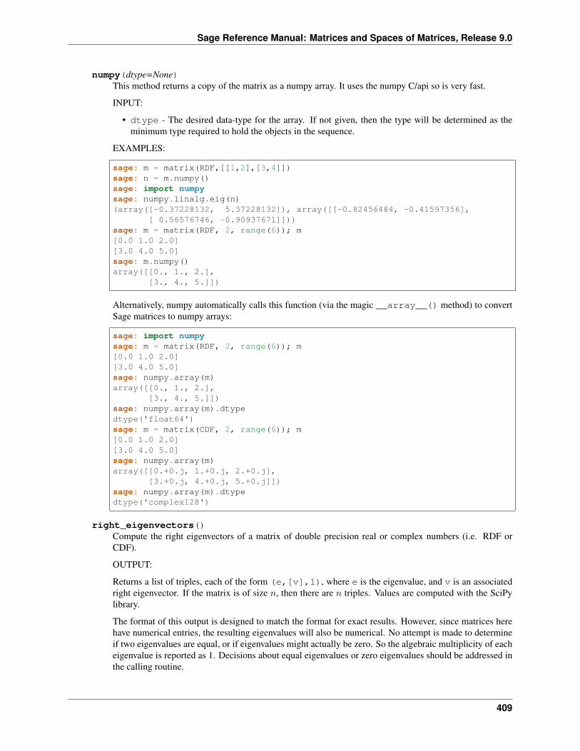
Sage Reference Manual: Matrices and Spaces of Matrices, Release 9.0
numpy(dtype=None)This method returns a copy of the matrix as a numpy array. It uses the numpy C/api so is very fast.
INPUT:
• dtype - The desired data-type for the array. If not given, then the type will be determined as theminimum type required to hold the objects in the sequence.
EXAMPLES:
sage: m = matrix(RDF,[[1,2],[3,4]])sage: n = m.numpy()sage: import numpysage: numpy.linalg.eig(n)(array([-0.37228132, 5.37228132]), array([[-0.82456484, -0.41597356],
[ 0.56576746, -0.90937671]]))sage: m = matrix(RDF, 2, range(6)); m[0.0 1.0 2.0][3.0 4.0 5.0]sage: m.numpy()array([[0., 1., 2.],
[3., 4., 5.]])
Alternatively, numpy automatically calls this function (via the magic __array__() method) to convertSage matrices to numpy arrays:
sage: import numpysage: m = matrix(RDF, 2, range(6)); m[0.0 1.0 2.0][3.0 4.0 5.0]sage: numpy.array(m)array([[0., 1., 2.],
[3., 4., 5.]])sage: numpy.array(m).dtypedtype('float64')sage: m = matrix(CDF, 2, range(6)); m[0.0 1.0 2.0][3.0 4.0 5.0]sage: numpy.array(m)array([[0.+0.j, 1.+0.j, 2.+0.j],
[3.+0.j, 4.+0.j, 5.+0.j]])sage: numpy.array(m).dtypedtype('complex128')
right_eigenvectors()Compute the right eigenvectors of a matrix of double precision real or complex numbers (i.e. RDF orCDF).
OUTPUT:
Returns a list of triples, each of the form (e,[v],1), where e is the eigenvalue, and v is an associatedright eigenvector. If the matrix is of size 𝑛, then there are 𝑛 triples. Values are computed with the SciPylibrary.
The format of this output is designed to match the format for exact results. However, since matrices herehave numerical entries, the resulting eigenvalues will also be numerical. No attempt is made to determineif two eigenvalues are equal, or if eigenvalues might actually be zero. So the algebraic multiplicity of eacheigenvalue is reported as 1. Decisions about equal eigenvalues or zero eigenvalues should be addressed inthe calling routine.
409
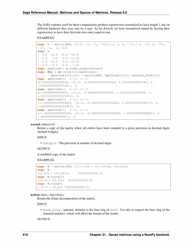
Sage Reference Manual: Matrices and Spaces of Matrices, Release 9.0
The SciPy routines used for these computations produce eigenvectors normalized to have length 1, but ondifferent hardware they may vary by a sign. So for doctests we have normalized output by forcing theireigenvectors to have their first non-zero entry equal to one.
EXAMPLES:
sage: m = matrix(RDF, [[-9, -14, 19, -74],[-1, 2, 4, -11],[-4, -12, 6, -32],→˓[0, -2, -1, 1]])sage: m[ -9.0 -14.0 19.0 -74.0][ -1.0 2.0 4.0 -11.0][ -4.0 -12.0 6.0 -32.0][ 0.0 -2.0 -1.0 1.0]sage: spectrum = m.right_eigenvectors()sage: for i in range(len(spectrum)):....: spectrum[i][1][0] = matrix(RDF, spectrum[i][1]).echelon_form()[0]sage: spectrum[0] # tol 1e-13(2.000000000000048, [(1.0, -2.0000000000001523, 3.000000000000181, 1.→˓0000000000000746)], 1)sage: spectrum[1] # tol 1e-13(0.999999999999941, [(1.0, -0.666666666666633, 1.333333333333286, 0.→˓33333333333331555)], 1)sage: spectrum[2] # tol 1e-13(-1.9999999999999483, [(1.0, -0.2000000000000063, 1.0000000000000173, 0.→˓20000000000000498)], 1)sage: spectrum[3] # tol 1e-13(-1.0000000000000406, [(1.0, -0.49999999999996264, 1.9999999999998617, 0.→˓499999999999958)], 1)
round(ndigits=0)Return a copy of the matrix where all entries have been rounded to a given precision in decimal digits(default 0 digits).
INPUT:
• ndigits - The precision in number of decimal digits
OUTPUT:
A modified copy of the matrix
EXAMPLES:
sage: M = matrix(CDF, [[10.234r + 34.2343jr, 34e10r]])sage: M[10.234 + 34.2343*I 340000000000.0]sage: M.round(2)[10.23 + 34.23*I 340000000000.0]sage: M.round()[ 10.0 + 34.0*I 340000000000.0]
schur(base_ring=None)Return the Schur decomposition of the matrix.
INPUT:
• base_ring - optional, defaults to the base ring of self. Use this to request the base ring of thereturned matrices, which will affect the format of the results.
OUTPUT:
410 Chapter 21. Dense matrices using a NumPy backend.
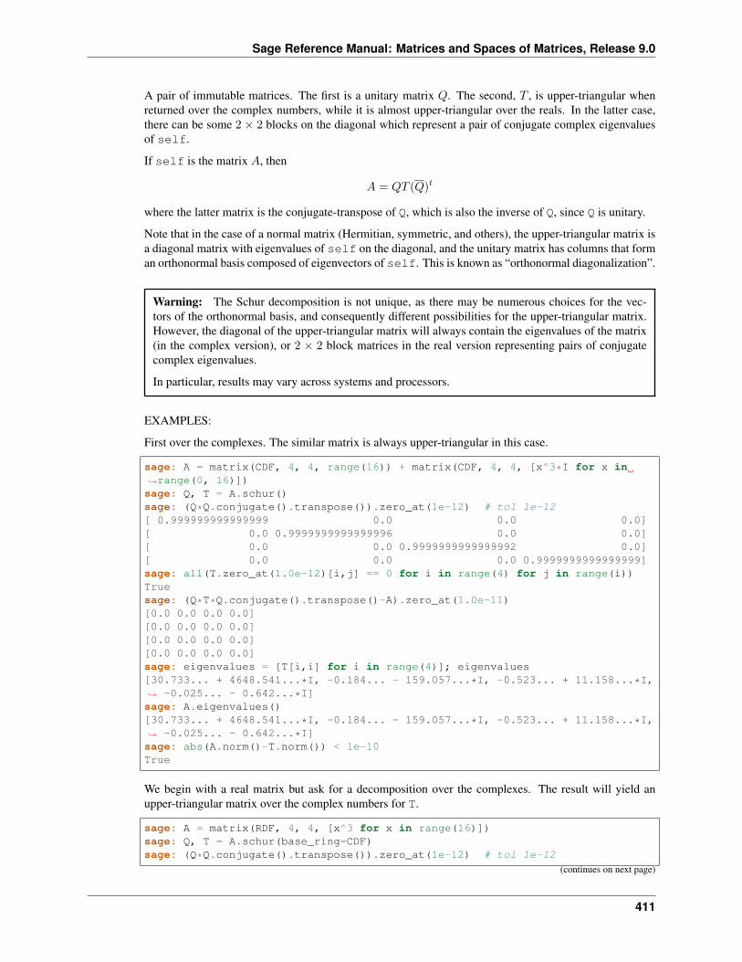
Sage Reference Manual: Matrices and Spaces of Matrices, Release 9.0
A pair of immutable matrices. The first is a unitary matrix 𝑄. The second, 𝑇 , is upper-triangular whenreturned over the complex numbers, while it is almost upper-triangular over the reals. In the latter case,there can be some 2 × 2 blocks on the diagonal which represent a pair of conjugate complex eigenvaluesof self.
If self is the matrix 𝐴, then
𝐴 = 𝑄𝑇 (𝑄)𝑡
where the latter matrix is the conjugate-transpose of Q, which is also the inverse of Q, since Q is unitary.
Note that in the case of a normal matrix (Hermitian, symmetric, and others), the upper-triangular matrix isa diagonal matrix with eigenvalues of self on the diagonal, and the unitary matrix has columns that forman orthonormal basis composed of eigenvectors of self. This is known as “orthonormal diagonalization”.
Warning: The Schur decomposition is not unique, as there may be numerous choices for the vec-tors of the orthonormal basis, and consequently different possibilities for the upper-triangular matrix.However, the diagonal of the upper-triangular matrix will always contain the eigenvalues of the matrix(in the complex version), or 2 × 2 block matrices in the real version representing pairs of conjugatecomplex eigenvalues.
In particular, results may vary across systems and processors.
EXAMPLES:
First over the complexes. The similar matrix is always upper-triangular in this case.
sage: A = matrix(CDF, 4, 4, range(16)) + matrix(CDF, 4, 4, [x^3*I for x in→˓range(0, 16)])sage: Q, T = A.schur()sage: (Q*Q.conjugate().transpose()).zero_at(1e-12) # tol 1e-12[ 0.999999999999999 0.0 0.0 0.0][ 0.0 0.9999999999999996 0.0 0.0][ 0.0 0.0 0.9999999999999992 0.0][ 0.0 0.0 0.0 0.9999999999999999]sage: all(T.zero_at(1.0e-12)[i,j] == 0 for i in range(4) for j in range(i))Truesage: (Q*T*Q.conjugate().transpose()-A).zero_at(1.0e-11)[0.0 0.0 0.0 0.0][0.0 0.0 0.0 0.0][0.0 0.0 0.0 0.0][0.0 0.0 0.0 0.0]sage: eigenvalues = [T[i,i] for i in range(4)]; eigenvalues[30.733... + 4648.541...*I, -0.184... - 159.057...*I, -0.523... + 11.158...*I,→˓ -0.025... - 0.642...*I]sage: A.eigenvalues()[30.733... + 4648.541...*I, -0.184... - 159.057...*I, -0.523... + 11.158...*I,→˓ -0.025... - 0.642...*I]sage: abs(A.norm()-T.norm()) < 1e-10True
We begin with a real matrix but ask for a decomposition over the complexes. The result will yield anupper-triangular matrix over the complex numbers for T.
sage: A = matrix(RDF, 4, 4, [x^3 for x in range(16)])sage: Q, T = A.schur(base_ring=CDF)sage: (Q*Q.conjugate().transpose()).zero_at(1e-12) # tol 1e-12
(continues on next page)
411
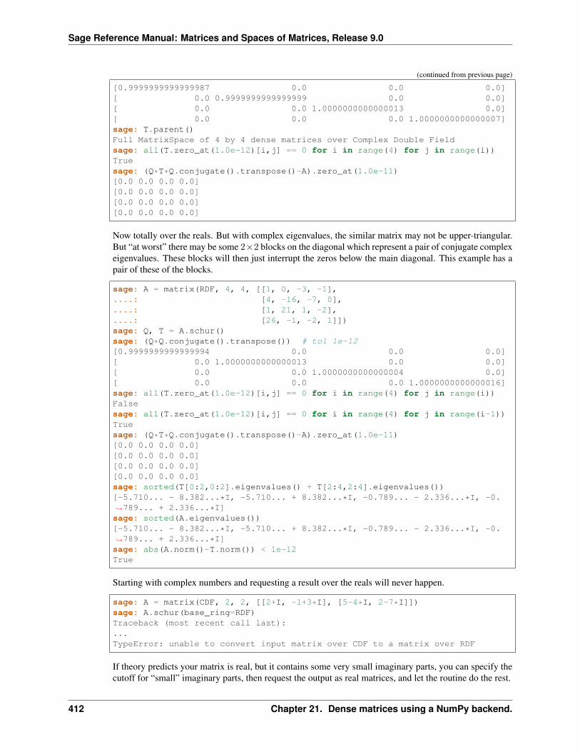
Sage Reference Manual: Matrices and Spaces of Matrices, Release 9.0
(continued from previous page)
[0.9999999999999987 0.0 0.0 0.0][ 0.0 0.9999999999999999 0.0 0.0][ 0.0 0.0 1.0000000000000013 0.0][ 0.0 0.0 0.0 1.0000000000000007]sage: T.parent()Full MatrixSpace of 4 by 4 dense matrices over Complex Double Fieldsage: all(T.zero_at(1.0e-12)[i,j] == 0 for i in range(4) for j in range(i))Truesage: (Q*T*Q.conjugate().transpose()-A).zero_at(1.0e-11)[0.0 0.0 0.0 0.0][0.0 0.0 0.0 0.0][0.0 0.0 0.0 0.0][0.0 0.0 0.0 0.0]
Now totally over the reals. But with complex eigenvalues, the similar matrix may not be upper-triangular.But “at worst” there may be some 2×2 blocks on the diagonal which represent a pair of conjugate complexeigenvalues. These blocks will then just interrupt the zeros below the main diagonal. This example has apair of these of the blocks.
sage: A = matrix(RDF, 4, 4, [[1, 0, -3, -1],....: [4, -16, -7, 0],....: [1, 21, 1, -2],....: [26, -1, -2, 1]])sage: Q, T = A.schur()sage: (Q*Q.conjugate().transpose()) # tol 1e-12[0.9999999999999994 0.0 0.0 0.0][ 0.0 1.0000000000000013 0.0 0.0][ 0.0 0.0 1.0000000000000004 0.0][ 0.0 0.0 0.0 1.0000000000000016]sage: all(T.zero_at(1.0e-12)[i,j] == 0 for i in range(4) for j in range(i))Falsesage: all(T.zero_at(1.0e-12)[i,j] == 0 for i in range(4) for j in range(i-1))Truesage: (Q*T*Q.conjugate().transpose()-A).zero_at(1.0e-11)[0.0 0.0 0.0 0.0][0.0 0.0 0.0 0.0][0.0 0.0 0.0 0.0][0.0 0.0 0.0 0.0]sage: sorted(T[0:2,0:2].eigenvalues() + T[2:4,2:4].eigenvalues())[-5.710... - 8.382...*I, -5.710... + 8.382...*I, -0.789... - 2.336...*I, -0.→˓789... + 2.336...*I]sage: sorted(A.eigenvalues())[-5.710... - 8.382...*I, -5.710... + 8.382...*I, -0.789... - 2.336...*I, -0.→˓789... + 2.336...*I]sage: abs(A.norm()-T.norm()) < 1e-12True
Starting with complex numbers and requesting a result over the reals will never happen.
sage: A = matrix(CDF, 2, 2, [[2+I, -1+3*I], [5-4*I, 2-7*I]])sage: A.schur(base_ring=RDF)Traceback (most recent call last):...TypeError: unable to convert input matrix over CDF to a matrix over RDF
If theory predicts your matrix is real, but it contains some very small imaginary parts, you can specify thecutoff for “small” imaginary parts, then request the output as real matrices, and let the routine do the rest.
412 Chapter 21. Dense matrices using a NumPy backend.
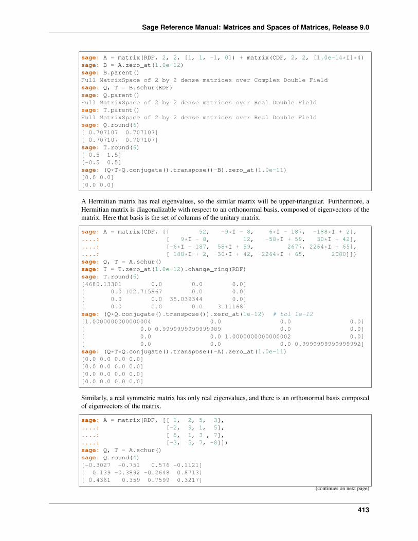
Sage Reference Manual: Matrices and Spaces of Matrices, Release 9.0
sage: A = matrix(RDF, 2, 2, [1, 1, -1, 0]) + matrix(CDF, 2, 2, [1.0e-14*I]*4)sage: B = A.zero_at(1.0e-12)sage: B.parent()Full MatrixSpace of 2 by 2 dense matrices over Complex Double Fieldsage: Q, T = B.schur(RDF)sage: Q.parent()Full MatrixSpace of 2 by 2 dense matrices over Real Double Fieldsage: T.parent()Full MatrixSpace of 2 by 2 dense matrices over Real Double Fieldsage: Q.round(6)[ 0.707107 0.707107][-0.707107 0.707107]sage: T.round(6)[ 0.5 1.5][-0.5 0.5]sage: (Q*T*Q.conjugate().transpose()-B).zero_at(1.0e-11)[0.0 0.0][0.0 0.0]
A Hermitian matrix has real eigenvalues, so the similar matrix will be upper-triangular. Furthermore, aHermitian matrix is diagonalizable with respect to an orthonormal basis, composed of eigenvectors of thematrix. Here that basis is the set of columns of the unitary matrix.
sage: A = matrix(CDF, [[ 52, -9*I - 8, 6*I - 187, -188*I + 2],....: [ 9*I - 8, 12, -58*I + 59, 30*I + 42],....: [-6*I - 187, 58*I + 59, 2677, 2264*I + 65],....: [ 188*I + 2, -30*I + 42, -2264*I + 65, 2080]])sage: Q, T = A.schur()sage: T = T.zero_at(1.0e-12).change_ring(RDF)sage: T.round(6)[4680.13301 0.0 0.0 0.0][ 0.0 102.715967 0.0 0.0][ 0.0 0.0 35.039344 0.0][ 0.0 0.0 0.0 3.11168]sage: (Q*Q.conjugate().transpose()).zero_at(1e-12) # tol 1e-12[1.0000000000000004 0.0 0.0 0.0][ 0.0 0.9999999999999989 0.0 0.0][ 0.0 0.0 1.0000000000000002 0.0][ 0.0 0.0 0.0 0.9999999999999992]sage: (Q*T*Q.conjugate().transpose()-A).zero_at(1.0e-11)[0.0 0.0 0.0 0.0][0.0 0.0 0.0 0.0][0.0 0.0 0.0 0.0][0.0 0.0 0.0 0.0]
Similarly, a real symmetric matrix has only real eigenvalues, and there is an orthonormal basis composedof eigenvectors of the matrix.
sage: A = matrix(RDF, [[ 1, -2, 5, -3],....: [-2, 9, 1, 5],....: [ 5, 1, 3 , 7],....: [-3, 5, 7, -8]])sage: Q, T = A.schur()sage: Q.round(4)[-0.3027 -0.751 0.576 -0.1121][ 0.139 -0.3892 -0.2648 0.8713][ 0.4361 0.359 0.7599 0.3217]
(continues on next page)
413
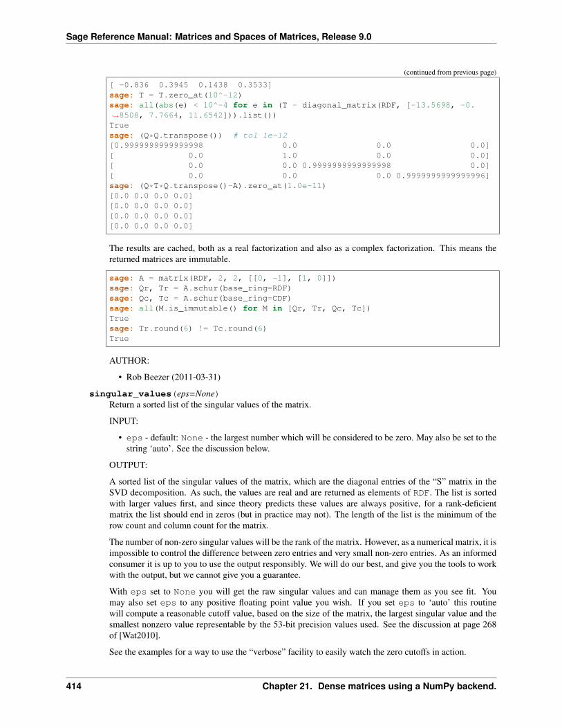
Sage Reference Manual: Matrices and Spaces of Matrices, Release 9.0
(continued from previous page)
[ -0.836 0.3945 0.1438 0.3533]sage: T = T.zero_at(10^-12)sage: all(abs(e) < 10^-4 for e in (T - diagonal_matrix(RDF, [-13.5698, -0.→˓8508, 7.7664, 11.6542])).list())Truesage: (Q*Q.transpose()) # tol 1e-12[0.9999999999999998 0.0 0.0 0.0][ 0.0 1.0 0.0 0.0][ 0.0 0.0 0.9999999999999998 0.0][ 0.0 0.0 0.0 0.9999999999999996]sage: (Q*T*Q.transpose()-A).zero_at(1.0e-11)[0.0 0.0 0.0 0.0][0.0 0.0 0.0 0.0][0.0 0.0 0.0 0.0][0.0 0.0 0.0 0.0]
The results are cached, both as a real factorization and also as a complex factorization. This means thereturned matrices are immutable.
sage: A = matrix(RDF, 2, 2, [[0, -1], [1, 0]])sage: Qr, Tr = A.schur(base_ring=RDF)sage: Qc, Tc = A.schur(base_ring=CDF)sage: all(M.is_immutable() for M in [Qr, Tr, Qc, Tc])Truesage: Tr.round(6) != Tc.round(6)True
AUTHOR:
• Rob Beezer (2011-03-31)
singular_values(eps=None)Return a sorted list of the singular values of the matrix.
INPUT:
• eps - default: None - the largest number which will be considered to be zero. May also be set to thestring ‘auto’. See the discussion below.
OUTPUT:
A sorted list of the singular values of the matrix, which are the diagonal entries of the “S” matrix in theSVD decomposition. As such, the values are real and are returned as elements of RDF. The list is sortedwith larger values first, and since theory predicts these values are always positive, for a rank-deficientmatrix the list should end in zeros (but in practice may not). The length of the list is the minimum of therow count and column count for the matrix.
The number of non-zero singular values will be the rank of the matrix. However, as a numerical matrix, it isimpossible to control the difference between zero entries and very small non-zero entries. As an informedconsumer it is up to you to use the output responsibly. We will do our best, and give you the tools to workwith the output, but we cannot give you a guarantee.
With eps set to None you will get the raw singular values and can manage them as you see fit. Youmay also set eps to any positive floating point value you wish. If you set eps to ‘auto’ this routinewill compute a reasonable cutoff value, based on the size of the matrix, the largest singular value and thesmallest nonzero value representable by the 53-bit precision values used. See the discussion at page 268of [Wat2010].
See the examples for a way to use the “verbose” facility to easily watch the zero cutoffs in action.
414 Chapter 21. Dense matrices using a NumPy backend.
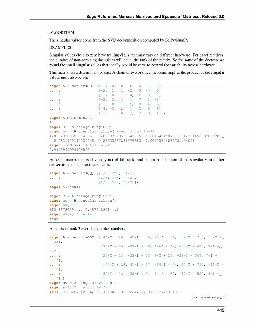
Sage Reference Manual: Matrices and Spaces of Matrices, Release 9.0
ALGORITHM:
The singular values come from the SVD decomposition computed by SciPy/NumPy.
EXAMPLES:
Singular values close to zero have trailing digits that may vary on different hardware. For exact matrices,the number of non-zero singular values will equal the rank of the matrix. So for some of the doctests weround the small singular values that ideally would be zero, to control the variability across hardware.
This matrix has a determinant of one. A chain of two or three theorems implies the product of the singularvalues must also be one.
sage: A = matrix(QQ, [[ 1, 0, 0, 0, 0, 1, 3],....: [-2, 1, 1, -2, 0, -4, 0],....: [ 1, 0, 1, -4, -6, -3, 7],....: [-2, 2, 1, 1, 7, 1, -1],....: [-1, 0, -1, 5, 8, 4, -6],....: [ 4, -2, -2, 1, -3, 0, 8],....: [-2, 1, 0, 2, 7, 3, -4]])sage: A.determinant()1sage: B = A.change_ring(RDF)sage: sv = B.singular_values(); sv # tol 1e-12[20.523980658874265, 8.486837028536643, 5.86168134845073, 2.4429165899286978,→˓0.5831970144724045, 0.26933287286576313, 0.0025524488076110402]sage: prod(sv) # tol 1e-120.9999999999999525
An exact matrix that is obviously not of full rank, and then a computation of the singular values afterconversion to an approximate matrix.
sage: A = matrix(QQ, [[1/3, 2/3, 11/3],....: [2/3, 1/3, 7/3],....: [2/3, 5/3, 27/3]])sage: A.rank()2sage: B = A.change_ring(CDF)sage: sv = B.singular_values()sage: sv[0:2][10.1973039..., 0.487045871...]sage: sv[2] < 1e-14True
A matrix of rank 3 over the complex numbers.
sage: A = matrix(CDF, [[46*I - 28, -47*I - 50, 21*I + 51, -62*I - 782, 13*I +→˓22],....: [35*I - 20, -32*I - 46, 18*I + 43, -57*I - 670, 7*I +→˓3],....: [22*I - 13, -23*I - 23, 9*I + 24, -26*I - 347, 7*I +→˓13],....: [-44*I + 23, 41*I + 57, -19*I - 54, 60*I + 757, -11*I -→˓ 9],....: [30*I - 18, -30*I - 34, 14*I + 34, -42*I - 522, 8*I +→˓12]])sage: sv = A.singular_values()sage: sv[0:3] # tol 1e-14[1440.7336659952966, 18.404403413369227, 6.839707797136151]
(continues on next page)
415
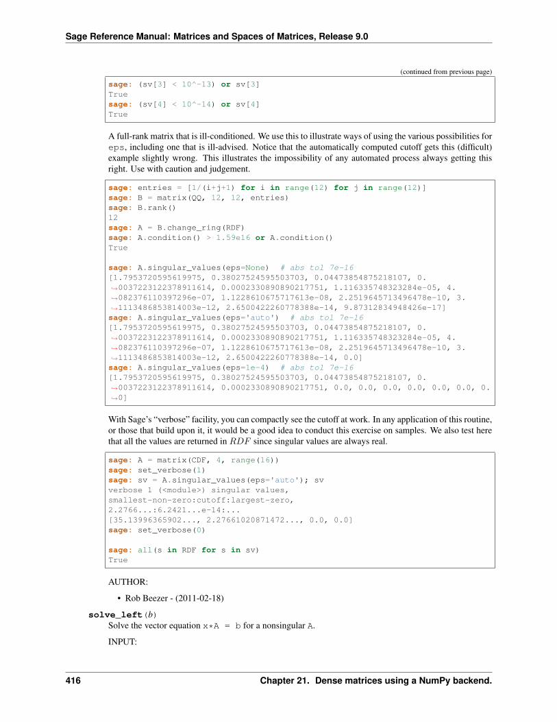
Sage Reference Manual: Matrices and Spaces of Matrices, Release 9.0
(continued from previous page)
sage: (sv[3] < 10^-13) or sv[3]Truesage: (sv[4] < 10^-14) or sv[4]True
A full-rank matrix that is ill-conditioned. We use this to illustrate ways of using the various possibilities foreps, including one that is ill-advised. Notice that the automatically computed cutoff gets this (difficult)example slightly wrong. This illustrates the impossibility of any automated process always getting thisright. Use with caution and judgement.
sage: entries = [1/(i+j+1) for i in range(12) for j in range(12)]sage: B = matrix(QQ, 12, 12, entries)sage: B.rank()12sage: A = B.change_ring(RDF)sage: A.condition() > 1.59e16 or A.condition()True
sage: A.singular_values(eps=None) # abs tol 7e-16[1.7953720595619975, 0.38027524595503703, 0.04473854875218107, 0.→˓0037223122378911614, 0.0002330890890217751, 1.116335748323284e-05, 4.→˓082376110397296e-07, 1.1228610675717613e-08, 2.2519645713496478e-10, 3.→˓1113486853814003e-12, 2.6500422260778388e-14, 9.87312834948426e-17]sage: A.singular_values(eps='auto') # abs tol 7e-16[1.7953720595619975, 0.38027524595503703, 0.04473854875218107, 0.→˓0037223122378911614, 0.0002330890890217751, 1.116335748323284e-05, 4.→˓082376110397296e-07, 1.1228610675717613e-08, 2.2519645713496478e-10, 3.→˓1113486853814003e-12, 2.6500422260778388e-14, 0.0]sage: A.singular_values(eps=1e-4) # abs tol 7e-16[1.7953720595619975, 0.38027524595503703, 0.04473854875218107, 0.→˓0037223122378911614, 0.0002330890890217751, 0.0, 0.0, 0.0, 0.0, 0.0, 0.0, 0.→˓0]
With Sage’s “verbose” facility, you can compactly see the cutoff at work. In any application of this routine,or those that build upon it, it would be a good idea to conduct this exercise on samples. We also test herethat all the values are returned in 𝑅𝐷𝐹 since singular values are always real.
sage: A = matrix(CDF, 4, range(16))sage: set_verbose(1)sage: sv = A.singular_values(eps='auto'); svverbose 1 (<module>) singular values,smallest-non-zero:cutoff:largest-zero,2.2766...:6.2421...e-14:...[35.13996365902..., 2.27661020871472..., 0.0, 0.0]sage: set_verbose(0)
sage: all(s in RDF for s in sv)True
AUTHOR:
• Rob Beezer - (2011-02-18)
solve_left(b)Solve the vector equation x*A = b for a nonsingular A.
INPUT:
416 Chapter 21. Dense matrices using a NumPy backend.
Sage Reference Manual: Matrices and Spaces of Matrices, Release 9.0
• self - a square matrix that is nonsingular (of full rank).
• b - a vector of the correct size. Elements of the vector must coerce into the base ring of the coefficientmatrix. In particular, if b has entries from CDF then self must have CDF as its base ring.
OUTPUT:
The unique solution x to the matrix equation x*A = b, as a vector over the same base ring as self.
ALGORITHM:
Uses the solve() routine from the SciPy scipy.linalg module, after taking the transpose of thecoefficient matrix.
EXAMPLES:
Over the reals.
sage: A = matrix(RDF, 3,3, [1,2,5,7.6,2.3,1,1,2,-1]); A[ 1.0 2.0 5.0][ 7.6 2.3 1.0][ 1.0 2.0 -1.0]sage: b = vector(RDF,[1,2,3])sage: x = A.solve_left(b); x.zero_at(2e-17) # fix noisy zeroes(0.666666666..., 0.0, 0.333333333...)sage: x.parent()Vector space of dimension 3 over Real Double Fieldsage: x*A # tol 1e-14(0.9999999999999999, 1.9999999999999998, 3.0)
Over the complex numbers.
sage: A = matrix(CDF, [[ 0, -1 + 2*I, 1 - 3*I, I],....: [2 + 4*I, -2 + 3*I, -1 + 2*I, -1 - I],....: [ 2 + I, 1 - I, -1, 5],....: [ 3*I, -1 - I, -1 + I, -3 + I]])sage: b = vector(CDF, [2 -3*I, 3, -2 + 3*I, 8])sage: x = A.solve_left(b); x(-1.55765124... - 0.644483985...*I, 0.183274021... + 0.286476868...*I, 0.→˓270818505... + 0.246619217...*I, -1.69003558... - 0.828113879...*I)sage: x.parent()Vector space of dimension 4 over Complex Double Fieldsage: abs(x*A - b) < 1e-14True
The vector of constants, b, can be given in a variety of forms, so long as it coerces to a vector over thesame base ring as the coefficient matrix.
sage: A = matrix(CDF, 5, [1/(i+j+1) for i in range(5) for j in range(5)])sage: A.solve_left([1]*5) # tol 1e-11(5.0, -120.0, 630.0, -1120.0, 630.0)
solve_right(b)Solve the vector equation A*x = b for a nonsingular A.
INPUT:
• self - a square matrix that is nonsingular (of full rank).
• b - a vector of the correct size. Elements of the vector must coerce into the base ring of the coefficientmatrix. In particular, if b has entries from CDF then self must have CDF as its base ring.
417
Sage Reference Manual: Matrices and Spaces of Matrices, Release 9.0
OUTPUT:
The unique solution x to the matrix equation A*x = b, as a vector over the same base ring as self.
ALGORITHM:
Uses the solve() routine from the SciPy scipy.linalg module.
EXAMPLES:
Over the reals.
sage: A = matrix(RDF, 3,3, [1,2,5,7.6,2.3,1,1,2,-1]); A[ 1.0 2.0 5.0][ 7.6 2.3 1.0][ 1.0 2.0 -1.0]sage: b = vector(RDF,[1,2,3])sage: x = A.solve_right(b); x # tol 1e-14(-0.1136950904392765, 1.3901808785529717, -0.33333333333333337)sage: x.parent()Vector space of dimension 3 over Real Double Fieldsage: A*x # tol 1e-14(1.0, 1.9999999999999996, 3.0000000000000004)
Over the complex numbers.
sage: A = matrix(CDF, [[ 0, -1 + 2*I, 1 - 3*I, I],....: [2 + 4*I, -2 + 3*I, -1 + 2*I, -1 - I],....: [ 2 + I, 1 - I, -1, 5],....: [ 3*I, -1 - I, -1 + I, -3 + I]])sage: b = vector(CDF, [2 -3*I, 3, -2 + 3*I, 8])sage: x = A.solve_right(b); x(1.96841637... - 1.07606761...*I, -0.614323843... + 1.68416370...*I, 0.→˓0733985765... + 1.73487544...*I, -1.6018683... + 0.524021352...*I)sage: x.parent()Vector space of dimension 4 over Complex Double Fieldsage: abs(A*x - b) < 1e-14True
The vector of constants, b, can be given in a variety of forms, so long as it coerces to a vector over thesame base ring as the coefficient matrix.
sage: A = matrix(CDF, 5, [1/(i+j+1) for i in range(5) for j in range(5)])sage: A.solve_right([1]*5) # tol 1e-11(5.0, -120.0, 630.0, -1120.0, 630.0)
transpose()Return the transpose of this matrix, without changing self.
EXAMPLES:
sage: m = matrix(RDF,2,3,range(6)); m[0.0 1.0 2.0][3.0 4.0 5.0]sage: m2 = m.transpose()sage: m[0,0] = 2sage: m2 #note that m2 hasn't changed[0.0 3.0][1.0 4.0][2.0 5.0]
418 Chapter 21. Dense matrices using a NumPy backend.
Sage Reference Manual: Matrices and Spaces of Matrices, Release 9.0
.T is a convenient shortcut for the transpose:
sage: m.T[2.0 3.0][1.0 4.0][2.0 5.0]
sage: m = matrix(RDF,0,3); m[]sage: m.transpose()[]sage: m.transpose().parent()Full MatrixSpace of 3 by 0 dense matrices over Real Double Field
zero_at(eps)Return a copy of the matrix where elements smaller than or equal to eps are replaced with zeroes. Forcomplex matrices, the real and imaginary parts are considered individually.
This is useful for modifying output from algorithms which have large relative errors when producing zeroelements, e.g. to create reliable doctests.
INPUT:
• eps - Cutoff value
OUTPUT:
A modified copy of the matrix.
EXAMPLES:
sage: a = matrix(CDF, [[1, 1e-4r, 1+1e-100jr], [1e-8+3j, 0, 1e-58r]])sage: a[ 1.0 0.0001 1.0 + 1e-100*I][ 1e-08 + 3.0*I 0.0 1e-58]sage: a.zero_at(1e-50)[ 1.0 0.0001 1.0][1e-08 + 3.0*I 0.0 0.0]sage: a.zero_at(1e-4)[ 1.0 0.0 1.0][3.0*I 0.0 0.0]
419

Sage Reference Manual: Matrices and Spaces of Matrices, Release 9.0
420 Chapter 21. Dense matrices using a NumPy backend.
CHAPTER
TWENTYTWO
DENSE MATRICES OVER THE REAL DOUBLE FIELD USING NUMPY
EXAMPLES:
sage: b = Mat(RDF,2,3).basis()sage: b[0,0][1.0 0.0 0.0][0.0 0.0 0.0]
We deal with the case of zero rows or zero columns:
sage: m = MatrixSpace(RDF,0,3)sage: m.zero_matrix()[]
AUTHORS:
• Jason Grout (2008-09): switch to NumPy backend, factored out the Matrix_double_dense class
• Josh Kantor
• William Stein: many bug fixes and touch ups.
class sage.matrix.matrix_real_double_dense.Matrix_real_double_denseBases: sage.matrix.matrix_double_dense.Matrix_double_dense
Class that implements matrices over the real double field. These are supposed to be fast matrix operations usingC doubles. Most operations are implemented using numpy which will call the underlying BLAS on the system.
EXAMPLES:
sage: m = Matrix(RDF, [[1,2],[3,4]])sage: m**2[ 7.0 10.0][15.0 22.0]sage: n = m^(-1); n # rel tol 1e-15[-1.9999999999999996 0.9999999999999998][ 1.4999999999999998 -0.4999999999999999]
To compute eigenvalues the use the functions left_eigenvectors or right_eigenvectors
sage: p,e = m.right_eigenvectors()
the result of eigen is a pair (p,e), where p is a list of eigenvalues and the e is a matrix whose columns are theeigenvectors.
To solve a linear system Ax = b where A = [[1,2],[3,4]] and b = [5,6].
421
Sage Reference Manual: Matrices and Spaces of Matrices, Release 9.0
sage: b = vector(RDF,[5,6])sage: m.solve_right(b) # rel tol 1e-15(-3.9999999999999987, 4.499999999999999)
See the commands qr, lu, and svd for QR, LU, and singular value decomposition.
422 Chapter 22. Dense matrices over the Real Double Field using NumPy
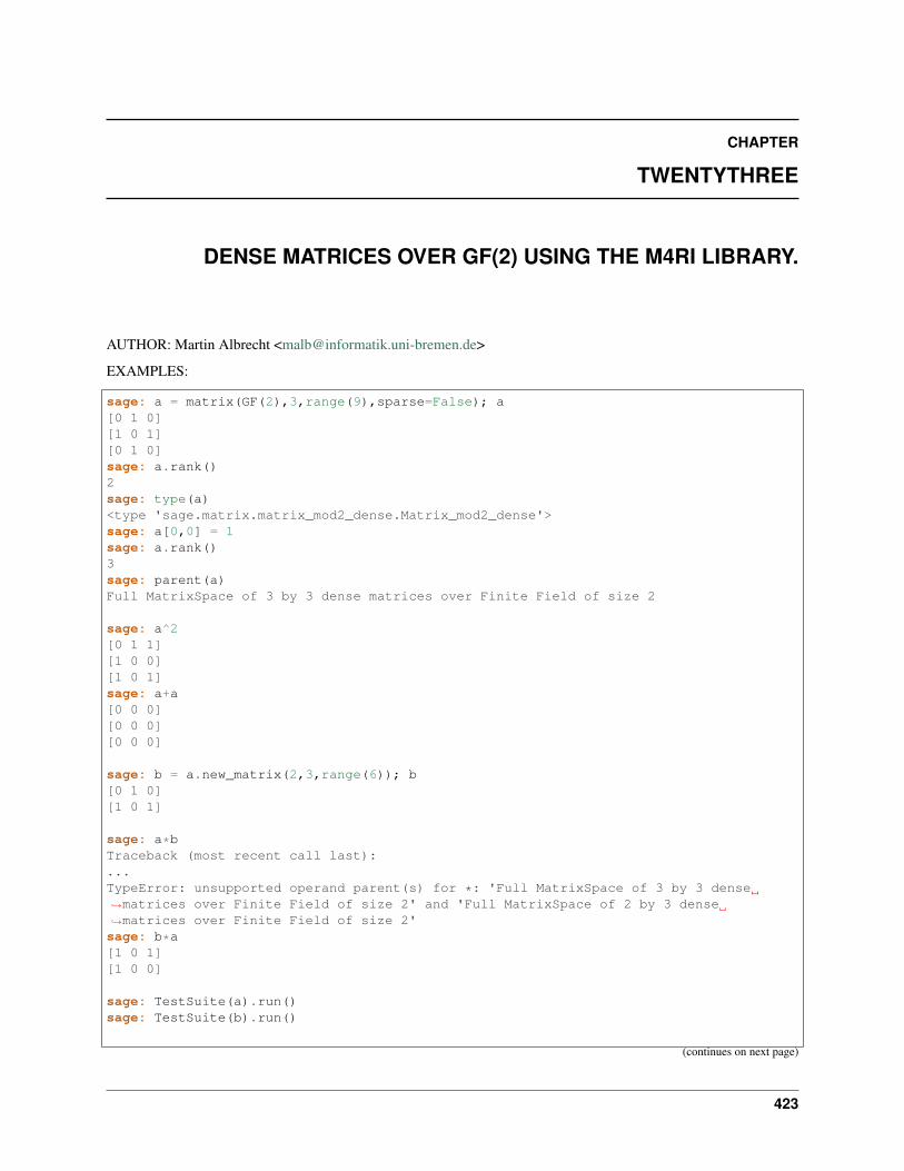
CHAPTER
TWENTYTHREE
DENSE MATRICES OVER GF(2) USING THE M4RI LIBRARY.
AUTHOR: Martin Albrecht <[email protected]>
EXAMPLES:
sage: a = matrix(GF(2),3,range(9),sparse=False); a[0 1 0][1 0 1][0 1 0]sage: a.rank()2sage: type(a)<type 'sage.matrix.matrix_mod2_dense.Matrix_mod2_dense'>sage: a[0,0] = 1sage: a.rank()3sage: parent(a)Full MatrixSpace of 3 by 3 dense matrices over Finite Field of size 2
sage: a^2[0 1 1][1 0 0][1 0 1]sage: a+a[0 0 0][0 0 0][0 0 0]
sage: b = a.new_matrix(2,3,range(6)); b[0 1 0][1 0 1]
sage: a*bTraceback (most recent call last):...TypeError: unsupported operand parent(s) for *: 'Full MatrixSpace of 3 by 3 dense→˓matrices over Finite Field of size 2' and 'Full MatrixSpace of 2 by 3 dense→˓matrices over Finite Field of size 2'sage: b*a[1 0 1][1 0 0]
sage: TestSuite(a).run()sage: TestSuite(b).run()
(continues on next page)
423
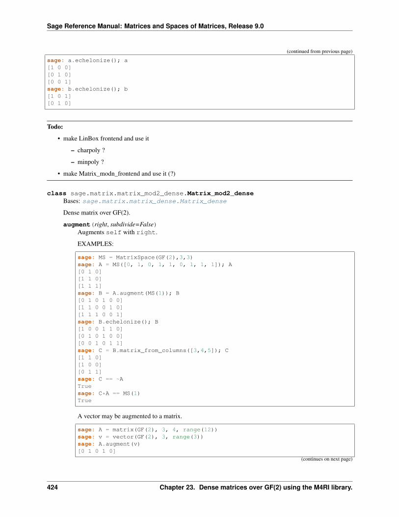
Sage Reference Manual: Matrices and Spaces of Matrices, Release 9.0
(continued from previous page)
sage: a.echelonize(); a[1 0 0][0 1 0][0 0 1]sage: b.echelonize(); b[1 0 1][0 1 0]
Todo:
• make LinBox frontend and use it
– charpoly ?
– minpoly ?
• make Matrix_modn_frontend and use it (?)
class sage.matrix.matrix_mod2_dense.Matrix_mod2_denseBases: sage.matrix.matrix_dense.Matrix_dense
Dense matrix over GF(2).
augment(right, subdivide=False)Augments self with right.
EXAMPLES:
sage: MS = MatrixSpace(GF(2),3,3)sage: A = MS([0, 1, 0, 1, 1, 0, 1, 1, 1]); A[0 1 0][1 1 0][1 1 1]sage: B = A.augment(MS(1)); B[0 1 0 1 0 0][1 1 0 0 1 0][1 1 1 0 0 1]sage: B.echelonize(); B[1 0 0 1 1 0][0 1 0 1 0 0][0 0 1 0 1 1]sage: C = B.matrix_from_columns([3,4,5]); C[1 1 0][1 0 0][0 1 1]sage: C == ~ATruesage: C*A == MS(1)True
A vector may be augmented to a matrix.
sage: A = matrix(GF(2), 3, 4, range(12))sage: v = vector(GF(2), 3, range(3))sage: A.augment(v)[0 1 0 1 0]
(continues on next page)
424 Chapter 23. Dense matrices over GF(2) using the M4RI library.
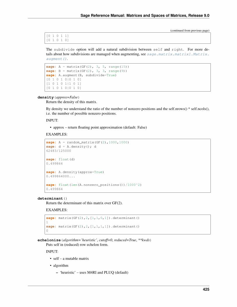
Sage Reference Manual: Matrices and Spaces of Matrices, Release 9.0
(continued from previous page)
[0 1 0 1 1][0 1 0 1 0]
The subdivide option will add a natural subdivision between self and right. For more de-tails about how subdivisions are managed when augmenting, see sage.matrix.matrix1.Matrix.augment().
sage: A = matrix(GF(2), 3, 5, range(15))sage: B = matrix(GF(2), 3, 3, range(9))sage: A.augment(B, subdivide=True)[0 1 0 1 0|0 1 0][1 0 1 0 1|1 0 1][0 1 0 1 0|0 1 0]
density(approx=False)Return the density of this matrix.
By density we understand the ratio of the number of nonzero positions and the self.nrows() * self.ncols(),i.e. the number of possible nonzero positions.
INPUT:
• approx – return floating point approximation (default: False)
EXAMPLES:
sage: A = random_matrix(GF(2),1000,1000)sage: d = A.density(); d62483/125000
sage: float(d)0.499864
sage: A.density(approx=True)0.499864000...
sage: float(len(A.nonzero_positions())/1000^2)0.499864
determinant()Return the determinant of this matrix over GF(2).
EXAMPLES:
sage: matrix(GF(2),2,[1,1,0,1]).determinant()1sage: matrix(GF(2),2,[1,1,1,1]).determinant()0
echelonize(algorithm=’heuristic’, cutoff=0, reduced=True, **kwds)Puts self in (reduced) row echelon form.
INPUT:
• self – a mutable matrix
• algorithm
– ‘heuristic’ – uses M4RI and PLUQ (default)
425
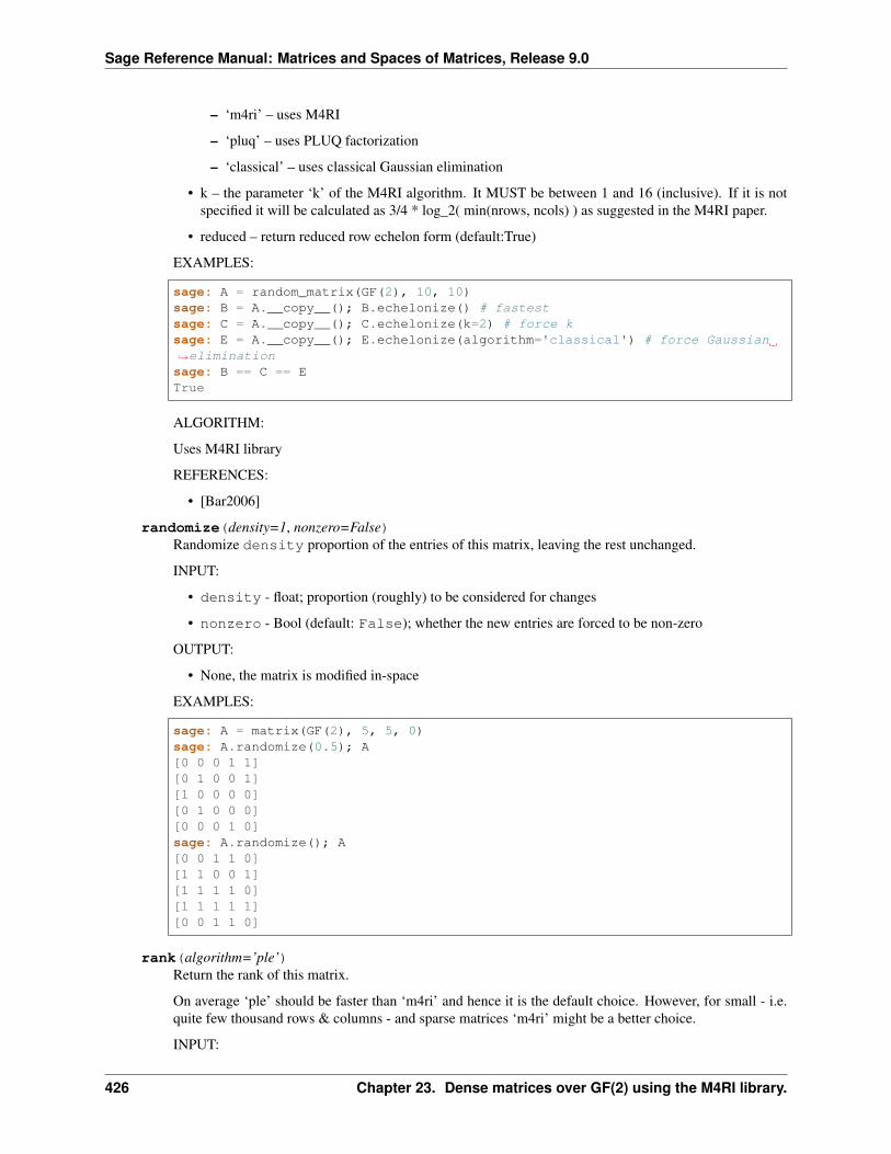
Sage Reference Manual: Matrices and Spaces of Matrices, Release 9.0
– ‘m4ri’ – uses M4RI
– ‘pluq’ – uses PLUQ factorization
– ‘classical’ – uses classical Gaussian elimination
• k – the parameter ‘k’ of the M4RI algorithm. It MUST be between 1 and 16 (inclusive). If it is notspecified it will be calculated as 3/4 * log_2( min(nrows, ncols) ) as suggested in the M4RI paper.
• reduced – return reduced row echelon form (default:True)
EXAMPLES:
sage: A = random_matrix(GF(2), 10, 10)sage: B = A.__copy__(); B.echelonize() # fastestsage: C = A.__copy__(); C.echelonize(k=2) # force ksage: E = A.__copy__(); E.echelonize(algorithm='classical') # force Gaussian→˓eliminationsage: B == C == ETrue
ALGORITHM:
Uses M4RI library
REFERENCES:
• [Bar2006]
randomize(density=1, nonzero=False)Randomize density proportion of the entries of this matrix, leaving the rest unchanged.
INPUT:
• density - float; proportion (roughly) to be considered for changes
• nonzero - Bool (default: False); whether the new entries are forced to be non-zero
OUTPUT:
• None, the matrix is modified in-space
EXAMPLES:
sage: A = matrix(GF(2), 5, 5, 0)sage: A.randomize(0.5); A[0 0 0 1 1][0 1 0 0 1][1 0 0 0 0][0 1 0 0 0][0 0 0 1 0]sage: A.randomize(); A[0 0 1 1 0][1 1 0 0 1][1 1 1 1 0][1 1 1 1 1][0 0 1 1 0]
rank(algorithm=’ple’)Return the rank of this matrix.
On average ‘ple’ should be faster than ‘m4ri’ and hence it is the default choice. However, for small - i.e.quite few thousand rows & columns - and sparse matrices ‘m4ri’ might be a better choice.
INPUT:
426 Chapter 23. Dense matrices over GF(2) using the M4RI library.
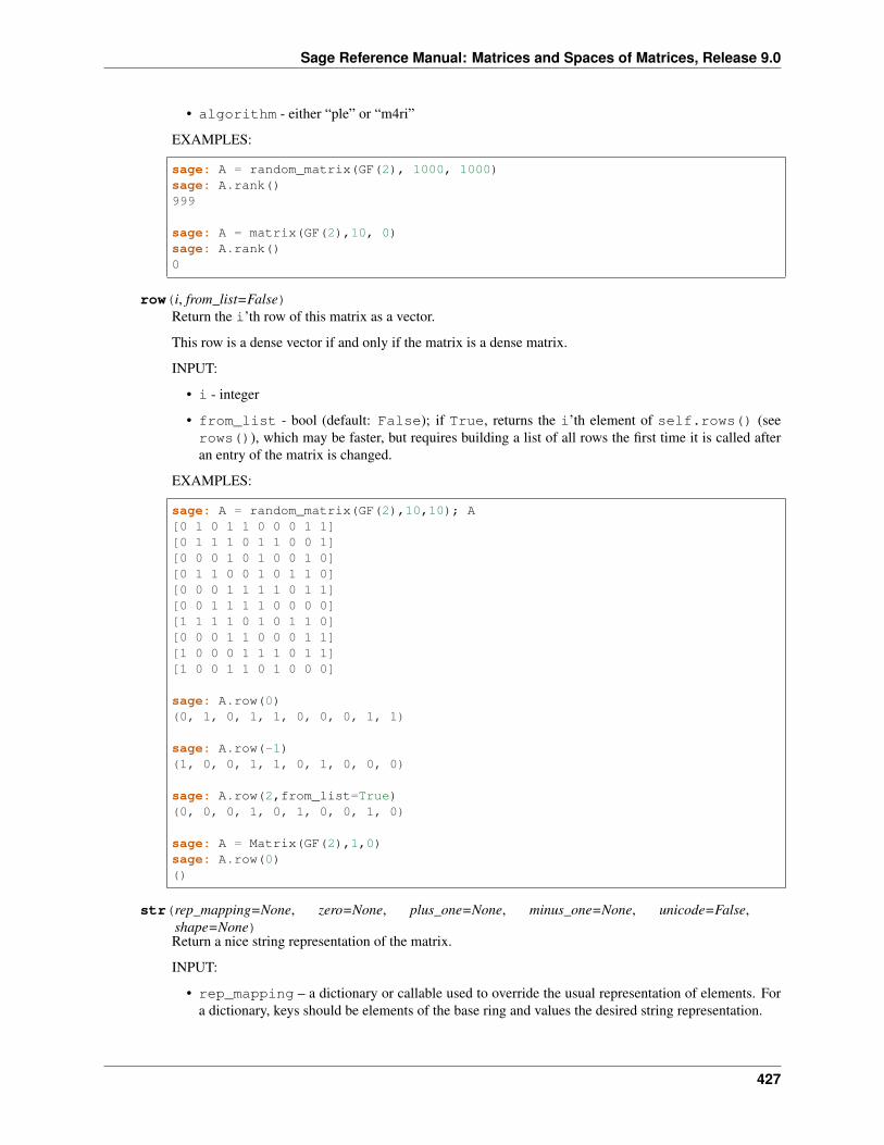
Sage Reference Manual: Matrices and Spaces of Matrices, Release 9.0
• algorithm - either “ple” or “m4ri”
EXAMPLES:
sage: A = random_matrix(GF(2), 1000, 1000)sage: A.rank()999
sage: A = matrix(GF(2),10, 0)sage: A.rank()0
row(i, from_list=False)Return the i’th row of this matrix as a vector.
This row is a dense vector if and only if the matrix is a dense matrix.
INPUT:
• i - integer
• from_list - bool (default: False); if True, returns the i’th element of self.rows() (seerows()), which may be faster, but requires building a list of all rows the first time it is called afteran entry of the matrix is changed.
EXAMPLES:
sage: A = random_matrix(GF(2),10,10); A[0 1 0 1 1 0 0 0 1 1][0 1 1 1 0 1 1 0 0 1][0 0 0 1 0 1 0 0 1 0][0 1 1 0 0 1 0 1 1 0][0 0 0 1 1 1 1 0 1 1][0 0 1 1 1 1 0 0 0 0][1 1 1 1 0 1 0 1 1 0][0 0 0 1 1 0 0 0 1 1][1 0 0 0 1 1 1 0 1 1][1 0 0 1 1 0 1 0 0 0]
sage: A.row(0)(0, 1, 0, 1, 1, 0, 0, 0, 1, 1)
sage: A.row(-1)(1, 0, 0, 1, 1, 0, 1, 0, 0, 0)
sage: A.row(2,from_list=True)(0, 0, 0, 1, 0, 1, 0, 0, 1, 0)
sage: A = Matrix(GF(2),1,0)sage: A.row(0)()
str(rep_mapping=None, zero=None, plus_one=None, minus_one=None, unicode=False,shape=None)Return a nice string representation of the matrix.
INPUT:
• rep_mapping – a dictionary or callable used to override the usual representation of elements. Fora dictionary, keys should be elements of the base ring and values the desired string representation.
427
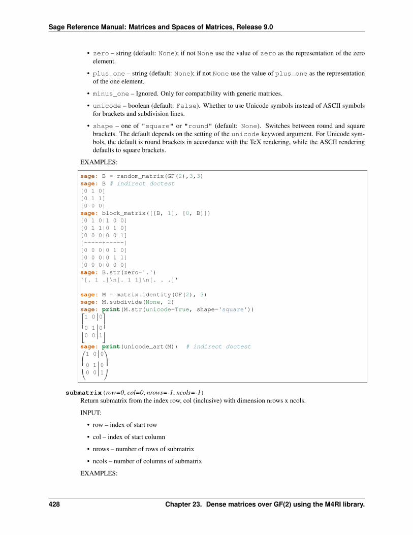
Sage Reference Manual: Matrices and Spaces of Matrices, Release 9.0
• zero – string (default: None); if not None use the value of zero as the representation of the zeroelement.
• plus_one – string (default: None); if not None use the value of plus_one as the representationof the one element.
• minus_one – Ignored. Only for compatibility with generic matrices.
• unicode – boolean (default: False). Whether to use Unicode symbols instead of ASCII symbolsfor brackets and subdivision lines.
• shape – one of "square" or "round" (default: None). Switches between round and squarebrackets. The default depends on the setting of the unicode keyword argument. For Unicode sym-bols, the default is round brackets in accordance with the TeX rendering, while the ASCII renderingdefaults to square brackets.
EXAMPLES:
sage: B = random_matrix(GF(2),3,3)sage: B # indirect doctest[0 1 0][0 1 1][0 0 0]sage: block_matrix([[B, 1], [0, B]])[0 1 0|1 0 0][0 1 1|0 1 0][0 0 0|0 0 1][-----+-----][0 0 0|0 1 0][0 0 0|0 1 1][0 0 0|0 0 0]sage: B.str(zero='.')'[. 1 .]\n[. 1 1]\n[. . .]'
sage: M = matrix.identity(GF(2), 3)sage: M.subdivide(None, 2)sage: print(M.str(unicode=True, shape='square'))⎡1 0 0
⎤⎢0 1 0
⎥⎣0 0 1
⎦sage: print(unicode_art(M)) # indirect doctest⎛1 0 0
⎞⎜0 1 0
⎟⎝0 0 1
⎠submatrix(row=0, col=0, nrows=-1, ncols=-1)
Return submatrix from the index row, col (inclusive) with dimension nrows x ncols.
INPUT:
• row – index of start row
• col – index of start column
• nrows – number of rows of submatrix
• ncols – number of columns of submatrix
EXAMPLES:
428 Chapter 23. Dense matrices over GF(2) using the M4RI library.
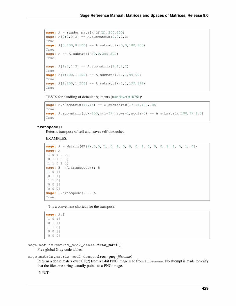
Sage Reference Manual: Matrices and Spaces of Matrices, Release 9.0
sage: A = random_matrix(GF(2),200,200)sage: A[0:2,0:2] == A.submatrix(0,0,2,2)Truesage: A[0:100,0:100] == A.submatrix(0,0,100,100)Truesage: A == A.submatrix(0,0,200,200)True
sage: A[1:3,1:3] == A.submatrix(1,1,2,2)Truesage: A[1:100,1:100] == A.submatrix(1,1,99,99)Truesage: A[1:200,1:200] == A.submatrix(1,1,199,199)True
TESTS for handling of default arguments (trac ticket #18761):
sage: A.submatrix(17,15) == A.submatrix(17,15,183,185)Truesage: A.submatrix(row=100,col=37,nrows=1,ncols=3) == A.submatrix(100,37,1,3)True
transpose()Returns transpose of self and leaves self untouched.
EXAMPLES:
sage: A = Matrix(GF(2),3,5,[1, 0, 1, 0, 0, 0, 1, 1, 0, 0, 1, 1, 0, 1, 0])sage: A[1 0 1 0 0][0 1 1 0 0][1 1 0 1 0]sage: B = A.transpose(); B[1 0 1][0 1 1][1 1 0][0 0 1][0 0 0]sage: B.transpose() == ATrue
.T is a convenient shortcut for the transpose:
sage: A.T[1 0 1][0 1 1][1 1 0][0 0 1][0 0 0]
sage.matrix.matrix_mod2_dense.free_m4ri()Free global Gray code tables.
sage.matrix.matrix_mod2_dense.from_png(filename)Returns a dense matrix over GF(2) from a 1-bit PNG image read from filename. No attempt is made to verifythat the filename string actually points to a PNG image.
INPUT:
429
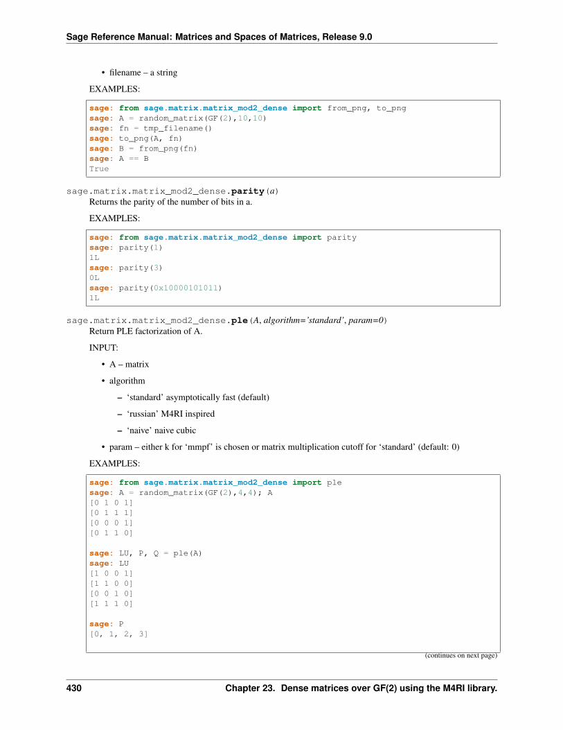
Sage Reference Manual: Matrices and Spaces of Matrices, Release 9.0
• filename – a string
EXAMPLES:
sage: from sage.matrix.matrix_mod2_dense import from_png, to_pngsage: A = random_matrix(GF(2),10,10)sage: fn = tmp_filename()sage: to_png(A, fn)sage: B = from_png(fn)sage: A == BTrue
sage.matrix.matrix_mod2_dense.parity(a)Returns the parity of the number of bits in a.
EXAMPLES:
sage: from sage.matrix.matrix_mod2_dense import paritysage: parity(1)1Lsage: parity(3)0Lsage: parity(0x10000101011)1L
sage.matrix.matrix_mod2_dense.ple(A, algorithm=’standard’, param=0)Return PLE factorization of A.
INPUT:
• A – matrix
• algorithm
– ‘standard’ asymptotically fast (default)
– ‘russian’ M4RI inspired
– ‘naive’ naive cubic
• param – either k for ‘mmpf’ is chosen or matrix multiplication cutoff for ‘standard’ (default: 0)
EXAMPLES:
sage: from sage.matrix.matrix_mod2_dense import plesage: A = random_matrix(GF(2),4,4); A[0 1 0 1][0 1 1 1][0 0 0 1][0 1 1 0]
sage: LU, P, Q = ple(A)sage: LU[1 0 0 1][1 1 0 0][0 0 1 0][1 1 1 0]
sage: P[0, 1, 2, 3]
(continues on next page)
430 Chapter 23. Dense matrices over GF(2) using the M4RI library.
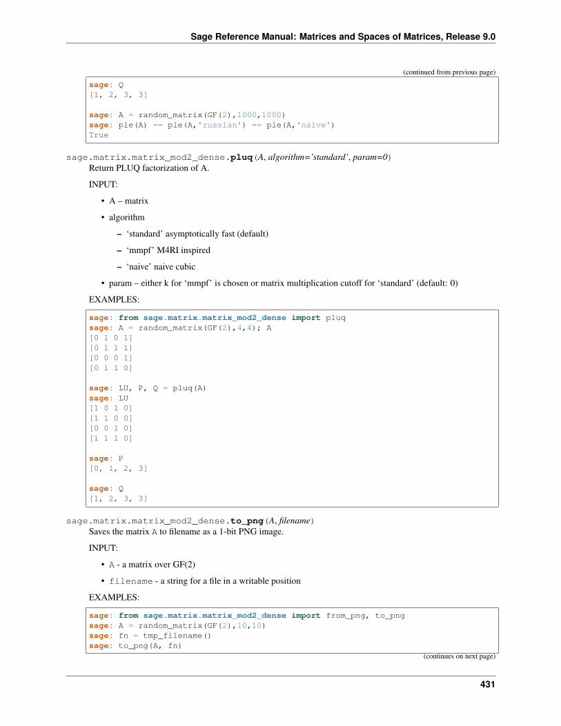
Sage Reference Manual: Matrices and Spaces of Matrices, Release 9.0
(continued from previous page)
sage: Q[1, 2, 3, 3]
sage: A = random_matrix(GF(2),1000,1000)sage: ple(A) == ple(A,'russian') == ple(A,'naive')True
sage.matrix.matrix_mod2_dense.pluq(A, algorithm=’standard’, param=0)Return PLUQ factorization of A.
INPUT:
• A – matrix
• algorithm
– ‘standard’ asymptotically fast (default)
– ‘mmpf’ M4RI inspired
– ‘naive’ naive cubic
• param – either k for ‘mmpf’ is chosen or matrix multiplication cutoff for ‘standard’ (default: 0)
EXAMPLES:
sage: from sage.matrix.matrix_mod2_dense import pluqsage: A = random_matrix(GF(2),4,4); A[0 1 0 1][0 1 1 1][0 0 0 1][0 1 1 0]
sage: LU, P, Q = pluq(A)sage: LU[1 0 1 0][1 1 0 0][0 0 1 0][1 1 1 0]
sage: P[0, 1, 2, 3]
sage: Q[1, 2, 3, 3]
sage.matrix.matrix_mod2_dense.to_png(A, filename)Saves the matrix A to filename as a 1-bit PNG image.
INPUT:
• A - a matrix over GF(2)
• filename - a string for a file in a writable position
EXAMPLES:
sage: from sage.matrix.matrix_mod2_dense import from_png, to_pngsage: A = random_matrix(GF(2),10,10)sage: fn = tmp_filename()sage: to_png(A, fn)
(continues on next page)
431
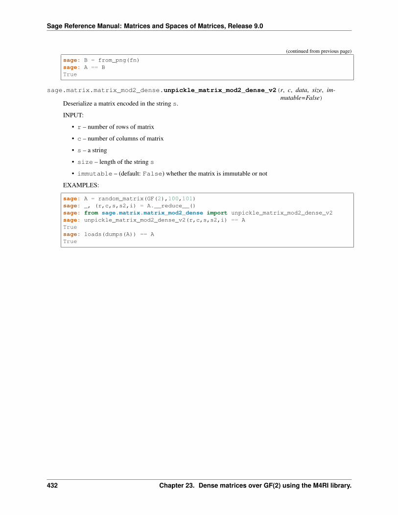
Sage Reference Manual: Matrices and Spaces of Matrices, Release 9.0
(continued from previous page)
sage: B = from_png(fn)sage: A == BTrue
sage.matrix.matrix_mod2_dense.unpickle_matrix_mod2_dense_v2(r, c, data, size, im-mutable=False)
Deserialize a matrix encoded in the string s.
INPUT:
• r – number of rows of matrix
• c – number of columns of matrix
• s – a string
• size – length of the string s
• immutable – (default: False) whether the matrix is immutable or not
EXAMPLES:
sage: A = random_matrix(GF(2),100,101)sage: _, (r,c,s,s2,i) = A.__reduce__()sage: from sage.matrix.matrix_mod2_dense import unpickle_matrix_mod2_dense_v2sage: unpickle_matrix_mod2_dense_v2(r,c,s,s2,i) == ATruesage: loads(dumps(A)) == ATrue
432 Chapter 23. Dense matrices over GF(2) using the M4RI library.
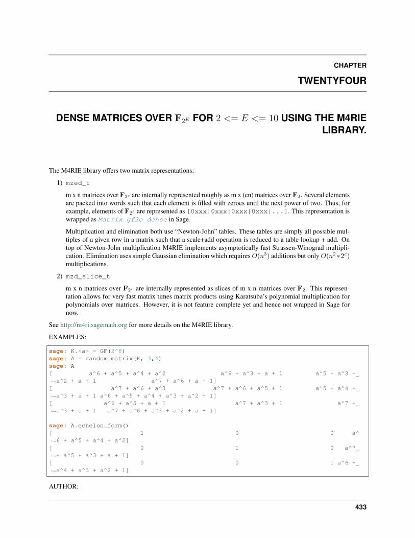
CHAPTER
TWENTYFOUR
DENSE MATRICES OVER F2𝐸 FOR 2 <= 𝐸 <= 10 USING THE M4RIELIBRARY.
The M4RIE library offers two matrix representations:
1) mzed_t
m x n matrices over F2𝑒 are internally represented roughly as m x (en) matrices over F2. Several elementsare packed into words such that each element is filled with zeroes until the next power of two. Thus, forexample, elements of F23 are represented as [0xxx|0xxx|0xxx|0xxx|...]. This representation iswrapped as Matrix_gf2e_dense in Sage.
Multiplication and elimination both use “Newton-John” tables. These tables are simply all possible mul-tiples of a given row in a matrix such that a scale+add operation is reduced to a table lookup + add. Ontop of Newton-John multiplication M4RIE implements asymptotically fast Strassen-Winograd multipli-cation. Elimination uses simple Gaussian elimination which requires 𝑂(𝑛3) additions but only 𝑂(𝑛2 *2𝑒)multiplications.
2) mzd_slice_t
m x n matrices over F2𝑒 are internally represented as slices of m x n matrices over F2. This represen-tation allows for very fast matrix times matrix products using Karatsuba’s polynomial multiplication forpolynomials over matrices. However, it is not feature complete yet and hence not wrapped in Sage fornow.
See http://m4ri.sagemath.org for more details on the M4RIE library.
EXAMPLES:
sage: K.<a> = GF(2^8)sage: A = random_matrix(K, 3,4)sage: A[ a^6 + a^5 + a^4 + a^2 a^6 + a^3 + a + 1 a^5 + a^3 +→˓a^2 + a + 1 a^7 + a^6 + a + 1][ a^7 + a^6 + a^3 a^7 + a^6 + a^5 + 1 a^5 + a^4 +→˓a^3 + a + 1 a^6 + a^5 + a^4 + a^3 + a^2 + 1][ a^6 + a^5 + a + 1 a^7 + a^3 + 1 a^7 +→˓a^3 + a + 1 a^7 + a^6 + a^3 + a^2 + a + 1]
sage: A.echelon_form()[ 1 0 0 a^→˓6 + a^5 + a^4 + a^2][ 0 1 0 a^7→˓+ a^5 + a^3 + a + 1][ 0 0 1 a^6 +→˓a^4 + a^3 + a^2 + 1]
AUTHOR:
433
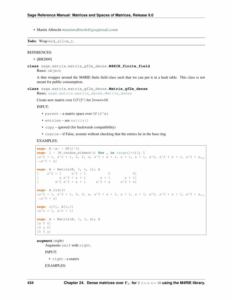
Sage Reference Manual: Matrices and Spaces of Matrices, Release 9.0
• Martin Albrecht <[email protected]>
Todo: Wrap mzd_slice_t.
REFERENCES:
• [BB2009]
class sage.matrix.matrix_gf2e_dense.M4RIE_finite_fieldBases: object
A thin wrapper around the M4RIE finite field class such that we can put it in a hash table. This class is notmeant for public consumption.
class sage.matrix.matrix_gf2e_dense.Matrix_gf2e_denseBases: sage.matrix.matrix_dense.Matrix_dense
Create new matrix over 𝐺𝐹 (2𝑒) for 2<=e<=10.
INPUT:
• parent – a matrix space over GF(2^e)
• entries – see matrix()
• copy – ignored (for backwards compatibility)
• coerce – if False, assume without checking that the entries lie in the base ring
EXAMPLES:
sage: K.<a> = GF(2^4)sage: l = [K.random_element() for _ in range(3*4)]; l[a^2 + 1, a^3 + 1, 0, 0, a, a^3 + a + 1, a + 1, a + 1, a^2, a^3 + a + 1, a^3 + a,→˓a^3 + a]
sage: A = Matrix(K, 3, 4, l); A[ a^2 + 1 a^3 + 1 0 0][ a a^3 + a + 1 a + 1 a + 1][ a^2 a^3 + a + 1 a^3 + a a^3 + a]
sage: A.list()[a^2 + 1, a^3 + 1, 0, 0, a, a^3 + a + 1, a + 1, a + 1, a^2, a^3 + a + 1, a^3 + a,→˓a^3 + a]
sage: l[0], A[0,0](a^2 + 1, a^2 + 1)
sage: A = Matrix(K, 3, 3, a); A[a 0 0][0 a 0][0 0 a]
augment(right)Augments self with right.
INPUT:
• right - a matrix
EXAMPLES:
434 Chapter 24. Dense matrices over F2𝑒 for 2 <= 𝑒 <= 10 using the M4RIE library.
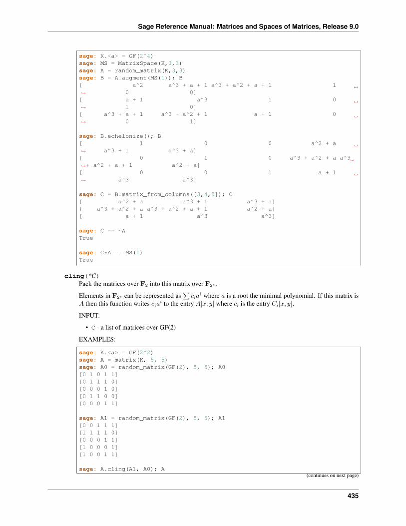
Sage Reference Manual: Matrices and Spaces of Matrices, Release 9.0
sage: K.<a> = GF(2^4)sage: MS = MatrixSpace(K,3,3)sage: A = random_matrix(K,3,3)sage: B = A.augment(MS(1)); B[ a^2 a^3 + a + 1 a^3 + a^2 + a + 1 1→˓ 0 0][ a + 1 a^3 1 0→˓ 1 0][ a^3 + a + 1 a^3 + a^2 + 1 a + 1 0→˓ 0 1]
sage: B.echelonize(); B[ 1 0 0 a^2 + a→˓ a^3 + 1 a^3 + a][ 0 1 0 a^3 + a^2 + a a^3→˓+ a^2 + a + 1 a^2 + a][ 0 0 1 a + 1→˓ a^3 a^3]
sage: C = B.matrix_from_columns([3,4,5]); C[ a^2 + a a^3 + 1 a^3 + a][ a^3 + a^2 + a a^3 + a^2 + a + 1 a^2 + a][ a + 1 a^3 a^3]
sage: C == ~ATrue
sage: C*A == MS(1)True
cling(*C)Pack the matrices over F2 into this matrix over F2𝑒 .
Elements in F2𝑒 can be represented as∑︀
𝑐𝑖𝑎𝑖 where 𝑎 is a root the minimal polynomial. If this matrix is
𝐴 then this function writes 𝑐𝑖𝑎𝑖 to the entry 𝐴[𝑥, 𝑦] where 𝑐𝑖 is the entry 𝐶𝑖[𝑥, 𝑦].
INPUT:
• C - a list of matrices over GF(2)
EXAMPLES:
sage: K.<a> = GF(2^2)sage: A = matrix(K, 5, 5)sage: A0 = random_matrix(GF(2), 5, 5); A0[0 1 0 1 1][0 1 1 1 0][0 0 0 1 0][0 1 1 0 0][0 0 0 1 1]
sage: A1 = random_matrix(GF(2), 5, 5); A1[0 0 1 1 1][1 1 1 1 0][0 0 0 1 1][1 0 0 0 1][1 0 0 1 1]
sage: A.cling(A1, A0); A(continues on next page)
435
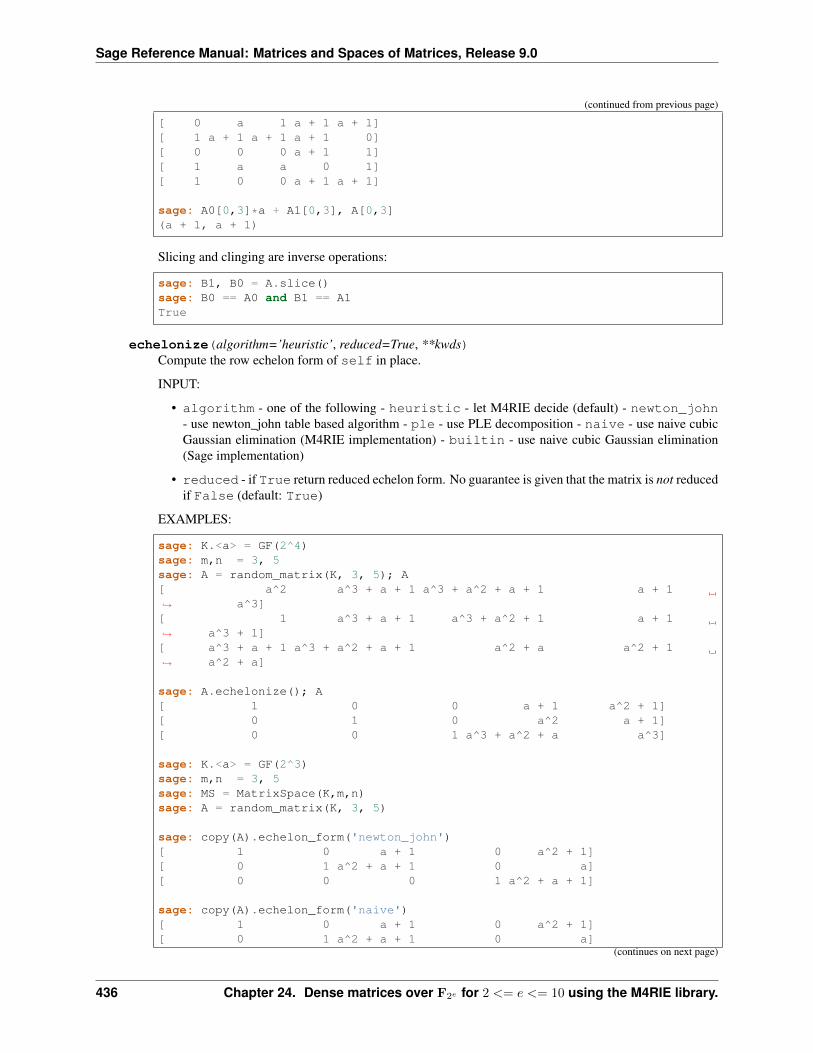
Sage Reference Manual: Matrices and Spaces of Matrices, Release 9.0
(continued from previous page)
[ 0 a 1 a + 1 a + 1][ 1 a + 1 a + 1 a + 1 0][ 0 0 0 a + 1 1][ 1 a a 0 1][ 1 0 0 a + 1 a + 1]
sage: A0[0,3]*a + A1[0,3], A[0,3](a + 1, a + 1)
Slicing and clinging are inverse operations:
sage: B1, B0 = A.slice()sage: B0 == A0 and B1 == A1True
echelonize(algorithm=’heuristic’, reduced=True, **kwds)Compute the row echelon form of self in place.
INPUT:
• algorithm - one of the following - heuristic - let M4RIE decide (default) - newton_john- use newton_john table based algorithm - ple - use PLE decomposition - naive - use naive cubicGaussian elimination (M4RIE implementation) - builtin - use naive cubic Gaussian elimination(Sage implementation)
• reduced - if True return reduced echelon form. No guarantee is given that the matrix is not reducedif False (default: True)
EXAMPLES:
sage: K.<a> = GF(2^4)sage: m,n = 3, 5sage: A = random_matrix(K, 3, 5); A[ a^2 a^3 + a + 1 a^3 + a^2 + a + 1 a + 1→˓ a^3][ 1 a^3 + a + 1 a^3 + a^2 + 1 a + 1→˓ a^3 + 1][ a^3 + a + 1 a^3 + a^2 + a + 1 a^2 + a a^2 + 1→˓ a^2 + a]
sage: A.echelonize(); A[ 1 0 0 a + 1 a^2 + 1][ 0 1 0 a^2 a + 1][ 0 0 1 a^3 + a^2 + a a^3]
sage: K.<a> = GF(2^3)sage: m,n = 3, 5sage: MS = MatrixSpace(K,m,n)sage: A = random_matrix(K, 3, 5)
sage: copy(A).echelon_form('newton_john')[ 1 0 a + 1 0 a^2 + 1][ 0 1 a^2 + a + 1 0 a][ 0 0 0 1 a^2 + a + 1]
sage: copy(A).echelon_form('naive')[ 1 0 a + 1 0 a^2 + 1][ 0 1 a^2 + a + 1 0 a]
(continues on next page)
436 Chapter 24. Dense matrices over F2𝑒 for 2 <= 𝑒 <= 10 using the M4RIE library.
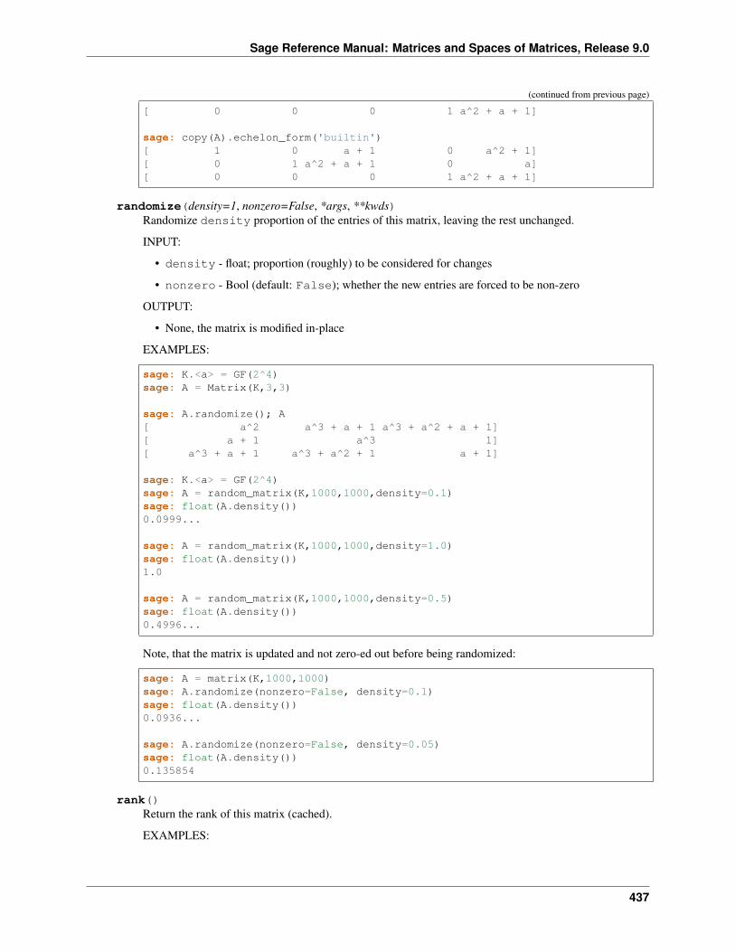
Sage Reference Manual: Matrices and Spaces of Matrices, Release 9.0
(continued from previous page)
[ 0 0 0 1 a^2 + a + 1]
sage: copy(A).echelon_form('builtin')[ 1 0 a + 1 0 a^2 + 1][ 0 1 a^2 + a + 1 0 a][ 0 0 0 1 a^2 + a + 1]
randomize(density=1, nonzero=False, *args, **kwds)Randomize density proportion of the entries of this matrix, leaving the rest unchanged.
INPUT:
• density - float; proportion (roughly) to be considered for changes
• nonzero - Bool (default: False); whether the new entries are forced to be non-zero
OUTPUT:
• None, the matrix is modified in-place
EXAMPLES:
sage: K.<a> = GF(2^4)sage: A = Matrix(K,3,3)
sage: A.randomize(); A[ a^2 a^3 + a + 1 a^3 + a^2 + a + 1][ a + 1 a^3 1][ a^3 + a + 1 a^3 + a^2 + 1 a + 1]
sage: K.<a> = GF(2^4)sage: A = random_matrix(K,1000,1000,density=0.1)sage: float(A.density())0.0999...
sage: A = random_matrix(K,1000,1000,density=1.0)sage: float(A.density())1.0
sage: A = random_matrix(K,1000,1000,density=0.5)sage: float(A.density())0.4996...
Note, that the matrix is updated and not zero-ed out before being randomized:
sage: A = matrix(K,1000,1000)sage: A.randomize(nonzero=False, density=0.1)sage: float(A.density())0.0936...
sage: A.randomize(nonzero=False, density=0.05)sage: float(A.density())0.135854
rank()Return the rank of this matrix (cached).
EXAMPLES:
437
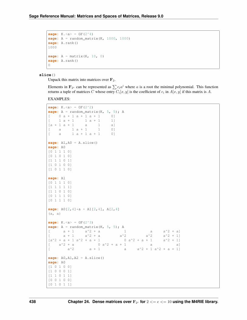
Sage Reference Manual: Matrices and Spaces of Matrices, Release 9.0
sage: K.<a> = GF(2^4)sage: A = random_matrix(K, 1000, 1000)sage: A.rank()1000
sage: A = matrix(K, 10, 0)sage: A.rank()0
slice()Unpack this matrix into matrices over F2.
Elements in F2𝑒 can be represented as∑︀
𝑐𝑖𝑎𝑖 where 𝑎 is a root the minimal polynomial. This function
returns a tuple of matrices 𝐶 whose entry 𝐶𝑖[𝑥, 𝑦] is the coefficient of 𝑐𝑖 in 𝐴[𝑥, 𝑦] if this matrix is 𝐴.
EXAMPLES:
sage: K.<a> = GF(2^2)sage: A = random_matrix(K, 5, 5); A[ 0 a + 1 a + 1 a + 1 0][ 1 a + 1 1 a + 1 1][a + 1 a + 1 a 1 a][ a 1 a + 1 1 0][ a 1 a + 1 a + 1 0]
sage: A1,A0 = A.slice()sage: A0[0 1 1 1 0][0 1 0 1 0][1 1 1 0 1][1 0 1 0 0][1 0 1 1 0]
sage: A1[0 1 1 1 0][1 1 1 1 1][1 1 0 1 0][0 1 1 1 0][0 1 1 1 0]
sage: A0[2,4]*a + A1[2,4], A[2,4](a, a)
sage: K.<a> = GF(2^3)sage: A = random_matrix(K, 5, 5); A[ a + 1 a^2 + a 1 a a^2 + a][ a + 1 a^2 + a a^2 a^2 a^2 + 1][a^2 + a + 1 a^2 + a + 1 0 a^2 + a + 1 a^2 + 1][ a^2 + a 0 a^2 + a + 1 a a][ a^2 a + 1 a a^2 + 1 a^2 + a + 1]
sage: A0,A1,A2 = A.slice()sage: A0[1 0 1 0 0][1 0 0 0 1][1 1 0 1 1][0 0 1 0 0][0 1 0 1 1]
438 Chapter 24. Dense matrices over F2𝑒 for 2 <= 𝑒 <= 10 using the M4RIE library.
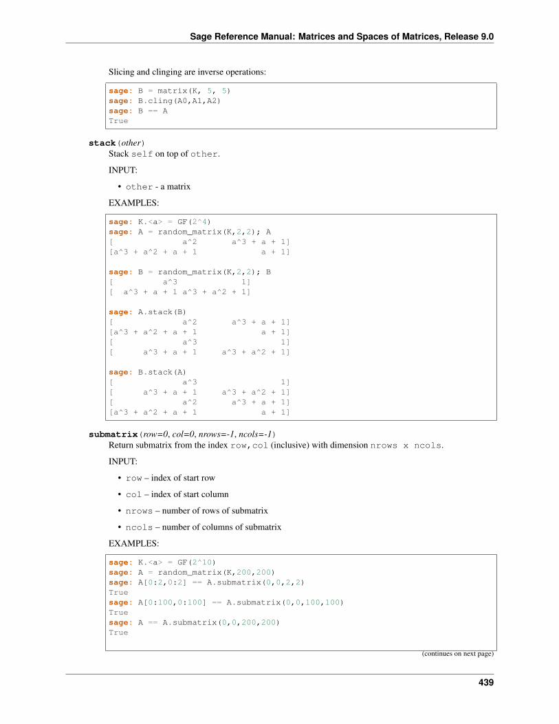
Sage Reference Manual: Matrices and Spaces of Matrices, Release 9.0
Slicing and clinging are inverse operations:
sage: B = matrix(K, 5, 5)sage: B.cling(A0,A1,A2)sage: B == ATrue
stack(other)Stack self on top of other.
INPUT:
• other - a matrix
EXAMPLES:
sage: K.<a> = GF(2^4)sage: A = random_matrix(K,2,2); A[ a^2 a^3 + a + 1][a^3 + a^2 + a + 1 a + 1]
sage: B = random_matrix(K,2,2); B[ a^3 1][ a^3 + a + 1 a^3 + a^2 + 1]
sage: A.stack(B)[ a^2 a^3 + a + 1][a^3 + a^2 + a + 1 a + 1][ a^3 1][ a^3 + a + 1 a^3 + a^2 + 1]
sage: B.stack(A)[ a^3 1][ a^3 + a + 1 a^3 + a^2 + 1][ a^2 a^3 + a + 1][a^3 + a^2 + a + 1 a + 1]
submatrix(row=0, col=0, nrows=-1, ncols=-1)Return submatrix from the index row,col (inclusive) with dimension nrows x ncols.
INPUT:
• row – index of start row
• col – index of start column
• nrows – number of rows of submatrix
• ncols – number of columns of submatrix
EXAMPLES:
sage: K.<a> = GF(2^10)sage: A = random_matrix(K,200,200)sage: A[0:2,0:2] == A.submatrix(0,0,2,2)Truesage: A[0:100,0:100] == A.submatrix(0,0,100,100)Truesage: A == A.submatrix(0,0,200,200)True
(continues on next page)
439
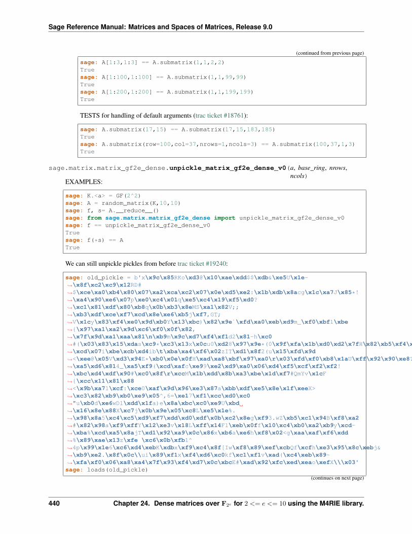
Sage Reference Manual: Matrices and Spaces of Matrices, Release 9.0
(continued from previous page)
sage: A[1:3,1:3] == A.submatrix(1,1,2,2)Truesage: A[1:100,1:100] == A.submatrix(1,1,99,99)Truesage: A[1:200,1:200] == A.submatrix(1,1,199,199)True
TESTS for handling of default arguments (trac ticket #18761):
sage: A.submatrix(17,15) == A.submatrix(17,15,183,185)Truesage: A.submatrix(row=100,col=37,nrows=1,ncols=3) == A.submatrix(100,37,1,3)True
sage.matrix.matrix_gf2e_dense.unpickle_matrix_gf2e_dense_v0(a, base_ring, nrows,ncols)
EXAMPLES:
sage: K.<a> = GF(2^2)sage: A = random_matrix(K,10,10)sage: f, s= A.__reduce__()sage: from sage.matrix.matrix_gf2e_dense import unpickle_matrix_gf2e_dense_v0sage: f == unpickle_matrix_gf2e_dense_v0Truesage: f(*s) == ATrue
We can still unpickle pickles from before trac ticket #19240:
sage: old_pickle = b'x\x9c\x85RKo\xd3@\x10\xae\xdd$$\xdb&\xe5U\x1e-→˓\x8f\xc2\xc9\x12RD#→˓$\xce\xa0\xb4\x80\x07\xa2\xca\xc2\x07\x0e\xd5\xe2:\x1b\xdb\x8acg\x1c\xa7J\x85*!→˓\xa4\x90\xe6\x07p\xe0\xc4\x01q\xe5\xc4\x19\xf5\xd0?→˓\xc1\x81\xdf\x80\xb8q\x0b\xb3\x8eMS\xa1\x82V;;→˓\xb3\xdf\xce\xf7\xcd\x8e\xe6\xb5j\xf7,GT;→˓V\x1cy\x83\xf4\xe0\x9d\xb0Y\x13\xbc)\x82\x9e`\xfd\xa0\xeb\xd9m_\xf0\xbf1\xbe→˓{\x97\xa1\xa2\x9d\xc6\xf0\x0f\x82,→˓\x7f\x9d\xa1\xaa\x81\n\xb9m\x9c\xd7\xf4\xf1d2\x81-h\xc0→˓#(\x03\x83\x15\xdas\xc9*\xc3\x13x\x0cu0\xd28\x97\x9e*(0\x9f\xfa\x1b\xd0\xd2\x7fH\x82\xb5\xf4\xa2@TO\xe19\x01I\xac\x136\x991\x9f\xa4\xf9&→˓\xcd\x07i\xbe\xcb\xd4ib\t\xba\xa4\xf6\x02zIT\xd1\x8f2(u\x15\xfd\x9d→˓<\xee@\x05V\xd3\x94E*\xb0\x0e\x0fH\xad\xa8\xbf\x97\xa0\r\x03\xfd\xf0\xb8\x1aU\xff\x92\x90\xe8?→˓\xa5\xd6\x814_\xa5\xf9(\xcd\xafc\xe99\xe2\xd9\xa0\x06\xd4\xf5\xcf\xf2\xf2!→˓\xbc\xd4\xdf\x90#\xc0\x8f\r\xccM\x1b\xdd\x8b\xa3\xbe\x1d\xf7#QmYv\x1cF→˓{\xcc\x11\x81\x88→˓<\x9b\xa71\xcf:\xce0\xaf\x9d\x96\xe3\x87a\xbb\xdf\xe5\x8e\x1f\xeeX>→˓\xc3\x82\xb9\xb0\xe9\x05^,6=\xe17\xf1\xcc\xd0\xc0→˓"u\xb0d\xe6wDl\xdd\x1fa)e\x8a\xbc\xc0\xe9U\xbd→˓\x16\x8e\x88X\xc7j\x0b\x9e\x05\xc8L\xe5\x1e%.→˓\x98\x8a5\xc4\xc5\xd9\xf7\xdd\xd0\xdf\x0b\xc2\x8eg\xf93.wZ\xb5\xc1\x94B\xf8\xa2→˓#\x82\x98a\xf9\xffY\x12\xe3v\x18L\xff\x14Fl\xeb\x0ff\x10\xc4\xb0\xa2\xb9y\xcd-→˓\xba%\xcd\xa5\x8ajT\xd1\x92\xa9\x0c\x86x\xb6a\xe6h\xf8\x02<g\xaa\xaf\xf6\xdd→˓%\x89\xae\x13z\xfe \xc6\x0b\xfb1^→˓4p\x99\x1e6\xc6\xd4\xebK\xdbx\xf9\xc4\x8f[Iw\xf8\x89\xef\xcbQf\xcfh\xe3\x95\x8c\xebj&→˓\xb9\xe2.\x8f\x0c\\ui\x89\xf1x\xf4\xd6\xc0kf\xc1\xf1v\xad(\xc4\xeb\x89~→˓\xfa\xf0\x06\xa8\xa4\x7f\x93\xf4\xd7\x0c\xbcE#\xad\x92\xfc\xed\xeao\xefX\\\x03'sage: loads(old_pickle)
(continues on next page)
440 Chapter 24. Dense matrices over F2𝑒 for 2 <= 𝑒 <= 10 using the M4RIE library.

Sage Reference Manual: Matrices and Spaces of Matrices, Release 9.0
(continued from previous page)
[ 0 a][a + 1 1]
441

Sage Reference Manual: Matrices and Spaces of Matrices, Release 9.0
442 Chapter 24. Dense matrices over F2𝑒 for 2 <= 𝑒 <= 10 using the M4RIE library.
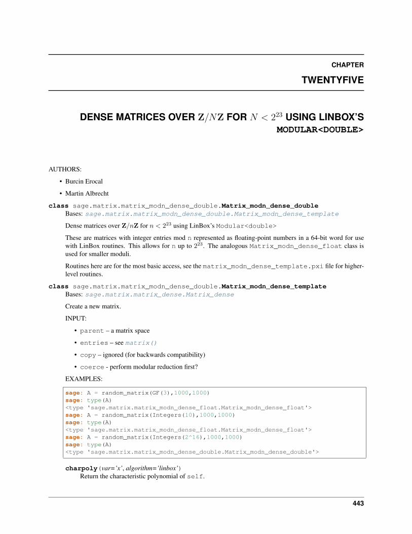
CHAPTER
TWENTYFIVE
DENSE MATRICES OVER Z/𝑁Z FOR 𝑁 < 223 USING LINBOX’SMODULAR<DOUBLE>
AUTHORS:
• Burcin Erocal
• Martin Albrecht
class sage.matrix.matrix_modn_dense_double.Matrix_modn_dense_doubleBases: sage.matrix.matrix_modn_dense_double.Matrix_modn_dense_template
Dense matrices over Z/𝑛Z for 𝑛 < 223 using LinBox’s Modular<double>
These are matrices with integer entries mod n represented as floating-point numbers in a 64-bit word for usewith LinBox routines. This allows for n up to 223. The analogous Matrix_modn_dense_float class isused for smaller moduli.
Routines here are for the most basic access, see the matrix_modn_dense_template.pxi file for higher-level routines.
class sage.matrix.matrix_modn_dense_double.Matrix_modn_dense_templateBases: sage.matrix.matrix_dense.Matrix_dense
Create a new matrix.
INPUT:
• parent – a matrix space
• entries – see matrix()
• copy – ignored (for backwards compatibility)
• coerce - perform modular reduction first?
EXAMPLES:
sage: A = random_matrix(GF(3),1000,1000)sage: type(A)<type 'sage.matrix.matrix_modn_dense_float.Matrix_modn_dense_float'>sage: A = random_matrix(Integers(10),1000,1000)sage: type(A)<type 'sage.matrix.matrix_modn_dense_float.Matrix_modn_dense_float'>sage: A = random_matrix(Integers(2^16),1000,1000)sage: type(A)<type 'sage.matrix.matrix_modn_dense_double.Matrix_modn_dense_double'>
charpoly(var=’x’, algorithm=’linbox’)Return the characteristic polynomial of self.
443
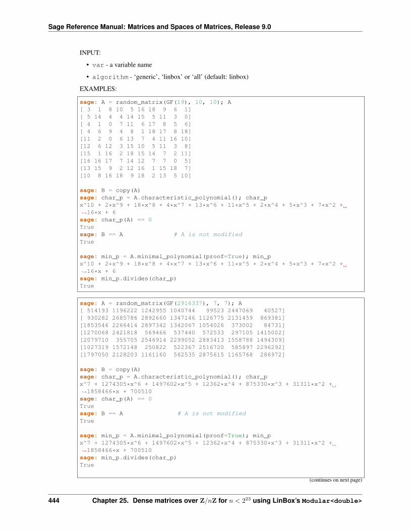
Sage Reference Manual: Matrices and Spaces of Matrices, Release 9.0
INPUT:
• var - a variable name
• algorithm - ‘generic’, ‘linbox’ or ‘all’ (default: linbox)
EXAMPLES:
sage: A = random_matrix(GF(19), 10, 10); A[ 3 1 8 10 5 16 18 9 6 1][ 5 14 4 4 14 15 5 11 3 0][ 4 1 0 7 11 6 17 8 5 6][ 4 6 9 4 8 1 18 17 8 18][11 2 0 6 13 7 4 11 16 10][12 6 12 3 15 10 5 11 3 8][15 1 16 2 18 15 14 7 2 11][16 16 17 7 14 12 7 7 0 5][13 15 9 2 12 16 1 15 18 7][10 8 16 18 9 18 2 13 5 10]
sage: B = copy(A)sage: char_p = A.characteristic_polynomial(); char_px^10 + 2*x^9 + 18*x^8 + 4*x^7 + 13*x^6 + 11*x^5 + 2*x^4 + 5*x^3 + 7*x^2 +→˓16*x + 6sage: char_p(A) == 0Truesage: B == A # A is not modifiedTrue
sage: min_p = A.minimal_polynomial(proof=True); min_px^10 + 2*x^9 + 18*x^8 + 4*x^7 + 13*x^6 + 11*x^5 + 2*x^4 + 5*x^3 + 7*x^2 +→˓16*x + 6sage: min_p.divides(char_p)True
sage: A = random_matrix(GF(2916337), 7, 7); A[ 514193 1196222 1242955 1040744 99523 2447069 40527][ 930282 2685786 2892660 1347146 1126775 2131459 869381][1853546 2266414 2897342 1342067 1054026 373002 84731][1270068 2421818 569466 537440 572533 297105 1415002][2079710 355705 2546914 2299052 2883413 1558788 1494309][1027319 1572148 250822 522367 2516720 585897 2296292][1797050 2128203 1161160 562535 2875615 1165768 286972]
sage: B = copy(A)sage: char_p = A.characteristic_polynomial(); char_px^7 + 1274305*x^6 + 1497602*x^5 + 12362*x^4 + 875330*x^3 + 31311*x^2 +→˓1858466*x + 700510sage: char_p(A) == 0Truesage: B == A # A is not modifiedTrue
sage: min_p = A.minimal_polynomial(proof=True); min_px^7 + 1274305*x^6 + 1497602*x^5 + 12362*x^4 + 875330*x^3 + 31311*x^2 +→˓1858466*x + 700510sage: min_p.divides(char_p)True
(continues on next page)
444 Chapter 25. Dense matrices over Z/𝑛Z for 𝑛 < 223 using LinBox’s Modular<double>
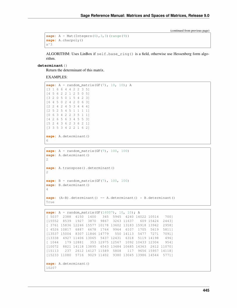
Sage Reference Manual: Matrices and Spaces of Matrices, Release 9.0
(continued from previous page)
sage: A = Mat(Integers(6),3,3)(range(9))sage: A.charpoly()x^3
ALGORITHM: Uses LinBox if self.base_ring() is a field, otherwise use Hessenberg form algo-rithm.
determinant()Return the determinant of this matrix.
EXAMPLES:
sage: A = random_matrix(GF(7), 10, 10); A[3 1 6 6 4 4 2 2 3 5][4 5 6 2 2 1 2 5 0 5][3 2 0 5 0 1 5 4 2 3][6 4 5 0 2 4 2 0 6 3][2 2 4 2 4 5 3 4 4 4][2 5 2 5 4 5 1 1 1 1][0 6 3 4 2 2 3 5 1 1][4 2 6 5 6 3 4 5 5 3][5 2 4 3 6 2 3 6 2 1][3 3 5 3 4 2 2 1 6 2]
sage: A.determinant()6
sage: A = random_matrix(GF(7), 100, 100)sage: A.determinant()2
sage: A.transpose().determinant()2
sage: B = random_matrix(GF(7), 100, 100)sage: B.determinant()4
sage: (A*B).determinant() == A.determinant() * B.determinant()True
sage: A = random_matrix(GF(16007), 10, 10); A[ 5037 2388 4150 1400 345 5945 4240 14022 10514 700][15552 8539 1927 3870 9867 3263 11637 609 15424 2443][ 3761 15836 12246 15577 10178 13602 13183 15918 13942 2958][ 4526 10817 6887 6678 1764 9964 6107 1705 5619 5811][13537 15004 8307 11846 14779 550 14113 5477 7271 7091][13338 4927 11406 13065 5437 12431 6318 5119 14198 496][ 1044 179 12881 353 12975 12567 1092 10433 12304 954][10072 8821 14118 13895 6543 13484 10685 14363 2612 11070][15113 237 2612 14127 11589 5808 117 9656 15957 14118][15233 11080 5716 9029 11402 9380 13045 13986 14544 5771]
sage: A.determinant()10207
445
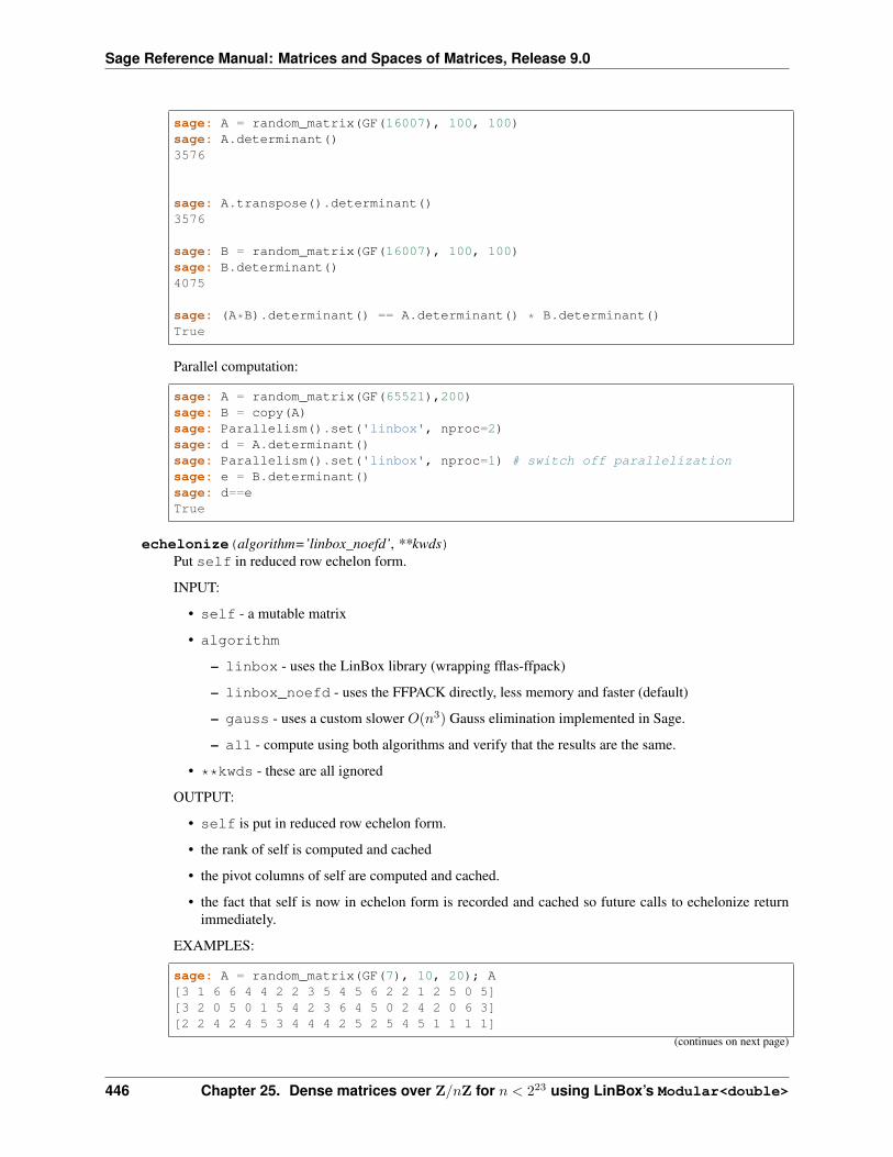
Sage Reference Manual: Matrices and Spaces of Matrices, Release 9.0
sage: A = random_matrix(GF(16007), 100, 100)sage: A.determinant()3576
sage: A.transpose().determinant()3576
sage: B = random_matrix(GF(16007), 100, 100)sage: B.determinant()4075
sage: (A*B).determinant() == A.determinant() * B.determinant()True
Parallel computation:
sage: A = random_matrix(GF(65521),200)sage: B = copy(A)sage: Parallelism().set('linbox', nproc=2)sage: d = A.determinant()sage: Parallelism().set('linbox', nproc=1) # switch off parallelizationsage: e = B.determinant()sage: d==eTrue
echelonize(algorithm=’linbox_noefd’, **kwds)Put self in reduced row echelon form.
INPUT:
• self - a mutable matrix
• algorithm
– linbox - uses the LinBox library (wrapping fflas-ffpack)
– linbox_noefd - uses the FFPACK directly, less memory and faster (default)
– gauss - uses a custom slower 𝑂(𝑛3) Gauss elimination implemented in Sage.
– all - compute using both algorithms and verify that the results are the same.
• **kwds - these are all ignored
OUTPUT:
• self is put in reduced row echelon form.
• the rank of self is computed and cached
• the pivot columns of self are computed and cached.
• the fact that self is now in echelon form is recorded and cached so future calls to echelonize returnimmediately.
EXAMPLES:
sage: A = random_matrix(GF(7), 10, 20); A[3 1 6 6 4 4 2 2 3 5 4 5 6 2 2 1 2 5 0 5][3 2 0 5 0 1 5 4 2 3 6 4 5 0 2 4 2 0 6 3][2 2 4 2 4 5 3 4 4 4 2 5 2 5 4 5 1 1 1 1]
(continues on next page)
446 Chapter 25. Dense matrices over Z/𝑛Z for 𝑛 < 223 using LinBox’s Modular<double>
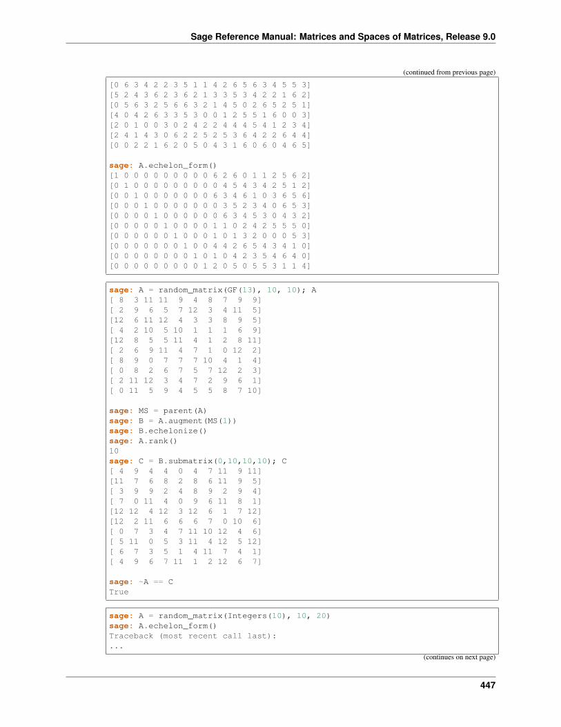
Sage Reference Manual: Matrices and Spaces of Matrices, Release 9.0
(continued from previous page)
[0 6 3 4 2 2 3 5 1 1 4 2 6 5 6 3 4 5 5 3][5 2 4 3 6 2 3 6 2 1 3 3 5 3 4 2 2 1 6 2][0 5 6 3 2 5 6 6 3 2 1 4 5 0 2 6 5 2 5 1][4 0 4 2 6 3 3 5 3 0 0 1 2 5 5 1 6 0 0 3][2 0 1 0 0 3 0 2 4 2 2 4 4 4 5 4 1 2 3 4][2 4 1 4 3 0 6 2 2 5 2 5 3 6 4 2 2 6 4 4][0 0 2 2 1 6 2 0 5 0 4 3 1 6 0 6 0 4 6 5]
sage: A.echelon_form()[1 0 0 0 0 0 0 0 0 0 6 2 6 0 1 1 2 5 6 2][0 1 0 0 0 0 0 0 0 0 0 4 5 4 3 4 2 5 1 2][0 0 1 0 0 0 0 0 0 0 6 3 4 6 1 0 3 6 5 6][0 0 0 1 0 0 0 0 0 0 0 3 5 2 3 4 0 6 5 3][0 0 0 0 1 0 0 0 0 0 0 6 3 4 5 3 0 4 3 2][0 0 0 0 0 1 0 0 0 0 1 1 0 2 4 2 5 5 5 0][0 0 0 0 0 0 1 0 0 0 1 0 1 3 2 0 0 0 5 3][0 0 0 0 0 0 0 1 0 0 4 4 2 6 5 4 3 4 1 0][0 0 0 0 0 0 0 0 1 0 1 0 4 2 3 5 4 6 4 0][0 0 0 0 0 0 0 0 0 1 2 0 5 0 5 5 3 1 1 4]
sage: A = random_matrix(GF(13), 10, 10); A[ 8 3 11 11 9 4 8 7 9 9][ 2 9 6 5 7 12 3 4 11 5][12 6 11 12 4 3 3 8 9 5][ 4 2 10 5 10 1 1 1 6 9][12 8 5 5 11 4 1 2 8 11][ 2 6 9 11 4 7 1 0 12 2][ 8 9 0 7 7 7 10 4 1 4][ 0 8 2 6 7 5 7 12 2 3][ 2 11 12 3 4 7 2 9 6 1][ 0 11 5 9 4 5 5 8 7 10]
sage: MS = parent(A)sage: B = A.augment(MS(1))sage: B.echelonize()sage: A.rank()10sage: C = B.submatrix(0,10,10,10); C[ 4 9 4 4 0 4 7 11 9 11][11 7 6 8 2 8 6 11 9 5][ 3 9 9 2 4 8 9 2 9 4][ 7 0 11 4 0 9 6 11 8 1][12 12 4 12 3 12 6 1 7 12][12 2 11 6 6 6 7 0 10 6][ 0 7 3 4 7 11 10 12 4 6][ 5 11 0 5 3 11 4 12 5 12][ 6 7 3 5 1 4 11 7 4 1][ 4 9 6 7 11 1 2 12 6 7]
sage: ~A == CTrue
sage: A = random_matrix(Integers(10), 10, 20)sage: A.echelon_form()Traceback (most recent call last):...
(continues on next page)
447
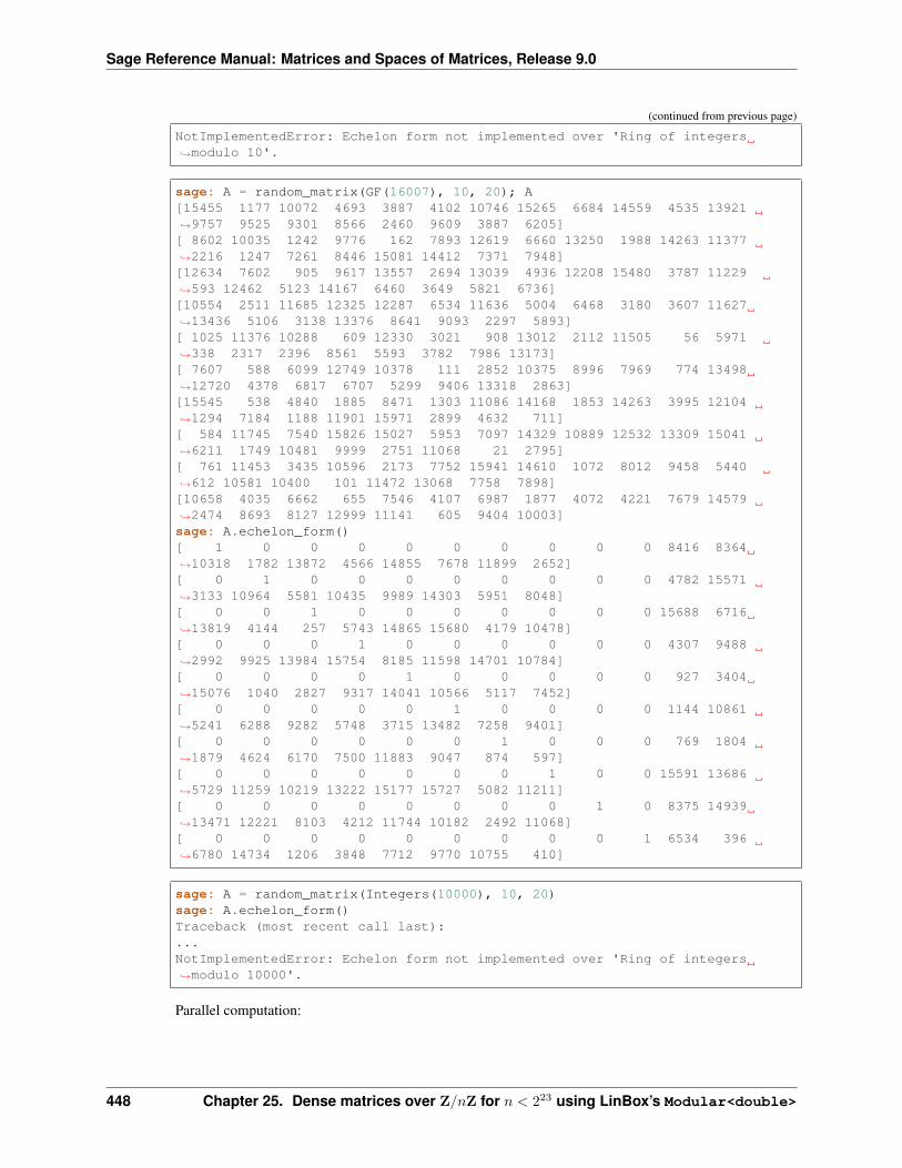
Sage Reference Manual: Matrices and Spaces of Matrices, Release 9.0
(continued from previous page)
NotImplementedError: Echelon form not implemented over 'Ring of integers→˓modulo 10'.
sage: A = random_matrix(GF(16007), 10, 20); A[15455 1177 10072 4693 3887 4102 10746 15265 6684 14559 4535 13921→˓9757 9525 9301 8566 2460 9609 3887 6205][ 8602 10035 1242 9776 162 7893 12619 6660 13250 1988 14263 11377→˓2216 1247 7261 8446 15081 14412 7371 7948][12634 7602 905 9617 13557 2694 13039 4936 12208 15480 3787 11229→˓593 12462 5123 14167 6460 3649 5821 6736][10554 2511 11685 12325 12287 6534 11636 5004 6468 3180 3607 11627→˓13436 5106 3138 13376 8641 9093 2297 5893][ 1025 11376 10288 609 12330 3021 908 13012 2112 11505 56 5971→˓338 2317 2396 8561 5593 3782 7986 13173][ 7607 588 6099 12749 10378 111 2852 10375 8996 7969 774 13498→˓12720 4378 6817 6707 5299 9406 13318 2863][15545 538 4840 1885 8471 1303 11086 14168 1853 14263 3995 12104→˓1294 7184 1188 11901 15971 2899 4632 711][ 584 11745 7540 15826 15027 5953 7097 14329 10889 12532 13309 15041→˓6211 1749 10481 9999 2751 11068 21 2795][ 761 11453 3435 10596 2173 7752 15941 14610 1072 8012 9458 5440→˓612 10581 10400 101 11472 13068 7758 7898][10658 4035 6662 655 7546 4107 6987 1877 4072 4221 7679 14579→˓2474 8693 8127 12999 11141 605 9404 10003]sage: A.echelon_form()[ 1 0 0 0 0 0 0 0 0 0 8416 8364→˓10318 1782 13872 4566 14855 7678 11899 2652][ 0 1 0 0 0 0 0 0 0 0 4782 15571→˓3133 10964 5581 10435 9989 14303 5951 8048][ 0 0 1 0 0 0 0 0 0 0 15688 6716→˓13819 4144 257 5743 14865 15680 4179 10478][ 0 0 0 1 0 0 0 0 0 0 4307 9488→˓2992 9925 13984 15754 8185 11598 14701 10784][ 0 0 0 0 1 0 0 0 0 0 927 3404→˓15076 1040 2827 9317 14041 10566 5117 7452][ 0 0 0 0 0 1 0 0 0 0 1144 10861→˓5241 6288 9282 5748 3715 13482 7258 9401][ 0 0 0 0 0 0 1 0 0 0 769 1804→˓1879 4624 6170 7500 11883 9047 874 597][ 0 0 0 0 0 0 0 1 0 0 15591 13686→˓5729 11259 10219 13222 15177 15727 5082 11211][ 0 0 0 0 0 0 0 0 1 0 8375 14939→˓13471 12221 8103 4212 11744 10182 2492 11068][ 0 0 0 0 0 0 0 0 0 1 6534 396→˓6780 14734 1206 3848 7712 9770 10755 410]
sage: A = random_matrix(Integers(10000), 10, 20)sage: A.echelon_form()Traceback (most recent call last):...NotImplementedError: Echelon form not implemented over 'Ring of integers→˓modulo 10000'.
Parallel computation:
448 Chapter 25. Dense matrices over Z/𝑛Z for 𝑛 < 223 using LinBox’s Modular<double>
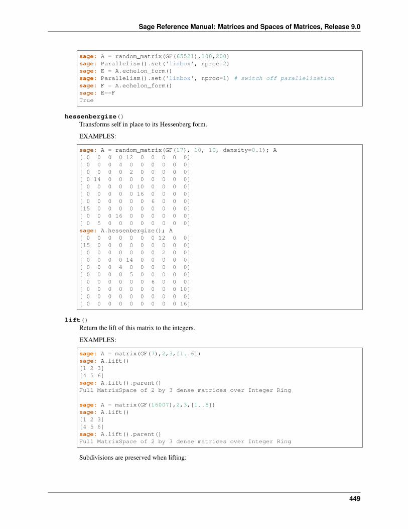
Sage Reference Manual: Matrices and Spaces of Matrices, Release 9.0
sage: A = random_matrix(GF(65521),100,200)sage: Parallelism().set('linbox', nproc=2)sage: E = A.echelon_form()sage: Parallelism().set('linbox', nproc=1) # switch off parallelizationsage: F = A.echelon_form()sage: E==FTrue
hessenbergize()Transforms self in place to its Hessenberg form.
EXAMPLES:
sage: A = random_matrix(GF(17), 10, 10, density=0.1); A[ 0 0 0 0 12 0 0 0 0 0][ 0 0 0 4 0 0 0 0 0 0][ 0 0 0 0 2 0 0 0 0 0][ 0 14 0 0 0 0 0 0 0 0][ 0 0 0 0 0 10 0 0 0 0][ 0 0 0 0 0 16 0 0 0 0][ 0 0 0 0 0 0 6 0 0 0][15 0 0 0 0 0 0 0 0 0][ 0 0 0 16 0 0 0 0 0 0][ 0 5 0 0 0 0 0 0 0 0]sage: A.hessenbergize(); A[ 0 0 0 0 0 0 0 12 0 0][15 0 0 0 0 0 0 0 0 0][ 0 0 0 0 0 0 0 2 0 0][ 0 0 0 0 14 0 0 0 0 0][ 0 0 0 4 0 0 0 0 0 0][ 0 0 0 0 5 0 0 0 0 0][ 0 0 0 0 0 0 6 0 0 0][ 0 0 0 0 0 0 0 0 0 10][ 0 0 0 0 0 0 0 0 0 0][ 0 0 0 0 0 0 0 0 0 16]
lift()Return the lift of this matrix to the integers.
EXAMPLES:
sage: A = matrix(GF(7),2,3,[1..6])sage: A.lift()[1 2 3][4 5 6]sage: A.lift().parent()Full MatrixSpace of 2 by 3 dense matrices over Integer Ring
sage: A = matrix(GF(16007),2,3,[1..6])sage: A.lift()[1 2 3][4 5 6]sage: A.lift().parent()Full MatrixSpace of 2 by 3 dense matrices over Integer Ring
Subdivisions are preserved when lifting:
449
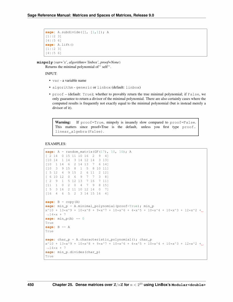
Sage Reference Manual: Matrices and Spaces of Matrices, Release 9.0
sage: A.subdivide([], [1,1]); A[1||2 3][4||5 6]sage: A.lift()[1||2 3][4||5 6]
minpoly(var=’x’, algorithm=’linbox’, proof=None)Returns the minimal polynomial of‘‘ self‘‘.
INPUT:
• var - a variable name
• algorithm - generic or linbox (default: linbox)
• proof – (default: True); whether to provably return the true minimal polynomial; if False, weonly guarantee to return a divisor of the minimal polynomial. There are also certainly cases where thecomputed results is frequently not exactly equal to the minimal polynomial (but is instead merely adivisor of it).
Warning: If proof=True, minpoly is insanely slow compared to proof=False.This matters since proof=True is the default, unless you first type proof.linear_algebra(False).
EXAMPLES:
sage: A = random_matrix(GF(17), 10, 10); A[ 2 14 0 15 11 10 16 2 9 4][10 14 1 14 3 14 12 14 3 13][10 1 14 6 2 14 13 7 6 14][10 3 9 15 8 1 5 8 10 11][ 5 12 4 9 15 2 6 11 2 12][ 6 10 12 0 6 9 7 7 3 8][ 2 9 1 5 12 13 7 16 7 11][11 1 0 2 0 4 7 9 8 15][ 5 3 16 2 11 10 12 14 0 7][16 4 6 5 2 3 14 15 16 4]
sage: B = copy(A)sage: min_p = A.minimal_polynomial(proof=True); min_px^10 + 13*x^9 + 10*x^8 + 9*x^7 + 10*x^6 + 4*x^5 + 10*x^4 + 10*x^3 + 12*x^2 +→˓14*x + 7sage: min_p(A) == 0Truesage: B == ATrue
sage: char_p = A.characteristic_polynomial(); char_px^10 + 13*x^9 + 10*x^8 + 9*x^7 + 10*x^6 + 4*x^5 + 10*x^4 + 10*x^3 + 12*x^2 +→˓14*x + 7sage: min_p.divides(char_p)True
450 Chapter 25. Dense matrices over Z/𝑛Z for 𝑛 < 223 using LinBox’s Modular<double>
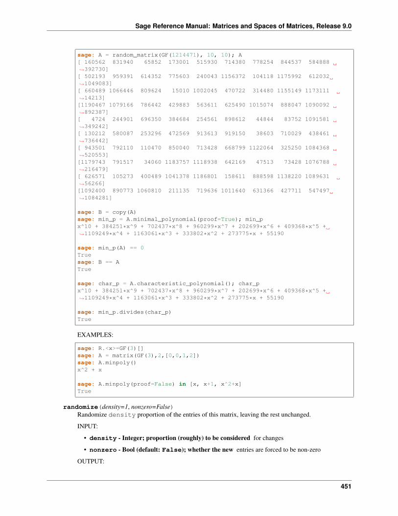
Sage Reference Manual: Matrices and Spaces of Matrices, Release 9.0
sage: A = random_matrix(GF(1214471), 10, 10); A[ 160562 831940 65852 173001 515930 714380 778254 844537 584888→˓392730][ 502193 959391 614352 775603 240043 1156372 104118 1175992 612032→˓1049083][ 660489 1066446 809624 15010 1002045 470722 314480 1155149 1173111→˓14213][1190467 1079166 786442 429883 563611 625490 1015074 888047 1090092→˓892387][ 4724 244901 696350 384684 254561 898612 44844 83752 1091581→˓349242][ 130212 580087 253296 472569 913613 919150 38603 710029 438461→˓736442][ 943501 792110 110470 850040 713428 668799 1122064 325250 1084368→˓520553][1179743 791517 34060 1183757 1118938 642169 47513 73428 1076788→˓216479][ 626571 105273 400489 1041378 1186801 158611 888598 1138220 1089631→˓56266][1092400 890773 1060810 211135 719636 1011640 631366 427711 547497→˓1084281]
sage: B = copy(A)sage: min_p = A.minimal_polynomial(proof=True); min_px^10 + 384251*x^9 + 702437*x^8 + 960299*x^7 + 202699*x^6 + 409368*x^5 +→˓1109249*x^4 + 1163061*x^3 + 333802*x^2 + 273775*x + 55190
sage: min_p(A) == 0Truesage: B == ATrue
sage: char_p = A.characteristic_polynomial(); char_px^10 + 384251*x^9 + 702437*x^8 + 960299*x^7 + 202699*x^6 + 409368*x^5 +→˓1109249*x^4 + 1163061*x^3 + 333802*x^2 + 273775*x + 55190
sage: min_p.divides(char_p)True
EXAMPLES:
sage: R.<x>=GF(3)[]sage: A = matrix(GF(3),2,[0,0,1,2])sage: A.minpoly()x^2 + x
sage: A.minpoly(proof=False) in [x, x+1, x^2+x]True
randomize(density=1, nonzero=False)Randomize density proportion of the entries of this matrix, leaving the rest unchanged.
INPUT:
• density - Integer; proportion (roughly) to be considered for changes
• nonzero - Bool (default: False); whether the new entries are forced to be non-zero
OUTPUT:
451
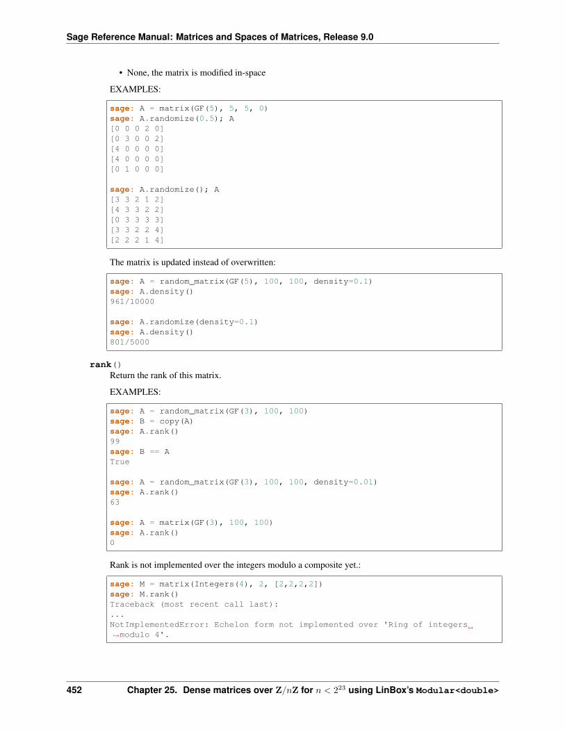
Sage Reference Manual: Matrices and Spaces of Matrices, Release 9.0
• None, the matrix is modified in-space
EXAMPLES:
sage: A = matrix(GF(5), 5, 5, 0)sage: A.randomize(0.5); A[0 0 0 2 0][0 3 0 0 2][4 0 0 0 0][4 0 0 0 0][0 1 0 0 0]
sage: A.randomize(); A[3 3 2 1 2][4 3 3 2 2][0 3 3 3 3][3 3 2 2 4][2 2 2 1 4]
The matrix is updated instead of overwritten:
sage: A = random_matrix(GF(5), 100, 100, density=0.1)sage: A.density()961/10000
sage: A.randomize(density=0.1)sage: A.density()801/5000
rank()Return the rank of this matrix.
EXAMPLES:
sage: A = random_matrix(GF(3), 100, 100)sage: B = copy(A)sage: A.rank()99sage: B == ATrue
sage: A = random_matrix(GF(3), 100, 100, density=0.01)sage: A.rank()63
sage: A = matrix(GF(3), 100, 100)sage: A.rank()0
Rank is not implemented over the integers modulo a composite yet.:
sage: M = matrix(Integers(4), 2, [2,2,2,2])sage: M.rank()Traceback (most recent call last):...NotImplementedError: Echelon form not implemented over 'Ring of integers→˓modulo 4'.
452 Chapter 25. Dense matrices over Z/𝑛Z for 𝑛 < 223 using LinBox’s Modular<double>
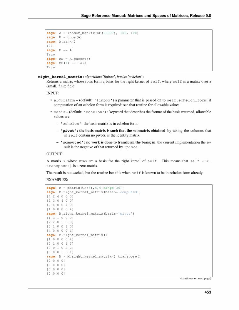
Sage Reference Manual: Matrices and Spaces of Matrices, Release 9.0
sage: A = random_matrix(GF(16007), 100, 100)sage: B = copy(A)sage: A.rank()100sage: B == ATruesage: MS = A.parent()sage: MS(1) == ~A*ATrue
right_kernel_matrix(algorithm=’linbox’, basis=’echelon’)Returns a matrix whose rows form a basis for the right kernel of self, where self is a matrix over a(small) finite field.
INPUT:
• algorithm – (default: 'linbox') a parameter that is passed on to self.echelon_form, ifcomputation of an echelon form is required; see that routine for allowable values
• basis – (default: 'echelon') a keyword that describes the format of the basis returned, allowablevalues are:
– 'echelon': the basis matrix is in echelon form
– 'pivot': the basis matrix is such that the submatrix obtained by taking the columns thatin self contain no pivots, is the identity matrix
– 'computed': no work is done to transform the basis; in the current implementation the re-sult is the negative of that returned by 'pivot'
OUTPUT:
A matrix X whose rows are a basis for the right kernel of self. This means that self * X.transpose() is a zero matrix.
The result is not cached, but the routine benefits when self is known to be in echelon form already.
EXAMPLES:
sage: M = matrix(GF(5),6,6,range(36))sage: M.right_kernel_matrix(basis='computed')[4 2 4 0 0 0][3 3 0 4 0 0][2 4 0 0 4 0][1 0 0 0 0 4]sage: M.right_kernel_matrix(basis='pivot')[1 3 1 0 0 0][2 2 0 1 0 0][3 1 0 0 1 0][4 0 0 0 0 1]sage: M.right_kernel_matrix()[1 0 0 0 0 4][0 1 0 0 1 3][0 0 1 0 2 2][0 0 0 1 3 1]sage: M * M.right_kernel_matrix().transpose()[0 0 0 0][0 0 0 0][0 0 0 0][0 0 0 0]
(continues on next page)
453
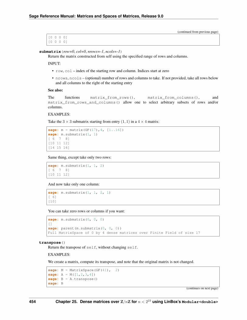
Sage Reference Manual: Matrices and Spaces of Matrices, Release 9.0
(continued from previous page)
[0 0 0 0][0 0 0 0]
submatrix(row=0, col=0, nrows=-1, ncols=-1)Return the matrix constructed from self using the specified range of rows and columns.
INPUT:
• row, col – index of the starting row and column. Indices start at zero
• nrows, ncols – (optional) number of rows and columns to take. If not provided, take all rows belowand all columns to the right of the starting entry
See also:
The functions matrix_from_rows(), matrix_from_columns(), andmatrix_from_rows_and_columns() allow one to select arbitrary subsets of rows and/orcolumns.
EXAMPLES:
Take the 3× 3 submatrix starting from entry (1, 1) in a 4× 4 matrix:
sage: m = matrix(GF(17),4, [1..16])sage: m.submatrix(1, 1)[ 6 7 8][10 11 12][14 15 16]
Same thing, except take only two rows:
sage: m.submatrix(1, 1, 2)[ 6 7 8][10 11 12]
And now take only one column:
sage: m.submatrix(1, 1, 2, 1)[ 6][10]
You can take zero rows or columns if you want:
sage: m.submatrix(0, 0, 0)[]sage: parent(m.submatrix(0, 0, 0))Full MatrixSpace of 0 by 4 dense matrices over Finite Field of size 17
transpose()Return the transpose of self, without changing self.
EXAMPLES:
We create a matrix, compute its transpose, and note that the original matrix is not changed.
sage: M = MatrixSpace(GF(41), 2)sage: A = M([1,2,3,4])sage: B = A.transpose()sage: B
(continues on next page)
454 Chapter 25. Dense matrices over Z/𝑛Z for 𝑛 < 223 using LinBox’s Modular<double>
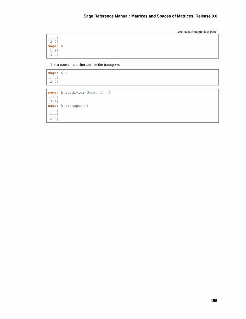
Sage Reference Manual: Matrices and Spaces of Matrices, Release 9.0
(continued from previous page)
[1 3][2 4]sage: A[1 2][3 4]
.T is a convenient shortcut for the transpose:
sage: A.T[1 3][2 4]
sage: A.subdivide(None, 1); A[1|2][3|4]sage: A.transpose()[1 3][---][2 4]
455

Sage Reference Manual: Matrices and Spaces of Matrices, Release 9.0
456 Chapter 25. Dense matrices over Z/𝑛Z for 𝑛 < 223 using LinBox’s Modular<double>
CHAPTER
TWENTYSIX
DENSE MATRICES OVER Z/𝑁Z FOR 𝑁 < 211 USING LINBOX’SMODULAR<FLOAT>
AUTHORS: - Burcin Erocal - Martin Albrecht
class sage.matrix.matrix_modn_dense_float.Matrix_modn_dense_floatBases: sage.matrix.matrix_modn_dense_float.Matrix_modn_dense_template
Dense matrices over Z/𝑛Z for 𝑛 < 211 using LinBox’s Modular<float>
These are matrices with integer entries mod n represented as floating-point numbers in a 32-bit word for usewith LinBox routines. This allows for n up to 211. The Matrix_modn_dense_double class is used forlarger moduli.
Routines here are for the most basic access, see the 𝑚𝑎𝑡𝑟𝑖𝑥𝑚𝑜𝑑𝑛𝑑𝑒𝑛𝑠𝑒𝑡𝑒𝑚𝑝𝑙𝑎𝑡𝑒.𝑝𝑥𝑖 file for higher-level rou-tines.
class sage.matrix.matrix_modn_dense_float.Matrix_modn_dense_templateBases: sage.matrix.matrix_dense.Matrix_dense
Create a new matrix.
INPUT:
• parent – a matrix space
• entries – see matrix()
• copy – ignored (for backwards compatibility)
• coerce - perform modular reduction first?
EXAMPLES:
sage: A = random_matrix(GF(3),1000,1000)sage: type(A)<type 'sage.matrix.matrix_modn_dense_float.Matrix_modn_dense_float'>sage: A = random_matrix(Integers(10),1000,1000)sage: type(A)<type 'sage.matrix.matrix_modn_dense_float.Matrix_modn_dense_float'>sage: A = random_matrix(Integers(2^16),1000,1000)sage: type(A)<type 'sage.matrix.matrix_modn_dense_double.Matrix_modn_dense_double'>
charpoly(var=’x’, algorithm=’linbox’)Return the characteristic polynomial of self.
INPUT:
• var - a variable name
457
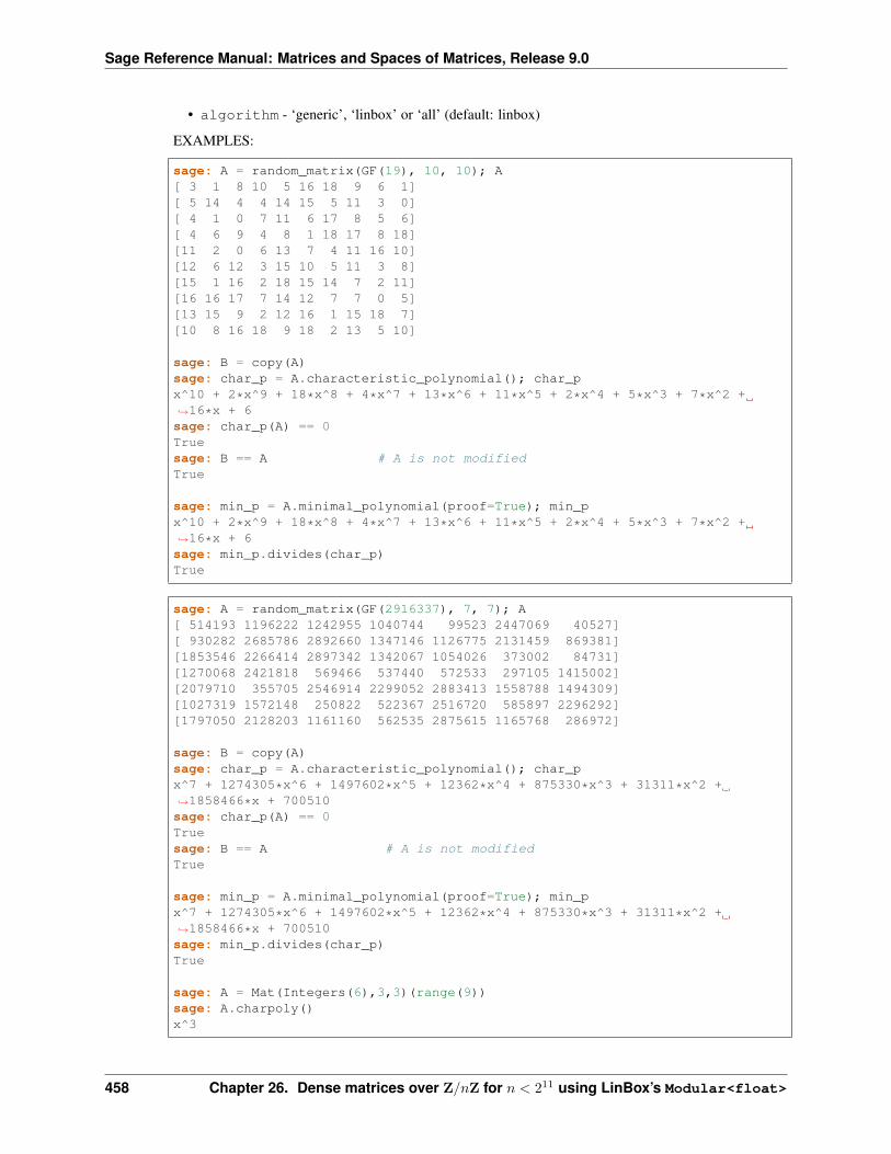
Sage Reference Manual: Matrices and Spaces of Matrices, Release 9.0
• algorithm - ‘generic’, ‘linbox’ or ‘all’ (default: linbox)
EXAMPLES:
sage: A = random_matrix(GF(19), 10, 10); A[ 3 1 8 10 5 16 18 9 6 1][ 5 14 4 4 14 15 5 11 3 0][ 4 1 0 7 11 6 17 8 5 6][ 4 6 9 4 8 1 18 17 8 18][11 2 0 6 13 7 4 11 16 10][12 6 12 3 15 10 5 11 3 8][15 1 16 2 18 15 14 7 2 11][16 16 17 7 14 12 7 7 0 5][13 15 9 2 12 16 1 15 18 7][10 8 16 18 9 18 2 13 5 10]
sage: B = copy(A)sage: char_p = A.characteristic_polynomial(); char_px^10 + 2*x^9 + 18*x^8 + 4*x^7 + 13*x^6 + 11*x^5 + 2*x^4 + 5*x^3 + 7*x^2 +→˓16*x + 6sage: char_p(A) == 0Truesage: B == A # A is not modifiedTrue
sage: min_p = A.minimal_polynomial(proof=True); min_px^10 + 2*x^9 + 18*x^8 + 4*x^7 + 13*x^6 + 11*x^5 + 2*x^4 + 5*x^3 + 7*x^2 +→˓16*x + 6sage: min_p.divides(char_p)True
sage: A = random_matrix(GF(2916337), 7, 7); A[ 514193 1196222 1242955 1040744 99523 2447069 40527][ 930282 2685786 2892660 1347146 1126775 2131459 869381][1853546 2266414 2897342 1342067 1054026 373002 84731][1270068 2421818 569466 537440 572533 297105 1415002][2079710 355705 2546914 2299052 2883413 1558788 1494309][1027319 1572148 250822 522367 2516720 585897 2296292][1797050 2128203 1161160 562535 2875615 1165768 286972]
sage: B = copy(A)sage: char_p = A.characteristic_polynomial(); char_px^7 + 1274305*x^6 + 1497602*x^5 + 12362*x^4 + 875330*x^3 + 31311*x^2 +→˓1858466*x + 700510sage: char_p(A) == 0Truesage: B == A # A is not modifiedTrue
sage: min_p = A.minimal_polynomial(proof=True); min_px^7 + 1274305*x^6 + 1497602*x^5 + 12362*x^4 + 875330*x^3 + 31311*x^2 +→˓1858466*x + 700510sage: min_p.divides(char_p)True
sage: A = Mat(Integers(6),3,3)(range(9))sage: A.charpoly()x^3
458 Chapter 26. Dense matrices over Z/𝑛Z for 𝑛 < 211 using LinBox’s Modular<float>
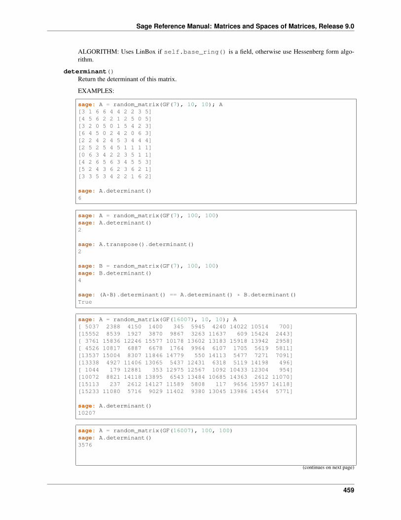
Sage Reference Manual: Matrices and Spaces of Matrices, Release 9.0
ALGORITHM: Uses LinBox if self.base_ring() is a field, otherwise use Hessenberg form algo-rithm.
determinant()Return the determinant of this matrix.
EXAMPLES:
sage: A = random_matrix(GF(7), 10, 10); A[3 1 6 6 4 4 2 2 3 5][4 5 6 2 2 1 2 5 0 5][3 2 0 5 0 1 5 4 2 3][6 4 5 0 2 4 2 0 6 3][2 2 4 2 4 5 3 4 4 4][2 5 2 5 4 5 1 1 1 1][0 6 3 4 2 2 3 5 1 1][4 2 6 5 6 3 4 5 5 3][5 2 4 3 6 2 3 6 2 1][3 3 5 3 4 2 2 1 6 2]
sage: A.determinant()6
sage: A = random_matrix(GF(7), 100, 100)sage: A.determinant()2
sage: A.transpose().determinant()2
sage: B = random_matrix(GF(7), 100, 100)sage: B.determinant()4
sage: (A*B).determinant() == A.determinant() * B.determinant()True
sage: A = random_matrix(GF(16007), 10, 10); A[ 5037 2388 4150 1400 345 5945 4240 14022 10514 700][15552 8539 1927 3870 9867 3263 11637 609 15424 2443][ 3761 15836 12246 15577 10178 13602 13183 15918 13942 2958][ 4526 10817 6887 6678 1764 9964 6107 1705 5619 5811][13537 15004 8307 11846 14779 550 14113 5477 7271 7091][13338 4927 11406 13065 5437 12431 6318 5119 14198 496][ 1044 179 12881 353 12975 12567 1092 10433 12304 954][10072 8821 14118 13895 6543 13484 10685 14363 2612 11070][15113 237 2612 14127 11589 5808 117 9656 15957 14118][15233 11080 5716 9029 11402 9380 13045 13986 14544 5771]
sage: A.determinant()10207
sage: A = random_matrix(GF(16007), 100, 100)sage: A.determinant()3576
(continues on next page)
459
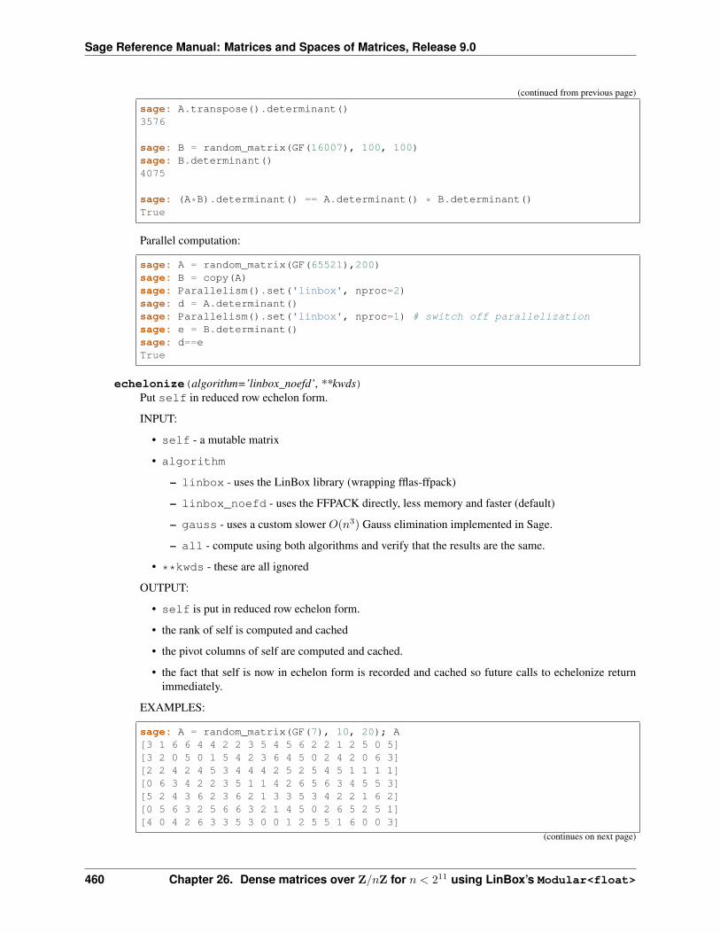
Sage Reference Manual: Matrices and Spaces of Matrices, Release 9.0
(continued from previous page)
sage: A.transpose().determinant()3576
sage: B = random_matrix(GF(16007), 100, 100)sage: B.determinant()4075
sage: (A*B).determinant() == A.determinant() * B.determinant()True
Parallel computation:
sage: A = random_matrix(GF(65521),200)sage: B = copy(A)sage: Parallelism().set('linbox', nproc=2)sage: d = A.determinant()sage: Parallelism().set('linbox', nproc=1) # switch off parallelizationsage: e = B.determinant()sage: d==eTrue
echelonize(algorithm=’linbox_noefd’, **kwds)Put self in reduced row echelon form.
INPUT:
• self - a mutable matrix
• algorithm
– linbox - uses the LinBox library (wrapping fflas-ffpack)
– linbox_noefd - uses the FFPACK directly, less memory and faster (default)
– gauss - uses a custom slower 𝑂(𝑛3) Gauss elimination implemented in Sage.
– all - compute using both algorithms and verify that the results are the same.
• **kwds - these are all ignored
OUTPUT:
• self is put in reduced row echelon form.
• the rank of self is computed and cached
• the pivot columns of self are computed and cached.
• the fact that self is now in echelon form is recorded and cached so future calls to echelonize returnimmediately.
EXAMPLES:
sage: A = random_matrix(GF(7), 10, 20); A[3 1 6 6 4 4 2 2 3 5 4 5 6 2 2 1 2 5 0 5][3 2 0 5 0 1 5 4 2 3 6 4 5 0 2 4 2 0 6 3][2 2 4 2 4 5 3 4 4 4 2 5 2 5 4 5 1 1 1 1][0 6 3 4 2 2 3 5 1 1 4 2 6 5 6 3 4 5 5 3][5 2 4 3 6 2 3 6 2 1 3 3 5 3 4 2 2 1 6 2][0 5 6 3 2 5 6 6 3 2 1 4 5 0 2 6 5 2 5 1][4 0 4 2 6 3 3 5 3 0 0 1 2 5 5 1 6 0 0 3]
(continues on next page)
460 Chapter 26. Dense matrices over Z/𝑛Z for 𝑛 < 211 using LinBox’s Modular<float>
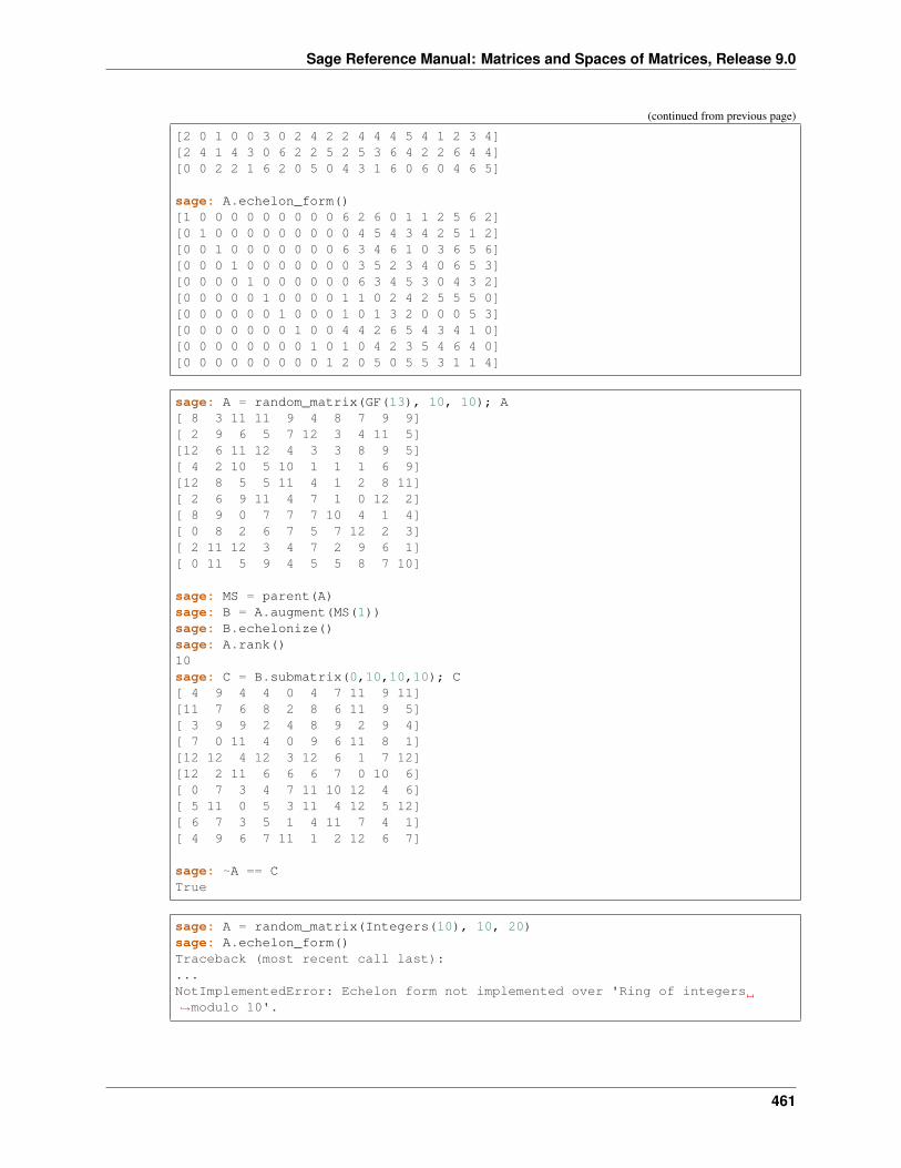
Sage Reference Manual: Matrices and Spaces of Matrices, Release 9.0
(continued from previous page)
[2 0 1 0 0 3 0 2 4 2 2 4 4 4 5 4 1 2 3 4][2 4 1 4 3 0 6 2 2 5 2 5 3 6 4 2 2 6 4 4][0 0 2 2 1 6 2 0 5 0 4 3 1 6 0 6 0 4 6 5]
sage: A.echelon_form()[1 0 0 0 0 0 0 0 0 0 6 2 6 0 1 1 2 5 6 2][0 1 0 0 0 0 0 0 0 0 0 4 5 4 3 4 2 5 1 2][0 0 1 0 0 0 0 0 0 0 6 3 4 6 1 0 3 6 5 6][0 0 0 1 0 0 0 0 0 0 0 3 5 2 3 4 0 6 5 3][0 0 0 0 1 0 0 0 0 0 0 6 3 4 5 3 0 4 3 2][0 0 0 0 0 1 0 0 0 0 1 1 0 2 4 2 5 5 5 0][0 0 0 0 0 0 1 0 0 0 1 0 1 3 2 0 0 0 5 3][0 0 0 0 0 0 0 1 0 0 4 4 2 6 5 4 3 4 1 0][0 0 0 0 0 0 0 0 1 0 1 0 4 2 3 5 4 6 4 0][0 0 0 0 0 0 0 0 0 1 2 0 5 0 5 5 3 1 1 4]
sage: A = random_matrix(GF(13), 10, 10); A[ 8 3 11 11 9 4 8 7 9 9][ 2 9 6 5 7 12 3 4 11 5][12 6 11 12 4 3 3 8 9 5][ 4 2 10 5 10 1 1 1 6 9][12 8 5 5 11 4 1 2 8 11][ 2 6 9 11 4 7 1 0 12 2][ 8 9 0 7 7 7 10 4 1 4][ 0 8 2 6 7 5 7 12 2 3][ 2 11 12 3 4 7 2 9 6 1][ 0 11 5 9 4 5 5 8 7 10]
sage: MS = parent(A)sage: B = A.augment(MS(1))sage: B.echelonize()sage: A.rank()10sage: C = B.submatrix(0,10,10,10); C[ 4 9 4 4 0 4 7 11 9 11][11 7 6 8 2 8 6 11 9 5][ 3 9 9 2 4 8 9 2 9 4][ 7 0 11 4 0 9 6 11 8 1][12 12 4 12 3 12 6 1 7 12][12 2 11 6 6 6 7 0 10 6][ 0 7 3 4 7 11 10 12 4 6][ 5 11 0 5 3 11 4 12 5 12][ 6 7 3 5 1 4 11 7 4 1][ 4 9 6 7 11 1 2 12 6 7]
sage: ~A == CTrue
sage: A = random_matrix(Integers(10), 10, 20)sage: A.echelon_form()Traceback (most recent call last):...NotImplementedError: Echelon form not implemented over 'Ring of integers→˓modulo 10'.
461
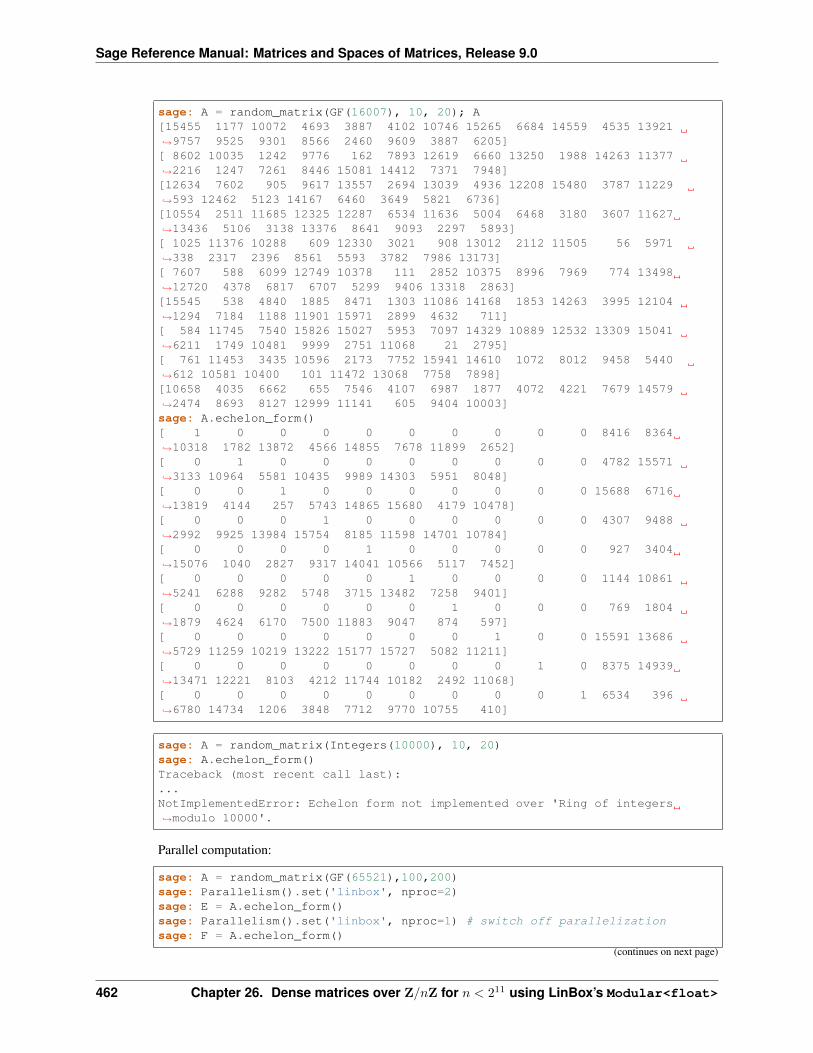
Sage Reference Manual: Matrices and Spaces of Matrices, Release 9.0
sage: A = random_matrix(GF(16007), 10, 20); A[15455 1177 10072 4693 3887 4102 10746 15265 6684 14559 4535 13921→˓9757 9525 9301 8566 2460 9609 3887 6205][ 8602 10035 1242 9776 162 7893 12619 6660 13250 1988 14263 11377→˓2216 1247 7261 8446 15081 14412 7371 7948][12634 7602 905 9617 13557 2694 13039 4936 12208 15480 3787 11229→˓593 12462 5123 14167 6460 3649 5821 6736][10554 2511 11685 12325 12287 6534 11636 5004 6468 3180 3607 11627→˓13436 5106 3138 13376 8641 9093 2297 5893][ 1025 11376 10288 609 12330 3021 908 13012 2112 11505 56 5971→˓338 2317 2396 8561 5593 3782 7986 13173][ 7607 588 6099 12749 10378 111 2852 10375 8996 7969 774 13498→˓12720 4378 6817 6707 5299 9406 13318 2863][15545 538 4840 1885 8471 1303 11086 14168 1853 14263 3995 12104→˓1294 7184 1188 11901 15971 2899 4632 711][ 584 11745 7540 15826 15027 5953 7097 14329 10889 12532 13309 15041→˓6211 1749 10481 9999 2751 11068 21 2795][ 761 11453 3435 10596 2173 7752 15941 14610 1072 8012 9458 5440→˓612 10581 10400 101 11472 13068 7758 7898][10658 4035 6662 655 7546 4107 6987 1877 4072 4221 7679 14579→˓2474 8693 8127 12999 11141 605 9404 10003]sage: A.echelon_form()[ 1 0 0 0 0 0 0 0 0 0 8416 8364→˓10318 1782 13872 4566 14855 7678 11899 2652][ 0 1 0 0 0 0 0 0 0 0 4782 15571→˓3133 10964 5581 10435 9989 14303 5951 8048][ 0 0 1 0 0 0 0 0 0 0 15688 6716→˓13819 4144 257 5743 14865 15680 4179 10478][ 0 0 0 1 0 0 0 0 0 0 4307 9488→˓2992 9925 13984 15754 8185 11598 14701 10784][ 0 0 0 0 1 0 0 0 0 0 927 3404→˓15076 1040 2827 9317 14041 10566 5117 7452][ 0 0 0 0 0 1 0 0 0 0 1144 10861→˓5241 6288 9282 5748 3715 13482 7258 9401][ 0 0 0 0 0 0 1 0 0 0 769 1804→˓1879 4624 6170 7500 11883 9047 874 597][ 0 0 0 0 0 0 0 1 0 0 15591 13686→˓5729 11259 10219 13222 15177 15727 5082 11211][ 0 0 0 0 0 0 0 0 1 0 8375 14939→˓13471 12221 8103 4212 11744 10182 2492 11068][ 0 0 0 0 0 0 0 0 0 1 6534 396→˓6780 14734 1206 3848 7712 9770 10755 410]
sage: A = random_matrix(Integers(10000), 10, 20)sage: A.echelon_form()Traceback (most recent call last):...NotImplementedError: Echelon form not implemented over 'Ring of integers→˓modulo 10000'.
Parallel computation:
sage: A = random_matrix(GF(65521),100,200)sage: Parallelism().set('linbox', nproc=2)sage: E = A.echelon_form()sage: Parallelism().set('linbox', nproc=1) # switch off parallelizationsage: F = A.echelon_form()
(continues on next page)
462 Chapter 26. Dense matrices over Z/𝑛Z for 𝑛 < 211 using LinBox’s Modular<float>
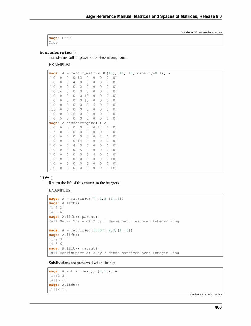
Sage Reference Manual: Matrices and Spaces of Matrices, Release 9.0
(continued from previous page)
sage: E==FTrue
hessenbergize()Transforms self in place to its Hessenberg form.
EXAMPLES:
sage: A = random_matrix(GF(17), 10, 10, density=0.1); A[ 0 0 0 0 12 0 0 0 0 0][ 0 0 0 4 0 0 0 0 0 0][ 0 0 0 0 2 0 0 0 0 0][ 0 14 0 0 0 0 0 0 0 0][ 0 0 0 0 0 10 0 0 0 0][ 0 0 0 0 0 16 0 0 0 0][ 0 0 0 0 0 0 6 0 0 0][15 0 0 0 0 0 0 0 0 0][ 0 0 0 16 0 0 0 0 0 0][ 0 5 0 0 0 0 0 0 0 0]sage: A.hessenbergize(); A[ 0 0 0 0 0 0 0 12 0 0][15 0 0 0 0 0 0 0 0 0][ 0 0 0 0 0 0 0 2 0 0][ 0 0 0 0 14 0 0 0 0 0][ 0 0 0 4 0 0 0 0 0 0][ 0 0 0 0 5 0 0 0 0 0][ 0 0 0 0 0 0 6 0 0 0][ 0 0 0 0 0 0 0 0 0 10][ 0 0 0 0 0 0 0 0 0 0][ 0 0 0 0 0 0 0 0 0 16]
lift()Return the lift of this matrix to the integers.
EXAMPLES:
sage: A = matrix(GF(7),2,3,[1..6])sage: A.lift()[1 2 3][4 5 6]sage: A.lift().parent()Full MatrixSpace of 2 by 3 dense matrices over Integer Ring
sage: A = matrix(GF(16007),2,3,[1..6])sage: A.lift()[1 2 3][4 5 6]sage: A.lift().parent()Full MatrixSpace of 2 by 3 dense matrices over Integer Ring
Subdivisions are preserved when lifting:
sage: A.subdivide([], [1,1]); A[1||2 3][4||5 6]sage: A.lift()[1||2 3]
(continues on next page)
463
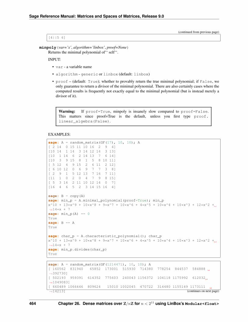
Sage Reference Manual: Matrices and Spaces of Matrices, Release 9.0
(continued from previous page)
[4||5 6]
minpoly(var=’x’, algorithm=’linbox’, proof=None)Returns the minimal polynomial of‘‘ self‘‘.
INPUT:
• var - a variable name
• algorithm - generic or linbox (default: linbox)
• proof – (default: True); whether to provably return the true minimal polynomial; if False, weonly guarantee to return a divisor of the minimal polynomial. There are also certainly cases where thecomputed results is frequently not exactly equal to the minimal polynomial (but is instead merely adivisor of it).
Warning: If proof=True, minpoly is insanely slow compared to proof=False.This matters since proof=True is the default, unless you first type proof.linear_algebra(False).
EXAMPLES:
sage: A = random_matrix(GF(17), 10, 10); A[ 2 14 0 15 11 10 16 2 9 4][10 14 1 14 3 14 12 14 3 13][10 1 14 6 2 14 13 7 6 14][10 3 9 15 8 1 5 8 10 11][ 5 12 4 9 15 2 6 11 2 12][ 6 10 12 0 6 9 7 7 3 8][ 2 9 1 5 12 13 7 16 7 11][11 1 0 2 0 4 7 9 8 15][ 5 3 16 2 11 10 12 14 0 7][16 4 6 5 2 3 14 15 16 4]
sage: B = copy(A)sage: min_p = A.minimal_polynomial(proof=True); min_px^10 + 13*x^9 + 10*x^8 + 9*x^7 + 10*x^6 + 4*x^5 + 10*x^4 + 10*x^3 + 12*x^2 +→˓14*x + 7sage: min_p(A) == 0Truesage: B == ATrue
sage: char_p = A.characteristic_polynomial(); char_px^10 + 13*x^9 + 10*x^8 + 9*x^7 + 10*x^6 + 4*x^5 + 10*x^4 + 10*x^3 + 12*x^2 +→˓14*x + 7sage: min_p.divides(char_p)True
sage: A = random_matrix(GF(1214471), 10, 10); A[ 160562 831940 65852 173001 515930 714380 778254 844537 584888→˓392730][ 502193 959391 614352 775603 240043 1156372 104118 1175992 612032→˓1049083][ 660489 1066446 809624 15010 1002045 470722 314480 1155149 1173111→˓14213] (continues on next page)
464 Chapter 26. Dense matrices over Z/𝑛Z for 𝑛 < 211 using LinBox’s Modular<float>
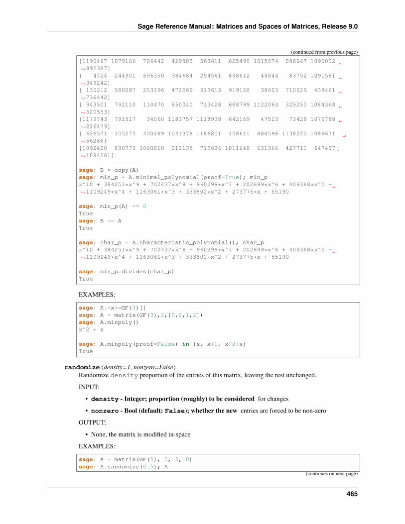
Sage Reference Manual: Matrices and Spaces of Matrices, Release 9.0
(continued from previous page)
[1190467 1079166 786442 429883 563611 625490 1015074 888047 1090092→˓892387][ 4724 244901 696350 384684 254561 898612 44844 83752 1091581→˓349242][ 130212 580087 253296 472569 913613 919150 38603 710029 438461→˓736442][ 943501 792110 110470 850040 713428 668799 1122064 325250 1084368→˓520553][1179743 791517 34060 1183757 1118938 642169 47513 73428 1076788→˓216479][ 626571 105273 400489 1041378 1186801 158611 888598 1138220 1089631→˓56266][1092400 890773 1060810 211135 719636 1011640 631366 427711 547497→˓1084281]
sage: B = copy(A)sage: min_p = A.minimal_polynomial(proof=True); min_px^10 + 384251*x^9 + 702437*x^8 + 960299*x^7 + 202699*x^6 + 409368*x^5 +→˓1109249*x^4 + 1163061*x^3 + 333802*x^2 + 273775*x + 55190
sage: min_p(A) == 0Truesage: B == ATrue
sage: char_p = A.characteristic_polynomial(); char_px^10 + 384251*x^9 + 702437*x^8 + 960299*x^7 + 202699*x^6 + 409368*x^5 +→˓1109249*x^4 + 1163061*x^3 + 333802*x^2 + 273775*x + 55190
sage: min_p.divides(char_p)True
EXAMPLES:
sage: R.<x>=GF(3)[]sage: A = matrix(GF(3),2,[0,0,1,2])sage: A.minpoly()x^2 + x
sage: A.minpoly(proof=False) in [x, x+1, x^2+x]True
randomize(density=1, nonzero=False)Randomize density proportion of the entries of this matrix, leaving the rest unchanged.
INPUT:
• density - Integer; proportion (roughly) to be considered for changes
• nonzero - Bool (default: False); whether the new entries are forced to be non-zero
OUTPUT:
• None, the matrix is modified in-space
EXAMPLES:
sage: A = matrix(GF(5), 5, 5, 0)sage: A.randomize(0.5); A
(continues on next page)
465
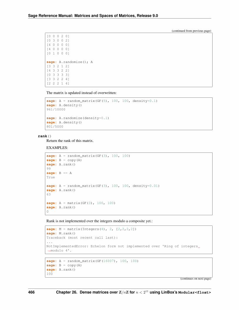
Sage Reference Manual: Matrices and Spaces of Matrices, Release 9.0
(continued from previous page)
[0 0 0 2 0][0 3 0 0 2][4 0 0 0 0][4 0 0 0 0][0 1 0 0 0]
sage: A.randomize(); A[3 3 2 1 2][4 3 3 2 2][0 3 3 3 3][3 3 2 2 4][2 2 2 1 4]
The matrix is updated instead of overwritten:
sage: A = random_matrix(GF(5), 100, 100, density=0.1)sage: A.density()961/10000
sage: A.randomize(density=0.1)sage: A.density()801/5000
rank()Return the rank of this matrix.
EXAMPLES:
sage: A = random_matrix(GF(3), 100, 100)sage: B = copy(A)sage: A.rank()99sage: B == ATrue
sage: A = random_matrix(GF(3), 100, 100, density=0.01)sage: A.rank()63
sage: A = matrix(GF(3), 100, 100)sage: A.rank()0
Rank is not implemented over the integers modulo a composite yet.:
sage: M = matrix(Integers(4), 2, [2,2,2,2])sage: M.rank()Traceback (most recent call last):...NotImplementedError: Echelon form not implemented over 'Ring of integers→˓modulo 4'.
sage: A = random_matrix(GF(16007), 100, 100)sage: B = copy(A)sage: A.rank()100
(continues on next page)
466 Chapter 26. Dense matrices over Z/𝑛Z for 𝑛 < 211 using LinBox’s Modular<float>
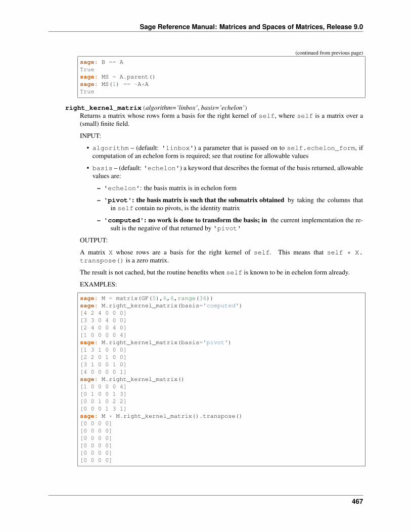
Sage Reference Manual: Matrices and Spaces of Matrices, Release 9.0
(continued from previous page)
sage: B == ATruesage: MS = A.parent()sage: MS(1) == ~A*ATrue
right_kernel_matrix(algorithm=’linbox’, basis=’echelon’)Returns a matrix whose rows form a basis for the right kernel of self, where self is a matrix over a(small) finite field.
INPUT:
• algorithm – (default: 'linbox') a parameter that is passed on to self.echelon_form, ifcomputation of an echelon form is required; see that routine for allowable values
• basis – (default: 'echelon') a keyword that describes the format of the basis returned, allowablevalues are:
– 'echelon': the basis matrix is in echelon form
– 'pivot': the basis matrix is such that the submatrix obtained by taking the columns thatin self contain no pivots, is the identity matrix
– 'computed': no work is done to transform the basis; in the current implementation the re-sult is the negative of that returned by 'pivot'
OUTPUT:
A matrix X whose rows are a basis for the right kernel of self. This means that self * X.transpose() is a zero matrix.
The result is not cached, but the routine benefits when self is known to be in echelon form already.
EXAMPLES:
sage: M = matrix(GF(5),6,6,range(36))sage: M.right_kernel_matrix(basis='computed')[4 2 4 0 0 0][3 3 0 4 0 0][2 4 0 0 4 0][1 0 0 0 0 4]sage: M.right_kernel_matrix(basis='pivot')[1 3 1 0 0 0][2 2 0 1 0 0][3 1 0 0 1 0][4 0 0 0 0 1]sage: M.right_kernel_matrix()[1 0 0 0 0 4][0 1 0 0 1 3][0 0 1 0 2 2][0 0 0 1 3 1]sage: M * M.right_kernel_matrix().transpose()[0 0 0 0][0 0 0 0][0 0 0 0][0 0 0 0][0 0 0 0][0 0 0 0]
467
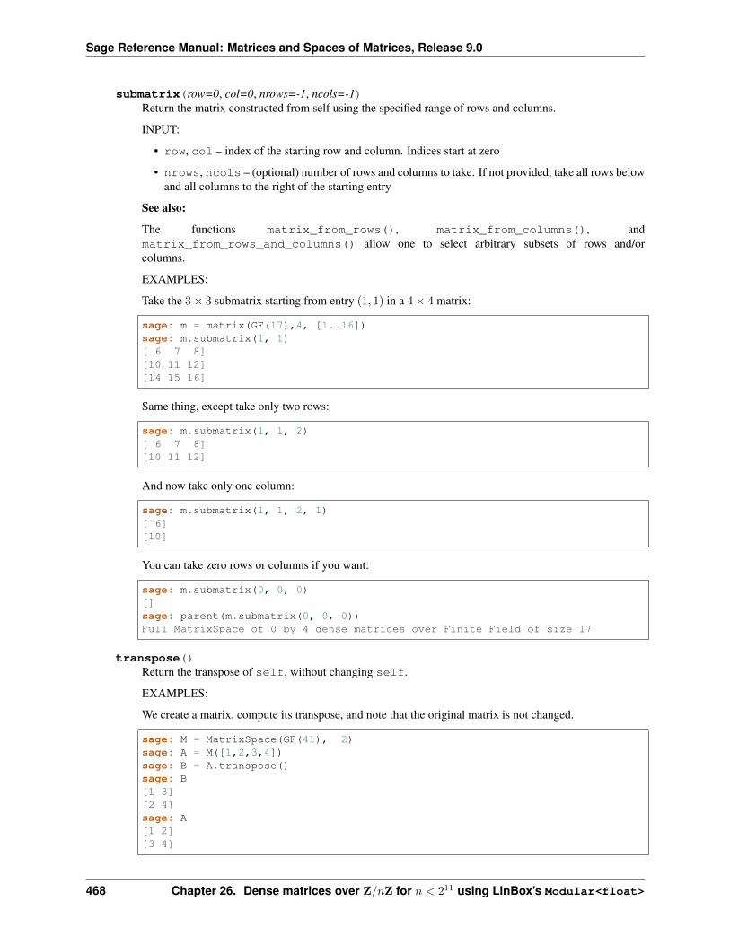
Sage Reference Manual: Matrices and Spaces of Matrices, Release 9.0
submatrix(row=0, col=0, nrows=-1, ncols=-1)Return the matrix constructed from self using the specified range of rows and columns.
INPUT:
• row, col – index of the starting row and column. Indices start at zero
• nrows, ncols – (optional) number of rows and columns to take. If not provided, take all rows belowand all columns to the right of the starting entry
See also:
The functions matrix_from_rows(), matrix_from_columns(), andmatrix_from_rows_and_columns() allow one to select arbitrary subsets of rows and/orcolumns.
EXAMPLES:
Take the 3× 3 submatrix starting from entry (1, 1) in a 4× 4 matrix:
sage: m = matrix(GF(17),4, [1..16])sage: m.submatrix(1, 1)[ 6 7 8][10 11 12][14 15 16]
Same thing, except take only two rows:
sage: m.submatrix(1, 1, 2)[ 6 7 8][10 11 12]
And now take only one column:
sage: m.submatrix(1, 1, 2, 1)[ 6][10]
You can take zero rows or columns if you want:
sage: m.submatrix(0, 0, 0)[]sage: parent(m.submatrix(0, 0, 0))Full MatrixSpace of 0 by 4 dense matrices over Finite Field of size 17
transpose()Return the transpose of self, without changing self.
EXAMPLES:
We create a matrix, compute its transpose, and note that the original matrix is not changed.
sage: M = MatrixSpace(GF(41), 2)sage: A = M([1,2,3,4])sage: B = A.transpose()sage: B[1 3][2 4]sage: A[1 2][3 4]
468 Chapter 26. Dense matrices over Z/𝑛Z for 𝑛 < 211 using LinBox’s Modular<float>
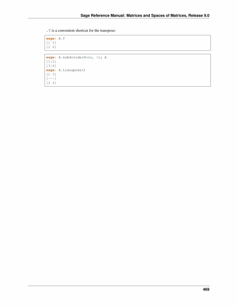
Sage Reference Manual: Matrices and Spaces of Matrices, Release 9.0
.T is a convenient shortcut for the transpose:
sage: A.T[1 3][2 4]
sage: A.subdivide(None, 1); A[1|2][3|4]sage: A.transpose()[1 3][---][2 4]
469

Sage Reference Manual: Matrices and Spaces of Matrices, Release 9.0
470 Chapter 26. Dense matrices over Z/𝑛Z for 𝑛 < 211 using LinBox’s Modular<float>
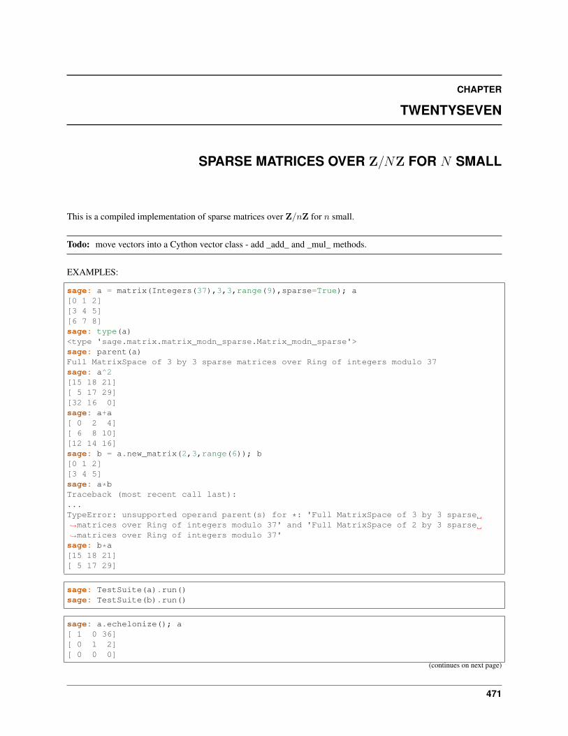
CHAPTER
TWENTYSEVEN
SPARSE MATRICES OVER Z/𝑁Z FOR 𝑁 SMALL
This is a compiled implementation of sparse matrices over Z/𝑛Z for 𝑛 small.
Todo: move vectors into a Cython vector class - add _add_ and _mul_ methods.
EXAMPLES:
sage: a = matrix(Integers(37),3,3,range(9),sparse=True); a[0 1 2][3 4 5][6 7 8]sage: type(a)<type 'sage.matrix.matrix_modn_sparse.Matrix_modn_sparse'>sage: parent(a)Full MatrixSpace of 3 by 3 sparse matrices over Ring of integers modulo 37sage: a^2[15 18 21][ 5 17 29][32 16 0]sage: a+a[ 0 2 4][ 6 8 10][12 14 16]sage: b = a.new_matrix(2,3,range(6)); b[0 1 2][3 4 5]sage: a*bTraceback (most recent call last):...TypeError: unsupported operand parent(s) for *: 'Full MatrixSpace of 3 by 3 sparse→˓matrices over Ring of integers modulo 37' and 'Full MatrixSpace of 2 by 3 sparse→˓matrices over Ring of integers modulo 37'sage: b*a[15 18 21][ 5 17 29]
sage: TestSuite(a).run()sage: TestSuite(b).run()
sage: a.echelonize(); a[ 1 0 36][ 0 1 2][ 0 0 0]
(continues on next page)
471
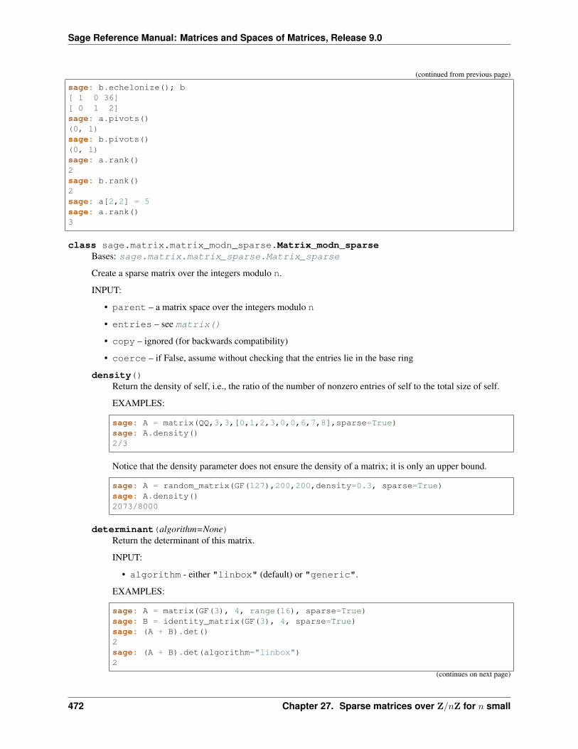
Sage Reference Manual: Matrices and Spaces of Matrices, Release 9.0
(continued from previous page)
sage: b.echelonize(); b[ 1 0 36][ 0 1 2]sage: a.pivots()(0, 1)sage: b.pivots()(0, 1)sage: a.rank()2sage: b.rank()2sage: a[2,2] = 5sage: a.rank()3
class sage.matrix.matrix_modn_sparse.Matrix_modn_sparseBases: sage.matrix.matrix_sparse.Matrix_sparse
Create a sparse matrix over the integers modulo n.
INPUT:
• parent – a matrix space over the integers modulo n
• entries – see matrix()
• copy – ignored (for backwards compatibility)
• coerce – if False, assume without checking that the entries lie in the base ring
density()Return the density of self, i.e., the ratio of the number of nonzero entries of self to the total size of self.
EXAMPLES:
sage: A = matrix(QQ,3,3,[0,1,2,3,0,0,6,7,8],sparse=True)sage: A.density()2/3
Notice that the density parameter does not ensure the density of a matrix; it is only an upper bound.
sage: A = random_matrix(GF(127),200,200,density=0.3, sparse=True)sage: A.density()2073/8000
determinant(algorithm=None)Return the determinant of this matrix.
INPUT:
• algorithm - either "linbox" (default) or "generic".
EXAMPLES:
sage: A = matrix(GF(3), 4, range(16), sparse=True)sage: B = identity_matrix(GF(3), 4, sparse=True)sage: (A + B).det()2sage: (A + B).det(algorithm="linbox")2
(continues on next page)
472 Chapter 27. Sparse matrices over Z/𝑛Z for 𝑛 small
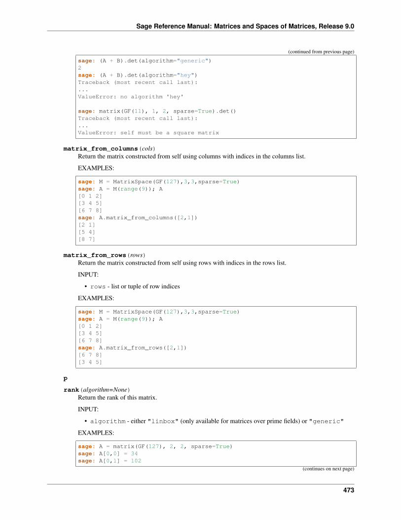
Sage Reference Manual: Matrices and Spaces of Matrices, Release 9.0
(continued from previous page)
sage: (A + B).det(algorithm="generic")2sage: (A + B).det(algorithm="hey")Traceback (most recent call last):...ValueError: no algorithm 'hey'
sage: matrix(GF(11), 1, 2, sparse=True).det()Traceback (most recent call last):...ValueError: self must be a square matrix
matrix_from_columns(cols)Return the matrix constructed from self using columns with indices in the columns list.
EXAMPLES:
sage: M = MatrixSpace(GF(127),3,3,sparse=True)sage: A = M(range(9)); A[0 1 2][3 4 5][6 7 8]sage: A.matrix_from_columns([2,1])[2 1][5 4][8 7]
matrix_from_rows(rows)Return the matrix constructed from self using rows with indices in the rows list.
INPUT:
• rows - list or tuple of row indices
EXAMPLES:
sage: M = MatrixSpace(GF(127),3,3,sparse=True)sage: A = M(range(9)); A[0 1 2][3 4 5][6 7 8]sage: A.matrix_from_rows([2,1])[6 7 8][3 4 5]
p
rank(algorithm=None)Return the rank of this matrix.
INPUT:
• algorithm - either "linbox" (only available for matrices over prime fields) or "generic"
EXAMPLES:
sage: A = matrix(GF(127), 2, 2, sparse=True)sage: A[0,0] = 34sage: A[0,1] = 102
(continues on next page)
473
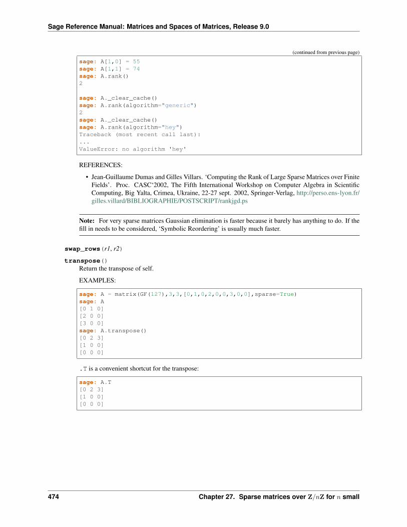
Sage Reference Manual: Matrices and Spaces of Matrices, Release 9.0
(continued from previous page)
sage: A[1,0] = 55sage: A[1,1] = 74sage: A.rank()2
sage: A._clear_cache()sage: A.rank(algorithm="generic")2sage: A._clear_cache()sage: A.rank(algorithm="hey")Traceback (most recent call last):...ValueError: no algorithm 'hey'
REFERENCES:
• Jean-Guillaume Dumas and Gilles Villars. ‘Computing the Rank of Large Sparse Matrices over FiniteFields’. Proc. CASC‘2002, The Fifth International Workshop on Computer Algebra in ScientificComputing, Big Yalta, Crimea, Ukraine, 22-27 sept. 2002, Springer-Verlag, http://perso.ens-lyon.fr/gilles.villard/BIBLIOGRAPHIE/POSTSCRIPT/rankjgd.ps
Note: For very sparse matrices Gaussian elimination is faster because it barely has anything to do. If thefill in needs to be considered, ‘Symbolic Reordering’ is usually much faster.
swap_rows(r1, r2)
transpose()Return the transpose of self.
EXAMPLES:
sage: A = matrix(GF(127),3,3,[0,1,0,2,0,0,3,0,0],sparse=True)sage: A[0 1 0][2 0 0][3 0 0]sage: A.transpose()[0 2 3][1 0 0][0 0 0]
.T is a convenient shortcut for the transpose:
sage: A.T[0 2 3][1 0 0][0 0 0]
474 Chapter 27. Sparse matrices over Z/𝑛Z for 𝑛 small
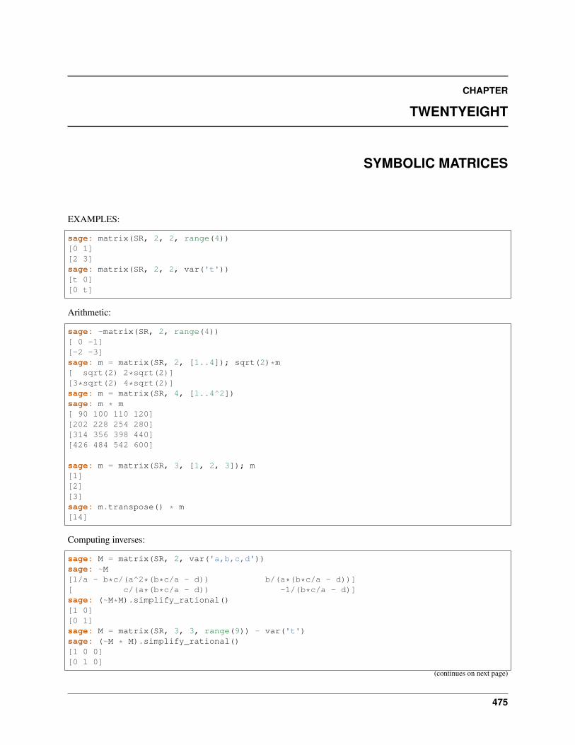
CHAPTER
TWENTYEIGHT
SYMBOLIC MATRICES
EXAMPLES:
sage: matrix(SR, 2, 2, range(4))[0 1][2 3]sage: matrix(SR, 2, 2, var('t'))[t 0][0 t]
Arithmetic:
sage: -matrix(SR, 2, range(4))[ 0 -1][-2 -3]sage: m = matrix(SR, 2, [1..4]); sqrt(2)*m[ sqrt(2) 2*sqrt(2)][3*sqrt(2) 4*sqrt(2)]sage: m = matrix(SR, 4, [1..4^2])sage: m * m[ 90 100 110 120][202 228 254 280][314 356 398 440][426 484 542 600]
sage: m = matrix(SR, 3, [1, 2, 3]); m[1][2][3]sage: m.transpose() * m[14]
Computing inverses:
sage: M = matrix(SR, 2, var('a,b,c,d'))sage: ~M[1/a - b*c/(a^2*(b*c/a - d)) b/(a*(b*c/a - d))][ c/(a*(b*c/a - d)) -1/(b*c/a - d)]sage: (~M*M).simplify_rational()[1 0][0 1]sage: M = matrix(SR, 3, 3, range(9)) - var('t')sage: (~M * M).simplify_rational()[1 0 0][0 1 0]
(continues on next page)
475
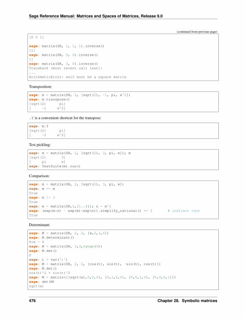
Sage Reference Manual: Matrices and Spaces of Matrices, Release 9.0
(continued from previous page)
[0 0 1]
sage: matrix(SR, 1, 1, 1).inverse()[1]sage: matrix(SR, 0, 0).inverse()[]sage: matrix(SR, 3, 0).inverse()Traceback (most recent call last):...ArithmeticError: self must be a square matrix
Transposition:
sage: m = matrix(SR, 2, [sqrt(2), -1, pi, e^2])sage: m.transpose()[sqrt(2) pi][ -1 e^2]
.T is a convenient shortcut for the transpose:
sage: m.T[sqrt(2) pi][ -1 e^2]
Test pickling:
sage: m = matrix(SR, 2, [sqrt(2), 3, pi, e]); m[sqrt(2) 3][ pi e]sage: TestSuite(m).run()
Comparison:
sage: m = matrix(SR, 2, [sqrt(2), 3, pi, e])sage: m == mTruesage: m != 3Truesage: m = matrix(SR,2,[1..4]); n = m^2sage: (exp(m+n) - exp(m)*exp(n)).simplify_rational() == 0 # indirect testTrue
Determinant:
sage: M = matrix(SR, 2, 2, [x,2,3,4])sage: M.determinant()4*x - 6sage: M = matrix(SR, 3,3,range(9))sage: M.det()0sage: t = var('t')sage: M = matrix(SR, 2, 2, [cos(t), sin(t), -sin(t), cos(t)])sage: M.det()cos(t)^2 + sin(t)^2sage: M = matrix([[sqrt(x),0,0,0], [0,1,0,0], [0,0,1,0], [0,0,0,1]])sage: det(M)sqrt(x)
476 Chapter 28. Symbolic matrices
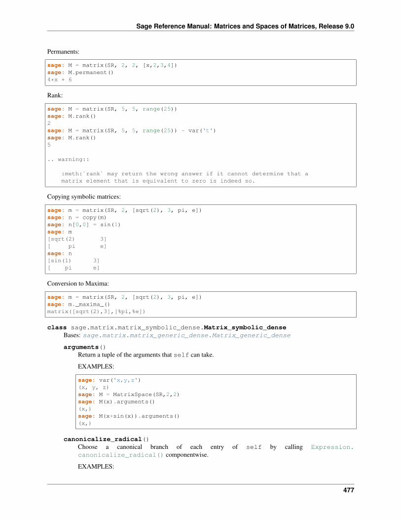
Sage Reference Manual: Matrices and Spaces of Matrices, Release 9.0
Permanents:
sage: M = matrix(SR, 2, 2, [x,2,3,4])sage: M.permanent()4*x + 6
Rank:
sage: M = matrix(SR, 5, 5, range(25))sage: M.rank()2sage: M = matrix(SR, 5, 5, range(25)) - var('t')sage: M.rank()5
.. warning::
:meth:`rank` may return the wrong answer if it cannot determine that amatrix element that is equivalent to zero is indeed so.
Copying symbolic matrices:
sage: m = matrix(SR, 2, [sqrt(2), 3, pi, e])sage: n = copy(m)sage: n[0,0] = sin(1)sage: m[sqrt(2) 3][ pi e]sage: n[sin(1) 3][ pi e]
Conversion to Maxima:
sage: m = matrix(SR, 2, [sqrt(2), 3, pi, e])sage: m._maxima_()matrix([sqrt(2),3],[%pi,%e])
class sage.matrix.matrix_symbolic_dense.Matrix_symbolic_denseBases: sage.matrix.matrix_generic_dense.Matrix_generic_dense
arguments()Return a tuple of the arguments that self can take.
EXAMPLES:
sage: var('x,y,z')(x, y, z)sage: M = MatrixSpace(SR,2,2)sage: M(x).arguments()(x,)sage: M(x+sin(x)).arguments()(x,)
canonicalize_radical()Choose a canonical branch of each entry of self by calling Expression.canonicalize_radical() componentwise.
EXAMPLES:
477
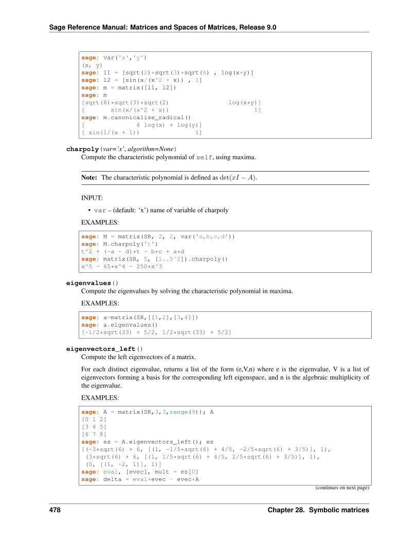
Sage Reference Manual: Matrices and Spaces of Matrices, Release 9.0
sage: var('x','y')(x, y)sage: l1 = [sqrt(2)*sqrt(3)*sqrt(6) , log(x*y)]sage: l2 = [sin(x/(x^2 + x)) , 1]sage: m = matrix([l1, l2])sage: m[sqrt(6)*sqrt(3)*sqrt(2) log(x*y)][ sin(x/(x^2 + x)) 1]sage: m.canonicalize_radical()[ 6 log(x) + log(y)][ sin(1/(x + 1)) 1]
charpoly(var=’x’, algorithm=None)Compute the characteristic polynomial of self, using maxima.
Note: The characteristic polynomial is defined as det(𝑥𝐼 −𝐴).
INPUT:
• var – (default: ‘x’) name of variable of charpoly
EXAMPLES:
sage: M = matrix(SR, 2, 2, var('a,b,c,d'))sage: M.charpoly('t')t^2 + (-a - d)*t - b*c + a*dsage: matrix(SR, 5, [1..5^2]).charpoly()x^5 - 65*x^4 - 250*x^3
eigenvalues()Compute the eigenvalues by solving the characteristic polynomial in maxima.
EXAMPLES:
sage: a=matrix(SR,[[1,2],[3,4]])sage: a.eigenvalues()[-1/2*sqrt(33) + 5/2, 1/2*sqrt(33) + 5/2]
eigenvectors_left()Compute the left eigenvectors of a matrix.
For each distinct eigenvalue, returns a list of the form (e,V,n) where e is the eigenvalue, V is a list ofeigenvectors forming a basis for the corresponding left eigenspace, and n is the algebraic multiplicity ofthe eigenvalue.
EXAMPLES:
sage: A = matrix(SR,3,3,range(9)); A[0 1 2][3 4 5][6 7 8]sage: es = A.eigenvectors_left(); es[(-3*sqrt(6) + 6, [(1, -1/5*sqrt(6) + 4/5, -2/5*sqrt(6) + 3/5)], 1),(3*sqrt(6) + 6, [(1, 1/5*sqrt(6) + 4/5, 2/5*sqrt(6) + 3/5)], 1),(0, [(1, -2, 1)], 1)]
sage: eval, [evec], mult = es[0]sage: delta = eval*evec - evec*A
(continues on next page)
478 Chapter 28. Symbolic matrices
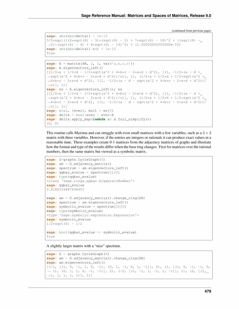
Sage Reference Manual: Matrices and Spaces of Matrices, Release 9.0
(continued from previous page)
sage: abs(abs(delta)) < 1e-103/5*sqrt(((2*sqrt(6) - 3)*(sqrt(6) - 2) + 7*sqrt(6) - 18)^2 + ((sqrt(6) -→˓2)*(sqrt(6) - 4) + 6*sqrt(6) - 14)^2) < (1.00000000000000e-10)sage: abs(abs(delta)).n() < 1e-10True
sage: A = matrix(SR, 2, 2, var('a,b,c,d'))sage: A.eigenvectors_left()[(1/2*a + 1/2*d - 1/2*sqrt(a^2 + 4*b*c - 2*a*d + d^2), [(1, -1/2*(a - d +→˓sqrt(a^2 + 4*b*c - 2*a*d + d^2))/c)], 1), (1/2*a + 1/2*d + 1/2*sqrt(a^2 +→˓4*b*c - 2*a*d + d^2), [(1, -1/2*(a - d - sqrt(a^2 + 4*b*c - 2*a*d + d^2))/→˓c)], 1)]sage: es = A.eigenvectors_left(); es[(1/2*a + 1/2*d - 1/2*sqrt(a^2 + 4*b*c - 2*a*d + d^2), [(1, -1/2*(a - d +→˓sqrt(a^2 + 4*b*c - 2*a*d + d^2))/c)], 1), (1/2*a + 1/2*d + 1/2*sqrt(a^2 +→˓4*b*c - 2*a*d + d^2), [(1, -1/2*(a - d - sqrt(a^2 + 4*b*c - 2*a*d + d^2))/→˓c)], 1)]sage: eval, [evec], mult = es[0]sage: delta = eval*evec - evec*Asage: delta.apply_map(lambda x: x.full_simplify())(0, 0)
This routine calls Maxima and can struggle with even small matrices with a few variables, such as a 3× 3matrix with three variables. However, if the entries are integers or rationals it can produce exact values in areasonable time. These examples create 0-1 matrices from the adjacency matrices of graphs and illustratehow the format and type of the results differ when the base ring changes. First for matrices over the rationalnumbers, then the same matrix but viewed as a symbolic matrix.
sage: G=graphs.CycleGraph(5)sage: am = G.adjacency_matrix()sage: spectrum = am.eigenvectors_left()sage: qqbar_evalue = spectrum[2][0]sage: type(qqbar_evalue)<class 'sage.rings.qqbar.AlgebraicNumber'>sage: qqbar_evalue0.618033988749895?
sage: am = G.adjacency_matrix().change_ring(SR)sage: spectrum = am.eigenvectors_left()sage: symbolic_evalue = spectrum[2][0]sage: type(symbolic_evalue)<type 'sage.symbolic.expression.Expression'>sage: symbolic_evalue1/2*sqrt(5) - 1/2
sage: bool(qqbar_evalue == symbolic_evalue)True
A slightly larger matrix with a “nice” spectrum.
sage: G = graphs.CycleGraph(6)sage: am = G.adjacency_matrix().change_ring(SR)sage: am.eigenvectors_left()[(-1, [(1, 0, -1, 1, 0, -1), (0, 1, -1, 0, 1, -1)], 2), (1, [(1, 0, -1, -1, 0,→˓ 1), (0, 1, 1, 0, -1, -1)], 2), (-2, [(1, -1, 1, -1, 1, -1)], 1), (2, [(1,→˓1, 1, 1, 1, 1)], 1)]
479
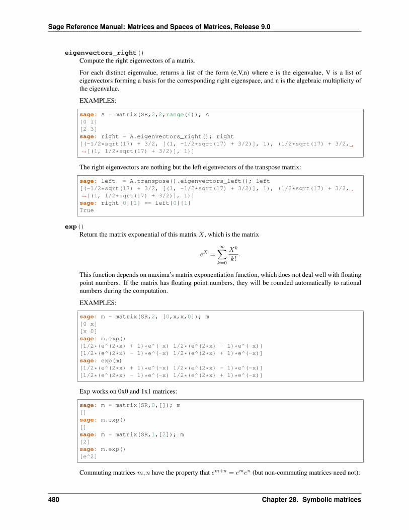
Sage Reference Manual: Matrices and Spaces of Matrices, Release 9.0
eigenvectors_right()Compute the right eigenvectors of a matrix.
For each distinct eigenvalue, returns a list of the form (e,V,n) where e is the eigenvalue, V is a list ofeigenvectors forming a basis for the corresponding right eigenspace, and n is the algebraic multiplicity ofthe eigenvalue.
EXAMPLES:
sage: A = matrix(SR,2,2,range(4)); A[0 1][2 3]sage: right = A.eigenvectors_right(); right[(-1/2*sqrt(17) + 3/2, [(1, -1/2*sqrt(17) + 3/2)], 1), (1/2*sqrt(17) + 3/2,→˓[(1, 1/2*sqrt(17) + 3/2)], 1)]
The right eigenvectors are nothing but the left eigenvectors of the transpose matrix:
sage: left = A.transpose().eigenvectors_left(); left[(-1/2*sqrt(17) + 3/2, [(1, -1/2*sqrt(17) + 3/2)], 1), (1/2*sqrt(17) + 3/2,→˓[(1, 1/2*sqrt(17) + 3/2)], 1)]sage: right[0][1] == left[0][1]True
exp()Return the matrix exponential of this matrix 𝑋 , which is the matrix
𝑒𝑋 =
∞∑︁𝑘=0
𝑋𝑘
𝑘!.
This function depends on maxima’s matrix exponentiation function, which does not deal well with floatingpoint numbers. If the matrix has floating point numbers, they will be rounded automatically to rationalnumbers during the computation.
EXAMPLES:
sage: m = matrix(SR,2, [0,x,x,0]); m[0 x][x 0]sage: m.exp()[1/2*(e^(2*x) + 1)*e^(-x) 1/2*(e^(2*x) - 1)*e^(-x)][1/2*(e^(2*x) - 1)*e^(-x) 1/2*(e^(2*x) + 1)*e^(-x)]sage: exp(m)[1/2*(e^(2*x) + 1)*e^(-x) 1/2*(e^(2*x) - 1)*e^(-x)][1/2*(e^(2*x) - 1)*e^(-x) 1/2*(e^(2*x) + 1)*e^(-x)]
Exp works on 0x0 and 1x1 matrices:
sage: m = matrix(SR,0,[]); m[]sage: m.exp()[]sage: m = matrix(SR,1,[2]); m[2]sage: m.exp()[e^2]
Commuting matrices 𝑚,𝑛 have the property that 𝑒𝑚+𝑛 = 𝑒𝑚𝑒𝑛 (but non-commuting matrices need not):
480 Chapter 28. Symbolic matrices
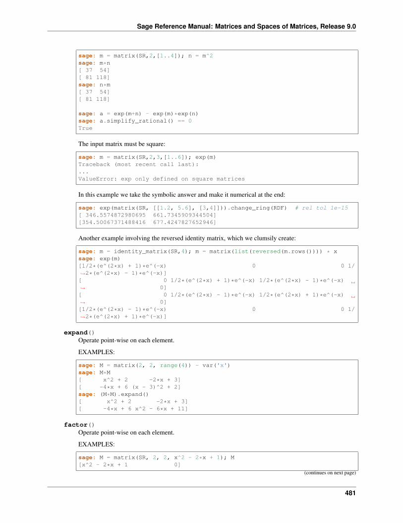
Sage Reference Manual: Matrices and Spaces of Matrices, Release 9.0
sage: m = matrix(SR,2,[1..4]); n = m^2sage: m*n[ 37 54][ 81 118]sage: n*m[ 37 54][ 81 118]
sage: a = exp(m+n) - exp(m)*exp(n)sage: a.simplify_rational() == 0True
The input matrix must be square:
sage: m = matrix(SR,2,3,[1..6]); exp(m)Traceback (most recent call last):...ValueError: exp only defined on square matrices
In this example we take the symbolic answer and make it numerical at the end:
sage: exp(matrix(SR, [[1.2, 5.6], [3,4]])).change_ring(RDF) # rel tol 1e-15[ 346.5574872980695 661.7345909344504][354.50067371488416 677.4247827652946]
Another example involving the reversed identity matrix, which we clumsily create:
sage: m = identity_matrix(SR,4); m = matrix(list(reversed(m.rows()))) * xsage: exp(m)[1/2*(e^(2*x) + 1)*e^(-x) 0 0 1/→˓2*(e^(2*x) - 1)*e^(-x)][ 0 1/2*(e^(2*x) + 1)*e^(-x) 1/2*(e^(2*x) - 1)*e^(-x)→˓ 0][ 0 1/2*(e^(2*x) - 1)*e^(-x) 1/2*(e^(2*x) + 1)*e^(-x)→˓ 0][1/2*(e^(2*x) - 1)*e^(-x) 0 0 1/→˓2*(e^(2*x) + 1)*e^(-x)]
expand()Operate point-wise on each element.
EXAMPLES:
sage: M = matrix(2, 2, range(4)) - var('x')sage: M*M[ x^2 + 2 -2*x + 3][ -4*x + 6 (x - 3)^2 + 2]sage: (M*M).expand()[ x^2 + 2 -2*x + 3][ -4*x + 6 x^2 - 6*x + 11]
factor()Operate point-wise on each element.
EXAMPLES:
sage: M = matrix(SR, 2, 2, x^2 - 2*x + 1); M[x^2 - 2*x + 1 0]
(continues on next page)
481
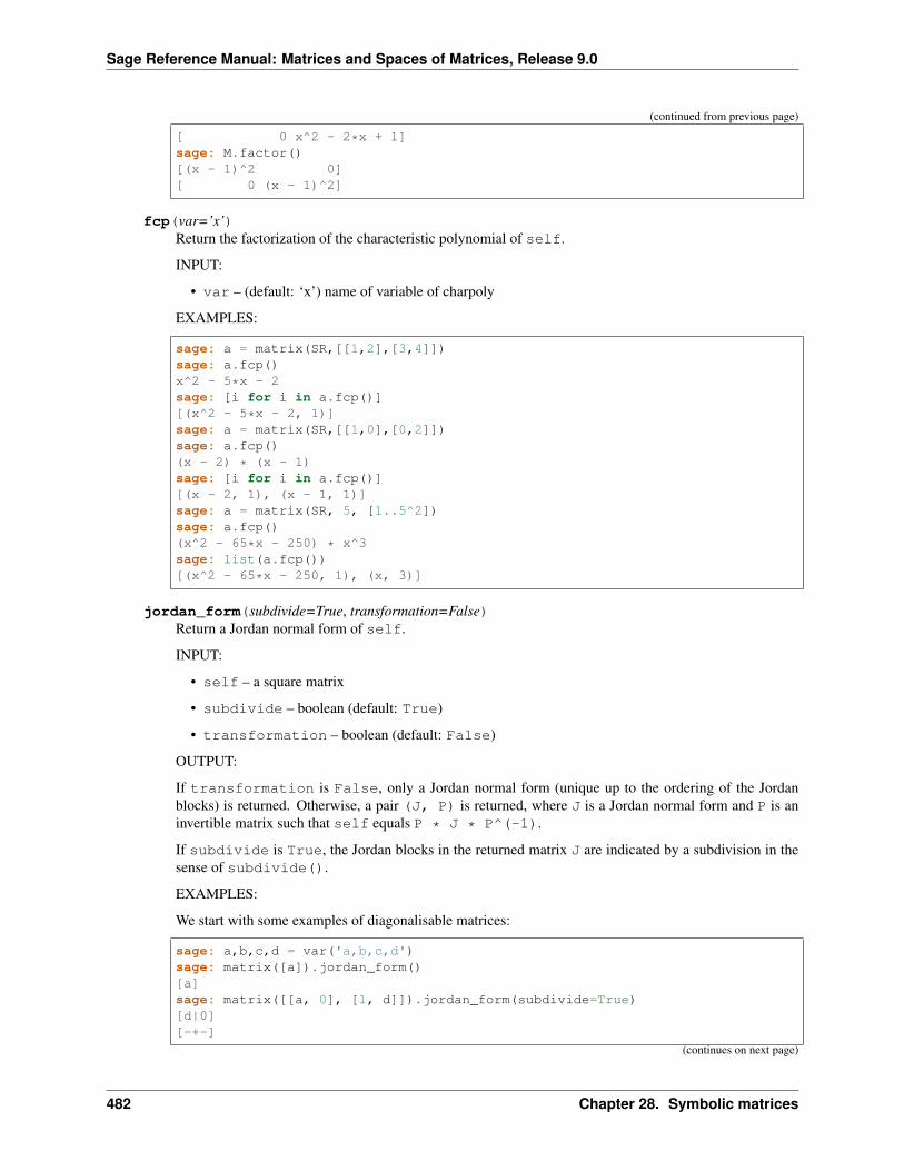
Sage Reference Manual: Matrices and Spaces of Matrices, Release 9.0
(continued from previous page)
[ 0 x^2 - 2*x + 1]sage: M.factor()[(x - 1)^2 0][ 0 (x - 1)^2]
fcp(var=’x’)Return the factorization of the characteristic polynomial of self.
INPUT:
• var – (default: ‘x’) name of variable of charpoly
EXAMPLES:
sage: a = matrix(SR,[[1,2],[3,4]])sage: a.fcp()x^2 - 5*x - 2sage: [i for i in a.fcp()][(x^2 - 5*x - 2, 1)]sage: a = matrix(SR,[[1,0],[0,2]])sage: a.fcp()(x - 2) * (x - 1)sage: [i for i in a.fcp()][(x - 2, 1), (x - 1, 1)]sage: a = matrix(SR, 5, [1..5^2])sage: a.fcp()(x^2 - 65*x - 250) * x^3sage: list(a.fcp())[(x^2 - 65*x - 250, 1), (x, 3)]
jordan_form(subdivide=True, transformation=False)Return a Jordan normal form of self.
INPUT:
• self – a square matrix
• subdivide – boolean (default: True)
• transformation – boolean (default: False)
OUTPUT:
If transformation is False, only a Jordan normal form (unique up to the ordering of the Jordanblocks) is returned. Otherwise, a pair (J, P) is returned, where J is a Jordan normal form and P is aninvertible matrix such that self equals P * J * P^(-1).
If subdivide is True, the Jordan blocks in the returned matrix J are indicated by a subdivision in thesense of subdivide().
EXAMPLES:
We start with some examples of diagonalisable matrices:
sage: a,b,c,d = var('a,b,c,d')sage: matrix([a]).jordan_form()[a]sage: matrix([[a, 0], [1, d]]).jordan_form(subdivide=True)[d|0][-+-]
(continues on next page)
482 Chapter 28. Symbolic matrices
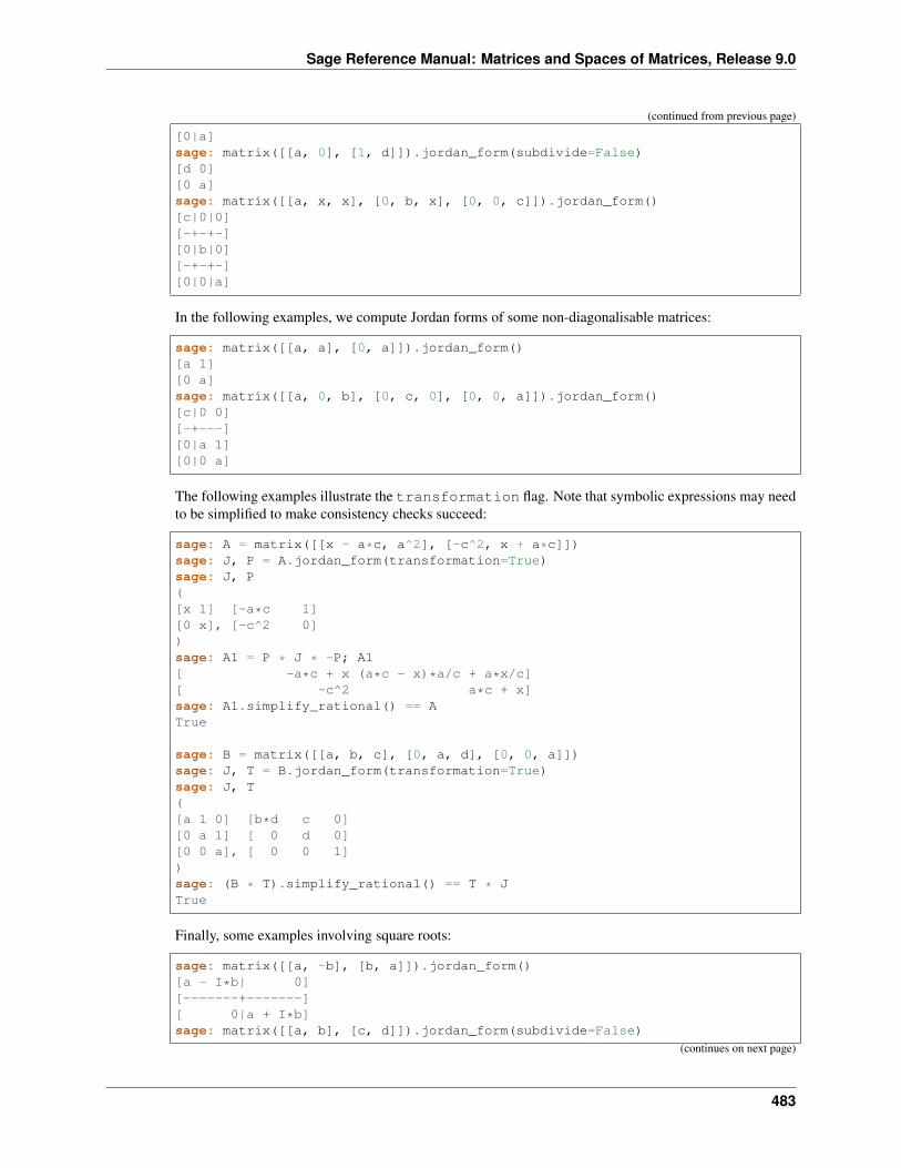
Sage Reference Manual: Matrices and Spaces of Matrices, Release 9.0
(continued from previous page)
[0|a]sage: matrix([[a, 0], [1, d]]).jordan_form(subdivide=False)[d 0][0 a]sage: matrix([[a, x, x], [0, b, x], [0, 0, c]]).jordan_form()[c|0|0][-+-+-][0|b|0][-+-+-][0|0|a]
In the following examples, we compute Jordan forms of some non-diagonalisable matrices:
sage: matrix([[a, a], [0, a]]).jordan_form()[a 1][0 a]sage: matrix([[a, 0, b], [0, c, 0], [0, 0, a]]).jordan_form()[c|0 0][-+---][0|a 1][0|0 a]
The following examples illustrate the transformation flag. Note that symbolic expressions may needto be simplified to make consistency checks succeed:
sage: A = matrix([[x - a*c, a^2], [-c^2, x + a*c]])sage: J, P = A.jordan_form(transformation=True)sage: J, P([x 1] [-a*c 1][0 x], [-c^2 0])sage: A1 = P * J * ~P; A1[ -a*c + x (a*c - x)*a/c + a*x/c][ -c^2 a*c + x]sage: A1.simplify_rational() == ATrue
sage: B = matrix([[a, b, c], [0, a, d], [0, 0, a]])sage: J, T = B.jordan_form(transformation=True)sage: J, T([a 1 0] [b*d c 0][0 a 1] [ 0 d 0][0 0 a], [ 0 0 1])sage: (B * T).simplify_rational() == T * JTrue
Finally, some examples involving square roots:
sage: matrix([[a, -b], [b, a]]).jordan_form()[a - I*b| 0][-------+-------][ 0|a + I*b]sage: matrix([[a, b], [c, d]]).jordan_form(subdivide=False)
(continues on next page)
483
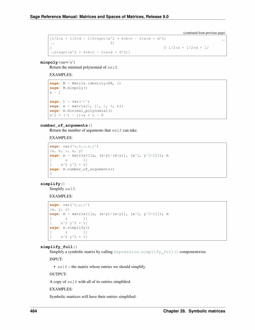
Sage Reference Manual: Matrices and Spaces of Matrices, Release 9.0
(continued from previous page)
[1/2*a + 1/2*d - 1/2*sqrt(a^2 + 4*b*c - 2*a*d + d^2)→˓ 0][ 0 1/2*a + 1/2*d + 1/→˓2*sqrt(a^2 + 4*b*c - 2*a*d + d^2)]
minpoly(var=’x’)Return the minimal polynomial of self.
EXAMPLES:
sage: M = Matrix.identity(SR, 2)sage: M.minpoly()x - 1
sage: t = var('t')sage: m = matrix(2, [1, 2, 4, t])sage: m.minimal_polynomial()x^2 + (-t - 1)*x + t - 8
number_of_arguments()Return the number of arguments that self can take.
EXAMPLES:
sage: var('a,b,c,x,y')(a, b, c, x, y)sage: m = matrix([[a, (x+y)/(x+y)], [x^2, y^2+2]]); m[ a 1][ x^2 y^2 + 2]sage: m.number_of_arguments()3
simplify()Simplify self.
EXAMPLES:
sage: var('x,y,z')(x, y, z)sage: m = matrix([[z, (x+y)/(x+y)], [x^2, y^2+2]]); m[ z 1][ x^2 y^2 + 2]sage: m.simplify()[ z 1][ x^2 y^2 + 2]
simplify_full()Simplify a symbolic matrix by calling Expression.simplify_full() componentwise.
INPUT:
• self – the matrix whose entries we should simplify.
OUTPUT:
A copy of self with all of its entries simplified.
EXAMPLES:
Symbolic matrices will have their entries simplified:
484 Chapter 28. Symbolic matrices
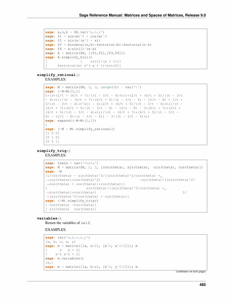
Sage Reference Manual: Matrices and Spaces of Matrices, Release 9.0
sage: a,n,k = SR.var('a,n,k')sage: f1 = sin(x)^2 + cos(x)^2sage: f2 = sin(x/(x^2 + x))sage: f3 = binomial(n,k)*factorial(k)*factorial(n-k)sage: f4 = x*sin(2)/(x^a)sage: A = matrix(SR, [[f1,f2],[f3,f4]])sage: A.simplify_full()[ 1 sin(1/(x + 1))][ factorial(n) x^(-a + 1)*sin(2)]
simplify_rational()EXAMPLES:
sage: M = matrix(SR, 3, 3, range(9)) - var('t')sage: (~M*M)[0,0]t*(3*(2/t + (6/t + 7)/((t - 3/t - 4)*t))*(2/t + (6/t + 5)/((t - 3/t- 4)*t))/(t - (6/t + 7)*(6/t + 5)/(t - 3/t - 4) - 12/t - 8) + 1/t +3/((t - 3/t - 4)*t^2)) - 6*(2/t + (6/t + 5)/((t - 3/t - 4)*t))/(t -(6/t + 7)*(6/t + 5)/(t - 3/t - 4) - 12/t - 8) - 3*(6/t + 7)*(2/t +(6/t + 5)/((t - 3/t - 4)*t))/((t - (6/t + 7)*(6/t + 5)/(t - 3/t -4) - 12/t - 8)*(t - 3/t - 4)) - 3/((t - 3/t - 4)*t)sage: expand((~M*M)[0,0])1sage: (~M * M).simplify_rational()[1 0 0][0 1 0][0 0 1]
simplify_trig()EXAMPLES:
sage: theta = var('theta')sage: M = matrix(SR, 2, 2, [cos(theta), sin(theta), -sin(theta), cos(theta)])sage: ~M[1/cos(theta) - sin(theta)^2/((sin(theta)^2/cos(theta) +→˓cos(theta))*cos(theta)^2) -sin(theta)/((sin(theta)^2/→˓cos(theta) + cos(theta))*cos(theta))][ sin(theta)/((sin(theta)^2/cos(theta) +→˓cos(theta))*cos(theta)) 1/→˓(sin(theta)^2/cos(theta) + cos(theta))]sage: (~M).simplify_trig()[ cos(theta) -sin(theta)][ sin(theta) cos(theta)]
variables()Return the variables of self.
EXAMPLES:
sage: var('a,b,c,x,y')(a, b, c, x, y)sage: m = matrix([[x, x+2], [x^2, x^2+2]]); m[ x x + 2][ x^2 x^2 + 2]sage: m.variables()(x,)sage: m = matrix([[a, b+c], [x^2, y^2+2]]); m
(continues on next page)
485
Sage Reference Manual: Matrices and Spaces of Matrices, Release 9.0
(continued from previous page)
[ a b + c][ x^2 y^2 + 2]sage: m.variables()(a, b, c, x, y)
486 Chapter 28. Symbolic matrices

CHAPTER
TWENTYNINE
DENSE MATRICES OVER THE COMPLEX DOUBLE FIELD USINGNUMPY
EXAMPLES:
sage: b = Mat(CDF,2,3).basis()sage: b[0,0][1.0 0.0 0.0][0.0 0.0 0.0]
We deal with the case of zero rows or zero columns:
sage: m = MatrixSpace(CDF,0,3)sage: m.zero_matrix()[]
AUTHORS:
• Jason Grout (2008-09): switch to NumPy backend
• Josh Kantor
• William Stein: many bug fixes and touch ups.
class sage.matrix.matrix_complex_double_dense.Matrix_complex_double_denseBases: sage.matrix.matrix_double_dense.Matrix_double_dense
Class that implements matrices over the real double field. These are supposed to be fast matrix operations usingC doubles. Most operations are implemented using numpy which will call the underlying BLAS on the system.
EXAMPLES:
sage: m = Matrix(CDF, [[1,2*I],[3+I,4]])sage: m**2[-1.0 + 6.0*I 10.0*I][15.0 + 5.0*I 14.0 + 6.0*I]sage: n= m^(-1); n # abs tol 1e-15[ 0.3333333333333333 + 0.3333333333333333*I 0.16666666666666669 - 0.→˓16666666666666666*I][-0.16666666666666666 - 0.3333333333333333*I 0.08333333333333331 + 0.→˓08333333333333333*I]
To compute eigenvalues the use the functions left_eigenvectors or right_eigenvectors:
sage: p,e = m.right_eigenvectors()
the result of eigen is a pair (p,e), where p is a list of eigenvalues and the e is a matrix whose columns are theeigenvectors.
487
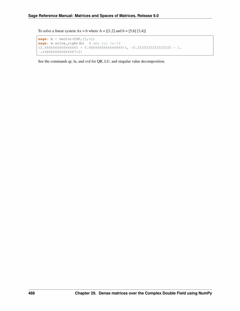
Sage Reference Manual: Matrices and Spaces of Matrices, Release 9.0
To solve a linear system Ax = b where A = [[1,2] and b = [5,6] [3,4]]
sage: b = vector(CDF,[5,6])sage: m.solve_right(b) # abs tol 1e-14(2.6666666666666665 + 0.6666666666666669*I, -0.3333333333333333 - 1.→˓1666666666666667*I)
See the commands qr, lu, and svd for QR, LU, and singular value decomposition.
488 Chapter 29. Dense matrices over the Complex Double Field using NumPy
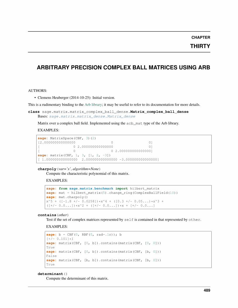
CHAPTER
THIRTY
ARBITRARY PRECISION COMPLEX BALL MATRICES USING ARB
AUTHORS:
• Clemens Heuberger (2014-10-25): Initial version.
This is a rudimentary binding to the Arb library; it may be useful to refer to its documentation for more details.
class sage.matrix.matrix_complex_ball_dense.Matrix_complex_ball_denseBases: sage.matrix.matrix_dense.Matrix_dense
Matrix over a complex ball field. Implemented using the acb_mat type of the Arb library.
EXAMPLES:
sage: MatrixSpace(CBF, 3)(2)[2.000000000000000 0 0][ 0 2.000000000000000 0][ 0 0 2.000000000000000]sage: matrix(CBF, 1, 3, [1, 2, -3])[ 1.000000000000000 2.000000000000000 -3.000000000000000]
charpoly(var=’x’, algorithm=None)Compute the characteristic polynomial of this matrix.
EXAMPLES:
sage: from sage.matrix.benchmark import hilbert_matrixsage: mat = hilbert_matrix(5).change_ring(ComplexBallField(10))sage: mat.charpoly()x^5 + ([-1.8 +/- 0.0258])*x^4 + ([0.3 +/- 0.05...)*x^3 +([+/- 0.0...])*x^2 + ([+/- 0.0...])*x + [+/- 0.0...]
contains(other)Test if the set of complex matrices represented by self is contained in that represented by other.
EXAMPLES:
sage: b = CBF(0, RBF(0, rad=.1r)); b[+/- 0.101]*Isage: matrix(CBF, [0, b]).contains(matrix(CBF, [0, 0]))Truesage: matrix(CBF, [0, b]).contains(matrix(CBF, [b, 0]))Falsesage: matrix(CBF, [b, b]).contains(matrix(CBF, [b, 0]))True
determinant()Compute the determinant of this matrix.
489
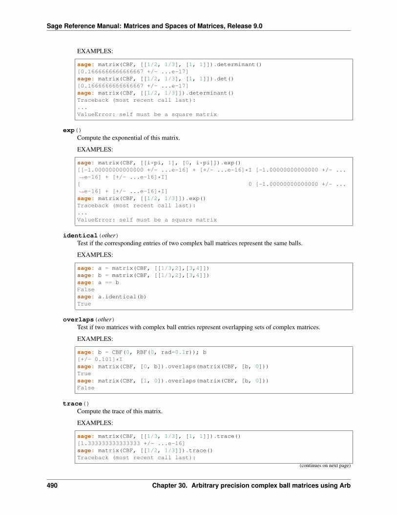
Sage Reference Manual: Matrices and Spaces of Matrices, Release 9.0
EXAMPLES:
sage: matrix(CBF, [[1/2, 1/3], [1, 1]]).determinant()[0.1666666666666667 +/- ...e-17]sage: matrix(CBF, [[1/2, 1/3], [1, 1]]).det()[0.1666666666666667 +/- ...e-17]sage: matrix(CBF, [[1/2, 1/3]]).determinant()Traceback (most recent call last):...ValueError: self must be a square matrix
exp()Compute the exponential of this matrix.
EXAMPLES:
sage: matrix(CBF, [[i*pi, 1], [0, i*pi]]).exp()[[-1.00000000000000 +/- ...e-16] + [+/- ...e-16]*I [-1.00000000000000 +/- ...→˓e-16] + [+/- ...e-16]*I][ 0 [-1.00000000000000 +/- ...→˓e-16] + [+/- ...e-16]*I]sage: matrix(CBF, [[1/2, 1/3]]).exp()Traceback (most recent call last):...ValueError: self must be a square matrix
identical(other)Test if the corresponding entries of two complex ball matrices represent the same balls.
EXAMPLES:
sage: a = matrix(CBF, [[1/3,2],[3,4]])sage: b = matrix(CBF, [[1/3,2],[3,4]])sage: a == bFalsesage: a.identical(b)True
overlaps(other)Test if two matrices with complex ball entries represent overlapping sets of complex matrices.
EXAMPLES:
sage: b = CBF(0, RBF(0, rad=0.1r)); b[+/- 0.101]*Isage: matrix(CBF, [0, b]).overlaps(matrix(CBF, [b, 0]))Truesage: matrix(CBF, [1, 0]).overlaps(matrix(CBF, [b, 0]))False
trace()Compute the trace of this matrix.
EXAMPLES:
sage: matrix(CBF, [[1/3, 1/3], [1, 1]]).trace()[1.333333333333333 +/- ...e-16]sage: matrix(CBF, [[1/2, 1/3]]).trace()Traceback (most recent call last):
(continues on next page)
490 Chapter 30. Arbitrary precision complex ball matrices using Arb

Sage Reference Manual: Matrices and Spaces of Matrices, Release 9.0
(continued from previous page)
...ValueError: self must be a square matrix
491

Sage Reference Manual: Matrices and Spaces of Matrices, Release 9.0
492 Chapter 30. Arbitrary precision complex ball matrices using Arb
CHAPTER
THIRTYONE
DENSE MATRICES OVER UNIVARIATE POLYNOMIALS OVER FIELDS
The implementation inherits from Matrix_generic_dense but some algorithms are optimized for polynomial matrices.
AUTHORS:
• Kwankyu Lee (2016-12-15): initial version with code moved from other files.
• Johan Rosenkilde (2017-02-07): added weak_popov_form()
• Vincent Neiger (2018-06-13): added basic functions (row/column degrees, leading positions, leading matrix,testing reduced and canonical forms)
• Vincent Neiger (2018-09-29): added functions for computing and for verifying minimal approximant bases
class sage.matrix.matrix_polynomial_dense.Matrix_polynomial_denseBases: sage.matrix.matrix_generic_dense.Matrix_generic_dense
Dense matrix over a univariate polynomial ring over a field.
For a field K, we consider matrices over the univariate polynomial ring K[𝑥].
They are often used to represent bases of some K[𝑥]-modules. In this context, there are two possible represen-tations which are both commonly used in the literature.
• Working column-wise: each column of the matrix is a vector in the basis; then, a $\Bold{K}[x]$-submodule of $\Bold{K}[x]^{m}$ of rank $n$ is represented by an $m \times n$ matrix, whose columnsspan the module (via $\Bold{K}[x]$-linear combinations). This matrix has full rank, and $n \leq m$.
• Working row-wise: each row of the matrix is a vector in the basis; then, a $\Bold{K}[x]$-submodule of$\Bold{K}[x]^{n}$ of rank $m$ is represented by an $m \times n$ matrix, whose rows span the module(via $\Bold{K}[x]$-linear combinations). This matrix has full rank, and $m \leq n$.
For the rest of this class description, we assume that one is working row-wise. For a given such module, all itsbases are equivalent under left-multiplication by a unimodular matrix, that is, a matrix which has determinant inK ∖ {0}.
There are bases which are called reduced or minimal: their rows have the minimal degree possible among allbases of this module. The degree of a row is the maximum of the degrees of the entries of the row. An equivalentcondition is that the leading matrix of this basis has full rank (see the description of leading_matrix()).There is a unique minimal basis, called the Popov basis of the module, which satisfies some additional normal-ization condition (see the description of row_degrees()).
These notions can be extended via a more general degree measure, involving a tuple of integers which is calledshift and acts as column degree shifts in the definition of row degree. Precisely, for given 𝑠1, . . . , 𝑠𝑛 ∈ Z anda row vector [𝑝1 · · · 𝑝𝑛] ∈ K[𝑥]1×𝑛, its shifted row degree is the maximum of deg(𝑝𝑗) + 𝑠𝑗 for 1 ≤ 𝑗 ≤ 𝑛.Then, minimal bases and Popov bases are defined similarly, with respect to this notion of degree.
493
Sage Reference Manual: Matrices and Spaces of Matrices, Release 9.0
Another important canonical basis is the Hermite basis, which is a lower triangular matrix satisfying a normal-ization condition similar to that for the Popov basis. In fact, if 𝑑 is the largest degree appearing in the Hermitebasis, then the Hermite basis coincide with the shifted Popov basis with the shifts (0, 𝑑, 2𝑑, . . . , (𝑛− 1)𝑑).
column_degrees(shifts=None)Return the (shifted) column degrees of this matrix.
For a given polynomial matrix 𝑀 = (𝑀𝑖,𝑗)𝑖,𝑗 with 𝑚 rows and 𝑛 columns, its column degrees is the tuple(𝑑1, . . . , 𝑑𝑛) where 𝑑𝑗 = max𝑖(deg(𝑀𝑖,𝑗)) for 1 ≤ 𝑗 ≤ 𝑛. Thus, 𝑑𝑗 = −1 if the 𝑗-th column of 𝑀 iszero, and 𝑑𝑗 ≥ 0 otherwise.
For given shifts 𝑠1, . . . , 𝑠𝑚 ∈ Z, the shifted column degrees of 𝑀 is (𝑑1, . . . , 𝑑𝑛) where 𝑑𝑗 =max𝑖(deg(𝑀𝑖,𝑗) + 𝑠𝑖). Here, if the 𝑗-th column of 𝑀 is zero then 𝑑𝑗 = min(𝑠1, . . . , 𝑠𝑚) − 1; other-wise 𝑑𝑗 is larger than this value.
INPUT:
• shifts – (optional, default: None) list of integers; None is interpreted as shifts=[0,...,0].
OUTPUT: a list of integers.
EXAMPLES:
sage: pR.<x> = GF(7)[]sage: M = Matrix(pR, [ [3*x+1, 0, 1], [x^3+3, 0, 0] ])sage: M.column_degrees()[3, -1, 0]
sage: M.column_degrees(shifts=[0,2])[5, -1, 0]
A zero column in a polynomial matrix can be identified in the (shifted) column degrees as the entries equalto min(shifts)-1:
sage: M.column_degrees(shifts=[-2,1])[4, -3, -2]
The column degrees of an empty matrix (0× 𝑛 or 𝑚× 0) is not defined:
sage: M = Matrix( pR, 0, 3 )sage: M.column_degrees()Traceback (most recent call last):...ValueError: empty matrix does not have column degrees
sage: M = Matrix( pR, 3, 0 )sage: M.column_degrees()Traceback (most recent call last):...ValueError: empty matrix does not have column degrees
See also:
The documentation of row_degrees().
degree()Return the degree of this matrix.
For a given polynomial matrix, its degree is the maximum of the degrees of all its entries. If the matrix isnonzero, this is a nonnegative integer; here, the degree of the zero matrix is -1.
OUTPUT: an integer.
494 Chapter 31. Dense matrices over univariate polynomials over fields
Sage Reference Manual: Matrices and Spaces of Matrices, Release 9.0
EXAMPLES:
sage: pR.<x> = GF(7)[]sage: M = Matrix( pR, [[3*x+1, 0, 1], [x^3+3, 0, 0]])sage: M.degree()3
The zero matrix has degree -1:
sage: M = Matrix( pR, 2, 3 )sage: M.degree()-1
For an empty matrix, the degree is not defined:
sage: M = Matrix( pR, 3, 0 )sage: M.degree()Traceback (most recent call last):...ValueError: empty matrix does not have a degree
degree_matrix(shifts=None, row_wise=True)Return the matrix of the (shifted) degrees in this matrix.
For a given polynomial matrix 𝑀 = (𝑀𝑖,𝑗)𝑖,𝑗 , its degree matrix is the matrix (deg(𝑀𝑖,𝑗))𝑖,𝑗 formed bythe degrees of its entries. Here, the degree of the zero polynomial is −1.
For given shifts 𝑠1, . . . , 𝑠𝑚 ∈ Z, the shifted degree matrix of 𝑀 is either (deg(𝑀𝑖,𝑗) + 𝑠𝑗)𝑖,𝑗 if workingrow-wise, or (deg(𝑀𝑖,𝑗) + 𝑠𝑖)𝑖,𝑗 if working column-wise. In the former case, 𝑚 has to be the numberof columns of 𝑀 ; in the latter case, the number of its rows. Here, if 𝑀𝑖,𝑗 = 0 then the correspondingentry in the shifted degree matrix is min(𝑠1, . . . , 𝑠𝑚)−1. For more on shifts and working row-wise versuscolumn-wise, see the class documentation.
INPUT:
• shifts – (optional, default: None) list of integers; None is interpreted as shifts=[0,...,0].
• row_wise – (optional, default: True) boolean, if True then shifts apply to the columns of thematrix and otherwise to its rows (see the class description for more details).
OUTPUT: an integer matrix.
EXAMPLES:
sage: pR.<x> = GF(7)[]sage: M = Matrix( pR, [[3*x+1, 0, 1], [x^3+3, 0, 0]])sage: M.degree_matrix()[ 1 -1 0][ 3 -1 -1]
sage: M.degree_matrix(shifts=[0,1,2])[ 1 -1 2][ 3 -1 -1]
The zero entries in the polynomial matrix can be identified in the (shifted) degree matrix as the entriesequal to min(shifts)-1:
sage: M.degree_matrix(shifts=[-2,1,2])[-1 -3 2][ 1 -3 -3]
495
Sage Reference Manual: Matrices and Spaces of Matrices, Release 9.0
Using row_wise=False, the function supports shifts applied to the rows of the matrix (which, in termsof modules, means that we are working column-wise, see the class documentation):
sage: M.degree_matrix(shifts=[-1,2], row_wise=False)[ 0 -2 -1][ 5 -2 -2]
hermite_form(include_zero_rows=True, transformation=False)Return the Hermite form of this matrix.
The Hermite form is also normalized, i.e., the pivot polynomials are monic.
INPUT:
• include_zero_rows – boolean (default: True); if False, the zero rows in the output matrixare deleted
• transformation – boolean (default: False); if True, return the transformation matrix
OUTPUT:
• the Hermite normal form 𝐻 of this matrix 𝐴
• (optional) transformation matrix 𝑈 such that 𝑈𝐴 = 𝐻
EXAMPLES:
sage: M.<x> = GF(7)[]sage: A = matrix(M, 2, 3, [x, 1, 2*x, x, 1+x, 2])sage: A.hermite_form()[ x 1 2*x][ 0 x 5*x + 2]sage: A.hermite_form(transformation=True)([ x 1 2*x] [1 0][ 0 x 5*x + 2], [6 1])sage: A = matrix(M, 2, 3, [x, 1, 2*x, 2*x, 2, 4*x])sage: A.hermite_form(transformation=True, include_zero_rows=False)([ x 1 2*x], [0 4])sage: H, U = A.hermite_form(transformation=True, include_zero_rows=True); H, U([ x 1 2*x] [0 4][ 0 0 0], [5 1])sage: U * A == HTruesage: H, U = A.hermite_form(transformation=True, include_zero_rows=False)sage: U * A[ x 1 2*x]sage: U * A == HTrue
See also:
is_hermite() .
is_hermite(row_wise=True, lower_echelon=False, include_zero_vectors=True)Return a boolean indicating whether this matrix is in Hermite form.
If working row-wise, a polynomial matrix is said to be in Hermite form if it is in row echelon form withall pivot entries monic and such that all entries above a pivot have degree less than this pivot. Being in row
496 Chapter 31. Dense matrices over univariate polynomials over fields
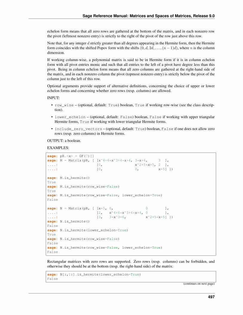
Sage Reference Manual: Matrices and Spaces of Matrices, Release 9.0
echelon form means that all zero rows are gathered at the bottom of the matrix, and in each nonzero rowthe pivot (leftmost nonzero entry) is strictly to the right of the pivot of the row just above this row.
Note that, for any integer 𝑑 strictly greater than all degrees appearing in the Hermite form, then the Hermiteform coincides with the shifted Popov form with the shifts (0, 𝑑, 2𝑑, . . . , (𝑛− 1)𝑑), where 𝑛 is the columndimension.
If working column-wise, a polynomial matrix is said to be in Hermite form if it is in column echelonform with all pivot entries monic and such that all entries to the left of a pivot have degree less than thispivot. Being in column echelon form means that all zero columns are gathered at the right-hand side ofthe matrix, and in each nonzero column the pivot (topmost nonzero entry) is strictly below the pivot of thecolumn just to the left of this row.
Optional arguments provide support of alternative definitions, concerning the choice of upper or lowerechelon forms and concerning whether zero rows (resp. columns) are allowed.
INPUT:
• row_wise – (optional, default: True) boolean, True if working row-wise (see the class descrip-tion).
• lower_echelon – (optional, default: False) boolean, False if working with upper triangularHermite forms, True if working with lower triangular Hermite forms.
• include_zero_vectors – (optional, default: True) boolean, False if one does not allow zerorows (resp. zero columns) in Hermite forms.
OUTPUT: a boolean.
EXAMPLES:
sage: pR.<x> = GF(7)[]sage: M = Matrix(pR, [ [x^4+6*x^3+4*x+4, 3*x+6, 3 ],....: [0, x^2+5*x+5, 2 ],....: [0, 0, x+5] ])
sage: M.is_hermite()Truesage: M.is_hermite(row_wise=False)Truesage: M.is_hermite(row_wise=False, lower_echelon=True)False
sage: N = Matrix(pR, [ [x+5, 0, 0 ],....: [2, x^4+6*x^3+4*x+4, 0 ],....: [3, 3*x^3+6, x^2+5*x+5] ])sage: N.is_hermite()Falsesage: N.is_hermite(lower_echelon=True)Truesage: N.is_hermite(row_wise=False)Falsesage: N.is_hermite(row_wise=False, lower_echelon=True)False
Rectangular matrices with zero rows are supported. Zero rows (resp. columns) can be forbidden, andotherwise they should be at the bottom (resp. the right-hand side) of the matrix:
sage: N[:,1:].is_hermite(lower_echelon=True)False
(continues on next page)
497
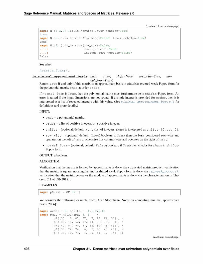
Sage Reference Manual: Matrices and Spaces of Matrices, Release 9.0
(continued from previous page)
sage: N[[1,2,0],1:].is_hermite(lower_echelon=True)Truesage: N[:2,:].is_hermite(row_wise=False, lower_echelon=True)Truesage: N[:2,:].is_hermite(row_wise=False,....: lower_echelon=True,....: include_zero_vectors=False)False
See also:
hermite_form() .
is_minimal_approximant_basis(pmat, order, shifts=None, row_wise=True, nor-mal_form=False)
Return True if and only if this matrix is an approximant basis in shifts-ordered weak Popov form forthe polynomial matrix pmat at order order.
If normal_form is True, then the polynomial matrix must furthermore be in shifts-Popov form. Anerror is raised if the input dimensions are not sound. If a single integer is provided for order, then it isinterpreted as a list of repeated integers with this value. (See minimal_approximant_basis() fordefinitions and more details.)
INPUT:
• pmat – a polynomial matrix.
• order – a list of positive integers, or a positive integer.
• shifts – (optional, default: None) list of integers; None is interpreted as shifts=[0,...,0].
• row_wise – (optional, default: True) boolean, if True then the basis considered row-wise andoperates on the left of pmat; otherwise it is column-wise and operates on the right of pmat.
• normal_form – (optional, default: False) boolean, if True then checks for a basis in shifts-Popov form.
OUTPUT: a boolean.
ALGORITHM:
Verification that the matrix is formed by approximants is done via a truncated matrix product; verificationthat the matrix is square, nonsingular and in shifted weak Popov form is done via is_weak_popov();verification that the matrix generates the module of approximants is done via the characterization in The-orem 2.1 of [GN2018] .
EXAMPLES:
sage: pR.<x> = GF(97)[]
We consider the following example from [Arne Storjohann, Notes on computing minimal approximantbases, 2006]:
sage: order = 8; shifts = [1,1,0,0,0]sage: pmat = Matrix(pR, 5, 1, [ \
pR([35, 0, 41, 87, 3, 42, 22, 90]), \pR([80, 15, 62, 87, 14, 93, 24, 0]), \pR([42, 57, 90, 87, 22, 80, 71, 53]), \pR([37, 72, 74, 6, 5, 75, 23, 47]), \pR([36, 10, 74, 1, 29, 44, 87, 74]) ])
(continues on next page)
498 Chapter 31. Dense matrices over univariate polynomials over fields
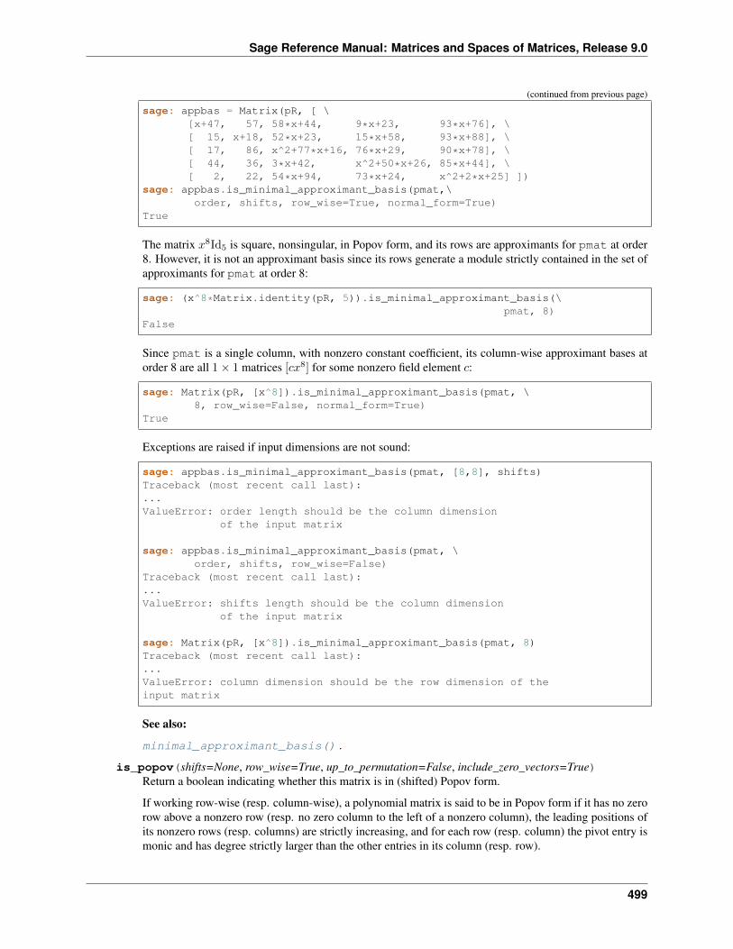
Sage Reference Manual: Matrices and Spaces of Matrices, Release 9.0
(continued from previous page)
sage: appbas = Matrix(pR, [ \[x+47, 57, 58*x+44, 9*x+23, 93*x+76], \[ 15, x+18, 52*x+23, 15*x+58, 93*x+88], \[ 17, 86, x^2+77*x+16, 76*x+29, 90*x+78], \[ 44, 36, 3*x+42, x^2+50*x+26, 85*x+44], \[ 2, 22, 54*x+94, 73*x+24, x^2+2*x+25] ])
sage: appbas.is_minimal_approximant_basis(pmat,\order, shifts, row_wise=True, normal_form=True)
True
The matrix 𝑥8Id5 is square, nonsingular, in Popov form, and its rows are approximants for pmat at order8. However, it is not an approximant basis since its rows generate a module strictly contained in the set ofapproximants for pmat at order 8:
sage: (x^8*Matrix.identity(pR, 5)).is_minimal_approximant_basis(\pmat, 8)
False
Since pmat is a single column, with nonzero constant coefficient, its column-wise approximant bases atorder 8 are all 1× 1 matrices [𝑐𝑥8] for some nonzero field element 𝑐:
sage: Matrix(pR, [x^8]).is_minimal_approximant_basis(pmat, \8, row_wise=False, normal_form=True)
True
Exceptions are raised if input dimensions are not sound:
sage: appbas.is_minimal_approximant_basis(pmat, [8,8], shifts)Traceback (most recent call last):...ValueError: order length should be the column dimension
of the input matrix
sage: appbas.is_minimal_approximant_basis(pmat, \order, shifts, row_wise=False)
Traceback (most recent call last):...ValueError: shifts length should be the column dimension
of the input matrix
sage: Matrix(pR, [x^8]).is_minimal_approximant_basis(pmat, 8)Traceback (most recent call last):...ValueError: column dimension should be the row dimension of theinput matrix
See also:
minimal_approximant_basis() .
is_popov(shifts=None, row_wise=True, up_to_permutation=False, include_zero_vectors=True)Return a boolean indicating whether this matrix is in (shifted) Popov form.
If working row-wise (resp. column-wise), a polynomial matrix is said to be in Popov form if it has no zerorow above a nonzero row (resp. no zero column to the left of a nonzero column), the leading positions ofits nonzero rows (resp. columns) are strictly increasing, and for each row (resp. column) the pivot entry ismonic and has degree strictly larger than the other entries in its column (resp. row).
499
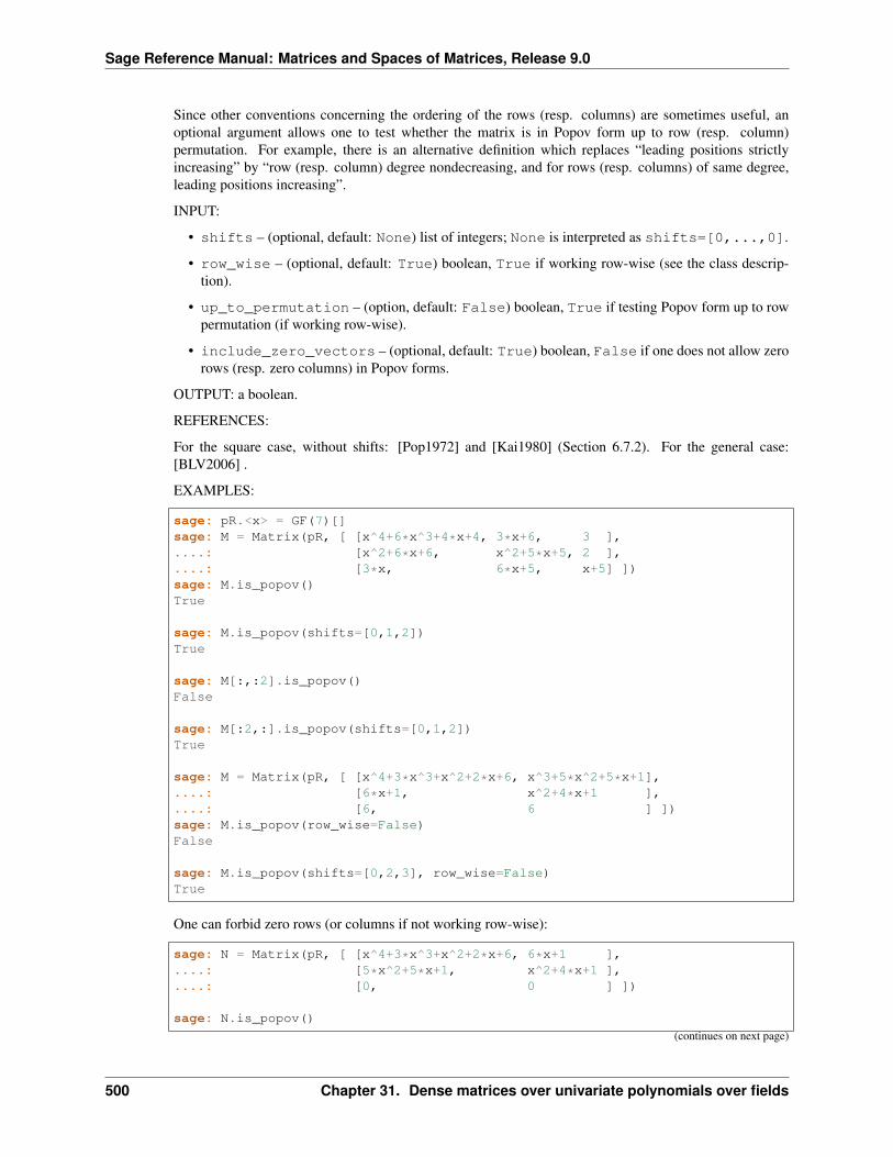
Sage Reference Manual: Matrices and Spaces of Matrices, Release 9.0
Since other conventions concerning the ordering of the rows (resp. columns) are sometimes useful, anoptional argument allows one to test whether the matrix is in Popov form up to row (resp. column)permutation. For example, there is an alternative definition which replaces “leading positions strictlyincreasing” by “row (resp. column) degree nondecreasing, and for rows (resp. columns) of same degree,leading positions increasing”.
INPUT:
• shifts – (optional, default: None) list of integers; None is interpreted as shifts=[0,...,0].
• row_wise – (optional, default: True) boolean, True if working row-wise (see the class descrip-tion).
• up_to_permutation – (option, default: False) boolean, True if testing Popov form up to rowpermutation (if working row-wise).
• include_zero_vectors – (optional, default: True) boolean, False if one does not allow zerorows (resp. zero columns) in Popov forms.
OUTPUT: a boolean.
REFERENCES:
For the square case, without shifts: [Pop1972] and [Kai1980] (Section 6.7.2). For the general case:[BLV2006] .
EXAMPLES:
sage: pR.<x> = GF(7)[]sage: M = Matrix(pR, [ [x^4+6*x^3+4*x+4, 3*x+6, 3 ],....: [x^2+6*x+6, x^2+5*x+5, 2 ],....: [3*x, 6*x+5, x+5] ])sage: M.is_popov()True
sage: M.is_popov(shifts=[0,1,2])True
sage: M[:,:2].is_popov()False
sage: M[:2,:].is_popov(shifts=[0,1,2])True
sage: M = Matrix(pR, [ [x^4+3*x^3+x^2+2*x+6, x^3+5*x^2+5*x+1],....: [6*x+1, x^2+4*x+1 ],....: [6, 6 ] ])sage: M.is_popov(row_wise=False)False
sage: M.is_popov(shifts=[0,2,3], row_wise=False)True
One can forbid zero rows (or columns if not working row-wise):
sage: N = Matrix(pR, [ [x^4+3*x^3+x^2+2*x+6, 6*x+1 ],....: [5*x^2+5*x+1, x^2+4*x+1 ],....: [0, 0 ] ])
sage: N.is_popov()
(continues on next page)
500 Chapter 31. Dense matrices over univariate polynomials over fields
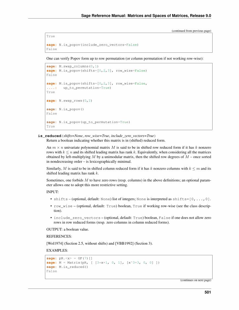
Sage Reference Manual: Matrices and Spaces of Matrices, Release 9.0
(continued from previous page)
True
sage: N.is_popov(include_zero_vectors=False)False
One can verify Popov form up to row permutation (or column permutation if not working row-wise):
sage: M.swap_columns(0,1)sage: M.is_popov(shifts=[0,2,3], row_wise=False)False
sage: M.is_popov(shifts=[0,2,3], row_wise=False,....: up_to_permutation=True)True
sage: N.swap_rows(0,2)
sage: N.is_popov()False
sage: N.is_popov(up_to_permutation=True)True
is_reduced(shifts=None, row_wise=True, include_zero_vectors=True)Return a boolean indicating whether this matrix is in (shifted) reduced form.
An 𝑚 × 𝑛 univariate polynomial matrix 𝑀 is said to be in shifted row reduced form if it has 𝑘 nonzerorows with 𝑘 ≤ 𝑛 and its shifted leading matrix has rank 𝑘. Equivalently, when considering all the matricesobtained by left-multiplying 𝑀 by a unimodular matrix, then the shifted row degrees of 𝑀 – once sortedin nondecreasing order – is lexicographically minimal.
Similarly, 𝑀 is said to be in shifted column reduced form if it has 𝑘 nonzero columns with 𝑘 ≤ 𝑚 and itsshifted leading matrix has rank 𝑘.
Sometimes, one forbids 𝑀 to have zero rows (resp. columns) in the above definitions; an optional param-eter allows one to adopt this more restrictive setting.
INPUT:
• shifts – (optional, default: None) list of integers; None is interpreted as shifts=[0,...,0].
• row_wise – (optional, default: True) boolean, True if working row-wise (see the class descrip-tion).
• include_zero_vectors – (optional, default: True) boolean, False if one does not allow zerorows in row reduced forms (resp. zero columns in column reduced forms).
OUTPUT: a boolean value.
REFERENCES:
[Wol1974] (Section 2.5, without shifts) and [VBB1992] (Section 3).
EXAMPLES:
sage: pR.<x> = GF(7)[]sage: M = Matrix(pR, [ [3*x+1, 0, 1], [x^3+3, 0, 0] ])sage: M.is_reduced()False
(continues on next page)
501
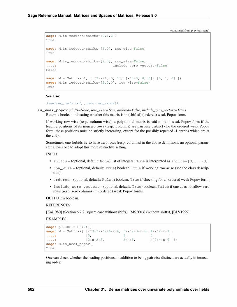
Sage Reference Manual: Matrices and Spaces of Matrices, Release 9.0
(continued from previous page)
sage: M.is_reduced(shifts=[0,1,2])True
sage: M.is_reduced(shifts=[2,0], row_wise=False)True
sage: M.is_reduced(shifts=[2,0], row_wise=False,....: include_zero_vectors=False)False
sage: M = Matrix(pR, [ [3*x+1, 0, 1], [x^3+3, 0, 0], [0, 1, 0] ])sage: M.is_reduced(shifts=[2,0,0], row_wise=False)True
See also:
leading_matrix() , reduced_form() .
is_weak_popov(shifts=None, row_wise=True, ordered=False, include_zero_vectors=True)Return a boolean indicating whether this matrix is in (shifted) (ordered) weak Popov form.
If working row-wise (resp. column-wise), a polynomial matrix is said to be in weak Popov form if theleading positions of its nonzero rows (resp. columns) are pairwise distinct (for the ordered weak Popovform, these positions must be strictly increasing, except for the possibly repeated -1 entries which are atthe end).
Sometimes, one forbids 𝑀 to have zero rows (resp. columns) in the above definitions; an optional param-eter allows one to adopt this more restrictive setting.
INPUT:
• shifts – (optional, default: None) list of integers; None is interpreted as shifts=[0,...,0].
• row_wise – (optional, default: True) boolean, True if working row-wise (see the class descrip-tion).
• ordered – (optional, default: False) boolean, True if checking for an ordered weak Popov form.
• include_zero_vectors – (optional, default: True) boolean, False if one does not allow zerorows (resp. zero columns) in (ordered) weak Popov forms.
OUTPUT: a boolean.
REFERENCES:
[Kai1980] (Section 6.7.2, square case without shifts), [MS2003] (without shifts), [BLV1999] .
EXAMPLES:
sage: pR.<x> = GF(7)[]sage: M = Matrix([ [x^3+3*x^2+6*x+6, 3*x^2+3*x+6, 4*x^2+x+3],....: [5, 1, 0 ],....: [2*x^2+2, 2*x+5, x^2+4*x+6] ])sage: M.is_weak_popov()True
One can check whether the leading positions, in addition to being pairwise distinct, are actually in increas-ing order:
502 Chapter 31. Dense matrices over univariate polynomials over fields
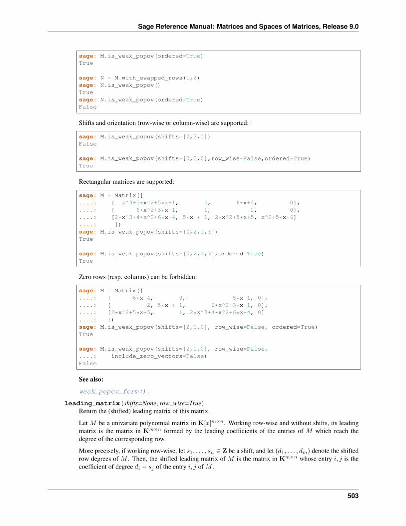
Sage Reference Manual: Matrices and Spaces of Matrices, Release 9.0
sage: M.is_weak_popov(ordered=True)True
sage: N = M.with_swapped_rows(1,2)sage: N.is_weak_popov()Truesage: N.is_weak_popov(ordered=True)False
Shifts and orientation (row-wise or column-wise) are supported:
sage: M.is_weak_popov(shifts=[2,3,1])False
sage: M.is_weak_popov(shifts=[0,2,0],row_wise=False,ordered=True)True
Rectangular matrices are supported:
sage: M = Matrix([....: [ x^3+5*x^2+5*x+1, 5, 6*x+4, 0],....: [ 6*x^2+3*x+1, 1, 2, 0],....: [2*x^3+4*x^2+6*x+4, 5*x + 1, 2*x^2+5*x+5, x^2+5*x+6]....: ])sage: M.is_weak_popov(shifts=[0,2,1,3])True
sage: M.is_weak_popov(shifts=[0,2,1,3],ordered=True)True
Zero rows (resp. columns) can be forbidden:
sage: M = Matrix([....: [ 6*x+4, 0, 5*x+1, 0],....: [ 2, 5*x + 1, 6*x^2+3*x+1, 0],....: [2*x^2+5*x+5, 1, 2*x^3+4*x^2+6*x+4, 0]....: ])sage: M.is_weak_popov(shifts=[2,1,0], row_wise=False, ordered=True)True
sage: M.is_weak_popov(shifts=[2,1,0], row_wise=False,....: include_zero_vectors=False)False
See also:
weak_popov_form() .
leading_matrix(shifts=None, row_wise=True)Return the (shifted) leading matrix of this matrix.
Let 𝑀 be a univariate polynomial matrix in K[𝑥]𝑚×𝑛. Working row-wise and without shifts, its leadingmatrix is the matrix in K𝑚×𝑛 formed by the leading coefficients of the entries of 𝑀 which reach thedegree of the corresponding row.
More precisely, if working row-wise, let 𝑠1, . . . , 𝑠𝑛 ∈ Z be a shift, and let (𝑑1, . . . , 𝑑𝑚) denote the shiftedrow degrees of 𝑀 . Then, the shifted leading matrix of 𝑀 is the matrix in K𝑚×𝑛 whose entry 𝑖, 𝑗 is thecoefficient of degree 𝑑𝑖 − 𝑠𝑗 of the entry 𝑖, 𝑗 of 𝑀 .
503
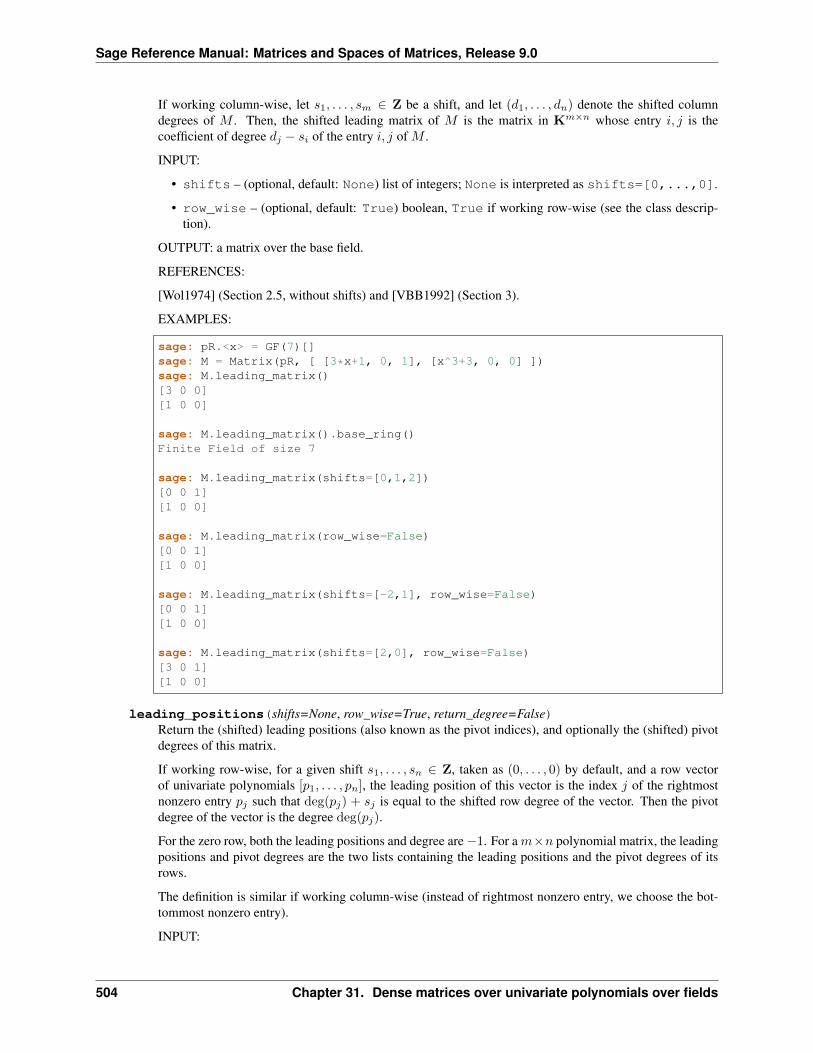
Sage Reference Manual: Matrices and Spaces of Matrices, Release 9.0
If working column-wise, let 𝑠1, . . . , 𝑠𝑚 ∈ Z be a shift, and let (𝑑1, . . . , 𝑑𝑛) denote the shifted columndegrees of 𝑀 . Then, the shifted leading matrix of 𝑀 is the matrix in K𝑚×𝑛 whose entry 𝑖, 𝑗 is thecoefficient of degree 𝑑𝑗 − 𝑠𝑖 of the entry 𝑖, 𝑗 of 𝑀 .
INPUT:
• shifts – (optional, default: None) list of integers; None is interpreted as shifts=[0,...,0].
• row_wise – (optional, default: True) boolean, True if working row-wise (see the class descrip-tion).
OUTPUT: a matrix over the base field.
REFERENCES:
[Wol1974] (Section 2.5, without shifts) and [VBB1992] (Section 3).
EXAMPLES:
sage: pR.<x> = GF(7)[]sage: M = Matrix(pR, [ [3*x+1, 0, 1], [x^3+3, 0, 0] ])sage: M.leading_matrix()[3 0 0][1 0 0]
sage: M.leading_matrix().base_ring()Finite Field of size 7
sage: M.leading_matrix(shifts=[0,1,2])[0 0 1][1 0 0]
sage: M.leading_matrix(row_wise=False)[0 0 1][1 0 0]
sage: M.leading_matrix(shifts=[-2,1], row_wise=False)[0 0 1][1 0 0]
sage: M.leading_matrix(shifts=[2,0], row_wise=False)[3 0 1][1 0 0]
leading_positions(shifts=None, row_wise=True, return_degree=False)Return the (shifted) leading positions (also known as the pivot indices), and optionally the (shifted) pivotdegrees of this matrix.
If working row-wise, for a given shift 𝑠1, . . . , 𝑠𝑛 ∈ Z, taken as (0, . . . , 0) by default, and a row vectorof univariate polynomials [𝑝1, . . . , 𝑝𝑛], the leading position of this vector is the index 𝑗 of the rightmostnonzero entry 𝑝𝑗 such that deg(𝑝𝑗) + 𝑠𝑗 is equal to the shifted row degree of the vector. Then the pivotdegree of the vector is the degree deg(𝑝𝑗).
For the zero row, both the leading positions and degree are −1. For a 𝑚×𝑛 polynomial matrix, the leadingpositions and pivot degrees are the two lists containing the leading positions and the pivot degrees of itsrows.
The definition is similar if working column-wise (instead of rightmost nonzero entry, we choose the bot-tommost nonzero entry).
INPUT:
504 Chapter 31. Dense matrices over univariate polynomials over fields
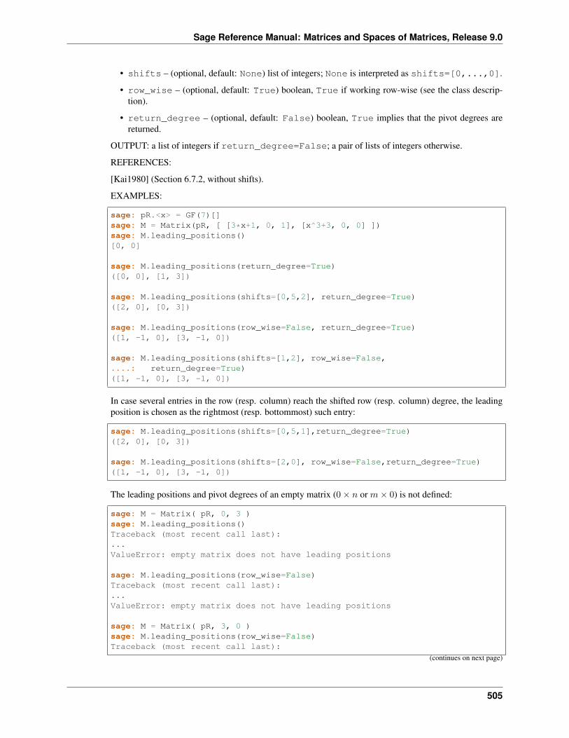
Sage Reference Manual: Matrices and Spaces of Matrices, Release 9.0
• shifts – (optional, default: None) list of integers; None is interpreted as shifts=[0,...,0].
• row_wise – (optional, default: True) boolean, True if working row-wise (see the class descrip-tion).
• return_degree – (optional, default: False) boolean, True implies that the pivot degrees arereturned.
OUTPUT: a list of integers if return_degree=False; a pair of lists of integers otherwise.
REFERENCES:
[Kai1980] (Section 6.7.2, without shifts).
EXAMPLES:
sage: pR.<x> = GF(7)[]sage: M = Matrix(pR, [ [3*x+1, 0, 1], [x^3+3, 0, 0] ])sage: M.leading_positions()[0, 0]
sage: M.leading_positions(return_degree=True)([0, 0], [1, 3])
sage: M.leading_positions(shifts=[0,5,2], return_degree=True)([2, 0], [0, 3])
sage: M.leading_positions(row_wise=False, return_degree=True)([1, -1, 0], [3, -1, 0])
sage: M.leading_positions(shifts=[1,2], row_wise=False,....: return_degree=True)([1, -1, 0], [3, -1, 0])
In case several entries in the row (resp. column) reach the shifted row (resp. column) degree, the leadingposition is chosen as the rightmost (resp. bottommost) such entry:
sage: M.leading_positions(shifts=[0,5,1],return_degree=True)([2, 0], [0, 3])
sage: M.leading_positions(shifts=[2,0], row_wise=False,return_degree=True)([1, -1, 0], [3, -1, 0])
The leading positions and pivot degrees of an empty matrix (0× 𝑛 or 𝑚× 0) is not defined:
sage: M = Matrix( pR, 0, 3 )sage: M.leading_positions()Traceback (most recent call last):...ValueError: empty matrix does not have leading positions
sage: M.leading_positions(row_wise=False)Traceback (most recent call last):...ValueError: empty matrix does not have leading positions
sage: M = Matrix( pR, 3, 0 )sage: M.leading_positions(row_wise=False)Traceback (most recent call last):
(continues on next page)
505
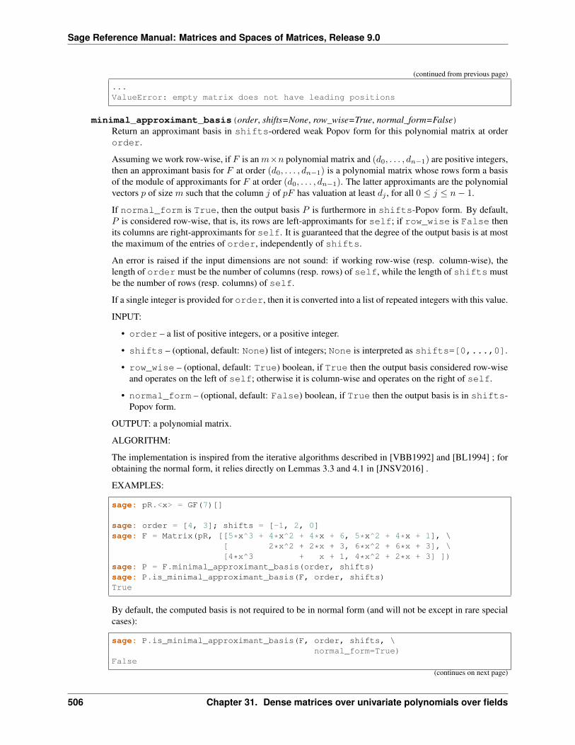
Sage Reference Manual: Matrices and Spaces of Matrices, Release 9.0
(continued from previous page)
...ValueError: empty matrix does not have leading positions
minimal_approximant_basis(order, shifts=None, row_wise=True, normal_form=False)Return an approximant basis in shifts-ordered weak Popov form for this polynomial matrix at orderorder.
Assuming we work row-wise, if 𝐹 is an 𝑚×𝑛 polynomial matrix and (𝑑0, . . . , 𝑑𝑛−1) are positive integers,then an approximant basis for 𝐹 at order (𝑑0, . . . , 𝑑𝑛−1) is a polynomial matrix whose rows form a basisof the module of approximants for 𝐹 at order (𝑑0, . . . , 𝑑𝑛−1). The latter approximants are the polynomialvectors 𝑝 of size 𝑚 such that the column 𝑗 of 𝑝𝐹 has valuation at least 𝑑𝑗 , for all 0 ≤ 𝑗 ≤ 𝑛− 1.
If normal_form is True, then the output basis 𝑃 is furthermore in shifts-Popov form. By default,𝑃 is considered row-wise, that is, its rows are left-approximants for self; if row_wise is False thenits columns are right-approximants for self. It is guaranteed that the degree of the output basis is at mostthe maximum of the entries of order, independently of shifts.
An error is raised if the input dimensions are not sound: if working row-wise (resp. column-wise), thelength of order must be the number of columns (resp. rows) of self, while the length of shifts mustbe the number of rows (resp. columns) of self.
If a single integer is provided for order, then it is converted into a list of repeated integers with this value.
INPUT:
• order – a list of positive integers, or a positive integer.
• shifts – (optional, default: None) list of integers; None is interpreted as shifts=[0,...,0].
• row_wise – (optional, default: True) boolean, if True then the output basis considered row-wiseand operates on the left of self; otherwise it is column-wise and operates on the right of self.
• normal_form – (optional, default: False) boolean, if True then the output basis is in shifts-Popov form.
OUTPUT: a polynomial matrix.
ALGORITHM:
The implementation is inspired from the iterative algorithms described in [VBB1992] and [BL1994] ; forobtaining the normal form, it relies directly on Lemmas 3.3 and 4.1 in [JNSV2016] .
EXAMPLES:
sage: pR.<x> = GF(7)[]
sage: order = [4, 3]; shifts = [-1, 2, 0]sage: F = Matrix(pR, [[5*x^3 + 4*x^2 + 4*x + 6, 5*x^2 + 4*x + 1], \
[ 2*x^2 + 2*x + 3, 6*x^2 + 6*x + 3], \[4*x^3 + x + 1, 4*x^2 + 2*x + 3] ])
sage: P = F.minimal_approximant_basis(order, shifts)sage: P.is_minimal_approximant_basis(F, order, shifts)True
By default, the computed basis is not required to be in normal form (and will not be except in rare specialcases):
sage: P.is_minimal_approximant_basis(F, order, shifts, \normal_form=True)
False
(continues on next page)
506 Chapter 31. Dense matrices over univariate polynomials over fields
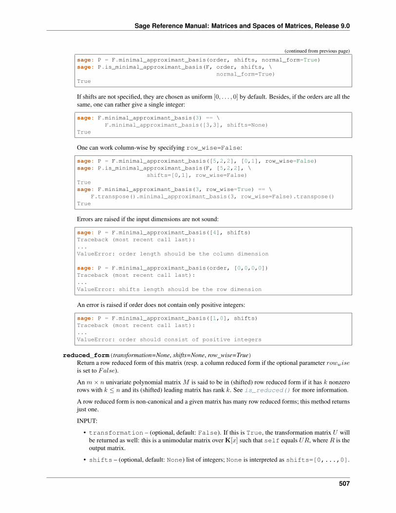
Sage Reference Manual: Matrices and Spaces of Matrices, Release 9.0
(continued from previous page)
sage: P = F.minimal_approximant_basis(order, shifts, normal_form=True)sage: P.is_minimal_approximant_basis(F, order, shifts, \
normal_form=True)True
If shifts are not specified, they are chosen as uniform [0, . . . , 0] by default. Besides, if the orders are all thesame, one can rather give a single integer:
sage: F.minimal_approximant_basis(3) == \F.minimal_approximant_basis([3,3], shifts=None)
True
One can work column-wise by specifying row_wise=False:
sage: P = F.minimal_approximant_basis([5,2,2], [0,1], row_wise=False)sage: P.is_minimal_approximant_basis(F, [5,2,2], \
shifts=[0,1], row_wise=False)Truesage: F.minimal_approximant_basis(3, row_wise=True) == \
F.transpose().minimal_approximant_basis(3, row_wise=False).transpose()True
Errors are raised if the input dimensions are not sound:
sage: P = F.minimal_approximant_basis([4], shifts)Traceback (most recent call last):...ValueError: order length should be the column dimension
sage: P = F.minimal_approximant_basis(order, [0,0,0,0])Traceback (most recent call last):...ValueError: shifts length should be the row dimension
An error is raised if order does not contain only positive integers:
sage: P = F.minimal_approximant_basis([1,0], shifts)Traceback (most recent call last):...ValueError: order should consist of positive integers
reduced_form(transformation=None, shifts=None, row_wise=True)Return a row reduced form of this matrix (resp. a column reduced form if the optional parameter 𝑟𝑜𝑤𝑤𝑖𝑠𝑒is set to 𝐹𝑎𝑙𝑠𝑒).
An 𝑚 × 𝑛 univariate polynomial matrix 𝑀 is said to be in (shifted) row reduced form if it has 𝑘 nonzerorows with 𝑘 ≤ 𝑛 and its (shifted) leading matrix has rank 𝑘. See is_reduced() for more information.
A row reduced form is non-canonical and a given matrix has many row reduced forms; this method returnsjust one.
INPUT:
• transformation – (optional, default: False). If this is True, the transformation matrix 𝑈 willbe returned as well: this is a unimodular matrix over K[𝑥] such that self equals 𝑈𝑅, where 𝑅 is theoutput matrix.
• shifts – (optional, default: None) list of integers; None is interpreted as shifts=[0,...,0].
507
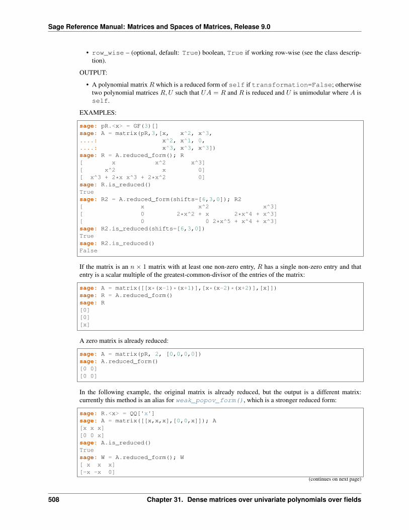
Sage Reference Manual: Matrices and Spaces of Matrices, Release 9.0
• row_wise – (optional, default: True) boolean, True if working row-wise (see the class descrip-tion).
OUTPUT:
• A polynomial matrix 𝑅 which is a reduced form of self if transformation=False; otherwisetwo polynomial matrices 𝑅,𝑈 such that 𝑈𝐴 = 𝑅 and 𝑅 is reduced and 𝑈 is unimodular where 𝐴 isself.
EXAMPLES:
sage: pR.<x> = GF(3)[]sage: A = matrix(pR,3,[x, x^2, x^3,....: x^2, x^1, 0,....: x^3, x^3, x^3])sage: R = A.reduced_form(); R[ x x^2 x^3][ x^2 x 0][ x^3 + 2*x x^3 + 2*x^2 0]sage: R.is_reduced()Truesage: R2 = A.reduced_form(shifts=[6,3,0]); R2[ x x^2 x^3][ 0 2*x^2 + x 2*x^4 + x^3][ 0 0 2*x^5 + x^4 + x^3]sage: R2.is_reduced(shifts=[6,3,0])Truesage: R2.is_reduced()False
If the matrix is an 𝑛 × 1 matrix with at least one non-zero entry, 𝑅 has a single non-zero entry and thatentry is a scalar multiple of the greatest-common-divisor of the entries of the matrix:
sage: A = matrix([[x*(x-1)*(x+1)],[x*(x-2)*(x+2)],[x]])sage: R = A.reduced_form()sage: R[0][0][x]
A zero matrix is already reduced:
sage: A = matrix(pR, 2, [0,0,0,0])sage: A.reduced_form()[0 0][0 0]
In the following example, the original matrix is already reduced, but the output is a different matrix:currently this method is an alias for weak_popov_form(), which is a stronger reduced form:
sage: R.<x> = QQ['x']sage: A = matrix([[x,x,x],[0,0,x]]); A[x x x][0 0 x]sage: A.is_reduced()Truesage: W = A.reduced_form(); W[ x x x][-x -x 0]
(continues on next page)
508 Chapter 31. Dense matrices over univariate polynomials over fields
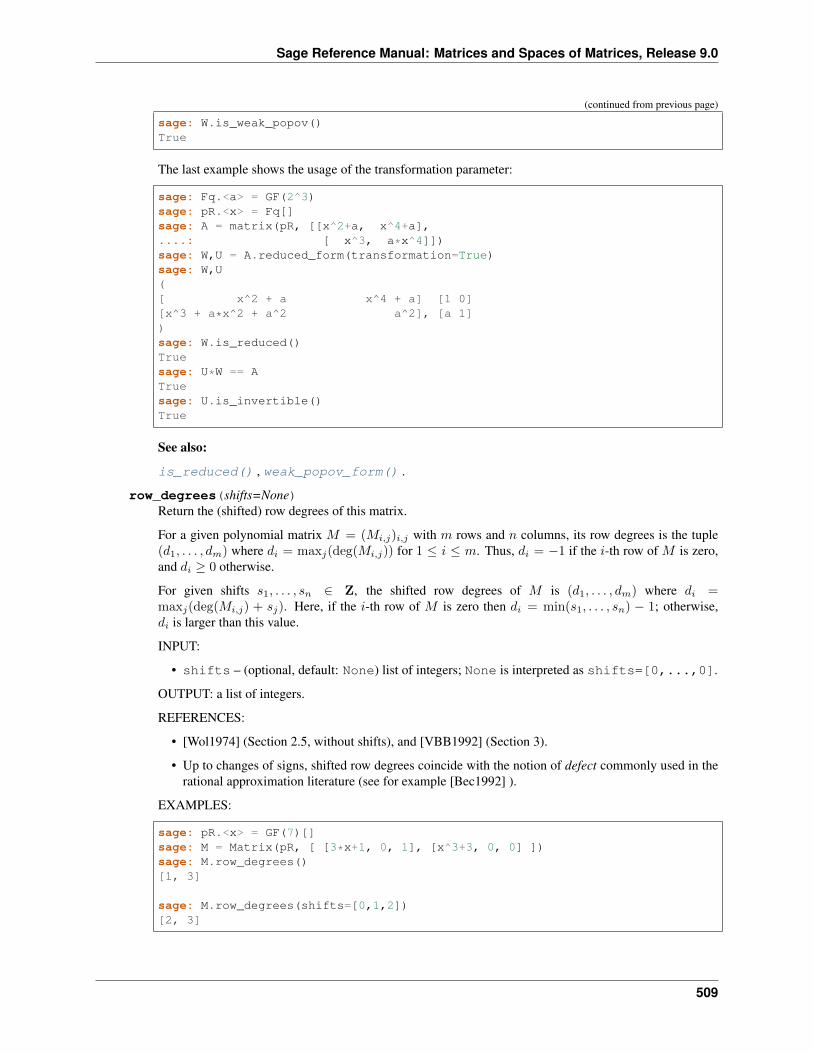
Sage Reference Manual: Matrices and Spaces of Matrices, Release 9.0
(continued from previous page)
sage: W.is_weak_popov()True
The last example shows the usage of the transformation parameter:
sage: Fq.<a> = GF(2^3)sage: pR.<x> = Fq[]sage: A = matrix(pR, [[x^2+a, x^4+a],....: [ x^3, a*x^4]])sage: W,U = A.reduced_form(transformation=True)sage: W,U([ x^2 + a x^4 + a] [1 0][x^3 + a*x^2 + a^2 a^2], [a 1])sage: W.is_reduced()Truesage: U*W == ATruesage: U.is_invertible()True
See also:
is_reduced() , weak_popov_form() .
row_degrees(shifts=None)Return the (shifted) row degrees of this matrix.
For a given polynomial matrix 𝑀 = (𝑀𝑖,𝑗)𝑖,𝑗 with 𝑚 rows and 𝑛 columns, its row degrees is the tuple(𝑑1, . . . , 𝑑𝑚) where 𝑑𝑖 = max𝑗(deg(𝑀𝑖,𝑗)) for 1 ≤ 𝑖 ≤ 𝑚. Thus, 𝑑𝑖 = −1 if the 𝑖-th row of 𝑀 is zero,and 𝑑𝑖 ≥ 0 otherwise.
For given shifts 𝑠1, . . . , 𝑠𝑛 ∈ Z, the shifted row degrees of 𝑀 is (𝑑1, . . . , 𝑑𝑚) where 𝑑𝑖 =max𝑗(deg(𝑀𝑖,𝑗) + 𝑠𝑗). Here, if the 𝑖-th row of 𝑀 is zero then 𝑑𝑖 = min(𝑠1, . . . , 𝑠𝑛) − 1; otherwise,𝑑𝑖 is larger than this value.
INPUT:
• shifts – (optional, default: None) list of integers; None is interpreted as shifts=[0,...,0].
OUTPUT: a list of integers.
REFERENCES:
• [Wol1974] (Section 2.5, without shifts), and [VBB1992] (Section 3).
• Up to changes of signs, shifted row degrees coincide with the notion of defect commonly used in therational approximation literature (see for example [Bec1992] ).
EXAMPLES:
sage: pR.<x> = GF(7)[]sage: M = Matrix(pR, [ [3*x+1, 0, 1], [x^3+3, 0, 0] ])sage: M.row_degrees()[1, 3]
sage: M.row_degrees(shifts=[0,1,2])[2, 3]
509
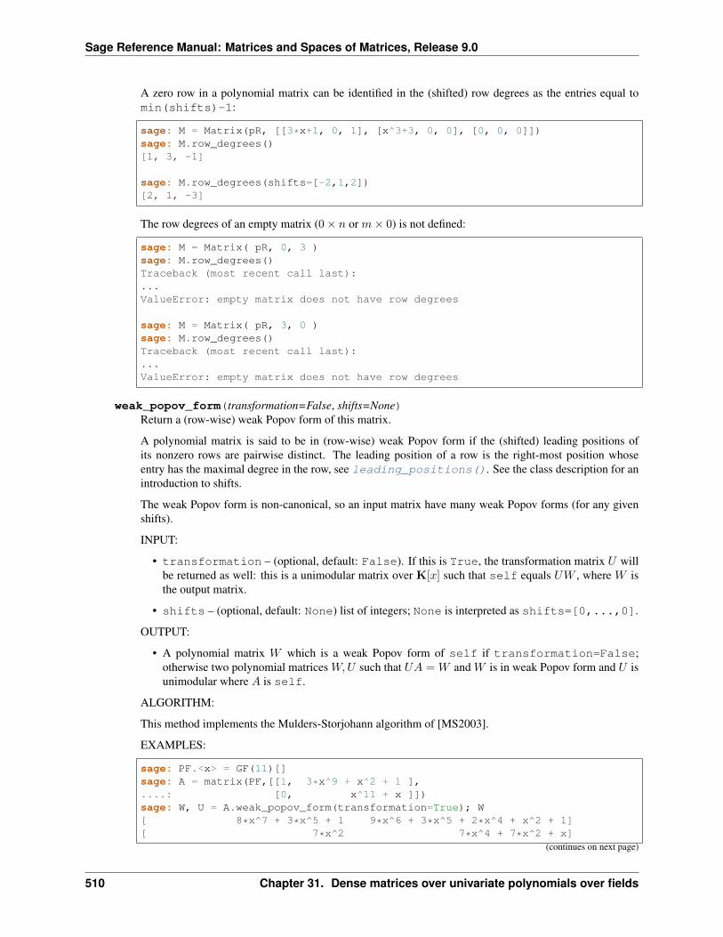
Sage Reference Manual: Matrices and Spaces of Matrices, Release 9.0
A zero row in a polynomial matrix can be identified in the (shifted) row degrees as the entries equal tomin(shifts)-1:
sage: M = Matrix(pR, [[3*x+1, 0, 1], [x^3+3, 0, 0], [0, 0, 0]])sage: M.row_degrees()[1, 3, -1]
sage: M.row_degrees(shifts=[-2,1,2])[2, 1, -3]
The row degrees of an empty matrix (0× 𝑛 or 𝑚× 0) is not defined:
sage: M = Matrix( pR, 0, 3 )sage: M.row_degrees()Traceback (most recent call last):...ValueError: empty matrix does not have row degrees
sage: M = Matrix( pR, 3, 0 )sage: M.row_degrees()Traceback (most recent call last):...ValueError: empty matrix does not have row degrees
weak_popov_form(transformation=False, shifts=None)Return a (row-wise) weak Popov form of this matrix.
A polynomial matrix is said to be in (row-wise) weak Popov form if the (shifted) leading positions ofits nonzero rows are pairwise distinct. The leading position of a row is the right-most position whoseentry has the maximal degree in the row, see leading_positions(). See the class description for anintroduction to shifts.
The weak Popov form is non-canonical, so an input matrix have many weak Popov forms (for any givenshifts).
INPUT:
• transformation – (optional, default: False). If this is True, the transformation matrix 𝑈 willbe returned as well: this is a unimodular matrix over K[𝑥] such that self equals 𝑈𝑊 , where 𝑊 isthe output matrix.
• shifts – (optional, default: None) list of integers; None is interpreted as shifts=[0,...,0].
OUTPUT:
• A polynomial matrix 𝑊 which is a weak Popov form of self if transformation=False;otherwise two polynomial matrices 𝑊,𝑈 such that 𝑈𝐴 = 𝑊 and 𝑊 is in weak Popov form and 𝑈 isunimodular where 𝐴 is self.
ALGORITHM:
This method implements the Mulders-Storjohann algorithm of [MS2003].
EXAMPLES:
sage: PF.<x> = GF(11)[]sage: A = matrix(PF,[[1, 3*x^9 + x^2 + 1 ],....: [0, x^11 + x ]])sage: W, U = A.weak_popov_form(transformation=True); W[ 8*x^7 + 3*x^5 + 1 9*x^6 + 3*x^5 + 2*x^4 + x^2 + 1][ 7*x^2 7*x^4 + 7*x^2 + x]
(continues on next page)
510 Chapter 31. Dense matrices over univariate polynomials over fields
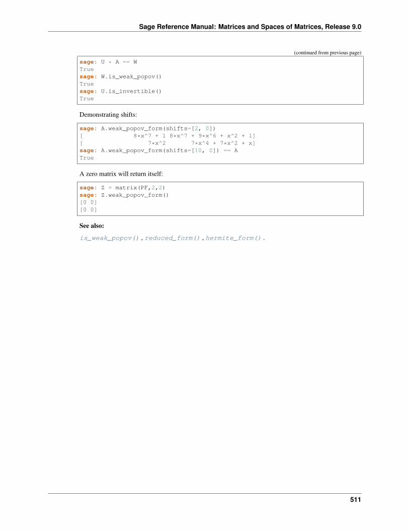
Sage Reference Manual: Matrices and Spaces of Matrices, Release 9.0
(continued from previous page)
sage: U * A == WTruesage: W.is_weak_popov()Truesage: U.is_invertible()True
Demonstrating shifts:
sage: A.weak_popov_form(shifts=[2, 0])[ 8*x^7 + 1 8*x^7 + 9*x^6 + x^2 + 1][ 7*x^2 7*x^4 + 7*x^2 + x]sage: A.weak_popov_form(shifts=[10, 0]) == ATrue
A zero matrix will return itself:
sage: Z = matrix(PF,2,2)sage: Z.weak_popov_form()[0 0][0 0]
See also:
is_weak_popov() , reduced_form() , hermite_form() .
511

Sage Reference Manual: Matrices and Spaces of Matrices, Release 9.0
512 Chapter 31. Dense matrices over univariate polynomials over fields
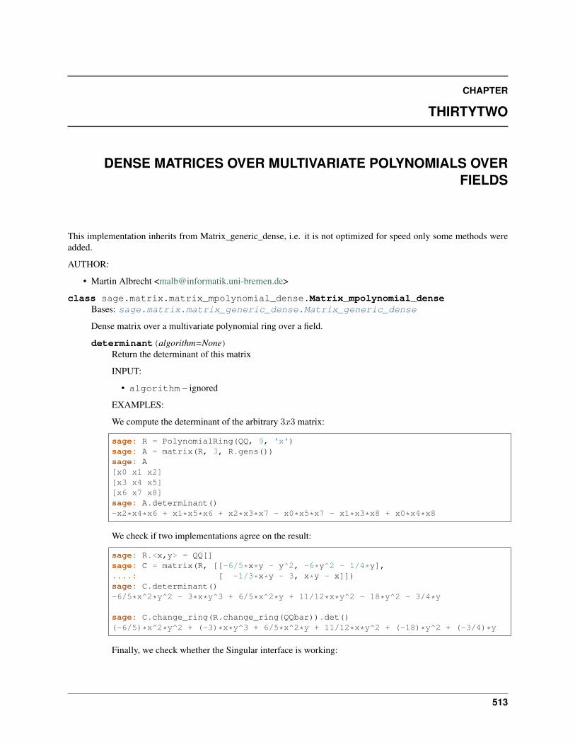
CHAPTER
THIRTYTWO
DENSE MATRICES OVER MULTIVARIATE POLYNOMIALS OVERFIELDS
This implementation inherits from Matrix_generic_dense, i.e. it is not optimized for speed only some methods wereadded.
AUTHOR:
• Martin Albrecht <[email protected]>
class sage.matrix.matrix_mpolynomial_dense.Matrix_mpolynomial_denseBases: sage.matrix.matrix_generic_dense.Matrix_generic_dense
Dense matrix over a multivariate polynomial ring over a field.
determinant(algorithm=None)Return the determinant of this matrix
INPUT:
• algorithm – ignored
EXAMPLES:
We compute the determinant of the arbitrary 3𝑥3 matrix:
sage: R = PolynomialRing(QQ, 9, 'x')sage: A = matrix(R, 3, R.gens())sage: A[x0 x1 x2][x3 x4 x5][x6 x7 x8]sage: A.determinant()-x2*x4*x6 + x1*x5*x6 + x2*x3*x7 - x0*x5*x7 - x1*x3*x8 + x0*x4*x8
We check if two implementations agree on the result:
sage: R.<x,y> = QQ[]sage: C = matrix(R, [[-6/5*x*y - y^2, -6*y^2 - 1/4*y],....: [ -1/3*x*y - 3, x*y - x]])sage: C.determinant()-6/5*x^2*y^2 - 3*x*y^3 + 6/5*x^2*y + 11/12*x*y^2 - 18*y^2 - 3/4*y
sage: C.change_ring(R.change_ring(QQbar)).det()(-6/5)*x^2*y^2 + (-3)*x*y^3 + 6/5*x^2*y + 11/12*x*y^2 + (-18)*y^2 + (-3/4)*y
Finally, we check whether the Singular interface is working:
513
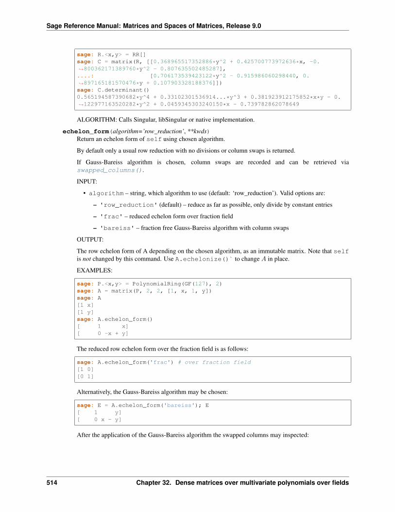
Sage Reference Manual: Matrices and Spaces of Matrices, Release 9.0
sage: R.<x,y> = RR[]sage: C = matrix(R, [[0.368965517352886*y^2 + 0.425700773972636*x, -0.→˓800362171389760*y^2 - 0.807635502485287],....: [0.706173539423122*y^2 - 0.915986060298440, 0.→˓897165181570476*y + 0.107903328188376]])sage: C.determinant()0.565194587390682*y^4 + 0.33102301536914...*y^3 + 0.381923912175852*x*y - 0.→˓122977163520282*y^2 + 0.0459345303240150*x - 0.739782862078649
ALGORITHM: Calls Singular, libSingular or native implementation.
echelon_form(algorithm=’row_reduction’, **kwds)Return an echelon form of self using chosen algorithm.
By default only a usual row reduction with no divisions or column swaps is returned.
If Gauss-Bareiss algorithm is chosen, column swaps are recorded and can be retrieved viaswapped_columns().
INPUT:
• algorithm – string, which algorithm to use (default: ‘row_reduction’). Valid options are:
– 'row_reduction' (default) – reduce as far as possible, only divide by constant entries
– 'frac' – reduced echelon form over fraction field
– 'bareiss' – fraction free Gauss-Bareiss algorithm with column swaps
OUTPUT:
The row echelon form of A depending on the chosen algorithm, as an immutable matrix. Note that selfis not changed by this command. Use A.echelonize()` to change 𝐴 in place.
EXAMPLES:
sage: P.<x,y> = PolynomialRing(GF(127), 2)sage: A = matrix(P, 2, 2, [1, x, 1, y])sage: A[1 x][1 y]sage: A.echelon_form()[ 1 x][ 0 -x + y]
The reduced row echelon form over the fraction field is as follows:
sage: A.echelon_form('frac') # over fraction field[1 0][0 1]
Alternatively, the Gauss-Bareiss algorithm may be chosen:
sage: E = A.echelon_form('bareiss'); E[ 1 y][ 0 x - y]
After the application of the Gauss-Bareiss algorithm the swapped columns may inspected:
514 Chapter 32. Dense matrices over multivariate polynomials over fields
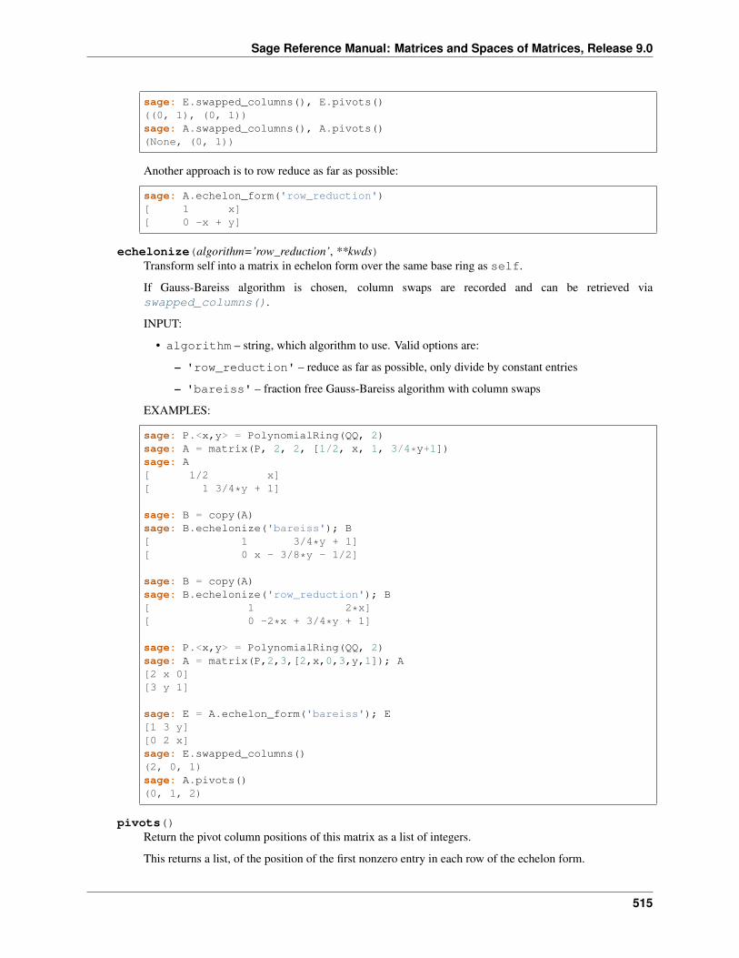
Sage Reference Manual: Matrices and Spaces of Matrices, Release 9.0
sage: E.swapped_columns(), E.pivots()((0, 1), (0, 1))sage: A.swapped_columns(), A.pivots()(None, (0, 1))
Another approach is to row reduce as far as possible:
sage: A.echelon_form('row_reduction')[ 1 x][ 0 -x + y]
echelonize(algorithm=’row_reduction’, **kwds)Transform self into a matrix in echelon form over the same base ring as self.
If Gauss-Bareiss algorithm is chosen, column swaps are recorded and can be retrieved viaswapped_columns().
INPUT:
• algorithm – string, which algorithm to use. Valid options are:
– 'row_reduction' – reduce as far as possible, only divide by constant entries
– 'bareiss' – fraction free Gauss-Bareiss algorithm with column swaps
EXAMPLES:
sage: P.<x,y> = PolynomialRing(QQ, 2)sage: A = matrix(P, 2, 2, [1/2, x, 1, 3/4*y+1])sage: A[ 1/2 x][ 1 3/4*y + 1]
sage: B = copy(A)sage: B.echelonize('bareiss'); B[ 1 3/4*y + 1][ 0 x - 3/8*y - 1/2]
sage: B = copy(A)sage: B.echelonize('row_reduction'); B[ 1 2*x][ 0 -2*x + 3/4*y + 1]
sage: P.<x,y> = PolynomialRing(QQ, 2)sage: A = matrix(P,2,3,[2,x,0,3,y,1]); A[2 x 0][3 y 1]
sage: E = A.echelon_form('bareiss'); E[1 3 y][0 2 x]sage: E.swapped_columns()(2, 0, 1)sage: A.pivots()(0, 1, 2)
pivots()Return the pivot column positions of this matrix as a list of integers.
This returns a list, of the position of the first nonzero entry in each row of the echelon form.
515
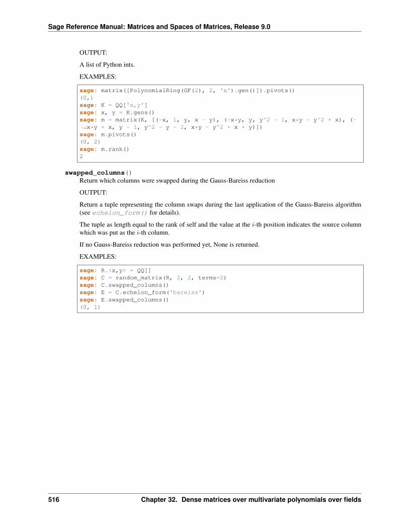
Sage Reference Manual: Matrices and Spaces of Matrices, Release 9.0
OUTPUT:
A list of Python ints.
EXAMPLES:
sage: matrix([PolynomialRing(GF(2), 2, 'x').gen()]).pivots()(0,)sage: K = QQ['x,y']sage: x, y = K.gens()sage: m = matrix(K, [(-x, 1, y, x - y), (-x*y, y, y^2 - 1, x*y - y^2 + x), (-→˓x*y + x, y - 1, y^2 - y - 2, x*y - y^2 + x + y)])sage: m.pivots()(0, 2)sage: m.rank()2
swapped_columns()Return which columns were swapped during the Gauss-Bareiss reduction
OUTPUT:
Return a tuple representing the column swaps during the last application of the Gauss-Bareiss algorithm(see echelon_form() for details).
The tuple as length equal to the rank of self and the value at the 𝑖-th position indicates the source columnwhich was put as the 𝑖-th column.
If no Gauss-Bareiss reduction was performed yet, None is returned.
EXAMPLES:
sage: R.<x,y> = QQ[]sage: C = random_matrix(R, 2, 2, terms=2)sage: C.swapped_columns()sage: E = C.echelon_form('bareiss')sage: E.swapped_columns()(0, 1)
516 Chapter 32. Dense matrices over multivariate polynomials over fields
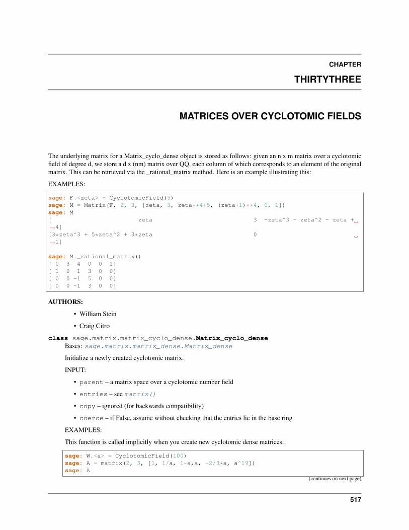
CHAPTER
THIRTYTHREE
MATRICES OVER CYCLOTOMIC FIELDS
The underlying matrix for a Matrix_cyclo_dense object is stored as follows: given an n x m matrix over a cyclotomicfield of degree d, we store a d x (nm) matrix over QQ, each column of which corresponds to an element of the originalmatrix. This can be retrieved via the _rational_matrix method. Here is an example illustrating this:
EXAMPLES:
sage: F.<zeta> = CyclotomicField(5)sage: M = Matrix(F, 2, 3, [zeta, 3, zeta**4+5, (zeta+1)**4, 0, 1])sage: M[ zeta 3 -zeta^3 - zeta^2 - zeta +→˓4][3*zeta^3 + 5*zeta^2 + 3*zeta 0→˓1]
sage: M._rational_matrix()[ 0 3 4 0 0 1][ 1 0 -1 3 0 0][ 0 0 -1 5 0 0][ 0 0 -1 3 0 0]
AUTHORS:
• William Stein
• Craig Citro
class sage.matrix.matrix_cyclo_dense.Matrix_cyclo_denseBases: sage.matrix.matrix_dense.Matrix_dense
Initialize a newly created cyclotomic matrix.
INPUT:
• parent – a matrix space over a cyclotomic number field
• entries – see matrix()
• copy – ignored (for backwards compatibility)
• coerce – if False, assume without checking that the entries lie in the base ring
EXAMPLES:
This function is called implicitly when you create new cyclotomic dense matrices:
sage: W.<a> = CyclotomicField(100)sage: A = matrix(2, 3, [1, 1/a, 1-a,a, -2/3*a, a^19])sage: A
(continues on next page)
517

Sage Reference Manual: Matrices and Spaces of Matrices, Release 9.0
(continued from previous page)
[ 1 -a^39 + a^29 - a^19 + a^9 -a + 1][ a -2/3*a a^19]sage: TestSuite(A).run()
charpoly(var=’x’, algorithm=’multimodular’, proof=None)Return the characteristic polynomial of self, as a polynomial over the base ring.
INPUT:
• algorithm
– ‘multimodular’ (default): reduce modulo primes, compute charpoly mod p, and lift (very fast)
– ‘pari’: use pari (quite slow; comparable to Magma v2.14 though)
– ‘hessenberg’: put matrix in Hessenberg form (double dog slow)
• proof – bool (default: None) proof flag determined by global linalg proof.
OUTPUT:
polynomial
EXAMPLES:
sage: K.<z> = CyclotomicField(5)sage: a = matrix(K, 3, [1,z,1+z^2, z/3,1,2,3,z^2,1-z])sage: f = a.charpoly(); fx^3 + (z - 3)*x^2 + (-16/3*z^2 - 2*z)*x - 2/3*z^3 + 16/3*z^2 - 5*z + 5/3sage: f(a)[0 0 0][0 0 0][0 0 0]sage: a.charpoly(algorithm='pari')x^3 + (z - 3)*x^2 + (-16/3*z^2 - 2*z)*x - 2/3*z^3 + 16/3*z^2 - 5*z + 5/3sage: a.charpoly(algorithm='hessenberg')x^3 + (z - 3)*x^2 + (-16/3*z^2 - 2*z)*x - 2/3*z^3 + 16/3*z^2 - 5*z + 5/3
sage: Matrix(K, 1, [0]).charpoly()xsage: Matrix(K, 1, [5]).charpoly(var='y')y - 5
sage: Matrix(CyclotomicField(13),3).charpoly()x^3sage: Matrix(CyclotomicField(13),3).charpoly()[2].parent()Cyclotomic Field of order 13 and degree 12
coefficient_bound()Return an upper bound for the (complex) absolute values of all entries of self with respect to all embed-dings.
Use self.height() for a sharper bound.
This is computed using just the Cauchy-Schwarz inequality, i.e., we use the fact that
\left| \sum_i a_i\zeta^i \right| \leq \sum_i |a_i|,
as |𝜁| = 1.
EXAMPLES:
518 Chapter 33. Matrices over Cyclotomic Fields

Sage Reference Manual: Matrices and Spaces of Matrices, Release 9.0
sage: W.<z> = CyclotomicField(5)sage: A = matrix(W, 2, 2, [1+z, 0, 9*z+7, -3 + 4*z]); A[ z + 1 0][9*z + 7 4*z - 3]sage: A.coefficient_bound()16
The above bound is just 9 + 7, coming from the lower left entry. A better bound would be the following:
sage: (A[1,0]).abs()12.997543663...
denominator()Return the denominator of the entries of this matrix.
OUTPUT:
integer – the smallest integer d so that d * self has entries in the ring of integers
EXAMPLES:
sage: W.<z> = CyclotomicField(5)sage: A = matrix(W, 2, 2, [-2/7,2/3*z+z^2,-z,1+z/19]); A[ -2/7 z^2 + 2/3*z][ -z 1/19*z + 1]sage: d = A.denominator(); d399
echelon_form(algorithm=’multimodular’, height_guess=None)Find the echelon form of self, using the specified algorithm.
The result is cached for each algorithm separately.
EXAMPLES:
sage: W.<z> = CyclotomicField(3)sage: A = matrix(W, 2, 3, [1+z, 2/3, 9*z+7, -3 + 4*z, z, -7*z]); A[ z + 1 2/3 9*z + 7][4*z - 3 z -7*z]sage: A.echelon_form()[ 1 0 -192/97*z - 361/97][ 0 1 1851/97*z + 1272/97]sage: A.echelon_form(algorithm='classical')[ 1 0 -192/97*z - 361/97][ 0 1 1851/97*z + 1272/97]
We verify that the result is cached and that the caches are separate:
sage: A.echelon_form() is A.echelon_form()Truesage: A.echelon_form() is A.echelon_form(algorithm='classical')False
height()Return the height of self.
If we let 𝑎𝑖𝑗 be the 𝑖, 𝑗 entry of self, then we define the height of self to be
max𝑣 max𝑖,𝑗 |𝑎𝑖𝑗 |𝑣 ,
519
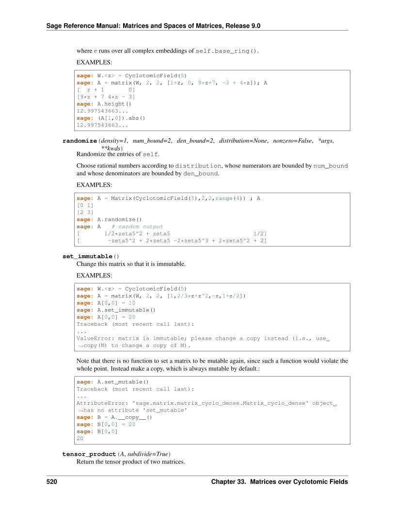
Sage Reference Manual: Matrices and Spaces of Matrices, Release 9.0
where 𝑣 runs over all complex embeddings of self.base_ring().
EXAMPLES:
sage: W.<z> = CyclotomicField(5)sage: A = matrix(W, 2, 2, [1+z, 0, 9*z+7, -3 + 4*z]); A[ z + 1 0][9*z + 7 4*z - 3]sage: A.height()12.997543663...sage: (A[1,0]).abs()12.997543663...
randomize(density=1, num_bound=2, den_bound=2, distribution=None, nonzero=False, *args,**kwds)
Randomize the entries of self.
Choose rational numbers according to distribution, whose numerators are bounded by num_boundand whose denominators are bounded by den_bound.
EXAMPLES:
sage: A = Matrix(CyclotomicField(5),2,2,range(4)) ; A[0 1][2 3]sage: A.randomize()sage: A # random output[ 1/2*zeta5^2 + zeta5 1/2][ -zeta5^2 + 2*zeta5 -2*zeta5^3 + 2*zeta5^2 + 2]
set_immutable()Change this matrix so that it is immutable.
EXAMPLES:
sage: W.<z> = CyclotomicField(5)sage: A = matrix(W, 2, 2, [1,2/3*z+z^2,-z,1+z/2])sage: A[0,0] = 10sage: A.set_immutable()sage: A[0,0] = 20Traceback (most recent call last):...ValueError: matrix is immutable; please change a copy instead (i.e., use→˓copy(M) to change a copy of M).
Note that there is no function to set a matrix to be mutable again, since such a function would violate thewhole point. Instead make a copy, which is always mutable by default.:
sage: A.set_mutable()Traceback (most recent call last):...AttributeError: 'sage.matrix.matrix_cyclo_dense.Matrix_cyclo_dense' object→˓has no attribute 'set_mutable'sage: B = A.__copy__()sage: B[0,0] = 20sage: B[0,0]20
tensor_product(A, subdivide=True)Return the tensor product of two matrices.
520 Chapter 33. Matrices over Cyclotomic Fields
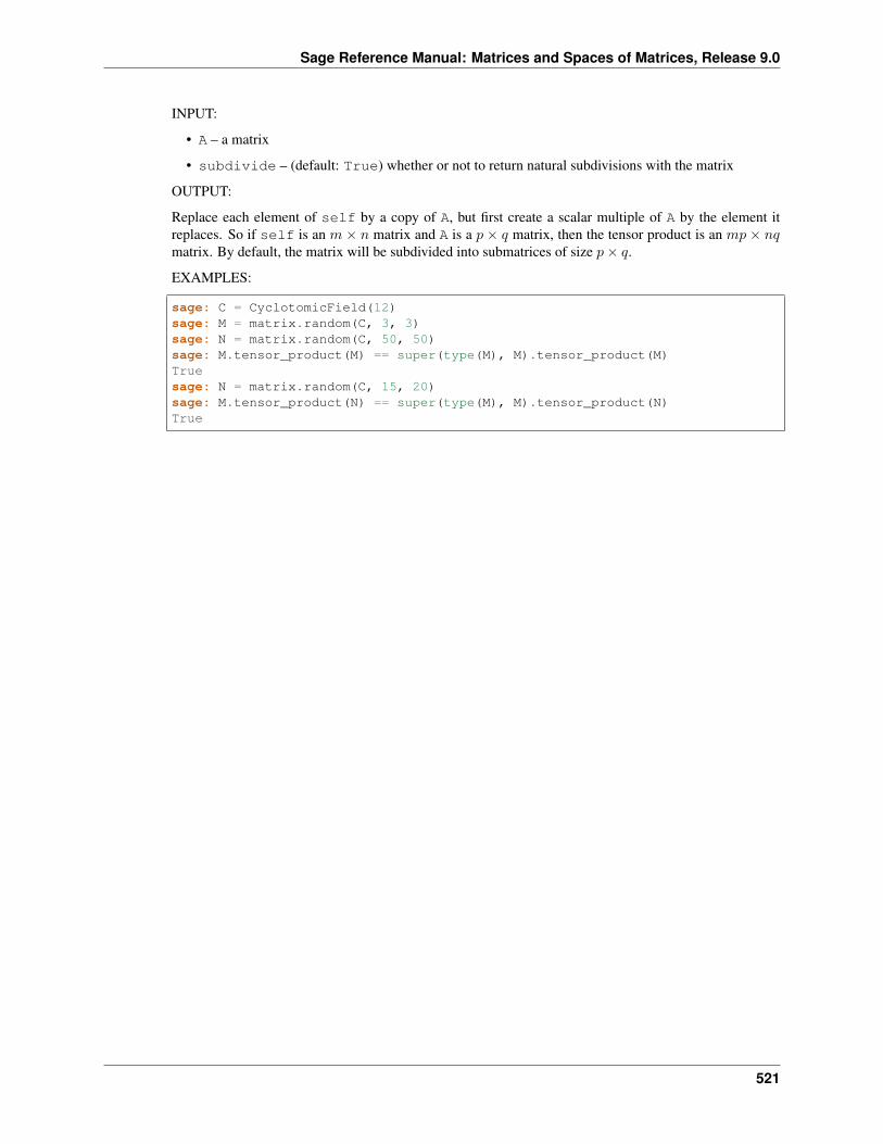
Sage Reference Manual: Matrices and Spaces of Matrices, Release 9.0
INPUT:
• A – a matrix
• subdivide – (default: True) whether or not to return natural subdivisions with the matrix
OUTPUT:
Replace each element of self by a copy of A, but first create a scalar multiple of A by the element itreplaces. So if self is an 𝑚 × 𝑛 matrix and A is a 𝑝 × 𝑞 matrix, then the tensor product is an 𝑚𝑝 × 𝑛𝑞matrix. By default, the matrix will be subdivided into submatrices of size 𝑝× 𝑞.
EXAMPLES:
sage: C = CyclotomicField(12)sage: M = matrix.random(C, 3, 3)sage: N = matrix.random(C, 50, 50)sage: M.tensor_product(M) == super(type(M), M).tensor_product(M)Truesage: N = matrix.random(C, 15, 20)sage: M.tensor_product(N) == super(type(M), M).tensor_product(N)True
521

Sage Reference Manual: Matrices and Spaces of Matrices, Release 9.0
522 Chapter 33. Matrices over Cyclotomic Fields
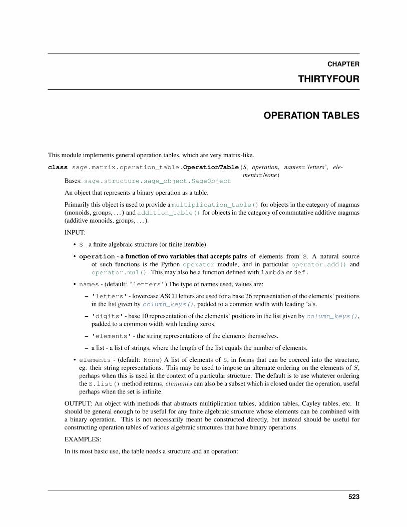
CHAPTER
THIRTYFOUR
OPERATION TABLES
This module implements general operation tables, which are very matrix-like.
class sage.matrix.operation_table.OperationTable(S, operation, names=’letters’, ele-ments=None)
Bases: sage.structure.sage_object.SageObject
An object that represents a binary operation as a table.
Primarily this object is used to provide a multiplication_table() for objects in the category of magmas(monoids, groups, . . . ) and addition_table() for objects in the category of commutative additive magmas(additive monoids, groups, . . . ).
INPUT:
• S - a finite algebraic structure (or finite iterable)
• operation - a function of two variables that accepts pairs of elements from S. A natural sourceof such functions is the Python operator module, and in particular operator.add() andoperator.mul(). This may also be a function defined with lambda or def.
• names - (default: 'letters') The type of names used, values are:
– 'letters' - lowercase ASCII letters are used for a base 26 representation of the elements’ positionsin the list given by column_keys(), padded to a common width with leading ‘a’s.
– 'digits' - base 10 representation of the elements’ positions in the list given by column_keys(),padded to a common width with leading zeros.
– 'elements' - the string representations of the elements themselves.
– a list - a list of strings, where the length of the list equals the number of elements.
• elements - (default: None) A list of elements of S, in forms that can be coerced into the structure,eg. their string representations. This may be used to impose an alternate ordering on the elements of 𝑆,perhaps when this is used in the context of a particular structure. The default is to use whatever orderingthe S.list() method returns. 𝑒𝑙𝑒𝑚𝑒𝑛𝑡𝑠 can also be a subset which is closed under the operation, usefulperhaps when the set is infinite.
OUTPUT: An object with methods that abstracts multiplication tables, addition tables, Cayley tables, etc. Itshould be general enough to be useful for any finite algebraic structure whose elements can be combined witha binary operation. This is not necessarily meant be constructed directly, but instead should be useful forconstructing operation tables of various algebraic structures that have binary operations.
EXAMPLES:
In its most basic use, the table needs a structure and an operation:
523

Sage Reference Manual: Matrices and Spaces of Matrices, Release 9.0
sage: from sage.matrix.operation_table import OperationTablesage: G=SymmetricGroup(3)sage: OperationTable(G, operation=operator.mul)
* a b c d e f+------------a| a b c d e fb| b a d c f ec| c e a f b dd| d f b e a ce| e c f a d bf| f d e b c a
With two operations present, we can specify which operation we want:
sage: from sage.matrix.operation_table import OperationTablesage: R=Integers(6)sage: OperationTable(R, operation=operator.add)+ a b c d e f+------------a| a b c d e fb| b c d e f ac| c d e f a bd| d e f a b ce| e f a b c df| f a b c d e
The default symbol set for elements is lowercase ASCII letters, which take on a base 26 flavor for structureswith more than 26 elements.
sage: from sage.matrix.operation_table import OperationTablesage: G=DihedralGroup(14)sage: OperationTable(G, operator.mul, names='letters')
* aa ab ac ad ae af ag ah ai aj ak al am an ao ap aq ar as at au av aw ax ay az→˓ba bb+-------------------------------------------------------------------------------
→˓-----aa| aa ab ac ad ae af ag ah ai aj ak al am an ao ap aq ar as at au av aw ax ay az→˓ba bbab| ab aa ad ac af ae ah ag aj ai al ak an am ap ao ar aq at as av au ax aw az ay→˓bb baac| ac ba aa ae ad ag af ai ah ak aj am al ao an aq ap as ar au at aw av ay ax bb→˓ab azad| ad bb ab af ac ah ae aj ag al ai an ak ap am ar ao at aq av as ax au az aw ba→˓aa ayae| ae az ba ag aa ai ad ak af am ah ao aj aq al as an au ap aw ar ay at bb av ab→˓ac axaf| af ay bb ah ab aj ac al ae an ag ap ai ar ak at am av ao ax aq az as ba au aa→˓ad awag| ag ax az ai ba ak aa am ad ao af aq ah as aj au al aw an ay ap bb ar ab at ac→˓ae avah| ah aw ay aj bb al ab an ac ap ae ar ag at ai av ak ax am az ao ba aq aa as ad→˓af auai| ai av ax ak az am ba ao aa aq ad as af au ah aw aj ay al bb an ab ap ac ar ae→˓ag ataj| aj au aw al ay an bb ap ab ar ac at ae av ag ax ai az ak ba am aa ao ad aq af→˓ah asak| ak at av am ax ao az aq ba as aa au ad aw af ay ah bb aj ab al ac an ae ap ag→˓ai ar
(continues on next page)
524 Chapter 34. Operation Tables
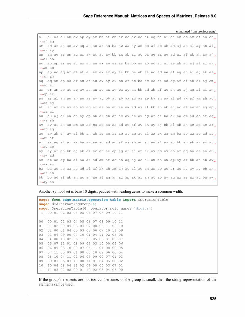
Sage Reference Manual: Matrices and Spaces of Matrices, Release 9.0
(continued from previous page)
al| al as au an aw ap ay ar bb at ab av ac ax ae az ag ba ai aa ak ad am af ao ah→˓aj aqam| am ar at ao av aq ax as az au ba aw aa ay ad bb af ab ah ac aj ae al ag an ai→˓ak apan| an aq as ap au ar aw at ay av bb ax ab az ac ba ae aa ag ad ai af ak ah am aj→˓al aoao| ao ap ar aq at as av au ax aw az ay ba bb aa ab ad ac af ae ah ag aj ai al ak→˓am anap| ap ao aq ar as at au av aw ax ay az bb ba ab aa ac ad ae af ag ah ai aj ak al→˓an amaq| aq an ap as ar au at aw av ay ax bb az ab ba ac aa ae ad ag af ai ah ak aj am→˓ao alar| ar am ao at aq av as ax au az aw ba ay aa bb ad ab af ac ah ae aj ag al ai an→˓ap akas| as al an au ap aw ar ay at bb av ab ax ac az ae ba ag aa ai ad ak af am ah ao→˓aq ajat| at ak am av ao ax aq az as ba au aa aw ad ay af bb ah ab aj ac al ae an ag ap→˓ar aiau| au aj al aw an ay ap bb ar ab at ac av ae ax ag az ai ba ak aa am ad ao af aq→˓as ahav| av ai ak ax am az ao ba aq aa as ad au af aw ah ay aj bb al ab an ac ap ae ar→˓at agaw| aw ah aj ay al bb an ab ap ac ar ae at ag av ai ax ak az am ba ao aa aq ad as→˓au afax| ax ag ai az ak ba am aa ao ad aq af as ah au aj aw al ay an bb ap ab ar ac at→˓av aeay| ay af ah bb aj ab al ac an ae ap ag ar ai at ak av am ax ao az aq ba as aa au→˓aw adaz| az ae ag ba ai aa ak ad am af ao ah aq aj as al au an aw ap ay ar bb at ab av→˓ax acba| ba ac ae aa ag ad ai af ak ah am aj ao al aq an as ap au ar aw at ay av bb ax→˓az abbb| bb ad af ab ah ac aj ae al ag an ai ap ak ar am at ao av aq ax as az au ba aw→˓ay aa
Another symbol set is base 10 digits, padded with leading zeros to make a common width.
sage: from sage.matrix.operation_table import OperationTablesage: G=AlternatingGroup(4)sage: OperationTable(G, operator.mul, names='digits')
* 00 01 02 03 04 05 06 07 08 09 10 11+------------------------------------
00| 00 01 02 03 04 05 06 07 08 09 10 1101| 01 02 00 05 03 04 07 08 06 11 09 1002| 02 00 01 04 05 03 08 06 07 10 11 0903| 03 06 09 00 07 10 01 04 11 02 05 0804| 04 08 10 02 06 11 00 05 09 01 03 0705| 05 07 11 01 08 09 02 03 10 00 04 0606| 06 09 03 10 00 07 04 11 01 08 02 0507| 07 11 05 09 01 08 03 10 02 06 00 0408| 08 10 04 11 02 06 05 09 00 07 01 0309| 09 03 06 07 10 00 11 01 04 05 08 0210| 10 04 08 06 11 02 09 00 05 03 07 0111| 11 05 07 08 09 01 10 02 03 04 06 00
If the group’s elements are not too cumbersome, or the group is small, then the string representation of theelements can be used.
525
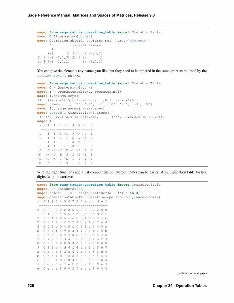
Sage Reference Manual: Matrices and Spaces of Matrices, Release 9.0
sage: from sage.matrix.operation_table import OperationTablesage: G=AlternatingGroup(3)sage: OperationTable(G, operator.mul, names='elements')
* () (1,2,3) (1,3,2)+------------------------
()| () (1,2,3) (1,3,2)(1,2,3)| (1,2,3) (1,3,2) ()(1,3,2)| (1,3,2) () (1,2,3)
You can give the elements any names you like, but they need to be ordered in the same order as returned by thecolumn_keys() method.
sage: from sage.matrix.operation_table import OperationTablesage: G = QuaternionGroup()sage: T = OperationTable(G, operator.mul)sage: T.column_keys()((), (1,2,3,4)(5,6,7,8), ..., (1,8,3,6)(2,7,4,5))sage: names=['1', 'I', '-1', '-I', 'J', '-K', '-J', 'K']sage: T.change_names(names=names)sage: sorted(T.translation().items())[('-1', (1,3)(2,4)(5,7)(6,8)), ..., ('K', (1,8,3,6)(2,7,4,5))]sage: T
* 1 I -1 -I J -K -J K+------------------------1| 1 I -1 -I J -K -J KI| I -1 -I 1 K J -K -J
-1| -1 -I 1 I -J K J -K-I| -I 1 I -1 -K -J K JJ| J -K -J K -1 -I 1 I
-K| -K -J K J I -1 -I 1-J| -J K J -K 1 I -1 -IK| K J -K -J -I 1 I -1
With the right functions and a list comprehension, custom names can be easier. A multiplication table for hexdigits (without carries):
sage: from sage.matrix.operation_table import OperationTablesage: R = Integers(16)sage: names=['{:x}'.format(Integer(a)) for a in R]sage: OperationTable(R, operation=operator.mul, names=names)
* 0 1 2 3 4 5 6 7 8 9 a b c d e f+--------------------------------
0| 0 0 0 0 0 0 0 0 0 0 0 0 0 0 0 01| 0 1 2 3 4 5 6 7 8 9 a b c d e f2| 0 2 4 6 8 a c e 0 2 4 6 8 a c e3| 0 3 6 9 c f 2 5 8 b e 1 4 7 a d4| 0 4 8 c 0 4 8 c 0 4 8 c 0 4 8 c5| 0 5 a f 4 9 e 3 8 d 2 7 c 1 6 b6| 0 6 c 2 8 e 4 a 0 6 c 2 8 e 4 a7| 0 7 e 5 c 3 a 1 8 f 6 d 4 b 2 98| 0 8 0 8 0 8 0 8 0 8 0 8 0 8 0 89| 0 9 2 b 4 d 6 f 8 1 a 3 c 5 e 7a| 0 a 4 e 8 2 c 6 0 a 4 e 8 2 c 6b| 0 b 6 1 c 7 2 d 8 3 e 9 4 f a 5c| 0 c 8 4 0 c 8 4 0 c 8 4 0 c 8 4d| 0 d a 7 4 1 e b 8 5 2 f c 9 6 3e| 0 e c a 8 6 4 2 0 e c a 8 6 4 2
(continues on next page)
526 Chapter 34. Operation Tables
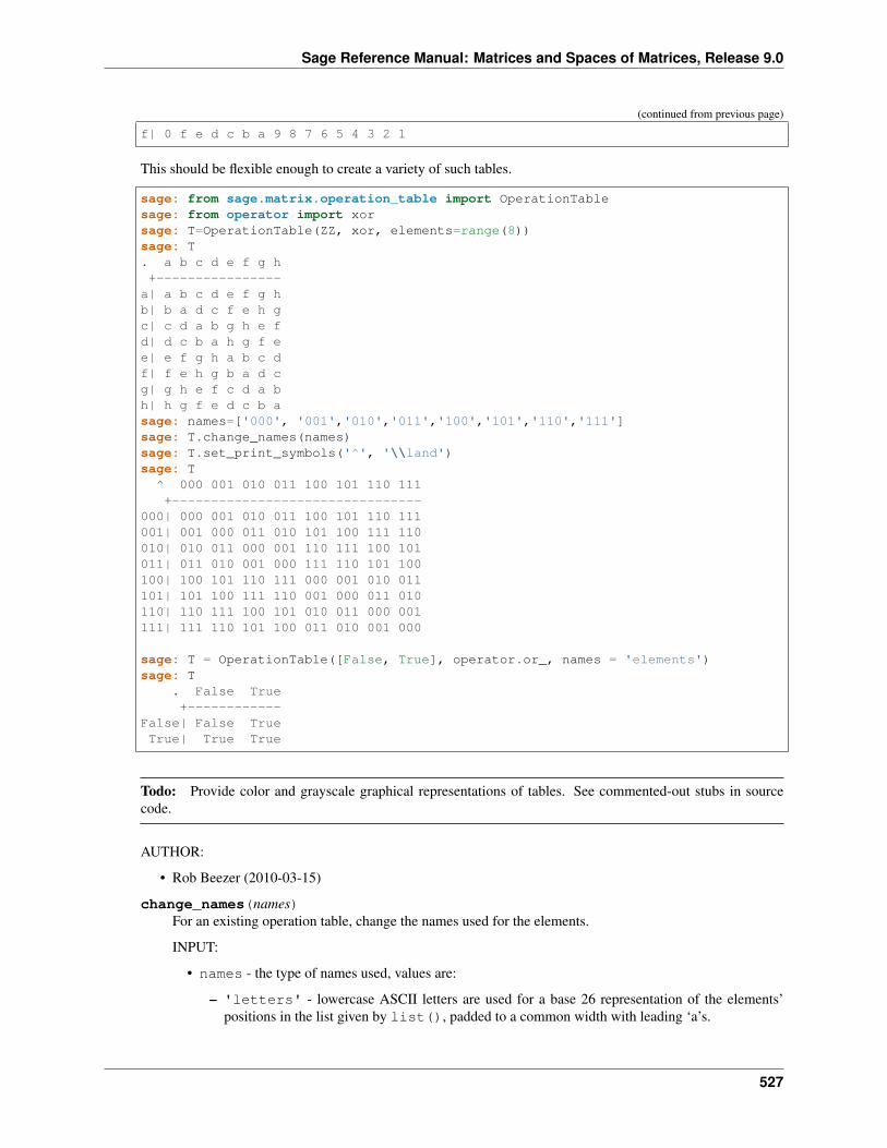
Sage Reference Manual: Matrices and Spaces of Matrices, Release 9.0
(continued from previous page)
f| 0 f e d c b a 9 8 7 6 5 4 3 2 1
This should be flexible enough to create a variety of such tables.
sage: from sage.matrix.operation_table import OperationTablesage: from operator import xorsage: T=OperationTable(ZZ, xor, elements=range(8))sage: T. a b c d e f g h+----------------a| a b c d e f g hb| b a d c f e h gc| c d a b g h e fd| d c b a h g f ee| e f g h a b c df| f e h g b a d cg| g h e f c d a bh| h g f e d c b asage: names=['000', '001','010','011','100','101','110','111']sage: T.change_names(names)sage: T.set_print_symbols('^', '\\land')sage: T^ 000 001 010 011 100 101 110 111+--------------------------------
000| 000 001 010 011 100 101 110 111001| 001 000 011 010 101 100 111 110010| 010 011 000 001 110 111 100 101011| 011 010 001 000 111 110 101 100100| 100 101 110 111 000 001 010 011101| 101 100 111 110 001 000 011 010110| 110 111 100 101 010 011 000 001111| 111 110 101 100 011 010 001 000
sage: T = OperationTable([False, True], operator.or_, names = 'elements')sage: T
. False True+------------
False| False TrueTrue| True True
Todo: Provide color and grayscale graphical representations of tables. See commented-out stubs in sourcecode.
AUTHOR:
• Rob Beezer (2010-03-15)
change_names(names)For an existing operation table, change the names used for the elements.
INPUT:
• names - the type of names used, values are:
– 'letters' - lowercase ASCII letters are used for a base 26 representation of the elements’positions in the list given by list(), padded to a common width with leading ‘a’s.
527
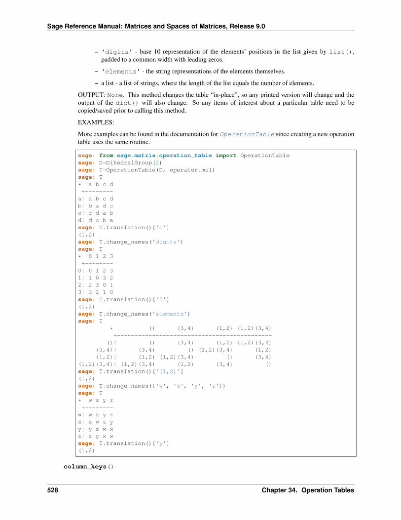
Sage Reference Manual: Matrices and Spaces of Matrices, Release 9.0
– 'digits' - base 10 representation of the elements’ positions in the list given by list(),padded to a common width with leading zeros.
– 'elements' - the string representations of the elements themselves.
– a list - a list of strings, where the length of the list equals the number of elements.
OUTPUT: None. This method changes the table “in-place”, so any printed version will change and theoutput of the dict() will also change. So any items of interest about a particular table need to becopied/saved prior to calling this method.
EXAMPLES:
More examples can be found in the documentation for OperationTable since creating a new operationtable uses the same routine.
sage: from sage.matrix.operation_table import OperationTablesage: D=DihedralGroup(2)sage: T=OperationTable(D, operator.mul)sage: T
* a b c d+--------
a| a b c db| b a d cc| c d a bd| d c b asage: T.translation()['c'](1,2)sage: T.change_names('digits')sage: T
* 0 1 2 3+--------
0| 0 1 2 31| 1 0 3 22| 2 3 0 13| 3 2 1 0sage: T.translation()['2'](1,2)sage: T.change_names('elements')sage: T
* () (3,4) (1,2) (1,2)(3,4)+--------------------------------------------
()| () (3,4) (1,2) (1,2)(3,4)(3,4)| (3,4) () (1,2)(3,4) (1,2)(1,2)| (1,2) (1,2)(3,4) () (3,4)
(1,2)(3,4)| (1,2)(3,4) (1,2) (3,4) ()sage: T.translation()['(1,2)'](1,2)sage: T.change_names(['w', 'x', 'y', 'z'])sage: T
* w x y z+--------
w| w x y zx| x w z yy| y z w xz| z y x wsage: T.translation()['y'](1,2)
column_keys()
528 Chapter 34. Operation Tables
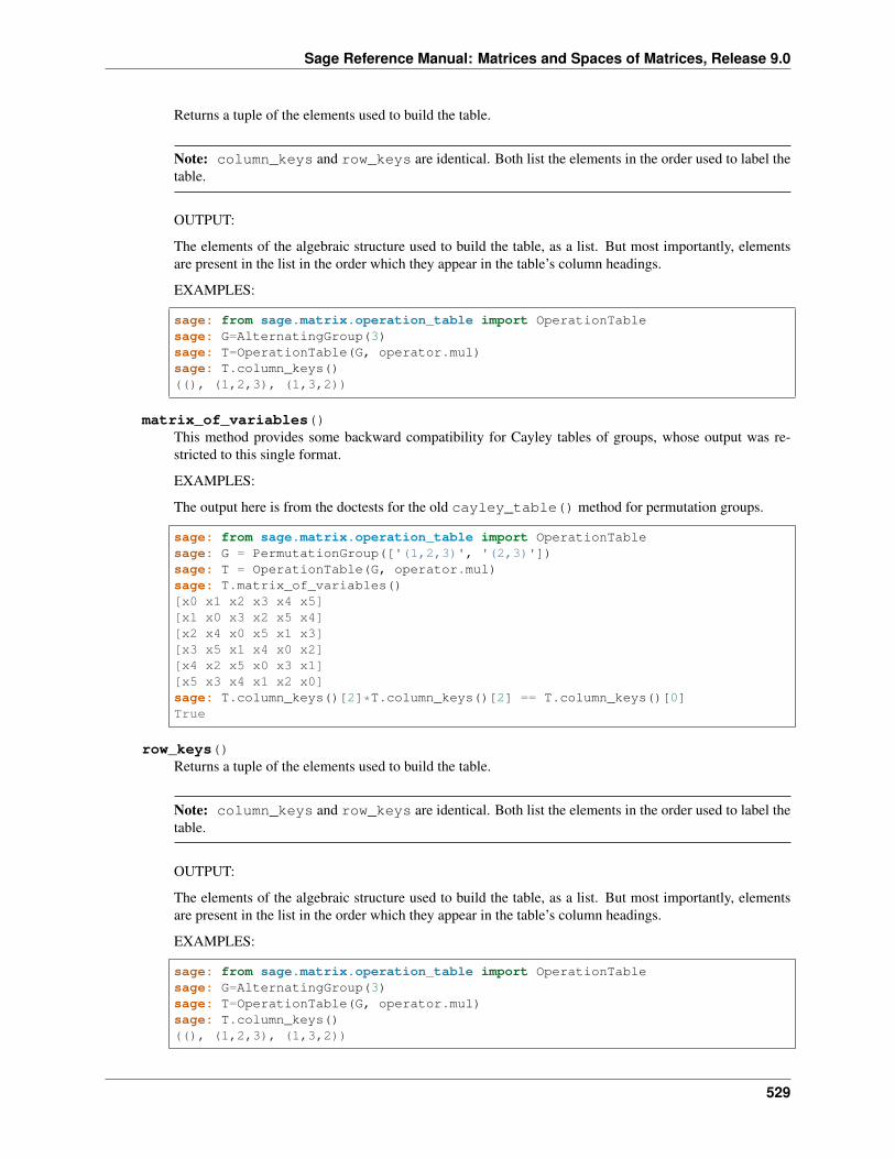
Sage Reference Manual: Matrices and Spaces of Matrices, Release 9.0
Returns a tuple of the elements used to build the table.
Note: column_keys and row_keys are identical. Both list the elements in the order used to label thetable.
OUTPUT:
The elements of the algebraic structure used to build the table, as a list. But most importantly, elementsare present in the list in the order which they appear in the table’s column headings.
EXAMPLES:
sage: from sage.matrix.operation_table import OperationTablesage: G=AlternatingGroup(3)sage: T=OperationTable(G, operator.mul)sage: T.column_keys()((), (1,2,3), (1,3,2))
matrix_of_variables()This method provides some backward compatibility for Cayley tables of groups, whose output was re-stricted to this single format.
EXAMPLES:
The output here is from the doctests for the old cayley_table() method for permutation groups.
sage: from sage.matrix.operation_table import OperationTablesage: G = PermutationGroup(['(1,2,3)', '(2,3)'])sage: T = OperationTable(G, operator.mul)sage: T.matrix_of_variables()[x0 x1 x2 x3 x4 x5][x1 x0 x3 x2 x5 x4][x2 x4 x0 x5 x1 x3][x3 x5 x1 x4 x0 x2][x4 x2 x5 x0 x3 x1][x5 x3 x4 x1 x2 x0]sage: T.column_keys()[2]*T.column_keys()[2] == T.column_keys()[0]True
row_keys()Returns a tuple of the elements used to build the table.
Note: column_keys and row_keys are identical. Both list the elements in the order used to label thetable.
OUTPUT:
The elements of the algebraic structure used to build the table, as a list. But most importantly, elementsare present in the list in the order which they appear in the table’s column headings.
EXAMPLES:
sage: from sage.matrix.operation_table import OperationTablesage: G=AlternatingGroup(3)sage: T=OperationTable(G, operator.mul)sage: T.column_keys()((), (1,2,3), (1,3,2))
529
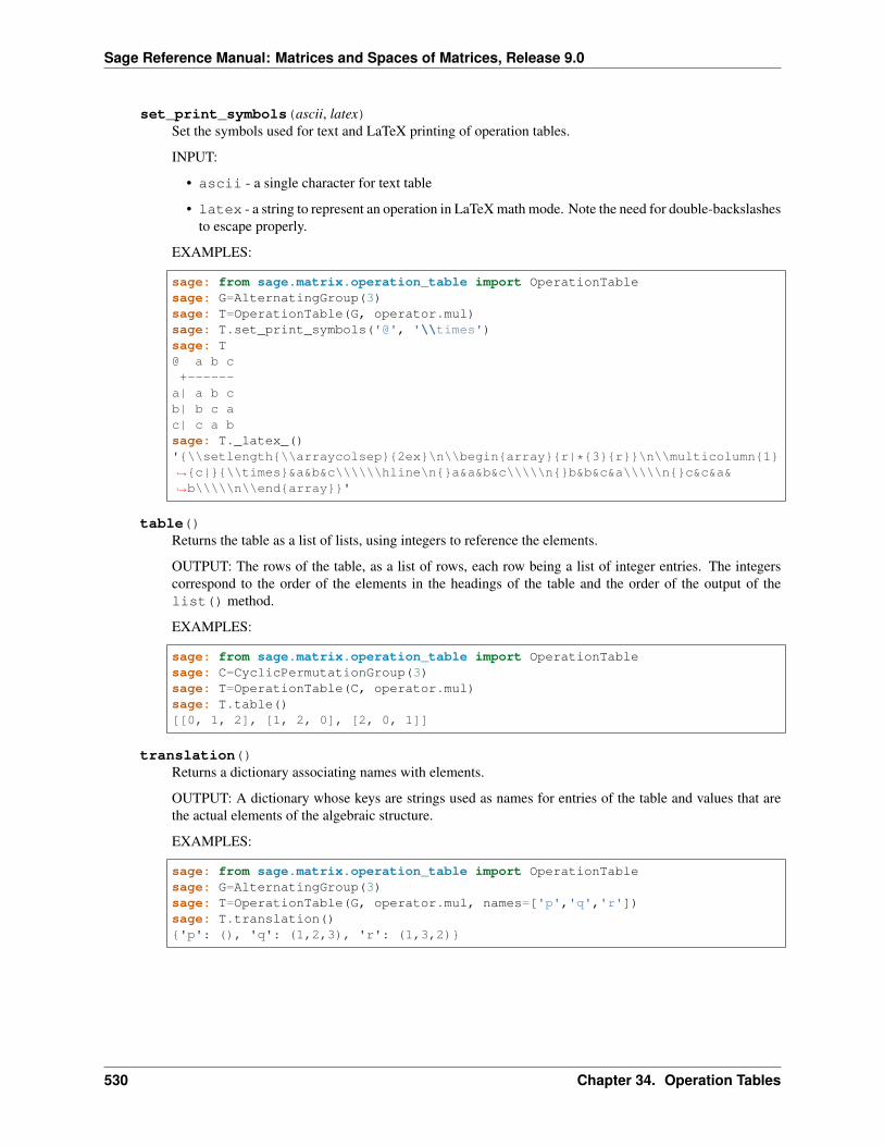
Sage Reference Manual: Matrices and Spaces of Matrices, Release 9.0
set_print_symbols(ascii, latex)Set the symbols used for text and LaTeX printing of operation tables.
INPUT:
• ascii - a single character for text table
• latex - a string to represent an operation in LaTeX math mode. Note the need for double-backslashesto escape properly.
EXAMPLES:
sage: from sage.matrix.operation_table import OperationTablesage: G=AlternatingGroup(3)sage: T=OperationTable(G, operator.mul)sage: T.set_print_symbols('@', '\\times')sage: T@ a b c+------
a| a b cb| b c ac| c a bsage: T._latex_()'{\\setlength{\\arraycolsep}{2ex}\n\\begin{array}{r|*{3}{r}}\n\\multicolumn{1}→˓{c|}{\\times}&a&b&c\\\\\\hline\n{}a&a&b&c\\\\\n{}b&b&c&a\\\\\n{}c&c&a&→˓b\\\\\n\\end{array}}'
table()Returns the table as a list of lists, using integers to reference the elements.
OUTPUT: The rows of the table, as a list of rows, each row being a list of integer entries. The integerscorrespond to the order of the elements in the headings of the table and the order of the output of thelist() method.
EXAMPLES:
sage: from sage.matrix.operation_table import OperationTablesage: C=CyclicPermutationGroup(3)sage: T=OperationTable(C, operator.mul)sage: T.table()[[0, 1, 2], [1, 2, 0], [2, 0, 1]]
translation()Returns a dictionary associating names with elements.
OUTPUT: A dictionary whose keys are strings used as names for entries of the table and values that arethe actual elements of the algebraic structure.
EXAMPLES:
sage: from sage.matrix.operation_table import OperationTablesage: G=AlternatingGroup(3)sage: T=OperationTable(G, operator.mul, names=['p','q','r'])sage: T.translation(){'p': (), 'q': (1,2,3), 'r': (1,3,2)}
530 Chapter 34. Operation Tables
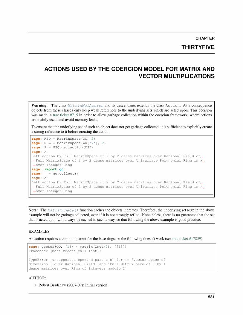
CHAPTER
THIRTYFIVE
ACTIONS USED BY THE COERCION MODEL FOR MATRIX ANDVECTOR MULTIPLICATIONS
Warning: The class MatrixMulAction and its descendants extends the class Action. As a consequenceobjects from these classes only keep weak references to the underlying sets which are acted upon. This decisionwas made in trac ticket #715 in order to allow garbage collection within the coercion framework, where actionsare mainly used, and avoid memory leaks.
To ensure that the underlying set of such an object does not get garbage collected, it is sufficient to explicitly createa strong reference to it before creating the action.
sage: MSQ = MatrixSpace(QQ, 2)sage: MSZ = MatrixSpace(ZZ['x'], 2)sage: A = MSQ.get_action(MSZ)sage: ALeft action by Full MatrixSpace of 2 by 2 dense matrices over Rational Field on→˓Full MatrixSpace of 2 by 2 dense matrices over Univariate Polynomial Ring in x→˓over Integer Ringsage: import gcsage: _ = gc.collect()sage: ALeft action by Full MatrixSpace of 2 by 2 dense matrices over Rational Field on→˓Full MatrixSpace of 2 by 2 dense matrices over Univariate Polynomial Ring in x→˓over Integer Ring
Note: The MatrixSpace() function caches the objects it creates. Therefore, the underlying set MSZ in the aboveexample will not be garbage collected, even if it is not strongly ref’ed. Nonetheless, there is no guarantee that the setthat is acted upon will always be cached in such a way, so that following the above example is good practice.
EXAMPLES:
An action requires a common parent for the base rings, so the following doesn’t work (see trac ticket #17859):
sage: vector(QQ, [1]) * matrix(Zmod(2), [[1]])Traceback (most recent call last):...TypeError: unsupported operand parent(s) for *: 'Vector space ofdimension 1 over Rational Field' and 'Full MatrixSpace of 1 by 1dense matrices over Ring of integers modulo 2'
AUTHOR:
• Robert Bradshaw (2007-09): Initial version.
531
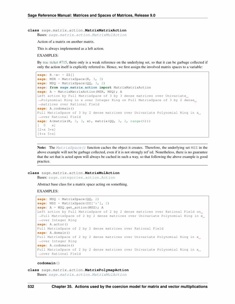
Sage Reference Manual: Matrices and Spaces of Matrices, Release 9.0
class sage.matrix.action.MatrixMatrixActionBases: sage.matrix.action.MatrixMulAction
Action of a matrix on another matrix.
This is always implemented as a left action.
EXAMPLES:
By trac ticket #715, there only is a weak reference on the underlying set, so that it can be garbage collected ifonly the action itself is explicitly referred to. Hence, we first assign the involved matrix spaces to a variable:
sage: R.<x> = ZZ[]sage: MSR = MatrixSpace(R, 3, 3)sage: MSQ = MatrixSpace(QQ, 3, 2)sage: from sage.matrix.action import MatrixMatrixActionsage: A = MatrixMatrixAction(MSR, MSQ); ALeft action by Full MatrixSpace of 3 by 3 dense matrices over Univariate→˓Polynomial Ring in x over Integer Ring on Full MatrixSpace of 3 by 2 dense→˓matrices over Rational Fieldsage: A.codomain()Full MatrixSpace of 3 by 2 dense matrices over Univariate Polynomial Ring in x→˓over Rational Fieldsage: A(matrix(R, 3, 3, x), matrix(QQ, 3, 2, range(6)))[ 0 x][2*x 3*x][4*x 5*x]
Note: The MatrixSpace() function caches the object it creates. Therefore, the underlying set MSZ in theabove example will not be garbage collected, even if it is not strongly ref’ed. Nonetheless, there is no guaranteethat the set that is acted upon will always be cached in such a way, so that following the above example is goodpractice.
class sage.matrix.action.MatrixMulActionBases: sage.categories.action.Action
Abstract base class for a matrix space acting on something.
EXAMPLES:
sage: MSQ = MatrixSpace(QQ, 2)sage: MSZ = MatrixSpace(ZZ['x'], 2)sage: A = MSQ.get_action(MSZ); ALeft action by Full MatrixSpace of 2 by 2 dense matrices over Rational Field on→˓Full MatrixSpace of 2 by 2 dense matrices over Univariate Polynomial Ring in x→˓over Integer Ringsage: A.actor()Full MatrixSpace of 2 by 2 dense matrices over Rational Fieldsage: A.domain()Full MatrixSpace of 2 by 2 dense matrices over Univariate Polynomial Ring in x→˓over Integer Ringsage: A.codomain()Full MatrixSpace of 2 by 2 dense matrices over Univariate Polynomial Ring in x→˓over Rational Field
codomain()
class sage.matrix.action.MatrixPolymapActionBases: sage.matrix.action.MatrixMulAction
532 Chapter 35. Actions used by the coercion model for matrix and vector multiplications
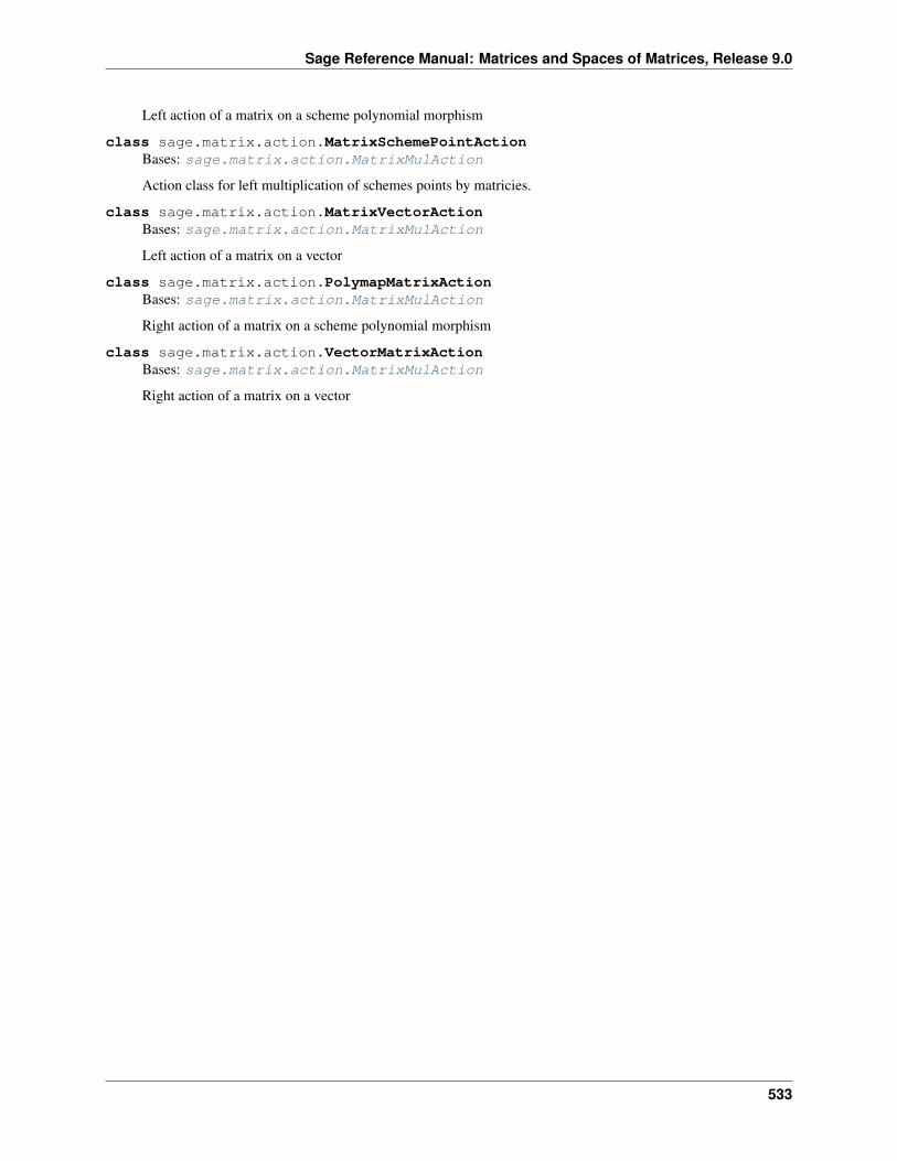
Sage Reference Manual: Matrices and Spaces of Matrices, Release 9.0
Left action of a matrix on a scheme polynomial morphism
class sage.matrix.action.MatrixSchemePointActionBases: sage.matrix.action.MatrixMulAction
Action class for left multiplication of schemes points by matricies.
class sage.matrix.action.MatrixVectorActionBases: sage.matrix.action.MatrixMulAction
Left action of a matrix on a vector
class sage.matrix.action.PolymapMatrixActionBases: sage.matrix.action.MatrixMulAction
Right action of a matrix on a scheme polynomial morphism
class sage.matrix.action.VectorMatrixActionBases: sage.matrix.action.MatrixMulAction
Right action of a matrix on a vector
533

Sage Reference Manual: Matrices and Spaces of Matrices, Release 9.0
534 Chapter 35. Actions used by the coercion model for matrix and vector multiplications
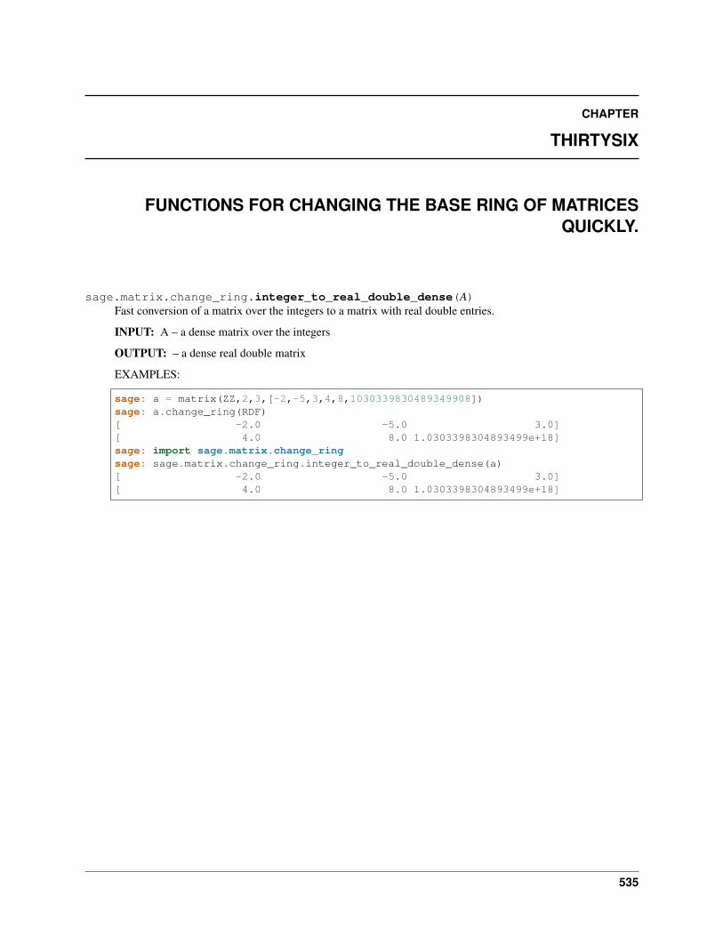
CHAPTER
THIRTYSIX
FUNCTIONS FOR CHANGING THE BASE RING OF MATRICESQUICKLY.
sage.matrix.change_ring.integer_to_real_double_dense(A)Fast conversion of a matrix over the integers to a matrix with real double entries.
INPUT: A – a dense matrix over the integers
OUTPUT: – a dense real double matrix
EXAMPLES:
sage: a = matrix(ZZ,2,3,[-2,-5,3,4,8,1030339830489349908])sage: a.change_ring(RDF)[ -2.0 -5.0 3.0][ 4.0 8.0 1.0303398304893499e+18]sage: import sage.matrix.change_ringsage: sage.matrix.change_ring.integer_to_real_double_dense(a)[ -2.0 -5.0 3.0][ 4.0 8.0 1.0303398304893499e+18]
535

Sage Reference Manual: Matrices and Spaces of Matrices, Release 9.0
536 Chapter 36. Functions for changing the base ring of matrices quickly.
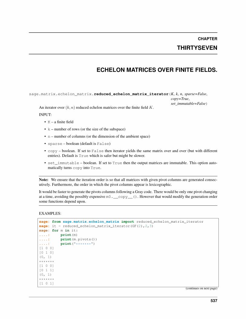
CHAPTER
THIRTYSEVEN
ECHELON MATRICES OVER FINITE FIELDS.
sage.matrix.echelon_matrix.reduced_echelon_matrix_iterator(K, k, n, sparse=False,copy=True,set_immutable=False)
An iterator over (𝑘, 𝑛) reduced echelon matrices over the finite field 𝐾.
INPUT:
• K – a finite field
• k – number of rows (or the size of the subspace)
• n – number of columns (or the dimension of the ambient space)
• sparse – boolean (default is False)
• copy – boolean. If set to False then iterator yields the same matrix over and over (but with differententries). Default is True which is safer but might be slower.
• set_immutable – boolean. If set to True then the output matrices are immutable. This option auto-matically turns copy into True.
Note: We ensure that the iteration order is so that all matrices with given pivot columns are generated consec-utively. Furthermore, the order in which the pivot columns appear is lexicographic.
It would be faster to generate the pivots columns following a Gray code. There would be only one pivot changingat a time, avoiding the possibly expensive m0.__copy__(). However that would modify the generation ordersome functions depend upon.
EXAMPLES:
sage: from sage.matrix.echelon_matrix import reduced_echelon_matrix_iteratorsage: it = reduced_echelon_matrix_iterator(GF(2),2,3)sage: for m in it:....: print(m)....: print(m.pivots())....: print("*******")[1 0 0][0 1 0](0, 1)
*******[1 0 0][0 1 1](0, 1)
*******[1 0 1]
(continues on next page)
537

Sage Reference Manual: Matrices and Spaces of Matrices, Release 9.0
(continued from previous page)
[0 1 0](0, 1)
*******[1 0 1][0 1 1](0, 1)
*******[1 0 0][0 0 1](0, 2)
*******[1 1 0][0 0 1](0, 2)
*******[0 1 0][0 0 1](1, 2)
*******
538 Chapter 37. Echelon matrices over finite fields.

CHAPTER
THIRTYEIGHT
MISCELLANEOUS MATRIX FUNCTIONS
sage.matrix.matrix_misc.permanental_minor_polynomial(A, permanent_only=False,var=’t’, prec=None)
Return the polynomial of the sums of permanental minors of A.
INPUT:
• 𝐴 – a matrix
• 𝑝𝑒𝑟𝑚𝑎𝑛𝑒𝑛𝑡𝑜𝑛𝑙𝑦 – if True, return only the permanent of 𝐴
• 𝑣𝑎𝑟 – name of the polynomial variable
• 𝑝𝑟𝑒𝑐 – if prec is not None, truncate the polynomial at precision 𝑝𝑟𝑒𝑐
The polynomial of the sums of permanental minors is
𝑚𝑖𝑛(𝑛𝑟𝑜𝑤𝑠,𝑛𝑐𝑜𝑙𝑠)∑︁𝑖=0
𝑝𝑖(𝐴)𝑥𝑖
where 𝑝𝑖(𝐴) is the 𝑖-th permanental minor of 𝐴 (that can also be obtained through the methodpermanental_minor() via A.permanental_minor(i)).
The algorithm implemented by that function has been developed by P. Butera and M. Pernici, see [BP2015]. Itscomplexity is 𝑂(2𝑛𝑚2𝑛) where 𝑚 and 𝑛 are the number of rows and columns of 𝐴. Moreover, if 𝐴 is a bandedmatrix with width 𝑤, that is 𝐴𝑖𝑗 = 0 for |𝑖 − 𝑗| > 𝑤 and 𝑤 < 𝑛/2, then the complexity of the algorithm is𝑂(4𝑤(𝑤 + 1)𝑛2).
INPUT:
• A – matrix
• permanent_only – optional boolean. If True, only the permanent is computed (might be faster).
• var – a variable name
EXAMPLES:
sage: from sage.matrix.matrix_misc import permanental_minor_polynomialsage: m = matrix([[1,1],[1,2]])sage: permanental_minor_polynomial(m)3*t^2 + 5*t + 1sage: permanental_minor_polynomial(m, permanent_only=True)3sage: permanental_minor_polynomial(m, prec=2)5*t + 1
539
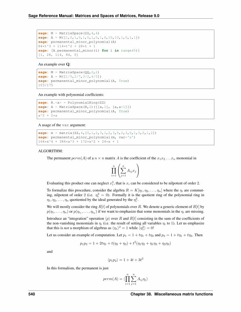
Sage Reference Manual: Matrices and Spaces of Matrices, Release 9.0
sage: M = MatrixSpace(ZZ,4,4)sage: A = M([1,0,1,0,1,0,1,0,1,0,10,10,1,0,1,1])sage: permanental_minor_polynomial(A)84*t^3 + 114*t^2 + 28*t + 1sage: [A.permanental_minor(i) for i in range(5)][1, 28, 114, 84, 0]
An example over Q:
sage: M = MatrixSpace(QQ,2,2)sage: A = M([1/5,2/7,3/2,4/5])sage: permanental_minor_polynomial(A, True)103/175
An example with polynomial coefficients:
sage: R.<a> = PolynomialRing(ZZ)sage: A = MatrixSpace(R,2)([[a,1], [a,a+1]])sage: permanental_minor_polynomial(A, True)a^2 + 2*a
A usage of the var argument:
sage: m = matrix(ZZ,4,[0,1,2,3,1,2,3,0,2,3,0,1,3,0,1,2])sage: permanental_minor_polynomial(m, var='x')164*x^4 + 384*x^3 + 172*x^2 + 24*x + 1
ALGORITHM:
The permanent 𝑝𝑒𝑟𝑚(𝐴) of a 𝑛× 𝑛 matrix 𝐴 is the coefficient of the 𝑥1𝑥2 . . . 𝑥𝑛 monomial in
𝑛∏︁𝑖=1
⎛⎝ 𝑛∑︁𝑗=1
𝐴𝑖𝑗𝑥𝑗
⎞⎠Evaluating this product one can neglect 𝑥2
𝑖 , that is 𝑥𝑖 can be considered to be nilpotent of order 2.
To formalize this procedure, consider the algebra 𝑅 = 𝐾[𝜂1, 𝜂2, . . . , 𝜂𝑛] where the 𝜂𝑖 are commut-ing, nilpotent of order 2 (i.e. 𝜂2𝑖 = 0). Formally it is the quotient ring of the polynomial ring in𝜂1, 𝜂2, . . . , 𝜂𝑛 quotiented by the ideal generated by the 𝜂2𝑖 .
We will mostly consider the ring 𝑅[𝑡] of polynomials over 𝑅. We denote a generic element of 𝑅[𝑡] by𝑝(𝜂1, . . . , 𝜂𝑛) or 𝑝(𝜂𝑖1 , . . . , 𝜂𝑖𝑘) if we want to emphasize that some monomials in the 𝜂𝑖 are missing.
Introduce an “integration” operation ⟨𝑝⟩ over 𝑅 and 𝑅[𝑡] consisting in the sum of the coefficients ofthe non-vanishing monomials in 𝜂𝑖 (i.e. the result of setting all variables 𝜂𝑖 to 1). Let us emphasizethat this is not a morphism of algebras as ⟨𝜂1⟩2 = 1 while ⟨𝜂21⟩ = 0!
Let us consider an example of computation. Let 𝑝1 = 1 + 𝑡𝜂1 + 𝑡𝜂2 and 𝑝2 = 1 + 𝑡𝜂1 + 𝑡𝜂3. Then
𝑝1𝑝2 = 1 + 2𝑡𝜂1 + 𝑡(𝜂2 + 𝜂3) + 𝑡2(𝜂1𝜂2 + 𝜂1𝜂3 + 𝜂2𝜂3)
and
⟨𝑝1𝑝2⟩ = 1 + 4𝑡+ 3𝑡2
In this formalism, the permanent is just
𝑝𝑒𝑟𝑚(𝐴) = ⟨𝑛∏︁
𝑖=1
𝑛∑︁𝑗=1
𝐴𝑖𝑗𝜂𝑗⟩
540 Chapter 38. Miscellaneous matrix functions

Sage Reference Manual: Matrices and Spaces of Matrices, Release 9.0
A useful property of ⟨.⟩ which makes this algorithm efficient for band matrices is the following: let𝑝1(𝜂1, . . . , 𝜂𝑛) and 𝑝2(𝜂𝑗 , . . . , 𝜂𝑛) be polynomials in 𝑅[𝑡] where 𝑗 ≥ 1. Then one has
⟨𝑝1(𝜂1, . . . , 𝜂𝑛)𝑝2⟩ = ⟨𝑝1(1, . . . , 1, 𝜂𝑗 , . . . , 𝜂𝑛)𝑝2⟩
where 𝜂1, .., 𝜂𝑗−1 are replaced by 1 in 𝑝1. Informally, we can “integrate” these variables beforeperforming the product. More generally, if a monomial 𝜂𝑖 is missing in one of the terms of a productof two terms, then it can be integrated in the other term.
Now let us consider an 𝑚× 𝑛 matrix with 𝑚 ≤ 𝑛. The sum of permanental ‘k‘-minors of ‘A‘ is
𝑝𝑒𝑟𝑚(𝐴, 𝑘) =∑︁𝑟,𝑐
𝑝𝑒𝑟𝑚(𝐴𝑟,𝑐)
where the sum is over the 𝑘-subsets 𝑟 of rows and 𝑘-subsets 𝑐 of columns and 𝐴𝑟,𝑐 is the submatrixobtained from 𝐴 by keeping only the rows 𝑟 and columns 𝑐. Of course 𝑝𝑒𝑟𝑚(𝐴,min(𝑚,𝑛)) =𝑝𝑒𝑟𝑚(𝐴) and note that 𝑝𝑒𝑟𝑚(𝐴, 1) is just the sum of all entries of the matrix.
The generating function of these sums of permanental minors is
𝑔(𝑡) =
⟨𝑚∏︁𝑖=1
⎛⎝1 + 𝑡
𝑛∑︁𝑗=1
𝐴𝑖𝑗𝜂𝑗
⎞⎠⟩
In fact the 𝑡𝑘 coefficient of 𝑔(𝑡) corresponds to choosing 𝑘 rows of 𝐴; 𝜂𝑖 is associated to the i-thcolumn; nilpotency avoids having twice the same column in a product of 𝐴’s.
For more details, see the article [BP2015].
From a technical point of view, the product in 𝐾[𝜂1, . . . , 𝜂𝑛][𝑡] is implemented as a subroutinein prm_mul(). The indices of the rows and columns actually start at 0, so the variables are𝜂0, . . . , 𝜂𝑛−1. Polynomials are represented in dictionary form: to a variable 𝜂𝑖 is associated thekey 2𝑖 (or in Python 1 << i). The keys associated to products are obtained by considering the de-velopment in base 2: to the monomial 𝜂𝑖1 . . . 𝜂𝑖𝑘 is associated the key 2𝑖1 + . . .+2𝑖𝑘 . So the product𝜂1𝜂2 corresponds to the key 6 = (110)2 while 𝜂0𝜂3 has key 9 = (1001)2. In particular all operationson monomials are implemented via bitwise operations on the keys.
sage.matrix.matrix_misc.prm_mul(p1, p2, mask_free, prec)Return the product of p1 and p2, putting free variables in mask_free to 1.
This function is mainly use as a subroutine of permanental_minor_polynomial().
INPUT:
• 𝑝1, 𝑝2 – polynomials as dictionaries
• 𝑚𝑎𝑠𝑘𝑓𝑟𝑒𝑒 – an integer mask that give the list of free variables (the 𝑖-th variable is free if the 𝑖-th bit ofmask_free is 1)
• 𝑝𝑟𝑒𝑐 – if 𝑝𝑟𝑒𝑐 is not None, truncate the product at precision 𝑝𝑟𝑒𝑐
EXAMPLES:
sage: from sage.matrix.matrix_misc import prm_mulsage: t = polygen(ZZ, 't')sage: p1 = {0: 1, 1: t, 4: t}sage: p2 = {0: 1, 1: t, 2: t}sage: prm_mul(p1, p2, 1, None){0: 2*t + 1, 2: t^2 + t, 4: t^2 + t, 6: t^2}
sage.matrix.matrix_misc.row_iterator(A)
541

Sage Reference Manual: Matrices and Spaces of Matrices, Release 9.0
542 Chapter 38. Miscellaneous matrix functions
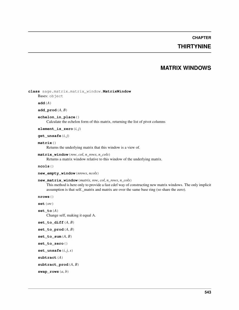
CHAPTER
THIRTYNINE
MATRIX WINDOWS
class sage.matrix.matrix_window.MatrixWindowBases: object
add(A)
add_prod(A, B)
echelon_in_place()Calculate the echelon form of this matrix, returning the list of pivot columns
element_is_zero(i, j)
get_unsafe(i, j)
matrix()Returns the underlying matrix that this window is a view of.
matrix_window(row, col, n_rows, n_cols)Returns a matrix window relative to this window of the underlying matrix.
ncols()
new_empty_window(nrows, ncols)
new_matrix_window(matrix, row, col, n_rows, n_cols)This method is here only to provide a fast cdef way of constructing new matrix windows. The only implicitassumption is that self._matrix and matrix are over the same base ring (so share the zero).
nrows()
set(src)
set_to(A)Change self, making it equal A.
set_to_diff(A, B)
set_to_prod(A, B)
set_to_sum(A, B)
set_to_zero()
set_unsafe(i, j, x)
subtract(A)
subtract_prod(A, B)
swap_rows(a, b)
543

Sage Reference Manual: Matrices and Spaces of Matrices, Release 9.0
to_matrix()Returns an actual matrix object representing this view.
544 Chapter 39. Matrix windows
CHAPTER
FORTY
MISC MATRIX ALGORITHMS
Code goes here mainly when it needs access to the internal structure of several classes, and we want to avoid circularcimports.
NOTE: The whole problem of avoiding circular imports – the reason for existence of this file – is now a non-issue,since some bugs in Cython were fixed. Probably all this code should be moved into the relevant classes and this filedeleted.
sage.matrix.misc.cmp_pivots(x, y)Compare two sequences of pivot columns.
If x is shorter than y, return -1, i.e., x < y, “not as good”. If x is longer than y, then x > y, so “better” and return+1. If the length is the same, then x is better, i.e., x > y if the entries of x are correspondingly <= those of y withone being strictly less.
INPUT:
• x, y – lists or tuples of integers
EXAMPLES:
We illustrate each of the above comparisons.
sage: sage.matrix.misc.cmp_pivots([1,2,3], [4,5,6,7])-1sage: sage.matrix.misc.cmp_pivots([1,2,3,5], [4,5,6])1sage: sage.matrix.misc.cmp_pivots([1,2,4], [1,2,3])-1sage: sage.matrix.misc.cmp_pivots([1,2,3], [1,2,3])0sage: sage.matrix.misc.cmp_pivots([1,2,3], [1,2,4])1
sage.matrix.misc.hadamard_row_bound_mpfr(A)Given a matrix A with entries that coerce to RR, compute the row Hadamard bound on the determinant.
INPUT:
A – a matrix over RR
OUTPUT:
integer – an integer n such that the absolute value of the determinant of this matrix is at most$10^n$.
EXAMPLES:
We create a very large matrix, compute the row Hadamard bound, and also compute the row Hadamard boundof the transpose, which happens to be sharp.
545
Sage Reference Manual: Matrices and Spaces of Matrices, Release 9.0
sage: a = matrix(ZZ, 2, [2^10000,3^10000,2^50,3^19292])sage: import sage.matrix.miscsage: sage.matrix.misc.hadamard_row_bound_mpfr(a.change_ring(RR))13976sage: len(str(a.det()))12215sage: sage.matrix.misc.hadamard_row_bound_mpfr(a.transpose().change_ring(RR))12215
Note that in the above example using RDF would overflow:
sage: b = a.change_ring(RDF)sage: b._hadamard_row_bound()Traceback (most recent call last):...OverflowError: cannot convert float infinity to integer
sage.matrix.misc.matrix_integer_dense_rational_reconstruction(A, N)Given a matrix over the integers and an integer modulus, do rational reconstruction on all entries of the matrix,viewed as numbers mod N. This is done efficiently by assuming there is a large common factor dividing thedenominators.
INPUT:
A – matrix N – an integer
EXAMPLES:
sage: B = ((matrix(ZZ, 3,4, [1,2,3,-4,7,2,18,3,4,3,4,5])/3)%500).change_ring(ZZ)sage: sage.matrix.misc.matrix_integer_dense_rational_reconstruction(B, 500)[ 1/3 2/3 1 -4/3][ 7/3 2/3 6 1][ 4/3 1 4/3 5/3]
sage.matrix.misc.matrix_integer_sparse_rational_reconstruction(A, N)Given a sparse matrix over the integers and an integer modulus, do rational reconstruction on all entries of thematrix, viewed as numbers mod N.
EXAMPLES:
sage: A = matrix(ZZ, 3, 4, [(1/3)%500, 2, 3, (-4)%500, 7, 2, 2, 3, 4, 3, 4, (5/7)→˓%500], sparse=True)sage: sage.matrix.misc.matrix_integer_sparse_rational_reconstruction(A, 500)[1/3 2 3 -4][ 7 2 2 3][ 4 3 4 5/7]
sage.matrix.misc.matrix_rational_echelon_form_multimodular(self,height_guess=None,proof=None)
Returns reduced row-echelon form using a multi-modular algorithm. Does not change self.
REFERENCE: Chapter 7 of Stein’s “Explicitly Computing Modular Forms”.
INPUT:
• height_guess – integer or None
• proof – boolean or None (default: None, see proof.linear_algebra or sage.structure.proof). Note that theglobal Sage default is proof=True
546 Chapter 40. Misc matrix algorithms
Sage Reference Manual: Matrices and Spaces of Matrices, Release 9.0
OUTPUT: a pair consisting of a matrix in echelon form and a tuple of pivot positions.
ALGORITHM:
The following is a modular algorithm for computing the echelon form. Define the height of a matrix to be themax of the absolute values of the entries.
Given Matrix A with n columns (self).
0. Rescale input matrix A to have integer entries. This does not change echelon form and makes reductionmodulo lots of primes significantly easier if there were denominators. Henceforth we assume A has integerentries.
1. Let c be a guess for the height of the echelon form. E.g., c=1000, e.g., if matrix is very sparse andapplication is to computing modular symbols.
2. Let M = n * c * H(A) + 1, where n is the number of columns of A.
3. List primes p_1, p_2, . . . , such that the product of the p_i is at least M.
4. Try to compute the rational reconstruction CRT echelon form of A mod the product of the p_i. If rationalreconstruction fails, compute 1 more echelon forms mod the next prime, and attempt again. Make sure tokeep the result of CRT on the primes from before, so we don’t have to do that computation again. Let E bethis matrix.
5. Compute the denominator d of E. Attempt to prove that result is correct by checking that
H(d*E)*ncols(A)*H(A) < (prod of reduction primes)
where H denotes the height. If this fails, do step 4 with a few more primes.
EXAMPLES:
sage: A = matrix(QQ, 3, 7, [1..21])sage: from sage.matrix.misc import matrix_rational_echelon_form_multimodularsage: E, pivots = matrix_rational_echelon_form_multimodular(A)sage: E[ 1 0 -1 -2 -3 -4 -5][ 0 1 2 3 4 5 6][ 0 0 0 0 0 0 0]sage: pivots(0, 1)
sage: A = matrix(QQ, 3, 4, [0,0] + [1..9] + [-1/2^20])sage: E, pivots = matrix_rational_echelon_form_multimodular(A)sage: E[ 1 0 0 -10485761/1048576][ 0 1 0 27262979/4194304][ 0 0 1 2]sage: pivots(0, 1, 2)
sage: A.echelon_form()[ 1 0 0 -10485761/1048576][ 0 1 0 27262979/4194304][ 0 0 1 2]sage: A.pivots()(0, 1, 2)
547

Sage Reference Manual: Matrices and Spaces of Matrices, Release 9.0
548 Chapter 40. Misc matrix algorithms
CHAPTER
FORTYONE
CALCULATE SYMPLECTIC BASES FOR MATRICES OVER FIELDSAND THE INTEGERS.
This module finds a symplectic basis for an anti-symmetric, alternating matrix M defined over a field or the integers.
Anti-symmetric means that 𝑀 = −𝑀 𝑡, where 𝑀 𝑡 denotes the transpose of 𝑀 . Alternating means that the diagonalof 𝑀 is identically zero.
A symplectic basis is a basis of the form 𝑒1, . . . , 𝑒𝑗 , 𝑓1, . . . , 𝑓𝑗 , 𝑧1, . . . , 𝑧𝑘 such that
• 𝑧𝑖𝑀𝑣𝑡 = 0 for all vectors 𝑣;
• 𝑒𝑖𝑀𝑒𝑗𝑡 = 0 for all 𝑖, 𝑗;
• 𝑓𝑖𝑀𝑓𝑗𝑡 = 0 for all 𝑖, 𝑗;
• 𝑒𝑖𝑀𝑓𝑗𝑡 = 0 for all 𝑖 not equal 𝑗;
and such that the non-zero terms
• 𝑒𝑖𝑀𝑓𝑖𝑡 are “as nice as possible”: 1 over fields, or integers satisfying divisibility properties otherwise.
REFERENCES:
Bourbaki gives a nice proof that can be made constructive but is not efficient (see Section 5, Number 1, Theorem 1,page 79):
Bourbaki, N. Elements of Mathematics, Algebra III, Springer Verlag 2007.
Kuperberg gives a more efficient and constructive exposition (see Theorem 18).
Kuperberg, Greg. Kasteleyn Cokernels. Electr. J. Comb. 9(1), 2002.
Todo: The routine over the integers applies over general principal ideal domains.
Warning: This code is not a good candidate for conversion to Cython. The majority of the execution time isspent adding multiples of columns and rows, which is already fast. It would be better to devise a better algorithm,perhaps modular or based on a fast smith_form implementation.
AUTHOR:
• Nick Alexander: initial implementation
• David Loeffler (2008-12-08): changed conventions for consistency with smith_form
sage.matrix.symplectic_basis.symplectic_basis_over_ZZ(M)Find a symplectic basis for an anti-symmetric, alternating matrix M defined over the integers.
549
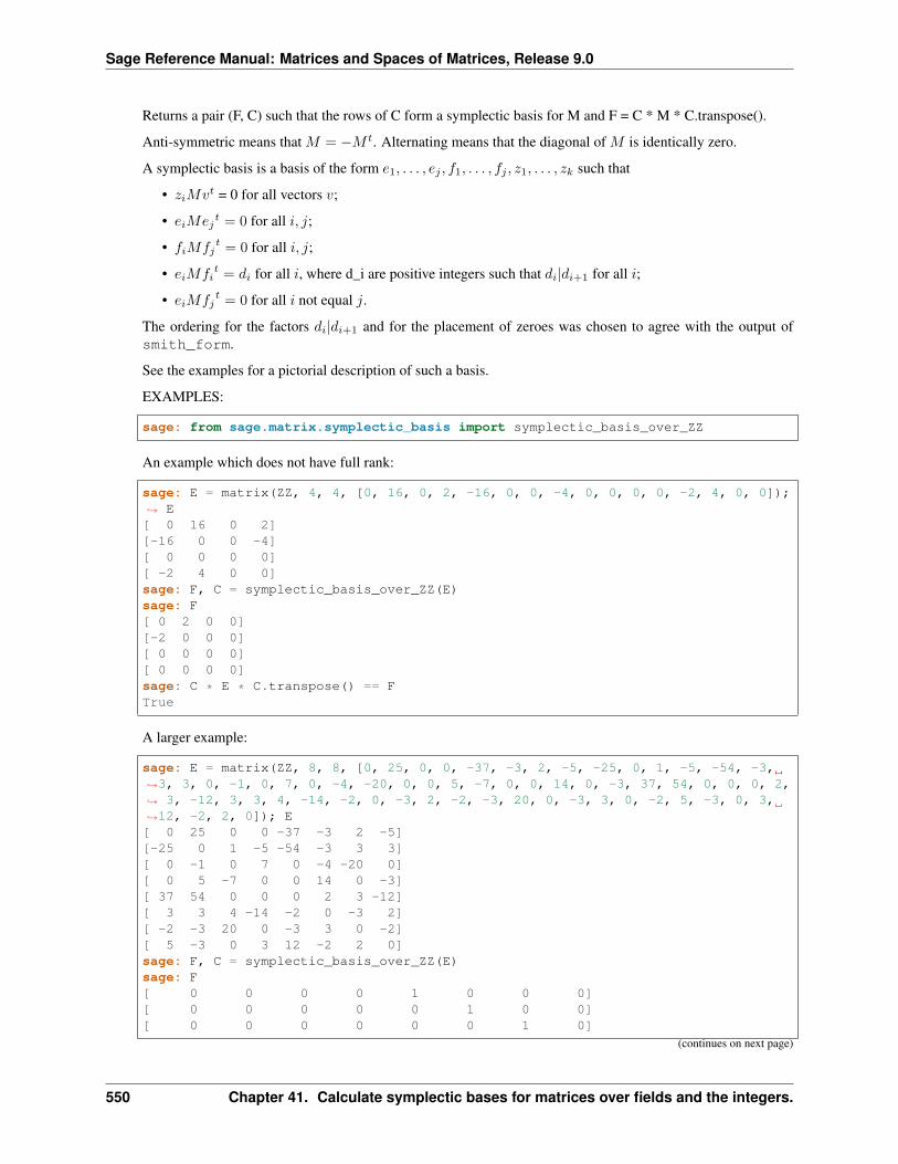
Sage Reference Manual: Matrices and Spaces of Matrices, Release 9.0
Returns a pair (F, C) such that the rows of C form a symplectic basis for M and F = C * M * C.transpose().
Anti-symmetric means that 𝑀 = −𝑀 𝑡. Alternating means that the diagonal of 𝑀 is identically zero.
A symplectic basis is a basis of the form 𝑒1, . . . , 𝑒𝑗 , 𝑓1, . . . , 𝑓𝑗 , 𝑧1, . . . , 𝑧𝑘 such that
• 𝑧𝑖𝑀𝑣𝑡 = 0 for all vectors 𝑣;
• 𝑒𝑖𝑀𝑒𝑗𝑡 = 0 for all 𝑖, 𝑗;
• 𝑓𝑖𝑀𝑓𝑗𝑡 = 0 for all 𝑖, 𝑗;
• 𝑒𝑖𝑀𝑓𝑖𝑡 = 𝑑𝑖 for all 𝑖, where d_i are positive integers such that 𝑑𝑖|𝑑𝑖+1 for all 𝑖;
• 𝑒𝑖𝑀𝑓𝑗𝑡 = 0 for all 𝑖 not equal 𝑗.
The ordering for the factors 𝑑𝑖|𝑑𝑖+1 and for the placement of zeroes was chosen to agree with the output ofsmith_form.
See the examples for a pictorial description of such a basis.
EXAMPLES:
sage: from sage.matrix.symplectic_basis import symplectic_basis_over_ZZ
An example which does not have full rank:
sage: E = matrix(ZZ, 4, 4, [0, 16, 0, 2, -16, 0, 0, -4, 0, 0, 0, 0, -2, 4, 0, 0]);→˓ E[ 0 16 0 2][-16 0 0 -4][ 0 0 0 0][ -2 4 0 0]sage: F, C = symplectic_basis_over_ZZ(E)sage: F[ 0 2 0 0][-2 0 0 0][ 0 0 0 0][ 0 0 0 0]sage: C * E * C.transpose() == FTrue
A larger example:
sage: E = matrix(ZZ, 8, 8, [0, 25, 0, 0, -37, -3, 2, -5, -25, 0, 1, -5, -54, -3,→˓3, 3, 0, -1, 0, 7, 0, -4, -20, 0, 0, 5, -7, 0, 0, 14, 0, -3, 37, 54, 0, 0, 0, 2,→˓ 3, -12, 3, 3, 4, -14, -2, 0, -3, 2, -2, -3, 20, 0, -3, 3, 0, -2, 5, -3, 0, 3,→˓12, -2, 2, 0]); E[ 0 25 0 0 -37 -3 2 -5][-25 0 1 -5 -54 -3 3 3][ 0 -1 0 7 0 -4 -20 0][ 0 5 -7 0 0 14 0 -3][ 37 54 0 0 0 2 3 -12][ 3 3 4 -14 -2 0 -3 2][ -2 -3 20 0 -3 3 0 -2][ 5 -3 0 3 12 -2 2 0]sage: F, C = symplectic_basis_over_ZZ(E)sage: F[ 0 0 0 0 1 0 0 0][ 0 0 0 0 0 1 0 0][ 0 0 0 0 0 0 1 0]
(continues on next page)
550 Chapter 41. Calculate symplectic bases for matrices over fields and the integers.
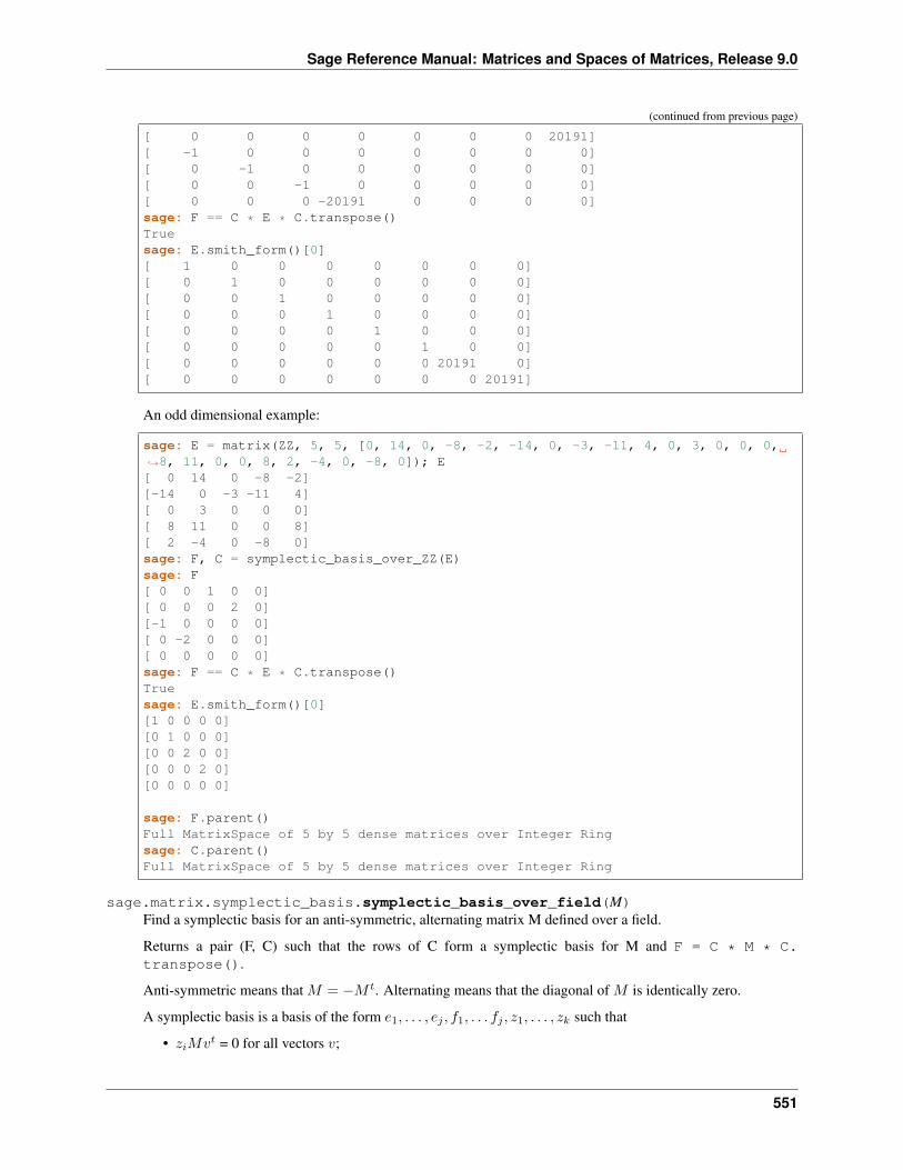
Sage Reference Manual: Matrices and Spaces of Matrices, Release 9.0
(continued from previous page)
[ 0 0 0 0 0 0 0 20191][ -1 0 0 0 0 0 0 0][ 0 -1 0 0 0 0 0 0][ 0 0 -1 0 0 0 0 0][ 0 0 0 -20191 0 0 0 0]sage: F == C * E * C.transpose()Truesage: E.smith_form()[0][ 1 0 0 0 0 0 0 0][ 0 1 0 0 0 0 0 0][ 0 0 1 0 0 0 0 0][ 0 0 0 1 0 0 0 0][ 0 0 0 0 1 0 0 0][ 0 0 0 0 0 1 0 0][ 0 0 0 0 0 0 20191 0][ 0 0 0 0 0 0 0 20191]
An odd dimensional example:
sage: E = matrix(ZZ, 5, 5, [0, 14, 0, -8, -2, -14, 0, -3, -11, 4, 0, 3, 0, 0, 0,→˓8, 11, 0, 0, 8, 2, -4, 0, -8, 0]); E[ 0 14 0 -8 -2][-14 0 -3 -11 4][ 0 3 0 0 0][ 8 11 0 0 8][ 2 -4 0 -8 0]sage: F, C = symplectic_basis_over_ZZ(E)sage: F[ 0 0 1 0 0][ 0 0 0 2 0][-1 0 0 0 0][ 0 -2 0 0 0][ 0 0 0 0 0]sage: F == C * E * C.transpose()Truesage: E.smith_form()[0][1 0 0 0 0][0 1 0 0 0][0 0 2 0 0][0 0 0 2 0][0 0 0 0 0]
sage: F.parent()Full MatrixSpace of 5 by 5 dense matrices over Integer Ringsage: C.parent()Full MatrixSpace of 5 by 5 dense matrices over Integer Ring
sage.matrix.symplectic_basis.symplectic_basis_over_field(M)Find a symplectic basis for an anti-symmetric, alternating matrix M defined over a field.
Returns a pair (F, C) such that the rows of C form a symplectic basis for M and F = C * M * C.transpose().
Anti-symmetric means that 𝑀 = −𝑀 𝑡. Alternating means that the diagonal of 𝑀 is identically zero.
A symplectic basis is a basis of the form 𝑒1, . . . , 𝑒𝑗 , 𝑓1, . . . 𝑓𝑗 , 𝑧1, . . . , 𝑧𝑘 such that
• 𝑧𝑖𝑀𝑣𝑡 = 0 for all vectors 𝑣;
551
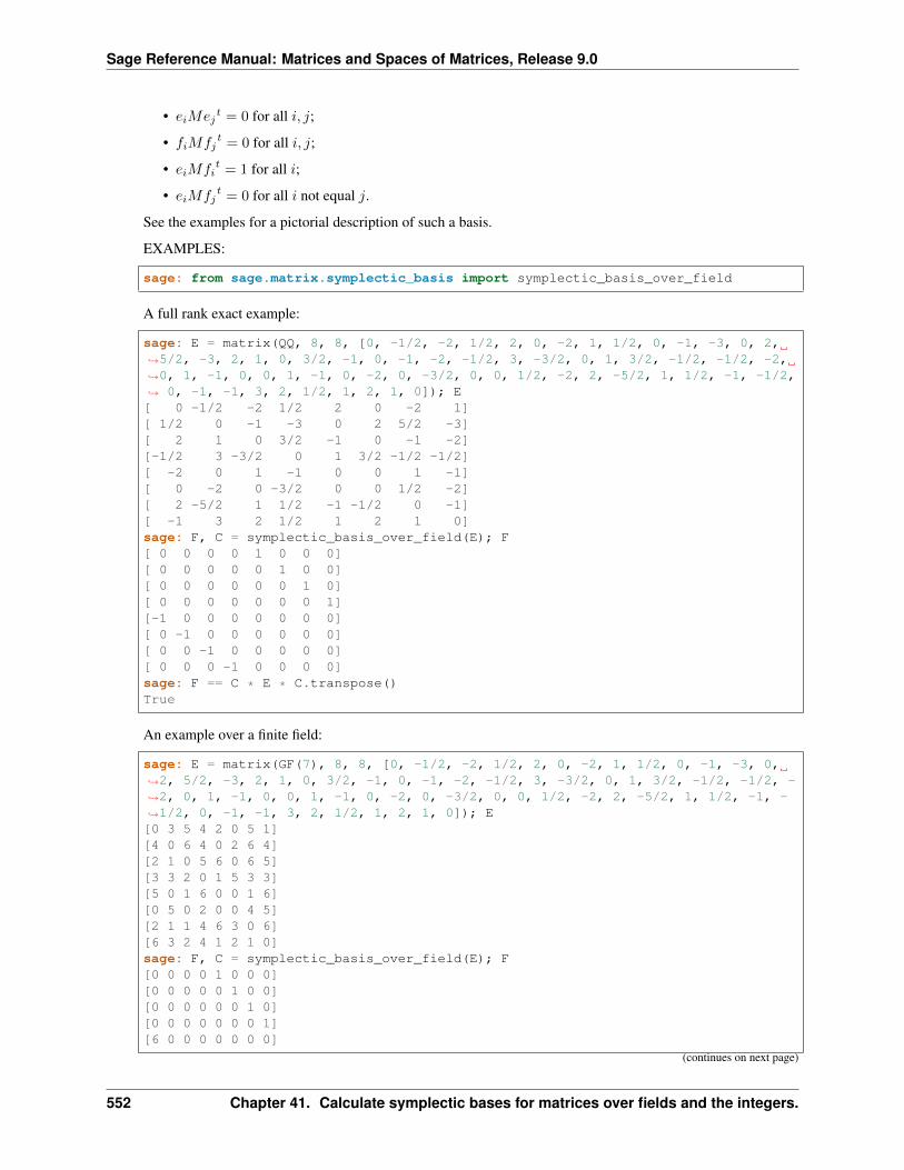
Sage Reference Manual: Matrices and Spaces of Matrices, Release 9.0
• 𝑒𝑖𝑀𝑒𝑗𝑡 = 0 for all 𝑖, 𝑗;
• 𝑓𝑖𝑀𝑓𝑗𝑡 = 0 for all 𝑖, 𝑗;
• 𝑒𝑖𝑀𝑓𝑖𝑡 = 1 for all 𝑖;
• 𝑒𝑖𝑀𝑓𝑗𝑡 = 0 for all 𝑖 not equal 𝑗.
See the examples for a pictorial description of such a basis.
EXAMPLES:
sage: from sage.matrix.symplectic_basis import symplectic_basis_over_field
A full rank exact example:
sage: E = matrix(QQ, 8, 8, [0, -1/2, -2, 1/2, 2, 0, -2, 1, 1/2, 0, -1, -3, 0, 2,→˓5/2, -3, 2, 1, 0, 3/2, -1, 0, -1, -2, -1/2, 3, -3/2, 0, 1, 3/2, -1/2, -1/2, -2,→˓0, 1, -1, 0, 0, 1, -1, 0, -2, 0, -3/2, 0, 0, 1/2, -2, 2, -5/2, 1, 1/2, -1, -1/2,→˓ 0, -1, -1, 3, 2, 1/2, 1, 2, 1, 0]); E[ 0 -1/2 -2 1/2 2 0 -2 1][ 1/2 0 -1 -3 0 2 5/2 -3][ 2 1 0 3/2 -1 0 -1 -2][-1/2 3 -3/2 0 1 3/2 -1/2 -1/2][ -2 0 1 -1 0 0 1 -1][ 0 -2 0 -3/2 0 0 1/2 -2][ 2 -5/2 1 1/2 -1 -1/2 0 -1][ -1 3 2 1/2 1 2 1 0]sage: F, C = symplectic_basis_over_field(E); F[ 0 0 0 0 1 0 0 0][ 0 0 0 0 0 1 0 0][ 0 0 0 0 0 0 1 0][ 0 0 0 0 0 0 0 1][-1 0 0 0 0 0 0 0][ 0 -1 0 0 0 0 0 0][ 0 0 -1 0 0 0 0 0][ 0 0 0 -1 0 0 0 0]sage: F == C * E * C.transpose()True
An example over a finite field:
sage: E = matrix(GF(7), 8, 8, [0, -1/2, -2, 1/2, 2, 0, -2, 1, 1/2, 0, -1, -3, 0,→˓2, 5/2, -3, 2, 1, 0, 3/2, -1, 0, -1, -2, -1/2, 3, -3/2, 0, 1, 3/2, -1/2, -1/2, -→˓2, 0, 1, -1, 0, 0, 1, -1, 0, -2, 0, -3/2, 0, 0, 1/2, -2, 2, -5/2, 1, 1/2, -1, -→˓1/2, 0, -1, -1, 3, 2, 1/2, 1, 2, 1, 0]); E[0 3 5 4 2 0 5 1][4 0 6 4 0 2 6 4][2 1 0 5 6 0 6 5][3 3 2 0 1 5 3 3][5 0 1 6 0 0 1 6][0 5 0 2 0 0 4 5][2 1 1 4 6 3 0 6][6 3 2 4 1 2 1 0]sage: F, C = symplectic_basis_over_field(E); F[0 0 0 0 1 0 0 0][0 0 0 0 0 1 0 0][0 0 0 0 0 0 1 0][0 0 0 0 0 0 0 1][6 0 0 0 0 0 0 0]
(continues on next page)
552 Chapter 41. Calculate symplectic bases for matrices over fields and the integers.

Sage Reference Manual: Matrices and Spaces of Matrices, Release 9.0
(continued from previous page)
[0 6 0 0 0 0 0 0][0 0 6 0 0 0 0 0][0 0 0 6 0 0 0 0]sage: F == C * E * C.transpose()True
The tricky case of characteristic 2:
sage: E = matrix(GF(2), 8, 8, [0, 0, 1, 1, 0, 1, 0, 1, 0, 0, 0, 0, 0, 0, 0, 0, 1,→˓0, 0, 0, 0, 0, 1, 1, 1, 0, 0, 0, 0, 0, 0, 1, 0, 0, 0, 0, 0, 1, 1, 0, 1, 0, 0, 0,→˓ 1, 0, 1, 1, 0, 0, 1, 0, 1, 1, 0, 0, 1, 0, 1, 1, 0, 1, 0, 0]); E[0 0 1 1 0 1 0 1][0 0 0 0 0 0 0 0][1 0 0 0 0 0 1 1][1 0 0 0 0 0 0 1][0 0 0 0 0 1 1 0][1 0 0 0 1 0 1 1][0 0 1 0 1 1 0 0][1 0 1 1 0 1 0 0]sage: F, C = symplectic_basis_over_field(E); F[0 0 0 1 0 0 0 0][0 0 0 0 1 0 0 0][0 0 0 0 0 1 0 0][1 0 0 0 0 0 0 0][0 1 0 0 0 0 0 0][0 0 1 0 0 0 0 0][0 0 0 0 0 0 0 0][0 0 0 0 0 0 0 0]sage: F == C * E * C.transpose()True
An inexact example:
sage: E = matrix(RR, 8, 8, [0.000000000000000, 0.420674846479344, -0.→˓839702420666807, 0.658715385244413, 1.69467394825853, -1.14718543053828, 1.→˓03076138152950, -0.227739521708484, -0.420674846479344, 0.000000000000000, 0.→˓514381455379082, 0.282194064028260, -1.38977093018412, 0.278305070958958, -0.→˓0781320488361574, -0.496003664217833, 0.839702420666807, -0.514381455379082, 0.→˓000000000000000, -0.00618222322875384, -0.318386939149028, -0.0840205427053993,→˓1.28202592892333, -0.512563654267693, -0.658715385244413, -0.282194064028260, 0.→˓00618222322875384, 0.000000000000000, 0.852525732369211, -0.356957405431611, -0.→˓699960114607661, 0.0260496330859998, -1.69467394825853, 1.38977093018412, 0.→˓318386939149028, -0.852525732369211, 0.000000000000000, -0.836072521423577, 0.→˓450137632758469, -0.696145287292091, 1.14718543053828, -0.278305070958958, 0.→˓0840205427053993, 0.356957405431611, 0.836072521423577, 0.000000000000000, 0.→˓214878541347751, -1.20221688928379, -1.03076138152950, 0.0781320488361574, -1.→˓28202592892333, 0.699960114607661, -0.450137632758469, -0.214878541347751, 0.→˓000000000000000, 0.785074452163036, 0.227739521708484, 0.496003664217833, 0.→˓512563654267693, -0.0260496330859998, 0.696145287292091, 1.20221688928379, -0.→˓785074452163036, 0.000000000000000]); E[ 0.000000000000000 0.420674846479344 -0.839702420666807 0.→˓658715385244413 1.69467394825853 -1.14718543053828 1.03076138152950→˓ -0.227739521708484][ -0.420674846479344 0.000000000000000 0.514381455379082 0.→˓282194064028260 -1.38977093018412 0.278305070958958 -0.0781320488361574→˓ -0.496003664217833][ 0.839702420666807 -0.514381455379082 0.000000000000000 -0.→˓00618222322875384 -0.318386939149028 -0.0840205427053993 1.→˓28202592892333 -0.512563654267693]
(continues on next page)
553
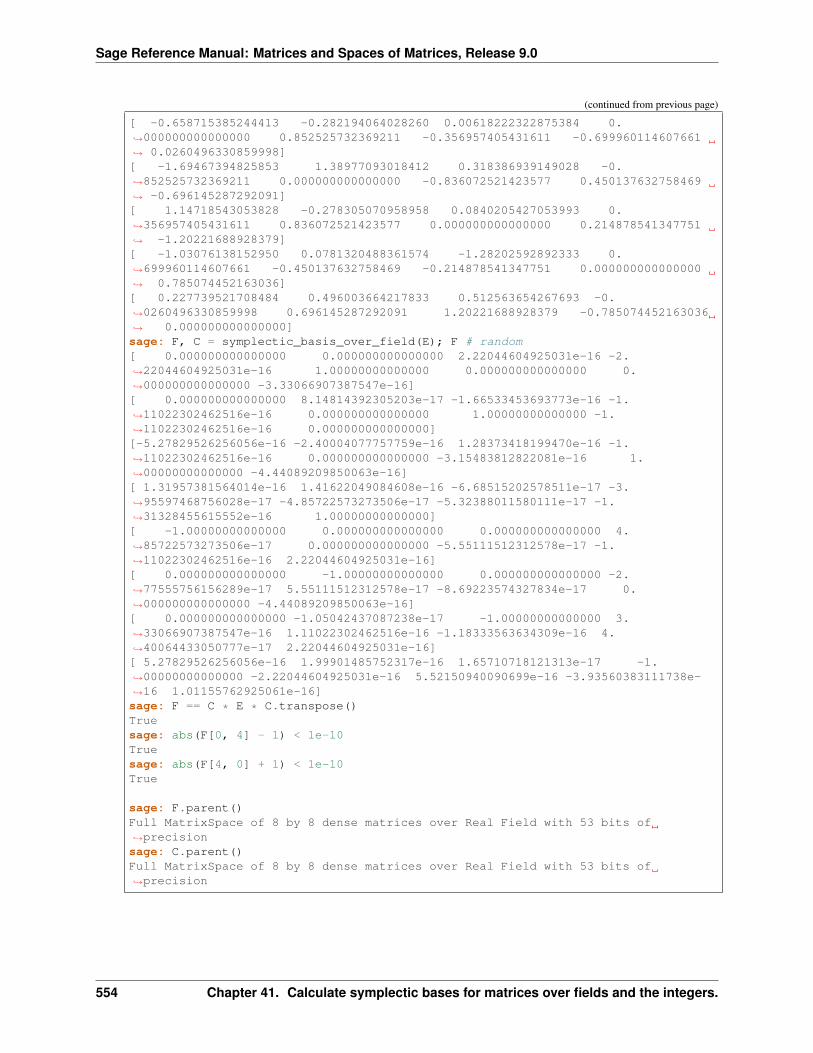
Sage Reference Manual: Matrices and Spaces of Matrices, Release 9.0
(continued from previous page)
[ -0.658715385244413 -0.282194064028260 0.00618222322875384 0.→˓000000000000000 0.852525732369211 -0.356957405431611 -0.699960114607661→˓ 0.0260496330859998][ -1.69467394825853 1.38977093018412 0.318386939149028 -0.→˓852525732369211 0.000000000000000 -0.836072521423577 0.450137632758469→˓ -0.696145287292091][ 1.14718543053828 -0.278305070958958 0.0840205427053993 0.→˓356957405431611 0.836072521423577 0.000000000000000 0.214878541347751→˓ -1.20221688928379][ -1.03076138152950 0.0781320488361574 -1.28202592892333 0.→˓699960114607661 -0.450137632758469 -0.214878541347751 0.000000000000000→˓ 0.785074452163036][ 0.227739521708484 0.496003664217833 0.512563654267693 -0.→˓0260496330859998 0.696145287292091 1.20221688928379 -0.785074452163036→˓ 0.000000000000000]sage: F, C = symplectic_basis_over_field(E); F # random[ 0.000000000000000 0.000000000000000 2.22044604925031e-16 -2.→˓22044604925031e-16 1.00000000000000 0.000000000000000 0.→˓000000000000000 -3.33066907387547e-16][ 0.000000000000000 8.14814392305203e-17 -1.66533453693773e-16 -1.→˓11022302462516e-16 0.000000000000000 1.00000000000000 -1.→˓11022302462516e-16 0.000000000000000][-5.27829526256056e-16 -2.40004077757759e-16 1.28373418199470e-16 -1.→˓11022302462516e-16 0.000000000000000 -3.15483812822081e-16 1.→˓00000000000000 -4.44089209850063e-16][ 1.31957381564014e-16 1.41622049084608e-16 -6.68515202578511e-17 -3.→˓95597468756028e-17 -4.85722573273506e-17 -5.32388011580111e-17 -1.→˓31328455615552e-16 1.00000000000000][ -1.00000000000000 0.000000000000000 0.000000000000000 4.→˓85722573273506e-17 0.000000000000000 -5.55111512312578e-17 -1.→˓11022302462516e-16 2.22044604925031e-16][ 0.000000000000000 -1.00000000000000 0.000000000000000 -2.→˓77555756156289e-17 5.55111512312578e-17 -8.69223574327834e-17 0.→˓000000000000000 -4.44089209850063e-16][ 0.000000000000000 -1.05042437087238e-17 -1.00000000000000 3.→˓33066907387547e-16 1.11022302462516e-16 -1.18333563634309e-16 4.→˓40064433050777e-17 2.22044604925031e-16][ 5.27829526256056e-16 1.99901485752317e-16 1.65710718121313e-17 -1.→˓00000000000000 -2.22044604925031e-16 5.52150940090699e-16 -3.93560383111738e-→˓16 1.01155762925061e-16]sage: F == C * E * C.transpose()Truesage: abs(F[0, 4] - 1) < 1e-10Truesage: abs(F[4, 0] + 1) < 1e-10True
sage: F.parent()Full MatrixSpace of 8 by 8 dense matrices over Real Field with 53 bits of→˓precisionsage: C.parent()Full MatrixSpace of 8 by 8 dense matrices over Real Field with 53 bits of→˓precision
554 Chapter 41. Calculate symplectic bases for matrices over fields and the integers.
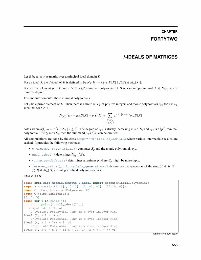
CHAPTER
FORTYTWO
𝐽-IDEALS OF MATRICES
Let 𝐵 be an 𝑛× 𝑛-matrix over a principal ideal domain 𝐷.
For an ideal 𝐽 , the 𝐽-ideal of 𝐵 is defined to be 𝑁𝐽(𝐵) = {𝑓 ∈ 𝐷[𝑋] | 𝑓(𝐵) ∈ 𝑀𝑛(𝐽)}.
For a prime element 𝑝 of 𝐷 and 𝑡 ≥ 0, a (𝑝𝑡)-minimal polynomial of 𝐵 is a monic polynomial 𝑓 ∈ 𝑁(𝑝𝑡)(𝐵) ofminimal degree.
This module computes these minimal polynomials.
Let 𝑝 be a prime element of 𝐷. Then there is a finite set 𝒮𝑝 of positive integers and monic polynomials 𝜈𝑝𝑠 for 𝑠 ∈ 𝒮𝑝
such that for 𝑡 ≥ 1,
𝑁(𝑝𝑡)(𝐵) = 𝜇𝐵𝐷[𝑋] + 𝑝𝑡𝐷[𝑋] +∑︁𝑠∈𝒮𝑝
𝑠≤𝑏(𝑡)
𝑝max{0,𝑡−𝑠}𝜈𝑝𝑠𝐷[𝑋]
holds where 𝑏(𝑡) = min{𝑟 ∈ 𝒮𝑝 | 𝑟 ≥ 𝑠}. The degree of 𝜈𝑝𝑠 is strictly increasing in 𝑠 ∈ 𝒮𝑝 and 𝜈𝑝𝑠 is a (𝑝𝑠)-minimalpolynomial. If 𝑡 ≤ max𝒮𝑝, then the summand 𝜇𝐵𝐷[𝑋] can be omitted.
All computations are done by the class ComputeMinimalPolynomials where various intermediate results arecached. It provides the following methods:
• p_minimal_polynomials() computes 𝒮𝑝 and the monic polynomials 𝜈𝑝𝑠.
• null_ideal() determines 𝑁(𝑝𝑡)(𝐵).
• prime_candidates() determines all primes 𝑝 where 𝒮𝑝 might be non-empty.
• integer_valued_polynomials_generators() determines the generators of the ring {𝑓 ∈ 𝐾[𝑋] |𝑓(𝐵) ∈ 𝑀𝑛(𝐷)} of integer valued polynomials on 𝐵.
EXAMPLES:
sage: from sage.matrix.compute_J_ideal import ComputeMinimalPolynomialssage: B = matrix(ZZ, [[1, 0, 1], [1, -2, -1], [10, 0, 0]])sage: C = ComputeMinimalPolynomials(B)sage: C.prime_candidates()[2, 3, 5]sage: for t in range(4):....: print(C.null_ideal(2^t))Principal ideal (1) of
Univariate Polynomial Ring in x over Integer RingIdeal (2, x^2 + x) of
Univariate Polynomial Ring in x over Integer RingIdeal (4, x^2 + 3*x + 2) of
Univariate Polynomial Ring in x over Integer RingIdeal (8, x^3 + x^2 - 12*x - 20, 2*x^2 + 6*x + 4) of
(continues on next page)
555
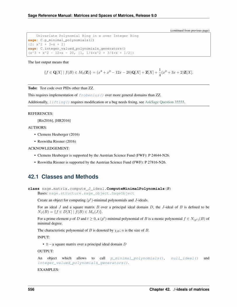
Sage Reference Manual: Matrices and Spaces of Matrices, Release 9.0
(continued from previous page)
Univariate Polynomial Ring in x over Integer Ringsage: C.p_minimal_polynomials(2){2: x^2 + 3*x + 2}sage: C.integer_valued_polynomials_generators()(x^3 + x^2 - 12*x - 20, [1, 1/4*x^2 + 3/4*x + 1/2])
The last output means that
{𝑓 ∈ Q[𝑋] | 𝑓(𝐵) ∈ 𝑀3(Z)} = (𝑥3 + 𝑥2 − 12𝑥− 20)Q[𝑋] + Z[𝑋] +1
4(𝑥2 + 3𝑥+ 2)Z[𝑋].
Todo: Test code over PIDs other than ZZ.
This requires implementation of frobenius() over more general domains than ZZ.
Additionally, lifting() requires modification or a bug needs fixing, see AskSage Question 35555.
REFERENCES:
[Ris2016], [HR2016]
AUTHORS:
• Clemens Heuberger (2016)
• Roswitha Rissner (2016)
ACKNOWLEDGEMENT:
• Clemens Heuberger is supported by the Austrian Science Fund (FWF): P 24644-N26.
• Roswitha Rissner is supported by the Austrian Science Fund (FWF): P 27816-N26.
42.1 Classes and Methods
class sage.matrix.compute_J_ideal.ComputeMinimalPolynomials(B)Bases: sage.structure.sage_object.SageObject
Create an object for computing (𝑝𝑡)-minimal polynomials and 𝐽-ideals.
For an ideal 𝐽 and a square matrix 𝐵 over a principal ideal domain 𝐷, the 𝐽-ideal of 𝐵 is defined to be𝑁𝐽(𝐵) = {𝑓 ∈ 𝐷[𝑋] | 𝑓(𝐵) ∈ 𝑀𝑛(𝐽)}.
For a prime element 𝑝 of 𝐷 and 𝑡 ≥ 0, a (𝑝𝑡)-minimal polynomial of 𝐵 is a monic polynomial 𝑓 ∈ 𝑁(𝑝𝑡)(𝐵) ofminimal degree.
The characteristic polynomial of 𝐵 is denoted by 𝜒𝐵 ; 𝑛 is the size of 𝐵.
INPUT:
• B – a square matrix over a principal ideal domain 𝐷
OUTPUT:
An object which allows to call p_minimal_polynomials(), null_ideal() andinteger_valued_polynomials_generators().
EXAMPLES:
556 Chapter 42. 𝐽-ideals of matrices
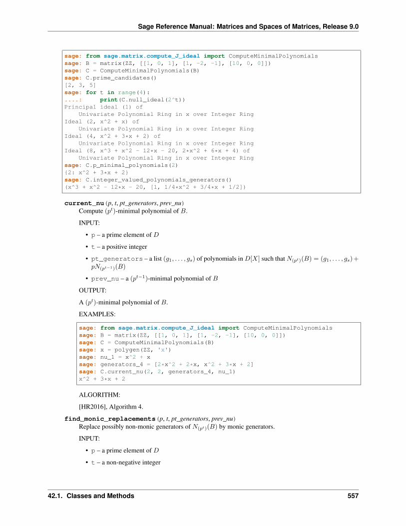
Sage Reference Manual: Matrices and Spaces of Matrices, Release 9.0
sage: from sage.matrix.compute_J_ideal import ComputeMinimalPolynomialssage: B = matrix(ZZ, [[1, 0, 1], [1, -2, -1], [10, 0, 0]])sage: C = ComputeMinimalPolynomials(B)sage: C.prime_candidates()[2, 3, 5]sage: for t in range(4):....: print(C.null_ideal(2^t))Principal ideal (1) of
Univariate Polynomial Ring in x over Integer RingIdeal (2, x^2 + x) of
Univariate Polynomial Ring in x over Integer RingIdeal (4, x^2 + 3*x + 2) of
Univariate Polynomial Ring in x over Integer RingIdeal (8, x^3 + x^2 - 12*x - 20, 2*x^2 + 6*x + 4) of
Univariate Polynomial Ring in x over Integer Ringsage: C.p_minimal_polynomials(2){2: x^2 + 3*x + 2}sage: C.integer_valued_polynomials_generators()(x^3 + x^2 - 12*x - 20, [1, 1/4*x^2 + 3/4*x + 1/2])
current_nu(p, t, pt_generators, prev_nu)Compute (𝑝𝑡)-minimal polynomial of 𝐵.
INPUT:
• p – a prime element of 𝐷
• t – a positive integer
• pt_generators – a list (𝑔1, . . . , 𝑔𝑠) of polynomials in 𝐷[𝑋] such that 𝑁(𝑝𝑡)(𝐵) = (𝑔1, . . . , 𝑔𝑠)+𝑝𝑁(𝑝𝑡−1)(𝐵)
• prev_nu – a (𝑝𝑡−1)-minimal polynomial of 𝐵
OUTPUT:
A (𝑝𝑡)-minimal polynomial of 𝐵.
EXAMPLES:
sage: from sage.matrix.compute_J_ideal import ComputeMinimalPolynomialssage: B = matrix(ZZ, [[1, 0, 1], [1, -2, -1], [10, 0, 0]])sage: C = ComputeMinimalPolynomials(B)sage: x = polygen(ZZ, 'x')sage: nu_1 = x^2 + xsage: generators_4 = [2*x^2 + 2*x, x^2 + 3*x + 2]sage: C.current_nu(2, 2, generators_4, nu_1)x^2 + 3*x + 2
ALGORITHM:
[HR2016], Algorithm 4.
find_monic_replacements(p, t, pt_generators, prev_nu)Replace possibly non-monic generators of 𝑁(𝑝𝑡)(𝐵) by monic generators.
INPUT:
• p – a prime element of 𝐷
• t – a non-negative integer
42.1. Classes and Methods 557
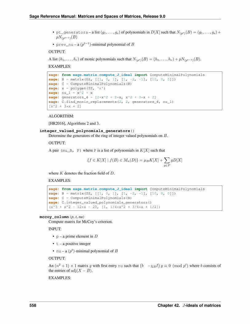
Sage Reference Manual: Matrices and Spaces of Matrices, Release 9.0
• pt_generators – a list (𝑔1, . . . , 𝑔𝑠) of polynomials in 𝐷[𝑋] such that 𝑁(𝑝𝑡)(𝐵) = (𝑔1, . . . , 𝑔𝑠)+𝑝𝑁(𝑝𝑡−1)(𝐵)
• prev_nu – a (𝑝𝑡−1)-minimal polynomial of 𝐵
OUTPUT:
A list (ℎ1, . . . , ℎ𝑟) of monic polynomials such that 𝑁(𝑝𝑡)(𝐵) = (ℎ1, . . . , ℎ𝑟) + 𝑝𝑁(𝑝𝑡−1)(𝐵).
EXAMPLES:
sage: from sage.matrix.compute_J_ideal import ComputeMinimalPolynomialssage: B = matrix(ZZ, [[1, 0, 1], [1, -2, -1], [10, 0, 0]])sage: C = ComputeMinimalPolynomials(B)sage: x = polygen(ZZ, 'x')sage: nu_1 = x^2 + xsage: generators_4 = [2*x^2 + 2*x, x^2 + 3*x + 2]sage: C.find_monic_replacements(2, 2, generators_4, nu_1)[x^2 + 3*x + 2]
ALGORITHM:
[HR2016], Algorithms 2 and 3.
integer_valued_polynomials_generators()Determine the generators of the ring of integer valued polynomials on 𝐵.
OUTPUT:
A pair (mu_B, P) where P is a list of polynomials in 𝐾[𝑋] such that
{𝑓 ∈ 𝐾[𝑋] | 𝑓(𝐵) ∈ 𝑀𝑛(𝐷)} = 𝜇𝐵𝐾[𝑋] +∑︁𝑔∈𝑃
𝑔𝐷[𝑋]
where 𝐾 denotes the fraction field of 𝐷.
EXAMPLES:
sage: from sage.matrix.compute_J_ideal import ComputeMinimalPolynomialssage: B = matrix(ZZ, [[1, 0, 1], [1, -2, -1], [10, 0, 0]])sage: C = ComputeMinimalPolynomials(B)sage: C.integer_valued_polynomials_generators()(x^3 + x^2 - 12*x - 20, [1, 1/4*x^2 + 3/4*x + 1/2])
mccoy_column(p, t, nu)Compute matrix for McCoy’s criterion.
INPUT:
• p – a prime element in 𝐷
• t – a positive integer
• nu – a (𝑝𝑡)-minimal polynomial of 𝐵
OUTPUT:
An (𝑛2 + 1) × 1 matrix 𝑔 with first entry nu such that(︀𝑏 −𝜒𝐵𝐼
)︀𝑔 ≡ 0 (mod 𝑝𝑡) where 𝑏 consists of
the entries of adj(𝑋 −𝐵).
EXAMPLES:
558 Chapter 42. 𝐽-ideals of matrices
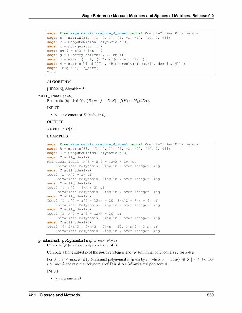
Sage Reference Manual: Matrices and Spaces of Matrices, Release 9.0
sage: from sage.matrix.compute_J_ideal import ComputeMinimalPolynomialssage: B = matrix(ZZ, [[1, 0, 1], [1, -2, -1], [10, 0, 0]])sage: C = ComputeMinimalPolynomials(B)sage: x = polygen(ZZ, 'x')sage: nu_4 = x^2 + 3*x + 2sage: g = C.mccoy_column(2, 2, nu_4)sage: b = matrix(9, 1, (x-B).adjugate().list())sage: M = matrix.block([[b , -B.charpoly(x)*matrix.identity(9)]])sage: (M*g % 4).is_zero()True
ALGORITHM:
[HR2016], Algorithm 5.
null_ideal(b=0)Return the (𝑏)-ideal 𝑁(𝑏)(𝐵) = {𝑓 ∈ 𝐷[𝑋] | 𝑓(𝐵) ∈ 𝑀𝑛(𝑏𝐷)}.
INPUT:
• b – an element of 𝐷 (default: 0)
OUTPUT:
An ideal in 𝐷[𝑋].
EXAMPLES:
sage: from sage.matrix.compute_J_ideal import ComputeMinimalPolynomialssage: B = matrix(ZZ, [[1, 0, 1], [1, -2, -1], [10, 0, 0]])sage: C = ComputeMinimalPolynomials(B)sage: C.null_ideal()Principal ideal (x^3 + x^2 - 12*x - 20) of
Univariate Polynomial Ring in x over Integer Ringsage: C.null_ideal(2)Ideal (2, x^2 + x) of
Univariate Polynomial Ring in x over Integer Ringsage: C.null_ideal(4)Ideal (4, x^2 + 3*x + 2) of
Univariate Polynomial Ring in x over Integer Ringsage: C.null_ideal(8)Ideal (8, x^3 + x^2 - 12*x - 20, 2*x^2 + 6*x + 4) of
Univariate Polynomial Ring in x over Integer Ringsage: C.null_ideal(3)Ideal (3, x^3 + x^2 - 12*x - 20) of
Univariate Polynomial Ring in x over Integer Ringsage: C.null_ideal(6)Ideal (6, 2*x^3 + 2*x^2 - 24*x - 40, 3*x^2 + 3*x) of
Univariate Polynomial Ring in x over Integer Ring
p_minimal_polynomials(p, s_max=None)Compute (𝑝𝑠)-minimal polynomials 𝜈𝑠 of 𝐵.
Compute a finite subset 𝒮 of the positive integers and (𝑝𝑠)-minimal polynomials 𝜈𝑠 for 𝑠 ∈ 𝒮.
For 0 < 𝑡 ≤ max𝒮, a (𝑝𝑡)-minimal polynomial is given by 𝜈𝑠 where 𝑠 = min{𝑟 ∈ 𝒮 | 𝑟 ≥ 𝑡}. For𝑡 > max𝒮, the minimal polynomial of 𝐵 is also a (𝑝𝑡)-minimal polynomial.
INPUT:
• p – a prime in 𝐷
42.1. Classes and Methods 559
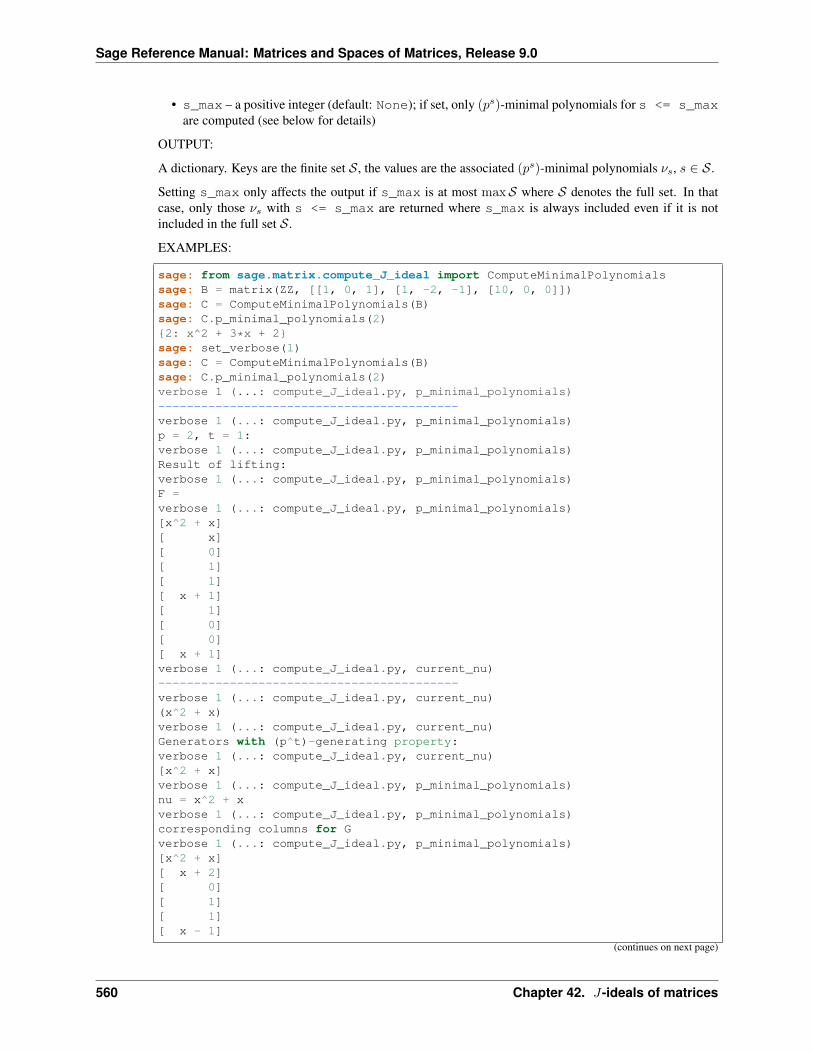
Sage Reference Manual: Matrices and Spaces of Matrices, Release 9.0
• s_max – a positive integer (default: None); if set, only (𝑝𝑠)-minimal polynomials for s <= s_maxare computed (see below for details)
OUTPUT:
A dictionary. Keys are the finite set 𝒮, the values are the associated (𝑝𝑠)-minimal polynomials 𝜈𝑠, 𝑠 ∈ 𝒮.
Setting s_max only affects the output if s_max is at most max𝒮 where 𝒮 denotes the full set. In thatcase, only those 𝜈𝑠 with s <= s_max are returned where s_max is always included even if it is notincluded in the full set 𝒮.
EXAMPLES:
sage: from sage.matrix.compute_J_ideal import ComputeMinimalPolynomialssage: B = matrix(ZZ, [[1, 0, 1], [1, -2, -1], [10, 0, 0]])sage: C = ComputeMinimalPolynomials(B)sage: C.p_minimal_polynomials(2){2: x^2 + 3*x + 2}sage: set_verbose(1)sage: C = ComputeMinimalPolynomials(B)sage: C.p_minimal_polynomials(2)verbose 1 (...: compute_J_ideal.py, p_minimal_polynomials)------------------------------------------verbose 1 (...: compute_J_ideal.py, p_minimal_polynomials)p = 2, t = 1:verbose 1 (...: compute_J_ideal.py, p_minimal_polynomials)Result of lifting:verbose 1 (...: compute_J_ideal.py, p_minimal_polynomials)F =verbose 1 (...: compute_J_ideal.py, p_minimal_polynomials)[x^2 + x][ x][ 0][ 1][ 1][ x + 1][ 1][ 0][ 0][ x + 1]verbose 1 (...: compute_J_ideal.py, current_nu)------------------------------------------verbose 1 (...: compute_J_ideal.py, current_nu)(x^2 + x)verbose 1 (...: compute_J_ideal.py, current_nu)Generators with (p^t)-generating property:verbose 1 (...: compute_J_ideal.py, current_nu)[x^2 + x]verbose 1 (...: compute_J_ideal.py, p_minimal_polynomials)nu = x^2 + xverbose 1 (...: compute_J_ideal.py, p_minimal_polynomials)corresponding columns for Gverbose 1 (...: compute_J_ideal.py, p_minimal_polynomials)[x^2 + x][ x + 2][ 0][ 1][ 1][ x - 1]
(continues on next page)
560 Chapter 42. 𝐽-ideals of matrices
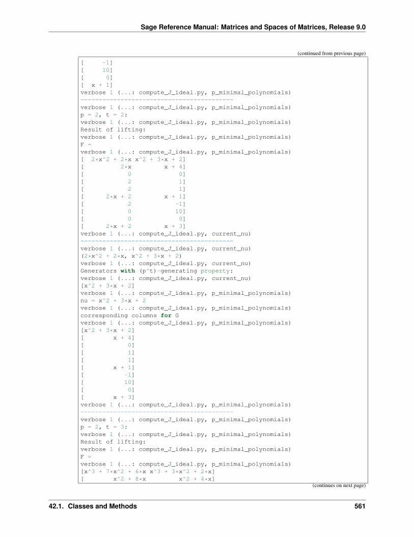
Sage Reference Manual: Matrices and Spaces of Matrices, Release 9.0
(continued from previous page)
[ -1][ 10][ 0][ x + 1]verbose 1 (...: compute_J_ideal.py, p_minimal_polynomials)------------------------------------------verbose 1 (...: compute_J_ideal.py, p_minimal_polynomials)p = 2, t = 2:verbose 1 (...: compute_J_ideal.py, p_minimal_polynomials)Result of lifting:verbose 1 (...: compute_J_ideal.py, p_minimal_polynomials)F =verbose 1 (...: compute_J_ideal.py, p_minimal_polynomials)[ 2*x^2 + 2*x x^2 + 3*x + 2][ 2*x x + 4][ 0 0][ 2 1][ 2 1][ 2*x + 2 x + 1][ 2 -1][ 0 10][ 0 0][ 2*x + 2 x + 3]verbose 1 (...: compute_J_ideal.py, current_nu)------------------------------------------verbose 1 (...: compute_J_ideal.py, current_nu)(2*x^2 + 2*x, x^2 + 3*x + 2)verbose 1 (...: compute_J_ideal.py, current_nu)Generators with (p^t)-generating property:verbose 1 (...: compute_J_ideal.py, current_nu)[x^2 + 3*x + 2]verbose 1 (...: compute_J_ideal.py, p_minimal_polynomials)nu = x^2 + 3*x + 2verbose 1 (...: compute_J_ideal.py, p_minimal_polynomials)corresponding columns for Gverbose 1 (...: compute_J_ideal.py, p_minimal_polynomials)[x^2 + 3*x + 2][ x + 4][ 0][ 1][ 1][ x + 1][ -1][ 10][ 0][ x + 3]verbose 1 (...: compute_J_ideal.py, p_minimal_polynomials)------------------------------------------verbose 1 (...: compute_J_ideal.py, p_minimal_polynomials)p = 2, t = 3:verbose 1 (...: compute_J_ideal.py, p_minimal_polynomials)Result of lifting:verbose 1 (...: compute_J_ideal.py, p_minimal_polynomials)F =verbose 1 (...: compute_J_ideal.py, p_minimal_polynomials)[x^3 + 7*x^2 + 6*x x^3 + 3*x^2 + 2*x][ x^2 + 8*x x^2 + 4*x]
(continues on next page)
42.1. Classes and Methods 561
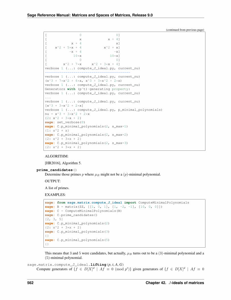
Sage Reference Manual: Matrices and Spaces of Matrices, Release 9.0
(continued from previous page)
[ 0 0][ x x + 4][ x + 4 x][ x^2 + 5*x + 4 x^2 + x][ -x + 4 -x][ 10*x 10*x][ 0 0][ x^2 + 7*x x^2 + 3*x + 4]verbose 1 (...: compute_J_ideal.py, current_nu)------------------------------------------verbose 1 (...: compute_J_ideal.py, current_nu)(x^3 + 7*x^2 + 6*x, x^3 + 3*x^2 + 2*x)verbose 1 (...: compute_J_ideal.py, current_nu)Generators with (p^t)-generating property:verbose 1 (...: compute_J_ideal.py, current_nu)...verbose 1 (...: compute_J_ideal.py, current_nu)[x^3 + 3*x^2 + 2*x]verbose 1 (...: compute_J_ideal.py, p_minimal_polynomials)nu = x^3 + 3*x^2 + 2*x{2: x^2 + 3*x + 2}sage: set_verbose(0)sage: C.p_minimal_polynomials(2, s_max=1){1: x^2 + x}sage: C.p_minimal_polynomials(2, s_max=2){2: x^2 + 3*x + 2}sage: C.p_minimal_polynomials(2, s_max=3){2: x^2 + 3*x + 2}
ALGORITHM:
[HR2016], Algorithm 5.
prime_candidates()Determine those primes 𝑝 where 𝜇𝐵 might not be a (𝑝)-minimal polynomial.
OUTPUT:
A list of primes.
EXAMPLES:
sage: from sage.matrix.compute_J_ideal import ComputeMinimalPolynomialssage: B = matrix(ZZ, [[1, 0, 1], [1, -2, -1], [10, 0, 0]])sage: C = ComputeMinimalPolynomials(B)sage: C.prime_candidates()[2, 3, 5]sage: C.p_minimal_polynomials(2){2: x^2 + 3*x + 2}sage: C.p_minimal_polynomials(3){}sage: C.p_minimal_polynomials(5){}
This means that 3 and 5 were candidates, but actually, 𝜇𝐵 turns out to be a (3)-minimal polynomial and a(5)-minimal polynomial.
sage.matrix.compute_J_ideal.lifting(p, t, A, G)Compute generators of {𝑓 ∈ 𝐷[𝑋]𝑑 | 𝐴𝑓 ≡ 0 (mod 𝑝𝑡)} given generators of {𝑓 ∈ 𝐷[𝑋]𝑑 | 𝐴𝑓 ≡ 0
562 Chapter 42. 𝐽-ideals of matrices
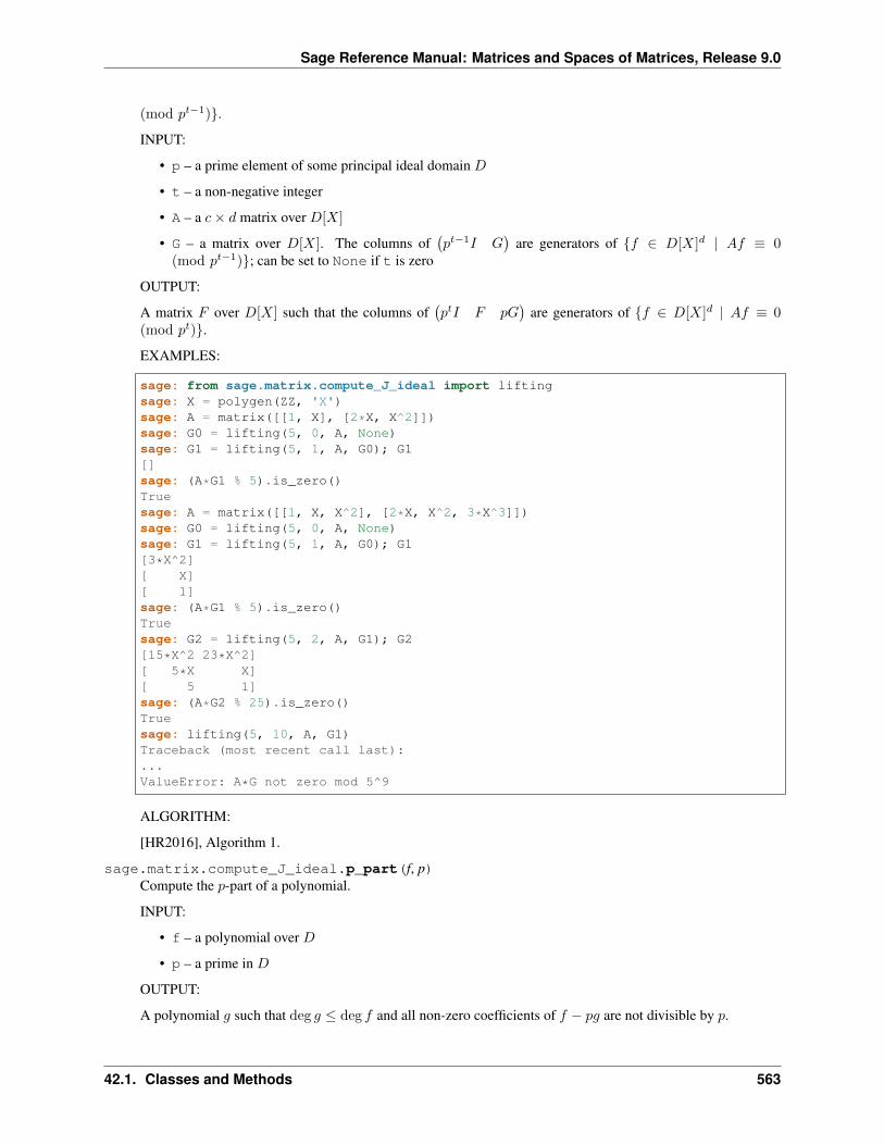
Sage Reference Manual: Matrices and Spaces of Matrices, Release 9.0
(mod 𝑝𝑡−1)}.
INPUT:
• p – a prime element of some principal ideal domain 𝐷
• t – a non-negative integer
• A – a 𝑐× 𝑑 matrix over 𝐷[𝑋]
• G – a matrix over 𝐷[𝑋]. The columns of(︀𝑝𝑡−1𝐼 𝐺
)︀are generators of {𝑓 ∈ 𝐷[𝑋]𝑑 | 𝐴𝑓 ≡ 0
(mod 𝑝𝑡−1)}; can be set to None if t is zero
OUTPUT:
A matrix 𝐹 over 𝐷[𝑋] such that the columns of(︀𝑝𝑡𝐼 𝐹 𝑝𝐺
)︀are generators of {𝑓 ∈ 𝐷[𝑋]𝑑 | 𝐴𝑓 ≡ 0
(mod 𝑝𝑡)}.
EXAMPLES:
sage: from sage.matrix.compute_J_ideal import liftingsage: X = polygen(ZZ, 'X')sage: A = matrix([[1, X], [2*X, X^2]])sage: G0 = lifting(5, 0, A, None)sage: G1 = lifting(5, 1, A, G0); G1[]sage: (A*G1 % 5).is_zero()Truesage: A = matrix([[1, X, X^2], [2*X, X^2, 3*X^3]])sage: G0 = lifting(5, 0, A, None)sage: G1 = lifting(5, 1, A, G0); G1[3*X^2][ X][ 1]sage: (A*G1 % 5).is_zero()Truesage: G2 = lifting(5, 2, A, G1); G2[15*X^2 23*X^2][ 5*X X][ 5 1]sage: (A*G2 % 25).is_zero()Truesage: lifting(5, 10, A, G1)Traceback (most recent call last):...ValueError: A*G not zero mod 5^9
ALGORITHM:
[HR2016], Algorithm 1.
sage.matrix.compute_J_ideal.p_part(f, p)Compute the 𝑝-part of a polynomial.
INPUT:
• f – a polynomial over 𝐷
• p – a prime in 𝐷
OUTPUT:
A polynomial 𝑔 such that deg 𝑔 ≤ deg 𝑓 and all non-zero coefficients of 𝑓 − 𝑝𝑔 are not divisible by 𝑝.
42.1. Classes and Methods 563
Sage Reference Manual: Matrices and Spaces of Matrices, Release 9.0
EXAMPLES:
sage: from sage.matrix.compute_J_ideal import p_partsage: X = polygen(ZZ, 'X')sage: f = X^3 + 5*X + 25sage: g = p_part(f, 5); gX + 5sage: f - 5*gX^3
564 Chapter 42. 𝐽-ideals of matrices
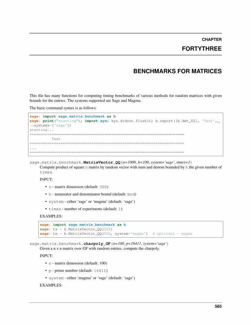
CHAPTER
FORTYTHREE
BENCHMARKS FOR MATRICES
This file has many functions for computing timing benchmarks of various methods for random matrices with givenbounds for the entries. The systems supported are Sage and Magma.
The basic command syntax is as follows:
sage: import sage.matrix.benchmark as bsage: print("starting"); import sys; sys.stdout.flush(); b.report([b.det_ZZ], 'Test',→˓systems=['sage'])starting...======================================================================
Test======================================================================...======================================================================
sage.matrix.benchmark.MatrixVector_QQ(n=1000, h=100, system=’sage’, times=1)Compute product of square n matrix by random vector with num and denom bounded by h the given number oftimes.
INPUT:
• n - matrix dimension (default: 300)
• h - numerator and denominator bound (default: bnd)
• system - either ‘sage’ or ‘magma’ (default: ‘sage’)
• times - number of experiments (default: 1)
EXAMPLES:
sage: import sage.matrix.benchmark as bsage: ts = b.MatrixVector_QQ(500)sage: tm = b.MatrixVector_QQ(500, system='magma') # optional - magma
sage.matrix.benchmark.charpoly_GF(n=100, p=16411, system=’sage’)Given a n x n matrix over GF with random entries, compute the charpoly.
INPUT:
• n - matrix dimension (default: 100)
• p - prime number (default: 16411)
• system - either ‘magma’ or ‘sage’ (default: ‘sage’)
EXAMPLES:
565
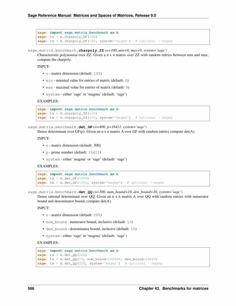
Sage Reference Manual: Matrices and Spaces of Matrices, Release 9.0
sage: import sage.matrix.benchmark as bsage: ts = b.charpoly_GF(100)sage: tm = b.charpoly_GF(100, system='magma') # optional - magma
sage.matrix.benchmark.charpoly_ZZ(n=100, min=0, max=9, system=’sage’)Characteristic polynomial over ZZ: Given a n x n matrix over ZZ with random entries between min and max,compute the charpoly.
INPUT:
• n - matrix dimension (default: 100)
• min - minimal value for entries of matrix (default: 0)
• max - maximal value for entries of matrix (default: 9)
• system - either ‘sage’ or ‘magma’ (default: ‘sage’)
EXAMPLES:
sage: import sage.matrix.benchmark as bsage: ts = b.charpoly_ZZ(100)sage: tm = b.charpoly_ZZ(100, system='magma') # optional - magma
sage.matrix.benchmark.det_GF(n=400, p=16411, system=’sage’)Dense determinant over GF(p). Given an n x n matrix A over GF with random entries compute det(A).
INPUT:
• n - matrix dimension (default: 300)
• p - prime number (default: 16411)
• system - either ‘magma’ or ‘sage’ (default: ‘sage’)
EXAMPLES:
sage: import sage.matrix.benchmark as bsage: ts = b.det_GF(1000)sage: tm = b.det_GF(1000, system='magma') # optional - magma
sage.matrix.benchmark.det_QQ(n=300, num_bound=10, den_bound=10, system=’sage’)Dense rational determinant over QQ. Given an n x n matrix A over QQ with random entries with numeratorbound and denominator bound, compute det(A).
INPUT:
• n - matrix dimension (default: 200)
• num_bound - numerator bound, inclusive (default: 10)
• den_bound - denominator bound, inclusive (default: 10)
• system - either ‘sage’ or ‘magma’ (default: ‘sage’)
EXAMPLES:
sage: import sage.matrix.benchmark as bsage: ts = b.det_QQ(200)sage: ts = b.det_QQ(10, num_bound=100000, den_bound=10000)sage: tm = b.det_QQ(200, system='magma') # optional - magma
566 Chapter 43. Benchmarks for matrices
Sage Reference Manual: Matrices and Spaces of Matrices, Release 9.0
sage.matrix.benchmark.det_ZZ(n=200, min=1, max=100, system=’sage’)Dense integer determinant over ZZ. Given an n x n matrix A over ZZ with random entries between min andmax, inclusive, compute det(A).
INPUT:
• n - matrix dimension (default: 200)
• min - minimal value for entries of matrix (default: 1)
• max - maximal value for entries of matrix (default: 100)
• system - either ‘sage’ or ‘magma’ (default: ‘sage’)
EXAMPLES:
sage: import sage.matrix.benchmark as bsage: ts = b.det_ZZ(200)sage: tm = b.det_ZZ(200, system='magma') # optional - magma
sage.matrix.benchmark.det_hilbert_QQ(n=80, system=’sage’)Runs the benchmark for calculating the determinant of the hilbert matrix over rationals of dimension n.
INPUT:
• n - matrix dimension (default: 300)
• system - either ‘sage’ or ‘magma’ (default: ‘sage’)
EXAMPLES:
sage: import sage.matrix.benchmark as bsage: ts = b.det_hilbert_QQ(50)sage: tm = b.det_hilbert_QQ(50, system='magma') # optional - magma
sage.matrix.benchmark.echelon_QQ(n=100, min=0, max=9, system=’sage’)Given a n x (2*n) matrix over QQ with random integer entries between min and max, compute the reduced rowechelon form.
INPUT:
• n - matrix dimension (default: 300)
• min - minimal value for entries of matrix (default: -9)
• max - maximal value for entries of matrix (default: 9)
• system - either ‘sage’ or ‘magma’ (default: ‘sage’)
EXAMPLES:
sage: import sage.matrix.benchmark as bsage: ts = b.echelon_QQ(100)sage: tm = b.echelon_QQ(100, system='magma') # optional - magma
sage.matrix.benchmark.hilbert_matrix(n)Returns the Hilbert matrix of size n over rationals.
EXAMPLES:
sage: import sage.matrix.benchmark as bsage: b.hilbert_matrix(3)[ 1 1/2 1/3]
(continues on next page)
567
Sage Reference Manual: Matrices and Spaces of Matrices, Release 9.0
(continued from previous page)
[1/2 1/3 1/4][1/3 1/4 1/5]
sage.matrix.benchmark.inverse_QQ(n=100, min=0, max=9, system=’sage’)Given a n x n matrix over QQ with random integer entries between min and max, compute the reduced rowechelon form.
INPUT:
• n - matrix dimension (default: 300)
• min - minimal value for entries of matrix (default: -9)
• max - maximal value for entries of matrix (default: 9)
• system - either ‘sage’ or ‘magma’ (default: ‘sage’)
EXAMPLES:
sage: import sage.matrix.benchmark as bsage: ts = b.inverse_QQ(100)sage: tm = b.inverse_QQ(100, system='magma') # optional - magma
sage.matrix.benchmark.invert_hilbert_QQ(n=40, system=’sage’)Runs the benchmark for calculating the inverse of the hilbert matrix over rationals of dimension n.
INPUT:
• n - matrix dimension (default: 300)
• system - either ‘sage’ or ‘magma’ (default: ‘sage’)
EXAMPLES:
sage: import sage.matrix.benchmark as bsage: ts = b.invert_hilbert_QQ(30)sage: tm = b.invert_hilbert_QQ(30, system='magma') # optional - magma
sage.matrix.benchmark.matrix_add_GF(n=1000, p=16411, system=’sage’, times=100)Given two n x n matrix over GF(p) with random entries, add them.
INPUT:
• n - matrix dimension (default: 300)
• p - prime number (default: 16411)
• system - either ‘magma’ or ‘sage’ (default: ‘sage’)
• times - number of experiments (default: 100)
EXAMPLES:
sage: import sage.matrix.benchmark as bsage: ts = b.matrix_add_GF(500, p=19)sage: tm = b.matrix_add_GF(500, p=19, system='magma') # optional - magma
sage.matrix.benchmark.matrix_add_ZZ(n=200, min=-9, max=9, system=’sage’, times=50)Matrix addition over ZZ Given an n x n matrix A and B over ZZ with random entries between min and max,inclusive, compute A + B times times.
INPUT:
568 Chapter 43. Benchmarks for matrices
Sage Reference Manual: Matrices and Spaces of Matrices, Release 9.0
• n - matrix dimension (default: 200)
• min - minimal value for entries of matrix (default: -9)
• max - maximal value for entries of matrix (default: 9)
• system - either ‘sage’ or ‘magma’ (default: ‘sage’)
• times - number of experiments (default: 50)
EXAMPLES:
sage: import sage.matrix.benchmark as bsage: ts = b.matrix_add_ZZ(200)sage: tm = b.matrix_add_ZZ(200, system='magma') # optional - magma
sage.matrix.benchmark.matrix_add_ZZ_2(n=200, bits=16, system=’sage’, times=50)Matrix addition over ZZ. Given an n x n matrix A and B over ZZ with random bits-bit entries, compute A +B.
INPUT:
• n - matrix dimension (default: 200)
• bits - bitsize of entries
• system - either ‘sage’ or ‘magma’ (default: ‘sage’)
• times - number of experiments (default: 50)
EXAMPLES:
sage: import sage.matrix.benchmark as bsage: ts = b.matrix_add_ZZ_2(200)sage: tm = b.matrix_add_ZZ_2(200, system='magma') # optional - magma
sage.matrix.benchmark.matrix_multiply_GF(n=100, p=16411, system=’sage’, times=3)Given an n x n matrix A over GF(p) with random entries, compute A * (A+1).
INPUT:
• n - matrix dimension (default: 100)
• p - prime number (default: 16411)
• system - either ‘magma’ or ‘sage’ (default: ‘sage’)
• times - number of experiments (default: 3)
EXAMPLES:
sage: import sage.matrix.benchmark as bsage: ts = b.matrix_multiply_GF(100, p=19)sage: tm = b.matrix_multiply_GF(100, p=19, system='magma') # optional - magma
sage.matrix.benchmark.matrix_multiply_QQ(n=100, bnd=2, system=’sage’, times=1)Given an n x n matrix A over QQ with random entries whose numerators and denominators are bounded by bnd,compute A * (A+1).
INPUT:
• n - matrix dimension (default: 300)
• bnd - numerator and denominator bound (default: bnd)
• system - either ‘sage’ or ‘magma’ (default: ‘sage’)
569
Sage Reference Manual: Matrices and Spaces of Matrices, Release 9.0
• times - number of experiments (default: 1)
EXAMPLES:
sage: import sage.matrix.benchmark as bsage: ts = b.matrix_multiply_QQ(100)sage: tm = b.matrix_multiply_QQ(100, system='magma') # optional - magma
sage.matrix.benchmark.matrix_multiply_ZZ(n=300, min=-9, max=9, system=’sage’,times=1)
Matrix multiplication over ZZ Given an n x n matrix A over ZZ with random entries between min and max,inclusive, compute A * (A+1).
INPUT:
• n - matrix dimension (default: 300)
• min - minimal value for entries of matrix (default: -9)
• max - maximal value for entries of matrix (default: 9)
• system - either ‘sage’ or ‘magma’ (default: ‘sage’)
• times - number of experiments (default: 1)
EXAMPLES:
sage: import sage.matrix.benchmark as bsage: ts = b.matrix_multiply_ZZ(200)sage: tm = b.matrix_multiply_ZZ(200, system='magma') # optional - magma
sage.matrix.benchmark.nullspace_GF(n=300, p=16411, system=’sage’)Given a n+1 x n matrix over GF(p) with random entries, compute the nullspace.
INPUT:
• n - matrix dimension (default: 300)
• p - prime number (default: 16411)
• system - either ‘magma’ or ‘sage’ (default: ‘sage’)
EXAMPLES:
sage: import sage.matrix.benchmark as bsage: ts = b.nullspace_GF(300)sage: tm = b.nullspace_GF(300, system='magma') # optional - magma
sage.matrix.benchmark.nullspace_RDF(n=300, min=0, max=10, system=’sage’)Nullspace over RDF: Given a n+1 x n matrix over RDF with random entries between min and max, compute thenullspace.
INPUT:
• n - matrix dimension (default: 300)
• min - minimal value for entries of matrix (default: 0)
• max - maximal value for entries of matrix (default: 10)
• system - either ‘sage’ or ‘magma’ (default: ‘sage’)
EXAMPLES:
570 Chapter 43. Benchmarks for matrices
Sage Reference Manual: Matrices and Spaces of Matrices, Release 9.0
sage: import sage.matrix.benchmark as bsage: ts = b.nullspace_RDF(100) # long timesage: tm = b.nullspace_RDF(100, system='magma') # optional - magma
sage.matrix.benchmark.nullspace_RR(n=300, min=0, max=10, system=’sage’)Nullspace over RR: Given a n+1 x n matrix over RR with random entries between min and max, compute thenullspace.
INPUT:
• n - matrix dimension (default: 300)
• min - minimal value for entries of matrix (default: 0)
• max - maximal value for entries of matrix (default: 10)
• system - either ‘sage’ or ‘magma’ (default: ‘sage’)
EXAMPLES:
sage: import sage.matrix.benchmark as bsage: ts = b.nullspace_RR(100)sage: tm = b.nullspace_RR(100, system='magma') # optional - magma
sage.matrix.benchmark.nullspace_ZZ(n=200, min=0, max=4294967296, system=’sage’)Nullspace over ZZ: Given a n+1 x n matrix over ZZ with random entries between min and max, compute thenullspace.
INPUT:
• n - matrix dimension (default: 200)
• min - minimal value for entries of matrix (default: 0)
• max - maximal value for entries of matrix (default: 2**32)
• system - either ‘sage’ or ‘magma’ (default: ‘sage’)
EXAMPLES:
sage: import sage.matrix.benchmark as bsage: ts = b.nullspace_ZZ(200)sage: tm = b.nullspace_ZZ(200, system='magma') # optional - magma
sage.matrix.benchmark.rank2_GF(n=500, p=16411, system=’sage’)Rank over GF(p): Given a (n + 10) x n matrix over GF(p) with random entries, compute the rank.
INPUT:
• n - matrix dimension (default: 300)
• p - prime number (default: 16411)
• system - either ‘magma’ or ‘sage’ (default: ‘sage’)
EXAMPLES:
sage: import sage.matrix.benchmark as bsage: ts = b.rank2_GF(500)sage: tm = b.rank2_GF(500, system='magma') # optional - magma
sage.matrix.benchmark.rank2_ZZ(n=400, min=0, max=18446744073709551616, system=’sage’)Rank 2 over ZZ: Given a (n + 10) x n matrix over ZZ with random entries between min and max, compute therank.
571
Sage Reference Manual: Matrices and Spaces of Matrices, Release 9.0
INPUT:
• n - matrix dimension (default: 400)
• min - minimal value for entries of matrix (default: 0)
• max - maximal value for entries of matrix (default: 2**64)
• system - either ‘sage’ or ‘magma’ (default: ‘sage’)
EXAMPLES:
sage: import sage.matrix.benchmark as bsage: ts = b.rank2_ZZ(300)sage: tm = b.rank2_ZZ(300, system='magma') # optional - magma
sage.matrix.benchmark.rank_GF(n=500, p=16411, system=’sage’)Rank over GF(p): Given a n x (n+10) matrix over GF(p) with random entries, compute the rank.
INPUT:
• n - matrix dimension (default: 300)
• p - prime number (default: 16411)
• system - either ‘magma’ or ‘sage’ (default: ‘sage’)
EXAMPLES:
sage: import sage.matrix.benchmark as bsage: ts = b.rank_GF(1000)sage: tm = b.rank_GF(1000, system='magma') # optional - magma
sage.matrix.benchmark.rank_ZZ(n=700, min=0, max=9, system=’sage’)Rank over ZZ: Given a n x (n+10) matrix over ZZ with random entries between min and max, compute the rank.
INPUT:
• n - matrix dimension (default: 700)
• min - minimal value for entries of matrix (default: 0)
• max - maximal value for entries of matrix (default: 9)
• system - either ‘sage’ or ‘magma’ (default: ‘sage’)
EXAMPLES:
sage: import sage.matrix.benchmark as bsage: ts = b.rank_ZZ(300)sage: tm = b.rank_ZZ(300, system='magma') # optional - magma
sage.matrix.benchmark.report(F, title, systems=[’sage’, ’magma’], **kwds)Run benchmarks with default arguments for each function in the list F.
INPUT:
• F - a list of callables used for benchmarking
• title - a string describing this report
• systems - a list of systems (supported entries are ‘sage’ and ‘magma’)
• **kwds - keyword arguments passed to all functions in F
EXAMPLES:
572 Chapter 43. Benchmarks for matrices
Sage Reference Manual: Matrices and Spaces of Matrices, Release 9.0
sage: import sage.matrix.benchmark as bsage: print("starting"); import sys; sys.stdout.flush(); b.report([b.det_ZZ],→˓'Test', systems=['sage'])starting...======================================================================
Test======================================================================...======================================================================
sage.matrix.benchmark.report_GF(p=16411, **kwds)Runs all the reports for finite field matrix operations, for prime p=16411.
INPUT:
• p - ignored
• **kwds - passed through to report()
Note: right now, even though p is an input, it is being ignored! If you need to check the performance for otherprimes, you can call individual benchmark functions.
EXAMPLES:
sage: import sage.matrix.benchmark as bsage: print("starting"); import sys; sys.stdout.flush(); b.report_GF(systems=[→˓'sage'])starting...======================================================================Dense benchmarks over GF with prime 16411======================================================================...======================================================================
sage.matrix.benchmark.report_ZZ(**kwds)Reports all the benchmarks for integer matrices and few rational matrices.
INPUT:
• **kwds - passed through to report()
EXAMPLES:
sage: import sage.matrix.benchmark as bsage: print("starting"); import sys; sys.stdout.flush(); b.report_ZZ(systems=[→˓'sage']) # long time (15s on sage.math, 2012)starting...======================================================================Dense benchmarks over ZZ======================================================================...======================================================================
sage.matrix.benchmark.smithform_ZZ(n=128, min=0, max=9, system=’sage’)Smith Form over ZZ: Given a n x n matrix over ZZ with random entries between min and max, compute theSmith normal form.
INPUT:
573
Sage Reference Manual: Matrices and Spaces of Matrices, Release 9.0
• n - matrix dimension (default: 128)
• min - minimal value for entries of matrix (default: 0)
• max - maximal value for entries of matrix (default: 9)
• system - either ‘sage’ or ‘magma’ (default: ‘sage’)
EXAMPLES:
sage: import sage.matrix.benchmark as bsage: ts = b.smithform_ZZ(100)sage: tm = b.smithform_ZZ(100, system='magma') # optional - magma
sage.matrix.benchmark.vecmat_ZZ(n=300, min=-9, max=9, system=’sage’, times=200)Vector matrix multiplication over ZZ.
Given an n x n matrix A over ZZ with random entries between min and max, inclusive, and v the first row of A,compute the product v * A.
INPUT:
• n - matrix dimension (default: 300)
• min - minimal value for entries of matrix (default: -9)
• max - maximal value for entries of matrix (default: 9)
• system - either ‘sage’ or ‘magma’ (default: ‘sage’)
• times - number of runs (default: 200)
EXAMPLES:
sage: import sage.matrix.benchmark as bsage: ts = b.vecmat_ZZ(300) # long timesage: tm = b.vecmat_ZZ(300, system='magma') # optional - magma
574 Chapter 43. Benchmarks for matrices

CHAPTER
FORTYFOUR
INDICES AND TABLES
• Index
• Module Index
• Search Page
575

Sage Reference Manual: Matrices and Spaces of Matrices, Release 9.0
576 Chapter 44. Indices and Tables
PYTHON MODULE INDEX
msage.matrix.action, 531sage.matrix.args, 63sage.matrix.benchmark, 565sage.matrix.berlekamp_massey, 301sage.matrix.change_ring, 535sage.matrix.compute_J_ideal, 555sage.matrix.constructor, 17sage.matrix.docs, 73sage.matrix.echelon_matrix, 537sage.matrix.matrix0, 81sage.matrix.matrix1, 119sage.matrix.matrix2, 139sage.matrix.matrix_complex_ball_dense, 489sage.matrix.matrix_complex_double_dense, 487sage.matrix.matrix_cyclo_dense, 517sage.matrix.matrix_dense, 303sage.matrix.matrix_double_dense, 383sage.matrix.matrix_generic_dense, 311sage.matrix.matrix_generic_sparse, 313sage.matrix.matrix_gf2e_dense, 433sage.matrix.matrix_integer_dense, 317sage.matrix.matrix_integer_dense_hnf, 351sage.matrix.matrix_integer_dense_saturation, 363sage.matrix.matrix_integer_sparse, 345sage.matrix.matrix_misc, 539sage.matrix.matrix_mod2_dense, 423sage.matrix.matrix_modn_dense_double, 443sage.matrix.matrix_modn_dense_float, 457sage.matrix.matrix_modn_sparse, 471sage.matrix.matrix_mpolynomial_dense, 513sage.matrix.matrix_polynomial_dense, 493sage.matrix.matrix_rational_dense, 367sage.matrix.matrix_rational_sparse, 379sage.matrix.matrix_real_double_dense, 421sage.matrix.matrix_space, 3sage.matrix.matrix_sparse, 305
577
Sage Reference Manual: Matrices and Spaces of Matrices, Release 9.0
sage.matrix.matrix_symbolic_dense, 475sage.matrix.matrix_window, 543sage.matrix.misc, 545sage.matrix.operation_table, 523sage.matrix.special, 25sage.matrix.strassen, 297sage.matrix.symplectic_basis, 549
578 Python Module Index
INDEX
Aact_on_polynomial() (sage.matrix.matrix0.Matrix method), 81add() (sage.matrix.matrix_window.MatrixWindow method), 543add_column() (in module sage.matrix.matrix_integer_dense_hnf ), 351add_column_fallback() (in module sage.matrix.matrix_integer_dense_hnf ), 351add_multiple_of_column() (sage.matrix.matrix0.Matrix method), 82add_multiple_of_row() (sage.matrix.matrix0.Matrix method), 82add_prod() (sage.matrix.matrix_window.MatrixWindow method), 543add_row() (in module sage.matrix.matrix_integer_dense_hnf ), 352add_to_entry() (sage.matrix.matrix0.Matrix method), 83add_to_entry() (sage.matrix.matrix_rational_dense.Matrix_rational_dense method), 368add_to_entry() (sage.matrix.matrix_rational_sparse.Matrix_rational_sparse method), 379adjoint() (sage.matrix.matrix2.Matrix method), 149adjoint_classical() (sage.matrix.matrix2.Matrix method), 149adjugate() (sage.matrix.matrix2.Matrix method), 150anticommutator() (sage.matrix.matrix0.Matrix method), 83antitranspose() (sage.matrix.matrix_dense.Matrix_dense method), 303antitranspose() (sage.matrix.matrix_integer_dense.Matrix_integer_dense method), 322antitranspose() (sage.matrix.matrix_rational_dense.Matrix_rational_dense method), 368antitranspose() (sage.matrix.matrix_sparse.Matrix_sparse method), 305apply_map() (sage.matrix.matrix2.Matrix method), 151apply_map() (sage.matrix.matrix_sparse.Matrix_sparse method), 305apply_morphism() (sage.matrix.matrix2.Matrix method), 152apply_morphism() (sage.matrix.matrix_sparse.Matrix_sparse method), 306arguments() (sage.matrix.matrix_symbolic_dense.Matrix_symbolic_dense method), 477as_bipartite_graph() (sage.matrix.matrix2.Matrix method), 153as_sum_of_permutations() (sage.matrix.matrix2.Matrix method), 153augment() (sage.matrix.matrix1.Matrix method), 119augment() (sage.matrix.matrix_gf2e_dense.Matrix_gf2e_dense method), 434augment() (sage.matrix.matrix_integer_dense.Matrix_integer_dense method), 323augment() (sage.matrix.matrix_mod2_dense.Matrix_mod2_dense method), 424augment() (sage.matrix.matrix_sparse.Matrix_sparse method), 307automorphisms_of_rows_and_columns() (sage.matrix.matrix2.Matrix method), 154
Bbase (sage.matrix.args.MatrixArgs attribute), 66base_extend() (sage.matrix.matrix_space.MatrixSpace method), 4
579
Sage Reference Manual: Matrices and Spaces of Matrices, Release 9.0
base_ring() (sage.matrix.matrix0.Matrix method), 83basis() (sage.matrix.matrix_space.MatrixSpace method), 4benchmark_hnf() (in module sage.matrix.matrix_integer_dense_hnf ), 352benchmark_magma_hnf() (in module sage.matrix.matrix_integer_dense_hnf ), 353berlekamp_massey() (in module sage.matrix.berlekamp_massey), 301BKZ() (sage.matrix.matrix_integer_dense.Matrix_integer_dense method), 318block_diagonal_matrix() (in module sage.matrix.special), 26block_matrix() (in module sage.matrix.special), 26block_sum() (sage.matrix.matrix1.Matrix method), 121
CC (sage.matrix.matrix2.Matrix attribute), 140cached_method() (sage.matrix.matrix_space.MatrixSpace method), 5canonicalize_radical() (sage.matrix.matrix_symbolic_dense.Matrix_symbolic_dense method), 477cardinality() (sage.matrix.matrix_space.MatrixSpace method), 6change_names() (sage.matrix.operation_table.OperationTable method), 527change_ring() (sage.matrix.matrix0.Matrix method), 83change_ring() (sage.matrix.matrix_rational_dense.Matrix_rational_dense method), 368change_ring() (sage.matrix.matrix_space.MatrixSpace method), 6change_ring() (sage.matrix.matrix_sparse.Matrix_sparse method), 307characteristic() (sage.matrix.matrix_space.MatrixSpace method), 7characteristic_polynomial() (sage.matrix.matrix2.Matrix method), 154charpoly() (sage.matrix.matrix2.Matrix method), 155charpoly() (sage.matrix.matrix_complex_ball_dense.Matrix_complex_ball_dense method), 489charpoly() (sage.matrix.matrix_cyclo_dense.Matrix_cyclo_dense method), 518charpoly() (sage.matrix.matrix_integer_dense.Matrix_integer_dense method), 323charpoly() (sage.matrix.matrix_integer_sparse.Matrix_integer_sparse method), 345charpoly() (sage.matrix.matrix_modn_dense_double.Matrix_modn_dense_template method), 443charpoly() (sage.matrix.matrix_modn_dense_float.Matrix_modn_dense_template method), 457charpoly() (sage.matrix.matrix_rational_dense.Matrix_rational_dense method), 369charpoly() (sage.matrix.matrix_sparse.Matrix_sparse method), 308charpoly() (sage.matrix.matrix_symbolic_dense.Matrix_symbolic_dense method), 478charpoly_GF() (in module sage.matrix.benchmark), 565charpoly_ZZ() (in module sage.matrix.benchmark), 566cholesky() (sage.matrix.matrix2.Matrix method), 157cholesky() (sage.matrix.matrix_double_dense.Matrix_double_dense method), 390circulant() (in module sage.matrix.special), 29cling() (sage.matrix.matrix_gf2e_dense.Matrix_gf2e_dense method), 435cmp_pivots() (in module sage.matrix.misc), 545codomain() (sage.matrix.action.MatrixMulAction method), 532coefficient_bound() (sage.matrix.matrix_cyclo_dense.Matrix_cyclo_dense method), 518column() (sage.matrix.matrix1.Matrix method), 122column() (sage.matrix.matrix_rational_dense.Matrix_rational_dense method), 369column_degrees() (sage.matrix.matrix_polynomial_dense.Matrix_polynomial_dense method), 494column_keys() (sage.matrix.operation_table.OperationTable method), 528column_matrix() (in module sage.matrix.special), 29column_module() (sage.matrix.matrix2.Matrix method), 160column_space() (sage.matrix.matrix2.Matrix method), 160column_space() (sage.matrix.matrix_space.MatrixSpace method), 7columns() (sage.matrix.matrix1.Matrix method), 122
580 Index
Sage Reference Manual: Matrices and Spaces of Matrices, Release 9.0
commutator() (sage.matrix.matrix0.Matrix method), 84companion_matrix() (in module sage.matrix.special), 31ComputeMinimalPolynomials (class in sage.matrix.compute_J_ideal), 556condition() (sage.matrix.matrix_double_dense.Matrix_double_dense method), 391conjugate() (sage.matrix.matrix2.Matrix method), 161conjugate_transpose() (sage.matrix.matrix2.Matrix method), 162construction() (sage.matrix.matrix_space.MatrixSpace method), 7contains() (sage.matrix.matrix_complex_ball_dense.Matrix_complex_ball_dense method), 489current_nu() (sage.matrix.compute_J_ideal.ComputeMinimalPolynomials method), 557cyclic_subspace() (sage.matrix.matrix2.Matrix method), 163
Ddecomp_seq() (in module sage.matrix.matrix2), 296decomposition() (sage.matrix.matrix2.Matrix method), 164decomposition() (sage.matrix.matrix_integer_dense.Matrix_integer_dense method), 324decomposition() (sage.matrix.matrix_rational_dense.Matrix_rational_dense method), 370decomposition_of_subspace() (sage.matrix.matrix2.Matrix method), 166degree() (sage.matrix.matrix_polynomial_dense.Matrix_polynomial_dense method), 494degree_matrix() (sage.matrix.matrix_polynomial_dense.Matrix_polynomial_dense method), 495delete_columns() (sage.matrix.matrix1.Matrix method), 123delete_rows() (sage.matrix.matrix1.Matrix method), 123denominator() (sage.matrix.matrix2.Matrix method), 167denominator() (sage.matrix.matrix_cyclo_dense.Matrix_cyclo_dense method), 519denominator() (sage.matrix.matrix_rational_dense.Matrix_rational_dense method), 371denominator() (sage.matrix.matrix_rational_sparse.Matrix_rational_sparse method), 379dense_columns() (sage.matrix.matrix1.Matrix method), 124dense_matrix() (sage.matrix.matrix1.Matrix method), 125dense_matrix() (sage.matrix.matrix_rational_sparse.Matrix_rational_sparse method), 380dense_rows() (sage.matrix.matrix1.Matrix method), 125density() (sage.matrix.matrix2.Matrix method), 167density() (sage.matrix.matrix_mod2_dense.Matrix_mod2_dense method), 425density() (sage.matrix.matrix_modn_sparse.Matrix_modn_sparse method), 472density() (sage.matrix.matrix_sparse.Matrix_sparse method), 308derivative() (sage.matrix.matrix2.Matrix method), 168det() (sage.matrix.matrix2.Matrix method), 168det_from_modp_and_divisor() (in module sage.matrix.matrix_integer_dense_hnf ), 353det_GF() (in module sage.matrix.benchmark), 566det_given_divisor() (in module sage.matrix.matrix_integer_dense_hnf ), 353det_hilbert_QQ() (in module sage.matrix.benchmark), 567det_padic() (in module sage.matrix.matrix_integer_dense_hnf ), 354det_QQ() (in module sage.matrix.benchmark), 566det_ZZ() (in module sage.matrix.benchmark), 566determinant() (sage.matrix.matrix2.Matrix method), 168determinant() (sage.matrix.matrix_complex_ball_dense.Matrix_complex_ball_dense method), 489determinant() (sage.matrix.matrix_double_dense.Matrix_double_dense method), 394determinant() (sage.matrix.matrix_integer_dense.Matrix_integer_dense method), 325determinant() (sage.matrix.matrix_mod2_dense.Matrix_mod2_dense method), 425determinant() (sage.matrix.matrix_modn_dense_double.Matrix_modn_dense_template method), 445determinant() (sage.matrix.matrix_modn_dense_float.Matrix_modn_dense_template method), 459determinant() (sage.matrix.matrix_modn_sparse.Matrix_modn_sparse method), 472
Index 581
Sage Reference Manual: Matrices and Spaces of Matrices, Release 9.0
determinant() (sage.matrix.matrix_mpolynomial_dense.Matrix_mpolynomial_dense method), 513determinant() (sage.matrix.matrix_rational_dense.Matrix_rational_dense method), 371determinant() (sage.matrix.matrix_sparse.Matrix_sparse method), 308diagonal() (sage.matrix.matrix2.Matrix method), 169diagonal_matrix() (in module sage.matrix.special), 33diagonalization() (sage.matrix.matrix2.Matrix method), 170dict() (sage.matrix.args.MatrixArgs method), 66dict() (sage.matrix.matrix0.Matrix method), 84dict_to_list() (in module sage.matrix.matrix_space), 13dimension() (sage.matrix.matrix_space.MatrixSpace method), 7dimensions() (sage.matrix.matrix0.Matrix method), 85dims() (sage.matrix.matrix_space.MatrixSpace method), 7double_det() (in module sage.matrix.matrix_integer_dense_hnf ), 355
Eechelon_form() (sage.matrix.matrix2.Matrix method), 171echelon_form() (sage.matrix.matrix_cyclo_dense.Matrix_cyclo_dense method), 519echelon_form() (sage.matrix.matrix_integer_dense.Matrix_integer_dense method), 326echelon_form() (sage.matrix.matrix_mpolynomial_dense.Matrix_mpolynomial_dense method), 514echelon_form() (sage.matrix.matrix_rational_dense.Matrix_rational_dense method), 372echelon_form() (sage.matrix.matrix_rational_sparse.Matrix_rational_sparse method), 380echelon_in_place() (sage.matrix.matrix_window.MatrixWindow method), 543echelon_QQ() (in module sage.matrix.benchmark), 567echelonize() (sage.matrix.matrix2.Matrix method), 173echelonize() (sage.matrix.matrix_gf2e_dense.Matrix_gf2e_dense method), 436echelonize() (sage.matrix.matrix_mod2_dense.Matrix_mod2_dense method), 425echelonize() (sage.matrix.matrix_modn_dense_double.Matrix_modn_dense_template method), 446echelonize() (sage.matrix.matrix_modn_dense_float.Matrix_modn_dense_template method), 460echelonize() (sage.matrix.matrix_mpolynomial_dense.Matrix_mpolynomial_dense method), 515echelonize() (sage.matrix.matrix_rational_dense.Matrix_rational_dense method), 373echelonize() (sage.matrix.matrix_rational_sparse.Matrix_rational_sparse method), 380eigenmatrix_left() (sage.matrix.matrix2.Matrix method), 175eigenmatrix_right() (sage.matrix.matrix2.Matrix method), 176eigenspaces_left() (sage.matrix.matrix2.Matrix method), 176eigenspaces_right() (sage.matrix.matrix2.Matrix method), 181eigenvalue_multiplicity() (sage.matrix.matrix2.Matrix method), 183eigenvalues() (sage.matrix.matrix2.Matrix method), 184eigenvalues() (sage.matrix.matrix_double_dense.Matrix_double_dense method), 394eigenvalues() (sage.matrix.matrix_symbolic_dense.Matrix_symbolic_dense method), 478eigenvectors_left() (sage.matrix.matrix2.Matrix method), 185eigenvectors_left() (sage.matrix.matrix_double_dense.Matrix_double_dense method), 396eigenvectors_left() (sage.matrix.matrix_symbolic_dense.Matrix_symbolic_dense method), 478eigenvectors_right() (sage.matrix.matrix2.Matrix method), 186eigenvectors_right() (sage.matrix.matrix_double_dense.Matrix_double_dense method), 397eigenvectors_right() (sage.matrix.matrix_symbolic_dense.Matrix_symbolic_dense method), 479element_is_zero() (sage.matrix.matrix_window.MatrixWindow method), 543elementary_divisors() (sage.matrix.matrix2.Matrix method), 186elementary_divisors() (sage.matrix.matrix_integer_dense.Matrix_integer_dense method), 328elementary_divisors() (sage.matrix.matrix_integer_sparse.Matrix_integer_sparse method), 345elementary_matrix() (in module sage.matrix.special), 35
582 Index
Sage Reference Manual: Matrices and Spaces of Matrices, Release 9.0
elementwise_product() (sage.matrix.matrix2.Matrix method), 186entries (sage.matrix.args.MatrixArgs attribute), 66entry (sage.matrix.args.SparseEntry attribute), 71exp() (sage.matrix.matrix2.Matrix method), 189exp() (sage.matrix.matrix_complex_ball_dense.Matrix_complex_ball_dense method), 490exp() (sage.matrix.matrix_double_dense.Matrix_double_dense method), 398exp() (sage.matrix.matrix_symbolic_dense.Matrix_symbolic_dense method), 480expand() (sage.matrix.matrix_symbolic_dense.Matrix_symbolic_dense method), 481extended_echelon_form() (sage.matrix.matrix2.Matrix method), 189extract_ones_data() (in module sage.matrix.matrix_integer_dense_hnf ), 355
Ffactor() (sage.matrix.matrix_symbolic_dense.Matrix_symbolic_dense method), 481fcp() (sage.matrix.matrix2.Matrix method), 192fcp() (sage.matrix.matrix_symbolic_dense.Matrix_symbolic_dense method), 482finalized() (sage.matrix.args.MatrixArgs method), 66find() (sage.matrix.matrix2.Matrix method), 192find_monic_replacements() (sage.matrix.compute_J_ideal.ComputeMinimalPolynomials method), 557free_m4ri() (in module sage.matrix.matrix_mod2_dense), 429frobenius() (sage.matrix.matrix_integer_dense.Matrix_integer_dense method), 329from_png() (in module sage.matrix.matrix_mod2_dense), 429
Ggcd() (sage.matrix.matrix_integer_dense.Matrix_integer_dense method), 330gen() (sage.matrix.matrix_space.MatrixSpace method), 7get_matrix_class() (in module sage.matrix.matrix_space), 13get_subdivisions() (sage.matrix.matrix2.Matrix method), 193get_unsafe() (sage.matrix.matrix_window.MatrixWindow method), 543gram_schmidt() (sage.matrix.matrix2.Matrix method), 194
HH (sage.matrix.matrix2.Matrix attribute), 140hadamard_bound() (sage.matrix.matrix2.Matrix method), 199hadamard_row_bound_mpfr() (in module sage.matrix.misc), 545hankel() (in module sage.matrix.special), 39height() (sage.matrix.matrix_cyclo_dense.Matrix_cyclo_dense method), 519height() (sage.matrix.matrix_integer_dense.Matrix_integer_dense method), 330height() (sage.matrix.matrix_rational_dense.Matrix_rational_dense method), 373height() (sage.matrix.matrix_rational_sparse.Matrix_rational_sparse method), 381hermite_form() (sage.matrix.matrix2.Matrix method), 200hermite_form() (sage.matrix.matrix_integer_dense.Matrix_integer_dense method), 330hermite_form() (sage.matrix.matrix_integer_sparse.Matrix_integer_sparse method), 346hermite_form() (sage.matrix.matrix_polynomial_dense.Matrix_polynomial_dense method), 496hessenberg_form() (sage.matrix.matrix2.Matrix method), 200hessenbergize() (sage.matrix.matrix2.Matrix method), 201hessenbergize() (sage.matrix.matrix_modn_dense_double.Matrix_modn_dense_template method), 449hessenbergize() (sage.matrix.matrix_modn_dense_float.Matrix_modn_dense_template method), 463hilbert() (in module sage.matrix.special), 40hilbert_matrix() (in module sage.matrix.benchmark), 567hnf() (in module sage.matrix.matrix_integer_dense_hnf ), 356
Index 583
Sage Reference Manual: Matrices and Spaces of Matrices, Release 9.0
hnf_square() (in module sage.matrix.matrix_integer_dense_hnf ), 356hnf_with_transformation() (in module sage.matrix.matrix_integer_dense_hnf ), 357hnf_with_transformation_tests() (in module sage.matrix.matrix_integer_dense_hnf ), 357
Ii (sage.matrix.args.SparseEntry attribute), 71identical() (sage.matrix.matrix_complex_ball_dense.Matrix_complex_ball_dense method), 490identity_matrix() (in module sage.matrix.special), 40identity_matrix() (sage.matrix.matrix_space.MatrixSpace method), 8image() (sage.matrix.matrix2.Matrix method), 201indefinite_factorization() (sage.matrix.matrix2.Matrix method), 202index_in_saturation() (in module sage.matrix.matrix_integer_dense_saturation), 363index_in_saturation() (sage.matrix.matrix_integer_dense.Matrix_integer_dense method), 332insert_row() (sage.matrix.matrix_integer_dense.Matrix_integer_dense method), 333int_range (class in sage.matrix.strassen), 297integer_kernel() (sage.matrix.matrix2.Matrix method), 204integer_to_real_double_dense() (in module sage.matrix.change_ring), 535integer_valued_polynomials_generators() (sage.matrix.compute_J_ideal.ComputeMinimalPolynomials
method), 558integer_valued_polynomials_generators() (sage.matrix.matrix_integer_dense.Matrix_integer_dense
method), 333interleave_matrices() (in module sage.matrix.matrix_integer_dense_hnf ), 357intervals() (sage.matrix.strassen.int_range method), 298inverse() (sage.matrix.matrix2.Matrix method), 205inverse() (sage.matrix.matrix_rational_dense.Matrix_rational_dense method), 374inverse_of_unit() (sage.matrix.matrix0.Matrix method), 85inverse_of_unit() (sage.matrix.matrix_integer_dense.Matrix_integer_dense method), 334inverse_QQ() (in module sage.matrix.benchmark), 568invert_hilbert_QQ() (in module sage.matrix.benchmark), 568is_alternating() (sage.matrix.matrix0.Matrix method), 86is_bistochastic() (sage.matrix.matrix2.Matrix method), 206is_cross_positive_on() (sage.matrix.matrix2.Matrix method), 207is_dense() (sage.matrix.matrix0.Matrix method), 86is_dense() (sage.matrix.matrix_space.MatrixSpace method), 8is_diagonalizable() (sage.matrix.matrix2.Matrix method), 208is_finite() (sage.matrix.matrix_space.MatrixSpace method), 8is_hermite() (sage.matrix.matrix_polynomial_dense.Matrix_polynomial_dense method), 496is_hermitian() (sage.matrix.matrix0.Matrix method), 86is_hermitian() (sage.matrix.matrix_double_dense.Matrix_double_dense method), 398is_immutable() (sage.matrix.matrix0.Matrix method), 87is_in_hnf_form() (in module sage.matrix.matrix_integer_dense_hnf ), 358is_invertible() (sage.matrix.matrix0.Matrix method), 88is_LLL_reduced() (sage.matrix.matrix_integer_dense.Matrix_integer_dense method), 334is_lyapunov_like_on() (sage.matrix.matrix2.Matrix method), 210is_MatrixSpace() (in module sage.matrix.matrix_space), 14is_minimal_approximant_basis() (sage.matrix.matrix_polynomial_dense.Matrix_polynomial_dense
method), 498is_mutable() (sage.matrix.matrix0.Matrix method), 88is_normal() (sage.matrix.matrix2.Matrix method), 211is_normal() (sage.matrix.matrix_double_dense.Matrix_double_dense method), 400
584 Index
Sage Reference Manual: Matrices and Spaces of Matrices, Release 9.0
is_one() (sage.matrix.matrix2.Matrix method), 213is_one() (sage.matrix.matrix_integer_dense.Matrix_integer_dense method), 334is_permutation_of() (sage.matrix.matrix2.Matrix method), 213is_popov() (sage.matrix.matrix_polynomial_dense.Matrix_polynomial_dense method), 499is_positive_definite() (sage.matrix.matrix2.Matrix method), 214is_positive_definite() (sage.matrix.matrix_double_dense.Matrix_double_dense method), 402is_positive_operator_on() (sage.matrix.matrix2.Matrix method), 216is_primitive() (sage.matrix.matrix_integer_dense.Matrix_integer_dense method), 334is_reduced() (sage.matrix.matrix_polynomial_dense.Matrix_polynomial_dense method), 501is_scalar() (sage.matrix.matrix2.Matrix method), 217is_similar() (sage.matrix.matrix2.Matrix method), 218is_singular() (sage.matrix.matrix0.Matrix method), 89is_skew_symmetric() (sage.matrix.matrix0.Matrix method), 89is_skew_symmetrizable() (sage.matrix.matrix0.Matrix method), 90is_sparse() (sage.matrix.matrix0.Matrix method), 91is_sparse() (sage.matrix.matrix_space.MatrixSpace method), 8is_square() (sage.matrix.matrix0.Matrix method), 91is_symmetric() (sage.matrix.matrix0.Matrix method), 91is_symmetric() (sage.matrix.matrix_double_dense.Matrix_double_dense method), 403is_symmetrizable() (sage.matrix.matrix0.Matrix method), 92is_unit() (sage.matrix.matrix0.Matrix method), 92is_unitary() (sage.matrix.matrix2.Matrix method), 222is_unitary() (sage.matrix.matrix_double_dense.Matrix_double_dense method), 404is_weak_popov() (sage.matrix.matrix_polynomial_dense.Matrix_polynomial_dense method), 502is_Z_operator_on() (sage.matrix.matrix2.Matrix method), 205iter() (sage.matrix.args.MatrixArgs method), 67iterates() (sage.matrix.matrix0.Matrix method), 93ith_to_zero_rotation_matrix() (in module sage.matrix.special), 41
Jj (sage.matrix.args.SparseEntry attribute), 71jordan_block() (in module sage.matrix.special), 42jordan_form() (sage.matrix.matrix2.Matrix method), 223jordan_form() (sage.matrix.matrix_symbolic_dense.Matrix_symbolic_dense method), 482
Kkernel() (sage.matrix.matrix2.Matrix method), 225kernel_on() (sage.matrix.matrix2.Matrix method), 227kwds (sage.matrix.args.MatrixArgs attribute), 68
Lleading_matrix() (sage.matrix.matrix_polynomial_dense.Matrix_polynomial_dense method), 503leading_positions() (sage.matrix.matrix_polynomial_dense.Matrix_polynomial_dense method), 504left_eigenmatrix() (sage.matrix.matrix2.Matrix method), 228left_eigenspaces() (sage.matrix.matrix2.Matrix method), 229left_eigenvectors() (sage.matrix.matrix2.Matrix method), 233left_eigenvectors() (sage.matrix.matrix_double_dense.Matrix_double_dense method), 405left_kernel() (sage.matrix.matrix2.Matrix method), 234left_nullity() (sage.matrix.matrix2.Matrix method), 236lehmer() (in module sage.matrix.special), 42
Index 585
Sage Reference Manual: Matrices and Spaces of Matrices, Release 9.0
lift() (sage.matrix.matrix1.Matrix method), 126lift() (sage.matrix.matrix_modn_dense_double.Matrix_modn_dense_template method), 449lift() (sage.matrix.matrix_modn_dense_float.Matrix_modn_dense_template method), 463lift_centered() (sage.matrix.matrix1.Matrix method), 126lifting() (in module sage.matrix.compute_J_ideal), 562linear_combination_of_columns() (sage.matrix.matrix0.Matrix method), 94linear_combination_of_rows() (sage.matrix.matrix0.Matrix method), 95list() (sage.matrix.args.MatrixArgs method), 68list() (sage.matrix.matrix0.Matrix method), 96LLL() (sage.matrix.matrix_integer_dense.Matrix_integer_dense method), 319LLL() (sage.matrix.matrix_rational_dense.Matrix_rational_dense method), 367LLL_gram() (sage.matrix.matrix_integer_dense.Matrix_integer_dense method), 321log_determinant() (sage.matrix.matrix_double_dense.Matrix_double_dense method), 406LU() (sage.matrix.matrix2.Matrix method), 140LU() (sage.matrix.matrix_double_dense.Matrix_double_dense method), 383LU_valid() (sage.matrix.matrix_double_dense.Matrix_double_dense method), 385
MM4RIE_finite_field (class in sage.matrix.matrix_gf2e_dense), 434Matrix (class in sage.matrix.matrix0), 81Matrix (class in sage.matrix.matrix1), 119Matrix (class in sage.matrix.matrix2), 139Matrix() (in module sage.matrix.constructor), 17matrix() (in module sage.matrix.constructor), 20matrix() (sage.matrix.args.MatrixArgs method), 68matrix() (sage.matrix.matrix_space.MatrixSpace method), 8matrix() (sage.matrix.matrix_window.MatrixWindow method), 543matrix_add_GF() (in module sage.matrix.benchmark), 568matrix_add_ZZ() (in module sage.matrix.benchmark), 568matrix_add_ZZ_2() (in module sage.matrix.benchmark), 569Matrix_complex_ball_dense (class in sage.matrix.matrix_complex_ball_dense), 489Matrix_complex_double_dense (class in sage.matrix.matrix_complex_double_dense), 487Matrix_cyclo_dense (class in sage.matrix.matrix_cyclo_dense), 517Matrix_dense (class in sage.matrix.matrix_dense), 303Matrix_double_dense (class in sage.matrix.matrix_double_dense), 383matrix_from_columns() (sage.matrix.matrix1.Matrix method), 127matrix_from_columns() (sage.matrix.matrix_modn_sparse.Matrix_modn_sparse method), 473matrix_from_columns() (sage.matrix.matrix_rational_dense.Matrix_rational_dense method), 375matrix_from_rows() (sage.matrix.matrix1.Matrix method), 127matrix_from_rows() (sage.matrix.matrix_modn_sparse.Matrix_modn_sparse method), 473matrix_from_rows_and_columns() (sage.matrix.matrix1.Matrix method), 127matrix_from_rows_and_columns() (sage.matrix.matrix_sparse.Matrix_sparse method), 309Matrix_generic_dense (class in sage.matrix.matrix_generic_dense), 311Matrix_generic_sparse (class in sage.matrix.matrix_generic_sparse), 314Matrix_gf2e_dense (class in sage.matrix.matrix_gf2e_dense), 434Matrix_integer_dense (class in sage.matrix.matrix_integer_dense), 317matrix_integer_dense_rational_reconstruction() (in module sage.matrix.misc), 546Matrix_integer_sparse (class in sage.matrix.matrix_integer_sparse), 345matrix_integer_sparse_rational_reconstruction() (in module sage.matrix.misc), 546matrix_method() (in module sage.matrix.special), 43
586 Index
Sage Reference Manual: Matrices and Spaces of Matrices, Release 9.0
Matrix_mod2_dense (class in sage.matrix.matrix_mod2_dense), 424Matrix_modn_dense_double (class in sage.matrix.matrix_modn_dense_double), 443Matrix_modn_dense_float (class in sage.matrix.matrix_modn_dense_float), 457Matrix_modn_dense_template (class in sage.matrix.matrix_modn_dense_double), 443Matrix_modn_dense_template (class in sage.matrix.matrix_modn_dense_float), 457Matrix_modn_sparse (class in sage.matrix.matrix_modn_sparse), 472Matrix_mpolynomial_dense (class in sage.matrix.matrix_mpolynomial_dense), 513matrix_multiply_GF() (in module sage.matrix.benchmark), 569matrix_multiply_QQ() (in module sage.matrix.benchmark), 569matrix_multiply_ZZ() (in module sage.matrix.benchmark), 570matrix_of_variables() (sage.matrix.operation_table.OperationTable method), 529matrix_over_field() (sage.matrix.matrix1.Matrix method), 128Matrix_polynomial_dense (class in sage.matrix.matrix_polynomial_dense), 493Matrix_rational_dense (class in sage.matrix.matrix_rational_dense), 367matrix_rational_echelon_form_multimodular() (in module sage.matrix.misc), 546Matrix_rational_sparse (class in sage.matrix.matrix_rational_sparse), 379Matrix_real_double_dense (class in sage.matrix.matrix_real_double_dense), 421matrix_space() (sage.matrix.matrix1.Matrix method), 128matrix_space() (sage.matrix.matrix_space.MatrixSpace method), 9Matrix_sparse (class in sage.matrix.matrix_sparse), 305Matrix_sparse_from_rows() (in module sage.matrix.matrix_generic_sparse), 314Matrix_symbolic_dense (class in sage.matrix.matrix_symbolic_dense), 477matrix_window() (sage.matrix.matrix2.Matrix method), 237matrix_window() (sage.matrix.matrix_window.MatrixWindow method), 543MatrixArgs (class in sage.matrix.args), 63MatrixArgs_init() (in module sage.matrix.args), 70MatrixMatrixAction (class in sage.matrix.action), 532MatrixMulAction (class in sage.matrix.action), 532MatrixPolymapAction (class in sage.matrix.action), 532MatrixSchemePointAction (class in sage.matrix.action), 533MatrixSpace (class in sage.matrix.matrix_space), 3MatrixVector_QQ() (in module sage.matrix.benchmark), 565MatrixVectorAction (class in sage.matrix.action), 533MatrixWindow (class in sage.matrix.matrix_rational_dense), 367MatrixWindow (class in sage.matrix.matrix_window), 543max_det_prime() (in module sage.matrix.matrix_integer_dense_hnf ), 358maxspin() (sage.matrix.matrix2.Matrix method), 237mccoy_column() (sage.matrix.compute_J_ideal.ComputeMinimalPolynomials method), 558minimal_approximant_basis() (sage.matrix.matrix_polynomial_dense.Matrix_polynomial_dense method),
506minimal_polynomial() (sage.matrix.matrix2.Matrix method), 238minors() (sage.matrix.matrix2.Matrix method), 238minpoly() (sage.matrix.matrix2.Matrix method), 239minpoly() (sage.matrix.matrix_integer_dense.Matrix_integer_dense method), 335minpoly() (sage.matrix.matrix_integer_sparse.Matrix_integer_sparse method), 347minpoly() (sage.matrix.matrix_modn_dense_double.Matrix_modn_dense_template method), 450minpoly() (sage.matrix.matrix_modn_dense_float.Matrix_modn_dense_template method), 464minpoly() (sage.matrix.matrix_rational_dense.Matrix_rational_dense method), 375minpoly() (sage.matrix.matrix_symbolic_dense.Matrix_symbolic_dense method), 484mod() (sage.matrix.matrix0.Matrix method), 96
Index 587
Sage Reference Manual: Matrices and Spaces of Matrices, Release 9.0
monomial_coefficients() (sage.matrix.matrix0.Matrix method), 97multiplicative_order() (sage.matrix.matrix0.Matrix method), 97mutate() (sage.matrix.matrix0.Matrix method), 98
Nncols (sage.matrix.args.MatrixArgs attribute), 69ncols() (sage.matrix.matrix0.Matrix method), 99ncols() (sage.matrix.matrix_space.MatrixSpace method), 10ncols() (sage.matrix.matrix_window.MatrixWindow method), 543new_empty_window() (sage.matrix.matrix_window.MatrixWindow method), 543new_matrix() (sage.matrix.matrix1.Matrix method), 129new_matrix_window() (sage.matrix.matrix_window.MatrixWindow method), 543ngens() (sage.matrix.matrix_space.MatrixSpace method), 10nonpivots() (sage.matrix.matrix0.Matrix method), 99nonzero_positions() (sage.matrix.matrix0.Matrix method), 100nonzero_positions_in_column() (sage.matrix.matrix0.Matrix method), 100nonzero_positions_in_row() (sage.matrix.matrix0.Matrix method), 101norm() (sage.matrix.matrix2.Matrix method), 239norm() (sage.matrix.matrix_double_dense.Matrix_double_dense method), 407nrows (sage.matrix.args.MatrixArgs attribute), 69nrows() (sage.matrix.matrix0.Matrix method), 101nrows() (sage.matrix.matrix_space.MatrixSpace method), 10nrows() (sage.matrix.matrix_window.MatrixWindow method), 543null_ideal() (sage.matrix.compute_J_ideal.ComputeMinimalPolynomials method), 559null_ideal() (sage.matrix.matrix_integer_dense.Matrix_integer_dense method), 336nullity() (sage.matrix.matrix2.Matrix method), 240nullspace_GF() (in module sage.matrix.benchmark), 570nullspace_RDF() (in module sage.matrix.benchmark), 570nullspace_RR() (in module sage.matrix.benchmark), 571nullspace_ZZ() (in module sage.matrix.benchmark), 571number_of_arguments() (sage.matrix.matrix_symbolic_dense.Matrix_symbolic_dense method), 484numerical_approx() (sage.matrix.matrix2.Matrix method), 240numpy() (sage.matrix.matrix1.Matrix method), 130numpy() (sage.matrix.matrix_double_dense.Matrix_double_dense method), 408
Oone() (sage.matrix.matrix_space.MatrixSpace method), 10ones() (in module sage.matrix.matrix_integer_dense_hnf ), 359ones_matrix() (in module sage.matrix.special), 43OperationTable (class in sage.matrix.operation_table), 523overlaps() (sage.matrix.matrix_complex_ball_dense.Matrix_complex_ball_dense method), 490
Pp (sage.matrix.matrix_modn_sparse.Matrix_modn_sparse attribute), 473p_minimal_polynomials() (sage.matrix.compute_J_ideal.ComputeMinimalPolynomials method), 559p_minimal_polynomials() (sage.matrix.matrix_integer_dense.Matrix_integer_dense method), 336p_part() (in module sage.matrix.compute_J_ideal), 563p_saturation() (in module sage.matrix.matrix_integer_dense_saturation), 363pad_zeros() (in module sage.matrix.matrix_integer_dense_hnf ), 359parity() (in module sage.matrix.matrix_mod2_dense), 430
588 Index
Sage Reference Manual: Matrices and Spaces of Matrices, Release 9.0
permanent() (sage.matrix.matrix2.Matrix method), 241permanental_minor() (sage.matrix.matrix2.Matrix method), 243permanental_minor_polynomial() (in module sage.matrix.matrix_misc), 539permutation_normal_form() (sage.matrix.matrix2.Matrix method), 244permute_columns() (sage.matrix.matrix0.Matrix method), 101permute_rows() (sage.matrix.matrix0.Matrix method), 102permute_rows_and_columns() (sage.matrix.matrix0.Matrix method), 103pfaffian() (sage.matrix.matrix2.Matrix method), 244pivot_rows() (sage.matrix.matrix2.Matrix method), 246pivots() (sage.matrix.matrix0.Matrix method), 103pivots() (sage.matrix.matrix_integer_dense.Matrix_integer_dense method), 337pivots() (sage.matrix.matrix_mpolynomial_dense.Matrix_mpolynomial_dense method), 515pivots_of_hnf_matrix() (in module sage.matrix.matrix_integer_dense_hnf ), 359ple() (in module sage.matrix.matrix_mod2_dense), 430plot() (sage.matrix.matrix2.Matrix method), 246pluq() (in module sage.matrix.matrix_mod2_dense), 431PolymapMatrixAction (class in sage.matrix.action), 533prime_candidates() (sage.matrix.compute_J_ideal.ComputeMinimalPolynomials method), 562principal_square_root() (sage.matrix.matrix2.Matrix method), 247prm_mul() (in module sage.matrix.matrix_misc), 541probable_hnf() (in module sage.matrix.matrix_integer_dense_hnf ), 360probable_pivot_columns() (in module sage.matrix.matrix_integer_dense_hnf ), 360probable_pivot_rows() (in module sage.matrix.matrix_integer_dense_hnf ), 361prod_of_row_sums() (sage.matrix.matrix2.Matrix method), 247prod_of_row_sums() (sage.matrix.matrix_integer_dense.Matrix_integer_dense method), 337prod_of_row_sums() (sage.matrix.matrix_rational_dense.Matrix_rational_dense method), 376pseudoinverse() (sage.matrix.matrix2.Matrix method), 247
QQR() (sage.matrix.matrix2.Matrix method), 145QR() (sage.matrix.matrix_double_dense.Matrix_double_dense method), 386
Rrandom_diagonalizable_matrix() (in module sage.matrix.special), 44random_echelonizable_matrix() (in module sage.matrix.special), 46random_element() (sage.matrix.matrix_space.MatrixSpace method), 10random_matrix() (in module sage.matrix.special), 48random_rref_matrix() (in module sage.matrix.special), 54random_sublist_of_size() (in module sage.matrix.matrix_integer_dense_saturation), 364random_subspaces_matrix() (in module sage.matrix.special), 55random_unimodular_matrix() (in module sage.matrix.special), 57randomize() (sage.matrix.matrix2.Matrix method), 249randomize() (sage.matrix.matrix_cyclo_dense.Matrix_cyclo_dense method), 520randomize() (sage.matrix.matrix_gf2e_dense.Matrix_gf2e_dense method), 437randomize() (sage.matrix.matrix_integer_dense.Matrix_integer_dense method), 338randomize() (sage.matrix.matrix_mod2_dense.Matrix_mod2_dense method), 426randomize() (sage.matrix.matrix_modn_dense_double.Matrix_modn_dense_template method), 451randomize() (sage.matrix.matrix_modn_dense_float.Matrix_modn_dense_template method), 465randomize() (sage.matrix.matrix_rational_dense.Matrix_rational_dense method), 376rank() (sage.matrix.matrix0.Matrix method), 104
Index 589
Sage Reference Manual: Matrices and Spaces of Matrices, Release 9.0
rank() (sage.matrix.matrix_gf2e_dense.Matrix_gf2e_dense method), 437rank() (sage.matrix.matrix_integer_dense.Matrix_integer_dense method), 338rank() (sage.matrix.matrix_integer_sparse.Matrix_integer_sparse method), 348rank() (sage.matrix.matrix_mod2_dense.Matrix_mod2_dense method), 426rank() (sage.matrix.matrix_modn_dense_double.Matrix_modn_dense_template method), 452rank() (sage.matrix.matrix_modn_dense_float.Matrix_modn_dense_template method), 466rank() (sage.matrix.matrix_modn_sparse.Matrix_modn_sparse method), 473rank() (sage.matrix.matrix_rational_dense.Matrix_rational_dense method), 377rank2_GF() (in module sage.matrix.benchmark), 571rank2_ZZ() (in module sage.matrix.benchmark), 571rank_GF() (in module sage.matrix.benchmark), 572rank_ZZ() (in module sage.matrix.benchmark), 572rational_form() (sage.matrix.matrix2.Matrix method), 250rational_reconstruction() (sage.matrix.matrix_integer_dense.Matrix_integer_dense method), 339rational_reconstruction() (sage.matrix.matrix_integer_sparse.Matrix_integer_sparse method), 348reduced_echelon_matrix_iterator() (in module sage.matrix.echelon_matrix), 537reduced_form() (sage.matrix.matrix_polynomial_dense.Matrix_polynomial_dense method), 507report() (in module sage.matrix.benchmark), 572report_GF() (in module sage.matrix.benchmark), 573report_ZZ() (in module sage.matrix.benchmark), 573rescale_col() (sage.matrix.matrix0.Matrix method), 104rescale_row() (sage.matrix.matrix0.Matrix method), 105restrict() (sage.matrix.matrix2.Matrix method), 256restrict_codomain() (sage.matrix.matrix2.Matrix method), 257restrict_domain() (sage.matrix.matrix2.Matrix method), 257reverse_rows_and_columns() (sage.matrix.matrix0.Matrix method), 106right_eigenmatrix() (sage.matrix.matrix2.Matrix method), 258right_eigenspaces() (sage.matrix.matrix2.Matrix method), 258right_eigenvectors() (sage.matrix.matrix2.Matrix method), 261right_eigenvectors() (sage.matrix.matrix_double_dense.Matrix_double_dense method), 409right_kernel() (sage.matrix.matrix2.Matrix method), 261right_kernel_matrix() (sage.matrix.matrix2.Matrix method), 267right_kernel_matrix() (sage.matrix.matrix_modn_dense_double.Matrix_modn_dense_template method),
453right_kernel_matrix() (sage.matrix.matrix_modn_dense_float.Matrix_modn_dense_template method), 467right_nullity() (sage.matrix.matrix2.Matrix method), 274rook_vector() (sage.matrix.matrix2.Matrix method), 275round() (sage.matrix.matrix_double_dense.Matrix_double_dense method), 410row() (sage.matrix.matrix1.Matrix method), 130row() (sage.matrix.matrix_mod2_dense.Matrix_mod2_dense method), 427row() (sage.matrix.matrix_rational_dense.Matrix_rational_dense method), 377row_degrees() (sage.matrix.matrix_polynomial_dense.Matrix_polynomial_dense method), 509row_iterator() (in module sage.matrix.matrix_misc), 541row_keys() (sage.matrix.operation_table.OperationTable method), 529row_module() (sage.matrix.matrix2.Matrix method), 276row_space() (sage.matrix.matrix2.Matrix method), 277row_space() (sage.matrix.matrix_space.MatrixSpace method), 11rows() (sage.matrix.matrix1.Matrix method), 131rref() (sage.matrix.matrix2.Matrix method), 277
590 Index

Sage Reference Manual: Matrices and Spaces of Matrices, Release 9.0
Ssage.matrix.action (module), 531sage.matrix.args (module), 63sage.matrix.benchmark (module), 565sage.matrix.berlekamp_massey (module), 301sage.matrix.change_ring (module), 535sage.matrix.compute_J_ideal (module), 555sage.matrix.constructor (module), 17sage.matrix.docs (module), 73sage.matrix.echelon_matrix (module), 537sage.matrix.matrix0 (module), 81sage.matrix.matrix1 (module), 119sage.matrix.matrix2 (module), 139sage.matrix.matrix_complex_ball_dense (module), 489sage.matrix.matrix_complex_double_dense (module), 487sage.matrix.matrix_cyclo_dense (module), 517sage.matrix.matrix_dense (module), 303sage.matrix.matrix_double_dense (module), 383sage.matrix.matrix_generic_dense (module), 311sage.matrix.matrix_generic_sparse (module), 313sage.matrix.matrix_gf2e_dense (module), 433sage.matrix.matrix_integer_dense (module), 317sage.matrix.matrix_integer_dense_hnf (module), 351sage.matrix.matrix_integer_dense_saturation (module), 363sage.matrix.matrix_integer_sparse (module), 345sage.matrix.matrix_misc (module), 539sage.matrix.matrix_mod2_dense (module), 423sage.matrix.matrix_modn_dense_double (module), 443sage.matrix.matrix_modn_dense_float (module), 457sage.matrix.matrix_modn_sparse (module), 471sage.matrix.matrix_mpolynomial_dense (module), 513sage.matrix.matrix_polynomial_dense (module), 493sage.matrix.matrix_rational_dense (module), 367sage.matrix.matrix_rational_sparse (module), 379sage.matrix.matrix_real_double_dense (module), 421sage.matrix.matrix_space (module), 3sage.matrix.matrix_sparse (module), 305sage.matrix.matrix_symbolic_dense (module), 475sage.matrix.matrix_window (module), 543sage.matrix.misc (module), 545sage.matrix.operation_table (module), 523sage.matrix.special (module), 25sage.matrix.strassen (module), 297sage.matrix.symplectic_basis (module), 549sanity_checks() (in module sage.matrix.matrix_integer_dense_hnf ), 361saturation() (in module sage.matrix.matrix_integer_dense_saturation), 364saturation() (sage.matrix.matrix_integer_dense.Matrix_integer_dense method), 339schur() (sage.matrix.matrix_double_dense.Matrix_double_dense method), 410set() (sage.matrix.matrix_window.MatrixWindow method), 543
Index 591

Sage Reference Manual: Matrices and Spaces of Matrices, Release 9.0
set_block() (sage.matrix.matrix2.Matrix method), 278set_col_to_multiple_of_col() (sage.matrix.matrix0.Matrix method), 107set_column() (sage.matrix.matrix1.Matrix method), 131set_immutable() (sage.matrix.matrix0.Matrix method), 107set_immutable() (sage.matrix.matrix_cyclo_dense.Matrix_cyclo_dense method), 520set_max_cols() (in module sage.matrix.matrix0), 116set_max_rows() (in module sage.matrix.matrix0), 116set_print_symbols() (sage.matrix.operation_table.OperationTable method), 529set_row() (sage.matrix.matrix1.Matrix method), 132set_row_to_multiple_of_row() (sage.matrix.matrix0.Matrix method), 108set_row_to_multiple_of_row() (sage.matrix.matrix_rational_dense.Matrix_rational_dense method), 377set_row_to_multiple_of_row() (sage.matrix.matrix_rational_sparse.Matrix_rational_sparse method), 381set_space() (sage.matrix.args.MatrixArgs method), 70set_to() (sage.matrix.matrix_window.MatrixWindow method), 543set_to_diff() (sage.matrix.matrix_window.MatrixWindow method), 543set_to_prod() (sage.matrix.matrix_window.MatrixWindow method), 543set_to_sum() (sage.matrix.matrix_window.MatrixWindow method), 543set_to_zero() (sage.matrix.matrix_window.MatrixWindow method), 543set_unsafe() (sage.matrix.matrix_window.MatrixWindow method), 543simplify() (sage.matrix.matrix_symbolic_dense.Matrix_symbolic_dense method), 484simplify_full() (sage.matrix.matrix_symbolic_dense.Matrix_symbolic_dense method), 484simplify_rational() (sage.matrix.matrix_symbolic_dense.Matrix_symbolic_dense method), 485simplify_trig() (sage.matrix.matrix_symbolic_dense.Matrix_symbolic_dense method), 485singular_values() (sage.matrix.matrix_double_dense.Matrix_double_dense method), 414slice() (sage.matrix.matrix_gf2e_dense.Matrix_gf2e_dense method), 438smith_form() (sage.matrix.matrix2.Matrix method), 279smith_form() (sage.matrix.matrix_integer_dense.Matrix_integer_dense method), 340smith_form() (sage.matrix.matrix_integer_sparse.Matrix_integer_sparse method), 348smithform_ZZ() (in module sage.matrix.benchmark), 573solve_left() (sage.matrix.matrix2.Matrix method), 281solve_left() (sage.matrix.matrix_double_dense.Matrix_double_dense method), 416solve_right() (sage.matrix.matrix2.Matrix method), 282solve_right() (sage.matrix.matrix_double_dense.Matrix_double_dense method), 417solve_system_with_difficult_last_row() (in module sage.matrix.matrix_integer_dense_hnf ), 362solve_system_with_difficult_last_row() (in module sage.matrix.matrix_integer_dense_saturation),
365some_elements() (sage.matrix.matrix_space.MatrixSpace method), 11space (sage.matrix.args.MatrixArgs attribute), 70sparse (sage.matrix.args.MatrixArgs attribute), 70sparse_columns() (sage.matrix.matrix1.Matrix method), 133sparse_matrix() (sage.matrix.matrix1.Matrix method), 133sparse_rows() (sage.matrix.matrix1.Matrix method), 133SparseEntry (class in sage.matrix.args), 70stack() (sage.matrix.matrix1.Matrix method), 134stack() (sage.matrix.matrix_gf2e_dense.Matrix_gf2e_dense method), 439str() (sage.matrix.matrix0.Matrix method), 108str() (sage.matrix.matrix_mod2_dense.Matrix_mod2_dense method), 427strassen_echelon() (in module sage.matrix.strassen), 298strassen_window_multiply() (in module sage.matrix.strassen), 299subdivide() (sage.matrix.matrix2.Matrix method), 285
592 Index
Sage Reference Manual: Matrices and Spaces of Matrices, Release 9.0
subdivision() (sage.matrix.matrix2.Matrix method), 286subdivision_entry() (sage.matrix.matrix2.Matrix method), 287subdivisions() (sage.matrix.matrix2.Matrix method), 288submatrix() (sage.matrix.matrix1.Matrix method), 137submatrix() (sage.matrix.matrix_gf2e_dense.Matrix_gf2e_dense method), 439submatrix() (sage.matrix.matrix_mod2_dense.Matrix_mod2_dense method), 428submatrix() (sage.matrix.matrix_modn_dense_double.Matrix_modn_dense_template method), 454submatrix() (sage.matrix.matrix_modn_dense_float.Matrix_modn_dense_template method), 467subs() (sage.matrix.matrix2.Matrix method), 288subtract() (sage.matrix.matrix_window.MatrixWindow method), 543subtract_prod() (sage.matrix.matrix_window.MatrixWindow method), 543SVD() (sage.matrix.matrix_double_dense.Matrix_double_dense method), 388swap_columns() (sage.matrix.matrix0.Matrix method), 109swap_rows() (sage.matrix.matrix0.Matrix method), 110swap_rows() (sage.matrix.matrix_modn_sparse.Matrix_modn_sparse method), 474swap_rows() (sage.matrix.matrix_window.MatrixWindow method), 543swapped_columns() (sage.matrix.matrix_mpolynomial_dense.Matrix_mpolynomial_dense method), 516symplectic_basis_over_field() (in module sage.matrix.symplectic_basis), 551symplectic_basis_over_ZZ() (in module sage.matrix.symplectic_basis), 549symplectic_form() (sage.matrix.matrix2.Matrix method), 289symplectic_form() (sage.matrix.matrix_integer_dense.Matrix_integer_dense method), 342
TT (sage.matrix.matrix2.Matrix attribute), 149table() (sage.matrix.operation_table.OperationTable method), 530tensor_product() (sage.matrix.matrix2.Matrix method), 289tensor_product() (sage.matrix.matrix_cyclo_dense.Matrix_cyclo_dense method), 520test() (in module sage.matrix.strassen), 299test_trivial_matrices_inverse() (in module sage.matrix.matrix_space), 14to_list() (sage.matrix.strassen.int_range method), 298to_matrix() (sage.matrix.matrix_window.MatrixWindow method), 543to_png() (in module sage.matrix.matrix_mod2_dense), 431toeplitz() (in module sage.matrix.special), 58trace() (sage.matrix.matrix2.Matrix method), 291trace() (sage.matrix.matrix_complex_ball_dense.Matrix_complex_ball_dense method), 490trace_of_product() (sage.matrix.matrix2.Matrix method), 291translation() (sage.matrix.operation_table.OperationTable method), 530transpose() (sage.matrix.matrix_dense.Matrix_dense method), 303transpose() (sage.matrix.matrix_double_dense.Matrix_double_dense method), 418transpose() (sage.matrix.matrix_integer_dense.Matrix_integer_dense method), 342transpose() (sage.matrix.matrix_mod2_dense.Matrix_mod2_dense method), 429transpose() (sage.matrix.matrix_modn_dense_double.Matrix_modn_dense_template method), 454transpose() (sage.matrix.matrix_modn_dense_float.Matrix_modn_dense_template method), 468transpose() (sage.matrix.matrix_modn_sparse.Matrix_modn_sparse method), 474transpose() (sage.matrix.matrix_rational_dense.Matrix_rational_dense method), 378transpose() (sage.matrix.matrix_sparse.Matrix_sparse method), 310transposed() (sage.matrix.matrix_space.MatrixSpace method), 12
Uunpickle() (in module sage.matrix.matrix0), 116
Index 593
Sage Reference Manual: Matrices and Spaces of Matrices, Release 9.0
unpickle_matrix_gf2e_dense_v0() (in module sage.matrix.matrix_gf2e_dense), 440unpickle_matrix_mod2_dense_v2() (in module sage.matrix.matrix_mod2_dense), 432
Vvandermonde() (in module sage.matrix.special), 59variables() (sage.matrix.matrix_symbolic_dense.Matrix_symbolic_dense method), 485vecmat_ZZ() (in module sage.matrix.benchmark), 574vector_on_axis_rotation_matrix() (in module sage.matrix.special), 59VectorMatrixAction (class in sage.matrix.action), 533visualize_structure() (sage.matrix.matrix2.Matrix method), 291
Wweak_popov_form() (sage.matrix.matrix_polynomial_dense.Matrix_polynomial_dense method), 510wiedemann() (sage.matrix.matrix2.Matrix method), 292with_added_multiple_of_column() (sage.matrix.matrix0.Matrix method), 110with_added_multiple_of_row() (sage.matrix.matrix0.Matrix method), 110with_col_set_to_multiple_of_col() (sage.matrix.matrix0.Matrix method), 111with_permuted_columns() (sage.matrix.matrix0.Matrix method), 111with_permuted_rows() (sage.matrix.matrix0.Matrix method), 112with_permuted_rows_and_columns() (sage.matrix.matrix0.Matrix method), 113with_rescaled_col() (sage.matrix.matrix0.Matrix method), 113with_rescaled_row() (sage.matrix.matrix0.Matrix method), 114with_row_set_to_multiple_of_row() (sage.matrix.matrix0.Matrix method), 114with_swapped_columns() (sage.matrix.matrix0.Matrix method), 115with_swapped_rows() (sage.matrix.matrix0.Matrix method), 115
Zzero() (sage.matrix.matrix_space.MatrixSpace method), 12zero_at() (sage.matrix.matrix_double_dense.Matrix_double_dense method), 419zero_matrix() (in module sage.matrix.special), 60zero_matrix() (sage.matrix.matrix_space.MatrixSpace method), 12zigzag_form() (sage.matrix.matrix2.Matrix method), 292
594 Index