IEEE TRANSACTIONS ON VEHICULAR TECHNOLOGY, VOL. 65, NO. 6, JUNE 2016 4053

SAINT: Self-Adaptive Interactive Navigation Toolfor Cloud-Based Vehicular Traffic OptimizationJaehoon Jeong, Member, IEEE, Hohyeon Jeong, Student Member, IEEE, Eunseok Lee, Member, IEEE,

Tae Oh, Senior Member, IEEE, and David H. C. Du, Fellow, IEEE

Abstract—This paper proposes a self-adaptive interactive nav-igation tool (SAINT), which is tailored for cloud-based vehicu-lar traffic optimization in road networks. The legacy navigationsystems make vehicles navigate toward their destination less ef-fectively with individually optimal navigation paths rather thannetwork-wide optimal navigation paths, particularly during rushhours. To the best of our knowledge, SAINT is the first attemptto investigate a self-adaptive interactive navigation approachthrough the interaction between vehicles and vehicular cloud. Thevehicles report their navigation experiences and travel paths to thevehicular cloud so that the vehicular cloud can know real-timeroad traffic conditions and vehicle trajectories for better naviga-tion guidance for other vehicles. With these traffic conditions andvehicle trajectories, the vehicular cloud uses a mathematical modelto calculate road segment congestion estimation for global trafficoptimization. This model provides each vehicle with a navigationpath that has minimum traffic congestion in the target roadnetwork. Using the simulation with a realistic road network, it isshown that our SAINT outperforms the legacy navigation scheme,which is based on Dijkstra’s algorithm with a real-time road trafficsnapshot. On a road map of Manhattan in New York City, ourSAINT can significantly reduce the travel delay during rush hoursby 19%.

Index Terms—Cloud, congestion, interactive, navigation, roadnetwork, self-adaptive, trajectory, vehicular network.

I. INTRODUCTION

E FFICIENT vehicle navigation is very important in termsof time and fuel. In daily life, many people drive from

their homes to their workplaces and back during rush hoursand waste many hours and much fuel by driving on congestedroadways. For efficient navigation, we use navigators in the

Manuscript received March 15, 2015; revised July 10, 2015; acceptedAugust 23, 2015. Date of publication September 4, 2015; date of current versionJune 16, 2016. This work was supported by the National Research Foun-dation of Korea funded by the Ministry of Science, ICT, and Future Planningthrough the Basic Science Research Program (2014006438) and the Next-Generation Information Computing Development Program (2015045358). Thereview of this paper was coordinated by Dr. A. Chatterjee. (Correspondingauthor: Eunseok Lee.)

J. Jeong is with the Department of Interaction Science, SungkyunkwanUniversity, Seoul 03063, Korea (e-mail: pauljeong@skku.edu).

H. Jeong and E. Lee are with the Department of Computer Scienceand Engineering, Sungkyunkwan University, Suwon 16419, Korea (e-mail:jeonghh89@skku.edu; leees@skku.edu).

T. Oh is with the Department of Information Sciences and Technologies,Rochester Institute of Technology, Rochester, NY 14623 USA (e-mail: tom.oh@rit.edu).

D. H. C. Du is with the Department of Computer Science and Engineer-ing, University of Minnesota, Minneapolis, MN 55455 USA (e-mail: du@cs.umn.edu).

Color versions of one or more of the figures in this paper are available onlineat http://ieeexplore.ieee.org.

Digital Object Identifier 10.1109/TVT.2015.2476958

form of either dedicated navigation systems (e.g., Garmin [1]and TomTom [2]) or smartphone navigation Apps (e.g., Waze[3] and Navfree [4]). These navigators provide vehicles withtheir navigation paths from the source to the destination withroad traffic statistics or real-time traffic conditions. Efficientnavigation will save time and fuel effectively; hence, researchon navigation will continue in the future.

Recently, vehicular ad hoc networks (VANETs) have beenspotlighted for communications among vehicles and infrastruc-ture for driving safety, driving efficiency, and entertainmentservices [5], [6]. The VANET can be constructed by dedicatedshort-range communications (DSRC) [7] among vehicles mov-ing either in one road segment or in multiple road segments.This DSRC technology has been standardized by IEEE 802.11pthat is an extension of IEEE 802.11a for vehicular networks.Since these DSRC-based vehicular networks will be deployedby the government for public safety and convenience, they canmitigate the cost of mobile users caused by cellular networks(e.g., fourth-generation Long-Term Evolution (4G-LTE) [8],[9]) that mainly provide mobile devices (e.g., vehicles andsmartphones) with mobile wireless network access to cloudservices (e.g., navigation). Moreover, as previously mentioned,Global Positioning System (GPS) navigation systems are pop-ularly used by drivers for efficient driving. Due to the trend ofwireless access diversity and navigator popularity, one naturalresearch question is how to design an efficient navigationsystem by utilizing both real-time traffic conditions and vehiclenavigation paths.

In this paper, a vehicular cloud for navigation is constructedwith the following settings. As a core computing and storagenode in the vehicular cloud, the Traffic Control Center (TCC)[10] collects road traffic statistics from road infrastructure andvehicles. The TCC also maintains the trajectories of vehicles inthe target road network and services the navigation of vehiclesas a vehicular cloud system. As wireless nodes connected to theInternet, road-side units (RSUs) [11] are deployed at intersec-tions to provide vehicles with Internet connectivity to the TCC.Vehicles with navigation systems communicate with RSUsto interact with the TCC for their navigation. The vehiclesperiodically report their own trajectory (i.e., future navigationpath) and their current position to the TCC. Of course, if RSUsare not available, the self-adaptive interactive navigation tool(SAINT) allows vehicles to communicate with base stationsin cellular networks, such as evolved Node B (eNodeB) in4G-LTE [8], for wireless access to the vehicular cloud. Nowa-days, most current navigation services [3], [4], [12], [13] areprovided for mobile devices via 4G-LTE communications.

0018-9545 © 2015 IEEE. Personal use is permitted, but republication/redistribution requires IEEE permission.See http://www.ieee.org/publications_standards/publications/rights/index.html for more information.

4054 IEEE TRANSACTIONS ON VEHICULAR TECHNOLOGY, VOL. 65, NO. 6, JUNE 2016

In the form of a one-way noninteractive navigation service,most current navigation systems [1]–[4], [12]–[14] provideeach vehicle with an individually optimized navigation pathinstead of the overall optimization for the road network. Whensome road segments are less congested, those navigation sys-tems will construct navigation paths using the light-traffic roadsegments. In this case, many vehicles will simultaneously usethe light-traffic road segments for their travel paths in a greedyway. As a result, those road segments will soon be congestedwith high probability. This phenomenon happens because thecurrent navigation systems compute time-wise shortest travelpaths, based only on the snapshot of road traffic conditionswithout considering the near-future congestion in currentlylight-traffic road segments. Thus, based on the snapshot ofroad traffic conditions, this locally optimal navigation schemedoes not work effectively during rush hours with high vehiculartraffic, leading to ineffective navigation service.

This paper proposes the SAINT for cloud-based vehiculartraffic optimization. To the best of our knowledge, this paper isthe first attempt to guiding vehicles through global transporta-tion optimization, utilizing vehicle trajectories and predictingbottleneck road segments in a target road network. In theform of a two-way interactive navigation service, the SAINTallows vehicles to interact with the vehicular cloud for opti-mal navigation experience with vehicles reporting their currenttrajectories and navigation experiences. This two-way interac-tive navigation service prevents vehicles from simultaneouslyusing currently light-traffic road segments for their travel in agreedy way. The TCC predicts the near-future congested roadsegments through the estimation of road segment congestionlevels along with the trajectories reported by the vehicles overtime. Whenever a new vehicle requests its navigation path tothe TCC, the TCC selects a globally optimal navigation pathas its vehicle trajectory that does not include highly congestedroad segments in the near future with a high probability. There-fore, this coordination by the TCC can spread out vehiculartraffic throughout the target road network, leading to the fastnavigation of all the vehicles in the target road network. Ourintellectual contributions are as follows.

• Vehicular navigation architecture: We propose a two-way interactive navigation system. The vehicles interactwith the TCC using RSUs in DSRC [7] or eNodeBsin 4G-LTE [8] so that the TCC can compute the opti-mal navigation paths for newly navigating vehicles. Thepaths are computed by identifying future congested roadsegments using the reported vehicle trajectories as thevehicles move in the target road network.

• Congestion contribution formulation: Given a vehicle’strajectory, a certain congestion weight is accumulated toeach road segment on the trajectory for the future conges-tion level, considering the arrival time that the vehicle willreach the road segment.

• Trajectory computation algorithm: Considering thecongestion contributions on road segments, the algorithmcomputes a trajectory that has a bounded travel delayincrease (e.g., by, at most, 50%) for the individuallyoptimized shortest path but minimizes the path congestioncontribution in the target road network.

Therefore, these contributions will be able to reduce roadtraffic congestion in urban areas during rush hours through ourcloud-based navigation service along with real-time road traffic,saving both time and fuel.

The rest of this paper is organized as follows. Section II sum-marizes and analyzes the current navigation systems. Section IIIformulates our navigation scheme. In Section IV, we describeour travel delay model for travel time prediction. Section V ex-plains the design of SAINT navigation. Section VI describes thenavigation procedure in the SAINT. Section VII evaluates theSAINT along with a state-of-the-art legacy navigation systemunder realistic settings. Finally, in Section VIII, we concludethis paper along with future work.

II. RELATED WORK

Currently, in the industry, GPS navigation systems are pop-ularly used in the form of either dedicated navigators (e.g.,Garmin [1], TomTom [2], and iNAVI [14]) or smartphonenavigator Apps (e.g., Waze [3], Navfree [4], Skobbler [12],and Tmap [13]). Most of them are using the shortest traveldelay path algorithm (e.g., Dijkstra’s shortest path algorithm[15]) based on real-time road traffic measurement or roadtraffic statistics. In the past, most dedicated navigators workedon the basis of the geographically shortest path, but somenavigators worked on the basis of the time-wise shortest travelpath with real-time traffic information by smartphone tetheringor road traffic statistics according to each hour in a day. Thelimitation of the legacy navigators is that the routes provided bythem are individually optimized paths for each vehicle [1]–[4],[12]–[14]. That is, they do not consider the collaboration amongvehicles in congested road areas for better navigation. On theother hand, our SAINT predicts road segments that have a highpossibility for traffic congestion in the near future and thenallows vehicles to bypass those road segments by detouring.Eventually, since vehicles navigate by the coordination of theTCC, the traffic spreads out evenly throughout the road networkto provide uniform traffic density. This uniform traffic densityallows the vehicles to experience less traffic congestion on roadsegments and shorter waiting time at intersections. Finally, ourSAINT assists drivers with optimal and adaptive navigationinformation from the vehicles in the target road network.

In academia, travel path planning for efficient navigation hasbeen researched [16], [17]. Wang et al. proposed real-time pathplanning based on both cellular networks and VANETs [16].The proposed scheme considers both each individual driver’sdriving preferences (e.g., short travel distance and drivingeasiness) and the overall road network utilization. However,this scheme cannot handle the case where many vehicles willuse the same road segment, which is currently idle, in the nearfuture in a similar time zone. As a result, the vehicles willexperience traffic congestion in the near future. On the otherhand, our SAINT uses the concept of the reservation of eachroad segment along the vehicle navigation path in terms ofcongestion increase by the vehicle in the timeline. Thus, theSAINT prevents some road segments from being congestedby spreading out vehicle traffic uniformly in the road network.Khosroshahi et al. proposed a real-time traffic collection scheme

JEONG et al.: SAINT FOR CLOUD-BASED VEHICULAR TRAFFIC OPTIMIZATION 4055

Fig. 1. Vehicular navigation architecture.

based on VANETs [17]. This scheme defines an appropriatecost function and its parameters for route guidance with real-time traffic information. With the cost function, this schemeuses the A∗ search algorithm for best-route search [18]. In thesame way with [16], this scheme provides an optimal travelpath for individual vehicles rather than the whole road network;hence, it cannot achieve global optimization for all the vehiclesmoving in the road network. Therefore, since the legacyschemes in the industry and academia are based on the currentnetwork conditions without the reservation concept in SAINT,they allow currently idle road segments to be congested soonby vehicles that greedily take those idle road segments as partsof their navigation paths.

III. PROBLEM FORMULATION

This section describes the goal, assumptions, and high-leveldesign for our navigation system called SAINT. Given thedestinations of vehicles in a target road network, our goalis to determine an optimal vehicle trajectory (i.e., navigationpath) of each vehicle. Our SAINT aims to minimize the trafficcongestion level per road segment for network-wide trafficoptimization, while bounding the expected vehicle detour traveltime. The increased detour delay is, at most, the product of adetour constraint parameterα (e.g., 50%) and the shortest traveltime from the source to the destination computed by Dijkstra’salgorithm [15], as discussed in Section V-C.

A. Vehicular Navigation Architecture

This section describes our vehicular navigation architec-ture and component nodes for vehicular cloud. Fig. 1 showsthe vehicular navigation architecture for our SAINT system.

The following items define nodes in the vehicular navigationarchitecture.

• TCC: The TCC is a road traffic management node fora vehicular cloud system in a target road network [10].The TCC maintains the trajectories and locations of ve-hicles for location management as used in Mobile IPv6[19]. The TCC has up-to-date vehicular traffic statistics,such as vehicle arrival rate and average speed per roadsegment in the road network under its management. Withthe vehicular traffic statistics and vehicle trajectories forthe target road network, the TCC computes the vehicu-lar traffic congestion level per road segment. With thiscongestion level per road segment, the TCC computesan optimal navigation path for a new navigation vehicleor a reroute requested vehicle with the vehicle trajectoryfor the demanding vehicle. Section V-A explains howto compute the congestion level per road segment for agiven vehicle trajectory as a navigation route candidate.Section V-B explains how to select a vehicle trajectoryalong with the congestion level information and vehiculartraffic statistics. For a large-scale road network, one TCCmay not be able to accommodate a large number ofvehicles for the navigation service. To address the scal-ability, the large-scale road network could be separatedinto multiple regions, where each region could have adedicated TCC. Moreover, even in each region, the TCCcan have multiple servers for efficient navigation serviceby allowing them to have the replicas of the vehicletrajectories for computation. The design issues for thisvehicular cloud are left as future work.

• RSU: An RSU is a wireless gateway to connect a wirelessVANET to the wired network (i.e., the Internet) [11]. TheRSU has a DSRC communication device to communicatewith vehicles with a DSRC communication device. OneRSU is deployed at each intersection or road segment ina target road network such that vehicles can exchangedata for navigation with the RSU. RSUs are connectedto each other through wired networks (e.g., the Internet).RSUs play a role of a backbone communication networkin the target road network. Moreover, RSUs collect thetrajectories of the vehicles participating in SAINT navi-gation service and report them to the TCC. Furthermore,they receive the route requests from vehicles and deliverthem to the TCC. When receiving the route responsesincluding vehicle trajectories from the TCC, they forwardthose responses to the navigating vehicles.

• eNodeB: eNodeB is a base station that connects mobiledevices (e.g., smartphones and vehicles) to 4G-LTE cellu-lar networks [8], [9]. It allows vehicles to access vehicularcloud in the TCC in an ubiquitous way, that is, anywhereand anytime. Whenever a vehicle cannot communicatewith RSUs, it will contact a nearby eNodeB to access thevehicular cloud.

• Vehicle: The vehicle is equipped with a DSRC com-munication device [7], [20] to communicate with RSUsand a 4G-LTE communication device [8] to communi-cate with eNodeBs. The vehicle is also equipped with a

4056 IEEE TRANSACTIONS ON VEHICULAR TECHNOLOGY, VOL. 65, NO. 6, JUNE 2016

GPS-based navigation system having digital road maps[1]–[4], [12], [13]. Vehicles report their travel experiencein road segments and at intersections along their travelpath to let RSUs compute road traffic statistics (such asthe mean and variance of the travel time for each roadsegment).

B. Assumptions

This section lists assumptions for the SAINT as follows.

• Vehicles can work with multiple wireless links, such asDSRC [7], [20] in vehicular networks and 4G-LTE [8]in cellular networks in a cost-effective way. Although thecurrent navigation services [3], [4], [12], [13] are providedto mobile devices using 4G-LTE, our SAINT will accom-modate vehicles in DSRC vehicular networks that will bedeployed by governments and be opened to drivers with-out service charge for the safety and efficiency operationsin road networks. These vehicular networks will be ableto reduce the cost of 4G-LTE usage by allowing vehiclesto maximize the usage of DSRC links and minimize theusage of 4G-LTE links. Under either fault in communi-cation systems or error in wireless media, the SAINTcan perform its navigation task well, since a vehicle’stravel delay is several orders of magnitude longer thanthe communication delay. For example, it takes 90 s for avehicle to travel along a road segment of 1 mi with a speedof 40 mi/h; however, it takes only tens of millisecondsto forward a packet to an RSU or an eNodeB, even afterconsidering the retransmission due to wireless link noiseor packet collision. Thus, this travel delay can accommo-date both packet delivery delay and computation time inthe vehicular cloud for the navigation service. Therefore,during their travel, vehicles can smoothly interact withthe TCC by DSRC links or cellular links to exchangenavigation information between vehicles and the TCC.

• Vehicles are equipped with GPS-based navigation sys-tems and digital road maps for navigation on the roadnetwork [1]–[4], [12], [13]. Traffic statistics, such asvehicle arrival rate λ and average vehicle speed v perroad segment, are collected and processed by RSUs andreported to the TCC. With these traffic statistics, the TCCcomputes link travel delay per road segment and intersec-tion waiting time per intersection for selecting navigationpaths for vehicles moving in a target road network.

• The TCC can accommodate all of the vehicles movingin its corresponding road network for the navigation ser-vice, while tracking the position and direction of vehiclessubscribed to the SAINT navigation service. On a large-scale road network, one TCC might not scale up toprovide large numbers of vehicles for navigation service.For scalability, the TCC can have multiple servers goodenough to compute trajectories in a prompt way [21]. Thatis, as more computation power is required for navigationservice, the TCC can be equipped with more servers invehicular cloud. Moreover, the large-scale road networkcan be divided into multiple regions that have their own

TCC for navigation service. For the sake of privacy andsecurity, the navigation request and response betweenvehicles and the TCC are encrypted and decrypted in aprivacy-preserving manner.

• Drivers input their travel destination into their GPS-basednavigation system as a navigation request before theirtravel starts. The navigation system sends the navigationrequest to the TCC. As a vehicular cloud, the TCC com-putes the vehicle trajectory based on the current locationand the final destination of each vehicle. SAINT-service-participatory vehicles send navigation requests to the TCCthrough either an RSU by the vehicle-to-infrastructure(V2I) data delivery scheme [6], [22] or an eNodeB by4G-LTE communications [8]. They also receive naviga-tion responses from the TCC via either an RSU by theinfrastructure-to-vehicle (I2V) data delivery scheme [23],[24] or an eNodeB by 4G-LTE communications.

C. Concept of Self-Adaptive Interactive Navigation

This section explains the concept of self-adaptive interactivenavigation. We define self-adaptiveness in the viewpoint ofthe road network rather than individual vehicles. Thus, ourself-adaptive interactive navigation means that the TCC inthe road network provides an efficient navigation service forvehicles through the interaction with the vehicles, consideringdynamically changing traffic conditions in road segments or in-tersections. The TCC identifies future bottleneck road segmentswith the vehicle trajectories and provides the navigating vehi-cles with the navigation paths avoiding such future bottleneckroad segments. The detailed interaction between the TCC andvehicles will be explained in Section VI.

Fig. 2(a) shows local traffic optimization for individual ve-hicles, which is used by legacy navigators [1]–[4], [12], [13].Since the upper road network area is less congested, all ofthe vehicles in the high-traffic path can simultaneously reroutetheir paths toward the alternative path, which is a light-trafficpath, as shown in the figure. The simultaneous rerouting willcause the alternative path to be congested very soon. Thus,this local traffic optimization causes traffic congestion in light-traffic road segments because it allows all of the vehicles tobehave in a greedy way only for their own navigation. As aresult, the vehicles will take longer navigation time due to thetraffic congestion from individually optimal navigation paths,not considering global traffic optimization.

The main contribution of the SAINT is to spread out vehic-ular traffic throughout the road network using a global trafficoptimization approach. For this global optimization, the SAINTtakes a collaborative approach based on the interaction betweenthe TCC and vehicles via RSUs or eNodeBs in the vehicularcloud system, as shown in Fig. 1. As shown in Fig. 2(b), theSAINT supports global navigation optimization, consideringthe mobility of all the vehicles in a target road network. InFig. 2(b), only some of the vehicles in a certain area rerouteto the light-traffic road segments rather than all of the vehiclesin the area. This strategy allows the high-traffic road segmentsto be lighter and all of the road segments to serve the vehiclesalmost with the same traffic load. As a result, the vehicles

JEONG et al.: SAINT FOR CLOUD-BASED VEHICULAR TRAFFIC OPTIMIZATION 4057

Fig. 2. Vehicular traffic optimization. (a) Local traffic optimization. (b) Globaltraffic optimization.

will experience not only shorter travel delay at road segmentsbut shorter queuing delay at intersections as well, overall lead-ing to faster navigation toward their destination. Therefore, theSAINT can achieve global traffic optimization in the target roadnetwork. In the following section, we will explain the traveldelay prediction for our global traffic optimization approach.

IV. TRAVEL DELAY PREDICTION

This section explains the modeling of travel delay on bothroad segments and an end-to-end (E2E) travel path, based onour early work [24], [25].

A. Travel Delay on Road Segment

Many researchers on transportation have demonstrated thatthe travel delay of one vehicle over a fixed distance in light-traffic vehicular networks follows the Gamma distribution[24]–[26]. The travel delay through a road segment i is definedas link travel delay. Let di denote the link travel delay for roadsegment i. di ∼ Γ(κi, θi), where κi is a shape parameter, andθi is a scale parameter [27]; note that di ∼ Γ(αi, βi), where

Fig. 3. E2E vehicle trajectory for navigation.

αi(= κi) is a shape parameter, and βi(= 1/θi) is an inverse-scale parameter [27]. Parameters κi and θi can be computedby mean μi and variance σ2

i of link travel delay di, using theformulas for κi and θi in [24], where the traffic statistics μi andσ2i can be computed through 1) the travel experience reports

from vehicles participating in our navigation service or 2) thevehicular traffic measurement at loop detectors in intelligenttransportation systems [28], [29].

B. Travel Delay on E2E Path

This section explains the delay model of an E2E travelpath (i.e., vehicle trajectory) from one position to another ina given road network [24], [25]. As previously discussed, thelink travel delay is modeled as the Gamma distribution of di ∼Γ(κi, θi) for road segment i. Note that, as shown in Fig. 3, twocontiguous edges (e.g., e1 and e2) are connected via a commonvertex (e.g., n2) corresponding to an intersection; hence, thereare some intersection waiting delay at the common vertex. Forsimplicity, we assume that intersection waiting delay wj atintersection nj for an edge eij (denoted as ei) is included inlink travel delay di.

Given a specific travel path (i.e., vehicle trajectory), weassume that the link travel delays of different road segments onthe path are independent. Under this assumption, we approxi-mate the mean (or variance) of the E2E travel delay as the sumof the means (or variances) of the link travel delays for the linksalong the E2E path. In the case where the vehicle trajectoryconsists of n− 1 road segments, as shown in Fig. 3, the meanand variance of the E2E travel delay D are computed on thebasis of link travel delay independence as follows:

E[D] =n−1∑i=1

E[di] =n−1∑i=1

μi (1)

V ar[D] =n−1∑i=1

V ar[di] =n−1∑i=1

σ2i . (2)

From (1) and (2), we model the E2E travel delay D as aGamma distribution as follows: D ∼ Γ(κD, θD), where κD andθD are computed by E[D] and V ar[D], using the formulas forκD and θD in [24]. It is noted that our travel delay predictioncan accommodate any better E2E path delay estimation if it isavailable from either another mathematical model (consideringtraffic congestion) or empirical measurement (e.g., navigator’stravel experience in real time). Therefore, we can compute avehicle’s E2E travel delay from the source to the destinationfor a given vehicle trajectory. In the following section, basedon our delay model, we will explain the design of our SAINTnavigation.

4058 IEEE TRANSACTIONS ON VEHICULAR TECHNOLOGY, VOL. 65, NO. 6, JUNE 2016

Fig. 4. Link congestion contribution model.

V. DESIGN OF SELF-ADAPTIVE INTERACTIVE

NAVIGATION TOOL NAVIGATION

This section explains the design of SAINT navigation withthe following three parts: 1) link congestion contribution met-ric; 2) delay-constrained shortest path (DSP) algorithm; and 3)detour constraint parameter selection. First, we define a roadnetwork graph for a given target road network for navigation.

Definition V.1 (Road Network Graph): Let the Road Net-work Graph be a directed graph G = (V,E) for a road map,where V is the set of vertices (i.e., intersections), and E isthe set of directed edges eij (i.e., road segments) for i, j ∈ V .Let dij be the link travel delay for edge eij whose length islij and whose average speed is vij . Note that dij includesintersection waiting delay wj at exit intersection j toward thenext edge. Thus, the link travel delay for edge eij is computedas dij = lij/vij + wj .

The goal of each navigator in SAINT is to find the lowestcongestion increase travel path from source position u todestination position v, while satisfying the travel delay increasebound (e.g., α-percent increase) for a time-wise shortest travelpath. Let α be a delay increase threshold (e.g., 30%) for thetime-wise shortest travel path delay as the detour constraintparameter. With this travel delay increase bound, we defineα-increase travel path as follows.

Definition V.2 (α-Increase Travel Path): Let Duv be thetravel delay of a time-wise shortest travel path puv from sourceposition u to destination position v. Let α-Increase TravelPath p̂uv be a travel path whose travel delay D̂uv does notexceed α percent of travel delay Duv plus Duv such that D̂uv≤(1+α)Duv.

A. Link Congestion Contribution Metric

This section introduces a link congestion contribution met-ric in each road segment along a vehicle trajectory for globaltraffic optimization. This link congestion contribution metricmeasures the congestion level of each road segment caused byboth current and near-future vehicular traffic. Fig. 4 shows ourlink congestion contribution model for a given vehicle trajec-tory. Link congestion contribution (denoted ci) is defined asthe increase in vehicular traffic volume caused by a vehiclein the fractional number of vehicles passing through an edge(denoted as ei) currently or in the near future. In this figure,a vehicle (labeled My Car) has its vehicle trajectory such thate1 → e2 → · · · → en−1. For this given vehicle trajectory, a linkcongestion contribution for each edge ei is denoted as ci. Ourdesign of link congestion contribution is that as the edge isfarther away from the vehicle, the link congestion contributionfor the edge decreases. This design reflects the observation thatthe edge farther away from the vehicle will be visited later by

Fig. 5. Congestion contribution curve.

the vehicle in time, and the vehicle will contribute to vehiculartraffic volume for the edge later.

For example, in Fig. 4, the first edge e1 has the linkcongestion contribution of the vehicle as c1 = 1 because thevehicle enters edge e1; hence, e1 becomes having one morevehicle. According to our design of link congestion contri-bution, the inequality in link congestion contributions of theedges along the trajectory is that c1 > c2 > · · · > cn−1. Thisinequality means that the vehicle will contribute to vehiculartraffic volume by a fractional number inversely proportionallyto the visit time (i.e., travel time) to each edge along its vehicletrajectory.

Now, we explain how to implement our design of link con-gestion contribution mathematically such that the congestioncontribution curve is a linearly decreasing function for a givenvehicle travel time to an edge along a vehicle trajectory, asshown in Fig. 5. We have the following settings for the opti-mization for a target road network graph G. Let M = (mij)be a congestion contribution matrix, where mij is the linkcongestion contribution metric (i.e., cumulative link congestioncontribution value) by the vehicle trajectories of all vehicles,passing currently or in the near future through road segmenteij for i, j ∈ V . Let vs be a vehicle with the SAINT navigator.Let csij be the per-trajectory link congestion contribution valueby the vehicle trajectory of a vehicle vs passing currently orin the near future through edge eij . Thus, the link congestioncontribution metric mij for an edge eij is the sum of csij ’s forall vehicles vs ∈ S passing through edge eij , where S is the setof vehicles in the target road network graph G.

Let T1,n be the vehicle trajectory that is the path of inter-sections visited by vehicle vs such that T1,n = 1 → 2 → 3 →· · · → n without loss of generality, as shown in Fig. 4. Letan edge ei denote eij for i = 1, . . . , n− 1 on trajectory T1,n.Let a link delay di denote dij for i = 1, . . . , n− 1 on T1,n.Let Di be the subpath delay from the starting intersection1 to an intermediate intersection i on T1,n such that Di =∑i−1

k=1 dk for i = 1, . . . , n on T1,n. Note that D1 for the startingintersection 1 is 0 as the initial value for trajectory T1,n and thatDn(= D) is the travel delay from the starting intersection 1 tothe destination intersection n such that Dn =

∑n−1k=1 dk. Let a

congestion contribution ci denote csij for i = 1, . . . , n− 1 on

JEONG et al.: SAINT FOR CLOUD-BASED VEHICULAR TRAFFIC OPTIMIZATION 4059

T1,n, which represents the congestion contribution of vehiclevs to edge eij on trajectory T1,n.

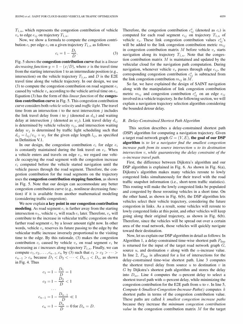
Now, we show a formula to compute the congestion contri-bution ci per edge ei on a given trajectory T1,n as follows:

ci = 1 − Di

D. (3)

Fig. 5 shows the congestion contribution curve that is a lineardecreasing function y = 1 − (x/D), where x is the travel timefrom the starting intersection 1 to an intermediate position (e.g.,intersection) on the vehicle trajectory T1,n, and D is the E2Etravel time along the vehicle trajectory. In our design, we use(3) to compute the congestion contribution on road segment eicaused by vehicle vs according to the vehicle arrival time on ei.Equation (3) has the form of this linear function of the conges-tion contribution curve in Fig. 5. This congestion contributioncurve considers both vehicle velocity and traffic light. The traveltime from an intersection i to the next intersection j includesthe link travel delay from i to j (denoted as dij ) and waitingdelay at intersection j (denoted as wj). Link travel delay dijis determined by vehicle velocity vij , and intersection waitingdelay wj is determined by traffic light scheduling such thatdij = lij/vij + wj for the given edge length lij , as specifiedin Definition V.1.

In our design, the congestion contribution ci for edge eiis constantly maintained during the link travel on ei. Whena vehicle enters and travels on edge ei, we regard one vehi-cle occupying the road segment with the congestion increaseci computed before the vehicle started navigation until thevehicle passes through the road segment. Therefore, the con-gestion contribution for the road segments on the trajectoryuses the congestion contribution stepping function, as shownin Fig. 5. Note that our design can accommodate any bettercongestion contribution curve (e.g., nonlinear decreasing func-tion) if it is available from another mathematical modeling(considering traffic congestion).

We now explain a key point in our congestion contributionmodeling. As road segment ei is farther away from the startingintersection n1, vehicle vs will reach ei later. Therefore, vs willcontribute to the increase in vehicular traffic congestion on thefarther road segment ei by a lesser amount right now. In otherwords, vehicle vs reserves its future passing to the edge by thevehicular traffic increase inversely proportional to the visitingtime to the edge. By this rationale, (3) makes the congestioncontribution ci caused by vehicle vs on road segment ei bedecreasing as i increases along trajectory T1,n. Finally, we cancompute c1, c2, . . . , cn−1, cn by (3) such that c1 > c2 > · · · >cn−1 > cn because D1 < D2 < · · · < Dn−1 < Dn, as shownin Fig. 4. Thus

c1 = 1 − D1

D= 1

c2 = 1 − D2

D< 1

. . .

cn−1 = 1 − Dn−1

D� 1

cn = 1 − Dn

D= 0 for Dn = D.

Therefore, the congestion contribution csij (denoted as ci) iscomputed for each road segment eij on trajectory T1,n ofvehicle vs. These link congestion contribution values csij’swill be added to the link congestion contribution metric mij

in congestion contribution matrix M before vehicle vs startsnavigation along its trajectory T1,n. Note that the conges-tion contribution matrix M is maintained and updated by thevehicular cloud for the navigation path computation. Duringnavigation, whenever vehicle vs passes through edge eij , thecorresponding congestion contribution csij is subtracted fromthe link congestion contribution mij in M .

So far, we have explained the design of SAINT navigationalong with the manipulation of link congestion contributionmetric mij and congestion contribution csij on an edge eijinvolved in a vehicle trajectory. In the following section, we willexplain a navigation trajectory selection algorithm consideringthe bounded detour delay.

B. Delay-Constrained Shortest Path Algorithm

This section describes a delay-constrained shortest path(DSP) algorithm for computing a navigation trajectory. Givena target road network graph G = (V,E), the goal of our DSPalgorithm is to let a navigator find the smallest congestionincrease path from its source intersection u to its destinationintersection v, while guaranteeing the delay constraint of theα-increase travel path.

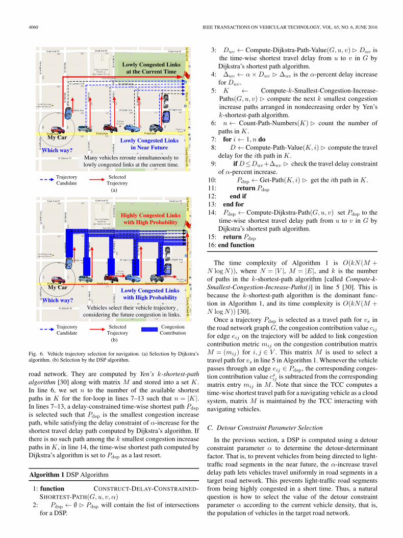
First, the difference between Dijkstra’s algorithm and ourDSP algorithm is explained in Fig. 6. As shown in Fig. 6(a),Dijkstra’s algorithm makes many vehicles reroute to lowlycongested links simultaneously for their travel with the roadtraffic snapshot information (i.e., short-term traffic statistics).This routing will make the lowly congested links be populatedand congested by those rerouting vehicles in a short time. Onthe other hand, as shown in Fig. 6(b), the DSP algorithm letsvehicles select their vehicle trajectory, considering the futurecongestion in links. As a result, some vehicles will reroute tolowly congested links at this point, and other vehicles will keepgoing along their original trajectory, as shown in Fig. 6(b).Therefore, since the vehicles will be spread out over a certainarea of the road network, those vehicles will quickly navigatetoward their destination.

Now, let us explain our DSP algorithm in detail as follows: InAlgorithm 1, a delay-constrained time-wise shortest path Pdsp

is returned for the input of the target road network graph G,source u, and destination v along with the α-increase value.In line 2, Pdsp is allocated for a list of intersections for thedelay-constrained time-wise shortest path. Line 3 computesthe shortest travel delay from source u to destination v inG by Dijkstra’s shortest path algorithm and stores the delayinto Duv . Line 4 computes the α-percent delay to select ashortest travel path with α-percent delay, while minimizing thecongestion contribution for the E2E path from u to v. In line 5,Compute-k-Smallest-Congestion-Increase-Paths() computes kshortest paths in terms of the congestion contribution value.These paths are called k smallest congestion increase pathsbecause they increase the minimum congestion contributionvalue in the congestion contribution matrix M for the target

4060 IEEE TRANSACTIONS ON VEHICULAR TECHNOLOGY, VOL. 65, NO. 6, JUNE 2016

Fig. 6. Vehicle trajectory selection for navigation. (a) Selection by Dijkstra’salgorithm. (b) Selection by the DSP algorithm.

road network. They are computed by Yen’s k-shortest-pathalgorithm [30] along with matrix M and stored into a set K .In line 6, we set n to the number of the available shortestpaths in K for the for-loop in lines 7–13 such that n = |K|.In lines 7–13, a delay-constrained time-wise shortest path Pdsp

is selected such that Pdsp is the smallest congestion increasepath, while satisfying the delay constraint of α-increase for theshortest travel delay path computed by Dijkstra’s algorithm. Ifthere is no such path among the k smallest congestion increasepaths in K , in line 14, the time-wise shortest path computed byDijkstra’s algorithm is set to Pdsp as a last resort.

Algorithm 1 DSP Algorithm

1: function CONSTRUCT-DELAY-CONSTRAINED-SHORTEST-PATH(G, u, v, α)

2: Pdsp ← ∅ � Pdsp will contain the list of intersectionsfor a DSP.

3: Duv ← Compute-Dijkstra-Path-Value(G, u, v)� Duv isthe time-wise shortest travel delay from u to v in G byDijkstra’s shortest path algorithm.

4: Δuv ← α×Duv � Δuv is the α-percent delay increasefor Duv.

5: K ← Compute-k-Smallest-Congestion-Increase-Paths(G, u, v) � compute the next k smallest congestionincrease paths arranged in nondecreasing order by Yen’sk-shortest-path algorithm.

6: n ← Count-Path-Numbers(K)� count the number ofpaths in K .

7: for i ← 1, n do8: D ← Compute-Path-Value(K, i)� compute the travel

delay for the ith path in K .9: if D≤Duv+Δuv � check the travel delay constraint

of α-percent increase.10: Pdsp ← Get-Path(K, i) � get the ith path in K .11: return Pdsp

12: end if13: end for14: Pdsp ← Compute-Dijkstra-Path(G, u, v) set Pdsp to the

time-wise shortest travel delay path from u to v in G byDijkstra’s shortest path algorithm.

15: return Pdsp

16: end function

The time complexity of Algorithm 1 is O(kN(M +N logN)), where N = |V |, M = |E|, and k is the numberof paths in the k-shortest-path algorithm [called Compute-k-Smallest-Congestion-Increase-Paths()] in line 5 [30]. This isbecause the k-shortest-path algorithm is the dominant func-tion in Algorithm 1, and its time complexity is O(kN(M +N logN)) [30].

Once a trajectory Pdsp is selected as a travel path for vs inthe road network graph G, the congestion contribution value cijfor edge eij on the trajectory will be added to link congestioncontribution metric mij on the congestion contribution matrixM = (mij) for i, j ∈ V . This matrix M is used to select atravel path for vs in line 5 in Algorithm 1. Whenever the vehiclepasses through an edge eij ∈ Pdsp, the corresponding conges-tion contribution value csij is subtracted from the correspondingmatrix entry mij in M . Note that since the TCC computes atime-wise shortest travel path for a navigating vehicle as a cloudsystem, matrix M is maintained by the TCC interacting withnavigating vehicles.

C. Detour Constraint Parameter Selection

In the previous section, a DSP is computed using a detourconstraint parameter α to determine the detour-determinantfactor. That is, to prevent vehicles from being directed to light-traffic road segments in the near future, the α-increase traveldelay path lets vehicles travel uniformly in road segments in atarget road network. This prevents light-traffic road segmentsfrom being highly congested in a short time. Thus, a naturalquestion is how to select the value of the detour constraintparameter α according to the current vehicle density, that is,the population of vehicles in the target road network.

JEONG et al.: SAINT FOR CLOUD-BASED VEHICULAR TRAFFIC OPTIMIZATION 4061

According to the vehicle density, the value of the detour con-straint parameter α can affect the performance of navigation.In light-traffic cases, α = 0.1 gives the best performance interms of average link delay, average maximum link delay, andaverage E2E delay. This is because these small α values allowthe SAINT to work similarly as Dijkstra. On the other hand, inmost traffic cases, except for light-traffic cases, α = 0.5 givesthe best performance. This means that when vehicles using theSAINT take 50% delay increase travel paths with minimumcongestion increase for global traffic optimization, they cantravel faster than vehicles using Dijkstra that lets vehiclesnavigate in a greedy way, leading to local traffic optimization.We will show the impact of the detour constraint parameter αon performance through simulations in Section VII-C. In thefollowing section, we will explain the navigation procedure inSAINT.

VI. SELF-ADAPTIVE INTERACTIVE NAVIGATION TOOL

NAVIGATION PROCEDURE

This section explains the navigation procedure in SAINTinvolving vehicles as navigators, RSUs (or eNodeBs), andthe TCC in vehicular cloud. The navigation procedure is asfollows.

1) As a SAINT Client, a vehicle with a navigator contactsthe SAINT Server in the TCC for navigating from itssource to its destination. The SAINT Client sends anavigation request to the SAINT Server by the V2I datadelivery scheme, such as that proposed by Jeong et al. in[22] or 4G-LTE communications [8].

2) SAINT Server maintains a matrix (called congestioncontribution matrix M ) for a target road network graphto estimate the level of congestion per road segment inthe graph.

3) With this matrix, the SAINT Server computes an optimalroute for the SAINT Client to minimize the path conges-tion contribution from the source to the destination forglobal traffic optimization while bounding the detouredtravel delay by parameter α.

4) SAINT Server gives a navigation response including anoptimal route to SAINT Client for navigation. Data de-livery from SAINT Server to SAINT Client is performedby the I2V data delivery scheme, such as that proposedby Jeong et al. in [24] or 4G-LTE communications [8].This is possible because the TCC maintains the trajectoryof the vehicle as SAINT Client for location management.

5) When receiving this route from the SAINT Server, theSAINT Client starts its travel along the guided route.

6) If the SAINT Client goes out of the guided route, itrepeats steps 1 through 5 to get a new route from theSAINT Server.

So far, we have explained the design and procedure of ourSAINT. In the following section, we will evaluate our SAINTwith a state-of-the-art commercial navigation scheme.

VII. PERFORMANCE EVALUATION

This section evaluates the performance of SAINT in termsof link delay of all the vehicles for all the road segments and

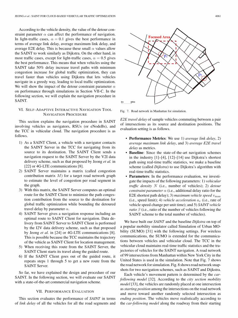
Fig. 7. Road network in Manhattan for simulation.

E2E travel delay of sample vehicles commuting between a pairof intersections as its source and destination positions. Theevaluation setting is as follows.

• Performance Metrics: We use 1) average link delay, 2)average maximum link delay, and 3) average E2E traveldelay as metrics.

• Baseline: Since the state-of-the-art navigation schemesin the industry [1]–[4], [12]–[14] use Dijkstra’s shortestpath using real-time traffic statistics, we make a baselinescheme (called Dijkstra) to use Dijkstra’s algorithm withreal-time traffic statistics.

• Parameters: In the performance evaluation, we investi-gate the impacts of the following parameters: 1) vehiculartraffic density N (i.e., number of vehicles); 2) detourconstraint parameter α (i.e., additional delay ratio for theE2E shortest path delay); 3) maximum vehicle speed vmax

(i.e., speed limit); 4) vehicle acceleration av (i.e., rate ofvehicle speed change per unit time); and 5) SAINT vehicleratio β (i.e., ratio of the number of vehicles following theSAINT scheme to the total number of vehicles).

We have built our SAINT and the baseline Dijkstra on top ofa popular mobility simulator called Simulation of Urban MO-bility (SUMO) [31] with the following settings. For wirelesscommunications, the SUMO is extended for the communica-tions between vehicles and vehicular cloud. The TCC in thevehicular cloud maintains real-time traffic statistics and the tra-jectories of vehicles for the SAINT navigation. A road networkof 99 intersections from Manhattan within New York City in theUnited States is used in the simulation. Note that Fig. 7 showsthe road network for simulation. Fig.8 shows road network snap-shots for two navigation schemes, such as SAINT and Dijkstra.

Each vehicle’s movement pattern is determined by the car-following model [32]. According to the city section mobilitymodel [33], the vehicles are randomly placed at one intersectionas starting position among the intersections on the road networkand move toward another randomly selected intersection asending position. The vehicles move realistically according tothe car-following model along the roadway from their starting

4062 IEEE TRANSACTIONS ON VEHICULAR TECHNOLOGY, VOL. 65, NO. 6, JUNE 2016

Fig. 8. Road network snapshots for two navigation schemes. (a) Navigationby SAINT. (b) Navigation by Dijkstra.

Fig. 9. Loop detector installation in the road network.

position to their ending position. Moreover, the vehicles waitfor green traffic light at intersections. Note that traffic lightphases are determined by a static traffic light scheduler [31]. Inour simulation, we measure the link delay including intersec-tion waiting delay that is determined by traffic light scheduling(see Fig. 9). We install two detectors into the start point and endpoint of each road segment, respectively, as shown in Fig. 9.

TABLE ISIMULATION CONFIGURATION

Fig. 10. Cdfs of navigation delays. (a) Link delay cdf. (b) E2E delay cdf.

When a vehicle arrives at an edge, the start detector stores thevehicle’s arrival time into its repository. The end detector storesthe vehicle’s departure time into its repository when the vehicleleaves the edge. With these timestamps, the link delay for theroad segment is measured. Once the vehicle arrives at its endingposition, it randomly selects another ending position for anothertravel. Thus, this vehicle travel process is repeated during thesimulation time, based on both the car-following model andthe city section mobility model. On the other hand, among thevehicles, 20 vehicles among 300 vehicles (i.e., 6.67%) are usedas sample vehicles, commuting between two positions (denotedas p1 and p2 in Fig. 7) as their source and destination positionsto measure E2E travel delay.

The vehicle speed is updated according to realistic vehicularmechanics based on the car-following model under the speedlimit confined per road segment, as shown in Table I. Forsimplicity, we let all of the road segments have the same speedlimit in the road network for the simulation; note that our designcan easily extend this simulation setting to having the variety of

JEONG et al.: SAINT FOR CLOUD-BASED VEHICULAR TRAFFIC OPTIMIZATION 4063

Fig. 11. Impact of vehicle number (α = 0.5). (a) Link delay versus vehicle number. (b) Max link delay versus vehicle number. (c) E2E delay versus vehiclenumber.

speed limits for road segments. The simulation time is set to2 h, and the simulations are repeated with different seeds(i.e., 10 or 30 seeds). The default values of the simulation arespecified in Table I.

A. Navigation Behavior Comparison

This section compares the navigation behaviors of SAINT andDijkstra with the cumulative distribution function (cdf) of E2Enavigation delay. Fig. 10 shows the cdfs of SAINT and Dijkstrafor the navigation delay in the road segment (i.e., link delay)and the navigation delay in the E2E travel path (i.e., E2E delay).

For link delay, as shown in Fig. 10(a), SAINT allows its cdfcurve to be above Dijkstra’s all the time, which means thatSAINT has a higher cumulative distribution than Dijkstra atany given link delay in the horizontal line. As a result, SAINTallows its cdf to reach 1 at a much shorter delay (i.e., 34 s) thanDijkstra. In the case of Dijkstra, the cdf does not reach 1 evenat the delay of 35.5 s.

For E2E delay, as shown in Fig. 10(b), SAINT allows its cdfcurve to be equal to or above Dijkstra’s. Moreover, SAINT’scdf is increasing fast, reaching 1 at the delay of 670 s. On theother hand, Dijkstra’s cdf is slowly increasing, reaching 1 atthe delay of 860 s, that is, 1.3 times the cdf completion point ofSAINT (i.e., 30% longer delay), which is the delay value withthe cdf 1. Thus, SAINT has the E2E delay that is bounded withina narrow range of delay; however, Dijkstra has the E2E delaythat is spread out within a larger range of delay.

Why does this performance difference happen betweenSAINT and Dijkstra? Fig. 8 explains this performance dif-ference. As shown in Fig. 8(a), SAINT allows for uniformlydistributed traffic flow to let vehicles bypass congested roadsegments with a high probability in the near future. On theother hand, Dijkstra allows vehicles to try to use road segmentswith light traffic at the moment of travel path computation inthe greedy per-vehicle basis rather than the road network’sperformance basis. As a result, as shown in Fig. 8(b), someroad segments are highly congested, but other road segmentshave almost zero traffic, leading to partially congested trafficflow. Therefore, by considering the overall road network per-formance, SAINT lets vehicles experience much shorter traveldelay than Dijkstra.

B. Impact of Vehicle Number (N)

This section shows the impact of vehicle number on navi-gation performance. For link delay, max link delay, and E2E

delay, as shown in Fig. 11(a)–(c), our SAINT outperformsDijkstra in all the range of the number of vehicles. For light-traffic conditions from N = 50 to N = 150, the performancegap between SAINT and Dijkstra is small. On the other hand,for relatively heavy traffic conditions from N = 200 to N =500, the performance gap between SAINT and Dijkstra issignificantly large. In particular, in Fig. 11(c), for N = 250,SAINT has 64% of the E2E delay of Dijkstra. Even for theheaviest traffic condition of N = 500, SAINT has 89% of theE2E delay of Dijkstra, that is, reducing 11% of the E2E delayof Dijkstra. Thus, it can be seen that SAINT can support moreeffective navigation in heavy-traffic conditions, such as duringrush hours.

C. Impact of Detour Constraint Parameter (α)

This section shows the impact of detour constraint parameter(α) on the performance along with the number of vehicles. InSection VII-B, a fixed value of α = 0.5 was used. Note thatthe detour constraint parameter α determines the delay boundof a selected detour travel path to minimize the congestioncontribution caused by the detour path in the road network.Thus, this means that each vehicle takes an α-increase travelpath as a detour travel path whose travel delay is, at most,(1 + α)Duv , where Duv is the travel delay of the time-wiseshortest travel path puv from source position u to destinationposition v, as specified in Definition V.2. This section showsthe best performance by changing the value of α from 0.1 to 1by 0.1.

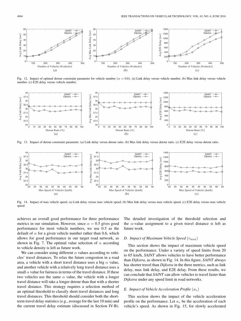
As shown in Fig. 12(a) and (b), SAINT with α optimizationdoes not outperform SAINT without α optimization [as shown inFig. 11(a) and (b)] in both the link delay and the max link delay.However, as shown in Fig. 12(c), for heavy-traffic conditionsfrom N = 300 to N = 500, the performance improvement inE2E delay is significantly observable. In Fig. 12(c), for N =500, SAINT with α = 0.6 has 81% of the E2E delay of Dijkstra,that is, reducing 19% of the E2E delay of Dijkstra. Note thatin Fig. 11(c), for N = 500, SAINT with α = 0.5 has 89% ofthe E2E delay of Dijkstra, that is, reducing 11% of the E2Edelay of Dijkstra. SAINT with α = 0.6 can reduce 8% morefor Dijkstra than SAINT with α = 0.5. Thus, an optimal valueselection of α can let SAINT achieve better performance. Fromour simulations, an optimal value of α is case by case for thevehicle number; hence, it is difficult to select an optimal valueof α according to vehicle density. Fig. 13 shows that α = 0.6

4064 IEEE TRANSACTIONS ON VEHICULAR TECHNOLOGY, VOL. 65, NO. 6, JUNE 2016

Fig. 12. Impact of optimal detour constraint parameter for vehicle number (α = 0.6). (a) Link delay versus vehicle number. (b) Max link delay versus vehiclenumber. (c) E2E delay versus vehicle number.

Fig. 13. Impact of detour constraint parameter. (a) Link delay versus detour ratio. (b) Max link delay versus detour ratio. (c) E2E delay versus detour ratio.

Fig. 14. Impact of max vehicle speed. (a) Link delay versus max vehicle speed. (b) Max link delay versus max vehicle speed. (c) E2E delay versus max vehiclespeed.

achieves an overall good performance for three performancemetrics in our simulation. However, since α = 0.5 gives goodperformance for most vehicle numbers, we use 0.5 as thedefault of α for a given vehicle number rather than 0.6, whichallows for good performance in our target road network, asshown in Fig. 7. The optimal value selection of α accordingto vehicle density is left as future work.

We can consider using different α values according to vehi-cles’ travel distances. To relax the future congestion in a roadarea, a vehicle with a short travel distance uses a big α value,and another vehicle with a relatively long travel distance uses asmall α value for fairness in terms of the travel distance. If thesetwo vehicles use the same α value, the vehicle with a longertravel distance will take a longer detour than that with a shortertravel distance. This strategy requires a selection method ofan optimal threshold to classify short travel distances and longtravel distances. This threshold should consider both the short-term travel delay statistics (e.g., average for the last 10 min) andthe current travel delay estimate (discussed in Section IV-B).

The detailed investigation of the threshold selection andthe α-value assignment to a given travel distance is left asfuture work.

D. Impact of Maximum Vehicle Speed (vmax)

This section shows the impact of maximum vehicle speedon the performance. Under a variety of speed limits from 20to 65 km/h, SAINT allows vehicles to have better performancethan Dijkstra, as shown in Fig. 14. In this figure, SAINT alwayshas shorter travel than Dijkstra in the three metrics, such as linkdelay, max link delay, and E2E delay. From these results, wecan conclude that SAINT can allow vehicles to travel faster thanDijkstra under any speed limit in road networks.

E. Impact of Vehicle Acceleration Profile (av)

This section shows the impact of the vehicle accelerationprofile on the performance. Let av be the acceleration of eachvehicle’s speed. As shown in Fig. 15, for slowly accelerated

JEONG et al.: SAINT FOR CLOUD-BASED VEHICULAR TRAFFIC OPTIMIZATION 4065

Fig. 15. Impact of acceleration profile. (a) Link delay versus acceleration profile. (b) Max link delay versus acceleration profile. (c) E2E delay versus accelerationprofile.

Fig. 16. Impact of SAINT vehicle ratio. (a) Link delay versus SAINT vehicle ratio. (b) Max link delay versus SAINT vehicle ratio. (c) E2E delay versus SAINTvehicle ratio.

vehicles from av = 1.0 m/s to av = 2.0 m/s, SAINT has, onaverage, 78% of the E2E delay of Dijkstra. For medium-accelerated vehicles from av = 2.5 m/s to av = 4.0 m/s, SAINThas, on average, 72% of the E2E delay of Dijkstra. Finally, forfast-accelerated vehicles from av = 4.5 m/s to av = 5.5 m/s,SAINT has, on average, 77% of the E2E delay of Dijkstra. Fromthese results, it can be concluded that SAINT can allow vehiclesto travel faster than Dijkstra under any acceleration profile inthe target road network.

F. Impact of SAINT Vehicle Ratio (β)

This section shows the impact of SAINT vehicle ratio thatis the percentage of vehicles using SAINT among the totalvehicles in the target road network. We may raise the followingquestion: What happens if some vehicles use SAINT for theirnavigation and others use Dijkstra for their navigation? Thissection answers this possible question.

Fig. 16 shows the impact of SAINT vehicle ratio, that is,the portion of vehicles using SAINT over the total number ofvehicles. As shown in the figure, when at least 30% of vehiclesuse SAINT, the performance of SAINT is significantly better inall the three metrics than that of Dijkstra. This figure showsthat SAINT performs ever better as the SAINT vehicle ratioincreases. Therefore, even partial deployment of SAINT will beeffective in real navigation scenarios during market penetration.

G. Impact of Nonlinear Formulation of Link CongestionContribution

This section shows the impact of a nonlinear formulation forlink congestion contribution on performance. We replace the

linear formula in (3) with a nonlinear formula as follows:

ci = 1 −exp

(−Di

D

)(4)

where Di is the travel time for the subpath from the startingintersection 1 to an intermediate intersection i along the vehicletrajectory, and D is the E2E travel time along the vehicletrajectory.

Fig. 17 shows that in most traffic conditions from N = 50 toN = 500, the performance gap between SAINT and Dijkstra issmaller than the performance gap between SAINT and Dijkstrain the case of the linear formulation, as shown in Fig. 11. Fromthis result, it is seen that a simple nonlinear formulation forlink congestion contribution is not more effective than the linearformulation. The investigation for a good nonlinear formula forcongestion contribution is left as future work.

H. Impact of Dynamic Update of Link CongestionContribution

This section shows the impact of the dynamic update oflink congestion contributions (called dynamic version) for theremaining edges on the performance, while a vehicle arrivesat each intersection along the vehicle trajectory. Note that theoriginal SAINT lets a vehicle have a trajectory with static linkcongestion contributions at the beginning of navigation. Thatis, it lets the link congestion contributions for the edges onthe trajectory be not updated during the vehicle travel alongits trajectory, as discussed in Section V. This management oflink congestion contributions is called the static link congestioncontribution method (shortly static version).

4066 IEEE TRANSACTIONS ON VEHICULAR TECHNOLOGY, VOL. 65, NO. 6, JUNE 2016

Fig. 17. Impact of nonlinear congestion contributions on vehicle number. (a) Link delay versus vehicle number. (b) Max link delay versus vehicle number. (c)E2E delay versus vehicle number.

Fig. 18. Impact of dynamic update of link congestion contribution on vehicle number. (a) Link delay versus vehicle number. (b) Max link delay versus vehiclenumber. (c) E2E delay versus vehicle number.

As shown in Fig. 18, except for the lowest density (N = 50)and the highest density (N = 500), in most cases of density, thedynamic version has worse performance than the static version.This is because the dynamic version cannot provide the roadcapacity reservation consistently to avoid the traffic congestionbetter than the static version.

So far, we have showed that SAINT significantly outperformsDijkstra under a variety of settings (i.e., vehicular traffic den-sity, speed limit, and SAINT vehicle ratio) in the target roadnetwork for the performance metrics (i.e., link delay, max linkdelay, and E2E delay). Therefore, we conclude that SAINT willbe a good foundation to enhance the cloud-based navigation inthe future.

VIII. CONCLUSION

This paper has proposed the SAINT for cloud-based vehic-ular traffic optimization in road networks. With the increasingpopularity of GPS-based navigation systems and mobile net-works (e.g., DSRC and 4G-LTE communications), we believethat our SAINT will improve the traffic flow in road networksby providing vehicles with globally optimal navigation pathsin the viewpoint of the transportation network rather thanindividual vehicles through vehicular cloud. This paper sug-gests a new metric called congestion contribution to estimatethe near-future congestion level of each road segment. Withthis congestion contribution metric, our SAINT will set up anavigation path for each vehicle for global road traffic opti-mization. As future work, we will enhance the modeling oflink congestion contribution by considering road capacity interms of the number of lanes for better traffic optimization.Moreover, we will extend our SAINT for accident scenarios so

that emergency vehicles (e.g., ambulance, police car, and fireengine) can reach an accident spot quickly, and other vehiclesaround the accident spot can navigate quickly toward theirdestination. In addition, we will investigate how to combineour SAINT with traffic light control systems so that trafficlight scheduling at intersections can be dynamically adapted forbetter vehicular traffic optimization in a self-adaptive way.

REFERENCES

[1] Garmin, Dedicated Navigator. [Online]. Available: http://www.garmin.com

[2] TomTom, Dedicated Navigator. [Online]. Available: http://www.tomtom.com

[3] Waze, Smartphone App for Navigator. [Online]. Available: https://www.waze.com

[4] Navfree, Free GPS Navigation for Android Smartphone. [Online]. Avail-able: http://navfree.android.informer.com

[5] Q. Xu, R. Sengupta, and D. Jiang, “Design and analysis of highway safetycommunication protocol in 5.9 GHz dedicated short range communicationspectrum,” in Proc. IEEE VTC Spring, Apr. 2003, pp. 2451–2455.

[6] J. Zhao and G. Cao, “VADD: Vehicle-assisted data delivery in vehicular adhoc networks,” IEEE Trans. Veh. Technol., vol. 57, no. 3, pp. 1910–1922,May 2008.

[7] Y. L. Morgan, “Notes on DSRC & WAVE standards suite: Its architecture,design, and characteristics,” IEEE Commun. Surveys Tuts., vol. 12, no. 4,pp. 504–518, 4th Quart. 2010.

[8] R. Kirui, “Accessing cloud computing resources over 4G LTE,” HelsinkiMetropolia Univ. Appl. Sci., Espoo, Finland, Tech. Rep., May 2014.

[9] C. D. Monfreid, “The LTE network architecture—A comprehensivetutorial,” Alcatel-Lucent, Tech. Rep., 2009. [Online]. Available: http://www.cse.unt.edu/~rdantu/FALL_2013_WIRELESS_NETWORKS/LTE_Alcatel_White_Paper.pdf

[10] Traffic Control Center in Philadelphia Department of Transportation.[Online]. Available: http://philadelphia.pahighways.com/philadelphiatcc.html

[11] A. Abdrabou and W. Zhuang, “Probabilistic delay control and roadside unit placement for vehicular ad hoc networks with disrupted con-nectivity,” IEEE J. Sel. Areas Commun., vol. 29, no. 1, pp. 129–139,Jan. 2011.

JEONG et al.: SAINT FOR CLOUD-BASED VEHICULAR TRAFFIC OPTIMIZATION 4067

[12] Skobbler, Smartphone App for GPS Navigation and Maps. [Online].Available: http://www.skobbler.com/apps/navigation/android

[13] Tmap, SKT Smartphone Navigator. [Online]. Available: http://www.tmap.co.kr/tmap2

[14] iNAVI, iNAVI Navigation System. [Online]. Available: http://www.inavi.com

[15] T. H. Cormen, C. E. Leiserson, R. L. Rivest, and C. Stein, Introduction toAlgorithms, 3rd ed. Cambridge, MA, USA: MIT Press, 2009.

[16] M. Wang et al., “Real-time path planning based on hybrid-VANET-enhanced transportation system,” IEEE Trans. Veh. Technol., vol. 64,no. 5, pp. 1664–1678, May 2015.

[17] A. H. Khosroshahi, P. Keshavarzi, Z. D. KoozehKanani, and J. Sobhi,“Adaptive demand-driven multicast routing in multi-hop wireless ad hocnetworks,” in Proc. IEEE Int. Conf. Comput., Control Ind. Eng., Wuhan,China, pp. 33–44, Aug. 2011.

[18] S. J. Russell and P. Norvig, Artificial Intelligence: A Modern Approach,2nd ed. Upper Saddle River, NJ, USA: Prentice-Hall, 2002.

[19] C. Perkins, D. Johnson, and J. Arkko, Mobility support in IPv6, RFC6275,Jul. 2011.

[20] ETSI, DSRC Standardization. [Online]. Available: http://www.etsi.org/WebSite/Technologies/DSRC.aspx

[21] J. Jeong, T. He, and D. H. Du, “TMA: Trajectory-based Multi-anycast formulticast data delivery in vehicular networks,” Comput. Netw., vol. 57,no. 13, pp. 2549–2563, May 2013.

[22] J. Jeong, S. Guo, Y. Gu, T. He, and D. Du, “Trajectory-based data for-warding for light-traffic vehicular ad-hoc networks,” IEEE Trans. ParallelDistrib. Syst., vol. 22, no. 5, pp. 743–757, May 2011.

[23] Y. Ding and L. Xiao, “SADV: Static-node-assisted adaptive data dissem-ination in vehicular networks,” IEEE Trans. Veh. Technol., vol. 59, no. 5,pp. 2445–2455, Jun. 2010.

[24] J. Jeong, S. Guo, Y. Gu, T. He, and D. Du, “Trajectory-based statisticalforwarding for multihop infrastructure-to-vehicle data delivery,” IEEETrans. Mobile Comput., vol. 11, no. 10, pp. 1523–1537, Oct. 2012.

[25] J. Jeong and E. Lee, “Vehicular cyber-physical systems for smart roadnetworks,” KICS Inf. Commun. Mag., vol. 31, no. 3, pp. 103–116,Mar. 2014.

[26] A. Polus, “A study of travel time and reliability on arterial routes,” Trans-portation, vol. 8, no. 2, pp. 141–151, Jun. 1979.

[27] M. DeGroot and M. Schervish, Probability and Statistics, 3rd ed.Reading, MA, USA: Addison-Wesley, 2001.

[28] G. Dimitrakopoulos and P. Demestichas, “Intelligent transportation sys-tems based on cognitive networking principles,” IEEE Veh. Technol. Mag.,vol. 5, no. 1, pp. 77–84, Mar. 2010.

[29] Res. Innovative Technol. Admin. (RITA), IntelliDrive: Safer, Smarter andGreener. [Online]. Available: http://trid.trb.org/view.aspx?id=968739

[30] J. Y. Yen, “Finding the K shortest loopless paths in a network,” Manage.Sci., vol. 17, no. 11, pp. 712–716, Jul. 1971.

[31] SUMO, Simulation of Urban MObility. [Online]. Available: http://sumo-sim.org

[32] R. W. Rothery, “Car-following models,” Transp. Res. Board, Washington,DC, USA, Revised Monograph on Traffic Flow Theory, Tech. Rep., 1997,[Online]. Available: http://www.tfhrc.gov/its/tft/chap4.pdf

[33] T. Camp, J. Boleng, and V. Davies, “A survey of mobility models forad hoc network research,” Wireless Commun. Mobility Comput., vol. 2,no. 5, pp. 483–502, Aug. 2002.

Jaehoon (Paul) Jeong (M’09) received the B.S. de-gree from the Department of Information Engineer-ing, Sungkyunkwan University, Suwon, Korea, in1999; the M.S. degree from the School of ComputerScience and Engineering, Seoul National University,in 2001; and the Ph.D. degree from the Departmentof Computer Science and Engineering, University ofMinnesota, Minneapolis, MN, USA, in 2009.

He is an Assistant Professor with the Departmentof Software, Sungkyunkwan University. His researchareas include vehicular networks, wireless sensor

networks, and mobile ad hoc networks.Dr. Jeong’s two data-forwarding schemes (called TBD and TSF) for vehic-

ular networks were selected as spotlight papers in the IEEE TRANSACTIONS

ON PARALLEL AND DISTRIBUTED SYSTEMS in 2011 and the IEEE TRANS-ACTIONS ON MOBILE COMPUTING in 2012, respectively. He is a member ofthe Association for Computing Machinery and the IEEE Computer Society.

Hohyeon Jeong (S’15) received the B.S. and M.S.degrees from the School of Electrical and Com-puter Engineering, Ajou University, Suwon, Korea,in 2012 and 2014, respectively. He is currently work-ing toward the Ph.D. degree with the Department ofComputer Science and Engineering, SungkyunkwanUniversity, Suwon, Korea.

His research area is self-adaptive softwaresystems.

Eunseok Lee (M’15) received the B.S. degreefrom the Department of Electronic Engineering,Sungkyunkwan University, Suwon, Korea, in 1985and the M.S. and Ph.D. degrees from the Depart-ment of Information Engineering, Tohoku Univer-sity, Sendai, Japan, in 1988 and 1991, respectively.

He is a Professor with the Department of Com-puter Engineering, Sungkyunkwan University. Hewas an Assistant Professor with Tohoku Univer-sity. Before that, he was a Research Scientist withMitsubishi Electric Corporation. His research areas

are self-adaptive software systems, software testing, and autonomic computing.

Tae (Tom) Oh (SM’15) received the B.S. degreefrom Texas Tech University, Lubbock, TX, USA, in1991 and the M.S. and Ph.D. degrees from SouthernMethodist University, Dallas, TX, USA, in 1995 and2001, respectively, all in electrical engineering.

He obtained his degrees while working fortelecommunication and defense companies. He is anAssociate Professor with the Department of Infor-mation Sciences and Technologies and the Depart-ment of Computing Security, Rochester Institute ofTechnology, Rochester, NY, USA. He has published

numerous technical articles. His research interests include mobile ad hocnetworks, vehicle area networks, sensor networks, and mobile device security.

Dr. Oh is a Technical Editor of the IEEE COMMUNICATIONS MAGAZINE

and an Associate Technical Editor of the IEEE NETWORKS. He is a memberof the Association for Computing Machinery.

David H. C. Du (F’98) received the B.S. degree inmathematics from National Tsing Hua University,Hsinchu, Taiwan, in 1974 and the M.S. and Ph.D.degrees in computer science from the University ofWashington, Seattle, WA, USA, in 1980 and 1981,respectively.

He is currently the Qwest Chair Professor with theDepartment of Computer Science and Engineering,University of Minnesota, Minneapolis, MN, USA.His research interests include cyber security, sensornetworks, multimedia computing, storage systems,

and high-speed networking.