This article was downloaded by: [University of Western Ontario]On: 08 October 2014, At: 19:35Publisher: Taylor & FrancisInforma Ltd Registered in England and Wales Registered Number: 1072954 Registered office: Mortimer House,37-41 Mortimer Street, London W1T 3JH, UK

IIE TransactionsPublication details, including instructions for authors and subscription information:http://www.tandfonline.com/loi/uiie20

Salesforce design with experience-based learningSANJOG MISRA a , EDIEAL J. PINKER a & ROBERT A. SHUMSKY aa William E. Simon School of Business Administration, University of Rochester , Rochester,NY, 14627, USA E-mail:Published online: 17 Aug 2010.

To cite this article: SANJOG MISRA , EDIEAL J. PINKER & ROBERT A. SHUMSKY (2004) Salesforce design with experience-basedlearning, IIE Transactions, 36:10, 941-952, DOI: 10.1080/07408170490487777

To link to this article: http://dx.doi.org/10.1080/07408170490487777

PLEASE SCROLL DOWN FOR ARTICLE

Taylor & Francis makes every effort to ensure the accuracy of all the information (the “Content”) containedin the publications on our platform. However, Taylor & Francis, our agents, and our licensors make norepresentations or warranties whatsoever as to the accuracy, completeness, or suitability for any purpose of theContent. Any opinions and views expressed in this publication are the opinions and views of the authors, andare not the views of or endorsed by Taylor & Francis. The accuracy of the Content should not be relied upon andshould be independently verified with primary sources of information. Taylor and Francis shall not be liable forany losses, actions, claims, proceedings, demands, costs, expenses, damages, and other liabilities whatsoeveror howsoever caused arising directly or indirectly in connection with, in relation to or arising out of the use ofthe Content.

This article may be used for research, teaching, and private study purposes. Any substantial or systematicreproduction, redistribution, reselling, loan, sub-licensing, systematic supply, or distribution in anyform to anyone is expressly forbidden. Terms & Conditions of access and use can be found at http://www.tandfonline.com/page/terms-and-conditions

IIE Transactions (2004) 36, 941–952Copyright C© “IIE”ISSN: 0740-817X print / 1545-8830 onlineDOI: 10.1080/07408170490487777

Salesforce design with experience-based learning

SANJOG MISRA, EDIEAL J. PINKER∗ and ROBERT A. SHUMSKY

William E. Simon School of Business Administration, University of Rochester, Rochester, NY 14627, USAE-mail: misra or pinker or shumsky@simon.rochester.edu

Received September 2002 and accepted January 2004

This paper proposes and analyzes an integrated model of salesforce learning, product portfolio pricing and salesforce design. Weconsider a firm selling two products, with a pool of sales representatives that is split into separate salesforces, one for each product.The salesforce assigned to each product is faced with an independent stream of sales leads. The salesforce may also handle leadsthat overflow from other product salesforces. In addition, salespeople “learn by doing” over their tenure on the job. In particular, themore time they spend selling a particular product, the more productive the sales effort. The objective of the firm is to maximizeprofits by optimizing the size of all salesforces as well as the prices of all products. Using data collected from the salesforce ofa large manufacturer, we provide evidence for the link between experience and sales, and we demonstrate how parameters of themodel may be estimated from real data. Numerical experiments using parameters derived from the data analysis indicate that theoptimal salesforce size increases with both sales productivity and the learning rate, and decreases with salesforce costs (e.g., wage perrepresentative), product production costs and consumer price sensitivity. We also find that worker learning can significantly dampenthe effect of rising costs (or decreasing margins) on staffing levels. Finally, we examine the impact of learning on both the optimalsalesforce structure (specialists versus generalists) as well as the optimal routing of sales leads to sales representatives.

1. Introduction

By broadening the range of tasks assigned to individualworkers, firms hope to create workforces that are responsiveto variability in workloads. In the case of a salesforce, suchjob flexibility is often implemented by pooling salespeo-ple across product lines. In a sales organization with pool-ing, each salesperson may have a primary responsibility forsome product line but is also able to sell some subset of theother product lines. Two important factors that influencethe performance of such a salesforce are pricing and experi-ence. Product price will influence the demand for a product,while the salesperson’s experience influences the likelihoodof making a sale. Therefore, when sizing and structuring asalesforce, a firm must consider pricing and the impact ofstaffing decisions on the experience of the salesforce. Un-derstaffing the sales team for a product may lead to lostsales and possibly to lost future market share. Overstaffingthe sales team can be expensive since good sales people aretypically well compensated. Assigning staff to product linesmust also be done carefully. Some products are complex andsales success depends upon experience, while simpler prod-ucts require little experience on the part of the salesforce.

In this paper, we examine the interactions among staffing,learning, and pricing in the management of a salesforce. We

∗Corresponding author

develop a model of a salesforce that receives sales leads withthe sales volume generated from each lead depending uponthe experience of the salesperson and the price of the prod-uct. The firm’s goal is to maximize profit by adjusting prod-uct prices as well as how many salespeople are allocated toeach product. Our model applies to firms with the followingthree attributes: (i) sufficient market power to have controlover pricing; (ii) complex products that require experienceto sell effectively; and (iii) large marketing efforts, such asadvertising in the media and at tradeshows, so that most ofthe leads are generated by activities outside of the salesforce.Specifically, a firm selling high-technology industrial prod-ucts in a mature market would satisfy all of these criteria(such a firm satisfies attribute (iii), for in a mature marketthere are few untapped sales leads, and its salesforce focusesits energy on following up requests by existing customersrather than unearthing new customers). After developingthe model, we estimate its parameters using data collectedfrom the salesforce of one such firm.

This paper makes use of the framework developed inPinker and Shumsky (2000) for modeling learning in servicesystems. We combine a model of job tenure with a modelof experience-based learning and apply it to the problemof salesforce design. The current paper, however, has foursignificant differences and extensions that lead to interest-ing results not previously seen in the literature. Firstly, theservice level, defined as the throughput of sales leads, is de-termined endogenously while it is exogenously determined

0740-817X C© 2004 “IIE”

Dow

nloa

ded

by [

Uni

vers

ity o

f W

este

rn O

ntar

io]

at 1

9:35

08

Oct

ober

201

4

942 Misra et al.

in Pinker and Shumsky (2000). Therefore, we are able to seehow optimal staffing responds to changes to cost parame-ters. Given this additional degree of freedom, we also findthat worker learning can significantly dampen the effect ofrising costs (or decreasing margins) on staffing levels. Forexample, if learning is a significant factor, an increase ordecrease in the cost of salesforce compensation has a rela-tively small impact on the optimal salesforce size. Secondly,we model a more complex routing of customers (sales leads)to workers (salespeople) that more accurately reflects a com-mon practice in sales organizations. Given this routing, wearrive at the surprising result that, with learning, pooling ofworkers may lead to optimal staffing levels that are higherthan when workers specialize. This contradicts the conven-tional wisdom that the economy of scale provided by pool-ing reduces staffing requirements. Thirdly, the model incor-porates pricing decisions and their effect on demand. As aresult we are able to study the relationship among staffinglevels, job flexibility, and price levels. In particular, we findthat the optimal salesforce size declines as price sensitivityincreases. We also find that when learning is a significantfactor in determining sales volume, a specialized (or “ex-clusive”) salesforce leads to higher optimal prices than theoptimal prices for a pooled salesforce. Fourthly, motivatedby data collected from the salesforce of a large manufac-turer, we propose a learning-curve model different from themodel in Pinker and Shumsky (2000), and we demonstratehow parameters of the model may be estimated from thedata.

In the next section, we present an overview of the rel-evant literature. In Section 3, we formulate our model byintegrating a service process model with an employee tenuremodel, a model of experience-based learning, and a modelof consumer demand. Section 4 contains analytical resultsthat describe the impact of various parameters on the opti-mal price. Section 5 describes the analysis of industry salesdata that provide baseline parameters for the numerical ex-periments of Section 6. These numerical experiments pro-vide insights into how learning effects staffing and pricing.Section 7 summarizes our results and discusses possible ex-tensions of the model.

2. Literature review

As noted above, this paper is most closely related to Pinkerand Shumsky (2000). Other researchers have also consid-ered parts of the problem addressed in this paper but webelieve that ours is the first to integrate all of them into onemodel. Some researchers have studied the control problemof how to hire, fire and promote workers to maintain ap-propriate staff levels when career paths are stochastic, andthese are listed in Pinker and Shumsky (2000). None of thesestudies consider the effect of pricing on staffing and there-fore do not connect staffing and learning to sales, limitingtheir applicability to salesforce design.

The literature on salesforce management has focusedon either salesforce incentives, see for example Basu et al.(1985), Lal and Srinivasan (1993), Joseph and Thevaranjan(1998) and Bhardwaj (2001), or salesforce sizing and mixissues. In this paper, we do not focus our attention on com-pensation issues. In particular, we assume that effort is per-fectly observable and hence a fixed wage, forcing contractis optimal.

Montgomery and Urban (1969) and Lucas et al. (1975)use profit maximization models to solve for the optimalsalesforce size. A limitation of their approach is that theyignore the presence of multiple products and/or territories.Lodish et al. (1988) use a more sophisticated approach tomodeling the issue in the case of one particular firm. Theyshowed, for this one firm, that adding salespeople and re-deploying them would result in increased profits. Zoltners(1976), Lodish (1976, 1980), Rangaswamy et al. (1990), andMantrala et al. (1992) consider the problem of finding theoptimal allocation of salespeople to territories, products orcustomers. These studies use static frameworks that do notincorporate learning effects within the salesforce. Anotherissue that has not been addressed adequately in the litera-ture is specialization and the effect it has on structuring thesalesforce. Given that salespeople often specialize in partic-ular products and that such specialists are scarce, there areinstances when a non-specialist serves a customer, whichmay have an impact on sales.

Dewan and Mendelson (1990), Stidham (1992) and Soand Song (1998) are examples of works in which both ca-pacity and pricing are endogenous to the firm’s decisionproblem. In all of these, the firm is modeled as a single-server queue and capacity is determined by the service rate.In this paper, we are explicitly modeling capacity as thestaffing level in a multi-server queue. Furthermore, we con-sider the interaction of parallel queues serving different cus-tomer types. Finally, in our model price determines the salesquantity rather than the customer arrival process. As wementioned in the Introduction, our formulation is appro-priate for environments in which sales leads are “handedoff” to the salesforce.

To summarize, we are studying a set of problems thathave been looked at in isolation from various perspectives inthe marketing and operations literature. We aim to integratethese diverse perspectives into a unified model that will helpus to understand the dynamics of learning and its impacton pricing, salesforce size and salesforce design.

3. Model formulation

Consider a firm that sells two products, A and B, and hastwo types of salespeople, A and B. We assume that salesleads representing customers interested in each of theseproducts arrive according to a Poisson process with arrivalrates of λA and λB respectively. In the following, we referto customers and sales leads interchangeably. We can state

Dow

nloa

ded

by [

Uni

vers

ity o

f W

este

rn O

ntar

io]

at 1

9:35

08

Oct

ober

201

4

Salesforce design with experience-based learning 943

the profit function of the firm in very general terms as afunction of the staffing S = (SA, SB) and the price of eachproduct p = (pA, pB) as follows:

�(S, p) =∑

i=A,B

∑j=A,B

rijqij(pi − ci) − diSi, (1)

where rij is the throughput of type-i leads through type-j salespeople, qij is the expected quantity of a product isold by a type j salesperson pursuing a type-i lead, ci isthe production cost of each unit of product i and di is thecost per unit time of each salesperson. Both ci and di areexogenous parameters. The following sections describe howwe find the throughput of each customer type (rij) and thequantity sold (qij).

3.1. Throughput statistics

In practice, sales leads must be allocated to individual sales-people. Each salesperson may work on many leads simulta-neously with a particular lead being active for days, weeksor months depending upon the nature and characteristicsof the product class. As we discussed in the Introduction,it is common for salespeople to be assigned primary re-sponsibility for one set of products and secondary respon-sibility for others. For example, the firm would prefer thattype-i salespeople sell type-i products, but if all i salespeo-ple are occupied the firm may want a type-j salesperson tofollow-up on the lead rather than lose the sales opportunityaltogether. In practice, salesforce compensation is often de-signed as a matrix that assigns a commission to salesperson-type and product-type pairs. The purpose of such a matrixis to encourage salespeople to focus on their primary prod-uct lines while keeping the option open for cross-selling. Tosimplify our analysis, we assume that the assignment of cus-tomers to salespeople occurs as follows. When a type-i saleslead arrives it is directed to a type-i salesperson. However,if all type-i salespeople are busy pursuing other leads thelead is routed to a type-j salesperson. If all salespeople (i.e.,of both types) are busy, the lead/customer is lost. Withineach group of salespeople, arrivals are routed so that workis shared equitably among the salespeople. Figure 1 showsthe routing of leads through the salesforce in our model.We refer to this as a hierarchical salesforce design.

Fig. 1. Routing of leads through a hierarchical salesforce.

We are modeling the salesforce as a pair of multi-serverservice systems with exponential service times that operatein parallel and receive their own independent Poisson ar-rival streams with rates λA and λB but also allow leads tooverflow into each other. Later we will also examine systemsin which a group of salespeople are dedicated to a singleproduct. Because the “single-product” model is relativelysimple (e.g., the sales leads flow through an M/M/S/Squeueing system), we will focus on the more general two-product model here. We will assume that the service rateof each salesperson, µ, is the same (although it is not dif-ficult to relax this assumption). Note that we are modelingeach lead as being processed sequentially by a salespersonwhile in practice a salesperson would be pursuing multipleleads simultaneously. We make this abstraction to simplifythe calculation of queueing statistics, and we believe thatexplicitly modeling the simultaneous processing of leadswould be an interesting topic for further research. In addi-tion, we assume that sales quantity does not affect the timeit takes to pursue a sales lead.

The sales quantity model described in the next sectionuses two sets of statistics from this model: throughput andutilization. Let rAB represent the throughput of type A leadsthrough type B salespeople; rBA, rAA, and rBB have similarinterpretations. Note that rij is a function of the staffingvector S = (SA, SB). Utilization is represented as ρAB, ρBB,ρAA, and ρBA, and each of these is calculated easily fromthe appropriate values of rij.

Calculating the throughput statistics of the salespeople ismore difficult than finding the throughput of a standard losssystem because the arrival process to each group of sales-people is not purely Poisson but is instead a combination ofa Poisson process and bursts of arrivals that are sent whenthe other sales group is fully occupied. For this system wecalculate throughput statistics numerically. Specifically, wedefine a two-dimensional state space (NA, NB) where Nirepresents the number of busy salespeople of type i. Thebalance equations for this state space are relatively simpleto enumerate, and we use these equations to solve itera-tively for the steady-state probabilities of (NA, NB) (Grossand Harris, 1985, p. 437). Given the steady-state probabili-ties, we calculate the expected throughput and utilization.

3.2. Quantity sold

The quantity of the product sold as a result of pursuing alead depends upon the price of the product and the experi-ence of the salesperson with that product. Here we developa model of demand that is based upon customer sensitivityto both price and the experience of the salesforce as wellas a model of the career path and experience accrual of anindividual salesperson.

Given that a type-j salesperson pursues a lead for prod-uct i, we assume that the sales generated by that lead isa random variable Dij = αij − βipi, where αij is a randomvariable that depends upon the (random) experience level

Dow

nloa

ded

by [

Uni

vers

ity o

f W

este

rn O

ntar

io]

at 1

9:35

08

Oct

ober

201

4

944 Misra et al.

of the salesperson encountered by a customer and β i is thesensitivity of demand to price for product i. Therefore, inthe profit function of Equation (1):

qij = E[Dij].

The important difference between our specification andthe traditional, linear demand model is that we allow theintercept to vary across salespeople. In the marketing lit-erature sales volume is typically described as a function ofthe skill of a salesperson. Rao (1990) for example, proposesthe functional form:

s = s0(1 − e−nb), (2)

where s is the sales, s0 is the maximum achievable saleslevel, b is the skill of the salesperson and n is a parameterdetermining the rate at which s0 is approached. From thelearning-curve literature (Yelle, 1979; Badiru, 1992), we cansee that often heterogeneity in skill is a result of heterogene-ity in experience levels. In this paper we combine these twoperspectives by expressing sales volume as a function of ex-perience. We use the same functional form as in Equation(2), in particular we assume that αij = Kij(1 − exp(−nwij))where wij is the accrued experience of a type-j salespersonselling product i (measured in units of time), Kij is a con-stant representing the upper limit of sales ability, i.e., thesales volume of a salesperson with infinite experience, andn is a learning parameter. Much of the traditional literatureon learning curves uses units of work, for example widgetsbuilt, as a measure of experience. In manufacturing set-tings where unit labor costs decrease with learning becauseworkers become faster, and it is easy to measure costs, thisapproach is appropriate. In our application the work unit isa sales lead and it is difficult to obtain data on the numberof leads handled. Furthermore, it is not clear that the timespent per lead will decrease with experience. Rather, as wemodel it, the likelihood of a sale will increase with experi-ence. Therefore, additional experience selling a product hasthe effect of increasing the intercept of the demand for thatproduct. This functional form is appealing for a number ofreasons. First it is consistent with the marketing literature,second, it is consistent with the learning-curve literature inwhich most learning curves are asymptotic, and finally wehave found that it provides a reasonable fit to actual sales-force performance data. The learning-curve literature typ-ically models production costs as a decreasing function ofexperience that asymptotically approaches zero. In our casewe are modeling the effect of experience on sales (or rev-enue generation) and therefore use an increasing functionof experience that asymptotically approaches some upperlimit. Note that the proposed function differs from the un-bounded “power function” used in Pinker and Shumsky(2000) to describe the relationship between experience andservice quality. We found that the bounded function pro-posed here provided a better fit to the sales data that willbe described in Section 5.

Given our discussion above we can now define quantitysold as:

Dij = Kij(1 − e−nwij )−β ipi. (3)

Let y be the tenure of a salesperson. Then the expected salesquantity is:

qij = E[Dij] = Kij − KijEy [E[e−nwij | y]] − βipi. (4)

The outer expected value is over the tenure of the type-jsalesperson serving a given customer and the inner expectedvalue is over the experience of the salesperson with the type-i product, given tenure y.

It can be shown that when the average time spent on asales lead is small relative to the tenure of a salesperson thenE[exp(−nwij) | y] can be closely approximated by exp(−nρijy).This approximation is similar to one that appears in Pinkerand Shumsky (2000) and its accuracy here has been verifiedusing simulation. Therefore:

qij ≈∫ ∞

0Kij(1 − e−nρij t )gy(t)dt − βipi. (5)

The probability density function for y, gy(t), is derivedfrom a model of a salesperson’s tenure process in which acareer is divided into stages, so that the stages of the ca-reer can be modeled as states of a continuous-time Markovchain. The tendency to end employment (by being fired orquitting) varies from stage to stage, and the time a sales-person stays in a stage before leaving is exponentially dis-tributed. The parameter λ1 is the rate at which salespeoplemove from the first stage to the second stage, λ2 is the rateat which they end their employment in the first stage, λ3is the rate at which workers in the second stage end theiremployment, and λ2 > λ3.

Using this model of the tenure process it can be shownthat:

qij ≈ Kijnρij

λ1 + λ2 + nρij

(1 + λ2

1 + λ1λ2

(λ1 + λ3)(λ3 + nρij)

)− βipi.

(6)

Equation (6) accounts for price, learning and the tenureprocess to determine the quantity sold. Since ρij is a by-product of the staffing levels, S = (SA, SB), Equation (6)also links staffing to sales.

3.3. The complete objective function

We can now restate the optimization problem faced by thefirm as:

MaxS,p

�(S, p)

where

�(S, p) =∑

i=A,B

∑j=A,B

{rij(S)

[Kij

(rij(S)µSj

)

×(

nλ1 + λ2 + n(rij(S)/µSj)

)

Dow

nloa

ded

by [

Uni

vers

ity o

f W

este

rn O

ntar

io]

at 1

9:35

08

Oct

ober

201

4

Salesforce design with experience-based learning 945

×(

1 + λ21 + λ1λ2

(λ1 + λ3)(λ3 + n(rij(S)|µSj))

)

− βipi

](pi − ci) − diSi

}. (7)

There are a number of trade offs explicitly represented inthis objective function. First we know that throughput (rij)is increasing in staffing and therefore there is a trade-off be-tween the additional revenue brought by increased staffingand the marginal cost of an additional salesperson di. How-ever, while increasing staffing increases the number of salesleads that can be pursued, increasing staffing also reducesthe number of units sold per lead because it reduces theutilization and therefore the experience of the salesforce.This complex effect of utilization on experience and prof-its can be seen by the appearance of the variable S in thedenominator of some of the terms in Equation (7). Thistrade-off is clear when the salesforce sells a single product.In Section 6 we will see that this utilization effect also hasa significant influence on salesforce design decisions whenthere are multiple products, e.g., whether to deploy a spe-cialized or pooled salesforce.

4. Optimizing prices, given salesforce size

The complex interactions among staffing, sales and ex-perience make it difficult to derive an analytical charac-terization of the optimal decision. However, given the ex-pected profit function, Equations (1) and (7), it is relativelystraightforward to solve for optimal prices given a specificstaffing of each type of salesperson.

To obtain the optimal prices given staffing we differenti-ate expected profit, Equation (1), with respect to price andobtain:∑

j=A,B

[rij

∂qij

∂pi(pi − ci) + rijqij

]= 0 for i = A, B. (8)

Solving for price and using the notation of Equation (7) wefind:

pi = c2

+∑

j

rilKij

(rij(S)µSj

)(n

λ1 + λ2 + n(rij(S)/µSj)

)

×(

1 + λ21 + λ1λ2

(λ1 + λ3)(λ3 + n(rij(S)/µSj))

)/2βi

∑j

rij,

for i = A, B. (9)

This expression is similar to the standard monopolistic pricefor a linear demand curve, except that the intercept is aweighted average of the intercepts of the two sources of de-mand. If there were only one product, no learning effects (sothat the demand intercept is a constant, α), and throughputwere equal to one, then the price equation is:

p = c2

+ α

2β,

which is the standard monopoly price.

We now describe a few properties that follow directlyfrom the price equation. The price of product i,

1. increases with the cost, ci, of product i;2. increases with the maximum productivity, Kij, of a type-j

salesperson with product i;3. decreases with the price sensitivity βi, of product i;4. increases with the learning rate, n (while this is not obvi-

ous from Equation (9), it can be shown that ∂pi/∂n > 0).

One property we do not specify here is the relationship be-tween staffing and pricing. While it might seem appropriateto conjecture that prices and staffing (for a given product)move in the same direction, this is not clear from our model.While throughput is increasing in staffing, utilization is not,and this may create a non-monotone relationship betweenthe two. We revisit this issue in the numerical experimentsof Section 6.

5. Industry data analysis

The model described in Section 3 assumes that sales produc-tivity grows with the experience of a particular salesperson.While the impact of experience on manufacturing produc-tivity has been well documented by empirical research (seethe summary by Yelle (1979)), to our knowledge there havebeen no published studies linking sales and experience ina salesforce. The data analysis in this section helps us toidentify reasonable learning-curve parameters that will beused in the numerical experiments of the next section.

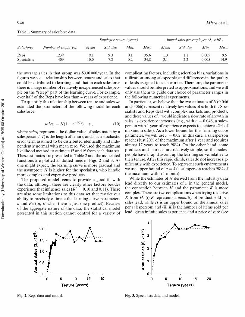
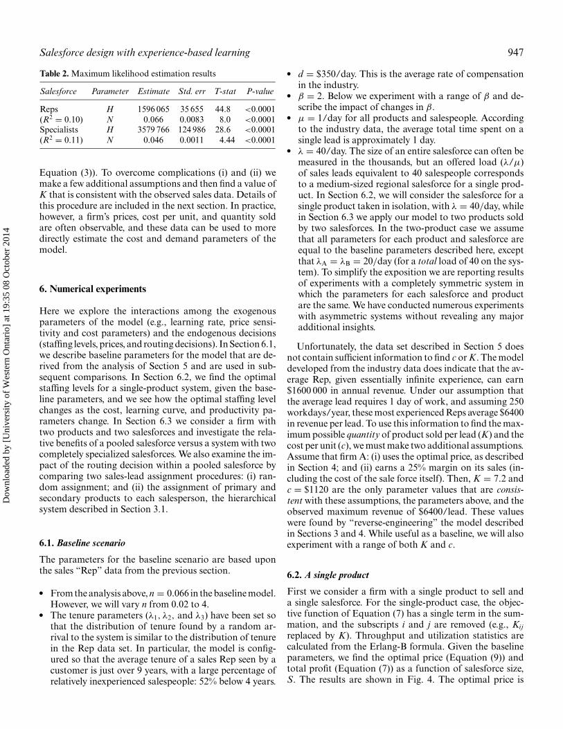
For our analysis we have obtained sales data from oneparticular company, “Firm A,” a market leader in officeproducts with an annual sales revenue of over $10 billionand over 40 000 employees. Although the firm operates invarious product and service markets we restrict our focus tothe division that is the flagship of the company and accountsfor a substantial proportion of its revenues. The business en-vironment of this division conforms to the assumptions ofour model: the firm is a market leader and has some pricingpower, the product is complex, and the market is mature sothat salespeople primarily respond to requests from exist-ing customers, rather than finding new leads. The divisionhas two primary salesforces, “Representatives” (or “Reps”)and “Specialists”. Specialists sell technologically advanced,high-priced equipment to large corporations while Reps fo-cus on less-complex and less expensive products for smalland medium-sized firms. Our data set is cross-sectional: itrecords the number of years a salesperson has been with thefirm (tenure) and the most recent annual sales figure for eachemployee. Table 1 contains a summary of the data. Figures 2and 3 display the relationship between tenure and sales ineach sale force. Each ‘•’ in Fig. 2 represents the average salesof 50 salespeople, while each data point in Fig. 3 representsa group of 40 salespeople. For example, the first point onthe lower left of Fig. 2 shows the average sales of the 50 mostinexperienced Reps: their average tenure was 5 months, and

Dow

nloa

ded

by [

Uni

vers

ity o

f W

este

rn O

ntar

io]

at 1

9:35

08

Oct

ober

201

4

946 Misra et al.

Table 1. Summary of salesforce data

Employee tenure (years) Annual sales per employee ($, ×106)

Salesforce Number of employees Mean Std. dev. Min. Max. Mean Std. dev. Min. Max.

Reps 1239 9.1 9.3 0.1 35.6 1.3 1.1 0.005 9.5Specialists 409 10.0 7.8 0.2 34.8 3.1 2.2 0.005 14.9

the average sales in that group was $330 000/year. In thefigures we see a relationship between tenure and sales thatcould be attributed to learning, and that in each salesforcethere is a large number of relatively inexperienced salespeo-ple on the “steep” part of the learning curve. For example,over half of the Reps have less than 4 years of experience.

To quantify this relationship between tenure and sales weestimated the parameters of the following model for eachsalesforce:

salesi = H(1 − e−NTi ) + εi, (10)

where salesi represents the dollar value of sales made by asalesperson i, Ti is the length of tenure, and εi is a stochasticerror term assumed to be distributed identically and inde-pendently normal with mean zero. We used the maximumlikelihood method to estimate H and N from each data set.These estimates are presented in Table 2 and the associatedfunctions are plotted as dotted lines in Figs. 2 and 3. Asone might expect, the learning curve is more gradual andthe asymptote H is higher for the specialists, who handlemore complex and expensive products.

The proposed model seems to provide a good fit withthe data, although there are clearly other factors besidesexperience that influence sales (R2 = 0.10 and 0.11). Thereare also some limitations to this data set that restrict ourability to precisely estimate the learning-curve parametersn and Kij (or, K when there is just one product). Becauseof the aggregate nature of the data, the statistical modelpresented in this section cannot control for a variety of

Fig. 2. Reps data and model.

complicating factors, including selection bias, variations inutilization among salespeople, and differences in the qualityof leads assigned to each worker. Therefore, the parametervalues should be interpreted as approximations, and we willonly use them to guide our choice of parameter ranges inthe following numerical experiments.

In particular, we believe that the two estimates of N (0.046and 0.066) represent relatively low values of n: both the Spe-cialists and Reps deal with complex markets and products,and these values of n would indicate a slow rate of growth insales as experience increases (e.g., with n = 0.046, a sales-person with 1 year of experience expects to achieve 42% ofmaximum sales). As a lower bound for this learning-curveparameter, we will use n = 0.02 (in this case, a salespersonreaches just 20% of the maximum after 1 year and requiresalmost 17 years to reach 98%). On the other hand, someproducts and markets are relatively simple, so that sales-people have a rapid ascent up the learning curve, relative totheir tenure. After this rapid climb, sales do not increase sig-nificantly with experience. To represent such environmentswe use upper bound of n = 4 (a salesperson reaches 98% ofthe maximum within 1 month).

While the estimates of N derived from the industry datalead directly to our estimates of n in the general model,the connection between H and the parameter K is morecomplex. There are two complications when trying to deriveK from H: (i) K represents a quantity of product sold persales lead, while H is an upper bound on the annual salesper salesperson; and (ii) K is the number of items sold perlead, given infinite sales experience and a price of zero (see

Fig. 3. Specialists data and model.

Dow

nloa

ded

by [

Uni

vers

ity o

f W

este

rn O

ntar

io]

at 1

9:35

08

Oct

ober

201

4

Salesforce design with experience-based learning 947

Table 2. Maximum likelihood estimation results

Salesforce Parameter Estimate Std. err T-stat P-value

Reps H 1596 065 35 655 44.8 <0.0001(R2 = 0.10) N 0.066 0.0083 8.0 <0.0001Specialists H 3579 766 124 986 28.6 <0.0001(R2 = 0.11) N 0.046 0.0011 4.44 <0.0001

Equation (3)). To overcome complications (i) and (ii) wemake a few additional assumptions and then find a value ofK that is consistent with the observed sales data. Details ofthis procedure are included in the next section. In practice,however, a firm’s prices, cost per unit, and quantity soldare often observable, and these data can be used to moredirectly estimate the cost and demand parameters of themodel.

6. Numerical experiments

Here we explore the interactions among the exogenousparameters of the model (e.g., learning rate, price sensi-tivity and cost parameters) and the endogenous decisions(staffing levels, prices, and routing decisions). In Section 6.1,we describe baseline parameters for the model that are de-rived from the analysis of Section 5 and are used in sub-sequent comparisons. In Section 6.2, we find the optimalstaffing levels for a single-product system, given the base-line parameters, and we see how the optimal staffing levelchanges as the cost, learning curve, and productivity pa-rameters change. In Section 6.3 we consider a firm withtwo products and two salesforces and investigate the rela-tive benefits of a pooled salesforce versus a system with twocompletely specialized salesforces. We also examine the im-pact of the routing decision within a pooled salesforce bycomparing two sales-lead assignment procedures: (i) ran-dom assignment; and (ii) the assignment of primary andsecondary products to each salesperson, the hierarchicalsystem described in Section 3.1.

6.1. Baseline scenario

The parameters for the baseline scenario are based uponthe sales “Rep” data from the previous section.

� From the analysis above, n = 0.066 in the baseline model.However, we will vary n from 0.02 to 4.

� The tenure parameters (λ1, λ2, and λ3) have been set sothat the distribution of tenure found by a random ar-rival to the system is similar to the distribution of tenurein the Rep data set. In particular, the model is config-ured so that the average tenure of a sales Rep seen by acustomer is just over 9 years, with a large percentage ofrelatively inexperienced salespeople: 52% below 4 years.

� d = $350/day. This is the average rate of compensationin the industry.

� β = 2. Below we experiment with a range of β and de-scribe the impact of changes in β.

� µ = 1/day for all products and salespeople. Accordingto the industry data, the average total time spent on asingle lead is approximately 1 day.

� λ = 40/day. The size of an entire salesforce can often bemeasured in the thousands, but an offered load (λ/µ)of sales leads equivalent to 40 salespeople correspondsto a medium-sized regional salesforce for a single prod-uct. In Section 6.2, we will consider the salesforce for asingle product taken in isolation, with λ = 40/day, whilein Section 6.3 we apply our model to two products soldby two salesforces. In the two-product case we assumethat all parameters for each product and salesforce areequal to the baseline parameters described here, exceptthat λA = λB = 20/day (for a total load of 40 on the sys-tem). To simplify the exposition we are reporting resultsof experiments with a completely symmetric system inwhich the parameters for each salesforce and productare the same. We have conducted numerous experimentswith asymmetric systems without revealing any majoradditional insights.

Unfortunately, the data set described in Section 5 doesnot contain sufficient information to find c or K. The modeldeveloped from the industry data does indicate that the av-erage Rep, given essentially infinite experience, can earn$1600 000 in annual revenue. Under our assumption thatthe average lead requires 1 day of work, and assuming 250workdays/year, these most experienced Reps average $6400in revenue per lead. To use this information to find the max-imum possible quantity of product sold per lead (K) and thecost per unit (c), we must make two additional assumptions.Assume that firm A: (i) uses the optimal price, as describedin Section 4; and (ii) earns a 25% margin on its sales (in-cluding the cost of the sale force itself). Then, K = 7.2 andc = $1120 are the only parameter values that are consis-tent with these assumptions, the parameters above, and theobserved maximum revenue of $6400/lead. These valueswere found by “reverse-engineering” the model describedin Sections 3 and 4. While useful as a baseline, we will alsoexperiment with a range of both K and c.

6.2. A single product

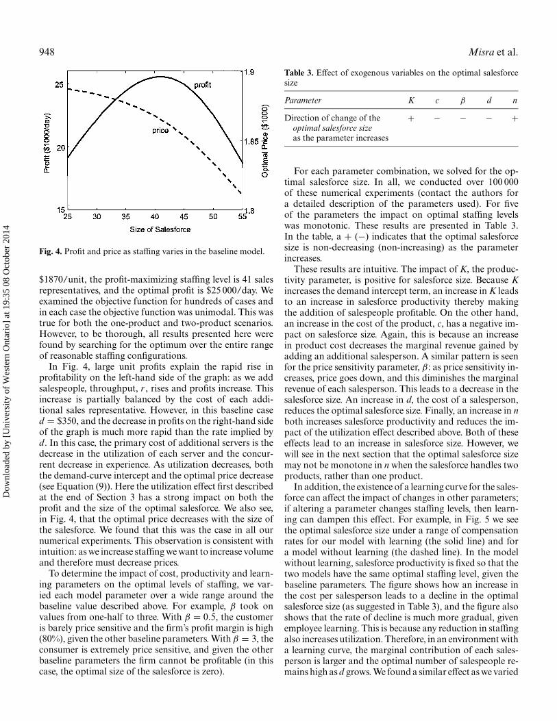
First we consider a firm with a single product to sell anda single salesforce. For the single-product case, the objec-tive function of Equation (7) has a single term in the sum-mation, and the subscripts i and j are removed (e.g., Kijreplaced by K). Throughput and utilization statistics arecalculated from the Erlang-B formula. Given the baselineparameters, we find the optimal price (Equation (9)) andtotal profit (Equation (7)) as a function of salesforce size,S. The results are shown in Fig. 4. The optimal price is

Dow

nloa

ded

by [

Uni

vers

ity o

f W

este

rn O

ntar

io]

at 1

9:35

08

Oct

ober

201

4

948 Misra et al.

Fig. 4. Profit and price as staffing varies in the baseline model.

$1870/unit, the profit-maximizing staffing level is 41 salesrepresentatives, and the optimal profit is $25 000/day. Weexamined the objective function for hundreds of cases andin each case the objective function was unimodal. This wastrue for both the one-product and two-product scenarios.However, to be thorough, all results presented here werefound by searching for the optimum over the entire rangeof reasonable staffing configurations.

In Fig. 4, large unit profits explain the rapid rise inprofitability on the left-hand side of the graph: as we addsalespeople, throughput, r , rises and profits increase. Thisincrease is partially balanced by the cost of each addi-tional sales representative. However, in this baseline cased = $350, and the decrease in profits on the right-hand sideof the graph is much more rapid than the rate implied byd. In this case, the primary cost of additional servers is thedecrease in the utilization of each server and the concur-rent decrease in experience. As utilization decreases, boththe demand-curve intercept and the optimal price decrease(see Equation (9)). Here the utilization effect first describedat the end of Section 3 has a strong impact on both theprofit and the size of the optimal salesforce. We also see,in Fig. 4, that the optimal price decreases with the size ofthe salesforce. We found that this was the case in all ournumerical experiments. This observation is consistent withintuition: as we increase staffing we want to increase volumeand therefore must decrease prices.

To determine the impact of cost, productivity and learn-ing parameters on the optimal levels of staffing, we var-ied each model parameter over a wide range around thebaseline value described above. For example, β took onvalues from one-half to three. With β = 0.5, the customeris barely price sensitive and the firm’s profit margin is high(80%), given the other baseline parameters. With β = 3, theconsumer is extremely price sensitive, and given the otherbaseline parameters the firm cannot be profitable (in thiscase, the optimal size of the salesforce is zero).

Table 3. Effect of exogenous variables on the optimal salesforcesize

Parameter K c β d n

Direction of change of the + − − − +optimal salesforce sizeas the parameter increases

For each parameter combination, we solved for the op-timal salesforce size. In all, we conducted over 100 000of these numerical experiments (contact the authors fora detailed description of the parameters used). For fiveof the parameters the impact on optimal staffing levelswas monotonic. These results are presented in Table 3.In the table, a + (−) indicates that the optimal salesforcesize is non-decreasing (non-increasing) as the parameterincreases.

These results are intuitive. The impact of K, the produc-tivity parameter, is positive for salesforce size. Because Kincreases the demand intercept term, an increase in K leadsto an increase in salesforce productivity thereby makingthe addition of salespeople profitable. On the other hand,an increase in the cost of the product, c, has a negative im-pact on salesforce size. Again, this is because an increasein product cost decreases the marginal revenue gained byadding an additional salesperson. A similar pattern is seenfor the price sensitivity parameter, β: as price sensitivity in-creases, price goes down, and this diminishes the marginalrevenue of each salesperson. This leads to a decrease in thesalesforce size. An increase in d, the cost of a salesperson,reduces the optimal salesforce size. Finally, an increase in nboth increases salesforce productivity and reduces the im-pact of the utilization effect described above. Both of theseeffects lead to an increase in salesforce size. However, wewill see in the next section that the optimal salesforce sizemay not be monotone in n when the salesforce handles twoproducts, rather than one product.

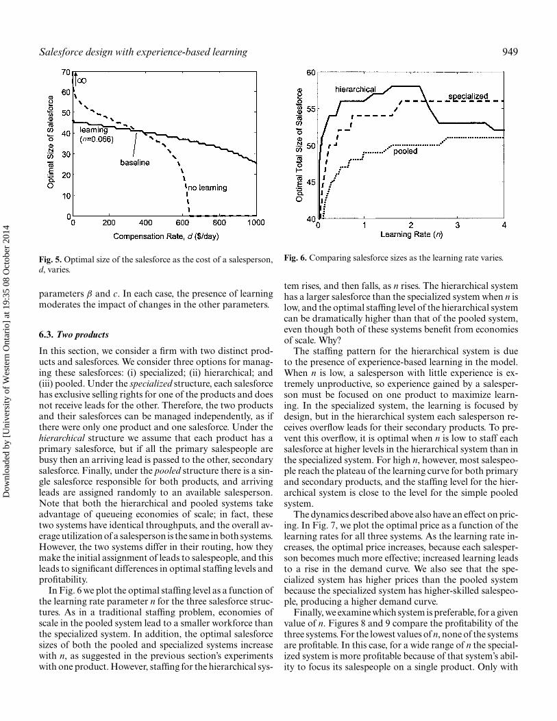
In addition, the existence of a learning curve for the sales-force can affect the impact of changes in other parameters;if altering a parameter changes staffing levels, then learn-ing can dampen this effect. For example, in Fig. 5 we seethe optimal salesforce size under a range of compensationrates for our model with learning (the solid line) and fora model without learning (the dashed line). In the modelwithout learning, salesforce productivity is fixed so that thetwo models have the same optimal staffing level, given thebaseline parameters. The figure shows how an increase inthe cost per salesperson leads to a decline in the optimalsalesforce size (as suggested in Table 3), and the figure alsoshows that the rate of decline is much more gradual, givenemployee learning. This is because any reduction in staffingalso increases utilization. Therefore, in an environment witha learning curve, the marginal contribution of each sales-person is larger and the optimal number of salespeople re-mains high as d grows. We found a similar effect as we varied

Dow

nloa

ded

by [

Uni

vers

ity o

f W

este

rn O

ntar

io]

at 1

9:35

08

Oct

ober

201

4

Salesforce design with experience-based learning 949

Fig. 5. Optimal size of the salesforce as the cost of a salesperson,d, varies.

parameters β and c. In each case, the presence of learningmoderates the impact of changes in the other parameters.

6.3. Two products

In this section, we consider a firm with two distinct prod-ucts and salesforces. We consider three options for manag-ing these salesforces: (i) specialized; (ii) hierarchical; and(iii) pooled. Under the specialized structure, each salesforcehas exclusive selling rights for one of the products and doesnot receive leads for the other. Therefore, the two productsand their salesforces can be managed independently, as ifthere were only one product and one salesforce. Under thehierarchical structure we assume that each product has aprimary salesforce, but if all the primary salespeople arebusy then an arriving lead is passed to the other, secondarysalesforce. Finally, under the pooled structure there is a sin-gle salesforce responsible for both products, and arrivingleads are assigned randomly to an available salesperson.Note that both the hierarchical and pooled systems takeadvantage of queueing economies of scale; in fact, thesetwo systems have identical throughputs, and the overall av-erage utilization of a salesperson is the same in both systems.However, the two systems differ in their routing, how theymake the initial assignment of leads to salespeople, and thisleads to significant differences in optimal staffing levels andprofitability.

In Fig. 6 we plot the optimal staffing level as a function ofthe learning rate parameter n for the three salesforce struc-tures. As in a traditional staffing problem, economies ofscale in the pooled system lead to a smaller workforce thanthe specialized system. In addition, the optimal salesforcesizes of both the pooled and specialized systems increasewith n, as suggested in the previous section’s experimentswith one product. However, staffing for the hierarchical sys-

Fig. 6. Comparing salesforce sizes as the learning rate varies.

tem rises, and then falls, as n rises. The hierarchical systemhas a larger salesforce than the specialized system when n islow, and the optimal staffing level of the hierarchical systemcan be dramatically higher than that of the pooled system,even though both of these systems benefit from economiesof scale. Why?

The staffing pattern for the hierarchical system is dueto the presence of experience-based learning in the model.When n is low, a salesperson with little experience is ex-tremely unproductive, so experience gained by a salesper-son must be focused on one product to maximize learn-ing. In the specialized system, the learning is focused bydesign, but in the hierarchical system each salesperson re-ceives overflow leads for their secondary products. To pre-vent this overflow, it is optimal when n is low to staff eachsalesforce at higher levels in the hierarchical system than inthe specialized system. For high n, however, most salespeo-ple reach the plateau of the learning curve for both primaryand secondary products, and the staffing level for the hier-archical system is close to the level for the simple pooledsystem.

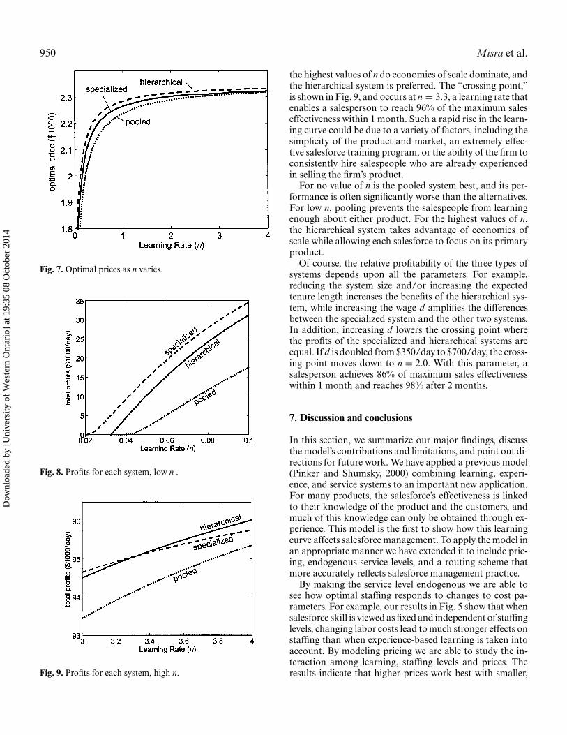
The dynamics described above also have an effect on pric-ing. In Fig. 7, we plot the optimal price as a function of thelearning rates for all three systems. As the learning rate in-creases, the optimal price increases, because each salesper-son becomes much more effective; increased learning leadsto a rise in the demand curve. We also see that the spe-cialized system has higher prices than the pooled systembecause the specialized system has higher-skilled salespeo-ple, producing a higher demand curve.

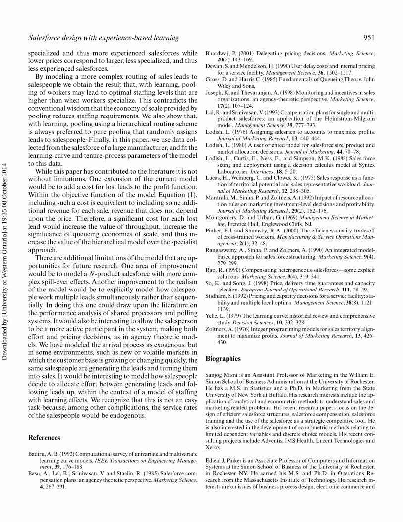
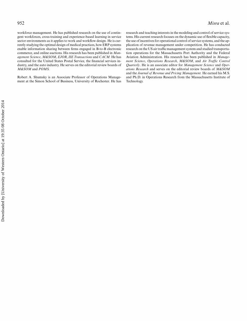
Finally, we examine which system is preferable, for a givenvalue of n. Figures 8 and 9 compare the profitability of thethree systems. For the lowest values of n, none of the systemsare profitable. In this case, for a wide range of n the special-ized system is more profitable because of that system’s abil-ity to focus its salespeople on a single product. Only with

Dow

nloa

ded

by [

Uni

vers

ity o

f W

este

rn O

ntar

io]

at 1

9:35

08

Oct

ober

201

4

950 Misra et al.

Fig. 7. Optimal prices as n varies.

Fig. 8. Profits for each system, low n .

Fig. 9. Profits for each system, high n.

the highest values of n do economies of scale dominate, andthe hierarchical system is preferred. The “crossing point,”is shown in Fig. 9, and occurs at n = 3.3, a learning rate thatenables a salesperson to reach 96% of the maximum saleseffectiveness within 1 month. Such a rapid rise in the learn-ing curve could be due to a variety of factors, including thesimplicity of the product and market, an extremely effec-tive salesforce training program, or the ability of the firm toconsistently hire salespeople who are already experiencedin selling the firm’s product.

For no value of n is the pooled system best, and its per-formance is often significantly worse than the alternatives.For low n, pooling prevents the salespeople from learningenough about either product. For the highest values of n,the hierarchical system takes advantage of economies ofscale while allowing each salesforce to focus on its primaryproduct.

Of course, the relative profitability of the three types ofsystems depends upon all the parameters. For example,reducing the system size and/or increasing the expectedtenure length increases the benefits of the hierarchical sys-tem, while increasing the wage d amplifies the differencesbetween the specialized system and the other two systems.In addition, increasing d lowers the crossing point wherethe profits of the specialized and hierarchical systems areequal. If d is doubled from $350/day to $700/day, the cross-ing point moves down to n = 2.0. With this parameter, asalesperson achieves 86% of maximum sales effectivenesswithin 1 month and reaches 98% after 2 months.

7. Discussion and conclusions

In this section, we summarize our major findings, discussthe model’s contributions and limitations, and point out di-rections for future work. We have applied a previous model(Pinker and Shumsky, 2000) combining learning, experi-ence, and service systems to an important new application.For many products, the salesforce’s effectiveness is linkedto their knowledge of the product and the customers, andmuch of this knowledge can only be obtained through ex-perience. This model is the first to show how this learningcurve affects salesforce management. To apply the model inan appropriate manner we have extended it to include pric-ing, endogenous service levels, and a routing scheme thatmore accurately reflects salesforce management practice.

By making the service level endogenous we are able tosee how optimal staffing responds to changes to cost pa-rameters. For example, our results in Fig. 5 show that whensalesforce skill is viewed as fixed and independent of staffinglevels, changing labor costs lead to much stronger effects onstaffing than when experience-based learning is taken intoaccount. By modeling pricing we are able to study the in-teraction among learning, staffing levels and prices. Theresults indicate that higher prices work best with smaller,

Dow

nloa

ded

by [

Uni

vers

ity o

f W

este

rn O

ntar

io]

at 1

9:35

08

Oct

ober

201

4

Salesforce design with experience-based learning 951

specialized and thus more experienced salesforces whilelower prices correspond to larger, less specialized, and thusless experienced salesforces.

By modeling a more complex routing of sales leads tosalespeople we obtain the result that, with learning, pool-ing of workers may lead to optimal staffing levels that arehigher than when workers specialize. This contradicts theconventional wisdom that the economy of scale provided bypooling reduces staffing requirements. We also show that,with learning, pooling using a hierarchical routing schemeis always preferred to pure pooling that randomly assignsleads to salespeople. Finally, in this paper, we use data col-lected from the salesforce of a large manufacturer, and fit thelearning-curve and tenure-process parameters of the modelto this data.

While this paper has contributed to the literature it is notwithout limitations. One extension of the current modelwould be to add a cost for lost leads to the profit function.Within the objective function of the model Equation (1),including such a cost is equivalent to including some addi-tional revenue for each sale, revenue that does not dependupon the price. Therefore, a significant cost for each lostlead would increase the value of throughput, increase thesignificance of queueing economies of scale, and thus in-crease the value of the hierarchical model over the specialistapproach.

There are additional limitations of the model that are op-portunities for future research. One area of improvementwould be to model a N-product salesforce with more com-plex spill-over effects. Another improvement to the realismof the model would be to explicitly model how salespeo-ple work multiple leads simultaneously rather than sequen-tially. In doing this one could draw upon the literature onthe performance analysis of shared processors and pollingsystems. It would also be interesting to allow the salespersonto be a more active participant in the system, making botheffort and pricing decisions, as in agency theoretic mod-els. We have modeled the arrival process as exogenous, butin some environments, such as new or volatile markets inwhich the customer base is growing or changing quickly, thesame salespeople are generating the leads and turning theminto sales. It would be interesting to model how salespeopledecide to allocate effort between generating leads and fol-lowing leads up, within the context of a model of staffingwith learning effects. We recognize that this is not an easytask because, among other complications, the service ratesof the salespeople would be endogenous.

References

Badiru, A. B. (1992) Computational survey of univariate and multivariatelearning curve models. IEEE Transactions on Engineering Manage-ment, 39, 176–188.

Basu, A., Lal, R., Srinivasan, V. and Staelin, R. (1985) Salesforce com-pensation plans: an agency theoretic perspective. Marketing Science,4, 267–291.

Bhardwaj, P. (2001) Delegating pricing decisions. Marketing Science,20(2), 143–169.

Dewan, S. and Mendelson, H. (1990) User delay costs and internal pricingfor a service facility. Management Science, 36, 1502–1517.

Gross, D. and Harris C. (1985) Fundamentals of Queueing Theory. JohnWiley and Sons,

Joseph, K. and Thevaranjan, A. (1998) Monitoring and incentives in salesorganizations: an agency-theoretic perspective. Marketing Science,17(2), 107–124.

Lal, R. and Srinivasan, V. (1993) Compensation plans for single and multi-product salesforces: an application of the Holmstrom-Milgrommodel. Management Science, 39, 777–793.

Lodish, L. (1976) Assigning salesmen to accounts to maximize profits.Journal of Marketing Research, 13, 440–444.

Lodish, L. (1980) A user oriented model for salesforce size, product andmarket allocation decisions. Journal of Marketing, 44, 70–78.

Lodish, L., Curtis, E., Ness, E., and Simpson, M.K. (1988) Sales forcesizing and deployment using a decision calculus model at SyntexLaboratories. Interfaces, 18, 5–20.

Lucas, H., Weinberg, C. and Clowes, K. (1975) Sales response as a func-tion of territorial potential and sales representative workload. Jour-nal of Marketing Research, 12, 298–305.

Mantrala, M., Sinha, P. and Zoltners, A. (1992) Impact of resource alloca-tion rules on marketing investment-level decisions and profitability.Journal of Marketing Research, 29(2), 162–176.

Montgomery, D. and Urban, G. (1969) Management Science in Market-ing, Prentice Hall, Englewood Cliffs, NJ.

Pinker, E.J. and Shumsky, R.A. (2000) The efficiency-quality trade-offof cross-trained workers. Manufacturing & Service Operations Man-agement, 2(1), 32–48.

Rangaswamy, A., Sinha, P. and Zoltners, A. (1990) An integrated model-based approach for sales force structuring. Marketing Science, 9(4),279–299.

Rao, R. (1990) Compensating heterogeneous salesforces—some explicitsolutions. Marketing Science, 9(4), 319–341.

So, K. and Song, J. (1998) Price, delivery time guarantees and capacityselection. European Journal of Operational Research, 111, 28–49.

Stidham, S. (1992) Pricing and capacity decisions for a service facility: sta-bility and multiple local optima. Management Science, 38(8), 1121–1139.

Yelle, L. (1979) The learning curve: historical review and comprehensivestudy. Decision Sciences, 10, 302–328.

Zoltners, A. (1976) Integer programming models for sales territory align-ment to maximize profits. Journal of Marketing Research, 13, 426–430.

Biographies

Sanjog Misra is an Assistant Professor of Marketing in the William E.Simon School of Business Administration at the University of Rochester.He has a M.S. in Statistics and a Ph.D. in Marketing from the StateUniversity of New York at Buffalo. His research interests include the ap-plication of analytical and econometric methods to understand sales andmarketing related problems. His recent research papers focus on the de-sign of efficient salesforce structures, salesforce compensation, salesforcetraining and the use of the salesforce as a strategic competitive tool. Heis also interested in the development of econometric methods relating tolimited dependent variables and discrete choice models. His recent con-sulting projects include Adventis, IMS Health, Lucent Technologies andXerox.

Edieal J. Pinker is an Associate Professor of Computers and InformationSystems at the Simon School of Business of the University of Rochester,in Rochester NY. He earned his M.S. and Ph.D. in Operations Re-search from the Massachusetts Institute of Technology. His research in-terests are on issues of business process design, electronic commerce and

Dow

nloa

ded

by [

Uni

vers

ity o

f W

este

rn O

ntar

io]

at 1

9:35

08

Oct

ober

201

4

952 Misra et al.

workforce management. He has published research on the use of contin-gent workforces, cross-training and experience-based learning in servicesector environments as it applies to work and workflow design. He is cur-rently studying the optimal design of medical practices, how ERP systemsenable information sharing between firms engaged in B-to-B electroniccommerce, and online auctions. His research has been published in Man-agement Science, M&SOM, EJOR, IIE Transactions and CACM. He hasconsulted for the United States Postal Service, the financial services in-dustry, and the auto industry. He serves on the editorial review boards ofM&SOM and POMS.

Robert A. Shumsky is an Associate Professor of Operations Manage-ment at the Simon School of Business, University of Rochester. He has

research and teaching interests in the modeling and control of service sys-tems. His current research focuses on the dynamic use of flexible capacity,the use of incentives for operational control of service systems, and the ap-plication of revenue management under competition. He has conductedresearch on the US air traffic management system and studied transporta-tion operations for the Massachusetts Port Authority and the FederalAviation Administration. His research has been published in Manage-ment Science, Operations Research, M&SOM, and Air Traffic ControlQuarterly. He is an associate editor for Management Science and Oper-ations Research and serves on the editorial review boards of M&SOMand the Journal of Revenue and Pricing Management. He earned his M.S.and Ph.D. in Operations Research from the Massachusetts Institute ofTechnology.

Dow

nloa

ded

by [

Uni

vers

ity o

f W

este

rn O

ntar

io]

at 1

9:35

08

Oct

ober

201

4