salmonella outbreaks: assessing causes and trends · background information •what is salmonella?...
TRANSCRIPT
S A R A H R . S A L T E R
A M A N D A S . L U B Y
K E V I N A . T O R R E S
K A T E C O W L E S , P H D
Salmonella outbreaks: Assessing causes and trends
Background Information
• What is salmonella?
• Rod shaped bacteria
• Causes 2 diseases called salmonellosis
enteric fever
acute gastric enteritis
• Most common causes are raw meat, raw eggs, raw shellfish or unpasteurized animal products such as milk and cheese
• Not harmful until it is ingested
• Most harmful to compromised immune systems
Background Information
• Symptoms: • Nausea
• Vomiting
• Abdominal pain
• Diarrhea
• Fever
• Blood in the stool
• 12-72 hours after ingestion
Severe cases of salmonella end up in dehydration,
leading to a possible death.

Public Health Concern
• Actual number of infections could be thirty or more times greater (CDC)
• 1.2 million U.S. illnesses annually
• Most common cause of hospitalization and death tracked by FoodNet
• Incidence of Salmonella was nearly three times the 2010 national health objective target.
• Lab results since 1998 shows a positive trend
http://www.cdc.gov/foodborneburden/trends-in-foodborne-illness.html
Diamond Pet Food
Manufacturer linked to Salmonella Infantis outbreak in humans
Location: Gaston, SC
Detected through random sampling –by MDARD
Recall occurred April 2nd
Infections identified from October 2011 – June 2012
Illnesses caused by improper handling of pet food or feces
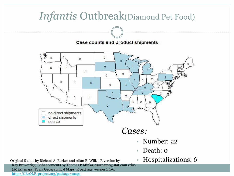
Infantis Outbreak(Diamond Pet Food)
Cases: • Number: 22
• Death: 0
• Hospitalizations: 6
Original S code by Richard A. Becker and Allan R. Wilks. R version by Ray Brownrigg. Enhancements by Thomas P Minka <[email protected]>. (2012). maps: Draw Geographical Maps. R package version 2.2-6. http://CRAN.R-project.org/package=maps
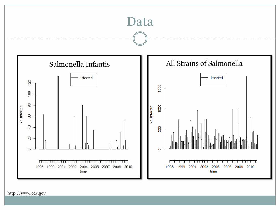
Data
Salmonella Infantis All Strains of Salmonella
http://www.cdc.gov

Research Approach
Method: Bayesian Statistics 1. Analysis using Models:
Poisson Changepoint Model • Fitted using Markov Chain Monte Carlo
Poisson-Gamma Model • Fitted Using Analytic Computation
1. Simulation Study:
Simulate data comparable to our data set.
Run 1000 data sets for each set of parameters.
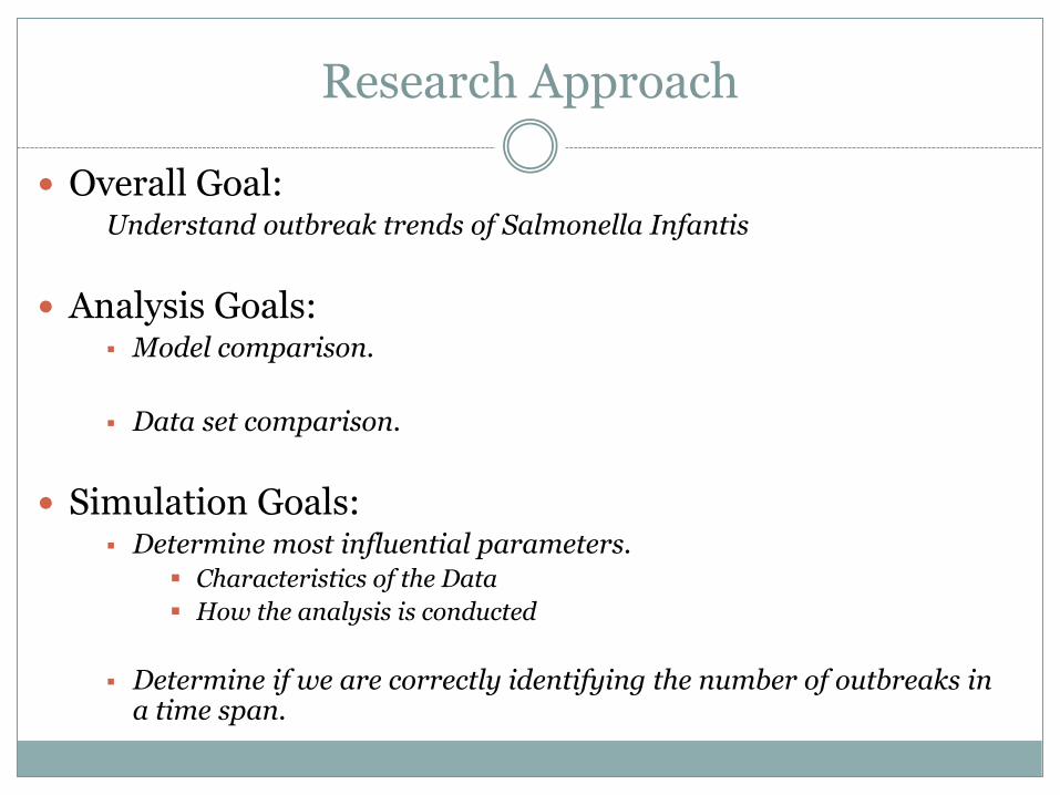
Research Approach
Overall Goal: Understand outbreak trends of Salmonella Infantis
Analysis Goals: Model comparison.
Data set comparison.
Simulation Goals: Determine most influential parameters.
Characteristics of the Data
How the analysis is conducted
Determine if we are correctly identifying the number of outbreaks in a time span.

Research Approach
Analysis Hypotheses:
Our two models will produce similar results.
Simulation Hypotheses:
The frequency and magnitude of outbreaks will be the most influential factors in detecting the correct number of outbreaks.
A smaller upper bound probability will produce more accurate count of outbreaks.
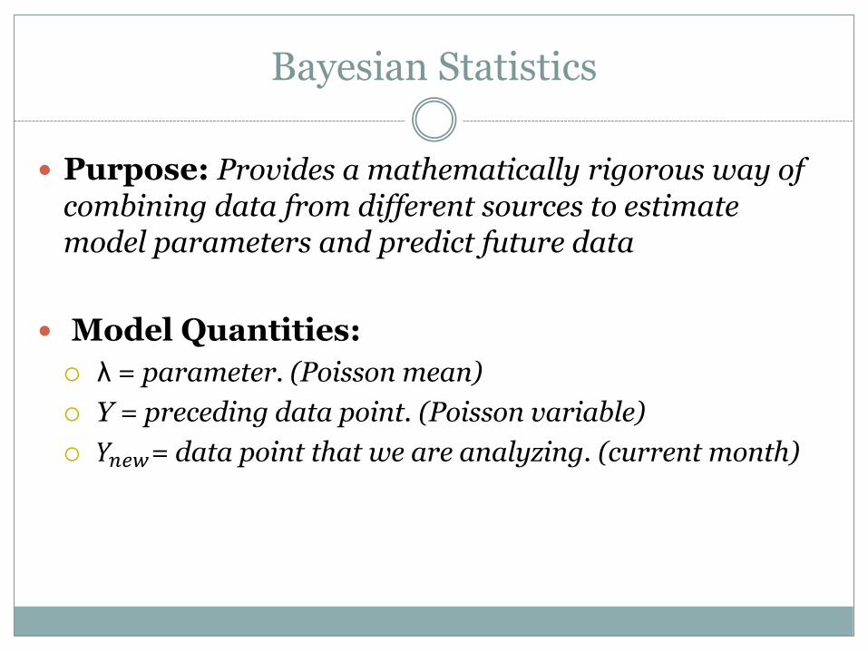
Bayesian Statistics
Purpose: Provides a mathematically rigorous way of combining data from different sources to estimate model parameters and predict future data
Model Quantities:
λ = parameter. (Poisson mean)
Y = preceding data point. (Poisson variable)
𝑌𝑛𝑒𝑤= data point that we are analyzing. (current month)
Bayesian Statistics
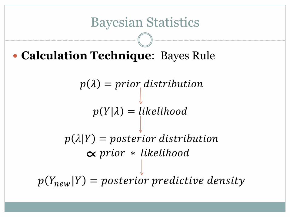
Calculation Technique: Bayes Rule
𝑝 𝜆 = 𝑝𝑟𝑖𝑜𝑟 𝑑𝑖𝑠𝑡𝑟𝑖𝑏𝑢𝑡𝑖𝑜𝑛
𝑝 𝑌|𝜆 = 𝑙𝑖𝑘𝑒𝑙𝑖ℎ𝑜𝑜𝑑
𝑝 𝜆|𝑌 = 𝑝𝑜𝑠𝑡𝑒𝑟𝑖𝑜𝑟 𝑑𝑖𝑠𝑡𝑟𝑖𝑏𝑢𝑡𝑖𝑜𝑛
𝑝𝑟𝑖𝑜𝑟 ∗ 𝑙𝑖𝑘𝑒𝑙𝑖ℎ𝑜𝑜𝑑
𝑝 𝑌𝑛𝑒𝑤|𝑌 = 𝑝𝑜𝑠𝑡𝑒𝑟𝑖𝑜𝑟 𝑝𝑟𝑒𝑑𝑖𝑐𝑡𝑖𝑣𝑒 𝑑𝑒𝑛𝑠𝑖𝑡𝑦
Bayesian Statistics
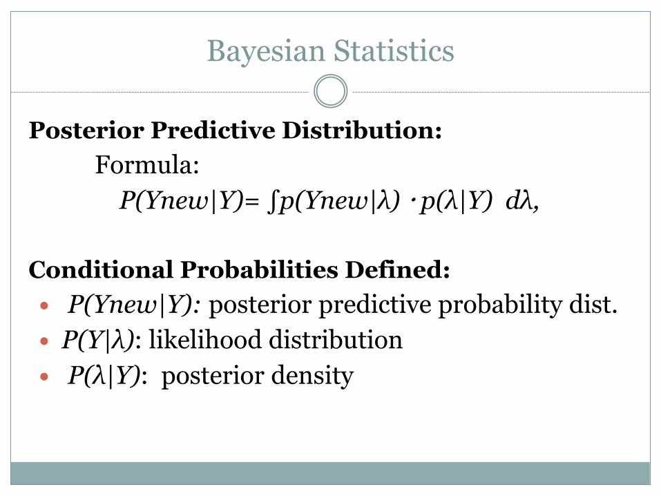
Posterior Predictive Distribution:
Formula:
P(Ynew|Y)= ∫p(Ynew|λ) p(λ|Y) dλ,
Conditional Probabilities Defined:
P(Ynew|Y): posterior predictive probability dist.
P(Y|λ): likelihood distribution
P(λ|Y): posterior density
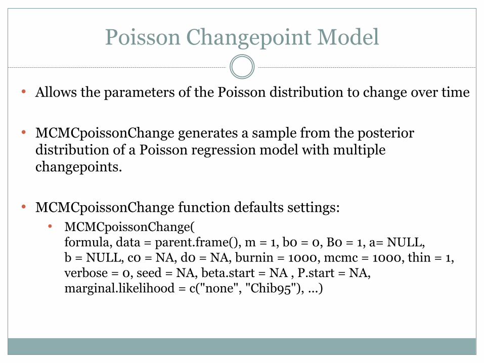
Poisson Changepoint Model
• Allows the parameters of the Poisson distribution to change over time
• MCMCpoissonChange generates a sample from the posterior distribution of a Poisson regression model with multiple changepoints.
• MCMCpoissonChange function defaults settings:
• MCMCpoissonChange( formula, data = parent.frame(), m = 1, b0 = 0, B0 = 1, a= NULL, b = NULL, c0 = NA, d0 = NA, burnin = 1000, mcmc = 1000, thin = 1, verbose = 0, seed = NA, beta.start = NA , P.start = NA, marginal.likelihood = c("none", "Chib95"), ...)

Poisson Changepoint Model
BayesFactor(): best model is the model with highest log marginal likelihood (Method of Chib)
Andrew D. Martin, Kevin M. Quinn, Jong Hee Park (2011). MCMCpack:
Markov Chain Monte Carlo in R. Journal of Statistical Software. 42(9): 1-21. URL http://www.jstatsoft.org/v42/i09/.
Sylvia Fruhwirth-Schnatter and Helga Wagner 2006. “Auxiliary Mixture Sampling for Parameter-driven Models of Time Series of Counts with Applications to State Space Modelling.” Biometrika. 93:827–841.
Siddhartha Chib. 1998. “Estimation and comparison of multiple change-point models.” Journal of Econometrics. 86: 221-241.
Package: MCMCpack
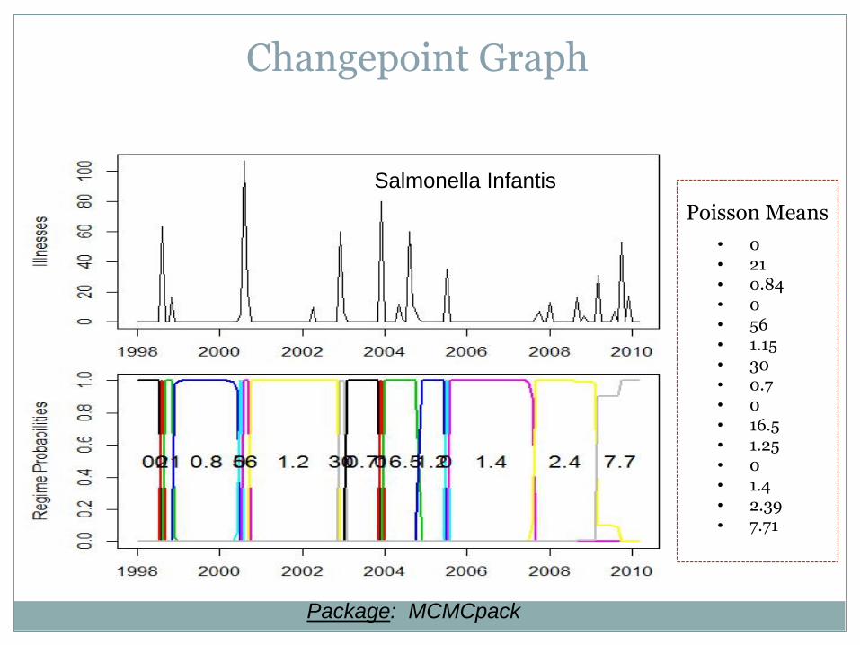
Salmonella Infantis
Changepoint Graph
• 0 • 21 • 0.84 • 0 • 56 • 1.15 • 30 • 0.7 • 0 • 16.5 • 1.25 • 0 • 1.4 • 2.39 • 7.71
Poisson Means

Package: MCMCpack
Total Salmonella
NO GRAPH
Unable to detect changepoints
Changepoint Graph

Bayesian Poisson-Gamma
• Poisson likelihood; gamma prior; Negative Binomial posterior predictive
• Fits a poisson-gamma model to data to determine which timepoints are improbably large compared to previous data values
• Bayes Algorithm for surveillance • algo.bayes(disProgObj, control = list(range = range,
b = 0, w = 6, actY = TRUE, alpha=0.05))
surveillance: An R package for the surveillance of infectious diseases (2007), M. Hoehle, Computational Statistics, 22(4), pp.571--582.
Riebler A (2004) Empirischer Vergleich von statistischen Methoden zur
Ausbruchserkennung bei Surveillance
Daten. Bachelor’s thesis, Department of Statistics, University of Munich
Predicting Alarms
Based on posterior predictive distribution, Bayes algorithm creates a maximum typical value
Depends on probability level set by user (α)
Based on preceding data, there is a (1-α) probability that the current month case count will be at or below the upper bound
If value is above upper bound, flagged as alarm
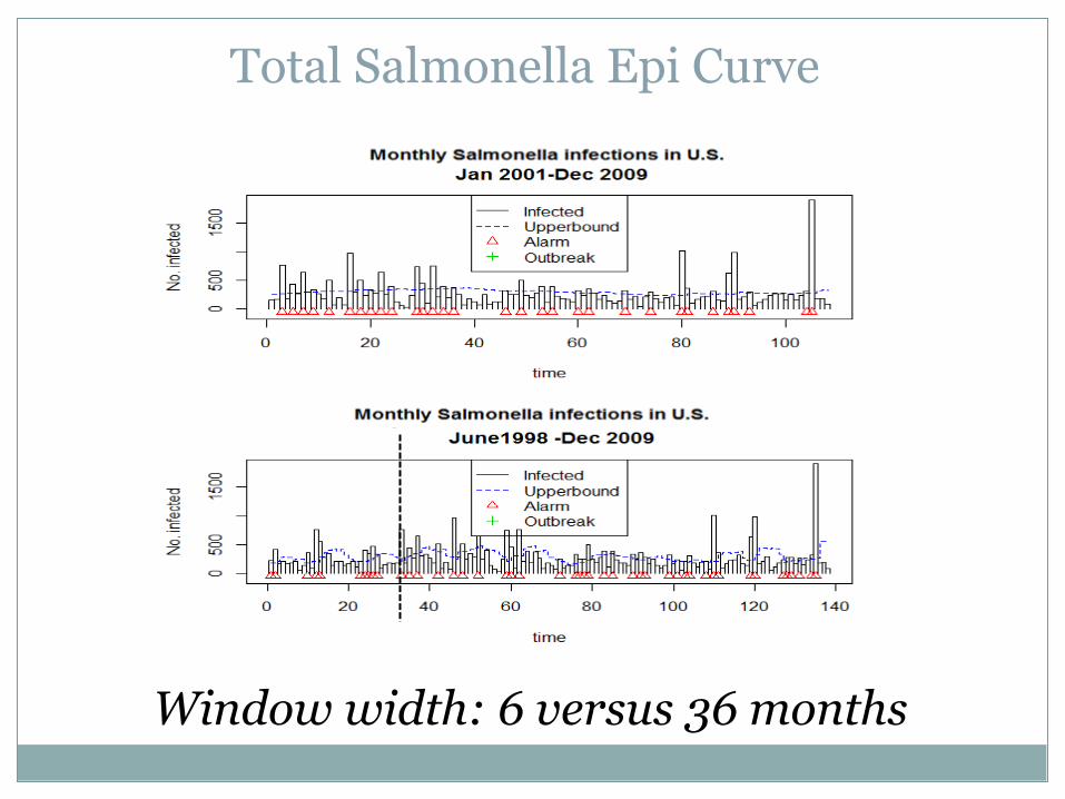
Window width: 6 versus 36 months
Total Salmonella Epi Curve
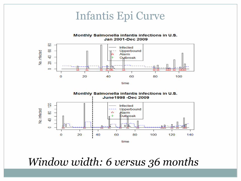
Infantis Epi Curve
Window width: 6 versus 36 months
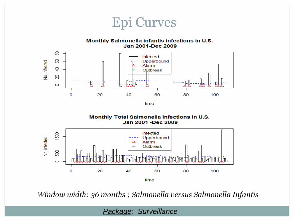
Epi Curves
Package: Surveillance
Window width: 36 months ; Salmonella versus Salmonella Infantis
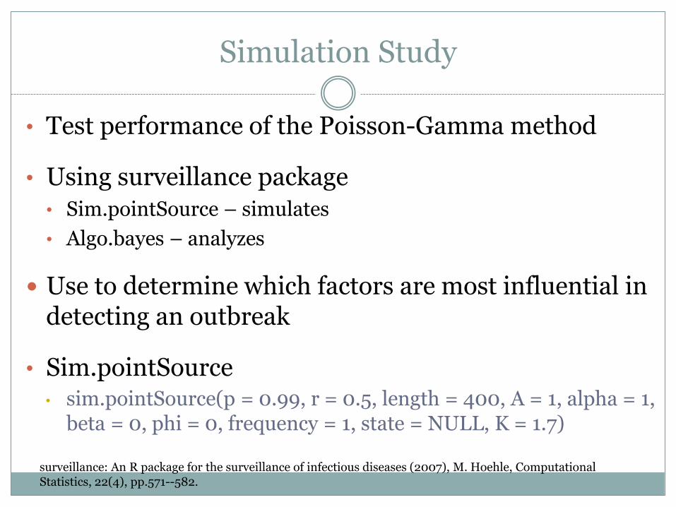
Simulation Study
• Test performance of the Poisson-Gamma method
• Using surveillance package • Sim.pointSource – simulates
• Algo.bayes – analyzes
Use to determine which factors are most influential in detecting an outbreak
• Sim.pointSource • sim.pointSource(p = 0.99, r = 0.5, length = 400, A = 1, alpha = 1,
beta = 0, phi = 0, frequency = 1, state = NULL, K = 1.7)
surveillance: An R package for the surveillance of infectious diseases (2007), M. Hoehle, Computational Statistics, 22(4), pp.571--582.
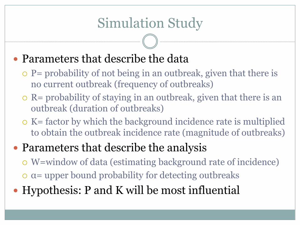
Simulation Study
Parameters that describe the data
P= probability of not being in an outbreak, given that there is no current outbreak (frequency of outbreaks)
R= probability of staying in an outbreak, given that there is an outbreak (duration of outbreaks)
K= factor by which the background incidence rate is multiplied to obtain the outbreak incidence rate (magnitude of outbreaks)
Parameters that describe the analysis
W=window of data (estimating background rate of incidence)
α= upper bound probability for detecting outbreaks
Hypothesis: P and K will be most influential

Example of Simulated Data

Simulation Study: Code
survsim=function(p,r,k,nsets, alpha,w){
trueCount<-rep(NA, nsets)
estCount<-rep(NA,nsets)
for (i in 1:nsets){
#Simulate the disProg object using specified parameters
object<-sim.pointSource(p=p, r=r, length=144, A=0, alpha=.001,
beta=0, phi=0, frequency=12, state=NULL, K=k)
#Counts number of actual outbreaks in simulated object
#If more than one outbreak month in a row, only counts it once
trueCount[i]<-sum(diff(c(object$state[(w+1):144],0))==-1)
#Performs algo bayes analysis on simulated object
res <- algo.bayes(object, control=list( w=w, range=(w+1):144, alpha=alpha))
#Counts number of detected outbreaks in simulated object
#If more than one outbreak month in a row, only counts it once
estCount[i]<-sum(diff(c(res$alarm,0))==-1) }
#Returns list of true counts, estimated counts, as well as
#specified parameters to identify simulation
return(list(trueCount=trueCount, estCount=estCount, p=p, r=r, k=k))
}
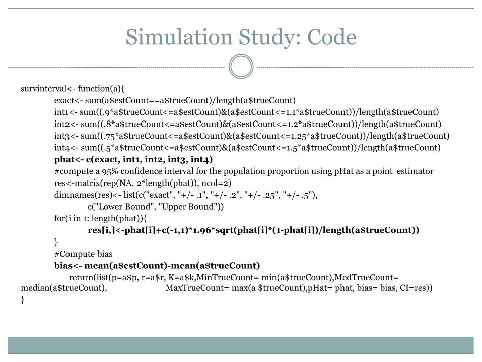
Simulation Study: Code
survinterval<- function(a){
exact<- sum(a$estCount==a$trueCount)/length(a$trueCount)
int1<- sum((.9*a$trueCount<=a$estCount)&(a$estCount<=1.1*a$trueCount))/length(a$trueCount)
int2<- sum((.8*a$trueCount<=a$estCount)&(a$estCount<=1.2*a$trueCount))/length(a$trueCount)
int3<- sum((.75*a$trueCount<=a$estCount)&(a$estCount<=1.25*a$trueCount))/length(a$trueCount)
int4<- sum((.5*a$trueCount<=a$estCount)&(a$estCount<=1.5*a$trueCount))/length(a$trueCount)
phat<- c(exact, int1, int2, int3, int4)
#compute a 95% confidence interval for the population proportion using pHat as a point estimator
res<-matrix(rep(NA, 2*length(phat)), ncol=2)
dimnames(res)<- list(c("exact", "+/- .1", "+/- .2", "+/- .25", "+/- .5"),
c("Lower Bound", "Upper Bound"))
for(i in 1: length(phat)){
res[i,]<-phat[i]+c(-1,1)*1.96*sqrt(phat[i]*(1-phat[i])/length(a$trueCount))
}
#Compute bias
bias<- mean(a$estCount)-mean(a$trueCount)
return(list(p=a$p, r=a$r, K=a$k,MinTrueCount= min(a$trueCount),MedTrueCount= median(a$trueCount), MaxTrueCount= max(a $trueCount),pHat= phat, bias= bias, CI=res))
}

Simulation Study: Results R: probability of staying in an outbreak given that there is already an outbreak (duration of outbreaks)
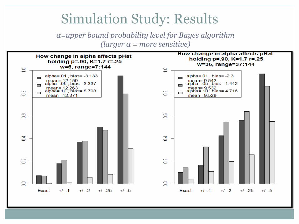
Simulation Study: Results α=upper bound probability level for Bayes algorithm
(larger α = more sensitive)
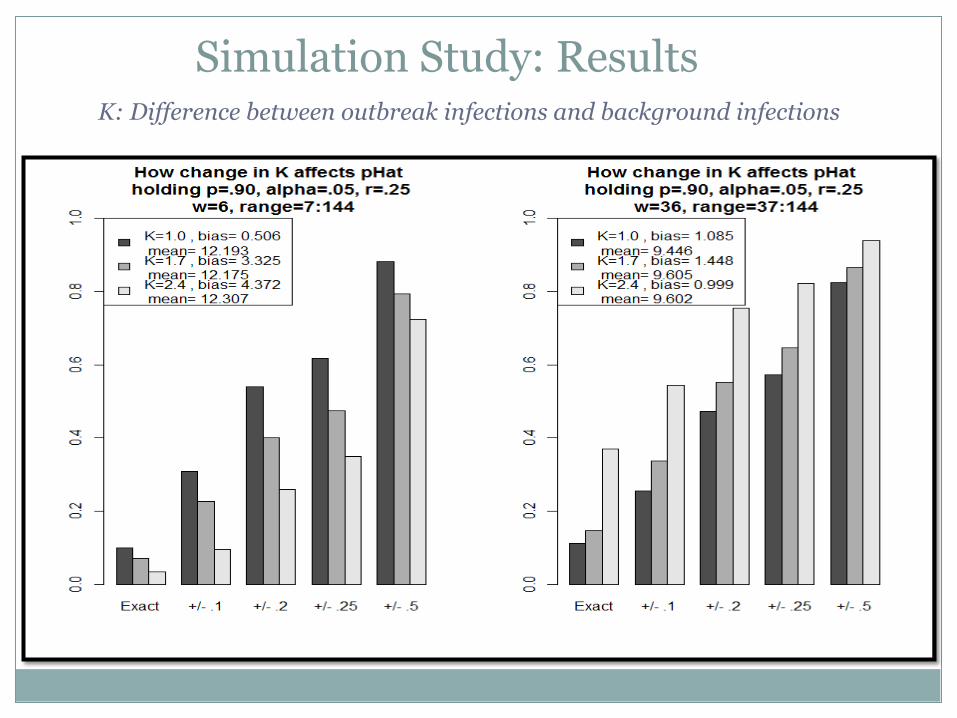
Simulation Study: Results K: Difference between outbreak infections and background infections

Simulation Study: Results P: probability of not being in an outbreak given that there is no outbreak
(frequency of outbreaks)
Conclusions
• Data Analysis:
o Poisson-Gamma method can handle different types of data better than the Changepoint analysis
o Tendency to overestimate number of outbreaks in data like Infantis (ie. long stretches of zeros and then high counts)
• Simulation:
o Frequency of outbreaks (p)
o Upper bound probability (alpha)
o Bias

Questions?

Appendix: Poisson-Gamma Distribution
surveillance: An R package for the surveillance of infectious diseases (2007), M. Hoehle, Computational Statistics, 22(4), pp.571--582.