WP/16/6

SAMA Working Paper:

On The Stability of Money Demand in Saudi

Arabia

November 2016

By

Moayad H. Al Rasasi

Economic Research Department

Saudi Arabian Monetary Agency

The views expressed are those of the author(s) and do not necessarily reflect the position of the

Saudi Arabian Monetary Agency (SAMA) and its policies. This Working Paper should not be

reported as representing the views of SAMA

2

On the Stability of Money Demand in Saudi Arabia*

Moayad H. Al Rasasi

Economic Research Department

Saudi Arabian Monetary Agency (SAMA)

November 2016

Abstract

This paper assesses the stability of money demand function for Saudi Arabia over

the period 1993:Q1-2015:Q3. This paper finds evidence indicating the stability of

money demand function over the long run. Likewise, it finds the parameter

estimates of the long run relationship are consistent with theory expectations. In

other words, a rise in income by one percent is associated with higher demand for

money by 2.47 percent. On other hand, money demand falls by 0.15 percent due to

the increase of the interest rate by one percent; likewise, money demand declines

by 0.5 percent when the nominal effective exchange rate increases by one percent.

Keywords: Money Demand; Stability; Cointegration; Saudi Arabia.

JEL Classification: C13, C22, E41, E52, F41

* The author would like to thank Dr. Waheed Banafea and Mr. Ahmad Albakr for their valuable

comments and suggestions to enhance this paper.

3

1. Introduction

Analyzing the behavior of money demand has been one of the substantial subjects

in both theoretical and empirical research due to its importance for monetary

policymakers. In other words, sustaining a stable money demand is crucial because

it enables monetary policymakers for some countries1 to fight inflationary

pressures and to stimulate the economy through targeting money growth. Likewise,

maintaining stable money demand is essential for other countries adopting fixed

exchange rate regime (e.g. Saudi Arabia) to sustain stable nominal exchange rate.

As a result, there has been ongoing research examining the stability of money

demand function for advanced and less advanced economies. However, the

findings of these studies on particular countries seem to be conflicting, in which

some studies conclude the stability of money demand whereas other studies do not.

Hence, in order to avoid conflicting results and to implement the appropriate

monetary policy, it is necessary to understand the source of instability for money

demand. The existing literature points out to some factors that may lead to instable

demand for money. The sources of instability might be due to financial innovations

(i.e. Arrau and Gregorio 1993), shifts in exchange rate regime (i.e. Boughton

1981), currency substitution (i.e. Girton and Roper 1981), and output uncertainty

(i.e. Choi and Oh 2003). Likewise, some economists point out to some

econometric issues leading to the existence of instable money demand function.

Cheong (2003) indicates that the misspecification of money demand function is a

1 According to the 2014 IMF annual report on Exchange Arrangements and Exchange Restrictions, there

are 25 countries adopting monetary aggregate targeting to eliminate inflationary pressures; for instance,

some of these countries are China, Uzbekistan, Sierra Leone, Ukraine, and Uruguay.

4

key factor leading to instability. Additional factor playing essential role in arising

instability is the frequency of data as implied by Gregory and Hansen (1996).

Changes in regulations, global uncertainty or oil price volatility are other elements

contributing to money demand instability.

Therefore, there is a large body of the literature focusing on examining the

money demand function over long run. The existing studies not only aim to

identify factors leading to instability, but also to provide monetary policymakers

with the appropriate policy averting money demand instability. Nonetheless,

despite the numerous studies on money demand, the existing literature focusing on

Saudi Arabia is very limited. This limitation might be due to lack of interest from

researchers or due to the lack of data availability or both.

This in turn motivates us to fill the gap by re-examining the stability of

money demand relationship with its determinants over long run. Additional

motivation for this study is the recent research paper of Banafea (2014) who

documents evidence in favor of the instability of Saudi money demand function via

the implementation of various structural break tests. In sum, the main objective of

this research paper is to investigate the relationship between money demand and its

determinants in Saudi Arabia and whether this relationship is stable over long run

or not.

The outline of the paper is as follows: section 2 presents the framework of

money demand function while section 3 overviews the existing literature on Saudi

Arabia. Section 4 describes the data; section 5 outlines the empirical methodology

alongside the discussion of the results; the conclusion of the paper is contained in

section 6.

5

2. Money Demand Framework

In modeling the demand for money, it is common in practice to assume that both

real output and nominal interest rate as main factors determining the demand for

money in any economy, in which the nominal interest rate reflects the opportunity

cost of holding money while the real output is a scale variable. Thus, the general

form representing long run demand for money can be specified as follows:

(𝑚

𝑝) = 𝑓(𝑦, 𝑖) (1)

where (𝑚

𝑝) 𝑜𝑟 𝑚𝑑 represents the real money balance; in which 𝑚 denotes the

monetary aggregate deflated by the consumer price index (𝑝); 𝑦, 𝑎𝑛𝑑 𝑖 denote the

real output, and nominal interest rate respectively.

It is worthy emphasizing that other studies incorporate the exchange rate as

an additional determinant to money demand function due to its influence on money

demand (i.e. Bahmani-Oskooee & Shabsigh 1996, Bahmani 2000). Likewise, it is

essential to bear in mind that Mundell (1963) was among the pioneers suggesting

the incorporation of exchange rate into money demand function. However, he does

not provide any convincing reason for the insertion of exchange rate and without

presenting any estimates for money demand function. This in turn encourages

other researchers to provide intuitive explanations for inserting the exchange rate

variable into money demand function. For instance, Arango and Nadiri (1981)

provide an argument illustrating how changes in exchange rates may influence the

demand for money. Based on their argument, the fall (depreciation) of domestic

currency relative to foreign currency would increase the local currency value,

which in turn leads to rise domestic individuals’ foreign assets. If this increase

6

considered as an increase of wealth, then the demand for money may increase.

Bahmani-Oskooee and Pourheydarian (1990) provide alterative explanation. They

argue that the demand for money fluctuates based on the public’s expectation. In

other words, if the public expects further depreciation of their domestic currency

relative to foreign currency, they would reduce their demand for domestic currency

and increase their demand for foreign currency resulting in a decline of demand for

money. The opposite would occur if the public expects the appreciation of foreign

currency relative to their domestic currency.

Therefore, we follow Bahmani-Oskooee & Shabsigh (1996) and Bahmani

(2000) and incorporate the exchange rate variable into the money demand function.

The motivation for the inclusion of exchange rate into the Saudi money demand

function is that Saudi Arabia pegs its currency to the US dollar at fixed exchange

rate since 1986, so any fluctuations of the US dollar may influence the currency of

Saudi Arabia.

Therefore, the money demand function augmented with nominal effective

exchange rate can be formulated as follows:

(𝑚

𝑝) ≡ 𝑚𝑑 = 𝑓(𝑌, 𝐼, 𝑁𝐸) (2)

which in turn can be written as follows:

𝑚𝑡𝑑 = 𝛼 + 𝛽𝑌𝑡 + 𝛾𝐼𝑡 + 𝛿𝑁𝐸𝑡 + 휀𝑡 (3)

where 𝑚𝑑 , 𝐼𝑡 , 𝐼𝑡 , 𝐸𝑡 , 𝑎𝑛𝑑 휀𝑡 denote the demand for money, real output proxied by

industrial production, nominal interest rate, nominal effective exchange rate, and

error term at time 𝑡 respectively. Based on economic theory2, we expect a positive

2 According to the Keynesian theory for money demand, money demand is positively associated with

income because people are willing to demand money to for transactional and cautionary (future

uncertainty) purposes. Nonetheless, the money demand is negatively associated with interest rate because

7

relationship between the demand for money and output implying 𝛽 > 0 whereas

the demand for money is negatively associated with nominal interest rate implying

𝛾 < 0. On the other hand, the sign of 𝛿 may have either positive or negative

impacts on the demand for money as suggested by Bahmani-Oskooee and

Pourheydarian (1990).

3. Literature Review

There is a rich literature on money demand function investigating the determinants

of money demand as well as assessing the stability of money demand function. The

existing literature focuses on both developed and developing countries and applies

various econometric methodologies. For example, some studies analyze the

behavior of money demand function and its stability on industrial countries (i.e.

Bahmani-Oskooee and Chomsisengphet 2002), Asian countries (i.e. Bahmani-

Oskooee and Rehman 2005), European countries (i.e. Coenen & Vega 2001),

African countries (i.e. Bahmani-Oskooee and Gelan 2009), and Middle Eastern

countries (i.e. Bahmani 2008). Sriram (2000) and Banafea (2012) provide a

comprehensive review for money demand literature.

Despite the large share of empirical studies on money demand on developed

and developing countries, Saudi Arabia’s share from the literature is scarce. A

handful number of studies analyze how the demand for money in Saudi Arabia

behaves over the long run. Starting with Alkaswani and Al-Towaijri (1999) who

employ quarterly data starting from 1977-1997 to examine the long run

relationship between money demand and its determinants in Saudi Arabia. Their

evidence reveals that over long run inflation and interest rates affect the demand

people prefer to hold financial assets (i.e. bonds) rather than money when the interest rate is high and vice

versa.

8

for money significantly and negatively whereas real income and real exchange rate

affect money demand positively and significantly.

Harb (2004) with aid of panel cointegration techniques explores the

elements affecting money demand in the Gulf Cooperation Council3 (GCC)

countries using annual data spanning from 1979 to 2000. Harb finds evidence

suggesting the long run relationship between money demand and its determinants

(real output, interest rate, and nominal exchange rate) is consistent with economic

theory expectation. Likewise, Lee et al. (2008) carry out their analysis based on

new panel data tests to examine the factors influencing money demand over long

run for GCC countries using the dataset of Harb (2004). Their evidence points out

to the presence of a stable long run relationship between money demand and its

determinants.

On the other hand, Bahmani (2008) employs annual data spanning from

1971 to 2004 for fourteen Middle Eastern countries including Saudi Arabia.

Bahmani adopts the autoregressive distributed lag (ARDL) model to examine

whether there exists a stable long run relationship between money demand and its

determinants (income, inflation, and nominal effective exchange rate) or not. Her

results reveal that in most countries including Saudi Arabia there is evidence

indicating the stability of money demand function over long run. Results related to

Saudi Arabia reveal that over long run the effects of real income and inflation rate

on money demand are in line with theory expectation. Furthermore, Masih and

Algahtani (2008) rely on annual data covering the period of 1986-2004 and apply

the cointegration approach of Pesaran and Shin (2002) to investigate the behavior

of money demand over long run in Saudi Arabia. Their analysis suggests that the

3 The GCC countries consist of Bahrain, Kuwait, Oman, Qatar, Saudi Arabia, and the United Arab

Emirates.

9

existence of a stable long run relationship between the demand for money and its

determinants.

Abdulkheir (2013) analyzes whether there exists a long relationship between

the demand of money in Saudi Arabia and its determinants or not through

employing annual data from 1987 to 2009. His results indicate the presence of a

cointegration relationship between the demand for money, exchange rate, inflation

rate, and interest rates. On the other hand, Banafea (2014) focus on the issue of

stability of money demand function for Saudi Arabia by employing various

structural break tests. Banafea uses annual data over the period 1980 to 2012 for

money supply M1, real income, and interest rate. The results of the employed

structural break tests indicate the instability of money demand in Saudi Arabia

though the parameter estimates of long run relationship agree with theory

expectation. Hamdi et al. (2015) re-examine the determinants affecting money

demand over long run in the GCC countries based on panel data analysis using

quarterly data covering the period of 1980:Q1 - 2010:Q4. Their findings confirm

the existence of a long run relationship between money demand and its

determinants.

The drawbacks of existing literature on Saudi Arabia can be summarized in

three points. First, most studies rely either on annual data or on interpolation

techniques to disaggregate data from annual frequencies to quarterly frequencies.

Second, most studies interpret the existence of cointegration relationship as a sign

of stability. Third, some studies (e.g. Bahmani (2008) and Masih & Algahtani

(2008)) rely on old stability tests rather than implementing newly developed tests.

4. Data

10

The data used in this paper to outline the determinants of money demand function

for Saudi Arabia include industrial production (Y) as a proxy for GDP, money

supply (M3), the consumer price index (P), nominal effective exchange rate (ER),

and the 3-month US Libor interest rate (R). We use the US interest rate as a proxy

for Saudi Arabia interest rate because Saudi Arabia pegs its currency to the US

dollar at a fixed rate. The sampling period starts from 1993:Q1 to 2015:Q3, with

91 observations. The interest rate data downloaded from the website of the St.

Louis Federal Reserve Bank while the money supply data obtained from various

issues of Saudi Arabian Monetary Authority (SAMA) quarterly statistics bulletin.

The remaining data sourced from the international Financial Statistics of the

International Monetary Fund (IFS-IMF) database. All variables transformed into

log form with exception to the interest rate.

5. Empirical Methodology and Results

5.1. Unit Root Tests

The first stage of the analysis is to check the stationarity of the economic variables

in order to determine the order of integration. In doing so, various tests of unit root

are applied; in particular, we apply the tests of the Augmented Dickey-Fuller

(1981) and Phillips–Peron (1988), which are the most common tests in the

literature to ensure the stationarity of the economic variables. However, Schwert

(1987) finds that when the true generating process is of order one with a large and

negative moving average coefficient, then the ADF and PP tests’ performance is

poor due to the rejection of the null when it is true. Therefore, we rely on more

efficient unit root tests consisting of the KPSS (Kwiatkowski, Phillips, Schmidt

and Shin 1992) and ERS (Elliot, Rothenberg and Stock 1996) in order to ensure the

11

stationarity of the economic variables. The results of all implemented tests, as

shown in tables 1.1 and 1.2, confirm the nonstationarity of the economic variables

in their levels; however, the variables become stationary when we take the first

difference of these variables.

Table 1.1: Augmented Dickey–Fuller (1979) and Phillips-Perron (1988) Unit Root Tests

ADF Test PP Test

Level Data First Difference Level Data First Difference

None Trend Drift None Trend Drift Constant Trend Constant Trend

IP 0.50 -3.41 -2.36 -8.26 -8.29 -8.25 -1.71 -2.73 -7.33 -7.32

CPI 2.75 -0.77 1.60 -3.01 -4.33 -3.83 1.90 -0.48 -5.21 -5.95

M3 5.37 -3.24 1.84 -3.14 -6.13 -5.62 2.01 -2.92 -7.65 -8.22

NEER 0.48 -1. 85 -1.85 -6.12 -6.08 -6.10 -1.51 -1.44 -6.67 -6.63

Libro -1.18 -3.07 -1.52 -4.18 -4.18 -4.17 -1.11 -2.50 -4.93 -4.95

Note: The ADF 5% critical values are for None=-1.95, Trend= -3.43, and Drift=-2.88. The PP 5% critical values for constant=-2.87 and Trend= -3.43.

Table 1.2: Schmidt-Phillips (1992) and Elliott-Rothenberg- Stock (1996) Unit Root Tests

KPSS Test ERS Test

Level Data First Difference Level Data First Difference

Constant Trend Constant Trend Constant Trend Constant Trend

IP 1.03 0.16 0.09 0.03 -1.72 -2.62 -4.03 -5.00

CPI 0.55 1.89 0.82 0.19 0.32 -1.31 -1.86 -2.08

M3 0.51 2.35 0.30 0.82 -0.52 -1.32 -2.65 -2.54

NEER 0.13 0.45 0.13 0.14 -1.50 -1.55 -1.66 -2.84

Libor 1.45 0.11 0.11 0.07 -1.23 -2.93 -3.35 -3.72

Note: The KPSS 5% critical values for constant = 0.46, and for trend= 0.14. for the Elliott et al. constant = -1.94, and for trend= -3.03.

5.2. Cointegration Tests

Since unit root tests confirm that the economic variables are integrated of

order one or I(1), then it is essential to check whether these variables are

cointegrated or not as suggested by Engle and Granger (1987). Hence, we apply

the tests of Johansen and Juselius (1990) for multiple cointegration relationships.

12

The results of both Trace and Eigenvalue tests of Johansen and Juselius (1990) as

shown in Table 2 confirm the existence of at least two-cointegration vectors at

10% significance level.

Table 2: Johansen and Juselius (1990) Cointegration Test

Trace Test

𝐻0 𝑟 = 0 𝑟 ≤ 1 𝑟 ≤ 2 𝑟 ≤ 3

Test statistics 73.88* 34.76* 13.55 3.81

Eigenvalue Test

𝐻0 𝑟 = 0 𝑟 ≤ 1 𝑟 ≤ 2 𝑟 ≤ 3

Test statistics 39.12* 21.20† 9.74 3.81

∗ and † indicate the rejection of the 𝐻0 at 5% and 10% significance levels

respectively.

5.3. Stability Tests

Before interpreting the parameter estimates of the long-run relationship

between money demand and its determinants, as given by equation (3), it is crucial

to test that whether these estimates are stable during long run or not. To do so, we

apply a series of structural break tests that are similar to those implemented by

Banafea (2014). By doing this, we start with Hansen’s (1992) stability tests with I

(1) series. These tests are Sup F, Mean F, and Lc and have the null hypothesis of

parameter stability. Both Mean F and Lc tests are useful if we are interested in

assessing the ability of the model in capturing a stable relationship. On the other

hand, Sup F is useful if we are interested in testing the existence of a swift shift of

the regime. The results of these tests, as presented in table (3), reveal the stability

13

of parameter estimates over long run at 5% significance level. In addition, these

tests can be viewed as cointegration test as noted by Hansen (1992) in which the

null of cointegration against the alternative of no cointegration. The results of these

tests also verify the previous cointegration results, reported in table (2), since they

confirm the existence of cointegration relationship.

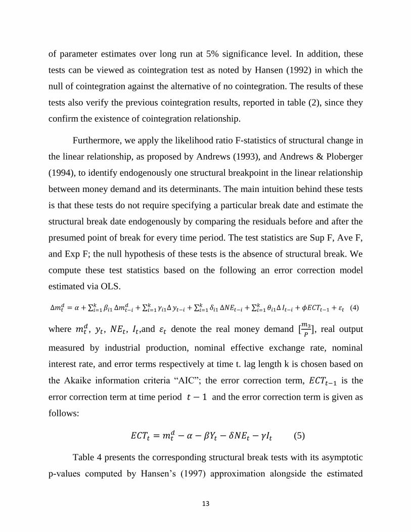
Furthermore, we apply the likelihood ratio F-statistics of structural change in

the linear relationship, as proposed by Andrews (1993), and Andrews & Ploberger

(1994), to identify endogenously one structural breakpoint in the linear relationship

between money demand and its determinants. The main intuition behind these tests

is that these tests do not require specifying a particular break date and estimate the

structural break date endogenously by comparing the residuals before and after the

presumed point of break for every time period. The test statistics are Sup F, Ave F,

and Exp F; the null hypothesis of these tests is the absence of structural break. We

compute these test statistics based on the following an error correction model

estimated via OLS.

∆𝑚𝑡𝑑 = 𝛼 + ∑ 𝛽𝑖1

𝑘𝑖=1 ∆𝑚𝑡−𝑖

𝑑 + ∑ 𝛾𝑖1∆𝑘𝑖=1 𝑦𝑡−𝑖 + ∑ 𝛿𝑖1

𝑘𝑖=1 ∆𝑁𝐸𝑡−𝑖 + ∑ 𝜃𝑖1∆𝑘

𝑖=1 𝐼𝑡−𝑖 + 𝜙𝐸𝐶𝑇𝑡−1 + 휀𝑡 (4)

where 𝑚𝑡𝑑, 𝑦𝑡, 𝑁𝐸𝑡, 𝐼𝑡,and 휀𝑡 denote the real money demand [

𝑚3

𝑃], real output

measured by industrial production, nominal effective exchange rate, nominal

interest rate, and error terms respectively at time t. lag length k is chosen based on

the Akaike information criteria “AIC”; the error correction term, 𝐸𝐶𝑇𝑡−1 is the

error correction term at time period 𝑡 − 1 and the error correction term is given as

follows:

𝐸𝐶𝑇𝑡 = 𝑚𝑡𝑑 − 𝛼 − 𝛽𝑌𝑡 − 𝛿𝑁𝐸𝑡 − 𝛾𝐼𝑡 (5)

Table 4 presents the corresponding structural break tests with its asymptotic

p-values computed by Hansen’s (1997) approximation alongside the estimated

14

break date. The test statistics suggest the presence of a stable relationship between

money demand and its determinants; in other words, we fail to reject the null

hypothesis of no structural break at significance level of 5%.

It is also worthy to note that our evidence suggesting the existence of a

stable money demand function contradicts the findings of Banafea (2014). This in

turn encourages us to understand the reasons of contradiction, which might be

attributed to several factors. One possible factor to the different results might be

the money demand specification. In other words, Banafea (2014) defines the

demand for money as function of output and interest rate whereas we define money

demand with additional variable, which is the nominal exchange rate. The

frequency of the data is an additional factor that may lead to instability as

suggested by Gregory and Hansen (1996) since we employ quarterly data while

Banafea (2014) employs annual data. Moreover, using different measures for

output and money supply might be other factor; we use the industrial production as

a proxy for GDP and the broad definition for money supply (M3) unlike Banafea

(2014) who use the narrow definition for money supply (M1) alongside the GDP.

These factors may contribute to the results of instable money demand function.

It is also important to emphasize other essential elements indicating the

stability of money demand in Saudi Arabia. For instance, the ratio of broad money

supply to GDP is about 74.2% in 2015 for Saudi Arabia. This reflects the velocity

of money in the economy and it seems reasonable compared to other oil-exporting

and emerging market economies4. Moreover, Saudi Arabia succeeded in

maintaining a stable fixed exchange rate policy since 1986, which reflects

sustaining stable macroeconomic policy during geopolitical and financial crisis

4 For Russia 63.8%, Mexico 53.2%, Turkey 63.1%, Oman 56.1%, India 79.2%, these statistics

are obtained from the World Bank website;

www.data.worldbank.org/indicator/FM.LBL.BMNY.GD.

15

events. In particular, the Saudi Arabian Monetary Authority succeeded during

1993 and 1998 in stabilizing the Saudi nominal exchange rate5; this in turn

increases foreign investors’ credibility in investing in a stabilized economy such as

Saudi Arabia. Also, the financial sector exposure is limited in Saudi Arabia6, which

indicates the availability of liquidity to maintain the demand for money. Lastly, the

government did not crowd out the private sectors in borrowing money from

financial sectors. All these factors are reasonable indicators reflecting the stability

of money demand in Saudi Arabia over time.

Table 3: Hansen (1992) Stability Tests

Lc Mean F Sup F

Test statistics 0.74 7.40 17.31

P-value (0.10) (0.13) (0.10)

Table 4: Andrews (1993) and Andrews & Ploberger (1994) Structural Break Tests

Estimated Break

Date

Ave F Exp F Sup F

Test statistics 1999:Q1 7.95 6.65 19.15

P-value (0.18) (0.06) (0.07)

5.4. Parameter Estimates of Money Demand Function

Now since we confirm the stability of the parameter estimates, we estimate the

long-run relationship as given by equation (3) via OLS estimation method. Table

(5) summarizes the parameter estimates of the long run money demand function.

5 For further discussion of SAMA interventions, see Al- Hamidy and Banafe (2005). 6 For further information, see the financial stability report published on SAMA website.

16

Evidently, the parameter estimates of money demand function, as given by

equation (3), are in line with theory expectation suggesting the positive (negative)

relationship between output (interest rate and exchange rate) and demand for

money with 5% significance level for both output and interest rate. In other words,

changes in output influence the demand for money with statistical significance

leading to the rise in money demand by 2.47 percent as a result of an increase in

output by one percent. On the other hand, we find the nominal interest rate affects

the demand for money negatively with statistical significance leading to the decline

of money demand by 0.15 percent due to the rise of interest rate by one percent.

Likewise, when the exchange rate increases by one percent, we find the demand

for money falls by 0.5 percent though statistically insignificant. Furthermore, the

parameter estimate, 𝜙, from equation (4) enables us to get some insight into how

long-run equilibrium is restored between money demand and its determinants.

Clearly, the estimated coefficient (�̂�= - 0.014) is negative and statistically

significant at 10% level. This in turn implies that it takes the money demand about

1.4% each quarter to adjust to its long run equilibrium when money demand

deviates from its long run equilibrium.

Table 4: The Estimates of Long Run Relationship

𝛼 𝛽 𝛾 𝛿

Parameter estimates 0.01 2.47** -0.15** -0.50

t-statistics (0.003) (5.81) (-9.92) (-1.12)

** denotes the 5% significance level.

6. Conclusion

The goal of this paper is to examine the long run relationship between the demand

for money and its determinants and whether this relationship is stable or not. To do

17

so, this paper employs quarterly data starting from 1993:Q1 to 2015:Q3 for money

supply M3 deflated by consumer price index, nominal effective exchange rate,

industrial production, and the US Libro interest rate. We find evidence indicating

the existence of a stable long run relationship between the money demand and its

determinants. In specific, we find evidence supporting economic theory

expectations; in other words, a rise in industrial production by one percent leads to

higher money demand by 2.5 percent. Likewise, when the nominal exchange rate

(interest rate) increases by one percent, we find the demand for money falls by 0.2

(0.5) percent.

The findings of this study have key implications for monetary policymakers

in Saudi Arabia. For instance, having stable demand for money would enable

monetary policymakers to maintain stable nominal exchange rate policy. In

addition, the stability of money demand is necessary in order to forecast the

movements of nominal exchange rate since monetary models of exchange rate (i.e.

the monetary model of exchange rate under flexible prices) are built on the

assumption of stable money demand function. Therefore, it is crucial to maintain

stable money demand function in order to have accurate forecast for the nominal

exchange rate.

For further research, it is would be interesting to examine the economic

consequences of uncertainty shocks on the demand for money in Saudi Arabia;

likewise, with the development of econometric techniques, it would be remarkable

to rely on nonlinear models rather than linear models to analyze the behavior of

money demand in Saudi Arabia.

18

Reference

Abdulkheir, A. Y. (2013). “An Analytical Study of the Demand for Money in

Saudi Arabia.” International Journal of Economics and Finance, 5 (4), 31 –

38.

19

Al-Hamidy, A., Banafea, A. (2005). “Foreign Exchange Intervention in Saudi

Arabia,” Bank of International Settlements Paper # 73, 301-306.

AlKaswani, M., Al-Towaijari, H. (1999). Cointegration, Error Correction and the

Demand for Money in Saudi Arabia.” Economia Internazionale/

International Economics, 52 (3), 299-308.

Andrews, D.W.K. (1993). “Tests for Parameter Instability and Structural-Change

with Unknown Change Point.” Econometrica, 61 (4), 821-856.

Andrews, D.W.K., Ploberger, W. (1994). “Optimal tests when a nuisance

parameter is present only under the alternative.” Econometrica, 62 (6), 531-

549.

Arrau, P., Gregorio, J.D. (1993). “Financial Innovation and Money Demand:

Application to Chile and Mexico.” The Review of Economics and Statistics,

75 (3), 524-530.

Arango, S., Nadiri, M.I. (1981). “Demand for Money in Open Economies.”

Journal of Monetary Economics, 7 (1), 69-83.

Bahmani-Oskooee, M., Pourheydarian, M. (1990). “Exchange Rate Sensitivity of

the Demand for Money and Effectiveness of Fiscal and Monetary Policy.”

Applied Economics, 22 (7), 917 – 925.

Bahmani-Oskooee, M., Shabsigh, G. (1996) “The demand for money in Japan:

evidence from cointegration analysis.” Japan and the World Economy, 8, 1-

10.

Bahmani-Oskooee, M., Chomsisengphet, S. (2002). “Stability of M2 money

demand function in industrial countries.” Applied Economics, 34 (16), 2075

– 2083.

20

Bahmani-Oskooee, M., Gelan, A. (2009). “How stable is the demand for money in

African countries?” Journal of Economic Studies, 36 (3), 216-235.

Bahmani-Oskooee, M., Rehman, H. (2005) “Stability of the money demand

function in Asian developing countries.” Applied Economics, 37, 773-792.

Bahmani, S. (2008). “Stability of the Demand for Money in the Middle East.”

Emerging Markets Finance & Trade, 44 (1), 62 – 83.

Banafea, W.A. (2012). “Essays on structural breaks and stability of the money

demand function.” PhD Thesis, Kansas State University.

Banafea, W. A. (2014). “Endogenous Structural Breaks and Stability of the Money

Demand Function in Saudi Arabia.” International Journal of Economics and

Finance, 6 (1), 155 – 164.

Boughton, J.M., (1981). “Recent Instability of the Demand for Money: An

International Perspective.” Southern Economic Journal, 47 (3), 579-597.

Cheong, C. (2003) “Regime changes and econometric modeling of the demand for

money in Korea.” Economic Modeling, 20 (3), 437–453.

Choi, W.G., Oh, S. (2003). “A Money Demand Function with Output Uncertainty,

Monetary Uncertainty, and Financial Innovation.” Journal of Money, Credit

and Banking, 35 (5), 685-709.

Coenen, G., Vega, J-L. (2001). “The Demand for M3 in the Euro Area.” Journal of

Applied Econometrics, 16 (6), 727-748.

Dickey, K., Fuller, W. (1981). “Likelihood Ratio Statistics for Autoregressive

Time Series with a Unit Root.” Econometrica, 49 (2), 1057-1072.

21

Elliot, G., Rothenberg, T.J., Stock, J.H. (1996). “Efficient Tests for an

Autoregressive Unit Root.” Econometrica, 64 (4), 813-836.

Engle, R.F., Granger, C.W.J., (1987). “Cointegration and Error Correction:

Representation, Estimation, and Testing.” Econometrica 55 (2) 251-276.

Gregory, A., Hansen, B. (1996). “Residual-based tests for cointegration in models

with regime shifts.” Journal of Econometrics, 70 (1), 99–126.

Girton, L., Roper, D., (1981). “Theory and Implications of Currency Substitution.”

Journal of Money, Credit and Banking, 13 (1), 12-30.

Hansen, B., (1992). “Tests for parameter instability in regressions with I(1)

Processes.” Journal of Business and Economic Statistics 10 (3) 321-335.

Hansen, B. E. (1997). “Approximate asymptotic p values for structural-change

tests.” Journal of Business and Economic Statistics, 15 (1), 60-67.

Hamdi, H., Said, A., Sbia, R. (2015). “Empirical Evidence on the Long-Run

Money Demand Function in the Gulf Cooperation Council Countries.”

International Journal of Economics and Financial Issues, 5 (2), 603 – 612.

Harb, N. (2004). “Money demand function: a heterogeneous panel application.”

Applied Economics Letters, 11 (9), 551 – 555.

Johansen, S., Juselius, K., (1990). “Maximum Likelihood Estimated and Inference

on Cointegration with Application to the Demand for Money.” Oxford

Bulletin of Economics and Statistics 52 (2) 169-210.

Kwiatkowski, D., Phillips, P.C.B., Schmidt, P., Shin, Y. (1992). “Testing the Null

Hypothesis of Stationarity Against the Alternative of a Unit Root.” Journal

of Econometrics, 54 (1-3), 159-178.

22

Lee, C., Chang, C., Chen, P. (2008). “Money demand function versus monetary

integration: Revisiting panel cointegration among GCC countries.”

Mathematics and Computers in Simulation, 79(1), 85-93.

Masih, M., Algahtani, I. (2008). “Estimation of long- run demand for money: An

application of long- run structural modeling to Saudi Arabia.” Economia

Internazionale/ International Economics, 61 (1), 81–99.

Mundell, A.R. (1963). “Capital mobility and stabilization policy under fixed and

flexible exchange rates.” Canadian Journal of Economics and Political

Sciences, 29 (4), 475-485.

Pesaran, M.H., Shin, Y. (2002), “Long-Run Structural Modelling”, Econometric

Reviews, 21(1), 49-87.

Phillips, P.C.B., Perron, P. (1988). “Testing for Unit Roots in Time Series

Regression.” Biometrika, 75 (2), 335-346.

Schwert, G.W. (1987). “Effects of model specification on tests for unit roots in

macroeconomic data.” Journal of Monetary Economics, 20 (1), 73-103.

Sriram, S. (2001). “A Survey of recent empirical money demand studies.” IMF

Staff Papers, 47 (3), 334-365.