1

SAMPLE J-DSP EXERCISES DISCRETE-TIME SIGNALS AND SYSTEMS

Andreas Spanias

This computer exercise is given to expose signals and systems (S&S) students to select applications of discrete-

time signals and systems. We provide two groups of exercises; one on digital filters and one on spectral analysis

using the FFT. We use the NSF funded Java-DSP environment to perform the computer exercises. First, general

information on J-DSP is given to enable students to establish and run simple J-DSP simulations. It is important for

the students to read this section carefully and go through the initial steps so as to become familiar with the software.

The development of the exercises and their assessment are part of an effort to enhance the educational experience of

S&S students by exposing them to simple DSP applications. It is also within the objectives of an NSF joint

Curriculum and Research Development and Educational Innovation project (NSF CRCD-EI) that aims to introduce

junior-level undergraduate students to DSP algorithms and research.

1. GENERAL INFORMATION ON J-DSP

This laboratory’s objective is to provide hands-on learning experiences to junior students on select DSP topics.

The laboratories are based on the object-oriented Java tool called Java Digital Signal Processing (J-DSP). J-DSP

has been developed at Arizona State University (ASU) and is written as a platform-independent Java applet that can

be accessed at http://jdsp.asu.edu. J-DSP has a rich suite of signal processing functions that include signal

generators, digital filters, pole-zero root computation, filter design algorithms, an FFT, a plot function, a sound

player, multi-rate converters, statistical signal analysis, spectral estimation, and many others. J-DSP provides a user-

friendly environment that embodies Java’s graphical capabilities. Its highly intuitive graphical user interface (GUI)

is easy to learn. All functions appear as graphical blocks that are divided into groups according to their functionality.

Selecting and establishing individual blocks can be done by a drag-and-drop process. Each block is linked to

software that performs a specific signal processing task. Block parameters can be entered using dialog windows and

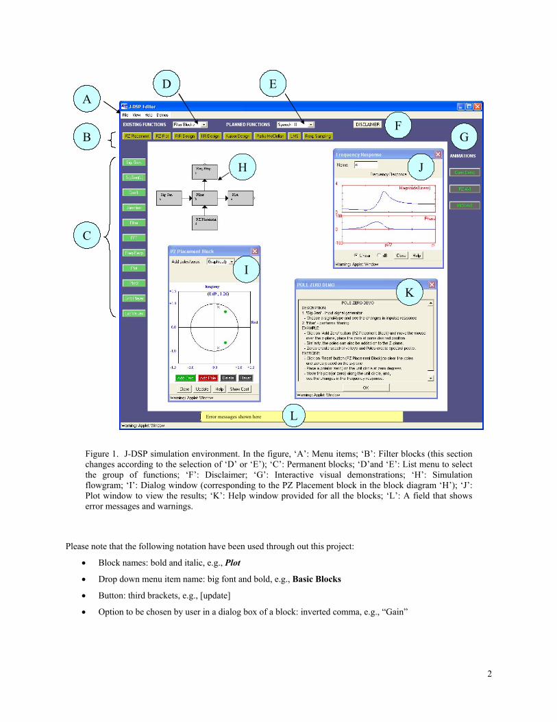
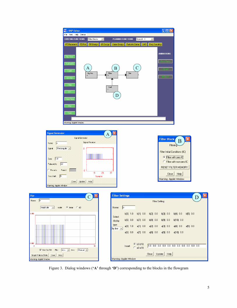
simulation results can be listed or plotted. Figure 1 shows the J-DSP editor environment. By connecting blocks,

signal flow is established and an algorithm can be simulated. Signals at any point of a simulation can be visualized

through appropriate plot blocks. Blocks can be manipulated (i.e., edit, move, delete and connect) using the mouse.

System execution is dynamic, i.e., any change at any point of a system will automatically take effect in all

subsequent blocks. Windows can be left open to enable the user to view signals at different points.

2

A

H

C

I

J

K

G

D E

FB

Error messages shown here L

A

H

C

I

J

K

G

D E

FB

Error messages shown here L

Figure 1. J-DSP simulation environment. In the figure, ‘A’: Menu items; ‘B’: Filter blocks (this section changes according to the selection of ‘D’ or ‘E’); ‘C’: Permanent blocks; ‘D’and ‘E’: List menu to select the group of functions; ‘F’: Disclaimer; ‘G’: Interactive visual demonstrations; ‘H’: Simulation flowgram; ‘I’: Dialog window (corresponding to the PZ Placement block in the block diagram ‘H’); ‘J’: Plot window to view the results; ‘K’: Help window provided for all the blocks; ‘L’: A field that shows error messages and warnings.

Please note that the following notation have been used through out this project:

• Block names: bold and italic, e.g., Plot

• Drop down menu item name: big font and bold, e.g., Basic Blocks

• Button: third brackets, e.g., [update]

• Option to be chosen by user in a dialog box of a block: inverted comma, e.g., “Gain”

3

1.1. GETTING STARTED – GENERATING AND ANALYZING SIGNALS

The easiest way to explain some of the functions of J-DSP is to work through a simple example. To start J-DSP,

open a browser window and type the URL, http://jdsp.asu.edu/, and press skip animation to enter the J-DSP web

page. If J-DSP resides on your computer’s hard drive then double click on the pertinent shortcut. With the mouse

navigate to the upper left frame where it says “Start Center” and press “Start.” Read the information in the panel

and press “proceed.” The Java applet will launch when you press the “Start” button. Read the disclaimer and if you

agree press “I accept.” The J-DSP environment appears and is ready for programming a DSP simulation. Please

note that it may take 30 seconds or more to download the program and a few more seconds to establish the first

block but once the first block is established, the program should run quickly.

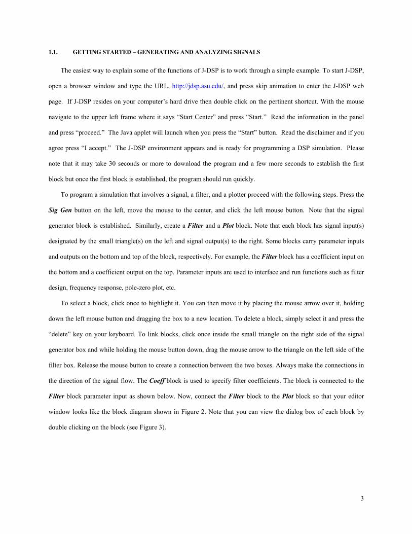
To program a simulation that involves a signal, a filter, and a plotter proceed with the following steps. Press the

Sig Gen button on the left, move the mouse to the center, and click the left mouse button. Note that the signal

generator block is established. Similarly, create a Filter and a Plot block. Note that each block has signal input(s)

designated by the small triangle(s) on the left and signal output(s) to the right. Some blocks carry parameter inputs

and outputs on the bottom and top of the block, respectively. For example, the Filter block has a coefficient input on

the bottom and a coefficient output on the top. Parameter inputs are used to interface and run functions such as filter

design, frequency response, pole-zero plot, etc.

To select a block, click once to highlight it. You can then move it by placing the mouse arrow over it, holding

down the left mouse button and dragging the box to a new location. To delete a block, simply select it and press the

“delete” key on your keyboard. To link blocks, click once inside the small triangle on the right side of the signal

generator box and while holding the mouse button down, drag the mouse arrow to the triangle on the left side of the

filter box. Release the mouse button to create a connection between the two boxes. Always make the connections in

the direction of the signal flow. The Coeff block is used to specify filter coefficients. The block is connected to the

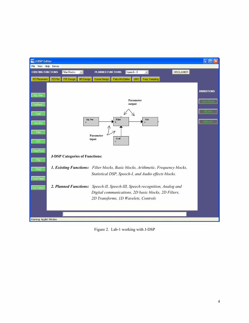
Filter block parameter input as shown below. Now, connect the Filter block to the Plot block so that your editor

window looks like the block diagram shown in Figure 2. Note that you can view the dialog box of each block by

double clicking on the block (see Figure 3).

4

Parameter input

Parameter output

1. Existing Functions: Filter blocks, Basic blocks, Arithmetic, Frequency blocks,Statistical DSP, Speech-I, and Audio effects blocks.

J-DSP Categories of Functions:

2. Planned Functions: Speech-II, Speech-III, Speech recognition, Analog andDigital communications, 2D basic blocks, 2D Filters, 2D Transforms, 1D Wavelets, Controls

Parameter input

Parameter output

1. Existing Functions: Filter blocks, Basic blocks, Arithmetic, Frequency blocks,Statistical DSP, Speech-I, and Audio effects blocks.

J-DSP Categories of Functions:

2. Planned Functions: Speech-II, Speech-III, Speech recognition, Analog andDigital communications, 2D basic blocks, 2D Filters, 2D Transforms, 1D Wavelets, Controls

Figure 2. Lab-1 working with J-DSP

5

A B C

D

A B C

D

A

B

C

D

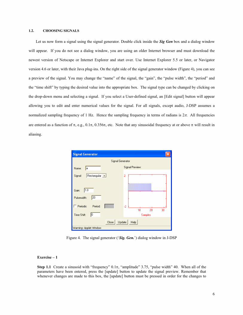
Figure 3. Dialog windows (‘A’ through ‘D’) corresponding to the blocks in the flowgram

6

1.2. CHOOSING SIGNALS

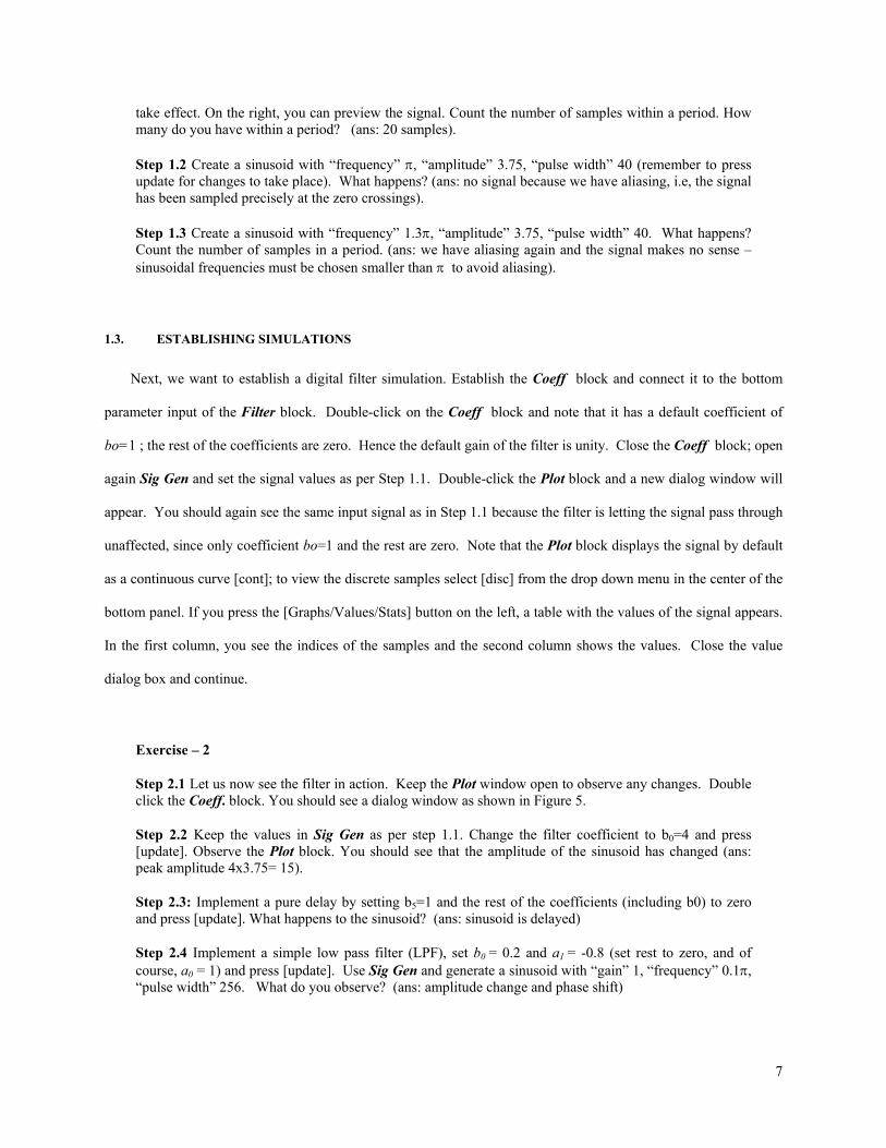
Let us now form a signal using the signal generator. Double click inside the Sig Gen box and a dialog window

will appear. If you do not see a dialog window, you are using an older Internet browser and must download the

newest version of Netscape or Internet Explorer and start over. Use Internet Explorer 5.5 or later, or Navigator

version 4.6 or later, with their Java plug-ins. On the right side of the signal generator window (Figure 4), you can see

a preview of the signal. You may change the “name” of the signal, the “gain”, the “pulse width”, the “period” and

the “time shift” by typing the desired value into the appropriate box. The signal type can be changed by clicking on

the drop-down menu and selecting a signal. If you select a User-defined signal, an [Edit signal] button will appear

allowing you to edit and enter numerical values for the signal. For all signals, except audio, J-DSP assumes a

normalized sampling frequency of 1 Hz. Hence the sampling frequency in terms of radians is 2π. All frequencies

are entered as a function of π, e.g., 0.1π, 0.356π, etc. Note that any sinusoidal frequency at or above π will result in

aliasing.

Figure 4. The signal generator (‘Sig. Gen.’) dialog window in J-DSP

Exercise – 1

Step 1.1 Create a sinusoid with “frequency” 0.1π, “amplitude” 3.75, “pulse width” 40. When all of the parameters have been entered, press the [update] button to update the signal preview. Remember that whenever changes are made to this box, the [update] button must be pressed in order for the changes to

7

take effect. On the right, you can preview the signal. Count the number of samples within a period. How many do you have within a period? (ans: 20 samples).

Step 1.2 Create a sinusoid with “frequency” π, “amplitude” 3.75, “pulse width” 40 (remember to press update for changes to take place). What happens? (ans: no signal because we have aliasing, i.e, the signal has been sampled precisely at the zero crossings).

Step 1.3 Create a sinusoid with “frequency” 1.3π, “amplitude” 3.75, “pulse width” 40. What happens? Count the number of samples in a period. (ans: we have aliasing again and the signal makes no sense – sinusoidal frequencies must be chosen smaller than π to avoid aliasing).

1.3. ESTABLISHING SIMULATIONS

Next, we want to establish a digital filter simulation. Establish the Coeff block and connect it to the bottom

parameter input of the Filter block. Double-click on the Coeff block and note that it has a default coefficient of

bo=1 ; the rest of the coefficients are zero. Hence the default gain of the filter is unity. Close the Coeff block; open

again Sig Gen and set the signal values as per Step 1.1. Double-click the Plot block and a new dialog window will

appear. You should again see the same input signal as in Step 1.1 because the filter is letting the signal pass through

unaffected, since only coefficient bo=1 and the rest are zero. Note that the Plot block displays the signal by default

as a continuous curve [cont]; to view the discrete samples select [disc] from the drop down menu in the center of the

bottom panel. If you press the [Graphs/Values/Stats] button on the left, a table with the values of the signal appears.

In the first column, you see the indices of the samples and the second column shows the values. Close the value

dialog box and continue.

Exercise – 2

Step 2.1 Let us now see the filter in action. Keep the Plot window open to observe any changes. Double click the Coeff. block. You should see a dialog window as shown in Figure 5.

Step 2.2 Keep the values in Sig Gen as per step 1.1. Change the filter coefficient to b0=4 and press [update]. Observe the Plot block. You should see that the amplitude of the sinusoid has changed (ans: peak amplitude 4x3.75= 15).

Step 2.3: Implement a pure delay by setting b5=1 and the rest of the coefficients (including b0) to zero and press [update]. What happens to the sinusoid? (ans: sinusoid is delayed)

Step 2.4 Implement a simple low pass filter (LPF), set b0 = 0.2 and a1 = -0.8 (set rest to zero, and of course, a0 = 1) and press [update]. Use Sig Gen and generate a sinusoid with “gain” 1, “frequency” 0.1π, “pulse width” 256. What do you observe? (ans: amplitude change and phase shift)

8

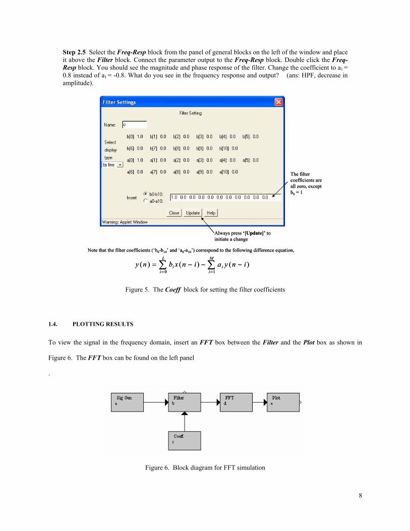
Step 2.5 Select the Freq-Resp block from the panel of general blocks on the left of the window and place it above the Filter block. Connect the parameter output to the Freq-Resp block. Double click the Freq-Resp block. You should see the magnitude and phase response of the filter. Change the coefficient to a1 = 0.8 instead of a1 = -0.8. What do you see in the frequency response and output? (ans: HPF, decrease in amplitude).

The filter coefficients are all zero, except b0 = 1

Always press ‘[Update]’ to initiate a change

0 1( ) ( ) ( )

L M

i ii i

y n b x n i a y n i= =

= − − −∑ ∑

Note that the filter coefficients (‘b0-b10’ and ‘a0-a10’) correspond to the following difference equation,

The filter coefficients are all zero, except b0 = 1

Always press ‘[Update]’ to initiate a change

0 1( ) ( ) ( )

L M

i ii i

y n b x n i a y n i= =

= − − −∑ ∑

Note that the filter coefficients (‘b0-b10’ and ‘a0-a10’) correspond to the following difference equation,

Figure 5. The Coeff block for setting the filter coefficients

1.4. PLOTTING RESULTS

To view the signal in the frequency domain, insert an FFT box between the Filter and the Plot box as shown in

Figure 6. The FFT box can be found on the left panel

.

Figure 6. Block diagram for FFT simulation

9

Exercise – 3

Step 3.1 Set the Filter parameters and input as per step 2.4. Double click on the FFT block and change the “FFT size” to 256 points and then press [Close]. Now, you can see the magnitude and the phase of the signal in the frequency domain. The magnitude has a sharp peak approximately at 0.31, i.e., the frequency of our sinusoidal signal (0.1π).

Step 3.2 Change the sinusoidal frequencies as per steps 1.2 and 1.3 but with “pulse width” 256 and observe the changes in the plot.

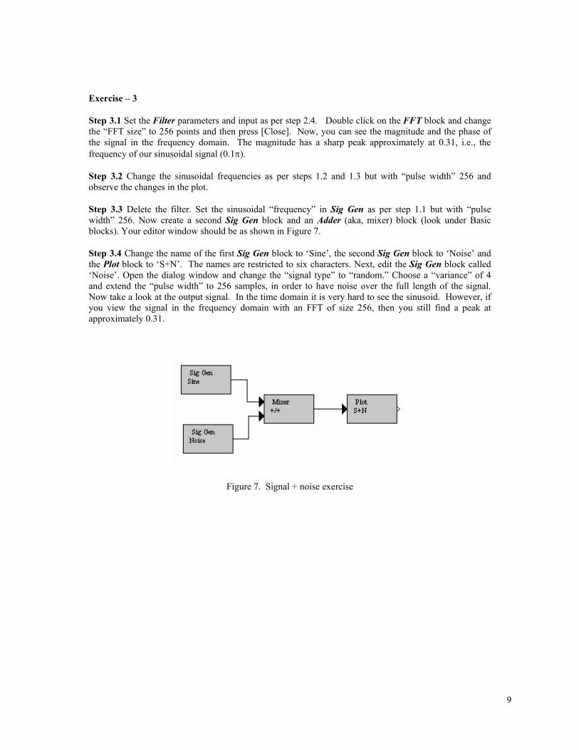
Step 3.3 Delete the filter. Set the sinusoidal “frequency” in Sig Gen as per step 1.1 but with “pulse width” 256. Now create a second Sig Gen block and an Adder (aka, mixer) block (look under Basic blocks). Your editor window should be as shown in Figure 7.

Step 3.4 Change the name of the first Sig Gen block to ‘Sine’, the second Sig Gen block to ‘Noise’ and the Plot block to ‘S+N’. The names are restricted to six characters. Next, edit the Sig Gen block called ‘Noise’. Open the dialog window and change the “signal type” to “random.” Choose a “variance” of 4 and extend the “pulse width” to 256 samples, in order to have noise over the full length of the signal. Now take a look at the output signal. In the time domain it is very hard to see the sinusoid. However, if you view the signal in the frequency domain with an FFT of size 256, then you still find a peak at approximately 0.31.

Figure 7. Signal + noise exercise

10

2. FILTERS AND FREQUENCY RESPONSES

In this section, we study FIR and IIR digital filters. We also examine certain special types of filters called

shelving and peaking filters. Their frequency responses are plotted using J-DSP. The FFT is also introduced and

applied for the estimation of the spectral content of MIDI and DTMF signals.

2.1. TRANSFER FUNCTIONS OF DIGITAL FILTERS

The transfer function of a digital filter is given by,

10 1

11

...( )

1 ...

LL

MM

b b z b zH z

a z a z

− −

− −

+ + +=

+ + +

In J-DSP, the maximum number of numerator and denominator coefficients allowed is 11.

Exercise – 4

Step 4.1 We will again use the procedure given in Section 1.3 to establish filter simulations. Consider the filter coefficients: a0 = 1, a1 = 0, a2 = 0.9, b0 = 1. Write the transfer function below.

( )H z =

Step 4.2 Program these coefficients in J-DSP (as per Section 1.3 ) and use the frequency response (Freq-Resp) function to create frequency-response plots. Include your frequency response in your report and state the kind of digital filter realized? (i.e., all-pass, low-pass, band-Pass, or high-pass?) _____________

Step 4.3 Again use J-DSP and program the filter coefficients to b0 = 1.0, b1 = 0.0 and a1 = -0.9 and write the new transfer function in your report.

Step 4.4 Program the above coefficients in J-DSP and use the frequency response function to create frequency response plots. Include your frequency response in your report and state the kind of digital filter realized? (All-pass? Low-pass? Band-Pass,? High-pass?) _____________

2.2. IMPULSE RESPONSES AND EXPONENTIAL SEQUENCES

Exercise – 5

Step 5.1 To see the impulse response of a filter, use the signal generator and create a unit impulse (delta) input. Excite the filter (again use the process of Section 1.3 to set up the simulation) with the “delta” input signal. Note that single-pole IIR filters have exponential impulse responses.

11

Simulate in J-DSP a digital filter that has an exponential impulse response, h(n), as shown in Eq. (1). In J-DSP this is done by setting a filter with coefficients b0=1 and a1= - 0.9 and exciting it with a delta sequence. Use J-DSP to plot h(n) and also plot the associated frequency response (use Freq-Resp).

1

1( ) 0.9 ( ) ( )1 0.9

nh n u n H zz−= ⇔ =

− (1)

Step 5.2 For the same filter, use the pole-zero plot block (use PZ-Plot under the Filter Blocks menu) and connect to the top output of the filter. If you have trouble with setting up the simulation see the AVI file (PZ-AVI). Obtain the pole-zero diagram for the filter. Note the location of the poles and zeros.

2.3. IIR FILTER DESIGN USING J-DSP

Exercise – 6

Step 6.1 In this exercise, students will design IIR filters with J-DSP. Under the Filters Blocks establish the IIR Design block and connect its output to the bottom input of the filter block. The filter will be designed using two different IIR methods (Butterworth and Chebychev I) so that results of the two different methods can be compared. The specifications for the filter are shown below.

• Filter Type = Lowpass • Cutoff frequencies: ωp1=0.4π (pass band edge) and ωs1=0.6π (stop band edge) • Tolerance in passband = 1.0dB • Tolerance(rejection) in stopband = -45.0dB

The IIR Design block will automatically calculate the filter coefficients based on the filter specifications provided. Enter the cutoff frequencies into the IIR block as fractions of the sampling frequency. For ωp1=0.4π simply enter 0.4.

For each of the two filter designs, include in your report the following: Plot the filter's frequency response. Examine the filter's frequency response in the passband and in the stopband.

In your remarks try to provide answers to the following questions. Which filter requires the highest order to meet these specifications? Comment on the ripple effect.

2.4. SPECIAL TYPES OF FILTERS: SHELVING AND PEAKING FILTERS

2.4.1. INTRODUCTION

Shelving filters, peaking filters and graphic equalizers are linear filters that are used in audio equipment. In the

old days these filters were implemented using analog circuits. Nowadays, these filters are programmed on

microprocessors or on DSP chips. By making these filters programmable, manufacturers provide a general compact

LCD interface (much like the one on your CD player or car stereo) and can accommodate all the signal conditioning

functions (bass, treble, equalization) without having to implement additional discrete circuit components for each

12

filtering function. Not only programmable signal processing and filtering functions are effective, but they are also

less expensive and enable user-friendly interfaces and ergonomics that appeal more to most users. The exercise

below will familiarize you with filter functions that are used to implement bass, treble, and equalizer filters.

Shelving filter

A shelving filter is a specially designed transfer function that realizes a tone audio control by applying a gain or

attenuation to a specific frequency band. The low frequencies (bass) are controlled by a low-pass shelving filter

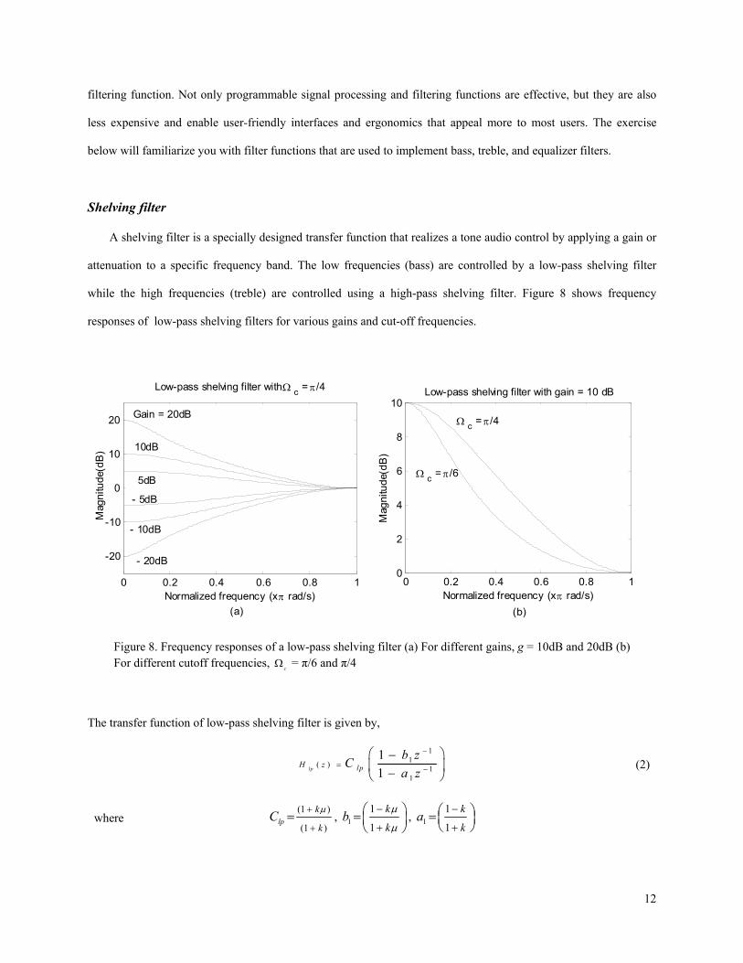
while the high frequencies (treble) are controlled using a high-pass shelving filter. Figure 8 shows frequency

responses of low-pass shelving filters for various gains and cut-off frequencies.

0 0.2 0.4 0.6 0.8 10

2

4

6

8

10Low-pass shelving filter with gain = 10 dB

Mag

nitu

de(d

B)

Normalized frequency (x π rad/s)0 0.2 0.4 0.6 0.8 1

-20

-10

0

10

20

Low-pass shelving filter with Ω c = π/4

Mag

nitu

de(d

B)

Normalized frequency (x π rad/s)(a) (b)

Gain = 20dB

10dB

5dB

- 5dB

- 10dB

- 20dB

Ω c = π/4

Ω c = π/6

Figure 8. Frequency responses of a low-pass shelving filter (a) For different gains, g = 10dB and 20dB (b) For different cutoff frequencies, cΩ = π/6 and π/4

The transfer function of low-pass shelving filter is given by,

1

11

1

( )11lp lpH z

b zCa z

−

−= − −

(2)

where (1 )

(1 )lp

k

kC µ+

+= , 1

1

1

k

kb µ

µ

−

+

=

, 11

1

k

ka −

+ =

13

/ 2 0

tan4

an d1 2

1 0

;c

g

kµ

µ

Ω=

+

=

where 2 /c c s

f fπΩ = is the normalized cutoff frequency and g is the gain in dB. Using bilinear transformation,

the transfer function of high-pass shelving filter can be derived,

1

11

1

( )11hp hpH z C

b za z

−

−= − −

(3)

where 1

hpp

pC µ +

+= , 1

p

pb µ

µ

−

+

=

, 11

1

p

pa −

+

=

/ 20tan1

104 2

c gandpµ

µ+ Ω

= =

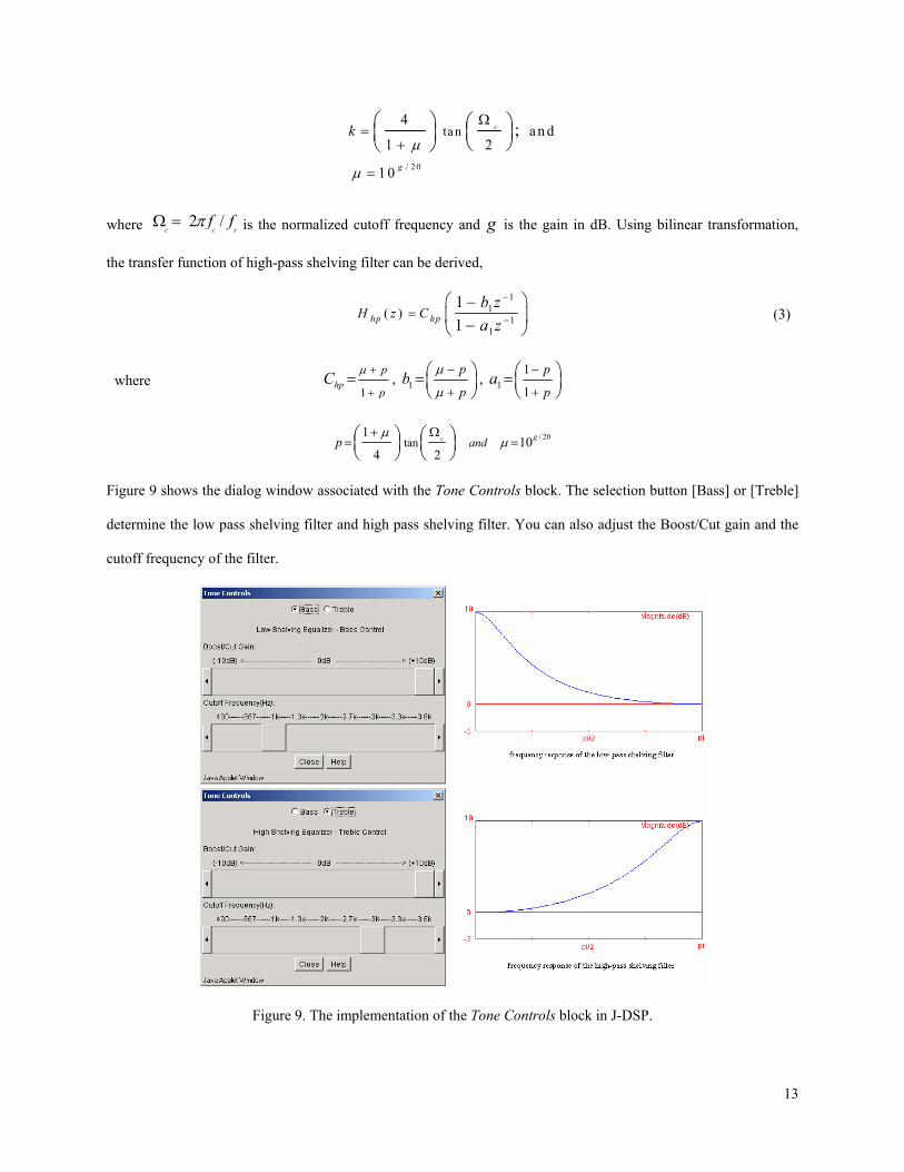
Figure 9 shows the dialog window associated with the Tone Controls block. The selection button [Bass] or [Treble]

determine the low pass shelving filter and high pass shelving filter. You can also adjust the Boost/Cut gain and the

cutoff frequency of the filter.

Figure 9. The implementation of the Tone Controls block in J-DSP.

14

Peaking filter

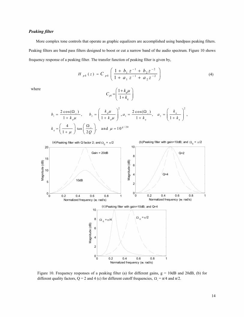
More complex tone controls that operate as graphic equalizers are accomplished using bandpass peaking filters.

Peaking filters are band pass filters designed to boost or cut a narrow band of the audio spectrum. Figure 10 shows

frequency response of a peaking filter. The transfer function of peaking filter is given by,

1 2

1 21 2

1 2

( )11p k p kH z

b z b zCa z a z

− −

− −= + + + +

(4)

where 11

qpk

q

kC

kµ +

= +

1 2 1 2

2 2

/ 20tan ,

2 cos( ) 2 cos( ), ,

1 1 1 1

4and 10

1 2

, ,q qc c

q q q q

cq

g

k kb b a a

k k k k

kQ

µ

µ µ

µµ

Ω Ω= = = =

+ + + +

Ω= =

+

0 0.2 0.4 0.6 0.8 10

5

10

15

20

Normalized frequency (x π rad/s)

Mag

nitu

de (

dB)

Peaking filter with Q factor 2; and Ωc = π/2

0 0.2 0.4 0.6 0.8 10

2

4

6

8

10

Normalized frequency (x π rad/s)

Mag

nitu

de (

dB)

Peaking filter with gain=10dB; and Ωc = π/2

0 0.2 0.4 0.6 0.8 10

2

4

6

8

10

Normalized frequency (x π rad/s)

Mag

nitu

de (

dB)

Peaking filter with gain=10dB; and Q=4

Gain = 20dB

10dB

Q=2

Q=4

Ω c = π/4Ω c = π/2

(a) (b)

(c)

Figure 10. Frequency responses of a peaking filter (a) for different gains, g = 10dB and 20dB, (b) for different quality factors, Q = 2 and 4 (c) for different cutoff frequencies, cΩ = π/4 and π/2.

15

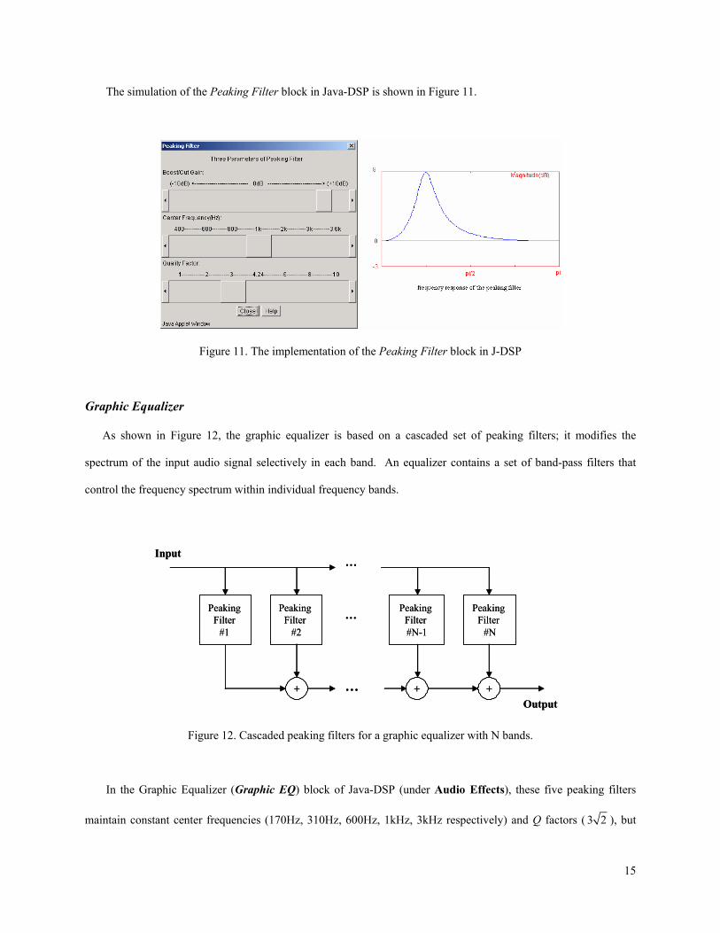
The simulation of the Peaking Filter block in Java-DSP is shown in Figure 11.

Figure 11. The implementation of the Peaking Filter block in J-DSP

Graphic Equalizer

As shown in Figure 12, the graphic equalizer is based on a cascaded set of peaking filters; it modifies the

spectrum of the input audio signal selectively in each band. An equalizer contains a set of band-pass filters that

control the frequency spectrum within individual frequency bands.

Peaking Filter

#1

Peaking Filter

#2

Peaking Filter #N-1

Peaking Filter

#N

+ + +

Input

Output

…

…

…Peaking Filter

#1

Peaking Filter

#2

Peaking Filter #N-1

Peaking Filter

#N

+ + +

Input

Output

…

…

…

Figure 12. Cascaded peaking filters for a graphic equalizer with N bands.

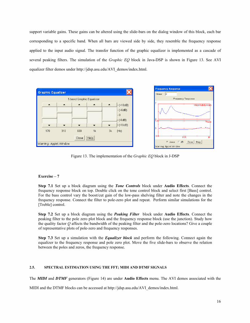
In the Graphic Equalizer (Graphic EQ) block of Java-DSP (under Audio Effects), these five peaking filters

maintain constant center frequencies (170Hz, 310Hz, 600Hz, 1kHz, 3kHz respectively) and Q factors ( 3 2 ), but

16

support variable gains. These gains can be altered using the slide-bars on the dialog window of this block, each bar

corresponding to a specific band. When all bars are viewed side by side, they resemble the frequency response

applied to the input audio signal. The transfer function of the graphic equalizer is implemented as a cascade of

several peaking filters. The simulation of the Graphic EQ block in Java-DSP is shown in Figure 13. See AVI

equalizer filter demos under http://jdsp.asu.edu/AVI_demos/index.html.

Figure 13. The implementation of the Graphic EQ block in J-DSP

Exercise – 7

Step 7.1 Set up a block diagram using the Tone Controls block under Audio Effects. Connect the frequency response block on top. Double click on the tone control block and select first [Bass] control. For the bass control vary the boost/cut gain of the low-pass shelving filter and note the changes in the frequency response. Connect the filter to pole-zero plot and repeat. Perform similar simulations for the [Treble] control.

Step 7.2 Set up a block diagram using the Peaking Filter block under Audio Effects. Connect the peaking filter to the pole zero plot block and the frequency response block (use the junction). Study how the quality factor Q affects the bandwidth of the peaking filter and the pole-zero locations? Give a couple of representative plots of pole-zero and frequency responses.

Step 7.3 Set up a simulation with the Equalizer block and perform the following. Connect again the equalizer to the frequency response and pole zero plot. Move the five slide-bars to observe the relation between the poles and zeros, the frequency response.

2.5. SPECTRAL ESTIMATION USING THE FFT; MIDI AND DTMF SIGNALS

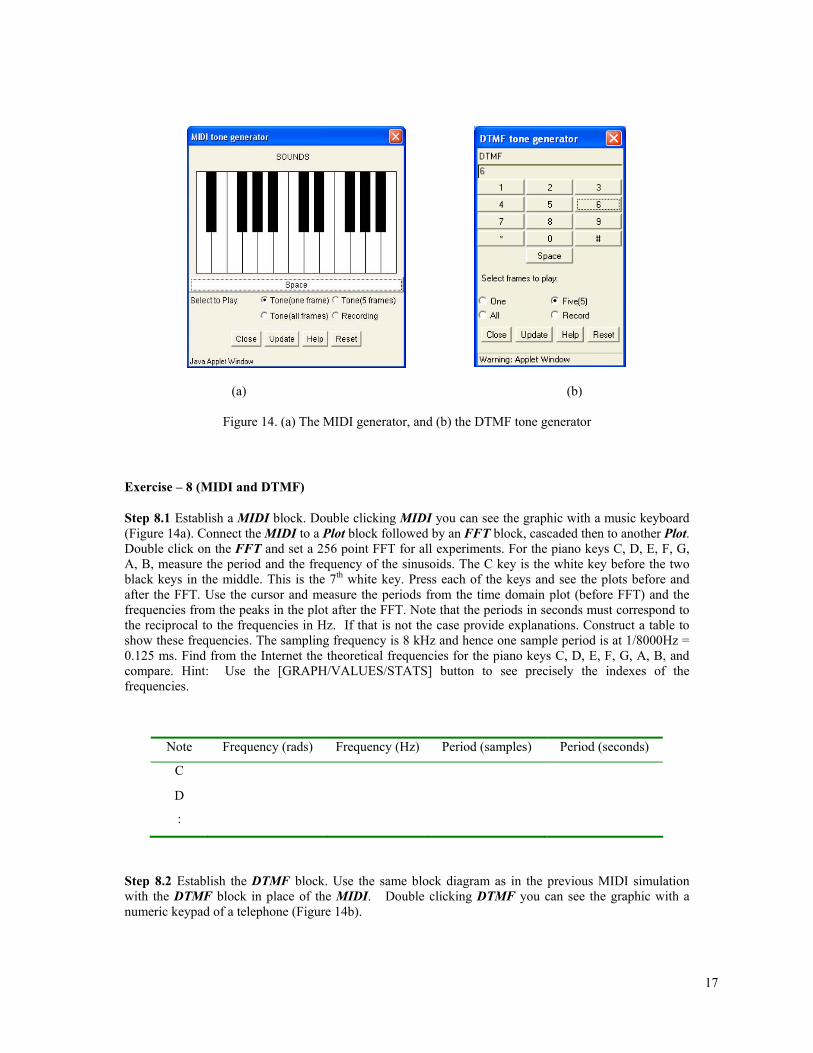
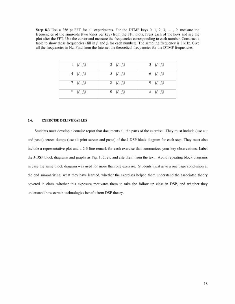
The MIDI and DTMF generators (Figure 14) are under Audio Effects menu. The AVI demos associated with the

MIDI and the DTMF blocks can be accessed at http://jdsp.asu.edu/AVI_demos/index.html.

17

(a) (b)

Figure 14. (a) The MIDI generator, and (b) the DTMF tone generator

Exercise – 8 (MIDI and DTMF)

Step 8.1 Establish a MIDI block. Double clicking MIDI you can see the graphic with a music keyboard (Figure 14a). Connect the MIDI to a Plot block followed by an FFT block, cascaded then to another Plot. Double click on the FFT and set a 256 point FFT for all experiments. For the piano keys C, D, E, F, G, A, B, measure the period and the frequency of the sinusoids. The C key is the white key before the two black keys in the middle. This is the 7th white key. Press each of the keys and see the plots before and after the FFT. Use the cursor and measure the periods from the time domain plot (before FFT) and the frequencies from the peaks in the plot after the FFT. Note that the periods in seconds must correspond to the reciprocal to the frequencies in Hz. If that is not the case provide explanations. Construct a table to show these frequencies. The sampling frequency is 8 kHz and hence one sample period is at 1/8000Hz = 0.125 ms. Find from the Internet the theoretical frequencies for the piano keys C, D, E, F, G, A, B, and compare. Hint: Use the [GRAPH/VALUES/STATS] button to see precisely the indexes of the frequencies.

Note Frequency (rads) Frequency (Hz) Period (samples) Period (seconds)

C

D

:

Step 8.2 Establish the DTMF block. Use the same block diagram as in the previous MIDI simulation with the DTMF block in place of the MIDI. Double clicking DTMF you can see the graphic with a numeric keypad of a telephone (Figure 14b).

18

Step 8.3 Use a 256 pt FFT for all experiments. For the DTMF keys 0, 1, 2, 3, … , 9, measure the frequencies of the sinusoids (two tones per key) from the FFT plots. Press each of the keys and see the plot after the FFT. Use the cursor and measure the frequencies corresponding to each number. Construct a table to show these frequencies (fill in f1 and f2 for each number). The sampling frequency is 8 kHz. Give all the frequencies in Hz. Find from the Internet the theoretical frequencies for the DTMF frequencies.

1 (f1, f2) 2 (f1, f2) 3 (f1, f2)

4 (f1, f2) 5 (f1, f2) 6 (f1, f2)

7 (f1, f2) 8 (f1, f2) 9 (f1, f2)

* (f1, f2) 0 (f1, f2) # (f1, f2)

2.6. EXERCISE DELIVERABLES

Students must develop a concise report that documents all the parts of the exercise. They must include (use cut

and paste) screen dumps (use alt print-screen and paste) of the J-DSP block diagram for each step. They must also

include a representative plot and a 2-3 line remark for each exercise that summarizes your key observations. Label

the J-DSP block diagrams and graphs as Fig. 1, 2, etc and cite them from the text. Avoid repeating block diagrams

in case the same block diagram was used for more than one exercise. Students must give a one page conclusion at

the end summarizing: what they have learned, whether the exercises helped them understand the associated theory

covered in class, whether this exposure motivates them to take the follow up class in DSP, and whether they

understand how certain technologies benefit from DSP theory.