sampling and chapter aliasing - uccs college of ...mwickert/ece2610/lecture_notes/ece2610...sampling...

er
Sampling and AliasingWith this chapter we move the focus from signal modeling andanalysis, to converting signals back and forth between the analog(continuous-time) and digital (discrete-time) domains. Back inChapter 2 the systems blocks C-to-D and D-to-C were intro-duced for this purpose. The question is, how must we choose thesampling rate in the C-to-D and D-to-C boxes so that the analogsignal can be reconstructed from its samples.
The lowpass sampling theorem states that we must sampleat a rate, , at least twice that of the highest frequency of interestin analog signal . Specifically, for having spectral con-tent extending up to B Hz, we choose in form-ing the sequence of samples

. (4.1)

Sampling

• We have spent considerable time thus far, with the continu-ous-time sinusoidal signal

, (4.2)

where t is a continuous variable

• To manipulate such signals in MATLAB or any other com-puter too, we must actually deal with samples of

fsx t x t

fs 1 Ts 2B=

x n x nTs = – n

x t A t + cos=

x t

Chapt

4

ECE 2610 Signal and Systems 4–1

Sampling

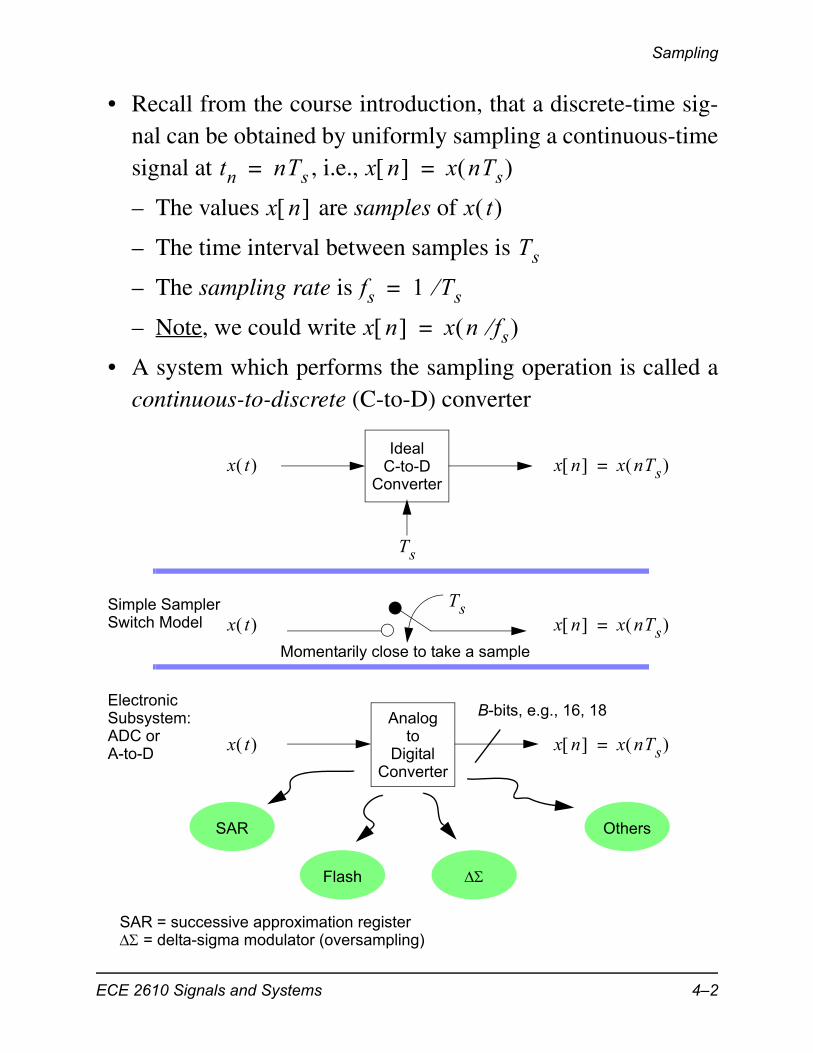
• Recall from the course introduction, that a discrete-time sig-nal can be obtained by uniformly sampling a continuous-timesignal at , i.e.,

– The values are samples of

– The time interval between samples is

– The sampling rate is

– Note, we could write

• A system which performs the sampling operation is called acontinuous-to-discrete (C-to-D) converter

tn nTs= x n x nTs =

x n x t

Tsfs 1 Ts=

x n x n fs =

IdealC-to-D

Converter

Ts

x t x n x nTs =

TsSimple SamplerSwitch Model

Analogto

DigitalConverter

ElectronicSubsystem:ADC or

SAR

x t x n x nTs =

x t x n x nTs =

Flash

Others

SAR = successive approximation register = delta-sigma modulator (oversampling)

A-to-D

B-bits, e.g., 16, 18

Momentarily close to take a sample

ECE 2610 Signals and Systems 4–2

Sampling

• A real C-to-D has imperfections, with careful design they canbe minimized, or at least have negligible impact on overallsystem performance

• For testing and simulation only environments we can easilygenerate discrete-time signals on the computer, with no needto actually capture and C-to-D process a live analog signal

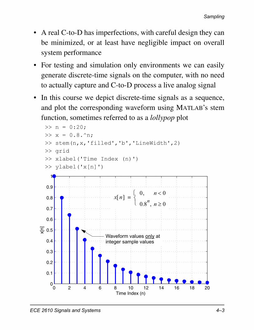
• In this course we depict discrete-time signals as a sequence,and plot the corresponding waveform using MATLAB’s stemfunction, sometimes referred to as a lollypop plot>> n = 0:20;>> x = 0.8.^n;>> stem(n,x,'filled','b','LineWidth',2)>> grid>> xlabel('Time Index (n)')>> ylabel('x[n]')

0 2 4 6 8 10 12 14 16 18 200

0.1

0.2

0.3

0.4

0.5

0.6

0.7

0.8

0.9

1

Time Index (n)

x[n]

x n 0, n 0

0.8n, n 0

=

Waveform values only atinteger sample values


Sampling

Sampling Sinusoidal Signals

• We will continue to find sinusoidal signals to be useful whenoperating in the discrete-time domain

• When we sample (4.2) we obtain a sinusoidal sequence

(4.3)

• Notice that we have defined a new frequency variable

rad, (4.4)

known as the discrete-time frequency or normalized continu-ous-time frequency

– Note that has units of radians, but could also be calledradians/sample, to emphasize the fact that sampling isinvolved

– Note also that many values of map to the same valueby virtue of the fact that is a system parameter that isnot unique either

– Since , we could also define as the dis-crete-time frequency in cycles/sample

Example: Sampling Rate Comparisons

• Consider at sampling rates of 240and 1000 samples per second

x n x nTs =

A nTs + cos=

A n + cos=

Ts fs----=

Ts

2f= f fTs

x t 2 60 t cos=


Sampling

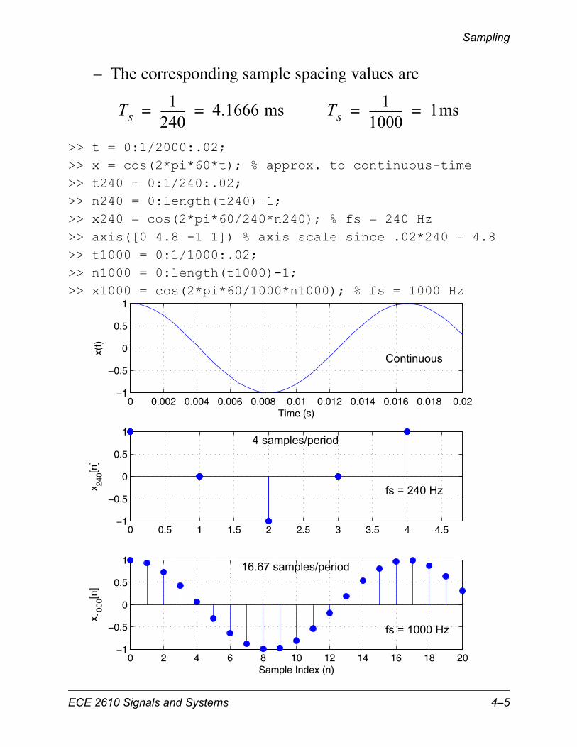
– The corresponding sample spacing values are

>> t = 0:1/2000:.02; >> x = cos(2*pi*60*t); % approx. to continuous-time>> t240 = 0:1/240:.02; >> n240 = 0:length(t240)-1;>> x240 = cos(2*pi*60/240*n240); % fs = 240 Hz>> axis([0 4.8 -1 1]) % axis scale since .02*240 = 4.8>> t1000 = 0:1/1000:.02;>> n1000 = 0:length(t1000)-1;>> x1000 = cos(2*pi*60/1000*n1000); % fs = 1000 Hz

Ts1

240--------- 4.1666 ms= = Ts

11000------------ 1ms= =

0 0.002 0.004 0.006 0.008 0.01 0.012 0.014 0.016 0.018 0.02−1

−0.5

0

0.5

1

Time (s)

x(t)

0 0.5 1 1.5 2 2.5 3 3.5 4 4.5−1

−0.5

0

0.5

1

x 240[n

]

0 2 4 6 8 10 12 14 16 18 20−1

−0.5

0

0.5

1

Sample Index (n)

x 1000

[n]

Continuous

fs = 240 Hz

fs = 1000 Hz

4 samples/period

16.67 samples/period


Sampling

• The analog frequency is rad/s or 60 Hz

• When sampling with and 1000 Hz

respectively

• The sinusoidal sequences are

respectively

• It turns out that we can reconstruct the original fromeither sequence

• Are there other continuous-time sinusoids that when sam-pled, result in the same sequence values as and ?

• Are there other sinusoid sequences of different frequency that result in the same sequence values?

The Concept of Aliasing

• In this section we begin a discussion of the very importantsignal processing topic known as aliasing

• Alias as found in the Oxford American dictionary: noun

– A false or assumed identity: a spy operating under an alias.

– Computing: an alternative name or label that refers to a file, com-mand, address, or other item, and can be used to locate or access it.

2 60

fs 240=

240 2 60 240 2 0.25 rad= =

1000 2 60 1000 2 0.06 rad= =

x240 n 0.5n cos=

x1000 n 0.12n cos=

x t

x240 x1000


Sampling

– Telecommunications: each of a set of signal frequencies that, whensampled at a given uniform rate, would give the same set of sampledvalues, and thus might be incorrectly substituted for one anotherwhen reconstructing the original signal.

• Consider the sinusoidal sequence

(4.5)

– Clearly,

• We know that cosine is a function, so

(4.6)

– We see that gives the same sequence values as, so and are aliases of each other

• We can generalize the above to any multiple, i.e.,

(4.7)

result in identical frequency samples for due to the property of sine and cosine

• We can take this one step further by noting that since, we can write

(4.8)

x1 n 0.4n cos=

0.4=

mod 2

x2 n 2.4n cos=

2 0.4+ n cos 0.4n 2n+ cos==

0.4n cos x1 n ==

2.4= 0.4= 2.4 0.4

2

l 0 2l+ l 0 1 2 3 = =

ln cosmod 2

cos – cos=

x3 n 1.6n cos=

2 0.4– n cos 2n 0.4n– cos==

0.4n– cos 0.4n cos==


Sampling

– We see that gives the same sequence values as, so and are aliases of each other

• We can generalize this result to saying

(4.9)

result in identical frequency samples for due to the property and evenness property of cosine

– This result also holds for sine, expect the amplitude isinverted since

• In summary, for any integer l, and discrete-time frequency, the frequencies

(4.10)

all produce the same sequence values with cosine, and withsine may differ by the numeric sign

– A generalization to handle both cosine and sine is to con-sider the inclusion of an arbitrary phase ,

(4.11)

– Note in the second grouping the sign change in the phase

• The frequencies of (4.10) are aliases of each other, in termsof discrete-time frequencies

1.6= 0.4= 1.6 0.4

l 2l 0– l 0 1 2 3 = =

ln cosmod 2

– sin sin–=

0

0 0 2l+ 2l 0– l 1 2 3 =

A 2l+ n + cos A n 2l n + + cos=

A n + cos=

A 2l – n – cos A 2l n n– – cos=

A n– – cos=

A n + cos=


Sampling

• The smallest value, , is called the principal alias

• These aliased frequencies extend to sampling a continuous-time sinusoid using the fact that or

, thus we may rewrite (4.10) in terms of the continu-ous-time frequency

(4.12)

– In terms of frequency in Hz we also have

(4.13)

• When viewed in the continuous-time domain, this means thatsampling with results in

(4.14)

being equivalent sequences for any n and any l

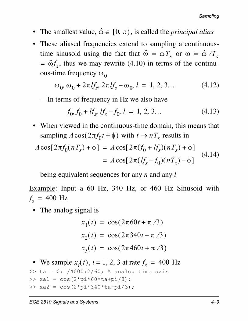
Example: Input a 60 Hz, 340 Hz, or 460 Hz Sinusoid with Hz

• The analog signal is

• We sample , i = 1, 2, 3 at rate Hz>> ta = 0:1/4000:2/60; % analog time axis>> xa1 = cos(2*pi*60*ta+pi/3);>> xa2 = cos(2*pi*340*ta-pi/3);

[0 )

Ts= Ts=fs=

0

0 0 2lfs+ 2lfs 0– l 1 2 3 =

f0 f0 lfs+ lfs f0– l 1 2 3 =

A 2f0t + cos t nTs

A 2f0 nTs + cos A 2 f0 lfs+ nTs + cos=

A 2 lfs f0– nTs – cos=

fs 400=

x1 t 260t 3+ cos=

x2 t 2340t 3– cos=

x3 t 2460t 3+ cos=

xi t fs 400=


Sampling

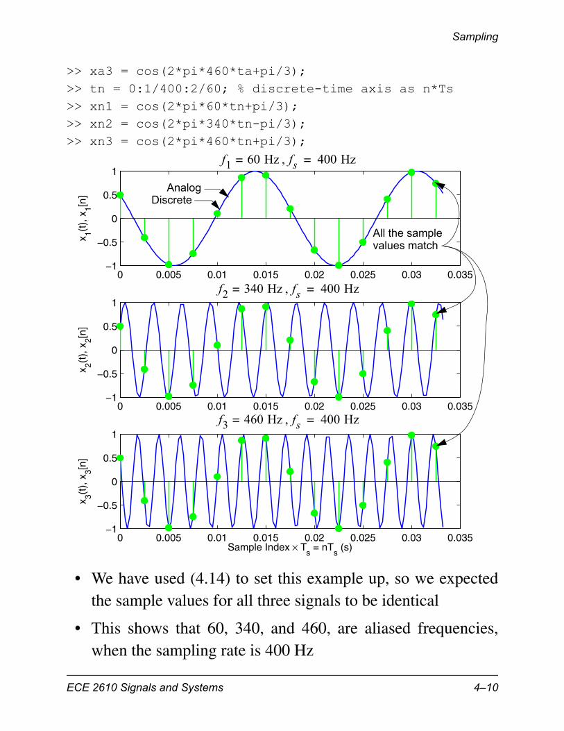
>> xa3 = cos(2*pi*460*ta+pi/3);>> tn = 0:1/400:2/60; % discrete-time axis as n*Ts>> xn1 = cos(2*pi*60*tn+pi/3);>> xn2 = cos(2*pi*340*tn-pi/3);>> xn3 = cos(2*pi*460*tn+pi/3);

• We have used (4.14) to set this example up, so we expectedthe sample values for all three signals to be identical

• This shows that 60, 340, and 460, are aliased frequencies,when the sampling rate is 400 Hz

0 0.005 0.01 0.015 0.02 0.025 0.03 0.035−1

−0.5

0

0.5

1

x 1(t),

x1[n

]

0 0.005 0.01 0.015 0.02 0.025 0.03 0.035−1

−0.5

0

0.5

1

x 2(t),

x2[n

]

0 0.005 0.01 0.015 0.02 0.025 0.03 0.035−1

−0.5

0

0.5

1

Sample Index × Ts = nT

s (s)

x 3(t),

x3[n

]

f1 60 Hz = fs 400 Hz=

f2 340 Hz = fs 400 Hz=

f3 460 Hz = fs 400 Hz=

All the samplevalues match

AnalogDiscrete


Sampling

– Note: 400 - 340 = 60 Hz and 460 - 400 = 60 Hz

• The discrete-time frequencies are

– Note: rad and rad

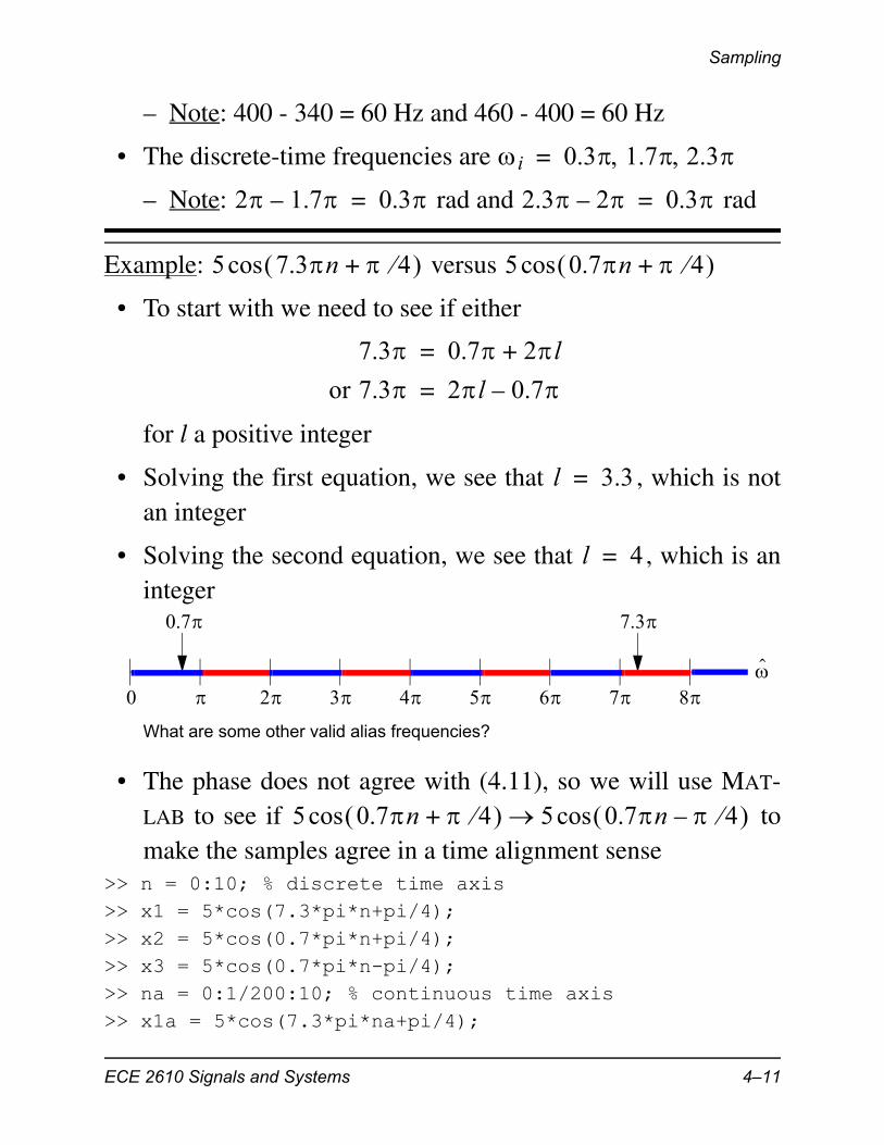
Example: versus

• To start with we need to see if either

for l a positive integer

• Solving the first equation, we see that , which is notan integer

• Solving the second equation, we see that , which is aninteger

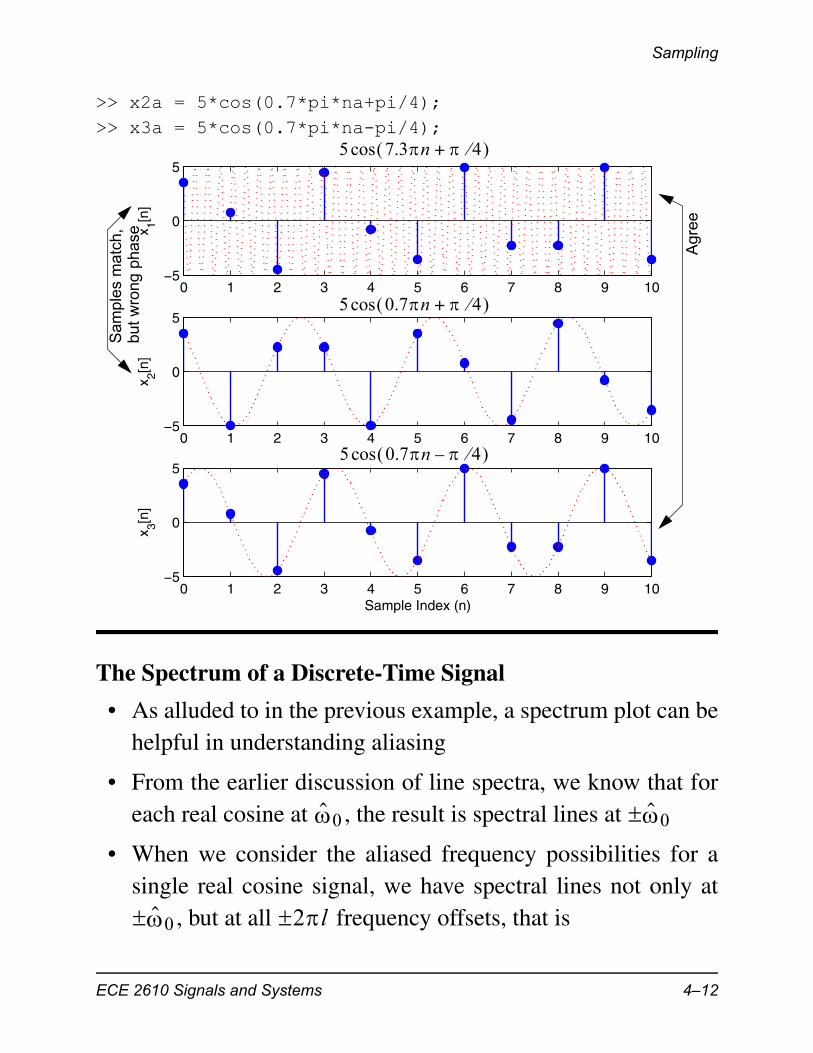
• The phase does not agree with (4.11), so we will use MAT-LAB to see if tomake the samples agree in a time alignment sense

>> n = 0:10; % discrete time axis>> x1 = 5*cos(7.3*pi*n+pi/4);>> x2 = 5*cos(0.7*pi*n+pi/4);>> x3 = 5*cos(0.7*pi*n-pi/4);>> na = 0:1/200:10; % continuous time axis>> x1a = 5*cos(7.3*pi*na+pi/4);

i 0.3 1.7 2.3 =

2 1.7– 0.3= 2.3 2– 0.3=

5 7.3n 4+ cos 5 0.7n 4+ cos

7.3 0.7 2l+=

or 7.3 2l 0.7–=

l 3.3=

l 4=

0 2 3 4 5 6 7 8

0.7 7.3

What are some other valid alias frequencies?

5 0.7n 4+ cos 5 0.7n 4– cos


Sampling

>> x2a = 5*cos(0.7*pi*na+pi/4);>> x3a = 5*cos(0.7*pi*na-pi/4);

The Spectrum of a Discrete-Time Signal

• As alluded to in the previous example, a spectrum plot can behelpful in understanding aliasing

• From the earlier discussion of line spectra, we know that foreach real cosine at , the result is spectral lines at

• When we consider the aliased frequency possibilities for asingle real cosine signal, we have spectral lines not only at

, but at all frequency offsets, that is

0 1 2 3 4 5 6 7 8 9 10−5

0

5

x 1[n]

0 1 2 3 4 5 6 7 8 9 10−5

0

5

x 2[n]

0 1 2 3 4 5 6 7 8 9 10−5

0

5

x 3[n]

Sample Index (n)

Agr

ee

Sam

ple

s m

atch

,bu

t wro

ng p

hase

5 7.3n 4+ cos

5 0.7n 4+ cos

5 0.7n 4– cos

0 0

0 2l


Sampling

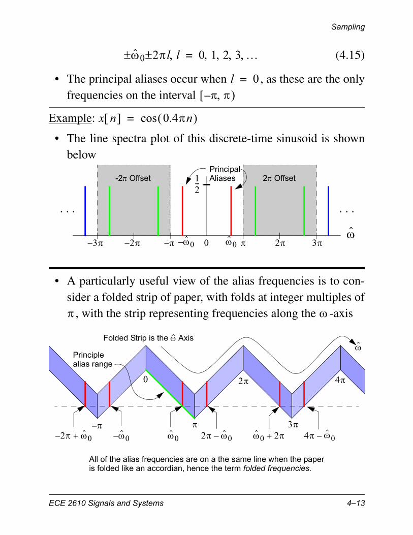
(4.15)

• The principal aliases occur when , as these are the onlyfrequencies on the interval

Example:

• The line spectra plot of this discrete-time sinusoid is shownbelow

• A particularly useful view of the alias frequencies is to con-sider a folded strip of paper, with folds at integer multiples of

, with the strip representing frequencies along the -axis

0 2l l 0 1 2 3 =

l 0=[ )–

x n 0.4n cos=

2 3–2–3– 0

. . .. . .

00–

PrincipalAliases1

2----2 Offset 2 Offset

0

2

3

4

–

Folded Strip is the Axis

0 2 0– 0 2+– 02– 0+ 4 0–

All of the alias frequencies are on a the same line when the paperis folded like an accordian, hence the term folded frequencies.

Principlealias range


Sampling

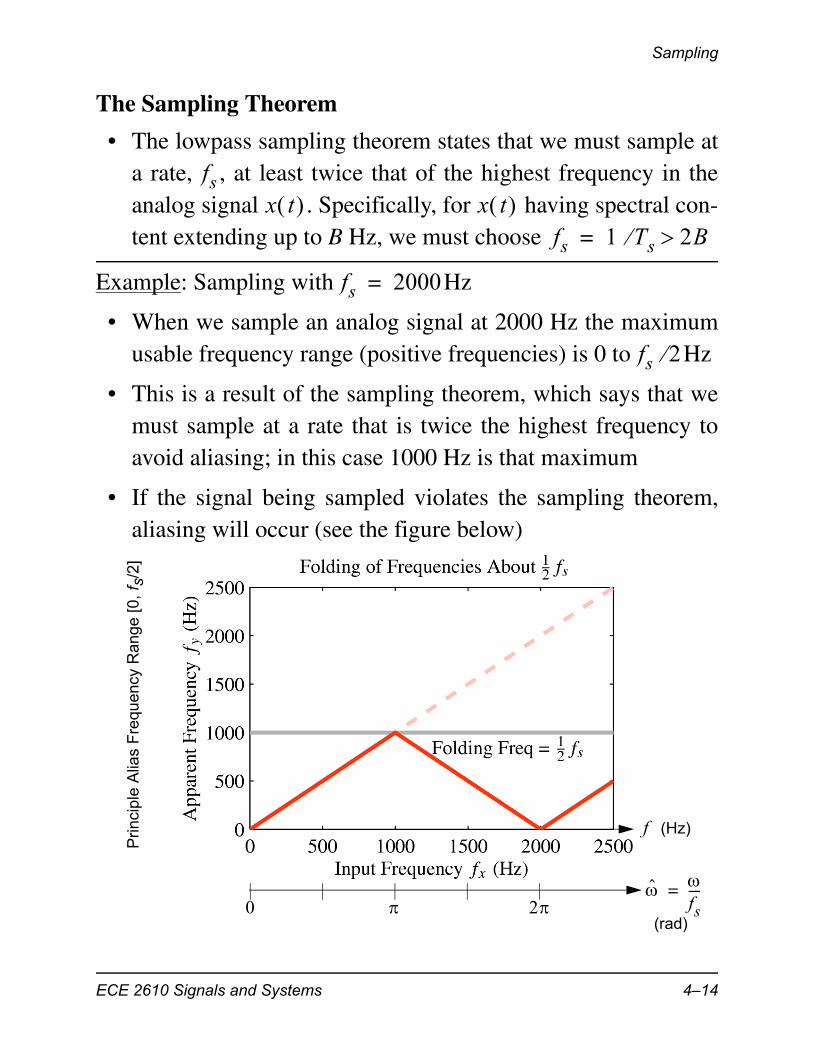
The Sampling Theorem

• The lowpass sampling theorem states that we must sample ata rate, , at least twice that of the highest frequency in theanalog signal . Specifically, for having spectral con-tent extending up to B Hz, we must choose

Example: Sampling with Hz

• When we sample an analog signal at 2000 Hz the maximumusable frequency range (positive frequencies) is 0 to Hz

• This is a result of the sampling theorem, which says that wemust sample at a rate that is twice the highest frequency toavoid aliasing; in this case 1000 Hz is that maximum

• If the signal being sampled violates the sampling theorem,aliasing will occur (see the figure below)

fsx t x t

fs 1 Ts 2B=

fs 2000=

fs 2

fs----=

0 2

f

(rad)

(Hz)

Prin

cipl

e A

lias

Fre

quen

cy R

ange

[0,

f s/2

]


Sampling

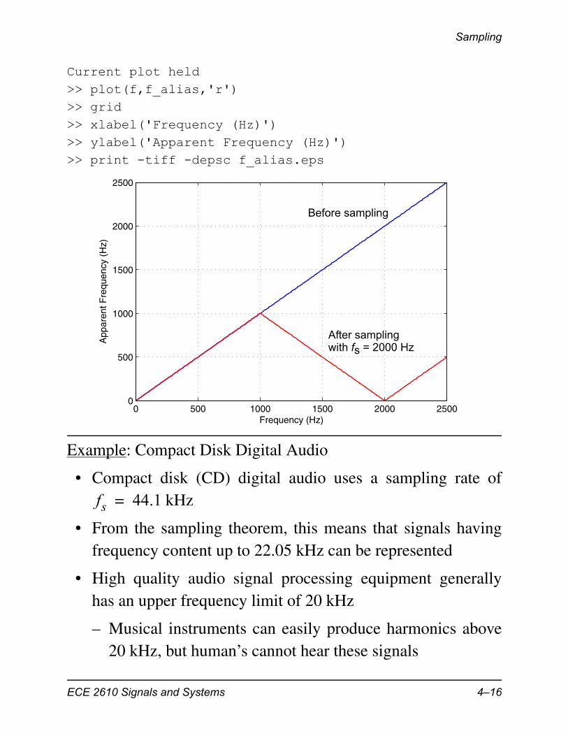
• An input frequency of 1500 Hz aliases to 500 Hz, as does aninput frequency of 2500 Hz

• The behavior of input frequencies being converted to princi-ple value alias frequencies, continues as f increases

• Notice also that the discrete-time frequency axis can be dis-played just below the continuous-time frequency axis, usingthe fact that rad

• We can just as easily map from the –axis back to the con-tinuous-time frequency axis via

• Working this in MATLAB we start by writing a support func-tion function f_out = prin_alias(f_in,fs)% f_out = prin_alias(f_in,fs)%% Mark Wickert, October 2006

f_out = f_in;

for n=1:length(f_in) while f_out(n) > fs/2 f_out(n) = abs(f_out(n) - fs); endend

• We now create a frquency vector that sweeps from 0 to 2500and assume that Hz

>> f = 0:5:2500;>> f_alias = prin_alias(f,2000);>> plot(f,f)>> hold

2f fs=

f fs 2 =

fs 2000=


Sampling

Current plot held>> plot(f,f_alias,'r')>> grid>> xlabel('Frequency (Hz)')>> ylabel('Apparent Frequency (Hz)')>> print -tiff -depsc f_alias.eps

Example: Compact Disk Digital Audio

• Compact disk (CD) digital audio uses a sampling rate of kHz

• From the sampling theorem, this means that signals havingfrequency content up to 22.05 kHz can be represented

• High quality audio signal processing equipment generallyhas an upper frequency limit of 20 kHz

– Musical instruments can easily produce harmonics above20 kHz, but human’s cannot hear these signals

0 500 1000 1500 2000 25000

500

1000

1500

2000

2500

Frequency (Hz)

App

aren

t Fre

quen

cy (

Hz)

Before sampling

After samplingwith fs = 2000 Hz

fs 44.1=


Sampling

• The fact that aliasing occurs when the sampling theorem isviolated leads us to the topic of reconstructing a signal fromits samples

• In the previous example with Hz, we see that tak-ing into account the principle alias frequency range, theusable frequency band is only [0, 1000] Hz

Ideal Reconstruction

• Reconstruction refers using just the samples to return to the original continuous-time signal

• Ideal reconstruction refers to exact reconstruction of from its samples so long as the sampling theorem is satisfied

• In the extreme case example, this means that a sinusoid hav-ing frequency just less than , can be reconstructed fromsamples taken at rate

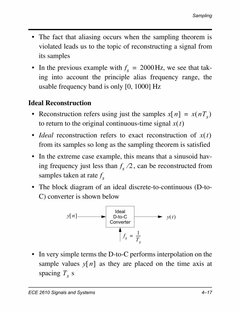
• The block diagram of an ideal discrete-to-continuous (D-to-C) converter is shown below

• In very simple terms the D-to-C performs interpolation on thesample values as they are placed on the time axis atspacing s

fs 2000=

x n x nTs =x t

x t

fs 2fs

IdealD-to-C

Convertery n y t

fs1Ts-----=

y n Ts


Sampling

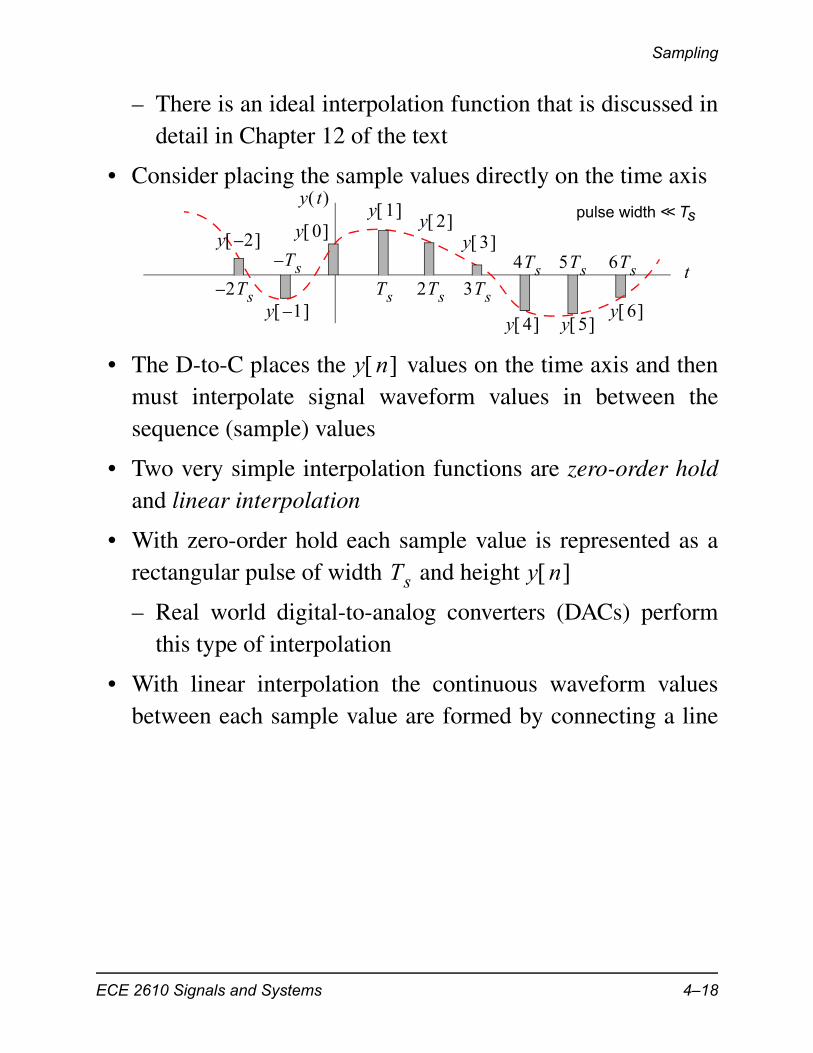
– There is an ideal interpolation function that is discussed indetail in Chapter 12 of the text

• Consider placing the sample values directly on the time axis

• The D-to-C places the values on the time axis and thenmust interpolate signal waveform values in between thesequence (sample) values

• Two very simple interpolation functions are zero-order holdand linear interpolation

• With zero-order hold each sample value is represented as arectangular pulse of width and height

– Real world digital-to-analog converters (DACs) performthis type of interpolation

• With linear interpolation the continuous waveform valuesbetween each sample value are formed by connecting a line

t

y t

y 0

y 1–

y 2–

y 1 y 2

y 3

y 4 y 5 y 6

Ts 2Ts 3Ts

4Ts 5Ts 6TsT– s2T– s

pulse width << Ts

y n

Ts y n


Sampling

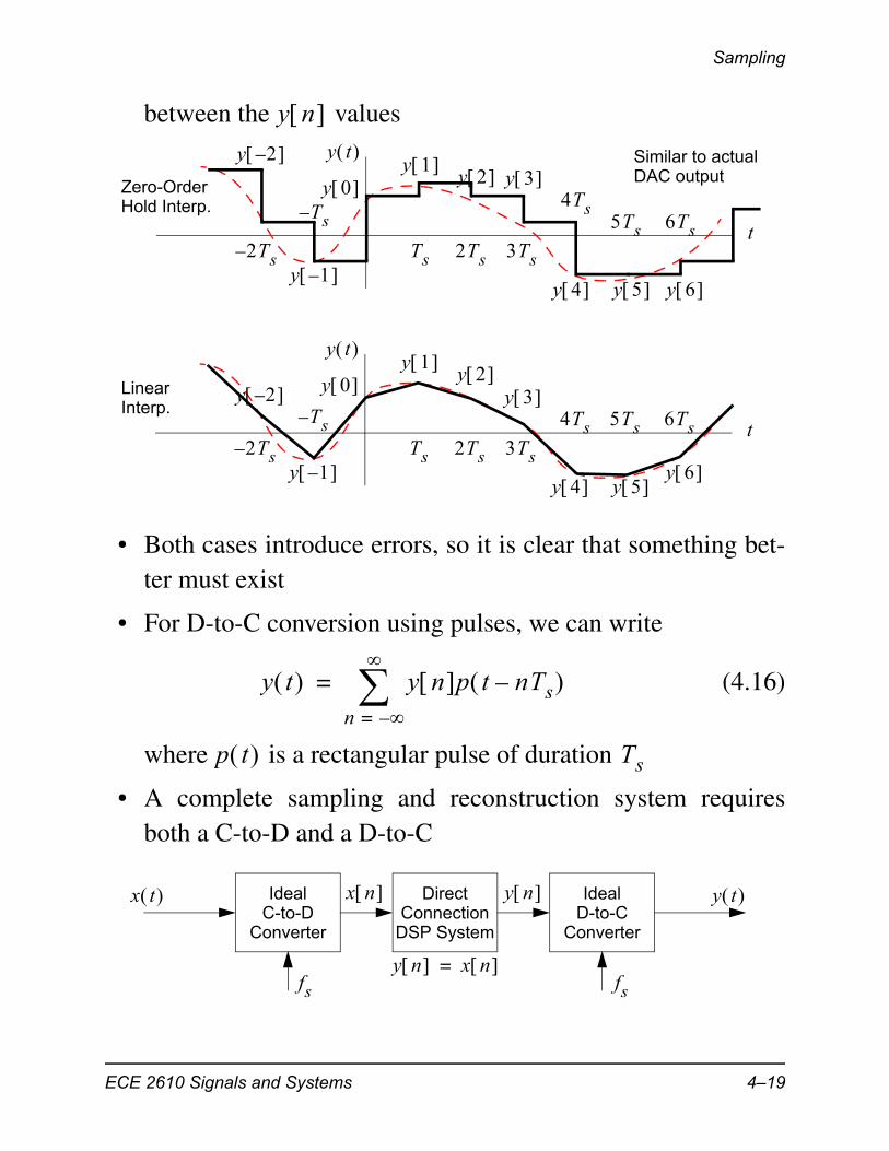
between the values

• Both cases introduce errors, so it is clear that something bet-ter must exist

• For D-to-C conversion using pulses, we can write

(4.16)

where is a rectangular pulse of duration

• A complete sampling and reconstruction system requiresboth a C-to-D and a D-to-C

y n

t

y t

y 0

y 1–

y 2– y 1 y 2 y 3

y 4 y 5 y 6

Ts 2Ts 3Ts

4Ts5Ts 6Ts

T– s

2T– s

t

y t

y 0

y 1–

y 2–

y 1 y 2

y 3

y 4 y 5 y 6

Ts 2Ts 3Ts

4Ts 5Ts 6TsT– s2T– s

Zero-OrderHold Interp.

LinearInterp.

Similar to actualDAC output

y t y n p t nTs– n –=

=

p t Ts

IdealD-to-C

Converter

IdealC-to-D

Converter

DirectConnection

DSP System

x t y t x n y n

y n x n =fs fs


Sampling

• With this system we can sample analog signal to pro-duce , and at the very least we may pass directly to

, then reconstruct the samples into

– The DSP system that sits between the C-to-D and D-to-C,should do something useful, but as a starting point we con-sider how well a direct connection system does at returning

– As long as the sampling theorem is satisfied, we expectthat will be close to for frequency content in that is less than Hz

– What if some of the signals contained in do not satisfythe sampling theorem?

– Typically the C-to-D is designed to block signals above from entering the C-to-D (antialiasing filter)

– A practical D-to-C is designed to reconstruct the principlealias frequencies that span

(4.17)

x t x n x n

y n y n y t

y t x t

y t x t x t fs 2

x t

fs 2

– f fs 2 fs 2–


Spectrum View of Sampling and Reconstruction

Spectrum View of Sampling and Reconstruc-tion

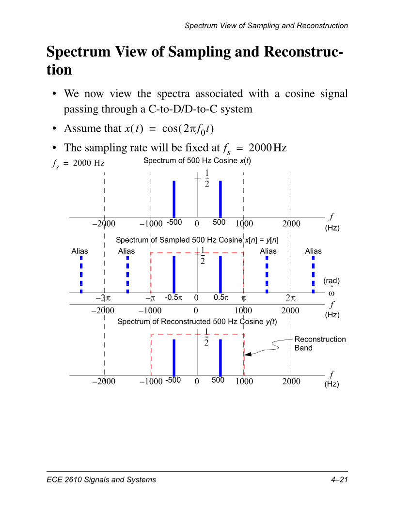
• We now view the spectra associated with a cosine signalpassing through a C-to-D/D-to-C system

• Assume that

• The sampling rate will be fixed at Hz

x t 2f0t cos=

fs 2000=

f

f

f

Spectrum of 500 Hz Cosine x(t)

2–2– 0

200010001000–2000– 0

200010001000–2000– 0

200010001000–2000– 0

Spectrum of Sampled 500 Hz Cosine x[n] = y[n]

Spectrum of Reconstructed 500 Hz Cosine y(t)

fs 2000 Hz=12---

12---

12--- Reconstruction

Band

500-500

0.5-0.5

500-500

AliasAliasAliasAlias

(Hz)

(Hz)

(Hz)

(rad)



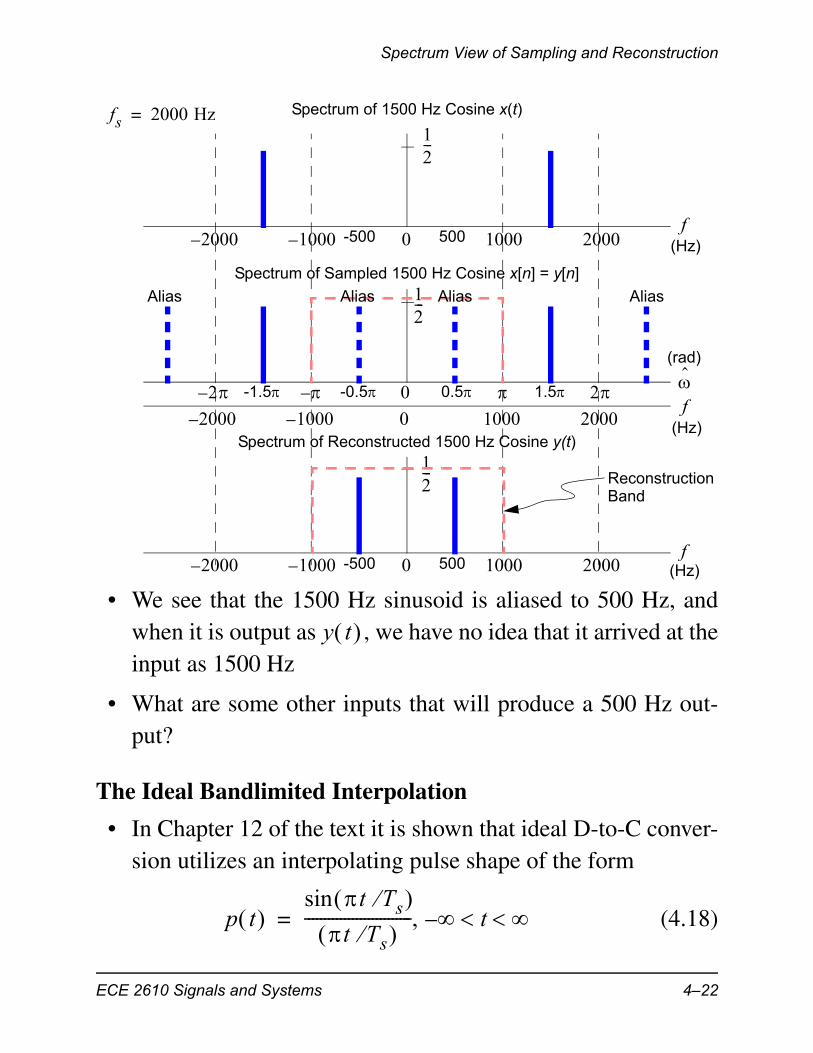
• We see that the 1500 Hz sinusoid is aliased to 500 Hz, andwhen it is output as , we have no idea that it arrived at theinput as 1500 Hz

• What are some other inputs that will produce a 500 Hz out-put?

The Ideal Bandlimited Interpolation

• In Chapter 12 of the text it is shown that ideal D-to-C conver-sion utilizes an interpolating pulse shape of the form

(4.18)

f

f

f

Spectrum of 1500 Hz Cosine x(t)

2–2– 0

200010001000–2000– 0

200010001000–2000– 0

200010001000–2000– 0

Spectrum of Sampled 1500 Hz Cosine x[n] = y[n]

Spectrum of Reconstructed 1500 Hz Cosine y(t)

fs 2000 Hz=12---

12---

12---

500-500

1.5-1.5 0.5-0.5

500-500

AliasAliasAlias Alias

ReconstructionBand

(Hz)

(Hz)

(Hz)

(rad)

y t

p t t Ts sin

t Ts --------------------------- – t =



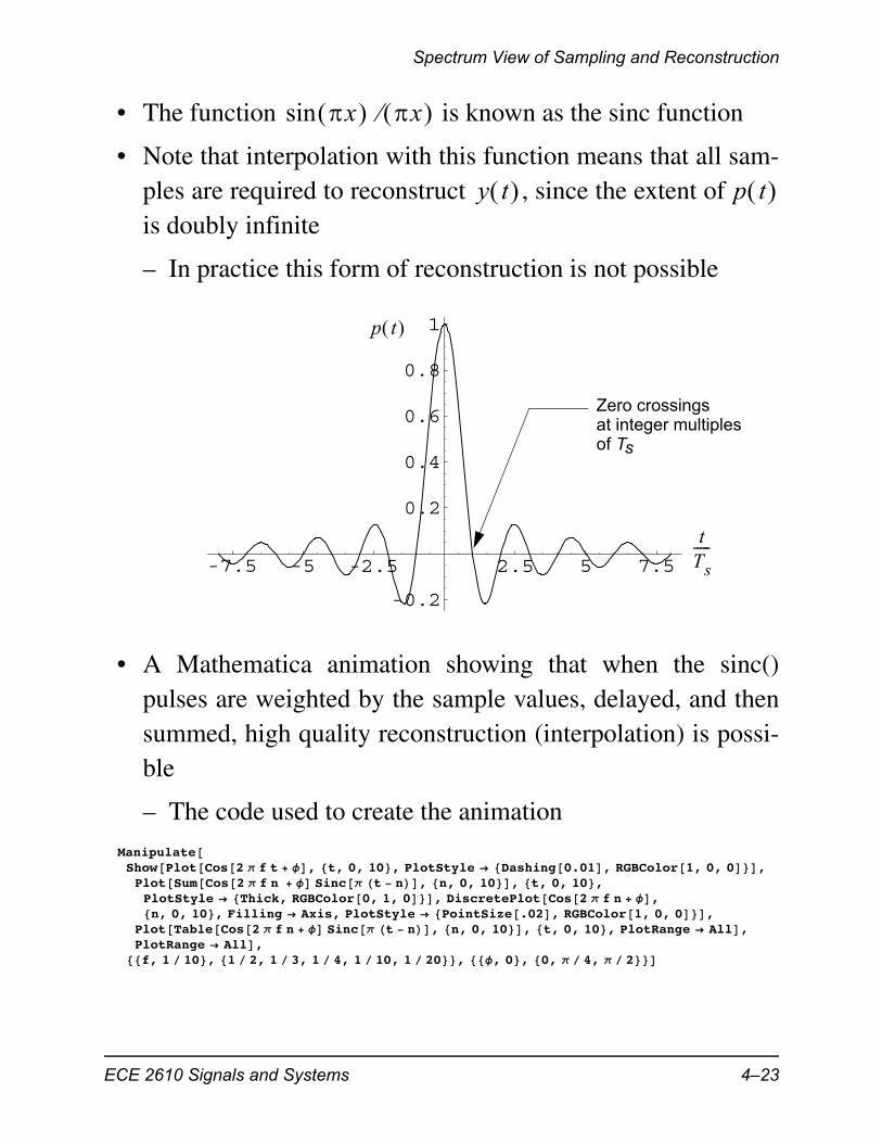
• The function is known as the sinc function

• Note that interpolation with this function means that all sam-ples are required to reconstruct , since the extent of is doubly infinite

– In practice this form of reconstruction is not possible

• A Mathematica animation showing that when the sinc()pulses are weighted by the sample values, delayed, and thensummed, high quality reconstruction (interpolation) is possi-ble

– The code used to create the animation

x sin x

y t p t

-7.5 -5 -2.5 2.5 5 7.5

-0.2

0.2

0.4

0.6

0.8

1p t

tTs-----

Zero crossingsat integer multiplesof Ts

Manipulate@Show@Plot@Cos@2 p f t + fD, 8t, 0, 10<, PlotStyle Ø [email protected], RGBColor@1, 0, 0D<D,Plot@Sum@Cos@2 p f n + fD Sinc@p Ht - nLD, 8n, 0, 10<D, 8t, 0, 10<,PlotStyle Ø 8Thick, RGBColor@0, 1, 0D<D, DiscretePlot@Cos@2 p f n + fD,8n, 0, 10<, Filling Ø Axis, PlotStyle Ø [email protected], RGBColor@1, 0, 0D<D,

Plot@Table@Cos@2 p f n + fD Sinc@p Ht - nLD, 8n, 0, 10<D, 8t, 0, 10<, PlotRange Ø AllD,PlotRange Ø AllD,

88f, 1 ê 10<, 81 ê 2, 1 ê 3, 1 ê 4, 1 ê 10, 1 ê 20<<, 88f, 0<, 80, p ê 4, p ê 2<<D



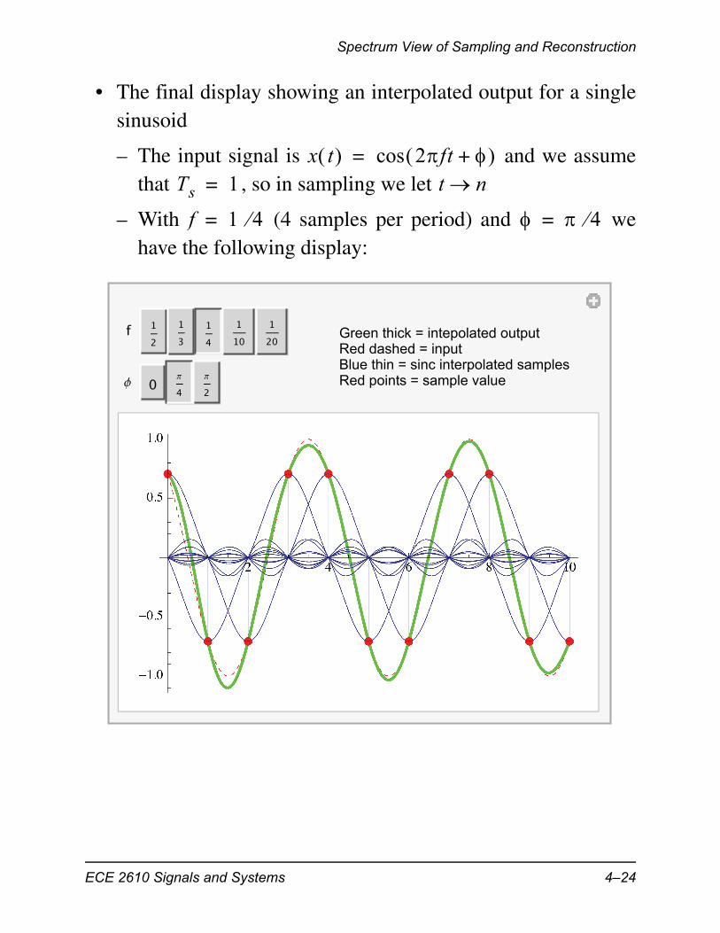
• The final display showing an interpolated output for a singlesinusoid

– The input signal is and we assumethat , so in sampling we let

– With (4 samples per period) and wehave the following display:

x t 2ft + cos=Ts 1= t n

f 1 4= 4=

f 12

13

14

110

120

f 0 p

4p

2

Green thick = intepolated outputRed dashed = inputBlue thin = sinc interpolated samplesRed points = sample value


sampling and chapter aliasing - uccs college of ...mwickert/ece2610/lecture_notes/ece2610...sampling...

Documents