sampling and quantization for optimal reconstruction€¦ · sampling and quantization for optimal...
TRANSCRIPT

Sampling and Quantization for Optimal Reconstructionby
Shay MaymonSubmitted to the Department of Electrical Engineering and Computer Science
in partial fulfillment of the requirements for the degree of
Doctor of Philosophy in Electrical Engineering
at the
MASSACHUSETTS INSTITUTE OF TECHNOLOGY
June 2011
c⃝ Massachusetts Institute of Technology 2011. All rights reserved.
Author . . . . . . . . . . . . . . . . . . . . . . . . . . . . . . . . . . . . . . . . . . . . . . . . . . . . . . . . . . . . .Department of Electrical Engineering and Computer Science
May 17, 2011
Certified by . . . . . . . . . . . . . . . . . . . . . . . . . . . . . . . . . . . . . . . . . . . . . . . . . . . . . . . . .Alan V. Oppenheim
Ford Professor of EngineeringThesis Supervisor
Accepted by. . . . . . . . . . . . . . . . . . . . . . . . . . . . . . . . . . . . . . . . . . . . . . . . . . . . . . . . .Professor Leslie A. Kolodziejski
Chairman, Department Committee on Graduate Theses

2

Sampling and Quantization for Optimal Reconstruction
by
Shay Maymon
Submitted to the Department of Electrical Engineering and Computer Scienceon May 17, 2011, in partial fulfillment of the
requirements for the degree ofDoctor of Philosophy in Electrical Engineering
AbstractThis thesis develops several approaches for signal sampling and reconstruction given differ-ent assumptions about the signal, the type of errors that occur, and the information availableabout the signal. The thesis first considers the effects of quantization in the environment ofinterleaved, oversampled multi-channel measurements with the potential of different quan-tization step size in each channel and varied timing offsets between channels. Consideringsampling together with quantization in the digital representation of the continuous-timesignal is shown to be advantageous. With uniform quantization and equal quantizer stepsize in each channel, the effective overall signal-to-noise ratio in the reconstructed outputis shown to be maximized when the timing offsets between channels are identical, result-ing in uniform sampling when the channels are interleaved. However, with different levelsof accuracy in each channel, the choice of identical timing offsets between channels is ingeneral not optimal, with better results often achievable with varied timing offsets corre-sponding to recurrent nonuniform sampling when the channels are interleaved. Similarly,it is shown that with varied timing offsets, equal quantization step size in each channel isin general not optimal, and a higher signal-to-quantization-noise ratio is often achievablewith different levels of accuracy in the quantizers in different channels.
Another aspect of this thesis considers nonuniform sampling in which the sampling gridis modeled as a perturbation of a uniform grid. Perfect reconstruction from these nonuni-form samples is in general computationally difficult; as an alternative, this work presents aclass of approximate reconstruction methods based on the use of time-invariant lowpass fil-tering, i.e., sinc interpolation. When the average sampling rate is less than the Nyquist rate,i.e., in sub-Nyquist sampling, the artifacts produced when these reconstruction methods areapplied to the nonuniform samples can be preferable in certain applications to the aliasingartifacts, which occur in uniform sampling. The thesis also explores various approaches toavoiding aliasing in sampling. These approaches exploit additional information about thesignal apart from its bandwidth and suggest using alternative pre-processing instead of thetraditional linear time-invariant anti-aliasing filtering prior to sampling.
Thesis Supervisor: Alan V. OppenheimTitle: Ford Professor of Engineering


Acknowledgments
I am fortunate to have had the privilege of being supervised and mentored by Professor AlanOppenheim, and I am most grateful for his guidance and support throughout the course ofthis thesis. Working with Al has been an invaluable experience for me; I have benefitedtremendously from his dedication to my intellectual and personal growth. Encouragingme to unconventional thinking and to creativity, stimulating me, and providing me withunlimited freedom, he has made this journey enjoyable and rewarding. I look forward tocollaborating with him in the future.
I wish to express my warm and sincere thanks to Professor Ehud Weinstein of Tel-Aviv University. I had a unique opportunity of working with Udi while co-teaching thegraduate level course ”Detection and Estimation Theory,” when we also collaborated onseveral research problems. Working and interacting with him has been invaluable to mydevelopment personally, professionally, and academically: Udi has become my friend andmentor.
I would also like to express my sincere appreciation to Professors Vivek Goyal andLizhong Zheng for serving as readers on the thesis committee and for their valuable com-ments and suggestions throughout this thesis work.
I am grateful to have been part of the Digital Signal Processing Group (DSPG) at MIT.For providing a stimulating and enjoyable working environment, I would like to acknowl-edge past and present members of DSPG: Tom Baran, Ballard Blair, Petros Boufounos,Sefa Demirtas, Sourav Dey, Dan Dudgeon, Xue Feng, Zahi Karam, John Paul Kitchens,Jeremy Leow, Joseph McMichael, Martin McCormick, Milutin Pajovic, Charles Rohrs,Melanie Rudoy, Joe Sikora, Archana Venkataraman, and Dennis Wei. The intellectualatmosphere of the group as well as the willingness to share ideas and to collaborate onresearch problems has made it a very exciting and enriching experience. Special thanks toEric Strattman and Kathryn Fischer for providing administrative assistance, for running thegroup smoothly and efficiently, and for always being friendly and willing to help.
No words can fully convey my gratitude to my family. I am deeply grateful to myparents for their ever present love, their support throughout my education, and their en-couraging me to strive for the best. I sincerely thank my sisters, brother, nephews, andnieces for the continuous love and support. I appreciate my wife’s family for their careand encouragement. Finally, my deep gratitude to my best friend and wife, Keren, for hermany sacrifices during the last four years, unconditional love, boundless patience, encour-agement, and for being there for me every step in the way. Ending my doctoral training andlooking forward with Keren to our new roles as parents, I am as excited about earning thetitle ABBA as I am about receiving my Ph.D.


The Thesis Ends;
Research Continues Forever

8
Contents
1 Introduction 19
1.1 Background . . . . . . . . . . . . . . . . . . . . . . . . . . . . . . . . . . 19
1.1.1 Sampling Theory - A Historical Overview . . . . . . . . . . . . . . 19
1.1.2 Extensions of the Sampling Theorem . . . . . . . . . . . . . . . . 20
1.1.3 Error and Aliasing . . . . . . . . . . . . . . . . . . . . . . . . . . 25
1.2 Objectives . . . . . . . . . . . . . . . . . . . . . . . . . . . . . . . . . . . 27
1.3 Outline . . . . . . . . . . . . . . . . . . . . . . . . . . . . . . . . . . . . 28
2 Perfect Reconstruction in Multi-channel Nonuniform Sampling 29
2.1 Introduction . . . . . . . . . . . . . . . . . . . . . . . . . . . . . . . . . . 29
2.2 Multi-channel Sampling and Reconstruction . . . . . . . . . . . . . . . . . 31
2.2.1 Perfect Reconstruction . . . . . . . . . . . . . . . . . . . . . . . . 33
2.2.2 Optimal Reconstruction in the Presence of Quantization Error . . . 38
2.2.3 Optimal Signal-to-Quantization-Noise Ratio (SQNR) . . . . . . . . 45
2.2.4 Simulations . . . . . . . . . . . . . . . . . . . . . . . . . . . . . . 50
2.3 Differential Uniform Quantization . . . . . . . . . . . . . . . . . . . . . . 57
3 MMSE Reconstruction in Multi-channel Nonuniform Sampling 63
3.1 Reconstruction Error . . . . . . . . . . . . . . . . . . . . . . . . . . . . . 63
3.2 Optimal Reconstruction Filters . . . . . . . . . . . . . . . . . . . . . . . . 66
3.2.1 Optimal Reconstruction for the Case of Uniform Sampling . . . . . 68
3.3 Illustrative Examples & Simulations . . . . . . . . . . . . . . . . . . . . . 69
9

4 Sinc Interpolation of Nonuniform Samples 75
4.1 Introduction . . . . . . . . . . . . . . . . . . . . . . . . . . . . . . . . . . 75
4.2 Reconstruction of Bandlimited Signals from Nonuniform Samples . . . . . 77
4.3 Sinc Interpolation of Nonuniform Samples . . . . . . . . . . . . . . . . . . 79
4.3.1 Mathematical Formulation . . . . . . . . . . . . . . . . . . . . . . 80
4.3.2 Randomized Sinc Interpolation . . . . . . . . . . . . . . . . . . . . 82
4.3.3 Uniform Sinc Interpolation . . . . . . . . . . . . . . . . . . . . . . 83
4.3.4 Nonuniform Sinc Interpolation . . . . . . . . . . . . . . . . . . . . 86
4.3.5 Independent Sinc Interpolation . . . . . . . . . . . . . . . . . . . . 86
4.3.6 RSI - Minimum Mean Square Reconstruction Error . . . . . . . . . 88
4.3.7 Discussion . . . . . . . . . . . . . . . . . . . . . . . . . . . . . . 91
5 Timing Errors in Discrete-time Processing of Continuous-time Signals 93
5.1 Introduction . . . . . . . . . . . . . . . . . . . . . . . . . . . . . . . . . . 93
5.2 The Effects of Timing Errors in Discrete-time Processing of Continuous-
time Signals . . . . . . . . . . . . . . . . . . . . . . . . . . . . . . . . . . 95
5.3 Jitter Compensation . . . . . . . . . . . . . . . . . . . . . . . . . . . . . . 99
6 Sub-Nyquist Sampling - Aliasing Mitigation 101
6.1 Introduction . . . . . . . . . . . . . . . . . . . . . . . . . . . . . . . . . . 101
6.2 Sinc Interpolation of sub-Nyquist Samples . . . . . . . . . . . . . . . . . . 103
6.2.1 Randomized Sinc Interpolation . . . . . . . . . . . . . . . . . . . . 103
6.2.2 Uniform Sinc Interpolation . . . . . . . . . . . . . . . . . . . . . . 104
6.2.3 Nonuniform Sinc Interpolation . . . . . . . . . . . . . . . . . . . . 105
6.2.4 Independent Sinc Interpolation . . . . . . . . . . . . . . . . . . . . 107
6.3 Simulations . . . . . . . . . . . . . . . . . . . . . . . . . . . . . . . . . . 108
7 Sub-Nyquist Sampling & Aliasing 111
7.1 Introduction . . . . . . . . . . . . . . . . . . . . . . . . . . . . . . . . . . 111
7.2 Sampling a Non-negative Bandlimited Signal . . . . . . . . . . . . . . . . 111
7.2.1 Bandlimited Square-roots . . . . . . . . . . . . . . . . . . . . . . 113
10

7.2.2 Signals with Real Bandlimited Square-roots . . . . . . . . . . . . . 116
7.2.3 Nonlinear Anti-aliasing . . . . . . . . . . . . . . . . . . . . . . . . 118
7.2.4 Generalization . . . . . . . . . . . . . . . . . . . . . . . . . . . . 126
7.3 Inphase and Quadrature Anti-aliasing . . . . . . . . . . . . . . . . . . . . 127
7.3.1 Inphase and Quadrature Decomposition . . . . . . . . . . . . . . . 127
7.3.2 IQ Anti-aliasing . . . . . . . . . . . . . . . . . . . . . . . . . . . 130
7.4 Co-sampling . . . . . . . . . . . . . . . . . . . . . . . . . . . . . . . . . . 134
7.4.1 Perfect Reconstruction . . . . . . . . . . . . . . . . . . . . . . . . 135
7.4.2 Blind Co-sampling . . . . . . . . . . . . . . . . . . . . . . . . . . 137
Appendices 139
A Optimal Constrained Reconstruction filters 141
B Derivation of See(e jω) 143
C Optimal MMSE Reconstruction Filters 149
D Randomized Sinc Interpolation - MSE Derivation 151
E The Autocorrelation Function of a Bandlimited Signal 153
F Time Jitter in Discrete-time Processing of Continuous-time Signals 155
G Randomized Sinc Interpolation - Sub-Nyquist Sampling 159
11

12

List of Figures
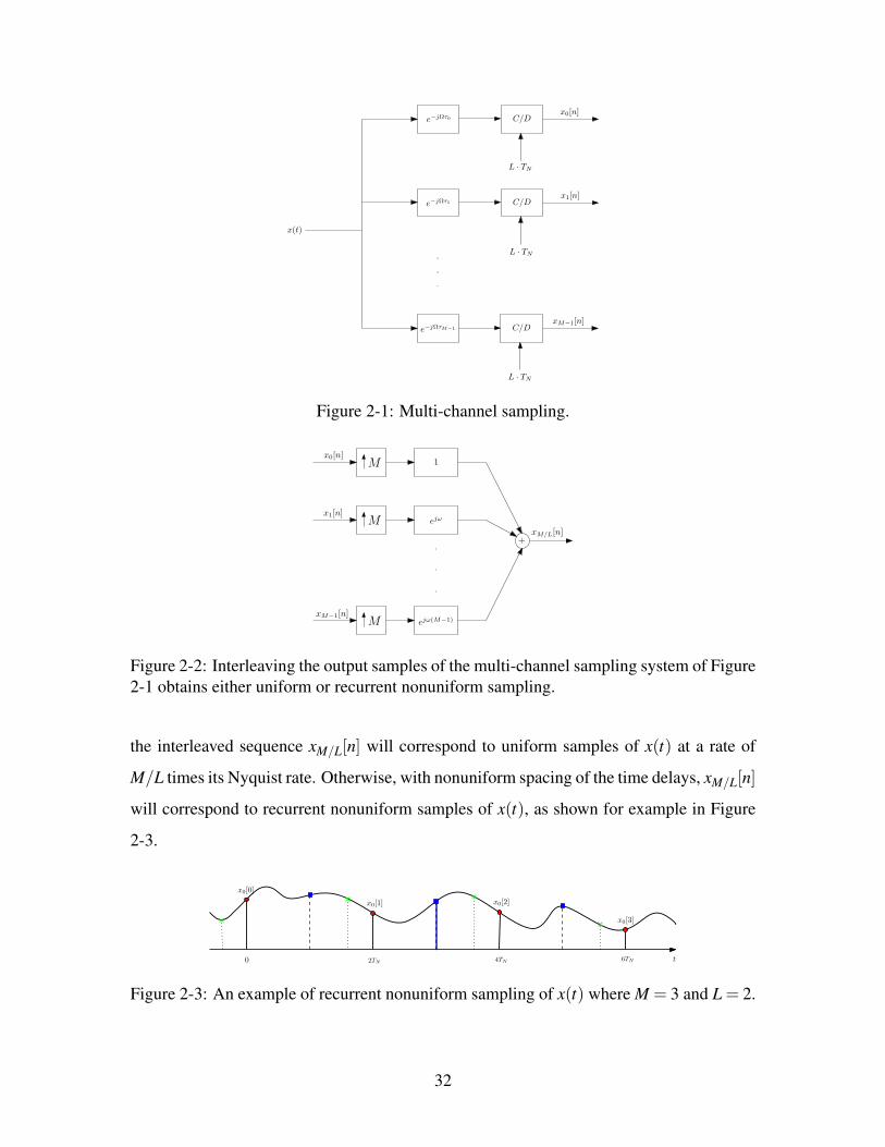
2-1 Multi-channel sampling. . . . . . . . . . . . . . . . . . . . . . . . . . . . 32
2-2 Interleaving the output samples of the multi-channel sampling system of
Figure 2-1 obtains either uniform or recurrent nonuniform sampling. . . . . 32
2-3 An example of recurrent nonuniform sampling of x(t) where M = 3 and
L = 2. . . . . . . . . . . . . . . . . . . . . . . . . . . . . . . . . . . . . . 32
2-4 Multi-channel reconstruction. . . . . . . . . . . . . . . . . . . . . . . . . . 33
2-5 Interleaving followed by sampling rate conversion. . . . . . . . . . . . . . 34
2-6 Multi-channel sampling rate conversion. . . . . . . . . . . . . . . . . . . . 35
2-7 Multi-channel sampling and quantization. . . . . . . . . . . . . . . . . . . 38
2-8 Single channel in the reconstruction system of Figure 2-4. . . . . . . . . . . 39
2-9 The kth branch of the polyphase implementation of the system in Figure 2-4. 42
2-10 The reduction factor γ in the average noise power at the output of the
reconstruction of Figure 2-4 achieves its maximum value at τ1 = −τ2 =
±(2/3) ·TN , i.e., when the multi-channel sampling is equivalent to uniform
sampling. Since this curve is based on the additive noise model of the quan-
tization error, which assumes uncorrelated errors, it is less accurate in the
vicinity of τ1 = 0, τ2 = 0, and τ1 = τ2. . . . . . . . . . . . . . . . . . . . . 51
2-11 The reduction factor γ in the average noise power at the output of the re-
construction system of Figure 2-4 where actual quantizers are applied to
the multi-channel output samples with accuracy of 10 bits. . . . . . . . . . 52
13

2-12 Each vector represents a channel whose time delay τm is determined by
the vector’s phase ωm according to the transformation ωm = 2πτm/(LTN),
which maps the region τm ∈ [−TN ,TN ] into the region ωm ∈ [−π,π]. The
numbers associated with each of the vectors are the optimal bit allocations
for the case of τ0 = 0, τ1 = TN/8, and τ2 =−3TN/4. . . . . . . . . . . . . 54
2-13 With bit allocation N0 = 3, N1 = 4, and N2 = 4, the optimal choice of
time delays is τ1 =−τ2 =±0.54TN , for which the multi-channel sampling
system is equivalent to recurrent nonuniform sampling. . . . . . . . . . . . 54
2-14 The relative performance compared to uniform sampling as a function of
τ1 and τ2 when τ0 = 0, N0 = 3, N1 = 4, and N2 = 4. Since this curve is
based on the additive noise model of the quantization error, which assumes
uncorrelated errors, it is less accurate in the vicinity of τ1 = 0, τ2 = 0, and
τ1 = τ2. . . . . . . . . . . . . . . . . . . . . . . . . . . . . . . . . . . . . 55
2-15 Optimal time delays for different choices of N2 (a) based on the additive
noise model, (b) based on simulations with actual quantizers. . . . . . . . . 56
2-16 Block diagram of differential quantization: coder and decoder. . . . . . . . 58
3-1 Optimal reconstruction is equivalent to interleaving of the multi-channel
samples followed by Wiener filtering. . . . . . . . . . . . . . . . . . . . . 69
3-2 Interleaving followed by sampling rate converter and Wiener filtering. . . . 73
3-3 The relative gain of d(ω1,ω2) as compared to the case of uniform sampling
when N0 = 3, N1 = 4, N2 = 4. . . . . . . . . . . . . . . . . . . . . . . . . 74
4-1 Reconstruction using sinc interpolation. . . . . . . . . . . . . . . . . . . . 81
4-2 A second-order statistics model for nonuniform sampling followed by Ran-
domized Sinc Interpolation for the case where T ≤ TN . . . . . . . . . . . . 82
4-3 Q(Ω) for the case where ξn ∼ u[−T/2,T/2] and T = TN = 1. . . . . . . . . 91
4-4 The optimal choice of β that minimizes σ2eR as a function of Bx for the case
where T = TN = 1. . . . . . . . . . . . . . . . . . . . . . . . . . . . . . . 91
5-1 Discrete-time processing of continuous-time signals. . . . . . . . . . . . . 93
14

5-2 Time jitter in discrete-time processing of continuous-time signals. . . . . . 95
5-3 A second-order statistics model for the system of Figure 5-2. . . . . . . . . 96
5-4 A second-order statistics model for the system of Figure 5-2 with G(e jω) =
G(ωT ), |ω|< π and where ξn = 0. . . . . . . . . . . . . . . . . . . . . . . 98
5-5 A second-order statistics model for the system of Figure 5-2 with G(e jω) =
G(ωT ), |ω|< π and where ζn = 0. . . . . . . . . . . . . . . . . . . . . . . 98
6-1 Anti-aliasing followed by nonuniform sampling and Lagrange interpolation. 102
6-2 Reconstruction from nonuniform samples for the case T > TN using sinc
interpolation. . . . . . . . . . . . . . . . . . . . . . . . . . . . . . . . . . 103
6-3 A second-order-statistics equivalent of nonuniform sampling followed by
Uniform Sinc Interpolation for the case where T > TN . . . . . . . . . . . . 105
6-4 A second-order-statistics equivalent of nonuniform sampling followed by
Nonuniform Sinc Interpolation for the case where T > TN . . . . . . . . . . 106
6-5 A second-order-statistics equivalent of nonuniform sampling followed by
Independent Sinc Interpolation for the case where T > TN . . . . . . . . . . 107
6-6 Pole-zero diagram of the transfer function Hc(s). . . . . . . . . . . . . . . 108
6-7 Artifacts with sub-Nyquist sampling. (a) The estimated power spectrum
of x(t). The estimated power spectrum vs. analytic results in the case
of (b) Uniform Sampling, (c) USI applied to nonuniform sampling, (d)
NSI applied to nonuniform sampling, and (e) ISI applied to nonuniform
sampling. (f) The estimated power spectrum of x(t) and of its approximations.110
7-1 A sampling-reconstruction scheme of a non-negative bandlimited signal.
The sampling system consists of non-linear pre-processing whose output
signal x(t) is bandlimited to ±π/T and satisfies the relation y(t) = |x(t)|2. . 112
7-2 The region within which all possible |Y (Ω)| that satisfy (7.21) lie. . . . . . 117
7-3 Non-linear anti-aliasing. . . . . . . . . . . . . . . . . . . . . . . . . . . . 118
7-4 The frequency response H(Ω) of the LTI system in Figure 7-3. . . . . . . . 119
15

7-5 Complex anti-alising applied to y(t) from (7.35) where a=−π/2 and Ωx =
π/T . (a) The spectrums of the complex bandlimited square roots. (b) The
partial energies of the complex bandlimited square roots. (c) The frequency
responses of y(t) and of its approximations y(t) = |x(t)|2 where the cut-off
frequency of H(Ω) is γ = π/(2T ). (d) The frequency responses of y(t) and
of its approximations y(t) = |x(t)|2 where the cut-off frequency of H(Ω) is
γ = π/(4T ). . . . . . . . . . . . . . . . . . . . . . . . . . . . . . . . . . . 123
7-6 An example for which the bandwidth of y(t) is equal to the sum of the
bandwidths of x1(t) and x2(t). . . . . . . . . . . . . . . . . . . . . . . . . 126
7-7 An example for which the bandwidth of y(t) is greater than the sum of the
bandwidths of x1(t) and x2(t). . . . . . . . . . . . . . . . . . . . . . . . . 126
7-8 An example for which the bandwidth of y(t) is less than the sum of the
bandwidths of x1(t) and x2(t). . . . . . . . . . . . . . . . . . . . . . . . . 126
7-9 Decomposing Y (Ω) into Y1(Ω) and Y2(Ω). . . . . . . . . . . . . . . . . . . 129
7-10 Iterative decomposition of y(t) into its inpahse and quadrature components
after two iterations (N = 2). . . . . . . . . . . . . . . . . . . . . . . . . . . 131
7-11 A comparison between LTI anti-aliasing filtering and IQ anti-aliasing ap-
plied to a signal whose spectrum is triangular to reduce its bandwidth to 0.3
times its original bandwidth. (a) LTI anti-aliasing (original signal dashed).
(b) IQ anti-aliasing with N = 4 iterations (original signal dashed). . . . . . 132
7-12 Generating y1(t) and y2(t) through sub-Nyquist sampling of y(t) followed
by lowpass filtering. The Nyquist interval TN = π/Ωc. . . . . . . . . . . . 133
7-13 The multi-channel model. . . . . . . . . . . . . . . . . . . . . . . . . . . . 134
7-14 Reconstruction of x1(t) and x2(t) from uniform samples of y1(t) and y2(t). . 135
16

List of Tables
2.1 The performance gain for different bit allocations. . . . . . . . . . . . . . . 53
2.2 Examples of overall improvement in SQNR when replacing uniform quan-
tization with differential uniform quantization . . . . . . . . . . . . . . . . 61
4.1 Sinc Interpolation Reconstruction Methods . . . . . . . . . . . . . . . . . 82
17

18

CHAPTER 1
INTRODUCTION
1.1 Background
1.1.1 Sampling Theory - A Historical Overview
Sampling theory is a fundamental concept in signal processing and its applications. It plays
an important role as a connecting link between continuous-time and discrete-time signals
as it allows representation, without loss of information, of continuous-time bandlimited
signals by discrete-time sequences, which can then be processed digitally. The most com-
monly used sampling theorem asserts that a bandlimited signal, observed over the entire
time axis, can be perfectly reconstructed from its equally spaced samples taken at a rate
which exceeds twice the highest frequency present in the signal. The sampling theorem
was first introduced in information theory and communication engineering by C. E. Shan-
non in 1940. However, it did not appear in the engineering literature until after World War
II in 1949 [79]. Shannon states the sampling theorem in the following terms: ”Theorem 1:
If a function f (t) contains no frequencies higher than W cps, it is completely determined by
giving its ordinates at a series of points spaced 1/(2W ) seconds apart.” Shannon did not
claim it as his own, and in fact following the theorem he notes: ”This is a fact which is com-
mon knowledge in the communication art.” However, later he adds, ”Theorem 1 has been
given previously in other forms by mathematicians but in spite of its evident importance
seems not to have appeared explicitly in the literature of communication theory.”
The sampling theorem has been attributed in the literature to numerous different authors
including E. T. Whittaker [92], H. Nyquist [67], J. M. Whittaker [93, 94], V. A. Kotel’nikov
19

[50], D. Gabor [28], and C. E. Shannon [79], and its historical roots have been often dis-
cussed. The Mathematician E. T. Whittaker [92] is considered to be the first to address
the sampling theorem in 1915 in his study of the cardinal functions. The sampling theo-
rem introduced by Shannon is very close to the more refined statement in 1935 of J. M.
Whittaker [94], concerning the relation between the cardinal functions and the finite-limit
Fourier integral. Shannon was aware of the mathematical work of J. M. Whittaker and he
acknowledged it in his paper. Nyquist [67] (1928) did not explicitly consider the problem of
sampling and reconstruction of continuous-time bandlimited signals, but a different prob-
lem which has some mathematical similarities. Considering the problem of distortionless
transmission of telegraphic signals, Nyquist showed that up to 2W independent pulse sam-
ples could be sent through a system of bandwidth W . When Shannon stated the sampling
theorem, he referred to the critical sampling interval T = 1/(2W ) as the Nyquist interval
corresponding to the band W , in recognition of Nyquist’s discovery of the fundamental
importance of this interval in connection with telegraphy. In the late fifties, it became
known that Kotel’nikov [50] introduced the sampling theorem in the Russian literature to
communications theory in 1933.
Sampling theory has found application in many fields including signal analysis, system
theory, information theory, spectroscopy and image processing, radar, sonar, acoustics, op-
tics, holography, meteorology, oceanography, crystallography, physical chemistry, medical
imaging, and there are important connections with multi-resolution analysis and wavelets.
1.1.2 Extensions of the Sampling Theorem
Many extensions and generalizations of the Nyquist-Shannon sampling theorem exist. Kohlen-
berg [49] (1953) extended the sampling theorem to bandpass signals. For a bandpass signal
to be accurately represented by a set of its equally spaced samples at the minimum possi-
ble rate, the lowest frequency occupied by the signal must be an integer multiple of the
signal’s bandwidth. Introducing “second-order sampling,” which involves two interleaved
sequences of uniformly spaced sampling points, Kohlenberg proved that perfect reconstruc-
tion of bandpass signals is possible at a rate equal to twice the bandwidth of the signal, with
20

no restrictions on the range of frequencies that the signal occupies.
The first to extend the Nyquist-Shannon sampling theorem to bandlimited signals in
higher dimensions was Parzen [72] in 1956. Petersen and Middleton [74] show that in the
case of multidimensional sampling, the most efficient lattice is in general not rectangular.
Hexagonal sampling and its higher dimensional generalizations are shown in [63, 64] to
yield a lower sampling density. Sampling expansions for radially symmetric functions that
are bandlimited to the unit sphere in RN have also been obtained [42].
When the Nyquist-Shannon sampling theorem is applied to the autocorrelation function
of a bandlimited wide-sense stationary stochastic process, the optimal linear estimator, in
the mean square sense, of the stochastic process based on its Nyquist-rate samples achieves
zero mean square error, as shown by A. V. Balakrishnan [2] in 1957. Generalization to
bandpass or multipass stochastic processes is presented in [56]. Extension of stochastic
sampling to n-dimensional processes is introduced in [66]. Sampling theorems for nonsta-
tionary random processes are also presented [29, 75, 101].
Another interesting extension involves the reconstruction of a bandlimited signal from
samples of the signal and its derivatives. When Shannon [79] introduced the sampling
theorem, he also remarked that a bandlimited signal could be reconstructed from uniform
samples of the signal and its derivative at half the Nyquist rate. He then generalized his
remark to higher derivatives. The details were later worked out and Shannon’s statements
were mathematically formulated and proved by L. Fogel [27], D. Jagerman and L. Fogel
[39], D. Linden [54], and D. Linden and N. Abramson [55]. Specifically, it was shown
that a bandlimited signal can be perfectly reconstructed from equally spaced samples of the
signal and its first M −1 derivatives taken at a rate that is M times lower than the Nyquist
rate of the signal. The importance of this result lies in its application. For example, the
velocity and the position of an aircraft are sampled at half the Nyquist rate to determine
a continuous course of its path. Linden [55] also showed that for large M, the expansion
approaches a Taylor-type series weighted by a Gaussian density function centered about
each sample point.
Papoulis’ generalized sampling expansion [71] (1977) is a further generalization of
the sampling theorem which suggests reconstructing a bandlimited signal using data other
21

than the sampled values of the signal and its derivatives. Papoulis has shown that under
certain conditions on multi-channel systems for which the input is bandlimited, the ban-
dlimited input signal can be perfectly reconstructed from samples of the responses of M
linear time-invariant (LTI) systems, each sampled at 1/M times the Nyquist rate. The sam-
pling expansion introduced by Linden [55] can be viewed as a special case of Papoulis’
generalized sampling expansion, in which the LTI systems of the multi-channel system are
chosen so the multi-channel outputs correspond to the signal and its first M−1 derivatives.
The generalized sampling expansion of Papoulis suggests various ways to split a signal
into different channels in which the analog-to-digital (A/D) converter in each channel pro-
vides different information about the signal. This parallelism is one possibility for improv-
ing data acquisition systems whose performance is limited by the A/D converters, which
work at their limits and cannot be pushed further. A very common method for splitting a
signal into different channels is the use of time-interleaved A/D converters [46], in which
the input signal in each of the M channels is first time-delayed and then sampled at a rate
which is M times lower than the signal’s Nyquist rate. With the time-delays appropriately
designed, interleaving the multi-channel output samples produces uniform samples of the
input signal at the Nyquist rate. Thus, sampling with an ideal time-interleaved A/D con-
verter with M channels is equivalent to sampling with an ideal A/D converter with a sam-
pling rate M times higher. In practice, however, channel mismatches limit the performance
of time-interleaved A/D converters.
Papoulis [70] also generalizes the sampling theorem for the case in which the sampling
rate exceeds the Nyquist rate, i.e., oversampling. He shows that in this case the demands
on the reconstruction filter can be considerably relaxed. Reconstructing the signal from
its Nyquist rate samples requires an ideal lowpass filter, which is, of course, impossible to
realize. Alternatively, by increasing the sampling rate above Nyquist, the requirement of a
sharp cut-off of the interpolation filter is removed due to the existence of a free attenuation
interval. There are other advantages of oversampling. When a signal is oversampled, its
samples become dependent and the signal reconstruction is not affected when losing an
arbitrarily large but finite number of sampled values. Oversampling can also improve the
performance in the presence of quantization error [15, 69]. Specifically, a high-resolution
22

A/D converter can be achieved by oversampling a low-resolution A/D converter followed
by discrete-time processing of the digital oversampled signal.
The sampling expansions discussed so far assumed that the entire signal is observed.
Brown [13] considers the problem of predicting bandlimited signals from their past values.
He shows that a bandlimited signal can be approximated fairly well by a linear combination
of past samples, provided that the sampling rate exceeds twice the Nyquist rate of the signal.
The first to extend the sampling theorem for the analysis of signals specified by a time-
varying spectrum with time-varying bands was Horiuchi [35]. In this expansion, the coef-
ficients are in general not the same as the samples of the continuous-time signal.
Reconstruction of a bandlimited signal from nonuniform samples has also been exten-
sively explored in the literature. J. R. Higgins [33] suggests that irregular sampling is a
norm: ”Irregular sampling arises mathematically by simply asking the question ”What is
special about equidistantly spaced sample points?”; and then finding that the answer is
”Within certain limitations, nothing at all”. In practice it is often said that irregular sam-
pling is the norm rather than the exception.” In a variety of contexts, nonuniform sampling
naturally arises or is preferable to uniform sampling. Uniform sampling with missing sam-
ples or with time-jitters can be regarded as nonuniform sampling. In the spatial domain,
non-uniformity of the spacing of the array elements in an antenna or acoustic sensor ar-
ray is often part of the array design as a trade off between the length of the array and the
number of elements. A signal specified by time-varying spectrum is another example for
which nonuniform sampling is more natural than uniform sampling. When the signal is
varying rapidly it is more appropriate to sample it at a higher rate than when it is varying
slowly. Reconstruction from nonuniform sampling has been used in many fields including
Computed Tomography (CT), Magnetic Resonance Imaging (MRI), optical and electronic
imaging systems. H. S. Black [7] credits Cauchy [16] for the origin of nonuniform sam-
pling in 1841 and offers the following translation to Cauchy’s statement: ”If a signal is a
magnitude-time function, and if time is divided into equal intervals such that each subdi-
vision comprises an interval T seconds long, where T is less than half the period of the
highest significant frequency component of the signal, and if one instantaneous sample is
taken from each sub-interval in any manner, then a knowledge of the instantaneous mag-
23

nitude of each sample plus a knowledge of the instant within each sub-interval at which
the sample is taken, contains all the information of the original signal.” J. R. Higgins [32],
however, notes that such a statement was not included in the paper by Cauchy.
With unequal spacing of the sampling instants, the reconstruction process is often more
involved. Yen [100] (1956) considers the reconstruction of a bandlimited signal from its
nonuniform samples for various special cases which possess simple reconstruction formu-
las. Specifically, he treats the case of uniform sampling where a finite number of samples
migrate to distinct new positions. He also provides an explicit reconstruction formula for
the case in which an infinite number of samples are shifted by the same amount, resulting in
a gap in an otherwise uniform sampling grid. The case of recurrent nonuniform sampling,
in which the nonuniform sampling grid has a periodic structure, is also analyzed by Yen,
who provides an exact reconstruction formula. The sampling instants in this case can be
divided into groups of M samples each, where each group has a recurrent period, which is
M times the Nyquist period of the input signal. Recurrent nonuniform sampling can also be
viewed as a special case of the generalized sampling expansion of Papoulis [71], in which
the LTI systems are pure delays. Comparing the reconstruction formulas for the different
cases of nonuniform sampling with that of uniform sampling, Yen remarks that it is evident
that the composing functions become more and more complicated as the sampling grid
deviates more and more from a uniform grid.
More generally, Beutler [5] (1966) proved that a bandlimited signal can be perfectly re-
constructed from its nonuniform samples, under certain conditions on the nonuniform grid
and provided that the average sampling rate exceeds the Nyquist rate, i.e., that the number
of samples per unit time exceeds (on the average) twice the highest frequency present in
the signal. This result, which is shown for deterministic signals as well as for wide-sense
stationary stochastic signals, depends most directly on some closure theorems first obtained
by Levinson [53]. Yao and Thomas [98, 99] later derived a sampling expansion for nonuni-
form samples of a bandlimited signal for the case, in which each of the sampling instants
deviates less than (1/π) ln2 from the corresponding uniform grid. They also considered the
question of stable reconstruction and showed that Lagrange interpolation is stable when the
deviation of the sampling instants from a uniform sampling grid is less than 1/4.
24
Landau [51] considers the question of whether the Nyquist rate can be improved if the
sampling instants are chosen differently; or the signals are bandpass or multi-band; or at
the cost of more computing than is required by sinc interpolation. He proves that stable
sampling cannot be performed at a rate lower than the Nyquist, regardless of the location
of sampling instants, the nature of the set of frequencies which the signals occupy, or the
method of construction.
There are also other extensions of the sampling theorem in which the sampling instants
are dependent on the signal. Representing a bandlimited signal by its zero crossings or
by its crossings with a cosine function are just a few examples. This kind of sampling is
referred to as implicit sampling and it was first considered by Bond and Cahn [9]. Since
nonlinear transformation may increase the signal’s bandwidth, this sampling approach may
be advantageous in reconstructing a bandlimited signal that was processed through a non-
linear zero-crossing-preserving transformation.
A comprehensive review of literature concerning other extensions and generalizations
of the sampling theorem can be found in [33, 38, 43, 88, 102].
1.1.3 Error and Aliasing
The sampling theorem assumes that the signal is bandlimited, it is observed over the entire
time axis, its exact sampled values are accurately known, and the sampling instants are
uniformly spaced. However, in many cases of practical interest, the underlying signal is
not strictly band-limited, it is observed only over a finite time interval, its exact sampled
values are not known, and jitter occurs in acquiring the samples. These deviations from the
ideal scenario influence the accuracy of the signal reconstruction and result in interpolation
error.
When the signal is not band-limited or, alternatively, it is bandlimited but sampled at
a rate lower than its Nyquist rate, frequency components of the original signal that are
higher than half the sampling rate are folded into lower frequencies resulting in aliasing.
The aliasing error is defined as the difference between the original signal and the series
constructed using the signal’s samples. A classical result giving an upper bound on the
25

aliasing error was stated originally by P. Weiss [91] in 1963 and proved in 1967 by J. L.
Brown [12], who also obtained an upper bound for the aliasing error of bandpass signals.
To avoid aliasing in sampling, the continuous-time signal must be forced to be ban-
dlimited to frequencies below one-half the desired sampling rate. This aim is often accom-
plished by processing the continuous-time signal through an LTI anti-aliasing low-pass
filter prior to sampling it. There is a variety of other contexts, in which the alias of the
signal is preferable to the original signal. This is the case, for example, with band-pass
signals, in which the aliasing is exploited for modulating the signal into baseband frequen-
cies. Another example in the same category is a sampling oscilloscope. This instrument
is intended for observing very high-frequency waveforms, and it exploits the principles of
sampling to alias these frequencies into ones that are more easily displayed. In other cases,
aliasing is deliberately distributed to various channels in such a way that when they are
combined properly, aliasing is cancelled and perfect recovery is achieved. This is the case,
for example, with interlaced sampling as in interleaved A/D converters or more generally
with Papoulis’ generalized sampling expansion.
When the signal is observed over a finite time interval, only a finite number of samples
can be used for the signal reconstruction. Since the sampling expansion requires an infinite
number of terms to exactly interpolate a bandlimited signal from its samples, an interpola-
tion error, referred to as a truncation error, occurs. Several results concerning the truncation
error were obtained by several authors including B. Tsybakov and V. Iakovlev, [87], Helms
and Thomas [31], and Papoulis [70].
The amplitude error arises when the exact sampled values are not accurately known and
their approximations are used for the interpolation of the signal. Round-off and quantiza-
tion errors may be considered as special cases of amplitude error. Papoulis [70] shows that
even if the errors in the sampled values are bounded, the amplitude error may exceed all
bounds for some values of t.
Deviations of the sampling instants from the uniform sampling grid also occur in prac-
tice, and the problem is to determine the original signal based on these samples. This error
is referred to as a time-jitter error and is similar in its treatment to the amplitude error.
Assuming that the timing errors are known, Papoulis [70] derives an approximation of the
26

reconstructed signal from these samples. Butzer [14] provides a bound for the time-jitter
error which is similar to the bound obtained on the amplitude error.
In practice, more than one of the errors mentioned above can occur. Butzer [14] pro-
vides an upper bound for the error caused by approximating a not-necessarily band-limited
signal by a truncated series with quantized sampled values taken at jittered time instants.
1.2 Objectives
This thesis considers the problem of reconstructing a bandlimited signal from its sampled
values. It develops various methods for optimal reconstruction given different assumptions
about the signal, the sampling grid and the type of errors that arise. The thesis also explores
the benefits of nonuniform sampling over uniform sampling in the presence of quantization
error and when aliasing occurs as a result of sub-Nyquist sampling.
The work discusses optimal reconstruction of the continuous-time bandlimited signal
in the environment of interleaved multi-channel measurements in the presence of quanti-
zation error. A new approach for mitigating the effects of quantization error on the re-
constructed signal is introduced. This approach involves time-varying quantization whose
time-dependent parameters are specified according to the relative timing between adjacent
samples. In a broader view, this approach suggests the benefits of considering sampling
together with quantization in the digital representation of the continuous-time signal.
The thesis also considers an extension of the Nyquist-Shannon sampling theorem, in
which additional information is available about the continuous-time signal apart from its
bandwidth. Utilizing this additional information can result in perfect reconstruction of the
bandlimited signal from samples taken at a rate lower than the Nyquist rate.
In the context of sub-Nyquist sampling, the thesis also suggests various methods for
mitigating or avoiding aliasing, which may be preferable in some contexts to the tradi-
tional LTI anti-aliasing filtering. Among these methods are non-linear methods, linear
time-varying methods and methods in which aliasing mitigation is accomplished by per-
turbation of the uniform sampling grid. In the scenario of multiple correlated signals, co-
sampling is introduced as a way to possibly reduce the overall sampling rate by distributing
27

co-aliasing in sampling so that it gets cancelled in reconstruction.
1.3 Outline
The thesis is organized as follows. Chapter 2 considers the case of multi-channel measure-
ments as may arise in interleaved A/D converter or in distributed sensor networks. We con-
sider the case of oversampling and design optimal reconstruction filters under the constraint
of perfect reconstruction in the absence of errors. Chapter 3 takes a different approach to
the design of the reconstruction filters in which the constraints of perfect reconstruction
are relaxed. In both approaches, the effects of quantization error on the reconstructed out-
put are analyzed, and optimal design of the relative timing between the channels and the
quantizer step size in each of the channels is discussed.
Chapter 4 considers the case in which the nonuniform sampling grid is modeled as a
perturbation of a uniform grid. The exact reconstruction in this case is comuptationally
difficult, and a class of simple approximate reconstruction methods based on the use of
LTI low-pass filtering is suggested and analyzed. Chapter 5 analyzes the effects of timing
errors in processing continuous-time bandlimited signals using discrete-time systems. It
also discusses the design of a discrete-time system which compensates for the timing errors.
In Chapter 6 we use the class of approximate reconstruction methods developed in Chapter
4 for the reconstruction from nonuniform samples at a rate lower than the Nyquist rate. We
show that the artifacts due to sub-Nyquist sampling can be controlled so that aliasing is
traded off with uncorrelated noise, which may be beneficial in various contexts.
In Chapter 7, we assume that additional information about the signal apart from its
bandwidth is available and suggest a sampling-reconstruction scheme which exploits this
information for reducing the sampling rate. In this chapter we also discuss various alterna-
tive methods to avoid aliasing in sampling.
28

CHAPTER 2
PERFECT RECONSTRUCTION IN
MULTI-CHANNEL NONUNIFORM
SAMPLING
This chapter considers interleaved, multi-channel measurements as arise for example in
time-interleaved analog-to-digital (A/D) converters and in distributed sensor networks.
Such systems take the form of either uniform or recurrent nonuniform sampling, depending
on the relative timing between the channels. Uniform quantization in each channel results
in an effective overall signal-to-quantization-error ratio (SQNR) in the reconstructed output
which is dependent on the quantizer step size in each channel, the relative timing between
the channels and the oversampling ratio. It is shown that in the multi-channel sampling
system when the quantization step size is not restricted to be the same in each channel and
the channel timing is not constrained to correspond to uniform sampling, it is often possible
to reduce the SQNR relative to the uniform case.
2.1 Introduction
High bandwidth signals or the use of large oversampling ratios often require the use of
time-interleaved A/D converters [46]. Similarly in a sensor network environment, separate
sensors might independently sample a shifted version of an underlying signal with the sen-
sor outputs then transmitted to a fusion center for interleaving and processing. The relative
timing of the channels is typically chosen so that simple interleaving results in uniform
29

sampling. More generally, the interleaved samples correspond to recurrent nonuniform
sampling [23, 43, 61, 71, 100].
When interleaving is assumed to correspond to uniform sampling but fails to do so
because of timing errors, the channel timing is often referred to as mismatched; if not
accounted for, this mismatch can lead to significant degradation in performance. A variety
of methods have been suggested in the literature to mitigate these problems. To reduce the
errors introduced by timing mismatches it is first required to detecting the timing errors.
In general, there exist two approaches for detection of timing errors: one which does not
assume prior knowledge and is based on the output samples of the time-interleaved A/D
converter [21, 22, 36, 37, 59, 78, 83, 90], and another which incorporates a known signal at
the input to the system [41, 44]. Once the timing errors have been measured, the correction
can be done either by adjusting the sampling clock in each A/D converter to eliminate the
timing errors, or by digital processing of the output samples to obtain uniform samples.
In single or multi-channel sampling systems for A/D conversion, quantization effects
must also be taken into account. Oversampling is a well established approach to mitigating
the effects of quantization, effectively trading off between the oversampling ratio and the
required quantization step size for a fixed signal-to-quantization-error ratio. This trade-
off can be accomplished in a direct way by following the quantizer with a sampling rate
converter or by using noise-shaping techniques as in delta-sigma A/D converters [15, 69].
A systematic alternative approach is introduced in [47, 48] to derive the time-interleaved
equivalent structure for an arbitrary delta-sigma converter. A vector quantization approach
is used in [85] to develop a lower bound on the mean squared reconstruction error for
periodic bandlimited signals from the quantized oversampled signal.
The multi-channel sampling system which we consider is presented in section 2.2,
where we also suggest a multi-channel reconstruction scheme. In section 2.2.1 we design
the multi-channel reconstruction filters to achieve perfect reconstruction of the input signal
in the absence of quantization error. In sections 2.2.2 we consider the effects of uniform
quantization in the environment of interleaved, oversampled multi-channel measurements
and the design of the optimal reconstruction filters, which compensate for the nonuniform
spacing of the channel offsets and for the quantization error. Modeling quantization er-
30

ror with an additive noise model, we show in section 2.2.3 that for the multi-channel case,
when the quantizer step size is not constrained to be the same in each channel and the chan-
nel timing is not constrained to result in uniform sampling, it is often possible to reduce the
SQNR relative to the uniform case. Specifically, we show that timing mismatches between
channels can be compensated for by appropriate choice of quantization step size in each
channel rather than attempting to correct the timing mismatch. Alternatively, the choice of
using different quantizer step size in each channel can be matched by appropriate choice of
the relative timing between channels together with properly designed compensation filters.
The concept of having different levels of accuracy in different channels is similar to the
approach in sub-band coding [19, 76, 89], in which each sub-band is quantized with an
accuracy based upon appropriate criteria. Replacing uniform quantization with differential
uniform quantization, it is shown in section 2.3 that higher performance gain is achieved
when the channel offsets are nonuniformly spaced.
2.2 Multi-channel Sampling and Reconstruction
The basic multi-channel sampling which we consider is shown in Figure 2-11. In this
system, the Nyquist rate of the bandlimited input signal x(t) is denoted by 1/TN , and each
of the M channels is sampled at a rate of 1/T = 1/(LTN) with M > L, corresponding to
an effective oversampling factor of ρ = M/L > 1. We assume the usual Nyquist-Shannon
sampling model but with the sampling done in a multi-channel structure. The notation
C/D in Figure 2-1 represents continuous-to-discrete-time conversion and refers to ideal
sampling, i.e., xm[n] = x(nT − τm) with τm as the time delay of the mth channel.
Interleaving the outputs of the multi-channel sampling system, as shown in Figure 2-2,
we obtain either uniform or recurrent nonuniform samples of x(t), depending on the relative
timing between the channels. Specifically, when
τm = (m/M) ·T, m = 0,1, . . . . ,M−1, (2.1)
1This system can be viewed as a special case of the multi-channel case discussed by Papoulis [71].
31
x(t)
e−jΩτ1
e−jΩτM−1
x0[n]C/D
L · TN
C/Dx1[n]
L · TN
xM−1[n]C/D
L · TN
e−jΩτ0
Figure 2-1: Multi-channel sampling.
ejω
1
M
x0[n]
x1[n]
M ejω(M−1)
xM−1[n]
+
M
xM/L[n]
Figure 2-2: Interleaving the output samples of the multi-channel sampling system of Figure2-1 obtains either uniform or recurrent nonuniform sampling.
the interleaved sequence xM/L[n] will correspond to uniform samples of x(t) at a rate of
M/L times its Nyquist rate. Otherwise, with nonuniform spacing of the time delays, xM/L[n]
will correspond to recurrent nonuniform samples of x(t), as shown for example in Figure
2-3.
0 2TN4TN
6TN t
x0[0]
x0[1] x0[2]
x0[3]
Figure 2-3: An example of recurrent nonuniform sampling of x(t) where M = 3 and L = 2.
32

2.2.1 Perfect Reconstruction
In [71], Papoulis has shown that under certain conditions on multi-channel systems for
which the input is bandlimited, the bandlimited input signal can be perfectly reconstructed
from samples of the responses of M linear time-invariant (LTI) systems, each sampled
at 1/M times the Nyquist rate. Specifically, perfect reconstruction is possible when the
condition in (2.2) on the frequency response Hm(Ω) of each channel in the multi-channel
systems is satisfied.
∣∣∣∣∣∣∣∣∣∣∣∣∣∣∣
H0(Ω) . . . HM−1(Ω)... . . . ...
H0(Ω− k · 2πMTN
) . . . HM−1(Ω− k · 2πMTN
)... . . . ...
H0
(Ω− (M−1) · 2π
MTN
). . . HM−1
(Ω− (M−1) · 2π
MTN
)
∣∣∣∣∣∣∣∣∣∣∣∣∣∣∣= 0, Ω ∈
[πTN
− 2πMTN
,πTN
].
(2.2)
Similarly, perfect reconstruction of x(t) is possible from the multi-channel outputs of Figure
2-1, provided that the effective sampling rate meets or exceeds the Nyquist rate of the input
signal x(t). For example, perfect reconstruction can be accomplished by combining the
sequences xm[n] to form uniform Nyquist samples of x(t), as shown in Figure 2-4, from
which x(t) is obtained by sinc interpolation.
G1(ejω)
G0(ejω)
L
Lx0[n]
x1[n]
+x[n]
TN
L GM−1(ejω)
xM−1[n]
∑nx[n]δ(t− nTN )Sample
toImpulse
x(t)
Ω
TN
−
π
TN
π
TN
Figure 2-4: Multi-channel reconstruction.
33

2.2.1.1 Uniform spacing of the time delays
When the time delays of the multi-channel system of Figure 2-1 are uniformly spaced as in
(2.1), choosing the reconstruction filters in the system of Figure 2-4 as
Gm(e jω) =LM
e jω LM m, |ω|< π, m = 0,1, . . . ,M−1, (2.3)
results in perfect reconstruction of x(t). With this choice of Gm(e jω), the discrete-time
processing in the multi-channel reconstruction of Figure 2-4 is equivalent to interleaving
the outputs of the multi-channel sampling system followed by sampling rate conversion by
a noninteger factor of L/M, as shown in Figure 2-5.
ejω
1
M
x0[n]
x1[n]
M ejω(M−1)
xM−1[n]
+
M
xM/L[n] x[n]
ωπ
Mπ
M−
L
L M
Figure 2-5: Interleaving followed by sampling rate conversion.
This follows by first noting that interchanging the sampling rate expanders with filtering
in the system of Figure 2-5 resulting in the system of Figure 2-6. Then, the reconstruction
filters in (2.3) can be shown to be equivalent to the processing follows the sampling rate
expanders in Figure 2-6.
More generally, the filters Gm(e jω) are chosen to compensate for the nonuniform spac-
ing of the channel offsets τm so that x[n] represents uniform samples of x(t).
2.2.1.2 Nonuniform spacing of the time delays
Perfect reconstruction of x(t) is obtained in the system of Figure 2-4 when
M−1
∑m=0
Gm(e jω)Xm(e jωL) =1
TNX(
ωTN
), |ω |< π, (2.4)
34

ejωL
1
ejω(M−1)L
+
ωπ
Mπ
M−
L
M
ωπ
Mπ
M−
L
M
ωπ
Mπ
M−
L
M
x[n]
M
L
x0[n]
x1[n]
LxM−1[n]
L M
M
G1(ejω)
GM−1(ejω)
G0(ejω)
Figure 2-6: Multi-channel sampling rate conversion.
or equivalently when
M−1
∑m=0
Gm(e jω) ·
[1T
L−1
∑k=−(L−1)
X
(ω − 2π
L kTN
)· e− j(ω− 2π
L k) τmTN
]=
1TN
X(
ωTN
), |ω |< π.
(2.5)
Since the sampling rate in each channel is 1/L times the Nyquist rate of the input signal,
only L shifted replicas of the spectrum of x(t) contribute to each frequency ω in the spec-
trum of each signal xm[n] in Figure 2-1. Consequently, at each frequency ω , equation (2.5)
imposes L constraints on the M reconstruction filters Gm(e jω). Of these constraints we
impose L−1 to remove the aliasing components and one to preserve X(Ω).
Rearranging eq. (2.5), we obtain
1T
L−1
∑k=−(L−1)
X
(ω − 2π
L kTN
)·
(M−1
∑m=0
Gm(e jω) · e− j(ω− 2πL k) τm
TN
)=
1TN
X(
ωTN
), |ω |< π, (2.6)
which results in the following set of constraints:
M−1
∑m=0
Gm(e jω) · e− j(ω− 2πL k)τm/TN = L ·δ [k] ω ∈ ∆ω i, (2.7)
k =−i,−i+1, . . . ,L−1− i, i = 0,1, . . . ,L−1,
where ∆ω i =[π − (i+1)2π
L ,π − i2πL
].
35

2.2.1.3 Nyquist-rate Sampling
With no oversampling, i.e, when M = L, eqs. (2.8) uniquely determine the reconstruction
filters Gm(e jω). To obtain the reconstruction filters in this case, we first write the set of
equations in (2.8) in a matrix form, i.e.,
V ·
e− jω0i ·G0(e jω) · e− jωτ0/TN
e− jω1i ·G1(e jω) · e− jωτ1/TN
. . .
e− jωM−1i ·GM−1(e jω) · e− jωτM−1/TN
= L · ei, ω ∈ ∆ωi, i = 0,1, . . . ,L−1,
(2.8)
where ei is an indicator vector whose ith entry is 1 and all other entries are zero, and V is in
general an LxM Vandermonde matrix of the form
V =
1 1 . . . 1
α1 α2 . . . αM
α21 α2
2 . . . α2M
. . .. . . . . . . . .
αL−11 αL−1
2 . . . αL−1M
, (2.9)
with αm+1 = e jωm, m = 0,1, . . . ,M−1. When M = L and all αm are distinct, V is invert-
ible. Using the explicit formula in [57] for the inverse of a square Vandermonde matrix, the
solution to the set of eqs. in (2.8) for the case M = L becomes
Gm(e jω) = L · e jωmi · e jωτm/TN · (−1)L−1−i
∏L−1l=0,l =m (αm+1 −αl+1)
·σm+1L−1−i,L−1,
ω ∈ ∆ωi, i = 0,1, . . . ,L−1, m = 0,1, . . . ,L−1, (2.10)
where the coefficients σm+1L−1−i,L−1
L−1i=0 are determined by the following expansion
L
∏l=1,l =m+1
(x−αl) =L−1
∑i=0
(−1)L−1−ixiσm+1L−1−i,L−1. (2.11)
36

Denoting by gm(t) the impulse response corresponding to the frequency response
Gm(Ω) =
TN ·Gm(e jΩTN ) |Ω|< π/TN
0 otherwise, m = 0,1, . . . ,M−1, (2.12)
it follows from eqs. (2.10) and (2.11) that
gm(t − τm) =1
2π
∫ π/TN
−π/TN
TNGm(e jΩTN )e jΩ(t−τm)dΩ
=
(∑L−1
i=0 (−1)L−1−i(αm+1e− j 2πLTN
t)i ·σm+1
L−1−i,L−1
)∏L−1
l=0,l =m(αm+1 −αl+1)· sinc(πt/T ) · e j π
TN( L−1
L )t
=L−1
∏l=0,l =m
(αm+1e− j 2πLTN
t −αl+1)
(αm+1 −αl+1)· sinc(πt/T ) · e j π
TN( L−1
L )t, m = 0,1, . . . ,L−1.
(2.13)
Substituting αm+1 = e jωm in (2.13) results in
gm(t) = sinc(π
T(t + τm)
)·
(L−1
∏l=0,l =m
sin(π
T (t + τl))
sin(πT (τl − τm))
)m = 0,1, . . . ,L−1. (2.14)
Consequently, with the reconstruction filters corresponding to gm(t) in (2.14), the output
of the system in Figure 2-4 is a perfect reconstruction of the continuous-time signal x(t).
Specifically,
x(t) =M−1
∑m=0
∞
∑n=−∞
xm[n] ·gm(t −nT )
=M−1
∑m=0
∞
∑n=−∞
xm[n]sinc(π
T(t −nT + τm)
)·
(L−1
∏l=0,l =m
sin(π
T (t −nT + τl))
sin(πT (τl − τm))
).
(2.15)
The reconstruction formula in (2.15) is consistent with [100] and [23]. While the derivation
in [23] is based on the Lagrange interpolation formula, the derivation here is carried out by
forcing the conditions for perfect reconstruction.
37

2.2.2 Optimal Reconstruction in the Presence of Quantization Error
In this section we consider uniform quantization applied to the multi-channel output sam-
ples of Figure 2-1, i.e., xm[n] = Q(xm[n]), and we analyze its effect on the reconstructed
signal at the output of the system in Figure 2-4. With M > L, i.e., with oversampling, and
with L constraints for perfect reconstruction, there remain M −L degrees of freedom for
the design of the reconstruction filters. These degrees of freedom can be used to minimize
the average noise power at the output of the reconstruction system due to quantization of
the multi-channel output samples, as shown in Figure 2-7.
x(t)
x0[n] x0[n]QuantizerC/D
nT − τ0
C/Dx1[n] x1[n]
Quantizer
nT − τ1
xM−1[n] xM−1[n]QuantizerC/D
nT − τM−1
Figure 2-7: Multi-channel sampling and quantization.
2.2.2.1 Quantization Noise Analysis
In our analysis we represent the error due to the uniform quantizer in each channel of Figure
2-7 through an additive noise model [4, 81, 95, 96]. Specifically, the quantizer output xm[n]
in the mth channel is represented as
xm[n] = xm[n]+qm[n], (2.16)
where qm[n] is assumed to be a white-noise process uniformly distributed between ±∆m/2
and uncorrelated with xm[n], where ∆m denotes the quantizer step size. Correspondingly,
the variance of qm[n] is σ2m = ∆m
2/12.
38

To analyze the effect of each channel of Figure 2-4 on the corresponding quantization
noise we consider the system of Figure 2-8 whose output qm(t) is
qm(t) =∞
∑k=−∞
qm[k]sinc(
πTN
(t − kTN)
)
=∞
∑k=−∞
(∞
∑n=−∞
qm[n]gm[k−nL]
)sinc
(πTN
(t − kTN)
)
=∞
∑n=−∞
qm[n]
(∞
∑k=−∞
gm[k−nL]sinc(
πTN
(t − kTN)
))
=∞
∑n=−∞
qm[n]
(∞
∑k=−∞
gm[k]sinc(
πTN
(t −n(LTN)− kTN)
))
=∞
∑n=−∞
qm[n]gm(t −nT ). (2.17)
Gm(ejω)Lqm[n]qm[n]
TN
qm(t)
Ω
TN
−
π
TN
π
TN
Sampleto
Impulse
Figure 2-8: Single channel in the reconstruction system of Figure 2-4.
Under the assumption that qm[n] is a zero-mean white-noise process with variance σ2m,
the autocorrelation function of qm(t) is
Rqmqm(t, t − τ) = σ2m ·
∞
∑k=−∞
gm(t − kT )gm(t − τ − kT ), (2.18)
which is periodic in t with period T = LTN , and qm(t) is therefore a wide-sense cyclo-
stationary random process. Alternatively, Rqmqm(t, t − τ) can be expressed as
Rqmqm(t, t − τ) =1
2π
∫ π/TN
−π/TN
Sqmqm(Ω; t) · e jΩτdΩ, (2.19)
39

where
Sqmqm(Ω; t) =∫ ∞
−∞Rqmqm(t, t − τ) · e− jΩτdτ
= σ2m ·
∞
∑k=−∞
gm(t − kT )∫ ∞
−∞gm(t − τ − kT ) · e− jΩτdτ
= σ2m ·G∗
m(Ω) ·∞
∑k=−∞
gm(t − kT )e− jΩ(t−kT )
=
σ2m ·TNGm
∗(e jΩTN ) ·∑∞k=−∞ gm(t − kT )e− jΩ(t−kT ) |Ω|< π
TN
0 otherwise.
(2.20)
We denote by e(t) the total noise component due to quantization in the system of Figure
2-4, i.e.,
e(t) =M−1
∑m=0
qm(t). (2.21)
With the assumption that the quantization noise is uncorrelated between channels,
Ree(t, t − τ) =M−1
∑m=0
Rqmqm(t, t − τ), (2.22)
from which it follows that e(t) is also a wide-sense cyclo-stationary random process. Thus,
the ensemble average power E(e2(t)) of e(t) is periodic with period T . Averaging also over
time and denoting by σ2e the time and ensemble average power of e(t), we obtain
σ2e =
1T
∫ T
0E(e2(t))dt =
1T
∫ T
0Ree(t, t)dt =
M−1
∑m=0
1T
∫ T
0Rqmqm(t, t)dt. (2.23)
Expressing Rqmqm(t, t) in terms of Sqmqm(Ω; t) as in (2.20), eq. (2.23) becomes
σ2e =
M−1
∑m=0
σ2m
2πL·∫ π/TN
−π/TN
Gm∗(e jΩTN ) ·
(∞
∑k=−∞
∫ T
0gm(t − kT )e− jΩ(t−kT )dt
)dΩ
=1
2π
∫ π
−π
M−1
∑m=0
(σ2m/L) · |Gm(e jω)|2dω. (2.24)
40

2.2.2.2 Optimal reconstruction filters
In general, the design of Gm(e jω) can be formulated in a variety of ways, one of which is
to use all degrees of freedom to minimize the reconstruction error (Chapter 3). However,
in the specific approach taken in this chapter, the only characteristic of the signal assumed
to be known is its bandwidth. Consequently, we choose the optimal reconstruction filters
Gm(e jω) to minimize σ2e under the set of constraints in (2.8), which guarantees perfect
reconstruction in the absence of error due to quantization. As shown in Appendix A, the
reconstruction filters Gm(e jω) that minimize σ2e under the set of constraints in (2.8) are
Gm(e jω) = 1/σ2m · e jωτm/TN
(L−1−i
∑l=−i
λ (i)l · e− j2π(τm/LTN)l
)= 1/σ2
m · e jωτm/TN ·Λ(i)(e jωm) (2.25a)
= 1/σ2m · e jωτm/TN ·
(vm
Hλ (i))
e jωmi, ω ∈ ∆ω i (2.25b)
i = 0,1, . . . ,L−1, m = 0,1, . . . ,M−1,
where Λ(i)(e jωm) is the discrete-time Fourier transform of the finite-length sequence λ (i)k L−1−i
k=−isampled in frequency at
ωm = 2πτm/(LTN), (2.26)
and
vmH =
[1,e− j2π τm
LTN , . . . ,e− j2π τmLTN
(L−1)]. (2.27)
For each i = 0,1, . . . ,L− 1, the sequence λ (i) = λ (i)k L−1−i
k=−i is defined as the solution tothe following set of equations:
AM ·λ (i) = L · ei, (2.28)
with ei an indicator vector whose ith entry is 1 and all other entries are zeros, and AM is an
LxL Hermitian Toeplitz matrix such that
AM =M−1
∑m=0
(vm · vmH)/σ2
m. (2.29)
41

2.2.2.3 Polyphase Implementation of the reconstruction filters
If the reconstruction filters in Figure 2-4 are designed as finite impulse response (FIR) fil-
ters, considerable gain in computational efficiency can be achieved by utilizing a polyphase
decomposition of Gm(e jω) and rearranging the operations so that the filtering is done at the
low sampling rate. Specifically, Gm(e jω) can be expressed as
Gm(e jω) =L−1
∑n=0
E(n)m (e jωL) · e− jωn, (2.30)
where E(n)m (e jω) are the discrete-time Fourier transforms of the polyphase components
e(n)m [k] of gm[n] defined as
e(n)m [k] = gm[n+ kL] n = 0,1, . . . ,L−1, k = 0,±1, . . . (2.31)
Interchanging filtering with the sampling rate expanders using the noble identity [69],
x[n] is obtained from a superposition of L sub-systems of the form of Figure 2-9 in which
the filters are implemented at the low sampling rate.
L e−jωk
E(k)0 (ejω)
E(k)1 (ejω)
E(k)M−1(e
jω)
x0[n]
xM−1[n]
x1[n]
x(k)[n]
Figure 2-9: The kth branch of the polyphase implementation of the system in Figure 2-4.
42

2.2.2.4 Minimum average quantization noise power
Substituting the expression for Gm(e jω) from (2.25a) into (2.24) we obtain for the mini-
mum achievable value of σ2e
σe2min =
1L
L−1
∑i=0
12π
∫ π−i 2πL
π−(i+1) 2πL
M−1
∑m=0
(1/σ2m) · |Λ(i)(e jωm)|2dω
=1L
L−1
∑i=0
(1L
M−1
∑m=0
|Λ(i)(e jωm)|2/σ2m
). (2.32)
Alternatively, using the expression for Gm(e jω) from (2.25b), the integrand in eq. (2.24)
can be expressed as
M−1
∑m=0
(σ2m/L) · |Gm(e jω)|2 =
1L·(
λ (i))H(
M−1
∑m=0
(vm · vH
m)/σ2
m
)λ (i)
=1L·(
λ (i))H
AMλ (i)
=(
λ (i))H
· ei, ω ∈ ∆ωi, i = 0,1, . . . ,L−1. (2.33)
Since V = [v1,v2, . . . ,vM−1] is a full-rank matrix, it follows from (2.29) that
cHAMc =M−1
∑m=0
|vHmc|2
σ2m
> 0, ∀c = 0, (2.34)
and thus AM is a positive-definite matrix. Using (2.33) together with (2.34), an equivalent
expression for the minimum value of σ2e follows
σe2min =
1L
L−1
∑i=0
(λ (i))H
· ei =L−1
∑i=0
eiHA−1
M ei = tr(A−1M ). (2.35)
With no oversampling, i.e., when M = L, it is intuitively reasonable and straight forward
to show that the optimal filters in (2.25) are consistent with gm(t) in (2.14). In addition, AL
can be represented as
AL =V Σ−1V H , (2.36)
43

where V is given by (2.9) and Σ = diag[σ20 ,σ
21 , . . . ,σ
2L−1]. Since V is invertible, the mini-
mum achieved output average noise power can be written as
σ2e,L = tr(A−1
L ) = tr(UΣUH) =L−1
∑m=0
σ2m|um|2, (2.37)
where UH = V−1 and um denotes the mth column of U . Using the formula in [57] for the
inverse of V in calculating the norm of um, we obtain
|um|2 =L−1
∑i=0
|ui,m|2 =∑L−1
i=0
∣∣∣(−1)L−1−i ·σm+1L−1−i,L−1
∣∣∣2∏L−1
l=0,l =m(αm+1 −αl+1). (2.38)
Substituting x = e− j 2πL k in (2.11) results in the Discrete Fourier Transform of the sequence
(−1)L−1−i ·σm+1L−1−i,L−1
L−1i=0 . Specifically,
L−1
∑i=0
(−1)L−1−i ·σm+1L−1−i,L−1e− j 2π
L ki =L−1
∏l=0,l =m
(e− j 2π
L k −αl+1
), k = 0,1, . . . ,L−1,
(2.39)
from which the numerator of the expression in (2.38) can be calculated using Parseval
relation and the output average noise power in eq. (2.37) becomes
σ2e,L =
L−1
∑m=0
σ2m ·
12π∫ π−π ∏L−1
l=0,l =M sin2(ωl−ω2 )dω
∏L−1l=0,l =M sin2(ωm−ωl
2 ). (2.40)
When M > L, eq. (2.35) together with the Woodbury matrix identity [97] suggest a
simple recursive formula for the update of the output average noise power σe2min. Specifi-
cally,
A−1n = A−1
n−1 −A−1n−1vnvH
n A−1n−1/(σ
2n + vH
n A−1n−1vn), n = L+1, . . . ,M, (2.41)
σ2e,n = tr(A−1
n ) = σ2e,n−1 −
vHn A−2
n−1vn
σ2n + vH
n A−1n−1vn
, n = L+1, . . . ,M. (2.42)
44

2.2.3 Optimal Signal-to-Quantization-Noise Ratio (SQNR)
In previous sections, the effects of quantization in the multi-channel sampling system of
Figure 2-7 were analyzed, and optimal reconstruction filters were designed to compensate
for the nonuniform spacing of the channel offsets and for the quantization error. It was
shown that the effective overall signal-to-noise ratio in the reconstructed output depends
on the quantizer step size, the relative timing between the channels and the oversampling
ratio. We next discuss how to appropriately choose these parameters for optimal overall
SQNR.
Noting that the ith equation in (2.28) corresponds to
M−1
∑m=0
1/σ2m ·Λ(i)(e jωm) = L, (2.43)
and applying the Cauchy-Schwartz inequality to (2.43) results in
M−1
∑n=0
1/σ2n ·
M−1
∑m=0
|Λ(i)(e jωm)|2/σ2m ≥ L2, (2.44)
for each i = 0,1, . . . ,L−1. Combining eqs. (2.32) and (2.44) it follows that
σe2min ≥
L
∑M−1m=0 1/σ2
m, (2.45)
where equality is achieved if and only if the following condition is satisfied
M−1
∑m=0
1/σ2m · e jωml = 0 l = 1,2, . . . ,L−1. (2.46a)
This condition is equivalent to each of the following conditions:
Λ(i)(e jωm) =L
∑M−1n=0 1/σ2
n
i = 0,1, . . . ,L−1
m = 0,1, , . . . ,M−1,(2.46b)
λ (i)k =
L
∑M−1m=0 1/σ2
mδ [k] k =−i,−i+1, . . . ,L−1− i. (2.46c)
45
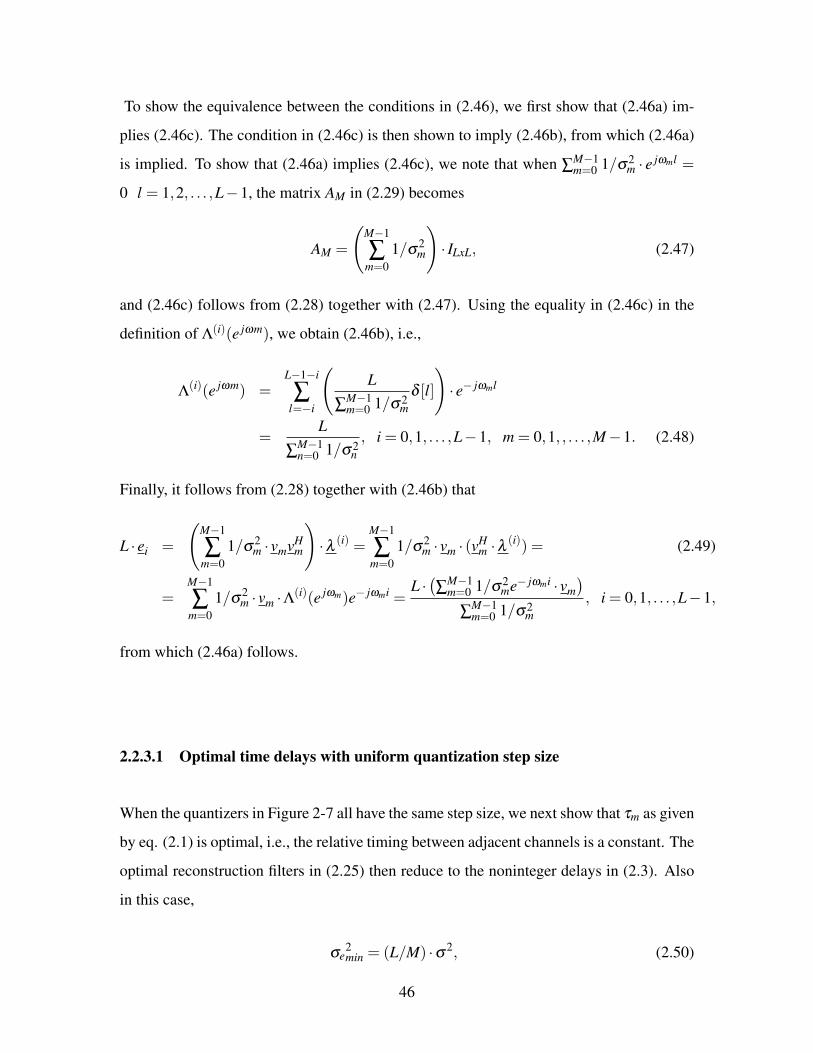
To show the equivalence between the conditions in (2.46), we first show that (2.46a) im-
plies (2.46c). The condition in (2.46c) is then shown to imply (2.46b), from which (2.46a)
is implied. To show that (2.46a) implies (2.46c), we note that when ∑M−1m=0 1/σ2
m · e jωml =
0 l = 1,2, . . . ,L−1, the matrix AM in (2.29) becomes
AM =
(M−1
∑m=0
1/σ2m
)· ILxL, (2.47)
and (2.46c) follows from (2.28) together with (2.47). Using the equality in (2.46c) in the
definition of Λ(i)(e jωm), we obtain (2.46b), i.e.,
Λ(i)(e jωm) =L−1−i
∑l=−i
(L
∑M−1m=0 1/σ2
mδ [l]
)· e− jωml
=L
∑M−1n=0 1/σ2
n, i = 0,1, . . . ,L−1, m = 0,1, , . . . ,M−1. (2.48)
Finally, it follows from (2.28) together with (2.46b) that
L · ei =
(M−1
∑m=0
1/σ2m · vmvH
m
)·λ (i) =
M−1
∑m=0
1/σ2m · vm · (vH
m ·λ (i)) = (2.49)
=M−1
∑m=0
1/σ2m · vm ·Λ(i)(e jωm)e− jωmi =
L ·(∑M−1
m=0 1/σ2me− jωmi · vm
)∑M−1
m=0 1/σ2m
, i = 0,1, . . . ,L−1,
from which (2.46a) follows.
2.2.3.1 Optimal time delays with uniform quantization step size
When the quantizers in Figure 2-7 all have the same step size, we next show that τm as given
by eq. (2.1) is optimal, i.e., the relative timing between adjacent channels is a constant. The
optimal reconstruction filters in (2.25) then reduce to the noninteger delays in (2.3). Also
in this case,
σe2min = (L/M) ·σ2, (2.50)
46

where σ2 denotes the variance of the quantization noise source in each channel. To show
this, we note that with σ2m = σ2, the condition of eq. (2.46a) becomes
M−1
∑m=0
e jωml = 0 l = 1,2, . . . ,L−1, (2.51)
which is clearly satisfied for any L and M when the values e jωm are uniformly spaced on
the unit circle, corresponding to uniform sampling. However, this is in general not a unique
solution as there are other distributions of ωm which satisfy eq. (2.51).
In summary, it follows from eq. (2.45) that for the reconstruction structure suggested
in Figure 2-4 and with the quantization step size the same in each channel, the uniform
sampling grid achieves the minimum average quantization noise power (L/M) ·σ2. Any
other choice of τm, for which (2.51) is not satisfied, results in a higher average quantization
noise power.
2.2.3.2 Optimal time delays with nonuniform quantization step size
As we next show, by allowing the quantization step size to be chosen separately for each
channel, so that quantization noise sources qm[n] in the different channels have different
variances σ2m, better SQNR can often be achieved. For comparison purposes, we will as-
sume that the quantization noise power averaged over all channels is equal to a pre-specified
fixed value σ2, i.e.,
1M
M−1
∑m=0
σ2m = σ2. (2.52)
Applying the Cauchy-Schwartz inequality to the identity ∑M−1m=0 σm · 1/σm = M, it follows
that
M−1
∑n=0
σ2n ·
M−1
∑m=0
1/σ2m ≥ M2, (2.53)
47

and equivalently
L
∑M−1m=0 1/σ2
m≤ (L/M) ·σ2, (2.54)
with equality if and only if
σ2m = σ2, m = 0,1, . . . ,M−1. (2.55)
Together with (2.45), we conclude that by having different levels of accuracy in the quan-
tizers in the different channels, there is the possibility of reducing the average quantization
noise power. This suggests a way to compensate for the mismatched timing in the channels
of Figure 2-7 and increase the total SQNR. Alternatively, we can deliberately introduce
timing mismatch so that with appropriate design of the quantizers, we will achieve better
SQNR as compared to the equivalent uniform sampling with equal quantizer step size in
each channel. The analysis and conclusions of course rely on the validity of the additive
noise model used for the quantizer, which becomes less appropriate as the quantizer step
size increases or the relative timing between adjacent channels decreases.
A similar result to that in (2.54) can be shown under other normalizations. Specifi-
cally, instead of fixing the average power of the quantization noise sources in each of the
channels, we now fix the total number of bits used to quantize the samples, i.e.,
NT =M−1
∑m=0
Nm,
where Nm represents the number of bits allocated in channel m. Consequently,
∆m =2X2Nm
(2.56)
and
σ2m =
∆2m
12= (X2/3)︸ ︷︷ ︸
α
(14
)Nm
, (2.57)
where X represents the full scale level of the A/D converter. It then follows from (2.57)
48

that
L
∑M−1m=0 1/σ2
m=
L(1/α) ·∑M−1
m=0 4Nm. (2.58)
Using convexity arguments to show 1M ∑M−1
m=0 4Nm ≥ 4NT /M, it follows that
L
∑M−1m=0 1/σ2
m≤ (L/M) ·σ2, (2.59)
where σ2 = α ·(1
4
)NT /Mrepresents the variance of the quantization error of an NT
M -bit quan-
tizer, based on the additive noise model.
Another important aspect in comparing systems is the total number of comperators used
in the implementation of the A/D converters. With flash architecture used for the design
of the converters, 2n −1 comperators are required for an n-bit quantizer. With M channels
and an Nm-bit quantizer in the mth channel, the total number of comperators Nc in the
multi-channel system is
Nc =M−1
∑m=0
(2Nm −1
). (2.60)
The number of bits NAve allocated to each of the channels in an equivalent system, all of
whose quantizers are the same and whose total number of comperators is identical to Nc in
(2.60), is obtained by solving
2NAve −1 =1M
M−1
∑m=0
(2Nm −1
), (2.61)
which results in NAve = log2( 1
M ∑M−1m=0 2Nm
). Using the following inequality,
1M
M−1
∑m=0
4Nm ≥
(1M
M−1
∑m=0
2NM
)2
, (2.62)
49

which follows from Cauchy-Schwartz inequality, or the equivalent form of (2.62)
1M
M−1
∑m=0
4Nm ≥ 2log2( 1M ∑M−1
m=0 2Nm)2
= 4NAve, (2.63)
we obtain
L
∑M−1m=0 1/σ2
m=
L/M1α ·( 1
M ∑M−1m=0 4Nm
) ≤ (L/M) ·σ2, (2.64)
where σ2 = α ·(1
4
)NAve .
2.2.4 Simulations
In this section, we consider the multi-channel sampling system of Figure 2-7 with M = 3
and L = 2. Following a derivation of the mean squared error for this special case, we
then consider four cases, each corresponding to a different assumption with respect to the
relative timing between the channels and the quantization step size in each channel. In the
first case, the quantization step size in each channel is fixed and equal in all channels, and
the relative timing between channels is optimized. In the second case, the relative timing
between the channels is specified, and the bit allocation is optimized subject to a bit-budget
constraint. In the third case, each channel is allocated a different number of bits, and the
relative timing between channels is optimized to maximize the SQNR. In the fourth case,
we fix the number of bits in channel 0 and channel 1 and analyze the behavior of the optimal
relative timing between the channels as the number of bits allocated to channel 2 varies.
To obtain the expression for the minimum mean square error for the case of M = 3 and
L = 2, we first note that
A3 =
∑2m=0 1/σ2
m ∑2m=0 e− jωm/σ2
m
∑2m=0 e jωm/σ2
m ∑2m=0 1/σ2
m
. (2.65)
Assuming without loss of generality that τ0 = 0 (ω0 = 0), it then follows from (2.35) and
50

(2.65) that
σe2min = tr(A−1
3 ) =
(σ2
0 σ21 +σ2
0 σ22 +σ2
1 σ22)/2
σ20 sin2 (ω1−ω2
2
)+σ2
1 sin2 (ω12
)+σ2
2 sin2 (ω22
) . (2.66)
When σ20 = σ2
1 = σ22 = σ2, the minimum mean squared error in (2.66) reduces to
σe2min =
(3/2)σ2
sin2 (ω1−ω22
)+ sin2 (ω1
2
)+ sin2 (ω2
2
) . (2.67)
Figure 2-10 shows the factor γ = σ2/σe2min representing the reduction in the average noise
power at the output of the reconstruction of Figure 2-4 with M = 3, L = 2, and τ0 = 0, for
the case of σ20 = σ2
1 = σ22 = σ2. As follows from eq. (2.67) and is indicated in Figure
2-10, the maximum noise reduction is achieved for τ1 = −τ2 = ±(2/3) · TN , for which
σe2min = (2/3) ·σ2.
Figure 2-10: The reduction factor γ in the average noise power at the output of the recon-struction of Figure 2-4 achieves its maximum value at τ1 = −τ2 = ±(2/3) ·TN , i.e., whenthe multi-channel sampling is equivalent to uniform sampling. Since this curve is based onthe additive noise model of the quantization error, which assumes uncorrelated errors, it isless accurate in the vicinity of τ1 = 0, τ2 = 0, and τ1 = τ2.
To verify the analysis based on the additive noise model of the quantization error, a
simulation of the multi-channel sampling and reconstruction system was obtained in [62],
in which actual quantizers were applied to the multi-channel output samples. Figure 2-11
shows the reduction factor γ obtained from simulation for which a 10-bit quantizer is used
in each of the channels. Comparing Figure 2-10 which corresponds to the additive noise
51

Figure 2-11: The reduction factor γ in the average noise power at the output of the re-construction system of Figure 2-4 where actual quantizers are applied to the multi-channeloutput samples with accuracy of 10 bits.
model with Figure 2-11 obtained from simulations, we conclude that the analysis based on
the additive noise model is valid except in the vicinity of τ1 = τ2, τ1 = 0, and τ2 = 0, where
discrepancies occur. Figure 2-11 indicates performance degradation in the vicinity of these
lines, which is not predicted with the analysis based on the additive noise model. These
discrepancies between the analysis and the simulations occur when the sampling instants of
two channels or more fall quite close to each other or exactly on the same grid and the un-
correlated assumption of the additive noise model is no longer reasonable. As analyzed in
[62], when the relative timing between adjacent channels is small and the same number of
bits is allocated to each of the channels, a positive correlation between the corresponding
quantization errors occurs. The positive correlation between the errors results in perfor-
mance degradation as compared to the performance predicted with the analysis based on
the additive noise model.
It follows from eq. (2.45) and as illustrated in the preceding example, for the recon-
struction structure suggested in Figure 2-4 and with the quantization step size the same in
each channel, the uniform sampling grid achieves the minimum average quantization noise
power (L/M) ·σ2. Any other choice of τm for which (2.51) is not satisfied results in a
higher average quantization noise power.
We next illustrate with an example that with appropriate design of the quantizer in each
52

channel we can compensate for the mismatched timing in the channels of Figure 2-7. With
4-bit uniform quantizers in each of the channels, it follows from eq. (2.66) that when the
time delays are τ0 = 0, τ1 = TN/8 and τ2 = −(3/4)TN , the output average noise power is
increased by approximately 20% relative to the case in which τm are chosen according
to (2.1). However, when the quantizer step size is not constrained to be the same in each
channel, the reconstruction error variance can be reduced.
Table 2.1 shows the performance gain for different bit allocations as compared to the
case in which each channel is allocated 4 bits. The results are sorted from the most to the
least preferable where in each choice only 1 bit is shifted from one channel to another,
keeping the total number of bits the same.
N0 N1 N2 (σe2min)(4,4,4)/(σe
2min)(N0,N1,N2)
3 4 5 1.464 3 5 1.363 5 4 1.265 3 4 1.144 5 3 0.415 4 3 0.38
Table 2.1: The performance gain for different bit allocations.
In general, we might intuitively expect that since the sampling instants of channel 2
are relatively far from those of the other two channels, it should be allocated more bits in
compensation. Also, the relative timing between channel 0 and channel 2 is smaller than
the relative timing between channel 2 and channel 1, suggesting allocation of more bits
to channel 1 as compared to channel 0. This intuition of bit allocation according to the
relative timing between adjacent channels is consistent with the results in Table 2.1 and in
particular with the optimal choice shown in Figure 2-12, which suggests allocating 3 bits
to channel 0, 4 bits to channel 1, and 5 bits to channel 2. The same results are obtained in
[62] in simulating the system using actual quantizers. Once again, the simulations confirm
the error analysis based on the additive noise model.
We next fix the number of bits in channel 0 to 3, channel 1 to 4, and channel 2 to 4,
and without loss of generality set τ0 = 0. The values of τ1 and τ2 are chosen to minimize
the output average noise power. Note that when τ1 =−τ2 =±(2/3)TN , the multi-channel
53
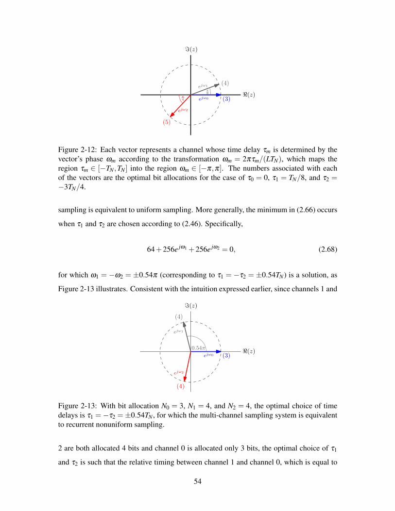
ℑ(z)
ℜ(z)
(4)
(3)
(5)
ejω2
ejω1
ejω0
π
8
π
4
Figure 2-12: Each vector represents a channel whose time delay τm is determined by thevector’s phase ωm according to the transformation ωm = 2πτm/(LTN), which maps theregion τm ∈ [−TN ,TN ] into the region ωm ∈ [−π,π]. The numbers associated with eachof the vectors are the optimal bit allocations for the case of τ0 = 0, τ1 = TN/8, and τ2 =−3TN/4.
sampling is equivalent to uniform sampling. More generally, the minimum in (2.66) occurs
when τ1 and τ2 are chosen according to (2.46). Specifically,
64+256e jω1 +256e jω2 = 0, (2.68)
for which ω1 = −ω2 = ±0.54π (corresponding to τ1 = −τ2 = ±0.54TN) is a solution, as
Figure 2-13 illustrates. Consistent with the intuition expressed earlier, since channels 1 and
ℑ(z)
ℜ(z)
(4)
(3)
(4)
ejω2
ejω1
ejω0
0.54π
Figure 2-13: With bit allocation N0 = 3, N1 = 4, and N2 = 4, the optimal choice of timedelays is τ1 =−τ2 =±0.54TN , for which the multi-channel sampling system is equivalentto recurrent nonuniform sampling.
2 are both allocated 4 bits and channel 0 is allocated only 3 bits, the optimal choice of τ1
and τ2 is such that the relative timing between channel 1 and channel 0, which is equal to
54
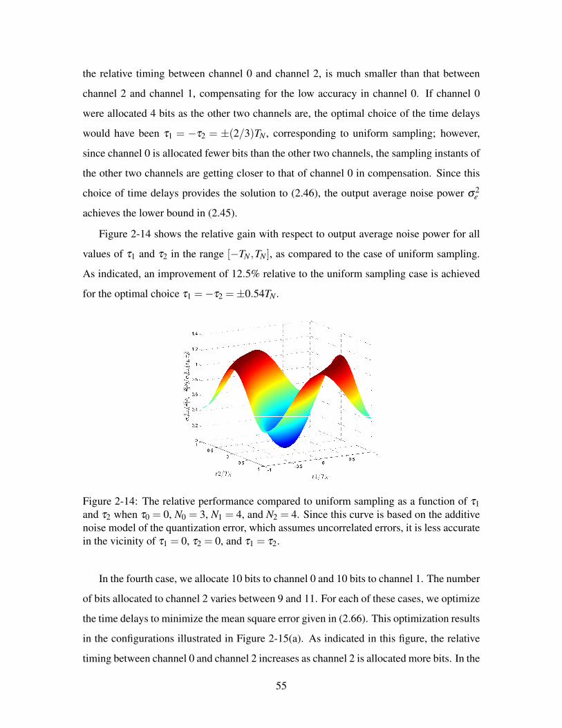
the relative timing between channel 0 and channel 2, is much smaller than that between
channel 2 and channel 1, compensating for the low accuracy in channel 0. If channel 0
were allocated 4 bits as the other two channels are, the optimal choice of the time delays
would have been τ1 = −τ2 = ±(2/3)TN , corresponding to uniform sampling; however,
since channel 0 is allocated fewer bits than the other two channels, the sampling instants of
the other two channels are getting closer to that of channel 0 in compensation. Since this
choice of time delays provides the solution to (2.46), the output average noise power σ2e
achieves the lower bound in (2.45).
Figure 2-14 shows the relative gain with respect to output average noise power for all
values of τ1 and τ2 in the range [−TN ,TN ], as compared to the case of uniform sampling.
As indicated, an improvement of 12.5% relative to the uniform sampling case is achieved
for the optimal choice τ1 =−τ2 =±0.54TN .
Figure 2-14: The relative performance compared to uniform sampling as a function of τ1and τ2 when τ0 = 0, N0 = 3, N1 = 4, and N2 = 4. Since this curve is based on the additivenoise model of the quantization error, which assumes uncorrelated errors, it is less accuratein the vicinity of τ1 = 0, τ2 = 0, and τ1 = τ2.
In the fourth case, we allocate 10 bits to channel 0 and 10 bits to channel 1. The number
of bits allocated to channel 2 varies between 9 and 11. For each of these cases, we optimize
the time delays to minimize the mean square error given in (2.66). This optimization results
in the configurations illustrated in Figure 2-15(a). As indicated in this figure, the relative
timing between channel 0 and channel 2 increases as channel 2 is allocated more bits. In the
55

same time, the relative timing between channel 1 and channel 0 decreases, in compensation.
(10)
ℑ(z)
ℜ(z)(10)(11) ω2 = π ω1 = 0
ω0 = 0
N2 = 11
(10)
ℑ(z)
ℜ(z)
(10)
(10)
ω2 = −
2π
3
ω1 =2π
3
ω0 = 0
N2 = 10
(10)
ℑ(z)
ℜ(z)(10)
(9)
ω2 = −0.54π
ω1 = 0.92π
ω0 = 0
N2 = 9
(a)
(10)
ℑ(z)
ℜ(z)(10)
(11)ω2 = −0.95π
ω1 = 0.1π
ω0 = 0
N2 = 11
(10)
ℑ(z)
ℜ(z)
(10)
(10)
ω2 = −
2π
3
ω1 =2π
3
ω0 = 0
N2 = 10
(10)
ℑ(z)
ℜ(z)(10) (9)ω2 = 0ω1 = π
ω0 = 0
N2 = 9
(b)
Figure 2-15: Optimal time delays for different choices of N2 (a) based on the additive noisemodel, (b) based on simulations with actual quantizers.
As Figure 2-15(b) illustrates, when N2 = 10 the optimal time delays resulting from
simulations with actual quantizers, obtained in [62], are consistent with the optimal time
delays derived from the analysis based on the additive noise model. However, for N2 = 9
or N2 = 11, the optimal configurations from the simulations are different than those based
on the additive noise model. Specifically, for optimal performance, the simulation with
N2 = 11 suggests separating channel 0 from channel 1. In addition, due to symmetry, the
simulation also suggests setting the time delay of channel 2 to space its sampling instants
equidistant from the sampling instants of the other two channels. This nonzero gap be-
tween channel 0 and channel 1 is intuitively reasonable since positive correlation between
the quantization errors in adjacent channels occurs when the channels are allocated the
same number of bits and their relative timing is getting small. As mentioned earlier, this
positive correlation results in degradation in performance. For the case of N2 = 9, optimal
performance based on simulations is achieved when both a) the sampling instants of chan-
56

nel 0 are maximally separated from those of channel 1, i.e., the relative timing between the
channels is TN , and b) the time delay of channel 2 is chosen equal to that of either channel
0 or channel 1. This optimal configuration is significantly different from the one based on
the analysis with the additive noise model. This discrepancy occurs due to the occurrence
of negative correlation between quantization errors of adjacent channels with different bit
allocation as their relative timing approaches 0. The negative correlation between the quan-
tization errors together with the optimal reconstruction filters which were designed under
the assumption of uncorrelated quantization errors, results in an overall improvement in
performance, which is not predicted by the additive noise model.
In summary, we have illustrated that with nonuniform spacing of the time delays, for
which the interleaved multi-channel outputs correspond to recurrent nonuniform sampling,
equal quantization step size in each channel is not optimal. Allowing different levels of ac-
curacy in the quantizers in the different channels achieves a reduction in the noise variance.
Alternatively, when the quantization step size in each of the channels is fixed and varies
among channels, choosing the relative timing between adjacent channels to be the same is
not optimal, and lower average noise power is achieved with nonuniform spacing of the
time delays.
2.3 Differential Uniform Quantization
In this section, differential uniform quantization [20, 24, 40, 68] which is based on the no-
tion of quantizing a prediction error signal rather than the signal itself is incorporated into
the multi-channel sampling system of Figure 2-7. By exploiting redundancies in the cor-
related input signal and representing it in terms of prediction error samples, an increased
SQNR can be achieved for a given bit rate or equivalently, a reduction of bit rate for a given
SQNR. It is shown that replacing uniform quantization with differential uniform quantiza-
tion in the multi-channel system of Figure 2-7 results in a higher performance gain when
the channel offsets are nonuniformly spaced. It is also shown that with differential quanti-
zation, uniform sampling is not necessarily optimal even when using the same number of
bits in the quantizers of the different channels.
57

Uniform quantization can be applied to deterministic signals and does not require the
use of a stochastic model, but can also be applied to stochastic signals. The analysis of
differential uniform quantization specifically requires stochastic modeling. We therefore
assume in this section that x(t) is a realization of a zero-mean stationary Gaussian ran-
dom process whose autocorrelation function is Rxx(τ), its power spectrum Sxx(Ω) = 0 for
|Ω| ≥ Ωc, and its variance is denoted by σ2x . The basic differential quantization system we
consider is shown in Figure 2-16 where x[n] = ∑Nj=1 h jx[n− j] is a linear predictor of x[n]
based on the quantized values x[n].
Q(·)
h
x[n]
x[n]x[n]
u[n]d[n]
y[n] = x[n]
x[n] h
v[n] = u[n]
Figure 2-16: Block diagram of differential quantization: coder and decoder.
An important property of the ”closed-loop” structure in Figure 2-16 is that quantization
error does not accumulate, i.e., with error free transmission of u[n], the reconstruction error
r[n] = y[n]− x[n] is equal to the quantization error q[n] = u[n]−d[n]. With optimal predic-
tion and adequately fine quantization, modeling the quantization error as an uncorrelated
random process is well justified. Also, in the case of fine quantization, x[n] can be well
approximated as
x[n] =N
∑j=1
h jx[n− j] =N
∑j=1
h jx[n− j]+N
∑j=1
h jq[n− j]≈N
∑j=1
h jx[n− j], (2.69)
and the quantization error feedback is therefore not considered [40]. The optimal predictor
coefficients h jNj=1 are then chosen to minimize the mean square prediction error based
on previous unquantized samples, i.e., E(
x[n]−∑Nj=1 h jx[n− j]
)2
.
Note that when the relative timing between adjacent channels in the system of Figure 2-
7 are not equal, the optimal choice for the predictor coefficients will in general be different
for each of the outputs of the multi-channel sampling system, resulting in a periodic lin-
58

ear time-varying FIR system and a wide-sense cyclo-stationary prediction error sequence.
Consequently, both the quantization error q[n] and the reconstruction error r[n] will be
wide-sense cyclo-stationary uncorrelated sequences, and the noise analysis of section 2.2
will remain valid.
To relate the quantization error variance σ2q to the quantizer input signal variance σ2
i ,
we define as in [40] the quantizer performance factor, i.e.,
ε2q = σ2
q/σ2i , (2.70)
which depends on the type of quantizer used, the number of quantization levels, and the
pdf of the quantizer input. With differential uniform quantization incorporated into the
multi-channel system of Figure 2-7, the variance of the reconstruction error for each of the
channels outputs is given by
σ2r [m] = σ2
q [m] = ε2q [m]
(D) ·σ2d [m] m = 0,1, . . . ,M−1, (2.71)
where σ2d [m] and ε2
q [m](D) are the variance of the prediction error and the quantizer perfor-
mance factor corresponding to channel m.
As follows from (2.70) and (2.71), replacing uniform quantization by differential uni-
form quantization results in a reduction in reconstruction error in each channel by a factor
of
ε2q [m] ·σ2
x
ε2q [m]
(D) ·σ2d [m]
= (ε2q [m]/ε2
q [m](D)
) · (σ2x /σ2
d [m]) m = 0,1, . . . ,M−1. (2.72)
The ratio ε2q [m]/ε2
q [m](D) is in general not equal to unity. However, it tends to be close
to unity in several cases one of which is the case of Gaussian sources [40] for which the
prediction error is also Gaussian and we therefore consider only the performance gain due
to the linear predictor. With that assumption and when the same type of quantizer with
the same number of levels is used for all channels, it follows from eqs. (2.35), (2.70) and
(2.71) that when replacing uniform quantization with differential uniform quantization, the
59

overall improvement in SQNR at the output of the reconstruction system of Figure 2-4 is
σ2e min
σ2e(D)min
=tr((
∑M−1m=0 (vm · vH
m)/σ2x)−1)
tr((
∑M−1m=0 (vm · vH
m)/σ2d [m]
)−1) , (2.73)
with vm as defined in (2.27).
To illustrate, we consider again the case of M = 3 and L = 2, where the time delays
are now fixed to τ0 = 0, τ1 = 0.9TN , and τ2 = 1.1TN . The output samples are quantized
according to the system of Figure 2-16 where a first-order predictor is used, and 4 bits
uniform quantization is applied to the prediction error samples, satisfying the assumption of
fine quantization. Assuming τ0 < τ1 < τ2, the optimum value of h1[m] and its corresponding
minimum prediction variance are
h1[m] =Rxx(τm+1 − τm)
Rxx(0), σ2
d [m] =(1−h2
1[m])
σ2x m = 0,1,2, (2.74)
where τ3 = τ0 +T > τ2.
As follows from eq. (2.35), with uniform quantization and with τ0 = 0, τ1 = 0.9TN ,
and τ2 = 1.1TN for which the interleaved multi-channel outputs corresponds to recurrent
nonuniform samples, there is a degradation in performance by approximately 10% relative
to the case of uniform sampling. However, as illustrated in Table 2.2, eq. (2.73) implies that
when replacing uniform quantization with differential uniform quantization a higher per-
formance gain in SQNR is achieved in this case as compared to that achieved with uniform
sampling. It is also indicated that the relative improvement in SQNR due to differential
uniform quantization in uniform and recurrent nonuniform sampling is dependent on the
power spectrum of the input signal. Specifically, when the signal’s energy is mostly concen-
trated at high frequencies, the improvement achieved with differential uniform quantization
applied in recurrent nonuniform sampling is much more significant than that achieved in
uniform sampling.
To summarize, with the same number of bits in each channel, and with uniform quan-
tization, uniform sampling is optimal. When differential uniform quantization is incorpo-
rated in the multi-channel sampling system, nonuniform spacing of the channel offsets can
60

Rxx(τ)↔ Sxx(Ω) (τ0 = 0,τ1 =23TN ,τ2 =
43TN) (τ0 = 0,τ1 = 0.9TN ,τ2 = 1.1TN)
σ2d [0] = σ2
d [1] = σ2d [2] = 0.53 σ2
d [0] = σ2d [1] = 0.76
sinc2(
τ
2TN
) 2TN
π
TN−
π
TN
Ω σe2min/σe
2(D)min = 1.88 σ2
d [2] = 0.064,σe2min/σe
2(D)min = 1.9
σ2d [0] = σ2
d [1] = σ2d [2] = 0.83 σ2
d [0] = σ2d [1] = 0.99
sinc
(
τ
TN
)
TN
π
TN
−
π
TN
Ω σe2min/σe
2(D)min = 1.21 σ2
d [2] = 0.12,σe2min/σe
2(D)min = 1.41
σ2d [0] = σ2
d [1] = σ2d [2] = 0.98 σ2
d [0] = σ2d [1] = 0.93
Ω2sinc
(
τ
TN
)
− sinc2(
τ
2TN
)
2TN
π
TN−
π
TN σe2min/σe
2(D)min = 1.02 σ2
d [2] = 0.18,σe2min/σe
2(D)min = 1.43
Table 2.2: Examples of overall improvement in SQNR when replacing uniform quantiza-tion with differential uniform quantization
result in a higher SQNR.
61

62

CHAPTER 3
MMSE RECONSTRUCTION IN
MULTI-CHANNEL NONUNIFORM
SAMPLING
In Chapter 2 we considered the environment of interleaved multi-channel measurements
and the design of optimal reconstruction filters from multi-channel measurements. We de-
signed the reconstruction filters to minimize the averaged noise power at the output of the
reconstruction system due to quantization error, under the constraints for perfect recon-
struction in the absence of quantization error. In this chapter, we relax the constraints for
perfect reconstruction and take an alternative approach to the design of the reconstruction
filters, for which the mean squared reconstruction error is reduced.
3.1 Reconstruction Error
We consider the multi-channel sampling and quantization system shown in Figure 2-7,
whose input x(t) is now treated as a realization of a bandlimited wide-sense stationary
stochastic process. We assume that the random process x(t) is zero-mean, with its autocor-
relation function denoted as Rxx(τ), and that its power spectrum Sxx(Ω) vanishes outside
the region |Ω|< Ωc = π/TN .
Similar to the analysis in Chapter 2, we use the additive noise model for the quantization
63

error and represent the output samples of the multi-channel system as
xm[n] = xm[n]+qm[n], m = 0,1, . . . ,M−1, (3.1)
where xm[n] = x(nT − τm) are uniform samples of x(t) at a rate 1/T = 1/(LTN), and
qm[n] is assumed to be a white-noise random process, uniformly distributed over the range
[−∆m,∆m], where ∆m is the step-size level of the quantizer in the m-th channel. The model
also assumes that the sequences qm[n] are uncorrelated among themselves and uncorrelated
with samples of x(t).
For the reconstruction of the Nyquist-rate samples of x(t) from the multi-channel mea-
surements xm[n], we consider the same structure used in Chapter 2, which is shown in
Figure 2-4. The signal x[n] at the output of the reconstruction system can be represented as
x[n] =M−1
∑m=0
∞
∑k=−∞
xm[k]gm[n− kL], (3.2)
where gm[n] denotes the impulse response corresponding to the frequency response Gm(e jω).
Denoting e[n] = x[n]− x[n] as the reconstruction error, we obtain
e[n] =
(M−1
∑m=0
∞
∑k=−∞
xm[k]gm[n− kL]− x[n]
)+
M−1
∑m=0
∞
∑k=−∞
qm[k]gm[n− kL], (3.3)
which is a zero-mean random process whose autocorrelation function Ree[n,n− l] is
Ree[n,n− l] = Rexex [n,n− l]+Reqeq [n,n− l], (3.4)
where
Rexex [n,n− l] = E
(M−1
∑m1=0
∞
∑k1=−∞
xm1[k1]gm1[n− k1L]− x[n]
)·
·
(M−1
∑m2=0
∞
∑k2=−∞
xm2 [k2]gm2[n− l − k2L]− x[n− l]
)(3.5)
64
and
Reqeq[n,n− l] = E
M−1
∑m1=0
∞
∑k1=−∞
qm1[k1]gm1[n− k1L]M−1
∑m2=0
∞
∑k2=−∞
qm2[k2]gm2[n− l − k2L]
.
(3.6)
We denote by σ2e the time and ensemble average of the noise power, i.e.,
σ2e =
1L
L−1
∑n=0
Ree[n,n] =1
2π
∫ π
−πSee(e jω)dω, (3.7)
where See(e jω) is treated as the power spectrum of the random process e[n] as if it were
stationary. We show in Appendix B that
See(e jω) =L−1
∑k=−(L−1)
1TN
Sxx
(ω − 2π
L kTN
)∣∣∣∣∣1L M−1
∑m=0
Gm(e jω)e− j(ω− 2πL k)τm/TN −δ [k]
∣∣∣∣∣2
+M−1
∑m=0
(σ2m/L) · |Gm(e jω)|2. (3.8)
Note that in the absence of error due to quantization, i.e., when σ2m = 0, ∀m, and indepen-
dent of the signal’s characteristics, zero mean-squared reconstruction error is achieved in
the system of Figure 2-4 when
M−1
∑m=0
Gm(e jω)e− j(ω− 2πL k)τm/TN = Lδ [k], ω ∈ ∆ωi,
k =−i,−i+1 . . . ,L−1− i, i = 0,1, . . . ,L−1. (3.9)
These conditions in (3.9) are consistent with the constraints imposed in (2.8) with the de-
terministic model for perfect reconstruction in the absence of quantization error. Note that
using the optimal reconstruction filters that were obtained in Chapter 2 and which satisfy
the constraints for perfect reconstruction, makes the first term in (3.8) vanish. Note also
that in the design of the reconstruction filters, the remaining degrees of freedom were used
to minimize the output average noise power due to quantization error, which is identical
to the second term in (3.8). Therefore, by not restricting the filters Gm(e jω) to satisfy the
65
constraints in (3.9), and instead utilizing all degrees of freedom in the filters’ design to min-
imize the overall mean-squared error, we can achieve lower mean-squared reconstruction
error. As the next section shows, this reduction in the mean-squared reconstruction error
comes at the expense of requiring more information about the input signal x(t).
3.2 Optimal Reconstruction Filters
This section considers the design of the reconstruction filters Gm(e jω) in the multi-channel
reconstruction system of Figure 2-4. The optimal filters Gm(e jω) are chosen to min-
imize the mean-squared reconstruction error in (3.7). These filters can be obtained by
differentiating See(e jω) in (3.8) with respect to GRm(e
jω) = ℜ
Gm(e jω)
and GIm(e
jω) =
ℑ
Gm(e jω)
, as shown in Appendix C. Alternatively, as we next show, the filters can be
achieved by expanding (3.8) as a quadratic form of Gm(e jω). Specifically, it follows from
(3.8) that
See(e jω) =1L
M−1
∑m1=0
Gm1(ejω)e− jωτm1/TN
M−1
∑m2=0
G∗m2(e jω)e jωτm2/TN ·
·
(1L
L−1
∑k=−(L−1)
1TN
Sxx
(ω − 2π
L kTN
)e j 2π
L
( τm1−τm2TN
)k+σ2
mδ [m1 −m2]
)
− 1TN
Sxx
(ωTN
)(M−1
∑m=0
Gm(e jω)e− jωτm/TN
)
− 1TN
Sxx
(ωTN
)(M−1
∑m=0
Gm(e jω)e− jωτm/TN
)∗+
1TN
Sxx
(ωTN
). (3.10)
To simplify, we introduce the following notation:
G = [G0(e jω) · e− jωτ0/TN , . . . ,GM−1(e jω) · e− jωτM−1/TN ]T , (3.11a)
Σ = diagonal[σ20 ,σ
21 , . . . ,σ
2M−1], (3.11b)
66

and
Sm,l(i) =
1L
L−1
∑k=−(L−1)
(1
TNSxx
(ω − 2π
L kTN
))e j 2π
L (τm−τl
TN)k
=1L
L−1−i
∑k=−i
Sxx
(e j(ω− 2π
L k))
e j 2πL (
τm−τlTN
)k, ω ∈ ∆ωi i = 0,1, . . . ,L−1
m = 0,1, . . . ,M−1, l = 0,1, . . . ,M−1, (3.11c)
which are the elements of an MxL Hermitian matrix S(i). An alternative representation of
S(i) is
S(i) = V (i)SD(i)(V (i))H , ω ∈ ∆ωi, i = 0,1, . . . ,L−1, (3.12)
where SD(i) is a diagonal matrix whose elements on the main diagonal are
Sxx
(e j(ω− 2π
L l))L−1−i
l=−i,
and V (i) = (1/√
L) ·V (i) where V (i) is an MxL matrix whose elements are
Vm,l(i) = e j 2π
L (τm/TN)(l−i), m = 0,1, . . . ,M−1, l = 0,1, . . . ,L−1. (3.13)
Using the notations defined in (3.11), See(e jω) in (3.10) can be written as
See(e jω) =1L
(GH
(S(i)+Σ)G−Sxx(e jω)(1T G)−Sxx(e jω)(GH ·1))+Sxx(e jω),
ω ∈ ∆ωi, i = 0,1, . . . ,L−1, (3.14)
or equivalently as
See(e jω) =1L
∣∣∣(S(i)+Σ)1/2G−Sxx(e jω)(S(i)+Σ)−1/2 ·1∣∣∣2
+ Sxx(e jω)(1−Sxx
(e jω) · 1T (S(i)+Σ)−11
L
),
ω ∈ ∆ωi, i = 0,1, . . . ,L−1, (3.15)
provided that the inverse involved exists, where for the case M > L it is true only if σ2m =
67

0 ∀m. It then follows from (3.15) that the choice of G that minimizes See(e jω) is
Gopt= Sxx(e jω)(S(i)+Σ)−1 ·1, ω ∈ ∆ωi, i = 0,1, . . . ,L−1, (3.16)
for which the first term in (3.15) is vanished, and See(e jω) becomes
Seemin(e jω) = Sxx
(e jω)(1−Sxx
(e jω) · 1T (S(i)+Σ)−11
L
), ω ∈ ∆ωi, i = 0,1, . . . ,L−1.
(3.17)
3.2.1 Optimal Reconstruction for the Case of Uniform Sampling
We now consider the special case of M = L where τm = mTN , i.e., the case of uniform
sampling at the Nyquist rate. When in addition σ2m = σ2 ∀m, eq. (3.16) reduces to
Gopt= Sxx(e jω)
(V (i)SD
(i)(V (i))H +σ2I)−1
·1, ω ∈ ∆ωi, i = 0,1, . . . ,L−1. (3.18)
Noting that V (i) in this case is a unitary matrix, i.e., (V (i))HV (i) = V (i)(V (i))H = I, it follows
that
Gopt= Sxx
(e jω)(V (i)(SD
(i)+σ2I)(V (i))H)−1
·1
= Sxx(e jω)V (i)(SD
(i)+σ2I)−1(V (i))H ·1, ω ∈ ∆ωi, i = 0,1, . . . ,L−1.
(3.19)
Using the identity
((V (i))H ·1
)m=
1√L
(L−1
∑l=0
e− j 2πL l(m−i)
)=√
L ·δ [m− i], m = 0,1, . . . ,L−1, (3.20)
eq. (3.19) reduces to
Gopt=
Sxx(e jω)
Sxx (e jω)+σ2 ·1, (3.21)
68

which is equivalent to
Gmopt(e jω) =
Sxx(e jω)
Sxx (e jω)+σ2 · ejωm, m = 0,1, . . . ,L−1. (3.22)
Similarly, it can be shown that
Seemin(e jω) = Sxx
(e jω)(1−Sxx
(e jω) · 1TV (i)(SD
(i)+σ2I)−1(V (i))H1L
)
= Sxx(e jω)(1−
Sxx(e jω)
Sxx (e jω)+σ2
)=
Sxx(e jω) ·σ2
Sxx (e jω)+σ2 . (3.23)
As expected, for the case of uniform sampling at the Nyquist rate and where the quantizers
in the different channels are the same, the optimal reconstruction filters Gmopt(e jω) in
(3.22) suggest that optimal reconstruction is achieved with interleaving of the multi-channel
samples xm[n] followed by Wiener filtering, as illustrated in Figure 3-1.
ejω
1
L
x0[n]
x1[n]
L ejω(L−1)xL−1[n]
+x[n]
L
Sxx(ejω)
Sxx(ejω)+σ2
x[n]
Figure 3-1: Optimal reconstruction is equivalent to interleaving of the multi-channel sam-ples followed by Wiener filtering.
3.3 Illustrative Examples & Simulations
This section discusses and illustrates with examples the design of the quantizers and of the
relative timing between the channels in the multi-channel system of Figure 2-7. It considers
two cases. The first case illustrates the multi-channel sampling system with two channels,
69

i.e., M = 2, where the sampling rate in each channel is 1/T = 1/(2TN), resulting in an
overall sampling rate that is equal to the Nyquist rate of the input signal. The second case
illustrates the multi-channel sampling system with M = 3 and L = 2, corresponding to an
oversampling ratio of M/L = 3/2. In both cases we develop the optimal reconstruction
filters and the corresponding minimum mean-squared reconstruction error.
For the first case, the multi-channel sampling system of Figure 2-7 is considered, where
M = L = 2, and without loss of generality the time delay τ0 = 0. We assume that the
quantizer step size is the same in both channels, corresponding to σ20 = σ2
1 = σ2. The
matrix S(0) in (3.12) then becomes
S(0) =12·
1 1
1 e jω1
· Sxx(e jω) 0
0 Sxx(e j(ω−π))
· 1 1
1 e− jω1
(3.24)
=12
Sxx(e jω)+Sxx(e j(ω−π)) Sxx(e jω)+ e− jω1Sxx(e j(ω−π))
Sxx(e jω)+ e jω1Sxx(e j(ω−π)) Sxx(e jω)+Sxx(e j(ω−π))
, ω ∈ [0,π],
where ω1 = π · (τ1/TN). Substituting (3.24) into (3.16) and into (3.17), we obtain for the
optimal reconstruction filters
Gopt(e jω) =
Sxx(e jω) ·
σ2
σ2
+Sxx(e j(ω−π)) ·
(1− e− jω1)/2
(1− e jω1)/2
(Sxx(e jω)+σ2) ·
(Sxx(e j(ω−π))+σ2
)−Sxx(e jω)Sxx(e j(ω−π))cos2(ω1
2 ),
ω ∈ [0,π], (3.25)
and for the minimum achievable See(e jω)
Seemin(e jω) =
σ2Sxx(e jω) ·(
Sxx(e j(ω−π))+σ2)
(Sxx(e jω)+σ2) ·(Sxx(e j(ω−π))+σ2
)−Sxx(e jω)Sxx(e j(ω−π))cos2(ω1
2 ).
(3.26)
It is clear from eq. (3.26) that the choice of ω1 that minimizes the mean squared reconstruc-
tion error is ω1 = π , which corresponds to τ1 = TN , i.e., uniform sampling. This observation
is consistent with the conclusions obtained with the deterministic model in which the re-
70
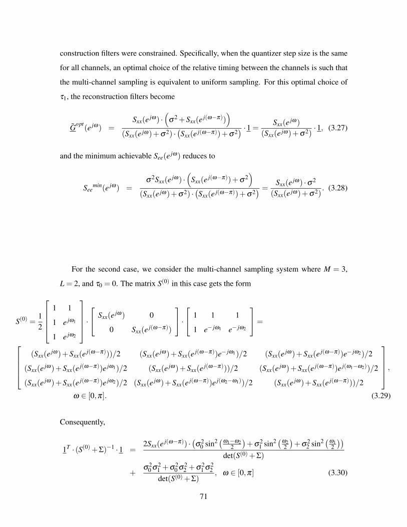
construction filters were constrained. Specifically, when the quantizer step size is the same
for all channels, an optimal choice of the relative timing between the channels is such that
the multi-channel sampling is equivalent to uniform sampling. For this optimal choice of
τ1, the reconstruction filters become
Gopt(e jω) =
Sxx(e jω) ·(
σ2 +Sxx(e j(ω−π)))
(Sxx(e jω)+σ2) ·(Sxx(e j(ω−π))+σ2
) ·1 =Sxx(e jω)
(Sxx(e jω)+σ2)·1, (3.27)
and the minimum achievable See(e jω) reduces to
Seemin(e jω) =
σ2Sxx(e jω) ·(
Sxx(e j(ω−π))+σ2)
(Sxx(e jω)+σ2) ·(Sxx(e j(ω−π))+σ2
) = Sxx(e jω) ·σ2
(Sxx(e jω)+σ2). (3.28)
For the second case, we consider the multi-channel sampling system where M = 3,
L = 2, and τ0 = 0. The matrix S(0) in this case gets the form
S(0) =12
1 1
1 e jω1
1 e jω2
· Sxx(e jω) 0
0 Sxx(e j(ω−π))
· 1 1 1
1 e− jω1 e− jω2
=
(Sxx(e jω)+Sxx(e j(ω−π)))/2 (Sxx(e jω)+Sxx(e j(ω−π))e− jω1)/2 (Sxx(e jω)+Sxx(e j(ω−π))e− jω2)/2
(Sxx(e jω)+Sxx(e j(ω−π))e jω1)/2 (Sxx(e jω)+Sxx(e j(ω−π)))/2 (Sxx(e jω)+Sxx(e j(ω−π))e j(ω1−ω2))/2
(Sxx(e jω)+Sxx(e j(ω−π))e jω2)/2 (Sxx(e jω)+Sxx(e j(ω−π))e j(ω2−ω1))/2 (Sxx(e jω)+Sxx(e j(ω−π)))/2
,ω ∈ [0,π]. (3.29)
Consequently,
1T · (S(0)+Σ)−1 ·1 =2Sxx(e j(ω−π)) ·
(σ2
0 sin2 (ω1−ω22
)+σ2
1 sin2 (ω22
)+σ2
2 sin2 (ω12
))det(S(0)+Σ)
+σ2
0 σ21 +σ2
0 σ22 +σ2
1 σ22
det(S(0)+Σ), ω ∈ [0,π] (3.30)
71
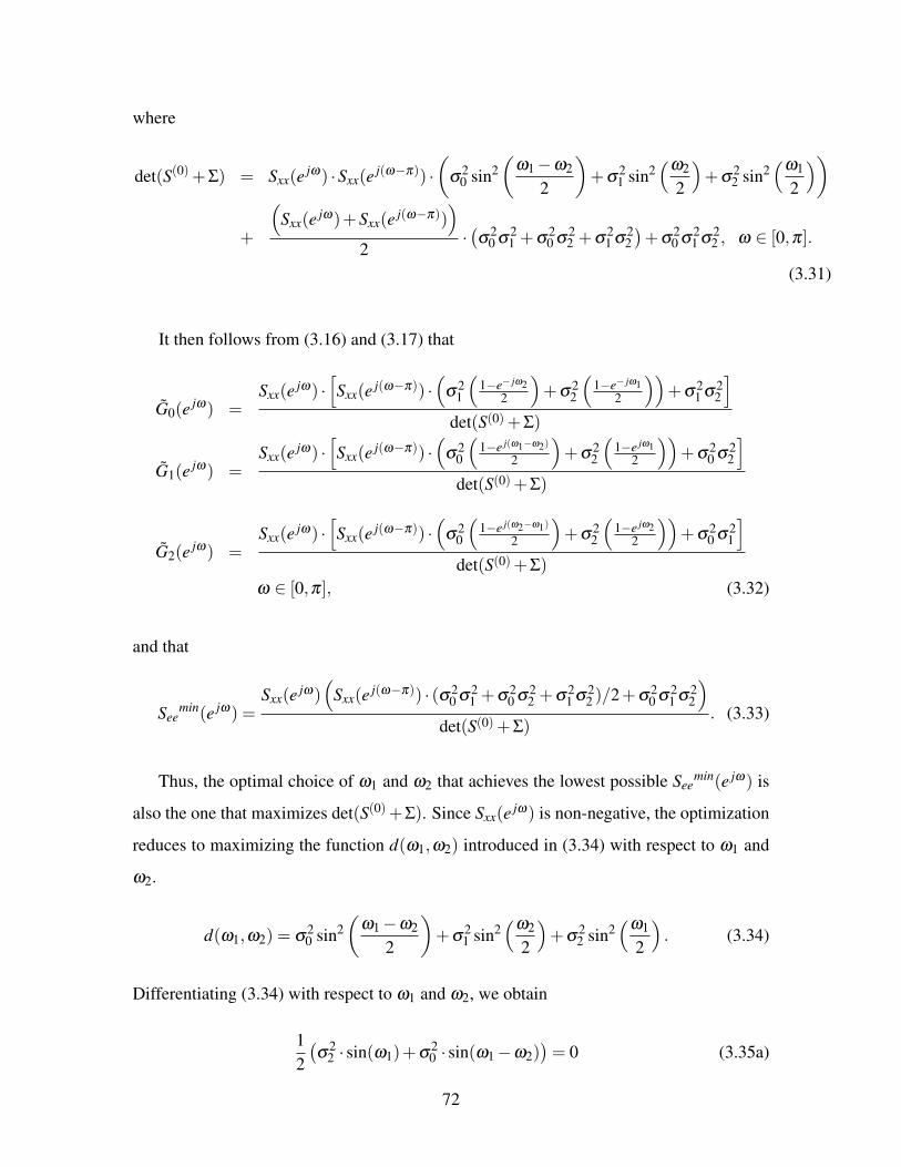
where
det(S(0)+Σ) = Sxx(e jω) ·Sxx(e j(ω−π)) ·(
σ20 sin2
(ω1 −ω2
2
)+σ2
1 sin2(ω2
2
)+σ2
2 sin2(ω1
2
))
+
(Sxx(e jω)+Sxx(e j(ω−π))
)2
·(σ2
0 σ21 +σ2
0 σ22 +σ2
1 σ22)+σ2
0 σ21 σ2
2 , ω ∈ [0,π].
(3.31)
It then follows from (3.16) and (3.17) that
G0(e jω) =Sxx(e jω) ·
[Sxx(e j(ω−π)) ·
(σ2
1
(1−e− jω2
2
)+σ2
2
(1−e− jω1
2
))+σ2
1 σ22
]det(S(0)+Σ)
G1(e jω) =Sxx(e jω) ·
[Sxx(e j(ω−π)) ·
(σ2
0
(1−e j(ω1−ω2)
2
)+σ2
2
(1−e jω1
2
))+σ2
0 σ22
]det(S(0)+Σ)
G2(e jω) =Sxx(e jω) ·
[Sxx(e j(ω−π)) ·
(σ2
0
(1−e j(ω2−ω1)
2
)+σ2
2
(1−e jω2
2
))+σ2
0 σ21
]det(S(0)+Σ)
ω ∈ [0,π], (3.32)
and that
Seemin(e jω) =
Sxx(e jω)(
Sxx(e j(ω−π)) · (σ20 σ2
1 +σ20 σ2
2 +σ21 σ2
2 )/2+σ20 σ2
1 σ22
)det(S(0)+Σ)
. (3.33)
Thus, the optimal choice of ω1 and ω2 that achieves the lowest possible Seemin(e jω) is
also the one that maximizes det(S(0)+Σ). Since Sxx(e jω) is non-negative, the optimization
reduces to maximizing the function d(ω1,ω2) introduced in (3.34) with respect to ω1 and
ω2.
d(ω1,ω2) = σ20 sin2
(ω1 −ω2
2
)+σ2
1 sin2(ω2
2
)+σ2
2 sin2(ω1
2
). (3.34)
Differentiating (3.34) with respect to ω1 and ω2, we obtain
12(σ2
2 · sin(ω1)+σ20 · sin(ω1 −ω2)
)= 0 (3.35a)
72

12(σ2
1 · sin(ω2)−σ20 · sin(ω1 −ω2)
)= 0. (3.35b)
Note that eqs. (3.35a) and (3.35b) are equivalent to the equations in (2.46a) which set the
conditions to achieve the lower bound on the mean squared reconstruction error, i.e., to
achieve equality in (2.45).
When the quantizer step size is the same in all channels, i.e., when σ20 = σ2
1 = σ22 = σ2,
eqs. (3.35) are solved for ω1 =−ω2 =±2π/3, corresponding to τ1 =−τ2 =±2/3TN , i.e.,
uniform sampling. In that case, the optimal reconstruction filters are
Gm(e jω) =23
Sxx(e jω)
Sxx(e jω)+ 23σ2
, (3.36)
with which the multi-channel reconstruction is equivalent to interleaving the multi-channel
output samples followed by sampling rate conversion and Wiener filtering, as illustrated in
Figure 3-2.
x[n]2 3
ωπ
3π
3−
2 Sxx(ejω)
Sxx(ejω)+23σ
2
x[n]+
x3/2[n]
1x0[n]
3x2[n]
3
x1[n]ejω3
ej2ω
Figure 3-2: Interleaving followed by sampling rate converter and Wiener filtering.
Correspondingly,
Seemin(e jω) =
σ2 ·Sxx(e jω)32Sxx(e jω)+σ2
≤ σ2 ·Sxx(e jω)
Sxx(e jω)+σ2 , (3.37)
where the right side of the inequality is achieved with uniform sampling at the Nyquist rate.
73

Note also that by writing Seemin(e jω) from (3.37) as
Seemin(e jω) =
11
23 σ2 +
1Sxx(e jω )
, (3.38)
we conclude that Seemin(e jω) ≤ 2
3σ2, from which it follows that σ2e
min ≤ 23σ2. In other
words, the minimum mean squared reconstruction error achieved with this approach is
lower than 23σ2, corresponding to the minimum mean squared reconstruction error achieved
with the constrained reconstruction filters.
However, when the quantizer step size is not the same for all channels, the choice of
τ1 = −τ2 = ±2/3TN , which corresponds to uniform sampling, is no longer optimal, and
better performance can be achieved with a different choice of the time delays τ1 and τ2, for
which the multi-channel sampling is equivalent to recurrent nonuniform sampling. Figure
3-3 illustrates the relative gain of d(ω1,ω2) over the case of uniform sampling when 3 bits
are allocated to channel 0, 4 bits to channel 1, and 4 bits to channel 2. As illustrated, the
optimal time delays are τ1/TN =−τ2/TN =±0.54, which are identical to those obtained in
(2.68) where the filters are constrained, and correspond to recurrent nonuniform sampling.
Figure 3-3: The relative gain of d(ω1,ω2) as compared to the case of uniform samplingwhen N0 = 3, N1 = 4, N2 = 4.
74

CHAPTER 4
SINC INTERPOLATION OF
NONUNIFORM SAMPLES
It is well known that a bandlimited signal can be uniquely recovered from nonuniformly
spaced samples under certain conditions on the nonuniform grid and provided that the
average sampling rate meets or exceeds the Nyquist rate. However, reconstruction of the
continuous-time signal from nonuniform samples is typically more difficult to implement
than from uniform samples. Motivated by the fact that sinc interpolation results in perfect
reconstruction for uniform sampling, we develop a class of approximate reconstruction
methods from nonuniform samples based on the use of time-invariant lowpass filtering,
i.e., sinc interpolation. The methods discussed consist of four cases incorporated in a single
framework.
4.1 Introduction
Discrete-time signals can arise in many ways, but they most commonly occur as repre-
sentations of sampled continuous-time signals. The most common form of sampling used
in the context of discrete-time processing of continuous-time signals is uniform sampling
corresponding to samples of continuous-time signals obtained at equally spaced time inter-
vals. Under certain conditions, specified by the Nyquist-Shannon sampling theorem, the
original signal can be reconstructed from this set of equally-spaced samples. The recon-
struction is done through sinc interpolation1 corresponding to the impulse response of a
1Throughout the thesis we refer to convolution of an impulse train of samples with the functionh(t) = sinc( π
T t) as sinc interpolation and use the historical unnormalized definition of the sinc function,
75

linear time-invariant ideal lowpass filter.
In a variety of contexts, nonuniform sampling naturally arises or is preferable to uni-
form sampling. For example, some biomedical devices utilize low-power sensors that use
self-timed circuits, thus removing the need for power-intensive clock buffers and clock
distribution. However, these self-timed circuits tend to introduce nonuniformity in the
sampling clock [1]. Nonuniform sampling also often arises in time-interleaved analog-to-
digital converters, where a signal is passed through multiple parallel channels, each uni-
formly sampling the signal at the same rate. The output samples of the channels are then
multiplexed to obtain a full discrete-time representation of the signal. For the case in which
the clock phases of these channels are asynchronous, interleaving samples from each chan-
nel leads to recurrent nonuniform sampling [100]. Recurrent nonuniform sampling also
often arises in sensor networks in which each sensor uniformly samples the environment
asynchronously and transmits to a main base station, where the samples are interleaved.
In many cases nonuniform sampling is deliberate and advantageous. In the spatial
domain, non-uniformity of the spacing of the array elements in an antenna or acoustic
sensor array is often part of the array design as a trade off between the length of the array
and the number of elements. In ray traced computer graphics, it has been shown that
nonuniform sampling yields aliasing that is less conspicuous to the observer [65].
Exact reconstruction of a bandlimited continuous-time signal from nonuniform samples
is based on Lagrange interpolation. For the case of uniform sampling, Lagrange interpo-
lation reduces to sinc interpolation and can be approximated with well designed low pass
filtering. When the sampling grid is not uniform, Lagrange interpolation is more difficult
as discussed in section 4.2. In this chapter we consider sinc interpolation of nonuniform
samples as a way to approximately reconstruct the continuous-time signal. A class of
approximate reconstruction methods is proposed in which each method corresponds to a
different assumption with respect to the knowledge of the exact sampling times and of the
probability distribution of their deviation from a uniform sampling grid.
i.e., sinc(x), sin(x)x
76

4.2 Reconstruction of Bandlimited Signals from Nonuni-
form Samples
A variety of approaches to reconstruction of signals from nonuniform samples have been
previously proposed and discussed. In a classic paper on nonuniform sampling of bandlim-
ited signals [100], Yen introduced several reconstruction theorems to address the cases of a
finite number of nonuniform samples on an otherwise uniform grid, a single gap in uniform
sampling and recurrent nonuniform sampling. Other reconstruction approaches, specific to
recurrent nonuniform sampling have also been proposed [71], [43], [61], [23], [82]. In the
work of Yao and Thomas [98], the Lagrange interpolation functions were applied to the
reconstruction of bandlimited signals from nonuniform samples. It is shown there that a
finite-energy signal x(t) bandlimited to ±π/TN can be reconstructed from its nonuniform
samples x(tn) using Lagrange interpolation when the sampling instants tn do not deviate by
more than TN/4 from a uniform grid with spacing of TN . Specifically, if
|tn −nTN | ≤ d < TN/4, ∀n ∈ Z , (4.1)
then
x(t) =∞
∑n=−∞
x(tn)ln(t) , (4.2a)
where
ln(t) =G(t)
G′(tn)(t − tn), (4.2b)
G(t) = (t − t0)∞
∏k=−∞k =0
(1− t
tk
), (4.2c)
and G′(t)=dG(t)dt . Interpolation using eqs. (4.2) is referred to as Lagrange interpolation.
This theorem is based on a theorem proved by Levinson [53] which states that the functions
Ln(Ω), defined as the Fourier transform of ln(t), are bandlimited and form a sequence
biorthogonal to e jΩtn over [− πTN, π
TN] given that the condition of eq. (4.1) is satisfied.
77

Specifically,
Ln(Ω) =∫ ∞
−∞ln(t)e− jΩtdt = 0, |Ω|> π
TN, (4.3)
and
12π
∫ πTN
− πTN
Ln(Ω)e jΩtkdΩ = ln(tk) = δ [n− k]. (4.4)
Eq. (4.4) utilizes the interpolation condition of the Lagrange kernel which ensures that the
property of consistent resampling is upheld, i.e., that sampling the reconstructed signal on
the nonuniform grid tn yields the original samples x(tn). Note that expressing Ln(Ω)
as the Fourier transform of ln(t) in (4.4) results in biorthogonality of the sequences ln(t)
and sinc(π/TN(t − tn)), i.e.,
∫ ∞
−∞ln(t)sinc(π/TN(t − tk))/TNdt = δ [n− k], (4.5)
from which the expansion in (4.2) for bandlimited signals is clearly followed.
The difficulty of exact reconstruction of bandlimited signals from nonuniform samples
through Lagrange interpolation is partly due to the fact that the interpolating functions
at different sampling times do not have the same form except in special cases. Also, each
interpolating function depends on all sampling instants. The complexity of the implementa-
tion motivates the need for simpler approximate approaches to reconstruction and a variety
of methods has previously been proposed. One practical approach to recovering a signal
from its nonuniform samples has been the use of nonuniform splines [10]. Iterative re-
construction methods for nonuniform sampling which are computationally demanding and
have potential issues of convergence have also been previously proposed [25], [26], [30].
In a different approach, time-warping methods were applied by Papoulis in [70] to recon-
struct bandlimited signals from jittered samples. In [17] and [103], time-warping was used
for reconstruction from samples of signals with time-varying frequency content. A method
of designing FIR filters in such a way that the effect of input clock jitter is diminished is
discussed in [84]. In [60] several approaches are suggested and analyzed for approximate
78

reconstruction from jittered samples. Mean-square comparison of various interpolators is
done in [52] for the case of uniform sampling, uniform sampling with skips, and Poisson
sampling. A modification of the conventional Lagrange interpolator is proposed in [77]
which allows approximating a bandlimited signal from its nonuniform samples with high
accuracy. A comprehensive review of literature concerning other techniques in nonuniform
sampling can be found in [33] and [58].
4.3 Sinc Interpolation of Nonuniform Samples
With uniform sampling, i.e., when tn = nT , G(t) of eq. (4.2c) reduces to
G(t) =sin(π
T )tπT
, (4.6)
and Lagrange interpolation reduces to sinc interpolation. In this section we restrict ln(t)
in eq. (4.2a) to be of the form ln(t) = (T/TN)sinc(π/TN · (t − tn)) corresponding to sinc
interpolation. Note that since the kernel used in this framework is time-invariant, the exact
sampling instants are not needed in designing the reconstruction filter. This is in contrast
to Lagrange interpolation in which this knowledge is required in forming the interpolating
functions since these functions do not have the same form at each sampling instant and
each interpolating function depends on all sampling instants, i.e., it is not a time-invariant
convolution. It will be assumed throughout this section that the average sampling rate
meets or exceeds the Nyquist rate, or equivalently that T ≤ TN where T denotes the nominal
sampling interval.
We consider and analyze four cases incorporated in a single framework where the
choice for the values tn differs for each of the methods discussed below. In the first case,
it is assumed that both the exact sampling instants and the probability distribution of their
deviation from a uniform sampling grid are known. As we will see in section 4.3.6, even
with the knowledge of the exact sampling instants, it can sometimes be beneficial to place
the samples on a grid other than the actual nonuniform grid corresponding to the sampling
instants. In determining this grid we utilize the probability distribution of the deviation of
79

the sampling instants from a uniform sampling grid. In the second case, sinc interpolation
is applied to the samples placed on a uniform grid with spacing corresponding to the av-
erage or nominal spacing of the nonuniform sampling grid. In that approximation it is not
necessary to know the exact sampling instants since they are not used. This may occur in
situations where the samples are stored in memory and their exact timing information is
lost. The third case consists of applying sinc interpolation to the samples located at the ac-
tual nonuniform sampling times. This method requires knowledge of the nonuniform grid.
However, as opposed to Lagrange interpolation where the sampling instants are needed
in advance to generate the interpolating functions, the sinc interpolation function requires
only knowledge of the nominal sample spacing. In the fourth case, it is assumed that the
exact sampling times are not known but that the probability distribution of their deviation
from a uniform sampling grid is known.
4.3.1 Mathematical Formulation
To have a common framework that incorporates these four cases, we denote by x[n] a se-
quence of nonuniform samples of x(t), i.e.,
x[n] = x(tn) (4.7)
where tn represent a nonuniform grid which we model as a perturbation of a uniform grid
with spacing T , i.e.,
tn = nT +ξn. (4.8)
For analysis purposes, we consider x(t) to be a continuous-time zero-mean wide-sense
stationary random process with autocorrelation function Rxx(τ) and power spectral density
(PSD) Sxx(Ω) which is zero for |Ω| ≥ Ωc = π/TN . ξn is characterized as an i.i.d. sequence
of zero-mean random variables independent of x(t) with probability density function (pdf)
fξ (ξ ) and characteristic function Φξ (Ω) =∫ ∞−∞ fξ (ξ ′)e jΩξ ′
dξ ′.
For the reconstruction of x(t) from its nonuniform samples x[n], we apply sinc interpo-
lation to the samples placed on a second nonuniform grid tn = nT + ζn that in general is
80
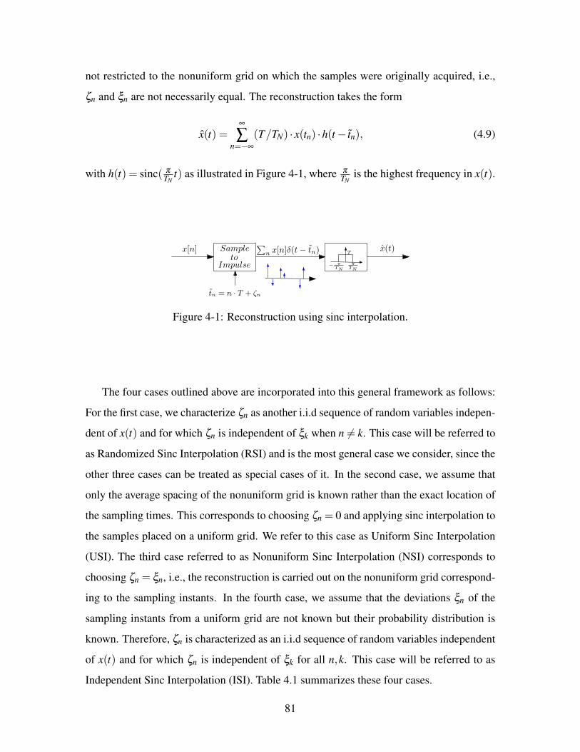
not restricted to the nonuniform grid on which the samples were originally acquired, i.e.,
ζn and ξn are not necessarily equal. The reconstruction takes the form
x(t) =∞
∑n=−∞
(T/TN) · x(tn) ·h(t − tn), (4.9)
with h(t) = sinc( πTN
t) as illustrated in Figure 4-1, where πTN
is the highest frequency in x(t).
T
π
TN
x(t)
−
π
TN
∑nx[n]δ(t− tn)x[n]
tn = n · T + ζn
Sampleto
Impulse
Figure 4-1: Reconstruction using sinc interpolation.
The four cases outlined above are incorporated into this general framework as follows:
For the first case, we characterize ζn as another i.i.d sequence of random variables indepen-
dent of x(t) and for which ζn is independent of ξk when n = k. This case will be referred to
as Randomized Sinc Interpolation (RSI) and is the most general case we consider, since the
other three cases can be treated as special cases of it. In the second case, we assume that
only the average spacing of the nonuniform grid is known rather than the exact location of
the sampling times. This corresponds to choosing ζn = 0 and applying sinc interpolation to
the samples placed on a uniform grid. We refer to this case as Uniform Sinc Interpolation
(USI). The third case referred to as Nonuniform Sinc Interpolation (NSI) corresponds to
choosing ζn = ξn, i.e., the reconstruction is carried out on the nonuniform grid correspond-
ing to the sampling instants. In the fourth case, we assume that the deviations ξn of the
sampling instants from a uniform grid are not known but their probability distribution is
known. Therefore, ζn is characterized as an i.i.d sequence of random variables independent
of x(t) and for which ζn is independent of ξk for all n,k. This case will be referred to as
Independent Sinc Interpolation (ISI). Table 4.1 summarizes these four cases.
81

Table 4.1: Sinc Interpolation Reconstruction MethodsRandomized Sinc Interpolation (RSI) Nonuniform Sinc Interpolation (NSI)
Sinc interpolation is applied to the samples Sinc interpolation is applied to the samplesplaced on a grid determined by both the placed on the nonuniform grid correspondingexact sampling instants and the pdf of their to the sampling instantsdeviation from a uniform sampling grid
Independent Sinc Interpolation (ISI) Uniform Sinc Interpolation (USI)Sinc interpolation is applied to the samples Sinc interpolation is applied to the sampleslocated on a grid independent of the actual placed on a uniform gridnonuniform grid
4.3.2 Randomized Sinc Interpolation
Appendix D shows an equivalence with respect to second-order statistics2 between the
nonuniform sampling discussed above when followed by Randomized Sinc Interpolation
and the system in Figure 4-2.
Φξζ(Ω,−Ω)y(t)
v(t)
z(t)x(t)
Figure 4-2: A second-order statistics model for nonuniform sampling followed by Ran-domized Sinc Interpolation for the case where T ≤ TN .
The frequency response of the LTI system in Figure 4-2 is the joint characteristic func-
tion Φξ ζ (Ω1,Ω2) of ξn and ζn, defined as the Fourier transform of their joint pdf fξ ζ (ξ ,ζ ).
In the same figure, v(t) is zero-mean additive colored noise, uncorrelated with x(t), with
PSD as follows:
Svv(Ω) =
T2π∫ Ωc−Ωc
Sxx(Ω′)(1−|Φξ ζ (Ω
′,−Ω)|2)dΩ′ |Ω|< Ωc
0 |Ω| ≥ Ωc
. (4.10)
Thus, with respect to second-order statistics, x(t) can equivalently be represented by the
signal z(t) in Figure 4-2.
2Throughout the thesis we use the terminology of equivalence between two systems with respect tosecond-order statistics to mean that for the same input, the output means, auto-correlation functions, andcross-correlation functions are identical.
82

We denote eR(t) = x(t)− x(t) as the error between x(t) and its approximation x(t)
obtained by RSI. Then, as shown in Appendix D, the corresponding mean square error
(MSE) is given by
σ2eR =
12π
∫ Ωc
−Ωc
Sxx(Ω) ·Q(Ω)dΩ, (4.11)
where
Q(Ω) =∣∣1−Φξ ζ (Ω,−Ω)
∣∣2 + 1r·∫ Ωc
−Ωc
1−|Φξ ζ (Ω,−Ω1)|2
2ΩcdΩ1, (4.12)
and r = TN/T ≥ 1 denotes the oversampling ratio.
4.3.3 Uniform Sinc Interpolation
In the case where neither the sampling instants nor their distribution is known, we set the
perturbations ζn in the reconstruction of Figure 4-1 to zero. This results in
x(t) =∞
∑n=−∞
(T/TN) · x(tn) ·h(t −nT ), (4.13)
which corresponds to treating the nonuniform samples as being on a uniform grid and
reconstructing x(t) with sinc interpolation of these samples as though the sampling was
uniform, corresponding to USI. Note that when USI is used for reconstruction, the signal
x(t) in the equivalent system of Figure 4-2 is in effect pre-filtered by the characteristic
function Φξ (Ω) of ξn, and the additive uncorrelated noise v(t) is white. Since |Φξ (Ω)| ≤
Φξ (Ω)|Ω=0 = 1, the characteristic function has in general the behavior of a lowpass filter
when viewed as a frequency response of an LTI system3.
The error between x(t) and its approximation x(t) obtained by USI is denoted by eU(t)
and the corresponding MSE follows directly from (4.11) by replacing Φξ ζ (Ω1,Ω2) with
3Note that when ξn is symmetrically distributed on (−T/2,T/2), the characteristic function Φξ (Ω) is realand symmetric. In addition, in the region Ω ∈ (−π/T,π/T ) Φξ (Ω) is non-negative, concave and boundedfrom below by cos(ΩT/2), as elaborated in Appendix E. Its radius of curvature at Ω = 0 is also shown to beinversely proportional to the variance σ2
ξ of ξn.
83

Φξ (Ω1), i.e.,
σ2eU =
12π
∫ Ωc
−Ωc
Sxx(Ω) ·|1−Φξ (Ω)|2 + 1
r·(1−|Φξ (Ω)|2
)dΩ . (4.14)
For the case of no oversampling, i.e., when the oversampling factor r = 1, the MSE in
eq. (4.14) reduces to
σ2eU = 2 · 1
2π
∫ Ωc
−Ωc
Sxx(Ω) ·(1−ℜ(Φξ (Ω))
)dΩ
= 2 ·(
Rxx(0)−1
2π
∫ Ωc
−Ωc
Sxx(Ω) ·ℜ(Φξ (Ω))dΩ)
= 2 ·(
Rxx(0)−∫ ∞
−∞Rxx(τ) · f (even)
ξ (τ)dτ), (4.15)
where f (even)ξ (τ) = ( fξ (τ)+ fξ (−τ))/2 is the even part of fξ (τ). When in addition, ξn is
symmetrically distributed on (−TN/2,TN/2), the following inequalities on the mean square
reconstruction error follow by utilizing the properties of Rxx(τ) and Φξ (Ω) given in Ap-
pendix E,
1−min(ρxx(ξ0),Φξ (Ω0)
)≤
σ2eU
2Rxx(0)≤ 1−max
(ρxx(TN/2),Φξ (π/TN)
), (4.16)
where ρxx(τ) = Rxx(τ)/Rxx(0), ξ0 = E(|ξ |) and Ω0 =∫ Ωc−Ωc
|Ω| · Sxx(Ω)∫Ωc−Ωc Sxx(Ω′)dΩ′ dΩ. The fact
that Rxx(τ) is monotonically decreasing in (0,TN/2) and Φξ (Ω) is monotonically decreas-
ing in (0,π/TN) leads to
∫ TN/2
−TN/2Rxx(τ) fξ (τ)dτ ≥ Rxx(TN/2)
∫ TN/2
−TN/2fξ (τ)dτ = Rxx(TN/2), (4.17)
12π
∫ Ωc
−Ωc
Sxx(Ω) ·Φξ (Ω)dΩ ≥ 12π
∫ Ωc
−Ωc
Sxx(Ω)dΩ ·Φξ (π/TN) = Rxx(0) ·Φξ (π/TN),
(4.18)
from which the upper bound in (4.16) clearly follows. To obtain the lower bound in (4.16)
84

we use the concavity of Rxx(τ) and Φξ (Ω) in the appropriate regions. Specifically,
∫ TN/2
−TN/2Rxx(τ) fξ (τ)dτ =
∫ TN/2
0Rxx(τ) ·2 fξ (τ)dτ ≤ Rxx
(∫ TN/2
0τ ·2 fξ (τ)dτ
)=
Rxx
(∫ TN/2
0τ · ( fξ (τ)+ fξ (−τ))dτ
)= Rxx(E(|ξ |)), (4.19)
and
12π
∫ Ωc
−Ωc
Sxx(Ω) ·Φξ (Ω)dΩ = Rxx(0) ·1
2π
∫ Ωc
−Ωc
Sxx(Ω)1
2π∫ Ωc−Ωc
Sxx(Ω′)dΩ′·Φξ (Ω)dΩ =
Rxx(0) ·∫ Ωc
0
2Sxx(Ω)∫ Ωc−Ωc
Sxx(Ω′)dΩ′·Φξ (Ω)dΩ ≤ Rxx(0) ·Φξ
(∫ Ωc
0Ω · 2Sxx(Ω)∫ Ωc
−ΩcSxx(Ω′)dΩ′
dΩ
)=
Rxx(0) ·Φξ
(∫ Ωc
−Ωc
|Ω| · Sxx(Ω)∫Ωc−Ωc
Sxx(Ω′)dΩ′dΩ
). (4.20)
Note that the inequality in (4.19) suggests that when E(|ξ |) = ξ0 < TN/2 is fixed, mini-
mum mean square reconstruction error of USI is achieved when ξn takes the values ±ξ0
with equal probabilities, i.e., when Φξ (Ω) = cos(ξ0Ω). Alternatively, when∫ Ωc−Ωc
|Ω| ·Sxx(Ω)∫Ωc
−Ωc Sxx(Ω′)dΩ′ dΩ = Ω0 < π/TN is fixed, it follows from (4.20) that minimum mean square
reconstruction error of USI is achieved when ρxx(τ)= cos(Ω0τ). The lower bound in (4.16)
together with the fact that when a lower bound is achieved it is the greatest lower bound
results in the following upper bounds on ρxx(τ) and Φξ (Ω),
ρxx(τ) ≤ cos(Ω0τ) |τ|< TN/2,
Φξ (Ω) ≤ cos(ξ0Ω) |Ω|< π/TN . (4.21)
We would expect the performance of USI to be inversely proportional to the signal’s
bandwidth Bx, as defined in (4.31). This is intuitively reasonable since with slow variations
of the signal, the uniform samples x(nTN) are accurately approximated by the nonuniform
samples x(tn). The upper bound on σ2eU seems to agree with this intuition since it decreases
as Rxx(TN/2) increases, and Rxx(TN/2) is expected to increases as the radius of curvature
of Rxx(τ) at τ = 0 increases or equivalently as the bandwidth Bx of x(t) decreases.
85

4.3.4 Nonuniform Sinc Interpolation
When the sampling instants tn are known, we can alternatively set the reconstruction per-
turbations ζn to be equal to the sampling perturbations ξn so that the impulses in Figure
4-1 are located on the correct grid. This is another special case of eq. (4.9) for which the
reconstruction takes the form
x(t) =∞
∑n=−∞
(T/TN) · x(tn) ·h(t − tn). (4.22)
Note that for this approximation, referred to as Nonuniform Sinc Interpolation, the dis-
tribution of the perturbations is not needed. The corresponding MSE of the reconstruction
error eN(t) follows directly from eq. (4.11) by replacing Φξ ζ (Ω1,Ω2) with Φξ (Ω1 −Ω2),
i.e.,
σ2eN =
1r·(
Rxx(0)−1
2Ωc
∫ Ωc
−Ωc
(Sxx(Ω)∗ |Φξ (Ω)|2
)dΩ)
=1r· 1
2π
∫ Ωc
−Ωc
Sxx(Ω) ·
(∫ Ω+Ωc
Ω−Ωc
1−|Φξ (Ω′)|2
2ΩcdΩ
′
)dΩ. (4.23)
4.3.5 Independent Sinc Interpolation
When the exact sampling times are not known but the probability distribution fξ (ξ ) of their
deviation from a uniform sampling grid is known, and choosing ζn in the reconstruction of
Figure 4-1 to be independent of ξk for all n, k, we obtain
σ2eI =
12π
∫ Ωc
−Ωc
Sxx(Ω) ·∣∣1−Φξ (Ω)Φζ (−Ω)
∣∣2 dΩ+
+1r· 1
2π
∫ Ωc
−Ωc
Sxx(Ω) ·(
1−|Φξ (Ω)|2 · 12Ωc
∫ Ωc
−Ωc
|Φζ (Ω1)|2dΩ1
)dΩ. (4.24)
As with any characteristic function, |Φζ (Ω)| ≤ 1 for all Ω. Consequently, the second term
in eq. (4.24) is minimized when Φζ (Ω) = 1, corresponding to ζn = 0, i.e., Uniform Sinc
Interpolation. In minimizing the first term in eq. (4.24) we restrict fξ (ξ ) to be symmet-
ric. Furthermore, the deviation from the uniform grid is restricted to be less than T/2, i.e.,
fξ (ξ ) = 0 for |ξ | ≥ T/2. From this it follows that the Fourier transform of fξ (ξ ), i.e.,
86
Φξ (Ω) is guaranteed to be real and non-negative for |Ω| ≤ π/T (see Appendix E). Since
the average sampling rate is at or above the Nyquist rate, i.e., πT ≥ Ωc, Φξ (Ω) will always
be real and non-negative in the interval of integration for the first term in eq. (4.24). Con-
sequently, to minimize that term we again choose Φζ (Ω) = 1, corresponding to Uniform
Sinc Interpolation.
In summary, when the probability density function of ξn is symmetric and has bounded
support, Uniform Sinc Interpolation is an optimal reconstruction within this framework.
More generally, the optimal choice for fζ (ζ ) may not correspond to Uniform Sinc Interpo-
lation and lower MSE may be achieved with Φζ (Ω) = e− jζ0Ω corresponding to ζn =−ζ0,
i.e., Uniform Sinc Interpolation with an offset of the uniform grid. The offset ζ0 can be
optimized to minimize σ2eI in (4.24). Specifically,
ζ opt0 = argmin
ζ0ℜ
12π
∫ Ωc
−Ωc
Sxx(Ω) ·∣∣∣1−Φξ (Ω)e jζ0Ω
∣∣∣2 dΩ
+1r· 1
2π
∫ Ωc
−Ωc
Sxx(Ω) ·(1−|Φξ (Ω)|2
)dΩ
= argmaxζ0
ℜ
12π
∫ Ωc
−Ωc
Sxx(Ω)Φξ (Ω)e jζ0ΩdΩ, (4.25)
or equivalently,
ζ opt0 = argmax
ζ0
Rxx(τ)∗ fξ (τ)|τ=ζ0
= argmaxζ0
∫ ∞
−∞Rxx(τ −ζ0) fξ (τ)dτ
= argmaxζ0
Eξ (Rxx(ξ −ζ0)) . (4.26)
Note that when fξ (ξ ) is symmetric and the deviation from the uniform grid is less
than T/2, ζ opt0 = 0 consistent with the observation that the optimal reconstruction in this
case does not depend on the specific shape of the pdf and corresponds to Uniform Sinc
87

Interpolation. This follows by noting that
∫ T/2
−T/2Rxx(τ −ζ0) fξ (τ)dτ =
∫ T/2
0[Rxx(τ −ζ0)+Rxx(τ +ζ0)] fξ (τ)dτ ≤
∫ T/2
−T/2Rxx(τ) fξ (τ)dτ,
(4.27)
where we used the symmetry of the pdf fξ (ξ ) and of Rxx(τ), and the property that
Rxx(τ)≥12(Rxx(τ −ζ0)+Rxx(τ +ζ0)) ∀ |τ|< T/2, ζ0, (4.28)
which is shown to be true in Appendix E for the autocorrelation function of a bandlimited
signal.
4.3.6 RSI - Minimum Mean Square Reconstruction Error
As eq. (4.11) shows, the performance of RSI depends on the power spectrum Sxx(Ω) of
the continuous-time signal x(t) as well as on the joint characteristic function Φξ ζ (Ω1,Ω2)
of the perturbations, which can be designed to reduce the MSE. In order to formulate the
optimal reconstruction within the framework of RSI, i.e., to design ζn in the reconstruc-
tion method of Figure 4-1 to achieve minimum MSE, eq. (4.11) should be optimized with
respect to Φξ ζ (Ω1,Ω2) subject to the constraint Φξ ζ (Ω,0) = Φξ (Ω). This optimization
requires in general the knowledge of both the exact sampling instants and the probability
distribution of their deviation from a uniform sampling grid. As we will next see, even
though the exact sampling instants are known, the optimal reconstruction may not corre-
spond to NSI, i.e., the optimal grid on which the samples are placed in reconstruction prior
to sinc interpolation may possibly be different than the actual nonuniform sampling grid.
In minimizing the MSE we consider two cases. The first is the case of small, zero-
mean perturbations from a uniform grid, for which in the region |Ω1|< Ωc and |Ω2|< Ωc,
Φξ ζ (Ω1,Ω2) can be approximated well by the second-order Taylor expansion
Φξ ζ (Ω1,Ω2)≈ 1−σξ ζ Ω1Ω2 −12
σ2ξ Ω2
1 −12
σ2ζ Ω2
2, (4.29)
88

with the corresponding standard deviations σξ and σζ of ξn and ζn assumed to be small
enough relative to T so that (4.29) holds. Substituting (4.29) into (4.11) for the case r = 1
yields
σ2eR ≈ Rxx(0) ·
(σ2
ξ ·Bx +1/3 ·σ2ζ ·Ωc
2), (4.30)
where Bx is a measure of the signal’s bandwidth defined as
Bx =∫ Ωc
−Ωc
Ω2 ·
(Sxx(Ω)∫ Ωc
−ΩcSxx(Ω
′)dΩ′
)dΩ. (4.31)
From (4.30) we see that independent of the detailed characteristics of the perturbation or
the signal spectrum, as long as the perturbations around the uniform grid are small enough
so that (4.29) holds, it is preferable to reconstruct the signal using USI, corresponding to
ζn = 0. This is despite the fact that USI uses only the nominal rather than actual sampling
times.
We next consider the case in which the sampling perturbation errors are uniformly dis-
tributed over the range(−T
2 ,T2
). As previously mentioned, the optimal perturbations ζn in
the reconstruction of Figure 4-1 are chosen to minimize (4.11) with respect to Φξ ζ (Ω1,Ω2).
One interesting case is when the joint characteristic function Φξ ζ (Ω1,Ω2) is characterized
by a finite set of parameters, and the optimization of the MSE in (4.11) reduces to opti-
mization over those parameters. Consider as an example the case when ζn is a kth-order
polynomial of ξn whose coefficients are to be designed. For simplicity, we will consider
here only the linear case, i.e., ζn = βξn with β ∈ [0,1] for which the case of β = 0 corre-
sponds to USI and the case of β = 1 corresponds to NSI. It then follows that the Fourier
transform of the joint pdf fξ ζ (ξ ,ζ ) is
Φξ ζ (Ω1,Ω2) = Φξ (Ω1 +βΩ2) , (4.32)
89
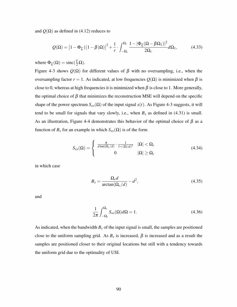
and Q(Ω) as defined in (4.12) reduces to
Q(Ω) =∣∣1−Φξ ((1−β )Ω)
∣∣2 + 1r·∫ Ωc
−Ωc
1−|Φξ (Ω−βΩ1)|2
2ΩcdΩ1, (4.33)
where Φξ (Ω) = sinc(T2 Ω).
Figure 4-3 shows Q(Ω) for different values of β with no oversampling, i.e., when the
oversampling factor r = 1. As indicated, at low frequencies Q(Ω) is minimized when β is
close to 0, whereas at high frequencies it is minimized when β is close to 1. More generally,
the optimal choice of β that minimizes the reconstruction MSE will depend on the specific
shape of the power spectrum Sxx(Ω) of the input signal x(t). As Figure 4-3 suggests, it will
tend to be small for signals that vary slowly, i.e., when Bx as defined in (4.31) is small.
As an illustration, Figure 4-4 demonstrates this behavior of the optimal choice of β as a
function of Bx for an example in which Sxx(Ω) is of the form
Sxx(Ω) =
π
d tan(Ωc/d) ·1
1+(Ω/d)2 |Ω|< Ωc
0 |Ω| ≥ Ωc
(4.34)
in which case
Bx =Ωcd
arctan(Ωc/d)−d2, (4.35)
and
12π
∫ Ωc
−Ωc
Sxx(Ω)dΩ = 1. (4.36)
As indicated, when the bandwidth Bx of the input signal is small, the samples are positioned
close to the uniform sampling grid. As Bx is increased, β is increased and as a result the
samples are positioned closer to their original locations but still with a tendency towards
the uniform grid due to the optimality of USI.
90

−π/Τ −π/2Τ 0 π/2Τ π/Τ0
0.1
0.2
0.3
0.4
0.5
0.6
0.7
Ω
Q(Ω
)
β=0β=0.25β=0.5β=0.75β=1
Figure 4-3: Q(Ω) for the case where ξn ∼ u[−T/2,T/2] and T = TN = 1.
0 0.5 1 1.5 2 2.5 30
0.02
0.04
0.06
0.08
0.1
0.12
0.14
0.16
0.18
0.2
Bx
β
Figure 4-4: The optimal choice of β that minimizes σ2eR as a function of Bx for the case
where T = TN = 1.
4.3.7 Discussion
While USI uses only the zero-mean assumption of the perturbation error and does not re-
quire the knowledge of the exact sampling instants, this knowledge is necessary for NSI.
Comparing USI with NSI with respect to mean square reconstruction error, it is in general
not possible to claim which of these methods is preferable. Their relative performance is
dependent on the power spectrum Sxx(Ω) of the continuous-time signal, the distribution
fξ (ξ ) of the sampling perturbations and the oversampling ratio r. For ISI, not only the
mean but the entire probability distribution function of the deviation from a uniform sam-
pling grid is needed in general. Since USI can be viewed as a special case of ISI for which
91

fζ (ζ ) = δ (ζ ), it might be possible in general to obtain a lower MSE with ISI than with
USI. As previously discussed, there are cases in which even though the entire probability
distribution of the sampling perturbations is known, the mean square reconstruction error
of ISI is minimized when fζ (ζ ) = δ (ζ ), corresponding to USI. USI, NSI and ISI can all be
formulated as special cases of RSI, which is more general. With an appropriate choice of
fξ ζ (ξ ,ζ ), it might be possible in general to obtain a lower MSE with RSI than with USI,
NSI or ISI.
In the problem formulation, the samples were taken on a nonuniform grid that is a
perturbation of a uniform grid, and the objective was to design the grid on which to locate
the samples in reconstruction prior to sinc interpolation. Nevertheless, this framework can
handle other cases of interest as well. Consider for example the case in which the samples
are taken on an accurate uniform grid, but there are timing inaccuracies in the discrete-to-
continuous processing. This case can be formed as a special case of the general framework
for which Φξ ζ (Ω1,Ω2) = Φζ (Ω2).
92

CHAPTER 5
TIMING ERRORS IN DISCRETE-TIME
PROCESSING OF CONTINUOUS-TIME
SIGNALS
A major application of discrete-time systems occurs in the processing of continuous-time
signals. When timing errors arise in the conversion from continuous to discrete time and
from discrete to continuous, discrepancies between the desired continuous-time system and
its implementation by a discrete-time system occur. This chapter explores these discrep-
ancies and proposes a method of designing the discrete-time system to compensate for the
timing errors.
5.1 Introduction
In an ideal scenario, the system of Figure 5-1, which consists of sampling followed by an
LTI discrete-time system and discrete-to-continuous conversion, is equivalent under certain
conditions [69], to continuous-time LTI processing of the bandlimited input signal.
C/D D/CG(ejω)x[n] y[n] y(t)x(t)
T T
Figure 5-1: Discrete-time processing of continuous-time signals.
In particular, when the input signal x(t) is bandlimited and the sampling interval T
satisfies the Nyquist condition, the overall system in Figure 5-1 has an effective frequency
93

response of the form
Ge f f (Ω) =
G(e jΩT ) |Ω|< πT
0 |Ω| ≥ πT .
(5.1)
Thus, for the system in Figure 5-1 to correspond, in the absence of errors, to a specified
continuous-time LTI system whose frequency response is
Ge f f (Ω) =
G(Ω) |Ω|< πT
0 |Ω| ≥ πT ,
(5.2)
the frequency response of the discrete-time LTI system should satisfy the following condi-
tion:
G(e jω) = G(ω
T
), |ω|< π. (5.3)
We next discuss the effects of timing errors in the conversion from continuous to dis-
crete time and from discrete to continuous in the system of Figure 5.1 and the design of
an optimal discrete-time LTI system G(e jω), which compensates for these timing errors.
The time jitter problem was first considered in 1962 by Balakrishnan [3], who studied
the properties of the jittered samples and proposed an explicit solution for optimal (in the
mean-square sense) linear operation of these samples. Independently, in 1963 Brown [11]
provided optimum interpolation of sampled data when various types of jitter are present.
Tarczynski [84] presents a method of designing FIR filters whose input signals are sampled
irregularly due to clock jitter. These filters which were designed to diminish the input clock
jitter are claimed to perform better than traditional filters, for which the effect of jitter is
ignored at the designing stage. Similar to [84], we consider in this chapter the design of a
discrete-time system that compensates for the time jitter errors for the more general case in
which time jitter occurs both in acquiring the samples and in forming the interpolation.
94

5.2 The Effects of Timing Errors in Discrete-time Process-
ing of Continuous-time Signals
To analyze the effects of timing errors in discrete-time processing of continuous-time sig-
nals, we consider the system of Figure 5-2. The input signal x(t) is assumed to be a realiza-
tion of a zero-mean wide-sense stationary random process with an autocorrelation function
Rxx(τ) and power spectrum Sxx(Ω) = 0 for Ω ≥ π/T . Due to timing imperfections, the
sampling instants do not form an exact uniform grid. The sampling grid is modeled as a
perturbation of a uniform grid with spacing T , i.e.,
tn = nT +ξn, (5.4)
where ξn is characterized as an i.i.d sequence of zero-mean random variables, independent
of x(t) with pdf fξ (ξ ) and characteristic function Φξ (Ω). The sequence y[n] is obtained
from processing x[n] = x(tn) with a discrete-time LTI system whose frequency response
is G(e jω). The grid on which the samples are placed prior to sinc interpolation in the
conversion from discrete to continuous is modeled as another perturbation of a uniform
grid with spacing T , i.e.,
tn = nT +ζn, (5.5)
where ζn is an i.i.d sequence of random variables independent of x(t) and of ξk for all n,k.
C/D D/CG(ejω)x[n] y[n] y(t)x(t)
tn = nT + ξn tn = nT + ζn
Figure 5-2: Time jitter in discrete-time processing of continuous-time signals.
With respect to second-order statistics, the system of Figure 5-2 is shown in Appendix
F to be equivalent to the continuous-time system of Figure 5-3. In this system, the signals
x(t), vξ (t), vζ (t), and vξ ζ (t) are zero-mean, uncorrelated, wide-sense stationary random
processes. vξ (t) is a white-noise process whose power spectrum Svξ vξ =T2π∫ π/T−π/T Sxx(Ω′)(1−
95

|Φξ (Ω′)|2)dΩ′. The power spectrums of vζ (t) and vξ ζ (t) are
Svζ vζ (Ω) =
(1−|Φζ (−Ω)|2) T2π∫ π/T−π/T Sxx(Ω′)|Φξ (Ω
′)|2|G(e jΩ′
T )|2dΩ′ |Ω|< πT
0 |Ω| ≥ πT ,
(5.6)
and
Svξ ζ vξ ζ (Ω) =
(1−|Φζ (−Ω)|2) · T2π∫ π/T−π/T Sxx(Ω′)(1−|Φξ (Ω
′)|2)dΩ′ · 1
2π∫ π−π |G(e jω)|2dω |Ω|< π
T
0 |Ω| ≥ πT ,
(5.7)
Φξ(Ω)x(t)
G(ejΩT ) Φζ(−Ω)z(t)
vξ(t) vζ(t) + vξζ(t)
Figure 5-3: A second-order statistics model for the system of Figure 5-2.
To show the equivalence between the systems, we first show that the cross-spectrum
between the output y(t) of the system in Figure 5-2 and its input is
Syx(Ω) =
Sxx(Ω)Φξ (Ω)Φζ (−Ω)G(e jΩT ) |Ω|< πT
0 |Ω| ≥ πT ,
(5.8)
and the power spectrum of y(t) is
Syy(Ω) =
(
Sxx(Ω) · |Φξ (Ω)|2 +Svξ vξ
)|Φζ (−Ω)|2|G(e jΩT )|2 ++Svζ vζ (Ω)+Svξ ζ vξ ζ (Ω) |Ω|< π
T
0 |Ω| ≥ πT
.(5.9)
We then note that the power spectrum Szz(Ω) of the output z(t) in the system of Figure 5-3
is identical to Syy(Ω) in (5.9) and the cross-spectrum Szx(Ω) is identical to Syx(Ω) in (5.8).
Thus, as a result of the timing errors in sampling and in reconstruction, the signal x(t) in
the equivalent system of Figure 5-3 is filtered by the LTI system whose frequency response
is Φξ (Ω)Φζ (−Ω), and additive zero-mean uncorrelated noise components occur.
96

For comparison purposes, we denote e(t) = y(t)− x(t) ∗ g(t) as the error between the
output of processing x(t) with a continuous-time LTI system whose impulse response is
g(t) and the output y(t) of the system in Figure 5-2 to an input x(t). It then follows from
eqs. (5.8) and (5.9) that the power spectrum See(Ω) of e(t) is
See(Ω) = Syy(Ω)−Syx(Ω)G∗(Ω)−Sxy(Ω)G(Ω)+Sxx(Ω)|G(Ω)|2 (5.10)
= Sxx(Ω) ·(|Φξ (Ω)|2|Φζ (−Ω)|2|G(e jΩT )|2 −Φξ (Ω)Φζ (−Ω)G(e jΩT )G∗(Ω)
− Φ∗ξ (Ω)Φ∗
ζ (−Ω)G∗(e jΩT )G(Ω)+ |G(Ω)|2)
+ |G(e jΩT )|2|Φζ (−Ω)|2 · T2π
∫ π/T
−π/TSxx(Ω′)(1−|Φξ (Ω′)|2)dΩ′
+ (1−|Φζ (−Ω)|2) · T2π
∫ π/T
−π/TSxx(Ω′)(1−|Φξ (Ω
′)|2)dΩ
′· 1
2π
∫ π
−π|G(e jω)|2dω
+ (1−|Φζ (−Ω)|2) · T2π
∫ π/T
−π/TSxx(Ω′)|Φξ (Ω
′)|2|G(e jΩ′
T )|2dΩ′|Ω|< π
T.
As expected, in the absence of timing errors, i.e., when ξn = 0 and ζn = 0, the choice of
G(e jω) as in (5.3) results in zero mean-squared error. More generally, the power spectrum
See(Ω) of eq. (5.11) for the case in which G(e jω) is specified in (5.3) becomes
See(Ω) = Sxx(Ω) · |G(Ω)|2 ·∣∣1−Φξ (Ω)Φζ (−Ω)
∣∣2+ |G(Ω)|2|Φζ (−Ω)|2 · T
2π
∫ π/T
−π/TSxx(Ω′)(1−|Φξ (Ω′)|2)dΩ′
+ (1−|Φζ (−Ω)|2) · T2π
∫ π/T
−π/TSxx(Ω′)(1−|Φξ (Ω
′)|2)dΩ
′· T
2π
∫ π/T
−π/T|G(Ω
′)|2dΩ
′
+ (1−|Φζ (−Ω)|2) · T2π
∫ π/T
−π/TSxx(Ω′)|Φξ (Ω
′)|2|G(Ω
′)|2dΩ
′, |Ω|< π
T. (5.11)
With ideal uniform sampling, i.e., when ξn = 0, the second-order statistics modeling
of Figure 5-3 reduces to that shown in Figure 5-4, and the power-spectrum See(Ω) in eq.
(5.11) reduces to
See(Ω) = Sxx(Ω) · |G(Ω)|2 ·∣∣1−Φζ (−Ω)
∣∣2+ (1−|Φζ (−Ω)|2) · T
2π
∫ π/T
−π/TSxx(Ω′)|G(Ω
′)|2dΩ
′, |Ω|< π
T. (5.12)
97

Φζ(−Ω)z(t)
vζ(t)
x(t)G(Ω)
Figure 5-4: A second-order statistics model for the system of Figure 5-2 with G(e jω) =G(ω
T ), |ω|< π and where ξn = 0.
Alternatively, if there are no timing errors in reconstruction, i.e., ζn = 0, the second-
order statistics modeling of Figure 5-3 reduces to that shown in Figure 5-5, and
See(Ω) = Sxx(Ω) · |G(Ω)|2 ·∣∣1−Φξ (Ω)
∣∣2+ |G(Ω)|2 · T
2π
∫ π/T
−π/TSxx(Ω′)(1−|Φξ (Ω′)|2)dΩ′, |Ω|< π
T. (5.13)
Φξ(Ω)x(t) z(t)
vξ(t)
G(Ω)
Figure 5-5: A second-order statistics model for the system of Figure 5-2 with G(e jω) =G(ω
T ), |ω|< π and where ζn = 0.
With respect to second-order statistics, the effect of timing errors is similar in both
cases, i.e., lowpass filtering of x(t) and the occurrence of additive uncorrelated noise. Fig-
ure 5-4 and eq. (5.12) suggest that with ideal uniform sampling, the effect of the additive
uncorrelated noise due to timing errors in reconstruction is more significant at high fre-
quencies. This severity in high frequencies contrasts with the case of ideal reconstruction,
in which the additive uncorrelated noise component due to perturbations in sampling is
shaped according to the frequency response G(Ω) of the desired system, as Figure 5-5 and
eq. (5.13) show.
The next section discusses the design of the discrete-time system G(e jω) to compensate
for the timing errors in the implementation of the continuous-time system.
98

5.3 Jitter Compensation
The previous section discusses the effects of timing errors on the overall system of Figure
5-1. Specifically, we show that the system of Figure 5-2 with G(e jω) = G(ωT ), |ω |< π/T
is no longer equivalent to the desired continuous-time system represented by Ge f f (Ω) in
(5.2). In this section, we design the discrete-time system G(e jω) to mitigate the effects
of the timing errors by reducing the mean-squared error between the output of the desired
continuous-time system and the output of its implementation by a discrete-time system.
Optimizing See(Ω) in (5.11) with respect to G(e jΩT ) is analytically difficult. How-
ever, since the mean-squared error can be expressed as an integral of a quadratic form of
G(e jΩT ), the optimization becomes much easier. Specifically, integrating See(Ω) in (5.11),
we obtain the following mean-squared error
σ2e =
12π
∫ π/T
−π/TA(Ω) · |G(e jΩT )|2 −G(e jΩT ) ·Sxx(Ω)Φξ (Ω)Φζ (−Ω)G∗(Ω)
− G∗(e jΩT ) ·Sxx(Ω)Φ∗ξ (Ω)Φ∗
ζ (−Ω)G(Ω)+Sxx(Ω)|G(Ω)|2dΩ, (5.14)
where
A(Ω) = Sxx(Ω) · |Φξ (Ω)|2|Φζ (−Ω)|2 + |Φζ (−Ω)|2 T2π
∫ π/T
−π/TSxx(Ω′)(1−|Φξ (Ω
′)|2)dΩ
′
+T2π
∫ π/T
−π/TSxx(Ω′)(1−|Φξ (Ω
′)|2)dΩ
′· T
2π
∫ π/T
−π/T(1−|Φζ (−Ω
′)|2)dΩ
′
+ Sxx(Ω)|Φξ (Ω)|2 · T2π
∫ π/T
−π/T(1−|Φζ (−Ω
′)|2)dΩ
′, |Ω|< π
T. (5.15)
Then, the optimal filter G(e jΩT ) that minimizes the mean-squared error σ2e is obtained
by differentiating the integrand in (5.14) with respect to G(e jΩT ), which results in
Gopt(e jΩT ) =Φ∗
ξ (Ω)Φζ (Ω)Sxx(Ω)
A(Ω)·G(Ω), |Ω|< π
T. (5.16)
Substituting Gopt(e jΩT ) from (5.16) into (5.14), the minimum mean-squared error (MMSE)
99

is obtained
σ2e min =
12π
∫ π/T
−π/TSxx(Ω)|G(Ω)|2
(1−
Sxx(Ω)|Φξ (Ω)|2|Φζ (−Ω)|2
A(Ω)
)dΩ. (5.17)
When ξn = 0, the optimal filter Gopt(e jΩT ) reduces to
Gopt(e jΩT ) =Φζ (Ω)
|Φζ (−Ω)|2 + T2π∫ π/T−π/T (1−|Φζ (−Ω′
)|2)dΩ′·G(Ω), |Ω|< π
T, (5.18)
and its corresponding MMSE is
σ2e min =
12π
∫ π/T
−π/TSxx(Ω)|G(Ω)|2
T2π∫ π/T−π/T (1−|Φζ (−Ω′
)|2)dΩ′
|Φζ (−Ω)|2 + T2π∫ π/T−π/T (1−|Φζ (−Ω′
)|2)dΩ′
dΩ.
(5.19)
Interestingly, when ξn = 0, the characteristics of the input signal x(t) are not needed in the
design of the optimal discrete-time filter G(e jω). Alternatively, when ζn = 0, Gopt(e jΩT )
reduces to
Gopt(e jΩT ) =Φ∗
ξ (Ω)Sxx(Ω)
Sxx(Ω) · |Φξ (Ω)|2 + T2π∫ π/T−π/T Sxx(Ω′)(1−|Φξ (Ω
′)|2)dΩ′
·G(Ω), |Ω|< πT,
(5.20)
and the corresponding MMSE is
σ2e min =
12π
∫ π/T
−π/TSxx(Ω)|G(Ω)|2
T2π∫ π/T−π/T Sxx(Ω′)(1−|Φξ (Ω
′)|2)dΩ′
Sxx(Ω) · |Φξ (Ω)|2 + T2π∫ π/T−π/T Sxx(Ω′)(1−|Φξ (Ω
′)|2)dΩ′
dΩ.
(5.21)
When both ξn = 0 and ζn = 0, it follows that
Gopt(e jΩT ) = G(Ω), |Ω|< πT, (5.22)
and σ2e min = 0.
100

CHAPTER 6
SUB-NYQUIST SAMPLING - ALIASING
MITIGATION
The Nyquist-Shannon sampling theorem provides a sufficient condition for perfect recon-
struction of a bandlimited signal from its equally spaced samples. When the Nyquist con-
dition is not satisfied, frequency components of the original signal that are higher than half
the sampling rate are then folded into lower frequencies resulting in aliasing. The common
approach to avoid aliasing in sampling is pre-filtering of the continuous-time signal, prior
to sampling, with an LTI low-pass filter, whose cut-off frequency is lower than half the
sampling rate. This processing is referred to as anti-aliasing. For certain applications such
as ray-traced computer graphics, anti-aliasing filters are either not possible or not prefer-
able to implement, and non-uniform sampling is used as an effective technique to mitigate
the impact of aliasing. By appropriate design of the non-uniform sampling grid and of
the reconstruction method, we show in this chapter that aliasing can be traded off with
uncorrelated noise, which may be preferable in some circumstances.
6.1 Introduction
In Chapter 4 we considered the case where the sampling interval T is less or equal to
the Nyquist interval TN for which, under certain conditions, perfect reconstruction of a
continuous-time bandlimited signal from its nonuniform samples is possible using La-
grange interpolation. When T > TN perfect reconstruction is in general not possible. How-
ever, the biorthogonality condition in (4.4) guarantees that whether or not T ≤ TN , the
101

output of the system in Figure 6-1 with ln(t) as given by eq. (4.2b) corresponds to the least
squares approximation of x(t). In other words, when the sampling instants tn satisfy the
condition
|tn −nT | ≤ d < T/4 ∀n ∈ Z, (6.1)
the use of an anti-aliasing LTI filter with cut-off frequency of half the average sampling
rate, followed by nonuniform sampling and Lagrange interpolation results in an orthogonal
projection from the space of finite energy signals to the subspace of finite energy bandlim-
ited signals.
|tn − nT | ≤ d <T
4
x(t)
tn
x(t)
π
T−
π
T
1
ln(t) x(t) =∑
nx[n]ln(t)
x[n]C/D
Figure 6-1: Anti-aliasing followed by nonuniform sampling and Lagrange interpolation.
In certain applications, such as ray-traced computer graphics, it is either not possible
or not preferable to implement anti-aliasing filtering. With uniform sampling and when
the Nyquist condition is not satisfied, frequency components of the original signal that
are higher than half the sampling rate are then folded into lower frequencies resulting in
aliasing. More generally, when the sampling grid is nonuniform and satisfies the condition
of eq. (6.1), the approximation resulting from Lagrange interpolation can be viewed in
general as an oblique projection from the space of finite energy signals into the space
of finite energy bandlimited signals. This follows from noting that the composition of
sampling at times tn and reconstruction using the kernel ln(t) as given by eq. (4.2b) is a
linear operator f (·). Since the Lagrange kernel is bandlimited, applying the operator f (·)
to x(t) yields a bandlimited signal x(t) = f (x(t)). Since Lagrange interpolation results in
perfect reconstruction from nonuniform samples of bandlimited signals, f (x(t)) = f (x(t)),
i.e., f (·) is a projection. Consequently, aliasing with uniform or nonuniform sampling is a
projection from the space of out of band signals into the space of bandlimited signals [88].
The projection representing aliasing with nonuniform sampling is in general an oblique
rather than orthogonal projection.
102
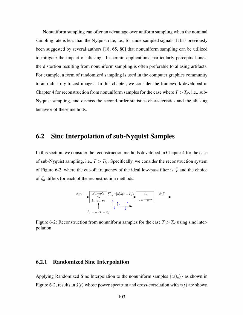
Nonuniform sampling can offer an advantage over uniform sampling when the nominal
sampling rate is less than the Nyquist rate, i.e., for undersampled signals. It has previously
been suggested by several authors [18, 65, 80] that nonuniform sampling can be utilized
to mitigate the impact of aliasing. In certain applications, particularly perceptual ones,
the distortion resulting from nonuniform sampling is often preferable to aliasing artifacts.
For example, a form of randomized sampling is used in the computer graphics community
to anti-alias ray-traced images. In this chapter, we consider the framework developed in
Chapter 4 for reconstruction from nonuniform samples for the case where T > TN , i.e., sub-
Nyquist sampling, and discuss the second-order statistics characteristics and the aliasing
behavior of these methods.
6.2 Sinc Interpolation of sub-Nyquist Samples
In this section, we consider the reconstruction methods developed in Chapter 4 for the case
of sub-Nyquist sampling, i.e., T > TN . Specifically, we consider the reconstruction system
of Figure 6-2, where the cut-off frequency of the ideal low-pass filter is πT and the choice
of ζn differs for each of the reconstruction methods.
T
π
T
x(t)
−
π
T
∑nx[n]δ(t− tn)x[n]
tn = n · T + ζn
Sampleto
Impulse
Figure 6-2: Reconstruction from nonuniform samples for the case T > TN using sinc inter-polation.
6.2.1 Randomized Sinc Interpolation
Applying Randomized Sinc Interpolation to the nonuniform samples x(tn) as shown in
Figure 6-2, results in x(t) whose power spectrum and cross-correlation with x(t) are shown
103

in Appendix G to be
Sxx(Ω) =∞
∑n=−∞
Sxx
(Ω− 2π
Tn)|Φξ ζ
(Ω− 2π
Tn,−Ω
)|2
+T2π
∫ Ωc
−Ωc
Sxx(Ω′)(
1−|Φξ ζ (Ω′,−Ω)|2
)dΩ
′|Ω|< π
T, (6.2)
and
Rxx(t, t − τ) =1
2π
∫ π/T
−π/T
∞
∑n=−∞
(Sxx
(Ω− 2π
Tn)
Φξ ζ
(Ω− 2π
Tn,−Ω
)e j 2π
T n(t−τ))
e jΩτdΩ
=∫ ∞
−∞Rxx(t1) ·
∞
∑n=−∞
[fξ ζ (t1 + t −nT − τ,ζ )∗ sinc(
πT
ζ )]|ζ=t−nT dt1.
(6.3)
Once again, the perturbations in sampling and reconstruction can be designed to shape
the power spectrum of the reconstructed signal through the joint characteristic function
Φξ ζ (Ω1,Ω2). Notice that in the case of T = TN , eqs. (6.2) and (6.3) coincide with the
output power spectrum and the input-output cross-correlation of the system in Figure 4-2.
6.2.2 Uniform Sinc Interpolation
In the case of Uniform Sinc Interpolation, sinc interpolation is applied to the samples placed
on a uniform grid with spacing corresponding to the average spacing of the nonuniform
sampling grid. With respect to second-order statistics, nonuniform sampling followed by
USI is equivalent to the system of Figure 6-3 where vU(t) is zero-mean additive white
noise, uncorrelated with x(t). For the system of Figure 6-3 it is straight forward to show
that
SzU zU (Ω) =∞
∑n=−∞
Sxx
(Ω− 2π
Tn)·∣∣∣∣Φξ
(Ω− 2π
Tn)∣∣∣∣2
+T2π
∫ Ωc
−Ωc
Sxx(Ω′) ·(
1−|Φξ (Ω′)|2)
dΩ′
︸ ︷︷ ︸T 2·SvU vU (Ω)
|Ω|< πT, (6.4)
104

and that
RzU x(t, t − τ) =1
2π
∫ π/T
−π/T
(∞
∑n=−∞
Sxx
(Ω− 2π
Tn)
Φξ
(Ω− 2π
Tn)
e j 2πT n(t−τ)
)e jΩτdΩ.
(6.5)
∑n δ(t− nT )
Φξ(Ω)x(t)
vU (t)
zU (t)T
π
T−
π
T
Figure 6-3: A second-order-statistics equivalent of nonuniform sampling followed by Uni-form Sinc Interpolation for the case where T > TN .
To show the equivalence, we note that with Uniform Sinc Interpolation, i.e., when
ζn = 0, Sxx(Ω) in eq. (6.2) reduces to SzU zU (Ω) in eq. (6.4) and the cross-correlation
Rxx(t, t − τ) in eq. (6.3) reduces to RzU x(t, t − τ) in eq. (6.5). The structure of Figure 6-3
suggests that with respect to second-order statistics, nonuniform sampling with stochastic
perturbations can be modeled as uniform sampling of the signal pre-filtered by the Fourier
transform of the pdf of the sampling perturbation. Correspondingly, the pdf fξ (ξ ) can
be designed subject to the constraints on fξ (ξ ) as a probability density function so that
the characteristic function Φξ (Ω) acts as an equivalent anti-aliasing LPF. Of course the
stochastic perturbation still manifests itself through the additive white noise source vU(t)
in Figure 6-3. Thus, Figure 6-3 suggests that aliasing can be traded off with uncorrelated
white noise by appropriate design of the pdf of the sampling perturbation.
6.2.3 Nonuniform Sinc Interpolation
In the case of Nonuniform Sinc Interpolation, sinc interpolation is applied to the samples
located at the actual nonuniform sampling grid. With respect to second-order statistics
this is equivalent to the system in Figure 6-4 where vN(t) is zero-mean additive noise,
uncorrelated with x(t).
105

p(t) =∑
nfξ(t− nT )
x(t)
vN (t)
zN (t)T
π
T−
π
T
Figure 6-4: A second-order-statistics equivalent of nonuniform sampling followed byNonuniform Sinc Interpolation for the case where T > TN .
For the system of Figure 6-4 it is straight forward to show that
SzNzN (Ω) =∞
∑n=−∞
Sxx
(Ω− 2π
Tn)·∣∣∣∣Φξ
(2πT
n)∣∣∣∣2
+T2π
∫ Ωc
−Ωc
Sxx(Ω′) ·(
1−∣∣∣Φξ (Ω−Ω
′)∣∣∣2)dΩ
′
︸ ︷︷ ︸T 2·SvN vN (Ω)
|Ω|< πT, (6.6)
and that
RzNx(t, t − τ) =∫ ∞
−∞Rxx(τ − τ
′)p(t − τ
′)sinc
(πT
τ′)
dτ′, (6.7)
where p(t) =∑∞n=−∞ fξ (t−nT ). The equivalence is shown by noting that with Nonuniform
Sinc Interpolation, i.e., when ζn = ξn, Sxx(Ω) in eq. (6.2) reduces to SzNzN (Ω) in eq. (6.6)
and Rxx(t, t − τ) in eq. (6.3) reduces to RzNx(t, t − τ) in eq. (6.7). Figure 6-4 suggests that
with respect to second-order statistics, nonuniform sampling followed by NSI is equivalent
to modulating the signal with a periodic signal p(t) with period T , obtained from the pdf
fξ (ξ ) of the perturbation error and adding uncorrelated noise. In the frequency domain,
this corresponds to scaling each replica of the spectrum by |Φξ (2πT n)|2. Correspondingly,
the components in (6.6) associated with aliasing can be eliminated by designing the pdf
fξ (ξ ) so that Φξ (2πT n) = 0 for all n = 0, which corresponds in the time-domain to p(t) = c
where c is a nonzero constant. Of course, similar to USI, the stochastic perturbation still
manifests itself through additive uncorrelated noise, as shown in Figure 6-4. However,
as opposed to USI where the additive noise is white and the signal is pre-filtered by the
characteristic function of the perturbation, the additive noise in NSI is in general not white,
its power spectrum is determined by the convolution of Sxx(Ω) with (1− |Φξ (Ω)|2), and
the shape of the original signal is preserved in reconstruction.
106

6.2.4 Independent Sinc Interpolation
With respect to second-order statistics, Independent Sinc Interpolation corresponds to the
system of Figure 6-5 where vI(t) is zero-mean additive noise, uncorrelated with both vU(t)
and x(t),
SzIzI(Ω) =
∞
∑n=−∞
Sxx
(Ω− 2π
Tn)∣∣∣∣Φξ
(Ω− 2π
Tn)∣∣∣∣2 + T
2π
∫ Ωc
−Ωc
Sxx(Ω′)(
1−|Φξ (Ω′)|2)
dΩ′
︸ ︷︷ ︸T 2·SvU vU (Ω)
· |Φζ (−Ω)|2 +
(1−|Φζ (−Ω)|2
)· T
2π
∫ Ωc
−Ωc
Sxx(Ω′)dΩ
′
︸ ︷︷ ︸T 2·SvIvI (Ω)
|Ω|< πT
(6.8)
and
RzIx(t, t − τ) =1
2π
∫ π/T
−π/T
(∞
∑n=−∞
Sxx
(Ω− 2π
Tn)
Φξ
(Ω− 2π
Tn)
e j 2πT n(t−τ)
)Φζ (−Ω)e jΩτdΩ.
(6.9)
∑n δ(t− nT )
Φξ(Ω)x(t)
Φζ(−Ω)
vI (t)vU (t)
zI (t)T
π
T−
π
T
Figure 6-5: A second-order-statistics equivalent of nonuniform sampling followed by In-dependent Sinc Interpolation for the case where T > TN .
As Figure 6-5 suggests, perturbing the grid on which the samples are placed prior to
sinc interpolation has a similar effect to that of the stochastic perturbations in sampling, i.e.,
the characteristic function of the perturbations acts as a low-pass filter and an uncorrelated
noise is added.
107

6.3 Simulations
In Figure 6-7 we illustrate the different types of artifacts resulting from sub-Nyquist sam-
pling and with each of the reconstruction methods discussed above. We choose the signal
x(t) to be the output of an LTI system driven by white noise for which the transfer function
Hc(s) has unity gain at s = 0, and as shown in Figure 6-6 its poles and zeros locations are
0.1πe jπ(2k+9)/2010k=1 and 0.1π(−0.1± 5
8 j), respectively.
−0.5 −0.4 −0.3 −0.2 −0.1 0 0.1 0.2 0.3 0.4 0.5
−0.5
−0.4
−0.3
−0.2
−0.1
0
0.1
0.2
0.3
0.4
0.5
ℜ (s)
Im(s
)
Figure 6-6: Pole-zero diagram of the transfer function Hc(s).
To simulate a discrete-time signal whose power spectrum is consistent with the power
spectrum of x(t), we process discrete-time white noise with a discrete-time LTI system
whose impulse response h[n] is obtained using the method of impulse invariance, i.e., by
sampling the impulse response hc(t) of the continuous-time system every Td = 1 [sec].
The spacing on this grid is considered to be sufficiently dense so that aliasing is negligible
and it accurately represents the impulse response of the continuous-time system. Figure
6-7(a) shows Sxx(Ω), the estimated power spectrum of x(t) obtained by applying Welch’s
method [73] with Hanning window of length 6656 [sec] and with 50% overlap. 500 blocks
are averaged to obtain the estimate. This method and parameters are used for all spectral
estimates in Figure 6-7.
From the parameters used for generating x(t) and consistent with Figure 6-7(a) we
consider the bandwidth of x(t) to be approximately 0.14π [rad/sec] and the corresponding
value of TN to be approximately 7 [sec]. In the remaining simulations in Figure 6-7, the
average or nominal spacing is T = 13 [sec]≈ 1.8TN , and the power spectrum estimates are
shown over the region [−πT ,
πT ] as if an ideal reconstruction filter was applied.
108
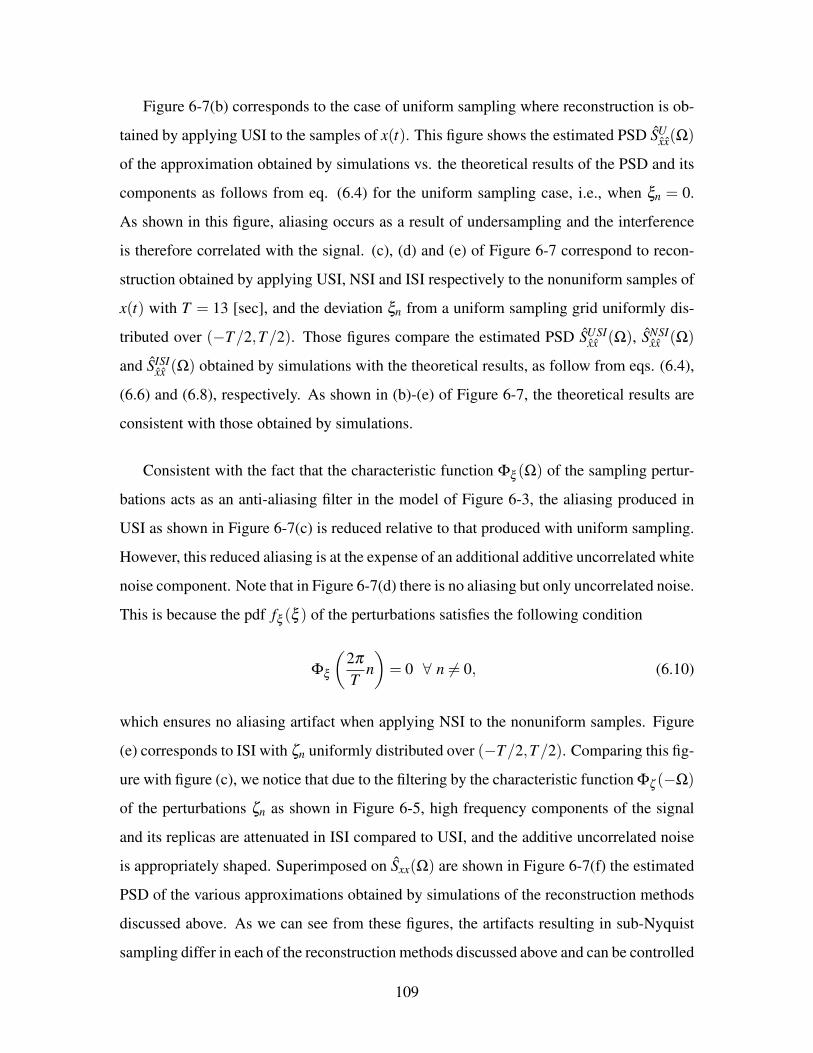
Figure 6-7(b) corresponds to the case of uniform sampling where reconstruction is ob-
tained by applying USI to the samples of x(t). This figure shows the estimated PSD SUxx(Ω)
of the approximation obtained by simulations vs. the theoretical results of the PSD and its
components as follows from eq. (6.4) for the uniform sampling case, i.e., when ξn = 0.
As shown in this figure, aliasing occurs as a result of undersampling and the interference
is therefore correlated with the signal. (c), (d) and (e) of Figure 6-7 correspond to recon-
struction obtained by applying USI, NSI and ISI respectively to the nonuniform samples of
x(t) with T = 13 [sec], and the deviation ξn from a uniform sampling grid uniformly dis-
tributed over (−T/2,T/2). Those figures compare the estimated PSD SUSIxx (Ω), SNSI
xx (Ω)
and SISIxx (Ω) obtained by simulations with the theoretical results, as follow from eqs. (6.4),
(6.6) and (6.8), respectively. As shown in (b)-(e) of Figure 6-7, the theoretical results are
consistent with those obtained by simulations.
Consistent with the fact that the characteristic function Φξ (Ω) of the sampling pertur-
bations acts as an anti-aliasing filter in the model of Figure 6-3, the aliasing produced in
USI as shown in Figure 6-7(c) is reduced relative to that produced with uniform sampling.
However, this reduced aliasing is at the expense of an additional additive uncorrelated white
noise component. Note that in Figure 6-7(d) there is no aliasing but only uncorrelated noise.
This is because the pdf fξ (ξ ) of the perturbations satisfies the following condition
Φξ
(2πT
n)= 0 ∀ n = 0, (6.10)
which ensures no aliasing artifact when applying NSI to the nonuniform samples. Figure
(e) corresponds to ISI with ζn uniformly distributed over (−T/2,T/2). Comparing this fig-
ure with figure (c), we notice that due to the filtering by the characteristic function Φζ (−Ω)
of the perturbations ζn as shown in Figure 6-5, high frequency components of the signal
and its replicas are attenuated in ISI compared to USI, and the additive uncorrelated noise
is appropriately shaped. Superimposed on Sxx(Ω) are shown in Figure 6-7(f) the estimated
PSD of the various approximations obtained by simulations of the reconstruction methods
discussed above. As we can see from these figures, the artifacts resulting in sub-Nyquist
sampling differ in each of the reconstruction methods discussed above and can be controlled
109

−0.06 −0.04 −0.02 0 0.02 0.04 0.06
0.5
1
1.5
Ω/(2π)(a)
Sxx(Ω)
−0.03 −0.02 −0.01 0 0.01 0.02 0.030
0.5
1
1.5
Ω/(2π)(f)
Sxx (Ω)
SUxx(Ω)
SUSIxx (Ω)
SNSIxx (Ω)
SISIxx (Ω)
−0.03 −0.02 −0.01 0 0.01 0.02 0.030
0.5
1
1.5
2
Ω/(2π)(b)
SU
xx(Ω)
SzUzU(Ω)|Φξ(Ω)=1
Replicas
−0.03 −0.02 −0.01 0 0.01 0.02 0.030
0.5
1
1.5
2
Ω/(2π)(c)
SUSI
xx (Ω)
SzUzU(Ω)
T2 · SvU vU(Ω)
Replicas
−0.03 −0.02 −0.01 0 0.01 0.02 0.030
0.5
1
1.5
2
Ω/(2π)(d)
SNSI
xx (Ω)
SzN zN(Ω)
T2 · SvN vN(Ω)
Replicas
−0.03 −0.02 −0.01 0 0.01 0.02 0.030
0.5
1
1.5
2
2.5
Ω/(2π)(e)
SI SI
xx (Ω)
SzIzI(Ω)
T2(
SvU vU(Ω)|Φζ(−Ω)|2 + SvIvI(Ω))
Replicas
Figure 6-7: Artifacts with sub-Nyquist sampling. (a) The estimated power spectrum of x(t).The estimated power spectrum vs. analytic results in the case of (b) Uniform Sampling, (c)USI applied to nonuniform sampling, (d) NSI applied to nonuniform sampling, and (e)ISI applied to nonuniform sampling. (f) The estimated power spectrum of x(t) and of itsapproximations.
by designing the perturbations in sampling and in reconstruction to trade off aliasing with
uncorrelated noise. The artifacts correspond to uniform sampling are more severe in high
frequencies and are correlated with the signal, whereas the artifacts correspond to the re-
construction methods from nonuniform sampling have reduced or no correlation with the
signal and are more balanced across frequency.
110
CHAPTER 7
SUB-NYQUIST SAMPLING & ALIASING
7.1 Introduction
This chapter explores various sampling schemes for which the sampling rate is below the
Nyquist rate, but additional information about the signal apart from its bandwidth is ex-
ploited. Specifically, in Section 7.2 we consider sampling of non-negative bandlimited
signals, in which nonlinearity is incorporated prior to sampling as a way to decrease the
signal’s bandwidth. When perfect reconstruction is not possible with this approach, the
nonlinear processing is viewed as an alternative to anti-aliasing LTI lowpass filtering. Sec-
tion 7.3 suggests a different approach, referred to as inphase-quadrature anti-aliasing, in
which a bandlimited signal is approximated by another bandlimited signal with reduced
bandwidth. In Section 7.4 we develop co-sampling which suggests exploiting dependen-
cies between signals in order to reduce their effective total sampling rate.
7.2 Sampling a Non-negative Bandlimited Signal
The Nyquist-Shannon sampling theorem provides a sufficient rate for which perfect recon-
struction of a bandlimited signal is possible from its equally spaced samples. If the only
information available about a bandlimited signal is its bandwidth, the Nyquist rate is the
minimum sampling rate for which perfect reconstruction is possible. With additional in-
formation exploited apart from the signal’s bandwidth, there is the possibility of reducing
the sampling rate below the Nyquist rate and still achieving perfect reconstruction. For
example, when a bandlimited signal is processed through a nonlinear system, the informa-
111

tion about the system can sometimes be exploited to reduce the signal’s sampling rate. To
illustrate the concept, consider the following example:
y(t) = |x(t)|2 = x(t) · x∗(t), (7.1)
where x(t) is bandlimited. Utilizing the fact that the bandwidth of x(t) is half the bandwidth
of y(t), we can extract the signal x(t) and sample it at its Nyquist rate, which is half the
Nyquist rate of y(t). Provided that x(t) is real, we achieve with this approach a sampling
rate reduction by a factor of two. However, obtaining x(t) from y(t) is not a trivial task
since the absolute square root of y(t) does not yield in general a bandlimited signal. For
example, when y(t) = sinc2(πT t), its absolute square root is clearly not bandlimited as it has
infinitely many non-differentiable points. Thus, the recovery of the signal’s phase becomes
crucial for this sampling approach. The bandlimitedness of x(t) can be exploited for this
purpose.
Figure 7-1 suggests a system for sampling and reconstruction of the bandlimited signal
y(t), in which the relation in (7.1) is utilized. The sampling system consists of bandlimited-
square-root processing, whose output is a bandlimited signal x(t) such that y(t) = |x(t)|2,
followed by uniform sampling at half the Nyquist rate of y(t). The reconstruction is ac-
complished by taking the magnitude square of the continuous-time signal obtained from
sinc interpolation of the equally-spaced samples of x(t).
Non-linear Sampling Non-linear Reconstruction
C/Dx(t) x[n]
T
BLy(t)·
x[n]D/C
·
x(t) y(t)2
T
Figure 7-1: A sampling-reconstruction scheme of a non-negative bandlimited signal. Thesampling system consists of non-linear pre-processing whose output signal x(t) is bandlim-ited to ±π/T and satisfies the relation y(t) = |x(t)|2.
112

7.2.1 Bandlimited Square-roots
Boas and Kak [45] have shown that for a real non-negative function y(t), integrable on
(−∞,∞), and whose spectrum has no component at or above the frequency 2π/T , there
exists a function x(t) whose spectrum X(Ω) vanishes outside (−π/T ,π/T ), and for which
Y (Ω) =1
2π
∫ π/T
−π/TX(ξ )X∗(ξ −Ω)dξ . (7.2)
This theorem asserts that there exists a bandlimited signal x(t) that satisfies (7.1) and whose
bandwidth is half the bandwidth of y(t). The signal x(t) will be referred to as a bandlimited
square-root of y(t).
The problem of finding bandlimited square-roots of a real non-negative bandlimited
signal is equivalent in the time-domain to the problem of finding the set of all time-limited
functions having a specified autocorrelation function, a problem which E. M. Hofstetter
considered in [34]. To explore the former problem, we take a similar approach to that
introduced in [34]. Specifically, we obtain the analytic continuation of y(t) on the complex
plane by transforming the frequency response Y (Ω) into the complex s-domain, i.e.,
y(s) =1
2π
∫ ∞
−∞Y (Ω) · e−sΩdΩ, (7.3)
from which y(t) is obtained along the line s =− jt.
According to the Paley-Wiener theorem [8], since y(t) is bandlimited or, equivalently,
since the support of Y (Ω) is finite, y(s) is an entire function of an exponential type, meaning
that there is a constant C such that
|y(s)| ≤Ceα|s|. (7.4)
This fact combined with Hadamard’s factorization theorem [86] implies that
y(s) = Asneas∞
∏k=1
(1− s
sk
)es/sk , (7.5)
i.e., y(s) is completely specified (up to a complex constant) by the location of its zeros.
113

With (7.2) substituted into (7.3), we obtain
y(s) = x(s) · x∗(−s∗), (7.6)
from which it follows that the same spectrum Y (Ω) can correspond to two different signals
x1(s) and x2(s), provided that
x1(s) · x∗1(−s∗) = x2(s) · x∗2(−s∗). (7.7)
Specifically, if x1(t) is bandlimited and its analytic continuation on the complex plane x1(s)
satisfies (7.6), then any other signal obtained from x1(s) by replacing its zeros with their
negative conjugates will also correspond to a bandlimited signal which satisfies (7.6) [34].
The number of different bandlimited square-roots may be either finite or infinite, depending
on the signal y(t).
7.2.1.1 Min-Phase Bandlimited Square-root
As discussed in the previous section, we can replace some or all zeros of one solution of
eq. (7.6) with their negative conjugates to obtain other solutions of eq. (7.6). Provided that
y(s) has no zeros on the imaginary axis, the solution whose zeros are all located in the left
region of the complex plane is of particular interest. This solution, denoted as xmin(s), will
be referred to as the min-phase bandlimited square-root. Defining the partial energy of x(t)
as
EX(ξ ) =1
2π
∫ ξ
−∞|X(Ω)|2 dΩ, (7.8)
it can be shown that the energy of the min-phase signal is delayed the least of all signals
x(t) satisfying eq. (7.1), i.e.,
12π
∫ ξ
−∞|Xmin(Ω)|2 dΩ ≥ 1
2π
∫ ξ
−∞|X(Ω)|2 dΩ, ∀ξ . (7.9)
To prove the inequality in (7.9), we first note that since all solutions satisfy the relation
114

|x(t)|2 = y(t), they all have the same total energy. Therefore, equality in (7.9) is achieved
for ξ → ∞, i.e.,
12π
∫ ∞
−∞|Xmin(Ω)|2dΩ =
12π
∫ ∞
−∞|X(Ω)|2dΩ. (7.10)
To prove that (7.9) is true for any other ξ , we follow a similar argument to that presented
in [69] for the discrete-time case. Specifically, we assume that s0 is a zero of xmin(s) and
represent it as
xmin(s) = q(s) · (s− s0), (7.11)
where q(s) is another min-phase signal. Processing xmin(s) through an all-pass term which
moves its zero at s = s0 to its mirror image location, s =−s∗0, we obtain
x(s) = xmin(s) ·s+ s∗0s− s0
= q(s) · (s+ s∗0), (7.12)
which is another solution of (7.6). Denoting Q(Ω) as the frequency response correponding
to q(s), it follows from (7.11) and (7.12) that the frequency response Xmin(Ω) correspond-
ing to xmin(s) and the frequency response X(Ω) corresponding to x(s) can be represented
as follows:
Xmin(Ω) =dQ(Ω)
dΩ− s0 ·Q(Ω),
X(Ω) =dQ(Ω)
dΩ+ s∗0 ·Q(Ω), (7.13)
from which it follows that
|Xmin(Ω)|2 −|X(Ω)|2 =−4ℜ(s0) ·ℜ(
Q(Ω) · dQ∗(Ω)
dΩ
)=−2ℜ(s0) ·
d |Q(Ω)|2
dΩ. (7.14)
Integrating (7.14) with respect to Ω and noting that s0 lies in the left half plane, we obtain
12π
∫ ξ
−∞
(|Xmin(Ω)|2 −|X(Ω)|2
)dΩ =−ℜ(s0)
π· |Q(ξ )|2 ≥ 0. (7.15)
115

Rearranging (7.15) completes the proof of (7.9). The minimum delay energy property will
be utilized in section 7.2.3.
7.2.1.2 Real Bandlimited Square-roots
If x(t) is real, its Fourier transform is conjugate symmetric and x(s) = x∗(−s∗). It then
follows that zeros of x(s) which are not purely imaginary occur in pairs (s0,−s∗0) and that
y(s) = x2(s). (7.16)
As suggested by eq. (7.16), a necessary condition for the existence of a real bandlimited
square root is that all zeros of y(s) will have an even order.
7.2.2 Signals with Real Bandlimited Square-roots
We next discuss some of the characteristics of a real non-negative bandlimited signal y(t)
which possess a real bandlimited square-root. Applying the Fourier transform to eq. (7.1),
we obtain
Y (Ω) =1
2π
∫ ∞
−∞X(ξ ) ·X∗(ξ −Ω)dξ , (7.17)
from which the following inequality clearly follows:
|Y (Ω)| ≤ Y (Ω)|Ω=0. (7.18)
Adding the fact that x(t) is bandlimited to ±π/T , it follows from (7.17) that
Y (Ω) =
12π∫ π/T−π/T+Ω X(ξ ) ·X∗(ξ −Ω)dξ 0 ≤ Ω < 2π
T1
2π∫ π/T−Ω−π/T X(ξ ) ·X∗(ξ −Ω)dξ −2π
T < Ω < 0. (7.19)
Applying the Cauchy-Schwartz inequality to (7.19) results in the following inequality:
|Y (Ω)|2 ≤ 12π
∫ π/T
|Ω|−π/T|X(ξ )|2dξ · 1
2π
∫ π/T
|Ω|−π/T|X∗(−ξ )|2dξ 0 ≤ |Ω| ≤ 2π/T, (7.20)
116

which reduces to the following inequality when x(t) is real
|Y (Ω)| ≤ 12π
∫ πT
|Ω|− πT
|X(ξ )|2 dξ , 0 ≤ |Ω|< 2π/T
=
12Y (Ω)|Ω=0 +
12π∫ 0|Ω|− π
T|X(ξ )|2 dξ , ∀ 0 ≤ |Ω| ≤ π
T ,
12Y (Ω)|Ω=0 − 1
2π∫ |Ω|− π
T0 |X(ξ )|2 dξ , ∀ π
T ≤ |Ω| ≤ 2πT .
(7.21)
As implied from (7.21), a necessary but not sufficient condition for a non-negative ban-
dlimited signal to possess a real bandlimited square root is that
|Y (π/T −|ξ |)|+ |Y (π/T + |ξ |)| ≤ Y (Ω) |Ω=0 ∀ 0 ≤ |ξ | ≤ π/T . (7.22)
The inequality in (7.22) suggests alternative upper bounds to those implied by (7.18) on the
value of |Y (π/T )| and on the area under |Y (Ω)| . Specifically,
|Y (π/T )| ≤ (1/2) ·Y (Ω) |Ω=0 , (7.23a)
and
T2π
∫ 2πT
0|Y (Ω)|dΩ ≤ (1/2) ·Y (Ω)|Ω=0. (7.23b)
Figure 7-2 specifies a region that bounds all possible |Y (Ω)| that satisfy (7.21). Indicated
within this region is the triangular-shape frequency response of y(t) = sinc2(πT t), which
achieves (7.21) with equality. Note that a non-negative real bandlimited signal y(t) whose
absolute frequency response |Y (Ω)| violates the boundaries of this region cannot possess a
real bandlimited square-root.
− 2π
T
2π
T
π
T− π
T
|Y (Ω)|
Ω
Y (0)
Y (0)/2
Figure 7-2: The region within which all possible |Y (Ω)| that satisfy (7.21) lie.
117

7.2.3 Nonlinear Anti-aliasing
When the Nyquist condition is not satisfied and we wish to avoid aliasing in sampling, addi-
tional information about the signal apart from its bandwidth can be exploited to developing
alternative pre-processing instead of the traditional LTI anti-aliasing lowpass filter. With
these alternative approaches there is the possibility of reducing the approximation error ob-
tained with LTI anti-aliasing. In addition, when the bandlimited signal is non-negative, for
example, LTI anti-aliasing may be undesirable as it does not preserve the non-negativity
of the signal. We next address various nonlinear approaches for processing a non-negative
bandlimited signal prior to sampling it. This processing will be referred to as non-linear
anti-aliasing. The general structure of the sampling-reconstruction system that will be con-
sidered here is motivated by the system of Figure 7-1.
7.2.3.1 Complex Nonlinear Anti-aliasing
This section considers the system depicted in Figure 7-3, in which the bandlimited signal
y(t) is assumed to possess only complex bandlimited square roots. The signal x(t), rep-
resenting a complex bandlimited square-root of y(t), is processed through an LTI system,
whose impulse response, possibly complex, is h(t), to yield the following approximation:
x(t) = x(t)∗h(t). (7.24)
h(t)y(t) x(t) x(t)
BL
·
Figure 7-3: Non-linear anti-aliasing.
Approximating the signal y(t) with y(t) = |x(t)|2 and denoting e(t) = y(t)− y(t) as the
approximation error, its energy can be represented as follows:
∫ ∞
−∞(y(t)− y(t))2 dt =
12π
∫ 2πT
− 2πT
|Y (Ω)− Y (Ω)|2dΩ (7.25)
=1
2π
∫ 2πT
− 2πT
∣∣∣∣ 12π
∫ πT
−πT
(X(ξ )X∗(ξ −Ω)− X(ξ )X∗(ξ −Ω)
)dξ∣∣∣∣2 dΩ.
118

Using the Cauchy-Schwartz inequality in (7.26), the following upper bound on the approx-
imation error is obtained
∫ ∞
−∞(y(t)− y(t))2 dt ≤ 1
T· 1
2π
∫ 2πT
− 2πT
(1
2π
∫ πT
−πT
∣∣X(ξ )X∗(ξ −Ω)− X(ξ )X∗(ξ −Ω)∣∣2 dξ
)dΩ
=1T
(EX
2 −2|RXX |2 +EX
2) , (7.26)
in which
EX =1
2π
∫ πT
−πT
|X(Ω)|2 dΩ,
EX =1
2π
∫ πT
−πT
∣∣X(Ω)∣∣2 dΩ, (7.27)
and
RXX =1
2π
∫ πT
−πT
X(Ω)X∗(Ω)dΩ. (7.28)
We now consider the LTI system in Figure 7-3, whose impulse response is h(t), to have
the following frequency response:
H(Ω) =
1 −π/T ≤ Ω ≤ γ < π/T
0 otherwise, (7.29)
as depicted in Figure 7-4.
−
π
Tγ
1
Ω
H(Ω)
Figure 7-4: The frequency response H(Ω) of the LTI system in Figure 7-3.
With this choice of h(t), the bandwidth of the approximation x(t) is reduced relative to
119
the bandwidth of x(t), and the upper bound in (7.26) satisfies the following inequalities:
1T
(EX
2 −2|RXX |2 +EX
2) ≥ 1T
(EX
2 −2EX · 12π
∫ γ
−π/T|X(Ω)|2dΩ+EX
2)
≥ 1T
(EX
2 −∣∣∣∣ 12π
∫ γ
−π/T|X(Ω)|2dΩ
∣∣∣∣2)
≥ 1T
(EX
2 −∣∣∣∣ 12π
∫ γ
−π/T|Xmin(Ω)|2dΩ
∣∣∣∣2). (7.30)
The first inequality is obtained from applying the Cauchy-Schwartz inequality on RXX in
(7.28), i.e.,
|RXX |2 ≤ 1
2π
∫ γ
−π/T|X(Ω)|2dΩ · 1
2π
∫ γ
−π/T|X∗(Ω)|2dΩ, (7.31)
where equality is achieved if and only if
X(Ω) = X(Ω), −π/T ≤ Ω ≤ γ . (7.32)
The second inequality follows by noting that with respect to EX we have a quadratic form
whose minimum occurs at EX = 12π∫ γ−π/T |X(Ω)|2dΩ. The last inequality exploits the min-
imum energy delay property of the min-phase solution xmin(s), as discussed in section
7.2.1.1, while taking into account the fact that the energy EX is the same for all signals
satisfying (7.1).
Thus, it follows from (7.26) together with (7.30) that the upper bound on the error in
approximating y(t) with y(t) = |x(t)|2 is minimized when
X(Ω) = Xmin(Ω) = Xmin(Ω) ·H(Ω) =
Xmin(Ω) −π/T ≤ Ω ≤ γ
0 otherwise. (7.33)
In this case,
∫ ∞
−∞(y(t)−|xmin(t)|)2 dt ≤ 1
T·
(Ex
2 −∣∣∣∣ 12π
∫ γ
−π/T|Xmin(Ω)|2dΩ
∣∣∣∣2). (7.34)
120

In this approach, we first extract the min-phase bandlimited square-root xmin(t) of y(t),
and then process it through the LTI system whose impulse response is h(t). Though the
min-phase solution can be obtained from spectral decomposition of y(s), an alternative ap-
proach can be taken, in which we utilize the facts that for min-phase signals, the continuous-
time phase arg(xmin(t)) is related to log|xmin(t)| by the Hilbert transform and that the mag-
nitude |xmin(t)| is the absolute square root of y(t).
As a simple illustratation of the nonlinear anti-aliasing approach, we consider the signal
used in [34]
y(t) =sinh2(aΩx)
π2(a2 + t2), (7.35)
whose frequency response is zero outside the support (−2Ωx,2Ωx), and
Y (Ω) =
sinh(a(2Ωx−Ω))
2πa 0 ≤ Ω < 2Ωx
sinh(a(2Ωx+Ω))2πa −2Ωx < Ω < 0.
(7.36)
Transforming Y (Ω) into the complex s-domain using (7.6), we obtain
y(s) =1
2π2 ·cosh(2sΩx)− cosh(2aΩx)
(s−a)(s+a)
=sinh((s−a)Ωx)
π(s−a)· sinh((s+a)Ωx)
π(s+a), (7.37)
from which it follows that the zeros of y(s) are located at
s =±a+ jπ
Ωxk, k =±1,±2, . . . (7.38)
Since the zeros of y(s) do not have an even order, y(t) does not possess a real bandlimited
square root. Instead, there are infinitely many complex solutions. One of particular interest
is the min-phase solution
xmin(s) =sinh((s−a)Ωx)
π(s−a), (7.39)
121

whose zeros are all located in the left half plane, i.e.,
zk = a+ j(π/Ωx)k, k =±1,±2, . . . (7.40)
and its corresponding frequency response is
Xmin(Ω) =
eaΩ |Ω|< Ωx
0 |Ω| ≥ Ωx
. (7.41)
Other solutions may be obtained by replacing zeros of xmin(s) with their negative conju-
gates. Specifically, applying the all-pass system
H(s) =s+(a− jπ/Ωx)
s− (a+ jπ/Ωx)· s+(a+ jπ/Ωx)
s− (a− jπ/Ωx)
=(s+a)2 +(π/Ωx)
2
(s−a)2 +(π/Ωx)2
= 1+4as−a
(s−a)2 +(π/Ωx)2 +4a2
π/Ωx· π/Ωx
(s−a)2 +(π/Ωx)2 (7.42)
to xmin(s) will replace its zeros located at a± jπ/Ωx with their negative conjugates −(a±
jπ/Ωx). In the frequency domain, this processing corresponds to convolving Xmin(Ω) with
H(Ω) = 2π ·[
δ (Ω)+4aeaΩ ·(
cos(πΩ/Ωx)+aΩx
πsin(πΩ/Ωx)
)u(Ω)
], (7.43)
which yields
X1(Ω) =1
2πXmin(Ω)∗H(Ω)
=
eaΩ(
1+ 4aπ/Ωx
·(
aΩxπ + aΩx
π · cos(πΩ/Ωx)− sin(πΩ/Ωx)))
, |Ω|< Ωx
0, |Ω| ≥ Ωx
.
(7.44)
Replacing the even index zeros of xmin(s) with their negative conjugates will obtain
122

another solution, x2(s), whose frequency response is
X2(Ω) =
ea(Ω+Ωx) −Ωx ≥ Ω < 0
ea(Ω−Ωx) 0 ≤ Ω < Ωx.(7.45)
−π/Τ −π/2Τ 0 π/2Τ π/Τ
0
1
2
3
4
Ω(a)
Xmin (Ω)
X1(Ω)X2(Ω)
−π/Τ −π/2Τ 0 π/2Τ π/Τ
0.2
0.4
0.6
0.8
1
Ω(b)
EXmin (Ω)
EX1(Ω)
EX2(Ω)
−2π/Τ −π/Τ 0 π/Τ 2π/Τ 0
0.2
0.4
0.6
0.8
1
Ω(c)
Y (Ω)
Ymin (Ω)
Y1(Ω)
Y2(Ω)
−2π/Τ −π/Τ 0 π/Τ 2π/Τ 0
0.2
0.4
0.6
0.8
1
Ω(d)
Y (Ω)
Ymin (Ω)
Y1(Ω)
Y2(Ω)
Figure 7-5: Complex anti-alising applied to y(t) from (7.35) where a = −π/2 and Ωx =π/T . (a) The spectrums of the complex bandlimited square roots. (b) The partial energiesof the complex bandlimited square roots. (c) The frequency responses of y(t) and of itsapproximations y(t) = |x(t)|2 where the cut-off frequency of H(Ω) is γ = π/(2T ). (d)The frequency responses of y(t) and of its approximations y(t) = |x(t)|2 where the cut-offfrequency of H(Ω) is γ = π/(4T ).
Figure (a) of 7-5 shows the spectrums Xmin(Ω), X1(Ω) and X2(Ω), as indicated in (7.41),
(7.44) and (7.45) for the case of a =−π/2 and Ωx = π/T . In Figure (b) the partial energies
of these signals are shown and the minimum energy delay property is illustrated, i.e., the
energy of the min-phase signal is shown to be delayed the least of the other two signals
considered. (c) and (d) of Figure 7-5 show the spectrum Y (Ω) of the given signal y(t)
along with the spectrums of its approximations obtained from the system of Figure 7-3 for
123

different bandlimited square roots, i.e., ymin(t) = |xmin(t)|2, y1(t) = |x1(t)|2, and y2(t) =
|x2(t)|2. The cut-off frequency γ of H(Ω) used in the approximations of Figure (c) is
π/(2T ) and in the approximation of Figure (d) is π/(4T ). In both cases, the approximation
of y(t) obtained with the min-phase bandlimited square-root yields the lowest error.
This approach suggests a constructive procedure for obtaining a non-negative approx-
imation of y(t) whose bandwidth is reduced. In addition, the choice x(t) = xmin(t) min-
imizes, among all bandlimited square-roots, the error in approximating x(t) with x(t) =
x(t) ∗ h(t), where h(t) is the impulse response whose frequency response is specified in
(7.29). Note, however, that minimizing the error in approximating x(t) with x(t) = x(t) ∗
h(t) does not necessarily imply that the error in approximating y(t) with y(t) = |x(t)|2 is
the minimum possible for that bandwidth constraint. In fact, a lower error may be achieved
with LTI anti-aliasing filter at the expense of not preserving the non-negativity property of
the signal.
The complex bandlimited square-root signal can be a base for a variety of other approx-
imate non-negative representations of y(t) with a reduced bandwidth. The signal y(t) can
be still approximated with |x(t)|2; however, we may consider other ways for approximating
x(t). For example,
x(t) = ℜx(t)∗h1(t)+ jℑx(t)∗h2(t), (7.46)
where h1(t) and h2(t) are LTI selective filters that determine the total bandwidth of the
approximate representation. Special cases of this choice are the real part xR(t) = ℜx(t)
or the imaginary part xi(t) = ℑx(t) of the complex bandlimited square root x(t). Note
that since with this choice of x(t), the actual bandwidth of y(t) may be larger than its
effective bandwidth, this approximation may produce a lower error than that produced with
the appropriate LTI anti-aliasing lowpass filtering.
7.2.3.2 Bandlimited Square-root as a Nonlinear Least-squares Problem
If a real bandlimited square root does not exist, a real bandlimited signal x(t) can be ob-
tained whose square is closest, in the least square sense, to the non-negative bandlimited
124

signal y(t). Specifically, we formulate the following nonlinear least-squares problem,
y(t)≈ x2(t), (7.47)
and solve for x(t). To restrict the solution to be bandlimited, we represent x(t) in (7.47)
as the sinc interpolation of its Nyquist rate samples x[n] = x(nT ). We then choose these
samples to minimize the least-squares error, i.e.,
minx[n]
∫ ∞
−∞
y(t)−
(∞
∑n=−∞
x[n] ·h(t −nT )
)22
dt, (7.48)
where h(t) = sinc(πT t). Rather than solving the nonlinear optimization in (7.48), we will
linearize it and solve instead a linear least squares problem [6]. Linearization of x2(t) =
(∑∞n=−∞ x[n]h(t −nT ))2 around x[n] = x∗[n] will obtain
x2(t)≈
(∞
∑k=−∞
x∗[k]h(t − kT )
)2
+2
(∞
∑k=−∞
x∗[k]h(t − kT )
)·
∞
∑n=−∞
h(t −nT )(x[n]− x∗[n]).
(7.49)
Denoting by y∗(t)= (x∗(t))2 =(∑∞
k=−∞ x∗[k]h(t − kT ))2 and by z∗(t)= (y(t)+y∗(t))/2,
the solution to the non-linear least squares problem in (7.47) can be approximated by the
solution to the following linear least-squares problem
z∗(t)≈ x∗(t) ·∞
∑n=−∞
x[n]h(t −nT ). (7.50)
Iteratively solving the linear least-squares problem in (7.50), we obtain
12π
∫ πT
− πT
X (l+1)(ξ ) ·Y (l)(Ω−ξ )dξ =1
2π
∫ πT
− πT
X (l)(ξ ) ·Z(l)(Ω−ξ )dξ ∀ |Ω| ≤ πT, (7.51)
where X (l)(Ω), Y (l)(Ω) and Z(l)(Ω) are the frequency responses of x(l)(t), y(l)(t) and z(l)(t),
respectively, and where the superscripts indicate the iteration number. Note that as sug-
gested by eq. (7.51), the nonlinear deconvolution of the original problem is replaced with
125

an iterative set of linear deconvolutions.
7.2.4 Generalization
Given two bandlimited signals x1(t) and x2(t) whose bandwidths are W1 and W2, the band-
width W of the signal y(t) obtained from multiplying x1(t) with x2(t) can in general be
equal, greater or lower than the sum of their bandwidths. Each of these cases is illustrated
in the examples of Figures (7-6), (7-7) and (7-8).
∗ =
1−1 Ω
X1(Ω)
1−1 Ω
X2(Ω)
2−2 Ω
Y (Ω) = X1(Ω) ∗X2(Ω)
Figure 7-6: An example for which the bandwidth of y(t) is equal to the sum of the band-widths of x1(t) and x2(t).
−1 1 −1−2 1 2
∗ =
−3 3
X1(Ω)
Ω
X2(Ω)
Ω
Y (Ω) = X1(Ω) ∗X2(Ω)
Ω
Figure 7-7: An example for which the bandwidth of y(t) is greater than the sum of thebandwidths of x1(t) and x2(t).
41 2
∗ =
X1(Ω)
Ω
X2(Ω)
Ω
Y (Ω) = X1(Ω) ∗X2(Ω)
Ω12 3 −6 −2−4 2 4 6
Figure 7-8: An example for which the bandwidth of y(t) is less than the sum of the band-widths of x1(t) and x2(t).
This observation may suggest approximating a bandlimited signal as a multiplication
of two or more signals whose total bandwidth is lower than the bandwidth of the original
signal. This is a further generalization of the notion of nonlinear anti-aliasing to a broader
class of signals, not just non-negative bandlimited signals, which offers a way to optimize
the trade off between the sampling rate and the approximation error.
126

7.3 Inphase and Quadrature Anti-aliasing
A straightforward generalization of anti-aliasing low pass filtering is multi-channel anti-
aliasing. In this case, the continuous-time signal is first decomposed in the frequency do-
main into sub-bands. Each sub-band is then processed according to its frequency content
through a frequency selective filter, and the outputs are finally composed to obtain the re-
duced bandwidth approximation. As a special case, the selective filters can be replaced
by multipliers with zero or one depending on the energy of the corresponding sub-band
component and the desired bandwidth with which we wish to approximate the signal. The
resulting approximation is associated with an error which is proportional to the total energy
of the sub-band components that were filtered out. Clearly, the more sub-bands we include
in the approximation, the higher its bandwidth is and the lower its corresponding error is.
In this section we introduce a different orthogonal decomposition, which suggests an
alternative anti-aliasing method referred to as inphase-quadrature (IQ) anti-aliasing. With
this method there is the possibility of reducing the approximation error as compared to
the error associated with LTI anti-aliasing filtering. Section 7.3.1 introduces the inphase-
quadrature decomposition. In section 7.3.2, we propose an anti-aliasing approach that uti-
lizes the IQ decomposition and discuss its relation to recurrent nonuniform sampling.
7.3.1 Inphase and Quadrature Decomposition
Consider a bandlimited signal y(t) whose frequency response Y (Ω) contains no component
at or above the frequency Ωc. Defining the inphase and quadrature components of y(t) as
iy(t) =(√
2/2)· cos(Ωct/2) · y(t)+
(√2/2)· sin(Ωct/2) · y(t), (7.52a)
and
qy(t) =(√
2/2)· sin(Ωct/2) · y(t)−
(√2/2)· cos(Ωct/2) · y(t), (7.52b)
where y(t) = 1/π∫ ∞−∞ y(τ)/(t − τ)dτ is the Hilbert transform of y(t), we can decompose
y(t) as
127

y(t) =√
2 · cos(Ωc/2t) · iy(t)︸ ︷︷ ︸y1(t)
+√
2 · sin(Ωc/2t) ·qy(t)︸ ︷︷ ︸y2(t)
. (7.53)
Since iy(t) and qy(t) are real valued signals and each is bandlimited with half the bandwidth
of y(t), the equivalent representation of y(t) in terms of the signals iy(t) and qy(t) has an
effective bandwidth equal to the bandwidth of y(t).
We next show that the signals y1(t)=√
2·cos(Ωc/2t)·iy(t) and y2(t)=√
2·sin(Ωc/2t)·
qy(t) are orthogonal projections of the signal y(t). Orthogonality is shown by proving that
the inner product ⟨y1(t),y2(t)⟩= 0. Specifically,
⟨y1(t),y2(t)⟩ =∫ ∞
−∞y1(t) · y2(t)dt =
=∫ ∞
−∞
√2 · cos(Ωc/2t) · iy(t) ·
√2 · sin(Ωc/2t) ·qy(t)dt, (7.54)
from which it follows by using Parseval’s relation
⟨y1(t),y2(t)⟩ = 2 · 12π
∫ ∞
−∞
12[Iy(Ω+Ωc/2)+ Iy(Ω−Ωc/2)]
· 12 j
[Qy(Ω+Ωc/2)−Qy(Ω−Ωc/2)]∗ dΩ
=1
4π j·∫ ∞
−∞Iy(Ω+Ωc/2) ·Qy
∗(Ω+Ωc/2)dΩ
−∫ ∞
−∞Iy(Ω−Ωc/2) ·Qy
∗(Ω−Ωc/2)dΩ= 0. (7.55)
To show that y1(t) is a projection of y(t), we note that an alternative representation of
y1(t) in terms of y(t) and y(t) can be obtained by using iy(t) from (7.52a). Specifically,
y1(t) =12[y(t)+ cos(Ωct)y(t)+ sin(Ωct)y(t)] , (7.56)
or in the frequency domain,
Y1(Ω) =12[Y (Ω)+Y−(Ω−Ωc)+Y+(Ω+Ωc)] , (7.57)
128

where
Y−(Ω) =
Y (Ω) −Ωc < Ω < 0
0 otherwise, (7.58)
and
Y+(Ω) =
Y (Ω) 0 < Ω < Ωc
0 otherwise. (7.59)
Then, denoting by f1(·) the linear transformation from Y (Ω) to Y1(Ω) in (7.57) and apply-
ing f1(·) again on Y1(Ω), we obtain f1 (Y1(Ω)) =Y1(Ω), from which it follows that y1(t) is
an orthogonal projection of y(t). Similar to the representation in (7.57), it is straightforward
to show that the Fourier transform Y2(Ω) of y2(t) obeys
Y2(Ω) =12[Y (Ω)−Y−(Ω−Ωc)−Y+(Ω+Ωc)] , (7.60)
and that y2(t) is an orthogonal projection of y(t). Figure 7-9 illustrates the decomposition
of Y (Ω) into Y1(Ω) and Y2(Ω), as implied from (7.57) and (7.60).
Ω
Y2(Ω) =1
2(Y (Ω)− Y
−(Ω− Ωc)− Y+(Ω + Ωc))
Ω Ω
Y (Ω)
Y+(Ω + Ωc)Y−(Ω− Ωc)
Ωc−Ωc
−ΩcΩc
Ωc Ωc−Ωc −Ωc
Y1(Ω) =1
2(Y (Ω) + Y
−(Ω− Ωc) + Y+(Ω + Ωc))
Figure 7-9: Decomposing Y (Ω) into Y1(Ω) and Y2(Ω).
129
The orthogonality in (7.55) between y1(t) and y2(t) implies that the energy Ey =∫ ∞−∞ y2(t)dt
of y(t) is equal to the sum of the energies E1 of y1(t) and E2 of y2(t). Using Parseval’s re-
lation, it can also be shown that E1 = Ei and E2 = Eq. Specifically,
E1 =∫ ∞
−∞y1
2(t)dt =∫ ∞
−∞
(iy(t) ·
√2 · cos(Ωc/2t)
)2dt
=12· 1
2π
∫ ∞
−∞
∣∣Iy(Ω+Ωc/2)+ Iy(Ω−Ωc/2)∣∣2 dΩ
=∫ ∞
−∞i2y(t)dt = Ei, (7.61a)
and
E2 =∫ ∞
−∞y2
2(t)dt =∫ ∞
−∞
(qy(t) ·
√2 · sin(Ωc/2t)
)2dt
=12· 1
2π
∫ ∞
−∞
∣∣∣∣1j Qy(Ω+Ωc)−1jQy(Ω−Ωc)
∣∣∣∣2 dΩ
=∫ ∞
−∞qy
2(t)dt = Eq. (7.61b)
Note, however, that the energy Ey of y(t) is not equally distributed between y1(t) and y2(t),
or alternatively between iy(t) and qy(t). Specifically,
E1 =12·Ey +ℜ
1
2π
∫ Ωc
0Y (Ω) ·Y ∗(Ω−Ωc)dΩ
,
E2 =12·Ey −ℜ
1
2π
∫ Ωc
0Y (Ω) ·Y ∗(Ω−Ωc)dΩ
, (7.62)
as follows from (7.57) and (7.60). This property will be exploited in the next section in
which we discuss approximation of y(t) in terms of its IQ components.
7.3.2 IQ Anti-aliasing
As an alternative approach to LTI anti-aliasing, the IQ decomposition suggests decompos-
ing the bandlimited signal y(t) into iy(y) and qy(t) and then processing these components
through LTI selective filters to yield the approximations iy(t) and qy(t) from which we
130

obtain
y(t) =√
2 · cos(Ωc/2t) · iy(t)+√
2 · sin(Ωc/2t) · qy(t), (7.63)
whose effective bandwidth is reduced as compared to that of y(t). Denoting ey(t) = y(t)−
y(t) as the error in approximating y(t) with y(t), it can be shown by using Parseval’s relation
that
∫ ∞
−∞ey
2(t)dt =∫ ∞
−∞ei
2(t)dt +∫ ∞
−∞eq
2(t)dt, (7.64)
where ei(t) and eq(t) are the errors corresponding to approximating iy(t) with iy(t) and
qy(t) with qy(t), respectively. As follows from (7.64), the approximation of y(t) specified
in (7.63) is improved as the individual approximations of iy(t) and qy(t) are improved.
The orthogonal decomposition in (7.53) can be iteratively applied to the resulting IQ
components so that after N iterations the original signal y(t) will be decomposed into 2N
real components, each is bandlimited with a bandwidth which is 1/2N times the bandwidth
of the original signal. Figure 7-10 illustrates the decomposition obtained after two itera-
tions, i.e., when N = 2.
y(1)0 (t)
y(1)1 (t)
Q
Q
Q
I
I
I
y(t)
y(2)0 (t)
y(2)1 (t)
y(2)2 (t)
y(2)3 (t)
Figure 7-10: Iterative decomposition of y(t) into its inpahse and quadrature componentsafter two iterations (N = 2).
131

Clearly, perfect reconstruction of the original signal can be obtained if all IQ compo-
nents are used. However, if the desired sampling rate is lower than the Nyquist rate of
y(t), a reduced bandwidth approximation of the signal is of interest. Reducing the signal’s
bandwidth can be accomplished by processing the IQ components of the signal through
LTI selective filters, or simply by choosing a subset of IQ components for the approximate
representation. To minimize the least squares approximation error, the subset should be
chosen to contain the components with the highest energy. The approximation y(t) ob-
tained from these components will be associated with an error whose energy is equal to the
total energy of the IQ components that were filtered out. Since all components have the
same bandwidth, which is 1/2N times the bandwidth of y(t), the effective bandwidth of the
approximation will be proportional to the number of components used to obtain it.
Figure 7-11 illustrates the two approaches, LTI and IQ anti-aliasing, for approximating
a bandlimited signal whose spectrum is triangular with another bandlimited signal with
reduced effective bandwidth. As indicated, when the bandwidth of the approximated sig-
nal is constrained to 0.3 the bandwidth of the original signal, LTI anti-aliasing filtering
achieves poor results as compared to the IQ-based approximation. Specifically, while LTI
anti-aliasing achieves zero error in the pass-band region and large error in the stop-band
region, the error associated with the IQ-based anti-aliasing is equally spread over the entire
spectrum of the signal and its energy is lower. Note also that the effective bandwidth of
−1 −0.8 −0.6 −0.4 −0.2 0 0.2 0.4 0.6 0.8 10
0.1
0.2
0.3
0.4
0.5
0.6
0.7
0.8
0.9
1
Ω
Reconstruction Error = 0.35874
Y (Ω)
Y (Ω)
(a)
−1 −0.8 −0.6 −0.4 −0.2 0 0.2 0.4 0.6 0.8 10
0.1
0.2
0.3
0.4
0.5
0.6
0.7
0.8
0.9
1
Ω
Reconstruction Error = 0.0040904
Y (Ω)
Y (Ω)|e|
(b)
Figure 7-11: A comparison between LTI anti-aliasing filtering and IQ anti-aliasing appliedto a signal whose spectrum is triangular to reduce its bandwidth to 0.3 times its originalbandwidth. (a) LTI anti-aliasing (original signal dashed). (b) IQ anti-aliasing with N = 4iterations (original signal dashed).
132

the approximation in both methods is the same; however, the actual bandwidth of the ap-
proximation obtained with LTI anti-aliasing filtering is the same as the desired bandwidth,
whereas the actual bandwidth of the approximation obtained with IQ anti-aliasing is as
large as the bandwidth of the original signal. This is significant in scenarios for which all
spectrum regions are equally important and we would rather avoiding the use of LTI anti-
aliasing filtering, which completely removes components outside its pass-band region. The
IQ anti-aliasing method provides us with a way that trades off accuracy in the pass-band
with accuracy in the stop-band of the corresponding LTI anti-aliasing filter.
7.3.2.1 IQ Anti-aliasing and Recurrent Nonuniform Sampling
Eqs. (7.57) and (7.60) suggest that the signals y1(t) and y2(t) can be obtained as the outputs
of the system in Figure 7-12, which consists of sub-Nyquist sampling of y(t) followed by
lowpass filtering.
y(t) p1(t) =∑
n δ(t− 2nTN )
TN
Ωc−Ωc
y1(t)
y2(t)
s(t) =√
2 sin(ωct/2)
c(t) =√
2 cos(ωct/2)
1
Ωc/2−Ωc/2
1
Ωc/2−Ωc/2
iy(t)
qy(t)
p2(t) =∑
n δ(t− 2nTN − TN )
TN
Ωc−Ωc
Figure 7-12: Generating y1(t) and y2(t) through sub-Nyquist sampling of y(t) followed bylowpass filtering. The Nyquist interval TN = π/Ωc.
The decomposition of y(t) into its IQ components can be interpreted as a decomposition
of a signal into two signals; one which depends only on the odd Nyquist rate samples of
y(t) and another which depends only on the even Nyquist rate samples of y(t). Since
the IQ anti-aliasing method produces the reduced bandwidth approximation by iteratively
decomposing y(t) into its IQ components and eliminating some of them, this method can
be shown to correspond in the time-domain to sampling y(t) on a recurrent nonuniform
grid.
133

7.4 Co-sampling
In this section we explore sampling in a multi-input environment and exploit dependencies
between signals to reduce their overall sampling rate. Without loss of generality, we will
consider here the case of two inputs y1(t) and y2(t). The input signals are assumed to be
correlated and to satisfy the following set of equations:
y1(t) = h11(t)∗ x1(t)+h12(t)∗ x2(t),
y2(t) = h22(t)∗ x2(t)+h21(t)∗ x1(t), (7.65)
where x1(t) and x2(t) are bandlimited to Ω1 and Ω2, respectively, and Ω1 < Ω2. The multi-
channel model of eq. (7.65) is shown in Figure 7-13 where H11(Ω), H12(Ω), H21(Ω),
H22(Ω) represent the frequency responses of the LTI systems whose impulse responses are
h11(t), h12(t), h21(t), and h22(t), respectively.
x1(t)
x2(t)
H11(Ω)
H22(Ω)
H12(Ω)
H21(Ω)
y1(t)
y2(t)+
+
Figure 7-13: The multi-channel model.
According to the Nyquist-Shannon sampling theorem, perfect reconstruction of each
of the signals y1(t) and y2(t) can be obtained from their corresponding equally-spaced
Nyquist rate samples. However, the bandwidth of both signals y1(t) and y2(t) is in general
the largest bandwidth of x1(t) and x2(t). Thus, alias-free reconstruction of y1(t) and y2(t)
is possible if each is sampled at a rate which meets or exceeds the Nyquist rate 2Ω2.
Utilizing the dependence between y1(t) and y2(t), as implied from (7.65), the signals
x1(t) and x2(t) can be extracted and sampled at their corresponding Nyquist rates. This
approach will enable us to reduce the overall sampling rate from 2(Ω2 +Ω2) to 2(Ω1 +
134

Ω2). However, each signal will be sampled at a different rate corresponding to its Nyquist
rate. There are some advantages in sampling the signals at the same rate. For example, if
time-division multiplexing (TDM) of the samples is of interest, the fact that each sequence
corresponds to a different sampling rate makes the multiplexing difficult.
The signals y1(t) and y2(t) can be alternatively sampled at a unified rate equal to half
the average Nyquist rate of x1(t) and x2(t), i.e., Ωs =2πTs
= Ω1+Ω2, in which case aliasing
will be in general introduced in both channels. This aliasing will be referred to as co-
aliasing. As we next show, the co-aliasing can be removed and the signals can be perfectly
reconstructed from those samples. With this approach, we reduce the sampling rate of one
signal at the expense of increasing the sampling rate of the other, thus achieving the lowest
possible overall sampling rate for which perfect reconstruction is possible.
7.4.1 Perfect Reconstruction
For the reconstruction of the signals x1(t) and x2(t) from uniform samples of y1(t) and
y2(t) at half the average Nyquist rate of x1(t) and x2(t), i.e., Ωs = Ω1 +Ω2, we consider
the following multi-channel system
y1(t)
y2(t)
x1(t)
x2(t)
G11(Ω)
G22(Ω)
G12(Ω)
G21(Ω)
+
∑nδ(t− nTs)
∑nδ(t− nTs)
y1(t)
y2(t)
+
Figure 7-14: Reconstruction of x1(t) and x2(t) from uniform samples of y1(t) and y2(t).
The Fourier transforms of the outputs x1(t) and x2(t) of the reconstruction system of
Figure 7-14 are given by
X1(Ω) = G11(Ω) · Y1(Ω)+G12(Ω) · Y2(Ω),
X2(Ω) = G21(Ω) · Y1(Ω)+G22(Ω) · Y2(Ω), (7.66)
135

where G11(Ω), G12(Ω), G21(Ω) and G22(Ω) are the frequency responses of the LTI recon-
struction filters, and Y1(Ω) and Y2(Ω) represent the Fourier transforms of y1(t) and y2(t),
which are periodic and given by
Y1(Ω) =1Ts
[X1(Ω) ·H11(Ω)+X2(Ω) ·H12(Ω)
+ X2(Ω−Ωs)H12(Ω−Ωs)+X2(Ω+Ωs)H12(Ω+Ωs)] |Ω|< Ωs, (7.67)
and
Y2(Ω) =1Ts
[X1(Ω) ·H21(Ω)+X2(Ω) ·H22(Ω)
+ X2(Ω−Ωs)H22(Ω−Ωs)+X2(Ω+Ωs)H22(Ω+Ωs)] |Ω|< Ωs. (7.68)
Designing the reconstruction filters G11(Ω), G12(Ω), G21(Ω) and G22(Ω) in the system
of Figure 7-14 to cancel the co-aliasing in Y1(Ω) and in Y2(Ω), and to obtain X1(Ω)=X1(Ω)
and X2(Ω) = X2(Ω), results in
G11(Ω)
G12(Ω)
=
H11(Ω) H21(Ω)
H12(Ω) H22(Ω)
−1
·
Ts
0
|Ω|< Ω1, (7.69a)
and G21(Ω)
G22(Ω)
=
H11(Ω) H21(Ω)
H12(Ω) H22(Ω)
−1
·
0
Ts
|Ω|< Ω1 (7.69b)
G21(Ω)
G22(Ω)
=
H12(Ω) H22(Ω)
H12(Ω−Ωs) H22(Ω−Ωs)
−1
·
Ts
0
Ω1 < Ω < Ω2,
G21(Ω)
G22(Ω)
=
H12(Ω) H22(Ω)
H12(Ω+Ωs) H22(Ω+Ωs)
−1
·
Ts
0
−Ω2 < Ω <−Ω1,
provided that the inverses involved exist. To reconstruct y1(t) and y2(t), we process x1(t)
136
and x2(t) through the multi-channel system of Figure 7-13, i.e.,
y1(t) = h11(t)∗ x1(t)+h12(t)∗ x2(t),
y2(t) = h22(t)∗ x2(t)+h21(t)∗ x1(t). (7.70)
Sampling rate reduction is possible with this approach due to the dependency between the
signals and the knowledge of the exact model they satisfy, as specified in (7.65). In section
7.4.2 we discuss the case in which the model for generating the signals y1(t) and y2(t) is
not fully specified and only partial information is available.
7.4.2 Blind Co-sampling
We now assume that the signals y1(t) and y2(t) were generated according to the model
y1(t) = x1(t)+l−1
∑l=0
al · x2(t − τl),
y2(t) = x2(t), (7.71)
where al,τl are unknown parameters. This model corresponds to the model in eq. (7.65)
where h11(t) = h22(t) = δ (t), h21(t) = 0, and
h12(t) =L−1
∑l=0
al ·δ (t − τl)=h(t). (7.72)
Extracting the signals x1(t) and x2(t) from y1(t) and y2(t) requires the knowledge of
al,τlL−1l=0 . If these parameters are not known, blind separation techniques may be incor-
porated prior to sampling to extract these signals. Alternatively, the signals y1(t) and y2(t)
can be sampled at a unified rate equal to half the average Nyquist rate of x1(t) and x2(t),
in which case x1(t) and x2(t) will be extracted in reconstruction. To extract the signals, we
use the reconstruction system of Figure 7-14 whose reconstruction filters are obtained from
eqs. (7.69) where H11(Ω) = H22(Ω) = 1, H21(Ω) = 0, and
H12(Ω) =L−1
∑l=0
al · e jΩτl=H(Ω), (7.73)
137

where H(Ω) is an estimate of H(Ω). In that case, the Fourier transforms of the outputs
x1(t) and x2(t) of the reconstruction system are
X1(Ω) = Ts ·(Y1(Ω)− H(Ω) · Y2(Ω)
)|Ω|< Ω1, (7.74)
and
X2(Ω) =
Ts ·
(Y1(Ω)−H(Ω+Ωs)·Y2(Ω))(H(Ω)−H(Ω+Ωs))
−Ω2 < Ω <−Ω1,
Ts · Y2(Ω) |Ω|< Ω1
Ts ·(Y1(Ω)−H(Ω−Ωs)·Y2(Ω))
(H(Ω)−H(Ω−Ωs))Ω1 < Ω < Ω2.
(7.75)
Substituting (7.67) and (7.68) into (7.74) and (7.75), we obtain
X1(Ω) = X1(Ω)+(H(Ω)− H(Ω)
)X2(Ω), |Ω|< Ω1, (7.76)
and
X2(Ω) =
X2(Ω) · (H(Ω)−H(Ω+Ωs))
(H(Ω)−H(Ω+Ωs))+X2(Ω+Ωs) ·
(H(Ω+Ωs)−H(Ω+Ωs))(H(Ω)−H(Ω+Ωs))
−Ω2 < Ω <−Ω1,
X2(Ω) |Ω|< Ω1,
X2(Ω) · (H(Ω)−H(Ω−Ωs))(H(Ω)−H(Ω−Ωs))
+X2(Ω−Ωs) ·(H(Ω−Ωs)−H(Ω−Ωs))(H(Ω)−H(Ω−Ωs))
Ω1 < Ω < Ω2.
(7.77)
As expected, when H(Ω) is known, eqs. (7.76) and (7.77) with H(Ω) = H(Ω) achieve
perfect reconstruction of x1(t) and x2(t). Otherwise, assuming that x1(t) and x2(t) are
orthogonal and choosing al and τl in H(Ω) to minimize the average power of x1(t) will
yield an estimate of H(Ω), which can be used in X1(Ω) and X2(Ω). There is a variety of
other methods to estimate these unknown parameters one of which is to decorrelate x1(t)
and x2(t).
138

Appendices
139

140
APPENDIX A
OPTIMAL CONSTRAINED
RECONSTRUCTION FILTERS
To find the filters Gm(e jω) which minimize σ2e in (2.24) under the constraints in (2.8), we
use the Lagrange multipliers, where the Lagrangian is defined as
L =M−1
∑m=0
σ2m · |Gm(e jω)|2 +
L−1−i
∑k=−i
λ (i)k ·
(M−1
∑m=0
Gm(e jω)e− j(ω− 2πL k) τm
TN −L ·δ [k]
)ω ∈ ∆ωi, i = 0,1, . . . ,L−1. (A-1)
Differentiating (A-1) with respect to GRm(e
jω) = ℜ(Gm(e jω)) and GIm(e
jω) = ℑ(Gm(e jω)),
we obtain
∂L∂GR
m(e jω)= 2σ2
mGRm(e
jω)+L−1−i
∑k=−i
ℜ(λ (i)k )·ℜ
(e− j(ω− 2π
L k) τmTN
)+ℑ(λ (i)
k )·ℑ(
e− j(ω− 2πL k) τm
TN
)∂L
∂GIm(e jω)
= 2σ2mGI
m(ejω)+
L−1−i
∑k=−i
−ℜ(λ (i)k )·ℑ
(e− j(ω− 2π
L k) τmTN
)+ℑ(λ (i)
k )·ℜ(
e− j(ω− 2πL k) τm
TN
),
ω ∈ ∆ωi, m = 0,1, . . . ,M−1. (A-2)
Solving (A-2) for Gm(e jω) results in
Gm(e jω) = 1/σ2m · e jωτm/TN
(L−1−i
∑l=−i
λ (i)l · e− j2π(τm/LTN)l
)ω ∈ ∆ωi,
i = 0,1, . . . ,L−1, m = 0,1, . . . ,M−1, (A-3)
141

where the values of λ (i)l are determined by the constraints in (2.8), i.e.,
L−1−i
∑k=−i
λ (i)k ·
M−1
∑m=0
1/σ2m · e− j 2π
L (k−p) τmTN = L ·δ [p] p =−i,−i+1, . . . ,L−1− i, i = 0,1, . . . ,L−1.
(A-4)
142

APPENDIX B
DERIVATION OF See(e jω)
The autocorrelation function of ex[n] is given by
Rexex [n,n− l] = E
(M−1
∑m1=0
∞
∑k1=−∞
xm1[k1]gm1[n− k1L]− x[n]
)·
·
(M−1
∑m2=0
∞
∑k2=−∞
xm2 [k2]gm2[n− l − k2L]− x[n− l]
). (B-1)
To compute the first term in (B-1), we first compute
E (xm1[k1]xm2 [k2]) = E (x(k1LTN − τm1)x(k2LTN − τm2))
= Rxx((k1 − k2)LTN − τm1 + τm2)
=1
2π
∫ Ωc
−Ωc
Sxx(Ω)e jΩ[(k1−k2)LTN−τm1+τm2]dΩ,
(B-2)
from which it follows
E
M−1
∑m1=0
∞
∑k1=−∞
xm1[k1]gm1 [n− k1L] ·M−1
∑m2=0
∞
∑k2=−∞
xm2[k2]gm2[n− l − k2L]
=M−1
∑m1=0
∞
∑k1=−∞
M−1
∑m2=0
∞
∑k2=−∞
gm1 [n− k1L]gm2[n− l − k2L]E (xm1[k1]xm2 [k2])
=1
2π
∫ Ωc
−Ωc
Sxx(Ω)
[M−1
∑m1=0
e− jΩτm1
(∞
∑k1=−∞
gm1 [n− k1L]e jΩk1LTN
)]·
·
[M−1
∑m2=0
e jΩτm2
(∞
∑k2=−∞
gm2 [n− l − k2L]e− jΩk2LTN
)]dΩ. (B-3)
143

Note also that
∞
∑k1=−∞
gm1[n− k1L]e jΩk1LTN =∞
∑k1=−∞
12π
∫ π
−πGm1(e
jω)e jω(n−k1L)dωe jΩk1LTN
=1
2π
∫ π
−πGm1(e
jω)
(∞
∑k1=−∞
e j(ΩTN−ω)k1L
)︸ ︷︷ ︸2πL ∑∞
k1=−∞ δ (ΩTN−ω− 2πL k1)
e jωndω
=1L ∑
k1
Gm1(ej(ΩTN− 2π
L k1))e j(ΩTN− 2πL k1)n, k1 : |ΩTN − 2π
Lk1| ≤ π
(B-4)
and
∞
∑k2=−∞
gm2[n− l − k2L]e− jΩk2LTN =∞
∑k2=−∞
12π
∫ π
−πG∗
m2(e jω)e− jω(n−l−k2L)dωe− jΩk2LTN
=1
2π
∫ π
−πG∗
m2(e jω)
(∞
∑k2=−∞
e− j(ΩTN−ω)k2L
)︸ ︷︷ ︸
2πL ∑∞
k2=−∞ δ (ΩTN−ω− 2πL k2)
e− jω(n−l)dω
=1L ∑
k2
G∗m2(e j(ΩTN− 2π
L k2))e− j(ΩTN− 2πL k2)(n−l),
k2 : |ΩTN − 2πL
k2| ≤ π (B-5)
Thus,
E
M−1
∑m1=0
∞
∑k1=−∞
xm1[k1]gm1 [n− k1L] ·M−1
∑m2=0
∞
∑k2=−∞
xm2[k2]gm2[n− l − k2L]
=1
2π
∫ Ωc
−Ωc
Sxx(Ω)
[M−1
∑m1=0
e− jΩτm11L ∑
k1
Gm1(ej(ΩTN− 2π
L k1))e j(ΩTN− 2πL k1)n
]·
·
[M−1
∑m2=0
e jΩτm21L ∑
k2
G∗m2(e j(ΩTN− 2π
L k2))e− j(ΩTN− 2πL k2)(n−l)
]dΩ
=1
2π
∫ Ωc
−Ωc
Sxx(Ω)
[M−1
∑m1=0
e− jΩτm11L ∑
k1
Gm1(ej(ΩTN− 2π
L k1))e− j 2πL k1n
]·
·
[M−1
∑m2=0
e jΩτm21L ∑
k2
G∗m2(e j(ΩTN− 2π
L k2))e j 2πL k2(n−l)
]e jΩTN ldΩ (B-6)
144
To compute the second term of (B-1), we first note that
E xm1 [k1]x[n− l] = E (x(k1LTN − τm1)x((n− l)TN))
= Rxx((k1L−n+ l)TN − τm1) =1
2π
∫ Ωc
−Ωc
Sxx(Ω)e jΩ((k1L−n+l)TN−τm1)dΩ.
(B-7)
Therefore,
M−1
∑m1=0
∞
∑k1=−∞
E xm1[k1]x[n− l]gm1[n− k1L]
M−1
∑m1=0
∞
∑k1=−∞
12π
∫ Ωc
−Ωc
Sxx(Ω)e jΩ((k1L−n+l)TN−τm1)dΩgm1[n− k1L]
=M−1
∑m1=0
12π
∫ Ωc
−Ωc
Sxx(Ω)e jΩ((l−n)TN−τm1)
(∞
∑k1=−∞
gm1 [n− k1L]e jΩk1LTN
)dΩ.
(B-8)
Using (B-4) in (B-8), we obtain
M−1
∑m1=0
∞
∑k1=−∞
E xm1 [k1]x[n− l]gm1 [n− k1L]
=M−1
∑m1=0
12π
∫ Ωc
−Ωc
Sxx(Ω)e jΩ((l−n)TN−τm1)
(1L ∑
k1
Gm1(ej(ΩTN− 2π
L k1))e j(ΩTN− 2πL k1)n
)dΩ
=1
2π
∫ Ωc
−Ωc
Sxx(Ω)e jΩlTNM−1
∑m1=0
e− jΩτm1
(1L ∑
k1
Gm1(ej(ΩTN− 2π
L k1))e− j 2πL k1n
)dΩ
(B-9)
Similarly, the third term of (B-1) is shown to be
M−1
∑m2=0
∞
∑k2=−∞
E x[n]xm2 [k2]gm2[n− l − k2L]
12π
∫ Ωc
−Ωc
Sxx(Ω)e jΩlTNM−1
∑m2=0
e jΩτm2
(1L ∑
k2
G∗m2(e j(ΩTN− 2π
L k2))e j 2πL k2n
)dΩ
(B-10)
145

To obtain σ2ex= 1
L ∑L−1n=0 Rexex [n,n], i.e., the time and ensemble average of e2
x [n], we
average over time each of the components of Rexex [n,n]. Averaging (B-6) over time for
l = 0, we obtain
12π
∫ Ωc
−Ωc
Sxx(Ω)1L ∑
k1
1L ∑
k2
[M−1
∑m1=0
e− jΩτm1 Gm1(ej(ΩTN− 2π
L k1))
]·
·
[M−1
∑m2=0
e jΩτm2 G∗m2(e j(ΩTN− 2π
L k2))
]1L
(L−1
∑n=0
e j 2πL (k2−k1)n
)︸ ︷︷ ︸
∑∞n=−∞ δ [k2−k1−nL]
dΩ
=1
2π
∫ Ωc
−Ωc
Sxx(Ω)∑k
∣∣∣∣∣1L M−1
∑m=0
e− jΩτmGm(e j(ΩTN− 2πL k))
∣∣∣∣∣2
dΩ (B-11)
which can be shown to be equivalent to
L−1
∑i=0
12π
∫∆Ωi
Sxx(Ω)
(1L
)2 L−1−i
∑k1=−i
L−1−i
∑k2=−i
[M−1
∑m1=0
Gm1(ej(ΩTN− 2π
L k1))e− jΩτm1
]·
·
[M−1
∑m2=0
G∗m2(e j(ΩTN− 2π
L k2))e jΩτm2
]1L
(L−1
∑n=0
e j 2πL (k2−k1)n
)︸ ︷︷ ︸
∑∞n=−∞ δ [k2−k1−nL]
dΩ
=L−1
∑i=0
12π
∫∆Ωi
Sxx(Ω)L−1−i
∑k=−i
∣∣∣∣∣1L M−1
∑m=0
Gm(e j(ΩTN− 2πL k))e− jΩτm
∣∣∣∣∣2
dΩ
=L−1
∑i=0
12π
∫∆ωi
Sxx(Ω)L−1−i
∑k=−i
∣∣∣∣∣1L M−1
∑m=0
Gm(e j(ΩTN− 2πL k))e− jΩτm
∣∣∣∣∣2
dΩ
=1
TN
L−1
∑i=0
12π
∫∆ωi
L−1−i
∑k=−i
Sxx
(ω + 2π
L kTN
)∣∣∣∣∣1L M−1
∑m=0
Gm(e jω)e− j(ω+ 2πL k)τm/TN
∣∣∣∣∣2
dω
=1
TN
12π
∫ π
−π
L−1
∑k=−(L−1)
Sxx
(ω − 2π
L kTN
)∣∣∣∣∣1L M−1
∑m=0
Gm(e jω)e− j(ω− 2πL k)τm/TN
∣∣∣∣∣2
dω
(B-12)
146

Similarly, averaging over time (B-8) and (B-10) for l = 0 results in
12π
∫ Ωc
−Ωc
Sxx(Ω)
(1L
M−1
∑m1=0
Gm1(ejΩTN )e− jΩτm1
)dΩ
=1
TN
12π
∫ π
−πSxx
(ωTN
)(1L
M−1
∑m=0
Gm(e jω)e− jωτm/TN
)dω (B-13)
and
12π
∫ Ωc
−Ωc
Sxx(Ω)
(1L
M−1
∑m2=0
Gm2(ejΩTN )e− jΩτm2
)∗
dΩ
=1
TN
12π
∫ π
−πSxx
(ωTN
)(1L
M−1
∑m=0
Gm(e jω)e− jωτm/TN
)∗
dω (B-14)
Thus,
σ2ex
=1
2π
∫ π
−π
L−1
∑k=−(L−1)
1TN
Sxx
(ω − 2π
L kTN
)∣∣∣∣∣1L M−1
∑m=0
Gm(e jω)e− j(ω− 2πL k)τm/TN
∣∣∣∣∣2
dω
− 12π
∫ π
−π
1TN
Sxx
(ωTN
)(1L
M−1
∑m=0
Gm(e jω)e− jωτm/TN
)dω
− 12π
∫ π
−π
1TN
Sxx
(ωTN
)(1L
M−1
∑m=0
Gm(e jω)e− jωτm/TN
)∗
dω
+1
2π
∫ π
−π
1TN
Sxx
(ωTN
)dω
=1
2π
∫ π
−π
L−1
∑k=−(L−1)
1TN
Sxx
(ω − 2π
L kTN
)∣∣∣∣∣1L M−1
∑m=0
Gm(e jω)e− j(ω− 2πL k)τm/TN −δ [k]
∣∣∣∣∣2
dω
(B-15)
and since σ2eq= 1
2π∫ π−π ∑M−1
m=0 (σ2m/L) · |Gm(e jω)|2dω , we obtain
See(e jω) =L−1
∑k=−(L−1)
1TN
Sxx
(ω − 2π
L kTN
)∣∣∣∣∣1L M−1
∑m=0
Gm(e jω)e− j(ω− 2πL k)τm/TN −δ [k]
∣∣∣∣∣2
+M−1
∑m=0
(σ2m/L) · |Gm(e jω)|2 (B-16)
147

148
APPENDIX C
OPTIMAL MMSE RECONSTRUCTION
FILTERS
Taking the derivative of See(e jω) from (3.8) with respect to GRm(e
jω) = ℜ
Gm(e jω)
and
GIm(e
jω) = ℑ
Gm(e jω)
, we obtain
∂See(e jω)
∂GRl (e
jω)=
L−1
∑k=−(L−1)
1TN
Sxx
(ω − 2π
L kTN
)·
(1L
M−1
∑m=0
Gm(e jω)e− j(ω− 2πL k)τm/TN −δ [k]
)1L
e j(ω− 2πL k)τl/TN
+1L
e− j(ω− 2πL k)τl/TN
(1L
M−1
∑m=0
G∗m(e
jω)e j(ω− 2πL k)τm/TN −δ [k]
)+2
σ2l
LGR
l (ejω) = 0,
l = 0,1, . . . ,M−1, ω ∈ [−π,π]
(C-1)
and
∂σ2e
∂GIl (e
jω)=
L−1
∑k=−(L−1)
1TN
Sxx
(ω − 2π
L kTN
)(1L
M−1
∑m=0
Gm(e jω)e− j(ω− 2πL k)τm/TN −δ [k]
)(− j)
1L
e j(ω− 2πL k)τl/TN
+ j1L
e− j(ω− 2πL k)τl/TN
(1L
M−1
∑m=0
G∗m(e
jω)e j(ω− 2πL k)τm/TN −δ [k]
)+2
σ2l
LGI
l (ejω) = 0,
l = 0,1, . . . ,M−1, ω ∈ [−π,π], (C-2)
from which it follows that
L−1
∑k=−(L−1)
1TN
Sxx
(ω − 2π
L kTN
)(1L
M−1
∑m=0
Gm(e jω)e− j(ω− 2πL k)τm/TN −δ [k]
)e j(ω− 2π
L k)τl/TN
+ σ2
l Gl(e jω) = 0, l = 0,1, . . . ,M−1, , ω ∈ [−π,π]. (C-3)
149

Rearranging eq. (C-3) results in the following set of equations
M−1
∑m=0
Gm(e jω)
(1L
L−1
∑k=−(L−1)
1TN
Sxx
(ω − 2π
L kTN
)e j 2π
L k(τm−τl)/TN
)e− jω(τm−τl)/TN +σ2
l δ [m− l]
=1
TNSxx
(ωTN
)e jωτl/TN , l = 0,1, . . . ,M−1, ω ∈ [−π,π], (C-4)
from which the optimal reconstruction filters can be obtained.
150

APPENDIX D
RANDOMIZED SINC INTERPOLATION -
MSE DERIVATION
The autocorrelation function of x(t) = ∑∞n=−∞ x[n]h(t − tn) is
Rxx(t, t − τ) = E
∑n
x(nT +ξn)h(t −nT −ζn)·
· ∑k
x(kT +ξk)h(t − τ − kT −ζk)
(D-1)
where h(t) = T/TN · h(t). Using iterated expectation and representing Rxx(t) and h(t) in
terms of their corresponding Fourier transforms Sxx(Ω) and H(Ω), we obtain
Rxx(t, t − τ) =1
2π
∫ Ωc
−Ωc
1T 2 |H(Ω)|2 ·Sxx(Ω) ·
· |Φξ ζ (Ω,−Ω)|2e jΩτdΩ+1
2π
∫ Ωc
−Ωc
1T|H(Ω)|2 ·
·[
Rxx(0)−1
2π
∫ Ωc
−Ωc
Sxx(Ω1) · |Φξ ζ (Ω1,−Ω)|2dΩ1
]· e jΩτdΩ. (D-2)
Similarly, the cross correlation of x(t) and x(t) can be expressed as
Rxx(t, t − τ) =
= E
∑n
x(nT +ξn)h(t −nT −ζn) · x(t − τ)=
=1
2π
∫ Ωc
−Ωc
1T
Sxx(Ω)H(Ω) ·Φξ ζ (Ω,−Ω)e jΩτdΩ. (D-3)
151

Taking the Fourier transform of (D-2) and (D-3) with respect to τ results in
Sxx(Ω) = Sxx(Ω) · |Φξ ζ (Ω,−Ω)|2 +
· T2π
∫ Ωc
−Ωc
Sxx(Ω1) ·[1−|Φξ ζ (Ω1,−Ω)|2
]dΩ1 |Ω|< Ωc (D-4)
and
Sxx(Ω) = Sxx(Ω) ·Φξ ζ (Ω,−Ω) |Ω|< Ωc, (D-5)
from which the second-order statistics model of Figure (4-2) clearly follows. The power
spectrum of the reconstruction error eR(t) = x(t)− x(t) is
SeReR(Ω) = Sxx(Ω)−Sxx(Ω)−
− Sxx(Ω)+Sxx(Ω) (D-6)
where Sxx(Ω) and Sxx(Ω) are given in (D-4) and (D-5) respectively, and Sxx(Ω) = Sxx∗(Ω).
Consequently,
SeReR(Ω) = Sxx(Ω) ·∣∣1−Φξ ζ (Ω,−Ω)
∣∣2 ++
T2π
∫ Ωc
−Ωc
Sxx(Ω1) ·[1−|Φξ ζ (Ω1,−Ω)|2
]dΩ1 |Ω|< Ωc.
Integrating the power spectrum over frequency, we obtain the MSE
E(eR(t)2) =1
2π
∫ Ωc
−Ωc
SeReR(Ω)dΩ =
=1
2π
∫ Ωc
−Ωc
Sxx(Ω) ·∣∣1−Φξ ζ (Ω,−Ω)
∣∣2 dΩ+
+TTN
· 12π
∫ Ωc
−Ωc
Sxx(Ω) ·[
1− 12Ωc
∫ Ωc
−Ωc
|Φξ ζ (Ω,−Ω1)|2dΩ1
]dΩ. (D-7)
152

APPENDIX E
THE AUTOCORRELATION FUNCTION
OF A BANDLIMITED SIGNAL
The autocorrelation function Rxx(τ) of a bandlimited signal x(t) whose spectrum Sxx(Ω) =
0 for all Ω ≥ π/TN satisfies the following properties:
1. Non-negativity -
Rxx(τ)> 0 ∀ |τ|< TN/2,
2. For all ζ0
Rxx(τ)≥12(Rxx(τ −ζo)+Rxx(τ +ζo)) ∀ |τ|< TN/2
where in general equality is achieved if and only if ζ0 = 0,
3. Strictly concave in the region (−TN/2,TN/2).
To prove the first property we first use symmetry and real arguments of the power spectrum
which results in
Rxx(τ) =1
2π
∫ π/TN
−π/TN
Sxx(Ω)cos(Ωτ)dΩ. (E-1)
We then note that in the interval of integration cos(Ωτ) > 0 for all |τ | < TN/2, which
completes the proof since Sxx(Ω)≥ 0 for all Ω.
153

The second property follows by noting that
12(Rxx(τ −ζo)+Rxx(τ +ζo)) =
12π
∫ π/TN
−π/TN
Sxx(Ω)cos(Ωζ0)cos(Ωτ)dΩ, (E-2)
and that for every |τ|< TN/2,
12π
∫ π/TN
−π/TN
Sxx(Ω)cos(Ωζ0)cos(Ωτ)dΩ ≤ 12π
∫ π/TN
−π/TN
Sxx(Ω)cos(Ωτ)dΩ. (E-3)
To show concavity, we differentiate twice eq. (E-1) with respect to τ , i.e.
R′′xx(τ) =− 1
2π
∫ π/TN
−π/TN
Ω2Sxx(Ω)cos(Ωτ)dΩ (E-4)
and note that R′′xx(τ) is negative for all |τ| < TN/2, excluding the degenerate case where
Sxx(Ω) = 2πRxx(0)δ (Ω) in which R′′xx(τ) = 0.
Properties (1)-(3) are not limited to autocorrealtion functions of bandlimited signals
and hold for any function whose Fourier transform pair is real, non-negative, symmetric,
and has bounded support, e.g. the chracteristic function of a symmetric pdf whose support
is bounded.
154
APPENDIX F
TIME JITTER IN DISCRETE-TIME
PROCESSING OF CONTINUOUS-TIME
SIGNALS
The cross-correlation function between y(t) and x(t) can be expressed as
Ryx(t, t − τ) = E
(∞
∑n=−∞
(∞
∑l=−∞
x((n− l)T +ξn−l) ·g[l]
)·h(t −nT −ζn) · x(t − τ)
),(F-1)
where h(t) = sinc(π
T t). Using iterated expectation and representing Rxx(t) and h(t) in
terms of their corresponding Fourier transforms Sxx(Ω) and H(Ω), we obtain
Ryx(t, t − τ) =∞
∑n=−∞
∞
∑l=−∞
E (Rxx((n− l)T +ξn−l − t + τ) ·g[l] ·h(t −nT −ζn))
=
(1
2π
)2 ∫ π/T
−π/T
∫ π/T
−π/TSxx(Ω1)Φξ (Ω1)e jΩ1(−t+τ)H(Ω2)Φζ (−Ω2)e jΩ2t ·
·
(∞
∑n=−∞
e j(Ω1−Ω2)nT
)·
(∞
∑l=−∞
g[l]e− j(Ω1T )l
)dΩ1dΩ2 =
=1
2π
∫ π/T
−π/TSxx(Ω)Φξ (Ω)G(e jΩT )e jΩτdΩ. (F-2)
155

The autocorrelation function of y(t) can be expressed as
Ryy(t, t − τ) = E
(∞
∑n=−∞
y[n]h(t −nT −ζn)∞
∑m=−∞
y[m]h(t − τ −mT −ζm)
)= (F-3)
E
(∞
∑n=−∞
∞
∑l=−∞
x(lT +ξl)g[n− l]h(t −nT −ζn) ·∞
∑m=−∞
∞
∑p=−∞
x(pT +ξp)g[m− p]h(t − τ −mT −ζm)
)=
∞
∑n=−∞
∞
∑l=−∞
∞
∑m=−∞
∞
∑p=−∞
g[n− l]g[m− p] ·E (Rxx((l − p)T +ξl −ξp)h(t −nT −ζn)h(t − τ −mT −ζm)) .
Expressing Rxx(t), h(t) and g[n] in terms of their corresponding Fourier transforms Sxx(Ω),
H(Ω) and G(e jω), we obtain
Ryy(t, t − τ) =
(1
2π
)5 ∫ π/T
−π/T
∫ π/T
−π/T
∫ π/T
−π/T
∫ π
−π
∫ π
−πSxx(Ω)H(Ω1)H∗(Ω2)e jΩ1te− jΩ2(t−τ) ·
G(e jω1)G∗(e jω2)
(∞
∑l=−∞
∞
∑p=−∞
e j(ΩT )(l−p)E(e jΩ(ξl−ξp))e j(ω2 p−ω1l)
)·(
∞
∑n=−∞
∞
∑m=−∞
e j(Ω2m−Ω1n)T E(e j(Ω2ζm−Ω1ζn))e j(ω1n−ω2m)
)dw1dw2dΩ1dΩ2dΩ,
(F-4)
where
∞
∑l=−∞
∞
∑p=−∞
e j(ΩT )(l−p)E(e jΩ(ξl−ξp))e j(ω2 p−ω1l) =
∣∣Φξ (Ω)∣∣2( ∞
∑l=−∞
e j(ΩT−ω1)l
)(∞
∑p=−∞
e j(ω2−ΩT )p
)+(
1−∣∣Φξ (Ω)
∣∣2)( ∞
∑l=−∞
e j(ω2−ω1)l
)(F-5)
156

and
∞
∑n=−∞
∞
∑m=−∞
e j(Ω2m−Ω1n)T E(e j(Ω2ζm−Ω1ζn))e j(ω1n−ω2m) =
Φζ (−Ω1)Φζ (Ω2)
(∞
∑n=−∞
e j(ω1−Ω1T )n
)(∞
∑m=−∞
e j(Ω2T−ω2)m
)+
+(Φζ (Ω2 −Ω1)−Φζ (−Ω1)Φζ (Ω2)
)( ∞
∑n=−∞
e j((Ω2−Ω1)T+ω1−ω2)n
). (F-6)
Thus,
Ryy(t, t − τ) =1
2π
∫ π/T
−π/TSxx(Ω) ·
∣∣Φξ (Ω)∣∣2 ∣∣Φζ (Ω)
∣∣2 ∣∣∣G(e jΩT )∣∣∣2 e jΩτdΩ+
12π
∫ π/T
−π/TT(
1−∣∣Φζ (Ω1)
∣∣2)e jΩ1τdΩ1 ·1
2π
∫ π/T
−π/TSxx(Ω)
∣∣Φξ (Ω)∣∣2 ∣∣∣G(e jΩT )
∣∣∣2 dΩ+
T2π
∫ π/T
−π/TSxx(Ω)
(1−∣∣Φξ (Ω)
∣∣2)dΩ · 12π
∫ π/T
−π/T
∣∣Φζ (Ω1)∣∣2 ∣∣∣G(e jΩ1T )
∣∣∣2 e jΩ1τdΩ1 +
12π
∫ π/T
−π/TSxx(Ω)
(1−∣∣Φξ (Ω)
∣∣2)dΩ · 12π
∫ π/T
−π/TT(
1−∣∣Φζ (Ω1)
∣∣2)e jΩ1τdΩ1 ·1
2π
∫ π
−π
∣∣G(e jω1)∣∣2 dω1.
(F-7)
Applying the Fourier transform to Ryx(τ) in (F-2) and to Ryy(τ) in (F-7) results in
Syx(Ω) and Syy(Ω).
157

158

APPENDIX G
RANDOMIZED SINC INTERPOLATION -
SUB-NYQUIST SAMPLING
The autocorrelation function of x(t) = ∑∞n=−∞ x(tn)hT (t − tn) is
Rxx(t, t − τ) = E
(∞
∑n=−∞
x(nT +ξn)hT (t −nT −ζn)∞
∑k=−∞
x(kT +ξk)hT (t − τ − kT −ζk)
)
= Rxx(0)E
(∞
∑n=−∞
hT (t −nT −ζn)hT (t − τ −nT −ζn)
)+ ∑
n=kE (Rxx((n− k)T +ξn −ξk)hT (t −nT −ζn)hT (t − τ − kT −ζk)) (G-1)
where hT (t) = sinc(πT t). Representing Rxx(t) and hT (t) in terms of Sxx(Ω) and HT (Ω), we
obtain
E
(∞
∑n=−∞
hT (t −nT −ξn)hT (t − τ −nT −ξn)
)= hT (τ) (G-2)
and
∑n=k
E (Rxx((n− k)T +ξn −ξk)hT (t −nT −ζn)hT (t − τ − kT −ζk)) =
=1
2π
∫ πT
− πT
n=∞
∑n=−∞
Sxx(Ω− 2πT
n) · |Φξ ζ (Ω− 2πT
n,−Ω)|2e jΩτdΩ
+1
2π
∫ πT
− πT
T2π
∫ Ωc
−Ωc
Sxx(Ω)|Φξ ζ (Ω,−Ω1)|2dΩe jΩ1τdΩ1. (G-3)
Substituting (G-2) and (G-3) into (G-1) and taking the Fourier transform with respect
159

to τ , we obtain
Sxx(Ω) =∞
∑n=−∞
Sxx(Ω− 2πT
n)|Φξ ζ (Ω− 2πT
n,−Ω)|2
+T2π
∫ Ωc
−Ωc
Sxx(Ω1)(1−|Φξ ζ (Ω1,−Ω)|2
)dΩ1 |Ω|< π
T. (G-4)
The cross-correlation of x(t) and x(t) is
Rxx(t, t − τ) = E
(∞
∑n=−∞
x(nT +ξn)hT (t −nT −ζn)x(t − τ)
)
=∞
∑n=−∞
E (Rxx(nT +ξn + τ − t)hT (t −nT −ζn)) (G-5)
where, again, by representing Rxx(t) and hT (t) in terms of Sxx(Ω) and HT (Ω), we obtain
Rxx(t, t − τ) =1
2π
∫ π/T
−π/T
∞
∑n=−∞
(Sxx(Ω− 2π
Tn)Φξ ζ (Ω− 2π
Tn,−Ω)e j 2π
T n(t−τ))
e jΩτdΩ.
(G-6)
An alternative representation is obtained by representing Sxx(Ω) and Φξ ζ (Ω1,Ω2) in terms
of Rxx(t) and fξ ζ (ξ ,ζ ), i.e.,
Rxx(t, t − τ) =∫ ∞
−∞Rxx(t1) ·
∞
∑n=−∞
[fξ ζ (t1 + t −nT − τ,ζ )∗hT (
πT
ζ )]|ζ=t−nT dt1. (G-7)
160

Bibliography
[1] R. Amirtharajah, J. Collier, J. Siebert, B. Zhou, and A. Chandrakasan. Dsps for en-ergy harvesting sensors: applications and architectures. IEEE Pervasive Computing,4(3):72–79, July 2005.
[2] A. V. Balakrishnan. A note on the sampling principle for continuous signals. IRETrans. Information Theory, 3(2):143–146, 1957.
[3] A. V. Balakrishnan. On the problem of time jitter in sampling. IRE Trans. Inform.Theory, 8:226–236, 1962.
[4] W.R. Bennett. Spectra of quantized signals. Bell System Technical J., 27:446–472,1948.
[5] F. J. Beutler. Error-free recovery of signals from irregularly spaced samples. SIAMRev., 8(3):328–335, 1966.
[6] A. Bjrck. Numerical methods for least squares problems. SIAM, Philadelphia, 1996.
[7] H. S. Black. Modulation Theory. D. Van Nostrand Co., Inc., New York, N.Y.
[8] R. P. Boas. Entire Functions. Academic Press, Inc., New York, N. Y., 1954.
[9] F. E. Bond and C. R. Cahn. On sampling the zeroes of bandwidth limited signals.IRE Trans. Inform. Theory, IT-4:110–113, 1958.
[10] C. De Boor. On calculating with b-splines. J. Approximat. Theory, 6:50–62, 1970.
[11] William M. Brown. Sampling with random jitter. Journal of the Society for Indus-trial and Applied Mathematics, 11(2):460–473, 1963.
[12] J. L. Brown, Jr. On the error in reconstructing a nonband-limited function by meansof the band pass sampling theorem. J. Math. Anal. Appls., 18:75–84, 1967.
[13] J. L. Brown, Jr. Uniform linear prediction of bandlimited processes from past sam-ples. IEEE Trans. Inform. Theory, IT-18, 1972.
[14] P. L. Butzer, W. Splettstosser, and R. L. Stens. The sampling theorem and linearprediction in signal analysis. Jber. d. Dt. Math. Verein., 90:1–70, 1988.
161

[15] J.C. Candy and G.C. Temes. Oversampling Delta-Sigma Data Converters. IEEEPress New York, NY, 1992.
[16] A. L. Cauchy. Memoire sur diverse formulaes de analyse. Compt. Rend. Paris,12:283–298, 1841.
[17] J. J. Clark, M. R. Palmer, and P. D. Lawrence. A transformation method for the re-construction of functions from nonuniformly spaced samples. IEEE Trans. Acoust.,Speech, Signal Processing, ASSP-33(4):1151–1165, October 1985.
[18] Robert L. Cook. Stochastic sampling in computer graphics. ACM Transactions onGraphics, 5(1):51–72, January 1986.
[19] R. E. Crochiere, S. A. Webber, and J. L. Flanagan. Digital coding of speech insub-bands. Bell System Technical Journal, 55(8):1069–1085, 1976.
[20] C. C. Cutler. Differential quantization for communication signals. U.S. Patent2,605,361, July 29,1952.
[21] Vijay Divi and Gregory W. Wornell. Blind calibration of timing skew in time-interleaved analog-to-digital converters. IEEE Journal of Selected Topics in SignalProcessing, 3(3):509, 2009.
[22] J. Elbornsson, F. Gustafsson, and J.-E. Eklund. Blind adaptive equalization of mis-match errors in time-interleaved A/D converter system. IEEE Trans. Circuits Syst.,51(1):151–158, 2004.
[23] Y. C. Eldar and A. V. Oppenheim. Filterbank reconstruction of bandlimited sig-nals from nonuniform and generalized samples. IEEE Trans. Signal Processing,48(10):2864–2875, 2000.
[24] P. Elias. Predictive coding. IRE Trans. on Information Theory, pages 16–33, 1955.
[25] H. G. Feichtinger and K. Grochenig. Irregular sampling theorems and series expan-sions of band-limited functions. J. Math. Anal. and Appl., 167:530–556, 1992.
[26] H. G. Feichtinger, K. Grochenig, and T. Strohmer. Efficient numerical methods innon-uniform sampling theory. Numerische Mathematik, 69(4):423–440, July 1995.
[27] L. Fogel. A note on the sampling theorem. IRE Trans., 1:47–48, 1955.
[28] D. Gabor. Theory of communication. J. IEE, 93:429–457, 1946.
[29] W. A. Gardner. A sampling theorem for nonstationary random processes. IEEETrans. Inform. Theory, IT-18:808–809, 1972.
[30] K. Grochenig. Reconstruction algorithms in irregular sampling. Math. Comp.,59(199):181–194, July 1992.
162

[31] H. D. Helms and J. B. Thomas. Truncation error of sampling theorem expansion.Proc. IRE, 50:179–184, 1962.
[32] J. R. Higgins. Five short stories about the cardinal series. Bull. Amer. Math. Soc.,12:45–89, 1985.
[33] J. R. Higgins. Sampling Theory in Fourier and Signal Analysis: Foundations. Ox-ford Science Publications, Clarendon Press, Oxford, 1996.
[34] E.M. Hofstetter. Construction of time-limited functions with specified autocorrela-tion functions. IEEE Trans. Information Theory, 10(2):119–126, 1964.
[35] H. Horiuchi. Sampling principle for continuous signals with time-varying bands.Inform. Contr., 13:53–61, 1968.
[36] S. Huang and B. C. Levy. Adaptive blind calibration of timing offset and gainmismatch for two-channel time-interleaved ADCs. IEEE Trans. Circuits Syst.,53(6):12781288, 2006.
[37] S. Huang and B. C. Levy. Blind calibration of timing offsets for four channel time-interleaved ADCs. IEEE Trans. Circuits Syst., 54(4):863876, 2007.
[38] Robert J. Marks II. Introduction to Shannon Sampling and Interpolation Theory.Springer-Verlag New York Inc., 1991.
[39] D. L. Jagerman and L. Fogel. Some general aspects of the sampling theorem. IRETrans. Inform. Theory, IT-2:139–146, 1956.
[40] N.S. Jayant and Peter Noll. Digital Coding of Waveforms: Principles and Applica-tions to Speech and Video. Prentice Hall, 1984.
[41] Y. C. Jenq. Digital spectra of nonuniformly sampled signals: a robust sampling timeoffset estimation algorithm for ultra high-speed waveform digitizers using interleav-ing. IEEE Trans. Instrum. Meas., 39(1):71–75, 1990.
[42] A. J. Jerri. Integral and Discrete Transforms with Applications and Error Analysis.Mercel Dekker publ., New York, 1992.
[43] Abdul J. Jerri. The Shannon sampling theorem-its various extensions and applica-tions: A tutorial review. Proceedings of the IEEE, 65(11):1565–1596, 1977.
[44] H. Jin and E. K. F. Lee. A digital-background calibration technique for mini-mizing timing-error effects in time-interleaved ADCs. IEEE Trans. Circuits Syst.,47(4):603–613, 2000.
[45] R.P. Boas Jr. and M. Kac. Inequalities for Fourier transforms of positive functions.Duke Math. J., 12(1):189–206, 1945.
[46] W. C. Black Jr. and D. A. Hodges. Time interleaved converter arrays. IEEE J.Solid-State Circuits, SC-15:1022–1029, Dec 1980.
163

[47] Ramin Khoini-Poorfard and David A. Johns. Time-interleaved oversampling con-vertors. Electronics Letters, 29(19):1673 – 1674, 2002.
[48] Ramin Khoini-Poorfard, Lysander B. Lim, and David A. Johns. Time-interleavedoversampling A/D converters: Theory and practice. IEEE Trans. Circuits and Sys-tems, 44(8):634–645, 1997.
[49] A. Kohlenberg. Exact interpolation of band-limited functions. J. Appl. Physics,24:1432–1436, 1953.
[50] V. A. Kotel’nikov. On the transmission capacity of ether and wire inelectrocommu-nications. Izd. Red. Upr. Svyazi RKKA, 1933.
[51] H.J. Landau. Sampling, data transmission, and the Nyquist rate. Proceedings of theIEEE, 55(10):1701 – 1706, 1967.
[52] O. A. Z. Leneman and J. B. Lewis. Random sampling of random processes: Mean-square comparison of various interpolators. IEEE Transactions on Automatic Con-trol, 11(3):396–403, July 1966.
[53] Norman Levinson. Gap and Density Theorems. American Mathematical Society,1940.
[54] D. A. Linden. A discussion of sampling theorems. Proc. IRE, 47:1219–1226, 1959.
[55] D. A. Linden and N. M. Abramson. A generalization of the sampling theorem.Inform. Contr., 3:26–31, 1960.
[56] S. P. Lloyd. A sampling theorem for stationary (wide sense) stochastic process.Trans. Am. Math. Soc., 92:1–12, 1959.
[57] N. Macon and A. Spitzbart. Inverses of vandermonde matrices. The American Math-ematical Monthly, 65(2):95–100, 1958.
[58] F. Marvasti. Nonuniform Sampling. Kluwer Academic, New York, 2001.
[59] P. Marziliano and Martin Vetterli. Reconstruction of irregularly sampled discrete-time bandlimited signal with unknown sampling locations. IEEE Trans. Signal Pro-cessing, 48(12):3462–3471, 2000.
[60] Shay Maymon and Alan V. Oppenheim. Randomized sinc interpolation of nonuni-form samples. EUSIPCO 2009, 17th European Signal Processing Conference, Au-gust 2009.
[61] Shay Maymon and Alan V. Oppenheim. Quantization and compensation in sampledinterleaved multi-channel systems. ICASSP 2010, IEEE International Conferenceon Acoustics, Speech and Signal Processing, March 2010.
164
[62] J. G. McMichael. Trade-off between timing offsets and quantization error in in-terleaved multi-channel measurements. Master’s thesis, Massachusetts Institute ofTechnology, Cambridge, MA, June 2011.
[63] R. Mersereau. The processing of hexagonally sampled two dimensional signals.Proc. IEEE, 67:930–949, 1979.
[64] R. Mersereau and T. Speake. The processing of periodically sampled multidimen-sional signals. IEEE Trans. Acoust. Speech Signal Process., ASSP-31:188–194,1983.
[65] Don P. Mitchell. Generating antialiased images at low sampling densities. Interna-tional Conference on Computer Graphics and Interactive Techniques, 5(1):65–72,January 1987.
[66] H. Miyakawa. Sampling theorem of stationary stochastic variables in multidimen-sional space. J. Inst. Elec. Commun. Engrs.,Japan, 42:421–427, 1959.
[67] H. Nyquist. Certain topics in telegraph transmission theory. AIEE Trans., 47:617–644, 1928.
[68] B.M. Oliver. Efficient coding. Bell System Technical J., pages 724–756, 1952.
[69] Alan V. Oppenheim and Ronald W. Schafer. Discrete-Time Signal Processing. Pren-tice Hall, 2010.
[70] A. Papoulis. Error analysis in sampling theory. Proceedings of the IEEE, 54(7):947–955, July 1966.
[71] A. Papoulis. Generalized sampling expansion. IEEE Trans. Circuits and Systems,CAS-24(11):652–654, 1977.
[72] E. Parzen. A simple proof and some extensions of sampling theorems. StanfordUniversity, Stanford, CA, Tech. Rep., (7), 1956.
[73] Welch PD. The use of fast fourier transform for the estimation of power spectra: Amethod based on time averaging over short, modified periodograms. IEEE Transac-tions on Audio Electroacoustics, AU-15:7073, 1967.
[74] D. P. Petersen and D. Middleton. Sampling and reconstruction of wave number-limited function in n-dimensional euclidean spaces. Informat. Contr., 5:279–323,1962.
[75] Z. A. Pirnashvilli. On the problem of interpolation of random processes. TheoryProb. Appl., 12:647–657, 1967.
[76] Lawrence Rabiner and Ronald Schafer. Theory and Applications of Digital SpeechProcessing. Prentice Hall, 2010.
165

[77] J. Selva. Functionally weighted Lagrange interpolation of band-limited signals fromnonuniform samples. Trans. Sig. Proc., 57(1), January 2009.
[78] M. Seo, M. J. W. Rodwell, and U. Madhow. Blind correction of gain and timingmismatches for a two-channel time-interleaved analog-to digital converter. Proc.39th Asilomar Conf. Signals, Syst., page 11211125, 2005.
[79] C. E. Shannon. Communications in the presence of noise. Proc. IRE, 37:10–21,1949.
[80] H. S. Shapiro and R. A. Silverman. Alias-free sampling of random noise. Journalof the Society for Industrial and Applied Mathematics, 8(2):225–248, 1960.
[81] Anekal B. Sripad and Donald L. Snyder. A necessary and sufficient condition forquantization errors to be uniform and white. IEEE Trans. Acoustics, Speech, andSignal Processing, ASSP-25(5):442–448, 1977.
[82] T. Strohmer and J. Tanner. Fast reconstruction methods for bandlimited functionsfrom periodic nonuniform sampling. SIAM J. Numer. Anal., 44(3):1073–1094, 2006.
[83] T. Strohmer and J. Xu. Fast algorithms for blind calibration in time interleavedanalog-to-digital converters. Proc. IEEE ICASSP, page 12251228, 2007.
[84] A. Tarczynski. Fir filters for systems with input clock jitter. Circuits and Systems,2001. Iscas2001, 2:617–620, 2001.
[85] Nguyen T. Thao and Martin Vetterli. Lower bound on the mean-squared error inoversampled quantization of periodic signals using vector quantization analysis.IEEE Trans. Information Theory, 42(2):469–479, 1996.
[86] E. C. Titchmarsh. The Theory of Functions. Oxford University Press, New York, N.Y., 1939.
[87] B. S. Tsybakov and V. P. Iakovlev. On the accuracy of reconstructing a function witha finite number of terms of kotel’nikov series. Radio Eng. Electron., 4(3):274, 1959.
[88] Michael Unser. Sampling - 50 years after Shannon. Proceedings of the IEEE,88(4):569–587, April 2000.
[89] M. Vetterli, J. Kovacevic, and V. K. Goyal. Fourier and Wavelet Signal Processing.2011. Release α2.0 available online at http://FourierAndWavelets.org.
[90] C. Vogel. A frequency domain method for blind identification of timing mismatchesin time-interleaved ADCs. Proc. Norchip Conf., pages 45–48, 2006.
[91] P. Weiss. An estimation of the error arising from misapplication of the samplingtheorem. Amer. Math. Soc. Notices, 10:351, 1963.
[92] E. T. Whittaker. On the functions which are represented by the expansion of inter-polating theory. Proc. Roy. Soc. Edinburgh, 35:181–194, 1915.
166

[93] J. M. Whittaker. The fourier theory of the cardinal functions. Proc. Math. Soc.Edinburgh, 1:169–176, 1929.
[94] J. M. Whittaker. Interpolatory Function Theory. Number 33. Cambridge,U.K.: Cambridge Univ. Press (Cambridge Tracts in Mathematics and Mathemati-cal Physics), 1935.
[95] Bernard Widrow, Istvan Kollar, and Ming Chang Liu. Statistical theory of quantiza-tion. IEEE Trans. Instrumentation and Measurement, 45(2):353–361, 1996.
[96] Bernard Widrow and Istvn Kollr. Quantization Noise: Roundoff Error in DigitalComputation, Signal Processing, Control, and Communications. Cambridge Uni-versity Press, 2008.
[97] Max A. Woodbury. Inverting modified matrices. Memorandum Rept. 42, StatisticalResearch Group, Princeton University, Princeton, NJ, 1950.
[98] Kung Yao and John B. Thomas. On some stability and interpolatory properties ofnonuniform sampling expansions. IEEE Trans. Circuit Theory, CT-14(4):404–408,1967.
[99] Kung Yao and John B. Thomas. On a class of nonuniform sampling representation.Symp. Signal Trans. Processing, pages 69–75, 1968.
[100] J. L. Yen. On nonuniform sampling of bandwidth-limited signals. IRE Trans. CircuitTheory, 3(4):251–257, 1956.
[101] M. Zakai. Band-limited functions and the sampling theorem. Inform. Contr., 8:143–158, 1965.
[102] Ahmed I. Zayed. Advances in Shannon’s Sampling Theory. CRC Press, Inc., 1993.
[103] Y. Y. Zeevi and E. Shlomot. Nonuniform sampling and antialiasing in image repre-sentation. IEEE Trans. Signal Processing, 41(3):1223–1236, March 1993.
167