sampling, density estimation and spatial relationships · sampling, density estimation and spatial...

Association for Biology Laboratory Education (ABLE) ~ http://www.zoo.utoronto.ca/able 197

Chapter 12

Sampling, Density Estimation and Spatial Relationships

Maggie Haag

and William M. Tonn

Department of Biological Sciences

University of Alberta Edmonton, Alberta T6G 2E9

[email protected] [email protected]

Maggie Haag received her B.A. from Russell Sage College (1971) and M.Sc. from the University of Alberta (1975). She has taught courses in introductory biology, environmental biology, vertebrate biology and comparative physiology. She coordinates the laboratory curriculum and supervises the graduate teaching program. Her current research interests are biology curriculum development and graduate teacher training.

Bill Tonn received his B.A. from Macalester College (1976), M.Sc. (1980) and Ph.D from University of Wisconsin (1983). Since 1984 he has been on faculty at the University of Alberta, in the Departments of Zoology then Biological Sciences. He teaches courses in introductory ecology, community ecology, boreal ecology, aquatic biology, ichthyology and ecology and systematics of fishes. His research interests include the ecology of fishes in boreal and arctic regions, addressing what factors affect the ecology of fishes at the individual, population and community levels.

© University of Alberta

Reprinted From: Haag, M and W. M. Tonn. 1998. Sampling, density estimation and spatial relationships. Pages 197-216, in Tested studies for laboratory teaching, Volume 19 (S. J. Karcher, Editor). Proceedings of the 19th Workshop/Conference of the Association for Biology Laboratory Education (ABLE), 365 pages.

- Copyright policy: http://www.zoo.utoronto.ca/able/volumes/copyright.htm

Although the laboratory exercises in ABLE proceedings volumes have been tested and due consideration has been given to safety, individuals performing these exercises must assume all responsibility for risk. The Association for Biology Laboratory Education (ABLE) disclaims any liability with regards to safety in connection with the use of the exercises in its proceedings volumes.

198 Sampling and Density

Contents Introduction ........................................................................................................... 198 Materials ............................................................................................................... 198 Notes for the Instructor ......................................................................................... 199 Student Outline...................................................................................................... 200 Introduction ........................................................................................... 200 Procedures ............................................................................................. 206 Written Assignment............................................................................... 210 Acknowledgements ............................................................................................... 210 Literature Cited ..................................................................................................... 210 Appendix A: Key to Aquatic Arthropod Taxa ..................................................... 212

Introduction

Determining if a sample is representative of the total population requires that the sample size be adequate and that there not be any biases when the samples were taken. This lab deals with these features of sampling while looking at population density and spatial relationships using the mark-recapture and quadrat methods. This lab is used as the fourth in a series of our introductory ecology labs. The first two labs are field trips, one aquatic and one terrestrial. Both field experiences involve the measurement of abiotic factors of the study sites as well as the sampling of the biota to determine the number and kinds of particular organisms. In the aquatic trip, a number of sampling techniques are used to sample zooplankton and benthos species. In the terrestrial lab, the quadrat method is used to determine the number and kinds of vegetation within a particular habitat. A third lab is on statistical analysis of samples, introducing students to the use and application of mean, standard deviation, standard error of the mean, confidence limits, t-tests and chi square. The mark-recapture experiment described involves the fin clipping of fathead minnows. There are many arguments for and against the use of living material in this type of protocol. While the sampling principles can be demonstrated using exercises such as the “populations of beans”, such exercises do not give students any hands-on experience with field-related techniques. We favored this experiment because it affords students the opportunity to use a legitimate sampling technique used by fishery biologists and to learn some of the biology of a local species. Also, students seem to be able to apply the theory more readily with the bonus of learning the proper handling of living material in research. While a few students have expressed concern over the clipping of the caudal fin of the fatheads, to our surprise, this has been the exception rather than the rule. The use of zooplankton in the quadrat sampling exercise allows students to use data collected from a previous field exercise and allows us to relate discussions of field sampling techniques with applications of reliability and precision of different sampling techniques. It is much preferred to use student samples as opposed to “canned data.” Materials Mark-recapture ( Set up for 4 groups of students) 150-200 fish (i.e. fathead minnows or small feeder goldfish) 4 300-400 liter tanks (preferably circular) dechlorinated water 4 large dip nets 4 small dip nets 4 large enamel pans or plastic tubs

Sampling and Density 199

8 pairs sharp, fine-tipped scissors latex gloves paper towels antibiotics (tetracycline or Furan, dosage as directed) Zooplankton (Set up per pair of students) 1 small sample jar of zooplankton (collected previously and preserved in 70% ethanol) 1 small mesh sieve 1 pair forceps 1 Petri dish with grid dissecting microscope diagrams of copepods and cladocerans

Notes for the Instructors Mark-recapture The fathead minnows are collected from local lakes using standard minnow traps. A collecting permit is required in most jurisdictions as is a complete submission of protocols to be carried out to an on-campus Animal Care Committee. Trapping is done during the summer months and the fish are transported back to the building in standard coolers containing cooled (~17°C) lake water. Fish are stored in flow-through tanks in our aquatic facility. Flow-through tanks are essential for fathead minnows as they are quite sensitive to nitrogenous waste accumulation. Fish are fed daily with a standard fish pellet (e.g. Nutrafin©) and maintained at 17°C in a diurnal photoperiod. The fish are treated with antibiotics upon entering the facility and then immediately after the experiment. These fish are kept indefinitely as the caudal fins regenerate in two to two and half months. Only occasional replenishing of the stocks are necessary for subsequent experiments, as fish can be kept indefinitely. During the student experiments, known samples of fish (100 to 200) are transferred to 300 -400 liter circular tanks containing dechlorinated water and an airstone. A larger number is preferred to ensure good statistical results. Fathead minnows are great jumpers so one is advised not to fill the tanks completely and to cover the tanks when not in use. If fathead minnows or some other small native fish are not available, small feeder goldfish may be used and may, in fact, be preferred. Goldfish are easy to handle, have larger caudal fins for clipping which can be easily identified, and can be maintained in static tanks with aerated, dechlorinated water. What one loses in discussions of the biology of native fish species may be off-set by what one gains in the ease of set-up and handling of this protocol. Proper student handling of the fish is extremely important to the long term success of this protocol. Once netted, fish samples should be placed in a bucket of dechlorinated water. Using a small net, individual fish should be removed and placed in a shallow pan of dechlorinated water. When handling the fish, students should wear gloves to minimize damage to the fish’s scales and protective mucous covering. Students should carefully lay the fish on its side, gently applying pressure on the body to prevent wiggling. Quickly remove a ~2 mm piece of the tip of the caudal fin (Appendix A). Carefully return the fish to a bucket of dechlorinated water. Once all fish have been clipped, return them to the experimental tank. Allow a few minutes for the fish to recover before initiating sampling. The technique of mark-recapture can be applied to many mobile species. One could also adapt the technique to non-mobile species by using dried beans or even poker chips, although such materials may not be quite as interesting for students. (See Brewer and McCann, 1982.)


Zooplankton Zooplankton samples can be collected on previous aquatic field trips or by the instructor. Having students collect and work on their own samples reinforces the concepts and makes them aware of sources of sampling error and reliability. Preserve samples in 70% ethanol for future study. We tint the ethanol with a very small amount of phenolphthalein indicator (the amount used depends on the volume of alcohol0. This slightly stains the zooplankton making them easier to identify. It also prevents students from confusing distilled water with the alcohol as similar squirt bottles are used in the field. Students should familiarize themselves with various types of zooplankton before proceeding with the lab. Any invertebrate textbook (i.e. Pennak, 1989) will serve as a good resource for this review. Our samples have a preponderance of cladocerans and copepods (see Appendix B), regardless of the time of year in which the samples are taken. Small mesh sieves can be made by cutting 1 inch pieces of PVC pipe ( 2 inch diameter) and attaching fine mesh plastic screening with silicon sealer. Mosquito screening or even sections of nylon pantihose may be used. Alcohol will break down the silicon sealer with time. Check the sieves often before using them. Alternatively, fine mesh aquarium nets may be used. The mesh is used to prevent loss of organisms when decanting samples. Petri dishes with grids can be purchased or made by photocopying graph paper onto sheets of acetate. Cut out circular pieces of the acetate to fit the Petri dish. You may also just use a permanent marker to make a grid on the outside surface of the dish. If zooplankton samples are not available, other samples may be used. For example, during our winter term students use data collected during their terrestrial ecology field trip to determine the density of two shrub species. Students do quadrat sampling of a mixed wood deciduous forest, counting the number of shrubs per quadrate. Species identification of the shrub species relies on twig and bud characteristics. A key specifying the characteristic of local shrub species should be available for student use. Both experiments have been successful.

Student Outline

Introduction Determining population size by direct counts can be impractical as the cost per unit effort is often too high, especially if dealing with mobile populations. Obtaining a representative sample of the entire population is usually more practical. The sample must be of sufficient size and unbiased. If the representative sample is taken at random from a statisical population, then one can generalize from the sample to the entire population as a whole. In this lab we will look at some features of sampling while using techniques to estimate density and spatial relationships of two different animal populations. In the first exercise we will look at estimating the density of a population of fathead minnows by using the mark-recapture method. In the second exercise we will determine the densities of two zooplankton species using a quadrat method, while looking at the reliability and precision of the sampling by means of a performance curve and two-step sampling. This exercies is adapted from: Brewer, R. and M.T. McCann. 1982. Laboratory and field manual of Ecology. Saunders College Publishing, Philadelphia. Choosing Samples For a sample to be unbiased it must be taken at random. Random sampling implies that each measurement in the population has an equal opportunity of being selected as part of the sample (Brouwer and Zar, 1984). Contrasted with random samples are systematic samples which involves


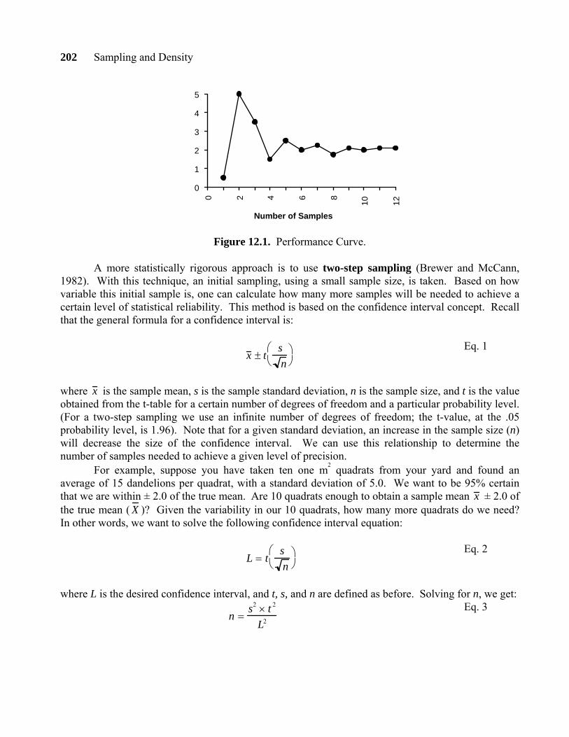
taking samples that have some sort of systematic or regular arrangement, e.g., sample plots may be located every 10 meters, etc. The advantage of systematic sampling is that it is usually simpler than random sampling. Bias will be present only if the pattern of the sampling is picking up some pattern in the population. If systematic sampling is used, it is up to the investigator to demonstrate that no such bias is present. Because statistical theory has been developed on random samples, random rather than systematic samples are recommended. Taking a random sample requires procedures to assure randomness (Brewer and McCann, 1982). Trying to place samples haphazardly, avoiding conscious bias, is usually not successful. When samples are located in this manner, tests usually disclose definite biases - the samples somehow avoid swampy areas, include the largest tree, or turn out to be too evenly spaced. Since the aim is to give every unit of the population an equal and independent likelihood of being chosen, the basic approach to randomizing samples is to let chance determine the samples. Drawing numbers from hats, flipping coins, rolling dice, and the like are all methods of making random decisions; however, we can usually achieve the same effect more simply by using random numbers generated on a calculator or computer or included in tables. A table of random numbers often helps obtain random samples. A random numbers table consists of a long series of digits that have been checked for non-randomness. To use it, simply enter the table in some way that prevents you exercising choice in the first sample. For example, close your eyes and drop your finger on the table. Then simply take the numbers in some predetermined order, such as left to right. For example, the table can be used to select random map coordinates within a study area or to select numbered sampling sites. Adequacy of Sampling The number and size of samples, or study units, are important in relation to the accuracy and precision of the estimates obtained from sampling data. In carrying out a sampling program, acquiring the samples or study units, an ecologist wants to obtain the maximum amount of information for the minimum amount of effort. Because sampling is generally a labor intensive and time consuming matter (which can be very expensive), an ecologist should consider such things as location, size, and number of samples. It is usually not possible to specify ahead of time how large a sample will be adequate. A large number of small- or medium-sized samples is better than a small number of large-sized samples, since the former gives a better picture of the variation within the population being sampled (Brewer and McCann, 1982). On the other hand taking more samples than is necessary for a particular problem is a waste of time (and money). A simple, homogeneous area will require less sampling than a complex, heterogeneous one. If the ecologist has prior knowledge of differences within the study area (e.g., low, wet areas vs. dry upland sites) it might be better to sample each area separately. A few quadrats may be sufficient to estimate the density of common species but may not even detect rare species. Highly clumped populations may require more samples than random or uniform populations. As you can see, sampling theory can become quite complex. For further reading see Green (1979), Grieg-Smith (1964), Poole (1974) and Seber (1973). In this lab we will be looking at with two ways of assessing sampling adequacy: The Performance Curve and Two-Step Sampling. A performance curve (Fig. 1) plots the cumulative mean value of some trait (e.g., density, biomass, length) against number of samples. The first few samples probably will not give a very close approximation of the true mean, so that the early part of the performance curve tends to be jagged. As more samples are taken, the true population mean is approached and the curve flattens out. When the change in the mean becomes very small with the addition of another sample, we assume that our sample mean has closely approached the true population mean (Brewer and McCann, 1982).


0

1

2

3

4

5

0 2 4 6 8

10 12

Number of Samples

Figure 12.1. Performance Curve.

A more statistically rigorous approach is to use two-step sampling (Brewer and McCann, 1982). With this technique, an initial sampling, using a small sample size, is taken. Based on how variable this initial sample is, one can calculate how many more samples will be needed to achieve a certain level of statistical reliability. This method is based on the confidence interval concept. Recall that the general formula for a confidence interval is:

x ± tsn

⎛ ⎝

⎞ ⎠

Eq. 1

where x is the sample mean, s is the sample standard deviation, n is the sample size, and t is the value obtained from the t-table for a certain number of degrees of freedom and a particular probability level. (For a two-step sampling we use an infinite number of degrees of freedom; the t-value, at the .05 probability level, is 1.96). Note that for a given standard deviation, an increase in the sample size (n) will decrease the size of the confidence interval. We can use this relationship to determine the number of samples needed to achieve a given level of precision. For example, suppose you have taken ten one m2 quadrats from your yard and found an average of 15 dandelions per quadrat, with a standard deviation of 5.0. We want to be 95% certain that we are within ± 2.0 of the true mean. Are 10 quadrats enough to obtain a sample mean x ± 2.0 of the true mean ( X )? Given the variability in our 10 quadrats, how many more quadrats do we need? In other words, we want to solve the following confidence interval equation:

L = tsn

⎛ ⎝

⎞ ⎠

Eq. 2

where L is the desired confidence interval, and t, s, and n are defined as before. Solving for n, we get:

n =s2 × t 2

L2 Eq. 3


In our example:

n =52 ×1.962

22 = 24.01

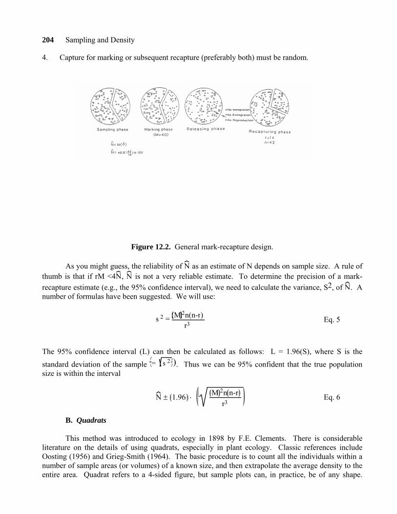
Thus we will need to take 14 more quadrats (10 + 14 = 24) to achieve our desired level of precision. Note that if we would have been satisfied with a lower level of precision, e.g., 95% sure of being ± 3.0 of the population mean, then we would have needed to take only one more sample. The ecologist can choose the level of precision to be achieved. The level chosen will typically depend on the problem, the variability of the population, and the cost of sampling. Density Estimation Two common methods of estimating absolute population density are the mark-recapture method and the quadrat method (or a variation thereof). The former is more appropriate for larger and more mobile organisms and the latter is typically used with small, sessile, or less mobile organisms (plants and many invertebrates). A. Mark-recapture This technique was first developed by C.G.J. Petersen, a Danish fisheries biologist in the 1890's, and reintroduced for studying bird populations by F.C. Lincoln in 1930 (as a result, aquatic ecologists often refer to the method as the Petersen Method, whereas terrestrial ecologists refer to it as the Lincoln Index). Details of the method, including many variations, are given in Seber (1973) and Ricker (1975). Generally, if someone puts a mark on some members of a population, releases these marked individuals back into the population, then resamples the population to find out what percentage of the sample has the mark, then we can, by a simple proportionality, estimate the total population size. This proportionality is:

total # marked in population (M)

total population size (N) = marked in sample (r, for recapture)

total # in sample (n) Rearranging, our estimated total population size (called N to symbolize that it is an estimate):

N = M nr

Eq. 4

Note, N is an estimate of population size at the time of marking, not at the time of recapture. This method makes several assumptions, each of which may be violated to a greater or lesser extent in the studies of natural populations. The field ecologist must be aware of the assumptions and how well or how poorly they are met in a particular study. The assumptions are (Brewer and McCann, 1982): 1. Marks must not be lost or overlooked. 2. No recruitment into the population by reproduction, immigration, or growth. 3. Marked and unmarked animals must be similar in all aspects (e.g., mortality rates, activity,

response to traps), except for the presence or absence of marks.


4. Capture for marking or subsequent recapture (preferably both) must be random.

Figure 12.2. General mark-recapture design.

As you might guess, the reliability of N as an estimate of N depends on sample size. A rule of thumb is that if rM <4N, N is not a very reliable estimate. To determine the precision of a mark-recapture estimate (e.g., the 95% confidence interval), we need to calculate the variance, S2, of N. A number of formulas have been suggested. We will use:

s 2 = M 2n(n-r)

r3 Eq. 5

The 95% confidence interval (L) can then be calculated as follows: L = 1.96(S), where S is the standard deviation of the sample = s 2 ). Thus we can be 95% confident that the true population size is within the interval

N ± 1.96 ⋅ M 2n n-r

r3 Eq. 6

B. Quadrats This method was introduced to ecology in 1898 by F.E. Clements. There is considerable literature on the details of using quadrats, especially in plant ecology. Classic references include Oosting (1956) and Grieg-Smith (1964). The basic procedure is to count all the individuals within a number of sample areas (or volumes) of a known size, and then extrapolate the average density to the entire area. Quadrat refers to a 4-sided figure, but sample plots can, in practice, be of any shape.


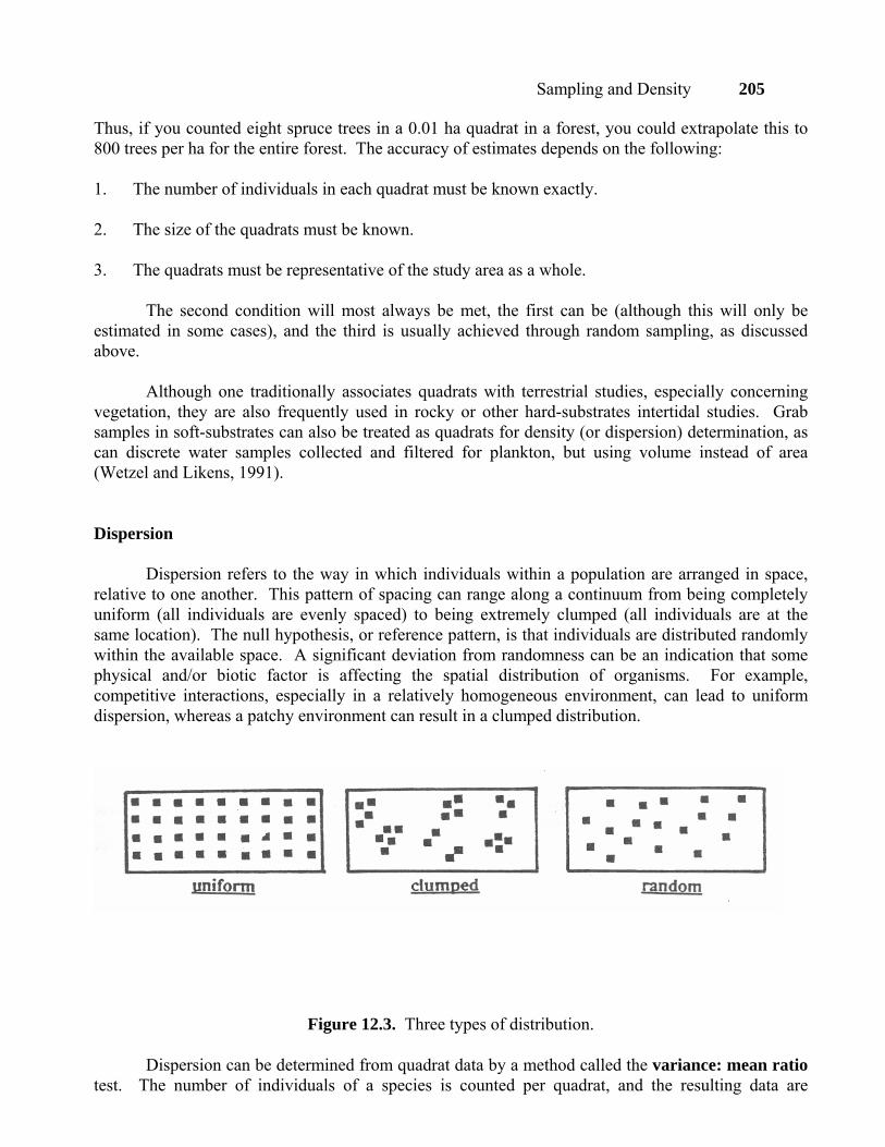
Thus, if you counted eight spruce trees in a 0.01 ha quadrat in a forest, you could extrapolate this to 800 trees per ha for the entire forest. The accuracy of estimates depends on the following: 1. The number of individuals in each quadrat must be known exactly. 2. The size of the quadrats must be known. 3. The quadrats must be representative of the study area as a whole. The second condition will most always be met, the first can be (although this will only be estimated in some cases), and the third is usually achieved through random sampling, as discussed above. Although one traditionally associates quadrats with terrestrial studies, especially concerning vegetation, they are also frequently used in rocky or other hard-substrates intertidal studies. Grab samples in soft-substrates can also be treated as quadrats for density (or dispersion) determination, as can discrete water samples collected and filtered for plankton, but using volume instead of area (Wetzel and Likens, 1991). Dispersion Dispersion refers to the way in which individuals within a population are arranged in space, relative to one another. This pattern of spacing can range along a continuum from being completely uniform (all individuals are evenly spaced) to being extremely clumped (all individuals are at the same location). The null hypothesis, or reference pattern, is that individuals are distributed randomly within the available space. A significant deviation from randomness can be an indication that some physical and/or biotic factor is affecting the spatial distribution of organisms. For example, competitive interactions, especially in a relatively homogeneous environment, can lead to uniform dispersion, whereas a patchy environment can result in a clumped distribution.

Figure 12.3. Three types of distribution. Dispersion can be determined from quadrat data by a method called the variance: mean ratio test. The number of individuals of a species is counted per quadrat, and the resulting data are


statistically compared with what would be expected if the dispersion were random (Brewer and McCann, 1982). The comparison involves the Poisson Distribution which describes the probability distribution for random, relatively rare events (like individuals in a quadrat). In other words, if we know the average density of a population (e.g., number per square meter), which we can determine from the same quadrat data (as described above), then the Poisson Distribution will tell us what proportion of our square meter quadrats will have 0 individuals, what proportion will have 1,2,3 etc. individuals if the population dispersion is random and a small number. We can then statistically compare the observed frequency distribution from our quadrat data with the Poisson-generated expected distribution via the chi-square test. If this sounds a bit confusing, you are in luck. There is an alternative, perhaps more straightforward, method that makes use of the fact that in the Poisson distribution, the variance is equal to the mean, or variance/mean = 1. Thus, we can simply record the number of individuals of our species present in each quadrat, and determine the variance:mean ratio. If the ratio is around 1, the population is randomly dispersed, if less than 1 the population tends toward a uniform distribution, and if greater than 1, towards a clumped distribution. Why? Determining whether a particular ratio is significantly different than 1 (in either direction) requires statistical testing, involving a form of the t-test. Calculate the following t:

t =

s2

x ⎛ ⎝ ⎜ ⎞

⎠ −1

2n −1

Eq. 7

where n = number of samples, s2 = sample variance, and x = sample mean. This value is compared with the value in the t-table at the desired probability level (typically 0.05) and n-1 degrees of freedom. If the calculated t value is greater than the t value in the table, we can conclude that the variance:mean ratio is significantly different than 1, and the population is either uniform or clumped. If the calculated t value is less than the value in the table then we cannot conclude that the ratio is different than 1, and therefore cannot reject the null hypothesis that the population has a random dispersion.

Procedures The object of this exercise is to estimate the population size and the variability of your estimates, and to examine how sample size, in either the marking or sampling phase, affect the accuracy and precision of your estimates. Your T.A. will instruct you on the details of fin clipping (Appendix B). Work with members of your lab bench.


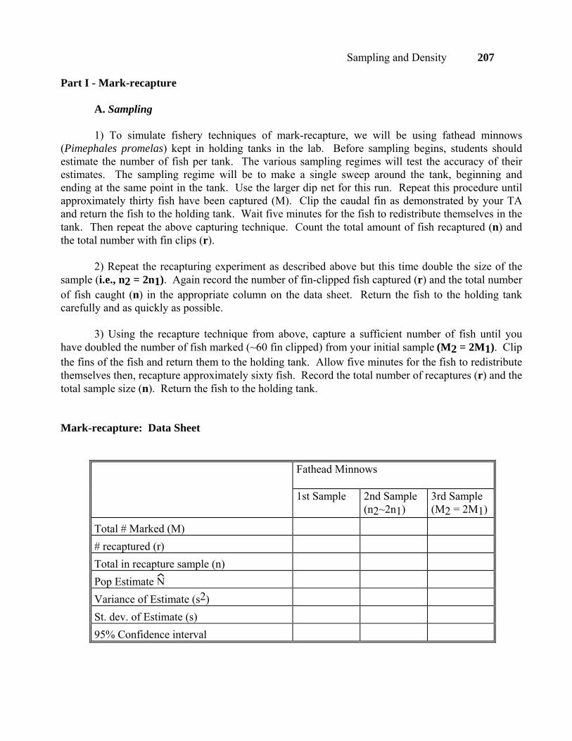
Part I - Mark-recapture A. Sampling 1) To simulate fishery techniques of mark-recapture, we will be using fathead minnows (Pimephales promelas) kept in holding tanks in the lab. Before sampling begins, students should estimate the number of fish per tank. The various sampling regimes will test the accuracy of their estimates. The sampling regime will be to make a single sweep around the tank, beginning and ending at the same point in the tank. Use the larger dip net for this run. Repeat this procedure until approximately thirty fish have been captured (M). Clip the caudal fin as demonstrated by your TA and return the fish to the holding tank. Wait five minutes for the fish to redistribute themselves in the tank. Then repeat the above capturing technique. Count the total amount of fish recaptured (n) and the total number with fin clips (r). 2) Repeat the recapturing experiment as described above but this time double the size of the sample (i.e., n2 = 2n1). Again record the number of fin-clipped fish captured (r) and the total number of fish caught (n) in the appropriate column on the data sheet. Return the fish to the holding tank carefully and as quickly as possible. 3) Using the recapture technique from above, capture a sufficient number of fish until you have doubled the number of fish marked (~60 fin clipped) from your initial sample (M2 = 2M1). Clip the fins of the fish and return them to the holding tank. Allow five minutes for the fish to redistribute themselves then, recapture approximately sixty fish. Record the total number of recaptures (r) and the total sample size (n). Return the fish to the holding tank. Mark-recapture: Data Sheet

Fathead Minnows

1st Sample 2nd Sample (n2~2n1)

3rd Sample (M2 = 2M1)

Total # Marked (M) # recaptured (r) Total in recapture sample (n) Pop Estimate N Variance of Estimate (s2) St. dev. of Estimate (s) 95% Confidence interval


B. Mark-Recapture: Data Analysis and Questions to Consider 1. Using the data from the first recapture sample, calculate the population estimate N and its

standard deviations for the number of fatheads. Record these on your data sheet. 2a. Calculate the population estimate and its standard deviation using the data from the second

recapture sample (in which the sample size n is doubled). Record these results. Did the N change substantially? Were the standard deviations from the second estimate larger or smaller than from the first sample? By how much?

b. Calculate the population estimate and standard deviation for each species using data from the

third recapture sample (in which the number of marked fatheads (M) was doubled). Record the results. Were the new standard deviations larger or smaller than the originals? Did doubling the recapture sample (n) or the number marked (M) cause a greater change in the standard deviation?

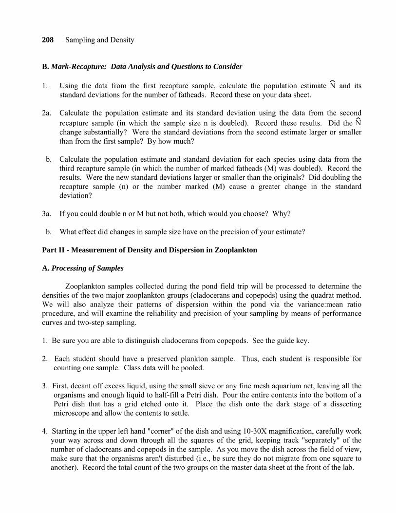
3a. If you could double n or M but not both, which would you choose? Why? b. What effect did changes in sample size have on the precision of your estimate? Part II - Measurement of Density and Dispersion in Zooplankton A. Processing of Samples Zooplankton samples collected during the pond field trip will be processed to determine the densities of the two major zooplankton groups (cladocerans and copepods) using the quadrat method. We will also analyze their patterns of dispersion within the pond via the variance:mean ratio procedure, and will examine the reliability and precision of your sampling by means of performance curves and two-step sampling. 1. Be sure you are able to distinguish cladocerans from copepods. See the guide key. 2. Each student should have a preserved plankton sample. Thus, each student is responsible for

counting one sample. Class data will be pooled. 3. First, decant off excess liquid, using the small sieve or any fine mesh aquarium net, leaving all the

organisms and enough liquid to half-fill a Petri dish. Pour the entire contents into the bottom of a Petri dish that has a grid etched onto it. Place the dish onto the dark stage of a dissecting microscope and allow the contents to settle.

4. Starting in the upper left hand "corner" of the dish and using 10-30X magnification, carefully work

your way across and down through all the squares of the grid, keeping track "separately" of the number of cladocreans and copepods in the sample. As you move the dish across the field of view, make sure that the organisms aren't disturbed (i.e., be sure they do not migrate from one square to another). Record the total count of the two groups on the master data sheet at the front of the lab.


Dispersion Patterns Data Sheet

(density #/L)

Sample Copepods Cladocerans 1 2 3 4 5 6 7 8 9 10 11 12 13 14 15 16 17 18 19 20 x s

B. Density and Dispersion of Pond Zooplankton: Data Analysis and Questions to Consider 1. You must first convert the numbers of cladocerans and copepods per sample into numbers per liter: #/liter = #/sample volume of sample (liter)

The volume of the sample (this is the volume of pond water sampled, not the volume of the contents of the jar!) can be calculated by multiplying the area of the opening of the plankton net times the length of the haul:

V (l) = Area (cm2) x Length (cm) 1000

The length of the haul was 100 cm (1 m), and the area of the opening of the plankton net can be calculated using the formula for the area of a circle: A = πr2 (π = 3.14; your instructor will give


you the diameter of the plankton net you used to collect the samples; the radius of a circle is equal to half the diameter).

Use all of the samples analyzed in your lab to determine the overall mean densities (number per liter) of cladocerans and copepods. Also determine the standard deviations about the means of the samples.

Do cladocerans or copepods have higher densities (or are their densities similar)? Compare via a t-test. Show your work.

2. Construct a performance curve for the cladocerans, using all of the samples. Use the samples in

the order they appear on the master data sheet. Based on the shape of the curve, indicate on the figure what level of sampling intensity you would recommend for future studies.

3. Suppose you wanted to be 95% confident that the true mean density of cladocerans in the pond

was within ± 10% of the sample mean you obtained using the pond data. How many total samples would be necessary? Show your work. How did this number compare with your answer in question 2?

4. For the mean densities of cladocerans and copepods, determine the pattern of dispersion in the

pond, using the variance:mean ratio test. Were the distributions uniform, random, or clumped? Can you propose an ecological mechanism that may have contributed to the pattern you found? How might different dispersion patterns affect the number of samples needed to achieve a particular level of precision (determined in question 3)? With which pattern would you need the largest number of samples? The smallest? Or is there no relation between dispersion and the ability to precisely determine mean density?

Written Assignment

Using the mark-recapture data and the zooplankton material from the pond lab, write an Results section of a laboratory report based on today's lab. You should be incorporating your data analysis from above, including the outcomes of statistical tests and graphs. Remember the results section is where you summarize your findings using words, tables, and graphs. See Ambrose (1987) or Day (1994) for examples or any journal ( ie. Ecology, Canadian Journal of Zoology ).

Acknowledgements The introductory material was adapted from Brewer and McCann, 1982. Revisions of this exercise have been carried out by Lorne LeClair and Donna Wakeford, Department of Biological Sciences, University of Alberta.

Literature Cited

Ambrose, H. W. and K. P, Ambrose. 1995. A handbook of biological investigation. Hunter Textbooks, Winston-Salem (North Carolina).

Brewer, R. and Margaret T. McCann. 1982. Laboratory and field manual of ecology. Saunders College Publishing, New York.


Brouwer, James E. and Jarrold H. Zar. 1984. Field and laboratory methods for general ecology. W.C. Brown, New York.

Clifford, H.F. 1991. Aquatic invertebrates of Alberta. University of Alberta Press, Edmonton (Alberta).

Cox, George W. 1985. Laboratory manual of general ecology. W.C. Brown, New York. Day, R. A. 1994. How to write and publish a scientific paper. The Oryx Press, Phoenix (Arizona) Green, R.H. 1979. Sampling design and statistical methods for environmental biologists. John Wiley

& Sons, New York. Grieg-Smith, P. 1964. Statistical plant ecology, 2nd Ed. Butterworth & Co., London. Lind, O.T. 1974. Handbook of common methods in limnology. C.V. Mosby, St. Louis. Oosting, H.J. 1956. The study of plant communities. W.H. Freeman & Co., San Francisco. Pennak, R. W. 1989. Freshwater invertebrates of the United States: Protozoa to mullusca. John

Wiley and Sons (New York). Poole, R.W. 1974. An introduction to quantitative ecology. McGraw Hill, New York. Ricker, W.E. 1975. Computation and interpretation of biological statistics of fish populations.

Bulletin of the Fisheries Research Board of Canada 191. Scott, W.B. & E.J. Crossman. 1973. Freshwater fishes of Canada. Bulletin of the Fisheries Research

Board of Canada 184. Seber, G.A.F. 1973. The estimation of animal abundance. Hafner Press, New York. Sullivan, M. 1990. Commercial Fisheries as a Management Technique. The Alberta Game Warden.

9(2):28-29. Wetzel, R.G. and G.E. Likens. 1991. Limnological analyses. Springer-Verlag, New York.


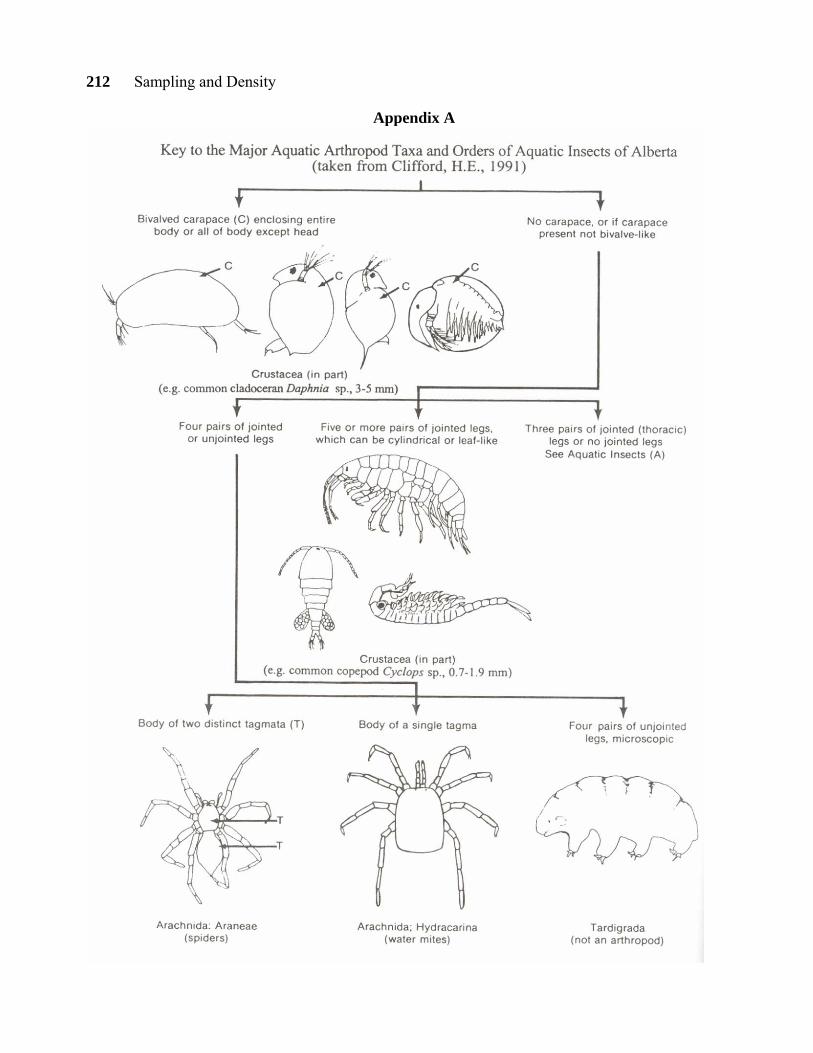
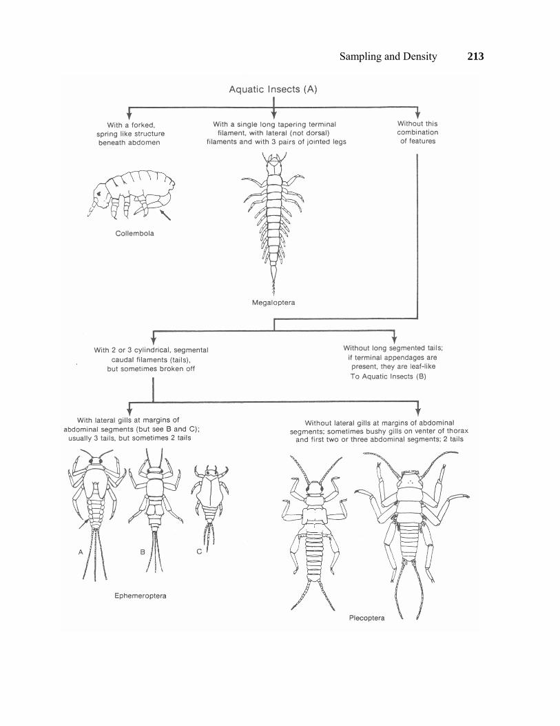
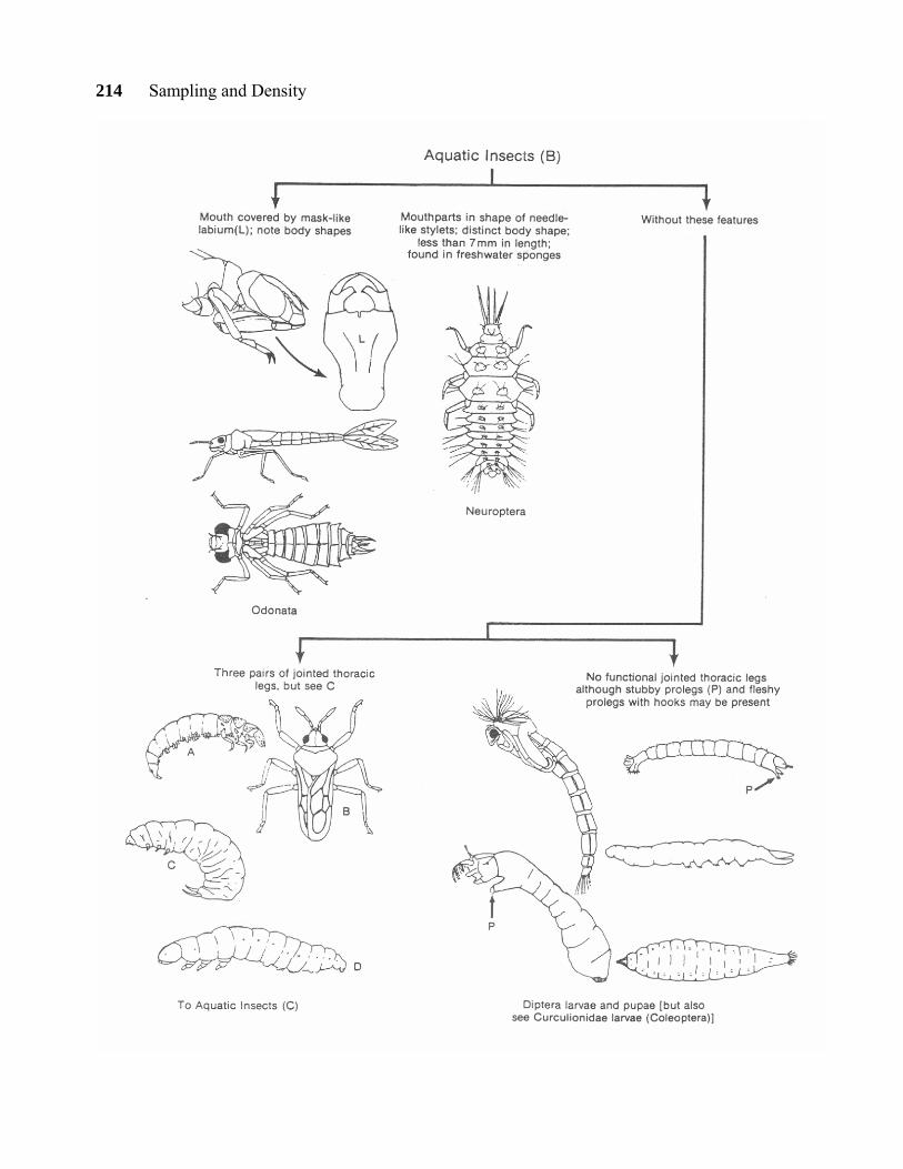
Appendix A

sampling, density estimation and spatial relationships · sampling, density estimation and spatial...

Documents