satellite data assimilation of upper-level sounding … zou xiaolei, weng fuzhong, vijay...
TRANSCRIPT
NO.1 ZOU Xiaolei, WENG Fuzhong, Vijay TALLAPRAGADA, et al. 1
Satellite Data Assimilation of Upper-Level Sounding Channelsin HWRF with Two Different Model Tops
ZOU Xiaolei1∗ (���), WENG Fuzhong2 (���), Vijay TALLAPRAGADA3, LIN Lin4 (� �),
ZHANG Banglin3 (�DZ�), WU Chenfeng5 (���), and QIN Zhengkun6 (���)
1 Earth System Science Interdisciplinary Center, University of Maryland, MD 20740, USA
2 NOAA Center for Satellite Applications and Research, College Park, MD 20740, USA
3 NOAA NCEP Environmental Modeling Center, College Park, MD 20740, USA
4 I. M. Systems Group, Inc., Rockville, MD 20850, USA
5 Xiamen Meteorological Bureau, Xiamen 361012, China
6 Nanjing University of Information Science & Technology, Nanjing 210044, China
(Received October 19, 2014; in final form January 12, 2015)
ABSTRACT
The Advanced Microwave Sounding Unit-A (AMSU-A) onboard the NOAA satellites NOAA-18 andNOAA-19 and the European Organization for the Exploitation of Meteorological Satellites (EUMETSAT)MetOp-A, the hyperspectral Atmospheric Infrared Sounder (AIRS) onboard Aqua, the High resolution In-fraRed Sounder (HIRS) onboard NOAA-19 and MetOp-A, and the Advanced Technology Microwave Sounder(ATMS) onboard Suomi National Polar-orbiting Partnership (NPP) satellite provide upper-level soundingchannels in tropical cyclone environments. Assimilation of these upper-level sounding channels data in theHurricane Weather Research and Forecasting (HWRF) system with two different model tops is investigatedfor the tropical storms Debby and Beryl and hurricanes Sandy and Isaac that occurred in 2012. It is shownthat the HWRF system with a higher model top allows more upper-level microwave and infrared soundingchannels data to be assimilated into HWRF due to a more accurate upper-level background profile. Thetrack and intensity forecasts produced by the HWRF data assimilation and forecast system with a highermodel top are more accurate than those with a lower model top.
Key words: model top, data assimilation, satellite, hurricane
Citation: Zou Xiaolei, Weng Fuzhong, Vijay Tallapragada, et al., 2015: Satellite data assimilation of upper-level sounding channels in HWRF with two different model tops. J. Meteor. Res., 29(1), 001–027, doi: 10.1007/s13351-015-4108-9.
1. Introduction
Tropical cyclogenesis, tropical cyclone (TC) in-tensity change and movement are controlled by manyenvironmental factors. The motion of a tropical stormis driven mostly by the large-scale environmental steer-ing, which is defined as a weighted average of the envi-ronmental winds between 300 and 850 hPa (Carr andElsberry, 1990; Velden and Leslie, 1991; Chan, 2005;Wu and Zou, 2008). Tropical cyclogenesis and TCintensification are affected by the vertical wind sheardefined by the wind difference between 200 and 850
hPa. Although weak shear may aid genesis by forc-ing synoptic-scale ascent in baroclinic environments(Bracken and Bosart, 2000; Davis and Bosart, 2006),strong vertical wind shears are detrimental to tropi-cal cyclogenesis (McBride and Zehr, 1981; Zehr, 1992)and impede TC intensification (DeMaria, 1996; Gal-lina and Velden, 2002). There are a number of hy-potheses as to what causes the weakening of TC in-tensity in the presence of strong vertical wind shear.One hypothesis is that vertical wind shear acts to de-crease the efficiency of the hurricane heat engine byventilating the TC eyewall with low-entropy air at mid
Supported by the NOAA Hurricane Forecast Improvement Program (HFIP) and National Natural Science Foundation of China(91337218).
∗Corresponding author: [email protected].
©The Chinese Meteorological Society and Springer-Verlag Berlin Heidelberg 2015

2 JOURNAL OF METEOROLOGICAL RESEARCH VOL.29
levels by eddy fluxes (Simpson and Riehl, 1958; Cramet al., 2007; Marin et al., 2009). Convective down-draft air originating outside eyewall and having thelow-entropy air due to evaporative cooling into theboundary layer is advected inwards into the sub-cloudlayer of the eyewall by the radial inflow (Powell, 1990;Riemer et al., 2010; Riemer and Montgomery, 2011).Tang and Emanuel (2012) developed a ventilation in-dex, which is defined as product of the environmentalvertical wind shear and the non-dimensional midlevelentropy deficit divided by the potential intensity, forevaluating whether ventilation plays a detectable rolein current TC climatology. Steering flow, vertical windshear, an approaching upper-level trough, upper-leveleddy angular momentum flux convergence, strato-spheric cooling, and quasi-biennial oscillation in thestratosphere are factors that involve atmospheric con-ditions in the upper troposphere and the stratosphere.
The interaction of upper-level troughs and/or cut-off lows with TCs is another important factor influ-encing TC intensification (Molinari and Vollaro, 2010;Leroux et al., 2013). An approaching trough may in-duce significant vertical wind shear, enhance the out-flow poleward of the storm, or introduce the cyclonicpotential vorticity (PV) into the TC core through ad-vection. The vertical wind shear is usually detrimen-tal and the PV advection into the TC core is usu-ally beneficial to TC intensity (Leroux et al., 2013),and the asymmetric outflow increases the eddy an-gular momentum flux convergence calculated at 200hPa over a 300–600-km radial range around the TCcenter (Molinari and Vollaro, 2010) and leads to TCintensification for storms whose intensity is well belowtheir maximum potential intensity (Pfeffer and Challa,1981; Challa and Pfeffer, 1990; DeMaria et al., 1993;Bosart et al., 2000). The intensity of TCs could also beaffected by the stratospheric cooling associated withclimate change (Ramsay, 2013). With stratosphericcooling, the rising heated air would be able to rise evenhigher than normal and entering the stratosphere, nar-rowing the eye of the storm. In turn, the outer rain-bands of the TC will retract, decreasing the size of thestorm while increasing its strength. A strong corre-lation between decreasing stratospheric temperatures
and increasing hurricane intensity has been found from25-yr hurricane data records (Emanuel et al., 2013).Cooling near and above the model tropopause (about90 hPa) modifies the storm’s outflow temperature andcould increase the potential intensity (PI) at a rateof 1 m s−1 per degree cooling with fixed sea sur-face temperature (SST) (Emanuel, 1986; Bister andEmanuel, 1997). Chan (1995) noted a relationship be-tween the interannual variations in TC activity andthe quasi-biennial oscillation in the stratosphere inthe western North Pacific. Modeling of TC trackand those opposing effects of TC-trough interaction,stratospheric cooling, and the quasi-biennial oscilla-tion in the stratosphere on the environmental factorsaffecting TC intensification requires a sufficiently highmodel top to fully capture these stratospheric featuresand their interactions with troposphere in hurricaneenvironments.
A large amount of remote sensing data from re-search and operational satellites becomes availablefor obtaining an improved description of the initialstate of the atmosphere in the upper troposphereand stratosphere. The primary source of data in-cludes those upper-level sounding channels from theAdvanced Microwave Sounding Unit-A (AMSU-A) on-board NOAA-18, NOAA-19, MetOp-A, and MetOp-B; the High resolution InfraRed Sounder (HIRS) on-board NOAA-19, MetOp-B, and MetOp-A; the hy-perspectral Atmospheric Infrared Sounder (AIRS) on-board EOS Aqua; as well as the Advanced TechnologyMicrowave Sounder (ATMS) and the Cross-Track In-frared Sounder (CrIS) onboard Suomi NPP (NationalPolar-orbiting Partnership) satellite. These six polar-orbiting satellites (NOAA-18, NOAA-19, MetOp-A,Aqua, MetOp-B, and Suomi NPP) provide microwaveand infrared radiance observations to the NCEP oper-ational numerical weather prediction (NWP) systemmore than 12 times daily. These satellite observationshave an excellent global coverage and good spatial res-olution varying from about 15 km to around 100 km.However, the satellite radiation is contributed fromthe stratosphere and the assimilation of the data intoNWP requires that the model top be placed at a suf-ficiently high altitude. For this reason, the ECMWF

NO.1 ZOU Xiaolei, WENG Fuzhong, Vijay TALLAPRAGADA, et al. 3
model top was raised from 10 hPa to about 0.1 hPa in1999 (Untch et al., 1999).
It is well known that direct assimilation of satel-lite infrared (McNally et al., 2006) and microwave(Derber and Wu, 1998) radiances provided by thepolar-orbiting meteorological satellites out-performedthe assimilation of temperature and moisture re-trievals for NWP forecasts. Radiance measurementsfrom different satellites instruments are now routinelyassimilated in operational global medium-range fore-cast modeling systems, which have brought signifi-cantly positive impacts on the medium-range forecast(3–7 days). Positive impacts of satellite data assim-ilation for short-range forecasts using mesoscale re-gional models have also been demonstrated by severalstudies. For examples, assimilation of AMSU-A radi-ance observations and conventional observations usingthe HIgh Resolution Limited Area Model (HIRLAM)four-dimensional variational data assimilation (4D-Var) consistently out-performed the HIRLAM 3D-Var,particularly for cases with strong mesoscale storm de-velopments (Gustafsson et al., 2012). Using the sameHIRLAM 4D-Var, Stengel et al. (2009) demonstratedthe benefit of a regional NWP model’s analyses andforecasts gained by the assimilation of three of SE-VIRI’s infrared channels (i.e., the two water vaporchannels located at 6.2 and 7.3 µm, and the CO2
channel placed around 13.4 µm). Montmerle et al.(2007) investigated the relative impact of geostation-ary versus polar-orbiting satellites and their possi-ble complementarity using the Aladin/France opera-tional regional 3D-Var system at Meteo-France. Ra-diance observations from the Spinning Enhanced Visi-ble and Infrared Imager (SEVIRI) on board Meteosat-8; AMSU-A radiances from NOAA-15, NOAA-16,and AQUA; AMSU-B radiances from NOAA-16 andNOAA-17; and HIRS radiances from NOAA-17 andthe Advanced Infrared Sounder (AIRS) on board theNOAA and AQUA satellites, were assimilated. Anal-yses were strongly controlled by SEVIRI data in themiddle to high troposphere, resulting in a positiveimpact on forecast scores and predicted precipitationpatterns. Weng and Liu (2003) studied the forwardradiative transfer and Jacobian modeling in cloudy
atmospheres, and Weng et al. (2007) employed rain-affected microwave radiance observations for hurricanevortex analysis. Positive impacts of a 3D-Var assimila-tion of the Advanced Technology Microwave Sounder(ATMS) onboard Suomi NPP satellite on hurricaneforecasts have also been demonstrated (Zou et al.,2013). The wealth of more accurate remote sensingdata from research and operational satellites, the de-velopment of more sophisticated hurricane forecastingmodels, and the availability of more powerful comput-ers, provide unprecedented opportunities to advancefurther our knowledge, understanding, and forecastskill of TCs.
This study investigates the impact of the altitudeof the model top on satellite radiance assimilation andthe track and intensity forecasts of tropical storms us-ing the Hurricane Weather Research and Forecasting(HWRF) system. In the following, a brief descriptionof data, the TC case, and the data assimilation andTC forecast model are provided in Section 2. Satelliteobservation instruments are introduced in Section 3.Impacts of model top on biases of satellite radiancesimulation by a radiative transfer model are describedin Section 4. Section 5 depicts the case and the HWRFexperiment setup. In Section 6, data assimilation re-sults from the HWRF are discussed. Forecast resultsare presented in Section 7, in which how the tropicalstorm forecasts are affected by model tops are elabo-rated. Section 8 presents a summary of this study.
2. A brief description of the HWRF system
This study employs the HWRF system, which hasevolved from a single-domain system (Gopalakrishnanet al., 2011), to a doubly nested version (Bozeman etal., 2011; Pattanayak et al., 2011; Zhang et al., 2011;Yeh et al., 2012), and finally a triply nested version(Zhang et al., 2011). The triply nested 2012 version ofthe HWRF system is configured with a parent domainat 27-km horizontal resolution, an intermediate two-way moving nesting domain at 9 km, and an innermosttwo-way moving nesting domain at 3 km. The par-ent, intermediate, and innermost domains have about750 × 750, 238 × 150, and 50 × 50 model grid points,

4 JOURNAL OF METEOROLOGICAL RESEARCH VOL.29
respectively (Zhang et al., 2011). Both the interme-diate and innermost domains are centered at the ini-tial storm location and configured to follow the pro-jected path of the storm. All the three domains of theHWRF have the same 43 hybrid vertical levels withmore than 10 model levels located below 850 hPa anda model top located at about 50 hPa. The ghost do-main has the same spatial resolution as the interme-diate domain but is slightly larger than the interme-diate domain. The data assimilation has a model toplocated at 50 hPa in the 2012 HWRF version, whichis raised to 0.5 hPa in this study. It will be demon-strated that a higher HWRF model top is required forHWRF to better assimilate those upper troposphericand low stratospheric sounding channels even if theirweighting functions peak well below 50 hPa, as wellas for HWRF to fully describe the physical and dy-namical processes in the upper troposphere and thestratosphere that are important for the development,
movement, and intensity change of tropical cyclones.Figure 1 shows the parent domain, 3X domain,
ghost domain, middle nest, and inner nest for forecast-ing the track and intensity change of tropical stormDebby. The observed track and the surface pressurefield from the background field at 1800 UTC 27 June2012 within the parent domain are also shown. It isseen that the parent domain is sufficiently large fordescribing TC environmental flow evolution. Both theintermediate and innermost domains are centered atthe initial storm location and move on the projectedpath of the storm to capture storm’s inner core struc-tures. The HWRF atmospheric model employs Fer-rier microphysics, NCEP global forecast system (GFS)planetary boundary layer physics, SAS deep convec-tion and shallow convection, and Geophysical FluidDynamics Laboratory (GFDL) land surface model andradiation. The atmosphere component is coupled tothe Princeton Ocean Model (POM) for all three do-
Fig. 1. Sea level pressure (shaded; hPa) from the background field at 1800 UTC 23 June 2012 for tropical storm Debby.
The parent domain, 3X domain, ghost domain, middle nest, and inner nest are also indicated. The NHC (National
Hurricane Center) best track from 1800 UTC 20 to 1800 UTC 27 June 2012 is indicated in the thick black curve.

NO.1 ZOU Xiaolei, WENG Fuzhong, Vijay TALLAPRAGADA, et al. 5
mains (Gopalakrishnan et al., 2012).The NCEP unified Gridpoint Statistical Interpo-
lation (GSI) system employed by the HWRF for dataassimilation was described in Derber and Wu (1998)and Wu et al. (2002). A recursive filter was usedto obtain a non-homogenous grid-point representationof background errors in the GSI system (Wu et al.,2002; Purser et al., 2003a, b). The Community Ra-diative Transfer Model (CRTM) developed by the USJoint Center for Satellite Data Assimilation (JCSDA)(Han et al., 2007; Weng, 2007) is used for simulationof all observations from satellite instruments. Satel-lite data assimilation is carried out in both the parentand the ghost D2 domains at 27- and 9-km resolu-tions.
The quality control (QC) procedure for each typeof satellite data consists of several QC tests to removeoutliers under cloudy conditions, outliers associatedwith uncertainty in surface emissivity, and those fieldof views (FOVs) with mixed surface types. The GSIbias correction consists of a constant scan bias cor-rection and an air mass bias correction. Spatial datathinning is applied to all ATMS, AMSU-A, HIRS, andAIRS instruments based on the spatial distance be-tween observation and the center of an analysis gridbox, the temporal difference between observation andanalysis time, terrain height, surface type, etc. A de-tailed description of the QC, bias correction, and datathinning employed in GSI for ATMS can be found inZou et al. (2013).
The vortex initialization is performed at the 9-km resolution 3X domain (see Fig. 1). A pre-specifiedbogus vortex is merged with an environmental fieldextracted from the GFS analysis. Once the 6-h dataassimilation cycle starts, the 6-h HWRF forecasts areused for extracting the environmental fields. Themerged field with a corrected vortex and the environ-ment field are the background field for data assimila-tion that employs the NCEP GSI analysis system.
3. Satellite observations
The AMSU-A onboard both the NOAA and EU-
METSAT polar-orbiting satellites measures the atmo-spheric radiation in microwave frequency range from23 to 89 GHz. AMSU-A is a cross-track radiometer.The extreme scan position of the earth view to thebeam center is 48.3◦. The cross-track size of AMSU-AFOV is 48 km at nadir and that at the outmost scanangle is 105 km. The AMSU-A instruments have 15channels, in which 3 channels are window channels.Figure 2 presents the normalized weighting functionsfor AMSU-A channels 1–15, which are overlapped ontothe 43 vertical levels of the HWRF model with itsmodel top located at 50 hPa and the 61 vertical levelswith its model top located at 0.5 hPa. It is pointedout that the peak of weighting function increases withscan angle. However, such a shift is much smaller forupper-level channels than for low level channels (seeFig. 2 in Zou et al., 2013). The radiative energymeasured by AMSU-A primarily comes from the emis-sion of oxygen whose concentration is nearly uniformlydistributed through the earth’s atmosphere. Each ofthe 12 sounding channels provides measurements of aweighted average of radiation emitted from a partic-ular layer of the atmosphere at a specified frequency.The 12 AMSU-A sounding channels are evenly dis-tributed throughout the earth’s atmosphere. There-fore, AMSU-A satellite instruments are ideal for re-motely sounding the global atmospheric temperature.More details on the channel characteristics of AMSU-A can be found in Mo (1996) and the NOAA KLM(abbreviated for NOAA-15/16/17) User Guide 1○ .
ATMS is a cross-track microwave radiometer,which scans the earth scene within ±52.7◦ with re-spect to the nadir direction. It has a total of 22channels with channels 1–16 designed for atmospherictemperature soundings below about 0.1 hPa and chan-nels 17–22 for atmospheric humidity soundings in thetroposphere below approximately 200 hPa (Weng etal., 2012, 2013). The ATMS weighting functions canbe found in Weng et al. (2012). Fourteen of ATMStemperature sounding channels (ATMS channels 1–3and 5–15) have the same frequencies as its predecessorAMSU-A (AMSU-A channels 1–14). The ATMS tem-perature channel 16 has slightly different frequency
1○http://www2.ncdc.noaa.gov/docs/klm/c7/sec7-3
6 JOURNAL OF METEOROLOGICAL RESEARCH VOL.29
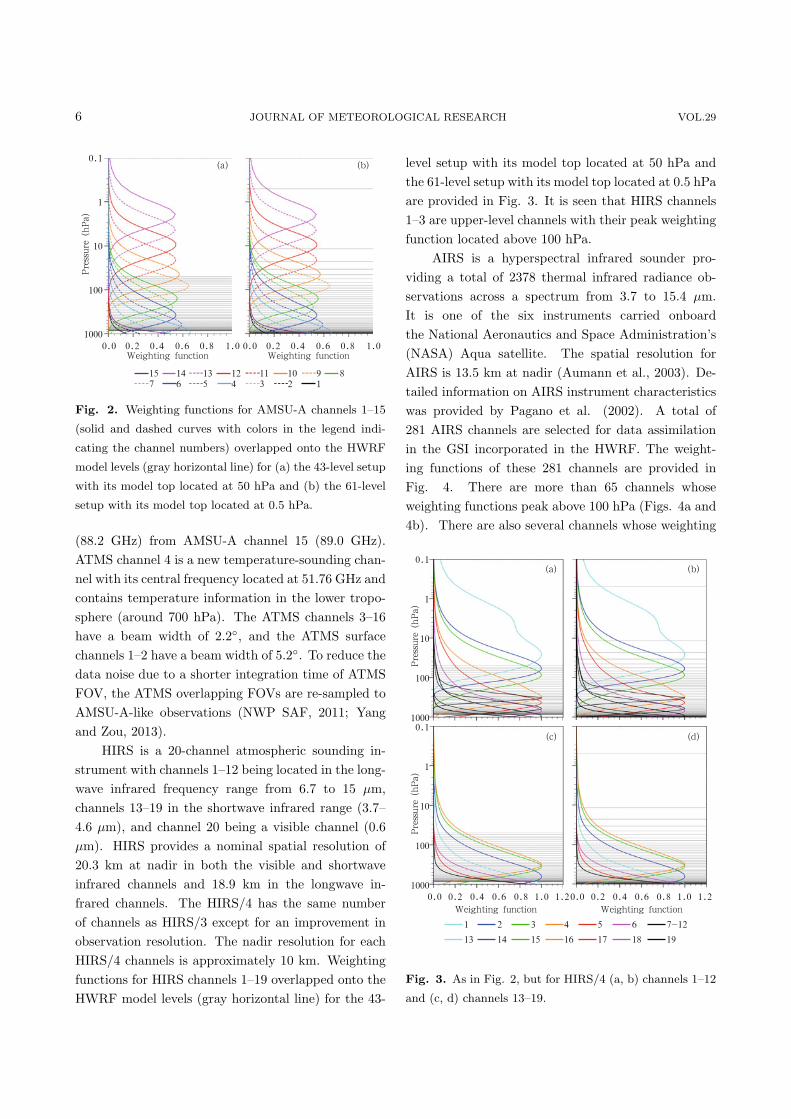
Fig. 2. Weighting functions for AMSU-A channels 1–15
(solid and dashed curves with colors in the legend indi-
cating the channel numbers) overlapped onto the HWRF
model levels (gray horizontal line) for (a) the 43-level setup
with its model top located at 50 hPa and (b) the 61-level
setup with its model top located at 0.5 hPa.
(88.2 GHz) from AMSU-A channel 15 (89.0 GHz).ATMS channel 4 is a new temperature-sounding chan-nel with its central frequency located at 51.76 GHz andcontains temperature information in the lower tropo-sphere (around 700 hPa). The ATMS channels 3–16have a beam width of 2.2◦, and the ATMS surfacechannels 1–2 have a beam width of 5.2◦. To reduce thedata noise due to a shorter integration time of ATMSFOV, the ATMS overlapping FOVs are re-sampled toAMSU-A-like observations (NWP SAF, 2011; Yangand Zou, 2013).
HIRS is a 20-channel atmospheric sounding in-strument with channels 1–12 being located in the long-wave infrared frequency range from 6.7 to 15 µm,channels 13–19 in the shortwave infrared range (3.7–4.6 µm), and channel 20 being a visible channel (0.6µm). HIRS provides a nominal spatial resolution of20.3 km at nadir in both the visible and shortwaveinfrared channels and 18.9 km in the longwave in-frared channels. The HIRS/4 has the same numberof channels as HIRS/3 except for an improvement inobservation resolution. The nadir resolution for eachHIRS/4 channels is approximately 10 km. Weightingfunctions for HIRS channels 1–19 overlapped onto theHWRF model levels (gray horizontal line) for the 43-
level setup with its model top located at 50 hPa andthe 61-level setup with its model top located at 0.5 hPaare provided in Fig. 3. It is seen that HIRS channels1–3 are upper-level channels with their peak weightingfunction located above 100 hPa.
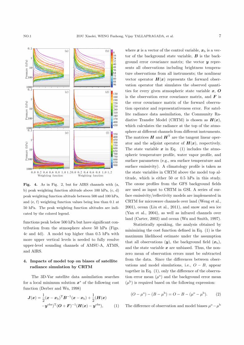
AIRS is a hyperspectral infrared sounder pro-viding a total of 2378 thermal infrared radiance ob-servations across a spectrum from 3.7 to 15.4 µm.It is one of the six instruments carried onboardthe National Aeronautics and Space Administration’s(NASA) Aqua satellite. The spatial resolution forAIRS is 13.5 km at nadir (Aumann et al., 2003). De-tailed information on AIRS instrument characteristicswas provided by Pagano et al. (2002). A total of281 AIRS channels are selected for data assimilationin the GSI incorporated in the HWRF. The weight-ing functions of these 281 channels are provided inFig. 4. There are more than 65 channels whoseweighting functions peak above 100 hPa (Figs. 4a and4b). There are also several channels whose weighting
Fig. 3. As in Fig. 2, but for HIRS/4 (a, b) channels 1–12
and (c, d) channels 13–19.
NO.1 ZOU Xiaolei, WENG Fuzhong, Vijay TALLAPRAGADA, et al. 7
Fig. 4. As in Fig. 2, but for AIRS channels with (a,
b) peak weighting function altitude above 100 hPa, (c, d)
peak weighting function altitude between 500 and 100 hPa,
and (e, f) weighting function values being less than 0.1 at
50 hPa. The peak weighting function altitudes are indi-
cated by the colored legend.
functions peak below 500 hPa but have significant con-tribution from the atmosphere above 50 hPa (Figs.4c and 4d). A model top higher than 0.5 hPa withmore upper vertical levels is needed to fully resolveupper-level sounding channels of AMSU-A, ATMS,and AIRS.
4. Impacts of model top on biases of satelliteradiance simulation by CRTM
The 3D-Var satellite data assimilation searchesfor a local minimum solution x∗ of the following costfunction (Derber and Wu, 1998)
J(x) =12(x − xb)TB−1(x − xb) +
12(H(x)
−yobs)T(O + F )−1(H(x) − yobs), (1)
where x is a vector of the control variable, xb is a vec-tor of the background state variable, B is the back-ground error covariance matrix; the vector y repre-sents all observations including brightness tempera-ture observations from all instruments; the nonlinearvector operator H(x) represents the forward obser-vation operator that simulates the observed quanti-ties for every given atmospheric state variable x, O
is the observation error covariance matrix, and F isthe error covariance matrix of the forward observa-tion operator and representativeness error. For satel-lite radiance data assimilation, the Community Ra-diative Transfer Model (CRTM) is chosen as H(x),which calculates the radiance at the top of the atmo-sphere at different channels from different instruments.The matrices H and HT are the tangent linear oper-ator and the adjoint operator of H(x), respectively.The state variable x in Eq. (1) includes the atmo-spheric temperature profile, water vapor profile, andsurface parameters (e.g., sea surface temperature andsurface emissivity). A climatology profile is taken asthe state variables in CRTM above the model top al-titude, which is either 50 or 0.5 hPa in this study.The ozone profiles from the GFS background fieldsare used as input to CRTM in GSI. A series of sur-face emissivity/reflectivity models are implemented inCRTM for microwave channels over land (Weng et al.,2001), ocean (Liu et al., 2011), and snow and sea ice(Yan et al., 2004), as well as infrared channels overland (Carter, 2002) and ocean (Wu and Smith, 1997).
Statistically speaking, the analysis obtained byminimizing the cost function defined in Eq. (1) is themaximum likelihood estimate under the assumptionthat all observations (y), the background field (xb),and the state variable x are unbiased. Thus, the non-zero mean of observation errors must be subtractedfrom the data. Since the differences between obser-vations and model simulations, i.e., O − B, appeartogether in Eq. (1), only the difference of the observa-tion error mean (µo) and the background error mean(µb) is required based on the following expression:
(O − µo) − (B − µb) = O − B − (µo − µb). (2)
The difference of observation and model biases µo−µb
8 JOURNAL OF METEOROLOGICAL RESEARCH VOL.29
in Eq. (2) can be estimated based on a large sampleof O −B statistics since O − B = O − T − (B − T ) =µo − µb.
If the model top is located too low (e.g., 50 hPa),radiances of many upper-level channels could be diffi-cult to use. Significant temporally and spatially vary-ing biases would be introduced for the assimilation ofthose channels that have a significant sensitivity tothe atmosphere above the model top. If these chan-nels were assimilated and adjusted during the assimila-tion process, signals in the satellite-observed radiancesfrom above the model top would be aliased, resultingin erroneous adjustments to model initial conditionswithin the model domain. The quality of forecastswould be reduced. It is thus important to have arelatively higher model top for the TC forecasts totake full advantage of upper-level radiance observa-tions.
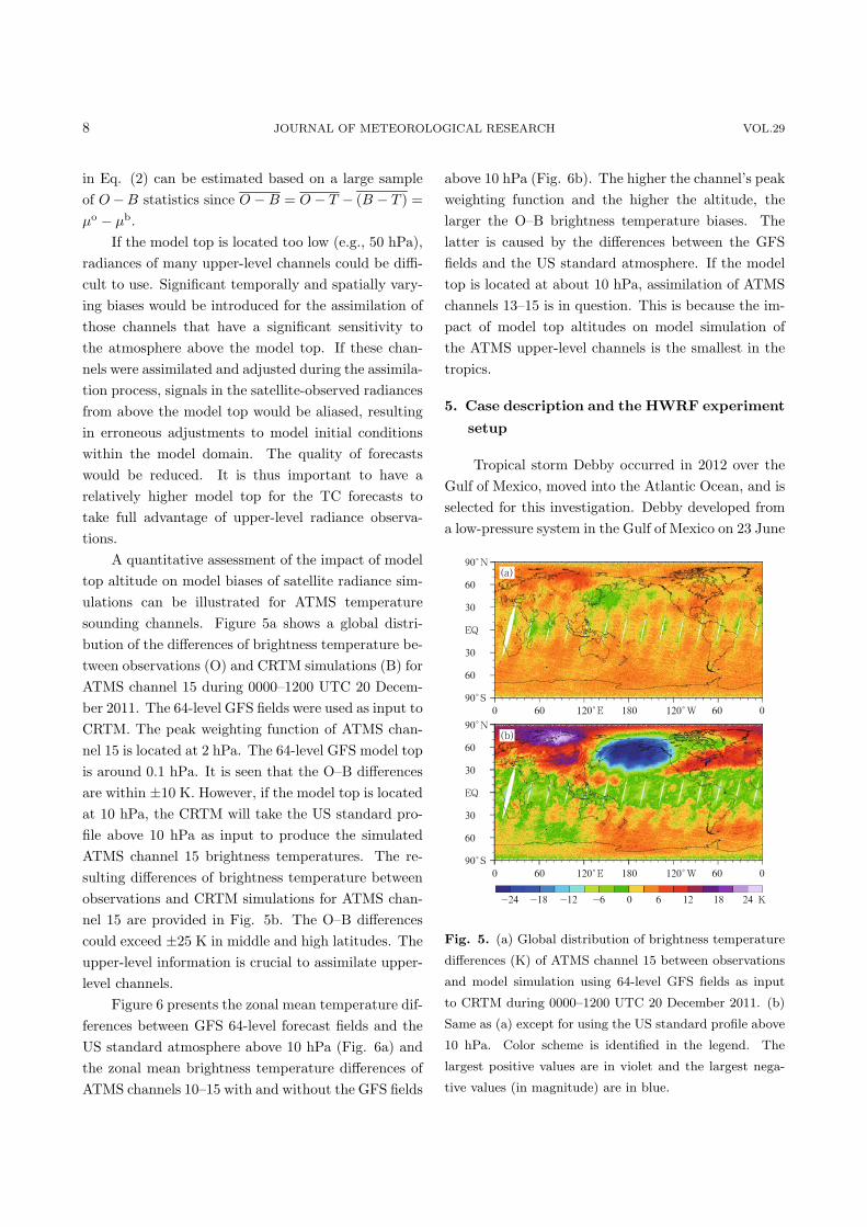
A quantitative assessment of the impact of modeltop altitude on model biases of satellite radiance sim-ulations can be illustrated for ATMS temperaturesounding channels. Figure 5a shows a global distri-bution of the differences of brightness temperature be-tween observations (O) and CRTM simulations (B) forATMS channel 15 during 0000–1200 UTC 20 Decem-ber 2011. The 64-level GFS fields were used as input toCRTM. The peak weighting function of ATMS chan-nel 15 is located at 2 hPa. The 64-level GFS model topis around 0.1 hPa. It is seen that the O–B differencesare within ±10 K. However, if the model top is locatedat 10 hPa, the CRTM will take the US standard pro-file above 10 hPa as input to produce the simulatedATMS channel 15 brightness temperatures. The re-sulting differences of brightness temperature betweenobservations and CRTM simulations for ATMS chan-nel 15 are provided in Fig. 5b. The O–B differencescould exceed ±25 K in middle and high latitudes. Theupper-level information is crucial to assimilate upper-level channels.
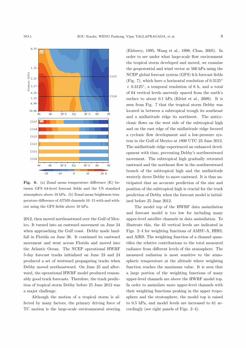
Figure 6 presents the zonal mean temperature dif-ferences between GFS 64-level forecast fields and theUS standard atmosphere above 10 hPa (Fig. 6a) andthe zonal mean brightness temperature differences ofATMS channels 10–15 with and without the GFS fields
above 10 hPa (Fig. 6b). The higher the channel’s peakweighting function and the higher the altitude, thelarger the O–B brightness temperature biases. Thelatter is caused by the differences between the GFSfields and the US standard atmosphere. If the modeltop is located at about 10 hPa, assimilation of ATMSchannels 13–15 is in question. This is because the im-pact of model top altitudes on model simulation ofthe ATMS upper-level channels is the smallest in thetropics.
5. Case description and the HWRF experiment
setup
Tropical storm Debby occurred in 2012 over theGulf of Mexico, moved into the Atlantic Ocean, and isselected for this investigation. Debby developed froma low-pressure system in the Gulf of Mexico on 23 June
Fig. 5. (a) Global distribution of brightness temperature
differences (K) of ATMS channel 15 between observations
and model simulation using 64-level GFS fields as input
to CRTM during 0000–1200 UTC 20 December 2011. (b)
Same as (a) except for using the US standard profile above
10 hPa. Color scheme is identified in the legend. The
largest positive values are in violet and the largest nega-
tive values (in magnitude) are in blue.
NO.1 ZOU Xiaolei, WENG Fuzhong, Vijay TALLAPRAGADA, et al. 9
Fig. 6. (a) Zonal mean temperature difference (K) be-
tween GFS 64-level forecast fields and the US standard
atmosphere above 10 hPa. (b) Zonal mean brightness tem-
perature difference of ATMS channels 10–15 with and with-
out using the GFS fields above 10 hPa.
2012, then moved northeastward over the Gulf of Mex-ico. It turned into an eastward movement on June 24when approaching the Gulf coast. Debby made land-fall in Florida on June 26. It continued its eastwardmovement and went across Florida and moved intothe Atlantic Ocean. The NCEP operational HWRF5-day forecast tracks initialized on June 23 and 24produced a set of westward propagating tracks whenDebby moved northeastward. On June 25 and after-ward, the operational HWRF model produced reason-ably good track forecasts. Therefore, the track predic-tion of tropical storm Debby before 25 June 2012 wasa major challenge.
Although the motion of a tropical storm is af-fected by many factors, the primary driving force ofTC motion is the large-scale environmental steering
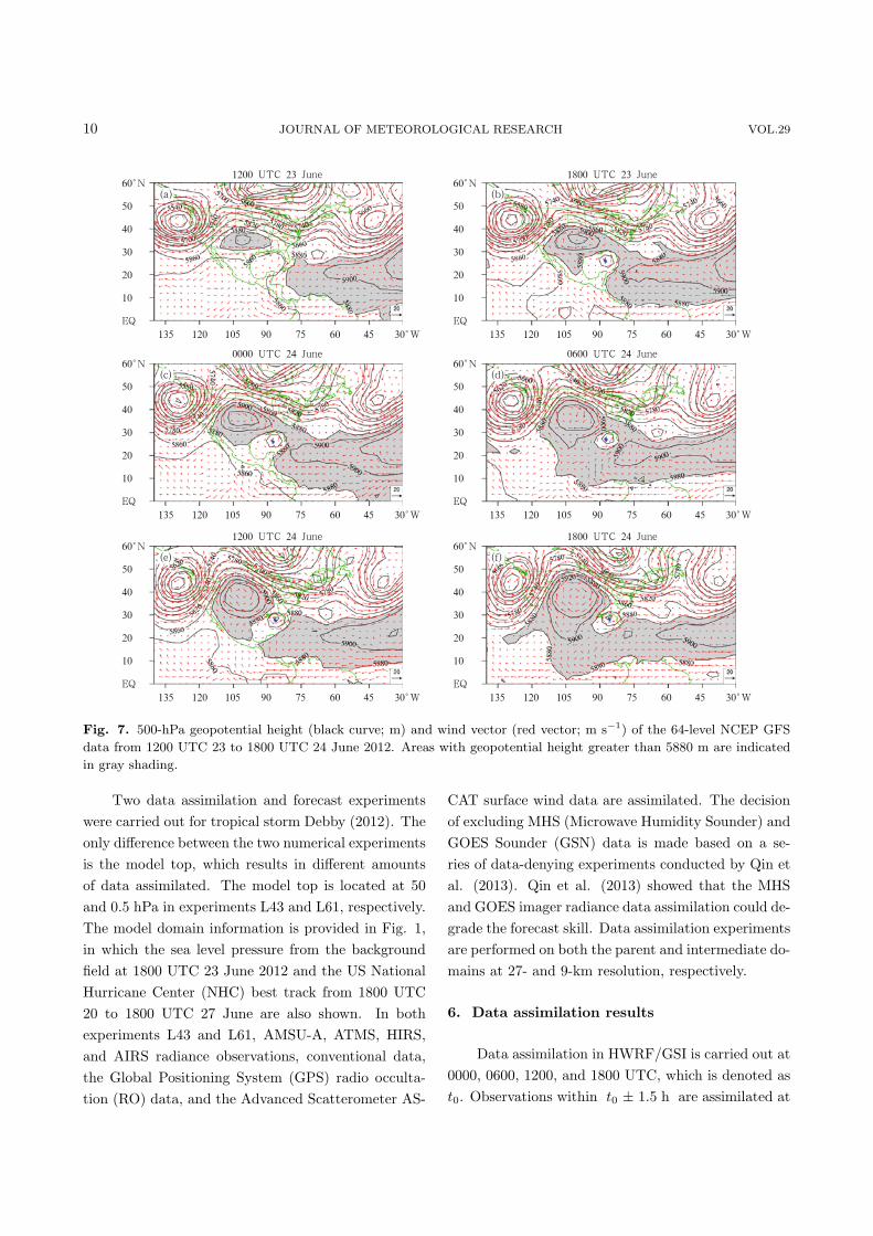
(Elsberry, 1995; Wang et al., 1998; Chan, 2005). Inorder to see under what large-scale flow environmentthe tropical storm developed and moved, we examinethe geopotential and wind vector at 500 hPa using theNCEP global forecast system (GFS) 6-h forecast fields(Fig. 7), which have a horizontal resolution of 0.3125◦
× 0.3125◦, a temporal resolution of 6 h, and a totalof 64 vertical levels unevenly spaced from the earth’ssurface to about 0.1 hPa (Kleist et al., 2009). It isseen from Fig. 7 that the tropical storm Debby waslocated in between a subtropical trough its southeastand a midlatitude ridge its northwest. The anticy-clonic flows on the west side of the subtropical highand on the east edge of the midlatitude ridge favoreda cyclonic flow development and a low-pressure sys-tem in the Gulf of Mexico at 1800 UTC 23 June 2012.The midlatitude ridge experienced an enhanced devel-opment with time, preventing Debby’s northwestwardmovement. The subtropical high gradually retreatedeastward and the northeast flow in the southwestwardbranch of the subtropical high and the midlatitudewesterly drove Debby to move eastward. It is thus an-ticipated that an accurate prediction of the size andposition of the subtropical high is crucial for the trackprediction of Debby when the forecast model is initial-ized before 25 June 2012.
The model top of the HWRF data assimilationand forecast model is too low for including manyupper-level satellite channels in data assimilation. Toillustrate this, the 43 vertical levels are indicated inFigs. 2–4 for weighting functions of AMSU-A, HIRS,and AIRS. The weighting function of a channel quan-tifies the relative contributions to the total measuredradiance from different levels of the atmosphere. Themeasured radiation is most sensitive to the atmo-spheric temperature at the altitude where weightingfunction reaches the maximum value. It is seen thata large portion of the weighting functions of manyupper-level channels are above the HWRF model top.In order to assimilate more upper-level channels withtheir weighting functions peaking in the upper tropo-sphere and the stratosphere, the model top is raisedto 0.5 hPa, and model levels are increased to 61 ac-cordingly (see right panels of Figs. 2–4).
10 JOURNAL OF METEOROLOGICAL RESEARCH VOL.29
Fig. 7. 500-hPa geopotential height (black curve; m) and wind vector (red vector; m s−1) of the 64-level NCEP GFS
data from 1200 UTC 23 to 1800 UTC 24 June 2012. Areas with geopotential height greater than 5880 m are indicated
in gray shading.
Two data assimilation and forecast experimentswere carried out for tropical storm Debby (2012). Theonly difference between the two numerical experimentsis the model top, which results in different amountsof data assimilated. The model top is located at 50and 0.5 hPa in experiments L43 and L61, respectively.The model domain information is provided in Fig. 1,in which the sea level pressure from the backgroundfield at 1800 UTC 23 June 2012 and the US NationalHurricane Center (NHC) best track from 1800 UTC20 to 1800 UTC 27 June are also shown. In bothexperiments L43 and L61, AMSU-A, ATMS, HIRS,and AIRS radiance observations, conventional data,the Global Positioning System (GPS) radio occulta-tion (RO) data, and the Advanced Scatterometer AS-
CAT surface wind data are assimilated. The decisionof excluding MHS (Microwave Humidity Sounder) andGOES Sounder (GSN) data is made based on a se-ries of data-denying experiments conducted by Qin etal. (2013). Qin et al. (2013) showed that the MHSand GOES imager radiance data assimilation could de-grade the forecast skill. Data assimilation experimentsare performed on both the parent and intermediate do-mains at 27- and 9-km resolution, respectively.
6. Data assimilation results
Data assimilation in HWRF/GSI is carried out at0000, 0600, 1200, and 1800 UTC, which is denoted ast0. Observations within t0 ± 1.5 h are assimilated at
NO.1 ZOU Xiaolei, WENG Fuzhong, Vijay TALLAPRAGADA, et al. 11
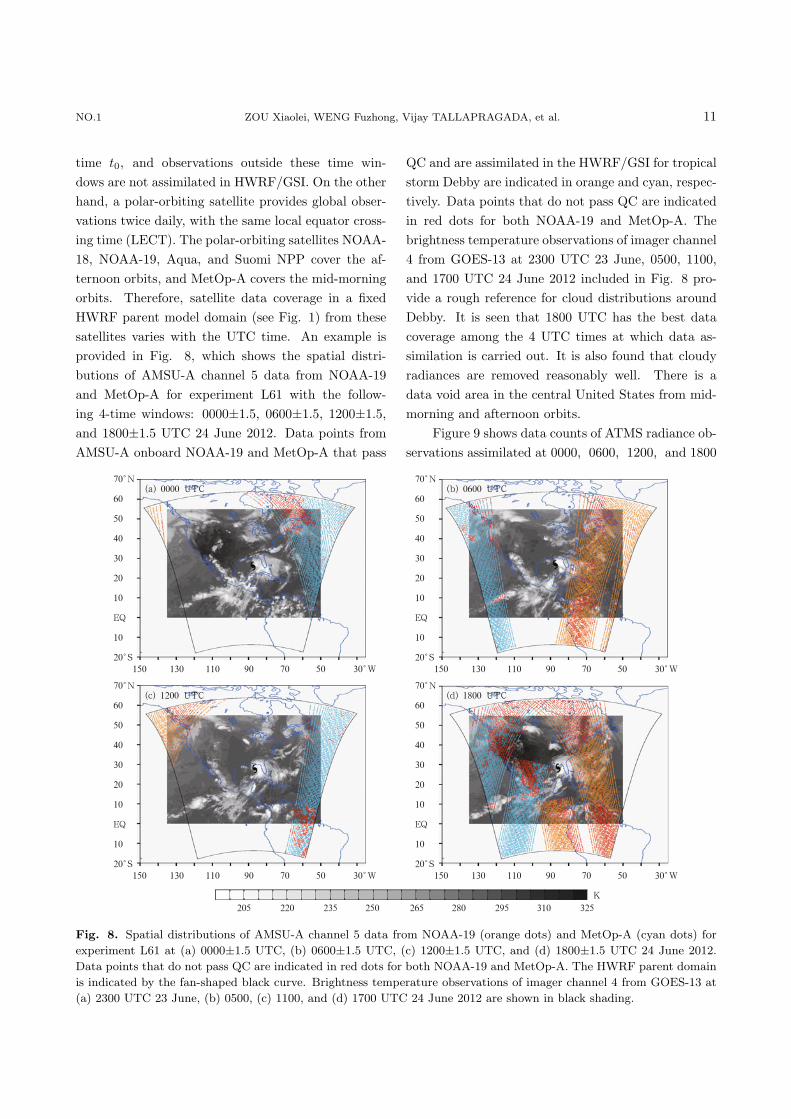
time t0, and observations outside these time win-dows are not assimilated in HWRF/GSI. On the otherhand, a polar-orbiting satellite provides global obser-vations twice daily, with the same local equator cross-ing time (LECT). The polar-orbiting satellites NOAA-18, NOAA-19, Aqua, and Suomi NPP cover the af-ternoon orbits, and MetOp-A covers the mid-morningorbits. Therefore, satellite data coverage in a fixedHWRF parent model domain (see Fig. 1) from thesesatellites varies with the UTC time. An example isprovided in Fig. 8, which shows the spatial distri-butions of AMSU-A channel 5 data from NOAA-19and MetOp-A for experiment L61 with the follow-ing 4-time windows: 0000±1.5, 0600±1.5, 1200±1.5,and 1800±1.5 UTC 24 June 2012. Data points fromAMSU-A onboard NOAA-19 and MetOp-A that pass
QC and are assimilated in the HWRF/GSI for tropicalstorm Debby are indicated in orange and cyan, respec-tively. Data points that do not pass QC are indicatedin red dots for both NOAA-19 and MetOp-A. Thebrightness temperature observations of imager channel4 from GOES-13 at 2300 UTC 23 June, 0500, 1100,and 1700 UTC 24 June 2012 included in Fig. 8 pro-vide a rough reference for cloud distributions aroundDebby. It is seen that 1800 UTC has the best datacoverage among the 4 UTC times at which data as-similation is carried out. It is also found that cloudyradiances are removed reasonably well. There is adata void area in the central United States from mid-morning and afternoon orbits.
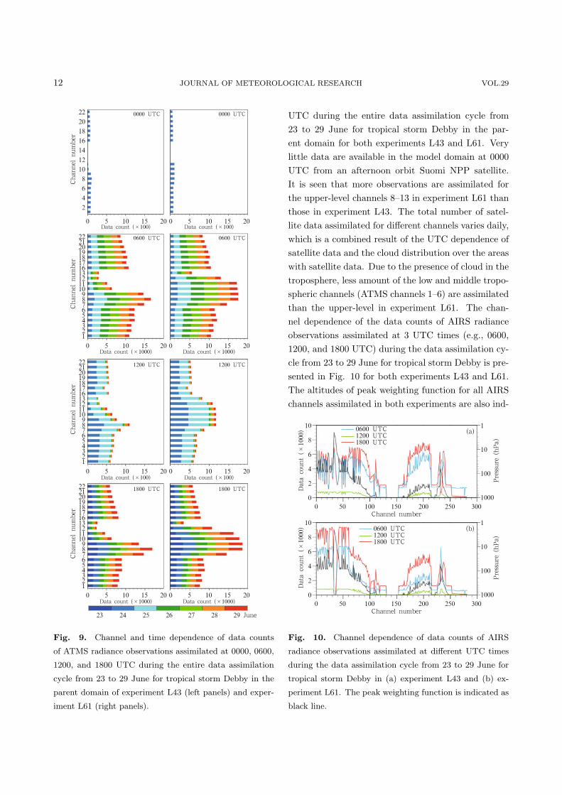
Figure 9 shows data counts of ATMS radiance ob-servations assimilated at 0000, 0600, 1200, and 1800
Fig. 8. Spatial distributions of AMSU-A channel 5 data from NOAA-19 (orange dots) and MetOp-A (cyan dots) for
experiment L61 at (a) 0000±1.5 UTC, (b) 0600±1.5 UTC, (c) 1200±1.5 UTC, and (d) 1800±1.5 UTC 24 June 2012.
Data points that do not pass QC are indicated in red dots for both NOAA-19 and MetOp-A. The HWRF parent domain
is indicated by the fan-shaped black curve. Brightness temperature observations of imager channel 4 from GOES-13 at
(a) 2300 UTC 23 June, (b) 0500, (c) 1100, and (d) 1700 UTC 24 June 2012 are shown in black shading.
12 JOURNAL OF METEOROLOGICAL RESEARCH VOL.29
Fig. 9. Channel and time dependence of data counts
of ATMS radiance observations assimilated at 0000, 0600,
1200, and 1800 UTC during the entire data assimilation
cycle from 23 to 29 June for tropical storm Debby in the
parent domain of experiment L43 (left panels) and exper-
iment L61 (right panels).
UTC during the entire data assimilation cycle from23 to 29 June for tropical storm Debby in the par-ent domain for both experiments L43 and L61. Verylittle data are available in the model domain at 0000UTC from an afternoon orbit Suomi NPP satellite.It is seen that more observations are assimilated forthe upper-level channels 8–13 in experiment L61 thanthose in experiment L43. The total number of satel-lite data assimilated for different channels varies daily,which is a combined result of the UTC dependence ofsatellite data and the cloud distribution over the areaswith satellite data. Due to the presence of cloud in thetroposphere, less amount of the low and middle tropo-spheric channels (ATMS channels 1–6) are assimilatedthan the upper-level in experiment L61. The chan-nel dependence of the data counts of AIRS radianceobservations assimilated at 3 UTC times (e.g., 0600,1200, and 1800 UTC) during the data assimilation cy-cle from 23 to 29 June for tropical storm Debby is pre-sented in Fig. 10 for both experiments L43 and L61.The altitudes of peak weighting function for all AIRSchannels assimilated in both experiments are also ind-
Fig. 10. Channel dependence of data counts of AIRS
radiance observations assimilated at different UTC times
during the data assimilation cycle from 23 to 29 June for
tropical storm Debby in (a) experiment L43 and (b) ex-
periment L61. The peak weighting function is indicated as
black line.
NO.1 ZOU Xiaolei, WENG Fuzhong, Vijay TALLAPRAGADA, et al. 13
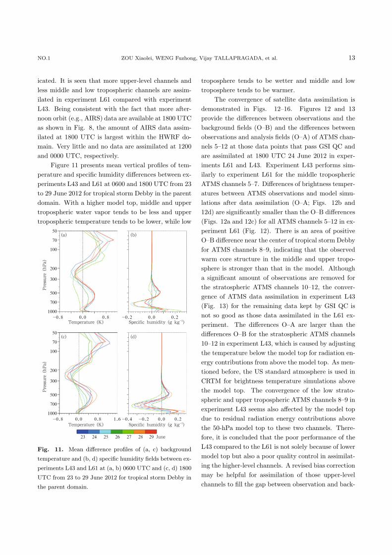
icated. It is seen that more upper-level channels andless middle and low tropospheric channels are assim-ilated in experiment L61 compared with experimentL43. Being consistent with the fact that more after-noon orbit (e.g., AIRS) data are available at 1800 UTCas shown in Fig. 8, the amount of AIRS data assim-ilated at 1800 UTC is largest within the HWRF do-main. Very little and no data are assimilated at 1200and 0000 UTC, respectively.
Figure 11 presents mean vertical profiles of tem-perature and specific humidity differences between ex-periments L43 and L61 at 0600 and 1800 UTC from 23to 29 June 2012 for tropical storm Debby in the parentdomain. With a higher model top, middle and uppertropospheric water vapor tends to be less and uppertropospheric temperature tends to be lower, while low
Fig. 11. Mean difference profiles of (a, c) background
temperature and (b, d) specific humidity fields between ex-
periments L43 and L61 at (a, b) 0600 UTC and (c, d) 1800
UTC from 23 to 29 June 2012 for tropical storm Debby in
the parent domain.
troposphere tends to be wetter and middle and lowtroposphere tends to be warmer.
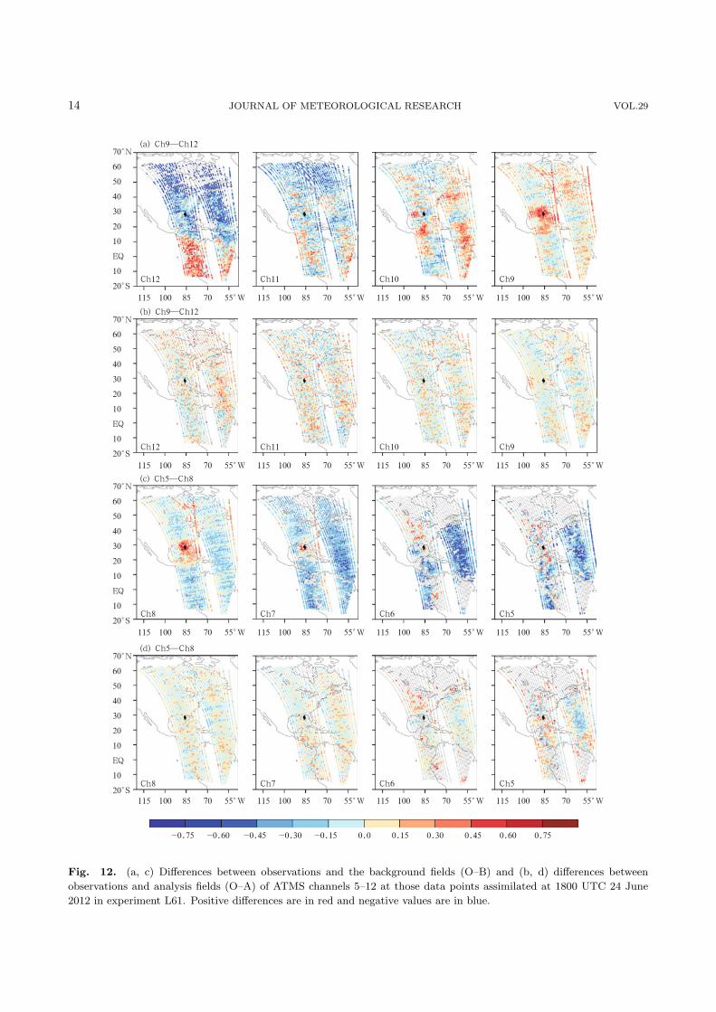
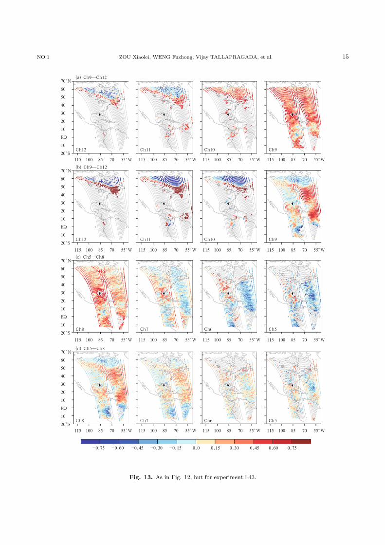
The convergence of satellite data assimilation isdemonstrated in Figs. 12–16. Figures 12 and 13provide the differences between observations and thebackground fields (O–B) and the differences betweenobservations and analysis fields (O–A) of ATMS chan-nels 5–12 at those data points that pass GSI QC andare assimilated at 1800 UTC 24 June 2012 in exper-iments L61 and L43. Experiment L43 performs sim-ilarly to experiment L61 for the middle troposphericATMS channels 5–7. Differences of brightness temper-atures between ATMS observations and model simu-lations after data assimilation (O–A; Figs. 12b and12d) are significantly smaller than the O–B differences(Figs. 12a and 12c) for all ATMS channels 5–12 in ex-periment L61 (Fig. 12). There is an area of positiveO–B difference near the center of tropical storm Debbyfor ATMS channels 8–9, indicating that the observedwarm core structure in the middle and upper tropo-sphere is stronger than that in the model. Althougha significant amount of observations are removed forthe stratospheric ATMS channels 10–12, the conver-gence of ATMS data assimilation in experiment L43(Fig. 13) for the remaining data kept by GSI QC isnot so good as those data assimilated in the L61 ex-periment. The differences O–A are larger than thedifferences O–B for the stratospheric ATMS channels10–12 in experiment L43, which is caused by adjustingthe temperature below the model top for radiation en-ergy contributions from above the model top. As men-tioned before, the US standard atmosphere is used inCRTM for brightness temperature simulations abovethe model top. The convergence of the low strato-spheric and upper tropospheric ATMS channels 8–9 inexperiment L43 seems also affected by the model topdue to residual radiation energy contributions abovethe 50-hPa model top to these two channels. There-fore, it is concluded that the poor performance of theL43 compared to the L61 is not solely because of lowermodel top but also a poor quality control in assimilat-ing the higher-level channels. A revised bias correctionmay be helpful for assimilation of those upper-levelchannels to fill the gap between observation and back-
14 JOURNAL OF METEOROLOGICAL RESEARCH VOL.29
Fig. 12. (a, c) Differences between observations and the background fields (O–B) and (b, d) differences between
observations and analysis fields (O–A) of ATMS channels 5–12 at those data points assimilated at 1800 UTC 24 June
2012 in experiment L61. Positive differences are in red and negative values are in blue.
NO.1 ZOU Xiaolei, WENG Fuzhong, Vijay TALLAPRAGADA, et al. 15
Fig. 13. As in Fig. 12, but for experiment L43.
16 JOURNAL OF METEOROLOGICAL RESEARCH VOL.29
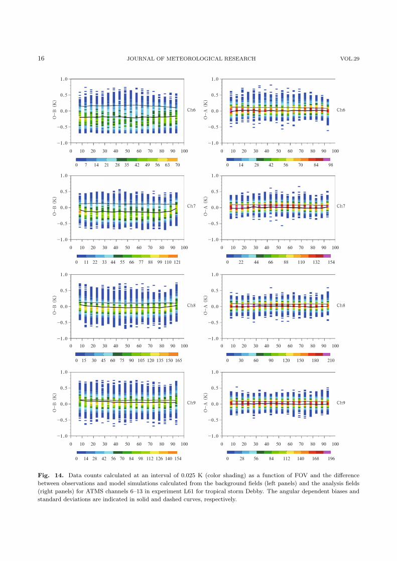
Fig. 14. Data counts calculated at an interval of 0.025 K (color shading) as a function of FOV and the difference
between observations and model simulations calculated from the background fields (left panels) and the analysis fields
(right panels) for ATMS channels 6–13 in experiment L61 for tropical storm Debby. The angular dependent biases and
standard deviations are indicated in solid and dashed curves, respectively.
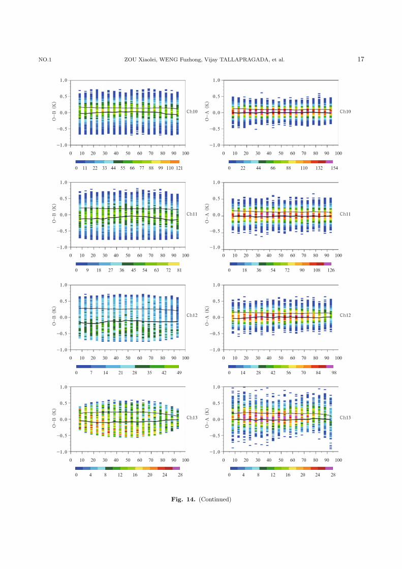
NO.1 ZOU Xiaolei, WENG Fuzhong, Vijay TALLAPRAGADA, et al. 17
Fig. 14. (Continued)

18 JOURNAL OF METEOROLOGICAL RESEARCH VOL.29
Fig. 15. As in Fig. 14, but for experiment L43.
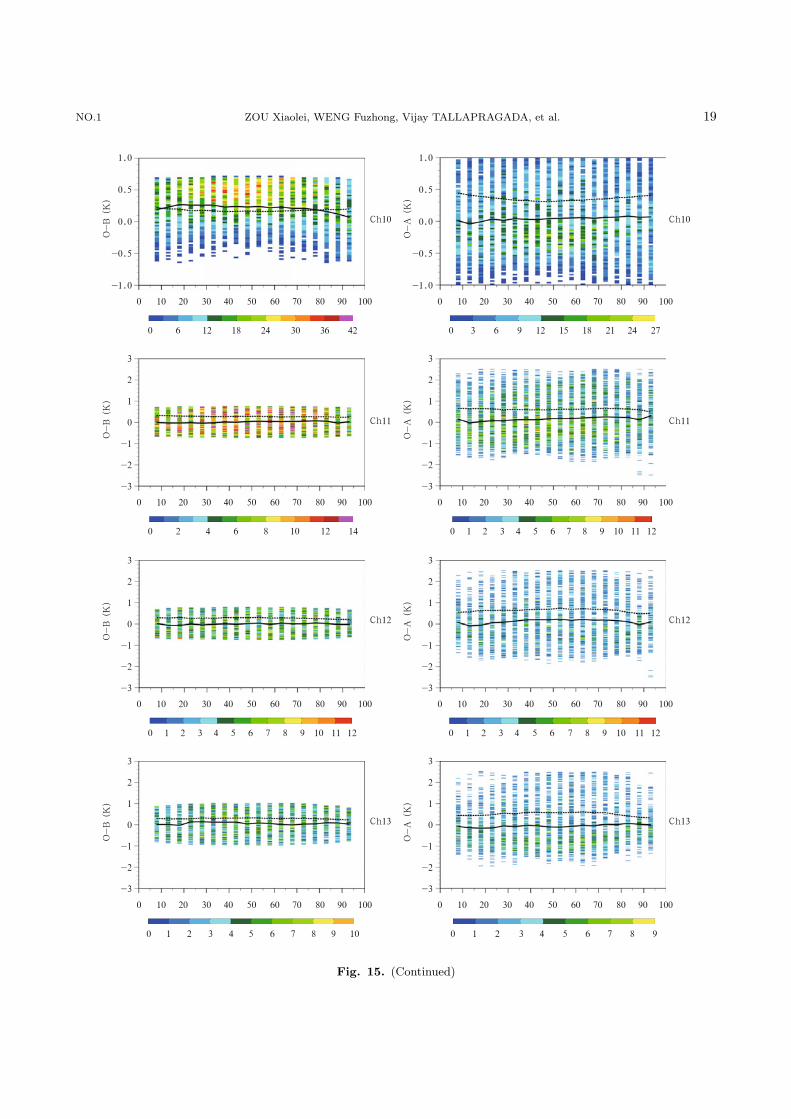
NO.1 ZOU Xiaolei, WENG Fuzhong, Vijay TALLAPRAGADA, et al. 19
Fig. 15. (Continued)

20 JOURNAL OF METEOROLOGICAL RESEARCH VOL.29
Fig. 16. (a, b) Standard deviations for O–B (red) and
O–A (blue) differences of AIRS brightness temperatures in
(a) experiment L43 and (b) experiment L61 during the en-
tire data assimilation cycle from 23 to 29 June for tropical
storm Debby. (c) The differences of the standard devia-
tions of O–B (red) and O–A (blue) between experiments
L43 and L61 (L43 minus L61). The wavelength of each
AIRS channel assimilated is indicated in (a, b) in black.
The peak weighting function of each AIRS channel assim-
ilated is indicated in (c) in black.
ground. Further investigation on a revised bias cor-rection for assimilation of upper-level channels with alow model top, which could be the case to save compu-tational cost, will be carried out to see if useful infor-mation can be provided into model initial conditionsinstead of simply removing these channels.
Figures 14 and 15 compare the data count dis-tributions as a function of scan angle and the differ-ences O–B or O–A from the 8th to 93th FOV at aninterval of 5 FOVs for ATMS channels 6–13 betweenexperiments L43 (Fig. 15) and L61 (Fig. 14). The
angular-dependent biases and standard deviations arealso plotted in Figs. 14–15. In experiment L61 (Fig.14), the O–A data spread is much narrower than thatof O–B. The biases and standard deviations are signifi-cantly reduced at all scan angles for all ATMS channels6–13. However, the O–A data spread becomes muchbroader than that of O–B for ATMS channels 9–13in experiment L43, which is consistent with Fig. 13.These results confirm an improved fit of NWP modelfields to ATMS observations through satellite data as-similation when the model top is raised from 50 to 0.5hPa, especially for upper-level channels. Similar re-sults are obtained for AIRS data assimilation.
Figure 16 shows a channel-dependent reduction ofthe differences between AIRS observations and modelsimulated brightness temperatures after data assim-ilation, including all data assimilated during 23–29June for tropical storm Debby in experiments L43 andL61. The wavelength for each of the 281 AIRS chan-nels assimilated in both experiments is also indicatedin Fig. 16. Similar to what was seen in microwaveupper-level channels, the spread of the differences be-tween observations and model simulations is increasedby data assimilation for most AIRS channels whosepeak weighting functions are above 100 hPa when themodel top is located at 50 hPa (Fig. 16a). The modelsimulated brightness temperatures based on the anal-ysis compare more favorably to AIRS observations forthose channels whose wavelengths are between 6 and10 µm and peak weighting function altitudes are be-low 100 hPa. If the model top is raised to 0.5 hPa, thestandard deviations of the differences between obser-vations and model simulations are reduced for all chan-nels after satellite data assimilation in experiment L61(Fig. 16b). Although more AIRS tropospheric chan-nels data are assimilated in L43 than in L61 (see Fig.10), the convergence (i.e., fit to observations) of L61is consistently better than that of L43 for almost allAIRS channels assimilated (see Fig. 16c).
7. Forecast differences between the two model
tops
The track forecasts by NWP models initialized 2–3 days before the landfall of tropical storm Debby was
NO.1 ZOU Xiaolei, WENG Fuzhong, Vijay TALLAPRAGADA, et al. 21
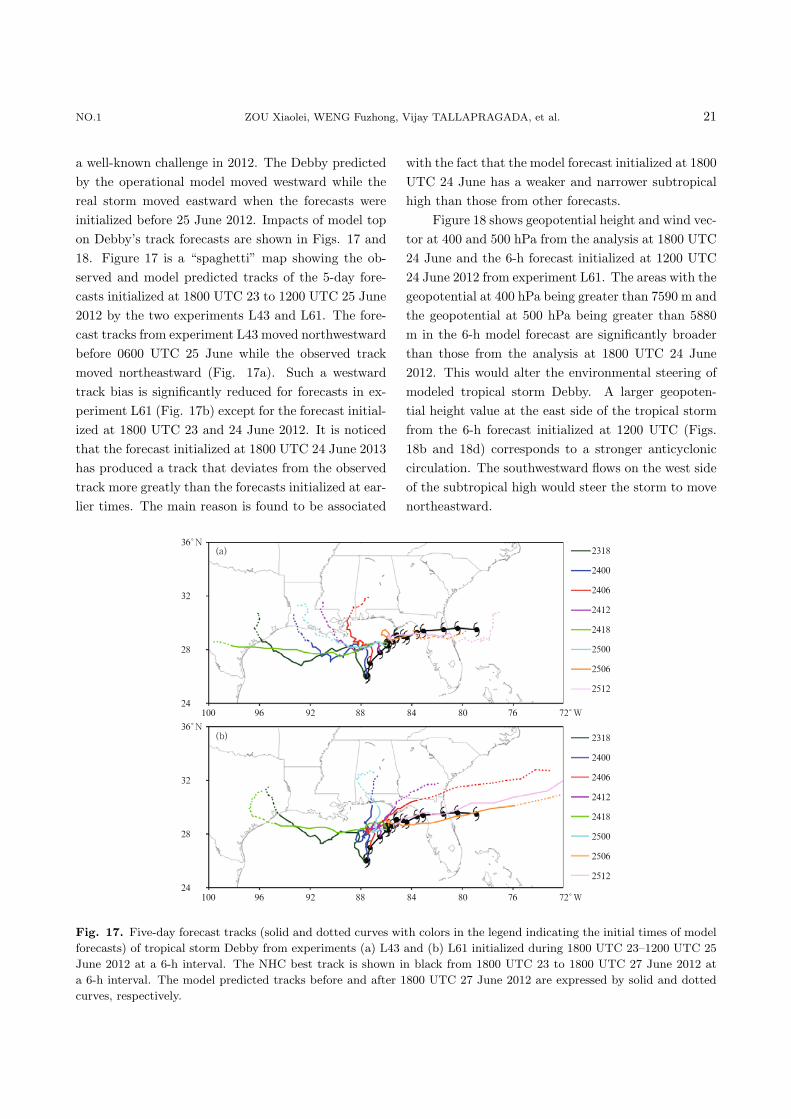
a well-known challenge in 2012. The Debby predictedby the operational model moved westward while thereal storm moved eastward when the forecasts wereinitialized before 25 June 2012. Impacts of model topon Debby’s track forecasts are shown in Figs. 17 and18. Figure 17 is a “spaghetti” map showing the ob-served and model predicted tracks of the 5-day fore-casts initialized at 1800 UTC 23 to 1200 UTC 25 June2012 by the two experiments L43 and L61. The fore-cast tracks from experiment L43 moved northwestwardbefore 0600 UTC 25 June while the observed trackmoved northeastward (Fig. 17a). Such a westwardtrack bias is significantly reduced for forecasts in ex-periment L61 (Fig. 17b) except for the forecast initial-ized at 1800 UTC 23 and 24 June 2012. It is noticedthat the forecast initialized at 1800 UTC 24 June 2013has produced a track that deviates from the observedtrack more greatly than the forecasts initialized at ear-lier times. The main reason is found to be associated
with the fact that the model forecast initialized at 1800UTC 24 June has a weaker and narrower subtropicalhigh than those from other forecasts.
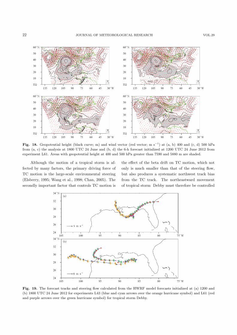
Figure 18 shows geopotential height and wind vec-tor at 400 and 500 hPa from the analysis at 1800 UTC24 June and the 6-h forecast initialized at 1200 UTC24 June 2012 from experiment L61. The areas with thegeopotential at 400 hPa being greater than 7590 m andthe geopotential at 500 hPa being greater than 5880m in the 6-h model forecast are significantly broaderthan those from the analysis at 1800 UTC 24 June2012. This would alter the environmental steering ofmodeled tropical storm Debby. A larger geopoten-tial height value at the east side of the tropical stormfrom the 6-h forecast initialized at 1200 UTC (Figs.18b and 18d) corresponds to a stronger anticycloniccirculation. The southwestward flows on the west sideof the subtropical high would steer the storm to movenortheastward.
Fig. 17. Five-day forecast tracks (solid and dotted curves with colors in the legend indicating the initial times of model
forecasts) of tropical storm Debby from experiments (a) L43 and (b) L61 initialized during 1800 UTC 23–1200 UTC 25
June 2012 at a 6-h interval. The NHC best track is shown in black from 1800 UTC 23 to 1800 UTC 27 June 2012 at
a 6-h interval. The model predicted tracks before and after 1800 UTC 27 June 2012 are expressed by solid and dotted
curves, respectively.
22 JOURNAL OF METEOROLOGICAL RESEARCH VOL.29
Fig. 18. Geopotential height (black curve; m) and wind vector (red vector; m s−1) at (a, b) 400 and (c, d) 500 hPa
from (a, c) the analysis at 1800 UTC 24 June and (b, d) the 6-h forecast initialized at 1200 UTC 24 June 2012 from
experiment L61. Areas with geopotential height at 400 and 500 hPa greater than 7590 and 5880 m are shaded.
Although the motion of a tropical storm is af-fected by many factors, the primary driving force ofTC motion is the large-scale environmental steering(Elsberry, 1995; Wang et al., 1998; Chan, 2005). Thesecondly important factor that controls TC motion is
the effect of the beta drift on TC motion, which notonly is much smaller than that of the steering flow,but also produces a systematic northwest track biasfrom the TC track. The northeastward movementof tropical storm Debby must therefore be controlled
Fig. 19. The forecast tracks and steering flow calculated from the HWRF model forecasts initialized at (a) 1200 and
(b) 1800 UTC 24 June 2012 for experiments L43 (blue and cyan arrows over the orange hurricane symbol) and L61 (red
and purple arrows over the green hurricane symbol) for tropical storm Debby.
NO.1 ZOU Xiaolei, WENG Fuzhong, Vijay TALLAPRAGADA, et al. 23
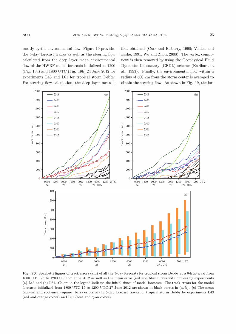
mostly by the environmental flow. Figure 19 providesthe 5-day forecast tracks as well as the steering flowcalculated from the deep layer mean environmentalflow of the HWRF model forecasts initialized at 1200(Fig. 19a) and 1800 UTC (Fig. 19b) 24 June 2012 forexperiments L43 and L61 for tropical storm Debby.For steering flow calculation, the deep layer mean is
first obtained (Carr and Elsberry, 1990; Velden andLeslie, 1991; Wu and Zhou, 2008). The vortex compo-nent is then removed by using the Geophysical FluidDynamics Laboratory (GFDL) scheme (Kurihara etal., 1993). Finally, the environmental flow within aradius of 500 km from the storm center is averaged toobtain the steering flow. As shown in Fig. 19, the for-
Fig. 20. Spaghetti figures of track errors (km) of all the 5-day forecasts for tropical storm Debby at a 6-h interval from
1800 UTC 23 to 1200 UTC 27 June 2012 as well as the mean error (red and blue curves with circles) by experiments
(a) L43 and (b) L61. Colors in the legend indicate the initial times of model forecasts. The track errors for the model
forecasts initialized from 1800 UTC 15 to 1200 UTC 27 June 2012 are shown in black curves in (a, b). (c) The mean
(curves) and root-mean-square (bars) errors of the 5-day forecast tracks for tropical storm Debby by experiments L43
(red and orange colors) and L61 (blue and cyan colors).
24 JOURNAL OF METEOROLOGICAL RESEARCH VOL.29
ecast tracks closely follow the steering flow, confirm-ing that the Debby’s motion is mostly driven by theenvironmental steering flow. In experiment L61, thestorm initialized at 1800 UTC moved westward (Fig.19b) while that from 1200 UTC followed a more real-istic northeastward track.
The forecast tracks from experiment L61 at otherUTC times followed the observed track more closely.The performance of all the 5-day forecasts for tropi-cal storm Debby initialized from 1800 UTC 23 to 1200UTC 27 June 2012 is provided in Fig. 20. It is seenthat both the mean and the root-mean-square errorsof the track forecasts by experiment L61 are smallerthan those from experiment L43.
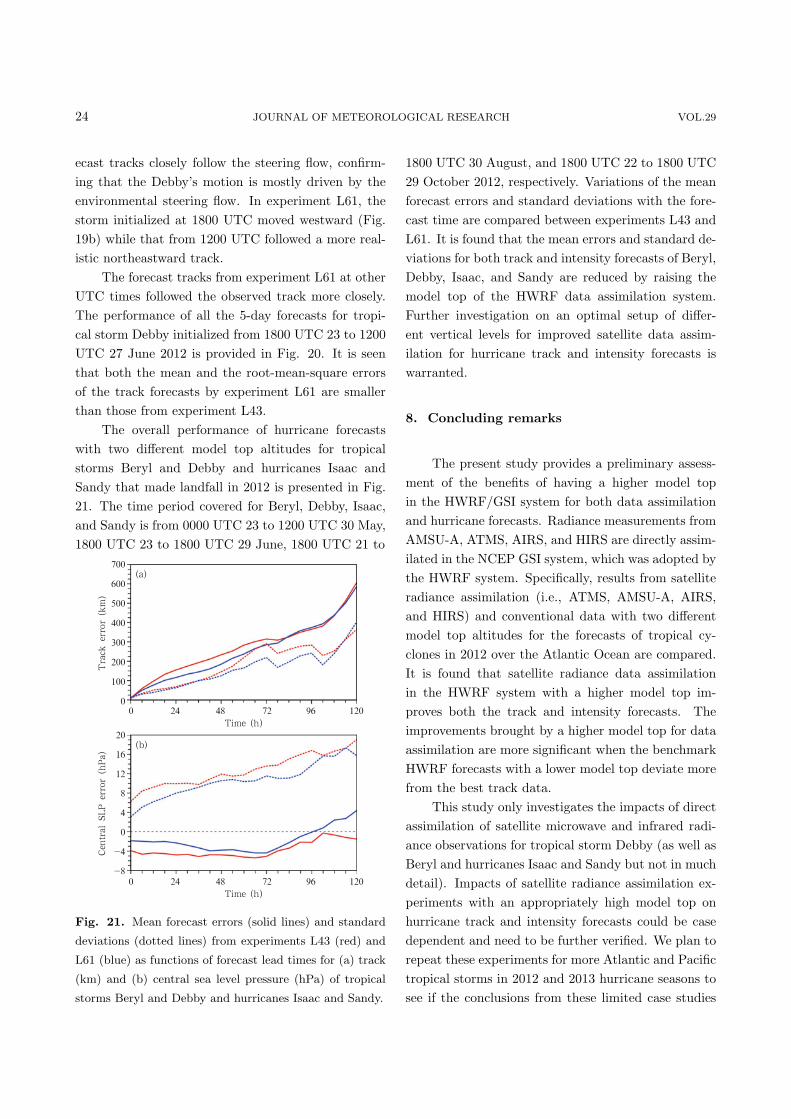
The overall performance of hurricane forecastswith two different model top altitudes for tropicalstorms Beryl and Debby and hurricanes Isaac andSandy that made landfall in 2012 is presented in Fig.21. The time period covered for Beryl, Debby, Isaac,and Sandy is from 0000 UTC 23 to 1200 UTC 30 May,1800 UTC 23 to 1800 UTC 29 June, 1800 UTC 21 to
Fig. 21. Mean forecast errors (solid lines) and standard
deviations (dotted lines) from experiments L43 (red) and
L61 (blue) as functions of forecast lead times for (a) track
(km) and (b) central sea level pressure (hPa) of tropical
storms Beryl and Debby and hurricanes Isaac and Sandy.
1800 UTC 30 August, and 1800 UTC 22 to 1800 UTC29 October 2012, respectively. Variations of the meanforecast errors and standard deviations with the fore-cast time are compared between experiments L43 andL61. It is found that the mean errors and standard de-viations for both track and intensity forecasts of Beryl,Debby, Isaac, and Sandy are reduced by raising themodel top of the HWRF data assimilation system.Further investigation on an optimal setup of differ-ent vertical levels for improved satellite data assim-ilation for hurricane track and intensity forecasts iswarranted.
8. Concluding remarks
The present study provides a preliminary assess-ment of the benefits of having a higher model topin the HWRF/GSI system for both data assimilationand hurricane forecasts. Radiance measurements fromAMSU-A, ATMS, AIRS, and HIRS are directly assim-ilated in the NCEP GSI system, which was adopted bythe HWRF system. Specifically, results from satelliteradiance assimilation (i.e., ATMS, AMSU-A, AIRS,and HIRS) and conventional data with two differentmodel top altitudes for the forecasts of tropical cy-clones in 2012 over the Atlantic Ocean are compared.It is found that satellite radiance data assimilationin the HWRF system with a higher model top im-proves both the track and intensity forecasts. Theimprovements brought by a higher model top for dataassimilation are more significant when the benchmarkHWRF forecasts with a lower model top deviate morefrom the best track data.
This study only investigates the impacts of directassimilation of satellite microwave and infrared radi-ance observations for tropical storm Debby (as well asBeryl and hurricanes Isaac and Sandy but not in muchdetail). Impacts of satellite radiance assimilation ex-periments with an appropriately high model top onhurricane track and intensity forecasts could be casedependent and need to be further verified. We plan torepeat these experiments for more Atlantic and Pacifictropical storms in 2012 and 2013 hurricane seasons tosee if the conclusions from these limited case studies
NO.1 ZOU Xiaolei, WENG Fuzhong, Vijay TALLAPRAGADA, et al. 25
could be generalized.
REFERENCES
Aumann, H., M. Chahine, and D. Barron, 2003: Sea
surface temperature measurements with AIRS:
RTG.SST comparison. SPIE Proc., 5151-30, Au-
gust 2003.
Bister, M., and K. Emanuel, 1997: The genesis of Hurri-
cane Guillermo: TEXMEX analyses and a modeling
study. Mon. Wea. Rev., 125, 2662–2682.
Bosart, L. F., C. S. Velden, W. E. Bracken, et al., 2002:
Environmental influences on the rapid intensification
of Hurricane Opal (1995) over the Gulf of Mexico.
Mon. Wea. Rev., 128, 322–352.
Bozeman, M. L., D. Niyogi, S. Gopalakrishnan, et al.,
2011: An HWRF-based ensemble assessment of the
land surface feedback on the post-landfall intensifi-
cation of Tropical Storm Fay (2008). Nat. Hazards,
63, 1543–1571, doi: 10.1007/s11069-011-9841-5.
Bracken, W. E., and L. F. Bosart, 2000: The role of
synoptic-scale flow during tropical cyclogenesis over
the North Atlantic Ocean. Mon. Wea. Rev., 128,
353–376.
Carr III, L. E., and R. L. Elsberry, 1990: Observational
evidence for predictions of tropical cyclone propa-
gation relative to environmental steering. J. Atmos.
Sci., 47, 542–546.
Carter, C., Q. Liu, W. Yang, et al., 2002: Net heat flux,
visible/infrared imager/radiometer suite algorithm
theoretical basis document. Available at http://np
oesslib.ipo.noaa.gov/u−listcategory−v3.php?35.
Challa, M., and R. L. Pfeffer, 1990: Formation of Atlantic
hurricanes from cloud clusters and depressions. J.
Atmos. Sci., 47, 909–927.
Chan, J. C. L., 1995: Tropical cyclone activity in the
western North Pacific in relation to the stratospheric
quasi-biennial oscillation. Mon. Wea. Rev., 123,
2567–2571.
Chan, J. C. L., 2005: The physics of tropical cyclone
motion. Ann. Rev. Fluid Mech., 37, 99–128.
Cram, T., J. Persing, M. Montgomery, et al., 2007: A
Lagrangian trajectory view on transport and mixing
processes between the eye, eyewall, and environment
using a high-resolution simulation of Hurricane Bon-
nie (1998). J. Atmos. Sci., 64, 1835–1856.
Davis, C., and L. Bosart, 2006: The formation of Hur-
ricane Humberto (2001): The importance of extra-
tropical precursors. Quart. J. Roy. Meteor. Soc.,
132, 2055–2085.
DeMaria, M., J.-J. Baik, and J. Kaplan, 1993: Upper-
level eddy angular momentum flux and tropical
cyclone intensity change. J. Atmos. Sci., 50, 1133–
1147.
DeMaria, M., 1996: The effect of vertical shear on trop-
ical cyclone intensity change. J. Atmos. Sci., 53,
2076–2087.
Derber, J. C., and W.-S. Wu, 1998: The use of TOVS
cloud-cleared radiances in the NCEP SSI analysis
system. Mon. Wea. Rev., 126, 2287–2299.
Elsberry, R. L., 1995: Tropical cyclone motion. Global
Perspectives of Tropical Cyclones, WMO Report
No. TCP-38, Elsberry, R. L., Ed., World Meteoro-
logical Organization, Geneva, 106–197.
Emanuel, K. A., 1986: An air-sea interaction theory for
tropical cyclones. Part I: Steady-state maintenance.
J Atmos. Sci., 42, 1062–1071.
Emanuel, K. A., S. Solomon, D. Folini, et al., 2013: Influ-
ence of tropical tropoause layer cooling on Atlantic
hurricane activity. J. Climate, 26, 2288–2301, doi:
10.1175/JCLI-D-12-0024z.1.
Gallina, G., and C. Velden, 2002: Environmental vertical
wind shear and tropical cyclone intensity change uti-
lizing enhanced satellite derived wind information.
Preprints, 25th Conf. on Hurricanes and Tropical
Meteorology, San Diego, CA, Amer. Meteor. Soc.,
172–173.
Gopalakrishnan, S., F. Marks, X. Zhang, et al., 2011:
The experimental HWRF system: A study on the
influence of horizontal resolution on the structure
and intensity changes in tropical cyclones using an
idealized framework. Mon. Wea. Rev., 139, 1762–
1784.
Gopalakrishnan, S., S. Goldenberg, T. Quirino, et al.,
2012: Towards improving high-resolution numerical
hurricane forecasting: Influence of model horizontal
grid resolution, initialization, and physics. Wea.
Forecasting, 27, 647–666.
Gustafsson, N., X. Y. Huang, X. Yang, et al., 2012:
Four-dimensional variational data assimilation for
a limited area model. Tellus, 64A, 14985, doi:
0.3402/tellusa.v64i0.14985.
Han, Y, F. Weng, Q. Liu, et al., 2007: A fast radiative
transfer model for SSMIS upper atmosphere sound-
ing channels. J. Geophys. Res., 112, D11121, doi:
10.1029/2006JD008208.

26 JOURNAL OF METEOROLOGICAL RESEARCH VOL.29
Kleist, D. T., D. F. Parrish, J. C. Derber, et al., 2009:
Introduction of the GSI into the NCEP Global Data
Assimilation System. Wea. Forecasting, 24, 1691–
1705.
Kurihara, Y., M. A. Bender, and R. J. Ross, 1993: An
initialization scheme of hurricane models by vortex
specification. Mon. Wea. Rev., 121, 2030–2045.
Leroux, M.-D., M. Plu, D. Barbary, et al., 2013: Dynami-
cal and physical processes leading to tropical cyclone
intensification under upper-level trough forcing. J.
Atmos. Sci., 70, 2547–2565.
Liu, Q., F. Weng, and S. J. English, 2011: An improved
fast microwave water emissivity model. IEEE Trans.
Geosci. Remote Sens., 49, 1238–1250.
Marin, J., D. Raymond, and G. Raga, 2009: Intensifica-
tion of tropical cyclones in the GFS model. Atmos.
Chem. Phys., 9, 1407–1417.
McBride, J., and R. Zehr, 1981: Observational analysis
of tropical cyclone formation. Part II: Comparison
of non-developing versus developing systems. J. At-
mos. Sci., 38, 1132–1151.
McNally, A. P., P. D. Watts, J. A. Smith, et al., 2006:
The assimilation of AIRS radiance data at ECMWF.
Quart. J. Roy. Meteor. Soc., 132, 935–957.
Mo, T., 1996: Prelaunch calibration of the Advanced
Microwave Sounding Unit-A for NOAA-K. IEEE
Trans. Microwave Theory Technol., 44, 1460–1469,
doi: 10.1109/22.536029.
Molinari, J., and D. Vollaro, 2010: Rapid intensification
of a sheared tropical storm. Mon. Wea. Rev., 138,
3869–3885.
Montmerle, T., F. Rabier, and C. Fischer, 2007: Relative
impact of polar-orbiting and geostationary satellite
radiances in the Aladin/France numerical weather
prediction system. Quart. J. R. Meteor. Soc., 133,
655–671.
NWP SAF, 2011: Annex to AAPP Scientific Documenta-
tion: Pre-Processing of ATMS and CrIS, Document
NWPSAF-MO-UD-027. Available at http://resea
rch.metoffice.gov.uk/research/interproj/nwpsaf/aap
p/index.html.
Pagano, T. S., H. H. Aumann, S. E. Broberg, et al., 2002:
On-board calibration techniques and test results for
the Atmospheric Infrared Sounder (AIRS). Proceed-
ings of SPIE on Earth Observing Systems VII, 7
July 2002, Seattle, USA.
Pattanayak, S., U. C. Mohanty, and S. G. Gopalakrish-
nan, 2011: Simulation of very severe cyclone Mala
over Bay of Bengal with HWRF modeling system.
Nat. Hazards, 63, 1413–1437, doi: 10.1007/s11069-
011-9863-z.
Pfeffer, R. L., and M. Challa, 1981: A numerical study
of the role of eddy fluxes of momentum in the devel-
opment of Atlantic hurricanes. J. Atmos. Sci., 38,
2393–2398.
Powell, M., 1990: Boundary layer structure and dynam-
ics in outer hurricane rainbands. Part II: Downdraft
modification and mixed layer recovery. Mon. Wea.
Rev., 118, 918–938.
Purser, R. J., W.-S. Wu, D. F. Parrish, et al., 2003a: Nu-
merical aspects of the application of recursive filters
to variational statistical analysis. Part I: Spatially
homogeneous and isotropic Gaussian covariances.
Mon. Wea. Rev., 131, 1524–1535.
Purser, R. J., W.-S. Wu, D. F. Parrish, et al., 2003b: Nu-
merical aspects of the application of recursive filters
to variational statistical analysis. Part II: Spatially
inhomogeneous and anisotropic general covariances.
Mon. Wea. Rev., 131, 1536–1548.
Qin, Z., X. Zou, and F. Weng, 2013, Evaluating added
benefits of assimilating GOES imager radiance data
in GSI for coastal QPFs. Mon. Wea. Rev., 141,
75–92.
Ramsay, H. A., 2013: The effects of imposed strato-
spheric cooling on the maximum intensity of tropical
cyclones in axisymmetric radiative-convective equi-
librium. J. Climate, 26, 9977–9985, doi: http://dx.
doi.org/10.1175/JCLI-D-13-00195.1.
Riemer, M., M. Montgomery, and M. Nicholls, 2010: A
new paradigm for intensity modification of tropical
cyclones: Thermodynamic impact of vertical wind
shear on the inflow layer. Atmos. Chem. Phys., 10,
3163–3188.
Riemer, M., and M. Montgomery, 2011: Simple kinematic
models for the environmental interaction of tropi-
cal cyclones in vertical wind shear. Atmos. Chem.
Phys., 11, 9395–9414.
Simpson, R., and R. Riehl, 1958: Mid-tropospheric venti-
lation as a constraint on hurricane development and
maintenance. Preprints, Tech. Conf. on Hurricanes,
Miami Beach, FL, Amer. Meteor. Soc., D4-1-D4-10.
Stengel, M., P. Unden, M. Lindskog, et al., 2009: Assim-
ilation of SEVIRI infrared radiances with HIRLAM
4D-Var. Quart. J. R. Meteor. Soc., 135, 2100–2109.
Tang, B., and K. Emanuel, 2010: Midlevel ventilation’s
constraint on tropical cyclone intensity. J. Atmos.
Sci., 67, 1817–1830.
NO.1 ZOU Xiaolei, WENG Fuzhong, Vijay TALLAPRAGADA, et al. 27
Untch, A., and A. Simmons, 1999: Increased strato-
spheric resolution in the ECMWF forecasting sys-
tem. Proceedings of SODA Workshop on Chemical
Data Assimilation. ECMWF Newsletter, 82, 2–8.
Velden, C. S., and L. M. Leslie, 1991: The basic rela-
tionship between tropical cyclone intensity and the
depth of the environmental steering layer in the
Australian region. Wea. Forecasting, 6, 244–253.
Wang Bin, R. L. Elsberry, Wang Yuqing, et al., 1998:
Dynamics in tropical cyclone motion: A review.
Chinese J. Atmos. Sci., 22, 416–434.
Weng, F., B. Yan, and N. Grody, 2001: A microwave land
emissivity model. J. Geophys. Res., 106, 20115–
20123.
Weng, F., and Q. Liu, 2003: Satellite data assimilation in
numerical weather prediction models. Part I: For-
ward radiative transfer and Jacobian modeling in
cloudy atmospheres. J. Atmos. Sci., 60, 2633–2646.
Weng, F., 2007: Advances in radiative transfer modeling
in support of satellite data assimilation. J. Atmos.
Sci., 64, 3799–3807.
Weng, F., T. Zhu, and B. Yan, 2007: Satellite data as-
similation in numerical weather prediction models.
Part II: Uses of rain-affected radiances from mi-
crowave observations for hurricane vortex analysis.
J. Atmos. Sci., 64, 3910–3925.
Weng, F., X. Zou, X. Wang, et al., 2012: Introduc-
tion to Suomi national polar-orbiting partnership
advanced technology microwave sounder for numer-
ical weather prediction and tropical cyclone ap-
plications. J. Geophys. Res., 117, D19112, doi:
10.1029/2012JD018144.
Weng, F., H. Yang, and X. Zou, 2013: On convertibility
from antenna to sensor brightness temperature for
ATMS. IEEE Trans. Geo. Remote Sen., 10, 771–
775.
Wu, W.-S., R. J. Purser, and D. F. Parrish, 2002: Three-
dimensional variational analysis with spatially in-
homogeneous covariances. Mon. Wea. Rev., 130,
2905–2916.
Wu, X., and W. L. Smith, 1997: Emissivity of rough sea
surface for 8–13 m: Modeling and verification. Appl.
Opt., 36, 2609–2619.
Wu, Y., and X. Zou, 2008: Numerical test of a simple
approach for using TOMS total ozone data in hurri-
cane environment. Quart. J. R. Meteor. Soc., 134,
1397–1408.
Yang, H., and X. Zou, 2013: Optimal ATMS remapping
algorithm for climate research. IEEE Trans. Geo.
Remote Sensing, 52, 7290–7296.
Yan, B., F. Weng, and K. Okamoto, 2004: Improved
estimation of snow emissivity from 5 to 200 GHz.
Proceedings of 8th Specialist Meeting on Microwave
Radiometry and Remote Sensing Applications, 24–
27 February 2004, Rome, Italy.
Yeh, K.-S., X. Zhang, S. Gopalakrishnan, et al., 2012:
The AOML/ESRL hurricane research system: Per-
formance in the 2008 hurricane season. Nat. Haz-
ards, 63, 1439–1449, doi: 10.1007/s11069-011-9787-
7.
Zehr, R., 1992: Tropical Cyclogenesis in the Western
North Pacific. NOAA Tech. Rep. NESDIS 61, 181
pp.
Zhang, X., T. S. Quirino, K.-S. Yeh, et al., 2011:
HWRFx: Improving hurricane forecast with high-
resolution modeling. Comput. Sci. Eng., 13, 13–21.
Zou, X., F. Weng, B. L. Zhang, et al., 2013: Impacts of
assimilation of ATMS data in HWRF on track and
intensity forecasts of 2012 four landfall hurricanes.
J. Geophys. Res., 118, 11558–11576.
Zou, X., L. Lin, and F. Weng, 2013: Absolute calibration
of ATMS upper level temperature sounding channels
using GPS RO observations. IEEE Trans. Geosci.
Remote Sens., 52, 1397–1406.