satellite data compression - the eye archive/satellite_data... · printed on acid-free paper ... 4...

Satellite Data Compression

Bormin HuangEditor

Satellite Data Compression

Editor

Bormin HuangSpace Science and Engineering CenterUniversity of Wisconsin – MadisonMadison, WI, [email protected]

ISBN 978-1-4614-1182-6 e-ISBN 978-1-4614-1183-3DOI 10.1007/978-1-4614-1183-3Springer New York Dordrecht Heidelberg London

Library of Congress Control Number: 2011939205

# Springer Science+Business Media, LLC 2011All rights reserved. This work may not be translated or copied in whole or in part without the writtenpermission of the publisher (Springer Science+Business Media, LLC, 233 Spring Street, New York,NY 10013, USA), except for brief excerpts in connection with reviews or scholarly analysis. Use in

connection with any form of information storage and retrieval, electronic adaptation, computer software,or by similar or dissimilar methodology now known or hereafter developed is forbidden.The use in this publication of trade names, trademarks, service marks, and similar terms, even if theyare not identified as such, is not to be taken as an expression of opinion as to whether or not they aresubject to proprietary rights.

Printed on acid-free paper

Springer is part of Springer Science+Business Media (www.springer.com)

Contents

1 Development of On-Board Data Compression Technologyat Canadian Space Agency. . . . . . . . . . . . . . . . . . . . . . . . . . . . . . . . . . . . . . . . . . . . . 1

Shen-En Qian

2 CNES Studies for On-Board Compression of High-ResolutionSatellite Images . . . . . . . . . . . . . . . . . . . . . . . . . . . . . . . . . . . . . . . . . . . . . . . . . . . . . . . . . 29

Carole Thiebaut and Roberto Camarero

3 Low-Complexity Approaches for Lossless and Near-LosslessHyperspectral Image Compression . . . . . . . . . . . . . . . . . . . . . . . . . . . . . . . . . . . 47

Andrea Abrardo, Mauro Barni, Andrea Bertoli, Raoul Grimoldi,

Enrico Magli, and Raffaele Vitulli

4 FPGA Design of Listless SPIHT for OnboardImage Compression . . . . . . . . . . . . . . . . . . . . . . . . . . . . . . . . . . . . . . . . . . . . . . . . . . . . 67

Yunsong Li, Juan Song, Chengke Wu, Kai Liu, Jie Lei,

and Keyan Wang

5 Outlier-Resilient Entropy Coding . . . . . . . . . . . . . . . . . . . . . . . . . . . . . . . . . . . . . 87

Jordi Portell, Alberto G. Villafranca, and Enrique Garcıa-Berro

6 Quality Issues for Compression of Hyperspectral ImageryThrough Spectrally Adaptive DPCM . . . . . . . . . . . . . . . . . . . . . . . . . . . . . . . . . 115

Bruno Aiazzi, Luciano Alparone, and Stefano Baronti

7 Ultraspectral Sounder Data Compression by thePrediction-Based Lower Triangular Transform . . . . . . . . . . . . . . . . . . . . . 149

Shih-Chieh Wei and Bormin Huang

8 Lookup-Table Based Hyperspectral Data Compression . . . . . . . . . . . . 169

Jarno Mielikainen

v

9 Multiplierless Reversible Integer TDLT/KLTfor Lossy-to-Lossless Hyperspectral Image Compression . . . . . . . . . . . 185

Jiaji Wu, Lei Wang, Yong Fang, and L.C. Jiao

10 Divide-and-Conquer Decorrelation for HyperspectralData Compression . . . . . . . . . . . . . . . . . . . . . . . . . . . . . . . . . . . . . . . . . . . . . . . . . . . . . . 215

Ian Blanes, Joan Serra-Sagrista, and Peter Schelkens

11 Hyperspectral Image Compression Using SegmentedPrincipal Component Analysis . . . . . . . . . . . . . . . . . . . . . . . . . . . . . . . . . . . . . . . . 233

Wei Zhu, Qian Du, and James E. Fowler

12 Fast Precomputed Vector Quantization with OptimalBit Allocation for Lossless Compressionof Ultraspectral Sounder Data . . . . . . . . . . . . . . . . . . . . . . . . . . . . . . . . . . . . . . . . 253

Bormin Huang

13 Effects of Lossy Compression on HyperspectralClassification . . . . . . . . . . . . . . . . . . . . . . . . . . . . . . . . . . . . . . . . . . . . . . . . . . . . . . . . . . . . 269

Chulhee Lee, Sangwook Lee, and Jonghwa Lee

14 Projection Pursuit-Based Dimensionality Reductionfor Hyperspectral Analysis . . . . . . . . . . . . . . . . . . . . . . . . . . . . . . . . . . . . . . . . . . . . 287

Haleh Safavi, Chein-I Chang, and Antonio J. Plaza

vi Contents

Contributors

Andrea Abrardo Dip. di Ingegneria dell’Informazione,

Universita di Siena, Siena, Italy

Bruno Aiazzi IFAC-CNR, Via Madonna del Piano 10, 50019 Sesto F.no, Italy

Luciano Alparone Department of Electronics & Telecommunications,

University of Florence, Via Santa Marta 3, 50139 Florence, Italy

Mauro Barni Dip. di Ingegneria dell’Informazione, Universita di Siena,

Siena, Italy

Stefano Baronti IFAC-CNR, Via Madonna del Piano 10, 50019 Sesto F.no, Italy

Andrea Bertoli Carlo Gavazzi Space S.p.A., Milan, Italy

Ian Blanes Universitat Autonoma de Barcelona, E-08290 Cerdanyola

del Valles (Barcelona), Spain

Roberto Camarero Ctr. National d’Etudes Spatiales (CNES), Toulouse, France

Chein-I Chang Remote Sensing Signal and Image Processing Laboratory,

Department of Computer Science and Electrical Engineering,

University of Maryland, Baltimore, MD, USA

Department of Electrical Engineering, National Chung

Hsing University, Taichung, Taiwan

Qian Du Department of Electrical and Computer Engineering,

Mississippi State University, Starkville, USA

Yong Fang College of Information Engineering, Northwest A&F University,

yangling, China

James E. Fowler Department of Electrical and Computer Engineering,


vii

Enrique Garcıa-Berro Institut d’Estudis Espacials de Catalunya,

Barcelona, Spain

Departament de Fısica Aplicada, Universitat Politecnica de Catalunya,

Castelldefels, Spain

Raoul Grimoldi Carlo Gavazzi Space S.p.A., Milan, Italy

Bormin Huang Space Science and Engineering Center,

University of Wisconsin–Madison, Madison, WI, USA

L.C. Jiao School of Electronic Engineering, Xidian University, xi’an, China

Chulhee Lee Yonsei University, South Korea

Jonghwa Lee Yonsei University, South Korea

Sangwook Lee Yonsei University, South Korea

Jie Lei State Key Laboratory of Integrated Service Networks,

Xidian University, Xi’an, China

Yunsong Li State Key Laboratory of Integrated Service Networks,


Kai Liu State Key Laboratory of Integrated Service Networks,


Enrico Magli Dip. di Elettronica, Politecnico di Torino, Torino, Italy

Jarno Mielikainen School of Electrical and Electronic Engineering,

Yonsei University, Seoul, South Korea

Antonio J. Plaza Department of Technology of Computers and Communications,

University of Extremadura, Escuela Politecnica de Caceres, Caceres, SPAIN

Jordi Portell Departament d’Astronomia i Meteorologia/ICCUB,

Universitat de Barcelona, Barcelona, Spain

Institut d’Estudis Espacials de Catalunya, Barcelona, Spain

Shen-En Qian Canadian Space Agency, St-Hubert, QC, Canada

Haleh Safavi Remote Sensing Signal and Image Processing Laboratory,

Department of Computer Science and Electrical Engineering,

University of Maryland, Baltimore, MD, USA

Peter Schelkens Department of Electronics and Informatics,

Vrije Universiteit Brussel, Pleinlaan 2, B-1050 Brussels, Belgium

Interdisciplinary Institute for Broadband Technology, Gaston Crommenlaan 8,

b102, B-9050 Ghent, Belgium

viii Contributors

Joan Serra-Sagrista Universitat Autonoma de Barcelona, E-08290 Cerdanyola

del Valles (Barcelona), Spain

Juan Song State Key Laboratory of Integrated Service Networks,


Carole Thiebaut Ctr. National d’Etudes Spatiales (CNES), Toulouse, France

Alberto G. Villafranca Institut d’Estudis Espacials de Catalunya,

Barcelona, Spain

Departament de Fısica Aplicada, Universitat Politecnica de Catalunya,

Castelldefels, Spain

Raffaele Vitulli European Space Agency – ESTEC TEC/EDP,

Noordwijk, The Netherlands

Keyan Wang State Key Laboratory of Integrated Service Networks,


Lei Wang School of Electronic Engineering, Xidian University, xi’an, China

Shih-Chieh Wei Department of Information Management,

Tamkang University, Tamsui, Taiwan

Chengke Wu State Key Laboratory of Integrated Service Networks,


Jiaji Wu School of Electronic Engineering, Xidian University, xi’an, China

Wei Zhu Department of Electrical and Computer Engineering,


Contributors ix

Chapter 1

Development of On-Board Data CompressionTechnology at Canadian Space Agency

Shen-En Qian

Abstract This chapter reviews and summarizes the researches and developments

on data compression techniques for satellite sensor data at the Canadian Space

Agency in collaboration with its partners in other government departments, acade-

mia and Canadian industry. This chapter describes the subject matters in the order

of the following sections.

1 Review of R&D of Satellite Data Compressionat the Canadian Space Agency

The Canadian Space Agency (CSA) began developing data compression algorithms

as an enabling technology for a hyperspectral satellite in the 1990s. Both lossless and

lossy data compression techniques have been studied. Compression techniques for

operational use have been developed [1–16]. The focus of the development is the

vector quantization (VQ) based near lossless data compression techniques. Vector

quantization is an efficient coding technique for data compression of hyperspectral

imagery because of its simplicity and its vector nature for preservation of the spectral

signatures associated with individual ground samples in the scene. Reasonably high

compression ratios (>10:1) can be achieved with significantly high compression

fidelity for most of remote sensing applications and algorithms.

S.-E. Qian (*)

Canadian Space Agency, St-Hubert, QC, Canada

e-mail: [email protected]

B. Huang (ed.), Satellite Data Compression, DOI 10.1007/978-1-4614-1183-3_1,# Springer Science+Business Media, LLC 2011

1

mailto:[email protected]

1.1 Lossless Compression

In the 1990s, a prediction-based approach was adopted. It used a linear or nonlinear

predictor in spatial or/and spectral domain to generate prediction and applies

DPCM to generate residuals followed by an entropy coding. A total of 99 fixed

coefficient predictors covering 1D, 2D and 3D versions were investigated [15].

An adaptive predictor that chose the best predictor from a pre-selected predictor

bank was also investigated. The Consultative Committee for Space Data System

(CCSDS) recommended lossless algorithm (mainly the Rice algorithm) [17] was

selected as the entropy encoder to encode the prediction residuals. In order to

evaluate the performance of the CCSDS lossless algorithm, an entropy encoder

referred to as Base-bit Plus Overflow-bit Coding (BPOC) [18] was also utilized to

compare the entropy coding efficiency.

Three hyperspectral datacubes acquired using both the Airborne Visible/Near

Infrared Imaging Spectrometer (AVIRIS) and the Compact Airborne Spectro-

graphic Imager (casi) were tested. Two 3D predictors, which use five and seven

nearest neighbor pixels in 3D, produced the best residuals. Compression ratios

around 2.4 were achieved after encoding the residuals produced by using these two

entropy encoders. All other predictors produced compression ratios smaller than

2:1. The BPOC slightly outperformed the CCSDS lossless algorithm.

1.2 Wavelet Transform Lossy Data Compression

Wehave also developed a compression technique for hyperspectral data usingwavelet

transform techniques [16]. The method for creating zerotrees as proposed by Shapiro

[19] has been modified for use with hyperspectral data. An optimized multi-level

lookup table was introduced which improves the performance of an embedded

zerotree wavelet algorithm. In order to evaluate the performance of the algorithm,

this algorithm was compared to SPIHT [20] and JPEG. The new algorithm was found

to perform as well as or to surpass published algorithms which are much more

computationally complex and not suitable for compression of hyperspectral data.

As in Sect. 1.1 testing was done with both AVIRIS and casi data and compression

ratios over 32:1 were obtained with fidelities greater than 40.0 dB.

1.3 Vector Quantization Data Compression

We selected VQ technique for data compression of hyperspectral imagery because

of its simplicity and because its vector nature can preserve the spectra associated

with individual ground samples in the scene. Vector quantization is an efficient

coding technique. The generalized Lloyed algorithm (GLA) (sometimes also called

LBG) is the most widely used VQ algorithm for image compression [21].

2 S.-E. Qian

In our application, we associate the vectors used in the VQ algorithm with the

full spectral dimension of each ground sample of a hyperspectral datacube that we

refer to as a spectral vector. Since the number of targets in the scene of a datacube is

limited, the number of trained spectral vectors (i.e. codevectors) can be much smaller

than the total number of spectral vectors of the datacube. Thus, we can represent all

the spectral vectors using a codebook with comparatively few codevectors and

achieve good reconstruction fidelity.

VQ compression techniques make good use of the high correlation often found

between bands in the spectral domain and achieves a high compression ratio.

However, a big challenge to VQ compression techniques for hyperspectral imagery

in terms of operational use is that it requires large computational resources,

particularly for the codebook generation phase. Since the size of hyperspectral

datacubes can be hundreds of times larger than those for traditional remote sensing,

the processing time required to train a codebook or to encode a datacube using the

codebook could also be tens to hundreds of times larger. In some applications,

the problem of training time can largely be avoided by training a codebook only

once, and henceforth applying it repeatedly to all subsequent datacubes to be

compressed as adopted in the conventional 2D image compression. This works

well when the datacube to be compressed is bounded by the training set used to train

the codebook.

However, in hyperspectral remote sensing, it is in general very difficult to obtain a

so-called “universal” codebook that spans many datacubes to the required degree of

fidelity. This is partly because the characteristics of the targets (season, location,

illumination, view angle, the needs for accurate atmospheric effects) and instrument

configuration (spectral and spatial resolution, spectral range, SNR of the instruments)

introduce high variability in the datacubes and partly because of the need for

high reconstruction fidelity in its downstream use. For these reasons, it is preferred

that a new codebook is generated for every datacube that is to be compressed, and is

transmitted to the decoder together with the index map as the compressed data. Thus,

the main goal in the development of VQ based techniques to compress hyperspectral

imagery is to seek a much faster and more efficient compression algorithm to

overcome this challenge, particularly for on-board applications. In this chapter, the

compression of a hyperspectral datacube using the conventional GLA algorithm with

a new trained codebook for a datacube is referred to as 3DVQ herein.

The CSA developed an efficient method of representing spectral vectors of

hyperspectral datacubes referred to as Spectral Feature Based Binary Code

(SFBBC) [1]. With SFBBC code, Hamming distance, rather than Euclidean dis-

tance, could be used in codebook training and codevector matching (coding) in the

process of the VQ compression for hyperspectral imagery. The Hamming distance

is a simple sum of logical bit-wise exclusive-or operations. It is much faster than

Euclidean distance. The SFBBC based VQ compression technique can speed up the

compression process by a factor of 30–40 at a fidelity loss of PSNR <1.5 dB

compared to the 3DVQ. This compression technique is referred to as SFBBC

based 3DVQ.

1 Development of On-Board Data Compression Technology. . . 3

Later, the Correlation Vector Quantization (CVQ) was developed [2]. It uses a

movable window to cover a block of 2 � 2 spectral vectors of adjacent ground

samples of a hyperspectral datacube and removes both the spectral and spatial

correlation of the datacube simultaneously. The coding time (CT) can be improved

by a factor of 1/(1 � b), where b is the probability that a spectral vector in the

window can be approximated by one of the three coded spectral vectors in the

window. The experimental results showed that the coding time could be improved

by a factor of around 2 and the compression ratio was 30% higher than that using

3DVQ. CVQ can be combined with SFBBC to further speed up the coding time

of 3DVQ [3].

The codebook generation phase is an iterative process and dominates the overall

processing time of the 3DVQ, thus it is critical to reduce the codebook generation

time (CGT). Since the CGT is roughly proportional to the size of the training set, it

follows that a faster compression system can be obtained simply by reducing the

size of the training set. The CSA developed three spectral vector selection schemes

to sub-sample spectral vectors in a datacube to be compressed to form a small and

yet efficient training set for codebook generation. The numerical analysis showed

that a sub-sampling rate of 4% is the optimal for preserving the reconstruction fidelity

and reducing the CGT. The experimental results showed that the processing time

could be improved by a factor of 15.6–17.4 at a loss of PSNR of 0.6–0.7 dB, when

the training set was composed of sub-sampling the datacube at a rate of 2.0% [4].

The CSA further improved 3DVQ using remote sensing knowledge contained in

a hyperspectral datacube to be compressed. A spectral index, such as the

Normalized Difference Vegetation Index (NDVI), was introduced to benefit the

compression algorithm. A novel VQ based compression technique referred to as

spectral index based Multiple Sub-Codebook Algorithm (MSCA) was developed [5].

A spectral index map is first created for a datacube to be compressed. Then it is

segmented into n (usually 8 or 16) distinct regions (or classes) based on the index

values. The datacube is divided into n subsets according to the segmented index map.

Each subset corresponds to a region (or class). An independent codebook is trained

for each of the subsets, and is applied to compress the corresponding subset. The

MSCA can speed up both the CGT and CT by a factor of around n. The experimental

results showed that both CGT and CT were improved by a factor of 14.1 and 14.8

when the scene of the test datacube is segmented into 16 regions, while the recon-

struction fidelity was almost the same as that using 3DVQ.

Three VQ data compression systems for hyperspectral imagery were created and

tested using the combination of the previously developed fast 3DVQ techniques:

SFBBC, sub-sampling, and MSCA. The simulation results showed that the CGT

could be reduced by over three orders of magnitude, while the quality of the

codebooks remained good. The overall processing speed of the 3DVQ could be

improved by a factor of around 1,000 at an average PSNR penalty of <1.0 dB [6].

A fast search method for VQ based compression algorithm has been proposed [7].

It makes use of the fact that in the full search of the GLA a training vector does not

require a search to find the minimum distance partition if its distance to the partition

is improved in the current iteration compared to its distance to the partition in the

4 S.-E. Qian

previous iteration. The proposed method has the advantage of being simple, producing

a large computation time saving and yielding compression fidelity as good as the GLA.

Four hyperspectral datacubes covering a wide variety of scene types were tested. The

experimental results showed that the proposed method improved the compression time

by a factor of 3.08–27.35 for the four test datacubes with codebook size from 16 to

2048. The larger the codebook size, the more the time savings. The loss of spectral

information due to compression was evaluated using the spectral angle mapper and a

remote sensing application.

Following the work in [7], CSA further improved search method for vector

quantization compression techniques [8]. It makes use of the fact that in GLA a

vector in a training sequence is either placed in the same minimum distance

partition (MDP) as in the previous iteration or in a partition within a very small

subset of partitions. The proposed method searches for the MDP for a training

vector only in this subset of partitions plus the single partition that was the MDP in

the previous iteration. As the size of this subset is much smaller than the total

number of codevectors, the search process is speeded up significantly. The pro-

posed method generates a codebook identical to that generated using the GLA.

The experimental results show that the computation time of codebook training was

improved by factors from 6.6 to 50.7 and from 5.8 to 70.4 for two test data

sets when codebooks of sizes from 16 to 2048 were trained. The computation

time was improved by factors from 7.7 to 58.7 and from 13.0 to 128.7 for

two test data sets when it was combined with the fast search method in [7].

Figure 1.1 shows the processing speed improvements of the fast VQ techniques

above and their combination compared against to the 3DVQ. With a single fast

technique, the factor of processing speed improvement is up to 70. The largest

factor of processing speed improvement is around 1,000 when the three fast

MSCA+Sub-sampling

MSCA+SFBBC+Sub-sampling

Sub-sampling+SFBBC

Fast search methods [8]+[9]

Fast searchmethod [9]

Fast searchmethod [8]

MSCA+SFBBC

Sub-sampling MSCA

CVQ+SFBBC

SFBBCCVQ

0

100

200

300

400

500

600

700

800

900

1000

VQ

Pro

ce

ss

ing

Sp

ee

d Im

pro

ve

me

nt

Fig. 1.1 Improvements on processing speed of 3DVQ attained by the CSA fast algorithms and

their combination


techniques are combined. The PSNR fidelity loss of the fast techniques is <1.5 dB

compared to the 3DVQ when SFBBC technique is used. The fidelity loss of the fast

techniques is <1.0 dB when sub-sampling is used. Other fast techniques have

almost no loss of fidelity.

CSA has developed and patented two near lossless VQ data compression techniques

for on-board processing: Successive Approximation Multi-stage Vector Quantization

(SAMVQ) [10, 11] and Hierarchical Self-Organizing Cluster Vector Quanti-

zation (HSOCVQ) [12, 13]. Both of them are simple and efficient and have been

designed specifically for on-board use [14] with multi-dimensional sensor data. These

algorithms also have application to on-ground data compression although they are

optimized for on-board hyperspectral data. In the next two sections we will briefly

describe these two compression techniques and their features that allow them to be

termed as near lossless compression.

2 Near Lossless Compression Technologies: SAMVQand HSOCVQ

In our data compression development, we restrict the compression error introduced

in the lossy compression process to the level of the intrinsic noise of the original

data set. The intrinsic noise here refers to the overall noise or error contained in an

original data set that is caused by the instrument noise and other error sources of

the data set, such as errors or uncertainty introduced in the data processing chain

(e.g. detector dark current removal, non-uniformity correction, radiometric calibra-

tion and atmospheric correction, etc.). This level of compression error is expected

to have small to negligible impact on remote sensing applications of the data set

compared to the original data. This kind of lossy data compression is referred to as

near lossless compression in our practice. It is different from the visual near lossless

reported in [22, 23] for medical images and the virtual-near lossless in [24, 25]

for multi/hyperspectral imagery.

2.1 Successive Approximation Multi-Stage Vector Quantization

(SAMVQ)

The SAMVQ is a multi-stage VQ compression algorithm and compresses a

datacube using extremely small codebooks in successive approximations manner.

The computational burden present in the conventional VQ methods is no longer a

problem, as the codebook size N is over two orders of magnitude smaller. Assume

that SAMVQ compresses a datacube using four codebooks in the multi-stage

approximation process each containing eight codevectors. The equivalent conven-

tional VQ codebook would need N ¼ 84 ¼ 4,096 codevectors to achieve

6 S.-E. Qian

the similar reconstruction fidelity, whereas the SAMVQ codebooks contain only

N0 ¼ 8 � 4 ¼ 32 codevectors between them. Both the codebook training time and the

coding time are improved by a factor of approximately N=N0 ¼ 4;096=32 ¼ 128,

as they are both proportional to the codebook size. Since the total number of codevectors

is much smaller, the compression ratio of SAMVQ is greater than the conventional

VQ method for the same fidelity of the reconstructed data. Equivalently, SAMVQ

can obtain much higher reconstruction fidelity than the conventional VQ, at the

same compression ratio as conventional VQ.

In addition, SAMVQ adaptively classifies/divides a datacube to be compressed

into clusters (subsets) based on the similarity of spectrum features and compresses

each subset individually. This feature further speeds up the processing time for on-

board use, as it allows parallel operation in hardware implementations by assigning

each subset to an individual processing unit. The processing time can be further

improved by a factor of roughly 8, for example, if a datacube is divided into eight

subsets. This feature also improves the reconstruction fidelity, since spectral vectors

in each cluster are similar and can be encoded with much smaller coding distortions

when the same number of codevectors is used.

The compression ratio and fidelity can be easily controlled by properly selecting

the codebook size and the number of stages. The greater the number of stages, the

higher the compression fidelity. In the course of compression, the algorithm can

adaptively select the size of the codebook at each approximation stage to minimize

distortion and maximize the compression ratio. For on-board use, SAMVQ can be

set to operate in either Compression Ratio (CR) mode or Fidelity mode. In CR

mode, a desired CR can be achieved by setting the parameters prior to compression.

The compression fidelity then varies for different datacubes. The root mean squared

error (RMSE) is often used as measure of fidelity; in the Fidelity mode, a threshold

RMSE is set prior to compression and the algorithm will then ensure that the

compression error will be less than or equal to the set threshold. Near lossless

compression can be achieved when the threshold is set to the level consistent with

the intrinsic noise of the original data. A detailed description of the SAMVQ

algorithm can be found in [10, 11, 14].

2.2 Hierarchical Self-Organizing Cluster Vector Quantization

(HSOCVQ)

Given a desired fidelity measure (such as RMSE), HSOCVQ compresses clusters of

spectral vectors in a datacube until each spectral vector is encoded with an error less

than the threshold. This feature allows HSOCVQ to better preserve the spectra of

infrequent or small targets in compressed hyperspectral datacubes.

HSOCVQ first trains an extremely small number of codevectors (such as 8) from

a datacube to be compressed and uses these codevectors to classify spectral vectors

of the datacube into clusters. It then compresses spectral vectors in each of the


clusters by training a small number of new codevectors. If all the spectral vectors in

the cluster are encoded with an error less than the threshold, it completes to encode

the current cluster and goes to next cluster. Otherwise, it splits the cluster into sub-

clusters by classifying the spectral vectors in the cluster. A cluster is split into

sub-clusters hierarchically until all the spectral vectors in each of the sub-clusters

are encoded with an error less than the threshold. In HSOCVQ, the number of sub-

clusters of a cluster to be split (i.e. the number of new codevectors) is determined

adaptively. If the fidelity of a cluster is far from the threshold, a larger number of

sub-clusters are generated. The clusters generated in this way are disjoint and their

sizes decrease with splitting going to deep levels. Thus the compression process is

fast and efficient, as both the training set (cluster) size and the codebook size are

small and the spectral vectors in each cluster or sub-cluster are only trained once.

Thanks to the unique way of clustering and splitting, codevectors trained in

HSOCVQ have a well-controlled reconstruction fidelity and there are few codevectors

overall. High reconstruction fidelity is attained with a high compression ratio. For on

board application, HSOCVQ operates only in Fidelity mode. Similar to SAMVQ, near

lossless compression can be achieved when the error threshold is set to a level

consistent with the intrinsic noise of an original data. A detailed description of the

HSOCVQ algorithm can be found in [12–14].

3 Evaluation of Near Lossless Features of SAMVQand HSOCVQ

The CSA carried out the evaluation study to examine the near lossless features of

SAMVQ and HSOCVQ by comparing the compression errors with the intrinsic

noise of the original data to see if the level of compression errors is consistent with

that of intrinsic noise of the original data [14].

A data set acquired using the Airborne Visible/Near Infrared Imaging Spectro-

meter (AVIRIS) at low altitude in the Greater VictoriaWatershed District, Canada on

August 12, 2002 was used [26]. The ground sample distance (GSD) of the data set is

4 � 4 m with AVIRIS nominal SNR of 1,000:1 in the visible and near infrared

(VNIR) region. A low-resolution datacube was derived by spatially averaging the

4 � 4 m GSD data set to form a 28 � 28 m GSD datacube. The nominal SNR of the

spatially aggregated datacube is 1;000�ffiffiffiffiffiffiffiffiffiffiffi

7� 7p

¼ 7;000 : 1. This datacube is

viewed as a noise free datacube in the evaluation, as the noise is too small to have

a significant impact. This datacube is referred to as the “reference datacube”.

A “simulated datacube” with SNR ¼ 600:1 was generated by adding simulated

instrument noise and photon noise to the “reference datacube”. The simulated

datacube is considered to be representative of a real satellite hyperspectral data set,

since SNR for such an instrument is likely to be around that level [27]. This simulated

datacube was used as an input to the compression techniques for evaluation of the

SAMVQ at a compression ratio of 20:1 and for HSOCVQ at a compression ratio of

10:1. The output of the techniques is “compressed data”. The amplitude within all

datacubes is expressed as a 16-bit digital numbers (DN).

8 S.-E. Qian

When the “simulated datacube” is compared with the “reference datacube”, the

calculated error is the “intrinsic noise”. When the “reconstructed datacubes” that

were produced by decompressing the compressed data is compared with the

“simulated datacube”, the calculated error is the “compression error”. When

“reconstructed datacubes” is compared with the “reference datacube” the calculated

error is the “intrinsic noise + compression error”, which is the overall error or the

final noise budget of the datacube, if the reconstructed data is sent to a data user for

deriving their remote sensing products.

The standard deviation for each comparison was calculated and plotted as a

function of spectral band number (wavelength). These standard deviations were

used to evaluate the “compression error”, “intrinsic noise” and the “intrinsic

noise + compression error” as shown in Fig. 1.2. For SAMVQ, the “compression

error” (solid line) is generally smaller than “the intrinsic noise” (dotted line) for

most bands except in the blue region where the input data has low signal levels. The

“intrinsic noise + compression error” (thick broken line) are smaller than the intrinsic

noise (dotted line) in all bands. For HSOCVQ, the “compression error” is about

5–10 DN larger than the “intrinsic noise” for most bands, but the “compression error”

is smaller for the bands with high amplitude. The “compression error + intrinsic

noise” is smaller than “the intrinsic noise” between bands 35 and 105.

The evaluation results demonstrated that the compression errors introduced by

SAMVQ and HSOCVQ are smaller than or comparable to the “intrinsic noise”,

which justifies that SAMVQ and HSOCVQ algorithms are considered as nearly

lossless for remote sensing applications.

4 Effect of Anomalies on Compression Performance

It is important to evaluate the effect of anomalies in raw hyperspectral imagery on

data compression. The evaluation results could help to decide whether or not an

on-board data cleaning is required before compression. The CSA carried out the

evaluation of the effect of anomalies in the raw hyperspectral data caused by

detector and instrument defects on data compression. The anomalies examined

were dead detector pixels, frozen detector pixels, spikes (isolated over-responded

pixels) and saturation. Two raw hyperspectral datacubes acquired using airborne

hyperspectral sensors Short Wave Infrared Full Spectrum Imager II (SFSI-II) and

Compact Airborne Spectrographic Imager (casi) were tested. Statistics based

measures RMSE, SNR and %E were used to evaluate the compression perfor-

mance. Difference spectra between the original and reconstructed datacubes at

spatial locations where anomalies occur were plotted and verified. The compressed

SFSI-II datacubes were also evaluated using a remote sensing application – target

detection [28].

Dead detector elements (zeros) are of fixed pattern in the same bands of the raw

data and have no impact on VQ data compression, since they do not contribute to the

codevector training or to the calculation of the compression fidelity. Frozen detector


elements have a minor impact on data compression, since their values do not change

in the bands of spectra where frozen detector elements occur. Thus, the evaluation

was focused on the impact of spikes and saturation in raw hyperspectral data.

The experimental results showed that HSOCVQ is insensitive to both the spikes

and saturations when the raw hyperspectral data is compressed. It produced almost

the same statistical results, no matter if the spike and saturation anomalies were

removed or not before compression.

The experimental results showed that SAMVQ is almost insensitive to spikes

removal, since the compression fidelity is only slightly reduced (0.12–0.2 dB of SNR)

after spikes were removed from the raw datacube before it was compressed. SAMVQ

produced slightly better compression fidelity (from 0.08 to 0.3 dB of SNR) with

removing the saturations than without removing the saturations when the raw

0

10

20

30

40

50

60

70

80

90

200105100500

Spectral Band Number

Sta

nd

ard

Devia

tio

n (

DN

)

Intrinsic Noise

Compression Error

Intrinsic Noise + Compression Error

0

10

20

30

40

50

60

70

80

90

200105100500

Spectral Band Number

Sta

nd

ard

Devia

tio

n (

DN

)

Intrinsic Noise

Compression Error

Intrinsic Noise + Compression Error

Fig. 1.2 Standard deviations of single band images for “intrinsic noise”, “compression error” and

overall error (“intrinsic noise + compression error”). Left: compressed using SAMVQ at 20:1,

Right: compressed using HSOCVQ at 10:1

10 S.-E. Qian

datacube was compressed at ratios of 10:1 and 20:1. This is because (1) removal of

the saturations did not change the dynamic range of the datacube and (2) an entire

spectrum was replaced by a unique typical spectrum if a spectrum was found

containing saturation in a single spectral band. This approach to removing saturations

increases the occurrence frequency of the typical spectrum and ultimately increases

the compressibility of the datacube.

For the SFSI-II datacube, target detection was selected as an example of remote

sensing applications to assess the anomaly effect. Double blind test approach was

adopted in the evaluation. There are five targets in the scene of the test datacube.

Each target was assigned a full score of four points if it was perfectly detected. The

total score of all the targets is 20 points for the test datacube. Two reconstructed

SFSI-II datacubes compressed using HSOCVQ at compression ratio 10:1 without

and with removing the spikes before compression were assessed. The reconstructed

datacube without removing the spikes before compression received 10 points out of

the full score of 20, while the reconstructed datacube with the spikes removed

before compression received 11 points. Two reconstructed SFSI-II datacubes

compressed using SAMVQ at compression ratio 12:1 without and with removing

the spikes before compression were also evaluated. The reconstructed datacube

without removing the spikes before compression received 14 points, while the

reconstructed datacube with the spikes removed before compression received

15 points. The experimental results showed that there is no impact on the applica-

tion with respect to removal of spikes, since the evaluation scores are close.

It was concluded that an on-board data cleaning to remove the anomalies before

compression is not recommended, since the evaluation results did not show signifi-

cant gain of the compression performance after the anomalies were removed.

5 Impact of Pre-Processing and Radiometric Conversionon Compression Performance

The CSA carried out studies to evaluate the impact of pre-processing and radiomet-

ric conversion to radiance on data compression on board hyperspectral satellites to

examine whether or not these processes should be applied onboard before compres-

sion [29]. In other words, the compression should be applied on either a raw data or

on its radiance version [30]. The pre-processing includes removal of detector’s dark

current, offset, noise and correction of non-uniformity. Radiometric conversion refers

to the conversion of the raw detector digital number data to the at-sensor radiance.

Since the pre-processing and radiometric conversion processes alter the raw

data, the evaluation of their impact on data compression could not be performed by

comparing the statistical measures, such as RMSE, SNR and percentage error,

obtained for the raw data with those for the radiance data. Two remote sensing

products were used as metrics to evaluate the impact. The retrieval of leaf area

index (LAI) from hyperspectral datacubes in agriculture applications was selected.


The spectral un-mixing based target detection from short wave infrared

hyperspectral datacubes in defence applications was also selected. Double blind

test approach was adopted in the evaluation.

Three casi datacubes for retrieval of LAI in agriculture applications and one

SFSI-II datacube acquired for target detection were tested. For the casi datacubes,

the LAI images derived from the compressed datacubes were assessed using visual

inspection as the qualitative measure (Fig. 1.3). The R2, absolute RMSE and

relative RMSE between the LAI derived from a compressed datacube and the

measured LAI (ground truth) were used as the quantitative measures. The evalua-

tion results showed that pre-processing and radiometric conversion applied before

or after compression had no impact on retrieval of LAI product, since there was no

significant difference between the R2, absolute RMSE and relative RMSE values

obtained for the compressed raw datacubes and for the compressed radiance

datacubes. The visual inspection did not find difference between the LAI images

derived from the compressed datacubes with pre-processing and radiometric

conversion applied after and before the compression.

For the SFSI-II datacube, the impact of pre-processing and radiometric conver-

sion on compression was evaluated on a target-by-target basis using four quantita-

tive criteria measured by the total scores per datacube. The evaluation results

showed that pre-processing and radiometric-conversion did have impact on the

target detection application. Compression on the raw SFSI-II datacube produced

lower evaluation scores and poorer user acceptability than the compression on the

radiance datacube that had undergone pre-processing and conversion of raw data to

radiance units before compression.

The evaluation studies concluded that pre-processing and radiometric conver-

sion applied before or after compression have no impact on retrieval of LAI

products of the casi datacubes, but have impact on the target detection application

of the SFSI-II datacube.

6 Effect of Keystone and Smile on Compression Performance

The effect of spatial distortion (keystone) and spectral distortion (smile) of

hyperspectral sensors on compression was also evaluated at CSA to examine

whether or not these distortions have any impact on compression performance,

thus should be corrected on board before compression [47, 48]. In an imaging

spectrometer, the keystone refers to the across-track spatial mis-registration of the

ground sample pixels of the various spectral bands of the spectrograph. It is caused

by geometric distortion, as can be seen in camera lenses, or chromatic aberration,

or a combination of both. The smile, also known as spectral line curvature, refers to

the spatial non-linearity of monochromatic image of a straight entrance slit as it

appears in the focal plane of a spectrograph. It is caused by dispersion element,

prism or grating, or by aberrations in the collimator and imaging optics. These

distortions have the potential to affect compression performance.

12 S.-E. Qian

A datacube acquired using an airborne hyperspectral sensor casi in an application

of boreal forest environment was used as a test datacube. It has 72 spectral bands with

a spectral sampling distance of approximately 7.2 nm. The half-bandwidth used is

4.2 nm. Keystone and smile were simulated and then ingested into the test datacube

(Fig. 1.4). The generated keystone was to simulate the shift of nominal data due to a

SAMVQ 20:1, Raw

0.51 - 1.00 1.01 1.50 1.51 - 2.00 2.01 - 2.50

0.51 - -

5.01 - 6.00 6.01 - 7.00 7.01 - 8.00

LAI:

0.15 - 0.200.21 - 0.250.26 - 0.350.36 - 0.50

--

2.51 3.00 3.01 - 4.00 4.01 - 5.00

-

LAI:

HSOCVQ 20:1, Raw

Original, IFC-2

HSOCVQ 20:1, RadSAMVQ 20:1, Rad

Fig. 1.3 LAI images derived

from the original datacube

(IFC-2) and from the

compressed datacubes using

SAMVQ and HSOCVQ at

compression ratio 20:1 with

compression applied on the

raw and on the radiance

(Rad.) datacube


linear keystone whose maximum amplitude can be specified by a user. The amplitude

for the keystone is defined as the maximum angular shift in the pixel center position

from the nominal value in the full detector array. Since the keystone is linear and

symmetric around the array center, the maximum keystone is located at the array

edges (i.e. at the first and last pixel in the array and for the first and last bands in the

array). The generated keystone is the same from one focal plane frame to the next.

The generated smile was to simulate the shift of nominal data due to a quadratic

spectral line curvature whose maximum amplitude can also be specified by a user.

The simulation approach assumes that the diffraction slit is curved in order that the

smile is minimal in the middle of the array. The amplitude for the smile is defined as

the maximum spectral shift in the band center wavelength from the nominal value in

the full detector array. Since the smile is quadratic and symmetric around the array

center, the maximum smile is located at the array edges.

Compression was applied to the test datacube and the datacubes with simulated

keystone and smile. Experimental results showed that keystone has little or no

impact on the compression fidelity produced by both SAMVQ and HSOCVQ. The

PSNR fidelity loss is <1 dB. Smile has little to some impact on the compression

fidelity. The PSNR fidelity loss is typically 2 dB with HSOCVQ and <1 dB with

SAMVQ. Figure 1.5 shows the curves of compression fidelity (PSNR) produced

using SAMVQ as function of magnitude of keystone and smile.

Intensity

Filter

Function

Filter

Function

Intensity

Accros track pixels

Nominal

Shifted

Shifted

Nominal

Intensity

Filter

Function

Filter

Function

Intensity

Spectral Band

Nominal

Shifted

Shifted

Nominal

Intensity

Filter

Function

Filter

Function

Intensity

Spectral Band

Nominal

Shifted

Shifted

Nominal

The approach to simulating spectral curvature: (a)nominal spectrum; (b) a nominal set of band filterfunctions; (c) the bands spectral positions are shiftedaccording to the spectral curvature of the specificacross track pixel to process; (d) shifted spectrum

with smile.

The approach to simulating Keystone: (a) nomin-al transection profile; (b) a nominal set of angular pixel response functions; (c) the pixels' angular positions are shifted according to the keystone of the specific band to process; (d) shifted transec-

tion profile with keystone.

a

b

c

d

a

b

c

d

Fig. 1.4 Simulation of keystone (left) and smile (right) of hyperspectral datacubes

14 S.-E. Qian

7 Multi-Disciplinary User Acceptability Studyfor Compressed Data

Since the SAMVQ and HSOCVQ are lossy compression techniques, users of

hyperspectral data are concerned about the possible loss of information as a result

of compression [30]. In order to respond to this concern, a multi-disciplinary user

acceptability study has been carried out [31]. Eleven hyperspectral data users

covering a wide range of application areas and a variety of hyperspectral sensors

assessed the usability of the compressed data qualitatively and quantitatively using

42

44

46

48

50

52

54

56

58

60

62

0.00 0.20 0.40 0.60 0.80 1.00 1.20 1.40 1.60 1.80 2.00

Keystone (pixel fraction)

PS

NR

(d

B)

SAMVQ PSNR as a function of spectral curvature

SAMVQ PSNR as a function of keystone

40

45

50

55

60

65

3.002.001.000.00

Spectral curvature (pixel fraction)

PS

NR

(d

B)

CR 10 CR 20 CR 30 CR 50 CR 100

CR 10 CR 20 CR 30 CR 50 CR 100

Fig. 1.5 Compression fidelity (PSNR) produced using SAMVQ as function of magnitude of

keystone (left) and smile (right)


their well understood datacubes and application products in terms of predefined

evaluation criteria. The hyperspectral data application areas included agriculture,

geology, oceanography, forestry and target detection. A total of nine different

hyperspectral sensors were covered including the spaceborne hyperspectral sensor

Hyperion. These users ranked and accepted/rejected the compressed datacubes

according to the impact on the remote sensing applications. The original datacubes

were provided by the users prior to the compression using both techniques.

Evaluations are made on the original datacube and reconstructed datacubes with a

variety of compression ratios. Double blind testing was adopted in the study to

eliminate bias in the evaluation. That is, random names were assigned to the

original and reconstructed datacubes before sending them back to the users.

The study intentionally attempted to avoid a comparison of the products derived

from compressed datacubes with those derived from the original datacube. When

making comparisons to the original datacube, users may focus on minute changes

whose significance is not well assessed. Since an original datacube is not exempt

from intrinsic noise and errors due to calibration or atmospheric correction, these

errors can also propagate into the remote sensing products derived from the original

data. Whenever possible, the products derived from blind compressed datacubes

were assessed and ranked according to their agreement with ground truth.

The 11 users evaluated the compressed datacubes using both SAMVQ and

HSOCVQ at compression ratios between 10:1 and 50:1. Four out of the 11 users

had ground truth available and used it as the metric to assess the remote sensing

products derived from the blind compressed datacubes. They qualitatively and

quantitatively accepted all the compressed datacubes, as the compressed datacubes

provided the same amount of information as the original datacubes for their

applications. Two users who did not have ground truth available evaluated the

impact of compression by comparing the products derived from the blind compressed

datacubes with those derived from the original datacube. These two users accepted

the compressed datacubes evaluated. All but one of the remaining users accepted or

marginally accepted the compressed datacubes. These users rejected six datacubes

out of the 48 compressed datacubes using SAMVQ, and rejected six datacubes out of

the 44 compressed datacubes using HSOCVQ. In general, SAMVQ shows better

acceptability than HSOCVQ.

Details of the user acceptability study are provided in [31–33]. Individual studies

for the impact of the CSA developed VQ data compression techniques on

hyperspectral data applications can also be found in [34–42].

8 Enhancement of Resilience to Bit-Errorsof the Compression Techniques

After data compression the compressed data become vulnerable to bit-errors.

Compressed data produced by the traditional compression algorithms can be easily

corrupted by bit-errors in the downlink channel and the bit-errors are propagated to

16 S.-E. Qian

the whole data set. Experimental results showed that compressed data using

SAMVQ or HSOCVQ are much more robust to bit-errors than those compressed

using the traditional compression algorithms. There is almost no loss of compression

fidelity when bit-error rate (BER) is smaller than 10�6. Although both SAMVQ and

HSOCVQ are more bit-error resistant than the traditional compression techniques,

when the BER exceeds 10�6, the compression fidelity starts to drop. The level of

resilience to bit-error rate of 10�6 may not be adequate for certain applications. The

CSA explored the benefits of employing forward error correction (FEC) on top of

data compression to enhance the resilience to bit-errors of the compressed data to deal

with higher BERs [43].

Error control in digital communications is often accomplished using FEC, also

known as channel coding. Channel codes add redundancy to the information in a

controlled way to give the receiver the opportunity to correct the errors induced by

the noise in the channel. The convolutional codes recommended by the CCSDS

were employed to protect hyperspectral data compressed by SAMVQ and

HSOCVQ against bit errors. Convolutional codes add redundancy to the com-

pressed data in a controlled way before the transmission of the data over noisy

channels. At the receiver side, the channel decoder uses the added redundancy to

correct the errors that are induced by the noise in the channel. Afterwards, the

compressed data is decompressed and the hyperspectral data is reconstructed for

evaluating the fidelity loss. The experimental results for three test datacubes

showed that while the uncoded compressed data hardly endured bit errors even at

BERs as low as 2 � 10�6, the coded compressed data perfectly tolerates bit errors

even at BERs as high as 1 � 10�4 to 5 � 10�4 by allowing redundancy overheads

of 12.5–20%, respectively (Fig. 1.6).

It is demonstrated that by proper use of convolutional codes, the resilience of

compressed hyperspectral data against bit errors can be improved by close to two

orders of magnitude.

Fig. 1.6 Compression fidelity (SNR) versus bit-error rate before and after the enhancement of

resilience of compressed hyperspectral data against bit errors


9 Development of On-Board Prototype Compressors

Two versions of hardware compressor prototypes that implement the SAMVQ and

HOSCVQ techniques for on-board applications have been built. The first version

was targeted for real-time application whereas the second was for non-real-time

application.

Three top-level topologies were considered to meet the initial design objective.

These processing approaches included a digital signal processor (DSP) engine

based, a high performance general purpose CPU based and Application Specific

Integrated Circuits (ASIC) or Field Programmable Gate Arrays (FPGA). The resulting

on-board data compression engines were evaluated for various configurations. After

studying the topologies, the hardware and software architectural options and candidate

components, an architectural preference was placed on a hardware compressor that

would exhibit both modularity and scalability. The performance trade-off studies for

these architectures showed that the best performance and scalability could be achieved

from a dedicated compression engine (CE) based on an ASIC/FPGA topology.

The advantages of the ASIC/FPGA approach include the ability to:

– Apply parallel processing to increase throughput.

– Provide for successive upgrades of compression algorithms and electronic

components over a long term.

– Support high speed direct memory access (DMA) transfers for read and write

operations.

– Optimize the scale of the design to mission requirements.

– Provide data integrity features throughout the data handling process.

Candidate components were procured and performance simulation was carried

out for the candidate architecture by coding the FPGA using Very high-speed

integrated circuit Hardware Description Language (VHDL). This also verified

that the proposed architecture supports expansion to arrays of CEs. The design of

a real-time data compressor, using VHDL tools, benefited from generic functions

that provide for rapid re-design or re-sizing. With these infrastructure tools, the CEs

can adapt to the scale of different data requirements of a hyperspectral mission.

Figure 1.7 shows a block diagram of the real-time compressor. A proof-of-concept

prototype compressor has been built. Figure 1.8 shows the prototype compression

engine board. It is composed of multiple standalone CEs each with the ability to

compress a subset of spectral vectors in parallel. These are autonomous devices and

once programmed perform compression in continuous mode, subset by subset. A

CE is composed of a FPGA chip. The prototype board also has a Network Switch, a

Fast Memory and a PCI bus interface. The Network Switch which is composed of a

FPGA chip is used to serve the data flow transfer in and out of each of the CEs

serving up to eight CEs in parallel using a high-speed serial link.

In the prototype compressor, the Fast Memory is temporally treated as the

continuous data flow source of focal plane images from a hyperspectral sensor.

The imagery data are fed into CEs via Wide Bus and the PCI Bus of the controller

18 S.-E. Qian

FAST

MemoryPCI Bus Interface

Network Switch

Program

Bus

Serial B

us

Serial B

us

Serial B

us

Serial B

us

PCI Bus

Wide

Bus

Parallel

Bus

CompressionEngine # 1




Fig. 1.7 Block diagram of the real-time hardware data compressor

Fig. 1.8 The proof-of-concept prototype compressor board (on the board there are four compres-

sion engines and one network switch each of which uses a FPGA chip)


computer and distributed to each CE by the Network Switch. The data rate of

transfer from the Fast Memory to the Network Switch may be lower than the real

data rate of the focal plane images produced by a hyperspectral sensor. But the

throughput of the compressor from the point where data reaches the Network

Switch to the point of output of the compressor must be greater than or equal to

the real data rate. In the real case, the Fast Memory will be replaced by the data

buffer after the A/D or pre-processing of a hyperspectral sensor.

The calculation of distance between a spectral vector and a codevector is the

most frequent operation in the VQ based compression algorithms. The architecture

of computing the distance between a spectral vector and a codevector dominates the

performance of a CE. During the design and breadboarding phases, two CE

architectures referred to as “Along Spectral Bands” and “Across Spectral Bands”

were developed. They are the two main families of CE architectures. Each family

has many variable CE architectures. In the “Along Spectral Bands” architecture, a

spectral vector in a data subset to be compressed is compared to a codevector by

processing all spectral bands in parallel. The distance between the spectral vector

and the codevector is obtained in a few system clock cycles. This architecture uses a

large amount of the available hardware resources. In the “Across Spectral Bands”

architecture, a matrix of m � n vector distances is computed for one band in a

system clock cycle [where m spectral vectors and n codevectors are processed]. The

number of spectral bands determines the number of system clock cycles to obtain

the whole m � n vector distances. This architecture is less resource intensive.

A patent has been granted for both architectures that capture the unique design of

the hardware compressor and the CEs. For a detailed description of the techniques

please refer to [44].

The design of the hardware compressor is capable of accepting varying datacube

sizes, numbers of spectral bands, and codebook sizes. The system is truly scalable,

as any number of CE components can be used according to the mission

requirements. The compression board shown in Fig. 1.8 was developed in 2001.

The Xilinx XC2V6000 FPGA chips were used. The size of the fast memory was

64 MB. The bus interface width was 128 bits. The power consumption of each

FPGA chip was about 5 W (0.2 W/Msamples/s). It has been benchmarked that each

CE can compress data at a throughput of 300 Mbps (25 Msamples/s). Four CEs in

parallel on the board can provide a total throughput up to 1.2 Gbps, which met the

requirement of the throughput �1 Gbps.

In the second version of the hardware compressor implementation, a non real-

time hardware compressor has been developed based on a commercial-off-the-shelf

(COTS) board as shown in Fig. 1.9. The use of a COTS product decreased

development cost and provided a shorter design cycle. The board accommodates

two Virtex II Pro FPGA chips, a 64 MB memory with each chip and ancillary

circuitry. Each FPGA chip has a 160-bit width bus to the PCI interface. There are

two sets of 50 differential pairs and two sets of 20 Rocket I/O pairs between the two

FPGA chips. The architecture uses a two-stage cascade compression. The first stage

CE groups spectral vectors of a hyperspectral datacube into clusters (subsets) and

performs coarse compression, the second stage CE performs fine compression on a

20 S.-E. Qian

subset-by-subset basis. In the non real-time option, the ratio of time to compress an

imagery compared to the time to acquire imagery is assumed to be 12:1 (based on

the HEROmission concept [27]). For example, if there are only 7.4 min for imaging

within one orbit of duration 96 min, a non real-time compression with process ratio

of 12:1 meets the requirement. The throughput of the first stage CE was 500 Mbps,

while the throughput of the second stage CE is 120 Mbps. Thus the throughput of

the system was 120 Mbps, which met the requirement for non real-time

compression.

Recently, a new COTS board, which contains two Virtex-6 LXT FPGA chips,

has been procured and is to replace the existing COTS board, which was based on

9 years old Xilinx Virtex II technology. The FPGA chips in the new board have

significantly more gates and multipliers, larger internal RAM and flash memory than

in the current board. High processing performance is expected with the new board.

10 Participation in Development of International Standardsfor Satellite Data Systems

The Consultative Committee for Space Data System (CCSDS) [45] is developing

new international standards for satellite multispectral and hyperspectral data com-

pression. The CSA’s SAMVQ compression technique has been selected as a

candidate. The preliminary evaluation results show that the SAMVQ produces

competitive rate-distortion performance on the CCSDS test images acquired by

the hyperspectral sensors and hyperspectral sounders. There is a constraint to

achieve lower bit rates when the SAMVQ is applied to the multispectral images

due to their small number of bands. This is because the SAMVQ was designed for

compression of hyperspectral imageries, which contain much more spectral bands

than the multispectral images. In response to CCSDS’ action items, the CSA carried

out studies to compare the rate-distortion performance of the SAMVQ with

other proposed compression techniques using the CCSDS hyperspectral and

hyperspectral sounders test images and to investigate how to enhance the capability

Fig. 1.9 Non real-time compressor based on a COTS board (2 Virtex II Pro FPGA chips on the

board)


of the SAMVQ for compressing multispectral images while maintaining its unique

properties for hyperspectral images [46].

The CCSDS test images contain:

• Four sets of hyperspectral images for different applications acquired using four

hyperspectral sensors, i.e., AVIRIS, casi, SFSI-II and Hyperion.

• Two sets of hyperspectral sounder images acquired using Infrared Atmospheric

Sounding Interferometer (IASI) and Atmospheric Infrared Sounder (AIRS).

• Six sets of multispectral images acquired using SPOT5, Landsat, MODIS, MSG

(Meteosat Second Generation) and PLEIATES (simulation).

Seven lossy data compression techniques selected by the CCSDS working group

were compared. These compression techniques are:

• JPEG 2000 compressor with bit-rate allocation (JPEG 2000 BA)

• JPEG 2000 compressor with spectral decorrelation (JPEG 2000 SD)

• CCSDS Image Data Compressor – Frame Mode – 9/7 wavelet floating – Block 2

(CCSDS-IDC)

• ICER-3D

• Fast lossless/near lossless (FL-NLS)

• Fast lossless/near lossless, updated version in 2009 (FLNLS 2009)

• CSA SAMVQ

The experimental results show that SAMVQ produces the best rate-distortion

performance over the other six compression techniques for all the tested hyperspectral

images and sounder images when the bit rates are lower (e.g. �1.0 bits/pixel,

an example shown in Fig. 1.10). For the multispectral data sets acquired using

MODIS, the SAMVQ still outperforms to other compression techniques.

Due to the compression ratio attained by the SAMVQ proportional to the length

of vectors, the short vectors formed in multispectral data compression prevent

SAMVQ from achieving lower bit rates (i.e. higher compression ratios).

Three schemes to form longer vectors have been investigated. The experimental

results showed that for multispectral images with relatively larger number of bands

(>10, such as MODIS images) after longer vectors are used, SAMVQ not only

produced the lower bit rates, but also improved (up to 4.0 dB) the rate-distortion

performance. For the multispectral images whose number of bands is extremely

small (e.g. 4), SAMVQ produced the best rate-distortion performance from the high

bit rates to a certain low bit rate when vector length is equal to the number of bands.

Beyond this point of bit rate, SAMVQ produced better rate-distortion performance

only when the longer vectors were used. The detailed description on this study can

be found in [46].

11 Summary

This chapter reviewed and summarized the researches and developments of the near

lossless data compression techniques for satellite sensor data at the Canadian Space

Agency in collaboration with its partners and industry in the last decade. It briefly

22 S.-E. Qian

described two vector quantization based near lossless data compression techniques

for use on-board a hyperspectral satellite: Successive Approximation Multi-stage

Vector Quantization (SAMVQ) and Hierarchical Self-Organizing Cluster Vector

Quantization (HSOCVQ). It reviewed the evaluation of the features of the com-

pression techniques that allow them to be termed near lossless compression. The

evaluation results demonstrated that the compression errors introduced by SAMVQ

and HSOCVQ are smaller than or comparable to the intrinsic noise. This level of

compression errors has no impact or minor impact on the afterwards application

utilization comparing with the original data. This kind of compression is referred to

as near lossless compression in our practice.

For on board data compression, it is important to know how the data quality

related to the sensor’s system characteristics and the data product level impact the

compression performance. This chapter reviewed the activities for evaluating these

impacts. The study of the impact of the anomalies in the raw hyperspectral data was

reviewed. These anomalies, such as dead detector pixels, frozen detector pixels,

spikes (isolated over-responded pixels) and saturation, are caused by detector and

instrument defects. This study was to help making decision whether or not an on-

board data cleaning is required before compression. The evaluation study

concluded that an on-board data cleaning to remove the anomalies before compres-

sion is not required, since the evaluation results did not show significant gain of the

compression performance after the anomalies were removed.

The activities to study the impact of pre-processing and radiometric conversion

to radiance on data compression were reviewed. The pre-processing includes

AVIRIS Scene 0

20

30

40

50

60

70

80

0.0 1.0 2.0 3.0 4.0

Bit Rate (bits/pixel)

PS

NR

(d

B)

JPEG2000 BAJPEG2000 SDCCSDS IDCFL-NLSICER3DCSA SAMVQFLNLS2009

Fig. 1.10 Rate–distortion curves of a test AVIRIS datacube compressed using the SAMVQ and

the six compression techniques selected by the CCSDS


removal of dark current, offset, noise and correction of non-uniformity. Radiometric

conversion refers to the conversion of the raw detector digital number data to at

sensor radiance. These studies were to examine whether or not the pre-processing and

radiometric conversion should be applied on-board before compression. In other

words, the compression should be applied on either raw data or on its radiance

version. The evaluation results did not provide a unanimous conclusion with the

two applications studied. The pre-processing and radiometric conversion applied

before or after compression had no impact on retrieval of LAI products from

the casi datacubes, but had impact on the target detection application of the

SFSI-II datacube.

The studies on the effect of spatial distortion (keystone) and spectral distortion

(smile) of hyperspectral sensors on compression was also reviewed. These studies

were to examine whether or not these distortions have an impact on compression

performance, thus should be corrected on board before compression. Experimental

results showed that keystone has little or no impact on the both SAMVQ and

HSOCVQ compression, while smile has minor impact on the compression perfor-

mance. The PSNR fidelity loss is <1 dB with SAMVQ and typically 2 dB with

HSOCVQ.

This chapter also summarized the activities of systematically assessing the

impacts of the near lossless compression techniques on remote sensing products

and applications in a multi-disciplinary user acceptability study. This study was

carried out by 11 users covering a wide range of application areas and a variety of

hyperspectral sensors. The study concluded that most of the users qualitatively and

quantitatively accepted the compressed datacubes, as the compressed datacubes

provided the same amount of information as the original datacubes for their

applications.

Although for on board use, both SAMVQ and HSOCVQ are more bit-error

resistant than the traditional compression algorithms, the compression fidelity starts

to drop when the bit-error rate exceeds 10�6. This chapter reviewed the CSA’s

effort to explore the benefits of employing forward error correction on top of data

compression to enhance the resilience to bit-errors of the compressed data to deal

with higher bit-error rates. It is demonstrated that by proper use of convolutional

codes, the resilience of compressed hyperspectral data against bit errors can be

improved by close to two orders of magnitude.

This chapter summarized the activities of CSA and its industry on hardware

implementation of the two compression techniques. Two versions of hardware

compressor prototypes, which implement the SAMVQ and HOSCVQ techniques

for on-board use, have been built. The first version was targeted for real-time

application whereas the second was for non-real-time application. The design of

the hardware compressor is capable of accepting varying datacube sizes, numbers

of spectral bands, and codebook sizes. The system is scalable, as any number of

compression engines can be used according to the mission requirements. The

prototype compressor has been benchmarked. A commercial-off-the-shelf

(COTS) FPGA board based hardware compressor prototype has been developed

for a non real-time application. The use of a COTS product decreased development

cost and provided a shorter design cycle.

24 S.-E. Qian

The Consultative Committee for Space Data System (CCSDS) is developing

new international standards for satellite multispectral and hyperspectral data com-

pression. The CSA’s SAMVQ compression technique has been selected as a

candidate. This chapter reported the CSA’s participation in the development of

international standards for satellite data systems within the CCSDS organization.

The experimental results show that SAMVQ produces the best rate-distortion

performance compared to the six compression techniques selected by the CCSDS

for the tested hyperspectral images and sounder images when the bit rates are lower

(e.g. �1.0 bits/pixel).

Acknowledgments The author would like to thank his colleagues A. Hollinger, M. Bergeron, I.

Cunningham and M. Maszkiewicz; his post-doctor visiting fellows C. Serele, H. Othman and P.

Zarrinkhat, and over 30 internship students, for their contributions to the work summarized in this

chapter. The author thanks D. Goodenough at the Pacific Forestry Centre, Natural Resources

Canada, K. Staenz (now at University of Lethbridge), L. Sun and R. Neville at the Canada Center

for Remote Sensing, Natural Resources Canada, J. Levesque and J.-P. Ardouin at the Defence

Research and Development Canada, J. Miller and B. Hu at York University, for providing data sets

and for actively collaborating on the user acceptability study and the impact assessments. The

author thanks the following users for their participation and contribution to the multi-disciplinary

user acceptability study: A. Dyk at the Pacific Forestry Centre, B. Ricketts and N. Countway at

Satlantic Inc., J. Chen at University of Toronto, H. Zwick, C. Nadeau, G. Jolly, M. Davenport and

J. Busler at MacDonald Dettwiler Associates (MDA), M. Peshko at Noranda/Falconbridge,

B. Rivard and J. Feng at the University of Alberta, J. Walls and R. McGregor at RJ Burnside

International Ltd., M. Carignan and P. Hebert at Tecsult, J. Huntington and M. Quigley at the

Commonwealth Scientific and Industrial Research Organization in Australia, R. Hitchcock at the

Canada Centre for Remote Sensing. The author thanks L. Gagnon, W. Harvey, B. Barrette, and

C. Black at former EMS Technologies Canada Ltd. (NowMDA Space Missions) and the technical

teams for the development and fabrication of the hardware compression prototypes. The author

thanks V. Szwarc and M. Caron at Communication Research Centre, Canada for discussion on

enhancement of the resilience to bit-errors of the compression techniques, and P. Oswald and

R. Buckingham for discussion on on-board data compression. The author also thanks the CCSDS

MHDC Working Group for providing the test data sets and the members of the working group for

providing the compression results. The Work in the chapter was created by a public servant acting

in the course of his employment for the Government of Canada and within the scope of his duties

in writing the Work, whereas the copyright in the Work vests in Her Majesty the Queen in right

of Canada for all intents and purposes under the Copyright Act of Canada# Government of

Canada 2011.

References

1. S.-E. Qian, A. Hollinger, D. Williams and D. Manak, “Fast 3D data compression of

hyperspectral imagery using vector quantization with spectral-feature-based binary coding,”

Opt. Eng. 35, 3242–3249 (1996) [doi:10.1117/1.601062]

2. S.-E. Qian, A. Hollinger, D. Williams and D. Manak, “A near lossless 3-dimensional data

compression system for hyperspectral imagery using correlation vector quantization,” Proc.

47th Inter. Astron. Congress, Beijing, China (1996).


3. S.-E. Qian, A. Hollinger, D. Williams and D. Manak, “3D data compression system based on

vector quantization for reducing the data rate of hyperspectral imagery,” in Applications of

Photonic Technology II, G. Lampropoulos, Ed., pp. 641–654, Plenum Press, New York (1997)

4. D. Manak, S.-E. Qian, A. Hollinger and D. Williams, “Efficient Hyperspectral Data Compres-

sion using vector Quantization and Scene Segmentation,” Canadian J. Remote Sens., 24,133–143 (1998).

5. S.-E. Qian, A. Hollinger, D. Williams and D. Manak, “3D data compression of hyperspectral

imagery using vector quantization with NDVI-based multiple codebooks,” Proc. IEEE Geosci.

Remote Sens. Symp., 3, 2680–2684 (1998).

6. S.-E. Qian, A. Hollinger, D. Williams and D. Manak, “Vector quantization using spectral index

based multiple sub-codebooks for hyperspectral data compression,” IEEE Trans. Geosci.

Remote Sens., 38(3), 1183–1190 (2000) [doi:10.1109/36.843010]

7. S.-E. Qian, “Hyperspectral data compression using a fast vector quantization algorithm,” IEEE

Trans. Geosci. Remote Sens., 42(8), 1791–1798 (2004) [doi: 10.1109/TGRS.2004.830126]

8. S.-E. Qian, “Fast vector quantization algorithms based on nearest partition set search,” IEEE

Trans. Image Processing, 15(8), 2422–2430 (2006) [doi:10.1109/TIP.2006.875217]

9. S.-E. Qian and A. Hollinger, “Current Status of Satellite Data Compression at Canadian Space

Agency,” Invited chapter in Proc. SPIE 6683, 04.01-12 (2007).

10. S.-E. Qian, and A. Hollinger, “System and method for encoding/decoding multi-dimensional

data using Successive Approximation Multi-stage Vector Quantization (SAMVQ),” U. S.

Patent No. 6,701,021 B1, issued on March 2, 2004.

11. S.-E. Qian and A. Hollinger, “Method and System for Compressing a Continuous Data Flow in

Real-Time Using Cluster Successive Approximation Multi-stage Vector Quantization

(SAMVQ),” U.S. Patent No. 7,551,785 B2, issued on June 23, 2009.

12. S.-E. Qian, and A. Hollinger, “System and method for encoding multi-dimensional data using

Hierarchical Self-Organizing Cluster Vector Quantization (HSOCVQ),” U. S. Patent No.

6,724,940 B1, issued on April 20, 2004.

13. S.-E. Qian and A. Hollinger, “Method and System for Compressing a Continuous Data Flow in

Real-Time Using Recursive Hierarchical Self-Organizing Cluster Vector Quantization

(HSOCVQ),” U.S. Patent No. 6,798,360 B1 issued on September 28, 2004.

14. S.-E. Qian, M. Bergeron, I. Cunningham, L. Gagnon and A. Hollinger, "Near Lossless Data

Compression On-board a Hyperspectral Satellite," IEEE Trans. Aerosp. Electron. Syst., 42(3),

851-866 (2006) [doi:10.1109/TAES.2006.248183]

15. S.-E. Qian, A. Hollinger and Yann Hamiaux, “Study of real-time lossless data compression for

hyperspectral imagery,” Proc. IEEE Int. Geosci. Remote Sens. Symp., 4, 2038–2042 (1999)

16. S-E Qian and A Hollinger, “Applications of wavelet data compression using modified

zerotrees in remotely sensed data,” Proc. IEEE Geosci. Remote Sens. Symp., 6, 2654–2656

(2000)

17. CCSDS, “Lossless Data Compression,” CCSDS Recommendation for Space Data System

Standards, Blue Book 120.0-B-1, May 1997.

18. S.-E. Qian, “Difference Base-bit Plus Overflow-bit Coding,” Journal of Infrared & Millimeter

Waves, 11(1), 59–64 (1992).

19. J. M. Shapiro, "Embedded image coding using zerotrees of wavelet coefficients," IEEE Trans.

Signal Processing, 41, 3445–3462 (1993).

20. A. Said andW.A. Pearlman, “A new, fast and efficient image codec based on set partitioning in

hierarchical trees,” IEEE Trans. on Circuits and Systems for Video Technology, 6, 243–250

(1996).

21. A. Gersho and R.M. Gray, Vector Quantization and Signal Compression, Boston, MA:

Kluwer, 1992.

22. K. Chen and T.V. Ramabadran, “Near-lossless compression of medical images through

entropy-coded DPCM,” IEEE Trans. Med. Imaging 13, 538–548 (1994) [doi:10.1109/

42.310885]

26 S.-E. Qian

23. X. Wu and P. Bao, “Constrained high-fidelity image compression via adaptive context

modeling,” IEEE Trans. Image Processing, 9, 536–542 (2000) [doi:10.1109/83.841931]

24. B Aiazzi, L. Alparone and S. Baronti, “Near-lossless compression of 3-D optical data,” IEEE

Trans. Geosci. Remote Sens., 39(11), 2547–2557 (2001) [doi:10.1109/36.964993]

25. E. Magli, G. Olmo and E. Quacchio, “Optimized onboard loeelsess and near-lossless com-

pression of hyperspectral data using CALIC,” IEEE Geosci. Remote Sens. Lett., 1, 21–25

(2004) [doi:10.1109/LGRS.2003.822312]

26. Low altitude AVIRIS data of the Greater Victoria Watershed District, http://aviris.jpl.nasa.

gov/ql/list02.html

27. A. Hollinger, M. Bergeron, M. Maszkiewicz, S.-E. Qian, K. Staenz, R.A. Neville and D.G.

Goodenough, “Recent Developments in the Hyperspectral Environment and Resource

Observer (HERO) Mission” Proc. IEEE Geosci. Remote Sens. Symp., 3, 1620–1623 (2006).

28. S.-E. Qian, M. Bergeron, A. Hollinger and J. Levesque, “Effect of Anomalies on Data

Compression Onboard a Hyperspectral Satellite”, Proc. SPIE 5889, (02)1–11 (2005)

29. S.-E. Qian, M. Bergeron, J. Levesque and A. Hollinger, “Impact of Pre-processing and

Radiometric Conversion on Data Compression Onboard a Hyperspectral Satellite,” Proc.

IEEE Geosci. Remote Sens. Symp., 2, 700–703 (2005).

30. S.-E. Qian, B. Hu, M. Bergeron, A. Hollinger and P. Oswald, “Quantitative evaluation of

hyperspectral data compressed by near lossless onboard compression techniques,” Proc. IEEE

Geosci. Remote Sens. Symp., 2, 1425–1427 (2002).

31. S.-E. Qian, A. Hollinger, M. Bergeron, I. Cunningham, C. Nadeau, G. Jolly and H. Zwick, “A

Multi-disciplinary User Acceptability Study of Hyperspectral Data Compressed Using

Onboard Near Lossless Vector Quantization Algorithm,” Inter. J. Remote Sens., 26(10),

2163–2195 (2005) [doi:10.1080/01431160500033500]

32. C. Nadeau, G. Jolly and H. Zwick, “Evaluation of user acceptance of compression of

hyperspectral data cubes (Phase I),” final report of Canadian Government Contract No.

9F028-013456/001MTB, Feb. 6, 2003.

33. C. Nadeau, G. Jolly and H. Zwick, “Evaluation of user acceptance of compression of

hyperspectral data cubes (Phase II),” final report of Canadian Government Contract No.

9F028-013456/001MTB, July 24, 2003.

34. S.-E. Qian, A. B. Hollinger, M. Dutkiewicz and H. Zwick, “Effect of Lossy Vector

Quantization Hyperspectral Data Compression on Retrieval of Red Edge Indices,” IEEE

Trans. Geosc. Remote Sens., 39, 1459–1470 (2001) [doi:10.1109/36.934077]

35. S.-E. Qian, M. Bergeron, C. Serele and A. Hollinger, “Evaluation and comparison of JPEG

2000 and VQ based on-board data compression algorithm for hyperspectral imagery,” Proc.

IEEE Geosci. Remote Sens. Symp., 3, 1820–1822 (2003).

36. B. Hu, S.-E. Qian and A. Hollinger, “Impact of lossy data compression using vector

quantization on retrieval of surface reflectance from CASI imaging spectrometry data,”

Canadian J. Remote Sens., 27, 1–19 (2001).

37. B. Hu, S.-E. Qian, D. Haboudane, J.R. Miller, A. Hollinger and N. Tremblay, “Impact of

Vector Quantization Compression on Hyperspectral Data in the Retrieval Accuracies of Crop

Chlorophyll Content for Precision Agriculture,” Proc. IEEE Geosci. Remote Sens. Symp., 3,

1655–1657 (2002).

38. B. Hu, S.-E. Qian, D. Haboudane, J. R. Miller, A. Hollinger and N. Tremblay, “Retrieval of

crop chlorophyll content and leaf area index from decompressed hyperspectral data: the effects

of data compression,” Remote Sens. Environ., 92(2), 139–152 (2004) [doi:10.1016/j.

rse.2004.05.009]

39. K. Staenz, R. Hitchcock, S.-E. Qian and R.A. Neville, “Impact of on-board hyperspectral data

compression on mineral mapping products,” Int. ISPRS Conf. 2002, India (2002).

40. K. Staenz, R. Hitchcock, S.-E. Qian, C. Champagne and R.A. Neville, “Impact of On-Board

Hyperspectral Data Compression on Atmospheric Water Vapour and Canopy Liquid Water

Retrieval,” Int. ISSSR Conf. (2003).


http://aviris.jpl.nasa.gov/ql/list02.html

http://aviris.jpl.nasa.gov/ql/list02.html

41. C. Serele, S.-E. Qian, M. Bergeron, P. Treitz, A. Hollinger and F. Cavayas, “A Comparative

Analysis of two Compression Algorithms for Retaining the Spatial Information in

Hyperspectral Data,” Proc. 25th Canadian Remote Sens. Symp., Montreal, Canada, 14–16

(2003).

42. A. Dyk, D.G. Goodenough, S. Thompson, C. Nadeau, A. Hollinger and S.-E. Qian, “Com-

pressed Hyperspectral Imagery for Forestry,” Proc. IEEE Geosci. Remote Sens. Symp., 1,

294–296 (2003).

43. P. Zarrinkhat and S.-E. Qian, “Enhancement of Resilience to Bit-Errors of Compressed Data

On-board a Hyperspectral Satellite using Forward Error Correction” Proc. SPIE 7084, 07.1–9

(2008)

44. S.-E. Qian, A. Hollinger and L. Gagnon, “Data Compression Engines and Real-Time Wide-

band Compressor for Multi-Dimensional Data” U.S. Patent No. 7,251,376 B2, issued on July

31, 2007.

45. Consultative Committee for Space Data System (CCSDS), http://public.ccsds.org/default.

aspx.

46. S.-E. Qian, “Study of hyperspectral and multispectral images compression using vector

quantization in development of CCSDS international standards” Proc. SPIE 7477A, 23.1–11

(2009)

47. M. Bergeron, K. Kolmaga and S.-E. Qian “Assessment of Keystone Impact on VQ Compres-

sion Fidelity,” Canadian Space Agency internal technical report on May 20th, 2003.

48. M. Bergeron, K. Kolmaga and S.-E. Qian “Assessment of Spectral Curvature Impact on VQ

Compression Fidelity,” Canadian Space Agency internal technical report on May 20th, 2003.

28 S.-E. Qian

http://public.ccsds.org/default.aspx

http://public.ccsds.org/default.aspx

Chapter 2

CNES Studies for On-Board Compressionof High-Resolution Satellite Images

Carole Thiebaut and Roberto Camarero

Abstract Future high resolution instruments planned by CNES for space remote

sensing missions will lead to higher bit rates because of the increase in resolution

and dynamic range. For example, the ground resolution improvement induces a

data rate multiplied by 8 from SPOT4 to SPOT5 and by 28 to PLEIADES-HR.

Lossy data compression with low complexity algorithms is then needed while

compression ratio must considerably rise. New image compression algorithms

have been used to increase their compression performance while complying with

image quality requirements from the community of users and experts. Thus, DPCM

algorithm used on-board SPOT4 was replaced by a DCT-based compressor on-

board SPOT5. Recent compression algorithms such as PLEIADES-HR one use

wavelet-transforms and bit-plane encoders. But future compressors will have to be

more powerful to reach higher compression ratios. New transforms have been studied

by CNES to exceed the DWT but other techniques as selective compression are

required in order to obtain a significant performance gap. This chapter gives an

overview of CNES past, present and future studies of on-board compression

algorithms for high-resolution images.

1 Introduction

The French Space Agency (Centre National d’Etudes Spatiales – CNES) is in charge

of the conception, development and operation of satellites. For more than 20 years,

optical Earth observation missions have been one of its specialities. Indeed, since

1986, CNES has launched several Earth observation satellites with gradual improve-

ment of the spatial resolution. The SPOT family is a good example of this progress:

SPOT1/2/3/4 launched from 1986 to 1998 had a spatial resolution of 10 m and

C. Thiebaut (*) • R. Camarero

Ctr. National d’Etudes Spatiales (CNES), Toulouse, France

e-mail: [email protected]; [email protected]


29



SPOT5 launched in 2002 had a resolution of 5 m for the panchromatic band

(HRG instrument) with an unchanged swath of 60 km [1]. Moreover, the THR

mode of SPOT5 could produce images of 2.5 m thanks to a quincunx sampling.

With the very agile satellite PLEIADES-HR, CNES is going further with a panchro-

matic band at 70 cm and a swath reduced to 20 km [2]. This spatial resolution

improvement from 10m to 0.7 m (see Fig. 2.1) induces a natural increase of data rate.

Simultaneously, transmission bit rate of telemetry has not increased in the same order

of magnitude. For example, for SPOT1-4, only one channel of 50 Mbits/s was used.

Two such channels are used for SPOT5.

For PLEIADES-HR, each one of the three telemetry channels will have a

capacity of 155 Mbits/s. This limitation combined with the growth of instrument

data rate leads to an increasing need in compression. As shown on the on-board to

ground image channel depicted in Fig. 2.2, on-board compression is useful to

reduce the amount of data stored in the mass-memory and transmitted to the ground.

On-board compression algorithms studied and implemented by CNES have been

Fig. 2.1 SPOT5 (left hand side) and PLEIADES-HR (right hand side) images of a famous place

in Toulouse. SPOT5 image resolution is 2.5 m and PLEIADES-HR one is 0.7 m

Fig. 2.2 On-board to ground image channel

30 C. Thiebaut and R. Camarero

adapted to the user’s constraints in terms of image quality while using performing

tools available in the image processing domain. High-resolution Earth observation

images have very strong constraints in terms of image quality as described in [3].

Requirements such as perfect image quality are asked whatever the landscape

viewed by satellite. Furthermore, the on-board implementation issue is also a big

challenge to deal with. Fortunately, highly integrated circuits (ASIC technology)

make possible the implementation of high bit-rate functions such as image com-

pression. Indeed, high-resolution missions have very high instrument bit-rate

(128 Mbits/s for SPOT5, 4.3 Gbits/s for PLEIADES–HR) which makes impossible

the implementation of software compression units. The hardware circuits available

for space applications have lower performances than ground-based ones which

prevent the chosen algorithms to have comparable performances. This chapter

gives an overview of CNES studies in terms of development of image compression

algorithms for high-resolution satellites. Section 2.2 gives a brief overview of

implemented compressors since 1980s up to current developments. Section 2.3

illustrates present and future of on-board compression domain. New spatial

decorrelators are also described and the principle of selective compression is

introduced. Authors explain why and how this type of techniques could lead to

higher compression ratios. Section 2.4 is a conclusion of this overview.

2 On-Board Compression Algorithms: Historyand Current Status

2.1 First Compressors

In 1986, a 1D-DPCM (Differential Pulse Code Modulation) with fixed length

coding was implemented on-board SPOT1. The same algorithm was used up to

SPOT4. As shown in Fig. 2.3, it provided a low compression ratio equal to 1.33.

Every three pixels, one complete pixel was transmitted (on 8-bits) and the two

following values were predicted as the mean value of the previously coded and

DPCMNon-Uniform

Quantizer

Fixed-length

codesSource

DataBit

Stream

33.1558

/83=

++

×=

pixelbitspixelsCR

line of an image

A DB C

valuesquantizedbitsCCandBB

DACB

5

2

=−−

+==

⌢⌢

⌢⌢

DPCMNon-Uniform

Quantizer

Fixed-length

codesSource

DataBit

Stream

33.1558

/83=

++

×=

pixelbitspixelsCR

line of an image

A DB C

valuesquantizedbitsCCandBB

DACB

5

2

=−−

+==

Fig. 2.3 SPOT1-4 compression scheme and its resulting compression ratio

2 CNES Studies for On-Board Compression of High-Resolution Satellite Images 31

the next one. Errors between prediction and real values for those pixels were

non-uniformly quantized and coded on 5 bits. This simple algorithm had a com-

plexity of three operations per pixel which was compatible to the very poor space

qualified electronics of that time.

Shortly after, studies on the Discrete Cosine Transform (DCT) started, first with

a fixed length coding (used on Phobos missions) and an off-line software imple-

mentation. Then, in 1990, with the development of a compression module using a

DCT and a variable length encoder with space qualified components [4]. The

throughput of this module was 4 Mpixels/s and the compression ratio was

adjustable between 4 and 16. This module – called MCI for Module de Compres-

sion d’Image (Image Compression Module) – was used for several exploration

missions (CLEMENTINE Lunar Mission, Mars 94/96 Probes, Cassini Probe . . .).

Since this module did not specifically target Earth observation missions, another

algorithm was developed for SPOT5 satellite images.

2.2 DCT-Based Compressor

SPOT5 algorithm introduced a DCT with a uniform scalar quantizer and a variable

length coding (JPEG-like coding stage). Moreover, an external rate allocation

procedure was implemented because fixed-rate bit-streams were required. The

rate regulation loop was adapted to push-broom scanned data. It computed the

complexity criteria over a line of blocks (8 lines high by 12,000 pixels) which gave

an optimal quantization factor for each line of blocks using rate-prediction

parameters [3]. After iteration with the user’s community, a compression ratio

was decided. This ratio is equal to 2.81 and is associated with a very good image

quality both around block boundaries and in the homogeneous regions. The com-

pression unit and SPOT5 satellite are shown in Fig. 2.4.

Fig. 2.4 SPOT5 satellite and its compression unit


Nevertheless, a so-called “exceptional processing” was performed for some

blocks presenting poor image quality compared to the whole line of blocks.

These blocks are low-energy areas which are too much quantized compared to

the mean complexity of the line of blocks. According to the number of

DCT-transformed AC coefficients, the quantization step could be divided by 2 or

4 for those blocks [3]. Due to the very local characteristic of the modification

(3.4% of exceptional blocks in average), the algorithm’s behavior is not perturbed

and the rate regulation remains stable. The proposed modification leads to a slight

increase of the quantization factor and a negligible rise in average RMSE (Root Mean

Square Error). However, as seen in Fig. 2.5, the obtained image quality is more

uniform. In fact, the [signal]/[compression noise] ratio between image blocks is more

homogeneous and the image quality of the final product is significantly enhanced.

This algorithm and its exceptional processing were validated on simulated and real

SPOT4 images before SPOT5 launch date and then during its commissioning period.

Even with the exceptional processing described above, it was observed that

beyond a compression ratio of 3, block artefacts due to the DCT appeared. It is a

well-known drawback of this decorrelator at high compression ratios [5]. Accord-

ingly, this algorithm is limited to compression ratios lower than 3, meaning a bit

rate larger than 3 bits/pixel for 8-bits images. This was the reason why CNES

looked for a new transform for PLEIADES-HR satellite images. Furthermore

PLEIADES images are encoded on 12 bits with a targeted compression ratio

close to 6.

2.3 Wavelet-Based Compressor

A wavelet-based algorithm was developed for PLEIADES-HR images [5]. This

algorithm uses a 9/7 biorthogonal filter and a bit-plane encoder to encode the

wavelet coefficients. The PLEIADES-HR panchromatic images are compressed

with a bit rate equal to 2.5 bits/pixel and the multispectral bands are compressed at

2.8 bits/pixel. As for SPOT5, user’s community, including French army, tuned this

Fig. 2.5 (a) SPOT5 image of Toulouse (5 m). (b) Zoom before exceptional processing. (c) Zoomafter exceptional processing


data rate for preserving the image quality of final products. The in-flight

commissioning period will confirm this choice. A module with ASICs including

both Mass-Memory and compression module was designed for this mission.

This unit integrates a generic compression module called WICOM (Wavelet

Image Compression Module). This high-performance image compression module

implements a wavelet image compression algorithm close to JPEG2000 standard.

ASIC optimized internal architecture allows efficient lossless and lossy image

compression at high data rate up to 25 Mpixels/s. The compression is done at a

fixed bit-rate and enforced on each strip or on full images. No compression

parameter needs to be adjusted except the compression data rate. Input image

dynamic range up to 13-bits can be handled by the module which has a radiation-

tolerant design. The compression unit and the satellite are presented in Fig. 2.6.

2.4 A Standard for Space Applications: CCSDS Recommendation

CNES chose a non-standard algorithm for PLEIADES-HR compression because

JPEG2000 standard [6] was considered too complex for a rad-tolerant hardware

implementation. In the same time, CNES was involved in the Image Data Com-

pression (IDC) Working Group of the CCSDS (Consultative Committee for Space

Data System). In 2006, the new recommendation CCSDS-IDC was published [7].

In this algorithm, a wavelet transform and a bit-plane encoding of wavelet

coefficients organized in trees (8 � 8 coefficients) are performed. Even if it was

too late to be used for PLEIADES-HR, this recommendation was adapted to Earth

observation missions’ throughput. An ASIC implementation is currently avail-

able, it has been developed at the University of Idaho’s Center for Advanced

Microelectronics and Biomolecular Research (CAMBR) facility where the

Radiation-Hardness-By-Design (RHBD) technique is being applied to produce

high-speed space-qualified circuits. The projected throughput is over 20 Mpixels/s.

Fig. 2.6 PLEIADES-HR satellite and its compression unit


This implementation separates the DWT and the Bit Plane Encoder into two ASICs.

CNES has performed several comparative studies on several reference data sets

(PLEIADES simulated images, very-high resolution images from airborne sensors,

CCSDS reference data set). Both PLEIADES and CCSDS have very similar

performances in terms of quantitative criteria (Mean Error, Maximum Error and

Root Mean Squared Error).

2.5 Image Quality Assessment

As explained in [3], image quality is a very strong requirement for the choice of a

compression algorithm. Criteria that are usually taken into account in this trade-off

are statistical, such as the Root Mean Squared Error, though it has been proved that

these quantitative criteria are not enough to specify a compression algorithm.

Expert users’ analyses are useful to evaluate different algorithms and several

compression ratios. These experimentations belong to an iterative process between

algorithm refinement and image quality requirement assessment. Lately, better

statistical criteria, more related to the experimental results, are being considered.

The signal variance to noise variance ratio is a candidate. In fact, a set of criteria

should be used to validate and finalize a compression algorithm but users’ feed-

back remains necessary. In addition, high-resolution imagers need a restoration

phase including deconvolution and denoising. These steps are performed on-ground

after decompression. These techniques are necessary to produce a good-quality

image without blurring effect due to the MTF (Modulation Transfer Function) and

instrumental noise. Until now, statistical criteria used to evaluate the compression

efficiency were computed between original and decompressed images, meaning

that restoration functions were not taken into account. In 2009, CNES started a

study to optimize both compression and restoration steps. The complete image

chain from instrument through on-board compression to ground restoration will

be considered.

3 On-Board Compression Algorithms: Present and Future

3.1 Multispectral Compression

Future high resolution instruments planned by CNES will have higher number of

spectral channels than current instruments. In the case of so-called multi-spectral or

super-spectral missions about ten bands are acquired simultaneously with a narrow

swath and a spatial resolution from 10 m to 1 km. In the case of very high resolution

instruments, a smaller number of bands are acquired, typically four bands: blue, red,

green and near infra-red, sometimes completed with the short-wave infrared or a


panchromatic band with a better spatial resolution. This is the case for PLEIADES

images which have a panchromatic band and four multispectral bands. Up to now,

data compression is done independently on each channel, which means on the

panchromatic one and on each multispectral channel. In this case, the so-called

“monospectral” compressor only exploits the spatial redundancies of the image,

ignoring the redundancy between the different images of the same scene taken in

different spectral bands. For optimum compression performance of such data,

algorithms must take advantage of both spectral and spatial correlation. In the

case of multispectral images, CNES studies (in cooperation with Thales Alenia

Space) studies have led to an algorithm using a fixed transform to decorrelate the

spectral bands, where the CCSDS codec compresses each decorrelated band using a

suitable multispectral rate allocation procedure [8].

As shown in Fig. 2.7 this low-complexity decorrelator is adapted to hardware

implementation on-board satellite. It is suited to high-resolution instruments for a

small number of spectral bands. For higher number of bands (superspectral and

hyperspectral images), CNES has also led several studies based on a spectral

decorrelator followed by an entropy encoder (CCSDS, SPIHT3D, JEPG2000) [9].

In the framework of the new CCSDS Multispectral and Hyperspectral Data Com-

pression Working Group, CNES is currently studying a hyperspectral compression

algorithm suitable for space applications and based on a spectral decorrelator and

the CCSDS Image Data Compression recommendation [10].

3.2 Wavelet Limitations

Using the PLEIADES-HR compressor or the CCSDS recommendation, it can

be seen that artefacts appear for high compression ratios. These artefacts can be

well-known blurring effects, high quantization of low-complexity regions (due to

Fig. 2.7 Spectral decorrelation module based on an exogenous KLT


the rate-allocation procedure over large swath of pixels) but also bad definition of

image edges. This last artefact is due to the wavelet transform which has residual

directional correlation between wavelet coefficients in a small neighborhood

(see Fig. 2.8). In [11], Delaunay has shown that EBCOT is very efficient in

capturing these residual values. This context coding makes JPEG2000 among the

best existing compressors but its implementation complexity issue has been previ-

ously explained in this chapter.

3.3 A New Transform for On-Board Compression

Since 2004, CNES has investigated new spatial decorrelators while considering the

on-board satellite implementation constraints. Several promising transforms such

as contourlets, curvelets, ridgelets and bandelets have been studied. Finally a post-

transform optimization based on wavelet coefficients and very close to the basic

idea of the bandelet transform has been achieved [12]. Transform bases are

designed based on directional groupings and on Principal Component Analysis

(hereafter PCA) on blocks of wavelet coefficients. A Lagrangian rate-distortion

optimization process is used to select the best transform for each 4 � 4 wavelet

coefficients block. An internal study showed that this size was optimal in terms of

performances versus complexity trade-off. In [13], it is proved that bases resulting

from PCA on various sets of blocks are better than directional bases. These

performances are compared to CCSDS and JPEG2000 compressors on a set of

very high resolution images (Fig. 2.9). We observe a gain from 0.5 to 1 dB in the

range [0.6, 2.6 bpp] over the CCSDS. Nevertheless, the JPEG2000 performances

are never reached and whatever the post-transform, results are around 0.6 dB lower

than JPEG2000.

In terms of implementation complexity, the post-transform studied in this case

does not mean complex operations. Wavelet coefficients are projected on 12 bases

Fig. 2.8 High-resolution image from airborne sensor (left) and its wavelet transform (right) with a

zoom on some coefficients


of 16 � 16 coefficients. Then, a Lagrangian cost is computed and post-transformed

coefficients are encoded.

The arithmetic coder is used for experimental testing but a last study of best basis

selection was performed to do a complete analysis of optimal quantization steps,

Lagrangian multiplier and transform bases. We plan to replace the arithmetic coding

stage, which is known to have difficult implementation issues, by a bit-plane encoder

allowing bit accurate and progressive encoding. This encoder has to be adapted to the

post-transformwavelet coefficients. An efficient bit-plane encoding procedure should

provide as good results as the arithmetic coder. The final bit-stream should be fully

embedded like the CCSDS recommendation or the PLEIADES-HR compressor

allowing progressive transmission.

3.4 COTS for On-Board Compression

CNES, as a member of the JPEG2000 standard committee plan to use this algorithm

on-board satellites. Consequently it performed in 2000, an implementation study of

the JPEG2000 standard with radiation hardened components. The results were quite

disappointing because this algorithm was considered too complex to be implemented

on this kind of hardware, principally because of the arithmetic coder and the rate

allocation procedure (handling of optimal truncation points). This was the same

conclusion of the CCSDS Image Data Compression Working Group when it started

to look for a candidate for the CCSDS-IDC recommendation. The published recom-

mendation is finally half complex than the JPEG2000 standard with performances

2 dB lower in a scan-based mode (memory limited). In 2008, CNES started a com-

plete study of the commercial component from Analog Device compliant to the

JPEG2000 standard (ADV212). The ADV212 integrated circuit is a System-On-Chip

designed to be a JPEG2000 codec and targeted for video and high bandwidth image

Fig. 2.9 Post-transforms

performances in peak signal

to noise ratio compared to

CCSDS and JPEG2000

standards


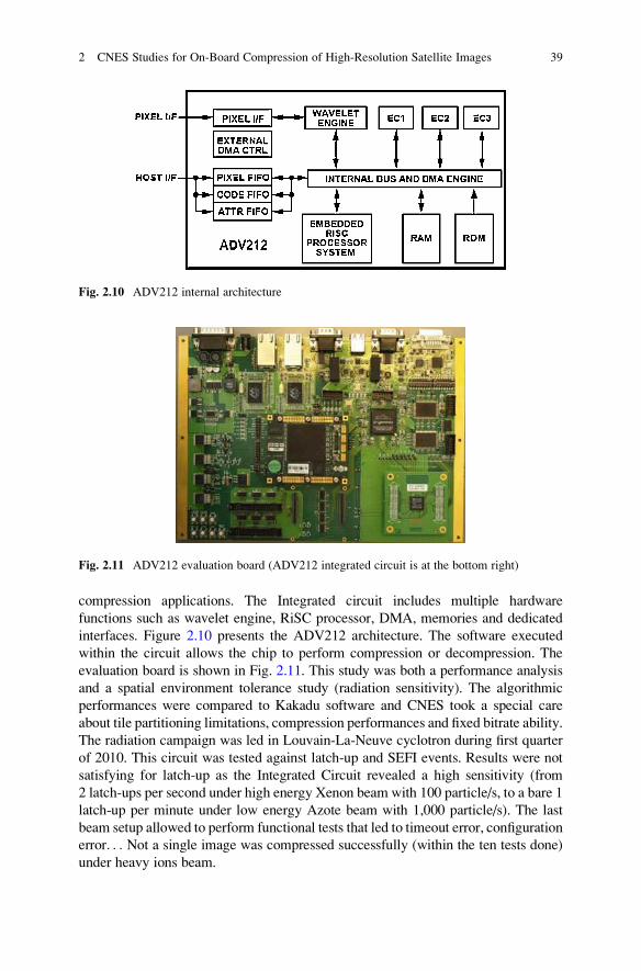
compression applications. The Integrated circuit includes multiple hardware

functions such as wavelet engine, RiSC processor, DMA, memories and dedicated

interfaces. Figure 2.10 presents the ADV212 architecture. The software executed

within the circuit allows the chip to perform compression or decompression. The

evaluation board is shown in Fig. 2.11. This study was both a performance analysis

and a spatial environment tolerance study (radiation sensitivity). The algorithmic

performances were compared to Kakadu software and CNES took a special care

about tile partitioning limitations, compression performances and fixed bitrate ability.

The radiation campaign was led in Louvain-La-Neuve cyclotron during first quarter

of 2010. This circuit was tested against latch-up and SEFI events. Results were not

satisfying for latch-up as the Integrated Circuit revealed a high sensitivity (from

2 latch-ups per second under high energy Xenon beam with 100 particle/s, to a bare 1

latch-up per minute under low energy Azote beam with 1,000 particle/s). The last

beam setup allowed to perform functional tests that led to timeout error, configuration

error. . . Not a single image was compressed successfully (within the ten tests done)

under heavy ions beam.

Fig. 2.10 ADV212 internal architecture

Fig. 2.11 ADV212 evaluation board (ADV212 integrated circuit is at the bottom right)


According to these results, the use of this COTS (Commercial of the Shelf) for

space applications seems really inappropriate despite its efficiency for JPEG2000

compression.

3.5 Exceptional Processing for DWT Algorithms

In Sect. 2.2.2, the DCT-based SPOT5 compressor has been presented and the

associated exceptional processing briefly explained. In that particular case the occur-

rence of the defects or artefacts was linked to the choice of a locally unsuitable

quantization factor in the rate regulation loop, as this factor was the same for

the whole line of blocks. The exceptional processing developed and validated for

SPOT5 locally corrected the quantization factor by a factor of 2 or 4, depending on the

number of AC coefficients in the block. For both DWT-based PLEIADES compressor

described in 2.3 and CCSDS standard described in 2.4, no rate regulation loop is

needed, because bit plane encoders hierarchically organize the output bit-stream so

that targeted fixed bit rate can be obtained by truncating this bit-stream. However,

because of on-board memory limitations, the DWT, bit-plane encoding and truncation

are performed over a fixed-size image area. For PLEIADES compressor, this image

area is 16 lines (width equal to image width). For CCSDS compressor, this image area

is called a segment and its size is defined by the user. In both cases, the quantization

induced by truncation of the bit planes description is the same for the studied image

area and some defects already observed in SPOT5 compressed images still appear

with these DWT-based compressors. In order to locally correct the defected blocks,

CNES has studied exceptional processing. The criteria used to decide whether excep-

tional processing is needed for a block is the [signal variance]/[compression noise

variance ratio]. As defined in [7], a block of wavelet coefficients consists of a single

coefficient from the LL3 subband, referred to as the DC coefficient, and 63 AC

coefficients. Depending on this ratio value, the wavelet coefficients of the block are

multiplied by a positive factor before bit-plane encoding. These multiplied coefficients

will be treated earlier than in the nominal case (without exceptional processing) by the

encoder. This wavelet coefficients processing is similar to what is done in JPEG2000

standard for Region of Interest handling [6]. The image quality improvement brought

by the exceptional processing has been confirmed by image analysis. However, its

utilization is not needed for PLEIADES images because the targeted bit rate is high

enough to prevent such defects.

3.6 Selective Compression

Algorithms presented above are associated with low performance gain while

preserving a good image quality whatever the scene and wherever in the scene.

However, this gain is not enough compared to the increase of data rate. Unfortu-

nately, any transform has been able to obtain a significant gain on compression ratio


for the same image degradation. To reach such bigger compression ratios, it is

necessary to perform “smart” compression, meaning different compression ratios

inside a scene. Thus, on-board detection of useful or non-useful data is required, the

non-useful data being more compressed to ensure a compression gain. This kind of

compression is called “selective compression” and consists of detecting and then

compressing a so-called region-of-interest (ROI) or non-interest. Nevertheless, on-

board detection for Earth observation missions must be performed at high data rate

and detection algorithms are often too complex. Moreover, selective compression is

not so famous because it is hard to describe useful or non-useful data. Fortunately,

one type of data can be considered, for almost all CNES High-Resolution

applications, as non-useful data: the clouds. In fact, despite the use of weather

forecast in satellite scheduling, most of optical satellite images are cloudy; this is

the case of SPOT5 for which up to 80% of the images are classified as cloudy by the

SPOT-image neural network classifier.

Figure 2.12 gives an example of a cloudy image and its associated binary

mask indicating a cloud-pixel when pixel is white (output of a classifier) and a non-

cloud-pixel when pixel is black. Considerable mass-memory and transmission gains

could be reached by detecting and suppressing or significantly compressing the clouds.

Compression algorithms should use this kind of mask during the encoding stage to

differently compress both regions of the scene.

3.6.1 On-Board Cloud-Detection Feasibility

During the last years, CNES has studied the implementation of a cloud detection

module on-board satellite [14]. The idea was to simplify and optimize for on-board

implementation an already existing cloud-detection module used on-ground for

PLEIADES-HR album images [15]. This algorithm uses a Support Vector Machine

Fig. 2.12 Cloudy SPOT5 image and its associated cloud mask


classifier on images at low resolution (wavelet transform 3rd decomposition level).

The main stages of this algorithm consist in computing top of atmosphere radiance

of the image using the absolute calibration factor, computing classification criteria

and finally classifying these criteria with the trained SVM configuration.

The on-board implementation study firstly analyzed independently all the phases

of this process to propose an on-board simplified model of cloud cover detection

algorithm based on SVM technique. The proposed restrictions computed together,

via a floating-point software model, showed that equivalent performances could be

obtained by the on-board simplified model (<1% of error).

In order to prepare the VHDL description other restrictions were taken into

account as the ranges and targeted accuracies of each computing parameter for

fixed-point operations.

Finally, an HLS tool was used to obtain fixed-point and VHDL descriptions and

to verify the performances if compared with the reference model. Table 2.1 shows

some main results for 13 different sites: maximum error complies with the initial

specifications with about 1% of error in cloud detection coverage and mask

generation. Furthermore, as worst-case errors correspond to cloud pixels considered

as ground pixels (common coverage ~100%), almost any additional loss will be

introduced in the region of interest by this cloud compression stage.

3.6.2 ROI Coding

The last step of selective compression is the “smart” encoding of the Region Of

Interest. In the case of on-board cloud-detection, the background is the cloud-mask

and the foreground (ROI) is the rest of the image. ROI coding methods already exist

and the principle of the general ROI scaling-based method is to scale (or shift)

wavelet coefficients so that the bits associated with the ROI are placed in higher

Table 2.1 Comparative global results between the reference model and fixed-point/VHDL model

Cloud mask

coverage

Cloud mask

surface in pixels

(ref. model)

Cloud mask surface

in pixels (fixed-point

model)

Common

coverage (ref. vs.

fixed point) (%)

Different

coverage (ref. vs.

fixed point) (%)

Acapulco_1 298,570 299,871 100.0 0.4

Bayonne_1 243,113 244,345 100.0 0.5

Dakar_2 475,644 481,180 100.0 1.1

La_Paz_1 167,772 168,542 100.0 0.4

La_Paz_2 749,313 753,932 100.0 0.6

London_1 418,660 416,966 99.5 0.4

Los_Angeles_2 120,225 120,428 100.0 0.1

Marseille_1 153,887 155,251 100.0 0.8

Papeete_1 361,610 362,916 100.0 0.3

Quito_1 724,569 726,453 100.0 0.2

Quito_2 544,185 545,662 100.0 0.2

Seattle 275,310 276,590 100.0 0.4

Toulouse 123,691 123,872 100.0 0.1


bit-planes than those of the background (see Fig. 2.13). Then, during the embedded

coding process, the most significant ROI bit-planes are placed in the bit-stream

before background bit-planes of the image.

Two different ROI coding capabilities, Maxshift and Scaling, have been already

added by CNES to existing compressors (CCSDS IDC. . .) in order to perform

selective compression over all kind of image including cloudy ones.

Of course, both methods have particular advantages and drawbacks considering

the application: thus, Maxshift is a better candidate for cloud detection applications

as it preserves the best reachable image quality over the ROI and the decompressor

can automatically decode the cloud covering mask. Its main drawback is that users

cannot control the image quality over the background region (e.g. clouds), or between

regions with different degree of interest. The Scaling method will be preferable for

this kind of applications but extra over-head must be expected for ROI mask

transmission. Other techniques, as Bitplane-By-Bitplane Shift, may also be studied

with the aim of allying the advantages of these two methods.

On-going CNES studies will provide rate allocation compatibility for these ROI

compression techniques.

3.7 Fixed Quality: Variable Data Rate Compression

Actual on-board compressors assign “almost” the same data rate to every image

segment on the scene in order to globally simplify the system data handling by

providing highly-predictable volumes and data rates. This is not, however, the best

Fig. 2.13 Standard vs. shifted bit plane coding with “Scaling” and “MaxShift” methods


way of achieving the optimum image quality for a scene or a group of scenes for a

given amount of data (i.e.: on-board mass memory capacity).

Even if selective compression can offer a significant improvement if compared

to classical fixed data rate compression, it is still hard to describe the different

regions of interest and even more to handle them in order to obtain efficient

compression schemes.

Thus, Fixed Quality-Variable data rate compression algorithms seem to be a

better option to optimally compress images with the lowest amount of data:

depending on the image complexity (computed by block or segment inside a

scene), the compressor will assign the appropriate compression ratio to comply

with the selected quality requirements. Nevertheless, as image complexity will

vary, variable data rates will be obtained after compression. Satellite data system

must be then overvalued to be able to handle the highest volumes/data rates

associated with very complex images (i.e. urban areas). Accordingly, CNES will

study during the next years the application and the impact of such techniques for

High-Resolution satellite systems. The main idea is that compressors will be able to

prior compute the image complexity in order to assign the optimum description level

(bitplane) for a chosen quality limit. A global limit in terms of data amount should be

also imposed for on-board handling and storage issues. Some good approaches,

as quality-limit parameters BitPlaneStop and StageStop of CCSDS IDC algorithm,

will certainly play an important role in these future compression methods.

4 Conclusions

In this chapter, we have firstly given an overview of past compression algorithms

that have been implemented on-board CNES satellites devoted to Earth observation

missions. The development of compression algorithms has to deal with several

constraints: telemetry budget limiting the data rate after compression, image quality

constraints from expert image users and space qualified electronics devices also

limiting the implementation and its performances. By using performing techniques

such as DCT and then DWT, CNES has developed several modules for Earth

observation missions that have been described here. As shown in Fig. 2.14, the

used techniques allow a gain in compression ratio while preserving a very good

image quality. This gain is more and more necessary to face up to the growing data

rate of very high resolution missions. But for coming missions, new compression

techniques have to be found. New transforms with better decorrelation power, on-

board detection techniques for selective compression or algorithms performing

fixed quality compression represent the CNES main fields of study to prepare the

future.

Acknowledgments Authors would like to thank all the people who have contributed to CNES

on-board compression studies and developments presented in this chapter.


References

1. C. Fratter, M. Moulin, H. Ruiz, P. Charvet, D. Zobler, “The SPOT5 mission”, 52nd Interna-

tional Astronautical Congress, Toulouse, France, 1–5 Oct 2001.

2. P. Kubik, V. Pascal, C. Latry, S. Baillarin, “PLEIADES image quality from users’ needs to

products definition”, SPIE Europe International Symposium on Remote Sensing, Bruges,

Belgium, September 19–22, 2005.

3. P. Lier, G. Moury, C. Latry and F. Cabot, “Selection of the SPOT-5 Image Compression

algorithm”, in Proc. of SPIE 98, San Diego, vol.3439–70, July 1998.

4. C. Lambert-Nebout, J.E. Blamont, “Clementine: on-board image compression”, 26th Lunar

and Planetary Science Conference LPCE, Houston, 1995.

5. C. Lambert-Nebout, G. Moury, J.E. Blamont, “A survey of on-board image compression for

CNES space missions”, in Proc. of IGARSS 1999, Hambourg, June 1999.

6. ISO/IEC 15444–2, “Information technology – JPEG 2000 image coding system: Extensions”,

2004

7. CCSDS, Image Data Compression Recommended Standard, CCSDS 122.0-B-1 Blue Book,

Nov. 2005

8. C. Thiebaut et al., “On-Board Compression Algorithm for Satellite Multispectral Images”, in

Proc. of Data Compression Conference 2006, Snowbird, March 28–30, 2006.

9. C. Thiebaut, E. Christophe, D. Lebedeff, C. Latry, “CNES Studies of On-Board Compression

for Multispectral and Hyperspectral Images”, Proc. of SPIE Satellite Data Compression,

Communications and Archiving III, San Diego CA, vol. 6683, pp. 668305.1-668305.15,

August 2007.

10. C. Thiebaut & R. Camarero, “Multicomponent compression with the latest CCSDS recom-

mendation”, Proc. of SPIE Satellite Data Compression, Communications and Processing V,

San Diego CA, Vol. 7455, 745503, August 2009.

11. X. Delaunay, M. Chabert, G. Morin and V. Charvillat “Bit-plane analysis and contexts

combining of JPEG2000 contexts for on-board satellite image compression”, In Proc. of

ICASSP’07, I-1057–1060, IEEE, April 2007, Honolulu, HI.

Evolution of compression algorithm performance with time

35

37

39

41

43

45

47

49

51

53

55

0 2 4 6 8 10

Compression Ratio

PS

NR

(in

dB

)SPOT5 (1997)

PLEIADES-HR (2002)

Fig. 2.14 Evolution of compression algorithm performance with time: from SPOT5 to PLEIA-

DES-HR


12. G. Peyre and S. Mallat, “Discrete bandelets with geometric orthogonal filters,” in IEEE

International Conference on Image Processing, Sept. 2005, vol. 1, pp. I– 65–8.

13. X. Delaunay, M. Chabert, V. Charvillat, G. Morin and R. Ruiloba “Satellite image compres-

sion by directional decorrelation of wavelet coefficients”, to appear in Proc. of ICASSP’08,

IEEE, April 2008, Las Vegas, Nevada, USA

14. R. Camarero, C. Thiebaut, Ph. Dejean, A. Speciel « CNES studies for on-board implementa-

tion via HLS tools of a cloud-detection module for selective compression”, In Satellite Data

Compression, Communication, and Processing VI, Vol. 7810, 781004, SPIE, San Diego, CA,

USA, 24 August 2010.

15. C. Latry, C. Panem, P. Dejean, “Cloud Detection with SVM Technique”, in Proc. of

IGARSS’07, Barcelone, Spain, 13–27 Jul. 2007.


Chapter 3

Low-Complexity Approaches for Losslessand Near-Lossless Hyperspectral ImageCompression

Andrea Abrardo, Mauro Barni, Andrea Bertoli, Raoul Grimoldi,Enrico Magli, and Raffaele Vitulli

Abstract There has recently been a strong interest towards low-complexity

approaches for hyperspectral image compression, also driven by the standardization

activities in this area and by the new hyperspectral missions that have been

deployed. This chapter overviews the state-of-the-art of lossless and near-lossless

compression of hyperspectral images, with a particular focus on approaches that

comply with the requirements typical of real-world mission, in terms of low

complexity and memory usage, error resilience and hardware friendliness. In

particular, a very simple lossless compression algorithm is described, which is

based on block-by-block prediction and adaptive Golomb coding, can exploit

optimal band ordering, and can be extended to near-lossless compression. We

also describe the results obtained with a hardware implementation of the algorithm.

The compression performance of this algorithm is close to the state-of-the-art, and

its low degree of complexity and memory usage, along with the possibility to

compress data in parallel, make it a very good candidate for onboard hyperspectral

image compression.

A. Abrardo (*) • M. Barni

Dip. di Ingegneria dell’Informazione, Universita di Siena, Siena, Italy


A. Bertoli • R. Grimoldi

Carlo Gavazzi Space S.p.A., Milan, Italy


E. Magli

Dip. di Elettronica, Politecnico di Torino, Torino, Italy


R. Vitulli

European Space Agency – ESTEC TEC/EDP, Noordwijk, The Netherlands



47






1 Introduction and Motivation

Compression of hyperspectral images has been an important and active research

topic for a long time. All spectral imagers such as those of the multispectral,

hyperspectral and ultraspectral type are generating increasing amounts of data,

calling for image compression to reduce the data volume prior to transmission to

the ground segment. Different spectral imagers differ in how much data are

available in the spatial and spectral dimensions, potentially requiring different

compression techniques. For example, multispectral images typically have very

fine spatial resolution and coarse spectral resolution, and their compression mostly

exploits the spatial correlation. The opposite is typically true of hyper- and

ultraspectral imagers, in which the spectral correlation dominates. Compression is

most useful for spaceborne sensors, as it is not possible to physically unmount or

read the mass storage device that archives the acquired data, e.g. at the end of a

measurement campaign. However, if the sensor resolution is very high or the mission

is very long, compression may also be needed onboard an airborne platform.

Image compression techniques allow to transmit more data in the same amount

of time, so much as more compression is applied. Several types of compression are

possible. In lossless compression, the reconstructed image is identical to the

original. In near-lossless compression, the maximum absolute difference between

the reconstructed and original image does not exceed a user-defined value. In lossy

compression, the reconstructed image is as similar as possible to the original

“on average”, i.e., typically in mean-squared error sense, given a target bit-rate.

Lossless compression is highly desired to preserve all the information contained in

the image; unfortunately, the best algorithms provide limited compression ratios,

typically from 2:1 to 3:1 for 3D datasets. Near-lossless and lossy techniques yield

larger size reductions, at the expense of some information loss. Although these

kinds of compression have always received less attention because of the loss of

quality and, even more, of the difficulty to assess the effect of the losses on the

applications, they are becoming more and more important when the required

compression ratio is large. E.g., in [1] it is shown that bit-rates of 0.5 and 0.1 bpp

can be achieved with little or no impact on image classification performance.

This chapter overviews the requirements and the state-of-the-art of lossless image

compression for hyperspectral images, with a particular focus on low-complexity

approaches amenable for onboard implementation. It should be noted that most near-

lossless algorithms can be seen as an extension of a predictive scheme, in which the

prediction error is quantized in the DPCM loop. As a consequence, near-lossless

compression can be obtained as a side-product of any predictive scheme, and for this

reason we will not explicitly review existing near-lossless compression algorithms.

However, in Sect. 3.4 we will show how the proposed algorithm can be extended to

near-lossless compression, and what kind of performance can be expected.

This chapter is organized as follows. In Sect. 3.2 we review prior work in this

area, including the existing lossless compression standards that are relevant to

onboard compression. In Sect. 3.3 we outline the main requirements of onboard

48 A. Abrardo et al.

compression, and discuss the most relevant approaches. In Sect. 3.4 we describe a

low-complexity approach that employs a block-based predictor. In Sect. 3.5 we

show compression results and discuss the complexity of the proposed approach.

Sect. 3.6 describes the hardware implementation, whereas in Sect. 3.7 we draw

some conclusions and highlight important open problems.

2 Background

2.1 Compression Techniques

Lossless compression of hyperspectral images has mostly been based on the

predictive coding paradigm, whereby each pixel is predicted from past data, and

the prediction error is entropy coded [2, 3]. In [4] fuzzy prediction is introduced,

switching the predictor among a predefined set using on a fuzzy logic rule. In [5] the

prediction is improved using analysis of edges. In [6] classified prediction is

introduced for near-lossless compression. Classified prediction is further developed

in [7] for lossless and near-lossless compression. In [8] spectral prediction is

performed using adaptive filtering. In [9] vector quantization is employed to yield

lossless compression. In [10] the concept of clustered differential pulse code

modulation (C-DPCM) is introduced. The spectra of the image are clustered, and

an optimal predictor is computed for each cluster and used to decorrelate the

spectra; the prediction error is coded using a range coder. In [11] it is proposed to

employ a spectral predictor that is based on two previous bands. In [12] the spectral

redundancy is exploited using a context matching method driven by the spectral

correlation. In [13, 14] it is proposed to employ distributed source coding to achieve

lossless compression with a very simple encoder. In [15] a simple algorithm is

proposed, which encodes each image block independently. In [16] a low-complex-

ity algorithm is introduced, based on linear prediction in the spectral domain. In

[17] the performance of JPEG 2000 [18] is evaluated for lossless compression of

AVIRIS scenes, in the framework of progressive lossy-to-lossless compression;

lossy compression results are reported in [1]. Along the same lines, the CCSDS

image data compression recommendation [19] uses wavelets for lossless compres-

sion, as does the algorithm in [20]. In [21] it is proposed to employ as predictor a

pixel in the previous band, whose value is equal to the pixel co-located to the one to

be coded; the algorithm is further refined in [22]. In [23] spectral correlation is

exploited through context matching. Recent work has also borrowed ideas from

distributed source coding to construct extremely simple and error-resilient

algorithms [13, 14].

Band reordering has also been used in [24–26] to obtain improved performance;

specifically, in band reordering the spectral channels of the image are reordered in

such a way as to maximize the correlation of adjacent bands, optimizing the

performance of the subsequent compression stage. In [27] it is shown that raw

3 Low-Complexity Approaches for Lossless and Near-Lossless. . . 49

data have very different characteristics from calibrated data, and an algorithm able

to exploit calibration-induced artifacts is proposed.

Finally, it should also be mentioned that lossy compression can be achieved via

transform coding employing a reversible transform. This is the approach followed

in JPEG 2000, allowing to achieve progressive lossy-to-lossless compression,

although its performance is generally not as good as the best predictive approaches.

2.2 International Standards

Data and image compression are so important for space applications, that relevant

international standards have been developed and approved. In the following we

discuss the available lossless compression standards and their use for onboard

image compression.

2.2.1 CCSDS 101: Lossless Data Compression

The first compression standard for space applications has been developed by the

consultative committee for space data systems (CCSDS). The standard is titled

“lossless data compression”, meaning that it was developed for general purpose

data compression, including but not specifically tailored to image compression. The

standard defines a lossless compression algorithm that can be coupled with a user-

defined or a default predictor, allowing the user to employ a predictor that has been

developed for the target data, coupled with a standardized low-complexity entropy

coding stage. The entropy coding stage consists of a mapper followed by an entropy

coding stage. This latter operates on short blocks of mapped samples. For each

block, all samples are coded using a Golomb power-of-two code [28] with the

parameters that minimizes the bit-rate, provided that the other available options

(zero-block, no compression) do not yield an even smaller bit-rate. A low-entropy

option is also available (second extension), although it is covered by patent.

This entropy coder is somewhat suboptimal with respect to similar coders based

on Golomb codes and developed specifically for images (e.g. [29]) that select a

different coding parameter for each sample based on a window of previous samples.

The performance loss is typically less than 0.2 bpp. The algorithm has very low

complexity, and an ASIC implementation exists [30].

2.2.2 CCSDS 122: Image Data Compression

More recently, the CCSDS has developed a new standard for image compression

[19]. The algorithm is somewhat similar in spirit to JPEG 2000, as it employs a 2D

discrete wavelet transform followed by a simple entropy coder based on bit-planes.

We mention this standard as, although it is natively a lossy compression standard,


it also has a lossless mode based on a reversible wavelet transform. However,

this standard is not suitable for the compression of 3D data, as it only captures

the correlation in two dimensions. Repeated application of the algorithm to 2D

slices of a 3D dataset is possible, but certainly suboptimal in terms of performance.

Moreover, the algorithm complexity is significantly larger than that of the lossless

data compression recommendation.

2.2.3 JPEG-LS

The JPEG-LS standard addresses both lossless and near-lossless compression of 2D

images. It is based on a simple non-linear predictor, followed by a context-based

entropy coder, and uses a quantizer in the prediction loop for near-lossless

compression [29]. Although this standard has not been developed specifically for

space applications, its low complexity and good performance make it suitable for

spectral image compression. In several papers a “differential” JPEG-LS algorithm

is used for compression of 3D images, which simply takes differences of adjacent

bands and encodes them using JPEG-LS. To maximize coding efficiency, the same

principle can be applied to spatial-spectral slices, with the difference being taken in

the remaining spatial dimension.

3 Onboard Compression Requirements

Although compression performance is certainly a key aspect for onboard compres-

sion, there are other very important requirements that should also be taken into

account. These requirements draw a scenario that is somewhat different from

typical image compression, typically leading to the design of low-complexity and

hardware-friendly compression algorithms.

Low encoder complexity. Since spectral imagers can generate very high data rates,

it is of paramount importance that the encoder has low-complexity, in order to be

able to operate in real time. It is worth mentioning that the computational power

available for compression is generally limited, and nowhere near that yielded by a

processor for workstation applications. A typical design involves the compression

algorithm being implemented on an FPGA, although certain missions will afford

the ad-hoc design of an application-specific integrated circuit (ASIC), while other

missions may only use a digital signal processor. Typical clock frequencies are of

the order of 100 MHz.

The low-complexity requirement generally rules out the application of transform

coding methods because of their complexity. While these methods are suitable for

2D images, the 3D case would entail to apply 2D transform coding repeatedly after

taking a transform in the third dimension. This is possible only with very significant

computational resources.


The prediction plus entropy coding paradigm is amenable to low complexity.

Although very sophisticated predictors exist, adequate performance can be obtained

using relatively simple ones (e.g., as done in JPEG-LS). Traditionally, onboard

compression algorithms avoid using arithmetic coding, as it is deemed to be a

relatively complex coding scheme, especially for large alphabets. Instead, Golomb

power-of-two codes are the preferred choice, as they achieve a good balance between

performance and complexity. The use of simplified low-complexity arithmetic codes

has not been evaluated extensively for space applications; such codes are used in

JPEG 2000 and H.264/AVC compression standards, just to mention a few.

Error-resilience. Algorithms should be capable of contain the effect of bit-flippings

or packet losses in the compressed file. These errors typically occur because of

noise on the communication channel. Compressed data are known to be very

sensitive to errors, to the extent that a single erroneous bit could prevent from

decoding the remainder of the data. This problem can be alleviated in many ways, e.

g. employing error-resilient entropy codes such as reversible variable-length codes

[20], coset codes [14] or error-resilient arithmetic codes [31]. Another approach is

to partition the data into units that are coded independently, in such a way that an

error in one unit will not prevent from decoding other units. This latter solution is

usually preferred, as it is indeed very simple, and guarantees that the scope of an

error is limited to one partition.

As partitioning incurs a cost in terms of compression performance, these units

should not be too small; the optimal size ultimately depends on how many errors or

packet losses are expected on the communication channel. E.g., while typical Earth

observation missions usually have very few losses, deep-space missions are subject

to higher bit-error rates. The shape of the partition also plays some role. E.g. should

the partition have a large spatial size and a low spectral size, or the opposite? This is

also application-dependent, in that there are applications in which spatial infor-

mation is critical and should be retained as much as possible while spectral

information may be sacrificed, and vice versa.

Hardware friendliness. Since onboard compression algorithms are typically

implemented on FPGA or ASIC, the algorithm has to be designed in such a way

that its hardware implementation is simple, i.e., it must be able to operate using

integer arithmetic, it must fit into a relatively small FPGA, and must use the

available resources effectively, possibly not needing an external memory. More-

over, it is desirable that the algorithm can be parallelized in order to speed up the

compression process for high data-rate sensors.

In this chapter we describe a compression solution that aims at fulfilling the

criteria above. The algorithm performs lossless and near-lossless compression with

very low complexity. The prediction stage is based on the design in [15]. This

predictor has low complexity, as it computes a single optimal predictor for each

16 � 16 block of input samples. Working on 16 � 16 blocks, the predictor performs

data partitioning, in that any 16 � 16 block can be decoded without reference to any

other 16 � 16 block in different spatial locations in other bands. Thus, while there is

a performance loss for working on a block-by-block basis, this is small with respect to

pixel-based predictors as in [8]; it is possible to employ a block-based predictor along


with coset coding to achieve increased error resilience [14], at the expense of an

additional performance loss. The performance of the algorithm, for both lossless and

near-lossless compression, is improved by using band reordering. Band reordering

has never been given much attention for onboard compression, because it requires

additional computations to obtain the optimal ordering. However, we show that,

in a realistic application scenario, band reordering could be performed at the ground

segment, requiring no additional computations onboard, providing most of the

performance gain of optimal band reordering.

4 Block-Based Coding Approach

In the following we denote as xm,n,i the pixel of an hyperspectral image X in

mth line, nth pixel, and ith band, with m ¼ 0, . . ., M � 1, n ¼ 0, . . ., N � 1 and

i ¼ 0, . . ., B � 1. The algorithm compresses independent non-overlapping spatial

blocks of size N � N, with N typically equal to 16; each block is processed

separately. This approach entails a small performance penalty, as all the prediction

and entropy coding operations have to be reset at the end of each block. However,

it has two important advantages.

• It allows parallelization, as each spatial block (with all bands) can be encoded as

a completely independent data unit.

• It provides error resilience, as erroneous decoding of a block has no effect on the

decoding of other blocks in different spatial positions.

Moreover, additional spectral error resilience and spectral parallelization can be

obtained by periodically encoding a band without spectral prediction (i.e., intra-

mode). The group of bands contained between two intra-coded bands, including the

first and excluding the last, can be encoded and decoded independently and will

generate an independent error containment segment.

4.1 Prediction

For the first band (i ¼ 0), 2D compression is performed, as there is no “previous”

band to be exploited. The choice of the 2D predictor is not critical, and several

reasonably good predictors will work. The predictor we have used is defined as

x0m,n,0 ¼ (xm�1,n,0 + xm,n�1,0)�1, where � denotes right-shift, i.e., it takes the

average of the pixels on the top and left of the pixel to be predicted.

Except for the first sample of the block, all prediction error samples are mapped

to nonnegative values using the following formula:

S ¼2jej � 1 if e > 0

2jej if e � 0

(


where e is the prediction error value, and S is the corresponding mapped value.

This mapping function is also used for all other bands. For all other bands, a N � N

block in band i is processed as follows. The samples xm,n,i belonging to the block

(with m,n ¼ 0, . . ., N � 1), are predicted from the samples xm,n,l of another already

coded band (i.e., a spatially co-located block with index l different from i). In the

following we assume that l ¼ i � 1, i.e., the co-located block in the previous band

i � 1 is used as reference to predict the block in the current band i. In Sect. 3.4.4

we will show how to set l to a value generally different from i � 1.

In order to make xm,n,i�1 globally as “similar” as possible to xm,n,i in minimum

mean-squared error sense, a least-squares estimator can be computed over

the block as a ¼ aN/aD [15], with aN ¼P

m;n2A

ðxm;n;l � mlÞðxm;n;i � miÞ and

aD ¼P

m;n2A

ðxm;n;l � mlÞðxm;n;l � mlÞ, and ml and mi are average values of the

block, as defined below.

Note that the original predictor [15] does not remove the mean value in

the computation of aN and aD. However, we have found that removing the mean

value provides improved performance, even though mi has to be written in the

compressed file. If aD is equal to zero, then it is set to one to avoid dividing by zero.

In the equations above, the summations are computed over the set o indexes A.

While in [15] A contains all indexes m∈[0, . . ., N � 1] and n∈[0, . . ., N � 1], we

did not choose to do so. In fact, since a is going to be quantized, it is sufficient to use

enough samples so that its precision is smaller than the quantization error. On the

other hand, using fewer samples can greatly reduce the number of computations

required to compute a. In particular, it has been empirically found that one fourth

of the samples are enough to estimate a with sufficient accuracy. Therefore, we select

A as a set of 64 positions uniformly picked at random in the block, as random

positions yield slightly better performance than regularly spaced ones. The positions

are the same for all spatial blocks and all bands, and need not be communicated to the

decoder. mi and ml are the average values of the co-located blocks in bands i and l.

They are also computed from the reduced set of samples A. Note that ml does not

need to be computed, as it had already been computed during the encoding of band

l; only mi has to be computed.

A quantized version of a is generated using a uniform scalar quantizer with

256 levels in the range [0,2]. In particular, the quantization yields a0 ¼ floor(128a),

and a0 is then clipped between 0 and 255. The dequantized gain factor is obtained

as a00 ¼ a0/128.

A drawback of the original version of this predictor is that computing a ¼ aN/aDrequires a floating-point division, which is very undesirable in hardware. In prac-

tice, this division can be avoided. This is based on the fact that, after computing a,

the obtained value will be quantized to a00 using 8 bits. That is, out of all the

infinitely many possible values, only 256 values will actually be taken. Therefore,

instead of computing the division, the encoder can simply select, out of all the

256 values, the one that is closest to a in squared-error sense. In particular, to speed

up the search, the encoder can perform a dicotomic search over the 256 possible


values of a00, seeking the value that minimizes |a00aD/aN|. This is equivalent to

minimizing |a0aD – 128aN |.

Once a00 has been computed, the predicted values within the block are computed

for all m ¼ 0, . . ., N and n ¼ 0, . . ., N as x0m,n,i ¼ round[mi + a00(xm,n,l – ml)].

The prediction error vector can be calculated in each block for all m ¼ 0, . . ., N

and n ¼ 0, . . ., N as em,n,i ¼ xm,n,i – x0m,n,i. Subsequently, the prediction error

samples are mapped to nonnegative integers.

4.2 Near-Lossless Compression

Predictive schemes are suitable for near-lossless compression, since quantization in

the DPCM feedback loop [32] produces the same maximum absolute error on each

pixel, which is equal to half of the quantizer step size. Near-lossless compression

can hence be achieved by means of a uniform scalar quantizer with step size 2d + 1

and midpoint reconstruction, such that, letting em,n,i be the prediction error, its

reconstructed value e0m,n,i is given by

e0m;n;i ¼ signðem;n;iÞð2dþ 1Þfloorjem;n;ij þ d

2dþ 1

� �

4.3 Entropy Coding

The proposed algorithm has two coding options, namely Golomb codes and

Golomb power-of-two codes; the same context is employed for either code.

4.3.1 Golomb Coding

The N � Nmapped prediction residuals of a block are encoded in raster order using

a Golomb code [28], except for the first sample of the block that is encoded using an

exp-Golomb code of order 0 [33].

The Golomb code parameter kj for the jth sample of the block is computed from

a running count Sj of the sum of the last 32 mapped values of the block; for samples

with index less than 32, only the available mapped values are used. In particular,

the following formula is used [34]: kj ¼ floor[(0.693/J) Sj + 1], where

Sj ¼P

j�1

k¼j�32;k�0

Skj j, 0.693 approximates log(2), J � 32 is the number of available

samples in the running count Sj, Sj are the mapped values.

Note that computing kj simply requires to update Sj�1 as Sj ¼ Sj�1 – |

Sj�33| + |Sj�1|, requiring at most two operations per sample.


4.3.2 Golomb Power-of-Two Coding

For Golomb power-of-two (GPO2) codes, the code parameter is computed in a

similar way. The context is defined exactly as in the Golomb code case, except for

the fact that the running count is taken over the magnitude of the unmapped

prediction error residuals, rather than the mapped values. The parameter kjis computed using the well-known C-language one-liner below [29], where D is

the running count of sum of magnitudes of prediction residuals.

for (kj = 0; (j << kj) < = d;kj + +);

4.3.3 Coding of Predictor Parameters

Since the predictor is not causal, it is necessary to write in the compressed file two

parameters, namely a0 and mi; it is not necessary to write ml, as it can be computed

by the decoder. For a0, 8 bits are used to specify its binary representation. For mi,

a more sophisticated technique is employed. Letting the first band be denoted by

index i ¼ 0, for the second band (i ¼ 1) mi is written using 16 bits. For the other

bands (i > 1), the difference mi – ml is taken; that is, mi is coded predictively in

order to exploit its correlation across bands. The sign bit of the difference is written

in the compressed file, followed by the exp-Golomb code of the magnitude.

4.3.4 File Format

For each block, the following information is written in the compressed file. For all

bands other than the first one, the parameter a0 and the coded value of mi are written.

Then, the coded values of all samples of the block are written in raster order.

4.4 Band Reordering

The principle of band reordering [24] is that the previous band is not necessarily the

best metric for predicting the current band. This raises the problem of finding the

best reference band l for the prediction of band i. The reference band has to be

sought among the bands that have already been encoded. Band reordering is

interesting for onboard compression in that, if the ordering is given, picking a

reference band other than the previous band does not entail any additional

operations or more hardware complexity, when all bands for a given pixel or line

are buffered.


Solving the band reordering problem entails the definition of a similarity metric

rl,i that describes how “similar” band l and band i are, and hence how good the

prediction of band i using band l as reference band is expected to be. In [24] this

metric is taken as the number of bits needed to encode band i from band l; however,

this requires to perform the actual encoding, and is ad-hoc for a specific comp-

ression algorithm. In [25] rl,i is taken as the correlation coefficient between band l

and band i. In [26] the correlation coefficient is also used, but band grouping is

introduced to limit the complexity.

It is worth noting that band reordering is an additional option that the user may or

may not use, without affecting the algorithm design and implementation. As will be

seen in Sect. 3.5, not all datasets benefit from band reordering. In some cases the

gain is negligible, while in other cases it is not. It is up to the user to decide whether

the effort in calculating an optimal reordering is worth the performance gain.

For the algorithm described here, we have employed a band reordering scheme

based on [25], improving it in a few aspects. The similarity metric is taken as

the correlation coefficient. The metrics are used to construct a weighted undirected

graph, in which every band is represented by a vertex, and rl,i is the weight of an arc

linking bands l and i. To keep the number of arcs limited, each band i is “connected”

with a maximum number M of previous and next bands (from i � M to i + M),

and considering that rl,I ¼ ri,l. The optimal ordering is achieved solving a maxi-

mum weight tree (equivalent to a minimum spanning tree) problem over the graph.

This can be done using Prim’s algorithm as in [25].

For optimal band reordering, a specific ordering has to be computed and used for

each image, possibly increasing complexity. Therefore, we also investigate a

different approach. In this approach, a “good” band ordering is computed at the

ground station based on sample data, and then it is uploaded to the satellite for

subsequent use in the compression of all images. The motivation is that the optimal

ordering arguably depends on both the sensor and the scene, with the former

potentially dominating the ordering. If the contribution of the scene to the optimal

ordering is small, then a per-sensor ordering would be almost as good as the optimal

per-image ordering. In Sect. 3.5 we show that this is indeed the case. Thus, this

approach achieves the twofold benefit of improving the performance via use of an

almost-optimal ordering, and to do that without adding complexity to the algorithm,

as all computations needed to solve the band reordering problem would be

performed on the ground on sample data.

4.5 Complexity

We have analyzed the algorithm described above in order to calculate the average

number of operations needed to encode one sample of input data. The prediction

stage requires approximately nine operations per sample.


5 Compression Performance

5.1 Dataset Description

We present compression results for two different sensors.

The first is the well-known AVIRIS (Airborne Visible/Infrared Imaging

Spectrometer), an airborne hyperspectral system that collects spectral radiance in

224 contiguous spectral bands with wavelengths from 400 to 2,500 nm. Most

scientic papers in the field of hyperspectral image compression report results on

five scenes from the 1997 missions, namely Cuprite, Jasper Ridge, Moffett Field,

Lunar Lake and Low Altitude. However, these images are calibrated. It has been

shown [27, 35] that the calibrated data have a peculiar histogram that can favor

certain classes of algorithms, and which is not present on the raw data. Therefore, in

this paper we employ the new corpus of raw AVIRIS images recently made

available by NASA. These are five images acquired over Yellowstone park in

2006 (called sc0, sc3, sc10, sc11, sc18), available at http://compression.jpl.nasa.

gov/hyperspectral/. Each image is a 512-line scene containing 224 spectral bands

and 680 pixels per line.

The second is the AIRS (Atmospheric Infrared Sounder) instrument onboard the

Aqua satellite. AIRS is used to create 3Dmaps of air and surface temperature, water

vapor, and cloud properties. With 2,378 spectral channels, AIRS qualifies as an

ultraspectral sensor. For the compression studies, ten granules have been simulated

from the data obtained from NASA AIRS observations, removing 270 channels,

converting radiances into brightness temperatures and scaling as unsigned 16-bit

integers. The data are available via anonymous ftp (ftp://ftp.ssec.wisc.edu/pub/

bormin/HES). For this study, we have considered only 1,501 bands, removing the

unstable channels.

These AVIRIS and AIRS data are part of the dataset employed by the CCSDS

(Consultative Committee for Space Data Systems) to assess the performance of

multispectral and hyperspectral compression algorithms.

5.2 AVIRIS

Results for AVIRIS images are shown in Table 3.1. We compare the proposed

algorithm using Golomb codes and GPO2 codes, but without band reordering, the

LUT algorithm [10] and the FL algorithm [27], and the 3D-CALIC algorithm with

BSQ ordering [36]. Results for the LUT algorithm are also taken from [27]. As can

be seen the proposed algorithm is significantly better than LUT, and almost as good

as FL, but with lower complexity. This is a very good result, as FL has a very

competitive performance. LAIS-LUT [22] would score an average of 6.50 bpp,

which is significantly larger than the proposed algorithm. The use of GPO2 codes

does not significantly reduce performance.


http://compression.jpl.nasa.gov/hyperspectral/


ftp://ftp.ssec.wisc.edu/pub/bormin/HES

ftp://ftp.ssec.wisc.edu/pub/bormin/HES

Next, we analyze the performance of band reordering in the optimal and

per-sensor mode. In this latter case, the optimal reordering has been computed on

the sc0 image, and used for all five images. The band reordering computation has

been performed using M ¼ 7. Results are obtained using Golomb codes. The

results are reported in Table 3.2. As can be seen, the improvement yielded by

band reordering is very small (around 1%). Visual inspection of the optimal

ordering shows that for these AVIRIS scenes it is almost identical to the sequential

ordering. Therefore, for the AVIRIS dataset band reordering would not be useful.

Interestingly, there is no performance loss in optimizing the ordering per-sensor

instead of per-image.

5.3 AIRS

Compression results for AIRS granules are shown in Table 3.3. We compare the

proposed algorithm using Golomb codes and GPO2 codes, but without band

reordering, the LUT algorithm and the 3D-CALIC algorithm with BSQ ordering.

Results for the LUT algorithm have been generated using the software kindly

provided by the authors of [10].

Also in this case the GPO2 codes show a very limited performance loss with

respect to Golomb codes. 3D-CALIC achieves better performance than the pro-

posed algorithm, but exhibits a very high complexity. The LUT algorithm does not

perform well on these data.

In Table 3.4 we analyze the performance of band reordering in the optimal and

per-sensor mode. In this latter case, the optimal reordering has been computed on

granule 120, and used for all the other granules. The band reordering computation

has been performed using M ¼ 25. Results are obtained using Golomb codes.

Table 3.1 Compression performance (bit-rate in bpp) on AVIRIS yellowstone images

Proposed (Golomb) Proposed (GPO2) LUT FL 3D-CALIC (BSQ)

Sc0 6.44 6.45 7.14 6.23 6.41

Sc3 6.29 6.30 6.91 6.10 6.23

Sc10 5.61 5.62 6.26 5.65 5.62

Sc11 6.02 6.04 6.69 5.86 n.a.

Sc18 6.38 6.39 7.20 6.32 n.a.

Average 6.15 6.16 6.84 6.03 n.a.

Table 3.2 Compression performance (bit-rate in bpp) of band reordering on AVIRIS yellowstone

images

Proposed (Golomb) BR (optimal) BR (per-sensor)

Sc0 6.44 6.37 6.37

Sc3 6.29 6.21 6.22

Sc10 5.61 5.57 5.57

Sc11 6.02 6.00 5.97

Sc18 6.38 6.31 6.31

Average 6.15 6.09 6.09


As can be seen, the performance improvement obtained applying band reordering

to AIRS data is significant (around 6%), and exceeds 0.3 bpp on average. Even more

interestingly, the performance loss incurred by optimizing the reordering at the

ground station is small (about 0.04 bpp), showing that band reordering provides a

nice performance gain while not adding any complexity to the onboard compression

algorithm. Therefore, for the AIRS dataset band reordering seems a viable option.

5.4 Near-Lossless Compression

For near-lossless compression, we show performance results on the AVIRIS

sc0 scene. In particular, Fig. 3.1 reports rate-distortion curves for the proposed

algorithm (without band reordering) and JPEG 2000 [37]. This latter is Part 2 of the

standard, employing a spectral discrete wavelet transform in the spectral dimension,

followed by a spatial wavelet transform, with full 3D post-compression rate-distortion

optimization, and no line-based transform. As can be seen, the rate-distortion curve

of the near-lossless algorithm shows the typical behavior of very good performance at

high rates. The Golomb code (like a Huffman code) is unable to produce codewords

Table 3.3 Compression performance (bit-rate in bpp) on AIRS granules

Proposed (Golomb) Proposed (GPO2) LUT 3D-CALIC (BSQ)

Gran9 4.58 4.59 5.32 4.34

Gran16 4.52 4.53 5.26 4.34

Gran60 4.80 4.81 5.65 4.52

Gran82 4.36 4.38 5.03 4.24

Gran120 4.65 4.66 5.40 4.40

Gran126 4.78 4.79 5.64 4.51

Gran129 4.44 4.45 5.17 4.24

Gran151 4.80 4.82 5.73 4.51

Gran182 4.89 4.90 5.94 4.54

Gran193 4.83 4.84 5.62 4.53

Average 4.66 4.68 5.48 4.42

Table 3.4 Compression performance (bit-rate in bpp) of band reordering on AIRS granules

Proposed (Golomb) BR (optimal) BR (per-sensor)

Gran9 4.58 4.25 4.27

Gran16 4.52 4.21 4.24

Gran60 4.80 4.38 4.46

Gran82 4.36 4.13 4.16

Gran120 4.65 4.32 4.32

Gran126 4.78 4.39 4.45

Gran129 4.44 4.15 4.19

Gran151 4.80 4.44 4.48

Gran182 4.89 4.48 4.53

Gran193 4.83 4.42 4.48

Average 4.66 4.32 4.36


shorter than one bit, and this is the reason why the rate-distortion curve has a vertical

asymptote at 1 bpp. To achieve low bit-rates it would be necessary to employ a

different entropy code, e.g. an arithmetic code. Still, the algorithm is better than JPEG

2000 at bit-rates larger than 1.8 bpp, with significantly lower complexity, buffering

and local memory requirements.

It should be noted that, unlike other block-based lossy compression algorithms

such as JPEG, at low bit-rates the decoded images do not suffer from blockiness. In

fact, JPEG blocking artifacts are due to quantization in the DCT domain, which acts

as a vector quantizer over small blocks, which can generate discontinuities at the

boundary of different blocks. Conversely, in the proposed scheme the prediction

errors are quantized independently inside the block and between different blocks,

yielding independent reconstruction errors. This is shown in Fig. 3.2 for band 63 of

the sc0 image. On the left is a 64 � 64 crop of the original image. The center figure

is the image decoded by the proposed algorithm at very low bit-rate, whereas the

image on the right is a JPEG reconstruction. As can be seen, JPEG is very good at

preserving structures, but it blurs the texture and introduces visible blocking

artifacts. The proposed algorithm preserves some texture and does not exhibit any

blockiness, even though the structures are partly compromised.

6 Hardware Implementation

A rapid prototyping implementation on hardware of the lossless compression

algorithm has been performed. The design and modeling phase of the algorithm

has been supported by Matlab/Simulink Xilinx system generator tool, a rapid

prototyping environment for the design and implementation in FPGA.

0 1 2 3 4 545

50

55

60

65

70

75

80

85

90

95

Rate (bpp)

PS

NR

(d

B)

JPEG 2000 Part 2 (DWT)

Proposed near-lossless

Fig. 3.1 Near-lossless compression results on the sc0 image and comparison with JPEG 2000


The algorithm has been decomposed in elementary functional blocks communicating

with ping-pong buffer. Each functional block is in charge of executing the macro

computation as defined in Sect. 3.4, and the parallel execution in FPGA of the

functional block is exploiting obtaining excellent results in term of samples rate

processing of the algorithm.

System Generator is a DSP design tool from Xilinx that enables the use of The

Mathworks model-based design environment Matlab-Simulink for FPGA design.

The following key features have been exploited:

• Build and debug high-performance digital signal processing and generic

algorithms in Simulink using the Xilinx blockset that contains functions for

signal processing.

• Automatic code generation from Simulink for specific Xilinx IP cores from the

Xilinx Blockset.

• Code generation option that allows to validate hardware and accelerate

simulations in Simulink and MATLAB.

• Xilinx System Generator compatible board (i.e. ADM-XRC-II) available for

hardware-in-the-loop for rapid prototyping and test.

In particular, the ADM-XRC-II is a high performance PCI Mezzanine Card

format device designed for supporting development of applications using the

Virtex-II series of FPGA’s from Xilinx. Drivers and the software package including

Xilinx System Generator blockset are available to interface the board with Matlab/

Simulink/Sys generator host computer via PCI bus.

VHDL has been automatically generated starting from the rapid prototyping tool

for two Xilinx FPGA components. The selected FPGA components also have an

equivalent radiation-tolerant chip, and they are particularly interesting for space

applications. Further, a second implementation step has been performed by using a

high-level C- to VHDL converter tool applying the same approach used in the

modelling phase. VHDL code has been generated and FPGA algorithm resources

have been computed. Table 3.5 collects the data of the requested resources for the

algorithm implementation in FPGA.

The algorithm can be implemented in a single FPGA requiring low total

resources. Two instances of the algorithm can be included in the same FPGA,

allowing parallel processing of two 16 � 16 blocks.

Fig. 3.2 Visual quality at very low bit-rate. Left: original; center: proposed algorithm; right:

JPEG


In the space applications, an additional important constraint is the power

consumption. An accurate estimation of the power consumption for Xilinx FPGA

is given by the following formula:

P ¼ 250mWþ 20mW�MSample/s

The power consumption has been also evaluated by using Xpower Xilinx tool for

Xilinx xq2v3000 family. The tool yields an estimate of 1.1 W dynamic power

consumption at throughput of 80 Msample/s on the xq2v3000 device. The static

power consumption reported in the datasheet is less than 250 mW (typical) and less

than 1.5 W (maximum). As can be seen, the proposed algorithm leads to a very

efficient implementation with extremely low power consumption.

7 Conclusions

This chapter has overviewed current approaches to low-complexity lossless

compression of hyperspectral images. We have discussed the requirements

and possible solutions, and described a specific solution based on block-based

compression and optimal band ordering. Experimental results on AVIRIS and

AIRS data show that the algorithm has very competitive performance, with a

minor performance loss with respect to the state-of-the-art, but significantly lower

complexity. Moreover, it has been shown that band reordering can be effectively

performed at the ground station using training data, with a small performance loss

with respect to optimal reordering. This allows to avoid increasing the number of

operations to be performed onboard, while still obtaining most of the advantages

of reordering.

Table 3.5 Algorithm implementation on Xilinx FPGA

Device xqr4vlx200 xq2v3000

Used LUT 10,306 (5%) 10,248 (35%)

Ram16s 21 of 336 (6%) 21 of 96 (22%)

Mult18 � 18s 9 of 96 (9%)

DSP48 9 of 96 (9%)

Max freq. (MHz) 81 79

Throughput (Msamples/s) 70 69


References

1. B. Penna, T. Tillo, E. Magli, and G. Olmo, “Transform coding techniques for lossy

hyperspectral data compression,” IEEE Transactions on Geoscience and Remote Sensing,

vol. 45, no. 5, pp. 1408–1421, May 2007.

2. R.E. Roger and M.C. Cavenor, “Lossless compression of AVIRIS images,” IEEE Transactions

on Image Processing, vol. 5, no. 5, pp. 713–719, May 1996.

3. J. Mielikainen, A. Kaarna, and P. Toivanen, “Lossless hyperspectral image compression via

linear prediction,” Proc. SPIE, vol. 4725, 2002.

4. B. Aiazzi, P. Alba, L. Alparone, and S. Baronti, “Lossless compression of multi/hyperspectral

imagery based on a 3-D fuzzy prediction,” IEEE Transactions on Geoscience and Remote

Sensing, vol. 37, no. 5, pp. 2287–2294, Sept. 1999.

5. S.K. Jain and D.A. Adjeroh, “Edge-based prediction for lossless compression of hyperspectral

images,” Proc. IEEE Data Compression Conference, 2007.

6. B. Aiazzi, L. Alparone, and S. Baronti, “Near-lossless compression of 3-D optical data,” IEEE

Transactions on Geoscience and Remote Sensing, vol. 39, no. 11, pp. 2547–2557, Nov. 2001.

7. B. Aiazzi, L. Alparone, S. Baronti, and C. Lastri, “Crisp and fuzzy adaptive spectral

predictions for lossless and near-lossless compression of hyperspectral imagery,” IEEE Geo-

science and Remote Sensing Letters, vol. 4, no. 4, pp. 532–536, Oct. 2007.

8. M. Klimesh, “Low-complexity lossless compression of hyperspectral imagery via adaptive

filtering,” in The Interplanetary Network Progress Report, 2005.

9. M.J. Ryan and J.F. Arnold, “The lossless compression of AVIRIS images by vector

quantization,” IEEE Transactions on Geoscience and Remote Sensing, vol. 35, no. 3,

pp. 546–550, May 1997.

10. J. Mielikainen and P. Toivanen, Clustered DPCM for the lossless compression of hyperspectral

images, IEEE Transactions on Geoscience and Remote Sensing, vol. 41, no. 12,

pp. 2943–2946, Dec. 2003.

11. E Magli, G Olmo, and E. Quacchio, “Optimized onboard lossless and near-lossless compres-

sion of hyperspectral data using CALIC,” IEEE Geoscience and Remote Sensing Letters, vol.

1, no. 1, pp. 21–25, Jan. 2004

12. H. Wang, S.D. Babacan, and K. Sayood, “Lossless hyperspectral image compression using

context-based conditional averages,” Proc. of IEEE Data Compression Conference, 2005.

13. E. Magli, M. Barni, A. Abrardo, and M. Grangetto, “Distributed source coding techniques for

lossless compression of hyperspectral images,” EURASIP Journal on Advances in Signal

Processing, vol. 2007, 2007.

14. A. Abrardo, M. Barni, E. Magli, and F. Nencini, “Error-resilient and low-complexity onboard

lossless compression of hyperspectral images by means of distributed source coding,” IEEE

Transactions on Geoscience and Remote Sensing, Vol.48, No.4, pp.1892–1904, Apr. 2010.

15. M. Slyz and L. Zhang, “A block-based inter-band lossless hyperspectral image compressor,”

Proc. of IEEE Data Compression Conference, 2005, pp. 427–436.

16. F. Rizzo, B. Carpentieri, G. Motta, and J.A. Storer, “Low-complexity lossless compression of

hyperspectral imagery via linear prediction,” IEEE Signal Processing Letters, vol. 12, no. 2,

pp. 138–141, Feb. 2005.

17. B. Penna, T. Tillo, E. Magli, and G. Olmo, “Progressive 3D coding of hyperspectral images

based on JPEG 2000,” IEEE Geoscience and Remote Sensing Letters, vol. 3, no. 1,

pp. 125–129, Jan. 2006.

18. D.S. Taubman and M.W. Marcellin, JPEG2000: Image Compression Fundamentals,

Standards, and Practice, Kluwer, 2001.

19. CCSDS-122.0-B-1 Blue Book, Image Data Compression, November 2005.

20. B. Huang, A. Ahuja, H.-L. Huang, and M.D. Goldberg, “Real-time DSP implementation of 3D

wavelet reversible variable-length coding for hyperspectral sounder data compression,” Proc.

of IEEE IGARSS, 2006.


21. J. Mielikainen, “Lossless compression of hyperspectral images using lookup tables,” IEEE

Signal Processing Letters, vol. 13, no. 3, pp. 157–160, Mar. 2006.

22. B. Huang and Y. Sriraja, “Lossless compression of hyperspectral imagery via lookup tables

with predictor selection,” Proc. SPIE, vol. 6365, 2006.

23. H. Wang, S.D. Babacan, and K. Sayood, “Lossless hyperspectral-image compression using

context-based conditional average,” IEEE Transactions on Geoscience and Remote Sensing,

vol. 45, no. 12, pp. 4187–4193, Dec. 2007.

24. S.R. Tate, “Band ordering in lossless compression of multispectral images,” IEEE

Transactions on Computers, vol. 46, no. 4, pp. 477–483, 1997.

25. P. Toivanen, O. Kubasova, and J. Mielikainen, “Correlation-based band-ordering heuristic for

lossless compression of hyperspectral sounder data,” IEEE Geoscience and Remote Sensing

Letters, vol. 2, no. 1, pp. 50–54, Jan. 2005.

26. J. Zhang and G. Liu, “An efficient reordering prediction-based lossless compression algorithm

for hyperspectral images,” IEEE Geoscience and Remote Sensing Letters, vol. 4, no. 2,

pp. 283–287, Apr. 2007.

27. A.B. Kiely and M.A. Klimesh, “Exploiting calibration-induced artifacts in lossless compres-

sion of hyperspectral imagery,” IEEE Transactions on Geoscience and Remote Sensing, vol.

47, n. 8, pp. 2672–2678, Aug. 2009.

28. S.W. Golomb, “Run-length encodings,” IEEE Transactions on Information Theory, vol. IT-12,

no. 3, pp. 399–401, July 1966.

29. M.J. Weinberger, G. Seroussi, , and G. Sapiro, “The LOCO-I lossless image compression

algorithm: Principles and standardization into JPEG-LS,” IEEE Transactions on Image

Processing, vol. 9, no. 8, pp. 1309–1324, Aug. 2000.

30. R. Vitulli, “PRDC: an ASIC device for lossless data compression implementing the Rice

algorithm,” Proc. of IEEE IGARSS,2006.

31. M. Grangetto, E. Magli, and G. Olmo, “Robust video transmission over error-prone channels

via error correcting arithmetic codes,” IEEE Communications Letters, vol. 7, no. 12,

pp. 596–598, 2003.

32. N.S. Jayant and P. Noll, Digital Coding of Waveforms, Prentice-Hall, 1984.

33. J. Teuhola, “A compression method for clustered bit-vectors,” Information Processing Letters,

vol. 7, pp. 308–311, Oct. 1978.

34. M.J. Slyz and D.L. Neuhoff, “Some simple parametric lossless image compressors,” Proc. of

IEEE ICIP, 2000, pp. 124–127.

35. E. Magli, “Multiband lossless compression of hyperspectral images,” IEEE Transactions on

Geoscience and Remote Sensing, vol. 47, no. 4, pp. 1168–1178, Apr. 2009.

36. X. Wu and N. Memon, “Context-based lossless interband compression – extending CALIC,”

IEEE Transactions on Image Processing, vol. 9, no. 6, pp. 994–1001, June 2000.

37. Document ISO/IEC 15444–2, JPEG 2000 Part 2 – Extensions.


Chapter 4

FPGA Design of Listless SPIHT for OnboardImage Compression

Yunsong Li, Juan Song, Chengke Wu, Kai Liu, Jie Lei, and Keyan Wang

1 Introduction

Space missions are designed to leave Earth’s atmosphere and operate in outer

space. Satellite imaging payloads operate mostly with a store-and-forward mecha-

nism, in which captured images are stored on board and transmitted to ground later

on. With the increase of spatial resolution, space missions are faced with the

necessity of handling an extensive amount of imaging data. The increased volume

of image data exerts great pressure on limited bandwidth and onboard storage.

Image compression techniques provide a solution to the “bandwidth vs. data

volume” dilemma of modern spacecraft. Therefore, compression is becoming a

very important feature in the payload image processing units of many satellites [1].

There are several types of redundancy in an image, including spatial redundancy,

statistical redundancy, and human vision redundancy. Basically, compression is

achieved by removing these types of redundancy. A typical image-compression system

architecture consists of spatial decorrelation followed by quantization and entropy

coding. According to the different methods used for decorrelation, compression

systems can be classified into prediction, discrete cosine transform (DCT), and

wavelet-based systems. Prediction-based compression methods include differential

pulse-code modulation (DPCM) [2, 3], adaptive DPCM [4], and JPEG-LS [5]. DCT-

based compression methods include JPEG-baseline [6] and specifically designed

DCT compression methods.

Y. Li (*) • J. Song • C. Wu • K. Liu • J. Lei • K. Wang

State Key Laboratory of Integrated Service Networks, Xidian University, Xi’an, China



67


The introduction of wavelet transforms to image coding has brought about a

great revolution in image compression because of the multiresolution analysis and

high energy compactness offered by this approach. Since the 1990s, many image

compression methods based on wavelet transforms have been developed, which

make it possible to obtain satisfying reconstructed images at high compression

ratios. Among these wavelet-based image compression methods, embedded image

coding has become the mainstream approach because of its high compression

efficiency and unique characteristics such as progressive transmission, random

access to the bit stream, and region-of-interest (ROI) coding.

Typical embedded image-coding methods include the Embedded Zerotree

Wavelet (EZW) [7] algorithm proposed by Shapiro, the Set Partition In Hierarchical

Tree (SPIHT) [8] algorithm by Said and Pearlman, and the Embedded Block Coding

with Optimized Truncation (EBCOT) [9] algorithm by Taubman. The EBCOT

algorithm was finally adopted by the JPEG2000 [10] image-coding international

standard (ISO/IECJTC1/SC29/WG1) published in December 2000. An image data

compression group was established by the Consultative Committee for Space Data

Systems (CCSDS) to research compression of remote sensing images. The CCSDS

proposed a new image-data compression standard [11] and its implementation in

November 2005 and October 2007 respectively. This standard is an improvement on

SPIHT and has much lower complexity.

Because of the conflict between increased data volume and limited data trans-

mission capability, many countries have made efforts in research and implementation

of remote sensing image compression methods and onboard image compression

systems. Utah State University proposed a “statistical lossless” image compre-

ssion method that combined the advantages of vector quantization and lossless com-

pression, and a corresponding CMOS VLSI chip was developed in 1989. It could

process images in real time at 100 ns/pixel with a lossy compression ratio of 5:1 when

compressing images from the NASA [12–14] “DE-1” satellite. The image compres-

sion system on the IKONOS2 [15] satellite launched in 1999 used the adaptive DPCM

(ADPCM) method, which achieved a lossy compression ratio of approximately 4:1.

SPOT2–SPOT4 [16], launched by France, used DPCM, and SPOT5 [17], launched in

2002, used a DCT-based method with a lossy compression ratio near 3:1. The Mars

detectors “SPIRIT” and “OPPORTUNITY”, called “MER-A” [18] and “MER-B”

[19], which landed onMars in 2004, used the efficient ICER [20] compression method

developed by JPL, which is a simplification of EBCOT. This system achieved

lossy compression ratios as high as 12:1 with a bit rate of 168 KB/s. It can be seen

that the development of onboard compression systems has followed that of image-

compression theory as it has evolved from DPCM, vector quantization, and JPEG to

efficient wavelet-based image compression methods.

In this chapter, several typical embedded image-coding methods are first briefly

introduced. Then the listless SPIHT [8] algorithm with lower memory requirement

and the FPGA implementation proposed by the authors of this chapter are described

in detail. The proposed methods have been successfully used in China’s lunar

exploration project. Finally, these related methods are compared, and conclusions

are drawn.

68 Y. Li et al.

2 SPIHT

Embedded coding yields two results after quantization: zero and nonzero values.

The nonzero values, called significant values, determine the reconstructed image

quality, and the zero values are used to reconstruct the original data structure,

through which the position information of the significant values is determined. The

term “significance map” is used to represent the significance of the quantized

coefficients. The true cost of encoding the actual symbols is as follows:

Total Cost ¼ Cost of Significance Map + Cost of Nonzero Values.

Given a fixed target bit rate, if a lower bit rate were used to create the signifi-

cance map, more bits could be used to represent the significant values, and a higher

reconstructed image quality could be achieved. Therefore, a simple and efficient

model is needed to encode the significance map.

The embedded zero-tree wavelet (EZW) algorithm, proposed by Shapiro [7],

included the definition of a new data structure called the zero tree. The zero tree is

based on the hypothesis that if a wavelet coefficient at a coarse scale is insignificant

with respect to a given threshold T, then all wavelet coefficients of the same

orientation in the same spatial location at finer scales are likely to be insignificant.

Zero-tree coding reduces the cost of encoding the significance map using this

internal similarity.

Said and Pearlman [8] proposed a new, fast, and efficient image coding method

called SPIHT. The SPIHT algorithm provided a new way of set partitioning which

is more effective than previous implementations of EZW coding.

2.1 Progressive Image Transmission

Wavelet coefficients with larger magnitude should be transmitted first because they

have greater information content than smaller coefficients. Figure 4.1 shows a

schematic binary representation of a list of magnitude-ordered coefficients. Each

sign s s s s s s s s

1 1 0 0 0 0 0 0

1 1 0 0 0 0

1 1 1 0

1

7

6

5

4

3

2

1

Fig. 4.1 Binary

representation of magnitude-

ordered coefficients

4 FPGA Design of Listless SPIHT for Onboard Image Compression 69

column k in Fig. 4.1 contains the bits associated with a single coefficient. The bits in

the top row indicate the sign of the coefficient. The rows are numbered from the

bottom up, and the bits in the lowest row are the least significant.

In this way, a progressive transmission scheme can be presented as two

concepts: ordering the coefficients by magnitude, and transmitting the most signifi-

cant bits in each row, as indicated by the arrows in Fig. 4.1.

The progressive transmission method outlined above can be implemented as the

following algorithm.

1. Initialization: output n ¼ log2ðmaxði;jÞfjci;jjgÞ� �

to the decoder.

2. Sorting pass: output the number mn of significant coefficients that satisfy

2n � jci;jj < 2nþ1, followed by the pixel coordinates hðkÞ and the sign of each

of the mn coefficients.

3. Refinement pass: output the nth most significant bit of all the coefficients with

ci;j � 2nþ1 (i.e., those that had their coordinates transmitted in previous sorting

passes) in the same order used to send the coordinates.

4. Decrement n by one, and go to Step 2.

The algorithm stops at the desired rate or level of distortion.

2.2 Set Partitioning Sorting Algorithm

The sorting information represents the spatial position of the significant coefficients

in the transformed image and is used to recover the original structure. Therefore, the

performance of the sorting algorithm affects the efficiency of the whole coding

algorithm.

The sorting algorithm does not need to sort all the coefficients. Actually, all that is

needed is an algorithm that simply selects the coefficients such that 2n£jci;jj < 2nþ1,

with n decremented in each pass. Equation 4.1 is used to perform the magnitude test:

SnðtÞ ¼1;max

ði;jÞ2tfjci;jjg � 2n

0;otherwise

8

<

:

(4.1)

To reduce the number of magnitude comparisons (sorting information), a set

partitioning rule is defined that uses an expected ordering in the hierarchy defined

by the subband pyramid. The objective is to create new partitions such that subsets

expected to be insignificant contain a large number of elements and subsets

expected to be significant contain only one element.

A tree structure, called the spatial orientation tree, naturally defines the spatial

relationship in the hierarchical pyramid. Figure 4.2 shows how the spatial orienta-

tion tree is defined in a hierarchical pyramid. Each node of the tree corresponds to a

pixel. Its direct offspring correspond to the pixels of the same spatial orientation at

the next finer level of the pyramid. The tree is defined in such a way that each node

has either no offspring, or four offspring which always form a group of 2 � 2

70 Y. Li et al.

adjacent pixels. In Fig. 4.2, the arrows are oriented from the parent node to its four

offspring. The pixels at the highest level of the pyramid are the tree roots and are

also grouped in sets of 2 � 2 adjacent pixels. However, their offspring branching

rule is different, and in each group, one of them (indicated by a star in Fig. 4.2)

has no descendants.

In the SPIHT coding algorithm, if a set tests as insignificant, the whole set can be

represented as one bit; thus, the expression of the set partition is simplified. Because

of the internal similarity of the spatial orientation tree, this set partitioning method

is more efficient than the EZW coding method.

2.3 Coding Algorithm

The following sets of coordinates and ordered lists are used to present the SPIHT

coding method:

• Oði; jÞ: set of coordinates of all offspring of node ði; jÞ.• Dði; jÞ: set of coordinates of all descendants of node ði; jÞ.• H: set of coordinates of all spatial orientation tree roots (nodes at the highest

level of the pyramid).

• Lði; jÞ ¼ Dði; jÞ � Oði; jÞ.• LIS: list of insignificant sets. An LIS entry is of type A if it represents Dði; jÞ

and of type B if it represents Lði; jÞ.• LIP: list of insignificant pixels.

• LSP: list of significant pixels.

The SPIHT algorithm can be represented as follows:


; set the LSP to be an empty list,

add the coordinates ði; jÞIHto the LIP, and add only those with descendants to the

LIS as type A entries.

Fig. 4.2 Examples of parent-

offspring dependencies in the

spatial orientation tree


2. Sorting Pass:

2.1. For each entry ði; jÞ in the LIP do

2.1.1. Output Snði; jÞ2.1.2. If Snði; jÞ ¼ 1 then move ði; jÞ to the LSP and output the sign of ci;j

2.2. For each entry ði; jÞ in the LIS do:

2.2.1. If the entry is of type A then

• Output SnðDði; jÞÞ• If SnðDði; jÞÞ ¼ 1 then

• for each ðk; lÞIOði; jÞdo:

• output Snðk; lÞ;• if Snðk; lÞ ¼ 1 then add ðk; lÞ to the LSP and output the sign of

ck;l;

• if Snðk; lÞ ¼ 0 then add ðk; lÞ to the end of the LIP;

• if Lði; jÞ 6¼ f then move ði; jÞ to the end of the LIS as an entry

of type B, and go to Step 2.2.2; otherwise, remove entry ði; jÞfrom the LIS;

2.2.2. if the entry is of type B then

• output SnðLði; jÞÞ;• if SnðLði; jÞÞ ¼ 1 then

• add each ðk; lÞ 2 Oði; jÞ to the end of the LIS as an entry of type

A;

• remove ði; jÞ from the LIS.

3. Refinement Pass: for each entry ði; jÞ in the LSP, except those included in the lastsorting pass (i.e., with the same n), output the nth most significant bit of jci;jj.

4. Quantization-Step Update: decrement n by 1 and go to Step 2.

3 Listless SPIHT and FPGA Implementation

As illustrated above, SPIHT [22–24] is a very simple and efficient way to code a

wavelet-transformed image. However, SPIHT needs to maintain three lists to store

the image’s zero-tree structure and significant information. These three lists repre-

sent a major drawback for hardware implementation because a large amount of

memory is needed to maintain these lists. For example, for a 512 � 512 gray

image, each entry in the list needs 18 bits of memory to store the row and column

72 Y. Li et al.

coordinates. Given that the total number of list entries for an image is approxi-

mately twice the total number of coefficients, the total memory required is 18

(bits) � 512(pixels) � 512(lines) � 2/8bits/1 K/1 K ¼ 1.125 MB, and the mem-

ory requirement will increase if the bit rate increases. This large memory require-

ment means that SPIHT is not a cost-effective compression algorithm for VLSI

implementation.

For this reason, researchers have tried to design listless SPIHT algorithms to

reduce the memory requirement. Lin and Burgess proposed a new zero-tree coding

algorithm called LZC [21] in which no lists are needed during encoding and

decoding. Based on the LZC algorithm, the authors of this chapter have proposed

an improved listless SPIHT algorithm and its FPGA implementation structure.

3.1 LZC

The zero-tree relations for the LZC algorithm [21] are shown in Fig. 4.3a. Unlike

the SPIHT’s zero-tree relations, a coefficient in the LL band has one child in each of

the high-frequency bands: LH, HL, and HH. A coefficient in a high-frequency band

has four children in the same spatial location at the next finer transform level. By

using this tree relation in LZC, the image can be wavelet-transformed to several

levels, leaving coefficients in the LL band while maintaining good coding results.

Hence, LZC is a better algorithm than SPIHT for images that have relatively few

dyadic wavelet transform levels. In addition, for this tree relation, LZC is also better

Fig. 4.3 (a) LZC tree structures; (b) Sizes of the FD map and the FC map


than SPIHT because LZC does not require the dimension of the LL band to be even,

whereas SPIHT needs the LL band to have an even number of dimensions.

The maps used to indicate the significance of C and D are called the FC map and

the FD map respectively, as shown in Fig. 4.3b. The size of the FC map is the same

as that of the image, whereas the FD map is only one-quarter of the image size

because coefficients at level 1 do not have any descendants. Therefore, for a

512 � 512 gray image, the total memory required to store the zero-tree structure is

only 512 � 512(FC) + 256 � 256(FD)/8 bit/1 K ¼ 40 K for all bit rates. Compared

with the 1.125-MB memory requirement for SPIHT, the memory requirement

for LZC has been reduced significantly.

3.2 Proposed Listless SPIHT

To improve compression performance and further reduce the memory requirement,

the authors have proposed a listless SPIHT (L-SPIHT) coding method [22]. In

L-SPIHT, each independent spatial orientation tree, beginning with the root

coefficients, is extracted from the whole wavelet-transformed image and encoded

separately to reduce the memory requirement. Moreover, L-set partitioning is added

to the LZC to express the significance map more efficiently and to exploit the

correlation among the different scales more effectively. In this way, the L-SPIHT

method can achieve performance comparable with that of SPIHT with a lower

memory requirement.

As shown in Fig. 4.4, the size of the FL map is only 1/16 that of a spatial

orientation tree. Moreover, the size of a spatial orientation tree is determined by the

level of the wavelet transform. Taking a four-level wavelet transform as an exam-

ple, for a 512 � 512 gray image, the total memory required to store the zero-tree

structure is only 16 � 16(FC) + 8 � 8(FD) + 4 � 4(FL)/8 bit/1 K ¼ 42 bytes.

The tree symbols used in the L-SPIHT zero tree are:

• Cði; jÞ: wavelet coefficient at coordinate ði; jÞ;

Fl

map

Fd map

Fc map

Fig. 4.4 Size of the FL, FD,

and FC maps in L-SPIHT

74 Y. Li et al.

• pði; jÞ: parent node of Cði; jÞ;• Oði; jÞ: set of child coefficients of Cði; jÞ;• Dði; jÞ: set of descendant coefficients of Cði; jÞ, i.e., all offspring of Cði; jÞ;• Lði; jÞ ¼ Dði; jÞ � Oði; jÞ.• FCði; jÞ: significant map of coefficient Cði; jÞ;• FDði; jÞ: significant map of set Dði; jÞ;• FLði; jÞ: significant map of set Lði; jÞ;• Rði; jÞ: set of root coefficients in the LL band.

The detailed L-SPIHT algorithm can be described as follows:


; the FC, FD, and FL maps are

set to be zero;

2. LL subband encoding:

For each (i,j) ∈R(i,j) do:

• if FC(i,j) ¼ 0, then do:

• output Sn(C(i,j));

• if Sn(C(i,j)) ¼ 1, then output the sign of C(i,j) and set FC(i,j) to 1;

• if FC(i,j) ¼ 1, then output the nth most significant bit of C(i,j);

• if FD(i,j) ¼ 0, then

• output Sn(D(i,j));

• if Sn(D(i,j)) ¼ 1;then set FD(i,j) to 1;

• if FL(i,j) ¼ 0 and FD(i,j) ¼ 1, then:

• output Sn(L(i,j));

• if Sn(L(i,j)) ¼ 1,then set FL(i,j) to 1;

3. high-frequency-band coding:

for each (i,j) in the high-frequency bands;

• if FD(P(i,j)) ¼ 1 do:

• if FC(i,j) ¼ 0 do:

• output Sn(C(i,j));

• if Sn(C(i,j)) ¼ 1, then output the sign of C(i,j) and set FC(i,j) to 1;

• if FC(i,j) ¼ 1, then output the nth most significant bit of C(i,j);

• if FL(P(i,j)) ¼ 1 do:

• if FD(i,j) ¼ 0, then

• output Sn(D(i,j));

• if Sn(D(i,j)) ¼ 1;then set FD(i,j) to 1;

• if FL(i,j) ¼ 0 and FD(i,j) ¼ 1,then

• output Sn(L(i,j));


• if Sn(L(i,j)) ¼ 1,then set FL(i,j) to 1;

4. Quantization-Step Update: decrement n by 1 and go to Step 2.

3.3 Performance Analysis

The performance of the proposed scheme was tested on AVIRIS hyperspectral

images and visible remote-sensing images. AVIRIS is a Jet Propulsion Laboratory

instrument with 224 continuous bands ranging from the visible to the near-infrared

regions (400–2500 nm) (the test images are available at http://aviris.jpl.nasa.gov).

The spectral components were sampled with 12-bit precision; after radiometric

correction, the data were stored as 16-bit signed integers. The resolution of one

hyperspectral image scene is 512 rows by 614 columns by 224 bands. The

hyperspectral images used for this test are shown in Figs. 4.5a, b, c, d. For conve-

nience, each band was cropped to 512 � 512. The resolution of the visible remote

sensing images shown in Figs. 4.5e, 5f is 1024 rows by 1024 columns. The image

data are stored as 8-bit unsigned integers.

1. RD performance comparison

Table 4.1 shows an RD performance comparison with SPIHT. The peak signal-

to-noise ratio (PSNR) of L-SPIHT is approximately 0.5 dB lower than that of

SPIHT at the lower bit rate and approximately 1 dB lower at the higher bit rate.

In fact, the difference in MSE is much less, although that of the PSNR is much

greater at the higher bit rate).

2. Lossless compression performance comparison

The lossless compression performance of L-SPIHT has also been compared with

that of SPIHT. The lossless bit rates achieved are shown in Table 4.2. It is clear

that the lossless compression ratio of the proposed L-SPIHT is quite close to that

of SPIHT.

3. Memory budget comparison

Although the PSNR of L-SPIHT is a little lower than that of SPIHT, the required

memory is much less than for SPIHT because three bit maps are used instead of

three lists and because each spatial orientation tree beginning with each root

coefficient is coded separately. It is acceptable for onboard compression to

reduce the memory requirement at the cost of a slight loss in PSNR. The memory

budget to store the significance map of one 512 � 512 image for each algorithm

is shown in Table 4.3. It is evident that the required memory for L-SPIHT is

much less than for SPIHT or LZC and that therefore the proposed L-SPIHT

is highly preferable for onboard compression.

76 Y. Li et al.

http://aviris.jpl.nasa.gov

Fig. 4.5 Test images


3.4 FPGA Implementation

The hardware implementation structure of the L-SPIHT algorithm, as shown in

Fig. 4.6, consists of four parts: wavelet transform, spatial orientation tree extraction,

bit-plane encoding, and code-stream organization. First, the original input images

are wavelet-transformed, and the wavelet coefficients obtained are reorganized

according to the orientation-tree structure. Then the bit-plane encoding method

described above is performed, proceeding from the most significant to the least

significant bit planes. Finally, the bit stream of each bit plane is disassembled and

reorganized.

Table 4.1 RD performance comparison with SPIHT

Image Compression ratio 16 8 6 4 2

Cuprite L-SPIHT(dB) 71.06884 75.87616 79.11098 86.43692 122.3861

SPIHT(dB) 71.4396 76.31545 79.70018 87.27964 123.7242

Jasper L-SPIHT(dB) 66.74982 71.9254 75.40152 82.65513 128.0219

SPIHT(dB) 66.20326 72.4554 75.91509 83.51281 130.2662

Low altitude L-SPIHT(dB) 66.02848 71.20379 74.7096 81.86174 115.6257

SPIHT(dB) 66.3446 71.66942 75.19085 82.60853 116.543

Lunar L-SPIHT(dB) 71.57442 76.74754 79.96625 86.9421 123.8183

SPIHT(dB) 71.85982 77.16701 80.52804 87.85067 125.7163

Airport L-SPIHT(dB) 29.55 32.46 33.64 37.03 46.29

SPIHT(dB) 29.83 32.57 34.01 37.09 47.59

Los Angeles L-SPIHT(dB) 31.97 36.05 38.66 41.56 51.06

SPIHT(dB) 32.42 36.57 38.7 42.3 52.14

Table 4.2 Lossless compression ratio comparison with SPIHT

Algorithm Cuprite Jasper Low-altitude Lunar Airport Los Angeles

SPIHT 2.224 2.049 2.007 2.257 1.399 1.635

L-SPIHT 2.222 2.047 2.006 2.255 1.397 1.634

Table 4.3 Memory budget to store the

significance map of a single bit plane

Algorithm Memory budget

SPIHT 1.125 MB

LZC 40 KB

L-SPIHT 42 bytes

Original

image Wavelet

transform

Single

orientation tree

extraction

Bit-plane

coding

Code stream

organization

Fig. 4.6 Hardware implementation structure of L-SPIHT

78 Y. Li et al.

3.4.1 Line-based Wavelet Transform Structure

The line-based wavelet transform [24] structure can not only process row and

column data simultaneously, but can also process different levels at the same

time. This approach can completely satisfy the requirement of real-time data

processing. A 9/7-float wavelet is taken as an example to analyze the proposed

high-speed parallel hardware implementation structure.

Figure 4.7 shows the 9/7-float wavelet transform of one row (or column) of data,

in which row s0 (or d0) contains the one-dimensional input, rows d1and s1

represent the four listing steps, and rows d and s contain the final high- and

low-frequency coefficients output from this one-dimensional wavelet transform.

It can be seen in Fig. 4.7 that in a row transform, the first lifting step can be

performed once the third data point has been entered, and the final transform

coefficient after the four lifting steps can be obtained when the fifth data point

has been entered. This means that the first lifting step of the column transform can

be performed once the data transform for the first three rows has been completed.

The first level of the row and column transform for the first-row data can be

performed when the transform of five rows of data has been completed. The

coefficients of the first row can thus be obtained and sent to the second-level

wavelet-transform module. In this way, the third and fourth levels of the wavelet

Row 0/

column

Row 1/

column

Row 2/

column

Row 3/

column

Row 4/

column

Row 5/

column

Row 6/

column

Row 7/

column

Row 8/

column

Row 9/

column

s0

[0]

s0

[1]

d0

[1]

s0

[2]

d0

[2]

s0

[3]

d0

[3]

s0

[4]

d0

[4]

d0

[0]

d1

[0]

s1

[0]

d

[0]

d

[1]

d

[2]

d

[3]

d

[4]

s

[4]

s

[3]

s

[2]s

[1]

s

[0]

s1

[1]

s1

[2]

s1

[3]

s1

[4]

d1

[1]

d1

[2]

d1

[3]

d1

[4]

α

β

γ γ γγ γγ γ γ γ

δδδδδδδδδ

β β β β ββββ

α αα α α α α α

Fig. 4.7 Process of a row/column wavelet transform


transform can start to work simultaneously, meaning that the multilevel wavelet

transform will be completed in parallel with the process of entering the original

images without occupying extra processing time. Thus, a high-speed real-time

wavelet transform of the image data can be guaranteed. Figure 4.8 shows the

hardware structure of the wavelet-transform system.

As shown in Fig. 4.8, the wavelet transform can process in rows, columns, and

levels in parallel, and each column transform needs five or six row buffers with the

capacity of the row width, which are used for buffering the intermediate results of

the row transforms. With the expectation that the LL subband will be delivered to

the next level of the wavelet transform, the other three subbands are sent to external

memory.

3.4.2 Bit-Plane Parallel VLSI Architecture for the L-SPIHT

Before bit-plane coding, each independent spatial orientation tree, beginning with

the root coefficients in the LL subband, is extracted from the whole wavelet-

transformed image in depth-first search order [23].

Because only the significance status of the wavelet coefficients in each coded bit

planes must be known before encoding the current bit plane, a bit-plane parallel

processing algorithm should be implemented in the L-SPIHT code. A hardware

implementation structure for this is shown in Fig. 4.9, in which an FPGA with two

external SRAM modules is used.

A block diagram for each bit plane of the significance scanning procedure and

the internal principle of the quantization coding is shown in Fig. 4.10:

The bit-plane encoder consists of a significance scanning module and a

quantization coding module. The former is the core of the whole encoder and is

responsible for obtaining the three sign bitmaps, FC, FD, and FL, and the

parent–child relations among them from the spatial orientation tree. The latter

Firs

t-level c

olu

mn

transfo

rmer

Firs

t-level ra

w

transfo

rmer

Second-le

vel c

olu

mn

transfo

rmer

Second-le

vel ra

w

transfo

rmer

Third

-level c

olu

mn

transfo

rmer

Third

-level r a

w

transfo

rmer

inte

rmedia

te

resu

lt

FIF

O ra

w b

uffe

r

inte

rmedia

te

result

FIF

O ra

w b

uffe

r

inte

rmedia

te

resu

lt

FIF

O ra

w b

uffe

r

Read

the w

av

ele

t

co

effic

ien

t

Output of the 1st

wavelet

coefficient

Output of the

2nd wavelet

coefficient

Output of the

3rd wavelet

coefficient

Wavelet coefficient

memoryEach sub-band's output buffer and polling read control

K-

weighted

K-

weighted

K-

weighted

external

SRAM

memory

LL1 LL2

Fig. 4.8 Hardware structure of the wavelet-transform system

80 Y. Li et al.

forms the final code stream from the available significant information by means of a

truth table search.

3.4.3 Hardware Implementation

A systematic diagram of the L-SPIHT is shown in Fig. 4.11. In the image compres-

sion system, the SPIHT core algorithm is executed on the FPGA, the external

SRAM1 and SRAM2 are used to buffer the DWT coefficients by alternating

processing, and the external SRAM3 and SRAM4 are used to buffer the coding

streams by alternating processing. The coding streams are created from the bit-

plane coding results. The input signals include the image data, the clock signal, the

frame, and row synchronization signals, while the output signals include the clock

Significance Scanning and

quantization coding module

of the 1st

bit-plane



of the 2nd

bit-plane



of the 3rd

bit-plane



of the 10th

bit-plane

Module of

bit-plane

coding data

written time

sequence to

external

SRAM

External

SRAM1

External

SRAM1

Module of

bit-plane

coding data

written time

sequence to

external

SRAM

Module of

RS coding

and code

stream

output

data

address

address

data

write

write

address

data

address

data

.

.

.

Fig. 4.9 Block diagram of hardware implementation of quantitative coding units

Scanning

moduleQuantization

truth table

Bit

organization

FIFO

(64 16)

Pixel layer, set, and symbolic informationTo next-level scanning

module

To external slice

buffer

16-bit code steam

0~4 BIT

intermittent bit stream

Fig. 4.10 Block diagram for each bit plane of the significance scanning procedure


signal, the data synchronization signal, and the code stream. The FPGA verification

system of the L-SPIHT is shown in Fig. 4.12.

1. Simulation results of the wavelet transform implementation in hardware

An FPGA device (XC2V3000-6BG728) is used to perform wavelet transform

using VHDL. The block RAM (BRAM) inside the FPGA is used for storage and

image compression coder

XC2V3000-6BG728

SRAM1

DWT coefficient

memory

SRAM2

DWT coefficient

memory

SRAM3

coding stream

memory

SRAM4

coding stream

memory

input the original image output the coding

stream

Clock ICLK

row synchronization

ILVAL

frame synchronization

IFVAL

Data

IDATA[7:0]

Clock

OCLK

Synchronization

OLVAL

Data

ODATA[7:0]

D2[1

5:0

]D

4[1

5:0

]

D1[1

5:0

]D

3[1

5:0

]

A2[1

9:0

]

A1[1

9:0

]

A4[1

9:0

]

A3[1

9:0

]

WE

3

WE4

CS4

CS3

WE1

CS1

WE

2

CS2

Fig. 4.11 Systematic diagram of the listless SPIHT

Fig. 4.12 FPGA verification system of the proposed L-SPIHT

82 Y. Li et al.

output organization of the wavelet coefficients. The input image resolution

supported is 1024 � 1024, and the four-level float-97 wavelet transform is

accomplished at high speed. Table 4.4 shows the simulation results of hardware

implementation of the wavelet transform.

2. Simulation results of the hardware implementation for spatial orientation tree

extraction and bit-plane coding

The hardware design of the L-SPIHT encoder using VHDL has been implemented

on an FPGA device (xc2v3000-6BG728). The input image resolution supported is

1024 � 1024, and a four-level float 97 wavelet transform is used. The wavelet

coefficients are then reconstructed as a hierarchical tree. A maximum of 13 bit

planes can be coded in parallel in the proposed hardware design. Table 4.5 shows

the simulation results for FPGA hardware implementation.

3. Simulation results for hardware implementation of the overall compression

system

The image-compression encoding system using VHDL has been implemented on

the XILINX (XC2V3000-6BG728) as a target device. The input image resolution

supported is 8 bits, and the system data throughput rate is 560 Mbps. This image-

compression encoding system uses 10181 logic units and 83 blocks of RAM with

Table 4.4 Simulation results

of the hardware

implementation of the

wavelet transform

Target device XILINX XC2V3000-6BG728

Programming language VHDL

Synthesis tool Synplify Pro

Logic unit (slice) 6,249

BRAM 70

System clock 75.236 MHz

Table 4.5 Simulation results

for FPGA hardware

implementation





BRAM 13

System clock 80.711 MHz

Table 4.6 Overall

simulation results for

hardware implementation

of the compression system





BRAM 83

Image pixel precision supported 8 bits

Data throughput rate 560 Mbps

Power consumption 1.5 W


the Synplify Pro synthesis tool. A data throughput rate as high as 560 Mbps was

achieved. Table 4.6 shows the overall specifications for hardware implementation

of the compression system.

4 Conclusions

In this chapter, several typical embedded image-coding methods were first briefly

introduced. Then the listless SPIHT algorithm and the FPGA implementation

proposed by the authors have been described in detail.

In the proposed listless SPIHT algorithm, three bit maps, FC, FD, and FL,

are used instead of three lists to represent the significance of the set, which

significantly reduces the memory requirement. Moreover, each independent spatial

orientation tree beginning with the each root coefficient is extracted from the whole

wavelet-transformed image and encoded separately to reduce the memory require-

ment further.

As for hardware implementation, a line-based real-time wavelet transform

structure was proposed to perform horizontal and vertical filtering simultaneously.

This structure makes it possible to complete the 2-D wavelet transform in parallel

with image data input. A bit-plane-parallel VLSI structure for listless SPIHT was

also proposed, in which the coding information for each bit plane can be obtained

simultaneously. These structures make it possible to guarantee real-time implemen-

tation of the listless SPIHT image-compression system.

Experimental results show that the listless SPIHT algorithm needs much less

memory and achieves an only slightly lower PSNR than the original SPIHT

algorithm. The proposed listless SPIHT FPGA implementation can compress

image data in real time and is highly suitable for onboard application. The proposed

listless SPIHT and its FPGA implementation have been successfully used in

China’s lunar exploration project.

References

1. Yu, G., Vladimirova, T., Sweeting, M. (2009). Image compression systems on board satellites.

Acta Astronautica 64: 988–1005.

2. Jayant, N.S., Noll, P. (1984). Digital Coding of Waveforms: Principles and Applications to

Speech and Video. Prentice-Hall, Englewood Cliffs NJ.

3. Rabbani, M., Jones, P.W. (1991). Digital Image Compression Techniques. SPIE Press,

Bellingham WA.

4. Brower, B.V., Couwenhoven, D., Gandhi, B., Smith, C. (1993). ADPCM for advanced

LANDSAT downlink applications. Conference Record of the 27th Asilomar Conference on

Signals, System, and Computers, vol. 2, November 1–3, 1993: 1338–1341.

5. Weinberger, M.J., Seroussi, G., Sapiro, G. (2000). The LOCO-I lossless image compression

algorithm: principles and standardization into JPEG-LS. IEEE Transactions on Image

Processing 9(8): 1309–1324.

84 Y. Li et al.

6. Pennebaker, W.B., Mitchell, J.L. (1993). JPEG Still Image Data Compression Standard.

Chapman & Hall, New York.

7. Shapiro, J.M. (1993). Embedded image coding using zero trees of wavelet coefficients. IEEE

Trans. on Signal Processing 41(12): 3445–3462.

8. Said, A., Pearlman, W.A. (1996). A new, fast, and efficient image codec based on set

partitioning in hierarchical trees. IEEE Trans. on Circuits and Systems for Video Technology

6(3): 243–250.

9. Taubman, D. (2000). High-performance scalable image compression with EBCOT. IEEE

Trans. on Image Processing 9(7): 1158–1170.

10. Information Technology—JPEG2000 Image Coding System—Part 1: Core Coding System.

ISO/IEC 15444–1, 2000.

11. CCSDS 120.1-G-1, Image Data Compression. CCSDS Recommendation for Space Data

System Standards, June 2007.

12. Kremic, T., Anderson, D.J., Dankanich, J.W. (2008). NASA’s in-space propulsion technology

project overview and mission applicability. IEEE Conference on Aerospace, Big Sky,

Montana, March 1–8: 1–10.

13. Shapiro, A.A. (2005). An ultra-reliability project for NASA. IEEE Conference on Aerospace

Big Sky, Montana, March 5–12: 99–110 .

14. NASA’s footprints in space for 50 years. International Aviation (12), 2008.

15. http://www.satimagingcrop.com/satellite-sensors/ikonos.html..

16. Baraldi, A., Durieux, L., Simonetti, D., Conchedda, G., Holecz, F., Blonda, P. (2010).

Automatic spectral rule-based preliminary classification of radiometrically calibrated SPOT-

4/-5/IRS, AVHRR/MSG, AATSR, IKONOS/QuickBird/OrbView/GeoEye, and DMC/SPOT-

1/-2 imagery—Part II: classification accuracy assessment. IEEE Transactions on Geoscience

and Remote Sensing,48 (3) :1326–1354 .

17. http://www.satimagingcrop.com/satellite-sensors/spot-5.html.

18. Steltzner, A., Kipp, D., Chen, A., Burkhart, D., Guernsey, C., Mendeck, G., Mitcheltree, R.,

Powell, R., Rivellini, T., San Martin, M., Way, D. (2006). Mars Science Laboratory entry,

descent, and landing system. IEEE Conference on Aerospace, Big Sky, Montana, March

3–10:1–19.

19. Hurd, W.J., Estabrook, P., Racho, C.S., Satorius, E.H. (2002). Critical spacecraft-to-Earth

communications for Mars Exploration Rover (MER) entry, descent, and landing. IEEE

Aerospace Conference Proceedings, vol. 3: 1283–1292.

20. Kiely, A., Klimesh, M. (2003). The ICER Progressive Wavelet Image Compressor. IPN

Progress Report 42–155, November 15, 2003.

21. Lin, W.K., Burgess, N. (1999). Low memory color image zero-tree coding. Proceedings,

Information, Decision, and Control (IDC 99) Conference, Adelaide, SA , Australia: 91–95.

22. Chen, J., Li, Y., Wu, C. (2001). A listless minimum zero-tree coding algorithm for wavelet

image compression. Chinese Journal of Electronics 10(2): 200–203.

23. Liu, K., Wu, C., Li, Y., et al. (2004). Bit-plane-parallel VLSI architecture for a modified

SPIHT algorithm using depth-first search bit stream processing (in Chinese). Journal of Xidian

University 31(5): 753–756.

24. Liu, K., Wang, K., Li, Y., Wu, C. (2007). A novel VLSI architecture for real-time line-based

wavelet transform using lifting scheme. Journal of Computer Science and Technology 22(5):

661–672.


http://www.satimagingcrop.com/satellite-sensors/ikonos.html

http://www.satimagingcrop.com/satellite-sensors/spot-5.html

Chapter 5

Outlier-Resilient Entropy Coding

Jordi Portell, Alberto G. Villafranca, and Enrique Garcıa-Berro

Abstract Many data compression systems rely on a final stage based on an entropy

coder, generating short codes for the most probable symbols. Images, multispec-

troscopy or hyperspectroscopy are just some examples, but the space mission

concept covers many other fields. In some cases, especially when the on-board

processing power available is very limited, a generic data compression system with

a very simple pre-processing stage could suffice. The Consultative Committee for

Space Data Systems made a recommendation on lossless data compression in the

early 1990s, which has been successfully used in several missions so far owing to its

low computational cost and acceptable compression ratios. Nevertheless, its simple

entropy coder cannot perform optimally when large amounts of outliers appear in

the data, which can be caused by noise, prompt particle events, or artifacts in the

data or in the pre-processing stage. Here we discuss the effect of outliers on the

compression ratio and we present efficient solutions to this problem. These

solutions are not only alternatives to the CCSDS recommendation, but can also

be used as the entropy coding stage of more complex systems such as image or

spectroscopy compression.

J. Portell (*)

Departament d’Astronomia i Meteorologia/ICCUB, Universitat de Barcelona, Barcelona, Spain



A.G. Villafranca • E. Garcıa-Berro


Departament de Fısica Aplicada, Universitat Politecnica de Catalunya, Castelldefels, Spain



87




1 Introduction and Motivation

Data compression systems for satellite payloads use to have tight restrictions on

several aspects. First, the data block size should be rather small, in order to avoid

losing large amounts of data when transmission errors occur [1, 2]. That is, data

should be compressed in independent and small blocks of data, which contradicts

with the fact that most of the adaptive data compression systems perform optimally

only after a large amount of data is processed [3]. Second, the processing power for

software implementations (or electrical power, in case of hardware implementations)

is largely limited in space. Thus, the compression algorithm should be as simple and

quick as possible. Finally, the required compression ratios are becoming larger as

new missions are conceived and launched. When all these restrictions are combined

with the need of a lossless operation, the design of such a data compression system

becomes a true challenge.

The Consultative Committee for Space Data Systems (CCSDS) proposed a

general-purpose compression solution [4, 5] based on a two-stage strategy –

an otherwise typical approach. Firstly, a simple pre-processing stage changes the

statistics of the data by applying a reversible function, often implemented as a data

predictor followed by a differentiator. Secondly, a coding stage based on an entropy

coder outputs a variable number of bits for each of the symbols calculated by

the first stage. While no specific pre-processing method is included in the recom-

mendation, the coding stage is mainly based on the Rice-Golomb codes [6, 7],

which are simple to calculate and, hence, quick implementations are available –

specially in hardware. This CCSDS recommendation (codenamed 121.0) operates

with blocks of 8 or 16 samples, determining the best Rice code to be used for them.

Summarizing, it is a quick algorithm that yields good compression ratios, and what

is most important, it rapidly adapts to the statistical variations of the data to be

compressed. Hence, this recommendation is widely used in scientific payloads [8],

and it still remains the reference in terms of generic data compression for space

missions, owing to its flexibility and speed. Although new techniques improving its

performance have appeared, they mostly focus on a specific kind of data, such as

image [9] or multi/hyperspectroscopy. However, it is important to realize that these

new methods require more computational resources – and what is most important

for the purpose of this chapter, they also require a final stage for entropy coding.

The CCSDS 121.0 recommendation is not exempt of problems. In particular,

Rice codes offer excellent compression ratios for data following a geometric

probability distribution, but any deviation from this leads to a decrease in the

compression efficiency. One solution to this problem is to use a different kind of

Golomb or prefix codes with a smoother growth for high values, but within the same

framework and adaptive stage as CCSDS 121.0 [10]. Yet another solution is

to develop a brand new set of codes, such as the Prediction Error Coder (PEC)

[11, 12]. It is a semi-adaptive entropy coder that selects, from a given set of pre-

configured codes, the best suitable one for each of the input values. This coder

requires an also new adaptive stage, leading to what has been called the Fully

Adaptive PEC (FAPEC) [12], which autonomously determines the nearly-optimal

set of codes for a given block of data.

88 J. Portell et al.

In this chapter we first discuss the limitations of the Rice coder and of the

CCSDS 121.0 lossless compression standard. This is done in Sect. 5.2, while

Sect. 5.3 presents the concept of outlier-resilient entropy coding, describing some

examples inspired on the Rice codes as well as the new PEC coder. Section 5.4

describes some methods for analyzing these codes, including models for generating

representative test data and also including illustrative results. The adaptive stages

for these codes are described in Sect. 5.5, leading to nearly-optimal and autono-

mous data compressors. Finally, Sect. 5.6 shows some results that can be achieved

using the synthetic tests previously mentioned, thus testing the entropy coders

under a controlled environment. It also introduces a data corpus compiled from a

variety of instruments useful to evaluate the compressors with real data, and it

presents the results obtained with the several solutions previously described. The

chapter finishes with a brief summary and some conclusions obtained from the

developments and tests presented here.

2 Limitations of Rice and of CCSDS 121.0

Rice codes are optimal for data following discrete Laplacian (or two-sided geometric)

probability distributions [13], which are expected after the CCSDS 121.0 pre-

processing stage [4] – or, in general, after any adequate pre-processing stage.

However, this assumes a correct operation of the predictor, which cannot be taken

for granted as noisy samples and outliers can modify the expected distribution. This is

especially true for the space environment, where prompt particle events (such as

cosmic rays or solar protons) will affect the on-board instrumentation. Any deviation

from the expected statistic can lead to a significant decrease in the resulting comp-

ression ratio.

As it is well known, the Rice-Golomb coder is based on a k parameter that must

be chosen very carefully in order to obtain the expected compression ratios for a

given set of data. Table 5.1 illustrates some Rice codes for small values and low

k configurations. The lowest values of k lead to a rapid increase in the length of the

output code – although such low k values are the ones leading to the shortest codes

for small values. If we would use Rice codes statically (that is, manually calibrating

the k value by means of simulations), an unacceptable risk would appear. That is, it

could happen that we expect to code a dataset for which we always expect low

values, and thus we select a low k such as 1. With this configuration, receiving a

single high value such as 20,000 would lead to an output code of about 10,000 bits.

Fortunately, the adaptive layer introduced by the CCSDS 121.0 recommendation

automatically selects the best configuration for each given data block. It determines

the total length of the coded block using k ¼ 1 to k ¼ 13, and then it selects the

value of k leading to the shortest total length. Note that k ¼ 0 is not considered,

since it coincides with the Fundamental Sequence option already included in

CCSDS 121.0. This automatic calibration significantly reduces the effect of outliers

5 Outlier-Resilient Entropy Coding 89

present in the data, leading to acceptable ratios even in case of rapidly changing

statistics. Nevertheless, this is done at the expense of increasing k when such

outliers are found. For example, in a data block where all the values are small

(or even zero), a single high value makes CCSDS 121.0 to select a high value of k,

thus leading to a small compression ratio. Our goal is to reduce the effect of such

outliers even within a data block, making possible to select smaller values of k and,

thus, increasing the achievable compression ratios.

3 Outlier-Resilient Codes

Data compression through entropy coding basically assigns very short codes to the

most frequent symbols, while letting less frequent symbols generate longer codes. If

a code is not carefully designed, less frequent symbols can lead to prohibitively

long codes – affecting the overall compression ratio. Here we define outlier-

resilient entropy coding as this careful design of an entropy coder in the sense

that less frequent symbols lead to relatively short codes, typically of the order of

just twice the original symbol size or even less.

The goal of the codes presented here is to be resilient in front of outliers in the

data. It is very important to emphasize at this point that we do not refer to error-

resiliency or data integrity here. We refer to outlier-resiliency as the ability of

achieving high compression efficiencies despite of having large amounts of outliers

in a data block – that is, despite of compressing data which does not strictly follow

an expected probability distribution. It should also be emphasized that the

developments shown here require an adequate pre-processing stage. This is crucial

Table 5.1 Some rice and subexponential codes, and bit length differences between them

k ¼ 0 k ¼ 1

n Rice Subexp Diff. Rice Subexp Diff.

0 0| 0| 0 0|0 0|0 0

1 10| 10| 0 0|1 0|1 0

2 110| 110|0 +1 10|0 10|0 0

3 1110| 110|1 0 10|1 10|1 0

4 11110| 1110|00 +1 110|0 110|00 +1

5 111110| 1110|01 0 110|1 110|01 +1

6 1111110| 1110|10 �1 1110|0 110|10 0

7 11111110| 1110|11 �2 1110|1 110|11 0

8 111111110| 11110|000 �1 11110|0 1110|000 +1

9 1111111110| 11110|001 �2 11110|1 1110|001 +1

10 11111111110| 11110|010 �3 111110|0 1110|010 0

. . . . . . . . .

31 1. . .(�31). . .10| 111110|1111 �22 1. . .(�15). . .10|1 11110|1111 �8


to data compression, because a well-designed pre-processing algorithm can boost

the final ratios, while the second stage is limited by the entropy level achieved at the

output of the first stage. Besides, if the second stage is largely affected by outliers in

the pre-processed data, the ratios are further limited. This effect is what we intend to

minimize in this chapter.

The coders presented here can be used as the coding stage of elaborated data

compression systems, such as those used in imaging or hyperspectroscopy. It is also

worth mentioning that these coders are especially applicable when high comp-

ression ratios are needed but the processing resources available are low – which is

the usual case in satellite data compression. Other entropy coders such as adaptive

Huffman [14] or arithmetic coding [15] could provide better results, but at the

expense of more processing resources. Adaptive Huffman could even be not

applicable at all, since it requires large block lengths in order to get optimal results.

Finally, a lossless operation is assumed throughout the whole chapter, which is the

most frequent premise of an entropy coder. Lossy compression is typically

implemented at the pre-processing stage, although an entropy coder could be

modified in order to operate in a near-lossless mode – such as ignoring some

least-significant bits from the input data.

3.1 Subexponential Codes

The main reason for the CCSDS 121.0 performance to drop abruptly when noise or

outliers are introduced is that Rice codes are not intended to be used with noisy

data. This limitation is due to the fact that the length of Rice codes grows too fast for

large input values, especially when low values are assigned to the k parameter. On

the other hand, there are some Golomb codes the length of which grows slowly in

case of outliers. One example is the Exponential-Golomb coding [16], which

provides shorter lengths than Rice codes for large values. However, smooth code

growth for small data values provided by the Rice codes is lost. Simulations with

synthetic data reveal that the compression gain obtained when coding large values

does not compensate the loss when compressing smaller values, introducing unde-

sirable effects in the resulting compression ratio.

Subexponential codes are prefix codes used in the Progressive FELICS coder

[3, 17]. Similarly to the Golomb codes, the subexponential coder depends on a

configuration parameter k, with k � 0. Actually, subexponential codes are related

to both Rice and exponential Golomb codes. The design of this coder is supposed to

provide a smoother growth of the code lengths, as well as a smoother transition

from the inherent CCSDS 121.0 strategies (Zero Block, Second Extension or

Fundamental Sequence) to the prefix coding strategy. In particular, for small

dispersions, moving from these strategies to subexponential coding does not

imply a significant increase in the output code length and, thus, we avoid the poor

performance that the exponential Golomb coder has in this region.


Essentially, subexponential codes are a combination of Rice and exponential-

Golomb codes. These two coding strategies are used depending on the value being

coded and the value of k. When n < 2k+1, the length of the code increases linearly

with n, while for n � 2k+1 the length increases logarithmically. The first linear part

resembles a Rice coding strategy and maintains a slow code growth for small

values, while the second part resembles the exponential-Golomb code. Table 5.1

shows some subexponential codes for several values of n and k. These two different

coding strategies combined provide an advantage with respect to both Rice and

exponential-Golomb codes. In particular, this strategy allows obtaining similar

code lengths to Rice for small input values, and additionally, in the case of outliers

or large values, the code length is shorter than that of Rice due to the exponential

steps in the second stage. This is also shown in Table 5.1, which includes the

difference in code length (in bits) between Rice and subexponential. While this

second exponential behavior is also present in the exponential-Golomb coder, the

average code length is estimated to be shorter, since smaller values have higher

probabilities. Specifically, in those scenarios where there are few or no outliers, the

coder is expected to deliver higher compression ratios than the exponential-Golomb

coder while at the same time providing robustness against outliers.

3.2 Limited-Length Signed Rice Codes

In some specific cases, an adaptive data compressor such as the CCSDS lossless

compression standard may not even be applicable due to very tight limitations in the

processing resources. Let us give a good example of this. The payload of Gaia [18],

the astrometric mission of the European Space Agency, will generate a complex set

of data which will contain, among other fields, a large number of tiny images of the

stars observed by the satellite. The data compression solutions initially proposed for

the mission [1], although in the good direction, were not applicable when consider-

ing the flight-realistic limitations of the mission. More specifically, the available

processing power on-board was not enough for compressing a data stream of about

5 Mbps or more (which is the requirement for that mission). Even a quick algorithm

like the CCSDS 121.0 lossless compression technique required a slightly excessive

percentage of the on-board processor capacity, and moreover a software implemen-

tation was mandatory in this case – thus making useless the efficient hardware

implementations available for CCSDS 121.0. A possible solution would be to

remove the adaptive routines, which are probably the most time-consuming ones.

That is, to use only the Rice coder – the core of the CCSDS recommendation – with

some fixed (pre-calibrated) value of k for each set of samples. However, this

solution is not reliable at all. As it is well known, the value of k must be chosen

very carefully in order to obtain the expected compression ratios for a given set of

data. Furthermore, and most important, a single outlier can lead to large expansion

ratios, as previously explained. This is a very important limitation of the Rice coder,


and is obviously one of the reasons why the CCSDS introduced the adaptive layer –

which significantly compensates any outlier found in a data block.

This limitation of the isolated Rice coder can be solved if we get rid of the

mapping stage as well (called PEM in the CCSDS recommendation). That is,

separately storing the sign bits coming from the pre-processing stage. Then, the

Rice codes are calculated only for the moduli of the samples, and the sign bits are

simply inserted at the beginning of the codes. By removing the PEM stage we save

further processing resources, while at the same time we introduce an interesting

feature. This is, the possibility of generating a�0 (“minus zero”) code. This special

Rice coding was devised within the frame of the GOCA Technology Research

Programme (Gaia Optimum Compression Algorithm), proposing to generate such

special code when detecting a value that would lead to a large Rice code. This code

is then followed by the value in its original coding, thus using the �0 code as an

“escape sequence”. The JPEG-LS coding stage uses a similar feature [3]. This very

simple method can be called Limited-Length Signed Rice Coding (or signed Rice

coding with escape sequence), and it makes the Rice codes much more resilient in

front of noise and outliers, and hence it is highly recommended to apply it when

only the Rice core is to be used.

Table 5.2 illustrates an example of Limited-Length Signed Rice code for k ¼ 0

(the most “dangerous” case) and 16-bit values. The sign bits coming from the pre-

processing stage are indicated with an S here. As we can see, when the code reaches

a too large size, the minus zero special code is generated (assuming S ¼ 1 as the

negative sign), followed by the signed value in its 16-bit (plus sign) original format.

It limits the total code length to just 19 bits in this case – or, in general, to 19 + k

bits. Alternatively, the original value (prior to pre-processing) without the sign bit

could be output after the �0 code, thus saving one additional bit for outliers –

assuming that such original value is available to the coder.

3.3 Prediction Error Coder (PEC)

Rice codes are the adequate solution when the data to be compressed follow a

geometric statistical distribution, which often arise after an adequate pre-processing

stage [13]. However, any deviation from this statistic can lead to a significant

Table 5.2 An example of limited-length signed Rice codes,

for k ¼ 0 and 16-bit values

n k ¼ 0

0 S|0|

1 S|10|

2 S|110|

3 S|1110|

. . . . . .

17 S|11 1111 1111 1111 1110|

�18 1|0|S|XXXX XXXX XXXX XXXX


decrease in the final compression ratio. Despite of the adaptive stage, the CCSDS

recommendation also suffers from this limitation. Additionally, and most impor-

tantly, even with such adaptive stage we have found important decreases in the

compression efficiency when realistic fractions of outliers are found in the data, as it

will be demonstrated in Sect. 5.6.1 below. Improvements based on the codes

described in Sects. 5.3.1 and 5.3.2 can mitigate it, but a more flexible and robust

solution is preferable.

The Prediction Error Coder [11, 12] has been developed to solve this weakness

of the Rice-like codes. As its name indicates, PEC is focused on the compression of

prediction errors, and hence a pre-processing stage outputting signed values is

required – such as a data predictor plus a differentiator. Similarly as the Limited-

Length Signed Rice coding, PEC was devised and developed within the frame of

the GOCA Technology Research Programme of ESA. Efforts were put on the

development of a very fast and robust compression algorithm, and PEC was the

outcome – a partially adaptive entropy coder based on a segmentation strategy.

PEC is composed of three coding options, namely, Low Entropy (LE), Double-

Smoothed (DS) and Large Coding (LC). All of them are segmented variable-length

codes (VLC). LC also makes use of unary prefix codes [3], while LE and DS rely on

the “minus zero” feature of signed prediction errors, similarly as the Limited-Length

Signed Rice codes previously described. In Fig. 5.1 a schematic view of PEC is

shown and the coding strategy of each of the options and segments is unveiled. The

number of bits per segment (h, i, j and k) are independent parameters, which fix the

compression ratio achievable for each range of input values. In the first range (or

segment) PEC outputs X[h], that is, the h least-significant bits of the value (X).

It obviously means that the first range is only applicable to values smaller than 2h

(or smaller than 2h�1, in the DS option). For other ranges (that is, for higher values),

an adequate number of zeroes or ones are output if using the LE or DS option, then

subtracting an adequate value to X and finally outputting the i, j or k least-significant

bits of the result. The sign bit of the value is indicated with ‘�’ in the figure, while a

fixed negative bit is noted with ‘–’.

As can be seen, the coding scheme is completely different to that of the Rice

coder. The three coding options share the same principles: the dynamic range of the

data to be coded is split into four smaller ranges (or segments). The size of each

segment is determined by its corresponding coding parameter (h, i, j or k), which

indicates the number of bits dedicated to code the values of that segment. This set of

parameters is called coding table. Then, for each value to be coded, the appropriate

Fig. 5.1 Illustration of the three PEC coding strategies, for data with low, medium and high

entropy levels


segment and number of bits to code the value are chosen, following the procedure

indicated in Fig. 5.1. PEC follows the assumption that most values to be coded are

close to zero – although this premise is not really mandatory for a successful

operation of PEC. When this is true, the coding parameters must be fixed in a

way that the first segments are significantly smaller than the original symbol size,

while the last segments are slightly larger. This obviously leads to a compressed

output, while the ratio will be determined by the probability density function (PDF)

of the data combined with the selected coding table. Additionally, one of the main

advantages of PEC is that it is flexible enough to adapt to data distributions with

probability peaks far from zero. With an adequate choice of parameters, good

compression ratios can still be reached with such distributions.

It is worth emphasizing that a pre-processing stage is required when using PEC,

and that separate sign bits shall be used for its outcome – that is, avoiding any

mapping stage. Although it adds some redundancy because of the existence of +0

and�0 codes, they are used as a key feature in both the LE and DS options. The last

value of a segment (all bits set to one) is also used as an escape value in these two

options. Thus, we use these sequences to implicitly indicate the coding segment to

be used. On the other hand, the LC option simply uses the unary coding to indicate

the segment used, and it avoids the output of the sign bit when coding a zero. If

required, PEC could also be used for coding unsigned values, by using only the LC

option without outputting any sign bit.

An adequate coding table and coding option must be selected for the operation of

PEC. In order to easily determine the best configuration for each case an automated

PEC calibrator can be used, which just requires a representative histogram of the

values to be coded. It exhaustively analyzes such histogram and determines the

optimum configuration of PEC. This is done by testing each of the possible PEC

configurations on the histogram of values and selecting the one offering the highest

compression ratio – that is, a trial-and-error process. Although this calibration

process is much quicker than it may seem (less than 1 s on a low-end computer

for a 16-bit histogram), it is too expensive in computational terms for being

included in an on-board coder. In the case of space missions the calibrator must

be run on-ground with simulated data before launch. PEC is robust enough for

offering reasonable compression ratios despite of variations in the statistics of the

data. Nevertheless, the calibration process should be repeated periodically during

the mission, re-configuring PEC with the data being received in order to guarantee

the best results.

PEC can be considered a partially adaptive algorithm. That is, the adequate

segment (and hence the code size) is selected for each one of the values. This is

obviously an advantage with respect to the Rice coder, which uses a fixed parameter

for all the values – at least within a given coding block, in the case of the CCSDS

recommendation. Another advantage with respect to Rice is that, by construction,

PEC limits the maximum code length to twice the symbol size in the worst of the

cases (depending to the coding table). Nevertheless, despite of these features, it is

true that PEC must be trained for each case in order to get the best compression

ratios. Therefore, if the statistics of the real data significantly differ from those of

the training data, the compression ratio will decrease.


4 Analysis of the Codes

In this section we introduce the necessary formulation and metrics to evaluate the

performance of an entropy coder, both under controlled conditions (with synthetic

data) and on real data. We also show here some performances obtained with

the coders previously described.

4.1 Modeling the Input Data

It is widely known that the output of a pre-compression (or pre-processing) stage can

usually be well approximated by a geometric distribution. Exponential distributions,

the continuous equivalent to the geometric distribution, are very common in some

processes, as they are related with homogeneous Poisson processes. In the case of

signed predictions (as required by PEC, for example), the corresponding distribution

would be a discrete Laplacian. This distribution naturally arises when subtracting two

realizations of random samples following geometric distributions. Hence, this result

is expected when dealing with data following the exponential distribution, sampled

and then passed through a prediction error filter.

The continuous Laplacian distribution can be seen as a two-sided exponential –

that is, one exponential coupled to an inverse exponential. When the mean of the

distribution is 0, it follows the equation:

f ðxjbÞ ¼ 1

2bexp � jxj

b

� �

(5.1)

This distribution can be compared with the exponential one:

f ðxjlÞ ¼ le�lx; x � 0

0; x < 0

( )

(5.2)

Rather obviously, it turns out that there is a correspondence between l and b,

l ¼ 1/b. Additionally, there is a 1/2 factor, which is the scale factor applied due to

the two sides of the Laplacian and the single side of the exponential. Thus, the

frequency of the positive values in an exponential distribution is twice that of a

Laplacian distribution. However, it is important to realize that in the case of our

coders, which deal with discrete distributions, there is one exception. This exception

is the frequency of the value 0, which is the same for both distributions, due to the fact

that a �0 value does not exist. It is illustrated in the right panel of Fig. 5.2. The left

panel of the figure shows a simulated Laplacian compared to the actual Laplacian

realization following 5.3 below. The right panel of the figure, on the other hand,

shows the modulus of the same simulated Laplacian compared to an actual exponen-

tial realization given by 5.2 for which we adopted l ¼ 1/b ¼ 0.1. We can clearly see

the divergence in the probability of value 0.


Tests with real data assess that entropy coders usually receive this kind of

distributions in pre-processed data. Thus, it seems reasonable to use them to evaluate

the compression efficiency under controlled conditions. In some cases – especially

when using too simple pre-processing stages, or when dealing with certain data

sources – the data may be better modeled by a Gaussian distribution, so it should

be included in the testbed for entropy coders. Finally, we should also include a model

for the outliers. This is more difficult to model, since they could either appear as

Gaussian-like samples (with a very wide distribution) added to the original data,

or even as saturated samples, or also as values spread rather uniformly over the whole

dynamic range. As a first approach, we will model here the outliers as a simple

uniform distribution superimposed to the original function. The following equations

summarize the models used in our initial tests, for Laplacian and Gaussian

distributions respectively:

l½i� ¼ ð1� PÞ 1

2bexp � jij

b

� ��

þ P1

A

� �

(5.3)

g½i� ¼ ð1� PÞ 1ffiffiffiffiffiffiffiffiffiffi

2ps2p exp

�i2

2s2

� ��

þ P1

A

� �

(5.4)

where P is the fraction of noise and A the normalization factor. Experience tells us

that the typical conditions found in space leads to noise fractions between 0.1% and

10%. For example, in the Gaia mission it is estimated to find about 2% of pixels

affected by outliers, but in other missions values as high as 10% can be reached [19].

We emphasize that a uniformly distributed noise is just a first approach to the

different sources of noise that can be found in many space instruments. For example,

Prompt Particle Events (PPEs), which can be caused by cosmic rays and solar

protons, increase the accumulated charge of the pixels in CCDs, leading to high or

even saturated readout values. Nevertheless, the resulting effect highly depends on

the actual response of the instrument. Tests with saturating outliers have been carried

out, revealing results very close to those obtained using flat noise.

Fig. 5.2 Simulated Laplacian distribution with b ¼ 10 (left panel) and its modulus (right panel)


Finally, regarding the width of the data distribution (that is, b or s), the whole

significant parameter range shall be explored, covering from very small to very

large entropies. Additionally, converting the b or s parameter to an entropy level

gives a better interpretation of the results. As an illustrative example, in the results

shown hereafter we test our coders on 16-bit samples for entropy levels of 2–12

bits – which translate into maximum theoretical ratios of 8.0–1.3 respectively.

4.2 Performance Metrics

The most common and well-understood evaluation of the performance of a data

compressor is the compression ratio that it achieves on some given test data.

Nevertheless, as previously mentioned, it highly depends on the kind of data and

on the pre-processing stage used. We should objectively evaluate the performance of

an entropy coder, and hence an adequate metric shall be used. If we fix both the input

data and the pre-processing stage we obtain a given entropy value for the values to be

coded. In other words, we can obtain the Shannon theoretical compression limit –

which is the original symbol size (SS) divided by the entropy (H). We define the

compression efficiency as the compression ratio achieved by the entropy coder

divided by the Shannon limit of the pre-processed data block. The goal is, obviously,

a compression efficiency of 100% – that is, reaching the compression limit fixed by

the Information Theory [20]. This result must be evaluated under different conditions,

such as different entropy levels and different outliers (or noise) levels. Alternatively,

we can also use the relative coding redundancy (h), which gives the difference

between the Shannon limit and the actual compression ratio obtained using a given

coder, obviously targeting a result of 0%:

hCl¼ LC

l� Hl

Hl

¼ LCl

�P

2Ss�1

i¼�2Ssþ1

P½i� � log2ðP½i�Þ� 1 (5.5)

where LClis the average coding length for a given coder (C) and distribution (l), Hl

is the entropy of the pre-processed data, and SS is the symbol size in bits. Both the

coding redundancy and the compression efficiency can be evaluated for either real

or synthetic data (e.g., generated with the models described in the previous section).

If using synthetic data, considering its stochastic nature, it is highly recommended

to run several realizations (for each entropy and noise level) and average the result,

in order to obtain a more reliable metric. This process has been followed in the

results shown hereafter. Something similar happens when we wish to evaluate the

computing performance (or processing requirements) of an entropy coder: several

repetitions shall be done, but in this case we should only consider the shortest

execution time. The reason is that typical domestic and research computers usually

run non-realtime operative systems together with many other programs and routines


(such as the graphical environment). Considering only the shortest time is a good

approach to what we can get in an optimized implementation onboard a satellite

payload.

4.3 Rice-Golomb Codes

Figure 5.3 illustrates the compression efficiency that can be obtained with Rice-

Golomb codes on synthetic data following a Laplacian (or two-sided geometric)

distribution, using the models shown in Sect. 5.4.1 on 16-bit samples. Thick solid

lines indicate the best result that can be obtained, while thin dashed lines show the

efficiencies for each given configuration. The right panel features an additional

0.1% of uniformly distributed noise, modeling outliers. As we can see in the left

panel, this coder performs almost optimally when the data perfectly follows a

Laplacian distribution without any outlier. The efficiency decreases below 90%

only for highly compressible data (below 2 bits of entropy), for which case the

CCSDS 121.0 recommendation chooses more “aggressive” compression options

such as the Fundamental Sequence, the Second Extension or even the Zero Block

[4]. On the other hand, when adding just 0.1% of outliers (right panel of the figure),

the Rice coder cannot reach a desirable 90% of efficiency except for high entropies

(such as 7 bits and above), and the low k configurations lead to very poor

efficiencies (typically below 50%). This is caused by the high sensitivity to outliers

previously indicated in Sect. 5.2.

4.4 Subexponential Codes

Subexponential codes are equivalent to Rice codes when the data to be compressed

perfectly follows a Laplacian distribution. It is demonstrated in the left panel of

Fig. 5.4, which illustrates the best compression efficiency achievable for both

Fig. 5.3 Expected compression efficiency of the Rice coder on Laplacian data, clean (left panel)

and with 0.1% of outliers (right panel)


subexponential and Rice codes. Here we allow k ¼ 0 for Rice, which is equivalent

to the Fundamental Sequence of the CCSDS 121.0 recommendation. On the other

hand, the right panel of Fig. 5.4 reveals the resiliency of subexponential codes when

dealing with outliers. Here we have increased the level of outliers to 1% in order to

better appreciate the resiliency. Rice codes offer even a worse efficiency than in the

right panel of Fig. 5.3, being unable to reach 90% for almost any entropy level.

On the other hand, subexponential codes keep performing better than 90% even for

entropies as low as 1.5 bits.

4.5 Limited-Length Signed Rice Codes

As can be seen in the left panel of Fig. 5.5, the inclusion of the sign bit in the

Limited-Length Signed Rice codes leads to worse compression efficiencies than

standard Rice when applied to clean Laplacian data. This decrease can only be seen

for entropies lower than 6 bits, but it can reach �25% for entropies as low as 1 bit.

But when including 1% of outliers (right panel of Fig. 5.5), this improved Rice

coder offers an almost identical efficiency throughout the whole range of data

Fig. 5.5 Expected compression efficiency of signed Rice codes with escape sequence, on clean

Laplacian data (left panel) and on data with 1% of outliers (right panel)

Fig. 5.4 Expected compression efficiency of subexponential and Rice codes on Laplacian data,

clean (left panel) and including 1% of outliers (right panel)


entropy. Actually, in some cases the efficiency is slightly better than in the clean

case. This is caused by the excellent adaptability of this coder to large outliers in the

data. Nevertheless, the overall efficiency for this entropy coder is still smaller than

that of the subexponential coder, although tests with their adaptive versions will

reveal the ultimate efficiency that we can expect from them.

4.6 PEC Codes

For PEC we have essayed again the same test as in the previous subsections. That is,

evaluating the compression efficiency for different entropy levels on clean and

noisy data. The difference, in this case, is that we have directly tried with 10% of

outliers instead of the modest 0.1% used in the Rice tests or the 1% used in the

improved Rice-based coders. Figure 5.6 shows the results, combining the best

results into the thick solid lines while thin dashed lines show the efficiencies for

each given configuration, as in Sect. 5.4.3. In the left panel we can see that PEC is

not as efficient as the Rice family coders when dealing with ideal data distributions,

although the results are very good. Efficiencies of 90–95% are obtained for the most

common ranges – that is, for entropy levels higher than 2 bits. The figure also

highlights the optimality ranges of each PEC option. On the other hand, when

analyzing the results of PEC with 10% of outliers (right panel), we can clearly see

that PEC is an outlier-resilient entropy coder. While Rice was almost unable to reach

high efficiencies even with tiny fractions of outliers, PEC still can perform above

80% for the most typical dispersions even with large amounts of contamination.

The reason lies in the segmentation strategy used by PEC. Figure 5.7 better illustrates

this advantage of PEC with respect to other prefix codes. The results with Rice have

been included in the figure for a better comparison. In this test, both Rice and PEC

have been calibrated (or configured) to only three entropy levels (3, 5 and 11 bits),

and the results for each configuration on the whole entropy range are shown. The

figure reveals the relatively narrow range for which a given Rice configuration is

optimal. As can be seen, the Rice efficiency quickly drops even below 30% when the

Fig. 5.6 Expected compression efficiency of PEC on Laplacian data, clean (left panel) and with

10% of outliers (right panel)


entropy level unexpectedly increases by just 4 bits. On the other hand, PEC always

offers efficiencies better than 40% – except for very low entropy levels. It is worth

mentioning that the apparent “recovery” seen for very high entropies does not mean

that PEC is able to compress better there. Instead, it just indicates that the expansion

ratio is limited by construction (typically below 2), while Rice can reach huge

expansion ratios as previously shown. Summarizing, although PEC cannot reach

the excellent compression efficiencies of Rice-like coders on clean data, it signifi-

cantly mitigates the effects of outliers on the final compression ratio even under very

unfavorable conditions.

5 Adaptive Coders

Section 5.4 has introduced the several base codes for entropy coding, each with

different outlier resiliency levels. Even in the most robust of the solutions (that is,

PEC), an adaptive layer automatically selecting the best configuration for each data

block is highly recommended. Here we briefly describe the most suitable

implementations for each case.

5.1 Adaptive Subexponential

The case of subexponential codes is the easiest one: they can be directly integrated

within the CCSDS 121.0 framework, substituting the Rice coder. The rest of the

recommendation can be kept unchanged, also including the Prediction Error Map-

per (PEM). Only one change is required, namely, the k ¼ 0 option must be allowed,

in order to lead to a smooth transition between the Fundamental Sequence option

and the subexponential coding. On the other hand, the k ¼ 13 option is not required

Fig. 5.7 Coding efficiency of Rice and PEC when using only three fixed calibrations


anymore (at least for 16-bit samples), so the configuration header output at the

beginning of each data block can be of the same size. Figure 5.8 illustrates this

integration of the subexponential coder within the CCSDS 121.0 framework.

Another change is recommended in order to improve further the compression

efficiency. CCSDS 121.0 originally works with very small blocks of data (8 or 16

samples). Owing to the better resiliency of subexponential in front of outliers,

32-sample blocks can be used, slightly decreasing the overhead introduced by the

configuration header.

5.2 Adaptive Limited-Length Signed Rice Coder

For the signed Rice coder with escape sequence, the PEM stage of the 121.0

recommendation must be removed in order to generate signed prediction errors.

The remainder of the recommendation can be kept identical, including the auto-

matic selection of the adequate k configuration for each data block – or the selection

of a low-entropy option. In case an additional improvement is desired, the original

data should be made available to the coder so that it can be directly output without

the sign bit when an outlier is found, as described in Sect. 5.3.2. Finally, the block

size can also be slightly increased in order to reduce the header overhead.

5.3 Fully Adaptive PEC (FAPEC)

An adaptive algorithm for PEC has been designed and implemented which solves

the previously commented limitations of the coder. The solution, protected by a

Fig. 5.8 Implementation of the adaptive subexponential coder within the CCSDS 121.0

framework


patent, has been called Fully Adaptive Prediction Error Coder (FAPEC) [12].

Similarly to the CCSDS recommendation, where an adaptive stage selects the

most appropriate value of k for a given data block, FAPEC adds an adaptive layer

to PEC in order to configure its coding table and coding option according to the

statistics of each data block. In this way, nearly-optimal compression results can be

achieved without the need of any preliminary configuration of PEC, and without

requiring any knowledge of the statistics of the data to be compressed. The block

length is configurable and not restricted to a power of two, with typical

(recommended) values of 250–500 samples. One of the main premises in the design

of FAPEC was the quickest possible operation, even if at the expense of a slight

decrease in the optimality of the PEC configuration – and hence a slight decrease in

the compression ratio. The intrinsic robustness of PEC guarantees that such

decrease will be negligible.

FAPEC accumulates the values to be coded and, at the same time, a histogram of

their moduli is calculated on-the-fly. This is a logarithmic-like histogram, in the

sense that higher sample values (which are less frequent) are grouped and mapped

to fewer bins, and values close to zero are mapped to independent bins. This reduces

the memory required for the histogram and, most important, the time required to

analyze it. This logarithmic-like resolution in the statistics is enough for our case.

Once the required amount of values has been loaded, an algorithm analyzes the

histogram and determines the best coding option (LE, DS or LC) and coding table,

based on the accumulated probability for each value and a set of probability

thresholds. A default threshold configuration has been fixed in the algorithm, deter-

mined heuristically using simulations of two-sided geometric distribution with

outliers, looking for the highest possible ratios. Despite of this specific training set,

this default configuration offers excellent ratios for almost any dataset with a decreas-

ing trend in its PDF as we move towards higher values, such as the abovementioned

two-sided geometric, bigamma [21] or Gaussian. The results shown later confirm this

assertion. Nevertheless, such thresholds could be modified if necessary. In this way,

FAPEC could be fine-tuned to better adapt to other statistical distributions if really

needed. This is an interesting feature that the CCSDS recommendation does not have.

Finally, once the coding option and the corresponding parameters have been deter-

mined, they are output as a small header followed by all the PEC codes for the values

of that block. Explicitly indicating the PEC configuration makes possible to change the

FAPEC decision algorithms without requiring any modification in the receiver.

Figure 5.9 illustrates the overall operation of FAPEC.

Fig. 5.9 Operation of the fully adaptive prediction error coder (FAPEC)


6 Testing the Coders

In this section we illustrate the compression results obtained with software

implementations of the coders previously described. Both the compressors and

decompressors have been implemented, so that we have also been able to assess

their lossless operation.

6.1 Synthetic Tests

The first recommended step to test an entropy coder is through synthetic data, that

is, random data following a given probability density function (PDF). The models

described in Sect. 5.4.1 make possible to test a coder under the most typical scenarios

that we can expect for space-borne instrumentation. It also makes possible to

objectively compare different entropy coders, such as those presented in the previous

sections. Here we illustrate this testing procedure using Laplacian (or two-sided

geometric) and Gaussian distributions, with outlier levels of 0.1%, 1% and 10%.

Figure 5.10 shows the results obtained for CCSDS 121.0, Adaptive Limited-Length

Signed Rice (titled “C-ImRi” in the figure) and FAPEC. Adaptive Subexponential is

not included here for the sake of readability, but its results are very similar to those of

the adaptive improvedRice, except for better efficiencies at high entropies. For the sake

of completeness we also include the “Best PEC” results, that is, the best possible ratios

achievable by PEC (when adequately calibrated to each entropy level). While we

have previously seen figures showing the compression efficiency, here we illus-

trate the results as coding redundancy.

The figure demonstrates that the CCSDS 121.0 recommendation is too sensitive

to outliers in the data, despite of the adaptive stage added to Rice. Not only this,

Fig. 5.10 Coding redundancy of some entropy coders on Gaussian (top panels) and Laplacian

(bottom panels) distributions. From left to right, 0.1%, 1% and 10% of outliers


but also the sensitivity to non-Laplacian distributions has been assessed. Even with

just 0.1% of outliers in the data, CCSDS 121.0 can be beaten by PEC and FAPEC at

low entropies. Thus, the current standard is only optimal for Laplacian data with

fractions of outliers as low as 0.1%. When just 1% of the data is uniformly

distributed throughout the whole dynamic range, CCSDS 121.0 typically keeps at

least 10% of the original data redundancy – that is, it performs less than 90% of the

Shannon limit. Finally, when 10% of the data is outliers, the current lossless

standard almost cannot remove any redundancy from the data – except for very

high entropies. It translates into CCSDS 121.0 being unable to reach ratios higher

than 2 for data with high amounts of outliers.

Regarding the outlier-resilient coders introduced here, both Rice-based

improvements offer typical efficiencies above 90% of the Shannon limit – that is,

typically less than 10% of redundancy is left. For high amounts of outliers the

adaptive subexponential coder performs better than the adaptive Limited-Length

Signed Rice coder, which cannot remove the last 10% of redundancy.

Finally, both PEC and FAPEC appear as excellent outlier-resilient coders. Their

efficiency is almost identical when moving from 0.1% to 1% of outliers, always

performing at about 90–95% of the Shannon limit – even for Gaussian distributions.

Only with high amounts of outliers they decrease a bit their efficiency (specially at

low entropies), but the modest 15% redundancy kept at an entropy of 3 bits is much

better than the results obtained with the other coders – specially when compared to

CCSDS 121.0. It is also worth mentioning the correct operation of the FAPEC

adaptive algorithm, since the FAPEC performance is always very close to the best

results achievable with PEC. Actually, in some cases, FAPEC can outperform an

optimally configured PEC. It can happen on real data with varying statistics, where

FAPEC adapts to each data block while PEC is configured for the whole data set.

Also, in very low entropies, FAPEC features some low-entropy improvements

similar to those existing in CCSDS 121.0, such as the handling of sequences with

many zeroes.

6.2 Data Compression Corpus

After evaluating any entropy coder with synthetic data, we should obviously

determine how it performs under real conditions in order to assess the initial results.

In order to do this, representative space-borne data should be used, such as

astronomical imaging, planetary imaging, spectroscopy, etc. Here we present a

data compression corpus suitable for testing space-borne entropy coders, compiled

from real and simulated datasets. The testing dataset includes astronomical images,

realistic simulations of the Gaia instruments [22], GPS measurements data, photo-

metric and spectroscopic data, and data from some instruments of the Lisa

PathFinder mission (LPF). Seismogram data have also been included in order to

obtain a more complete range of instrument types. The dataset has been compiled

by the authors and it is available upon request.


It is worth mentioning that a pre-processing stage was obviously required in

order to perform these tests, as previously mentioned. Very simplistic stages have

been used here, typically using just a differentiator – that is, predicting each sample

as equal to the previous one. In other words, the entropy coders have just received

the differences between the consecutive values to be compressed. In some cases we

have essayed up to third-order filtering (within the prediction loop), thus smoothing

the quick variations or noise that the data may have. The pre-processing stage

leading to the best ratios has been used for each of the data files, but it is obviously

far from the elaborated stages that we can find for imaging, spectroscopy or GPS,

just to mention some examples. Thus, the ratios shown here can be seen as the

“worst result” that we can get for a given file.

In some cases, large symbol sizes are used in the data files, such as 32 or even

64 bits per sample. The implementations used in the tests of the entropy coders

described here can handle up to 28 bits per sample, and thus a sample splitting

process has been applied. That is, 32-bit samples have been split into two, alterna-

tively compressing the most and least significant 16-bit words of the prediction

errors. Similarly, in case of 64-bit samples, four 16-bit words have been used. The

effect on the coders is that the compressor receives values with very different

statistics. The most significant portions of the samples appear as very low-entropy

values, while the least significant portions resemble uniformly distributed noise and

thus appear as outliers. In other words, huge amounts of outliers appear in the data.

This operation has interesting effects on the results, as we will see hereafter, since

PEC and FAPEC are able to deal with this situation without significantly affecting

the overall performance.

Starting with imaging data, the corpus includes FOCAS data [23] which is a

standardized dataset of astronomical data, commonly used for testing calibration

methods that must be able to deal with very different astronomical images. Images

simulated by GIBIS [22] are also included, which is a very detailed simulator of the

images that will be seen by Gaia [18]. The FITS images generated by the simulator

are used here. Finally, a miscellaneous group of data files is included, covering

extended sources such as galaxies, stellar fields, accretion disks, nebulae, or

microphotographs of ground samples. Table 5.3 summarizes the most relevant

results for each coder, also indicating the Shannon Limit (SL) and the word length

or sample size in bits (WL). The best result for each file is highlighted in bold face,

and its corresponding compression efficiency is shown in the last column. Further

tests on the remainder of imaging data of the corpus can be found in [24].

As we can see, the optimality of each coder depends on the kind of data, but

generally speaking the CCSDS 121.0 recommendation is beaten by the outlier-

resilient entropy coders introduced in this chapter. The most elaborated solutions,

that is, PEC and FAPEC, use to offer the best results. We remind that PEC has been

optimally calibrated for each of these data files. If we wish to focus only on the

adaptive systems, then FAPEC is probably the best option. In the worst of the cases

it offers ratios 5% smaller than CCSDS 121.0, while in the best of the cases in can

double the ratios obtained with such system. Such extremely good results are due to

the sample splitting procedure previously mentioned, applied when the sample size


is too large for the current implementations, leading to a situation equivalent to

having even more than 50% of outliers. In such cases the best efficiency is around

50%, an otherwise expected result for such high amounts of outliers. The worst

efficiency is 46% of the Shannon limit (obtained with PEC), but in that case the

CCSDS 121.0 is only able to offer an efficiency of 27%.

We can also see that FAPEC indeed achieves nearly-optimal calibrations for its

PEC core, even offering better results – due to the reasons previously explained. In

the worst of the cases FAPEC achieves a performance around 5% worse than PEC,

but we remind that this is achieved with a completely adaptive operation. Regarding

the modifications to CCSDS 121.0 (Adaptive Subexponential and Adaptive Lim-

ited-Length Signed Rice), they also use to outperform the current standard,

although the improvement uses to be smaller than with PEC or FAPEC. Finally,

it is worth mentioning the results with the 8-bit file, where we can see that all the

adaptive compressors are able to surpass the Shannon theoretical limit. It is

achieved by using the low-entropy extensions that both the CCSDS 121.0 frame-

work and FAPEC include, specially the zero block extension.

The data corpus continues with GIBIS telemetry data [22], which correspond to

highly realistic simulations of Gaia [18], roughly following the same data format

that the on-board Video Processing Units will deliver during the mission. Some

results are shown in Table 5.4, where we can see that FAPEC outperforms CCSDS

121.0 again – although with a slightly smaller margin this time. The best improve-

ment is for low-resolution images (Sky Mapper, SM) with a 7%. We must mention

that the Rice-based coders with outlier resiliency improvements also offer very good

results, specially for the SM data mentioned and for spectroscopy (Radial Velocity

Table 5.3 Compression ratios achieved by several entropy coders on real imaging data

File

CCSDS

121.0

Adaptive

Subexp ALLSR PEC FAPEC SL WL (bits)

Best Eff.

(%)

FOCAS

tuc0004 3.18 3.01 3.08 3.00 3.07 3.22 16 99

com0001 2.00 1.95 2.00 1.98 2.00 2.07 16 97

ngc0001 1.79 1.84 1.81 1.81 1.83 1.92 16 96

for0001 3.13 2.99 3.08 3.04 3.13 3.22 16 97

gal0003 3.59 3.74 3.51 4.25 4.09 4.98 32 85

sgp0002 4.16 4.27 4.14 4.54 4.41 5.44 32 83

GIBIS

7135_SM1_6 3.48 3.39 3.40 3.62 3.59 3.77 16 96

5291_AF1_5 2.12 2.22 2.20 2.51 2.62 2.83 32 93

5291_RP1_2 2.29 2.37 2.38 2.63 2.89 3.04 32 95

5291_RVS1_5 1.94 2.02 2.05 2.39 2.61 2.69 32 97

Miscellaneous

stellar_field 1.12 2.14 2.49 2.87 2.63 5.14 64 56

noisy_source 1.01 1.03 1.00 1.12 1.15 1.19 32 97

Galaxy 1.14 2.17 2.39 2.85 2.58 4.84 64 59

nebula_stellar 1.02 1.19 1.59 1.75 1.64 3.78 64 46

ground_2 1.92 1.86 1.81 1.70 1.83 1.81 8 106


Spectrometer, RVS), although the difference with respect to FAPEC is a modest 1%.

Finally, in this case we have reached again the Shannon limit (on Red Photometer

data), owing to the low entropy coding improvements.

We have also included GPS data in the corpus because the signal model and the

kind of data generated are adequate for this study. A more sophisticated data

compression system for GPS data for geophysics applications – specifically a better

pre-processing stage – can be found in [25]. There are two sub-groups of GPS data in

the corpus, namely, raw data of a GPS observation file and data already processed

from the GPS system. Table 5.5 shows some results, where we can see again that PEC

and FAPEC outperform the other systems (especially CCSDS 121.0) in most cases.

The Lisa PathFinder space mission (LPF) is a technology demonstrator specifi-

cally designed to test and assess the key technologies that will be used in the LISA

mission. Table 5.6 shows some results obtained on data kindly provided by the

IEEC LPF team, generated from instrumentation for accurate temperature

measurements and from a simulation of the nominal acceleration of one test mass

Table 5.4 Compression ratios achieved by several entropy coders on simulated telemetry data

from CCD images

File

CCSDS

121.0

Adaptive


Best Eff.

(%)

SM_L90b40 2.21 2.39 2.31 2.34 2.38 2.53 16 94

AF_L10b70 1.68 1.69 1.68 1.61 1.69 1.73 16 98

BP_L170b60 3.56 3.52 3.47 3.38 3.58 3.68 16 97

RP_L10b70 3.29 3.24 3.23 3.10 3.30 3.30 16 100

RVS_L1b1 2.15 2.19 2.24 2.20 2.21 2.35 16 95

Table 5.5 Compression ratios achieved by several entropy coders on real GPS data

File

CCSDS

121.0

Adaptive


Best Eff.

(%)

Raw GPS data

global_S1 2.30 2.25 2.29 2.22 2.29 2.35 16 98

global_L1 1.57 1.64 1.65 1.68 1.67 1.76 24 95

global_C1 1.74 1.82 1.84 1.85 1.84 1.93 24 96

Treated GPS data

is07_lat 3.61 3.56 3.47 3.79 3.68 4.40 16 86

nun2_height 2.99 2.92 2.96 3.04 3.06 3.22 16 95

nun2_lon 4.45 4.45 4.48 4.61 4.64 4.93 24 94

Table 5.6 Compression ratios achieved by several entropy coders on real and simulated LPF data

File

CCSDS

121.0

Adaptive


Best Eff.

(%)

kp30_row2 3.86 3.85 3.91 3.88 4.00 4.12 24 97

kp30_row5 1.76 1.74 1.76 1.74 1.76 1.80 24 98

kp30_row10 12.83 15.34 11.07 11.85 13.76 20.35 24 75

acc_intrf 1.02 1.00 1.02 1.01 1.02 1.21 24 84


with respect to the spacecraft. Here the differences between the several coders are

typically smaller, except for very low entropies – where the low-entropy extensions

of the architectures play a major role. FAPEC reveals to deal nicely with such low

dispersions, although the CCSDS 121.0 framework combined with subexponential

codes offer the best results. We can also see that the last file cannot be compressed at all,

either caused by the too high noise levels or by the too-simple pre-processing stage.

This is a clear demonstration of the importance of an adequate pre-processing algorithm

adapted to each kind of data.

The table with the results on seismogram data is not included for the sake of

brevity, since all the coders offer very similar results, obtaining ratios of 1.85–2.87

depending on the seismic event or conditions. Finally, Table 5.7 shows some results

obtained on spectroscopic data, including the solar spectral atlas and stellar

libraries, both with high and low spectral resolutions. Here FAPEC is not the

best solution anymore, although it is always at less than 3% below CCSDS 121.0.

Actually, all the coders offer very similar results – as in the case of seismic data –

with differences of only 2.5% at most. This is most probably caused by the naıve

pre-processing stages used here. It is worth mentioning that some tests have

revealed that more elaborated algorithms always benefit more to FAPEC than to

the CCSDS recommendation. Again, this is caused by the ability of FAPEC to

reduce the effect of outliers. A more elaborated pre-processing stage may lead to a

steeper statistic but will probably keep similar portions of outliers in the data. As we

have seen in the synthetic tests, FAPEC easily takes advantage of steep statistics

(that is, low entropies) without being significantly affected by outliers.

7 Summary and Conclusions

In this chapter we have discussed the importance of an adequate entropy coder in

order to build an efficient data compression solution, either for simple and generic

compressors, or for specific and elaborated systems such as imaging, hyperspec-

troscopy or various instrumental data. The adequate models and metrics for

evaluating an entropy coder have been presented and applied to several systems,

including the current lossless compression standard for space (CCSDS 121.0) and

also a brand new solution with promising results (FAPEC). Table 5.8 summarizes

the main features of the entropy coders discussed here.

Table 5.7 Compression ratios achieved by several entropy coders on real spectroscopic data

File

CCSDS

121.0

Adaptive

subexp ALLSR PEC FAPEC SL

WL

(bits)

Best Eff.

(%)

observ_irrad 2.79 2.75 2.77 2.50 2.72 2.68 16 104

er_spec 1.62 1.61 1.62 1.56 1.61 1.63 24 99

all_relative_stars 2.09 2.06 2.08 2.00 2.05 2.12 16 98

bkg-1o0235_freq_lin 1.30 1.31 1.31 1.26 1.29 2.63 24 50

ganimedes_freq_log 1.05 1.06 1.06 1.06 1.05 2.41 24 44


The availability of a data compression corpus has made possible to evaluate the

several coders under real conditions. The compression ratios achieved with these

tests reveal that the new FAPEC algorithm is a reliable alternative to the CCSDS

121.0 recommendation. Its software implementation has been evaluated, indicating

very similar processing requirements than those for CCSDS 121.0. Additionally, a

hardware prototype implemented on an FPGA device is available, which assesses

the applicability of FAPEC in space missions.

Alternatively, the CCSDS 121.0 recommendation could be improved by

substituting the Rice-Golomb codes by outlier-resilient codes, such as subexponential

Table 5.8 Summary of the main features of the entropy coders discussed in this chapter

Entropy coding

solution

Typical

efficiency Pros Cons

Rice-Golomb ~0% to ~100% Very quick Too dangerous to be used in

isolation (adaptive stage

mandatory)Optimal for Laplacian

distributions and “clean”

data It can generate huge codes

CCSDS 121.0 ~50% to ~99% Quick Too sensitive to outliers in the

data (efficiency can

decrease below 50%) and

to non-Laplacian data

Adaptive

Good enough in many cases

Efficient hardware

implementations available

Subexponential

codes

~70% to ~98% Very quick Adaptive stage highly

recommendedHigh efficiencies achievable

Sensitive to non-Laplacian

distributionsReduced expansion ratio for

outliers

Good integration within

CCSDS 121.0 framework

Limited-length

signed rice

codes

~80% to ~95% Very quick Efficiency limited by the

additional sign bitExpansion ratio <2

Adaptive stage highly

recommendedCould run in isolation if

needed

Good integration within

CCSDS 121.0 framework

PEC ~85% to ~95% Very quick Efficiency at low entropies

limited by the sign bitSemi-adaptive

Adaptive stage recommendedRobust enough for being used

in isolation Four configuration parameters

Adequate for most typical

distributions

FAPEC ~85% to ~97% Quick Efficiency slightly limited by

the sign bitAdaptive

Completely different to

CCSDS 121.0Good results for any case

Excellent for large sample

sizes

Low-entropy extensions

Fine-tuning possible.

Hardware prototype available


or a Limited-Length Signed Rice coder. Although the results with such systems are

often slightly worse than those of FAPEC, they are resilient enough in front of

outliers in the data, and thus appear as another reliable alternative.

In general, it is highly recommended to use outlier-resilient entropy coders when

data from space-borne instrumentation is to be compressed. While guaranteeing

almost the same compression ratios as the current standards under any situation,

they can take much more advantage of the data redundancies when large amounts of

outliers appear – such as those caused by Prompt Particle Events or artifacts in the

data or in the instruments.

References

1. J. Portell, E. Garcıa-Berro, X. Luri, and A. G. Villafranca, “Tailored data compression using

stream partitioning and prediction: application to Gaia,” Experimental Astronomy 21, 125–149

(2006).

2. CCSDS-101.0-B-5 Blue Book, Telemetry channel coding, 2001.

3. D. Solomon, Data Compression. The complete reference, Springer, 2004.

4. CCSDS-121.0-B-1 Blue Book, Lossless data compression, 1993.

5. CCSDS-120.0-G-2 Informational Report, Lossless data compression, 2006.

6. R. F. Rice, “Some practical universal noiseless coding techniques,” JPL Technical Report

79–22 (1979).

7. S. W. Golomb, “Run-lengths encodings,” IEEE Transactions on Information Theory 12,

399–401 (1966).

8. P.-S. Yeh, “Implementation of CCSDS lossless data compression for space and data archive

applications,” Proc. CCSDS Space Operations Conf., 60–69, 2002.

9. P.-S. Yeh, P. Armbruster, A. Kiely, B. Masschelein, G. Moury, C. Schaefer, and C. Thiebaut,

“The new CCSDS image compression recommendation,” IEEE Aerospace Conf., 4138–4145,

2005.

10. M. Clotet, J. Portell, A. G. Villafranca, and E. Garcıa-Berro, “Simple resiliency improvement

of the CCSDS standard for lossless data compression,” Proc. SPIE 7810, 2010.

11. J. Portell, A. G. Villafranca, and E. Garcıa–Berro, “Designing optimum solutions for lossless

data compression in space,” Proc. ESA On-Board Payload Data Compression Workshop,

35–44, 2008.

12. J. Portell, A. G. Villafranca, and E. Garcıa-Berro, “A resilient and quick data compression

method of prediction errors for space missions,” Proc. SPIE 7455, 2009.

13. P.-S. Yeh, R. Rice, and W. Miller, “On the optimality of code options for a universal noiseless

coder,” JPL Technical Report 91–2 (1991).

14. D. Huffman, “A method for the construction of minimum redundancy codes,” Proc. IRE 40,

1098–1101 (1952).

15. I. H. Witten, R. M. Neal, and J. G. Cleary, “Arithmetic coding for data compression,”

Communicat. ACM 30, 520–540 (1987).

16. Teuhola, J., “A compression method for clustered bit-vectors,” Information Processing Letters

7(6), 308–311 (1978).

17. Howard, P. and Vitter, J., “Fast progressive lossless image compression,” in Image and Video

Compression Conference, SPIE, 98–109 (1994).

18. M. A. C. Perryman, K. S. de Boer, G. Gilmore, E. Hoeg, M. G. Lattanzi, L. Lindegren, X. Luri,

F. Mignard, O. Pace, and P. T. Zeeuw, “Gaia: Composition, formation and evolution of the

Galaxy,” Astronomy & Astrophysics 369, 339–363 (2001).


19. Nieto-Santisteban, M. A., Fixsen, D. J., Offenberg, J. D., Hanisch, R. J. & Stockman, H. S.,

“Data Compression for NGST”, in Astronomical Data Analysis Software and Systems VIII,

vol. 172 of Astronomical Society of the Pacific Conference Series, 137–140 (1999).

20. C. E. Shannon, “A mathematical theory of communication,” Bell system technical journal, vol.

27, 1948.

21. A. Kiely and M. Klimesh, “Generalized Golomb codes and adaptive coding of

wavelettransformed image subbands,” JPL Technical Report, IPN 42–154 (2003).

22. C. Babusiaux, “The Gaia Instrument and Basic Image Simulator,” in The Three-Dimensional

Universe with Gaia, ESA SP-576, 125–149 (2005).

23. F. Murtagh and R. H.Warmels, “Test image descriptions,” in Proc. 1st ESO/ST-ECF Data

Analysis Workshop, 17(6), 8–19 (1989).

24. Portell, J., Villafranca, A. G., and Garcıa-Berro, E., “Quick outlier-resilient entropy coder for

space missions,” Journal of Applied Remote Sensing 4 (2010).

25. A. G. Villafranca, I. Mora, P. Ruiz-Rodrıguez, J. Portell, and E. Garcıa-Berro, “Optimizing

GPS data transmission using entropy coding compression”, Proc. SPIE 7810, 2010.


Chapter 6

Quality Issues for Compression of HyperspectralImagery Through Spectrally Adaptive DPCM

Bruno Aiazzi, Luciano Alparone, and Stefano Baronti

Abstract To meet quality issues of hyperspectral imaging, differential pulse code

modulation (DPCM) is usually employed for either lossless or near-lossless data

compression, i.e., the decompressed data have a user-defined maximum absolute

error, being zero in the lossless case. Lossless compression thoroughly preserves

the information of the data but allows a moderate decrement in transmission bit

rate. Lossless compression ratios attained even by the most advanced schemes are

not very high and usually lower than four. If strictly lossless techniques are not

employed, a certain amount of information of the data will be lost. However, such

an information may be partly due to random fluctuations of the instrumental noise.

The rationale that compression-induced distortion is more tolerable, i.e., less

harmful, in those bands, in which the noise is higher, and vice-versa, constitutes

the virtually lossless paradigm.

1 Introduction

Technological advances in imaging spectrometry have lead to acquisition of data

that exhibit extremely high spatial, spectral, and radiometric resolution. To meet the

quality issues of hyperspectral imaging, differential pulse code modulation

B. Aiazzi (*)

IFAC-CNR, Via Madonna del Piano 10, 50019 Sesto F.no, Italy


L. Alparone

Department of Electronics & Telecommunications, University of Florence,

Via Santa Marta 3, 50139 Florence, Italy


S. Baronti

IFAC-CNR, Via Madonna del Piano 10, 50019 Sesto F.no, Italy



115




(DPCM) is usually employed for either lossless or near-lossless data compression,

i.e., the decompressed data have a user-defined maximum absolute error, being zero

in the lossless case. Several variants exist in prediction schemes, the most per-

forming being adaptive [2, 6, 42].

When the hyperspectral imaging instrument is onboard a satellite platform, data

compression is crucial. Lossless compression thoroughly preserves the information

of the data but allows a moderate decrement in transmission bit rate to be achieved.

Compression ratios attained even by themost advanced schemes are lower than four,

with respect to plain PCM coding of raw data [10, 11, 27]. Thus, the bottleneck of

downlink to ground stations may severely hamper the wide coverage capabilities of

modern satellite instruments. If strictly lossless techniques are not employed, a

certain amount of information of the data will be lost. However, such a statistical

information may be partly due to random fluctuations of the instrumental noise. The

rationale that compression-induced distortion is more tolerable, i.e., less harmful, in

those bands, in which the noise is higher, and vice-versa, constitutes the virtually

lossless paradigm [29].

In the literature, there exist several distortion measurements, some of which are

suitable for quality assessment of decompressed hyperspectral data. Mean square

error (MSE), maximum absolute deviation (MAD), i.e., peak error, average and

maximum spectral angle, are usually adopted to measure the distortion of lossy

compressed hyperspectral data. The problem is that they measure the distortion

introduced in the data, but cannot measure the consequences of such a distortion,

i.e., how the information loss would affect the outcome of an analysis performed on

the data.

In this perspective, discrimination of materials is one of the most challenging

task, in which hyperspectral data reveal their full potentiality. In fact, if remote

sensing imagery is analyzed with the goal of recognizing broad classes of land

cover, like vegetation, bare soil, urban, ice, etc., also data acquired by multispectral

instruments are effective. Instead, if more specific tasks are concerned, such as

minerals identification or geological inspections, especially on coastal waters, in

order to identify the presence of chlorophyll, phytoplankton or dissolved organic

materials, the high spectral resolution captured by hyperspectral instruments is

beneficial.

2 Lossless/Near-Lossless Image Compression Algorithms

Considerable research efforts have been recently spent in the development of

lossless image compression techniques. The first specific standard has been the

lossless version of JPEG [36, 39], which may use either Huffman or arithmetic

coding. A more interesting standard, which provides also near-lossless compression

is JPEG-LS [49]. It is based on an adaptive nonlinear prediction and exploits

context modeling followed by Golomb-Rice entropy coding. A similar context-

based algorithm named CALIC has also been successively proposed [52].

116 B. Aiazzi et al.

The simple adaptive predictors used by JPEG-LS and CALIC, however, the median

adaptive predictor (MAP) and the gradient adjusted predictor (GAP), respectively,

are both empirical. Thorough comparisons with more advanced methods [8] have

revealed that their performance is actually limited and still far from the entropy

bounds. It is noteworthy that, unlike a locally MMSE linear prediction, a nonlinear

prediction, like GAP of CALIC and MAP of JPEG-LS, that may occur to minimize

the mean absolute error (MAE), does not ensure local entropy minimization [31].

Therefore only linear prediction, yet adaptive, will be concerned for a 3D extension

suitable for multi/hyperspectral data.

A number of integer-to-integer transforms, e.g., [1, 5, 40, 44], are capable of

ensuring a perfect reconstruction with integer arithmetics. Their extension to

multiband data is straightforward, if a spectral decorrelation is preliminarily

performed [17]. However, the drawback of all critically-subsampled

multiresolution transforms, is that they are suitable for L2-constrained compression

only. Thanks to Parceval’s theorem, if the transformation is orthogonal, the MSE,

or its square root (RMSE), namely the L2 distortion between original and decoded

data, is controlled by the user, up to possibly yield lossless compression, by

resorting to the aforementioned integer-to-integer transforms. The problem is that

L1-constrained, i.e., near-lossless, compression is not trivial and, whenever feasible

[14] is not rewarding in terms of L1-bitrate plots with respect to DPCM. Indeed,

DPCM schemes, either causal (prediction-based) or noncausal, i.e., interpolation-

based or hierarchical [12], are suitable for L1-constrained compression, that is either

lossless or near-lossless. The latter is recommended for lower quality compression

(i.e., higher CR), the former for higher-quality, which is the primary concern in remote

sensing applications.

Eventually, it is worth mentioning that Part I of the JPEG2000 image coding

standard [46] incorporates a lossless mode, based on reversible integer wavelets,

and is capable of providing a scalable bit stream, that can be decoded from the lossy

(not near-lossless) up to the lossless level. However, image coding standards are not

suitable for the compression of 3D data sets: in spite of their complexity, they are

not capable of exploiting the 3D signal redundancy featured, e.g., by multi/

hyperspectral imagery.

2.1 Prediction-Based DPCM

Prediction-based DPCM basically consists of a decorrelation followed by entropy

coding of the outcome prediction errors according to the scheme of Fig. 6.1 that

outlines the flowcharts of the encoder, featuring context modeling for entropy

coding, and of the decoder. The quantization noise feedback loop at the encoder

allows the L1 error to be constrained, by letting prediction at the encoder be carried

out from the same distorted samples that will be available at the decoder.

The simplest way to design a predictor, once a causal neighborhood is set, is to

take a linear combination of pixel values within such a neighborhood, in particular

6 Quality Issues for Compression of Hyperspectral Imagery. . . 117

with coefficients optimized in order to yield minimum mean square error (MMSE)

over the whole image. Such a prediction, however, is optimum only for stationary

signals. To overcome this drawback, adaptive DPCM (ADPCM) [39] has been

proposed, in which the coefficients of predictors are continuously recalculated from

the incoming new data at each pixel location. A more significant alternative is

classified DPCM [22], in which a number of statistical classes are preliminary

recognized and an optimized predictor (in the MMSE sense) is calculated for each

class and utilized to encode the pixels of that class [9]. Alternatively, predictors

may be adaptively combined [21], also based on a fuzzy-logic concept [8], to

attain an MMSE space-varying prediction. These two strategies of classified predic-

tion will be referred to as adaptive selection/combination of adaptive predictors

(ASAP/ACAP). In the ACAP case, the linearity of prediction makes it possible to

formulate the problem as an approximation of the optimum space-varying linear

predictor at each pixel through its projection onto a set of nonorthogonal prototype

predictors capable of embodying the statistical properties of the data. Two algorithms

featuring the ASAP/ACAP strategies, respectively, have been developed in [9, 8] and

named Relaxation Labeled Prediction (RLP) and Fuzzy Matching Pursuit (FMP),

respectively.

To enhance the entropy coding performance, both RLP and FMP schemes may

use context modeling (see Sect. 2.2) of prediction errors followed by arithmetic

coding. It is noteworthy that the original 2D FMP [8] achieves lossless compression

ratios 5% better than CALIC and 10% than JPEG-LS, on an average. Although 2D

RLP encoder [9] is slightly less performing than 2D FMP, its feature of real-time

decoding is highly valuable in application contexts, since an image is usually

encoded only once, but decoded many times.

2.2 Context Modeling for Entropy Coding

A notable feature of all advanced image compression methods [19] is the statistical

context modeling for entropy coding. The underlying rationale is that prediction errors

should be similar to stationary white noise as much as possible. As a matter of fact,

ab

Fig. 6.1 Flowchart of DPCM with quantization noise feedback loop at the encoder, suitable for

near-lossless compression: (a) encoder; (b) decoder


they are still spatially correlated to a small extent and especially are non-stationary,

which means that they exhibit space-varying variance. The better the prediction,

however, the more noise-like prediction errors will be.

Following a trend established in the literature, first in themedical field [37], then for

lossless coding in general [44, 49, 52], and recently for near-lossless coding [7, 51],

prediction errors are entropy coded by means of a classified implementation of an

entropy coder, generally arithmetic [50] or Golomb-Rice [41]. For this purpose, they

are arranged into a predefined number of statistically homogeneous classes based on

their spatial context. If such classes are statistically discriminated, then the entropy of a

context-conditionedmodel of prediction errors will be lower than that derived from a

stationary memoryless model of the decorrelated source [48].

3 Hyperspectral Data Compression Through DPCM

Whenever multiband images are to be compressed, advantage may be taken from

the spectral correlation of the data for designing a prediction that can be both spatial

and spectral, from a causal neighborhood of pixels [43, 47]. Causal means that only

previously scanned pixels on the current and previously encoded bands must be

used for predicting the current pixel value. This strategy is more effective when the

data are more spectrally correlated, as in the case of hyperspectral data. If the

interband correlation of the data is weak, as it usually occurs for data with few and

sparse spectral bands, a 3D prediction may lead to negligible coding benefits, unless

the available bands are reordered in such a way that the average correlation between

two consecutive bands is maximized [45]. In this case, however, advantage may be

taken from a bidirectional spectral prediction [38], in which once the (k � 1)st

band is available, the kth band is skipped and the (k + 1)st band is predicted from

the (k � 1)st one; then, both these two bands are used to predict the kth band in a

spatially causal but spectrally noncausal fashion. In practice, the bidirectional

prediction is achieved by applying a causal prediction to a permutation of the

sequence of bands. This strategy, however, is not rewarding when hyperspectral

data have to be compressed [6].

When hyperspectral data are concerned, the non-stationarity characteristics of

the data in both spatial and spectral domains, together with computational constraints,

make the jointly spatial and spectral prediction to take negligible extra advantage

from a number of previous bands greater than two. In this case, a different and more

effective approach is to consider a purely spectral prediction. A first attempt has been

introduced by [33, 34], and provides compression ratios among the very best in the

literature. This method classifies the original hyperspectral pixel vectors into spatially

homogeneous classes, whose map must be transmitted as side information. Then a

purely spectral prediction is carried out on pixel spectra belonging to each class, by

means of a large set of linear spectral predictors of length up to 20, i.e., spanning up to

20 previous bands. However, such drawbacks exist as the computational effort for

pre-classifying the data, as well as a crucial adjustment of such parameters as number


of classes and length of predictors (one for each wavelength of each class), which

determine a large coding overhead. Finally, since the cost of overhead (classification

map and set of spectral predictors) is independent of the target compression ratio, the

method seems to be not recommendable for near-lossless compression, even if it

might be achieved in principle.

A different situation involves the FMP and RLP algorithms, which can be easily

adapted to spatial/spectral or purely spectral modalities, by simply changing the

prediction causal neighborhood. In this way, their features of near-lossless and

virtually-lossless working modalities are perfectly preserved. In the spatial/spectral

case the FMP encoder has been extended by the authors to 3D data [13], same as the

RLP encoder [6], by simply changing the 2D neighborhood into a 3D one spanning

up to three previous bands. The obtained algorithms will be referred as 3D-FMP

and 3D-RLP, respectively. In a similar way, a purely spectral prediction can be

achieved by considering a 1D spectral causal neighborhood spanning up to 20

previous bands, as in the case of [33, 34]. The two algorithms will be referred as

S-FMP and S-RLP [11]. The hyperspectral versions of FMP and RLP will be

reviewed in the following Sect. 4. Eventually, we wish to remind that a forerunner

of the ACAP paradigm has been proposed in the fuzzy 3D DPCM method [2], in

which the prototype MMSE spatial/spectral linear predictors constituting the dic-

tionary were calculated on clustered data, analogously to [33].

Another interesting approach specific to hyperspectral images is the extension of

3D CALIC [53], originally conceived for color images, having few spectral bands,

to image data having a larger number of highly correlated bands. The novel

algorithm, referred to as M-CALIC [30] significantly outperforms 3D CALIC, to

which it largely sticks, with a moderately increased computational complexity and

absence of setup parameters crucial for performances.

Eventually, it is important to remind that in satellite on-board compression

computing power is limited and coding benefits must be traded off with computa-

tional complexity [30, 42]. In this framework, fast and simple DPCMmethods have

been recently proposed by researchers involved in sensor development [27, 28].

4 Crisp/Fuzzy Classified 3D/Spectral Prediction

Figure 6.2 depicts the classified DPCM encoders (ACAP/ASAP paradigms) in the

case of hyperspectral compression. The initialization phase is the same for the crisp

and fuzzy-based methods, while the differentiation between the two strategies is

apparent in the refinement and prediction phases. The switch from the spatial/

spectral methods (3D-FMP and 3D-RLP) to the purely spectral ones (S-FMP and

S-RLP) is simply obtained by considering the spectral neighborhood instead of the

3D neighborhood for calculating the predicted values. Being S-FMP and S-FMP

the most performing methods, they are described in this section, while a complete

description of 3D-RLP and 3D-FMP can be found in [6, 13], respectively.


4.1 S-FMP and S-RLP Basic Definitions

Let g(x, y, z) (0 � g(x, y, z) < gfs) denote the intensity level of the sequence at row

x (1 � x � Nx), column y (1 � y � Ny), and band z (1 � z � Nz). For a fixed

wavelength z, the discrete grey scale image {g(x, y)} may be scanned left to right

and top to bottom by successive lines, so as to yield a 1D set of coordinates {n}. For

a fixed pixel in the n position, a purely spectral causal neighborhood can be defined

by taking the coordinates of the pixels in the same position n from a fixed number of

spectral bands previously transmitted, namelyW, so as to yield a vector of lengthW.

Let us denote this vector as NWðnÞ.Prediction is obtained as a linear combination of pixels whose coordinates lay in

NWðnÞ. Let us define as prediction support of size S of the current pixel n and

denote it as PsðnÞ the subset of NWðnÞ that includes these coordinates. Let C(n)

denote the vector containing the grey levels of the S samples laying within PSðnÞsorted by increasing spectral distance from the pixel n. Let also f ¼ ffk 2 R; k ¼1; � � � ; SgT denote the vector comprising the S coefficients of a linear predictor

operating on PS. Thus, a linear prediction for g(n) is defined as

gðnÞ ¼ PSk¼1 fk � ckðnÞ, in which < � , � > indicates scalar (inner) product.

4.2 Initialization

The determination of the initial dictionary of predictors is the key to the success of

the coding process. It starts from observing that patterns of pixel values, occurring

within PSðnÞ; n ¼ 1; � � � ;N � 1 (PSð0Þ ¼ �), reflect local spectral properties and

that such patterns are spatially correlated due to the scene features, e.g., homoge-

neous areas, edges and textures. A proper prediction should be capable of reflecting

such features as much as possible. An effective algorithm consists in preliminarily

Fig. 6.2 Flowchart of the classified DPCM encoders. Prediction is accomplished either on a 3D

neighborhood (jointly spatial and spectral) or on an 1D neighborhood (purely spectral), whose

pixels are labeled by increasing Euclidean distance from the current pixel (CP). The encoder is

switchable between fuzzy prediction (upper branch) and crisp prediction (lower branch)


partitioning the input image into square blocks, e.g., 16 �16, and calculating

the S coefficients of an MMSE linear predictor for each block by means of a least

squares (LS) algorithm. Specifically, if B denotes one block of the partition, the

LS algorithm is fed by the pairs {(C(n), g(n)) j n ∈ B} to yield the related

predictor fB.

The above process produces a large number of predictors, each optimized for

a single block. The S coefficients of each predictor are arranged into an S-dimensional

space. It can be noticed that statistically similar blocks exhibit similar predictors.

Thus, the predictors found previously tend to cluster when represented on a hyper-

plane, instead of being uniformly spread.

Figure 6.3 shows how predictors calculated from a band of a true hyperspectral

image tend to cluster in the hyperspace, in the case of S ¼ 3. A reduced set of

M representative predictors, four in this case and plotted as stars, with M defined by

the user or empirically adjusted, is thus obtained by applying a clustering algorithm to

the optimal block predictors. Such “dominant” predictors are calculated as centroids

of as many clusters in the predictors’ space, according to a vector Euclidean metrics.

Although a variety of fuzzy clustering algorithms exists [16], thewidespreadBezdek’s

Fuzzy CMeans (FCM) algorithm [18] was used because it yields centroids that speed-

up convergence of the successive refinement and training procedure, as experimen-

tally noticed. Thus, an S �M matrix Fð0Þ ¼ ffð0Þm ; m ¼ 1; � � � ;Mg containing the

coefficients of the M predictors is produced. The superscript (0) highlights that such

predictors are start-up values of the iterative refinement procedure whichwill yield the

final “dictionary” of predictors.

0

0.5

1

1.5 −0.40

0.40.8

−0.8

−0.4

0

0.4

0.8

φ2

φ1

φ3

Fig. 6.3 Example of block predictors of length three (dots) and four clusters (stars) obtained

through the fuzzy-C-means algorithm


4.3 Iterative Refinement of Predictors

The initial predictors obtained by the FCM procedure are used as the input for the

iterative refinement procedure. This procedure will be crisp for the S-RLP algo-

rithm, or fuzzy for the S-FMP method. In the former case, each image block is

assigned to one of theM classes by considering how each predictor performs on the

pixels of the block. In the latter case, instead, the prediction is fuzzy, by considering

a cumulative predictor given to the sum of all the predictors, each of them weighted

by its membership to the pixel to be predicted.

4.3.1 S-FMP Membership Function and Training of Predictors

For the S-FMP method theM predictors found out through fuzzy clustering are used

to initialize a training procedure in which firstly pixels are given degrees of

membership to predictors, then each predictor is recalculated based only on pixels

whose membership to it exceeds a threshold m pre-defined by the user.

The choice of the fuzzy-membership function is crucial for optimizing

performances. It must be calculated from a causal subset of pixels, not necessarily

identical to the prediction support. A suitable fuzzy membership function of the nth

pixel to the mth predictor was devised as the reciprocal of the weighted squared

prediction error, produced by the mth predictor on a causal neighborhood of pixel

n, raised to an empirical exponent g, and incremented by one to avoid divisions

by zero.

The causal neighborhood adopted is a 2D spatial square and, thus, uniquely

defined by its side R as N R1ðnÞ, being R user defined. MR

D¼N R1 will be referred to

as membership support in the following.

The weighted squared prediction error produced by the mth predictor on the nth

pixel is defined as

�d2mðnÞ ¼

P

k2MRðnÞd�1k � ½gðkÞ �<fm ;cðkÞ>�2

P

k2MR

d�1k

: (6.1)

The weight of each squared prediction error is taken to be inversely proportional to

the distance dk from the current pixel n. Thus, closer neighbors will contribute more

than farther ones. The weighted squared error (6.1) is normalized to the sum of its

weights. Thus, its magnitude is roughly independent of the neighborhood size.

The membership of the nth pixel to the mth predictor will be

UmðnÞ ¼1

1þ ½�d2mðnÞ�g : (6.2)


As a matter of fact, (6.2) measures the capability of fm to predict the grey levels of

the closest causal neighbors of the current pixel n. By a fuzzy inference, it also

reflects the ability of fm to predict the value g(n) itself. If the outputs of the mth

predictor exactly fit the grey levels within the membership support of pixel n, then�d2mðnÞ will be zero and, hence, Um(n) ¼ 1. The membership exponent g rules the

degree of fuzziness of the membership function; it was adjusted empirically.

Since the fuzzy membership will be used to measure a projection pursuit, same

as a scalar product, the absolutemembership given by (6.2) is normalized to yield a

relative membership

~UmðnÞ ¼UmðnÞ

PMm¼1 UmðnÞ

(6.3)

suitable for a probabilistic clustering.

With reference to the flowchart of Fig. 6.2, the iterative procedure is outlined in

the following steps:

• Step 0: for each pixel n, n ¼ 1; � � � ;N � 1, calculate the initial membership array,

~UðoÞm (n), m ¼ 1, � � � , M, from the initial set of predictors

Fð0Þ ¼ ffð0Þm ;m ¼ 1; � � � ;Mg by using (6.1)–(6.3); set the iteration step h ¼ 0

and a membership threshold m.

• Step 1: recalculate predictors ffðhþ1Þm ; m ¼ 1; � � � ;Mg from those pixels whose

membership ~UðhÞm ðnÞ exceeds m; weight by ~U

ðhÞm ðnÞ the contribution of the pair

(C(n), g(n)) to fm(h + 1) in the LS algorithm.

• Step 2: recalculate memberships to the new set of predictors, ~Uðhþ1Þm ðnÞ;

m ¼ 1; � � � ;M; n ¼ 1; � � � ;N � 1.

• Step 3: check convergence; if realized, stop; otherwise, increment h by one and

go to Step 1.

Convergence can be checked by thresholding the decrement in cumulative mean

square prediction error (MSPE) associated to the current iteration. Another itera-

tion is executed if such an amount exceeds a preset threshold. Such an open loop

check is ruled by thresholds that can be calculated once through a closed loop

procedure, in which the coder of Fig. 6.2 is enabled to produce code bits at each

iteration.

Notice that the standard LS algorithm has been modified to account for the

memberships of pixels to predictors at the previous iteration. Pixels having larger

degrees of memberships to one predictor will contribute to the determination of that

predictor more than pixels having smaller degrees. Furthermore, depending on the

threshold m, a pixel may contribute, though with different extents, to more

predictors, in the fuzzy-logic spirit. The membership threshold m is non-crucial

for coding performances.


Eventually, an S�M matrix F ¼ ffm; m ¼ 1; � � � ;Mg, containing the

coefficients of the M predictors after the last iteration stage is produced and stored

in the file header.

4.3.2 S-RLP Relaxation Block Labeling and Predictors Refinement

The initial guess of classified predictors is delivered to an iterative labelling

procedure which classifies image blocks, simultaneously refining the associated

predictors. All the predictors are transmitted along with the label of each block.

The image blocks are assigned to M classes, and an optimized predictor is

obtained for each class, according to the following procedure.

Step 0: classify blocks based on their MSPE. The label of the predictor minimizing

MSPE for a block is assigned to the block itself. This operation has the effect of

partitioning the set of blocks into M classes that are best matched by the predictors

previously found out.

Step 1: recalculate each of theM predictors from the data belonging to the blocks of

each class. The new set of predictors is thus designed so as to minimize MSPE for

the current block partition into M classes.

Step 2: reclassify blocks: the label of the new predictor minimizing MSPE for a

block is assigned to the block itself. This operation has the effect of moving some

blocks from one class to another, thus repartitioning the set of blocks into M new

classes that are best matched by the current predictors.

Step 3: check convergence; if found, stop; otherwise, go to Step 1.

Convergence is checked in the same way as for S-FMP.

Conversely from S-FMP, the prediction is now crisp by considering only the

predictor representative to the class to which the pixel belongs. The final sets of

refined predictors, one per wavelength, are transmitted as side information together

with the set of block labels.

4.3.3 Prediction

Although the concept of fuzzy prediction, as opposed to a classified or crisp

prediction is not novel, the use of linear predictions makes it possible, besides an

LS adjustment of predictors, to formulate the fuzzy prediction as a problem of

matching pursuit (MP).

In fact, by the linearity of prediction, a weighted sum of the outputs of predictors

is equal to the output of a linear combination of the same predictors with the same

weights, that is to calculate an adaptive predictor at every pixel:

fðnÞD¼X

M

m¼1

~UmðnÞ � fm(6.4)


in which the weights are still provided by ~Um(n), i.e., (6.3), with (6.1) calculated

from the predictors {fm, m ¼ 1, � � � , M} after the last iteration stage. The predic-

tor (6.4) will yield the adaptive linear prediction as g(n) ¼ < f(n), C(n) > .

Equivalently, each pixel value g(n) can be predicted as a fuzzy switching, i.e., a

blending, of the outputs of all the predictors, which are defined as

gmðnÞ ¼ <fm ;CðnÞ> (6.5)

with the fuzzy prediction, g(n), given by

gðnÞ ¼ roundX

M

m¼1

~UmðnÞ � gmðnÞ" #

(6.6)

The right term of (6.6) is rounded to integer to yield integer valued prediction

errors, i.e., eðnÞ ¼ gðnÞ � gðnÞ, that are sent to the entropy coding section.

Concerning S-RLP, once blocks have been classified and labeled, together with the

attached optimized predictor, each band is raster scanned and predictors are activated

based on the classes of crossed blocks. Thus, each pixel belonging to one block of the

original partition, g(x, y), is predicted as a g(x, y) by using the one out of the M

predictors that was found to better fit the statistics of that class of data block in the

MMSE sense. The integer valued prediction errors, viz., eðx; yÞ ¼ gðx; yÞ�round½gðx; yÞ�, are delivered to the context-coding section, identical to that of FMP.

4.4 Context Based Arithmetic Coding

As evidenced in Fig. 6.2, a more efficient coding of the prediction errors can be

obtained if a context classification of the residuals is put ahead the arithmetic

coding block. A context function may be defined and measured on prediction errors

laying within a causal neighborhood, possibly larger than the prediction support, as

the RMS value of prediction errors (RMSPE). The context function should capture

the non-stationarity of prediction errors, regardless of their spatial correlation.

Again, causality of neighborhood is necessary in order to make the same informa-

tion available both at the encoder and at the decoder. At the former, the probability

density function (PDF) of RMSPE is calculated and partitioned into a number of

intervals chosen as equally populated; thus, contexts are equiprobable as well.

This choice is motivated by the use of adaptive arithmetic coding for encoding

the errors belonging to each class. Adaptive entropy coding, in general, does not

require previous knowledge of the statistics of the source, but benefits from a number

of data large enough for training, which happens simultaneously with coding. The

source given by each class is further split into sign bit and magnitude. The former

is strictly random and is coded as it stands, the latter exhibits a reduced variance

in each class; thus, it may be coded with fewer bits than the original residue.

It is noteworthy that such a context-coding procedure is independent of the particular


method used to decorrelate the data. Unlike other schemes, e.g., CALIC [52],

in which context-modeling is embedded in the decorrelation procedure, the method

[7] can be applied to any DPCM scheme, either lossless or near-lossless, without

adjustments in the near-lossless case, as it happens to other methods [51].

5 Lossless Hyperspectral Image Compression Based on LUTs

In a recent published paper [32], Mielikainen introduced a very simple prediction

method, referred as LUT-NN, which predicts the current pixel by taking the value

of its nearest neighbor (NN), defined as the pixel previously transmitted in the

current band, having the following two properties: (1) the pixel in the previous

band, at the same position of the NN pixel, has the same value of the pixel in the

previous band at the same position of the current pixel, and (2) among all the pixels

fulfilling the previous property, the NN pixel is the spatially closest to the current

pixel along the scan path. Such an algorithm can be effectively implemented by

means of a dynamically updated lookup table (LUT). The prediction value taken

from the LUT is that of the cell indexed by the value of the pixel at the current pixel

position in the previous band and corresponds to the value of the NN pixel, which

has been inserted in this cell in a previous updating pass [32]. Surprisingly, such a

simple method, notwithstanding only one previous band is considered, performs

comparably to the most advanced DPCM methods on the 1997 AVIRIS data set

(16-bit radiance format). However, this improvement occurs only if some particular

calibrated sequences are considered. Actually, in the case of the 1997 AVIRIS data

set, the calibration procedures produces for each band radiance histograms that are

very unbalanced, i.e., some values are much more frequent than others. So, the

LUT-NN method forces its predictions to yield the most frequent values in the band

to be compressed, unlike conventional prediction strategies usually do.

In any case, this artificial efficiency has suggested the investigation of more

sophisticated versions of LUT-NN. A first attempt was the method proposed by

Huang et al., which was named LAIS-LUT [23]. This algorithm utilizes two LUTs,

respectively containing the values of the two closest NNs to the current pixel. The

prediction of the current pixel is obtained by choosing the value that is more similar

to a reference prediction, which takes into account the interband gain between the

current and the previous bands, as it is indicated by its acronym Locally Average

Interband Scaling (LAIS). The LAIS-LUT algorithm yields significant coding

benefits over LUT-NN at a moderate extra cost, thanks to its better accounting of

the spatial correlation, even if the exploitation of the spectral correlation is still

limited to the previous band only.

The idea underlying LUT-NN and LAIS-LUT can be further generalized by

considering amore advanced reference prediction and by exploiting also the spectral

correlation of the sequences. The adoption of the S-RLP and S-FMP methods as

reference predictors has brought to the two generalizations proposed in [10] and

denoted as S-RLP-LUT and S-FMP-LUT.


These two algorithms feature a complete exploitation of spatial and spectral

correlations, because the prediction value is obtained by considering more than two

LUTs for bands, say M, where M is usually chosen equal to 4, and an arbitrary

number of previous bands, say N, where N may reach 20. The decision among the

M �N possible prediction values is based on the closeness of the candidate

predictions to the S-FMP or S-RLP reference predictions, which can span the

same N previous bands. The advantage of considering a large number of LUTs is

strictly connected to the utilization of S-FMP and S-RLP as reference predictors. In

fact, by adopting the simpler LAIS predictor as reference, the advantages of more

than one band for LUT-based prediction and of more than two LUTs for each

band quickly vanish as M and N increase.

Figure 6.4 shows how S-FMP-LUT and S-RLP-LUTwork, i.e., how an algorithm

based on multiple LUTs can be connected with the S-RLP and S-FMP advanced

DPCM predictors. By using the same notation of Sect. 4.3.1, let g(x, y, z) (0 � g

(x, y, z) < gfs) denote the intensity level of the sequence at row x (1 � x � Nx),

column y (1 � y � Ny), and band z (1 � z � Nz). Let also Lm;n;z½��; m ¼ 1; � � �M;n ¼ 1; � � �N indicate the set of N �M LUTs used for prediction of band z. All LUTs

are of length gfs. Eventually, let grðx; y; zÞ be the reference prediction for pixel (x, y)in band z, obtained by means of S-RLP or S-FMP. The multiband LUT prediction is

given by

gðx; y; zÞ ¼ gm;nðx; y; zÞ (6.7)

in which

fm; ng¼ arg minm¼1;��Mn¼1;��N

gm;nðx; y; zÞ � grðx; y; zÞ�

�

�

�

n o

(6.8)

and

gm;nðx; y; zÞ ¼ Lm;n;z½gðx; y; z� nÞ�;m ¼ 1; � � �M; n ¼ 1; � � �N (6.9)

are the N �M possible prediction values among which the final prediction gðx; y; zÞis chosen. The values of gm;nðx; y; zÞ belong to the current band and have been storedin the set of multiband LUTs during the previous updating steps.

After the final prediction value has been produced according to (6.7), the set of

multiple LUTs is updated, analogously to [23, 32] in the following way:

Lm;n;z½gðx; y; z� nÞ� ¼ Lm�1;n;z½gðx; y; z� nÞ�;m ¼ M;M � 1; � � � 2; n ¼ 1; � � �NL1;n;z½gðx; y; z� nÞ� ¼ gðx; y; zÞ;

n ¼ 1; � � �N: (6.10)


All LUTs are initialized with the gfs value that is outside the range of the data.

Whenever such a value is returned by (6.7), i.e., no pixel exists fulfilling the two NN

properties, the reference prediction grðx; y; zÞ is used instead of gm;nðx; y; zÞ. At thedecoder, the set ofmultibandLUTsand the referencepredictionare calculated from the

previously decoded lossless data, by following the same procedure as at the encoder.

The performances of S-FMP-LUT and S-RLP-LUT on the 1997 AVIRIS data set

are impressive and shows an average improvement with respect to LAIS-LUT of

CRISP OR FUZZY

ADAPTIVE

PREDICTION

(reference prediction)

a

b

LUT PREDICTIONS

(4 per previous band

max 20 bands)

FINAL LUT

PREDICTION

(the most fitting with

reference prediction)

Previous

Bands

Current

Band

+−

+CODING OF

RESIDUALS

CRISP OR FUZZY

ADAPTIVE

PREDICTION

(reference prediction)

LUT PREDICTIONS

(4 per previous band

max 20 bands)

FINAL LUT

PREDICTION

(the most fitting with

reference prediction)

Previous

Bands

Reconstructed

Current Band

++

DECODING OF

RESIDUALS

+Z-1

Fig. 6.4 General scheme for the adaptation of the basic LUT method to S-RLP and S-FMP

algorithms (a) encoder; (b) decoder. The crisp or fuzzy adaptiveDPCMalgorithmswork as advanced

reference predictors for an optimal selection among the multiple LUT-based prediction values


more than 20%. However, in the same paper [10], the authors note that LUT-based

methods lose their effectiveness on unprocessed, i.e., non-calibrated, images, which

do not contain calibration-induced artifacts. This limitation of the LUT-based

algorithms has been strengthened in [27], where it is shown that LUT-based

methods are ineffective on the 2006 AVIRIS data set. In fact, a different calibration

procedure is applied to the new data, that exhibit an improved radiometric resolu-

tion. Such procedure does not generate recurrent pixel values in the radiance

histogram. Finally, LUT-based methods are ineffective also in lossy compression,

and in particular in near-lossless and virtually-lossless cases, because the

quantization of the predictor errors smoothes the data histograms from which

these algorithms take the prediction values.

6 Near-Lossless Compression

So far, quantization in the FMP and RLP schemes was not addressed; that is,

lossless compression was described. Quantization is necessarily introduced to

allow a reduction in the code rate to be achieved [24] at the price of some distortions

in the decompressed data. Although trellis coded quantization may be optimally

coupled with a DPCM scheme [25], its complexity grows with the number of output

levels and especially with the complexity of predictors. Therefore, in the following

only linear and logarithmic quantization will be concerned. The latter is used to

yield relative error bounded compression.

6.1 Distortion Measurements

Before discussing quantization in DPCM schemes, let us review the most widely used

distortion measurements suitable for single-band image data (2D) and multiband

image data (3D), either multispectral or hyperspectral.

6.1.1 Radiometric Distortion

Let 0 � g(x, y) � gfs denote an N-pixel digital image and let ~gðx; yÞ be its possiblydistorted version achieved by compressing g(x, y) and decompressing the outcome

bit stream. Widely used distortion measurements are reported in the following.

Mean absolute error (MAE), or L1 norm,

MAE ¼ 1

N

X

x

X

y

jgðx; yÞ � ~gðx; yÞj; (6.11)


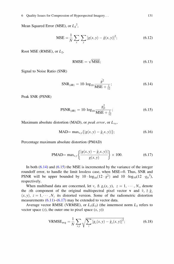
Mean Squared Error (MSE), or L22,

MSE ¼ 1

N

X

x

X

y

½gðx; yÞ � ~gðx; yÞ�2; (6.12)

Root MSE (RMSE), or L2,

RMSE ¼ffiffiffiffiffiffiffiffiffiffi

MSEp

; (6.13)

Signal to Noise Ratio (SNR)

SNRðdBÞ ¼ 10� log10�g2

MSEþ 112

; (6.14)

Peak SNR (PSNR)

PSNRðdBÞ ¼ 10� log10g2fs

MSEþ 112

; (6.15)

Maximum absolute distortion (MAD), or peak error, or L1,

MAD¼ maxx;yfjgðx; yÞ � ~gðx; yÞjg; (6.16)

Percentage maximum absolute distortion (PMAD)

PMAD¼ maxx;yjgðx; yÞ � ~gðx; yÞj

gðx; yÞ

� �

� 100: (6.17)

In both (6.14) and (6.15) the MSE is incremented by the variance of the integer

roundoff error, to handle the limit lossless case, when MSE¼0. Thus, SNR and

PSNR will be upper bounded by 10 � log10ð12 � �g2Þ and 10 �log10(12 �gfs2),respectively.

When multiband data are concerned, let vz ≜ gz(x, y), z ¼ 1, � � � , Nz, denote

the zth component of the original multispectral pixel vector v and ~vz D¼ ~gzðx; yÞ; z ¼ 1; � � � ;Nz its distorted version. Some of the radiometric distortion

measurements (6.11)–(6.17) may be extended to vector data.

Average vector RMSE (VRMSE), or L1(L2) (the innermost norm L2 refers to

vector space (z), the outer one to pixel space (x, y))

VRMSEavg ¼1

N

X

x;y

ffiffiffiffiffiffiffiffiffiffiffiffiffiffiffiffiffiffiffiffiffiffiffiffiffiffiffiffiffiffiffiffiffiffiffiffiffiffiffiffiffiffiffiffiffiffiffi

X

z

½gzðx; yÞ � ~gzðx; yÞ�2r

; (6.18)


Peak VRMSE, or L1(L2),

VRMSEmax¼ maxx;y

ffiffiffiffiffiffiffiffiffiffiffiffiffiffiffiffiffiffiffiffiffiffiffiffiffiffiffiffiffiffiffiffiffiffiffiffiffiffiffiffiffiffiffiffiffiffiffi

X

z

½gzðx; yÞ � ~gzðx; yÞ�2r

; (6.19)

SNR

SNR ¼ 10� log10P

x;y;z g2z ðx; yÞ

P

x;y;z ½gzðx; yÞ � ~gzðx; yÞ�2; (6.20)

PSNR

PSNR ¼ 10� log10N � Nz � g2fs

P

x;y;z ½gzðx; yÞ � ~gzðx; yÞ�2; (6.21)

MAD, or L1(L1),

MAD¼ maxx;y;z

fjgzðx; yÞ � ~gzðx; yÞjg; (6.22)

PMAD

PMAD¼ maxx;y;z

jgzðx; yÞ � ~gzðx; yÞjgzðx; yÞ

� �

� 100: (6.23)

In practice, (6.18) and (6.19) are respectively the average and maximum of the

Euclidean norm of the distortion vector. SNR (6.20) is the extension of (6.14) to the

3D data cube. PSNR is the maximum SNR, given the full-scales of each vector

component. MAD (6.22) is the maximum over the pixel set of the maximum

absolute component of the distortion vector. PMAD (6.23) is the maximum per-

centage error over each vector component of the data cube.

6.1.2 Spectral Distortion

Given two spectral vectors v and ~v both having L components, let v ¼ {v1, v2, � � � ,vL} be the original spectral pixel vector vz ¼ gz(x, y) and ~v ¼ f~v1;~v2; � � � ;~vLg its

distorted version obtained after lossy compression and decompression, i.e.,

~vz ¼ ~gzðx; yÞ. Analogously to the radiometric distortion measurements, spectral

distortion measurements may be defined.

The spectral angle mapper (SAM) denotes the absolute value of the spectral

angle between the couple of vectors:

SAMðv; ~vÞD¼ arccos<v; ~v>

jjvjj2 � jj~vjj2

� �

(6.24)


in which < �, � > stands for scalar product. SAM can be measured in either degrees

or radians. Another measurement especially suitable for hyperspectral data (i.e., for

data with large number of components) is the spectral information divergence (SID)

[20] derived from information-theoretic concepts:

SIDðv; ~vÞ ¼ Dðvjj~vÞ þ Dð~vjjvÞ (6.25)

with Dðvjj~vÞ being the Kullback-Leibler distance (KLD), or entropy divergence, ordiscrimination [24], defined as

Dðvjj~vÞD¼X

L

z¼1

pz logpzqz

� �

(6.26)

in which

pzD¼

vz

jjvjj1and qz

D¼~vz

jj~vjj1(6.27)

In practice SID is equal to the symmetric KLD and can be compactly written as

SIDðv; ~vÞ ¼X

L

z¼1

ðpz � qzÞ logpzqz

� �

(6.28)

which turns out to be symmetric, as one can easily verify. It can be proven as well

that SID is always nonnegative, being zero iff. pz � qz, 8z, i.e., if v is parallel to ~v.The measure unit of SID depends on the base of logarithm: nat/vector with natural

logarithms and bit/vector with logarithms in base two.

Both SAM (6.24) and SID (6.28) may be either averaged on pixel vectors, or

the maximum may be taken instead, as more representative of spectral quality.

Note that radiometric distortion does not necessarily imply spectral distortion.

Conversely, spectral distortion is always accompanied by a radiometric distortion,

that is minimal when the couple of vectors have either the same Euclidean length

(L2) for SAM, or the same city-block length (L1), for SID.

6.2 Linear and Logarithmic Quantization

In this subsection, linear and logarithmic quantization are described. Quantization

has the objective of reducing the transmission rate. Linear quantization is capable of

controlling near-lossless coding while logarithmic quantization is used to yield

relative error bounded compression.


6.2.1 Linear Quantization

In order to achieve reduction in bit rate within the constraint of a near-lossless

compression, prediction errors are quantized, with a quantization noise feedback

loop embedded into the encoder, so that the current pixel prediction is formulated

from the same “noisy” data that will be available at the decoder, as shown in

Fig. 6.1a,b. Prediction errors, e(n) ≜ g(n) � gðnÞ, may be linearly quantized with a

step size D as eDðnÞ ¼ round½eðnÞ=D� and delivered to the context-coding section,

as shown in Fig. 6.1a. The operation of inverse quantization, ~eðx; yÞ ¼ eDðx; yÞ � Dintroduces an error, whose variance and maximum modulus are D2 / 12 and bD / 2c,respectively. Since the MSE distortion is a quadratic function of the D, an odd-valued

step size yields a lower L1 distortion for a given L2 than an even size does; thus, odd

step sizes are preferred for near-lossless compression. The relationship between the

target peak error, i.e., e 2 Zþ, and the step size to be used is D ¼ 2eþ 1.

6.2.2 Logarithmic Quantization

For the case of a relative-error bounded compression a rational version of prediction

error must be envisaged. Let us define the relative prediction error (RPE) as ratio of

original to predicted pixel value:

rðnÞD¼gðnÞgðnÞ (6.29)

The rational nature of RPE, however, makes linear quantization unable to guarantee

a strictly user-defined relative-error bounded performance.

Given a step size D 2 R (D > 0, D6¼1), define direct and inverse logarithmic

quantization (Log-Q) of t 2 R, t > 0, as

QDðtÞD¼round logDðtÞ½ � ¼ round logðtÞ= logðDÞ½ �

Q�1D ðlÞ ¼ Dl (6.30)

Applying (6.30) to (6.29) yields

QD½rðnÞ� ¼ roundlogðgðnÞÞ � logðgðnÞÞ

logD

�

(6.31)

Hence, Log-Q of RPE is identical to Lin-Q of logðgðnÞÞ � logðgðnÞÞ with a step

size logD. If a Log-Q with a step size D is used to encode pixel RPE’s (6.29),

it can be proven that the ratio of original to decoded pixel value is strictly bounded

around one


minffiffiffiffi

Dp

;1ffiffiffiffi

Dp

� �

� gðnÞ~gðnÞ � max

ffiffiffiffi

Dp

;1ffiffiffiffi

Dp

� �

(6.32)

From (6.32) and (6.29) it stems that the percentage pixel distortion is upper

bounded

PMAD ¼ maxffiffiffiffi

Dp

� 1; 1� 1ffiffiffiffi

Dp

� �

� 100 (6.33)

depending on whether D > 1, or 0 < D < 1. Hence, the relationship between the

target percentage peak error, r, and the step size will be, e.g., for D > 0,

D ¼ ð1þ r=100Þ2.

7 Virtually Lossless Compression

The term virtually lossless indicates that the distortion introduced by compression

appears as an additional amount of noise, besides the intrinsic observation noise,

being statistically independent of the latter, as well as of the underlying signal. Its

first order distribution should be such that the overall probability density function

(PDF) of the noise corrupting the decompressed data, i.e., intrinsic noise plus

compression-induced noise, closely matches the noise PDF of the original data.

This requirement is trivially fulfilled if compression is lossless, but may also hold if

the difference between uncompressed and decompressed data exhibits a peaked and

narrow PDF without tails, as it happens for near lossless techniques, whenever the

user defined MAD is sufficiently smaller than the standard deviation sn of the

background noise. Both MAD and sn are intended to be expressed in either physical

units, for calibrated data, or as digital counts otherwise. Therefore, noise modeling

and estimation from the uncompressed data becomes a major task to accomplish a

virtually lossless compression [6]. The underlying assumption is that the depen-

dence of the noise on the signal is null, or weak. However, signal independence of

the noise may not strictly hold for hyperspectral images, especially for new-

generation instruments. This further uncertainty in the noise model may be over-

come by imposing a margin on the relationship between target MAD and RMS

value of background noise.

For a DPCM scheme, the relationship between MAD and quantization step size

is D ¼ 2MAD + 1, while the relationship between the variance of quantization

noise, which is equal to MSE, and the step size is e 2 ¼ D2=12. Hence, the rationaleof virtually lossless compression can be summarized as follows. Firstly, measure

the background noise RMS, sn; if sn < 1, lossless compression is mandatory.

If 1 � sn < 3, lossless compression is recommended, but near lossless compres-

sion with MAD ¼ 1 (D ¼ 3) is feasible. For 3 � sn < 5, a strictly virtually

lossless compression would require MAD ¼ 1, and so on.


The signal may have been previously quantized based on different requirement;

afterwards a check on the noise is made to decide whether lossless compression is

really necessary, or near lossless compression could be used instead without

penalty, being “de facto” virtually lossless.

The key to achieve a compression preserving the scientific quality of the data for

remote-sensing is represented by the following twofold recommendation:

1. Absence of tails in the PDF of the error between uncompressed and decompressed

image, in order to maximize the ratio RMSE / MAD, i.e., e/MAD, or equivalently

to minimize MAD for a given RMSE.

2. MSE lower by one order of magnitude (10 dB) than the variance of background

noise sn2.

Near-lossless methods are capable to fulfill such requirements, provided that the

quantization step size D is chosen as an odd integer such that D sn. More exactly,

the relationship between MAD and sn, also including a margin of approximately

1 dB, is:

MAD ¼ bmaxf0; ðsn � 1Þ=2gc (6.34)

Depending on application context and type of data, the relationship (6.34) may be

relaxed, e.g., by imposing that the ratio sn2 / e2 is greater than, say, 3 dB, instead of

the 11 dB, given by (6.34). If the data are intrinsically little noisy, the protocol may

lead to the direct use of lossless compression, i.e., D ¼ 1.

If compression ratios greater than those of the reversible case are required, near

lossless compression with MAD 1 of low-noise bands may be inadequate to

preserve the scientific quality of the data, because the compression-induced MSE is

not one order of magnitude lower than sn2, as it would be recommended for

virtually lossless compression. However, it may become mandatory to increase

compression ratios above the values typical of the strictly virtually lossless proto-

col. To adjust the compression ratio, a real valued positive scale factor q can be

introduced, such that the quantization step size of the nth band is given by:

Dn ¼ round½q � sn�: (6.35)

where the roundoff is to the nearest odd integer. If q � 1 a strictly virtually

lossless compression is achieved, since the compression-induced quadratic dis-

tortion is less than one tenth of the intrinsic noisiness of the data. Otherwise, if

q > 1, compression is widely virtually lossless, even though distortion is properly

allocated among the spectral bands. As an example, Fig. 6.5 shows quantization

step sizes for three different values of q, if the test sequence Cuprite Mine of

AVIRIS 1997 is near lossless compressed by means of the S-RLP algorithm. The

estimation of the background noise RMS of the test sequence has been performed

by considering a method based on the joint 2D PDF of the local statistics,

described in [4]. To compare virtually lossless compression with a unique quan-

tizer for the whole data cube, the step size of the latter, yielding the same


compression ratio as the former, is the odd integer roundoff of the geometric mean

of the step sizes in (6.35), at least for small distortions, in order to have an

independent quantizer at each band.

8 Experimental Results and Comparisons

Experimental results are presented for the two data sets constituted by AVIRIS

1997 and AVIRIS 2006 data. Lossless compression is first considered on both data

sets. Afterwards some results are presented for near-lossless and virtually lossless

compression on a particular scene of the Cuprite Mine sequence of the AVIRIS

1997 data set. Eventually, some considerations on virtually lossless compression on

discrimination of materials are introduced.

8.1 Lossless Compression Performance Comparisons

The lossless compression experiments have been performed by comparing some of

the most performing schemes reported in the literature such as FL [27], SLSQ [42],

M-CALIC [30], C-DPCM [33], S-RLP and S-FMP for the classical methods, and

LUT-NN [32], LAIS-LUT [23], S-RLP-LUT and S-FMP-LUT for the LUT-based

algorithms. Eventually, also TSP [27] is reported, an algorithm specifically

designed to cope with the calibrated-induced artifacts. Some of these methods

have not been made available by authors on the 2006 AVIRIS data set.

0 50 100 150 2000

50

100

150

200

250

Band number

∆

q=0.5

q=1

q=2

Fig. 6.5 Quantization step size varying with band number for the test sequence Cuprite Mine


8.1.1 1997 AVIRIS Data Set

Table 6.1 lists the bit rates for several lossless compression methods applied to

the standard 1997 AVIRIS images. The compared methods are FL [27], SLSQ [42],

M-CALIC [30], C-DPCM [33], S-RLP, S-FMP, LUT-NN [32], LAIS-LUT [23],

S-RLP-LUT, S-FMP-LUT and TSP [27].

It is apparent from the results reported in Table 6.1 that the best average

performance is obtained by TSP and by the LUT-based algorithms, which are

very effective even if not specifically designed for this type of data, because they

are able to exploit the artificial regularities in the image histogram.

Concerning the S-RLP algorithm, Fig. 6.6 reports a comparison with 3D-RLP by

varying the number S of the pixels in the prediction causal neighborhood PSðnÞ.In this experiment, the fourth scene of the test image Cuprite ’97 has been

reversibly compressed by means of S-RLP and 3D-RLP. Bit rates, reported in bits

per pixel per band, include all coding overhead: predictor coefficients, block labels,

and arithmetic codewords. For each l, prediction lengths equal to 5, 14, and 20 have

been considered together with 16 predictors. 3D prediction of RLP is always carried

out from a couple of previous bands, except for the first band, coded in intra mode,

i.e., by 2D DPCM, and the second band, which is predicted from one previous band

only. The purely spectral 1D prediction of S-RLP is carried out from the available

previous bands up the requested prediction length.

As it appears from the plots in Fig. 6.6, S-RLP outperforms 3D-RLP, especially

when prediction length is lower, a case of interest for customized satellite on-board

implementations. The performance of both S-RLP and 3D-RLP cannot be improved

significantly by increasing the number and length of predictors, because of over-

head information increasing as well.

Table 6.1 Bit rates (bit/pel/band on disk) for lossless compression of AVIRIS 1997 test

hyperspectral images. S-RLP-LUT and S-FMP-LUT use N ¼ 20 previous bands and M ¼ 4

LUT’s per band. Best results are reported in bold

Cuprite Jasper Lunar Moffett Average

FL 4.82 4.87 4.83 4.93 4.86

SLSQ 4.94 4.95 4.95 4.98 4.96

M-CALIC 4.89 4.97 4.80 4.65 4.83

C-DPCM 4.68 4.62 4.75 4.62 4.67

S-RLP 4.69 4.65 4.69 4.67 4.67

S-FMP 4.66 4.63 4.66 4.63 4.64

LUT-NN 4.66 4.95 4.71 5.05 4.84

LAIS-LUT 4.47 4.68 4.53 4.76 4.71

S-RLP-LUT 3.92 4.05 3.95 4.09 4.00

S-FMP-LUT 3.89 4.03 3.92 4.05 3.97

TSP 3.77 4.08 3.81 4.12 3.95


8.1.2 2006 AVIRIS Data Set

A new data set of calibrated and uncalibrated AVIRIS images has been provided

by Consultative Committee for Space Data Systems (CCSDS) and is now available

to scientific users for compression experiments at the web site of address:(http://

compression.jpl.nasa.gov/hyperspectral). This data set consists of five calibrated

and the corresponding raw 16-bit images acquired over Yellowstone, WY. Each

image is composed by 224 bands and each scene (the scene numbers are 0, 3, 10, 11,

18) has 512 lines [27]. The 50th band of Yellowstone 10 is reported in Fig. 6.7.

5 pels 14 pels 20 pels4.5

4.55

4.6

4.65

4.7

4.75

4.8

4.85

4.9

4.95

5

Prediction Length

Bit R

ate

(b

it/p

el/b

an

d)

3D−RLP

S−RLP

Fig. 6.6 S-RLP versus 3D-RLP varying with the prediction length. Bit rates on disk for the

lossless compression of the fourth scene of AVIRIS Cuprite Mine 1997

Fig. 6.7 Band 50 of the 2006 AVIRIS Yellowstone 10 scene


http://compression.jpl.nasa.gov/hyperspectral

http://compression.jpl.nasa.gov/hyperspectral

Tables 6.2 and 6.3 report the lossless compression performances on the 2006

AVIRIS calibrated and uncalibrated data sets, respectively. The compared methods

are FL [28], S-RLP, S-FMP, LUT-NN [32], LAIS-LUT [23], TSP [27], S-RLP-

LUT and S-FMP-LUT. For these last algorithms, only two scenes have been

compressed.

The scores show that the LUT-based methods and TSP are not able to obtain the

same performances on both calibrated and uncalibrated 2006 AVIRIS data set with

respect to the best performances obtained on the 1997 AVIRIS data set. S-RLP and

S-FMP are the most effective and gain more than 10% and 6% over FL and 12%

and 7% on TSP, on calibrated and uncalibrated data, respectively. FL algorithm is

effective notwithstanding its simplicity.

8.2 Near Lossless Compression Performance Comparisons

Near lossless compression tests have been performed on the fourth scene of Cuprite

Mine. Rate-Distortion (RD) plots are reported in Fig. 6.8a for S-RLP and 3D-RLP

operating with M ¼ 16 predictors and S ¼ 20 coefficients per predictor. PSNR of

Table 6.2 Bit rates (bit/pel/band on disk) for lossless compression of the calibrated 2006 AVIRIS

data set. S-RLP-LUT and S-FMP-LUT have been utilized only for the first two scenes. The best

results are reported in bold

Yellowstone

0

Yellowstone

3

Yellowstone

10

Yellowstone

11

Yellowstone

18 Average

FL 3.91 3.79 3.37 3.59 3.90 3.71

S-RLP 3.58 3.43 2.95 3.27 3.46 3.34

S-FMP 3.54 3.39 2.94 3.25 3.44 3.31

LUT-NN 4.82 4.62 3.96 4.34 4.84 4.52

LAIS-LUT 4.48 4.31 3.71 4.02 4.48 4.20

SRLP-LUT 3.95 3.82 n.a. n.a. n.a. n.a.

S-FMP-LUT 3.91 3.78 n.a. n.a. n.a. n.a.

TSP 3.99 3.86 3.42 3.67 3.97 3.78

Table 6.3 Bit rates (bit/pel/band on disk) for lossless compression of the uncalibrated 2006

AVIRIS data set. S-RLP-LUT and S-FMP-LUT have been utilized only for the first two scenes.

The best results are reported in bold

Yellowstone

0

Yellowstone

3

Yellowstone

10

Yellowstone

11

Yellowstone

18 Average

FL 6.20 6.07 5.60 5.81 6.26 5.99

S-RLP 5.88 5.72 5.21 5.54 5.75 5.62

S-FMP 5.84 5.67 5.18 5.48 5.68 5.57

LUT-NN 7.14 6.91 6.26 6.69 7.20 6.84

LAIS-LUT 6.78 6.60 6.00 6.30 6.82 6.50

SRLP-LUT 6.21 6.05 n.a. n.a. n.a. n.a.

S-FMP-LUT 6.17 6.01 n.a. n.a. n.a. n.a.

TSP 6.27 6.13 5.64 5.88 6.32 6.05


the whole image is calculated from the average MSE of the sequence of bands.

Due to the sign bit, the full scale gfs in (6.15) was set equal to 215 � 1 ¼ 32,767

instead of 65,535, since small negative values, introduced by removal or dark

current during calibration, are very rare and totally missing in some scenes.

Hence, the PSNR attains a value of 10log10(12gfs2) 102 dB, due to integer

roundoff noise only, when reversibility is reached. The correction for roundoff

noise has a twofold advantage. Firstly, lossless points appear inside the plot and

can be directly compared. Secondly, all PSNR-bit rate plots are straight lines with

slope 6 dB/bit for bit rates larger than, say, 1 bit/pel, in agreement with RD theory

[24] (with a uniform threshold quantizer). For lower bit rates, the quantization noise

feedback causes an exponential drift from the theoretical straight line.

The results follow the same trends as the lossless case for S-RLP and are

analogous to those of 3D-RLP, reported in [6], and of M-CALIC, reported in

[30]. The near-lossless bit rate profiles are rigidly shifted downward from the

lossless case by amounts proportional to the logarithm of the quantization-induced

distortion. This behavior does not occur for low bit rates, because of the

quantization noise feedback effect: prediction becomes poorer and poorer as it is

obtained from the highly distorted reconstructed samples used by the predictor,

which must be aligned to the decoder.

Interestingly, the difference in bit rate between S-RLP and 3D-RLP at a given

PSNR is only two hundredths of bit/pel near the lossless point, but grows up to one

tenth of bit/pel at a rate equal to 1.5 bit/pel, typical of a high-quality lossy

compression. Comparisons with an up-to-date algorithm [35], implementing the

state-of-the-art JPEG2000 multi-component approach, reveal that S-RLP

outperforms the wavelet-based encoder by approximately 3.5 dB at 2 bit/pel.

However, this difference reduces to 2.5 dB at 1 bit/pel and vanishes around

0.25 bit/pel, because of the quantization noise feedback effect, which is missing

in the 3D wavelet coder. This moderate loss of performance is the price that

70

75

80

85

90

95

100

105

a bP

SN

R (

dB

)

0 1 3 4 52

Bit Rate (bit/pel per band)

0 1 3 4 52

Bit Rate (bit/pel per band)

0

2

4

6

8

10

12

14

16

MA

D

3D-RLP

SRLP

3D-RLP

SRLP

Fig. 6.8 Performance plots for near-lossless compression of AVIRIS CupriteMine ’97 test

hyperspectral images: (a) PSNR vs. bit rate; (b) maximum absolute distortion (MAD) vs. bit rate


embedded coders have to pay. DPCM does not allow progressive reconstruction to

be achieved, but yields higher PSNR, at least for medium-high bit rates. The further

advantage of DPCM is that it is near-lossless, unlike JPEG 2000, which can be

made lossless, but not near-lossless, unless an extremely cumbersome quantizer is

employed, with further loss in performances [15].

The near-lossless performance is shown in the MAD-bit rate plots of Fig. 6.8b.

Since the average standard deviation of the noise was found to be around 10

according to [3], a virtually-lossless compression (maximum compression-induced

absolute error lower than the standard deviation of the noise [29]) is given by

S-RLP at a bit rate around 1.6 bit/pel/band, thereby yielding a compression ratio CR

¼ 10 with respect to uncompressed data and CR 3 relative to lossless compres-

sion. Figure 6.8 evidences that the increment in performance of S-RLP over

3D-RLP is more relevant for such a bit rate than for higher rates.

A different experiment reported for 3D-RLP but representative of all DPCM-

based methods is reported in Fig. 6.9a for linear quantization and in Fig. 6.9b for

the logarithmic quantizer.

All bands have been compressed in both MAD-constrained mode (linear

quantization) and PMAD constrained mode (logarithmic quantization). Bit rates

varying with band number, together with the related distortion parameters are

shown in Fig. 6.9. The bit rate plots follow similar trends varying with the amount

of distortion, but quite different trends for the two types of distortion (i.e., either

MAD or PMAD). For example, around the water vapor absorption wavelengths

( Band 80) the MAD-bounded plots exhibit pronounced valleys, that can be

explained because the intrinsic SNR of the data becomes lower; thus the linear

quantizer dramatically abates the noisy prediction errors. On the other hand, the

PMAD-bounded encoder tends to quantize the noisy residuals more finely when

the signal is lower. Therefore bit rate peaks are generated instead of valleys.

More generally speaking, bit rate peaks from the PMAD-bounded encoder are

0 50 100 150 2000

2

4

6

8

10

12

Spectral band number

Bit r

ate

(b

it/p

ixe

l)

MAD = 1MAD = 3MAD = 5MAD = 7MAD = 9MAD = 11

0 50 100 150 2000

2

4

6

8

10

12

Spectral band number

Bit r

ate

(b

it/p

ixe

l)

PMAD = 0.075PMAD = 0.125PMAD = 0.1875PMAD = 0.4

a b

Fig. 6.9 Bit rates produced by 3DRLP on theCuprite sequence of bands: (a) linear quantization toyield user-defined MAD values; (b) logarithmic quantization to yield user-defined PMAD values


associated with low responses from the spectrometer. This explains why the bit rate

plots of Fig. 6.9b never fall below 1 bit/pixel per band.

Some of the radiometric distortion measures defined in Sect. 6.1 have been

calculated on the distorted hyperspectral pixel vectors achieved by decompressing

the bit streams generated by the near-lossless 3D-RLP encoder, both MAD- and

PMAD-bounded. VRMSEs of the vector data, both average (6.18) and maximum

(6.19), are plotted in Fig. 6.10a as a function of the bit rate from the encoder.

The MAD-bounded encoder obviously minimizes both the average and maxi-

mum of VRMSE, that is the Euclidean norm of the pixel error vector. A further

advantage is that average and maximum VRMSE are very close to each other for all

bit rates. The PMAD-bounded encoder is somewhat poorer: average VRMSE is

comparable with that of the former, but peak VRMSE is far larger, due to the high-

signal components that are coarsely quantized in order to minimize PMAD. Trivial

results, not reported in the plots, are that MAD of the data cube (6.22) is exactly

equal to the desired value, whereas the PMAD, being unconstrained, is higher.

Symmetric results have been found by measuring PMAD on MAD-bounded and

PMAD-bounded decoded data.

As far as radiometric distortion is concerned, results are not surprising. Radio-

metric distortions measured on vectors are straightforwardly derived from those

measured on scalar pixel values. The introduction of such spectralmeasurements as

SAM (6.24) and SID (6.28) may overcome the rationale of distortion, as established

in the signal/image processing community. Figure 6.10b shows spectral distortions

between original and decompressed hyperspectral pixel vectors. The PMAD-

bounded algorithm yields plots that lie in the middle between the corresponding

ones produced by the MAD-bounded algorithm and are very close to each other too.

Since themaximum SAM is a better clue of spectral quality of the decoded data than

the average SAM may be, a likely conclusion would be that PMAD-bounded

compression optimizes the spectral quality of the data, while MAD-bounded is

superior in terms of radiometric quality. Furthermore, the maximum SAM

1 1.5 2 2.5 3 3.5 4 4.50

50

100

150

200

250

300

Average bit rate (bit per pixel per band)

1 1.5 2 2.5 3 3.5 4 4.5

Average bit rate (bit per pixel per band)

V−

RM

SE

PMAD−bounded (max)PMAD−bounded (avg.)MAD−bounded (max)MAD−bounded (avg.)

0

0.02

0.04

0.06

0.08

0.1

0.12

0.14

0.16

0.18

SA

M (

de

gre

es)

PMAD−bounded (max)PMAD−bounded (avg.)MAD−bounded (max)MAD−bounded (avg.)

a b

Fig. 6.10 Vector distortions vs bit rate for compressed AVIRIS Cuprite Mine ’97 data.

Radiometric distortion (a) VRMSE; spectral distortion (b) SAM


introduced by the P-MAD bounded logarithmic quantizer is lower than 0.2 ∘ for an

average rate of 1 bit/pixel per vector component, i.e., CR¼16.

8.3 Discrimination of Materials

Analysis procedures of hyperspectral vectors are usually performed on reflectance

data, especially when the goal is identification of materials by comparing their

remotely sensed spectra with sample spectra extracted from reference spectral

libraries. Whenever measured spectra are to be compared to laboratory spectra,

the radiance data are converted into reflectances, e.g., by means of the following

simplified formula:

rðlÞ ¼ RðlÞ � pIðlÞ � TðlÞ (6.36)

in which r(l) is reflectance, I(l) is solar irradiance on ground, T(l) is atmospheric

transmittance, and R(l) is at-sensor radiance, all functions of wavelength l.

Distortions introduced by compression on radiance will be amplified or attenuated

depending on the values of the product I(l) �T(l). So, spectral distortion, e.g., SAM,

must be measured between reflectance pixel spectra, rather than radiance pixel

spectra. Extensive results of spectral discrimination from compressed hyperspectral

data have demonstrated that a SAM distortion lower than 0.5 ∘ has negligible

impact on the capability of automated classifiers of identifying spectral signatures

of materials [26].

As a matter of fact, uniform distortion allocation over the entire spectrum yields

minimum angle error between original and decompressed vectors. Band-variable

distortion allocation following the virtually lossless protocol does not minimize

error. However, when decompressed radiance data are converted into reflectance

data by means of (6.36), the distribution of errors in decompressed reflectance spectra

becomes approximately flat with the wavelength. In fact, quantization step sizes for

virtually lossless compression follow the trend in Fig. 6.5, while the product I(l) � T(l) by which compression errors on radiance are multiplied to yield compression

errors on reflectance follows an opposite trend. Eventually, virtually lossless com-

pression is preferable to near-lossless compression at the same rate, at least for

detection of materials using spectral libraries, because SAM of reflectances produced

from virtually lossless data are in average lower than those coming from near lossless

data.


9 Conclusions

This chapter has pointed out that quality issues are crucial for compression of

radiance data produced by imaging spectrometers. Most widely used lossless com-

pression techniques may be possibly replaced by lossy, yet error-bounded,

techniques (near-lossless compression). Both lossless and near-lossless compression

techniques can be implemented as adaptive DPCM encoders, with minor differences

between the former and the latter. The rationale that compression-induced distortion

is more tolerable, i.e., less harmful, in those bands, in which the noise is higher, and

vice-versa, constitutes the virtually lossless paradigm, which provides operational

criteria to design quantization in DPCM schemes. The quantization step size of each

band should be a fraction of the measured standard deviation of instrumental noise.

For typical VNIR+SWIR (400–2500 nm) spectra, virtually lossless compression

exploits a band-varying quantization, with step sizes approximately decaying with

increasing wavelengths. Once decompressed radiance spectra are converted to

reflectance by removing the contribution of solar irradiance and atmospheric trans-

mittance, the distribution of compression-induced errors with the wavelength is

roughly equalized. Hence, angular errors introduced by compression errors on

radiances will be lower for virtually lossless compression than for near-lossless

compression. This feature is expected to be useful for discrimination of materials

from compressed data and spectral libraries.

References

1. Abrardo, A., Alparone, L., Bartolini, F.: Encoding-interleaved hierarchical interpolation for

lossless image compression. Signal Processing 56(2), 321–328 (1997)

2. Aiazzi, B., Alba, P., Alparone, L., Baronti, S.: Lossless compression of multi/hyper-spectral

imagery based on a 3-D fuzzy prediction. IEEE Trans. Geosci. Remote Sensing 37(5),2287–2294 (1999)

3. Aiazzi, B., Alparone, L., Barducci, A., Baronti, S., Marcoionni, P., Pippi, I., Selva, M.: Noise

modelling and estimation of hyperspectral data from airborne imaging spectrometers. Annals

of Geophysics 41(1), 1–9 (2006)

4. Aiazzi, B., Alparone, L., Barducci, A., Baronti, S., Pippi, I.: Estimating noise and information

of multispectral imagery. J. Optical Engin. 41(3), 656–668 (2002)

5. Aiazzi, B., Alparone, L., Baronti, S.: A reduced Laplacian pyramid for lossless and progressive

image communication. IEEE Trans. Commun. 44(1), 18–22 (1996)

6. Aiazzi, B., Alparone, L., Baronti, S.: Near-lossless compression of 3-D optical data. IEEE

Trans. Geosci. Remote Sensing 39(11), 2547–2557 (2001)

7. Aiazzi, B., Alparone, L., Baronti, S.: Context modeling for near-lossless image coding. IEEE

Signal Processing Lett. 9(3), 77–80 (2002)

8. Aiazzi, B., Alparone, L., Baronti, S.: Fuzzy logic-based matching pursuits for lossless predic-

tive coding of still images. IEEE Trans. Fuzzy Systems 10(4), 473–483 (2002)

9. Aiazzi, B., Alparone, L., Baronti, S.: Near-lossless image compression by relaxation-labelled

prediction. Signal Processing 82(11), 1619–1631 (2002)

10. Aiazzi, B., Alparone, L., Baronti, S.: Lossless compression of hyperspectral images using

multiband lookup tables. IEEE Signal Processing Lett. 16(6), 481–484 (2009)


11. Aiazzi, B., Alparone, L., Baronti, S., Lastri, C.: Crisp and fuzzy adaptive spectral predictions

for lossless and near-lossless compression of hyperspectral imagery. IEEE Geosci. Remote

Sens. Lett. 4(4), 532–536 (2007)

12. Aiazzi, B., Alparone, L., Baronti, S., Lotti, F.: Lossless image compression by quantization

feedback in a content-driven enhanced Laplacian pyramid. IEEE Trans. Image Processing 6(6), 831–843 (1997)

13. Aiazzi, B., Alparone, L., Baronti, S., Santurri, L.: Near-lossless compression of multi/

hyperspectral images based on a fuzzy-matching-pursuits interband prediction. In: S.B.

Serpico (ed.) Image and Signal Processing for Remote Sensing VII, vol. 4541, pp. 252–263

(2002)

14. Alecu, A., Munteanu, A., Cornelis, J., Dewitte, S., Schelkens, P.: On the optimality of

embedded deadzone scalar-quantizers for wavelet-based L-infinite-constrained image coding.

IEEE Signal Processing Lett. 11(3), 367–370 (2004)

15. Alecu, A., Munteanu, A., Cornelis, J., Dewitte, S., Schelkens, P.: Wavelet-based scalable

L-infinity-oriented compression. IEEE Trans Image Processing 15(9), 2499–2512 (2006)

16. Baraldi, A., Blonda, P.: A survey of fuzzy clustering algorithms for pattern recognition–Parts

I and II. IEEE Trans. Syst. Man Cybern.–B 29(6), 778–800 (1999)

17. Benazza-Benyahia, A., Pesquet, J.C., Hamdi, M.: Vector-lifting schemes for lossless coding

and progressive archival of multispectral images. IEEE Trans. Geosci. Remote Sensing 40(9),2011–2024 (2002)

18. Bezdek, J.C.: Pattern Recognition with Fuzzy Objective Function Algorithm. Plenum Press,

New York (1981)

19. Carpentieri, B., Weinberger, M.J., Seroussi, G.: Lossless compression of continuous-tone

images. Proc. of the IEEE 88(11), 1797–1809 (2000)

20. Chang, C.I.: An information-theoretic approach to spectral variability, similarity, and discrim-

ination for hyperspectral image analysis. IEEE Trans. Inform. Theory 46(5), 1927–1932(2000)

21. Deng, G., Ye, H., Cahill, L.W.: Adaptive combination of linear predictors for lossless image

compression. IEE Proc.-Sci. Meas. Technol. 147(6), 414–419 (2000)

22. Golchin, F., Paliwal, K.K.: Classified adaptive prediction and entropy coding for lossless

coding of images. In: Proc. IEEE Int. Conf. on Image Processing, vol. III/III, pp. 110–113

(1997)

23. Huang, B., Sriraja, Y.: Lossless compression of hyperspectral imagery via lookup tables with

predictor selection. In: L. Bruzzone (ed.) Proc. of SPIE, Image and Signal Processing for

Remote Sensing XII, vol. 6365, pp. 63650L.1–63650L.8 (2006)

24. Jayant, N.S., Noll, P.: Digital Coding of Waveforms: Principles and Applications to Speech

and Video. Prentice Hall, Englewood Cliffs, NJ (1984)

25. Ke, L., Marcellin, M.W.: Near-lossless image compression: minimum entropy, constrained-

error DPCM. IEEE Trans. Image Processing 7(2), 225–228 (1998)

26. Keshava, N.: Distance metrics and band selection in hyperspectral processing with

applications to material identification and spectral libraries. IEEE Trans. Geosci. Remote

Sensing 42(7), 1552–1565 (2004)

27. Kiely, A.B., Klimesh, M.A.: Exploiting calibration-induced artifacts in lossless compression

of hyperspectral imagery. IEEE Trans. Geosci. Remote Sensing 47(8), 2672–2678 (2009)

28. Klimesh, M.: Low-complexity adaptive lossless compression of hyperspectral imagery.

In: Satellite Data Compression, Communication and Archiving II, Proc. SPIE, vol. 6300

pp. 63000N.1–63000N.9 (2006)

29. Lastri, C., Aiazzi, B., Alparone, L., Baronti, S.: Virtually lossless compression of astrophysical

images. EURASIP Journal on Applied Signal Processing 2005(15), 2521–2535 (2005)

30. Magli, E., Olmo, G., Quacchio, E.: Optimized onboard lossless and near-lossless compression

of hyperspectral data using CALIC. IEEE Geosci. Remote Sensing Lett. 1(1), 21–25 (2004)

31. Matsuda, I., Mori, H., Itoh, S.: Lossless coding of still images using minimum-rate predictors.

In: Proc. IEEE Int. Conf. on Image Processing, vol. I/III, pp. 132–135 (2000)


32. Mielikainen, J.: Lossless compression of hyperspectral images using lookup tables. IEEE

Signal Proc. Lett. 13(3), 157–160 (2006)

33. Mielikainen, J., Toivanen, P.: Clustered DPCM for the lossless compression of hyperspectral

images. IEEE Trans. Geosci. Remote Sensing 41(12), 2943–2946 (2003)

34. Mielikainen, J., Toivanen, P., Kaarna, A.: Linear prediction in lossless compression of

hyperspectral images. J. Optical Engin. 42(4), 1013–1017 (2003)

35. Penna, B., Tillo, T., Magli, E., Olmo, G.: Progressive 3-D coding of hyperspectral images

based on JPEG 2000. IEEE Geosci. Remote Sensing Lett. 3(1), 125–129 (2006)

36. Pennebaker, W.B., Mitchell, J.L.: JPEG: Still Image Compression Standard. Van Nostrand

Reinhold, New York (1993)

37. Ramabadran, T.V., Chen, K.: The use of contextual information in the reversible compression

of medical images. IEEE Trans. Medical Imaging 11(2), 185–195 (1992)

38. Rao,A.K., Bhargava, S.:Multispectral data compression using bidirectional interband prediction.

IEEE Trans. Geosci. Remote Sensing 34(2), 385–397 (1996)39. Rao, K.K., Hwang, J.J.: Techniques and Standards for Image, Video, and Audio Coding.

Prentice Hall, Engl. Cliffs, NJ (1996)

40. Reichel, J., Menegaz, G., Nadenau, M.J., Kunt, M.: Integer wavelet transform for embedded

lossy to lossless image compression. IEEE Trans. Image Processing 10(3), 383–392 (2001)

41. Rice, R.F., Plaunt, J.R.: Adaptive variable-length coding for efficient compression of space-

craft television data. IEEE Trans. Commun. Technol. COM-19(6), 889–897 (1971)

42. Rizzo, F., Carpentieri, B., Motta, G., Storer, J.A.: Low-complexity lossless compression of

hyperspectral imagery via linear prediction. IEEE Signal Processing Lett. 12(2), 138–141(2005)

43. Roger, R.E., Cavenor, M.C.: Lossless compression of AVIRIS images. IEEE Trans. Image

Processing 5(5), 713–719 (1996)

44. Said, A., Pearlman, W.A.: An image multiresolution representation for lossless and lossy

compression. IEEE Trans. Image Processing 5(9), 1303–1310 (1996)

45. Tate, S.R.: Band ordering in lossless compression of multispectral images. IEEE Trans.

Comput. 46(4), 477–483 (1997)

46. Taubman, D.S., Marcellin, M.W.: JPEG2000: Image compression fundamentals, standards

and practice. Kluwer Academic Publishers, Dordrecht, The Netherlands (2001)

47. Wang, J., Zhang, K., Tang, S.: Spectral and spatial decorrelation of Landsat-TM data for

lossless compression. IEEE Trans. Geosci. Remote Sensing 33(5), 1277–1285 (1995)

48. Weinberger, M.J., Rissanen, J.J., Arps, R.B.: Applications of universal context modeling to

lossless compression of gray-scale images. IEEE Trans. Image Processing 5(4), 575–586(1996)

49. Weinberger, M.J., Seroussi, G., Sapiro, G.: The LOCO-I lossless image compression algo-

rithm: principles and standardization into JPEG-LS. IEEE Trans. Image Processing 9(8),1309–1324 (2000)

50. Witten, I.H., Neal, R.M., Cleary, J.G.: Arithmetic coding for data compression. Commun.

ACM 30, 520–540 (1987)

51. Wu, X., Bao, P.: L1 constrained high-fidelity image compression via adaptive context

modeling. IEEE Trans. Image Processing 9(4), 536–542 (2000)

52. Wu, X., Memon, N.: Context-based, adaptive, lossless image coding. IEEE Trans. Commun.

45(4), 437–444 (1997)

53. Wu, X., Memon, N.: Context-based lossless interband compression–Extending CALIC. IEEE

Trans. Image Processing 9(6), 994–1001 (2000)


Chapter 7

Ultraspectral Sounder Data Compressionby the Prediction-Based LowerTriangular Transform

Shih-Chieh Wei and Bormin Huang

Abstract The Karhunen–Loeve transform (KLT) is the optimal unitary transform

that yields the maximum coding gain. The prediction-based lower triangular trans-

form (PLT) features the same decorrelation and coding gain properties as KLT but

with lower complexity. Unlike KLT, PLT has the perfect reconstruction property

which allows its direct use for lossless compression. In this paper, we apply PLT

to carry out lossless compression of the ultraspectral sounder data. The experiment

on the standard ultraspectral test dataset of ten AIRS digital count granules shows

that the PLT compression scheme compares favorably with JPEG-LS, JPEG2000,

LUT, SPIHT, and CCSDS IDC 5/3.

1 Introduction

Contemporary and future ultraspectral infrared sounders such as AIRS [1], CrIS [2],

IASI [3] and GIFTS [4] represent a significant technical advancements in for

environmental and meteorological prediction and monitoring. Given the large 3D

volume of data obtained from high spectral and spatial observations, the use of

effective data compression techniques will be beneficial for data transfer and

storage. When the ultraspectral sounder data is used to retrieve geophysical

parameters like the vertical profiles of atmospheric temperature, moisture and

trace gases, the retrieval process involves solving the radiative transfer equation

which is an ill-posed inverse problem and sensitive to the noise and error in the

S.-C. Wei (*)

Department of Information Management, Tamkang University, Tamsui, Taiwan


B. Huang

Space Science and Engineering Center, University of Wisconsin, Madison, USA



149



data [5]. Thus, lossless or near lossless compression of the data is desired in order

to avoid substantial degradation during retrieval.

Past studies on lossless compression of the ultraspectral sounder data can be

categorized into clustering-based, prediction-based and transform-based methods

[6]. Since a higher correlation exists in spectral dimension than in spatial dimension

of ultraspectral sounder data [6], there were studies on band reordering as

preprocessing before compression [7, 8]. The Karhunen–Loeve transform (KLT),

a.k.a. the principal component analysis (PCA) or the Hoteling transform, is the

optimal unitary transform that yields the maximum coding gain. However, consid-

ering its data-dependent computational cost involving the eigenvectors from the

input covariance matrix, KLT is often only used as a benchmark for performance

comparison. Phoong and Lin [9] developed the prediction-based lower triangular

transform (PLT) that features the same decorrelation and coding gain properties as

KLT but with a lower design and implementational cost. They showed promising

results when PLT was applied to lossy compression of 2D imagery and the AR(1)

process [9]. However, the original PLT by Phoong et al. requires the input vector to

be a blocked version of a scalar wide sense stationary (WSS) process. Weng et al.

[10] proposed a generalized triangular decomposition (GTD) which allows the

input vector to be a vector WSS process. GTD has the same coding gain as KLT

and it includes KLT and PLT as special cases [10].

Furthermore, unlike KLT, PLT has a perfect reconstruction (PR) property which

makes it usefull for lossless compression. Since PLT provides the same coding gain

as KLT, with lower complexity and PR property, we were motivated to apply PLT

to carry out lossless compression of the ultraspectral sounder data. The compression

method consists of using PLT for spectral prediction, followed by the arithmetic

coding. The PLT compression ratio will be compared with prediction-based

methods like LUT [11] and JPEG-LS [12], and wavelet-transform-based methods

like JPEG2000 [13], SPIHT [14] and CCSDS IDC 5/3 [15].

The rest of the paper is arranged as follows. Section 2 describes the ultraspectral

sounder data used in this study. Section 3 introduces our compression scheme.

Section 4 shows the compression results on the ultraspectral sounder data. Section 5

gives the conclusions.

2 Data

The ultraspectral sounder data can be generated from either a Michelson interfer-

ometer (e.g. CrIS [2], IASI [3], GIFTS [4]) or a grating spectrometer (e.g. AIRS

[1]). A standard ultraspectral sounder data set for compression is publicly available

via anonymous ftp at ftp://ftp.ssec.wisc.edu/pub/bormin/Count/. It consists of

ten granules, five daytime and five nighttime, selected from representative geo-

graphical regions of the Earth. Their locations, UTC times and local time

adjustments are listed in Table 7.1. This standard ultraspectral sounder data set

adopts the NASA EOS AIRS digital counts made on March 2, 2004. The AIRS data

150 S.-C. Wei and B. Huang

ftp://ftp.ssec.wisc.edu/pub/bormin/Count/

includes 2,378 infrared channels in the 3.74–15.4 mm region of the spectrum.

A day’s worth of AIRS data is divided into 240 granules, each of 6 min durations.

Each granule consists of 135 scan lines containing 90 cross-track footprints per scan

line; thus there are a total of 135 � 90 ¼ 12,150 footprints per granule. More

information regarding the AIRS instrument may be acquired from the NASA

AIRS web site at http://www-airs.jpl.nasa.gov.

The digital count data ranges from 12 to 14 bits for different channels. Each

channel is saved using its own bit depth. To make the selected data more generic to

other ultraspectral sounders, 271 AIR-specific bad channels identified in the sup-

plied AIRS infrared channel properties file are excluded. Each resulting granule is

saved as a binary file, arranged as 2,107 channels, 135 scan lines, and 90 pixels for

each scan line. Figure 7.1 shows the AIRS digital counts at wavenumber

800.01 cm�1 for some of the ten selected granules. In these granules, coast lines

are depicted by solid curves and multiple clouds at various altitudes are shown as

different shades of pixels.

Table 7.1 Ten selected airs granules for study of ultraspectral sounder data compression

Granule number UTC time Local time adjustment Location

Granule 9 00:53:31 UTC �12 H Pacific Ocean, daytime

Granule 16 01:35:31 UTC +2 H Europe, nighttime

Granule 60 05:59:31 UTC +7 H Asia, daytime

Granule 82 08:11:31 UTC �5 H North America, nighttime

Granule 120 11:59:31 UTC �10 H Antarctica, nighttime

Granule 126 12:35:31 UTC �0 H Africa, daytime

Granule 129 12:53:31 UTC �2 H Arctic, daytime

Granule 151 15:05:31 UTC +11 H Australia, nighttime

Granule 182 18:11:31 UTC +8 H Asia, nighttime

Granule 193 19:17:31 UTC �7 H North America, daytime

Fig. 7.1 The ten selected AIRS digital count granules at wavenumber 800.01 cm�1 on March 2,

2004

7 Ultraspectral Sounder Data Compression by the Prediction-Based. . . 151

http://www-airs.jpl.nasa.gov

Fig. 7.1 (continued)


3 The Compression Scheme

For ultraspectral sounder data, the spectral correlation is generally much stronger than

the spatial correlation [6]. To de-correlate the spectral dependency, a linear prediction

with a fixed number of predictors has been used [16]. The prediction-based lower

triangular transform (PLT) is also based on linear prediction but uses asmanyorders of

predictors as possible. However, without doing linear regression on each order, PLT

can be directly computed by the LDU matrix decomposition [9]. Figure 7.2 gives the

schematic of the PLT transform coding scheme.

Let x(n) be a sequence of scalar observation signals. In order to exploit the

correlation in the sequence, M consecutive scalar signals are grouped together to

form a blocked version of vector signal ~xðtÞ. Each vector signal ~xðtÞ then goes

through a PLT transform T to obtain a vector of transform coefficients ~yðtÞ.The transform coefficients are often quantized and have smaller variances than

the original signal for storage or transfer purposes. Finally, when necessary, an

inverse PLT transform T�1 is applied to the transform coefficients to restore the

original signal.

To compute the PLT transform and the inverse transform, the statistic of

the source signal are required. Suppose a total of N � M samples are collected,

the N � M signal matrix X can be expressed as:

X ¼

xð1Þ xðM þ 1Þ xð2M þ 1Þ � � � xððN � 1ÞM þ 1Þ



.

.

....

.

.

...

....

xðMÞ xð2MÞ xð3MÞ � � � xðNMÞ

0

B

B

B

B

B

B

B

@

1

C

C

C

C

C

C

C

A

¼ ð~x(1) ~x(2) ~x(3) �� ~x(N))



Assume that Rx is the autocorrelation matrix of the observation signal x(n) with

order M, by the LDU decomposition of Rx, the PLT transform for the signal X can

be computed as follows:

P ¼ L�1with Rx ¼ LDU

where L is the lower triangular matrix with all diagonal entries equal to 1, D is a

diagonal matrix,U is the upper triangular matrix with all diagonal entries equal to 1,

and P is the desired prediction-based lower triangular (PLT) transform T which can

be computed by the matrix inversion of L. Since Rx is symmetric and the LDU

matrix decomposition is unique [17], we have LDU ¼ Rx ¼ RxT ¼ U

TD L

T or

U ¼ LT. Let y(n) be the coefficient of the transform P on x(n). y(n) will be the error

between the original signal x(n) and the prediction based on previousM�1 signals,

i.e. x(n � 1) through x(n � M + 1). Let Ry be the autocorrelation matrix of the

prediction error y(n). By the transform property Ry ¼ P Rx(M) PT and the LDU

decomposition of Rx ¼ LDU, Ry can be shown to be diagonal as follows [9]:

Ry ¼ PRxPT ¼ PðLDUÞPT ¼ PP�1DðPTÞ�1PT ¼ D

It means that the prediction error is de-correlated by the initial selection of

P ¼ L�1. The entries on the diagonal of D will be the variance of the prediction

error of orders 0 throughM�1. Since the lower triangular transform P consists of all

linear predictors below order M, computation of P can be carried out by the

Levinson-Durbin algorithm [18] which has lower complexity than the LDU decom-

position when the scalar signal satisfies the wide sense stationary (WSS) property.

For compression of the ultraspectral sounder data, each granule is considered to

consist of N ¼ ns observations at different locations with each observation

containing M ¼ nc channels of data. Specifically, we select the prediction order

M as the number of channels nc to fully exploit the spectral correlation in reducing

the prediction error. That is, all previous available channels are used to predict the

current channel. Figure 7.3 gives the schematic of the PLT transform coding model

for our compression scheme.

Let X ¼ [x1 x2 x3 . . . xnc]T be the original mean-subtracted ultraspectral sounder

data consisting of nc channels by ns observations, Y ¼ [y1 y2 y3 . . . ync]T be the nc x

T

y(1)

y(M)

y(2)

y(3)

x(1)

x(2)

x(3)

x(M)

x(1)

x(2)

x(3)

x(M)

T-1

Fig. 7.2 The schematic of

the original PLT transform

coding scheme


ns transform coefficients or prediction errors, and P be the prediction-based lower

triangular transform. Here X, Y, and P can be written as follows:

X ¼

~x1

~x2

~x3

.

.

.

~xnc

0

B

B

B

B

B

B

B

@

1

C

C

C

C

C

C

C

A

¼

x1ð1Þ x1ð2Þ x1ð3Þ � � � x1ðnsÞ



.

.

....

.

.

...

....

xncð1Þ xncð2Þ xncð3Þ � � � xncðnsÞ

0

B

B

B

B

B

B

B

@

1

C

C

C

C

C

C

C

A

¼ ~x(1) ~x(2) ~x(3) �� ~x(ns))ð

Y ¼

~y1

~y2

~y3

.

.

.

~ync

0

B

B

B

B

B

B

B

@

1

C

C

C

C

C

C

C

A

¼

y1ð1Þ y1ð2Þ y1ð3Þ � � � y1ðnsÞ



.

.

....

.

.

...

....

yncð1Þ yncð2Þ yncð3Þ � � � yncðnsÞ

0

B

B

B

B

B

B

B

@

1

C

C

C

C

C

C

C

A

¼ ~y(1) ~y(2) ~y(3) �� ~y(ns))ð

P ¼

1 0 0 � � � 0

p1;0 1 0 � � � 0

p2;0 p2;1 1 � � � 0

.

.

....

.

.

...

....

pnc�1;0 pnc�1;1 pnc�1;2 � � � 1

0

B

B

B

B

B

@

1

C

C

C

C

C

A

Then the transform coefficient or prediction errorY can be computed byY ¼ PX or

y1 ¼ x1

y2 ¼ x2 � x2 ¼ x2 þ p1;0x1

y3 ¼ x3 � x3 ¼ x3 þ p2;0x1 þ p2;1x2

:::

ync ¼ xnc � xnc

¼ xnc þ pnc�1;0x1 þ pnc�1;1x2 þ pnc�1;2x3 þ :::þ pnc�1;nc�2xnc�1

where xm is the prediction of channel m by use of the linear combination of all

previous m�1 channels. A similar result can be obtained for the inverse transform

T

y1

ync

y2

y3

x1

x2

x3

xnc

x1

x2

x3

xnc

T-1

Fig. 7.3 The schematic of

the PLT transform coding

model for our compression

scheme


S ¼ P�1 which is derived from L in the LDU decomposition. Let the inverse

transform S, which is also a lower triangular matrix, be of the form

S ¼

1 0 0 � � � 0

s1;0 1 0 � � � 0

s2;0 s2;1 1 � � � 0

.

.

....

.

.

...

....

snc�1;0 snc�1;1 snc�1;2 � � � 1

0

B

B

B

B

B

@

1

C

C

C

C

C

A

Then the original signal X can be computed by X ¼ SY or

x1 ¼ y1

x2 ¼ y2 þ x2 ¼ y2 þ s1;0y1

x3 ¼ y3 þ x3 ¼ y3 þ s2;0y1 þ s2;1y2

:::

xnc ¼ ync þ xnc

¼ ync þ snc�1;0y1 þ snc�1;1y2 þ snc�1;2y3 þ :::þ snc�1;nc�2ync�1

From the above formulation, it can be seen that either the transform P or the

inverse transform S alone can be used to compress the signal X into the prediction

error Y in order to reconstruct the original X from Y. However, to minimize the

amount of data in transfer, quantization on transform kernels P or S and

quantization on the prediction error Y are required. Furthermore, perfect recon-

struction is required for our lossless compression application. To meet these

requirements, a minimum noise ladder-based structure with the perfect reconstruc-

tion property is adopted [9]. When the transform P is used for both encoding and

decoding, a minimum noise ladder-based structure for encoding follows. Note that

the flooring function is chosen for quantization. Both X and Y will be integers.

y1 ¼ x1

y2 ¼ x2 þ floorðp1;0x1Þ

y3 ¼ x3 þ floorðp2;0x1 þ p2;1x2Þ

:::

ync ¼ xnc þ floorðpnc�1;0x1 þ pnc�1;1x2 þ pnc�1;2x3 þ :::þ pnc�1;nc�2xnc�1Þ

A corresponding minimum noise ladder-based structure using P for decoding

follows:

x1 ¼ y1

x2 ¼ y2 � floorðp1;0x1Þ

x3 ¼ y3 � floorðp2;0x1 þ p2;1x2Þ

:::

xnc ¼ ync � floorðpnc�1;0x1 þ pnc�1;1x2 þ pnc�1;2x3 þ :::þ pnc�1;nc�2xnc�1Þ:


Similarly when the inverse transform S is used for both encoding and decoding, a

minimum noise ladder-based structure with the perfect reconstruction property

follows. Note that the ceiling function is chosen here for quantization.

y1 ¼ x1

y2 ¼ x2 � ceilðs1;0y1Þ

y3 ¼ x3 � ceilðs2;0y1 þ s2;1y2Þ

:::

ync ¼ xnc � ceilðsnc�1;0y1 þ snc�1;1y2 þ snc�1;2y3 þ :::þ snc�1;nc�2ync�1Þ

A corresponding minimum noise ladder-based structure using S for decoding

follows.

x1 ¼ y1

x2 ¼ y2 þ ceilðs1;0y1Þ

x3 ¼ y3 þ ceilðs2;0y1 þ s2;1y2Þ

:::

xnc ¼ ync þ ceilðsnc�1;0y1 þ snc�1;1y2 þ snc�1;2y3 þ :::þ snc�1;nc�2ync�1Þ

Figure 7.4 shows the diagram for a minimum noise ladder-based structure of

PLT for encoding and decoding where the transform P and the flooring quantizer

are used. Similarly, Fig. 7.5 shows the diagram for a minimum noise ladder-based

structure of PLT for encoding and decoding where the inverse transform S and the

ceiling quantizer are used.

Note that in both designs, all inputs to the multipliers of the transform kernel are

quantized values so that these same values can be used in reconstruction to restore

the original values. To save storage space, quantization is not only applied to

ync

floor

floor

floor

p1,0p2,0y2

p2,1y3

1

x2

x3

xnc

pnc-1,0

pnc-1,1

pnc-1,2

pnc-1,nc-2

floor

floor

floor

-p1,0 -p2,0

-p2,1

1

x2

x3

-pnc-1,0

-pnc-1,1

-pnc-1,2

-pnc-1,nc-2xnc

xx y1

Fig. 7.4 A minimum noise ladder-based structure of PLT based on the transform P and the

flooring quantizer. It has the perfect reconstruction property for lossless compression


the transform coefficients but also to the transform kernel. Furthermore, the tradi-

tional standard scalar or vector quantization techniques, which require transmission

of the codebook, are not used. Instead, a simple ceiling or flooring on a specified

number of decimal places is used for the codebook free quantization. With the

minimum noise ladder-based structure being used, only the quantized transform

kernel and the quantized prediction error need to be sent for restoration. Both then

go through the arithmetic coder [19] in order to enhance the compression ratio.

The data flow diagrams of our PLT compression and decompression schemes are

shown in Figs. 7.6 and 7.7 respectively. As the original granule in Fig. 7.6 is mean-

subtracted, in addition to the compressed transform kernel and the compressed

prediction error, a mean vector of nc � 1 has to be sent to the decoder in Fig. 7.7 to

recover the original granule.

Mean

Subtracted

Granule

Transform

Kernel

Quantized Transform

Kernel

Compressed

Granule

Compute

Transform

Kernel

Quantizer

PLT Transform

Arithmetic

Coding

Prediction

Error

Original

Granule

Mean

Subtraction

Mean

Fig. 7.6 The data flow diagram of the PLT compression scheme

ceil

ceil

ceil

s1,0s2,0x2

s2,1x3

y2

y3

snc-1,0

snc-1,1

snc-1,2

snc-1,nc-2

x2

x3

x

ceil

ceil

ceil

-s1,0 -s2,0

-s2,1

-snc-1,0

-snc-1,1

-snc-1,2

-snc-1,nc-2

nc

x1 y1 x1

xncync

Fig. 7.5 Aminimum noise ladder-based structure of PLT based on the inverse transform S and the

ceiling quantizer. It also has the perfect reconstruction property for lossless compression


4 Results

The standard test data of ten AIRS ultraspectral digital count granules are tested.

As performance index, the compression ratio and the bit rate are used. Both

minimum noise ladder-based structures of PLT based on the transform P (PLT-P)

and the inverse transform S (PLT-S) are tested. The quantizer used in PLT-S is

tuned to keep the precision of the multipliers in transform S to two decimal places

while the quantizer used in PLT-P is tuned to keep the precision of the multipliers in

transform P to three decimal places. As the transformation process uses ceiling or

flooring quantizers, the transform coefficient or the prediction error is an integer.

A context-based arithmetic coder [20] is used to encode the transform kernel and

the prediction error.

The ten plots in Fig. 7.8 show the variances of channels for the ten AIRS test

granules before and after the PLT transform. The dotted curve for X is the variances

of channels before the PLT transform. The solid curve for Y is the variances of

channels after the PLT transform. Throughout the ten semilog plots for the ten

granules, it can be seen that the variances of Y are significantly lower than those of

X at most channels. The lower variances of the transform coefficients Y promise

less bits in need for compression.

Figure 7.9 shows the amount of energy compaction in terms of the AM/GM ratio

for the ten granules. The AM of a signal is the arithmetic mean of the variances of

its subbands. The GM of a signal is the geometric mean of the variances of its

subbands. It is shown that the ratio of AM to GM will always be greater than or

equal to 1 [21]. AMwill be equal to GM only when the variances of all subbands are

equal. When a signal has a higher AM/GM ratio, there is a higher amount of energy

compaction in its subband signals and the signal is good for data compression [22].

In Fig. 7.9, the AM/GM ratio is consistently much higher for the transformed

coefficient Y than for the original signal X. This means that the energy compaction

is much higher after the PLT transform than before the transform.

Figure 7.10 shows the coding gain of the PLT transform. The coding gain of a

transform coding T is defined as the mean squared reconstruction error in PCM

coding divided by the mean squared reconstruction error in the transform coding T[23]. The reconstruction error is the absolute difference between the reconstructed

signal and the original signal. In fact, the coding gain of the PLT transform can be

Compressed

Granule

Recovered

Granule

PLT Inverse

TransformArithmetic

DecodingPrediction Error

Quantized Transform

Kernel+

Mean

Fig. 7.7 The data flow diagram of the PLT decompression scheme


Fig. 7.8 The variances of channels X and Y before and after the PLT transform respectively for

the ten AIRS granules in the dataset


computed by dividing the arithmetic mean of the subband variances (AM) of the

original signal by the geometric mean of the subband variances (GM) of the trans-

form coefficient [9]. In Fig. 7.10, the PLT transform has achieved the maximum

coding gain, same as the KLT transform.

Figure 7.11 shows the compression ratio of the ten tested granules. The com-

pression ratio is defined as the size of the original file divided by the size of the

compressed file. For the AIRS granules, an original file containing 135�90�2107

samples takes up about 41.2 MB. A higher compression ratio denotes a better

compression result. The figure shows that PLT-S is slightly better than PLT-P.

0

2

4

6

8

10

12

14

9 126 129 151 193

AM

/GM

Granule No.

X

Y

12016 60 82 182

Fig. 7.9 The amount of energy compaction of the original signal X and the transformed signal Y

as measured by the ratio of AM/GM for the ten AIRS granules in the dataset

1

10

100

1000

10000

100000

Codin

g G

ain

Granule No.

9 126 129 151 19312016 60 82 182

Fig. 7.10 The coding gain of the PLT transform for the ten AIRS granules in the dataset. The PLT

transform has the same maximum coding gain as the KLT transform


Moreover both PLT-S and PLT-P compare favorably with the prediction-based

methods like LUT [11], JPEG-LS [12], the wavelet-transform-based methods like

JPEG2000 [13], SPIHT [14] and the CCSDS recommendation for Image Data

Compression (IDC)-5/3 scheme [15, 24] in all 10 granules [24].

The alternative compression result in terms of the bit rate is summarized in

Table 7.2. The bit rate is defined as the number of bits used per sample. A lower bit

rate means that fewer bits are required to encode a sample and therefore denotes

1.0

1.5

2.0

2.5

3.0

Com

pre

ssio

n R

atio

Granule Number

PLT-S PLT-P JPEG-LS JPEG2000 LUT SPIHT CCSDS IDC 5/3

9 126 129 151 19312016 60 82 182

Fig. 7.11 The compression ratios of our compression scheme using the transform P (PLT-P) and

the inverse transform S (PLT-S) in comparison with JPEG-LS, JPEG2000, LUT, SPIHT,

and CCSDS IDC 5/3 on the ten ultraspectral granules

Table 7.2 Bit rates for our scheme using the transform P (PLT-P) and the inverse transform S

(PLT-S) compared with JPEG-LS, JPEG2000, LUT, SPIHT, and CCSDS IDC 5/3 on the ten

ultraspectral granules

Granule number PLT-S PLT-P JPEG-LS JPEG2000 LUT SPIHT CCSDS IDC 5/3

9 4.21 4.26 5.24 5.46 5.63 6.48 6.45

16 4.23 4.19 5.14 5.26 5.39 6.29 6.29

60 4.32 4.34 5.37 5.75 5.73 6.86 6.82

82 4.22 4.19 5.00 5.06 5.30 6.08 6.05

120 4.28 4.27 5.20 5.68 5.65 6.71 6.68

126 4.31 4.37 5.37 5.60 5.68 6.68 6.68

129 4.15 4.17 5.00 5.14 6.11 6.17 6.14

151 4.42 4.41 5.28 5.81 5.81 6.82 6.82

182 4.44 4.47 5.44 5.65 5.94 6.68 6.68

193 4.30 4.33 5.35 5.81 5.81 6.86 6.86


better result of compression. For the AIRS granules, a sample takes up 12–14 bits

depending on its channel. In average, the bit rate of the original file is 12.9 bits

per samples.

5 Conclusions

The ultraspectral sounder data is characterized by its huge size and low tolerance

of noise and error. Use of lossless or near lossless compression is thus desired for

data transfer and storage. There have been prior works on lossless compression

of ultraspectral sounder data which can be categorized into clustering-based,

prediction-based, and transformation-based methods. In this work, a transformation-

based method using the prediction-based lower triangular transform (PLT) is pro-

posed. In our formulation, the PLT can use theP transform (PLT-P) or the S transform

(PLT-S) for compression. To save space, a simple codebook-free quantization is

applied to the transform kernel and the transform coefficient which is the prediction

error for the PLT transform. Due to the minimum noise ladder structure in the PLT

design, we can fully recover the granule from the quantized transform kernel and

coefficients. To enhance the compression ratio, both the quantized transform kernel

and the quantized transform coefficients are fed to the arithmetic coder for entropy

coding.

In terms of the compression ratio, the result shows that the PLT compression

scheme compares favorably with the prediction-based methods like LUT and

JPEG-LS, the wavelet-transform-based methods like JPEG2000, SPIHT and

CCSDS IDC 5/3 on all the ten standard AIRS granules. However, one disadvantage

of the method is that intensive CPU computation is required by our PLT compres-

sion scheme. Therefore, future work includes reduction of the CPU time

requirements by adopting parallel computation.

References

1. H. H. Aumann and L. Strow, “AIRS, the first hyper-spectral infrared sounder for operational

weather forecasting,” Proc. of IEEE Aerosp. Conf., 4, pp. 1683–1692, 2001.

2. H. J. Bloom, “The Cross-track Infrared Sounder (CrIS): a sensor for operational meteorological

remote sensing,” Proc. of the 2001 Int. Geosci. and Remote Sens. Symp., pp. 1341–1343, 2001.

3. T. Phulpin, F. Cayla, G. Chalon, D. Diebel, and D. Schlussel, “IASI onboard Metop: Project

status and scientific preparation,” 12th Int. TOVS Study Conf., Lorne, Victoria, Australia,

pp. 234–243, 2002.

4. W. L. Smith, F. W. Harrison, D. E. Hinton, H. E. Revercomb, G. E. Bingham, R. Petersen, and

J. C. Dodge, “GIFTS – the precursor geostationary satellite component of the future Earth

Observing System,”Proc. of the 2002 Int. Geosci. and Remote Sens. Symp., 1, pp. 357–361, 2002.

5. B. Huang, W. L. Smith, H.-L. Huang, and H. M. Woolf, “Comparison of linear forms of the

radiative transfer equation with analytic Jacobians”, Appl. Optics, vol. 41, no. 21,

pp. 4209–4219, 2002.


6. B. Huang, A. Ahuja, and H.-L. Huang, “Lossless compression of ultraspectral sounder data,”

Hyperspectral Data Compression, G. Motta and J. Storer; Eds., Springer-Verlag, pp. 75–106,

2005.

7. P. Toivanen, O. Kubasova, and J. Mielikainen, “Correlation-based band-ordering heuristic for

lossless compression of hyperspectral sounder data”, IEEE Geosci. Remote Sens. Lett., vol. 2,

no. 1, pp.50–54, 2005.

8. B. Huang, A. Ahuja, H.-L. Huang, T. J. Schmit, and R.W. Heymann, “Lossless compression of

3D hyperspectral sounding data using context-based adaptive lossless image codec with bias-

adjusted reordering,” Optical Engineering, vol. 43, no. 9, pp. 2071–2079, 2004.

9. S.-M. Phoong and Y.-P. Lin, “Prediction-based lower triangular transform,” IEEE Trans.

Signal Processing, vol. 48, no. 7, pp. 1947–1955, 2000.

10. C.-C. Weng, C.-Y. Chen and P. P. Vaidyanathan, “Generalized triangular decomposition in

transform coding,” IEEE Trans. Signal Processing, vol. 58, no. 2, pp. 566–574, 2010.

11. B. Huang, and Y. Sriraja, “Lossless compression of hyperspectral imagery via lookup tables

with predictor selection,” Proc. SPIE, vol. 6365, pp.63650L.1, 2006.

12. ISO/IEC 14495–1 and ITU Recommendation T.87, “Information Technology – lossless and

near-lossless compression of continuous-tone still images,” 1999.

13. D. S. Taubman and M. W. Marcellin, JPEG2000: Image compression fundamentals,

standards, and practice, 2002.

14. A. Said, and W. A. Pearlman, “A new, fast, and efficient image codec based on set partitioning

in hierarchical trees,” IEEE Trans. Circuits. Sys. Video Tech., vol. 6, pp. 243–250, June 1996.

15. CCSDS, “Consultative Committee for Space Data Systems,” http://www.ccsds.org.

16. B. Huang, A. Ahuja, H.-L. Huang, T.J. Schmit, R.W. Heymann, “Fast precomputed VQ with

optimal bit allocation for lossless compression of ultraspectral sounder data”, Proc. IEEE Data

Comp. Conf., pp. 408–417, March 2005.

17. G. H. Golub and C. F. V. Loan, Matrix computations, John Hopkins University Press, 1996.

18. A. Gersho and R. M. Gray, Vector quantization and signal compression, Kluwer Academic

Publishers, 1992.

19. I. Witten, R. Neal, and J. Cleary, “Arithmetic coding for data compression”, Comm. ACM,

vol. 30, no. 6, pp. 520–540, June 1987.

20. M. R. Nelson, “Arithmetic coding and statistical modeling”, Dr. Dobb’s Journal, pp. 16–29,

February 1991.

21. Y. You, Audio coding- theories and applications, Springer, 2010.

22. K. Sayood, Introduction to data compression, 2nd Ed., Morgan Kaufmann Publishers, 2000.

23. N. S. Jayant and P. Noll, Digital coding of waveforms- principles and applications to speech

and video, Prentice Hall, 1984.

24. J. Serra-Sagrista, F. Garcia, J. Minguillon, D. Megias, B. Huang, and A. Ahuja, “Wavelet

lossless compression of ultraspectral sounder data,” Proc. Int. Geosci. Rem. Sens. Symp.,

vol. 1, pp. 148–151, July 2005.


http://www.ccsds.org

Chapter 8

Lookup-Table Based HyperspectralData Compression

Jarno Mielikainen

Abstract This chapter gives an overview of the lookup table (LUT) based lossless

compression methods for hyperspectral images. The LUT method searches the

previous band for a pixel of equal value to the pixel co-located to the one to be

coded. The pixel in the same position as the obtained pixel in the current band is

used as the predictor. Lookup tables are used to speed up the search. Variants of the

LUT method include predictor guided LUT method and multiband lookup tables.

1 Introduction

Hyperspectral imagers produce enormous data volumes. Thus, a lot of effort has

been spent to research more efficient ways to compress hyperspectral images. Three

different types of compression modalities for hyperspectral images can be defined.

Lossy compression achieves the lowest bit rate among the three modalities. It does

not bind the difference between each reconstructed pixel and the original pixel.

Instead, the reconstructed image is required to be similar to the original image on

mean-squared error sense. Near lossless compression bounds the absolute differ-

ence between each reconstructed pixel and the original pixel by a predefined

constant. Lossless compression requires the exact original image to be

reconstructed from the compressed data. Since lossless compression techniques

involve no loss of information they are used for applications that cannot tolerate any

difference between the original and reconstructed data.

In hyperspectral images the interband correlation is much stronger than the

intraband correlation. Thus, interband correlation must be utilized for maximal

compression performance. Transform-based and vector-quantization-based

methods have not been able to achieve state-of-the-art lossless compression results

J. Mielikainen (*)

School of Electrical and Electronic Engineering, Yonsei University, Seoul, South Korea



169


for hyperspectral images. Therefore, lossless compression of hyperspectral data is

performed by using prediction-based approaches. However, there have been some

studies on transform-based [1–3] and vector-quantization based [4–6] methods.

Vector quantization is an asymmetric compression method; compression is much

more computationally intensive than decompression. On the other hand, transform-

based methods have been more successful in lossy compression than lossless

compression.

Prediction based methods for lossless compression of hyperspectral images can

be seen as consisting of three steps:

1. Band ordering.

2. Modeling extracting information on the redundancy of the data and describing

this redundancy in the form of a model.

3. Coding describes the model and how it differs from the data using a binary

alphabet.

The problem of optimal band ordering for hyperspectral image compression has

been solved in [7]. Optimal band reordering is achieved by computing a minimum

spanning tree for a directed graph containing the sizes of the encoded residual

bands. A correlation-based heuristic for estimating the optimal order was proposed

in [8]. Another prediction method based on reordering was introduced in [9].

However, in this chapter, all the experiments are performed using natural ordering

of the bands to facilitate comparisons to the other methods in the literature.

In this chapter, we concentrate on lookup table (LUT) based approaches to

modeling and we are will gives an overview of LUT based lossless compression

methods for hyperspectral images.

This chapter is organized as follows. In Sect. 2 we will present a short review of

previous work in lossless compression of hyperspectral images. Section 3 presents

basic LUT method. In Sect. 4 predictor guided LUT is described. Use of a quantized

index in LUT method is discussed in Sect. 5. Multiband generalization of LUT

method is presented in Sect. 6. Experiments results are shown in Sect. 7. Finally,

conclusions are drawn in Sect. 8.

2 Lossless Compression of Hyperspectral Images

Previous approaches to lossless compression of hyperspectral images include A1,

which is one of three distributed source coding algorithms proposed in [10].

It focuses on coding efficiency and the other two algorithms proposed in [10] are

more focused on error-resiliency. The A1 algorithm independently encodes non-

overlapped blocks of 16 � 16 samples in each band. This independency makes it

easy to parallelize the algorithm. The first block of each band is transmitted

uncompressed. The pixel values are predicted by a linear prediction that utilizes

pixel value in previous bans, the average pixel values of both the current block and

the co-located block in the previous band. Instead of sending prediction parameters

170 J. Mielikainen

to decoder they are guessed by the decoder. For each guess the pixels of the block

are reconstructed and the Cyclic Redundancy Check (CRC) is computed. Once

CRC matches the one included in the compressed file, the process terminates.

The FL algorithm [11] employs the previous band for prediction and adapts the

predictor coefficients using recursive estimation. The BG block-based compression

algorithm [12] employs a simple block-based predictor followed by an adaptive

Golomb code. IP3 (third-order interband predictor) [13] method takes advantage of

spatial data correlation and derives spectral domain predictor using Wiener filter-

ing. They also employed a special backward pixel search (BPS) module for

calibrated image data.

Clustered differential pulse code modulation (C-DPCM) [14] method partitions

spectral vectors into clusters and then applies a separate least-squares optimized

linear predictor to each cluster of each band. The method can be seen as an

extension of the vector quantization method in [5]. However, the quantization

step of [5] is omitted. In [15], another approach using clustering was presented.

The causal neighborhoods of each pixel are clustered using fuzzy-c-means cluster-

ing. For each of the clusters, an optimal linear predictor is computed from the

values, the membership degrees of which exceed a threshold. The final estimate is

computed as a weighted sum of the predictors, where the weights are the member-

ship degrees. The Spectral Fuzzy Matching Pursuits (S-FMP) method exploits a

purely spectral prediction. In the same paper, a method called Spectral Relaxation-

Labeled Prediction (S-RLP) was also proposed. The method partitions image bands

into blocks, and a predictor, out of a set of predictors, is selected for prediction.

A method based on Context-Adaptive Lossless Image Coding (CALIC), which

is called 3-D CALIC [28], switches between intra- and interband prediction modes

based on the strength of the correlation between the consecutive bands. In multi-

band CALIC (M-CALIC) method [16], the prediction estimate is performed using

two pixels in the previous bands in the same spatial position as the current pixel.

The prediction coefficients are computed using an offline procedure on training

data. An adaptive least squares optimized prediction technique called Spectrum-

oriented Least SQuares (SLSQ) was presented in [17]. The prediction technique

used is the same as the one in [18], but a more advanced entropy coder was used.

The predictor is optimized for each pixel and each band in a causal neighborhood of

the current pixel. SLSQ-HEU uses a heuristic to select between the intra- and

interband compression modes. Also, an optimal method for inter-/intracoding

mode selection called SLSQ-OPT was presented.

Selecting between a Correlation-based Conditional Average Prediction (CCAP)

and a lossless JPEG was proposed in [19]. The selection is based on a correlation

coefficient for contexts. The CCAP estimate is a sample mean of pixels

corresponding to the current pixel in contexts that match the current pixel context.

BH [20] is a block-based compressor. Each band of the input image is divided into

square blocks. Next, the blocks are predicted based on the corresponding block in the

previous band. Nonlinear Prediction for Hyperspectral Images (NPHI) [21] predicts

the pixel in the current band based on the information in the causal context in the

current band and pixels colocated in the reference band. NPHI was also extended

8 Lookup-Table Based Hyperspectral Data Compression 171

into an edge-based technique, called the Edge-based Prediction for Hyperspectral

Images, which classifies the pixels into edge and nonedge pixels. Each pixel is then

predicted using information from pixels in the same pixel class within the context.

In [23], a method called KSP, which employs a Kalman filter in the prediction stage,

was proposed.

3 LUT Method

The LUT method [22] makes a prediction of the current pixel px,y,z (xth row, yth

column, and zth band) using all the causal pixels in the current and previous band.

LUT method is based on the idea of Nearest Neighbor (NN) search. The NN

procedure searches for the nearest neighbor in the previous band that has the

same pixel value as the pixel located in the same spatial position as the current

pixel in the previous band px,y,z�1. The search is performed in reverse raster-scan

order. First, a pixel value equal to px,y,z�1 is searched. If an equal valued pixel is

found at position (x’,y’,z�1), then estimated pixel is predicted to have the same

value as the pixel in the same position as obtained pixel in the current band px’,y’,z.

Otherwise, the estimated pixel value is equal to the pixel value in the previous

band px,y,z�1.

LUT method accelerates NN method by replacing time consuming search

procedure with a lookup table operation, which uses the pixel co-located in the

previous band as an index in the lookup table. The lookup table returns the nearest

matching pixel.

An example illustrating the search process is shown in Figs. 8.1–8.3. The

example uses two consecutive image bands, which have 3�8 pixels each. The

previous band (band number 1) and current band (band number 2) are shown in

Figs. 8.1 and 8.2, respectively. The corresponding lookup table is shown in Fig. 8.3.

In the example, pixel p3,8,2 ¼ 325 is the current pixel to be predicted in the current

band. The causal pixels in the previous band are searched to find a match for the co-

located pixel p3,8,1 ¼ 315. Both current pixel and its co-located pixel have yellow

background in Figs. 8.2 and 8.1, respectively. Three matches (green background)

are returned. The pixel value in the current band that is present at the nearest

matching location, p2,6,1 ¼ 315, is used as the predictor for p’3,8,2 ¼ p2,6,2 ¼ 332.

A time-consuming search was avoided because the lookup table directly returned

the predictor value.

4 Predictor Guided LUT Method

In the LUT method the nearest matching pixel value might be not be as good of a

match as many other matching pixels. In the previous example the pixels in the

current band corresponding to the other two matching locations are closer to

172 J. Mielikainen

the actual pixel value 325 than the nearest matching pixel value 332. This type of

behavior of LUT method motivated the development of Locally Averaged

Interband Scaling (LAIS)-LUT method [29], which uses a predictor to guide the

selection between two LUTs.

LAIS-LUT method works by first computing a LAIS estimate by scaling pixel

co-located in the previous band. The LAIS scaling factor is an average of ratios

between three neighboring causal pixels in the current and previous band:

1

3

px�1;y;z

px�1;y;z�1þ

px;y�1;z

px;y�1;z�1þ

px�1;y�1;z

px�1;y�1;z�1

� �

(8.1)

LAIS scaling factor in (8.1) is used to compute an estimate for the current pixel:

p00x;y;z ¼1

3

px�1;y;z

px�1;y;z�1þ

px;y�1;z

px;y�1;z�1þ

px�1;y�1;z

px�1;y�1;z�1

� �

px;y;z�1 (8.2)

336 335 314 335 314 335 319 327

316 315 317 315 328 315 325 319

322 334 329 314 329 324 317 315

Fig. 8.1 Previous image

band. Co-located pixel has

yellow background. Matching

pixels have green background

Index Value

314 328

315 332

316 335

317 333

Fig. 8.3 Lookup table

328 339 323 339 328 332 331 335

330 350 339 324 333 325 333 325

335 324 325 327 320 332 327 335

Fig. 8.2 Current image band.

Current pixel has yellow

background. Pixels

corresponding to the

matching pixel have green

backgrounds


LAIS-LUT uses two LUTs, which are similar to the one used in the LUT

method. The second LUT is updated with the past entries of the first LUT. The

predictor returned by the LUT that is the closest one to the LAIS estimate is chosen

as the predictor for the current pixel. If the LUTs return no match then the LAIS

estimate is used as the estimated pixel value.

We use the LUT example to illustrate the search process in LAIS-LUT. LAIS

estimates for the three matching pixels in the previous example are shown in

Fig. 8.4. Two LUTs corresponding to bands in Figs. 8.1 and 8.2 are shown in

Fig. 8.5. Recall that the current pixel is p3,8,2 ¼ 325 and the causal pixels in the

previous band are searched to find a match for the co-located pixel p3,8,1 ¼ 315.

Out of the three matching pixels two are in LUTs (green background in Fig. 8.5).

LAIS estimate (321.9) for 2nd LUT value 327 is closer than LAIS estimate (316.2)

for the first LUT value 332. Therefore, pixel value from second LUT is used as the

predictor for p’3,8,2 ¼ p2,5,2 ¼ 327.

Pixel

Position

(2,3)

(2,5)

(2,7)

324

327

332

320.1

321.9

316.2

Pixel

Value

LAIS

Estimate

Fig. 8.4 LAIS estimates for

LAIS-LUT

index1st

LUT

2nd

LUT

314

315

316

317

324

327

-

325

328

332

335

333

Fig. 8.5 Two lookup tables

for LAIS-LUT

174 J. Mielikainen

5 Uniform Quantization of Co-Located Pixels

In [24], a quantization of indices in LUT method was proposed. In LAIS-QLUT

method a uniform quantization of the co-located pixels is performed before using

them for indexing the LUTs. The use of quantization reduces the size of the LUTs

by an order of magnitude A quantized interband predictor is formed by uniformly

quantizing the colocated pixel px,y,z�1 before using it as an index to the LUT.

Naturally, this reduces the size of the LUTs by the factor that is used in the uniform

quantization.

Except for a slightly simpler LAIS from [25] LAIS and an additional

quantization step, LAIS-QLUT is the same algorithm as LAIS-LUT.

The LAIS scaling factor in LAIS-QLUT is an average of ratios between three

neighboring causal pixels in current and previous band:

1

3

px�1;y;z þ px;y�1;z þ px�1;y�1;z

px�1;y;z�1 þpx;y�1;z�1 þ

px�1;y�1;z�1

� �

(8.3)

Thus, the corresponding LAIS estimate the current pixel is the following:

p00x;y;z ¼1

3

px�1;y;z þ px;y�1;z þ px�1;y�1;z

px�1;y;z�1 þpx;y�1;z�1 þ

px�1;y�1;z�1

� �

px;y;z�1 (8.4)

LAIS in LAIS-QLUT requires a division operation and four addition operations

compared to the three division, one multiplication, and two addition operations

required by LAIS in LAIS-LUT.

The search process in LAIS-QLUT will be illustrated using the same image bands

are in the previous example. Quantized version of the previous image band is shown in

Fig. 8.6 for a quantization factor 10. LAIS-Q estimates for two matching pixels are

shown in Fig. 8.7. TwoLUTs for LAIS-QLUT are shown in Fig. 8.8 for a quantization

factor 10. The current pixel is p3,8,2 ¼ 325 and the causal pixels in the previous band

are searched to find a match for quantized co-located pixel p3,8,1 / 10 ¼ 32. Two of

matching pixels, which are in LUTs have LAIS-Q estimates of 328.2 for first LUT

value 333 and 328.3 for second LUT value 325. The second LUT value is closer to the

corresponding LAIS-Q estimate than the other one. Therefore, pixel value from the

first LUT is used as the predictor for p’3,8,2 ¼ p3,6,2 ¼ 324.

34

32

32 32323233 33 3331

32 32 32 32 3233 33

34 32 3331 34 3431

Fig. 8.6 Quantized previous

image band. Co-located pixel

has yellow background.

Matching pixels have green

background


There are two separate variants of LAIS-QLUT. The first variant, The

LAIS-QLUT-OPT method selects the optimal uniform quantization factor for each

band. In order to find the optimal quantization factor, an exhaustive search of all

possible quantization values is performed. Thus, the quantization factor selection is

based on which quantization factor achieves the best compression efficiency for that

specific band. The excessive time complexity of the LAIS-QLUT-OPT method could

be decreased slightly by computing entropy of the residual image instead of actually

encoding residuals for the determination of the optimal quantization factor.

The second variant of LAIS-QLUT is called LAIS-QLUT-HEU and it uses con-

stant quantization factors. The constant quantization factors are selected using a

heuristic. The heuristic selects the constant quantization factors to be the bandwise

mean values of the optimal quantization factors of an image set. A division operation

required by the quantization represents the only increase in the time complexity of

LAIS-QLUT-HEU compared to LAIS-LUT.

6 Multiband LUT

In [26], LUT and LAIS-LUT method have been generalized to a multiband and

multi-LUT method. In the extended method, the prediction of the current band

relies on N previous bands. LUTs are defined on each of the previous bands

Pixel

Position

(3,6)

(3,7)

325

333

328.3

328.2

Pixel

Value

LAIS

Estimate

Fig. 8.7 LAIS estimates for

LAIS-QLUT

index

31 324 328

32 333 325

33 339 350

34 332 339

1st

LUT

2nd

LUT

Fig. 8.8 Two lookup table

for LAIS-QLUT

176 J. Mielikainen

and each band containsM LUTs. Thus, there are NM different predictors to choose

from. The decision among one of the possible prediction values is based on the

closeness of the values contained in the LUTs to a reference prediction.

Two different types of purely spectral multiband prediction estimates were

proposed for. One of the reference predictors is crisp and the other one is fuzzy.

The first method is S-RLP [15]. The method partitions image bands into blocks, and

a predictor, out of a set of predictors, is selected for prediction. In the S-FMP

method [15] the causal neighborhoods of each pixel are clustered using fuzzy-c-

means clustering. For each of the clusters, an optimal linear predictor is computed

from the values, the membership degrees of which exceed a threshold. The final

estimate is computed as a weighted sum of the predictors, where the weights are the

membership degrees. The LUT based compression methods based on S-RLP and

S-FMP are denoted as S-RLP-LUT and S-FMP-LUT, respectively.

7 Experimental Results

Airborne Visible/Infrared Imaging Spectrometer (AVIRIS) is an airborne

hyperspectral system collecting spectral radiance in 224 contiguous spectral bands

with wavelengths from 370 to 2,500 nm. The AVIRIS instrument consists of four

spectrometers that view a 20-m2 spot on the ground fromaflight altitude of 20 km. This

spot is simultaneously viewed in all the spectral bands. A spatial image is formed by

moving the spectrometers perpendicular to the direction of the aircraft [27].

Experimental results are shown for two different AVIRIS data sets. The first data

set consists of four calibrated radiance images from 1997 AVIRIS sample data

product. The AVIRIS images are from the following four different areas: Cuprite,

NV; Jasper Ridge, CA; Lunar Lake, NV; and Moffett Field, CA. They are the most

widely used data for benchmarking hyperspectral image compression algorithms.

Image features and the number of lines are listed in Table 8.1. Each image contains

614 samples/line and they are stored as 16-bit signed integers. A gray scale image

of Moffett Field image can be seen in Fig. 8.9.

Newer data set was acquired on 2006. A new AVIRIS data set consists of five

calibrated and uncalibrated 16-bit images from Yellowstone, WY and two 12-bit

uncalibrated images one from Hawaii and one from Maine. Summary of the new

Consultative Committee for Space Data Systems (CCSDS) AVIRIS data is given

in Table 8.2. Each image is a 512-line scene containing 224 spectral bands.

An example of a scene can be seen in Fig. 8.10 in the form of a false color image

of calibrated Yellowstone scene 11.

Table 8.1 The standard 1997 AVIRIS images [11]

Site Features Lines

Cuprite Geological features 2,206

Jasper Ridge Vegetation 2,586

Lunar Lake Calibration 1,431

Moffett Field Vegetation, urbar, water 2,031


This AVIRIS data is a part of the CCSDS data set, which is used to assess the

performance of hyperspectral compression algorithms.

Table 8.3 shows results for the NN method. The first column depicts the length

of the search window; 0 lines means that only the current line is searched. The

following columns are bit rates in bits/pixel for the four test images and the average,

respectively. When the search window’s length is equal to the length of image, the

method naturally predicts the same values as the LUT method. These results show

Fig. 8.9 Gray scale image of

Moffett Field image from

AVIRIS 1997 image set

178 J. Mielikainen

Table 8.2 AVIRIS images included in the CCSDS test set [11]

Site Scene numbers Year Samples/line Bit depth Type

Yellowstone 0,3,10,11,18 2006 677 16 Calibrated

Yellowstone 0,3,10,11,18 2006 680 16 Uncalibrated

Hawaii 1 2001 614 12 Uncalibrated

Maine 10 2003 680 12 Uncalibrated

Fig. 8.10 False color image of calibrated Yellow stone 11 from CCSDS AVIRIS data set

Table 8.3 Compression results in bits/pixel for calibrated AVIRIS 1997 test images in bits per

pixel

# of lines Cuprite Jasper ridge Lunar lake Moffett field

0 5.69 5.84 5.78 6.02

1 5.41 5.63 5.50 5.80

2 5.29 5.50 5.33 5.65

4 5.05 5.35 5.14 5.48

8 4.89 5.21 4.98 5.32

16 4.79 5.10 4.88 5.21

32 4.72 5.03 4.79 5.14

64 4.69 5.00 4.75 5.10

128 4.68 4.98 4.73 5.08

256 4.66 4.97 4.72 5.06

512 4.66 4.97 4.72 5.05

1,024 4.65 4.95 4.71 5.05


that limiting the search window size significantly affects the performance of the NN

method compared to the full search. Thus, a large search window is necessary in

order to achieve good compression ratios.

Table 8.4 shows compression results for AVIRIS 1997 data. The results are

reported for the band-interleaved-by-line (BIL) and band-sequential (BSQ)

formats. In the BIL format, the current line, along with the two previous lines, is

available. For BSQ data, the current band and several previous bands are available

for processing. The LUT family does not benefit from the BSQ data format. This is

due to two factors. First, LUT and LAIS-LUT methods only utilize one previous

band. Second, LAIS-LUTmethods need only the data from the current and previous

image lines. Those lines were already provided by the BIL data format. Most

compression method exhibit identical compression results for both BIL and BSQ

data. Only one bits/pixel value is shown for those methods. For the other methods

both BIL and BSQ results are provided. The results for the two different data

formats are separated by a forward-slash and dash denotes unavailable results.

Differential JPEG-LS computes the difference between each band and the previous

band before running JPEG-LS on residual data.

Experimental results show that LUT based algorithms work extremely well for

calibrated AVIRIS 1997 data. Even the low time complexity LAIS-LUT and

QLAIS-LUT variants have close to the state-of-the-art compression ratios. IP3-

BPS method takes ten times longer than LUT and five times longer than LAIS-LUT

or LAIS-QLUT-HEU to compress AVIRIS image [13].

Table 8.4 Compression results in bits/pixel for calibrated AVIRIS 1997 test images in bits

per pixel

Cuprite Jasper ridge Lunar lake Moffett field Average

JPEG-LS 7.66 8.38 7.48 8.04 7.89

Diff. JPEG-LS 5.50 5.69 5.46 5.63 5.57

3D-CALIC 5.23/5.39 5.19/5.37 5.18/5.32 4.92/5.05 5.19/5.28

BH –/5.11 –/5.23 –/5.11 –/5.26 –/5.18

M-CALIC 4.97/5.10 5.05/5.23 4.88/5.02 4.72/4.89 4.98/5.06

SLSQ-OPT 4.94/5.08 4.95/5.08 4.95/5.08 4.98/5.10 4.96/5.09

CCAP –/4.92 –/4.95 –/4.97 – –

KSP –/4.88 –/4.95 –/4.89 –/4.92 –/4.91

FL# 4.82 4.87 4.82 4.93 4.86

NPHI 4.79 4.89 4.97 4.79 4.86

C-DPCM –/4.68 –/4.62 –/4.75 –/4.62 –/4.67

S-RLP 4.69 4.65 4.69 4.67 4.67

S-FMP 4.66 4.63 4.66 4.63 4.64

LUT 4.66 4.95 4.71 5.05 4.84

LAIS-LUT 4.47 4.68 4.53 4.76 4.61

LAIS-QLUT-HEU 4.30 4.62 4.36 4.64 4.48

LAIS-QLUT-OPT 4.29 4.61 4.34 4.63 4.47

S-RLP-LUT 3.92 4.05 3.95 4.09 4.00

S-FMP-LUT 3.89 4.03 3.92 4.05 3.97

IP3-BPS 3.76 4.06 3.79 4.06 3.92

180 J. Mielikainen

The LUT method requires a full LUT for each band. Assuming 16-bit LUTs,

each LUT’s memory requirements are roughly equivalent to 107 lines of an

AVIRIS image data. The LUT’s memory requirements are independent of the

spatial size of the image. Therefore, the relative size of the LUTs compared to

the image gets smaller as the spatial size of the image gets larger. For our test

images, the amount of the memory required by LUTs is 4–7% of the memory used

by the image. The average quantization factor for LAIS-QLUT-HEU was 28. Thus,

the average LUT memory requirement is roughly equivalent to four lines of

AVIRIS image data compared to 107 lines of data in the original LUT method.

We have also experimented with the optimization of the quantization factors for

each image instead of for each band. That procedure gave a quantization factor of

ten for all the test images. The average bit rate was 4.60 bits/pixel. This compares

unfavorably to the 4.47 bits/pixel average bit rate of LAIS-QLUT-HEU. Therefore,

separate bandwise quantization factors are worthwhile.

Tables 8.5–8.7 depict compression results for new AVIRIS data in bits per pixel

for various different compression methods. C-DPCM-20 and C-DPCM-80 refer to

the prediction length 20 and 80 for C-DPCM, respectively. A modified C-DPCM

method uniformly quantizes coefficients to 12 bits instead of 16 bits in the original

C-DPCM.

Table 8.5 Compression results in bits/pixel for 16-bit raw CCSDS AVIRIS test images in bits

per pixel

Algorithm Scene 0 Scene 3 Scene 10 Scene 11 Scene 18 Average

JPEG-LS 9.18 8.87 7.32 8.50 9.30 8.63

BG 6.46 6.31 5.65 6.05 6.40 6.17

A1 6.92 6.78 6.10 6.53 6.92 6.65

LUT 7.13 6.91 6.25 6.69 7.20 6.84

LAIS-LUT 6.78 6.60 6.00 6.30 6.82 6.50

FL# 6.20 6.07 5.60 5.81 6.26 5.99

IP3 6.20 6.08 5.56 5.81 6.25 5.98

C-DPCM-20 5.88 5.71 5.20 5.52 5.75 5.61

C-DPCM-80 5.82 5.65 5.17 5.47 5.69 5.56

Table 8.6 Compression results in bits/pixel for 12-bit raw CCSDS AVIRIS test images in bits

per pixel

Algorithm Hawaii Maine Average

JPEG-LS 4.58 4.50 4.54

A1 3.49 3.65 3.57

LUT 3.27 3.44 3.36

LAIS-LUT 3.05 3.19 3.12

BG 3.03 3.17 3.10

IP3 2.55 2.68 2.62

FL# 2.58 2.63 2.61

C-DPCM-20 2.43 2.57 2.50

C-DPCM-80 2.38 2.52 2.45


The results for uncalibrated CCSDS AVIRIS test data in Tables 8.5 and 8.6 show

that LUT-based methods lose their performance advantage when applied to uncali-

brated data. Moreover, the results in Table 8.7 show that LUT-based algorithms that

exploit calibration artifacts in AVIRIS 1997 images have no performance advan-

tage on the calibrated CCSDS AVIRIS images.

8 Conclusions

An overview of the lookup table (LUT) based lossless compression methods for

hyperspectral images have been presented in this chapter. Experimental results on

AVIRIS data showed that the LUT based algorithms work extremely well for old

calibrated AVIRIS data. Even the low-complexity LAIS-LUT and QLAIS-LUT

variants have close to the state-of-the-art compression ratios.

LUT-based methods exploit artificial regularities that are introduced by the

conversion of raw data values to radiance units [11]. The calibration-induced

artifacts are not present in the newer AVIRIS images in Consultative Committee

for Space Data Systems (CCSDS) test set. Thus, LUT based method do not work as

well on raw or the newer AVIRIS images in 2006, which use new calibration

measures.

Acknowledgement This work was supported by the Academy of Finland.

References

1. A. Bilgin, G. Zweig, and M. Marcellin, “Three-dimensional image compression with integer

wavelet transforms,” Appl. Opt., vol. 39, no. 11, pp. 1799–1814, Apr. 2000.

2. B. Baizert, M. Pickering, and M. Ryan, “Compression of hyperspectral data by spatial/spectral

discrete cosine transform,” in Proc. Int. Geosci. Remote Sens. Symp., 2001, vol. 4,

pp. 1859–1861, doi: 10.1109/IGARSS.2001.977096.

Table 8.7 Compression results in bits/pixel for calibrated CCSDS AVIRIS test images in bits

per pixel

Algorithm Scene 0 Scene 3 Scene 10 Scene 11 Scene 18 Average

JPEG-LS 6.95 6.68 5.19 6.24 7.02 6.42

A1 4.81 4.69 4.01 4.41 4.77 4.54

LUT 4.81 4.62 3.95 4.34 4.84 4.51

LAIS-LUT 4.48 4.31 3.71 4.02 4.48 4.20

BG 4.29 4.16 3.49 3.90 4.23 4.01

FL# 3.91 3.79 3.37 3.59 3.90 3.71

IP3 3.81 3.66 3.13 3.45 3.75 3.56

C-DPCM-20 3.61 3.43 2.97 3.28 3.49 3.36

C-DPCM-80 3.53 3.36 2.93 3.22 3.43 3.29

182 J. Mielikainen

3. J. Mielikainen and A. Kaarna, “Improved back end for integer PCA and wavelet transforms for

lossless compression of multispectral images,” in Proc. 16th Int. Conf. Pattern Recog., Quebec

City, QC, Canada, 2002, pp. 257–260, doi: 10.1109/ICPR.2002.1048287.

4. M. Ryan and J. Arnold, “The lossless compression of AVIRIS images vector quantization,”

IEEE Trans. Geosci. Remote Sens., vol. 35, no. 3, pp. 546–550, May 1997, doi: 10.1109/

36.581964.

5. J. Mielikainen and P. Toivanen, “Improved vector quantization for lossless compression

of AVIRIS images,” in Proc. XI Eur. Signal Process. Conf., Toulouse, France, Sep. 2002,

pp. 495–497.

6. G. Motta, F. Rizzo, and J. Storer, “Partitioned vector quantization application to lossless

compression of hyperspectral images,” in Proc. IEEE Int. Conf. Acoust., Speech, Signal

Process., Jul. 2003, vol. 1, pp. 553–556, doi: 10.1109/ICME.2003.1220977.

7. S. Tate, “Band ordering in lossless compression of multispectral images,” IEEE Trans.

Comput., vol. 46, no. 4, pp. 477–483, Apr. 1997, doi: 10.1109/12.588062.

8. P. Toivanen, O. Kubasova, and J. Mielikainen, “Correlation-based bandordering heuristic for

lossless compression of hyperspectral sounder data,” IEEE Geosci. Remote Sens. Lett., vol. 2,

no. 1, pp. 50–54, Jan. 2005, doi: 10.1109/LGRS.2004.838410.

9. J. Zhang and G. Liu, “An efficient reordering prediction based lossless compression algorithm

for hyperspectral images,” IEEE Geosci. Remote Sens. Lett., vol. 4, no. 2, pp. 283–287,

Apr. 2007, doi: 10.1109/LGRS.2007.890546.

10. A. Abrardo, M. Barni, E. Magli, F. Nencini, “Error-Resilient and Low-Complexity On-board

Lossless Compression of Hyperspectral Images by Means of Distributed Source Coding,”

IEEE Trans. Geosci. Remote Sens., vol. 48, no. 4, pp. 1892–1904, 2010, doi:10.1109/

TGRS.2009.2033470.

11. A. B. Kiely, M. A. Klimesh, “Exploiting Calibration-Induced Artifacts in Lossless Compres-

sion of Hyperspectral Imagery,” IEEE Trans. Geosci. Remote Sens., vol. 47, no. 8,

pp. 2672–2678, 2009, doi:10.1109/TGRS.2009.2015291.

12. M. Slyz, L. Zhang, “A block-based inter-band lossless hyperspectral image compressor,” in

Proc. of IEEE Data Compression Conference, pp. 427–436, 2005, doi: 10.1109/DCC.2005.1.

13. C.-C. Lin, Y.-T. Hwang., “An Efficient Lossless Compression Scheme for Hyperspectral

Images Using Two-Stage Prediction”, vol. 7, no. 3, pp. 558–562, 2010, doi:10.1109/

LGRS.2010.2041630.

14. J. Mielikainen, P. Toivanen, “Clustered DPCM for the Lossless Compression of Hyperspectral

Images”, IEEE Trans. Geosci. Remote Sens., vol. 41, no. 12, pp. 2943–2946, 2003

doi:10.1109/TGRS.2003.820885.

15. B. Aiazzi, L. Alparone, S. Baronti, and C. Lastri, “Crisp and fuzzy adaptive spectral predictions

for lossless and near-lossless compression of hyperspectral imagery,” IEEE Geosci. Remote

Sens. Lett., vol. 4, no. 4, pp. 532–536, Oct. 2007, 10.1109/LGRS.2007.900695.

16. E. Magli, G. Olmo, and E. Quacchio, “Optimized onboard lossless and near-lossless compres-

sion of hyperspectral data using CALIC,” IEEE Geosci. Remote Sens. Lett., vol. 1, no. 1, pp.

21–25, Jan. 2004, doi:10.1109/LGRS.2003.822312.

17. F. Rizzo, B. Carpentieri, G. Motta, and J. Storer, “Low-complexity lossless compression o

hyperspectral imagery via linear prediction,” IEEE Signal Process. Lett., vol. 12, no. 2,

pp. 138–141, Feb. 2005, doi:10.1109/LSP.2004.840907.

18. J. Mielikainen and P. Toivanen, “Parallel implementation of linear prediction model for

lossless compression of hyperspectral airborne visible infrared imaging spectrometer images,”

J. Electron. Imaging, vol. 14, no. 1, pp. 013010-1–013010-7, Jan.–Mar. 2005, doi:10.1117/

1.1867998.

19. H. Wang, S. Babacan, and K. Sayood, “Lossless Hyperspectral-Image Compression Using

Context-Based Conditional Average,” IEEE Transactions on Geoscience and Remote Sensing,

vol. 45, no. 12, pp. 4187–8193, Dec. 2007, doi:0.1109/TGRS.2007.906085.


http://0.1109/TGRS.2007.906085

20. M. Slyz and L. Zhang, “A block-based inter-band lossless hyperspectral image compressor,”

in Proc. Data Compression Conf., Snowbird, UT, 2005, pp. 427–436, doi:10.1109/

DCC.2005.1.

21. S. Jain and D. Adjeroh, “Edge-based prediction for lossless compression of hyperspectral

images,” in Proc. Data Compression Conf., Snowbird, UT, 2007, pp. 153–162, doi:10.1109/

DCC.2007.36.


Sig. Proc. Lett., vol. 13, no. 3, pp. 157–160, 2006, doi:10.1109/LSP.2005.862604.

23. E. Magli, “Multiband lossless compression of hyperspectral images,” IEEE Transactions on

Geoscience and Remote Sensing, vol. 47, no. 4, pp. 1168–1178, Apr. 2009, doi:10.1109/

TGRS.2008.2009316.

24. J. Mielikainen, P. Toivanen, “Lossless Compression of Hyperspectral Images Using a Quan-

tized Index to Lookup Tables,” vol. 5, no. 3, pp. 474–477, doi:10.1109/LGRS.2008.917598.

25. J. Mielikainen, P. Toivanen, and A. Kaarna, “Linear prediction in lossless compression of

hyperspectral images,” Opt. Eng., vol. 42, no. 4, pp. 1013–1017, Apr. 2003, doi:10.1117/

1.1557174.

26. B. Aiazzi, S. Baronti, S., L. Alparone, “Lossless Compression of Hyperspectral Images Using

Multiband Lookup Tables,” IEEE Signal Processing Letters, vol. 16, no. 6, pp. 481–484.

Jun. 2009, doi:10.1109/LSP.2009.2016834, 0.1109/LSP.2009.2016834.

27. W. Porter and H. Enmark, “A system overview of the Airborne Visible/Infrared Imaging

Spectrometer (AVIRIS),” Proc. SPIE, vol. 834, pp. 22–31, 1997

28. X. Wu and N. Memon, “Context-based lossless interband compression—Extending CALIC,”

IEEE Trans. Image Process., vol. 9, no. 6, pp. 994–1001, Jun. 2000, doi:10.1109/83.846242.

29. B. Huang, Y. Sriraja, “Lossless compression of hyperspectral imagery via lookup tables with

predictor selection,” in Proc. SPIE, vol. 6365, pp. 63650L.1–63650L.8, 2006, doi:10.1117/

12.690659.

184 J. Mielikainen

Chapter 9

Multiplierless Reversible Integer TDLT/KLTfor Lossy-to-Lossless Hyperspectral ImageCompression

Jiaji Wu, Lei Wang, Yong Fang, and L.C. Jiao

1 Introduction

Hyperspectral images have wide applications nowadays such as in atmospheric

detection, remote sensing andmilitary affairs. However, the volume of a hyperspectral

image is so large that a 16bit AVIRIS imagewith a size 512 � 512 � 224will occupy

112 M bytes. Therefore, efficient compression algorithms are required to reduce the

cost of storage or bandwidth.

Lossy-to-lossless compression will be of great importance in telemedicine and

satellite communications for legal reasons and research requirements. To realize

scalable coding, most of the state-of-the-art compression methods adopt three

dimensional discrete wavelet transform (3D-DWT) [1–3] or wavelet transform/

karhunen-loeve transform (DWT/KLT) [4–6], where a 9/7 floating-point filter (9/7F

filter) is always used for de-correlation in lossy compression. Lossless compression

schemes include methods based on vector quantization (VQ), prediction, integer

transforms and so on. Although prediction-based methods perform well, they do not

have the ability to perform progressive lossy-to-lossless compression since this

depends on transform-based methods [7]. Sweldens [8, 9] proposed a lifting scheme

for the realization of wavelet transforms. Bilgin et al. [10] introduced a reversible

integer wavelet transform method for 3D image compression. Xiong et al. [11]

applied 3D integer wavelet transforms for medical image compression and pointed

out that the transform has to be unitary to achieve good lossy coding performance.

Some researchers have studied integer KLT for spectral decorrelation. Hao et al.

[12] proposed reversible integer KLT (RKLT) and Galli et al. [13] improved it.

However, in the spatial domain, integer wavelet transforms are still commonly

J. Wu (*) • L. Wang • L.C. Jiao

School of Electronic Engineering, Xidian University, xi’an, China


Y. Fang

College of Information Engineering, Northwest A&F University, yangling, China


185


used. A drawback of the wavelet-based compression method is that 53DWT is

usually applied instead of 97DWT in lossy-to-lossless compression schemes, and

this will lead to performance degradation. Another disadvantage of DWT is that it

cannot compete with DCT, due to the constraint of CPU performance and computer

memory, especially in real-time and low-complexity applications, because the

computing complexity of DWT increases exponentially with image size [14].

The computational complexity of DWT increases when the image size increases

because of the global transform [14]. However, DCT has its own special advantages

such as low memory cost, flexibility at block by block level and parallel processing.

DCT is approximately equal to the KLT basis matrix for the first-order Markov

process while image segments always satisfy this condition. Therefore, DCT

performs well in image decorrelation and it is widely adopted by image/video

compression standards such as JPEG, MPEG, and H.26X. Although the DCT-

based coding method has been a popular method for image and video compression,

a key problem of this type of coding at low bit rates is the so-called “block effect”.

The reason is because DCT-based coding always independently processes each

block. In order to reduce the block effect of DCT compression, some deblocking

methods based on filtering were proposed [15, 16], in which some low-pass filters

were applied to the boundary pixels. However, filtering-based methods usually blur

image content.

To resolve the problem of the block effect of DCT, lapped orthogonal transform

(LOT) was proposed by Cassereau [17] and an analytical solution has been given by

Malvar [18]. LOT improves DCT by designing basis functions which impose

themselves on neighboring segments, as depicted in Fig. 9.1. Correlations between

neighboring segments can be explored in this way, and discontinuity between

reconstructed segments can be reduced [19]. In lossy compression, although LOT

can reduce block effects efficiently, the lapped filtering of LOT has to follow behind

the DCT. For this reason, forward LOT is difficult to make compatible with a DCT-

based coding standard.

To overcome the disadvantage of traditional LOT, Tran et al. [20, 21] have

designed a family of time domain lapped transforms (TDLT) by adding various pre-

and post-filters in the existing block-based architecture in the time domain. Tran’s

algorithm can achieve competitive compression performance compared with DWT-

based methods while reducing or even eliminating the block artifacts to guarantee

good visual quality. TDLT, a combination of pre- and post-filters with DCT

transform, can be illustrated in this way; the inputs of DCT and the outputs of the

0 4321 5

B-F B-F

B-F B-F

Fig. 9.1 B-F standards for basis functions of LOT; one B-F imposes on three neighboring

segments but just output one segment of values

186 J. Wu et al.

inverse DCT are processed by a pre-filter and post-filter, respectively. The pre-filter

for TLDT is placed in front of the forward DCT, so the TDLT is easily made

compatible with current DCT-based coding standards. The filtering process is

conducted on the two neighboring blocking coefficients. The function of the pre-

filter is to make the input data of each DCT block as homogenous as possible, like a

flattening operation, whereas the function of the post-filter is to reduce the block

artifacts. In [20], lossy compression has been realized by using different versions of

TDLT based on various decompositions of the filtering matrix, and lossless com-

pression has also been realized by using a reversible transform for lifting-based

filters and multiplier-less approximations of DCT, known as binDCT in [22].

BinDCT is realized by quantizing the transform coefficients of conventional

plane rotation-based factorizations of the DCT matrix, and can be implemented

using only binary shift and addition operations.

Microsoft has developed a TDLT-based image coding technique called HD-

Photo [23, 24], which enables reversible compression by using lifting scheme.

HD-Photo has been taken as the basis technique for JPEG-XR, which is a new

compression format supporting high dynamic range and promising significant

improvements in image quality and performance for end-to-end digital photo-

graphy. In HD-Photo, a hierarchical lapped biorthogonal transform (LBT) is

adopted and the Huffman coding is performed in chunks organized as a function

of resolution [23]. Both lossy and lossless compression can be realized by HD-

Photo and this is one of its advantages over JPEG, which needs two coders in

different applications. In HD-Photo, the LBT is realized by factorizing the core

transform and overlap filtering into rotation operators and is implemented using

a lifting structure to promise a reversible integer transform [25]. In addition, the

new compression scheme retains advantages such as in-place calculation, amen-

ability to parallelized implementation, flexibility and adaptivity on the block level

and so on.

Although TDLT performs even better than DWT does in energy compatibility

and lossy compression, it does not perform well in the lossless compression

where the reversible transform is required. In fact, for hyperspectral image com-

pression, a completely reversible transform method is often required to realize

lossy-to-lossless coding.

In this chapter, we take a practical and innovative approach to replace integer

DWT with integer reversible time domain lapped transform (RTDLT) in the spatial

domain, and RKLT is applied in the spectral dimension. Here this RTDLT and

RKLT are realized by an improved matrix factorization method. RTDLT can

realize integer reversible transform and hence we have adopted a progressive

lossy-to-lossless hyperspectral image compression method based on RTDLT and

RKLT. Block transforming coefficients in the spatial domain are reorganized into

sub-band structures so as to be coded by wavelet-based coding methods. In addi-

tion, an improved 3D embedded zero-block coding method used to code

transformed coefficients is integrated in this work.

Moverover, we also extend RTDLT to 3D reversible integer lapped transform (3D-

RLT), which can replace 3D integer WT and realize progressive lossy- to-lossless

9 Multiplierless Reversible Integer TDLT/KLT. . . 187

compression and performs better than 3D-WT inmost cases. 3D-RLT is implemented

at block-level and has a fixed transform basis matrix. It is therefore suitable for

memory-limited systems or on board spacecraft where component constraints are

significant.

Our proposed methods retain the character of scalability in reconstruction

quality and spatial resolution so, at the decoder, observers can review the whole

image from inferior quality to the completely reconstructed image. Experimental

results show that the proposed methods perform well in both lossy and lossless

compression. To reduce complexity, our proposed methods are implemented using

shift and addition without any multiplier, with the help of multi-lifting.

2 Multi-lifting Scheme

We adopt a lifting scheme to realize the reversible integer transform since lifting

schemes have been widely used and have many advantages such as (a) fast

implementation, (b) in-place calculations, (c) immediate access to inverse trans-

form, (d) a natural understanding of original complex transforms. Firstly, we give a

simple review of our lifting scheme.

2.1 Lifting Scheme and Applications

To realize a reversible integer transform, traditional algorithms always adopt dual-

lifting, as depicted in Fig. 9.2 where xiand yistand for input and output signal,

respectively and p and ustand for prediction and update coefficients, respectively.

For instance, Daubechies and Sweldens proposed a lifting-based wavelet transform

method [9], Chen et al. [26] proposed Integer DCT using the Walsh-Hadamard

Transform (WHT) and lifting scheme, Abhayaratne [27] proposed an N-point

integer-to-integer DCT (I2I-DCT) by applying recursive methods and lifting

techniques, where N is power of 2 and Liang et al. [22] proposed two kinds of

fast multiplier-less approximations of the DCT called binDCT, also with the lifting

scheme. In the HD-Photo process from Microsoft, the LBT is realized by

factorizing the core transform and overlap filtering into rotational operators, as

depicted in Fig. 9.3; the rotation operations are also realized by a dual-lifting

structure [25].

Matrix lifting has also been proposed by Li [28], andis applied in embedded

audio codec. Cheng et al. have introduced the properties of the lifting matrix, based

on which a new family of lapped biorthogonal transforms has been designed [29].

Lifting-based transforms can realize completely reversible integer transforms

and hence can be applied in lossless compression. At the same time, lifting is lower

in CPU cost and memory usage since it allows a fully in-place calculation.

188 J. Wu et al.

2.2 Reversible Integer Transform based on Multi-lifting Scheme

In this chapter, we adopt a multi-lifting scheme, which is an extension of traditional

dual lifting. Multi-lifting is the same concept as matrix lifting, which has been used

in the JPEG2000 color transform.

If a 2 � 2 matrix U is an upper triangular matrix with the diagonal elements

equal to 1, then Y ¼ UX can be realized as (9.1) from integer to integer; it can also

be implemented by the lifting depicted in Fig. 9.4a. In addition, X ¼ U�1Y can be

realized using inverse-lifting as depicted in Fig.9.4b.

y0y1

� �

¼ 1 p

0 1

� �

x0x1

� �

! y0 ¼ x0 þ px1b cy1 ¼ x1

;x1 ¼ y1

x0 ¼ y0 � py1b c(9.1)

In our proposed transforming scheme, 4-order, 8-order and 16-order lifting are

used. For example, the 4-point reversible integer-to-integer transforms Y ¼ UXand its inverse transform can be realized as (9.2), where U is an upper triangular

Fig. 9.3 Transform structure of LBT in HD-Photo

Fig. 9.2 Dual lifting structure: (a) Forward. (b) Inverse


matrix of size 4. The multi-lifting implementation is also depicted in Fig. 9.5. What

should be noted is that the same rounding operation is implied on the sum of a set of

multiplications (PN�1

j¼iþ1 ui;jxj) in the forward and inverse transforms to guarantee

completely reversible integer-to-integer transforms.

y0 ¼ x0 þ u01x1 þ u02x2 þ u03x3b cy1 ¼ x1 þ u12x2 þ u13x3b cy2 ¼ x2 þ u23x3b cy3 ¼ x3

x3 ¼ y3;

x2 ¼ y2 � u23x3b c;x1 ¼ y1 � u12x2 þ u13x3b c;x0 ¼ y0 � u01x1 þ u02x2 þ u03x3b c; (9.2)

Fig. 9.4 Reversible integer to integer transform based on lifting: (a) Forward integer lifting.

(b) Inverse integer lifting

Fig. 9.5 Forward and inverse multi-lifting schemes

190 J. Wu et al.

3 Reversible Integer to Integer TDLT/RKLT

In this section, we will introduce the implementation of RTDLT/RKLT which is

based on the matrix factorization method [30]. We will first introduce techniques of

integer-to-integer transform by multi-lifting based on matrix factorization. We will

then demonstrate details in the design of RTDLT/RKLT.

3.1 Matrix Factorization and Multi-lifting

Based on matrix factorization theory [30], a nonsingular matrix can be factorized

into a product of at most three triangular elementary reversible matrices (TERMs).

If the diagonal elements of the TERM are equal to 1, the reversible integer to

integer transform can be realized by multi-lifting.

First, we review how to realize an approximation of floating-point to integer for

a transform basis using matrix factorization theory.

Suppose A is a transform basis matrix,

A ¼

að0Þ1;1 a

ð0Þ1;2 . . . a

ð0Þ1;N

að0Þ2;1 a

ð0Þ2;2 . . . a

ð0Þ2;N

.

.

.

.

.

.

.

.

.

.

.

.

að0ÞN;1 a

ð0ÞN;2 . . . a

ð0ÞN;N

0

B

B

B

B

B

B

B

@

1

C

C

C

C

C

C

C

A

: (9.3)

There exists a permutation matrix P1 which can make P11;N not equal to zero:

P1A ¼

pð1Þ1;1 p

ð1Þ1;2 � � � p

ð1Þ1;N

pð1Þ2;1 p

ð1Þ2;2 � � � p

ð1Þ2;N

.

.

.

.

.

.

.

.

.

.

.

.

pð1ÞN;1 p

ð1ÞN;2 p

ð1ÞN;N

0

B

B

B

B

B

B

B

@

1

C

C

C

C

C

C

C

A

: (9.4)

There is an operator s1 satisfying the following formula,

Pð1Þ1;1 � s1P

ð1Þ1;N ¼ 1: (9.5)

Formula (9.5) can be rewritten as,

s1 ¼ Pð1Þ1;1 � 1

� �

=Pð1Þ1;N: (9.6)


Then

P1AS1 ¼ P1A

1

I

�s1 0 1

2

4

3

5 ¼

1 pð1Þ1;2 � � � p

ð1Þ1;N

pð1Þ2;1 � s1p

ð1Þ2;N p

ð1Þ2;2 � � � p

ð1Þ2;N

.

.

.

.

.

.

.

.

.

.

.

.

pð1ÞN;1 � s1p

ð1ÞN;N p

ð1ÞN;2 � � � p

ð1ÞN;N

2

6

6

6

6

6

6

6

4

3

7

7

7

7

7

7

7

5

: (9.7)

L1 ¼

1

s1pð1Þ2;N � p

ð1Þ2;1 1

.

.

.

.

.

.

I

s1pð1ÞN;N � p

ð1ÞN;1 � � � 1

2

6

6

6

6

6

6

4

3

7

7

7

7

7

7

5

: (9.8)

A Gaussian matrix which satisfies formula (9.8) will produce the following

result,

L1P1AS1 ¼

1

s1pð1Þ2;N � p

ð1Þ2;1 1

.

.

.

.

.

.

I

s1pð1ÞN;N � p

ð1ÞN;1 � � � 1

2

6

6

6

6

6

4

3

7

7

7

7

7

5

P1AS1 ¼

1 að2Þ1;2 � � � a

ð2Þ1;N

0 að2Þ2;2 � � � a

ð2Þ2;N

� � � � � � � � � � � �0 a

ð2ÞN;2 � � � a

ð2ÞN;N

2

6

6

6

6

6

4

3

7

7

7

7

7

5

:

(9.9)

Denoting Að1Þ ¼ L1P1AS1, according to the method described above, there exists

a P2which satisfies Pð2Þ2;N 6¼ 0, together with an s2 which satisfies formula (9.10).

Pð2Þ2;2 � s2P

ð2Þ2;N ¼ 1: (9.10)

Following this recursive process, Pk; sk; Lk ðk ¼ 1; 2; � � �NÞ can be determined.

Accordingly, we arrive at the following formula:

LN�1PN�1 � � � L2P2L1P1AS1S2 � � � SN�1 ¼

1 aðN�1Þ1;2 � � � a

ðN�1Þ1;N

0 1 � � � aðN�1Þ2;N

� � � � � � � � � � � �0 0 � � � a

ðN�1ÞN;N

2

6

6

6

6

6

4

3

7

7

7

7

7

5

¼ DRU;

(9.11)

where

DR ¼ diagð1; 1; � � � ; 1; eiyÞ: (9.12)

192 J. Wu et al.

U ¼

1 aðN�1Þ1;2 � � � a

ðN�1Þ1;N

0 1 � � � aðN�1Þ2;N

� � � � � � � � � � � �0 0 � � � 1

2

6

6

6

6

6

4

3

7

7

7

7

7

5

: (9.13)

Setting

L�1 ¼ LN�1ðPN�1LN�2PTN�1Þ � � � ðPN�1PN�2 � � �P2L1P

T2P

T3 � � �PT

N�2PTN�1Þ: (9.14)

PT ¼ PN�1PN�2 � � �P2P1: (9.15)

S�1 ¼ S1S2 � � � SN�1: (9.16)

We conclude that

L�1PTAS�1 ¼ DRU: (9.17)

We then get A ¼ PLUS.What should be noted is that the factorization is not unique and different

factorizations affect the error between the integer approximation transform and

the original transform. This will also affect the intrinsic energy-compacting capa-

bility of the original transform, so that the error should be reduced as much as

possible. Quasi-complete pivoting is suggested in the progress of matrix factoriza-

tion [13]. In our experiments, we found this method to be very effective in reducing

the error and enhancing the stability, so achieving better integer approximation to

the original floating-point transform. The improved implementation proceeds as

follows:

Create a new matrix Sc1 using the transform basis matrix A:

Sc1 ¼

ðað0Þ1;1Þ � 1=að0Þ1;2 � � � ðað0Þ1;1Þ � 1=a

ð0Þ1;N

.

.

.

.

.

.

.

.

.

ðað0ÞN;1Þ � 1=að0ÞN;2 � � � ðað0ÞN;1Þ � 1=a

ð0ÞN;N

2

6

6

6

4

3

7

7

7

5

: (9.18)

Choose a parameter s1which has a minimum absolute value in matrix Sc1. This

method is different from the traditional method which places a nonzero element at

the end of every row of the transform basis matrix A in order to perform the

calculation.

s1 ¼ minfSc1g ¼ ðað0Þi;1 � 1Þ=að0Þi;j : (9.19)


If i is not equal to 1, that is, s1is not located in the first row of A, then the i-th row

must be permuted to the first row using a permutation matrix P1.

P1A ¼

qð1Þ1;1 q

ð1Þ1;2 � � � q

ð1Þ1;N

qð1Þ2;1 q

ð1Þ2;2 � � � q

ð1Þ2;N

.

.

.

.

.

.

.

.

.

.

.

.

qð1ÞN;1 q

ð1ÞN;2 q

ð1ÞN;N

0

B

B

B

B

B

B

@

1

C

C

C

C

C

C

A

: (9.20)

Create a matrix S1which has the following shape:

S1 ¼

1 0 � � � 0 � � � 0

0 1 � � � 0 � � � 0

.

.

.

.

.

.

.

.

.

.

.

.

s1 0 1 0

.

.

.

.

.

.

.

.

.

.

.

.

0 0 � � � 0 � � � 1

2

6

6

6

6

6

6

6

6

6

6

6

4

3

7

7

7

7

7

7

7

7

7

7

7

5

: (9.21)

Then according to formula (9.18) to (9.21), we can get a more stable A ¼ PLUS.

It can be proved that, based on the theory described above, matrix A has a unit

TERM factorization ofA ¼ PLUS if and only if detA ¼ detP ¼ �1, where L and

S are unit lower triangular matrices, U is an unit upper triangular matrix and P is a

permutation matrix.

The type-II DCT [31] in one dimension is given by the following formula:

XCðkÞ ¼ ek

ffiffiffiffi

2

N

r

X

N�1

n¼0

xðnÞ cosðð2nþ 1Þ pk2N

Þ; (9.22)

for k ¼ 0. . . N�1, where ek¼ 1=ffiffiffi

2p

if k ¼ 0, and ek ¼ 1 otherwise. The four point

DCT matrix can be calculated from the above formula

A ¼0:5000 0:5000 0:5000 0:50000:6533 �0:2706 �0:2706 �0:65330:5000 �0:5000 �0:5000 0:50000:2706 �0:6533 0:6533 �0:2706

0

B

B

@

1

C

C

A

(9.23)

The permutation matrix and TERMs factorized from matrix A are listed in

Table 9.1.

194 J. Wu et al.

Tab

le9.1

PermutationmatrixandTERMsfactorizedfrom

4-pointDCTmatrix

PL

US

01

00

11

�0.2929

�0.0137

�0.6533

1

10

00

0.2346

11

0.3066

0.6533

01

00

01

0.4142

�0.7654

11

0.5000

00

1

00

10

0.2346

0�0.6934

11

0.5307

�0.8626

0.3933

1


In this way, the matrix has been decomposed into TERMs, and diagonal

elements of triangular matrices are equal to 1, so the 4-point DCT can be realized

by multi-lifting as depicted in Fig. 9.6.

From left to right, the input signals pass through S, U, L, and P in turn. If

round the floating-point multiplication results to integers, then integer inputs will

be transformed into integers. So in the inverse transform, original integers can

be perfectly reconstructed as long as we subtract what was added as depicted

in Fig. 9.5b.

3.2 Design of Reversible Integer to Integer TDLT/RKLT

In the proposed transform scheme, we use the modified matrix factorizing method,

introduced above, to decompose the filtering matrix and DCT matrix into TERMs

to realize reversible integer to integer transforms using the multi-lifting scheme.

TDLT consists of pre- and post-filters with intact DCT between them. The pre-

and post-filters are exact inverses of each other. The framework of TDLT [21] can

be illustrated as Fig. 9.7.

The general formula for the pre-filter [21] can be defined as:

F ¼ 1

2

I JJ �I

� �

I 00 V

� �

I JJ �I

� �

; (9.24)

where I and J are identity matrix and reversal identity matrix, respectively. Differ-

ent types of TDLT can be derived with different matrices V. Two basic types of

TDLT include time domain lapped orthogonal transform (TDLOT) and time

domain lapped biorthogonal transform (TDLBT). The free-control matrix V is

defined by the following two equations:

VLOT ¼ JðCIIM=2Þ

TCIVM=2J; (9.25)

VLBT ¼ JðCIIM=2Þ

TDSCIVM=2J; (9.26)

u01 u02 u03

u12 u13

u23 l32l31l30

l21l20

l10

P

s32s31s30

x0

x3

x2

x1

S U L

y0

y3

y2

y1

Fig. 9.6 Four-point forward DCT implemented by multi-lifting

196 J. Wu et al.

where CIIM=2 and CIV

M=2 stand for the M/2 point type-II and type-IV DCT matrix

respectively, DS ¼ diag s; 1; � � � ; 1f gis a diagonal matrix where s is a scaling factor

and we set s ¼ffiffiffi

2p

in our experiments. Now we take 2 � 2 filters to illustrate how

they work. In this case, sub-matrices of F degenerate into matrices of one single

element with I ¼ J ¼ CIIM=2 ¼ CIV

M=2 ¼ 1 and DS ¼ s. Let xif gand x0if grepresent theinput and output of the pre-filter, respectively, as depicted in Fig. 9.8.

The 2 � 2 pre-filter operates on the two adjacent elements of neighboring

blocks, so just x4 and x5have been modified. The relationship between {x4, x5}

and {x04, x05} can be obtained as follows.

x04

x05

!

¼ 1

2

1 1

1 �1

� �

1 0

0 s

� �

1 1

1 �1

� �

x4

x5

!

(9.27)

Before pre-filtering

After pre-filtering

Before pre-filtering

a

b

Fig. 9.8 Pre-filtering effect

Fig. 9.7 Forward and inverse TDLT


x04 ¼1

2½x4 þ x5 � s � ðx5 � x4Þ� ¼ x4 �

s� 1

2ðx5 � x4Þ (9.28)

x05 ¼1

2½x4 þ x5 þ s � ðx5 � x4Þ� ¼ x5 þ

s� 1

2ðx5 � x4Þ (9.29)

From (9.28) and (9.29) we can see that adjacent elements are modified by the

pre-filter by enlarging their difference, aiming to lower the smaller-value pixel

while increasing the larger-value pixel. Pre-filters with long-length basis not only

enlarge the difference at boundaries from one block to another, but also make the

pixels as homogenous as possible within each block. From another point of view,

correlations between neighboring blocks have been reduced while correlations

within one block have been increased.

The post-filter is the exact inverse of the pre-filter, and its effect on the one-

dimensional vector has been depicted in Fig. 9.9, where x_0

i

n o

and x_

i

n o

represent

the input and output of the post-filters. The post-filter decreases the difference

between adjacent elements in neighboring blocks, aiming to increase the smaller-

value pixel while lowering the larger-value pixel. For two-dimensional images, the

post-filter aims to decrease blocking artifacts. The visual quality of post-filtered

images will be shown in the experimental section, from which we will see that the

post-filter performs very well.

After pre-filtering, the input data will be transformed by DCT so that most

energy can be concentrated in the low frequency region which will be beneficial

to coding. Type-II DCT has been adopted in this paper.

In the proposed method, we use the modified matrix factorization method [13] to

decompose the filtering and DCT matrix into TERMs. This means that we do not

need to search for other complex decomposition formations of the filtering matrix

or DCT matrix, but simply factorize both of them to realize reversible integer-to-

integer transform.

TDLOT has largely reduced the blocking artifacts of DCT and greatly improved

image compression but it cannot eliminate the blocking artifacts. TDLBT is

Before post-filtering

After post-filtering

Before post-filtering

a

b

Fig. 9.9 Post-filtering effect

198 J. Wu et al.

constructed to modify TDLOT by inserting a diagonal matrix S in V acting as a

scaling factor in order to further reduce the block artifacts. It should be pointed out

that the determinant of the filter matrix F does not equal 1 and should be modified to

satisfy detF ¼ �1 before factorizing TDLBT. In our method we normalize F in the

following way:

F� ¼ Fffiffiffiffiffiffiffiffiffiffiffiffiffi

detFj jMp ; (9.30)

where F is the original M � M filter matrix, and F* is the normalized matrix.

As soon as the filtering matrix and DCT matrix have been factorized into

TERMs, RTDLT can be obtained, which includes reversible time domain lapped

orthogonal transform (RTDLOT) and reversible time domain lapped biorthogonal

transform (RTDLBT). If AF and ADCT denote the filtering matrix and DCT matrix,

respectively, their factorizations will have the same format:

AF ¼ PFLFUFSF (9.31)

ADCT ¼ PDCTLDCTUDCTSDCT : (9.32)

Therefore, we can obtain the multi-lifting structure of RTDLT if we replace the

filters and DCT in Fig. 9.7 with the structure as in Fig. 9.6.

PF, LF, UF, SFand PDCT , LDCT , UDCT , SDCT are TERMs decomposed from the

matrices of Pre-filter and DCT, respectively. For RTDLT, because the PLUS

factorizations only depend on the transform basis, we can calculate them in advance.

Obviously, the best compression method should reduce redundancies in both the

spatial and spectral dimensions for hyperspectral images. In our scheme, a spatial

transform (RTDLT) is first applied. Then the spectral components of each spatial

frequency band are decorrelated using a Reversible Integer Karhunen-Loeve Trans-

form (RKLT).The dataset of hyperspectral images can be represented as below:

X ¼ X1;X2f ;X3; � � �;XngT ; (9.33)

where the subscript n denotes the number of bands and Xnrepresent the sequence of

the different spectral images. The W after RTDLT is represented as

X�!RTDLT W ¼ W1;f W2;W3; � � �;WngT (9.34)

The covariance matrix Cw is defined as

Cw ¼ E W � mwÞ W � mwÞð T�h i

¼ 1

M

X

M�1

i¼0

Wi � mwÞð Wi � mwÞð T(9.35)


mw ¼ E Wf g ¼ 1

M

X

M�1

i¼0

Wi (9.36)

where M represents the number of the RTDLT coefficient vectors. Let li be the

eigenvalues of matrixCw, with ei as the corresponding eigenvectors. When the

eigenvalues li are arranged in descending order so that l1 � l2 �l3 � � � � � li, the auto-correlations of the transformed signal vector are arranged

in descending order. The transformation matrix TKLT is represented as TKLT ¼e1; e2f ; e3; � � �; engT . The matrixY, a result of the KLT, is represented asY ¼ TKLTW.

According to our proposal, the KLT matrix can be also realized by multiplierless

multi-lift, based on matrix factorization. Integer approximation of the floating-point

transform can be achieved if rounding operations are added, just as Eq. (9.2).

Reversible integer KLT and TDLT are realized in the same way.

The RKLT concentrates much of the energy into a single band, improving

overall coding efficiency.

KLT is the most efficient linear transform in the sense of energy compaction.

The transform matrix can be obtained by calculating the eigenvectors of the

covariance of the input data. To reduce the high computation complexity, low-

complexity-KLT has been proposed by Penna et al. [32].

In our proposed method, integer reversible low-complexity-KLT (Low-RKLT)

is designed for decorrelation in the spectral direction. The evaluation of the

covariance matrix is simplified by sampling the input signal vectors.

If using downsampling in KLT, then formula (9.36) should be rewritten as

below:

m0

w ¼ 1

M0

X

M0�1

i¼0

Wi: (9.37)

M0denotes the number of the downsampled coefficients.

In our experiments, 100:1 scaling is applied in the sampling process. As

illustrated in [32], the performance of Low-RKLT is very similar to the full-

complexity RKLT, but reduced the computation complexity significantly. The

computational comparison will be given in Sect. 4.

Reversible integer KLT and TDLT are realized in the same way. The integer

transform can be realized by shifting and adding, only without any multiplier if the

floating-point lifting coefficients are replaced by fractions, whose dominators are

power of 2. For example, 15/64 ¼ 1/8 + 1/16 + 1/32 + 1/64 while 1/8, 1/16, 1/32

and 1/64 can be realized by shifting only. The multi-lifting coefficients of matrixces

L, U, S decomposed from 4-point DCT have been tabulated in Table 9.2.

Experimental results show that the multiplier-less DCT based on multi-lifting

approximates the floating-point DCT very well. Further experiments to study

the efficiency of multiplier-less RTDLT based on multi-lifting applied in

lossy-to-lossless image compression will be discussed in the next section.

200 J. Wu et al.

4 Experimental Results and Discussion of RTDLT/RKLT-basedHyperspectral Image Compression

A progressive hyperspectral image compression method is designed, based on

RKLT and RTDLT, with higher compression ratio and better rate distortion (RD)

performance compared with the 3D-DWT-based method. The flow graph is

depicted in Fig. 9.10. In the spatial domain, 2-level RTDLT and 5-level DWT are

adopted separately. In addition, as shown in Figs. 9.11 and 9.12, RTDLT transform

coefficients are reorganized into a tree-structure [33] so as to be coded by wavelet-

based methods. In the coding method, 3DSPECK algorithm [34, 35] is applied, and

JPEG2000-MC [36] has been applied in lossless.

AVIRIS hyperspectral images [37], “Jasper Ridge” (scene 1), “Cuprite” (scene 3),

“Lunar Lake” (scene 2), “Low Altitude” (scene 3) and “Moffett” (scene 1) (spatially

cropped to 512 � 512, 224 bands) are used in our experiments to test the performance

of different algorithms. The test images are coded with 16 bands in a group, so the

entire image of 224 bands are divided into 14 groups.

Figure 9.13 shows Jasper Ridge, Cuprite, Lunar Lake, Low Altitude and Moffett,

respectively.

Lossless compression performance is compared in Table 9.3, where two coding

methods, 3DSPECK and JPEG2000-MC have been adopted, and transforms include

asymmetric 3D-5/3DWT (3D-53DWT), 53DWT+RKLT and RTDLT+RKLT. Based

on the same codec – 3DSPECK, we can see that our proposed RTDLT/RKLT

performs 7.35 ~ 8.6% better than 3D-DWT and is comparable to 53DWT+RKLT.

Lossy compression performance is given in Table 9.4. In our experiments, the

performance of five types of transforms combined with 3D SPECK is compared at

different bit rates, where 3D SPECK is carried with QccPack Version 0.56 [38]. It

can be seen that our proposed RTDLT/RKLT consistently outperforms asymmetric

3D-97DWT by a large margin (up to 5 dB), combined with the same coding

method. It also gives a gain of 0.38 ~ 0.69 dB compared with 53DWT+RKLT.

Although the proposed method performs not as well as 97DWT+FloatKLT, it is

capable of complete reversible transform while the latter cannot.

Figure 9.14 depicts the rate distortion (RD) performance of different transform

schemes using the same codec – 3D SPECK.

From the above experimental results, we can conclude that the proposed

compression method performs well in both lossy and lossless hyperspectral

image compression. Among conventional transforms based on integer wavelet

Table 9.2 Triangular TERM matrices with dyadic coefficients

L U S

1 1 �75/256 �1/64 �167/256 1

15/64 1 1 39/128 167/256 0 1

53/128 �49/64 1 1 1/2 0 0 1

15/64 0 �89/128 1 1 17/32 �221/256 101/256 1


Fig. 9.11 Spatial coefficients reorganization for each band: (a) Original spatial coefficients

distribution after RTDLT. (b) Reorganized coefficients as wavelet-liked subband structure

Fig. 9.12 Representations of block transform coefficients for Lena image: (a) Block representa-

tion after TDLT. (b) Wavelet-liked subband structure after coefficients reorganization

Fig. 9.10 Flow graph of the Proposed RTDLT/RKLT Compression Scheme

202 J. Wu et al.

(i.e. 5/3 DWT), the non-unitary transform gives the best lossless compression

performance but will decrease the performance of lossy compression. Therefore,

from a single lossless codestream, the decoder cannot obtain such good lossy results

shown in Table 9.4. However, we don’t need to consider unitary problem by using

Fig. 9.13 Original AVRIS images


uniform RTDLT framework to obtain embedded and high efficient lossy-to-lossless

coding performance.

In Table 9.5, we give a computation comparison between the low-complexity

KLT and full-complexity KLT. From the table we can see that the low-complexity

KLT has significantly reduced the computational time of full-complexity KLT.

Table 9.3 Lossless compression performance comparison (in bits per pixel per band, BPPPB)

Codec 3D SPECK JPEG2000-MC

Transform 3D-53DWT 53DWT + Low-

RKLT

RTDLT + low-

RKLT

3D-53DWT 53DWT + Low-

RKLT

Cuprite 5.32 4.97 4.95 5.44 5.07

Jasper 5.52 4.99 5.01 5.65 5.11

Lunar 5.29 4.97 4.96 5.42 5.08

Low 5.75 5.22 5.23 5.90 5.35

Moffett 6.67 6.11 6.11 6.86 6.32

Table 9.4 Lossy compression, SNR comparison (in dB)

Transform methods/BPPPB 1 0.75 0.5 0.25 0.125

Cuprite Reversible 3D-53DWT 41.79 40.64 38.78 34.72 30.73

2D-53DWT + 1D-LowRKLT 43.77 43.07 42.21 39.29 34.33

2D-RTDLT + 1D-LowRKLT 44.61 43.91 43.03 40.13 35.16

Irreversible 3D-97DWT 43.24 41.93 39.89 35.77 31.62

2D-97DWT + 1D-LowFKLT 45.65 44.65 43.54 40.46 35.38

Jasper Reversible 3D-53DWT 34.80 33.01 30.35 25.52 21.06

2D-53DWT + 1D-LowRKLT 38.63 37.57 35.75 30.7 25.14

2D-RTDLT + 1D-LowRKLT 39.45 38.43 36.52 31.45 25.93


2D-97DWT + 1D-LowFKLT 40.54 39.28 37.05 31.77 26.06

Lunar Reversible 3D-53DWT 42.75 41.68 39.89 35.84 31.63

2D-53DWT + 1D-LowRKLT 44.55 43.85 43.05 40.42 35.61

2D-RTDLT + 1D-LowRKLT 45.34 44.61 43.75 41.01 36.10


2D-97DWT + 1D-LowFKLT 46.42 45.44 44.36 41.51 36.67

Low Reversible 3D-53DWT 34.36 32.82 30.51 26.31 22.43

2D-53DWT + 1D-LowRKLT 38.04 37.06 35.65 31.84 26.89

2D-RTDLT + 1D-LowRKLT 38.68 37.66 36.19 32.22 27.33


2D-97DWT + 1D-LowFKLT 39.49 38.34 36.72 32.64 27.61

Moffett Reversible 3D-53DWT 41.24 39.61 37.04 31.55 26.28

2D-53DWT + 1D-LowRKLT 43.36 41.69 39.27 33.49 27.64

2D-RTDLT + 1D-LowRKLT 43.99 42.36 39.83 34.15 28.34


2D-97DWT + 1D-LowFKLT 44.22 42.62 40.03 34.21 28.37

204 J. Wu et al.

0.1 0.2 0.3 0.4 0.5 0.6 0.7 0.8 0.9 1.020

22

24

26

28

30

32

34

36

38

40

42a

b

SN

R (dB

)

Bit Rate(bpppb)

3D-53DWT 2D-53DWT+1D-LowRKLT 2D-RTDLT+1D-LowRKLT 3D-97DWT 2D-97DWT+1D-LowFKLT

Jasper Ridge

0.1 0.2 0.3 0.4 0.5 0.6 0.7 0.8 0.9 1.028

30

32

34

36

38

40

42

44

46

SN

R (

dB

)

Bit Rate(bpppb)

3D-53DWT 2D-53DWT+1D-LowRKLT 2D-RTDLT+1D-LowRKLT 3D-97DWT 2D-97DWT+1D-LowFKLT

Cuprite

Fig. 9.14 RD performance of

different transform schemes

combined with the same

codec—3DSPECK

Table 9.5 Computational time comparison (in seconds)

Different KLTa Full-FKLT Low-FKLT Full-RKLT Low-RKLT

Covariance computation 39.4375 0.2344 39.9844 0.2344

Spectral transform 71.8125 43.2813 98.2813 41.2031aFull-FKLT full-complexity float KLT, Low-FKLT low-complexity float KLT, Full-RKLT full-

complexity reversible KLT, Low-RKLT Low-complexity reversible KLT. The running times are

measured on a Pentium IV PC at 3.20 GHz using C# Language


However, there are also disadvantages, since the coding gain can be accompanied

by lower speed. The complexity of RTDLT/RKLT is higher than that of 3D integer

wavelet transforms.

In Table 9.6, the performance comparison of various sampled 2D-53DWT+KLT

is shown. The KLT compression performance degradation is negligible, when the

scaling is 10:1~100:1 in the sampling process.

5 3D-RLT-based Hyperspectral Image Compression

Following on from RTDLT/RKLT-based hyperspectral image compression, some

readers might think intuitively whether RTDLT could be extended to apply to a

spectral domain. Certainly, the RTDLT can be extended to 3D reversible integer

lapped transform (3D-RLT), which is realized by cascading three 1D RLT along

spatial and spectral dimensions.

RLT is derived from reversible integer time-domain lapped transform (RTDLT)

which was introduced in Sect. 3. Compared with RTDLT/RKLT, the new 3D block

transform – 3D-RLT is much less complex.

We have extended RLT to three dimensions, and designed a 3D-RLT-based

compression algorithm for hyperspectral images as follows.

Table 9.6 The performance comparison of various sampled KLT(SNR, in dB)

Transform methods, sampling rates/BPPPB 1 0.75 0.5 0.25 0.125

Cuprite (512 � 512 � 224)

Full-FKLT 43.81 43.06 42.22 39.37 34.43

Low-FKLT, 1/10 43.78 43.05 42.22 39.38 34.42

Low-FKLT, 1/100 43.76 43.02 42.19 39.33 34.37

Full-RKLT 43.83 43.13 42.26 39.34 34.35

Low-RKLT, 1/10 43.82 43.11 42.26 39.35 34.36

Low-RKLT, 1/100 43.77 43.07 42.21 39.29 34.33

Jasper (512 � 512 � 224)

Full-FKLT 38.67 37.57 35.78 30.75 25.22

Low-FKLT, 1/10 38.67 37.57 35.77 30.73 25.20

Low-FKLT, 1/100 38.68 37.57 35.79 30.71 25.19

Full-RKLT 38.56 37.48 35.66 30.68 25.05

Low-RKLT, 1/10 38.61 37.55 35.71 30.69 25.06

Low-RKLT, 1/100 38.63 37.57 35.75 30.70 25.14

Lunar (512 � 512 � 224)

Full-FKLT 44.53 43.81 43.01 40.49 35.74

Low-FKLT, 1/10 44.53 43.81 43.02 40.49 35.73

Low-FKLT, 1/100 44.53 43.81 43.02 40.48 35.69

Full-RKLT 44.55 43.84 43.05 40.44 35.62

Low-RKLT, 1/10 44.55 43.84 43.05 40.46 35.63

Low-RKLT, 1/100 44.55 43.85 43.05 40.42 35.61

206 J. Wu et al.

It is necessary to perform 2D RLT on each band of the entire image along the

horizontal and vertical dimensions, followed by 1D RLT along the spectral dimen-

sion, as shown in Fig. 9.15. RLT is realized by performing a reversible integer pre-

filter (R-P-F) and reversible integer DCT (RDCT) successively. In the spatial

domain, RLT is performed on the unit of a block. Here, we adopt blocks with

size 8 � 8. The test images are coded with 16 bands in a group in the spectral

dimension. R-P-F can be turned on or off depending on the performance require-

ment and complexity limitation. If R-P-F is turned off, RLT converts to RDCT.

6 Experimental Results of 3D-RLT-based HyperspectralImage Compression

To demonstrate the validity of the proposed 3D-RLT coding scheme, we again

conducted experiments on the AVIRIS hyperspectral images [37]. 3D floating-point

9/7-tap biorthogonal WT (3D-97WT), 3D integer 5/3-tap WT (3D-53WT), 3D

floating-point DCT (3D-FDCT), 3D-RDCT, 3D floating-point TDLT (3D-FLT)

and 3D-RLT have been tested. It has been proved that the asymmetric 3D-WT

(anisotropic wavelet) performs better than the symmetric 3D-WT (isotropic wave-

let) [39]. In our experiment, we adopt asymmetric 3D-WT. RLT coefficients are

approximated by hardware-friendly dyadic values which realize operations in the

transforming process be realized by only shifts and additions. All the transform

methods are combined with the same coding method, namely the 3D set partitioned

embedded block (3D-SPECK) codec [35], to ensure a fair comparison.

Lossy compression results, based on the criterion of signal-to-noise ratio (SNR),

are given in Table 9.7, from which we can see that at most bit-rates 3D-RLT

performs better than all the other reversible transform methods except the float-

ing-point transforms. Although the floating-point transforms produce the better

results, 3D-RLT can be applied in progressive lossy-to-lossless compression.

Reversible Integer

DCT (RDCT)

Reversible Integer

DCT (RDCT)

Reversible Integer

DCT (RDCT)

Reversible Integer

DCT (RDCT)

Pre-Filter (R-P-F) Pre-Filter (R-P-F)

Reversible Integer

Pre-Filter (R-P-F)

Reversible Integer Reversible Integer

Ban

d 1

Ban

d 3

Ban

d n

Ban

d 2

…………

Reversible Lapped

Transform

(RLT) on the

spectral dimension

Input

Output

Fig. 9.15 The diagram of reversible lapped transform (RLT) on the spectral dimension


Table 9.7 Lossy compression performance (SNR, in dB)

Transform methods/BPPPB 1 0.75 0.5 0.25 0.125

Cuprite Reversible 3D-53DWT 41.79 40.64 38.78 34.72 30.73

3D-RDCT 42.86 41.65 39.77 35.57 31.49

3D-RLT 42.76 41.81 40.25 36.71 32.59

2D-RLT + 1D-RDCT 42.76 41.66 39.92 35.87 31.89


2D-97DWT + 1D-FDCT 43.48 42.23 40.24 36.11 31.95

2D-97DWT + 1D-FLT 43.56 42.39 40.64 36.92 32.68

3D-FDCT 43.34 42.02 40.01 35.73 31.59

3D-FLT 43.53 42.35 40.67 36.98 32.83

Jasper Reversible 3D-53DWT 34.80 33.01 30.35 25.52 21.06

3D-RDCT 35.78 33.92 31.29 26.48 22.10

3D-RLT 35.73 34.07 31.80 27.39 23.09

2D-RLT + 1D-RDCT 35.79 34.03 31.47 26.79 22.51


2D-97DWT + 1D-FDCT 36.32 34.41 31.64 26.81 22.43

2D-97DWT + 1D-FLT 36.35 34.52 32.00 27.45 23.01

3D-FDCT 36.09 34.13 31.39 26.53 22.06

3D-FLT 36.24 34.49 32.02 27.43 23.03

Lunar Reversible 3D-53DWT 42.75 41.68 39.89 35.84 31.63

3D-RDCT 43.77 42.59 40.65 36.44 32.16

3D-RLT 43.66 42.72 41.14 37.59 33.38

2D-RLT + 1D-RDCT 43.68 42.62 40.85 36.87 32.67


2D-97DWT + 1D-FDCT 44.44 43.20 41.31 37.28 33.01

2D-97DWT + 1D-FLT 44.51 43.36 41.66 38.01 33.71

3D-FDCT 44.26 42.96 40.91 36.69 32.33

3D-FLT 44.45 43.31 41.59 37.92 33.68

Low Reversible 3D-53DWT 34.36 32.82 30.51 26.31 22.43

3D-RDCT 35.04 33.48 31.13 26.92 23.01

3D-RLT 35.07 33.62 31.65 27.72 23.97


2D-97DWT + 1D-FDCT 35.55 33.92 31.62 27.46 23.56

2D-97DWT + 1D-FLT 35.66 34.16 32.03 28.04 24.23

3D-FDCT 35.31 33.65 31.22 26.94 22.95

3D-FLT 35.51 33.92 31.76 27.79 23.91

Moffett Reversible 3D-53DWT 41.24 39.61 37.04 31.55 26.28

3D-RDCT 40.72 39.23 36.91 31.97 26.73

3D-RLT 37.82 36.69 34.88 31.06 26.59


2D-97DWT + 1D-FDCT 40.91 39.46 37.26 32.41 27.18

2D-97DWT + 1D-FLT 37.96 36.85 35.13 31.37 26.93

3D-FDCT 40.77 39.26 36.96 32.03 26.71

3D-FLT 37.83 36.75 34.98 31.24 26.79

208 J. Wu et al.

3D-RLT performs better than 3D-53DWT by about 0.71~2.03 dB, and better than

3D-97DWT in most cases. However, for the Moffett image, it is clear in compari-

son with 3D-DWT the performance of 3D-RLT is degraded significantly. This is

because Moffett’s spectral profile is much smoother than that of other images, as

shown in Fig. 9.16. It is well-known, either DCT or lapped transform can be

considered to be a kind of multi-band filters, so DCT and lapped transform are

not suitable in the spectral dimension of this kind of images which has simple

frequency characteristic.

The lossless compression performance of reversible integer transforms com-

bined with 3DSPECK is compared in Table 9.8 based on the criterion of bit per

pixel per band (bpppb). From Table 9.8 we can see that 3D-RLT is competitive with

3D-53DWT and better than 3D-RDCT in most cases.

Fig. 9.16 Spectral profiles of various images


7 Conclusions

In this chapter, we first presented a new transform scheme of RTDLT/RKLT for the

compression of hyperspectral images with a performance that is competitive or

even superior to that of state-of-the-art conventional transform-based techniques.

The proposed RTDLT/RKLT scheme can realize reversible integer-to-integer

transform, and so it can be applied in progressive lossy-to-lossless compression

combined with zero-block-based bit-plane coders. The new transforming scheme

has some advantages such as multiplierless computing, flexibility in processing,

and parallel implementation and so on. In addition, it also preserves the desirable

features of the lifting scheme, such as low memory request, in-place calculation,

and perfect reconstruction. While high performance means high complexity, com-

pared with 1D wavelet transform, RKLT still has much higher complexity in the

spectral dimension.

We also presented a simple but efficient compression algorithm based on 3D-

RLT for hyperspectral images. In other words, the 1D reversible integer lapped

transform is applied on all dimensions of hypespectral images. Our experiments

showed that 3D-RLT can defeat the integer 5/3 wavelet easily in a lossy applica-

tion. At the same time, the lossless performance of 3D-RLT is near that of 5/3 WT.

In addition, the 3D-RLT-based method can be simplified if much lower complexity

is required. When the pre/post filters are cancelled, the RLT can be converted into

RDCT.

At this point, it should be noted that in our experiments 5/3 WT is unitary in

lossy mode in order to obtain better performance, so the experimental results of 5/3

WT do not support completely progressive transforms. If, in order to support

progressive transforms completely and, at the same time, to ensure the best lossless

performance, 5/3 WT should be non-unitary, although that will degenerate the lossy

performance. In contrast, the unitary wavelet transform will cause the degeneration

of lossless compression. However, our proposed methods do not suffer this prob-

lem, and both RTDLT/RKLT and 3D-RLT supports progressive coding

completely.

No transform provides a perfect result and is only one of many topics relating to

image compression. Although our proposed RTDLT/RKLT and 3D-RLT methods

are suitable for the lossy-to-lossless compression of hyperspectral images (actually,

RTDLT is also suitable for the compression of natural images [40]), they are not

suitable to transform 3D medical images. The reason is because DCT-based lapped

Table 9.8 Lossless compression performance (in bits per pixel per band, BPPPB)

Images 3D-53DWT 3D-RDCT 3D-RLT

Cuprite 5.32 5.38 5.33

Jasper 5.52 5.65 5.63

Lunar 5.29 5.36 5.32

Low 5.75 5.87 5.83

Moffett 6.67 7.31 7.61

210 J. Wu et al.

transform is not suitable for medical images with a smooth texture. In this case, the

wavelet transform is rather good.

In addition, if a given application is only for 3D lossless compression of

hyperspectral images, it would be better to use the lookup table (LUT) coding

method [41] which has low complexity and high lossless performance.

References

1. J. Xu, Z. Xiong, S. Li, and Y. Zhang, “3-D embedded subband coding with optimal truncation

(3-D ESCOT),” Applied and Computational Harmonic Analysis, vol.10, pp.290–315, May

2001.

2. J. E. Fowler and D. N. Fox, “Embedded wavelet-based coding of three dimensional oceano-

graphic images with land masses,” IEEE Transactions on Geoscience and Remote Sensing,

vol.39, no.2, pp.284–290, February 2001.

3. X. Tang, W. A. Pearlman, and J. W. Modestino, “Hyperspectral image compression using

three-dimensional wavelet coding,” in proceedings SPIE, vol.5022, pp.1037–1047, 2003.

4. Q. Du and J. E. Fowler, “Hyperspectral Image Compression Using JPEG2000 and Principal

Component Analysis,” IEEE Geoscience and Remote sensing letters, vol.4, pp.201–205, April

2007.

5. P. L. Dragotti, G. Poggi, and A. R. P. Ragozini, “Compression of multispectral images by

three-dimensional SPIHT algorithm,” IEEE Geoscience and Remote sensing letters, vol.38,

no. 1, pp. 416–428, January 2000.

6. B. Penna, T. Tillo, E. Magli, and G. Olmo, “Transform Coding Techniques for Lossy

Hyperspectral Data Compression,” IEEE Geoscience and Remote sensing letters, vol.45,

no.5, pp.1408–1421, May 2007.

7. B. Penna, T. Tillo, E. Magli, and G. Olmo, “Progressive 3-D coding of hyperspectral images

based on JPEG 2000,” IEEE Geoscience and Remote sensing letters, vol.3, no.1, pp.125–129,

January 2006.

8. W. Sweldens, “The lifting scheme: A construction of second generation wavelet,” in SIAM

Journal on Mathematical Analysis, vol.29, pp.511–546, 1997.

9. I. Daubechies and W. Sweldens, “Factoring wavelet transforms into lifting steps,” The Journal

of Fourier Analysis and Applications, vol.4, pp.247–269, 1998.

10. A.Bilgin, G. Zweig, and M. W. Marcellin, “Three-dimensional image compression using

integer wavelet transforms,” Applied Optics, vol.39, pp.1799–1814, April 2000.

11. Z. Xiong, X. Wu, S. Cheng, and J. Hua, “Lossy-to-Lossless Compression of Medical Volu-

metric Data Using Three-Dimensional Integer Wavelet Transforms,” IEEE Transactions on

Medical Imaging, vol.22, no.3, pp.459–470, March 2003.

12. P. Hao and Q. Shi, “Reversible integer KLT for progressive-to-lossless compression of

multiple component images,” in Proceedings IEEE International Conference Image Processing

(ICIP’03), Barcelona, Spain, pp.I-633–I-636, 2003.

13. L. Galli and S. Salzo, “Lossless hyperspectral compression using KLT,” IEEE International

Geoscience and Remote Sensing Symposium, (IGARSS2004), vol.1, pp.313–316, September

2004.

14. C. Kwan, B. Li, R. Xu, X. Li, T. Tran, and T. Nguyen, “A Complete Image Compression

Method Based on Overlapped Block Transform with Post-Processing,” EURASIP Journal on

Applied Signal Processing, pp.1–15, January 2006.

15. P. List, A. Joch, J. Lainema, G. Bjontegaard, M. Karczewicz, “Adaptive deblocking filter,”

IEEE Transactions on Circuits and Systems for Video Technology, vol.13, no.7, pp.614–619,

July 2003.


16. Xiong ZX, Orchard MT, Zhang YQ, “A deblocking algorithm for JPEG compressed images

using overcomplete wavelet representations,” IEEE Transactions on Circuits and Systems for

Video Technology, vol.7, no.2, pp.433–437, April 1997.

17. P. Cassereau, “A New Class of Optimal Unitary Transforms for Image Processing”, Master’s

Thesis, Massachusetts Institute of Technology, Cambridge, MA, May 1985.

18. H. S. Malvar, “Lapped transforms for efficient transform/subband coding”, IEEE Transactions

on Acoustics, Speech, and Signal Processing, pp.969–978, ASSP-38. 1990.

19. C.W. Lee and H. Ko, “Arbitrary resizing of images in DCT domain using lapped transforms”,

Electronics Letters, vol.41, pp.1319–1320, November 2005.

20. T. D. Tran, J. Liang, and C. Tu, “Lapped transform via time-domain pre- and post-processing,”

IEEE Transactions on Signal Processing, vol.51, no.6, pp.1557–1571, January 2003.

21. Chengjie Tu, and Trac D. Tran, “Context-based entropy coding of block transform coefficients

for image compression,” IEEE Transactions on Image Processing, vol.11, no.11,

pp. 1271–1283, January 2002.

22. Jie Liang, Trac D. Tran, “Fast Multiplierless Approximations of the DCT with the Lifting

Scheme,” IEEE Transactions on Signal Processing, vol.49, no.12, pp.3032–3044, December

2001.

23. http://www.microsoft.com/whdc/xps/hdphotodpk.mspx

24. S. Srinivasan, C. Tu, S. L. Regunathan, and G. J. Sullivan, “HD Photo: a new image coding

technology for digital photography,” in Proceedings SPIE Applications of Digital Image

Processing XXX, San Diego, vol.6696, pp.66960A, August 2007.

25. C. Tu, S. Srinivasan, G. J. Sullivan, S. Regunathan, and H. S. Malvar, “Low-complexity

hierarchical lapped transform for lossy-to-lossless image coding in JPEG XR//HD Photo,” in

Proceedings SPIE Applications of Digital Image Processing XXXI, San Diego,vol.7073,

pp.70730 C1-12,August 2008.

26. Y. Chen, S. Oraintara, and T. Nguyen, “Integer discrete cosine transform (IntDCT),” in

Proceedings 2nd International Conference Information and Communication of Signal

Processing, December 1999.

27. G.C.K. Abhayaratne, “Reversible integer-to-integer mapping of N-point orthonormal block

transforms,” Signal Processing, vol.87, no.5, pp.950–969, 2007.

28. J. Li, “Reversible FFT and MDCT via matrix lifting,” in Proceedings IEEE International

Conference on Acoustics, Speech, and Signal Processing, vol. 4, pp. iv-173–iv-176, May 2004.

29. L.Z. Cheng, G.J. Zhong, and J.S. Luo, “New family of lapped biorthogonal transform via

lifting steps,” IEE Proceedings -Vision, Image and Signal Processing, Vol. 149, no. 2,

pp. 91–96, April 2002.

30. P. Hao and Q. Shi, “Matrix Factorizations for Reversible Integer Mapping,” IEEE

Transactions on Signal Processing, vol.42, no.10, pp. 2314–2324,October 2001.

31. K. R. Rao and P. Yip, Discrete Cosine Transform: Algorithms, Advantages, Applications. New

York: Academic, 1990.

32. B. Penna, T. Tillo, E. Magli, and G. Olmo, “Transform Coding Techniques for Lossy

Hyperspectral Data Compression,” IEEE Geosciense and Remote Sensing, vol. 45, no. 5,

pp. 1408–1421, May 2007.

33. Z. Xiong, O. Guleryuz, and M. T. Orchard, “A DCT-based embedded image coder”. IEEE

Signal Processing Letters, vol. 3, pp. 289–290, 1996.

34. X. Tang and W. A. Pearlman, “Three-Dimensional Wavelet-Based Compression of

Hyperspectral Images,” in Hyperspectral Data Compression, pp.273–308, 2006.

35. Jiaji Wu, Zhensen Wu, Chengke Wu, “Lossly to lossless compression of hyperspectral images

using three-dimensional set partitioning algorithm,” Optical Engineering, vol.45, no.2, pp.1–8,

February 2006.

36. Information Technology—JPEG 2000 Image Coding System—Part 2: Extensions, ISO/IEC

15444–2, 2004.

37. http://aviris.jpl.nasa.gov/html/aviris.freedata.html

38. http://qccpack.sourceforge.net/

212 J. Wu et al.

http://www.microsoft.com/whdc/xps/hdphotodpk.mspx

http://aviris.jpl.nasa.gov/html/aviris.freedata.html

http://qccpack.sourceforge.net/

39. E. Christophe, C. Mailhes and P. Duhamel, “Hyperspectral image compression: adapting

SPIHT and EZW to Anisotropic 3-D Wavelet Coding”, IEEE Transactions on Image

Processing, vol.17, no.12, pp.2334–2346, 2008.

40. Lei Wang, Jiaji Wu, Licheng Jiao, Li Zhang and Guangming Shi, “Lossy to Lossless Image

Compression Based on Reversible Integer DCT. IEEE International Conference on Image

Processing 2008 (ICIP2008), pp.1037–1040, 2008.


Signal Processing Letters, vol.13, no.3, pp.157–160, 2006.


Chapter 10

Divide-and-Conquer Decorrelationfor Hyperspectral Data Compression

Ian Blanes, Joan Serra-Sagrista, and Peter Schelkens

Abstract Recent advances in the development of modern satellite sensors have

increased the need for image coding, because of the huge volume of such collected

data. It is well-known that the Karhunen-Loeve transform provides the best spectral

decorrelation. However, it entails some drawbacks like high computational cost,

high memory requirements, its lack of component scalability, and its difficult

practical implementation. In this contributed chapter we revise some of the recent

proposals that have been published to mitigate some of these drawbacks, in

particular, those proposals based on a divide-and-conquer decorrelation strategy.

In addition, we provide a comparison among the coding performance, the compu-

tational cost, and the component scalability of these different strategies, for lossy,

for progressive lossy-to-lossless, and for lossless remote-sensing image coding.

1 Introduction

When coding a hyperspectral image in a lossy or progressive lossy-to-lossless way,

it is common to employ a spectral decorrelating transform followed by a traditional

transform coder. In this regard, the Karhunen-Loeve Transform (KLT) and its

derivatives are the transforms that provide some of the best results [20]. Yet, the

KLT has a very high computational cost that hinders its adoption in many situations.

I. Blanes (*) • J. Serra-Sagrista

Universitat Autonoma de Barcelona, E-08290 Cerdanyola del Valles (Barcelona), Spain


P. Schelkens

Department of Electronics and Informatics, Vrije Universiteit Brussel,

Pleinlaan 2, B-1050 Brussels, Belgium

Interdisciplinary Institute for Broadband Technology, Gaston Crommenlaan 8,

b102, B-9050 Ghent, Belgium



215




Recently, a variety of divide-and-conquer strategies have been proposed to ease

the computational requirements of the KLT. These strategies rely on the fact that the

KLT has a quadratic costO(n2), but that if the full transform is approximated by a set

of smaller ones, then the computational cost becomes a fraction of the original cost.

The rationale behind these strategies is that only spectral components with high

covariances are worth decorrelating, since in the other cases, coding gains are

negligible. Hence, in these strategies, a transform is decomposed into a set of

smaller transforms that provide decorrelation where it is needed and the other

regions are neglected.

One of such transform decompositions is shown in Fig. 10.1. In this example,

first, local decorrelation is provided by three KLT clusters, and then, some outputs

of each clusters are processed again together to achieve global decorrelation.

Note that due to the properties of the KLT, output components are by convention

arranged in descending order according to their variance, therefore, components

with low variances are discarded by not selecting the last outputs from each cluster.

This chapter reviews divide-and-conquer strategies for the KLT, and provides

some insights into the details found in their practical implementation. Additionally,

it includes an experimental evaluation and comparison of the various strategies in

the context of the compression of hyperspectral remote-sensing images.

We note that some other recent approaches to alleviate some of the issues of the

KLT are not addressed here. In particular, the reader should be aware that coding

gains can be improved by not assuming Gaussian sources, and finding the Optimal

Spectral Transform with an Independent Component Analysis (ICA)-based algo-

rithm [3, 4], which could also be pre-trained [2, 5]; or that, to overcome the high

computational cost of the KLT, the Discrete Cosine Transform (DCT) was pro-

posed [1] – it assumes a Toeplitz matrix as data covariance matrix. However, the

DCT has a poor performance as spectral decorrelator [20]. Similar approaches

to reduce the computational cost are the fast Approximate Karhunen-Loeve

Transform (AKLT) [19] and the AKLT2 [21], which extend the DCT with first

and second order perturbations.

The rest of this chapter is organized as follows: Sect. 10.2 provides an overview

of the Karhunen-Loeve Transform. In Sect. 10.3 we present the different variants of

divide-and-conquer strategies for spectral decorrelation. Section 10.4 provides

some experimental results for compression of satellite data using the different

decorrelation strategies. Finally, Sect. 10.5 contains some conclusions.

c1 c3 c8c2 c7c4 c6c5 c9 c10 c11 c12 c13 c14 c15

Fig. 10.1 Example of divide-and-conquer strategy for 15 spectral components

216 I. Blanes et al.

2 The Karhunen-Loeve Transform

This section describes the KLT and its practical application when used as part of a

divide-and-conquer strategy. For an image of N spectral components, each one with

a mean required to be zero, the KLT is defined as follows: let X be a matrix that

has N rows, one for each source, and M columns, one for each spatial location.

Then, Y , the outcome after applying the transform, is computed as

Y ¼ KLTSXðXÞ ¼ QTX; (10.1)

where SX ¼ ð1=MÞXXT is the covariance matrix of X, and Q is the orthogonal

matrix obtained from the Eigenvalue Decomposition (ED) of SX, i.e., SX ¼

QLQ�1, with L ¼ diag(l1, . . ., lN), jl1j � jl2j � . . . � jlNj . Being SX an

Hermitian matrix, according to the spectral theorem, such a decomposition

always exists.

The covariance matrix of Y is the diagonal matrix L (i.e., SY ¼ ð1=MÞYYT ¼

ð1=MÞQTXXTQ ¼ QTSXQ ¼ L), and l1, . . ., lN are the variances of each compo-

nent after the transform.

The ED of the covariance matrix is usually performed using an iterative proce-

dure that converges to the solution, such as the algorithm based on a preprocessing

tridiagonalization by Householder transformations, followed by iterative QR

decompositions [13]. Other diagonalization procedures with lower complexities

exist [10], at the expense of higher implementation difficulties. It is highly

recommended to rely on one of the existing libraries for this purpose, as several

numerical stability issues appear in the process that may lead to a non-converging

algorithm.

Note that this transform is dependent on SX and hence different for each input.

For this reason, the specific transform matrix QT used has to be signaled as side

information, so that the decoder is able to invert the transformation.

2.1 Centering and Covariance Particularities

As noted in its definition, the KLT has to be applied on image components of zero

mean. It is rare to find image components with zero mean, thus, a variable change is

usually applied to address this issue, i.e.,

X0 ¼ X �

1M

P

M

j¼1

xð1; jÞ

.

.

.

1M

P

M

j¼1

xðN; jÞ

0

B

B

B

B

B

B

@

1

C

C

C

C

C

C

A

1; . . . ; 1ð Þ: (10.2)

10 Divide-and-Conquer Decorrelation for Hyperspectral Data Compression 217

As the KLT does not affect the mean of components, this change of variable is

only required once per image, regardless of whether a sequence of transforms or

just one transform is applied.

Some particularities of the covariance calculation are also worth noting. With

large enough spatial sizes, image subsampling in the KLT has been known to

substantially reduce the training cost of the KLT [20]. The aim is to use only a

small sample of the image spatial locations to compute the covariance matrix.

A subsampling factor of r ¼ 0. 01 (1%) is known to provide almost the same

compression performance results, and effectively reduce transforms training cost,

leaving the application of the transform matrix – the QTXmatrix multiplication – as

the main source of computational cost.

To select sampling locations, some sort of Pseudo-Random Number Generator

(PRNG) is required. High quality PRNG have high cost, but, in this case, with a

poor generator, results stay similar. A very fast Park-Miller PRNG (10.3) can be

used, only taking four operations for each random number.

Yn ¼ M � Xn div ð232 � 5Þ

Xn ¼ ð279470273 � Xn�1Þ mod ð232 � 5Þ (10.3)

Another particularity of the covariance matrix calculation appears when the

KLT is used in a divide-and-conquer strategy, where one or more components are

transformed more than once. When a component has been previously transformed

and has to be transformed again, its variance does not have to be computed, as it is

already available as one of the eigenvalues li from the previous transform.

2.2 Spatial Subdivision

Spatial subdivision – also known as segmentation or blocking – might be used in

this context for several reasons, e.g., to ease memory requirements or to limit the

impact of data loss. Some issues are here discussed in relation to its use.

If a transform is applied in multiple spatial blocks, or an image spatial size is

small enough, then the computational cost for the ED step stops being negligible

and might mean an important fraction of the total computational cost. To address

this issue, improved methods of ED can be used [10, 14].

It is also worth noting that the size of the transform side information is only

dependent on the spectral size, thus with multiple spatial divisions or small spatial

sizes, the size of the transform side information becomes more relevant, as the total

amount of data per transform becomes smaller. Covariance subsampling is also

affected by spatial subdivision for the same reasons; as the spatial size decreases,

the number of sampled pixels also decreases. Hence, subsampling factors have to be

increased –i.e., a larger number of samples has to be used–, to still produce good

estimations. When spatial sizes are very small, covariance subsampling might even


be more costly than a regular covariance calculation because of the small overhead

of sample selection becoming noticeable.

Finally, in case of multiple spatial blocks, blocking artifacts might also appear

on the spatial boundaries and have to be taken into consideration when evaluating

specific transforms.

2.3 The Reversible KLT

Given an almost exactly-reversible floating-point KLT matrix, like the one obtained

in the previous steps, one can adapt it to be used in a lossless way. This adaptation is

performed factorizing the transform matrix into an equivalent sequence of Elemen-

tary Reversible Matrices (ERMs) [9]. Each of these ERMs can later be applied in an

approximate way with respect to the original multiplication, which maps integers to

integers, and is fully reversible. In addition to the reversibility, as the transformed

coefficients are integers instead of floating-point values, the number of bitplanes to

be encoded later is reduced.

A factorization known as the Reversible KLT (RKLT) with quasi-complete

pivoting [12] is described now. The factorization is based on the one introduced

in [16], and improves it by minimizing the adaptation differences with the original

lossy transform.

The factorization is as follows: given an orthogonal KLT matrix QT, an iterative

process over Ai is applied, starting with A1 ¼ QT.

1. A permutation matrix Pi is selected such that (PiAi)(i, N) 6¼ 0.

2. The matrix Si is computed as Si ¼ I � siekeiT , where em is the m-th vector of the

standard basis, and si ¼ðPiAiÞðj;iÞ�1

ðPiAiÞðj;kÞ. Indices j and k are selected so that si is

minimal over i � j � N, i þ 1 � k � N.

3. Gaussian elimination is applied to PiAiSi, obtaining the Gaussian elimination

matrix Li that guarantees (LiPiAiSi)(k, i) ¼ 0 for all k > i.

4. Ai þ 1 is set to the product LiPiAiSi, and a new iteration is started.

After N � 1 iterations, AN is an upper triangular matrix, from now on called U,

where all diagonal elements are 1 except the last one which might be � 1. Then all

the partial results obtained in the previous step are merged,

S�1 ¼Y

N�1

k¼1

Sk; (10.4)

L�1 ¼ LN�1 � ðPN�1LN�2PN�1TÞ � � � � � ðP2L1P2

TÞ; (10.5)


PT ¼Y

N�1

k¼1

PN�k; (10.6)

and finally the factorization is reached:

A ¼ PLUS; (10.7)

where P is a permutation matrix, and L and S are lower triangular matrices with

ones in the diagonal.

Once the matrix is factorized, the transform is applied in the forward and inverse

directions using interleaved rounding operations within each specially crafted matrix

multiplication. The rounding operator —denoted by [�]— is defined as the function

that rounds its argument to the closest integer value, with half-way values rounded

to the nearest even value. For lower triangular matrices, the multiplication – for

instance for Y ¼ LX– is as follows:

Y ¼

y1

.

.

.

yi

.

.

.

yN

0

B

B

B

B

B

B

@

1

C

C

C

C

C

C

A

¼

x1

.

.

.

xi þP

1�j<i lði; jÞxj

h i

.

.

.

xN þP

1�j<N lðN; jÞxj

h i

0

B

B

B

B

B

B

B

@

1

C

C

C

C

C

C

C

A

¼ LX½ �; (10.8)

and for the upper triangular matrix the operation follows the same principle, but

takes into account that, as (U)(N, N) ¼ � 1, yN ¼ (U)(N, N)xN.

The inverse operation is applied by undoing the previous steps in a similar way

as they are applied. In this case, for the lower triangular matrices the operation is

X ¼

x1

.

.

.

xi

.

.

.

xN

0

B

B

B

B

B

@

1

C

C

C

C

C

A

¼

y1

.

.

.

yi �P

1�j<i lði; jÞxj

h i

.

.

.

yN �P

1�j�N lðN; jÞxj

h i

0

B

B

B

B

B

B

B

@

1

C

C

C

C

C

C

C

A

¼ L�1Y� �

: (10.9)

Special care has to be taken of the order of the operations. Between rounding

steps, operations must be performed exactly in the same order in the forward and

the inverse transforms, while blocks of operations delimited by rounding steps have

to be undone in the opposite order.

On a related note, if the use of integer multiplications is to be avoided, for

example because of a slow multiplication operation on embedded hardware, a


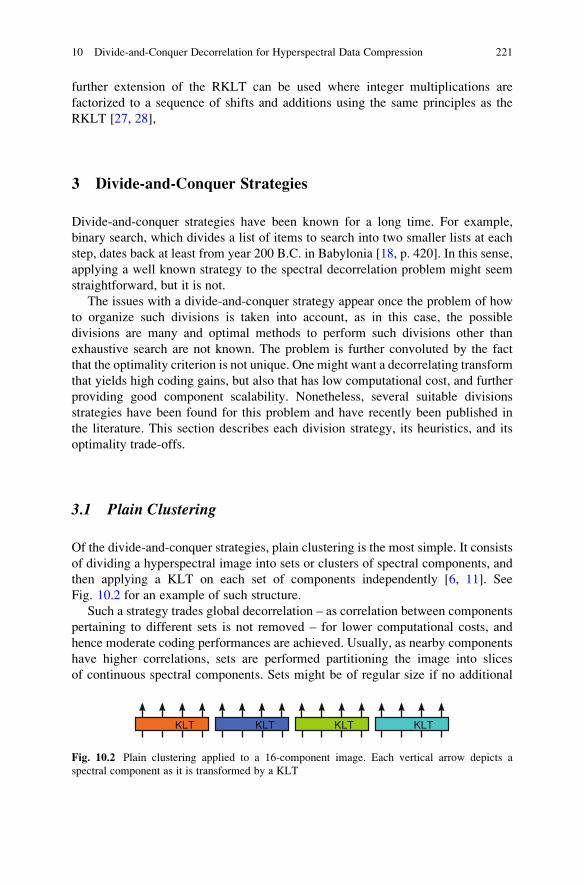
further extension of the RKLT can be used where integer multiplications are

factorized to a sequence of shifts and additions using the same principles as the

RKLT [27, 28],

3 Divide-and-Conquer Strategies

Divide-and-conquer strategies have been known for a long time. For example,

binary search, which divides a list of items to search into two smaller lists at each

step, dates back at least from year 200 B.C. in Babylonia [18, p. 420]. In this sense,

applying a well known strategy to the spectral decorrelation problem might seem

straightforward, but it is not.

The issues with a divide-and-conquer strategy appear once the problem of how

to organize such divisions is taken into account, as in this case, the possible

divisions are many and optimal methods to perform such divisions other than

exhaustive search are not known. The problem is further convoluted by the fact

that the optimality criterion is not unique. One might want a decorrelating transform

that yields high coding gains, but also that has low computational cost, and further

providing good component scalability. Nonetheless, several suitable divisions

strategies have been found for this problem and have recently been published in

the literature. This section describes each division strategy, its heuristics, and its

optimality trade-offs.

3.1 Plain Clustering

Of the divide-and-conquer strategies, plain clustering is the most simple. It consists

of dividing a hyperspectral image into sets or clusters of spectral components, and

then applying a KLT on each set of components independently [6, 11]. See

Fig. 10.2 for an example of such structure.

Such a strategy trades global decorrelation – as correlation between components

pertaining to different sets is not removed – for lower computational costs, and

hence moderate coding performances are achieved. Usually, as nearby components

have higher correlations, sets are performed partitioning the image into slices

of continuous spectral components. Sets might be of regular size if no additional

KLTKLT KLT KLT

Fig. 10.2 Plain clustering applied to a 16-component image. Each vertical arrow depicts a

spectral component as it is transformed by a KLT


information of the image to be decorrelated is known a priory, or might be carefully

picked so that the set boundaries fall in the border of two uncorrelated zones of

an image.

This strategy might also be used when, due to the small spatial size of an image,

or due to the use of small spatial subdivisions, the amount of side information

required becomes significant and impacts the coding performance. In Fig. 10.3,

the cost of side information is plotted in relation to the spatial size of an image.

For images as small as 100�100 pixels the amount of side information is around

0. 7 bpppb, which, for low bitrates, has a very negative impact on coding perfor-

mance. In [11] it is shown that for low bitrates and small image sizes, the reduction

of side information provided by plain clustering is more beneficial in coding

performance terms than the penalty introduced by the lack of global decorrelation.

3.2 Recursive Structure

A recursive division of the KLT is proposed in [29, 30]. While originally proposed

only for pure lossless compression of electroencephalograms and MRI data, it can

also be used in lossy and progressive lossy-to-lossless coders for remote-sensing

imagery compression.

The idea is to replace a full transform by three half-size blocks. The first two

half-size blocks decorrelate one half of the input each, while the third decorrelates

the first half of the output of the first two blocks. Then each of the three half-size

blocks are further divided using the same procedure in a recursive fashion until

a minimum block size is reached.

An example of such a recursive structure is provided in Fig. 10.4, where

an image of eight components is decorrelated by a recursive structure divided in

blocks of two components or, said otherwise, with two levels of recursion.

0

0.5

1

1.5

2

64 128 192 256 320 384 448 512

Bitra

te (

bpppb)

Spatial region side (pixels)

No clustering4 clusters

16 clusters

Fig. 10.3 Side information cost for a transform on an image of 224 spectral components given a

square region of variable size


When dividing a full transform, it is important that, at each level of recursion, an

interleaving permutation between the outputs of the first two half-size transforms is

added before processing the inputs of the third half-size transform. If such permu-

tation is not added, then groups of components from the first two transforms that

have already been decorrelated together are again decorrelated by the third trans-

form with no additional benefit. In Fig. 10.4, that would mean that transforms

marked as a and b would perform the same task twice.

Recursive transforms provide a very comprehensive decorrelation, but at the

expenses of many superfluous operations which substantially increase their compu-

tational cost, and reduce component scalability.

3.3 Two-Level Structures

Another kind of divide-and-conquer structures are the ones introduced in [22, 23].

The proposed structures are composed by two levels of decorrelation; the first level

provides local decorrelation, while the second provides global decorrelation. At the

first level, spectral components are decorrelated as in a clustered transform, and the

most significant components of each of the clusters of the first level are forwarded

to the second level for a second decorrelation, while the remaining components

proceed to further coding stages as is. The most significant component of each

cluster of the first level is decorrelated together with the most significant component

of the other first-level clusters. The second most significant component with the

second most significant components and so on and so forth until all the most

significant components of each cluster are decorrelated.

An example of a two-level structure is shown in Fig. 10.5. In this particular case,

the structure selects only the two most significant components of each of the three

first-level clusters for further decorrelation.

In order to select the structure parameters, i.e., the number of clusters and how

many components are significant at each first level cluster, two approaches are

provided by the authors: a static approach and a dynamic approach.

c1 c3 c8c2 c7c4 c6c5

a

b

Fig. 10.4 An example of a

recursive structure applied to

an image of eight spectral

components, with transforms

of size two


On a static structure, a fixed number of most significant components are selected

for all clusters. On the other hand, on dynamic structures, the amount of

components is selected on the training stage by a process similar to pruning a static

structure. The pruning consists in discarding, from entering the second stage,

components that have small influence on the first components of the output of the

second stage, and the influence is determined by the relative weights set to

each input component by the transform matrix of the second stage of an equivalent

static structure.

Both structures provided a good trade-off between computational cost and

coding performance. Due to the second stage of static transforms decorrelating

together one component from each cluster, the static variant provides low compo-

nent scalability.

3.4 Multilevel Structures

In parallel with two-level structures, multilevel structures where proposed in [6–8].

There are four variations, each of themwith its own trade-offs, but all of them share the

same idea, multiple levels of clustering are applied, each of them further decorrelating

the most significant components of previous levels.

The first variation is a simple multilevel structure proposed in [6], where a plain

clustering with clusters of fixed size is applied and then the most significant half of

each cluster is selected to be further decorrelated in a next level, until only one

cluster remains in the last level. No component interleaving is applied in any

multilevel structure. This first kind of multilevel structures is superseded by the

ones proposed in [7], where instead of using a naive regular structure, eigen-

thresholding methods – methods that determine the amount of significant

components after a KLT – are used to determine the amount of components to be

selected from each cluster.

Two approaches are proposed to select a good structure among all the possible

variations of cluster size. The first approach produces static structures, by setting a

cluster size regularity constrain in each level, and performing exhaustive search on

the cluster sizes for a training corpus. In this case, eigen-thresholding methods are

used to estimate the best number of components to be selected for each cluster, but a

single amount is fixed for all clusters of one level during the search process to

Fig. 10.5 Example of a

two-level static structure


minimize the combinatorial explosion. The second approach produces structures

with a single cluster size but allows that the number of selected components of each

cluster is determined at runtime, thus producing a dynamic structure.

Examples of both approaches are provided in Fig. 10.6 a,b. In the first case,

cluster sizes are selected to be 7, 16, 12, 8 respectively at each level, and the amount

of selected components for each cluster of the first level is two, six on the second

level, and four on the third. In the second case, the cluster size is fixed to four for the

whole structure, and an eigenthresholding algorithm selects the appropriate amount

of components from each cluster, until only one cluster remains at the last level.

The fourth variation of multilevel structures is the Pairwise Orthogonal Trans-

form (POT) introduced in [8], which is a regular structure of clusters of two

components where one component is always selected from each cluster. An example

structure for an image of eight spectral components is provided in Fig. 10.7. The

POT provides a minimalistic fixed structure that provides moderate decorrelation

with a very low cost, and is suitable for real-time processing, and power or memory-

constrained environments like on-board sensors.

.... .... .... .... .... .... .... ....(4 (....

Example of a static multilevel

structure. This particular structure

is the one that was found to be

better for the hyperspectral

AVIRIS sensor.

.... .... .... .... .... .... ....((....

Example of a dynamic

multilevel structure.

32

14

56

a b

Fig. 10.6 Examples of multilevel structures

c1 c3 c8c2 c7c4 c6c5

Fig. 10.7 An example of the pairwise orthogonal transform for an image of eight spectral

components


4 Experimental Results

In this section, an experimental evaluation of the previously described divide-

and-conquer strategies is presented. This evaluation compares all the strategies in a

common scenario and in three fundamental aspects: coding performance, computa-

tional cost, and component scalability.

The divide-and-conquer strategies are evaluated over radiance images captured

with the Hyperion sensor on board the Earth Observing One satellite [17].

The images used are the radiance corrected version or level 1, which have a fixed

width of 256 columns, a variable height, and 242 spectral components covering

wavelengths from 357 to 2,576 nm. The last 18 components are uncalibrated and

have been discarded so that images have 224 spectral components.

To evaluate coding performance, spectral transforms have to be paired with a

complete coding system. In this case, JPEG2000 [26, 24] has been used for this

purpose using the software implementation Kakadu [25]. As for the spectral

transforms, an open source implementation is provided by the authors of this

Chapter [15].

The following are the exact transforms that have been tested: Four levels of

recursion have been used in the recursive transform. The two-level static structure

has 28 clusters in the first level and selects four components of each cluster. The

two-level dynamic structure has 28 clusters in the first level and selects four

components of each cluster but only decorrelates in each second level cluster the

four most significant components. The multilevel dynamic structure has clusters of

size four, and selects components with eigenvalues above average. The multilevel

static structure has four levels with 32, 8, 2, and 1 clusters in each, and selects three,

five, and seven components from each cluster from the first, second and third levels

respectively. The POT is not applied in a line-by-line basis, as initially described in

its original report, to provide a fair comparison with the other transforms, which

cannot use a line-by-line application because of too much side information costs.

The described spectral transforms are compared against a traditional KLT, and

against wavelets, using a Cohen-Doubechies-Feauveau (CDF) 9/7 for lossy and a

CDF 5/3 for Lossy-to-Lossless (PLL) and lossless, in both cases with five levels of

transform.

Coding performance is reported in Fig. 10.8 for lossy performance, in Fig. 10.9

for PLL, and in Table 10.1 for pure lossless. For the sake of clarity, lossy and PLL

results are reported using the difference of Signal-to-Noise Ratio (SNR) perfor-

mance as compared with the performance of the full KLT. In this case, SNR is

defined as SNR ¼ 10 log10ðs2=MSEÞ, where s2 is the variance of the original

image. Lossless results are reported with the real bitrate required for lossless.

In Figs. 10.8 and 10.9, the first plot reports results for a plain clustering strategy

and for a recursive structure, the second plot reports results for two-level structures,

and the third plot reports results for the multi-level structures.

For all the experiments, evaluating either the lossy performance, the PLL

performance, or the lossless performance, results for the KLT transform are usually


-3

-2.5

-2

-1.5

-1

-0.5

0

0.5

0 0.5 1 1.5 2 2.5 3 3.5 4

∆S

NR

σ2 (

dB

)

-3

-2.5

-2

-1.5

-1

-0.5

0

0.5

0 0.5 1 1.5 2 2.5 3 3.5 4

∆S

NR

σ2 (

dB

)

-3

-2.5

-2

-1.5

-1

-0.5

0

0.5

0 0.5 1 1.5 2 2.5 3 3.5 4

∆S

NR

σ2 (

dB

)

Bitrate (bpppb)

Hyperion LakeMonona (ref. KLT)

Bitrate (bpppb)


Bitrate (bpppb)


KLT

16 CLUSTERS

RECURSIVE

DWT 9/7

KLT

TWO-LEVEL STATIC

TWO-LEVEL DYNAMIC

DWT 9/7

KLT

ML DYNAMIC

ML STATIC

POT

DWT 9/7

Fig. 10.8 Lossy coding performance of the divide-and-conquer spectral transforms in relation to

the performance of a regular KLT

Table 10.1 Bitrate required for lossless coding of Hyperion Radiance images. Bitrate is reported

in bpppb

RKLT

16

clusters Recursive

Two-

level

static

Two-level

dynamic

ML

dynamic

ML

static POT

IWT

5/3

Erta Ale 5.95 5.95 5.90 5.99 5.96 6.00 5.89 6.05 6.24

Lake

Monona

6.11 6.09 6.07 6.16 6.10 6.16 6.03 6.23 6.37

Mt. St.

Helens

6.00 6.06 5.97 6.04 6.06 6.11 5.93 6.23 6.38


the highest ones, while results for a wavelet transform are always the lowest ones,

and results for the different divide-and-conquer decorrelation strategies lie some-

where in between.

As expected, the recursive structure provides very competitive coding performance

results, reaching those of the classical KLT, although its computational cost is too

demanding. Interestingly, the multi-level static structure also yields very good coding

results, with a lower computational cost. Results for the two-level structures, either

static or dynamic, are quite acceptable, withmoderate penalty, similar to that achieved

by a plain clustering strategy of 16 clusters. Among all the divide-and-conquer

-3

-2.5

-2

-1.5

-1

-0.5

0

0.5

0 0.5 1 1.5 2 2.5 3 3.5 4

∆S

NR

σ2 (

dB

)

Bitrate (bpppb)

Hyperion LakeMonona (ref. RKLT)

RKLT

16 CLUSTERS

RECURSIVE

IWT 5/3

-3

-2.5

-2

-1.5

-1

-0.5

0

0.5

0 0.5 1 1.5 2 2.5 3 3.5 4

∆S

NR

σ2 (

dB

)

Bitrate (bpppb)


RKLT

TWO-LEVEL STATIC

TWO-LEVEL DYNAMIC

IWT 5/3

-3

-2.5

-2

-1.5

-1

-0.5

0

0.5

0 0.5 1 1.5 2 2.5 3 3.5 4

∆S

NR

σ2

(d

B)

Bitrate (bpppb)


RKLT

ML DYNAMIC

ML STATIC

POT

IWT 5/3

Fig. 10.9 PLL coding performance of the divide-and-conquer spectral transforms in relation to

the performance of a regular KLT


strategies, the POT produces the worst coding performance results, but its computa-

tional cost and its component scalability is the best one.

Computational cost results are reported in Fig. 10.10 for lossy transforms and in

Fig. 10.11 for pure lossless and PLL transforms. Themain difference between them is

KLT

16 clusters

recursive

two-level static

two-level dynamic

ML dynamic

ML static

POT

DWT 9/7

0×100 50×109 100×109 150×109 200×109 250×109

Operations (flops)

Inverse Transform

Forward TransformTraining

Fig. 10.10 Computational cost of lossy transforms when applied to the image Hyperion lake

Monona

0×100 50×109 100×109 150×109 200×109 250×109 300×109

RKLT

16 clusters

recursive

two-level static

two-level dynamic

ML dynamic

ML static

POT

IWT 5/3

Operations (flops)

Inverse Transform

Forward TransformTraining

Fig. 10.11 Computational cost of lossless transforms when applied to the image Hyperion lake

Monona


that, for lossless results, a lifting scheme has to be used to ensure reversibility, which

requires a few extra operations on the application and removal of transforms.

Figures 10.10 and 10.11 clearly show that the classical KLT is extremely

expensive, with the recursive structure having about one fourth its computational

cost. All other divide-and-conquer strategies have a much lower complexity, with

static structures being more costly than dynamic structures. POT strategy has a

similar complexity than wavelets.

As for component scalability, results are reported in Table 10.2.

Again, we see that the classical KLT entails the poorest component scalability,

while the recursive and the two-level static structure provide about twice compo-

nent scalability performance. The best two divide-and-conquer strategies are the

two-level dynamic and the POT, both improving the performance of wavelets.

5 Summary

In this chapter, we overviewed the major divide-and-conquer strategies for spectral

decorrelation to alleviate some of the drawbacks of the Karhunen-Loeve transform,

which is known to be optimal for Gaussian sources. We reviewed several popular

transform approaches that have been considered for the coding of hyperspectral

imagery. We also provided a comparison among these different strategies,

addressing the drawbacks of the classical KLT, in particular, and for satellite data

coding, we evaluated the coding performance, the computational cost, and the

component scalability.

As for coding performance, and for lossy, progressive lossy-to-lossless, and

lossless image compression, we found that all divide-and-conquer strategies yield

results in between the performance of the KLT and the performance of wavelets. The

recursive structure produces competitive coding results, closely followed by the

multi-level static structure. POT structure shows the lowest coding performance,

although still above that of wavelets.

Table 10.2 Transform scalability (in components required to recover one component). Reported

wavelet scalability may be reduced on transform edges due to coefficient mirroring (up to a half)

Avg. Min. Max.

Full KLT 224.0 224 224

16 clusters 14.0 14 14

Recursive 119.0 119 119

Two-level static 116.0 116 116

Two-level dynamic 9.7 8 14

ML dynamic 13.1 12 15

ML static 38.0 38 38

POT 8.9 8 9

Wavelet CDF 9/7 36.0 32 38

Wavelet CDF 5/3 16.0 11 17


As for computational complexity, all divide-and-conquer strategies –but the

recursive structure–, provide a significant saving as compared to KLT. POT struc-

ture matches the cost of wavelets.

As for component scalability, the recursive and the two-level static structures

have a poor performance, the multi-level static has a medium performance, similar

to that of lossy CDF 9/7 wavelets, and all the other strategies have a competitive

performance, matching that of lossless CDF 5/3 wavelets, with POT yielding the

best component scalability among all.

In conclusion, a POT divide-and-conquer strategy retains all the good properties

of wavelet spectral transforms, and yet provides superior coding performance,

becoming a convenient replacement of wavelets where the KLT is not suitable.

Acknowledgements This work was supported in part by the Spanish Government, by the Catalan

Government, and by FEDER under grants TIN2009-14426-C02-01, TIN2009-05737-E/TIN,

SGR2009-1224, and FPU2008. Computational resources used in this work were partially provided

by the Oliba Project of the Universitat Autonoma de Barcelona. This work was also supported by

the Belgian Government via the Fund for Scientific Research Flanders (postdoctoral fellowship

Peter Schelkens). The authors would like to thank NASA and USGS for providing the Hyperion

images.

References

1. N. Ahmed, T. Natarajan, and K.R. Rao. Discrete cosine transfom. IEEE Trans. Comput.,

C-23(1):90–93, Jan. 1974.

2. Isidore Paul Akam Bita, Michel Barret, Florio Dalla Vedova, and Jean-Louis Gutzwiller.

Lossy compression of MERIS superspectral images with exogenous quasi optimal coding

transforms. In Bormin Huang, Antonio J. Plaza, and Raffaele Vitulli, editors, Satellite Data

Compression, Communication, and Processing V, volume 7455, page 74550U. SPIE, 2009.

3. Isidore Paul Akam Bita, Michel Barret, and Dinh-Tuan Pham. On optimal orthogonal

transforms at high bit-rates using only second order statistics in multicomponent image coding

with JPEG2000. Elsevier Signal Processing, 90(3):753 – 758, 2010.

4. Isidore Paul Akam Bita, Michel Barret, and Dinh-Tuan Pham. On optimal transforms in lossy

compression of multicomponent images with JPEG2000. Elsevier Signal Processing,

90(3):759–773, 2010.

5. Michel Barret, Jean-Louis Gutzwiller, Isidore Paul Akam Bita, and Florio Dalla Vedova.

Lossy hyperspectral images coding with exogenous quasi optimal transforms. In Data Com-

pression Conf. 2009 (DCC 2009), pages 411–419. IEEE Press, Mar. 2009.

6. I. Blanes and J. Serra-Sagrista. Clustered reversible-KLT for progressive lossy-to-lossless 3d

image coding. In Data Compression Conf. 2009 (DCC 2009), pages 233–242. IEEE Press,

Mar. 2009.

7. I. Blanes and J. Serra-Sagrista. Cost and scalability improvements to the Karhunen-Loeve

transform for remote-sensing image coding. IEEE Trans. Geosci. Remote Sens.,

48(7):2854–2863, Jul. 2010.

8. I. Blanes and J. Serra-Sagrista. Pairwise orthogonal transform for spectral image coding. IEEE

Trans. Geosci. Remote Sens., 49(3):961–972, Mar. 2011.

9. F. A. M. L. Bruekers and A. W. M. van den Enden. New networks for perfect inversion and

perfect reconstruction. IEEE J. Sel. Areas Commun., 10(1):130–137, 1992.


10. Inderjit Singh Dhillon. A New O(n2) Algorithm for the Symmetric Tridiagonal Eigenvalue/

Eigenvector Problem. PhD thesis, EECS Department, University of California, Berkeley,

Oct 1997.

11. Q. Du, W. Zhu, H. Yang, and J. E. Fowler. Segmented principal component analysis for

parallel compression of hyperspectral imagery. IEEE Geosci. Remote Sens. Lett., 6

(4):713–717, Oct. 2009.

12. L. Galli and S. Salzo. Lossless hyperspectral compression using KLT. IEEE Int’l Geosci.

and Remote Sens. Symp. Proc. (IGARSS 2004), 1–7:313–316, 2004.

13. G.H. Golub and C.F. van Loan. Matrix Computations. The Johns Hopkins University Press,

Oct. 1996.

14. Ian R. Greenshields and Joel A. Rosiene. A fast wavelet-based Karhunen-Loeve transform.

Pattern Recognition, 31(7):839–845, Jul. 1998.

15. Group on Interactive Coding of Images. Spectral transform software. http://gici.uab.cat/, 2010.

16. P. W. Hao and Q. Y. Shi. Matrix factorizations for reversible integer mapping. IEEE Trans.

Signal Process., 49(10):2314–2324, 2001.

17. Jet Propulsion Laboratory, NASA. Hyperspectral image compression website. http://compres-

sion.jpl.nasa.gov/hyperspectral/.

18. Donald E. Knuth. Sorting and Searching, volume 3 of The Art of Computer Programming.

Addison-Wesley, second edition, 1998.

19. L.S. Lan and I.S. Reed. Fast approximate Karhunen-Loeve transform (AKLT) with

applications to digital image-coding. Elsevier Visual Commun. and Image Process.

93, 2094:444–455, 1993.

20. Barbara Penna, Tammam Tillo, Enrico Magli, and Gabriella Olmo. Transform coding

techniques for lossy hyperspectral data compression. IEEE Trans. Geosci. Remote Sens.,

45(5):1408–1421, May 2007.

21. A.D. Pirooz and I.S. Reed. A new approximate Karhunen-Loeve transform for data compres-

sion. Conference Record of the Thirty-Second Asilomar Conference on Signals, Systems and

Computers, 1–2:1471–1475, 1998.

22. John A. Saghri and Seton Schroeder. An adaptive two-stage KLT scheme for spectral

decorrelation in hyperspectral bandwidth compression. Proc. SPIE, 7443:744313, Sept. 2009.

23. John A. Saghri, Seton Schroeder, and Andrew G. Tescher. Adaptive two-stage Karhunen-

Loeve-transform scheme for spectral decorrelation in hyperspectral bandwidth compression.

SPIE Optical Engineering, 49:057001, May 2010.

24. Peter Schelkens, Athanassios Skodras, and Touradj Ebrahimi, editors. The JPEG 2000 Suite.

Wiley, Sept. 2009.

25. D.S. Taubman. Kakadu software. http://www.kakadusoftware.com/, 2000.

26. D.S. Taubman and M.W. Marcellin. JPEG2000: Image Compression Fundamentals,

Standards, and Practice, volume 642. Kluwer International Series in Engineering and Com-

puter Science, 2002.

27. Lei Wang, Jiaji Wu, Licheng Jiao, and Guangming Shi. 3D medical image compression based

on multiplierless low-complexity RKLT and shape-adaptive wavelet transform. ICIP 2009.

Proceedings of 2009 International Conference on Image Processing, pages 2521–2524, Nov.

2009.

28. Lei Wang, Jiaji Wu, Licheng Jiao, and Guangming Shi. Lossy-to-lossless hyperspectral image

compression based on multiplierless reversible integer TDLT/KLT. IEEE Geosci. Remote

Sens. Lett., 6(3):587–591, July 2009.

29. Y. Wongsawat. Lossless compression for 3-D MRI data using reversible KLT. Int’l Conf. on

Audio, Language and Image Processing, 2008. (ICALIP 2008)., pages 1560–1564, July 2008.

30. Y. Wongsawat, S. Oraintara, and K. R. Rao. Integer sub-optimal Karhunen-Loeve transform

for multi-channel lossless EEG compression. European Signal Processing Conference, 2006.


http://gici.uab.cat/



http://www.kakadusoftware.com/

Chapter 11

Hyperspectral Image Compression UsingSegmented Principal Component Analysis

Wei Zhu, Qian Du, and James E. Fowler

Abstract Principal component analysis (PCA) is the most efficient spectral

decorrelation approach for hyperspectral image compression. In conjunction with

JPEG2000-based spatial coding, the resulting PCA+JPEG2000 can yield superior

rate-distortion performance. However, the involved overhead bits consumed by the

large operation matrix for principal component transform may affect compression

performance at low bitrates, particularly when the spatial size of an image patch to be

compressed is relatively small compared to the spectral dimension. In our previous

research, we proposed to apply the segmented principal component analysis (SPCA)

to mitigate this effect, and the resulting compression algorithm, denoted as SPCA

+JPEG2000, can improve the rate-distortion performance even when PCA

+JPEG2000 is applicable. In this chapter, we investigate the quality of reconstructed

data after SPCA+JPEG2000 compression based on the performance in spectral

fidelity, classification, linear unmixing, and anomaly detection. The experimental

results show thatSPCA+JPEG2000canoutperform in termsof preservingmoreuseful

data information, in addition to offer excellent rate-distortion performance. Since the

spectral partition in SPCA relies on the calculation of a data-dependent spectral

correlation coefficientmatrix, we investigate a sensor-dependent suboptimal partition

approach, which can accelerate the compression process with no much distortion.

1 Introduction

Data compression is a frequently applied technique to reduce the vast data volume

of a hyperspectral image. It has been shown that principal component analysis

(PCA) in conjunction with JPEG2000 [1, 2] provides prominent rate-distortion

W. Zhu • Q. Du (*) • J.E. Fowler

Department of Electrical and Computer Engineering, Mississippi State University,

Starkville, USA



233


performance for hyperspectral image compression, where PCA is for spectral

coding and JPEG2000 is for spatial coding of principal component (PC) images

(referred to as PCA+JPEG2000); in particular, PCA+JPEG2000 outperforms its

discrete wavelet transform (DWT) counterpart, DWT+JPEG2000, where DWT is

applied for spectral coding [3–7]. PCA+JPEG2000 also outperforms other DWT-

based algorithms, such as 3-dimensional (3D) set partitioning in hierarchical trees

(SPIHT) [8] and 3D set partitioned embedded block (SPECK) [9]. When only a set

of principal components (PCs) are used for compression, the resulting SubPCA

+JPEG2000 can further improve the rate-distortion performance [6].

Table 11.1 lists the signal-to-noise ratio (SNR) for PCA+JPEG2000 and DWT

+JPEG2000 at 1.0 bpppb (bit per pixel per band); also shown is the performance

when JPEG2000 is used with no spectral decorrelation. Here, SNR is defined as the

ratio between signal variance and reconstruction error variance. We see that in all

cases, although DWT-based spectral decorrelation improves SNR by around 15 dB

with respect to no spectral decorrelation, PCA-based spectral decorrelation results

in a further 5-dB increase. From a statistical perspective, PCA offers optimal

decorrelation while highly structured correlation is known to exist between DWT

coefficients, both with subbands and across subbands. While JPEG2000 exploits

this DWT correlation structure spatially, no attempt is made to exploit residual

correlation across components, i.e., spectrally. As a consequence, a spectral DWT

leaves a significant degree of correlation present in the spectral direction; the

spectral PCA, with its optimal decorrelation, thus performs better.

Figure 11.1 shows the rate-distortion curves of the DWT group (i.e., 3D SPIHT,

3D SPIHT, DWT+JPEG2000) and PCA group (PCA+JPEG2000, SubPCA

+JPEG2000). Obviously, the PCA group significantly outperforms the DWT

group. The rate distortion performance evaluates the data point fidelity. In order

to evaluate the fidelity of pixel spectrum after compression, spectral angle mapper

(SAM) is used to calculate the spectral angles before and after compression, and the

angle difference is averaged and shown in Fig. 11.2. It demonstrates that the PCA

group can do a better job in preserving pixel spectral signatures than the DWT

group. PCA+JPEG2000 and SubPCA+JPEG2000 have been modified for anomaly

detection and multi-temporal image compression [10–12]. Since SubPCA

+JPEG2000 requires the estimation of an optimal number of PCs to be used at

difference bitrates, we limit the discussion about PCA+JPEG2000 only in this

chapter. Moreover, only DWT+JPEG2000 is used for comparison purpose hereaf-

ter, because it is the best in the DWT group.

It is worth mentioning that the Consultative Committee for Space Data Systems

(CCSDS) has created the Multispectral Hyperspectral Data Compression (MHDC)

Table 11.1 SNR (dB) at 1.0 bpppb with different spectral decorrelation approaches for the

compression of AVIRIS Jasper Ridge radiance data of size 512 � 512 with 224 bands

None DWT PCA

Cuprite 38.3 51.0 54.1

Jasper Ridge 29.8 44.8 50.3

Moffett 30.6 45.5 50.9

234 W. Zhu et al.

0.1 0.2 0.3 0.4 0.5 0.6 0.7 0.8 0.9 125

30

35

40

45

50

55

Rate (bpppb)

SN

R (

dB

)

3D SPIHT

3D SPECK

DWT+JPEG2000

PCA+JPEG2000

SubPCA+JPEG2000

Fig. 11.1 Rate-distortion performance of PCA- and DWT-based compression algorithms for

AVIRIS Jasper Ridge radiance data of size 512 � 512 with 224 bands

0.1 0.2 0.3 0.4 0.5 0.6 0.7 0.8 0.9 10

0.2

0.4

0.6

0.8

1

1.2

1.4

1.6

Rate (bpppb)

Avera

ge S

AM

(degre

e)

SubPCA+JPEG2000

PCA+JPEG2000

DWT+JPEG2000

3D SPECK

3D SPIHT

Fig. 11.2 Spectral distoration of PCA- and DWT-based compression algorithms for AVIRIS

Jasper Ridge radiance data of size 512 � 512 with 224 bands

11 Hyperspectral Image Compression Using Segmented Principal. . . 235

Working group to recommend the standard for multispectral and hyperspectral

image compression. Since it targets onboard compression, where a careful tradeoff

between compression performance and computational complexity has to be consid-

ered, JPEG2000 is not selected. However, during the design of CCSDS standard,

PCA+JPEG2000 and DWT+JPEG2000 have been used as comparison baseline due

to their excellent rate-distortion performance [13].

However, due to its data-dependent nature, PCA+JPEG2000 requires overhead

bits carrying PCA transform information, which may not be negligible. For

instance, for an image with L bands and M�N pixels, the size of transformation

matrix is L�L; if 32-bit floating point values are used to transmit this matrix, the

number of overhead bits is approximately 32�L�L and the resulting change in

bitrate in bpppb is (32�L)/(M�N). When image spatial size M � N is large

compared to the value of L, this bitrate change is very small. However, when

image spatial size is small, this overhead severely degrades compression perfor-

mance due to insufficient bits being used for data information encoding at low

bitrates. This is an intrinsic problem in parallel compression, where image spatial

partition is often applied to reduce computational complexity [14]. Figure 11.3

illustrates this problem in parallel compression when the image of size 512 � 512

with 224 bands is spatially partitioned into p segments, where p equals the number

of processing elements (PEs). When PEs ¼ 1, it is the original PCA+JPEG2000.

When PEs ¼ 4 (i.e., the subimage spatial size is 256 � 256), PCA fails at 0.1

bpppb; when PEs ¼ 8 (i.e., the subimage spatial size is 128 � 128), PCA cannot

work properly at 0.1 and 0.2 bpppb.

0 0.2 0.4 0.6 0.8 15

10

15

20

25

30

35

40

45

50

55

Rate (bpppb)

SN

R (

dB

)

PEs=1

PEs=2

PEs=4

PEs=8

Fig. 11.3 Rate-distortion performance of parallel PCA+JPEG2000 with spatial partition for

AVIRIS Jasper Ridge radiance data of size 512 � 512 with 224 bands

236 W. Zhu et al.

To overcome such a practical application problem of PCA+JPEG2000, we have

proposed a segmented PCA (SPCA)-based compression method to improve

the performance of PCA+JPEG2000 when the impact of overhead bits cannot

be ignored [15]. The basic idea is to conduct spectral partition based on spectral

correlation coefficient, and then PCA is applied to each spectral segment. The

resulting compression method is referred to as SPCA+JPEG2000. In [15], we

have shown that SPCA+JPEG2000 can not only solve the problem of the original

PCA+JPEG2000 but also improve the rate-distortion performance even when PCA

+JPEG2000 is applicable. In this chapter, we will investigate the quality of

reconstructed data after SPCA+JPEG2000 compression by evaluating its spectral

fidelity and the discrepancy on data applications in classification, anomaly detec-

tion, and linear unmixing results. Due to the lack of ground truth in practice, all the

data analysis algorithms used in the evaluation are unsupervised. Since SPCA

calculates the correlation coefficient matrix for spectral partition, which is data

dependent, we propose a sensor-dependent suboptimal segment approach to accel-

erate the compression process. Its performance in rate-distortion, spectral fidelity,

and data applications are also evaluated.

This chapter is organized as follows. In Sect. 2, the spectral partition for SPCA is

briefly introduced. In Sect. 3, the compression scheme of SPCA+JPEG2000

is reviewed, and its performance in data analysis is thoroughly investigated in

Sect. 4. In Sect. 5, the sensor-specific suboptimal SPCA is proposed to expedite

the compression process and its performance in data analysis is also presented. The

conclusion remarks are given in Sect. 6.

2 Segmented Principal Component Analysis

Band partition can be conducted uniformly (denoted as SPCA-U) or via the

examination of spectral correlation coefficient (CC) as proposed in [16] (denoted

as SPCA-CC). For an L-band image, its data covariance matrix S is L-by-L, from

which the spectral correlation coefficient matrix A can be derived as

A i; jð Þ ¼S i; jð Þ

ffiffiffiffiffiffiffiffiffiffiffiffiffiffiffiffiffiffiffiffiffiffiffiffi

S i; ið ÞS j; jð Þp (11.1)

Aj j can be displayed as a gray-scale image. As illustrated in Fig. 11.4, a white pixel

at location (i,j) means high correlation between the i-th and j-th band, and the

highest value is 1 along the diagonal line. Obviously, the white blocks along the

diagonal lines represent the adjacent bands being highly correlated, which should

be grouped together. Thus, spectral bands in a hyperspectral image can be

partitioned based on their correlation. Using the uniform partition, less correlated

bands may be assigned to the same group.


Spectral partition can also be achieved by using mutual information in [17].

Since spectral correlation performs similarly as mutual information, resulting in

similar band partitions, but with simpler computation, here we focus on SPCA with

spectral correlation coefficient only.

Assume the original L bands are partitioned into p groups, i.e.,Pp

i¼1 Li ¼ Lwhere Li is the number of bands in the i-th group. There are three

major advantages of SPCA:

(1) Band decorrelation may be more efficient since PCA is applied to highly

correlated bands [16].

(2) Computational complexity is greatly reduced. The number of multiplications

for calculating the data covariance matrix S is N2M2L2; similarly, this number

for Si in the i-th group is N2M2L2i . Obviously, the number of multiplications in

the SPCA is less than that of PCA due to the factPp

i¼1 L2i<L2. The computa-

tional complexity in the eigen-decomposition of S is O L3ð Þ, which is larger

than that in the eigen-decomposition of Si sincePp

i¼1 L3i<L3. Thus, SPCA can

mitigate the computational burden of the original PCA through the reduction of

matrix size [18].

(3) When SPCA is used for compression, the overhead related to the transforma-

tion matrix is reduced. Now the overhead bits are aboutPp

i¼1 32L2i , less than

32L2 in PCA.

3 SPCA+JPEG2000

When applying PCA+JPEG2000, the JPEG2000 encoder embeds the transform

matrix into bitstream as an overhead. Assume there is an L�M�N hyperspectral

image with L bands and M�N pixels. The size of the transform matrix is L�L,

while the size of other vectors, e.g., mean vector of spectral bands, is negligible.

Given the transform matrix is coded in 32-bit floating point value, the overhead

occupies approximately 32L2 bits. In terms of bitrate, this overhead requires at least

a bitrate of

Fig. 11.4 The spectral

correlation coefficient matrix

(224 � 224) of AVIRIS

Jasper Ridge data displayed

as an gray-scale image

238 W. Zhu et al.

Rmin ¼32L

MNbpppb: (11.2)

For PCA+JPEG2000, it requires R > Rmin to properly encode useful transform

coefficients into bitstream. On the contrary, if R < Rmin, no enough bits can be used

for data encoding, resulting in poor compress performance. For instance, when the

image size is 224 � 64 � 64, it requires at least 1.75 bpppb for correct encoding;

any compression ratio below 1.75 bpppb is simply insufficient for encoding actual

data information. Table 11.2 shows the rate distortion performance when data size

is changed. Obviously, PCA can provide better performance than DWT only when

the image spatial size is relatively large enough.

Therefore, the size of the transformation matrix has to be dramatically reduced

through SPCA to make the overhead negligible. To apply SPCA+JPEG2000 for

hyperspectral image compression, the major steps of PCA+JPEG2000 are still

needed. After a group of spectral bands are decorrelated by PCA, their principal

components will be sent to JPEG2000 encoder for a three-stage process: spatial

DWT, codeblock coding (CBC), and post-compression rate-distortion (PCRD)

optimal truncation of codeblock bitstreams, to generate the final compressed

bitstream. One approach is to process all three stages independently for each

spectral group and then concatenate the bitstreams out of different encoders

together, as illustrated in Fig. 11.5, where the PCRD optimizes the bitstream locally

within each spectral group. The other approach is to process first two stages

independently while applying PCRD globally within all codeblocks of all spectral

groups, as shown in Fig. 11.6. The former approach is called local bit allocation

(LBA) and the latter global bit allocation (GBA).

The AVIRIS Jasper Ridge dataset with different spatial and spectral sizes are

spectrally partitioned into several band segments as listed in Table 11.3. The

segments from CC have different sizes. It should be noted that the spectral correla-

tion coefficient matrix A is recalculated when the image spatial size is different.

Table 11.2 SNR in dB of PCA+JPEG2000 and DWT+JPEG2000 on the datasets with various

spatial and spectral sizes

Rmin 1.1Rmin 1.5Rmin

224 � 512 � 512 DWT 13.85 14.09 14.95

PCA 5.45 12.49 16.08

224 � 256 � 256 DWT 20.58 21.09 23.05

PCA 7.49 16.24 23.96

112 � 256 � 256 DWT 21.38 21.91 23.78

PCA 7.97 16.95 26.03

224 � 128 � 128 DWT 31.06 31.84 34.40

PCA 9.86 21.67 33.28

112 � 128 � 128 DWT 32.46 33.21 35.78

PCA 11.85 23.86 36.29

56 � 128 � 128 DWT 29.67 30.57 32.84

PCA 12.53 15.25 27.16


……

Bitstream

Concatenation

Image

Band Partition

Bitstream

PCA

JPEG2000 Encoder

DWT CBC PCRD

PCA

JPEG2000 Encoder

DWT CBC PCRD

PCA

JPEG2000 Encoder

DWT CBC PCRD

Fig. 11.5 The local bit allocation (LBA) procedure of SPCA+JPEG2000

……

PCA

JPEG2000 stage 1+2

DWT CBC

PCA

JPEG2000 stage 1+2

DWT CBC Bitstream Concatenation

Bitstream

PCRD

PCA

JPEG2000 stage 1+2

DWT CBCImage

Band Partition

Fig. 11.6 The global bit allocation (GBA) procedure of SPCA+JPEG2000

Table 11.3 Band segments when the AVIRIS Jasper Ridge dataset is spatially and spectrally

partitioned into subimages with different sizes

Spatial

size

Spectral

size

Number

of

Segments SPCA-CC

Number of Segments

SPCA-U

512 � 512 224 6 [1 38], [39 107], [108 113],

[114 154], [155 166],

[167 224]

[1 37], [38 74], [75 111], [112

148], [149 185], [186 224]

256 � 256 224 6 [1 38], [39 107], [108 113],

[114 154], [155 166],

[167 224]

[1 37], [38 74], [75 111], [112

148], [149 185], [186 224]

112 3 [1 38], [39 107], [108 112] [1 37], [38 74], [75 112]

128 � 128 224 7 [1 38], [39 82],[83 107], [108

113], [114 154], [155 166],

[167 224]

[1 32], [33 64], [65 96], [97

128], [129 160], [161

192], [193 224]

112 4 [1 38], [39 82], [83 107], [108

112]

[1 28], [29 56], [57 84],

[85 112]

56 3 [1 19], [20 38], [39 56] [1 19], [20 38], [39 56]

240 W. Zhu et al.

This is because the estimated correlation may be different when the enclosed pixels

for estimation are changed.

The rate-distortion performance of SPCA+JPEG2000 is listed in Table 11.4. We

can see that GBA-based SPCA clearly yielded better rate-distortion performance

than LBA. In addition, SPCA-CC yielded similar rate-distortion results as SPCA-U.

To provide a more comprehensive view of performance, Figs. 11.7 and 11.8

show SNR for rates ranging from 0.1 to 1.0 bpppb for both the 224 � 512 � 512

and 224 � 128 � 128 subscene sizes. These sizes are chosen because, in

Table 11.4, the non-segmented PCA transform achieves the best performance for

the former, and the worst for the latter. As shown in Fig. 11.7, when PCA-based

JPEG2000 coding works properly (i.e., the spatial size is relatively large with

respect to the spectral size such that the PCA transform matrix occupies negligible

rate overhead in the compressed bitstream), the performance of SPCA-CC-GBA is

slightly below that of non-segmented PCA. However, as shown in Fig. 11.8, when

the non-segmented PCA is overwhelmed with transform-matrix rate overhead (i.e.,

at rates close to Rmin for datasets with spatial size relatively small with respect

to spectral size), SPCA can significantly improve performance. In both cases, the

CC-based partition outperforms the uniform partition.

Table 11.4 SNR in dB for various compression algorithms applied to AVIRIS Jasper Ridge

dataset

Algorithms Rmin 1.1Rmin 1.5Rmin Rmin 1.1Rmin 1.5Rmin

224 � 512 � 512, Rmin ¼ 0.0273 bpppb 224 � 128 � 128, Rmin ¼ 0.4375 bpppb

DWT 13.85 14.09 14.95 DWT 31.06 31.84 34.40

PCA 5.45 12.49 16.08 PCA 9.86 21.67 33.28

SPCA-U-LBA 15.01 15.29 16.34 SPCA-U-LBA 28.24 29.20 32.61

SPCA-U-GBA 15.60 15.97 17.52 SPCA-U-GBA 34.77 35.63 38.25

SPCA-CC-LBA 15.27 15.52 16.30 SPCA-CC-LBA 24.60 25.15 27.75

SPCA-CC-GBA 16.36 16.82 18.64 SPCA-CC-GBA 35.50 36.27 38.69


DWT 20.58 21.09 23.05 DWT 32.46 33.21 35.78

PCA 7.49 16.24 23.96 PCA 11.85 23.86 36.29






DWT 21.38 21.91 23.78 DWT 29.67 30.57 32.84

PCA 7.97 16.95 26.03 PCA 12.53 15.25 27.16






4 Data Analysis Performance of SPCA+JPEG2000

The performance of a lossy image compression algorithm is usually evaluated in

terms of distortion and compression ratio. However, to evaluate the useful data

information preserved during the compression process, we are particularly inter-

ested in application-specific distortions [19–21]. Depending on the nature of lost

information, the impact on the following data analysis can be quite different. Thus,

we will evaluate the performance of classification, detection, and spectral unmixing

0.1 0.2 0.3 0.4 0.5 0.6 0.7 0.8 0.9 115

20

25

30

35

40

45

bitrate (bpppb)

rate

-dis

tort

ion p

erf

orm

ance (

SN

R)

DWT

PCA

SPCA-U-GBA

SPCA-CC-GBA

Fig. 11.7 Rate-distortion performance for Jasper Ridge dataset with size 224 � 512 � 512

0.1 0.2 0.3 0.4 0.5 0.6 0.7 0.8 0.9 15

10

15

20

25

30

35

40

45

bitrate (bpppb)

rate

-dis

tort

ion p

erf

orm

ance (

SN

R)

DWT

PCA

SPCA-U-GBA

SPCA-CC-GBA

Fig. 11.8 Rate-distortion performance for Jasper Ridge dataset with size 224 � 128 � 128

242 W. Zhu et al.

using reconstructed data. Unsupervised algorithms are more useful due to the lack

of prior information in practice.

Within the SPCA algorithms, we focus on GBA hereafter since its rate distortion

performance is significantly better than LBA. The Jasper Ridge dataset of size

224 � 512 � 512 and 224 � 128 � 128 were used in the experiments. Five

bitrates, i.e., 0.2, 0.4, 0.6, 0.8, 1.0 bpppb, were examined. For the

224 � 128 � 128 image, the Rmin is 0.4375 bpppb, so PCA did not work at 0.2

and 0.4 bpppb.

4.1 Spectral Fidelity

Instead of data point fidelity assessed by rate-distortion performance, spectral

fidelity can be evaluated by average spectral angle between original and

reconstructed pixels [22]. It is important to evaluate spectral fidelity because

many hyperspectral analysis algorithms utilize pixel spectral information. Let rand r denote an original pixel vector and its reconstructed version after compres-

sion. Their spectral angle is defined as

y ¼ cos�1 rT r

rk k rk k(11.3)

A smaller angle corresponds to less spectral distortion.

As listed in Table 11.5, for the original image with relatively large spatial

dimension, e.g., 224 � 512 � 512, PCA and SPCA performed similarly; for the

image of size 224 � 128 � 128 after spatial shrinking, SPCA provided much

smaller spectral angles. In both cases, the CC-based spectral partition yielded less

spectral degradation than the uniform partition.

4.2 Unsupervised Classification

Unsupervised classification was conducted on the original and reconstructed image

using independent component analysis (ICA). Specifically, the fastICA algorithm

Table 11.5 Spectral fidelity evaluated in average spectral angle

Size Algorithms 0.2 0.4 0.6 0.8 1

224 � 512 � 512 DWT 3.15� 1.69� 1.14� 0.85� 0.67�

PCA 1.37� 0.78� 0.56� 0.45� 0.37�

SPCA-U-GBA 1.69� 0.90� 0.63� 0.50� 0.41�

SPCA-CC-GBA 1.43� 0.80� 0.58� 0.46� 0.38�

224 � 128 � 128 DWT 2.42� 1.50� 1.11� 0.83� 0.66�

PCA 7.07� 7.07� 1.32� 0.99� 0.81�

SPCA-U-GBA 1.77� 0.76� 0.51� 0.40� 0.32�

SPCA-CC-GBA 1.56� 0.69� 0.48� 0.38� 0.31�


was adopted [23, 24]. Let Z ¼ ½z1z2 � � � zMN � be an L�MN data matrix with

L-dimensional pixels. And let w be the desired projector and y ¼ y1y2 � � � yMNð Þbe the projected data (after mean removal and data whitening). Denote F(•) as a

function measuring independency. For instance, F(y) can measure the kurtosis k(y)

of the projected data, i.e.,

FðyÞ ¼ kðyÞ ¼ E½ðyÞ4� � 3: (11.4)

Then the task is to find an optimalw such that k(y) is maximal. This optimization

problem can be formulated into the following objective function

J wð Þ ¼ maxw

kðyÞf g ¼ maxw

k wTz� ��

: (11.5)

Taking the derivative with respect to w yields

Dw ¼@k

@w¼ 4E y3z

� �

: (11.6)

Then gradient-descent or fixed-point adaptation can be used to determine w.After the first w, denoted as w1, is found, it is used to transform the data for the first

classification map. To find a second w, denoted as w2, for another class, data matrix

Z is projected onto the orthogonal subspace of w1 before searching w2. The

algorithm continues until all the classes are classified.

The corresponding classification maps can be compared with spatial correlation

coefficient; a larger average correlation coefficient means classification maps were

closer. Let C and C denote classification maps using the original and reconstructed

data, respectively. Their spatial correlation coefficient r is defined as

r ¼

P

x;y C x; yð Þ � mCð Þ C x; yð Þ � mC� �

sCsC(11.7)

where mC and mC are the data mean of the two maps, and sC and sC are their

corresponding standard deviation. In the experiment, ten classes were identified and

compared. As shown in Table 11.6, both SPCA results were better than PCA result,

Table 11.6 Classification performance evaluated in spatial correlation coefficient


224 � 512 � 512 DWT 0.2996 0.3804 0.5357 0.5363 0.6245

PCA 0.5563 0.5149 0.6591 0.7465 0.7281

SPCA-U-GBA 0.4967 0.6615 0.8108 0.8100 0.8180

SPCA-CC-GBA 0.5474 0.6238 0.6979 0.7563 0.7612

224 � 128 � 128 DWT 0.4024 0.4155 0.6259 0.6853 0.7695

PCA N/A N/A 0.6035 0.6375 0.6747

SPCA-U-GBA 0.4739 0.4842 0.6547 0.6726 0.8004

SPCA-CC-GBA 0.3958 0.4707 0.6107 0.7023 0.7742

244 W. Zhu et al.

which were also better than the DWT result. In this case, uniform partition

generally provided slightly better performance than the CC-based partition.

4.3 Anomaly Detection

Anomaly detection is applied to the data before and after compression. The

algorithm for anomaly detection is the well-known RX algorithm [25]:

dRXD ðrÞ ¼ ðr� mÞT S�1 ðr� mÞ (11.8)

where m is the sample mean vector. Thus, for a hyperspectral image with spatial

size M�N, the RX algorithm generates an M�N detection map. The receiver

operating characteristic (ROC) curves are plotted, and the areas under the curves

are computed. A large area means better performance. The maximum area is 1, and

the minimum is 0.5.

As listed in Table 11.7, for the 224 � 512 � 512 image, all the compression

schemes worked well as the areas were close to 1, which is the ideal case. For the

224 � 128 � 128 image, SPCA worked better than PCA and DWT; SPCA-CC-

GBA provided slightly better performance than SPCA-U-GBA; PCA could not

perform correctly at bitrates equal or below 0.4 bpppb, so the areas under ROC

curves were 0.5.

4.4 Unsupervised Linear Unmixing

Let E be an L � p endmember signature matrix that is composed of e1; e2; � � � ; ep� �

,

where p is the number of endmembers in an image scene and ei is an L � 1 column

vector representing the signature of the ith endmember material. Let

a ¼ ða1a2 � � � apÞTbe a p � 1 abundance column vector, where ai denotes the

fraction of the ith signature presented in a pixel vector r. With the assumption of

Table 11.7 Anomaly detection performance evaluated in the area covered by ROC


224 � 512 � 512 DWT 0.999997 0.999998 0.999999 0.999999 0.999999

PCA 0.999999 0.999999 0.999996 0.999989 0.999998

SPCA-U-GBA 0.999998 0.999999 0.999999 0.999998 0.999998

SPCA-CC-GBA 0.999999 0.999999 0.999999 0.999998 0.999998

224 � 128 � 128 DWT 0.980516 0.994166 0.996685 0.997357 0.998568

PCA 0.5 0.5 0.990899 0.994811 0.998955

SPCA-U-GBA 0.987356 0.998220 0.999515 0.999369 0.999688

SPCA-CC-GBA 0.996060 0.996302 0.999661 0.999368 0.999790


linear mixing, the spectral signature of a pixel vector r can be represented by the

linear mixture model as

r ¼ Eaþ n (11.9)

where n is the noise or measurement error. There are two constraints for the

abundance vector a ¼ ða1a2 � � � apÞT: abundance sum-to-one constraint (ASC) and

abundance nonnegativity constraint (ANC). The estimate from the least squares

solution is to minimize the reconstruction residual

min ðr� EaÞT ðr� EaÞ: (11.10)

There are no closed-form solutions to such a constrained optimization problem.

But quadratic programming (QP) can be used to iteratively estimate the optimal

solution, which minimizes the least squares estimation error and satisfies the two

constraints, ASC and ANC, simultaneously [26]. The FCLS method requires a

complete knowledge about the endmember signature matrix E. In order to handle asituation where no a priori information is available, an unsupervised FCLS

(UFCLS) method can be used for endmember extraction [27, 28].

The corresponding endmembers are compared using spectral angles defined in

Eq. 11.3, and a smaller average spectral angle �y means better performance. The

corresponding abundance maps are compared using spatial correlation coefficient

defined in Eq. 11.7; the performance is claimed to be better if the average coeffi-

cient �r is larger. As shown in Table 11.8, for the 224 � 512 � 512 image, all the

four schemes worked well; for the 224 � 128 � 128 image, PCA did not perform

correctly for 0.2 and 0.4 bpppb; SPCA-U-GBA and SPCA-CC-GBA were better

than DWT and PCA, and SPCA-CC-GBA provided the best performance.

Table 11.8 Linear unmixing performance of SPCA+JPEG2000


224 � 512 � 512 DWT �r 0.97 1.00 1.00 1.00 1.00�y 6.34� 1.50� 0.82� 0.60� 0.45�

PCA �r 0.72 1.00 1.00 1.00 1.00�y 14.80� 0.57� 0.38� 0.33� 0.27�

SPCA-U-GBA �r 0.71 0.73 0.99 1.00 1.00�y 14.70� 14.63� 1.42� 0.31� 0.25�

SPCA-CC-GBA �r 1.00 1.00 1.00 1.00 1.00�y 1.26� 0.59� 0.38� 0.30� 0.22�

224 � 128 � 128 DWT �r 0.60 0.99 0.85 1.00 1.00�y 14.89� 1.42� 2.03� 0.64� 0.52�

PCA �r N/A N/A 0.98 1.00 1.00�y N/A N/A 1.17� 0.60� 0.42�

SPCA-U-GBA �r 0.59 0.99 0.85 0.85 0.85�y 14.82� 0.81� 1.78� 1.70� 1.65�

SPCA-CC-GBA �r 0.59 0.99 0.85 0.85 0.85

�y 14.43� 0.78� 1.76� 1.69� 1.64�

246 W. Zhu et al.

5 Sensor-Specific Suboptimal Partitions for SPCA+JPEG2000

It is time-consuming if spectral partition is conducted for each specific dataset since

data covariance coefficient matrix needs to be evaluated. It is helpful if a sensor-

wide spectral partition is adopted for datasets collected by the same sensor.

The resulting technique is denoted as “SPCA-CC-S”. The concept is illustrated in

Fig. 11.9.

In the experiment, the spectral partition for AVIRIS Jasper Ridge image scenes

was applied to AVIRIS Moffett data. As presented in Table 11.9, the SNR values

from such an SPCA-CC-S-GBA approach were slightly lower than the optimal

SPCA-CC-GBA approach specific for Moffett data, but they were still higher than

those from SPCA-U-GBA. Actually, for the image with small size (i.e.,

224 � 128 � 128), the SNR values from the SPCA-CC-S-GBA approach were

Table 11.9 Rate-distortion performance (SNR in dB) for Moffett data using spectral partitions

based on correlation coefficients in Jasper Ridge data

Bitrate Rmin 1.1Rmin 1.5Rmin

Data size: 224 � 512 � 512 (Rmin ¼ 0.0273 bpppb)

DWT 7.88 8.18 9.23

PCA 3.00 5.73 7.37

SPCA-U-GBA 8.71 9.32 11.20

SPCA-CC-GBA 8.76 9.38 11.58

SPCA-CC-S-GBA 8.63 9.26 11.54


DWT 26.28 27.38 31.19

PCA 2.51 11.63 31.86

SPCA-U-GBA 33.53 34.77 38.28

SPCA-CC-GBA 34.89 36.03 39.11

SPCA-CC-S-GBA 34.89 36.03 39.11

A typical dataset

D1 acquired by a

sensor with a

certain type of

image scene

Compute

Spectral

correlation

coefficient

matrix A

Spectral partition for dataset D2

acquired by the same senor operated

at the same condition with the same

type of image scene

Spectral partition for dataset Dn

acquired by the same senor operated

at the same condition with the same

type of image scene

.

.

.

Fig. 11.9 The concept of the sensor-specific SPCA (SPCA-CC-S)


similar to the optimal SPCA-CC-GBA approach. This proves the feasibility of a

general sensor-specific spectral partition for the SPCA-based compression, which

yields suboptimal compression performance but facilitates fast processing in

practice.

The reconstructed AVIRISMoffett data was also analyzed using the application-

oriented evaluation approaches in Sect. 4. Here we evaluated two bitrates: 1.1Rmin

and 1.5Rmin. As shown in Table 11.10 for spectral fidelity, SPCA-CC-GBA and

SPCA-CC-S-GBA yielded similar spectral angles, which were smaller than other

methods. Table 11.11 lists the spatial correlation coefficients after applying fastICA

to both original and reconstructed data. The three SPCA versions generated similar

classification performance, which were better than DWT and PCA. Table 11.12 is

Table 11.10 Spectral fidelity evaluated in average spectral angle for Moffett data using spectral

partitions based on correlation coefficients in Jasper Ridge data

1.1Rmin 1.5Rmin


DWT 13.46� 12.10�

PCA 18.94� 15.15�

SPCA-U-GBA 11.76� 9.51�

SPCA-CC-GBA 11.57� 8.97�

SPCA-CC-S-GBA 11.77� 9.04�


DWT 2.01� 1.32�

PCA 11.10� 1.23�

SPCA-U-GBA 0.88� 0.59�

SPCA-CC-GBA 0.76� 0.54�

SPCA-CC-S-GBA 0.76� 0.54�

Table 11.11 Classification performance for Moffett data using spectral partitions based on

correlation coefficients in Jasper Ridge data

1.1Rmin 1.5Rmin


DWT 0.61 0.62

PCA 0.53 0.54

SPCA-U-GBA 0.62 0.62

SPCA-CC-GBA 0.55 0.61

SPCA-CC-S-GBA 0.59 0.58


DWT 0.79 0.87

PCA 0.73 0.87




248 W. Zhu et al.

the anomaly detection result, which was evaluated by the area covered by the ROC

curves. Again, the three SPCA versions had similar performance. Linear unmixing

result is shown in Table 11.13. The three SPCA versions performed similarly on

unsupervised linear unmixing.

Table 11.13 Linear unmixing performance for Moffett data using spectral partitions based on


1.1Rmin 1.5Rmin


DWT �r 0.33 0.36�y 10.10� 8.92�

PCA �r 0.40 0.47�y 11.12� 9.24�

SPCA-U-GBA �r 0.39 0.66�y 11.07� 8.55�

SPCA-CC-GBA �r 0.39 0.67�y 13.54� 9.58�

SPCA-CC-S-GBA �r 0.39 0.67�y 13.30� 9.65�


DWT �r 0.58 0.41

�y 1.51� 2.63�

PCA �r 0.58 0.71

�y 7.34� 2.21�

SPCA-U-GBA �r 0.81 0.86

�y 2.16� 1.96�

SPCA-CC-GBA �r 0.75 0.87

�y 2.06� 1.95�

SPCA-CC-S-GBA �r 0.75 0.87

�y 2.06� 1.95�

Table 11.12 Anomaly detection performance for Moffett data using spectral partitions based on


1.1Rmin 1.5Rmin


DWT 0.91 0.92

PCA 0.59 0.62





DWT 0.62 0.63

PCA 0.51 0.60





6 Conclusion

There exists a minimum bitrate Rmin, below which PCA+JPEG2000 cannot perform

properly due to the overhead bits consumed by the large transformation matrix.

When Rmin is significantly large, we recommend the SPCA with CC-based band

partition and global bit allocation, which can improve the performance dramati-

cally. Even when PCA+JPEG2000 can perform properly, SPCA may yield compa-

rable compression performance with lower computational complexity. The

experimental results show that SPCA+JPEG2000 outperforms PCA+JPEG2000 in

terms of preserving more useful data information. In addition, we propose a sensor-

dependent suboptimal partition approach to accelerate the compression process

without introducing much distortion.

References

1. Information Technology—JPEG 2000 Image Coding System—Part 1: Core Coding System,

ISO/IEC 15444–1, 2000.

2. Information Technology—JPEG 2000 Image Coding System—Part 2: Extensions, ISO/IEC

15444–2, 2004.

3. J. E. Fowler and J. T. Rucker, “3D wavelet-based compression of hyperspectral imagery,” in

Hyperspectral Data Exploitation: Theory and Applications, C.-I. Chang, Ed., John Wiley &

Sons, Inc., Hoboken, NJ, 2007.


based on JPEG 2000,” IEEE Geosciences and Remote Sensing Letters, vol. 3, no. 1,

pp. 125–129, 2006.

5. B. Penna, T. Tillo, E. Magli, and G. Olmo, “Transform coding techniques for lossy

hyperspectral data compression,” IEEE Transactions on Geosciences and Remote Sensing,

vol. 45, no. 5, pp. 1408–1421, 2007.

6. Q. Du and J. E. Fowler, “Hyperspectral image compression using JPEG2000 and principal

components analysis,” IEEE Geoscience and Remote Sensing Letters, vol. 4, no. 2,

pp. 201–205, 2007.

7. W. Zhu, On the Performance of JPEG2000 and Principal Component Analysis in

Hyperspectral Image Compression, Master’s Thesis, Mississippi State University, 2007.

8. B.-J. Kim, Z. Xiong, and W. A. Pearlman, “Low bit-rate scalable video coding with 3D set

partitioning in hierarchical trees (3D SPIHT),” IEEE Transactions on Circuits and Systems for

Video Technology, vol. 10, pp. 1374–1387, 2000.

9. X. Tang and W. A. Pearlman, “Scalable hyperspectral image coding,” Proceedings of IEEE

International Conference on Acoustics, Speech, and Signal Processing, vol. 2, pp. 401–404,

2005.

10. B. Penna, T. Tillo, E. Magli, and G. Olmo, “Hyperspectral image compression employing a

model of anomalous pixels,” IEEE Geoscience and Remote Sensing Letters, vol. 4, no. 4,

pp. 664–668, 2007.

11. Q. Du, W. Zhu, and J. E. Fowler, “Anomaly-based JPEG2000 compression of hyperspectal

imagery,” IEEE Geoscience and Remote Sensing Letters, vol. 5, no.4, pp. 696–700, 2008.

12. W. Zhu, Q. Du, and J. E. Fowler, “Multi-temporal hyperspectral image compression,” IEEE

Geoscience and Remote Sensing Letters, vol. 8, no. 3, pp. 416–420, 2011.

250 W. Zhu et al.

13. F. Garcia-Vilchez and J. Serra-Sagrista, “Extending the CCSDS recommendation for image

data compression for remote sensing scenarios,” IEEE Transactions on Geoscience and

Remote Sensing, vol. 47, no. 10, pp. 3431–3445, 2009.

14. H. Yang, Q. Du, W. Zhu, J. E. Fowler, and I. Banicescu, “Parallel data compression for

hyperspectral imagery,” Proceedings of IEEE International Geoscience and Remote Sensing

Symposium, vol. 2, pp. 986–989, 2008.

15. Q. Du, W. Zhu, H. Yang, and J. E. Fowler, “Segmented principal component analysis for

parallel compression of hyperspectral imagery,” IEEE Geoscience and Remote Sensing

Letters, vol. 6, no. 4, pp. 713–717, 2009.

16. X. Jia and J. A. Richards, “Segmented principal components transformation for efficient

hyperspectral remote-sensing image display and classification,” IEEE Transactions on

Geosciences and Remote Sensing, vol. 37, no. 1, pp. 538–542, 1999.

17. V. Tsagaris, V. Anastassopoulos, and G. A. Lampropoulos, “Fusion of hyperspectral data

using segmented PCT for color representation and classification,” IEEE Transactions on

Geoscience and Remote Sensing, vol. 43, no. 10, pp. 2365–2375, 2005.

18. Q. Du and J. E. Fowler, “Low-complexity principal component analysis for hyperspectral

image compression,” International Journal of High Performance Computing Applications,

vol. 22, no. 4, pp. 438–448, 2008.

19. Q. Du, N. H. Younan, R. L. King, and V. P. Shah, “On the performance evaluation of pan-

sharpening techniques,” IEEE Geoscience and Remote Sensing Letters, vol. 4, no. 4,

pp. 518–522, 2007.

20. G. Martin, V. Gonzalez-Ruiz, A. Plaza, J. P. Ortiz, and I. Garcia, “Impact of JPEG2000

compression on endmember extraction and unmixing of remotely sensed hyperspectral data,”

Journal of Applied Remote Sensing, vol. 4, Article ID 041796, 2010.

21. F. Garcia-Vilchez, J. Munoz-Mari, M. Zortea, I. Blanes, V. Gonzalez-Ruiz, G. Camps-Valls,

A. Plaza, and J. Serra-Sagrista, “On the impact of lossy compression on hyperspectral image

classification and unmixing,” IEEE Geoscience and Remote Sensing Letters, vol. 8, no. 2,

pp. 253–257, 2011.

22. F. A. Kruse, A. B. Lefkoff, J. W. Boardman, K. B. Heidebrecht, A. T. Shapiro, J. P. Barloon,

and A. F. H. Goetz, “The spectral image processing system (SIPS) – Interactive visualization

and analysis of imaging spectrometer data,” Remote Sensing of Environment, vol. 44, no. 2–3,

pp. 145–163, 1993.

23. A. Hyv€arinen, “Fast and robust fixed-point algorithms for independent component analysis,”

IEEE Transactions on Neural Network, vol. 10, no. 3, pp. 626–634, 1999.

24. Q. Du, N. Raksuntorn, S. Cai, and R. J. Moorhead, “Color display for hyperspectral imagery,”

IEEE Transactions on Geoscience and Remote Sensing, vol. 46, no. 6, pp. 1858–1866, Jun.

2008.

25. I. S. Reed and X. Yu, “Adaptive multiple-band CFAR detection of an optical pattern with

unknown spectral distribution,” IEEE Transactions on Acoustic, Speech and Signal

Processing, vol. 38, no. 10, pp. 1760–1770, 1990.

26. Q. Du, “Optimal linear unmixing for hyperspectral image analysis,” Proceedings of IEEE

International Geoscience and Remote Sensing Symposium, vol. 5, pp. 3219–3221, Anchorage,

AK, Sep. 2004.

27. D. Heinz and C.-I Chang, “Fully constrained least squares linear mixture analysis for material

quantification in hyperspectral imagery,” IEEE Transactions on Geoscience Remote Sensing,

vol. 39, no. 3, pp. 529–545, 2001.

28. Q. Du and C.-I Chang, “Linear mixture analysis-based compression for hyperspectal image

analysis,” IEEE Transactions on Geoscience and Remote Sensing, vol. 42, no. 4, pp. 875–891,

2004.


Chapter 12

Fast Precomputed Vector Quantizationwith Optimal Bit Allocation for LosslessCompression of Ultraspectral Sounder Data

Bormin Huang

Abstract The compression of three-dimensional ultraspectral sounder data is a

challenging task given its unprecedented size. We develop a fast precomputed

vector quantization (FPVQ) scheme with optimal bit allocation for lossless

compression of ultraspectral sounder data. The scheme comprises of linear predic-

tion, bit-depth partitioning, vector quantization, and optimal bit allocation. Linear

prediction approach a Gaussian Distribution serves as a whitening tool to make the

prediction residuals of each channel close to a Gaussian distribution. Then these

residuals are partitioned based on bit depths. Each partition is further divided into

several sub-partitions with various 2k channels for vector quantization. Only the

codebooks with 2m codewords for 2k-dimensional normalized Gaussian

distributions are precomputed. A new algorithm is developed for optimal bit

allocation among sub-partitions. Unlike previous algorithms [19, 20] that may

yield a sub-optimal solution, the proposed algorithm guarantees to find the mini-

mum of the cost function under the constraint of a given total bit rate. Numerical

experiments performed on the NASA AIRS data show that the FPVQ scheme gives

high compression ratios for lossless compression of ultraspectral sounder data.

1 Introduction

In the era of contemporary and future spaceborne ultraspectral sounders such as

Atmospheric Infrared Sounder (AIRS) [1], Infrared Atmospheric Sounding Inter-

ferometer (IASI) [2], Geosynchronous Imaging Fourier Transform Spectrometer

(GIFTS) [3] and Hyperspectral Environmental Suite (HES) [4], improved weather

and climate prediction is expected. Given the large volume of 3D data that will be

B. Huang (*)

Cooperative Institute for Meteorological Satellite Studies, Space Science and Engineering Center,

University of Wisconsin–Madison, Madison, WI, USA



253


generated each day by an ultraspectral sounder with thousands of infrared channels,

the use of robust data compression techniques will be beneficial to data transfer and

archiving. The main purpose of ultraspectral sounder data is to retrieve atmospheric

temperature, moisture and trace gases profiles, surface temperature and emissivity,

as well as cloud and aerosol optical properties. The physical retrieval of these

geophysical parameters involves the inverse solution of the radiative transfer

equation, which is a mathematically ill-posed problem, i.e. the solution is sensitive

to the error or noise in the data [5]. Therefore, in order to avoid or near-lossless

compression of ultraspectral sounder data to avoid potential degradation of geo-

physical parameters during retrieval, owing to lossy compression.

Vector Quantization (VQ) has been getting popular as a compression tool since

the introduction of the Linde-Buzo-Gray (LBG) algorithm [6]. It has been previ-

ously applied to hyperspectral imager data compression [7–11]. To reduce the

computational burden in ultraspectral sounder data compression, we develop the

Fast Precomputed VQ (FPVQ) scheme that first converts the data into a Gaussian

source via linear prediction, and then partitions the data based on their bit depths.

Sub-partitions with various 2k channels are created for each partition. Vector

quantization using a set of precomputed 2k-dimensional normalized Gaussian

codebooks with 2m codewords is then performed. Bit allocation for all sub-

partitions is done via a new bit allocation scheme that reaches an optimal solution

under the constraint of a given total bit rate. The FPVQ eliminates the time for

online codebook generation and the precomputed codebooks are not required to be

sent to decoder as side information.

The rest of the paper is arranged as follows. Section 2 describes the ultraspectral

sounder data used in this study. Section 3 details the proposed compression scheme

while Sect. 4 elaborates the results. Section 5 summarizes the paper.

2 Data

The ultraspectral sounder data could be generated from either a Michelson

interferometer (e.g. CrIS, IASI and GIFTS) or a grating spectrometer (e.g. AIRS).

Compression is performed on the standard ultraspectral sounder data set that is

publicly available via anonymous ftp [12]. It consists of ten granules, five daytime

and five nighttime, selected from the representative geographical regions of the

Earth. Their locations, UTC times and local time adjustments are listed in

Table 12.1. This standard ultraspectral sounder data set adopts the NASA AIRS

digital counts made on March 2, 2004. The AIRS data includes 2,378 infrared

channels in the 3.74–15.4 mm region of the spectrum. A day’s worth of AIRS data is

divided into 240 granules, each of 6 min durations. Each granule consists of 135

scan lines containing 90 cross-track footprints per scan line; thus there are a total of

135 � 90 ¼ 12,150 footprints per granule. More information regarding the AIRS

instrument may be acquired from the NASA AIRS website [13].

254 B. Huang

The digital count data ranges from 12-bit to 14-bit for different channels. Each

channel is saved using its own bit depth. To make the selected data more generic to

other ultraspectral sounders, 271 bad channels identified in the supplied AIRS

infrared channel properties file are excluded. It is assumed that they occur only in

the AIRS sounder. Each resulting granule is saved as a binary file, arranged as 2,107

channels, 135 scan lines, and 90 pixels for each scan line. Figure 12.1 shows the

AIRS digital counts at wavenumber 800.01 cm�1 for the ten selected granules on

March 2, 2004. In these granules, coast lines are depicted by solid curves and

multiple clouds at various altitudes are shown as different shades of colored pixels.

3 Compression Scheme

The proposed FPVQ scheme consists of the following five steps.

1. Linear Prediction: The purpose of this step is to reduce the data variance and

make the data approach the Gaussian distribution. Popat and Zeger [23] proposed

dispersive FIR filters to convert arbitrary data to appear Gaussian. Linear prediction

appears to be a good whitening tool for ultraspectral sounder data. It employs a set

of neighboring pixels to predict the current pixel [14–16]. For ultraspectral sounder

data, the spectral correlation is generally much stronger than the spatial correlation

[17]. Thus, it is natural to predict a channel as a linear combination of neighboring

channels. The problem can be formulated as

Xi ¼Xnp

k¼1

ck Xi�k or Xi ¼ XpC ; (12.1)

where Xi is the vector of the current channel representing a 2D spatial frame, Xp is

the matrix consisting of np neighboring channels, and C is the vector of the

prediction coefficients. The prediction coefficients is obtained from

C ¼ ðXpTXpÞ

yðXpTXiÞ ; (12.2)

Table 12.1 Ten selected AIRS granules for hyperspectral sounder data compression studies

Granule 9 00:53:31 UTC �12 H (Pacific Ocean, daytime)

Granule 16 01:35:31 UTC +2 H (Europe, nighttime)

Granule 60 05:59:31 UTC +7 H (Asia, daytime)

Granule 82 08:11:31 UTC �5 H (North America, nighttime)

Granule 120 11:59:31 UTC �10 H (Antarctica, nighttime)

Granule 126 12:35:31 UTC �0 H (Africa, daytime)

Granule 129 12:53:31 UTC �2 H (Arctic, daytime)

Granule 151 15:05:31 UTC +11 H (Australia, nighttime)

Granule 182 18:11:31 UTC +8 H (Asia, nighttime)

Granule 193 19:17:31 UTC �7 H (North America, daytime)

12 Fast Precomputed Vector Quantization with Optimal Bit. . . 255

Fig. 12.1 AIRS digital counts at wavenumber 800.01 cm�1 for the ten selected granules on March

2, 2004

256 B. Huang

where the superscript y represents the pseudo-inverse that is robust against the caseof the matrix being ill-conditioned [18]. The prediction error is the rounded

difference between the original channel vector and its predicted counterpart.

2. Bit-depth Partitioning: To reduce the computational burden, channels with the

same bit depth of prediction error are assigned to the same partition. Given nd

distinct bit depths, the channels are partitioned such thatPndi¼1

ni ¼ ncwhere ni is the

number of channels in the i-th partition. The precomputed VQ codebooks are

applied to each partition independently.

3. Vector Quantization with Precomputed Codebooks: Online VQ codebook

generation using the well known Linde-Buzo-Gray (LBG) algorithm [6] is a costly

operation. A precomputed VQ scheme is developed in order to avoid online

codebook generation for ultraspectral sounder data compression. After the linear

prediction, the prediction error of each channel is close to a Gaussian distribution

with a different standard deviation. Only the codebooks with 2m codewords for 2k-

dimensional normalized Gaussian distributions are precomputed via the LBG

algorithm. It is known that any number of channels, ni, in the i-th partition can be

represented as a linear combination of 2k as follows

ni ¼Xlog

ni2b c

k¼0

dik2k; dik ¼ 0 or 1 (12.3)

All the 2k channels with dik ¼ 1 form a sub-partition within the i-th bit-depth

partition. The total number of the sub-partitions is

ns ¼Xnd

i¼1

nib; (12.4)

where nib is the number of sub-partitions within the i-th bit-depth partition. It was

reported that constraining the codebook size to be a power of two only slightly

degrades the performance [20]. The actual, data-specific Gaussian codebook is the

precomputed normalized Gaussian codebook scaled by the standard deviation

spectrum, and the rounded quantization errors of the data within that sub-partition

can be computed.

4. Optimal Bit Allocation: The number of bits used for representing the quantization

errors within each sub-partition depends on its dimension and the codebook size.

Several bit allocation algorithms [19, 20] based on marginal analysis [21] have

been proposed in literature. These algorithms may not guarantee an optimal solution

because they terminate as soon as the constraint of their respective minimization

problems is met, and thus have no chance to move further along the hyperplane

of the constraint to reach a minimum solution. Here we develop an improved bit


allocation scheme that guarantees an optimal solution under the constraint. The

minimization problem can be formulated as follows

f ðb�ijÞ ¼ minbij

Xnd

i¼1

Xnib

j¼1

LijðbijÞ (12.5)

subject to

Xnd

i¼1

Xnib

j¼1

bij ¼ nb; (12.6)

where

LijðbijÞ ¼ �nijXnpðbijÞ

k¼1

pkðbijÞ logpkðbijÞ2 þ

nij

nkbij (12.7)

is the expected total number of bits for the quantization errors in the i-th partition

and the j-th sub-partition and for the quantization indices; nij the number of pixels

within that sub-partition; nk the number of channels in that sub-partition; bij the

codebook size in bits for that sub-partition; nb the total bits of all the codebooks; npis the number of distinct values of quantization errors, and pk is the probability of

the k-th distinct value. Both np and pk depend on the codebook size bij. For lossless

compression, measurement using the total bits for the quantization errors and the

quantization indices appears superior to using the squared error measure.

The new optimal bit assignment algorithm for finding the solution to (12.5) with

the constraint (12.6) consists of the following steps:

Step (1) Set bi j ¼ 1; 8 i; j.Step (2) Compute the marginal decrement D LijðbijÞ ¼ Lijðbij þ 1Þ� LijðbijÞ; 8i; j.Step (3) Find indices a; b for which DLabðbabÞ is minimum.

Step (4) Set bab ¼ bab þ 1.

Step (5) Update DLabðbabÞ ¼ Labðbab þ 1Þ � LabðbabÞ.Step (6) Repeat Steps 3–5 until

Pndi¼1

Pnibj¼1 bij ¼ nb.

Step (7) Compute the next marginal decrementd Li j ¼ Li jðbi j þ 1Þ� Li jðbi jÞ;8 i; j.Step (8) Find ðk; lÞ ¼ argmin

ði;jÞ

dLi j and ðn; yÞ ¼ argmaxði;jÞ6¼ðk;lÞ

D Li jðbi jÞ.

Step (9) If d Lkl<D LnyðbnyÞ, set bkl ¼ bkl þ 1, bny ¼ bny � 1, update

dLk l ¼ Lk lðbkl þ 1Þ � Lk lðbk lÞ ; and go to Step 8. else, STOP.

The idea of the marginal analysis in Steps 1–6 is similar to the algorithms

developed by Riskin (with convexity assumption) [19] and Cuperman [20] for

lossy compression. The operational rate-distortion functions derived from our train-

ing data with the precomputed Gaussian codebooks do not exhibit the convexity. An

algorithm for nonconvex assumption was also proposed by Riskin [19], which

258 B. Huang

requires time-consuming computation of all possible margins for all sub-divisions.

It may not guarantee to satisfy the constraint because the number of deallocated bits

is determined by the smallest slope of the rate-distortion function between the two

possible rates. Our algorithm is much faster in the sense that it only needs to update

the margin for the sub-partition that gives the minimummargin for both convex and

nonconvex cases. After Step 6, the desired rate as the constraint in (12.6) is reached

but the result may not be a minimum solution to (12.5). Steps 7–9 did not exist in the

algorithms proposed by Riskin and Cuperman. They allow the comparison of

neighboring bit allocations along the hyperplane of the constraint to reach to a

(local) minimum of the cost function in (12.5). The proposed optimal bit algorithm

is illustrated in Fig. 12.2 for a case of two partitions, where the green dots show the

process of executing the first six steps and the red dots reflect the process of the last

three steps. The black curve represents the constraint. As seen, the codebook sizes of

the two partitions start with n1 ¼ 1 and n2 ¼ 1 and arrive at the green dot on the

constraint curve after the tradition marginal analysis (Steps 1–6). The cost function

values can be further decreased along the red dots on the constraint curve while

executing Steps 7–9 of the proposed algorithm.

5. Entropy Coding: Arithmetic coding [22] is an entropy coding method that can

represent symbols using variable number of bits. The basic idea of the arithmetic

coding is to locate a proper interval [Il, Iu] for the given stream. An initial interval

[Il0 ¼ 0, Iu

0 ¼ 1] between 0 and 1 is iteratively reduced to a smaller subinterval

[Ili, Iu

i] based on the distribution model of the input source symbol. Assuming that

the source symbols are numbered from 1 to n, and that symbol s has probability Pr(s),

the interval reduction process for input source symbol x at iteration i can be

computed according to (12.8) as follows.

Iiþ1l ¼ Iil þ ðIiu � IilÞ

Xx�1

s¼1

PrðsÞ

Iiþ1u ¼ Iiu þ ðIiu � IilÞ

Xx

s¼1

PrðsÞ (12.8)

Symbolswith a higher probabilitywill reduce to bigger subintervalswhich require

lesser number of bits to be represented while symbols with a lower probability will

reduce to smaller subintervals which require more number of bits to be represented.

This conforms to the general principle of compression. After theVQ stage, a context-

based adaptive arithmetic coder [22] is used to encode the data quantization indices

and quantization errors. In this way, the current interval is continued to be reduced to

a smaller size until the end of stream. During the interval reduction process, the

encoder can output the leading bits which are the same for the lower bound Ili and the

upper bound Iui of the current interval. Then interval renormalization or rescaling can

be applied to the interval bounds to save their precision bits. Using the leading bits

and the same distribution model of symbols, the decoder can also iteratively locate

the correct symbol and duplicate the same interval reduction process.


4 Results

The aforementioned ten 3DNASAAIRSgranules are studied for lossless compression

of ultraspectral sounder data. Each granule has 12,150 spectra collected from the 2D

spatial domain, consisting of 135 scan lines containing 90 cross-track footprints per

Fig. 12.2 (a) An example of the cost function in the new optimal bit allocation algorithm for two

partitions with codebook sizes n1 and n2 bits, respectively (b) Cost function values along the

constraint curve

260 B. Huang

scan line. Figure 12.3 shows the original 2D scene and the linear prediction residual

scene for three selected channels in Granule 193. Thirty-two predictors are used in

linear prediction. The randomness of the prediction residuals indicates that they are

decorrelated quite well.

Figure 12.4 shows the data distributions after linear prediction for two selected

channels in granule 82. As seen, the distributions appear close to Gaussian.

After the linear prediction, various channels may have different bit depths as

illustrated in Fig. 12.5. The corresponding bit-depth partitioning result is shown in

Fig. 12.6.

The results for FPVQ using a total bit budget of 50 are shown in Table 12.2.

For comparison, we also show the compression ratios for JPEG2000 and for the

Fig. 12.3 (a) The original scene (upper) and the linear prediction residual scene (lower) for

wavenumber 800.01 cm�1 in Granule 193 (b). Same as Fig. 3a except for wavenumber

1330.4 cm�1 (c) Same as Fig. 3a except for wavenumber 2197 cm�1


linear prediction (LP) followed by the entropy coding of the residual granule

without VQ. As seen in Table 12.2, FPVQ produces significantly higher compress

ratios than JPEG2000 and LP.

5 Summary

The Fast Precomputed VQ (FPVQ) scheme is proposed for lossless compression of

ultraspectral sounder data. The VQ codebooks with 2m codewords are precomputed

for 2k-dimensional normalized Gaussian distributions. The ultraspectral sounder

data is converted to a Gaussian distribution via linear prediction in spectral


262 B. Huang


Table 12.2 Compression

ratios of JPEG2000, LP and

FPVQ for the ten tested AIRS

granules

Granule No. JPEG2000 LP FPVQ

9 2.378 3.106 3.373

16 2.440 3.002 3.383

60 2.294 3.232 3.324

82 2.525 3.141 3.406

120 2.401 2.955 3.330

126 2.291 3.221 3.313

129 2.518 3.230 3.408

151 2.335 3.194 3.278

182 2.251 2.967 3.235

193 2.302 2.827 3.295

Average 2.374 3.087 3.334


dimension. The data is first partitioned based on bit depths, followed by division of

each partition into several sub-partitions with various 2k channels. A novel marginal

analysis scheme is developed for optimal bit allocation among sub-partitions.

The FPVQ scheme is fast in the sense that we avoid the generation of time

consuming online codebooks by using precomputed codebooks. Numerical results

upon the ten NASA AIRS granules show that FPVQ yields significantly higher

compression ratio than the other methods.

Fig. 12.4 Data distribution

of linear prediction errors for

channels 244 (upper) and

1,237 (lower) in granule 82.

The fitted Gaussian

distributions and standard

deviations are also shown

264 B. Huang

Fig. 12.5 Bit depth vs. original channel index after the linear prediction

Fig. 12.6 Bit depth vs. new channel index after bit-depth partitioning


Acknowledgement This research was supported by National Oceanic and Atmospheric

Administration’s National Environmental Satellite, Data, and Information Service under grant

NA07EC0676. The views, opinions, and findings contained in this report are those of the author(s)

and should not be construed as an official National Oceanic and Atmospheric Administration or

U.S. Government position, policy, or decision.

References

1. H. H. Aumann and L. Strow, “AIRS, the first hyper-spectral infrared sounder for operational

weather forecasting,” in Proc. of IEEE Aerospace Conf., vol. 4, pp. 1683–1692, 2001.

2. T. Phulpin, F. Cayla, G. Chalon, D. Diebel, and D. Schl€ussel, “IASI onboard Metop: Project

status and scientific preparation,” in 12th Int. TOVS Study Conf., Lorne, Victoria, Australia,

pp. 234–243, 2002.

3. W. L. Smith, F. W. Harrison, D. E. Hinton, H. E. Revercomb, G. E. Bingham, R. Petersen, and

J. C. Dodge, “GIFTS – the precursor geostationary satellite component of the future Earth

Observing System,” in Proc. IGARSS’02, vol. 1, pp 357–361.

4. B. Huang, H.-L. Huang, H. Chen, A. Ahuja, K. Baggett, T. J. Schmit, and R. W. Heymann,

“Data compression studies for NOAA hyperspectral environmental suite using 3D integer

wavelet transforms with 3D set partitioning in hierarchical trees,” in SPIE Int. Symp. Remote

Sensing Europe, 8–12 Sept. 2003, Barcelona, Spain, Proc. SPIE, vol. 5238, pp. 255–265,

2003.

5. B. Huang, W. L. Smith, H.-L. Huang, H. M. Woolf, “Comparison of linear forms of the

radiative transfer equation with analytic Jacobians,” Applied Optics, 41 (21), 4209–4219.

6. Y. Linde, A. Buzo, and R. M. Gray, “An Algorithm for vector quantizer design,” IEEE Trans.

Commun., vol. COM-28, pp. 84–95, Jan. 1980.

7. G. P. Abousleman, M. W. Marcellin, and B. R. Hunt, “Hyperspectral image compression using

entropy-constrained predictive trellis coded quantization,” IEEE Trans. Image Processing,

vol. 6, no. 4, pp. 566–573, 1997.

8. G. R. Canta and G. Poggi, “Kronecker-product gain-shape vector quantization for multispectral

and hyperspectral image coding,” IEEE Trans. Image Processing, vol. 7, no. 5, pp. 668–678,

1998.

9. G. Gelli and G. Poggi, “Compression of multispectral images by spectral classification and

transform coding,” IEEE Trans. Image Processing, vol. 8, no. 4, pp. 476–489, 1999.

10. G. Motta, F. Rizzo, and J. A. Storer, “Compression of hyperspectral imagery,” in Proc. 2003

Data Comp. Conf., pp. 333–342, 2003.

11. F. Rizzo, B. Carpentieri, G. Motta, and J. A. Storer, “High performance compression of

hyperspectral imagery with reduced search complexity in the compressed domain,” in Proc.

2004 Data Comp. Conf., pp. 479–488, 2004.

12. ftp://ftp.ssec.wisc.edu/pub/bormin/Count/.

13. http://www-airs.jpl.nasa.gov.

14. R. E. Roger, and M. C. Cavenor, “Lossless compression of AVIRIS images,” IEEE Trans.

Image Processing, vol. 5, no. 5, pp. 713–719, 1996.

15. X. Wu and N. Memon, “Context-based lossless interband compression – extending CALIC,”

IEEE Trans. Image Processing, vol. 9, pp. 994–1001, Jun. 2000.

16. D. Brunello, G. Calvagno, G. A. Mian, and R. Rinaldo, “Lossless compression of video using

temporal information,” IEEE Tran. Image Processing, vol. 12, no. 2, pp. 132–139, 2003.

17. B. Huang, A. Ahuja, H.-L. Huang, T. J. Schmit, and R.W. Heymann, “Lossless compression of

3D hyperspectral sounding data using context-based adaptive lossless image codec with Bias-

Adjusted Reordering,” Opt. Eng., vol. 43, no. 9, pp. 2071–2079, 2004.

18. G. H. Golub and C. F. Van Loan,Matrix Computations, John Hopkins University Press, 1996.

266 B. Huang

ftp://ftp.ssec.wisc.edu/pub/bormin/Count/

http://www-airs.jpl.nasa.gov

19. E. A. Riskin, “Optimal bit allocation via the generalized BFOS algorithm,” IEEE Trans.

Inform. Theory, vol. 37, pp. 400–402, Mar. 1991.

20. V. Cuperman, “Joint bit allocation and dimensions optimization for vector transform

quantization,” IEEE Trans. Inform. Theory, vol. 39, pp. 302–305, Jan. 1993.

21. B. Fox, “Discrete optimization via marginal analysis,” Management Sci., vol. 13, no. 3,

Nov. 1966.

22. I. H Witten., R. M. Neal, and J. Cleary, “Arithmetic coding for data compression,” Comm.

ACM, vol. 30, no. 6, pp. 520–540, 1987.

23. K. Popat and K. Zeger, “Robust quantization of memoryless sources using dispersive FIR

filters,” IEEE Trans. Commun., vol. 40, pp. 1670–1674, Nov. 1992.


Chapter 13

Effects of Lossy Compressionon Hyperspectral Classification

Chulhee Lee, Sangwook Lee, and Jonghwa Lee

1 Introduction

Rapid advancements in sensor technology have produced remotely sensed data with

hundreds of spectral bands. As a result, there is now an increasing need for efficient

compression algorithms for hyperspectral images. Modern sensors are able to

generate a very large amount of data from satellite systems and compression is

required to transmit and archive this hyperspectral data in most cases. Although

lossless compression is preferable in some applications, its compression efficiency

is around three [1–3]. On the other hand, lossy compression can achieve much

higher compression rates at the expense of some information loss. Due to its

increasing importance, many researchers have studied the compression of

hyperspectral data and numerous methods have been proposed, including trans-

form-based methods (2D and 3D), vector quantization [3–5], and predictive

techniques [6]. Several authors have used principal component analysis to remove

redundancy [7–9] and some researchers have used standard compression algorithms

such as JPEG and JPEG 2000 for the compression of hyperspectral imagery [9–14].

The discrete wavelet transform has been applied to the compression of

hyperspectral images [15, 16] and several authors have applied the SPIHT algo-

rithm to the compression of hyperspectral imagery [17–23].

Hyperspectral images present opportunities as well as challenges. With detailed

spectral information, it is possible to classify subtle differences among classes.

However, as the data size increases sharply, transmitting and archiving

hyperspectral data is a challenge. In most cases, it is impossible to exchange or

store the hyperspectral images as raw data, and as a result, compression is required.

However, when hyperspectral images are compressed with conventional image

compression algorithms, which have been developed to minimize mean-squared

C. Lee (*) • S. Lee • J. Lee

Yonsei University, South Korea



269


errors between the original and reconstructed data, discriminant features of the

original data may not be well preserved, even though the overall mean squared error

is small. Figure 13.1 shows an illustration of such a case. Although most energies

are distributed along ’1, all the information necessary to distinguish between the

classes is distributed along ’2.

In order to preserve the discriminant information for pattern classification

problems, care should be taken when applying compression algorithms. In this

chapter, we examine the discriminant characteristics of high dimensional data and

investigate how hyperspectral images can be compressed with minimal loss of these

discriminant characteristics.

2 Compression and Classification Accuracy

Principal component analysis (PCA) is optimal for signal representation in the

sense that it provides the smallest mean-squared error. However, quite often those

features defined by PCA are not optimal with regard to classification. Preserving the

discriminating power of the hyperspectral images is important if quantitative

analyses are later performed to compress the data.

Figure 13.2 shows an AVIRIS (Airborne Visible/Infrared Imaging Spectrome-

ter) image containing 220 spectral bands [24]. Figure 13.3 shows a SNR compari-

son of 2D SPIHT, 3D SPIHT and PCA-based compression. Although the PCA-

based compression method produces the best SNR performance, its classification

accuracy is not satisfactory (as can be seen in Fig. 13.4). Higher classification

accuracy at lower bit rates is mainly due to the nature of the AVIRIS data, which

was taken in agricultural areas. The classification accuracy of the original data was

about 89.5%. However, the classification accuracy of the PCA-based compression

methodwas about 88.6%at 1 bit per pixel per band (bpppb) even though the SNRwas

higher than 45.59 dB. Table 13.1 shows the eigenvalues along with their proportions

and accumulations. The first three eigenimages provided about 98.9% of the total

energy and the first six eigenimages provided 99.5%. It appears that using more than

1

2

ϕ

ϕ

Fig. 13.1 Illustration of

discriminant features which

are small in energy

270 C. Lee et al.

Fig. 13.2 AVIRIS image with selected classes

0 0.1 0.2 0.3 0.4 0.5 0.6 0.7 0.8 0.9 1 1.1 1.223

27

31

35

39

43

47

bpp

SN

R(d

B)

2D SPIHT

3D SPIHTPCA

Fig. 13.3 Performance comparison of three compression methods (2D SPIHT, 3D SPIHT, PCA)

in terms of SNRs

13 Effects of Lossy Compression on Hyperspectral Classification 271

84

86

88

90

92

94

96

98

100

bpp

Accu

racy(%

)

Original

2D SPIHT

3D SPIHT

PCA

0 0.1 0.2 0.3 0.4 0.5 0.6 0.7 0.8 0.9 1 1.1 1.2

Fig. 13.4 Performance comparison of three compression methods (2D SPIHT, 3D SPIHT, PCA)

in terms of classification accuracy

Table 13.1 Eigenvalues of

hyperspectral images along

with proportions and

accumulations

Eigenvalues Proportion (%) Accumulation (%)

1 1.67 � 107 67.686 67.686

2 6.84 � 106 27.601 95.287

3 8.93 � 105 3.601 98.889

4 6.82 � 104 0.275 99.164

5 5.28 � 104 0.213 99.377

6 2.59 � 104 0.105 99.482

7 2.40 � 104 0.097 99.578

8 1.28 � 104 0.051 99.630

9 7.72 � 103 0.031 99.661

10 5.62 � 103 0.023 99.684

11 4.90 � 103 0.020 99.704

12 4.25 � 103 0.017 99.721

13 3.54 � 103 0.014 99.735

14 3.02 � 103 0.012 99.747

15 2.94 � 103 0.012 99.759

16 2.82 � 103 0.011 99.770

17 2.15 � 103 0.009 99.779

18 1.88 � 103 0.008 99.787

19 1.77 � 103 0.007 99.794

20 1.60 � 103 0.006 99.800

21 1.53 � 103 0.006 99.806

22 1.52 � 103 0.006 99.813

23 1.46 � 103 0.006 99.818

24 1.43 � 103 0.006 99.824

25 1.40 � 103 0.006 99.830

26 1.36 � 103 0.005 99.835

27 1.33 � 103 0.005 99.841

28 1.29 � 103 0.005 99.846

29 1.25 � 103 0.005 99.851

30 1.19 � 103 0.005 99.856

272 C. Lee et al.

7–10 eigenimagesmay not improve themean squared error. All these results indicate

that minimizing mean squared errors may not necessarily preserve the discriminant

information required to distinguish between classes. Since most compression

algorithms have been developed to minimize mean squared errors, they should

show similar performance to the PCA-based compression method.

3 Feature Extraction and Compression

A number of feature extraction algorithms have been proposed for pattern classifi-

cation [11, 25–29]. In canonical analysis [26], a within-class scatter matrix Sw and a

between-class scatter matrix Sb can be used to formulate a criterion function and

a vector d can be selected to maximize:

dtSbd

dtSwd(13.1)

where the within-class scatter matrix and between-class scatter matrix are

computed as follows:

Sw ¼X

i

PðoiÞSi

(within-class scatter matrix),

Sb ¼X

i

PðoiÞðMi �M0ÞðMi �M0Þt

(between-class scatter matrix),

M0 ¼X

i

PðoiÞMi:

Here Mi, Si, and PðoiÞare the mean vector, the covariance matrix, and the prior

probability of class oi, respectively. In canonical analysis, the effectiveness of

feature vectors for classification is quantified by (13.1).

In the decision boundary feature extraction method [27], feature vectors are

directly extracted from decision boundaries. The decision boundary feature matrix

SDBFM can be defined as:

SDBFM ¼ 1

K

Z

S

NðXÞNtðXÞpðXÞ dX

where NðXÞ represents the unit normal vector to the decision boundary at the point

X and pðXÞis a probability density function, K ¼R

SpðXÞ dX, and S is the decision

boundary, and the integral function is performed over the entire decision boundary.


The eigenvectors of the decision boundary feature matrix of a pattern recognition

problem corresponding to the non-zero eigenvalues are the necessary feature

vectors to achieve the same classification accuracy as in the original space [15].

In decision boundary feature extraction, the effectiveness of feature vectors for

classification is represented by the corresponding eigenvalue.

As can be seen in the two examples, a feature extraction method produces a set

of feature vectors, which can be used to compute new features. For example, let f’igbe a new feature vector set produced by a feature extraction algorithm, and let f’igbe a basis of the N-dimensional Euclidean space. It is possible to make an indepen-

dent feature vector set into an orthonormal basis by using the Gram-Schmidt

procedure [30]. Let fcig be the set of eigenvectors produced by principal component

analysis, where fci g is orthogonal. Then, the inner product between f’ig and ci

indicates how well f’ig can be represented by the eigenvectors of principal compo-

nent analysis. Table 13.2 shows the angles between the eigenvectors and the feature

vectors produced by the decision boundary feature extraction method. As can be

seen, the eigenvectors are almost perpendicular to the feature vectors in most cases.

These results indicate that the important feature vectors may not be well preserved in

most conventional compression algorithms since they are not large in signal energy.

Therefore, to preserve the discriminant information during compression, this dis-

criminant information needs to be enhanced in some way prior to compression.

4 Preserving Discriminant Features

4.1 Pre-enhancing Discriminant Features

One possible way of preserving discriminant information is to increase the energy

of the discriminant features found by feature extraction. Also, several methods have

been proposed to enhance discriminant information [31–34]. In [32], enhancing the

discriminant information was proposed before compression was applied to the

Table 13.2 Angles between the eigenvectors and the feature vectors produced by the decision

boundary feature extraction method

c1 c2 c3 c4 c5 c6 c7 c8 c9 c10

’1 90.7 90.5 87.2 93.7 96.6 89.0 90.1 90.5 88.6 88.1

’2 89.3 88.5 89.2 88.3 84.9 86.8 92.2 91.2 89.1 88.6

’3 90.5 90.4 86.0 87.9 92.0 87.2 92.5 92.1 88.0 87.2

’4 90.4 91.0 92.6 92.3 92.0 93.0 87.5 88.0 91.8 93.5

’5 91.9 91.3 87.3 90.3 94.9 95.7 89.0 90.4 89.2 89.0

’6 89.6 88.5 87.0 88.7 86.0 87.2 92.0 91.4 88.1 86.0

’7 90.8 90.3 86.9 90.9 96.9 88.7 91.2 91.5 87.7 86.3

’8 91.1 90.8 89.9 88.3 98.4 92.3 90.9 91.7 88.7 89.8

’9 91.0 90.9 88.5 90.9 95.8 88.1 90.9 90.9 88.1 88.7

’10 91.0 90.6 89.7 90.5 94.4 90.5 89.9 90.2 90.0 90.0

274 C. Lee et al.

hyperspectral images. As explained in the previous section, effectiveness can be

quantized in most feature extraction algorithms. In general, feature extraction

methods produce a new feature vector set f’ig, where class separability is better

represented. In particular, the subset of f’ig retains the most discriminating power.

Thus, in [32, 34], the dominant discriminant feature vectors were enhanced and

then a conventional compression algorithm was used, such as the 3D SPIHT

algorithm or JPEG 2000 [8, 22].

Let f’ig be a new feature vector set produced by a feature extraction algorithm,

and let f’ig be a basis. Then, X can be expressed as follows:

X ¼X

N

i¼1

ai’i (13.2)

To enhance the discriminant features, the coefficients of feature vectors that are

dominant in discriminant power can be enhanced as follows:

X0 ¼X

N

i¼1

wiai’i (13.3)

where wi represents a weight that reflects the discriminating power of the

corresponding feature vector. Then, a conventional compression algorithm can be

applied to this pre-enhanced data (X0). During the decoding procedure, the weights

should be considered to obtain the reconstructed data:

X ¼X

N

i¼1

1

wi

bi’i (13.4)

where X represents reconstructed data. In this case, both f’i g and fwig need to be

transmitted or stored.

There are a number of possible weight functions for (13.3). In [32, 34], the

following weight functions were proposed:

Weight function 1. wi ¼ffiffiffiffi

lip

þ 1 (li: eigenvalue of the decision boundary feature

matrix)

Weight function 2. wi¼ a stair function (width ¼ 5 bands)

Weight function 3. wi ¼K 0� i� L<N

1 otherwise

(

(K, L: constants)

Figure 13.5 illustrates some of the weighting functions.

In hyperspectral data, the covariance matrix of the original dimension may not

be invertible, even if the covariance matrix is estimated from a large number of

training data. In order to address this problem, two methods have been proposed:

grouping the spectral bands [31] and combining the adjacent bands [32, 34]. In the

grouping method, the spectral bands are divided into a number of groups and a

covariance matrix is estimated from each group. With the reduced dimensions, the


covariance matrices can be invertible. Then, feature extraction is performed in each

group. A problem with this approach is that by dividing the spectral bands, the

correlation information between the groups is lost. As a result, feature extraction

may be sub-optimal.

In the combining method, the dimensionality is first reduced by combining the

adjacent bands and feature extraction is then performed in this reduced dimension

[32, 34]. For example, every two adjacent bands can be combined as follows:

Y ¼ AX

where

A ¼

1 1 0 0 0 0 0 ::: 0 0

0 0 1 1 0 0 0 ::: 0 0

0 0 0 0 1 1 0 ::: 0 0

: : : : : : : ::: : :

0 0 0 0 0 0 0 ::: 1 1

2

6

6

6

6

6

6

4

3

7

7

7

7

7

7

5

:

Let {cj} be a set of feature vectors in the reduced dimension. The corresponding

feature vector in the original space can be obtained by repeating every element as

follows:

cexpand by 2i ¼ 1

ffiffiffi

2p ½ci;1;ci;1;ci;2;ci;2;ci;3;ci;3; :::;ci;110;ci;110�T ;

where ci ¼ ½ci;1;ci;2; :::ci;110�Trepresents a feature vector in the reduced dimension

and 1ffiffiffi

2p�

is a normalization constant. Using the Gram-Schmidt procedure [35],

fcexpand by2i g can be expanded to an orthonormal basis in the original space, which

can then be used as a feature vector in the original space.

Fig. 13.5 Illustration of weight functions

276 C. Lee et al.

Figure 13.6 shows the SNR comparison when the weight function 3 was used.

As expected, the pre-enhanced images showed lower SNR performance.

On the other hand, Figs. 13.7–13.9 show classification accuracy comparison at

0.1 bpppb, 0.4 bpppb and 0.8 bpppb. The pre-enhanced images showed noticeably

improved classification accuracies.

4.2 Enhancing Discriminant Informative Spectral Bands

In feature extraction, a new feature can be computed by taking the inner product

between an observation and a feature vector:

yi ¼ X � ’i ¼X

N

j¼1

xj’i;j

where yi represents the new feature, X represents the observation, yi represents a

feature vector, xj represents the j-th spectral band of the observation, and ’i;j is the

j-th element of the feature vector. Thus, it is possible to measure the importance of

each spectral band by examining the elements of the feature vector. If the feature

vector has a large element, the corresponding spectral band will play a key role in

classification since the spectral band will be heavily reflected in computing the

new feature. Therefore, by examining the elements of the feature vectors, it is

Fig. 13.6 Performance comparison when the weight function 3 was used (SNR)


Fig. 13.8 Comparison of classification accuracies of test data with 100 training samples at 0.4

bpppb when the weight function 3 was used



possible to determine the discriminant usefulness of each spectral band. For exam-

ple, it is possible to calculate the absolute mean vector of the feature vectors (’AS)

from k dominant feature vectors as follows:

’AS ¼ ½’1AS; ’

2AS; . . . ; ’

LAS�

T ¼ 1

k

X

k

i¼1

’ij j (13.5)

where ’i represents a feature vector (L� 1), L represents the number of channels

and k represents the number of selected feature vectors [33, 34]. Figure 13.10 shows

the absolute mean vector for different numbers of feature vectors. Although the

numbers are different, similar patterns were observed. Generally, a large element of

the absolute mean vector indicates that the corresponding spectral band is important

for classification.

Although 3D compression methods are more efficient in encoding hyperspectral

images, 2D compression methods can be more suitable if random access to spectral

band images is desirable [7, 36]. If 2D compression methods are used, it is possible

to allocate more bits to the spectral bands, which is a useful way of discriminating




among classes. First, a portion of the total bits must be retained to enhance the

discriminant information as follows [33]:

Ndiscriminant ¼ aNtotal ð0 � a � 1Þ (13.6)

where Ntotal represents the total number of bits to be used for compression,

Ndiscriminant represents the number of bits used to enhance the discriminant infor-

mation, and a represents a coefficient. These discriminant bits can be assigned to

the j-th spectral band image as follows:

Njdiscriminant ¼ Ndiscriminant

’ jAS

P

L

j¼1

’jAS

(13.7)

where ’AS ¼ ½’1AS; ’

2AS; . . .’

LAS�T ;Nj

discriminant represents the number of bits

assigned to the j-th spectral band image and ’jAS is the j-th element of vector ’AS.

The remaining bits (ð1� aÞNtotal) can be used to minimize the mean squared error.

For example, the remaining bits can be equally divided and assigned to each

spectral band image.

a b

c d

the number of feature vectors : 5 the number of feature vectors: 10

the number of feature vectors: 20 the number of feature vectors: 30

Fig. 13.10 The absolute mean vector of feature vectors. (a) the number of feature vectors : 5.

(b) the number of feature vectors: 10. (c) the number of feature vectors: 20. (d) the number of

feature vectors: 30

280 C. Lee et al.

Figure 13.11 shows SNR comparison for different values of a and bit rates, and

a¼0 indicates that all bits are equally assigned to each spectral band images.

Figure 13.12 shows some selected classes and Table 13.3 provides the class

description. Figure 13.13 shows classification accuracy for the different values of

a and bit rates. Although the SNR of the algorithm with discriminant bit allocation

[33, 34] was slightly lower, it provided better classification performance. Table 13.4

shows the SNRs and classification accuracy in terms of bit rate, the number of

feature images and the value of a.

Fig. 13.11 SNR comparison

Fig. 13.12 The selected classes


5 Conclusions

Compression is an important consideration when dealing with hyperspectral

images. Although many compression algorithms provide good compression perfor-

mance in terms of the mean squared error, discriminant information, which may not

be necessarily large in energy, might not be well preserved. In this chapter, we

investigated this problem and presented several ways of enhancing the discriminant

features of hyperspectral images.

Table 13.3 Class description

Class index Class species No. samples No. training samples

1 Buildings 375 200

2 Corn 819 200

3 Corn-Clean Till 966 200

4 Corn-Clean Till-EW 1,320 200

5 Hay 231 200

6 NotCorpped 480 200

7 Pasture 483 200

8 Soybeans 836 200

9 Soybeans-Clean Till 1,050 200

10 Soybeans-Clean Till-EW 1,722 200

11 Trees 330 200

12 Wheat 940 200

13 Woods 252 200

Fig. 13.13 Comparison of classification accuracy

282 C. Lee et al.

References

1. B. Aiazzi, P. Alba, L. Alparone, and S. Baronti, “Lossless compression of multi/hyper-spectral

imagery based on a 3-D fuzzy prediction,” IEEE Trans. Geosci. Remote Sens., vol. 37, no. 5,

pp. 2287–2294, 1999.

2. E. Magli, G. Olmo, and E. Quacchio, “Optimized onboard lossless and near-lossless compres-

sion of hyperspectral data using CALIC,” IEEE Geosci. Remote Sens. Lett., vol. 1, no. 1,

pp. 21–25, 2004.

3. M. J. Ryan, and J. F. Arnold, “Lossy compression of hyperspectral data using vector

quantization,” Remote Sensing of Environment, vol. 61, no. 3, pp. 419–436, 1997.

4. M. J. Ryan, and J. F. Arnold, “The lossless compression of AVIRIS images by vector

quantization,” IEEE Trans. Geosci. Remote Sens., vol. 35, no. 3, pp. 546–550, 1997.

5. Q. Shen-En, “Hyperspectral data compression using a fast vector quantization algorithm,”

IEEE Trans. Geosci. Remote Sens., vol. 42, no. 8, pp. 1791–1798, 2004.

6. G. Gelli, and G. Poggi, “Compression of hyperspectral images by spectral classification and

transform coding,” IEEE Trans. Image Process., vol. 8, pp. 476–489, 1999.

7. A. Kaarna, “Integer PCA and wavelet transforms for hyperspectral image compression,” in

Proc. IEEE IGARSS’01, 2001, pp. 1853–1855.

8. S. Lim, K. Sohn, and C. Lee, “Principal component analysis for compression of hyperspectral

images,” in Proc. IEEE IGARSS’01, 2001, pp. 97–99.

Table 13.4 SNRs and classification accuracy

bpp

No. feature

image

Alpha value

0.5 0.4 0.3 0.2 0.1 0

SNR 0.3 5 29.48 29.86 30.2 30.5 30.78 31.04

10 29.45 29.81 30.16 30.47 30.77 31.04

30 29.35 29.75 30.12 30.45 30.76 31.04

0.5 5 31.45 31.83 32.17 32.45 32.7 32.92

10 31.39 31.79 32.14 32.44 32.69 32.92

30 31.31 31.74 32.11 32.42 32.66 32.92

0.7 5 32.6 32.92 33.19 33.41 33.57 33.71

10 32.57 32.9 33.2 33.41 33.56 33.71

30 32.54 32.89 33.17 33.4 33.57 33.71

1 5 34.44 34.66 34.82 35.43 35.89 36.67

10 34.43 34.66 34.72 35.41 35.85 36.67

30 34.38 34.61 34.6 35.41 35.86 36.67

Accuracy 0.3 5 91.87 90.68 90.25 90.19 89.71 90.36

10 92.47 90.69 90.23 90.05 89.76 90.36

30 92.12 90.07 90.24 90.58 89.92 90.36

0.5 5 91.2 90.04 89.43 89.4 88.92 89.12

10 91.14 90.16 89.37 89.58 89.14 89.12

30 91.15 89.87 89.62 89.79 89.45 89.12

0.7 5 90.42 88.96 89.22 89.45 88.91 88.58

10 90.5 88.88 89.41 89.51 88.78 88.58

30 90.74 89.08 89.31 89.28 88.53 88.58

1 5 90.09 88.85 89.15 89.15 88.87 88.89

10 90.06 88.98 89.21 89.19 88.92 88.89

30 90.29 89.2 89.02 88.91 88.84 88.89


9. D. Qian, and J. E. Fowler, “Hyperspectral Image Compression Using JPEG2000 and Principal

Component Analysis,” IEEE Geosc. Remote Sens. Lett., vol. 4, no. 2, pp. 201–205, 2007.

10. H. S. Lee, N. H. Younan, and R. L. King, “Hyperspectral image cube compression combining

JPEG-2000 and spectral decorrelation,” in IGARSS ’02., 2002, pp. 3317–3319.

11. M. D. Pal, C. M. Brislawn, and S. R. Brumby, “Feature extraction from hyperspectral images

compressed using the JPEG-2000 standard,” in Image Analysis and Interpretation, 2002.

Proceedings. Fifth IEEE Southwest Symposium on, 2002, pp. 168–172.

12. J. T. Rucker, J. E. Fowler, and N. H. Younan, “JPEG2000 coding strategies for hyperspectral

data,” in IEEE IGARSS ’05, 2005, pp. 4 pp.


based on JPEG 2000,” Geosci. Remote Sens. Lett., vol. 3, no. 1, pp. 125–129, 2006.

14. B. Aiazzi, P. S. Alba, L. Alparone, and S. Baronti, “Reversible compression of hyperspectral

imagery based on an enhanced inter-band JPEG prediction,” in Proc. IEEE IGARSS’97, 1997,

pp. 1990–1992.

15. L. M. Bruce, C. H. Koger, and L. Jiang, “Dimensionality reduction of hyperspectral data using

discrete wavelet transform feature extraction,” IEEE Trans. Geosci. Remote Sens., vol. 40,

no. 10, pp. 2331–2338, 2002.

16. S. Kaewpijit, J. Le Moigne, and T. El-Ghazawi, “Automatic reduction of hyperspectral

imagery using wavelet spectral analysis,” IEEE Trans. Geosci. Remote Sens., vol. 41, no. 4,

pp. 863–871, 2003.

17. P. L. Dragotti, G. Poggi, and A. R. P. Ragozini, “Compression of hyperspectral images by

three-dimensional SPIHT algorithm,” IEEE Trans. Geosci. Remote Sens., vol. 38,

pp. 416–428, 2000.

18. B.-J. Kim, and Z. Xiong, “Low bit-rate scalable video coding with 3-D set partition in

hierarchical trees(3-D SPIHT),” IEEE Trans. Circuits Syst. Video Technol., vol. 10, no. 8,

pp. 1374–1387, 2000.

19. E. Christophe, C. Mailhes, and P. Duhamel, “Hyperspectral Image Compression: Adapting

SPIHT and EZW to Anisotropic 3-D Wavelet Coding,” IEEE Trans. Image Process., vol. 17,

no. 12, pp. 2334–2346, 2008.

20. T. Xiaoli, C. Sungdae, and W. A. Pearlman, “Comparison of 3D set partitioning methods in

hyperspectral image compression featuring an improved 3D-SPIHT,” in Data Compression

Conference, 2003. Proceedings. DCC 2003, 2003, pp. 449.

21. X. Tang, S. Cho, and W. A. Pearlman, “3D set partitioning coding methods in hyperspectral

image compression,” in IEEE ICIP’03, 2003, pp. II-239–42 vol.3.

22. A. Said, and W. A. Pearlman, “A new fast and efficient image codec based on set partitioning

in hierarchical trees,” IEEE Trans. Circuits Syst. Video Technol., vol. 6, pp. 243–250, 1996.

23. S. Lim, K. Sohn, and C. Lee, “Compression for hyperspectral images using three dimensional

wavelet transform,” in Proc. IEEE IGARSS’01, 2001, pp. 109–111

24. R. O. Green, M. L. Eastwood, C. M. Sarture, T. G. Chrien, M. Aronsson, B. J. Chippendale,

J. A. Faust, B. E. Pavri, C. J. Chovit, M. Solis, M. R. Olah, and O. Williams, “Imaging

Spectroscopy and the Airborne Visible/Infrared Imaging Spectrometer (AVIRIS),” Remote

Sensing of Environment, vol. 65, no. 3, pp. 227–248, 1998.

25. Fukunaga, Introduction to Statistical Pattern Recognition, New York: Academic Press, 1990.

26. J. A. Richards, Remote Sensing Digital Image Analysis, Berlin, Germany: Springer-Verlag,

1993.

27. C. Lee, and D. A. Landgrebe, “Feature extraction based on the decision boundaries,” IEEE

Trans. Pattern Anal. Machine Intell., vol. 15, pp. 388–400, 2002.

28. S. Kumar, J. Ghosh, and M. M. Crawford, “Best-bases feature extraction algorithms for

classification of hyperspectral data,” IEEE Trans. Geosci. Remote Sens., vol. 39, no. 7,

pp. 1368–1379, 2001.

29. A. Cheriyadat, and L. M. Bruce, “Why principal component analysis is not an appropriate

feature extraction method for hyperspectral data,” in IGARSS ’03., 2003, pp. 3420–3422 vol.6.

284 C. Lee et al.

30. G. Strang, Linear Algebra and Its Applications, Tokyo, Japan: Harcourt Brace Jovanovich,

Inc., 1998.

31. C. Lee, and E. Choi, “Compression of hyperspectral images with enhanced discriminant

features,” in IEEE Workshop on Advances in Techniques for Analysis of Remotely Sensed

Data, 2003, pp. 76–79.

32. C. Lee, E. Choi, J. Choe, and T. Jeong, “Dimension Reduction and Pre-emphasis for Com-

pression of Hyperspectral Images,” in Proc. LNCS (ICIAR), 2004, pp. 446–453.

33. S. Lee, J. Lee, and C. Lee, “Bit allocation for 2D compression of hyperspectral images for

classification,” in Proc. SPIE 7455, 2009, pp. 745507.

34. C. Lee, E. Choi, T. Jeong, S. Lee, and J. Lee, “Compression of hyperspectral images with

discriminant features enhanced,” Journal of Applied Remote Sensing, Satellite Data Compres-

sion Special, 2010.

35. C. Lee, and D. Landgrebe, “Analyzing high dimensional hyperspectral data,” IEEE Trans.

Geosci. Remote Sens., vol. 31, no. 4, pp. 792–800, 2002.

36. J. A. Saghri, A. G. Tescher, and J. T. Reagan, “Practical transform coding of hyperspectral

imagery,” IEEE Signal Process. Mag., vol. 12, pp. 32–43, 1995.


Chapter 14

Projection Pursuit-Based DimensionalityReduction for Hyperspectral Analysis

Haleh Safavi, Chein-I Chang, and Antonio J. Plaza

Abstract Dimensionality Reduction (DR) has found many applications in

hyperspectral image processing. This book chapter investigates Projection Pursuit

(PP)-based Dimensionality Reduction, (PP-DR) which includes both Principal

Components Analysis (PCA) and Independent Component Analysis (ICA) as

special cases. Three approaches are developed for PP-DR. One is to use a Projection

Index (PI) to produce projection vectors to generate Projection Index Components

(PICs). Since PP generally uses random initial conditions to produce PICs, when

the same PP is performed in different times or by different users at the same time, the

resulting PICs are generally different in terms of components and appearing orders.

To resolve this issue, a second approach is called PI-based PRioritized PP (PI-PRPP)

which uses a PI as a criterion to prioritize PICs. A third approach proposed as an

alternative to PI-PRPP is called Initialization-Driven PP (ID-PIPP) which specifies

an appropriate set of initial conditions that allows PP to produce the same PICs as

well as in the same order regardless of how PP is run. As shown by experimental

results, the three PP-DR techniques can perform not only DR but also separate

various targets in different PICs so as to achieve unsupervised target detection.

H. Safavi (*)

Remote Sensing Signal and Image Processing Laboratory, Department of Computer Science and

Electrical Engineering, University of Maryland, Baltimore, MD, USA


C.-I Chang

Remote Sensing Signal and Image Processing Laboratory, Department of Computer Science and

Electrical Engineering, University of Maryland, Baltimore, MD, USA

Department of Electrical Engineering, National Chung Hsing University, Taichung, Taiwan


A.J. Plaza

Department of Technology of Computers and Communications, University of Extremadura,

Escuela Politecnica de Caceres, Caceres, SPAIN



287




1 Introduction

One of great challenging issues in hyperspectral analysis is how to deal with

enormous data volumes acquired by hyperspectral imaging sensors’ hundreds of

contiguous spectral bands. A general approach is to perform Dimensionality

Reduction (DR) as a pre-processing step to represent the original data in a manage-

able low dimensional data space prior to data processing. The Principal

Components Analysis (PCA) is probably the most commonly used DR technique

that reduces data dimensionality by representing the original data via a small set of

Principal Components (PCs) in accordance with data variances specified by

eigenvalues of the data sample covariance matrix. However, the PCA can only

capture information characterized by second-order statistics as demonstrated in [1]

where small targets may not be preserved in PCs. In order to retain the information

preserved by statistically independent statistics, Independent Component Analysis

(ICA) [2] was suggested for DR in [1]. This evidence was further confirmed by [3]

where High-Order Statistics (HOS) were able to detect subtle targets such as

anomalies, small targets. Since the independent statistics can be measured by

mutual information [2], it will be interesting to see if PCA (i.e., 2nd order statistics),

HOS and ICA can be integrated into a general setting so that each of these three

cases can be considered as a special circumstance of this framework. However, this

is easier said than done because several issues need to be addressed. First of all,

both PCA and ICA have different ways to generate their projection vectors. For the

PCA it first calculate the characteristic polynomial to find eigenvalues from which

their associated eigenvectors can be generated as projection vectors to produce

Principal Components (PCs) ranked by sample data variances. On the other hand,

unlike the PCA, the ICA does not have a similar characteristic polynomial that

allows it to find solutions from which projection vectors can be generated. Instead,

it must rely on numerical algorithms to find these projection vectors. In doing so it

makes use of random initial vectors to generate projection vectors in a random order

so that the projection vector-produced Independent Components (ICs) also appear

randomly. As a result of using different sets of random initial conditions, the

generated ICs not only appear in a random order, but also are different even if

they appear in the same order. Consequently, the results produced by different runs

using different sets of random initial conditions or by different users will be also

different. This same issue is also encountered in the ISODATA (K-means) cluster-

ing method in [4]. Therefore, the first challenging issue is how to rank components

such as ICs in an appropriate order like PCs ranked by data variances. Recently, this

issue has been addressed for ICA in [1] and for HOS-based components in [3]

where a concept of using priority scores to rank components was developed to

prioritize components according to the significance of the information contained in

each component measured by a specific criterion. The goal of this chapter is to

extend the ICA-based DR in [1] and the work in [3] by unifying these approaches in

context of a more general framework, Projection Pursuit (PP) [5]. In the mean time

it also generalizes the prioritization criteria in [3, 4] to the Projection Index (PI)

288 H. Safavi et al.

used by PP where the components generated by the PP using a specific PI are

referred to as Projection Index Components (PICs). For example, the PI used to

rank PCA-generated components is reduced to data variance with PICs being PCs,

while the PI used to generate components by the FastICA in [2] turns out to be the

neg-entropy and PICs become ICs.

Three approaches are proposed in this chapter to implement the PP with the PI

specified by a particular prioritization criterion. The first approach is commonly

used in the literature which makes use of the PI to produce components, referred to

as PIPP. With this interpretation when the PI is specified by data variance, the

resulting PP becomes PCA. On the other hand, if the PI is specified by mutual

information to measure statistical independence, the resulting PP turns out to be

ICA. While the first approach is focused on component generation, the second and

third approaches can be considered as component prioritization. More specifically,

the second approach, referred to as PI-PRioritized PP (PI-PR PP) utilizes the PI as a

criterion to prioritize PICs produced by PIPP. In other words, due to the use of

random initial conditions the PIPP-generated PICs generally appear in a random

order. Using a PI-PRPP allows users to rank and prioritize PICs regardless of what

random initial condition is used. Despite that the PI-PRPP resolves the issue of

random order in which PICs appear, it does not necessarily imply that PICs ranked

by the same order are identical. To further remedy this problem, the third approach,

referred to as Initialization-Driven PP (ID-PIPP) is proposed to specify an appropri-

ate set of initial conditions for PIPP so that as long as the PIPP uses the same initial

condition, it always produces identical PICs which are ranked by the same order.

Bymeans of the 2nd and 3rd approaches the PP-DR can be accomplished by retaining

a small number of components whose priorities are ranked by PI-PRPP using a

specific prioritization criterion or the first few components produced by ID-PIPP.

In order to evaluate the three different versions of the PP, PIPP, PI-PRPP and ID-

PIPP, real hyperspectral image experiments are conducted for performance analysis.

2 Projection Pursuit-Based Component Analysisfor Dimensionality Reduction

Dimensionality reduction is an important preprocessing technique that represents

multi-dimensional data in a lower dimensional data space without significant loss of

desired data information. A common approach which has been widely used in many

applications such as data compression is the PCA which represents data to be

processed in a new data space whose dimensions are specified by eigenvectors in

descending order of eigenvalues. Another example is the ICA which represents data

to be processed in a new data space whose dimensions are specified by a set of

statistically independent projection vectors. This section presents a Projection

Index (PI)-based dimensionality reduction technique, referred to as PI-based Proj-

ect Pursuit (PIPP) which uses a PI as a criterion to find directions of interestingness

14 Projection Pursuit-Based Dimensionality Reduction. . . 289

of data to be processed and then represents the data in the data space specified by

these new interesting directions. Within the context of PIPP the PCA and ICA can

be considered as special cases of PIPP in the sense that PCA uses data variance as a

PI to produce eigenvectors while the ICA uses mutual information as a PI to

produce statistically independent projection vectors.

The term of “Projection Pursuit (PP)” was first coined by Friedman and

Tukey [5] which was used as a technique for exploratory analysis of multivariate

data. The idea is to project a high dimensional data set into a low dimensional data

spacewhile retaining the information of interest. It designs a PI to explore projections

of interestingness. Assume that there areN data points fXngNn�1 eachwith dimension-

alityK andX ¼ r1r2 � � � rN½ � is aK � N data matrix and a is aK-dimensional column

vector which serves as a desired projection. Then aTX represents an N-dimensional

row vector that is the orthogonal projections of all sample data points mapped onto

the direction a. Now if we let Hð�Þ is a function measuring the degree of the

interestingness of the projection aTX for a fixed data matrix X, a Projection Index

(PI) is a real-valued function of a, IðaÞ : RK ! R defined by

IðaÞ ¼ HðaTXÞ (14.1)

The PI can be easily extended to multiple directions, fajgJj�1. In this case, A ¼

a1a2 � � � aJ½ � is a K � J projection direction matrix and the corresponding projection

index is also a real-valued function, IðAÞ : RK�J ! R is given by

IðAÞ ¼ HðATXÞ (14.2)

The choice of the Hð�Þ in (14.1) and (14.2) is application-dependent. Its purposeis to reveal interesting structures within data sets such as clustering. However,

finding an optimal projection matrix A in (14.2) is not a simple matter [6]. In this

chapter, we focus on PIs which are specified by statistics of high orders such as

skewness, kurtosis, etc. [7].

Assume that the ith projection index-projected component can be described by a

random variable ziwith values taken by the gray level value of the nth pixel denoted

by zin. In what follows, we present a general form for the kth-order orders of

statistics: kth moment by solving the following eigen-problem [7, 8]

E ri rTi w

� �k�2rTi

h i

� l0I� �

w ¼ 0 (14.3)

It should be noted that when k ¼ 2, 3, 4 in (14.3) is then reduced to variance,

skewness and kurtosis respectively.

An algorithm for finding a sequence of projection vectors to solve (14.3) can be

described as follows [7, 8]

Projection-Index Projection Pursuit (PIPP)

1. Initially, assume that X ¼ r1r2 � � � rN½ � is data matrix and a PI is specified.


2. Find the first projection vector w�1 by maximizing the PI.

3. Using the found w�1, generate the first projection image Z1 ¼ w�

1

� �TX ¼

z1i jz1i ¼ w�

1

� �Tri

n o

which can be used to detect the first endmember.

4. Apply the orthogonal subspace projector (OSP) specified by P?w1

¼ I� w1

ðwT1w1Þ

�1wT1 to the data setX to produce the first OSP-projected data set denoted

by X1, X1 ¼ P?w1X.

5. Use the data set X1 and find the second projection vector w�2 by maximizing the

same PI again.

6. Apply P?w2

¼ I� w2ðwT2w2Þ

�1wT2 to the data set X1 to produce the second OSP-

projected data set denoted by X2, X2 ¼ P?w2X1 which can be used to produce the

third projection vector w�3 by maximizing the same PI again. Or equivalently, we

define a matrix projection matrix W2 ¼ w1w2½ � and apply P?W2 ¼ I�W2

W2� �T

W2� ��1

ðW2ÞT to the data set X to obtain X2 ¼ P?W2X.

7. Repeat the procedure of steps 5 and 6 over and over again to produce w�3; � � � ;w

�k

until a stopping criterion is met. It should be noted that a stopping criterion can

be either a predetermined number of projection vectors required to be generated

or a predetermined threshold for the difference between two consecutive projec-

tion vectors.

3 Projection Index-Based Prioritized PP

According to the PIPP described in Sect. 2 a vector is randomly generated as an

initial condition to produce projection vectors that are used to generate PICs.

Accordingly, different initial condition may produce different projection vectors

and so are their generated PICs. In other words, if the PIPP is performed in different

times by different sets of random initial vectors or different users who will use

different sets of random vectors to run the PIPP, the resulting final PICs will also be

different. In order to correct this problem, this section presents a PI-based

Prioritized PP (PI-PRPP) which uses a PI as a prioritization criterion to rank

PIPP-generated PICs so that all PICs will be prioritized in accordance with the

priorities measured by the PI. In this case, the PICs will be always ranked and

prioritized by the PI in the same order regardless of what initial vectors are used to

produce projection vectors. It should be noted that there is a major distinction

between PIPP and PI-PRPP. While the PIPP uses a PI as criterion to produce a

desired projection vector for each of PICs, the PI-PRPP uses a PI to prioritize PICs

and this PI may not the same PI used by the PIPP to generate PICs. Therefore, the PI

used in both PP and PI-PRPP is not necessarily the same and can be different. As a

matter of fact, on many occasions, different PIs can be used in various applications.

In what follows, we describe various criteria that can be used to define PI. These

criteria are statistics-based measures that go beyond the 2nd order statistics.


Projection Index (PI)-Based Criteria

1. Sample mean of 3rd order statistics: skewness for zj.

PIskewnessðPICjÞ ¼ k3j

h i2

(14.4)

where k3j ¼ E z3j

h i

¼ 1=MNð ÞPMN

n¼1 zjn� �3

is the sample mean of the 3rd order of

statistics in the PICj.

2. Sample mean of 4th order statistics: kurtosis for zi.

PIkurtosisðPICjÞ ¼ k4j

h i2

(14.5)

where k4j ¼ E z4j

h i

¼ 1=MNð ÞPMN

n¼1 zjn� �4

is the sample mean of the 4th order of

statistics in the PICj.

3. Sample mean of k-th order statistics: k-th moments for zj.

PIk�momentðPICjÞ ¼ kkj

h i2

(14.6)

where kkj ¼ E zkj

h i

¼ 1=MNð ÞPMN

n¼1 zjn� �k

is the sample mean of the k-th

moment of statistics in the PICj.

4. Negentropy: combination of 3rd and 4th orders of statistics for zj.

PInegentropyðPICjÞ ¼ 1=12ð Þ k3j

h i2

þ 1=48ð Þ k4j � 3h i2

(14.7)

It should be note that (14.7) is taken from (5.35) in Hyvarinen and Oja [2, p. 115],

which is used to measure the negentropy by high-order statistics.

5. Entropy

PIentropyðPICjÞ ¼ �XMN

j¼1pji log pj (14.8)

where pj ¼ pj1; pj2; � � � ; pjMN

� �Tis the probability distribution derived from the

image histogram of PICi.

6. Information Divergence (ID)

PIIDðPICjÞ ¼XMN

j¼1pji log pji=qi

� �

(14.9)

where pj ¼ pj1; pj2; � � � ; pjMN

� �Tis the probability distribution derived from the

image histogram of PICi and qj ¼ qj1; qj2; � � � ; qjMN

� �Tis the Gaussian probabil-

ity distribution with the mean and variance calculated from PICi..


4 Initialization-Driven PIPP

The PI-PRPP in Sect. 3 intended to remedy the issue that PICs can appear in a

random order due to the use of randomly generated initial vectors. The PI-PRPP

allows users to prioritize PICs according to information significance measured by a

specific PI. Despite the fact that the PICs ranked by PI-PRPP may appear in the

same order independent of different sets of random initial conditions they are not

necessarily identical because the slight discrepancy in two corresponding PICs at

the same appearing order may be caused by randomness introduced by their used

initial conditions. Although such a variation may be minor compared to different

appearing orders of PICs without prioritization, the inconsistency may still cause

difficulty in data analysis. Therefore, this section further develops a new approach,

called Initialization-Driven PP (ID-PIPP) which custom-designs an initialization

algorithm to produce a specific set of initial conditions for PIPP so that the same

initial condition is used all along whenever PIPP is implemented. Therefore, the

ID-PIPP-generated PICs are always identical. When a particular initial algorithm,

say X, is used to produce an initial set of vectors for the ID-PIPP to converge to

projection vectors to produce PICs, the resulting PIPP is referred to as X-PIPP.

One such initialization algorithm described above that can be used for the

ID-PIPP is the Automatic Target Generation Process (ATGP) previously developed

in [10]. It makes use of an orthogonal subspace projector defined in [11] by

P?U ¼ I� UU# (14.10)

where U# ¼ UTU� ��1

UT is the pseudo inverse of the U, repeatedly to find target

pixel vectors of interest from the data without prior knowledge regardless of what

types of pixels are these targets. Details of implementing the ATGP are provided in

the following steps.

Automatic Target Generation Process (ATGP)

1. Initial condition: Let p be the number of target pixels needed to be generated.

Select an initial target pixel vector of interest denoted by t0. In order to initializethe ATGP without knowing t0, we select a target pixel vector with the maximum

length as the initial target t0, namely, t0 ¼ arg maxrrTrf g, which has the highest

intensity, i.e., the brightest pixel vector in the image scene. Set n ¼ 1

andU0 ¼ t0½ �. (It is worth noting that this selection may not be necessarily the

best selection. However, according to our experiments it was found that the

brightest pixel vector was always extracted later on, if it was not used as an

initial target pixel vector in the initialization).


2. At nth iteration, apply P?t0via (14.10) to all image pixels r in the image and find

the nth target tn generated at the n-th stage which has the maximum orthogonal

projection as follows.

tn ¼ arg maxr P?½Un�1tn�

r� �T

P?½Un�1tn�

r� �

� ��

(14.11)

where Un�1 ¼ t1t2 � � � tn�1½ �is the target matrix generated at the (n�1)st stage.

3. Stopping rule: If n<p� 1, let Un ¼ Un�1tn½ � ¼ t1t2 � � � tn½ � be the n-th target

matrix, go to step 2. Otherwise, continue.

4. At this stage, the ATGP is terminated. At this point, the target matrix is Up�1,

which contains p�1 target pixel vectors as its column vectors, which do not

include the initial target pixel vector t0.

As a result of the ATGP, the final set of target pixel vectors produced by the

ATGP at step 4 is the final target set which comprises p target pixel vectors,

t0; t1; t2; � � � ; tp�1

�

¼ t0f g [ t1; t2; � � � ; tp�1

�

which were found by repeatedly

using (14.11). It should be noted that the stopping rule used in the above ATGP

was set by a pre-determined number of targets that should be generated. Of course

this stopping rule can be replaced by any other rule such as the one used in [10].

Finally, a PIPP using the ATGP as its initialization algorithm is called ATGP-

PIPP.

5 Real Hyperspectral Image Experiments

The image scene to be studied for experiments is a real image scene collected by

HYperspectral Digital Imagery Collection Experiments (HYDICE) sensor shown in

Fig. 14.1a, which has a size of 64� 64pixel vectors with 15 panels in the scene and

the ground truth map in Fig. 14.1b. It was acquired by 210 spectral bands with a

spectral coverage from 0.4 mm to 2.5 mm. Low signal/high noise bands: bands 1–3

and bands 202–210; and water vapor absorption bands: bands 101–112 and bands

137–153 were removed. So, a total of 169 bands were used in experiments. The

spatial resolution is 1.56 m and spectral resolution is 10 nm.

Within the scene in Fig. 14.1a, there is a large grass field background, and a

forest on the left edge. Each element in this matrix is a square panel and denoted by

pij with rows indexed by i and columns indexed by j ¼ 1; 2; 3. For each

row i ¼ 1; 2; � � � ; 5, there are three panels pi1, pi2, pi3, painted by the same paint

but with three different sizes. The sizes of the panels in the first, second and third

columns are 3m� 3m and 2m� 2m and 1m� 1m respectively. Since the size of

the panels in the third column is1m� 1m, they cannot be seen visually from

Fig. 14.1a due to the fact that its size is less than the 1.56 m pixel resolution. For


each column j ¼ 1; 2; 3, the five panels, p1j, p2j, p3j, p4j, p5j have the same size but

with five different paints. However, it should be noted that the panels in rows 2 and

3 were made by the same material with two different paints. Similarly, it is also the

case for panels in rows 4 and 5. Nevertheless, they were still considered as different

panels but our experiments will demonstrate that detecting panels in row 5 (row 4)

may also have effect on detection of panels in row 2 (row 3). The 1.56 m-spatial

resolution of the image scene suggests that most of the 15 panels are one pixel in

size except that p21, p31, p41, p51 which are two-pixel panels, denoted by p211, p221,p311, p312, p411, p412, p511, p521. Since the size of the panels in the third column

is 1m� 1m, they cannot be seen visually from Fig. 14.1a due to the fact that its

size is less than the 1.56 m pixel resolution. Figure 14.1b shows the precise

spatial locations of these 15 panels where red pixels (R pixels) are the panel center

pixels and the pixels in yellow (Y pixels) are panel pixels mixed with the back-

ground. Figure 14.1c plots the five panel spectral signatures pi for i ¼ 1; 2; � � � ; 5obtained by averaging R pixels in the 3m� 3mand 2m� 2m panels in row i in

Fig. 14.1b. It should be noted the R pixels in the 1m� 1m panels are not included

because they are not pure pixels, mainly due to that fact that the spatial resolution

of the R pixels in the 1m� 1m panels is 1 m smaller than the pixel resolution is

a b

c

0 20 40 60 80 100 120 140 160 1800

1000

2000

3000

4000

5000

6000

7000

8000 p1 p2 p3 p4 p5

p211

, p22, p

23

p221

p311

, p312

, p32, p

33

p411

, p412

, p42, p

43

p511

, p52, p

53

p521

p11, p

12, p

13

Fig. 14.1 (a) A HYDICE panel scene which contains 15 panels; (b) Ground truth map of spatial

locations of the 15 panels; (c) Spectral signatures of p1, p2, p3, p4 and p5


1.56 m. These panel signatures along with the R pixels in the3m� 3mand 2m� 2m

panels were used as required prior target knowledge for the following comparative

studies.

In order to perform dimensionality reduction we must know how many PICs

needed to be retained, denoted by p after PIPP. Over the past years this knowledge

has been obtained by preserving a certain level of energy percentage based on

accumulative sum of eignevlaues. Unfortunately, it has been shown in [6, 12] that

this was ineffective. Instead, a new concept, called Virtual Dimensionality (VD)

was proposed to address this issue and has shown success and promise in [1, 3]

where the VD estimated for the HYDICE scene in Fig. 14.1a was 9 with false alarm

probability PF greater than or equal to 10�4 . So, in the following experiments, the

value of p was set to p ¼ 9 where three versions of PIPP were evaluated for

applications in dimensionality reduction and endmember extraction. Due to limited

space including all experimental results are nearly impossible. In this case, only

representatives are included in this chapter, which are PI ¼ skewness (3rd order

statistics), kurtosis (4th order statistics) and negentropy (infinite order statistics, i.e.,

statistical independence).

5.1 PIPP with Random Initial Conditions

In order to demonstrate inconsistent results from using two different sets of random

initial vectors by the PIPP Figs. 14.2–14.4 show nine PICs resulting from

performing PIPP with PI ¼ skewness, kurtosis and negentropy respectively

where it should be noted that the PIPP with PI ¼ negentropy was carried out by

the FastICA developed by Hyvarinen and Oja in [9] to produce PICs.

As we can see from these figures, due to the use of random initial conditions the

appearing orders of interesting PICs generally are not the same in each run. In

particular, some PICs which did not appear in one run actually appeared in another

run. In addition, some of the PICs that contained little information showed up

among the first a few PICs.

Now, these nine components obtained in Figs. 14.2–14.4 can then be used for

endmember extraction performed by the well-known algorithm developed by

Winter, referred to as N-FINDR [13] and the results of nine endmember extracted

by the N-FINDR are shown in Figs. 14.5–14.7 where it is clear to see that

endmembers were extracted in different orders by the PIPP with the same PI

using two different sets of random initial vectors.

According to the results in Figs. 14.5–14.7, the best performance was given by

the PIPP using PI ¼ negentropy where all five panel signatures were extracted as

endmembers.


Fig. 14.2 First nine PICs extracted by PI-PP with PI ¼ skewnes using random initial conditions.

(a) One set of initial random vectors. (b) Another set of initial random vectors


Fig. 14.3 First nine PICs extracted by PI-PP with PI ¼ kurtosis using random initial conditions.

(a) One set of initial random vectors. (b) Another set of initial random vectors


Fig. 14.4 First nine PICs extracted by PI-PP with PI ¼ negentropy PI using random initial

conditions. (a) One set of initial random vectors. (b) Another set of initial random vectors


Fig. 14.5 Nine endmembers extracted by PIPP with PI ¼ skewnes using random initial

conditions. (a) One set of initial random vectors. (b) another set of initial random vectors

Fig. 14.6 Nine endmembers extracted by PIPP with PI ¼ kurtosis using random initial conditions

(a) One set of initial random vectors. (b) another set of initial random vectors

Fig. 14.7 Nine endmembers extracted by PIPP with PI ¼ negentropy using random initial

conditions. (a) One set of initial random vectors. (b) another set of initial random vectors

5.2 PI-PRPP

As noted, the first nine PIPP-generated components in each of Figs. 14.2–14.4 were

different not only in order but also in information contained in components.

Accordingly, the endmember extraction results were also different in

Figs. 14.5–14.7. The PI-PRPP was developed to remedy this problem. In order to

make comparison with the results in Figs. 14.2–14.4, the PI-PRPP used the same

three PIs, skewness, kurtosis and negentroy to produce PICs which were further

prioritized by the same PI ¼ negentropy. Figures 14.8a, 14.9a and 14.10a show the

Fig. 14.8 PI-PRPP with PI ¼ skewness. (a) 9 PICs produced by PI-PRPP using PI ¼ skewness.

(b) Nine endmembers extracted by N-FINDR using the nine PICs in (a)


nine negentropy-prioritized PICs produced by PI ¼ skewness, kurtosis and

negentropy respectively. Figures 14.8b, 14.9b and 14.10b also show the

endmember extraction results by applying the N-FINDR to the nine prioritized

PICs as image cubes where five panel pixels corresponding to all the five

endmembers were successfully extracted compared to only four endmembers

Fig. 14.9 PI-PRPP with PI ¼ kurtosis. (a) Nine PICs produced by PI-PRPP using PI ¼ kurtosis.

(b) Nine endmembers extracted by N-FINDR using the nine PICs in (a)


extracted by the PIPP in one run shown in Figs. 14.5a, 14.6a and 14.7a. These

experiments clearly demonstrated advantages of using the PR-PIPP over the PIPP.

It should be noted that similar results were also obtained for nine PICs prioritized

by PI ¼ skewness and kurtosis. Thus, their results are not included here.

Fig. 14.10 PI-PRPP with PI ¼ negentropy. (a) Nine PICs produced by PI-PRPP using PI ¼negentropy. (b) Nine endmembers extracted by N-FINDR using the nine PICs in (a)


5.3 ID-PIPP

In the experiments of the PIPP and PI-PRPP, the initial conditions were generated

by a random generator. This section investigates the ID-PIPP and compares its

performance against the PIPP and PI-PRPP. The ATGP was the initialization

algorithm used to produce a set of initial vectors to initialize the PIPP.

Figures 14.11–14.13 show the results of 9 PICs produced by the ATGP-PIPP and

Fig. 14.11 ATGP-PIPP with PI ¼ skewness. (a) Nine PICs produced by ID-PIPP using PI ¼skewness. (b) Nine endmembers extracted by N-FINDR using the nine PICs in (a)


endmember extraction by the N-FINDR using the nine ATGP-PIPP-generated PICs

using PI ¼ skewness, kurtosis and negentropy respectively where like the PI-PRPP

there were five panel pixels corresponding to five endmembers which were suc-

cessfully extracted.

Finally, in order to complete our comparative study and analysis, we also

included experiments performed by the PCA which is the 2nd order statistics.

Fig. 14.12 ATGP-PIPP with PI ¼ kurtosis. (a) Nine PICs produced by ATGP-PIPP using PI ¼kurtosis. (b) Nine endmembers extracted by N-FINDR using the Nine PICs in (a)


Figure 14.14a shows the nine PCs produced by the PCA. These nine PCs were then

formed as an image cube to be processed by the N-FINDR to extract nine

endmembers shown in Fig. 14.14b where only three panel pixels in rows 1, 3 and

5 corresponding to three endmembers were extracted. These experiments provided

simple evidence that the PCA was ineffective in preserving endmember informa-

tion in its PCs.

Fig. 14.13 ATGP-PIPP with PI ¼ negentropy. (a) Nine PICs produced by ATGP-PIPP using

PI ¼ negentropy. (b) Nine endmembers extracted by N-FINDR using the nine PICs in (a)


As a final concluding remark, the same experiments can also be conducted for

other data sets such as various synthetic image-based scenarios [14] and another

HYDICE scene in [15]. Similar results and conclusions can be also drawn from

these experiments. Therefore, in order to avoid duplicates, these results are not

presented here.

Fig. 14.14 PCA results. (a) Nine PCs produced by PCA. (b) Nine endmembers extracted by

N-FINDR using the nine PCs in (a)


6 Conclusions

Dimensionality Reduction (DR) is a general pre-processing technique to reduce the

vast amount of data volumes provided by multi-dimensional data while retaining

most significant data information in a lower dimensional space. One type of multi-

dimensional data involving enormous data volumes is hyperspectral imagery. This

chapter presents a new approach to DR for hyperspectral data exploitation, called

Projection- Index-based Projection Pursuit-based (PIPP) DR technique which

includes the commonly used PCA and a recently developed ICA as its special

cases. Three version of PIPP are developed for DR, Projection Index-Based PP

(PIPP), PI-Prioritized PP (PI-PRPP) and Initialization-Driven PIPP (ID-PIPP). The

PIPP uses a selected PI as a criterion to produce projection vectors that are used to

specify components, referred to as Projection Index Components (PICs) for data

representation. For example, when PI is used as sample data variance, the PIPP is

reduced to PCA where the PICs are considered as PCs. On the other hand, when the

PI is used as mutual information, the PIPP becomes ICA and PICs are actually ICs.

Unfortunately, the PIPP still suffers from two major drawbacks which prevent it

from practical implementation. This may be reasons that very little work done on

the use of PIPP to perform DR. One of most serious problems with implementing

the PIPP is the use of random initial conditions which result in different appearing

orders of PICs when two different sets of random initial conditions are used. Under

these circumstances PICs appear earlier do not necessarily imply that they are more

significant than those PICs appear later as demonstrated in our experiments (see

Figs. 14.2–14.4). Another problem is that when DR is performed, there is no

appropriate guideline to be used to determine how many PICs should be selected.

This issue is very crucial and closely related to the first problem addressed above.

In order to cope with the second problem, a recently developed concept, called

Virtual Dimensionality (VD) can be used for this purpose. However, this only

solves half a problem. As noted, because the PIPP uses a random generator to

generate initial conditions, a PIC generated earlier by the PIPP does not necessarily

have more useful information that the one generated later by the PIPP. Once the

number of PIC, p is determined by the VD, we must ensure that all desired PICs

appear as the first p PICs. To this end, two versions of the PIPP are developed to

address this issue. One is referred to as PI-based Prioritized PP (PI-PRPP) which

uses a PI to rank appearing order of PICs in accordance with the information

contained in PICs prioritized by the PI. It should be noted that the PI used for

prioritization is not necessarily the same one used by the PIPP as also illustrated in

Figs. 14.8–14.10. Although the PI-PRPP prioritizes PICs by a specific PI, it does not

necessarily imply that the PI-PRPP generated PICs with same priorities are identi-

cal due to the randomness caused by random initial conditions. Therefore, a second

version of the PIPP is further developed to mitigate this inconsistency issue. It is

called Initialization-Driven PP (ID-PIPP) which uses a custom-designed

initialization algorithm to produce a specific set of initial conditions for the PIPP.

Since the initial conditions are always the same, the final PP-generated PICs are


always consistent. Finally, experiments are conducted to demonstrate the utility of

these three PP-based DR techniques and results show their potentials in various

applications.

References

1. Wang, J. and Chang, C.-I, “Independent component analysis-based dimensionality reduction

with applications in hyperspectral image analysis,” IEEE Trans. on Geoscience and Remote

Sensing, 44(6), 1586–1600 (2006).

2. Hyvarinen, A., Karhunen, J. and Oja, E., [Independent Component Analysis], John Wiley &

Sons (2001).

3. Ren, H., Du, Q., Wang, J., Chang, C.-I and Jensen, J., “Automatic target recognition

hyperspectral imagery using high order statistics,” IEEE Trans. on Aerospace and Electronic

Systems, 1372–1385 (2006).

4. Duda, R. O. and Hart, P. E., Pattern Classification and Scene analysis, John Wiley & Sons,

1973.

5. Friedman, J. H., and Tukey, J. W., “A projection pursuit algorithm for exploratory data

analysis,” IEEE Transactions on Computers, c-23(9), 881–889 (1974).

6. Chang, C.-I, Hyperspectral Imaging: Techniques for Spectral Detection and Classification,

Kluwer Academic/Plenum Publishers, New York (2003).

7. Ren, H., Du, Q., Wang, J., Chang, C.-I and Jensen, J., “Automatic traget recognition

hyperspectral imagery using high order statistics,” IEEE Trans. on Aerospace and Electronic

Systems, 42(4), 1372–1385 (2006).

8. Chu, S., Ren, H. and Chang, C.-I, “High order statistics-based approaches to endmember

extraction for hyperspectral imagery,” to be presented in SPIE 6966, (2008).

9. Hyvarinen, A. and Oja, E., “A fast fixed-point for independent component analysis,” Neural

Comp., 9(7), 1483–1492 (1997).

10. Ren, H. and Chang, C.-I, “Automatic spectral target recognition in hyperspectral imagery,”

IEEE Trans. on Aerospace and Electronic Sys., 39(4), 1232–1249 (2003).

11. Harsanyi, J. and Chang, C.-I, “Hyperspectral image classification and dimensionality reduc-

tion: an orthogonal subspace projection approach,” IEEE Trans. on Geoscience and Remote

Sensing, 32(4), 779–785 (1994).

12. Chang, C.-I, and Du, Q., “Estimation of number of spectrally distinct signal sources

in hyperspectral imagery,” IEEE Trans. on Geoscience and Remote Sensing, vol. 42, no. 3,

pp. 608–619, March 2004.

13. Winter, M.E., “N-finder: an algorithm for fast autonomous spectral endmember determination

in hyperspectral data,” Image Spectrometry V, Proc. SPIE 3753, pp. 266–277, 1999.

14. Chang, Y.-C., Ren, H., Chang, C.-I and Rand, B., “How to design synthetic images to validate

and evaluate hyperspectral imaging algorithms,” SPIE Conference on Algorithms and

Technologies for Multispectral, Hyperspectral, and Ultraspectral Imagery XIV, March

16–20, Orlando, Florida, 2008.

15. Safavi, H., and Chang, C.-I , “Projection pursuit-based dimensionality reduction,” SPIE

Conference on Algorithms and Technologies for Multispectral, Hyperspectral, and

Ultraspectral Imagery XIV, March 16–20, Orlando, Florida, 2008.


satellite data compression - the eye archive/satellite_data... · printed on acid-free paper ... 4...

Documents