Marcos Portabella, UTM-CSICAd Stoffelen, KNMI

Antonio Turiel, ICM-CSIC Joaquim Ballabrera, UTM-CSIC

Satellite ocean vector wind observations

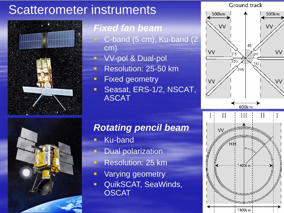
Fixed fan beamC-band (5 cm), Ku-band (2 cm)VV-pol & Dual-polResolution: 25-50 kmFixed geometrySeasat, ERS-1/2, NSCAT, ASCAT

Scatterometer instruments

Rotating pencil beamKu-bandDual polarizationResolution: 25 kmVarying geometryQuikSCAT, SeaWinds, OSCAT

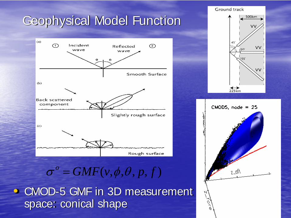
Geophysical Model Function

• CMOD-5 GMF in 3D measurement space: conical shape

),,,,( fpvGMFo θφσ =

),,,(m λθφνσ ,= pfo

Observations Inversion Ambiguity Removal

Wind Field

INPUT OUTPUT

Measurements Inversion Ambiguity Removal

Quality ControlQuality Control

Observations

Wind Field

INPUT OUTPUT

Quality Monitor

Radar backscatter

Level 2 Wind Processing

UTM

Institut de Ciències del Mar / Unitat de Tecnologia Marina

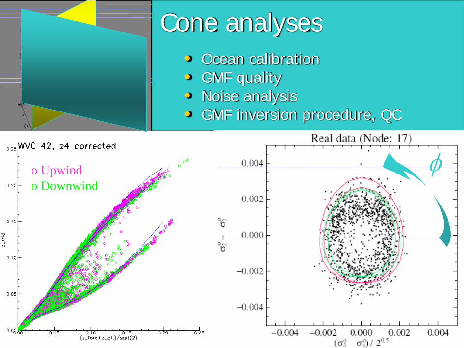
• Ocean calibration• GMF quality • Noise analysis• GMF inversion procedure, QC

Cone analyses

φo Upwindo Downwind

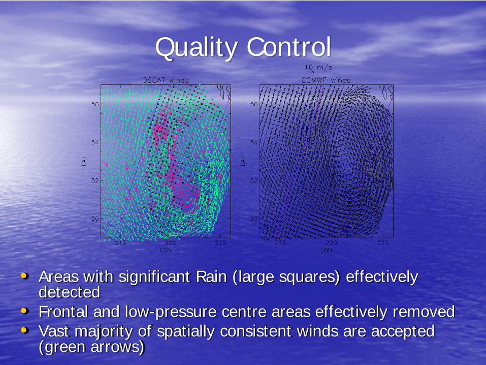
• Areas with significant Rain (large squares) effectively detected

• Frontal and low-pressure centre areas effectively removed• Vast majority of spatially consistent winds are accepted

(green arrows)

Quality Control

Inversion problem

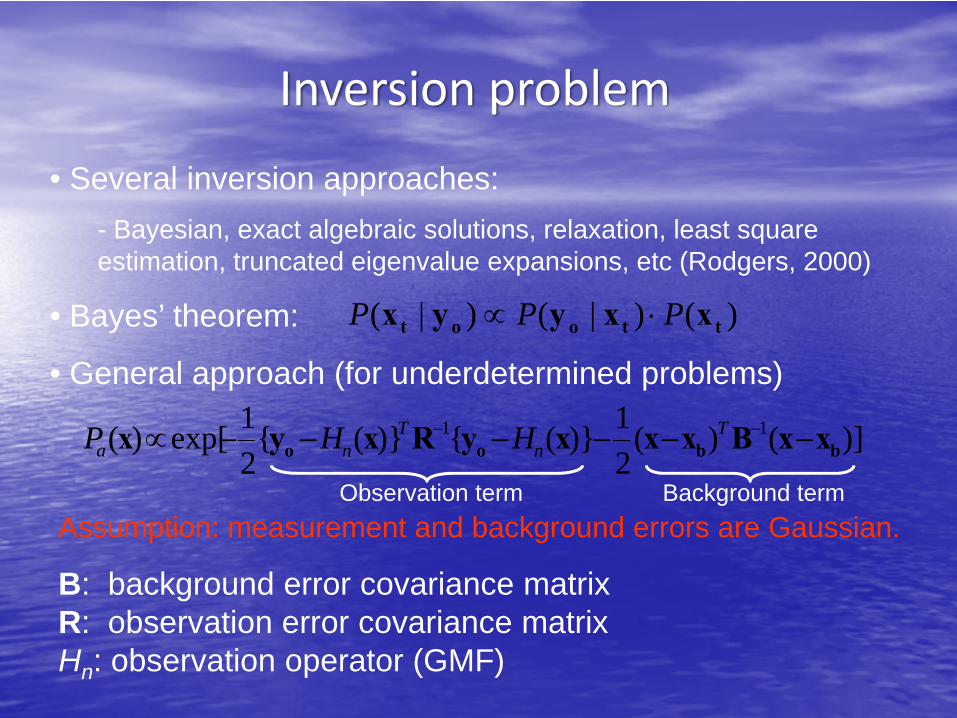
• Several inversion approaches:- Bayesian, exact algebraic solutions, relaxation, least square estimation, truncated eigenvalue expansions, etc (Rodgers, 2000)

• Bayes’ theorem:

• General approach (for underdetermined problems)

Assumption: measurement and background errors are Gaussian.

B: background error covariance matrix R: observation error covariance matrixHn: observation operator (GMF)

)()|()|( ttoot xxyyx PPP ⋅∝

)]()(21)}({)}({

21exp[)( 11

bboo xxBxxxyRxyx −−−−−−∝ −− Tn

Tna HHPObservation term Background term

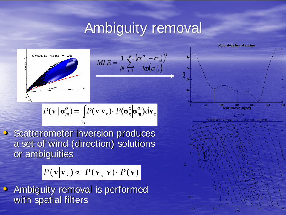
• Scatterometer inversion produces a set of wind (direction) solutions or ambiguities

• Ambiguity removal is performed with spatial filters

( )( )∑

=

−=

N

iosi

osi

omi

kpNMLE

1

21

σσσ

Ambiguity removal

som

oss

om dPPP vσσvvσv

sv

)()()|( ∫ ⋅=

)()()( vvvvv PPP ss ⋅∝

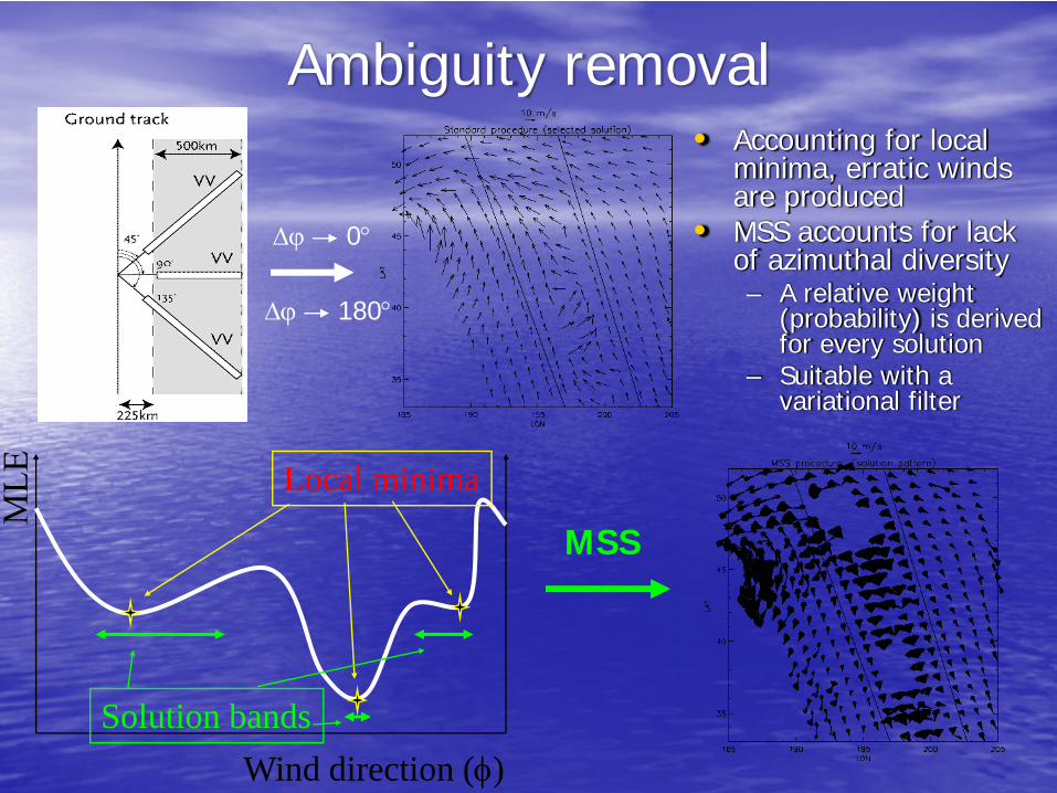
• Accounting for local minima, erratic winds are produced

• MSS accounts for lack of azimuthal diversity– A relative weight

(probability) is derived for every solution

– Suitable with a variational filter

Ambiguity removal

Wind direction (φ)

Local minima

Solution bands

Δϕ 0°

Δϕ 180°

MSS

UTM

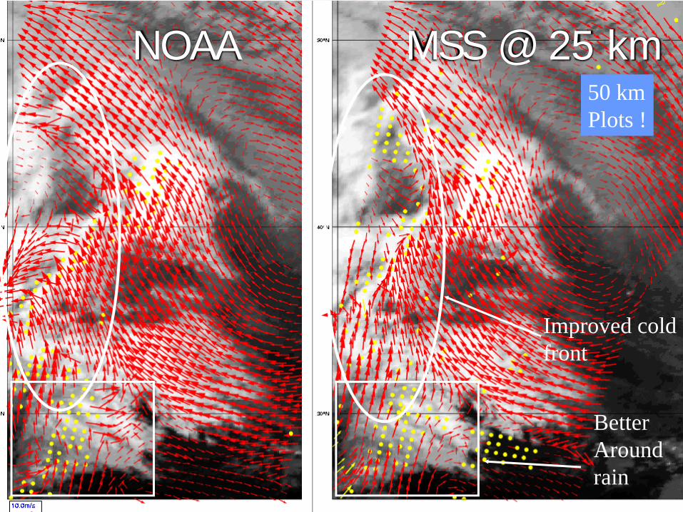
Institut de Ciències del Mar / Unitat de Tecnologia MarinaNOAA MSS @ 25 km

Improved coldfront

BetterAroundrain

50 kmPlots !

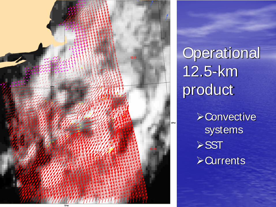
Operational 12.5-km product

Convective systemsSSTCurrents

11

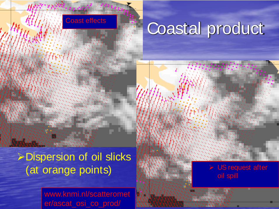
Coastal product

US request afteroil spill

www.knmi.nl/scatterometer/ascat_osi_co_prod/

Dispersion of oil slicks(at orange points)

Coast effects

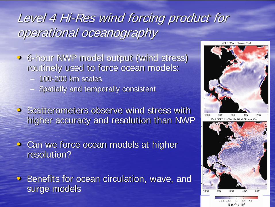
Level 4 Hi-Res wind forcing product for operational oceanography

• 6-hour NWP model output (wind stress) routinely used to force ocean models:– 100-200 km scales– Spatially and temporally consistent

• Scatterometers observe wind stress with higher accuracy and resolution than NWP

• Can we force ocean models at higher resolution?

• Benefits for ocean circulation, wave, and surge models

Marine Core Service

Satellite Wind and Wave Workshop, 18 Dec 2009

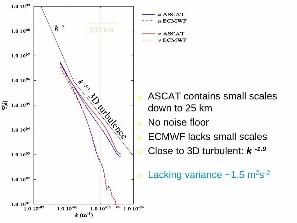
100 km

ASCAT contains small scales down to 25 kmNo noise floorECMWF lacks small scalesClose to 3D turbulent: k -1.9

Lacking variance ~1.5 m2s-2

k -3

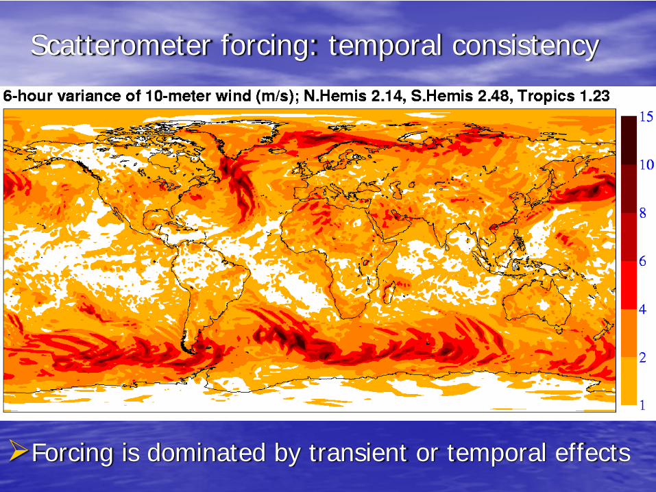
Forcing is dominated by transient or temporal effects

Scatterometer forcing: temporal consistency

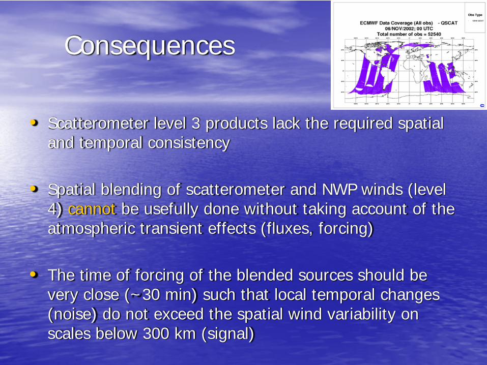
Consequences

• Scatterometer level 3 products lack the required spatialand temporal consistency

• Spatial blending of scatterometer and NWP winds (level 4) cannot be usefully done without taking account of the atmospheric transient effects (fluxes, forcing)

• The time of forcing of the blended sources should be very close (~30 min) such that local temporal changes (noise) do not exceed the spatial wind variability on scales below 300 km (signal)

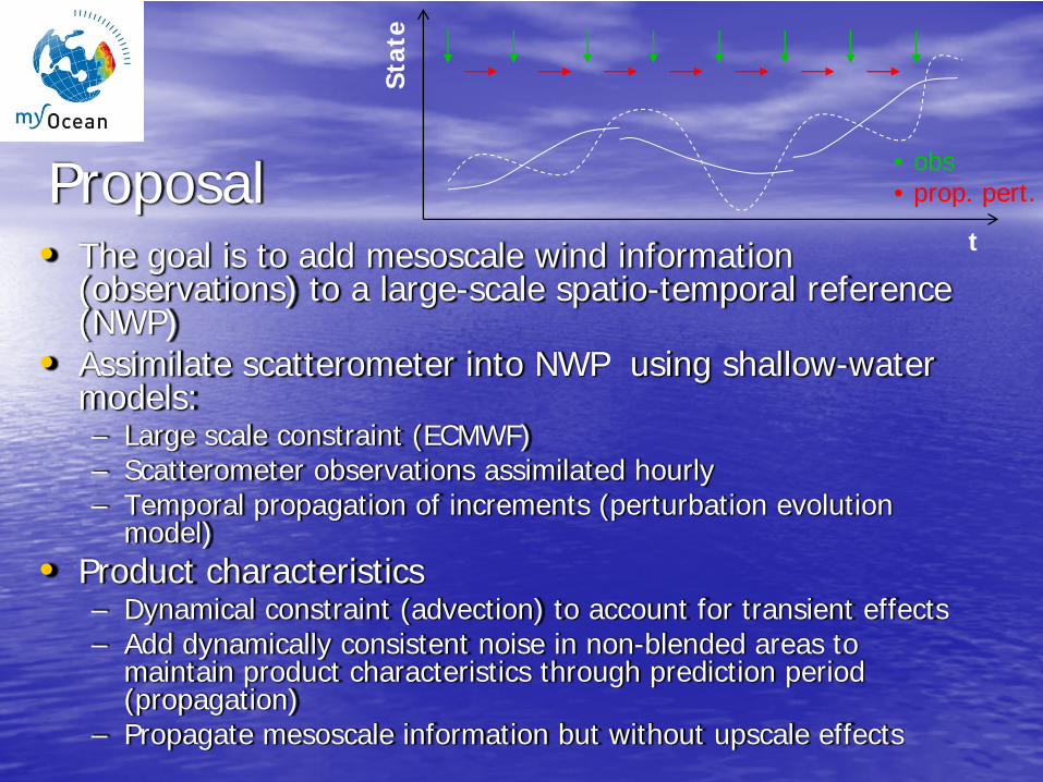
Proposal• The goal is to add mesoscale wind information

(observations) to a large-scale spatio-temporal reference (NWP)

• Assimilate scatterometer into NWP using shallow-water models:– Large scale constraint (ECMWF)– Scatterometer observations assimilated hourly– Temporal propagation of increments (perturbation evolution

model)• Product characteristics

– Dynamical constraint (advection) to account for transient effects– Add dynamically consistent noise in non-blended areas to

maintain product characteristics through prediction period (propagation)

– Propagate mesoscale information but without upscale effects

Stat

e

t

• obs• prop. pert.

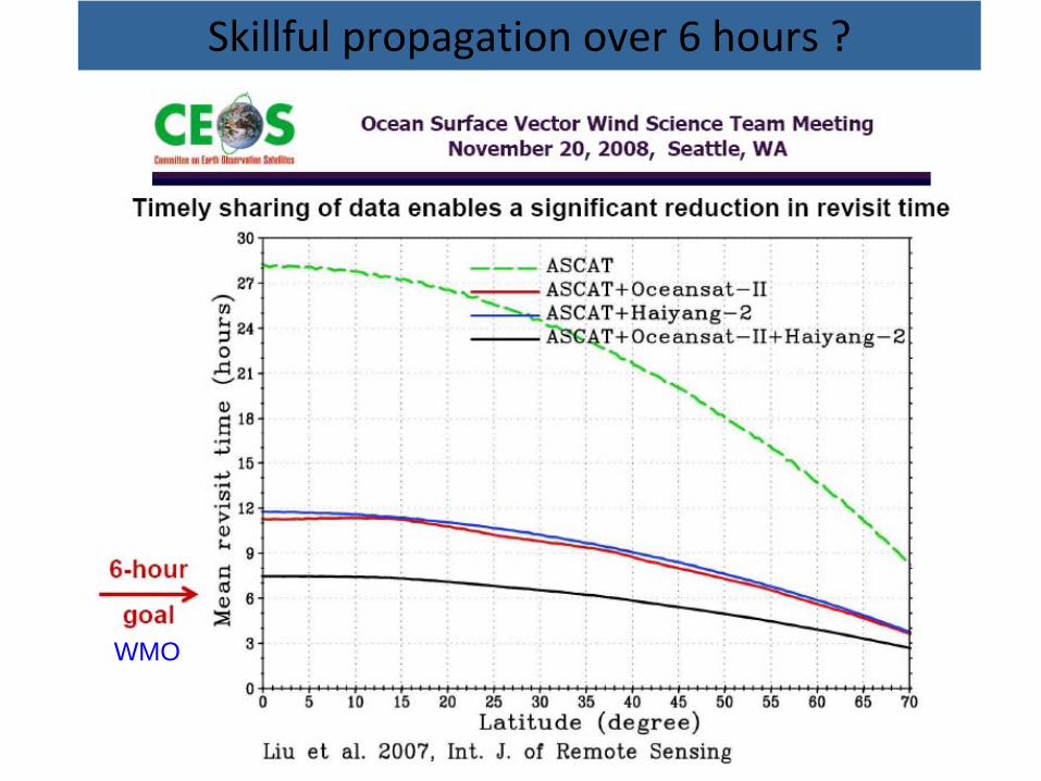
Skillful propagation over 6 hours ?

WMO

Scatterometer Data access and helpdesk

NRT Data (nowadays only ASCAT) are available• For free to any interested user• In WMO BUFR (Binary Universal Form for Representation) format,

global ASCAT data also in NetCDF• On FTP server at KNMI (FTP pull), on EUMETSAT satellite

broadcast system (EUMETCast) and (some) on the Global Telecommunication System (GTS)

Helpdesk facilities• For data access: contact scat@knmi.nl• For any other questions or feedback: contact scat@knmi.nlArchived data are available• At the EUMETSAT Data Center (www.eumetsat.int, ASCAT and

some SeaWinds) - online• At PO.DAAC

(http://podaac.jpl.nasa.gov/DATA_CATALOG/ascatinfo.html, ASCAT in NetCDF format, SeaWinds in HDF format) - online

• At KNMI (scat@knmi.nl, SeaWinds, ERS) - offline