SAVING BEFORE AND AFTER RETIREMENT:A STUDY OF CANADIAN COUPLES,

1969-1992

Xiaofen Lin

IESOP Research Paper No. 13

April 1997

The Program for Research on the Independence and Economic Security of the Older Populationis an interdisciplinary research program established at McMaster University with support fromHealth Canada’s Seniors’ Independence Research Program. The Research Paper series providesa vehicle for distributing the results of studies undertaken by those associated with the program. Authors take full responsibility for all expressions of opinion.

For further information about the research program and other papers in this series, see our website at: http://socserv2.mcmaster.ca/~iesop/

* This paper is drawn from my doctoral dissertation supervised by Professors Martin Browning,John Burbidge, Lonnie Magee and Michael Veall, Department of Economics, McMaster University. Ialso gratefully acknowledge the research support of SSHRCC doctoral fellowship, 1995-1996.

Saving Before and After Retirement:A Study of Canadian Couples,

1969-1992*

Xiaofen Lin

Department of EconomicsMcMaster University

Hamilton, Ontario, CanadaL8S 4M4

Abstract

This essay examines issues of life-cycle savings of Canadian elderly married-couplehouseholds just before and after retirement within both a pooled cross-sectional and a syntheticlongitudinal framework. We investigate whether the saving behaviour of elderly couplesappears to be motivated by life-cycle factors, how the growth of our economy has affectedlifetime income, consumption and savings across generations, and, because we use repeatedcross-sectional data, the 1969-1992 FAMEX, how to correct the age profiles distorted by thepresence of differential mortality between the rich and the poor. We intend to provide evidenceboth for the empirical justification of the standard life-cycle model and for policy makersconcerned with various social programs for the elderly in Canada.

The pooled cross-section results on overall median age pattern indicate that, thoughincome and consumption are both decreasing with age, the decrease in consumption is relativelysmooth while income falls considerably at retirement age. Savings and saving rates thus exhibita distinct pattern: they drop sharply at retirement age, but rise again thereafter. When house-holds are grouped into four types according to retirement status of both spouses, it is clear thatthis saving dip is found only among both-retired couples. For couples with at least one spouseworking, saving rates remain high throughout the age span. It is also found that controlling forincome, households with both spouses retired have the highest saving rate among all types.

In the cohort analysis, the age profiles show that income and consumption remain atabout the same level or even increase with age after retirement. There are significant cohorteffects in both income and consumption in that younger cohorts have higher income and higherconsumption than older cohorts. Moreover, these effects are about the same for both variables. However, the age profile for the saving rate is very similar to those based on pooled cross-sections: a sharp drop at retirement, a quick rise thereafter. We find no cohort effects on savingrates in our sample. This is the core reason that saving profiles are the same in both cross-section and cohort analysis.

Synthetic cohort analysis, however, is biased by the fact that the poorer tend to drop outfrom the sample earlier because of higher mortality. Based on the idea that decreasing quantileswith age should be used instead of the straight median for every age, a new method is developedto correct the median profiles for differential mortality. Two cases, the extreme case and thenormal case, are illustrated in detail. Using population survival rates from the Canadian LifeTable and the top 20% (in wealth distribution) survival rates from a Canadian study due toWolfson, et al., we are able to estimate the varying quantiles and to correct the age profiles fromthe cohort studies. Differential mortality does make a difference in estimated lifetime behaviour. The corrected income profile is fairly constant after retirement. Consumption decreasesthroughout the age range. Saving rates now are lower and flatter after retirement. However,there is no sign of a further drop in saving rates after an initial drop at retirement age. Ifanything, we still see a tendency for the saving rates to rise after retirement.

“Mom, you’ve always been so frugal. You should ENJOY your money more.”

“Well, Sylvia, we have to make our savings last us the rest of our lives.”

“Mother, you and Dad have enough money to last you until you’re A HUNDRED AND TEN.”

“And THEN what’ll we do?”

“PICKLES”Hamilton Spectator Oct. 13th, 1995

Contents

Part One: Introduction . . . . . . . . . . . . . . . . . . . . . . . . . . . . . . . . . . . . . . . . . . . . . . . . . . . . . . . . . 2

Part Two: Data Issues . . . . . . . . . . . . . . . . . . . . . . . . . . . . . . . . . . . . . . . . . . . . . . . . . . . . . . . . . . 8

Part Three: Cross-Section Evidence . . . . . . . . . . . . . . . . . . . . . . . . . . . . . . . . . . . . . . . . . . . . . . 143.1 Income, Consumption and Savings: A First Look . . . . . . . . . . . . . . . . . . . . . . . . . 14

General Age Pattern . . . . . . . . . . . . . . . . . . . . . . . . . . . . . . . . . . . . . . . . . . . . . . . 15Age Pattern by Income Quartiles . . . . . . . . . . . . . . . . . . . . . . . . . . . . . . . . . . . . . 17Section Summary . . . . . . . . . . . . . . . . . . . . . . . . . . . . . . . . . . . . . . . . . . . . . . . . . 20

3.2 Does Retirement Status Matter? . . . . . . . . . . . . . . . . . . . . . . . . . . . . . . . . . . . . . . . . 21Saving Rates by Type of Couples: An Overall description . . . . . . . . . . . . . . . . . 22Saving Rates by Type of Couples: Controlling for Other Variables . . . . . . . . . . 25Section Summary . . . . . . . . . . . . . . . . . . . . . . . . . . . . . . . . . . . . . . . . . . . . . . . . . 28

3.3 Summary and Comments on Cross-Section Evidence . . . . . . . . . . . . . . . . . . . . . . . 29

Part Four: Cohort Analysis . . . . . . . . . . . . . . . . . . . . . . . . . . . . . . . . . . . . . . . . . . . . . . . . . . . . . 324.1 The Structure of the Cohorts: . . . . . . . . . . . . . . . . . . . . . . . . . . . . . . . . . . . . . . . . . . 324.2 Modelling and Estimating the Overall Age Profiles . . . . . . . . . . . . . . . . . . . . . . . . . 354.3 Age-Saving Rate Profiles by Relative Income Quartiles . . . . . . . . . . . . . . . . . . . . . 434.4 Age Profiles Controlling for Retirement Status . . . . . . . . . . . . . . . . . . . . . . . . . . . . 444.5 Summary and Implications . . . . . . . . . . . . . . . . . . . . . . . . . . . . . . . . . . . . . . . . . . . . 46

Part Five: Correction for Differential Mortality . . . . . . . . . . . . . . . . . . . . . . . . . . . . . . . . . . . . . 505.1 The Method . . . . . . . . . . . . . . . . . . . . . . . . . . . . . . . . . . . . . . . . . . . . . . . . . . . . . . . . 525.2 The Extreme Case . . . . . . . . . . . . . . . . . . . . . . . . . . . . . . . . . . . . . . . . . . . . . . . . . . . 555.3 The "Normal" Case . . . . . . . . . . . . . . . . . . . . . . . . . . . . . . . . . . . . . . . . . . . . . . . . . . 565.4 Estimating Quantiles . . . . . . . . . . . . . . . . . . . . . . . . . . . . . . . . . . . . . . . . . . . . . . . . . 595.5 Correcting Median Age Profiles . . . . . . . . . . . . . . . . . . . . . . . . . . . . . . . . . . . . . . . . 635.6 Summary . . . . . . . . . . . . . . . . . . . . . . . . . . . . . . . . . . . . . . . . . . . . . . . . . . . . . . . . . . 64

Part Six: Conclusions . . . . . . . . . . . . . . . . . . . . . . . . . . . . . . . . . . . . . . . . . . . . . . . . . . . . . . . . . . 66

References . . . . . . . . . . . . . . . . . . . . . . . . . . . . . . . . . . . . . . . . . . . . . . . . . . . . . . . . . . . . . . . . . . 69

Tables and Figures . . . . . . . . . . . . . . . . . . . . . . . . . . . . . . . . . . . . . . . . . . . . . . . . . . . . . . . . . . . . 72

2

1 Browning and Lusardi (1995) give nine motives for “why do people save?”, one of which is thelife-cycle motive, which is the focus of our analysis.

Part One: Introduction

This essay examines issues of life-cycle savings of Canadian elderly married-couple households

just before and after retirement within both a pooled cross-sectional and a synthetic longitudinal

frameworks. We investigate whether the saving behaviour of elderly couples appears to be

motivated by life-cycle factors,1 how the growth of our economy has affected lifetime income,

consumption and saving across generations, and, because we use a time series of repeated cross-

sections data set, how to correct the profiles distorted by the presence of differential mortality

between the rich and the poor. We provide evidence against the prediction of standard life-cycle

theory that the typical household dissaves in retirement. Our analysis could be of use to policy

makers concerned with various social programs for the elderly in Canada.

The basic theory of saving behaviour is the life-cycle model of Modigliani and Brumberg

(1954). In its simplest version, a consumer decides his lifetime consumption and savings by

solving the problem of maximizing lifetime utility, which is the sum of all present and future

instantaneous utilities, subject to a present and future resource constraint. Assuming an

unchanging utility function for each period, no uncertainty, no changes in the interest rate and

time discount rate, and perfect capital markets (people can borrow and lend at the known interest

rate), the theory has very sharp implications for the life-cycle pattern of consumption, saving and

wealth. Derived from the optimality condition of the maximization problem that consumers seek

to keep marginal utility of expenditure constant from one period to the next, an important

implication is that the shape of the lifetime path of consumption is independent of the shape of

the expected path of income. In other words, people save to smooth consumption in the face of

3

2 Also see Browning and Lusardi (1995), page 10-11, for a discussion of this assumption.3 Also see Baker and Benjamin (1995).

an uneven income profile. As most people have high income during their working life and low

income when they retire, a simple but powerful prediction is that people save until retirement,

then dissave. Consequently, individual assets accumulate up to the retirement age and then

decumulate down to zero by the (certain) date of death, producing the well-known hump shaped

wealth-age pattern.

This basic life-cycle theory is also a forward-looking theory. It assumes that people

decide how much to consume and to save by looking at present and future resources and present

and future needs. Thus, in addition to the assumptions of the basic model above, it is also

assumed that an increase in lifetime resources (lifetime wealth or permanent income) leads to a

proportional increase in consumption at each stage in life.2 An important prediction of this

"proportionality" assumption is that, in a growing economy, since the resources available to each

generation (or cohort) increase over time due to technical progress, consumption in any period

should also increase proportionally to the increase in permanent income for younger cohorts. In

other words, the cohort effects of income and consumption should line up. Consequently, unless

cohorts expect other economic circumstances to be different for them than for their predecessors,

the saving rates should not vary across cohorts.3

Though powerful and intuitive, the basic life-cycle model is restrictive and so is likely to

be rejected by the data. A recent volume edited by Poterba (1994) provides international

comparisons of household saving behaviour in six OECD countries: Canada, Italy, Japan,

Germany, the United Kingdom, and the United States. The authors from each country examine

micro data sets of household saving patterns by age, income, and other demographic factors.

The country studies provide very little evidence that supports the life-cycle model. In virtually

4

4 See Burbidge and Davies (1994), table 1.1, in Poterba (1994).

all nations, the saving rate is positive even after retirement. In Italy and Japan, the saving rate

among the elderly households, those aged 65 and over, actually exceeds 30%. Among low-

saving countries, however, there is some evidence that saving rates peak in the years prior to the

retirement. In Canada, for example, the median saving rates, as estimated by the 1990 FAMEX

data using all observations, is 11% for households aged 55-59, compared to 9% for those aged

60-64 and 6% for those aged 65-69 and 70-74. But for the oldest age group, those aged 75 and

older, the saving rate increases to 8%.4 The data in Germany and the United Kingdom exhibit a

similar saving pattern. The U.S. data, however, show the lowest saving rate (1.1%) for the oldest

age group, the 70-74 year olds. In another recent Canadian study by Baker and Benjamin

(1995), which uses the 1982-1992 FAMEX data set and includes all households, the results

suggests a steady decline in saving rates across all cohorts studied. That is, each successive

cohort is saving less than the previous one, which is in contradiction to what the life-cycle model

would predict. Yet, the age effects in saving rates in their study are more consistent with the

life-cycle model: the elderly appear to reduce their savings as they age.

Various extensions and modifications to the basic life-cycle model have been explored in

the literature in the past several decades. The presence of liquidity constraints, in particular, that

people are unable to convert their future income into current consumption, may explain why

consumption tracks income closely at younger ages. But Browning and Lusardi (1995) argue

this is much less credible for the older households. Precautionary saving models incorporate

various forms of uncertainty into the life-cycle model. Uncertainty about future income, future

health hazards or length of lifetime may depress current consumption and thereby increase

current saving. But for the elderly, future incomes are, in most part, observable because they

consist of various government-provided social security programs, private pensions and the return

5

5 See, for example, Davies (1982) and Hurd (1990b).6 BÐrsch-Supan and Stahl (1991) and BÐrsch-Supan (1992) also explore the model in which there

exists an upper limit to consumption depending on health status and age, with zero marginal utility ifconsumption is above this ceiling, so the elderly reduce their consumption as they age or as their healthstatus declines.

to capital. If a nation offers a comprehensive system of health insurance or health care, for

example like that in Canada, the need to set aside resources as a precaution against illness will

also be reduced. Davies (1981) suggests that even with life time uncertainty wealth must decline

at some age (not necessarily at retirement) and that after this age wealth should continue to

decline smoothly. Another important modification is to introduce a bequest motive for saving.

The requirement that wealth to be positive on the date of death entails a lower level of consump-

tion at each age during retirement. But it does not rule out dissaving by the elderly. Many

studies and tests5 also show that the bequest-motive of the elderly is not as important as it might

at first appear. Introducing uncertain life spans and bequests may extend the age at which saving

becomes negative, but it does not invalidate the basic prediction that the elderly will eventually

dissave.6

Because panel data are rare or even non-existent in many countries, for example in

Canada, cross-section survey data have been the most common source for empirical research in

this area. However, the evidence from a single cross-section (single sample year) data con-

founds age and cohort effects. If we have repeated cross-sections for more than a few years, we

can make better estimates for both cross-sectional and longitudinal analysis. By pooling

repeated cross-sections survey data and controlling the year by year differentials in the variables

of interest, cohort effects can be partially washed out and the resulting “cross-section” evidence

can give us much better estimates than those available with a single cross-sectional sample.

Better still, by following the same year of birth cohort through these series of cross-sections, we

can get estimates that actually describe life-cycle paths of the variables of interest for a particular

6

7 For example, Browning and Lusardi (1995) point out that "we have also to be careful aboutfamily composition since the decumulation of couples can be lower than singles given that the expected`lifetime' of the household is greater for couples."

cohort. Though this alternative longitudinal analysis has proven useful for pre-retirement

households in various studies, for the elderly this suffers from the fact that the survival rate is

positively correlated with wealth and that living arrangements may also be correlated with

income or wealth. This means that the poor would vanish from the sample earlier than the rich,

resulting in an upward bias in the cohort average over time.

In the present study, therefore, we use repeated cross-sections of time series data, the

Canadian Family Expenditure Surveys (FAMEX) from 1969-1992, to examine the life-cycle

saving pattern of elderly couples. Unlike most other Canadian studies which include all

households in the analysis, we focus only on elderly couples because we believe that wealth

decumulation behaviour may be very different between couples and singles,7 and most elderly

households are typically couples. In light of the discussion in the previous paragraph, we first

investigate the pooled cross-sectional evidence on age patterns of income, consumption and

savings, both for overall households and specific household types. We then re-organize the data

so that we can follow the same cohorts over time. Life-cycle patterns and cohort patterns of

saving are then examined together in detail. We also respond to the pitfalls of using repeated

cross-sections data to examine the behaviour of the elderly by developing a method to correct the

estimated age profiles for differential mortality.

Thus, the present study contributes to the literature in two major respects. First, the age

profiles of income, consumption and the saving rate using all available FAMEX data for the

elderly couples-only households has not yet been estimated within both pooled cross-sectional

and synthetic longitudinal frameworks and this study fills that gap. Second, the method

developed in this study to correct the age profiles for differential mortality is new to the

7

literature, although there are alternatives (Shorrocks (1975); Attanasio and Hoynes (1995)).

Here are some of the key results. For Canadian elderly couples within the sample years

studied, because incomes fall considerably at retirement and maintain a stable level thereafter

while consumption is relatively smooth and decreasing over time, the saving rate has a sharp

drop at retirement age, and rises steadily thereafter. The dip of the saving rate at retirement is

found both in pooled cross-sections and cohort analysis. There are strong cohort effects in both

income and consumption variables: younger cohorts have higher income and higher consumption

in any given age, and the increase in consumption appears the same as that in income. There are

no cohort effects in the saving rate: each cohort saved the same portion of income at any given

age. Thus the relation between the saving rate and age looks much the same whether we employ

pooled cross-section or a cohort analysis. Differential mortality does make a difference to all

estimated profiles, but the corrected median saving rate profile still does not become negative

after retirement.

The rest of the study is organized as follows. Part Two discusses some data issues. Part

Three gives the results on the pooled cross-sectional study, both on overall households and on

specific types of couples according to their retirement status. Part Four contains cohort analysis

where again overall and specific studies are attempted. Part Five is devoted specially to the

development of a method to correct the median age profiles for differential mortality with

detailed illustration for the two cases: the extreme case and the normal case. The application of

the method is demonstrated on the cohort profiles in Part Four. A summary and conclusions are

offered in Part Six.

8

8 FAMEX Public Use Micro Tape documentation, various years. The difference between the twodefinitions of sample unit should not concern us much because we only select two-person, married couplehouseholds.

Part Two: Data Issues

The data used for this study are all publicly available Canadian Family Expenditure

Surveys (FAMEX) for sample years 1969, 1974, 1978, 1982, 1984, 1986, 1990 and 1992, which

are multistage stratified clustered samples selected from the Labour Force Survey sampling

frame. The surveys are carried out in February and March and collect information by recall

referencing to the previous calendar year on each household's total annual income and expendi-

tures, their components, changes in assets and liabilities and information on many other

characteristics of each household, including education levels and working status of both spouses

(if any). The term family (or the spending unit) upon which FAMEX data are based is defined,

prior to 1990, "as a group of persons dependent on a common or pooled income for the major

items of expense and living in the same dwelling or one financially independent individual living

alone". After 1990, it is "a person or group of persons occupying one dwelling unit."8 The

coverage of the survey includes urban and rural areas throughout the ten provinces of Canada as

well as Whitehorse and Yellowknife with the exception of sample years 1984 and 1990, in which

only seventeen major cities of Canada whose population is 100,000 or more are covered. All

surveys exclude persons living full-time in institutions such as old age homes, penal institutions

and hospitals.

Because the subjects of this study are a relatively homogeneous population of elderly

couples, the sample selection criteria include:

(1) using only two-person married couple households with male household head whose

age is 55 or higher (in cross-section study), or is 53 or higher (in cohort study);

9

9 There is a variable in the data set specifying that the unit is farm or non-farm. Another variablerelated to this is "area", farm is the same as area=rural farm (there is also a rural non-farm category).

10 Details on the structure of cohorts will be explained in Part Four: Cohort Analysis.

(2) excluding households who are farmers;9

(3) excluding households whose head or spouse are self-employed if they are working;

(4) for the cross-section study, in order to be comparable across sample years, only those

households who live in cities whose population is 100,000 or more are selected from each

sample year;

(5) for cohort study, in order to increase sample size because certain sample observations

used in cross-section study have to be dropped due to the cohort structure,10 households who live

in cities whose population is less than 100,000 and who live in rural areas but are not farmers are

included.

Farm and self-employed households are excluded to achieve a relatively consistent

picture of the general elderly saving pattern. Due to the nature of their profession, farm and self-

employed bear higher income risk, so their saving patterns may differ from the others. For

example, the theory on precautionary savings predicts that high income risk motivates high

savings (Skinner, 1988; Zeldes, 1989). Their spending pattern may differ too, particularly if

measurement error in the observation included some business expenditures as household

expenditures or vice versa.

However, just to see whether the exclusion of farmers and self-employed would affect

the results and whether using different sample arrangements for pooled cross-section and cohort

analysis would change the main conclusions, several sensitivity analyses are incorporated in both

the pooled cross-section and cohort analyses below to compare the results. We find no major

difference in the median age patterns between including and excluding farmers and self-

employed households in the analysis. There is a slightly higher level of saving rates in all age

10

11 In the data set, year 1982 has the highest saving rate among all sample years.

ranges if we use the cohort sample to get the cross-section age patterns, but the shape of the age

patterns are essentially the same as that of using cross-section sample. This slightly higher level

of saving rates is due to the exclusion of some observations consisting of only short-period

cohorts which are in the low saving years.11

Saving is defined here as disposable income (or net income) minus total current con-

sumption. In the FAMEX data set, gross income consists of wages and salaries, self-employed

income, investment income, government transfers and miscellaneous income. Capital gains are

not included in income. Government transfers include many income sources such as Old Age

Security, Guaranteed Income Supplement, C/QPP benefits, Unemployment Insurance and social

assistance. Because these transfers are lumped together, there is no way to allow further

investigation as to how different sources affect spending and saving patterns differently.

Miscellaneous income includes retirement pensions arising out of previous employment,

individually purchased annuities and other money income. In addition to the above gross

income, other money receipts is another separate variable in the data, which includes money

gifts, inheritance and lump sum settlements.

Although, given the data, one can form other definitions of disposable income, the

preferred disposable income measure in this study is: gross income plus other money receipts,

less personal tax, less UI and C/QPP premiums [definition (1)]. The inclusion of other money

receipts in income is for obvious reasons: it is one's income and is at one's disposal. UI and

C/QPP premiums are compulsory and are deducted directly from one's payroll. Moreover, as

government transfers include UI and C/QPP benefits, including UI and C/QPP premiums as

income would result in double counting. Another definition of net income used in this study is:

income definition (1) less life insurance premiums [definition (2)]. However, as this definition is

11

12 Household additions and renovations is a component of the variable: change of assets andliabilities (Dassets), a saving measure by Statistics Canada. In this definition, we assume that the averagelifetime of the vehicle purchased and the addition and renovation part of the house are 5 years.

more controversial, it is only used in the general description section of cross-section studies.

The expenditure for total current consumption is defined by Statistics Canada as expenses

incurred during the survey year for food; housing, fuel, light and water; household operations;

clothing; automobile purchase and operation; other transportation; medical care; personal care;

reading; recreation; education; smoking and alcoholic drinks and miscellaneous. However, in

this study, one more item is added to the consumption expenditure, namely, gifts and contribu-

tions, which is also given in the data set as a separate variable. If we do not include this as

consumption expenditure, the saving and saving rate variables, defined here as a residual of

income after consumption, will be less informative, if not biased. This definition of total

consumption expenditure [definition (1)] will be used throughout the study. There is another

issue concerning the measurement of consumption. As noted, the above measure of consump-

tion includes durable purchases such as cars and recreational vehicles which are not to be totally

consumed within a year. Yet, some expenditures, namely, house additions and renovations, are

treated totally as new additions to the stock of real assets, and are not at all reported as expendi-

tures. To correct for this unreasonable treatment, another measure of total consumption is also

used. This is consumption definition (1) less 80% of vehicle purchases and plus 20% of the

expenditure on house additions and renovations12 [definition (2)]. Within this context, the

depreciation of the existing consumer durables should also be added to consumption, but the

limitations of the data preclude this possibility. Thus this definition (2) of total consumption is

examined only in the cross-section study.

As mentioned above, saving is defined as the residual of income less consumption. The

12

13 In the analysis for saving rates, observations with zero incomes are excluded. We also excludeobservations with both negative saving and negative income. Only around 5 observations are deleted onthis accord.

saving rate here is always defined as saving divided by income.13 It is worth noting that there is

another measure of saving provided with the public use FAMEX data, i.e., change of assets and

liabilities (Dassets), which includes the net change in all financial and real assets (cash, saving

accounts, RRSPs, bonds and stocks, home equity and investment in non-incorporated business,

etc.) and the net change in debt. According to these components of Dassets, it should be equal to

the definition: gross income + other money receipts - personal tax - social security - (total

consumption + gifts and contributions). Because social security includes UI and C/QPP

premiums, life insurance premium, annuity contracts and other retirement and pension payments

(excluding RRSPs), it is clear that the residual measure of saving used in this study will be

higher than Dassets because it also includes life insurance premiums (if using income definition

(1)), annuity contracts and other retirement and pension payments, while these are not in

Dassets. In the general description part of the cross-section study, Dassets will be examined

along with the other definitions of saving variables, but it will be dropped in later sections,

including the cohort analysis.

There is also a concern regarding whether the withdrawal of one’s RRSP is included in

one’s current income variable in our data set because if so, we would observe an increase in

income in later ages due to this withdrawal. According to the Canadian tax system, individuals

can make a contribution to a retirement plan and deduct the contributions from income for tax

purposes. Interest from the contributions then accrue tax-free until withdrawal, when income

taxes are paid based on income including the withdrawals. Although the amount of withdrawal

is in the base for calculation of income tax, it is not counted as FAMEX current income. Large

withdrawals, if not spent, are rearranged as another form of saving, namely, in the annuity

13

contracts component of social security. Records extracted from FAMEX data with large RRSP

withdrawals are consistent with this treatment. This fact can make it clear for the results we will

present later in the cohort analysis that the withdrawals of RRSPs at later ages are not the cause

of the increasing income with age for the older elderly.

14

Part Three: Cross-Section Evidence

This part examines saving behaviour of elderly Canadian couples based on pooled cross-section

analysis. To ensure a relatively homogeneous subsample, we include only those couples who are

not farmers, who live in major urban centres, who reported no self-employment income, and who

are headed by males aged over 55. All income, consumption and saving variables are deflated

by the Canadian Consumer Price Index series to 1986 dollars. Table 1.0 shows sample size by

age group and sample year. These five age groups, arranged by the age of household heads, 56-

60, 61-65, 66-70, 71-75 and 76+, are the primary focus for the examination of age patterns of

income, consumption and savings in our cross-section analysis. Data on all sample years are

pulled together to form the base sample for cross section study in the concern that using any one

particular sample year may lose the representativeness of a general age pattern because of the

small sample size.

The rest of this part is divided into three sections. Section one looks at the general age

patterns of income, consumption and savings. Section two presents a more detailed picture of

savings by examining the age pattern of four distinct types of couples according to their working

status. Summary and additional comments follow in section three.

3.1 Income, Consumption and Savings: A First Look

We start with a general description of the data. Because of fat tails in the distribution of

the variables in question, especially income and saving rates, we use the median rather than

mean most of the time as our primary measure of the central tendency of the variables. The

medians of the variables for each age group are estimated by running quantile regressions with

15

14 All work in this essay including data management, estimation, simulation and graphing aredone using STATA version 3.1.

15 Because the year dummies are not interacted with other variables, the age patterns are affectedby all observations. We set all non-omitted year dummies to zero to get the predicted medians of all agegroups for all the tables in the cross-section analysis. The medians in the tables are thus affected by allobservations in the sample, not just by observations in reference year 1992.

16 Because the regressions include constant terms, standard errors of the coefficients on dummyvariables are not the standard errors of the medians we want and these cannot be calculated by simplyadding to standard error of the constant. We solved this problem by adding a test procedure after eachregression, which tests, for each dummy variable, whether the sum of the coefficients on the constant andthe respective dummy variable equal to zero. The F values resulting from this test procedure are thenused to calculate the standard errors of the medians which are presented in all the tables below.

the quantile set to 0.5 (the same as Least Absolute Deviation regression or median regression).14

The right hand side variables are just a set of age dummies (or other dummies of interest) and a

set of year dummies with a constant term. We add the year dummies to pick up different year

effects in our pooled eight-year samples with 1992 as the reference (omitted) group.15 Thus the

age coefficients (plus the constant term) in regressions correspond to the medians of age groups

(with an adjustment to allow for yearly differences).

The advantage of using the quantile regression method to describe our data is that we can

control for independent variables as well to find patterns that are beyond the reach of simple

descriptive statistics. Adding year dummies is an example. Later on, we will also control for

other variables that affect the shape of the profiles we study.

General Age Pattern

Tables 1.1-1.3b present general age patterns for household income, consumption, savings

and saving rates of the Canadian elderly couples. Table 1.1 shows the age patterns for the

medians of net income and total consumption, with two definitions for each. Standard errors of

the medians are also presented.16 We note certain important trends from the table. First, income

and consumption are uniformly decreasing with age for both definitions. Second, the declines in

consumption are very evenly paced with age, while the declines in income experience a large

16

drop from ages 61-65 to ages 66-70 when most people begin retirement. Here there seems to be

some evidence in favour of the "consumption smoothing" prediction from Life-Cycle theory if

we believe that the age pattern from cross-section data is valid for the prediction. As stated in

Part One: Introduction, using pooled cross-section should yield much better results than using

only a one year sample because cohort effects can be partially washed out. We shall see later

that this relatively smooth consumption pattern also exists in cohort analysis. Lastly, there is no

fundamental difference in the age patterns between the two definitions of income or between the

two definitions of consumption. For income, even the levels are very close, especially after ages

66-70. For consumption, definition (2) always yields a lower value than definition (1). Their

differences are much higher in the first two age groups than in the oldest two groups. This tells

us that the older elderly are much less active in buying cars and recreational vehicles than the

younger elderly.

Table 1.2 gives age patterns for four definitions of saving plus a measure of saving by

Statistics Canada: change of net assets and liabilities (Dassets). Saving (1) to (4), defined as the

residual of income less consumption, are also declining quickly up to, and including, ages 66-70.

But as age continues to increase, saving rises again. This pattern also holds for Dassets, albeit its

levels are just around half of the other saving definitions. The differences in magnitudes

between the four definitions also depend on the differences between two definitions of income

and consumption. Because the measure of incomes (1) and (2) are almost the same, saving (1)

and (3) are almost identical and so are saving (2) and (4). Saving (2) and (4) are greater than

saving (1) and (3) because the former treats a portion of durable goods purchases as saving.

Tables 1.3a and 1.3b show median and truncated mean saving rates, defined as saving as

a proportion of the corresponding income. From table 1.3a, all four definitions of median saving

rates display a very distinct pattern: they have a modest decline in ages 61-65, and then have a

big dip in ages 66-70. Thereafter, saving rates rise steadily. Notice also that, even at the trough,

17

17 We should note that poor/rich should be defined in terms of wealth, not of current income. However, because wealth information is not observed in our data, we use income as an approximation.

saving rates remain positive in the range of 5 to 11 percent, and they are also statistically

significant. This is certainly in contradiction with what would be predicted by the Life-Cycle

Model. There is also a similar observation as in table 1.2 above concerning the different

definitions.

As a comparison to median figures, table 1.3b also gives truncated mean saving rates

which include only couples whose saving rates are between -100% and +100%. Only about 2%

or less of the couples are excluded. We see that the age pattern of saving rates in this table is

very similar to table 1.3a, although the levels are lower. This suggests that saving rates are

symmetric.

A final observation on tables 1.3a and 1.3b is for the measure of saving rate on Dassets as

a proportion of income. Although as expected, the figures are much lower than for other

definitions, the age shape for this measure is the same as described above: a big dip (but still

well above zero) in ages 66-70, and rising quickly thereafter.

Age Pattern by Income Quartiles

The tables we have presented so far all give median (or mean) age patterns. They are

sufficient for the purpose of studying the average tendency of household saving behaviour. In

this subsection, however, we also want to answer the question: Do the poor and the rich have the

same age pattern of saving? We study the age pattern by income quartiles.17

We could have used the current net income variable to rank households if the households

were in the same age group and from the same sample year. But now, given the structure of our

data, ranking households according to current income is inappropriate. First, if an older elderly

household unit has the same current income as the median income of the younger elderly unit, it

18

18 As we mentioned earlier, definitions (1) and (3), (2) and (4) on saving and saving rate are veryclose in magnitude as well as in shape. Therefore, we examine only definitions (1) and (2) below. Laterwe will only study definition (1).

will be at a much higher position in the income distribution of its peers (table 1.1 makes this

clear), and so may save a higher proportion of its income than the younger unit does. Second,

given that our data consist of eight sample years, even if all units being compared are within one

age group, a unit from an earlier sample year with the same income as a unit from a later sample

year is also at a higher position in the income distribution of its peers of the same year (e.g.,

considering the growth of the economy).

We define now a new concept of income: relative income, which is comparable across all

age groups and all sample years (see Danziger et al. 1981). We assume the following relation-

ship:

where: = net income of household I of age group j in sample year k,

= median net income of age group j in sample year k.

Now when we rank households by , a unit in the oldest age group with a median income, say

$17,346 in table 1.1, will be ranked the same position as a unit in the youngest age group with

median income of $29,162.

We now return to our task. Tables 1.4a and 1.4b give the age pattern of median saving

(1) and (2) by quartiles of relative income , while tables 1.5a and 1.5b examine saving rates

(1) and (2) of the same kind.18 The figures on the tables are obtained by running median

regressions of saving and saving rates on a set of 19 age-quartile cell dummy variables plus a

constant term and a set of year dummies (omitted from the tables) with reference year 1992.

19

Standard errors of the medians are also given. Within each column, households have roughly the

same relative position in the distribution of income of their age/year group. Within each row, we

can examine savings or saving rates of different income classes for a given age group.

We first look at tables 1.4a and 1.4b. For each age group, the median saving, either (1) or

(2), rise as income rises. Within each column (i.e., for each income class), the by now familiar

age pattern is still very clear, at least for the three upper income classes. Saving declines quickly

until reaching ages 66-70, and remains constant or even rises thereafter. We observe dissaving

only below the first quartile. Even so, the oldest age group below the first quartile still has

positive saving, though the saving levels are not statistically significant (see standard errors).

Comparing the magnitude of definition (1) in table 1.4a with that of definition (2) in table 1.4b,

we observe that the richer members of the elderly (above the second quartile) also have more

durable consumption than the poorer ones.

Tables 1.5a and 1.5b are for median saving rates (1) and (2) by age group and quartiles of

. There is an even more distinct and robust shape to saving rates within all quartiles (see

table 1.5a). For all couples above the first quartile, saving rates drop sharply in ages 66-70, then

rise steadily thereafter. For the couples below the first quartile, the trough now occurs between

ages 61-65. The saving dip occurring earlier for the poorest may reflect the fact that, as we shall

see later, most early retirees (not working while in ages less than 65) have very low income

levels, and thus there are more people below the first quartile who retired at ages 61-65 than

there are above the first quartile. Thus, it may be more appropriate to state that the dip in saving

rates occurs at retirement, not simply at ages 66-70. Nevertheless, the oldest group below the

first quartile still has a positive saving rate, although all the other groups in the same income

class are dissaving.

For the households above the third quartile, the median of saving rates is far higher than

20

19 Note that stratifying by income introduces a spurious correlation between saving rates andincome if the latter has any measurement error so that some but not all of the positive correlation betweenincome and saving rates can be explained this way. As we noted before, it would be better to use some‘permanent’ measure, such as wealth or permanent income, that is not based on current income.

that of the middle higher households for every age group. This is also true comparing the lowest

and the middle lower income households. This observation reflects the high sensitivity of saving

rates to income.19

Section Summary

So far, we have shown the general age patterns in income, consumption and saving for

elderly Canadian couples. We have also shown the age pattern of saving and saving rates for

each income quartile. Income and consumption are both decreasing with age, but the decline in

consumption is very evenly paced while income experiences a large drop around age 65 or, more

accurately, retirement age. Saving and saving rates, measured as a residual of income after

consumption and its relation to income, thus exhibit distinct age patterns: a big dip at ages 66-70,

and a quick rise thereafter. Although there are small variations in levels as well as in shapes

among the different definitions, these general trends in saving are very robust. This can also be

seen in the study of age patterns by relative income quartiles. For most income quartiles, the

saving pattern is the same as the general pattern above. We observe dissaving only in house-

holds within the first income quartile, and only for the age range below 76+. For the general age

pattern, the medians of saving and saving rates are always far higher than zero even in the

trough. These observations do not seem to be consistent with the prediction of the Life-Cycle

model.

One of the most striking results from this section is the robust age pattern of the saving

rates. This shape is closely related to the retirement status of the couples. To examine this point

further, we will study the relationship between retirement status and the age patterns of saving in

21

20 It is worth stating that “retired” for many wives in these cohorts is not quite right since theymay not have been in the labour force for a long time.

21 The individuals themselves may not know whether they are “unemployed” or “retired”.

the next section.

3.2 Does Retirement Status Matter?

We begin this enquiry by grouping couples in terms of their working/retirement status.

"Working" is defined as having either full time or part time work with positive earnings within a

sample year. Thus "retired" is just "not working" for the whole year. Each age group is divided

into four mutually exclusive types: both husband and wife are working (type (0, 0)); husband is

working but wife is retired (type (0, 1)); wife is working but husband is retired (type (1, 0)) and

both husband and wife are retired (type (1, 1)).20 Note that we do not distinguish between

couples that are not working for different reasons. The FAMEX data set does not provide this

information on retirement status, and so it is difficult to assess the labour market status of

individuals who are out of work close to their retirement age.21 However, we believe that the

proportion of the individuals 60 years of age and older in our sample who are not working at all

during the year and who are still in the labour market (e.g., looking for a job) is relatively small,

especially for those over age 65. For the age 56-60 group, the percentage of couples with non-

working heads itself is small (see table 2.1a below), and this age range is not our primary focus

in any case. Nevertheless, we should still keep in mind the fuzziness in the definition of the

"retired" in the work that follows. Another note is that we define "retired" as not working for a

whole year; that is, if an individual retires in the middle of the year when he turns to age 65, he

will still be classified as "working" in that year.

Table 2.1a shows a very clear relationship between ages and types. Before ages 66-70, at

least one of most couples is still working; but from ages 66-70 onward, the majority of couples

22

are both retired. Notice that couples with retired heads (types (1, 0) and (1, 1) in ages 61-65)

account only for about one third of the total couples in the age 61-65 range, while couples of

these types in ages 66-70 account for over 80 percent of the total couples in their age range.

Within ages 56-60, however, the percentage of the couples with non-working heads is small

(about 17%), as we noted earlier.

As an interesting aside, table 2.1b also presents the average differences between the ages

of husband and wife (husband's age less wife's age) by type of couples and age group. We see

that type (0, 0) and (1, 0), in which the wives are working regardless of their husbands, have

much larger age differences than the other types do. Especially for type (1, 0), in which the

husbands are already retired, the age differences reach as high as four times of the average

difference of total sample, which is only three years. While these are interesting background

facts to note, preliminary analysis shows that age difference itself adds little explanatory power

if we include it as one of control variables to explain saving rates, and so it is not included in the

main analysis below.

Saving Rates by Type of Couples: An Overall description

We now give a general picture of saving rates for different types of couples. Table 2.2a

looks at the median saving rate (1) by type of couples and age group. The cell median figures

and standard errors are obtained by running quantile regressions of saving rates on a set of type-

age specific cell dummy variables and a set of year dummies plus a constant term as we did

before. The total figures on the bottom row come from replacing type-age dummies with only

age dummies. Likewise, the total figures on the second to last column are obtained by replacing

type-age dummies with only type dummies. Finally, by removing type-age dummies together,

we obtain the gross median figure of 10.0%. These separate regressions for the different total

figures are necessary because the measurement on the table is median, not mean, and the median

23

22 Because quantile regression requires a constant term, all coefficients represent the differencebetween the variable and constant term. The test procedure thus involves, for the first three types, testingwhether the coefficients of all age group dummies are equal (the constant term is for the cell of type (1, 1)and age group 76+) and for type (1, 1), testing whether the coefficients on the first four age groupdummies are jointly zero.

of the total is not equal to the average of cell medians. The remaining tables (except 2.3) are

also obtained in this way. The main regression results (for type-age cell) for the coefficients of

year dummies can be found in column one of table 2.3. Tables 2.2b (truncated mean saving rate

(1)) and 2.2c (median saving rate (2)) may also be compared with table 2.2a.

Looking across age groups in table 2.2a, we first notice that, for types (0, 0), (0, 1) and

(1, 0), there is virtually no age pattern. Saving rates oscillate, but there is no obvious relation-

ship with age. We have tested the hypothesis that the saving rates across age groups are equal

for each type22, and the values of the test statistic (see the last column of the table) show

acceptance of this null hypothesis for all three types. The only noticeable difference among the

three types is the much higher level of saving rates for type (0, 0) with both couples are working.

For types (0, 1) and (1, 0), saving rates are around the same level: the median is about 12.7%

and 14.3%, respectively, compared to 21% for type (0, 0).

For type (1, 1), however, there is another story. First, the levels of saving rates, whether

as a whole or within each specific age groups, are the lowest amongst all types. Second, saving

rates increase with age, with the median of the oldest age group saving almost the same

proportion of income (11.3%) as the overall median of type (1, 0) which is 12.7%. The

hypothesis that the saving rates across age groups are equal for this type now is strongly rejected.

Finally, we also notice that the two youngest age groups of this type are saving less than we

expected. Age group 56-60, with some of the members of (1, 1) probably unemployed, has a

median saving rate of -2.4%. This is the only case of dissaving in the whole table. For the age

group 61-65, in which most members are early retirees, the saving rate is only 0.5%, far less

24

than the other types in the same age range. Note also that the saving rates of the two groups are

not statistically significantly different from zero.

Tables 2.2b and 2.2c provide an alternative perspective on saving behaviour. Table 2.2b

uses the same definition of saving rate as table 2.2a but uses the truncated mean instead of the

median. Table 2.2c uses medians but uses definition (2) of saving rates. Except for the lower

level of saving rates for most cells in table 2.2b and the higher level of saving rates in table 2.2c,

the general patterns are the same as in table 2.2a. The first three types have no significant age

patterns. Notice that type (1, 1) at ages 60-65 is now also dissaving using the truncated mean

measure, while type (1, 1) at ages 56-60 now has a small positive saving rate using saving

definition (2). Because of the similarities, from now on, we only focus on saving rate definition

one and only use the median as our measure of overall tendencies.

Tables 2.2d, 2.2e and 2.2f provide an alternative perspective by addressing the question

using different subsamples. As mentioned in Part Two: Data Issues, data used in cross-section

analysis exclude farmers and self-employed households and households residing in smaller cities

and rural areas. The cross-section data also include some observations that will not be in the

cohort analysis in later sections due to cohort structure. How would the results in table 2.2a

change if we used an alternative data set that includes farmers and self-employed, or the sample

used in the cohort analysis? Table 2.2d provides a comparison to table 2.2a, which uses cross-

section data as in table 2.2a, but also includes farmers and self-employed households. Table 2.2e

uses the cohort data we will use in later sections, which also excludes farmers and self-employed

households. Table 2.2f uses cohort data but excludes farmers and self-employed households. In

general, there is no major difference in saving patterns between including or excluding farmers

and self-employed households in the data set, comparing table 2.2a with 2.2d, and table 2.2e

with 2.2f. Because we use the median as our measure, it may not be affected much even if

farmers and self-employed households do have different saving behaviour. Saving rates across

25

23 See table 2.3, the regression results, for the coefficients of year dummies. The highest savingyear is 1982.

all cells in the tables are about 2% higher if we use cohort data instead of cross-section data,

comparing tables 2.2a with 2.2e, and tables 2.2d with 2.2f. But the main patterns in the saving

rates are essentially the same. The higher level in saving rates is because the excluded observa-

tions due to cohort structure are from the low saving years (70's and 90's).23 Thus, using

different subsamples essentially do not affect our results, and the saving patterns remain the

same as in table 2.2a.

As further confirmation that saving rates do rise significantly for type (1, 1) but remain at

the same level for other three types in the last part of life after retirement age, we also conduct a

series of tests of the hypothesis that saving rates in ages 66-70 are the same as saving rates in

ages 76+. The tests, which are shown in table 2.2g, are for saving rate definitions (1) and (2) in

tables 2.2a and 2.2c respectively. For type (1, 1), the hypothesis is strongly rejected for both

definitions of saving rates. But this is not the case for the other three types. We can conclude

that it is only for the both-retired couples that there is strong evidence that saving rates are rising

with age. For other types of couples, saving rates stay at a high level for all ages.

Saving Rates by Type of Couples: Controlling for Other Variables

The results to this point are based on quantile regressions using dummy variables for age

and household type (as well as year, although the year dummy coefficients have been suppressed

for brevity.) Now we wish to exploit further the regression method to control for other charac-

teristics. We want to answer the question: will the saving behaviour for each type change if we

also control for education and home ownership, or even control for income, because these factors

may affect households' saving rates?

Our first attempt is to control for education and home ownership in addition to years.

26

24 "Non-homeowner" also consists of a small number of households owning a home but havingoutstanding mortgages. Because these households exhibit almost the same saving rates as households notowning a home, we combined them together.

The quantile (median) regression results for the control variables can be found in column (2) of

table 2.3. The control variables other than year dummies are: a dummy variable for head having

high school education (“high school”), a dummy for head having post secondary education

("post high school") and a dummy for "homeowner” defined as owning a home without

outstanding mortgage.24 The constant term thus represents the reference group (type four at ages

76+) with elementary education, non-homeowner and for the year 1992. We see that the saving

rate is 5.8% higher for home owners than for non-homeowners and 5.5% higher for couples with

heads having post secondary education than for couples with heads having only elementary

education, although there is not much difference between high school and elementary education

(only 1.2%). The coefficient on the high school dummy is not significant.

Table 2.4 shows the estimated median saving rates and their standard errors by type and

age, for couples where the heads have a high school education and are homeowners. The

calculations of these figures are the same as before for table 2.2 except that now we have to add

the coefficients of the high school dummy and the homeowner dummy to the constant to get our

results. Comparing these results with those in table 2.2a, which is unconditional, this table

shows higher saving rates for almost every cell as well as the total figures. Yet, the general

patterns are the same. There is no age pattern for types with at least one working spouse. The

saving rate is increasing with age for households with both couples retired. But recalling table

2.3, we can see that if we had focussed on non-homeowners, the median couple in the first two

age groups of type four may well be dissaving because non-homeowners save 5.8% less than

homeowners.

Our next task is to control for income as well to describe the saving pattern by types.

27

Unlike controlling for education and home ownership which are thought of as exogenous

variables, controlling for income raises econometric questions because income is likely

endogenous. While some authors simply do not include income as a regressor to explain the

saving rate (e.g., Attanasio, 1994), others do and still treat it as exogenous (e.g., Skinner, 1988).

Our purpose, however, is simply descriptive; we do not attach any structural interpretation to the

regression (and there may even be no correct ones).

We run median regressions of saving rates on the same set of right-hand side variables as

in table 2.4 plus the Log Net Income variable. The main regression results other than the

coefficients of type-age cell dummies are in column (3) of table 2.3. Comparing them with those

in column (2) of the same table, we have some interesting observations. First, after we con-

trolled for income, the signs of the coefficients on two education dummies now are reversed:

post secondary graduates now would save a smaller proportion of their income than those with

high school education, or even those with elementary education. Yet homeowners still save

more than non-homeowners. Second, the fit of the regression is noticeably improved as is

evidenced by the pseudo R square value of 0.128 now instead of only 0.0442 in column (2).

Lastly, the income variable is the most significant factor positively affecting saving rates. It

seems that it is this income effect that makes the "post high school" dummy correspond to a

higher coefficient than the other education dummies in the previous regression (column (2) of

table 2.3). Since income itself is strongly affected by education, however, we must interpret the

coefficients carefully.

It is also interesting at this point that we examine the pattern of Log Income for the type-

age cells. We run median regressions of Log Net Income on the same set of regressors used for

table 2.4. Table 2.5 shows estimated median log income (definition one) and standard errors

conditional on education (for high school) and home ownership (for homeowner) for the omitted

year dummy (year 1992). The regression results (except for cell dummy coefficients) can be

28

found in the last column of table 2.3. We note in table 2.5 that median income for the retired

couples (type (1, 1)) is the lowest among all types, and it rises until ages 66-70, then falls from

this age onward. We also note from table 2.3 that having post secondary education is associated

with much higher income than having elementary and high school education; homeowners also

have higher income than non-homeowners.

We now want to ask the question: what if all types of couples have the same income level

regardless of their retirement status? Using the above saving regression results controlling for

income, we set income equal to the gross median log income of 10.024 (in the bottom right

corner of table 2.5) for every cell to calculate the cell median saving rates. Table 2.6 gives the

results. Two marked changes emerge compared with previous ones. First is the uniformly

decreased level of saving rates for types (0, 0), (0, 1) and (1, 0), although there is still no age

pattern to be found. Type (0, 0) has the highest decline so that the three types are now at the

same level of saving rates, around 10% in total. The other change is in type (1, 1). For the two

age groups below 66-70, saving rates of type (1, 1) now are as high as the other three types. This

suggest that the reason for low savings rates in those groups was their relatively low income

levels. From ages 66-70 onward, the saving rate rises so sharply that the oldest age group now

has the highest saving rate (21%) among all cells in the table.

Section Summary

In this section, we gained more insight into the saving behaviour for the four types of

couples defined by their working status. We studied their saving patterns with and without

controls for other variables such as education, home ownership and family income. The general

shapes of savings from most of these exercises are the same. For the three types of couples in

which at least one spouse is working, saving rates are higher (with the highest rate for couples

with both spouses working) than for couples with both spouses retired, yet their saving rates

29

25 Note that this path is the average pattern for 1969-1992. It may not be so typical now.

exhibit no relationship with age. When both spouses are retired, however, saving rates are

increasing with age. Finally, if we assume an equal level of income for every type and age, the

prediction is that all couples with at least one spouse working would save less than both-retired

couples, though there is still no age pattern, and both retired couples still exhibit increasing

saving rates with age at older ages. In such a case, the oldest group with both spouses retired

would then have the highest saving rate among all cells in the table.

3.3 Summary and Comments on Cross-Section Evidence

In the previous two sections, we have studied the general pattern of saving behaviour for

all households together as well as a more detailed picture by household types. How do the newly

discovered detailed patterns we just summarized above in section 3.2 relate to and explain the

earlier results in section 3.1, which showed "a sharp drop in saving rates at retirement age, rising

again thereafter"?

We can say now that the "drop" part can be explained by a "drop in income" effect while

keeping consumption relatively stable. Suppose we take the typical case that couples usually

switch from at least one spouse working when in ages 56-60 and 61-65 to both spouses retired

when in ages 66-70 up to 76+, as the typical path indicated in table 2.1a with large cell sizes in

each age range.25 The saving rates in this section of tables 2.2a and 2.4, whether unconditional,

or conditional on education and home ownership, both exhibit this sharp "drop" when reaching

ages 66-70 from ages 61-65. But if, in addition, we control for income and assume the same

level of income for each cell, this pattern virtually vanishes: the newly retired couples in ages

66-70 would save about the same portion of their income as their working counter part in ages

61-65. As we pointed out earlier, this "drop", in some sense, is consistent with the prediction of

30

life-cycle model, although we hardly observe dissaving.

The subsequent rising saving rates amongst older retired couples, however, seems very

robust: the effect is not reduced (and may even be enhanced) by controlling for income as well as

other variables. We have also learned that this robust "rising" pattern is exclusively observed for

the both-retired elderly couples and not for couples with at least one spouse working. In other

words, the age effect on saving rate is significant only when both spouses are retired. For other

types of couples, age has no effect on saving. This evidence is in sharp contrast to what life-

cycle theory would predicts.

However, there may still be some questions about these results. One concerns the

suitability of using cross-section evidence to address lifetime issues. But in our analysis so far,

all available sample years are pooled together, and so cohort or generation differences should be

partially washed out. The results from our pooled cross-section analysis should be more reliable

than that of using only a single sample year. It also serves us as a foundation or a starting point

from which to further build our knowledge about lifetime behaviour. Furthermore, as we will

see later, if there are no cohort effects in the data set for a particular variable of interest, our

pooled cross-section results would be the same as cohort analysis. However, to establish

definitively the saving pattern over the later lifespan, we need to further examine it longitudi-

nally. Given that our data is a repeated time series of cross sections, it is possible to follow a

sequence of birth cohorts over time. We take up this task in Part Four below.

The second question is the concern over differential mortality. It is well known that the

rich survive the poor. Because wealthy individuals have a lower mortality rate, more rich people

are in higher age groups, causing an upward bias in a median saving rate if savings are positively

related to income or wealth. While this effect could be present in the pooled cross-section

evidence we discussed above, the cross-section analysis itself is not sufficient to establish the

pattern of lifetime behaviour. We will deal with this problem only in conjunction with the

31

26 This is exactly the case in our data set, as will be shown later in the cohort analysis.

cohort analysis.

It is also worth noting here that to detect whether differential mortality affects the results

by simply looking at the age pattern of income (whether increasing or decreasing) from cross-

section evidence is not appropriate because even if income is decreasing with age in the cross-

sections, it may be increasing with age longitudinally.26 Furthermore, even if income is also

decreasing with age longitudinally, it does not necessarily lead to the conclusion of no differen-

tial mortality effect, because without this effect, income may decrease more with age.

32

Part Four: Cohort Analysis

In this part, we will study the dynamic relationships between income, consumption and savings

by linking the data over time. Our data covers twenty four years, from 1969 to 1992. Many key

features affecting individual life cycle behaviour changed over this period. For example, the

productivity of an individual entering the labour force in the thirties may be lower than that of an

individual entering in the sixties. Since the older generations are, in general, poorer than the

younger ones over their lifetime, they also have lower permanent income and wealth which may

affect their life cycle behaviour. To capture these differences, we have to take cohort effects into

account in our analysis.

This part is organized as follows. Section 1 discusses the structure of the cohorts.

Section 2 illustrates how the cohort’s age profiles of income, consumption and saving rates are

modelled and estimated, and the age profiles and cohort profiles are presented graphically. We

also provide age-saving rate profiles by relative income quartiles in section 3. Section 4 shows

the age profiles controlling for retirement status. The final section gives a summary of the

evidence and discusses its linkage to cross section results and differential mortality.

4.1 The Structure of the Cohorts:

Given that the FAMEX data set is a repeated time series of cross sections, we can form

synthetic cohorts along the lines suggested by Browning, Deaton and Irish (1985). A cohort in

this concept is defined by the year of birth of the individual. We define cohort for our couples

by the year of birth of the husband. The choice of the interval that defines a cohort is arbitrary

and is often determined by the available data and the purpose of the study. Narrower intervals

(say one or two years) can reduce within cell differences of the individual characteristics, but at

33

27 Thus, cohorts, within the available sample years, whose oldest ages are less than 64 or whoseyoungest ages are greater than 66 (the short-period, or very young and very old cohorts) are excludedfrom our study. Banks and Blundell (1994) and Jappelli (1995) also constructed cohorts this way.

28 The age should be only 76-77 in this age range in the cohort. Thus all couples aged 78+ are notthe members of this cohort.

the expense of reducing cell size. For our data set, because available sample years are either two

or four years apart, our choice is to use a 2-year date of birth band to divide the households. The

sample we use for the cohort analysis is essentially the same as used in cross sections except that

some observations are now dropped because they are not within a defined cohort, and that, as

explained before, households living in small cities and in rural areas (but not farmers) are also

included to increase sample size.

Because our purpose is to study the behaviour of the couples around and after retirement

age, we focus on cohorts for which we have more than a few years data on either side of

retirement.27 Thus our cohorts are defined as follows: cohort 1 includes all couples with

husbands born between 1905-1906, cohort 2 those born between 1907-1908, and so on up to

cohort 10, those born between 1923-1924. Couples with husbands born before 1905 and after

1924 are excluded. Note that a smaller cohort number always indicates an older cohort. When

we show our results graphically later, we will also label the cohorts as ‘age in 1982'. For

example, the age of cohort 10 in 1982 is 58-59, which is the youngest cohort in our sample.

Another point to note is about the age 76+ group. Because of the top coding in age in the

FAMEX data set, all people aged 76 or older are recorded as age 76+ except in sample year 1969

and 1986 in which the top coding is at 80+. We have used the 76+ age group in the cross-section

study and we still use it now.28 Some existing work using the FAMEX data to form cohorts and

examine the economic behaviour of the households chose to exclude the 76+ group (Burbidge

and Davies (1994); Baker and Benjamin (1995)). Our reason to include this age group is simply

that we do not want to lose the information: at least it can give us the information on the

34

29 We combined two cohorts in each column to calculate the proportions. Note the table alsogives a rough illustration of our cohort structure discussed in the previous paragraph.

directions the oldest age group would go, and that, as we will explain later, including this last

observation will not alter our estimation results much. On the other hand, in reading the results,

the reader should keep in mind this point about the 76+ group.

One important feature about the structure of the cohorts from repeated time series of

cross sections data is that, as also can be seen from table 3.1, age, cohort (if labelled as year of

birth) and sample year are perfectly linked by the relationship: age = sample year - year of birth.

This causes a difficulty in identifying age, cohort and year effects to examine the age profile of

the variable in question. We will achieve identification using macro variables to model the year

effect in what follows. Details will be presented later.

We have already seen in the cross section study that the retirement status of households

has a very distinct age pattern: the majority of couples retire at normal ages while less than one

third are early retirees. Is this still so across cohorts? Table 3.1 gives the information on

proportion of both spouses retired by age and cohort.29 Note that we use "both spouses are

retired" as the definition of the retirement of the household in what follows. This is even a

stronger requirement since it excludes households with retired heads but working wives. As we

have learned in the cross section study, households with at least one of the spouses working have

very similar saving behaviour, and this similar saving pattern is in sharp contrast to that of the

households with both spouses retired.

From table 3.1, looking from top to bottom for each column, we still see the familiar

retirement pattern by age. There is a big jump in the proportion of retired households comparing

the age group (62-65) with about 28% and the age group (66-69) with 72%. This is a very

similar pattern to that in the cross section study. Note that if we look across each row for each

age group (i.e., we compare different cohorts at a given age), we see that the proportions tend to

35

30 See Deaton and Paxson (1994); Attanasio (1993, 1994); Gosling, Machin and Meghir (1994);Baker and Benjamin (1995); Jappelli (1995), among others.

be higher for younger cohorts, especially at ages 61-65. For this age group, the proportion of

couples that are both retired reaches 44% for the two youngest cohorts compared to only 14% for

the two oldest cohorts. This is in agreement with our expectation.

Having formed the year of birth cohorts and examined their working status by age and

cohort, we are now ready to continue our task of investigating age profiles of the variables of

interest.

4.2 Modelling and Estimating the Overall Age Profiles

There is now a growing literature estimating cohort-adjusted age profiles using repeated

cross-sections data.30 The basic functional form for the estimation from most existing studies

can be summarized as:

where W is the variable of interest such as wealth, income, consumption and saving rate. a, c

and y denote age, cohort and year, respectively. f (.), g(.) and h(.) are specific functions of their

arguments. Thus, the equation specifies that the dependent variable W is the sum of the pure age

effects f (a), the cohort-specific effects g(c) and the year fixed effects h(y). The difference is on

the specifications of the age, cohort and year effects, i.e., the f (.), g(.) and h(.). For the age

effects, some authors simply use a set of age dummies, one for each age or age group (e.g.,

Deaton and Paxson (1994); Baker and Benjamin (1995)), while others prefer a smoothed profile

and use an age polynomial of certain order instead (e.g., Attanasio (1993, 1994); Jappelli

(1995)). For the cohort effects, they are most often specified as a set of cohort dummies, but

they can also be modelled as a cohort polynomial of certain order (e.g., Gosling, Machin and

36

31 In their paper, cohorts are measured as "age in 1976". Thus, the higher the "age in 1976", theolder the cohort.

32 Figures 1.4a-1.4f give two smoothed versions. One is quadratic spline (in the left panel) withknots at ages 60, 65 and 71, the other is cubic spline (the right panel) with knots at 62, 67 and 72. Tosave space, the fourth order polynomial is omitted, but mainly they are the same shape as for the quadraticspline.

Meghir (1994)). The additive nature of the age and cohort effects within the equation implicitly

assumes that the shape of the age profile is the same for all cohorts, which thus differ only in the

level of the profile.

As we noted earlier, the dependency between age, cohort and year introduces a perfect

multicollinearity into the equation and so we cannot get estimates of all three effects separately.

However, Deaton and Paxson (1994) noted that "In effect, any trend in the data can be arbitrarily

reinterpreted as a year trend, or ... as trends in ages and cohorts that are equal but of opposite

sign. [...] A steady growth in year effects simply means that consumption is growing with age

and declining with cohort, and it is appropriate to attribute the effects to age and cohort, not

time." (pp. 348).31 Thus, in essence, leaving the year fixed effects out of the equation will not

affect the results. Nevertheless, Deaton and Paxson (1994) uses a normalization procedure

requiring that the coefficients of year dummies be constrained to be orthogonal to a time trend

and to add to zero. This treatment is adopted by much of the work cited above.

In light of the literature, we experimented with several versions of the functional form

trying to get the most reasonable one for our particular problem and data set. For the age effects

f (a), we used both the unrestricted specification, namely using a dummy variable for every age

in our sample, and the restricted specification, namely the smoothed version. For the smoothed

version, we experimented with several different functions: age polynomial, quadratic spline and

cubic spline functions. These smoothed profiles are then compared to the unrestricted profiles

(see figures 1.4a-1.4f for a comparison).32 Because we are particularly interested in the detailed

saving path before and after retirement and going further into the very old ages, the smoothed

37

33 By "overall age profile", we mean that we do not control the working status and othercharacteristics (e.g., eduction) of the households in the regression, i.e., the profiles are for all types ofcouples together. We will include these variables later to supplement the current ones. Also note thatonly definition one is used for each variable in the rest of the analysis.

profiles may not suitable for our purpose since they yield only a probable path that understates

the peak and, most importantly, overstates the trough. Although higher order polynomial or

spline functions may accommodate additional twists that are apparent in the unrestricted profile

using age dummies, concern over the arbitrariness of the smoothed profile leads us finally to

choose the unrestricted version for our age effects. In this way, the reader can always judge the

profile by his or her own interpretation. Moreover, because the part of households in 76+ groups

are not genuine members of their cohorts as we pointed out before, using this unrestricted profile

will not affect much the coefficients of other age dummies and yet it still gives us information on

this last age group.

For the cohort effects g(c), we follow the most common way using a set of cohort

dummies. For the year effects h(y), though leaving them out of the equation has little conse-

quence for the predicted profile as explained before, but because the effects show up by the

presence of macroeconomic ups and downs that affect all cohorts to a more or lesser degree at

particular times, we have decided to use a set of macro variables to pick up these effects. The

macro variables chosen are the nominal interest rate, the inflation rate and the unemployment

rate.

In addition to these three types of effects, a set of geographical location variables are also

used to pick up the locational differences. They are four regional dummies: the east coast

provinces, Quebec, the prairie provinces and British Columbia (Ontario is the excluded group),

and one dummy variable for households residing in rural areas.

The median regression results for the overall age profiles are presented in table 3.2 for

Log Net Income, Log Consumption and Saving Rate33 along with joint F tests at the bottom of

38

the table. To save space, all 23 coefficients on age dummies are omitted. They will be shown in

the graphs later. The base group excluded from the regressions in the table is for age 76+, cohort

number 10 and province Ontario. Before we going further, we note several interesting observa-

tions from table 3.2. First, for income and consumption, there are very strong cohort effects.

Both variables are, generally, significantly lower for successively older cohorts at all ages. Yet,

cohort effects disappear completely for the saving rate. All cohorts, young and old, have very

similar saving rates, and in no case is the difference in saving rates between the indicated cohort

and the youngest (excluded) cohort significant. These results can also be verified from the joint

F tests of all coefficients on cohort dummies being zeros for the three regressions in the table.

Second, all three regressions have very strong regional effects. We note, in particular, that the

median saving rate in Quebec is significantly much lower (over 5%) than that in Ontario. Third,

for the three macro variables, while their effects are significant only at 10% level for income and

consumption from the joint F tests, their effects on saving rate are very significant (at 1%). We

also see that, individually, though the interest rate and the inflation rate have no effect in all three

regressions, the unemployment rate has a positive and significant effect on saving rate. An

increase in the unemployment rate by 1% would lead to an increase in saving rate by about

0.9%, controlling for other variables in the regression. Yet, while the unemployment rate tends

to be positively related to income and negatively related to consumption, it is not significant in

either income or consumption regressions. Because the majority of households in our sample

consist of older couples, the unemployment rate can hardly affect their income as most of their

incomes are not earnings. Finally, although the age coefficients are not presented in the table,

the joint F tests in all three regressions show highly significant age effects.

The age effects on income, consumption and saving rates are most conveniently

presented in visual form. Figures 1.1-1.3b plot the lifetime path of these three variables along

with the cohort profiles. As explained before, because the shape of the time path is the same for

39

34 That is, when we use regression results to predict the cohort profiles, age 66 dummy is alwaysset to 1 while all other age dummies are set to zero for each cohort. We chose to set age to 66 becausefrom the saving rate regression, age 66 in the age profile is the lowest point and so will predict the lowestcohort profile which should be as different as possible from the age profile. Remember that the patternsof cohort profiles are also the same for each age.

35 Thus the base region is Ontario and the interest rate, the inflation rate and the unemploymentrate are set to 9.593%, 6.026% and 8.638%, respectively.

each cohort, we plot only one such profile (for the base cohort number 10) for each variable.

Cohort profiles (identified by age in 1982) are also plotted in the same graphs as age profiles to

provide a complete picture of age and cohort effects for each regression. To spread lines in the

graph as much as possible, we have selected age 66 as the base age for the prediction of cohort

profiles.34 In any case, we are most interested in the relative position of the ages and cohorts, so

whichever age and cohort is chosen as base has little consequence for our analysis. We also set

all regional variables to zero and set all three macro variables to the average rates over the

sample years.35

Figure 1.1 is for Log Income variable. The circled line at the top of the figure is the pure

age profile of income for a given cohort. The general trend is that income decreases with age

until reaching age 69 (a larger decline from age 60 to 65, then smaller declines until age 69),

then rises or remains constant thereafter and never falls below the level at age 69. As we have

shown in table 3.1, because the proportion of retired couples in the sample are increasing with

age for every cohort, we should expect that the median log income for the overall age profile

would decrease with age. Yet this is not the case from figure 1.1. The triangled line at the

bottom of the figure is the cohort profile (defined as age in 1982) for a given age. As we have

already seen in the regression result in table 3.3, there is, in general, a steady improvement from

old to young generations (cohorts) of about 2.7% per cohort in income, a confirmation that older

generations are poorer than younger ones in lifetime wealth. This is the key reason that we

control for cohort effects in our analysis.

40

36 Remember, our cohort is defined using 2-year interval band.

Figure 1.2 plots the age-consumption and cohort-consumption profiles. Comparing it

with the income profiles in figure 1.1, the consumption path is flatter throughout, although it still

declines slowly and continuously until about age 72. Afterwards, it rises continuously again

until age 75. The large drop in consumption at age 76+ seems a little out of place with the whole

picture. But as we noted earlier, we can read it as the general direction the oldest households

aged 76 and over in the sample will go, not just for those at age 76. The relatively flat consump-

tion path compared to income path in figure 1.1 indicates again that consumption is less sensitive

to age, or to working status of the couples than income, which is consistent with the life-cycle

model. The cohort profile at the bottom of the figure resembles the shape of the income profile,

except that it seems somewhat steeper, i.e., the cohort effects on consumption seem larger than

on income. This can also be seen on table 3.2, where the coefficient on cohort 1 (i.e., the

difference between cohort 1 and cohort 10) is about 5% larger (in absolute value) in consump-

tion than that in income. This translates to an average 3.2% higher in consumption per cohort

from the old to the young, compared with 2.7% higher per cohort in income. But as it covers

about twenty years span,36 this differences in cohort effects between income and consumption

may not be as big as it seems. The F test on cohort effects in the saving rate regression in table

3.2 gives an indirect piece of evidence that because cohort effects on income and consumption

are roughly in the same order of magnitude, there is no significant cohort effects on saving rates.

This is in agreement with Permanent Income Hypothesis which implies that the life-time

consumption profiles shift with the life-time income profiles, i.e., the cohort effects of income

and consumption should line up.

Figures 1.3a and 1.3b show the age profile and cohort profile for the saving rates. In

figure 1.3a, we plot age-income and age-consumption profiles together to examine the possible

41

37 Because our sample consists of elderly households with head's age being over 55, other motivesfor saving before age 65 such as saving for buying a house, saving for the education costs of theirchildren seems far less likely than saving for retirement, though it is also possible that they save forbequests.

38 Note that, in figure 1.3a, log income and log consumption are almost the same in age 67 andexactly the same in age 69, yet saving rates in these ages are not zeros. This is possible because savingrates do not aggregate. That is, the group median of income minus the group median of consumptiondoes not equal to the group median of saving rate in our definition.

age path of saving rates. Figure 1.3b shows estimated age-saving rate profile and cohort-saving

rate profile. The gap between income and consumption before age 65 indicates that couples do

seem to save for their retirement,37 and the high saving rates below age 65 in figure 1.3b catches

this phenomenon. In the ages between 65-69, however, income and consumption are very close,

and saving rates in this age range in figure 1.3b fall dramatically38 with age 66 being the lowest

point in the entire age profile. Just as the relatively flat consumption path implies, this sharp

drop in saving rate is also consistent with the prediction of the life-cycle model, albeit the

median is still positive. After age 69, income and consumption paths again diverge, and saving

rates also rise as a consequence. The age path of the saving rate is already familiar to us as it is

the same pattern in the cross-section analysis.

Is the dip in saving rate near retirement statistically significant? We have conducted several

significance tests based on the saving rate regression in table 3.2. The null hypotheses are: 1) the

saving rates of pre-retirement ages are equal to the saving rates at ages just following retirement; 2)

the saving rates at ages just following retirement are equal to the saving rates at older ages later in

the retirement. We use the average saving rate over a range of ages in a particular period to

represent the saving rates at that period. The test results are shown in table 3.3.

The left panel of table 3.3 shows the test results for the first hypothesis that there is no

drop in saving rates at retirement. Two test results are given: one averaged over 4 years of age

and the other averaged over 5 years of age for each test period. Both tests are strongly rejected,

indicating that the saving rates following retirement are significantly lower than that of before

42

retirement age. The right panel gives the test results for the second hypothesis that the saving

rates at ages just following retirement are the same as the saving rates at later ages further into

retirement. Average saving rates over some particular age ranges are also used for testing as

indicated in the table. Five test results are given. Each one uses a different age range and the

ranges are larger for successive tests. Four out of five results are significant at 1% level, and one

result is significant at 5% level. Thus the second hypothesis can also be rejected. We can

conclude that saving rates do rise significantly with age after retirement for the elderly couples.

The cohort-saving rate profile is also plotted in figure 1.3b. While there may seem to be,

if we omit the two cohorts aged 62 and 64 in 1982, a declining tendency to save for younger

cohorts. But as the F test in table 3.3 shows, there is no overall evidence of statistically

significant cohort effects on saving rates. One reason, as we mentioned in the previous para-

graph, is that cohort effects on income and consumption are the same. These results are different

from Baker and Benjamin (1995, hereafter B&B) who report a steady decline in saving rates

across cohorts (younger cohorts have lower saving rates) and a decline in saving rates as couples

age. There may be many reasons which can lead to this difference. Imagine that all available

FAMEX data can be represented in a two dimensional space: the horizontal axis is labelled AGE

which can be from 25 to 76+; the vertical axis is labelled YEAR which can be from 1969 to

1992. Cohorts can thus be represented by the diagonal lines from bottom left to upper right. The

sub-sample studied by B&B is in the upper half of the space: from 1982 to 1992 in years and

from 25 to 75 in ages, while the sub-sample used for this essay is in the right half of the space:

from 1969 to 1992 in years and from 55 to 76+ in ages. Thus, there is only a portion of the space

overlapping in the two studies: the upper right portion. The younger half of the cohorts in our

study are the older half of the cohorts in B&B. Moreover, our study includes only married

couples, while B&B includes all households, whether they are singles or couples, living with or

without children. Thus the results from the two studies are not directly comparable.

43

39 See Part Three : Cross-Section Evidence, for a discussion of using relative income.

4.3 Age-Saving Rate Profiles by Relative Income Quartiles

The saving rate regression in table 3.3 does not include income as control variable. As

explained in the cross-section study, there is an endogeneity issue about using income as

regressor. Yet, saving rates are believed to be highly correlated to and affected by income. To

examine this relationship and also to avoid using income as control variable, we run median

saving rate regressions separately by relative income quartiles. Relative income is defined in the

same way as used in the cross-section study; that is, log income divided by age-year specific

median of log income.39 The four regression results for the saving rates by relative income

quartiles are shown in table 3.4 and the age-saving rate profiles for each income quantile are

plotted in figure 1.5. For brevity, we will indicate the phrase, e.g., “between the first and second

income quartiles” and “between the second and the third income quartiles” as just “the second

income quartile” and “the third income quartile”, respectively, in what follows.

We first look at table 3.4. The regressors are the same as in table 3.2, only that now the

coefficients on 9 cohort dummies are omitted to save space. The results on the joint F test for

the significance of group variables are also provided on the bottom of the table. We first note

that macro effects are significant in three out of four regressions and are stronger with higher

income quartiles. Above the third income quartile, the evidence suggests that a 1% increase in

inflation rate can lead to 1.3% increase in the saving rates. We also note that, below the first

income quartile, the median saving rates in Ontario (the excluded group) are significantly lower

(9-16% lower) than any other provinces in Canada. This result is startling given that the median

income and median saving rates in Ontario are higher (see table 3.2) than in most regions,

especially the east coast provinces and Quebec.

Figure 1.5 plots the age profiles of median saving rates for each relative income quartile.

44

For comparison purposes, the age profile of the overall median saving rate is also imposed on the

figure without the connecting line (the small circles in the middle). We note several general

tendencies. First, saving rates are positively correlated with income. Higher saving rate profiles

are almost always associated with higher income quartiles and, in general, the profiles for each

different income quartile do not cross. In addition, the overall median saving rate profile (the

small circles) lies almost everywhere in between the saving profiles associated with the second

and the third income quartiles. Second, saving rates for couples in the upper three income

quartiles exhibit the same general tendencies. The patterns of saving rates tend to drop around

retirement age, and then tilt up gradually at later ages. For couples below the first income

quartile, saving rates are continuously rising with age for the entire age rage.

4.4 Age Profiles Controlling for Retirement Status

All above profiles we present are for all couples together, whether they are working or

not and whatever their other characteristics are. Will the profiles of income, consumption and

saving rates change if we also take into account these factors in the regressions? We rerun the

median regressions for income, consumption and saving rates as in table 3.2 but with additional

regressors including a retirement dummy variable, the retirement dummy crossed with the set of

age dummies, a dummy variable for elementary education of the household heads, a dummy

variable for post high-school education of the household heads and a dummy variable for

households not owning a home or owning a home but with outstanding mortgages. The

regression results are presented in table 3.5 along with the joint F tests, and the age profiles are

plotted in figures 1.6a and 1.6b.

Looking at table 3.5, we note that, as expected, age and retirement effects are highly

significant in all three regressions (see F tests). However, the test for the interaction effect, i.e.,

45

testing all retirement and age dummy interaction terms are zeros, is significant only at the 5%

level for consumption, compared with the 1% significance level for both income and saving

rates. Thus, the difference in consumption profiles between retired and not retired households

are not as significant as that for income and saving rates. Education effects are also highly

significant in all three regressions. A higher education level is associated with higher income,

higher consumption and higher saving rates. Non-homeowners have significantly less income

than homeowners, yet their consumption is somewhat higher (though not significantly so). This

in turn leads to significantly lower saving rates for non-homeowners. We also note that, as in the

overall regressions, there is, again, strong cohort effects in income and consumption and no

cohort effect in saving rates. Macro effects are now very significant in income as well as in

saving rates, but there is still no effect in consumption. Lastly, the strong regional effects in

saving rates in the overall regression now disappears completely after controlling for retirement,

education and home ownership, though they still have strong effects in income and consumption.

Figures 1.6a and 1.6b give the age profiles for the three variables. The profiles are

predicted from the estimated regressions by using only the base group (the excluded group) for

every age, using average rates for three macro variables and setting the retirement dummy to

zero for ages below 66 and to one for ages 66 and over. We chose age 66 as the starting

retirement age for the prediction because: 1) if a person retires in the middle of the year when he

is age 65, he is still counted as working in that year in our data; 2) according to table 3.1, the

majority of the couples in the sample (over 70%) are working before age 66 and not working

(also over 70%) after age 66. We plot the predicted income and consumption profiles together in

figure 1.6a and plot the predicted saving rate profile in figure 1.6b.

Comparing figures 1.6a and 1.6b with figures 1.3a and 1.3b of overall age profiles, we

note a general resemblance in the two sets of figures, except the former ones are more dramatic

in the shapes around the retirement age. Income falls sharply at retirement and remains constant

46

and even rises when couples age further. Consumption, too, falls at retirement, but apparently

much less so than income, so that consumption and income are almost at the same level at the

ages just following retirement. Afterwards, because consumption does not rise and sometimes

even falls a bit, the gap between income and consumption appears again, but not as much as in

pre-retirement ages. As a result, the saving rate profile experiences a very large drop by about

10 - 15% at retirement (compared to about 4 - 8% in the overall profile), remains there for a

while and then rises quickly and remains at a level about half way between the pre- and at-

retirement saving rates throughout the rest of the life cycle. It is worth noting that the age

profiles in figures 1.3a-b represent all members of the cohorts at each age regardless of their

working status and other characteristics and so it should be read in combination with the fact that

there is a decreasing proportion of working couples at successive ages according to table 3.1,

while the age profiles in figures 1.6a-b represent couples within a cohort who are working (or at

least one of them working) before age 66 and not working afterwards. This is why the profiles in

figures 1.3a-b have less dramatic shapes than figures 1.6a-b.

4.5 Summary and Implications

We have examined the age profiles of income, consumption and saving rates controlling

for cohort and year as well as other household characteristics such as retirement status. We find,

as in the cross-section study, that income and consumption are falling with age until about age

70. We also find, in contradiction to the cross-section study, that income and consumption

remain at about the same level or even rise with age after age 70. There are significant cohort

effects in both income and consumption. For any given age, each successive cohort has higher

income and higher consumption than their predecessors. But as the cohort effects are about the

same between income and consumption, saving rates do not exhibit a cohort pattern. Each

47

cohort in our sample has about the same level of saving rates in any given age. As a result, the

age profiles of the saving rates do not differ much between cross-section and cohort analysis.

Couples have high saving rates before retirement age in anticipation of retirement. The saving

rates drop sharply once couples have retired, then rise again with age as couples age further.

How should we interpret the now different profiles of income and consumption after

around age 70? First of all, we see that the cross-section analysis was not sufficient to examine

the lifetime path of a variable for an individual or household. To appreciate this point, figures

1.7a-b provide comparisons between cross section and cohort age profiles in income and

consumption. The two profiles are estimated from the same data set used in this cohort analysis,

only the control variables differ from each other. The age profiles controlling for cohorts are the

same as in figures 1.1 and 1.2. The cross-section age profiles are predicted from the same

regressions in table 3.2 but without cohort dummies. Thus, the only difference between the two

profiles is the inclusion or exclusion of the set of cohort dummies. We even used the same

macro variables in the regressions and used the same average levels of the macro variables for

the prediction. It is clear that the two profiles are not the same. The cross-section profiles

(triangled lines) are steeper throughout than the cohort profiles for both income and consumption

and, in particular, are decreasing with age in the later part of the life cycle. Using only cross

section results may indeed mislead us with respect to lifetime paths. In figure 1.7c, we also plot

cohort and cross-section profiles for saving rates. As explained before, because there are no

cohort effects in saving rates, the two profiles have almost the same age patterns. Note that the

profile for cohort is predicted using cohort 10 (the youngest cohort) as the base group while

cross-section profile does not even consider the cohort effects, so the levels of the two age

profiles are not directly comparable.

The most striking new feature of the cohort study is the rising income and non-decreasing

consumption with age after age 70. An explanation based on retirement status alone is not

48

40 One may argue that some people may go back to part-time work after retirement resulting anincrease in income. But in our study, the proportion of retirement is calculated over a group ofhouseholds for each cross-sections in the data, so this effect is already counted in the proportions.

41 In fact, because RRSP withdrawals should be accompanied with a relatively larger taxes, theyin turn reduce current disposable income.

42 B&B shows that investment income is rising with age in cross-sections, but this rising tendencyis mostly driven by cohort effects, not by age. Controlling for cohorts, the age profile is almost flatexcept a slight decline in older ages. But as their sample households are not the same as this study, theconclusion cannot be used here directly.

enough now because the proportion of retired couples is increasing with age even after age 70

and this increasing proportion should predict a decreasing median income for the overall age

profiles.40 We also explained in Part Two: Data Issues that the withdrawals of the RRSPs after

retirement are not counted as current income in the data set, so that this possibility can be ruled

out.41 Because capital gains are not included as income in the data set, this is also not an

explanation. The two components in income which have a chance of increasing with age are

investment income including interest income and dividends, etc., and other income, which

mostly consists in pensions for the elderly. Given that the age profile of median saving rates is

always positive, it is possible that investment income is increasing with age.42 However, the

chance that this possible increase in investment income and other income could overcome the

expected decrease in income due to the reduction in earnings seems small.

A final possibility is that the phenomenon is caused by differential mortality between the

rich and the poor. If the poorer individuals die younger, there will be a higher proportion of

richer people within the surviving population in higher age groups. Thus, even if all households

maintain their income, the median income of the surviving population will be higher as they age

because of this differential mortality. As a consequence, we would overestimate the last part of

the age profile if we use repeated cross-sections of time series survey data such as FAMEX, even

if cohort effects have been already controlled for.

The income age profile has provided evidence of existing differential mortality. To the

49

extent that the rich are also spending more and have higher saving rates, as is highly plausible,

consumption and saving rate age profiles are overestimated as well. Thus, unless and until we

have a way to correct these profiles distorted by differential mortality, we cannot proceed

further. We start this task in part five below.

50

43 See for example, Attanasio and Hoynes (1995), Baker and Benjamin (1995), BÐrsch-Supan andStahl (1991), Burbidge and Robb (1985), Diamond and Houseman (1984), Hamermesh (1984), Hurd(1990b), Shorrocks (1975), among others.

44 The Canadian Institute for Advanced Research (CIAR) Publication No. 5, "The Determinantsof Health", Toronto, August 1991.

Part Five: Correction for Differential Mortality

The central implication of the Life-Cycle theory of consumer behaviour is the hump

pattern of individual wealth holdings, increasing during the working lifetime and declining in

later years. To have this pattern of wealth holdings, saving or saving rates, as the measure of

additions to and subtractions from the wealth stock, should be positive during the working

lifetime and negative in later years. Much research has focused on establishing whether people

actually decumulate wealth or dissave in the last part of the life cycle.43 Evidence varies

considerably depending upon the available data. Even with the same data, the conclusion would

also vary depending on the estimation procedures. Because it is very difficult to follow the same

individuals over time, cross-section survey data for a single year or, if possible, repeated cross-

sections for several years are often used for the analysis.

As we explained before, an examination from a single period cross-section information

can be misleading because of cohort effects. While using repeated cross-sections data can

overcome the shortcomings by forming synthetic cohorts, it would bring a different nature of

bias into the results, an upward bias due to a non-random attrition caused by differential

mortality between the rich and the poor. "It is a universal finding, across all nations, that overall

mortality and most forms of morbidity ... follow a gradient across socioeconomic classes. Lower

income and/or lower social status are associated with poorer health."44 Thus, poorer people tend

to vanish earlier from the sample, leaving the surviving population for the successive cross-

sections surveys becoming 'richer' as it ages. Note that, although there are many reasons that

51

45 NBER working paper #5126, May 1995. The paper is mainly centred with the estimation ofdifferential mortality given wealth. The correction of wealth profiles for differential mortality is a naturalapplication in the paper using the estimated differential mortality as weights. I received this paper after Ihad already completed all the work for this essay and was in the middle of finishing writing the first draft.

households may leave or enter the sample, for example, divorce, remarriage, immigration and

emigration, if these are considered random events or, at least, if they are not considered a

'universal finding' of a trend that is correlated with socio-economic class, they do not bias the

mean or median wealth profiles. The importance of the differential mortality effect is that it is

non-random, and thus causes an upward bias in the mean or median wealth profile, especially for

the last part of life cycle.

Shorrocks (1975) first raised this problem and roughly corrected the observed wealth

profile which was based on a sample of estate records data. The method used for the correction

involves dividing the proportion of individuals in the surviving population whose wealth exceeds

a certain level by a weight which is the survival ratio of the wealthy to the general population,

and then recalculate the statistics. The corrected profiles for the top 1 to 10 percent of the wealth

values showed asset decumulation while the uncorrected profiles did not. However, this method

would hardly ever affect the median profile because only individuals in some upper portion of

the wealth distribution received weights.

Attanasio and Hoynes (1995)45 use a similar method of weighting individuals by the

reciprocal of their estimated probability of survival to a certain age to correct estimated cross

sectional wealth profiles. Unlike Shorrocks', their correction involves weighting each observa-

tion in the sample, not just the upper portion, thus allowing them to correct the mean and median

of wealth profiles. Their results show significantly more dissaving among the elderly than when

there is no correction. However, the method of weighting every observation demands estimating

the survival probability for each observation, which makes application of this approach quite

difficult.

52

The method we propose to correct the wealth profile for differential mortality is different

from the methods in both papers above. The method is to correct longitudinal median profiles

directly (as for our synthetic cohort data), using wealth specific as well as population survival

rates which are easier to acquire. Note that although we call it correction for differential

mortality by wealth, we believe that this correction would apply equally to other economic

variables such as the ones we have discussed so far.

This part is organized as follows. We first state the main idea of our correction method

and give some assumptions. We then derive the relationship between quantile and mortality for

a simple but unrealistic case (the extreme case) which assumes that all deaths are from the

bottom of the wealth distribution. By analogy, we also derive the relationship for a more

involved but more realistic case (the normal case) which recognize that some wealthy people

also die at younger ages and there are differential survival rates between the wealthy and the

poor. Establishing their relationships, using a Canadian source on the differential mortality

information combined with Canadian Life Table on the information of population survival rates,

we are able to estimate the varying quantiles with age for the two cases. Finally, we demonstrate

how to use these estimated varying quantiles to correct our empirical median age profiles

presented in figures 1.3a and 1.3b. A summary is also provided in the end of the section.

5.1 The Method

As stated in the previous section, if we use repeated time series of cross section data to

form synthetic cohorts, although we can follow same date-of-birth cohorts over time, the

proportion of the wealthy among the surviving population will be larger with higher age groups

because the poor tend to die younger. This is especially the case if the relevant population under

study is the elderly. The consequence is that, if we use the median measure (as in this study) of

53

income, consumption or saving rates to trace the time path of a cohort throughout the lifespan,

we will go farther astray with age from the original median of the cohort population had they all

survived to that age.

As a simple example, the following figure illustrates the consequence:

At t = 0, the starting age, individuals in the population are ranked in terms of wealth and we

assume that their wealth will be constant over time. The point marked 0.5 in the middle is the

median location in terms of wealth. Suppose the individual who is at this median location has

wealth of $50,000. It is also presumed that all members of the population are present at t = 0, so

we marked 1 for the whole range (i.e., the population survival rate, say S(t), is 1 at t = 0). Now

suppose some fraction of the population (say 10%) in the bottom distribution did not survive to

age 1, as illustrated by dashed portion of the line at t = 1. Thus, at age 1 (t = 1), the total

fraction of population surviving S(t) (or wealth distribution of population) is now 1- 0.1 = 0.9 at

t=1 instead of 1 at t = 0. But because people who died were in the lower quantiles, the person

at the median location of income distribution at time t =0 (the point marked 0.5) would not be at

the median at time t=1. He would be at a lower quantile than at the median even though his

wealth is still $50,000 at t=1.

Thus, the main idea of our correction scheme is to use decreasing quantiles with age

54

instead of using the median throughout lifespan. This scheme allows us to trace the original

location of the median over time as if there is no such differential mortality. However, to

determine how the quantiles vary with age, we have to rely on the information of differential

mortality rates among the wealth classes in order to establish the relationship between quantile

and mortality.

As in the simple example above, the correction scheme we develop relies on several

conditions. First, we make a crucial assumption about the relative position of individuals in the

distribution of wealth among their cohort. We assume a stationary ranking with age; that is, the

rank of the individual in terms of wealth is fixed with age. For example, if individual A is

ranked lower than individual B at age t, A's rank will also be lower than B's at age t+1. This

assumption may seem unreasonable for young individuals. But for the elderly population in our

sample, because most of them have already passed their peak-earning ages, presumably fulfilled

their career goals, and their incomes for the last part of their lives are almost completely

observable, this assumption may be a workable approximation.

Second, we need to set a starting age, and all work concerning the survival rates are

conditional on survival to this age, which corresponds to t=0 as in the figure above with the

survival rate of population equals one. In the empirical application, this age is set to 55, the

youngest age that appears in the figures presented later. Because in ages before 55 the mortality

rates are low and the difference in mortality rates between classes are small compared to those in

the older ages, we believe this setting will not seriously distort the results. This zero age setting

together with the stationary ranking assumption allows us to convert the median wealth at age t

to a quantile corresponding to the median wealth at age zero.

Finally, at this stage, we have made no allowance for differential mortality between

classes other than wealth (e.g., between educational classes). To introduce an additional

dimension of differential mortality, we would need information on how different are the

55

mortalities jointly by wealth and education and such data are not available to us.

5.2 The Extreme Case

We start with the extreme case which are the same as the simple example in section 5.1.

This case establishes a foundation to understand how the varying quantiles are related to

mortality. It also serves as a lower bound for the correction of differential mortality.

This simple case, as the figure in section 5.1 illustrates, assumes that all people who died

are from the lowest part of wealth distribution in the cohort. We denote Q(t) as the wealth

quantiles we seek which are decreasing with age t. Note that Q(t) = 0.5 (median) when t = 0;

that is, Q(t) is the original (t=0) location of the median wealth at age t. We denote S(t) as the

population survival rate at age t from t = 0, conditional on survival to age 0. Note also that this

is a cumulative surviving rate. If s(t) is the surviving rate of the population from the beginning

of t to the beginning of t+1 (we call this the age specific population survival rate), then S(t) = Π

s( i), for i = 0, 1, . . , t-1, and S(t) = 1 at t = 0.

The relationship between quantiles and mortality in this simple case can be expressed as

follows:

The denominator in this equation is the fraction of population surviving from age 0 to age t.

Note that all individuals who survive are in the upper quantiles. The numerator represents the

fraction of population, up to the median, that has survived from age 0 to age t. The "- 0.5" in the

numerator exactly reflect the assumption that individuals in the quantiles above the median have

all survived. This can be generalized to any age t after the starting age t = 0. The only differ-

56

ence for age t other than age 1 is that we need to calculate the cumulative population survival

rate S(t) for every t, which depends on each age specific population survival rate s( i), i = 0, 1, ...

, t-1, as we have already noted before.

Note that, in this extreme case, the only information we need to calculate Q(t) is the age

specific population survival rate s( i), i = 0, 1, ... , t-1, which can be found directly from the Life

Table of the relevant population.

5.3 The "Normal" Case

This case recognizes that some wealthy people also die at younger ages and there are

differential mortality rates between the rich and the poor. The task is still to find the Q(t). But

under this new situation, Q(t) now also depends on different survival rates of the rich and the

poor. We denote Sw(t) as the survival rate of the wealthy at age t from age 0, conditional on

survival to age 0. Here, "wealthy" is defined as individuals who are in the top A percent of the

wealth distribution at age 0. Sw(t) is also a cumulative survival rate as S(t). If we let sw(t) be the

age specific survival rate of the wealthy, then Sw(t) = Π sw( i), i = 0, 1, ... , t-1, and Sw(t) = 1 at

t = 0. By the same token, we denote Sp(t) as the survival rate of the poor at age t from age 0,

conditional on survival to age 0. "Poor" is defined as individuals who are in the bottom B percent

of the wealth distribution at age 0. If sp(t) is the age specific survival rate of the poor, then Sp(t) =

Π sp( i), i = 0, 1, ... , t-1, and Sp(t) = 1 at t = 0. For expositional convenience, we also denote Sm(t)

as the survival rate of the middle group between age 0 and age t. This group consists of individu-

als who are in the middle (1-A-B) percent of the wealth distribution at age 0. Later on, we will

show that as long as we know the population survival rate S(t), we do not actually need informa-

tion on Sm(t).

The derivation of the relationship between Q(t) and these survival rates is based on the

57

same logic as in the extreme case above. We still need to calculate the fraction of surviving

individuals below the median at t = 0 over the wealth distribution of surviving population at age

t. In terms of this fraction, we start with the following equation:

We also note that:

That is, the denominator in the Q(t) equation has the same meaning as in the extreme case: the

distribution of wealth of the survival population at t from t = 0. To appreciate this, note that each

of the three terms in the S(t) equation represent what fraction of each wealth class at t = 0 has

survived to age t. S(t) is thus the average survival rate across all wealth classes from t = 0 to t,

i.e., the population survival rate from t = 0 to t, as we have already defined in the extreme case.

The numerator in the Q(t) equation is the survival rate at t for individuals who are at or below the

median wealth position at t = 0. The first term is the fraction of the poor at the bottom B percent

at t = 0 who have survived to t. Because the bottom B fraction is supposedly less than 0.5 at t =0,

there should be another (0.5 - B)/ (1 - A - B) fraction of the middle class which consists of

individuals who are also in the position below the median wealth at t = 0. The second term in

the numerator then represent the survival rate of just this (0.5-B)/(1-A-B) portion of the middle

class at t = 0 who has survived to t.

Thus, while it seems complicated, Q(t) for this normal case uses the same logic as in the

simple extreme case, and its relationship with the various mortality rates can also be simplified.

First, as information on S(t), the population survival rate, is always available, we can eliminate a

particular survival rate for a wealth class using S(t) equation. For example, express Sm(t) in terms

58

of S(t), Sp(t) and Sw(t). Thus, the Sm(t) term in the numerator of Q(t) equation can be substituted

out. Next, we can substitute the whole denominator in Q(t) equation by S(t), and divide both

numerator and denominator by S(t). We then can further simplify it by expressing the ratio of the

poor to population survival rate Sp(t) / S(t) as ; the ratio of the wealthy to population survival

rate Sw(t) / S(t) as . The final form for Q(t) is then as follows:

The reader can verify that these are the same as the previous Q(t). Thus, if we know S(t), Sw(t)

and Sp(t), and also know the proportion of the rich and the poor at t = 0, we can calculate this Q(t)

series which estimates the path of median person at t = 0 over time.

Some points are worth noting here. First, bear in mind that the actual raw information we

need is s( i), sw( i) and sp( i), i = 0, 1, ... , t-1. Second, by the derivation of Q(t), we implicitly

assumed that individuals within their corresponding wealth classes die randomly, i.e., all

individuals within their classes have the same probability of survival; these are Sw(t) and Sp(t).

But by analogy to S(t), these survival rates themselves are also the average survival rates across

all individuals within the classes, so this assumption may not, at least on average, affect the

results. Third, the derivation of Q(t) above is for a discrete version. It can be generalized to a

continuous version as well. For this, see Attanasio and Hoynes (1995).

5.4 Estimating Quantiles

To estimate the quantiles for the two cases, the availability of the relevant information on

59

46 We do not have life tables for married male and female population. As many research show,married people live longer than singles. So our population (couple) survival rates may be lower thanwhat should have been used. However, we believe this will not cause too much difference because mostpeople within population marry.

47 These age ranges are the same as the older half of the 10 cohorts in our study.

mortality is critical. Because this study is based on the Canadian data, we also require mortality

information for Canadians.

First, for obtaining s( i), i = 0, 1, ... , t-1, the age specific population survival rate, we use

information on "proportion surviving" (same as s( i)) directly from the Canadian Life Table for

1985-1987 for ages 55-76. Further, because our sample consists of families of two persons, to

capture the fact that, if any one of spouses die, husband or wife, this observation would vanish

from our sample, we have to use both males and females surviving rates to form s( i). We

calculate s( i) as the product of male's and female's "proportion surviving" from i-1 to i to

approximate the joint probability that the couple would survive within age i.46 Note we choose

age 55 to be age 0. S(t) for every t then can be calculated using the cumulative formula given

before.

Second, to obtain sw( i), i = 0, 1, ... , t-1, we use the results from another Canadian study

by Wolfson et al. (1991). This study uses a sample of over half a million administrative records

of the Canada Pension Plan. The analysis is restricted to those males who attained age 65 on or

after September 1, 1979.47 All records used contain at least 13 years of year-by-year earnings

history prior to attaining age 65 and provide mortality data (year and month of death) for up to

nine years after age 65. The study shows (in Figure 3 of that paper) survival curves by year and

month for five average pre-retirement earnings quintile groups after age 65 to age 74, conditional

on reaching age 65. The curves do not cross and the distance between them gradually become

wider, implying a significant mortality gradient throughout the earnings spectrum. However,

because the CPP data exclude those with no employment incomes or very little incomes (the

60

48 Thus the survival rate at age 65 is one.49 We note that the issue regarding married people live longer than singles do not exist here

because we are using the top quintile survival rates, and the rates for married people will always stay atthe top. This implies that the survival ratio of the wealthy to population we are using may overstate the‘true’ ratio.

poor) since there is no need to file tax returns, the bottom quintile group in that study cannot

represent the actual Canadian population at the same position.

The sw( i) we use is from the survival curve for the top quintile group in Figure 3 of the

above cited paper combined with the information (from Life Table) of the ratio of female to male

survival rates. Because the survival curve for the top quintile is conditional on survival to age

6548 and only for males from age 65 to 74, it cannot be used directly for our purpose. The

procedure to convert the available information to applicable information involves several steps.

We first calculate the age specific survival rate of males (one component of sw( i)) for ages 66 to

74, from the available survival curve (which is cumulative and empirical, i.e., not smoothed as

that from the Life Table). Because age 66 is still far away from age 55, our starting age, we pick

up this one observation at age 55 using data from Shorrocks (1975) as an approximation. The top

quintile female's survival rates are obtained by multiplying top quintile male's survival rates by

the ratio of population female's to male's survival rates as an approximation. As before, sw( i) is

just the product of the top quintile male's and female's survival rates.49 Next, using this 10 raw

observations, we are able to fit a nonlinear curve and get predicted sw( i), for a whole age range

from 55 to 76. The nonlinear function is exponential of the type: sw(t) = a + bA rt , and the

estimated non-linear regression result is:

sw(t) = 0.9952495 - 0.0019258 × 1.156291t t = 1, 2, ..., 22

(.00356) (.00136) (.03704) R2 adjusted = .9457

where standard errors are in parentheses, and the actual age is t + 54. The raw (10 observations)

and the predicted sw(t) using above regression result together with s(t) from Life Table are plotted

61

against age in Figure 2.1. We see clearly that the mortality rates are lower (higher proportion of

surviving) for the top 20% than for the whole population, and the gap is gradually widening with

higher age.

Figure 2.2 recovers the survival curves (cumulative survival probability) for the wealthy

as well as the population, Sw(t) and S(t), from age 55 to age 76, conditional on survival to age 55.

The shapes of the two curves seem similar to the ones on the left of the top panel, but note that the

scale on the vertical axis is now from 0.5 onward, and both survival rates start at probability one

at age 55.

From the two survival rates, we can formulate the wealthy to population survival ratio

which equals Sw(t) / S(t). This ratio for the whole age range is plotted in Figure 2.3, the

circled line above the horizontal line at 1 on the vertical axis indicating relative position of the

population. Note that this ratio is always greater than one except at age 55, and rises with age.

Because the CPP data exclude the individuals with little or no incomes, we do not have suitable

Sp(t) in hand. However, by combining the existing information and the findings from other

studies, it is possible to make some assumptions about the survival ratio of the poor to population.

First of all, it is very likely that this ratio should be in the range that is about the same distance as

the top quintile to population ratio from one but in opposite direction (from below one). For

example, if the wealthy to population survival ratio is 1.2 and the poor to population survival ratio

might be around 0.8. Second, as other studies show, for example Attanasio and Hoynes (1995),

most of the effect of wealth is from the high death rates among the lowest wealth quartile. For

these reasons, we assume the survival ratio of the poor to population has the following form:

and assume B = .25 (A = .2 as already indicated above). These assumptions imply that we give

62

50 This is also consistent with our earlier notion that the wealthy to population survival ratio mayoverstate the ‘true’ ratio, thus making differential mortality more important in the correction process.

51 The negative quantiles in the oldest ages for the extreme case indicates that, by that age, morethan half of the initial population has ‘died’ and this includes the original median household.

more weight for the low wealth group, i.e., towards higher differential mortality, but still within

the reasonable range.50 The computed poor to population ratio is plotted on the same picture of

that for the top 20% to population ratio in Figure 2.3. The gap between the two ratios widens

with age, as expected.

The final step is to use the two survival ratios to calculate the adjusted quantiles Q(t)

according to the relationships we have derived for the two cases. In Figure 2.4, we plot these two

adjusted quantile series against age. The bottom circled line is for the extreme case, and the

middle triangled line is for the normal case. The horizontal line at 0.5 is the usual median

measure throughout the entire age range. Note that two quantiles for the oldest two ages in the

bottom line of the figure for the extreme case are omitted because they are running out of the

possible quantile range (i.e., become negative). This is not a surprise given that this case cannot

happen. We see clearly a decreasing quantiles with age for both cases, although for the normal

case, the decrease is much slower than the extreme case, as expected. Note that the last two

observations in the extreme case are missing because the two calculated quantiles become

negative and so are discarded.51 As we stated at the beginning of the section, the extreme case

can serve as an absolute lower bound (and the horizontal line as the upper bound) within which

the quantiles can be adjusted according to whatever information we have on the actual differential

mortality. For example, if we believe that the mortality rates in the bottom quartile are actually

higher than we assumed above, the triangled line in the normal case may be lower than we

plotted, but surely it will never exceed or even reach the circled line for the extreme case.

63

52 Remember, there are 22 quantiles in total. It would be too crowded if we plot all 22 quantiles. The selected quantiles in the figures are approximately .05-.07 quantiles apart and the lowest quantile inthe figures is about .05.

5.5 Correcting Median Age Profiles

Having estimated the quantiles for every age, we are now in a position to correct the

median profiles for income, consumption and saving rates given in Part Four: Cohort Analysis.

The method of correction consists in running a set of quantile regressions according to Q(t). In

our case, because the age range contains 22 years, we need to run a set of 22 regressions, one for

each quantile, and all have the same regressors. We then can use the regression results to predict

the dependent variables for each age from their corresponding quantiles. For example, because

the quantile at age 60 is .459, the predicted value at age 60 will be picked up only from the

predictions of .459 quantile regression. After age-by-age correction from their corresponding

quantile regressions, a new age profile is formed, which purges away the bias generated by

differential mortality, at least approximately.

To illustrate the correction process more clearly, figures 3.1a, 3.2a and 3.3a give the steps

we take to correct the age profiles for income, consumption and saving rates for the extreme case.

In each figure, we plot a set of selected quantile profiles52 as well as the original median profile.

From each quantile profile, we pick up one point corresponding to its age. The corrected age

profiles for the extreme case are the circled lines in the figures travelling, from young to old,

across all quantiles. They are formed by connecting all these age-by-age correction points from

different quantiles. Comparing the corrected profiles to the median ones (the top line) in each

figure shows that the gaps between them widens with age.

We use the same steps to correct for the normal case. The median corrected and uncor-

rected age profiles for the normal case together with the profile for extreme case are shown in

figures 3.1b, 3.2b and 3.3b for income, consumption and saving rates, respectively. The

64

53 Remember that our procedure to calculate the Q(t) series is biased toward making differentialmortality more important than it probably is. Thus, if any doubts should arise here, the ‘true’ correctedprofile should be higher everywhere than the ones we have presented in the figures.

intermediate process showing a set of quantiles for the normal case is omitted from the figures.

Looking at these figures, first of all, we see that the effect of differential mortality increases with

age for all three variables. But apparently the degree of the effects is different among the

variables. Because the quantiles near the median of the income distribution are so close,

differential mortality effect does not have much force before age 70. However, in the last part of

lifetime, the corrected profile reduces median income by the amount that make the level of

income in the oldest ages about the same as that in ages just following the retirement. For

consumption, the effects start to show at about age 65, and is increasing with age. Now the

corrected age profile for consumption exhibits decreasing consumption with age throughout the

entire age range.

The most notable effect of differential mortality for the normal case is shown on the

saving rate profiles. To see the correction more clearly, figure 3.4 re-plots the corrected and

uncorrected saving rate profiles for normal case with a re-scaling in vertical axis the same as that

in figure 1.3b. Starting around age 60, the corrected profile reduces the median saving rate by

around 3% on average before age 70, and by over 5% on average after age 70. This shows that

differential mortality does make a difference in the estimates of saving behaviour among the

elderly, especially in the later ages. As a consequence, the shape of the corrected age profile for

saving rates is much flatter after age 65, comparing to the uncorrected profile. However, there is

no sign of further drop in saving rates after an initial drop at the retirement age. If anything, we

still see a tendency for the saving rates to rise in the last part of the life cycle.53

5.6 Summary

65

In this part, we first developed a relation between quantiles and differential mortality for

two cases. We then use the information from another Canadian study on differential mortality as

well as information on Canadian Life Tables for males and females to calculate the quantile series

for the two cases. The quantiles are then used to correct the median age profiles. Comparing the

corrected and uncorrected profiles for income, consumption and saving rates shows that differen-

tial mortality does make a difference for the estimated median profiles for all three variables. The

corrected age profiles show that, after retirement age, income remains at approximately the same

level throughout the last part of the lifetime; consumption is decreasing continuously with age;

and the saving rate, though lower and flatter than the uncorrected profile, shows no sign of

declining. If anything, there is still a tendency the for saving rate to rise with age after retirement.

66

Part Six: Conclusions

In this essay, we have examined issues of life-cycle savings of Canadian elderly couples

just before and after retirement within both pooled cross-sectional and synthetic longitudinal

frameworks. We have also developed a method to correct the age profiles for differential

mortality because the data we use are repeated cross-sections.

For the pooled cross-section analysis, the results on overall median age patterns indicate

that, though income and consumption are both decreasing with age, the decrease in consumption

is relatively smooth while income falls considerably at retirement age. Savings and saving rates

thus exhibit a distinct pattern: they drop sharply at retirement age, but rise again thereafter. When

households are grouped into four types according to retirement status of both spouses, it is clear

that this saving dip is found only among both-retired couples. For couples with at least one

spouse working, saving rates remain high throughout later life. It is also found that controlling

for income, households with both spouses retired have the highest saving rate among all types.

A cohort analysis is carried out by following over time couples whose head has the same

year of birth. The cohort effects are mainly shown in lifetime wealth differences or productivity

differences among different generations. The age profiles show that income and consumption

remain at about the same level, or even increases with age after retirement. There are significant

cohort effects in both income and consumption and these effects are about the same for both

variables. However, the results on saving rates are very similar to those based on pooled cross-

section studies: a sharp drop at retirement, a quick rise thereafter. We find no cohort effects on

saving rates in our sample. This is the core reason that we have the same results on saving

profiles from both cross-section and cohort analysis.

67

Synthetic cohort analysis, however, is biased by the fact that the poorer tend to drop out

from the sample earlier because of higher mortality. Based on the idea that decreasing quantiles

with age should be used instead of straight median for every age, a new method is developed to

correct the median profiles for differential mortality. Two cases, the extreme case and the normal

case, are illustrated in detail. Using population survival rates from the Canadian Life Table and

the top 20% (in wealth distribution) survival rates from a Canadian study due to Wolfson et al.

(1991) we are able to estimate the varying quantiles and to correct the age profiles from the

cohort analysis. Differential mortality does make a difference in the estimated lifetime behaviour.

The corrected income profile is fairly constant after retirement. Consumption decreases through-

out the age range. Saving rates now are lower and flatter after retirement. However, there is no

sign of further drop in saving rates after an initial drop at retirement age. If anything, we still see

a tendency for the saving rates to rise after retirement.

The above results exhibit some consistency with the life-cycle model: consumption is

relatively smooth over the later life despite a large fall in income at retirement; saving rates also

experience a sharp drop at retirement age; the similarity in cohort effects on consumption and

income does imply that lifetime consumption is proportional to lifetime wealth. However, a

puzzle in the saving pattern of the elderly, which is of vital importance to the life-cycle model,

still remains: the saving rates are positive and rising with age after retirement. Even though we

have corrected the profiles for differential mortality, they still do not have any tendency to fall.

This is in sharp contrast to what the life-cycle model would predict.

We also want to remind the reader that our results on saving rates are different from those

of Baker and Benjamin (1995) who find that the elderly do appear to reduce their savings as they

age and the cohort effects suggest a steady decline in saving rates with younger cohorts. Because

we look at a broader time span from 1969 to 1992 (instead of from 1982 to 1992 in B&B); a

narrower age range which consists of only elderly married couples (instead of all households and

68

from young to old in B&B), and our analysis includes more older cohorts and less younger

cohorts, the results in the two studies are thus not directly comparable.

We have investigated a broad relationships between income, consumption and savings for

the elderly couples in Canada. The most significant finding is the saving dip at the retirement

age. Our future work, therefore, will explore in more detail the changing patterns of the compo-

nents of these variables and in what way they are related to this dip in the savings rates.

69

References

Attanasio, Orazio P. (1993), ‘A Cohort Analysis of Saving Behaviour by US Households’, NBERWorking Paper No. 4454.

Attanasio, Orazio P. and Martin Browning (1994), ‘Consumption Over the Life Cycle and Overthe Business Cycle’, forthcoming, American Economic Review.

Attanasio, Orazio P. (1994), ‘Personal Saving in the United States’, in James M. Poterba, (eds),International Comparisons of Household Saving, Chicago: University of Chicago Press.

Attanasio, Orazio P. and Hilary W. Hoynes (1995), ‘Differential Mortality and Wealth Accumula-tion’, NBER Working Paper No. 5126.

Baker, Michael and Dwayne Benjamin (1995), ‘The Economics of Aging in Canada: A Survey ofSome Issues and Preliminary Evidence’, Preliminary Draft, University of Toronto.

Banks, James, Richard Blundell and Sarah Tanner (1994), ‘Is There a Retirement-Saving Puzzle?Evidence from UK Micro-Data’, Preliminary Draft, Institute for Fiscal Studies, UK.

Banks, James and Richard Blundell (1994), ‘Household Saving Behaviour in the United King-dom’, in James M. Poterba (eds), International Comparisons of Household Saving, Chicago:University of Chicago Press.

BÐrsch-Supan, Axel and Konrad Stahl (1991), ‘Life Cycle Savings and Consumption Constrains’,Journal of Population Economics, 4, pp. 233-255.

BÐrsch-Supan, Axel (1992), ‘Saving and Consumption Patterns of the Elderly: The GermanCase’, Journal of Population Economics, 5, pp. 289-303.

Browning, Martin, Angus Deaton and Margaret Irish (1985), ‘A Profitable Approach to LabourSupply and Commodity Demand Over the Life-Cycle’, Econometrica, 53, pp. 503-543.

Browning, Martin and Annamaria Lusardi (1995), ‘Household Saving: Micro Theories and MicroFacts’, Progress Report 29, Center for Economic Research, Tilburg University.

Burbidge, John B. and A. Leslie Robb (1985), ‘Evidence on Wealth-Age Profiles in CanadianCross-Section Data’, Canadian Journal of economics, 18, pp. 854-875.

Burbidge, John B. (1991), ‘Pension Reform and Elderly Women: Some Evidence for OntarioUrban Centres’, in A. Asimakopulos, R.D. Cairns and C. Green, editors, Economic Theory,Welfare and the State, London: Macmillan, pp. 238-259.

Burbidge, John B. and James B. Davies (1994), ‘Household Data on Saving Behaviour inCanada’, in James M. Poterba (eds) International Comparisons of Household Saving, Chicago:University of Chicago Press.

70

Danziger, Sheldon, Jacques Van Der Gaag, Eugene Smolensky and Michael K. Taussig (1983),‘The Life-Cycle Hypothesis and the Consumption Behaviour of the Elderly’, Journal of PostKeynesian Economics, Winter 1982-1983, 5, pp. 208-227.

Davies, James B. (1981), ‘Uncertain Lifetime, Consumption and Dissaving in Retirement’,Journal of Political Economy, 89, pp. 561-577.

Deaton, Angus S. and Christina H. Paxson (1994), ‘Saving, Growth, and Aging in Taiwan’, in D.Wise (eds), Studies in the Economics of Aging, Chicago: University of Chicago Press.

Diamond, Peter and Jerry Hausman (1984), ‘Individual Retirement and Savings Behaviour’,Journal of Public Economics, 23, pp. 81-114.

Fuchs, Victor R. (1984), ‘”Though Much is Taken”: Reflections on Aging, Health, and MedicalCare’, Milbank Memorial Fund Quarterly, 62, pp. 143-165.

Gosling, Amanda, Stephen Machin and Costas Meghir (1994), ‘The Changing Distribution ofMale Wages in the UK, 1966-1992', mimeo, Institute for Fiscal Studies and University CollegeLondon, UK.

Hamermesh, Daniel S. (1984), ‘Consumption During Retirement: The Missing Link in the LifeCycle’, Review of Economics and Statistics, 66, pp. 1-7.

Hurd, Michael (1990a), ‘Research on the Elderly: Economic Status, Retirement, and Consump-tion and Saving’, Journal of Economic Literature, 28, pp. 565-637.

Hurd, Michael (1990b), ‘Wealth Depletion and Life Cycle Consumption by the Elderly’, NBERWorking Paper No. 3472.

Jappelli, Tullio (1995), ‘The Age-Wealth Profile and The Life-Cycle Hypotheses: A CohortAnalysis with a Time Series of Cross-Sections of Italian Households’, Istituto UniversitarioNavale, Napoli and CEPR.

Modigliani, Franco and Richard Brumberg (1954), ‘Utility Analysis and the ConsumptionFunction: An Interpretation of the Cross-Section Evidence’, in Kenneth Kurihara (ed.), Post-Keynesian Economics, New Brunswick, Rutgers University Press.

Poterba, James M. (Ed.) (1994), International Comparisons of Household Saving, Chicago:University of Chicago Press.

Robb, A. Leslie and John B. Burbidge (1989), ‘Consumption, Income, and Retirement’, CanadianJournal of Economics, 22, pp. 522-542.

Shorrocks, Anthony (1975), ‘The Age-Wealth Relationship: A Cross-Section and CohortAnalysis’, Review of Economics and Statistics, 57, pp. 155-163.

Skinner, Jonathan (1988), ‘Risky Income, Life Cycle Consumption, and Precautionary Savings’,

71

Journal of Monetary Economics, 22, pp. 237-255.

Statistics Canada, Famex Public Use Micro Tape documentation, various years.

Venti, Steven F. and David A. Wise (1994), ‘RRSPs and Saving in Canada’, mimeo, DartmouthCollege and Harvard University.

Wolfson, Michael C., Geoff Rowe, Jane F. Gentleman and Monica Tomiak (1991), ‘CareerEarnings and Death: A Longitudinal Analysis of Older Canadian Men’, Canadian Institute forAdvanced Research (CIAR), Population Health Working Paper No. 12.

Zeldes, Stephen P. (1989), ‘Optimal Consumption with Stochastic Income: Deviation fromCertainty Equivalence’, Quarterly Journal of Economics, 104, pp. 275-298.

“The Determinants of Health”, Program in Population Health, the Canadian Institute for Ad-vanced Research (CIAR) Publication No. 5, August 1991.

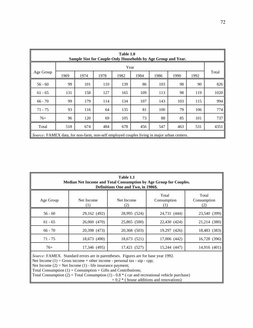
72

Table 1.0 Sample Size for Couple-Only Households by Age Group and Year.

Age GroupYear

Total1969 1974 1978 1982 1984 1986 1990 1992

56 - 60 99 101 110 139 86 103 98 90 826

61 - 65 131 158 127 165 109 113 98 119 1020

66 - 70 99 179 114 134 107 143 103 115 994

71 - 75 93 116 64 135 81 100 79 106 774

76+ 96 120 69 105 73 88 85 101 737

Total 518 674 484 678 456 547 463 531 4351

Source: FAMEX data, for non-farm, non-self employed couples living in major urban centers.

Table 1.1Median Net Income and Total Consumption by Age Group for Couples.

Definitions One and Two, in 1986$.

Age Group Net Income(1)

Net Income

(2)

Total Consumption

(1)

TotalConsumption

(2)

56 - 60 29,162 (492) 28,995 (524) 24,731 (444) 23,540 (399)

61 - 65 26,060 (470) 25,865 (500) 22,430 (424) 21,214 (380)

66 - 70 20,398 (473) 20,368 (503) 19,297 (426) 18,483 (383)

71 - 75 18,673 (490) 18,673 (521) 17,006 (442) 16,728 (396)

76+ 17,346 (495) 17,421 (527) 15,244 (447) 14,916 (401)

Source: FAMEX. Standard errors are in parentheses. Figures are for base year 1992.Net Income (1) = Gross income + other income - personal tax - uip - cpp;Net Income (2) = Net Income (1) - life insurance payment;Total Consumption (1) = Consumption + Gifts and Contributions;Total Consumption (2) = Total Consumption (1) - 0.8 * ( car and recreational vehicle purchase) + 0.2 * ( house additions and renovations)

73

Table 1.2Median Saving by Age Group for Couples.

All Definitions, in 1986$.

Age Group Saving(1)

Saving(2)

Saving(3)

Saving(4)

Saving(Dassets)

56 - 60 3,713 (312) 4,686 (349) 3,418 (265) 4,379 (333) 2,168 (255)

61 - 65 2,464 (297) 3,483 (333) 2,351 (253) 3,401 (318) 1,568 (243)

66 - 70 1,264 (299) 1,879 (335) 1,104 (254) 1,758 (320) 781 (244)

71 - 75 1,565 (310) 1,919 (347) 1,441 (264) 1,740 (332) 781 (253)

76 + 1,755 (314) 1,988 (351) 1,724 (267) 1,970 (335) 974 (257)

Source: FAMEX. Standard errors are in parentheses. Figures are for base year 1992.Saving (1) = Net Income (1)-Total Consumption (1); Saving (2) = Net Income (1) - Total Consumption (2);Saving (3) = Net Income (2)-Total Consumption (1); Saving (4) = Net Income (2) - Total Consumption (2);Saving (Dassets) = Change of Net Assets and Liabilities.

Table 1.3aMedian Saving Rates (%) by Age Group for Couples.

All Definitions

AgeGroup

Saving Rate(1)

Saving Rate(2)

Saving Rate(3)

Saving Rate(4)

Saving Rate(Dasset/Y)

56 - 60 12.6 (1.4) 17.7 (1.6) 12.1 (1.6) 17.5 (1.4) 8.8 (1.0)

61 - 65 10.0 (1.4) 16.6 (1.5) 9.9 (1.5) 15.8 (1.3) 8.2 (1.0)

66 - 70 5.6 (1.4) 10.8 (1.5) 5.2 (1.6) 10.4 (1.3) 4.3 (1.0)

71 - 75 7.5 (1.4) 11.3 (1.6) 7.3 (1.6) 11.2 (1.4) 4.7 (1.0)

76+ 10.2 (1.4) 12.8 (1.6) 10.4 (1.6) 12.9 (1.4) 6.5 (1.0)

Source: FAMEX. Standard errors are in parentheses. Figures are for base year 1992.Saving rate (1)-(4) are saving (1)-(4) divided by their corresponding Net Income.Dassets/Y: Y = After tax income + other money receipts - security payment.

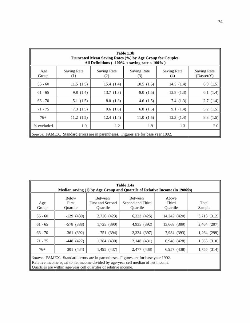
74

Table 1.3bTruncated Mean Saving Rates (%) by Age Group for Couples.

All Definitions ( -100% # saving rate # 100% )

AgeGroup

Saving Rate(1)

Saving Rate(2)

Saving Rate(3)

Saving Rate(4)

Saving Rate(Dasset/Y)

56 - 60 11.5 (1.5) 15.4 (1.4) 10.5 (1.5) 14.5 (1.4) 6.9 (1.5)

61 - 65 9.8 (1.4) 13.7 (1.3) 9.0 (1.5) 12.8 (1.3) 6.1 (1.4)

66 - 70 5.1 (1.5) 8.0 (1.3) 4.6 (1.5) 7.4 (1.3) 2.7 (1.4)

71 - 75 7.3 (1.5) 9.6 (1.6) 6.8 (1.5) 9.1 (1.4) 5.2 (1.5)

76+ 11.2 (1.5) 12.4 (1.4) 11.0 (1.5) 12.3 (1.4) 8.3 (1.5)

% excluded 1.9 1.2 1.9 1.3 2.0

Source: FAMEX. Standard errors are in parentheses. Figures are for base year 1992.

Table 1.4aMedian saving (1) by Age Group and Quartile of Relative Income (in 1986$s)

AgeGroup

BelowFirst

Quartile

Between First and Second

Quartile

Between Second and Third

Quartile

AboveThird

QuartileTotal

Sample

56 - 60 -129 (430) 2,726 (423) 6,323 (425) 14,242 (420) 3,713 (312)

61 - 65 -578 (388) 1,725 (390) 4,935 (392) 13,668 (389) 2,464 (297)

66 - 70 -361 (392) 751 (394) 2,334 (397) 7,984 (393) 1,264 (299)

71 - 75 -448 (427) 1,284 (430) 2,148 (431) 6,948 (428) 1,565 (310)

76+ 301 (434) 1,495 (437) 2,477 (438) 6,957 (438) 1,755 (314)

Source: FAMEX. Standard errors are in parentheses. Figures are for base year 1992.Relative income equal to net income divided by age-year cell median of net income.Quartiles are within age-year cell quartiles of relative income.

75

Table 1.4bMedian saving (2) by Age Group and Quartile of Relative Income (in 1986$s)

AgeGroup

BelowFirst

Quartile

Between First and Second

Quartile

Between Second and Third

Quartile

AboveThird

QuartileTotal

Sample

56 - 60 418 (358) 3,975 (362) 7,047 (365) 16,373 (360) 4,686 (349)

61 - 65 -151 (330) 2,796 (334) 6,695 (336) 14,789 (334) 3,483 (333)

66 - 70 61 (352) 1,263 (337) 3,531 (340) 9,799 (336) 1,879 (335)

71 - 75 -1 (350) 1,656 (367) 2,811 (369) 8,398 (367) 1,919 (347)

76+ 557 (371) 1,931 (376) 3,066 (376) 7,885 (376) 1,988 (351)

Source: FAMEX. Standard errors are in parentheses. Figures are for base year 1992.Relative income equal to net income divided by age-year cell median of net income.Quartiles are within age-year cell quartiles of relative income.

Table 1.5aMedian (%) Saving Rates (1) by Age Group and Quartile of Relative Income

AgeGroup

Belowfirst

Quartile

Between First and Second

Quartile

Between Second and Third

Quartile

AboveThird

QuartileTotal

Sample

56 - 60 -1.1 (2.4) 11.0 (2.4) 18.3 (2.5) 30.7 (2.4) 12.6 (1.4)

61 - 65 -4.5 (2.2) 7.3 (2.3) 16.9 (2.3) 30.7 (2.2) 10.0 (1.4)

66 - 70 -4.0 (2.3) 3.0 (2.3) 9.6 (2.3) 21.8 (2.3) 5.6 (1.4)

71 - 75 -2.5 (2.5) 7.0 (2.5) 10.0 (2.5) 23.8 (2.5) 7.5 (1.4)

76+ 1.4 (2.5) 9.1 (2.5) 12.9 (2.5) 26.1 (2.5) 10.2 (1.4)

Source: FAMEX. Standard errors are in parenthesis. Figures are for base year 1992.Relative income equal to net income divided by age-year cell median of net income.Quartiles are within age-year cell quartiles of relative income.

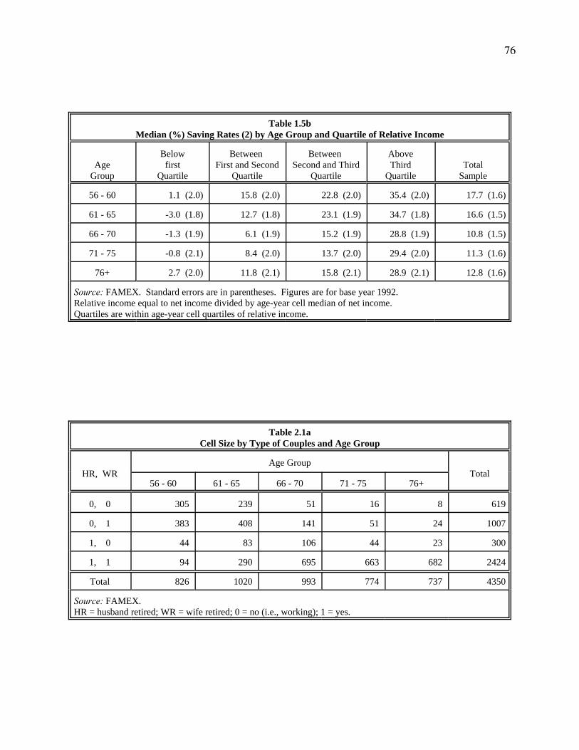
76

Table 1.5bMedian (%) Saving Rates (2) by Age Group and Quartile of Relative Income

AgeGroup

Belowfirst

Quartile

Between First and Second

Quartile

Between Second and Third

Quartile

AboveThird

QuartileTotal

Sample

56 - 60 1.1 (2.0) 15.8 (2.0) 22.8 (2.0) 35.4 (2.0) 17.7 (1.6)

61 - 65 -3.0 (1.8) 12.7 (1.8) 23.1 (1.9) 34.7 (1.8) 16.6 (1.5)

66 - 70 -1.3 (1.9) 6.1 (1.9) 15.2 (1.9) 28.8 (1.9) 10.8 (1.5)

71 - 75 -0.8 (2.1) 8.4 (2.0) 13.7 (2.0) 29.4 (2.0) 11.3 (1.6)

76+ 2.7 (2.0) 11.8 (2.1) 15.8 (2.1) 28.9 (2.1) 12.8 (1.6)

Source: FAMEX. Standard errors are in parentheses. Figures are for base year 1992.Relative income equal to net income divided by age-year cell median of net income.Quartiles are within age-year cell quartiles of relative income.

Table 2.1aCell Size by Type of Couples and Age Group

HR, WR

Age GroupTotal

56 - 60 61 - 65 66 - 70 71 - 75 76+

0, 0 305 239 51 16 8 619

0, 1 383 408 141 51 24 1007

1, 0 44 83 106 44 23 300

1, 1 94 290 695 663 682 2424

Total 826 1020 993 774 737 4350

Source: FAMEX. HR = husband retired; WR = wife retired; 0 = no (i.e., working); 1 = yes.

77

Table 2.1bAverage Differences between the Age of Husband and Wife

by Type of Couples and Age Group.

HR, WRAge Group

Total56 - 60 61 - 65 66 - 70 71 - 75 76+

0, 0 3.6 4.1 6.3 8.3 5.4 4.2

0, 1 1.1 2 3.1 4.8 4.8 2

1, 0 3.3 5.2 6.6 10.1 11.9 6.7

1, 1 1.1 1.4 2.3 3.5 3.2 2.7

Total 2.1 2.6 3.1 4.1 3.6 3

Source: FAMEX. HR = husband retired; WR = wife retired; 0 = no (i.e., working); 1 = yes.

Table 2.2aMedian % Saving Rate (1) by Type of Couples and Age Group

HR, WRAge Group

TotalTest of

Equality( F=..; P>F=..) 56 - 60 61 - 65 66 - 70 71 - 75 76+

0, 0 21.3(2.2)

24.3(2.4)

16.7(4.4)

24.1(7.6)

15.0(10.2)

21.0(1.7)

F = .87P = .4819

0, 1 13.9(2.1)

15.7(2.0)

15.0(2.9)

9.4(4.5)

21.0(6.3)

14.3(1.6)

F = .82P = .5098

1, 0 9.0(4.8)

12.6(3.5)

12.5(3.2)

15.6(4.8)

16.1(6.4)

12.7(2.1)

F = .34P = .8535

1, 1 -2.4(3.4)

0.5(2.2)

4.8(1.7)

8.6(1.7)

11.3(1.7)

6.3(1.3)

F = 10.07P = .0000

Total 12.6(1.4)

10.0(1.4)

5.6(1.4)

7.5(1.4)

10.2(1.4)

10.0(1.3)

F = 9.32P = .0000

Source: FAMEX. Standard errors (in %) are in parentheses. Figures are for base year 1992.HR = husband retired; WR = wife retired; 0 = no (i.e., working); 1 = yes.

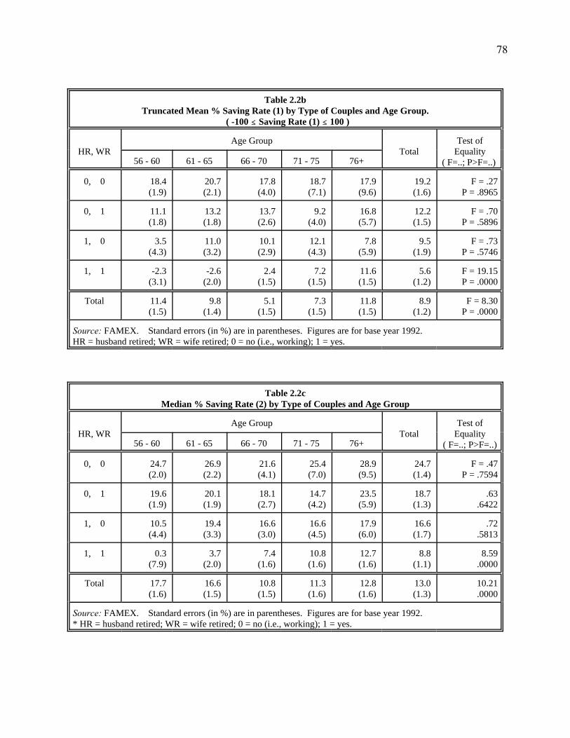
78

Table 2.2bTruncated Mean % Saving Rate (1) by Type of Couples and Age Group.

( -100 # Saving Rate (1) # 100 )

HR, WRAge Group

TotalTest of

Equality( F=..; P>F=..) 56 - 60 61 - 65 66 - 70 71 - 75 76+

0, 0 18.4(1.9)

20.7(2.1)

17.8(4.0)

18.7(7.1)

17.9(9.6)

19.2(1.6)

F = .27P = .8965

0, 1 11.1(1.8)

13.2(1.8)

13.7(2.6)

9.2(4.0)

16.8(5.7)

12.2(1.5)

F = .70P = .5896

1, 0 3.5(4.3)

11.0(3.2)

10.1(2.9)

12.1(4.3)

7.8(5.9)

9.5(1.9)

F = .73P = .5746

1, 1 -2.3(3.1)

-2.6(2.0)

2.4(1.5)

7.2(1.5)

11.6(1.5)

5.6(1.2)

F = 19.15P = .0000

Total 11.4(1.5)

9.8(1.4)

5.1(1.5)

7.3(1.5)

11.8(1.5)

8.9(1.2)

F = 8.30P = .0000

Source: FAMEX. Standard errors (in %) are in parentheses. Figures are for base year 1992.HR = husband retired; WR = wife retired; 0 = no (i.e., working); 1 = yes.

Table 2.2cMedian % Saving Rate (2) by Type of Couples and Age Group

HR, WRAge Group

TotalTest of

Equality( F=..; P>F=..)56 - 60 61 - 65 66 - 70 71 - 75 76+

0, 0 24.7(2.0)

26.9(2.2)

21.6(4.1)

25.4(7.0)

28.9(9.5)

24.7(1.4)

F = .47P = .7594

0, 1 19.6(1.9)

20.1(1.9)

18.1(2.7)

14.7(4.2)

23.5(5.9)

18.7(1.3)

.63.6422

1, 0 10.5(4.4)

19.4(3.3)

16.6(3.0)

16.6(4.5)

17.9(6.0)

16.6(1.7)

.72.5813

1, 1 0.3(7.9)

3.7(2.0)

7.4(1.6)

10.8(1.6)

12.7(1.6)

8.8(1.1)

8.59.0000

Total 17.7(1.6)

16.6(1.5)

10.8(1.5)

11.3(1.6)

12.8(1.6)

13.0(1.3)

10.21.0000

Source: FAMEX. Standard errors (in %) are in parentheses. Figures are for base year 1992.* HR = husband retired; WR = wife retired; 0 = no (i.e., working); 1 = yes.

79

Table 2.2dCompare to Table 2.2a: Cross-Section data, but include self-employed

Median % Saving Rate (1) by Type of Couples and Age Group

HR, WRAge Group

TotalTest of

Equality( F=..; P>F=..) 56 - 60 61 - 65 66 - 70 71 - 75 76+

0, 0 20.9(2.0)

24.0(2.3)

20.1(4.0)

15.3(6.9)

13.5(10.2)

20.6(1.6)

F = .80P = .5220

0, 1 13.0(2.0)

14.4(2.0)

11.0(2.8)

13.8(4.1)

20.8(5.8)

12.9(1.5)

F = .81P = .5183

1, 0 10.0(4.5)

12.6(3.5)

14.6(3.3)

15.7(4.5)

16.1(6.1)

12.9(2.0)

F = .31P = .8733

1, 1 0.0(3.4)

0.6(2.2)

4.7(1.7)

8.9(1.7)

11.1(1.7)

6.3(1.3)

F = 8.33P = .0000

Total 13.2(1.4)

10.6(1.4)

6.2(1.4)

8.2(1.5)

10.9(1.5)

10.1(1.2)

F = 8.57P = .0000

Source: FAMEX. Standard errors (in %) are in parentheses. Figures are for base year 1992.HR = husband retired; WR = wife retired; 0 = no (i.e., working); 1 = yes.

Table 2.2eCompare to Table 2.2a: Cohort Data, no self-employed & farmMedian % Saving Rate (1) by Type of Couples and Age Group

HR, WRAge Group

TotalTest of

Equality( F=..; P>F=..) 56 - 60 61 - 65 66 - 70 71 - 75 76+

0, 0 23.0(2.5)

25.3(2.4)

17.8(4.1)

10.6(7.4)

14.3(9.7)

25.5(1.5)

F = 1.69P = .1494

0, 1 15.1(2.2)

15.7(2.0)

11.8(2.7)

16.1(4.5)

14.2(7.4)

17.4(1.4)

F = .52P = .7183

1, 0 6.3(5.8)

12.3(3.6)

11.3(2.9)

13.1(4.3)

31.0(7.6)

14.5(1.8)

F = 1.84P = .1180

1, 1 -0.6(3.5)

2.1(2.2)

6.1(1.6)

9.1(1.5)

12.5(1.5)

9.8(1.0)

F = 8.25P = .0000

Total 14.5(1.9)

12.5(1.7)

7.9(1.5)

9.8(1.4)

12.6(1.5)

10.8(1.2)

F = 6.58P = .0000

Source: FAMEX. Standard errors (in %) are in parentheses. Figures are for base year 1992.HR = husband retired; WR = wife retired; 0 = no (i.e., working); 1 = yes.

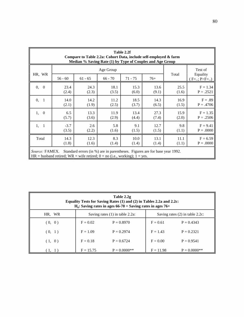
80

Table 2.2fCompare to Table 2.2a: Cohort Data, include self-employed & farm

Median % Saving Rate (1) by Type of Couples and Age Group

HR, WRAge Group

TotalTest of

Equality( F=..; P>F=..) 56 - 60 61 - 65 66 - 70 71 - 75 76+

0, 0 23.4(2.4)

24.3(2.3)

18.1(3.5)

15.3(6.0)

13.6(9.1)

25.5(1.6)

F = 1.34P = .2521

0, 1 14.0(2.1)

14.2(1.9)

11.2(2.5)

18.5(3.7)

14.3(6.5)

16.9(1.5)

F = .89P = .4706

1, 0 6.5(5.7)

13.3(3.6)

11.9(2.9)

13.4(4.4)

27.3(7.4)

15.9(2.0)

F = 1.35P = .2506

1, 1 -3.7(3.5)

2.6(2.2)

5.8(1.6)

9.1(1.5)

12.7(1.5)

9.8(1.1)

F = 9.41P = .0000

Total 14.3(1.8)

12.3(1.6)

8.3(1.4)

10.0(1.4)

13.1(1.4)

11.1(1.1)

F = 6.59P = .0000

Source: FAMEX. Standard errors (in %) are in parentheses. Figures are for base year 1992.HR = husband retired; WR = wife retired; 0 = no (i.e., working); 1 = yes.

Table 2.2gEquality Tests for Saving Rates (1) and (2) in Tables 2.2a and 2.2c:

H0: Saving rates in ages 66-70 = Saving rates in ages 76+

HR, WR Saving rates (1) in table 2.2a: Saving rates (2) in table 2.2c:

( 0, 0 )

( 0, 1 )

( 1, 0 )

( 1, 1 )

F = 0.02 P = 0.8970

F = 1.09 P = 0.2974

F = 0.18 P = 0.6724

F = 15.75 P = 0.0000**

F = 0.61 P = 0.4343

F = 1.43 P = 0.2321

F = 0.00 P = 0.9541

F = 11.98 P = 0.0000**

81

Table 2.3Median Regressions for Saving Rate (1) and Log Net Income

VariableSaving Rate (1)

(1)Saving Rate (1)

(2)Saving Rate (1)

(3)Log Net Income

(4)

Type-Age CellDummies

---- ---- ---- ----

Year 1969 -7.13 (1.9) -4.96 (1.8) 3.99 (1.7) -.3686 (.025)

Year 1974 -1.38 (1.8) 1.28 (1.7) 6.99 (1.6) -.2748 (.023)

Year 1978 2.84 (1.9) 4.56 (1.8) 5.71 (1.7) -.0914 (.025)

Year 1982 5.12 (1.8) 7.06 (1.7) 8.85 (1.5) -.0369 (.023)

Year 1984 2.45 (2.0) 3.69 (1.8) 2.70 (1.7) -.0073 (.025)

Year 1986 1.81 (1.9) 2.97 (1.7) 1.16 (1.6) .0008 (.024)

Year 1990 0.79 (2.0) 1.07 (1.8) 0.61 (1.7) .0162 (.025)

Log Net Income ---- ---- 27.24 (1.0) ----

Post High school ---- 5.51 (1.4) -9.59 (1.4) .5271 (.019)

High School ---- 1.19 (1.0) -3.31 (0.9) .1988 (.013)

Home Owner ---- 5.83 (0.9) 3.27 (0.8) .0626 (.012)

Pseudo R square 0.0354 0.0442 0.128 0.2846

Source: FAMEX. Standard errors in parenthesis.Coefficients and standard errors for three Saving Rate regressions are multiplied by 100 (i.e., in %).Omitted categories are: year 1992, elementary school and non-homeowner.

82

Table 2.4Median % Saving Rate (1) by Type of Couples and Age Group,

Conditional on Education and Homeownership.

HR, WRAge Group

TotalTest of

Equality( F=..; P>F=..) 56 - 60 61- 65 66 - 70 71 - 75 76+

0, 0 21.8(2.1)

24.0(2.3)

18.3(4.2)

28.5(7.0)

15.0(9.5)

22.8(1.9)

F = .86P = .4867

0, 1 15.9(2.0)

16.1(1.9)

15.2(2.8)

11.4(4.2)

18.3(5.9)

16.2(1.8)

F = .38P = .8196

1, 0 9.8(4.5)

14.1(3.3)

12.1(3.0)

16.3(4.5)

20.9(6.0)

14.9(2.2)

F = .78P = .5397

1, 1 0.2(6.3)

2.8(2.2)

6.1(1.7)

9.4(1.7)

12.5(1.7)

9.2(1.5)

F = 9.74P = .0000

Total 15.8(1.6)

12.3(1.5)

8.3(1.5)

9.6(1.6)

12.3(1.6)

10.8(1.2)

F = 9.20P = .0000

Source: FAMEX. Standard errors (in %) are in parentheses.HR = husband retired; WR = wife retired; 0 = no (i.e., working); 1 = yes.Base group is: highschool education, homeowner and year 1992.

Table 2.5Median Log Net Income (1) by Type of Couples and Age Group,

Conditional Education and Homeownership.

HR, WRAge Group

Total56 - 60 61 - 65 66 - 70 71 - 75 76+

0, 0 10.562(.028)

10.468(.031)

10.350(.057)

10.434(.099)

10.496(.130)

10.516(.024)

0, 1 10.291(.027)

10.262(.027)

10.200(.038)

10.157(.057)

10.287(.080)

10.274(.022)

1, 0 10.098(.061)

10.296(.045)

10.225(.041)

10.208(.061)

10.091(.082)

10.239(.028)

1, 1 9.668(.044)

9.839(.029)

9.898(.023)

9.867(.023)

9.804(.023)

9.866(.019)

Total 10.314(.026)

10.203(.025)

9.962(.025)

9.891(.025)

9.808(.026)

10.024(.032)

Source: FAMEX. Standard errors are in parenthese.HR = husband retired; WR = wife retired; 0 = no (i.e., working); 1 = yes.Base group is: highschool education, homeowner and year 1992.

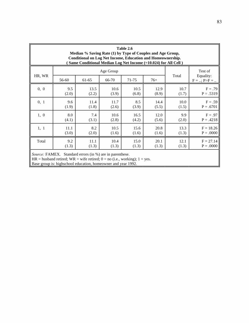
83

Table 2.6Median % Saving Rate (1) by Type of Couples and Age Group,

Conditional on Log Net Income, Education and Homeownership.( Same Conditional Median Log Net Income (=10.024) for All Cell )

HR, WRAge Group

TotalTest of

Equality:F = ..; P>F = ..56-60 61-65 66-70 71-75 76+

0, 0 9.5(2.0)

13.5(2.2)

10.6(3.9)

10.5(6.8)

12.9(8.9)

10.7(1.7)

F = .79P = .5319

0, 1 9.6(1.9)

11.4(1.8)

11.7(2.6)

8.5(3.9)

14.4(5.5)

10.0(1.5)

F = .59P = .6701

1, 0 8.0(4.1)

7.4(3.1)

10.6(2.8)

16.5(4.2)

12.0(5.6)

9.9(2.0)

F = .97P = .4218

1, 1 11.1(3.0)

8.2(2.0)

10.5(1.6)

15.6(1.6)

20.8(1.6)

13.3(1.3)

F = 18.26P = .0000

Total 9.2(1.3)

11.1(1.3)

10.4(1.3)

15.0(1.3)

20.1(1.3)

12.1(1.3)

F = 27.14P = .0000

Source: FAMEX. Standard errors (in %) are in parenthese.HR = husband retired; WR = wife retired; 0 = no (i.e., working); 1 = yes.Base group is: highschool education, homeowner and year 1992.

84

Table 3.1Proportion Both Spouses are not Working, by Age and Cohort

For Couples-Only Households

Age Group

Cohort Number( Year Household Heads Were Born )

Total100-Total

1, 2(1905-1908)

3, 4(1909-1912)

5, 6(1913-1916)

7, 8(1917-1920)

9, 10(1921-1924)

54 - 57 - - (69) 4.3 (74) 10.8 (78) 10.8 8.1 91.9

58 - 61 - (69) 8.8 (74) 14.3 (78) 11.6 (82) 18.9 13.3 86.7

60 - 63 - - - - (84) 22.7 22.7 77.3

62 - 65 (69) 14.0 (74) 25.8 (78) 30.9 (82) 30.0 (86) 43.6 28.1 71.9

64 -67 - - - (84) 57.3 - 57.3 42.7

66 - 69 (74) 67.6 (78) 63.2 (82) 75.9 (86) 78.9 (90) 75.3 72.3 27.7

68 - 71 - - (84) 74.2 - (92) 82.2 79.7 20.3

70 - 73 (78) 82.1 (82) 86.0 (86) 88.2 (90) 85.5 - 85.5 14.5

72 - 75 - (84) 84.1 - (92) 87.0 - 86.2 13.8

74 - 77* (82) 93.2 (86) 90.4 (90) 93.9 - - 92.6 7.4

76+ (84) 94.5 - (92) 95.7 - - 95.4 4.6

Source: FAMEX.1. The last column gives the proportion of at least one of spouses working for each age group.2. In sample year 1969, the age group selected is one year younger than indicated (e.g., in cohort 1 and 2 year 69, the age group is 61-64 instead of 62-65) in order to keep the households within the same cohort.3. For age group 74-77*, only in sample year 1986 is it the indicated age 74-77, other two years 1982 and 1990include ages 74, 75 and 76+ because of the topcoding in the data.4. Sample years are in parentheses; figures are for each pair of cohorts indicated.

85

Table 3.2Median Regressions for Income, Consumption and Saving Rates

for Overall Age Profiles of the Elderly Couples

Median Regression

Log Net Income Log Consumption Saving Rate

Coef. | t | Coef. | t | Coef. | t |

23 age dummies

interest rateinflation rate

unemploy. raterural area

East CoastQuebecPrairie

British Columbiacohort 1cohort 2cohort 3cohort 4cohort 5cohort 6cohort 7cohort 8cohort 9

_cons

(See Fig. 1.1)

.0039 0.74 .0016 0.34.0087 1.12-.1680 6.24-.1794 6.75-.1723 5.94-.0356 1.41 .0338 1.18-.2663 4.02-.2702 4.43-.1994 3.42-.1646 3.01-.1135 2.17-.1271 2.72-.0556 1.17-.0002 0.00 -.0083 0.189.8485 88.21

(See Fig. 1.2)

.0014 0.32-.0039 1.09-.0082 1.34-.1816 8.49-.1393 6.60-.1219 5.30-.0457 2.29 .0253 1.11-.3231 6.16-.3093 6.41-.2345 5.09-.1678 3.88-.1611 3.90-.1624 4.39-.0900 2.40-.0154 0.46-.0342 0.94

9.9387 112.67

(See Fig. 1.3b)

.0000 0.02 .0030 1.50 .0087 2.60-.0190 1.63-.0271 2.35-.0507 4.04 .0076 0.70-.0112 0.90 .0252 0.88 .0130 0.49 .0243 0.97 .0031 0.13 .0117 0.52 .0081 0.40 .0305 1.49 .0319 1.72 .0053 0.27 .0379 0.79

N: Pseudo R2:

49150.1073

49200.0964

49150.0123

Joint F Tests: All Coefficients of the Indicated Groups Are Zeros ( P-Values in %)

Age effect (23):

Cohort effect (9)

Macro effect (3):

Provinces (4):

F=4.23 P=.00**

F= 4.21 P=.00**

F= 2.26 P=7.95

F=23.41 P=.00**

F= 2.12 P=.14**

F= 7.92 P=.00**

F= 2.10 P=9.86

F= 20.9 P=.00**

F= 2.38 P=.02**

F= 0.83 P=58.50

F= 7.57 P=.00**

F= 7.09 P=.00**

Source: FAMEX.The omitted group is: age 76+, cohort 10 and province Ontario.In the test results, * indicates significance at the 5% level, ** indicates sig. at the 1% level.

86

Table 3.3Equality Tests of the Age Effect

For the Saving Rate Regression in Table 3.3 and in Fig. 1.3b

H0: Saving rates of pre-retirement ages =Saving rates at ages just following retirement

H0: Saving rates at ages just following retirement =Saving rates at later retirement ages

avg (pre-ages) = avg (ret-ages) F= P= (in %) avg (ret-ages) = avg (later-ages) F= P= (in %)

avg (59 - 62) = avg (66 - 69)

avg (59 - 63) = avg (65 - 69)

24.87 0.00**

28.24 0.00**

avg (66 - 67) = avg (75 - 76)

avg (66 - 68) = avg (74 - 76)

avg (66 - 69) = avg (73 - 76)

avg (65 - 69) = avg (72 - 76)

avg (65 - 69) = avg (71 - 76)

8.90 0.29**

7.99 0.47**

7.32 0.68**

5.61 1.79*

7.17 0.74**

Table 3.4Median Saving Rate Regressions Separated by Relative Income Quartiles

For Elderly Couples

MedianRegression

Within FirstQuartile

Coef. | t |

Within SecondQuartile

Coef. | t |

Within ThirdQuartile

Coef. | t |

Within Fourth Quar-tile

Coef. | t |

23 age dummies9 cohort dummies

interest rateinflation rate

unemploy. raterural area

East CoastQuebecPrairie

British Columbia

(See Fig. 1.5)(Omitted)

.0004 0.09

.0050 1.38

.0069 1.12

.0308 1.68

.1566 7.16

.1149 4.86

.0882 3.80

.0935 3.64

(See Fig. 1.5)(Omitted)

-.0001 0.03 .0002 0.05 .0124 1.69 .0102 0.44 .0183 0.74-.0051 0.19 .0197 0.84 .0069 0.24

(See Fig. 1.5)(Omitted)

.0055 1.06 .0040 0.90 .0085 1.10-.0189 0.65-.0308 1.15-.0453 1.55-.0154 0.64-.0011 0.04

(See Fig. 1.5)(Omitted)

.0015 0.29 .0131 2.98 .0018 0.24 .0212 0.54 .0177 0.64-.0508 1.66 .0115 0.51 .0102 0.40

N: Pseudo R2:

12540.0344

12200.0261

12070.0425

12340.0509

Joint F Tests: all Group Coefficients Are Zeros

Group Coefficients F= P=(in%) F= P=(in%) F= P=(in%) F= P=(in%)

Ages (23):

Cohorts (9)

Macro effect (3):

Provinces (4):

1.04 40.53

1.68 8.90

3.10 2.59*

13.21 .00**

1.13 30.33

0.43 91.68

1.55 20.04

0.39 81.71

1.66 2.65*

0.65 75.55

4.57 0.34**

0.86 48.77

1.71 1.95*

1.04 40.77

7.50 .00**

1.28 27.78

Source: FAMEX. * indicates significance at the 5% level; ** indicates significance at the 1% level.

87

Table 3.5Median Regressions for Income, Consumption and Saving Rates

Controlling for Retirement, Education and Homeownership

Median RegressionLog Net Income Log Consumption Saving Rate

Coef. | t | Coef. | t | Coef. | t |

23 age dummies24 ret. & ret*age dummies

9 cohort dummies

non-homeownerelementary school

post highschoolinterest rate

inflation rateunemploy. rate

rural areaEast Coast

QuebecPrairie

British Columbia

(See Fig. 1.6a)(See Fig. 1.6a)

(Omitted)

-.0450 3.90-.1883 15.8 .3209 18.7 .0004 0.12 .0048 1.70 .0135 2.81-.1099 6.41-.1379 8.34-.0755 4.12-.0165 1.06 .0187 1.05

(See Fig. 1.6a)(See Fig. 1.6a)

(Omitted)

.0244 1.59-.1878 11.8 .2588 11.3-.0002 0.04-.0035 0.93 .0016 0.26-.0845 3.70-.1178 5.34-.0583 2.39-.0261 1.25 .0025 0.11

(See Fig. 1.6b)(See Fig. 1.6b)

(Omitted)

-.0535 5.78-.0244 2.54 .0506 3.67-.0002 0.06 .0042 1.86 .0064 1.65-.0228 1.66-.0046 0.35-.0178 1.21 .0139 1.11-.0039 0.27

N: Pseudo R2:

49150.2372

49200.1779

49150.0347

Joint F Tests: All Coefficients of the Indicated Groups Are Zeros ( P-Values in%)

Age effect (46):

Retirement effect (24):

Interaction effect (23):

education effect (2):

Cohort effect (9):

Macro effect (3):

Provinces (4):

F=18.4 P=.00**

F= 50.1 P=.00**

F=9.28 P=.00**

F= 417 P=.00**

F=10.7 P=.00**

F=9.68 P=.00**

F=27.0 P=.00**

F=1.67 P=.32**

F=9.32 P=.00**

F=1.57 P=4.05*

F=187 P=.00**

F=5.64 P=.00**

F=0.51 P=67.60

F=9.47 P=.00**

F=24.6 P=.00**

F=12.2 P=.00**

F=6.56 P=.00**

F=13.8 P=.00**

F=0.68 P=72.65

F=5.59 P=.08**

F=1.35 P=24.77

Source: FAMEX.The omitted group is: age 76+, cohort 10, province Ontario, not both retired, homeowner and highschooleducation of the household head.In the test results, * indicates significance at the 5% level, ** indicates sig. at the 1% level.

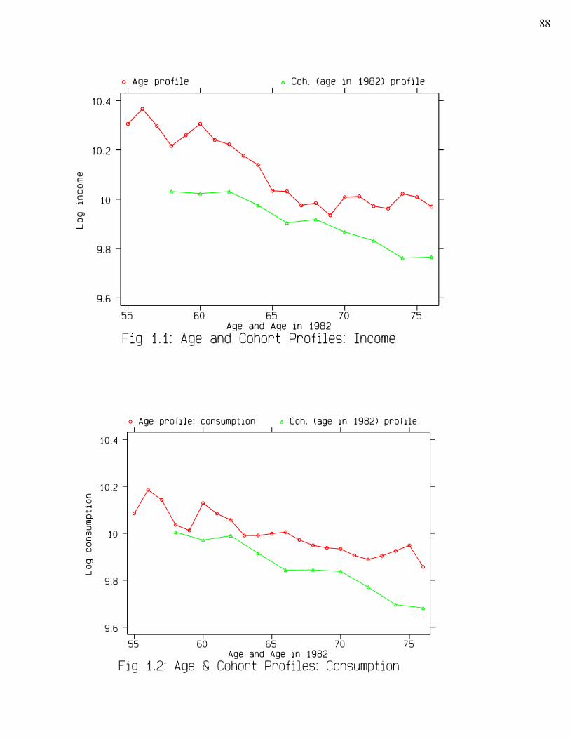
88

89

90

91

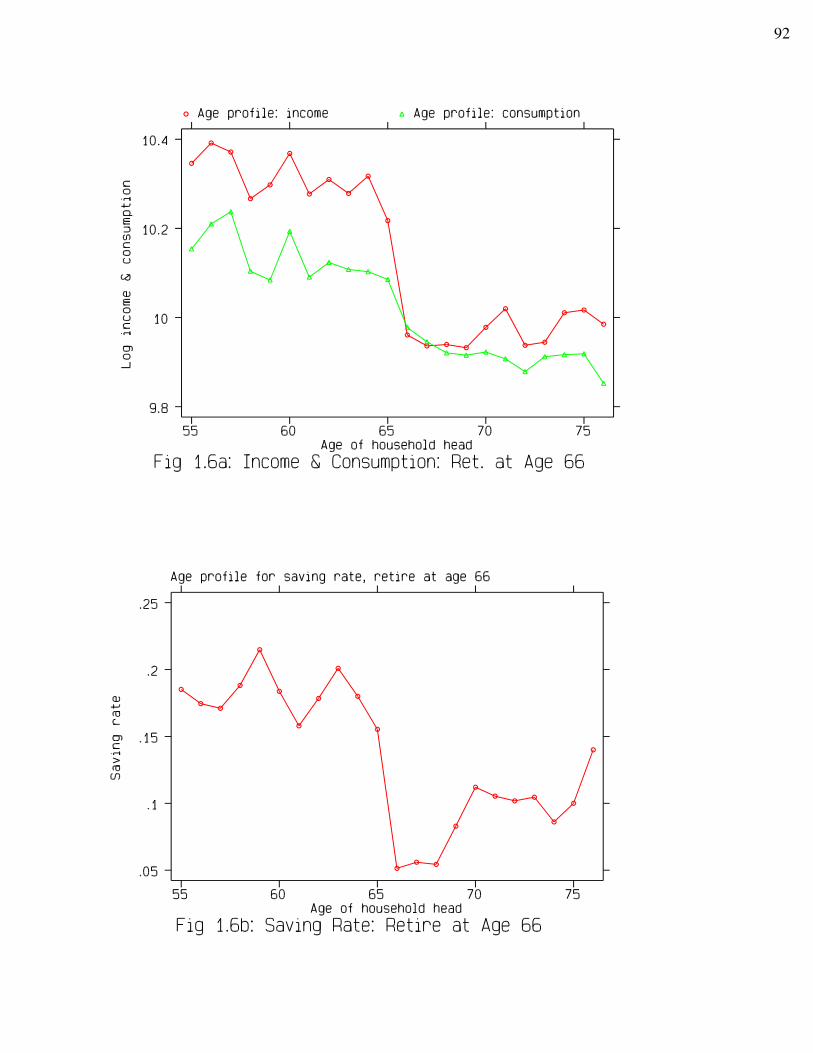
92

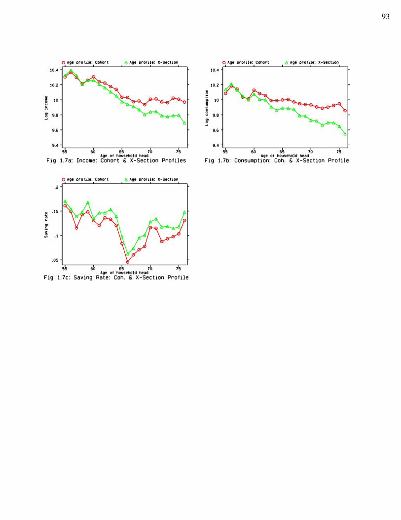
93

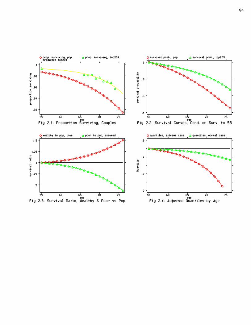
94

95

96

97

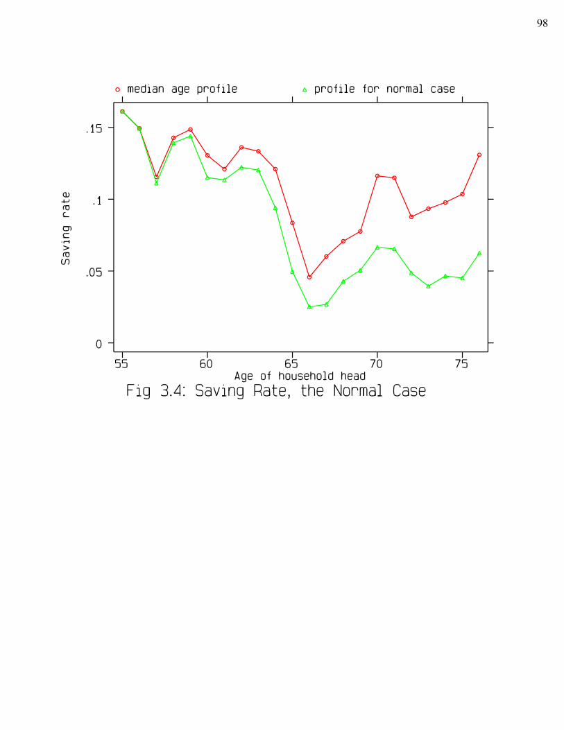
98