scalable implicit methods, scidac, and ice sheet modelingkd2112/icesheets09.pdf · ice sheet...

Ice Sheet Modeling 16-Sep-2009

David Keyes

Towards Optimal Petascale Simulations (TOPS), SciDAC Program, U.S. DOE

Mathematical and Computer Sciences & Engineering, KAUST

Applied Physics & Applied Mathematics, Columbia University

Scalable Implicit Methods,

SciDAC, and

Ice Sheet Modeling

Slides of this lecture are available at

http://www.columbia.edu/~kd2112/IceSheets09.pdf


Caveats �� My HPC colleagues can now go to get coffee

�� Nothing particularly new in this talk

�� My new geophysics/glaciologist/climatologist colleagues may at first

think the talk has limited perspective

�� In fact, it is of very broad perspective

�� The feel of limited perspective is related to my relative newcomer status to

ice sheets

�� No one is naïve enough to think that all PDEs are the same; ice sheet

modeling will have unique difficulties, which we in the enabling

technologies of computational science read as unique opportunities

�� We know that we have a lot to learn before we present to your colleagues

at geophysical or climate meetings, but this is an internal, working meeting

among new colleagues who are getting acquainted

�� This talk is designed to acquaint with a particular SciDAC

center, which is representative of a wealth of others

�� We are all working on software for general purposes that is

customizable under a relatively stable interface to particular purposes


Another caveat

�� The number of slides in this talk exceeds my

time limit �� I will skip many of them, but I wanted to leave you with a

document with more detail for later exploration

�� A review that captures the spirit of this talk is also available:

�� D. A. Knoll , D. E. Keyes, Jacobian-free Newton-Krylov methods: a

survey of approaches and applications, Journal of Computational

Physics, v.193 n.2, p.357-397, 2004

“I have only made this letter longer because I have

not had the time to make it shorter.”

Blaise Pascal (1623-1662), Lettres provinciales.


Going implicit?

�� Why you would, if you could :

1.� multiscale problems with good scale separation

2.� coupled problems (“multiphysics”)

3.� problems with uncertain or controllable inputs

(optimization: design, control, inversion)

�� You can, so you should !

1.� optimal and scalable algorithms known

2.� freely available software

3.� reasonable learning curve that harvests legacy

code


Current focus on Jacobian-free implicit methods

�� Two stories to track in

supercomputing

�� raise the peak capability

�� lower the entry threshold

higher capability

for hero users

best practices

for all users

New York

Blue at

BNL

(#45 on

the Top

500)

first frontier

“new” frontier

�� Jacobian a steep price,

in terms of coding

�� very valuable to have, but

not necessary

�� approximations thereto

often sufficient

�� meanwhile, automatic

differentiation tools are

lowering the threshold


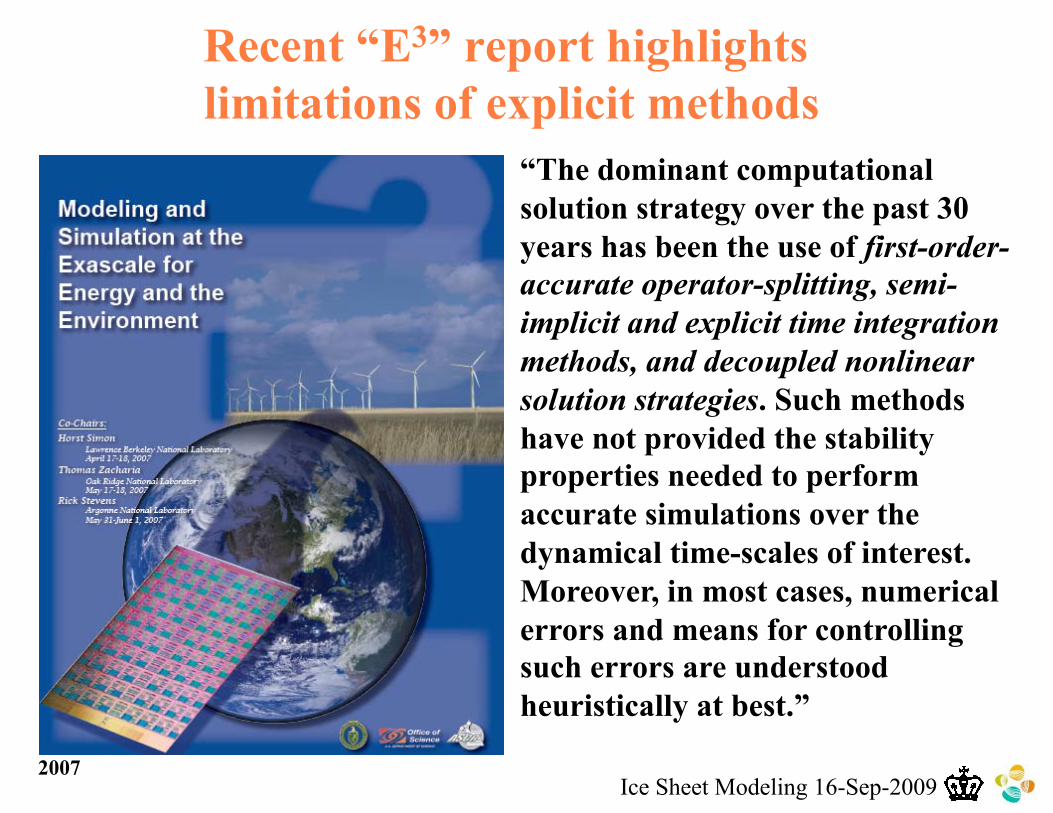
Recent “E3” report highlights

limitations of explicit methods

“The dominant computational

solution strategy over the past 30

years has been the use of first-order-

accurate operator-splitting, semi-

implicit and explicit time integration

methods, and decoupled nonlinear

solution strategies. Such methods

have not provided the stability

properties needed to perform

accurate simulations over the

dynamical time-scales of interest.

Moreover, in most cases, numerical

errors and means for controlling

such errors are understood

heuristically at best.”

2007


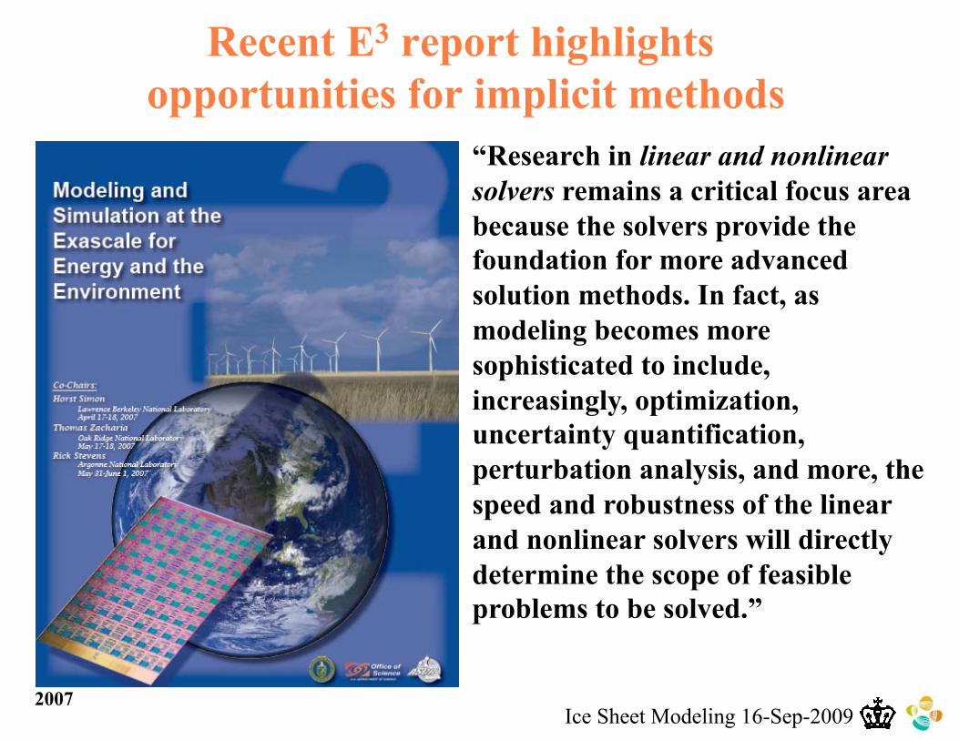
Recent E3 report highlights

opportunities for implicit methods

“Research in linear and nonlinear

solvers remains a critical focus area

because the solvers provide the

foundation for more advanced

solution methods. In fact, as

modeling becomes more

sophisticated to include,

increasingly, optimization,

uncertainty quantification,

perturbation analysis, and more, the

speed and robustness of the linear

and nonlinear solvers will directly

determine the scope of feasible

problems to be solved.”

2007


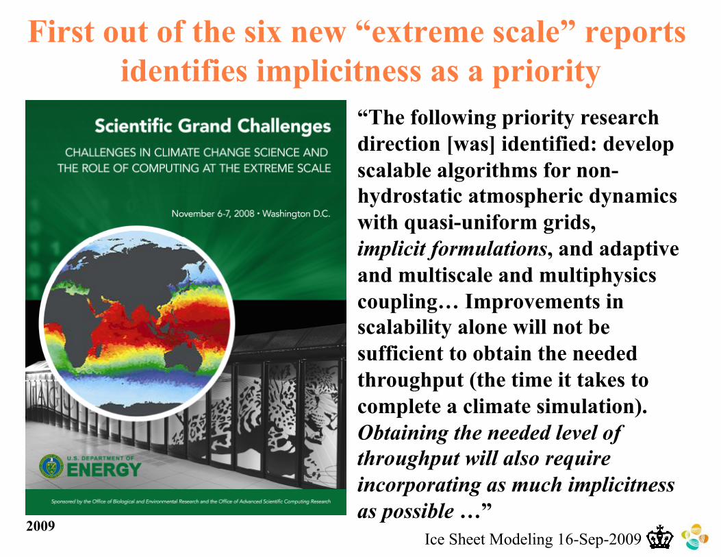
First out of the six new “extreme scale” reports

identifies implicitness as a priority

“The following priority research

direction [was] identified: develop

scalable algorithms for non-

hydrostatic atmospheric dynamics

with quasi-uniform grids,

implicit formulations, and adaptive

and multiscale and multiphysics

coupling… Improvements in

scalability alone will not be

sufficient to obtain the needed

throughput (the time it takes to

complete a climate simulation).

Obtaining the needed level of

throughput will also require

incorporating as much implicitness

as possible …” 2009


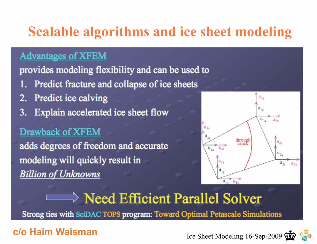
Scalable algorithms and ice sheet modeling

c/o Haim Waisman


2002

2003

2003-2004 (2 vol )

2004 2006

2006

2007

Some reports predicated upon

scalable implicit

solvers

Fusion Simulation

Project

June 2007

2007

Mathematical

Challenges for the

Department of

Energy

January 2008

2008

These are

all downloadable;

e-mail me for pointers


Plan of presentation

�� Motivations for implicit solvers

�� multi-scale, multi-physics, multi-solve (sensitivity, stability,

uncertainty quantification, design, control, inversion)

�� one-dimensional model problems, linear and nonlinear

�� State-of-the-art for large-scale nonlinearly implicit

solvers

�� brief look at algorithms and software

�� intuition about how they scale

�� An illustrative story from the trenches

�� an undergraduate semester project “gone Broadway”


“Explicit” versus “implicit”

�� Implicit methods solve a

function of state data at the

current time, to update all

components simultaneously

�� equivalent to inverting a

matrix, in linear problems

�� Explicit methods evaluate a

function of state data at

prior time, to update each

component of the current

state independently

�� equivalent to matrix-vector

multiplication, in linear

problems


Explicit methods can be unstable –

linear example

Stable

for all �

Unstable

for �>1/2

c/o K. Morton & D. Mayers, 2005

initial

data

after 1

step

after 25

steps

after 50

steps

�t = 0.0012 �t = 0.0013


Explicit methods can be unphysically oscillatory –

nonlinear example (“profile stiffness”)

Linearly implicit, nonlinearly explicit:

Linearly and nonlinearly implicit:

history at station 10

history at station 10

Oscillatory

Non-

oscillatory


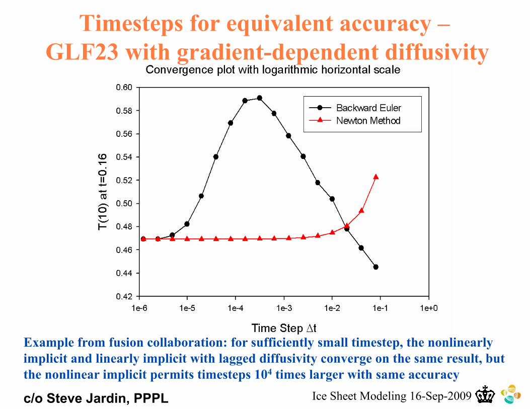
Timesteps for equivalent accuracy –

GLF23 with gradient-dependent diffusivity

Example from fusion collaboration: for sufficiently small timestep, the nonlinearly

implicit and linearly implicit with lagged diffusivity converge on the same result, but

the nonlinear implicit permits timesteps 104 times larger with same accuracy

c/o Steve Jardin, PPPL


However –

implicit methods can be unruly and expensive

Explicit Naïve Implicit

Reliability robust when stable uncertain

Performance predictable data-dependent

Concurrency O(N) limited

Synchronization once per step many times per step

Communication nearest neighbor* global, in principle

Workspace O(N) O(Nw), e.g., w=5/3

Complexity O(N) O(Nc), e.g., c=7/3

* plus the estimation of the stable step size


Motivation #1:

Many simulation opportunities are multiscale �� Multiple spatial scales

�� interfaces, fronts, layers

�� thin relative to domain

size, � << L

�� Multiple temporal scales

�� fast waves

�� small transit times

relative to convection or

diffusion, � << T

�� Analyst must isolate dynamics of interest and model the rest in a

system that can be discretized over more modest range of scales

�� Often involves filtering of high frequency modes, quasi-

equilibrium assumptions, etc.

�� May lead to infinitely “stiff” subsystem requiring implicit

treatment

Richtmyer-Meshkov instability, c/o A. Mirin, LLNL


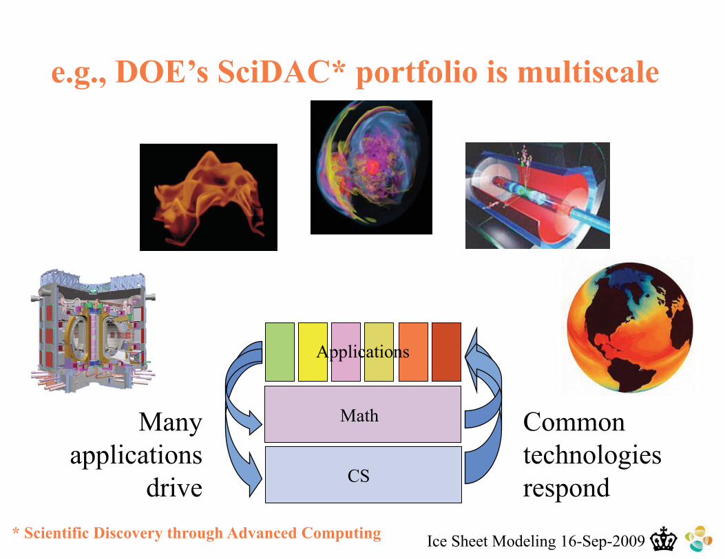
CS

Math

Applications

Common

technologies

respond

Many

applications

drive

e.g., DOE’s SciDAC* portfolio is multiscale

* Scientific Discovery through Advanced Computing


Examples of scale-separated features

of multiscale problems

�� Gravity surface waves in global climate

�� Alfvén waves in tokamaks

�� Acoustic waves in aerodynamics

�� Fast transients in detailed kinetics chemical

reaction

�� Bond vibrations in protein folding (?)

Explicit methods are restricted to marching out the long-scale dynamics

on short scales. Implicit methods can “step over” or “filter out” with

equilibrium assumptions the dynamically irrelevant short scales,

ignoring stability bounds. (Accuracy bounds must still be satisfied; for

long time steps, one can use high-order temporal integration schemes!)

IBM’s BlueGene/P: 72K

quad-core procs w/ 2

FMADD @ 850 MHz

= 1.008 Pflop/s

13.6 GF/s

8 MB EDRAM

4 processors

1 chip

13.6 GF/s

2 GB DDRAM

32 compute cards

435 GF/s

64 GB

32 node cards

72 racks

1 PF/s

144 TB

Rack

System

Node Card

Compute Card

Chip

14 TF/s

2 TB

Thread concurrency:

288K (or 294,912) processors

Available at Argonne

National Laboratory soon

What’s “big iron” for, if not multiscale?


Review: two definitions of scalability �� “Strong scaling”

�� execution time (T) decreases in

inverse proportion to the number

of processors (p)

�� fixed size problem (N) overall

�� often instead graphed as

reciprocal, “speedup”

�� “Weak scaling” (memory

bound)

�� execution time remains constant,

as problem size and processor

number are increased in

proportion

�� fixed size problem per processor

�� also known as “Gustafson scaling”

T

p

good

poor

poor

N � p

log T

log p

good

Slope

= -1

Slope

= 0


�� Algebraic multigrid a key algorithmic technology �� Discrete operator defined for finest grid by the application, itself, and for many

recursively derived levels with successively fewer degrees of freedom, for solver purposes

�� Unlike geometric multigrid, AMG not restricted to problems with “natural” coarsenings derived from grid alone

�� Optimality (cost per cycle) intimately tied to the ability to coarsen aggressively

�� Convergence scalability (number of cycles) and parallel efficiency also sensitive to rate of coarsening

Solvers are scaling:

algebraic multigrid (AMG) on BG/L (hypre)

Figure shows weak scaling result for AMG out to

120K processors, with one 25��25��25block per

processor (up to 1.875B dofs) procs

�� While much research and development remains, multigrid will clearly be practical at BG/P-scale concurrency 2B dofs

15.6K dofs

sec

c/o U. M. Yang, LLNL


Explicit methods do not weak scale! �� Illustrate for CFL-limited

explicit time stepping*

�� Parallel wall clock time

d-dimensional domain, length scale L

d+1-dimensional space-time, time scale T

h computational mesh cell size

� computational time step size

�=O(h�) stability bound on time step

n=L/h number of mesh cells in each dim

N=nd number of mesh cells overall

M=T/� number of time steps overall

O(N) total work to perform one time step

O(MN) total work to solve problem

P number of processors

S storage per processor

PS total storage on all processors (=N)

O(MN/P) parallel wall clock time

� (T/�)(PS)/P � T S1+�/d P�/d

(since � � h� � 1/n� = 1/N�/d = 1/(PS)�/d )

3 months 10 days 1 day Exe. time

105�105�105104�104�104103� 103�103Domain

�� Example: explicit wave

problem in 3D (�=1, d=3)

27 years 3 months 1 day Exe. time

105� 105104� 104103� 103Domain

�� Example: explicit diffusion

problem in 2D (�=2, d=2)

*assuming dynamics needs to be

followed only on coarse scales

“blackboard”


�� Interfacial coupling

�� Ocean-atmosphere coupling

in climate

�� Core-edge coupling in

tokamaks

�� Fluid-structure vibrations in

aerodynamics

�� Boundary layer-bulk

phenomena in fluids

�� Surface-bulk phenomena in

solids

�� Bulk-bulk coupling

�� Radiation-hydrodynamics

�� Magneto-hydrodynamics

Motivation #2:

Many simulation opportunities are multiphysics

SST Anomalies, c/o A. Czaja, MIT

�� Coupled systems may admit destabilizing modes not

present in either system alone


�� Model problem

�� Exact solution

�� Numerical approx.

�� Phase 1 (“R”)

�� Phase 2 (“D”)

�� Overall advance

�� Phase 1 solution

�� Phase 2 solution

�� Overall advance

Well defined for

all time if � > u0

Operator splitting can destabilize multiphysics

Can blow up in

finite time!


�� Example from Estep et al. (2007), � = 2, u0 = 1

�� 50 time steps, phase 1 subcycled inside phase 2

Operator splitting can destabilize multiphysics

1 “R” per “D” 5 “R” per “D” 10 “R” per “D”


This is a prototype for a reaction-diffusion PDE

�� Diffusive time-scale is constant in time (for each wave

number), whereas reactive time-scale changes with solution

magnitude

�� Besides opening the possibility of finite-time blow-up for a

problem that is well defined for all time, operator splitting

leaves a first-order error, independent of integration errors

for the two phases

�� Splitting a single equation is just the simplest example

�� Other types of multiphysics (multiple equations in one

domain, multiple domains) similarly treatable (see D.

Estep, et al. 2007)


�� Climate prediction

�� Subsurface contaminant

transport or petroleum

recovery, and seismology

�� Medical imaging

�� Stellar dynamics, e.g.,

supernovae

�� Nondestructive evaluation

of structures

�� Uncertainty can be in

�� constitutive laws

�� initial conditions

�� boundary conditions

Motivation #3:

Many simulation opportunities face uncertainty

Subsurface property estimation, c/o Roxar

�� Sensitivity, optimization, parameter estimation, boundary

control require the ability to apply the inverse action of the

Jacobian or its adjoint – available in all Newton-like

implicit methods


Adjoints “probe” uncertain problems efficiently

�� “Forward” operator equation

�� Desired functional of solution

�� If we can solve for v given �

�� Then desired output …

… reduces to an inner product

for each forcing f !

�� Define adjoint operator


Significance and nonlinear generalizations �� For one solution of the adjoint problem (per output

functional desired) one can evaluate many outputs per

input to the forward problem

�� at a cost of one inner product each

�� Otherwise, one would have to solve the forward

problem for each input

�� Many types of generalization to nonlinear operators

are possible, involving local linearizations

�� Only price to be paid in coding (ability to solve with

linearized adjoint) is often already included in the price

paid to take the forward problem implicit

�� Caveat: shortcuts for solving with L not always available for L*


Forward vs. inverse problems

model

forward problem

solution

inverse problem

model

params

+ regularization


Significance for implicit methods �� Inverse problems can be formulated as PDE-

constrained optimization problems

�� objective function (mismatch of model output and “true” output)

�� equality constraints (PDE)

�� possible inequality constraints, in addition

�� Cast as nonlinear rootfinding problem

�� Form (augmented) Lagrangian

�� Take gradient of Lagrangian with respect to design variables, state

variables, and Lagrange multipliers

�� Obtain large nonlinear rootfinding problem

�� Solving with Newton requires Jacobian of gradient, or

Hessian of Lagrangian

�� Major blocks are Jacobian of PDE system and its adjoint �


Constrained optimization w/Lagrangian

�� Consider Newton’s method for solving the nonlinear

rootfinding problem derived from the necessary

conditions for constrained optimization

�� Constraints

�� Objective

�� Lagrangian

�� Form the gradient of the Lagrangian with respect to

each of x, u, and � to get a root-finding problem:


Newton reduced SQP �� Applying Newton’s method leads to the KKT system

for states x , designs u , and multipliers �

�� Then

�� Newton Reduced SQP solves the Schur complement

system H �u = g , where H is the reduced Hessian


Applications requiring scalable solvers –

conventional and progressive

�� Magnetically confined fusion

�� Poisson problems

�� nonlinear coupling of multiple

physics codes

�� Accelerator design

�� Maxwell eigenproblems

�� shape optimization subject to

PDE constraints

�� Porous media flow

�� div-grad Darcy problems

�� parameter estimation

actual

ailments

presenting

symptoms


The TOPS Center for Enabling Technology

spans 4 labs & 5 universities

Towards Optimal Petascale Simulations

Our mission: Enable scientists and engineers to take full advantage

of petascale hardware by overcoming the scalability bottlenecks

traditional solvers impose, and assist them to move beyond “one-

off” simulations to validation and optimization (~$32M/10 years)

Columbia University University of Colorado University of Texas

Southern Methodist

University

Lawrence Livermore

National Laboratory

Sandia National Laboratories


TOPS institutions

UCB/LBNLANL

UT

TOPS lab (4)

CU

LLNL

TOPS university (5)

SMU

CU-B

Towards Optimal Petascale Simulations�

SNL


TOPS is building a toolchain of proven

solver components that interoperate �� We aim to carry users from “one-off” solutions

to the full scientific agenda of sensitivity,stability, and optimization (from heroic pointstudies to systematic parametric studies) all in one software suite

�� TOPS solvers are nested, from applications-hardened linear solvers outward, leveraging common distributed data structures

�� Communication and performance-oriented details are hidden so users deal with mathematical objects throughout

�� TOPS features these trusted packages, whose

functional dependences are illustrated (right):Hypre, PETSc, ScaLAPACK, SUNDIALS,

SuperLU, TAO, Trilinos

Optimizer

Linear solver

Eigensolver

Time

integrator

Nonlinear

solver

Indicates

dependence

Sens. Analyzer

These are in use and actively debugged in dozens of high-performance computing environments, in dozens of applications domains, by thousands of user groups around the world.


Adams Baker Cai Demmel Falgout Ghattas

Heroux Hu Kaushik Keyes Knepley Li

Manteuffel McCormick McInnes Moré Munson Ng Reynolds

Rouson Salinger Smith Woodward C. Yang U. Yang Zhang

Faces of TOPS


It’s all about algorithms (at the petascale)

�� Given, for example:

�� a “physics” phase that scales as O(N)

�� a “solver” phase that scales as O(N3/2)

�� computation is almost all solver after several doublings

�� Most applications groups have not yet “felt” this curve in their gut

�� as users actually get into queues with more than 4K processors, this will change

Solver takes

50% time on

128 procs

Solver takes

97% time on

128K procs

Weak scaling limit, assuming efficiency of

100% in both physics and solver phases

problem size


Reminder: solvers evolve underneath “Ax = b”

�� Advances in algorithmic efficiency rival advances in

hardware architecture

�� Consider Poisson’s equation on a cube of size N=n3

�� If n=64, this implies an overall reduction in flops of

~ 16 million

Year Method Reference Storage Flops

1947 GE (banded) Von Neumann &

Goldstine

n5 n7

1950 Optimal SOR Young n3 n4 log n

1971 CG-MILU Reid n3 n3.5 log n

1984 Full MG Brandt n3 n3

�2u=f 64

6464

*Six months is reduced to 1 second

*


year

relative

speedup

Algorithms and Moore’s Law

�� This advance took place over a span of about 36 years, or 24

doubling times for Moore’s Law

�� 224 16 million the same as the factor from algorithms alone!

16 million

speedup

from each

Algorithmic and

architectural

advances work

together!


SPMD parallelism w/domain decomposition

puts off limitation of Amdahl in weak scaling

Partitioning of the grid induces

block structure on the system

matrix (Jacobian)

Computation scales with area;

communication scales with

perimeter; ratio fixed in weak

scaling

�1

�2

�3

A23 A21 A22

rows assigned

to proc “2”


Domain decomposition relevant

to any local stencil formulation

finite differences finite elements finite volumes

•� lead to sparse Jacobian matrices

J=

node i

row i

•� however, the inverses are generally

dense; even the factors suffer

unacceptable fill-in in 3D

•� want to solve in subdomains only,

and use to precondition full sparse

problem


There is no “scalable” without “optimal”

�� “Optimal” for a theoretical numerical analyst means a

method whose floating point complexity grows at most

linearly in the data of the problem, N, or (more practically

and almost as good) linearly times a polylog term

�� For iterative methods, this means that the product of the

cost per iteration and the number of iterations must be O(N

logp N)

�� Cost per iteration must include communication cost as

processor count increases in weak scaling, P � N

�� BlueGene, for instance, permits this with its log-diameter

hardware global reduction

�� Number of iterations comes from condition number for

linear iterative methods; Newton’s superlinear convergence

is important for nonlinear iterations


Why optimal algorithms?

�� The more powerful the computer, the greater the

importance of optimality

�� though the counter argument is often employed �

�� Example:

�� Suppose Alg1 solves a problem in time C N2, where N is the

input size

�� Suppose Alg2 solves the same problem in time C N log2 N

�� Suppose Alg1 and Alg2 parallelize perfectly on a machine of

1,000,000 processors

�� In constant time (compared to serial), Alg1 can run a

problem 1,000 X larger, whereas Alg2 can run a

problem nearly 65,000 X larger


Components of scalable solvers for PDEs

�� Subspace solvers

�� elementary smoothers

�� incomplete factorizations

�� full direct factorizations

�� Global linear preconditioners

�� Schwarz and Schur methods

�� multigrid

�� Linear accelerators

�� Krylov methods

�� Nonlinear rootfinders

�� Newton-like methods

alone unscalable:

either too many

iterations or too

much fill-in

opt. combins. of

subspace solvers

mat-vec algs.

vec-vec algs.

+ linear solves


Newton-Krylov-Schwarz:

a PDE applications “workhorse”

Newton nonlinear solver

asymptotically quadratic

Krylovaccelerator

spectrally adaptive

Schwarzpreconditioner

parallelizable


“Secret sauce” #1:

iterative correction w/ each step O(N)

�� The most basic idea in iterative methods for Ax = b

�� Evaluate residual accurately, but solve approximately,

where is an approximate inverse to A

�� A sequence of complementary solves can be used, e.g.,

with first and then one has

�� Scale recurrence, e.g., with ,

leads to multilevel methods

�� Optimal polynomials of lead to various

preconditioned Krylov methods


smoother

Finest Grid

First Coarse Grid

coarser grid has fewer cells

(less work & storage)

Restriction

transfer from fine to coarse grid

Recursively apply this

idea until we have an easy problem to solve

A Multigrid V-cycle

Prolongation

transfer from coarse to fine grid


treat each error component in optimal subspace

c/o R. Falgout, LLNL



skip the Jacobian

�� In the Jacobian-Free Newton-Krylov (JFNK) method

for F(u) = 0 , a Krylov method solves the linear Newton

correction equation, requiring Jacobian-vector

products

�� These are approximated by the Fréchet derivatives

(where is chosen with a fine balance between

approximation and floating point rounding error) or

automatic differentiation, so that the actual Jacobian

elements are never explicitly needed

�� One builds the Krylov space on a true F�(u) (to within

numerical approximation)

Carl Jacobi


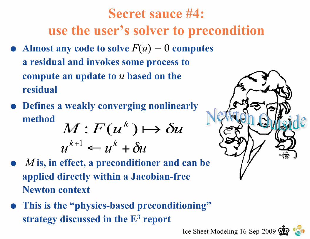
Secret sauce #4:

use the user’s solver to precondition

�� Almost any code to solve F(u) = 0 computes

a residual and invokes some process to

compute an update to u based on the

residual

�� Defines a weakly converging nonlinearly

method

�� M is, in effect, a preconditioner and can be

applied directly within a Jacobian-free

Newton context

�� This is the “physics-based preconditioning”

strategy discussed in the E3 report


Example: fast spin-up of ocean circulation model

using Jacobian-free Newton-Krylov

�� State vector, u(t)

�� Propagation operator (this is any code) � (u,t): u(t) = � (u(0),t)�� here, single-layer quasi-geostrophic ocean

forced by surface Ekman pumping, damped with biharmonic hyperviscosity

�� Task: find state u that repeats every period T (assumed known)

�� Difficulty: direct integration (DI) to find steady state may require thousands of years of physical time

�� Innovation: pose as Jacobian-free NK rootfinding problem, F(u) = 0,where F(u) � u - � (u(0),T)�� Jacobian is dense, would never think of

forming!

converged streamfunction

difference between DI and

NK (10-14)


Example: fast spin-up of ocean circulation model

using Jacobian-free Newton-Krylov 2-3 orders of

magnitude

speedup of

Jacobian-free

NK relative to

Direct

Integration

(DI)

OGCM:

Helfrich-

Holland

integrator

Implemented

in PETSc as

undergraduate

research

project

c/o T. Merlis (Columbia’05, now Caltech, Dept. Environmental Science & Engineering)


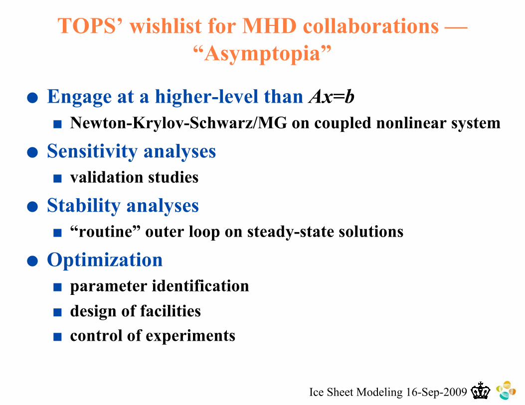
�� Engage at a higher-level than Ax=b

�� Newton-Krylov-Schwarz/MG on coupled nonlinear system

�� Sensitivity analyses

�� validation studies

�� Stability analyses

�� “routine” outer loop on steady-state solutions

�� Optimization

�� parameter identification

�� design of facilities

�� control of experiments

TOPS’ wishlist for MHD collaborations —

“Asymptopia”


Hardware Infrastructure

ARCHITECTURES

Applications

A “perfect storm” for scientific simulation

scientific models

numerical algorithms

computer architecture

scientific software engineering

(dates are symbolic)

1686

1947

1976

1992


TOPS dreams that users will…

�� Understand range of algorithmic options w/

tradeoffs

e.g., memory vs. time, comp. vs. comm., inner iteration

work vs. outer

�� Try all reasonable options “easily”

without recoding or extensive recompilation

�� Know how their solvers are performing

with access to detailed profiling information

�� Intelligently drive solver research

e.g., publish joint papers with algorithm researchers

�� Simulate truly new physics free from solver limits

e.g., finer meshes, complex coupling, full nonlinearity

User’s

Rights


SciDAC’s computational math “centers”�� Interoperable Tools for Advanced Petascale Simulations (ITAPS)

PI: L. Freitag-Diachin, LLNL

For complex domain geometry

�� Algorithmic and Software Framework for Partial Differential Equations (APDEC)

PI: P. Colella, LBNL

For solution adaptivity

�� Combinatorial Scientific Computing and Petascale Simulation (CSCAPES)

PI: A. Pothen, Purdue U

For partitioning and ordering

�� Towards Optimal Petascale Simulations (TOPS)

PI: D. Keyes, Columbia U

For scalable solution

See: www.scidac.gov/math/math.html


ITAPSInteroperable Tools for Advanced Petascale Simulations

Develop framework for use of multiple mesh and discretization strategies within a single PDE simulation. Focus on high-quality hybrid mesh generation for representing complex and evolving domains, high-order discretization techniques, and adaptive strategies for automatically optimizing a mesh to follow moving fronts or to capture important solution features.

c/o L. Freitag, LLNL


Algorithmic and Software Framework for PDEsDevelop framework for PDE simulation based on locally structured grid methods, including adaptive meshes for problems with multiple length scales; embedded boundary and overset grid methods for complex geometries; efficient and accurate methods for particle and hybrid particle/mesh simulations.

c/o P. Colella, LBNL

APDEC


CSCAPESCombinatorial Scientific Computing and Petascale Simulation

Develop toolkit of partitioners, dynamic load balancers, advanced sparse matrix reordering routines, and automatic differentiation procedures, generalizing currently available graph-based algorithms to hypergraphs

c/o A. Pothen, Purdue

Contact detection Particle Simulations

x bA

=

Linear solvers & preconditioners


EOF�

scalable implicit methods, scidac, and ice sheet modelingkd2112/icesheets09.pdf · ice sheet...

Documents