Scalable MAP inference in Bayesiannetworks based on a Map-Reduce

approach

Darío Ramos-López1, Antonio Salmerón1, Rafael Rumí1,Ana M. Martínez2, Thomas D. Nielsen2, Andrés R. Masegosa3,

Helge Langseth3, Anders L. Madsen2,4

1Department of Mathematics, University of Almería, Spain2Department of Computer Science, Aalborg University, Denmark

3 Department of Computer and Information Science,The Norwegian University of Science and Technology, Norway

4 Hugin Expert A/S, Aalborg, Denmark

8th Int. Conf. on Probabilistic Graphical Models, Lugano, Sept. 6–9, 2016 1

Outline

1 Motivation

2 MAP in CLG networks

3 Scalable MAP

4 Experimental results

5 Conclusions

8th Int. Conf. on Probabilistic Graphical Models, Lugano, Sept. 6–9, 2016 2

Outline

1 Motivation

2 MAP in CLG networks

3 Scalable MAP

4 Experimental results

5 Conclusions

8th Int. Conf. on Probabilistic Graphical Models, Lugano, Sept. 6–9, 2016 3

Motivation

I Aim: Provide scalable solutions to the MAP problem.

I Challenges:I Data coming in streams at high speed, and

a quick response is required.

I For each observation in the stream, themost likely configuration of a set ofvariables of interest is sought.

I MAP inference is highly complex.

I Hybrid models come along with specificdifficulties.

8th Int. Conf. on Probabilistic Graphical Models, Lugano, Sept. 6–9, 2016 4

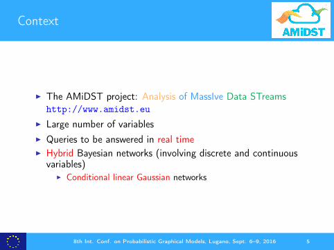
Context

I The AMiDST project: Analysis of MassIve Data STreamshttp://www.amidst.eu

I Large number of variablesI Queries to be answered in real timeI Hybrid Bayesian networks (involving discrete and continuous

variables)I Conditional linear Gaussian networks

8th Int. Conf. on Probabilistic Graphical Models, Lugano, Sept. 6–9, 2016 5

Outline

1 Motivation

2 MAP in CLG networks

3 Scalable MAP

4 Experimental results

5 Conclusions

8th Int. Conf. on Probabilistic Graphical Models, Lugano, Sept. 6–9, 2016 6

Conditional Linear Gaussian networks

Y

W

TU

S

P(Y ) = (0.5, 0.5)P(S) = (0.1, 0.9)f (w |Y = 0) = N (w ;−1, 1)f (w |Y = 1) = N (w ; 2, 1)f (t|w , S = 0) = N (t;−w , 1)f (t|w , S = 1) = N (t;w , 1)f (u|w) = N (u;w , 1)

8th Int. Conf. on Probabilistic Graphical Models, Lugano, Sept. 6–9, 2016 7

Querying a Bayesian network

I Belief update: Computing the posterior distribution of a variable:

p(xi |xE ) =

∑xD

∫xC

p(x , xE )dxC

∑xDi

∫xCi

p(x , xE )dxCi

I Maximum a posteriori (MAP): For a set of target variables X I , seek

x∗I = argmaxx I

p(x I |XE = xE )

where p(x I |XE = xE ) is obtained by first marginalizing out fromp(x) the variables not in X I and not in XE

I Most probable explanation (MPE): A particular case of MAP whereX I includes all the unobserved variables

8th Int. Conf. on Probabilistic Graphical Models, Lugano, Sept. 6–9, 2016 8

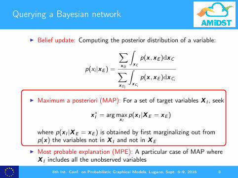
Querying a Bayesian network

I Belief update: Computing the posterior distribution of a variable:

p(xi |xE ) =

∑xD

∫xC

p(x , xE )dxC

∑xDi

∫xCi

p(x , xE )dxCi

I Maximum a posteriori (MAP): For a set of target variables X I , seek

x∗I = argmaxx I

p(x I |XE = xE )

where p(x I |XE = xE ) is obtained by first marginalizing out fromp(x) the variables not in X I and not in XE

I Most probable explanation (MPE): A particular case of MAP whereX I includes all the unobserved variables

8th Int. Conf. on Probabilistic Graphical Models, Lugano, Sept. 6–9, 2016 8

Outline

1 Motivation

2 MAP in CLG networks

3 Scalable MAP

4 Experimental results

5 Conclusions

8th Int. Conf. on Probabilistic Graphical Models, Lugano, Sept. 6–9, 2016 9

MAP by Hill Climbing

HC_MAP(B ,x I ,xE ,r)while stopping criterion not satisfied do

x∗I ← GenerateConfiguration(B , x I , xE , r)

if p(x∗I , xE ) ≥ p(x I , xE ) then

x I ← x∗I

endendreturn x I

I Max. number of non-improving iterationsI Target prob. thresholdI Max. number of iterations

I Never move to a worse configuration

I Estimated using importance sampling:

p(x I , xE ) =∑

x∗∈ΩX∗

p(x I , xE , x∗) =∑

x∗∈ΩX∗

p(x I , xE , x∗)f ∗(x∗)

f ∗(x∗)

= Ef ∗

[p(x I , xE , x∗)

f ∗(x∗)

]≈ 1

n

n∑i=1

p(x I , xE , x∗(i)

)f ∗(x∗(i)

) ,

I We’ll see later

8th Int. Conf. on Probabilistic Graphical Models, Lugano, Sept. 6–9, 2016 10

MAP by Hill Climbing

HC_MAP(B ,x I ,xE ,r)while stopping criterion not satisfied do

x∗I ← GenerateConfiguration(B , x I , xE , r)

if p(x∗I , xE ) ≥ p(x I , xE ) then

x I ← x∗I

endendreturn x I

I Max. number of non-improving iterationsI Target prob. thresholdI Max. number of iterations

I Never move to a worse configuration

I Estimated using importance sampling:

p(x I , xE ) =∑

x∗∈ΩX∗

p(x I , xE , x∗) =∑

x∗∈ΩX∗

p(x I , xE , x∗)f ∗(x∗)

f ∗(x∗)

= Ef ∗

[p(x I , xE , x∗)

f ∗(x∗)

]≈ 1

n

n∑i=1

p(x I , xE , x∗(i)

)f ∗(x∗(i)

) ,

I We’ll see later

8th Int. Conf. on Probabilistic Graphical Models, Lugano, Sept. 6–9, 2016 10

MAP by Hill Climbing

HC_MAP(B ,x I ,xE ,r)while stopping criterion not satisfied do

x∗I ← GenerateConfiguration(B , x I , xE , r)

if p(x∗I , xE ) ≥ p(x I , xE ) then

x I ← x∗I

endendreturn x I

I Max. number of non-improving iterationsI Target prob. thresholdI Max. number of iterations

I Never move to a worse configuration

I Estimated using importance sampling:

p(x I , xE ) =∑

x∗∈ΩX∗

p(x I , xE , x∗) =∑

x∗∈ΩX∗

p(x I , xE , x∗)f ∗(x∗)

f ∗(x∗)

= Ef ∗

[p(x I , xE , x∗)

f ∗(x∗)

]≈ 1

n

n∑i=1

p(x I , xE , x∗(i)

)f ∗(x∗(i)

) ,

I We’ll see later

8th Int. Conf. on Probabilistic Graphical Models, Lugano, Sept. 6–9, 2016 10

MAP by Hill Climbing

HC_MAP(B ,x I ,xE ,r)while stopping criterion not satisfied do

x∗I ← GenerateConfiguration(B , x I , xE , r)

if p(x∗I , xE ) ≥ p(x I , xE ) then

x I ← x∗I

endendreturn x I

I Max. number of non-improving iterationsI Target prob. thresholdI Max. number of iterations

I Never move to a worse configuration

I Estimated using importance sampling:

p(x I , xE ) =∑

x∗∈ΩX∗

p(x I , xE , x∗) =∑

x∗∈ΩX∗

p(x I , xE , x∗)f ∗(x∗)

f ∗(x∗)

= Ef ∗

[p(x I , xE , x∗)

f ∗(x∗)

]≈ 1

n

n∑i=1

p(x I , xE , x∗(i)

)f ∗(x∗(i)

) ,

I We’ll see later

8th Int. Conf. on Probabilistic Graphical Models, Lugano, Sept. 6–9, 2016 10

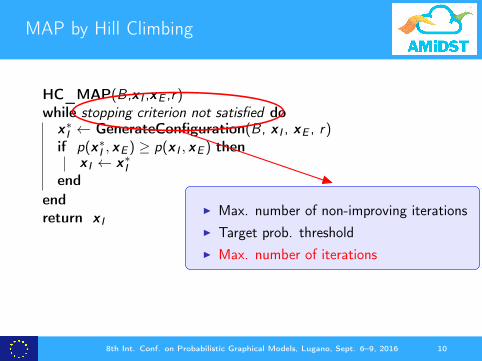
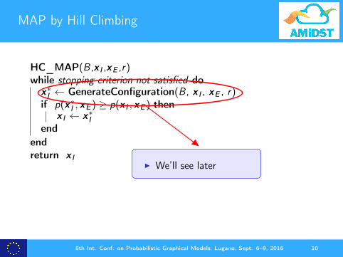
MAP by Hill Climbing

HC_MAP(B ,x I ,xE ,r)while stopping criterion not satisfied do

x∗I ← GenerateConfiguration(B , x I , xE , r)

if p(x∗I , xE ) ≥ p(x I , xE ) then

x I ← x∗I

endendreturn x I

I Max. number of non-improving iterationsI Target prob. thresholdI Max. number of iterations

I Never move to a worse configuration

I Estimated using importance sampling:

p(x I , xE ) =∑

x∗∈ΩX∗

p(x I , xE , x∗) =∑

x∗∈ΩX∗

p(x I , xE , x∗)f ∗(x∗)

f ∗(x∗)

= Ef ∗

[p(x I , xE , x∗)

f ∗(x∗)

]≈ 1

n

n∑i=1

p(x I , xE , x∗(i)

)f ∗(x∗(i)

) ,

I We’ll see later

8th Int. Conf. on Probabilistic Graphical Models, Lugano, Sept. 6–9, 2016 10

MAP by Simulated Annealing

SA_MAP(B ,x I ,xE ,r)T ← 1 000; α← 0.90; ε > 0while T ≥ ε do

x∗I ← GenerateConfiguration(B , x I , xE , r)

Simulate a random number τ ∼ U(0, 1)if p(x∗

I , xE ) > p(x I , xE )/(T · ln(1/τ)) thenx I ← x∗

I

endT ← α · T

endreturn x I

I Default values of the temperature parametersI T 1: almost completely randomI T 1: almost completely greedy

I Accept x∗I if its prob. increases

or decreases < T · ln(1/τ)I Cool down the temperature

8th Int. Conf. on Probabilistic Graphical Models, Lugano, Sept. 6–9, 2016 11

MAP by Simulated Annealing

SA_MAP(B ,x I ,xE ,r)T ← 1 000; α← 0.90; ε > 0while T ≥ ε do

x∗I ← GenerateConfiguration(B , x I , xE , r)

Simulate a random number τ ∼ U(0, 1)if p(x∗

I , xE ) > p(x I , xE )/(T · ln(1/τ)) thenx I ← x∗

I

endT ← α · T

endreturn x I

I Default values of the temperature parametersI T 1: almost completely randomI T 1: almost completely greedy

I Accept x∗I if its prob. increases

or decreases < T · ln(1/τ)I Cool down the temperature

8th Int. Conf. on Probabilistic Graphical Models, Lugano, Sept. 6–9, 2016 11

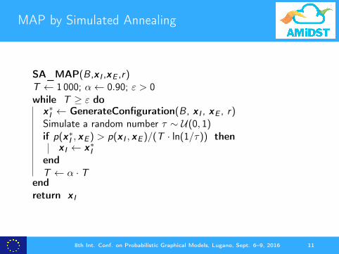
MAP by Simulated Annealing

SA_MAP(B ,x I ,xE ,r)T ← 1 000; α← 0.90; ε > 0while T ≥ ε do

x∗I ← GenerateConfiguration(B , x I , xE , r)

Simulate a random number τ ∼ U(0, 1)if p(x∗

I , xE ) > p(x I , xE )/(T · ln(1/τ)) thenx I ← x∗

I

endT ← α · T

endreturn x I

I Default values of the temperature parametersI T 1: almost completely randomI T 1: almost completely greedy

I Accept x∗I if its prob. increases

or decreases < T · ln(1/τ)

I Cool down the temperature

8th Int. Conf. on Probabilistic Graphical Models, Lugano, Sept. 6–9, 2016 11

MAP by Simulated Annealing

SA_MAP(B ,x I ,xE ,r)T ← 1 000; α← 0.90; ε > 0while T ≥ ε do

x∗I ← GenerateConfiguration(B , x I , xE , r)

Simulate a random number τ ∼ U(0, 1)if p(x∗

I , xE ) > p(x I , xE )/(T · ln(1/τ)) thenx I ← x∗

I

endT ← α · T

endreturn x I

I Default values of the temperature parametersI T 1: almost completely randomI T 1: almost completely greedy

I Accept x∗I if its prob. increases

or decreases < T · ln(1/τ)

I Cool down the temperature

8th Int. Conf. on Probabilistic Graphical Models, Lugano, Sept. 6–9, 2016 11

Generating a new configuration of variables

Only discrete variablesI The new values are chosen at random

A variable whose parents are discrete or observed

Y

W

TU

S

P(Y ) = (0.5, 0.5)P(S) = (0.1, 0.9)f (w |Y = 0) = N (w ;−1, 1)f (w |Y = 1) = N (w ; 2, 1)f (t|w ,S = 0) = N (t;−w , 1)f (t|w ,S = 1) = N (t;w , 1)f (u|w) = N (u;w , 1)

8th Int. Conf. on Probabilistic Graphical Models, Lugano, Sept. 6–9, 2016 12

Generating a new configuration of variables

Hybrid modelsI We take advantage of the properties of the CLG distribution

A variable whose parents are discrete or observed

Y

W

TU

S

P(Y ) = (0.5, 0.5)P(S) = (0.1, 0.9)f (w |Y = 0) = N (w ;−1, 1)f (w |Y = 1) = N (w ; 2, 1)f (t|w ,S = 0) = N (t;−w , 1)f (t|w ,S = 1) = N (t;w , 1)f (u|w) = N (u;w , 1)

8th Int. Conf. on Probabilistic Graphical Models, Lugano, Sept. 6–9, 2016 12

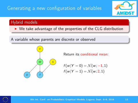
Generating a new configuration of variables

Hybrid modelsI We take advantage of the properties of the CLG distribution

A variable whose parents are discrete or observed

Y

W

TU

S

P(Y ) = (0.5, 0.5)P(S) = (0.1, 0.9)f (w |Y = 0) = N (w ;−1, 1)f (w |Y = 1) = N (w ; 2, 1)f (t|w ,S = 0) = N (t;−w , 1)f (t|w ,S = 1) = N (t;w , 1)f (u|w) = N (u;w , 1)

8th Int. Conf. on Probabilistic Graphical Models, Lugano, Sept. 6–9, 2016 12

Generating a new configuration of variables

Hybrid modelsI We take advantage of the properties of the CLG distribution

A variable whose parents are discrete or observed

Y

W

TU

S

Return its conditional mean:

f (w |Y = 0) = N (w ;−1, 1)f (w |Y = 1) = N (w ; 2, 1)

A variable with unobserved continuous parents

Y

W

TU

S

Simulate a value usingits conditional distribution:

f (t|w ,S = 0) = N (t;−w , 1)f (t|w ,S = 1) = N (t;w , 1)

8th Int. Conf. on Probabilistic Graphical Models, Lugano, Sept. 6–9, 2016 13

Generating a new configuration of variables

Hybrid modelsI We take advantage of the properties of the CLG distribution

A variable with unobserved continuous parents

Y

W

TU

S

Simulate a value usingits conditional distribution:

f (t|w ,S = 0) = N (t;−w , 1)f (t|w ,S = 1) = N (t;w , 1)

8th Int. Conf. on Probabilistic Graphical Models, Lugano, Sept. 6–9, 2016 13

Scalable implementation

8th Int. Conf. on Probabilistic Graphical Models, Lugano, Sept. 6–9, 2016 14

Outline

1 Motivation

2 MAP in CLG networks

3 Scalable MAP

4 Experimental results

5 Conclusions

8th Int. Conf. on Probabilistic Graphical Models, Lugano, Sept. 6–9, 2016 15

Experimental analysis

PurposeAnalyze the scalability in terms of

I SpeedI Accuracy

Experimental setupI Synthetic networks with 200 variables (50% discrete)I 70% of the variables observed at randomI 10% of the variables selected as target ⇒ 20% to be

marginalized out

8th Int. Conf. on Probabilistic Graphical Models, Lugano, Sept. 6–9, 2016 16

Experimental analysis

PurposeAnalyze the scalability in terms of

I SpeedI Accuracy

Experimental setupI Synthetic networks with 200 variables (50% discrete)I 70% of the variables observed at randomI 10% of the variables selected as target ⇒ 20% to be

marginalized out

8th Int. Conf. on Probabilistic Graphical Models, Lugano, Sept. 6–9, 2016 16

Experimental analysis

Computing environmentI AMIDST Toolbox with Apache FlinkI Multi-core environment based on a dual-processor AMD

Opteron 2.8 GHz server with 32 cores and 64 GB of RAM,running Ubuntu Linux 14.04.1 LTS

I Multi-node environment based on Amazon Web Services(AWS)

8th Int. Conf. on Probabilistic Graphical Models, Lugano, Sept. 6–9, 2016 17

Scalability: run times

100

200

300

400

500

600

1 2 4 8 16 24 32Number of cores

Exe

cutio

n tim

e (

s)

method HC Global HC Local SA Global SA Local

Scalability of MAP in a multi−core node

5

10

15

Sp

ee

d-u

p fa

ctor 5

10

15

20

1 2 4 8 16 24 32Number of nodes (4 vCPUs per node)

Sp

ee

d−

up fact

or

method HC Global HC Local SA Global SA Local

Scalability of MAP in a multi−node cluster

25

50

75

100

125

1 2 4 8 16 24 32Number of nodes (4 vCPUs per node)

Exe

cutio

n t

ime

(s)

method HC Global HC Local SA Global SA Local

Scalability of MAP in a multi−node cluster

5

10

15

20

Sp

ee

d-u

p fa

ctor

8th Int. Conf. on Probabilistic Graphical Models, Lugano, Sept. 6–9, 2016 18

Scalability: accuracy (Simulated Annealing)

−230

−220

−210

−200

−190

1 2 4 8 16 32Number of cores

log

Pro

ba

bility

cores

1

2

4

8

16

32

Simulated Annealing global

−200

−195

−190

−185

1 2 4 8 16 32Number of cores

log

Pro

ba

bility

cores

1

2

4

8

16

32

Simulated Annealing local

Estimated log-probabilities of the MAP configurations found by each algorithm

8th Int. Conf. on Probabilistic Graphical Models, Lugano, Sept. 6–9, 2016 19

Scalability: accuracy (Hill Climbing)

−240

−220

−200

1 2 4 8 16 32Number of cores

log

Pro

ba

bility

cores

1

2

4

8

16

32

Hill Climbing global

−240

−220

−200

1 2 4 8 16 32Number of cores

log

Pro

ba

bility

cores

1

2

4

8

16

32

Hill Climbing local

Estimated log-probabilities of the MAP configurations found by each algorithm

8th Int. Conf. on Probabilistic Graphical Models, Lugano, Sept. 6–9, 2016 20

Outline

1 Motivation

2 MAP in CLG networks

3 Scalable MAP

4 Experimental results

5 Conclusions

8th Int. Conf. on Probabilistic Graphical Models, Lugano, Sept. 6–9, 2016 21

Conclusions

I Scalable MAP for CLG models in terms of accuracy and runtime

I Available in the AMIDST ToolboxI Valid for multi-cores and cluster systemsI MapReduce-based design on top of Apache Flink

8th Int. Conf. on Probabilistic Graphical Models, Lugano, Sept. 6–9, 2016 22

Thank you for your attentionYou can download our open source Java toolbox:

http://www.amidsttoolbox.com

Acknowledgments: This project has received funding from the European Union’sSeventh Framework Programme for research, technological development and

demonstration under grant agreement no 619209

8th Int. Conf. on Probabilistic Graphical Models, Lugano, Sept. 6–9, 2016 23