scalable translation validation - tu wien · scalable translation validation tools, ... visual...
TRANSCRIPT

Scalable Translation Validation
Tools, Techniques and Framework
DISSERTATION
submitted in partial fulfillment of the requirements for the degree of
Doktor der technischen Wissenschaften
by
Dipl.-Ing. Roland Lezuo
Registration Number 0227059
to the Faculty of Informatics
at the Vienna University of Technology
Advisor: Ao.Univ.Prof. Dipl.-Ing. Dr. Andreas Krall
The dissertation has been reviewed by:
(Ao.Univ.Prof. Dipl.-Ing. Dr.
Andreas Krall)
(Prof. Dr. rer. nat. habil. Wolf
Zimmermann)
Wien, 20.03.2014
(Dipl.-Ing. Roland Lezuo)
Technische Universität Wien
A-1040 Wien � Karlsplatz 13 � Tel. +43-1-58801-0 � www.tuwien.ac.at


Erklärung zur Verfassung der Arbeit
Dipl.-Ing. Roland LezuoBurggasse 35/1, 1070 Wien
Hiermit erkläre ich, dass ich diese Arbeit selbständig verfasst habe, dass ich die verwende-ten Quellen und Hilfsmittel vollständig angegeben habe und dass ich die Stellen der Arbeit -einschließlich Tabellen, Karten und Abbildungen -, die anderen Werken oder dem Internet imWortlaut oder dem Sinn nach entnommen sind, auf jeden Fall unter Angabe der Quelle als Ent-lehnung kenntlich gemacht habe.
(Ort, Datum) (Unterschrift Verfasser)
i


For Maya


Acknowledgments
First I want to thank my wife for her encouraging support and understanding during this time ofups and downs and my children for cheering me up as only children can.
Many thanks to my advisor, Andreas Krall, for letting me pursue the topic with such a highdegree of freedom and personal responsibility. The trust he put into me was always motivatingfor me. I also want to thank Wolf Zimmermann for the enlightening discussion on the topicsof programming language semantics and translation validation. Without his support this workwould not have been possible. And last, but not least, I want to thank Laura Kovács for herinvaluable support regarding theorem provers.
I also want to mention all my colleagues at the Complang group in Vienna which alwaysmade going to the office a joy. Especially I want to emphasize Gergö Barany for his precisecomments on paper drafts and fruitful discussion on CASM and Ioan Dragan for his collabora-tion regarding vanHelsing. Special thanks go to Dominik Inführ and Philipp Paulweber for theircommitment to provide solid implementations of my prototypes. And very special thanks to mysister Cornelia for her heroic proof reading.
Funding: This work is partially supported by the Austrian Research Promotion Agency (FFG)under contract 827485, Correct Compilers for Correct Application Specific Processors and CatenaDSP GmbH.
v


Abstract
Today embedded computer systems are often used in safety-critical applications. A malfunctionin such a system (e.g. X-by-wire) often has severe effects, even life-threatening consequences.Lots of effort is put into certification to assure the correct and safe behavior of safety-critical ap-plications. Due to the high complexity of modern technical systems, a high-level programminglanguage like C is commonly used to implement their software.
This makes the compiler a critical component in the certification of safety-critical systems.Even if the source code is fully certified and error-free an erroneous compiler could introduceunintended behavior and hence the certification would be in vain. This is one motivation ofresearch in compiler correctness, a discipline which develops methods to show that the compilerbehaves correctly. One approach, namely translation validation, formally proves that a single,specific run of the compiler was error-free.
This thesis contributes a framework which allows to apply translation validation from thesource code down to its binary representation. The CASM language, based on the formal methodof Abstract State Machines (ASM), has been developed as part of this thesis to specify the se-mantics of the source language and machine code. Using the novel technique of direct symbolicexecution a first-order logic representation is created as the foundation for the formal proofs. Toexploit the common structure found in problems originating from translation validation prob-lems a specialized prover called vanHelsing has been implemented as part of this thesis. Itsvisual proof debugger enables non-domain experts to analyze failing proofs and pinpoint thecausing, erroneous translation.
The detailed evaluation shows that CASM is by far the best performing ASM implemen-tation. It is efficient enough to synthesize Instruction Set Simulation and Compiled Simula-tion tools. The vanHelsing prover performs much better than other state of the art provers onproblems stemming from translation validation. These efficient tools and the high degree ofparallelism in our translation validation framework enable fast validations. The implementedprototypes for instruction selection, register allocation and VLIW scheduling demonstrate thatvalidation of real-world applications like bzip2 is possible within a few dozen minutes.
vii

Kurzfassung
Viele der heute verwendeten eingebetteten Computersysteme übernehmen sicherheitskritische(safety-critical) Aufgaben. Die Fehlfunktion eines sicherheitskritischen Systems führt per Defi-nition zu großen Schäden, unter ungünstigen Umständen auch zur Gefahr für Leib und Leben.Teure Zertifizierungsverfahren werden durchlaufen um das korrekte und sichere Verhalten sol-cher Systeme sicherzustellen. Aufgrund der allgemein hohen Komplexität moderner technischerSysteme wird die Software, auch von sicherheitskritischen Anwendungen, oft in Hochsprachenwie C implementiert.
Dadurch wird der Übersetzer (compiler) dieser Sprache zertifizierungsrelevant. Selbst wennder zugrunde liegende Quellcode der Software bewiesenermaßen fehlerfrei ist kann ein einzi-ger Übersetzungsfehler ein verändertes Verhalten in der Ausführung bewirken. Dieser würdejedoch die komplette Zertifizierung obsolet machen, eine Motivationen für Forschung im Gebietder Übersetzerkorrektheit (compiler correctness), einer Disziplin welche Techniken und Metho-den erforscht um mit Hilfe formaler Verfahren die Korrektheit von Übersetzern sicherzustellen.Ein methodisches Vorgehen, die sogenannte Translation Validation, prüft dabei a posteriori diesemantische Äquivalenz des Quellcodes mit dem übersetzten Programm.
Diese Dissertation beschreibt einen strukturellen Ansatz, welcher es ermöglicht, alle Schrit-te einer Übersetzung mit der Translation Validation Methode zu verifizieren. Um eine präziseBeschreibung der Semantik des Quellcodes und der ausführenden Maschine zu erstellen wurde,basierend auf der Theorie der Abstract State Machine (ASM), eine geeignete Sprache (CASM)spezifiziert und implementiert. Durch die innovative Technik der direkten symbolischen Ausfüh-rung von ASM kann die Semantikspezifikation konkreter Programme in Prädikatenlogik ersterStufe dargestellt werden. Diese Darstellung bildet die Grundlage für den formalen Beweis derÜbersetzerkorrektheit. Die sich ergebenden Beweisverpflichtungen weisen eine gemeinsame,problembezogene Struktur auf. Der im Zuge dieser Arbeit entwickelte vanHelsing Beweiser istin Hinblick auf diese Struktur optimiert. Die Möglichkeit nicht bewiesene Probleme grafisch zuuntersuchen bietet, auch ungeübten Anwendern von Theorembeweisern, ein Werkzeug um diejeweilige Ursache in der Problemdomäne zu identifizieren.
In der ausführlichen empirischen Untersuchung wird gezeigt, dass die CASM Sprache we-sentlich schnellere Programmausführung ermöglicht als andere ASM Implementierungen. DieGeschwindigkeit ist hoch genug um sowohl Befehlssatz Simulatoren (Instruction Set Simula-
tor) als auch übersetzende Simulation (compiled simulation) aus den CASM Spezifikationender Maschine zu erzeugen. Der vanHelsing Beweiser ist, für Probleme hinsichtlich derer er opti-miert wurde, wesentlich schneller als andere Theorembeweiser. Erst diese effizienten Implemen-
ix

tierungen ermöglichen dass die Laufzeiten, der im Zuge dieser Arbeiten erstellten Prototypenfür Translation Validation (Codeerzeugung, Registerzuteilung und Befehlsanordnung für VLIWMaschinen), selbst für realistisch große Programme wie z.B.: bzip2, jeweils nur wenige Minutenbetragen.

List of used Acronyms
ABI Application Binary Interface
ADL Architecture Description Language
ALU Arithmetic Logic Unit
ASM Abstract State Machine
AST Abstract Syntax Tree
ATP Automated Theorem Proving
BV Bit Vector
CFA Control Flow Association
CFG Control Flow Graph
cLIR causal LIR
CS Compiled Simulation
DFT Data Flow Tree
DSL Domain Specific Language
EBNF Extended Backus-Naur Form
EMF Eclipse Modeling Framework
FFT Fast Fourier Transformation
FU Functional Unit (part of CPU dedicated to specific operation)
FUF FU Field (part of internal state of a FU)
FV Field Value (decoded field of an instruction)
ILP Instruction Level Parallelism
xi

IR Intermediate Representation
ISS Instruction Set Simulation
LASM Linked Assembly Module
LIR Low-level IR
LOC Lines of Code
MIR Mid-End IR
mMIR matcher MIR
SIMD Single Instruction Multiple Data
sLIR scheduled LIR
SMT Satisfiability Modulo Theories
STS State Transition System
SSA Static Single Assignment
VLIW Very Long Instruction Word
XML eXtensible Markup Language

Contents
1 Introduction 1
2 Related Work 5
2.1 Compiler Verification . . . . . . . . . . . . . . . . . . . . . . . . . . . . . . . 52.2 Abstract State Machines . . . . . . . . . . . . . . . . . . . . . . . . . . . . . 72.3 First-Order Theorem Provers . . . . . . . . . . . . . . . . . . . . . . . . . . . 8
3 CASM - Efficient Abstract State Machines 11
3.1 CASM - An Implementation of ASM . . . . . . . . . . . . . . . . . . . . . . 113.2 Direct symbolic execution of ASM . . . . . . . . . . . . . . . . . . . . . . . . 143.3 Efficient Compilation of CASM . . . . . . . . . . . . . . . . . . . . . . . . . 20
4 Semantics and Compilers 25
4.1 ADL for Retargetable Compilers . . . . . . . . . . . . . . . . . . . . . . . . . 254.2 Compiler Overview . . . . . . . . . . . . . . . . . . . . . . . . . . . . . . . . 274.3 Semantics of Compiler IR . . . . . . . . . . . . . . . . . . . . . . . . . . . . 284.4 A unified Machine Model . . . . . . . . . . . . . . . . . . . . . . . . . . . . . 31
5 Proof Techniques 35
5.1 Program Checking . . . . . . . . . . . . . . . . . . . . . . . . . . . . . . . . 355.2 Simulation Proofs . . . . . . . . . . . . . . . . . . . . . . . . . . . . . . . . . 35
6 The Big Picture - Chain of Trust 41
6.1 Definition of Correct Compilation . . . . . . . . . . . . . . . . . . . . . . . . 426.2 Front-end . . . . . . . . . . . . . . . . . . . . . . . . . . . . . . . . . . . . . 446.3 Mid-end - Verification of Analyses . . . . . . . . . . . . . . . . . . . . . . . . 446.4 Back-end - Verification of Transformations . . . . . . . . . . . . . . . . . . . 456.5 Multiple Iterated Passes . . . . . . . . . . . . . . . . . . . . . . . . . . . . . . 45
7 Correctness of Selected Back-end Transformations 47
7.1 Prolog and Epilog Insertion . . . . . . . . . . . . . . . . . . . . . . . . . . . . 477.2 Instruction Selection . . . . . . . . . . . . . . . . . . . . . . . . . . . . . . . 497.3 If Conversion . . . . . . . . . . . . . . . . . . . . . . . . . . . . . . . . . . . 527.4 VLIW Scheduling . . . . . . . . . . . . . . . . . . . . . . . . . . . . . . . . . 54
xiii

7.5 Software Pipelining . . . . . . . . . . . . . . . . . . . . . . . . . . . . . . . . 567.6 Register Allocation & Spilling . . . . . . . . . . . . . . . . . . . . . . . . . . 587.7 Stack Finalization . . . . . . . . . . . . . . . . . . . . . . . . . . . . . . . . . 617.8 Linking . . . . . . . . . . . . . . . . . . . . . . . . . . . . . . . . . . . . . . 617.9 Summary . . . . . . . . . . . . . . . . . . . . . . . . . . . . . . . . . . . . . 62
8 vanHelsing: Prover and Debugger 63
8.1 Input Language . . . . . . . . . . . . . . . . . . . . . . . . . . . . . . . . . . 648.2 Implementation . . . . . . . . . . . . . . . . . . . . . . . . . . . . . . . . . . 658.3 Proof Debugger . . . . . . . . . . . . . . . . . . . . . . . . . . . . . . . . . . 678.4 Defining Expressions . . . . . . . . . . . . . . . . . . . . . . . . . . . . . . . 69
9 Instruction Set Simulation & Compiled Simulation 71
9.1 Instruction Set Simulation . . . . . . . . . . . . . . . . . . . . . . . . . . . . 719.2 Instruction Set Simulator Verification . . . . . . . . . . . . . . . . . . . . . . 729.3 Compiled Simulation . . . . . . . . . . . . . . . . . . . . . . . . . . . . . . . 75
10 Evaluation 79
10.1 CASM implementation . . . . . . . . . . . . . . . . . . . . . . . . . . . . . . 7910.2 vanHelsing Prover . . . . . . . . . . . . . . . . . . . . . . . . . . . . . . . . . 8910.3 Translation Validation . . . . . . . . . . . . . . . . . . . . . . . . . . . . . . . 90
11 Future Work 97
11.1 CASM Object Model . . . . . . . . . . . . . . . . . . . . . . . . . . . . . . . 9711.2 Update Placement Optimization for the CASM Compiler . . . . . . . . . . . . 9711.3 Translation Validation of the CASM Compiler . . . . . . . . . . . . . . . . . . 9811.4 Synthesization of the Compiler Specification . . . . . . . . . . . . . . . . . . . 98
12 Conclusion 99
Bibliography 101
A Vocabulary and Axioms 109
B The CASM Language 119
C vanHelsing Input Language 125
D Colophon 129
E Curriculum Vitae 131

1 Introduction
The number of embedded systems used in everyday life has increased significantly in the lastdecade and will increase further. With the increasing prevalence, more and more systems areused in safety-critical applications. According to Wikipedia a malfunction of a safety-criticalsystem may result in death or serious injury to people, or loss of severe damage to equipmentor environmental harm. To manage the complexity, software used to operate critical systems isoften written in a high-level programming language, like C. There are industry-wide standardson the usage of C in such systems, e.g. MISRA C:2004 1, a guideline to the use of the C language
in critical systems.To assure the correctness of safety-critical systems a significant effort is put into their veri-
fication. A good point in case is the seL4 micro-kernel [40], a kernel for security-critical appli-cations with high reliability demands. It has been shown that this approximately 10.000 Linesof Code (LOC) C program is consistent with its specification models and free of a large classof common bugs (including null pointer access, alignment constraints, termination, processingunchecked user data). The manual labor put in (and therefore the costs of) such a verificationare very high, i.e. many person years of work. The result of the verification is a trusted base ofC code.
But the guaranteed properties of verified source code do not imply that those properties holdin the embedded system. The source code is compiled to the target hardware and executed bya real micro-processor, and both, the compiler and the hardware, may be erroneous. Hardwareverification is a well studied problem and today’s designs are at least partially verified [37].Although there exist hardware bugs (e.g. the famous Intel FDIV bug 2) they are much lessproblematic than software bugs in today’s systems.
1http://www.misra.org.uk/
2http://en.wikipedia.org/wiki/Pentium_FDIV_bug
1

1 Introduction
All it takes to invalidate the verification results is a single compilation error resulting in abehavioral difference between source code and binary. Such an change in behavior invalidatesthe preconditions made to verify the source code, and thous the results don’t hold for the binary.A recent study by Yang et al. [68] reports on a large scale random testing of 11 C compilersincluding GCC, LLVM and CompCert [43]. They found silently erroneous compiled code inevery single compiler, including the CompCert compiler, which is the only major commercialavailable (in large parts) verified C compiler. The conclusion is that compiler errors are probablymore common than anticipated and can not be ignored in safety-critical systems.
Compiler verification is the field of research which deals with methods and techniques toshow that a compiler behaves as specified. A verified compiler is a compiler for which hasbeen shown that it is error-free, i.e. each program translated with a verified compiler is error-free. A disadvantage of this approach is that the smallest change in the compiler triggers a fullre-verification. The other major approach is translation validation, which does not show thatthe compiler is correct, but that a specific, single compilation is correct. The compiler itselfmay contain errors, but they do not matter as long as those errors do not manifest themselves(i.e. changing the behavior of the binary). One advantage of this approach is that the compilercan be developed using common software engineering techniques, the disadvantage is that thevalidation has to be performed for each compilation.
To apply translation validation the semantics of the source and target languages must beknown concisely (formally). The proof itself relies on formal methods and tools. AutomatedTheorem Proving (ATP) is an established field of research and a number of mature theoremprovers is available. The method presented in this thesis makes use of that knowledge by creatinga problem formulation suitable for ATP tools.
Contribution
This thesis contributes to the field of compiler verification by developing scalable, fully auto-mated methods which allow to verify the whole compilation process (from source to binary).A translation validation framework is proposed which splits the validation task along compilerpasses. This allows each pass to be validated in isolation (local correctness), keeping the valida-tors simple. The validators further split the validation task along basic blocks of the program.This gives a very high degree of parallelism which can be exploited to achieve fast validationeven for very large programs. The framework allows to extend those local proofs to the notionof a global correctness.
We developed a variant of Abstract State Machine (ASM), called CASM, to formally specifythe semantics of the involved languages. The novel technique of direct symbolic execution isused to create first-order logic representations of the CASM specifications, which allows the useof theorem provers.
Another contribution of this work is the vanHelsing theorem prover. This prover is special-ized for the type of problems stemming from translation validation. Due to the specializationon this specific class of problems it also delivers excellent performance. A distinct feature isits support for graphical debugging failing proofs. This allows to analyze problems in proofswithout expert knowledge in theorem proving. Even a novice user is able pinpoint the causingissue in the problem domain.
2

We also feel that verification in an industrial context should not be an isolated task. Thereforewe developed tools to reuse the semantic models to synthesize instruction set simulators andperform compiled simulation. We argue that a single rigorous (formal) specification of thehardware is sufficient for verification, and synthesization of Instruction Set Simulation (ISS)and Compiled Simulation (CS) tools.
Layout of the Thesis
The remainder of this thesis is structured as follows: Chapter 2 discusses related work in thefield of compiler verification, ASM and first-order theorem provers. Chapter 3 introduces theCASM language developed as part of this thesis. It defines the novel method of direct symbolic
execution and describes the optimizing compiler. In chapter 4 the semantic aspects of compilerIntermediate Representations (IRs) are presented. A method to specify the semantics for a retar-getable compiler for application specific processors is given. The technical aspects of creatingIR dumps as CASM programs are presented. Chapter 5 introduces the proof techniques usedin this work. The simulation proof technique and the common semantic vocabulary are a coreconcept of this thesis.
After the technical foundations have been laid chapter 6 presents our translation validationframework and describes the verification from C source code down to machine code. The defi-nition of the term correct compilation is given. Front-end and mid-end are discussed, while thefocus of this thesis is on the compiler back-end. In chapter 7 the validator tools for specific back-end passes developed in this work are presented. This chapter is the technical core of this thesis.Chapter 8 describes the vanHelsing prover, a fully-mechanized first-order theorem prover devel-oped as part of this thesis. The main motivation to implement a custom prover is its ability toprovide graphical debugging aids for failing proofs. vanHelsing is specialized on a specific classof proofs which commonly occur in the context of translation validation. This chapter describesthe proof class and argues why a specific prover performs significantly better than more generaltheorem provers. Chapter 9 describes the implementation details of ISS and CS based on theCASM models. Chapter 10 reports on the performance of the methods developed in this work.We present benchmark data of selected validator prototypes, the vanHelsing prover and our ISSand CS implementations. In chapter 11 possible extensions to the tools and open issues whichwere not addressed by this work are discussed, and chapter 12 finally concludes this thesis.
3


2 Related Work
pic unrelated
2.1 Compiler Verification
Compiler verification is a very old idea with its roots in the 1960s. One idea is to prove thata compiler will only generate correct code. In this work we call this a verified compiler in the
strict sense. The main disadvantage of this approach is that any change in the compiler triggersa complete re-verification. A verified compiler is therefore a piece of software set in stone.
Nonetheless Leroy’s CompCert [43], the most important commercial available verified com-piler, is a verified compiler in the strict sense. Large parts of CompCert are specified in Coq [9],an interactive proving tool which allows to extract executable code out of a specification. Thecompiler front-end (parser, type-checker and simplifier) and the assembler output module arenot verified, though. With Yang et al. [68] recently finding serious bugs in the simplifier a com-plete source-to-binary verification seems to be necessary. The CompCert approach also fullytrusts the assembler (creating the binary representation of the assembler language) and linker.Our approach covers parsing and linking.
The second important approach to compiler verification is translation validation. It has beensuggested by Pnueli [57] and only verifies that a specific compilation is correct. The idea is sim-ilar to program checking [10]. An external observer (the validator) determines the correctnessof an computation by inspection of the input and the calculated output. After a source programhas been translated by an unverified compiler a validator tries to prove the target program to bea correct compilation. The proofs are performed by simulating source and target in a commonsemantic framework. The motivation of translation validation is that the validator may be signif-icantly easier to write (and verify) than the compiler itself. In addition the software developmentprocess of the compiler is unconstrained (as changes don’t trigger expensive re-verification).
Zimmermann and Gaul showed that this approach can be applied to realistic compilers (Ver-ifix project [70]). They suggested ASM to build the common semantic framework, an idea also
5
2 Related Work
used in this work. Tree pattern matching rules are partially checked when generating the Verifixback-end, it is therefore (partly) verified in the strict sense. It is also entangled with register allo-cation. Our approach separates these passes and fully validates tree pattern matching at compiletime.
Zuck et al. present VOC, a translation validation framework and tool for an optimizing com-piler. They focus on the compiler IR and optimizations performed on it but do not cover machinecode. Otherwise their notation of correctness is very similar to ours. Using a common semanticframework to describe source and target program they rely on simulation proofs to show thatthe target is a refinement of the source. Our approach is more general as we allow the sourceand target program to be in different IR languages. The validation tool operates on functionsand considers whole paths through the function which may lead to scalability issues for largefunctions. Our approach operates on basic blocks which are on average significant smaller. Theyalso discuss structure changing loop transformations which are quite hard to validate. In contrastto our work they do not consider pointers and aliasing at all.
Leviatan [44] presents a translation validation tool for software pipelining. They derivea large number (depending on the number of parallel stages) of correctness conditions to beverified. Pointers and aliasing is also not handled by this approach.
In [53] Necula describes a translation validation tool for an unmodified version of the GCCcompiler. His approach operates on GCC’s IR directly which is dumped before and after eachoptimization pass has been performed. Using a small set of heuristics enables identification ofthe applied transformations in the majority of the cases (i.e. there are false negatives). As in ourapproach symbolic execution of basic blocks combined with tracking of liveness informationyields a good scalability. The main limitations of this approach are that it is unclear how toextend it to machine code as it operates on GCC IR directly.
More work on compiler verification can be found in Maulik’s bibliography [20].
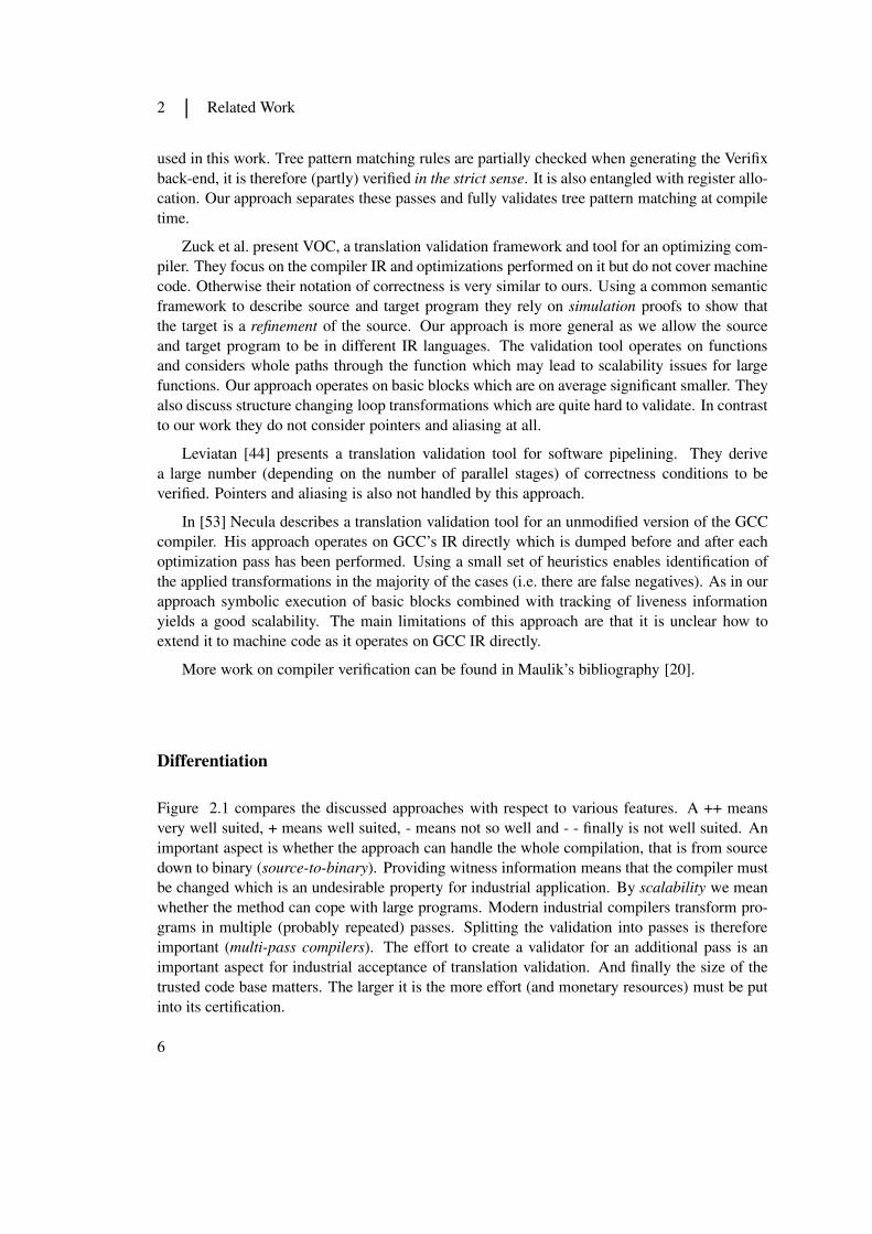
Differentiation
Figure 2.1 compares the discussed approaches with respect to various features. A ++ meansvery well suited, + means well suited, - means not so well and - - finally is not well suited. Animportant aspect is whether the approach can handle the whole compilation, that is from sourcedown to binary (source-to-binary). Providing witness information means that the compiler mustbe changed which is an undesirable property for industrial application. By scalability we meanwhether the method can cope with large programs. Modern industrial compilers transform pro-grams in multiple (probably repeated) passes. Splitting the validation into passes is thereforeimportant (multi-pass compilers). The effort to create a validator for an additional pass is animportant aspect for industrial acceptance of translation validation. And finally the size of thetrusted code base matters. The larger it is the more effort (and monetary resources) must be putinto its certification.
6

CompCert Necula VOC Verifix this worksource-to-binary - - - - - ++ ++compiler-provided witness ++ + - - –scalability ++ ++ - - ++multi-pass compilers + ++ + - ++effort for additional pass - - + + - ++size of trusted code-base - ++ ++ + +
Figure 2.1: Compiler verification feature matrix
2.2 Abstract State Machines
ASM was introduced by Gurevich (originally named evolving algebras) in the Lipari Guide [31].The original motivation was to bridge the gap created by the computational model of Turingmachines. A coding-free technique to describe algorithms on a natural abstraction level wassought.
The ideas of ASMs were further developed by Gurevich and others at Microsoft Researchresulting in a powerful specification language called AsmL [33]. AsmL is designed to be simple,precise, executable, testable, inter operable, integrated, scalable and analyzable. The languageis statically typed, supports object oriented features, has call-by-value semantics and supportsexceptions. An efficient compiler for .NET has been developed and the language has been fullyintegrated into the .NET framework and the Microsoft development environment [7]. The toolenvironment comprehends parameter generation for providing method calls with parameter sets,finite state machine generation from an ASM, sequence generation for deriving test sequencesand run-time verification for testing if an implementation performs conforming to the model.The tool environment around AsmL is the most advanced currently available.
One of the most performance critical issue in ASMs is the problem of partial updates. Gure-vich and Tillmann discussed the problem in detail and showed how concurrent data modifica-tions can be implemented efficiently [34]. Similar problems occur in version control systems onsoftware merging [52]. Techniques which work only on the delta (the differences) of the datasets inspire optimizations on efficient update implementation in CASM.
Castillo describes the ASM Workbench in [17]. Similar to CASM he added a type systemto his language. The ASM Workbench is implemented in ML1 in an extensible way. Castillodescribes an interpreter and a plugin for a model checker, which allows to translate certainrestricted classes of ASMs to models for the SMV2 model checker.
Schmid describes compiling ASM to C++ [60]. The compiler uses the ASM Workbenchlanguage as input. He proposes a double buffering technique avoiding implementing update setsat all. This approach is limited to parallel execution semantics only, though.
Schmid also introduced AsmGofer in [61]. AsmGofer is an interpreter for an ASM basedlanguage. It is written in the Gofer3 language (a subset of Haskell) and covers most of the
1http://en.wikipedia.org/wiki/Standard_ML
2http://www.cs.cmu.edu/~modelcheck/smv.html
3http://web.cecs.pdx.edu/~mpj/goferarc/index.html
7

2 Related Work
features described in the Lipari guide. The author notes however that the implementation isaimed at prototype modeling and too slow for performance critical applications.
Anlauff introduces XASM, a component based ASM language compiled to C [4]. The novelfeature of XASM is the introduction of a component model, allowing implementation of reusablecomponents. XASM supports functions implemented in C using the extern keyword. CASMdoes not feature modularization, but can be extended using C code as well. XASM was used asthe core of the gem-mex system, a graphical language for ASMs.
Gargantini et al. report on ASMETA [28]. Part of the development is a compiler translatingASM models into Eclipse Modeling Framework (EMF). The focus of this ASM implementationare high level models and design space exploration.
Farahbod designed CoreASM, an extensible ASM execution engine [23]. The CoreASMproject is actively maintained and has a large user base. The CASM language is inspired by theCoreASM language, but over time they have diverged significantly.
Teich, Kutter and Weper describe a method to extract an ASM based instruction set descrip-tion from a hardware description language [66]. This description is then used to automaticallygenerate C code for a cycle accurate simulator of the processor. The Gem-Mex tool used pro-vides support for implementing a parser which is used to read in assembler files for the simulator.Bit-true arithmetic functions are implemented in C and linked to the generated code. The feasi-bility of the approach is demonstrated by simulating very short programs on an ARM processor.No comparison to conventional simulators and no performance data are presented however.
Differentiation of CASM
The available ASM tools are not implemented with efficient execution of ASM in mind. Onereason is that ASM are often used to create high level models and explore the design space.Concrete implementations are written by hand and verified against the ASM model, often us-ing model checkers. CASM differs from these approaches as it aims to be executed efficiently.Our models are not just specifications, but concrete and efficient implementations are synthe-sized. For that purpose we have developed an optimizing compiler. CASM is to the best of ourknowledge the only ASM implementation offering symbolic execution.
2.3 First-Order Theorem Provers
Most state-of-the art theorem provers are based on the superposition calculus [6, 54]. Thoseprovers try to perform proofs by refutation, i.e. by deriving an contradiction. A common clas-sification of provers is whether they use an OTTER [50] style saturation algorithm or DIS-COUNT [5] style. The difference is in the treatment of generated clauses. As this set constantlygrows the prover may need to remove inferred clauses at some point in time. DISCOUNT basedprover therefore never utilize clauses from this set for inference or simplification. Schulz’s E [62]prover is a modern, fast implementation based on DISCOUNT.
Vampire [59, 41] on the other hand implements both variants. Vampire is among the fastesttheorem prover and has won the first-order section of the CASC [64] competition many years ina row now.
8

Satisfiability Modulo Theories (SMT) is another major branch in ATP. SMT is a general-ization of the boolean SAT problem. Certain predicates in a SMT problem are interpreted usingadditional theories (hence the name SMT). The solvers for the theories (e.g. bit vector arith-metic) need to feed back results into the generic SAT solving part. A popular implementation isMicrosoft’s Z3 [21] prover. It is available under a shared-source license for many platforms.
Manna et al.’s STeP prover [49] has a rich graphical user interface allowing the user to guidethe proof system. Counter examples can be derived automatically and debugging of problems ispossible. STeP is an interactive tool, though, and its primarily intended for temporal specifica-tions.
Differentiation of vanHelsing
The proving tool developed in this thesis is solely unification based. In contrast to superpositionbased provers, it is not searching for a refutation of the problem but performing unification untila fix-point is reached. The conjecture must then be provable with the found unifications. Thissimplicity allows a very efficient implementation based on a graph data structure. The graphdata structure can be visualized and allows graphical introspection and debugging of problems.We are not aware of a fully-mechanized prover which offers graphical proof introspection.
In contrast to SMT proving no background theories are implemented. Uninterpreted predi-cates are axiomatized using first-order formulae. This allows more flexibility, but may negativelyinfluence performance.
9


3 CASM - Efficient Abstract State Machines
restrain from equiring whether the name comes from the letters, the
pillars, the leather, the place, or the mode of behavior
Puck, The Sandman by Neil Gaiman
This chapter introduces the CASM language, its tools and focuses on the features distinguishingCASM from other ASM implementations. The novel technique of direct symbolic execution ofASM is formally defined and the implementation in the CASM interpreter is described. Furtheran efficient compilation scheme and an optimizing compiler are presented. During this thesispython prototypes of the CASM interpreter (including symbolic execution) and the compilerhave been developed. The knowledge gained by the prototypes influenced the language de-sign. A more efficient implementation of the interpreter using the C language was developedby Dominik Inführ in his bachelor thesis [36] under supervision by the author. The optimizingcompiler was implemented by Philipp Paulweber in his master thesis [56] under supervision bythe author. Interpreter and compiler are implemented as a single binary sharing the front-end(parser, type annotation, AST).
3.1 CASM - An Implementation of ASM
For a formal definition of CASM we refer to Gurevich’s Lipari guide [31], Börger and Schmid’sintroduction of sequential execution [11] and Farahbod’s CoreASM handbook [22]. More detailson the CASM language can be found in [45]. An Extended Backus-Naur Form (EBNF) grammarcan be found in appendix B. A novel feature of the interpreter is its capability to symbolically
execute [39, 18] ASM models.
3.1.1 Types
The CASM language is statically typed and offers Int, sub-range Int, Boolean, and String asatomic types. Compound types are List and Tuple. There are no implicit type conversions
11
3 CASM - Efficient Abstract State Machines
performed by CASM. If desired the programmer can convert types using the (range checking)built-in functions: Int2Boolean, Boolean2Int, Int2Enum, Enum2Int.
3.1.2 State
The central notion of ASM is the state. It is described using a set of functions. Each function
has an arity. Let a be an vector of arity n and f and n-ary function, then (a) is called a location.In ASM functions are mathematical objects and are therefore defined over their whole range.CASM functions are typed and programs are checked statically. A (finite) program only usesa finite subset of values (of the state). The special value undef is assigned to locations whichhave never been defined by the CASM program. Undef is a continuation of the underlyingfunction which assures a mathematical sound model. This gives a sound semantics to programsreading undefined locations, in contrast to C’s behavior which e.g. is undefined if a programreads undefined memory.
ASM rules (statements) do not change the state directly, but create updates. An update is atuple (f(a), v) which describes that the location f(a) was changed to value v. ASM rules areexecuted in parallel, the updates produced by rules are joined to an update set. An update setwhich contains more than one update to the same location is called inconsistent. Inconsistentupdate sets are a run-time error in CASM.
Each CASM program has a top-level rule. This distinct rule is executed repeatedly, until theprogram is terminated explicitly. Whenever the top-level rule concludes (function return) the up-date set is applied to the state in an atomic operation. Hence ASM programs have transactional
semantics.
3.1.3 Rules
The following list briefly summarizes the most important rules implemented in CASM. Börgerand Schmid [11] is an excellent reference and we use the notational conventions introducedthere. All rules except the call rule have exactly the semantics given there (and we omit it here).Ri is a rule and tj : Type is a term of the specific type. We omit the type specification for someterms if it is not needed to capture the semantics, but keep in mind that all terms are typed inCASM.
• Skip Rule: This rule does nothing and returns an empty update set.
skip
• Update Rule: Creates an update for a n-ary function f , assigning v to f(a).
f(a0, a1, . . . , an):=v
• Block Rule: This is the most basic rule defining parallel composition of enclosed rules.
{ R1R2 . . . Rn }
12

• Sequential Block Rule: All enclosed rules are composed using sequential execution se-mantics.
{| R1R2 . . . Rn |}
• Conditional Rule: The basic ASM conditional rule. The conditional expression must beof boolean type and the else-branch is optional.
if t : Boolean then R1 else R2
• Case Rule: An optional default case label is provided which will be executed if none ofthe given cases match the value of the conditional expression t. The types of all ti mustbe equal to the type of t.
case t : Enum, Int ,String of
t0 : R0
...
tn : Rn
default : R
endcase
• Forall Rule: The forall rule evaluates the rule of the body composing the resulting updatesets in parallel. Rule R will be evaluated for each element of the set described by t,binding the element’s value to i. t may be an Enum type in which case each element ofthe enumeration is used as value or a List (with obvious semantics).
forall i in t : Enum,List do R
• Iterate Rule: Turbo ASM’s iterate rule iteratively evaluates R using the intermediate stateof the previous iteration (sequential composition) until R’s update set is empty.
iterate R
• Let Rule: This rule adds a variable v to the environment. v is assigned the value t and Ris evaluated in this environment. CASM performs type inference so the type of v can beskipped in most cases.
let v = t in R
• Call Rule: Basic ASM call semantics are defined as call-by-name which can be imple-mented by a so called thunk [8], but this mechanism is not very efficient. CASM there-fore has a modified semantics of the call rule. All arguments are evaluated before beingpassed as arguments (one could simulate this with let rules in the basic ASM definition).This makes call-by-name equivalent to call-by-value which is what CASM actually im-plements. The other change is that a call rule is evaluated in a new (empty) environment.
13
3 CASM - Efficient Abstract State Machines
This effectively reduces the scope of variables introduced by let and forall rules (and thescope of rule arguments). Dynamically scoped variables cannot be compiled efficientlyand cannot be typed statically. For all arguments ai of the rule R the type of ai must matchthe type of the term ti. (A is a state, ζ the environment, ζ x
ucreates a new environment
ζ ′ which equals ζ except that ζ ′(x) = u. ζ x0
u0
x1
u0is the obvious composition of the new
environment operator and ζ∅ is the empty environment.)
Jcall R(t0 , . . . , tn )KA
ζ = JRKAζ∅a0v0
...anvn
where vi = JtiKA
ζ
• Indirect Call Rule: CASM supports indirect invocation of rules. This mechanism usesa slightly different syntax where r is an expression returning a reference to a rule. Thesemantics is otherwise identical to the call rule.
call (r : RuleRef )(t0, . . . , tn)
Further implemented rules are print, debuginfo (in accordance to [22]) and assert. Thedebuginfo facilities support named channels and CASM tools accept a list of active channels.Only the output produced by active channels is actually printed. The assert rule is in accordanceto the assert statement of the C language.
3.1.4 Expressions
The common boolean operations and, or, xor and not are implemented for Boolean values. Int
operations are +,−,∗,/ and modulo (%). Comparisons operators are <=, >=, ! = and equality(=).
A standard library is provided by CASM providing the following operations: cons, app forlist construction, peek, tail to extract the list head (and tail) and hex converts an Int to a String
with its hexadecimal representation.
3.2 Direct symbolic execution of ASM
This section introduces symbolic execution of ASM and describes how it is implemented inthe CASM interpreter. We first define the formal foundations of symbolic execution in thecontext of ASM. A way to represent symbolic trace as first-order logic predicates is given andthe implementation is described.
3.2.1 Definition of a Symbolic ASM
In this section we introduce symbolic execution and present an extension of Gurevich’s basicASM definition [31]. We tried our best to extend the basic ASM in a most natural way and inthe spirit of the original definition. Although we output symbolic traces as first-order logicalpredicates, the definition of a symbolic ASM is generic and output formats (e.g. for modelcheckers) could be generated as well. The remainder of this section discusses various designdecisions and gives definitions S1-S5 of a symbolic ASM.
14

Symbolic Execution
Symbolic execution is a technique where input values for a program may be so called symbols
representing any possible concrete value. When a symbolic value appears as argument to anoperation the result of the operation becomes a symbolic expression. Assume an addition y =x+1 and let x be a symbol, y then becomes the symbolic expression x+1. Symbolic expressionsitself may be used as arguments for operations, e.g. z = y∗2. The value of z would then becomethe symbolic expression (x + 1) ∗ 2. By construction symbolic expressions are expressionsconsisting of operations applied to input symbols. There may be multiple input symbols for aprogram and there must be a way to distinguish them.
Things get difficult (but interesting) when a symbolic expression appears as the conditionalin a control flow statement. The exact program continuation can’t be determined and executionis forked to consider all paths. Instead of a single trace a tree of possible traces is generated. Thecontinuation chosen on a fork point implies a condition for the (symbolic) conditional (i.e. con-ditional evaluated to true or false). The sum of all those conditions is called the path condition.
A system performing symbolic execution can without loss of generality create a fresh (neverused before) symbol for each symbolic expression and only operate on symbols. We assumesuch a system for the remainder of this paper and use symbolic expressions, symbol and symbolic
value synonymous.
The Symbolic Universe
All basic ASM [31] contain the special null-ary function undef to deal with partial functions.One could allow symbols to represent that value, but we think it is in the spirit of the basic ASMdefinition that symbols cannot represent the value undef. We define symbols to be a distinct sort(although compatible to other sorts), therefore:
A symbolic ASM is a basic ASM with addition of an universe Symbol. (S1)
All symbolic values are elements of this universe. Following the rule that undef is not partof any universe we state:
s ∈ Symbol =⇒ s 6= undef. (S2)
A symbolic value is an unknown but concrete value, whereas undef is used to express thevalue of an undefined location. In that sense the definition is natural. Finally it is important tonote that symbols can be uniquely identified (e.g. by numbering them), or in other words
The equality operator (=) is defined for all s1, s2 ∈ Symbol . (S3)
Summarizing S1-S3 a symbolic ASM contains at least 2 universes (Boolean and Symbol).All symbols are unique and part of the Symbol universe, they cannot represent the value undef.
Symbolic Functions
To perform symbolic execution a way to provide input symbols to the ASM programs is needed.Similar to undef being a continuation of partially defined functions, we define a symbolic con-tinuation of partially defined symbolic functions. Partially defined symbolic functions are con-tinued using pairwise distinct symbols. Obviously this definition implies an infinite number
15

3 CASM - Efficient Abstract State Machines
of symbols for infinite domains. This allows to model systems with an unknown or unboundnumber of input symbols. In section 3.2.3 we present a technique to efficiently handle infinitedomains.
In ASM different types of functions (e.g. static for read-only) are possible. We add a newfunction type – symbolic – which can be combined with the existing types. Only symbolic
functions are continued with pairwise distinct symbols.
Functions tagged symbolic =⇒ associated locations to be symbolic. (S4)
Each symbolic location contains a unique symbolic value. (S5)
3.2.2 Mapping Symbolic Traces to First Order Logic
While building symbolic expressions is well understood, presenting them for further processingis an open issue. There is no single, clearly superior solution to the problem. Various authorsproposed different solutions, all suited for their special needs. Boyer’s [12] SELECT tool al-lows the user to symbolically execute a program under his interactive control to support manualproving of properties. Khurshid et al. [38] generate output for model checkers supporting non-deterministic choice. Coen et al. [19] present symbolic expressions in the path descriptionlanguage (PDL) output and process them using the SAVE tool.
We wanted a human readable format also suitable for automated processing and provingtools. First-order theorem-proving is a mature branch of automated theorem proving with anumber of commercial and free provers available (e.g. Isabelle [55], SPASS [67] or Otter [51])and is well suited for our needs. The TPTP language proposed by Sutcliffe et al. [65] is a textbased format understood by a wide range of automated theorem provers. We therefore decidedto generate symbolic traces as first-order logic formulas in TPTP format. Each trace createddescribes exactly one path the program takes while being executed symbolically.
There is a semantic gap between a bunch of logic formulas and a trace describing a (sym-bolical) program execution. The later has a notion of time whilst a set of logical formulas is nottime-aware. The remainder of this section describes how to map symbolic expressions and thechanged state produced by each computation step to first-order formulas.
Mapping of State and a Notion of Time
The basic idea is to map the value v of a location f(a) to a predicate f(a, v). Locations canchange their value over time, therefore they cannot be mapped to a logical predicate directly.One needs to add a notion of time. We add a logical time-stamp as an additional (first) argumentto functions.
For a basic ASM, only consisting of synchronous parallel updates, a notion of time is easyto give. Gurevich argues that each step of the computation corresponds to a tick of the logicalclock [32]. Assume the ASM (infinitely) executing rule = x := x+ 1. The trace of predicatesresulting of this program would be the (infinite) set {x(t, xi + t) : t = 0, 1, . . . } where xi is theinitial value of the function x.
16

A critical question is how to measure (logical) time in presence of the sequential block rule.Consider a parallel block containing a sequential block, i.e.
{
{| R1 R2 |}
R3
}
Clearly the time-stamp for rule R1 < R2, as R1 is executed before R2. On the other handboth of them are executed in parallel to R3. So R3 = R1 ∧ R3 = R2 also is an arguablerequirement for the time-stamps. Obviously these requirements are contradicting. Followingthe definition of hidden internal computation steps (Fruja and Stärk [26]) we simply do not emitpredicates for sequential block internal state changes at all. As a consequence, the model mustmake all state transitions an application wants to reason about non-hidden. We think this isreasonable.
After each computation step of the (symbolic) ASM, predicates for all symbolic locationsare written to the symbolic trace. The logical time-stamp of each of the predicates equals thenumber of computation steps the ASM performed so far. Due to definition S5 there is an infinitenumber of symbolic locations if there is at least one symbolic function with an infinite domain.Obviously only a relevant subset of symbolic locations can be written to the symbolic trace. Fornow we vaguely define the relevant set as the set of symbolic locations the application using thesymbolic trace is interested in. In section 3.2.3 we present a solution to this problem.
The initial state is assigned logical time 1. The final state is (additionally) labeled withlogical time 0. Thus the time-stamps of the initial and final states are always known which iscomfortable for many proofs.
Mapping of Symbolic Expressions - DFT
At the beginning of program execution only input symbols exists. During program executionmore complex symbolic expressions are built (by applying operators to symbols). Internally weuse fresh symbols to abbreviate complex symbolic expressions. A simple inductive argumentshows that each fresh symbol implicitly represents a tree of of input symbols and operators.
We therefore map each application of a n-ary ASM operator to a n+1-ary predicate. The ad-ditional (last) argument is a fresh symbol (the result of the operation), the name of the predicateis the name of the operator. Again assume the program calculating y := x + 1 and z = 2 ∗ yyielding the symbolic expression 2 ∗ (x + 1) for z and let x be the (input) symbol sym1. Theaddition will be mapped to the predicate add(sym1, 1, sym2) where sym2 is a fresh symbol. Thiscan be read as: it is true that the result of the addition of sym1 and 1 is named sym2. Next themultiplication will be mapped to mul(2, sym2, sym3) with a fresh symbol sym3.
One may wonder about expressions modifying intermediate state inside of a sequential block
rule. Although the intermediate state is not visible in the symbolic trace it may be updatedand read by expressions. The above argument however showed that symbolic expressions areexpressed solely by means of input symbols and operator application. An update may store a
17

3 CASM - Efficient Abstract State Machines
symbolic expression to an intermediate location, if it should be read again it is the symbolicexpression itself, not the state, that matters.
Actually the state is completely transparent for expression evaluation. Consider for exam-ple the following ASM program fragment: {| x := x + 1; x := x ∗ 2 |}, further assume xto contain the symbolic value sym0. The addition operator creates a fresh symbol sym1 rep-resenting sym0 + 1 and updates x. The multiplication operator creates a fresh symbol sym2representing sym1 ∗ 2. This will be mapped to the two predicates add(sym0, 1, sym1) andmul(sym1, 2, sym2), correctly representing the resulting symbolic expression but without anyreference to the (intermediate) state x.
In our proof applications the input symbols are mapped to program variables and registers.The symbolic expressions directly correspond to the concept of Data Flow Tree (DFT) which isimplicitly described by the predicates.
3.2.3 Implementation of Symbolic Execution in CASM
This section describes the implementation of symbolic execution in the CASM interpreter.
Lazy Initialization of Symbolic Functions
As indicated in section 3.2.2 one needs to identify a relevant subset of symbolic locations to bewritten to the symbolic trace after each computation step of the ASM. The CASM implementa-tion uses a technique called lazy initialization (Khurshid et al. [38]). A fresh symbol is createdfor a symbolic location when it is accessed for the very first time. Therefore a CASM symbolictrace contains the (finite) set of all symbols ever accessed during program execution. Unless theapplication wants to reason about locations not affected by the CASM program it is justified toassume that this set forms a super-set of the relevant set.
Two problems need to be considered implementing lazy initialization of symbolic functions.A symbolic location f(a) may first be accessed in computation step n > 1, leading to creationof a fresh symbolic value sk. All symbols accessed in a symbolic function are considered tobe input symbols. Therefore predicates for all previous computation steps have to be emitted aswell. This allows to reason about symbolic value in the preceding steps (including the initialone).
The second problem is due to the tree structure of currently active intermediate states inducedby sequential block rules. Assume two rules Rx and Ry both accessing the same uninitializedsymbolic location f(a) and the following context:
{
{| R1 Rx |}
{| R2 Ry |}
}
The intermediate states used to evaluate Rx and Ry are different, nonetheless the implementationof symbolic execution has to assure that both rules read the same symbolic value for f(a).
18

Trace Output Format
TPTP is a human-readable text based format in essence consisting of annotated formulas withthe following general form: language(name, role, formula). The language speci-fies the type of the formula, we exclusively use first-order forms with the language specifierfof. While name is an otherwise ignored arbitrary identifier, role specifies the user semanticsof the formula (e.g. axiom, hypothesis, conjecture). An example of a formula isfof(id, hypothesis, sym3 = 5) stating that the constant term sym3 equals to 5.
An Example
Consider the CASM program (fragment) given in listing 3.1 which swaps and increases valuesof foo and bar with bar being symbolic. Listing 3.2 shows the symbolic trace resulting from asingle evaluation of rule r.
1 function (symbolic) foo : -> Int
2 initially {3}
3 function (symbolic) bar : -> Int
45 rule r = {
6 {|
7 foo := bar
8 foo := foo + 1
9 |}
10 bar := foo + 1
11 }
Listing 3.1: Swap and increment
1fof(0, hypothesis, bar(1, sym2)).
2fof(1, hypothesis, add(sym2, 1, sym3)).
3fof(2, hypothesis, foo(2, sym3)).
4fof(3, hypothesis, bar(2, 4)).
5
Listing 3.2: Symbolic trace in TPTP
Line 7 in the program corresponds to line 1 in the trace. The location bar is used by theupdate rule (assignment) which triggers creation of the symbol sym2. This symbol is temporarilystored at location foo, but this is a hidden intermediate state not visible in the trace. Line 8 (ofthe program) triggers the output of the add predicate describing the addition which creates asymbolic expression named sym3 (line 2 in of the trace). Finally sym3 is assigned to locationfoo, which can be seen in line 3 of the trace. In line 4 of the trace one sees that location bar
contains the concrete value 4 (foo was initially 3 and the sequential block is executed in parallelto this update, so foo is still 3 here) after the first computation step (logical time is now 2).
Semantic Annotation
For some proofs it is useful to know when exactly a certain symbolic location was accessed forthe very first time. Assume this happens at logical time t. As the symbolic value existed sincethe initial state (and will exist till the final state unless updated), the trace contains predicatesfor all this logical times. The trace alone is therefore not sufficient to determine time t. Thepredicates emitted for times less than t are therefore annotated by appending the TPTP comment%SYMBOLIC at the end of the line. Predicates emitted when a symbolic location is accessedthe very first time are annotated with the comment %CREATE. Although the annotations for
19
3 CASM - Efficient Abstract State Machines
predicates corresponding to the update of a location (%UPDATE) are redundant and could beextracted from the trace, they are added to ease the programming of validators.
Symbolic Control Flow
In the CASM language we implemented symbolic execution for if-then-else and case rules.When the conditional expression of the rule is a symbolic value, all continuations are possible.That is if-branch taken or (optional) else-branch taken for if-then-else and each of the cases
(including an optional default case) taken for the case rule. Program execution needs to beforked and continued for each of the possible continuations. Each continuation writes its traceto a separate trace file, so the application can reason about different paths taken by the program.Which continuation has been chosen induces a constraint for the symbol presenting the condi-tional expression. Those constraints are memorized in a path condition store and further controlflow decisions on the symbolic values are evaluating the store. This eliminates the creation ofcontradicting traces.
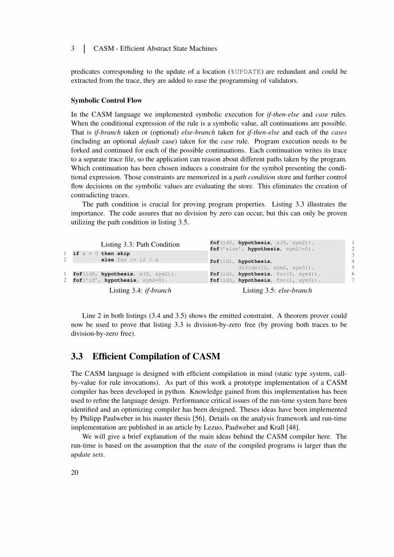
The path condition is crucial for proving program properties. Listing 3.3 illustrates theimportance. The code assures that no division by zero can occur, but this can only be provenutilizing the path condition in listing 3.5.
Listing 3.3: Path Condition1 if x = 0 then skip
2 else foo := 12 / x
1 fof(id0, hypothesis, x(0, sym2)).
2 fof(’if’, hypothesis, sym2=0).
Listing 3.4: if-branch
1fof(id0, hypothesis, x(0, sym2)).
2fof(’else’, hypothesis, sym2!=0).
34fof(id1, hypothesis,
5divide(12, sym2, sym3)).
6fof(id2, hypothesis, foo(0, sym4)).
7fof(id3, hypothesis, foo(1, sym3)).
Listing 3.5: else-branch
Line 2 in both listings (3.4 and 3.5) shows the emitted constraint. A theorem prover couldnow be used to prove that listing 3.3 is division-by-zero free (by proving both traces to bedivision-by-zero free).
3.3 Efficient Compilation of CASM
The CASM language is designed with efficient compilation in mind (static type system, call-by-value for rule invocations). As part of this work a prototype implementation of a CASMcompiler has been developed in python. Knowledge gained from this implementation has beenused to refine the language design. Performance critical issues of the run-time system have beenidentified and an optimizing compiler has been designed. Theses ideas have been implementedby Philipp Paulweber in his master thesis [56]. Details on the analysis framework and run-timeimplementation are published in an article by Lezuo, Paulweber and Krall [48].
We will give a brief explanation of the main ideas behind the CASM compiler here. Therun-time is based on the assumption that the state of the compiled programs is larger than theupdate sets.
20

3.3.1 Dynamic Memory Allocation
Only functions and updates need to be allocated dynamically. Due to the transactional semanticsof ASM languages the life-span of an update is exactly one step of the machine. A pre-allocatedmemory pool is used to store updates until a step is made and all updates are committed to thefunction storage. This pool can simply be reused in subsequent steps (dump-allocation). Therun-time therefore has virtually no memory management overheads.
3.3.2 Storage for CASM Functions
To properly implement functions, set operations are necessary. All locations which are notexplicitly defined otherwise have the special value undef (demanding an is-element-of set op-eration). A distinct hash-map (with linear probing) is used as storage for each function. Thefunction arguments are concatenated to form the key. Each slot of the map has two specialproperties, undef and branded. The undef property is set if the location has the special valueundef. An update may set a previously defined location to undef, so such locations need to betracked explicitly. A slot is branded when its corresponding location is accessed for the firsttime. (Branding allows to use other default values than undef, CASM supports this feature). Therun-time uses the slot’s address, which must be guaranteed to be stable, as a unique identifier.
After each step of the machine the hash-map can safely be enlarged, if the load factor shouldhave become too large. In the rare case that during a single step the hash-map would overflow,additional memory is allocated. In-between the next machine step the hash-map is resized andthe overflow memory gets merged.
If a sub range integer type is used for the domain of a CASM function, an array is used asfunction storage instead of a hash-map (for reasonable sizes of the domain). An additional byteis needed to keep track of the special value undef.
3.3.3 Updates and Pseudo States
Due to the interleaving of parallel and sequential execution semantics the state used to evaluate astatement and the state affected by its updates are in general not equal [26]. Listing 3.6 illustratesthe problem. stmt1 and the sequential blocks containing stmt2 and stmt4 are in a parallelblock. Therefore they are evaluated under the same state S0, their updates however are appliedto different states. While updates produced by stmt1 are applied to S0, updates produced bystmt2 are used to create a temporary state S1. The sequential composition with stmt3 maymodify updates produced by stmt2 and only the resulting update set will be applied to S0. Thesame situation is with stmt4 and stmt5. As e.g. stmt4 may contain a nested parallel blocka tree-like structure of states is created. The nesting of update sets is very similar to nestedtransactions in software transactional memory (STM) [2]. The major difference is that an STMtransaction aborts when reading an object for which a commit is pending while in ASM readaccess can never fail. Multiple updates to the same location in a parallel context is a run-timeerror (inconsistent update) in CASM.
Our assumption is that the number of updated locations (in a single ASM step) is muchsmaller than the whole state of the program. We therefore do not duplicate the state but keep
21

3 CASM - Efficient Abstract State Machines
{
stmt1{| stmt2
stmt3|}
{| stmt4stmt5
|}
}
Listing 3.6: Interleaving PAR/SEQ
track of all updates produced so far in a data structure called update set. When looking up alocation the run-time has to query the update set for updates affecting the current state (due tosequential execution semantics).
We use the notation of pseudo state to keep track of updates affecting the current state. Thepseudo state is a counter which is increased (at run-time) when a block with different executionsemantics is entered. When a block is left (and control-flow returns into a block with different
execution semantics) the update set is merged into the update set of the surrounding block. Thisis a serialization of the (partial) parallel execution semantics of ASM. Initially the system startsin parallel execution state, so pseudo state 0 denotes a block with parallel execution semantics.When entering a block with sequential semantics the pseudo state will be increased by 1. Byconstruction this counter is odd when executing a block with sequential execution semantics andeven when in parallel mode.
The update set is implemented as a hash-map. The keys are 64 bit values, the lower 16 bitsare the pseudo state of the block the update originates from, the remaining bits are the lower bitsof the slot used to store the location. (This limits the number of nested states to 65536 and thekeys may collide for slots whose addresses only differ in the uppermost 16 bits. A key collisiontriggers an erroneous program abort, but no wrong behavior. We never hit any of the limits inour applications.)
Additionally the slots in the update set are forming a linked list with the latest update beingthe head. This property is used when merging update sets. Figure 3.1 shows the update set datastructure.
3.3.4 Lookup and Update
A lookup for a specific location first needs to query the functions storage to acquire the addressof the slot. This address and the current pseudo state are used to query the update set for anyupdates to this location which may be visible in the current state. By construction of the update
set the corresponding keys can be efficiently calculated using the current key. The sequentialstates are all odd numbered pseudo states with a number that is lower than the current one. Thecomplexity of this operation is linear in the number of active pseudo states (dynamic nestingdepth of parallel and sequential blocks).
An update also needs to query the functions storage to acquire the address of the slot corre-sponding to the location. This address and the current pseudo state form the key for the update
22

Address (48 bit)
&update
Pseudo state (16 bit)
last update
key
lookup: O(#ps), merge: O(#updates), insert&collision: O(1)
Figure 3.1: CASM Update Set
set. If the slot in the update set already contains a value, the further behavior depends on the cur-rent pseudo state. In sequential execution mode (odd pseudo state) the value will be overwritten,in parallel mode an inconsistent update error is triggered. The complexity of the inconsistency
check is constant.
3.3.5 Merging of Update Sets
When leaving a block (with different execution semantics) the list property of the update set isexploited to efficiently merge all updates into the surrounding update set. The list is traversedbackwards until the first update not belonging to the current update set is found (encoded in thelower 16 bits of the key). All updates are removed from the update set and re-inserted with thepseudo state part of their key reduced by one. Merging of update sets produced by sequentialblocks may trigger inconsistent update errors as they are re-inserted into an update set withparallel execution semantics. The complexity of merging is linear in the size of the update set tobe merged.
3.3.6 Optimizations
The hash-maps used to implement the update set and functions are obviously very expensive interms of performance. In this section we describe two optimizations called lookup elimination
and update elimination that aim to reduce the number of hash-map operations. The first ob-servation is that lookups from a parallel execution context will always retrieve the same value(for same locations). In such situations only the first lookup needs to query the function storageand the update set to retrieve the value. The second observation is that, in sequential executioncontext, updates and lookup behave like local variables in the language C.
The idea is to introduce so called local locations. That is a rule-local storage which willbe used by optimized lookup and update code. Once fetched, the local location can be used by
23

3 CASM - Efficient Abstract State Machines
{
if X(3) = 3 then
skip
if X(3) = 4 then
skip
}
{
local X_3 = X(3) in
if X_3 = 3 then
skip
if X_3 = 4 then
skip
}
Table 3.1: Redundant Lookup and its Elimination
{|
X(4) := foo
if X(4) > 0 then
skip
|}
local L_1 = foo in
{|
X(4) := L_1
if L_1 > 0 then
skip
|}
Table 3.2: Preceded Lookup and its Elimination
{|
X(5) := foo
X(5) := bar
|}
{|
X(5) := bar
|}
Table 3.3: Redundant Update and its Elimination
subsequent lookups without the overheads of a hash-map. Table 3.1 illustrates the basic idea(local is not a valid CASM keyword).
Another pattern which allows the elimination of a lookup arises from updates (to the samelocation) preceding the lookup in a sequential context. In this case the value to be retrieved isknown already and can be propagated instead of performing an expensive lookup. We call thispattern a preceded lookup, for an example see table 3.2.
Update elimination tries to reduce the number of updates stored in the update set. If aspecific location is updated multiple times in a sequential context, only the last update willbe committed to the state. All preceding updates can safely be omitted. See table 3.3 for anexample.
Paulweber [56] has developed an analysis framework and implemented the described opti-mizations as part of this master thesis. In section 10.1 we report on the effectiveness of theseoptimizations.
24

4 Semantics and Compilers
ופר�סן! תק²ל מנ¾א מנ¾א
This chapter describes how CASM is used in our retargetable research compiler. A methodto give concise semantics to a configurable instruction set based on a Architecture DescriptionLanguage (ADL) is described. The technical aspects of creating CASM representations of thematcher MIR (mMIR) and Low-level IR (LIR) languages are discussed. The ADL containshighly redundant specifications for ISS and CS tools, which motivate using CASM as an unifiedmodel.
4.1 ADL for Retargetable Compilers
Our industrial partner offers a retargetable toolchain for application specific processors. Theinstruction set of such a processor is created by the custom demands of its software application.This includes removal of unused instructions, choosing an optimal instruction encoding andproviding instructions tailored for the application and customization of the data paths. A richeXtensible Markup Language (XML) based ADL has been developed to cover all the demands(Farfeleder et al. [25]).
So called micro instructions describe the hardware building blocks for the Arithmetic LogicUnit (ALU) Each instruction implemented by a specific processor is built from such micro in-
structions. The set of implemented instructions define the data paths and layout of the resultingALU. Listing 4.1 shows the micro instruction describing a hardware add operation. The data-flow of this instruction accepts 2 operands (lines 2 and 3) and defines 3 values (lines 4 to 6). Thebit width is not determined yet, but the result has the same width as the first operand (line 4).The semantics of this micro instruction is specified by the asm_semantic tag.
In listing 4.2 the specification of a full machine instruction (addition) is shown. Lines 2-4specify 3 variants with different assembler mnemonics. The expr attribute of the mnemonicnodes specify the value of the instruction’s flags which are then used to conditionally invokemicro instructions. In this example the addition instruction is available as half word addi-tion and saturated addition. The when attribute specifies the pipeline stage the micro opera-
tion is executed at. A normal addition variant would therefore execute the micro instruction
25

4 Semantics and Compilers
1 <minstr id="ADD">
2 <in name="op1"/>
3 <in name="op2"/>
4 <out name="sum" width="%in(op1)"/>
5 <out name="overflow" width="1"/>
6 <out name="overflow_sign" width="1"/>
7 <asm_semantic>
8 %fuvar(%out(sum)) :=
9 BVadd_result(%width(%in(op1)), %fuvar(%in(op1)), %fuvar(%in(op2)))
10 %fuvar(%out(overflow)) :=
11 BVadd_overflow(%width(%in(op1)), %fuvar(%in(op1)), %fuvar(%in(op2)))
12 %fuvar(%out(overflow_sign)) :=
13 BVadd_overflowsign(%width(%in(op1)), %fuvar(%in(op1)), %fuvar(%in(op2)))
14 </asm_semantic>
15 </minstr>
Listing 4.1: Micro Instruction for addition
READ_REGISTER at time CMP_READ_OPERAND_1 and store that as op_left_ (line 12) tolater copy the value to op_left (as h==0, line 16). Line 18 - 25 read the second operand andthe remaining markup handles performing the hardware add operation (line 28) and storing theresult in the register set (line 38).
To specify the semantics of the micro-processor the semantics of each instruction (and allits variants) must be defined. Listing 4.1 showed that the semantics is attached to micro instruc-
tions. Lines 8-13 show CASM markup where concrete input and output values still need to bereplaced by a simple macro substitution. All % prefixed strings are preprocessed and replacedby strings. E.g. %in(op1) is replaced by the input operand of that name (op_left) in this case(%out(overflow) by ov).
A tool called casm_gen is used to create a complete CASM specification for a specific pro-cessor out of the ADL. Each instruction is mapped to a single CASM rule implementing allvariants thereof. Listing 4.3 shows the general structure of an instruction’s CASM model.
rule ADDITION(bndladdr:Int, addr:Int, stage:PipelineStages,
phase:PipelineCycles) =
let h = decode_field(addr, FV_h) in
let r = decode_field(addr, FV_r) in
let sa = decode_field(addr, FV_sa) in
{
if h=0 and r=0 and sa=0 then
{
{|
if stage=EX1 and phase=begin then { /* ... */ }
if stage=EX1 and phase=end then { /* ... */ }
|}
/* for more stages */
}
/* more variants */
}
Listing 4.3: CASM markup of an instruction
26

1 <instr id="ADDITION" group="CMP" xml:base="../instructions.xml">
2 <mnemonic expr="sa==0 and h==0">add</mnemonic>
3 <mnemonic expr="sa==1 and h==0">add.s</mnemonic>
4 <mnemonic expr="sa==0 and h==1">add.h</mnemonic>
56 <op field="a"/>
7 <op field="b"/>
8 <op field="c"/>
9 <op_type field="r" operands="op1,op2,op3">TYPE_COMBINATION_ALU_SAME_3</op_type>
1011 <invoke when="CMP_READ_OPERAND_1">
12 op_left_ = READ_REGISTER(%op(1),1)</invoke>
13 <invoke when="CMP_READ_OPERAND_1" expr="h==1">
14 op_left = SIGN_EXTEND1(op_left_)</invoke>
15 <invoke when="CMP_READ_OPERAND_1" expr="h==0">
16 op_left = op_left_</invoke>
1718 <invoke when="CMP_READ_OPERAND_2">
19 reg_right_ = READ_REGISTER(%op(2),2)</invoke>
20 <invoke when="CMP_READ_OPERAND_2" expr="h==1">
21 reg_right = SIGN_EXTEND1(reg_right_)</invoke>
22 <invoke when="CMP_READ_OPERAND_2" expr="h==0">
23 reg_right = reg_right_</invoke>
24 <invoke when="CMP_READ_OPERAND_2">
25 op_right = reg_right</invoke>
2627 <invoke when="CMP_WRITE_OPERAND_3" expr="h==0">
28 [sum, ov, os] = ADD(op_left, op_right)</invoke>
29 <invoke when="CMP_WRITE_OPERAND_3" expr="h==1">
30 sum = ADD_HALVE(op_left, op_right)</invoke>
31 <invoke when="CMP_WRITE_OPERAND_3" expr="h==1">
32 [ov, os] = [0, 0]</invoke>
33 <invoke when="CMP_WRITE_OPERAND_3" expr="sa==0">
34 result = sum</invoke>
35 <invoke when="CMP_WRITE_OPERAND_3" expr="sa==1">
36 result = SATURATE(sum, ov, os)</invoke>
37 <invoke when="CMP_WRITE_OPERAND_3">
38 WRITE_REGISTER(%op(3), result, ov, os, 0)</invoke>
39 </instr>
Listing 4.2: Addition Instruction
4.2 Compiler Overview
Our research compiler uses a number of IRs. The front-end is based on GCC and therefore usesGIMPLE [63]. GIMPLE is then translated to a tree-ish Mid-End IR (MIR) language. Mid-endoptimizations are implemented as MIR to MIR transformations. Before the program is loweredto a sequential machine like LIR certain MIR operations are replaced. This restricted languageis called mMIR and is used to perform instruction selection. LIR has two main variants, codewhich is not scheduled yet (causal LIR (cLIR)) and fully scheduled code (scheduled LIR (sLIR)).
27

4 Semantics and Compilers
+
p i
n0
n1 n2
POINTER(n0):=true,
WIDTH(n0):=20
POINTER(n1):=true,
WIDTH(n1):=20
INTEGER(n2):=true,
WIDTH(n2):=16,
SIGN(n2):=true
Figure 4.1: mMIR example
4.3 Semantics of Compiler IR
For translation validation the compiler must dump the IR before (pre) and after (post) each pass.In this section the modeling of the IRs and creation of the dump is described.
4.3.1 mMIR
MIR code is a tree-ish language which needs to be translated into a sequential (CASM) notation.The nodes are either instruction nodes (that are operations, e.g. addition, multiplication) oroperand nodes (e.g. constant values, variables, results created by instruction nodes).
Figure 4.1 shows an example of a mMIR tree (addition of a signed offset i to a pointerp). Each node has a unique label (n0, n1, n2) and is of a specific type. The top-level node isan addition, while its leaves are variables (mMIR is in Static Single Assignment (SSA) form).mMIR nodes are polymorph and the exact type of the operation is determined by its operandsand result. The CASM functions POINTER, INTEGER, WIDTH and SIGN are used to describethe exact types of variables. Evaluating trees is implemented by updating the VALUE functionwhich associates values to nodes. The result of this addition is stored in VALUE(n0).
Table 4.1 shows the most important CASM functions used to model mMIR. The VALUE
function contains the (dynamically) calculated values associated to nodes. WIDTH, SIGN,
SIMDTYPE, SIMDFACTOR, INTEGER, POINTER are used to describe the types of variables.mMIR operates on Bit Vectors (BVs) of arbitrary size. WIDTH determines the size of the BV.INTEGER and POINTER are used to determine whether a value is used arithmetically or as apointer. SIGN is only used to INTEGER types and specifies whether an integer is signed orunsigned. SIMDTYPE is also only valid for INTEGER types and if set to true the underlyingbit vector is interpreted as a container holding multiple data points. SIMDFACTOR finally spec-ifies the number of data points (of equal size) in an Single Instruction Multiple Data (SIMD)container. mMIR operates on a linear memory which has the same properties as the target ma-chine’s memory (endianess, word size). Control flow is modeled using a dedicated call stack(MIRHWSTACK). mMIR also has support for hardware based loops and has explicit supportthrough MIRHWLOOP. Loops are denoted by their start node, end node and number of iter-
28

function signature commentVALUE Node → Int the value of a nodeWIDTH Node → Int width of value in bitsSIGN Node → Boolean signed or unsigned valueSIMDTYPE Node → Boolean value is a SIMD containerSIMDFACTOR Node → Int number of SIMD wordsINTEGER Node → Boolean value is a numberPOINTER Node → Boolean value is a pointerMIRMEMORY Int → Int the system memoryMIRHWSTACK → List (Node) MIR call stackMIRHWLOOP → List (Tuple(Node,Node,Int)) hardware loopMIRPC → Node currently executed MIR nodeNEXTMIRPC Node → Node static successor MIR node
Table 4.1: mMIR State Representation
ations. A node’s (statically) determined successor node is modeled using the CASM functionNEXTMIRPC and MIRPC addresses the node currently executed.
The tree is traversed in a depth-first fashion, processing all child nodes before the parent isprocessed. Each node is assumed to have a unique identifier. MIR is polymorph in the sensethat the exact semantics of an instruction may depend on the type of its operands and type ofthe result (i.e. conversions). For operand nodes all type information is emitted in hash-maps(their CASM equivalents), e.g. WIDTH, SIGN, with the unique node identifier serving as key.Instruction nodes are replaced using a macro expansion.
Listing 4.4 shows the template used when replacing an ADDITION node. The %in macrois replaced by the numbered child of the node, the result is the last child (by convention).BVadd_result is the CASM operation corresponding to the semantic operation add_result. Fourcases are handled i) both operands have the same width (line 2) ii) first operand is wider and sec-ond signed (sign-extend second operand, line 6) iii) first operand is wider and second unsigned(zero-extend second operand, line 10) and iv) second operand is wider (extract relevant bits fromsecond operand, line 15).
Our reference implementation is limited to handle mMIR programs, which are basicallysingle expressions (see section 7.2). A full execution semantics would need to model the currentenvironment (mapping variable name to value) and the activation records as well.
4.3.2 cLIR and sLIR
cLIR and sLIR consist of sequentially executed instructions closely resembling the target ma-chine. The difference between the two is that sLIR instructions are forming bundles and areexecuted in a pipeline. cLIR instructions are scalar and not pipelined (they can be seen as afunctional model of the same sLIR instruction). In this work cLIR instruction models are cre-ated from sLIR instruction models by consecutively executing all pipeline stages. Thus during
29

4 Semantics and Compilers
1 if TYPE(%in(1)) = TYPE(%in(2)) or WIDTH(%in(1)) = WIDTH(%in(2)) then
2 VALUE(%in(3)) := BVadd_result(WIDTH(%in(1)), VALUE(%in(1)), VALUE(%in(2)))
3 else
4 if WIDTH(%in(1)) > WIDTH(%in(2)) then {
5 if SIGN(%in(2)) then
6 VALUE(%in(3)) := BVadd_result(WIDTH(%in(1)), VALUE(%in(1)),
7 BVse(WIDTH(%in(2)),WIDTH(%in(1)),VALUE(%in(2))))
8 else {
9 // ! SIGN(%in(2))
10 VALUE(%in(3)) := BVadd_result(WIDTH(%in(1)), VALUE(%in(1)),
11 BVze(WIDTH(%in(2)),WIDTH(%in(1)),VALUE(%in(2))))
12 }
13 } else {
14 // ! WIDTH(%in(1)) > WIDTH(%in(2))
15 VALUE(%in(3)) := BVadd_result(WIDTH(%in(1)), VALUE(%in(1)),
16 BVex( 0, WIDTH(%in(1)) -1,VALUE(%in(2))))
17 }
Listing 4.4: ADDITION MIR macro template
execution at most a single cLIR instruction is in the pipeline, preventing subsequent cLIR in-structions to interact with each other.
Table 4.2 shows the most important functions used to model the state. PC is the programcounter used to address the currently executed machine instruction. The target machines aresupposed to have a hardware loop unit which state is modeled by the HWLOOP function. Eachactive hardware loop consists of the first and last instruction of the loop as well as the numberof iterations (still to be done). MEM and HWSTACK model the machines memory and hardwarecall stacks. All functions starting with REG_ are used to model the register file of the targetmachine, in this case data and address registers, flags and so called modify registers. The targetmachine used in this example offers auto post and pre increments, circular buffer addressing anda special addressing mode for Fast Fourier Transformation (FFT). PMEM models the programmemory (instruction stream) while PARG holds the decoded Field Values (FVs) for each in-struction. Internal state of each Functional Unit (FU) is modeled by the FUstate function. Eachcomponent of the internal state is called a FU Field (FUF). The target hardware features pred-icated execution which may disable certain FUs. This is modeled using the PE_unit_disabled
function which holds the disabled status for each pipeline stages and FU. pipeline holds a listof instructions (addresses) for each pipeline stage of the CPU. For cLIR the size of the list is atmost one, but for sLIR (which models Very Long Instruction Word (VLIW) bundles) larger val-ues are valid. The branching unit may trigger (partial) flushes of the pipeline which is modeledby the functions inval_pipeline.
Technically cLIR models are simulated by sLIR models. cLIR is semantically equivalent tosLIR without considering (potentially conflicting) pipeline resources. By consecutive executionof each pipeline step of a sLIR model in an otherwise empty pipeline model the semantic effectsof the cLIR model are simulated.
30

CASM function function signature commentPC → Int current program counterHWLOOP → List(Tuple(Int,Int,Int)) hardware loop (start, end, iterations)MEM Int → Int machine data memoryHWSTACK → List(Int) machine call stackFUstate FU * FUF → Int internal state of FUPE_unit_disabled PS * FU → Boolean predicated executionpipeline PS → List(Int) CPU pipelineinval_pipeline_AL → Boolean interaction pipeline, branch unitinval_pipeline_EX1 → Boolean interaction pipeline, branch unitREG_GuardBits Int → Int DSP register guard bitsREG_DataRegister Int → Int data registersREG_AddressRegister Int → Int address registersREG_ModifyRegister Int → Int auto modification for address registersREG_Flag Int → Int separate flags for each data registerPMEM Int → RuleRef program memoryPARG Int * FV → Int decoded instruction fields
Table 4.2: cLIR State Representation
On Predicated Execution
The used research architecture features predicated execution. The actual instructions operateon bundles, hence they are only available in sLIR code. For cLIR code wrapper instructionshave been implemented which are aware of the condition and condition registers. During VLIWscheduling (see section 7.4) actual sLIR instructions are created and added to predicated bundles.
Predicated instructions create forks during symbolic execution (caused by symbolic evalu-ation of the conditions). The traces can easily be matched by inspection of the path condition,though. No special treatment is therefore needed to handle predicated execution in our frame-work.
To validate passes which create predicates (i.e. if-conversion, see section 7.3), it may benecessary to create a trace where the result of the conditions is known a-priori (i.e. whether con-dition evaluates to true or false). To support such validators we have added override fields to theLIR instructions, i.e. BRANCH_CONDITION_OVERRIDE and PE_CONDITION_OVERRIDE.The models for conditional branching check those fields first and can be forced act as if thecondition were true of false. If no override is given they (symbolically) evaluate the conditionand (if needed) create forks. Our current validators do not use this feature, though.
4.4 A unified Machine Model
The ADL of our research compiler contains two (highly redundant) semantic specifications foreach micro-instruction. Two types of simulators are synthesized out of the ADL, an cycle-accurate ISS and a tool to perform CS. Each of the tools have a different run-time system but
31

4 Semantics and Compilers
both need semantics specifications of the instructions. Interaction with the simulator run-timeis explicitly encoded in those specifications. Each simulator uses (preprocessed) snippets of Ccode which invokes its run-time functions. Figure 4.2 shows the simulator specifications forthe addition. Without going into the details here the semantics of the addition is given by aC implementation. In the ISS specification (listing 4.5) the $-prefixed strings are replaced bymacro substitution (similar to %-prefixed strings in listing 4.1). The CS specification (listing 4.6)uses $-prefixed and %-prefixed strings to be replaced. There are two different specificationsin use, because ISS operates on structured models of the hardware (i.e. the execution unit)while CS performs partial evaluation on level of architecture features and operates on temporaryvariables [24].
Our CASM specification 4.1 is similar to the ISS specification, the %fuvar hides the struc-tured access to the models of the underlying functional units of the micro-processor. A compilerwhich allows CASM programs to be executed efficiently could enable the reuse of the CASMspecification to synthesize an ISS. An optimizing compiler which is able to perform partialevaluation could enable to synthesize the CS specification out of the CASM models as well.We have developed ISS and CS synthesization as part of this work which is covered in chap-ter 9. Therefore the two highly redundant simulator specifications can be replaced by our CASMspecification, which also acts as the formal foundation used for translation validation.
32

<idata id="xsim_impl">
exec_unit_->result_ = exec_unit_
->operand1_ +
exec_unit_->operand2_;
if (width_$2_ < width_$1_)
{
if (exec_unit_->operand2_
& (1llu <<
(width_$2_ - 1)))
exec_unit_->result_ +=
(uint64)-1 << width_$2_;
}
if (((exec_unit_->operand1_ &
exec_unit_->operand2_ &
~exec_unit_->result_) >>
(width_$1_ - 1)) & 0x1)
{
exec_unit_->
check_negative_overflow_ = true;
}
else if (((~exec_unit_->operand1_
& ~exec_unit_->operand2_
& exec_unit_->result_)
>> (width_$1_ - 1))
& 0x1)
{
exec_unit_->
check_positive_overflow_ = true;
}
</idata>
Listing 4.5: ISS Specification
<idata id="csim_impl">
%tmp(result) = %tmp($1) + %tmp($2);
\#if (%width($2) < %width($1))
if (%tmp($2) &
TWO_POWER_N(%width($2) - 1))
%tmp(result) += (uintmax_t)-1
<< %width($2);
\#endif
%tmp(overflow) = (((%tmp($1)
& %tmp($2)
& ~%tmp(result))
| (~%tmp($1)
& ~%tmp($2)
& %tmp(result)))
>> (%width(result) - 1))
& 0x1;
if (%tmp(overflow))
{
if (!(%tmp(result)
>> (%width(result)-1)
& 0x1))
{
%tmp(overflow_sign) = 1;
}
}
</idata>
Listing 4.6: CS Specification
Figure 4.2: Simulator Specification Languages
33


5 Proof Techniques
PROOF, n. Evidence having a shade more of plausibility than of unlikelihood.
The Devil’s Dictionary
In this chapter the proving techniques used to implement validations tools are described.
5.1 Program Checking
Program Checking is a very old technique first described by Blum and Kannan [10]. A checkeris a program which is able to verify if the output of another program is correct on a giveninput. At first glance the checker may look like a re-implementation of the original program butthere are many problems which are much easier to prove than to solve. In a compiler a lot ofheuristics are applied to optimize non-functional requirements, i.e. performance and code size.These heuristics often need to consider various contradicting optimization goals (low registerpressure, high Instruction Level Parallelism (ILP)) and are therefore difficult and error-prone toimplement. The result of the heuristic transformations may have correctness properties whichare easy to check, though. In such cases a program checker is a viable option to implement avalidator resulting in a small trusted code base.
5.2 Simulation Proofs
In this section we describe the flavor of simulation proofs used in this work. We assume two StateTransition Systems (STSs), p and C(p). The original problem is to show that C(p) (in targetlanguage TL) is a correct compilation of the source program p (in language SL). Semantics ofp and C(p) is given by corresponding CASM models as described in chapter 4. This reducesthe problem to show that the CASM models are in a relation which is compatible to correct
compilation (w). In this section we define correct compilation as equivalence. This is adequateto explain the technique but too restrictive in practice. We will refine the correct compilation
relation in section 6.1. Symbolic execution (see section 3.2) results in a first-order representationof p and C(p). Figure 5.1 shows the overview.
35

5 Proof Techniques
p ∈ SL C(p) ∈ TL
JpKSL JC(p)KTL
first-order formulae first-order formulae
compile
SL semantics (ASM) TL semantics (ASM)
w
symbolic execution symbolic execution
Theorem Prover
Figure 5.1: Generic Simulation Proof
To prove the STSs JpKSL and JC(p)KTL equivalent it can be shown that both STSs inducethe same state transition for all initial states. Because of the symbolic execution technique theinitial state is a symbolic state. Showing that the symbolic state transition of the STSs on anarbitrary initial state results in an equivalent final state is therefore enough.
Our proof technique assumes the same symbolic initial state for p and C(p). Technicallyprefix pre is assigned to all CASM functions used by p and post to the ones used by C(p). Theinitial state has time-stamp 1, therefore the first-order formula 5.1 is sufficient to assume equalinitial state for the STSs p and C(p). function is the set of CASM functions (i.e. their predicaterepresentation resulted from symbolic execution).
∀f ∈ function : pref(1, a, v0) ∧ postf(1, a, v1) =⇒ v0 = v1 (5.1)
The similar formula 5.2 is the first-order formulation for an identical final state. This is theconjecture which remains to be shown by a theorem prover.
∀f ∈ function : pref(0, a, v0) ∧ postf(0, a, v1) =⇒ v0 = v1 (5.2)
5.2.1 Common Semantic Vocabulary
To prove the conjecture the implicitly encoded data-flow (resulted from symbolic execution)must be formulated using a common semantic vocabulary. The chosen abstraction level has agreat impact on the performance of the validation system. The lowest level would be bit-levelformulation. Each operation is defined by its effects on single bits. The advantage of such aformulation is that all calculations leading to bitwise equal results are recognized by the valida-tion system without additional information. The disadvantage is the permanent rediscovering ofbasic algebraic laws (i.e. the impacts on performance).
A high level of abstraction is a word-wise formulation, the approach chosen in this work. Thedisadvantage of this approach is that semantically equal but syntactical different formulationsmust be axiomatized. The main advantage is the gain in performance. Our experience has shownthat real-world compilers only use a limited set of equalities which have to be axiomatized (a
36
complete list can be found in appendix A). The common semantic vocabulary is also quite small(43 operations) as the listing in appendix A shows. Two examples are given in the followingexcerpt. Each item is the name of a predicate, in braces the arguments and a short description ofits semantic meaning.
• and (w, o1, o2, res) logical and operation on w-bit wide values o1 and o2. The result iscalled res.
• mir_if (w, c, ai, ae, res) res contains the value ai if the w-bit wide value c does not equalzero, ae otherwise. This predicate is used to model conditional control flow in mMIR.
• . . . (the full list is in appendix A)
The set of operations is designed according to the mMIR language of the compiler and istherefore architecture independent. Each operation is implemented in CASM, prefixed with BV
(i.e. BVand corresponds to the semantic operation and).
IR conditional branches
The only surprising operation is the mir_if operation which is used to encapsulate conditionalbranches of the mMIR language. In essence the problem is that control flow can not be easilydescribed using symbolic execution. A motivating example is given in figure 5.2. Assume atranslation with identical source and target language. Let listing 5.1 be the source program andlisting 5.4 the translation. Obviously the translation is erroneous (x and y have been swappedin the condition). The validator tool is confronted with the task to find corresponding tracesin the set of pre and post traces. But the traces resulting from symbolic execution can not bedistinguished by inspection of the final (and initial state), though. Lines 7-9 in listings 5.2, 5.3,5.5 and 5.6.
A translation validation tool would need to inspect the whole trace and identify symbolswhich forked the control flow. This could be done easily, but identifying corresponding symbolsin pre and post traces (if there is more than 1 fork) seems to be a hard problem. Notably thecompiler may transform the expressions leading to forking symbols. Instead of tackling thisproblem we use the semantic mir_if operation. This allows the formulation of a conditionalbranch without an if-then-else statement (in CASM) and bind the conditional expression to theprogram counter. Figure 5.3 shows a CASM fragment (listing 5.7) and its symbolic trace (list-ing 5.8). The crucial difference in the trace is that the program counter PC is now a symbol (line10). Validation tools now do not need to inspect the whole trace, conditional expressions arepart of the final state.
In our concrete setting we use mir_if to model mMIR and conditional branches modeled withif-then-else in LIR. LIR code therefore may create multiple traces when executed symbolically,but its source program (mMIR) creates exactly one trace. The validation tool therefore hasno problem to identify corresponding pairs of traces (as the correspondence is one to many).The path condition of each LIR trace makes the value of forking (LIR) symbols concrete. Thetheorem prover must be able to derive a concrete value (from the path condition) for mir_if’s
37

5 Proof Techniques
1 function (symbolic) x : -> Int
2 function (symbolic) y : -> Int
3 function (symbolic) PC : -> Int
45 ...
67 let c = BVand(1,x, BVnot(1,y)) in
8 if Int2Boolean(c) then
9 PC := 23
10 else
11 PC := 42
Listing 5.1: x ∧ ¬y
1 fof(0,hypotesis,x(1,sym2)).
2 fof(1,hypothesis,y(1,sym3)).
3 fof(2,hypothesis,not(sym3,sym5)).
4 fof(3,hypothesis,and(sym2,sym5,sym7)).
5 fof(’if’,hypothesis,sym7=1).
6 fof(4,hypothesis,stPC(1,sym8)).
7 fof(final0,hypothesis,x(0,sym2)).
8 fof(final1,hypothesis,y(0,sym3)).
9 fof(final2,hypothesis,PC(0,23)).
Listing 5.2: Trace If
1 fof(0,hypothesis,x(1,sym2)).
2 fof(1,hypothesis,y(1,sym3)).
3 fof(2,hypothesis,not(sym3,sym5)).
4 fof(3,hypothesis,and(sym2,sym5,sym7)).
5 fof(’else’,hypothesis,sym7=0).
6 fof(4,hypothesis,PC(1,sym8)).
7 fof(final0,hypothesis,x(0,sym2)).
8 fof(final1,hypothesis,y(0,sym3)).
9 fof(final2,hypothesis,PC(0,42)).
Listing 5.3: Trace Else
1function (symbolic) x : -> Int
2function (symbolic) y : -> Int
3function (symbolic) PC : -> Int
45...
67let c = BVand(1,y, BVnot(1,x)) in
8if Int2Boolean(c) then
9PC := 23
10else
11PC := 42
Listing 5.4: y ∧ ¬x
1fof(0,hypothesis,y(1,sym2)).
2fof(1,hypothesis,x(1,sym3)).
3fof(2,hypothesis,not(sym3,sym5)).
4fof(3,hypothesis,and(sym2,sym5,sym7)).
5fof(’if’,hypothesis,sym7=1).
6fof(4,hypothesis,PC(1,sym8)).
7fof(final0,hypothesis,x(0,sym3)).
8fof(final1,hypothesis,y(0,sym2)).
9fof(final2,hypothesis,PC(0,23)).
Listing 5.5: Trace If
1fof(0,hypothesis,y(1,sym2)).
2fof(1,hypothesis,x(1,sym3)).
3fof(2,hypothesis,not(sym3,sym5)).
4fof(3,hypothesis,and(sym2,sym5,sym7)).
5fof(’else’,hypothesis,sym7=0).
6fof(4,hypothesis,PC(1,sym8)).
7fof(final0,hypothesis,x(0,sym3)).
8fof(final1,hypothesis,y(0,sym2)).
9fof(final2,hypothesis,PC(0,42)).
Listing 5.6: Trace Else
Figure 5.2: Control Flow and Symbolic Execution w/o mir_if
1 function (symbolic) x : -> Int
2 function (symbolic) y : -> Int
3 function (symbolic) PC : -> Int
45 ...
67 let c = BVand(x, BVnot(1, y)) in
8 PC := mir_if(c, 23, 42)
Listing 5.7: x ∧ ¬y
1fof(0,hypothesis,x(1,sym2)).
2fof(1,hypothesis,y(1,sym3)).
3fof(2,hypothesis,not(sym3,sym5)).
4fof(3,hypothesis,and(sym2,sym5,sym7)).
5fof(4,hypothesis,mir_if(sym7,23,42,
6sym9)).
7fof(5,hypothesis,PC(1,sym10)).
8fof(final0,hypothesis,x(0,sym2)).
9fof(final1,hypothesis,y(0,sym3)).
10fof(final2,hypothesis,PC(0,sym9)).
Listing 5.8: Trace
Figure 5.3: Control Flow and Symbolic Execution with mir_if
38

conditional for the proof to succeed. This is done by providing a proper axiomization of thecommon semantic vocabulary.
39


6 The Big Picture - Chain of Trust
This chapter presents our translation validation framework (see figure 6). The compilation isperformed in consecutive passes. Each pass is understood as a free-standing compilation ac-
source lexing parsing
SSA...
instr.sel. ... linking binary
validator
validator
validator
validator
checking
constraints
...Witness Information
checking
... AST
... Machine Instructions
Figure 6.1: The Big Picture - Chain of Trust
41
6 The Big Picture - Chain of Trust
cepting an input (pre) and producing an output (post). The compiler dumps witness informationfor each pass describing the performed transformations. A validation tool checks the (local)correctness of each of these passes, based on pre, post and the witness information.
The validation framework assures that pre of any single pass equals post of the precedingone. The correctness of the whole compilation can the be argued by following the chain back-
wards. Starting with a given binary it must be assured that linking was correct. If it has beenverified that linking was indeed correct, the problem is reduced to the question whether the pre-
IR (i.e. the input to the linker) is correct. Which is assured by a validator for the pass precedinglinking (and assuring that post of this preceding past equal pre of the linker pass). Eventuallythe lexing and parsing pass is validated, and at this stage the validation framework is able toassociate the source code to the binary which ultimately answers the question whether the givenbinary is a correct compilation of the given source code. It is so if all passes have been translatedcorrectly. This sequence of (locally) correct passes is called the chain of trust.
Some aspects of the transformation can not be locally validated, though. A prime example isthe correct translation of function calls. In most stages of the compilation functions are named
entities. Only in the linking stage addresses become known. The branch instructions at all callsites must be patched (correctly).
During the (local) validation constraints are collected (e.g. a specific branch instruction is acall to a specific named function). Constraints are maintained by the validation framework andare used in later validators (e.g. the linking validator needs to verify that all call sites have beenpatched). These constraints are essential to achieve (global) correctness of the whole compila-tion.
6.1 Definition of Correct Compilation
Real world languages like C have properties which make the definition of a correct compilerquite hard. There are 54 unspecified, 190 undefined, 112 implementation-defined and 15 locale-specific behaviors listed in Annex J of the C99 (TC3 draft) specification [1].
The implementation-defined behavior includes such elementary things like the number ofbits in a byte. Even the order of evaluating function arguments (they are expressions) is un-specified behavior. As they may have side-effects and even call further functions the order ofevaluation has impacts on the semantics of a C program.
As a result of this language properties a C program can only be compiled correctly with re-spect to a specific compiler. A specific conforming compiler however will provide definitions forall implementation-defined behavior. Theoretically it may (randomly) choose among differentconforming implementations of implementation-defined behavior. For such a compiler a correcttranslation must be one of the (many) possible conforming behaviors. In the remainder of thiswork we assume a concrete (deterministic) implementation of the C language (i.e. the validationtools know the exact behavior of the compiler).
42

6.1.1 Resource Limitations
In contrast to a C program a concrete machine has resource limitations (i.e. program size andavailable memory). An infinite number of C programs violate the constraints of any concretemachine (i.e. all programs larger than the machines memory). A translation is still consideredcorrect if it fails solely due to resource limitations [30].
6.1.2 Observable Behavior
A correct compilation of a C program can be characterized as preserving the observable behav-
ior. Assuming a concrete implementation of the C language a precise semantics is associatedwith any C program not invoking undefined behavior. The question of what a correct translationis boils down to the question of what exactly observable behavior is. In this work we assumetypical embedded C programs, executed in a hosted environment though. The external observer
therefore is
• The hosting operating system (i.e. its system call interface)
• Memory mapped I/O regions (for programs directly accessing hardware)
The observable behavior of a program is any interaction of the program with the system call
interface and with memory mapped I/O. A translation of a C program is called correct if it re-sults in the exactly same sequence of system calls (with exactly same arguments) and operationsto memory mapped I/O regions. This definition has the advantage of being as generic as pos-sible, but due to its global scope hard to prove in concrete situations. On the other hand thedefinition can easily be tightened by adding more external observable events (i.e. function entryand exit, basic block entry and exit) which allows to give local correctness conditions for manytransformations.
6.1.3 Undefined Behavior
While undefined behavior of a C program (i.e. accessing arrays out of bound) is a major problemin real-world applications (so called buffer overflows have security impacts) it barely affects thecorrectness of its translation. By definition the behavior of such a program is undefined, henceany behavior of the compiled program is conforming to the C standard (and therefore a correctcompilation).
6.1.4 Function Invocation
One common tightening is the addition of function invocations to the list of observable behavior.This disallows arbitrary inlining optimizations by the compiler. The proof system otherwisewould always need to investigate whether deviating behavior could be explained by inlining (oreven worse, partial inlining). Function invocations act as a black box, locally having the samesemantic effect if invoked with the same arguments.
43

6 The Big Picture - Chain of Trust
6.2 Front-end
The front-end of a compiler includes lexical, syntactic and semantic analysis of a program’ssource representation. After these steps an intermediate representation is available often in formof a decorated Abstract Syntax Tree (AST). Only after the AST has been created it is possibleto reason about semantics of the program (a stream of lexer token has no semantics). A verify-ing compiler needs to rule out the possibility of errors in the front-end part as well. Semanticcorrectness can not be checked, though, so program checking is a viable option. If the originalprogram representation can be reconstructed using the resulting AST as input its constructionwas correct.
A C compiler front-end includes a preprocessing step performing text substitutions resultingin a valid C compilation unit. Traditional C compilers also compute compile-time constantsand remove parentheses, braces and semicolons before building the AST. To reconstruct a pro-gram’s representation all those transformations need to be reversible stored in the AST. LLVM’sAST implementation keeps track of this information utilizing the clang::SourceRange class, thecurrent implementation is incomplete though 1.
6.3 Mid-end - Verification of Analyses
A program’s AST is subject to analyses and transformations. While certain transformationshave a clear semantics which can be used to verify their correctness (e.g. substitution of theAST describing the arithmetic expression 1 * a by just a), other don’t. Consider dead functionelimination, and its semantics. The key insight is that this transformation does not change aprogram semantics, iff the analysis results have been correct. A proof justifying the removalof a function would need to make sure that it is indeed dead, thereby in a way performing theanalysis. We therefore propose a method to correctly perform analysis in the first place.
In a separate project a Domain Specific Language (DSL) called Hydra has been developedwhich allows to describe analyses on a very high abstraction level. The Hydra specificationcan be used in two different modes. In checking mode it takes as input an AST, the name ofan analysis and the analysis results computed by the compiler (witness information). Hydraperforms the specified analysis on the AST and checks if the compiler results are consistent withits own results. This allows the compiler to produce weaker results (or no results at all when e.g.skipping a pass).
In generating mode a specification of the AST and an analysis is used to synthesize sourcecode implementing the analysis. This allows the hydra specification to be used directly in thecompiler. Please note that the compiler can always use a different implementation (which maybe more resource efficient) as long as the results are always weaker than the results of the versionused in checking mode.
A more detailed description of Hydra is out-of-scope for this work. In the remainder of thiswork we assume that correct analysis results are available throughout the compiler.
1http://clang.llvm.org/docs/IntroductionToTheClangAST.html
44

6.4 Back-end - Verification of Transformations
In contrast to the front-end most transformations performed in the back-end can be verified se-mantically. Each back-end pass accepts an input language (pre) and produces an output language(post). The languages pre and post have each defined semantics which allows to prove whetherthe observable behavior is preserved or not.
For each pass the compiler produces 3 artifacts i) input IR ii) output IR iii) witness informa-tion. The translation validation tool of each pass tests whether the given output IR is consistentto the given input IR under the (pass-specific) transformations described by the witness infor-mation. If the output IR is not consistent a compiler error is reported. Please note that the exacttype of error is not important, i.e. it is irrelevant if just the witness information is corrupt or areal error occurred.
Additionally each pass may produce constraints which can only be checked in later stagesof the compilation. One example is spilling registers to local stack slots. To be correct all spilllocations must be pairwise non-overlapping. As the exact stack locations may only becomeavailable in a later pass validating these constraints must be deferred.
6.5 Multiple Iterated Passes
Modern optimizing compilers commonly perform certain transformations until a fix-point isreached. For example register allocation and VLIW scheduling are tightly coupled [29]. Com-mon implementations come up with an initial schedule and try to allocate registers afterwards.In case the register pressure is to high (spill code) a less tight schedule is tried until a satisfactoryresult is found.
A compiler could implement this in an iterative fashion, i.e. it could have regions of codefor which a schedule and register allocation was found and other for which no solution has beenfound yet. Each of these intermediate steps could be dumped and processed by the validationtool. This would complicate implementation of the validator, as it would need to distinguishsuch regions and either validate the transformation or skip non-transformed regions. For eachiteration it would either re-validate previously transformed regions (expensive in terms of CPUtime) or cache validation results.
We assume a compiler which only dumps its IR for the final solution and suppressed the IRdumps for unsuccessful attempts. The compiler needs to try the transformations on intermediateIR which are fully rolled back if any transformation fails. It therefore needs to build up internaldata structures to keep track of information regarding future transformation attempts (and cannot store them in its IR directly).
45


7 Correctness of Selected Back-endTransformations
Das also war des Pudels Kern!
Faust
In this chapter validators for selected passes are presented. For each pass the IRs it operates on,needed witness information, the criterion for local correctness and possible constraints are given.The observable behavior of all back-end passes is tightened to include function invocations (seesection 6.1). Technically, basic blocks are ended on function calls (even if the function is knownto return in all cases).
A formal description of each validator could be given, but is of limited applicability forcompilers others than our research compiler. The validators need to be adapted to the concreteimplementation of the passes for each specific compiler. Passes also depend on the semanticsof the source (and IR) languages, e.g. in Java a stack overflow triggers an exception at run-time.Validators for passes modifying the stack-size (e.g. register allocation due to spilling) must thenalso validate that overflow detection is updated accordingly. In a language like C such behavioris undefined and needs not be validated at all.
Figure 7.1 gives an overview and also shows the IR each pass operates on. MIR is thecompiler’s tree-ish internal representation used in the mid-end. Before instruction selection isperformed MIR is rewritten to mMIR, which is a variant of MIR. Instruction selection is thefirst back-end pass producing an IR closely resembling machine code. The IR is now organizedin blocks of sequentially executed instructions operating on an infinite number of registers. Itsname cLIR comes from the fact that pipeline effects are not considered yet, thus causal. Afterscheduling the VLIW bundles have been constructed and pipeline resources are considered. TheIR is now called sLIR. Only after linking the final binary representation is constructed, calledLinked Assembly Module (LASM).
7.1 Prolog and Epilog Insertion
This pass transforms function invocations into branching instructions supported by the hardware.For each function prolog and epilog code is inserted to implement its activation record and
47

7 Correctness
from mid-end
Prolog and Epilog Insertion
Instruction Selection
If Conversion
RegAllocation, Scheduling, Spilli
ng
Software Pipelining
Stack Finalization
Linking
LASM
MIR
mMIR cLIR cLIR sLIR sLIR
Figure 7.1: Covered Back-end Passes
preserve callee saved registers. Function arguments are mapped to argument registers and stackslots according to the machine Application Binary Interface (ABI).
In MIR function arguments in the callee are represented by PARAMETER nodes (listing7.1). This pass replaces all PARAMETER nodes by i) register copies (into a named register) ifthe argument has been passed by register ii) a stack-relative load if the argument was passedon stack (see listing 7.2). A MIR RETURNVAL node is converted into a RETURN node and aninstruction copying the value to be returned into the result register is inserted. The call site isalso rewritten by this pass (see listings 7.3 and 7.4). All arguments to the function are eithercopied to hardware registers or stack slots (determined by the calling conventions). A potentialreturn value is copied from the hardware register to its named register. All calls are converted tocalls without any arguments.
Function foo
param A
param B
/* implementation of function */
returnval C
EndFunction
Listing 7.1: MIR function w/o epilog
Function foo
/* setup stack frame */
/* stored callee saved registers */
MOVE_REGISTER hwRegArg0 symRegVarA
MOVE_REGISTER hwRegArg1 symRegVarB
/* implementation of function */
MOVE_REGISTER symRegVarC hwRegRet
/* restore calle saved registers */
/* remove stack frame */
EndFunction
Listing 7.2: LIR function with epilog
48

...
res <- call func arg0 arg1
...
Listing 7.3: MIR call site
...
MOVE_IMMEDIATE arg0 hwRegArg0
MOVE_IMMEDIATE arg1 hwRegArg1
BRANCH_SUBROUTINE func
MOVE_REGISTER hwRegRet res
...
Listing 7.4: LIR call site
7.1.1 Constraints
• All named registers holding function arguments (copies of PARAMETERs) are live-in.
• The named register holding the return value (if any) is live-out.
• The liveness constraints are used during register allocation (see section 7.6).
• Stack locations used by arguments, validated as part of stack finalization (see section 7.7).
• The initial Control Flow Association (CFA) (see section 7.2.1) is build here as MIR calls
are translated into machine branching instructions.
7.1.2 The Validator
A validator tool for this pass must check that i) all function prologs have been inserted correctlyii) all function epilogues have been inserted correctly iii) all function arguments (parameters)have been rewritten to copy instructions iv) return values have been copied to the return registerv) each call site has been rewritten correctly and vi) no other changes have been made. Allthe checks require the validator to exactly know the used calling-conventions. The copying ofarguments to registers and stack slots create constraints which affect later validation steps. Thevalidator can be implemented using simple program checking techniques (see section 5.1).
7.2 Instruction Selection
This pass is one of the most important back-end transformations as the tree-ish mMIR getslowered to the machine-like cLIR. While mMIR still operates on (named) variables cLIR uses aninfinite number of (named) registers. The validator tool must verify that the selected instructionsare semantically equivalent to their mMIR counterparts and that the mapping of (symbolic)variables to (symbolic) registers is consistent.
As a preparatory step the MIR nodes are partitioned into trees with respect to dependencies(true, anti, output) of registers and memory. Control flow modifying MIR instructions alwaysstart a new tree as well. By construction the partitioned trees match either a side-effect freeexpression, a function call, a conditional branch or an expression with a single side-effect at theroot node (e.g. pre/post increment load and store instructions). The validator needs to check i)the partition is complete ii) no additional instructions were added and iii) the partition is correctrelative to the dependencies. This can easily be implemented by program checking techniques(see section 5.1).
49
7 Correctness
The challenging part of instruction selection is whether the selected sequence of machineinstructions is a correct translation of the MIR tree. In this work we implemented a full semanticvalidation of the selected instructions utilizing the simulation proof technique (5.2). Because theIR is changed during this transformation a mapping of the state (mMIR → cLIR) needs to bedefined.
7.2.1 Mapping State Representation: mMIR → cLIR
To apply the simulation proof technique (5.2) the cLIR state (see section 4.3.1) needs to bemapped to the mMIR state (see section 4.3.2). As only observable behavior is of interest thismapping needs only to be defined for observable program state. For the instruction selectionthe definition of observable behavior is tightened to include program state before and after eachmatched mMIR tree.
Most LIR functions are not observable (although they indirectly affect observable behavior).E.g. FUstate which holds intermediate results is not directly observable in the states beforeand after mMIR trees and is therefore not part of the mapping. The same argument holds forREG_Flag, REG_ModifyRegister and REG_GuardBits. pipeline and inval_pipeline_* are notused by cLIR models, PE_unit_disabled can only be observed indirectly. PARG only containsdecoded FV and is not part of the mapping either. This only leaves a few functions for which amapping must be defined. MEM and MIRMEMORY is a simple one-to-one mapping (by designof mMIR memory).
MIRHWLOOP and HWLOOP, MIRHWSTACK and HWSTACK as well as MIRPC and PC
are one-to-one mappings with the delicate difference of different addresses: mMIR operates onunique node identifiers and cLIR instructions have addresses. The final value of those addressesis only known after linking (see section 7.8), though. Unique instruction identifiers are thereforeused in cLIR as well.
A data-structure called CFA is used to map mMIR node identifiers to cLIR instruction identi-fiers. Passes modifying LIR instructions must update the CFA accordingly. The CFA is handledlike any other constraint (see chapter 6).
The most important mapping is mMIR’s VALUE function which will be mapped to eitherREG_DataRegister or REG_AddressRegister. Which of mMIR’s variables is mapped to whichregister number is part of the compiler’s register allocation mapping. Both (mMIR and cLIR)are in SSA form, the mapping is therefore one-to-one.
7.2.2 Semantic Validation
By construction of the mMIR trees, side-effects (memory and control flow) can only occur atthe root node. As a result only the last cLIR instruction of the selected sequence may be abranch instruction. Because mMIR conditional branches are modeled using the semantic mir_if
operations (see section 5.2.1) the corresponding traces of pre and post are trivial to find (there isonly one mMIR trace). The simulation proof technique (see section 5.2) is then applied to showthat each trace of a cLIR instruction sequence is a correct translation of its corresponding mMIRtrace.
50
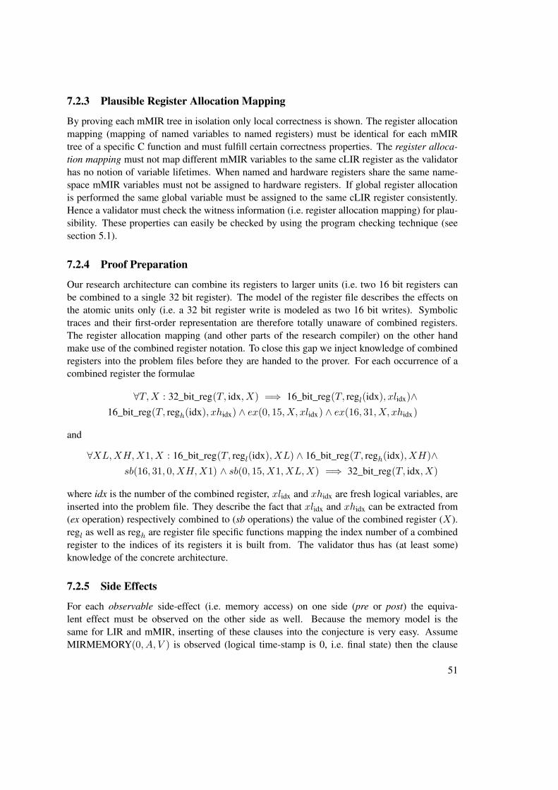
7.2.3 Plausible Register Allocation Mapping
By proving each mMIR tree in isolation only local correctness is shown. The register allocationmapping (mapping of named variables to named registers) must be identical for each mMIRtree of a specific C function and must fulfill certain correctness properties. The register alloca-
tion mapping must not map different mMIR variables to the same cLIR register as the validatorhas no notion of variable lifetimes. When named and hardware registers share the same name-space mMIR variables must not be assigned to hardware registers. If global register allocationis performed the same global variable must be assigned to the same cLIR register consistently.Hence a validator must check the witness information (i.e. register allocation mapping) for plau-sibility. These properties can easily be checked by using the program checking technique (seesection 5.1).
7.2.4 Proof Preparation
Our research architecture can combine its registers to larger units (i.e. two 16 bit registers canbe combined to a single 32 bit register). The model of the register file describes the effects onthe atomic units only (i.e. a 32 bit register write is modeled as two 16 bit writes). Symbolictraces and their first-order representation are therefore totally unaware of combined registers.The register allocation mapping (and other parts of the research compiler) on the other handmake use of the combined register notation. To close this gap we inject knowledge of combinedregisters into the problem files before they are handed to the prover. For each occurrence of acombined register the formulae
∀T,X : 32_bit_reg(T, idx,X) =⇒ 16_bit_reg(T, regl(idx), xlidx)∧
16_bit_reg(T, regh(idx), xhidx) ∧ ex(0, 15,X, xlidx) ∧ ex(16, 31,X, xhidx)
and
∀XL,XH,X1,X : 16_bit_reg(T, regl(idx),XL) ∧ 16_bit_reg(T, regh(idx),XH)∧
sb(16, 31, 0,XH,X1) ∧ sb(0, 15,X1,XL,X) =⇒ 32_bit_reg(T, idx,X)
where idx is the number of the combined register, xlidx and xhidx are fresh logical variables, areinserted into the problem file. They describe the fact that xlidx and xhidx can be extracted from(ex operation) respectively combined to (sb operations) the value of the combined register (X).regl as well as regh are register file specific functions mapping the index number of a combinedregister to the indices of its registers it is built from. The validator thus has (at least some)knowledge of the concrete architecture.
7.2.5 Side Effects
For each observable side-effect (i.e. memory access) on one side (pre or post) the equiva-lent effect must be observed on the other side as well. Because the memory model is thesame for LIR and mMIR, inserting of these clauses into the conjecture is very easy. AssumeMIRMEMORY(0, A, V ) is observed (logical time-stamp is 0, i.e. final state) then the clause
51

7 Correctness
if (x == 0) {
y = 1;
} else {
y = 3;
}
Listing 7.5: C
mov.i 3, R0
b0:
mov.i 3, R0
br.cn R0!=0, b3
b1:
mov.i 1, R0
b3:
Listing 7.6: assembler
mov.i 3, R0
(R0==0) mov.i 1, R0
Listing 7.7: predicated
Figure 7.2: If-Conversion example
MEM(0, A, V ) must be part of the conjecture and vice versa. The symbolic trace is scannedusing regular expressions to find occurrences of observed side-effects and the correspondingfunction (e.g. MIRMEMORY and MEM) is substituted. More complex mappings than this sim-ple one-to-one could be realized in this step. Thus the validator must have knowledge about themapping of (CASM) state functions (their predicate representation) onto their counterparts fortranslations changing the IR. Because each mMIR tree has at most one side-effect (by construc-tion) the order of side-effects is not important for the correctness of this pass.
7.2.6 Constraints
The register allocation mapping of each function is a global constraint. It must be consistent foreach mMIR tree of a specific C function.
7.2.7 Validator
The complete validator therefore has to verify that i) the mMIR partition is a complete, non-overlapping cover of the MIR tree ii) without any additional nodes iii) the register allocation
mapping is plausible (see 7.2.3) iv) each mMIR tree is semantically equivalent to its corre-sponding cLIR instruction sequence (simulation proofs) and that v) the same side-effects occur(under the state mapping function).
7.3 If Conversion
If-conversion [3] is a technique converting conditional branches into predicated execution. Asmall increase in code size (adding predicates) removes costs associated with mispredictedbranches. But the conversion of control dependencies into data dependencies also enlarges basicblocks. Especially on VLIW architectures the scheduler may therefore better exploit ILP whichenables better loop optimizations [69]. Figure 7.2 illustrates the basic idea of if-conversion.
In our research compiler if-conversion is implemented on cLIR. Conditional branches de-pend on the contents of a register.
The 4 basic patterns shown in figure 7.3 are optimized. Rectangles represent single basicblocks, branches are denoted by arrows. Pattern 1 is the classic if-then-else diamond shapewithout branches in the then and else block. The predicates added to the instruction in the else
52

if if
then
else
join
then
else
join
if if
then
join
then
join
if if
then*
else then*
else
if
then
else*
if
then
else*
normal instructions predicated instructions unrestricted control flow*
join join join join
1) 2)
3) 4)
Figure 7.3: Supported If-Conversion Patterns
block are the negation of the then block predicate. Two conditional branches are removed (lastinstruction of if-block and last instruction of then-block). The result is one large basic block.Pattern 2 has an empty else block. An earlier transformation assures (by inverting the branchcondition) that only this form occurs. The conditional branch in the if-block can be removed.Pattern 3 and 4 handle the cases were branch instructions occur in either the then or else block(unrestricted control flow). Only the block without branch instruction will then be converted intopredicated form. Application of pattern 3 removes a conditional branch in the if-block, but addsa predicated unconditional one to the else-block. The unconditional branch of the then-block isremoved. Pattern 4 removes the conditional branch of the if-block and turns the unconditionalbranch of the then block into a predicated unconditional one.
While the branch condition is evaluated exactly once (at the end of the if-block) predicatesare evaluated together with each instruction. The register contents of the evaluated register maybe changed, though. Therefore the register used by the conditional branch in the if-block will becopied to a fresh register which will then be used to evaluate the predicates.
7.3.1 Constraints
If the unique identifier of subroutine branch instructions has been changed the CFA must beupdated.
7.3.2 Validator
The witness information consists of i) if-block, then-block, join-block ii) optional else-blockiii) unique identifier of branching instruction iv) condition on which is branched v) conditional
53

7 Correctness
register used by branching instruction vi) register containing the copy of the conditional registerand the vii) unique identifier of copy instruction.
The validator therefore has to verify i) if-conversion patterns have been identified correctly(inspection of branching instructions and involved basic blocks) ii) only blocks identified to bepart of if-conversion patterns have been modified iii) no other blocks were added or removed iv)a register copy instruction was inserted directly before the branch instruction v) which copiesthe condition registers vi) into a fresh register not used anywhere else in the whole function vii)predicates were added to the blocks according to the identified pattern (predicate condition andregister are known) viii) branching instructions were added, removed or changed according tothe pattern. This validator can be implemented by program checking, no simulation proof needsto be performed.
7.4 VLIW Scheduling
This compiler pass is a further essential transformation of the back-end. It combines causalinstructions of the sequential stream of cLIR instructions into resource-dependency aware bun-dles. A new compiler intermediate representation called sLIR is introduced to represent suchbundles. The target architecture of our research compiler has a non-interlocking pipeline. Thismeans that resource conflicts are not detected by the hardware and lead to undefined behaviorof the program instead of just performance penalties. From a verification point of view VLIWscheduling for non-interlocked micro-processors is a correctness critical transformation.
The VLIW scheduler of the research compiler works on a basic block scope, no instructionsare moved between them. Alias analysis is used to reorder load and store operations.
A scheduled block is a correct transformation if it changes the state as the unscheduledblock would. The simulation proof technique (see section 5.2) depends on identical initial state,though. Because sLIR has a notion of the pipeline (and cLIR does not) the initial state whenentering a sLIR block is not identical with the state when entering the cLIR block. The pipelinestate has to be considered as well.
A pipeline has a certain depth and that is the number of preceding bundles which may affectthe pipeline state. By extending each basic block to include exactly this number of precedingbundles the pipeline state when entering a basic block can be reconstructed. Depending on thenumber and size of predecessors (and their predecessors) of a basic block multiple extensionsare possible. We call all such extensions the snake blocks. Figure 7.4 illustrates the concept.The pipeline depth in the example is 2 bundles. 3 paths can be constructed by extending thebasic block with 2 preceding bundles, each of which (may) result in a different pipeline stagewhen entering the block. If a blocks predecessors are not statically known the first bundles of theblock must contain no instructions. Branching to statically unknown labels can not be validatedand such code is rejected.
The cLIR instructions used to form the bundles are then used to extend the correspondingcLIR basic block. Assuming an identical state at the beginning of each of the snake blocks
the extended cLIR and the extended sLIR blocks must now result in identical final states. Theproperties of symbolic execution ensure that dependency violations introduced by reordering the
54

cLIR sLIR
Snake 1 Snake 2 Snake 3
Figure 7.4: Snake Blocks
instructions will change the DFT of the transformed block and verification will fail. Memorydependencies on the other hand are more problematic.
7.4.1 Memory Dependencies and Symbolic Execution
Performing symbolic execution leads to symbolic memory addresses (in the general case). Sometransformations reorder instructions which may include memory instructions. Reordering ofmemory instructions is not safe in general when aliasing is possible (i.e. write before read con-flicts). By inspection of the symbolic trace aliased memory addresses can not be recognized,they are simply different symbols. Hence a validator would need to assume all symbolic mem-ory addresses to be aliases, which would prevent any reordering. Clearly such a validator is notdesirable.
Symbols representing memory addresses can easily be recognized in the traces (second argu-ment of the MEM and MIRMEMORY predicates). Those symbols are associated with a symbolic
expression. As result of the unification performed during the proof a canonical symbolic expres-
sion becomes available. This defining expression (see section 8.4) is identical for symbolicvalues resulting from the semantically identical operations on identical input symbols. Identi-cal symbolic memory addresses are therefore expressed by identical defining expressions. ThevanHelsing prover (see chapter 8) writes defining expressions to a separate file accompanyingeach proof. The validator uses this file to identify aliasing memory addresses. Input symbols aremapped to registers (or stack slots), for which the mapping to named program variables is avail-able (by means of constraints, see section 7.2). Alias information of named program variableshas been computed by a front-end analysis and is also available as constraints.
55

7 Correctness
If the validator detects that a memory operation has been reordered (i.e. the addresses are notaliased) by the transformation it can validate if the reordering is coherent to the available aliasinformation. The relative order of memory accesses is encoded in the logical time-stamps of theMEM and MIRMEMORY predicates.
7.4.2 Resource Conflicts
The research target architecture has a pipeline without interlocking. Undetected resource con-flicts thus lead to undefined behavior of the hardware. By construction of the CASM modelsresource conflicts in the pipeline manifest as run-time errors (exploiting CASM’s property thatmultiple updates to the same location from a parallel context are inconsistent).
7.4.3 The Validator
The validator has to verify that i) the basic block structure of post is identical to the one of pre
(no blocks added or removed) ii) for each basic block all corresponding pairs of pre and post
snake blocks are semantically equivalent iii) all identified reordered memory operations werenot aliased.
7.5 Software Pipelining
Software pipelining is a class of optimizations which aim to remove the scheduling barrier im-posed by back-edges of loops. The idea is to initiate a number of parallel loop executions in theprolog. The so called steady state then consists of the number of parallel executed loop itera-
tions. A epilog is needed to finish loop iterations started by the steady state but no finished yet.Iterative modulo scheduling is one effective algorithm which allows to do so [42, 58]. Especiallyfor VLIW architectures a much higher degree of ILP can be exploited by the enlarged loop body(kernel, steady state).
The sLIR to sLIR transformation is sketched in figure 7.5. A hardware loop (green) whichconsists of a single basic block without branches is transformed. Additional code in the prolog(proaddpost) initiates a number of parallel iterations (blue), which reduces the number of loop iter-ations. The iteration counter has to be adopted (orange). A temporary register may be allocatedto calculate the new value (if the number of iterations isn’t a compile time constant). Finallycode is added to the epilog (epiaddpost) finishing the started loop iterations (dark blue). Optionallythe loop body may be unrolled (by a factor fu) which also affects the loop iteration counter.This transformation is only performed if the minimum number of transformations is known andunrolling is only performed (in this implementation) if the exact number of iterations is known.The steady state will be executed at least one time (on the target machine hardware loops mustbe executed at least once).
Our validator prototype uses a combination of program checking, simulation proofs (seesection 5.2) and an inductive argument to verify this transformation.
Let JK be the semantics of the enclosed expression, + denote sequential execution of sLIRinstruction sequences, propost, bdypost, epipost the prolog, loop body (steady state) respectivelythe epilog of the post transformation program. Let proaddpost (blue in figure 7.5) and epiaddpost (dark
56
steady state
prolog
loop iteration adaptionloop instruction
epilog
Figure 7.5: Software Pipelining
blue in figure 7.5) be the additional code in the post prolog and epilog. Let propre, bdypre, epiprebe the prolog, loop body and epilog of pre. Finally let iterprologpost be the number of iterations
initiated in the prolog code and iterbdypost the number of iterations initiated by each execution ofpost loop body (including unrolling).
Due to the nature of the transformation the states when entering the pre and post loops arenever identical. Without identical states our simulation proof technique can not be applied. Thepre loop always executes one full iteration, while the post loop still has unfinished iterations in-flight. Intermediate results of these in-flight iterations are used in each execution of the post loopbody. The proof technique is based on the DFT encoded in the symbolic traces and for in-flightintermediate results the DFT is unknown. However, it is known how to calculate the unknownDFT, that is exactly what the software pipelining prolog (JproaddpostK) does. Let the initial post
state be the (symbolic) state when entering the post loop body, and the synchronized initial post
state be the very same state but assume that proaddpost was executed before. (In other words, theoperations to compute the current in-flight values are replayed.) Similar the synchronized final
post state is the state at the end of the post loop body, after epiaddpost was executed.
Now an inductive argument can be made to prove software pipelining using simulationproofs. Equation 7.1 is the base case, for exactly one iteration of the post loop body. Thepost prolog, body and epilog are executed exactly once. Pre loop body is executed exactlyiterprologpost + iterbdypost times, which is the guaranteed minimum loop execution time (a precondi-tion for the transformation to be applied).
57

7 Correctness
Jproaddpost + bdypost + epiaddpostK = J
iterprologpost +iter
bdypost
︷ ︸︸ ︷
bdypre + . . .+ bdypreK (7.1)
To finish the inductive argument it must be shown that an additional execution of the post
loop body is semantically equivalent to an increased number of executions of the pre loop body.Now the synchronized states come into play as equation 7.2 shows. The post loop body isexecuted twice and hence the pre loop body must be executed twice as well (plus the iterprologpost
to account for in-flight iterations).
J
synchronized︷ ︸︸ ︷
proaddpost + bdypost+bdypost +
synchronized︷ ︸︸ ︷
epiaddpost K = J
iterprologpost +2iter
bdypost
︷ ︸︸ ︷
bdypre + . . .+ bdypreK (7.2)
It remains to be shown that proaddpost and epiaddpost have been correctly added to the prolog andepilog blocks. The simulation proof shown in formula 7.3 ensures this.
Jpropost + bdypost + epipostK = Jpropre +
iterprologpost +iter
bdypost
︷ ︸︸ ︷
bdypre + . . .+ bdypre+epipreK (7.3)
The post state may differ by additionally used registers (modulo register renaming), and adifferent loop counter register. Finally the modification of the loop counter must be verified.This can not be achieved by symbolic evaluation, but the correctness conditions are very simple,so program checking (see section 5.1) is performed.
7.5.1 Validator
The witness information contains i) identifiers for involved basic blocks (prolog, loop body,epilog) ii) additional instructions added to the prolog initiating loop iterations (proaddpost) iii) addi-
tional instructions added to the epilog finishing in flight loop iterations (epiaddpost) iv) identifier of
loop instruction v) identifiers for loop iteration adaption code (orange in figure 7.5) vi) iterprologpost
and iterbdypost vii) and modulo renamed registers.The validator must verify that i) formulas 7.1, 7.2 and 7.3 hold (by simulation proofs) ii) cor-
rect insertion of iteration adaption code (program checking) iii) modification of loop instruction(program checking) iv) additionally used registers (iteration adaption code, register renamingcaused by loop unrolling) are not used anywhere else in containing function v) reordered mem-ory operations are coherent with alias information (see section 7.4) vi) and no other changeswere made.
7.6 Register Allocation & Spilling
Register allocation and spill code generation is another indispensable pass of a compiler back-end. In our research compiler register allocation is a sLIR to sLIR transformation. Pre usesvirtual registers, although some registers are pre-allocated (i.e. function prolog and epilog, seesection 7.1) and each register is defined exactly once. Post only uses hardware registers and may
58

reg vregsrred v0, v3, v5rblue v1, v4stack0 v2
v0
v1
v2
spill
v3 v4
v5
v0
v1v2
v3
v4v5
BB
pre post
rred
rblue
stack0
Figure 7.6: Register Allocation and Live-In Live-Out Sets
use additional stack slots (for spilled registers). Each virtual register is mapped to one hardwareregister for the scope of a whole function (i.e. no live range splitting). Spill code is added to thebasic block containing the use and def (i.e. no spill code motion). Each virtual register of pre istherefore mapped to a hardware register of stack slot in post (this mapping is called the register
allocation map). Although the scope of the register allocator is the whole function, a basic blocklocal correctness criterion can mainly be used to prove its correctness.
The register allocation map must be proven to be correct, though. Program checking is aviable option here. By inspection of the pre trace the def-use information for virtual registerscan be computed. This allows to create an interference graph. It can easily be checked if theregister allocation map is a correct coloring of this graph.
The idea is to identify the live-in and live-out set of each basic block. By inspection of thepre and post traces the def-use set for each basic block can be computed. Using the Control FlowGraph (CFG) (assumed to be available and correct see section 6.3) a simple backwards data-flowanalysis is used to calculate the liveness of pre and post registers. The initial state of a pre basicblock can be used to compute an equivalent initial state for the post basic block utilizing theregister allocation map. We tighten the observable behavior to include the live-in and live-out
sets of each basic block, which still allows a wide range of transformations to be applied by theregister allocator. Using the simulation proof technique 5.2 it must be shown that an equivalentinitial live-in state results in an equivalent final live-out state.
Figure 7.6 shows an example with interference graph, register allocation map and the live-in
and live-out set of a basic block (for pre and post). The example architecture has two registers(red and blue). For the translation to be correct the live-out sets of pre and post must be equiv-alent (considering the register allocation map). Also note that the register allocator may mapvirtual register v0 (here mapped to register red) without any constraints, as long as the semanticsof the block is not changed and the live-out set is correct.
All side-effects to the memory observed by pre must be performed by post without beingreordered. Post may perform additional memory operations as long as the affected addressesare spilled virtual registers according to the register allocation map. It is possible that a spilledvirtual register is used by a basic block but not in its live-in or live-out set (e.g. v0 in figure 7.6).
59
7 Correctness
1 fof(idclir620,hypothesis,stclirMEM(4,symclir368,symclir375)).%CREATE
23 symclir368=fadd_result(20,stclirREG_AddressRegister(14),csclirPARG(28,eFV_o))
Listing 7.8: Symbolic address (symclir368) & defining expression
7.6.1 Identifying Spill Code
To identify whether an additional memory access in post is a (valid) access to a spill location weagain rely on the defining expressions (see section 8.4). In listing 7.8 line 1 is an example of aclause describing the first reading access (CREATE annotation, see section 3.2.3) to a memorycell (function stclirMEM). The address is the (symbolic) value symclir368, while the value readis the (symbolic) value symclir375. Line 3 of the listing shows the defining expression of thememory address symclir368. It was calculated by a 20 bit addition of the address register 14 (thestack pointer of the architecture) and the immediate field eFV_o of the instruction with uniqueidentifier 28. By consultation of the constraints (see section 6) the validator can check whetherinstruction 28 references a spill slot (access is okay) or not (report error).
7.6.2 Integrated Rematerialization
Register allocators often perform various other trival, small, obvious optimzations on the fly. Fora validator these optimizations are of course troublesome, as their correctness must be shown aswell. This section describes an enhancement which enables the validation of rematerialization.
LLVM’s greedy allocator (the coalescer actually)1 utilizes trivial rematerialization2 to re-move uses of a register which are the result of a register copy. The register copy can be replacedby rematerializing the content of the source register. This reduces the lifespan of a register andmay reduce register pressure. Loading immediate constants into registers are perfect candidatesfor rematerialization because load and copy instructions are easily interchanged on many archi-tectures.
Our prototype register allocation validator has support for rematerialization of constant val-ues. After the validator calculated the live-out sets a forward data-flow analysis is performedpropagating constant register values. When the problem file is generated, clauses are emittedfor registers with known constant values (stating the said register contains said constant value).The register allocator may then rematerialize or copy the register, the resulting DFT will be thesame.
7.6.3 Constraints
• The register allocation is added to the constraints. For each basic block of a specificfunction the register allocation must be identical.
• The liveness information created by the prolog and epilog insertion validator (see sec-tion 7.1) is used.
1used version: 3.22TargetInstrInfo::isTriviallyReMaterializable()
60

7.6.4 The Validator
The validator must verify that i) the register allocation map is a correct coloring of the interfer-ence graph (by constructing the graph from the traces) ii) calculate live-in and live-out sets foreach basic block (by inspection of the traces) and optionally constant register values iii) for eachpair of pre and post basic blocks the live-out sets are equivalent, given an equivalent live-in set(equivalent with respect to the register allocation map iv) all memory side-effects of pre happenin the same order in post (by inspection of the traces) v) all memory side-effects exclusivelyhappening in post affect spill memory only.
All spill locations, their defining expressions to be exact, are constrained to be otherwiseunused stack slots. This property will be verified in the stack finalization pass (see section 7.7).
7.7 Stack Finalization
This pass is responsible to allocate concrete stack slots for all stack allocations of a function.Stack allocations are needed for callee-saved registers, stack-passed arguments, local variableswhose address is used and spilled registers. Those previous passes emitted stack slot constraints.Our research compiler patches immediate fields of sLIR instructions in this pass.
Earlier passes created stack slot constraints of the generic form: instruction X referencesstack object S of size Ss at offset So. The witness information produced by this pass containsthe stack offset o for all stack objects of each function. Our research compiler implements stackslot coalescing, stack objects with disjunctive lifespans may therefore be allocated to the samestack offsets. The same technique is used to reconstruct the interference graph and proves itscoloring discussed for register allocation (see section 7.6) can be applied to prove stack slotallocation correct.
7.7.1 The Validator
The validator has to verify that i) stack slot coalescing is correct (by construction of the inter-ference graph from the traces) ii) all stack allocations are non-overlapping iii) the immediatefields of all instructions are patched correctly (collected stack constraints) iv) no other changesare made.
7.8 Linking
The linker finally defines the layout of the binary, including the address of each function and theaddresses of global variables. We assume a static linker commonly used for embedded systemswhich often don’t support dynamic linking at all. All instructions referencing functions or globalvalues must be patched (fix-ups, relocations). On some architectures the linker may even injectinstructions.
Instructions referencing function addresses have been generated during instruction selection.The name of the called function is known in mMIR code. A constraint is emitted for each
61

7 Correctness
function invocation associating the function name with the unique identifier of the cLIR callinstruction. Global variables are handled identical.
The linker emits the chosen addresses of functions and global variables as witness informa-tion, the validator can be implemented by program checking. There are additional correctnessissues to verify, i.e. different objects must not overlap, alignment and others. They all can beverified by program checking, no semantic transformations are performed by a (correct) linker.
7.8.1 The Validator
The validator must verify that i) all global objects are assigned to unique, non-overlapping ma-chine addresses ii) considering alignment constraints, validity (i.e. address mapped to actualmemory) and properties of the underlying memory (i.e. read-only, execute) iii) all relocations(fix-ups) of instruction fields have been performed correct and consistent iv) no other changeswere made.
7.9 Summary
The investigated passes include instruction selection 7.2, register allocation 7.6 and VLIWscheduling 7.4. These are the foundation passes of our research compiler’s back-end, with-out these passes no machine code can be generated at all. The other passes deal with interestingproperties of our research architecture, namely predicated execution and optimization of hard-ware loops.
Each of the passes can be verified using a combination of the simulation proof technique andprogram checking (see chapter 5). We were able to develop local correctness criteria therebylimiting the sizes of the simulation proofs to the size of a basic block. Global correctness isachieved by creating constraints (and validating them in later passes). A high degree of paral-lelism can be exploited when executing the proofs. All basic blocks (many thousands for largerprojects) of a program can be validated in parallel. Utilizing a large cluster even very largeprograms can therefore be validated within minutes (depending on the longest running proofs).
62

8 vanHelsing: Prover and Debugger
With superposition based provers like Vampire [59, 41] and Eprover [62] there are two problemswith our application i) if the symbolic traces created from the (not trusted) IR dumps contain acontradiction a spurious refutation will be found (interpreted as proof success) and ii) if thetranslation was erroneous the prover states satisfiability, but gives no hint about the nature of theproblem. Problem i) can be solved by running the prover on the symbolic trace and axiom setwithout the conjecture, they must be satisfiable. We are not aware of a solution of the secondproblem, though. A domain expert has to manually check the problem to locate the reason whythe proof failed (and locate the compiler bug). This is a tedious and time-consuming task.
Using the same problem formulation SMT produces a model for erroneous translation (theyare satisfiable) which helps in identifying the bug in the compiler. For more complex problemsfinding a model seems to be a very time consuming task (at least for the Z3 prover, see sec-tion 10.2). For unsatisfiable problems no further information is given, while superposition basedprovers create an evidence. (The problem can be formulated in a different fashion so a modelis found as evidence, losing the models for erroneous translations, though.) A missing evidenceweakens the strength of the argument that the compilation is proven to be correct (proof can notbe retraced independently). The other issue is that if the translation facts produced by the (nottrusted) compiler are unsatisfiable in itself, the whole problem will be spuriously unsatisfiable.
Due to the large size of our problems (often more than 10.000 predicates) our tool shouldalso provide a debug mode to analyze failing proofs. A representation of the encoded DFT asgraph helps to catch the interrelation of predicates and values, but also creates the connection tothe problem domain. vanHelsing can print a graph representation of the problem utilizing thewidely used DOT language [27]. Figure 8.1 shows the initial graph built from the example givenin listing 8.2. Function applications are printed as structured rectangular boxes. The first fieldcontains the name of the predicate, the following fields its arguments. By convention the lastargument represents the result. All arguments are linked to the referenced value nodes (printed
63

8 vanHelsing: Prover and Debugger
in ellipses). Unified values (that are equal values) are printed as list after the equal sign (thereare none).
8.1 Input Language
As input language the vanHelsing prover uses a subset of TPTP v6.0 [65]. This section specifiesthe supported features and restrictions. A specification of the language in EBNF can be foundin appendix C.
As top-level elements TFF (type information for predicates and variables) and FOF (first-order formula) are accepted. TFF formulas are accepted but ignored and vanHelsing assumesinteger types for all values. Nonetheless correct type information should be added to achievecompatibility with other provers (i.e. Vampire). All TPTP formulas have the generic formlanguage(id, role, formula). with language being fof or tff. The role of a FOFformula is one of axiom, hypothesis or conjecture (formula to be proven). The subset of acceptedFOF formulas is tailored for the problems of our application and all accepted elements are listedbelow:
• Values / Variables – $true, 1, -4, sym2
The values $true and $false encode the boolean constants true and false. Integer constantsrepresent the corresponding integer value. Boolean and Integer constants are called well-
defined values (that is: their semantic value is known). All other values (e.g. sym2 aresupposed to be (unknown) integer values. Variables starting with an upper case letter areall-quantor bound free variables used in patterns.
• Functor Application – pred(x,y,z)A translation fact, encoded as a predicate. If a functor application may also be part of theconjecture, the corresponding fact must eventually be derived for the proof to succeed.
• Equality – x = y
Should x and y both be well-defined (but different) values the problem contains a contra-diction. If equality is used in the conjecture the values x and y must eventually be unifiedfor the proof to succeed.
• Inequality – x != y
Should x and y both be the same value the problems contains a contradiction. If inequalityis used in the conjecture the values x and y must not be unified for the proof to succeed.
• Implication – lhs => rhs
If lhs (the pattern) evaluates to true rhs (the action) will be performed. An action mayeither be a function application, in that case a new fact will be added to the problem oran equality, which triggers an unification. No unbound free variables must occur in theaction. An exemplary usage is the implication (add(A,B,X) & add(A,B,Y)) =>
X=Y). Implications drive the unification, as their rhs usually contains new equalities.
64

• Conjunction - formula1 & formula2
Informally introduced in above example, conjunction of terms is possible. Important ap-plications of the conjunction is a conjecture consisting of multiple clauses and of coursein complex patterns of implications.
• Equivalence – lhs <=> rhs
The equivalence pattern will be translated into two implications (lhs => rhs and rhs=> lhs).
8.2 Implementation
In this section we describe the algorithm and data structures used to implement vanHelsing aswell as implemented optimizations. The whole problem is represented as graph with 2 basicnode types, values and functors. Values are linked to functors using or defining them, andfunctors are linked to all values they reference. Any path in the graph therefore is an alternatingsequence of value and functor nodes.
Each value is exactly stored once in the graph. When unifying two values the node with thefewer edges will be removed from the graph. All its neighbors will be linked to the value it wasunified with.
We also remove duplicated functor nodes, that are functors of the same type connected toexactly the same value nodes (in the same order). Initially there are no such nodes by construc-tion. Whenever two value nodes are unified we test their linked functor nodes for duplicates.Due to the structure of our problems a lot of duplicate functor nodes will be produced. The testfor duplicated functors can be performed efficiently utilizing the problem graph.
vanHelsing is a command line tool designed for batch processing and implemented in C++.The current implementation uses 64 bit machine integers to represent integer values. Their rangeis sufficient for our applications.
8.2.1 Unification Algorithm
The idea is to repeatedly match all patterns until the graph does not change any more (problembecomes stable). Only when the problem is stable it is assured that no contradiction has beenderived. The fix-point unification algorithm is given in listing 8.1. This is a major difference tosuperposition based theorem prover which report the first derived contradiction as proof.
When the number of unification reaches 0 we break the main loop (line 5). The patterns getmatched one additional time to assure that no contradicting unification was performed duringthe last round (line 8). Due to the special structure of our problems (the conjecture consists ofequalities) it is sufficient to consider the conjecture only here. Either all unifications to prove theconjecture have been derived or we report failure (line 14).
A so-called proof script is written into a separate file, containing all performed unification(and which rules induced them). It is also in TPTP format, which allows a vanHelsing derivedproof to be validated using other provers.
65

8 vanHelsing: Prover and Debugger
1 while True:
2 nr_uni,contra = patternMatching()
3 if contra:
4 reportContradiction()
5 if nr_uni = 0:
6 break
78 nr_uni,contra = patternMatching()
9 if contra:
10 reportContradiction()
1112 allconj = checkConjectures()
13 if not allconj:
14 reportFailure()
1516 reportSuccess()
Listing 8.1: vanHelsing Unification Algorithm
8.2.2 The problem graph
We distinguish 2 types of value nodes. A well-defined value node is an integer constant, a stringor one of the boolean constants true and false. They are well-defined in the sense that theirsemantic value is known.
A hash-map is used to implement efficient lookup of values by their name. This also decou-ples patterns (which use variable names) from the problem graph. When a variable is referencedby a pattern this hash-map is used to lookup the value node. This allows unification of valuenodes without considering the patterns.
8.2.3 Pattern Matching
As complex patterns are constructed using conjunction this is the only interesting case. The firstfunctor pattern is matched against the problem graph by looking up all functors of the name.Each of the functors looked up binds the free variables of the pattern. When matching the nextpattern all the looked up functors would need to be tested against the current assignment of freevariables. The number of looked up functors can drastically be reduced by using term indexing(described in the next section).
8.2.4 Optimization techniques
We improved the performance of the vanHelsing prover by many magnitudes using the followingoptimizations.
Dead patterns
A rather obvious optimizations which does not try to match a function application pattern (e.g.add(A,2,B)) if there are no terms (here predicated names add) it could match. This optimiza-tion becomes effective if conjecture patterns inherit this property from their clauses. A genericset of axioms can then be used for each problem as they don’t incur to the execution time.
66

Term Indexing
The unification process is driven by implications. Many of the axioms describe the syntacticequivalence of the data-flow trees. They all have the generic form
pred(A,B,X) ∧ pred(A,B, Y ) =⇒ X = Y
The first predicate is matched and concrete values are bound to the the free variables A and B.Matching the second predicate can now be accelerated if A or B are well-defined (their valueis known). vanHelsing stores all functors of a specific type in a hash-map (for the first lookup)and maintains hash-maps for functors with well-defined arguments. The current implementationconsidered the first 3 arguments. This is the most important single optimization.
Functor freezing
We call a sort of functors frozen if no functor of their name has been modified in the currentround. A pattern is called frozen if it matches a functor which is frozen itself. The conjecturepattern inherits its frozen status from its clauses. Initially there are no frozen functors, assuringthat each pattern is matched at least once. Frozen patterns may be skipped during the patternmatching phase as they can not produce any new unifications. A functor sort must be unfrozenwhen a new fact involving this sort is added to the problem.
8.3 Proof Debugger
A distinct feature of the vanHelsing prover is its capability to debug failing proofs. Exploitingthe regular structure of our problems it is possible to identify a subgraph relevant to each failingconjecture.
The listing 8.3 shows a failing equality conjecture. Assuming that initially sym1 equals sym6
and sym4 equals sym8 (that is mapping MI ) it should be shown that sym5 equals sym9 (MF ).The calculation resulting in sym7 exploits the fact that 1 plus 1 equals 2, which is unknownto the prover. Figure 8.2 shows the failing proof graph. The DFT of both values (sym5 andsym9) are constructed. One is colored red, the other yellow. Nodes being part of both DFTs arecolored orange. Figure 8.2 shows the resulting graph (unrelated nodes have been removed, i.e.the unrelated functor and its values are not printed). Visual inspection quickly reveals that thefirst different colors begin to appear with sym2 and sym7.
By adding the needed axiom shown in listing 8.4 the proof succeeds. The resulting graph isshown in figure 8.3.
1 fof(id0,hypothesis,add(sym1,1,sym2)).
2 fof(id1,hypothesis,add(sym2,1,sym3)).
3 fof(id2,hypothesis,add(sym3,sym4,sym5)).
45 fof(id3,hypothesis,add(sym6,2,sym7)).
6 fof(id4,hypothesis,add(sym7,sym8,sym9)).
78 fof(id5,hypothesis,unrelated(sym10, sym11, sym12)).
Listing 8.2: Translation facts with 3 data-flows
67

8 vanHelsing: Prover and Debugger
sym2 =
addsym7
sym8
sym9unrelated
sym10
sym11
sym12
sym5 =
sym1 =
sym3 =
sym11 =
sym9 =
add
sym2
1
sym3
sym4 =
add
sym3
sym4
sym5sym7 =
add
sym1
1
sym2
sym12 =
sym10 = sym8 =
sym6 =add
sym6
2sym7
Figure 8.1: Initial Data Flow Trees
1 fof(ax1,axiom,(add(A,B,X) &
2 add(A,B,Y)) => X=Y).
3 fof(op1,hypothesis, sym1=sym6).
4 fof(op2,hypothesis, sym4=sym8).
56 fof(cj1,conjecture, sym5=sym9).
Listing 8.3: Missing an axiom
fof(ax2,axiom,(add(A,1,B) & add(B,1,C)
& add(A,2,D)) => C=D).
Listing 8.4: The missing axiom
sym5=sym9
add
sym6
1
sym2 sym2 =
sym9 =
addsym7
sym8
sym9
add
sym6
2sym7
sym5 =
add
sym3
sym8
sym5
add
sym2
1
sym3
sym7 =
sym8 = sym4
sym6 = sym1
sym3 =
Figure 8.2: A failing proof
sym9 = sym5
sym2 =
unrelated
sym10
sym11
sym12
sym8 = sym4
add
sym6
2sym7
sym12 =sym11 =
sym6 = sym1
sym10 =
addsym7
sym8
sym9
sym7 = sym3
add
sym6
1
sym2
add
sym2
1sym7
Figure 8.3: A succeeding proof
68

8.4 Defining Expressions
In our problems by convention the last argument of each predicate is the value computed by thefunction. Therefore for each value an expression leading to its calculation can be computed by asimple recursive algorithm. A function is part of the expression iff the value is its last argument.
Listing 8.5 shows the output for the input of listing 8.2 combined with listing 8.3. Thedefining expression is a canonical representation and computed after initial equalities (i.e. lines3 and 4 in listing 8.3 have been resolved). Different symbolic values, calculated by the sameexpression operating on equal symbolic values therefore have syntactical equal defining expres-
sions. This property is used in validation tools which need to assure that memory operations arenot reordered. The problem is that a memory operation has the form memory(timestamp,
symbolic_address, symbolic_value). Pre and post traces have different symbolsfor the (semantically) same addresses. By computing the defining expressions those differentsymbols are canonized and corresponding addresses can be identified by string comparison.
sym10=sym10
sym9=add(add(sym6,2),sym8)
sym7=add(sym6,2)
sym5=add(add(add(sym6,1),1),sym8)
sym4=sym8
sym3=add(add(sym6,1),1)
sym2=add(sym6,1)
sym8=sym8
sym6=sym6
sym1=sym6
sym12=unrelated(sym10,sym11)
sym11=sym11
Listing 8.5: Defining Expressions
69

9 Instruction Set Simulation & CompiledSimulation
This chapter describes how the formal CASM models of a micro-processor can be used to syn-thesize efficient simulators. The empirical evidence (see section 10.1) shows that CASM canserve as the only, unified model for micro-processors and thus eliminate redundant special pur-pose specifications.
9.1 Instruction Set Simulation
In section 4.4 we showed the similarity of the CASM models with the simulator specificationsof ISS in our research toolchain. Elimination of those redundant specifications in the ADL wasthe main motivation to develop the CASM compiler. By compilation of the CASM models thecore for an ISS can be synthesized re-using the semantic specification of the micro-processor.
An ISS commonly works like an interpreter. It processes a stream of instruction words (ofthe micro-processor to be simulated) and applies their effect on a representation of the micro-processor state. An ISS alone is of little use, because most programs rely on an environment tooperate in. System Simulators emulate the needed environment and are widely used. The maininterest is the to ability to execute C programs.
It is therefore sufficient to emulate a hosted C environment (to execute operating systemsone would need to emulate peripheral hardware). Our implementation is based on newlib 1,which has a well defined system call layer. Other C libraries are similar, though. We haveimplemented the following elementary C functions: open, close, read, write, fstat, lseek, isatty,
gettimeofday, unlink, lstat, exit. Additionally a mechanism to pass command line arguments tothe simulatee’s main function has been implemented (by customization of the _start function). Acustomized linker script overrides the default implementations of the elementary functions with
1http://sourceware.org/newlib/
71

9 Instruction Set Simulation & Compiled Simulation
.globl open
.ent open
open:
nop
nop
nop
syscall 0
/* return value in r2,r3 errono in r8 */
lui $9,%hi(errno)
addiu $9,$9,%lo(errno)
sw $8,0($9)
jr $ra
.end open
Listing 9.1: Elementary C Function Stub
our own when compiling the simulatee. Listing 9.1 shows the (MIPS assembly) implementationof the open function. All elementary C functions invoke a special trap instruction (i.e. syscall
on MIPS).
The goal is to map those elementary C functions to corresponding calls of the host oper-ating system. This is not possible if the syscall rule would be implemented in CASM. A socalled provider mechanism is implemented in CASM which allows rules to be implemented inC. The CASM compiler includes header files and links with the provider implementation. Pro-
vided rules must interact with the CASM run-time, i.e. make use of the update set and lookupmechanism.
We have developed implementations for our proprietary DSP micro-processor and for theMIPS architecture. To realize an ISS the common semantic vocabulary must not only be eval-uated symbolically, but also concrete (called BitVector Operations Library). We have chosenMIPS because well-known benchmark suites like MiBench [35] are available to evaluate theperformance of this approach. An unmodified GCC toolchain (CodeSourcery MIPS 2012.03) isused to compile and link programs for use with the simulator. Figure 9.1 gives an overview ofthe architecture.
The system memory is also provided. This allows the ELF binary loader to efficiently initial-ize data sections of the program. Two CASM functions are used to read instructions. The opcodeis read using the PMEM: Int ->RuleRef function, while instruction fields are accessed using thePARG: Int * FieldValues ->Int. FieldValues is an enumeration of MIPS instruction fields (e.g.RT, RS). The simulator run-time on-demand decodes instructions fetched using those two func-tions. An evaluation of the synthesized ISS for the MIPS architecture is given in section 10.1.2.
9.2 Instruction Set Simulator Verification
Three specifications of the MIPS instruction set have been developed for this thesis. One is thefunctional model of the MIPS instruction set. An example is given in listing 9.2. This specifica-tion only models the effects of an instruction visible to the programmer, hence functional model.A concrete implementation of a MIPS micro-processor uses a pipeline and the other two spec-
72
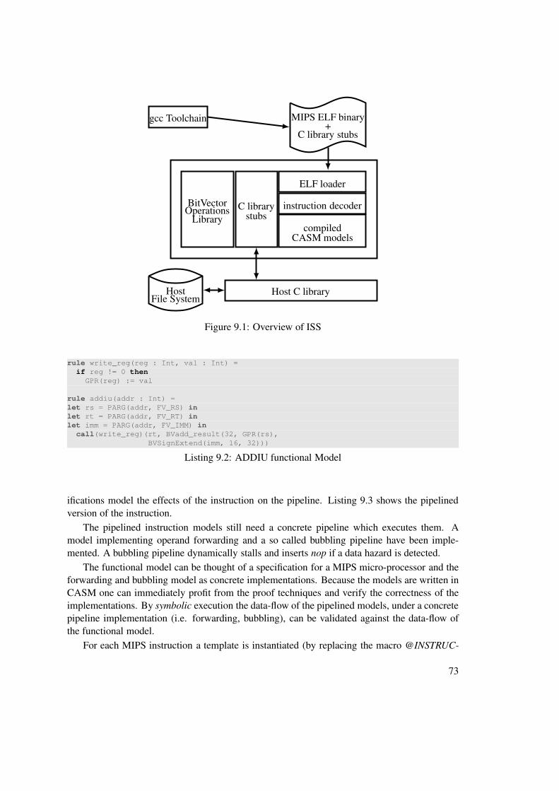
MIPS ELF binary+
C library stubs
gcc Toolchain
compiledCASM models
ELF loader
instruction decoderC librarystubs
Host C libraryHostFile System
BitVectorOperations
Library
Figure 9.1: Overview of ISS
rule write_reg(reg : Int, val : Int) =
if reg != 0 then
GPR(reg) := val
rule addiu(addr : Int) =
let rs = PARG(addr, FV_RS) in
let rt = PARG(addr, FV_RT) in
let imm = PARG(addr, FV_IMM) in
call(write_reg)(rt, BVadd_result(32, GPR(rs),
BVSignExtend(imm, 16, 32)))
Listing 9.2: ADDIU functional Model
ifications model the effects of the instruction on the pipeline. Listing 9.3 shows the pipelinedversion of the instruction.
The pipelined instruction models still need a concrete pipeline which executes them. Amodel implementing operand forwarding and a so called bubbling pipeline have been imple-mented. A bubbling pipeline dynamically stalls and inserts nop if a data hazard is detected.
The functional model can be thought of a specification for a MIPS micro-processor and theforwarding and bubbling model as concrete implementations. Because the models are written inCASM one can immediately profit from the proof techniques and verify the correctness of theimplementations. By symbolic execution the data-flow of the pipelined models, under a concretepipeline implementation (i.e. forwarding, bubbling), can be validated against the data-flow ofthe functional model.
For each MIPS instruction a template is instantiated (by replacing the macro @INSTRUC-
73

9 Instruction Set Simulation & Compiled Simulation
enum PipelineStages = {ID, EX, MEM, WB}
enum PipelinePhases = {begin, end}
rule addiu(addr:Int, stage:Int, phase:Int) =
{
if stage = ID and phase = end then
let rs = PARG(addr, FV_RS) in
let rt = PARG(addr, FV_RT) in
let imm = PARG(addr, FV_IMM) in
{
call(ID_READ_OP1)(rs)
IDOP2 := BVSignExtend(imm, 16, 32)
IDRESREG := rt
}
if stage = EX and phase = begin then
EXRES := BVadd_result(32, EXOP1, EXOP2)
if stage = WB and phase = begin then
call(write_reg)(WBRESREG, WBRES)
}
Listing 9.3: ADDIU pipelined Model
function (symbolic) SYMBOL : Int -> Int
function (symbolic) MEMORY : Int -> Int
function (symbolic) PARG : Int * FieldValues -> Int
rule initR = {|
BRANCH := undef
call(@INSTRUCTION@)(0)
program(self) := undef
|}
Listing 9.4: Template for functional Instruction Models
TION@), which is then used to create the data-flows. Listing 9.4 shows the template used toexecute functional models and listing 9.5 for pipelined models.
The traces created by symbolic execution of those 2 programs must result in semanticallyequal expressions for observable state (i.e. register file, memory). This problem is very similarto the translation validation problem and can be expressed by the same techniques.
This does not validate all aspects of the pipeline implementation and instruction models,though. For each pipelined instruction model it has been shown that it correctly implementsthe semantics, iff executed in the pipeline without interference of other instructions. Thus avalidation of the pipeline model itself is still needed.
Listing 9.6 shows the CASM program used to perform the pipeline validation (for functionalmodels, pipelined is similar but more complex). A special crafted instruction (binop, line 9) issubsequently executed in each pipeline stage (and triggers data hazards). A correct pipelineimplementation (either forwarding or bubbling) must generate the same data-flow as the func-tional model. If a concrete implementation passes this test its operand forwarding is most likelycorrect. Please note that due the nature of symbolic execution this is not just a simple test.
74

function (symbolic) SYMBOL : Int -> Int
function (symbolic) MEMORY : Int -> Int
function (symbolic) PARG : Int * FieldValues -> Int
function PMEM : Int -> RuleRef initially {0 -> @@INSTRUCTION@}
rule initR = {|
call init_pipeline
PC := 0
CYCLES := 0
BRANCH := undef
call IF_stage
call execute_pipeline
call step_pipeline
call execute_pipeline
call step_pipeline
call execute_pipeline
call step_pipeline
call execute_pipeline
call step_pipeline
program(self) := undef
|}
Listing 9.5: Template for pipelined Instruction Models
Any (hidden, non-obvious) control flow branches (e.g. WRITE_REGISTER rule in line 6) aretaken (creating multiple traces) and verified. This validation therefore has 100% path coverage,something which is very hard to achieve with ordinary testing.
Although not all aspects of the micro-processor specifications have been validated in thiswork, it has been demonstrated how easy such a validation can be performed with CASM mod-els. This is a big advantage of formal specifications compared to simulator specifications.
9.3 Compiled Simulation
Compiled Simulation [16] is a technique which aims to increase the simulation speed of singleapplications by partial evaluation performed at compile time. The program to be simulated(simulatee) and a model of the simulated machine are compiled to a single binary. Only thoseparts of the state which are actually needed for the simulation are computed. In this section wewant to investigate the applicability of compiled simulation to CASM models.
Our prototype implementation transforms binary MIPS programs into CASM models ona basic block level. Handling of computed goto and function pointers is currently not imple-mented, but could easily be done by integrating the CASM based ISS (line 12 in listing 9.9). Apython script performs a simple basic block analysis of a MIPS binary and emits a representa-tion using the CASM functions BASICBLOCK (mapping of a basic block number to a CASMrule implementing this block), BASICBLOCK_SA (original address of first instruction of block),PARG (branching instructions have target basic blocks in an additional virtual instruction field)and PMEM (branching instructions have been replaced by models using target basic blocks).
75

9 Instruction Set Simulation & Compiled Simulation
1 function (symbolic) SYMBOL : Int -> Int
2 function (symbolic) GPR : Int -> Int
3 function PARG : Int * FieldValues -> Int
45 rule WRITE_REGISTER(reg, val) =
6 if reg != 0 then
7 GPR(reg) := val
89 rule binop(addr:Int) =
10 call(WRITE_REGISTER)
11 (PARG(addr, FV_RD), BVbinop(GPR(PARG(addr, FV_RS)),
12 GPR(PARG(addr, FV_RT))))
1314 rule initR = {|
15 PARG(0, FV_RD) := SYMBOL(0)
16 PARG(0, FV_RS) := SYMBOL(1)
17 PARG(0, FV_RT) := SYMBOL(2)
1819 PARG(1, FV_RD) := SYMBOL(3)
20 PARG(1, FV_RS) := SYMBOL(0)
21 PARG(1, FV_RT) := SYMBOL(0)
2223 PARG(2, FV_RD) := SYMBOL(4)
24 PARG(2, FV_RS) := SYMBOL(3)
25 PARG(2, FV_RT) := SYMBOL(3)
2627 call(binop)(0) // s0 := s1 binop s2
28 call(binop)(1) // s3 := s0 binop s0
29 call(binop)(2) // s4 := s3 binop s3
3031 program(self) := undef
32 |}
Listing 9.6: Validation of Pipeline Model
Figure 9.2 gives an example for a modified branching instruction (listing 9.7) and the originalmodel (listing 9.8). A branch to an instruction address is signaled by setting the CASM functionBRANCH while a branch to a basic block address is signaled using the function BLOCK.
Our main rule of the simulator is given in listing 9.9. As long as the simulatee did not trap
and BLOCK contains a valid block identifier the rule implementing the referenced basic blockwill be evaluated. Each such rule is a sequential composition of the instructions forming thebasic block.
Because all instructions are captured in a sequential execution context the internal state tran-sition is hidden and can not be observed by the calling rule. As long as the resulting update setis not changed, i.e. the semantics of the basic block is preserved, arbitrary optimizations may beperformed on the CASM program. Listing 9.10 shows an example of such a block. The succes-sor block is written to BLOCK in line 8. The remaining lines of the rule call bb_call which loadsthe given instruction into the pipeline and executes a cycle of the CPU. Note this rule is inlinedby the compiler, as well as bb_execute and step_pipeline.
The optimizer (see section 3.3) then applies the three optimizations redundant lookup, pre-ceded lookup and redundant update elimination. Combined with constant folding and propaga-tion these optimizations cover the partial evaluation done by CS tools. The effect of a preceded
76

rule bne(addr:Int,
stage:PipelineStages,
phase : PipelinePhases) =
if stage = ID and phase = end then
let rs = PARG(addr, FV_RS) in
let rt = PARG(addr, FV_RT) in
let offset = PARG(addr, FV_OFF) in
{|
call (ID_READ_OP1)(rs)
call (ID_READ_OP2)(rt)
if BVunequal(32,IDOP1,IDOP2)=1 then
BRANCH := BVadd_result(32, addr+4,
BVse(18, 32,
BVshift_result(18, 0, 0,
offset, 2)))
|}
Listing 9.7: Original BNE Model
rule bb_bne(addr:Int,
stage:PipelineStages,
phase : PipelinePhases) =
if stage = ID and phase = end then
let rs = PARG(addr, FV_RS) in
let rt = PARG(addr, FV_RT) in
let offset = PARG(addr, FV_BBOFF) in
{|
call (ID_READ_OP1)(rs)
call (ID_READ_OP2)(rt)
if BVunequal(32,IDOP1,IDOP2)=1 then
BLOCK := offset
|}
Listing 9.8: Modified BNE Model
Figure 9.2: Modifies branch instructions for CS
1 rule run_program dumps (BLOCK, BRANCH, GPR, LO, HI) -> trace =
2 {|
3 if BLOCK = undef and BRANCH = undef then
4 {
5 print "program stopped (BLOCK and BRANCH undef)"
6 call dump_machine_state
7 program(self) := undef
8 }
9 else if BLOCK = undef then
10 {
11 print "ERROR, BLOCK is undef, BRANCH=" + hex(BRANCH) +
12 " need to enter interpreter -> not implemneted!"
13 call dump_machine_state
14 program(self) := undef
15 }
1617 debuginfo block "executing " + BLOCK + "@" + hex(BASICBLOCK_SA(BLOCK))
18 call (BASICBLOCK(BLOCK))
1920 if trapped then
21 {
22 print "program stopped (trapped)"
23 call dump_machine_state
24 program(self) := undef
25 }
26 |}
Listing 9.9: Compiled Simulation Main Rule
77

9 Instruction Set Simulation & Compiled Simulation
1 rule bb_call(r: RuleRef, i: Int) = {|
2 pipeline(ID) := [r, i]
3 call bb_execute
4 call step_pipeline
5 |}
67 rule bb_42 = {|
8 BLOCK:=38
9 call bb_call (@sll, 0x8000132c)
10 call bb_call (@sll, 0x80001330)
11 call bb_call (@sll, 0x80001334)
12 call bb_call (@_syscall, 0x80001338)
13 call bb_call (@lui, 0x8000133c)
14 call bb_call (@addiu, 0x80001340)
15 call bb_call (@bb_jr, 0x80001344)
16 call bb_call (@sw, 0x80001348)
17 |}
Listing 9.10: An optimizable Basic Block
lookup optimization e.g. is comparable to map register file access to local variables. Redundantupdate elimination will prevent the calculations of all unused updates to the flag register file (onmicro processors which can implicitly set flags). The combination of redundant and precedinglookup elimination eliminates access to the pipeline function. Benchmark results are presentedin section 10.1.2.
A CASM specification can therefore with minimal further tool support be used to performcompiled simulation. Because the optimization is performed on CASM code this approach isfully portable across various architectures.
78

10 Evaluation
Measure what is measurable, and make measurable what is not so.
Galileo Galilei
The evaluation section of this work is split into three parts Section 10.1 covers performanceaspects of the CASM implementation. In section 10.2 we compare the performance of thevanHelsing prover with other well-known tools in the ATP realm. And in section 10.3 we reporton the performance of the implemented validator prototypes.
10.1 CASM implementation
Evaluation of the CASM tools is split into three sections. Section 10.1.1 compares the CASMinterpreter and baseline compiler to other ASM implementations. In section 10.1.2 we measurethe performance of the ISS synthesized from the CASM models. And in section 10.1.2 wefinally benchmark the optimization implemented in the CASM compiler. This used benchmarksare an application of the CS approach and therefore also document the ability to synthesize CStools from CASM models.
10.1.1 CASM and other ASM implementations
In this section we evaluate the quality of the CASM implementation (i.e. interpreter and baselinecompiler). For this purpose we compare it to other available implementations of ASM basedlanguages, namely CoreASM and AsmL. CoreASM is an interpreter written in Java while theAsmL language is compiled to .NET code. A small suite of programs each stressing a differentimplementation detail of ASM languages has been implemented for each language.
The bubblesort program (a very naive implementation of the well known sorting algorithm)performs many steps with small update sets. It aims to benchmark the effectiveness of apply-ing update sets to ASM functions. Fibonacci uses dynamic programming to calculate the wellknown numbers. It benchmarks rule invocation (recursive) and has a moderate size of the updateset. Quicksort (the sorting algorithm) makes heavy use of sequential execution, although the up-date sets are very small. The sieve program is an implementation of Eratosthenes famous prime
79

10 Evaluation
small data setstrivial sieve quicksort gray fibonacci bubblesort
CASM 0.0865 0.0857 0.0842 0.0882 0.0854 0.0859AsmL 0.1292CASM-i 0.0048 0.10 0.0212 0.2287 0.0107 0.0466CoreASM 1.3604 13.82 32.51 57.61 67.24 213.62
large date setssieve quicksort gray fibonacci bubblesort
CASM 0.0822 0.586 0.7702 3.0436 2.5458AsmL 74.39 3.0628 24.3702 4.1752 5.2748CASM-i 1.05 35.41 40.83 79.17 95.43CoreASM
Table 10.1: Execution times CoreASM, AsmL, CASM
number sieve. This program heavily stresses the implementation of the update set, everything isexecuted sequentially producing large update sets. The benchmark program gray calculates graycodes for a given word length. It is the program with the most output and a mix of sequentialexecution, rule invocation and numeric operations. Trivial is the trivial program, immediatelyexiting without any operation. It is used to measure start-up overheads of the various implemen-tations
The performance of the various implementations varies a lot. We use small data sets for theinterpreters and larger sets for the compilers to have measurable execution times.
For benchmarking we use the CASM compiler (rev. 1a092c) and gcc 4.7.2 (as shipped withUbuntu 12.10). We do not perform any CASM specific optimizations and disable optimizationsof the C compiler (-O0 flag). The CASM interpreter (CASM-i) is the same version as thecompiler.
The CoreASM engine version used is 1.5.6-beta using the command line driver Carma 0.7.3(latest release). We executed CoreASM using Java 1.7 with the 64 bit Server VM (23.7-b01).
Microsoft’s AsmL implementation compiles to .NET code and is available under the MSR-LA (free for research) license on http://asml.codeplex.com/. We downloaded version80132 and followed their build instructions using Visual Studio C# 2005 Express Edition.
The benchmarks involving small data sets were executed on a Core i7-Q820 @1.73 GHzwith 8 GiB memory under 64 bit Ubuntu 12.10. For the large data sets a dual boot system (Corei7-2600k @3.4 GHz, 8GiB memory) using 64 bit Windows 7 Enterprise SP1 and 64 bit Ubuntu13.10 was used. We report on the average of 10 runs and started the AsmL binary once beforethe benchmark to exclude overheads induced by the .NET framework 1.
Our own implementation of a CASM interpreter (CASM-i) is designed to have very lowstart-up times and is used to execute small programs only. It is used in the compiler verificationproject. The baseline compiler is a magnitude faster than the interpreter (up to 60 times) whichis a good indicator that the baseline compiler performs well.
1http://msdn.microsoft.com/en-us/library/cc656914(v=vs.110).aspx
80

trivial
sievequickort
grayfibonacci
bubbleort
10−1
100
101
102
10315.73
161.29
386.11
653.27
787.36
2,486.85
5.55·10−
2
12.73
60.42
53.01
26.01
37.49
1.82
905.1
5.23
31.64
1.37
2.07
Fac
tor CoreASM CASM-i AsmL
Figure 10.1: CASM relative Performance (Compiler is Baseline, smaller is better, log-scale)
When it comes to performance CoreASM is clearly inferior to the other implementations.Programs compiled by our compiler perform up to 2500 times better and even our interpreter isa magnitude faster. The focus of CoreASM are high level models though.
The AsmL results are varying a lot. For fibonacci performance is on par with the CASMcompiler (still 35% slower, though). But fibonacci is also the benchmark putting the least pres-sure on ASM specifics. Its mostly recursive function invocation with a comparable small updateset. Bubblesort is slower by a moderate factor of 2 while sieve is slower by a factor of 900.A detailed examination showed that AsmL has quadratic run-time for increased sizes of thesieve. The main difference in the two programs is that bubblesort executes a large number ofmachine steps each with a small update set, while sieve exactly executes one step. The updateset produced by sieve is quite large (the whole array) and a lot of updates need to be merged se-quentially. This indicates that AsmL is not optimized for this case and agrees with the observedbehavior of quicksort (small sequential update sets) and gray (moderate sized sequential updatesets). Overall the performance of AsmL compiled programs is significantly lower than programscompiled by the CASM compiler.
Figure 10.1 shows the relative performance (with CASM compiler being the baseline) of the4 implementations, please note the logarithmic scaling of the y axis. Numeric values are foundin table 10.1. The CASM baseline compiler is by far the best performing ASM implementation.
10.1.2 Symbolic Execution
We developed a micro-benchmark to stress all important implementation aspects of symbolicexecution in the CASM interpreter. The size of the tests is much larger than the size of the
81

10 Evaluation
Engine Creation Expression Forking Start-up
CASM 2.14 s 3.54 s 2.82 s 0.009 sCoreASM n/a n/a n/a 1.3 s
Table 10.2: Micro Benchmark Results
problems coming from translation validation. Hence we don’t expect scalability issues with theimplementation of symbolic execution.
This benchmark was executed on a Core i7 @ 1.73 GHz using a 64 bit Ubuntu 12.10 andwe report the average value of 5 runs. We compared start-up times to CoreASM 1.5.6-betausing Carma engine 0.7.3. Each of the following tests stresses an implementation detail of thesymbolic ASM. Table 10.2 summarizes the results.
• Creation of symbols: The lazy initialization of symbols is an important feature of our im-plementation. Each computation step of the ASM induces one predicate for each symbolin use. The later a symbol is created the more predicates have to be emitted at creationtime (as the symbol existed in all previous states as well). To stress the lazy initializationimplementation a test program computing 1000 steps is used. In each step a new symbolis created. This results in 1000 symbols and 1002000 predicates to describe the wholestate transition (1000 symbols in 1000 states plus initial and final state).
• Expression evaluation: Symbols are also created when evaluation expressions containingsymbolic values. This test program performs 100000 operations using 100000 differentsymbols (in a single computation step). This results in 100000 predicates to be written tothe symbolic trace.
• Forking on symbolic conditions: When control flow branches on a symbolic conditionboth traces need to be created. This can lead to a problem known as state explosion. Anapplication may be able to handle a certain amount of branching however. A test programconsisting of 11 nested if-then-else rules resulting in 2048 traces is executed. For ourapplications we observed a much smaller number of traces (2-8).
• Start-up of interpreter: As the interpreter is intended to execute a large number of shortrunning programs the run-time overhead is of interest as well. A test program exe-cuting the trivial CoreASM/CASM program (rule initR = program(self) :=
undef producing one update and then terminating) was executed to measure this start-upoverhead.
The empirical data show that the implementation of symbolic execution is efficient even forvery large traces. Especially the low start-up overhead (absolute and compared to CoreASM)is very important for the intended application (execute many small CASM programs duringtranslation validation).
82

MIPS cycles secondsBMIPS MIPS FMIPS BMIPS MIPS FMIPS
basicmath 550341866 333880341 328575616 2537,37 1323,53 132,62bf.d 64946652 43557768 43556830 295,12 170,97 18,66bf.e 64448155 43639002 43638063 292,23 172,02 18,62crc 802657273 482047058 482020990 3600,91 1967,50 212,58dijkstra 95287437 48939093 48859858 421,00 190,69 20,01patricia 144287533 89624367 88147670 655,57 375,17 38,64qsort 25761496 18442379 18255010 120,51 78,59 10,28rawcaudio 59614091 34035944 34035911 265,53 138,41 14,82rawdaudio 15208266 8664016 8663983 68,99 35,83 4,69rijndael.d 42564700 38204264 38105252 203,91 158,03 16,10rijndael.e 42567131 38381668 38282652 200,67 186,60 18,30search 8757478 5776268 5689169 41,81 24,37 3,49sha 13927633 12093339 12092840 66,36 49,94 5,79susan 4820668 3420921 3401906 23,06 14,51 2,33
Table 10.3: Performance of FMIPS, MIPS and BMIPS ISSs
CASM synthesized ISS
To evaluate the performance of the synthesized ISSs we have created simulators based on theMIPS models. We compare all three MIPS implementations, that is the functional models(FMIPS), the models implementing a pipeline with operand forwarding (MIPS) and the bub-bling pipeline (BMIPS). The most expensive operations in the CASM run-time are the onesinvolving the update set. Because the simulated state of FMIPS is the smallest we expect thosemodels to deliver the best performance. MIPS and BMIPS are expected to have similar perfor-mance, their state is similar in size. Execution of MIPS programs using the BMIPS simulatorwill absolutely perform worse than MIPS. The reason is that pipeline bubbles are added whendata hazards occur. The number of executed MIPS cycles is therefore higher than the number ofcycles a pipeline with operand forwarding will need.
In table 10.3 we given the number of cycles and seconds each of the ISSs spent on thebenchmark programs taken from the MiBench [35] suite. MiBench’s small data sets have beenused for all but the search benchmark. In figure 10.2 the achieved relative performance in MIPSinstructions per seconds is presented.
The FMIPS ISS reaches up to 2.47 MHz which is a very good performance. (Brandner [15]reports on approx. 3 MHz peak performance for an interpretative MIPS ISS.) Simulating thewhole pipeline (and the resulting update set operations) drastically reduces the performance forthe MIPS and BMIPS ISSs. Nonetheless the CASM run-time, i.e. the branded hash and linked
list update-set (see chapter 3) performs much better than the old python prototypes, which onlyachieved up to 1 MHz (Lezuo and Krall [47]).
83

10 Evaluation
basicmath
bf.dbf.e
crcdijkstra
patricia
qsortrawcaudio
rawdautio
rijndael.d
rijndael.e
search
shasusan.e
0
1,000,000
2,000,000
2,477,572
2,334,235
2,343,612
2,267,480
2,441,772
2,281,254
1,775,779 2,296,620
1,847,331 2,366,785
2,091,948
1,630,134
2,088,573
1,460,045
252,265
254,768
253,685
245,004
256,642
238,890
234,665
245,906
241,808
241,753
205,689
237,023
242,157
235,762
216,894
220,068
220,539
222,904
226,335
220,094
213,770
224,509
220,441
208,742
212,125
209,458
209,879
209,048
Hz
FMIPS MIPS BMIPS
Figure 10.2: Performance of FMIPS, MIPS and BMIPS ISSs
CASM synthesized CS
We have applied our CS approach to a set of MiBench [35] programs using the functional MIPSmodels. As our optimizations perform aggressive inlining we only want to optimize the kernelof the applications to keep the increase in code size small. Our code generator can instrumentthe code to collect profiling information measuring the total execution time of each CASM rule(including time spent in invoked rules). Applying a simple heuristic all rules contributing at least1% to the total run-time have been selected for optimization. Our assumption is that the effectson code size by inlining are small but the achieved effect (in terms of performance gains) large.
Lookup and update elimination work best on large rules, so their impact should be high if thefrequently executed rules are large and low for small rules. Figure 10.3 depicts the contributionof a rule’s execution time to total program execution time (bars) and their size in LOC (crosses)for the rijndael program. (The rule contribution 100% to total program execution time is thetop-level rule, the second bar is a dispatching rule, all further bars correspond to basic blocks orinstructions.) Note that two of the most contributing rules each have 1000 LOC. We expect tosee a high impact of lookup and update elimination for the rijndael program. Figure 10.5 on theother hand shows that the patricia program has many small rules and the first large rule does notcontribute much to total execution time. A high impact can not be expected. Figure 10.4 showsthe same diagram for the dijkstra program. Medium sized rules with moderate contribution. Weexpect our optimizations to have an impact for this program.
We use 3 configurations of our compiler in this evaluation. Baseline is without CASMspecific optimizations and without optimizations of the C compiler (-O0). The configuration
84

0
50
100
%
contribution
0
200
400
600
800
1,000LOC
Figure 10.3: Rule Contribution and Size - Rijndael
0
50
100
%
contribution
0
5
10LOC
Figure 10.4: Rule Contribution and Size - Dijkstra
0
50
100
%
contribution
0
10
20
30
40LOC
Figure 10.5: Rule Contribution and Size - Patricia
titled O0 has CASM specific, but no C compiler optimizations (-O0). O3 has CASM and full Ccompiler optimizations (-O3). The benchmarks were executed on Xeon E5504 @ 2.00GHz with8GiB memory (on the Infragrid cluster 2). We used gcc 4.4.7 on a Red Hat Enterprise LinuxServer release 6.4 for compilation. Due to the shared nature of the cluster we report on the bestof 10 runs here. MiBench’s small data sets have been used for all but the search benchmark.
Table 10.4 lists for each benchmark program the total number of rules and the number ofrules optimized as well as the total number of optimizations performed. We report on the numberof constant propagation (cp), lookup eliminations and update eliminations. As expected we seea large number of optimizations performed in the rijndael program. Although patricia is doingwell in numbers the effects do not materialize due to the disadvantageous distribution of blockcontribution to the total run-time.
2http://hpc.uvt.ro/infrastructure/infragrid/
85
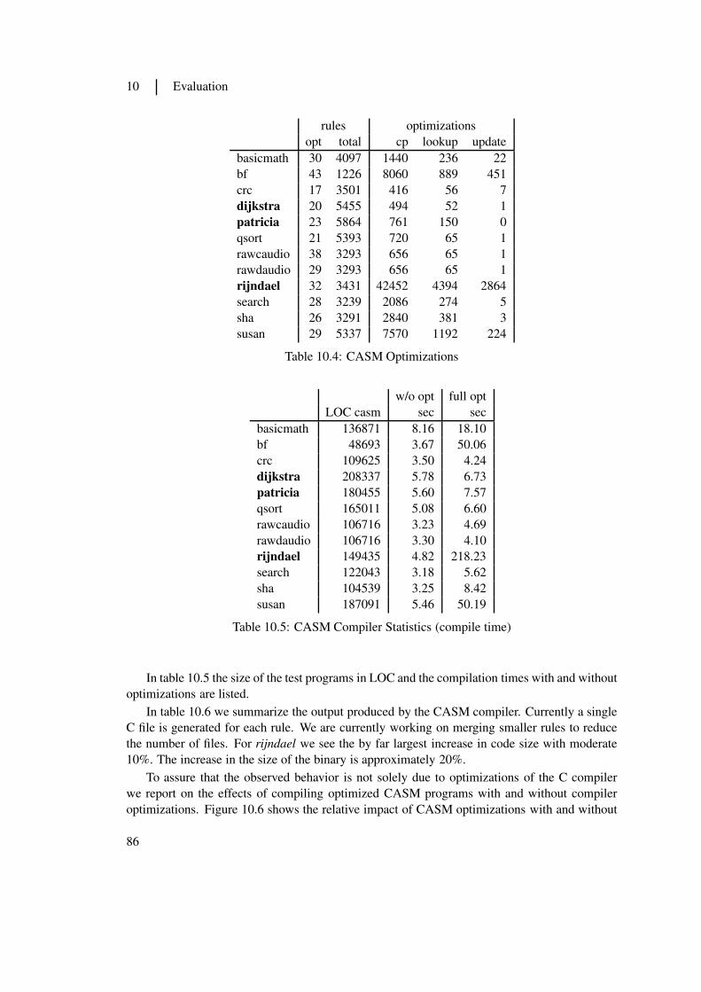
10 Evaluation
rules optimizationsopt total cp lookup update
basicmath 30 4097 1440 236 22bf 43 1226 8060 889 451crc 17 3501 416 56 7dijkstra 20 5455 494 52 1patricia 23 5864 761 150 0qsort 21 5393 720 65 1rawcaudio 38 3293 656 65 1rawdaudio 29 3293 656 65 1rijndael 32 3431 42452 4394 2864search 28 3239 2086 274 5sha 26 3291 2840 381 3susan 29 5337 7570 1192 224
Table 10.4: CASM Optimizations
w/o opt full optLOC casm sec sec
basicmath 136871 8.16 18.10bf 48693 3.67 50.06crc 109625 3.50 4.24dijkstra 208337 5.78 6.73patricia 180455 5.60 7.57qsort 165011 5.08 6.60rawcaudio 106716 3.23 4.69rawdaudio 106716 3.30 4.10rijndael 149435 4.82 218.23search 122043 3.18 5.62sha 104539 3.25 8.42susan 187091 5.46 50.19
Table 10.5: CASM Compiler Statistics (compile time)
In table 10.5 the size of the test programs in LOC and the compilation times with and withoutoptimizations are listed.
In table 10.6 we summarize the output produced by the CASM compiler. Currently a singleC file is generated for each rule. We are currently working on merging smaller rules to reducethe number of files. For rijndael we see the by far largest increase in code size with moderate10%. The increase in the size of the binary is approximately 20%.
To assure that the observed behavior is not solely due to optimizations of the C compilerwe report on the effects of compiling optimized CASM programs with and without compileroptimizations. Figure 10.6 shows the relative impact of CASM optimizations with and without
86

total LOC C binary MiBC files w/o opt full opt w/o opt full opt
basicmath 4104 531769 +1357 29 35bf 1233 179890 +10369 9.1 11crc 3508 419546 +679 24 29dijkstra 5462 691294 +866 38 46patricia 5871 694523 +622 39 48qsort 5400 641228 +1328 36 44rawcaudio 3300 402138 +901 23 27rawdaudio 3300 402138 +946 23 27rijndael 3438 524481 +49198 26 32search 3246 419649 +4660 23 28sha 3298 408628 +5506 23 28susan 5344 727943 +10029 28 46
Table 10.6: Generated Output Statistics
optimizations by the C compiler. The relative performance is clearly decreased but our opti-mizations still account for a factor of 2 (rijndael) to at least 1% for patricia. (On a side note: byusing well-known compiled simulation techniques (e.g. [16]) the size of the basic blocks can beenlarged from which our compiler would profit immediately.) In figure 10.7 the overall speedupfactors for the applications are shown along with absolute performance data. The speedup is rel-ative from the non-optimized version to the fully optimized one. We are able to achieve factors6 and above here. For rijndael (factor 5.44) more than 50% of this speedup is due to CASMoptimizations (the rest is due to the C compiler).
The MHz value relates the total number of simulated MIPS instructions to the absolute run-time of the programs. A solid performance of more than 3 MHz simulation speed is achieved.The numbers also indicate that the natural performance of the programs would be approximately500 kHz. Search and susan show very low performance here. This is due to the very shortexecution time of these two programs (5 and 4 seconds). The start-up time of the programsis approximately 1 second (the initial memory state of the MIPS programs (data section) isinitialized by a CASM rule producing updates) therefore a significant reduction of simulationspeed is expected.
The experimental data show a huge performance increase achieved by the CASM compiler.A speedup of more than factor 6 can be achieved. We showed that the C code generated by theCASM compiler can be very efficiently optimized. Our novel optimizations lookup eliminationand update reduction can increase program performance up to 264%. This shows that they arehighly effective.
From a pure CS perspective this results are not competitive. Farfeleder [24] reports onsimulation speeds of 78 MHz up to 181 MHz for fully cycle-accurate simulation (which oursimulation is). By reducing the precision up to 566 MHz are achieved. The main reason that ourCS approach does not perform significantly better than synthesized ISS is in the increased sizeof the update set. In the bf benchmark the average size of the update set produced by each rule
87

10E
valuation
basicmath bf.d
bf.ecrc
dijkstra
patricia
qsortrawcaudio rawdaudio rijndael.d rijndael.e search
shasusan.e
0 1 2
1.2
2.08
2.1
1.97
1.54
1.09
1.28
1.72
1.67
2.64
2.62
1.23
1.7
1.28
1.07
1.46
1.54
1.61
1.3
1.01
1.08
1.42
1.4
2.08
2.05
1.05
1.27
1.04
Factor
O0
O3
Figure
10.6:Im
pactof
CA
SM
Optim
izations
basicmath bf.d
bf.ecrc
dijkstra
patricia
qsortrawcaudio rawdaudio rijndael.d rijndael.e search
shasusan.e
0 2 4 6
3.14
4.89
5.03
6.23
4.27
2.8
3.04
4.77
4.54
5.44
5.46
2.46
3.4
1.85
Speedup (factor)
Speedup
0 1 2 3
1.72
2.78
2.86
3.29
2.41
1.29
1.32
2.79
2.55
3.07
3.08
0.98
1.93
0.79
MHz
MH
z
Figure
10.7:Im
provements
andT
otalP
erformance
88
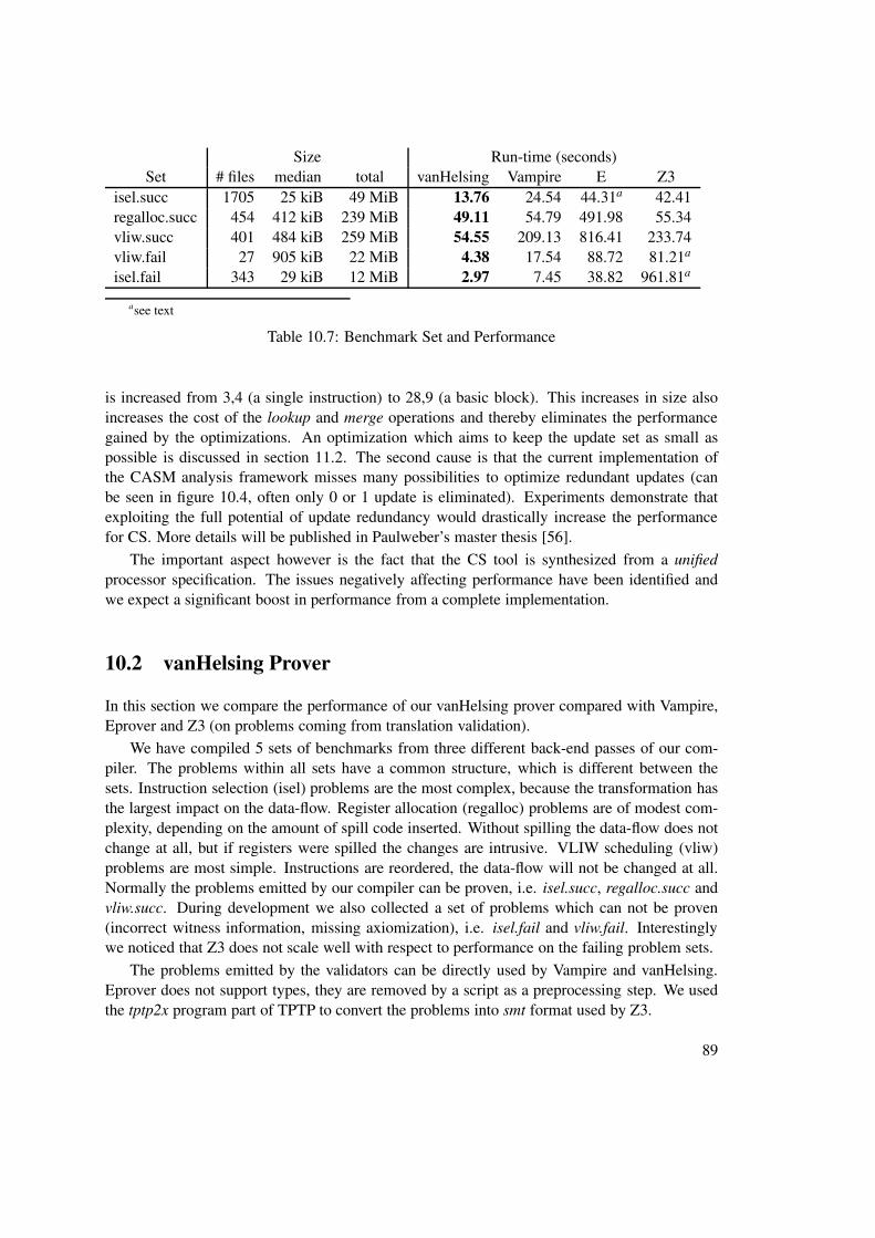
Size Run-time (seconds)Set # files median total vanHelsing Vampire E Z3
isel.succ 1705 25 kiB 49 MiB 13.76 24.54 44.31a 42.41regalloc.succ 454 412 kiB 239 MiB 49.11 54.79 491.98 55.34vliw.succ 401 484 kiB 259 MiB 54.55 209.13 816.41 233.74vliw.fail 27 905 kiB 22 MiB 4.38 17.54 88.72 81.21a
isel.fail 343 29 kiB 12 MiB 2.97 7.45 38.82 961.81a
asee text
Table 10.7: Benchmark Set and Performance
is increased from 3,4 (a single instruction) to 28,9 (a basic block). This increases in size alsoincreases the cost of the lookup and merge operations and thereby eliminates the performancegained by the optimizations. An optimization which aims to keep the update set as small aspossible is discussed in section 11.2. The second cause is that the current implementation ofthe CASM analysis framework misses many possibilities to optimize redundant updates (canbe seen in figure 10.4, often only 0 or 1 update is eliminated). Experiments demonstrate thatexploiting the full potential of update redundancy would drastically increase the performancefor CS. More details will be published in Paulweber’s master thesis [56].
The important aspect however is the fact that the CS tool is synthesized from a unified
processor specification. The issues negatively affecting performance have been identified andwe expect a significant boost in performance from a complete implementation.
10.2 vanHelsing Prover
In this section we compare the performance of our vanHelsing prover compared with Vampire,Eprover and Z3 (on problems coming from translation validation).
We have compiled 5 sets of benchmarks from three different back-end passes of our com-piler. The problems within all sets have a common structure, which is different between thesets. Instruction selection (isel) problems are the most complex, because the transformation hasthe largest impact on the data-flow. Register allocation (regalloc) problems are of modest com-plexity, depending on the amount of spill code inserted. Without spilling the data-flow does notchange at all, but if registers were spilled the changes are intrusive. VLIW scheduling (vliw)problems are most simple. Instructions are reordered, the data-flow will not be changed at all.Normally the problems emitted by our compiler can be proven, i.e. isel.succ, regalloc.succ andvliw.succ. During development we also collected a set of problems which can not be proven(incorrect witness information, missing axiomization), i.e. isel.fail and vliw.fail. Interestinglywe noticed that Z3 does not scale well with respect to performance on the failing problem sets.
The problems emitted by the validators can be directly used by Vampire and vanHelsing.Eprover does not support types, they are removed by a script as a preprocessing step. We usedthe tptp2x program part of TPTP to convert the problems into smt format used by Z3.
89

10 Evaluation
isel.succ isel.failvliw.succ vliw.failregalloc.succ
0
5
10
15
201 11 111.78
2.53.83
4
1.123.22
13.07
14.97
20.26
10.02
3.08
323.95
4.28
18.55
1.13
Fac
tor
vanHelsingVampireeprover
Z3
Table 10.8: Relative Performance (Factor), smaller is better
Table 10.7 contains the number of problems in the set, average file size (median) as anindicator of the complexity of each problem, the total size of the set and the time each proverneeds to process the whole problem set. We report on the best of 3 runs of vanHelsing (versionaa115e4), Vampire (1.8 rev. 1362), Eprover (E 1.8-001 Gopaldhara) and Z3 (4.3.1). The testswere performed on a Core i7 @ 1.73 GHz using a 64 bit Ubuntu 12.10. Eprover has beenexecuted in silent mode and failed to prove one problem of the isel.succ set. Vampire is a veryfast prover and has won the FOF section of the CASC [64] competition for many years now.vanHelsing always performs better than Vampire (roughly factor 2), which itself always is thesecond fastest prover. Eprover’s performance is generally worse (factor of up to 20). Z3 ingeneral performs similar to Vampire, but has a hard time when the problem has no proof (issat). We used hard timeouts (-T:3 -t:3) of 3 seconds (vanHelsing needs less than 3 secondsfor all 343 problems in the set), but Z3 failed on all problems of the vliw.fail set and onlyfound the solution on 28 problems of isel.fail. Increasing the timeout to 240 second results infinding 309 (of 343) models for the isel.fail set, but still no solution for any of the problems invliw.fail. Figure 10.8 shows the relative performance for all provers on each of the problem sets,normalized to vanHelsing’s total run-time.
The empirical data clearly demonstrate that the simple problem structure produced by ourtranslation validation approach enables the use of a much simpler and therefore more effectivespecialized prover like vanHelsing. Even the current implementation performs much better thanwidely used and highly optimized off the shelf provers like Vampire and Z3.
10.3 Translation Validation
In this section we report on the performance of 3 prototype validators which have been imple-mented as part of this thesis. The tests were performed on a Core i7 @ 1.73 GHz using a 64bit Ubuntu 12.10 using all 8 available cores to utilize the parallelism. We report the Wall-clock
90

preprocessing executionMIR CASM 11 s 7 sLIR CASM 146 s 6 svanHelsing 19 stotal 156 s 33 svalidation 244 s
Table 10.9: Instruction Selection Time Spent (8 cores)
time.
10.3.1 Instruction Selection
Our research compiler dumps the mMIR and cLIR as described in sections 4.3.1 and 4.3.2.To ease implementation the compiler also creates a first-order representation of the equalitiesfor the initial state and the conjecture to be proven (using the register allocation mapping, seesection 7.2). In a productive version the validator needs to calculate this (as part of the trustedcode base).
The dumped CASM fragments are then combined with the machine model (which has beencreated by the casm_gen tool, see section 4.1). We use the C preprocessor to implement this,which is not very efficient and will be changed in a productive version. A specialized CASMmain rule then drives the generation of the symbolic traces.
The research compiler is still in development and the number of applications which cansuccessfully be compiled is therefore limited. We chose the largest well-known supported appli-cation as our benchmark program, the AES (rijndael) reference implementation, consisting of 3source files (rijndael-alg-ref.c, rijndael-api-ref.c and rijndael_main.c).
The compiler matches 1904 mMIR trees in the instruction selection pass. This results in thesame number of symbolic mMIR traces (1904), but, due to branches, 2116 cLIR traces. Thevalidator combines them into single problem files and adds the initial equalities, conjecture andthe axiom set. Those 2116 problem files are then handed to the vanHelsing prover. To assurethe correctness of the proofs our prototype implements an additional validation step. The proof
script created by vanHelsing is validated against the conjecture (using the Vampire prover),which assures that the proof actually shows the conjecture. vanHelsing’s proof script is alsochecked to have no contradiction with the original problem file (again using Vampire). Thosetwo steps (no contradiction unified from original problem file and proof script is a witness forthe conjecture), validated by a third-party prover, give us a very high confidence in the proofs(and the implementation of the vanHelsing prover). The total execution time of the validator(including the validation step) is 7 minutes and 20 seconds. Table 10.9 breaks this down to thesingle tasks performed.
The research compiler was not developed with creation of witness information in mind andis very eager to free its internal data structures as quickly as possible. The prototype witnessgeneration code therefore can’t access some mapping information and the witness information
91

10 Evaluation
is wrong in a small number of cases. This results in the proofs to fail. We have investigatedthose proofs and by manually adding the missing information they can be proven successfully.
It can clearly be seen that most of the time is spent validating the results and in preprocessingthe LIR CASM fragments. Validation is not mandatory in a productive implementation and theuse of GCC to preprocess the CASM fragments is not optimal. A productive tool would reducethe times spent in preprocessing dramatically. The validation core task (symbolic execution andproving) only needs 33 s (8 cores) for a 841 LOC (excluding header files) C program.
10.3.2 Register allocation
The register allocation prototype was implemented for the MIPS architecture using the LLVMtoolchain (version 3.2, basic register allocator). We chose a different compiler for three reasons i)to demonstrate that our approach can be applied to various compilers, ii) to have a more complexregister allocator which performs some other optimizations on-the-fly (i.e. rematerialization) andiii) to be able to compile larger programs than it is currently possible with the research compiler.
Dumps of llc’s IR were obtained using the command-line options -print-before=virtregmap
and -print-after=virtregrewriter. To include the register allocation mapping (VirtRegMap) intothe dumps a small modification of the method VirtRegRewriter::runOnMachineFunction mustbe made. Those dump files are then processed by a python script which translated each Cfunction (pre and post transformation) into CASM code and extracts the CFG and function live-in, live-out registers. Each function is then split into their basic blocks and those blocks arecombined with CASM models of the MIPS architecture (i.e. instruction set models, register fileand memory). The blocks are then symbolically executed to create the trace files.
On the traces a def-use analysis is performed to ultimately calculate liveness (backwardsanalysis) and constness (fix-point analysis). The current prototype relies on the correctnessof the compiler provided CFG and function live-in, live-out registers. However a productiveimplementation would have a correct CFG available in our proposed framework, and live-in,live-out register would be known due to the prolog and epilog insertion pass (see section 7.1).
For each live-in register a formulae is emitted stating equivalence with the value in the allo-cated register (or stack slot, if spilled). For all registers which hold a constant value a formulaestating that fact is emitted as well (the compiled may now rematerialize at will). The live-outregisters are finally used to create the conjecture for the problem file. A register may be live-outbut without a definition in this block. In this case the symbolic trace will contain no informa-tion about it and it must be excluded from the conjecture. Memory side-effects are added to theconjecture as well, the details are described in section 7.6.
Axioms are then added and the problem file is passed to the vanHelsing prover. A validationphase utilizing the Vampire prover is performed again (see instruction selection validator insection 10.9). Validation of register allocation of the bzip2 program, part of SPECINT2000,(including the validation step) needs 15 minutes and 19 seconds. Table 10.10 breaks this downto the single tasks performed.
We can successfully prove all problem files.The majority of time is consumed by the validation step (again using Vampire instead of
vanHelsing). While validation is a good thing during development a productive tool would notneed to perform this step. The remaining time is spent in preprocessing of the problem files (38
92
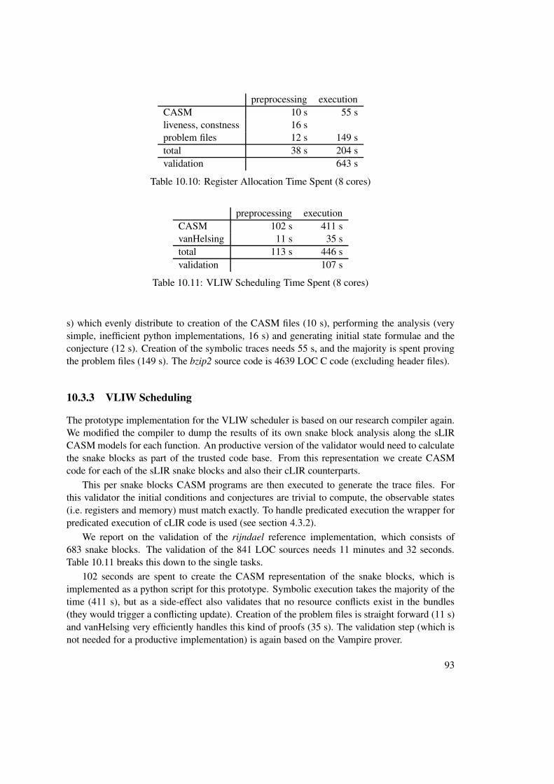
preprocessing executionCASM 10 s 55 sliveness, constness 16 sproblem files 12 s 149 stotal 38 s 204 svalidation 643 s
Table 10.10: Register Allocation Time Spent (8 cores)
preprocessing executionCASM 102 s 411 svanHelsing 11 s 35 stotal 113 s 446 svalidation 107 s
Table 10.11: VLIW Scheduling Time Spent (8 cores)
s) which evenly distribute to creation of the CASM files (10 s), performing the analysis (verysimple, inefficient python implementations, 16 s) and generating initial state formulae and theconjecture (12 s). Creation of the symbolic traces needs 55 s, and the majority is spent provingthe problem files (149 s). The bzip2 source code is 4639 LOC C code (excluding header files).
10.3.3 VLIW Scheduling
The prototype implementation for the VLIW scheduler is based on our research compiler again.We modified the compiler to dump the results of its own snake block analysis along the sLIRCASM models for each function. An productive version of the validator would need to calculatethe snake blocks as part of the trusted code base. From this representation we create CASMcode for each of the sLIR snake blocks and also their cLIR counterparts.
This per snake blocks CASM programs are then executed to generate the trace files. Forthis validator the initial conditions and conjectures are trivial to compute, the observable states(i.e. registers and memory) must match exactly. To handle predicated execution the wrapper forpredicated execution of cLIR code is used (see section 4.3.2).
We report on the validation of the rijndael reference implementation, which consists of683 snake blocks. The validation of the 841 LOC sources needs 11 minutes and 32 seconds.Table 10.11 breaks this down to the single tasks.
102 seconds are spent to create the CASM representation of the snake blocks, which isimplemented as a python script for this prototype. Symbolic execution takes the majority of thetime (411 s), but as a side-effect also validates that no resource conflicts exist in the bundles(they would trigger a conflicting update). Creation of the problem files is straight forward (11 s)and vanHelsing very efficiently handles this kind of proofs (35 s). The validation step (which isnot needed for a productive implementation) is again based on the Vampire prover.
93
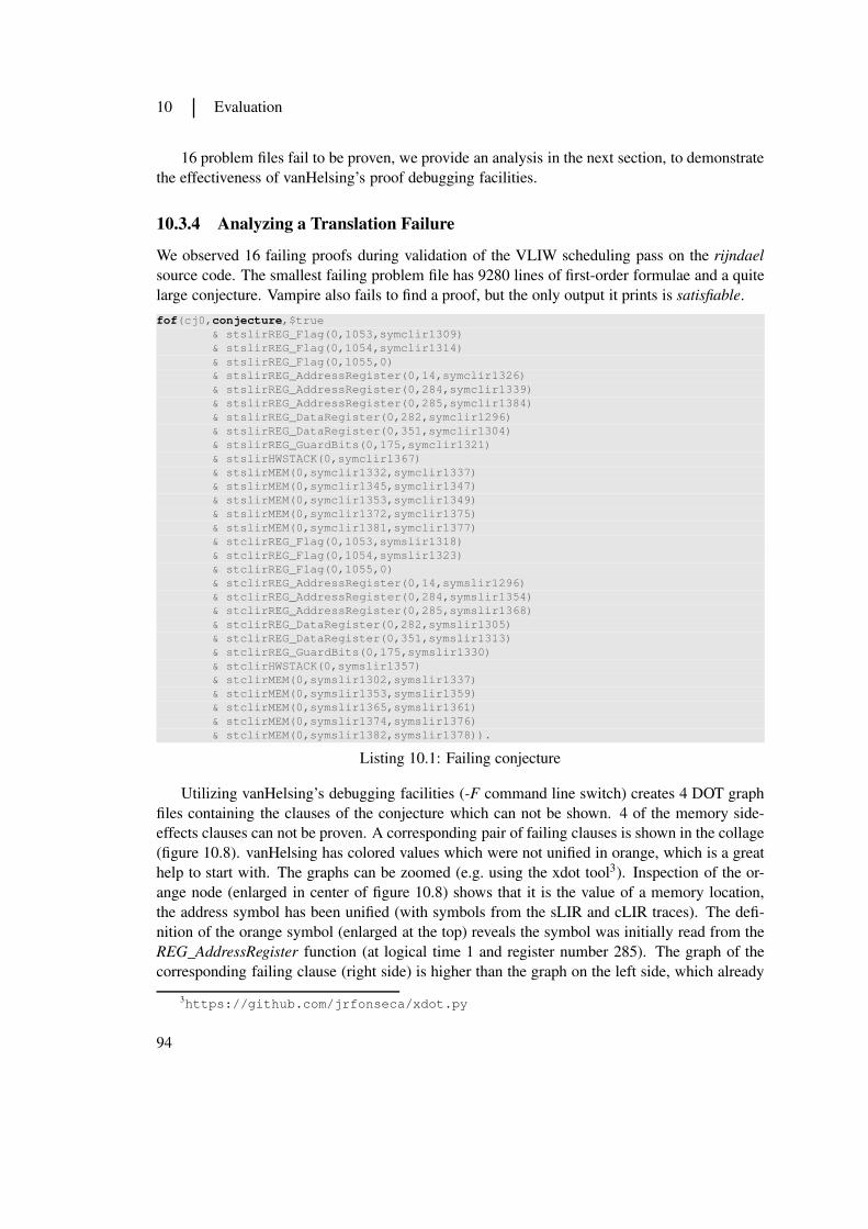
10 Evaluation
16 problem files fail to be proven, we provide an analysis in the next section, to demonstratethe effectiveness of vanHelsing’s proof debugging facilities.
10.3.4 Analyzing a Translation Failure
We observed 16 failing proofs during validation of the VLIW scheduling pass on the rijndael
source code. The smallest failing problem file has 9280 lines of first-order formulae and a quitelarge conjecture. Vampire also fails to find a proof, but the only output it prints is satisfiable.
fof(cj0,conjecture,$true
& stslirREG_Flag(0,1053,symclir1309)
& stslirREG_Flag(0,1054,symclir1314)
& stslirREG_Flag(0,1055,0)
& stslirREG_AddressRegister(0,14,symclir1326)
& stslirREG_AddressRegister(0,284,symclir1339)
& stslirREG_AddressRegister(0,285,symclir1384)
& stslirREG_DataRegister(0,282,symclir1296)
& stslirREG_DataRegister(0,351,symclir1304)
& stslirREG_GuardBits(0,175,symclir1321)
& stslirHWSTACK(0,symclir1367)
& stslirMEM(0,symclir1332,symclir1337)
& stslirMEM(0,symclir1345,symclir1347)
& stslirMEM(0,symclir1353,symclir1349)
& stslirMEM(0,symclir1372,symclir1375)
& stslirMEM(0,symclir1381,symclir1377)
& stclirREG_Flag(0,1053,symslir1318)
& stclirREG_Flag(0,1054,symslir1323)
& stclirREG_Flag(0,1055,0)
& stclirREG_AddressRegister(0,14,symslir1296)
& stclirREG_AddressRegister(0,284,symslir1354)
& stclirREG_AddressRegister(0,285,symslir1368)
& stclirREG_DataRegister(0,282,symslir1305)
& stclirREG_DataRegister(0,351,symslir1313)
& stclirREG_GuardBits(0,175,symslir1330)
& stclirHWSTACK(0,symslir1357)
& stclirMEM(0,symslir1302,symslir1337)
& stclirMEM(0,symslir1353,symslir1359)
& stclirMEM(0,symslir1365,symslir1361)
& stclirMEM(0,symslir1374,symslir1376)
& stclirMEM(0,symslir1382,symslir1378)).
Listing 10.1: Failing conjecture
Utilizing vanHelsing’s debugging facilities (-F command line switch) creates 4 DOT graphfiles containing the clauses of the conjecture which can not be shown. 4 of the memory side-effects clauses can not be proven. A corresponding pair of failing clauses is shown in the collage(figure 10.8). vanHelsing has colored values which were not unified in orange, which is a greathelp to start with. The graphs can be zoomed (e.g. using the xdot tool3). Inspection of the or-ange node (enlarged in center of figure 10.8) shows that it is the value of a memory location,the address symbol has been unified (with symbols from the sLIR and cLIR traces). The defi-nition of the orange symbol (enlarged at the top) reveals the symbol was initially read from theREG_AddressRegister function (at logical time 1 and register number 285). The graph of thecorresponding failing clause (right side) is higher than the graph on the left side, which already
3https://github.com/jrfonseca/xdot.py
94

indicates a problem. Inspecting the marked area (enlarged at bottom) shows that the (also notunified) symbol of the right graph was initially read from an instruction field (at logical time 1and instruction with id 25).
The problem so far seems to be that a value written into memory is read from a register (oncLIR side) but from an instruction field (on sLIR side). From the graph we learned the identifierof the involved instruction (25) and can now inspect the cause. It turns out that an immediatemove and a store instruction have been combined into a bundle. The architecture allows this,as the immediate move writes to the register file a pipeline stage before the store reads its datasource registers. In the witness information used to create the cLIR CASM code those twoinstructions end up swapped, i.e. the store operation is executed before the move. It thereforestores the old register contents to the memory, while the sLIR code (correctly) reads the movedimmediate value. This is exactly what we learned by inspection of the failing proofs graphs. The15 other failing proofs turned out to be caused by the very same bug.
While this bug was just caused by an erroneous witness information it must not have goneunnoticed by the validator, a real data dependency bug in the scheduler would show exactly thesame behavior. Finding and isolating this bug demonstrates the effectiveness of our validationtools.
95

10 Evaluation
Figure 10.8: Visual debugging a VLIW Scheduling Bug
96

11 Future Work
Die Wissenschaft fängt eigentlich erst da an interessant zu werden, wo sie aufhört.
Justus von Liebig
This chapter sketches interesting ideas which came up but have not been further investigated inthis thesis.
11.1 CASM Object Model
The CASM language currently operates on one global state. To create composable models,it would be advantageous to have objects. Rules would then operate on their object’s state.An open research question however is the composition of objects, especially considering thetransactional semantics of ASM. When will modification of an object’s state be visible fromother objects? One idea is to have a top-level rule (as in the current implementation) whichorchestrates all existing objects. The global state would then be updated when the top-levelrule concludes (returns). Following this approach objects would implement namespaces for theglobal state and not be independent STS. It remains to be shown whether this approach is goodsuited to model complex hardware or if independent STS (and a different object model or adifferent mechanism) is desirable.
11.2 Update Placement Optimization for the CASM Compiler
The CASM run-time needs to merge collected updates when leaving a pseudo state. For cor-rectly detecting conflicting updates this merging is needed for each pseudo state. Most updateswill never conflict, though, and in many cases this property can be analyzed statically. The ideais to initially put updates into the lowest possible pseudo state which would reduce the numberof merged updates significantly (and thus directly boost performance as update set operationsare very expensive). By placing the updates in the lowest pseudo state the size of the update setwould decrease, the main reason why our CS is not performing well.
97

11 Future Work
11.3 Translation Validation of the CASM Compiler
The CASM compiler performs the optimizations directly on the AST itself. Because the ASTis shared between the compiler and interpreter the translation validation approach presented inthis thesis could directly be applied to the CASM compiler itself. The modified rules would justneed to be symbolically executed by the interpreter before and after the transformation.
11.4 Synthesization of the Compiler Specification
The approach proposed by in this thesis removes a lot of redundancy from the ADL by modelingthe architecture in CASM. Because the CASM models capture the semantics of each instruction,it should be possible to derive the compiler specification (matcher tree patterns). The naïveapproach would be to guess a tree pattern for a mMIR input and validate whether the pattern is avalid translation (i.e. perform instruction selection validation). Accumulating correctly guessedpatterns would finally result in a complete compiler specification. Brandner [13] has shownthat the completeness of a generated compiler specification can be shown automatically. So atleast a criterion to stop the search for patterns can be given. A realistic implementation howevershould use a better algorithm and also the quality of the generated compiler specification mustbe measured. Brandner’s results [14] on deriving tree patterns from a micro-instruction basedADL may be directly applicable to our ADL. As the benefit of such a synthesization a largeredundant and tedious to write part of the ADL (the tree patterns) could be removed.
98

12 Conclusion
Everything that has a beginning has an end, Neo.
Agent Smith, The Matrix Revolutions
We have presented the CASM language, a statically typed implementation of Abstract State Ma-chine. Due to its parallel execution semantics CASM is well-suited to specify micro-processors.This has been demonstrated by modeling a proprietary micro-processor and two variants ofMIPS implementations (forwarding and bubbling). A compiler for CASM has been developedwhich allows synthesization of efficient Instruction Set Simulation based on the instruction setspecification (up to 2.47 MHz). The highly efficient optimizer (increasing performance up to264%) can be used to synthesize Compiled Simulation tools. Thus we were able to removetwo highly redundant (ISS and CS) specifications from our research compiler’s ArchitectureDescription Language and have CASM as the unified specification.
Due to the formal nature of ASM the micro-processor specifications have a concise (for-mal) meaning. By using a set of common semantic vocabulary to specify compiler IRs and theinstruction set, simulation proofs can be performed on these specifications. Technically we rep-resent these common semantic operations as traces of first-order logic predicates. These tracesare created by our novel method of direct symbolic execution (of ASM).
Based on this formal foundation a translation validation framework is defined. Each com-piler pass is validated in isolation, applying a local correctness criterion. Certain properties ofa translation must be validated during later passes (so called constraints). Our proposed frame-work validates each single pass of the compiler and makes sure that the output of the precedingpass is used as input to the succeeding one (chain of trust). In addition it collects the constraints
and provides them to later passes which ultimately validate these properties.The focus of this thesis is on the compiler back-end. We have discussed validators for
all back-end passes of our research compiler and implemented prototypes for the crucial ones(instruction selection, register allocation and VLIW scheduling). All those validators operateon individual basic blocks which limits the complexity of the proofs and allows a high degreeof parallelization. To evaluate the effectiveness of our approach we applied our validators torealistic industrial programs (AES implementation and bzip2) and are able to achieve convincingvalidation times (some minutes).
99

12 Conclusion
An additional contribution is the vanHelsing tool, a highly specialized first-order proverwhich handles the problems arising from translation validation very efficiently. A distinct fea-ture of vanHelsing is its capability to provide graphical debugging aids which allow to quicklyinvestigate translation error and pinpoint the issue. We have demonstrated this ability on a real-istic bug by identifying the causing instructions without manual inspection of the problem file(more than 9000 lines).
We hope that the tools, techniques and results presented in this thesis act as a stimulation tolaunch translation validation projects for industrial compilers.
100

Bibliography
[1] Iso/iec jtc1/sc22/wg14. 9899:tc3: Programming languages-c. Technical report,2007. URL: http://www.open-std.org/jtc1/sc22/wg14/www/docs/
n1256.pdf.
[2] Kunal Agrawal, Jeremy T. Fineman, and Jim Sukha. Nested parallelism in transactionalmemory. In Proceedings of the 13th ACM SIGPLAN Symposium on Principles and Practice
of Parallel Programming, PPoPP ’08, pages 163–174, New York, NY, USA, 2008. ACM.doi:10.1145/1345206.1345232.
[3] J. R. Allen, Ken Kennedy, Carrie Porterfield, and Joe Warren. Conversion of control depen-dence to data dependence. In Proceedings of the 10th ACM SIGACT-SIGPLAN symposium
on Principles of programming languages, POPL ’83, pages 177–189, New York, NY, USA,1983. ACM. doi:10.1145/567067.567085.
[4] Matthias Anlauff. XASM- an extensible, component-based abstract state machineslanguage. In Yuri Gurevich, PhilippW. Kutter, Martin Odersky, and Lothar Thiele,editors, Abstract State Machines - Theory and Applications, volume 1912 of Lec-
ture Notes in Computer Science, pages 69–90. Springer Berlin Heidelberg, 2000.doi:10.1007/3-540-44518-8_6.
[5] Jürgen Avenhaus, Jörg Denzinger, and Matthias Fuchs. Discount: A system for distributedequational deduction. In RTA, pages 397–402, 1995.
[6] Leo Bachmair and Harald Ganzinger. Resolution theorem proving. In Handbook of Auto-
mated Reasoning, pages 19–99. 2001.
[7] Mike Barnett, Wolfgang Grieskamp, Lev Nachmanson, Wolfram Schulte, Nikolai Till-mann, and Margus Veanes. Towards a tool environment for model-based testing withAsmL. In Formal Approaches to Software Testing, FATES 2003, volume 2931 of LNCS,pages 264–280. Springer, 2003.
[8] John Bergin and Stuart Greenfield. Teaching parameter passing by exam-ple using thunks in C and C++. SIGCSE Bull., 25(1):10–14, March 1993.doi:10.1145/169073.169083.
101

BIBLIOGRAPHY
[9] Yves Bertot, Pierre Castéran, Gérard (informaticien) Huet, and Christine Paulin-Mohring.Interactive theorem proving and program development : Coq’Art : the calculus of inductive
constructions. Texts in theoretical computer science. Springer, Berlin, New York, 2004.URL: http://opac.inria.fr/record=b1101046.
[10] Manuel Blum, Sampath Kannan, Comp Sci, and Comp Sci. Designing programs that checktheir work, 1989.
[11] Egon Börger and Joachim Schmid. Composition and submachine concepts for sequentialASMs. In Computer Science Logic (Proceedings of CSL 2000), volume 1862 of LNCS,pages 41–60. Springer-Verlag, 2000.
[12] Robert S. Boyer, Bernard Elspas, and Karl N. Levitt. SELECT - a formal system fortesting and debugging programs by symbolic execution. In Proceedings of the interna-
tional conference on Reliable software, pages 234–245, New York, NY, USA, 1975. ACM.doi:10.1145/800027.808445.
[13] F. Brandner. Completeness of automatically generated instruction selec-tors. In Application-specific Systems Architectures and Processors (ASAP),
2010 21st IEEE International Conference on, pages 175–182, 2010.doi:10.1109/ASAP.2010.5540994.
[14] Florian Brandner, Dietmar Ebner, and Andreas Krall. Compiler generation from structuralarchitecture descriptions. In Proceedings of the 2007 International Conference on Com-
pilers, Architecture, and Synthesis for Embedded Systems, CASES ’07, pages 13–22, NewYork, NY, USA, 2007. ACM. doi:10.1145/1289881.1289886.
[15] Florian Brandner, Andreas Fellnhofer, Andreas Krall, and David Riegler. Fast and accuratesimulation using the LLVM compiler framework. In RAPIDO ’09: 1st Workshop on Rapid
Simulation and Performance Evaluation: Methods and Tools, 2009.
[16] Florian Brandner, Nigel Horspool, and Andreas Krall. DSP instruction set simulation.In Shuvra S. Bhattacharyya, Ed F. Deprettere, Rainer Leupers, and Jarmo Takala, edi-tors, Handbook of Signal Processing Systems, pages 945–974. Springer New York, 2013.doi:10.1007/978-1-4614-6859-2_29.
[17] Giuseppe Del Castillo. The ASM workbench - A tool environment for computer-aidedanalysis and validation of abstract state machine models. In Proceedings of the 7th Inter-
national Conference on Tools and Algorithms for the Construction and Analysis of Systems,TACAS 2001, pages 578–581, London, UK, UK, 2001. Springer-Verlag.
[18] Lori A. Clarke. A program testing system. In Proceedings of the 1976 an-
nual conference, ACM ’76, pages 488–491, New York, NY, USA, 1976. ACM.doi:10.1145/800191.805647.
[19] Alberto Coen-Porisini, Giovanni Denaro, Carlo Ghezzi, and Mauro Pezzé. Using symbolicexecution for verifying safety-critical systems. SIGSOFT Softw. Eng. Notes, 26(5):142–151, September 2001. doi:10.1145/503271.503230.
102

[20] Maulik A. Dave. Compiler verification: A bibliography. SIGSOFT Softw. Eng. Notes,28(6):2–2, November 2003. doi:10.1145/966221.966235.
[21] Leonardo De Moura and Nikolaj Bjørner. Z3: An efficient smt solver. In Proceedings of
the Theory and Practice of Software, 14th International Conference on Tools and Algo-
rithms for the Construction and Analysis of Systems, TACAS’08/ETAPS’08, pages 337–340, Berlin, Heidelberg, 2008. Springer-Verlag.
[22] Roozbeh Farahbod. CoreASM language user manual. URL: http://coreasm.svn.sourceforge.net/viewvc/coreasm/engine-carma/trunk/doc/user_
manual/CoreASM-UserManual.pdf.
[23] Roozbeh Farahbod, Vincenzo Gervasi, and Uwe Glässer. CoreASM: An extensible ASMexecution engine. Fundamenta Informaticae, 77:1–33, 2007.
[24] Stefan Farfeleder, Andreas Krall, and Nigel Horspool. Ultra fast cycle-accurate compiledemulation of inorder pipelined architectures. J. Syst. Archit., 53(8):501–510, August 2007.doi:10.1016/j.sysarc.2006.11.003.
[25] Stefan Farfeleder, Andreas Krall, Edwin Steiner, and Florian Brandner. Effectivecompiler generation by architecture description. In Proceedings of the 2006 ACM
SIGPLAN/SIGBED Conference on Language, Compilers, and Tool Support for Em-
bedded Systems, LCTES ’06, pages 145–152, New York, NY, USA, 2006. ACM.doi:10.1145/1134650.1134671.
[26] Nicu G. Fruja and Robert F. Stärk. The hidden computation steps of Turbo Abstract StateMachines. In Abstract State Machines — Advances in Theory and Applications, 10th In-
ternational Workshop, ASM 2003, pages 244–262. Springer-Verlag, 2003.
[27] Emden R. Gansner and Stephen C. North. An open graph visualization system and itsapplications to software engineering. SOFTWARE - PRACTICE AND EXPERIENCE,30(11):1203–1233, 2000.
[28] Angelo Gargantini, Elvinia Riccobene, and Patrizia Scandurra. Model-driven languageengineering: The asmeta case study. In Proceedings of the 2008 The Third International
Conference on Software Engineering Advances, ICSEA ’08, pages 373–378, Washington,DC, USA, 2008. IEEE Computer Society. doi:10.1109/ICSEA.2008.62.
[29] J. R. Goodman and W.-C. Hsu. Code scheduling and register allocation in large basicblocks. In Proceedings of the 2Nd International Conference on Supercomputing, ICS ’88,pages 442–452, New York, NY, USA, 1988. ACM. doi:10.1145/55364.55407.
[30] Gerhard Goos and Wolf Zimmermann. Verifying compilers and ASMs. In Proceedings of
the International Workshop on Abstract State Machines, Theory and Applications, ASM’00, pages 177–202, London, UK, 2000. Springer-Verlag.
[31] Yuri Gurevich. Evolving algebras 1993: Lipari guide, pages 9–36. Oxford UniversityPress, Inc., New York, NY, USA, 1995.
103

BIBLIOGRAPHY
[32] Yuri Gurevich. Sequential abstract-state machines capture sequential algorithms. ACM
Trans. Comput. Logic, 1(1):77–111, July 2000. doi:10.1145/343369.343384.
[33] Yuri Gurevich, Benjamin Rossman, and Wolfram Schulte. Semanticessence of AsmL. Theor. Comput. Sci., 343(3):370–412, October 2005.doi:10.1016/j.tcs.2005.06.017.
[34] Yuri Gurevich and Nikolai Tillmann. Partial updates. Theoretical Computer Science,336(2):311–342, 2005.
[35] M. R. Guthaus, J. S. Ringenberg, D. Ernst, T. M. Austin, T. Mudge, and R. B. Brown.Mibench: A free, commercially representative embedded benchmark suite. In Proceed-
ings of the Workload Characterization, 2001. WWC-4. 2001 IEEE International Work-
shop, WWC ’01, pages 3–14, Washington, DC, USA, 2001. IEEE Computer Society.doi:10.1109/WWC.2001.15.
[36] Dominik Inführ. AST interpreter for CASM. 2013. URL: http://publik.tuwien.ac.at/files/PubDat_227295.pdf.
[37] Christoph Kern and Mark R. Greenstreet. Formal verification in hardware design:A survey. ACM Trans. Des. Autom. Electron. Syst., 4(2):123–193, April 1999.doi:10.1145/307988.307989.
[38] Sarfraz Khurshid, Corina S. Pasareanu, and Willem Visser. Generalized symbolic execu-tion for model checking and testing. In In Proceedings of the Ninth International Confer-
ence on Tools and Algorithms for the Construction and Analysis of Systems, pages 553–568. Springer, 2003.
[39] James C. King. Symbolic execution and program testing. Commun. ACM, 19(7):385–394,July 1976. doi:10.1145/360248.360252.
[40] Gerwin Klein, Kevin Elphinstone, Gernot Heiser, June Andronick, David Cock, PhilipDerrin, Dhammika Elkaduwe, Kai Engelhardt, Rafal Kolanski, Michael Norrish, ThomasSewell, Harvey Tuch, and Simon Winwood. seL4: Formal verification of an OS kernel.In ACM SYMPOSIUM ON OPERATING SYSTEMS PRINCIPLES, pages 207–220. ACM,2009.
[41] Laura Kovács and Andrei Voronkov. First-Order Theorem Proving and Vampire. In CAV,pages 1–35, 2013.
[42] M. Lam. Software pipelining: An effective scheduling technique for vliw machines.In Proceedings of the ACM SIGPLAN 1988 Conference on Programming Language De-
sign and Implementation, PLDI ’88, pages 318–328, New York, NY, USA, 1988. ACM.doi:10.1145/53990.54022.
[43] Xavier Leroy. Formal verification of a realistic compiler. Commun. ACM, 52:107–115,2009. doi:10.1145/1538788.1538814.
104

[44] Raya Leviathan and Amir Pnueli. Validating software pipelining optimizations. In Pro-
ceedings of the 2002 international conference on Compilers, architecture, and synthesis
for embedded systems, CASES ’02, pages 280–287, New York, NY, USA, 2002. ACM.doi:10.1145/581630.581676.
[45] Roland Lezuo, Gergö Barany, and Andreas Krall. CASM: Implementing an Abstract StateMachine based Programming Language. In Stefan Wagner and Horst Lichter, editors,Software Engineering 2013 Workshopband, 26. Februar - 1. März 2013 in Aachen, vol-ume 215 of GI Edition - Lecture Notes in Informatics, pages 75–90, February 2013. (6.Arbeitstagung Programmiersprachen (ATPS’13)).
[46] Roland Lezuo and Andreas Krall. A unified processor model for compiler verification andsimulation using ASM. In Proceedings of the Third international conference on Abstract
State Machines, Alloy, B, VDM, and Z, ABZ’12, pages 327–330, Berlin, Heidelberg, 2012.Springer-Verlag. doi:10.1007/978-3-642-30885-7_24.
[47] Roland Lezuo and Andreas Krall. Using the CASM language for simulator synthesis andmodel verification. In Proceedings of the 2013 Workshop on Rapid Simulation and Per-
formance Evaluation: Methods and Tools, RAPIDO ’13, pages 6:1–6:8, New York, NY,USA, 2013. ACM. doi:10.1145/2432516.2432522.
[48] Roland Lezuo, Philipp Paulweber, and Andreas Krall. CASM - Optimized Compilation ofAbstract State Machines. LCTES ’07, New York, NY, USA, 2014 (to appear). ACM.
[49] Z Manna, Anuchit Anuchitanukul, Nikolaj Bjorner, Anca Browne, Edward Chang, MichaelColon, Luca de Alfaro, Harish Devarajan, Henny Sipma, and Tomas Uribe. STeP: TheStanford Temporal Prover. Technical report, Stanford, CA, USA, 1994. URL: http://theory.stanford.edu/~zm/papers/step.ps.Z.
[50] William McCune. Otter 3.3 reference manual. CoRR, cs.SC/0310056, 2003.
[51] William McCune and Larry Wos. Otter - the CADE-13 competition incarnations. Journal
of Automated Reasoning, 18:211–220, 1997. doi:10.1023/A:1005843632307.
[52] Tom Mens. A state-of-the-art survey on software merging. Software Engineering, IEEE
Transactions on, 28(5):449–462, 2002.
[53] George C. Necula. Translation validation for an optimizing compiler. In Pro-
ceedings of the ACM SIGPLAN 2000 conference on Programming language design
and implementation, PLDI ’00, pages 83–94, New York, NY, USA, 2000. ACM.doi:10.1145/349299.349314.
[54] Robert Nieuwenhuis and Albert Rubio. Paramodulation-based theorem proving. In Hand-
book of Automated Reasoning, pages 371–443. 2001.
[55] Lawrence Paulson, Tobias Nipkow, and Markus Wenzel. The isabelle reference manual.Technical report, 1995.
105

BIBLIOGRAPHY
[56] Philipp Paulweber. Masterthesis. 2014 (to appear).
[57] A. Pnueli, M. Siegel, and F. Singerman. Translation validation. pages 151–166. Springer,1998.
[58] B. Ramakrishna Rau. Iterative modulo scheduling: An algorithm for softwarepipelining loops. In Proceedings of the 27th Annual International Symposium on
Microarchitecture, MICRO 27, pages 63–74, New York, NY, USA, 1994. ACM.doi:10.1145/192724.192731.
[59] Alexandre Riazanov and Andrei Voronkov. The design and implementation of VAMPIRE.AI Commun., 15:91–110, August 2002.
[60] J. Schmid. Compiling abstract state machines to C++. Journal of Universal Computer
Science, 7(11):1068–1087, 2001.
[61] Joachim Schmid. Introduction to AsmGofer, 2001. URL: http://www.tydo.de/AsmGofer.
[62] Stephan Schulz. E - a brainiac theorem prover. AI Commun., 15(2,3):111–126, August2002.
[63] Richard Stallman and GCC Developer Community. GNU Compiler Collection Internals.Free Software Foundation, 2010.
[64] G. Sutcliffe and C. Suttner. The State of CASC. AI Communications, 19(1):35–48, 2006.
[65] Geoff Sutcliffe, Stephan Schulz, Koen Claessen, and Allen Van Gelder. Using the TPTPlanguage for writing derivations and finite interpretations. In Proceedings of the Third
international joint conference on Automated Reasoning, IJCAR’06, pages 67–81, Berlin,Heidelberg, 2006. Springer-Verlag. doi:10.1007/11814771_7.
[66] Jürgen Teich, Philipp W. Kutter, and Ralph Weper. Description and simulation of micro-processor instruction sets using ASMs. In Proceedings of the International Workshop on
Abstract State Machines, Theory and Applications, ASM ’00, pages 266–286, London,UK, 2000. Springer-Verlag.
[67] Christoph Weidenbach, Dilyana Dimova, Arnaud Fietzke, Rohit Kumar, Martin Suda, andPatrick Wischnewski. SPASS version 3.5. In RenateA. Schmidt, editor, Automated De-
duction – CADE-22, volume 5663 of Lecture Notes in Computer Science, pages 140–145.Springer Berlin Heidelberg, 2009. doi:10.1007/978-3-642-02959-2_10.
[68] Xuejun Yang, Yang Chen, Eric Eide, and John Regehr. Finding and understanding bugsin C compilers. In Proceedings of the 32nd ACM SIGPLAN conference on Programming
language design and implementation, PLDI ’11, pages 283–294, New York, NY, USA,2011. ACM. doi:10.1145/1993498.1993532.
106

[69] Han-Saem Yun and Jihong Kim. Power-aware modulo scheduling for high-performanceVLIW processors. In Proceedings of the 2001 international symposium on Low power
electronics and design, ISLPED ’01, pages 40–45, New York, NY, USA, 2001. ACM.doi:10.1145/383082.383091.
[70] Wolf Zimmermann and Thilo Gaul. On the construction of correct compiler back-ends:An ASM approach. Journal of Universal Computer Science, 3:504–567, 1997.
107


A Common Semantic Vocabulary andAxiomatization
... has caused more and bloodier wars than anything else in the history of creation.
Douglas Adams on the poor babel fish
The following listing contains all semantic operations used to model the (integer parts only) ofthe MIPS instruction set and a proprietary DSP micro-processor. Each item is the name of apredicate, in braces the arguments and a short description of its semantic meaning.
• ex (from, to, val, res) extracts bits from to to from val and puts them into res
• ze (old, new, val, res) zero-extends val from a old-bit vector to a new-bit vector and putsinto res.
• se (old, new, val, res) sign-extends val from a old-bit vector to a new-bit vector and putsinto res.
• sb (from, to, tmpl, val, res) sets bits from to to in tmpl to val and puts results in res.
• or (w, o1, o2, res) logical or of width w.
• and (w, o1, o2, res) logical and of width w.
• xor (w, o1, o2, res) logical xor of width w.
• max (w, o1, o2, res) the maximum of the signed w-bit wide values o1 and o2 is put intores.
• max_select (w, o1, o2, res) res is 0 is o1 is max (see above), 1 otherwise
• min (w, o1, o2, res) the minimum of the signed w-bit wide values o1 and o2 is put into res.
• min_select (w, o1, o2, res) res is 0 is o1 is min (see above), 1 otherwise
• saturate (w, ov, os, val, res) saturates w-bit wide value val depended on overflow condition(ov = 1) and whether overflow was towards negative values (os = 1).
109

A Vocabulary and Axioms
• equal (w, o1, o2, res) res = 1 if w-bit wide values o1 and o2 are equal, 0 otherwise.
• unequal (w, o1, o2, res) res = 1 if w-bit wide values o1 and o2 are not equal, 0 otherwise.
• gez (w, o1, res) res = 1 if signed w-bit wide value o1 is greater or equal zero, 0 otherwise.
• gtz (w, o1, res) res = 1 if signed w-bit wide value o1 is greater than zero, 0 otherwise.
• lez (w, o1, res) res = 1 if signed w-bit wide value o1 is less or equal zero, 0 otherwise.
• ltz (w, o1, res) res = 1 if signed w-bit wide value o1 is less than zero, 0 otherwise.
• testbit (w, o1, o2, res) res 0 1 if bit o2 is 1 in w-bit wide value o1, 0 otherwise.
• add_result (w, o1, o2, res) res contains result of unsigned addition of w-bit wide values o1
and o2.
• add_overflow (w, o1, o2, res) res = 1 if above addition overflows, 0 otherwise.
• add_overflowsign (w, o1, o2, res) res = 1 if above addition overflows towards negativevalues, 0 otherwise.
• shift_result (w, r, s, val, nrbits, res) res contains the results of a shift operation. If r = 1 aright shift is performed, left otherwise. A right shift may be arithmetic (s = 1) or logical.val will be shifted nrbits bits.
• shift_overflow (w, r, s, val, nrbits, res) res = 1 if above shift overflows, 0 otherwise.
• shift_overflowsign (w, r, s, val, nrbits, res) res = 1 if above shift overflows towards negativevalues, 0 otherwise.
• rotate (w, r, val, nrbits, res) res contains results of a nrbits rotation of a w-bit wide valueval. If r = 1 the rotation direction is right, left otherwise.
• abs_result (w, val, res) res contains the absolute value of the signed w-bit wide value val.
• abs_overflow (w, val, res) res = 1 if above operation overflows, 0 otherwise.
• negate_result (w, val, res) res contains the negation of the signed w-bit wide value val.
• negate_overflow (w, val, res) res = 1 if above operation overflows, 0 otherwise.
• not (w, val, res) logical negation of w-bit wide value val.
• clz (w, val, res) counts leading zero bits of the w-bit wide value val, puts results in res.
• clz (w, val, res) counts leading one bits of the w-bit wide value val, puts results in res.
• multiply_fract (w, op1, op2, res) res contains result of fractional multiplication of w-bitwide values op1 andop2.
110

• multiply_result (w, s1, s2, op1, op2, res) res contains the lower half of the result of amultiplication of w-bit wide values op1 and op2. If s1 (s2) = 1 op1 (op2) is treated assigned value.
• multiply_result_hi (w, s1, s2, op1, op2, res) res contains the upper half of the result of amultiplication of w-bit wide values op1 and op2. If s1 (s2) = 1 op1 (op2) is treated assigned value.
• multiply_overflow (w, s1, s2, o1, o2, res) res = 1 if above multiplication overflows, 0otherwise.
• multiply_overflowsign (w, s1, s2, o1, o2, res) res = 1 if above multiplication overflowstowards negative values, 0 otherwise.
• divide_result (w, s1, s2, o1, o2, res) res contains the results of the division of the w-bitwide value op1 by the w-bit wide value op2. If s1 (s2) = 1 op1 (op2) is treated as signedvalue.
• divide_remainder (w, s1, s2, o1, o2, res) res contains the remainder of the above division.
• mir_if (w, c, ai, ae, res) res contains the value ai if the w-bit wide value c does not equalzero, ae otherwise. This predicate is used to model conditional control flow in mMIR.
The following listing contains the axiomatization of the semantic operations used in thevalidator prototypes.
∀A0, A1, A2,X0,X1 :
fex(A0, A1, A2,X0) ∧ fex(A0, A1, A2,X1) =⇒ (X0 = X1)
∀A0, A1, A2,X0,X1 :
fze(A0, A1, A2,X0) ∧ fze(A0, A1, A2,X1) =⇒ (X0 = X1)
∀A0, A1, A2,X0,X1 :
fse(A0, A1, A2,X0) ∧ fse(A0, A1, A2,X1) =⇒ (X0 = X1)
∀A0, A1, A2, A3,X0,X1 :
fsb(A0, A1, A2, A3,X0) ∧ fsb(A0, A1, A2, A3,X1) =⇒ (X0 = X1)
∀A0, A1, A2,X0,X1 :
for(A0, A1, A2,X0) ∧ for(A0, A1, A2,X1) =⇒ (X0 = X1)
111

A Vocabulary and Axioms
∀A0, A1, A2,X0,X1 :
fand(A0, A1, A2,X0) ∧ fand(A0, A1, A2,X1) =⇒ (X0 = X1)
∀A0, A1, A2,X0,X1 :
fxor(A0, A1, A2,X0) ∧ fxor(A0, A1, A2,X1) =⇒ (X0 = X1)
∀A0, A1, A2,X0,X1 :
fmax(A0, A1, A2,X0) ∧ fmax(A0, A1, A2,X1) =⇒ (X0 = X1)
∀A0, A1, A2,X0,X1 :
fmax_select(A0, A1, A2,X0) ∧ fmax_select(A0, A1, A2,X1)
=⇒ (X0 = X1)
∀A0, A1, A2,X0,X1 :
fmin(A0, A1, A2,X0) ∧ fmin(A0, A1, A2,X1) =⇒ (X0 = X1)
∀A0, A1, A2,X0,X1 :
fmin_select(A0, A1, A2,X0) ∧ fmin_select(A0, A1, A2,X1)
=⇒ (X0 = X1)
∀A0, A1, A2, A3,X0,X1 :
fsaturate(A0, A1, A2, A3,X0) ∧ fsaturate(A0, A1, A2, A3,X1)
=⇒ (X0 = X1)
∀A0, A1, A2,X0,X1 :
fequal(A0, A1, A2,X0) ∧ fequal(A0, A1, A2,X1) =⇒ (X0 = X1)
∀A0, A1, A2,X0,X1 :
funequal(A0, A1, A2,X0) ∧ funequal(A0, A1, A2,X1) =⇒ (X0 = X1)
∀A0, A1,X0,X1 :
fgez(A0, A1,X0) ∧ fgez(A0, A1,X1) =⇒ (X0 = X1)
112
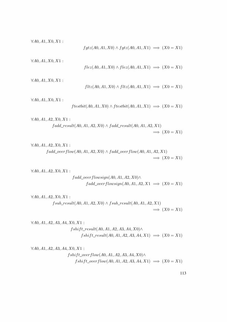
∀A0, A1,X0,X1 :
fgtz(A0, A1,X0) ∧ fgtz(A0, A1,X1) =⇒ (X0 = X1)
∀A0, A1,X0,X1 :
flez(A0, A1,X0) ∧ flez(A0, A1,X1) =⇒ (X0 = X1)
∀A0, A1,X0,X1 :
fltz(A0, A1,X0) ∧ fltz(A0, A1,X1) =⇒ (X0 = X1)
∀A0, A1,X0,X1 :
ftestbit(A0, A1,X0) ∧ ftestbit(A0, A1,X1) =⇒ (X0 = X1)
∀A0, A1, A2,X0,X1 :
fadd_result(A0, A1, A2,X0) ∧ fadd_result(A0, A1, A2,X1)
=⇒ (X0 = X1)
∀A0, A1, A2,X0,X1 :
fadd_overflow(A0, A1, A2,X0) ∧ fadd_overflow(A0, A1, A2,X1)
=⇒ (X0 = X1)
∀A0, A1, A2,X0,X1 :
fadd_overflowsign(A0, A1, A2,X0)∧
fadd_overflowsign(A0, A1, A2,X1 =⇒ (X0 = X1)
∀A0, A1, A2,X0,X1 :
fsub_result(A0, A1, A2,X0) ∧ fsub_result(A0, A1, A2,X1)
=⇒ (X0 = X1)
∀A0, A1, A2, A3, A4,X0,X1 :
fshift_result(A0, A1, A2, A3, A4,X0)∧
fshift_result(A0, A1, A2, A3, A4,X1) =⇒ (X0 = X1)
∀A0, A1, A2, A3, A4,X0,X1 :
fshift_overflow(A0, A1, A2, A3, A4,X0)∧
fshift_overflow(A0, A1, A2, A3, A4,X1) =⇒ (X0 = X1)
113
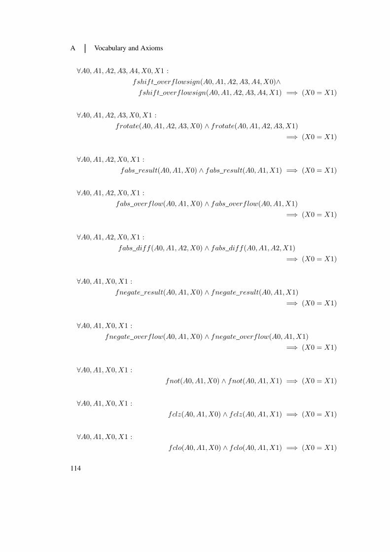
A Vocabulary and Axioms
∀A0, A1, A2, A3, A4,X0,X1 :
fshift_overflowsign(A0, A1, A2, A3, A4,X0)∧
fshift_overflowsign(A0, A1, A2, A3, A4,X1) =⇒ (X0 = X1)
∀A0, A1, A2, A3,X0,X1 :
frotate(A0, A1, A2, A3,X0) ∧ frotate(A0, A1, A2, A3,X1)
=⇒ (X0 = X1)
∀A0, A1, A2,X0,X1 :
fabs_result(A0, A1,X0) ∧ fabs_result(A0, A1,X1) =⇒ (X0 = X1)
∀A0, A1, A2,X0,X1 :
fabs_overflow(A0, A1,X0) ∧ fabs_overflow(A0, A1,X1)
=⇒ (X0 = X1)
∀A0, A1, A2,X0,X1 :
fabs_diff(A0, A1, A2,X0) ∧ fabs_diff(A0, A1, A2,X1)
=⇒ (X0 = X1)
∀A0, A1,X0,X1 :
fnegate_result(A0, A1,X0) ∧ fnegate_result(A0, A1,X1)
=⇒ (X0 = X1)
∀A0, A1,X0,X1 :
fnegate_overflow(A0, A1,X0) ∧ fnegate_overflow(A0, A1,X1)
=⇒ (X0 = X1)
∀A0, A1,X0,X1 :
fnot(A0, A1,X0) ∧ fnot(A0, A1,X1) =⇒ (X0 = X1)
∀A0, A1,X0,X1 :
fclz(A0, A1,X0) ∧ fclz(A0, A1,X1) =⇒ (X0 = X1)
∀A0, A1,X0,X1 :
fclo(A0, A1,X0) ∧ fclo(A0, A1,X1) =⇒ (X0 = X1)
114
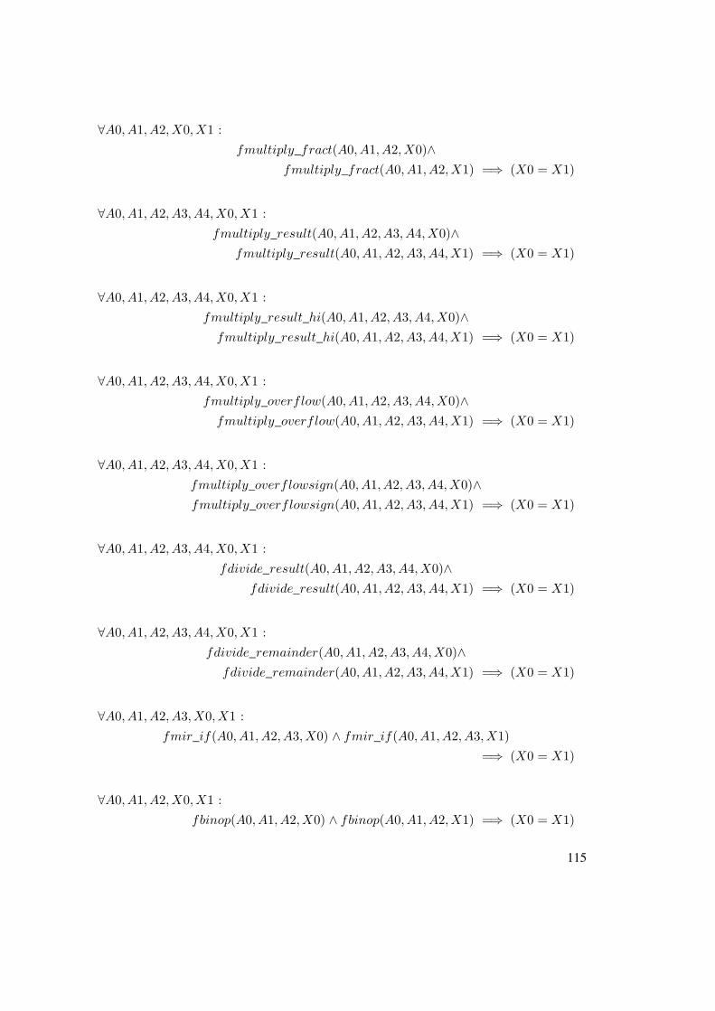
∀A0, A1, A2,X0,X1 :
fmultiply_fract(A0, A1, A2,X0)∧
fmultiply_fract(A0, A1, A2,X1) =⇒ (X0 = X1)
∀A0, A1, A2, A3, A4,X0,X1 :
fmultiply_result(A0, A1, A2, A3, A4,X0)∧
fmultiply_result(A0, A1, A2, A3, A4,X1) =⇒ (X0 = X1)
∀A0, A1, A2, A3, A4,X0,X1 :
fmultiply_result_hi(A0, A1, A2, A3, A4, X0)∧
fmultiply_result_hi(A0, A1, A2, A3, A4,X1) =⇒ (X0 = X1)
∀A0, A1, A2, A3, A4,X0,X1 :
fmultiply_overflow(A0, A1, A2, A3, A4,X0)∧
fmultiply_overflow(A0, A1, A2, A3, A4,X1) =⇒ (X0 = X1)
∀A0, A1, A2, A3, A4,X0,X1 :
fmultiply_overflowsign(A0, A1, A2, A3, A4,X0)∧
fmultiply_overflowsign(A0, A1, A2, A3, A4,X1) =⇒ (X0 = X1)
∀A0, A1, A2, A3, A4,X0,X1 :
fdivide_result(A0, A1, A2, A3, A4,X0)∧
fdivide_result(A0, A1, A2, A3, A4,X1) =⇒ (X0 = X1)
∀A0, A1, A2, A3, A4,X0,X1 :
fdivide_remainder(A0, A1, A2, A3, A4,X0)∧
fdivide_remainder(A0, A1, A2, A3, A4,X1) =⇒ (X0 = X1)
∀A0, A1, A2, A3,X0,X1 :
fmir_if(A0, A1, A2, A3,X0) ∧ fmir_if(A0, A1, A2, A3,X1)
=⇒ (X0 = X1)
∀A0, A1, A2,X0,X1 :
fbinop(A0, A1, A2,X0) ∧ fbinop(A0, A1, A2,X1) =⇒ (X0 = X1)
115
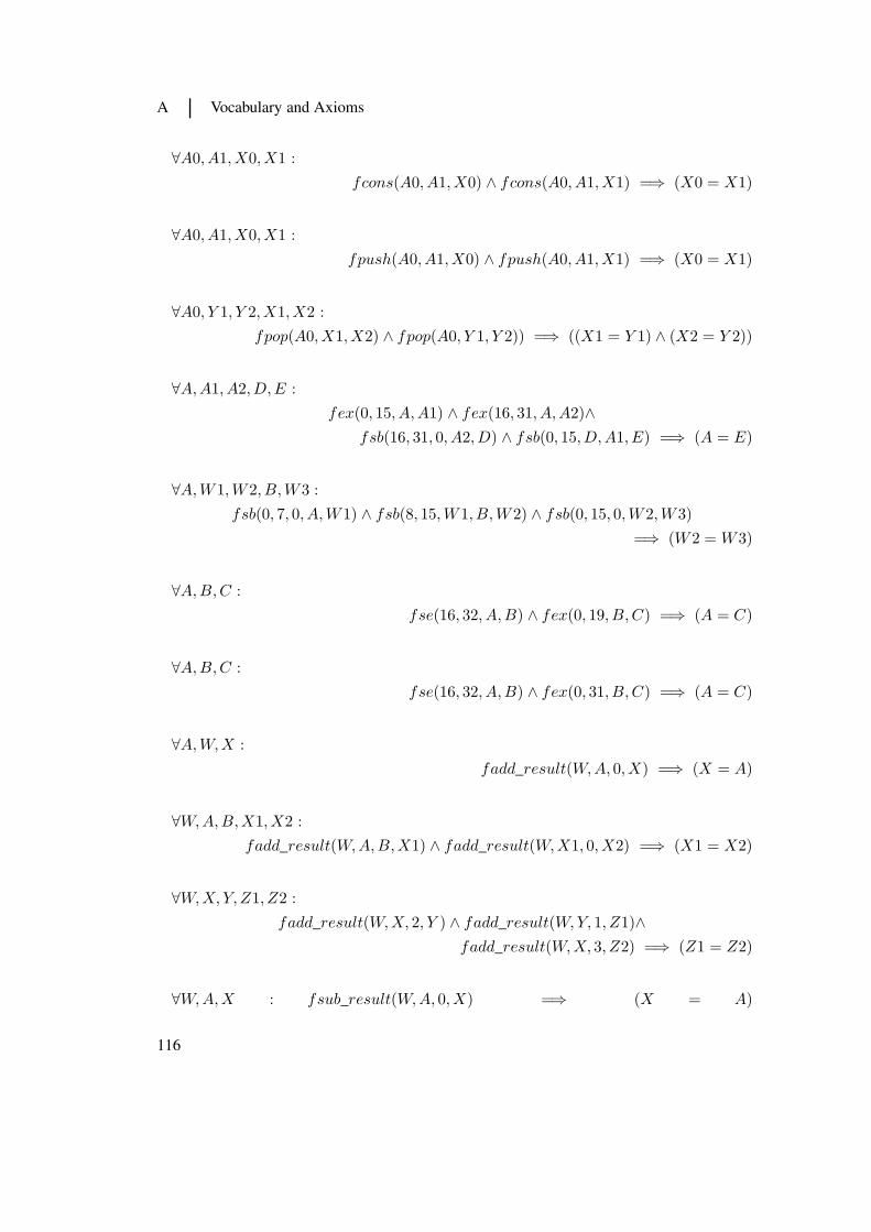
A Vocabulary and Axioms
∀A0, A1,X0,X1 :
fcons(A0, A1,X0) ∧ fcons(A0, A1,X1) =⇒ (X0 = X1)
∀A0, A1,X0,X1 :
fpush(A0, A1,X0) ∧ fpush(A0, A1,X1) =⇒ (X0 = X1)
∀A0, Y 1, Y 2,X1,X2 :
fpop(A0,X1,X2) ∧ fpop(A0, Y 1, Y 2)) =⇒ ((X1 = Y 1) ∧ (X2 = Y 2))
∀A,A1, A2,D,E :
fex(0, 15, A,A1) ∧ fex(16, 31, A,A2)∧
fsb(16, 31, 0, A2,D) ∧ fsb(0, 15,D,A1, E) =⇒ (A = E)
∀A,W1,W2, B,W3 :
fsb(0, 7, 0, A,W1) ∧ fsb(8, 15,W1, B,W2) ∧ fsb(0, 15, 0,W2,W3)
=⇒ (W2 = W3)
∀A,B,C :
fse(16, 32, A,B) ∧ fex(0, 19, B,C) =⇒ (A = C)
∀A,B,C :
fse(16, 32, A,B) ∧ fex(0, 31, B,C) =⇒ (A = C)
∀A,W,X :
fadd_result(W,A, 0,X) =⇒ (X = A)
∀W,A,B,X1,X2 :
fadd_result(W,A,B,X1) ∧ fadd_result(W,X1, 0,X2) =⇒ (X1 = X2)
∀W,X, Y,Z1, Z2 :
fadd_result(W,X, 2, Y ) ∧ fadd_result(W,Y, 1, Z1)∧
fadd_result(W,X, 3, Z2) =⇒ (Z1 = Z2)
∀W,A,X : fsub_result(W,A, 0,X) =⇒ (X = A)
116

∀W,A,B,X1,X2 :
fxor(W,A,B,X1) ∧ fxor(W,B,A,X2) =⇒ (X1 = X2)
∀A,B,C,D,E, F :
fadd_result(20, A,B,C) ∧ fex(0, 15, C,D)∧
fadd_result(20, A,B,E) ∧ fex(0, 15, E, F ) =⇒ (D = F )
∀W,A,B,X1,X2 :
fadd_result(W,A,B,X1) ∧ fadd_result(W,B,A,X2) =⇒ (X1 = X2)
∀B,A : fequal(A,B, 0, 1) =⇒ (B = 0)
∀B,A : fequal(A,B, 0, 0) =⇒ (B 6= 0)
∀B,A : funequal(A,B, 0, 1) =⇒ (B 6= 0)
∀B,A : funequal(A,B, 0, 0) =⇒ (B = 0)
∀A,C,D,E : fmir_if(A, 0, C,D,E) =⇒ (D = E)
∀A,C,D,E : fmir_if(A, 1, C,D,E) =⇒ (C = E)
∀W,X,Xn,Z :
fnot(W,X,Xn) ∧ fadd_result(W, 1,Xn,Z)
=⇒ fnegate_result(W,X,Z)
∀A,X, Y : fze(A,A,X, Y ) =⇒ (X = Y )
∀A,X, Y : fse(A,A,X, Y ) =⇒ (X = Y )
117


B The CASM Language
A EBNF grammar definition of the CASM language.
〈specification〉 ::= 〈header〉 〈body_elements〉
〈header〉 ::= ’casm’ 〈identifier〉
〈body_elements〉 ::= 〈body_elements〉 〈body_element〉| 〈body_element〉
〈body_element〉 ::= 〈provider〉| 〈enum〉| 〈function_definition〉| 〈derived〉| 〈init〉| 〈rule〉
〈init〉 ::= ’init’ 〈identifier〉
〈provider〉 ::= ’provider’ 〈identifier〉
〈enum〉 ::= ’enum’ 〈identifier〉 ’=’ ’{’ 〈identifier_list〉 ’}’
〈derived〉 ::= ’derived’ 〈identifier〉 ’(’ 〈param_list〉 ’)’ ’=’ 〈expression〉| ’derived’ 〈identifier〉 ’(’ 〈param_list〉 ’)’ ’ :’ 〈type〉 ’=’ 〈expression〉| ’derived’ 〈identifier〉 ’=’ 〈expression〉| ’derived’ 〈identifier〉 ’ :’ 〈type〉 ’=’ 〈expression〉| ’derived’ 〈identifier〉 ’(’ ’)’ ’=’ 〈expression〉| ’derived’ 〈identifier〉 ’(’ ’)’ ’ :’ 〈type〉 ’=’ 〈expression〉
119
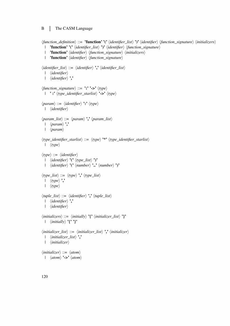
B The CASM Language
〈function_definition〉 ::= ’function’ ’(’ 〈identifier_list〉 ’)’ 〈identifier〉 〈function_signature〉 〈initializers〉| ’function’ ’(’ 〈identifier_list〉 ’)’ 〈identifier〉 〈function_signature〉| ’function’ 〈identifier〉 〈function_signature〉 〈initializers〉| ’function’ 〈identifier〉 〈function_signature〉
〈identifier_list〉 ::= 〈identifier〉 ’,’ 〈identifier_list〉| 〈identifier〉| 〈identifier〉 ’,’
〈function_signature〉 ::= ’:’ ’->’ 〈type〉| ’ :’ 〈type_identifier_starlist〉 ’->’ 〈type〉
〈param〉 ::= 〈identifier〉 ’:’ 〈type〉| 〈identifier〉
〈param_list〉 ::= 〈param〉 ’,’ 〈param_list〉| 〈param〉 ’,’
| 〈param〉
〈type_identifier_starlist〉 ::= 〈type〉 ’*’ 〈type_identifier_starlist〉| 〈type〉
〈type〉 ::= 〈identifier〉| 〈identifier〉 ’(’ 〈type_list〉 ’)’
| 〈identifier〉 ’(’ 〈number〉 ’..’ 〈number〉 ’)’
〈type_list〉 ::= 〈type〉 ’,’ 〈type_list〉| 〈type〉 ’,’
| 〈type〉
〈tuple_list〉 ::= 〈identifier〉 ’,’ 〈tuple_list〉| 〈identifier〉 ’,’
| 〈identifier〉
〈initializers〉 ::= 〈initially〉 ’{’ 〈initializer_list〉 ’}’
| 〈initially〉 ’{’ ’}’
〈initializer_list〉 ::= 〈initializer_list〉 ’,’ 〈initializer〉| 〈initializer_list〉 ’,’
| 〈initializer〉
〈initializer〉 ::= 〈atom〉| 〈atom〉 ’->’ 〈atom〉
120

〈atom〉 ::= 〈function〉| 〈value〉| 〈bracket_expression〉
〈value〉 ::= 〈ruleref 〉| 〈number〉| 〈strconst〉| 〈listconst〉| 〈number_range〉| ’self’
| ’undef’
| ’true’
| ’false’
〈number〉 ::= ’+’ 〈intconst〉| ’-’ 〈intconst〉| 〈intconst〉| ’+’ 〈floatconst〉| ’-’ 〈floatconst〉| 〈floatconst〉| ’+’ 〈rationalconst〉| ’-’ 〈rationalconst〉| 〈rationalconst〉
〈ruleref 〉 ::= ’@’ 〈identifier〉
〈number_range〉 ::= ’[’ 〈number〉 ’..’ 〈number〉 ’]’
| ’[’ 〈identifier〉 ’..’ 〈identifier〉 ’]’
〈listconst〉 ::= ’[’ 〈expression_list〉 ’]’
| ’[’ ’]’
〈expression_list〉 ::= 〈expression〉 ’,’ 〈expression_list〉| 〈expression〉 ’,’
| 〈expression〉
〈expression〉 ::= 〈expression〉 ’+’ 〈expression〉| 〈expression〉 ’-’ 〈expression〉| 〈expression〉 ’!=’ 〈expression〉| 〈expression〉 ’=’ 〈expression〉| 〈expression〉 ’<’ 〈expression〉| 〈expression〉 ’>’ 〈expression〉| 〈expression〉 ’<=’ 〈expression〉
121

B The CASM Language
| 〈expression〉 ’>=’ 〈expression〉| 〈expression〉 ’*’ 〈expression〉| 〈expression〉 ’/’ 〈expression〉| 〈expression〉 ’%’ 〈expression〉| 〈expression〉 ’div’ 〈expression〉| 〈expression〉 ’or’ 〈expression〉| 〈expression〉 ’xor’ 〈expression〉| 〈expression〉 ’and’ 〈expression〉| ’not’ 〈expression〉| 〈atom〉
〈bracket_expression〉 ::= ’(’ 〈expression〉 ’)’
〈function〉 ::= 〈identifier〉| 〈identifier〉 ’(’ ’)’
| 〈identifier〉 ’(’ 〈expression_list〉 ’)’
〈rule〉 ::= ’rule’ 〈identifier〉 ’=’ 〈statement〉| ’rule’ 〈identifier〉 ’(’ ’)’ ’=’ 〈statement〉| ’rule’ 〈identifier〉 ’(’ 〈param_list〉 ’)’ ’=’ 〈statement〉| ’rule’ 〈identifier〉 ’dumps’ 〈dumpspec_list〉 ’=’ 〈statement〉| ’rule’ 〈identifier〉 ’(’ ’)’ ’dumps’ 〈dumpspec_list〉 ’=’ 〈statement〉| ’rule’ 〈identifier〉 ’(’ 〈param_list〉 ’)’ ’dumps’ 〈dumpspec_list〉 ’=’ 〈statement〉
〈dumpspec_list〉 ::= 〈dumpspec〉 ’,’ 〈dumpspec_list〉| 〈dumpspec〉
〈dumpspec〉 ::= ’(’ 〈identifier_list〉 ’)’ ’->’ 〈identifier〉
〈statement〉 ::= 〈assert〉| 〈assure〉| 〈diedie〉| 〈impossible〉| 〈debuginfo〉| 〈print〉| 〈update〉| 〈case〉| 〈call〉| 〈kw_seqblock〉| 〈seqblock〉| 〈kw_parblock〉| 〈parblock〉| 〈ifthenelse〉| 〈let〉| 〈push〉
122
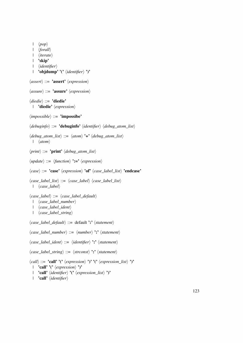
| 〈pop〉| 〈forall〉| 〈iterate〉| ’skip’
| 〈identifier〉| ’objdump’ ’(’ 〈identifier〉 ’)’
〈assert〉 ::= ’assert’ 〈expression〉
〈assure〉 ::= ’assure’ 〈expression〉
〈diedie〉 ::= ’diedie’
| ’diedie’ 〈expression〉
〈impossible〉 ::= ’impossibe’
〈debuginfo〉 ::= ’debuginfo’ 〈identifier〉 〈debug_atom_list〉
〈debug_atom_list〉 ::= 〈atom〉 ’+’ 〈debug_atom_list〉| 〈atom〉
〈print〉 ::= ’print’ 〈debug_atom_list〉
〈update〉 ::= 〈function〉 ’:=’ 〈expression〉
〈case〉 ::= ’case’ 〈expression〉 ’of’ 〈case_label_list〉 ’endcase’
〈case_label_list〉 ::= 〈case_label〉 〈case_label_list〉| 〈case_label〉
〈case_label〉 ::= 〈case_label_default〉| 〈case_label_number〉| 〈case_label_ident〉| 〈case_label_string〉
〈case_label_default〉 ::= default ’:’ 〈statement〉
〈case_label_number〉 ::= 〈number〉 ’:’ 〈statement〉
〈case_label_ident〉 ::= 〈identifier〉 ’:’ 〈statement〉
〈case_label_string〉 ::= 〈strconst〉 ’:’ 〈statement〉
〈call〉 ::= ’call’ ’(’ 〈expression〉 ’)’ ’(’ 〈expression_list〉 ’)’
| ’call’ ’(’ 〈expression〉 ’)’
| ’call’ 〈identifier〉 ’(’ 〈expression_list〉 ’)’
| ’call’ 〈identifier〉
123

B The CASM Language
〈kw_seqblock〉 ::= ’seqblock’ 〈statements〉 ’endseqblock’
〈seqblock〉 ::= ’{Š’ 〈statements〉 ’Š}’
〈kw_parblock〉 ::= ’parblock’ 〈statements〉 ’endparblock’
〈parblock〉 ::= ’{’ 〈statements〉 ’}’
〈statements〉 ::= 〈statements〉 〈statement〉| 〈statement〉
〈ifthenelse〉 ::= ’if’ 〈expression〉 ’then’ 〈statement〉| ’if’ 〈expression〉 ’then’ 〈statement〉 ’else’ 〈statement〉
〈let〉 ::= ’let’ 〈identifier〉 ’=’ 〈expression〉 ’in’ 〈statement〉| ’let’ 〈identifier〉 ’:’ 〈type〉 ’=’ 〈expression〉 ’in’ 〈statement〉
〈push〉 ::= ’push’ 〈expression〉 ’into’ 〈identifier〉
〈pop〉 ::= ’pop’ 〈identifier〉 ’from’ 〈identifier〉
〈forall〉 ::= ’forall’ 〈identifier〉 ’in’ 〈expression〉 ’do’ 〈statement〉
〈iterate〉 ::= ’iterate’ 〈statement〉
124

C vanHelsing Input Language
A EBNF grammar definition of the vanHelsing input language.
〈top_level〉 ::= 〈tptp_file〉| ǫ
〈tptp_file〉 ::= 〈tptp_file〉 〈tptp_input〉| 〈tptp_input〉
〈tptp_input〉 ::= 〈tff_annotated〉| 〈fof_annotated〉
〈name〉 ::= 〈atomic_word〉| 〈integer〉
〈tff_annotated〉 ::= ’tff’ ’(’ 〈name〉 ’,’ 〈formulae_role〉 ’,’ 〈tff_formula〉 ’)’ ’.’
〈tff_formula〉 ::= 〈tff_typed_atom〉
〈tff_typed_atom〉 ::= 〈tff_untyped_atom〉 ’:’ 〈tff_top_level_type〉| ’(’ 〈tff_typed_atom〉 ’)’
〈tff_untyped_atom〉 ::= 〈functor〉| 〈system_functor〉
〈tff_top_level_type〉 ::= 〈tff_atomic_type〉| 〈tff_mapping_type〉| ’(’ 〈tff_top_level_type〉 ’)’
〈tff_atomic_type〉 ::= 〈atomic_word〉| 〈defined_type〉
125

C vanHelsing Input Language
| 〈atomic_word〉 ’(’ 〈tff_type_arguments〉 ’)’
| 〈variable〉
〈tff_type_arguments〉 ::= 〈tff_atomic_type〉| 〈tff_type_arguments〉 〈tff_atomic_type〉
〈tff_mapping_type〉 ::= 〈tff_unitary_type〉 ’>’ 〈tff_atomic_type〉
〈tff_unitary_type〉 ::= 〈tff_atomic_type〉| ’(’ 〈tff_xprod_type〉 ’)’
〈tff_xprod_type〉 ::= 〈tff_unitary_type〉 ’*’ 〈tff_atomic_type〉| 〈tff_xprod_type〉 ’*’ 〈tff_atomic_type〉
〈fof_annotated〉 ::= ’fof’ ’(’ 〈name〉 ’,’ 〈formulae_role〉 ’,’ 〈fof_formula〉 ’)’ ’.’
〈fof_formula〉 ::= 〈fof_logic_formula〉
〈fof_logic_formula〉 ::= 〈fof_binary_formula〉| 〈fof_unitary_formula〉
〈fof_binary_formula〉 ::= 〈fof_binary_nonassoc〉| 〈fof_binary_assoc〉
〈fof_binary_nonassoc〉 ::= 〈fof_unitary_formula〉 〈binary_connective〉 〈fof_unitary_formula〉
〈fof_binary_assoc〉 ::= 〈fof_or_formula〉| 〈fof_and_formula〉
〈fof_or_formula〉 ::= 〈fof_unitary_formula〉 ’Š’ 〈fof_unitary_formula〉| 〈fof_or_formula〉 ’|’ 〈fof_unitary_formula〉
〈fof_and_formula〉 ::= 〈fof_unitary_formula〉 ’&’ 〈fof_unitary_formula〉| 〈fof_and_formula〉 ’&’ 〈fof_unitary_formula〉
〈fof_unitary_formula〉 ::= 〈fof_quantified_formula〉| 〈fof_unary_formula〉| 〈atomic_formula〉| ’(’ 〈fof_logic_formula〉 ’)’
〈fof_quantified_formula〉 ::= 〈fol_quantifier〉 ’[’ 〈fof_variable_list〉 ’]’ ’:’ 〈fof_unitary_formula〉
〈fof_variable_list〉 ::= 〈variable〉| 〈fof_variable_list〉 ’,’ 〈variable〉
〈fof_unary_formula〉 ::= ’~’ 〈fof_unitary_formula〉| 〈fol_infix_unary〉
126

〈fol_infix_unary〉 ::= 〈term〉 ’!=’ 〈term〉| 〈term〉 ’=’ 〈term〉
〈fol_quantifier〉 ::= ’!’
| ’?’
〈term〉 ::= 〈function_term〉| 〈variable〉
〈function_term〉 ::= 〈plain_term〉| 〈defined_term〉
〈plain_term〉 ::= 〈constant〉| 〈functor〉 ’(’ 〈arguments〉 ’)’
〈constant〉 ::= 〈functor〉
〈defined_term〉 ::= 〈defined_atom〉| 〈defined_atomic_term〉
〈defined_atom〉 ::= 〈number〉| 〈distinct_object〉
〈number〉 ::= 〈integer〉
〈defined_plain_term〉 ::= 〈defined_constant〉| 〈defined_functor〉 ’(’ 〈arguments〉 ’)’
〈defined_constant〉 ::= 〈defined_functor〉
〈defined_functor〉 ::= 〈atomic_defined_word〉
〈defined_atomic_term〉 ::= 〈defined_plain_term〉
〈defined_atomic_formula〉 ::= 〈defined_plain_formula〉
〈defined_plain_formula〉 ::= 〈defined_plain_term〉
〈defined_infix_formula〉 ::= 〈term〉 〈defined_infix_pred〉 〈term〉
〈defined_infix_pred〉 ::= ’=’
〈atomic_formula〉 ::= 〈plain_atomic_formula〉| 〈defined_atomic_formula〉
〈atomic_defined_word〉 ::= 〈dollar_word〉
127

C vanHelsing Input Language
〈plain_atomic_formula〉 ::= 〈plain_term〉
〈distinct_object〉 ::= 〈double_quoted〉
〈arguments〉 ::= 〈term〉| 〈arguments〉 ’,’ 〈term〉
〈binary_connective〉 ::= ’=’
| ’=>’
| ’<=’
| ’<~>’
| ’~Š’| ’~&’
〈functor〉 ::= 〈atomic_word〉
〈atomic_word〉 ::= 〈single_quoted〉| 〈lower_word〉
〈variable〉 ::= 〈upper_word〉| 〈upper_word〉 ’:’ 〈dollar_word〉
〈defined_type〉 ::= 〈dollar_word〉
〈system_functor〉 ::= 〈atomic_system_word〉
〈atomic_system_word〉 ::= 〈dollar_dollar_word〉
〈formulae_role〉 ::= 〈lower_word〉
128

D Colophon
Image Copyrights
The chapter heading image for chapter 2 is used with the friendly permission of Marc Hennekes,the author of http://www.mandree.de/auf-den-schultern/. The chapter head-ing image for chapter 8 (Satanic Rites of Dracula) is licensed under CC-BY-3.0 by ONTV fromhttp://ontv.deviantart.com/art/Satanic-Rites-of-Dracula-100391613.The chapter heading image for chapter 3 has been created by the author and Phillip Paulweber.The other images are public domain (from wikipedia.org for chapters 1 and 6 and from opencli-part.org for chapter 9).
Version Information
Official Discordian Document Number: f870053 Di 18. Mär 13:28:22 CET 2014
129


E Curriculum Vitae
Personal Data
Name Roland LezuoDate of Birth 18-10-1979Place of Birth Innsbruck, AustriaAddress Burggasse 35/1, 1070 WienEmail [email protected]
Professional Experience
2001 - 2003 Cura Marketing GmbH, InnsbruckWeb Development
2004 - 2006 RISE Schwechat, SchwechatFirmware Development, Austrian eHealth set-top boxes
Software Development, Austrian Citizen Card
2008 - 2010 Secure Business Austria, WienFirmware Development, Smartcard Reader
Software Architect, German eHealth set-top boxes
Firmware Development, Road Tolling Equipment
Software Development, Austrian eHealth
2010 - 2013 Vienna University of TechnologyProject Assistant, Correct Compilers for Correct Application
Specific Processors (C3Pro)
131

E Curriculum Vitae
Education
1994 - 1999 HTL (Higher Technical Institute for electrical engineering),InnsbruckReifeprüfung and Diploma with excellent success
1999 - 2002 Computer Science, Fernuniversität in Hagen„Diplomvorprüfung II“ passed on 25.3.2002
2002 - 2004 Bachelor’s programme Computer Engineering, TU Wien2004 - 2007 Master’s programme Computer Engineering, TU Wien
Diploma Thesis: "Porting the CACAO Virtual Machine to
POWERPC64 and Coldfire", with distinction
2010 - current Doctoral programme in Engineering Sciences , TU WienPhD Thesis: Scalable Translation Validation
List of Publications
• Roland Lezuo and Felix Breitenecker. A Programmed Solution to ARGESIM Com-parison C 6 ‘Emergency Department’ with DSOL, a Java- based Suite. In Simulation
News Europe SNE 16/1, page 33, München, 2006, ARGESIM and ASIM.url: http://www.sne-journal.org/publications/?tx_pubdb_pi1%5Bpubid%5D=52&tx_pubdb_pi1%5Bppid%5D=87
• Roland Lezuo and Andreas Krall. A unified processor model for compiler verifica-tion and simulation using ASM. In Proceedings of the Third international conference
on Abstract State Machines, Alloy, B, VDM, and Z, ABZ’12, pages 327–330, Berlin,Heidelberg, 2012. Springer-Verlag. doi:10.1007/978-3-642-30885-7_24
• Roland Lezuo, Gergö Barany, and Andreas Krall. CASM: Implementing an AbstractState Machine based Programming Language. In Stefan Wagner and Horst Lichter,editors, Software Engineering 2013 Workshopband, 26. Februar - 1. März 2013 in
Aachen, volume 215 of GI Edition - Lecture Notes in Informatics, pages 75–90,February 2013. (6. Arbeitstagung Programmiersprachen (ATPS’13))
• Roland Lezuo and Andreas Krall. Using the CASM language for simulator synthesisand model verification. In Proceedings of the 2013 Workshop on Rapid Simulation
and Performance Evaluation: Methods and Tools, RAPIDO ’13, pages 6:1–6:8, NewYork, NY, USA, 2013. ACM. doi:10.1145/2432516.2432522
• Roland Lezuo, Philipp Paulweber, and Andreas Krall. CASM - Optimized Com-pilation of Abstract State Machines. LCTES ’07, New York, NY, USA, 2014 (toappear). ACM
• Roland Lezuo and Andreas Krall. Simulation Proofs by Direct Symbolic Executionof Abstract State Machines (under submission).
• Roland Lezuo, Ioan Dragan and Andreas Krall. vanHelsing: Tool and Proof Debug-ger for Expression Equivalence Problems (under submission).
132