scale invariance in biology: coincidence or footprint of a - citeseer
TRANSCRIPT

Biol. Rev. (2001) 76, pp. 161–209 Printed in the United Kingdom # Cambridge Philosophical Society 161
Scale invariance in biology: coincidence or
footprint of a universal mechanism?
T. GISIGER*
Groupe de Physique des Particules, UniversiteU de MontreUal, C.P. 6128, succ. centre-ville, MontreUal, QueUbec, Canada, H3C 3J7
(e-mail : gisiger!pasteur.fr)
(Received 4 October 1999; revised 14 July 2000; accepted 24 July 2000)
ABSTRACT
In this article, we present a self-contained review of recent work on complex biological systems which exhibitno characteristic scale. This property can manifest itself with fractals (spatial scale invariance), flicker noiseor 1}f-noise where f denotes the frequency of a signal (temporal scale invariance) and power laws (scaleinvariance in the size and duration of events in the dynamics of the system). A hypothesis recently putforward to explain these scale-free phenomomena is criticality, a notion introduced by physicists whilestudying phase transitions in materials, where systems spontaneously arrange themselves in an unstablemanner similar, for instance, to a row of dominoes. Here, we review in a critical manner work whichinvestigates to what extent this idea can be generalized to biology. More precisely, we start with a briefintroduction to the concepts of absence of characteristic scale (power-law distributions, fractals and 1}f-noise) and of critical phenomena. We then review typical mathematical models exhibiting such properties :edge of chaos, cellular automata and self-organized critical models. These notions are then brought togetherto see to what extent they can account for the scale invariance observed in ecology, evolution of species, typeIII epidemics and some aspects of the central nervous system. This article also discusses how the notion ofscale invariance can give important insights into the workings of biological systems.
Key words : Scale invariance, complex systems, models, criticality, fractals, chaos, ecology, evolution,epidemics, neurobiology.
CONTENTS
I. Introduction ............................................................................................................................ 162II. Power laws and scale invariance ............................................................................................. 165
(1) Definition and property of power laws ............................................................................. 165(2) Fractals in space................................................................................................................ 166(3) Fractals in time: 1}f-noise ................................................................................................ 167
(a) Power spectrum of signals........................................................................................... 168(b) Hurst’s rescaled range analysis method ...................................................................... 169(c) Iterated function system method ................................................................................ 170
(4) Power laws in physics : phase transitions and universality ................................................ 171(a) Critical systems, critical exponents and fractals.......................................................... 171(b) Universality ................................................................................................................ 173
III. Generalities on models and their properties ............................................................................ 174(1) Generalities ....................................................................................................................... 174(2) Chaos : iterative maps and differential equations.............................................................. 175
* Present address : Unite! de Neurobiologie Mole! culaire, Institut Pasteur, 25 rue du Dr Roux, 75724 Paris, Cedex 15,France.

162 T. Gisiger
(3) Discrete systems in space: cellular automata and percolation .......................................... 178(4) Self-organized criticality : the sandpile paradigm.............................................................. 179(5) Limitations of the complex systems paradigm .................................................................. 182
IV. Complexity in ecology and evolution ...................................................................................... 182(1) Ecology and population behaviour ................................................................................... 182
(a) Red, blue and pink noises in ecology ......................................................................... 182(b) Ecosystems as critical systems ..................................................................................... 184
(2) Evolution........................................................................................................................... 185(a) Self-similarity and power laws in fossil data............................................................... 186(b) Remarks on evolution and modelling ......................................................................... 190(c) Critical models of evolution........................................................................................ 191(d) Self-organized critical models ..................................................................................... 193(e) Non-critical model of mass extinction......................................................................... 195
V. Dynamics of epidemics ............................................................................................................ 196(1) Power laws in type III epidemics ..................................................................................... 196(2) Disease epidemics modelling with critical models ............................................................. 197
VI. Scale invariance in neurobiology............................................................................................. 199(1) Communication: music and language .............................................................................. 199(2) 1}f-noise in cognition ........................................................................................................ 201(3) Scale invariance in the activity of neural networks .......................................................... 202
VII. Conclusion ............................................................................................................................... 204VIII. Acknowledgements .................................................................................................................. 205
IX. References................................................................................................................................ 206
I. INTRODUCTION
Biology has come a long way since the days when,because of a lack of experimental means, it could beconsidered as a ‘ soft ’ science. Indeed, with therecent progress of molecular biology and geneticengineering, extremely detailed knowledge has beenacquired about the mechanisms of living beings atthe molecular scale. Hard facts about the chemicalcomposition and function of ionic channels, enzymes,neurotransmitters and neuroreceptors, and genes, toname a few, are now routinely gathered usingpowerful new methods and techniques. Parallel tothese experimental achievements, theoretical workhas been undertaken to test hypotheses usingmathematical models, which subsequently suggestnew theories and experiments. Such a dialoguebetween theory and experiment, already present inphysics and chemistry, is now becoming common inlife sciences.
However, after taking this path, one is sooner orlater confronted with the reality that knowing theelementary parts making up a system and the waythat they interact together, is not always sufficient tounderstand the global behaviour of the system. Thisfact is already being more and more recognized byphysicists about their own field. Indeed, after a verylengthy programme, particle physics has now ex-plored matter down to infinitesimal scales (less than10−") m). We now know, at least to the energies
accessible to current experiments, that matter ismade of very small elementary particles, calledquarks. The way quarks interact together to formprotons and neutrons, the interaction between theselatter particles to constitute nuclei, and finally howthey are bound together with electrons into atoms isalso relatively well known. In fact, particle physicistsclaim that only four forces are necessary to bind andhold the universe together. However, this is not thewhole story. Already in the 19th century it becameclear that knowing the interactions between twobodies was not enough to understand or solvecompletely the dynamics of a group of such bodiesput together. The classical example is ordinaryNewtonian gravity. It is possible to solve exactly,and therefore understand fully, the equations ofmotion of two bodies orbiting around one another,like the earth around the sun. However, when athird body is introduced, the system is no longersolvable, except perhaps numerically. Furthermore,even numerical solution of the problem cannotcompletely account for the behaviour of the systemsince the system is extremely sensitive to initialconditions. This means that any error in the positionsand velocities of the bodies at some initial time willbe amplified over time and will corrupt the solution.(This is similar to the so-called ‘butterfly effect ’which renders impossible any long-term weatherforecasting – see Lorenz, 1963). In other words, thethree-body problem can be studied, but it is much

163Scale invariance in biology
harder to understand than the two-body problem.Consequently, even if physicists knew how all theparticles in the universe interact with each other,they still could not explain why, after the big bang,matter has chosen to settle into a complex structurewith galaxies, stars, planets and life, instead of justbecoming a random-looking gas or a crystal. In anutshell, knowing how different parts of a systemwork and interact together does not necessarilyexplain how the whole system functions.
In the case of biology, it is not impossible that ina not too distant future, man might be able to builda computer capable of simulating the dynamics of asystem with approximately 10% types of components,roughly the number of proteins forming a bacteriafor instance. However, this machine would probablyadd very little to the understanding of why thebacteria behaves as a living organism, or of life itself.Similarly, even if we understood exactly how neuronswork and interact with each other, a purelynumerical approach would not solve the problem ofhow the brain thinks. What might be more useful isa better understanding of the emergent properties ofsystems once the interactions between their parts areknown. Such work is already under way, and it dealswith what is called complexity (Parisi, 1993;Ruthen, 1993; see also Nicolis & Prigogine, 1989from which much of this discussion is reproduced).
Complexity is a difficult term to define exactly.Here, we will only hint at its meaning in thefollowing way. Let us consider a system made of alarge number of constituents which interact witheach other in a simple way. What then will be thebehaviour of the system as a whole? If the systemrepresents molecules in a standard chemical reaction,then the outcome of the dynamics will probably bea chemical equilibrium of some sort, where reactantand product concentrations are constant in time. Ifinstead we are considering a gas in a vessel at sometemperature, the dynamics will settle in a molecularchaos where atoms bounce around the vessel in anuncoordinated, erratic way. These two typicalbehaviours are called ‘ simple’ because little in-formation is needed to describe them. They are not‘ interesting’ and as such are not considered complex.
Let us now consider the case of a fluid at restbetween two parallel plates upon which is imposed atemperature gradient ∆T" 0: the lower plate isheated but not the upper plate. For low values of∆T, a shallow density gradient establishes itself byheat conduction and dilatation of the liquid, but noconvection occurs because of the fluid’s viscocity.However, for ∆T larger than some critical value
∆Tc, convection motion sets in as convection rolls,
called Be!nard cells, with their axis parallel to theplates and a diameter of approximately 1 mm. Therotating cells allow cool liquid to sink towards thelower plate at the contact of which it heats up, whilethe less dense warm fluid rises and cools down (thisis very similar to the convection motion of air in acloud). Structures, the Be!nard cells, have sponta-neously appeared, created by the dynamics of thesystem to help the fluid dissipate the energy pouredinto it as heat. This is a first example of a complexsystem, as a fair amount of information is needed todescribe it (shape, size, rotational direction, numberof cells formed, etc.). Another classical example isthe Belouzov–Zhabotinski (B–Z) (Belousov, 1959;Zhabotinski, 1964) chemical reaction of Ce
#(SO
%)$
with CH#(COOH)
#and KBrO
$, all dissolved in
sulphuric acid. While constantly driven out ofequilibrium by addition of reactants and stirring,complex and beautiful structures appear in variousregimes (clock-like oscillations, target patterns, spiralwaves, multiarmed spirals, etc.). These patternsrequire even more information to be described, andas such are regarded as more complex.
In the spirit of the theory of complex systems, weshould try not to look at these examples as physicalprocesses or reactions between chemical reactants,but instead as systems made of many particles, or‘agents ’, which interact with each other via certainrules. This way, we can generalize what we know toother systems and vice versa. A good example is thecase of a population of amoebas Dictyostelium discoi-deum. Under ordinary conditions, the populationacts as a ‘gas ’, with each amoeba living, feeding onits own while ignoring the others. However, whensubject to starvation, the colony aggregates into aplasmodium and forms a single entity with a newdynamics of its own (pluricellular body). A closerinspection of the mechanisms regulating this ag-gregation (mainly the release of chemical messen-gers) shows that certain phases of the phenomenonare in fact similar to that of the B–Z reaction, andcan be described using the same vocabulary (seeNicolis & Prigogine, 1989 for details). This showsfirst that, in some situations, the nature of theconstituents of a system is important only in as far asit affects the interaction between them. Also, it hintsat how much the theory of complex systems canenrich our understanding of systems in biology,physics and chemistry, to mention only a few.However, a review of all complex systems would takeus much too far. We will therefore only concentratein this review on a particular class of complex

164 T. Gisiger
102
101
100
10–1
10–2
102 104 106
Earthquake magnitude s
Num
ber
D(s
) of e
arth
quak
es/y
ear
Fig. 1. The Gutenberg–Richter law: the frequency peryear D(s) of the magnitude s of earthquakes follows astraight line on a log–log scale and can be fitted by thepower law D(s)¯ 1.6592¬10$ s−!.)' (continuous line).The data shown here were recorded between 1974 and1983 in the south-eastern United States. Reproducedfrom Bak (1996). See also Gutenberg (1949). [This figure,as well as all others which present experimental results,was reproduced using a computer graphic package fromdata published in the literature. The source of the data ismentioned in the figure’s caption. The other plots wereobtained by the author using numerical simulations of themodels presented in this article.].
systems: those which are scale independent (Bak,1996).
A classical example of such systems in physics isthe earth’s crust (Gutenberg, 1949; Gutenberg &Richter, 1956; see also Turcotte, 1992). It is a well-established fact that a photograph of a geologicalfeature, such as a rock or a landscape, is useless if itdoes not include an object that defines the scale : acoin, a person, trees, buildings, etc. This fact, whichhas been known to geologists long before it came tointerest researchers from other fields, is described asscale invariance: a geological feature stays roughlythe same as we look at it at larger or smaller scales.In other words, there are no patterns there that theeye can identify as having a typical size. The samepatterns roughly repeat themselves on a whole rangeof scales. For this reason, such objects are sometimescalled self-similar or ‘ fractals ’, as we will see in moredetail in the next section (Mandelbrot, 1977, 1983).It is usually believed that landscapes, coastal lines,and the rest of the earth’s crust are scale-invariantbecause the dynamics of the processes which shapedthem, such as erosion and sedimentation, are also
scale-invariant. One line of evidence possibly sup-porting this hypothesis is the Gutenberg–Richter lawrepresented on Fig. 1, which shows a plot of thedistribution of earthquakes per year D(s) as afunction of their magnitude s. This empirical lawstates that the data follow a power-law distributionD(s)¯ 1.6592¬10$ s−!.)'. As we will see, power-lawdistributions, unlike Gaussian distributions for in-stance, have the particularity of not singling out anyparticular value. So, the fact that the distribution ofearthquakes follows such a law indicates thatearthquake phenomena are scale-invariant : there isno typical size for an earthquake. Smaller ones arejust (much) more probable than larger ones. Also,the fact that all earthquakes, from the very small(similar to a truck passing by) to the very large(which can wipe out entire cities) obey the samedistribution, is a strong indication that they are allproduced by the same dynamics. Therefore, tounderstand earthquakes, one should not exclusivelystudy the large events while neglecting the smallerones. It can also be shown that the distribution ofwaiting time between earthquakes follows a powerlaw similar to that of Gutenberg–Richter : thereappears to be no typical waiting time between twoconsecutive earthquakes. This could contradictclaims of finding periodicity in earthquake records.We arrive then at the following conclusions. Sincethe earth’s crust has not yet settled into a completelyrandom or equilibrium state, it is a complex system.Further, it is a scale-invariant complex system: itdoes not exhibit any characteristic scales of length,time or size of events. Any theory or model trying todescribe geological systems will have to reproducethese power-law distributions and fractal structures.Significant progress along these lines has been maderecently by using models of critical systems. Indeed,it has been known for quite some time that systemsbecome scale-invariant when they are put near aphase transition (such as the critical point of thevapour–liquid transition of water at the temperatureT
c¯ 647 K and density ρ
c¯ 0.323 g cm−$, where
the states of vapour and liquid coexist at all scales) :they become critical (see Section II.4 for a shortintroduction to critical phenomena). However, it isonly relatively recently that such ideas have beengeneralized and extended to complex systems (Bak,1996) such as the earth’s crust (Sornette & Sornette,1989).
During the last few decades, evidence for scaleinvariance has appeared in several fields other thanphysics, and biology is no exception. Fractal struc-tures have been observed in bones, the circulatory

165Scale invariance in biology
system and lungs, to name only a few. Thedistribution of gaps in the vegetation of rain forestsfollows a power law. There does not seem to be anycharacteristic time scale in extinction events com-piled from fossil data. All these findings might besuggestive of scale-free complex systems. Thesefindings raise the interesting question of the possibleexistence of criticality in some biological systems.Research on this subject is of a multidisciplinarycharacter, including ideas from biology, physics andcomputer science and it is sometimes published innon-biological journals. The aim of the presentreview is to put together these developments into aform available to non-specialists.
This paper is divided roughly into two parts. Thefirst (Sections II and III) deals with the math-ematical aspects of scale-invariant complex systems,and as such is rather on the mathematical side. Ihave tried to make this part as easy to read aspossible to non-mathematicians by avoiding un-necessary technicalities and details. The second part(Sections IV–VI) addresses the issue of scale in-variance in biological systems, first introducingexperimental evidence of scale-free behaviour andthen proposing models which account for it. Morespecifically, in Section II I present the concepts ofpower laws, fractals and 1}f-noise. In Section III, Ireview some typical models such as chaotic systems,cellular automata and self-organized critical models.I will insist here on the scale-free properties of thesemodels, as excellent reviews about the other aspectsof their dynamics are available in the literature. InSection IV, I review evidence and possible interpre-tations of scale-free dynamics in ecological systems(Section IV.1) and evolution (Section IV.2). InSection V, I present work done on the dynamics ofmeasles epidemics in small communities. I end thisreview by discussing some evidence of scale-freedynamics in the brain: communication (SectionVI.1), cognition (Section VI.2) and neural networks(Section VI.3).
II. POWER LAWS AND SCALE INVARIANCE
This section defines some of the mathematicalnotions which will be used throughout this article. Ibegin by introducing in Section II.1 the concept ofpower law and show how it differs from other morefamiliar functions. I then present in Section II.2 thenotion of fractals, structures without characteristiclength scales, and of fractal dimensions whichcharacterize them. This is followed in Section II.3 by
the definition of flicker or 1}f-noise, signals with notypical time scale, and which are therefore fractal intime. I end this section by an introduction to criticalphenomena, to the critical exponents which charac-terize critical systems and how they are related to thevery powerful notion of universality. This finalsection, though deeply rooted in physics, has far-reaching implications regarding complex systems inbiology.
(1) Definition and property of power laws
Let us consider the following function:
g(x)¯Axα, (1)
where A and α are real and constant (α being smallerthan zero) and x is a variable. For instance g(x)could represent the distribution D(s) of the size s ofevents in an experiment, or the power spectrumP( f ) of a signal as a function of its frequency f. Thistype of function is sometimes refered to as a powerlaw because of the exponent α. By taking the log ofboth sides, one obtains :
log g(x)¯ logAα log x. (2)
When plotted on a log–log scale, this type of functiontherefore gives a characteristic straight line of slopeα, which intersects the ordinate axis at logA (see Fig.1 for example). When trying to fit a power law toexperimental data, as I will do often in this review,it is customary to first take the log of the measure-ments, and then to fit a straight line to it (by theleast-square method for instance). This methodproves less susceptible to sampling errors.
Power laws are interesting because they are scale-invariant. We can demonstrate this fact by changingx for a new variable x« defined by x¯ a x«, where a issome numerical constant. Then replacing in equa-tion (2), one gets :
g(ax«)¯A(a x«)α
¯ (Aaα) x«α. (3)
The general form of the function is then the same asbefore, i.e. a power law with exponent α. Onlythe constant of proportionality has changed from A
to Aaα. We can therefore ‘zoom in’ or ‘zoom out’ onthe function by changing the value of a while itsgeneral shape stays the same. This is partly becauseno particular value of x is singled out by g(x),contrary to the exponential e−bx or the Gaussian
166 T. Gisiger
e−(x−x!)# distributions which are localized near x¯ 0
and x¯ x!, respectively (where b and x
!are arbitrary
positive constants). Also, by comparison, the powerlaw g(x) decreases slowly from infinity to zero whenx goes from zero to infinity. All these characteristicsgive it the property of looking the same no matterwhich scale is chosen: this is what is meant by thescale invariance property of power laws.
In this article, we will be more interested in theexponent α than the proportionality constant A.We will therefore often write g(x) as
g(x)£ xα (4)
where £ means ‘ is proportional to’.
(2) Fractals in space
As we briefly mentioned in the introduction, theearth’s crust is full of structures without anycharacteristic scale. This is, in fact, a property sharedby many objects found in nature. It was, however,only in the 1960s and 1970s, with the pioneeringwork of Mandelbrot (1977, 1983), that this fact wasgiven the recognition it deserved. We refer thereader to Mandelbrot’s beautiful and, sometimes,challenging books for an introduction to this newway of seeing and thinking about the world aroundus. Here, we will barely scratch the surface of thisvery vast subject by focusing on the concept offractal dimension which will be useful to us later on.
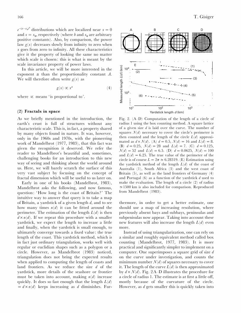
Early in one of his books (Mandelbrot, 1983),Mandelbrot asks the following, and now famous,question: ‘How long is the coast of Britain? ’ Theintuitive way to answer that query is to take a mapof Britain, a yardstick of a given length d, and to seehow many times n(d) it can be fitted around theperimeter. The estimation of the length L(d) is thend¬n(d). If we repeat this procedure with a smalleryardstick, we expect the length to increase a littleand finally, when the yardstick is small enough, toultimately converge towards a fixed value: the truelength of the coast. This yardstick method, which isin fact just ordinary triangulation, works well withregular or euclidian shapes such as a polygon or acircle. However, as Mandelbrot (1983) noticed,triangulation does not bring the expected resultswhen applied to computing the length of coasts andland frontiers. As we reduce the size d of theyardstick, more details of the seashore or frontiermust be taken into account, making n(d) increasequickly. It does so fast enough that the length L(d)¯ d¬n(d) keeps increasing as d diminishes. Fur-
A B C D
(1)
(3)
(4)
(5)
103102101
Yardstick length d (km)
104
103
Mea
sure
d le
ngth
L(d
) (km
)
(2)
(6)
E
Fig. 2. (A–D) Computation of the length of a circle ofradius 1 using the box counting method. A square latticeof a given size d is laid over the curve. The number ofsquares N(d) necessary to cover the circle’s perimeter isthen counted and the length of the circle L(d) approxi-mated as d¬N(d). (A) d¯ 0.5, N(d)¯ 16 and L(d)¯ 8.(B) d¯ 0.25, N(d)¯ 28 and L(d)¯ 7. (C) d¯ 0.125,N(d)¯ 52 and L(d)¯ 6.5. (D) d¯ 0.0625, N(d)¯ 100and L(d)¯ 6.25. The true value of the perimeter of thecircle is of course L¯ 2πD 6.28319. (E) Estimation usingthe yardstick method of the length L(d) of the coast ofAustralia (1), South Africa (3) and the west coast ofBritain (5), as well as the land frontiers of Germany (4)and Portugal (6) as a function of the yardstick d used tomake the evaluation. The length of a circle (2) of radiusD1500 km is also included for comparison. Reproducedfrom Mandelbrot (1983).
thermore, in order to get a better estimate, oneshould use a map of increasing resolution, wherepreviously absent bays and subbays, peninsulas andsubpenisulas now appear. Taking into account thesenew features will also increase the length L(d) evenmore.
Instead of using triangularization, one can rely ona similar and roughly equivalent method called boxcounting (Mandelbrot, 1977, 1983). It is morepractical and significantly simpler to implement on acomputer. One superimposes a square grid of size d
on the curve under investigation, and counts theminimum number N(d) of squares necessary to coverit. The length of the curve L(d) is then approximatedby d¬N(d). Fig. 2A–D illustrates the procedure fora circle of radius 1. The estimate is at first a little off,mostly because of the curvature of the circle.However, as d gets smaller this is quickly taken into

167Scale invariance in biology
account and the measured length converges towardthe true value L¯ 2πD 6.28319. Applying thesemethods to other curves like the coast of Britain givesdifferent results. Fig. 2E shows the variation of L(d)as a function of d for different coastways and landfrontiers. As can be seen, the data for each curvefollow a straight line over several orders of magnitudeof d. This suggests the power-law parametrization ofL(d) (Mandelbrot, 1977, 1983):
L(d)£ d"−$ (5)
where $ is some real parameter to be fitted on thedata.
As expected the perimeter of the circle quicklyconverges to a value, and stays there for any smallervalues of d. For this part of the curve L(d), $¯ 1 (ahorizontal line) fits the data well. The same goes inFig. 2E for the coast of South Africa (line 3).However, for all the other curves, L(d) follows astraight line with non-zero slope. For instance, in thecase of the west coast of Britain, the line has slopeC®0.25, and therefore L(d)£ d−!.#& and $D 1.25.Mandelbrot (1977, 1983) defined $ as the numberof dimensions (or box dimension when using the boxcounting method) of the curve. For the circle, $¯1 as L(d) is independent of d : we recover the intuitivefacts that a circle is a curve of dimension 1, with afinite value of its perimeter. The same is also almosttrue for the coast of South Africa.
However, for the coast of Britain for instance, $ isnot an integer, which indicates that the curve underinvestigation is not Euclidian. Mandelbrot coinedthe term ‘fractal ’ to designate objects with fractionalor a non-integer number of dimensions. Also, thedata in Fig. 2E indicate that Britain possesses a coastwith a huge length, which is best described as quasi-infinite : L(d)£ d−!.#& goes to infinity as d goes tozero. This is due to the fact that no matter howclosely we look at it, the coastway possesses structuressuch as bays, peninsulas, subbays and subpeninsulas,which constantly add to its length. It also means thatno matter what scale we use, we keep seeing roughlythe same thing: bays and peninsulas featuringsubbays and subpeninsulas, and so on. The coastwayis therefore effectively scale-invariant. Of course, thisscale invariance is not without bounds: there are nofeatures on the coastway larger than Britain itself,and no subbay smaller than an atom. We also notethat the more intricate a curve, the higher the valueof its box dimension $ : a curve which moves aboutso much as to completely fill an area of the plane willhave a box dimension 2.
The concept of non-integer dimension might seema little strange or artificial at first, but the geo-metrical content of the exponent $ is not. It is ameasure of the plane- (space-)filling properties of acurve (structure). It quantifies the fact that fractalswith a finite surface may have a perimeter of (quasi)infinite length. Similarly, it shows how a body withfinite volume may have an infinite area. It istherefore not surprising to find fractal geometry inthe shape of cell membranes (Paumgartner, Losa &Weibel, 1981), the lungs (McNamee, 1991) and thecardiovascular system (Goldberger & West, 1987;Goldberger, Rigney & West, 1990). Fractal ge-ometry also helps explain observed allometric scalinglaws in biology (West, Brown & Enquist, 1997).
Box dimension is just one measure of the intricate-ness of fractals. Other definitions of fractal dimensionhave been proposed in the literature (Mandelbrot1977, 1983; Falconer, 1985; Barnsley, 1988; Feder,1988), some better than others at singling out certainfeatures, or spatial correlations. However, they donot give much insight into how fractals come aboutin nature. Some mathematical algorithms have beenproposed to construct such fractals as the Julia andMandelbrot sets or even fractal landscapes, but theresults usually lack the richness and depth of the truefractals observed in the world around us.
(3) Fractals in time: 1/f-noise
In this subsection, we will introduce the notion offlicker or 1}f-noise, which is considered one of thefootprints of complexity. We will also see how itdiffers from white or Brownian noise using thespectral analysis method (Section II.3.a), Hurst’srescaled range analysis (Section II.3.b) and theiterated function system method (Section II.3.c).
Let us consider a record in time of a givenquantity h of a system. h can be anything from atemperature, a sound intensity, the number of speciesin an ecosystem or the voltage at the surface of aneuron. Such a record is obtained by measuring h atdiscrete times t
!,t",t#, ...,tN, giving a series of data
²ti,h(t
i)´, i¯ 1,...,N. This time series, also called
signal or noise, can be visualized by plotting h(t) asa function of t.
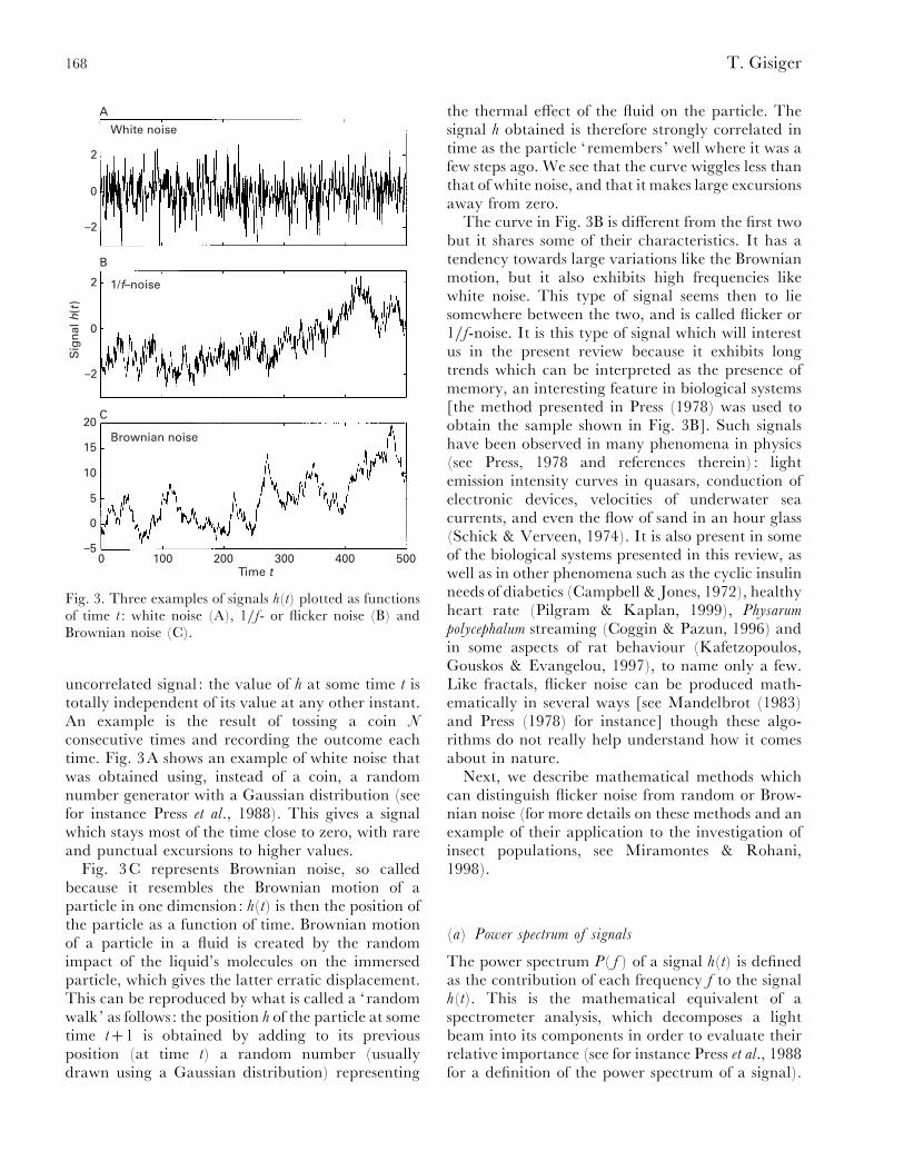
Fig. 3 shows three types of signals h(t) which willbe of interest to us (this subsection merely reproducesthe discussion from Press, 1978): white noise, flicker-or 1}f-noise and Brownian noise. Fig. 3A representswhat is usually called white noise : a randomsuperposition of waves over a wide range offrequencies. It can be interpreted as a completely
168 T. Gisiger
White noise
A
B
1/f–noise
Brownian noise20
15
10
5
0
–50 100 200 300 400 500
Time t
Sig
nal
h(t
)
C
2
0
–2
2
0
–2
Fig. 3. Three examples of signals h(t) plotted as functionsof time t : white noise (A), 1}f- or flicker noise (B) andBrownian noise (C).
uncorrelated signal : the value of h at some time t istotally independent of its value at any other instant.An example is the result of tossing a coin N
consecutive times and recording the outcome eachtime. Fig. 3A shows an example of white noise thatwas obtained using, instead of a coin, a randomnumber generator with a Gaussian distribution (seefor instance Press et al., 1988). This gives a signalwhich stays most of the time close to zero, with rareand punctual excursions to higher values.
Fig. 3C represents Brownian noise, so calledbecause it resembles the Brownian motion of aparticle in one dimension: h(t) is then the position ofthe particle as a function of time. Brownian motionof a particle in a fluid is created by the randomimpact of the liquid’s molecules on the immersedparticle, which gives the latter erratic displacement.This can be reproduced by what is called a ‘randomwalk’ as follows: the position h of the particle at sometime t1 is obtained by adding to its previousposition (at time t) a random number (usuallydrawn using a Gaussian distribution) representing
the thermal effect of the fluid on the particle. Thesignal h obtained is therefore strongly correlated intime as the particle ‘remembers ’ well where it was afew steps ago. We see that the curve wiggles less thanthat of white noise, and that it makes large excursionsaway from zero.
The curve in Fig. 3B is different from the first twobut it shares some of their characteristics. It has atendency towards large variations like the Brownianmotion, but it also exhibits high frequencies likewhite noise. This type of signal seems then to liesomewhere between the two, and is called flicker or1}f-noise. It is this type of signal which will interestus in the present review because it exhibits longtrends which can be interpreted as the presence ofmemory, an interesting feature in biological systems[the method presented in Press (1978) was used toobtain the sample shown in Fig. 3B]. Such signalshave been observed in many phenomena in physics(see Press, 1978 and references therein) : lightemission intensity curves in quasars, conduction ofelectronic devices, velocities of underwater seacurrents, and even the flow of sand in an hour glass(Schick & Verveen, 1974). It is also present in someof the biological systems presented in this review, aswell as in other phenomena such as the cyclic insulinneeds of diabetics (Campbell & Jones, 1972), healthyheart rate (Pilgram & Kaplan, 1999), Physarum
polycephalum streaming (Coggin & Pazun, 1996) andin some aspects of rat behaviour (Kafetzopoulos,Gouskos & Evangelou, 1997), to name only a few.Like fractals, flicker noise can be produced math-ematically in several ways [see Mandelbrot (1983)and Press (1978) for instance] though these algo-rithms do not really help understand how it comesabout in nature.
Next, we describe mathematical methods whichcan distinguish flicker noise from random or Brow-nian noise (for more details on these methods and anexample of their application to the investigation ofinsect populations, see Miramontes & Rohani,1998).
(a) Power spectrum of signals
The power spectrum P( f ) of a signal h(t) is definedas the contribution of each frequency f to the signalh(t). This is the mathematical equivalent of aspectrometer analysis, which decomposes a lightbeam into its components in order to evaluate theirrelative importance (see for instance Press et al., 1988for a definition of the power spectrum of a signal).
169Scale invariance in biology
White noise
A
B
1/f–noise
Brownian noise
100
Frequency f
Pow
er s
pect
rum
P(f
)
10–1
10–2
10–3
100
10–1
10–2
10–3
102
100
10–2
10–2 10–1
C
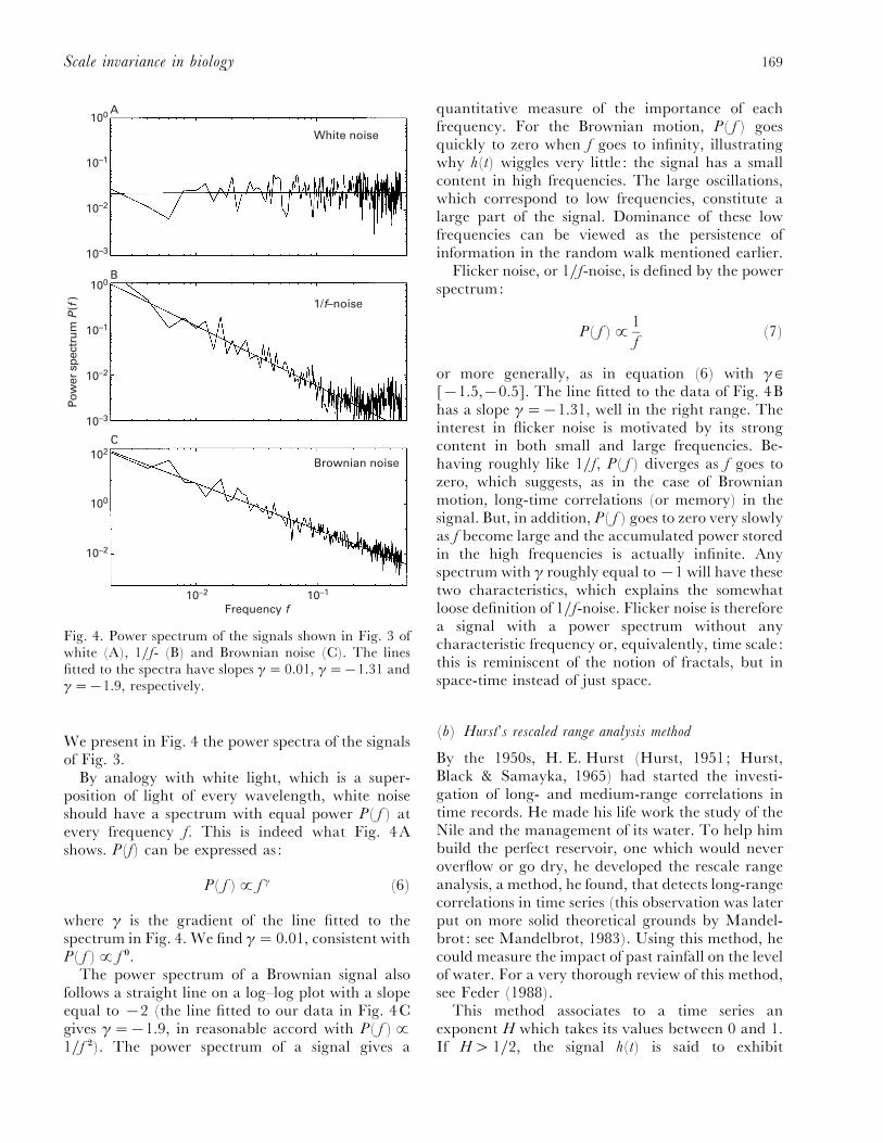
Fig. 4. Power spectrum of the signals shown in Fig. 3 ofwhite (A), 1}f- (B) and Brownian noise (C). The linesfitted to the spectra have slopes γ¯ 0.01, γ¯®1.31 andγ¯®1.9, respectively.
We present in Fig. 4 the power spectra of the signalsof Fig. 3.
By analogy with white light, which is a super-position of light of every wavelength, white noiseshould have a spectrum with equal power P( f ) atevery frequency f. This is indeed what Fig. 4Ashows. P(f) can be expressed as :
P( f )£ f γ (6)
where γ is the gradient of the line fitted to thespectrum in Fig. 4. We find γ¯ 0.01, consistent withP( f )£ f !.
The power spectrum of a Brownian signal alsofollows a straight line on a log–log plot with a slopeequal to ®2 (the line fitted to our data in Fig. 4Cgives γ¯®1.9, in reasonable accord with P( f )£1}f #). The power spectrum of a signal gives a
quantitative measure of the importance of eachfrequency. For the Brownian motion, P( f ) goesquickly to zero when f goes to infinity, illustratingwhy h(t) wiggles very little : the signal has a smallcontent in high frequencies. The large oscillations,which correspond to low frequencies, constitute alarge part of the signal. Dominance of these lowfrequencies can be viewed as the persistence ofinformation in the random walk mentioned earlier.
Flicker noise, or 1}f-noise, is defined by the powerspectrum:
P( f )£1
f(7)
or more generally, as in equation (6) with γ `[®1.5,®0.5]. The line fitted to the data of Fig. 4Bhas a slope γ¯®1.31, well in the right range. Theinterest in flicker noise is motivated by its strongcontent in both small and large frequencies. Be-having roughly like 1}f, P( f ) diverges as f goes tozero, which suggests, as in the case of Brownianmotion, long-time correlations (or memory) in thesignal. But, in addition, P( f ) goes to zero very slowlyas f become large and the accumulated power storedin the high frequencies is actually infinite. Anyspectrum with γ roughly equal to ®1 will have thesetwo characteristics, which explains the somewhatloose definition of 1}f-noise. Flicker noise is thereforea signal with a power spectrum without anycharacteristic frequency or, equivalently, time scale :this is reminiscent of the notion of fractals, but inspace-time instead of just space.
(b) Hurst’s rescaled range analysis method
By the 1950s, H. E. Hurst (Hurst, 1951; Hurst,Black & Samayka, 1965) had started the investi-gation of long- and medium-range correlations intime records. He made his life work the study of theNile and the management of its water. To help himbuild the perfect reservoir, one which would neveroverflow or go dry, he developed the rescale rangeanalysis, a method, he found, that detects long-rangecorrelations in time series (this observation was laterput on more solid theoretical grounds by Mandel-brot : see Mandelbrot, 1983). Using this method, hecould measure the impact of past rainfall on the levelof water. For a very thorough review of this method,see Feder (1988).
This method associates to a time series anexponent H which takes its values between 0 and 1.If H" 1}2, the signal h(t) is said to exhibit
170 T. Gisiger
persistence: if the signal has been increasing duringa period τ prior to time t, then it will show atendency to continue that trend for a period τ aftertime t. The same is true if h(t) has been decreasing:it will probably continue doing so. The signal willthen tend to make long excursions upwards ordownwards. Persistence therefore favours the pres-ence of low frequencies in the signal. This is the casefor the random walk of Fig. 3C, for which we find H
D 0.96. As H goes towards 1, the signal becomesmore and more monotonous. The 1}f-noise of Fig.3B has a Hurst exponent HE 0.88 which is a furtherindication of long-term correlations in the signal.
When H! 1}2, h(t) is said to exhibit anti-persistence: whatever trend has been observed priorto a certain time t for a duration τ, will have atendency to be reversed for the following period τ.This suppresses long-term correlations and favoursthe presence of high frequencies in the powerspectrum of the signal. The extreme case where HD0 is when h(t) oscillates in a very dense manner.
The case in between persistence and anti-per-sistence, H¯ 1}2, is when there is no correlationwhatsoever in the signal. This is the case of the whitenoise of Fig. 3A for which we find HD 0.57,consistent with the theoretical value of H¯ 1}2.
It can be shown that the different signals h(t)which we have presented here (white, flicker andBrownian noises) are curves which fill space[spanned by the time and h(t) axes] to a certainextent : they are in fact fractals and their boxdimension $ can be expressed as a function of theHurst exponent H (see Mandelbrot, 1983 and Feder,1988 for details).
(c) Iterated function system method
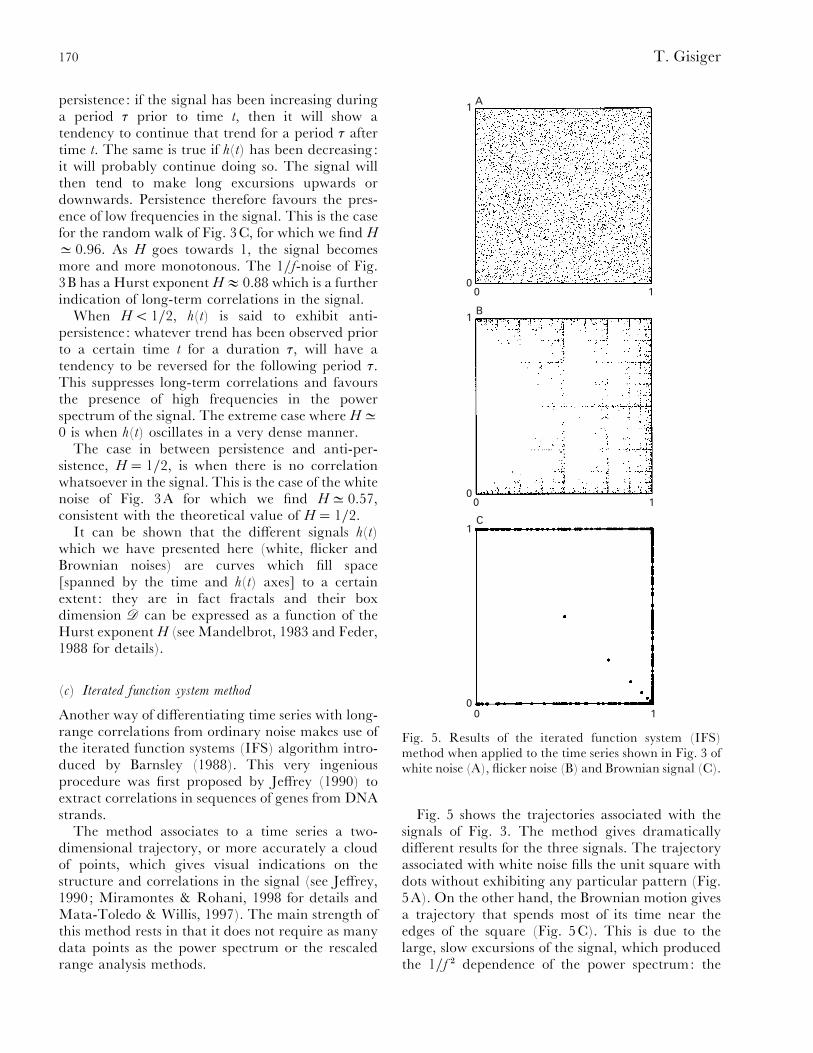
Another way of differentiating time series with long-range correlations from ordinary noise makes use ofthe iterated function systems (IFS) algorithm intro-duced by Barnsley (1988). This very ingeniousprocedure was first proposed by Jeffrey (1990) toextract correlations in sequences of genes from DNAstrands.
The method associates to a time series a two-dimensional trajectory, or more accurately a cloudof points, which gives visual indications on thestructure and correlations in the signal (see Jeffrey,1990; Miramontes & Rohani, 1998 for details andMata-Toledo & Willis, 1997). The main strength ofthis method rests in that it does not require as manydata points as the power spectrum or the rescaledrange analysis methods.
A
B
1
0
0
C
10
1
0 10
1
10
Fig. 5. Results of the iterated function system (IFS)method when applied to the time series shown in Fig. 3 ofwhite noise (A), flicker noise (B) and Brownian signal (C).
Fig. 5 shows the trajectories associated with thesignals of Fig. 3. The method gives dramaticallydifferent results for the three signals. The trajectoryassociated with white noise fills the unit square withdots without exhibiting any particular pattern (Fig.5A). On the other hand, the Brownian motion givesa trajectory that spends most of its time near theedges of the square (Fig. 5C). This is due to thelarge, slow excursions of the signal, which producedthe 1}f # dependence of the power spectrum: the
171Scale invariance in biology
signal h(t) stays in the same size range for quite sometime before moving to another. This produces atrajectory that aggregates near corners, sides anddiagonals. When the signal finally migrates toanother interval, it will produce a trajectory whichfollows the edges or the diagonals of the square.
Things are quite different for the flicker noise (Fig.5B). The pattern exhibits a complex structure whichrepeats itself at several scales, and actually looksfractal. The divergence of the power spectrum at lowfrequencies makes the trajectory spend a lot of timenear the diagonals and the edges, similarly to thecase of the Brownian motion. However, enough highfrequencies are present to move the dot away fromthe corners for short periods of time. The result is theappearance of patterns away from the edges and thediagonals. Their regular structure and scalingproperties make them easy to recognize visually evenin short time series.
(4) Power laws in physics: phase transitionsand universality
In this section, I briefly introduce the notion ofcritical phenomena. This is relevant to the generalsubject of this review because systems at, or near,their critical point exhibit power laws and fractalstructures. They also illustrate the very powerfulnotion of universality, which is of great interest to thestudy of complex systems in physics and biology.Critical systems being an active and vast field ofresearch in physics, it is not the goal of the presentreview to give it a complete introduction. I will onlyjustify the following affirmations [being obviouslyrather technical, Sections II.4.a and II.4.b can beskipped on first reading]:
(1) Systems near a phase transition becomecritical : they do not exhibit any characteristic lengthscale and spontaneously organize themselves infractals (see Section II.4.a).
(2) Critical systems behave in a simple manner:they obey a series of power laws with variousexponents, called ‘critical exponents ’, which can bemeasured experimentally (see Section II.4.a).
(3) Experiments during the 1970s and 1980sshowed that critical exponents of materials onlycome with certain special values : a classification ofsubstances can therefore be developed, where materi-als with identical exponents are grouped together inclasses. The principle claiming that all systemsundergoing phase transitions fall into one of alimited set of classes is known as universality (seeSection II.4.b).
This will be sufficient to the needs of this reviewwhere we will apply these concepts to biologicalsystems. For a more detailed account of criticalphenomena, the reader is referred to Wilson (1979)and the very abundant literature on the subject (seefor instance Maris & Kadanoff, 1978; Le Bellac,1988; Biney et al., 1992).
(a) Critical systems, critical exponents and fractals
Everybody is familiar with phase transitions such aswater turning into ice. This is an example ofdiscontinuous phase transition: matter suddenly goesfrom a disordered state (water phase) to an organisedstate (ice phase). The sudden change in thearrangement of the water molecules is accompaniedby the release of latent heat by the system. Here, wewill be interested in somewhat different systems.They still make transitions between two differentphases as the temperature changes, but they do so ina smooth and continuous manner (i.e. withoutreleasing latent heat). These are called continuousphase transitions and they are of great experimentaland theoretical interest. (Here, I use the terms‘discontinuous ’ and ‘continuous’ for phase transi-tions ; physicists prefer the terms ‘first order’ and‘second order’ phase transitions.)
The classical example of a system exhibiting acontinuous phase transition is a ferromagneticmaterial such as iron. Water too can be brought toa point where it goes through a continuous phasetransition: it is known as the critical point of water,characterized by the critical temperature T
c¯
647 K and the critical density ρc¯ 0.323 g cm−$.
There, the liquid and vapour states of water coexist,and in fact look alike. This makes the dynamics ofthe system difficult, even confusing, to describe withwords. Here, we will therefore use the paradigm ofthe ferromagnetic material as an example of criticalsystem, i.e. of a system near a continuous phasetransition.
It was shown by P. Curie at the turn of thecentury that a magnetized piece of iron loses itsmagnetization when it is heated over the criticaltemperature T
cD 1043 K. Similarly, if the same
piece is cooled again to below Tc, it spontaneously
becomes remagnetized. This is an example of acontinuous phase transition because the magnetiz-ation of the system, which we represent by the vectorM, varies smoothly as a function of temperature:M¯ 0 in the unmagnetized phase and it takes a non-zero value in the magnetized phase. The magnetiz-ation M of the sample, which is easily measured
172 T. Gisiger
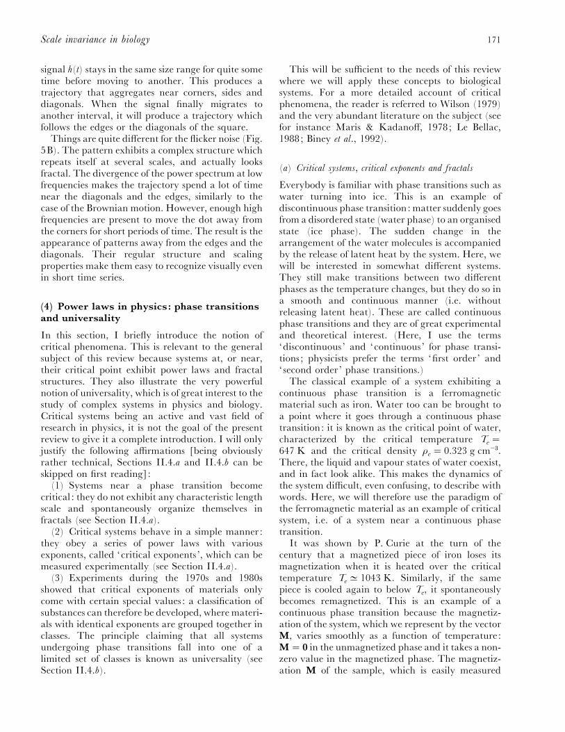
Fig. 6. Illustration of a two-dimensional sample ofmaterial in the magnetized phase (T!T
c) : the spins m
of the atoms, represented by the small arrows, are allaligned and produce a non-zero net magnetization M £Σ
samplem for the sample. T, temperature; T
c, critical
temperature.
using a compass or more accurately a magnetometer,therefore allows us to determine which phase thepiece of iron is in at a given instant.
To understand better the physics at work in thesystem, we have to look at the microscopic level. Thesample is made of iron atoms arranged in a roughlyregular lattice. In each atom, there are electronsspinning around a nucleus. This creates near eachatom a small magnetic field m called a spin, whichcan be approximated roughly by a little magnet likea compass arrow (see Fig. 6 for an illustration). m isof fixed length but it can be oriented in any direction.The total magnetization of the material is pro-portional to the sum of the spins :
M£ 3sample
m (8)
over all the atoms of the sample. Therefore, if all thespins point in the same direction, their magneticeffects add up and give the iron sample a non-zeromagnetization M. If they point in random directions,they cancel each other and the sample has nomagnetization (M¯ 0). This microscopic picturecan be used to explain what happens during thephase transition. If we start with a magnetized blockof iron (all m pointing roughly in the same direction)and heat it up, the thermal agitation in the solid willdisrupt the alignment of the spins, therefore loweringthe magnetization of the sample. When T¯T
c, the
agitation is strong enough to completely destroy thealignment and the total magnetization is zero at T
c
and for any temperature larger than Tc. Similarly,
when the sample is hot and is then cooled to belowthe critical temperature, the spins spontaneouslyalign with each other. It can be shown that for T
slightly smaller than Tc, the magnetization M follows
a power-law function of the temperature:
rMr£ rTc®Tr−ω, (9)
where ω can be measured to be approximately0.37 (if T is larger or equal to T
cthen M¯ 0). ω
therefore quantifies the behaviour of the magnetiz-ation of the sample as a function of temperature: itis called a critical exponent. It can be shown thatother measurable quantities of the system, such asthe correlation length ξ defined below, obey similarpower laws near the critical point (but with differentcritical exponents : besides ω, five other exponentsare necessary to describe systems near phase tran-sitions) (Maris & Kadanoff, 1978; Le Bellac, 1988;Biney et al., 1992).
Let us consider the sample at a given temperature,and measure the effect that flipping one spin has onthe other spins of the system. If T!T
c, the majority
of spins will be aligned in one direction. Flipping onespin will not influence the others because they will allbe subject at the same time to the much largermagnetic field of the rest of the sample. If T"T
c,
changing the orientation of one spin will modify onlythat of its neighbours since the net magnetization ofthe material is zero. However, near the phasetransition (TDT
c), one spin flip can change the
spins of all the others. This is because as we approachthe critical point, the range of interactions betweenspins gets infinite : every spin interacts with all otherspins. This can be formalized by the correlationlength, ξ, defined as the distance at which spinsinteract with each other. Near the phase transition,it follows the power law:
ξ £rT®Tcr−ν, (10)
with νD 0.69 for iron, and therefore diverges toinfinity as T goes to T
c: there is no characteristic
length scale in the system. Another way of under-standing this phenomenon is that, as T is fine-tunedto T
c, the spins of the sample behave like a row of
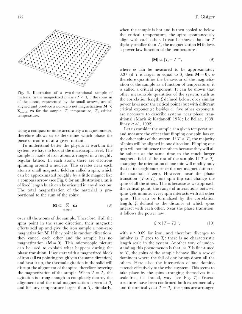
dominoes where the fall of one brings down all theothers. Here also, the interaction of one dominoextends effectively to the whole system. This seems totake place by the spins arranging themselves in ascale-free, i.e. fractal, way (see Fig. 7). Fractalstructures have been confirmed both experimentallyand theoretically : at T¯T
c, the spins are arranged
173Scale invariance in biology
A
B
C
Fig. 7. Spin disposition of a sample as simulated by theIsing model. Each black square represents a spin pointingup, and the white ones stand for a spin pointing down. (A)T!T
c: almost all the spins are pointing in the same
direction, giving the sample non-zero magnetization(magnetized phase). (B) T¯T
c: at the phase transition,
the net magnetization M¯ 0 but the spins have arrangedthemselves in islands within islands of spins pointing inopposite directions, which is a fractal pattern. (C) T"T
c: the system has zero magnetization and only short-
range correlations between spins exist (unmagnetizedphase). T, temperature; T
c, critical temperature.
in islands of all sizes where all m point up, withinothers where all point down, and so on at smallerscales, with net magnetization which is zero [see Fig.7 for a computer simulation (Gould & Tobochnik,1988) of a particularly simple spin system: the Isingmodel].
(b) Universality
During the 1970s and 1980s, there was a great dealof experimental work performed to measure thecritical exponents of materials : polymers, metals,alloys, fluids, gases, etc. It was expected that to eachmaterial would correspond a different set of ex-
ponents. However, experiments proved this sup-position wrong. Instead materials, even those withno obvious similarities, seemed to group themselvesinto classes characterised by a single set of criticalexponents. For instance, it can be shown that whentaking into account experimental errors, one-dimen-sional samples of the gas Xe and the alloy β-brasshave the same values for critical exponents (seeMaris & Kadanoff, 1978; Le Bellac, 1988; Biney et
al., 1992). This is also the case for the binary fluidmixture of methanol-hexane, trimethylpentane andnitroethane. This gas, alloy and liquid mixturetherefore all fall into a class of substances labeled bya single set of critical exponents. By contrast, a three-dimensional sample of Fe does not belong to thisclass. However, it has the same critical exponents asNi. They therefore both belong to another class.
Since critical exponents completely describe thedynamics of a system near a continuous phasetransition, the fact that the classification mentionedabove exists proves that arbitrary critical behaviouris not possible. Rather, only a limited number ofbehaviours exist in nature, which are said to beuniversal, and define disjoint classes called uni-versality classes. The principle which states thisclassification is therefore called universality. Thefollowing theoretical explanation of this astonishingfact has been proposed (Wilson, 1979; see also Maris& Kadanoff, 1978; Le Bellac, 1988; Biney et al.,1992) : near a continuous phase transition, a givensystem is not very sensitive to the nature of theparticles it is constituted of, or to the details of theinteractions which exist between them. Instead, itdepends on other, more fundamental, characteristicsof the system such as the number of dimensions of thesample (see Wilson, 1979). It is a point of view whichfits well within the philosophy of complex systems wementioned in the introduction.
Universality has been described as a physicist’sdream come true. Indeed, what it tells us is that asystem, whether it is a sample in a laboratory or amathematical model, is very insensitive to details ofits dynamics or structure near critical points. From atheoretical point of view, to study a given physicalsystem, one only has to consider the simplestmathematical model possibly conceivable in thesame universality class. It will then yield the samecritical exponents as the system under study. Afamous example is the Ising model proposed toexplain the ferromagnetic phase transition andwhich we introduce now. It represents spins of theiron atoms by a binary variable S which can eitherbe equal to 1 (spin up) or to ®1 (spin down). The

174 T. Gisiger
spins are distributed on a lattice and they interactonly with their nearest neighbours. Even though thismodel simply represents spins as or ®, does notallow for impurities, irregularities in the dispositionof spins, vibrations, etc., it yields the right criticalexponents.
Critical phenomena is a field where the intuitiveidea that the description of a system is dependent onthe amount of detail put into it does not hold. Aslong as a system is known to be critical, the simplestmodel (sometimes simple enough to be solved byhand) will do. This approach is not restricted tophysical systems. In fact, most of the biologicalsystems presented in this review will be studied usingextremely simple, usually critical, models.
III. GENERALITIES ON MODELS AND THEIR
PROPERTIES
So far, we have briefly introduced the notion ofcomplex systems and why they are of interest inscience. We have also presented in detail theproperty of some systems which do not possess anycharacteristic scale, and how it can be observed:scale invariance in fractals (measurable by the boxcounting method), correlations on all time scales in1}f-noise (diagnosed by the power spectrum of thesignal, for instance), and power-law distribution ofevent size or duration. Finally, we have brieflydescribed physical critical systems which exhibitscale-free behaviour naturally when one tunes thetemperature near its critical value. As a bonus, weencountered the notion of universality which tells usthat critical systems may be accurately described bymodels which only approximate roughly the interac-tions between its constituents.
We therefore have the necessary tools to detectscale invariance in biological systems, and a generalprinciple, criticality, which might explain how thisscale-free dynamics arises. However, to make contactbetween our understanding of a system and ex-perimental data, one needs mathematical models.Major types of models used in biology are differentialequation systems, iterative maps and cellular auto-mata, to name only a few. Here, we will review inturn those which can produce power laws and scaleinvariance.
We start in Section III.2 with differential equa-tions and discrete maps which exhibit transitions tochaotic behaviour. Section III.3 presents spatiallydiscretized models like percolating systems andcellular automata. We then move on, in Section
III.4, to the concept of self-organized criticality,illustrating it with the now famous sandpile model.This will be done with special care since most of themodels presented in this review are of this type. Atthe end of this Section we take a few steps back fromthese developments to discuss from a critical point ofview the limitations of the complex systems paradigm(Section III.5).
(1) Generalities
Changeux (1993) gives the following definition fortheoretical models : ‘…In short, a model is anexpanded and explicit expression of a concept. It isa formal representation of a natural object, process orphenomenon, written in an explicit language, in acoherent, non contradictory, minimal form, and, ifposssible, in mathematical terms. To be useful, amodel must be formulated in such a way that itallows comparison with biological reality. […] Amathematical algorithm cannot be identified withphysical reality. At most, it may adequately describesome of its features …’
I agree with this definition. However, I feel thattwo points need clarification.
First, there is the issue of the relationship betweena model and experimental data. In order to beuseful, a model should always reproduce, to asufficient extent, the available measurements. It isfrom an understanding of these data that hypothesesabout the system under study can emerge and becrystalized into a model. The latter can then betested against reality by its ability to account for theexperimental data and make further predictions.Without this two-way relationship, the line betweentheoretical construction and theoretical speculationcan become blurred, and easily be crossed.
History has shown that, in physics for instance (seeEinstein & Infeld, 1938 for a general discussion onmodelling and numerous examples), some of themost significant theoretical advances were made bythe introduction of powerful new concepts tointerpret a mounting body of experimental evidence.However, by no means do I imply here thattheoretical reflection should be confined to the smallgroup of problems solvable in the short of mediumterm. I just want to stress that one should be carefulabout the validity and robustness of results obtainedusing models based on intuition alone or sparseexperimental findings.
Second, I think that the adjective ‘minimal ’deserves to be elaborated on somewhat (see also Bak,1996).
175Scale invariance in biology
A good starting point for our discussion is weatherforecasting. The goal here is to use mathematicalequations to predict, from a set of initial conditions(temperature, pressure, humidity, etc.), the state ofthe system (temperature, form and amount ofprecipitation, etc.) with the best precision possibleover a range of approximately 12–36 hours. In thiscase, ‘minimal ’ translates to a model made ofhundreds or thousands of partial differential equa-tions with about the same amount of variables andinitial conditions. Such complexity allows the in-clusion of a lot of details in the system, and is oftenconsidered to be the most realistic representation ofnature. However, this approach has two seriouslimitations. The first is that the equations used areoften non-linear and their solutions are unstable andsensitive to errors in the initial conditions : any smallerror in temperature or pressure measurements atsome initial time will grow and corrupt the predic-tions of the model as the simulation time increases.This is the well-known ‘butterfly effect ’ (Lorenz,1963) which prevents any long-term weather fore-casting. It also explains why such models can givelittle insight into global warming or the prediction ofthe next ice age. The second limitation of thisapproach stems from the sheer complexity of themodel, which usually needs supercomputers to runon. It makes it difficult to get an intuitive feel of thedynamics of the system under investigation. Onethen has a right to wonder what has been gained,besides predictive power: prediction is then notalways synonymous with understanding.
At the other end of the complexity spectrum standmodels which have been simplified so much thatthey have been reduced to their backbone, takingthe minimal adjective as far as one dares. Suchmodels are sometimes frowned upon by experimen-talists, who do not recognize in them the realizationof the system they study. Theorists, on the otherhand, enjoy their simplicity : such models yield moreeasily to analysis and can be simulated withoutresorting to complicated algorithms or supercom-puters. They too can be extremely sensitive tovariations in initial conditions (like the Lorenzmodel presented in Section III.2) but in a moretractable and controled way. A lesser predictivepower, sometimes only qualitative predictions, isusually the price to pay for this simplicity. However,as we saw, in certain cases like the critical systemsdescribed in Section II.4, simplicity can coexist withspectacularly accurate quantitative results. One onlyhas to choose a simple, or simplistic, model in thesame universality class as the system under study. In
20
0
–20
40
30
20
10
0
–100
10x
z
y
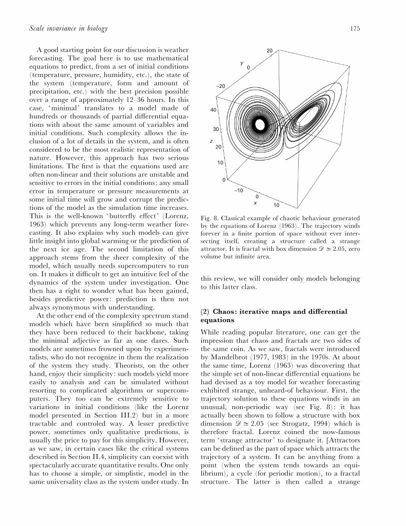
Fig. 8. Classical example of chaotic behaviour generatedby the equations of Lorenz (1963). The trajectory windsforever in a finite portion of space without ever inter-secting itself, creating a structure called a strangeattractor. It is fractal with box dimension $D 2.05, zerovolume but infinite area.
this review, we will consider only models belongingto this latter class.
(2) Chaos: iterative maps and differentialequations
While reading popular literature, one can get theimpression that chaos and fractals are two sides ofthe same coin. As we saw, fractals were introducedby Mandelbrot (1977, 1983) in the 1970s. At aboutthe same time, Lorenz (1963) was discovering thatthe simple set of non-linear differential equations hehad devised as a toy model for weather forecastingexhibited strange, unheard-of behaviour. First, thetrajectory solution to these equations winds in anunusual, non-periodic way (see Fig. 8) : it hasactually been shown to follow a structure with boxdimension $D 2.05 (see Strogatz, 1994) which istherefore fractal. Lorenz coined the now-famousterm ‘strange attractor ’ to designate it. [Attractorscan be defined as the part of space which attracts thetrajectory of a system. It can be anything from apoint (when the system tends towards an equi-librium), a cycle (for periodic motion), to a fractalstructure. The latter is then called a strange
176 T. Gisiger
attractor.] Second, this trajectory is also extremelysensitive to changes in initial conditions. Any smallmodification δ
!will grow with time t as eλt, with λ,
called a Lyapunov exponent, having a value ofroughly 0.9 for the system of Lorenz (Lorenz, 1963;May, 1976; Feigenbaum, 1978, 1979; Strogatz,1994). The variation induced by the introduction ofδ!will then increase extremely quickly: this model is
exponentially sensitive to changes in its initialconditions. This makes any long-term weatherforecasting with such systems impossible since anyerror in the initial conditions (which are present inany measurements) will corrupt its predictions.
The word ‘chaos ’ was chosen to describe thedynamics of systems which do not exhibit anyperiodicity in their behaviour and are exponentiallysensitive to change in their initial conditions. [Thus,they have positive values of their Lyapunov ex-ponents. For negative values of λ, eλt will quicklygo to zero and changes in initial conditions willtherefore not affect the dynamics.] This behaviourwas put in a wider context by the work ofFeigenbaum (1978, 1979) who showed that, byadjusting the values of their parameters, certain non-linear models can shift from a non-chaotic regime(i.e. periodic and not very sensitive to variations intheir initial conditions) to a chaotic state (i.e. non-periodic with high sensitivity to initial conditions).This transition takes place through a succession ofdiscrete changes in the dynamics of the system,which he called ‘bifurcations ’. Feigenbaum (1978,1979) used, in his studies a simplified model of anecological system, called the logistic map, proposedearlier by May (1976).
This classical model is a simple, non-linear,iterative equation which describes the evolution ofthe population x
tof an ecosystem as a function of
time t. Though comprising only one parameter r,which takes its values between 0 and 4 and quantifiesthe reproductive capabilities of the organisms, thismodel is capable of producing time series x
", x
#,…, xN
with increasingly complicated structures as r growsfrom small values to larger ones. For r close to zero,the population of the ecosystem tends to stabilizewith time to a constant value. For slightly higher r,it becomes periodic, oscillating between two valuesfor the population. This radical change in dynamicsis an example of bifurcation. As r rises further, thetime series of the population becomes more and morecomplicated as new values are added to the cycle byfurther bifurcations. For the value r3 r¢ D3.569946, the times series is still periodic but barely,as its period is infinitely long and it depends little on
variations in initial conditions. However, as r
increases still further, the population now evolveswithout any periodicity and computations give apositive value for the Lyapunov exponent: thesystem has entered a chaotic regime (May, 1976;Feigenbaum, 1978, 1979; Bai-Lin, 1989; Strogatz,1994).
One should note that transitions to chaoticdynamics are more than artefacts of models runningon computers. They have been identified in nu-merous experiments ranging from lasers (Harrison &Biswas, 1986) and convection in liquids (Libchaber,Laroche & Fauve, 1982) to muscle fibers of the chickembryo (Guevara, Glass & Shrier, 1981). We referthe interested reader to the literature for furtherdetails (see for instance Strogatz, 1994).
So, to summarize, by changing the values ofparameters of non-linear models, stable or periodicbehaviours can change to a chaotic regime where thesystem traces complicated (perhaps even complex)trajectories which have no apparent periods, aresometimes fractal, and are very sensitive to changesin initial conditions. It is therefore understandablethat these two concepts, fractals and chaos, arebelieved to be linked or even complementary.However, there seems to be little evidence to supportthis connection. In fact, there is evidence that seemsto suggest that it might not be well founded at all.Bak (1996), in his book on complexity, gives thefollowing strong statement: ‘ […] Also, simplechaotic systems cannot produce a spatial fractalstructure like the coast of Norway. In the popularliterature, one finds the subjects of chaos and fractalgeometry linked together again and again, despitethe fact that they have little to do with each other.[…] In short, chaos theory cannot explain com-plexity.’ The reader should note that Bak (1996) usesthe word ‘complexity ’ to describe the behaviour ofscale-invariant complex systems, and not that ofcomplex systems in their full generality. I will notadd to this debate. Instead, I will just say that onecan certainly see that the typical examples of chaoticsystems presented above do not create fractal objects,even if their trajectories indeed trace fractal struc-tures.
According to Bak (1996), chaotic systems are alsonot able to emit fractal time series such as 1}f-noise :‘ […] Chaos signals have a white noise spectrum, not1}f. One could say that chaotic systems are nothingbut sophisticated random noise generators. […]Chaotic systems have no memory of the past andcannot evolve. However, precisely at the ‘critical ’point where the transition to chaos occurs, there is

177Scale invariance in biology
Edge of chaos
Chaotic signal0.015
0.01
0.005
00 0.1 0.2 0.3 0.4 0.5
10–2
10–6
10–2 10–1
Frequency f
Pow
er s
pect
rum
P(f
)
A
B
Fig. 9. (A) Power spectrum P( f ) of a time series producedby the logistic map at the edge of chaos (r¯ r¢ D3.569946). The spectrum is not of a 1}f-form but doesexhibit an interesting shape which seems to be self-similar.(B) Power spectrum of a chaotic signal (r¯ 3.8). P( f )seems to follow a Gaussian distribution located in thehigh-frequency part of the spectrum. r, parameterquantifying the reproductive capabilities of the organismsof the ecosystem of May.
complex behaviour, with a 1}f-like signal. Thecomplex state is at the border between predictableperiodic behaviour and unpredictable chaos. Com-plexity occurs only at one very special point, and notfor the general values of r where there is real chaos.[…]’
This statement is easier to verify, for instance byusing May’s (1976) logistic map. Fig. 9B shows thepower spectrum of the signal for this map in thechaotic regime. P( f ) looks like a Gaussian dis-tribution located in the high-frequency range of thespectrum. The signal is therefore very poor in lowfrequencies. The rescaled range analysis method forthis chaotic signal gives HD 0.36, therefore showinganti-persistence, contrary to 1}f- and Browniannoise. Similarly, the IFS method gives graphicswhich looks nothing like that of the 1}f-noise : pointsgroup themselves in little islands along parallel lines.This seems to support Bak’s (1996) claim thatchaotic systems do not produce interesting signals.Because of their high sensitivity to changes in theinitial conditions, it is impossible to predict what
Chaotic signal
102
Time intervals 4
Dis
trib
uti
on
D(4
)
101
100
100 101 102
A
B
Fig. 10. (A) Signal for the Manneville iteration maptuned at the edge of chaos (upper), with the same signalafter being filtered (lower; a spike was drawn each timethe signal went over the value 0.6810). (B) Plot of thedistribution D(4) of time delays 4 between consecutivespikes.
chaotic systems will do in the long run. There is a lossof information as time passes. This suggests that, bylooking at this from the opposite point of view, achaotic system has a very short memory: it does notremember where it was for very long. It mighttherefore not be a good candidate to describebiological systems which must adapt and learn allthe time.
However, as Bak (1996) mentions, the mapexhibits a far richer behaviour at r¯ r¢, right at thepoint between periodic behaviour and the chaoticregime, therefore sometimes called the ‘edge ofchaos ’. Fig. 9A shows the power spectrum of thesignal there: the structure is certainly not 1}f, butit is interesting and appears to be self-similar. Itcan also be shown that the time series with infiniteperiodicity produced for r¯ r¢ falls on a discretefractal set with a box dimension smaller than 1,called a Cantor set. Furthermore, Costa et al. (1997)have shown that at the edge of chaos, the sensitivityto initial conditions of the logistic map is a lot milderthan in the chaotic regime. There, the Liapunovexponent is zero and instead the sensitivity to
178 T. Gisiger
changes in initial conditions follows a power lawwhich, as we saw in Section II.1, is a lot milder thanthe exponential eλt. This will sustain information inthe system a lot longer, and might provide long-termcorrelation in the time evolution of the population x
t.
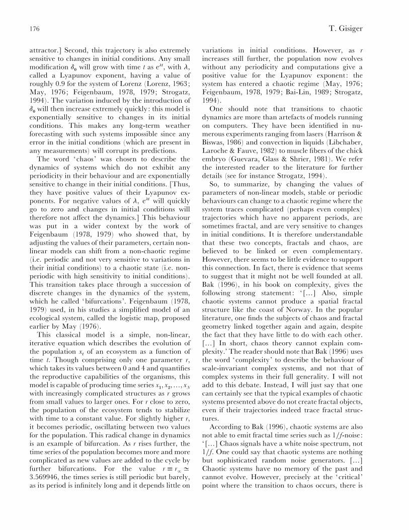
It was, however, Manneville (1980) who firstshowed that, tuned exactly, an iterative functionsimilar to that of May (1976) can produce interestingbehaviour and power laws (see also Procaccia &Schuster, 1983; Aizawa, Murakami & Kohyama,1984; Kaneko, 1989). Fig. 10A (upper panel) showsthe signal produced by his map: it is formed by asuccession of peaks which, when interpreted as aseries of spikes (Fig. 10A, lower panel) looks similarto the train of action potentials measured at themembrane of neurons (we will return to this analogyin Section VI.3). Fig. 10B shows the distribution ofintervals between successive spikes : it follows apower law D(4)£4−"
±$ over several orders of
magnitude. Manneville (1980) also computed thepower spectrum of the signal and found that is was1}f. This shows that it is indeed possible to generatepower laws and 1}f-noise from simple iterative mapsby fine-tuning the parameters of the system at theedge of chaos (see Manneville, 1980 for details).
(3) Discrete systems in space: cellularautomata and percolation
In this Section, we will introduce percolation systemsand cellular automata. This will be helpful sincemost models in this review belong to one of these twotypes.
Iterative functions and differential equations arenot always the most practical way to describebiological systems. Let us take the following example.How should we go about building a model for tree orplant birth and growth in an empty field? Themodel should be able to predict how many plantswill have grown after a given time interval, and alsoif they will be scattered in small patches or in just onelarge patch which spans the whole field. We willmake the simplifying assumption that seeds andspores are carried by the wind over the field, andscattered on it uniformly.
This is of course a difficult problem, and usingdifferential equations to solve it might not be themost practical method. The underlying dynamics ofhow a seed lands on the ground and decides, or not,to produce a plant is already delicate. Further, itdepends also on the types of seed and groundinvolved, the amount of precipitation, the vegetation
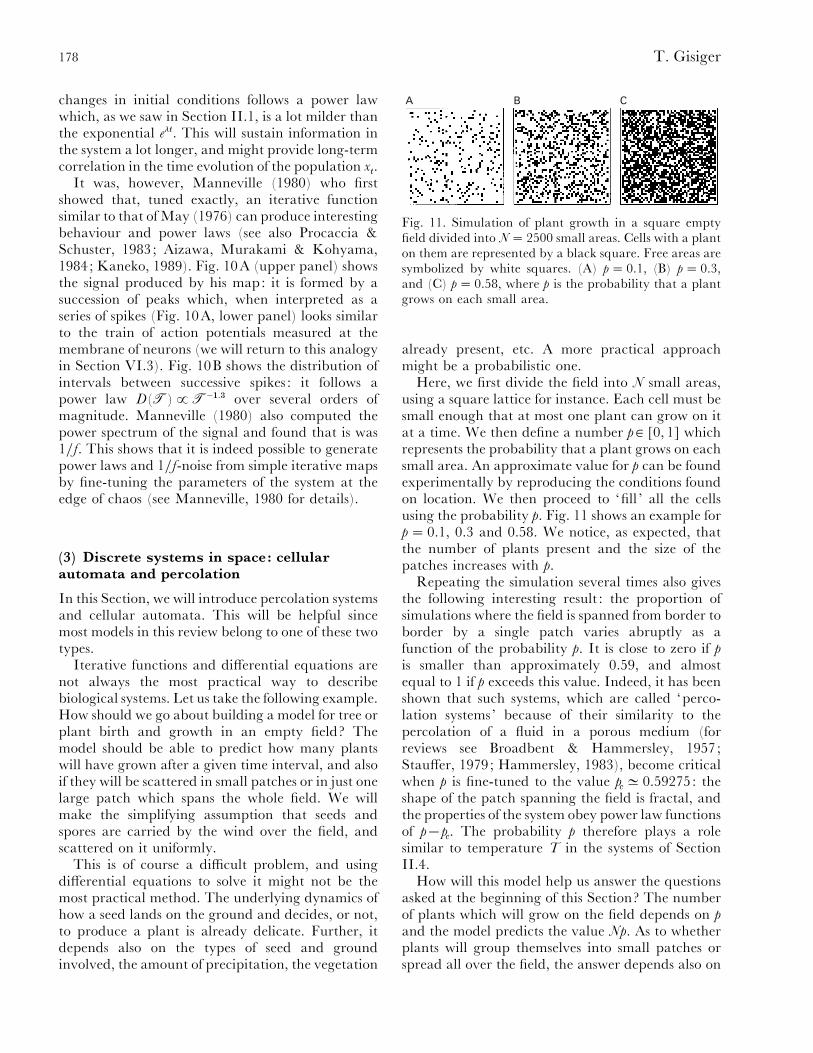
A B C
Fig. 11. Simulation of plant growth in a square emptyfield divided into N¯ 2500 small areas. Cells with a planton them are represented by a black square. Free areas aresymbolized by white squares. (A) p¯ 0.1, (B) p¯ 0.3,and (C) p¯ 0.58, where p is the probability that a plantgrows on each small area.
already present, etc. A more practical approachmight be a probabilistic one.
Here, we first divide the field into N small areas,using a square lattice for instance. Each cell must besmall enough that at most one plant can grow on itat a time. We then define a number p ` [0, 1] whichrepresents the probability that a plant grows on eachsmall area. An approximate value for p can be foundexperimentally by reproducing the conditions foundon location. We then proceed to ‘fill ’ all the cellsusing the probability p. Fig. 11 shows an example forp¯ 0.1, 0.3 and 0.58. We notice, as expected, thatthe number of plants present and the size of thepatches increases with p.
Repeating the simulation several times also givesthe following interesting result : the proportion ofsimulations where the field is spanned from border toborder by a single patch varies abruptly as afunction of the probability p. It is close to zero if p
is smaller than approximately 0.59, and almostequal to 1 if p exceeds this value. Indeed, it has beenshown that such systems, which are called ‘perco-lation systems’ because of their similarity to thepercolation of a fluid in a porous medium (forreviews see Broadbent & Hammersley, 1957;Stauffer, 1979; Hammersley, 1983), become criticalwhen p is fine-tuned to the value p
cD 0.59275: the
shape of the patch spanning the field is fractal, andthe properties of the system obey power law functionsof p®p
c. The probability p therefore plays a role
similar to temperature T in the systems of SectionII.4.
How will this model help us answer the questionsasked at the beginning of this Section? The numberof plants which will grow on the field depends on p
and the model predicts the value Np. As to whetherplants will group themselves into small patches orspread all over the field, the answer depends also on

179Scale invariance in biology
p (which one should be able to estimate exper-imentally). As we just saw, if p! 0.6 then smallscattered patches are probable. Otherwise, completecolonisation of the field by the plants is almostcertain.
This very simple model can be generalized to alarger number of dimensions instead of just the twoconsidered here. For instance, one can easily con-ceive of percolation in a three-dimensional cube.Dynamics in a number of dimensions larger thanthree, though harder to represent mentally, is easilyimplementable on computers.
This model will be generalized in later sections toimplement the dynamics of rain forests, forest firesand epidemics. Indeed, more complex dynamics caneasily be developed. For instance, we can change therules according to which we fill the areas from thefield. So far, we have only used a random numbergenerator for each cell. This means that there are nointeractions between plants : the growth at one placedoes not affect the growth at neighbouring sites.Overcrowding is therefore not present in our model.This can easily be remedied using slightly morecomplicated rules.
A good example of such models is the so-called‘Game of Life ’ introduced by Conway (see Gardner,1970 and Berlekamp, Conway & Guy, 1982) in the1970s, which mimics some aspects of life andecosystems. The Game of Life is defined on a squarelattice. Each lattice site can be either occupied by alive being or be empty. Time evolves in a discretefashion. At each time step, all the sites from thelattice are updated once using the following rules :
(1) An individual will die of over-exposure if ithas less than two neighbours, and of over-crowdingif it has more than three neighbours. The site itoccupied previously will then become empty at thenext time step.
(2) A new individual will be born at an empty siteonly if this site is surrounded by three live neigh-bours.
The dynamics generated by these simple rules hasproven to be very rich, with structures which glidewithout changing shape, others that do not move atall but are unstable, etc. There has been a recentrevival of interest in this model as power laws andfractals appear in its dynamics, possibly hinting atthe presence of criticality in models of ecosystems(see Bak, Chen & Creutz, 1989 and Sales, 1993).
Mathematical models of this latter type, calledcellular automata (Wolfram, 1983, 1984, 1986; seealso Langton, 1990) allow a simple and efficientimplementation of complicated interactions between
the constituents of a system using rules such as thoseabove.
(4) Self-organized criticality: the sandpileparadigm
Here, I present the principle of self-organizedcriticality introduced by Bak, Tang and Wiesenfeld(1987) and its paradigm, the sandpile. This subjecthas attracted quite a lot of attention since itsintroduction: hundreds of articles are published on itevery year in physics, mathematics, computer sci-ence, biology and economics journals. Short reviewsare available to the interested reader wishing tolearn more about this fast-moving field (Bak &Chen, 1989, 1991; Bak, 1990; Bak & Paczuski, 1993,1995; Bak, 1996).
Self-organized criticality is a principle whichgoverns the dynamics of systems, leading them to acomplex state characterized by the presence of frac-tals and power-law distributions. This state, as wewill see, is critical. However, self-organized criticalsystems differ from the systems we presented inSection II.4. There, one had to fine-tune a para-meter, the temperature T, to be in a critical state.Here, it is the dynamics of the system itself whichleads it to a scale-free state (it is therefore ‘ self-organized’). The classical example of such systems isthe sandpile (Bak et al., 1987; Bak, 1996) which weturn to now.
Let us consider a level surface, such as a table, andsome apparatus which allows to drop sand on it,grain by grain, every few seconds. With time, thiswill create a growing accumulation of sand in themiddle of the surface. At first, the sand grains willstay where they land. However, as the sand pile getssteeper, instabilities will appear: stress builds up inthe pile but it is compensated by friction betweensand grains. After a while, stress will be high enoughthat just adding one single grain will release it in theform of an avalanche: a particle of sand makes anunstable grain topple, and briefly slide. This has theeffect of slightly reducing the slope of the sandpile,rendering it stable again until more sand is added.Such toppling events will be small in the beginning,but they will grow in size with time. After a while,the sandpile will reach a state where avalanches ofall sizes are possible : from one grain of sand, to alarge proportion of the whole pile. This state iscritical since it exhibits the same domino effectwhich was present in the spin system: adding onegrain of sand might affect all the other grains fromthe pile. Further, this state has been attained without

180 T. Gisiger
Fig. 12. Cellular automaton introduced by Bak et al.(1987) on a square lattice of size N¯ 20 in the criticalstate. Grains of sand are represented by cubes, whichcannot be piled more than three particles high. Notice thecorrelations in the spatial distribution of the sand.
any fine tuning of parameters : all one has to do toreach it is to keep adding sand slowly enough so thatavalanches are over before the next grain lands.
To better understand the dynamics of the system,let us consider the cellular automaton proposed byBak et al. (1987). We represent the level surface by aN¬N square grid, and grains of sand by cubes ofunit sides which can be piled one on top of another(see Fig. 12). Let Z(i, j) be the amount of sand at theposition (i, j) on the grid. At each time step, arandom number generator will choose at whichposition (i, j) of the grid the next grain of sand willland, or equivalently which Z will increase by oneunit :
Z(i, j)!Z(i, j)1. (11)
To model the instabilities in the sandpile, we willnot allow sand to pile higher than a certain criticalvalue chosen arbitrarily to be 3. If at any given time,the height of sand Z(i, j) is larger than 3 then thatparticular site will distribute four grains to its fournearest neighbours :
Z(i, j)!Z(i, j)®4 (12)
Z(i1, j)!Z(i1, j)1 (13)
Z(i®1, j)!Z(i®1, j)1 (14)
Z(i, j1)!Z(i, j1)1 (15)
Z(i, j®1)!Z(i, j®1)1 (16)
A single toppling event like equations (12–16) is anavalanche of size 1. If this event happens next to asite where three grains are already piled up, sandwill topple there as well, giving an avalanche of size
500
400
300
200
100
00 20 40 60 80 100
103
102
101
100
100 101 102
Size s
Time t
Ava
lan
che
size
sD
istr
ibu
tio
n D
(s)
B
A
Fig. 13. (A) Record of avalanche size as a function of timefor a 20¬20 sandpile. (B) Distribution D(s) of avalanchesfor the same sandpile as a function of their size s. It clearlyfollows a straight line over more than two orders ofmagnitude, therefore implying a power law. Fit to thedata gives D(s)£ s−".!.
2, and so on. We apply the updating rule (equations12–16) until all Z are equal to 3 or smaller. Theduration of the avalanche is defined as the number ofconsecutive time steps during which Z(i, j)" 3somewhere in the sandpile. The result does not lookmuch like a real sandpile (see Fig. 12). It looks morelike small piles of height 3 and less, held closetogether. However, this automaton proves a loteasier to implement on a computer (and runs faster)than models of a more realistic piles, and it exhibitsthe same behaviour.
We now present the results of simulations of thecellular automaton on a 20¬20 grid. Fig. 13A showsa record of avalanche sizes as a function of time.Notice that avalanches of a wide range of sizes occur,and that the smaller ones are much more frequentthan the larger ones. In fact, as shown on Fig. 13B,the distribution D(s) of avalanche size s follows thepower law D(s)£ s−".!. Avalanche duration also

181Scale invariance in biology
50
40
30
20
10
00 20 40 60 80 100
103
102
101
100
100 101 102
Time t
Ava
lan
che
du
rati
on
sD
istr
ibu
tio
n D
(s)
B
A
Duration s
Fig. 14. (A) Record of avalanche duration τ as afunction of time t for a 20¬20 sandpile. (B) Thedistribution D(τ) of avalanches as a function of theirduration τ follows a straight line over roughly two ordersof magnitude therefore implying a power law. Fit to thedata gives D(τ)£ τ−!
±).
has interesting properties. Fig. 14A shows the timerecord of the avalanche duration τ for the data ofFig. 13. The two look similar. In fact, avalancheduration distribution also follows a power law asshown in Fig. 14B: D(τ)£ τ−!
±). We refer the
interested reader to the literature for further detailsabout this fascinating system (Bak, Tang & Wiesen-feld, 1988).
It is important to mention that in this system, thecriticality is only statistical, unlike the systems nearcontinuous phase transitions we presented in SectionII.4. In the case of the ferromagnetic sample, whenTDT
c, changing the orientation of one spin will
affect all the other spins of the sample. It is a kind ofavalanche, but it is always as large as the wholesample. In the sandpile, events of all size andduration are possible but their relative probability isgiven by a power-law distribution. This is stronglyreminiscent of the example of earthquakes, which wementioned in the introduction: there is no more
typical size for avalanches than there is a typical sizefor earthquakes. In the case of the sandpile, the sizeand duration of an event depends of course on wherewe put the grain of sand which triggers theavalanche, but it depends much more strongly onthe amount of stress built in the pile. At some times,the stress will be low and small events will occur. Atother times, it will be much higher and large eventswill become very probable. Apart from the numbergenerator which distributes sand on the pile, nothingis random in the system. One should therefore expectstrong long-term correlations in signals produced bythe dynamics of the sandpile, which is indeed whatis observed (we will come back to this point later).These characteristics (long-term correlation, scaleinvariance, and the absence of any fine tuning)makes self-organized criticality an attractive prin-ciple to explain the dynamics of scale-free biologicalsystems.
The sandpile exhibits a few more power laws. Forinstance, similarly to the logistic map at the edge ofchaos of Section III.2, the sensitivity of the pile tochanges in initial conditions is of a power-law type(Bak, 1990). The system also exhibits fractal struc-tures (Bak & Chen, 1989; Bak, 1990) (see also Fig.12). It was also claimed (Bak et al., 1987, 1988; Tang& Bak, 1988) that it emits 1}f-noise.
After the ground-breaking theoretical work of P.Bak and his colleagues, many efforts were made toobserve experimentally self-organized criticality.The experiments were difficult because it wasnecessary, in order to measure accurately thedistributions D(s) and D(τ), to count all the grains ofsand which moved during an avalanche. Carefulcompromises therefore had to be made whiledevising experimental devices. Early efforts were notvery successful, producing puzzling, and sometimesmisleading, results. It was not until the experimentalwork by Frette et al. (1996) that true power-lawscaling was measured. The pile was not made ofsand, neither was it three dimensional. Instead it wasmade of rice, constrained in a two-dimensional spacebetween two transparent plastic pannels throughwhich digital cameras could, with the assistance ofcomputers, follow the motion of all the particles ofthe pile. The power laws, signature of self-organizedcriticality, were reproduced but only when using acertain type of rice which provided enough frictionto reduce the size of avalanches. This experimentgave insight into another power-law distribution:that for the duration of the stay of a given grain ofrice in the pyramid (Christensen et al., 1996). It alsoserves as a warning that self-organized criticality
182 T. Gisiger
might not be as general and universal a principle itmight appear at first, since it seems to be sensitive todetails of the dynamics (such as the type of riceused).
Another unexpected development was the dem-onstration that the original sandpile automaton(Bak et al., 1987) does not produce 1}f-noise, butrather 1}f #-noise, like Brownian noise (Jensen,Christensen & Fogedby, 1989; Kerte! sz & Kiss,1990; Christensen, Fogedby & Jensen, 1991). How-ever, other self-organized critical systems do give1}f-noise (Jensen, 1990), and by incorporatingdissipation in the sandpile automaton, one can tunethe noise to be in the 1}f range (Christensen, Olami& Bak, 1992). Finally, in a recent paper, De LosRios and Zhang (1999) propose a sandpile-typemodel which includes dissipation and a preferreddirection for the propagation of energy whichproduces 1}f-noise in systems with any number ofdimensions. Interestingly enough, because of dis-sipation effects, this system does not exhibit power-law distributions of spatial correlations, unlike theoriginal sandpile model and other self-organizedcritical systems. This gives theoretical support to theexperimental observation of systems which emit 1}f-noise but are not scale-free (see references in De LosRios & Zhang, 1999). More work is therefore clearlyneeded to understand better the connection betweenflicker noise and criticality in nature.
(5) Limitations of the complex systemsparadigm
Before moving to scale invariance in biologicalsystems, I present a few limitations of the complexsystems paradigm proposed in the introduction, i.e.of the study of the emergent properties of systemsonce a knowledge of the interactions between theircomponents is accessed.
The first main problem of this approach, which isalso present in any type of modelling, is to definerigorous ways in which models can be tested againstreality. In the case of scale-invariant systems, thingsare relatively simple: quantities such as exponents ofpower laws and fractal dimensions can be measuredexperimentally and compared with predictions frommodels. The case of the Belouzov–Zhabotinskireaction for instance, is more complex as ways toquantify reliably the dynamics of the system aremore difficult to find. Indeed, it is possible toconstruct models which create various spatial pat-terns, but verifying their validity in accounting forthe mechanisms of the reaction just by comparing
‘by eye’ the structures obtained from simulationsand those observed experimentally is obviously notsatisfactory.
The second main problem is more central.Although the idea of complex behaviours emergingfrom systems of identical elementary units inter-acting with each other in simple ways is quiteattractive, it is seldom realized in nature. Indeed,most real systems are made of an heterogenous set ofhighly specialized elements which interact with eachother in complicated ways. Genetics and cell biology,for instance, are replete with such systems.
In the light of these arguments, we see thatalthough the complex system approach is an im-portant first step towards a unified theory of systems,it is unlikely to be the last, and many excitingdevelopments will have to take place in the future.
This concludes the part of this article devoted tomathematical notions and concepts. We can nowapply these tools to biological systems.
IV. COMPLEXITY IN ECOLOGY AND
EVOLUTION
(1) Ecology and population behaviour
(a) Red, blue and pink noises in ecology
Following the work of Feigenbaum (1978, 1979) onthe logistic map of May (1976), efforts were devotedto analysing experimental data from animal popu-lations using similar models. This aimed at a betterunderstanding of the variations in the populationdensity of ecosystems as well as how the environmentinfluences this variable. Another question whichattracted a lot of attention was whether ecosystemspoise themselves in a chaotic regime. A considerableamount of literature has been devoted to this subjectand the reader is referred to it for further details (seefor instance the review by Hastings et al. (1993) andreferences therein). Answering this second questionis especially difficult since time series obtained fromecosystems are usually short while methods used todetect chaotic behaviour require a large amount ofdata (Sugihara & May, 1990; Kaplan & Glass,1992; Nychka et al., 1992) : results are not alwaysclear cut. One could argue that, considering thecomplexity of the interactions between individuals,population dynamics should be strongly influencedby past events. However, as we saw earlier, one ofthe main characteristics of chaotic systems is to be sosensitive to initial conditions that information is lostafter a short period. I will not pursue this matter

183Scale invariance in biology
further and refer the reader to Berryman & Millstein(1989) for an interesting discussion on the subject.The question seems to be still open.
Additional insight into the dynamics of ecosystemswas revealed by the power spectra of populationdensity time series from diverse ecosystems. Pimm &Redfearn (1988) considered records of 26 terrestrialpopulations (insects, birds and mammals) compiledover more than 50 years for British farmlands.Computing the power spectrum of these data, theyfound that it contains a surprisingly high content inlow frequency, and described this signal as ‘rednoise ’. This indicates the presence of slow variationsor trends in population density, which might suggestthat the ecosystem is strongly influenced by pastevents (in other words, it possesses a memory). Thiscame quite as a surprise since simple chaotic models,which were thought at the time to capture theessential ingredients of the dynamics of ecosystems,generate time series rich in high frequency, so-called‘blue signals ’ (see Section III.2). However, it waslater shown that by including spatial degrees offreedom, chaotic models can exhibit complex spatialstructures (such as spirals or waves), very similar tothose in the Belouzov–Zhabotinski experiment(Hassel, Comins & May, 1991; Bascompte & Sole! ,1995). With this addition, the dynamics of the modelseem to generate signals with a higher content in lowfrequencies, as if the system was able to storeinformation in these patterns. There is, however, stillmuch debate about the role of such chaotic models inecology (Bascompte & Sole! , 1995; Cohen, 1995;Blarer & Doebeli, 1996; Kaitala & Ranta, 1996;Sugihara, 1996; White, Begon & Bowers, 1996a ;White, Bowers & Begon, 1996b).
With the presence of low frequencies in populationtime series now firmly established experimentally,other questions arise : where do they come from? Arethey induced by external influences from theenvironment, which typically have signals rich inlow frequencies (Steele, 1985; see also Grieger, 1992,and references therein)? Or are they produced bythe intrinsic dynamics of the population, i.e. by theinteractions between individuals? Also, in whatproportion do low frequencies arise? Are theystrongly dominant, like in the 1}f # spectrum of theBrownian signal? Or is it less predominant like in the1}f signal, sometimes called ‘pink noise’? (seeHalley, 1996, for a discussion).
Interesting results which address these issues havebeen published by Miramontes & Rohani (1998).Their approach consists of analysing time series fromlaboratory insect populations and extracting their
15000
10000
5000
00 100 200 300
Inse
ct p
op
ula
tio
n
Time t (days)
Fig. 15. Time series from a laboratory insect population ofLucilia cuprina. Notice the change in patterns afterapproximately 200 days of observation. Reproduced fromMiramontes & Rohani (1998).
low-frequency content. The insect population understudy is that of Lucilia cuprina, or Australian sheepbowfly, which Nicholson (1957) kept under identicalconditions with a constant food supply for a durationof approximately 300–400 days. Population densitywas evaluated roughly daily, providing a data set of360 points (see Fig. 15).
This data set has attracted an enormous amountof attention in the literature. This is first due to theirregularities it exhibits, even under constant en-vironmental conditions. Another interesting featureof the data is the change in the behaviour of the timeseries after approximately 200 days. This wasinvestigated by Nicholson (1957) who found that,unlike wild or laboratory stock flies, female flies aftertermination of the experiment could produce eggswhen given very small quantities of protein food (infact small enough that the original strains of fliescould not produce eggs with it). Mutant flies mighttherefore have appeared in the colony and, becausethey were better adapted to living in such closequarters and with a limited food supply, took overthe whole population. The effect of this change inthe insect colony can be seen in the behaviour of thepopulation density which fluctuates more andbecomes more ragged. For a theoretical investigationof this phenomenon using non-linear models, seeStokes et al. (1988).
The population time series of Nicholson’s (1957)experiment obviously contains low frequencies andlong trends. To better quantify this content, Mira-montes & Rohani (1998) applied the three methodsoutlined in Section II.3 to the population density of

184 T. Gisiger
Lucilia cuprina, and also to that of the wasp parasitoidHeterospilus prosopidis and its host the bean weevilCallosobruchus chinensis, cultured by Utida (1957).The results from their analyses are consistent with a1}f structure of the noise, rather than an 1}f #
structure. They also find a power-law distributionfor the absolute population changes D(s)£ s−α with αbetween 2.8 and 1.7, and D(τ)£ τ−β with β between0.95 and 1.23 for the distribution of the duration ofthese fluctuations. These studies show that theintrinsic dynamics of an ecosystem, even one com-prising a single species and without any externalperturbations, is able to generate long trends inpopulation density. It shows also that a 1}f powerspectrum seems to be favoured over redder signals.This frequency dependence, and the existence ofpower-law distributions of event size and duration inthe system, seems to hint toward a critical state,instead of a chaotic one.
(b) Ecosystems as critical systems
We end this Section on ecology by presenting furtherevidence suggesting that some ecological systemsseem to operate near a critical state. We start withthe investigation of rain forest dynamics by R. V.Sole! and S. C. Manrubia (Sole! & Manrubia, 1995a,b ; Manrubia & Sole! , 1997), and finish with the workof Keitt & Marquet (1996) on extinctions of birdsintroduced by man in the Hawaiian islands.
The two main forces which appear to shape thetree distribution in rain forests, which will be ofinterest to us here, are treefall and tree regeneration.There is also competition in the vegetation in orderto get as much sunlight as possible, inclining trees togrow to large heights. From time to time, old treesfall down, tearing a hole in the surroundingvegetation, or canopy. Because of the intricate natureof the forest, where trees are often linked to others byelastic lianas, when a large tree falls, it often bringsothers down with it. In fact, it has been observedthat treefalls bring the local area to the starting pointof vegetation growth. The gap in the vegetation isthen filled as new trees develop again. This constantprocess of renewal assures a high level of diversity inthe ecosystem.
Gaps in the vegetation, which are easy to pinpointand persist for quite some time, can be gathered bysurveys and displayed on maps. Sole! & Manrubia(1995a) chose the case of the rain forest on BarroColorado Island, which is an isolated forest inPanama. They present a 50 ha plot showing 2582low canopy points where the height of trees was less
103
102
101
100
100 101
Gap size s (m)
Gap
dis
trib
uti
on
D(s
)
B
A
Fig. 16. (A) Plot of canopy gaps obtained from numericalsimulations of the rain forest model of Sole! & Manrubia(1995a). Each dot represents a gap (zero tree height) inthe canopy. (B) Frequency distribution of gaps from theBarro Colorado Island rain forest for the years 1982 and1983. The dashed line, representing a power-law dis-tribution D(s)£ s−".(%, fits the data quite well. Re-produced from Sole! & Manrubia (1995a).
than 10 m, in the years 1982 and 1983 (see Fig. 16Afor a similar plot obtained by numerical simulationof the model described below). The map shows holesof various sizes in the vegetation, scattered across theplot, in a possibly fractal manner. To verify this, Sole!and Manrubia (1995a) first computed the frequencyof occurrence D(s) of canopy gap size s (see Fig 16B).The distribution fits a power law with exponent®1.74 quite well, showing that there does notappear to be any typical size for gaps. Anotherindication of the fractal nature of the gap distributioncan be gathered by computing the fractal dimensionsof this set. Using methods such as the basic boxcounting method presented in Section II.2, theauthors found the non-integer value $D 1.86. Sole!and Manrubia (1995a) show in fact that, typical ofreal fractals, the rain forest gaps set possesses a wholespectrum of fractal dimensions which shows corre-
185Scale invariance in biology
lations of the gaps on all scales and ranges : ittherefore seems to be a large, living fractal structure.
The presence of fractals and power-law distri-butions are strongly suggestive that the rain foresthas evolved to a critical state where fluctuations ofall sizes are present. To verify this hypothesis, Sole!and Manrubia (1995a, b) propose a simple, criticalmathematical model which reproduces some aspectsof the dynamics.
The forest is represented using a generalization ofthe model for plant growth of Section III.3 whichimplements tree birth and death by four rules. Treesstart to grow in vacant areas using the stochasticmechanism of Section III.3 (rule 1). Rule 2implements tree growth at locations where thesurrounding vegetation is not taller, so as toreproduce the effect of light screening by larger treeson smaller ones. Spontaneous tree death can takeplace for two reasons : because of age or because ofdisease. Rule 3 implements these mechanisms by theintroduction of a maximal value for tree age (afterwhich the tree dies) and a random elimination (witha small probability) of trees of all ages. Finally, rule4 reproduces the effect of treefall on the surroundingvegetation: when a tree dies and falls, it also bringsdown some of its neighbours. This rule takes intoaccount as well the fact that older trees are higherand will therefore damage a larger area of canopythan smaller ones. We can see that rules 2 and 4 areespecially important to the dynamics of the systembecause they introduce spatial and temporal corre-lations in the system.
During the simulations, the system evolves as thefour rules are applied successively at each time step.In doing so, the dynamics develops correlationsbetween different points of the forest, and finally onall length and time scales. The latter is observable bystudying the time series given by the variation of thetotal biomass of the ecosystem. The power spectrumof the signal reveals a 1}f γ dependence on frequencywith 0.87%γ% 1.02. Spatial correlations can bestudied by computing the fractal dimensions of thegap distribution in the system. Sole! & Manrubia(1995a, b) and Manrubia & Sole! (1997) foundresults quite similar, both qualitatively and quan-titatively, to those obtained from the real data set,giving strong arguments in favour of the rain forestoperating near or at a critical state. We refer theinterested reader to their articles for further detailsand applications of their models.
Keitt & Marquet (1996) approach the study ofthe possible critical nature of ecosystems from adifferent angle, focusing instead on their dynamics as
they are gradually filled by species. For this task,they chose the geographical area formed by sixHawaiian islands : Oahu, Kauai, Maui, Hawaii,Molokai and Lanai. These islands were originallypopulated by native Hawaiian birds, until they weredriven extinct by Polynesian settlers and afterwardsby immigrants from North America. Since then,other bird species have been artificially introduced.Records show that 69 such species were introducedbetween 1850 and 1984. They also contain dataregarding the number of extinctions that occuredduring this period (35 species went extinct duringthese 70 years). Keitt & Marquet (1996) analysedthese records and found several indications that thesystem might be operating in a critical state.
Extinction events seem not to have occured untilmore than eight species were introduced into theecosystem. This transition does not happen in acontinuous manner, but more in an abrupt fashion,reminiscent of a phase transition. Keitt & Marquet(1996) interpret this as the system going from a non-critical state to a critical one. Also, the number ofextinction events seem to follow a power-lawdistribution, with an exponent around ®0±91. Thismeans that small extinction events are a lot morecommon than larger ones. We will see below (SectionIV.2) that similar power laws are suggested by theanalysis of fossil records. Lastly, the distribution ofthe lifetimes of species, which range from a few yearsto more than 60 years, also follows a power law withexponent ®1.16. These findings might thereforeillustrate how an ecosystem self-organizes into acritical state as the web of interactions betweenspecies and individuals develops. However, moredata on this or similar ecosystems might provevaluable to support this claim.
(2) Evolution
In this Section, I will present the result of some recentwork done on evolution using mathematical models.There has been a great deal of activity in this area inthe last 10 years or so, mainly because of exciting andunexpected patterns emerging from fossil records forfamilies and genera. These patterns, which are bestdescribed by power laws and self-similarity, givebiologists solid data to build models and betterunderstand the mechanisms of evolution and selec-tion at the scale of species.
I will start by presenting some of the power lawsextracted from the fossil records (Section IV.2.a).This will be followed by a few remarks about models

186 T. Gisiger
70
60
50
40
30
20
10
0
70
60
50
40
30
20
10
0–500 –400 –300 –200 –100 0
Geological time (Myr)
Per
cen
t ex
tin
ctio
nP
er c
ent
ori
gin
atio
n
A
B
Fig. 17. Time series for the percentage of origination (A)and extinction (B) compiled from the 1992 edition of A
Compendium of Fossil Marine Families (see text). Reproducedfrom Sepkoski (1993). Myr, million years before recent.
in evolution, and the concepts and notions they use(Section IV.2.b). I will then present models proposedto reproduce these measurements (Sections IV.2.c–e).
(a) Self-similarity and power laws in fossil data
Traditionally, evolution is viewed as a continuous,steady process where mutations constantly introducenew characteristics into populations, and extinctionsweed out the less-fit individuals. Via reproduction,the advantageous mutations then spread to a largepart of the population, creating a new species orreplacing the former species altogether, thereforeinducing evolution of species. This mechanism,named after Darwin, is in fact a ‘microscopic ’ rule ofevolution, or microevolution (i.e. it plays at the levelof species or individuals), and it governs the wholeecosystem from this small scale. According to thismechanism one expects extinction records to showonly a background activity of evolution and ex-tinction, where a low number of species constantlyemerge and others die out.
However, fossil records show that history haswitnessed periods where a large percentage of species
and families became extinct, the so-called ‘massextinction events ’. The best documented case is theannihilation of dinosaurs at the end of the Cretaceousperiod, even though at least four such events areknown (see Raup & Sepkoski, 1982 for a detailed listof these events). These events clearly cannot beaccounted for in terms of continuous, backgroundextinctions as they represent discontinuous com-ponents to the fossil data.
To explain these occurrences, events external tothe ecosystems were introduced. It is known that theearth’s ecosystems have been subject to strongpertubations such as variations in sea level, world-wide climatic changes, volcanic eruptions andmeteorites, to name a few. Although the effect ofthese events on animal populations is not very wellunderstood, it is quite possible that they could haveaffected them enough to wipe out entire species andgenera (Hoffman, 1989; Raup, 1989). The record ofthe extinction rate as a function of time should thenconsist of several sharp spikes, each representing amass extinction event, dominating a constant back-ground of low extinctions as diversification is kept incheck by natural selection (see fig. 1 of Raup &Sepkoski, 1982 for data with such a structure).People interested in the interplay of evolution andextinction have therefore traditionally ‘pruned’ thedata, subtracting from it mass extinction events andany other contribution believed to have been causedby non-biological factors. However, with the ac-cumulation of fossil data and their careful systematicanalysis, a somewhat different picture of evolutionand extinction has developed recently.
The first such study was carried out by Sepkoski(1982) in A Compendium of Fossil Marine Families
which contained data from approximately 3500families spanning 600 million years before recent(Myr). This was recently updated to more than 4500families over the same time period (Sepkoski, 1993).This record enables one to see the variation in thenumber of families as a function of time, as well asthe percentage of origination and extinction (seeFig. 17). As can be seen in Fig. 17B, the extinctionsdo not clearly separate into large ones (mass ex-tinctions) and small ones (background extinctions).In fact, extinctions of many sizes are present : afew large ones, several medium-sized ones and lotsof small ones. This characteristic of the distributionseems to be robust as was shown by Sepkoski (1982),being already present in the 1982 Compendium. An-other striking fact is that the origination curve(Fig. 17A) is just as irregular as the extinctioncurve.
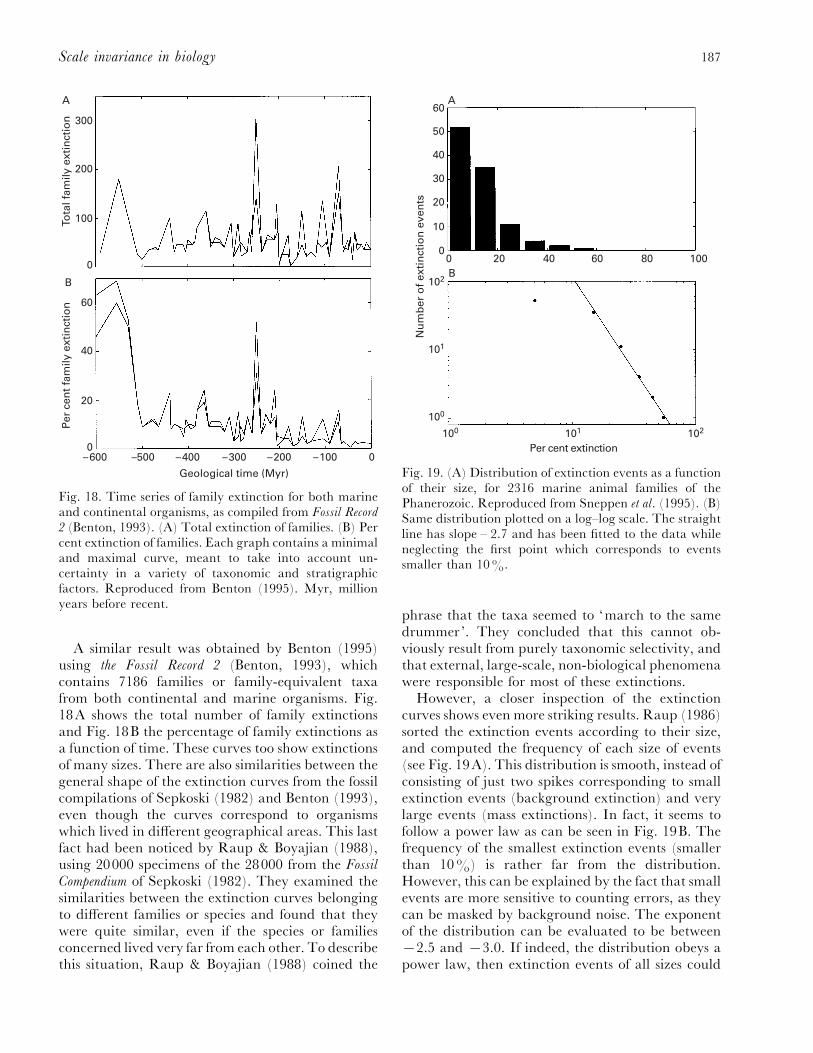
187Scale invariance in biology
300
0
60
40
20
0–500 –400 –300 –200 –100 0
Geological time (Myr)
Per
cen
t fam
ily e
xtin
ctio
nTo
tal f
amily
ext
inct
ion
A
B
200
100
–600
Fig. 18. Time series of family extinction for both marineand continental organisms, as compiled from Fossil Record
2 (Benton, 1993). (A) Total extinction of families. (B) Percent extinction of families. Each graph contains a minimaland maximal curve, meant to take into account un-certainty in a variety of taxonomic and stratigraphicfactors. Reproduced from Benton (1995). Myr, millionyears before recent.
A similar result was obtained by Benton (1995)using the Fossil Record 2 (Benton, 1993), whichcontains 7186 families or family-equivalent taxafrom both continental and marine organisms. Fig.18A shows the total number of family extinctionsand Fig. 18B the percentage of family extinctions asa function of time. These curves too show extinctionsof many sizes. There are also similarities between thegeneral shape of the extinction curves from the fossilcompilations of Sepkoski (1982) and Benton (1993),even though the curves correspond to organismswhich lived in different geographical areas. This lastfact had been noticed by Raup & Boyajian (1988),using 20000 specimens of the 28000 from the Fossil
Compendium of Sepkoski (1982). They examined thesimilarities between the extinction curves belongingto different families or species and found that theywere quite similar, even if the species or familiesconcerned lived very far from each other. To describethis situation, Raup & Boyajian (1988) coined the
60
0
102
Per cent extinction
Nu
mb
er o
f ex
tin
ctio
n e
ven
ts
A
B
50
40
30
20
10
0 20 40 60 80 100
101
100
100 101 102
Fig. 19. (A) Distribution of extinction events as a functionof their size, for 2316 marine animal families of thePhanerozoic. Reproduced from Sneppen et al. (1995). (B)Same distribution plotted on a log–log scale. The straightline has slope – 2.7 and has been fitted to the data whileneglecting the first point which corresponds to eventssmaller than 10%.
phrase that the taxa seemed to ‘march to the samedrummer’. They concluded that this cannot ob-viously result from purely taxonomic selectivity, andthat external, large-scale, non-biological phenomenawere responsible for most of these extinctions.
However, a closer inspection of the extinctioncurves shows even more striking results. Raup (1986)sorted the extinction events according to their size,and computed the frequency of each size of events(see Fig. 19A). This distribution is smooth, instead ofconsisting of just two spikes corresponding to smallextinction events (background extinction) and verylarge events (mass extinctions). In fact, it seems tofollow a power law as can be seen in Fig. 19B. Thefrequency of the smallest extinction events (smallerthan 10%) is rather far from the distribution.However, this can be explained by the fact that smallevents are more sensitive to counting errors, as theycan be masked by background noise. The exponentof the distribution can be evaluated to be between®2.5 and ®3.0. If indeed, the distribution obeys apower law, then extinction events of all sizes could
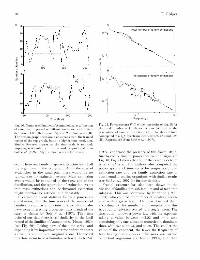
188 T. Gisiger
25
0
25
Time (Myr)
Nu
mb
er o
f fa
mili
es
A
B
20
15
10
5
300
20
15
10
550 100 150 200
200100
Fig. 20. Number of families of Ammonoidea as a functionof time over a period of 320 million years, with a timedefinition of 8 million years (A), and 2 million years (B).The bottom graph therefore is an expansion of the framedregion of the top graph, but at a higher time resolution.Similar features appear as the time scale is reduced,implying self-similarity in the record. Reproduced fromSole! et al. (1997). Myr, million years before recent.
occur: from one family or species, to extinction of allthe organisms in the ecosystem. As in the case ofavalanches in the sand pile, there would be notypical size for extinction events. Mass extinctionevents would be contained in the skew end of thedistribution, and the separation of extinction eventsinto mass extinctions and background extinctionmight therefore be artificial and debatable.
If extinction event statistics follow a power-lawdistribution, then the time series of the number offamilies present as a function of time should alsohave some interesting properties. This is indeed thecase, as shown by Sole! et al. (1997). They firstpointed out that there is self-similarity in the fossilrecord of the families of Ammonoidea (House, 1989)(see Fig. 20). Taking part of the time series, andexpanding it by improving the time definition showsa structure similar to the original record. The recordtherefore seems to be self-similar, or fractal. Sole! et al.
10–1
Frequency f
Po
wer
sp
ectr
um
P(f
)
A
B
10–2
Percentage of family extinctions
Total number of family extinctions
10–1
10–2
10–2 10–1
Fig. 21. Power spectra P( f ) of the time series of Fig. 18 forthe total number of family extinctions (A) and of thepercentage of family extinctions (B). The dashed linescorrespond to a 1}f γ spectrum with γD 0.97 (A) and 0.98(B). Reproduced from Sole! et al. (1997).
(1997) confirmed the presence of this fractal struc-ture by computing the power spectra of the signals ofFig. 18. Fig. 21 shows the result : the power spectrumis of a 1}f type. The authors also computed thepower spectra of time series for origination, totalextinction rate and per family extinction rate ofcontinental or marine organisms, with similar results(see Sole! et al., 1997 for further details).
Fractal structure has also been shown in thedivision of families into sub-families and of taxa intosub-taxa. This was performed by Burlando (1990,1993), who counted the number of sub-taxa associ-ated with a given taxon. He then classified themaccording to this number and compiled the dis-tribution of sub-taxa related to a single taxon. Thedistribution follows a power law with the exponenttaking a value between ®2.52 and ®1: taxacontaining only one subtaxon numerically dominatethose with two subtaxa, and so on. The smaller thevalue of the exponent, the fewer the frequency oftaxa having many subtaxa. This work was carriedon extant organisms (Burlando, 1990), and then
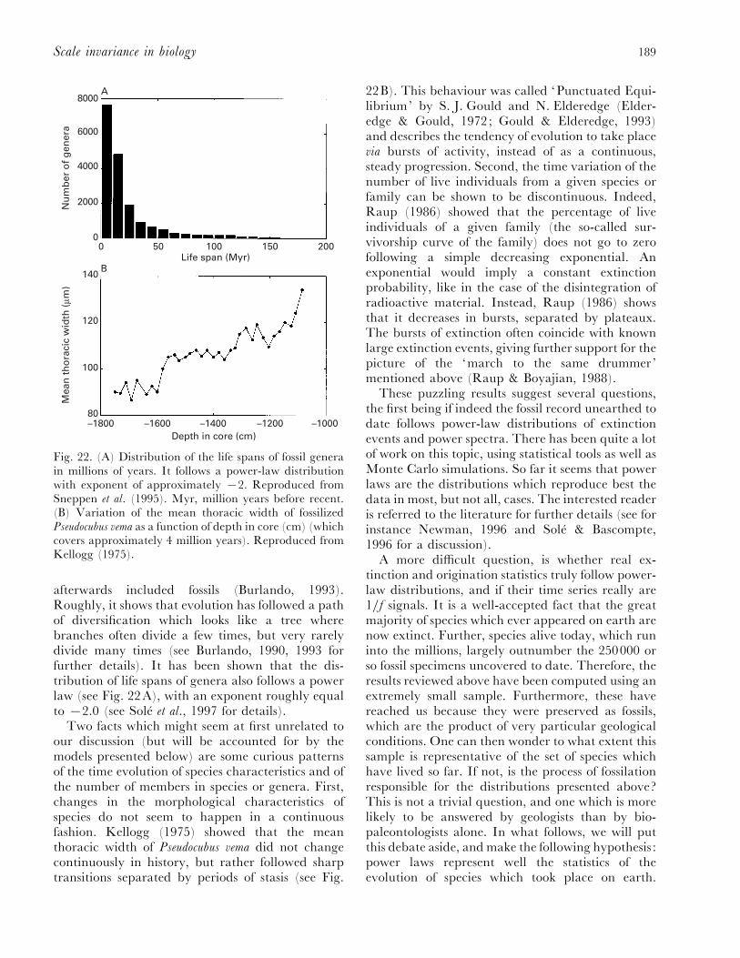
189Scale invariance in biology
8000
Depth in core (cm)
Mea
n t
ho
raci
c w
idth
(lm
)
A
BLife span (Myr)
140
6000
4000
2000
00 50 100 150 200
120
100
80–1800 –1600 –1400 –1200 –1000
Nu
mb
er o
f g
ener
a
Fig. 22. (A) Distribution of the life spans of fossil generain millions of years. It follows a power-law distributionwith exponent of approximately ®2. Reproduced fromSneppen et al. (1995). Myr, million years before recent.(B) Variation of the mean thoracic width of fossilizedPseudocubus vema as a function of depth in core (cm) (whichcovers approximately 4 million years). Reproduced fromKellogg (1975).
afterwards included fossils (Burlando, 1993).Roughly, it shows that evolution has followed a pathof diversification which looks like a tree wherebranches often divide a few times, but very rarelydivide many times (see Burlando, 1990, 1993 forfurther details). It has been shown that the dis-tribution of life spans of genera also follows a powerlaw (see Fig. 22A), with an exponent roughly equalto ®2.0 (see Sole! et al., 1997 for details).
Two facts which might seem at first unrelated toour discussion (but will be accounted for by themodels presented below) are some curious patternsof the time evolution of species characteristics and ofthe number of members in species or genera. First,changes in the morphological characteristics ofspecies do not seem to happen in a continuousfashion. Kellogg (1975) showed that the meanthoracic width of Pseudocubus vema did not changecontinuously in history, but rather followed sharptransitions separated by periods of stasis (see Fig.
22B). This behaviour was called ‘Punctuated Equi-librium’ by S. J. Gould and N. Elderedge (Elder-edge & Gould, 1972; Gould & Elderedge, 1993)and describes the tendency of evolution to take placevia bursts of activity, instead of as a continuous,steady progression. Second, the time variation of thenumber of live individuals from a given species orfamily can be shown to be discontinuous. Indeed,Raup (1986) showed that the percentage of liveindividuals of a given family (the so-called sur-vivorship curve of the family) does not go to zerofollowing a simple decreasing exponential. Anexponential would imply a constant extinctionprobability, like in the case of the disintegration ofradioactive material. Instead, Raup (1986) showsthat it decreases in bursts, separated by plateaux.The bursts of extinction often coincide with knownlarge extinction events, giving further support for thepicture of the ‘march to the same drummer’mentioned above (Raup & Boyajian, 1988).
These puzzling results suggest several questions,the first being if indeed the fossil record unearthed todate follows power-law distributions of extinctionevents and power spectra. There has been quite a lotof work on this topic, using statistical tools as well asMonte Carlo simulations. So far it seems that powerlaws are the distributions which reproduce best thedata in most, but not all, cases. The interested readeris referred to the literature for further details (see forinstance Newman, 1996 and Sole! & Bascompte,1996 for a discussion).
A more difficult question, is whether real ex-tinction and origination statistics truly follow power-law distributions, and if their time series really are1}f signals. It is a well-accepted fact that the greatmajority of species which ever appeared on earth arenow extinct. Further, species alive today, which runinto the millions, largely outnumber the 250000 orso fossil specimens uncovered to date. Therefore, theresults reviewed above have been computed using anextremely small sample. Furthermore, these havereached us because they were preserved as fossils,which are the product of very particular geologicalconditions. One can then wonder to what extent thissample is representative of the set of species whichhave lived so far. If not, is the process of fossilationresponsible for the distributions presented above?This is not a trivial question, and one which is morelikely to be answered by geologists than by bio-paleontologists alone. In what follows, we will putthis debate aside, and make the following hypothesis :power laws represent well the statistics of theevolution of species which took place on earth.

190 T. Gisiger
However, the exponents derived to date might nothave the right values.
Making this bold hypothesis raises further ques-tions. If indeed mass extinctions were caused bycatastrophes, then have the more minor events beencaused by smaller or more local perturbations? Thisconnection between the size of events and that of theperturbations was postulated by Hoffman (1989),Maynard Smith (1989) and Jablonski (1991). Inthat spirit, some work has also been carried out tofind periodicity in the records in an attempt to thenmatch them to cyclic perturbations or phenomena(Raup & Sepkoski, 1984). However, this raises thefollowing problems: (1) what perturbation distri-bution would give the power laws observed inextinction records? To answer this, one needs (2) tounderstand, to a certain degree at least, the impactof a given perturbation on an ecosystem. This, inturn, implies (3) knowledge about interactionsbetween species, since if one goes extinct because ofsome external factor, others, which are dependent onit in some way, might also disappear. In whatfollows, we review concepts and mathematicalmodels which address these three issues.
(b) Remarks on evolution and modelling
However, before considering models, some remarkshave to be made on exactly what can be expectedfrom them in this context (see also Bak, 1996 fromwhich this discussion is reproduced).
Ecosystems are, to say the least, extremelyintricate systems. They are formed by biologicalcomponents (individuals), which are themselvessubject to complicated influences from other individ-uals, as well as from their environment (geologicaland meteorological factors). It is certainly probablethat, at least for a small portion of its existence, theearth’s ecosystem has been sensitive to externalinfluences. Let us consider for example the criticalperiod where life had just appeared on our planet.Had the earth been subjected at that time to a largedose of X-rays from some not-so distant supernova,these first organisms might have died instead ofspreading and evolving as they did. Such anuntimely event might have delayed the appearanceof life on earth by millions of years, or maybe forever.It is therefore possible that if the history of the earthwas run over again from the beginning, our planetwould not be as it is now: removing a single smallevent in its history might change the present as weknow it. This explains why a ‘historical ’ approach toevolution is almost always adopted. Events are
explained a posteriori by finding probable causes forthem. For instance, man and the chimpanzee aresaid to have evolved from a common ancestorbecause of some geographical factor : the part of theinitial population which chose to live in the forestevolved to become the chimpanzee, while the partwhich stayed on the open plains evolved towardsman. Although this gives insight into the chronologyof events, it does not explain why this diversificationoccured. In light of this argument, it would thereforeappear foolish to aim at reproducing with math-ematical models the time series of Figs 17 and 18 forinstance. The question of what models of evolutioncould, or should, be able to reproduce is thereforenot trivial.
This difficulty can, however, be sidestepped byconsidering only the statistical aspects of the timeseries as relevant to modelling. To do so, oneconsiders the time series of extinctions as beinggenerated by a stochastic system, i.e. a systemsubject to random perturbations. Because theirdynamics include some randomness, stochastic sys-tems do not produce the same trajectories everytime, even when starting with the exactly sameinitial conditions. Let us consider the simple exampleof the percolation system of Section III.3 (per-colation is not exactly a stochastic system, but it willsuffice for the present purposes). Because tree growthon the field in that example was implemented usingan event generator with probability p, the positionsof trees will not be the same each time we run thesimulation. However, the statistical characteristics ofthe system will be constant from one run to another.For example, the number of trees will be roughly thesame each time and equal to Np. Similarly, oneshould try to reproduce only the statistical aspects ofthe extinction and evolution signals or, to be moreprecise, the exponents of the power law distributionsof event size and duration, and of the power spectraof the signals. Models will then be built by mimickingthe most important features of evolution andextinction, and afterwards be judged on their abilityto reproduce these exponents.
Another issue concerns the amount of detail onehas to include in models in order to reproduce thedata. This is a somewhat technical problem, but itwould be reassuring to have some conceptual handleon the question. After all, what good is a model if onehas to include in it an infinite amount of detail tomake it reproduce the data. However, here thenotion of universality proves helpful. The abundanceof self-similarity and power laws in fossil data issuggestive that ecosystems operate near a critical
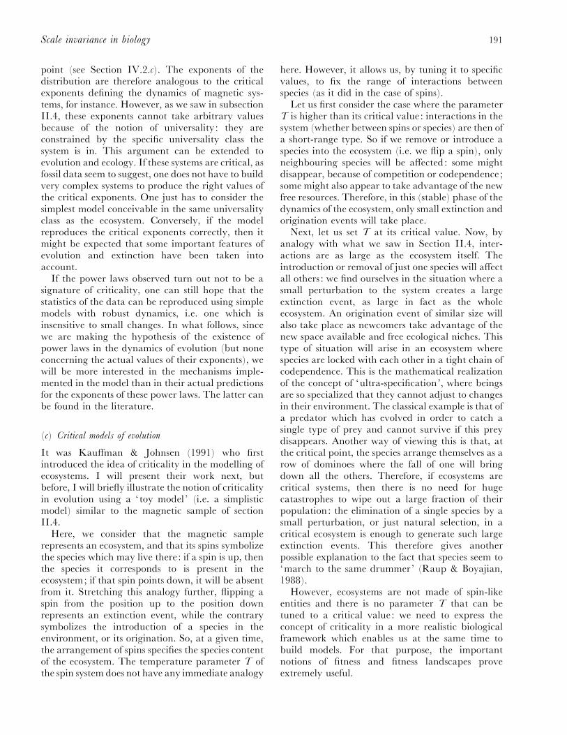
191Scale invariance in biology
point (see Section IV.2.c). The exponents of thedistribution are therefore analogous to the criticalexponents defining the dynamics of magnetic sys-tems, for instance. However, as we saw in subsectionII.4, these exponents cannot take arbitrary valuesbecause of the notion of universality : they areconstrained by the specific universality class thesystem is in. This argument can be extended toevolution and ecology. If these systems are critical, asfossil data seem to suggest, one does not have to buildvery complex systems to produce the right values ofthe critical exponents. One just has to consider thesimplest model conceivable in the same universalityclass as the ecosystem. Conversely, if the modelreproduces the critical exponents correctly, then itmight be expected that some important features ofevolution and extinction have been taken intoaccount.
If the power laws observed turn out not to be asignature of criticality, one can still hope that thestatistics of the data can be reproduced using simplemodels with robust dynamics, i.e. one which isinsensitive to small changes. In what follows, sincewe are making the hypothesis of the existence ofpower laws in the dynamics of evolution (but noneconcerning the actual values of their exponents), wewill be more interested in the mechanisms imple-mented in the model than in their actual predictionsfor the exponents of these power laws. The latter canbe found in the literature.
(c) Critical models of evolution
It was Kauffman & Johnsen (1991) who firstintroduced the idea of criticality in the modelling ofecosystems. I will present their work next, butbefore, I will briefly illustrate the notion of criticalityin evolution using a ‘toy model ’ (i.e. a simplisticmodel) similar to the magnetic sample of sectionII.4.
Here, we consider that the magnetic samplerepresents an ecosystem, and that its spins symbolizethe species which may live there: if a spin is up, thenthe species it corresponds to is present in theecosystem; if that spin points down, it will be absentfrom it. Stretching this analogy further, flipping aspin from the position up to the position downrepresents an extinction event, while the contrarysymbolizes the introduction of a species in theenvironment, or its origination. So, at a given time,the arrangement of spins specifies the species contentof the ecosystem. The temperature parameter T ofthe spin system does not have any immediate analogy
here. However, it allows us, by tuning it to specificvalues, to fix the range of interactions betweenspecies (as it did in the case of spins).
Let us first consider the case where the parameterT is higher than its critical value: interactions in thesystem (whether between spins or species) are then ofa short-range type. So if we remove or introduce aspecies into the ecosystem (i.e. we flip a spin), onlyneighbouring species will be affected: some mightdisappear, because of competition or codependence;some might also appear to take advantage of the newfree resources. Therefore, in this (stable) phase of thedynamics of the ecosystem, only small extinction andorigination events will take place.
Next, let us set T at its critical value. Now, byanalogy with what we saw in Section II.4, inter-actions are as large as the ecosystem itself. Theintroduction or removal of just one species will affectall others : we find ourselves in the situation where asmall perturbation to the system creates a largeextinction event, as large in fact as the wholeecosystem. An origination event of similar size willalso take place as newcomers take advantage of thenew space available and free ecological niches. Thistype of situation will arise in an ecosystem wherespecies are locked with each other in a tight chain ofcodependence. This is the mathematical realizationof the concept of ‘ultra-specification’, where beingsare so specialized that they cannot adjust to changesin their environment. The classical example is that ofa predator which has evolved in order to catch asingle type of prey and cannot survive if this preydisappears. Another way of viewing this is that, atthe critical point, the species arrange themselves as arow of dominoes where the fall of one will bringdown all the others. Therefore, if ecosystems arecritical systems, then there is no need for hugecatastrophes to wipe out a large fraction of theirpopulation: the elimination of a single species by asmall perturbation, or just natural selection, in acritical ecosystem is enough to generate such largeextinction events. This therefore gives anotherpossible explanation to the fact that species seem to‘march to the same drummer’ (Raup & Boyajian,1988).
However, ecosystems are not made of spin-likeentities and there is no parameter T that can betuned to a critical value: we need to express theconcept of criticality in a more realistic biologicalframework which enables us at the same time tobuild models. For that purpose, the importantnotions of fitness and fitness landscapes proveextremely useful.
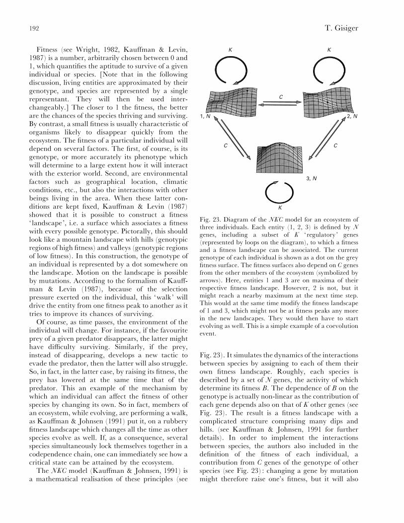
192 T. Gisiger
Fitness (see Wright, 1982, Kauffman & Levin,1987) is a number, arbitrarily chosen between 0 and1, which quantifies the aptitude to survive of a givenindividual or species. [Note that in the followingdiscussion, living entities are approximated by theirgenotype, and species are represented by a singlerepresentant. They will then be used inter-changeably.] The closer to 1 the fitness, the betterare the chances of the species thriving and surviving.By contrast, a small fitness is usually characteristic oforganisms likely to disappear quickly from theecosystem. The fitness of a particular individual willdepend on several factors. The first, of course, is itsgenotype, or more accurately its phenotype whichwill determine to a large extent how it will interactwith the exterior world. Second, are environmentalfactors such as geographical location, climaticconditions, etc., but also the interactions with otherbeings living in the area. When these latter con-ditions are kept fixed, Kauffman & Levin (1987)showed that it is possible to construct a fitness‘ landscape’, i.e. a surface which associates a fitnesswith every possible genotype. Pictorally, this shouldlook like a mountain landscape with hills (genotypicregions of high fitness) and valleys (genotypic regionsof low fitness). In this construction, the genotype ofan individual is represented by a dot somewhere onthe landscape. Motion on the landscape is possibleby mutations. According to the formalism of Kauff-man & Levin (1987), because of the selectionpressure exerted on the individual, this ‘walk’ willdrive the entity from one fitness peak to another as ittries to improve its chances of surviving.
Of course, as time passes, the environment of theindividual will change. For instance, if the favouriteprey of a given predator disappears, the latter mighthave difficulty surviving. Similarly, if the prey,instead of disappearing, develops a new tactic toevade the predator, then the latter will also struggle.So, in fact, in the latter case, by raising its fitness, theprey has lowered at the same time that of thepredator. This an example of the mechanism bywhich an individual can affect the fitness of otherspecies by changing its own. So in fact, members ofan ecosystem, while evolving, are performing a walk,as Kauffman & Johnsen (1991) put it, on a rubberyfitness landscape which changes all the time as otherspecies evolve as well. If, as a consequence, severalspecies simultaneously lock themselves together in acodependence chain, one can immediately see how acritical state can be attained by the ecosystem.
The NKC model (Kauffman & Johnsen, 1991) isa mathematical realisation of these principles (see
K K
CC
K
3, N
2, N1, N
C
Fig. 23. Diagram of the NKC model for an ecosystem ofthree individuals. Each entity (1, 2, 3) is defined by N
genes, including a subset of K ‘ regulatory’ genes(represented by loops on the diagram), to which a fitnessand a fitness landscape can be associated. The currentgenotype of each individual is shown as a dot on the greyfitness surface. The fitness surfaces also depend on C genesfrom the other members of the ecosystem (symbolized byarrows). Here, entities 1 and 3 are on maxima of theirrespective fitness landscape. However, 2 is not, but itmight reach a nearby maximum at the next time step.This would at the same time modify the fitness landscapeof 1 and 3, which might not be at fitness peaks any morein the new landscapes. They would then have to startevolving as well. This is a simple example of a coevolutionevent.
Fig. 23). It simulates the dynamics of the interactionsbetween species by assigning to each of them theirown fitness landscape. Roughly, each species isdescribed by a set of N genes, the activity of whichdetermine its fitness B. The dependence of B on thegenotype is actually non-linear as the contribution ofeach gene depends also on that of K other genes (seeFig. 23). The result is a fitness landscape with acomplicated structure comprising many dips andhills. (see Kauffman & Johnsen, 1991 for furtherdetails). In order to implement the interactionsbetween species, the authors also included in thedefinition of the fitness of each individual, acontribution from C genes of the genotype of otherspecies (see Fig. 23) : changing a gene by mutationmight therefore raise one’s fitness, but it will also
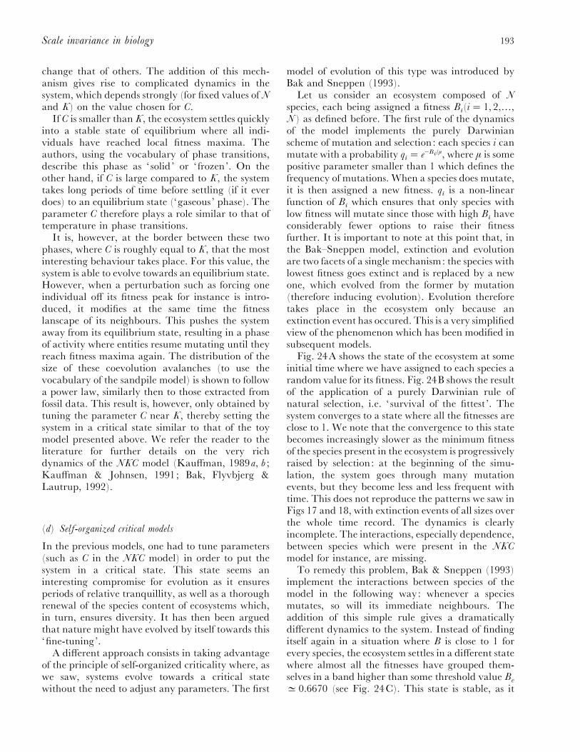
193Scale invariance in biology
change that of others. The addition of this mech-anism gives rise to complicated dynamics in thesystem, which depends strongly (for fixed values of Nand K) on the value chosen for C.
If C is smaller than K, the ecosystem settles quicklyinto a stable state of equilibrium where all indi-viduals have reached local fitness maxima. Theauthors, using the vocabulary of phase transitions,describe this phase as ‘ solid’ or ‘ frozen’. On theother hand, if C is large compared to K, the systemtakes long periods of time before settling (if it everdoes) to an equilibrium state (‘gaseous’ phase). Theparameter C therefore plays a role similar to that oftemperature in phase transitions.
It is, however, at the border between these twophases, where C is roughly equal to K, that the mostinteresting behaviour takes place. For this value, thesystem is able to evolve towards an equilibrium state.However, when a perturbation such as forcing oneindividual off its fitness peak for instance is intro-duced, it modifies at the same time the fitnesslanscape of its neighbours. This pushes the systemaway from its equilibrium state, resulting in a phaseof activity where entities resume mutating until theyreach fitness maxima again. The distribution of thesize of these coevolution avalanches (to use thevocabulary of the sandpile model) is shown to followa power law, similarly then to those extracted fromfossil data. This result is, however, only obtained bytuning the parameter C near K, thereby setting thesystem in a critical state similar to that of the toymodel presented above. We refer the reader to theliterature for further details on the very richdynamics of the NKC model (Kauffman, 1989a, b ;Kauffman & Johnsen, 1991; Bak, Flyvbjerg &Lautrup, 1992).
(d) Self-organized critical models
In the previous models, one had to tune parameters(such as C in the NKC model) in order to put thesystem in a critical state. This state seems aninteresting compromise for evolution as it ensuresperiods of relative tranquillity, as well as a thoroughrenewal of the species content of ecosystems which,in turn, ensures diversity. It has then been arguedthat nature might have evolved by itself towards this‘fine-tuning’.
A different approach consists in taking advantageof the principle of self-organized criticality where, aswe saw, systems evolve towards a critical statewithout the need to adjust any parameters. The first
model of evolution of this type was introduced byBak and Sneppen (1993).
Let us consider an ecosystem composed of N
species, each being assigned a fitness Bi(i¯ 1, 2,…,
N) as defined before. The first rule of the dynamicsof the model implements the purely Darwinianscheme of mutation and selection: each species i canmutate with a probability q
i¯ e−Bi/
µ, where µ is somepositive parameter smaller than 1 which defines thefrequency of mutations. When a species does mutate,it is then assigned a new fitness. q
iis a non-linear
function of Biwhich ensures that only species with
low fitness will mutate since those with high Bihave
considerably fewer options to raise their fitnessfurther. It is important to note at this point that, inthe Bak–Sneppen model, extinction and evolutionare two facets of a single mechanism: the species withlowest fitness goes extinct and is replaced by a newone, which evolved from the former by mutation(therefore inducing evolution). Evolution thereforetakes place in the ecosystem only because anextinction event has occured. This is a very simplifiedview of the phenomenon which has been modified insubsequent models.
Fig. 24A shows the state of the ecosystem at someinitial time where we have assigned to each species arandom value for its fitness. Fig. 24B shows the resultof the application of a purely Darwinian rule ofnatural selection, i.e. ‘ survival of the fittest ’. Thesystem converges to a state where all the fitnesses areclose to 1. We note that the convergence to this statebecomes increasingly slower as the minimum fitnessof the species present in the ecosystem is progressivelyraised by selection: at the beginning of the simu-lation, the system goes through many mutationevents, but they become less and less frequent withtime. This does not reproduce the patterns we saw inFigs 17 and 18, with extinction events of all sizes overthe whole time record. The dynamics is clearlyincomplete. The interactions, especially dependence,between species which were present in the NKC
model for instance, are missing.To remedy this problem, Bak & Sneppen (1993)
implement the interactions between species of themodel in the following way: whenever a speciesmutates, so will its immediate neighbours. Theaddition of this simple rule gives a dramaticallydifferent dynamics to the system. Instead of findingitself again in a situation where B is close to 1 forevery species, the ecosystem settles in a different statewhere almost all the fitnesses have grouped them-selves in a band higher than some threshold value B
c
D 0.6670 (see Fig. 24C). This state is stable, as it
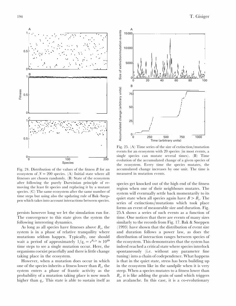
194 T. Gisiger
1
0.5
0
1
0.5
0
1
0.5
00 100 200
Species
Fitn
ess
A
B
C
Fig. 24. Distribution of the values of the fitness B for anecosystem of N¯ 200 species. (A) Initial state where allfitnesses are chosen randomly. (B) State of the ecosystemafter following the purely Darwinian principle of re-moving the least fit species and replacing it by a mutantspecies. (C) The same ecosystem after the same number oftime steps but using also the updating rule of Bak–Snep-pen which takes into account interactions between species.
persists however long we let the simulation run for.The convergence to this state gives the system thefollowing interesting dynamics.
As long as all species have fitnesses above Bc, the
system is in a phase of relative tranquility wheremutations seldom happen. Typically, one shouldwait a period of approximately 1}q
c¯ eBc/
µ D 10#*
time steps to see a single mutation occur. Here, theorganisms coexist peacefully and there is little changetaking place in the ecosystem.
However, when a mutation does occur in whichone of the species inherits a fitness lower than B
c, the
system enters a phase of frantic activity as theprobability of a mutation taking place is now muchhigher than q
c. This state is able to sustain itself as
15000
10000
5000
0
75
50
25
00 250 500 750 1000
Time (arbitrary units)Acc
um
ula
ted
ch
ang
e (a
rbit
rary
un
its)
Siz
e o
f ex
tin
ctio
n/m
uta
tio
n e
ven
ts
0 20 40 60 80 100
A
B
Fig. 25. (A) Time series of the size of extinction}mutationevents for an ecosystem with 20 species (in most events, asingle species can mutate several times). (B) Timeevolution of the accumulated change of a given species ofthe ecosystem. Every time the species mutates, theaccumulated change increases by one unit. The time ismeasured in mutation events.
species get knocked out of the high end of the fitnessregion when one of their neighbours mutates. Thesystem will eventually settle back momentarily to itsquiet state when all species again have B"B
c. The
series of extinctions}mutations which took placeforms an event of measurable size and duration. Fig.25A shows a series of such events as a function oftime. One notices that there are events of many sizessimilarly to the records from Fig. 17. Bak & Sneppen(1993) have shown that the distribution of event sizeand duration follows a power law, as does thedistribution of interaction ranges between species ofthe ecosystem. This demonstrates that the system hasindeed reached a critical state where species interlockspontaneously (i.e. without any parameter finetuning) into a chain of codependence. What happensis that in the quiet state, stress has been building upin the ecosystem like in the sandpile when it is verysteep. When a species mutates to a fitness lower thanB
c, it is like adding the grain of sand which triggers
an avalanche. In this case, it is a co-evolutionary
195Scale invariance in biology
avalanche where mutation of species induces furthermutations of their neighbours.
Fig. 25B shows the accumulated change of agiven species in the ecosystem as a function of time.Notice the periods of change (vertical lines) sepa-rated by periods of stasis (horizontal line). Thiscompares well with Fig. 22 illustrating the notion ofpunctuated equilibrium.
For further details on the model, its dynamics andhow it compares with fossil data, the reader isreferred to the literature (Sneppen, 1995; Sneppen et
al., 1995).Another interesting model which describes ecosys-
tems as critical system was introduced by Sole! (1996)and Sole! & Manrubia (1996). Here, evolvinginteractions between species is the key ingredientwhich drives the system towards a critical state. Ateach time step, the total stress imposed by the rest ofthe ecosystem on each species is computed. Specieswhich are subject to too much pressure go extinct,and are replaced by mutants of the remainingspecies. There are also spontaneous mutationsoccurring, but at a lower level. This will drive thesystem towards a state where removing just onespecies will perturb the existence of many others, andextinction events of all sizes will occur. Sole! ,Bascompte and Manrubia (1996) and Sole! andManrubia (1997) showed that this system hasbecome critical with an extinction event distribution,among other things, which follows a power law. Forfurther details see Sole! et al. (1996), Sole! & Manrubia(1997) and references therein.
(e) Non-critical model of mass extinction
So far in our developments, we have presented workwhich interprets the presence of power laws in fossildata as evidence that ecosystems operate at, or near,a critical state. However, power laws do not alwaysimply criticality as Newman (1996, 1997a, b)showed. Indeed, he proposes a model for evolutionwhere no interactions are explicitly present betweenspecies (although they may be implicit) whichaccounts well for the data and seems to indicate thatcodependence between species might, althoughimportant, not be an essential ingredient in eco-system dynamics. As we will see, his model thereforedoes not interpret mass extinction events as co-evolutionary avalanches, but rather as the result ofstrong external stress on a temporarily weakenedecosystem.
Part of the model of Newman (1997a, b) is theDarwinian mechanism of elimination of unfit species
by selection, and which is implemented as follows. Asin the Bak–Sneppen model, each species possesses afitness B. Stress, symbolized by a number between 0and 1, is drawn using a random number generatorand applied to the system, eliminating all specieswith fitness smaller than this number. This stress canbe of physical origin (geographic location, climate,volcanic eruptions, earthquakes, meteorites, etc.)but also it can be caused by other species (predators,competitors, parasites, etc.). Selection is then fol-lowed by diversification as free ecological niches (inthis case, the spaces left vacant by the species whichjust disappeared) are filled by new species. However,these dynamics of a purely Darwinian type lead tothe same situation as the one illustrated by Fig. 24Bwhere the ecosystem becomes increasingly stable byfilling itself with highly fit species. The interestingvariation which Newman (1997a, b) introduces tocomplement his model is, instead of codependence,the spontaneous ability of species to mutate andevolve at all times, even in times of little externalstress. A new rule is then added to the model whichallows at each time step a small proportion of thespecies of the ecosystem to mutate spontaneously.This changes radically the dynamics of the systemwhich favours now a rich and complex activity.Simulations show that the distribution of the size ofextinction events, as well as of species lifetimes obeypower laws. By making supplementary assumptionsabout the model, Newman (1997a) was also able toestimate the distribution of species in each genus,which is also of this type and in the spirit of thefindings of Burlando (1990, 1993) (see SectionIV.2.a).
That this model is able to produce power lawswithout any parameter fine tuning or resorting to acritical state is quite impressive. It is important tonote that the ecosystem of Newman’s model (1997a,b) is not critical : the species do not spontaneously setthemselves in highly unstable states to then becomeextinct like falling dominoes. These events, calledcoevolutionary avalanches, are a trademark ofcritical models of evolution and a prediction whichhas to be tested against fossil data. In Newman’smodel (1997a, b), on the other hand, there are nosuch avalanches as there are no direct interactionsbetween species. Interactions are implicitly includedin the stresses applied to the system. However, theparticular dynamics of the system allows it to makeoriginal predictions of its own.
The model first predicts that the longer thewaiting time for a large stress, the greater the nextextinction event will be. Indeed, periods of low
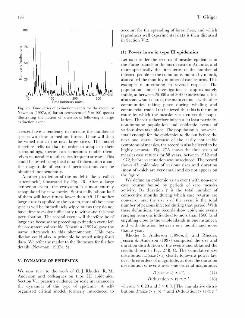
196 T. Gisiger
100
75
50
25
00 100 200 300
Time (arbitrary units)
Nu
mb
er o
f ex
tin
ctio
ns
Fig. 26. Time series of extinction events for the model ofNewman (1997a, b) for an ecosystem of N¯ 100 speciesillustrating the notion of aftershocks following a largeextinction event.
stresses have a tendency to increase the number ofspecies with low to medium fitness. These will thenbe wiped out at the next large stress. The modeltherefore tells us that in order to adapt to theirsurroundings, species can sometimes render them-selves vulnerable to other, less frequent stresses. Thiscould be tested using fossil data if information aboutthe magnitude of external perturbations can beobtained independently.
Another prediction of the model is the so-called‘aftershock’, illustrated by Fig. 26. After a largeextinction event, the ecosystem is almost entirelyrepopulated by new species. Statistically, about halfof them will have fitness lower than 0.5. If anotherlarge stress is applied to the system, most of these newspecies will be immediately wiped out as they do nothave time to evolve sufficiently to withstand this newperturbation. The second event will therefore be oflarge size because the preceding extinction event leftthe ecosystem vulnerable. Newman (1997a) gave thename aftershock to this phenomenon. This pre-diction could also in principle be tested using fossildata. We refer the reader to the literature for furtherdetails (Newman, 1997a, b).
V. DYNAMICS OF EPIDEMICS
We now turn to the work of C. J. Rhodes, R. M.Anderson and colleagues on type III epidemics.Section V.1 presents evidence for scale invariance inthe dynamics of this type of epidemic. A self-organized critical model, formerly introduced to
account for the spreading of forest fires, and whichreproduces well experimental data is then discussedin Section V.2.
(1) Power laws in type III epidemics
Let us consider the records of measles epidemics inthe Faroe Islands in the north-eastern Atlantic, andmore specifically the time series of the number ofinfected people in the community month by month,also called the monthly number of case returns. Thisexample is interesting in several respects. Thepopulation under investigation is approximatelystable, at between 25000 and 30000 individuals. It isalso somewhat isolated, the main contacts with othercommunities taking place during whaling andcommercial trade. It is believed that this is the mainroute by which the measles virus enters the popu-lation. The virus therefore infects a, at least partially,non-immune population and epidemic events ofvarious sizes take place. The population is, however,small enough for the epidemics to die out before thenext one starts. Because of the easily noticeablesymptoms of measles, the record is also believed to behighly accurate. Fig. 27A shows the time series ofmeasles case returns for 58 years, between 1912 and1972, before vaccination was introduced. The recordshows 43 epidemics of various sizes and duration(most of which are very small and do not appear onthe figure).
We define an epidemic as an event with non-zerocase returns bound by periods of zero measlesactivity. Its duration τ is the total number ofconsecutive months during which case returns arenon-zero, and the size s of the event is the totalnumber of persons infected during that period. Withthese definitions, the records show epidemic eventsranging from one individual to more than 1500 (andengulfing close to the whole islands in one instance),and with duration between one month and morethan a year.
Rhodes & Anderson (1996a, b) and Rhodes,Jensen & Anderson (1997) computed the size andduration distribution of the events and obtained theresults shown in Fig. 27B, C. The cumulative sizedistribution D(size" s) clearly follows a power lawover three orders of magnitude, as does the durationdistribution of events over one order of magnitude:
D(size" s)£ s−a, (17)
D(duration" τ)£ τ−b, (18)
where aD 0.28 and bD 0.8. [The cumulative distri-butions D(size" s)£−a and D(duration" τ)£ τ−b

197Scale invariance in biology
1000
500
01900 1920 1940 1960 1980
Time (years)
102
101
100
100 101 102 103
102
101
100
100 101
Epidemic size s
Epidemic duration s
D(d
ura
tio
n>s
)D
(siz
e>s)
Nu
mb
er o
f in
fect
ives
A
B
C
Fig. 27. (A) Monthly measles-case returns for the Faroeislands (population of approximately 25000 habitants),between 1912 and 1972. (B) Cumulative distributionD(size" s) of epidemics according to their size s compiledfrom A. The straight line represents a power law withexponent aD 0.28. (C) Cumulative distribution D(dura-tion" τ) of epidemic event duration τ. The straight linehas a slope of bD 0.8. Reproduced from Rhodes &Anderson (1996b).
are related to the non-cumulative distributions D(s)£ s−α and D(τ)£ τ−β since α¯ 1a and β¯ 1b.]Rhodes & Anderson (1996b) also performed thisanalysis on records between 1912 and 1970, for theisland of Bornholm, Denmark (aD 0.28 and bD0.85) and the town of Reykjavik, Iceland (aD 0.21and bD 0.62) (results not shown). They laterimproved their estimations of the parameter a formeasles, whooping cough and mumps epidemics inthe Faroe Islands, by using longer records which runfrom 1870 to 1970 (see Rhodes et al. , 1997).
This power-law behaviour shows the absence ofcharacteristic scale in the size and duration of
epidemics. So far, it has been difficult to reproducethe statistics of these events using traditional modelsof epidemiology. This is the case for the SEIR (whichstands for susceptible, exposed, infective and re-covered individuals) compartmentalmodel ofAnder-son & May (1991) as was shown by Rhodes &Anderson (1996a, b) and Rhodes et al. (1997). Theysuggest that the mass-action law, on which themodel is based, overestimates the interactions be-tween the susceptible (people who have not yet beeninfected but can be if exposed) and the infective(people who can infect other people), therefore over-producing large epidemics. Heterogeneity is a factorwhich differentiates different types of epidemicsdynamics. In large cities, because of the schoolenvironment, measles is usually considered a child-hood disease. However, in a mostly non-urban areasuch as the Faroe Islands, the measles epidemicsafflict all age groups : the entire population issusceptible to catching the virus. The epidemics ofthe case presented here are therefore different fromthose of urban areas, and are classified as type IIIepidemics (Bartlett, 1957, 1960) (i.e. epidemics in asmall, isolated population of susceptibles).
(2) Disease epidemics modelling withcritical models
Given that traditional models such as the SEIR
model apparently failed to reproduce the observeddata, Rhodes & Anderson (1996a, b) tried a differentapproach. They postulated that the power lawsobserved in the distributions are in fact criticalexponents of some critical system, and directed theirattention instead towards a model first developed tostudy turbulence in fluids and forest fire dynamics(see Bak, Chen & Tang, 1990 and Drossel &Schwabl, 1992 for details).
This model is somewhat similar to the percolationmodel of plant growth of Section III.3. Here again,at each time step, trees grow on empty areas of a fieldwith a probability p. Also present is a so-calledlightning mechanism which sets trees on fire with aprobability l. Once a tree is on fire it will burn in asingle time step and leave a vacant area behind it,where new trees can grow. It will also at the sametime set ablaze its immediate neighbours, which willdo the same to nearby trees and so on. A forest fireis then defined as the event where trees are burningon the field, and a size and duration can be associatedto it. Drossel & Schwabl (1992) showed that if theintroduction of new trees outnumbers the trees setablaze (so if p is much larger than l) then the system

198 T. Gisiger
1000
500
01400 1600 1800 2000
Time (arbitrary units)
102
101
100
100 101 102 103
102
101
100
100 101
Epidemic size s
Epidemic duration s
D(d
ura
tio
n>s
)D
(siz
e>s)
Nu
mb
er o
f in
fect
ives
A
B
C
Fig. 28. (A) Time series of infectives obtained from thesimulation of case returns using the forest-fire modeldescribed in the text. The time scale is arbitrary. (B)Cumulative distribution D(size" s) of events accordingto their size ; it is compatible with a power law withexponent aD 0.29 (solid line). (C) Cumulative dis-tribution D(duration" τ) of duration of events shownwith a power-law distribution of exponent bD 1.5.Reproduced from Rhodes & Anderson (1996b).
will settle into a critical state with size and durationdistributions of a power-law type. Also in this state,the distribution of burning trees in the forest can beshown to be fractal (see Bak et al., 1990 and Drossel& Schwabl, 1992 for details).
As Rhodes & Anderson (1996a) show, there are alot of similarities between the dynamics of forest firesand the spreading of a disease in a community: treeson the lattice represent susceptibles ; burning treescorrespond to infectives ; empty sites represent peopleimmune to the disease (or no people at all). Theforest fire model can then be viewed as a very simplemodel of disease spreading in a community, but onewhich does not enforce homogeneity as strongly as
the SEIR model, for instance. However, beforetrying to apply this model to the problem at hand,one must make sure that the fundamental conditionp( l is satisfied. Otherwise the system will notachieve a critical state. To do this, one must firstevaluate the parameters p and l corresponding to thepopulation of the Faroe Islands.
This population has been roughly constant overthe last century, at between 25000 and 30000people. Between 1912 and 1970, there have been 43documented epidemics. An estimate of the prob-ability of measles outbreaks would then be approxi-mately l¯ 43}58 D 0.74 per year. Also, to maintainthe population roughly constant, on average eachmember of the community will give birth to onechild. Estimating the average lifetime of people inthe community to be approximately 70 years, thisgives a probability of 1}70 per year of giving birth toa child. The number of newborn, and thereforesusceptibles, for the whole community is then25000}70D 357 per year which is roughly equal toone per day. Therefore, we obtain l}pD 0.74}365D1}493 which is very small compared to 1: thecondition for the system to settle into criticaldynamics is therefore well satisfied. There are clearlytwo time scales in the model : births, which happenalmost every day, and the introduction of the virus,which happens once a year. It is also important thatp is not too high, otherwise the birth of susceptiblesmight fuel the existing epidemics for too long, maybeeven until the next epidemic arises.
Rhodes & Anderson (1996b) used the followingparameters for their simulations : p¯ 0.000 026 andl¯ p}300. This gave them an average population ofapproximately 25000 and a distribution of epidemicevents following power laws with exponents aD 0.29and bD 1.5 (see Fig. 28). Later simulations, (Rhodes& Anderson, 1996a) where the system was allowed atransitory period of approximatively 130 years (toattain criticality) and the data was collected duringthe following 180 years, gave the improved expo-nents aD 0.25 and bD 1.27 which are quite close tothose extracted from the records. This was doneusing a two-dimensional lattice. Similar compu-tations on a three-dimensional and five-dimensionallattice were carried out by Clar, Drossel & Schwabl(1994), who found the values a¯ 0.23 and a¯ 0.45respectively. Apparently, the best match for theobserved measles and whooping cough patterns isthe three-dimensional forest-fire model, while thefive-dimensional version of the model reproducesbest the mumps critical exponent. Overall, theaccord is quite impressive.
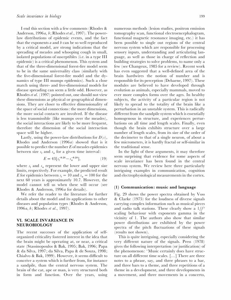
199Scale invariance in biology
I end this section with a few comments (Rhodes &Anderson, 1996a, b ; Rhodes et al., 1997). The power-law distributions of epidemic events, and the factthat the exponents a and b can be so well reproducedby a critical model, are strong indications that thespreading of measles and whooping cough in small,isolated populations of susceptibles (i.e. in a type IIIepidemic) is a critical phenomenon. This system andthat of the three-dimensional forest-fire model seemto be in the same universality class (similarly withthe five-dimensional forest-fire model and the dy-namics of type III mumps epidemics). Such a closematch using three- and five-dimensional models fordisease spreading can seem a little odd. However, asRhodes et al. (1997) pointed out, one should not viewthese dimensions as physical or geographical dimen-sions. They are closer to effective dimensionality ofthe space of social connections : the more dimensions,the more social contacts are involved. If the diseaseis less transmissible (like mumps over the measles),the social interactions are likely to be more frequent,therefore the dimension of the social interactionspace will be higher.
Lastly, using the power-law distributions for D(s),Rhodes and Anderson (1996a) showed that is itpossible to predict the number E of measles epidemicsbetween size s
land s
ufor a given time interval :
E¯ 43[s−!±#)
l®s−!±
#)u
], (19)
where sland s
urepresent the lower and upper size
limits, respectively. For example, the predicted resultE for epidemics between s
l¯ 10 and s
u¯ 100 for the
next 60 years is approximately 10.7. However, themodel cannot tell us when these will occur (seeRhodes & Anderson, 1996a for details).
We refer the reader to the literature for furtherdetails about the model and its applications to otherdiseases and population types (Rhodes & Anderson,1996a, b ; Rhodes et al., 1997).
VI. SCALE INVARIANCE INNEUROBIOLOGY
The recent successes of the application of self-organized criticality fostered interest in the idea thatthe brain might be operating at, or near, a criticalstate (Stassinopoulos & Bak, 1995; Bak, 1996; Papa& da Silva, 1997; da Silva, Papa & de Souza, 1998;Chialvo & Bak, 1999). However, it seems difficult toconceive a system which is further from, for instancea sandpile, than the central nervous system. Thebrain of the cat, ape or man, is very structured bothin form and function. Over the years, using
numerous methods (lesion studies, positron emissiontomography scan, functional electroencephalogram,functional magnetic resonance imaging, etc.) it hasbeen possible to single out regions of the centralnervous system which are responsible for processingsensory inputs, understanding and articulating lan-guage, as well as those in charge of reflection andbuilding strategies to solve problems, to name only afew (see Changeux, 1985 for a review). Recent workhas even suggested that a well-defined area of thebrain hardwires the notion of number and isresponsible for its perception (Dehaene, 1997). Thesemodules are believed to have developed throughevolution as animals, especially mammals, moved toever more complex forms over the ages. In healthysubjects, the activity of a particular region is notlikely to spread to the totality of the brain like aperturbation in an unstable system. This is radicallydifferent from the sandpile system which is essentiallyhomogenous in structure, and experiences pertur-bations on all time and length scales. Finally, eventhough the brain exhibits structure over a largenumber of length scales, from its size of the order ofthe decimeter to that of a single neuron, of about afew micrometers, it is hardly fractal or self-similar inthe traditional sense.
In the light of these arguments, it may thereforeseem surprising that evidence for some aspects ofscale invariance has been found in the centralnervous system. We review here three particularlyintriguing examples in communication, cognitionand electrophysiological measurements in the cortex.
(1) Communication: music and language
Fig. 29 shows the power spectra obtained by Voss& Clarke (1975) for the loudness of diverse signalscarrying complex information such as musical piecesand radio talk stations. These clearly show a 1}f γ
scaling behaviour with exponents gamma in thevicinity of 1. The authors also show that similarpower distributions are exhibited by the powerspectra of the pitch fluctuations of these signals(results not shown).
This is quite intriguing, especially considering thevery different nature of the signals. Press (1978)gives the following interpretation (or justification) ofthe phenomenon: ‘Music certainly does have struc-ture on all different time scales. […] There are threenotes to a phrase, say, and three phrases to a bar,and three bars to a theme, and three repetitions of atheme in a development, and three developments ina movement, and three movements in a concerto,
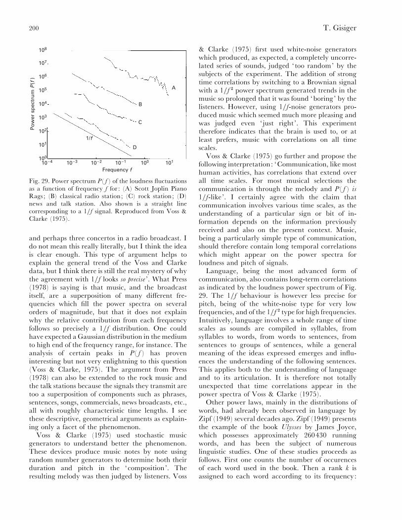
200 T. Gisiger
108
107
106
105
104
103
102
101
100
10–4 10–3 10–2 10–1 100 101
D
C
B
A
1/f
Frequency f
Po
wer
sp
ectr
um
P(f
)
Fig. 29. Power spectrum P( f ) of the loudness fluctuationsas a function of frequency f for : (A) Scott Joplin PianoRags ; (B) classical radio station; (C) rock station; (D)news and talk station. Also shown is a straight linecorresponding to a 1}f signal. Reproduced from Voss &Clarke (1975).
and perhaps three concertos in a radio broadcast. Ido not mean this really literally, but I think the ideais clear enough. This type of argument helps toexplain the general trend of the Voss and Clarkedata, but I think there is still the real mystery of whythe agreement with 1}f looks so precise ’. What Press(1978) is saying is that music, and the broadcastitself, are a superposition of many different fre-quencies which fill the power spectra on severalorders of magnitude, but that it does not explainwhy the relative contribution from each frequencyfollows so precisely a 1}f distribution. One couldhave expected a Gaussian distribution in the mediumto high end of the frequency range, for instance. Theanalysis of certain peaks in P( f ) has proveninteresting but not very enlightning to this question(Voss & Clarke, 1975). The argument from Press(1978) can also be extended to the rock music andthe talk stations because the signals they transmit aretoo a superposition of components such as phrases,sentences, songs, commercials, news broadcasts, etc.,all with roughly characteristic time lengths. I seethese descriptive, geometrical arguments as explain-ing only a facet of the phenomenon.
Voss & Clarke (1975) used stochastic musicgenerators to understand better the phenomenon.These devices produce music notes by note usingrandom number generators to determine both theirduration and pitch in the ‘composition’. Theresulting melody was then judged by listeners. Voss
& Clarke (1975) first used white-noise generatorswhich produced, as expected, a completely uncorre-lated series of sounds, judged ‘too random’ by thesubjects of the experiment. The addition of strongtime correlations by switching to a Brownian signalwith a 1}f # power spectrum generated trends in themusic so prolonged that it was found ‘boring’ by thelisteners. However, using 1}f-noise generators pro-duced music which seemed much more pleasing andwas judged even ‘ just right ’. This experimenttherefore indicates that the brain is used to, or atleast prefers, music with correlations on all timescales.
Voss & Clarke (1975) go further and propose thefollowing interpretation: ‘Communication, like mosthuman activities, has correlations that extend overall time scales. For most musical selections thecommunication is through the melody and P( f ) is
1}f-like ’. I certainly agree with the claim thatcommunication involves various time scales, as theunderstanding of a particular sign or bit of in-formation depends on the information previouslyreceived and also on the present context. Music,being a particularly simple type of communication,should therefore contain long temporal correlationswhich might appear on the power spectra forloudness and pitch of signals.
Language, being the most advanced form ofcommunication, also contains long-term correlationsas indicated by the loudness power spectrum of Fig.29. The 1}f behaviour is however less precise forpitch, being of the white-noise type for very lowfrequencies, and of the 1}f # type for high frequencies.Intuitively, language involves a whole range of timescales as sounds are compiled in syllables, fromsyllables to words, from words to sentences, fromsentences to groups of sentences, while a generalmeaning of the ideas expressed emerges and influ-ences the understanding of the following sentences.This applies both to the understanding of languageand to its articulation. It is therefore not totallyunexpected that time correlations appear in thepower spectra of Voss & Clarke (1975).
Other power laws, mainly in the distributions ofwords, had already been observed in language byZipf (1949) several decades ago. Zipf (1949) presentsthe example of the book Ulysses by James Joyce,which possesses approximately 260430 runningwords, and has been the subject of numerouslinguistic studies. One of these studies proceeds asfollows. First one counts the number of occurencesof each word used in the book. Then a rank k isassigned to each word according to its frequency:
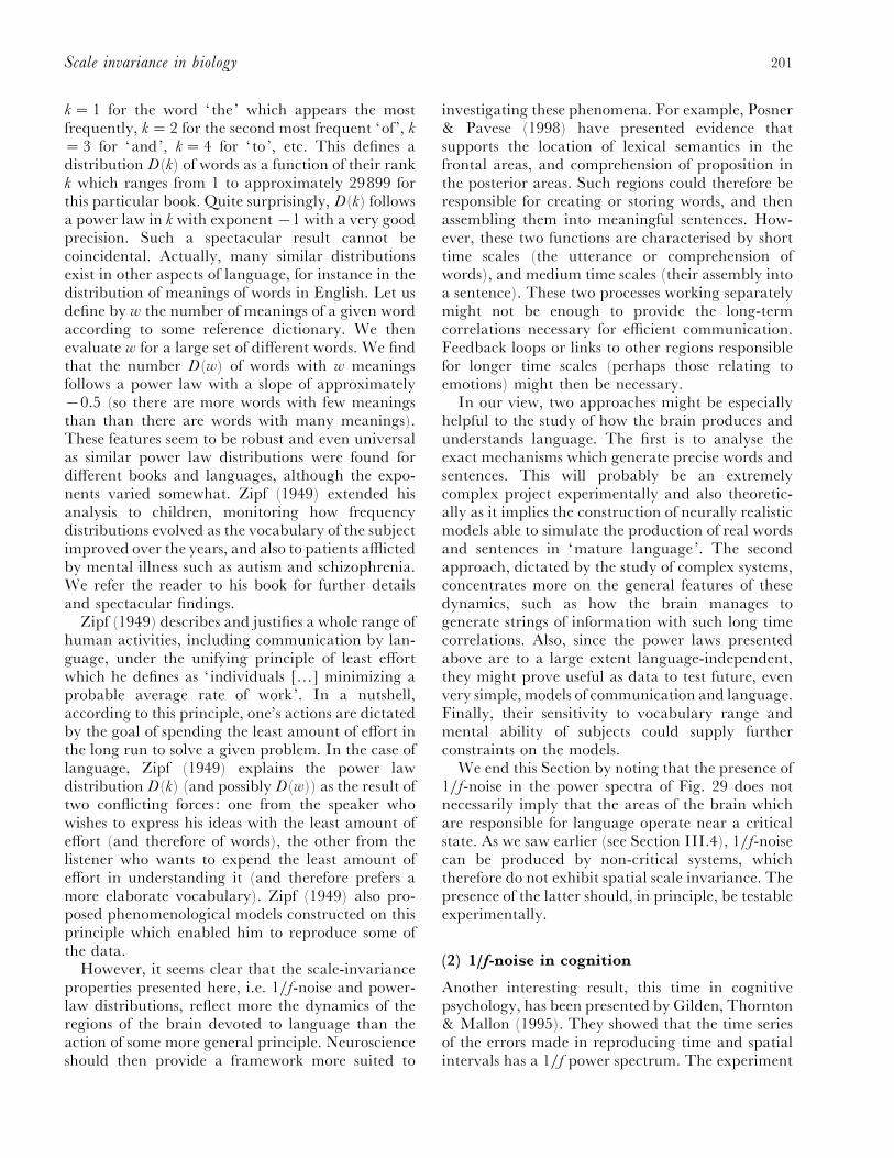
201Scale invariance in biology
k¯ 1 for the word ‘the’ which appears the mostfrequently, k¯ 2 for the second most frequent ‘of ’, k
¯ 3 for ‘and’, k¯ 4 for ‘ to’, etc. This defines adistribution D(k) of words as a function of their rankk which ranges from 1 to approximately 29899 forthis particular book. Quite surprisingly, D(k) followsa power law in k with exponent ®1 with a very goodprecision. Such a spectacular result cannot becoincidental. Actually, many similar distributionsexist in other aspects of language, for instance in thedistribution of meanings of words in English. Let usdefine by w the number of meanings of a given wordaccording to some reference dictionary. We thenevaluate w for a large set of different words. We findthat the number D(w) of words with w meaningsfollows a power law with a slope of approximately®0±5 (so there are more words with few meaningsthan than there are words with many meanings).These features seem to be robust and even universalas similar power law distributions were found fordifferent books and languages, although the expo-nents varied somewhat. Zipf (1949) extended hisanalysis to children, monitoring how frequencydistributions evolved as the vocabulary of the subjectimproved over the years, and also to patients afflictedby mental illness such as autism and schizophrenia.We refer the reader to his book for further detailsand spectacular findings.
Zipf (1949) describes and justifies a whole range ofhuman activities, including communication by lan-guage, under the unifying principle of least effortwhich he defines as ‘ individuals […] minimizing aprobable average rate of work’. In a nutshell,according to this principle, one’s actions are dictatedby the goal of spending the least amount of effort inthe long run to solve a given problem. In the case oflanguage, Zipf (1949) explains the power lawdistribution D(k) (and possibly D(w)) as the result oftwo conflicting forces : one from the speaker whowishes to express his ideas with the least amount ofeffort (and therefore of words), the other from thelistener who wants to expend the least amount ofeffort in understanding it (and therefore prefers amore elaborate vocabulary). Zipf (1949) also pro-posed phenomenological models constructed on thisprinciple which enabled him to reproduce some ofthe data.
However, it seems clear that the scale-invarianceproperties presented here, i.e. 1}f-noise and power-law distributions, reflect more the dynamics of theregions of the brain devoted to language than theaction of some more general principle. Neuroscienceshould then provide a framework more suited to
investigating these phenomena. For example, Posner& Pavese (1998) have presented evidence thatsupports the location of lexical semantics in thefrontal areas, and comprehension of proposition inthe posterior areas. Such regions could therefore beresponsible for creating or storing words, and thenassembling them into meaningful sentences. How-ever, these two functions are characterised by shorttime scales (the utterance or comprehension ofwords), and medium time scales (their assembly intoa sentence). These two processes working separatelymight not be enough to provide the long-termcorrelations necessary for efficient communication.Feedback loops or links to other regions responsiblefor longer time scales (perhaps those relating toemotions) might then be necessary.
In our view, two approaches might be especiallyhelpful to the study of how the brain produces andunderstands language. The first is to analyse theexact mechanisms which generate precise words andsentences. This will probably be an extremelycomplex project experimentally and also theoretic-ally as it implies the construction of neurally realisticmodels able to simulate the production of real wordsand sentences in ‘mature language’. The secondapproach, dictated by the study of complex systems,concentrates more on the general features of thesedynamics, such as how the brain manages togenerate strings of information with such long timecorrelations. Also, since the power laws presentedabove are to a large extent language-independent,they might prove useful as data to test future, evenvery simple, models of communication and language.Finally, their sensitivity to vocabulary range andmental ability of subjects could supply furtherconstraints on the models.
We end this Section by noting that the presence of1}f-noise in the power spectra of Fig. 29 does notnecessarily imply that the areas of the brain whichare responsible for language operate near a criticalstate. As we saw earlier (see Section III.4), 1}f-noisecan be produced by non-critical systems, whichtherefore do not exhibit spatial scale invariance. Thepresence of the latter should, in principle, be testableexperimentally.
(2) 1/f-noise in cognition
Another interesting result, this time in cognitivepsychology, has been presented by Gilden, Thornton& Mallon (1995). They showed that the time seriesof the errors made in reproducing time and spatialintervals has a 1}f power spectrum. The experiment
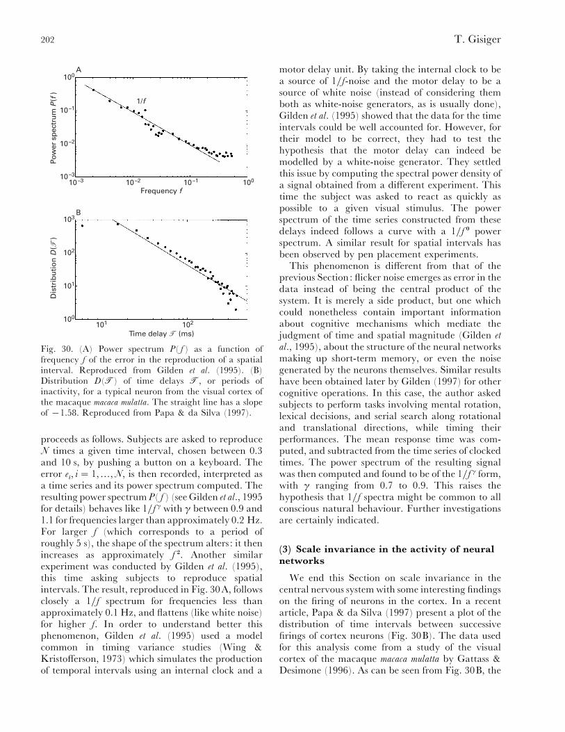
202 T. Gisiger
100
10–1
10–2
10–3
10–3 10–2 10–1 100
Frequency f
103
102
101
100101 102
Time delay 4 (ms)
Dis
trib
uti
on
D(4
)Po
wer
spe
ctru
m P
(f)
1/f
A
B
Fig. 30. (A) Power spectrum P( f ) as a function offrequency f of the error in the reproduction of a spatialinterval. Reproduced from Gilden et al. (1995). (B)Distribution D(4) of time delays 4, or periods ofinactivity, for a typical neuron from the visual cortex ofthe macaque macaca mulatta. The straight line has a slopeof ®1.58. Reproduced from Papa & da Silva (1997).
proceeds as follows. Subjects are asked to reproduceN times a given time interval, chosen between 0.3and 10 s, by pushing a button on a keyboard. Theerror e
i, i¯ 1,…,N, is then recorded, interpreted as
a time series and its power spectrum computed. Theresulting power spectrum P( f ) (see Gilden et al., 1995for details) behaves like 1}f γ with γ between 0.9 and1.1 for frequencies larger than approximately 0.2 Hz.For larger f (which corresponds to a period ofroughly 5 s), the shape of the spectrum alters : it thenincreases as approximately f #. Another similarexperiment was conducted by Gilden et al. (1995),this time asking subjects to reproduce spatialintervals. The result, reproduced in Fig. 30A, followsclosely a 1}f spectrum for frequencies less thanapproximately 0.1 Hz, and flattens (like white noise)for higher f. In order to understand better thisphenomenon, Gilden et al. (1995) used a modelcommon in timing variance studies (Wing &Kristofferson, 1973) which simulates the productionof temporal intervals using an internal clock and a
motor delay unit. By taking the internal clock to bea source of 1}f-noise and the motor delay to be asource of white noise (instead of considering themboth as white-noise generators, as is usually done),Gilden et al. (1995) showed that the data for the timeintervals could be well accounted for. However, fortheir model to be correct, they had to test thehypothesis that the motor delay can indeed bemodelled by a white-noise generator. They settledthis issue by computing the spectral power density ofa signal obtained from a different experiment. Thistime the subject was asked to react as quickly aspossible to a given visual stimulus. The powerspectrum of the time series constructed from thesedelays indeed follows a curve with a 1}f ! powerspectrum. A similar result for spatial intervals hasbeen observed by pen placement experiments.
This phenomenon is different from that of theprevious Section: flicker noise emerges as error in thedata instead of being the central product of thesystem. It is merely a side product, but one whichcould nonetheless contain important informationabout cognitive mechanisms which mediate thejudgment of time and spatial magnitude (Gilden et
al., 1995), about the structure of the neural networksmaking up short-term memory, or even the noisegenerated by the neurons themselves. Similar resultshave been obtained later by Gilden (1997) for othercognitive operations. In this case, the author askedsubjects to perform tasks involving mental rotation,lexical decisions, and serial search along rotationaland translational directions, while timing theirperformances. The mean response time was com-puted, and subtracted from the time series of clockedtimes. The power spectrum of the resulting signalwas then computed and found to be of the 1}f γ form,with γ ranging from 0.7 to 0.9. This raises thehypothesis that 1}f spectra might be common to allconscious natural behaviour. Further investigationsare certainly indicated.
(3) Scale invariance in the activity of neuralnetworks
We end this Section on scale invariance in thecentral nervous system with some interesting findingson the firing of neurons in the cortex. In a recentarticle, Papa & da Silva (1997) present a plot of thedistribution of time intervals between successivefirings of cortex neurons (Fig. 30B). The data usedfor this analysis come from a study of the visualcortex of the macaque macaca mulatta by Gattass &Desimone (1996). As can be seen from Fig. 30B, the
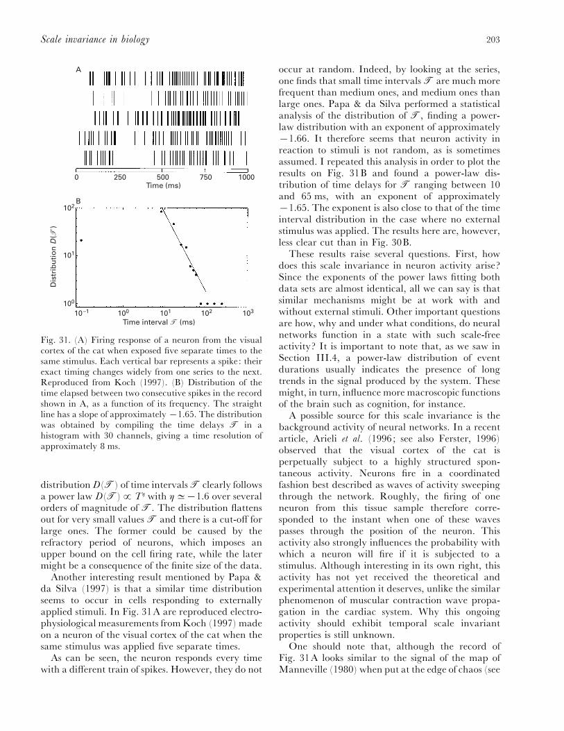
203Scale invariance in biology
1000
102
101
100
100 102
Time interval 4 (ms)
Dis
trib
uti
on
D(4
)
A
B
10–1 101 103
7505002500Time (ms)
Fig. 31. (A) Firing response of a neuron from the visualcortex of the cat when exposed five separate times to thesame stimulus. Each vertical bar represents a spike: theirexact timing changes widely from one series to the next.Reproduced from Koch (1997). (B) Distribution of thetime elapsed between two consecutive spikes in the recordshown in A, as a function of its frequency. The straightline has a slope of approximately ®1.65. The distributionwas obtained by compiling the time delays 4 in ahistogram with 30 channels, giving a time resolution ofapproximately 8 ms.
distribution D(4) of time intervals 4 clearly followsa power law D(4)£Tη with ηD®1.6 over severalorders of magnitude of 4. The distribution flattensout for very small values 4 and there is a cut-off forlarge ones. The former could be caused by therefractory period of neurons, which imposes anupper bound on the cell firing rate, while the latermight be a consequence of the finite size of the data.
Another interesting result mentioned by Papa &da Silva (1997) is that a similar time distributionseems to occur in cells responding to externallyapplied stimuli. In Fig. 31A are reproduced electro-physiological measurements from Koch (1997) madeon a neuron of the visual cortex of the cat when thesame stimulus was applied five separate times.
As can be seen, the neuron responds every timewith a different train of spikes. However, they do not
occur at random. Indeed, by looking at the series,one finds that small time intervals 4 are much morefrequent than medium ones, and medium ones thanlarge ones. Papa & da Silva performed a statisticalanalysis of the distribution of 4, finding a power-law distribution with an exponent of approximately®1.66. It therefore seems that neuron activity inreaction to stimuli is not random, as is sometimesassumed. I repeated this analysis in order to plot theresults on Fig. 31B and found a power-law dis-tribution of time delays for 4 ranging between 10and 65 ms, with an exponent of approximately®1.65. The exponent is also close to that of the timeinterval distribution in the case where no externalstimulus was applied. The results here are, however,less clear cut than in Fig. 30B.
These results raise several questions. First, howdoes this scale invariance in neuron activity arise?Since the exponents of the power laws fitting bothdata sets are almost identical, all we can say is thatsimilar mechanisms might be at work with andwithout external stimuli. Other important questionsare how, why and under what conditions, do neuralnetworks function in a state with such scale-freeactivity? It is important to note that, as we saw inSection III.4, a power-law distribution of eventdurations usually indicates the presence of longtrends in the signal produced by the system. Thesemight, in turn, influence more macroscopic functionsof the brain such as cognition, for instance.
A possible source for this scale invariance is thebackground activity of neural networks. In a recentarticle, Arieli et al. (1996; see also Ferster, 1996)observed that the visual cortex of the cat isperpetually subject to a highly structured spon-taneous activity. Neurons fire in a coordinatedfashion best described as waves of activity sweepingthrough the network. Roughly, the firing of oneneuron from this tissue sample therefore corre-sponded to the instant when one of these wavespasses through the position of the neuron. Thisactivity also strongly influences the probability withwhich a neuron will fire if it is subjected to astimulus. Although interesting in its own right, thisactivity has not yet received the theoretical andexperimental attention it deserves, unlike the similarphenomenon of muscular contraction wave propa-gation in the cardiac system. Why this ongoingactivity should exhibit temporal scale invariantproperties is still unknown.
One should note that, although the record ofFig. 31A looks similar to the signal of the map ofManneville (1980) when put at the edge of chaos (see

204 T. Gisiger
Fig. 10), the exponent of ®1.3 found there falls shortof the value of ®1.66 for the cortex of the cat.This model therefore overestimates the proportionof medium and large intervals between firingscompared to smaller ones. It also brings little in-sight into the mechanisms producing the observedpatterns.
Papa & da Silva (1997) propose that the power-law distribution observed is created by some mech-anism which self-organizes the cortex into a criticalstate via short-range interactions between neurons.The neural network model they introduce toillustrate this idea is mathematically very similar tothat used by Bak and Sneppen (1993) to modelevolution (see Section IV.2.d). As we saw above inthe sandpile model for instance, the distribution ofthe duration of avalanches follows a power law. Itcan be shown that so does the time one has to waitbetween avalanches, called ‘anti-avalanches ’ byPapa and colleagues (Papa & da Silva, 1997; daSilva et al., 1998). During these waiting periods, sandpiles up but does not slip, as the height of the sand isnowhere larger than the critical value 3. We cantherefore see how a self-organized critical modelmight reproduce the distribution of delays betweenspikes.
The model (Papa & da Silva, 1997; da Silva et al.,1998) that the authors propose represents neurons asdevices which fire stochastically with a probabilityroughly equal to e−σ. σ is a parameter of the neuronwhich quantifies its susceptibility to fire. The neuronsare then connected together in a network, with eachneuron only making synapses with its immediateneighbours. When a neuron fires, this changes(usually by raising it) the firing probability ofneighbouring cells as new values for σ are assignedto them. Also included in the model is the refractoryperiod which forbids a neuron from firing a secondtime before a minimum time delay R has passed.The dynamics of the model are then quite simple asneurons fire according to their intrinsic dynamics(quantified by parameter σ), itself subject to in-fluences from neighbouring cells. The dynamics,similar to that of the Bak–Sneppen model, leads thesystem to a critical state where numerous power lawsarise and, even though each neuron only connectsto its immediate neighbours, the firing of one cantrigger that of all other cells in the array. Themodel of Papa & da Silva (1997) and da Silvaet al. (1998) therefore predicts that cells in regions ofthe visual cortex can arrange themselves in a fallingdomino fashion. They also show that the exponentfor the anti-avalanche distribution, which approxi-
mates the time separating two firings from anarbitrary cell of the network, is roughly equal to®1.60, although it depends on the particular valuechosen for the refractory time R (Papa & da Silva,1997; da Silva et al., 1998). This value is quite closeto that obtained for the visual cortex of the cat (seeabove). Another strong point of this model for thespontaneous activity of neural networks is that thiscritical state is attained without fine tuning ofparameters such as synaptic weights. This is im-portant since there is mounting evidence that thereis not enough information contained in the genometo code for the strengths of all the synapses of thebrain (Koch, 1997) (i.e. to fine-tune synapticstrengths). Coding for such a simple algorithm as theone reviewed here, which adjusts the firing barriersof neurons, would certainly require a lot lessinformation.
VII. CONCLUSION
In this article, I have reviewed some recent advancesin the study of scale-free biological systems. Scaleinvariance is very common in nature, but it is onlysince the early 1970s that the mathematical toolsnecessary to define it more clearly were introduced.Objects without any characteristic length scales arenow called fractals (Mandelbrot, 1977, 1983) andtheir structure can be analyzed and quantified usingfractal dimensions. Signals with correlations onarbitrary time scales can be discriminated fromordinary background noise by computing theirpower spectrum or their Hurst exponent, or by usinggraphical methods. Scale invariance in the dynamicscan be detected by plotting on a log–log scale thedistribution of size or duration of events in thesystem.
Using these methods, scale invariance has beenobserved in diverse areas of biology. Ecosystemsseem to be highly scale-invariant : rain forestsgenerate fractal structures (Sole! & Manrubia, 1995a,b ; Manrubia & Sole! , 1997), population time seriescan exhibit 1}f behaviour (Halley, 1996; Mira-montes & Rohani, 1998), and extinction events seemto follow power-law distributions when enoughspecies are present (Keitt & Marquet, 1996). Scaleinvariance persists when considering the evolution ofecosystems on time scales of the order of hundreds ofmillions of years. The time evolution of the numberof families of organisms is self-similar on several timescales (Sole! et al., 1997), and has a 1}f powerspectrum. Also, distributions of extinction and

205Scale invariance in biology
diversification event sizes and durations follow powerlaws (Sneppen et al., 1995), as do the number oframifications of families in sub-families, and taxa insub-taxa (Burlando, 1990, 1993). Certain types ofepidemics too exhibit power-law distributions,clearly contrary to classical models of epidemics(Rhodes & Anderson, 1996b). Finally, even thecentral nervous system also seems to show some sortof scale invariance at different levels : 1}f-noise incommunication (Voss & Clarke, 1975) and cognition(Gilden et al., 1995; Gilden, 1997) power-lawdistributions in language (Zipf, 1949) and back-ground noise in the cortex (Papa & da Silva, 1997;da Silva et al., 1998).
Scale invariance is a phenomenon well known tophysicists who worked, also during the 1970s, oncritical phenomena and phase transitions. Thesesystems, when one sets the temperature to somecritical value, arrange themselves in states withoutany characteristic scale, exhibiting fractals andpower laws (Maris & Kadanoff, 1978; Wilson,1979). This theory was later generalized by Bak et al.(1987) to systems which spontaneously (i.e. withoutthe need for parameter fine tuning) organizethemselves in a critical state, therefore exhibitingscale invariance and sometimes producing 1}f-noise.In view of these remarkable advances, the importantquestion which arose from the work of Mandelbrot(1977, 1983) has shifted from ‘Why is there scaleinvariance in nature? ’ to ‘Is nature critical? ’ (Bak& Paczuski, 1993).
It is likely that no general answer exists to thisquestion. As we saw earlier, 1}f-noise, spatial scale-invariance and power-law distributions of events donot always implicate each other, let alone criticality.For instance, systems can generate 1}f-noise withoutbeing critical (see for instance De Los Rios & Zhang,1999 and references therein). In my view, thisquestion is therefore best answered case by case, bycarefully comparing experimental data with thepredictions of mathematical models of the systems.
Sole! & Manrubia (1995a, b) and Manrubia &Sole! (1997) make a strong case for rain forestvegetation being in a critical state, reproducingfractal dimensions of gaps in the vegetation. Thefindings of Rhodes & Anderson (1996a, b) andRhodes et al. (1997) on type III epidemics are just asimpressive, with a model which reproduces well thedata and gives further insight into the mechanism ofpropagation of diseases. Experimental evidence forcriticality in currently existing ecosystems of animalscould however be more convincing. By contrast, thepatterns obtained from fossil data are quite as-
tonishing and put under a lot of pressure theaccepted theory of the effect of catastrophes onecosystems. However, a firm confirmation of theoccurence of coevolutionary avalanches is needed toprove that ecosystems evolve to critical states. Thecase of the brain is the most puzzling of all, buttheoretical and mathematical investigation of thissystem is only at its beginning. Correlations on alltime scales are certainly possible in the brain, asthoughts, emotions and even communication areperpetually ongoing phenomena without any be-ginning or end. However, how this scale invariancecomes about and how it affects our actions and theway we communicate, is not known. This shouldprove an interesting starting point of investigation,complementing more traditional approaches inneurobiology.
Even if criticality turns out not to be a dominantprinciple in nature, work on critical systems andmodels has already tremendously increased ourcomprehension of the world around us. InChangeux’s (1993) words, models are abstractionswhich in no way can completely represent or beidentified with reality. However, every new type ofmodel adds to our understanding of dynamics andintroduces new concepts which help us understandreality. Chaotic systems triggered a revolution intheir days because no simple mathematical equationswere believed able to generate unstable and com-plicated trajectories. Even though chaotic systemshave been constructed and studied in the laboratory,few have been observed in nature, especially inbiology. However, concepts such as attractors,fractals and Lyapunov exponents, which wereintroduced by scholars of chaos, still serve as buildingblocks to understand the dynamics of non-chaotic oreven more complicated systems. Critical phenomenahave introduced physicists from all fields to phasetransitions, critical exponents and universality. It isprobable that in the future these concepts willbecome as commonly known to non-physicists asfractals are today. Perhaps by then even more exoticand exciting dynamics will have been encounteredelsewhere.
VIII. ACKNOWLEDGEMENTS
The author thanks M. B. Paranjape for his constantsupport throughout the entire preparation of this review,as well as M. Pearson, M. Kerszberg, J.-P. Changeux, R.Klink and V. Gisiger for many useful discussions and theircomments on the manuscript. The use of the libraries and
206 T. Gisiger
the computational facilities of the Centre de Calcul of theUniversite! de Montre! al, of the Laboratoire Rene! J. A.Le! vesque and of the Institut Pasteur are also gratefullyacknowledged.
IX. REFERENCES
A, Y., M, C. & K, T. (1984). Statistical
mechanics of intermittent chaos. Progress of Theoretical Physics
79, 96–124.
A, R. M. & M, R. M. (1991). Infectious Diseases of
Humans, Dynamics and Control. Oxford University Press.
A, A., S, A., G, A. & A, A. (1996).
Dynamics of ongoing activity : explanation of the large
variability in evoked cortical responses. Science 273, 1868–
1871.
B-L, H. (1989). Elementary Symbolic Dynamics. World Scien-
tific Publishing.
B, P. (1990). Self-organized criticality. Physica A163, 403–409.
B, P. (1996). How Nature Works: the Science of Self-Organized
Criticality. Springer-Verlag.
B, P. & C, K. (1989). The physics of fractals. Physica D38,
5–12.
B, P. & C, K. (1991). Self-organized criticality. Scientific
American 264, 46–53.
B, P., C, K. & C, M. (1989). Self-organized
criticality in the ‘Game of Life ’. Nature 342, 780–782.
B, P., C, K. & T, C. (1990). A forest-fire model and
some thoughts on turbulence. Physics Letters A147, 297–300.
B, P., F, H. & L, B. (1992). Coevolution in
a rugged fitness landscape. Physical Review A46, 6724–6730.
B, P. & P, M. (1993). Why nature is complex. Physics
World 6, 39–43.
B, P. & P, M. (1995). Complexity, contigency, and
criticality. Proceedings of the National Academy of Sciences of the
United States of America 92, 6689–6696.
B, P. & S, K. (1993). Punctuated equilibrium and
criticality in a simple model of evolution. Physical Review Letters
71, 4083–4086.
B, P., T, C. & W, K. (1987). Self-organized
criticality : an explanation of 1}f noise. Physical Review Letters
59, 381–384.
B, P., T, C. & W, K.. (1988). Self-organized
criticality. Physical Review A38, 364–374.
B, M. (1988). Fractals Everywhere. Academic Press Inc.
B, M. S. (1957). Measles periodicity and community
size. Journal of the Royal Statistical Society A120, 48–70.
B, M. S. (1960). The critical community size for measles
in the United States. Journal of the Royal Statistical Society A123,
37–44.
B, J. & S! , R. V. (1995). Rethinking complexity :
modelling spatiotemporal dynamics in ecology. Trends in
Ecology and Evolution 10, 361–366.
B, B. P. (1959). Sbornik Referatov po Radiacioni Medicine,
145ff (in Russian).
B, M. J. (1993). The Fossil Record 2, London: Chapman
and Hall.
B, M. J. (1995). Diversification and extinction in the
history of life. Science 268, 52–58.
B, E. R., C, J. H. G, R. K. (1982).
Winning Ways for Your Mathematical Plays, Vol. 2, Academic
Press.
B, A. A. & M, J. A. (1989). Are ecological
systems chaotic – And if not, why not? Trends in Ecology and
Evolution 4, 26–29.
B, J. J., D, N. J., F, A. J. & N, M. E. J.
(1992). The Theory of Critical Phenomena. Clarendon Press.
B, A. & D, M. (1996). In the red zone. Nature 380,
589–590.
B, S. R. & H, J. M. (1957). Percolation
processes. I. Crystals and mazes. Proceedings of the Cambridge
Philosophical Society 53, 629–641.
B, B. (1990). The fractal dimension of taxonomic
systems. Journal of Theoretical Biology 146, 99–114.
B, B. (1993). The fractal geometry of evolution. Journal
of Theoretical Biology 163, 161–172.
C, M. J. & J, B. W. (1972). Cyclic changes in
insulin needs of an unstable diabetic. Science 177, 889–891.
C, J.-P. (1985). Neuronal man: the biology of mind.
Pantheon Books.
C, J.-P. (1993). A critical view of neuronal models of
learning and memory. Memory concepts®1993: basic and
clinical aspects (Elsevier Science Publishers), 413–433.
C, D. R. & B, P. (1999). Learning from mistakes.
Neuroscience 90, 1137–1148.
C, K., C, A., F, V., F, J. & J,
T. (1996). Tracer dispersion in a self-organized critical
system. Physical Review Letters 77, 107–110.
C, K., F, H. C. & J, H. J. (1991).
Dynamical and spatial aspects of sandpile cellular automata.
Journal of Statistical Physics 63, 653–684.
C, K., O, Z. & B, P. (1992). Deterministic 1}f
noise in nonconservative models of self-organized criticality.
Physical Review Letters 68, 2417–2420.
C, S., D, B. & S, F. (1994). Scaling laws and
simulation results for the self-organized critical forest-fire
model. Physical Review E50, 1009–1018.
C, S. J. & P, J. L. (1996). Dynamic complexity in
Physarum polycephalum shuttle streaming. Protoplasma 194,
243–249.
C, J. L. (1995). Unexpected dominance of high frequencies
in chaotic nonlinear population models. Nature 378, 610–612.
C, U. M. S., L, M. L., P, A. R. & T, C.
(1997) Power-law sensitivity to initial conditions within a
logisticlike family of maps: fractality and nonextensivity.
Physical Review E56, 245–250.
D S, L., P, A. R. R. & D S, A. M. C. (1998).
Criticality in a simple model for brain functioning. Physical
Review A242, 343–348.
D, S. (1997). Number Sense: How the Brain Creates
Mathematics. Oxford University Press.
D L R, P. & Z, Y.-C. (1999). Universal 1}f noise
from dissipative self-organized criticality models. Physical
Review Letters 82, 472–475.
D B. & S, F. (1992). Self-organized critical forest-
fire model. Physical Review Letters 69, 1629–1632.
E, A. & I, L. (1938). The Evolution of Physics: the
Growth of Ideas from Early Concept to Relativity and Quanta. Simon
and Schuster, New York.
E, N. & G, S. J. (1972). Models in Paleobiology.
San Francisco: Freeman, Cooper.
F, K. J. (1985). The Geometry of Fractal Sets. Cambridge
University Press.
F, J. (1988). Fractals. Plenum Press.
207Scale invariance in biology
F, M. J. (1978). Quantitative universality for a class
of nonlinear transformations. Journal of Statistical Physics 19,
25–52.
F, M. J. (1979). The universal metric properties of
nonlinear transformations. Journal of Statistical Physics 21,
669–706.
F, D. (1996). Is neural noise just a nuisance? Science 273,
1812.
F, V., C, K., M-S, A., F,
J., J, T. & M, P. (1996). Avalanche dynamics in
a pile of rice. Nature 379, 49–52.
G, M. (1970). The fantastic combinations of John
Conway’s new solitaire game ‘ life ’. Scientific American 223, (4)
120–124.
G, R. & D, R. (1996). Responses of cells in the
superior colliculus during performance of a spatial attention
task in the macaque. Revista Brasileira de Biologia 56, 257–279.
G, D. L. (1997). Fluctuations in the time required for
elementary decisions, Psychological Science 8, 296–301.
G, D. L., T, T. & M, M. W. (1995). 1}f
noise in human cognition. Science 267, 1837–1839.
G, A. L., R, D. R. & W, B. J. (1990). Chaos
and fractals in human physiology. Scientific American 262,
42–49.
G, A. L. & W, B. J. (1987). Fractals in physiology
and medicine. Yale Journal of Biology and Medicine 60,
421–435.
G, S. J. & E, N. (1993). Punctuated equilibrium
comes of age. Nature 366, 223–227.
G, H. & T, J. (1988). An Introduction to Computer
Simulation Methods: applications to Physical Systems, Part II.
Addison-Wesley.
G, B. (1992). Quaternary climatic fluctuations as a
consequence of self-organized criticality. Physica A191, 51–56.
G, M. R., G, L. & S, A. (1981). Phase locking,
period-doubling bifurcations, and irregular dynamics in
periodically stimulated cardiac cells. Science 2l4, 1350–1353.
G, B. (1949). Seismicity of the Earth and Associated
Phenomena. Princeton University Press.
G, B. & R, C. F. (1956). Magnitude and
energy of earthquakes. Annali di Geofisica 9, 115ff.
H, J. M. (1996). Ecology, evolution and 1}f noise. Trends
in Ecology and Evolution 11, 33–37.
H, J. M. (1983). Origins of percolation theory.
Annals of the Israel Physical Society 5, 47–57.
H, R. G. B, D. J. (1986). Chaos in light.
Nature 321, 394–401.
H, M. P., C, H. N. & M, R. M. (1991). Spatial
structure and chaos in insect population dynamics. Nature
353, 255–258.
H, A., H, C. L., E, S., T, P. & G,
H. C. J. (1993). Chaos in ecology: Is mother nature a strange
attractor? Annual Review of Ecological Systems 24, 1–33.
H, A. (1989). What, if anything, are mass extinctions?
Philosophical Transactions of the Royal Society of London B325,
253–261.
H, M. R. (1989). Ammonoid extinction events. Philosophical
Transactions of the Royal Society of London B325, 307–326.
H, H. E. (1951) Transactions of the American Society of Civil
Engineers 116, 770–808.
H, H. E., B, R. P. & S, Y. M. (1965). Long-
Term Storage: an Experimental Study. Constable.
J, D. (1991). Extinctions : a paleontological perspective.
Science 253, 754–757.
J, H. J. (1990). Chaos game representation of gene
structure. Nucleic Acids Research 18, 2163–2170.
J, H. J. (1990). Lattice gas as a model of 1}f noise. Physical
Review Letters 64, 3103–3106.
J, H. J., C, K. & F, H. C. (1989). 1}f
noise, distribution of lifetimes, and a pile of sand. Physical
Review B40, 7425–7427.
K, E., G, S. & E, S. N. (1997).
1}f noise and multifractal fluctuations in rat behavior.
Nonlinear Analysis, Theory, Methods and Applications 30, 2007–
2013.
K, V. & R, E. (1996). Scientific correspondence.
Nature 381, 199.
K, K. (1989). Pattern dynamics in spatiotemporal chaos.
Physica D34, 1–41.
K, D. T. & G, L. (1992). Direct test for determinism
in a time series. Physical Review Letters 68, 427–430.
K, S. A. (1989a). Adaptation on rugged fitness land-
scapes. Lectures in the Sciences of Complexity. The Santa Fe Institute
Series (Addison Wesley), 527–618 and 619–712.
K, S. A. (1989b). Principles of adaptation in complex
systems. Lectures in the Sciences of Complexity. The Santa Fe Institute
Series (Addison Wesley), 619–712.
K, S. A. & J, S., (1991). Coevolution to the
edge of chaos : coupled fitness landscapes, poised states and
coevolutionary avalanches. Journal of Theoretical Biology 149,
467–505.
K, S. A. & L, S. (1987). Towards a general theory
of adaptive walks on rugged fitness landscapes. Journal of
Theoretical Biology 128, 11–45.
K, T. H. & M, P. A. (1996). The introduced
Hawaiian avifauna reconsidered: Evidence for self-organized
criticality? Journal of Theoretical Biology 182, 161–167.
K, D. E. (1975). The role of phyletic changes in the
evolution of Pseudocubus vema (Radiolaria). Paleobiology 1,
359–370.
K! , J. & K, L. B. (1990). The noise spectrum in the
model of self-organized criticality. Journal of Physics: Math-
ematical and General A23, L433–L440.
K, C. (1997). Computation and the single neuron. Nature
385, 207–210.
L, C. (1990). Computation at the edge of chaos : phase
transitions and emergent computation. Physica D42, 12–37.
L B, M. (1988). Des pheUnome[ nes critiques aux champs de jauge.
InterEditions}Editions du CNRS.
L, A., L, C. & F, S. (1982). Period
doubling cascade in mercury, a quantitative measurement.
Journal de Physique Lettres 43, L211–L216.
L, E. N. (1963). Deterministic nonperiodic flow. Journal of
the Atmospheric Sciences 20, 130ff.
M, B. B. (1977). Fractals: Form, Chance and Dimension,
W. H. Freeman.
M, B. B. (1983). The Fractal Geometry of Nature, W. H.
Freeman.
M, P. (1980). Intermittency, self-similarity and 1}f
spectrum in dissipative dynamical systems. Journal of Physics
(Paris) 41, 1235–1243.
M, S. C. & S! , R. V. (1997). On forest spatial
dynamics with gap formation. Journal of Theoretical Biology
187, 159–164.

208 T. Gisiger
M,H. J.&K,L. P.(1978).Teachingtherenormaliz-
ation group. American Journal of Physics 46, 652–657.
M-T, R. A. & W, M. A. (1997). Visualisation of
random sequences using the chaos game algorithm. Journal of
Systems and Software 39, 3–6.
M, R. M. (1976). Simple mathematical models with very
complicated dynamics. Nature 261, 459–467.
M S, J. (1989). The causes of extinction. Philo-
sophical Transactions of the Royal Society of London B325, 241–252.
MN, J. E. (1991). Fractal perspectives in pulmonary
physiology. Journal of Applied Physiology 71, 1–8.
M, O. & R, P. (1998). Intrinsically generated
coloured noise in laboratory insect populations. Proceedings of
the Royal Society of London B265, 785–792.
N, M. E. J. (1996). Self-organized criticality, evolution
and the fossil extinction record. Proceedings of the Royal Society
of London B263, 1605–1610.
N, M. E. J. (1997a). A model of mass extinction. Journal
of Theoretical Biology 189, 235–252.
N, M. E. J. (1997b). Evidence for self-organized criti-
cality in evolution. Physica D107, 293–296.
N, A. J. (1957). The self-adjustment of populations to
change. Cold Spring Harbour Symposia on Quantitative Biology 22,
153–173.
N, G. & P, I. (1989). Exploring Complexity: an
Introduction. Freeman.
N, D., E, S., MC, D. & G, A. R.
(1992). Finding chaos in noisy systems. Journal of the Royal
Statistical Society B54, 399–426.
P, A. R. R. & D S, L. (1997). Earthquakes in the
brain. Theory in Biosciences 116, 321–327.
P, G. (1993). Statistical physics and biology. Physics World
6, 42–47.
P, D., L, G. & W, E. R. (1981). Res-
olution effect on the stereological estimation of surface and
volume and its interpretation in terms of fractal dimension.
Journal of Microscopy 121, 51–63.
P, B. & K, D. T. (1999). Nonstationarity and 1}f
noise characteristics in heart rate. American Journal of
Physiology: Regulatory Integrative and Comparative Physiology 45,
R1–R9.
P, S. L. & R, A. (1988). The variability of
population densities. Nature 334, 613–614.
P, M. I. & P, A. (1998). Anatomy of word and
sentence meaning. Proceedings of the National Academy of Sciences
of the United States of America 95, 899–905.
P, W. H. (1978). Flicker noises in astronomy and elsewhere.
Comments on Astrophysics 7, 103–119.
P, W. H., T, S. A., V, W. T.,
F, B. P. (1988). Numerical Recipes in C: the Art of
Scientific Computing, Second Edition, Cambridge University
Press.
P, I. & S, H. (1983). Functional renormaliz-
ation-group theory of universal 1}f noise in dynamical
systems. Physical Review A28, 1210–1212.
R, D. M. (1986). Biological extinction in earth history.
Science 231, 1528–1533.
R, D. M. (1989). The case for extraterrestrial causes of
extinction. Philosophical Transactions of the Royal Society of London
B325, 421–435.
R, D. M. & B, G. E. (1988). Patterns of generic
extinction in the fossil record. Paleobiology 14, 109–125.
R, D. M. & S, J. J., J. (1982). Mass extinctions in
the marine fossil records. Science 215, 1501–1502.
R, D. M. & S, J. J., J. (1984). Periodicity of
extinctions in the geological past. Proceedings of the National
Academy of Sciences of the United States of America 81, 801–805.
R, C. J. & A, R. M. (1996a). A scaling analysis of
measles epidemics in a small population. Philosophical Trans-
actions of the Royal Society of London B351, 1679–1688.
R, C. J. & A, R. M. (1996b). Power laws
governing epidemics in isolated populations. Nature 381,
600–602.
R, C. J., J, H. J. & A, R. M. (1997). On the
critical behaviour of simple epidemics. Proceedings of the Royal
Society of London B264, 1639–1646.
R, R. (1993) Adapting to complexity. Scientific American
268, 130–140.
S, T. R. (1993). Life in one dimension: statistics and self-
organized criticality. Journal of Physics A: Mathematical and
General 26, 6187–6193.
S, K. L. & V, A. A. (1974) 1}f noise with a low
frequency white noise limit. Nature 251, 599–601.
S, J. J., J. (1982). A compendium of fossil marine families
Milwaukee. Public Museum Contributions in Biology and
Geology 51.
S, J. J., J. (1993). Ten years in the library: new data
confirm paleontological patterns. Paleobiology 19, 43–51.
S, K. (1995). Extremal dynamics and punctuated co-
evolution. Physica A221, 168–179.
S, K., B, P., F, H. & J, M. H. (1995).
Evolution as a self-organized critical phenomenon. Proceedings
of the National Academy of Sciences of the United States of America
92, 5209–5213.
S! , R. V. (1996). On macroevolution, extinctions and critical
phenomena. Complexity 1, 40–44.
S! , R. V. & B, J. (1996). Are critical phenomena
relevant to large-scale phenomena. Proceedings of the Royal
Society of London 263, 161–168.
S! , R. V., B, J. & M, S. C. (1996).
Extinction: bad genes or weak chaos. Proceedings of the Royal
Society of London B263, 1407–1413.
S! , R. V. & M, S. C. (1995a). Are rain forests self-
organized in a critical state? Journal of Theoretical Biology 173,
31–40.
S! , R. V. & M, S. C. (1995b). Self-similarity in rain
forests : Evidence for a critical state. Physical Review E51,
6250–6253.
S! , R. V. & M, S. C. (1996). Extinction and self-
organized criticality in a model of large-scale evolution.
Physical Review E54, R42–R45.
S! , R. V. & M, S. C. (1997). Criticality and
unpredictability in macroevolution. Physical Review E55,
4500–4507.
S! , R. V., M, S. C., B, M. & B, P. (1997).
Self-similarity of extinction statistics in the fossil record. Nature
388, 764–767.
S, A. & S, D. (1989). Self-organized criticality
and earthquakes. Europhysics Letters 9, 197–202.
S, D. & B, P. (1995). Democratic reinforce-
ment: a principle for brain function. Physical Review E51,
5033–5039.
S, D. (1979). Scaling theory of percolation clusters.
Physics Reports 54, 1–74.

209Scale invariance in biology
S, J. H. (1985). A comparison of terrestrial and marine
ecological systems. Nature 313, 355–358.
S, T. K., G, W. S. C., N, R. M. & B, S.
P. (1988). Parameter evolution in a laboratory insect
population. Theoretical Population Theory 34, 248–265.
S, S. H. (1994). Nonlinear Dynamics and Chaos. Addison-
Wesley Publishing.
S, G. (1996). Scientific correspondence. Nature 381,
199.
S, G. & M, R. M. (1990). Nonlinear forecasting as a
way of distinguishing chaos from measurement error in time
series. Nature 344, 734–741.
T, C. & B, P. (1988). Critical exponents and scaling
relations for self-organized critical phenomena. Physical Review
Letters 60, 2347–2350.
T, D. L. (1992). Fractals and Chaos in Geology and
Geophysics. Cambridge University Press.
U, S. (1957). Cyclic fluctuations of population density
intrinsic to the host-parasite system. Ecology 38, 442–449.
V, R. F. & C, J. (1975). 1}f noise in music and speech.
Nature 258, 317–318.
W, G. B., B, J. H. & E, B. J. (1997). A general
model for the origin of allosteric scaling laws in biology. Nature
276, 122–126.
W, A., B, M. & B, R. G. (1996a). Explaining
the colour of power spectra in chaotic ecological models.
Proceedings of the Royal Society of London B263, 1731–1737.
W, A., B, R. G. & B, M. (1996b). Red}Blue
chaotic power spectra. Nature 381, 198.
W, K. G. (1979). Problems in physics with many scales of
length. Scientific American 241, 158–179.
W, A. M. & K, A. B. (1973). The timing of
interresponse intervals. Perception and Psychophysics 14, 455–460.
W, S. (1983). Statistical mechanics of cellular automata.
Review of Modern Physics 55, 601–644.
W, S. (1984). Universality and complexity in cellular
automata. Physica D10, 1–35.
W, S. (1986). Theory and Applications of Cellular Automata.
World Scientific.
W, S. (1982). Character change, speciation, and the
higher taxa. Evolution 36, 427–443.
Z, A. (1964). Biofizika 9, 306ff (in Russian).
Z, G. K. (1949). Human Behaviour and the Principle of Least
Effort. Haffner Publishing.