scaling back the cl, cd, cm coefficients from normalized...

<www.excelunusual.com> 1

Longitudinal Aircraft Dynamics #6– worksheet implementation of the real dynamics by George Lungu

- This section proceeds with finalizing the dynamics formulas governing out 2D plane.

Scaling back the cl, cd, cm coefficients from normalized to real values:

- The data obtained from Xflr5 on the airfoils is two-dimensional data. This means that that the program simulates a section of a wing of infinite span. The data obtained is associated with just the airfoil and has no association with the span of the wing. Aerodynamic characteristics recorded include the lift coefficient cl , the drag coefficient cd and the pitching moment coefficient about the quarter-chord point (from the leading edge) cm. These coefficients are obtained by calculating the forces and moments per unit length of the airfoil wing and expressing them as follows:

cl= l / qc

- where l is the measured lift per unit length of the airfoil wing, q is the testing dynamic pressure or

1/2*(rv2), r is the ambient air density, v the speed of the air relative to the airfoil and c is the chord length of the airfoil section. Similarly:

A cutaway through the flying wing Atlantica – www.wingco.com

cd= d / qc

- where d is the measured drag per unit length of the airfoil wing

cm = m / qc2

- where m is the moment per unit length acting on the airfoil measured at the quarter point of the chord from the leading edge.


- Let’s extract the real un-normalized lift force:

ChordSpeedyAir_densit

Span

Lift

cv

Span

L

cq

lcl

22

22r

SpanChordSpeedyAir_densitcLift l 2

2

1

- Let’s extract the real

un-normalized drag force:Chord

SpeedyAir_densit

Span

Drag

cv

Span

D

cq

dcd

22

22r

SpanChordSpeedyAir_densitcDrag d 2

2

1

- Let’s extract the real

un-normalized pitching moment:

22

222

22Chord

SpeedyAir_densit

Span

Moment

cv

Span

M

cq

mcm

r

SpanChordSpeedyAir_densitcMoment m 22

2

1


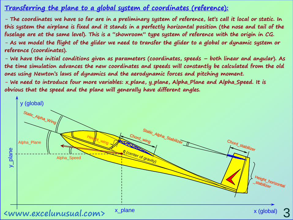
Transferring the plane to a global system of coordinates (reference):

- The coordinates we have so far are in a preliminary system of reference, let’s call it local or static. In this system the airplane is fixed and it stands in a perfectly horizontal position (the nose and tail of the fuselage are at the same level). This is a “showroom” type system of reference with the origin in CG.

- As we model the flight of the glider we need to transfer the glider to a global or dynamic system or reference (coordinates).

- We have the initial conditions given as parameters (coordinates, speeds – both linear and angular). As the time simulation advances the new coordinates and speeds will constantly be calculated from the old ones using Newton’s laws of dynamics and the aerodynamic forces and pitching moment.

- We need to introduce four more variables: x_plane, y_plane, Alpha_Plane and Alpha_Speed. It is obvious that the speed and the plane will generally have different angles.

y (global)

Static_Alpha_Wing

Static_Alpha_Stabilizer

0 (center of gravity)

Height_horizontal

_stabilizer

Height_wing Chord_stabilizer

Chord_wing

Static_Alpha_Wing



Height_horizontal

_stabilizer


Chord_wingAlpha_Plane

Alpha_Speed

x (global)x_plane

y_

pla

ne


Dynamic considerations – how does the model work?

- Essentially this model is the 2D model of a stick having a mass and a momentum of inertia.

- The stick is being launched from known conditions (coordinates and speeds – both linear and angular)

and knowing the forces (aerodynamic and gravity) and pitching momentum acting on the stick, we can

calculate both linear and angular accelerations within a small time interval (Newton’s second law).

- From accelerations (both linear and angular) we can calculate speeds by integration and then from

speeds (both linear and angular) we can calculate new coordinates by integration. We can do this

incrementally, within small time steps and recursively calculate new coordinates and speeds from the

old coordinates and speeds as a loop.

- For small enough time steps we can use very simple approximations of the integrals so that the

resulting formulas are simple. A flow chart of the calculation loop principle is shown below. This

technique has already been used in several models on this site.

Linear speed and coordinates (old) Angular speed and coordinate (old)

Newton 2nd law (linear) Newton 2nd law (angular)

Aerodynamic extracted functions (lift force, drag force and pitching moment)

Linear Acceleration

Angular speed and coordinate (new)

Integration

Lo

op

Lo

op

Gravity

Angular Acceleration

Integration

Linear speed and coordinates (new)

IntegrationIntegration

MassMoment

of inertia

The loop will be implemented as a “copy-the-present-

and-paste-it-in-the-past” infinite do loop macro.


Dynamic implementation:

- We saw that our method of calculation involves an infinite loop in which the data from the past is used to calculate the present results (speeds and coordinates).

- After the results are calculated, they are copied and pasted in the

location of the past data. It is a recursive feedback scheme in which the model constantly feeds itself with its own results and since the time step is small the recursive scheme can use simplified formulas for derivatives and integrals.

-In the snapshot above, the initial conditions (constants) will be contained in the yellow ranges (D47:G47 and I47:J47), the active formulas (present) will be contained in the green range (B51:J51) and the past data (constants) will be in the orange ranges (D52:G52 and I52:J52).

- Range K51:K52 handles the index which is an integer equal to the number of loop iterations.

The macros: - The role of the Boolean “runpause” variable in the “Run_Pause” macro is to allow this macro to be started of stopped using the same button.

- Any time by clicking on the Run_Pause button, the variable is toggled between True or False. Because of this, the conditional Do loop will be stopped if it’s running or started if it’s stopped. Otherwise, the macro does nothing more than copying data from present calculation area into the past buffer and shifting all the history back one time step. Since the copy-paste operation is done over 1000 rows, 1000 time steps of historical data will be available for charting later (we can plot an airplane trail for example, or some other historical data)

- The “Reset” macro first clears all the historical data then pastes the initial conditions in the “past” row.

Dim runpause As Boolean

Sub Run_Pause()

runpause = Not (runpause)

Do While runpause = True

DoEvents

[D52:K1052] = [D51:K1051].Value

Loop

End Sub

Sub Reset()

[D52:K1052].ClearContents

[D52:K52] = [D47:K47].Value

End Sub


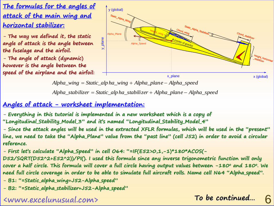
The formulas for the angles of

attack of the main wing and

horizontal stabilizer:

- The way we defined it, the static angle of attack is the angle between the fuselage and the airfoil.

- The angle of attack (dynamic) however is the angle between the speed of the airplane and the airfoil:

dAlpha_speeeAlpha_planzerha_stabiliStatic_alpilizerAlpha_stab

dAlpha_speeeAlpha_planha_wingStatic_alpAlpha_wing

y (global)

Static_Alpha_Wing



Height_horizontal

_stabilizer


Chord_wing

Static_Alpha_Wing



Height_horizontal

_stabilizer


Chord_wingAlpha_Plane

Alpha_Speed

x (global)x_plane

y_

pla

ne

- Everything in this tutorial is implemented in a new worksheet which is a copy of “Longitudinal_Stability_Model_3” and it’s named “Longitudinal_Stability_Model_4”

- Since the attack angles will be used in the extracted XFLR formulas, which will be used in the “present” line, we need to take the “Alpha_Plane” value from the “past line” (cell J52) in order to avoid a circular reference.

- First let’s calculate “Alpha_Speed” in cell O64: “=IF(E52>0,1,-1)*180*ACOS(-D52/SQRT(D52^2+E52^2))/PI(). I used this formula since any inverse trigonometric function will only cover a half circle. This formula will cover a full circle having output values between -180o and 180o. We need full circle coverage in order to be able to simulate full aircraft rolls. Name cell N64 “Alpha_speed”.

- B1: “=Static_alpha_wing+J52-Alpha_speed”

- B2: “=Static_alpha_stabilizer+J52-Alpha_speed”

Angles of attack - worksheet implementation:

To be continued…

scaling back the cl, cd, cm coefficients from normalized...

Documents