scaling constants and the lazy peeling of infinite boltzmann planar maps
TRANSCRIPT
Random Planar Structures and Statistical Mechanics, Isaac NewtonInstitute, Cambridge, 20-04-2015
Scaling constants and the lazy peeling of infiniteBoltzmann planar maps
Timothy Budd
Niels Bohr InstituteUniversity of [email protected]
http://www.nbi.dk/~budd/
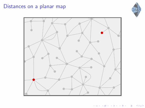
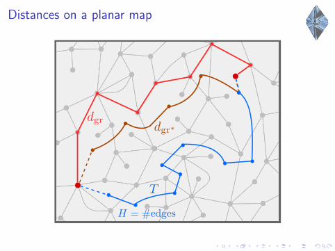
Distances on a planar map

Distances on a planar map
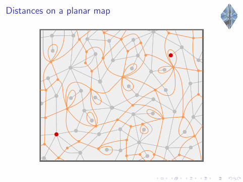
Distances on a planar map
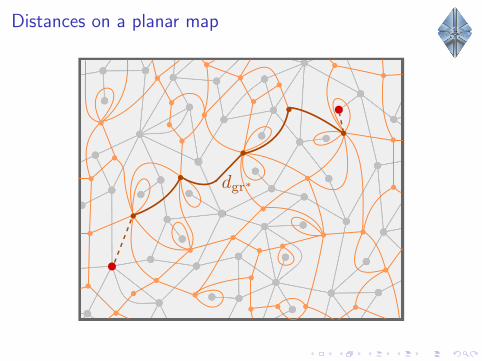
Distances on a planar map

Distances on a planar map

Distances on a planar map
Distances on a planar map
Outline
I Introduce lazy peeling of planar maps
I Description of the associated perimeter and volume processes
I Scaling limit
I Scaling constants from peeling:I First-passage timeI Hop countI Dual graph distance
I Miermont’s scaling constant for the graph distance
I Example: uniform infinite planar map.
I From lazy to simple peeling.
I Open questions.

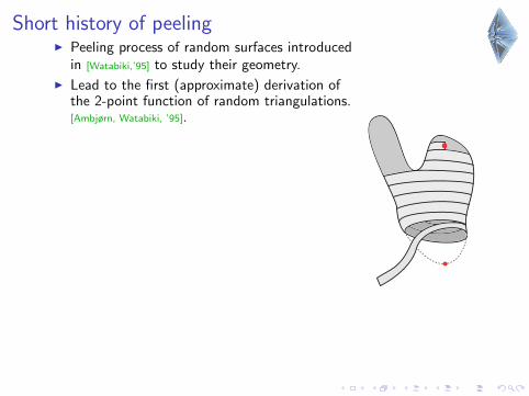
Short history of peelingI Peeling process of random surfaces introduced
in [Watabiki,’95] to study their geometry.
I Lead to the first (approximate) derivation ofthe 2-point function of random triangulations.[Ambjørn, Watabiki, ’95].
I Remark: Their 2-point function is not just an
approximation, it is exactly the “first-passage
time 2-point function” [Ambjørn,TB,’14].
I Peeling was formalized in the setting of infinitetriangulations (UIPT) in [Angel, ’03].
I Important tool to study properties of the UIPTand UIPQ: distances, percolation, randomwalks [Angel,’03’][Angel, Curien, ’13] [Benjamini, Curien
’13]...
I Precise scaling limits have been obtained forthe perimeter and volume of the exploredregion in the UIPT and UIPQ [Curien, Le Gall, ’14],
Le Gall’s talk!
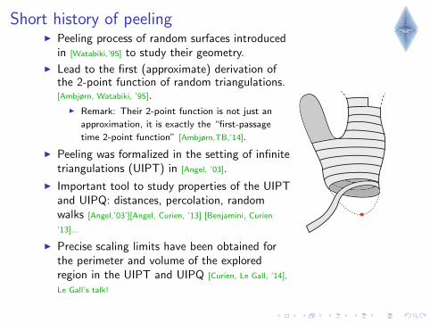

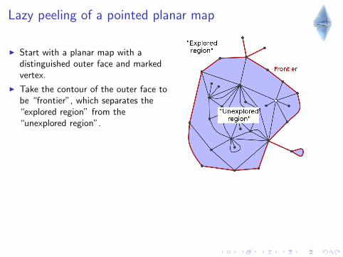
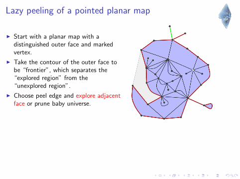
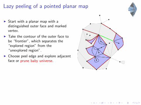
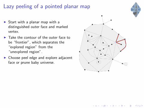
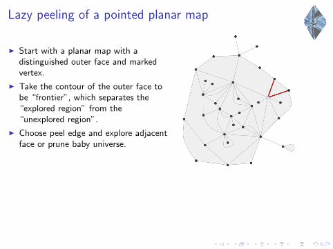
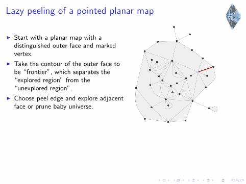
Lazy peeling of a pointed planar map
I Start with a planar map with adistinguished outer face and markedvertex.
I Take the contour of the outer face tobe “frontier”, which separates the“explored region” from the“unexplored region”.
I Choose peel edge and explore adjacentface or prune baby universe.
I After finite number of steps theunexplored region contains only themarked vertex.
I First goal: given a random disk, whatis the law of the perimeter (li )i≥0, i.e.the length of the frontier after i steps?
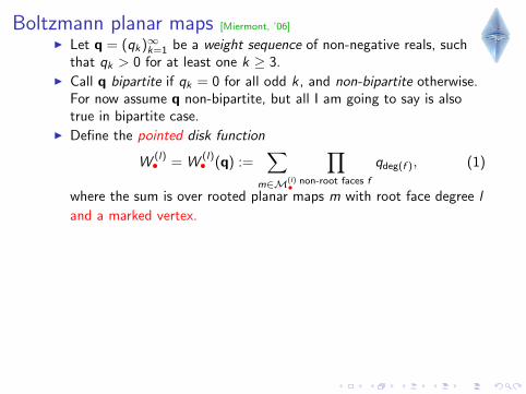
Boltzmann planar maps [Miermont, ’06]
I Let q = (qk)∞k=1 be a weight sequence of non-negative reals, suchthat qk > 0 for at least one k ≥ 3.
I Call q bipartite if qk = 0 for all odd k , and non-bipartite otherwise.For now assume q non-bipartite, but all I am going to say is alsotrue in bipartite case.
I Define the disk function
W(l)
•
= W(l)
•
(q) :=∑
m∈M(l)
•
∏non-root faces f
qdeg(f ), (1)
where the sum is over rooted planar maps m with root face degree l
and a marked vertex. If W(l)• finite, the summands determine a
probability measure, which we call the q-BPM.
I Call q admissible if Z• := W(2)• <∞. [Miermont, ’06]
Theorem (Miermont, ’06)
f •(x , y) :=∞∑
k,k′=0
xkyk′(
2k + k ′ + 1
k + 1
)(k + k ′
k
)q2+2k+k′ , f �(x , y) :=
∞∑k,k′=0
xkyk′(
2k + k ′
k
)(k + k ′
k
)q1+2k+k′ .
The sequence q is admissible if and only if there exist z+, z� > 0 such that f •(z+, z�) = 1− 1z+ , f �(z+, z�) = z�
and the matrix Mq(z+, z�) :=
0 0 z+ − 1z+
z� ∂x f �(z+, z�) ∂y f �(z+, z�) 0(z+)2
z+−1∂x f •(z+, z�) z+z�
z+−1∂y f •(z+, z�) 0
has spectral radius ≤ 1.
Boltzmann planar maps [Miermont, ’06]
I Let q = (qk)∞k=1 be a weight sequence of non-negative reals, suchthat qk > 0 for at least one k ≥ 3.
I Call q bipartite if qk = 0 for all odd k , and non-bipartite otherwise.For now assume q non-bipartite, but all I am going to say is alsotrue in bipartite case.
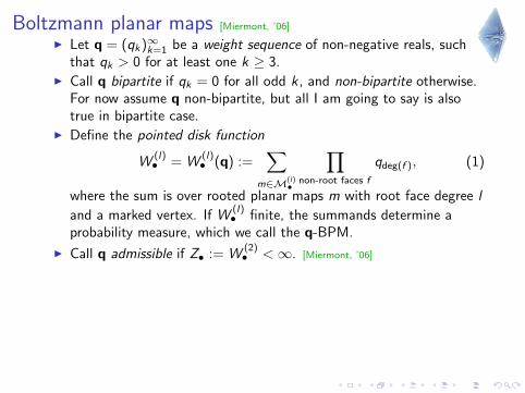
I Define the pointed disk function
W(l)• = W
(l)• (q) :=
∑m∈M(l)
•
∏non-root faces f
qdeg(f ), (1)
where the sum is over rooted planar maps m with root face degree l
and a marked vertex.
If W(l)• finite, the summands determine a
probability measure, which we call the q-BPM.
I Call q admissible if Z• := W(2)• <∞. [Miermont, ’06]
Theorem (Miermont, ’06)
f •(x , y) :=∞∑
k,k′=0
xkyk′(
2k + k ′ + 1
k + 1
)(k + k ′
k
)q2+2k+k′ , f �(x , y) :=
∞∑k,k′=0
xkyk′(
2k + k ′
k
)(k + k ′
k
)q1+2k+k′ .
The sequence q is admissible if and only if there exist z+, z� > 0 such that f •(z+, z�) = 1− 1z+ , f �(z+, z�) = z�
and the matrix Mq(z+, z�) :=
0 0 z+ − 1z+
z� ∂x f �(z+, z�) ∂y f �(z+, z�) 0(z+)2
z+−1∂x f •(z+, z�) z+z�
z+−1∂y f •(z+, z�) 0
has spectral radius ≤ 1.

Boltzmann planar maps [Miermont, ’06]
I Let q = (qk)∞k=1 be a weight sequence of non-negative reals, suchthat qk > 0 for at least one k ≥ 3.
I Call q bipartite if qk = 0 for all odd k , and non-bipartite otherwise.For now assume q non-bipartite, but all I am going to say is alsotrue in bipartite case.
I Define the pointed disk function
W(l)• = W
(l)• (q) :=
∑m∈M(l)
•
∏non-root faces f
qdeg(f ), (1)
where the sum is over rooted planar maps m with root face degree l
and a marked vertex. If W(l)• finite, the summands determine a
probability measure, which we call the q-BPM.
I Call q admissible if Z• := W(2)• <∞. [Miermont, ’06]
Theorem (Miermont, ’06)
f •(x , y) :=∞∑
k,k′=0
xkyk′(
2k + k ′ + 1
k + 1
)(k + k ′
k
)q2+2k+k′ , f �(x , y) :=
∞∑k,k′=0
xkyk′(
2k + k ′
k
)(k + k ′
k
)q1+2k+k′ .
The sequence q is admissible if and only if there exist z+, z� > 0 such that f •(z+, z�) = 1− 1z+ , f �(z+, z�) = z�
and the matrix Mq(z+, z�) :=
0 0 z+ − 1z+
z� ∂x f �(z+, z�) ∂y f �(z+, z�) 0(z+)2
z+−1∂x f •(z+, z�) z+z�
z+−1∂y f •(z+, z�) 0
has spectral radius ≤ 1.
Boltzmann planar maps [Miermont, ’06]
I Let q = (qk)∞k=1 be a weight sequence of non-negative reals, suchthat qk > 0 for at least one k ≥ 3.
I Call q bipartite if qk = 0 for all odd k , and non-bipartite otherwise.For now assume q non-bipartite, but all I am going to say is alsotrue in bipartite case.
I Define the pointed disk function
W(l)• = W
(l)• (q) :=
∑m∈M(l)
•
∏non-root faces f
qdeg(f ), (1)
where the sum is over rooted planar maps m with root face degree l
and a marked vertex. If W(l)• finite, the summands determine a
probability measure, which we call the q-BPM.
I Call q admissible if Z• := W(2)• <∞. [Miermont, ’06]
Theorem (Miermont, ’06)
f •(x , y) :=∞∑
k,k′=0
xkyk′(
2k + k ′ + 1
k + 1
)(k + k ′
k
)q2+2k+k′ , f �(x , y) :=
∞∑k,k′=0
xkyk′(
2k + k ′
k
)(k + k ′
k
)q1+2k+k′ .
The sequence q is admissible if and only if there exist z+, z� > 0 such that f •(z+, z�) = 1− 1z+ , f �(z+, z�) = z�
and the matrix Mq(z+, z�) :=
0 0 z+ − 1z+
z� ∂x f �(z+, z�) ∂y f �(z+, z�) 0(z+)2
z+−1∂x f •(z+, z�) z+z�
z+−1∂y f •(z+, z�) 0
has spectral radius ≤ 1.
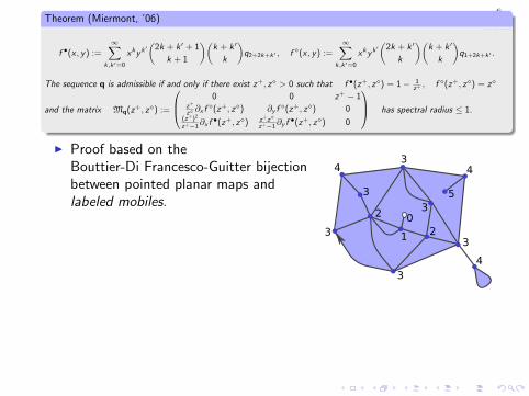
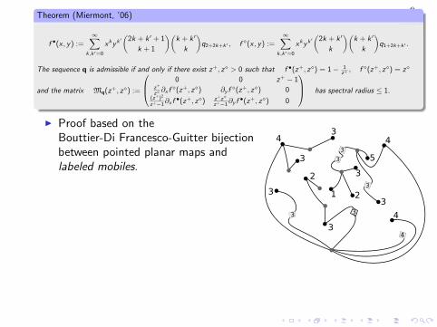
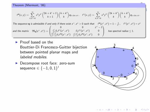
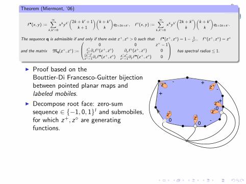
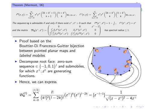
I Proof based on theBouttier-Di Francesco-Guitter bijectionbetween pointed planar maps andlabeled mobiles.
I Decompose root face:
zero-sumsequence ∈ {−1, 0, 1}l and submobiles,for which z+, z� are generatingfunctions.
I Hence, we can express
W(l)• =
bl/2c∑k=0
l!
(k!)2(l − 2k)!(z+)k(z�)l−2k = [z−l−1]
1√(z − z�)2 − 4z+
Theorem (Miermont, ’06)
f •(x , y) :=∞∑
k,k′=0
xkyk′(
2k + k ′ + 1
k + 1
)(k + k ′
k
)q2+2k+k′ , f �(x , y) :=
∞∑k,k′=0
xkyk′(
2k + k ′
k
)(k + k ′
k
)q1+2k+k′ .
The sequence q is admissible if and only if there exist z+, z� > 0 such that f •(z+, z�) = 1− 1z+ , f �(z+, z�) = z�
and the matrix Mq(z+, z�) :=
0 0 z+ − 1z+
z� ∂x f �(z+, z�) ∂y f �(z+, z�) 0(z+)2
z+−1∂x f •(z+, z�) z+z�
z+−1∂y f •(z+, z�) 0
has spectral radius ≤ 1.
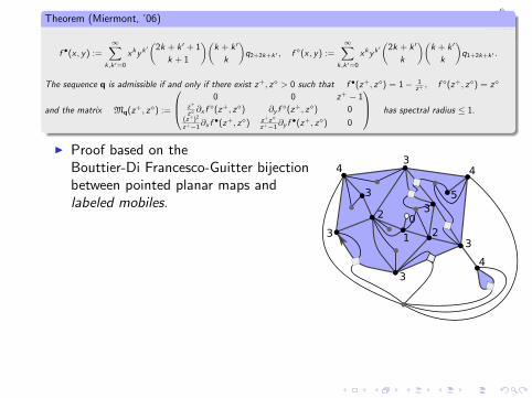
I Proof based on theBouttier-Di Francesco-Guitter bijectionbetween pointed planar maps andlabeled mobiles.
I Decompose root face:
zero-sumsequence ∈ {−1, 0, 1}l and submobiles,for which z+, z� are generatingfunctions.
I Hence, we can express
W(l)• =
bl/2c∑k=0
l!
(k!)2(l − 2k)!(z+)k(z�)l−2k = [z−l−1]
1√(z − z�)2 − 4z+
Theorem (Miermont, ’06)
f •(x , y) :=∞∑
k,k′=0
xkyk′(
2k + k ′ + 1
k + 1
)(k + k ′
k
)q2+2k+k′ , f �(x , y) :=
∞∑k,k′=0
xkyk′(
2k + k ′
k
)(k + k ′
k
)q1+2k+k′ .
The sequence q is admissible if and only if there exist z+, z� > 0 such that f •(z+, z�) = 1− 1z+ , f �(z+, z�) = z�
and the matrix Mq(z+, z�) :=
0 0 z+ − 1z+
z� ∂x f �(z+, z�) ∂y f �(z+, z�) 0(z+)2
z+−1∂x f •(z+, z�) z+z�
z+−1∂y f •(z+, z�) 0
has spectral radius ≤ 1.
I Proof based on theBouttier-Di Francesco-Guitter bijectionbetween pointed planar maps andlabeled mobiles.
I Decompose root face: zero-sumsequence ∈ {−1, 0, 1}l
and submobiles,for which z+, z� are generatingfunctions.
I Hence, we can express
W(l)• =
bl/2c∑k=0
l!
(k!)2(l − 2k)!(z+)k(z�)l−2k = [z−l−1]
1√(z − z�)2 − 4z+
Theorem (Miermont, ’06)
f •(x , y) :=∞∑
k,k′=0
xkyk′(
2k + k ′ + 1
k + 1
)(k + k ′
k
)q2+2k+k′ , f �(x , y) :=
∞∑k,k′=0
xkyk′(
2k + k ′
k
)(k + k ′
k
)q1+2k+k′ .
The sequence q is admissible if and only if there exist z+, z� > 0 such that f •(z+, z�) = 1− 1z+ , f �(z+, z�) = z�
and the matrix Mq(z+, z�) :=
0 0 z+ − 1z+
z� ∂x f �(z+, z�) ∂y f �(z+, z�) 0(z+)2
z+−1∂x f •(z+, z�) z+z�
z+−1∂y f •(z+, z�) 0
has spectral radius ≤ 1.
I Proof based on theBouttier-Di Francesco-Guitter bijectionbetween pointed planar maps andlabeled mobiles.
I Decompose root face: zero-sumsequence ∈ {−1, 0, 1}l and submobiles,for which z+, z� are generatingfunctions.
I Hence, we can express
W(l)• =
bl/2c∑k=0
l!
(k!)2(l − 2k)!(z+)k(z�)l−2k = [z−l−1]
1√(z − z�)2 − 4z+

Ingredients for peeling
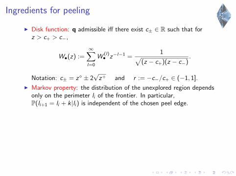
I Disk function: q admissible iff there exist c± ∈ R such that forz > c+ > c−,
W•(z) :=∞∑l=0
W(l)• z−l−1 =
1√(z − c+)(z − c−)
.
Notation: c± = z� ± 2√
z+ and r := −c−/c+ ∈ (−1, 1].
I Markov property: the distribution of the unexplored region dependsonly on the perimeter li of the frontier. In particular,P(li+1 = li + k|li ) is independent of the chosen peel edge.
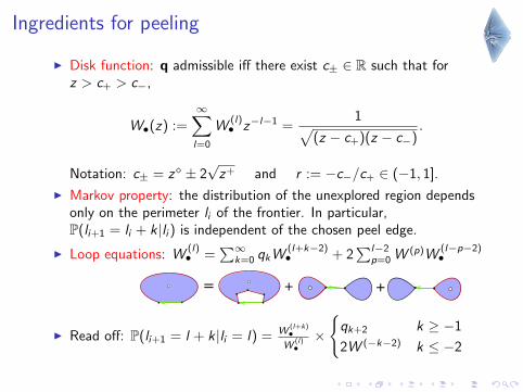
I Loop equations: W(l)• =
∑∞k=0 qkW
(l+k−2)• + 2
∑l−2p=0 W (p)W
(l−p−2)•
I Read off: P(li+1 = l + k|li = l) = W(l+k)•
W(l)•×
{qk+2 k ≥ −1
2W (−k−2) k ≤ −2
Ingredients for peeling
I Disk function: q admissible iff there exist c± ∈ R such that forz > c+ > c−,
W•(z) :=∞∑l=0
W(l)• z−l−1 =
1√(z − c+)(z − c−)
.
Notation: c± = z� ± 2√
z+ and r := −c−/c+ ∈ (−1, 1].
I Markov property: the distribution of the unexplored region dependsonly on the perimeter li of the frontier. In particular,P(li+1 = li + k|li ) is independent of the chosen peel edge.
I Loop equations: W(l)• =
∑∞k=0 qkW
(l+k−2)• + 2
∑l−2p=0 W (p)W
(l−p−2)•
I Read off: P(li+1 = l + k|li = l) = W(l+k)•
W(l)•×
{qk+2 k ≥ −1
2W (−k−2) k ≤ −2
Ingredients for peeling
I Disk function: q admissible iff there exist c± ∈ R such that forz > c+ > c−,
W•(z) :=∞∑l=0
W(l)• z−l−1 =
1√(z − c+)(z − c−)
.
Notation: c± = z� ± 2√
z+ and r := −c−/c+ ∈ (−1, 1].
I Markov property: the distribution of the unexplored region dependsonly on the perimeter li of the frontier. In particular,P(li+1 = li + k|li ) is independent of the chosen peel edge.
I Loop equations: W(l)• =
∑∞k=0 qkW
(l+k−2)• + 2
∑l−2p=0 W (p)W
(l−p−2)•
I Read off: P(li+1 = l + k |li = l) = W(l+k)•
W(l)•×
{qk+2 k ≥ −1
2W (−k−2) k ≤ −2
P(li+1 = l + k|li = l) =W
(l+k)•
W(l)•×
{qk+2 k ≥ −1
2W (−k−2) k ≤ −2(2)
I In the limit l →∞ this defines a random walk (Xi )i≥0 with stepprobabilities
ν(k) := liml→∞
P(li+1 = l + k |li = l) =
{qk+2ck
+ k ≥ −1
2W (−k−2)ck+ k ≤ −2
I Define function
s
h(0)r : Z→ R for r ∈ (−1, 1] by
h(0)r (l) = [y−l−1]
1√(y − 1)(y + r)
.
Then W(l)• = c l
+h(0)r (l) (recall r := −c−/c+).
I (2) implies h(0)r is ν-harmonic on Z>0, i.e.
∞∑k=−∞
h(0)r (l + k)ν(k) = h(0)
r (l) for all l > 0. (3)

P(li+1 = l + k|li = l) =W
(l+k)•
W(l)•×
{qk+2 k ≥ −1
2W (−k−2) k ≤ −2(2)
I In the limit l →∞ this defines a random walk (Xi )i≥0 with stepprobabilities
ν(k) := liml→∞
P(li+1 = l + k |li = l) =
{qk+2ck
+ k ≥ −1
2W (−k−2)ck+ k ≤ −2
I Define functions h(k)r : Z→ R for r ∈ (−1, 1] by
h(k)r (l) = [y−l−1]
1
(y − 1)k+1/2√
y + r.
Then W(l)• = c l
+h(0)r (l) (recall r := −c−/c+).
I (2) implies h(0)r is ν-harmonic on Z>0, i.e.
∞∑k=−∞
h(0)r (l + k)ν(k) = h(0)
r (l) for all l > 0. (3)

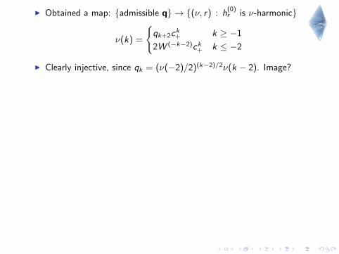
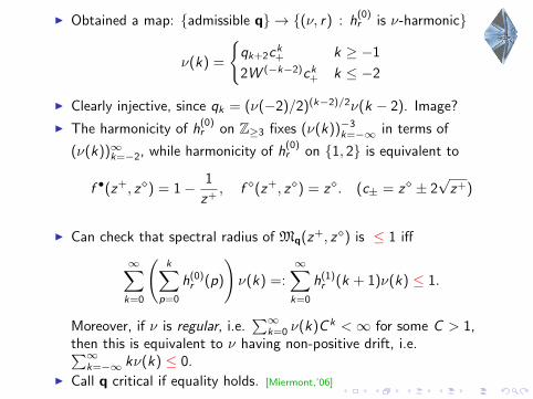
I Obtained a map: {admissible q} → {(ν, r) : h(0)r is ν-harmonic}
ν(k) =
{qk+2ck
+ k ≥ −1
2W (−k−2)ck+ k ≤ −2
I Clearly injective, since qk = (ν(−2)/2)(k−2)/2ν(k − 2). Image?
I The harmonicity of h(0)r on Z≥3 fixes (ν(k))−3
k=−∞ in terms of
(ν(k))∞k=−2
, while harmonicity of h(0)r on {1, 2} is equivalent to
f •(z+, z�) = 1− 1
z+, f �(z+, z�) = z�. (c± = z� ± 2
√z+)
I Can check that spectral radius of Mq(z+, z�) is ≤ 1 iff
∞∑k=0
(k∑
p=0
h(0)r (p)
)ν(k) =:
∞∑k=0
h(1)r (k + 1)ν(k) ≤ 1.
Moreover, if ν is regular, i.e.∑∞
k=0 ν(k)C k <∞ for some C > 1,then this is equivalent to ν having non-positive drift, i.e.∑∞
k=−∞ kν(k) ≤ 0.I Call q critical if equality holds. [Miermont,’06]

I Obtained a map: {admissible q} → {(ν, r) : h(0)r is ν-harmonic}
ν(k) =
{qk+2ck
+ k ≥ −1
2W (−k−2)ck+ k ≤ −2
I Clearly injective, since qk = (ν(−2)/2)(k−2)/2ν(k − 2). Image?
I The harmonicity of h(0)r on Z≥3 fixes (ν(k))−3
k=−∞ in terms of
(ν(k))∞k=−2, while harmonicity of h(0)r on {1, 2} is equivalent to
f •(z+, z�) = 1− 1
z+, f �(z+, z�) = z�. (c± = z� ± 2
√z+)
I Can check that spectral radius of Mq(z+, z�) is ≤ 1 iff
∞∑k=0
(k∑
p=0
h(0)r (p)
)ν(k) =:
∞∑k=0
h(1)r (k + 1)ν(k) ≤ 1.
Moreover, if ν is regular, i.e.∑∞
k=0 ν(k)C k <∞ for some C > 1,then this is equivalent to ν having non-positive drift, i.e.∑∞
k=−∞ kν(k) ≤ 0.
I Call q critical if equality holds. [Miermont,’06]
I Obtained a map: {admissible q} → {(ν, r) : h(0)r is ν-harmonic}
ν(k) =
{qk+2ck
+ k ≥ −1
2W (−k−2)ck+ k ≤ −2
I Clearly injective, since qk = (ν(−2)/2)(k−2)/2ν(k − 2). Image?
I The harmonicity of h(0)r on Z≥3 fixes (ν(k))−3
k=−∞ in terms of
(ν(k))∞k=−2, while harmonicity of h(0)r on {1, 2} is equivalent to
f •(z+, z�) = 1− 1
z+, f �(z+, z�) = z�. (c± = z� ± 2
√z+)
I Can check that spectral radius of Mq(z+, z�) is ≤ 1 iff
∞∑k=0
(k∑
p=0
h(0)r (p)
)ν(k) =:
∞∑k=0
h(1)r (k + 1)ν(k) ≤ 1.
Moreover, if ν is regular, i.e.∑∞
k=0 ν(k)C k <∞ for some C > 1,then this is equivalent to ν having non-positive drift, i.e.∑∞
k=−∞ kν(k) ≤ 0.I Call q critical if equality holds. [Miermont,’06]

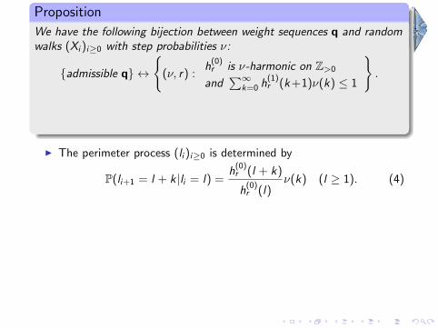
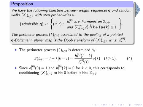
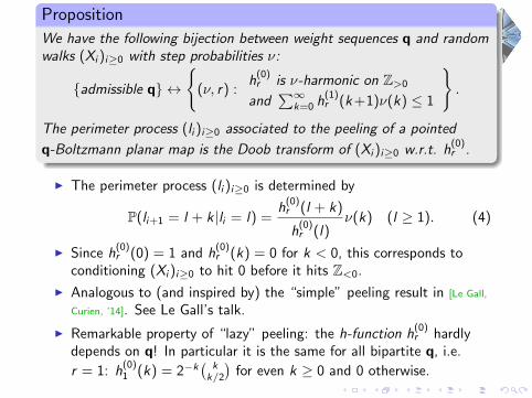
Proposition
We have the following bijection between weight sequences q and randomwalks (Xi )i≥0 with step probabilities ν:
{admissible q} ↔
{(ν, r) :
h(0)r is ν-harmonic on Z>0
and∑∞
k=0 h(1)r (k +1)ν(k) ≤ 1
}.
The perimeter process (li )i≥0 associated to the peeling of a pointed
q-Boltzmann planar map is the Doob transform of (Xi )i≥0 w.r.t. h(0)r .
I The perimeter process (li )i≥0 is determined by
P(li+1 = l + k|li = l) =h
(0)r (l + k)
h(0)r (l)
ν(k) (l ≥ 1). (4)
I Since h(0)r (0) = 1 and h
(0)r (k) = 0 for k < 0, this corresponds to
conditioning (Xi )i≥0 to hit 0 before it hits Z<0.
I Analogous to (and inspired by) the “simple” peeling result in [Le Gall,
Curien, ’14]. See Le Gall’s talk.
I Remarkable property of “lazy” peeling: the h-function h(0)r hardly
depends on q! In particular it is the same for all bipartite q, i.e.
r = 1: h(0)1 (k) = 2−k
(k
k/2
)for even k ≥ 0 and 0 otherwise.
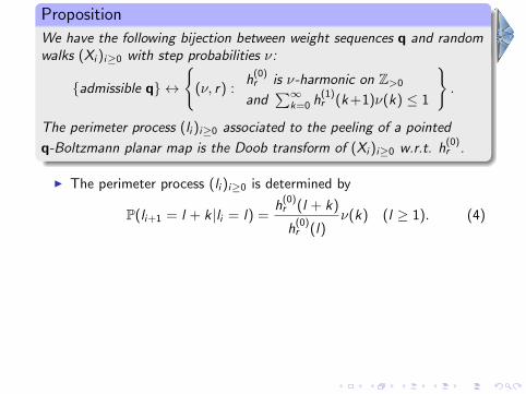
Proposition
We have the following bijection between weight sequences q and randomwalks (Xi )i≥0 with step probabilities ν:
{admissible q} ↔
{(ν, r) :
h(0)r is ν-harmonic on Z>0
and∑∞
k=0 h(1)r (k +1)ν(k) ≤ 1
}.
The perimeter process (li )i≥0 associated to the peeling of a pointed
q-Boltzmann planar map is the Doob transform of (Xi )i≥0 w.r.t. h(0)r .
I The perimeter process (li )i≥0 is determined by
P(li+1 = l + k |li = l) =h
(0)r (l + k)
h(0)r (l)
ν(k) (l ≥ 1). (4)
I Since h(0)r (0) = 1 and h
(0)r (k) = 0 for k < 0, this corresponds to
conditioning (Xi )i≥0 to hit 0 before it hits Z<0.
I Analogous to (and inspired by) the “simple” peeling result in [Le Gall,
Curien, ’14]. See Le Gall’s talk.
I Remarkable property of “lazy” peeling: the h-function h(0)r hardly
depends on q! In particular it is the same for all bipartite q, i.e.
r = 1: h(0)1 (k) = 2−k
(k
k/2
)for even k ≥ 0 and 0 otherwise.

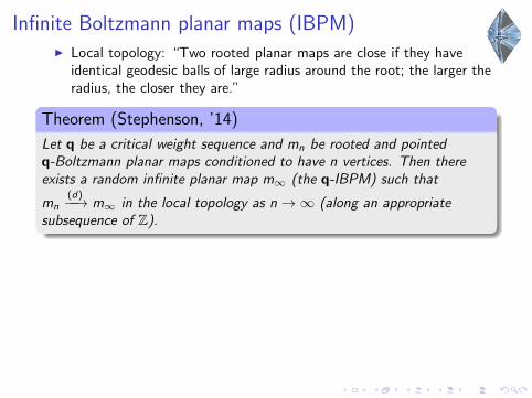
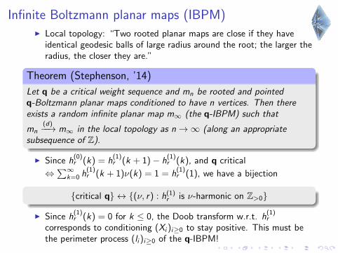
Infinite Boltzmann planar maps (IBPM)I Local topology: “Two rooted planar maps are close if they have
identical geodesic balls of large radius around the root; the larger theradius, the closer they are.”
Theorem (Stephenson, ’14)
Let q be a critical weight sequence and mn be rooted and pointedq-Boltzmann planar maps conditioned to have n vertices. Then thereexists a random infinite planar map m∞ (the q-IBPM) such that
mn(d)−−→ m∞ in the local topology as n→∞ (along an appropriate
subsequence of Z).
I Since h(0)r (k) = h
(1)r (k + 1)− h
(1)r (k), and q critical
⇔∑∞
k=0 h(1)r (k + 1)ν(k) = 1 = h
(1)r (1), we have a bijection
{critical q} ↔ {(ν, r) : h(1)r is ν-harmonic on Z>0}
I Since h(1)r (k) = 0 for k ≤ 0, the Doob transform w.r.t. h
(1)r
corresponds to conditioning (Xi )i≥0 to stay positive. This must bethe perimeter process (li )i≥0 of the q-IBPM!
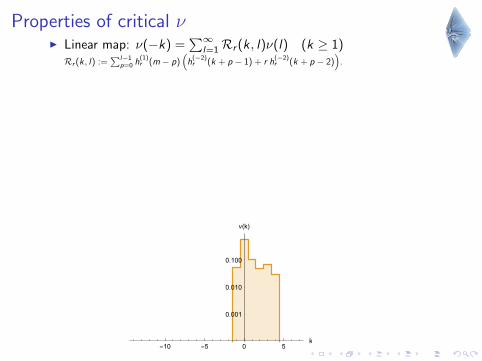
Properties of critical νI Linear map: ν(−k) =
∑∞l=1Rr (k , l)ν(l) (k ≥ 1)
Rr (k , l) :=∑l−1
p=0 h(1)r (m − p)
(h
(−2)r (k + p − 1) + r h
(−2)r (k + p − 2)
).
I Since h(1)r (k) ∼
√k as k →∞, need
∑∞k=1 ν(k)
√k <∞.
I Distinguish different cases:
I Heavy-tailed case: ν(k) ∼ k−α−1, α ∈ [1/2, 3/2]. See also[Le Gall, Miermont, ’11].
Then also ν(−k) ∼ k−α−1. Converges to α-stable processwith skewness β = − cot2(πα/2). Asymmetric except whenα = 1, for example:
ν(k) = 1/(k2 − 1) for even k 6= 0, otherwise ν(k) = 0

Properties of critical νI Linear map: ν(−k) =
∑∞l=1Rr (k , l)ν(l) (k ≥ 1)
Rr (k , l) :=∑l−1
p=0 h(1)r (m − p)
(h
(−2)r (k + p − 1) + r h
(−2)r (k + p − 2)
).
I Since h(1)r (k) ∼
√k as k →∞, need
∑∞k=1 ν(k)
√k <∞.
I Distinguish different cases:I Heavy-tailed case: ν(k) ∼ k−α−1, α ∈ [1/2, 3/2]. See also
[Le Gall, Miermont, ’11].
Then also ν(−k) ∼ k−α−1. Converges to α-stable processwith skewness β = − cot2(πα/2). Asymmetric except whenα = 1, for example:
ν(k) = 1/(k2 − 1) for even k 6= 0, otherwise ν(k) = 0

Properties of critical νI Linear map: ν(−k) =
∑∞l=1Rr (k , l)ν(l) (k ≥ 1)
Rr (k , l) :=∑l−1
p=0 h(1)r (m − p)
(h
(−2)r (k + p − 1) + r h
(−2)r (k + p − 2)
).
I Since h(1)r (k) ∼
√k as k →∞, need
∑∞k=1 ν(k)
√k <∞.
I Distinguish different cases:I Heavy-tailed case: ν(k) ∼ k−α−1, α ∈ [1/2, 3/2]. See also
[Le Gall, Miermont, ’11].Then also ν(−k) ∼ k−α−1. Converges to α-stable processwith skewness β = − cot2(πα/2).
Asymmetric except whenα = 1, for example:
ν(k) = 1/(k2 − 1) for even k 6= 0, otherwise ν(k) = 0

Properties of critical νI Linear map: ν(−k) =
∑∞l=1Rr (k , l)ν(l) (k ≥ 1)
Rr (k , l) :=∑l−1
p=0 h(1)r (m − p)
(h
(−2)r (k + p − 1) + r h
(−2)r (k + p − 2)
).
I Since h(1)r (k) ∼
√k as k →∞, need
∑∞k=1 ν(k)
√k <∞.
I Distinguish different cases:I Heavy-tailed case: ν(k) ∼ k−α−1, α ∈ [1/2, 3/2]. See also
[Le Gall, Miermont, ’11].Then also ν(−k) ∼ k−α−1. Converges to α-stable processwith skewness β = − cot2(πα/2). Asymmetric except whenα = 1, for example:
ν(k) = 1/(k2 − 1) for even k 6= 0, otherwise ν(k) = 0

Properties of critical νI Linear map: ν(−k) =
∑∞l=1Rr (k , l)ν(l) (k ≥ 1)
Rr (k , l) :=∑l−1
p=0 h(1)r (m − p)
(h
(−2)r (k + p − 1) + r h
(−2)r (k + p − 2)
).
I Since h(1)r (k) ∼
√k as k →∞, need
∑∞k=1 ν(k)
√k <∞.
I Distinguish different cases:I Heavy-tailed case: ν(k) ∼ k−α−1, α ∈ [1/2, 3/2]. See also
[Le Gall, Miermont, ’11].
I Non-heavy-tailed case: Lq :=∑∞
k=1 h(2)r (k + 1)ν(k) <∞.
(h(2)r (k) ∼ k3/2) Asymptotics of Rr (k, l) gives
ν(−k) ∼ 3Lq
√1 + r
4√π
k−5/2

Scaling limit when Lq <∞I If Lq <∞ the characteristic function of ν satisfies
ϕν(θ) :=∞∑
k=−∞
ν(k)e ikθ = 1−√
1 + r
2Lq|θ|1/2(|θ| − iθ) +O(|θ|5/2)
I Compare to the characteristic function of a 3/2-stable process S3/2
with no positive jumps:
E exp(iθS3/2(t)) = exp[−t|θ|1/2(|θ| − iθ)/
√2]
I It follows that we have the convergence in distribution in the senseof Skorokhod Xbntc(√
1 + rLqn) 2
3
t≥0
(d)−−−→n→∞
S
+
3/2(t) (5)
I Because perimeter process (li )i≥0 is obtained from (Xi )i≥0 byconditioning to stay positive, it follows from invariance principle in[Caravenna, Chaumont, ’08] that it converges to S+
3/2. See [Curien, Le Gall, ’14]
and Le Gall’s talk.
Notation: p`q = (√
1 + rLq)2/3
.
Scaling limit when Lq <∞I If Lq <∞ the characteristic function of ν satisfies
ϕν(θ) :=∞∑
k=−∞
ν(k)e ikθ = 1−√
1 + r
2Lq|θ|1/2(|θ| − iθ) +O(|θ|5/2)
I Compare to the characteristic function of a 3/2-stable process S3/2
with no positive jumps:
E exp(iθS3/2(t)) = exp[−t|θ|1/2(|θ| − iθ)/
√2]
I It follows that we have the convergence in distribution in the senseof Skorokhod lbntc(√
1 + rLqn) 2
3
t≥0
(d)−−−→n→∞
S+3/2(t) (5)
I Because perimeter process (li )i≥0 is obtained from (Xi )i≥0 byconditioning to stay positive, it follows from invariance principle in[Caravenna, Chaumont, ’08] that it converges to S+
3/2. See [Curien, Le Gall, ’14]
and Le Gall’s talk.
Notation: p`q = (√
1 + rLq)2/3
.
Scaling limit when Lq <∞I If Lq <∞ the characteristic function of ν satisfies
ϕν(θ) :=∞∑
k=−∞
ν(k)e ikθ = 1−√
1 + r
2Lq|θ|1/2(|θ| − iθ) +O(|θ|5/2)
I Compare to the characteristic function of a 3/2-stable process S3/2
with no positive jumps:
E exp(iθS3/2(t)) = exp[−t|θ|1/2(|θ| − iθ)/
√2]
I It follows that we have the convergence in distribution in the senseof Skorokhod (
lbntc
p`qn2/3
)t≥0
(d)−−−→n→∞
S+3/2(t) (5)
I Because perimeter process (li )i≥0 is obtained from (Xi )i≥0 byconditioning to stay positive, it follows from invariance principle in[Caravenna, Chaumont, ’08] that it converges to S+
3/2. See [Curien, Le Gall, ’14]
and Le Gall’s talk. Notation: p`q = (√
1 + rLq)2/3.
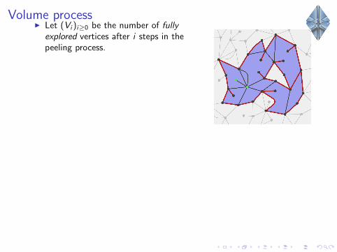
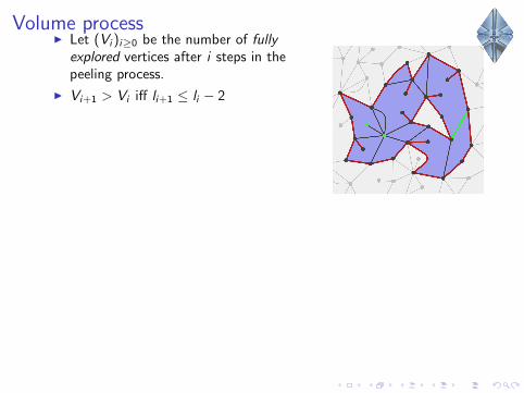
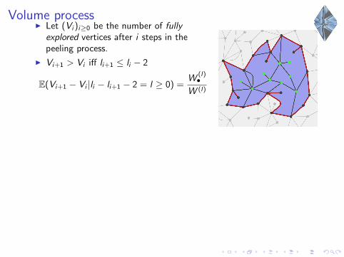
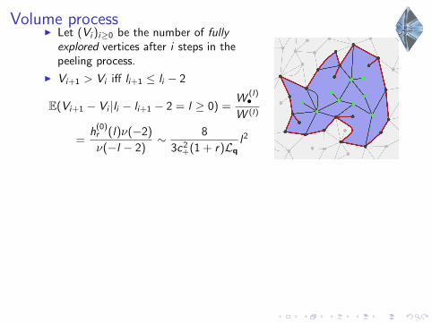
Volume processI Let (Vi )i≥0 be the number of fully
explored vertices after i steps in thepeeling process.
I Vi+1 > Vi iff li+1 ≤ li − 2
E(Vi+1 − Vi |li − li+1 − 2 = l ≥ 0) =W
(l)•
W (l)
=h
(0)r (l)ν(−2)
ν(−l − 2)∼ 8
3c2+(1 + r)Lq
l2
I Checking the details of the proof of Curien and Le Gall one gets (seeLe Gall’s talk for definition of process Z (t)):
Theorem (Direct consequence of [Curien, Le Gall, ’14])
The perimeter (li )i≥0 and volume (Vi )i≥0 of a peeling of a regular criticalq-IBPM converge jointly in distribution in the sense of Skorokhod to(
lbntc
p`qn2/3,
Vbntc
v`qn4/3
)t≥0
(d)−−−→n→∞
(S+3/2(t),Z (t))t≥0
p`q = (√
1 + rLq)2/3
v`q = 83c2
+
(Lq
1+r
)1/3

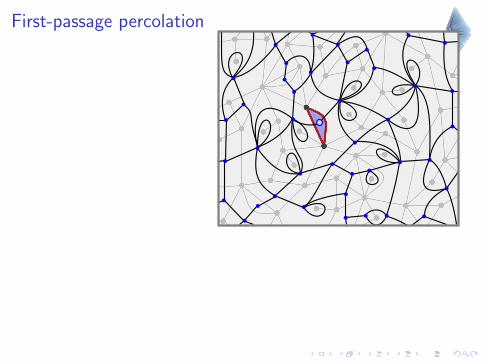
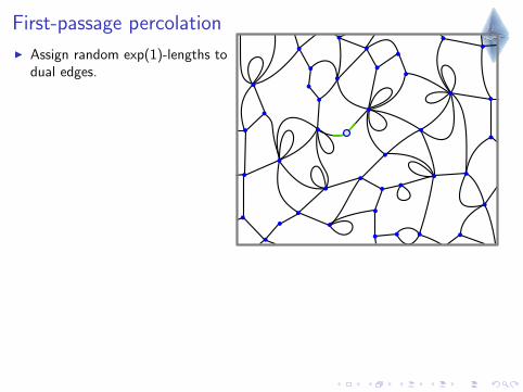
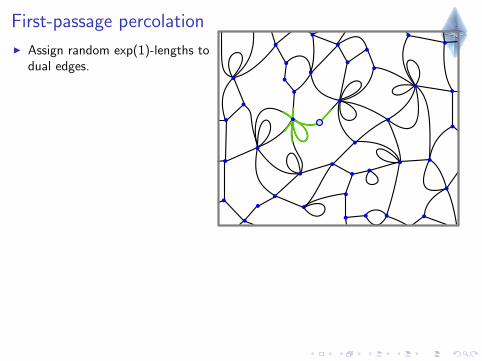
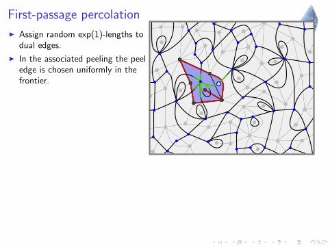
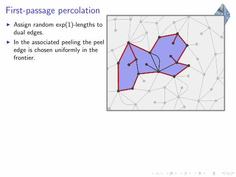
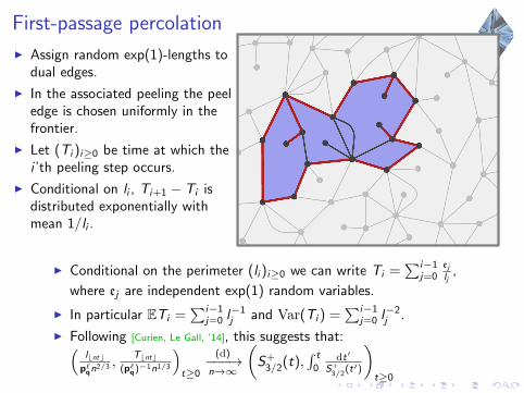
First-passage percolation
I Assign random exp(1)-lengths todual edges.
I In the associated peeling the peeledge is chosen uniformly in thefrontier.
I Let (Ti )i≥0 be time at which thei ’th peeling step occurs.
I Conditional on li , Ti+1 − Ti isdistributed exponentially withmean 1/li .
I Conditional on the perimeter (li )i≥0 we can write Ti =∑i−1
j=0ejlj
,
where ej are independent exp(1) random variables.
I In particular ETi =∑i−1
j=0 l−1j and Var(Ti ) =
∑i−1j=0 l−2
j .
I Following [Curien, Le Gall, ’14], this suggests that:(lbntc
p`qn
2/3 ,Tbntc
(p`q)−1n1/3
)t≥0
(d)−−−→n→∞
(S+
3/2(t),∫ t
0dt′
S+3/2
(t′)
)t≥0
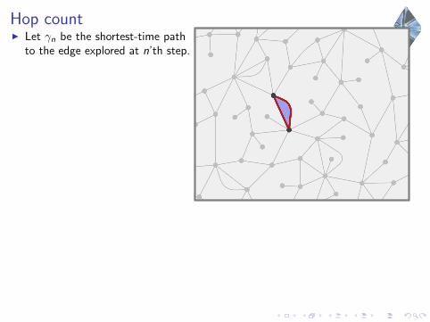
Hop countI Let γn be the shortest-time path
to the edge explored at n’th step.
I Let Hi (n) be the # of edges ofγn explored after i < n steps.
I Markov property: conditional on(li )i≥0 the probability Pi+1 thatHi+1(n)− Hi (n) = 1 is
Pi+1 =
{0 if li+1 < lili+1−li+1
li+1if li+1 ≥ li
I Law of Hi (n) independent of n (as long as n > i). Let us define thehop count process (Hi )i≥0 as the large n limit. Then (li ,Ti ,Hi )i≥0 is
a Markov process with Hi =∑i
j=1 bj , bj ∈ {0, 1},P(bi = 1) = Pi .I For regular critical q we have
E(Hi+1−Hi |li )=∞∑k=0
ν(k)k +1
k +li
h(1)r (k +li )
h(1)r (li )
=
Hq ≈ limi→∞ Hi/Ti︷ ︸︸ ︷
∞∑k=0
(k + 1)ν(k) E(Ti+1−Ti |li )+O(l−1i )
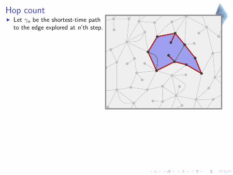
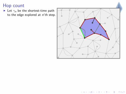
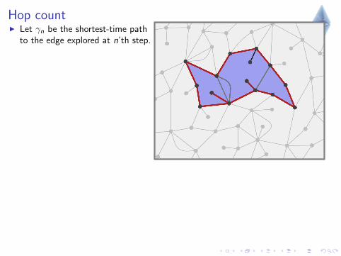
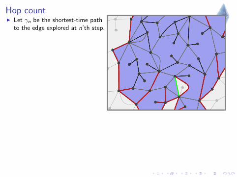
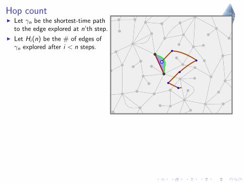
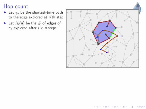
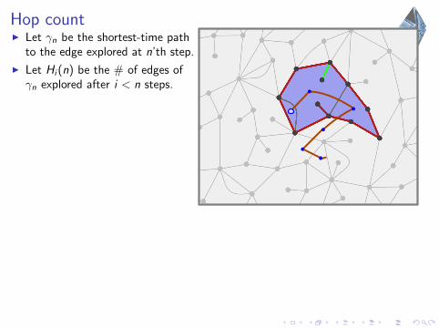
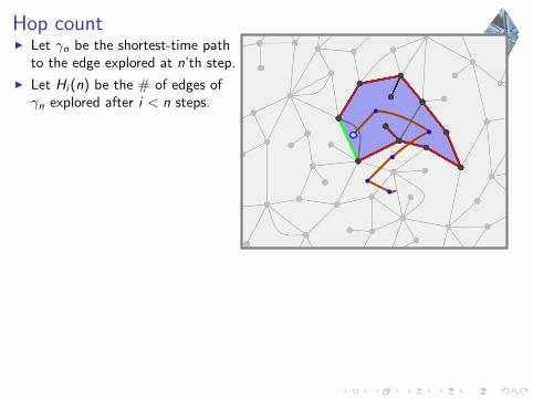
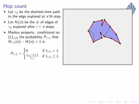

Hop countI Let γn be the shortest-time path
to the edge explored at n’th step.
I Let Hi (n) be the # of edges ofγn explored after i < n steps.
I Markov property: conditional on(li )i≥0 the probability Pi+1 thatHi+1(n)− Hi (n) = 1 is
Pi+1 =
{0 if li+1 < lili+1−li+1
li+1if li+1 ≥ li
I Law of Hi (n) independent of n (as long as n > i). Let us define thehop count process (Hi )i≥0 as the large n limit. Then (li ,Ti ,Hi )i≥0 is
a Markov process with Hi =∑i
j=1 bj , bj ∈ {0, 1},P(bi = 1) = Pi .
I For regular critical q we have
E(Hi+1−Hi |li )=∞∑k=0
ν(k)k +1
k +li
h(1)r (k +li )
h(1)r (li )
=
Hq ≈ limi→∞ Hi/Ti︷ ︸︸ ︷
∞∑k=0
(k + 1)ν(k) E(Ti+1−Ti |li )+O(l−1i )

Hop countI Let γn be the shortest-time path
to the edge explored at n’th step.
I Let Hi (n) be the # of edges ofγn explored after i < n steps.
I Markov property: conditional on(li )i≥0 the probability Pi+1 thatHi+1(n)− Hi (n) = 1 is
Pi+1 =
{0 if li+1 < lili+1−li+1
li+1if li+1 ≥ li
I Law of Hi (n) independent of n (as long as n > i). Let us define thehop count process (Hi )i≥0 as the large n limit. Then (li ,Ti ,Hi )i≥0 is
a Markov process with Hi =∑i
j=1 bj , bj ∈ {0, 1},P(bi = 1) = Pi .I For regular critical q we have
E(Hi+1−Hi |li )=∞∑k=0
ν(k)k +1
k +li
h(1)r (k +li )
h(1)r (li )
=
Hq ≈ limi→∞ Hi/Ti︷ ︸︸ ︷
∞∑k=0
(k + 1)ν(k) E(Ti+1−Ti |li )+O(l−1i )

Hop countI Let γn be the shortest-time path
to the edge explored at n’th step.
I Let Hi (n) be the # of edges ofγn explored after i < n steps.
I Markov property: conditional on(li )i≥0 the probability Pi+1 thatHi+1(n)− Hi (n) = 1 is
Pi+1 =
{0 if li+1 < lili+1−li+1
li+1if li+1 ≥ li
I Law of Hi (n) independent of n (as long as n > i). Let us define thehop count process (Hi )i≥0 as the large n limit. Then (li ,Ti ,Hi )i≥0 is
a Markov process with Hi =∑i
j=1 bj , bj ∈ {0, 1},P(bi = 1) = Pi .I For regular critical q we have
E(Hi+1−Hi |li )=∞∑k=0
ν(k)k +1
k +li
h(1)r (k +li )
h(1)r (li )
=
Hq ≈ limi→∞ Hi/Ti︷ ︸︸ ︷∞∑k=0
(k + 1)ν(k) E(Ti+1−Ti |li )+O(l−1i )
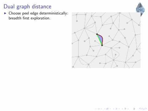
Dual graph distanceI Choose peel edge deterministically:
breadth first exploration.
I Frontier always of the form: N(d)i
edges adjacent to distance d face
followed by N(d+1)i edges adjacent
to distance d +1 face.
I Write Ni := N(d+1)i − N
(d)i .
I If N(d)i and N
(d+1)i both large then
E(Ni+1−Ni |li ) = 1+∞∑k=0
(k+1)ν(k)+O(1/li )
= 1+Hq+O(1/li )
I Takes roughly 2li1+Hq
steps to peel a full layer, since the perimeter
does not change significantly in order-li steps.
I Let T̃i have the same law as the first-passage time Ti before. ThenT̃i increases by 2
1+Hqwhen peeling a full layer.
I This suggests the asymptotic relation:dgr∗ ≈ 1
2 (1 +Hq)T̃ ≈ 12 (1 +Hq)T ≈ 1
2 (T + H)
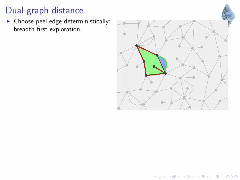
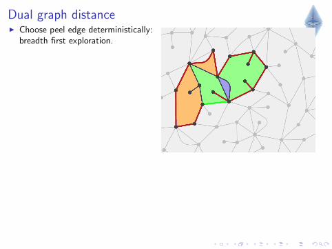
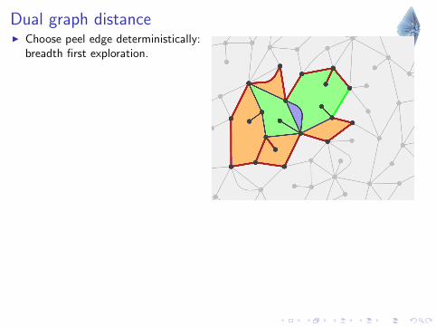
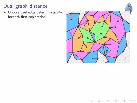
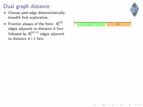
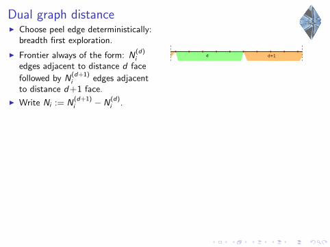
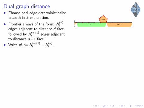
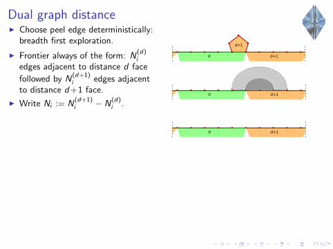
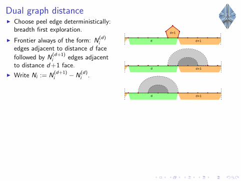
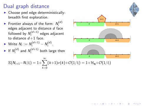
Dual graph distanceI Choose peel edge deterministically:
breadth first exploration.
I Frontier always of the form: N(d)i
edges adjacent to distance d face
followed by N(d+1)i edges adjacent
to distance d +1 face.
I Write Ni := N(d+1)i − N
(d)i .
I If N(d)i and N
(d+1)i both large then
E(Ni+1−Ni |li ) = 1+∞∑k=0
(k+1)ν(k)+O(1/li ) = 1+Hq+O(1/li )
I Takes roughly 2li1+Hq
steps to peel a full layer, since the perimeter
does not change significantly in order-li steps.
I Let T̃i have the same law as the first-passage time Ti before. ThenT̃i increases by 2
1+Hqwhen peeling a full layer.
I This suggests the asymptotic relation:dgr∗ ≈ 1
2 (1 +Hq)T̃ ≈ 12 (1 +Hq)T ≈ 1
2 (T + H)
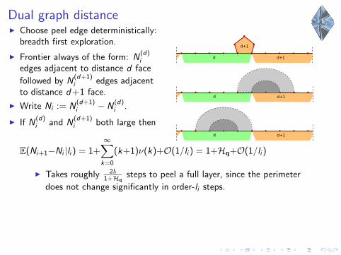
Dual graph distanceI Choose peel edge deterministically:
breadth first exploration.
I Frontier always of the form: N(d)i
edges adjacent to distance d face
followed by N(d+1)i edges adjacent
to distance d +1 face.
I Write Ni := N(d+1)i − N
(d)i .
I If N(d)i and N
(d+1)i both large then
E(Ni+1−Ni |li ) = 1+∞∑k=0
(k+1)ν(k)+O(1/li ) = 1+Hq+O(1/li )
I Takes roughly 2li1+Hq
steps to peel a full layer, since the perimeter
does not change significantly in order-li steps.
I Let T̃i have the same law as the first-passage time Ti before. ThenT̃i increases by 2
1+Hqwhen peeling a full layer.
I This suggests the asymptotic relation:dgr∗ ≈ 1
2 (1 +Hq)T̃ ≈ 12 (1 +Hq)T ≈ 1
2 (T + H)
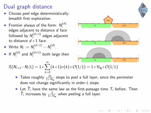
Dual graph distanceI Choose peel edge deterministically:
breadth first exploration.
I Frontier always of the form: N(d)i
edges adjacent to distance d face
followed by N(d+1)i edges adjacent
to distance d +1 face.
I Write Ni := N(d+1)i − N
(d)i .
I If N(d)i and N
(d+1)i both large then
E(Ni+1−Ni |li ) = 1+∞∑k=0
(k+1)ν(k)+O(1/li ) = 1+Hq+O(1/li )
I Takes roughly 2li1+Hq
steps to peel a full layer, since the perimeter
does not change significantly in order-li steps.
I Let T̃i have the same law as the first-passage time Ti before. ThenT̃i increases by 2
1+Hqwhen peeling a full layer.
I This suggests the asymptotic relation:dgr∗ ≈ 1
2 (1 +Hq)T̃ ≈ 12 (1 +Hq)T ≈ 1
2 (T + H)
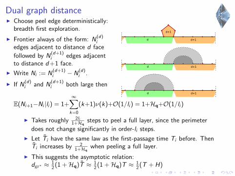
Dual graph distanceI Choose peel edge deterministically:
breadth first exploration.
I Frontier always of the form: N(d)i
edges adjacent to distance d face
followed by N(d+1)i edges adjacent
to distance d +1 face.
I Write Ni := N(d+1)i − N
(d)i .
I If N(d)i and N
(d+1)i both large then
E(Ni+1−Ni |li ) = 1+∞∑k=0
(k+1)ν(k)+O(1/li ) = 1+Hq+O(1/li )
I Takes roughly 2li1+Hq
steps to peel a full layer, since the perimeter
does not change significantly in order-li steps.
I Let T̃i have the same law as the first-passage time Ti before. ThenT̃i increases by 2
1+Hqwhen peeling a full layer.
I This suggests the asymptotic relation:dgr∗ ≈ 1
2 (1 +Hq)T̃ ≈ 12 (1 +Hq)T ≈ 1
2 (T + H)
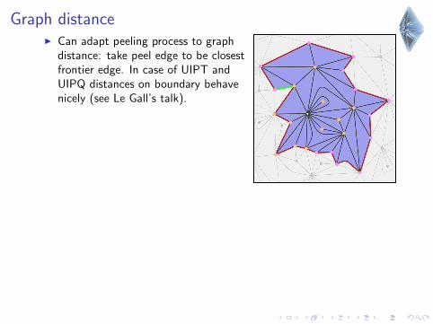
Graph distanceI Can adapt peeling process to graph
distance: take peel edge to be closestfrontier edge. In case of UIPT andUIPQ distances on boundary behavenicely (see Le Gall’s talk).
I Let Bd(m∞) be the hull of the ball ofradius d and ∂Bd(m∞) its boundary
I Curien & Le Gall prove convergence indistribution of the number of verticesin both:(
(h4)2
p4k2|∂Bbktc(m∞)|, (h4)4
v4k4|Bbktc(m∞)|
)t≥0
(d)−−−→k→∞
(L(t),M(t))t≥0
I In general the distances on the frontier are not so nice. Little hopeof generalizing the convergence to arbitrary q-IBPM’s. Can we atleast determine what the constants should be?
I Convergence implies limk→∞E|Bbktc(m∞)|
k4 =v`
q
(h`q)4 EM(t) =
v`q
(h`q)4
364 t4.
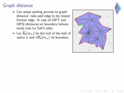
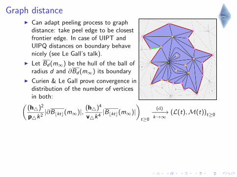

Graph distanceI Can adapt peeling process to graph
distance: take peel edge to be closestfrontier edge. In case of UIPT andUIPQ distances on boundary behavenicely (see Le Gall’s talk).
I Let Bd(m∞) be the hull of the ball ofradius d and ∂Bd(m∞) its boundary
I Curien & Le Gall prove convergence indistribution of the number of verticesin both:(
(h`q)2
p`qk2|∂Bbktc(m∞)|,
(h`q)4
v`qk4|Bbktc(m∞)|
)t≥0
?−−−→k→∞
(L(t),M(t))t≥0
I In general the distances on the frontier are not so nice. Little hopeof generalizing the convergence to arbitrary q-IBPM’s. Can we atleast determine what the constants should be?
I Convergence implies limk→∞E|Bbktc(m∞)|
k4 =v`
q
(h`q)4 EM(t) =
v`q
(h`q)4
364 t4.
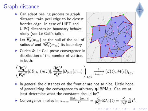
Graph distanceI Can adapt peeling process to graph
distance: take peel edge to be closestfrontier edge. In case of UIPT andUIPQ distances on boundary behavenicely (see Le Gall’s talk).
I Let Bd(m∞) be the hull of the ball ofradius d and ∂Bd(m∞) its boundary
I Curien & Le Gall prove convergence indistribution of the number of verticesin both:(
(h`q)2
p`qk2|∂Bbktc(m∞)|,
(h`q)4
v`qk4|Bbktc(m∞)|
)t≥0
?−−−→k→∞
(L(t),M(t))t≥0
I In general the distances on the frontier are not so nice. Little hopeof generalizing the convergence to arbitrary q-IBPM’s. Can we atleast determine what the constants should be?
I Convergence implies limk→∞E|Bbktc(m∞)|
k4 =v`
q
(h`q)4 EM(t) =
v`q
(h`q)4
364 t4.
I Luckily there is a different route:
Theorem (Miermont, ’06)
If q is regular critical and mn is a random (rooted) q-Boltzmann planarmap conditioned to have n vertices and v1, v2 are random vertices, thenthere exists a Cq > 0 and a q-independent random variable d∞ s.t.
dmn(v1, v2)
Cqn1/4
(d)−−−→n→∞
d∞.
I Miermont also outline an algorithm to compute Cq. With some work:
Proposition
Cq =
(2
9(z+)3/2
(∂y +√
x∂x)2
f �(x , y)∣∣∣x=z+
y=z�
)1/4
=
(c2
+
96(1 + r)3Lq
)1/4
.
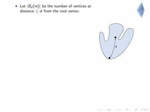
I Let |Bd(m)| be the number of vertices atdistance ≤ d from the root vertex.
I Corollary: with mn as before
limn→∞
1nE∣∣∣BbCqn1/4dc(mn)
∣∣∣ = P(d∞ < d)
I
I Assume limd→∞E|Bd (m∞)|E|Bd (m∞)| = 7
2 (see e.g. [Curien, Le Gall, ”Hull. . . ”, ’14])
I Then we finally get:v`
q
(h`q)4 = 64
372
221
1C4
q, i.e. h`q =
√38 (v`q)1/4Cq.
h`q = 14 (1 + r)2/3L1/3
q
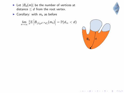
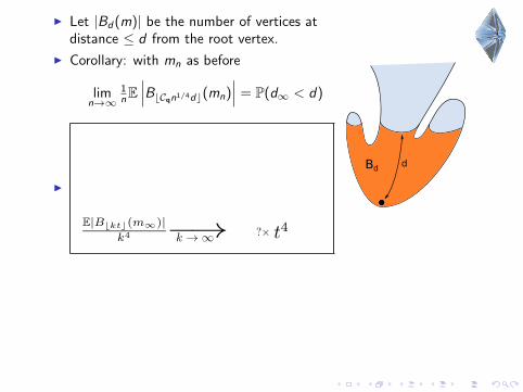
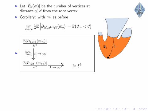
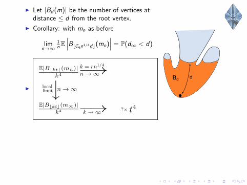
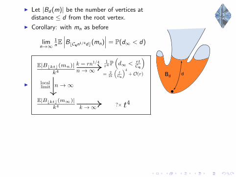
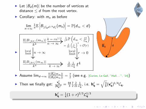

Conjectures (in search of mathematicians!)
p`q = (√
1 + rLq)2/3, v`q =8
3c2+
(Lq
1 + r
)1/3
, h`q =1
4(1 + r)2/3L1/3
q
I Notice the simple expression p`q/(h`q)2 =(
41+r
)2
, which is 4 in the
bipartite case.
Conjecture
Let (Ld)d≥0 be the length of the frontier when all vertices at distance dare discovered in a lazy peeling adapted to the distance of a bipartiteregular q-IBPM. Then (n−2Lbntc)t≥0 converges in distribution to aprocess independent of q (namely 4L(t), see Le Gall’s talk).
Conjecture
Let v be a random vertex at distance dgr from the root in a regularq-IBPM, then we have the following limits in probability as dgr →∞ forits first-passage time T , hop count H, and dual graph distance dgr∗ :
H
T→ Hq,
dgr∗
T→ 1 +Hq
2,
dgr
T→ p`qh`q = 1
4 (1 + r)Lq.
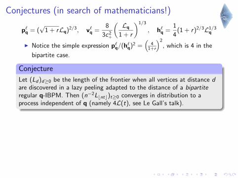
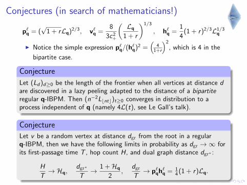
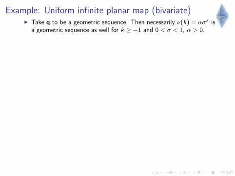
Example: Uniform infinite planar map (bivariate)I Take q to be a geometric sequence. Then necessarily ν(k) = ασk is
a geometric sequence as well for k ≥ −1 and 0 < σ < 1, α > 0.
I Now impose that h(1)r is ν-harmonic:
h(1)r (1) =
∞∑k=0
h(1)r (k +1)ν(k)
=α
(1− σ)3/2√
1 + rσ
h(1)r (2) =
∞∑k=−1
h(1)r (k +2)ν(k)
=1
σ
α
(1− σ)3/2√
1 + rσ
h(1)r (3) =
∞∑k=−2
h(1)r (k +3)ν(k)
=1− ασ2
+ ν(−2)
I Can easily compute various constants:
Hq :=∞∑k=0
(k + 1)ν(k) =
√3σ − 1
1− σ, Lq :=
∞∑k=1
h(2)r (k +1)ν(k) =
σ
1− σ,
dgr∗
dgr→ 2
1 +Hq
(1 + r)Lq=
2
Hq − 1,
vertices
faces=
(Hq + 3)(Hq − 1)
8Hq.
I Notice UIPM is σ = 56 , Hq = 3, and duality:
Hq−12 ↔ 2
Hq−1 .

Example: Uniform infinite planar map (bivariate)I Take q to be a geometric sequence. Then necessarily ν(k) = ασk is
a geometric sequence as well for k ≥ −1 and 0 < σ < 1, α > 0.
I Now impose that h(1)r is ν-harmonic:
1 =∞∑k=0
h(1)r (k +1)ν(k) =
α
(1− σ)3/2√
1 + rσ
h(1)r (2) =
∞∑k=−1
h(1)r (k +2)ν(k)
=1
σ
α
(1− σ)3/2√
1 + rσ
h(1)r (3) =
∞∑k=−2
h(1)r (k +3)ν(k)
=1− ασ2
+ ν(−2)
I Can easily compute various constants:
Hq :=∞∑k=0
(k + 1)ν(k) =
√3σ − 1
1− σ, Lq :=
∞∑k=1
h(2)r (k +1)ν(k) =
σ
1− σ,
dgr∗
dgr→ 2
1 +Hq
(1 + r)Lq=
2
Hq − 1,
vertices
faces=
(Hq + 3)(Hq − 1)
8Hq.
I Notice UIPM is σ = 56 , Hq = 3, and duality:
Hq−12 ↔ 2
Hq−1 .
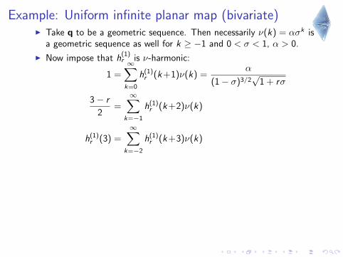
Example: Uniform infinite planar map (bivariate)I Take q to be a geometric sequence. Then necessarily ν(k) = ασk is
a geometric sequence as well for k ≥ −1 and 0 < σ < 1, α > 0.
I Now impose that h(1)r is ν-harmonic:
1 =∞∑k=0
h(1)r (k +1)ν(k) =
α
(1− σ)3/2√
1 + rσ
3− r
2=
∞∑k=−1
h(1)r (k +2)ν(k)
=1
σ
α
(1− σ)3/2√
1 + rσ
h(1)r (3) =
∞∑k=−2
h(1)r (k +3)ν(k)
=1− ασ2
+ ν(−2)
I Can easily compute various constants:
Hq :=∞∑k=0
(k + 1)ν(k) =
√3σ − 1
1− σ, Lq :=
∞∑k=1
h(2)r (k +1)ν(k) =
σ
1− σ,
dgr∗
dgr→ 2
1 +Hq
(1 + r)Lq=
2
Hq − 1,
vertices
faces=
(Hq + 3)(Hq − 1)
8Hq.
I Notice UIPM is σ = 56 , Hq = 3, and duality:
Hq−12 ↔ 2
Hq−1 .
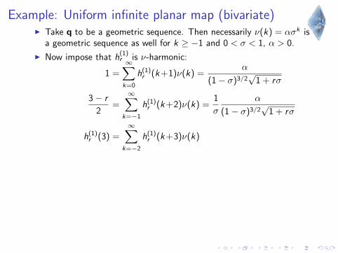
Example: Uniform infinite planar map (bivariate)I Take q to be a geometric sequence. Then necessarily ν(k) = ασk is
a geometric sequence as well for k ≥ −1 and 0 < σ < 1, α > 0.
I Now impose that h(1)r is ν-harmonic:
1 =∞∑k=0
h(1)r (k +1)ν(k) =
α
(1− σ)3/2√
1 + rσ
3− r
2=
∞∑k=−1
h(1)r (k +2)ν(k) =
1
σ
α
(1− σ)3/2√
1 + rσ
h(1)r (3) =
∞∑k=−2
h(1)r (k +3)ν(k)
=1− ασ2
+ ν(−2)
I Can easily compute various constants:
Hq :=∞∑k=0
(k + 1)ν(k) =
√3σ − 1
1− σ, Lq :=
∞∑k=1
h(2)r (k +1)ν(k) =
σ
1− σ,
dgr∗
dgr→ 2
1 +Hq
(1 + r)Lq=
2
Hq − 1,
vertices
faces=
(Hq + 3)(Hq − 1)
8Hq.
I Notice UIPM is σ = 56 , Hq = 3, and duality:
Hq−12 ↔ 2
Hq−1 .
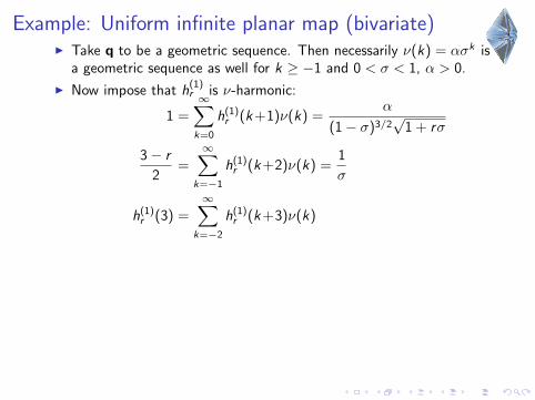
Example: Uniform infinite planar map (bivariate)I Take q to be a geometric sequence. Then necessarily ν(k) = ασk is
a geometric sequence as well for k ≥ −1 and 0 < σ < 1, α > 0.
I Now impose that h(1)r is ν-harmonic:
1 =∞∑k=0
h(1)r (k +1)ν(k) =
α
(1− σ)3/2√
1 + rσ
3− r
2=
∞∑k=−1
h(1)r (k +2)ν(k) =
1
σ
α
(1− σ)3/2√
1 + rσ
h(1)r (3) =
∞∑k=−2
h(1)r (k +3)ν(k)
=1− ασ2
+ ν(−2)
I Can easily compute various constants:
Hq :=∞∑k=0
(k + 1)ν(k) =
√3σ − 1
1− σ, Lq :=
∞∑k=1
h(2)r (k +1)ν(k) =
σ
1− σ,
dgr∗
dgr→ 2
1 +Hq
(1 + r)Lq=
2
Hq − 1,
vertices
faces=
(Hq + 3)(Hq − 1)
8Hq.
I Notice UIPM is σ = 56 , Hq = 3, and duality:
Hq−12 ↔ 2
Hq−1 .
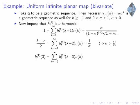
Example: Uniform infinite planar map (bivariate)I Take q to be a geometric sequence. Then necessarily ν(k) = ασk is
a geometric sequence as well for k ≥ −1 and 0 < σ < 1, α > 0.
I Now impose that h(1)r is ν-harmonic:
1 =∞∑k=0
h(1)r (k +1)ν(k) =
α
(1− σ)3/2√
1 + rσ
3− r
2=
∞∑k=−1
h(1)r (k +2)ν(k) =
1
σ(⇒ σ > 1
2 )
h(1)r (3) =
∞∑k=−2
h(1)r (k +3)ν(k)
=1− ασ2
+ ν(−2)
I Can easily compute various constants:
Hq :=∞∑k=0
(k + 1)ν(k) =
√3σ − 1
1− σ, Lq :=
∞∑k=1
h(2)r (k +1)ν(k) =
σ
1− σ,
dgr∗
dgr→ 2
1 +Hq
(1 + r)Lq=
2
Hq − 1,
vertices
faces=
(Hq + 3)(Hq − 1)
8Hq.
I Notice UIPM is σ = 56 , Hq = 3, and duality:
Hq−12 ↔ 2
Hq−1 .
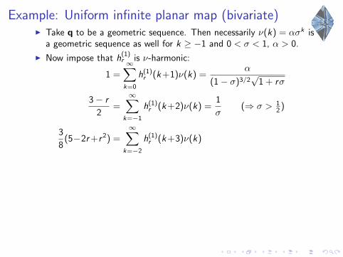
Example: Uniform infinite planar map (bivariate)I Take q to be a geometric sequence. Then necessarily ν(k) = ασk is
a geometric sequence as well for k ≥ −1 and 0 < σ < 1, α > 0.
I Now impose that h(1)r is ν-harmonic:
1 =∞∑k=0
h(1)r (k +1)ν(k) =
α
(1− σ)3/2√
1 + rσ
3− r
2=
∞∑k=−1
h(1)r (k +2)ν(k) =
1
σ(⇒ σ > 1
2 )
3
8(5−2r +r 2) =
∞∑k=−2
h(1)r (k +3)ν(k) =
1− ασ2
+ ν(−2)
I Can easily compute various constants:
Hq :=∞∑k=0
(k + 1)ν(k) =
√3σ − 1
1− σ, Lq :=
∞∑k=1
h(2)r (k +1)ν(k) =
σ
1− σ,
dgr∗
dgr→ 2
1 +Hq
(1 + r)Lq=
2
Hq − 1,
vertices
faces=
(Hq + 3)(Hq − 1)
8Hq.
I Notice UIPM is σ = 56 , Hq = 3, and duality:
Hq−12 ↔ 2
Hq−1 .
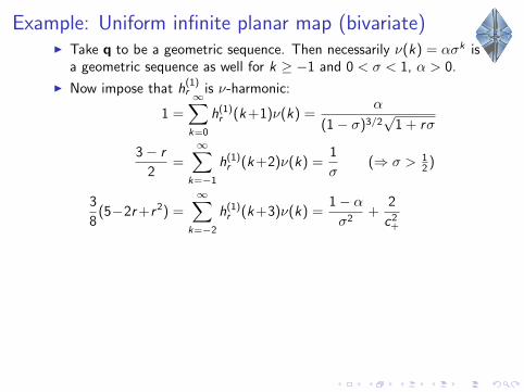
Example: Uniform infinite planar map (bivariate)I Take q to be a geometric sequence. Then necessarily ν(k) = ασk is
a geometric sequence as well for k ≥ −1 and 0 < σ < 1, α > 0.
I Now impose that h(1)r is ν-harmonic:
1 =∞∑k=0
h(1)r (k +1)ν(k) =
α
(1− σ)3/2√
1 + rσ
3− r
2=
∞∑k=−1
h(1)r (k +2)ν(k) =
1
σ(⇒ σ > 1
2 )
3
8(5−2r +r 2) =
∞∑k=−2
h(1)r (k +3)ν(k) =
1− ασ2
+2
c2+
I Can easily compute various constants:
Hq :=∞∑k=0
(k + 1)ν(k) =
√3σ − 1
1− σ, Lq :=
∞∑k=1
h(2)r (k +1)ν(k) =
σ
1− σ,
dgr∗
dgr→ 2
1 +Hq
(1 + r)Lq=
2
Hq − 1,
vertices
faces=
(Hq + 3)(Hq − 1)
8Hq.
I Notice UIPM is σ = 56 , Hq = 3, and duality:
Hq−12 ↔ 2
Hq−1 .
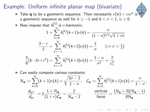
Example: Uniform infinite planar map (bivariate)I Take q to be a geometric sequence. Then necessarily ν(k) = ασk is
a geometric sequence as well for k ≥ −1 and 0 < σ < 1, α > 0.
I Now impose that h(1)r is ν-harmonic:
1 =∞∑k=0
h(1)r (k +1)ν(k) =
α
(1− σ)3/2√
1 + rσ
3− r
2=
∞∑k=−1
h(1)r (k +2)ν(k) =
1
σ(⇒ σ > 1
2 )
3
8(5−2r +r 2) =
∞∑k=−2
h(1)r (k +3)ν(k) =
1− ασ2
+2
c2+
I Can easily compute various constants:
Hq :=∞∑k=0
(k + 1)ν(k) =
√3σ − 1
1− σ, Lq :=
∞∑k=1
h(2)r (k +1)ν(k) =
σ
1− σ,
dgr∗
dgr→ 2
1 +Hq
(1 + r)Lq=
2
Hq − 1,
vertices
faces=
(Hq + 3)(Hq − 1)
8Hq.
I Notice UIPM is σ = 56 , Hq = 3, and duality:
Hq−12 ↔ 2
Hq−1 .
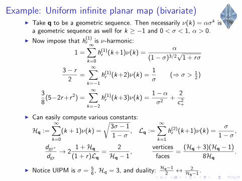
Example: Uniform infinite planar map (bivariate)I Take q to be a geometric sequence. Then necessarily ν(k) = ασk is
a geometric sequence as well for k ≥ −1 and 0 < σ < 1, α > 0.
I Now impose that h(1)r is ν-harmonic:
1 =∞∑k=0
h(1)r (k +1)ν(k) =
α
(1− σ)3/2√
1 + rσ
3− r
2=
∞∑k=−1
h(1)r (k +2)ν(k) =
1
σ(⇒ σ > 1
2 )
3
8(5−2r +r 2) =
∞∑k=−2
h(1)r (k +3)ν(k) =
1− ασ2
+2
c2+
I Can easily compute various constants:
Hq :=∞∑k=0
(k + 1)ν(k) =
√3σ − 1
1− σ, Lq :=
∞∑k=1
h(2)r (k +1)ν(k) =
σ
1− σ,
dgr∗
dgr→ 2
1 +Hq
(1 + r)Lq=
2
Hq − 1,
vertices
faces=
(Hq + 3)(Hq − 1)
8Hq.
I Notice UIPM is σ = 56 , Hq = 3, and duality:
Hq−12 ↔ 2
Hq−1 .
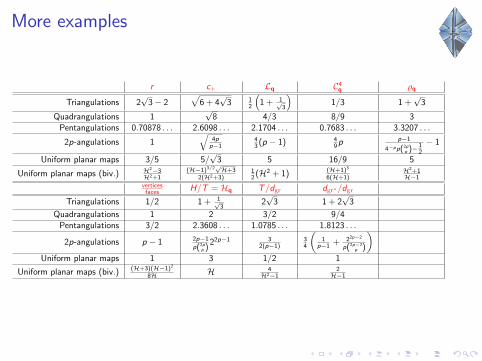
More examples
r c+ Lq C4q ρq
Triangulations 2√
3− 2√
6 + 4√
3 12
(1 + 1√
3
)1/3 1 +
√3
Quadrangulations 1√
8 4/3 8/9 3Pentangulations 0.70878 . . . 2.6098 . . . 2.1704 . . . 0.7683 . . . 3.3207 . . .
2p-angulations 1√
4pp−1
43 (p − 1) 4
9 p p−1
4−pp(2pp )− 1
2
− 1
Uniform planar maps 3/5 5/√
3 5 16/9 5
Uniform planar maps (biv.) H2−3H2+1
(H−1)3/2√H+3
2(H2+3)12 (H2 + 1) (H+1)3
6(H+1)H2+1H−1
verticesfaces H/T = Hq T/dgr dgr∗/dgr
Triangulations 1/2 1 + 1√3
2√
3 1 + 2√
3
Quadrangulations 1 2 3/2 9/4Pentangulations 3/2 2.3608 . . . 1.0785 . . . 1.8123 . . .
2p-angulations p − 1 2p−1
p(2pp )
22p−1 32(p−1)
34
(1
p−1 + 22p−2
p(2p−2p )
)Uniform planar maps 1 3 1/2 1
Uniform planar maps (biv.) (H+3)(H−1)2
8H H 4H2−1
2H−1

From lazy to simple peelingI During simple peeling the frontier is kept
simple, i.e. it does not touch itself.
I Compared to lazy peeling there are twoaspects that affect the scaling constants:When exploring, say, up to passage-time Tthe simple peeling. . .
I . . . requires less peeling steps, ns(T ) < n`(T )I . . . results in a shorter frontier, l s(T )< l`(T ).
I After passage-time T the explored region in the simple peelingshould agree in law with the hull of the explored region in the lazypeeling.
I The fraction of the length-l boundary of a (regular) q-IBPM that is“simple” converges in probability as l →∞ to 1/ρq with
ρq := Eν(−k − 1|k ≤ −2) =Hq − 1
Pν(k ≤ −2)> 1
I Therefore as T →∞, l`(T )l s (T ) → ρq and must also have n`(T )
ns (T ) → ρq.
psq = ρ−1/3
q p`q, vsq = ρ4/3
q v`q, hsq = ρ1/3
q h`q
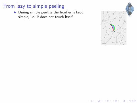
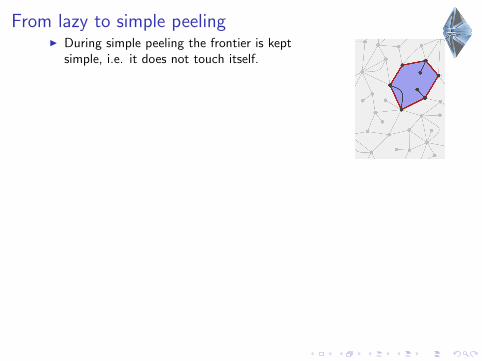
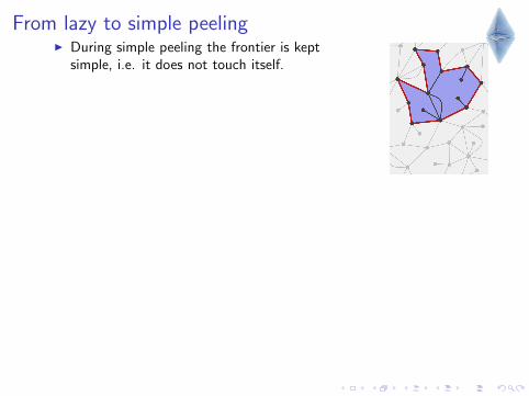
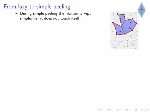
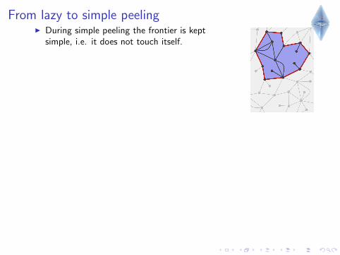
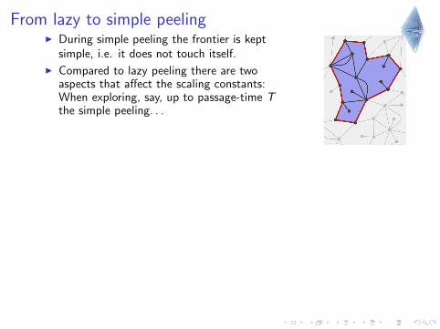

From lazy to simple peelingI During simple peeling the frontier is kept
simple, i.e. it does not touch itself.
I Compared to lazy peeling there are twoaspects that affect the scaling constants:When exploring, say, up to passage-time Tthe simple peeling. . .
I . . . requires less peeling steps, ns(T ) < n`(T )
I . . . results in a shorter frontier, l s(T )< l`(T ).
I After passage-time T the explored region in the simple peelingshould agree in law with the hull of the explored region in the lazypeeling.
I The fraction of the length-l boundary of a (regular) q-IBPM that is“simple” converges in probability as l →∞ to 1/ρq with
ρq := Eν(−k − 1|k ≤ −2) =Hq − 1
Pν(k ≤ −2)> 1
I Therefore as T →∞, l`(T )l s (T ) → ρq and must also have n`(T )
ns (T ) → ρq.
psq = ρ−1/3
q p`q, vsq = ρ4/3
q v`q, hsq = ρ1/3
q h`q
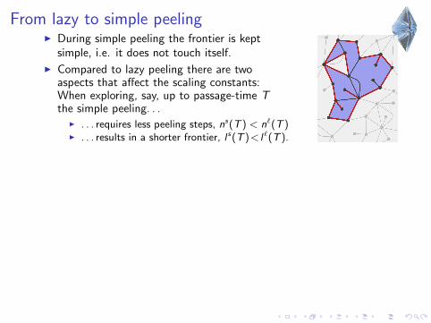
From lazy to simple peelingI During simple peeling the frontier is kept
simple, i.e. it does not touch itself.
I Compared to lazy peeling there are twoaspects that affect the scaling constants:When exploring, say, up to passage-time Tthe simple peeling. . .
I . . . requires less peeling steps, ns(T ) < n`(T )I . . . results in a shorter frontier, l s(T )< l`(T ).
I After passage-time T the explored region in the simple peelingshould agree in law with the hull of the explored region in the lazypeeling.
I The fraction of the length-l boundary of a (regular) q-IBPM that is“simple” converges in probability as l →∞ to 1/ρq with
ρq := Eν(−k − 1|k ≤ −2) =Hq − 1
Pν(k ≤ −2)> 1
I Therefore as T →∞, l`(T )l s (T ) → ρq and must also have n`(T )
ns (T ) → ρq.
psq = ρ−1/3
q p`q, vsq = ρ4/3
q v`q, hsq = ρ1/3
q h`q
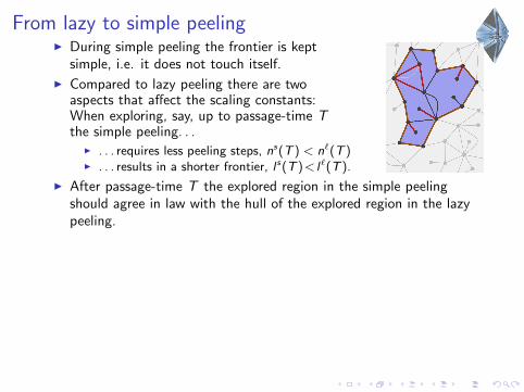
From lazy to simple peelingI During simple peeling the frontier is kept
simple, i.e. it does not touch itself.
I Compared to lazy peeling there are twoaspects that affect the scaling constants:When exploring, say, up to passage-time Tthe simple peeling. . .
I . . . requires less peeling steps, ns(T ) < n`(T )I . . . results in a shorter frontier, l s(T )< l`(T ).
I After passage-time T the explored region in the simple peelingshould agree in law with the hull of the explored region in the lazypeeling.
I The fraction of the length-l boundary of a (regular) q-IBPM that is“simple” converges in probability as l →∞ to 1/ρq with
ρq := Eν(−k − 1|k ≤ −2) =Hq − 1
Pν(k ≤ −2)> 1
I Therefore as T →∞, l`(T )l s (T ) → ρq and must also have n`(T )
ns (T ) → ρq.
psq = ρ−1/3
q p`q, vsq = ρ4/3
q v`q, hsq = ρ1/3
q h`q
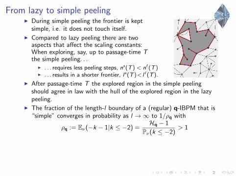
From lazy to simple peelingI During simple peeling the frontier is kept
simple, i.e. it does not touch itself.
I Compared to lazy peeling there are twoaspects that affect the scaling constants:When exploring, say, up to passage-time Tthe simple peeling. . .
I . . . requires less peeling steps, ns(T ) < n`(T )I . . . results in a shorter frontier, l s(T )< l`(T ).
I After passage-time T the explored region in the simple peelingshould agree in law with the hull of the explored region in the lazypeeling.
I The fraction of the length-l boundary of a (regular) q-IBPM that is“simple” converges in probability as l →∞ to 1/ρq with
ρq := Eν(−k − 1|k ≤ −2) =Hq − 1
Pν(k ≤ −2)> 1
I Therefore as T →∞, l`(T )l s (T ) → ρq and must also have n`(T )
ns (T ) → ρq.
psq = ρ−1/3
q p`q, vsq = ρ4/3
q v`q, hsq = ρ1/3
q h`q
Open problemsI Given that the peeling process of the q-IBPM is so simple, is there a
way to use it to construct the q-IBPM directly? (Curien’s talk?)
I Can the scaling constants Cq and h`q associated to the graphdistance be derived from a peeling process?
I For q-IBPM’s we have conjectured a universal asymptotic relationbetween the passage-time, hop count, and dual graph distance:dgr∗ ≈ (H + T )/2. Does it hold more generally? Empirically itseems to be a good heuristic for many other types of graphs.
I On a 2d lattice the relative fluctuations of dgr∗ and T are conjectureto be described by the Kardar–Parisi–Zhang universality class. Canwe start to say something about the situation on random graphs?
I Do any of the geometric constructions still make sense in theheavy-tailed case (α ∈ [ 1
2 ,32 ])? Le Gall and Miermont have shown
that w.r.t. the graph distance such finite maps converge to a metricspace with Hausdorff dimension 2α + 1. The metric space w.r.t.dual graph distance is quite different. Does it have a limit?
Thanks for your attention!