Scaling Deep Learning on GPU and Knights Landing clustersYang You

Computer Science DivisionUC Berkeley

youyang@cs.berkeley.edu

Aydın BulucComputer Science Division

LBNL and UC Berkeleyabuluc@lbl.gov

James DemmelComputer Science Division

UC Berkeleydemmel@cs.berkeley.edu

ABSTRACT�e speed of deep neural networks training has become a big bot-tleneck of deep learning research and development. For example,training GoogleNet by ImageNet dataset on one Nvidia K20 GPUneeds 21 days [11]. To speed up the training process, the currentdeep learning systems heavily rely on the hardware accelerators.However, these accelerators have limited on-chip memory com-pared with CPUs. To handle large datasets, they need to fetchdata from either CPU memory or remote processors. We use bothself-hosted Intel Knights Landing (KNL) clusters and multi-GPUclusters as our target platforms. From an algorithm aspect, currentdistributed machine learning systems [5] [18] are mainly designedfor cloud systems. �ese methods are asynchronous because ofthe slow network and high fault-tolerance requirement on cloudsystems. We focus on Elastic Averaging SGD (EASGD) [28] todesign algorithms for HPC clusters. Original EASGD [28] usedround-robin method for communication and updating. �e com-munication is ordered by the machine rank ID, which is ine�cienton HPC clusters.

First, we redesign four e�cient algorithms for HPC systems toimprove EASGD’s poor scaling on clusters. Async EASGD, AsyncMEASGD, and Hogwild EASGD are faster than their existing coun-terparts (Async SGD, Async MSGD, and Hogwild SGD, resp.) in allthe comparisons. Finally, we design Sync EASGD, which ties forthe best performance among all the methods while being determin-istic. In addition to the algorithmic improvements, we use somesystem-algorithm codesign techniques to scale up the algorithms.By reducing the percentage of communication from 87% to 14%, ourSync EASGD achieves 5.3× speedup over original EASGD on thesame platform. We get 91.5% weak scaling e�ciency on 4253 KNLcores, which is higher than the state-of-the-art implementation.

CCS CONCEPTS•Computingmethodologies→Massively parallel algorithms;

KEYWORDSDistributed Deep Learning, Knights Landing, Scalable Algorithm

ACM acknowledges that this contribution was authored or co-authored by an em-ployee, or contractor of the national government. As such, the Government retains anonexclusive, royalty-free right to publish or reproduce this article, or to allow othersto do so, for Government purposes only. Permission to make digital or hard copies forpersonal or classroom use is granted. Copies must bear this notice and the full citationon the �rst page. Copyrights for components of this work owned by others than ACMmust be honored. To copy otherwise, distribute, republish, or post, requires priorspeci�c permission and/or a fee. Request permissions from permissions@acm.org.SC17, Denver, CO, USA© 2017 ACM. 978-1-4503-5114-0/17/11. . .$15.00DOI: 10.1145/3126908.3126912

ACM Reference format:Yang You, Aydın Buluc, and James Demmel. 2017. Scaling Deep Learningon GPU and Knights Landing clusters. In Proceedings of SC17, Denver, CO,USA, November 12–17, 2017, 12 pages.DOI: 10.1145/3126908.3126912

1 INTRODUCTIONFor deep learning applications, larger datasets and bigger modelslead to signi�cant improvements in accuracy [1]. However, the com-putational power for training deep neural networks has become abig bo�leneck. �e current deep networks require days or weeks totrain, which makes real-time interaction impossible. For example,training ImageNet by GoogleNet on one Nvidia K20 GPU needs21 days [11]. Moreover, the neural networks are rapidly becomingmore and more complicated. For instance, state-of-the-art ResidualNets have 152 layers [9] while the best networks four years ago(AlexNet [14]) had only 8 layers. To speed up the training process,the current deep learning systems heavily rely on hardware acceler-ators because they can provide highly �ne-grained data-parallelism(e.g. GPGPUs) or fully-pipelined instruction-parallelism (e.g. FPGA).However, these accelerators have limited on-chip memory com-pared with CPUs. To handle big models and large datasets, theyneed to fetch data from either CPU memory or remote processors atruntime. �us, reducing communication and improving scalabilityare critical issues for distributed deep learning systems.

To explore architectural impact, in addition to multi-GPU plat-form, we choose the Intel Knights Landing (KNL) cluster as our tar-get platform. KNL is a self-hosted chip with more cores than CPUs(e.g. 68 or 72 vs 32). Compared with its predecessor Knights Corner(KNC), KNL signi�cantly improved both computational power (6T�ops vs 2 T�ops for single precision) and memory bandwidthe�ciency (450 GB/s vs 159 GB/s for STREAM benchmark). More-over, KNL introduced MCDRAM and con�gurable NUMA, whichare highly important for applications with complicated memoryaccess pa�erns. We design communication-e�cient deep learningmethods on GPU and KNL clusters for be�er scalability.

Algorithmically, current distributed machine learning systems[5] [18] are mainly designed for cloud systems. �ese methodsare asynchronous because of the slow network and high fault-tolerance requirement on cloud systems. A typical HPC cluster’sbisection bandwidth is 66.4 Gbps (NERSC Cori) while the datacenter’s bisection bandwidth is around 10 Gbps (Amazon EC2).However, as mentioned before, the critical issues for current deeplearning system are speed and scalability. �erefore, we need toselect the right method as the starting point. Regarding algorithms,we focus on Elastic Averaging SGD (EASGD) method since it hasa good convergence property [28]. Original EASGD used a round-robin method for communication. �e communication is orderedby the machine rank ID. At any moment, the master can interact

SC17, November 12–17, 2017, Denver, CO, USA Yang You, Aydın Buluc, and James Demmel

with just a single worker. �e parallelism is limited to the pipelineamong di�erent workers. Original EASGD is ine�cient on HPCsystems.

First, we redesign four e�cient distributed algorithms to improveEASGD’s poor scaling on clusters. By changing the round-robinstyle to parameter-server style, we got Async EASGD. A�er addingmomentum [24] to Async EASGD, we got Async MEASGD. �en wecombine Hogwild method and EASGD updating rule to get HogwildEASGD. Async EASGD, Async MEASGD, and Hogwild EASGD arefaster than their existing counterparts (i.e. Async SGD, AsyncMSGD, and Hogwild SGD, resp.). Finally, we design Sync EASGD,which ties for the best performance among all the methods whilebeing deterministic (Figure 8). Besides the algorithmic re�nements,the system-algorithm codesign techniques are important for scalingup deep neural networks. �e techniques we introduce include:(1) using single-layer layout and communication to optimize thenetwork latency and memory access, (2) using multiple copies ofweights to speedup the gradient descent, and (3) partitioning theKNL chip based on data/weight size and reducing communicationon multi-GPU systems. By reducing the communication percentfrom 87% to 14%, our Sync EASGD achieves 5.3× speedup overoriginal EASGD on the same platform. Using ImageNet dataset totrain GoogleNet on 2176 KNL cores, the weak scaling e�ciency ofIntel Ca�e is 87% while our implementation is 92%. Using ImageNetto train VGG on 2176 KNL cores, the weak scaling e�ciency ofIntel Ca�e is 62% while our implementation is 78.5%. To highlightthe di�erence between existing methods and our methods, we listour three major contributions:

(1) Sync EASGD and Hogwild EASGD algorithms. We havedocumented our process in arriving at these two algorithms, whichultimately perform be�er than existing methods. �e existingEASGD uses round-robin updating rule. We refer to the exist-ing method as Original EASGD. We �rst changed the round-robinrule to parameter-server rule to arrive at Async EASGD. �e dif-ference between Original-EASGD and Async-EASGD is that theupdating rule of Original-EASGD is ordered while Async-EASGDis unordered. Adding momentum to that we arrived at AsyncMEASGD. Neither Async EASGD nor Async MEASGD were signif-icantly faster than Original EASGD (Figure 8).

In both Original-EASGD and Async-EASGD, the master onlycommunicates with one worker at a time. �en we relaxed thisrequirement to allow the master to communicate with multipleworkers at a time to get Hogwild EASGD. �e master �rst receivesmultiple weights from di�erent workers. �e master then processesthese weights by the Hogwild (lock-free) Updating rule. We ob-serve that the lock-free Hogwild makes Hogwild EASGD run muchfaster than Original EASGD. For the convex case, we can prove thealgorithm is safe and faster under some assumptions1.

We used tree reduction algorithm to replace round-robin ruleto get Sync EASGD. Sync EASGD is much faster (Θ(logP) vs Θ(P)).�is is highly important because deep learning researchers o�enneed to tune many hyperparameters, which is exetremly time-consuming. While not being one of our major contributions, wealso documented the relative order of performance between inter-mediate algorithms we have considered. For instance, we observe

1h�ps://www.cs.berkeley.edu/∼youyang/HogwildEasgdProof.pdf

Figure 1: �e KNL Architecture. Our version has 68 cores.

that Async EASGD is faster than Async SGD and Async MEASGDis faster than Async MSGD.

(2)Algorithm-SystemCo-design formulti-GPU system. Af-ter the algorithm-level optimization, we need to produce an e�cientdesign on the multi-GPU system. We reduce the communicationoverhead by changing the data’s physical locations. We also designsome strategies to overlap the communication with the computa-tion. A�er the algorithm-system co-design, our implementationachieves a 5.3x speedup over the Original EASGD.

(3) Use KNL cluster to speedup DNN training. GPUs aregood tools to train deep neural networks. However, we also wantto explore more hardware options for deep learning applications.We choose KNL because it has powerful computation and memoryunits. Section 6.2 describes the optimization for small dataset DNNtraining on KNL platform. In our experiments, using an 8-core CPUto train CIFAR-10 dataset takes 8.2 hours. However, CIFAR-10 isonly 170 MB, which can not make full use of KNL’s 384 GB memory.�is optimization helps us to �nish the training in 10 minutes. �eoptimization in Section 5.2 is designed on KNL cluster, but it canbe used on regular clusters.

2 BACKGROUNDWe describe the Intel Knights Landing architecture, which is usedin this paper. We review necessary background on deep learningfor readers to understand this paper.

2.1 Intel Knights Landing ArchitectureIntel Knights Landing (KNL) Architecture is the latest version ofIntel Xeon Phi. Compared with the previous version, i.e. KnightsCorner (KNC), KNL has slightly more cores (e.g. 72 or 68 vs 60).Like KNC, each KNL core has 4 hardware threads and supports512-bit instruction for SIMD data parallelism. �e major distinctfeatures of KNL include the following:

(1) Self-hostedPlatform�e traditional accelerators (e.g. FPGA,GPUs, and KNC) rely on CPU for control and I/O management. Forsome applications, the transfer path like PCIE may become a bo�le-neck at runtime because the memory on accelerator is limited (e.g.12 GB GDDR5 on one Nvidia K80 GPU). �e KNL does not need ahost. It is self-hosted by an operating system like CentOS 7.

(2) Better Memory KNL’s DDR4 memory size is much largerthan that of KNC (384 GB vs 16 GB). Moreover, KNL is equipped

Scaling Deep Learning on GPU and Knights Landing clusters SC17, November 12–17, 2017, Denver, CO, USA

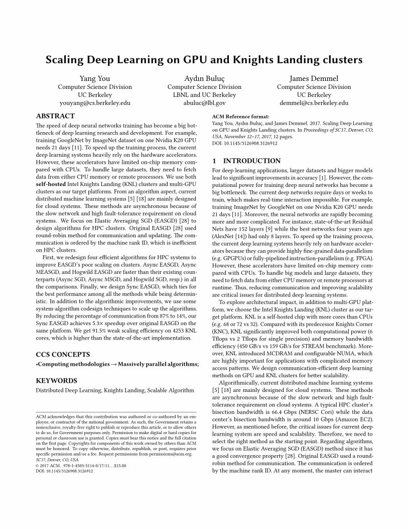
with 16 GB Multi-Channel DRAM (MCDRAM). MCDRAM’s mea-sured bandwidth is 475 GB/s (STREAM benchmark). �e bandwidthof KNL’s regular DDR4 is 90 GB/s. MCDRAM has three modes: a)Cache Mode: KNL uses it as the last level cache; b) Flat Mode: KNLtreats it as the regular DDR; c) Hybrid Mode: part of it is used ascache, the other is used as the regular DDR memory (Figure 2).

(3) Con�gurable NUMA KNL supports all-to-all (A2A), quad-rant/hemisphere (�ad/Hemi) and sub-NUMA (SNC-4/2) clusteringmodes of cache operation. For A2A, memory addresses are uni-formly distributed across all tag directories (TDs) on the chip. For�ad/Hemi, the tiles are divided into four parts called quadrants,which are spatially local to four groups of memory controllers.Memory addresses served by a memory controller in a quadrantare guaranteed to be mapped only to TDs contained in that quad-rant. Hemisphere mode functions the same way, except that thedie is divided into two hemispheres instead of four quadrants. �eSNC-4/2 mode partitions the chip into four quadrants or two hemi-spheres, and, in addition, expose these quadrants (hemispheres)as NUMA nodes. In this mode, NUMA-aware so�ware can pinso�ware threads to the same quadrant (hemisphere) that containsthe TD and access NUMA-local memory.

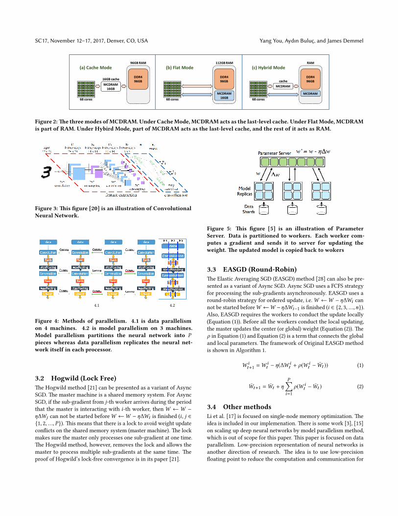
2.2 DNN and SGDWe focus on Convolutional Neural Networks (CNN) [16] in thissection. Figure 3 is an illustration of CNN. CNN is composed ofa sequence of tensors. We refer to these tensors as weights. Atruntime, the input of CNN is a picture X (e.g. X is stored as a32-by-32 matrix in Figure 3). A�er a sequence of tensor-matrixoperations, the output of CNN is an integer y (e.g. y ∈ {0, 1, 2, ..., 9}in Figure 3). �e tensor-matrix operations can be implementedby dense matrix-matrix multiplication, FFT, dense matrix-vectormultiplication, dense vector-vector add and non-linear transform(e.g. Tanh, Sigmoid, and ReLU [7]).

Figure 3 is an example of hand-wri�en image recognition. �einput pictureX should be recognized as 3 by a human. Ify is 3, thenthe input picture is correctly classi�ed by the CNN framework. Toget the correct classi�cation, we need to get a set of working weights.�e weights needs to be trained by using the real-world datasets.For simplicity, let us refer to the weights as W , and the trainingdataset as {Xi ,yi }, i ∈ {1, 2, ...,n}. n is the number of trainingpictures. yi is the correct label for Xi . �e training process includesthree parts: 1) Forward Propagation, 2) Backward Propagation, and3) Weight Update.

Forward Propagation Xi is passed from the �rst layer to thelast layer of the neural network (le� to right in Figure 3). �e outputis the prediction of Xi ’s label, which is referred to as yi .

Backward Propagation We get a numerical prediction error Eas the di�erence between yi and yi . �en we pass E from the lastlayer to the �rst layer to get the gradient ofW , which is ∆W .

Weight Update We re�ne the CNN framework by updating theweight: W ←W − η∆W , where η is a number called the learningrate (e.g. 0.01).

We conduct the above three steps iteratively over all the samplesuntil the model is optimized (i.e. randomly picks a batch of samplesat each iteration). �is method is called Stochastic Gradient Descent(SGD) [7]. Stochastic means we randomly pick a batch of b pictures

at each iteration. Usually b is an integer chosen from 16 to 2048. Ifb is too large, SGD’s convergence rate usually will decrease [19].

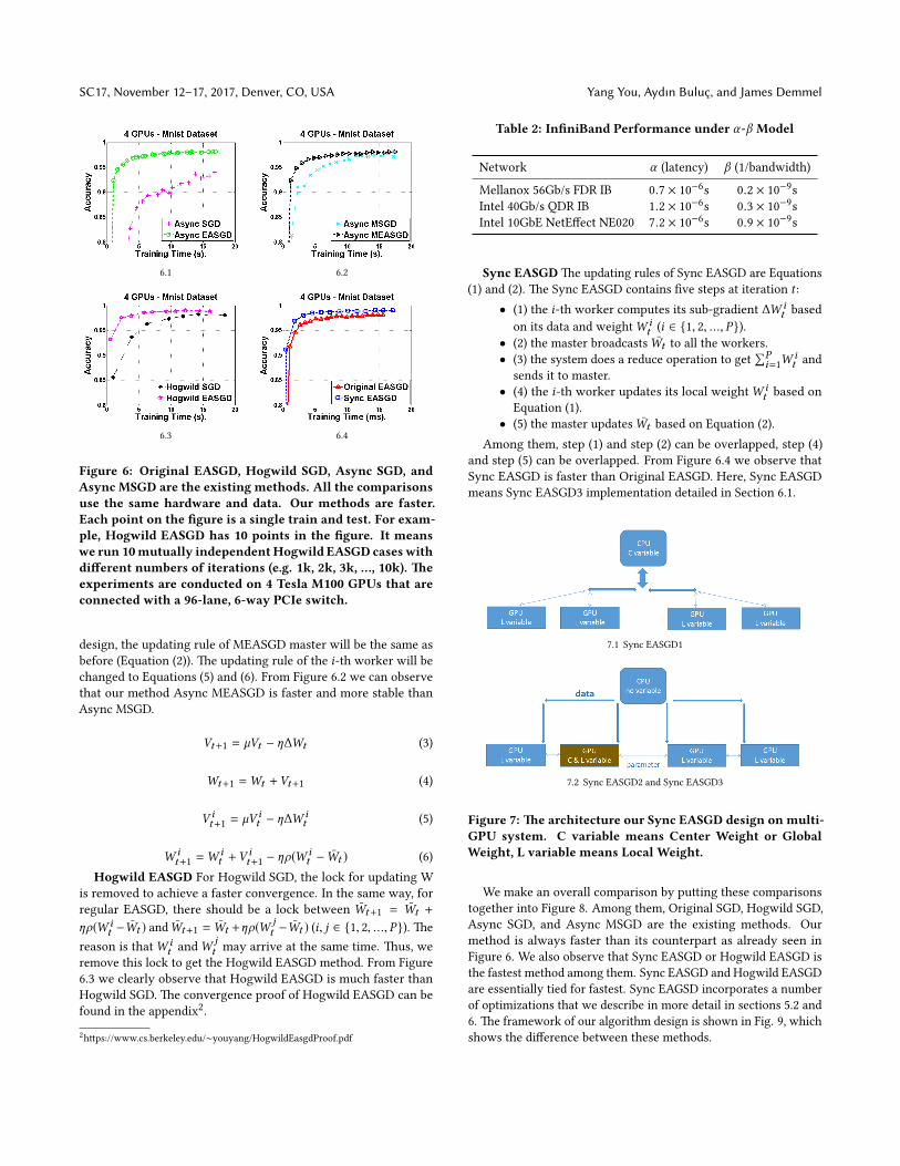
2.3 Data Parallelism and Model ParallelismLet us parallelize the DNN training process on P machines. �ereare two major parallelism strategies for this: Data Parallelism (Fig.4.1) and Model Parallelism (Fig. 4.2). All the later parallel methodsare the variants of these two methods.

Data Parallelism [5] �e dataset is partitioned into P partsand each machine only gets one part. Each machine has a copyof the neural network, hence the weights (W ). �e communica-tion includes sum of all the gradients ∆Wi and broadcast of W .�e �rst part of communication is conducted between BackwardPropagation and Weights Update. �e master updatesW byW ←W − η∑P

i=1 ∆Wi a�er it gets all the sub-gradients ∆Wi from theworkers. �en the master machine broadcastsW to all the workermachines, which is the second part of communication. Figure 4.1 isan example of data parallelism on 4 machines.

Model Parallelism [3] Data parallelism replicates the neuralnetwork itself on each machine while model parallelism partitionsthe neural network into P pieces. Partitioning the neural networkmeans parallelizing the matrix operations on the partitioned net-work. �us, model parallelism can get the same solution as thesingle-machine case. Figure 4.2 shows model parallelism on 3 ma-chines. �ese three machines partition the matrix operation ofeach layer. However, because both the batch size (<= 2048) and thepicture size (e.g. 32×32) typically are relatively small, the matrix op-erations are not large. For example, parallelizing a 2048×1024×1024matrix multiplication only needs one or two machines. �us, state-of-the-art methods o�en use data-parallelism ([1], [2], [5], [22]).

2.4 Evaluating Our Method�e objective of this paper is designing distributed algorithms onHPC systems to get the same or higher classi�cation accuracy(algorithm benchmark) in a shorter time. If our optimization mayin�uence the convergence of algorithm, we report both the timeand accuracy. Otherwise, we only report the time for experimentalresults. All algorithmic comparisons in this paper used the samehardware (e.g. # CPUs, # GPUs, and # KNLs) and the same hyper-parameters (e.g. batch size, learning rate). We do not comparedi�erent architectures (e.g. KNL vs K80 GPU) because they havedi�erent performance, power, and prices.

3 RELATEDWORKIn this section, we review the previous literature about scaling deepneural networks on parallel or distributed systems.

3.1 Parameter Server (Async SGD)Figure 5 illustrates the idea of parameter server or AsynchronousSGD [5]. Under this framework, each worker machine has a copy ofweightW . �e dataset is partitioned to all the worker machines. Ateach step, i-th worker computes a sub-gradient (∆Wi ) from its owndata and weight. �en the i-th worker sends ∆Wi to the master (i ∈{1, 2, ..., P}). �e master receives ∆Wi , conducts the weight update,and sends weight back to i-th worker machine. All the workers�nish this step asynchronously, using �rst come �rst serve (FCFS).

SC17, November 12–17, 2017, Denver, CO, USA Yang You, Aydın Buluc, and James Demmel

Figure 2: �e threemodes ofMCDRAM.Under CacheMode, MCDRAMacts as the last-level cache. Under FlatMode, MCDRAMis part of RAM. Under Hybird Mode, part of MCDRAM acts as the last-level cache, and the rest of it acts as RAM.

Figure 3: �is �gure [20] is an illustration of ConvolutionalNeural Network.

4.1 4.2

Figure 4: Methods of parallelism. 4.1 is data parallelismon 4 machines. 4.2 is model parallelism on 3 machines.Model parallelism partitions the neural network into Ppieces whereas data parallelism replicates the neural net-work itself in each processor.

3.2 Hogwild (Lock Free)�e Hogwild method [21] can be presented as a variant of AsyncSGD. �e master machine is a shared memory system. For AsyncSGD, if the sub-gradient from j-th worker arrives during the periodthat the master is interacting with i-th worker, then W ←W −η∆Wj can not be started beforeW ←W − η∆Wi is �nished (i , j ∈{1, 2, ..., P}). �is means that there is a lock to avoid weight updatecon�icts on the shared memory system (master machine). �e lockmakes sure the master only processes one sub-gradient at one time.�e Hogwild method, however, removes the lock and allows themaster to process multiple sub-gradients at the same time. �eproof of Hogwild’s lock-free convergence is in its paper [21].

Figure 5: �is �gure [5] is an illustration of ParameterServer. Data is partitioned to workers. Each worker com-putes a gradient and sends it to server for updating theweight. �e updated model is copied back to wokers

3.3 EASGD (Round-Robin)�e Elastic Averaging SGD (EASGD) method [28] can also be pre-sented as a variant of Async SGD. Async SGD uses a FCFS strategyfor processing the sub-gradients asynchronously. EASGD uses around-robin strategy for ordered update, i.e. W ←W − η∆Wi cannot be started beforeW ←W −η∆Wi−1 is �nished (i ∈ {2, 3, ...,n}).Also, EASGD requires the workers to conduct the update locally(Equation (1)). Before all the workers conduct the local updating,the master updates the center (or global) weight (Equation (2)). �eρ in Equation (1) and Equation (2) is a term that connects the globaland local parameters. �e framework of Original EASGD methodis shown in Algorithm 1.

W it+1 =W

it − η(∆W i

t + ρ(W it − Wt )) (1)

Wt+1 = Wt + ηP∑i=1

ρ(W it − Wt ) (2)

3.4 Other methodsLi et al. [17] is focused on single-node memory optimization. �eidea is included in our implemenation. �ere is some work [3], [15]on scaling up deep neural networks by model parallelism method,which is out of scope for this paper. �is paper is focused on dataparallelism. Low-precision representation of neural networks isanother direction of research. �e idea is to use low-precision�oating point to reduce the computation and communication for

Scaling Deep Learning on GPU and Knights Landing clusters SC17, November 12–17, 2017, Denver, CO, USA

Algorithm 1: Original EASGD on Multi-GPU systemmaster: CPU, workers: GPU1, GPU2, …, GPUP

Input: samples and labels: {Xi ,yi } i ∈ 1, ...,n#iterations: T , batch size: b, #GPUs: G

Output: model weightW1 Normalize X on CPU by standard deviation: E(X ) = 0 (mean)

and σ (X ) = 1 (variance)2 InitializeW on CPU: random and Xavier weight �lling3 for j = 1; j <= G; j++ do4 create local weightWj on j-th GPU, copyW toWj

5 create global weight W1 on 0-th GPU, copyW to W16 for t = 1; t <= T ; t++ do7 j = t mod G8 CPU randomly picks b samples9 CPU asynchronously copies b samples to j-th GPU

10 CPU sends Wt to j-th GPU11 Forward and Backward Propagation on j-th GPU12 CPU getsW j

t from j-th GPU13 j-th GPU updatesW j

t by Equation (1)14 CPU updates Wt by Wt+1 = Wt + ηρ(W j

t − Wt )

ge�ing the acceptable accuracy ([4], [8], [10], [22]). We reserve thisfor future study.

4 EXPERIMENTAL SETUP4.1 Experimental DatasetsOur test datasets are Mnist [16], Cifar [13], and ImageNet [6], whichare the standard benchmarks for deep learning research. Descrip-tions can be found in Table 1. �e application of Mnist dataset ishardwri�en digits recognition. �e images of Mnist were groupedinto 10 classes (0, 1, 2, …, 9). �e application of Cifar dataset isobject recognition. Cifar dataset includes 10 classes: airplane, au-tomobile, bird, cat, deer, dog, frog, horse, ship, truck. Each Cifarimage only belongs to one class. �e accuracy of random guess forMnist and Cifar image prediction is 0.1.

ImageNet [6] is a computer vision dataset of over 15 millionlabeled images belonging to more than 20,000 classes. �e imageswere collected from the web and labeled by human labelers us-ing Amazon’s Mechanical Turk crowd-sourcing tool. An annualcompetition called the ImageNet Large-Scale Visual RecognitionChallenge (ILSVRC) has been held since 2010. ILSVRC uses a subsetof ImageNet with 1200 images in each of 1000 classes. In all, thereare roughly 1.2 million training images, 50,000 validation images,and 150,000 testing images. In this paper, the ImageNet datasetmeans ILSVRC-2012 dataset. �e accuracy of random guess forImageNet image prediction is 0.001.

4.2 Neural Network ModelsWe use the state-of-the-art DNN models to process the datasets inthis paper. �e Mnist dataset was processed by LetNet [16], whichis shown in Figure 3. �e Cifar dataset is processed by AlexNet[14], which has 5 convolutional layers and 3 fully-connected layers.

Table 1: �e Test Datasets

Dataset Training Images Test Images Pixels Classes

Mnist [16] 60,000 10,000 28×28 10Cifar [13] 50,000 10,000 3×32×32 10ImageNet [6] 1.2 million 150,000 256×256 1000

ImageNet dataset is processed by GoogleNet [25] and VGG [25].GoogleNet has 22 layers and VGG has 19 layers.

4.3 �e baselineIn Section 5, the Original EASGD is our baseline. �e originalEASGD method (Algorithm 1) uses round-robin approach for sched-uling the way the master interacts with the workers. At any mo-ment, the master can interact with just a single worker. Addition-ally, the interactions of di�erent workers are ordered. �e (i + 1)-stworker can not begin before i-th �nishes.

5 DISTRIBUTED ALGORITHM DESIGN5.1 Redesigning the parallel SGD methodsIn this section we redesign some e�cient parallel SGD methodsbased on the existing methods (i.e. Original EASGD, Async SGD,Async MSGD, and Hogwild SGD). We will use our methods to makecomparisons with the existing methods (i.e. we will plot accuracyversus time, on the same data sets and computing resources). Sincethe existing SGD methods were originally implemented on GPUs,we also implement our methods on GPUs. �ese ideas work in thesame way for KNL chips because these methods are focused oninter-chip processing rather than intra-chip processing.

Async EASGD �e original EASGD method (Algorithm 1) usesround-robin approach for scheduling. �is method is ine�cientbecause the computation and update of di�erent GPUs are ordered(Section 3.3). �e (i + 1)-st worker can not begin before i-th �nishes.Although this method has good fault-tolerance and convergenceproperties, it is ine�cient. �erefore, our �rst optimization is to useparameter-server update to replace the round-robin update. �edi�erence between our Async EASGD and Original EASGD is thatwe use �rst-come �rst-served (FCFS) strategy to process multipleworkers while they use ordered rule to process multiple workers.We put the global (or center) weight W on the master machine. �ei-th worker machine has its own local weightW i . During the t-thiteration, there are three steps:

• (1) i-th worker �rst sends its local weight W it to master

and master returns Wt to i-th worker (i ∈ {1, 2, ..., P}).• (2) i-th worker computes gradient ∆W i

t and receives Wt .• (3) master does the update based on Equation (2) and

worker does the update based on Equation (1).From Figure 6.1 we can observe that our method Async EASGD

is faster than Async SGD.Async MEASGD Momentum [24] is an important method to

accelerate SGD. �e updating rule of Momentum SGD (MSGD) isshown in Equations (3) and (4). V is the momentum parameter,which has the same dimension as the weight and gradient. µ is themomentum rate. Rule of thumb is µ = 0.9 or a similar value. In our

SC17, November 12–17, 2017, Denver, CO, USA Yang You, Aydın Buluc, and James Demmel

6.1 6.2

6.3 6.4

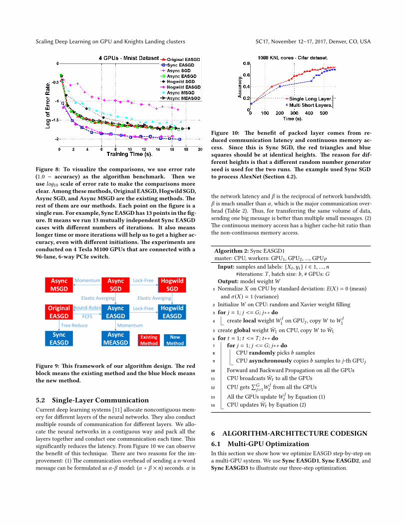
Figure 6: Original EASGD, Hogwild SGD, Async SGD, andAsync MSGD are the existing methods. All the comparisonsuse the same hardware and data. Our methods are faster.Each point on the �gure is a single train and test. For exam-ple, Hogwild EASGD has 10 points in the �gure. It meanswe run 10mutually independentHogwild EASGD caseswithdi�erent numbers of iterations (e.g. 1k, 2k, 3k, …, 10k). �eexperiments are conducted on 4 Tesla M100 GPUs that areconnected with a 96-lane, 6-way PCIe switch.

design, the updating rule of MEASGD master will be the same asbefore (Equation (2)). �e updating rule of the i-th worker will bechanged to Equations (5) and (6). From Figure 6.2 we can observethat our method Async MEASGD is faster and more stable thanAsync MSGD.

Vt+1 = µVt − η∆Wt (3)

Wt+1 =Wt +Vt+1 (4)

V it+1 = µV

it − η∆W i

t (5)

W it+1 =W

it +V

it+1 − ηρ(W

it − Wt ) (6)

Hogwild EASGD For Hogwild SGD, the lock for updating Wis removed to achieve a faster convergence. In the same way, forregular EASGD, there should be a lock between Wt+1 = Wt +

ηρ(W it −Wt ) andWt+1 = Wt +ηρ(W j

t −Wt ) (i, j ∈ {1, 2, ..., P}). �ereason is thatW i

t andWjt may arrive at the same time. �us, we

remove this lock to get the Hogwild EASGD method. From Figure6.3 we clearly observe that Hogwild EASGD is much faster thanHogwild SGD. �e convergence proof of Hogwild EASGD can befound in the appendix2.2h�ps://www.cs.berkeley.edu/∼youyang/HogwildEasgdProof.pdf

Table 2: In�niBand Performance under α-β Model

Network α (latency) β (1/bandwidth)

Mellanox 56Gb/s FDR IB 0.7 × 10−6s 0.2 × 10−9sIntel 40Gb/s QDR IB 1.2 × 10−6s 0.3 × 10−9sIntel 10GbE NetE�ect NE020 7.2 × 10−6s 0.9 × 10−9s

Sync EASGD �e updating rules of Sync EASGD are Equations(1) and (2). �e Sync EASGD contains �ve steps at iteration t :

• (1) the i-th worker computes its sub-gradient ∆W it based

on its data and weightW it (i ∈ {1, 2, ..., P}).

• (2) the master broadcasts Wt to all the workers.• (3) the system does a reduce operation to get

∑Pi=1W

it and

sends it to master.• (4) the i-th worker updates its local weightW i

t based onEquation (1).

• (5) the master updates Wt based on Equation (2).Among them, step (1) and step (2) can be overlapped, step (4)

and step (5) can be overlapped. From Figure 6.4 we observe thatSync EASGD is faster than Original EASGD. Here, Sync EASGDmeans Sync EASGD3 implementation detailed in Section 6.1.

7.1 Sync EASGD1

7.2 Sync EASGD2 and Sync EASGD3

Figure 7: �e architecture our Sync EASGD design on multi-GPU system. C variable means Center Weight or GlobalWeight, L variable means Local Weight.

We make an overall comparison by pu�ing these comparisonstogether into Figure 8. Among them, Original SGD, Hogwild SGD,Async SGD, and Async MSGD are the existing methods. Ourmethod is always faster than its counterpart as already seen inFigure 6. We also observe that Sync EASGD or Hogwild EASGD isthe fastest method among them. Sync EASGD and Hogwild EASGDare essentially tied for fastest. Sync EAGSD incorporates a numberof optimizations that we describe in more detail in sections 5.2 and6. �e framework of our algorithm design is shown in Fig. 9, whichshows the di�erence between these methods.

Scaling Deep Learning on GPU and Knights Landing clusters SC17, November 12–17, 2017, Denver, CO, USA

Figure 8: To visualize the comparisons, we use error rate(1.0 − accuracy) as the algorithm benchmark. �en weuse loд10 scale of error rate to make the comparisons moreclear. Among thesemethods, Original EASGD,Hogwild SGD,Async SGD, and Async MSGD are the existing methods. �erest of them are our methods. Each point on the �gure is asingle run. For example, Sync EASGDhas 13 points in the�g-ure. It means we run 13 mutually independent Sync EASGDcases with di�erent numbers of iterations. It also meanslonger time ormore iterations will help us to get a higher ac-curacy, even with di�erent initiations. �e experiments areconducted on 4 Tesla M100 GPUs that are connected with a96-lane, 6-way PCIe switch.

HogwildEASGD

HogwildSGD

AsyncSGD

AsyncEASGD

AsyncMEASGD

AsyncMSGD

OriginalEASGD

SyncEASGD

Momentum Lock-Free

Lock-Free

Elastic Averging Elastic Averging

Tree Reduce Momentum

FCFS

Round-Robin

ExistingMethod

NewMethod

Figure 9: �is framework of our algorithm design. �e redblock means the existing method and the blue block meansthe new method.

5.2 Single-Layer CommunicationCurrent deep learning systems [11] allocate noncontiguous mem-ory for di�erent layers of the neural networks. �ey also conductmultiple rounds of communication for di�erent layers. We allo-cate the neural networks in a contiguous way and pack all thelayers together and conduct one communication each time. �issigni�cantly reduces the latency. From Figure 10 we can observethe bene�t of this technique. �ere are two reasons for the im-provement: (1) �e communication overhead of sending a n-wordmessage can be formulated as α-β model: (α + β × n) seconds. α is

Figure 10: �e bene�t of packed layer comes from re-duced communication latency and continuous memory ac-cess. Since this is Sync SGD, the red triangles and bluesquares should be at identical heights. �e reason for dif-ferent heights is that a di�erent random number generatorseed is used for the two runs. �e example used Sync SGDto process AlexNet (Section 4.2).

the network latency and β is the reciprocal of network bandwidth.β is much smaller than α , which is the major communication over-head (Table 2). �us, for transferring the same volume of data,sending one big message is be�er than multiple small messages. (2)�e continuous memory access has a higher cache-hit ratio thanthe non-continuous memory access.

Algorithm 2: Sync EASGD1master: CPU, workers: GPU1, GPU2, …, GPUP

Input: samples and labels: {Xi ,yi } i ∈ 1, ...,n#iterations: T , batch size: b, # GPUs: G

Output: model weightW1 Normalize X on CPU by standard deviation: E(X ) = 0 (mean)

and σ (X ) = 1 (variance)2 InitializeW on CPU: random and Xavier weight �lling3 for j = 1; j <= G; j++ do4 create local weightW j

1 on GPUj , copyW toW j1

5 create global weight W1 on CPU, copyW to W16 for t = 1; t <= T ; t++ do7 for j = 1; j <= G; j++ do8 CPU randomly picks b samples9 CPU asynchronously copies b samples to j-th GPUj

10 Forward and Backward Propagation on all the GPUs11 CPU broadcasts Wt to all the GPUs12 CPU gets

∑Gj=1W

jt from all the GPUs

13 All the GPUs updateW jt by Equation (1)

14 CPU updates Wt by Equation (2)

6 ALGORITHM-ARCHITECTURE CODESIGN6.1 Multi-GPU OptimizationIn this section we show how we optimize EASGD step-by-step ona multi-GPU system. We use Sync EASGD1, Sync EASGD2, andSync EASGD3 to illustrate our three-step optimization.

SC17, November 12–17, 2017, Denver, CO, USA Yang You, Aydın Buluc, and James Demmel

6.1.1 Sync EASGD1. Algorithm 1 is the original EASGD algo-rithm. Multi-GPU system implementation contains 8 potentiallytime-consuming parts. For Algorithm 1, they are: (1) data I/O (In-put and Output); (2) data and weight initialization (lines 1-2); (3)GPU-GPU parameter communication (none); (4) CPU-GPU datacommunication (line 9); (5) CPU-GPU parameter communication(lines 10 and 12); (6) Forward and Backward propagation (line 11);(7) GPU weight update (line 13); (8) CPU weight update (line 14). Weignore parts (1) and (2) because they only cost a tiny percent of time.GPU-GPU parameter communication means di�erent GPUs ex-change weights. CPU-GPU data communication means GPU copiesa batch of samples each iteration. CPU-GPU parameter communi-cation means CPU sends global weight W to GPUs and receiveslocal weightsW i (i ∈ {1, 2, ..., P ) from GPUs. Parts (3), (4), and (5)are communication. Parts (6), (7), and (8) are computation. A�erbenchmarking the code, we found the major overhead of EASGD iscommunication (Figure 11), which costs 87% of the total trainingtime on an 8-GPU system. If we look deep into the communication,we observe that CPU-GPU parameter communication costs muchmore time than CPU-GPU data communication (86% vs 1%). �ereason is that the size of weights (number of elements in W ) ismuch larger than a batch of training data. For example, the weightsof AlexNet are 249 MB while 64 Cifar samples are only 64 × 32 × 32× 3 × 4B = 768 KB. To solve this problem, we design Sync EASGD1(Algorithm 2). In Sync EASGD1, P blocking send/receive opera-tions can be e�ciently processed by a tree-reduction operation(e.g. standard MPI reduction), which reduces the communicationoverhead from P(α + |W |β) to loдP(α + |W |β). Our experimentsshow that Sync EASGD1 achieves a 3.7× speedup over OriginalEASGD (Table 3 and Figure 11).

Algorithm 3: Sync EASGD2 & Sync EASGD3master: GPU1, workers: GPU1, GPU2, …, GPUP

Input: samples and labels: {Xi ,yi } i ∈ 1, ...,n#iterations: T , batch size: b, # GPUs: G

Output: model weightW1 Normalize X on CPU by standard deviation: E(X ) = 0 (mean)

and σ (X ) = 1 (variance)2 InitializeW on CPU: random and Xavier weight �lling3 for j = 1; j <= G; j++ do4 create local weightW j

1 on GPUj , copyW toW j1

5 create global weight W1 on GPU1, copyW to W16 for t = 1; t <= T ; t++ do7 for j = 1; j <= G; j++ do8 CPU randomly pick b samples9 CPU asynchronously copy b samples to j-th GPUj

10 Forward and Backward Propagation on all the GPUs11 GPU1 broadcasts Wt to all the GPUs12 GPU1 gets

∑Gj=1W

jt from all the GPUs

13 All the GPUs updateW jt by Equation (1)

14 GPU1 updates Wt by Equation (2)

6.1.2 Sync EASGD2. From Table 3 we observe that CPU-GPUcommunication is still the major overhead of communication. �us,we want to move either data or weights from CPU to GPU to reducethe communication overhead. We can not put all the data on theGPU card because the on-chip memory is very limited comparedwith CPU. For example, the training part of ImageNet dataset is 240GB while the on-chip memory of K80 is only around 12 GB. Sincethe algorithm needs to randomly pick samples from the dataset,we can not predict which part of dataset will be used by a certainGPU. �us, we put all the training and test data on the CPU. Weonly copy the required data to the GPUs at runtime each iteration.On the other hand, the weights are usually smaller than 1 GB,which can be stored on a GPU card. For example, the large DNNmodel VGG-19 [23] is 575 MB. Also, the weight will be reused everyiteration (Algorithm 3). �us, we put all the weights on GPU toreduce communication overhead. We refer to this method as SyncEASGD2, which achieves 1.3× speedup over Sync EASGD1. �eframework of Sync EASGD2 is shown in Algorithm 3.

6.1.3 Sync EASGD3. We further improve the algorithm by over-lapping the computation with the communication. We maximizethe overlapping bene�t inside the steps 7-14 of Algorithm 3. Be-cause Forward/Backward Propagation uses the data from the CPU,steps 7-10 are a critical path. �e GPU-GPU communication (steps11-12) is not dependent on steps 7-10. �us, we overlap steps 7-10 and steps 11-12 in Algorithm 3, yielding Sync EASGD3, whichachieves a 1.1× speedup over Sync EASGD2. In all, Sync EASGD3reduced the communication ratio from 87% to 14% and achieves5.3× speedup over original EASGD for ge�ing the same accuracy(Table 3 and Figure 11). �us we refer to Sync EASGD3 as Com-munication E�cient EASGD. We also design similar algorithmfor KNL cluster, which is shown in Algorithm 4, discussed next.

Algorithm4:Communication E�cient EASGD on KNL clustermaster: KNL1, workers: KNL1, KNL2, …, KNLPInput: samples and labels: {Xi ,yi } i ∈ 1, ...,n

#iterations: T , batch size: b, # KNL Nodes: KOutput: model weightW

1 All nodes read the samples and labels from disk2 Normalize X on all KNLs by standard deviation: E(X ) = 0

(mean) and σ (X ) = 1 (variance)3 InitializeW on 1-st KNL: random and Xavier weight �lling4 KNL1 broadcastsW to all KNLs5 for j = 1; j <= K ; j++ parallel do6 create local weightW j

1 on KNLj , copyW toW j1

7 create global weight W1 on KNL1, copyW to W18 for t = 1; t <= T ; t++ do9 for j = 1; j <= K ; j++ parallel do

10 KNLj randomly pick b samples from local memory11 Forward and Backward Propagation on all the KNLs12 KNL1 broadcasts Wt to all the KNLs13 KNL1 gets

∑Kj=1W

jt from all the KNLs

14 All the KNLs updateW jt by Equation (1)

15 KNL1 updates Wt by Equation (2)

Scaling Deep Learning on GPU and Knights Landing clusters SC17, November 12–17, 2017, Denver, CO, USA

11.1

11.2

Figure 11: Breakdown of time for EASGD variants. parameans parameter or weight. comm means communication.Computation includes forward/backward, gpu update, andcpu update. �ere is an overlap between for/backward andcpu-gpu para comm for Original EASGD. Let us refer to thenon-overlap version as Original EASGD*. Sync EASGD3 re-duced the communication percentage from 87% to 14% andgot 5.3× speedup over original EASGD for the same accuracy(98.8%). �e test is for MNIST dataset on 4 GPUs. More infor-mation is in Table 3.

6.2 Knights Landing OptimizationOur platform’s KNL chip has 68 cores or 72 cores, which is muchmore than that of a regular CPU chip. To make full use of KNL’scomputational power, data locality is highly important. Also, weneed to make the best use of KNL’s cluster mode (Section 2.1) at thealgorithm level. We partition the KNL chip into 4 parts like �ador SNC-4 mode. �e KNL acts like a 4-node NUMA system. In thisway, we also replicate the data into 4 parts and each NUMA nodegets one part. We make 4 copies of weights and each NUMA nodehas one copy. A�er all the NUMA nodes compute the gradients,we conduct a tree-reduction operation to sum these all gradients.Each NUMA node can get one copy of the gradient sum and useit to update its own weights. In this way, di�erent NUMA nodesdo not need to communicate with each other unless they share thegradients. �is is a divide-and-conquer method. �e divide stepincludes replicating the data and copying the weights. �e conquerstep is to sum up the gradients from all partitions. �is can speedupthe algorithm by the faster propagation of gradients.

In the same way, we can partition the chip into 8 parts, 16 parts,and so on. Let us partition the chip into P parts. �e limitation ofthis method is that the fast memory (cache and MCDRAM) should

Figure 12: Partitioning a KNL chip into group and makingeach group process one local weight can improve the perfor-mance.

be able to handle P copies of weight and P copies of data. Figure 12shows that this method works for P ≤ 16 when we use AlexNet toprocess Cifar dataset. �e reason is that the AlexNet is 249 MB andone Cifar data copy is 687 MB. �us, MCDRAM can hold at most16 copies of weight and data. Concretely, for achieving the sameaccuracy (0.625), 1-part case needs 1605 sec, 4-part case needs 1025sec, 8-part case needs 823 sec, and 16-part case only needs 490 sec.We achieve 3.3× speedup by copying weight and data to make fulluse of the fast memory and reduce communication.

7 ADDITIONAL RESULTS AND DISCUSSIONS

13.1

13.2

Figure 13: �e bene�ts of using more machines and moredata: (1) get the target accuracy in a shorter time, and (2)achieve a higher accuracy in a �xed time. Objective Lossmeans Error (lower is better).

SC17, November 12–17, 2017, Denver, CO, USA Yang You, Aydın Buluc, and James Demmel

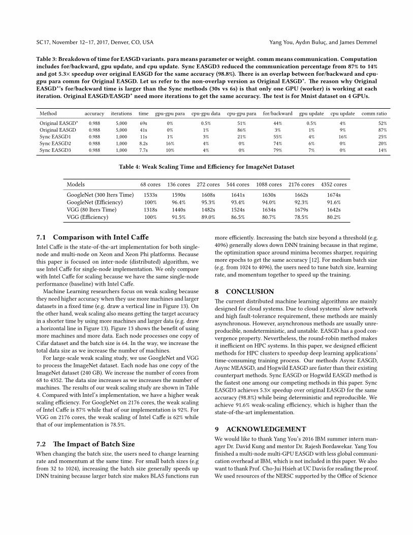
Table 3: Breakdownof time for EASGDvariants. parameans parameter orweight. commmeans communication. Computationincludes for/backward, gpu update, and cpu update. Sync EASGD3 reduced the communication percentage from 87% to 14%and got 5.3× speedup over original EASGD for the same accuracy (98.8%). �ere is an overlap between for/backward and cpu-gpu para comm for Original EASGD. Let us refer to the non-overlap version as Original EASGD*. �e reason why OriginalEASGD*’s for/backward time is larger than the Sync methods (30s vs 6s) is that only one GPU (worker) is working at eachiteration. Original EASGD/EASGD* need more iterations to get the same accuracy. �e test is for Mnist dataset on 4 GPUs.

Method accuracy iterations time gpu-gpu para cpu-gpu data cpu-gpu para for/backward gpu update cpu update comm ratio

Original EASGD* 0.988 5,000 69s 0% 0.5% 51% 44% 0.5% 4% 52%Original EASGD 0.988 5,000 41s 0% 1% 86% 3% 1% 9% 87%Sync EASGD1 0.988 1,000 11s 1% 3% 21% 55% 4% 16% 25%Sync EASGD2 0.988 1,000 8.2s 16% 4% 0% 74% 6% 0% 20%Sync EASGD3 0.988 1,000 7.7s 10% 4% 0% 79% 7% 0% 14%

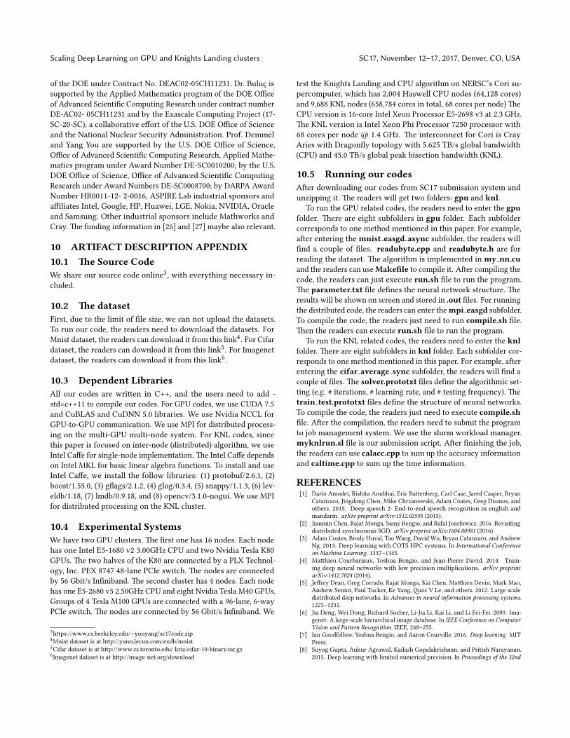
Table 4: Weak Scaling Time and E�ciency for ImageNet Dataset

Models 68 cores 136 cores 272 cores 544 cores 1088 cores 2176 cores 4352 coresGoogleNet (300 Iters Time) 1533s 1590s 1608s 1641s 1630s 1662s 1674sGoogleNet (E�ciency) 100% 96.4% 95.3% 93.4% 94.0% 92.3% 91.6%VGG (80 Iters Time) 1318s 1440s 1482s 1524s 1634s 1679s 1642sVGG (E�ciency) 100% 91.5% 89.0% 86.5% 80.7% 78.5% 80.2%

7.1 Comparison with Intel Ca�eIntel Ca�e is the state-of-the-art implementation for both single-node and multi-node on Xeon and Xeon Phi platforms. Becausethis paper is focused on inter-node (distributed) algorithm, weuse Intel Ca�e for single-node implementation. We only comparewith Intel Ca�e for scaling because we have the same single-nodeperformance (baseline) with Intel Ca�e.

Machine Learning researchers focus on weak scaling becausethey need higher accuracy when they use more machines and largerdatasets in a �xed time (e.g. draw a vertical line in Figure 13). Onthe other hand, weak scaling also means ge�ing the target accuracyin a shorter time by using more machines and larger data (e.g. drawa horizontal line in Figure 13). Figure 13 shows the bene�t of usingmore machines and more data. Each node processes one copy ofCifar dataset and the batch size is 64. In the way, we increase thetotal data size as we increase the number of machines.

For large-scale weak scaling study, we use GoogleNet and VGGto process the ImageNet dataset. Each node has one copy of theImageNet dataset (240 GB). We increase the number of cores from68 to 4352. �e data size increases as we increases the number ofmachines. �e results of our weak scaling study are shown in Table4. Compared with Intel’s implementation, we have a higher weakscaling e�ciency. For GoogleNet on 2176 cores, the weak scalingof Intel Ca�e is 87% while that of our implementation is 92%. ForVGG on 2176 cores, the weak scaling of Intel Ca�e is 62% whilethat of our implementation is 78.5%.

7.2 �e Impact of Batch SizeWhen changing the batch size, the users need to change learningrate and momentum at the same time. For small batch sizes (e.gfrom 32 to 1024), increasing the batch size generally speeds upDNN training because larger batch size makes BLAS functions run

more e�ciently. Increasing the batch size beyond a threshold (e.g.4096) generally slows down DNN training because in that regime,the optimization space around minima becomes sharper, requiringmore epochs to get the same accuracy [12]. For medium batch size(e.g. from 1024 to 4096), the users need to tune batch size, learningrate, and momentum together to speed up the training.

8 CONCLUSION�e current distributed machine learning algorithms are mainlydesigned for cloud systems. Due to cloud systems’ slow networkand high fault-tolerance requirement, these methods are mainlyasynchronous. However, asynchronous methods are usually unre-producible, nondeterministic, and unstable. EASGD has a good con-vergence property. Nevertheless, the round-robin method makesit ine�cient on HPC systems. In this paper, we designed e�cientmethods for HPC clusters to speedup deep learning applications’time-consuming training process. Our methods Async EASGD,Async MEASGD, and Hogwild EASGD are faster than their existingcounterpart methods. Sync EASGD or Hogwild EASGD method isthe fastest one among our competing methods in this paper. SyncEASGD3 achieves 5.3× speedup over original EASGD for the sameaccuracy (98.8%) while being deterministic and reproducible. Weachieve 91.6% weak-scaling e�ciency, which is higher than thestate-of-the-art implementation.

9 ACKNOWLEDGEMENTWe would like to thank Yang You’s 2016 IBM summer intern man-ager Dr. David Kung and mentor Dr. Rajesh Bordawekar. Yang You�nished a multi-node multi-GPU EASGD with less global communi-cation overhead at IBM, which is not included in this paper. We alsowant to thank Prof. Cho-Jui Hsieh at UC Davis for reading the proof.We used resources of the NERSC supported by the O�ce of Science

Scaling Deep Learning on GPU and Knights Landing clusters SC17, November 12–17, 2017, Denver, CO, USA

of the DOE under Contract No. DEAC02-05CH11231. Dr. Buluc issupported by the Applied Mathematics program of the DOE O�ceof Advanced Scienti�c Computing Research under contract numberDE-AC02- 05CH11231 and by the Exascale Computing Project (17-SC-20-SC), a collaborative e�ort of the U.S. DOE O�ce of Scienceand the National Nuclear Security Administration. Prof. Demmeland Yang You are supported by the U.S. DOE O�ce of Science,O�ce of Advanced Scienti�c Computing Research, Applied Mathe-matics program under Award Number DE-SC0010200; by the U.S.DOE O�ce of Science, O�ce of Advanced Scienti�c ComputingResearch under Award Numbers DE-SC0008700; by DARPA AwardNumber HR0011-12- 2-0016, ASPIRE Lab industrial sponsors anda�liates Intel, Google, HP, Huawei, LGE, Nokia, NVIDIA, Oracleand Samsung. Other industrial sponsors include Mathworks andCray. �e funding information in [26] and [27] maybe also relevant.

10 ARTIFACT DESCRIPTION APPENDIX10.1 �e Source CodeWe share our source code online3, with everything necessary in-cluded.

10.2 �e datasetFirst, due to the limit of �le size, we can not upload the datasets.To run our code, the readers need to download the datasets. ForMnist dataset, the readers can download it from this link4. For Cifardataset, the readers can download it from this link5. For Imagenetdataset, the readers can download it from this link6.

10.3 Dependent LibrariesAll our codes are wri�en in C++, and the users need to add -std=c++11 to compile our codes. For GPU codes, we use CUDA 7.5and CuBLAS and CuDNN 5.0 libraries. We use Nvidia NCCL forGPU-to-GPU communication. We use MPI for distributed process-ing on the multi-GPU multi-node system. For KNL codes, sincethis paper is focused on inter-node (distributed) algorithm, we useIntel Ca�e for single-node implementation. �e Intel Ca�e dependson Intel MKL for basic linear algebra functions. To install and useIntel Ca�e, we install the follow libraries: (1) protobuf/2.6.1, (2)boost/1.55.0, (3) g�ags/2.1.2, (4) glog/0.3.4, (5) snappy/1.1.3, (6) lev-eldb/1.18, (7) lmdb/0.9.18, and (8) opencv/3.1.0-nogui. We use MPIfor distributed processing on the KNL cluster.

10.4 Experimental SystemsWe have two GPU clusters. �e �rst one has 16 nodes. Each nodehas one Intel E5-1680 v2 3.00GHz CPU and two Nvidia Tesla K80GPUs. �e two halves of the K80 are connected by a PLX Technol-ogy, Inc. PEX 8747 48-lane PCIe switch. �e nodes are connectedby 56 Gbit/s In�niband. �e second cluster has 4 nodes. Each nodehas one E5-2680 v3 2.50GHz CPU and eight Nvidia Tesla M40 GPUs.Groups of 4 Tesla M100 GPUs are connected with a 96-lane, 6-wayPCIe switch. �e nodes are connected by 56 Gbit/s In�niband. We

3h�ps://www.cs.berkeley.edu/∼youyang/sc17code.zip4Mnist dataset is at h�p://yann.lecun.com/exdb/mnist5Cifar dataset is at h�p://www.cs.toronto.edu/ kriz/cifar-10-binary.tar.gz6Imagenet dataset is at h�p://image-net.org/download

test the Knights Landing and CPU algorithm on NERSC’s Cori su-percomputer, which has 2,004 Haswell CPU nodes (64,128 cores)and 9,688 KNL nodes (658,784 cores in total, 68 cores per node) �eCPU version is 16-core Intel Xeon Processor E5-2698 v3 at 2.3 GHz.�e KNL version is Intel Xeon Phi Processor 7250 processor with68 cores per node @ 1.4 GHz. �e interconnect for Cori is CrayAries with Dragon�y topology with 5.625 TB/s global bandwidth(CPU) and 45.0 TB/s global peak bisection bandwidth (KNL).

10.5 Running our codesA�er downloading our codes from SC17 submission system andunzipping it. �e readers will get two folders: gpu and knl.

To run the GPU related codes, the readers need to enter the gpufolder. �ere are eight subfolders in gpu folder. Each subfoldercorresponds to one method mentioned in this paper. For example,a�er entering the mnist easgd async subfolder, the readers will�nd a couple of �les. readubyte.cpp and readubyte.h are forreading the dataset. �e algorithm is implemented in my nn.cuand the readers can use Make�le to compile it. A�er compiling thecode, the readers can just execute run.sh �le to run the program.�e parameter.txt �le de�nes the neural network structure. �eresults will be shown on screen and stored in .out �les. For runningthe distributed code, the readers can enter the mpi easgd subfolder.To compile the code, the readers just need to run compile.sh �le.�en the readers can execute run.sh �le to run the program.

To run the KNL related codes, the readers need to enter the knlfolder. �ere are eight subfolders in knl folder. Each subfolder cor-responds to one method mentioned in this paper. For example, a�erentering the cifar average sync subfolder, the readers will �nd acouple of �les. �e solver.prototxt �les de�ne the algorithmic set-ting (e.g. # iterations, # learning rate, and # testing frequency). �etrain test.prototxt �les de�ne the structure of neural networks.To compile the code, the readers just need to execute compile.sh�le. A�er the compilation, the readers need to submit the programto job management system. We use the slurm workload manager.myknlrun.sl �le is our submission script. A�er �nishing the job,the readers can use calacc.cpp to sum up the accuracy informationand caltime.cpp to sum up the time information.

REFERENCES[1] Dario Amodei, Rishita Anubhai, Eric Ba�enberg, Carl Case, Jared Casper, Bryan

Catanzaro, Jingdong Chen, Mike Chrzanowski, Adam Coates, Greg Diamos, andothers. 2015. Deep speech 2: End-to-end speech recognition in english andmandarin. arXiv preprint arXiv:1512.02595 (2015).

[2] Jianmin Chen, Rajat Monga, Samy Bengio, and Rafal Jozefowicz. 2016. Revisitingdistributed synchronous SGD. arXiv preprint arXiv:1604.00981 (2016).

[3] Adam Coates, Brody Huval, Tao Wang, David Wu, Bryan Catanzaro, and AndrewNg. 2013. Deep learning with COTS HPC systems. In International Conferenceon Machine Learning. 1337–1345.

[4] Ma�hieu Courbariaux, Yoshua Bengio, and Jean-Pierre David. 2014. Train-ing deep neural networks with low precision multiplications. arXiv preprintarXiv:1412.7024 (2014).

[5] Je�rey Dean, Greg Corrado, Rajat Monga, Kai Chen, Ma�hieu Devin, Mark Mao,Andrew Senior, Paul Tucker, Ke Yang, �oc V Le, and others. 2012. Large scaledistributed deep networks. In Advances in neural information processing systems.1223–1231.

[6] Jia Deng, Wei Dong, Richard Socher, Li-Jia Li, Kai Li, and Li Fei-Fei. 2009. Ima-genet: A large-scale hierarchical image database. In IEEE Conference on ComputerVision and Pa�ern Recognition. IEEE, 248–255.

[7] Ian Goodfellow, Yoshua Bengio, and Aaron Courville. 2016. Deep learning. MITPress.

[8] Suyog Gupta, Ankur Agrawal, Kailash Gopalakrishnan, and Pritish Narayanan.2015. Deep learning with limited numerical precision. In Proceedings of the 32nd

SC17, November 12–17, 2017, Denver, CO, USA Yang You, Aydın Buluc, and James Demmel

International Conference on Machine Learning (ICML-15). 1737–1746.[9] Kaiming He, Xiangyu Zhang, Shaoqing Ren, and Jian Sun. 2016. Deep residual

learning for image recognition. In Proceedings of the IEEE Conference on ComputerVision and Pa�ern Recognition. 770–778.

[10] Itay Hubara, Ma�hieu Courbariaux, Daniel Soudry, Ran El-Yaniv, and YoshuaBengio. 2016. �antized neural networks: Training neural networks with lowprecision weights and activations. arXiv preprint arXiv:1609.07061 (2016).

[11] Forrest N Iandola, Ma�hew W Moskewicz, Khalid Ashraf, and Kurt Keutzer.2016. FireCa�e: near-linear acceleration of deep neural network training oncompute clusters. In Proceedings of the IEEE Conference on Computer Vision andPa�ern Recognition. 2592–2600.

[12] Nitish Shirish Keskar, Dheevatsa Mudigere, Jorge Nocedal, Mikhail Smelyanskiy,and Ping Tak Peter Tang. 2016. On large-batch training for deep learning:Generalization gap and sharp minima. arXiv preprint arXiv:1609.04836 (2016).

[13] Alex Krizhevsky. 2009. Learning multiple layers of features from tiny images.Master�s thesis, Department of Computer Science, University of Toronto (2009).

[14] Alex Krizhevsky, Ilya Sutskever, and Geo�rey E Hinton. 2012. Imagenet classi�ca-tion with deep convolutional neural networks. In Advances in neural informationprocessing systems. 1097–1105.

[15] �oc V Le. 2013. Building high-level features using large scale unsupervisedlearning. In Acoustics, Speech and Signal Processing (ICASSP), 2013 IEEE Interna-tional Conference on. IEEE, 8595–8598.

[16] Yann LeCun, Leon Bo�ou, Yoshua Bengio, and Patrick Ha�ner. 1998. Gradient-based learning applied to document recognition. Proc. IEEE 86, 11 (1998), 2278–2324.

[17] Chao Li, Yi Yang, Min Feng, Srimat Chakradhar, and Huiyang Zhou. 2016. Op-timizing memory e�ciency for deep convolutional neural networks on GPUs.In Proceedings of the International Conference for High Performance Computing,Networking, Storage and Analysis. IEEE Press, 54.

[18] Mu Li, David G Andersen, Jun Woo Park, Alexander J Smola, Amr Ahmed,Vanja Josifovski, James Long, Eugene J Shekita, and Bor-Yiing Su. 2014. ScalingDistributed Machine Learning with the Parameter Server.. In OSDI, Vol. 14.583–598.

[19] Mu Li, Tong Zhang, Yuqiang Chen, and Alexander J Smola. 2014. E�cientmini-batch training for stochastic optimization. In Proceedings of the 20th ACMSIGKDD international conference on Knowledge discovery and data mining. ACM,661–670.

[20] Maurice Peemen, Bart Mesman, and Henk Corporaal. 2011. E�ciency optimiza-tion of trainable feature extractors for a consumer platform. In InternationalConference on Advanced Concepts for Intelligent Vision Systems. Springer, 293–304.

[21] Benjamin Recht, Christopher Re, Stephen Wright, and Feng Niu. 2011. Hogwild:A lock-free approach to parallelizing stochastic gradient descent. In Advances inNeural Information Processing Systems. 693–701.

[22] Frank Seide, Hao Fu, Jasha Droppo, Gang Li, and Dong Yu. 2014. 1-bit stochasticgradient descent and its application to data-parallel distributed training of speechDNNs.. In Interspeech. 1058–1062.

[23] Karen Simonyan and Andrew Zisserman. 2014. Very deep convolutional net-works for large-scale image recognition. arXiv preprint arXiv:1409.1556 (2014).

[24] Ilya Sutskever, James Martens, George E Dahl, and Geo�rey E Hinton. 2013. Onthe importance of initialization and momentum in deep learning. (2013).

[25] Christian Szegedy, Wei Liu, Yangqing Jia, Pierre Sermanet, Sco� Reed, DragomirAnguelov, Dumitru Erhan, Vincent Vanhoucke, and Andrew Rabinovich. 2015.Going deeper with convolutions. In Proceedings of the IEEE Conference on Com-puter Vision and Pa�ern Recognition. 1–9.

[26] Yang You, James Demmel, Kenneth Czechowski, Le Song, and Richard Vuduc.2015. CA-SVM: Communication-avoiding support vector machines on distributedsystems. In Parallel and Distributed Processing Symposium (IPDPS), 2015 IEEEInternational. IEEE, 847–859.

[27] Yang You, Xiangru Lian, Ji Liu, Hsiang-Fu Yu, Inderjit S Dhillon, James Demmel,and Cho-Jui Hsieh. 2016. Asynchronous parallel greedy coordinate descent. InAdvances in Neural Information Processing Systems. 4682–4690.

[28] Sixin Zhang, Anna E Choromanska, and Yann LeCun. 2015. Deep learning withelastic averaging SGD. In Advances in Neural Information Processing Systems.685–693.