scaling limits and the schramm-loewner evolutioncpss/2011/lawler-notes.pdf · scaling limits and...

SCALING LIMITS AND THE SCHRAMM-LOEWNER

EVOLUTION

GREGORY F. LAWLER

Abstract. These notes are from my mini-courses given at the PIMS summerschool in 2010 at the University of Washington and at the Cornell ProbabilitySummer School in 2011. The goal was to give an introduction to the Schramm-Loewner evolution to graduate students with background in probability. This

is not intended to be a comprehensive survey of SLE.

These are a combination of notes from two mini-courses that I gave. In neithercourse did I cover all the material here. The Seattle course covered Sections 1, 4–6,and the Cornell course covered Sections 2,3,5,6. The first three sections discussparticular models. Section I, which was the initial lecture in Seattle, surveys anumber of models whose limit should be the Schramm-Loewner evolution. Sections2-3, which are from the Cornell school, focus on a particular model, the loop-erasedwalk and the corresponding loop measure. Section 3 includes a sketch of the proofof conformal invariance of the Brownian loop measure which is an important resultfor SLE. Section 4, which was covered in Seattle but not in Cornell, is a quicksummary of important facts about complex analysis that people should know inorder to work on SLE and other conformally invariant processes. The next sectiondiscusses the deterministic Loewner equation and the remaining sections are onSLE itself. I start with some very general comments about models in statisticalmechanics intended for mathematicians with little experience with physics models.

Introductory thoughts: models in equilibrium statistical physics

The Schramm-Loewner evolution is a particularly powerful tool in the under-standing of critical systems in statistical physics in two dimensions. Let me give arather general view of equilibrium statistical physics and its relationship to proba-bility theory. The typical form of a model is a collection of configurations γ and abase measure say m1. If the collection is finite, a standard base measure is count-ing measure, perhaps normalized to be a probability measure. If the collection isinfinite, there can be subtleties in defining the base measure. There is also a func-tion E(γ) on configurations called the energy or Hamiltonian. There are also someparameters; let us assume there is one that we call β ≥ 0. Many model choose β tobe a constant times the reciprocal of temperature. For this reason large values of βare called “low temperature” and small values of β are called “high temperature”.The physical assumption is that the system in equilibrium tries to minimize energy.In the Gibbsian framework, this means that we consider the new measure m2 whichcan be written as

(1) dm2 = e−βE dm1.1

2 GREGORY F. LAWLER

When mathematicians write down expressions like (1), it is implied that themeasure m2 is absolutely continuous with respect to m1. We might allow E to takeon on the value infinity, but m2 would give measure zero to such configurations.However, physicists are not so picky. They will write expressions like this when themeasures are singular and the energy E is infinite for all configurations. Let megive one standard example where m1 is “Lebesgue measure on all functions g on[0, 1] with g(0) = 0” and m2 is one-dimensional Wiener measure. In that case weset β = 1/2 and

E(g) =

∫ 1

0

|g′(x)|2 dx.

This is crazy in many ways. There is no “Lebesgue measure on all functions” and wecannot differentiate an arbitrary function — even a typical function in the measurem2. However, let us see how one can make some sense of this. For each integer Nwe consider the set of functions

g : 1/N, 2/N, . . . , 1 → R,

and denote such a function as a vector (x1, . . . , xN ). The remaining points have thedensity of Lebesgue measure in R

N . The energy is given by a discrete approximationof E(g):

EN (g) =1

N

N∑

j=1

(

xj − xj−1

1/N

)2

,

and hence

exp

−1

2EN (g)

= exp

− 1

2(1/N)

N∑

j=1

(xj − xj−1)2

.

If we multiply both sides by a scaling factor of (N/2π)N/2, then the right hand sidebecomes exactly the density of

(W1/N ,W2/N , . . .W1)

with respect to Lebesgue measure on RN where Wt denotes a standard Brownian

motion. Therefore as N → ∞, modulo scaling by a factor that goes to infinity, weget (1).

This example shows that even though the expression (1) is meaningless, thereis “truth” in it. The way to make it precise is in terms of a limit of objects thatare well defined. This is the general game in taking scaling limits of systems. Thebasic outline is as follows.

• Consider a sequence of simple configurations. In many cases, and we willassume it here, for each N , there is a set of configurations of cardinalitycN < ∞ (cN → ∞) and a well defined energy EN (γ) defined for eachconfiguration γ. For ease, let us take counting measure as our base measurem1,N .

• Define m2,N using (1).• Define the partition function ZN to be the total mass of the measure m2,N .

If m1 is counting measure

ZN =∑

γ

e−βEN (γ).

SCALING LIMITS AND THE SCHRAMM-LOEWNER EVOLUTION 3

• Find scaling factors rN and hope to show that rN m2,N has a limit as ameasure. (One natural choice is rN = 1/Zn in which case we hope to havea probability measure in the limit. However, this not the only importantpossibility.)

All of this has been done with β fixed. Critical phenomena studies systems wherethe behavior of the scaling limit changes dramatically at a critical value βc. (Theexample we did above with Brownian motion does not have a critical value; changingβ only changes the variance of the final Brownian motion.) We will be studyingsystems at this critical value. A nonrigorous (and, frankly, not precise) predictionof Belavin, Polyakov, and Zamolodchikov [1, 2] was that the scaling limits of manycritical systems in two-dimensional systems are conformally invariant. This ideawas extended by a number of physicists using nonrigorous ideas of conformal fieldtheory. This was very powerful, but it was not clear how to make it precise. A bigbreakthrough was made by Oded Schramm [21] when he introduced what he calledthe stochastic Loewner evolution (SLE). It can be considered the missing link (butnot the only link!) in making rigorous many predictions from physics.

Probability naturally rises in studying models from statistical physics. Indeed,any nontrivial finite measure can be made into a probability measure by normal-izing. Probabilistic techniques can then be very powerful; for example, the studyof Wiener measure is much, much richer when one uses ideas such as the strongMarkov property. However, some of the interesting measures in statistical physicsare not finite, and even for those that are one can lose information if one alwaysnormalizes. SLE, as originally defined, was a purely probabilistic technique butit has become richer by consider nonprobability measures given by (normalized)partition functions.

We will be going back and forth between two kinds of models:

• Configurational where one gives weights to configurations. This is the stan-dard in equilibrium statistical mechanics as well as combinatorics.

• Kinetic (or kinetically growing) where one builds a configuration in time.For deterministic models, this is leads to differential equations and for mod-els with randomness we are in the comfort zone for probabilists.

It is very useful to be able to go back and forth between these two approaches. Themodels in Section 1 and Section 2 are given as configurational models. However,when one has a finite measure one can create a probability measure by normalizationand then one can create a kinetic model by conditioning. For the case of the loop-erased walk discussed in Section 2, the kinetically growing model is the Laplacianwalk. Brownian motion, at least as probabilists generally view it, is a kinetic model.However, one get can get very important configurational models and Section 3 takesthis viewpoint. The Schramm-Loewner evolution, as introduced by Oded Schramm.is a continuous kinetic model derived from continuous configurational models thatare conjectured to be the scaling limit for discrete models. In some sense, SLE isan artificial construction — it describes a random configuration by giving randomdynamics even though the structure we are studying did not grow in this fashion.Although it is artificial, it is a very extremely powerful technique. However, it isuseful to remember that it is only a partial description of a configurational model.Indeed, our definition of SLE here is really configurational.

4 GREGORY F. LAWLER

1. Scaling limits of lattice models

The Schramm-Loewner evolution (SLE) is a measure on continuous curves thatis a candidate for the scaling limit for discrete planar models in statistical physics.Although my lectures will focus on the continuum model, it is hard to understandSLE without knowing some of the discrete models that motivate it. In this lecture,I will introduce some of the discrete models. By assuming some kind of “conformalinvariance” in the limit, we will arrive at some properties that we would like thecontinuum measure to satisfy.

1.1. Self-avoiding walk (SAW). A self-avoiding walk (SAW) of length n in theinteger lattice Z

2 = Z + iZ is a sequence of lattice points

ω = [ω0, . . . , ωn]

with |ωj−ωj−1| = 1, j = 1, . . . , n, and ωj 6= ωk for j < k. If Jn denotes the numberof SAWs of length n with ω0 = 0, it is well known that

Jn ≈ eβn, n→ ∞,

where eβ is the connective constant whose value is not known exactly. Here ≈means that log Jn ∼ βn where f(m) ∼ g(m) means f(m)/g(m) → 1. In fact, it isbelieved that there is an exponent, usually denoted γ, such that

Jn ≍ nγ−1 eβn, n→ ∞,

where ≍ means that each side is bounded by a constant times the other. Theexponent ν is defined roughly by saying that the typical diameter (with respectto the uniform probability measure on SAWs of length n with ω0 = 0) is of ordernν . The constant β is special to the square lattice, but the exponents ν and γare examples of lattice-independent critical exponents that should be observable ina “continuum limit”. For example, we would expect the fractal dimension of thepaths in the continuum limit to be d = 1/ν.

To take a continuum limit we let δ > 0 and

ωδ(jδd) = δ ω(j).

We can think of ωδ as a SAW on the lattice δZ2 parametrized so that it goes adistance of order one in time of order one. We can use linear interpolation to makeωδ(t) a continuous curve. Consider the square in C

D = x+ iy : −1 < x < 1,−1 < y < 1,and let z = −1, w = 1. For each integer N we can consider a finite measure oncontinuous curves γ : (0, tγ) → D with γ(0+) = z, γ(tγ) = w obtained as follows.To each SAW ω of length n in Z

2 with ω0 = −N,ωn = N and ω1, . . . , ωn−1 ∈ NDwe give measure e−βn. If we identify ω with ω1/N as above, this gives a measureon curves in D from z to w. The total mass of this measure is

ZN (D; z, w) :=∑

ω:Nz→Nw,ω⊂ND

e−β|ω|.

It is conjectured that there is a b such that as N → ∞,

(2) ZN (D; z, w) ∼ C(D; z, w)N−2b.

Moreover, if we multiply by N2b and take a limit, then there is a measure µD(z, w)of total mass C(D; z, w) supported on simple (non self-intersecting) curves from zto w in D. The dimension of these curves will be d = 1/ν.


0 N

N

z w

Figure 1. Self-avoiding walk in a domain

wz

Figure 2. Scaling limit of SAW

Similarly, if D is another domain and z, w ∈ ∂D, we can consider SAWs from zto w in D. If ∂D is smooth at z, w, then (after taking care of the local lattice effects— we will not worry about this here), we define the measure as above, multiplyby N2b and take a limit. We conjecture that we get a measure µD(z, w) on simplecurves from z to w in D. We write the measure µD(z, w) as

µD(z, w) = C(D; z, w)µ#D(z, w),

where µ#D(z, w) denotes a probability measure.

It is believed that the scaling limit satisfies some kind of “conformal invariance”.To be more precise we assume the following conformal covariance property: iff : D → f(D) is a conformal transformation and f is differentiable in neighborhoodsof z, w ∈ ∂D, then

f µD(z, w) = |f ′(z)|b |f ′(w)|b µf(D)(f(z), f(w)).

6 GREGORY F. LAWLER

z w

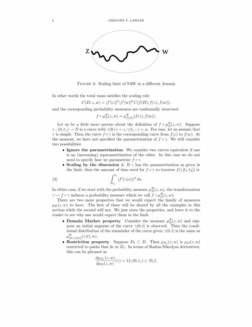
Figure 3. Scaling limit of SAW in a different domain

In other words the total mass satisfies the scaling rule

C(D; z, w) = |f ′(z)|b |f ′(w)|b C(f(D); f(z), f(w)),

and the corresponding probability measures are conformally invariant:

f µ#D(z, w) = µ#

f(D)(f(z), f(w)).

Let us be a little more precise about the definition of f µ#D(z, w). Suppose

γ : (0, tγ) → D is a curve with γ(0+) = z, γ(tγ−) = w. For ease, let us assume thatγ is simple. Then the curve f γ is the corresponding curve from f(z) to f(w). Atthe moment, we have not specified the parametrization of f γ. We will considertwo possibilities:

• Ignore the parametrization. We consider two curves equivalent if oneis an (increasing) reparametrization of the other. In this case we do notneed to specify how we parametrize f γ.

• Scaling by the dimension d. If γ has the parametrization as given inthe limit, then the amount of time need for f γ to traverse f(γ[t1, t2]) is

(3)

∫ t2

t1

|f ′(γ(s))|d ds.

In either case, if we start with the probability measure µ#D(z, w), the transformation

γ 7→ f γ induces a probability measure which we call f µ#D(z, w).

There are two more properties that we would expect the family of measuresµD(z, w) to have. The first of these will be shared by all the examples in thissection while the second will not. We just state the properties, and leave it to thereader to see why one would expect them in the limit.

• Domain Markov property. Consider the measure µ#D(z, w) and sup-

pose an initial segment of the curve γ(0, t] is observed. Then the condi-tional distribution of the remainder of the curve given γ(0, t] is the same as

µ#D\γ(0,t](γ(t), w).

• Restriction property. Suppose D1 ⊂ D. Then µD1(z, w) is µD(z, w)

restricted to paths that lie in D1. In terms of Radon-Nikodym derivatives,this can be phrased as

dµD1(z, w)

dµD(z, w)(γ) = 1γ(0, tγ) ⊂ D1.


z w

Figure 4. Domain Markov property

D’\D

Dw

z

γ

Figure 5. Illustrating the restriction property

We have considered the case where z, w ∈ ∂D. We could consider z ∈ ∂D,w ∈ D.In this case the measure is defined similarly, but (2) becomes

ZD(z, w) ∼ C(D; z, w)N−bN−b,

where b is a different exponent (see Lectures 5 and 6). The limiting measureµD(z, w) would satisfy the conformal covariance rule


Similarly we could consider µD(z, w) for z, w ∈ D.

1.2. Loop-erased random walk. We start with simple random walk. Let ωdenote a nearest neighbor random walk from z to w in D. We no longer putin a self-avoidance constraint. We give each walk ω measure 4−|ω| which is theprobability that the first n steps of an ordinary random walk in Z

2 starting at z

8 GREGORY F. LAWLER

are ω. The total mass of this measure is the probability that a simple randomwalk starting at z immediately goes into the domain and then leaves the domainat w. Using the “gambler’s ruin” estimate for one-dimensional random walk, onecan show that the total mass of this measure decays like O(N−2); in fact

(4) ZN (D; z, w) ∼ C(D; z, w)N−2, N → ∞,

where C(D; z, w) is the “excursion Poisson kernel”, H∂D(z, w), defined to be thenormal derivative of the Poisson kernelHD(·, w) at z. In the notation of the previoussection b = 1. For each realization of the walk, we produce a self-avoiding path byerasing the loops in chronological order.

0 N

N

z w

Figure 6. Simple random walk in D

Figure 7. The walk obtained from erasing loops chronologically

Again we are looking for a continuum limit µD(z, w) with paths of dimension d(not the same d as for SAW). The limit should satisfy

• Conformal covariance


• Domain Markov property

However, we would not expect the limit to satisfy the restriction property. Thereason is that the measure given to each self-avoiding walk ω by this procedure isdetermined by the number of ordinary random walks which produce ω after looperasure. If we make the domain smaller, then we lose some random walks that wouldproduce ω and hence the measure would be smaller. In terms of Radon-Nikodymderivatives, we would expect

dµD1(z, w)

dµD(z, w)< 1.

1.3. Percolation. Suppose that every point in the triangular lattice in the upperhalf plane is colored black or white independently with each color having probability1/2. A typical realization is illustrated in Figure 8 (if one ignores the bottom row).

Figure 8. The percolation exploration process.

We now put a boundary condition on the bottom row as illustrated — all blackon one side of the origin and all white on the other side. For any realization ofthe coloring, there is a unique curve starting at the bottom row that has all whitevertices on one side and all black vertices on the other side. This is called thepercolation exploration process. Similarly we could start with a domain D and twoboundary points z, w; give a boundary condition of black on one of the arcs andwhite on the other arc; put a fine triangular lattice inside D; color vertices blackor white independently with probability 1/2 for each; and then consider the pathconnecting z and w. In the limit, one might hope for a continuous interface. Incomparison to the previous examples, the total mass of the lattice measures is one;another way of saying this is that b = 0. We suppose that the curve is conformallyinvariant, and one can check that it should satisfy the domain Markov property.

The scaling limit of percolation satisfies another property called the locality prop-erty. Suppose D1 ⊂ D and z, w ∈ ∂D ∩ ∂D1 as in Figure 5. Suppose that only aninitial segment of γ is seen. To determine the measure of the initial segment, one

10 GREGORY F. LAWLER

only observes the value of the percolation cluster at vertices adjoining γ. Hencethe measure of the path is the same whether it is considered as a curve in D1 or acurve in D. The locality property is stronger than the restriction property whichSAW satisfies. The restriction property is a similar statement that holds for theentire curve γ but not for all initial segments of γ.

1.4. Ising model. The Ising model is a simple model of a ferromagnet. We willconsider the triangular lattice as in the previous section. Again we color the verticesblack or white although we now think of the colors as spins. If x is a vertex, we letσ(x) = 1 if x is colored black and σ(x) = −1 if x is colored white. The measure onconfigurations is such that neighboring spins like to have the same sign.

z

w

+1 −1

Figure 9. Ising interface.

It is easiest to define the measure for a finite collection of spins. Suppose Dis a bounded domain in C with two marked boundary points z, w which give ustwo boundary arcs. We consider a fine triangular lattice in D; and fix boundaryconditions +1 and −1 respectively on the two boundary arcs. Each configurationof spins is given energy

E = −∑

x∼y

σ(x)σ(y),

where x ∼ y means that x, y are nearest neighbors. We then give measure e−βE

to a configuration of spins. If β is small, then the correlations are localized andspins separated by a large distance are almost independent. If β is large, there islong-range correlation. There is a critical βc that separates these two phases.

For each configuration of spins there is a well-defined boundary between +1spins and −1 spins defined in exactly the same way as the percolation explorationprocess. At the critical βc it is believed that this gives an interesting fractal curveand that it should satisfy conformal covariance and the domain Markov property.

1.5. Assumptions on limits. Our goal is to understand the possible continuumlimits for these discrete models. We will discuss the boundary to boundary casehere but one can also have boundary to interior or interior to interior. (The terms“surface” and “bulk” are often used for boundary and interior.) Such a limit is a


measure µD(z, w) on curves from z to w in D which can be written

µD(z, w) = C(D; z, w)µ#D(z, w),

where µ#D(z, w) is a probability measure. The existence of µD(z, w) assumes smooth-

ness of ∂D near z, w, but the probability measure µ#D(z, w) exists even without the

smoothness assumption. The two basic assumptions are:

• Conformal covariance of µD(z, w) and conformal invariance of µ#D(z, w).

• Domain Markov property.

The starting point for the Schramm-Loewner evolution is to show that if weignore the parametrization of the curves, then there is only a one-parameter family

of probability measures µ#D(z, w) for simply connected domains D that satisfy con-

formal invariance and the domain Markov property. We will construct this family.The parameter is usually denoted κ > 0. By the Riemann mapping theorem, itsuffices to construct the measure for one simply connected domain and the easiestis the upper half plane H with boundary points 0 and ∞. As we will see, there area number of ways of parametrizing these curves.

2. Loop measures and loop-erased random walk

This section will focus on two closely related models: the loop-erased randomwalk and a measure on simple random walk loops. They are also closely relatedto the enumeration of spanning trees on a graph. Although much of what we sayhere can be generalized to Markov chains, we will only consider the case of randomwalk in Z

2. We will not give complete proofs; a reference for more details is [11,Chapter 9].

We write

ω = [ω0, ω1, . . . , ωn], ωj ∈ Z2, |ωj − ωj−1| = 1, j = 1, . . . , n,

for a (nearest neighbor) path in Z2. We write |ω| = n for the number of steps of the

path. We call the path a (rooted) loop if ω0 = ωn. For each path ω, we define

q(ω) = (1/4)|ω|.

Note that q(ω) is exactly the probability that a simple random walk in Z2 starting

at ω0 traverses ω in its first n steps. We view q as a measure on the set of paths offinite length.

More generally, we can define q(ω) = λω for some λ > 0, but 1/4 is the “critical” value

of the parameter and most interesting to us.

A path ω is self-avoiding if ωj 6= ωk for j 6= k. For every path ω there is a uniqueself-avoiding subpath

L(ω) = [η0, η1, . . . , ηk]

called its (chronological) loop-erasure satisfying the following.

• η0 = ω0, ηk = ωn.• For each j, ηj ∈ ω. Moreover, if

σ(j) = maxm : ωm = ηj,then σ(0) < σ(1) < · · · < σ(k) and

η0, . . . , ηj ∩ ωσ(j)+1, . . . , ωn = ∅.


Throughout this section, A will denote a nonempty finite subset of Z2 and

∂A = z ∈ Z2 : dist(z,A) = 1.

2.1. Excursion measure. An excursion in A is a random walk that starts on ∂A,immediately goes into A, and ends when it reaches ∂A. To be more precise, a(boundary) excursion in A is a path ω = [ω0, . . . , ωn] with n ≥ 2, ω0, ωn ∈ ∂A andωj ∈ A for 1 ≤ j ≤ n− 1. Let EA denote the set of excursions in A and if x, y ∈ ∂Alet EA(x, y) denote the set of excursions with ω0 = x, ωn = y. Let qA denote qrestricted to EA. Let

HA(x, y) = qA [EA(x, y)]

which is called the boundary or excursion Poisson kernel. Note that qA(EA) < ∞.Indeed, if x ∈ ∂A,

∑

y∈∂A

HA(x, y) = r/4,

where r denotes the number of nearest neighbors of x in A.

2.2. Loop-erased measure. Let EA denote the set of excursions in A that areself-avoiding and define EA(x, y) similarly. The (boundary) loop-erased measure qAis the measure on EA, where

qA(η) = qA ω ∈ EA : L(ω) = η .Note that qA[EA(x, y)] = HA(x, y). If η ∈ EA, it is not obvious how to calculate

qA(η) which is the measure of the set of excursions ω ∈ EA whose loop-erasureis η. It turns out that the calculation of this leads to some now classical formulasinvolving the determinant of the Laplacian for the random walk in A. We will write

qA(η) = qA(η)Fη(A),

where Fη(A) will be a quantity that depends only on the sites in η and not on theorder that they are traversed. In the next subsection we will Fη(A) in terms of ameasure on unrooted loops.

2.3. Random walk loop measure. If ω = [ω0, . . . , ωn] is a loop, we call ω0 = ωnthe root of the loop. We say that ω is in A and write ω ⊂ A if all the sites in ω arein A. Let L(A) denote the set of loops in A with length at least two, and Lx(A)the set of such loops rooted at x. We define the measure m = mA on L(A) by

(5) m(ω) =q(ω)

|ω| , ω ∈ L(A).

This called the rooted loop measure on A.

Throughout this section we will abuse notation so that ω can either refer to the path or

to the set of sites visited by ω. For example in the previous paragraph, the expression ω ⊂ A

uses ω to mean the set of sites while the expression ω ∈ L(A) uses ω to mean the path. I

hope this does not create confusion. Also, if x is a site, we also use x to denote the singleton

set x.

An unrooted loop is a rooted loop where one forgets which point is the startingpoint. More precisely, it is an equivalence class of rooted loops under the equivalence

[ω0, ω1, . . . , ωn] ∼ [ωj , ωj+1, . . . , ωn, ω1, . . . , ωj−1, ωj ].


We write ω for an unrooted loop and we write ω ∼ ω if ω is a rooted loop in theequivalence class ω. We write L(A) for the set of unrooted loops. The (unrooted)loop measure m is the measure given by

m(ω) =∑

ω∼ω

m(ω).

One thinks of the unrooted loop measure as assigning measure (1/4)n to each unrooted

loop of length n. However, this is not exactly correct because an unrooted loop of length n

may have fewer than n rooted representatives. For example, consider ω = [x, y, x, y, x]. The

length of the walk is four, but there are only two representatives of the unrooted loop.

Let

F (A) = exp

∑

ω∈L(A)

m(ω)

,

and if B ⊂ A, let FB(A) be the corresponding quantity restricted to loops thatintersect B,

FB(A) = exp

∑

ω∈L(A), ω∩B 6=∅

m(ω)

,

Note that

F (A) = FB(A)F (A \B).

In particular, if η = [η0, . . . , ηk] ∈ EA,

Fη(A) =

k∏

j=1

Fηj(A \ η1, . . . , ηj−1).

In the expression on the right it is not so obvious that Fη(A) is independent of theordering of the vertices.

Proposition 1. If η ∈ EA, then

(6) q(η) = q(η)Fη(A).

We will not prove the proposition, but we will state some other expressions forFη(A). Let G(x, x;A) denote the usual Green’s function for the random walk, thatis, the expected number of visits to x, starting at x, before leaving A. Then [11,Lemma 9.3.2],

(7) G(x, x;A) = Fx(A).

In particular,

Fη(A) =k

∏

j=1

G(ηj , ηj ;A \ η1, . . . , ηj−1).

The expression on the right-hand side is what one naturally gets if one tries tocompute q(η)/q(η). The proposition above then requires the generating functionidentity (7). Another expression involves the determinant of the Laplacian. LetQ = QA denote the #(A)×#(A) matrix Q(x, y) = 1/4 if |x−y| = 1 and Q(x, y) = 0


for other x. Then the (negative of the) Laplacian of the random walk on A is thematrix I −Q. Then [11, Proposition 9.3.3],

F (A) =1

det(I −Q).

2.4. Spanning trees and Wilson’s algorithm. A spanning tree of a connectedgraph is a subgraph that is also a tree. If A is a finite subset of Z

2, then a wiredspanning tree of A is a spanning tree of the graph A ∪ ∂ where a vertex x ∈ Ais adjacent to ∂ if dist(x, ∂A) = 1. Wilson’s algorithm [23] for choosing a wiredspanning tree is as follows.

• Choose a vertex in A and run a random walk until it reaches ∂A.• Perform loop-erasure on the walk and add those edges to the tree.• If there are vertices that are not on the tree, choose one and do a random

walk until it reaches a vertex in the tree.• Perform loop-erasure on this walk and add those new edges to the tree.• Continue this procedure until we have a full tree.

This is a very efficient way to choose a random tree, and the amazing fact isthat it chooses a tree uniformly over the set of all wired spanning trees. This iscalled informally a uniform spanning tree where this means “a spanning tree chosenuniformly among all spanning trees”.

Proposition 2. If T is a wired spanning tree of A, then the probability that T ischosen in Wilson’s algorithm is 4−#(A) F (A). In particular, every tree is equallylikely to be chosen and the total number of spanning trees is

4#(A)

F (A)= 4#(A) det[I −Q] = det[4(I −Q)].

While the algorithm is due to Wilson, the formula for the number of spanningtrees is much older, going back to Kirchhoff. In graph theory the Laplacian iswritten as 4(I −Q) which makes this formula nicer. To prove the proposition, onejust takes any tree and considers the probability that it is chosen, see [11, Propsition9.7.1].

2.5. Laplacian random walk. If x, y ∈ ∂A are distinct, then the loop-erasedwalk gives a measure qA,x,y on EA(x, y) of total mass HA(x, y). We can normalizeto make this a probability measure. Under this measure we have a stochasticprocess Xj with X0 = x and XT = y where T is a random stopping time. It isclearly nonMarkovian since, for example, we cannot visit any site that we havealready visited. To give the transition probabilities, we need to give for everyη = [η0 = a, . . . , ηj ] and z ∈ A \ η,

PXj+1 = z | [X0, . . . ,Xj ] = η.Using the definition, it is easy to check that this is given by

1

4HA\η(z, y).

Note that the function z 7→ HA\η(z, y) is the unique function that is discreteharmonic (satisfies the discrete Laplace equation) on A \ η with boundary valueδy on ∂[A \ η]. For this reason the loop-erased walk is often called the Laplacianrandom walk (with exponent 1).


Using the transition probability, one can check that the stochastic process Xn

satisfies the following domain Markov property.

• Given [X0, . . . ,Xj ] = η, the distribution of the remainder of the path is thesame as the loop-erased walk from Xj to w in A \ η.

The term “loop-erased random walk” has two different, but similar, meanings. Some-times it is used for the probability measure and sometimes for the measure qA or qA,x,y whichis not a probability measure. Of course we can write

qA,x,y = HA(x, y) q#

A,x,y

where q#

A,x,y is a probability measure. The Laplacian random walk is a description of the

probability measure.

2.6. Boundary perturbation. The boundary perturbation rule is the way tocompare qA and qA′ for different sets A,A′. It is easier to state this property usingthe unnormalized measure qA,x,y. It follows immediately from (6).

• Suppose A′ ⊂ A and x, y are distinct points in (∂A′)∪(∂A) withHA′(x, y) >0. Then for every η ∈ EA′(x, y),

qA′,x,y(η)

qA,x,y(η)=qA′(η)

qA(η)= exp

−∑

m(ω))

,

where the sum is over all loops ω ⊂ A that intersect both η and A \A′. Inother words, over loops in A that intersect η but are not loops in A′.

2.7. Loop soup. The measure q on EA(x, y) is obtained from the measure q onEA(x, y) by the deterministic operation of erasing loops. The total mass of themeasure does not change. This leads to asking if we can obtain q from q by “addingon loops”. Here we show how to do this. The operation is not deterministic (thereis no way it could be since many different simple paths give the same loop erasure).We will describe it by introducing independent randomness, the random walk loopsoup, and then giving a deterministic algorithm using the soup and the SAW η toproduce the path ω.

The random walk loop soup is a Poissonian realization of unrooted loops fromthe measure m. To be more precise, for each unrooted loop ω, there is a Poissonprocess Nω

t with rate m(ω). These processes are independent. A realization ofthese processes gives for each ω an increasing sequence of times

0 < t(1, ω) < t(2, ω) < · · ·where the corresponding Poisson process jumps. With probability one, the timest(j, ω) over all j, ω are distinct.

If we restrict loops to a finite set A, then∑

ω⊂A

m(ω) = logF (A) <∞,

from which we can conclude

t(j, ω) : t(j, ω) ≤ 1, ω ⊂ A,is finite. Writing this differently, we can write down the loops that have appearedby time one,

ω1, ω2, . . . , ωk


where k is finite (random) and the loops have been written in the order that theyappeared. Some loops may appear more than once in this listing. Indeed, if t(j, ω) <1 < t(j+1, ω), then the loop ω appears j times. We can now give the “loop addition”algorithm.

• Choose η = [η0, . . . , ηn] ∈ EA(x, y) using measure qA.• Take an independent loop soup inA and consider the loops that have arrived

by time one.• Take the subset of these which correspond to loops that have at least one

point in common with η. Let us write these loops (using the same order asbefore)

ω1, . . . , ωl.

• For each ωj let i be the smallest integer such that ηi ∈ ωj . Choose a rootedrepresentative of ωj that is rooted at ηi. If there is more than one choice atthis stage choose uniformly among the choices. This gives a finite sequenceof rooted loops

ω1, . . . , ωl

whose roots are ησ(1), . . . , ησ(l) with σ(i) ≤ σ(j) if i < j. Moreover,

ωj ∩ η0, . . . , ησ(j)−1 = ∅.

• Consider the loops

ω∗1 , . . . , ω

∗n−1

where ω∗i is the concatenation of all the loops ωj with σ(j) = i. If there

are no such loops, choose ω∗i to be the trivial loop of zero steps at ηi.

• Form a nearest neighbor path by

ω = [η0, η1] ⊕ ω∗1 ⊕ [η1, η2] ⊕ · · · ⊕ [ηn−2, ηn−1] ⊕ ω∗

n−1 ⊕ [ηn−1, ηn].

Proposition 3. If η is chosen according to the measure qA on EA and ω is formedusing the above algorithm. then the induced measure on paths is qA.

See [11, 9.4-9.5] for a proof.

3. Brownian loop measure

We will consider the scaling limit of the random walk loop measure described inthe last section. For any positive integer N , let ZN = N−1

Z2. If ω is a loop, we

let ωN denote the corresponding loop on Z obtained from scaling. If |ω| = n wecan also view ω as a continuous function ω : [0, n] → C obtained in the natural waymy linear interpolation. For ωN , we use Brownian scaling,

ωN (t) = N−1 ω(tN2), 0 ≤ t ≤ n/N2.

We consider the limit as N → ∞ of the rooted random walk loop measure. Whathappens is that small loops shrink to points; we will ignore these. However, at eachscaling level N there are “macroscopic” loops. The Brownian loop measure will bethe limit of these. We will define the Brownian loop measure directly, and thenreturn to the question of how the scaled random walk loop measure approaches thislimit.


3.1. Brownian measures. Probabilists tend to view Brownian motion as a sto-chastic process, that is, a probability measure on paths. However, it is usefulsometimes to consider “configurational” measures given by Brownian paths. Thiswill be useful when studying the Brownian loop measure, and also helps in under-standing other configurational measures such as that given by SLE. We will dothis for two-dimensional Brownian motion. We write |µ| for the total mass of ameasure µ, and if 0 < |µ| < ∞, we write µ# = µ/|µ| for the probability measureobtained by normalization. We will write µD(z, w; t) for measures on paths in D,starting at z, ending at w, of time duration t. When the t is omitted, we allowdifferent time durations, but we will always be considering paths of finite duration.When D = C we will drop the subscript.

Let µ(z, w; t) be the measure corresponding to Brownian paths starting at z,ending at w, of time duration t. We can write this as

µ(z, w; t) = pt(w − z)µ#(z, w; t),

where

pt(z) =1

2πtexp

−|z|22t

,

is the density for Brownian motion and µ#(z, w; t) is the corresponding probabilitymeasure often called the Brownian bridge. We let

µ(z, w) =

∫ ∞

0

µ(z, w; t) dt.

This is an example of an infinite measure. All of the infinite measures we deal withhere will be σ-finite. We could take other integrals. For example the measure

µ(z, ·; t) =

∫

C

µ(z, w; t) dA(w)

is a probability measure, exactly the measure on paths given by a Brownian motionstarting at z stopped at time t. Here and throughout dA will represent integralswith respect to usual Lebesgue measure (area) on C.

One might be worried about what it means to integrate when the integrands are mea-

sures. In all our examples, we could put topologies on measures so that the corresponding

functions are continuous and these integrals are Riemann integrals. We will not bother with

these tedious details.

We write µD(z, w; t), µD(z, w), etc. for the corresponding measures obtained byrestricting the measure to curves staying in D. By definition our measures will havethe restriction property: if D1 ⊂ D, then µD1

(· · · ) is µD(· · · ) restricted to curveslying in D1.

We emphasize that we are restricting rather than conditioning; in other words, we are

not normalizing to have total mass one. When we restrict a measure we decrease the total

mass.


If D is a bounded domain, or, more generally, a domain with sufficiently largeboundary that Brownian motion will eventually exit the domain, then if z 6= w themeasure µD(z, w) is a finite measure whose total mass is the Green’s function

G(z, w) =

∫ ∞

0

|µD(z, w; t)| dt <∞.

The measure µD(z, z) is well defined but is an infinite measure.

3.2. Conformal invariance. Brownian motion is a conformally invariant object.We will make a precise statement of this in terms of the measures above. SupposeD ⊂ C is a domain and f : D → f(D) is a conformal transformation. If γ : [0, tγ ] →D is a curve, we define the curve f γ as follows. Let

σ(t) =

∫ t

0

|f ′(γ(s))|2 ds.

Then f γ is the curve of time duration σ(tγ) given by

f γ(σ(s)) = f(γ(s)), 0 ≤ s ≤ tγ .

If µ is a measure on curves in D, we define f µ to be the pullback measure oncurves in f(D) defined by

(f µ)(V ) = µγ : f γ ∈ V .

Proposition 4 (Conformal invariance). Suppose z, w ∈ D and f : D → f(D) is aconformal transformation. Then

(8) f µD(z, w) = µf(D)(f(z), f(w)).

While this is not the usual way that conformal invariance is stated it is use-ful formulation when considering configurational measures. A consequence of thestatement is that the total masses of the measures are the same. Indeed, it is wellknown that the Green’s function is conformally invariant

Gf(D)(f(z), f(w)) = GD(z, w),

In studying the Brownian loop measure, we will use (8) with z = w where themeasures are infinite:

f µD(z, z) = µf(D)(f(z), f(z)).

There are no topological assumptions on the domain D. In particular, it can be multiply

connected.

We will consider the infinite measure on loops

µD =

∫

D

µD(z, z) dA(z).


The measure µD is not a conformal invariant. Indeed,

f µD =

∫

D

f µD(z, z) dA(z)

=

∫

D

µf(D)(f(z), f(z)) dA(z)

=

∫

D

µf(D)(f(z), f(z)) |f ′(z)|−2 |f ′(z)|2 dA(z)

=

∫

D

µf(D)(w,w) |g′(w)|2 dA(w),(9)

where g = f−1. We will write µD for the measure µD considered as a measure onunrooted loops by forgetting the root. The measure µD is the scaling limit of themacroscopic loops in D ∩ ZN under the measure q. The measure we want shouldbe the scaling limit under m and this leads to the following definition.

Definition

• The rooted Brownian loop measure in D is the measure on (rooted) loopsνD defined by

dνDdµD

(γ) =1

tγ.

• The (unrooted) Brownian loop measure in D is the measure on unrootedloops defined by

dνDdµD

(γ) =1

tγ.

Equivalently, it is the measure obtained from νD by forgetting the root.

The factor 1/tγ is analogous to the factor 1/|ω| in (5). The phrase Brownianloop measure refers to the unrooted version which is most important as it turnsout to be the conformal invariant as the next theorem shows. However, the rootedversion is often more convenient for computations.

Theorem 1. If f : D → f(D) is a conformal transformation, then

f νD = νf(D).

The family of measures µD satisfies both the restriction property and conformal

invariance. One can easily see that any nontrivial family that satisfies both of these properties

must be a family of infinite measures.

Sketch of proof. If γ is a loop of time duration tγ we can view γ as a curve γ :(−∞,∞) → C of period tγ . If s ∈ R, we write θsγ for the loop θsγ(t) = γ(t + s).Note that γ and θsγ generate the same unrooted loop. Suppose that νD is a measurethat is absolutely continuous with respect to µD with Radon-Nikodym derivativeφ. Note that νD is an example with φ(γ) = 1/tγ . Suppose that for every loop γ oftime duration tγ ,

∫ tγ

0

φ(θsγ) ds = 1.


Then νD viewed as a measure on unrooted loops is the same as νD. Let g = f−1

and choose

φ(θsγ) =|f ′(θsγ(0))|2

tfγ=

|f ′(γ(s))|2tfγ

.

By the definition of the parametrization of f γ we know that∫ tγ

0

φ(θsγ) ds =1

tfγ

∫ tγ

0

|f ′(γ(s))|2 ds = 1.

We will now give an important property of the measure µD. Consider the mea-sure on curves obtained by selecting γ according to µD; choosing a number s ∈ [0, tγ ]uniformly; and then outputting θsγ. Then the new measure is the same as µD.More generally, suppose that Ψ is a positive, continuous function on D. Considerthe measure µΨ defined by:

• For each γ, we have a measure ργ on θsγ : 0 ≤ s ≤ tγ with densityΨ(γ(s)). The total mass of this measure is

∫ tγ

0

Ψ(γ(s)) ds.

• First choose γ according to µD and then choose s according to ργ andoutput θsγ.

Then µΨ is the same as∫

D

Ψ(z)µD(z, z) dA(z).

In other wordsdµΨ

dµD(γ) = Ψ(γ(0)).

Computing as in (9), we see that

f µΦ =

∫

f(D)

Ψ(g(w)) |g′(w)|2 µD(z, z) dA(z).

In particular, if Ψ(z) = |f ′(z)|2,f µΦ = µf(D).

Returning to φ as above, we see that if νφ is the measure on rooted loops withdνφ/dµD = φ,

f νφ = νf(D).

Since νφ considered as a measure on unrooted loops is the same as νD, we get

f νD = νf(D).

3.3. Brownian loop soup. The Brownian loop soup is a Poissonian realizationfrom the measure νD. Alternatively, we can take a rooted Brownian loop soup,that is, a realization of νD, and then forget the roots of the loops. We can think ofthe soup as growing set of loops where At denotes the set of loops that have beencreated at time t. By conformal invariance, the conformal image of a soup in Dgives a soup in f(D). Soups also satisfy the restriction property.

The Brownian loop soup is the limit of the macroscopic loops from the randomwalk loop soup. This can be made precise. We refer to [14] for the precise result,but we give a rough version here. Let D be a bounded domain. There exists δ > 0


such that, except for an event of probability O(N−δ), a Brownian soup At in D and

a (scaled) random walk soup At in D ∩ZN can be defined on the same probabilityspace such that for 0 ≤ t ≤ 1, there is a one-to-one correspondence between theloops in At and those in At of time duration at least N−δ such that if two loops arepaired up, their time duration differs by at most N−2 and the parametrized curveslie within distance O(N−1 logN) of each other.

3.4. Excursion measure and boundary bubbles. Suppose D is a domain withpiecewise smooth boundary. The Poisson kernel HD(z, w), z ∈ D,w ∈ ∂D is thedensity of harmonic measure starting at z. In other words, the probability that aBrownian motion starting at z exists D at V ⊂ ∂D is

hmD(z, V ) :=

∫

V

HD(z, w) |dw|.

We can write the probability measure associated to Brownian motion starting at zstopped when it reaches ∂D as

∫

V

µD(z, w) |dw|

where µD(z, w) is a finite measure on paths starting at z ending at w. Indeed,

µD(z, w) = HD(z, w)µ#D(z, w),

where the probability measure µ#D(z, w) corresponds to Brownian motion started

at z conditioned to leave D at w. This is conditioning on an event of probabilityzero but one can make rigorous sense of this using a number of methods, e.g., thetheory of h-processes.

We will use µD(z, w) for various Brownian measures. Before we used it with z, w ∈ D

and here we use it with z ∈ D, w ∈ ∂D. Below we will define a version with z, w ∈ ∂D. I

hope that using the same notation will not be confusing.

Conformal invariance of Brownian motion implies that harmonic measure is con-formally invariant:

hmD(z, V ) = hmf(D)(f(z), f(V )).

If ∂D and ∂f(D) are smooth near w, f(w), this gives a conformal covariance rulefor µD(z, w)

f µD(z, w) = |f ′(w)|µf(D)(f(z), f(w)).

This is shorthand for the scaling rule on H:

HD(z, w) = |f ′(w)|Hf(D)(f(z), f(w)),

and the conformal invariance of the probability measures:

f µ#D(z, w) = µ#

f(D)(f(z), f(w)).

The scaling limit of the random walk excursion measure from Section 2.1 isthe (Brownian motion) excursion measure that we now describe. Suppose ∂D issmooth. If z, w are distinct points in D, let H∂D(z, w) be the boundary or excursionPoisson kernel defined by

H∂D(z, w) = ∂nHD(z, w),


where the derivative is in the first component and n = nz is the inward unit normalat z. We get the same number if we take ∂nw

in the second component. There is acorresponding measure on paths that we denote by

µD(z, w) = H∂D(z, w)µ#D(z, w).

Note that µD(z, w) satisfies the conformal covariance relation

(10) f µD(z, w) = |f ′(z)| |f ′(w)|µf(D)(f(z), f(w)).

A simple calculation shows that

H∂H(0, x) =1

πx2.

(Sometimes it is useful to multiply the Poisson kernel by π in order to avoid havinga constant in this formula.)

Combining these ideas we can say that the Brownian measures have a boundary scaling

exponent of 1 and an interior scaling exponent of 0.

Excursion measure is the infinite measure on paths connecting boundary pointsof D given by

ED =

∫

∂D

∫

∂D

µD(z, w) |dz| |dw|.

Using (10) we can check that the excursion measure is conformally invariant:

f ED = Ef(D).

In particular, it is well defined even if the boundaries are not smooth provided thatwe can map D conformally to a domain with piecewise smooth boundaries. (Thisis always possible for finitely connected domains.) The term excursion measure issometimes used for the measure on ∂D × ∂D given by

ED(V1, V2) =

∣

∣

∣

∣

∫

V1

∫

V2

µD(z, w) |dz| |dw|∣

∣

∣

∣

=

∫

V1

∫

V2

H∂D(z, w) |dz| |dw|.

This latter view of the excursion measure is a nice conformal invariant and can beused in the study of conformal mappings. It is related to, but not the same as,extremal distance or extremal length which is often used for such purposes.

As w → z, the measures µD(z, w) approach an infinite measure called the Brow-nian bubble measure. There are a number of ways of writing this measure. Forease, assume that D = H and z = 0. Then

µH(0, 0) = limx↓0

π µH(0, x) = limǫ↓0

π µH(ǫi, 0),

provided that one interprets these limits correctly. For example, if r > 0 andµH(0, 0; r), µH(0, x; r) denote these measures restricted to curves that do not line indisk of radius r about the origin, then these are finite measures and

µH(0, 0; r) = limx↓0

π µH(0, x; r).

(Convergence of finite measures means convergence of the total masses and conver-gence of the probability measures in some appropriate topology.) If D ⊂ H withdist(0, ∂D∩H) > 0, let Γ(D) denote the µH(0, 0) measure of loops that do not stayin D ∩ 0. The factor of π is put in the definition so that

Γ(D+) = 1, D+ = H ∩ D.


If D is simply connected and f : D → H is a conformal transformation withf(0) = 0, then [7, Proposition 5.22]

Γ(D) = −Sf(0)

6,

where S denotes the Schwarzian derivative

Sf(z) =f ′′′(z)

f ′(z)− 3f ′′(z)2

2f ′(z)2.

We know of no such nice formulas for multiply connected D. The Brownian bubblemeasure satisfies the conformal covariance rule

f µD(z, z) = |f ′(z)|2 µf(D)(f(z), f(z)).

We will state one more result which will be important in the analysis of SLE.Suppose K is a bounded, relatively closed subset of H. Then the half-plane capacityof K is defined by

hcap(K) = limy→∞

yEiy[Im(Bτ )],

where B is a standard Brownian motion and τ is the first time that that it hitsR ∪K. One can check that the limit exists. In fact

hcap(K) = Γ(D)

where D is the image of H \K under the inversion z 7→ −1/z.

Proposition 5. Suppose γ : (0,∞) → H is a curve with γ(0) = 0 and such thatfor each t,

hcap[γ(0, t]) = t.

Suppose D ⊂ H is a domain with dist(0,H\D) > 0. Let m(t) denote the Brownianloop measure of loops in H that intersect both γ(0, t] and H \D. Then as t ↓ 0,

(11) m(t) = Γ(D) t [1 + o(1)].

4. Complex variables and conformal mappings

In order to study SLE, one must know some basic facts about conformal maps.Some of this material appears in standard first courses in complex variables anda few are more specialized. We will discuss the main results here. For proofs andmore details see, e.g., [5, 6, 7].

4.1. Review of complex analysis.

Definition

• A domain in C is an open, connected subset. Two main examples are theunit disk

D = z : |z| < 1and the upper half plane

H = z = x+ iy : y > 0.• The Riemann sphere is the set C

∗ = C∪∞ with the topology of the spherewhich is to say that the open neighborhoods of ∞ are the complements ofcompact subsets of C.

• A domain D ⊂ C is simply connected if its complement in C∗ is a connected

subset of C∗.


• A domain D ⊂ C is finitely connected if its complement in C∗ has a finite

number of connected components.• A function f : D → H is holomorphic or analytic if the complex derivativef ′(z) exists at every point.

If 0 ∈ D, and f is holomorphic on D then we can write

f(z) =

∞∑

j=0

aj zj ,

where the radius of convergence is at least dist(0, ∂D). In particular, if f(0) = 0,then either f is identically zero, or there exists a nonnegative integer n such that

f(x) = zn g(z),

where g is holomorphic in a neighborhood of 0 with g(0) 6= 0. In particular, iff ′(0) 6= 0, then f is locally one-to-one, but if f ′(0) = 0, it is not locally one-to-one.

If we write a holomorphic function f = u + iv, then the functions u, v areharmonic functions and satisfy the Cauchy-Riemann equations

∂xu = ∂yv, ∂yu = −∂xv.Conversely, if u is a harmonic function on D and z ∈ D, then we can find a uniqueholomorphic function f = u + iv with v(z) = 0 defined in a neighborhood of zby solving the Cauchy-Riemann equations. It is not always true that f can beextended to all of D, but there is no problem if D is simply connected.

Proposition 6. Suppose D ⊂ C is simply connected.

• If u is a harmonic function on D and z ∈ D, there is a unique holomorphicfunction f = u+ iv on D with v(z) = 0.

• If f is a holomorphic function on D with f(z) 6= 0 for all z, then there existsa holomorphic function g on D with eg = f. In particular, if w ∈ C \ 0and h = eg/w, then hw = f .

The Cauchy integral formula states that if f is holomorphic in a domain con-taining the closed unit disk, then

f (n)(0) =n!

2πi

∫

∂D

f(z) dz

zn+1.

In particular, if f is holomorphic on D,

|f (n)(0)| ≤ n! ‖f‖∞.Here ‖f‖∞ denotes the maximum of f on D which (by the n = 0 case which iscalled the maximum principle) is the same as the maximum on ∂D.

Proposition 7. Suppose f is a holomorphic function on a domain D. Supposez ∈ D, and let

dz = dist(z, ∂D), Mz = sup|f(w)| : |w − z| < dz.Then,

|f (n)(z)| ≤ n! d−nz Mz.

Proof. Consider g(w) = f(z + dzw).

A similar estimate exists for harmonic functions in Rd. It can be proved by

representing a harmonic function in the unit ball in terms of the Poisson kernel.


Proposition 8. For all positive integers d, n, there exists C(d, n) < ∞ such thatif u is a harmonic function on the unit ball U = x ∈ R

d : |x| < 1 and D denotesan nth order mixed partial,

|Du(0)| ≤ C(d, n) ‖u‖∞.Derivative estimates allow one to show “equicontinuity” results. We write fn =⇒

f if for every compact K ⊂ D, fn converges to f uniformly on K. We statethe following for holomorphic functions, but a similar result holds for harmonicfunctions.

Proposition 9. Suppose D is a domain.

• If fn is a sequence of holomorphic functions on D, and fn =⇒ f , then f isholomorphic.

• If fn is a sequence of holomorphic functions on D that is locally bounded,then there exists a subsequence fnj

and a (necessarily, holomorphic) func-tion f such that fnj

=⇒ f .

Proposition 10 (Schwarz lemma). If f : D → D is holomorphic with f(0) = 0,then |f(z)| ≤ |z| for all z. If f is not a rotation, |f ′(0)| < 1 and |f(z)| < |z| for allz 6= 0.

Proof. Let g(z) = f(z)/z with g(0) = f ′(0) and use the maximum principle.

4.2. Conformal transformations.

Definition

• A holomorphic function f : D → D1 is called a conformal transformationif it is one-to-one and onto.

• Two domains D,D1 are conformally equivalent if there exists a conformaltransformation f : D → D1.

It is easy to verify that “conformally equivalent” defines an equivalence relation.A necessary, but not sufficient, condition for a holomorphic function f to be aconformal transformation onto f(D) is f ′(z) 6= 0 for all z. Functions that satisfythis latter condition can be called locally conformal. The function f(z) = ez isa locally conformal transformation on C that is not a conformal transformation.Proving global injectiveness can be tricky, but the following lemma gives a veryuseful criterion.

Proposition 11 (Hurwitz). Suppose fn is a sequence of one-to-one holomorphicfunctions on a domain D and fn =⇒ f . Then either f is constant or f is one-to-one.

This is the big theorem.

Theorem 2 (Riemann mapping theorem). If D ⊂ C is a proper, simply connecteddomain, and z ∈ D, there exists a unique conformal transformation

f : D → D

with f(0) = z, f ′(0) > 0.

Proof. The hard part is existence. We will not discuss the details, but just list themajor steps. The necessary ingredients to fill in the details are Propositions 6, 7,9, 10, and 11. Consider the set A of conformal transformations g : D → g(D) withg(z) = 0, g′(z) > 0, g(D) ⊂ D. Then one shows:


• A is nonempty.• M := supg′(z) : g ∈ A <∞.• There exists g ∈ A with g′(z) = M .• g(D) = D

If D is a simply connected domain, then to specify the conformal transformationf : D → D one needs to specify two quantities: z = f(0) and the argument of f ′(0).We can think of this as “three real degrees of freedom”. Similarly, to specify themap it suffices to specify where three boundary points are sent.

The Riemann mapping theorem does not say anything about the limiting behav-ior of f(z) as |z| → 1. One needs to assume more assumptions in order to obtainfurther results.

Proposition 12. Suppose D is a simply connected domain and f : D → D is aconformal transformation.

• If C\D is locally connected, then f extends to a continuous function on D.• If ∂D is a Jordan curve (that is, homeomorphic to the unit circle), then f

extends to a homeomorphism of D onto D.

4.3. Univalent function.

Definition

• A function f is univalent if f is holomorphic and one-to-one.• A univalent function f on D with f(0) = 0, f ′(0) = 1 is called a schlicht

function. Let S denote the set of schlicht functions.

The Riemann mapping theorem implies that there is a one-to-one correspondencebetween proper simply connected domains D containing the origin and (0,∞)×S.Any f ∈ S has a power series expansion at the origin

f(z) = z +∞∑

m=2

an zn.

Much of the work of classical function theory of the twentieth century was focusedon estimating the coefficients an of the schlict functions. Three early results are:

• [Bieberbach] |a2| ≤ 2• [Loewner] |a3| ≤ 3• [Littlewood] For all n, |an| < en.

Bieberbach’s conjecture was that the coefficients were maximized when the simplyconnected domain D was as large as possible under the constraint f ′(0) = 1. Agood guess would be that a maximizing domain would be of the form

D = C \ (−∞,−x]for some x > 0, where x is determined by the condition f ′(0) = 1. It is not hard toshow that the Koebe function

fKoebe(z) =z

(1 − z)2=

∞∑

n=1

n zn,

maps D conformally onto C\(−∞,−1/4]. This led to Bieberbach’s conjecture whichwas proved by de Branges.


Theorem 3 (de Branges). If f ∈ S, then |an| ≤ n for all n.

To study SLE, it is not necessary to use as powerful a tool as de Branges’theorem. Indeed, the estimates of Bieberbach and Littlewood above suffice formost problems. A couple of other simpler results are very important for analysis ofconformal maps. To motivate the first, suppose that f : D → f(D) is a conformaltransformation with f(0) = 0 and z ∈ C \ f(D) with |z| = dist(0, ∂f(D)). Ifone wanted to maximize f ′(0) under these constraints, then it seems that the bestchoice for f(D) would be the complex plane with a radial line to infinity startingat z removed. This indeed is the case which shows that the Koebe function is amaximizer.

Theorem 4 (Koebe-1/4). If f ∈ S, then f(D) contains the open disk of radius1/4 about the origin.

Uniform bounds on the coefficients an give uniform bounds on the rate of changeof |f ′(z)|. The optimal bounds are given in the next theorem.

Theorem 5 (Distortion). If f ∈ S and |z| = r < 1,

1 − r

(1 + r)3≤ |f ′(z)| ≤ 1 + r

(1 − r)3.

The distortion theorem can be used to analyze conformal transformations ofmultiply connected domains since such domains are “locally simply connected”.Suppose D is a domain. Let us write z ∼ w if

|z − w| < 1

2min dist(z, ∂D),dist(w, ∂D) .

The distortion theorem implies that if z ∼ w, then

|f ′(z)|12

≤ |f ′(w)| ≤ 12 |f ′(z)|.

The adjacency relation induces a metric ρ on D by ρ(z, w) = n where n is theminimal length of a sequence

z = z0, z1, . . . , zn = w,

with zj ∼ zj−1, j = 1, . . . , n. We then get the inequality

12−ρ(z,w) |f ′(z)| ≤ |f ′(w)| ≤ 12ρ(z,w) |f ′(z)|.For simply connected domains, one can get better estimates than this using thedistortion theorem directly. However, this kind of estimate applies to multiplyconnected domains (and also to estimates for positive harmonic functions in R

d).

4.4. Harmonic measure and the Beurling estimate. Harmonic measure is thehitting measure by Brownian motion. (This is not how it is defined in the complexvariables literature, but for probabilists it is the most direct definition.) If D is adomain, and Bt is a (standard) complex Brownian motion, let

τD = inft ≥ 0 : Bt 6∈ D.Definition

• The harmonic measure (in D from z ∈ D) is the probability measure sup-ported on ∂D given by

hmD(z, V ) = Pz BτD∈ V .


• The Poisson kernel, if it exists, is the function HD : D× ∂D → [0,∞) suchthat

hmD(z, V ) =

∫

V

H(z, w) |dw|.

Conformal invariance of Brownian motion implies conformal invariance of har-monic measure and conformal covariance of the Poisson kernel. To be more specific,if f : D → f(D) is a conformal transformation,

hmD(z, V ) = hmf(D)(f(z), f(V )),

HD(z, w) = |f ′(w)|Hf(D)(f(z), f(w)).

The latter equality requires some smoothness assumptions on the boundary; wewill only need to use it when ∂D is analytic in a neighborhood of w, and hence (bySchwarz reflection) the map f can be analytically continued in a neighborhood ofw. Two important examples are

HD(z, w) =1

2π

1 − |z|2|z − w|2 , HH(x+ iy, x) =

1

π

y

(x− x)2 + y2.

The Poisson kernel for any simply connected domain can be determined by con-formal transformation and the scaling rule above. Finding explicit formulas formultiply connected domains can be difficult. Using the strong Markov property, wecan see that if D1 ⊂ D and w ∈ ∂D ∩ ∂D1,

HD(z, w) = HD1(z, w) +

∫

∂D1\∂D

HD1(z, z1)HD(z1, w) |dz1|.

Example Let D = z ∈ H : |z| > 1. Then

f(z) = z +1

z, f ′(z) = 1 − 1

z2=

1

z[z − 1

z],

is a conformal transformation of D onto H. Therefore,

HD(z, eiθ) = |f ′(eiθ)|HH

(

z +1

z, f(eiθ)

)

= 2 [sin θ]HH

(

z +1

z, f(eiθ)

)

If we write z = reiψ, then we can see that for r ≥ 2,

HD(reiψ, eiθ) =2

π

sinψ sin θ

r

[

1 +O(r−1)]

.

Theorem 6 (Beurling projection theorem). Suppose D ⊂ D is a domain containingthe origin and let

V = r < 1 : reiθ 6∈ D for some 0 ≤ θ < 2π.Then,

hmD(0, ∂D) ≤ hmD\V (0, ∂D).

This theorem is particular important when D \D is a connected set connectedto ∂D. By conformal invariance, one can show that

hmD\[r,1)(0, ∂D) ≍ r−1/2.

This leads to the following corollary.


Proposition 13 (Beurling estimate). There exists c <∞ such that if D is a simplyconnected domain containing the origin, Bt is a standard Brownian motion startingat the origin, and r = dist(0, ∂D), then

P B[0, τD) 6⊂ D ≤ c r1/2.

In particular,

hmD(0, ∂D \ D) ≤ c r1/2.

4.5. Multiply connected domains. Since conformal transformations are alsotopological homeomorphisms, topological properties must be preserved. In particu-lar, multiply connected domains are not conformally equivalent to simply connecteddomains. In fact, for multiply connected domains, topological equivalence is notsufficient for conformal equivalence. When considering domains, isolated points inthe complement are not interesting because they can be added to the domain. LetR denote the set of domains that are proper subsets of the Riemann sphere andwhose boundary contains no isolated points. (In particular, C is not in R becauseits complement is an isolated point in the sphere; if we add this point to the domain,then the domain is no longer a proper subset.)

Definition A domain D ∈ R is k-connected if its complement consists of k + 1connected components. Let Rk denote the set of k-connected domains in R.

The Riemann mapping theorem states that all domains in R0 are conformallyequivalent. Domains in R1 are called conformal annuli. One example of such adomain is

Ar = z ∈ C : r < |z| < 1, 0 < r < 1.

The next theorem states that there is a one-parameter family of equivalence classesof 1-connected domains.

Theorem 7. If 0 < r1 < r2 < 1, then Ar1 and Ar2 are not conformally equivalent.If D ∈ R1, then there exists a (necessarily unique) r such that D is conformallyequivalent to Ar.

The next theorem shows that the equivalence classes for Dk are parametrized by3k − 2 variables. Let R∗

k denote the set of domains D in Rk of the form

D = H \n⋃

j=1

Ij , Ij = [x−j + iyj , x+j + iyj ].

Here x−j , x+j ∈ R, yj > 0, and we assume that the Ij are disjoint. The set R∗

k isparametrized by 3k variables. However, if D ∈ R∗

k, x ∈ R and r > 0, then x + Dand rD are clearly conformally equivalent to D.

Theorem 8. If D1,D2 ∈ R∗k and f : D1 → D2 is a conformal transformation with

f(∞) = ∞, then f(z) = rz+x for some r > 0, x ∈ R. Moreover, every k-connecteddomain is conformally equivalent to a domain in R∗

k.

5. The Loewner differential equation

5.1. Half-plane capacity.

Definition

• Let D denote the set of simply connected subdomains D of H such thatK = H \D is bounded.


• We call K = H \D a (compact) H-hull• Let D0 denote the set of D ∈ D with dist(0,K) > 0.

If D ∈ D, let gD denote a conformal transformation of D onto H. Such atransformation is not unique; indeed, if f is a conformal transformation of H ontoH, then f gD is also a transformation. In order to specify gD uniquely we specifythe following condition:

limz→∞

[gD(z) − z] = 0.

If we do this, then we can expand gD at infinity as

(12) gD(z) = z +a(D)

z+O(|z|−2).

Definition If K is a H-hull, the half-plane capacity of K, denoted hcap(K), isdefined by

hcap(K) = a(D),

where a(D) is the coefficient in (12).

Examples

• K = z ∈ H : |z| ≤ 1, gD(z) = z + 1z , hcap(K) = 1.

• K = (0, i], gD(z) =√z2 + 1 = z + 1

2z + · · · , hcap(K) = 12 .

Half-plane capacity satisifies the scaling rule

hcap(rK) = r2 hcap(K).

The next proposition gives a characterization of hcap in terms of Brownian motionkilled when it leaves D.

Proposition 14. If K is a H-hull then

ImgD(z) = Im(z) − Ez[Im(BτD)],

(13) hcap(K) = limy→∞

yEiy[Im(BτD)].

Here Bt is a complex Brownian motion and

τD = inft : Bt 6∈ D.

We could use (13) as the definition of hcap(K). This requires K to be bounded, but

it is not necessary for H \ K to be simply connected. One can use this formulation to show

that this definition of hcap is the same as that given in Section 3.4.

Proof. Write gD = u + iv. Then v is a positive harmonic function on D thatvanishes on ∂D and satisfies

(14) v(x+ iy) = y − a(D)y

|z|2 +O(|z|−2), z → ∞.

In particular, Im(z)− v(z) is a bounded harmonic function on D, and the optionalsampling theorem implies that

Im(z) − v(z) = Ez [Im(BτD) − v(BτD

)] = Ez [Im(BτD)] .

This gives the first equality, and the second follows from (14).


Definition The radius (with respect to zero) of a set is

rad(K) = sup|w| : w ∈ K.More generally, rad(K, z) = sup|w − z| : z ∈ K.Proposition 15. Suppose K is an H-hull and |z| ≥ 2rad(K). Then

Ez [Im(BτD)] = hcap(K) [πHH(z, 0)]

[

1 +O

(

rad(K)

|z|

)]

.

Sketch. By scaling, we may assume that rad(K) = 1. Let D = H \ D+, ξ = τD =inft : Bt ∈ R or |Bt| = 1. Note that ξ ≤ τD; indeed, any path from z that exitsD at K must first visit a point in ∂D+. By the strong Markov property,

Ez [Im(BτD)] =

∫ π

0

HD(z, eiθ)Eeiθ

[Im(BτD)] dθ.

The Poisson kernel HD(z, eiθ) can be computed exactly by finding an appropriateconformal map For our purposes we need only the estimate

HD+(z, eiθ) = 2HH(z, 0) sin θ [1 +O(|z|−1)].

Therefore,

HD(z, eiθ)

πHH(z, 0)=

[

1 +O(|z|−1)]

∫ π

0

Eeiθ

[Im(BτD)]

2

πsin θ dθ.

Using the Poisson kernel HD(iy, eiθ), we see that

hcap(K) = limy→∞

yEiy [Im(Bτ )] =

∫ π

0

Eeiθ

[Im(BτD)]

2

πsin θ dθ.

5.2. Loewner differential equation in H.

Definition A curve is a continuous function of time. It is simple if it is one-to-one.

Suppose γ : (0,∞) −→ H is a simple curve with γ(0+) = 0. Let

Kt = γ(0, t], Dt = H \Kt, gt = gDt, a(t) = hcap(Kt).

It is not hard to show that t 7→ a(t) is a continuous, strictly increasing, function.We will also assume that a(∞) = ∞.

Theorem 9 (Loewner differential equation). Suppose γ is a simple curve as abovesuch that a is continuous differentiable. Then for z ∈ H, gt(z) satisfies the differ-ential equation

∂tgt(z) =a(t)

gt(z) − Ut, g0(z) = z,

where Ut = gt(γ(t)) = limw→γ(t) gt(w). Moreover, the function t 7→ Ut is contin-uous. If z 6∈ γ(0,∞), then the equation is valid for all t. If z = γ(s), then theequation is valid for t < s.

Although we do not give the details, let us show where the equation arises bycomputing the right-derivative at time t = 0. Let rt = rad(Kt). If we writegt = ut + ivt, then Proposition (15) implies

vt(z) − Im(z) = −Ez[Im(BτDt] = −a(t) [πHH(z, 0)] [1 +O(rt/|z|)] .


Note that

Im[1/z] = −πHH(z, 0).

Hence (with a little care on the real part) we can show that

gt(z) − z = a(t) [1/z] [1 +O(rt/|z|)] ,which implies

limt→0+

gt(z) − z

t=a(t)

z.

We see that it is convenient to parametrize the curve γ so that a(t) is differen-tiable, and, in fact, and if we are going to go through the effort, we might as wellmake a(t) linear.

Definition The curve γ is parametrized by (half-plane) capacity with rate a > 0 ifa(t) = at.

The usual choice is a = 2. In this case, if the curve is parametrized by capacity,then the Loewner equation becomes

(15) ∂tgt(z) =2

gt(z) − Ut. g0(z) = z.

Example Suppose Ut = 0 for all t. Then the Loewner equation becomes

∂tgt(z) =2

gt(z), g0(z) = z,

which has the solution

gt(z) =√

z2 + 4t, Kt = (0, i2√t].

If we start with a simple curve, then the function Ut which is called the drivingfunction is continuous. Let us go in the other direction. Suppose t 7→ Ut is acontinuous, real-valued function. For each z ∈ H we define gt(z) as the solution to(15), then standard methods in differential equations show that the solution existsup to some time Tz ∈ (0,∞]. We define

Dt = z : Tz > t.Then it can be shown that gt is a conformal transformation of Dt onto H withgt(z) − z = o(1) as z → ∞. We would like to define a curve γ by

(16) γ(t) = g−1t (Ut) = lim

y→0+g−1t (Ut + iy).

The quantity g−1t (Ut + iy) always makes sense, but it is not true that the limit can

be taken for every continuous Ut. The “problem” functions Ut have the propertythat they move faster along the real line than the hull is growing. From the simpleexample above, we see that if the driving function remains constant, then in timeO(t) the hull grows at rate O(

√t). If Ut = o(

√t) for small t, then we are fine. In

fact, the following holds.

Theorem 10. [19]

• There exists c0 > 0 such that if Ut satisfies

|Ut+s − Ut| ≤ c0√s,

for all s sufficiently small, then the curve γ exists and is a simple curve.


• There exists c1 <∞ and a function Ut satisfying

|Ut+s − Ut| ≤ c1√s,

for all t, s for which the limit (16) does not exist for some t.

Definition Suppose t → Ut is a driving function. We say that Ut generates thecurve γ : [0,∞) → H if for each t, Dt is the unbounded component of H \ γ(0, t].

5.3. Radial parametrization. The half-plane capacity parametrization is con-venient for curves going from one boundary point to another (∞ is a boundarypoint of H). When considering paths going from a boundary point to an interiorpoint, it is convenient to consider the radial parametrization which is another kindof capacity parametrization. Suppose D is a simply connected domain and z ∈ D.

Definition If D is a simply connected domain and z ∈ D, then the conformal ra-dius of z in D is defined to be |f ′(0)| where f : D → D is a conformal transformationwith f(0) = z. We let ΥD(z) denote one-half times the conformal radius.

By definition ΥD(0) = 1/2 and a straightforward calculation shows that ΥH(z) =Im(z). (We put the factor 1/2 in the definition of ΥD(z) so that the latter equationholds.)

If γ : (0,∞) → D \ z is a simple curve with γ(0+) = w, γ(∞) = z. LetDt = D \ γ(0, t].Definition The curve γ has a radial parametrization (with respect to z) if log ΥDt

(z) =−at+ r for some a, r.

5.4. Radial Loewner differential equation in D. Suppose γ is a simple curveas in the last subsection with D = D, |w| = 1, and z = 0. For each t, let gt bethe unique conformal transformation of Dt onto D with gt(0) = 0, g′t(0) > 0. Weassume that the curve has the radial parametrization with log[2ΥDt

(0)] = −2at.In other words, g′t(0) = e2at. The following is proved similarly to Theorem 9.

Theorem 11 (Loewner differential equation). Suppose γ is a simple curve as above.Then for z ∈ D, gt(z) satisfies the differential equation

∂tgt(z) = 2a gt(z)gt(z) + ei2Ut

gt(z) − ei2Ut, g0(z) = z,

where ei2Ut = gt(γ(t)) = limw′→γ(t) gt(w′). Moreover, the function t 7→ Ut is

continuous. If z 6∈ γ(0,∞), then the equation is valid for all t. If z = γ(s), thenthe equation is valid for t < s.

For ease, let us assume a = 1, t = 0, Ut = 0, for which the equation becomes

∂tgt(z)|t=0 = zgt(z) + 1

gt(z) − 1,

or

∂t[log gt(z)] =gt(z) + 1

gt(z) − 1.

The function on the right hand side is (a multiple of) the complex form of thePoisson kernel HD(z, 1). In H we considered separately the real and imaginaryparts; in D we consider separately the radial and angular parts, or equivalently, thereal and imaginary parts of the logarithm.


When analyzing the radial equation, it is useful to consider the function ht(z)defined by

gt(e2iz) = e2iht(z).

Then the Loewner equation becomes

∂tht(z) = a cot(ht(z) − Ut).

If ht(z) − Ut is near zero, then

cot(ht(z) − Ut) ∼1

ht(z) − Ut,

and hence this can be approximated by the chordal Loewner equation.

6. Schramm-Loewner evolution (SLEκ)

6.1. Chordal SLEκ. Suppose we have a family of probability measures µ#D(z, w)

on simple curves (modulo reparametrization) connecting distinct boundary pointsin simply connected domains. By considering the measure on curves in H from 0to ∞, we see that this induces a probability measure on driving functions Ut. Thismeasure satisfies:

• For every s < t, the random variable Ut − Us is independent of Ur : 0 ≤r ≤ s and has the same distribution as Ut−s.

Since Ut is also a continuous process, a well known result in probability tells us thatUt must be a one-dimensional Brownian motion. Using the fact that the measureis invariant under dilations, we can see that the drift of the Brownian motion mustequal zero. This leaves one parameter κ, the variance parameter of the Brownianmotion. This gives Schramm’s definition.

Definition The chordal Schramm-Loewner evolution with parameter κ (SLEκ)(from 0 to ∞ in H) is the solution to the Loewner evolution

∂tgt(z) =2

gt(z) − Ut, g0(z) = z,

where Ut is a one-dimensional Brownian motion with variance parameter κ.

Schramm used the term stochastic Loewner evolution and this is still used by some in

the literature. It was renamed the Schramm-Loewner evolution by others.

As before, we let Dt be the domain of gt and Kt = H\ Dt. Under this definition,

hcap(Kt) = 2t. For computation purposes, it is useful to consider gt = gt/κ whichsatisfies

∂tgt(z) =(2/κ)

gt(z) − Ut/κ.

Since Ut/κ is a standard Brownian motion, we get an alternative definition. This isthe definition we will use; it is a linear time change of Schramm’s original definition.Throughout these notes we will write a = 2/κ.


Definition The chordal Schramm-Loewner evolution with parameter κ (SLEκ)(from 0 to ∞ in H) is the solution to the Loewner evolution

(17) ∂tgt(z) =a

gt(z) − Ut, g0(z) = z,

where Ut = −Bt is a standard one-dimensional Brownian motion and a = 2/κ.Under this parametrization, hcap(Kt) = at.

A Brownian motion path is Holder continuous of all orders less than 1/2, but isnot Holder continuous of order 1/2. Hence, we cannot use the criterion of Theorem10 to assert that this gives a random measure on curves. However, this is the caseand we state this as a theorem. In many of the statements below we leave out thephrase “with probability one”.

Theorem 12. Chordal SLEκ is generated by a (random) curve.

This was proved in [20] for κ 6= 8.The κ = 8 is more delicate, and the onlyproof involves showing that the measure is obtained as a limit of measures ondiscrete curves, see [12]. For κ 6= 8, the curve γ is Holder continuous of some order(depending on κ), but for κ = 8 it is not Holder continuous of any order α > 0.When we speak of Holder continuity here, we mean with respect to the capacityparametrization. It turns out that this is not the parametrization that gives theoptimal modulus of continuity. The next theorem describes the phases of SLE.

Theorem 13.

• If κ ≤ 4, then γ is a simple curve with γ(0,∞) ⊂ H.• If 4 < κ < 8, then γ has double points and γ(0,∞) ∩ R 6= ∅. The curve is

not plane-filling, that is to say, H \ γ(0,∞) 6= ∅.• If κ ≥ 8, then the curve is space-filling, that is, γ[0,∞) = H.

Sketch of proof. If γ(s) = γ(t) for some s < t, and s < r < t, then the image of thecurve γ[r, t] under gr has the property that it hits the real line. Hence, whether ornot there are double points is equivalent to whether or not the real line is hit. LetT be the first time that γ(t) ∈ [x,∞) where x > 0. Let

Xt = Xt(x) = gt(x) − Ut.

If T <∞, then XT = 0. By (17), we get

dXt =a

Xtdt+ dBt, X0 = x.

This is a Bessel equation and is the same equation satisfied by the absolute valueof a d-dimensional Brownian motion where a = (d − 1)/2. It is well known thatsolutions of this equation avoid the origin if and only if a ≥ 1/2 which correspondsto κ ≤ 4.

To see if the curve is plane-filling, let us fix z ∈ H and ask if γ(t) = z for somet. Let

Zt = Zt(z) = gt(z) − Ut,

which satisfies

dZt =a

Ztdt+ dBt.

(A little care must be taken in reading this equation — Zt is complex but Btis a real-valued Brownian motion.) We reparametrize the curve using the radial


parametrization with respect to z,

Zt = Zσ(t).

In this new parametrization, the lifetime will be finite if the curve stays away from z(for then the conformal radius does not go to zero), and the lifetime will be infinite

if the curve goes to z. For ease assume Im[z] = 1, and let Θt = arg[Zt]. Thenwith the aid of some standard stochastic calculus, we can see that Θt satisfies theequation

(18) dΘt = (1 − 2a) cot Θt dt+ dWt, Θ0 = arg z,

where Wt is a standard Brownian motion. Whether or not the lifetime is finite inthe radial parametrization boils down to whether or not a process satisfying (18)ever reaches 0, π. Recalling that cot θ ∼ 1/θ for small θ, by comparison with theBessel process we find that the process avoids the origin if and only if 1− 2a ≥ 1/2which corresponds to κ ≥ 8.

Two other interesting facts can be derived from (18).

• The process argZt is a martingale if and only if κ = 4 (1 − 2a = 0). Notethat it does not matter which parametrization we use when we want to seeif a process is a martingale. κ = 4 is related to the harmonic explorer andthe Gaussian free field.

• If κ < 8, and

φ(θ) = PΘT = π | Θ0 = θ,then φ(Θt∧T ) is a martingale, and hence by Ito’s formula, F satisfies

1

2φ′′(θ) + (1 − 2a)φ′(θ) = 0.

Solving this equation, with appropriate boundary conditions gives

φ(θ) = c

∫ θ

0

sin4a−2 x dx, c =

[∫ π

0

sin4a−2 x dx

]−1

.

Note that κ < 8 implies 4a− 2 > −1, and hence the integral is finite. Onecan check that φ(arg z) represents the probability that the curve γ goes tothe right of z.

The formula for φ was first given by Schramm [22] and written in terms of hypergeometric

functions. Many of the functions from SLE (and conformal field theory) are solutions of second

order differential equations which is why hypergeometric functions arise. Often one can give

alternative forms of the solution. An important case historically was the formula for percolation

crossing which was first given by Cardy [4] in the upper half plane terms of hypergeometric

functions but, as first noted by Carleson, is much simpler in an equilateral triangle.


6.2. Dimension of the path. If κ ≥ 8, the SLE curve is plane-filling and hencehas dimension two. For this section, we assume κ < 8. Roughly speaking, thefractal dimension of the curve γ[s, t] is given by d, where the number of balls ofradius ǫ needed to cover γ[s, t] grows like ǫ−d as ǫ → 0. For fixed z, let p(z, ǫ)denote the probability that the curve gets within distance ǫ of z. Then a “backof the envelope” calculation shows that the expected number of balls of radius ǫneeded to cover, say,

γ(0,∞) ∩ z ∈ H : |z − i| ≤ 1/2should decay like ǫ−2 p(i, ǫ), or we would expect that p(i, ǫ) ≈ ǫ2−d.

Let us be more precise. Let Υt(z) = ΥDt(z) where, as before, ΥD(z) equals

one-half times the conformal radius. Let Υ(z) = limt→∞ Υt(z). Then we might

expect that there is a function G(z) and a dimension d such that

P Υ(z) ≤ ǫ ∼ G(z) ǫ2−d, ǫ→ 0.

Again, let Zt = Zt(z) − gt(z). Then, if such a function existed, one can show that

|g′t(z)|2−d G(Zt),

would have to be a local martingale. Using Ito’s formula, we can show that thisimplies that G = cG where G is the chordal SLEκ Green’s function

G(z) = Im(z)2−d [arg z]4a−1, d = 1 +1

4a= 1 +

κ

8.

The proof of the following is discussed in [8].

Theorem 14. If κ < 8 and z ∈ H,

limǫ→0+

ǫd−2 PΥ(z) ≤ ǫ = c∗G(z), c∗ =

[∫ π

0

sin4a x dx

]−1

.

This “one-point” estimate is not good enough to compute the Hausdorff dimen-sion of the path. A more difficult “two-point” estimate of the form

PΥ(z) ≤ ǫΥ(w) ≤ ǫ ≍ ǫ2(2−d)|z − w|d−2,

was proved by Beffara [3] from which he concluded the following.

Theorem 15. If κ < 8, the SLEκ paths have Hausdorff dimension

d = 1 +κ

8.

In particular, for every 1 < d < 2, there exists a unique κ that produces pathsof dimension d.

6.3. SLE in simply connected domains. The starting assumption for chordalSLEκ was that it was a conformally invariant family of probability measures con-necting distinct boundary points. Using this, Schramm derived that there was onlya one-parameter family of possible measures which he defined as SLEκ. The defi-nition was given in the upper half-plane, but one can then define SLEκ connectingboundary points w1, w2 in a simply connected domain as the image of SLEκ in H

under a conformal transformation F : H → D with F (0) = w1, F (∞) = w2.

Remarks

• This definition is really a measure on curves modulo reparametrization.


• The map F is not unique but if F is another such map one can showthat F (z) = F (rz) for some r > 0. Using a scale invariance (moduloreparametrization) of SLEκ, which follows from a scaling rule for Brownianmotion, we see that the definition is independent of the choice of F .

In the calculation below, two important parameters will appear.

Definition ;

• The central charge c = c(κ) is defined by

c =(6 − κ) (3κ− 8)

2κ=

(3a− 1) (3 − 4a)

a

• The boundary scaling exponent b = b(κ) is defined by

b =6 − κ

2κ=

3a− 1

2.

• For any κ, its dual value κ′ is defined by κκ′ = 16.

We note that c ∈ (−∞, 1] and c(κ) = c(κ′). The relationship κ ↔ c(κ) istwo-to-one with a double root at κ = 4, c = 1. As κ increases from 0 to ∞, b(κ)decreases from ∞ to −1/2.

6.4. Subdomains of H. Suppose that D = H \K ∈ D with dist(0,K) > 0. LetF = FD be the conformal transformation of H onto D with F (0) = 0, F (∞) =∞, F ′(∞) = 1, and let Φ = F−1. If γ is an SLEκ curve in H, then γ∗(t) = F γ(t)is (a time change of) SLEκ inD from F (0) to infinity. Let us write γt = γ(0, t], γ∗t =γ∗t (0, t]. Since γ∗t is a curve in H, we can write its Loewner equation,

∂tg∗t (z) =

a∗(t)

g∗t (z) − U∗t

,

where a∗(t) = hcap[γ∗t ]. Let Ft = g∗t F g−1t , and note that Ft(Ut) = U∗

t

and that Ft is the corresponding conformal transformation of H onto g∗t (D) withFt(Ut) = U∗

t , Ft(∞) = ∞, F ′t (∞) = 1. By using the scaling rule for the half-plane

capacity, we can show that

∂ta∗(t) = aF ′(Ut)

2,

and hence

∂tg∗t (z) =

aF ′(Ut)2

g∗t (z) − U∗t

.

With the aid of some careful chain rule and stochastic calculus computations, onecan find the stochastic differential equation satisfied by the driving function U∗

t .It turns out to be nicer if one reparametrizes so that the half-plane capacity of γ∗

grows linearly at rate a. Let Ut = U∗σ(t) denote the driving function in the time

change and let Φt = F−1σ(t).

Proposition 16. Under the time change, the driving function Ut satisifes

dUt = bΦ′′t (Ut)

Φ′t(Ut)

dt+ dWt,

where Wt is a standard Brownian motion. This is valid up to the first time that thecurve hits K = H \D.


gt g

t*

Ut Ut*

Ft

F

Figure 10. The maps

This proposition implies that there is another way to define SLEκ inD. Considera solution to the Loewner equation (17) where Ut satisfies the SDE

dUt = bΦ′′t (Ut)

Φ′t(Ut)

dt+ dWt.

Here Φt is a conformal transformation of gt(D) onto H with Φt(∞) = ∞,Φ′t(∞) =

1. Let γ denote the corresponding curve and let

τ = inft : γ(t) ∈ K.Then this gives the distribution of SLEκ in D up to time τ .

The drift term is nontrivial unless b = 0 which corresponds to κ = 6. Thisparticular property of SLE6 is called locality. Note that the percolation explorationprocess satisfies a discrete analogue of the locality property, and this is one way tosee that κ = 6 should correspond to percolation.

Proposition 17 (Locality). If γ is an SLE6 curve in D, then the distribution ofγ is the same as that of SLE6 in H up to the first time that the curve hits H \D.

6.5. Fundamental local martingale. We will start this section by stating animportant computation which first appeared in [13]. We will not motivate it now,but we will discuss implication below. Suppose γ is an SLEκ curve in H withdriving function Ut = −Bt, and D is a domain as above. Let Φt, τ be defined as inthe previous subsection, and recall the values of b, c. Let S denote the Schwarzianderivative,

Sf(z) =f ′′′(z)

f ′(z)− 3f ′′(z)2

2f ′(z)2.

For t < τ , we define

Mt = Φ′t(Ut)

b exp

−ac12

∫ t

0

SΦs(Us) ds

.

Note that we can write Mt as

Mt = Ct Φ′t(Ut)

b

where Ct has paths that are continuously differentiable in t.


Proposition 18. Mt is a local martingale satisfying

dMt = bΦ′′t (Ut)

Φ′t(Ut)

Mt dUt, t < τ

It is not hard to show that Φ′t(Ut) ≤ 1, and hence for κ ≤ 8/3, Mt is a bounded

martingale.An important tool in understanding the curve is Giranov’s Theorem. The form

that we will need it is the following. Suppose Mt is a bounded martingale satisfying

dMt = Mt Jt dUt.

Then we can define a new probability measure by stating that if E is an eventdepending only on Us : 0 ≤ s ≤ t, then

Q(E) = M−10 E [Mt 1E ] .

The theorem states that

Wt = Ut −∫ t

0

Js ds,

is a standard Brownian motion with respect to Q, or equivalently,

dUt = Jt dt+ dWt.

This is a theorem about martingales, but we can apply this theorem to positivelocal martingales by choosing an increasing collection of stopping times ξn suchthat Mt∧ξn

are bounded martingales. Comparing this with Proposition 16 gives usthe following.

Proposition 19. SLEκ weighted (in the sense of the Girsanov theorem) by Mt

has the same distribution as SLEκ in D (up to the first time that the curve hitsH \D).

Recall that for κ ≤ 4, the SLEκ curve in H never hits the real line. This impliesthat the SLEκ curve in D never hits H \D and the last proposition is valid for alltime. With a little more argument, one can let t→ ∞ and prove the following. Ast→ ∞, gt(D) looks more and more like H and from this one gets Φ′

t(Ut) → 1.

Theorem 16. If κ ≤ 4,

Φ′(0)b = E[M0] = E[M∞] = E

[

1γ(0,∞) ⊂ D exp

−ac12

∫ ∞

0

SΦt(Ut) dt

]

.

6.6. Brownian loop measure. The “compensator” term

exp

−ac12

∫ t

0

SΦs(Us) ds

from last subsection comes from a direct calculation. However, there is a niceinterpretation of this quantity in terms of loops of the Brownian loop measure. Wegive a slightly different definition here, but one can easily check that this is thesame definition as given in Section 3.

A (rooted) loop ω is a continuous curve ω : [0, tω] → C with ω(0) = ω(tω). Sucha loop can also be considered as a periodic function of period tω. An unrooted loopis a rooted loop with the root forgotten. To specify a rooted loop, one can give atriple (z, t, ω) where z ∈ C is the root, t is the time duration, and ω is a loop of timeduration one. To obtain ω from the triple, one uses Brownian scaling to convert ωto a loop of time duration t and then translates the loop so it has root z.


Definition

• The rooted Brownian loop measure ν = νC is the measure on rooted loops(z, t, ω) given by

area × dt

2π t2× Brownian bridge ,

where Brownian bridge denotes the probability measure associated to Brow-nian motions Bt, 0 ≤ t ≤ 1 conditioned so that B0 = B1.

• The (unrooted) Brownian loop measure in C, ν = νC, is the measure onunrooted loops obtained from νC by forgetting the roots.

• If D ⊂ C, the measures νD and νD are obtained by restricting ν and ν,respectively, to loops staying in D.

By definition the Brownian loop measure satisfies the “restriction property”. Itis an infinite measure since small loops have large measure. However, if D is abounded domain Its importance comes from the fact that it also satisfies conformalinvariance. The following theorem only holds for the measure on unrooted loops.

Theorem 17. If f : D → f(D) is a conformal transformation, then

f νD = νf(D).

The relationship between the Brownian loop measure and the compensator is asfollows. If D is a domain and V1, V2 ⊂ D, let Λ(D;V1, V2) denote the Brownian loopmeasure of the set of loops in D that intersect both V1 and V2. Then, by analyzingthe Brownian loop measure infinitesimally (see (11)), we have the following.

Proposition 20. Suppose γ is a curve in H parametrized so that hcap(γt) = atand let D = H \K ∈ D. Then if

t < τ := infs : γ(s) ∈ K,we have

−a6

∫ t

0

SΦs(Us) ds = Λ(D; γt,K).

Therefore, the fundamental local martingale can be written as

Mt = Φ′t(Ut)

b expc

2Λ(D; γt,K)

,

and if κ ≤ 4, we have a limiting value

M∞ = 1γ ⊂ D expc

2Λ(D; γ,K)

,

where γ = γ∞. Combining this we get the main theorem comparing SLEκ in D toSLEκ ∈ H.

Theorem 18. Suppose D = H\K ∈ D with dist(0,K) > 0 and κ ≤ 4. Let γ be anSLEκ curve from 0 to ∞ in H defined on the probability space (Ω,F ,P), and let

M∞ = 1γ ⊂ D expc

2Λ(D; γ,K)

.

Then,E [M∞] = Φ′

D(0)b.

Moreover, if Q is defined by

dQ =M∞

Φ′D(0)b

dP,


then has the distribution of γ with respect to Q is that of SLEκ in D from 0 to ∞.

We review what we have done here. We used Ito’s formula to derive a local martingale

with a compensator term that had a Schwarzian derivative. We then interpreted this infinitesi-

mal calculation in terms of a more global quantity, the Brownian loop measure. Some of these

ideas can be extended to multiply connected domains, but the substitute for the Schwarzian

derivative is the Brownian bubble quantity Γ(D) from Section 3.4.

6.7. SLEκ as a nonprobability measure. For this subsection, we assume thatκ ≤ 4 so that SLEκ is supported on simple paths. If D is a simply connecteddomain, we say that z, w ∈ ∂D are smooth (boundary points of D) if ∂D is locallyanalytic near z, w. For any such D, there is a unique conformal transformation

F = FD : H → D

with F (0) = z, F (∞) = w, |F ′(∞)| = 1. Here we abuse notation somewhat, towrite F (∞) = w, |F ′(∞)| = 1 to denote that as w′ → ∞,

F (w′) = w − 1

w′n,

where n denotes the inward unit normal in D at w. We also call 0,∞ smoothboundary points for domains D ∈ D. In this case, the map F is the same as the Fdefined in Section 6.4.

Definition Suppose D is a simply connected domain and z, w are smooth. Ifκ ≤ 4, the (unparametrized) SLEκ measure µD(z, w) is defined by

µD(z, w) = CD(z, w)µ#D(z, w),

where:

• µ#D(z, w) is the probability measure on paths (modulo reparametrization)

obtained as the image of SLEκ in H under F .• CD(z, w) = |F ′(z)|b.

In particular, we have normalized the measure so that CH(0,∞) = 1. In fact,using the scaling rule for the Poisson kernel, we can see that for all simply connecteddomains

CD(z, w) = [πH∂D(z, w)]b,

where HD(z, w) is the excursion or boundary Poisson kernel defined as the normalderivative of HD(·, w) at z. In particular,

CH(0, x) = |x|−2b.

We can summarize a number of the results in this section as follows.

Theorem 19. Assume κ ≤ 4, D,D′ are simply connected domains, and z, w aresmooth boundary points.

• Conformal covariance. If f : D → f(D) is a conformal transformationand f(z), f(w) are smooth boundary points of f(D), then



• Boundary perturbation. If D1 ⊂ D and ∂D, ∂D1, then µD1(z, w) is

absolutely continuous with respect to µD(z, w) with

(19)dµD1

(z, w)

dµD(z, w)(γ) = Y (γ)

where

Y (γ) = Y (D1,D; z, w)(γ) = 1γ ⊂ D1 exp c

2Λ(D; γ,D \D1)

.

The above characterization gives a natural way to extend the definition of SLEκ to

multiply connected domains at least for κ ≤ 4. See [9, 10]

We can also state (19) in terms of probability measures,

dµ#D1

(z, w)

dµ#D(z, w)

(γ) =Y (γ)

E(Y )

where E denotes expectation with respect to µ#D(z, w). This formulation has the

advantage that it does not require z, w to be smooth boundary points. Note thatif f : D → f(D) is a conformal transformation, then

Y (f(D1), f(D); f(z), f(w))(f γ) = Y (D1,D; z, w)(γ).

The definition of µD(z, w) very much used the fact that the curve was goingfrom z to w. However, many of the discrete examples indicate that the measureshould be reversible, that is, the measure µD(w, z) can be obtained from µD(z, w)by reversing the paths. This is not easy to show from the definition of SLEκ, butfortunately, Zhan [24] has given a proof.

Theorem 20. For κ ≤ 4, µD(w, z) can be obtained from µD(z, w) by reversing thepaths.

6.8. Natural parametrization (length). Everything we have done so far hasconsidered SLEκ in the capacity parametrization or “up to time change”. Thenatural parametrization or length should be a d-dimensional measure where d is theHausdorff dimension of the path. Here we show how to define it. Let γ denote anSLEκ curve in H from 0 to ∞ and let Θt denote the amount of time to traverseγ[0, t] in the natural parametrization. If κ ≥ 8, the path is space filling and wedefine

Θt = area(γt).

For the remainder of this section, assume that κ < 8.The starting point for the definition is the belief that the expected amount of

time spend in a bounded domain V should be (up to an arbitrary constant multiple)equal to

∫

V

G(z) dA(z),

where G denotes the Green’s function and dA denotes integration with respect toarea. More generally, the expected amount of time spent in V after time t, giventhe path γt should be given by

Ψt(V ) :=

∫

V

GDt(z; γ(t),∞) dA(z).


For each z, the process Mt(z) = GDt(z; γ(t),∞) is a positive local martingale and

hence is a supermartingale. Using this, we see that Ψt(V ) is a supermartingale. Thisleads to the following definition which comes from the Doob-Meyer decompositionof a supermartingale.

Definition The natural parametrization Θt(V ) is the unique increasing processΘt(V ) such that

Θt(V ) + Ψt(V )

is a martingale. The natural parametrization is given by

Θt = limn→∞

Θt(Vn),

where Vn is an increasing sequence of sets whose union is H.

Work needs to be done to show that this is well defined and nontrivial [17, 18].Indeed, if Ψt(V ) were a local martingale, then we would not have a nontrivialprocess.

This defines the natural length in H; there are two ways to define in subdomains.Suppose D ∈ D. Then for each curve γ lying in D, we can consider as a curvein H and compute its length, or we could use the conformal covariance rule (3).Fortunately, they give the same answer [16].

It may be surprising at first, but the capacity parametrization and the naturalparametrization are singular with respect to each other.

References

[1] A. Belavin, A. Polyakov, A. Zamolodchikov (1984). Infinite conformal symmetry of criticalfluctuations in two dimensions, J. Stat. Phys. 34, 763–774.

[2] A. Belavin, A. Polyakov, A. Zamolodchikov (1984). Infinite conformal symmetry in two-dimensional quantum field theory, Nuclear Phys B 241, 333–380.

[3] V. Beffara (2008). The dimension of the SLE curves. Ann. Probab., 36(4):1421–1452.

[4] J, Cardy (1992). Critical percolation in finite geometries, J. Phys. A 25, L201–L206.[5] J. Conway (1978, 1995). Functions of One Complex Variable I and II, Springer-Verlag.[6] P. Duren (2001). Univalent Functions. Springer-Verlag.[7] G. Lawler (2005). Conformally Invariant Processes in the Plane, Amer. Math. Soc.

[8] G. Lawler (2009). Schramm-Loewner evolution, in Statistical Mechanics, S. Sheffield and T.Spencer, ed., IAS/Park City Mathematical Series, AMS, 231–295.

[9] G. Lawler (2009). Partition functions, loop measure, and versions of SLE, J. Stat. Phys. 134,

813–837.[10] G. Lawler, Defining SLE in multiply connected domains with the loop measure, in prepara-

tion.[11] G. Lawler, V. Limic (2010), Random Walk: A Modern Introduction, Cambridge Univ. Press.

[12] G. Lawler, O. Schramm, W. Werner (2004), Conformal invariance of planar loop-erasedrandom walks and uniform spanning trees, Annals of Probab. 32, 939–995.

[13] G. Lawler, O. Schramm. and W. Werner (2003). Conformal restriction: the chordal case. J.Amer. Math. Soc. 16, 917–955.

[14] G. Lawler, J. A. Trujillo Ferreras (2007). Random walk loop soup. Trans. Amer. Math. Soc.359, 767–787.

[15] G. Lawler, W. Werner (2004), The Brownian loop soup, Probab. Theory Related Fields 128,

565–588.[16] G. Lawler, M. Rezaei, in preparation.[17] G. Lawler, S. Sheffield. A natural parametrization for the Schramm-Loewner evolution, to

appear in Annals of Probab.

[18] G. Lawler, W. Zhou, SLE curves and natural parametrization, preprint.[19] D. Marshall, S. Rohde (2005), The Loewner differential equation and slit mappings. J. Amer.

Math. Soc. 18, 763–778.

[20] S. Rohde, O. Schramm (2005), Basic properties of SLE. Ann. of Math. 161, 883–924..


[21] O. Schramm (2000). Scaling limits of loop-erased random walk and uniform spanning trees,Israel J. Math. 118, 221-288.

[22] O. Schramm (2001). A percolation formula. Electron Comm. Probab. 6, 115–120.[23] D. Wilson (1996). Generating random spanning trees more quickly than the cover time, Proc.

STOC96, 296–303.[24] D. Zhan (2007), Reversibility of chordal SLE, Annals of Prob. 36, 1472–1494.

Department of Mathematics, University of Chicago

scaling limits and the schramm-loewner evolutioncpss/2011/lawler-notes.pdf · scaling limits and...

Documents