scaling scenery of (m, n) invariant measures
TRANSCRIPT
Scaling scenery of (×m,×n) invariant measures
Jonathan M. FraserThe University of Warwick, UK
Numbers in Ergodic Theory, Leiden, 23rd May 2014
joint work with Andrew Ferguson and Tuomas Sahlsten

My coauthors
My coauthors

Magnification dynamics
Key idea: One can understand a set or measure by understanding itstangents.
Refinement: One can understand a set or measure by understanding thedynamics of the process of zooming in to its tangents.
• Ideas date back to Hillel Furstenberg in the 60s-70s, but rediscoveredrecently by Furstenberg (2008), Gavish (2011), Hochman-Shmerkin(2012) and Hochman (2010/2013).• Hochman-Shmerkin (2012): Applications to projection theorems,
which yielded a solution to a conjecture of Furstenberg.• Hochman-Shmerkin (2013): Applications to equidistribution problems
in metric number theory.• Orponen (2012): Applications to distance set problems.• Käenmäki-Sahlsten-Shmerkin (2014): applications to Marstrand’s
conical density theorems, rectifiability and porosity.
Magnification dynamics
Key idea: One can understand a set or measure by understanding itstangents.
Refinement: One can understand a set or measure by understanding thedynamics of the process of zooming in to its tangents.
• Ideas date back to Hillel Furstenberg in the 60s-70s, but rediscoveredrecently by Furstenberg (2008), Gavish (2011), Hochman-Shmerkin(2012) and Hochman (2010/2013).
• Hochman-Shmerkin (2012): Applications to projection theorems,which yielded a solution to a conjecture of Furstenberg.• Hochman-Shmerkin (2013): Applications to equidistribution problems
in metric number theory.• Orponen (2012): Applications to distance set problems.• Käenmäki-Sahlsten-Shmerkin (2014): applications to Marstrand’s
conical density theorems, rectifiability and porosity.

Magnification dynamics
Key idea: One can understand a set or measure by understanding itstangents.
Refinement: One can understand a set or measure by understanding thedynamics of the process of zooming in to its tangents.
• Ideas date back to Hillel Furstenberg in the 60s-70s, but rediscoveredrecently by Furstenberg (2008), Gavish (2011), Hochman-Shmerkin(2012) and Hochman (2010/2013).• Hochman-Shmerkin (2012): Applications to projection theorems,
which yielded a solution to a conjecture of Furstenberg.
• Hochman-Shmerkin (2013): Applications to equidistribution problemsin metric number theory.• Orponen (2012): Applications to distance set problems.• Käenmäki-Sahlsten-Shmerkin (2014): applications to Marstrand’s
conical density theorems, rectifiability and porosity.
Magnification dynamics
Key idea: One can understand a set or measure by understanding itstangents.
Refinement: One can understand a set or measure by understanding thedynamics of the process of zooming in to its tangents.
• Ideas date back to Hillel Furstenberg in the 60s-70s, but rediscoveredrecently by Furstenberg (2008), Gavish (2011), Hochman-Shmerkin(2012) and Hochman (2010/2013).• Hochman-Shmerkin (2012): Applications to projection theorems,
which yielded a solution to a conjecture of Furstenberg.• Hochman-Shmerkin (2013): Applications to equidistribution problems
in metric number theory.
• Orponen (2012): Applications to distance set problems.• Käenmäki-Sahlsten-Shmerkin (2014): applications to Marstrand’s
conical density theorems, rectifiability and porosity.

Magnification dynamics
Key idea: One can understand a set or measure by understanding itstangents.
Refinement: One can understand a set or measure by understanding thedynamics of the process of zooming in to its tangents.
• Ideas date back to Hillel Furstenberg in the 60s-70s, but rediscoveredrecently by Furstenberg (2008), Gavish (2011), Hochman-Shmerkin(2012) and Hochman (2010/2013).• Hochman-Shmerkin (2012): Applications to projection theorems,
which yielded a solution to a conjecture of Furstenberg.• Hochman-Shmerkin (2013): Applications to equidistribution problems
in metric number theory.• Orponen (2012): Applications to distance set problems.
• Käenmäki-Sahlsten-Shmerkin (2014): applications to Marstrand’sconical density theorems, rectifiability and porosity.

Magnification dynamics
Key idea: One can understand a set or measure by understanding itstangents.
Refinement: One can understand a set or measure by understanding thedynamics of the process of zooming in to its tangents.
• Ideas date back to Hillel Furstenberg in the 60s-70s, but rediscoveredrecently by Furstenberg (2008), Gavish (2011), Hochman-Shmerkin(2012) and Hochman (2010/2013).• Hochman-Shmerkin (2012): Applications to projection theorems,
which yielded a solution to a conjecture of Furstenberg.• Hochman-Shmerkin (2013): Applications to equidistribution problems
in metric number theory.• Orponen (2012): Applications to distance set problems.• Käenmäki-Sahlsten-Shmerkin (2014): applications to Marstrand’s
conical density theorems, rectifiability and porosity.

Magnification dynamics
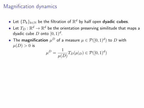
• Let {Dk}k∈N be the filtration of Rd by half open dyadic cubes.• Let TD : Rd → Rd be the orientation preserving similitude that maps a
dyadic cube D onto [0, 1)d.• The magnification µD of a measure µ ∈ P([0, 1)d) to D withµ(D) > 0 is
µD =1
µ(D)TD(µ|D) ∈ P([0, 1)d)
• If k ∈ N, let Dk(x) ∈ Dk be the cube with x ∈ Dk(x). Write
Ξ = {(x, µ) : µ ∈ P([0, 1)d) and µ(Dk(x)) > 0 for all k ∈ N}
and define the magnification operator M : Ξ→ Ξ by
M(x, µ) = (TD1(x)(x), µD1(x)).
Magnification dynamics
• Let {Dk}k∈N be the filtration of Rd by half open dyadic cubes.
• Let TD : Rd → Rd be the orientation preserving similitude that maps adyadic cube D onto [0, 1)d.• The magnification µD of a measure µ ∈ P([0, 1)d) to D withµ(D) > 0 is
µD =1
µ(D)TD(µ|D) ∈ P([0, 1)d)
• If k ∈ N, let Dk(x) ∈ Dk be the cube with x ∈ Dk(x). Write
Ξ = {(x, µ) : µ ∈ P([0, 1)d) and µ(Dk(x)) > 0 for all k ∈ N}
and define the magnification operator M : Ξ→ Ξ by
M(x, µ) = (TD1(x)(x), µD1(x)).
Magnification dynamics
• Let {Dk}k∈N be the filtration of Rd by half open dyadic cubes.• Let TD : Rd → Rd be the orientation preserving similitude that maps a
dyadic cube D onto [0, 1)d.
• The magnification µD of a measure µ ∈ P([0, 1)d) to D withµ(D) > 0 is
µD =1
µ(D)TD(µ|D) ∈ P([0, 1)d)
• If k ∈ N, let Dk(x) ∈ Dk be the cube with x ∈ Dk(x). Write
Ξ = {(x, µ) : µ ∈ P([0, 1)d) and µ(Dk(x)) > 0 for all k ∈ N}
and define the magnification operator M : Ξ→ Ξ by
M(x, µ) = (TD1(x)(x), µD1(x)).
Magnification dynamics
• Let {Dk}k∈N be the filtration of Rd by half open dyadic cubes.• Let TD : Rd → Rd be the orientation preserving similitude that maps a
dyadic cube D onto [0, 1)d.• The magnification µD of a measure µ ∈ P([0, 1)d) to D withµ(D) > 0 is
µD =1
µ(D)TD(µ|D) ∈ P([0, 1)d)
• If k ∈ N, let Dk(x) ∈ Dk be the cube with x ∈ Dk(x). Write
Ξ = {(x, µ) : µ ∈ P([0, 1)d) and µ(Dk(x)) > 0 for all k ∈ N}
and define the magnification operator M : Ξ→ Ξ by
M(x, µ) = (TD1(x)(x), µD1(x)).

Magnification dynamics
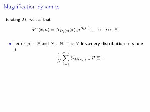
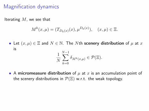
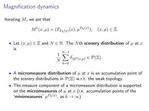
Iterating M , we see that
Mk(x, µ) = (TDk(x)(x), µDk(x)), (x, µ) ∈ Ξ.
• Let (x, µ) ∈ Ξ and N ∈ N. The N th scenery distribution of µ at xis
1
N
N−1∑k=0
δMk(x,µ) ∈ P(Ξ).
• A micromeasure distribution of µ at x is an accumulation point ofthe scenery distributions in P(Ξ) w.r.t. the weak topology.• The measure component of a micromeasure distribution is supported
on the micromeasures of µ at x (i.e. accumulation points of the‘minimeasures’ µDk(x), as k →∞)

Magnification dynamics
Iterating M , we see that
Mk(x, µ) = (TDk(x)(x), µDk(x)), (x, µ) ∈ Ξ.
• Let (x, µ) ∈ Ξ and N ∈ N. The N th scenery distribution of µ at xis
1
N
N−1∑k=0
δMk(x,µ) ∈ P(Ξ).
• A micromeasure distribution of µ at x is an accumulation point ofthe scenery distributions in P(Ξ) w.r.t. the weak topology.• The measure component of a micromeasure distribution is supported
on the micromeasures of µ at x (i.e. accumulation points of the‘minimeasures’ µDk(x), as k →∞)
Magnification dynamics
Iterating M , we see that
Mk(x, µ) = (TDk(x)(x), µDk(x)), (x, µ) ∈ Ξ.
• Let (x, µ) ∈ Ξ and N ∈ N. The N th scenery distribution of µ at xis
1
N
N−1∑k=0
δMk(x,µ) ∈ P(Ξ).
• A micromeasure distribution of µ at x is an accumulation point ofthe scenery distributions in P(Ξ) w.r.t. the weak topology.
• The measure component of a micromeasure distribution is supportedon the micromeasures of µ at x (i.e. accumulation points of the‘minimeasures’ µDk(x), as k →∞)
Magnification dynamics
Iterating M , we see that
Mk(x, µ) = (TDk(x)(x), µDk(x)), (x, µ) ∈ Ξ.
• Let (x, µ) ∈ Ξ and N ∈ N. The N th scenery distribution of µ at xis
1
N
N−1∑k=0
δMk(x,µ) ∈ P(Ξ).
• A micromeasure distribution of µ at x is an accumulation point ofthe scenery distributions in P(Ξ) w.r.t. the weak topology.• The measure component of a micromeasure distribution is supported
on the micromeasures of µ at x (i.e. accumulation points of the‘minimeasures’ µDk(x), as k →∞)
Magnification dynamics
Let Q̃ be the measure component of an M invariant measure Q.
• Q is a CP distribution, if the choice of (x, µ) according to Q can bemade by first choosing µ according to Q̃ and then x according to µ.I.e. we have a disintegration
ˆf(x, µ) dQ(x, µ) =
ˆˆf(x, µ) dµ(x) dQ̃(µ),
for any continuous f : Ξ→ R.• A CP distribution Q is (M -)ergodic if the Q measure of any M
invariant set is either 0 or 1. I.e. A = M−1A =⇒ Q(A) ∈ {0, 1}.• It is also possible to use more general (regular) filtrations than dyadic.
Then the dynamics is described by a Markov process (a CP chain)and the CP distribution is the stationary measure for this chain.

Magnification dynamics
Let Q̃ be the measure component of an M invariant measure Q.
• Q is a CP distribution, if the choice of (x, µ) according to Q can bemade by first choosing µ according to Q̃ and then x according to µ.
I.e. we have a disintegrationˆf(x, µ) dQ(x, µ) =
ˆˆf(x, µ) dµ(x) dQ̃(µ),
for any continuous f : Ξ→ R.• A CP distribution Q is (M -)ergodic if the Q measure of any M
invariant set is either 0 or 1. I.e. A = M−1A =⇒ Q(A) ∈ {0, 1}.• It is also possible to use more general (regular) filtrations than dyadic.
Then the dynamics is described by a Markov process (a CP chain)and the CP distribution is the stationary measure for this chain.

Magnification dynamics
Let Q̃ be the measure component of an M invariant measure Q.
• Q is a CP distribution, if the choice of (x, µ) according to Q can bemade by first choosing µ according to Q̃ and then x according to µ.I.e. we have a disintegration
ˆf(x, µ) dQ(x, µ) =
ˆˆf(x, µ) dµ(x) dQ̃(µ),
for any continuous f : Ξ→ R.
• A CP distribution Q is (M -)ergodic if the Q measure of any Minvariant set is either 0 or 1. I.e. A = M−1A =⇒ Q(A) ∈ {0, 1}.• It is also possible to use more general (regular) filtrations than dyadic.
Then the dynamics is described by a Markov process (a CP chain)and the CP distribution is the stationary measure for this chain.
Magnification dynamics
Let Q̃ be the measure component of an M invariant measure Q.
• Q is a CP distribution, if the choice of (x, µ) according to Q can bemade by first choosing µ according to Q̃ and then x according to µ.I.e. we have a disintegration
ˆf(x, µ) dQ(x, µ) =
ˆˆf(x, µ) dµ(x) dQ̃(µ),
for any continuous f : Ξ→ R.• A CP distribution Q is (M -)ergodic if the Q measure of any M
invariant set is either 0 or 1. I.e. A = M−1A =⇒ Q(A) ∈ {0, 1}.
• It is also possible to use more general (regular) filtrations than dyadic.Then the dynamics is described by a Markov process (a CP chain)and the CP distribution is the stationary measure for this chain.
Magnification dynamics
Let Q̃ be the measure component of an M invariant measure Q.
• Q is a CP distribution, if the choice of (x, µ) according to Q can bemade by first choosing µ according to Q̃ and then x according to µ.I.e. we have a disintegration
ˆf(x, µ) dQ(x, µ) =
ˆˆf(x, µ) dµ(x) dQ̃(µ),
for any continuous f : Ξ→ R.• A CP distribution Q is (M -)ergodic if the Q measure of any M
invariant set is either 0 or 1. I.e. A = M−1A =⇒ Q(A) ∈ {0, 1}.• It is also possible to use more general (regular) filtrations than dyadic.
Then the dynamics is described by a Markov process (a CP chain)and the CP distribution is the stationary measure for this chain.

Generating CP distributions
A CP distribution Q is generated by a measure µ, if(1) Q is the only micromeasure distribution of µ at µ almost every x;(2) and at µ almost every x the q-sparse scenery distributions
1
N
N−1∑k=0
δMqk(x,µ) ∈ P(Ξ)
converge to some distribution Qq for any q ∈ N, where each Qq maybe different from Q.
Condition (2) seems strange at first sight, but is essential to carrygeometric information from the micromeasure back to µ.
In ‘nice’ situations, (2) does not cause any problems in the proofs andoften Qq = Q for all q ∈ N.
Generating CP distributions
A CP distribution Q is generated by a measure µ, if(1) Q is the only micromeasure distribution of µ at µ almost every x;
(2) and at µ almost every x the q-sparse scenery distributions
1
N
N−1∑k=0
δMqk(x,µ) ∈ P(Ξ)
converge to some distribution Qq for any q ∈ N, where each Qq maybe different from Q.
Condition (2) seems strange at first sight, but is essential to carrygeometric information from the micromeasure back to µ.
In ‘nice’ situations, (2) does not cause any problems in the proofs andoften Qq = Q for all q ∈ N.

Generating CP distributions
A CP distribution Q is generated by a measure µ, if(1) Q is the only micromeasure distribution of µ at µ almost every x;(2) and at µ almost every x the q-sparse scenery distributions
1
N
N−1∑k=0
δMqk(x,µ) ∈ P(Ξ)
converge to some distribution Qq for any q ∈ N, where each Qq maybe different from Q.
Condition (2) seems strange at first sight, but is essential to carrygeometric information from the micromeasure back to µ.
In ‘nice’ situations, (2) does not cause any problems in the proofs andoften Qq = Q for all q ∈ N.
Example: CP chains in the conformal setting
When one zooms in on a set or measure with a self-conformal structure,roughly speaking, one expects the tangent objects to be the same as theoriginal object.
Proposition (Hochman-Shmerkin 2012)
Let µ be a self-similar measure in Rd satisfying the strong separationcondition. Then µ generates an ergodic CP chain Q for the dyadicpartition operator supported on the dyadic micromeasures of µ such thatthe dyadic micromeasures ν are of the form
ν = µ(B)−1S(µ|B)
for some Borel-set B with µ(B) > 0 and some similitude S of Rd.Moreover, the original measure can be recovered from a given micromeasureν as µ = ν(B′)−1S′(ν|′B), for some Borel-set B′ and similitude S′.

Example: dimensions of projections
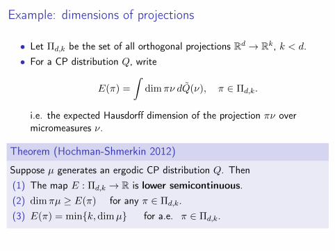
• Let Πd,k be the set of all orthogonal projections Rd → Rk, k < d.
• For a CP distribution Q, write
E(π) =
ˆdimπν dQ̃(ν), π ∈ Πd,k.
i.e. the expected Hausdorff dimension of the projection πν overmicromeasures ν.
Theorem (Hochman-Shmerkin 2012)
Suppose µ generates an ergodic CP distribution Q. Then(1) The map E : Πd,k → R is lower semicontinuous.(2) dimπµ ≥ E(π) for any π ∈ Πd,k.(3) E(π) = min{k, dimµ} for a.e. π ∈ Πd,k.
Example: dimensions of projections
• Let Πd,k be the set of all orthogonal projections Rd → Rk, k < d.• For a CP distribution Q, write
E(π) =
ˆdimπν dQ̃(ν), π ∈ Πd,k.
i.e. the expected Hausdorff dimension of the projection πν overmicromeasures ν.
Theorem (Hochman-Shmerkin 2012)
Suppose µ generates an ergodic CP distribution Q. Then(1) The map E : Πd,k → R is lower semicontinuous.
(2) dimπµ ≥ E(π) for any π ∈ Πd,k.(3) E(π) = min{k, dimµ} for a.e. π ∈ Πd,k.
Example: dimensions of projections
• Let Πd,k be the set of all orthogonal projections Rd → Rk, k < d.• For a CP distribution Q, write
E(π) =
ˆdimπν dQ̃(ν), π ∈ Πd,k.
i.e. the expected Hausdorff dimension of the projection πν overmicromeasures ν.
Theorem (Hochman-Shmerkin 2012)
Suppose µ generates an ergodic CP distribution Q. Then(1) The map E : Πd,k → R is lower semicontinuous.(2) dimπµ ≥ E(π) for any π ∈ Πd,k.
(3) E(π) = min{k, dimµ} for a.e. π ∈ Πd,k.
Example: dimensions of projections
• Let Πd,k be the set of all orthogonal projections Rd → Rk, k < d.• For a CP distribution Q, write
E(π) =
ˆdimπν dQ̃(ν), π ∈ Πd,k.
i.e. the expected Hausdorff dimension of the projection πν overmicromeasures ν.
Theorem (Hochman-Shmerkin 2012)
Suppose µ generates an ergodic CP distribution Q. Then(1) The map E : Πd,k → R is lower semicontinuous.(2) dimπµ ≥ E(π) for any π ∈ Πd,k.(3) E(π) = min{k, dimµ} for a.e. π ∈ Πd,k.
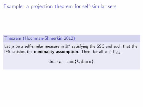
Example: a projection theorem for self-similar sets
Theorem (Hochman-Shmerkin 2012)
Let µ be a self-similar measure in Rd satisfying the SSC and such that theIFS satisfies the minimality assumption. Then, for all π ∈ Πd,k,
dimπµ = min{k,dimµ}.

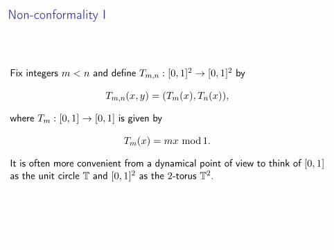
Non-conformality I
Fix integers m < n and define Tm,n : [0, 1]2 → [0, 1]2 by
Tm,n(x, y) = (Tm(x), Tn(x)),
where Tm : [0, 1]→ [0, 1] is given by
Tm(x) = mx mod 1.
It is often more convenient from a dynamical point of view to think of [0, 1]as the unit circle T and [0, 1]2 as the 2-torus T2.

Non-conformality I
Fix integers m < n and define Tm,n : [0, 1]2 → [0, 1]2 by
Tm,n(x, y) = (Tm(x), Tn(x)),
where Tm : [0, 1]→ [0, 1] is given by
Tm(x) = mx mod 1.
It is often more convenient from a dynamical point of view to think of [0, 1]as the unit circle T and [0, 1]2 as the 2-torus T2.
Non-conformality I
Fix integers m < n and define Tm,n : [0, 1]2 → [0, 1]2 by
Tm,n(x, y) = (Tm(x), Tn(x)),
where Tm : [0, 1]→ [0, 1] is given by
Tm(x) = mx mod 1.
It is often more convenient from a dynamical point of view to think of [0, 1]as the unit circle T and [0, 1]2 as the 2-torus T2.

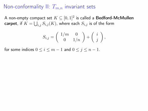
Non-conformality II: Tm,n invariant sets
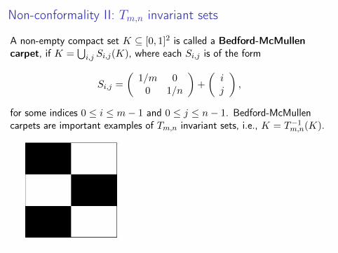
A non-empty compact set K ⊆ [0, 1]2 is called a Bedford-McMullencarpet, if K =
⋃i,j Si,j(K), where each Si,j is of the form
Si,j =
(1/m 0
0 1/n
)+
(ij
),
for some indices 0 ≤ i ≤ m− 1 and 0 ≤ j ≤ n− 1. Bedford-McMullencarpets are important examples of Tm,n invariant sets, i.e., K = T−1m,n(K).
Non-conformality II: Tm,n invariant sets
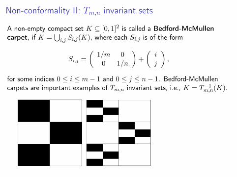
A non-empty compact set K ⊆ [0, 1]2 is called a Bedford-McMullencarpet, if K =
⋃i,j Si,j(K), where each Si,j is of the form
Si,j =
(1/m 0
0 1/n
)+
(ij
),
for some indices 0 ≤ i ≤ m− 1 and 0 ≤ j ≤ n− 1.
Bedford-McMullencarpets are important examples of Tm,n invariant sets, i.e., K = T−1m,n(K).

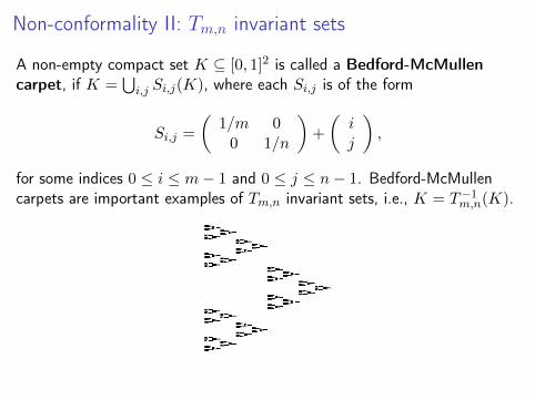
Non-conformality II: Tm,n invariant sets
A non-empty compact set K ⊆ [0, 1]2 is called a Bedford-McMullencarpet, if K =
⋃i,j Si,j(K), where each Si,j is of the form
Si,j =
(1/m 0
0 1/n
)+
(ij
),
for some indices 0 ≤ i ≤ m− 1 and 0 ≤ j ≤ n− 1. Bedford-McMullencarpets are important examples of Tm,n invariant sets, i.e., K = T−1m,n(K).
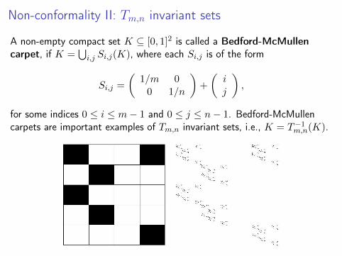
Non-conformality II: Tm,n invariant measures
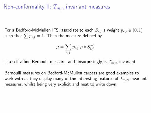
For a Bedford-McMullen IFS, associate to each Si,j a weight pi,j ∈ (0, 1)such that
∑pi,j = 1. Then the measure defined by
µ =∑i,j
pi,j µ ◦ S−1i,j
is a self-affine Bernoulli measure, and unsurprisingly, is Tm,n invariant.
Bernoulli measures on Bedford-McMullen carpets are good examples towork with as they display many of the interesting features of Tm,n invariantmeasures, whilst being very explicit and neat to write down.

Non-conformality II: Tm,n invariant measures
For a Bedford-McMullen IFS, associate to each Si,j a weight pi,j ∈ (0, 1)such that
∑pi,j = 1. Then the measure defined by
µ =∑i,j
pi,j µ ◦ S−1i,j
is a self-affine Bernoulli measure, and unsurprisingly, is Tm,n invariant.
Bernoulli measures on Bedford-McMullen carpets are good examples towork with as they display many of the interesting features of Tm,n invariantmeasures, whilst being very explicit and neat to write down.

Non-conformality III: Magnification
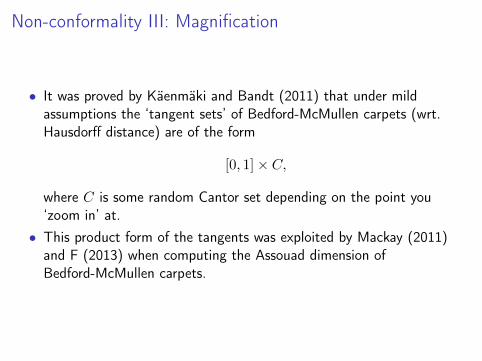
• It was proved by Käenmäki and Bandt (2011) that under mildassumptions the ‘tangent sets’ of Bedford-McMullen carpets (wrt.Hausdorff distance) are of the form
[0, 1]× C,
where C is some random Cantor set depending on the point you‘zoom in’ at.• This product form of the tangents was exploited by Mackay (2011)
and F (2013) when computing the Assouad dimension ofBedford-McMullen carpets.

Non-conformality III: Magnification
• It was proved by Käenmäki and Bandt (2011) that under mildassumptions the ‘tangent sets’ of Bedford-McMullen carpets (wrt.Hausdorff distance) are of the form
[0, 1]× C,
where C is some random Cantor set depending on the point you‘zoom in’ at.
• This product form of the tangents was exploited by Mackay (2011)and F (2013) when computing the Assouad dimension ofBedford-McMullen carpets.
Non-conformality III: Magnification
• It was proved by Käenmäki and Bandt (2011) that under mildassumptions the ‘tangent sets’ of Bedford-McMullen carpets (wrt.Hausdorff distance) are of the form
[0, 1]× C,
where C is some random Cantor set depending on the point you‘zoom in’ at.• This product form of the tangents was exploited by Mackay (2011)
and F (2013) when computing the Assouad dimension ofBedford-McMullen carpets.
Non-conformality III: Magnification
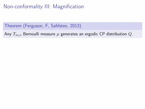
Theorem (Ferguson, F, Sahlsten, 2013)
Any Tm,n Bernoulli measure µ generates an ergodic CP distribution Q.
• Measure component Q̃ is the distribution of the random measure
St(π1µ× µx),
where x ∼ π1µ and µx ∈ P([0, 1]) is the conditional measure of µwith respect to the fibre π−11 {x} and St is the unique affine mapwhich sends [0, 1]2 to [0, 1/nt/2]× [0, nt/2] and t ∈ [0, 1) is drawnaccording to Lebesgue in the ‘irrational case’ and according to auniform measure on a periodic orbit in the ‘rational case’.

Non-conformality III: Magnification
Theorem (Ferguson, F, Sahlsten, 2013)
Any Tm,n Bernoulli measure µ generates an ergodic CP distribution Q.
• Measure component Q̃ is the distribution of the random measure
St(π1µ× µx),
where x ∼ π1µ and µx ∈ P([0, 1]) is the conditional measure of µwith respect to the fibre π−11 {x} and St is the unique affine mapwhich sends [0, 1]2 to [0, 1/nt/2]× [0, nt/2] and t ∈ [0, 1) is drawnaccording to Lebesgue in the ‘irrational case’ and according to auniform measure on a periodic orbit in the ‘rational case’.

Application I: Projections
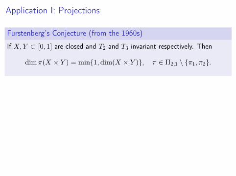
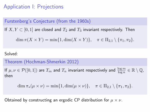
Furstenberg’s Conjecture (from the 1960s)
If X,Y ⊂ [0, 1] are closed and T2 and T3 invariant respectively. Then
dimπ(X × Y ) = min{1,dim(X × Y )}, π ∈ Π2,1 \ {π1, π2}.
Solved:
Theorem (Hochman-Shmerkin 2012)
If µ, ν ∈ P([0, 1]) are Tm and Tn invariant respectively and logmlogn ∈ R \Q,
then
dimπ∗(µ× ν) = min{1,dim(µ× ν)}, π ∈ Π2,1 \ {π1, π2}.
Obtained by constructing an ergodic CP distribution for µ× ν.
Application I: Projections
Furstenberg’s Conjecture (from the 1960s)
If X,Y ⊂ [0, 1] are closed and T2 and T3 invariant respectively. Then
dimπ(X × Y ) = min{1,dim(X × Y )}, π ∈ Π2,1 \ {π1, π2}.
Solved:
Theorem (Hochman-Shmerkin 2012)
If µ, ν ∈ P([0, 1]) are Tm and Tn invariant respectively and logmlogn ∈ R \Q,
then
dimπ∗(µ× ν) = min{1, dim(µ× ν)}, π ∈ Π2,1 \ {π1, π2}.
Obtained by constructing an ergodic CP distribution for µ× ν.

Application I: Projections
Conjecture
Suppose µ is a Tm,n invariant measure and logmlogn ∈ R \Q, then
dimπ∗µ = min{1, dimµ}, π ∈ Π2,1 \ {π1, π2}.
Theorem (Ferguson-Jordan-Shmerkin 2010)
Suppose K is a Bedford-McMullen carpet with logmlogn ∈ R \Q. Then
dimπ(K) = min{1,dimK}, π ∈ Π2,1 \ {π1, π2}.
Theorem (Ferguson, F, Sahlsten, 2013)
The conjecture above holds for Tm,n invariant Bernoulli measures.

Application I: Projections
Conjecture
Suppose µ is a Tm,n invariant measure and logmlogn ∈ R \Q, then
dimπ∗µ = min{1, dimµ}, π ∈ Π2,1 \ {π1, π2}.
Theorem (Ferguson-Jordan-Shmerkin 2010)
Suppose K is a Bedford-McMullen carpet with logmlogn ∈ R \Q. Then
dimπ(K) = min{1, dimK}, π ∈ Π2,1 \ {π1, π2}.
Theorem (Ferguson, F, Sahlsten, 2013)
The conjecture above holds for Tm,n invariant Bernoulli measures.

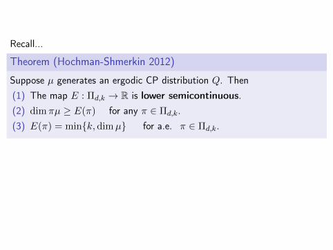
Recall...
Theorem (Hochman-Shmerkin 2012)
Suppose µ generates an ergodic CP distribution Q. Then(1) The map E : Πd,k → R is lower semicontinuous.(2) dimπµ ≥ E(π) for any π ∈ Πd,k.(3) E(π) = min{k, dimµ} for a.e. π ∈ Πd,k.
• In our setting, after suitable reparametrisation of Π2,1, the map E isinvariant under the irrational logm
logn rotation of the circle, so E isconstant as a lower semicontinuous function on Π2,1 \ {π1, π2}.

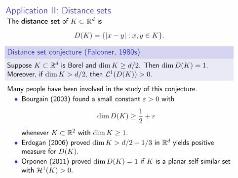
Application II: Distance sets
The distance set of K ⊂ Rd is
D(K) = {|x− y| : x, y ∈ K}.
Distance set conjecture (Falconer, 1980s)
Suppose K ⊂ Rd is Borel and dimK ≥ d/2. Then dimD(K) = 1.Moreover, if dimK > d/2, then L1(D(K)) > 0.
Many people have been involved in the study of this conjecture.• Bourgain (2003) found a small constant ε > 0 with
dimD(K) ≥ 1
2+ ε
whenever K ⊂ R2 with dimK ≥ 1.• Erdogan (2006) proved dimK > d/2 + 1/3 in Rd yields positive
measure for D(K).• Orponen (2011) proved dimD(K) = 1 if K is a planar self-similar set
with H1(K) > 0.

Application II: Distance setsThe distance set of K ⊂ Rd is
D(K) = {|x− y| : x, y ∈ K}.
Distance set conjecture (Falconer, 1980s)
Suppose K ⊂ Rd is Borel and dimK ≥ d/2. Then dimD(K) = 1.Moreover, if dimK > d/2, then L1(D(K)) > 0.
Many people have been involved in the study of this conjecture.• Bourgain (2003) found a small constant ε > 0 with
dimD(K) ≥ 1
2+ ε
whenever K ⊂ R2 with dimK ≥ 1.• Erdogan (2006) proved dimK > d/2 + 1/3 in Rd yields positive
measure for D(K).• Orponen (2011) proved dimD(K) = 1 if K is a planar self-similar set
with H1(K) > 0.

Application II: Distance sets
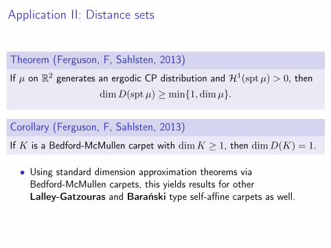
Theorem (Ferguson, F, Sahlsten, 2013)
If µ on R2 generates an ergodic CP distribution and H1(sptµ) > 0, then
dimD(sptµ) ≥ min{1,dimµ}.
Corollary (Ferguson, F, Sahlsten, 2013)
If K is a Bedford-McMullen carpet with dimK ≥ 1, then dimD(K) = 1.
• Using standard dimension approximation theorems viaBedford-McMullen carpets, this yields results for otherLalley-Gatzouras and Barański type self-affine carpets as well.

Application II: Distance sets
Theorem (Ferguson, F, Sahlsten, 2013)
If µ on R2 generates an ergodic CP distribution and H1(sptµ) > 0, then
dimD(sptµ) ≥ min{1,dimµ}.
Corollary (Ferguson, F, Sahlsten, 2013)
If K is a Bedford-McMullen carpet with dimK ≥ 1, then dimD(K) = 1.
• Using standard dimension approximation theorems viaBedford-McMullen carpets, this yields results for otherLalley-Gatzouras and Barański type self-affine carpets as well.

Possible further topics
• Scaling scenery of more general Tm,n invariant measures(Gibbs measures with strong mixing properties?)• Scaling scenery of general self-affine/other non-conformal sets• Conformal Hausdorff dimension of self-affine carpets• Applications of scaling scenery to other problems in geometric
measure theory
Possible further topics
• Scaling scenery of more general Tm,n invariant measures(Gibbs measures with strong mixing properties?)
• Scaling scenery of general self-affine/other non-conformal sets• Conformal Hausdorff dimension of self-affine carpets• Applications of scaling scenery to other problems in geometric
measure theory

Possible further topics
• Scaling scenery of more general Tm,n invariant measures(Gibbs measures with strong mixing properties?)• Scaling scenery of general self-affine/other non-conformal sets
• Conformal Hausdorff dimension of self-affine carpets• Applications of scaling scenery to other problems in geometric
measure theory
Possible further topics
• Scaling scenery of more general Tm,n invariant measures(Gibbs measures with strong mixing properties?)• Scaling scenery of general self-affine/other non-conformal sets• Conformal Hausdorff dimension of self-affine carpets
• Applications of scaling scenery to other problems in geometricmeasure theory

Possible further topics
• Scaling scenery of more general Tm,n invariant measures(Gibbs measures with strong mixing properties?)• Scaling scenery of general self-affine/other non-conformal sets• Conformal Hausdorff dimension of self-affine carpets• Applications of scaling scenery to other problems in geometric
measure theory

Thank you!
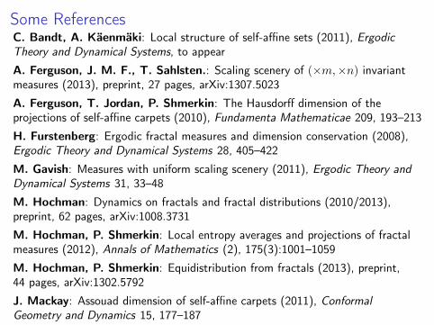
Some ReferencesC. Bandt, A. Käenmäki: Local structure of self-affine sets (2011), ErgodicTheory and Dynamical Systems, to appear
A. Ferguson, J. M. F., T. Sahlsten.: Scaling scenery of (×m,×n) invariantmeasures (2013), preprint, 27 pages, arXiv:1307.5023
A. Ferguson, T. Jordan, P. Shmerkin: The Hausdorff dimension of theprojections of self-affine carpets (2010), Fundamenta Mathematicae 209, 193–213
H. Furstenberg: Ergodic fractal measures and dimension conservation (2008),Ergodic Theory and Dynamical Systems 28, 405–422
M. Gavish: Measures with uniform scaling scenery (2011), Ergodic Theory andDynamical Systems 31, 33–48
M. Hochman: Dynamics on fractals and fractal distributions (2010/2013),preprint, 62 pages, arXiv:1008.3731
M. Hochman, P. Shmerkin: Local entropy averages and projections of fractalmeasures (2012), Annals of Mathematics (2), 175(3):1001–1059
M. Hochman, P. Shmerkin: Equidistribution from fractals (2013), preprint,44 pages, arXiv:1302.5792
J. Mackay: Assouad dimension of self-affine carpets (2011), ConformalGeometry and Dynamics 15, 177–187