scanner data and the treatment of quality change in ... · scanner data and the treatment of...
TRANSCRIPT

Scanner Data and the Treatment of Quality Change in Rolling Year GEKS Price Indexes
Jan de Haana and Frances Krsinichb
6 November, 2012
Abstract: The recently developed rolling year GEKS procedure makes maximum use
of all matches in the data in order to construct price indexes that are (approximately)
free from chain drift. A potential weakness is that unmatched items are ignored. In this
paper we use imputation Törnqvist price indexes as inputs into the rolling year GEKS
procedure. These indexes account for quality changes by imputing the ‘missing prices’
associated with new and disappearing items. Three imputation methods are discussed.
The first method makes explicit imputations using a hedonic regression model which is
estimated for each time period. The other two methods make implicit imputations; they
are based on time dummy hedonic and time-product dummy regression models and are
estimated on pooled data. We present empirical evidence for New Zealand from scanner
data on eight consumer electronics products and find that accounting for quality change
can make a substantial difference.
Key words: hedonic regression, imputation, multilateral index number methods, quality adjustment, scanner data, transitivity.
JEL Classification: C43, E31.
a Corresponding author; Division of Process Development, IT and Methodology, Statistics Netherlands,
P.O. Box 24500, 2490 HA The Hague, The Netherlands; [email protected].
b Prices Unit, Statistics New Zealand; [email protected].
The authors would like to thank participants at the following conferences and workshops for comments
on earlier versions of this paper: UNECE/ILO meeting of the group of experts on consumer price indexes,
Geneva, May 2012; Statistics Sweden’s workshop on scanner data, Stockholm, June 2012; and the New
Zealand Association of Economists conference, Palmerston North, June 2012. Thanks also to Alistair
Gray and Soon Song for contributions to discussions and empirical work. The authors gratefully
acknowledge the financial support from Eurostat (Multi-purpose Consumer Price Statistics Grant). The
research data was made available by the New Zealand branch of the market research company GfK. The
views expressed in this paper are those of the authors and do not necessarily reflect the views of Statistics
Netherlands or Statistics New Zealand.

1
1. Introduction
Barcode scanning data, or scanner data for short, contain information on the prices and
quantities sold of all individual items. One obvious advantage of using scanner data for
compiling the Consumer Price Index (CPI) is that price indexes can cover product
categories completely rather than being based on a small sample of items as is usual
practice. Another advantage of using scanner data is that the construction of superlative
indexes, such as Fisher or Törnqvist indexes, is now feasible.1 Superlative indexes treat
both time periods in a symmetric fashion and have attractive properties, like taking into
account the consumers’ substitution behavior. Most statistical agencies still rely today
on fixed-weight, Laspeyres-type indexes to compile the CPI.
Scanner data typically show substantial item attrition; many new items appear
and many ‘old’ items disappear. This makes it difficult if not impossible to construct
price indexes using the standard approach where the prices of a more or less fixed set of
items are tracked over time. Chain linking period-on-period price movements seems an
obvious solution, but that can lead to a drifting time series under certain circumstances.
Ivancic, Diewert and Fox (2011) resolved the problem of chain drift by adapting the
well-known GEKS (Gini, 1931; Eltetö and Köves; 1964; Szulc, 1964) method for
comparing prices across countries to comparing prices across time. Their rolling year
(RY) GEKS approach makes optimal use of the matches in the data and yields price
indexes that are approximately free from chain drift.
A potential weakness of matched-item approaches, including RYGEKS, is that
the price effects of new and disappearing items are neglected. High-tech products, such
as consumer electronics, usually experience rapid quality changes; new items are often
of higher quality than existing ones. It is well established in the literature that adjusting
for quality change is an essential part of price measurement (see e.g. ILO et al., 2004).
The purpose of this paper is to show how quality-adjusted RYGEKS price indexes can
be estimated. These indexes provide us with a benchmark measure that can be used to
assess the performance of easier-to-construct price indexes.
1 Statistics Netherlands has been using scanner data for supermarkets in the CPI since 2004. In 2010, a
new computation method was introduced and the coverage was expanded to include more supermarket
chains. However, the new Dutch method does not make use of weighting information at the individual
item level. Van der Grient and de Haan (2011) describe the method and explain the choice for using an
unweighted index number formula at the elementary aggregation level.

2
The RYGEKS procedure combines bilateral superlative indexes, which compare
two time periods, with different base periods. In the original setup, the bilateral indexes
only take account of the matched items, i.e. the items that are available in both periods
compared. Quality mix changes can occur within the set of matched items. For example,
overall quality will improve over time when consumers increasingly purchase higher-
quality items. Changes in the quality mix of a matched set do not need special attention
here, however; they will be handled appropriately using matched-item superlative price
indexes.
The issue at stake is how to account for quality changes associated with new and
disappearing items. We do this by estimating bilateral imputation price indexes, which
serve as inputs into the RYGEKS procedure. Imputation price indexes adjust for quality
changes by imputing the unobservable or ‘missing’ prices to construct price relatives for
the new and disappearing items.
The paper is structured as follows. Section 2 outlines the RYGEKS procedure.
Sections 3 to 5 discuss three regression-based bilateral imputation Törnqvist indexes.
The method outlined in section 3 makes explicit imputations using a hedonic regression
model which is estimated on cross-section data for each period. The two other methods
are based on making implicit imputations. In section 4 we discuss a result derived by de
Haan (2004) regarding how a weighted least squares time dummy hedonic model that is
estimated on the pooled data of two periods implicitly defines an imputation Törnqvist
index. A non-hedonic variant of the weighted time dummy model, referred to as the
time-product dummy model, is described in section 5. We show that this model leads to
a matched-item price index and therefore does not offer a solution to the quality-change
problem.
In section 6 we summarize the discussion by listing the steps to be followed for
estimating Imputation Törnqvist (IT) RYGEKS indexes using the time dummy hedonic
approach and point to a few additional issues. In section 7 we describe our data set and
explain that it unfortunately does not enable us to estimate separate regression models
for each period. The monthly scanner data cover purchases in New Zealand over a
three-year period on eight consumer electronics goods: camcorders, desktop computers,
digital cameras, DVD players/recorders, laptop computers, microwaves, televisions and
portable media players. Section 8 presents empirical evidence and shows that hedonic
imputations have, on average, a significant downward effect on the RYGEKS indexes.

3
We compare our ITRYGEKS indexes with indexes estimated as rolling year versions of
the weighted multi-period time dummy method. The latter are also quality-adjusted and
approximately drift-free, and appear to perform quite well.
Section 9 concludes the paper and suggests some topics for further work in this
area.
2. The rolling window GEKS method
Suppose that we know the prices tip and expenditure shares t
is for all items i belonging
to a product category U in all time periods Tt ,...,0= . For the moment, we assume that
there are no new or disappearing items so that U is fixed over time. The Törnqvist price
index going from the starting period 0 to period t (>0) is defined as
∏∈
+
=
Ui
ss
i
tit
T
tii
p
pP
2
00
0
; Tt ,...,1= . (1)
This index compares the prices in each period t (>0) directly with those in the starting or
base period 0. The Törnqvist index is superlative and has useful properties from both
the economic approach and the axiomatic approach to index number theory (ILO et al.,
2004). However, the index series defined by (1) is not transitive. That is, the results of
the price comparisons between two periods depend on the choice of base period.2 In (1),
the starting period 0 was chosen as the base or price reference period, but this choice is
rather arbitrary if we want to compare any pair of time periods.
To illustrate the non-transitivity property, let us take period 1 as the base instead
of period 0 and make a comparison with period T. The Törnqvist index tTP1 going from
period 1 to period T is
∏∈
+
=
Ui
ss
i
TiT
T
Tii
p
pP
2
11
1
. (2)
Using period 0 as the base (as in (1)), the price change between periods 1 and T will be
calculated as the ratio of the index numbers in periods T and 1:
2 In spatial price comparisons, transitivity is also known as circularity. This is an important requirement
because the choice of base country should not affect measured price level differences across countries.
4
2
1
101
2
0
1
2
0
01
01001
10
0
)()()(
=
= ∏∏∏∏
∏∈
−
∈
−
∈
−+
∈
∈
+
Ui
ssTi
Ui
ssi
Ui
ssi
TTss
Ui i
i
Ui
ss
i
Ti
T
TT iii
Ti
Tii
ii
Tii
pppP
p
p
p
p
P
P. (3)
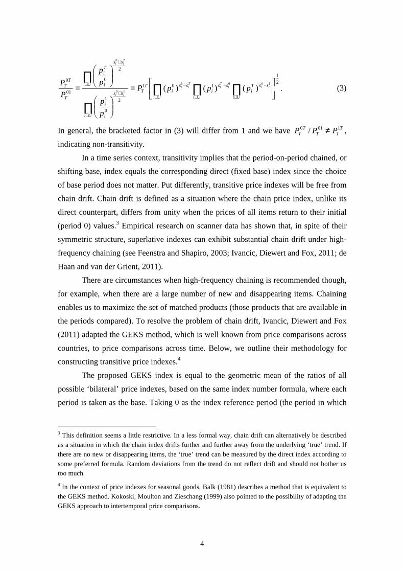
In general, the bracketed factor in (3) will differ from 1 and we have TTT
TT PPP 1010 / ≠ ,
indicating non-transitivity.
In a time series context, transitivity implies that the period-on-period chained, or
shifting base, index equals the corresponding direct (fixed base) index since the choice
of base period does not matter. Put differently, transitive price indexes will be free from
chain drift. Chain drift is defined as a situation where the chain price index, unlike its
direct counterpart, differs from unity when the prices of all items return to their initial
(period 0) values.3 Empirical research on scanner data has shown that, in spite of their
symmetric structure, superlative indexes can exhibit substantial chain drift under high-
frequency chaining (see Feenstra and Shapiro, 2003; Ivancic, Diewert and Fox, 2011; de
Haan and van der Grient, 2011).
There are circumstances when high-frequency chaining is recommended though,
for example, when there are a large number of new and disappearing items. Chaining
enables us to maximize the set of matched products (those products that are available in
the periods compared). To resolve the problem of chain drift, Ivancic, Diewert and Fox
(2011) adapted the GEKS method, which is well known from price comparisons across
countries, to price comparisons across time. Below, we outline their methodology for
constructing transitive price indexes.4
The proposed GEKS index is equal to the geometric mean of the ratios of all
possible ‘bilateral’ price indexes, based on the same index number formula, where each
period is taken as the base. Taking 0 as the index reference period (the period in which
3 This definition seems a little restrictive. In a less formal way, chain drift can alternatively be described
as a situation in which the chain index drifts further and further away from the underlying ‘true’ trend. If
there are no new or disappearing items, the ‘true’ trend can be measured by the direct index according to
some preferred formula. Random deviations from the trend do not reflect drift and should not bother us
too much.
4 In the context of price indexes for seasonal goods, Balk (1981) describes a method that is equivalent to
the GEKS method. Kokoski, Moulton and Zieschang (1999) also pointed to the possibility of adapting the
GEKS approach to intertemporal price comparisons.

5
the index equals 1) and denoting the link periods by l )0( Tl ≤≤ , the GEKS price index
going from 0 to t is
[ ] [ ]∏∏=
+
=
+ ×==T
l
TltlT
l
TtlltGEKS PPPPP
0
)1/(10
0
)1/(100 / ; Tt ,...,0= . (4)
Equation (4) presupposes that the bilateral indexes satisfy the time reversal test, (that 00 /1 tt PP = ). The GEKS index will then also satisfy this test. It can easily be shown
that the GEKS index is transitive and can therefore be written as a period-on-period
chained index.
Using the second expression of (4), the GEKS index going from period 0 to the
last (most recent) period T can be expressed as
[ ]∏=
+×=T
t
TtTtTGEKS PPP
0
)1/(100 . (5)
So far, the number of time periods (including the index reference period 0) was fixed at
1+T . In practice, we want to extend the series as time passes. If we add data pertaining
to the next period )1( +T , then the GEKS index for this period is
[ ]∏+
=
+++ ×=1
0
)2/(11,01,0T
t
TTttTGEKS PPP . (6)
Extending the time series in this way has two drawbacks. The GEKS index for the most
recent period 1+T does not only depend on the data of periods 0 and 1+T but also on
the data of all intermediate periods. Hence, when the time series is extended, there will
be an increasing loss of characteristicity.5 Furthermore, the GEKS method suffers from
revision: the price index numbers for periods T,...,1 computed using the extended data
set will differ from the previously computed index numbers.
To reduce the loss of characteristicity and circumvent the revision of previously
computed price index numbers, Ivancic, Diewert and Fox (2011) propose a rolling year
approach. This approach makes repeated use of the price and quantity data for the last
13 months (or 5 quarters) to construct GEKS indexes. A window of 13 months has been
chosen as it is the shortest period that can deal with seasonal products. The most recent
month-on-month index movement is then chain linked to the existing time series. Using
5 Caves, Christensen and Diewert (1982) define characteristicity as the “degree to which weights are
specific to the comparison at hand”.

6
12,0GEKSP as the starting point for compiling a monthly time series, the rolling year GEKS
(RYGEKS) index for the next month becomes
[ ] [ ] [ ]∏∏∏===
××=×=13
1
13/113,,1212
0
13/112,013
1
13/113,,1212,013,0
t
tt
t
tt
t
ttGEKSRYGEKS PPPPPPPP . (7)
One month later, the RYGEKS index is
[ ]∏=
×=14
2
13/114,,1313,014,0
t
ttRYGEKSRYGEKS PPPP . (8)
This chain linking procedure is repeated each next month.
Ivancic, Diewert and Fox (2011) used bilateral matched-item Fisher indexes in
the above formulas. Following de Haan and van der Grient (2011), we will use bilateral
Törnqvist indexes since their geometric structure facilitates a decomposition analysis, as
will be shown later on. Both the Fisher index and the Törnqvist index satisfy the time
reversal test and usually generate very similar results.
Unlike GEKS indexes, RYGEKS indexes are not by definition free from chain
drift. Nevertheless, it is most likely that any chain drift will be very small. Since each
13-month GEKS series is free from chain drift, we would expect chain linking the
GEKS index changes not to lead to a drifting series. Empirical evidence from scanner
data on goods sold at supermarkets lends support to our expectation that RYGEKS
indexes are approximately drift free. See Ivancic, Diewert and Fox (2011); de Haan and
van der Grient (2011); Johansen and Nygaard (2011); and Krsinich (2011).
Although matched-item GEKS indexes are free from chain drift, this does not
necessarily mean they are completely drift free; there may be other causes for a drifting
or biased time series. Greenlees and McClelland (2010) show that matched-item GEKS
price indexes for apparel suffer from significant downward bias. The prices of apparel
items typically exibit a downward trend so that any matched-item index will measure a
price decline. The problem here is a lack of explicit quality adjustment.6 Of course this
quality-change problem carries over to RYGEKS indexes.
The problem can in principle be dealt with by using bilateral imputation price
indexes as inputs into the RYGEKS procedure rather than their matched counterparts,
6 As mentioned by van der Grient and de Haan (2010), this problem may be partly due to the use of a too
detailed item identifier, in which case items that are comparable from the consumer’s perspective would
be treated as different items.
7
provided that the imputations make sense. Imputation price indexes use all the matches
in the data and, in addition, impute the ‘missing prices’ that are associated with new and
disappearing items. In section 3, we discuss the (hedonic) imputation Törnqvist index
and decompose this index into three factors: the contributions of matched items, new
items and disappearing items.
3. Hedonic imputation Törnqvist price indexes
The issue considered in this section (and in sections 4 and 5) is how the unmatched new
and disappearing items should be treated in a bilateral Törnqvist price index, where we
compare two time periods. For the sake of simplicity, we compare period 0 with period t
),...,1( Tt = . In section 6 we will show how to handle all the bilateral price comparisons
that show up in the RYGEKS framework.
We will denote the set of items that are available in both period 0 and period t by tU 0 . For these matched items, we have base period prices 0
ip and period t prices tip , so
that we can compute price relatives 0/ iti pp . The set of disappearing items, which were
observed in period 0 but are no longer available in period t, is denoted by 0)(tDU . Here,
the base period price is known but the period t price is unobservable. To compute price
relatives for the disappearing items, values tip̂ have to be predicted (imputed) for the
‘missing’ period t observations. The set of new items, which are observed in period t but
were not available in period 0, is denoted by tNU )0( . In this case the period t prices are
known but the base period prices are ‘missing’ and must be imputed by 0ˆ ip to be able to
compute the price relatives. Note that 00)(
0 UUU tDt =∪ , the total set of items in period
0, and ttN
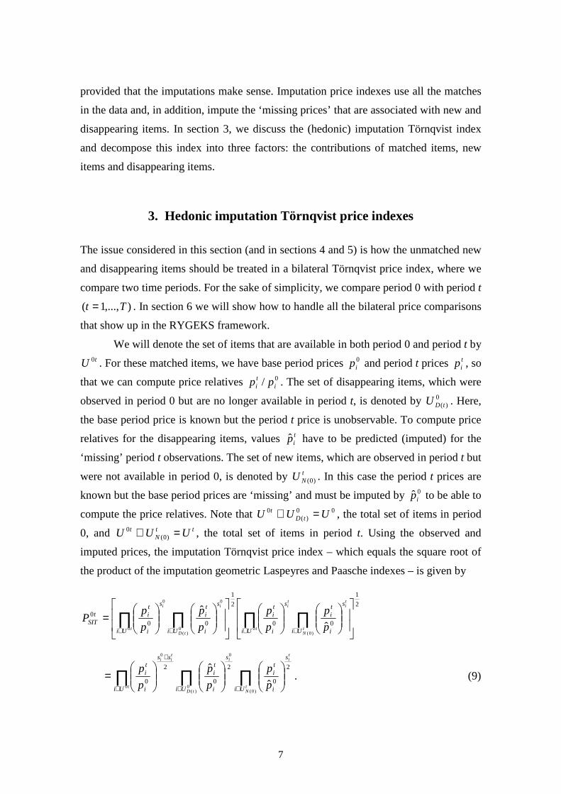
t UUU =∪ )0(0 , the total set of items in period t. Using the observed and
imputed prices, the imputation Törnqvist price index – which equals the square root of
the product of the imputation geometric Laspeyres and Paasche indexes – is given by
2
1
00
2
1
000
0)0(
0 0)(
00
ˆ
ˆ
= ∏ ∏∏ ∏
∈ ∈∈ ∈ t tN
ti
ti
ttD
ii
Ui Ui
s
i
ti
s
i
ti
Ui Ui
s
i
ti
s
i
tit
SITp
p
p
p
p
p
p
pP
∏∏∏∈∈∈
+
=
tN
ti
tD
i
t
tii
Ui
s
i
ti
Ui
s
i
ti
Ui
ss
i
ti
p
p
p
p
p
p
)0(0
)(
0
0
0
2
0
2
0
2
0 ˆ
ˆ. (9)
8
tSITP0 is a so-called single imputation Törnqvist index. Statistical agencies use the
term imputation for estimating missing observations, and so single imputation would be
the usual approach. In the index number literature, double imputation has also been
used. In a double imputation price index, the observed prices of the unmatched new and
disappearing items are replaced by predicted values. Hill and Melser (2008) discuss all
kinds of different imputation indexes based on hedonic regression. They argue that the
double imputation method may be less prone to omitted variables bias since the biases
in the numerator and denominator of the estimated price relatives for the unmatched
items are likely to cancel out, at least partially.7 Syed (2010) focuses on consistency
rather than bias and makes a similar case. However, the single imputation variant is our
point of reference because, as will be shown in section 4 below, this links up with the
use of a weighted time-dummy variable approach to hedonic regression.
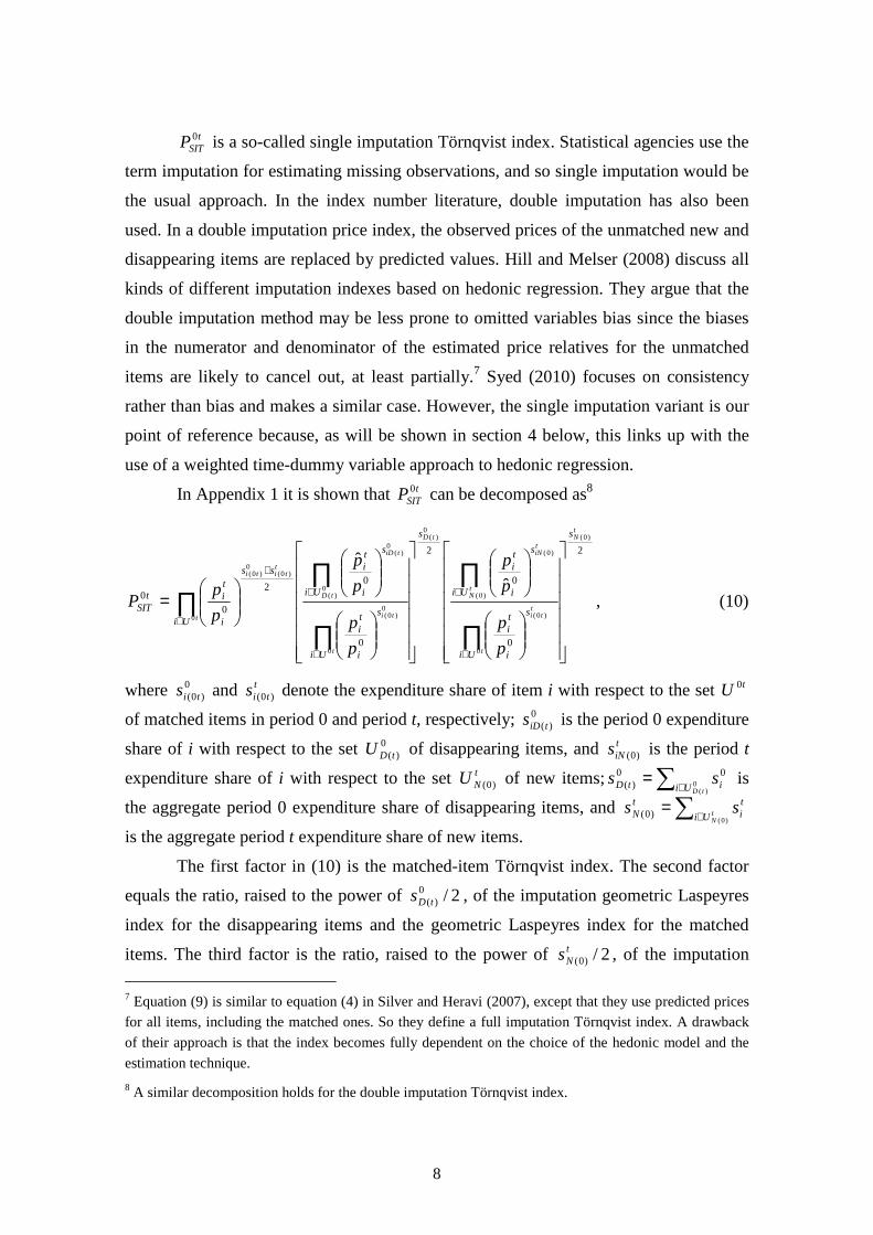
In Appendix 1 it is shown that tSITP0 can be decomposed as8
2
0
0
2
0
02
00
)0(
0
)0(
)0(
)0(
0)(
0
0)0(
0)(
0)(
0
)0(0
)0(
ˆ
ˆ
tN
t
tti
tN
tiN
tD
t
ti
tiD
tD
t
ttiti
s
Ui
s
i
ti
Ui
s
i
ti
s
Ui
s
i
ti
s
Ui i
ti
Ui
ss
i
tit
SIT
p
p
p
p
p
p
p
p
p
pP
=
∏
∏
∏
∏∏
∈
∈
∈
∈
∈
+
, (10)
where 0)0( tis and t
tis )0( denote the expenditure share of item i with respect to the set tU 0
of matched items in period 0 and period t, respectively; 0)(tiDs is the period 0 expenditure
share of i with respect to the set 0 )(tDU of disappearing items, and tiNs )0( is the period t
expenditure share of i with respect to the set tNU )0( of new items; ∑ ∈
= 0)(
00)(
tDUi itD ss is
the aggregate period 0 expenditure share of disappearing items, and ∑ ∈= t
NUi
ti
tN ss
)0()0(
is the aggregate period t expenditure share of new items.
The first factor in (10) is the matched-item Törnqvist index. The second factor
equals the ratio, raised to the power of 2/0)(tDs , of the imputation geometric Laspeyres
index for the disappearing items and the geometric Laspeyres index for the matched
items. The third factor is the ratio, raised to the power of 2/)0(tNs , of the imputation
7 Equation (9) is similar to equation (4) in Silver and Heravi (2007), except that they use predicted prices
for all items, including the matched ones. So they define a full imputation Törnqvist index. A drawback
of their approach is that the index becomes fully dependent on the choice of the hedonic model and the
estimation technique.
8 A similar decomposition holds for the double imputation Törnqvist index.

9
geometric Paasche index for the new items and the geometric Paasche index for the
matched items.
The product of the second and third factor can be viewed as an adjustment factor
by which the matched-item Törnqvist price index should be multiplied in order to obtain
a quality-adjusted price index. If someone would prefer the matched-item index as a
measure of aggregate price change, then from an imputations perspective they are either
assuming that the second and third factors cancel each other out (which would be a pure
coincidence) or that the ‘missing prices’ are imputed such that both factors are equal to
1. The latter occurs if tip̂ for the disappearing items is calculated through multiplying
the period 0 price by the matched-item geometric Laspeyres index ∏ ∈ tti
Ui
si
ti pp0
0)0()/( 0
and if 0ˆ ip for the new items is calculated through dividing the period t price by the
matched-item geometric Paasche index ∏ ∈ t
tti
Ui
si
ti pp0
)0()/( 0 . There is no a priori reason
to think this would be appropriate.
The imputations should measure the Hicksian reservation prices, which are the
prices that would have been observed if the items had been available on the market. Of
course, these fictitious prices can only be estimated by using some kind of modelling.
Hedonic regression is an obvious choice in this respect.9 The hedonic hypothesis states
that a good is a bundle of, say, K price determining characteristics. We will denote the
fixed ‘quantity’ of the k-th characteristic for item i by ikz ),...,1( Kk = . Triplett (2006)
and others have argued that the functional form should be determined empirically, but
we will only consider the logarithmic-linear model specification:
∑=
++=K
k
tiik
tk
tti zp
1
ln εβα ; Tt ,...,0= , (11)
where tkβ is the parameter for characteristic k in period t and t
iε is an error term with an
expected value of zero. The log-linear model specification has been frequently applied
and usually performs quite well. It has three advantages: it accounts for the fact that the
(absolute) errors are likely to be bigger for higher priced items, it is convenient for use
in a geometric index such as the Törnqvist, and it can be compared with the models we
will be using in sections 4 and 5.
9 This is true for product varieties which are comparable in the sense that they can be described by the
same set of characteristics so that their prices can be modeled by the same hedonic function. We do not
address the problem of entirely new goods, which have different characteristics than existing goods due
to, for example, new production techniques.
10
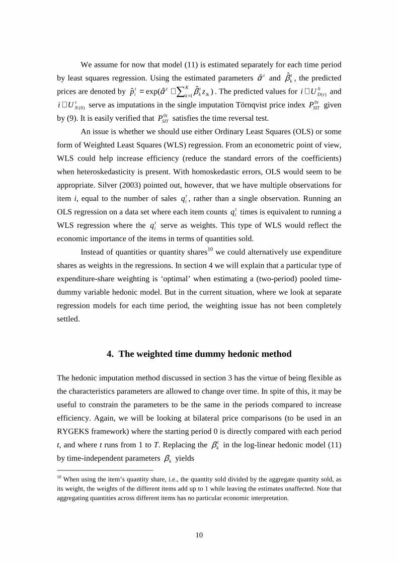
We assume for now that model (11) is estimated separately for each time period
by least squares regression. Using the estimated parameters tα̂ and tkβ̂ , the predicted
prices are denoted by )ˆˆexp(ˆ1∑ =
+= K
k iktk
tti zp βα . The predicted values for 0
)(tDUi ∈ and tNUi )0(∈ serve as imputations in the single imputation Törnqvist price index t
SITP0 given
by (9). It is easily verified that tSITP0 satisfies the time reversal test.
An issue is whether we should use either Ordinary Least Squares (OLS) or some
form of Weighted Least Squares (WLS) regression. From an econometric point of view,
WLS could help increase efficiency (reduce the standard errors of the coefficients)
when heteroskedasticity is present. With homoskedastic errors, OLS would seem to be
appropriate. Silver (2003) pointed out, however, that we have multiple observations for
item i, equal to the number of sales tiq , rather than a single observation. Running an
OLS regression on a data set where each item counts tiq times is equivalent to running a
WLS regression where the tiq serve as weights. This type of WLS would reflect the
economic importance of the items in terms of quantities sold.
Instead of quantities or quantity shares10 we could alternatively use expenditure
shares as weights in the regressions. In section 4 we will explain that a particular type of
expenditure-share weighting is ‘optimal’ when estimating a (two-period) pooled time-
dummy variable hedonic model. But in the current situation, where we look at separate
regression models for each time period, the weighting issue has not been completely
settled.
4. The weighted time dummy hedonic method
The hedonic imputation method discussed in section 3 has the virtue of being flexible as
the characteristics parameters are allowed to change over time. In spite of this, it may be
useful to constrain the parameters to be the same in the periods compared to increase
efficiency. Again, we will be looking at bilateral price comparisons (to be used in an
RYGEKS framework) where the starting period 0 is directly compared with each period
t, and where t runs from 1 to T. Replacing the tkβ in the log-linear hedonic model (11)
by time-independent parameters kβ yields
10 When using the item’s quantity share, i.e., the quantity sold divided by the aggregate quantity sold, as
its weight, the weights of the different items add up to 1 while leaving the estimates unaffected. Note that
aggregating quantities across different items has no particular economic interpretation.

11
∑=
++=K
k
tiikk
tti zp
1
ln εβα ; Tt ,...,0= . (12)
Model (13) should be estimated on the pooled data of the two periods compared. Using
a dummy variable tiD that has the value 1 if the observation relates to period t )0( ≠t
and the value 0 if the observation relates to period 0, the estimating equation for the
bilateral time dummy variable method becomes11
∑=
+++=K
k
tiikk
ti
tti zDp
1
ln εβδα ; Tt ,...,0= , (13)
where tiε is an error term with an expected value of zero, as before. Note that the time
dummy parameter tδ shifts the hedonic surface upwards or downwards. The estimated
time dummy and characteristics parameters are tδ̂ and kβ̂ . Since model (13) controls
for changes in the characteristics, tδ̂exp is a measure of quality-adjusted price change
between periods 0 and t. The predicted prices in the base period 0 and the comparison
periods t are )ˆˆexp(ˆ1
0 ∑ =+= K
k ikki zp βα and )ˆˆˆexp(ˆ1∑ =
++= K
k ikktt
i zp βδα , so we have 0ˆ/ˆˆexp i
ti
t pp=δ for all i ),...,1( Tt = .
The question arises as to what regression weights would properly reflect the
economic importance of the items when estimating equation (13) by WLS. In Appendix
2 it is shown that if the weights for the matched items are the same in periods 0 and t,
i.e., if ti
tii www 00 == for tUi 0∈ , then the time dummy index can be expressed as
tNtD
t
tN
ti
tD
i
t
ti www
Ui
w
i
ti
Ui
w
i
ti
Ui
w
i
titt
TDp
p
p
p
p
pP
)0(0
)(0
)0(0
)(
0
0
01
0000
ˆ
ˆˆexp++
∈∈∈
== ∏∏∏δ , (14)
where, as before, tU 0 is the set of matched items (with respect to periods 0 and t), 0)(tDU
is the set of disappearing items, and tNU )0( is the set of new items; ∑ ∈
= tUi
ti
t ww 0
00 ,
∑ ∈= 0
)(
00)(
tDUi itD ww and ∑ ∈= 1
)0()0(
NUi
ti
tN ww
Following up on the work of Diewert (2003), de Haan (2004) suggested taking
the average expenditure shares as weights for the matched items, i.e., 2/)( 00 tii
ti ssw +=
for tUi 0∈ , and taking half of the expenditures shares for the unmatched items (in the
periods they are available), i.e, 2/00ii sw = for 0
)(tDUi ∈ and 2/ti
ti sw = for t
NUi )0(∈ .
Since now 1)0(0
)(0 =++ t
NtDt www , substitution of the proposed weights into (14) gives
11 Diewert, Heravi and Silver (2009) and de Haan (2010) compare the (weighted) hedonic imputation and
time dummy approaches.

12
∏∏∏∈∈∈
+
==
tN
ti
tD
i
t
tii
Ui
s
i
ti
Ui
s
i
ti
Ui
ss
i
titt
TDp
p
p
p
p
pP
)0(0
)(
0
0
0
2
0
2
0
2
00
ˆ
ˆˆexpδ . (15)
The weighted time dummy hedonic index (15) is a special case of the single imputation
Törnqvist price index given by (9), where the ‘missing prices’ for the unmatched items
are imputed according to the estimated time dummy model. Note that the regression
weights are identical to the weights used to aggregate the price relatives in the Törnqvist
formula. So the notion of economic importance is the same in the weighted regression
and in the index number formula, which is reassuring. Note further that the time dummy
index satisfies the time reversal test.
If there are no new or disappearing items, then (15) reduces to the matched-item
Törnqvist index. Thus, the result is independent of the set of characteristics included in
the model. This is a desirable property: in this case we want the resulting price index not
to be affected by the model specification but to be based on the standard matched-model
methodology. If model (13) was estimated by OLS rather than WLS regression on the
pooled data of periods 0 and t, then in the matched-items case the time dummy index
would equal the (unweighted) Jevons index. The use of an unweighted index number
formula is obviously undesirable, so the weighting issue is particularly important for the
time dummy method.
5. The weighted time-product dummy method
As mentioned previously, the hedonic hypothesis states that a product can be seen as a
bundle of characteristics that determines the quality, hence the price, of the product. The
number of relevant characteristics differs across product groups. In practice the set of
characteristics is typically rather limited, often because sufficient information is lacking.
But what if detailed information on characteristics is missing? This is not an unrealistic
situation. Statistical agencies are increasingly getting access to highly disaggregated
data on prices and quantities purchased, but the data sets often include only loose item
descriptions. Obtaining sufficiently detailed information on item characteristics can be
difficult or costly.
Let us look at the extreme case where no price determining characteristics at all
are known and see what happens if the only ‘characteristic’ of an item that is included in

13
the time dummy model is a dummy variable that identifies the item. Suppose that we
have N different items, both matched and unmatched ones. The estimating equation for
the bilateral time dummy model then becomes
∑−
=
+++=1
1
lnN
i
tiii
ti
tti DDp εγδα , (16)
where the item or product dummy variable iD has the value 1 if the observation relates
to item i and 0 otherwise; iγ denotes the corresponding parameter. To prevent perfect
multicollinearity, the dummy for an arbitrary item N is excluded from model (16).12
Model (16) is a so-called fixed-effects model, which has been applied by several
researchers to estimate price indexes, e.g., by Aizcorbe, Corrado and Doms (2003) and
Krsinich (2011). In the international price comparisons literature, where countries are
compared instead of time periods, the method is known as the Country-Product Dummy
(CPD) method.13 In the present intertemporal context we will refer to it as the Time-
Product Dummy (TPD) method. The period 0 and period t predicted prices for item i are
given by )ˆˆexp(ˆ 0iip γα += and )ˆˆˆexp(ˆ i
ttip γδα ++= . The estimated fixed effect for
item i equals (the exponential of) iγ̂ , and the estimated two-period time dummy index is 0ˆ/ˆˆexp i
ti
t pp=δ , as before.
In the general exposition of section 4 we did not specify the set of characteristics
included in the time dummy model, so the main results also apply in the present context.
We list the most important properties:
• The TPD method automatically imputes the ‘missing prices’ for the unmatched
items.14
12 Alternatively, we could leave out the intercept term and add a dummy variable for this item (plus a time
dummy for the base period). This would not affect the results.
13 There is a large literature on international price comparisons and the associated measurement problems.
An elementary introduction can be found in Eurostat and OECD (2006). For more advanced overviews,
see Diewert (1999) and Balk (2001) (2008).
14 This property of ‘filling gaps’ in an incomplete data set was the reason for Summers (1973) to propose
the (multilateral) CPD method as an alternative to the (G)EKS method. It has been argued that another
advantage of the CPD method is the possibility for calculating standard errors. But the interpretation of
these standard errors is not straightforward if, as with scanner data, we observe the entire finite population
of items. For example, if all items are observed and matched, the bilateral weighted TPD index equals the
Törnqvist price index, which has no sampling error but does have a standard error attached to it. This
standard error is in fact a measure of model error rather than sampling error (unless one would be willing
to assume that the finite population is a sample from a ‘super population’).
14
• The TPD index satisfies the time reversal test.
• If all items are matched during the two time periods compared, and if the model
is estimated by OLS regression, then the bilateral TPD index equals the Jevons
price index.
• If a WLS regression is run on the pooled data of (the two) periods 0 and t with
appropriate expenditure share weights, then the resulting TPD index is a single
imputation Törnqvist index.
One interpretation of the TPD model is as follows. If, in agreement with the time
dummy variable method, all characteristics parameters are assumed constant over time,
then the combined effect on the price is ‘fixed’ for each item. So the TPD method can
be viewed as a variant of the time dummy method where item-specific effects are
measured through dummy variables. It could even be argued that the TPD method is
‘better’ than the time dummy hedonic method. The TPD method takes into account the
combined effect of all characteristics, whereas the hedonic method suffers from omitted
variables bias when some relevant price-determining characteristics are unobservable.
Also, because the weighted TPD method makes implicit imputations for the unmatched
items, the TPD index may seem preferable to the matched-item Törnqvist index.
There are a number of issues involved, however. First, if sufficient information
on characteristics is available, the TPD method is less efficient than the time dummy
hedonic method (although with enough observations, as we have in our data set, there
will not be a problem with degrees of freedom). Second, the item-specific effects will be
inaccurately estimated in the bilateral case because we have only one price observation
for an unmatched item. Third, and most importantly, because these effects are measured
through dummy variables, the observed prices of the unmatched items in the periods
they are available are equal to the predicted prices. Put differently, the bilateral TPD
method implicitly defines a double imputation index.
The third point has an interesting implication. Substituting 00 ˆ ii pp = for 0)(tDUi ∈
and ti
ti pp ˆ= for t
NUi )0(∈ into decomposition (10), and recalling that ti
ti pp δ̂expˆ/ˆ 0 = ,
the weighted bilateral TPD index turns out to be a weighted mean of the matched-item
geometric Laspeyres and Paasche price indexes:
tMM
tM
t
tti
tMM
M
t
ti ss
s
Ui
s
i
ti
ss
s
Ui
s
i
titt
TPDp
p
p
pP
+
∈
+
∈
== ∏∏
0
0
)0(0
0
0
0)0(
000 ˆexpδ , (17)
15
where 0Ms and t
Ms denote the aggregate expenditures shares of the matched items in the
two periods. If tMM ss >0 )( 0 t
MM ss < , the weight attached to the matched-item geometric
Laspeyres index will be greater (smaller) than the weight attached to the matched-item
geometric Paasche index. If 0M
tM ss = , then (17) reduces to the matched-item Törnqvist
index. In the unweighted case, the bilateral TPD index would be equal to the matched-
item Jevons index. This result was derived earlier by Silver and Heravi (2005), so our
result is a generalization of theirs.
It can be seen that, conditional on the weights for the matched items, expression
(17) is insensitive to the choice of weights for the unmatched items. That is, due to the
least squares orthogonality property with respect to the regression residuals, the new
and disappearing items become redundant in the bilateral TPD method; essentially, they
are dropped out from the estimation, and a matched-item index results. This method
therefore does not resolve the quality-change problem. Furthermore, there seems to be
no good reason to prefer the resulting index (17) over the (symmetric and superlative)
matched-item Törnqvist index.15
6. Estimating hedonic imputation Törnqvist-RYGEKS indexes
In sections 3 and 4 we discussed two variants of hedonic imputation in Törnqvist price
indexes: explicit imputation, based on a log-linear model which is estimated separately
for each time period, and implicit imputation, based on a weighted version of the time
dummy method. In both cases, the bilateral indexes compare each time period t directly
with the base period 0. For estimating hedonic imputation Törnqvist RYGEKS indexes,
we need all kinds of bilateral price comparisons. However, the general idea stays the
same, and the two methods can be easily extended to other comparisons.
Recall expression (5) for the GEKS price index, which we repeat here:
[ ]∏=
+×=T
t
TtTtTGEKS PPP
0
)1/(100 , (18)
15 Diewert (2004) discusses the weighted bilateral country-product dummy (CPD) approach in the context
of price comparisons between two countries. His expression for the implicit index number formula is
essentially equivalent to our equation (17) for the intertemporal case. He notes that the index number
formula “can deal with situations where say item n* has transactions in one country but not the other” –
an unmatched item in our language – and that “the prices of item n* will be zeroed out”.

16
where T denotes the most recent period; when using monthly data, T will be equal to 12.
This expression holds for the hedonic imputation Törnqvist price indexes as they satisfy
the time reversal test. In addition to bilateral indexes tP0 going from 0 to t, we require
bilateral indexes tTP going from t to T. The construction of tTP is similar to that of tP0 ; we only need to change the two periods compared. Extending this to a rolling year
framework is also straightforward. We move the 13-month window one month forward,
estimate GEKS price indexes again, compute the latest monthly index change and chain
link this change to the existing series. This procedure is repeated each month.
As will be explained later, our data set does not allow us to estimate hedonic
models for each time period separately. This means we are unable to apply the explicit
imputation variant but are only able to implement the weighted time dummy variant.
For convenience, we list the steps to be followed for estimating Imputation Törnqvist
Rolling Year GEKS (ITRYGEKS) price indexes using bilateral time dummy hedonic
indexes.
We distinguish eight steps:
1. Select an appropriate set of price-determining characteristics for the product
category in question that will be used in the log-linear time dummy hedonic
model.16
2. Estimate bilateral time dummy models by weighted least squares regression
using data pertaining to the first 13 months )12,...,0( , where the weights are
expenditure shares as defined in section 4.
3. Compute the corresponding bilateral time dummy price index numbers.
4. Calculate the GEKS index numbers for months 12,...,1 according to equation
(17) using these bilateral time index numbers; the index for period 0 is equal
to 1.
5. Repeat steps 2, 3, and 4 for the period covering months 13,...,1 .
6. Compute the most recent GEKS index change by dividing the index number
for month 13 by the index number for month 12.
7. Chain link the index change through multiplication to the existing series.
8. Repeat steps 5, 6, and 7 for subsequent 13-month windows.
16 For practical advice on the estimation of hedonic regression models, see ILO et al. (2004), Triplett
(2006), and Destatis (2009).
17
There are two issues that may need further clarification. First, the time dummy
method assumes that the characteristics parameters are constant over time. In a rolling-
year framework, this assumption is relaxed since the parameters are constrained to be
the same for no more than 13 months. There is an inconsistency in assuming fixity of
the parameters during, say, the first 13-month period (months 0,…,12) and then during
the second 13-month period (months 1,…,13) because the parameters relating to months
1,…,12 are allowed to take on different values in the two 13-month windows, which is
at variance with the underlying assumption. However, the flexibility of the rolling year
approach is a very useful property, and it seems to us that this type of inconsistency is
not a major problem.17 Note that the rolling year approach is also flexible in the sense
that it facilitates changing the set of characteristics included in the hedonic model when
deemed necessary or when entirely new characteristics are introduced.
Second, one may wonder why we are not using a more straightforward approach
to estimating transitive, quality-adjusted price indexes. In particular, pooling the data of
many periods and running a time dummy regression would generate transitive indexes
because the results of a pooled regression are insensitive to the choice of base period.
To mitigate the problem that the indexes will increasingly rely on model predictions as
the number of matched items decreases over time, we could restrict the regression to 13
months and apply a rolling year procedure; this would also circumvent the problem of
revisions.
The point is that our choice for the regression weights that implicitly produces a
single imputation Törnqvist price index in the two-period case cannot be extended to the
multi-period case because we would have multiple weights for the observations of the
matched items in the starting period 0. In the empirical section 8 we will nevertheless
estimate rolling year multilateral time dummy hedonic indexes, using monthly varying
expenditure shares as regression weights, to investigate how this easier-to-implement
method performs.
Two other important questions addressed in section 8 are the following. What is
the effect of imputing the ‘missing prices’ in Törnqvist-RYGEKS indexes as compared
to their matched-item counterparts? Are different product categories equally affected by
the imputations?
17 Even if the ‘true’ parameter values within each 13-month window were constant, the estimated values
for the bilateral comparisons will generally differ because they are estimated on different data sets.

18
7. New Zealand consumer electronics scanner data
Statistics New Zealand has been using scanner data for consumer electronics products
from market research company GfK for a number of years, to inform expenditure
weighting. This data is very close to full-coverage of the New Zealand market, and
contains sales values and quantities aggregated to quarterly levels for combinations of
brand, model and up to 6 characteristics.
Recently a much more detailed dataset was purchased for the three years from
mid 2008 to mid 2011 for eight products: camcorders, desktop computers, digital
cameras, DVD players and recorders, laptop computers, microwaves18, televisions, and
portable media players. Monthly sales values and quantities are disaggregated by brand,
model and around 40 characteristics.
Table 1 shows the eight products ordered by their expenditure weights. These
are the average of the monthly expenditure weights, across the three years from mid-
2008 to mid-2011. Televisions have by far the most significant weight of 44%, followed
by laptop computers which have an average expenditure weight of 26%. Desktop
computers have only 20% of the weight of laptop computers, at 6%.
Table 1. Average expenditure weights (%) for each product
Televisions 43.7
Laptop computers 26.0
Digital cameras 8.1
Portable media players 6.8
Desktop computers 6.0
DVD players and recorders 4.1
Microwaves 3.0
Camcorders 2.2
Figure 1 shows quantities sold of each product across time. For confidentiality
reasons, the total quantities are scaled so that portable media players = 1 in July 2008,
18 Microwaves are not really a ‘consumer electronics’ product but, as a product with less rapid
technological change, they can provide a useful comparison in terms of how different price index
methods perform.

19
which preserves the relative quantities between products and across time. As expected,
the quantities are strongly seasonal, with significant December/Christmas peaks for
portable media players and camcorders. For televisions and computers, the highest
number of sales tend to be the following month, in January.
Figure 1. Relative quantities sold of each product
Also for confidentiality reasons, any brand where a single retailer has a share of
more than 95%19 of total sales for the month is renamed to ‘tradebrand’ in GfK’s output
system; similarly at the model level when a single retailer accounts for more than 80%
of the sales of that model.20
We define an ‘item’ as a unique combination of brand, model and the full set of
characteristics21 available in the data. This can be seen as equivalent to the ‘barcode’
19 For all the products looked at in this paper except microwaves, which has a threshold of 99%. 20 Ideally we would hope to find a way to protect confidentiality without this aggregation to ‘tradebrand’
if we were to adopt scanner data in production.
21 Appendix 3 shows the set of characteristics used for each of the eight products.

20
because it corresponds to the full level of detail on characteristics of the products. Note
that the data is aggregated across outlets. The service associated with particular outlets
can be viewed as part of the total quality of a product, so any change in the composition
of the sample in terms of outlets should ideally be controlled for. We are not able to do
this.
A key feature of scanner data is that it reflects the high level of ‘churn’ in the
specific items available and being sold from month to month. That is, there are many
new specifications of the product becoming available in the market and, conversely, old
specifications dropping out of the market as they become obsolete.
Figure 2 shows, for each of our eight products, the number of distinct items
available over the three year period, alongside the percentage of items matched to those
available at the start and end of the three-year period. For each product, ‘all items’
shows the number of distinct items being sold in each month. For example, in July
2008, there are over 200 different specifications of televisions being sold, while there
are only around 70 different specifications of desktop computers being sold.
Figure 2. Total and matched items mid-2008 to mid-2011

21
For most of the products, the number of items being sold is gradually decreasing
over the three year period. It is not clear whether this is a real-world effect or whether it
is a consequence of the tradebrand aggregation. Perhaps concentration of particular
brands or models being sold by a particular retailer is increasing over time. While this
requires further investigation, for the main purpose of this paper – comparing different
methodologies on the same set of scanner data – it seems unlikely to be an issue.
‘Matched to July 2008’ shows, for each product, the number of distinct items
sold in each month that were also being sold at the start of the three year period, and
similarly ‘Matched to June 2011’ shows the number of distinct items sold in each month
that are also being sold in the final month of the three year period. For high technology
products, such as desktop and laptop computers, the rates of new and disappearing items
are very high while for low-technology products such as microwaves, the churn is far
less.
Figure 3 allows us to more easily compare attrition rates across different
products by showing the percentage of July 2008 items still being sold for all products
on one graph. This emphasises that computers – both desktops and laptops – have
significantly higher attrition rates than the other products.

22
Figure 3. Percentage of July 2008 items available
Figure 3. Percentage of July 2008 items available
8. Empirical evidence
Sections 3-5 provide the theoretical basis for Imputation Törnqvist RYGEKS indexes
based on three different imputation approaches – the explicit hedonic, the weighted time
dummy hedonic and the weighted time-product dummy approach.
Explicit hedonic imputation cannot be applied in the case of scanner data with
predominantly categorical characteristics,22 which can have new categories appearing or
disappearing. This is because no prediction can be made for the new category of a
categorical variable using only data from the period in which it does not exist.23
However, the time dummy hedonic method bases the prediction on the main effects
estimated for all the characteristics in the pooled data from both periods relevant to the
bilateral index being estimated.
22 Such as this GfK consumer electronics scanner data where, in fact, we treat even the few numeric
characteristics as categorical – see Appendix 4 for an explanation of the approach taken to the regression
modeling, and summaries of the adjusted R-squares.
23 Unlike new or disappearing items defined in terms of either new values of numeric variables, or new
combinations of existing categories of categorical variables (or a combination of both).

23
Section 5 explains why implicit imputation via the weighted time-product
dummy method is very similar to not imputing at all for new and disappearing items and
is therefore very close to the RYGEKS index. Any difference between the two reflects
the changing expenditure share of matched items, which is reflected in the weights used
for the time-product dummy regression modelling but not the RYGEKS.
We focus, therefore, on the weighted time dummy hedonic method, which we
will refer to as the ITRYGEKS(TD). We produced ITRYGEKS(TD) indexes for each of
the eight consumer electronics products, using a 13-month rolling window. These are
compared below, in figures 5 to 12, to indexes estimated by a range of other methods:
• RYGEKS - a rolling year GEKS index based on bilateral matched-item
Törnqvist indexes, with a 13-month rolling window;
• RYTD - a pooled time dummy hedonic index with monthly expenditure
share weights and a 13-month rolling window;
• ITRYGEKS(TPD) - the ITRYGEKS with implicit imputation based on the
weighted time-product dummy method;
• RYTPD - a pooled time-product dummy index with monthly expenditure
share weights and a 13-month rolling window;
• The monthly chained Törnqvist.
We also include a unit value index, calculated as the total expenditure divided by
the total quantity sold, for each product. This gives us an index of the prices unadjusted
for quality change which, in comparison to the quality-adjusted methods, enables us to
see how quality is changing over time. It also highlights seasonal patterns in the average
price.24
Chain drift in the monthly chained Törnqvist
Recent research on supermarket scanner data – Ivancic, Diewert and Fox (2011), de
Haan and van der Grient (2011) – shows that high-frequency chained superlative
indexes can have significant, and usually downward, chain drift. In figure 4 we test this
for the case of consumer electronics data by comparing the monthly chained Törnqvist
to the RYGEKS which is, by definition, free of chain drift.
24 For example, note the strong seasonal dips in figure 4 in the average price for digital cameras
corresponding to cheaper cameras being sold over the Christmas period. See Krsinich (2012) for more
analysis of unadjusted prices and quantities in this data.
24
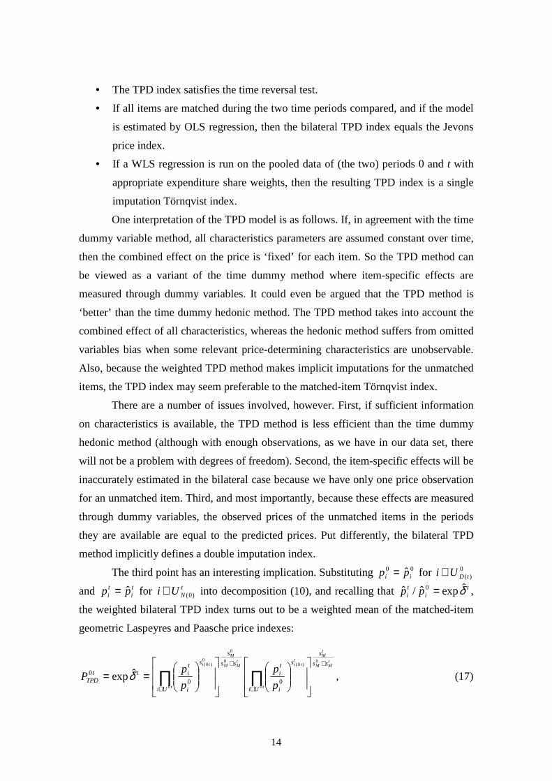
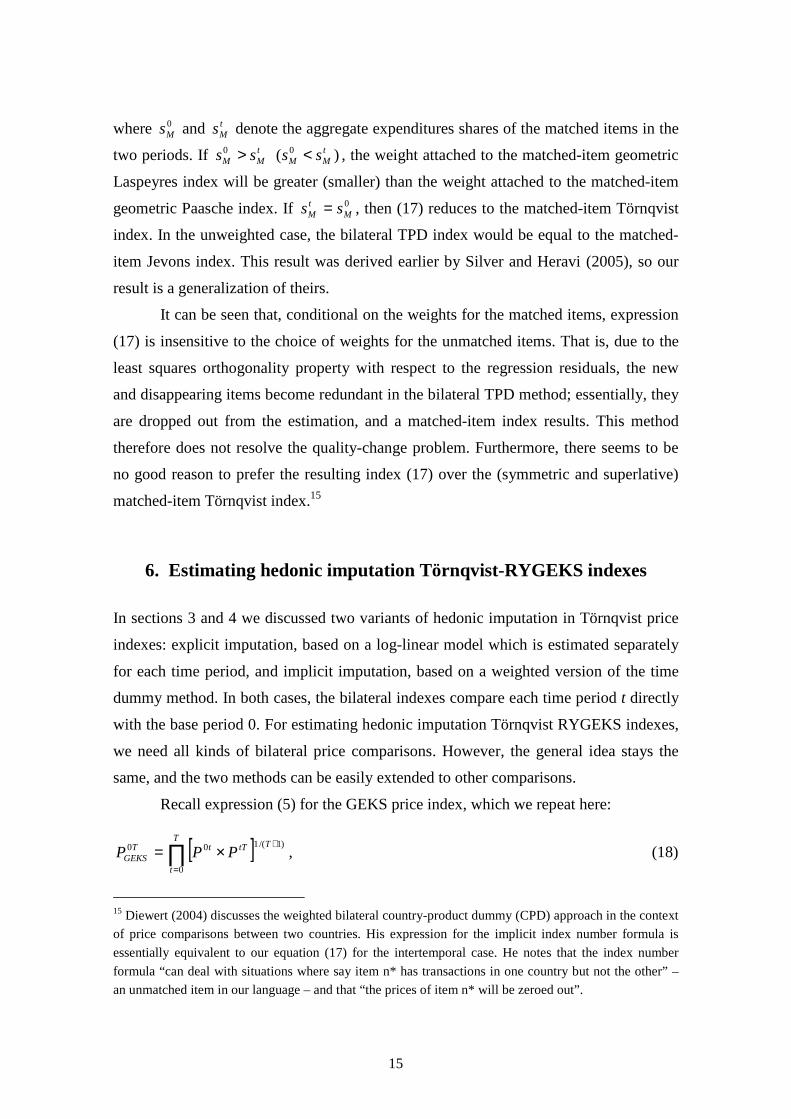
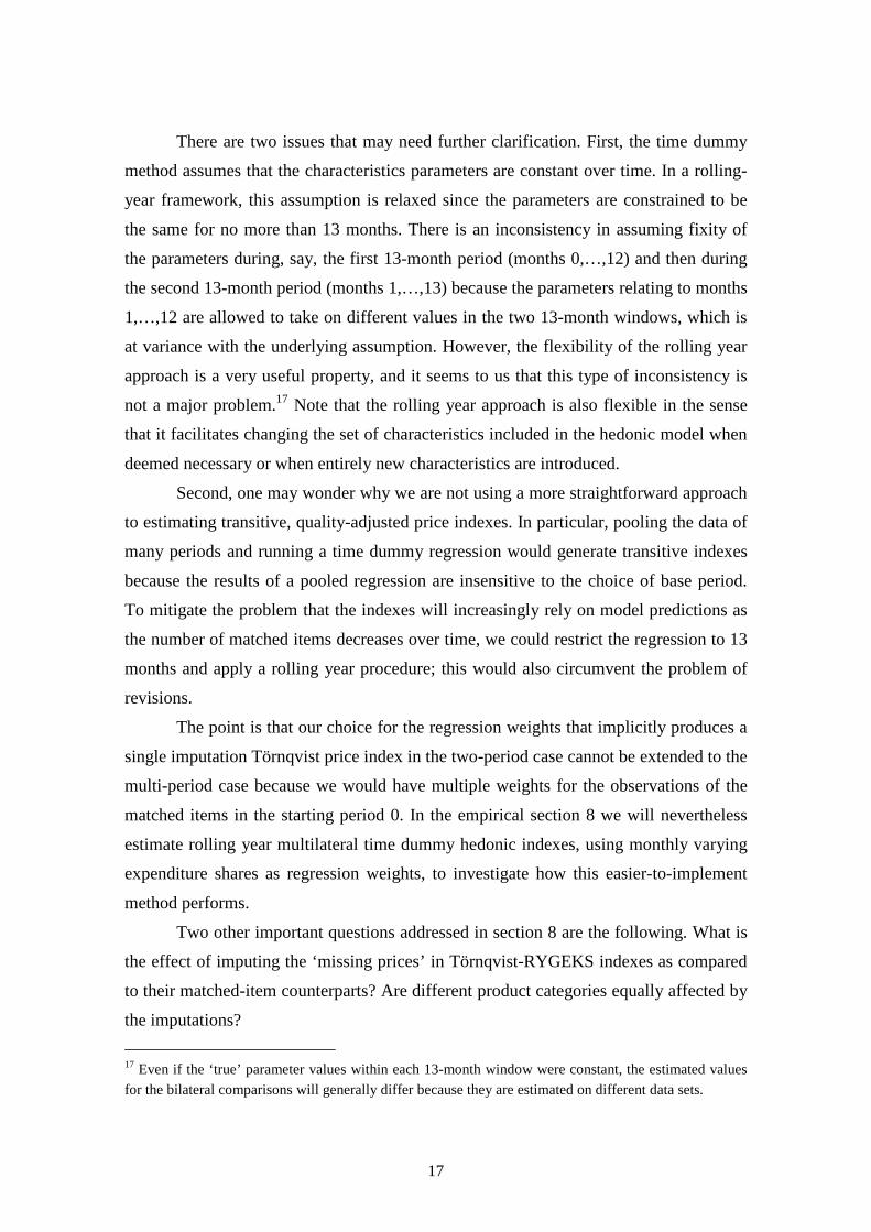
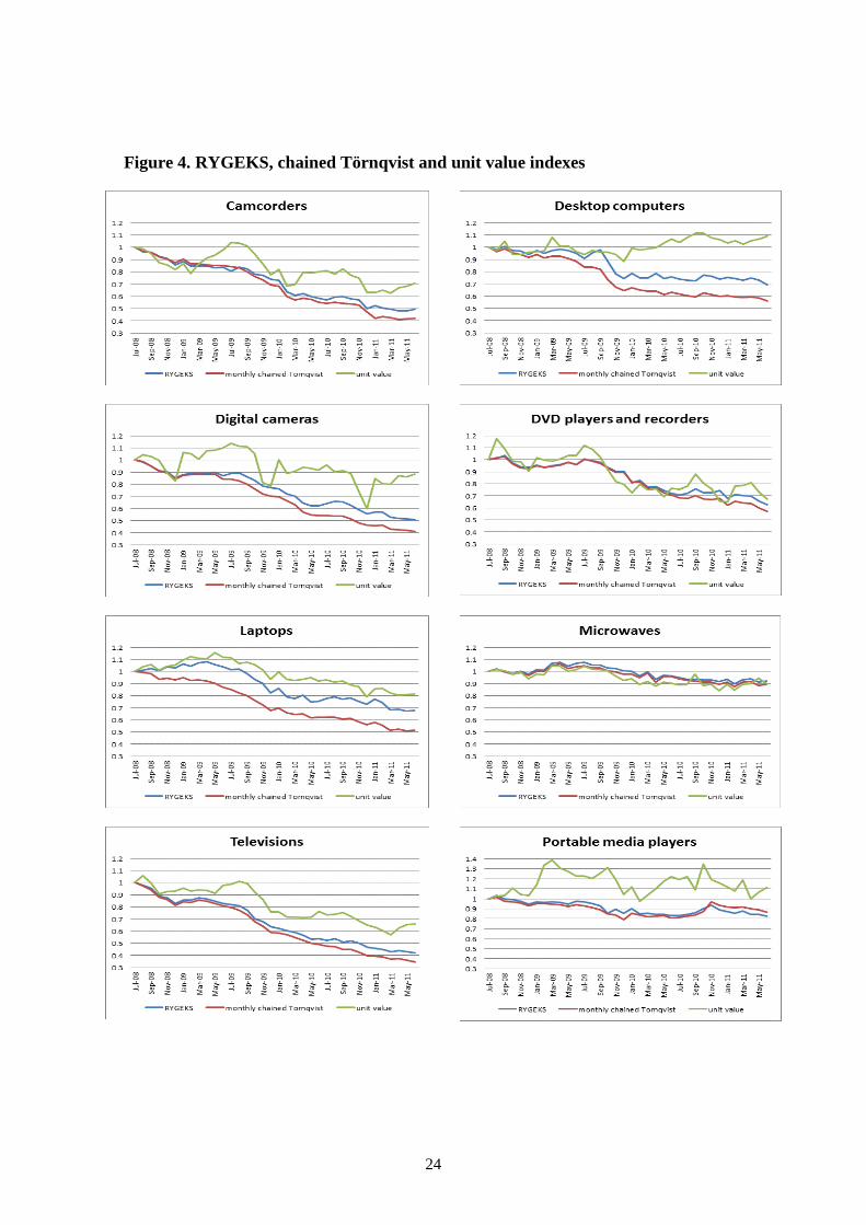
Figure 4. RYGEKS, chained Törnqvist and unit value indexes

25
Over the three year period the monthly-chained Törnqvist decreases faster than
the RYGEKS for all products except portable media players. We would expect the
RYGEKS and the monthly chained Törnqvist to suffer similarly from any bias due to
neglecting the price movements of new and disappearing items – i.e. bias due to
incorporating only matched items into the estimation – so it appears that the difference
between the monthly chained Törnqvist and the RYGEKS is evidence of downwards
chain drift in the monthly chained Törnqvist for most of these products.
Given the seasonal pattern in total quantities shown by figure 1 and the
seasonality of average prices at the product level, we would expect to see some chain
drift. It is reasonable to expect that, at particular seasons (such as Christmas) or during
sales, consumers are more likely to buy particular products, or particular specifications
of given products. However, consumers do not tend to stockpile, say, televisions during
sales in the way they stockpile bottles of soft drink or rolls of toilet paper. Therefore it
seems reasonable that the chain drift we find for consumer electronics is less significant
than the chain drift for supermarket products reported by others.
Quality change bias in the RYGEKS
The ITRYGEKS(TD) adjusts for quality change associated with new and disappearing
items by imputing their price movements based on time dummy hedonic models. Figure
5 compares this benchmark index with the RYGEKS, to determine whether there is
quality change bias in the RYGEKS for high-technology goods such as consumer
electronics. We also include results for the easier-to-implement RYTD.
As shown in figure 5, there is a significant upward quality-change bias in the
RYGEKS for computers (both desktops and laptops) and portable media players. To a
lesser extent, there is upward quality-change bias for camcorders and televisions. For
both microwaves and, surprisingly, digital cameras there is no evidence of quality-
change bias in the RYGEKS. The results for DVD players and recorders are interesting
– for this product the RYGEKS appears to be biased downwards, which would indicate
a net quality decrease due to new and disappearing items. This requires further
investigation.

26
Figure 5. RYGEKS, ITRYGEKS(TD) and RYTD

27
The easier-to-implement RYTD method gives very similar results to the
ITRYGEKS(TD) for computers (both desktops and laptops). For the other products the
results are mixed. RYTD gives similar results to ITRYGEKS(TD) for camcorders and
televisions, and sits between the RYGEKS and ITRYGEKS(TD) for portable media
players. For DVD players and recorders the RYTD actually appears to suffer from the
same level of quality-change bias as the RYGEKS, though it is less volatile. For digital
cameras, the RYTD sits below both the RYGEKS and the ITRYGEKS(TD), which
perhaps suggests that the quality effect of characteristics is changing at a faster rate than
the 13-month pooling window of the RYTD can reflect. Across all the products, though,
the RYTD is closer to the ITRYGEKS(TD) than the RYGEKS is.
When there are no characteristics available
In the absence of any, or sufficient, information on quality characteristics in the data25,
it is not possible to apply either the ITRYGEKS(TD) or the RYTD. The RYGEKS,
ITRYGEKS(TPD) and the RYTPD can all be applied in this situation by using the item
identifier itself as the ‘characteristic’ being controlled for in the regression models. In
section 5 we explained that the ITRYGEKS(TPD) effectively does no imputation for
new and disappearing items and will therefore give virtually the same result as the
RYGEKS - any differences will be due to changes in the expenditure share of the
matched items over time. Figure 6 compares both the RYGEKS and the
ITRYGEKS(TPD) to the benchmark ITRYGEKS(TD).
Silver and Heravi (2005) mention that the equivalence of the TPD method in the
two-period case to a matched-item index does not carry over to the case where there are
more than two periods, but “it can be seen that in the many-period case, the .... [TPD]
measures of price change will have a tendency to follow the chained matched-model
results.” In a preliminary version of their 2011 paper, Ivancic, Diewert and Fox (2009)
compared matched-item Fisher-GEKS and expenditure-share weighted multilateral TPD
indexes and found that these were very similar. So we would expect a rolling year
version of expenditure-share weighted TPD – i.e. the RYTPD, which is also included in
figure 6 – to also give similar results to the RYGEKS.
25 This will generally be the case with supermarket scanner data, which may separately include one or two
important characteristics, such as weight, but for which most descriptions of the item (i.e. the barcode)
will be stored in free-text fields. While there may be potential for parsing characteristics from these fields,
it is likely to be resource-intensive and product-specific.
28
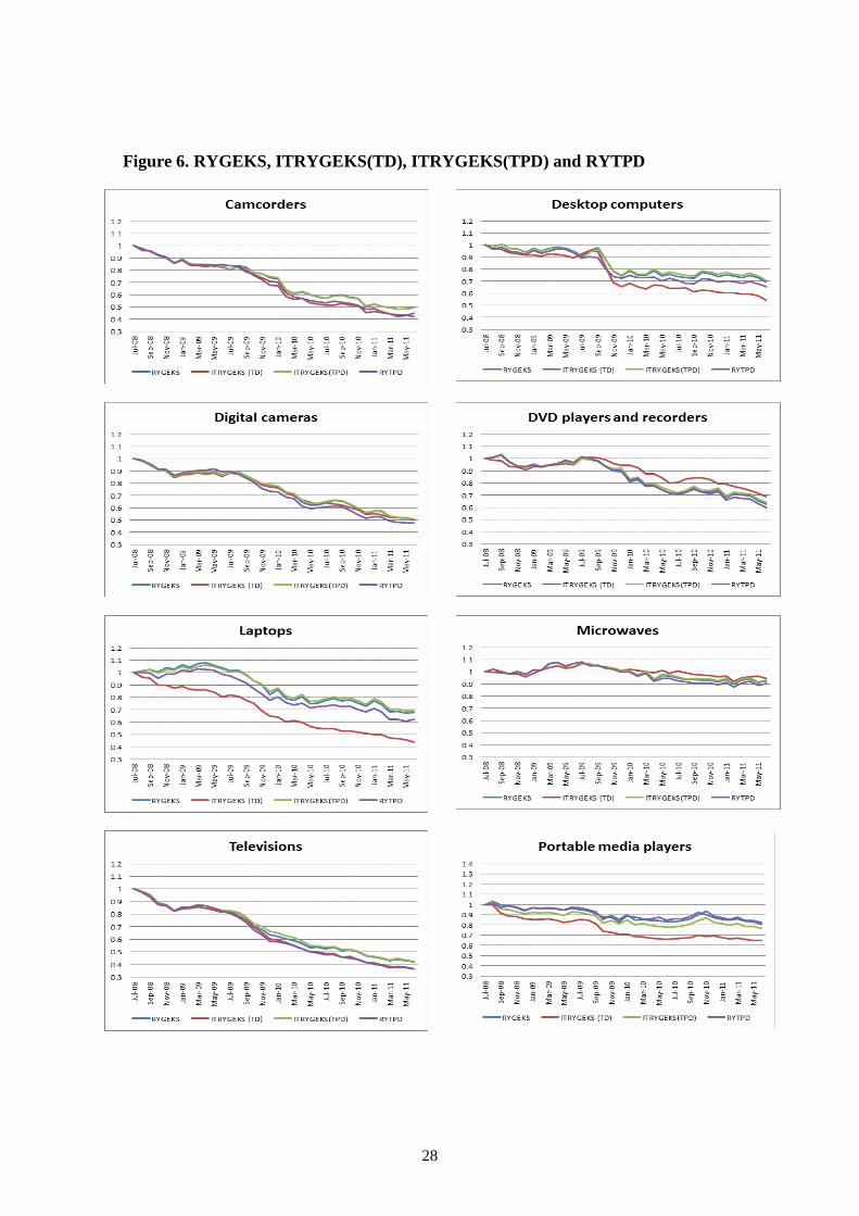
Figure 6. RYGEKS, ITRYGEKS(TD), ITRYGEKS(TPD) and R YTPD

29
As expected, the RYGEKS and the ITRYGEKS(TPD) are very similar, with the
exception of portable media players.26 But, to our surprise, the RYTPD generally sits in
between the RYGEKS and the ITRYGEKS(TD). This suggests that the RYTPD is less
biased by the quality change due to new and disappearing items than the RYGEKS is.
This calls for further research.
Volatility
For each product and method we calculated a volatility measure, which we define as the
average of the absolute monthly percentage changes. This is shown below in figure 7.
As we would expect, the index from the unit value is significantly more volatile than the
indexes produced using the other methods, for many of the products. In particular this
is the case for digital cameras and portable media players which, as shown in figures 1
and 4, have strong seasonality in their quantities sold and average prices.
Figure 7. Volatility of each method
26 Portable media players is often an exception to the patterns we see between these methods. This
requires further research but is likely to be a consequence of some very dominant items and/or sudden
shifts in expenditure weights. Perhaps, for portable media players, we are approaching some of the
extreme situations simulated by Ribe (2012) where the RYGEKS (and presumably, but perhaps to a lesser
extent, the ITRYGEKS) start to exhibit perverse behavior.

30
The ITRYGEKS(TD) and RYTD tend to be the least volatile of the methods
except for televisions – where the ITRYGEKS(TPD) is the least volatile and the
RYGEKS’ volatility lies between ITRYGEKS(TD) and RYTD; camcorders – where the
ITRYGEKS(TPD)’s volatility lies between that of the ITRYGEKS(TD) and the RYTD;
and desktop computers – where the volatility of the RYTPD and the monthly chained
Törnqvist lie between that of the RYTD and the ITRYGEKS(TD).
Aggregation across products
The different methods for calculating price indexes from the scanner data can give quite
different results at the product level. To see how these aggregate up the CPI hierarchy
we created a quasi ‘consumer electronics’ aggregate of the eight products, using the
monthly expenditures from the GfK data to weight together27 the individual products’
price indexes for each of the methods compared. This is shown below in figure 8.
Another important question is how a traditional CPI compares to our results
from scanner data at the aggregate consumer electronics level. We therefore include in
the comparison (using the same weighting as for the scanner data-derived indexes) the
price changes for the corresponding products from the New Zealand Consumers Prices
Index.28
Figure 8 shows that, at this aggregate level, the aggregation of existing New
Zealand CPI product-level indexes gives a result that is very similar to the RYGEKS.29
While these matched-item methods30 do not adjust for the quality change associated
with new and disappearing items, they do adjust for changes in quality mix of the
matched items. This component of the quality change is shown in the difference
between the unit value index and the RYGEKS, which indicates that, as we would
expect, the quality mix of matched items is improving over time.
27 Using upper level Törnqvist aggregation. Note that fixing the expenditure shares as at the start of the
three-year period – i.e. a Laspeyres-type approach – made virtually no difference. So there is no evidence
of substitution bias across these products.
28 Note that the New Zealand CPI is quarterly. The indexes shown in figure 9 are rebased to August 2008,
i.e. the middle of the third quarter.
29 And also the ITRYGEKS(TPD) which, as we have shown earlier, is equivalent to the RYGEKS except
for changes in the expenditure weight of the matched items.
30 The existing New Zealand CPI is approximately a matched-item approach in terms of what operational
practice is trying to achieve with replacement of items and manual quality adjustment.

31
Figure 8. Products aggregated to ‘consumer electronics’ for each method
The difference between the RYGEKS and the benchmark ITRYGEKS(TD)
shows that, at this aggregate level, the introduction and disappearance of items are
resulting in a further net quality improvement over time (and therefore a quality-
adjusted price decrease).
Surprisingly, the monthly chained Törnqvist index is very close to our
benchmark ITRYGEKS(TD) index. It appears that the mostly downward chain drift31 is
cancelling out against the upwards bias due to quality change of new and disappearing
items. We have seen evidence of chain drift at the product level, and we know that the
monthly chained Törnqvist will suffer from any quality change bias due to new and
disappearing items, so this result at the aggregate level should be seen as coincidental.
However it would be interesting to see whether these two biases cancel out so neatly for
other product groups.
31 Except for portable media players, for which the chain drift of the monthly chained Törnqvist is
upwards.
32
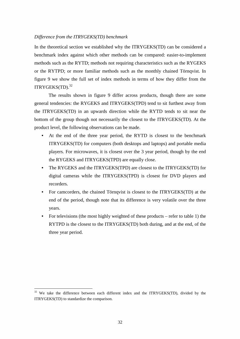
Difference from the ITRYGEKS(TD) benchmark
In the theoretical section we established why the ITRYGEKS(TD) can be considered a
benchmark index against which other methods can be compared: easier-to-implement
methods such as the RYTD; methods not requiring characteristics such as the RYGEKS
or the RYTPD; or more familiar methods such as the monthly chained Törnqvist. In
figure 9 we show the full set of index methods in terms of how they differ from the
ITRYGEKS(TD).32
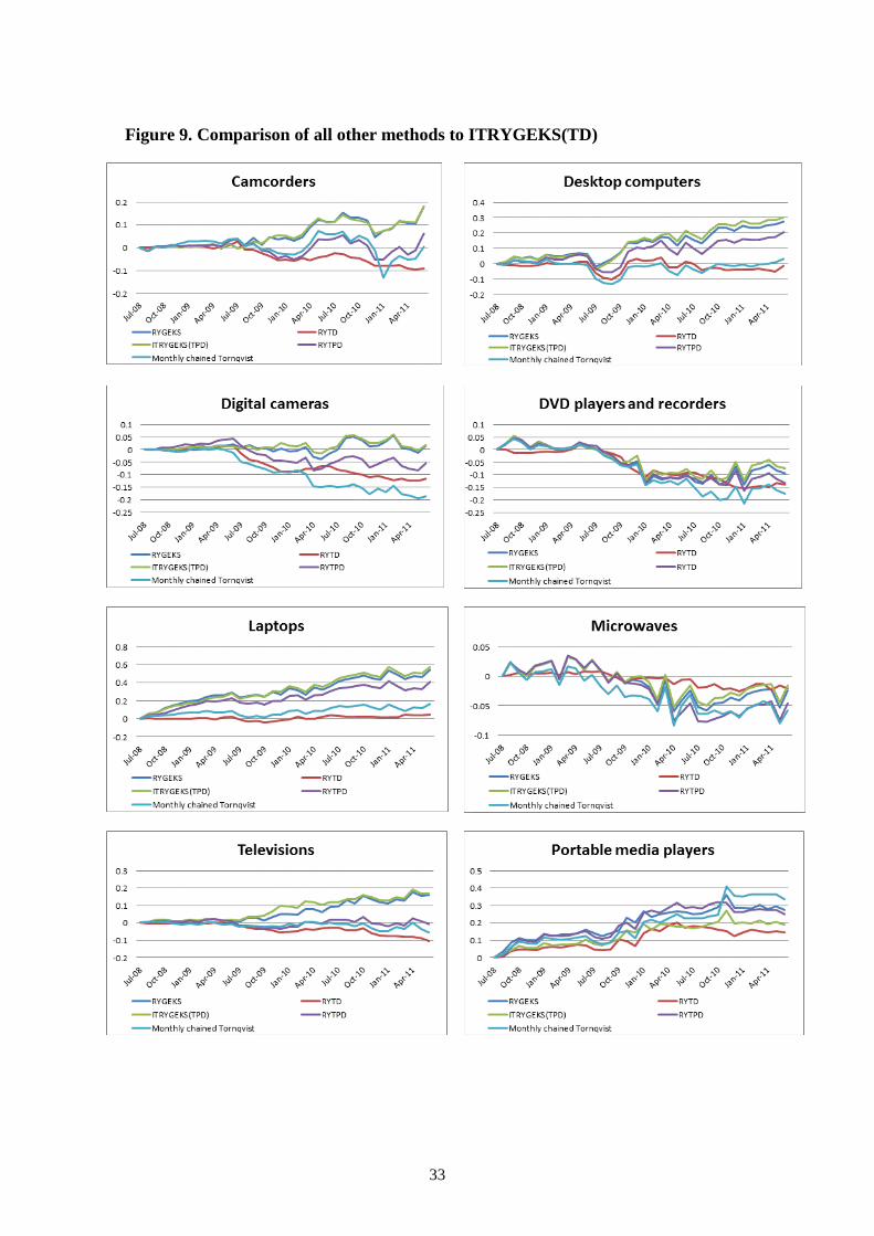
The results shown in figure 9 differ across products, though there are some
general tendencies: the RYGEKS and ITRYGEKS(TPD) tend to sit furthest away from
the ITRYGEKS(TD) in an upwards direction while the RYTD tends to sit near the
bottom of the group though not necessarily the closest to the ITRYGEKS(TD). At the
product level, the following observations can be made.
• At the end of the three year period, the RYTD is closest to the benchmark
ITRYGEKS(TD) for computers (both desktops and laptops) and portable media
players. For microwaves, it is closest over the 3 year period, though by the end
the RYGEKS and ITRYGEKS(TPD) are equally close.
• The RYGEKS and the ITRYGEKS(TPD) are closest to the ITRYGEKS(TD) for
digital cameras while the ITRYGEKS(TPD) is closest for DVD players and
recorders.
• For camcorders, the chained Törnqvist is closest to the ITRYGEKS(TD) at the
end of the period, though note that its difference is very volatile over the three
years.
• For televisions (the most highly weighted of these products – refer to table 1) the
RYTPD is the closest to the ITRYGEKS(TD) both during, and at the end, of the
three year period.
32 We take the difference between each different index and the ITRYGEKS(TD), divided by the
ITRYGEKS(TD) to standardize the comparison.
33
Figure 9. Comparison of all other methods to ITRYGEKS(TD)

34
We summarise the information in figure 9 to an ‘average difference from
ITRYGEKS(TD)’ by taking the geometric mean of the absolute of the (standardised)
differences between each index and the ITRYGEKS(TD). This is shown below in figure
10.
Figure 10. Average difference from ITRYGEKS(TD) for each method
Across the eight products, RYTD can arguably33 be said to perform the best. As
we might expect, the RYGEKS performs least well for the highest technology products,
desktop and laptop computers, and for portable media players, which have volatile
expenditure shares of matched items.34
The RYTPD performs better than the RYGEKS for all products except digital
cameras, DVD players and microwaves. It performs particularly well for televisions.
The monthly chained Törnqvist also performs well for televisions. Given that the
difference between the RYGEKS and the ITRYGEKS(TD) for televisions indicates that
there is quality-change bias due to new and disappearing items (which should exist
similarly for the matched-item chained monthly Törnqvist), this suggests that chain drift
and new goods bias are cancelling out to a certain extent at this product level in the
33 If we consider the products to be of equal weight in this assessment.
34 As shown in figure 7 by the large difference between RYGEKS and ITRYGEKS(TPD).

35
monthly chained Törnqvist, and given the very high expenditure weight of televisions
this is likely to be driving the cancelling out at the aggregate level shown earlier in
figure 8.
9. Conclusions
The Imputation Törnqvist (IT) RYGEKS method explicitly or implicitly imputes price
movements for new and disappearing items based on regression models. The paper
outlines three variants of the ITRYGEKS: explicit hedonic imputation, and implicit
imputation via either a weighted time dummy hedonic method or a weighted time-
product dummy method. We explain why, for the mainly categorical characteristics in
the consumer electronics scanner data, the use of the time dummy hedonic method – the
ITRYGEKS(TD) – is the appropriate method to estimate fully quality-adjusted price
indexes.
We confirm that the monthly chained Törnqvist is not a viable method for
consumer electronics, as it has downward chain-drift for most of the products examined,
with the exception of microwaves and portable media players.
The RYGEKS shows evidence of quality-change bias when compared to the
benchmark ITRYGEKS(TD), particularly for computers.
The easier-to-implement RYTD gives similar results to the ITRYGEKS(TD), in
particular for computers. Portable media players are an exception to this, presumably
because the 13 month windows of the RYTD smooth out the effect of volatility in the
expenditure shares of matched items for this product.35
In some cases, such as supermarket data, there will be few or no characteristics
available and so neither the ITRYGEKS(TD) nor the RYTD, which are both based on
time dummy hedonic models, will be feasible. Our results suggest that in this situation
the RYTPD does some adjustment for quality change and is therefore preferable to the
RYGEKS. Further empirical and theoretical work is required to fully understand this.
Aggregation of the eight products using their relative expenditure weights shows
that the current New Zealand Consumers Price Index gives results that are very similar
35 Though, arguably, this might be seen as a desirable characteristic of the RYTD in the case of volatile
expenditure shares.

36
to the matched-item RYGEKS. The RYTD and the monthly chained Törnqvist both
track the benchmark ITRYGEKS(TD) closely but in the case of the monthly chained
Törnqvist this appears to be a coincidental cancelling out of biases in two opposite
directions – chain drift and quality-change bias – for televisions, which have by far the
most significant weight of all the eight products.
Further work is required in two areas. First, the ITRYGEKS approach with
explicit imputation should be empirically tested with scanner data that has numeric
characteristics and/or categorical characteristics where no new categories appear or
disappear over the period investigated. Second, empirical and theoretical investigation
into the differences between the ITRYGEKS(TD) and the RYTPD can clarify whether
the latter is an effective method in situations where there is likely to be quality change
due to new and disappearing items but where no (or little) information on characteristics
is present in the data.
Appendix 1: Derivation of decomposition (10)
In this appendix we derive decomposition (10) of the single imputation Törnqvist index
(9). For convenience we write the index as
2
1
00000
0)0(
0)(
0
0
0
ˆ
ˆ
= ∏ ∏∏∏
∈ ∈∈∈t tN
ti
tD
i
t
tii
Ui Ui
s
i
ti
Ui
s
i
ti
Ui
s
i
ti
s
i
tit
SITp
p
p
p
p
p
p
pP , (A.1)
where 0ˆ ip and tip̂ are the imputed prices in periods 0 and t, and 0
is and tis are the
expenditure shares (with respect to the total set of items in periods 0 and t). As in the
main text, we will denote the expenditure shares with respect to the set tU 0 of matched
items in periods 0 and t by 0)0( tis and t
tis )0( ; 0)(tiDs and t
iNs )0( are the expenditure shares of
i with respect to the sets 0 )(tDU and tNU )0( of disappearing and new items; 0
)(tDs and tNs )0(
are the period 0 and t aggregate expenditure shares of the disappearing and new items; 0Ms and t
Ms are the period 0 and period t aggregate expenditure shares of the matched
items.
Since 00)0(
0Mtii sss = and t
Mt
titi sss )0(= for tUi 0∈ , 0
)(0
)(0
tDtiDi sss = for 0)(tDUi ∈ and
tN
tiN
ti sss )0()0(= for t
NUi )0(∈ , equation (A.1) can be written as

37
2
1
00000
)0(
)0()0(
0)(
0)(
0)(
0
)0(
0
00)0(
ˆ
ˆ
= ∏∏∏∏
∈∈∈∈ tN
tN
tiN
tD
tDtiD
t
tM
tti
t
Mti
Ui
ss
i
ti
Ui
ss
i
ti
Ui
ss
i
ti
Ui
ss
i
tit
SITp
p
p
p
p
p
p
pP
2
1
00
)1(
0
)1(
0
)0(
)0()0(
0)(
0)(
0)(
0
)0()0(
0
0)(
0)0(
ˆ
ˆ
= ∏∏∏∏
∈∈∈
−
∈
−
tN
tN
tiN
tD
tDtiD
t
tN
tti
t
tDti
Ui
ss
i
ti
Ui
ss
i
ti
Ui
ss
i
ti
Ui
ss
i
ti
p
p
p
p
p
p
p
p, (A.2)
using 00 1 DM ss −= and tN
tM ss −= 1 . Rearranging terms gives
2
1
0
0
2
1
0
02
1
000
0
)0()0(
)0(
)0()0(
0
0)(
0)0(
0)(
0)(
0)(
0
)0(
0
0)0( ˆ
ˆ
=
∏
∏
∏
∏∏∏
∈
∈
∈
∈
∈∈
t
tN
tti
tN
tN
tiN
t
tDti
tD
tDtiD
t
tti
t
ti
Ui
ss
i
ti
Ui
ss
i
ti
Ui
ss
i
ti
Ui
ss
i
ti
Ui
s
i
ti
Ui
s
i
tit
SIT
p
p
p
p
p
p
p
p
p
p
p
pP
2
0
0
2
0
02
0
)0(
0
)0(
)0(
)0(
0)(
0
0)0(
0)(
0)(
0
)0(0
)0(
ˆ
ˆ
tN
t
tti
tN
tiN
tD
t
ti
tiD
tD
t
ttiti
s
Ui
s
i
ti
Ui
s
i
ti
s
Ui
s
i
ti
s
Ui i
ti
Ui
ss
i
ti
p
p
p
p
p
p
p
p
p
p
=
∏
∏
∏
∏∏
∈
∈
∈
∈
∈
+
, (A.3)
which is equation (18) in the main text.
Appendix 2: Derivation of equation (14)
Following de Haan (2004), in this appendix we derive expression (14) for the bilateral
time dummy hedonic index. Because an intercept term is included in model (13), the
weighted sum of the regression residuals )ˆ/ln()ˆln()ln( ti
ti
ti
ti
ti ppppe =−= is equal to 0
in each period, hence
0ˆ
ln)ˆ/ln( =
=∑ ∏∈
∈t
t
ti
UiUi
w
ti
tit
iti
ti
p
pppw ; Tt ,...,0= , (A.4)
where tiw denotes the weight for item i in period t in a WLS regression. If we separate
the base period 0 from the comparison periods t, the second expression of (A.4) can be
written as

38
0ˆ
lnˆ
ln0
0
0
0
=
=
∏∏∈∈ t
tii
Ui
w
ti
ti
Ui
w
i
i
p
p
p
p; Tt ,...,1= . (A.5)
Exponentiating (A.5) yields the following relation:
∏ ∏∈ ∈
=
=
0
0
1ˆˆ 0
0
Ui Ui
w
ti
ti
w
i
i
t
tii
p
p
p
p; Tt ,...,1= . (A.6)
Next, we rewrite (A.6) as
∏ ∏ ∏∏∈ ∈ ∈∈
=
=
t t tN
ti
ti
tD
ii
Ui Ui Ui
w
ti
ti
w
ti
ti
Ui
w
i
i
w
i
i
p
p
p
p
p
p
p
p
0 0)0(
0)(
00
)1(ˆˆˆˆ 0
0
0
0
, (A.7)
where, as before, tU 0 denotes the set of matched items (with respect to periods 0 and t), 0
)(tDU is the set of disappearing items, and tNU )0( is the set of new items.
We now assume that the regression weights for the matched items are the same
in periods 0 and t, i.e., ti
tii www 00 == for tUi 0∈ . In that case, multiplying the right and
left hand side of equation (A.7) by ∏ ∈ t
ti
Ui
wi
ti pp0
0
)/ˆ( 0 gives
∏ ∏ ∏∏∈ ∈ ∈∈
=
t t tN
ti
ti
tD
it
i
Ui Ui Ui
w
ti
ti
w
i
ti
Ui
w
i
i
w
i
ti
p
p
p
p
p
p
p
p
0 0)0(
0
0)(
00
ˆˆˆ
ˆ00
0
0. (A.8)
Multiplying both sides of (A.8) by ∏ ∈ 0)(
0
)/ˆ( 0
tD
i
Ui
wi
ti pp yields
∏ ∏ ∏∏∏∈ ∈ ∈∈∈
=
t t tN
ti
tD
it
i
tD
it
i
Ui Ui Ui
w
ti
ti
Ui
w
i
ti
w
i
ti
Ui
w
i
ti
w
i
ti
p
p
p
p
p
p
p
p
p
p
0 0)0(
0)(
00
0)(
00
ˆ
ˆ
ˆ
ˆ
ˆ
ˆ0000
. (A.9)
Next, multiplying both sides of (A.9) by ∏ ∈ tN
ti
Ui
wi
ti pp
)0()ˆ/ˆ( 0 gives
∏ ∏ ∏∏∏∏∈ ∈ ∈∈∈∈
=
t t tN
ti
tD
it
i
tN
ti
tD
it
i
Ui Ui Ui
w
i
ti
Ui
w
i
ti
w
i
ti
Ui
w
i
ti
Ui
w
i
ti
w
i
ti
p
p
p
p
p
p
p
p
p
p
p
p
0 0)0(
0)(
00
)0(0
)(
00
000000 ˆ
ˆ
ˆ
ˆ
ˆ
ˆ
ˆ
ˆ. (A.10)
Using ti
ti pp δ̂expˆ/ˆ 0 = for all i, equation (A.10) can be written as
[ ] ∏∏∏∈∈∈
++
=
tN
ti
tD
i
t
ti
tNtD
t
Ui
w
i
ti
Ui
w
i
ti
Ui
w
i
tiwwwt
p
p
p
p
p
p
)0(0
)(
0
0
0
)0(0
)(0
000 ˆ
ˆˆexpδ , (A.11)
where ∑ ∈= tUi
ti
t ww 0
00 , ∑ ∈= 0
)(
00)(
tDUi itD ww and ∑ ∈= t
NUi
ti
tN ww
)0()0( . It follows that

39
tNtD
t
tN
ti
tD
i
t
ti www
Ui
w
i
ti
Ui
w
i
ti
Ui
w
i
tit
TDt
p
p
p
p
p
pP
)0(0
)(0
)0(0
)(
0
0
01
0000
ˆ
ˆˆexp++
∈∈∈
== ∏∏∏δ , (A.12)
which is equation (14) in the main text.
Appendix 3: Characteristics available for each product
Camcorders Desktop computers Digital Cameras DVD players and recordersCharacteristic Levels Characteristic Levels Characteristic Levels Characteristic Levels
16:9 REC#FORMAT 2 3D 3 ANZ CAMERA TYPE 3 1080P UPSCALING 33 CHIP 2 APPLE OS 3 AUTOFOCUS 2 3D CONVERSION 2BRAND 6 ASPECT RATIO 3 AVCHD / LITE 4 APP STORE(IPTV) 3CF CARD 3 BLUETOOTH 2 BATTERY TYPE 3 BD LIVE 2CHIPTYPE 2 BRAND 9 BAYONET MOUNT 7 BRAND 13DIGITAL INDEX 2 BRIGHTNESS 2 BLUETOOTH 3 CF CARD 3DIGITAL INPUT 2 CHIPSET BRAND 5 BRAND 15 COMMON INTER CI 3DSC CAMC RES# 3 CHIPSET TYPE 43 BRIDGE CAMERA 2 CONSUMP STANDBY 29HANDHELD POSIT# 2 CSP-MHZ 27 CHIPTYPE 5 CONSUMPTION W 43HD Formats 5 DEPTH IN CM 6 COMPACT FLASH 2 DIVX 2HDD CAPACITY 8 DESIGN 4 DEPTH IN MM 182 DLNA 2HDMI 3 DVD WRITER 4 DIGITAL ZOOM 12 DTS DECODER 4IEEE-1394 2 GPU BRAND 5 DISPL#RES# PIX# 30 DVB-T 3IMAGE STABIL# 3 GPU MODEL 66 DSC CAMC RES# 4 DVD AUDIO 3IMAGE STABILIZ# 4 HEIGHT IN CM 6 DUAL CAM 4 DVD Categories 10LCD SCREEN SIZE 8 LED 3 EFFECTIVE PIXEL 50 DVD REC# FORMAT 9MEMORY CAPACITY 15 MC-EDITION 2 FACE DETECTION 4 EPG 3MEMORY CARD 2 MEMORY TECHNO 3 FOLDABLE LCD 3 GOOGLE TV 2MEMORY STICK 3 MICROSOFT OS 10 FRAMES PER SEC 12 HDD CAPACITY 10MODEL 78 MODEL 82 GPS 2 HDMI 2MPEG STANDARD 3 NUMBER OF CORES 5 HDMI PORT 2 HDTV 3MULTIMEDIA CARD 3 OFFICE SUITE 2 HEIGHT IN MM 144 LAYER 3OPTICAL ZOOM 21 ONBOARD GRAPHIC 3 IMAGE STABIL# 3 LCD SCREEN SIZE 10OUTDOOR FUNCTIO 3 PLATFORM 2 INNER ZOOM 4 MEDIAPLAYER 4P2 2 PROCESSOR 23 KID CAMERA 3 MEMORY CARD 2PIXEL TOTAL 38 PROCESSOR NUMBE 91 LCD MONITOR SIZ 15 MEMORY STICK 3RESOLUTION 3 RAM-MB 9 LIVE VIEW 2 MODEL 105SD CARD 3 REMOTE-CONTROL 2 MAX VIDEO HT RE 10 MP3 ENCODING 2SD Format 7 SCREEN SIZE 2 MAX VIDEO WI RE 12 MP3 PLAYBACK 3SD/HD Format 10 SECURITY SW 2 MAX# ISO SENSIT 15 MPEG-4 RECORD# 2SMART MEDIA 2 SIZE/INCH 9 MEMORY TYPE 4 NO# OF DISC 3TOUCHSCREEN 3 STORAGE CAPAC# 13 MICRO DRIVE 2 PC STREAMING 3TYPE 2 TV OUT 2 MODEL 211 REAL DOLBY DEC# 6Type Memory Cards 7 VIDEOCARD 2 Multiple Slots 3 SD CARD 3USB CONNECTION 2 Vision 3 OPTICAL ZOOM 16 SUPER AUDIO CD 3VIDEO FORMAT 8 V-RAM 12 OUTDOOR FUNCTIO 5 USB RECORDING 3VIDEOTO MC 3 WEIGHT IN KG 5 PHOTOS PER SEC# 55 WEB CONTENT ACC 3VIEWFINDER 3 PICTBRIDGE 2 WIRELESS INTERF 3WEIGHT IN GRAM 62WIRELESS INTERF 2XD-PICTURE CARD 3

40
Laptop computers Microwaves Televisions Portable media playersCharacteristic Levels Characteristic Levels Characteristic Levels Characteristic Levels
3G/BB BUNDLE 2 ARTICLE FLAG 3 3D 2 AIRPLAY 2APPLE OS 4 BRAND 14 3D CONVERSION 2 BLUETOOTH 3ASPECT RATIO 4 CAVITY MATERIAL 6 BRAND 14 BRAND 13BLUETOOTH 3 CONSTR#2 2 BRIGHTNESS 20 BUILT IN CAMERA 3BRAND 13 CONSTRUCTION 3 CONSUMP STANDBY28 CE FUSION REPORTING5BRIGHTNESS 3 COOKING PLATE 4 CONSUMPTION W 128 CF CARD 3CE FUSION REPORTING2 COOKINGFUNCTION 4 CONTRAST RATIO 50 COLOUR DISPLAY 2CENTRINO 2 DEPTH IN CM 34 DISPLAY HD DC 3 DAB 2CHIPSET BRAND 5 DETAILED MAIN TYPES7 DIVX 3 Dictation Machine total 2CHIPSET TYPE 52 DIGITAL CLOCK 4 DLNA 3 DIGITAL SPEECH 2DVD WRITER 4 DOOR OPENING S# 4 DVB-C 3 DIGITAL SYSTEM 2FINGERPRINT-ID 2 DOOR TYPE 3 DVB-S 2 DISPLAY-TECHNO 6FORM FACTOR 7 FRONT DECORAT# 8 DVB-T 3 DIVX 3GPU BRAND 3 GROUPS AFFILIATION 7 DVD PLAYER/REC# 2 DRM 5GPU MODEL 88 HEIGHT 40 ENERGY STAR AU# 11 GAMING 3HARD DRIVE TYPE 2 HUMIDITY SENSOR 3 FRAME REFRESH 9 H264 PLAYBACK 3HEIGHT IN CM 116 INFRARED SENSOR 3 FREQUENCY 4 MEMORY CARD 3HYPER THREADING 2 INVERTER 3 HD READY 3 MEMORY STICK 2LED 2 KEYFEATURES 3 HD Types 3 MODEL 75LED TECHNOLOGY 2 LIMIT_HOURS 3 HDD CAPACITY 3 MODELTEXT 209MC-EDITION 2 LIMIT_MINUTES 5 ISDB-T 3 MP3 ENCODING 3MEMORY TECHNO 3 MAIN TYPES - IL- 4 LED TECHNOLOGY 4 MPEG 2 3MICROSOFT OS 15 MODEL 88 MEDIAPLAYER 4 MPEG 4 3MODEL 278 MODELTEXT 187 MODEL 245 MULTIMEDIA CARD 3Next Gen Core 25 NUMBER OF TRAYS 3 NO OF HDMI 6 OPERATING SYST# 4OFFICE SUITE 5 POWERSTEPS 10 PC STREAMING 4 PC CONNECTION 3ONBOARD GRAPHIC 3 PROGRAMMER 4 REFLECTION ANGL 12 PHOTO VIEWER 2PROCESSOR NUMBE 124 QUARTZ GRILL 4 RESOLUTION HIG# 9 RADIO BUILT-IN 2REMOTE-CONTROL 2 SKEWER 3 RESOLUTION WID# 11 SD CARD 3SCREEN SIZE 5 STEAM FUNCT#INT 4 RESPONSE TIME 18 SIZE/INCH 21TRUE RESOLUTION 11 THERMO SENSOR 4 SCREEN FORMAT 3 STOR# CAPACITY 20TV CARD 3 TIME CONTROL 3 SD CARD 3 TOUCHSCREEN 3TV OUT 2 TOUCH CONTROL 3 SIZE/CM 38 TV OUT 3USB PORTS 5 TURNTABLE 3 SIZE/INCH 26 VIDEORECORD 3V-RAM 7 TYPE OF MICROW# 6 TELE-TEXT 3 WEIGHT IN GRAM 70WIMAX 2 VOLUME LTRS 20 USB 3 XHTML BROWSER 3WIRELESS LAN 2 WATTAGE 11 USB RECORDING 3
WEIGHT SENSOR 3 WIFI 4WIDTH IN CM 42WITH FAN/CONVEC 2WITH GRILL 2WITH TOP/BOTTOM 2YEAR OF INTRO 6
Appendix 4: Regression modelling
The approach taken to the modelling of time dummy hedonic models – on both the
bilateral pooled data for the ITRYGEKS(TD) and the rolling 13-month windows of
pooled data for the RYTD – was to include all the characteristics we had available in the
data. We are ultimately interested in methods that can be incorporated into production
with as little manual intervention as possible.36 36 This goes in particular for Statistics New Zealand, where the plan is to put scanner data into production
for the Consumers Price Index for consumer electronics, and then supermarkets, in the near future.

41
All the characteristics, including the few numeric characteristics were modelled as
categorical, so we are not imposing any parametric form on the numeric characteristics.
Given the quantity of data, we do not need to worry about degrees of freedom.
Table 2 below summarises the adjusted R-squares for the regression models.37
Note that, because we are using monthly averages of prices (unit values), the R-squares
are significantly higher than if we were applying the same models to the underlying
prices. What this means is that it is not valid to compare these fit estimates to models on
actual prices or higher-frequency averages, for example weekly averages.
Table 2. Average38 adjusted R-squares
ITRYGEKS(TD) RYTD RYTPD
Camcorders 0.970 0.972 0.933
Desktop computers 0.979 0.983 0.969
Digital cameras 0.983 0.988 0.974
DVD players and recorders 0.973 0.977 0.980
Laptop computers 0.980 0.980 0.950
Microwaves 0.982 0.987 0.980
Televisions 0.988 0.989 0.979
Portable media players 0.988 0.991 0.990
37 We do not include results for the ITRYGEKS(TPD) because the relative goodness of fit compared to
the ITRYGEKS(TD) can be approximately inferred by comparing the RYTD and the RYTPD, and also
because it is not a viable method for quality adjusting this data.
38 The ITRYGEKS(TD) incorporates 630 regressions for each product, corresponding to all the distinct
pairs of months within the three year period. The rolling year methods – both the RYTD and the RYTPD
– are each based on 24 regressions for each product, corresponding to each of the 13-month rolling
windows over the three year period.

42
References
Aizcorbe, A., C. Corrado and M. Doms (2003), When Do Matched-Model and Hedonic Techniques Yield Similar Price Measures?, Working Paper no. 2003-14, Federal Reserve Bank of San Francisco.
Balk, B.M. (1981), A Simple Method for Constructing Price Indices for Seasonal Commodities, Statistische Hefte 22, 1-8.
Balk, B.M. (2001), Aggregation Methods in International Comparisons: What Have We Learned? ERIM Report, Erasmus Research Institute of Management, Erasmus University Rotterdam.
Balk, B.M. (1981), A Simple Method for Constructing Price Indices for Seasonal Commodities, Statistische Hefte 22, 1-8.
Caves, D.W., L.R. Christensen and W.E. Diewert (1982), Multilateral Comparisons of Output, Input and Productivity Using Superlative Index Numbers, The Economic Journal 92, 73-86.
Destatis (2009), Handbook on the Application of Quality Adjustment Methods in the Harmonised Index of Consumer Prices, Statistics and Science, Vol. 13. Federal Statistical Office of Germany, Wiesbaden.
Diewert, W.E. (1999), Axiomatic and Economic Approaches to International Comparisons, pp. 13-87 in A. Heston and R.E. Lipsey (eds.), International and Interarea Comparisons of Income, Output and Prices, Studies in Income and wealth, Vol. 61. University of Chicago Press, Chicago.
Diewert, W.E. (2003), Hedonic Regressions: A Review of Some Unresolved Issues, Paper presented at the Seventh Meeting of the International Working Group on Price Indices (Ottawa Group), 27-29 May 2003, INSEE, Paris.
Diewert, W.E. (2004), On the Stochastic Approach to Linking the Regions in the ICP, Discussion Paper no. 04-16, Department of Economics, The University of British Columbia, Vancouver, Canada.
Diewert, W.E., S. Heravi and M. Silver (2009), Hedonic Imputation versus Time Dummy Hedonic Indexes, pp. 87-116 in W.E. Diewert, J. Greenlees and C. Hulten (eds.), Price Index Concepts and Mesurement, Studies in Income and Wealth, Vol. 70. University of Chicago Press, Chicago.
Eltetö, O. and P. Köves (1964), On a Problem of Index Number Computation Relating to International Comparisons, Statisztikai Szemle 42, 507-518 (in Hungarian).
Eurostat and OECD (2006), Methodological manual on PPPs. Available at www.oecd.org/std/pricesandpurchasingpowerparitiesppp.

43
Feenstra, R.C. and M.D. Shapiro (2003), High Frequency Substitution and the Measurement of Price Indexes, pp. 123-146 in R.C. Feenstra and M.D. Shapiro (eds.), Scanner Data and Price Indexes, Studies in Income and Wealth, Vol. 61. University of Chicago Press, Chicago.
Gini, C. (1931), On the Circular Test of Index Numbers, Metron 9, 3-24.
Greenlees, J. and R. McClelland (2010), Superlative and Regression-Based Consumer Price Indexes for Apparel Using U.S. Scanner Data, Paper presented at the Conference of the International Association for Research in Income and Wealth, St. Gallen, Switzerland, August 27, 2010.
van der Grient, H.A. and J. de Haan (2010), The Use of Supermarket Scanner Data in the Dutch CPI, Paper presented at the Joint ECE/ILO Workshop on Scanner Data, 10 May 2010, Geneva. Available at www.cbs.nl.
van der Grient, H.A. and J. de Haan (2011), Scanner Data Price Indexes: The ’Dutch Method’ versus RYGEKS, Paper presented at the Twelfth Meeting of the International Working Group on Price Indices (Ottawa Group), 4-6 May 2011, Wellington, New Zealand.
de Haan, J. (2004), The Time Dummy Index as a Special Case of the Imputation Törnqvist Index, Paper presented at the Eighth Meeting of the International Working Group on Price Indices (Ottawa Group), 23-25 August 2004, Helsinki, Finland.
de Haan, J. (2010), Hedonic Price Indexes: A Comparison of Imputation, Time Dummy and ‘Re-pricing’ Methods, Journal of Economics and Statistics (Jahrbücher fur Nationalökonomie und Statistik) 230, 772-791.
de Haan, J. and H.A. van der Grient (2011), Eliminating Chain drift in Price Indexes Based on Scanner Data, Journal of Econometrics, Vol. 161, Issue 1, 36-46.
Hill, R.J. and D. Melser (2008), Hedonic Imputation and the Price Index Problem: An Application to Housing, Economic Inquiry 46, 593-609.
ILO/IMF/OECD/UNECE/Eurostat/The World Bank (2004), Consumer Price Index Manual: Theory and Practice. ILO Publications, Geneva.
Ivancic, L., W.E. Diewert and K.J. Fox (2009), Scanner Data, Time Aggregation and the Construction of Price Indexes, Discussion Paper 09-09, Department of Economics, University of British Columbia, Vancouver, Canada.
Ivancic, L., W.E. Diewert and K.J. Fox (2011), Scanner Data, Time Aggregation and the Construction of Price Indexes, Journal of Econometrics, Vol. 161, Issue 1, 24-35.
Johansen, I. and R. Nygaard (2011), Dealing with Bias in the Norwegian Superlative Price Index of Food and Non-alcoholic Beverages, Room document at the twelfth

44
meeting of the International Working Group on Price Indices (Ottawa Group), 4-6 May 2011, Wellington, New Zealand.
Kokoski, M.F., Moulton, B.R. and K.D. Zieschang (1999), Interarea Price Comparisons for Heterogeneous Goods and Several Levels of Commodity Aggregation, pp. 123-169 in A. Heston and R.E. Lipsey (eds.), International and Interarea Comparisons of Income, Output and Prices, Studies in Income and Wealth, Vol. 61. University of Chicago Press, Chicago.
Krsinich, F. (2011), Price Indexes from Scanner Data: A Comparison of Different Methods, Paper presented at the twelfth meeting of the International Working Group on Price Indices (Ottawa Group), 4-6 May 2011, Wellington, New Zealand.
Krsinich, F. (2012), A Fresh Look at Patterns in Gadget Sales. Economic News, Statistics New Zealand, April 2012.
Ribe, M. (2012), Some Properties of the RGEKS Index for Scanner Data, Paper presented at Statistics Sweden’s scanner data workshop, 7-8 June 2012, Stockholm, Sweden.
Silver, M. (2003), The Use of Weights in Hedonic Regressions: The Measurement of Quality-Adjusted Price Changes, pp. 135-147 in Th. Lacroix (ed.), Proceedings of the Seventh Meeting of the Ottawa Group. INSEE, Paris.
Silver, M. and S. Heravi (2005), A Failure in the Measurement of Inflation: Results from a Hedonic and Matched Experiment Using Scanner Data, Journal of Business & Economic Statistics 23, 269-281.
Silver, M. and S. Heravi (2007), The Difference Between Hedonic Imputation Indexes and Time Dummy Hedonic Indexes, Journal of Business & Economic Statistics 25, 239-246.
Summers, R. (1973), International Price Comparisons Based Upon Incomplete Data, Review of Income and Wealth 19, 1-16.
Syed, I. (2010), Consistency of Hedonic Price Indexes in the Presence of Unobserved Characteristics, Discussion Paper, School of Economics, University of New South Wales, Sydney, Australia.
Szulc, B. (1964), Indices for Multiregional Comparisons, Przeglad Statystycny 3, 239-254 (in Polish).
Triplett, J.E. (2006), Handbook on Hedonic Indexes and Quality Adjustments in Price Indexes. Organization for Economic Co-operation and Development, Paris.