SCENE CHANGE DETECTION METHOD

FOR MPEG VIDEO

WAN FAHIMI BIN WAN MOHAMED

UNIVERSITI TEKNOLOGI MALAYSIA

“I hereby declare that I have read this dissertation and in my

opinion this dissertation is sufficient in terms of scope and quality for the

award of the degree of Master of Engineering (Electrical – Electronic &

Telecommunication)”

Signature : ……………………………………

Name of Supervisor : Profesor Madya Muhammad Mun’im Bin

Ahmad Zabidi

Date : 3 April 2004

BAHAGIAN A – Pengesahan Kerjasama*

Adalah disahkan bahawa projek penyelidikan tesis ini telah dilaksanakan melalui

kerjasama antara _______________________ dengan ________________________

Disahkan oleh:

Tandatangan : ……………………………………......... Tarikh : ..........................

Nama : ………………………………………….

Jawatan : ………………………………………….

(Cop rasmi)

* Jika penyelidikan tesis/projek melibatkan kerjasama.

BAHAGIAN B – Untuk Kegunaan Pejabat Sekolah Pengajian Siswazah

Tesis ini telah diperiksa dan diakui oleh:

Nama dan Alamat Pemeriksa Luar: …………………………………………………

…………………………………………………

…………………………………………………

Nama dan Alamat Pemeriksa Dalam: …………………………………………………

…………………………………………………

…………………………………………………

Nama Penyelia Lain (jika ada): …………………………………………………

…………………………………………………

…………………………………………………

Disahkan oleh Penolong Pendaftar di SPS:

Tandatangan : ……………………………………......... Tarikh : ..........................

Nama : ………………………………………….

SCENE CHANGE DETECTION METHOD

FOR MPEG VIDEO

WAN FAHIMI BIN WAN MOHAMED

A dissertation submitted in fulfillment of the

requirements for the award of the degree of

Master of Engineering (Electrical – Electronic & Telecommunication)

Faculty of Electrical Engineering

Universiti Teknologi Malaysia

APRIL, 2005

ii

I declare that this dissertation entitled “Scene Change Detection Method for MPEG

Video” is the result of my own research except as cited in the references. The

dissertation has not been accepted for any degree and is not concurrently submitted

in candidature of any other degree.

Signature : ……………………………………

Name : Wan Fahimi Bin Wan Mohamed

Date : 3rd April 2005

iii

������������������

To my beloved mother and father

iv

ACKNOWLEDGEMENT

I would like to thank these people:

1. PM Muhammad Mun`im as my supervisor for all the guidance

and assistance.

2. Dr. Ahmad Zuri and Dr. Mohamad Kamal as course coordinator.

3. My classmates, especially Mr. Muslim and wife, Mrs. Hidayati.

4. My bosses, which very understanding.

and to all family, friends and professors who support me in completing this

research.

Thank you!

v

ABSTRACT

Indexing and editing large quantities of video material is becoming an

increasing problem today, especially when video acquire technology made video

archiving easy. Manually indexing video content is currently the most accurate

method but it is a very time consuming process. An efficient video indexing

technique is to temporally segment a sequence into shots. A shot is defined as a

sequence of frames captured from a single camera operation. A small subset of

frames can be used to retrieve information from the video and enable content-based

video browsing. To minimize the cost of time for video indexing and editing,

automated shot cut (scene change) detection is used. This paper will introduce two

types of scene change detection method based on frame by frame comparison. Both

methods apply for MPEG-1 video stream. First approach will use the nature of edge

continuity within video. Second approach uses grayscale level of extracted frames

from MPEG video stream. Both techniques use image processing tools for frames

analysis and comparison. Scene change decision is made with the reference of

several image processing operation and the threshold value. The performance of

detection will be evaluated on detection precision and false alarm. At the end, both

methods will produce the result of frame number where scene change is detected.

These values will be use for video indexing process.

vi

ABSTRAK

Proses mengindeks dan mengedit video dalam jumlah yang besar kini

menjadi satu masalah, terutamanya apabila perkembangan teknologi mendapatkan

video menjadikan proses pencapaian video semakin mudah. Mengindeks video

secara manual adalah cara paling yang tepat pada masa ini tetapi ia mengambil masa

yang lama. Teknik mengindeks video yang efisyen ialah dengan membahagikannya

kepada jujutan (sequence) shot. Shot boleh ditafsirkan sebagai jujutan ‘frame’ yang

diambil dari satu operasi kamera. Sub-set kecil daripada ‘frame’ boleh digunakan

untuk mengambil maklumat daripada video dan membolehkan penyemakan video

dibuat melalui kandungannya. Bagi meminimakan kos masa untuk proses

mengindeks dan mengedit, pengesan pemotongan shot (penukaran babak) secara

automatik digunakan. Kertas kerja kajian ini akan memperkenalkan dua jenis kaedah

pengesan penukaran babak berasaskan perbazaan antara ‘frame’. Kedua-dua kaedah

digunakan untuk video jenis MPEG-1. Kaedah pertama akan menggunakan

kesinambungan sisi (edge continuity) di dalam video. Kaedah kedua menggunakan

kaedah membandingkan darjah kekelabuan (grayscale level) untuk ‘frame’ yang

diambil dari video MPEG. Kedua-dua teknik ini menggunakan bantuan pemproses

imej untuk menganalisis dan membandingkan ‘frame-frame’ tersebut. Keputusan

penukaran babak dibuat berpandukan kepada beberapa operasi memproses imej dan

nilai tambatan (threshold). Prestasi pengesanan akan dinilai berdasarkan ketepatan

mengesan dan pengesanan palsu. Akhirnya, kedua-dua kaedah akan mengenalpasti

‘frame’ di mana penukaran babak dikesan. Nilai-nilai (nombor-nombor ‘frame’) ini

seterusnya akan digunakan dalam proses mengindeks video.

vii

TABLE OF CONTENTS

CHAPTER TITLE PAGE

1 INTRODUCTION 1

1.1 Objective 1

1.2 Overview 1

1.3 Problem Statement 2

1.4 Research Scope 2

1.5 Research Methodology 3

2 THEORETICAL FOUNDATION 4

2.1 Introduction 4

2.2 JPEG 5

2.3 MPEG 6

2.4 Frame Type in MPEG 7

2.4.1 Intraframes (I-frames) 7

2.4.2 Non-intra Frames (P-frames and B-frames) 8

2.5 MPEG Group of Pictures 10

2.6 MPEG-1 12

3 METHOD 1 – EDGE DETECTION 14

3.1 Overview 14

3.2 Frame Extraction 15

3.3 Computing the Edge Change Function 17

3.4 Detecting Cuts 18

viii

CHAPTER TITLE PAGE

4 METHOD 2 – GRAYSCALE LEVEL 23

4.1 Overview 23

4.2 Feature Extraction 23

4.3 Detecting Cuts 26

5 RESULT AND DISCUSSION 30

5.1 Analysis and Discussion 30

5.2 Detection Accuracy 31

5.2 Execution Time 33

6 CONCLUSION 36

6.1 Research Summary 36

6.2 Future Development 37

7 REFERENCES 38

APPENDICES A – D 39 – 42

ix

LIST OF TABLES

TABLE NO. TITLE PAGE

5.1 Edge detection method accuracy 31

5.2 Grayscale level method accuracy 31

5.3 Edge detection method execution time 32

5.4 Grayscale level method execution time 32

x

LIST OF FIGURES

FIGURE NO. TITLE PAGE

2.1 JPEG baseline encoding 6

2.2 Bidirectional references 9

2.3 Reference frame 10

2.4 Group of pictures 11

2.5 GOP transmit order 12

3.1 Frame i and frame i+1 extracted from video stream 15

3.2 Detected edge 16

3.3 Dilated edge 17

3.4 XOR operation result 18

3.5 Scene change frames 19

3.6 Percentage differences vs number of frame 20

3.7 Plotted graph from ‘figo.mpg’ 21

3.8 Plotted graph from ‘pgl.mpg’ 21

xi

FIGURE NO. TITLE PAGE

3.9 Potted graph from ‘seniman.mpg’ 22

4.1 Frames are extracted to grayscale 24

4.2 Result of subtraction 25

4.3 Thresholding process produces a binary image 25

4.4 Percentage of pixel grayscale difference vs number of frame 26

4.5 Percentage relative value vs number of frame 27

4.6 Plotted graph from ‘figo.mpg’ 28

4.7 Potted graph from ‘pgl.mpg’ 28

4.8 Plotted graph from ‘seniman.mpg’ 29

5.1 Time vs frame number for clip ‘cut.mpg’ 33

5.2 Time vs frame number for clip ‘figo.mpg’ 33

5.3 Time vs frame number for clip ‘pgl.mpg’ 34

5.4 Time vs frame number for clip ‘seniman.mpg’ 34

xii

LIST OF APPENDICES

APPENDIX TITLE PAGE

A m file code for edge detection method (full analysis) 39

B m file code for edge detection method (result only) 40

C m file code for grayscale level method (full analysis) 41

D m file code for grayscale level method (result only) 42

1

CHAPTER 1

INTRODUCTION

1.1 Objective

The objective of the research is to study, propose and analyze the methods or

algorithm of scene change detection in MPEG video. The methods will be compared

to determine which element of the methods could be further developed. Image

processing software is used to assist to test the proposed methods.

1.2 Overview

Rapid evolvements in computer technologies result on the amount of visual

information being generated, stored, accessed, transmitted and analyzed.

Conventionally, video is defined as a sequence of numerous consecutive frames,

each of which corresponds to a time interval.

Scene detection can be considered as video representation due to fact that a

scene corresponds to a continuous action of a single camera operation [1]. Thus,

scene change detection algorithms is first applied to video indexing and retrieval

systems to extract characteristics frames and shots on which video queries can be

applied.

Scene detection algorithms have attracted a numerous research interest,

especially in the framework of the MPEG-4 and MPEG-7 standards and several

2

algorithms have been reported in the literature dealing with the detection of scene

changes both in the compressed [2] or uncompressed domain. This paper proposes

two different methods for scene detection, all directly applied to MPEG-1 coded

video sequences and only abrupt scene changes are examined.

1.3 Problem Statement

Video editing is seldom using MPEG format but instead in QuickTime, AVI

or DV format. However, the availability of PC-based TV recording enables the PC

user to record very long MPEG recording with substantial redundant scenes, such as

commercials. A cut and extract editor with simple scene change detection will enable

a user to delete or extract specified sequences.

For MPEG video, there are several element that can be use to detect a scene

change. Few to name: brightness, object edge, luminance, RGB value and more.

Such information in each frame can be analyze either in compressed or

uncompressed domain and the analysis will leads to the decision whether if scene

change occurs on that particular frame. Automated scene change can be precise since

each frame is analyzed and no frame is skipped.

As many researchers introduced their method and algorithm of scene change

detection, nobody claimed their method is the best. Hence research in this field is

still wide open and new method is still acknowledgeable.

1.4 Research Scope

While there are many type of MPEG format at present (MPEG-1, MPEG-2

and MPEG-4), this research is subjected to MPEG-1 format. However, the basic

method used for processing MPEG file format is technically similar to other format.

MPEG-1 is chosen because most of the video file available in this format.

3

The files used for testing for this research are existing MPEG video file.

Hence, no encoding of MPEG file required but the fundamental of MPEG file

encoding is needed to understand the structure and the elements of MPEG video. The

proposed methods (algorithms) are tested using image processing software to carry

out the test. Therefore, the program developed for this research is the represent the

proposed methods and are meant for the particular software and might not be

compatible with other software.

1.5 Research Methodology

The project consists of two semesters. First semester the focus was on

literature review on MPEG’s basics and MPEG video compression. This is essential

to build up the understanding. The study of various techniques for scene change

detection also has been carried out especially from published paperwork and IEEE

journals.

The next semester, most of research is done on realizing the proposed method.

Below is the methodology for this research:

• Comparison of the various techniques and the advantages or disadvantages.

From this, the selection of technique; which to be enhanced; will be further

studied.

• Define the parameters which will enhance the performance of detection. Then,

to conduct research on enhancement method based on the defined parameters.

• To prepare a testing module and carry out a test for the proposed enhanced

technique.

• Performance analysis and evaluation from testing and compare to the existing

technique.

• Project documentation.

4

CHAPTER 2

THEORETICAL FOUNDATION

2.1 Introduction

A major concern nowadays is handling information. The information might

be in many forms: types-written text, spoken word, music, still pictures, moving

pictures, etc. Whatever the type of information, we can represent it by electrical

signals or data, transmit or store it. Complex information needs more data to

represent it.

Compression is the science of reducing the amount of data used to convey

information. Compression relies on the fact that information, by its very nature, is

not random but exhibits order and patterning. If this order and patterning can be

extracted, the essence of the information can often be represented and transmitted

using less data than would be needed for the original. We can then reconstruct the

original, or a close approximation of it, at the receiving point.

JPEG is an extensive standard offering a large number of options for both

lossless and lossy compression. This method uses DCT compression of 8x8 blocks of

pixels, followed by quantization of the DCT coefficients and entropy encoding of the

result.

5

2.2 JPEG

JPEG refers to a committee that reported to three international standards

organizations. The committee began work on a data compression standard for color

images in 1982 as the Photographic Experts Group of the International Organization

for Standardization (ISO). It was joined in 1986 by a study group from the

International Telecommunications Union (then CCITT, now ITU-R) and became the

Joint Photographic Experts Group (JPEG). In 1987 ISO and the International Elec-

trotechnical Commission (IEC) formed a Joint Technical Committee for information

technology, and JPEG continued to operate under this committee. Eventually the

JPEG standard was published both as an ISO International Standard and as a CCITT

Recommendation.

Baseline JPEG requires that an image be coded as 8-bit values. Compression

is specified in terms of one value per pixel; color images are encoded and handled as

(usually) three sets of data input. The JPEG standard is color-blind, in that there is no

specification of how the color encoding is performed. The data sets may be R, G, and

B, or some form of luminance plus color difference encoding, or any other coding

appropriate to the application.

JPEG baseline encoding and decoding consist of several processes. First, the

image is divided into its different components. Although the compressed data

derived from the components may be interleaved for transmission (reducing the need

for buffering at both ends), JPEG processes the various components quite

independently. If the color components are bandwidth-reduced, the effect is merely

that the coder operates on a smaller picture. For example, a Y, CB, CR 4:2:2 picture

might be processed as one 720x480 image (luminance) and two 360x480 images (CB

and CR), as shown below:

6

Figure 2.1: JPEG baseline encoding

2.3 MPEG

MPEG stands for Moving Pictures Experts Group and, like JPEG, it is,

committee formed under the Joint Technical Committee of ISO and IEC. The

committee was formed in 1988 under the leadership of Dr. Leonardo Chiariglione of

Italy.

The first task of the committee was to derive a standard for encoding motion

video at rates appropriate for transport over Tl data circuit and for replay from CD-

ROM-about 1.5 Mbits/s. A measure of the aggressiveness of this objective may be

seen by looking at the number for an audio CD. A regular audio CD, carrying two-

7

channel audio, a 16-bit resolution with a sampling rate of 44.1 kHz, has a data

transfer rate of more than 1.4 Mbits/s.

MPEG-l differs from JPEG in two major aspects [3]. The first big difference

is that both permit temporal compression as well as spatial compression. The second

difference follows from this-temporal compression requires three-dimensional

analysis of the image sequence, and all known methods of this type of analysis are

computationally much more demanding than two-dimensional analysis. Motion

estimation is how we approach three-dimensional analysis and practical

implementations are limited by available computational resources. MPEG-l and

MPEG-2 are both designed as asymmetric systems; the complexity of the encoder is

very much higher than that of the decoder. They are, therefore, best suited to applica-

tions where a small number of encoders are used to create bit streams that will be

used by a much larger number of decoders. Broadcasting in any form and large-

distribution CD-ROMs are obviously appropriate applications.

2.4 Frame Type in MPEG

2.4.1 Intraframes (I-frames)

The prefix "intra" means inside or within, and an intraframe or I-frame is a

frame that is encoded using only information from within that frame. In other words,

it is a frame that is encoded spatially with no information from any other frame-no

temporal compression. Coding of an I-frame is similar, but not identical, to coding of

an image in JPEG or a single frame in motion JPEG.

Intra is such an important concept in MPEG that it is used as a word rather

than just as a prefix. The intraframe is intracoded, as opposed to frames that use

information from other frames that are described as inter- or non-intra.

8

2.4.2 Non-intra Frames (P-frames and B-frames)

Non-intra frames use information from outside the current frame, from

frames that have already been encoded. In non-intra frames, motion-compensated

information, (as described in the previous chapter) is used for a macroblock where

this results in less data than directly (intra) coding the macroblock.

There are two types of non-intra frames, predicted frames (P-frames) and

bidirectional frames (B-frames). These are described with reference to the series of

images shown in Figure 2.2. The image X shows a background, a tree and a car.

Image Z shows the same scene somewhat later. The camera has panned to the right,

causing all static objects to move left within the frame, but the car has moved to the

right, and now obscures part of the tree. Image Y shows a point in time somewhere

between X and Z.

Image X is encoded as an I-frame; as we noted, this means that it is totally

spatially encoded without reference to any data outside that frame. When the frame

has been processed, the encoded data is sent to the decoder where it is decoded and

the reconstructed image is stored in memory. At the same time, the same encoded

data is decoded at the encoder to provide a reconstructed version of X identical with

that stored at the decoder. We'll call the reconstructed version X'. This is a lossy

compression scheme, so that the frame reconstructed at the decoder may not be

identical to the original. This frame is used as a reference; therefore the only version

available at the decoder is the reconstructed frame. It is essential to create an

identical frame at the encoder to be the reference as in Figure 2.3.

9

Figure 2.2: Bidirectional reference

Image Z will be encoded as a P-frame. For each macro block in Z the encoder

will search for a matching macroblock in X', the objective is to find a motion vector

that links the macroblock to an identical or very similar macroblock in X'.

Assuming that the motion detector is good and has an adequate search range,

we should be able to encode a large proportion of image Z with respect to X or X'.

Notable exceptions are the area behind the car in X and the strip of image at the

right-hand side of Z that was revealed by the camera pan-this information does not

exist in picture X.

10

Figure 2.3: Reference frame

This gives a clue about how to improve the efficiency of temporal encoding.

In the image sequence shown, X is the earliest in time, followed by Y, followed by Z.

The coding of Z is done, but as how Y is encoded is still an issue. We can use both

X' and Z' as reference frames while encoding Y. In this idealized case we should be

able to find a motion vector for almost every macroblock in Y. This type of encoding

is known as bidirectional encoding, and frame Y is said to have been encoded as a B-

frame.

2.5 MPEG Group of Pictures

A typical MPEG group of pictures is shown in Figure 2.4. The pictures are

now categorized in a slightly different way. I-frames and P-frames are called anchor

frames, because they are used as references in the coding of other frames using

motion compensation. B-frames, however, are not anchor frames, because they are

never used as a reference.

The GOP shown starts with an I-frame. It is essential to code an I-frame first

to start the sequence; if no previous information has been received there is no

possible reference for motion estimation. It is possible to have a number of B-frames

precede the I-frame because these are encoded and transmitted after the I-frame (see

below). The first P-frame is coded using the previous I-frame as a reference for

temporal encoding. Each subsequent P-frame uses the previous p-frame as its

reference. (This shows an important point; errors in P-frames can propagate, because

11

the P-frame becomes the reference for other frames.) B-frames are coded using the

previous anchor (for P) frame as a reference for forward prediction, and the

following 1- or P-frame for backward prediction. B-frames are never used as a

reference for prediction.

Figure 2.4: Group of pictures

Figure 2.4 shows a closed GOP, meaning that all predictions take place

within the block. Many MPEG practitioners prefer this approach, but there are

examples of open GOP structures such as I-B-IB-1... . Such structures can be quite

efficient, but there is no point at which the bit stream can be separated; every frame

boundary has predictions that cross it. The GOP in Figure 2.4 may also be described

as regular, in that there is a fixed pattern of P- and B-frames between I-frames.

Regular GOPs may be characterized by two parameters, M and N; M represents the

distance between I-frames, and N is the distance between P-frames (or closest anchor

frames). It is possible to construct irregular GOPs, but these are not commonly used.

Note that B-frames can be decoded only if both the preceding and following

anchor frames have been sent to the decoder. Figure 2.4 shows the GOP in display

order, but to enable decoding, the frames are actually transmitted in a different order,

as shown in Figure 2,5. It is important to note that this reordering, essential when B-

frames are used, adds substantially to the delay of the system.

12

Figure 2.5: GOP transmit order

2.6 MPEG-1

The MPEG-1 standard, established in 1992, is designed to produce reasonable

quality images and sound at low bit rates [4]. MPEG-1 consists of 4 parts:

• IS 11172-1: System describes synchronization and multiplexing of video and

audio.

• IS 11172-2: Video describes compression of non-interlaced video signals.

• IS 11172-3: Audio describes compression of audio signals using high

performance perceptual coding schemes.

• CD 11172-4: Compliance Testing describes procedures for determining the

characteristics of coded bit-streams and the decoding process and for testing

compliance with the requirements stated in the other parts.

MPEG-1, IS 11172-3, which describes the compression of audio signals,

specifies a family of three audio coding schemes, simply called Layer-1,-2,-3, with

increasing encoder complexity and performance (sound quality per bit-rate). The

three codecs are compatible in a hierarchical way, i.e. a Layer-N decoder is able to

decode bit-stream data encoded in Layer-N and all Layers below N (e.g., a Layer-3

decoder may accept Layer-1,-2 and -3, whereas a Layer-2 decoder may accept only

13

Layer-1 and -2.). MPEG-1 Layer-3 is more popularly known as MP3 and has

revolutionized the digital music domain.

MPEG-1 is intended to fit the bandwidth of CD-ROM, Video-CD and CD-i.

MPEG-1 usually comes in Standard Interchange Format (SIF), which is established

at 352x240 pixels NTSC at 1.5 megabits (Mbits) per second, a quality level about on

par with VHS. MPEG-1 can be encoded at bit rates as high as 4-5Mbits/sec, but the

strength of MPEG-1 is its high compression ratio with relatively high quality.

MPEG-1 is also used to transmit video over digital telephone networks such as

Asymmetrical Digital Subscriber Lines, Video on Demand (VOD), Video Kiosks,

and corporate presentations and training networks. MPEG-1 is also used as an

archival medium, or in an audio-only form to transmit audio over the internet.

14

CHAPTER 3

METHOD 1 – EDGE DETECTION

3.1 Overview

One possible approach to detection and classification of scene breaks in video

sequences is by detecting the appearance of intensity edges in a frame that are a fixed

distance away from the intensity edges in the previous frame. It is possible to not

only detect but classify a variety of scene breaks, including cuts, fades, dissolves and

wipes [5].

The detection and classification of scene breaks is a first step in the automatic

annotation of digital video sequences. Knowledge about scene breaks can be used to

look for higher-level structures (such as a sequence of cuts between cameras) or to

ensure that key frames or representative frames come from different scenes. The

objective of this project is to take in a video sequence, detect the frame number

where a shot break occured over two frames.

The edge detection method is broken down into three sections. The first

section, the imaging process takes in an MPEG-1 video stream and selects two

frames for processing. This result in two images containing the intensity edges of the

main objects in the frames and two images with their intensity edges dilated.

The next section of code calculates the edge change fraction, comparing

exiting and entering pixels from the intensity images in the first section of the code.

15

In the final section of resultant operation of the edge change fraction are analyzed

and manipulated to detect and classify shot breaks.

3.2 Frame Extraction

Edge detection method extracts MPEG-1 compressed data into sequence of

frame. The first two consecutive frames i and i+1 are selected.

Frame i

Frame i+1

Figure 3.1: Frame i and frame i+1 extracted from video stream

Colour is removed leaving two scaled gray-scaled images. Both images are

then filtered using the ‘prewitt’ filtering. This results in two images, E and E’, each

16

displaying only the intensity edges of the frames. Intensity edges are formed from

high luminance pixels that reside around the edges of main objects in an image.

Frame i

Frame i+1

Figure 3.2: Detected edge.

Finally the pixels in both edge detected images are dilated leaving two

dilation images. There are choices of different structure element (dilation) sizes [6]:

line, disk and square. Once again, the trade-off in using a higher structuring element

causes more execution time of the process. The centre element in each dilation

structure represents the original key pixel being dilated. For this research dilation of

line is used.

17

Frame i

Frame i+1

Figure 3.3: Dilated edge

The reason for dilating the pixels is to allow for movement between frames

when comparing them against each other. This can be seen more clearly in the next

section where the edge change fraction is calculated.

3.3 Computing the Edge Change Fraction

By comparing the edge change fraction for all frames in a video sequence, it

is possible to detect shot changes.

18

The method used to compute the edge change fraction, by comparing every

pixel in the dilated frame i with dilated frame i+1. XOR operation is applied to

compare the differences between these 2 frames. The result is a binary image

representing 1s and 0s on the XOR operation. 1 means pixel difference between two

dilated frames and 0 is where the pixel is the same.

Figure 3.4: XOR operation result

The edge change fraction is a value that ranges between 0 and 1. The more

edge difference in a sequence of two frames, the higher the edge difference fraction

(total number of 1s).

3.4 Detecting Cuts

The difference between the edge change fraction values for each frame is

calculated by applying XOR operation on the value of one edge change fraction

value for a frame from the previous frame. The result is in a binary image.

A comparison of the edge change fraction values (total number of 1s in the

binary image) plotted with frame number is shown below from cut.mpg. Each of the

high peaks in both plots represent a cut. The edge detection method can detect, miss

or falsely detect shot changes.

19

Frame i

Frame i+1

XOR operation between frame i and frame i+1

Figure 3.5: Scene change frames

20

A threshold value is set and if the difference value is found to cross the

threshold, a cut is considered to have occurred. It is not sufficient that one standard

threshold value be used across the wide range of different video types.

For example, a plot of 56 frame sequence taken from cut.mpg is shown below.

Figure 3.6: Percentage of difference vs number of frame

This can be clearly seen in the plot, where at frame 24 scene change is

detected. From frame 24 on, the scene continue without any further scene change.

A threshold value needed to decide scene change. Even though the threshold

value would detect false cuts, also known as false positives, and miss other real cuts.

Threshold value is set after analysis is done on other clips result.

21

Figure 3.7: Plotted graph for ‘figo.mpg’

Figure 3.8: Plotted graph from ‘pgl.mpg’

22

Figure 3.9: Plotted graph from clip ‘seniman.mpg’

From the observation from testing of edge detection method, scene change

occurred where the difference exceed around 20%. Therefore threshold value is

initially set to 20% of difference. More accuracy and performance analysis will be

discussed in Chapter 5.

23

CHAPTER 4

METHOD 2 – CHANGES OF GRAY SCALE LEVEL

4.1 Overview

Another method to measure the difference between two frames is to calculate

grayscale value, which represents the overall change in pixel intensities in the images.

Nagasaka and Tanaka [7] use the sum of absolute pixel-wise intensity differences

between two frames as a frame difference. The intensity of the grayscale level for

each pixel remains in one continuous shot, only a slight but unnoticeable changes

from the previous frame. This research takes the attribute of this character to

determine scene change in video sequence.

Gray level and color histograms are very useful as a difference measure

between two frames [8]. Histogram depicts the distribution of pixel values in an

image. The most straightforward method in histogram comparison is the simple

subtraction of the pair wise grayscale differences.

4.2 Feature Extraction

As before mentioned, the scene change detection can be divided into two

main parts. The first part is to extract all needed features of a video frame by frame.

The second part is to detect the scene change based on the previously extracted frame.

The shot scene change detected by examining the grayscales features independently.

24

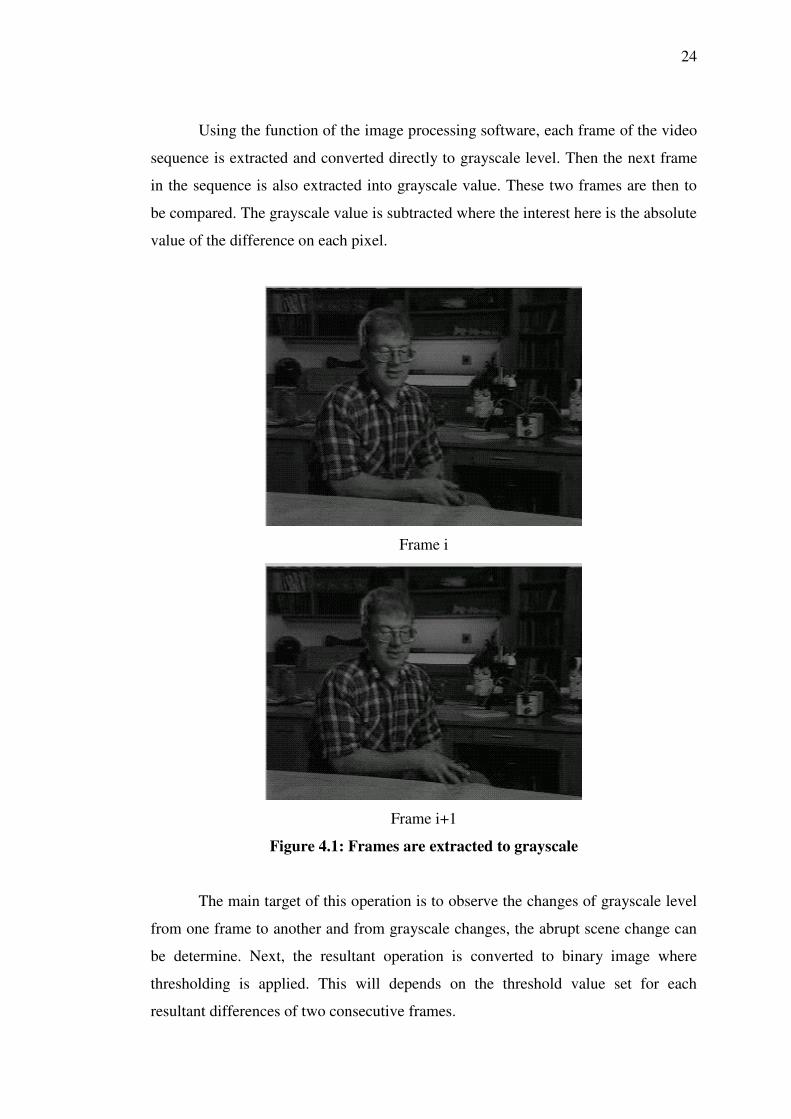
Using the function of the image processing software, each frame of the video

sequence is extracted and converted directly to grayscale level. Then the next frame

in the sequence is also extracted into grayscale value. These two frames are then to

be compared. The grayscale value is subtracted where the interest here is the absolute

value of the difference on each pixel.

Frame i

Frame i+1

Figure 4.1: Frames are extracted to grayscale

The main target of this operation is to observe the changes of grayscale level

from one frame to another and from grayscale changes, the abrupt scene change can

be determine. Next, the resultant operation is converted to binary image where

thresholding is applied. This will depends on the threshold value set for each

resultant differences of two consecutive frames.

25

A pixel luminance value can vary between 0 and 255, where 0 represents

white and 255 represents black. Each pixel on the frame is compared by subtracting

the grayscale level value on each pixel with the respective pixel on the previous

frame. The result will be almost black image where represent the difference value.

Figure 4.2: Result of subtraction.

Next is the thresholding process which will make the obtained image more

informative. By applying this threshold to each frame, the images are refined even

further, and therefore a more accurate grayscale change fraction will be calculated.

For this research the threshold is set to 0.1 of the grayscale level (in this case is 255

level).

Figure 4.3: Thresholding process produces a binary image.

26

Binary image obtained contains more informative data to analyze. White

pixel will refer to the pixel where the difference is greater then the threshold value.

While black pixel is the pixel where the difference value is smaller then the threshold

value compared in the two consecutive frames.

4.3 Detecting Cuts

The difference between the grayscale values for each frame is calculated by

subtracting the value of one frame and frame from the previous frame using point to

point operation. After thresholding, the result is a binary image.

The value of the number of white pixel is calculated in percentage and this

percentage of all frames in the video sequence is obtained. The graph shows that the

high peak shows where the abrupt scene changes occurred. A limit or threshold

needed to decide scene change between the examined frames.

Figure 4.4: Percentage of pixel grayscale difference vs number of frames

27

To avoid selecting the unsuitable or wrong threshold value, another approach

of deciding the scene change is proposed. Since all the percentage of difference of

frame is obtained, the realtive of difference of percentage is obtainable.

The adaptive thresholding technique used is designed by calculating the

percentage of differences for every frame. If noise is found in the first frame above

that of the initial threshold value, the threshold is increased for the next frame, and if

less noise is detected the threshold is decreased. For this method the threshold is 10

percent higher from the previous value of percentage differences.

Figure 4.5: Percentage relative value vs. number of frame

This threshold is best to determine the scene change since abrupt scene

change cause a great amount of grayscale level change from on frame to another.

Other clip graph for percentage differences as follows:

28

Figure 4.6: Plotted graph from clip ‘figo.mpg’

Figure 4.7: Plotted graph from clip ‘pgl.mpg’

29

Figure 4.8: Plotted graph from clip ‘seniman.mpg’

A change of grayscale value provides more information on the scene

continuity. From this research, this method takes further less time consuming. The

analysis will be discussed in next chapter.

30

CHAPTER 5

RESULT AND DISCUSSION

5.1 Analysis and Discussion

This section will discuss on the analysis and performance of the proposed

methods. The methods have been tested with 4 MPEG video streams:

1. cut.mpg

This is a short clips contain 1 scene change.

2. pgl.mpg

Clip from movie “Puteri Gunung Ledang”. 3 scene changes.

3. figo.mpg

Sport documentary. 3 scene changes.

4. seniman.mpg

Clip from movie “Seniman Bujang Lapuk”. 3 scene changes.

The performance of the method is evaluated based on detection accuracy and

execution time. Evaluation is done sing image processing software.

31

5.2 Detection Accuracy

For the proposed method, the result of accuracy as follows:

Method: Edge detection

cut.mpg figo.mpg pgl.mpg seniman.mpg

Total scene change 1 3 3 3

Total detected 1 3 3 3

False alarm 0 0 0 3

*Threshold value: 20%

Table 5.1: Edge detection method accuracy

Method: Grayscale Level

cut.mpg figo.mpg pgl.mpg seniman.mpg

Total scene change 1 3 3 3

Total detected 1 3 3 3

False alarm 0 0 0 0

*Threshold value: 10% more of percentage relative

Table 5.2: Grayscale level method accuracy

From testing, the accuracy for Edge detection method decrease for clip which

contain several moving object. This is due to each object will be counted as

additional detected edge. Moving object will cause moving edge and the differences

of edges will increase, hence exceed the threshold value.

From the testing result, the method using grayscale level was more accurate

and did not effected by object movement in the video. Thus, for movie with high

object move, i.e. sports and action movie, grayscale level method will have higher

accuracy.

32

5.3 Execution time

For testing purpose, each of the proposed method has been programmed into

2 set. The first programs run the detection method and will display each detected

frame. This program requires more execution time. Another program executes faster

and only capture the detected frame but did not the display frame. For execution time

text, the second program is used for performance analysis.

Method: Edge detection

cut.mpg figo.mpg pgl.mpg seniman.mpg

Number of frames 56 242 279 424

Scene duration (sec) 2.00 9.00 11.00 17.00

Execution time (sec) 16.86 69.88 82.42 194.32

*Threshold value: 20%

Table 5.3: Edge detection execution time

Method: Grayscale Level

cut.mpg figo.mpg pgl.mpg seniman.mpg

Number of frames 56 242 279 424

Scene duration (sec) 2.00 9.00 11.00 17.00

Execution time (sec) 2.04 7.37 8.12 18.80

*Threshold value: 10% more of percentage relative

Table 5.4: Grayscale level method accuracy

From execution time test, interesting result is produced. Grayscale level

method executes less time compared to edge detection method. It took more than

100% or even more for edge detection method to execute detection process of the

same clip compared to grayscale level method.

Time vs number of frame graph as follow (dotted line: edge detection, solid

line: grayscale level)

33

Figure 5.1: Time vs frame number for clip ‘cut.mpg’

Figure 5.2: Time vs frame number for clip ‘figo.mpg’

34

Figure 5.3: Time vs frame number for clip ‘pgl.mpg’

Figure 5.4: Time vs frame number for clip ‘seniman.mpg’

35

From the graph above, we can see that edge detection method require great

amount of total execution time compared to grayscale level method which execute as

same as the video duration.

36

CHAPTER 6

CONCLUSION

6.1 Research Summary

New methods for cut detection in video sequences have been presented. The

methods use frame correlation to obtain a measure of content similarity for

temporally adjacent frames and responds very well to simple cuts. The availability of

fast, dedicated hardware operating at video rates makes the useful and interactive and

real time applications.

Two methods have been proposed with both using different approach. From

testing and analysis, grayscale level method shows a great amount of improvement

on execution time compared to edge detection method. Hence, grayscale level

method is preferable to use for scene detection.

Grayscale level method just not only has better accuracy but also have the

execution time much lesser than edge detection method. This may be due to complex

algorithm, of edge detection and dilation. However with proper improvement, the

execution time for edge detection method can be speed up and the gap can be

reduced

37

6.2 Further Development

New methods have been proposed but there still plenty of room for

improvements. The next stage in the development of this project is to implement the

method for detecting dissolves scene change. The proposed method can only detect

on abrupt scene change and other scene change type should also be catered. Beside

dissolves, other scene change types that are popular are wipe and fade [9].

Detection execution time can be deducted with further development. With the

emerging computer technologies, it is possible to perform pre-analysis of the video

stream and the scene change can be detected even the video started. The main pursue

to decrease detection process is to increase video loading time.

Conversion of the proposed method to proper program will be a great

advantage and this development shall make the program independent of any other

program. Video indexing will become vast process with the improvement. Managing

huge amount of video database shall no be a big problem with the detection speed

and accuracy and the technology on MPEG-7 [10] and MPEG-21 standard.

38

REFERENCES

1. Zhang H. J. Content-Based Video Browsing and Retrieval. In: CRC Press. Handbook of Multimedia Computing. Florida: Boca Raton. 1999

2. B. Yeo and B. Liu (1995). Rapid Scene Analysis on Compressed Video. IEEE

Trans. On Circuits and Systems for Video Technology. 5 (6): 533-544. 3. Peter Symes. Video Compression Demystified. Int’l Edition, Singapore: Mc Graw

Hill. 2001 4. International Organisation of Standadisation. Coding Of Moving Pictures And

Audio. London, ISO/IEC JTC1/SC29/WG11. 1996 5. Ramin Zabih, J. Miller, and K. Mai (1995). A Feature-Based Algorithm for

Detecting and Classifying Scene Breaks. Proc. ACM Multimedia 95: 189-200. 6. Grainne Gormley. Technical Report. Scene Break Detection & Classification In

Digital Video Sequences. Dublin City University. 1999 7. A. Nagasaka and Y. Tanaka. Automatic Video Indexing and Full Video Search

for Object Appearance. Amsterdam: Elsevier. 1992 8. Zhou W., Asha V., Ye S. and Jay K. Online Scene Change Detection of Multicast

Video Journal. Journal of Visual Communications & Image Representation. 2001. 12: 1-16.

9. Sarah Porter. Detection and Classification of Shot Transitions. Bristol, UK:

University of Bristol. 2001 10. MPEG Requirement Group. Guide to Obtaining the MPEG-7 Content Set. Rome,

Doc ISO/MPEG N2570. 1998 11. MPEG Ofiicial web site: http://www.chiariglione.org/mpeg/ 12. Mathwork web site: http://www.mathworks.com/

39

APPENDIX A

m file code for edge detection method (full analysis)

t0 = clock; vid = mpgread(video,1:-1,'grayscale'); % open mpg file [m n]=size(vid); % n is the number of frame se = strel('disk',5); % dilate mask a = frame2im(vid(1)); %figure, imshow(a); [r s] = size(a); % r is frame height, s is frame width a1 = edge(a,'prewitt'); a1 = imdilate(a1,se); %figure, imshow(a1); disp (sprintf('number of frame: %d',n)); disp ('--------------------'); ctr = 0; z = 0; for i=2:1:n b = frame2im(vid(i)); %figure, imshow(b); b1 = edge(b,'prewitt'); b1 = imdilate(b1,se); %figure, imshow(b1); dif = xor(a1,b1); [t u] = size(find(dif)); % t is number of 1's in dif percentdif = t*100/(r*s); x(i) = i; y(i) = percentdif; disp(sprintf('analyzing frame %d of %d. %3.2f%% of difference.',i,n,percentdif)); if t > 20/100*r*s disp (sprintf('\tscene change detect at frame %d',i)); figure, imshow(b); title(sprintf('frame %d',i)); ctr=ctr+1; z(ctr) = i; end a = b; a1 = b1; end totaltime = etime(clock, t0); disp(sprintf('\n--------------------')); disp(sprintf('number of frame: \t%d', n)); disp(sprintf('video resolutions: \t%d x %d', s, r)); disp(sprintf('total detection: \t%d',ctr)); disp(sprintf('detected frame(s):')); disp(z); disp(sprintf('execution time: \t%3.2f s', totaltime)); disp(sprintf('--------------------\n')); figure, plot (x, y); title('% of pixel difference VS frames'); xlabel('frames'); ylabel('%');

40

APPENDIX B

m file code for edge detection method (result only)

t0 = clock; vid = mpgread(video,1:-1,'grayscale'); % open mpg file [m n]=size(vid); % n is the number of frame se = strel('disk',5); % dilate mask a = frame2im(vid(1)); %figure, imshow(a); [r s] = size(a); % r is frame height, s is frame width a1 = edge(a,'prewitt'); a1 = imdilate(a1,se); %figure, imshow(a1); disp (sprintf('number of frame: %d',n)); disp ('--------------------'); disp ('processing...'); ctr = 0; z = 0; for i=2:1:n b = frame2im(vid(i)); %figure, imshow(b); b1 = edge(b,'prewitt'); b1 = imdilate(b1,se); %figure, imshow(b1); dif = xor(a1,b1); %subplot (2,2,1), imshow(a2); title('frame1');subplot (2,2,2), %imshow(b2); title('frame2');subplot (2,2,3), imshow(dif); title('xor'); [t u] = size(find(dif)); % t is number of 1's in dif percentdif = t*100/(r*s); %x(i) = i; %y(i) = percentdif; %disp(sprintf('analyzing frame %d of %d. %3.2f%% of difference.',i,n,percentdif)); if t > 20/100*r*s %disp (sprintf('\tscene change detect at frame %d',i)); %figure, imshow(b); title(sprintf('frame %d',i)); ctr=ctr+1; z(ctr) = i; end a = b; a1 = b1; end totaltime = etime(clock, t0); disp(sprintf('\n--------------------')); disp(sprintf('number of frame: \t%d', n)); disp(sprintf('video resolutions: \t%d x %d', s, r)); disp(sprintf('total detection: \t%d',ctr)); disp(sprintf('detected frame(s):')); disp(z); disp(sprintf('execution time: \t%3.2f s', totaltime)); disp(sprintf('--------------------\n')); %figure, plot (x, y); title('% of pixel difference VS frames'); xlabel('frames'); ylabel('%');

41

APPENDIX C

m file code for grayscale level method (full analysis)

t0 = clock; vid = mpgread(video,1:-1,'grayscale'); % open mpg file [m n]=size(vid); % n is the number of frame a = frame2im(vid(1)); %figure, imshow(a); [r s] = size(a); % r is frame height, s is frame width a = im2double(a); %figure, imshow(a); disp (sprintf('number of frame: %d',n)); disp ('--------------------'); ctr = 0; z = 0; x=zeros(1,n); y=zeros(1,n); p=zeros(1,n); for i=2:1:n b = im2double(frame2im(vid(i))); %figure, imshow(b); c = abs(a-b); dif=im2bw(c,0.1); [t u] = size(find(dif)); % t is number of 1's in dif percentdif = t*100/(r*s); x(i) = i; y(i) = percentdif; p(i) = y(i)-y(i-1); disp(sprintf('analyzing frame %d of %d. %3.2f%% of threshold difference.',i,n,percentdif)); if p(i) > 10 disp (sprintf('\tscene change detect at frame %d',i)); figure, imshow(b); title(sprintf('frame %d',i)); ctr=ctr+1; z(ctr) = i; end a = b; end t1=clock; totaltime = etime(t1, t0); disp(sprintf('\n--------------------')); disp(sprintf('number of frame: \t%d', n)); disp(sprintf('video resolutions: \t%d x %d', s, r)); disp(sprintf('total detection: \t%d',ctr)); disp(sprintf('detected frame(s):')); disp(z); disp(sprintf('execution time: \t%3.2f s', totaltime)); disp(sprintf('--------------------\n')); figure, plot (x, y); title('% of pixel difference VS frames'); xlabel('frames'); ylabel('%'); figure, plot (x, p);

42

APPENDIX D

m file code for grayscale level method (result only)

t0 = clock; vid = mpgread(video,1:-1,'grayscale'); % open mpg file [m n]=size(vid); % n is the number of frame t1 = clock; a = frame2im(vid(1)); %figure, imshow(a); [r s] = size(a); % r is frame height, s is frame width a = im2double(a); %figure, imshow(a); disp (sprintf('number of frame: %d',n)); disp ('--------------------'); disp ('processing...'); ctr = 0; z = 0; %x=zeros(1,n); y=zeros(1,n); p=zeros(1,n); for i=2:1:n b = im2double(frame2im(vid(i))); %figure, imshow(b); c = abs(a-b); dif=im2bw(c,0.1); [t u] = size(find(dif)); % t is number of 1's in dif percentdif = t*100/(r*s); %x(i) = i; y(i) = percentdif; p(i) = y(i)-y(i-1); %disp(sprintf('analyzing frame %d of %d. %3.2f%% of threshold difference.',i,n,percentdif)); if p(i) > 10 %disp (sprintf('\tscene change detect at frame %d',i)); %figure, imshow(b); title(sprintf('frame %d',i)); ctr=ctr+1; z(ctr) = i; end a = b; end totaltimepreload = etime(clock, t0); totaltime = etime(clock, t0); disp(sprintf('done!\n\ncut detection analysis')); disp(sprintf('--------------------')); disp(sprintf('number of frame: \t%d', n)); disp(sprintf('video resolutions: \t%d x %d', s, r)); disp(sprintf('total detection: \t%d',ctr)); disp(sprintf('detected frame(s):')); disp(z); disp(sprintf('execution time: \t%3.2f s', totaltime)); disp(sprintf('exe time (preload): \t%3.2f s', totaltimepreload)); disp(sprintf('--------------------\n')); %figure, plot (x, y); title('% of pixel difference VS frames'); xlabel('frames'); ylabel('%'); %figure, plot (x, p);