1

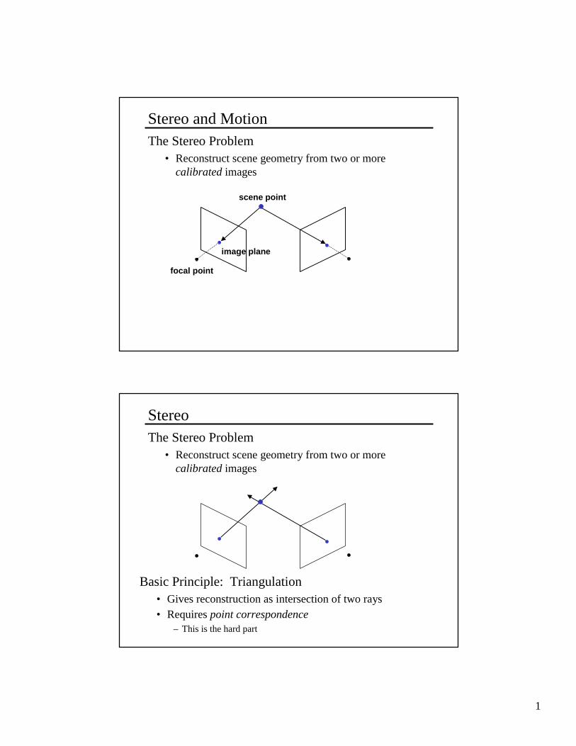
Stereo and MotionThe Stereo Problem

• Reconstruct scene geometry from two or more calibrated images

scene point

focal point

image plane

StereoThe Stereo Problem

• Reconstruct scene geometry from two or more calibrated images

Basic Principle: Triangulation• Gives reconstruction as intersection of two rays• Requires point correspondence

– This is the hard part

2

Stereo CorrespondenceDetermine Pixel Correspondence

• Pairs of points that correspond to same scene point

Epipolar Constraint• Reduces correspondence problem to 1D search along

conjugate epipolar lines

• Stereo rectification: make epipolar lines horizontal– this is what the prewarp did in view morphing

epipolar planeepipolar lineepipolar line

Correspondence and Optical FlowStereo requires just 1D motion estimationBut in general the motion field is 2D

• Epipolar lines not known in advance• Non-rigid motion (no epipolar lines)

True motion field: projected point displacements

Optical flow is apparent motion in the image• Generally these will not be the same

3

The Aperture ProblemWe can’t measure the true 2D motion field from

local image measurements

Example: Barber Pole Illusion

http://www.sandlotscience.com

Optical Flow Equation Several of the following slides adapted from P. Anandan, 1999

u = (u,v)

x

y

t

tyx

II

IvIuI

t

I

t

y

y

I

t

x

x

Idt

dI

+•∇=

++=∂∂+

∂∂

∂∂+

∂∂

∂∂=

=

u

0

),,(),,( tttvytuxItyxI δδδ +++=

Assumptions• Brightness Constancy: intensity I of a moving

point is constant over time• Pixel intensity is linear in t (for small time steps)

4

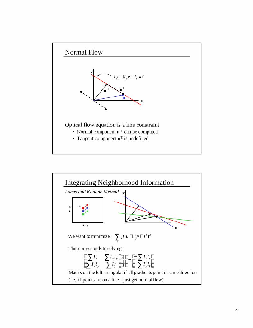
Normal Flow

Optical flow equation is a line constraint• Normal component u⊥ can be computed• Tangent component uT is undefined

u

v0=++ tyx IvIuI

⊥uTu

u

Integrating Neighborhood Information

u

v

x

y

2)( :minimize want toWe it

iy

i

ix IvIuI ++∑

flow) normalget -just -line aon are points if (i.e.,

direction samein point gradients all ifsingular isleft on theMatrix

:solving toscorrespond This

2

2

−−

=

∑∑

∑∑∑∑

ty

tx

yyx

yxx

II

II

v

u

III

III

Lucas and Kanade Method

5

Limits of the Gradient MethodFails When

• Not enough variation in local neighborhood

• Motion is large (much greater than a pixel)– Linear brightness assumption is not met

For larger displacements, match templates instead• Define a small area around a pixel as the template

• Search locally for template in next image

• Use a match measure such as correlation, normalized correlation, or sum-of-squares difference (SSD)

• Choose the maximum (or minimum) as the match

• Window size is important– small windows lead to false matches

– big windows lead to over-smoothing

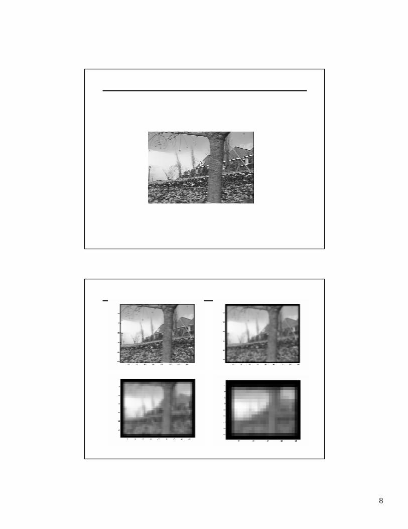
SSD Surface – Textured area

6

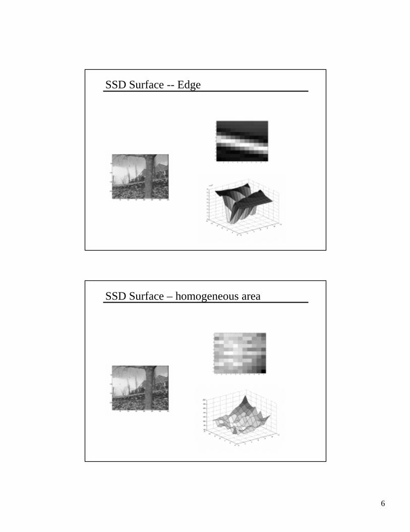
SSD Surface -- Edge

SSD Surface – homogeneous area

7

Coarse to Fine EstimationFirst use large windows and search over large displacement rangeRefine these estimates using smaller windows

Can do this more efficiently by using:

Steps:• Convolve image with a small kernel

– Typically 5x5 Gaussian or Laplacian filter

• Subsample to get lower resolution image• Repeat for more levels

Result:• A sequence of low-pass or band-pass filtered images

A PYRAMID!

PyramidsPyramids were introduced as a multi-resolution image

computation paradigm in the early 80s.

The most popular pyramid is the Burt pyramid, which foreshadows wavelets

Two kinds of pyramids:

Low pass or “Gaussian pyramid”

Band-pass or “Laplacian pyramid”

8

9

Coarse-to-Fine Flow Estimation (Anandan)Construct pyramids from each image (Gaussian)Start at coarsest level, initialize flow to 0

1. Do local search (3x3 or 5x5 area) using small (5x5) templates

2. Around the peak perform subpixel refinement1. Either analytically, using the Lucas-Kanade formulation or2. Numerically by fitting quadratic surface to the peak and

interpolating to find the sub-pixel peak

3. Warp one image toward the other using the flow field4. Repeat steps 1,2, and 3 a few times (usually 5-10)5. Project the flow field to next finer level6. Move to the next finer level and repeat 1-5.

Stop when you finish the iterations at the finest level

Stereo Matching

Stereo Pair Quantized Depth Mapnormalized cross-correlation search

10

Stereo Matching Algorithms• Pitfalls

– specularities (non-Lambertian surfaces)

– ambiguity (aperture problem, low-contrast regions)

– missing data (occlusions)

– intensity error (quantization, sensor error)

– position error (camera calibration)

• Numerous approaches– course-to-fine [Anandan 89]

– edge-based [Marr-Poggio]

– dynamic programming [Baker-Binford 81]

– MRF’s, graph cuts [Zabih]

– adaptive windows [Kanade 91]

– multi-baseline [Okutomi 93]

– many more...

Normalized cross-correlation Graph cuts [Zabih 99]

11

Active Stereo (Laser Scanning)One way to solve the aperture problem

• Create your own texture by projecting light patterns onto the object

• Most precise way is to use a laser

• Triangulate as before, but between laser and sensor

Figures by Brian Curless, 1999

Stanford’s Digital Michelangelo Project

maximum height of gantry: 7.5 meters

weight including subbase: 800 kilograms

http://graphics.stanford.edu/projects/mich/

12

Statistics about the scan

480 individually aimed scans

2 billion polygons

7,000 color images

32 gigabytes

30 nights of scanning

1,080 man-hours

22 people