schaums outline of electromagnetics 978-0-07-183147-5pdf.ebook777.com/071/0071831479.pdf ·...
TRANSCRIPT


ElectromagneticsFourth Edition
Joseph A. EdministerProfessor Emeritus of Electrical Engineering
The University of Akron
Mahmood Nahvi, PhDProfessor Emeritus of Electrical Engineering
California Polytechnic State University
Schaum’s Outline Series
New York Chicago San Francisco Athens London MadridMexico City Milan New Delhi Singapore Sydney Toronto

JOSEPH A. EDMINISTER is currently Director of Corporate Relations for the College of Engineering at Cornell University. In 1984, he held an IEEE Congressional Fellowship in the offi ce of Congressman Dennis E. Eckart (D-OH). He received BEE, MSE, and JD degrees from the University of Akron. He served as professor of electrical engineering, acting department head of electrical engineering, assistant dean and acting dean of engineering, all at the University of Akron. He is an attorney in the state of Ohio and a registered patent attorney.He taught electric circuit analysis and electromagnetic theory throughout his academic career. He is a Professor Emeritus of Electrical Engineering from the University of Akron.
MAHMOOD NAHVI is Professor Emeritus of Electrical Engineering at California Polytechnic State University in San Luis Obispo, California. He earned his BSc, MSc, and PhD, all in electrical engineering, and has 50 years of teaching and research in this fi eld. Dr. Nahvi’s areas of special interest and expertise include network theory, control theory, communications engineering, signal processing, neural networks, adaptive control and learning in synthetic and living systems, communication and control in the central nervous system, and engineering education. In the area of engineering education, he has developed computer modules for electric circuits, signals, and systems which improve the teaching and learning of the fundamentals of electrical engineering.
Copyright © 2014, 2011, 1993, 1979 by McGraw-Hill Education. All rights reserved. Except as permitted under the United States Copyright Act of 1976, no part of this publication may be reproduced or distributed in any form or by any means, or stored in a database or retrieval system, without the prior written permission of the publisher.
ISBN: 978-0-07-183148-2
MHID: 0-07-183148-7
The material in this eBook also appears in the print version of this title: ISBN: 978-0-07-183147-5, MHID: 0-07-183147-9.
eBook conversion by codeMantraVersion 1.0
All trademarks are trademarks of their respective owners. Rather than put a trademark symbol after every occurrence of a trademarked name, we use names in an editorial fashion only, and to the benefi t of the trademark owner, with no intention of infringement of the trademark. Where such designations appear in this book, they have been printed with initial caps.
McGraw-Hill Education eBooks are available at special quantity discounts to use as premiums and sales promotions or for use in corporate training programs. To contact a representative, please visit the Contact Us page at www.mhprofessional.com.
Trademarks: McGraw-Hill Education, the McGraw-Hill Education logo, Schaum’s, and related trade dress are trademarks or registered trademarks of McGraw-Hill Education and/or its affi liates in the United States and other countries, and may not be used without written permission. All other trademarks are the property of their respective owners. McGraw-Hill Education is not associated with any product or vendor mentioned in this book.
TERMS OF USE
This is a copyrighted work and McGraw-Hill Education and its licensors reserve all rights in and to the work. Use of this work is subject to these terms. Except as permitted under the Copyright Act of 1976 and the right to store and retrieve one copy of the work, you may not decompile, disassemble, reverse engineer, reproduce, modify, create derivative works based upon, transmit, distribute, disseminate, sell, publish or sublicense the work or any part of it without McGraw-Hill Education’s prior consent. You may use the work for your own noncommercial and personal use; any other use of the work is strictly prohibited. Your right to use the work may be terminated if you fail to comply with these terms.
THE WORK IS PROVIDED “AS IS.” McGRAW-HILL EDUCATION AND ITS LICENSORS MAKE NO GUARANTEES OR WARRANTIES AS TO THE ACCURACY, ADEQUACY OR COMPLETENESS OF OR RESULTS TO BE OBTAINED FROM USING THE WORK, INCLUDING ANY INFORMATION THAT CAN BE ACCESSED THROUGH THE WORK VIA HYPERLINK OR OTHERWISE, AND EXPRESSLY DISCLAIM ANY WARRANTY, EXPRESS OR IMPLIED, INCLUDING BUT NOT LIMITED TO IMPLIED WARRANTIES OF MERCHANTABILITY OR FITNESS FOR A PARTICULAR PURPOSE. McGraw-Hill Education and its licensors do not warrant or guarantee that the functions contained in the work will meet your requirements or that its operation will be uninterrupted or error free. Neither McGraw-Hill Education nor its licensors shall be liable to you or anyone else for any inaccuracy, error or omission, regardless of cause, in the work or for any damages resulting therefrom. McGraw-Hill Education has no responsibility for the content of any information accessed through the work. Under no circumstances shall McGraw-Hill Education and/or its licensors be liable for any indirect, incidental, special, punitive, consequential or similar damages that result from the use of or inability to use the work, even if any of them has been advised of the possibility of such damages. This limitation of liability shall apply to any claim or cause whatsoever whether such claim or cause arises in contract, tort or otherwise.
iii
Preface
The third edition of Schaum’s Outline of Electromagnetics offers several new features which make it a more pow-erful tool for students and practitioners of electromagnetic field theory. The book is designed for use as a textbookfor a first course in electromagnetics or as a supplement to other standard textbooks, as well as a reference andan aid to professionals. Chapter 1, which is a new chapter, presents an overview of the subject including funda-mental theories, new examples and problems (from static fields through Maxwell’s equations), wave propagation,and transmission lines. Chapters 5, 10, and 13 are changed greatly and reorganized. Mathematical tools such asthe gradient, divergence, curl, and Laplacian are presented in the modified Chapter 5. The magnetic field andboundary conditions are now organized and presented in a single Chapter 10. Similarly, time-varying fields andMaxwell’s equations are presented in a single Chapter 13. Transmission lines are discussed in Chapter 15. Thischapter can, however, be used independently from other chapters if the program of study would recommend it.
The basic approach of the previous editions has been retained. As in other Schaum’s Outlines, the empha-sis is on how to solve problems and learning through examples. Each chapter includes statements of pertinentdefinitions, simplified outlines of the principles, and theoretical foundations needed to understand the subject,interleaved with illustrative examples. Each chapter then contains an ample set of problems with detailed solu-tions and another set of problems with answers. The study of electromagnetics requires the use of rather advancedmathematics, specifically vector analysis in Cartesian, cylindrical and spherical coordinates. Throughout thebook, the mathematical treatment has been kept as simple as possible and an abstract approach has been avoided.Concrete examples are liberally used and numerous graphs and sketches are given. We have found in manyyears of teaching that the solution of most problems begins with a carefully drawn and labeled sketch.
This book is dedicated to our students from whom we have learned to teach well. Contributions of MessrsM. L. Kult and K. F. Lee to material on transmission lines, waveguides, and antennas are acknowledged. Finally,we wish to thank our wives Nina Edminister and Zahra Nahvi for their continuing support.
JOSEPH A. EDMINISTER
MAHMOOD NAHVI

iv
Contents
CHAPTER 1 The Subject of Electromagnetics 1
1.1 Historical Background 1.2 Objectives of the Chapter 1.3 Electric Charge1.4 Units 1.5 Vectors 1.6 Electrical Force, Field, Flux, and Potential 1.7 MagneticForce, Field, Flux, and Potential 1.8 Electromagnetic Induction 1.9 MathematicalOperators and Identities 1.10 Maxwell’s Equations 1.11 Electromagnetic Waves1.12 Trajectory of a Sinusoidal Motion in Two Dimensions 1.13 Wave Polarization1.14 Electromagnetic Spectrum 1.15 Transmission Lines
CHAPTER 2 Vector Analysis 31
2.1 Introduction 2.2 Vector Notation 2.3 Vector Functions 2.4 Vector Algebra2.5 Coordinate Systems 2.6 Differential Volume, Surface, and Line Elements
CHAPTER 3 Electric Field 44
3.1 Introduction 3.2 Coulomb’s Law in Vector Form 3.3 Superposition3.4 Electric Field Intensity 3.5 Charge Distributions 3.6 Standard ChargeConfigurations
CHAPTER 4 Electric Flux 63
4.1 Net Charge in a Region 4.2 Electric Flux and Flux Density 4.3 Gauss’s Law4.4 Relation between Flux Density and Electric Field Intensity 4.5 SpecialGaussian Surfaces
CHAPTER 5 Gradient, Divergence, Curl, and Laplacian 78
5.1 Introduction 5.2 Gradient 5.3 The Del Operator 5.4 The Del Operator andGradient 5.5 Divergence 5.6 Expressions for Divergence in Coordinate Systems5.7 The Del Operator and Divergence 5.8 Divergence of D 5.9 The DivergenceTheorem 5.10 Curl 5.11 Laplacian 5.12 Summary of Vector Operations
CHAPTER 6 Electrostatics:Work, Energy, and Potential 97
6.1 Work Done in Moving a Point Charge 6.2 Conservative Property of theElectrostatic Field 6.3 Electric Potential between Two Points 6.4 Potential of aPoint Charge 6.5 Potential of a Charge Distribution 6.6 Relationship between Eand V 6.7 Energy in Static Electric Fields

CHAPTER 7 Electric Current 113
7.1 Introduction 7.2 Charges in Motion 7.3 Convection Current Density J7.4 Conduction Current Density J 7.5 Concductivity σ 7.6 Current I7.7 Resistance R 7.8 Current Sheet Density K 7.9 Continuity of Current7.10 Conductor-Dielectric Boundary Conditions
CHAPTER 8 Capacitance and Dielectric Materials 131
8.1 Polarization P and Relative Permittivity �r 8.2 Capacitance 8.3 Multiple-Dielectric Capacitors 8.4 Energy Stored in a Capacitor 8.5 Fixed-Voltage D and E8.6 Fixed-Charge D and E 8.7 Boundary Conditions at the Interface of TwoDielectrics 8.8 Method of Images
CHAPTER 9 Laplace’s Equation 151
9.1 Introduction 9.2 Poisson’s Equation and Laplace’s Equation 9.3 Explicit Formsof Laplace’s Equation 9.4 Uniqueness Theorem 9.5 Mean Value and MaximumValue Theorems 9.6 Cartesian Solution in One Variable 9.7 Cartesian ProductSolution 9.8 Cylindrical Product Solution 9.9 Spherical Product Solution
CHAPTER 10 Magnetic Filed and Boundary Conditions 172
10.1 Introduction 10.2 Biot-Savart Law 10.3 Ampere’s Law 10.4 Relationship ofJ and H 10.5 Magnetic Flux Density B 10.6 Boundary Relations for MagneticFields 10.7 Current Sheet at the Boundary 10.8 Summary of Boundary Conditions10.9 Vector Magnetic Potential A 10.10 Stokes’ Theorem
CHAPTER 11 Forces and Torques in Magnetic Fields 193
11.1 Magnetic Force on Particles 11.2 Electric and Magnetic Fields Combined11.3 Magnetic Force on a Current Element 11.4 Work and Power 11.5 Torque11.6 Magnetic Moment of a Planar Coil
CHAPTER 12 Inductance and Magnetic Circuits 209
12.1 Inductance 12.2 Standard Conductor Configurations 12.3 Faraday’s Law and Self-Inductance 12.4 Internal Inductance 12.5 Mutual Inductance12.6 Magnetic Circuits 12.7 The B-H Curve 12.8 Ampere’s Law for MagneticCircuits 12.9 Cores with Air Gaps 12.10 Multiple Coils 12.11 ParallelMagnetic Circuits
CHAPTER 13 Time-Varying Fields and Maxwell’s Equations 233
13.1 Introduction 13.2 Maxwell’s Equations for Static Fields 13.3 Faraday’sLaw and Lenz’s Law 13.4 Conductors’ Motion in Time-Independent Fields13.5 Conductors’ Motion in Time-Dependent Fields 13.6 Displacement Current13.7 Ratio of JC to JD 13.8 Maxwell’s Equations for Time-Varying Fields
CHAPTER 14 Electromagnetic Waves 251
14.1 Introduction 14.2 Wave Equations 14.3 Solutions in Cartesian Coordinates14.4 Plane Waves 14.5 Solutions for Partially Conducting Media 14.6 Solutionsfor Perfect Dielectrics 14.7 Solutions for Good Conductors; Skin Depth
Contents v

14.8 Interface Conditions at Normal Incidence 14.9 Oblique Incidence andSnell’s Laws 14.10 Perpendicular Polarization 14.11 Parallel Polarization14.12 Standing Waves 14.13 Power and the Poynting Vector
CHAPTER 15 Transmission Lines 273
15.1 Introduction 15.2 Distributed Parameters 15.3 Incremental Models15.4 Transmission Line Equation 15.5 Sinusoidal Steady-State Excitation15.6 Sinusoidal Steady-State in Lossless Lines 15.7 The Smith Chart15.8 Impedance Matching 15.9 Single-Stub Matching 15.10 Double-StubMatching 15.11 Impedance Measurement 15.12 Transients in Lossless Lines
CHAPTER 16 Waveguides 311
16.1 Introduction 16.2 Transverse and Axial Fields 16.3 TE and TM Modes;Wave Impedances 16.4 Determination of the Axial Fields 16.5 Mode CutoffFrequencies 16.6 Dominant Mode 16.7 Power Transmitted in a LosslessWaveguide 16.8 Power Dissipation in a Lossy Waveguide
CHAPTER 17 Antennas 330
17.1 Introduction 17.2 Current Source and the E and H Fields 17.3 Electric(Hertzian) Dipole Antenna 17.4 Antenna Parameters 17.5 Small Circular-LoopAntenna 17.6 Finite-Length Dipole 17.7 Monopole Antenna 17.8 Self- andMutual Impedances 17.9 The Receiving Antenna 17.10 Linear Arrays17.11 Reflectors
APPENDIX 349
INDEX 350
Contentsvi

1
The Subject of Electromagnetics
1.1 Historical Background
Electric and magnetic phenomena have been known to mankind since early times. The amber effect is an exam-ple of an electrical phenomenon: a piece of amber rubbed against the sleeve becomes electrified, acquiring a forcefield which attracts light objects such as chaff and paper. Rubbing one’s woolen jacket on the hair of one’s headelicits sparks which can be seen in the dark. Lightning between clouds (or between clouds and the earth) isanother example of familiar electrical phenomena. The woolen jacket and the clouds are electrified, acquiringa force field which leads to sparks. Examples of familiar magnetic phenomena are natural or magnetized min-eral stones that attract metals such as iron. The magical magnetic force, it is said, had even kept some objectsin temples floating in the air.
The scientific and quantitative exploration of electric and magnetic phenomena started in the seventeenthand eighteenth centuries (Gilbert, 1600, Guericke, 1660, Dufay, 1733, Franklin, 1752, Galvani, 1771,Cavendish, 1775, Coulomb, 1785, Volta, 1800). Forces between stationary electric charges were explained byCoulomb’s law. Electrostatics and magnetostatics (fields which do not change with time) were formulated andmodeled mathematically. The study of the interrelationship between electric and magnetic fields and their time-varying behavior progressed in the nineteenth century (Oersted, 1820 and 1826, Ampere, 1820, Faraday, 1831,Henry, 1831, Maxwell, 1856 and 1873, Hertz, 1893)1. Oersted observed that an electric current produces amagnetic field. Faraday verified that a time-varying magnetic field produces an electric field (emf). Henry constructed electromagnets and discovered self-inductance. Maxwell, by introducing the concept of the dis-placement current, developed a mathematical foundation for electromagnetic fields and waves currently knownas Maxwell’s equations. Hertz verified, experimentally, propagation of electromagnetic waves predicted byMaxwell’s equations. Despite their simplicity, Maxwell’s equations are comprehensive in that they accountfor all classical electromagnetic phenomena, from static fields to electromagnetic induction and wave propa-gation. Since publication of Maxwell’s historical manuscript in 1873 more advances have been made in thefield, culminating in what is presently known as classical electromagnetics (EM). Currently, the importantapplications of EM are in radiation and propagation of electromagnetic waves in free space, by transmissionlines, waveguides, fiber optics, and other methods. The power of these applications far surpasses any allegedhistorical magical powers of healing patients or suspending objects in the air.
In order to study the subject of electromagnetics, one may start with electrostatic and magnetostatic fields,continue with time-varying fields and Maxwell’s equations, and move on to electromagnetic wave propagationand radiation. Alternatively, one may start with Maxwell’s equations. This book uses the first approach, startingwith the Coulomb force law between two charges. Vector algebra and vector calculus are introduced early andas needed throughout the book.
CHAPTER 1
1For some historical timelines see the references at the end of this chapter.

1.2 Objectives of the Chapter
This chapter is intended to provide a brief glance (and be easily understood by an undergraduate student in thesciences and engineering) of some basic concepts and methods of the subject of electromagnetics. The objec-tive is to familiarize the reader with the subject and let him or her know what to expect from it. The chapter canalso serve as a short summary of the main tools and techniques used throughout the book. Detailed treatmentsof the concepts are provided throughout the rest of the book.
1.3 Electric Charge
The source of the force field associated with an electrified object (such as the amber rubbed against the sleeve) isa quantity called electric charge which we will denote by Q or q. The unit of electric charge is the coulomb, shownby the letter C (see the next section for a definition). Electric charges are of two types, labeled positive and neg-ative. Charges of the same type repel while those of the opposite type attract each other. At the atomic level werecognize two types of charged particles of equal numbers in the natural state: electrons and protons. An electronhas a negative charge of 1.60219 � 10�9 C (sometimes shown by the letter e) and a proton has a positive chargeof precisely the same amount as that of an electron. The choice of negative and positive labels for electric chargeson electrons and protons is accidental and rooted in history. The electric charge on an electron is the smallestamount one may find. This quantization of charge, however, is not of interest in classical electromagnetics andwill not be discussed. Instead we will have charges as a continuous quantity concentrated at a point or distributedon a line, a surface, or in a volume, with the charge density normally denoted by the letter ρ.
It is much easier to remove electrons from their host atoms than protons. If some electrons leave a piece ofmatter which is electrically neutral, then that matter becomes positively charged. To takes our first exampleagain, electrons are transferred from cloth to amber when they are rubbed together. The amber then accumulatesa negative charge which becomes the source of an electric field. Some numerical properties of electrons aregiven in Table 1-1.
CHAPTER 1 The Subject of Electromagnetics2
TABLE 1-1 Some Numerical Properties of Electrons
Electric charge �1.60219 � 10�19 C
Resting mass 9.10939 � 10�31 kg
Charge to mass ratio 1.75 � 1011 C/kg
Order of radius 3.8 � 10�15 m
Number of electrons per 1 C 6.24 � 1018
TABLE 1-2 Four Basic Units in the SI System
QUANTITY SYMBOL SI UNIT ABBREVIATION
Length L, � Meter m
Mass M, m Kilogram kg
Time T, t Second s
Current I, i Ampere A
1.4 Units
In electromagnetics we use the International System of Units, abbreviated SI from the French le Système inter-national d’unités (also called the rationalized MKS system). The SI system has seven basic units for seven basicquantities. Three units come from the MKS mechanical system (the meter, the kilogram, and the second ). Thefourth unit is the ampere for electric current. One ampere is the amount of constant current in each of two infi-nitely long parallel conductors with negligible diameters separated by one meter with a resulting force betweenthem of 2 � 10�7 newtons per meter. These basic units are summarized in Table 1-2.

The other three basic quantities and their corresponding SI units are the temperature in degrees kelvin (K),
the luminous intensity in candelas (cd), and the amount of a substance in moles (mol). These are not of interest
to us. Units for all other quantities of interest are derived from the four basic units of length, mass, time, and
current using electromechanical formulae. For example, the unit of electric charge is found from its relationship
with current and time to be q �� i dt. Thus, one coulomb is the amount of charge passed by one ampere in one
second, 1 C � 1 A � s. The derived units are shown in Table 1-3.
CHAPTER 1 The Subject of Electromagnetics 3
TABLE 1-3 Additional Units in the SI System Derived from the Basic Units
QUANTITY SYMBOL SI UNIT ABBREVIATION
Force F, ƒ Newton N
Energy, work W, w Joule J
Power P, p Watt W
Electric charge Q, q Coulomb C
Electric field E, e Volt/meter V/m
Electric potential V, v Volt V
Displacement D Coulomb/meter2 C/m2
Resistance R Ohm ΩConductance G Siemens S
Capacitance C Farad F
Inductance L Henry H
Magnetic field intensity H Ampere/meter A /m
Magnetic flux φ Weber Wb
Magnetic flux density B Tesla T
Frequency ƒ Hertz Hz
TABLE 1-4 Decimal Multiples and Submultiples of Units in the SI System
PREFIX FACTOR SYMBOL
Atto 10�18 a
Femto 10�15 f
Pico 10�12 p
Nano 10�9 n
Micro 10�6 μMili 10�3 m
Centi 10�2 c
Deci 10�1 d
Kilo 103 k
Mega 106 M
Giga 109 G
Tera 1012 T
Peta 1015 P
Exa 1018 E
Magnetic flux density B is sometimes measured in gauss, where 104 gauss �1 tesla. The decimal multiples andsubmultiples of SI units will be used whenever possible. The symbols given in Table 1-4 are prefixed to the unitsymbols of Tables 1-2 and 1-3.

1.5 Vectors
In electromagnetics we use vectors to facilitate our calculations and explanations. A vector is a quantity specifiedby its magnitude and direction. Forces and force fields are examples of quantities expressed by vectors. To distin-guish vectors from scalar quantities, bold-face letters are used for the former. A vector whose magnitude is 1 is calleda unit vector. To represent vectors in the Cartesian coordinate space, we employ three basic unit vectors: ax, ay, andaz in the x, y, and z directions, respectively. For example, a vector connecting the origin to point A at (x � 2, y � �1, z � 3) is shown by A � 2ax � ay � 3az. Its magnitude is ⎟ A⎟ � A � �����22�����(�1)2�����32 � ���14.Its direction is given by the unit vector
Three basic vector operations are
addition and subtraction, A � B � (Ax � Bx )ax � (Ay � By )ay � (Az � Bz)az,
dot product, A · B � AB cos θ, where θ is the smaller angle between A and B,
cross product, A � B � AB sin θ an, where an is the unit vector normal to the plane parallel to A and B.
The dot product results in a scalar quantity; hence it is also called the scalar product. It can easily be shownthat A · B � Ax Bx � Ay By � AzBz. The cross product results in a vector quantity; hence, it is also called thevector product. A � B is normal to both A and B and follows the right-hand rule: With the fingers of theright hand rotating from A to B through angle θ, the thumb points in the direction of A � B. It can easilybe shown that
1.6 Electrical Force, Field, Flux, and Potential
Electrical Force. There is a force between two point charges. The force is directly proportional to the chargemagnitudes and inversely proportional to the square of their separation distance. The direction of the force isalong the line joining the two charges. For point charges of like sign the force is one of repulsion, while forunlike charges the force is attractive. The magnitude of the force is given by
This is Coulomb’s law, which was developed from work with small charged bodies (spheres) and a delicate tor-sion balance (Coulomb 1785). Rationalized SI units are used. The force is in newtons (N), the distance is inmeters (m), and the charge is in units called the coulomb (C). The SI system is rationalized by the factor 4π, intro-duced in Coulomb’s law in order that it not appear later in Maxwell’s equation. � is the permittivity of the mediumwith the unit C2/(N . m2) or, equivalently, farads per meter (F/m). For free space or vacuum,
For media other than free space, � � �0�r, where �r is the relative permittivity or dielectric constant. Free spaceis to be assumed in all problems and examples as well as the approximate value for �0, unless there is a statementto the contrary.
� �� � � ��
012
9
8 854 1010
36. F/m F/m�
π
FQ Q
d� 1 2
24π�
a a a
a a a
a a a
A Bx y z
y z x
z x y
y z zA B A B
� �
� �
� �
� � �
⎫
⎬⎪
⎭⎪
⇒ ( yy x z x x z y x x y x zA B A B A B A B) ( ) ( )a a a� � � �
Aa a a
140 5345 0 2673 0 8018� � �. . .x y z
CHAPTER 1 The Subject of Electromagnetics4

EXAMPLE 1. Two electrons in free space are separated by 1 A° (1 Angstrom � 10�10 m). We want to find andcompare Coulomb’s electrostatic force and Newton’s gravitational force between them. Since the distancebetween the two electrons, 10�10 m, is much more than their radii, � 3.8 � 10�15 m, they can be considered pointcharges and masses. Coulomb’s electrostatic force between them is
Newton’s gravitational force between two masses M1 and M2 separated by a distance d is Fg � GM1 M2/d2, whereFg is in newtons, M1 and M2 are in kg, d is in meters, and G, the gravitational constant, is G � 6.674 � 10�11. Withthe resting mass of an electron being 9.10939 � 10�31 kg, the gravitational force between them is
Therefore, the electrical force between two electrons is approximately 42 orders of magnitude stronger thantheir gravitational force.
Superposition Property. The presence of a third charge doesn’t change the mutual force between the othertwo charges, but rather adds (vectorially) its own force contribution. This is called the linear superposition prop-erty. It helps us define a vector quantity called the field intensity and use it in order to find the force on a chargeat any point in the field.
Electric Field. The force field associated with a charge configuration is called an electric field. It is a vectorfield specified by a quantity called the electric field intensity, shown by vector E. The electric field intensity ata given point is the force on a positive unit charge, called the test charge, placed at that point. The intensity ofthe electric field due to a point charge Q at a distance d is a vector directed away from the point charge (if Q ispositive) or toward it (if Q is negative). Its magnitude is
In vector notation
where a is the unit vector directed from the point charge to the test point. The unit of the electric field inten-sity is V/m. The superposition property of electric field is used to find the field due to any spatial charge configuration.
E a�Q
d4 2π�
EQ
d�
4 2π�
F GM M
dg � � �
� �
�1 2
211
31 2
6 674 109 10939 10
10.
.− ⎡⎣ ⎤⎦220
5255 4 10� . � � N
FQ Q
de �
��
�
� �
�
�1 2
02
19 2
94
1 60219 10
4104
1π π
π
.⎡⎣ ⎤⎦
00
23 1 1020
9
�
��� . N
CHAPTER 1 The Subject of Electromagnetics 5
Q1 Q2FF
Q1 Q2F F
d
(b)
(a)
Fig. 1-1 Coulomb’s law In (a) Q1 and Q2 are unlike charges, and in (b) they are of the same type.FQ Q
d�
1 224π�
.

EXAMPLE 2. The electric field intensity at 10 cm away from a point charge of 0.1 μC in vacuum is
where ar is the radial unit vector with the charge at the center. At the distance of 1 m its magnitude is reduced to900 V/m. If the medium is a dielectric with relative permittivity �r � 100 (such as titanium dioxide), the abovefield intensities are reduced to 900 and 9 V/m, respectively.
Electric Flux. An electric field is completely specified by its intensity vector. However, to help better explainsome phenomena, we also define a scalar field called the electric flux. Electric flux is considered a quantity,albeit an imaginary one, which originates on the positive charge, moves along a stream of directional lines(called flux lines), and terminates on the negative charge, or at infinity if there are no other charges in the field.Electrical forces are thus experienced when an electric charge encounters lines of electric flux. This is analogousto the example of fluid flow where the flux originates from a source and terminates at a sink or dissipates intothe environment. In this case, a vector field such as velocity defines the flux density, from which one can deter-mine the amount of fluid flow passing through a surface. Faraday envisioned the concept of electric flux, shownby Ψ, to explain how a positive charge induces an equal but negative charge on a shell which encloses it. Hisexperimental setup consisted of an inner shell enclosed by an outer sphere. Unlike flux, which is a scalar field,its density is a vector field.
Electric Flux Density. Flux density D in an electric field is defined by D � �E. In the SI system, the unit ofelectric flux is the coulomb (C) and that of flux density is C/m2. The flux passing through a differential surfaceelement ds is the dot product D · ds, which numerically is equal to the product of the differential surface ele-ment’s area, with the magnitude of the component of the flux density perpendicular to it.
Gauss’s Law. The total flux out of a closed surface is equal to the net charge enclosed within the surface.
EXAMPLE 3. Flux density through a spherical surface with radius d enclosing a point charge Q is
where a is the radial unit vector from the point charge to the test point on the sphere. The total flux coming outof the sphere is
Electric Potential. The work done to move a unit charge from point B to point A in an electric field is calledthe potential of point A with reference to point B and shown by VAB. It is equal to the line integral
The value of the integral depends only on the electric field and the two end-points. It is independent of the pathtraversed by the charge as long as all attempted paths share the same initial and destination points. The valueof the integral over a closed path is, therefore, zero. This is a property of a conservative field such as E. If thereference point B is moved to infinity, the integral defines a scalar field called the potential field. The unit ofthe potential is the volt (V), the work needed to move one C of charge a distance of 1 m along a field of E � 1 V/m.
The electric potential is introduced as a line integral of the electric field. It can also be found from chargedistributions. Conversely, field intensity and flux can be obtained from the potential (see Chapter 6).
V dABB
A
�� � E· l
� � � � � �4 44
2 22π π
πd D d
Q
dQ
D E� ��Q
d4 2πa
E a� ��
��
10
41036
10
907
92π
π⎛⎝⎜
⎞⎠⎟
r ra kV/m
CHAPTER 1 The Subject of Electromagnetics6

EXAMPLE 4. There exists a static electric field in the atmosphere directed downward which depends onweather conditions and decreases with height. Assuming that its intensity near the ground is about 150 V/mand remains the same within the tropospheric height, find the electric potential at a height of 333 m withrespect to the ground.
V � 150 V/m � 333 V/m � 50kV.
1.7 Magnetic Force, Field, Flux, and Potential
Magnetic Force. Permanent magnets, be they natural, such as a lodestone (Gilbert, 1600 AD), or manufactured,such as one bought from a store, establish a force field in their vicinity which exerts a force on some metallicobjects. The force here is called the magnetic force, and the field is called a magnetic field. The source of the mag-netic field is the motion of electric charges within the atomic structure of such permanent magnets. Moving elec-tric charges (such as an electric current) also produce a magnetic field which may be detected in the same wayas that of a permanent magnet. Hold a compass needle close to a wire carrying a DC current and the needle willalign itself, at a right angle with the current. Change the current direction in the wire and the needle will changeits direction. This experiment, performed by Oersted in 1820, indicates that the electric current produces a mag-netic field in its surroundings which exerts a force on the compass needle. Replace the compass with a solenoidcarrying a DC current and the solenoid will align itself, just like the compass, in a direction perpendicular to thecurrent. With a DC current, such generated magnetic fields are static in nature. In a similar experiment, a wire suspended along the direction of a magnetic field and carrying a sinusoidal current will vibrate at the frequencyof the current. (This effect was used in the early days of EKG monitoring. Passage of electrical heart pulsesthrough a wire which was suspended in the field of a permanent magnet causes it to deflect and vibrate, with apen recording the viberations and hence the electrical activity of the heart.) These observations indicate that themagnetic field exerts a force on the compass, another magnet, or a current-carrying wire or solenoid. They specif-ically show that a current-carrying wire generates a magnetic field in its neighborhood which exerts a force onanother current-carrying wire placed there.
Force Between Two Wires. Two infinitely long parallel wires carrying currents I1 and I2 and separated by dis-tance d experience a mutual force. They are pushed apart (when currents are in the same direction) or pulledtogether (when currents are in opposite directions). The magnitude of the magnetic force between the two wiresin free space is given by the following:
where μ0 � 4π � 10�7 (H/m) is the permeability of free space. The force is in newtons (N), the distance is inmeters (m), and the currents are in amperes (A).
Magnetic Field Strength. The magnetic field strength is a vector quantity, specified by a magnitude and adirection. In this book we work with magnetic fields whose sources are electric currents and moving charges.The magnitude of the differential field strength of a small element of conducting wire dl carrying a current I is
where R is the distance from the current element to the test point at which dH is being measured and θ is the anglebetween the current element and the line connecting it to the test point. The direction of the field is normal to theplane made of the current element and the connecting line, following the right-hand rule: With the right thumbpointing along the direction of current, the fingers point in the direction of the field. This is called the Biot-Savartlaw. In vector notation it is given by
where d l is the differential current element vector and aR is the unit vector directed from it to the test point.
dI d
RRH
l a�
�
4 2π
d HI dl
R�
sinθπ4 2
FI I
d�
μπ0 1 2
2
CHAPTER 1 The Subject of Electromagnetics 7
CHAPTER 1 The Subject of Electromagnetics8
Z
R
dH
dI
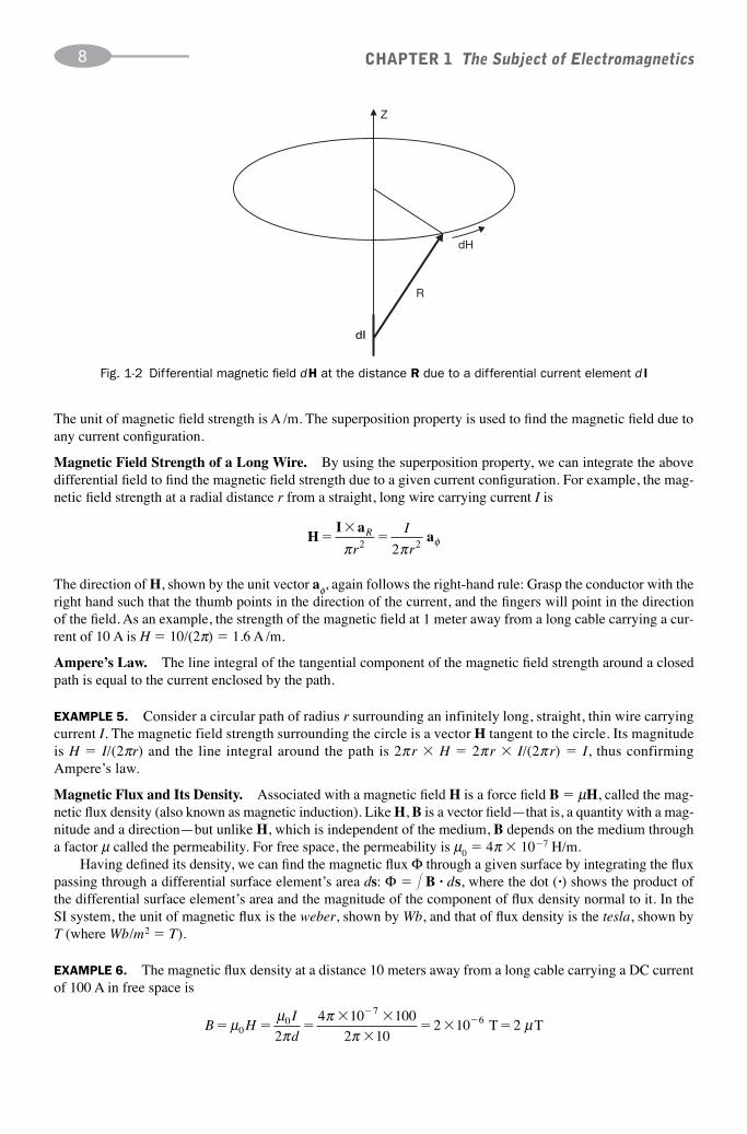
Fig. 1-2 Differential magnetic field dH at the distance R due to a differential current element d l
The unit of magnetic field strength is A /m. The superposition property is used to find the magnetic field due toany current configuration.
Magnetic Field Strength of a Long Wire. By using the superposition property, we can integrate the abovedifferential field to find the magnetic field strength due to a given current configuration. For example, the mag-netic field strength at a radial distance r from a straight, long wire carrying current I is
The direction of H, shown by the unit vector aφ, again follows the right-hand rule: Grasp the conductor with theright hand such that the thumb points in the direction of the current, and the fingers will point in the directionof the field. As an example, the strength of the magnetic field at 1 meter away from a long cable carrying a cur-rent of 10 A is H � 10/(2π) � 1.6 A /m.
Ampere’s Law. The line integral of the tangential component of the magnetic field strength around a closedpath is equal to the current enclosed by the path.
EXAMPLE 5. Consider a circular path of radius r surrounding an infinitely long, straight, thin wire carryingcurrent I. The magnetic field strength surrounding the circle is a vector H tangent to the circle. Its magnitudeis H � I/(2πr) and the line integral around the path is 2π r � H � 2π r � I/(2π r) � I, thus confirmingAmpere’s law.
Magnetic Flux and Its Density. Associated with a magnetic field H is a force field B � μH, called the mag-netic flux density (also known as magnetic induction). Like H, B is a vector field—that is, a quantity with a mag-nitude and a direction—but unlike H, which is independent of the medium, B depends on the medium througha factor μ called the permeability. For free space, the permeability is μ0 � 4π � 10�7 H/m.
Having defined its density, we can find the magnetic flux Φ through a given surface by integrating the fluxpassing through a differential surface element’s area ds: Φ � � B · ds, where the dot (·) shows the product of the differential surface element’s area and the magnitude of the component of flux density normal to it. In theSI system, the unit of magnetic flux is the weber, shown by Wb, and that of flux density is the tesla, shown byT (where Wb/m2 � T).
EXAMPLE 6. The magnetic flux density at a distance 10 meters away from a long cable carrying a DC currentof 100 A in free space is
B HI
d� � �
� �
�� � �
��μ μ
ππ
πμ0
07
6
2
4 10 100
2 102 10 T 2 T
HI a
a��
�R
r
I
rπ π φ2 22

The magnetic flux through a rectangular area (1 m � 10 cm) coplanar with the cable and placed length-wise alongit at a distance of 10 m is Φ � � B · ds � B � S � 2 μT � 10�1 m2 � 2 � 10�7 Wb. The flux is constant.
Force on a Moving Charge. Motion of a charged particle in a magnetic field generates a force on the particle.The magnitude of the force is proportional to the charge Q, magnetic flux density B, velocity of motion v, and thesine of the angle θ between the velocity and magnetic vectors, F � QvB sin θ. Its direction is perpendicular to theflux density vector B and the velocity vector v. In vector notation, the force is expressed by the vector product
Fmagnetic � Qv � B
If the field combines an electric field with the magnetic field, the total force on the moving particle is
Ftotal � Q (E � v � B)
Vector Magnetic Potential. In Section 1.6 we introduced the scalar quantity called electric potential which canserve as an intermediate quantity for field computations. Similarly, for magnetic fields we define a vector magneticpotential A such that
∇ � A � B
where ∇ � A is a vector called the curl of A (see Section 1.9 for the definition of curl). The vector magneticpotential can be obtained from the current distribution in the media and thus can serve as an intermediate quan-tity for calculation of B and H (see Chapter 10). The unit of the vector magnetic potential is the weber per meter(Wb/m).
1.8 Electromagnetic Induction
Static electric and magnetic fields are decoupled from each other. Each field works and exists by itself and canbe treated separately. Time variation couples them together. An early discovery of electromagnetic coupling wasmade by Faraday, who observed that a time-varying magnetic field generates a time-varying electric field, whichproduces a voltage and current in a conducting loop placed in the field. This is known as Faraday’s law of induc-tion. The effect was verified experimentally for the first time by Faraday in 1831. (Faraday also hypothesized thatin a similar way a time-varying electric field should produce a magnetic field, but he did not predict it theoreti-cally or demonstrated it experimentally. That was left to Maxwell’s equations in 1873 and Hertz in 1893.) It issaid that the time-varying magnetic flux induces an electric potential. The voltage is called the electromotiveforce (emf ). An emf can also be produced by a moving magnetic field or by a conductor moving in a magneticfield, even when that field is constant. Using the concept of magnetic flux linkage φ (the total magnetic flux linking the circuit), Faraday’s law, stated in mathematical form, is
where φ is the total magnetic flux linking the circuit. φ is called the magnetic flux linkage.
EXAMPLE 7. A very long straight wire carries a 60-Hz current with an RMS value I0 in free space. To deter-mine I0, a single-strand rectangular test loop (1 m � 10 cm) is placed coplanar with the wire and length-wise inparallel with it at a distance of 10 m. The rms of the induced emƒ in the loop is 95 μV. Find I0.
em fd
dt��
φ
CHAPTER 1 The Subject of Electromagnetics 9
i t I t
Hi
rB H
i
( ) sin( )
,
�
� � � � ��
�
2 377
24 10
2 1
0
07
πμ π
π 002 10
2 10 1 10 2 10
8
8 1 9
� �
� � � � � � � � �
�
� � �
i
B S i iφ ( ) ( ) 22 2 10 377
377 2 2 10
90
90
�
�� �� � �
�
�
I t
emfd
dtI
sin( )
φccos( ), .377 0 754 0t rms I Vwith an of μ
From the measured emƒ � 95μV we find I0 � 95/0.754 � 126 A.

Increasing Flux Linkage. Flux linkage is increased by a factor n if the test loop has n turns. Let the test loopof Example 7 have 100 turns and the induced emƒ will become 9.5 mV.
1.9 Mathematical Operators and Identities
Electromagnetic fields and forces are vector quantities specified by their magnitude and direction and shown byboldface letters, as seen in the previous sections. So far we have been content with simple cases and exampleswhich are handled without resorting to vector algebra and calculus. To analyze and study the subject of electro-magnetics rigorously, however, we need vector algebra and mathematical operators such as the gradient, diver-gence, curl, and Laplacian. These will be discussed in Chapter 5 and throughout the book as the need arises.Some important vector operators used in electromagnetics are briefly summarized in Table 1-5. They are givenin the Cartesian coordinate system. The unit vectors in the x, y, and z directions are shown by ax, ay, and az,respectively.
TABLE 1-5 Some Useful Vector Operators and Identities
(1) Cartesian vector: A � Axax � Ayay � Azaz
(2) Time-derivative of a vector:
(3) Dot product of two vectors: A · B � Ax Bx � Ay By � Az Bz
(4) Cross product of two vectors: A � B � (Ay Bz � Az By) ax � (Az Bx � AxBz)ay � (Ax By � Ay Bx)az
(5) Del operator:
(6) Gradient of a scalar field:
(7) Divergence of a vector field:
(8) Curl of a vector field:
(9) Laplacian (divergence of gradient)
of a scalar field:
(10) Curl curl of a vector field: ∇ � (∇ � A) � ∇(∇ · A) � ∇2 A
(11) Vector identities:
(a) Divergence of the curl is zero ∇ · (∇ � A) � 0
(b) Curl of the gradient is zero ∇ � (∇F ) � 0
1.10 Maxwell’s Equations
James Clerk Maxwell (1831–1879) was inspired by Faraday’s discovery in 1831 that a time-varying magneticfield generates an electric field and his hypothesis that a time-varying electric field would similarly generatea magnetic field (an idea that Faraday had neither demonstrated experimentally nor predicted theoretically).
∇ ∇ ∇22
2
2
2
2
2F FF
x
F
y
F
z� · � � �
∇⎛⎝⎜
⎞⎠⎟
⎛⎝⎜
⎞⎠⎟� � � � �A a a
A
y
A
z
A
z
A
xz y
xx z
y �� �
A
x
A
yy x
z⎛⎝⎜
⎞⎠⎟
a
∇ · A � � �
A
x
A
y
A
zx y z
∇FF
x
F
y
F
zx y z� � �
a a a
∇ �
( ) ( ) ( )
x y zx y za a a� �
Aa a a
t
A
t
A
t
A
tx
xy
yz
z� � �
CHAPTER 1 The Subject of Electromagnetics10

In his theoretical attempt to formulate the coupling between time-varying electric and magnetic fields,Maxwell recognized the inadequancy of Ampere’s law when applied to time-varying fields, as it contradictedthe conservation of electric charge principle (see Problem 1.17). Maxwell introduced the concept of a displace-ment current density ∂D—–∂t
in Ampere’s law to supplement the current density due to moving charges. The intro-duction of the displacement current removed that contradiction and predicted that a time-varying electricfield would also produce a (time-varying) magnetic field. The collective set of the following four equations(written in vector form) are called Maxwell’s equations.
(Faraday’s law)
(Ampere’s law supplemented by Maxwell’s displacement current)
∇ · D � ρ (Gauss’s law for the electric field)
∇ · B � 0 (Gauss’s law for the magnetic field)
Here ρ is the charge density and J is the current density. Maxwell’s equations form the main tenet of classicalelectromagnetics. They provide a general and complete framework for time-varying electromagnetic fields fromwhich the special case of static fields can also be deduced. But more importantly, the equations predict electro-magnetic waves which propagate through space at the speed of light.
In the case of sinusoidal time-variation (time dependence through e jωt, also called time harmonics), weobtain the phasor representation (also called the time harmonic form) of Maxwell’s equations.
∇ � E � �jωB ∇ · D � ρ∇ � H � J � jωD ∇ · B � 0
In the phasor domain, E and B are complex-valued vectors and functions of space (x, y, z) only. They sharethe same time dependency through e jω t. The phasor representation of Maxwell’s equations does not imposeany limitations and can be used without loss of generality.
Maxwell’s Equations in Source-Free Media. Maxwell’s equations in a linear medium with permeability μ,permittivity �, and containing no charges or currents (ρ � 0 and J � 0) become
These provide two first-order partial differential equations in E and H which couple derivatives with respect tospace and time. To find wave equations for E and H, we take the derivatives of the above equations and obtaintwo second-order partial differential equations in E and H, resulting in a decoupling of these two fields. Somewave equations for special and important situations are derived in the next section.
1.11 Electromagnetic Waves
Electromagnetic waves are time-varying field patterns which travel through space. An example is the sinusoidalplane wave in free space with constitutive fields given by
E a
H a
� �
� �
E t z
H t z
x
y
0 0 0
0 0 0
sin ( )
sin ( )
ω μ
ω μ
�
�
∇ ∇
∇ ∇
� �� �
� � �
EH
E
HE
H
μ
t
t
·
·
0
0�
∇ � � �H JD
t
∇ � ��EB
t
CHAPTER 1 The Subject of Electromagnetics 11

where ax and ay are unit vectors in the x and y directions, respectively. The electric field has a component in thex direction only, and the magnetic field is at a right angle to it. They are functions of (t � �����0μ0 z), with a timedelay of �����0μ0 z seconds from z � 0. This indicates that the field pattern propagates in the positive z direction ata speed of u � 1/ �����0μ0, which is the speed of light. Note that E, H, and the propagation direction z form a right-handed coordinate system. In conformity with Maxwell’s equations, H0 � E0������0 /μ0 (see Problem 1.18).
In this book we will also study electromagnetic waves in media other than free space; e.g., dielectrics, lossymatter, dispersive media, transmission lines, waveguides, and antennas. Equations governing waves and theirpropagations are called wave equations. They are derived from Maxwell’s equations and are in the form of par-tial differential equations. The solution to a wave equation determines E and H as functions of space and time(x, y, z, and t). In this section we illustrate wave equations for several simple cases, starting with plane wavesin source-free media. Full derivations and solutions are left until Chapter 14.
Plane Waves in Source-Free Media. In a plane wave, the electric and magnetic field intensities depend on timeand only one spatial coordinate: z. This also happens to be the direction of propagation and transmission of energy.The fields are also normal to each other. The electric field has only an x component Ex(z, t) and the magnetic fieldonly a y component Hy(z, t). Faraday’s and Ampere’s laws provide two first-order partial differential equationscoupling the derivatives of Ex and Hy with respect to z and t. With regard to the steps shown in Table 1-6, the equa-tions are decoupled and the wave equations shown below are derived.
The wave equation in the phasor domain can be derived from its time-domain counterpart. See Problem 1.19.
TABLE 1-6 Derivation of the Plane Wave Equation
2
2
2
2
2
2
2
2
E
z
E
t
H
z
H
tx x y y
� �μ μ� �and
CHAPTER 1 The Subject of Electromagnetics12
Faraday's law Ampere's law
EH
HE
⇓ ⇓
∇ ∇� �� � �μ
t�
tt
E E
H Hy z
x z
⇓ ⇓
for plane waves for plane wave
� �
� �
0
0
ss
E E
H H
E
z
H
t
H
z
E
y z
x z
x y y x
� �
� �
�� ��
0
0
⇓ ⇓
μ �
tt
z
⇓ ⇓
differentiation
with respect
to
different
�
iiation
with respect
to t
E
z
H
t zx y
⇓ ⇓
2
2
2 2
��μHH
z t
E
t
E
z
E
t
y x
x x
��
�
�
�
2
2
2
2
2
2
↘ ↙
μ

The wave equations have the form of the following general one-dimensional scalar equation:
where F is the magnitude of a field intensity at location z and time t and u is the wave velocity. Solutions to theabove equation are the wave patterns F � ƒ(z � ut) and F � g(z � ut). The electric and magnetic field inten-sity vectors are perpendicular to the z direction and the waves are plane waves traveling in the �z and �z direc-tions, respectively. For harmonic waves (having a time dependency of e jω t), the above equation becomes
Solutions to this equation are F � Ce j (ω t � βz) and F � De j (ω t � β z) or any real and imaginary parts of them suchas F � C sin(ωt � βz), which was introduced as the sinusoidal plane wave at the beginning of this section. ω is the angular frequency of time variation and β � ω /u. The waveform repeats itself when z changesby λ � 2π /β, called the wavelength. The frequency of the wave is ƒ � ω /(2π). The wavelength and frequencyare related by ƒ � λ � u.
Wave Equation in Source-Free Media. From Maxwell’s equations one obtains the second-order partial dif-ferential equations for E and H in source-free media. They are called the classical (Helmholtz) wave equations.See Table 1-7.
TABLE 1-7 Classical Wave Equations in Time and Phasor Domains
Time domain:
Phasor domain: ∇2E � ω2μ�E � 0 ∇2 H � ω2 μ�H � 0
where ∇2 is the Laplacian operator
These are waves which travel at a speed of u � 1/���μ�, which is the speed of light in the given medium. To derivethe wave equations, start with Maxwell’s equations in a medium with permeability μ and permittivity �, containingno charges or currents (ρ � 0 and J � 0). Then proceed as shown in Table 1-8 for the case of the E field.
TABLE 1-8 Derivation of the Wave Equation for the Electric Field in Source-Free Media
Step 1. Take the curl of both sides in Faraday’s law
Step 2. Substitute for ∇ � H from Ampere’s law
Step 3. Note that the curl of E is ∇� (∇�E) � ∇(∇ · E) � ∇2E
Step 4. Also note that the divergence of E is zero. ∇ · E � 0
Step 5. Therefore, ∇� (∇�E) � �∇2E
Step 6. Substitute the result of Step 5 into Step 2 to find ∇22
2E
E�μ�
t
∇ ∇� � ��( )EEμ�
2
2t
∇ ∇ ∇� � �� �( ) ( )E Hμ
t
∇⎛
⎝⎜
⎞
⎠⎟2
2
2
2
2
2
2E E� � �
x y z
∇22
2H
H�μ�
t∇2
2
2E
E�μ�
t
d F z
dz uF z
2
2
2
20
( )( )� �
ω
2
2 2
2
2
1F
z u
F
t�
CHAPTER 1 The Subject of Electromagnetics 13
The wave equation for the H field is found in a similar way. Start Step 1 by taking the curl of both sides inAmpere’s law and proceed as in Table 1-8. See Problem 1.20.
Power Flow and Poynting Vector. Electromagnetic waves, propagated from a source such as a radio stationor radiated from the sun, carry energy. The instantaneous density of power flow at a location and time is givenby the Poynting vector S � E � H, where E and H are real functions of space and time. For plane waves, powerflow is in the direction of propagation. In the SI system, the unit of S is (V/m) � (A /m) � (W/m2).
CHAPTER 1 The Subject of Electromagnetics14
For harmonic waves the fields are given by RE{Eejωt} and RE{Hejωt}, where the complex-valued vectors E and H are the electric and magnetic field phasors, respectively. We define the complex Poynting vector to beS � E � H*/2. The average power is then
EXAMPLE 9. The electric field in an FM radio signal in free space is measured to be 5 μV/m (rms). Find theaverage power of the signal impinging on an area of 1 m2.
In conformity with Faraday’s law, H0 � E0����� /μ � 2.6526 � 10�3 E0 � 13.263 � 10�9 T (rms). The aver-age power flow is Pavg � E0 � H0 � (5 � 10�15) � (13.263 � 10�9) � 66.214 � 10�15 W/m2 � 66.214 fW/m2.
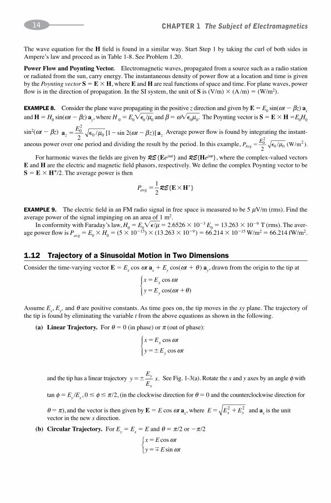
1.12 Trajectory of a Sinusoidal Motion in Two Dimensions
Consider the time-varying vector E � Ex cos ωt ax � Ey cos(ωt � θ ) ay, drawn from the origin to the tip at
Assume Ex, Ey, and θ are positive constants. As time goes on, the tip moves in the xy plane. The trajectory ofthe tip is found by eliminating the variable t from the above equations as shown in the following.
(a) Linear Trajectory. For θ � 0 (in phase) or π (out of phase):
and the tip has a linear trajectory See Fig. 1-3(a). Rotate the x and y axes by an angle φ with
tan φ � Ey /Ex , 0 φ π /2, (in the clockwise direction for θ � 0 and the counterclockwise direction for
θ � π), and the vector is then given by E � E cos ωt ax, where and ax is the unitvector in the new x direction.
(b) Circular Trajectory. For Ey � Ex � E and θ � π /2 or �π /2
x E t
y E t
�
�
cos
sin
ωω�
⎧⎨⎩
E E Ex y� �2 2
yE
Exy
x
�� .
x E t
y E tx
y
�
��
cos
cos
ωω
⎧⎨⎪
⎩⎪
x E t
y E tx
y
�
� �
cos
cos( )
ωω θ
⎧⎨⎪
⎩⎪
Pavg � �1
2RE{ }*E H
EXAMPLE 8. Consider the plane wave propagating in the positive z direction and given by E � E0 sin(ωt � βz) ax
and H � H0 sin(ωt � βz) ay, where H 0 � E0������0 /μ0 and β � ω������0μ0. The Poynting vector is S � E � H �E0H0
sin2(ωt � βz) Average power flow is found by integrating the instant-
aneous power over one period and dividing the result by the period. In this example, P EAvg � 0
2
0 02
2� / ( / ).μ W m
a az zE
t z� � � �02
0 021 2/ [ sin ( )] ,μ ω β

The tip has a circular trajectory x2 � y 2 � E 2. For θ � π /2 it moves in the clockwise direction, andfor θ � �π /2 it moves in the counterclockwise direction. See Fig. 1-3(b).
(c) Elliptical Trajectory. For the general case (but with still constant values for Ex, Ey, and θ ),
But cos2 ωt � sin2 ωt � 1. Therefore,
The tip of the vector moves along an elliptical trajectory. See Fig. 1-3(c).
The cross-product term xy in the above equation may be eliminated by aligning the major and minor axesof the ellipse in Fig. 1-3(c) with the horizontal and vertical directions. This is done by rotating the x and yaxes by an angle γ in the counterclockwise direction, where cot(2γ) � (k2 � 1) / 2k cos θ, k � Ex /Ey,and 0 γ pi /2.
x
E
y
E
xy
E Ex y x y
⎛⎝⎜
⎞⎠⎟
⎛⎝⎜
⎞⎠⎟
2 222
� � �cos sinθ θ
x E t
y E t t
tx
y
�
� �
cos
(cos cos sin sin )
cosωω θ ω θ
ω⎧⎨⎩
⇒��
��
x
E
tx E y E
x
x ysin( / ) cos ( / )
sinω
θθ
⎧
⎨⎪⎪
⎩⎪⎪
CHAPTER 1 The Subject of Electromagnetics 15
E
E Ey
(b) Circular polarization: LCP isleft-circular and RCP is right-circular.
Ex
ELEP
REP
E
E
(c) Elliptical polarization: LEP isleft-elliptic and REP is right-elliptic.
LCP
RCP
Ex
Ey
(a) Linear polarization.
Fig. 1-3 Three types of polarization and trajectories of the tip of the E vector in a plane wave propagating in the �zdirection (out of the page).
1.13 Wave Polarization
All plane waves share the property that the E (and H) fields are perpendicular to the direction of propagation(e.g., the z axis). In general, the electric field (as well as the magnetic field) has two components: namely, thesein the x and y directions. In the case of sinusoidal time variation (also called time harmonics) and dielectricmedia (e.g., free space), the fields are functions of e j (ω t � βz). For any given value of z, the electric field is givenby the time-varying vector
where ax and ay are unit vectors in the x and y directions, respectively, and θ is the phase difference between thex and y components of the field. Simply expressed, the electric field is an E vector with x and y components (eachof which vary sinusoidally with time)
x E t
y E tx
y
�
� �
cos
cos( )
ωω θ
⎧⎨⎩
E a a� �RE {(E E e ex x yj
yj tθ ω) }

This is the same vector we discussed in Section 1.12 with three possible tip trajectories. Each trajectory is asso-ciated with one type of wave polarization as summarized below.
(a) Linear Polarization. In a linearly polarized wave, the tip of the field vector moves back and forth alonga line in the xy plane as time goes by. See Fig. 1-3(a). The x and y components of the field can becombined, representing E by a one-dimensional vector which oscillates in time, as we have generallyconsidered plane waves with one component only. It is seen that the sum of several linearly polarizedwaves is linearly polarized as well. Linearly polarized waves are also called uniform plane waves.
(b) Circular Polarization. In a circularly polarized wave, the tip of the field vector moves along a circle astime goes by. With propagation in the �z direction, if the motion of the tip is in the counterclockwisedirection (direction of the right-hand fingers with the thumb pointing in the direction of propagation), thewave has right circular (also called right-hand circular) polarization. If the motion of the tip is in theclockwise direction (direction of the left-hand fingers with the thumb pointing in the direction ofpropagation), the wave has left circular (also called left-hand circular) polarization. See Fig. 1-3(b).
(c) Elliptical Polarization. In an elliptically polarized wave, the tip of the field vector moves on anellipse as time goes by. See Fig. 1-3(c). Here, as in the case of circular polarization, the rotation ofthe tip can be left-handed or right-handed, resulting in left elliptical or right elliptical polarizations.
(d) Some Practical Effects of Polarization. There are several practical correlates of, and benefits to,recognizing the polarization of a plane wave. Some examples are the following. The polarization of anantenna and the radiated energy from it are related. Similarly, the energy collected by an antenna froman incident wave is related to its polarization. On the other hand, orientation in some cases such as adipole antenna is not a critical factor in signal reception if it is carried by circularly polarized waves. In electromagnetics, the term “polarization” is also used in relation to a medium such as a dielectric.Although this second usage is unrelated to wave polarization, polarization of a medium can change itsrelative permittivity (see Section 8.1) and also influence polarization of the wave passing through it.
1.14 Electromagnetic Spectrum
A plane wave in free space propagating in the positive z direction is given by sin(ωt � βz), where ƒ � ω /(2π)is the frequency of the wave and λ � 2π /β is its wavelength. At any time the waveform repeats itself when zchanges by λ. The wavelength and frequency are related by ƒ � λ � u, where u is the speed of light. The elec-tromagnetic spectrum ranges from extremely low frequencies (ELF, 3-30 Hz) in the radio range to gamma rays(up to 1023 Hz). It is summarized in Table 1-9a. The radio frequency bands are summarized in Table 1-9b.
CHAPTER 1 The Subject of Electromagnetics16
TABLE 1-9a Electromagnetic Spectrum
100 Mm 1 mm 750 nm 380 nm 600 pm 3 fmRadio and microwave Infrared Visible light Ultraviolet X rays γ rays3 Hz 300 GHz 400 THz 760 THz 500 PHz 1023 Hz
TABLE 1-9b Radio Frequency Bands
NAME FREQUENCY WAVELENGTH APPLICATIONS
ELF 3–30 Hz 100 Mm to 10 MmSLF 30–300 Hz 10 Mm to 1 Mm Power gridsULF 300–3000 Hz 1 Mm to 100 kmVLF 3–30 kHz 100 km to 10 kmLF 30–300 kHz 10 km to 1 kmMF 300–3000 kHz 1 km to 100 m AM broadcastHF 3–30 MHz 100 m to 10 m ShortwaveVHF 30–300 MHz 10 m to 1 m FM, TVUHF 300–3000 MHz 1 m to 10 cm TV, cellularSHF 3–30 GHz 10 cm to 1 cm Radar, dataEHF 30–300 GHz 1 cm to 1 mm Radar, data
E � Extremely, S � Super, U � Ultra, V � Very, L � Low, M � Medium, H � High, F � Frequency.

1.15 Transmission Lines
Transmission lines are structures consisting of two conductors which guide electromagnetic waves between twodevices over a distance. Examples are power lines, telephone wires, coaxial cables, and microstrips. A transmis-sion line has resistance, capacitance, and inductance, all distributed throughout the structure. The wave equationsfor and behavior of a transmission line can be derived from a model with distributed parameters.
Transmission Line Equation. Consider an incremental line segment of length �x and model it by the lumped-element two-terminal circuit shown in Fig. 1-4.
CHAPTER 1 The Subject of Electromagnetics 17
v(x, t)
R L
G C
i(x, t)�
�Δ X
Fig. 1-4 Incremental lumped-element model of a segment of a transmission line.
By applying Kirchhoff’s current and voltage laws at the terminals of the incremental segment and dividing allsides by �x, we obtain the following equations:
where R and L are the resistance and inductance per unit length of the conductors. Similarly, G and C are theconductance and capacitance per unit length of the dielectric per unit length. In the limit �x → 0, the equationsbecome first-order partial differential equations:
Sinusoidal (AC) Steady State Excitation. In the sinusoidal (AC) steady state, the voltage and current can beexpressed as phasors, resulting in the equations derived in Table 1-10.
TABLE 1-10 Derivation of Transmission Line Equations in Phasor Form
v x t
xRi x t L
i x t
ti x t
xGv x
( , )( , )
( , )
( , )( ,
� �
� tt Cv x t
t)
( , )�
ΔΔ
ΔΔ
v x t
xRi x t L
i x t
t
i x t
xGv x
( , )( , )
( , )
( , )( ,
� �
�
tt Cv x t
t)
( , )�
v x t V x e i x t I x e
dV
j t j t( , ) { ˆ( ) } ( , ) { ˆ( ) }
ˆ
� �RE REω ω
(( ) ˆ( )ˆ( ) ˆ( )
ˆ( )
x
dxZ I x
dI x
dxYV x
d V x
dx
� �
�
↘ ↙2
22γ ˆ̂ ( )
ˆ( ) ˆ( )
V x
d I x
dxI x
2
22�γ
where Z � R � jLω, Y � G � jCω, and γ � ���ZY � �����(R � j����Lω�)(G��������jCω)�� � α � jβ is called the propaga-tion constant. The resulting equations have the same form as that of wave propagation. The solutions are
V̂(x) � V�0 e�γ x � V�
0 eγ x
Î(x) � I�0 e�γ x � I�
0 eγ x

where the complex numbers V�0 , V�
0 , I�0 , and I�
0 are constants of integration (and are constrained by the line’sboundary conditions as illustrated in Example 10). These constants are also related by the line equation
(Table 1-10). Therefore,
where Z0 � ����Z /Y (called the line’s characteristic impedance). These phasors can readily be transformed intotheir time-domain counterparts. For example, the time-domain representation of the voltage along the line is
v (x, t) � RE{V̂(x) e jωt} � ⎪V�0 ⎪e�α x cos(ωt � βx � φ�) � ⎪V�
0 ⎪eαx cos(ωt � βx � φ�)
where
V�0 � ⎪V�
0 ⎪e�φ � and V�0 � ⎪V�
0 ⎪e�φ�
At any point on the line, the current and voltage are made of two sinusoidal waves with decaying amplitudesand angular frequency ω; one wave, called the incident wave V̂inc, travels to the right (in the �x direction) withdecaying amplitude V�
0 e�αx. The other, called the reflected wave V̂reƒl, travels to the left (in the �x direction)with decaying amplitude V�
0 eαx. The following pointwise parameters are defined for a transmission line and areused in its analysis.
Reflection coefficent:
Impedance (looking back toward the receiving end):
AC Steady State in a Lossless Line. If R � G � 0 (or, at high frequencies, when their contribution to γ canbe ignored), the propagation constant becomes purely imaginary, γ � jβ. The solutions to the transmission lineequations then become
where β � ω���LC, Z0 � ��L�/�C. V�0 and V�
0 are determined from the boundary conditions (see Example 10).
EXAMPLE 10. A lossless transmission line connects an AC generator (Vg � 10 Vrms at 750 MHz with an out-put impedance of Zg � 10 Ω) to the load ZR � 150 Ω. See Fig. 1-5. The line is 20 cm long and has distributedparameters L � 0.2 μH/m and C � 80 pF/m. Find the voltage and current in the line.
ˆ( )
ˆ( )
V x V e V e
I xV
Ze
V
Z
j x j x
j x
� �
� �
� � �
��
�
0 0
0
0
0
β β
β
00
e j xβ
Z xV x
I xZ
x
x( )
ˆ( )ˆ( )
( )
( )� �
�
�0
1
1
ΓΓ
Γ( )ˆ ( )ˆ ( )
xV x
V xrefl
inc
�
IV
ZI
V
Z00
00
0
0
��
��
� ��and
dV x
dxZ I x
ˆ( ) ˆ( )�
CHAPTER 1 The Subject of Electromagnetics18
I
V ZRVg ��
Zg
Zin
x��� x�0
�
Fig. 1-5 A transmission line connecting a generator to a load.

Expressions developed for V̂(x) and Î(x) in the AC steady state will be used. From the given values for the line, Z0 � ����L /C � 50 Ω, β � ω ����LC � 6π, and β� � 1.2π. Let x � 0 at the load and x � �� at the gen-erator. Apply the boundary conditions at those two ends of the line to find V�
0 and V�0 .
(a) At x � 0 (the load)
However, the i � v characteristic of the load requires that V̂(0) � ZRÎ(0). Therefore,
from which
(b) At x � �� (the generator end of the line)
However, application of Kirchhoff’s voltage law at x � �� results in V̂ (�� ) � Vg � Zg Î(�� ).Therefore,
from which
By substituting for Vg � 10��2, Z0 � 50, β� � 1.2π, Γ � 0.5, and Zg � 10 in the above equation, we find V�
0 � 10.27∠160° and V0� � 5.13∠160°. The voltage and current throughout the line (�0.2 x 0) are
v (t) � 10.27 cos(ωt � βx � 2.7925) � 5.13 cos(ωt � βx � 2.7925)
i(t) � 0.2054 cos(ωt � βx � 2.7925) � 0.1027 cos(ωt � βx � 2.7925)
where the 160° phase angle is converted to 160π /180 � 2.7925 radians. A right-shift (delay) of 2.7925/ω � 593 psin the time origin produces Vg � 10��2∠�160° and
v(t) � 10.27 cos(ωt � βx) � 5.13 cos(ωt � βx)
i (t) � 0.2054 cos(ωt � βx) � 0.1027 cos(ωt � βx)
Input Impedance of a Lossless Line. The input impedance of a lossless line is the ratio of the voltage to cur-rent phasors at x � ��. It may be expressed in terms of the reflection coefficient:
Z ZV
IZ
V e V e
V ein � � �
�
��
�� � �
�( )
ˆ( )ˆ( )
���
� �
00 0
0
β β
ββ β
β
β� �
�
���
�
�� �
�
�V eZ
e
e00
2
2
1
1
ΓΓ
VV Z
Z e e Z e eg
j jg
j j00
0
�� �
�� � �( ) ( )β β β β� � � �Γ Γ
V e V e VZ
ZV e V ej j
gg j j
0 00
0 0� � � � � �� � � �β β β β� � � �[ ]
ˆ( )
ˆ( )
V V e V e
IV
Ze
V
j j
j
� � �
� � �
� � �
� �
�
�
� �
�
0 0
0
0
0
β β
β
ZZe j
0
� β�
V VZ Z
Z ZR
R0 0
0
0
0 5� �� ��
��Γ Γ, . .where
V VZ
ZV VR
0 00
0 0� � � �� � �[ ]
ˆ( )
ˆ( )
V V V
IV
Z
V
Z
0
0
0 0
0
0
0
0
� �
� �
� �
� �
CHAPTER 1 The Subject of Electromagnetics 19

where is the reflection coefficent at the load. The input impedance may also be expressed in termsà ��
�
V
V0
0
CHAPTER 1 The Subject of Electromagnetics20
of the load impedance by substituting in the above expression for . The result is
EXAMPLE 11. Replace the circuit of Fig. 1-5 by the equivalent circuit of Fig. 1-6 and use it to obtain V0�.
ZV
IZ
Z jZ
Z jZinR
R
��
��
�
�
ˆ( )ˆ( )
tan
tan
��
��0
0
0
ββ
à ��
�
Z Z
Z ZR
R
0
0
Vg ��
�
�
Zg I(��)
V(��) Zin
Fig. 1-6 Equivalent circuit of the transmission line of Fig. 1-5.
From Fig. 1-5,
From Fig. 1-6,
From equating the above expressions,
EXAMPLE 12. In the circuit of Example 10, (a) find the input impedance of the line (at the generator end lookingtoward the load), and (b) use the equivalent circuit of Fig. 1-6 to calculate V�
0 .
(a) Having Z0 � 50, ZR � 150, β� � 1.2π, and tan β� � 0.7265, we calculate Zin:
(b) Having Vg � 10��2, Zq � 10, Zin � 64.36∠ �51.74°, β� � 1.2π, and Γ � 0.5, we calculate V�0 :
Some Parameters of Lossless Transmission. The angular frequency is ω (frequency ƒ � ω /(2π) Hz and periodT � 1/ƒ seconds). The incident and reflected waves are sinusoids with constant amplitudes V�
0 and V�0 , respectively.
Each wave repeats itself after traveling a distance of λ � 2π /β, which is called the wavelength. The phase veloc-ity of the traveling wave in a lossless line is μρ � λ /T � ω /β � 1/���LC. For two-wire or coaxial transmission lines(made of perfect conductors and dielectrics), LC � μ�, which results in a phase velocity μp � 1/���μ�, where μ and� are the permeability and permittivity, respectively, of the insulation between the conductors. Because permeabil-ity and permittivity are specified in terms of their relative values to those of free space, μ � μrμ0 and � � �r�0, thephase velocity becomes μp � c/���μr�r, where c � 1/����μ0�0 is the speed of light in free space.
V VZ
Z Z e eg
in
g in0
1 10 2 6��
�� �
��⎛
⎝⎜⎞
⎠⎟⎛
⎝⎜⎞⎠⎟β β� �Γ
44 36 51 74
10 64 36 51 74 1 5 0
. .
. . ( . cos .
∠ °∠ °
�
� � � �β� j 5510 27 160
sin ).
β�� ∠ ° V
Z ZZ jZ
Z jZ
jin
R
R
��
��
� �0
0
0
50150 50 0 72tan
tan
.ββ��
665
50 150 0 726564 36 51 74
� �� �
j .. .∠ ° Ω
V VZ
Z Z e eg
in
g in0
1+ ⎛
⎝⎜⎞
⎠⎟⎛
⎝⎜⎞⎠⎟
�� � �β β� �Γ
ˆ( )V VZ
Z Zgin
g in
� ��
�
ˆ( ) ( ),V V e V e V e e� � � � �� � � � �� � � � �0 0 0
β β β βΓ Γwhere ���
�
Z
ZR
R
Z
Z0
0
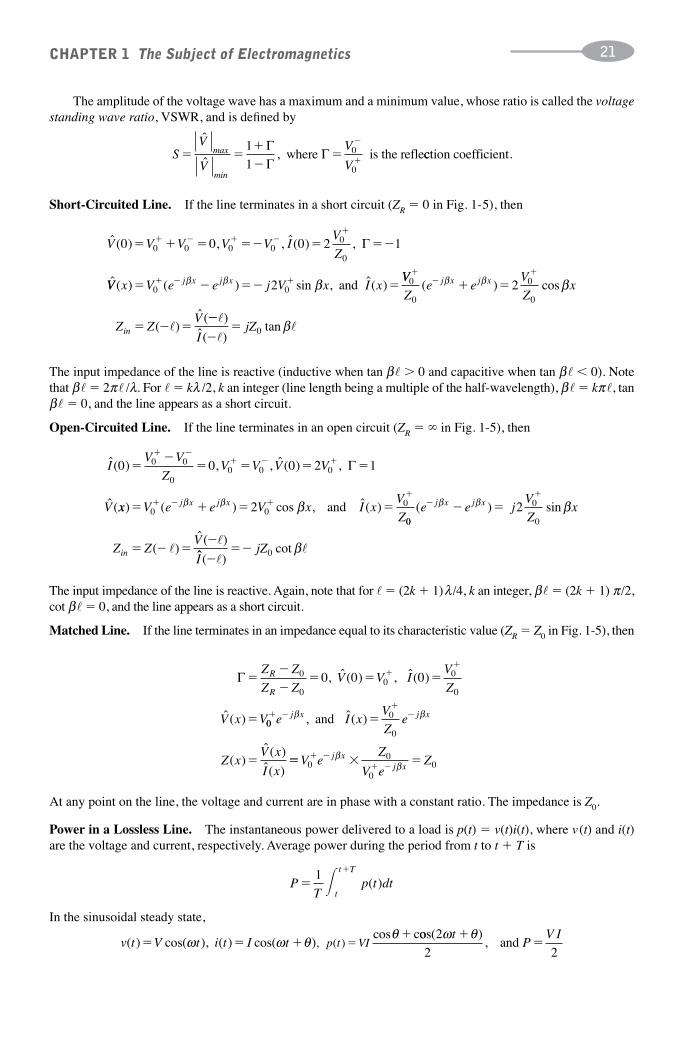
The amplitude of the voltage wave has a maximum and a minimum value, whose ratio is called the voltagestanding wave ratio, VSWR, and is defined by
Short-Circuited Line. If the line terminates in a short circuit (ZR � 0 in Fig. 1-5), then
The input impedance of the line is reactive (inductive when tan β� 0 and capacitive when tan β� � 0). Notethat β� � 2π� /λ. For � � kλ /2, k an integer (line length being a multiple of the half-wavelength), β� � kπ�, tanβ� � 0, and the line appears as a short circuit.
Open-Circuited Line. If the line terminates in an open circuit (ZR � ∞ in Fig. 1-5), then
The input impedance of the line is reactive. Again, note that for � � (2k � 1)λ /4, k an integer, β� � (2k � 1) π /2,cot β� � 0, and the line appears as a short circuit.
Matched Line. If the line terminates in an impedance equal to its characteristic value (ZR � Z0 in Fig. 1-5), then
At any point on the line, the voltage and current are in phase with a constant ratio. The impedance is Z0.
Power in a Lossless Line. The instantaneous power delivered to a load is p(t) � v(t)i(t), where v(t) and i(t)are the voltage and current, respectively. Average power during the period from t to t � T is
In the sinusoidal steady state,
v t V t i t I t p t VI( ) cos( ), ( ) cos( )cos c
, ( )� � ��
�ω ω θ θ oos( ),
2
2 2
ω θtP
V I��and
PT
p t dtt
t T
��1 � ( )
à ��
�� � �
�
��Z Z
Z ZV V I
V
Z
V x V
R
R
0
00
0
0
0 0 0, ˆ( ) , ˆ( )
ˆ( ) 000
0
� ��
��
�
e I xV
Ze
Z xV x
I x
j x j xβ β, ˆ( )
( )ˆ( )ˆ( )
and
�� � �� �� �
V eZ
V eZj x
j x00
00
ββ
ˆ( ) , , ˆ( ) ,
ˆ(
IV V
ZV V V V
V
0 0 0 2 10
��
� � � �� �
� � �0 00 0 0 Γ
xx V e e V x I xV
Zj x j x) ( ) cos , ˆ( )� � � �� � �
�
0 00andβ β β200 0
2( ) sin
( )ˆ( )
e e jV
Zx
Z ZV
j x j x
in
��
� �
� � ��
β β β0
��
ˆ̂( )cot
IjZ
���
��0 β
ˆ( ) , , ˆ( ) ,
ˆ
V V V V V IV
Z0 0 0 2 1
0
� � � �� � ��� � � ��
0 0 0 00 Γ
VV x V e e j V x I xj x j x( ) ( ) sin , ˆ( )� � �� �� � �0 0 andβ β β2
VV
Ze e
V
Zx
Z ZV
j x j x
in
0 0�
��
� �
� � �
0 0
2( ) cos
( )ˆ(
β β β
���
��
��
�)
ˆ( )tan
IjZ0 β
SV
V
V
V� �
�
��
�
�
ˆ
ˆ,max
min
1
1
ΓΓ
Γwhere is the refle0
0
cction coefficient.
CHAPTER 1 The Subject of Electromagnetics 21

In the phasor domain,
where V̂ is the voltage phasor across the load, Î* is the complex conjugate of its current phasor, and θ is the phaseangle of the current with reference to the voltage. Accordingly, in a lossless transmission line, the average powersdelivered to the load by the incident wave or reflected from it by the reflected wave are, respectively,
The net average power delivered to the load is
(Superposition of power applies because the incident and reflected waves have the same frequency.)
SOLVED PROBLEMS
Note: A Cartesian coordinate system (x, y, z) with unit vectors ax, ay, and az is assumed in the problemsbelow. Thus, by (a, b, c) is meant a point in three dimensional space with x � a, y � b, and z � c. Similarly, apoint in the xy plane is shown by (a, b).
1.1. Two identical point charges Q are separated by distance d in a homogeneous medium. Find the electricfield intensity at a point r m away from each charge. See Fig. 1-7. Find the near and far field intensities.
By the superposition principle, E � E1 � E2, where E1 and E2, each with magnitude Q /(4π�r2), are the field intensitiesdue to each charge. Designate the line connecting the two charges as the x axis with the origin at its middle. The testcharge will be at y � ����r2 ����d 2/4���. The x components of E1 and E2 cancel each other, while their y components add.From Coulomb’s law and the geometry of the problem we find the field intensity at a point on the y axis to be
where ay is the unit vector in the y direction. At the origin, r � d /2, and the field is zero. At r d, the field is
which is nearly the field intensity due to a point charge of 2Q.
1.2. Repeat Problem 1.1 for two equal charges of opposite signs.
Here the y components of E1 and E2 cancel each other and the x components add. See Fig. 1-8. From the geometryof the problem,
E a a� �Ed
r
Qd
rx x1 34π�
E a� Q
ry
2 2π�,
E a a� ��
22
41
2 2
3Ey
r
Q r d
ry yπ�
/
P P PV
Zinc refl� � � �
�0
2
0
2
21( )Γ
PV
ZP
V
Zinc ref l� ��� �
0
2
0
20
2
02 2, and
Γ
v t V e i t I e Pj t j t( ) { ˆ }, ( ) { ˆ }, { ˆ� � �RE RE REω ω and1
2VV I V I· ˆ } ˆ ˆ cos∗ �
1
2θ
CHAPTER 1 The Subject of Electromagnetics22
Q Q
rr
E
E1E2
d
Fig. 1-7 Electric field intensity along the orthogonalbisector of the line connecting two like charges �Q.
Q �Q
rr
E
E1
E2
d
Fig. 1-8 Electric field intensity along the orthogonalbisector of the line connecting two unlike charges �Q.

The field is inversely proportional to r3. At r � d /2, it becomes which is the field intensity due to apoint charge of 2Q.
1.3. Two point charges of magnitude 0.1 μ C and opposite signs are placed in vacuum on the x axis atpositions �1 m, respectively. (a) Calculate the field intensity at the point (0, 1). (b) Approximate thevalue of intensity at a point 10 cm away from one charge by ignoring the effect of the other charge anddetermine the percentage of error due to such an approximation.
(a) As in Fig. 1-8, the y components of the fields produced by each point charge cancel each other and their x
components add, resulting in . With Q � 0.1 μC, d � 2 m, and r � ��2 m, we find E � 636.4 ax V/m.
(b) Each point charge dominates the field in its 10-cm vicinity, resulting in E � �180 ar kV/m, where ar is theradial unit vector with that charge as the center. The field is directed outward at x � �1 and inward at x � 1. Themost error occurs when the test point is at (�.9, 0), with a relative percentage error of 100 � 1/(1 � 192) � 0.275%.
1.4. Three point charges Q, Q1, and Q2 are separated by a distance d from each other in a homogeneousmedium. Find the electric force on Q.
Let the line connecting Q1 and Q2 be the y axis with the origin at its center. The forces exerted by Q1 and Q2 on Qare given by the vectors F1 and F2.
F1 � kQ1a1 and F2 � kQ2a2
E a�Qd
rx
4 3π�
E a�Q
rx
2 2π�,
CHAPTER 1 The Subject of Electromagnetics 23
d
d
xd
y
Q2
Q1
F1
F2
Q
F
Fig. 1-9 Forces on charge Q due to charges Q1 and Q2.
where a1 and a2 are unit vectors from Q1 and Q2, respectively, toward Q, and k � Q /(4π�d 2). See Fig. 1-9. Thetotal force on Q is the vectorial addition F � F1 � F2 found by adding the x and y components of the two forces.Hence,
1.5. A charge Q1 is placed at the point (0, �d ) and another charge Q2 at (0, d ). Develop an equation for theelectric field intensity at a test point (x, y) as a function of d, Q1, Q2, x, and y.
F kQ F kQ
F kQ F kQ
F F
x y
x y
x
1 1 1 1
2 2 2 2
3 2 2
3 2 2
� �
� ��
�
/ /
/ /
11 2 1 2 1 2 1 23 2 2x x y y yF k Q Q F F F k Q Q
Q
� � � � � � �
�
( ) / ( ) /
F22
32 1 2 1 2π�dQ Q Q Qx y( ) ( )� � �a a⎡⎣ ⎤⎦

Let R1 and R2 represent vectors connecting Q1 and Q2, respectively, to (x, y).
1.6. Flux lines at any point in an electric field in a homogeneous medium are tangent to the field intensity atthat point. Consider the electric field in such a medium produced by two point charges �Q placed at�d m on the x axis, respectively. Find the direction of the flux lines at locations (�d, 0) and (0, y).
Each point charge dominates the field in its vicinity, resulting in a radial direction for the field intensity and flux lines(originating from x � d and sinking at x � �d). The flux lines become horizontal (going from right to left) whenthey cross the y axis because the y components of the individual fields cancel each other and their x components add.
1.7. Two small spherical bodies each with mass m � 1 gram are suspended near each other by two strings oflength � � 10 cm as in Fig. 1-10(a). Assume that the spheres are placed in a vacuum and experience agravitational pull(g � 9.81 m /s2). When each is loaded with a charge Q, the spheres separate by adistance of d � 1 cm as in Fig. 1-10(b). Find Q.
R a a aR a
1 12 2
11
1
12� � � � � � � �x y d R x y d
R
xx y R( ) , [ ( ) ] , xx y
x y
y d
R
x y d R x y d
� �
� � � � � �
( )
( ) , [ ( ) ]
a
R a a
1
2 12 2
12 ,,
( )a
R a a
E a
Rx y
R
R
x y d
RQ
R
Q
22
2 2
11
12 1
1
4 4
� �� �
� �π π� ��
� �
Rx y d
Q
R
Q
Rx
x y
R
13
22
22 2
2
234 4
[ ( ) ]
[
a a
E a
� �
� �π π
aa a
E E E
x y
x
y d
x Q
R
Q
R
� �
� � � �
( ) ]
1 a21
13
2
234π�
⎡⎣⎢
⎤⎦⎥
���
��1
41
13
2
23π�
Q y d
R
Q y d
Ry
( ) ( )⎡⎣⎢
⎤⎦⎥
a
CHAPTER 1 The Subject of Electromagnetics24
� �� �
d
Q Q
Θ Θ
mg mg
(a) (b)
F F
Fig. 1-10 Two charged bodies repel each other with a force FQ
d�
2
24π�.
The charge may be calculated from the separation distance d. The gravitational force on each sphere is mg in thedownward vertical direction. The Coulomb force is F � Q 2/(4π�d 2) in the horizontal direction, pushing thespheres away from each other. At equilibrium, each string aligns itself with the direction of the total force on itsbob. From the similarity of the force- and string-triangles we find
Substituting Q 2/(4π�d 2) for F and solving for Q we find
With �0 � 8.854 � 10�12 F/m, d � 0.01 m, � � 0.1 m, and m � 10�3 kg, we obtain Q � 2.3376 nC.
Qd
dmg2 0
3
2 2
2
2�
�
π�
� ( / )
F
m g F
dF
mgd
d2 2 2 2 2
2 2
2�� �
�
/ /
( / )� �⇒

1.8. An infinitely long, straight line has a uniform charge distribution of ρ C/m. Use Gauss’s law to find theelectric field at a point r m away from it.
Consider a cylindrical volume of height � with circular cross sectional area of radius r, which has the line as its axis.The volume contains a total charge of Q � ρ�. By symmetry, the E field is radial in direction and has the samemagnitude on the surface of the cylinder. The total flux through the surface is Ψ � �E � � � πr2. By Gauss’ law, Ψ � Q from which E � ρ /π�r2.
1.9. An infinite plane is uniformly charged with a distribution of ρ C/m2. Use Gauss’s law to find the electricfield at a point r m away from it.
Consider a cylindrical volume with the cross-section area S normal to the plane and bisected by it in two equallengths. The volume contains a total charge of Q � ρS. By symmetry, the E field is directed away from the planeand normal to it with the same magnitude on the cylinder’s cross sections. The total flux through the surface of thecylinder is Ψ � �E � 2 � S. By Gauss’s law, Ψ � Q from which E � ρ /(2�), which is independent of the distancefrom the plane.
1.10. A uniform charge distribution with density ρ C/m2 is established on the infinite xy plane (z � 0). Findthe electric potential at points above or below the plane.
For z 0, the electric field intensity is E � ρ/(2�) az and V � E � z � ρz /(2�). For z � 0, E � �ρ/(2�) az and V � �ρz/(2�).
1.11. An infinite plane at z � d is uniformly charged with a density ρ C/m2 and a second plane at z � 0 withdensity �ρ C/m2. Find the electric field intensity E and potential V at �∞ � z � �∞ with reference toz � 0.
Let E1 and E2 represent the electric fields due to the first and second planes, respectively. From the result ofProblem 1.10 and using the superposition principle we obtain
By integrating E along the z axis with reference to the potential at z � 0 we obtain
1.12. Two infinite parallel planes carry uniform charge distributions of �ρ0 cos(ωt), respectively. Find theelectric field intensity, the electric potential, and the displacement current in the space between them ifthe gap separating them is filled with (a) air, (b) a dielectric material with �r � 100.
Note that the displacement current remains the same in (a) and (b). The electric field intensity and the electricpotential are reduced by a factor of 100 in (b).
1.13. Find the average and rms values of the force per unit length between two infinitely long wires that areseparated by 1 m and carry 60-Hz AC currents of 100 amperes (rms) in opposing directions in air.
Average of F is 2 � 10�3 N. Its rms value is 2 10 11
22 45 103 3� � � �� �. N.
i t t i t t
F
( ) sin( ), ( ) [ cos( )]� � �
�
100 2 377 10 1 7542 4
μμπ
ππ
02 7
4
2
4 10
210 1 754 2 10
i t
dt
( )[ cos( )]�
�� � � �
��� �3 1 754[ cos( )] ( )t N
( ) cos( ), cos( ),a E t Vd
tD
t� �
� �� 0
0
0
0
0
� � ��ρ ω ρ ω ω
ρρ ω
ρ ω
0
00
0
1001
100
1
10
sin( )
( ) cos( ),
t
b E t V� ��
� � �00
0
00
ρ ω ω ρ ωdt
D
tt
�cos( ), sin( )
��
V
d z d
z z d
z
�
�
ρρ
/ ,
/ ,
,
�
� 0
0 0
� �
⎧⎨⎪
⎩⎪
Ea
aE
a
1 22
2
20
�
� �
�
� ρ
ρ
ρ
ρ�
�
�z
z
zz d
z d
z,
,
,⎧
⎨⎪⎪
⎩⎪⎪ 22
0
0
01 2
�
�
aE E E
a
z
z
z
z d
,
,
,�
� � �� � �
⎧
⎨⎪⎪
⎩⎪⎪
andels
ρ
eewhere
⎧⎨⎪
⎩⎪
CHAPTER 1 The Subject of Electromagnetics 25

1.14. Two infinitely long parallel wires separated by 1 m are at 6 m above ground. Each carries a 60-Hz ACcurrent of 100 amperes (rms), but in opposing directions. See Fig. 1-11. Find the magnetic flux densityB at a test location on the ground which is at an equal distance from the wires.
CHAPTER 1 The Subject of Electromagnetics26
B1B2
d
h
B
Fig. 1-11 Magnetic flux density B�B1�B2 due to a pair of overhead lines carrying currents in opposite directions.
The instantaneous current in the wires is i(t) � 100��2 sin (377t). The magnetic flux density due to each wire is
directed at a right angle to the line connecting the test point to that wire. The horizontal components of B1 and B2
cancel each other, but the vertical components add. From the similarity between the vector- and distance triangles,we find B � 0.78 ay μT.
1.15. An AC current in an overhead wire generates an AC magnetic field with BAC � 50 sin(377t) μT at a testlocation below. The earth’s static magnetic field at that location is BDC � 50 μT, directed toward themagnetic north. Find the total field (instantaneous, average, and rms values) at that location if thecurrent runs in a (a) west-east, or (b) south-north direction.
Let the west-east direction be the x axis and the south-north direction be the y axis, with unit vectors ax and ay,respectively. Then, B � BDC � BAC, where BDC � 50ay μT.
(a) I � I0 sin (377t)ax, BAC � 50 sin (377t)ay, B � 50 [sin (377t) � 1] ay, Bavg � 50, Brms � 61.23
(b) I � I0 sin (377t)ay, BAC � �50 sin (377t)ax, B � 50 [�sin (377t)ax � ay], Bavg � 60.8, Brms � 43.3
All magnetic field values are in μT.
1.16. A single-strand rectangular test loop (1 m � 10 cm) is placed length-wise in parallel with, and at adistance of 10 m from, a very long straight wire such that they form a plane. The wire carries a 50-A(rms) sinusoidal current at the frequency ƒ Hz, and the medium is free space. Obtain the emƒ induced inthe loop as a function of ƒ, and find its rms values at 60 Hz and 60 kHz.
The rms value of the induced emƒ is 0.2π ƒ (μV). At 60 Hz it is 37.7 μV, and at 60 kHz it becomes 37.7 mV.
i f t
B Hi
r
�
� � ��
��
�
50 2 2
2
4 10
2 1050 20
07
sin( )π
μ μπ
ππ
ssin( ) sin( )
sin(
2 10 2 2
10 2 2
6
7
π π
φ π
f t f t
B S f
�
� � �
�
� tt
emfd
dtf f t
)
cos( )�� � � �φ π π2 2 10 27
Bi
Rt� �
�
� ��
�μπ
ππ
07
2
4 10
2 36 0 25100 2 377 4 7
.sin( ) . ssin( ) ( )377t μT

1.17. Prove the necessity for the displacement current introduced by Maxwell in Ampere’s law.
First consider Ampere’s law in its original form, ∇ � H � J, and then take the divergence of both sides of it: ∇ · (∇ � H) � ∇ · J. But ∇ · (∇ � H) � 0 (divergence of the curl is always zero according to line 11(a) in Table 1-5).This would require ∇ · J � 0, contradicting, in time-varying fields, conservation of charge which states that ∇ · J � ∂ρ
—∂t� 0. Now consider Ampere’s law in the modified form with Maxwell’s displacement current
included, ∇ � H � J � ∂D—∂t
, and take the divergence of both sides: .
By Gauss’s law, . Therefore, which is the statement of
conservation of charge for a time-varying field. Adding the displacement current to Ampere’s law resolves the contradiction.
1.18. Consider the pair of vectors E � E0 sin ω(t � ����μ z) ax and H � H0 sin ω(t � ����μ z) ay, where ax and ay are unit vectors in the x and y directions, respectively. Show that in order to conform with Maxwell’s equations (i.e., represent electromagnetic waves in a homogeneous medium), H0 � E0����� /μ.
Faraday’s law requires . In this problem we have
and . To conform with Faraday’s law, we need E0ω����μ � μωH0, or H0 � E0�����/μ.
In free space, H0 � 2.65258 � 10�3E0.
1.19. Derive the source-free wave equation for E in the phasor domain from its time-domain form.
The time-domain wave equation for the E field is . For harmonic waves
Substitute the above in the time-domain equation and drop the common term ejωt from both sides to obtain ∇2E � ω2 μ�E � 0. This is the phasor-domain wave equation.
1.20. Derive the phasor-domain wave equation for a magnetic field in source-free media from Maxwell’sequations.
Start with Maxwell’s equations given below and proceed through Steps 1, 2, and 3.
Faraday’s law: ∇ � E � �jωμH Gauss’s law for the electric field: ∇ · E � 0
Ampere’s law: ∇ � H � jω�E Gauss’s law for the magnetic field: ∇ · H � 0
Step 1. Take the curl of both sides in Ampere’s law ⇒ ∇ � (∇ � H ) � jωμ(∇ � E)
From Faraday’s law, ⇒ ∇ � E � �jωμ ( jω�H ) � ω 2 μ�H
As a result, ⇒ ∇ � (∇ � H ) � ω 2 μ�H
Step 2. From mathematical identities, ⇒ ∇ � (∇ � H ) � ∇(∇ · H ) � ∇2H
But, divergence of H is zero. ⇒ ∇ · H � 0
Therefore, ⇒ ∇ � (∇ � H ) � �∇2H
Step 3. Equate results of Steps 1 and 2 to find that ⇒ ∇2 2H H�� �ω μ
E EE
E� ��( , , ) , ( , , ) ,x y z et
x y z ej t j tω ωω
2
22 2and ∇ EE E x y z� ∇2 ( , , ) .e j tω
∇22
2E
E�μ�
t
Ha
tH t z y� � �ω ω μ0 cos ( )
∇ � � �� � � �E a a
E
zE t zx
y y0ω μ ω μcos ( )∇ � ��EHμ
t
∇ ∇ ∇· · J( ) ,� � � �H
ρt
0
( )∇ · Dt t
�ρ
∇ ∇ ∇ ∇· · J
·( )
( )� � �H
D
t
CHAPTER 1 The Subject of Electromagnetics 27
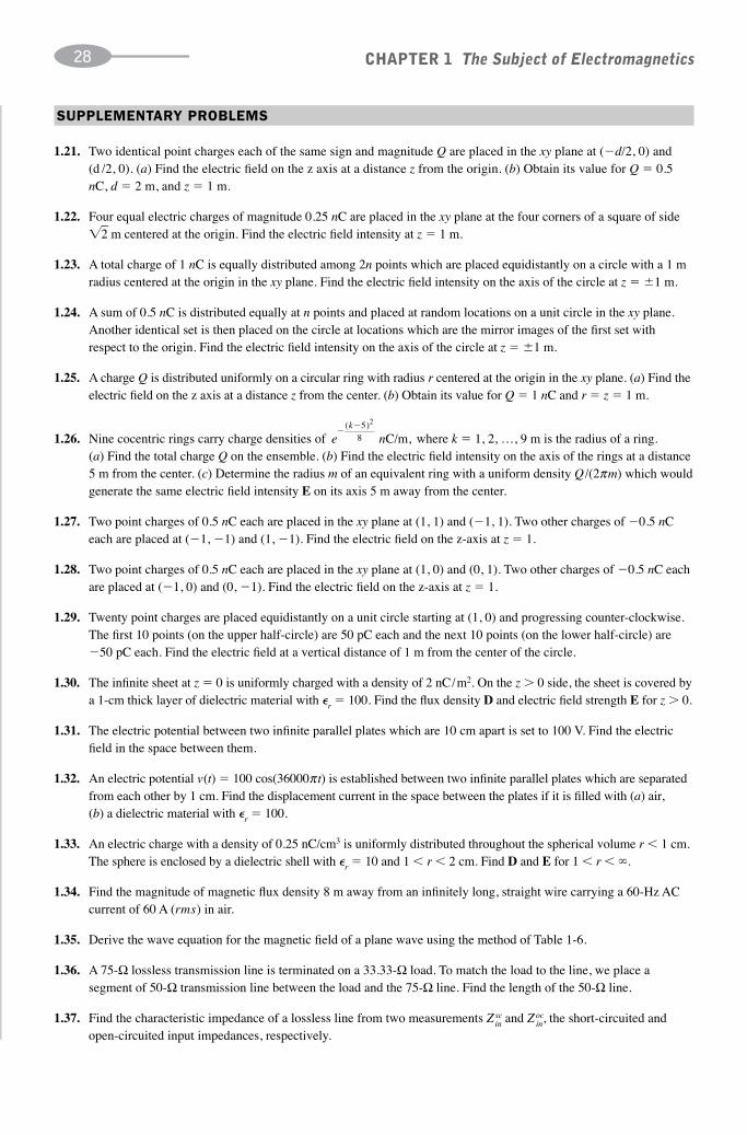
SUPPLEMENTARY PROBLEMS
1.21. Two identical point charges each of the same sign and magnitude Q are placed in the xy plane at (�d/2, 0) and(d /2, 0). (a) Find the electric field on the z axis at a distance z from the origin. (b) Obtain its value for Q � 0.5nC, d � 2 m, and z � 1 m.
1.22. Four equal electric charges of magnitude 0.25 nC are placed in the xy plane at the four corners of a square of side��2 m centered at the origin. Find the electric field intensity at z � 1 m.
1.23. A total charge of 1 nC is equally distributed among 2n points which are placed equidistantly on a circle with a 1 mradius centered at the origin in the xy plane. Find the electric field intensity on the axis of the circle at z � �1 m.
1.24. A sum of 0.5 nC is distributed equally at n points and placed at random locations on a unit circle in the xy plane.Another identical set is then placed on the circle at locations which are the mirror images of the first set withrespect to the origin. Find the electric field intensity on the axis of the circle at z � �1 m.
1.25. A charge Q is distributed uniformly on a circular ring with radius r centered at the origin in the xy plane. (a) Find theelectric field on the z axis at a distance z from the center. (b) Obtain its value for Q � 1 nC and r � z � 1 m.
1.26. Nine cocentric rings carry charge densities of where k � 1, 2, …, 9 m is the radius of a ring. (a) Find the total charge Q on the ensemble. (b) Find the electric field intensity on the axis of the rings at a distance 5 m from the center. (c) Determine the radius m of an equivalent ring with a uniform density Q /(2πm) which wouldgenerate the same electric field intensity E on its axis 5 m away from the center.
1.27. Two point charges of 0.5 nC each are placed in the xy plane at (1, 1) and (�1, 1). Two other charges of �0.5 nCeach are placed at (�1, �1) and (1, �1). Find the electric field on the z-axis at z � 1.
1.28. Two point charges of 0.5 nC each are placed in the xy plane at (1, 0) and (0, 1). Two other charges of �0.5 nC eachare placed at (�1, 0) and (0, �1). Find the electric field on the z-axis at z � 1.
1.29. Twenty point charges are placed equidistantly on a unit circle starting at (1, 0) and progressing counter-clockwise.The first 10 points (on the upper half-circle) are 50 pC each and the next 10 points (on the lower half-circle) are�50 pC each. Find the electric field at a vertical distance of 1 m from the center of the circle.
1.30. The infinite sheet at z � 0 is uniformly charged with a density of 2 nC/m2. On the z 0 side, the sheet is covered bya 1-cm thick layer of dielectric material with �r � 100. Find the flux density D and electric field strength E for z 0.
1.31. The electric potential between two infinite parallel plates which are 10 cm apart is set to 100 V. Find the electricfield in the space between them.
1.32. An electric potential v(t) � 100 cos(36000π t) is established between two infinite parallel plates which are separatedfrom each other by 1 cm. Find the displacement current in the space between the plates if it is filled with (a) air, (b) a dielectric material with �r � 100.
1.33. An electric charge with a density of 0.25 nC/cm3 is uniformly distributed throughout the spherical volume r � 1 cm.The sphere is enclosed by a dielectric shell with �r � 10 and 1 � r � 2 cm. Find D and E for 1 � r � ∞.
1.34. Find the magnitude of magnetic flux density 8 m away from an infinitely long, straight wire carrying a 60-Hz ACcurrent of 60 A (rms) in air.
1.35. Derive the wave equation for the magnetic field of a plane wave using the method of Table 1-6.
1.36. A 75-Ω lossless transmission line is terminated on a 33.33-Ω load. To match the load to the line, we place asegment of 50-Ω transmission line between the load and the 75-Ω line. Find the length of the 50-Ω line.
1.37. Find the characteristic impedance of a lossless line from two measurements Zscin and Zoc
in, the short-circuited andopen-circuited input impedances, respectively.
e nk
��( )
,5
8
2
C/m
CHAPTER 1 The Subject of Electromagnetics28
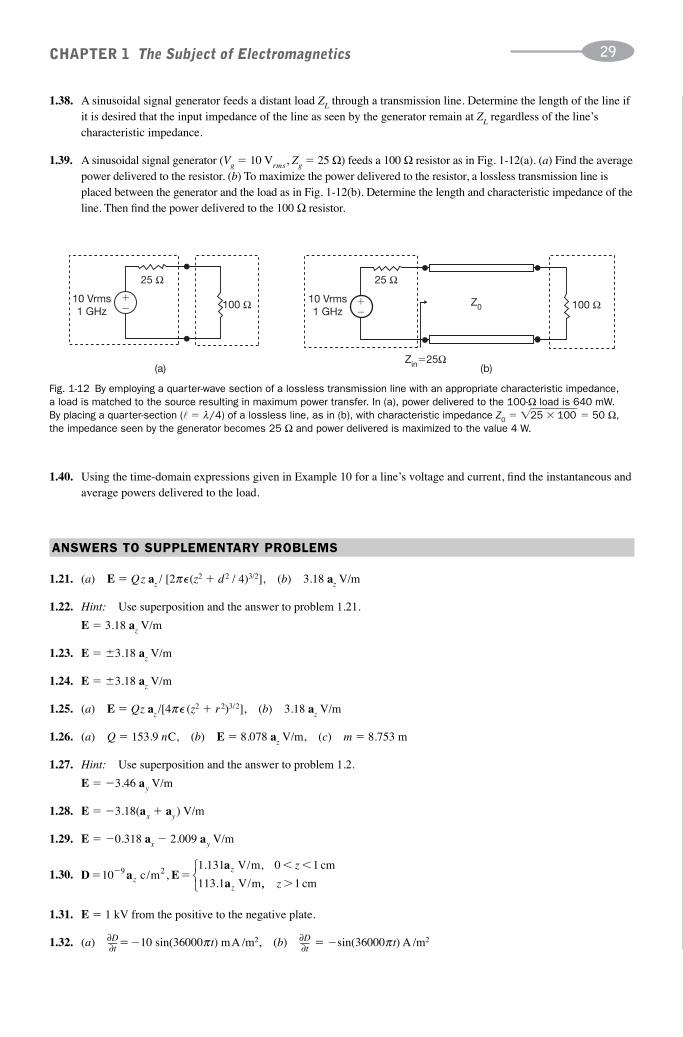
1.38. A sinusoidal signal generator feeds a distant load ZL through a transmission line. Determine the length of the line ifit is desired that the input impedance of the line as seen by the generator remain at ZL regardless of the line’scharacteristic impedance.
1.39. A sinusoidal signal generator (Vg � 10 Vrms, Zg � 25 Ω) feeds a 100 Ω resistor as in Fig. 1-12(a). (a) Find the averagepower delivered to the resistor. (b) To maximize the power delivered to the resistor, a lossless transmission line isplaced between the generator and the load as in Fig. 1-12(b). Determine the length and characteristic impedance of theline. Then find the power delivered to the 100 Ω resistor.
CHAPTER 1 The Subject of Electromagnetics 29
100 Ω
25 Ω
Zin�25Ω
25 Ω
��10 Vrms
1 GHzZ0
(b)(a)
10 Vrms1 GHz �
� 100 Ω
Fig. 1-12 By employing a quarter-wave section of a lossless transmission line with an appropriate characteristic impedance, a load is matched to the source resulting in maximum power transfer. In (a), power delivered to the 100-Ω load is 640 mW. By placing a quarter-section (� � λ/4) of a lossless line, as in (b), with characteristic impedance Z0 � ����25 �����100�� � 50 Ω,the impedance seen by the generator becomes 25 Ω and power delivered is maximized to the value 4 W.
1.40. Using the time-domain expressions given in Example 10 for a line’s voltage and current, find the instantaneous andaverage powers delivered to the load.
ANSWERS TO SUPPLEMENTARY PROBLEMS
1.21. (a) E � Qz az / [2π�(z2 � d 2 / 4)3/2], (b) 3.18 az V/m
1.22. Hint: Use superposition and the answer to problem 1.21.
E � 3.18 az V/m
1.23. E � �3.18 az V/m
1.24. E � �3.18 az V/m
1.25. (a) E � Qz az /[4π� (z2 � r 2)3/2], (b) 3.18 az V/m
1.26. (a) Q � 153.9 nC, (b) E � 8.078 az V/m, (c) m � 8.753 m
1.27. Hint: Use superposition and the answer to problem 1.2.
E � �3.46 ay V/m
1.28. E � �3.18(ax � ay) V/m
1.29. E � �0.318 ax � 2.009 ay V/m
1.30.
1.31. E � 1 kV from the positive to the negative plate.
1.32. (a) ∂D—∂t��10 sin(36000π t) mA /m2, (b) ∂D—∂t
� �sin(36000π t) A /m2
D a Ea
a� �
� ��10
1 131 0 19 2
zz
z
zc/m
V/m cm
113.1 V/m,
. ,
,, 1 cmz
⎧⎨⎩

1.33. ,
where ar is the radial unit vector away from the center of the sphere.
1.34. B � 2.12 sin(377t) (μT )
1.35. Hint: In both columns of Table 1-6 switch differentiations with respect to z and t.
1.36. � � λ /4
1.37. Zocin � �jZ0 cot(β� ), Zsc
in � jZ0 tan(β� ),
1.38. � � nλ /2
1.39. (a) 640 mW, (b) Z0 � 50 Ω, � � λ /4, P � 4 W
1.40. p (t) � v (t) i (t) � (15.4 cos ω t) � (0.1025 cos ω t) � 1.5785 cos2 ω t � 0.78925(1 � cos 2ω t). Pavg � 789.25 mW
SOME REFERENCES FOR HISTORICAL BACKGROUND
Following are some of the original works of the period before the twentieth century:
Gilbert, William (1540–1603), De magnete, 1600, 1893 translation by P. Fleury Mottelay, Dover Publications, New York, 1958.
Cavendish, Henry (1731–1810), The electrical researches of the Honourable Henry Cavendish written between 1771 and1781, ed. by J. Clerk Maxwell, Cambridge, 1879. A new impression of the first edition is published by Frank Cass & Co.,London, 1967.
Henry, Joseph (1797–1878), On a reciprocating motion produced by magnetic attraction and repulsion, first published in Silliman’s Journal, 1831. The paper is reprinted in Turning Points in American Electrical History, pp. 31–34,IEEE Press, New York, 1977.
Maxwell, James Clerk (1831–1879), A dynamical theory of electromagnetic field, Royal Society Transactions, Vol. CLV,1864. Reproduced in The scientific papers of James Clerk Maxwell, pp. 527–597, edited by W.D. Niven (1890), DoverPublications, New York, 1965.
Maxwell, James Clerk (1831–1879), A treatise on electricity and magnetism, Oxford, Clarendon, 1892. 3d ed., OxfordUniversity Press (Vol I and II, 1873), 1955.
Hertz, Heinrich (1857–1894), Electric Waves, being researches on the propagation of electric action with finite velocitythrough space, 1893 translation by D.E. Jones, with a preface by Lord Kelvin, Dover Publications, 1962.
For some historical accounts see the following:
Appleyard, Rollo, Pioneers of electrical communication, Books for Libraries Press, Freeport, New York, 1930, reprinted in 1968.
Dibner, Bern, Oersted and the discovery of electromagnetism, Blaisdell Publishing Company, New York, London, 1962.
Dunsheath, Percy, A history of electrical engineering, Faber and Faber Publishing, London, 1962.
Heilbron, J.L., Electricity in the 17th and 18th centuries: a study of early modern physics, University of California Press,Berkeley, 1979.
Meyer, Herbert W., A history of electricity and magnetism, MIT Press, Cambridge, Massachusetts, 1971.
National Electrical Manufacturers Association, A chronological history of electrical development from 600 B.C., New York, 1946.
Z Z Zo inoc
insc�
D a Ea
a� �
� ��10
12
3
3
10
9
22
2
2r
rr
r
r
r
C/mV/m, 1 2 cm
,
π
πrr rV/m, 2 cm
⎧
⎨⎪⎪
⎩⎪⎪
CHAPTER 1 The Subject of Electromagnetics30

31
Vector Analysis
2.1 Introduction
In electromagnetics, vectors are used extensively as the main tool of analysis. They were introduced brieflyin Section 1.5, along with some vector operations in the Cartesian coordinate system. This chapter expandsthe scope of vector algebra to a level needed throughout the rest of the book. It also introduces the cylindrical and spherical coordinate systems, as all three coordinate systems are used in electromagnetics.As the notation, both for the vectors and the coordinate systems, differs from one text to another, a thoroughunderstanding of the notation employed herein is essential for setting up the problems and obtaining solutions. In addition to this chapter, more vector operations (gradient, divergence, and curl) are introducedin Chapter 5.
2.2 Vector Notation
In order to distinguish vectors (quantities having magnitude and direction) from scalars (quantities having mag-nitude only), the vectors are denoted by boldface symbols. A unit vector, one of absolute value (or magnitudeor length) 1, will in this book always be indicated by a boldface, lowercase a. The unit vector in the directionof a vector A is determined by dividing A by its absolute value:
CHAPTER 2
aA
A
AA A
� or
A � � � �A A A Ax y z2 2 2
aA
Aa a aA x y z� � � �
2
7
3
7
6
7
By use of the unit vectors ax, ay, az along the x, y, and z axes, respectively, of a Cartesian coordinate system,an arbitrary vector can be written in component form:
A � Axax � Ayay � Azaz
In terms of components, the absolute value of a vector is defined by
EXAMPLE 1. A vector drawn from point M (2, 2, 0) to point N (4, 5, 6) is shown by A � 2ax � 3ay � 6az. Itsmagnitude is ⎪A⎪ � ���22�����32�����62 � 7. Its direction is given by the unit vector

2.3 Vector Functions
A vector function in a three-dimensional space assigns a vector to each point in that space. It specifies the mag-nitude and direction of the vector at that point. The spatial components of the vector are, in general, functionsof the coordinates of the location. Electric and magnetic fields are examples of vector functions.
EXAMPLE 2. The electric field intensity due to a point charge Q placed at the origin is
CHAPTER 2 Vector Analysis32
E a�Q
RR
4 2π�
Ea a a
E
( , , )( )
[ ]
( ,
x y zQ x y z
x y z
x y z�
� �
� �4
3 4
2 2 232π�
,, )( )
( , , )(
123 4 12
4 13
2 6 92
3�� �
�
��
Q
Q
x y z
x
a a a
Ea
π�
66 9
4 11
1 4 84 8
4 9
3
a a
Ea a a
y z
x y zQ
�
�
�� �
�
)
( , , )( )
π
π
�
� 33
34 5 62 3 6
4 7E
a a a( , , )
( )�
� �
�
Q x y z
π�
where aR is the radial unit vector. Express E in the Cartesian coordinate system and find its value at the pointsK(3, 4, 12), L(2, 6, 9), M(1, 4, 8), and N(4, 5, 6).
These points are located on concentric spheres with radii 13, 11, 9, and 7, respectively.
2.4 Vector Algebra
1. Vectors may be added and subtracted.
A � B � (Axax � Ayay � Azaz) � (Bxax � Byay � Bzaz)
� (Ax � Bx)ax � (Ay � By)ay � (Az � Bz)az
2. The associative, distributive, and commutative laws apply.
A � (B � C) � (A � B) � C
k(A � B) � kA � kB (k1 � k2)A � k1A � k2A
A � B � B � A
3. The dot product of two vectors is, by definition,
A · B � AB cos θ (read “A dot B”)
where θ is the smaller angle between A and B. In Example 3 it is shown that
A · B � AxBx � AyBy � AzBz
which gives, in particular, ⎪A⎪ � ���A · A.
EXAMPLE 3. The dot product obeys the distributive and scalar multiplication laws
A · (B � C) � A · B � A · C A · kB � k(A · B)

This being the case,
A · B � (Axax � Ayay � Azaz) · (Bxax � Byay � Bzaz )
� AxBx (ax · ax) � AyBy(ay · ay ) � AzBz (az · az )
� AxBy (ax · ay) � … � AzBy(az · ay)
However, ax · ax � ay · ay � az · az � 1 because the cos θ in the dot product is unity when the angle is zero. Andwhen θ � 90°, cos θ is zero; hence, all other dot products of the unit vectors are zero. Thus,
A · B � AxBx � AyBy � AzBz
4. The cross product of two vectors is, by definition,
A � B � (AB sin θ )an (read “A cross B”)
where θ is the smaller angle between A and B, and an is a unit vector normal to the plane determinedby A and B when they are drawn from a common point. There are two normals to the plane, so furtherspecification is needed. The normal selected is the one in the direction of advance of a right-hand screwwhen A is turned toward B (Fig. 2-1). Because of this direction requirement, the commutative law doesnot apply to the cross product; instead,
A � B � �B � A
CHAPTER 2 Vector Analysis 33
A B
a a a
a a a� � �
�
�� � �
x y z
x y z2 4 3
1 1 0
3 3 6
an
A B
Fig. 2-1
Expanding the cross product in component form,
A � B � (Axax � Ayay � Azaz) � (Bxax � Byay � Bzaz)
� (AyBz � AzBy)ax � (AzBx � AxBz)ay � (AxBy � AyBx)az
which is conveniently expressed as a determinant:
A B
a a a
� �
x y z
x y z
x y z
A A A
B B B
EXAMPLE 4. Given A � 2ax � 4ay � 3az and B � ax � ay, find A · B and A � B.
A · B � (2)(1) � (4)(�1) � (�3)(0) � �2

2.5 Coordinate Systems
A problem which has cylindrical or spherical symmetry could be expressed and solved in the familiar Cartesiancoordinate system. However, the solution would fail to show the symmetry and in most cases would be need-lessly complex. Therefore, throughout this book, in addition to the Cartesian coordinate system, the circularcylindrical and the spherical coordinate systems will be used. All three will be examined together in order to illus-trate the similarities and the differences.
A point P is described by three coordinates, in Cartesian (x, y, z), in circular cylindrical (r, φ, z), and inspherical (r, θ, φ), as shown in Fig. 2-2. The order of specifying the coordinates is important and should becarefully followed. The angle φ is the same angle in both the cylindrical and spherical systems. But, in theorder of the coordinates, φ appears in the second position in cylindrical, (r, φ, z), and the third position inspherical, (r, θ, φ). The same symbol, r, is used in both cylindrical and spherical for two quite different things.In cylindrical coordinates r measures the distance from the z axis in a plane normal to the z axis, while in thespherical system r measures the distance from the origin to the point. It should be clear from the context ofthe problem which r is intended.
CHAPTER 2 Vector Analysis34
P (x, y, z) P (r, , z) P (r, , )
y y y
x
y
(a) Cartesian (b) Cylindrical (c) Spherical
x x x
r
r
z
φ φ
z
zz
θ θ
z
φ φ
Fig. 2-2
z
(a) Cartesian (b) Cylindrical (c) Spherical
x
x
yyy
PP P
z z
z� const.z� const.� const.
� const.r � const.
� const.
y � const.
x � const.
x
r � const.
φ
φ
θ
Fig. 2-3
A point is also defined by the intersection of three orthogonal surfaces, as shown in Fig. 2-3. In Cartesian coor-dinates the surfaces are the infinite planes x � const., y � const., and z � const. In cylindrical coordinates, z � const. is the same infinite plane as in the Cartesian case; φ � const., is a half plane with its edge along thez axis; r � const. is a right circular cylinder. These three surfaces are orthogonal and their intersection locatespoint P. In spherical coordinates, φ � const. is the same half plane as in cylindrical; r � const. is a sphere withits center at the origin; θ � const. is a right circular cone whose axis is the z axis and whose vertex is at the ori-gin. Note that θ is limited to the range 0 θ π.

Fig. 2-4 shows the three unit vectors at point P. In the Cartesian system the unit vectors have fixed directions,independent of the location of P. This is not true for the other two systems (except in the case of az ). Each unitvector is normal to its coordinate surface and is in the direction in which the coordinate increases. Notice thatall these systems are right-handed:
ax � ay � az ar � aφ � az ar � aθ � aφ
The component forms of a vector in the three systems are
A � Axax � Ayay � Azaz (Cartesian)
A � Arar � Aφaφ � Azaz (cylindrical)
A � Arar � Aθaθ � Aφaφ (spherical)
It should be noted that the components Ax, Ar, Aφ, etc., are not generally constants but more often are functionsof the coordinates in that particular system.
CHAPTER 2 Vector Analysis 35
ax
a
a
az
ar
ay
ar
az
P PP
z
x x
(b) Cylindrical (c) Spherical(a) Cartesian
x
z z
y yyaθ
φ
φ
Fig. 2-4
z
y
x
dv � dx dy dz
(a) Cartesian (b) Cylindrical (c) Spherical
dv � r dr d dz dv � r2 sin dr d d
dz
dx
dyr dr d
r sin ddr
dr
dzP
P
P
x x
y y
z z
φ
φ
φ
φ
θ
θ
θ θ
Fig. 2-5
2.6 Differential Volume, Surface, and Line Elements
There are relatively few problems in electromagnetics that can be solved without some sort of integration—along a curve, over a surface, or throughout a volume. Hence, the corresponding differential elements must beclearly understood.
When the coordinates of point P are expanded to (x � dx, y � dy, z � dz) or (r � dr, φ � dφ, z � dz), or (r � dr, θ � dθ, φ � dφ), a differential volume dv is formed. To the first order in infinitesimal quantities, thedifferential volume is, in all three coordinate systems, a rectangular box. The value of dv in each system is givenin Fig. 2-5.

From Fig. 2-5 may also be read the areas of the surface elements that bound the differential volume. Forinstance, in spherical coordinates, the differential surface element perpendicular to ar is
dS � (r dθ )(r sin θ dφ) � r 2 sin θ dθ dφ
The differential line element, d� is the diagonal through P. Thus,
d� 2 � dx2 � dy2 � dz2 (Cartesian)
d� 2 � dr2 � r2 dφ2 � dz2 (cylindrical)
d� 2 � dr2 � r2 dθ 2 � r2 sin2 θ dφ2 (spherical)
SOLVED PROBLEMS
2.1. Show that the vector directed from M(x1, y1, z1) to N(x2, y2, z 2) in Fig. 2-6 is given by
(x2 � x1)ax � (y2 � y1)ay � (z2 � z1)az
CHAPTER 2 Vector Analysis36
N (x2 , y2 , z2)
M (x1 , y1 , z1)
y
x
B � A
B
A
z
Fig. 2-6
The coordinates of M and N are used to write the two position vectors A and B in Fig. 2-6.
A � x1ax � y1ay � z1az
B � x2ax � y2ay � z2az
Then B � A � (x2 � x1)ax � (y2 � y1)ay � (z2 � z1)az
2.2. Find the vector A directed from (2, �4, 1) to (0, �2, 0) in Cartesian coordinates and find the unitvector along A.
A a a a a a a
A
� � � � � � � � �� � �( ) [ ( )] ( )0 2 2 4 0 1 2 2
2
x y z x y z
�� � � � � �
� �� � �
( ) ( ) ( )2 2 1 9
2
3
2
3
1
3
2 2 2
aAA
a a aA x y z
2.3. Find the distance between (5, 3π /2, 0) and (5, π /2, 10) in cylindrical coordinates.
First, obtain the Cartesian position vectors A and B (see Fig. 2-7).
A � �5ay B � 5ay � 10az

Then B � A � 10ay � 10az and the required distance between the points is
⎪B � A⎪ � 10��2
The cylindrical coordinates of the points cannot be used to obtain a vector between the points in the same manneras was employed in Problem 2.1 in Cartesian coordinates.
2.4. Show that A � 4ax � 2ay � az and B � ax � 4ay � 4az are mutually perpendicular.
Since the dot product contains cos θ, a dot product of zero from any two nonzero vectors implies that θ � 90°.
A · B � (4)(1) � (�2)(4) � (�1)(�4) � 0
2.5. Given A � 2ax � 4ay and B � 6ay � 4az, find the smaller angle between them using (a) the crossproduct, (b) the dot product.
CHAPTER 2 Vector Analysis 37
y
x
(5, 3 /2, 0)
(5, /2, 10)
� /2
z
A
B�
A
B
π
ππφ
Fig. 2-7
A B
a a a
a a a
A
� �
�
�� � �
� �
x y z
x y z2 4 0
0 6 4
16 8 12
2 42 2( ) ( ) �� �
� � � � �
� � �
( ) .
( ) ( ) ( ) .
( )
0 4 47
0 6 4 7 21
16
2
2 2 2
2
B
A B �� � �( ) ( ) .8 12 21 542 2
sin.
( . )( . ).θ θ� � �
21 54
4 47 7 210 668 or 41.9�
cos( . )( . )
.θ θ� � � �A BA B
· 24
4 47 7 210 745 or 41.9�
Then, since ⎪A � B⎪ � ⎪A⎪ ⎪B⎪ sin θ,
(b) A · B � (2)(0) � (4)(6) � (0)(�4) � 24
2.6. Given F � (y � 1)ax � 2xay, find the vector at (2, 2, 1) and its projection on B, where B � 5ax � ay � 2az.
F(2, 2, 1) � (2 � 1)ax � (2)(2)ay
� ax � 4ay
(a)

As indicated in Fig. 2-8, the projection of one vector on a second vector is obtained by expressing the unit vector inthe direction of the second vector and taking the dot product.
CHAPTER 2 Vector Analysis38
Proj. onA B A aA B
B� �·
·B
Proj. onF BF B
B� �
� � ��
· ( )( ) ( )( ) ( )( )1 5 4 1 0 2
30
1
30
A B
a a a
a a a� � � � �
x y z
x y z1 1 0
1 0 2
2 2
Thus, at (2, 2, 1),
aB B
A
Proj. A on B
θ
Fig. 2-8
2.7. Given A � ax � ay, B � ax � 2az and C � 2ay � az, find (A � B) � C and compare it with A � (B � C).
( )A B C
a a a
a a� � � � � �� �
x y z
y z2 2 1
0 2 1
2 4
A B C· � �
A A A
B B B
C C C
x y z
x y z
x y z
Then
A similar calculation gives A � (B � C) � 2ax � 2ay � 3az. Thus, the cross product does not obey the vectortriple associative law.
2.8. Using the vectors A, B, and C of Problem 2.7, find A · B � C and compare it with A � B · C.
From Problem 2.7, B � C � �4ax � ay � 2az. Then
A · B � C � (1)(�4) � (1)(�1) � (0)(2) � �5
Also from Problem 2.7, A � B � 2ax � 2ay � az. Then
A � B · C � (2)(0) � (�2)(2) � (�1)(1) � �5
Parentheses are not needed in the scalar triple product, since it has meaning only when the cross product is takenfirst. In general, it can be shown that
As long as the vectors appear in the same cyclic order, the result is the same. The scalar triple products not in thiscyclic order have a change in sign.

2.9. Express the unit vector which points from z � h on the z axis toward (r, φ, 0) in cylindrical coordinates.See Fig. 2-9.
CHAPTER 2 Vector Analysis 39
z
h
R
x
y
(r, , 0)φ
Fig. 2-9
z
x
y
(x, y, �5)
(0, 0, 0)
R
Fig. 2-10
R a a
aRR
a a
� �
� ��
�
r h
r h
r h
r z
Rr z
2 2
R a a a
aa a a
�� � �
�� � �
� �
x y
x y
x y
x y z
Rx y z
5
5
252 2
The vector R is the difference of two vectors:
The angle φ does not appear explicitly in these expressions. Nevertheless, both R and aR vary with φ through ar.
2.10. Express the unit vector which is directed toward the origin from an arbitrary point on the plane z � �5,as shown in Fig. 2-10.
Since the problem is in Cartesian coordinates, the two-point formula of Problem 2.1 applies.
2.11. Use the spherical coordinate system to find the area of the strip α θ β on the spherical shell ofradius a (Fig. 2-11). What results when α � 0 and β � π ?
The differential surface element is [see Fig. 2-5(c)]
dS � r2 sin θ dθ dφ

Then
CHAPTER 2 Vector Analysis40
z
αβ
Fig. 2-11
z
2 m5 m
x/6
yπ π2 /3
Fig. 2-12
When α � 0 and β � π, A � 4πa2, the surface area of the entire sphere.
2.12. Obtain the expression for the volume of a sphere of radius a from the differential volume.
From Fig. 2-5(c), dv � r2 sin θ dr dθ dφ. Then
A a d d
a
�
� �
� �0
22
22
π
α
β
θ θ φ
π α β
sin
(cos cos )
v r dr d d aa
� �� � �0
2
0 0
2 34
3
π π
θ θ φ πsin
A d z�
�
� �0
5
6
2 3
2
2
5π
π
φ
π/
/
d
m
2.13. Use the cylindrical coordinate system to find the area of the curved surface of a right circular cylinderwhere r � 2 m, h � 5 m, and 30° φ 120° (see Fig. 2-12).
The differential surface element is dS � r dφ dz. Then
2.14. Transform
A a a a� � ��
y xx
x yx y z
2
2 2
from Cartesian to cylindrical coordinates.

Referring to Fig. 2-2(b),
x � r cos φ y � r sin φ r � ���x 2���y2��
Hence, A � r sin φax � r cos φay � r cos2 φaz
Now the projections of the Cartesian unit vectors on ar, aφ, and az are obtained:
ax · ar � cos φ ax · aφ � �sin φ ax · az � 0
ay · ar � sin φ ay · aφ � cos φ ay · az � 0
az · ar � 0 az · aφ � 0 az · az � 1
Therefore, ax � cos φar � sin φaφ
ay � sin φar � cos φaφ
az � az
and A � 2r sin φ cos φar � (r cos2 φ � r sin2 φ)aφ � r cos2 φaz
2.15. A vector of magnitude 10 points from (5, 5π /4, 0) in cylindrical coordinates toward the origin (Fig. 2-13).Express the vector in Cartesian coordinates.
CHAPTER 2 Vector Analysis 41
z
x
y
A
5 /45 π
Fig. 2-13
A A Ax y z� � � � �104
10
210
4
10
20cos sin
π π
A a a� �10
2
10
2x y
In cylindrical coordinates, the vector may be expressed as 10ar, where φ � π /4. Hence,
so that
Notice that the value of the radial coordinate, 5, is immaterial.
SUPPLEMENTARY PROBLEMS
2.16. Given A � 4ay � 10az and B � 2ax � 3ay, find the projection of A on B.
2.17. Given A � (10/��2 )(ax � az) and B � 3(ay � az), express the projection of B on A as a vector in the direction of A.
2.18. Find the angle between A � 10ay � 2az and B � �4ay � 0.5az using both the dot product and the cross product.
2.19. Find the angle between A � 5.8ay � 1.55az and B � �6.93ay � 4.0az using both the dot product and the crossproduct.

2.20. Given the plane 4x � 3y � 2z � 12, find the unit vector normal to the surface in the direction away from the origin.
2.21. Find the relationship which the Cartesian components of A and B must satisfy if the vector fields are to beeverywhere parallel.
2.22. Express the unit vector directed toward the origin from an arbitrary point on the line described by x � 0, y � 3.
2.23. Express the unit vector directed toward the point (x1, y1, z1) from an arbitrary point in the plane y � �5.
2.24. Express the unit vector directed toward the point (0, 0, h) from an arbitrary point in the plane z � �2.
2.25. Given A � 5ax and B � 4ax � Byay, find By such that the angle between A and B is 45°. If B also has a term Bzaz,what relationship must exist between By and Bz?
2.26. Show that the absolute value of A · B � C is the volume of the parallelepiped with edges A, B, and C.
2.27. Given A � 2ax � az, B � 3ax � ay, and C � �2ax � 6ay � 4az, show that C is ⊥ to both A and B.
2.28. Given A � ax � ay, B � 2az, and C � �ax � 3ay, find A · B � C. Examine other variations of this scalar tripleproduct.
2.29. Using the vectors of Problem 2.28 find (A � B) � C.
2.30. Find the unit vector directed from (2, �5, �2) toward (14, �5, 3).
2.31. Find the vector directed from (10, 3π /4, π /6) to (5, π /4, π), where the endpoints are given in sphericalcoordinates.
2.32. Find the distance between (2, π /6, 0) and (1, π, 2), where the points are given in cylindrical coordinates.
2.33. Find the distance between (1, π /4, 0) and (1, 3π /4, π), where the points are given in spherical coordinates.
2.34. Use spherical coordinates and integrate to find the area of the region 0 φ α on the spherical shell of radius a.What is the result when α � 2π ?
2.35. Use cylindrical coordinates to find the area of the curved surface of a right circular cylinder of radius a and height h.
2.36. Use cylindrical coordinates and integrate to obtain the volume of the right circular cylinder of Problem 2.35.
2.37. Use spherical coordinates to write the differential surface areas dS1 and dS2 and then integrate to obtain the areas ofthe surfaces marked 1 and 2 in Fig. 2-14.
CHAPTER 2 Vector Analysis42
z
x
y
1
21
1 60º1
dS2
dS1
Fig. 2-14

2.38. Use spherical coordinates to find the volume of a hemispherical shell of inner radius 2.00 m and outer radius 2.02m.
2.39. Using spherical coordinates to express the differential volume, integrate to obtain the volume defined by 1 r 2 m,0 θ π /2, and 0 φ π /2.
ANSWERS TO SUPPLEMENTARY PROBLEMS
2.16. 12 /��13
2.17. 1.50(ax � az)
2.18. 161.5°
2.19. 135°
2.20. (4ax � 3ay � 2az) /��29
CHAPTER 2 Vector Analysis 43
A
B
A
B
A
Bx
x
y
y
z
z
� �
aa a
�� �
�
3
9 2
y zz
z
aa a a
�� � � � �
� � �
( ) ( ) ( )
( ) ( )
x x y z z
x x y
x y z1 1 1
12
12
5
5 �� �( )z z12
aa a a
�� � � �
� � �
x y h
x y h
x y z( )
( )
2
22 2 2
a a a� �12
13
5
13x z
2.21.
2.22.
2.23.
2.24.
2.25. By � �4, ���B2y�����B��2z � 4
2.26. Hint: First show that the base has area ⎪B � C⎪.
2.28. �4, �4
2.29. �8az
2.30.
2.31. �9.66ax �3.54ay � 10.61az
2.32. 3.53
2.33. 2.0
2.34. 2α a2, A � 4π a2
2.35. 2πah
2.36. πa2h
2.37. π /4, π /6
2.38. 0.162π m3
2.39. 7π—6
m3

CHAPTER 3
44
Electric Field
3.1 Introduction
The concepts of electric force and field intensity were introduced in Chapter 1. This chapter elaborates furtheron those concepts and formulates them using vector notations, a necessary framework in electromagnetics. Indoing so, it expands upon, and refers to, some examples and problems from Chapter 1.
3.2 Coulomb’s Law in Vector Form
The force between two charges Q1 and Q2 is given by Coulomb’s law. This was introduced in Section 1.6 in scalarform. In vector form Coulomb’s law incorporates both the magnitude and direction of the force as follows:
F a R11 2
212 21
1 2
213 21
4 4� �
Q Q
R
Q Q
Rπ π� �
where F1 is the force on charge Q1 due to a second charge Q2, a21 is the unit vector directed from Q2 to Q1, R21 � R21a21, and � is the permittivity of the medium.
EXAMPLE 1. Find the force on charge Q1, 20 μC, due to charge Q2, �300 μC, where Q1 is at (0, 1, 2) m andQ2 at (2, 0, 0) m.
Because 1 C is a rather large unit, charges are often given in microcoulombs (μC), nanocoulombs (nC), orpicocoulombs (pC). (See Appendix for the SI prefix system.) Referring to Fig. 3-1,
R21 � �2ax � ay � 2a R21 � ����(�2)2�����12 ��� 22���� � 3
z
F1
Q2
(0, 1, 2)
(2, 0, 0)x
y
Q1
R21
Fig. 3-1

The force magnitude is 6 N and the direction is such that Q1 is attracted to Q2 (unlike charges attract).The force field in the region of an isolated charge Q is spherically symmetric. This is made evident by locat-
ing Q at the origin of a spherical coordinate system, so that the position vector R, from Q to a small test chargeQt �� Q, is simply rar. Then
CHAPTER 3 Electric Field 45
x
y
z
R � (x2� x1) ax � ( y2 � y1) ay � (z2� z1) az
(r, , ) (x2, y2, z2)
(x1, y1, z1)Q
(a) Spherical
E E
rar
(b) Cartesian
P
Q
P θ φ
Fig. 3-2
a a a a21
1
32� � � �( )2 x y zand
Then Fa
1
6 6
9 2
20 10 300 10
4 10 36 3
2�
� � � �� �
�
( )( )
( / )( )π πx �� �
�� �
a a
a a a
y z
x y z
2
3
63
⎛
⎝⎜⎞
⎠⎟
⎛
⎝⎜⎞
⎠⎟2
N
F att
rQ Q
r�
4 02π�
showing that on the spherical surface r � constant, ⎪Ft⎪ is constant, and Ft is radial.
3.3 Superposition
The force on a charge Q1 due to n � 1 other charges Q2, …, Qn is the vector sum of the individual forces:
F a a11 2
0 212 21
1 3
0 312 31
1
04 4 4� � � �
Q Q
R
Q Q
R
Q
π π π� � ��
Rk
kk
n
12 1
2
ak�∑
This superposition extends in a natural way to the case where charge is continuously distributed through somespatial region: One simply replaces the above vector sum by a vector integral (see Section 3.5).
3.4 Electric Field Intensity
Suppose that the above-considered test charge Qt is sufficiently small so as not to disturb significantly the fieldof the fixed point charge Q. Then the electric field intensity, E, due to Q is defined to be the force per unit chargeon Qt: E � Ft /Qt.
For Q at the origin of a spherical coordinate system [see Fig. 3-2(a)], the electric field intensity at an arbitrarypoint P is, from Section 3.2,
E a�Q
rr
4 02π�
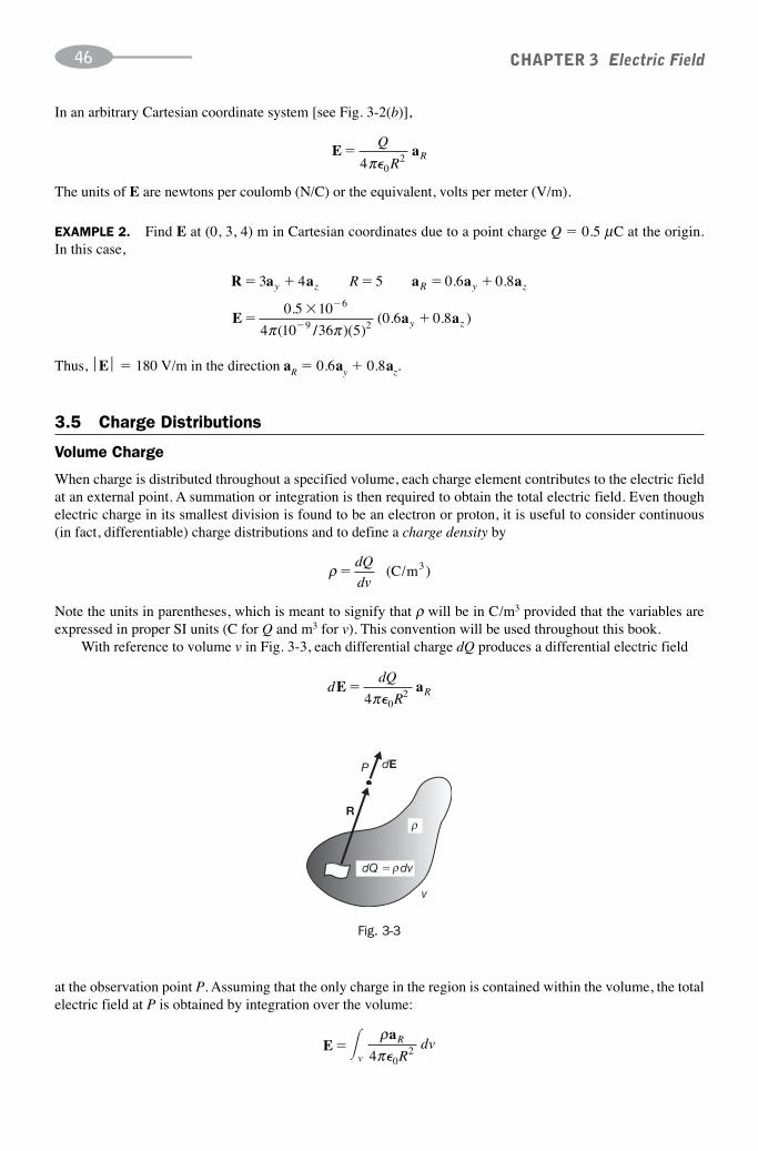
In an arbitrary Cartesian coordinate system [see Fig. 3-2(b)],
CHAPTER 3 Electric Field46
E a�Q
RR
4 02π�
The units of E are newtons per coulomb (N/C) or the equivalent, volts per meter (V/m).
EXAMPLE 2. Find E at (0, 3, 4) m in Cartesian coordinates due to a point charge Q � 0.5 μC at the origin.In this case,
R a a a a a
E
� � � � �
�� �
�
3 4 5 0 6 0 8
0 5 10
4 10
6
9
y z R y zR . .
.
(π // )( )( . . )
36 50 6 0 82π
a ay z�
Thus, ⎪E⎪ � 180 V/m in the direction aR � 0.6ay � 0.8az.
3.5 Charge Distributions
Volume Charge
When charge is distributed throughout a specified volume, each charge element contributes to the electric fieldat an external point. A summation or integration is then required to obtain the total electric field. Even thoughelectric charge in its smallest division is found to be an electron or proton, it is useful to consider continuous (in fact, differentiable) charge distributions and to define a charge density by
ρ �dQ
dv���( )C/m3
Note the units in parentheses, which is meant to signify that ρ will be in C/m3 provided that the variables areexpressed in proper SI units (C for Q and m3 for v). This convention will be used throughout this book.
With reference to volume v in Fig. 3-3, each differential charge dQ produces a differential electric field
ddQ
RRE a�
4 02π�
at the observation point P. Assuming that the only charge in the region is contained within the volume, the totalelectric field at P is obtained by integration over the volume:
R
P dE
v
dQ � dvρ
ρ
Fig. 3-3
Ea
� �v
R
Rdv
ρπ4 0
2�
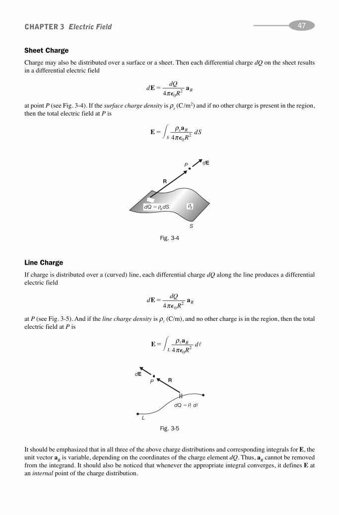
Sheet Charge
Charge may also be distributed over a surface or a sheet. Then each differential charge dQ on the sheet resultsin a differential electric field
CHAPTER 3 Electric Field 47
dERP
L
ρdQ � dll
Fig. 3-5
dQ � dS
R
s
P
S
dE
ρ sρ
Fig. 3-4
ddQ
RRE a�
4 02π�
at point P (see Fig. 3-4). If the surface charge density is ρs (C/m2) and if no other charge is present in the region,then the total electric field at P is
Ea
� �S
s R
RdS
ρπ4 0
2�
Line Charge
If charge is distributed over a (curved) line, each differential charge dQ along the line produces a differentialelectric field
ddQ
RRE a�
4 02π�
at P (see Fig. 3-5). And if the line charge density is ρ� (C/m), and no other charge is in the region, then the totalelectric field at P is
Ea
� �L
R
Rd
ρπ
� �4 0
2�
It should be emphasized that in all three of the above charge distributions and corresponding integrals for E, theunit vector aR is variable, depending on the coordinates of the charge element dQ. Thus, aR cannot be removedfrom the integrand. It should also be noticed that whenever the appropriate integral converges, it defines E atan internal point of the charge distribution.

3.6 Standard Charge Configurations
In three special cases the integration discussed in Section 3.5 is either unnecessary or easily carried out. In regardto these standard configurations (and to others which will be covered in this chapter), it should be noted that thecharge is not “on a conductor.” When a problem states that charge is distributed in the form of a disk, for exam-ple, it does not mean a disk-shaped conductor with charge on the surface. (In Chapter 7, conductors with sur-face charge will be examined.) Although it may now require a stretch of the imagination, these charges shouldbe thought of as somehow suspended in space, fixed in the specified configuration.
Point Charge
As previously determined, the field of a single point charge Q is given by
CHAPTER 3 Electric Field48
E a�Q
rr
4 02π�
���(spherical coordinates)
See Fig. 3-2(a). This is a spherically symmetric field that follows an inverse-square law (like gravitation).
Infinite Line Charge
If charge is distributed with uniform density ρ� (C/m) along an infinite, straight line—which will be chosen asthe z axis—then the field is given by
E a�ρπ
�
2 0� r r ���(cylindrical coordinates)
See Fig. 3-6. This field has cylindrical symmetry and is inversely proportional to the first power of the distancefrom the line charge. For a derivation of E, see Problem 3.9.
x
E
�∞
�∞
yρ
Fig. 3-6
EXAMPLE 3. A uniform line charge, infinite in extent, with ρ� � 20 nC/m, lies along the z axis. Find Eat (6, 8, 3) m.
In cylindrical coordinates r � ����62 ���82�� � 10 m. The field is constant with z. Thus,
E a a��
��
�
20 10
2 10 36 10
9
9π π( / )( )r r36 V/m

Infinite Plane Charge
If charge is distributed with uniform density ρs (C/m2) over an infinite plane, then the field is given by
CHAPTER 3 Electric Field 49
E
E
∞
∞
∞
∞
an
an
sρ
Fig. 3-7
z
x
(3, 1, 0)
y
R21
Q2
Q1(�1, 1, �3)
Fig. 3-8
E a�ρs
n2 0��
See Fig. 3-7. This field is of constant magnitude and has mirror symmetry about the plane charge. For a derivationof this expression, see Problem 3.12.
EXAMPLE 4. Charge is distributed uniformly over the plane z � 10 cm with a density ρs � (1/3π) nC/m2. Find E.
E � � ��
�
ρ ππ
s
2 0�
(1/3 )10
2(10 /36 )6 V/m�
9
9
Above the sheet (z 10 cm), E � 6az V/m; and for z � 10 cm, E � �6az V/m.
SOLVED PROBLEMS
3.1. Two point charges, Q1 � 50 μC and Q2 � 10 μC, are located at (�1, 1, �3) m and (3, 1, 0) m,respectively (Fig. 3-8). Find the force on Q1.
R a a
aa a
F a
21
21
11 2
212 21
4 34 3
5
4
�� �
�� �
�
x z
x z
Q Q
Rπ�0
��� � �� �
�
(50 10 6 )( )
( / )( )
10
4 10 36 5
4 3
5
5
9 2π πa ax z⎛
⎝⎝⎜⎞⎠⎟
� � �( . ) ( . . )0 18 0 8 0 6a ax z N
The force has a magnitude of 0.18 N and a direction given by the unit vector �0.8ax �0.6az. In component form,
F1 � 0.144ax � 0.108az N

3.2. Refer to Fig. 3-9. Find the force on a 100 μC charge at (0, 0, 3) m if four like charges of 20 μC arelocated on the x and y axes at �4 m.
CHAPTER 3 Electric Field50
z
x
y
20 C
100 C
(0, 4, 0)
(0, 0, 3)μ
μ
Fig. 3-9
z
Q2R21
Q1
xy
(3, �3, �2)(1, �1, �3)
Fig. 3-10
Consider the force due to the charge at y � 4,
( )( )
( / )( )
10 20 10
4 10 36 5
4 3
5
4 6
9 2
� �
�
� � �
π πa ay z⎛
⎝⎜⎞⎞
⎠⎟
The y component will be canceled by the charge at y � � 4. Similarly, the x components due to the other twocharges will cancel. Hence,
F a a� �418
25
3
51 73
⎛⎝⎜
⎞⎠⎟
⎛⎝⎜
⎞⎠⎟z z. N
3.3. Refer to Fig. 3-10. Point charge Q1 � 300 μC, located at (1, �1, �3) m, experiences a force
F1 � 8ax � 8ay � 4az N
due to point charge Q2 at (3, �3, �2) m. Determine Q2.
R21 � �2ax � 2ay �az
Note that, because
8
2
8
2
4
1��
��
�
F a
a a a
11 2
2
62
4
8 8 4300 10
4 1
�
� � �� �
Q Q
R
Q
R
x y z
π
π
�0
( )
( 00 36 3
2 2
39 2�
� � �
/ )( )πa a ax y z⎛
⎝⎜⎞
⎠⎟
the given force is along R21 (see Problem 2.21), as it must be.
Hence, Q2 � �40 μC.

3.4. Find the force on a point charge of 50 μC at (0, 0, 5) m due to a charge of 500π μC that is uniformlydistributed over the circular disk r 5 m, z � 0 m (see Fig. 3-11).
CHAPTER 3 Electric Field 51
R
dQ � r dr dx
y
z
(0, 0, 5)
sρ φ
Fig. 3-11
The charge density is
ρ ππs
Q
A� �
�� �
��500
50 2
2210
106
4
( ). C/m
In cylindrical coordinates,
R � �rar � 5az
Then each differential charge results in a differential force
dr dr d
r
rsF ��
�
��
�
( )( )
( / )( )
50
4 10 36 259 2
10 6 ρ φπ π
aa ar z
r
�
�
5
252
⎛
⎝⎜
⎞
⎠⎟
Before integrating, note that the radial components will cancel and that az is constant. Hence,
F �� �� �
�� �0
2
0
5
9
50 0 2 5
4 10
πφ
π( )( . )
( /
10 106 4 r dr d
336 25
2590
2 3 2
0
5
2 3 2
π
π π
) ( )
( )
/
/
r
r dr
r
z
z
�
��
�
a
a90 � ��
�
�1
2516 56
2
0
5
rz z
⎡
⎣⎢⎢
⎤
⎦⎥⎥
a a. N
3.5. Repeat Problem 3.4 for a disk of radius 2 m.
Reducing the radius has two effects: the charge density is increased by a factor
ρρ
2
1
2
2
5
26 25� �
( )
( ).
while the integral over r becomes
� �0
2
2 3 20
5
2250 0143
2
r dr
r
r dr
r( ).
(/��
�instead of
550 05863 2)
./ �
The resulting force is
F a a� �( . ).
.( .6 25
0 0143
0 058616 56
⎛⎝⎜
⎞⎠⎟ z N) 25.27 zz N
3.6. Find the expression for the electric field at P due to a point charge Q at (x1, y1, z1). Repeat with thecharge placed at the origin.
As shown in Fig. 3-12,
R � (x � x1)ax � (y � y1)ay � (z � z1)az
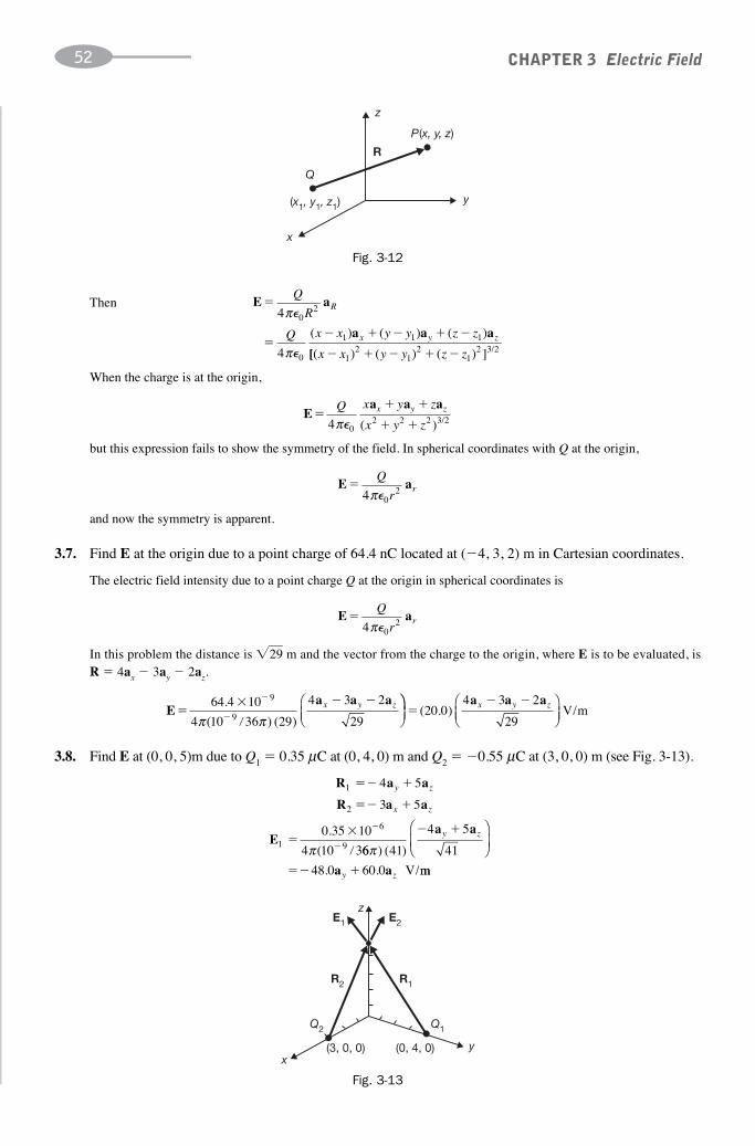
When the charge is at the origin,
CHAPTER 3 Electric Field52
z
R
Q
x
y
P(x, y, z)
(x1, y1, z1)
Fig. 3-12
z
R2
Q2 Q1
E2
R1
E1
xy(3, 0, 0) (0, 4, 0)
Fig. 3-13
E a
a a a
�
�� � � � �
Q
R
Q x x y y z z
R
x y z
4
4
2
1 1 1
π
π
�
�
0
0
( ) ( ) ( )
[[( ) ( ) ( ) ] /x x y y z z� � � � �12
12
12 3 2
Then
Ea a a
�� �
� �
Q x y z
x y zx y z
4 2 2 2 3 2π�0 ( ) /
but this expression fails to show the symmetry of the field. In spherical coordinates with Q at the origin,
E a�Q
rr
4 2π�0
and now the symmetry is apparent.
3.7. Find E at the origin due to a point charge of 64.4 nC located at (�4, 3, 2) m in Cartesian coordinates.
The electric field intensity due to a point charge Q at the origin in spherical coordinates is
E a�Q
rr
4 2π�0
In this problem the distance is ���29 m and the vector from the charge to the origin, where E is to be evaluated, isR � 4ax � 3ay � 2az.
Ea a a
��
�
� ��
�
64 4
4 29
4 3 2
29
9
9
.
( ) ( )
10
10 36π πx y z⎛
⎝⎜⎞⎞⎠⎟
⎛⎝⎜
⎞⎠⎟
�� �
( . )20 04 3 2
29
a a ax y z V/m
3.8. Find E at (0, 0, 5)m due to Q1 � 0.35 μC at (0, 4, 0) m and Q2 � �0.55 μC at (3, 0, 0) m (see Fig. 3-13).
R a a
R a a
E
1
2
1 9
4 5
3 5
0 35
4
�� �
�� �
��
�
�
�
y z
x z
.
(
10
10 3
6
π 66π ) ( )41
4 5
41
� �
�� �
a a
a a
y z
y z
⎛
⎝⎜⎞
⎠⎟
48.0 60.0 ��V/mm

3.9. Charge is distributed uniformly along an infinite straight line with constant density ρ�. Develop theexpression for E at the general point P.
Cylindrical coordinates will be used, with the line charge as the z axis (see Fig. 3-14). At P,
CHAPTER 3 Electric Field 53
P (�2, �1, 4)
(2, �4, z)
x
z
y
R
ρ
Fig. 3-15
z
dQ � dz
P
dE
z
r
�z
R
�∞
∞ρ
ρ
Fig. 3-14
Ea a
2 9
0 55
4 34
5
34�
� �
�
� ��
�
.
( )( )
10
10 36
36
π πx z⎛
⎝⎜⎞⎠⎠⎟
� �
� � � �
74 9
74 9 48 01 2
.
. .
a a
E E E a ax z
x y
124.9 �V/m
�� 64 9. �az V/mand
ddQ
R
r z
r z
r zEa a
��
�4 2 2 2π�0
⎛
⎝⎜
⎞
⎠⎟
Since for every dQ at z there is another charge dQ at �z, the z components cancel. Then
E a��
��
��
∞
∞ ρπ
ρπ
�
�
r dz
r z
r z
r r z
r4
4
2 2 3 2
2 2 2
�
�
0
0
( ) /
⎡⎡
⎣⎢⎢
⎤
⎦⎥⎥ ∞
∞
�
�a ar rr
ρπ
�
2 �0
3.10. On the line described by x � 2 m, y � � 4 m there is a uniform charge distribution of density ρ� � 20 nC/m.Determine the electric field E at (�2, �1, 4) m.
With some modification for Cartesian coordinates the expression obtained in Problem 3.9 can be used with thisuniform line charge. Since the line is parallel to az, the field has no z component. Referring to Fig. 3-15,
R a a
Ea a
�� �
�� � �
���
4 3
20
2 5
4 3
5
x y
x y10 9
0π� ( )
⎛
⎝⎜⎞
⎠⎟557 6 43 2. .a ax y� V/mand

3.11. As shown in Fig. 3-16, two uniform line charges of density ρ� � 4 nC/m lie in the x � 0 plane at y � �4 m. Find E at (4, 0, 10) m.
CHAPTER 3 Electric Field54
(0, �4, z)
(0, 4, z)
x
P0
y
E
ρ
ρ
Fig. 3-16
(r, , 0)
P(0, , z)
x
dE
dQ
R
z
y
∞
φ
φ
Fig. 3-17
The line charges are both parallel to az; their fields are radial and parallel to the xy plane. For either line charge, themagnitude of the field at P would be
E � �ρπ
�
2
18
2�0rV/m
The field due to both line charges is, by superposition,
E a a� �218
245cos �⎛
⎝⎜⎞⎠⎟ x x18 V/m
3.12. Develop an expression for E due to charge uniformly distributed over an infinite plane with density ρs.
The cylindrical coordinate system will be used, with the charge in the z � 0 plane as shown in Fig. 3-17.
dr dr d
r z
r z
r x
s r zEa a
��
� �
�
ρ φπ4 2 2 2�0
2( )
⎛
⎝⎜⎜
⎞
⎠⎟⎟

Symmetry about the z axis results in cancellation of the radial components.
CHAPTER 3 Electric Field 55
3
x
y
(x, 3, z)E
Ez
sρ
Fig. 3-18
E2E2E2
E1 E1 E11 2
0x
ρs ρs
Fig. 3-19
E a��
� �0
2
02 2 3 24
πρ φ
π
∞s
zrz dr d
r z�0 ( )
����������
/
���������
��
ρ ρsz z
z
r z2
12 2
0� �0
s
02⎡
⎣⎢⎢
⎤
⎦⎥⎥
∞
a a
This result is for points above the xy plane. Below the xy plane the unit vector changes to �az. The generalizedform may be written using an, the unit normal vector:
E a�ρs
n2�0
The electric field is everywhere normal to the plane of the charge, and its magnitude is independent of the distancefrom the plane.
3.13. As shown in Fig. 3-18, the plane y � 3 m contains a uniform charge distribution of density ρs � (10�8 /6π)C/m2. Determine E at all points.
For y 3 m,
E a
a
�
�
ρsn
y
2�0
30 V/m
and for y � 3 m,
E � �30ay V/m
3.14. Two infinite uniform sheets of charge, each with density ρs, are located at x � �1 (Fig. 3-19).Determine E in all regions.

Only parts of the two sheets of charge are shown in Fig. 3-19. Both sheets result in E fields that are directed along x,independent of the distance. Then
CHAPTER 3 Electric Field56
E E
a
a1 2 0 1 1
1
� �
� ��
� � �
( / )
( / )
ρ
ρ
s x
s x
x
x
x
�
�
0
0
1⎧⎨⎪
⎩⎪⎪
3.15. Repeat Problem 3.14 with ρs on x � �1 and �ρs on x � 1.
E E a1 2
0 1
1 1� �
��
� � �
x
xs x����( / ) �� ���ρ �0
00 1x
⎧⎨⎪
⎩⎪
3.16. A uniform sheet charge with ρs � (1/3π) nC /m2 is located at z � 5 m and a uniform line charge with ρ� � (�25/9) nC/m at z � �3 m, y � 3 m. Find E at (x, �1, 0) m.
The two charge configurations are parallel to the x axis. Hence the view in Fig. 3-20 is taken looking at the yz planefrom positive x. Due to the sheet charge,
E as n�ρ2
2�0
At P, an � �az and
Es � �6az V/m
Due to the line charge,
Es
EsEsE
03
5
P(x, �1, 0)
�3
z
y
s
ρ
ρ
Fig. 3-20
E a���
ρπ2 �0r r
and at P
E� � 8ay � 6az V/m
The total electric field is the sum, E � E� � Es � 8ay � 12az V/m.
3.17. Determine E at (2, 0, 2) m due to three standard charge distributions as follows: a uniform sheet at x � 0 m with ρs1 � (1/3π) nC/m2, a uniform sheet at x � 4 m with ρs2 � (�1/3π) nC/m2, and auniform line at x � 6 m, y � 0 m with ρ� � �2 nC/m.
Since the three charge configurations are parallel with az, there will be no z component of the field. Point (2, 0, 2)will have the same field as any point (2, 0, z). In Fig. 3-21, P is located between the two sheet charges, where thefields add due to the difference in sign.
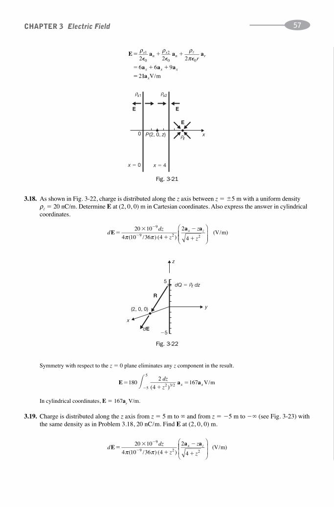
3.18. As shown in Fig. 3-22, charge is distributed along the z axis between z � �5 m with a uniform density ρ� � 20 nC/m. Determine E at (2, 0, 0) m in Cartesian coordinates. Also express the answer in cylindricalcoordinates.
CHAPTER 3 Electric Field 57
E
0 x
x � 0 x � 4
P(2, 0, z)
E
E
s1 s2
ρ
ρρ
Fig. 3-21
5
�5
z
x
y(2, 0, 0)
dE
R
dQ � dzρ
Fig. 3-22
ddz
z
z
z
x zEa a
��
�
�
�
�
�
20 1
4 1 36 4
2
4 2
0
0
9
9 2π π( / ) ( )
⎛
⎝⎜⎜⎜
⎞
⎠⎟⎟
���(V/m)
Symmetry with respect to the z � 0 plane eliminates any z component in the result.
E a a��
��
18045
5
2 3 2� 2 dz
zx x
( ) / 167 V/m
In cylindrical coordinates, E � 167ar V/m.
3.19. Charge is distributed along the z axis from z � 5 m to ∞ and from z � �5 m to �∞ (see Fig. 3-23) withthe same density as in Problem 3.18, 20 nC/m. Find E at (2, 0, 0) m.
ddz
z
z
z
x zEa a
��
�
�
�
�
�
20 1
4 1 36 4
2
4 2
0
0
9
9 2π π( / ) ( )
⎛
⎝⎜⎜⎜
⎞
⎠⎟⎟���(V/m)
E a a a
a a a
� � �
� � �
�
ρ ρ ρπ
sn
sn r
x x x
r1 2
2 2 2
6 9
2
� � �0 0 0
6
�
11axV/m

Again the z component vanishes.
CHAPTER 3 Electric Field58
x
y
5
(2, 0, 0)
�5
∞
�∞
dQ � dz
dE
R
ρl
ρl
ρl
Fig. 3-23
z
dE(0, , h)
R
ydQa
x
φ
Fig. 3-24
E ��
���
�
1804 45
2 3 2
5
2 3 2� �∞
∞
⎡
⎣⎢⎢
⎤2 2dz
z
dz
z( ) ( )/ /⎦⎦⎥⎥a
a
x
x�13 V/m
In cylindrical coordinates, E � 13ar V/m.
When the charge configurations of Problems 3.18 and 3.19 are superimposed, the result is a uniform line charge.
E a a� �ρπ
�
2180
�0r r r V/m
3.20. Find the electric field intensity E at (0, φ, h) in cylindrical coordinates due to the uniformly chargeddisk r a, z � 0 (see Fig. 3-24).
If the constant charge density is ρs,
dr dr d
r h
r h
r h
s r zEa a
��
� �
�
ρ φπ4 2 2 2 2�0 ( )
⎛
⎝⎜⎜
⎞
⎠⎟⎟
The radial components cancel. Therefore,
E a��
��
ρπ
φ
ρ
πs
a
z
s
h r dr d
r h
h
a
4
2
1
0
2
02 2 3 2�
�
0
0
� �( ) /
22 2
1
��
h h z
⎛
⎝⎜⎜
⎞
⎠⎟⎟a
Note that as a → ∞, E → (ρs /2�0)az, the field due to a uniform plane sheet.

3.21. Charge lies on the circular disk r a, z � 0 with density ρs � ρ0 sin2 φ. Determine E at (0, φ, h).
CHAPTER 3 Electric Field 59
(�2, �2, �3)
(2, �2, �3)
(�2, 2, �3)
(2, 2, �3)
dE
z
Ry
dQx
Fig. 3-25
dr dr d
r h
r h
r h
r zEa a
��
� �
�
ρ φ φπ
02
2 2 2 24
(sin )
( )�0
⎛
⎝⎜⎜
⎞
⎠⎟
The charge distribution, though not uniform, still is symmetrical such that all radial components cancel.
E a��
�ρπ
φ φ ρπ0
0
2
0
2
2 2 3 24
h r dr d
r h
a
z�0
0� � (sin )
( ) /
hh
a h h z4 0�
�
��
1 12 2
⎛
⎝⎜
⎞
⎠⎟ a
3.22. Charge lies on the circular disk r 4 m, z � 0 with density ρs � (10�4/r) (C/m2). Determine E at r � 0, z � 3 m.
dr r dr d
r
r
r
r zEa a
��
� �
�
�( / )
( )
10
4
3
9
4
2 2
φπ�0 9
⎛
⎝⎜⎜
⎞
⎠⎠⎟⎟
�(V/m)
As in Problems 3.20 and 3.21, the radial component vanishes by symmetry.
E a a� ��
� �( . )( )
./2 79
1 51 10
2
0
4
2 3 210 06 6� �π φdr d
rz zz zV/m�� �or ���1.51 MV/ma
3.23. Charge lies in the z � �3 m plane in the form of a square sheet defined by �2 x 2 m, �2 y 2 mwith charge density ρs � 2(x2 � y2 � 9)3/2 nC/m2. Find E at the origin.
From Fig. 3-25,R � �xax � yay � 3az (m)
dQ � ρs dx dy � 2(x2 � y2 � 9)3 /2 � 10�9 dx dy (C)
and so
dx y dx dy
x y
x xEa
�� � �
� �
� ��2( 9) 102 2 3/2 9
04 92 2π� ( )
yy
x y
y za a�
� �
3
9���(
2 2
⎛
⎝⎜
⎞
⎠⎟ V/m)
Due to symmetry, only the z component of E exists.
E a a��
�� �
�
� �2 2 0
2 2 96 10
4864
dx dyz zπ�
V/m
3.24. A charge of uniform density ρs � 0.3 nC/m2 covers the plane 2x � 3y � z � 6 m. Find E on the side ofthe plane containing the origin.
Since this charge configuration is a uniform sheet, E � ρs /2�0 and E � (17.0)an V/m. The unit normal vectors for aplane Ax � By � Cz � D are
aa a a
nx y zB C
A B C��
� �
� �
A2 2 2

Therefore, the unit normal vectors for this plane are
CHAPTER 3 Electric Field60
aa a a
nx y z
��� �2 3
14
From Fig. 3-26 it is evident that the unit vector on the side of the plane containing the origin is produced by thenegative sign. The electric field at the origin is
(0, �2, 0)
(0, 0, 6)
(3, 0, 0)
y
z
x
Fig. 3-26
SUPPLEMENTARY PROBLEMS
3.25. Two point charges, Q1 � 250 μC and Q2 � �300 μC, are located at (5, 0, 0) m and (0, 0, �5) m, respectively. Findthe force on Q2.
3.26. Two point charges, Q1 � 30 μC and Q2 � �100 μC, are located at (2, 0, 5) m and (�1, 0, �2) m, respectively.Find the force on Q1.
3.27. In Problem 3.26 find the force on Q2.
3.28. Four point charges, each 20 μC, are on the x and y axes at �4 m. Find the force on a 100-μC point charge at (0, 0, 3) m.
3.29. Ten identical charges of 500 μC each are spaced equally around a circle of radius 2 m. Find the force on a charge of�20 μC located on the axis, 2 m from the plane of the circle.
3.30. Determine the force on a point charge of 50 μC at (0, 0, 5) m due to a point charge of 500π μC at the origin.Compare the answer with Problems 3.4 and 3.5, where this same total charge is distributed over a circular disk.
3.31. Find the force on a point charge of 30 μC at (0, 0, 5) m due to a 4 m square in the z � 0 plane between x � �2 mand y � �2 m with a total charge of 500 μC, distributed uniformly.
3.32. Two identical point charges of Q(C) each are separated by a distance d(m). Express the electric field E for pointsalong the line joining the two charges.
3.33. Identical charges of Q(C ) are located at the eight corners of a cube with a side �(m). Show that the Coulombicforce on each charge has magnitude (3.29Q 2/4π �0�
2) N.
3.34. Show that the electric field E outside a spherical shell of uniform charge density ρs is the same as E due to the totalcharge on the shell located at the center.
3.35. Develop the expression in Cartesian coordinates for E due to an infinitely long, straight charge configuration ofuniform density ρ�.
Ea a a
�� � �
( . )17 02 3
14x y z⎛
⎝⎜⎞
⎠⎟V/m

3.36. Two uniform line charges of ρ� � 4 nC/m each are parallel to the z axis at x � 0, y � �4 m. Determine the electricfield E at (�4, 0, z) m.
3.37. Two uniform line charges of p� � 5 nC/m each are parallel to the x axis, one at z � 0, y � �2 m and the other at z � 0, y � 4 m. Find E at (4, 1, 3) m.
3.38. Determine E at the origin due to a uniform line charge distribution with ρ� � 3.30 nC/m located at x � 3 m, y � 4 m.
3.39. Referring to Problem 3.38, at what other points will the value of E be the same?
3.40. Two meters from the z axis, ⎪E⎪ due to a uniform line charge along the z axis is known to be 1.80 � 104 V/m. Findthe uniform charge density ρ�.
3.41. The plane �x � 3y � 6z � 6 m contains a uniform charge distribution ρs � 0.53 nC/m2. Find E on the sidecontaining the origin.
3.42. Two infinite sheets of uniform charge density ρs � (10�9/6π) C/m2 are located at z � �5 m and y � �5 m.Determine the uniform line charge density ρ� necessary to produce the same value of E at (4, 2, 2) m, if the linecharge is located at z � 0, y � 0.
3.43. Two uniform charge distributions are as follows: a sheet of uniform charge density ρs � �50 nC/m2 at y � 2 m anda uniform line of ρ� � 0.2 μC/m at z � 2 m, y � �1 m. At what points in the region will E be zero?
3.44. A uniform sheet of charge with ρs � (�1/3π) nC/m2 is located at z � 5 m and a uniform line of charge with ρ� � (�25/9) nC/m is located at z � �3 m, y � 3 m. Find the electric field E at (0, �1, 0) m.
3.45. A uniform line charge of ρ� � (��2 � 10�8/6)C/m lies along the x axis and a uniform sheet of charge is located at y � 5m. Along the line y � 3m, z � 3 m the electric field E has only a z component. What is ρs for the sheet?
3.46. A uniform line charge of ρ� � 3.30 nC/m is located at x � 3 m, y � 4 m. A point charge Q is 2 m from the origin.Find the charge Q and its location such that the electric field is zero at the origin.
3.47. A circular ring of charge with radius 2 m lies in the z � 0 plane, with center at the origin. If the uniform charge densityis ρ� � 10 nC/m, find the point charge Q at the origin which would produce the same electric field E at (0, 0, 5) m.
3.48. The circular disk r 2 m in the z � 0 plane has a charge density ρs � 10�8/r (C /m2). Determine the electric fieldE for the point (0, φ, h).
3.49. Examine the result in Problem 3.48 as h becomes much greater than 2 m and compare it to the field at h whichresults when the total charge on the disk is concentrated at the origin.
3.50. A finite sheet of charge, of density ρs � 2x(x2 � y2 � 4)3/ 2 (C/m2), lies in the z � 0 plane for 0 x 2 m and 0 y 2 m. Determine E at (0, 0, 2)m.
3.51. Determine the electric field E at (8, 0, 0) m due to a charge of 10 nC distributed uniformly along the x axis betweenx � �5 m and x � 5 m. Repeat for the same charge distributed between x � �1 m and x � 1 m.
3.52. The circular disk r l m, z � 0 has a charge density ρs � 2(r2 � 25)3/2e�10r (C/m2). Find E at (0, 0, 5)m.
3.53. Show that the electric field is zero everywhere inside a uniformly charged spherical shell.
3.54. Charge is distributed with constant density ρ throughout a spherical volume of radius a. By using the results ofProblems 3.34 and 3.53, show that
CHAPTER 3 Electric Field 61
E
a
a�
�
rr a
a
rr a
r
r
ρ
ρ
3
3
3
2
�
�
0
0
������
���
⎧
⎨⎪⎪
⎩⎪⎪
where r is the distance from the center of the sphere.

ANSWERS TO SUPPLEMENTARY PROBLEMS
3.25.
CHAPTER 3 Electric Field62
E a� ��
Q
x d xx4
12π�0
2
1
( )⎡⎣⎢
⎤⎦⎥
(V/m)
Ea a
��
�
ρπ
�
2 2 2�0
x y
x yx y
3.27. �F1
3.28. 1.73az N
3.29. (79.5)(�an ) N
3.30. 28.3az N
3.31. 4.66az N
3.32. If the charges are at x � 0 and x � d, then, for 0 � x � d,
3046
a a ax y z� �3 6⎛
⎝⎜
⎞
⎠⎟ �V/m
3.35.
3.36. �18ax V/m
3.37. 30az V/m
3.38. �7.13ax � 9.50ay V/m
3.39. (0, 0, z)
3.40. 2.0 μC/m
3.41.
1 13. �
�
10
4
3
2h hza (V/m)
3.42. 0.667 nC/m
3.43. (x, �2.273, 2.0) m
3.44. 8ay V/m
3.45. 125 pC/m2
3.46. 5.28 nC at (�1.2, �1.6, 0) m
3.47. 100.5 nC
( )1816
34 8 18
16
34� � � � � � �109 a a a a ax y z x
⎛⎝⎜
⎞⎠⎟
V/m yy z� 8a⎛⎝⎜
⎞⎠⎟
GV/m
3.48.
Fa a
2 13 52
��
( . ) x z⎛
⎝⎜
⎞
⎠⎟ N
Fa a
1 0 4653 7
58�
� �( . ) x z⎛
⎝⎜
⎞
⎠⎟ N3.26.
3.50.
3.51. 2.31ax V/m 1.43ax V/m
3.52. 5.66ax GV/m

63
Electric Flux
4.1 Net Charge in a Region
With charge density defined as in Section 3.5, it is possible to obtain the net charge contained in a specified volumeby integration. From
dQ � ρ dv (C)
it follows that
CHAPTER 4
Q dvv
� � ρ ( )C
ρ φ�
5 2
4
cos( )
rC/m3
Qr
r dr d d� �� � �0
2
0 1
2 2
425
5π π φ θ θ φ πcos
sin⎛
⎝⎜⎞⎠⎟
C
In general, ρ will not be constant throughout the volume v.
EXAMPLE 1. Find the charge in the volume defined by 1 r 2 m in spherical coordinates, if
By integration,
4.2 Electric Flux and Flux Density
Electric flux Ψ, a scalar field, and its density D, a vector field, are useful quantities in solving certain problems,as will be seen in this and subsequent chapters. Unlike E, these fields are not directly measurable; their existencewas inferred from nineteenth-century experiments in electrostatics.
EXAMPLE 2. Referring to Fig. 4-1, a charge �Q is first fixed in place and a spherical, concentric, conduct-ing shell is then closed around it. Initially the shell has no net charge on its surface. Now if a conducting pathto ground is momentarily completed by closing a switch, a charge �Q, equal in magnitude but of oppositesign, is discovered on the shell. This charge �Q might be accounted for by a transient flow of negative chargefrom the ground, through the switch, and onto the shell. But what could provoke such a flow? The earlyexperimenters suggested that a flux from �Q to the conductor surface induced, or displaced, the charge �Qonto the surface. Consequently, it has also been called displacement flux, and the use of the symbol D is areminder of this early concept.

By definition, electric flux Ψ originates on positive charge and terminates on negative charge. In the absence ofnegative charge, the flux Ψ terminates at infinity. Also by definition, one coulomb of electric charge gives riseto one coulomb of electric flux. Hence,
Ψ � Q (C)
In Fig. 4-2(a) the flux lines leave �Q and terminate on �Q. This assumes that the two charges are of equal mag-nitude. The case of positive charge with no negative charge in the region is illustrated in Fig. 4-2(b). Here theflux lines are equally spaced throughout the solid angle and reach out toward infinity.
CHAPTER 4 Electric Flux64
�Q
ψ
Fig. 4-1
�Q�Q
�Q
(a) (b)
Fig. 4-2
If in the neighborhood of point P the lines of flux have the direction of the unit vector a (see Fig. 4-3) and if an amount of flux dΨ crosses the differential area dS, which is a normal to a, then the electric fluxdensity at P is
D a�d
dS
Ψ(C/m )2

A volume charge distribution of density ρ (C/m3) is shown enclosed by surface S in Fig. 4-4. Since each coulombof charge Q has, by definition, one coulomb of flux Ψ, it follows that the net flux crossing the closed surface Sis an exact measure of the net charge enclosed. However, the density D may vary in magnitude and direction frompoint to point of S; in general, D will not be along the normal to S. If, at the surface element dS, D makes an angleθ with the normal, then the differential flux crossing dS is given by
dΨ � D dS cos θ � D · dSan � D · dS
where dS is the vector surface element, of magnitude dS and direction an. The unit vector an is always taken topoint out of S, so that dΨ is the amount of flux passing from the interior of S to the exterior of S through dS.
CHAPTER 4 Electric Flux 65
dSP D
a
Fig. 4-3
dS
an D
S
θ
ρ
Fig. 4-4
4.3 Gauss’s Law
Gauss’s law states that the total flux out of a closed surface is equal to the net charge within the surface. Thiscan be written in integral form as
D · dS � Qenc
A great deal of valuable information can be obtained from Gauss’s law through clever choice of the surface ofintegration; see Section 3.5.
4.4 Relation between Flux Density and Electric Field Intensity
Consider a point charge Q (assumed positive, for simplicity) at the origin (Fig. 4-5). If this is enclosed by aspherical surface of radius r, then, by symmetry, D due to Q is of constant magnitude over the surface and iseverywhere normal to the surface. Gauss’s law then gives
Q � D · dS � D dS � D(4π r 2)

from which D � Q/4πr 2. Therefore,
CHAPTER 4 Electric Flux66
D
y
x
z
dS
Q
an
Fig. 4-5
D a a� �Q
r
Q
rn r
4 42 2π π
E a�Q
rr
4 02π�
Q d d d� � �� � �1 2 3
D S D S D S· · ·
But, from Section 3.4, the electric field intensity due to Q is
It follows that D � �0E.More generally, for any electric field in an isotropic medium of permittivity �,
D � �E
Thus, D and E fields will have exactly the same form, since they differ only by a factor which is a constant ofthe medium. While the electric field E due to a charge configuration is a function of the permittivity �, the elec-tric flux density D is not. In problems involving multiple dielectrics, a distinct advantage will be found in firstobtaining D, then converting to E within each dielectric.
4.5 Special Gaussian Surfaces
The surface over which Gauss’s law is applied must be closed, but it can be made up of several surface elements.If these surface elements can be selected so that D is either normal or tangential, and if ⎪D⎪ is constant over anyelement to which D is normal, then the integration becomes very simple. Thus, the defining conditions of a spe-cial Gaussian surface are
1. The surface is closed.
2. At each point of the surface D is either normal or tangential to the surface.
3. D is sectionally constant over that part of the surface where D is normal.
EXAMPLE 3. Use a special Gaussian surface to find D due to a uniform line change with density ρ� (C/m).Take the line charge as the z axis of the cylindrical coordinate system (Fig. 4-6). By cylindrical symmetry, D canonly have an r component, and this component can only depend on r. Thus, the special Gaussian surface for thisproblem is a closed right circular cylinder whose axis is the z axis (Fig. 4-7). Applying Gauss’s law,

Over surfaces 1 and 3, D and dS are orthogonal, and so the integrals vanish. Over 2, D and dS are parallel (or antiparallel, if ρ� is negative), and D is constant because r is constant. Thus,
CHAPTER 4 Electric Flux 67
dQ
dQ
ar
(C/m)∞
�∞
ρ�
Fig. 4-6
dS
dS
dS
2
1
r
D
3 D
D
∞
�∞
ρ
Fig. 4-7
Q D dS D rL� ��2
( )2π
where L is the length of the cylinder. But the enclosed charge is Q � ρ�L. Hence,
Dr r r� �
ρπ
ρπ
� �
2 2and D a
Observe the simplicity of the above derivation as compared to Problem 3.9.The one serious limitation of the method of special Gaussian surfaces is that it can be utilized only for
highly symmetrical charge configurations. However, for other configurations, the method can still provide quickapproximations to the field at locations very close to or very far from the charges. See Problem 4.36.

SOLVED PROBLEMS
4.1. Find the charge in the volume defined by 0 x 1 m, 0 y 1 m, and 0 z 1 m if ρ � 30x2y(μC/m3). What change occurs for the limits �1 y 0 m?
Since dQ � ρ dv,
CHAPTER 4 Electric Flux68
Q x y dx dy dz� �� � �0
1
0
1
0
1230 5 μC
Q x y dx dy dz� ���
� � �0
1
1
0
0
1230 5 μC
Ψ � � �Qr
r dr d� �0
2
0
4 2
22
π φ φ πsin⎛⎝⎜
⎞⎠⎟ C
Ψ � � �Q r dr d� �0
2
0
4
12 0π
φ φ μ( sin ) C
For the change in limits on y,
4.2. Three point charges, Q1 � 30 nC, Q2 � 150 nC, and Q3 � �70 nC, are enclosed by surface S. What netflux crosses S?
Since electric flux was defined as originating on positive charge and terminating on negative charge, part of theflux from the positive charges terminates on the negative charge.
Ψnet � Qnet � 30 � 150 � 70 � 110 nC
4.3. What net flux crosses the closed surface S shown in Fig. 4-8, which contains a charge distribution in theform of a plane disk of radius 4 m with a density ρs � (sin2 φ)/2r (C/m2)?
4.4. A circular disk of radius 4 m with a charge density ρs � 12 sin φ μC/m2 is enclosed by surface S. Whatnet flux crosses S?
S
Fig. 4-8
Since the disk contains equal amounts of positive and negative charge [sin (φ � π) � �sin φ ], no net flux crosses S.
4.5. Charge in the form of a plane sheet with density ρs � 40 μC/m2 is located at z � �0.5m. A uniform linecharge of ρ� � �6 μC/m lies along the y axis. What net flux crosses the surface of a cube 2 m on anedge, centered at the origin, as shown in Fig. 4-9?
Ψ � Qenc

The charge enclosed from the plane is
Q � (4 m2)(40 μC/m2) � 160 μC
and from the line
Q � (2 m)(�6 μC/m) � �12 μC
Thus, Qenc � Ψ � 160 � 12 � 148 μC.
4.6. A point charge Q is at the origin of a spherical coordinate system. Find the flux which crosses the portionof a spherical shell described by α θ β (Fig. 4-10). What is the result if α � 0 and β � π /2?
CHAPTER 4 Electric Flux 69
x
yQ
r
z
α
β
Fig. 4-10
A r d d
r
�
� �
� �0
22
22
π
α
β
θ θ φ
π α β
sin
(cos cos )
Ψnet � � �A
rQ
Q
4 22πα β(cos cos )
ρ
s
y
x
2 m
2 m
2 m
z
�
1
1
1
ρ
Fig. 4-9
The total flux Ψ � Q crosses a complete spherical shell of area 4πr 2. The area of the strip is given by
Then the flux through the strip is
For α � 0, β � π /2 (a hemisphere), this becomes Ψnet � Q/2.

4.7. A uniform line charge with ρ� � 50 μC/m lies along the x axis. What flux per unit length, Ψ/L, crossesthe portion of the z � �3 m plane bounded by y � �2 m?
The flux is uniformly distributed around the line charge. Thus the amount crossing the strip is obtained from theangle subtended compared to 2π. In Fig. 4-11,
CHAPTER 4 Electric Flux70
α � �22
31 176arctan .
⎛⎝⎜
⎞⎠⎟
rad
ρ
x
α
z�
Fig. 4-11
x
yQ
R
D
(1, 3, �4)
z
Fig. 4-12
Then
4.8. A point charge, Q � 30 nC, is located at the origin in Cartesian coordinates. Find the electric fluxdensity D at (1, 3, �4) m.
Referring to Fig. 4-12,
ΨL
� � �501 176
29 36
..
πμ
⎛⎝⎜
⎞⎠⎟
C m
D a
a a a
�
�� � �
�
�
Q
RR
x y z
4
30 10
4 26
3 4
26
2
9
π
π ( )
(
⎛
⎝⎜⎞
⎠⎟
99 18 103 4
2611. )�
� ��� a a ax y z⎛
⎝⎜⎞
⎠⎟C m2
or, more conveniently, D � 91.8 pC/m2.

4.9. Two identical uniform line charges lie along the x and y axes with charge densities ρ� � 20 μC/m.Obtain D at (3, 3, 3) m.
The distance from the observation point to either line charge is 3��2m. Considering first the line charge on the x axis,
CHAPTER 4 Electric Flux 71
x
ydS
1053.2º
P(10, 53.2º, 2)
z
Fig. 4-13
D aa a
11
12
20
2� �
�ρπ
μπ
�
r ry zC/m
2 (3 2 m)
⎛
⎝⎜
⎞
⎠⎟
D aa a
22
22
20
2� �
�ρπ
μπ
�
r rx zC/m
2 (3 2 m)
⎛⎝⎜
⎞⎠⎟
Da a a a a a
�� �
�� �20 2
22 25
2
62 (3 2)πx y z x y z⎛
⎝⎜⎞
⎠⎟( . )
⎛⎛
⎝⎜⎞
⎠⎟μC m2�
and now the y axis line charge,
The total flux density is the vector sum,
4.10. Given that D � 10xax (C/m2), determine the flux crossing a 1-m2 area that is normal to the x axis at x � 3 m.
Since D is constant over the area and perpendicular to it,
Ψ � DA � (30 C/m2)(1 m2) � 30 C
4.11. Determine the flux crossing a 1 mm by 1 mm area on the surface of a cylindrical shell at r � 10 m, z � 2 m, φ � 53.2° if
D � 2xax � 2(1 � y)ay � 4zaz (C/m2)
At point P (see Fig. 4-13),
x � 10 cos 53.2° � 6
y � 10 sin 53.2° � 8
Then, at P,
D � 12ax � 14ay � 8az C/m2

Now, on a cylinder of radius 10 m, a 1-mm2 patch is essentially planar, with directed area
dS � 10�6(0.6ax � 0.8ay) m2
Then dΨ � D · dS � (12ax � 14ay � 8az) · 10�6(0.6ax � 0.8ay) � �4.0 μC
The negative sign indicates that flux crosses this differential surface in a direction toward the z axis rather thanoutward in the direction of dS.
4.12. A uniform line charge of ρ� � 3 μC/m lies along the z axis, and a concentric circular cylinder of radius2 m has ρs � (�1.5/4π) μC/m2. Both distributions are infinite in extent with z. Use Gauss’s law to findD in all regions.
Using the special Gaussian surface A in Fig. 4-14 and processing as in Example 3,
CHAPTER 4 Electric Flux72
D a� � �ρπ�
2 rrr 0 2
D a��
ρ πρ
π� 4
2srr
r2
Da
a�
� �
0 4770 2
0 2392
.( )
.( )
rr
rr
r
r
μ
μ
C/m m
C/m m�
2
2 �������
⎧
⎨⎪⎪
⎩⎪⎪
z
A
B
ρ
s
�
ρ
Fig. 4-14
Using the special Gaussian surface B,
Qenc � D · dS
(ρ� � 4πρs)L � D(2π rL)
from which
For the numerical data,
4.13. Use Gauss’s law to show that D and E are zero at all points in the plane of a uniformly charged circularring that are inside the ring.
Consider, instead of one ring, the charge configuration shown in Fig. 4-15, where the uniformly charged cylinder isinfinite in extent, made up of many rings. For Gaussian surface 1,
Qenc � 0 � D dS

Hence, D � 0 for r � R. Since Ψ is completely in the radial direction, a slice dz can be taken from the cylinder ofcharge and the result found above will still apply to this ring. For all points within the ring, in the plane of the ring,D and E are zero.
4.14. A charge configuration in cylindrical coordinates is given by ρ � 5re�2r (C/m3). Use Gauss’s law to find D.
Since ρ is not a function of φ or z, the flux Ψ is completely radial. It is also true that, for r constant, the flux densityD must be of constant magnitude. Then a proper special Gaussian surface is a closed right circular cylinder. Theintegrals over the plane ends vanish, so that Gauss’s law becomes
CHAPTER 4 Electric Flux 73
z
x
R
1
∞
�∞
dz
y
Fig. 4-15
z
∞
�∞
4 m
2 m
ρ (C/m3)
Fig. 4-16
Q d
re r drL r
r
enc lateralsurface
�
�
�
� � �
D S·
0 0
2
0
25π
dd dz D rL
L e r rr
φ π
π
�
� � � ��
( )2
51
2
1
22 2⎛
⎝⎜⎞⎠⎟
⎡
⎣⎢⎢
⎤
⎦⎥⎥⎥
� D rL( )2π
D a� � � � ��2 5 1
2
1
22 2.
( )r
e r rrr
⎛⎝⎜
⎞⎠⎟
⎡
⎣⎢⎢
⎤
⎦⎥⎥
C m2Hence,
4.15. The volume in cylindrical coordinates between r � 2 m and r � 4 m contains a uniform charge densityρ (C/m3). Use Gauss’s law to find D in all regions.
From Fig. 4-16, for 0 � r � 2 m,
Qenc � D(2πrL)
D � 0

For 2 r 4 m,
CHAPTER 4 Electric Flux74
πρ πρL r D rL
rr r
( ) ( )
( ) ( )
2
2
4 2
24
� �
� � �D a C m2
12 2
6
πρ πρL D rL
r r
�
�
( )
( )D a C/m2
Q d
r D r
enc �
�
D S·
4
343 2π ρ π( )
D a� ρr
r ar3
4
34
33 2
3
2π ρ π ρa D r
a
rr ar� � ( ) whence D a
Q d d denctop bottom side
bott
� � �
� �
� � ��D S D S D S· · ·
0oom
D S· d � 0
For r 4 m,
4.16. The volume in spherical coordinates described by r a contains a uniform charge density ρ. UseGauss’s law to determine D and compare your results with those for the corresponding E field, found inProblem 3.54. What point charge at the origin will result in the same D field for r a?
For a Gaussian surface such as Σ in Fig. 4-17,
and
z
x r � a
y
Σ
Fig. 4-17
For points outside the charge distribution,
If a point charge Q � 4–3
πa3ρ is placed at the origin, the D field for r a will be the same. This point charge is thesame as the total charge contained in the volume.
4.17. A parallel-plate capacitor has a surface charge on the lower side of the upper plate of �ρs (C/m2). Theupper surface of the lower plate contains �ρs (C/m2). Neglect fringing and use Gauss’s law to find Dand E in the region between the plates.
All flux leaving the positive charge on the upper plate terminates on the equal negative charge on the lower plate.The statement neglect fringing insures that all flux is normal to the plates. For the special Gaussian surface shownin Fig. 4-18,
or ρsA � D � dS � DA

where A is the area. Consequently,
CHAPTER 4 Electric Flux 75
� s
� s
ρ
ρ
Fig. 4-18
D a E a� � �ρ ρs n
sn( ) (C/m and V m)2
�0
ρ ρ φ� �0
02
20
( / )cos/
r re r r
ρ ρ��
�� �0 2sin (C m)
ρ μ��
�200
2r( C m )3
Both are directed from the positive to the negative plate.
ρ π μ� 502
2x ycos ( )⎛⎝⎜
⎞⎠⎟
C/m3
SUPPLEMENTARY PROBLEMS
4.18. Find the net charge enclosed in a cube 2 m on an edge, parallel to the axes and centered at the origin, if the chargedensity is
4.19. Find the charge enclosed in the volume 1 r 3 m, 0 φ π/3, 0 z 2 m given the charge density ρ � 2z sin2 φ (C/m3).
4.20. Given a charge density in spherical coordinates
find the amounts of charge in the spherical volumes enclosed by r � r0, r � 5r0, and r � ∞.
4.21. A closed surface S contains a finite line charge distribution, 0 � π m, with charge density
What net flux crosses the surface S?
4.22. Charge is distributed in the spherical region r 2 m with density
What net flux crosses the surfaces r � 1m, r � 4 m, and r � 500 m?
4.23. A point charge Q is at the origin of a spherical coordinate system and a spherical shell charge distribution at r � ahas a total charge of Q′ � Q, uniformly distributed. What flux crosses the surfaces r � k for k � a and k a?
4.24. A uniform line charge with ρ� � 3 μC/m lies along the x axis. What flux crosses a spherical surface centered at theorigin with r � 3 m?
4.25. If a point charge Q is at the origin, find an expression for the flux which crosses the portion of a sphere, centered atthe origin, described by α φ β.

4.26. A point charge of Q (C) is at the center of a spherical coordinate system. Find the flux Ψ which crosses an area of4π m2 on a concentric spherical shell of radius 3 m.
4.27. An area of 40.2 m2 on the surface of a spherical shell of radius 4 m is crossed by 10 μC of flux in an inwarddirection. What is the point charge at the origin?
4.28. A uniform line charge ρ� lies along the x axis. What percent of the flux from the line crosses the strip of the y � 6plane having �1 z 1?
4.29. A point charge, Q � 3 nC, is located at the origin of a Cartesian coordinate system. What flux Ψ crosses the portionof the z � 2 m plane for which �4 x 4 m and �4 y 4 m?
4.30. A uniform line charge with ρ� � 5 μC/m lies along the x axis. Find D at (3, 2, 1) m.
4.31. A point charge of �Q is at the origin of a spherical coordinate system, surrounded by a concentric uniformdistribution of charge on a spherical shell at r � a for which the total charge is �Q. Find the flux Ψ crossingspherical surfaces at r � a and r a. Obtain D in all regions.
4.32. Given that D � 500e�0.1xax (μC/m2), find the flux Ψ crossing surfaces of area 1 m2 normal to the x axis and locatedat x � 1 m, x � 5 m, and x � 10 m.
4.33. Given that D � 5x2ax � 10zax (C/m2), find the net outward flux crossing the surface of a cube 2 m on an edgecentered at the origin. The edges of the cube are parallel to the axes.
4.34. Given that
CHAPTER 4 Electric Flux76
D a a� ��30 2 2ez
br b
r z/ ( )C/m
D a a� �23
rr zcos
sinφ φφ
in cylindrical coordinates, find the outward flux crossing the right circular cylinder described by r � 2b, z � 0, andz � 5b (m).
4.35. Given that
in cylindrical coordinates, find the flux crossing the portion of the z � 0 plane defined by r a, 0 φ π/2.Repeat for 3π /2 φ 2π. Assume flux is positive in the az direction.
4.36. In cylindrical coordinates, the disk r a, z � 0 carries charge with nonuniform density ρs(r, φ). Use appropriatespecial Gaussian surfaces to find approximate values of D on the z axis (a) very close to the disk (0 � z � a), (b) very far from the disk (z � a).
4.37. A point charge, Q � 2000 pC, is at the origin of spherical coordinates. A concentric spherical distribution of chargeat r � 1 m has a charge density ρs � 40π pC/m2. What surface charge density on a concentric shell at r � 2 mwould result in D � 0 for r 2 m?
4.38. Given a charge distribution with density ρ � 5r (C/m3) in spherical coordinates, use Gauss’s law to find D.
4.39. A uniform charge density of 2 C/m3 exists in the volume 2 x 4 m (Cartesian coordinates). Use Gauss’s law tofind D in all regions.
4.40. Use Gauss’s law to find D and E in the region between the concentric conductors of a cylindrical capacitor. Theinner cylinder is of radius a. Neglect fringing.
4.41. A conductor of substantial thickness has a surface charge of density ρs. Assuming that Ψ � 0 within the conductor,show that D � �ρs just outside the conductor, by constructing a small special Gaussian surface.

ANSWERS TO SUPPLEMENTARY PROBLEMS
4.18. 84.9 μC
4.19. 4.91 C
4.20. 3.97ρ0 r 30, 6.24ρ0 r 3
0, 6.28ρ0 r 30
4.21. �2ρ 0 (C)
4.22. �800π μC, �1600π μC, �1600π μC
4.23. Q, Q′
4.24. 18 μC
CHAPTER 4 Electric Flux 77
β απ
�
2Q
( . )0 3562
5
a ay z��
⎛
⎝⎜⎞
⎠⎟μC m2
Ψ � �� �
4
02πr D
Q r a
r a
��
��� ��
⎧⎨⎩
( )( )
; ( ) ( , ),a bQ
zQ r r ds
a
sρ φ
πρ φ
π0
2 4 20
2
0where � � � rr dφ
4.25.
4.26. Q/9 (C)
4.27. �50 μC
4.28. 5.26%
4.29. 0.5 nC
4.30.
4.31.
4.32. 452 μC, 303 μ C, 184 μC
4.33. 80 C
4.34. 129b2 (C)
4.35. �a–3
, a–3
4.36.
4.37. �71.2 pC/m2
4.38. (5r2/4)ar (C/m2)
4.39. �2ax C/m2, 2(x � 3)ax (C/m2), 2ax C/m2
4.40. ρsa(a/r), ρsa(a/�0r)
Gradient, Divergence, Curl,and Laplacian
5.1 Introduction
In electromagnetics we need indicators for how a field, whether a scalar or a vector, changes within a segmentof space or integrates over that segment. In this chapter we present three operators for such purposes: gradient,divergence, and curl. The gradient provides a measure of how a scalar field changes. For vector fields we usethe divergence and the curl. For convenience, we may start with the Cartesian coordinate system. (However, notethat the above operators are definable and usable in all three coordinate systems.)
5.2 Gradient
The gradient is a vector defined for each point in a scalar field (e.g., potential in an electric field or the heightof points in a terrain). It is shown by the symbol ∇ applied to the scalar field (e.g., ∇V is the gradient of V ). Thegradient will be defined such that the change in the scalar function, dV, when traversed over a path dr is the dotproduct of ∇V and dr.
dV � ∇V · dr
In the Cartesian coordinate system, this leads to the following expression for the gradient ∇V.
CHAPTER 5
78
∇VV
x
V
y
V
zx y z� � �∂∂
∂∂
∂∂
a a a
To verify this, refer to Fig. 5-1(a). It shows two neighboring points, M and N, of the region in which a scalar func-tion V is defined.
MN
M(x, y, z)V (x, y, z) � c2
V(x, y, z) � c1
N (x � dx, y � dy, z � dz)z
(a) (b)
dr
z
V
Δ
x x
y y
r � dr
dr
r
Fig. 5-1

The vector separation of the two points is
dr � dxax � dyay � dzaz
Construction of the dot product of ∇V and dr results in
CHAPTER 5 Gradient, Divergence, Curl, and Laplacian 79
∇V dV
x
V
y
V
zdx dyx y z x y· ·r a a a a a� � � �
∂∂
∂∂
∂∂
⎛
⎝⎜⎞⎠⎟
( ��
��
�
� �
dz
i j
i j
V dV
xdx
V
ydy
z
i j
a
a a
r
)
·
·
1
0⎧⎨⎩∂∂
∂∂
∇ ��∂∂V
zdz
dVV
xdx
V
ydy
V
zdz� � �
∂∂
∂∂
∂∂
∇VV
x
V
y
V
zx y z� � �∂∂
∂∂
∂∂
a a a ����������������(Carttesian)
∇VV
r
V
r
V
zr z� � �∂∂
∂∂
∂∂
a a aφ φ ����������������
sin
(cylindrical)
∇VV
r
V
r
V
rr� � �∂∂
∂∂
∂a a
θ θθ ∂∂φ φa �����(spherical)
∇ �∂∂
∂∂
∂∂
(��) (��) (��)
x y zx y za a a� �
But, from the calculus, the change in V from M to N is
and it follows that
dV � ∇V · dr
The vector field ∇V (also written grad V ) is called the gradient of the scalar function V. It is seen that, for fixed⎪dr⎪, the change in V in a given direction dr is proportional to the projection of ∇V in that direction. Thus, ∇Vlies in the direction of maximum increase of the function V.
Another view of the gradient is obtained by allowing the points M and N to lie on the same equipotential(if V is a potential) surface, V(x, y, z) � c1 [see Fig. 5-1(b)]. Then dV � 0, which implies that ∇V is perpendi-cular to dr. But dr is tangent to the equipotential surface; indeed, for a suitable location of N, it represents anytangent through M. Therefore, ∇V must be along the surface normal at M. Since ∇V is in the direction of increas-ing V, it points from V(x, y, z) � c1 to V(x, y, z) � c2, where c2 c1. The gradient of a potential function is avector field that is everywhere normal to the equipotential surfaces.
The gradient in the cylindrical and spherical coordinate systems follows directly from that in the Cartesiansystem. It is noted that each term contains the partial derivative of V with respect to distance in the direction ofthat particular unit vector.
While ∇V is written for grad V in any coordinate system, it must be remembered that the del operator is definedonly in Cartesian coordinates.
5.3 The Del Operator
Vector analysis has its own shorthand notation which the reader must note with care. The ∇ vector operator inCartesian coordinates is defined by

In the calculus, the differential operator D is sometimes used to represent d/dx. The symbols �� and � arealso operators; standing alone, they give no indication of what they are to operate on. They look strange. And so ∇, standing alone, simply suggests the taking of certain partial derivatives, each followed by appli-cation of a unit vector in each of the three coordinates system directions. The del operator is defined only inCartesian coordinates.
5.4 The Del Operator and Gradient
When ∇ operates on the scalar function V, the result is the gradient vector
CHAPTER 5 Gradient, Divergence, Curl, and Laplacian80
∇VV
x
V
y
V
zx y z� � �∂∂
∂∂
∂∂
a a a
∇VV
r r
V V
zr z� � �∂∂
∂∂
∂∂
a a a1
φ φ
∇ � � �∂∂
∂∂
∂∂r r zr za a a
1
φ φ
Warning: ∇ is defined only in Cartesian coordinates. While ∇V is written for grad V in any coordinate system, it does not lead to the notion that a del operator can be defined for all these systems. For example, thegradient in cylindrical coordinates is written as
This does not imply that
in cylindrical coordinates. In fact, such a ∇ operator expression would give false results when determining ∇ · A(the divergence, Section 5.5) or ∇ � A (the curl, Section 5.10) in the same cylindrical coordinate system.
5.5 Divergence
There are two main indicators of the manner in which a vector field changes from point to point throughoutspace. The first of these is divergence, which will be examined here. It is scalar and bears a similarity to thederivative of a function. The second is curl, a vector which will be examined when magnetic fields are discussedin Chapter 10.
When the divergence of a vector field is nonzero, that region is said to contain sources or sinks—sourceswhen the divergence is positive and sinks when negative. In static electric fields there is a correspondencebetween positive divergence, sources, and positive electric charge Q. Electric flux Ψ by definition originates onpositive charges. Thus, a region which contains positive charges contains the sources of Ψ. The divergence ofthe electric flux density D will be positive in this region. A similar correspondence exists between negativedivergence, sinks, and negative electric charge.
Divergence of the vector field A at the point P is defined by
div AA S
� limΔ Δv
d
v→0
·
Here the integration is over the surface of an infinitesimal volume Δv that shrinks to point P.
5.6 Expressions for Divergence in Coordinate Systems
The divergence can be expressed for any vector field in any coordinate system. For the development in Cartesiancoordinates, a cube is selected with edges Δx, Δy, and Δz parallel to the x, y, and z axes, respectively, as shown inFig. 5-2. Then the vector field A is defined at P, the corner of the cube with the lowest values of the coordinates x, y, and z.
A � Axax � Ayay � Azaz

In order to express A · dS for the cube, all six faces must be covered. On each face, the direction of dS is out-ward. Since the faces are normal to the three axes, only one component of A will cross any two parallel faces.
In Fig. 5-3 the cube is turned such that face 1 is in full view; the x components of A over the faces to theleft and right of 1 are indicated. Since the faces are small,
CHAPTER 5 Gradient, Divergence, Curl, and Laplacian 81
��
left face
right face
A S
A S
·
·
d A x y z
d A x
x
x
�
�
� ( )
(
Δ Δ
��
�
Δ Δ Δ
Δ Δ Δ
x y z
A xA
xy zx
xx
)
( )�∂∂
⎡⎣⎢
⎤⎦⎥
∂∂A
xx y zx Δ Δ Δ
A S· dA
x
A
y
A
zx y zx y z�
∂∂
∂∂
∂∂
⎛
⎝⎜⎞
⎠⎟� � Δ Δ Δ
div (Cartesian)A � � �∂∂
∂∂
∂∂
A
x
A
y
A
zx y z �����
div (cylindriA � � �1 1
r rrA
r
A A
zrz∂
∂∂∂
∂∂
( ) �����φ
φccal)
div A � � �1 1 12
2
r rr A
rA
rr∂∂
∂∂
∂( )
sin( sin )
sinθ θθ
θθAAφ
φ∂�����(spherical)
z
1P
A
z
xy
x
yΔ
Δ
Δ
Fig. 5-2
1dS dS
x
Ax(x) Ax(x � x)Δ
Δ
Fig. 5-3
so that the total for these two faces is
The same procedure is applied to the remaining two pairs of faces and the results combined.
Dividing by Δx Δy Δz � Δv and letting Δv → 0, one obtains
The same approach may be used in cylindrical (Problem 5.1) and spherical coordinates.

EXAMPLE 1. Given the vector field find div A at x � 1.A a� 52
2xx
xsin ,�π⎛
⎝⎜⎞⎠⎟
CHAPTER 5 Gradient, Divergence, Curl, and Laplacian82
div A � � �∂∂
⎛⎝⎜
⎞⎠⎟
⎛⎝⎜
⎞⎠⎟x
xx
xx
52
52 2
12 2sin cosπ π π
002
5
2 210
22x
xx
xx
xsin cos sin
π π π π� �
div A � � � �1 122 2 5
r rr
rr
zre z∂
∂∂
∂∂∂
( sin ) ( cos ) (φφ
φ )) sin sin� � � �2 10 5φ φr re z
div A( / , / , )
sin sin1 2 2 0
022
1
2 210
1
2ππ π
� � � ��⎛⎝
⎞⎠ e
77
2
div A � � �1
51 1
2r r rr
r
∂∂
∂∂
( sin )sin
( sin cot )s
θθ θ
θ θiin
( sin cos ) sinθ φ
θ φ φ∂∂
r �� �1
∇ � � �∂∂
∂∂
∂∂
(��) (��) (��)
x y zx y za a a
∇ ·A ·� � � � �∂∂
∂∂
∂∂
⎛⎝⎜
⎞⎠⎟x y z
A A Ax y z x x y y z za a a a a a( ))� divA
∇ ·A � � �1
r rrA
r
A A
zrz∂
∂∂∂
∂∂
( )1 φ
φ
∇ � � �1
r rr
r
∂∂
∂∂
∂∂
( )a a ar z1
φ φ z
and div A⎪x �1 � 10.
EXAMPLE 2. In cylindrical coordinates a vector field is given by A � r sin φar � r2 cos φaφ � 2re�5zaz. Finddiv A at (1–
2, π /2, 0).
and
EXAMPLE 3. In spherical coordinates a vector field is given by A � (5/r2) sin θ ar � r cot θ aθ � r sin θ cos φ aφ.Find div A.
5.7 The Del Operator and Divergence
The del operator was defined in Cartesian coordinates by
When ∇ is dotted with a vector A, the result is the divergence of A.
Hereafter, the divergence of a vector field will be written ∇ · A.
Warning: The del operator is defined only in Cartesian coordinates. When ∇A is written for the divergenceof A in other coordinates systems, it does not mean that a del operator can be defined for these systems. Forexample, the divergence in cylindrical coordinates will be written as
This does not imply that
in cylindrical coordinates. In fact, the expression would give false results when used in determining ∇V(the gradient, Section 5.2) or ∇ � A (the curl, Section 5.10).

5.8 Divergence of D
From Gauss’s law (Section 4.3),
CHAPTER 5 Gradient, Divergence, Curl, and Laplacian 83
D S· d
v
Q
vΔ Δ� enc
lim limΔ Δ Δv v
d
v
Q
v→ →0 0
D SD
·
Δ� � �div enc ρ
div and divD E� �ρ ρ����� �����
�
div E � � �1
3
13
322
22
r rr
r
rr
∂∂
⎛⎝⎜
⎞⎠⎟
⎛⎝⎜
⎞⎠⎟
ρ ρ ρ� �0 0 ��0
div E � �1
302
23
2r rr
a
r
∂∂
⎛
⎝⎜⎞⎠⎟
ρ�0
�D S· d dv Q� �ρ enc
�D S D· ·d dv� ( )∇
divergence theorem A S A �S
dv
dv· ·� ( )∇
In the limit,
This important result is one of Maxwell’s equations for static fields:
if � is constant throughout the region under examination (if not, div �E � ρ). Thus, both E and D fields will havea divergence of zero in any isotropic charge-free region.
EXAMPLE 4. In spherical coordinates the region r a contains a uniform charge density ρ, while for r athe charge density is zero. From Problem 3.54, E � Erar, where Er � (ρr/3�0 ) for r a and Er � (ρa3/3�0r2 )for r a. Then, for r a,
and, for r a,
5.9 The Divergence Theorem
Gauss’s law states that the closed surface integral of D · dS is equal to the charge enclosed. If the charge den-sity function ρ is known throughout the volume, then the charge enclosed may be obtained from an integrationof ρ throughout the volume. Thus,
But ρ � ∇ · D, and so
This is the divergence theorem, also known as Gauss’s divergence theorem. It is a three-dimensional analog ofGreen’s theorem for the plane. While it was arrived at from known relationships among D, Q, and ρ, the theo-rem is applicable to any sufficiently regular vector field.
Of course, the volume v is that which is enclosed by the surface S.
EXAMPLE 5. The region r a in spherical coordinates has an electric field intensity
E a�ρr
r3�

Examine both sides of the divergence theorem for this vector field. For S, choose the spherical surface r � b a.
CHAPTER 5 Gradient, Divergence, Curl, and Laplacian84
�
��E S E
a a
· ·
·
d dv
bb d dr r
�( )
( sin
∇
ρ θ θ φ3
2
�
⎛⎝⎜
⎞⎠⎟
)) ��
s
∇ · E � �
�
1
3
3
22
0
2
0
3
r rr
r
b
∂∂
⎛⎝⎜
⎞⎠⎟
ρ ρ
ρπ π
� �
�� � iin sinθ θ φ ρ θ θ φπ π
d d r dr d db
then � � �0
2
0 0
2
�
� �4
3
4
3
3 3πρ πρb b
� �
( ) limcurl A aA l
··
nS
d
S�
Δ Δ→0
( ) limcurl A aA I
··
xy z
d
y z�
Δ Δ Δ Δ→0
The divergence theorem applies to time-varying as well as static fields in any coordinate system. The theoremis used most often in derivations where it becomes necessary to change from a closed surface integration to avolume integration. But it may also be used to convert the volume integral of a function that can be expressedas the divergence of a vector field into a closed surface integral.
5.10 Curl
The curl of a vector field A is another vector field. Point P in Fig. 5-4 lies in a plane area ∇S bounded by a closedcurve C. In the integration that defines the curl, C is traversed such that the enclosed area is on the left. The unitnormal an, determined by the right-hand rule, is as shown in the figure. Then the component of the curl of A inthe direction an is defined as
an
C
A
P
SΔ
Fig. 5-4
z
x
y
3
ax
4
2C
A
1
P
Sy
z
ΔΔ
Δ
Fig. 5-5
In the various coordinate systems, curl A is completely specified by its components along the three unit vectors.For example, the x component in Cartesian coordinates is defined by taking as the contour C a square in the x � const. plane through P, as shown in Fig. 5-5.

If A � Axax � Ayay � Azaz at the corner of ΔS closest to the origin (point 1), then
CHAPTER 5 Gradient, Divergence, Curl, and Laplacian 85
( )curl A a· xz yA
y
A
z� �
∂∂
∂∂
curl A a� � � �∂∂
∂∂
⎛
⎝⎜⎞
⎠⎟∂∂
∂∂
⎛⎝⎜
⎞⎠⎟
A
y
A
z
A
z
A
xz y
xx z aa ay
y xz
A
x
A
y� �
∂∂
∂∂
⎛
⎝⎜
⎞
⎠⎟ �(Cartesian)
curl A
a a a
�
x y z
x y z
x y z
A A A
∂∂
∂∂
∂∂
� � � �� � � �
� � �
1
2
2
3
3
4
4
1
A y AA
yyy z
zΔ Δ∂∂
⎛⎝⎜
⎞⎠⎟
ΔΔ Δ Δ Δz AA
zz y A z
A
y
yy
z
z
� � � � �
�
∂∂
⎛
⎝⎜
⎞
⎠⎟
∂∂
( ) ( )
��∂∂
⎛
⎝⎜
⎞
⎠⎟
A
zy zy Δ Δ
and
The y and z components can be determined in a similar fashion. Combining the three components,
A third-order determinant can be written, the expansion of which gives the Cartesian curl of A.
The elements of the second row are the components of the del operator. This suggests (see Section 2.4) that∇ � A can be written for curl A. As with other expressions from vector analysis, this convenient notation isused for curl A in other coordinate systems, even though ∇ is defined only in Cartesian coordinates.
Expressions for curl A in cylindrical and spherical coordinates can be derived in the same manner as above,though with more difficulty.
curl A a� � � �1
r
A A
z
A
z
A
rz
rr z∂
∂∂∂
⎛⎝⎜
⎞⎠⎟
∂∂
∂∂
⎛⎝⎜
⎞φ
φ⎠⎠⎟
∂∂
∂∂
⎡
⎣⎢
⎤
⎦⎥a aφ
φ
φ� �
1
r
rA
r
Arz
( )(cylindrical)
ccurl A a� � �1 1
r
A A
rrsin
( sin )
sθθ
θ φφ θ∂∂
∂∂
⎡
⎣⎢
⎤
⎦⎥
1
iin
( ) ( )
θ φ θφ
θθ∂
∂∂
∂⎡
⎣⎢
⎤
⎦⎥
∂∂
∂∂
A rA
r r
rA
r
Ar r� � �a1 ⎡⎡
⎣⎢⎤⎦⎥
aφ (spherical)
Frequently useful are two properties of the curl operator:
(1) The divergence of a curl is the zero scalar; that is,
∇ · (∇ � A) � 0
for any vector field A.
(2) The curl of a gradient is the zero vector; that is,
∇ � (∇ƒ) � 0
for any scalar function of position ƒ (see Problem 5.24).
Under static conditions, E � �∇V, and so, from (2),
∇ � E � 0

5.11 Laplacian
The divergence of the gradient of a scalar is called the Laplacian, ∇2. In the Cartesian coordinate system,
CHAPTER 5 Gradient, Divergence, Curl, and Laplacian86
∇ ∇ (∇ ) ∇2V VV
x
V
y
V
z
Vx y z� · ·� � � �
∂∂
∂∂
∂∂
⎛
⎝⎜⎞⎠⎟
∂a a a
2
∂∂∂∂
∂∂x
V
y
V
z2
2
2
2
2� �
∇ ∇ ∇2 2 2A A a a� � � � � �∂∂
∂∂
∂∂
⎛
⎝⎜⎞⎠⎟
2
2
2
2
2
2x y zA Ax x y y ∇∇2 Az za
Explicit forms of the Laplacian in cylindrical and spherical coordinates are given in the next section (see alsoSection 9.3).
EXAMPLE 6. In a charge-free region with uniform permittivity, ∇2V � 0.The Laplacian of a vector can be defined using the Laplacian of its coordinates components. For example,
the Laplacian of a vector specified by its Cartesian coordinate, A � Axax � Ayay � Azaz, is as follows
EXAMPLE 7. The following identity can be verified by direct substitution
∇2 A � ∇(∇ . A) � ∇ � (∇ � A)
5.12 Summary of Vector Operations
The vector operations introduced in this chapter are summarized below for three coordinate systems. Note thatthe del operator ∇ is defined for the Cartesian coordinate system only.
TABLE 5-1 Summary of Vector Operations
COORDINATE SYSTEM OPERATOR MATHEMATICAL FORMULA
Cartesian Del operator
Gradient
Divergence
Curl
Laplacian
Cylindrical Gradient
Divergence
Curl
Laplacian ∇2Vr r
rV
r r
V V
z� � �
1 12
2
2
2
2
∂∂
∂∂
⎛⎝⎜
⎞⎠⎟
∂∂
∂∂φ
∇ � � � � �A a1
r
A A
z
A
z
A
rz
rr z∂
∂∂∂
⎛
⎝⎜⎞
⎠⎟∂∂
∂∂
⎛⎝⎜
⎞⎠⎟φ
φ aa aφφ
φ� �
1
r
rA
r
Arz
∂∂
∂∂
⎡
⎣⎢
⎤
⎦⎥
( )
∇ ·A � � �1 1
r rrA
r
A A
zrz∂
∂∂∂
∂∂
( ) φ
φ
∇VV
r
V
r
V
zr z� � �∂∂
∂∂
∂∂
a a aφ φ
∇2VV
x
V
y
V
z� � �
∂∂
∂∂
∂∂
2
2
2
2
2
2
∇ � � � � �A a a∂∂
∂∂
⎛
⎝⎜⎞
⎠⎟∂∂
∂∂
⎛⎝⎜
⎞⎠⎟
A
y
A
z
A
z
A
xz y
xx z
y �� �∂∂
∂∂
⎛
⎝⎜⎞
⎠⎟A
x
A
yy x
za
∇ · A � � �∂∂
∂∂
∂∂
A
x
A
y
A
zx y z
∇VV
x
V
y
V
zx y z� � �∂∂
∂∂
∂∂
a a a
∇ � � �∂∂
∂∂
∂∂
(��) (��) (��)
x y zx y za a a

CHAPTER 5 Gradient, Divergence, Curl, and Laplacian 87
Spherical Gradient
Divergence
Curl
Laplacian ∇2Vr r
rV
r r
V� �
1 12
22
∂∂
∂∂
⎛⎝⎜
⎞⎠⎟
∂∂
∂∂
⎛⎝sinsin
θ θθ
θ⎜⎜⎞⎠⎟
∂∂
�1
2 2
2
2r
V
sin θ φ
∇ � � � �A a1 1 1
r
A A
rrsin
( sin )
sinθθ
θ φ θφ θ∂∂
∂∂
⎡
⎣⎢
⎤
⎦⎥
∂∂∂
∂∂
⎡
⎣⎢
⎤
⎦⎥
∂∂
∂∂
⎡⎣⎢
A rA
r
r
rA
r
A
r
r
φ
θ
φθ
θ
�
� �
( )
( )
a
1 ⎤⎤⎦⎥
aφ
∇ · A � � �1 1 12
2
r rr A
rA
r
Ar
∂∂
∂∂
∂( )
sin( )
sinθ θθ
θθ sin φφ
φ∂
∇VV
r r
V
r
Vr� � �
∂∂
∂∂
∂∂
a a a1 1
θ θ φθ φsin
SOLVED PROBLEMS
5.1. Develop the expression for divergence in cylindrical coordinates.
A delta-volume is shown in Fig. 5-6 with edges Δr, r Δφ, and Δz. The vector field A is defined at P, the corner withthe lowest values of the coordinates r, φ, and z, as
A � Arar � Aφ aφ � Az az
z
rr
y
x
z
P
A
φΔΔ
Δ
Fig. 5-6
dS
dS
ΔAr (r � r)
Ar (r)
Fig. 5-7
By definition,
div AA S
� limΔ Δv
d
v→0
·(1)
To express A · dS, all six faces of the volume must be covered. For the radial component of A refer to Fig. 5-7.

Over the left face,
� A · dS � �Arr Δφ Δz
and over the right face,
CHAPTER 5 Gradient, Divergence, Curl, and Laplacian88
� A S· d A r r r r z
AA
rr
r
rr
�
�
( ) ( )
(
� �
�
Δ Δ Δ Δ
Δ
φ
∂∂
⎛⎝⎜
⎞⎠⎟
rr r z
A r z A rA
rr zr r
r
�
� �
Δ Δ Δ
Δ Δ Δ Δ Δ
) φ
φ φ�∂∂
⎛⎝⎜
⎞⎠⎟
A rA
rr z
rrA r z
r rrr
r� � �∂∂
⎛⎝⎜
⎞⎠⎟
∂∂
∂∂
Δ Δ Δ Δ Δ Δφ φ( )1
(( )rA vr Δ
A r z AA
rφ φφ
φφΔ Δ Δ Δ������� ��������and �
∂∂
⎛
⎝⎜⎞
⎠⎟ΔΔz
1
r
Av
∂∂
φ
φΔ
A r r AA
zz rz z
zΔ Δ Δφ ������� ��������and �∂∂
⎛⎝⎜
⎞⎠⎟
ΔΔ Δr φ
∂∂A
zvz Δ
div A � � �1 1
r
rA
r r
A A
zr z∂
∂∂∂
∂∂
( ) φ
φ
where the term in (Δr)2 has been neglected. The net contribution of this pair of faces is then
(2)
since Δv � r Δr Δφ Δz.
Similarly, the faces normal to aφ yield
for a net contribution of
(3)
and the faces normal to az yield
for a net contribution of
(4)
When (2), (3), and (4) are combined to give A · dS, (1) yields
5.2. Show that ∇ · E is zero for the field of a uniform line charge.
For a line charge, in cylindrical coordinates,
E a�ρ
π�
2 �0r r
∇ · E � �1
20
r rr
r
∂∂
⎛⎝⎜
⎞⎠⎟
ρπ
�
�0
Then
The divergence of E for this charge configuration is zero everywhere except at r � 0, where the expression isindeterminate.
CHAPTER 5 Gradient, Divergence, Curl, and Laplacian 89
5.3. Show that the D field due to a point charge has a divergence of zero.
For a point charge, in spherical coordinates,
D a�Q
rr
4 2π
∇ · D � �1
402
22r r
rQ
r
∂∂
⎛⎝⎜
⎞⎠⎟π
∇ · A � � � � �� � � �∂∂
∂∂x
e xy
e x e x ey y y( cos ) ( sin ) sin )( yy x(sin ) � 0
∇ · A � � � � �∂∂
∂∂
∂∂x
xy
yzz
xy x z( ) ( ) )2 2(
∇ · A � � �
�
1 12
2
2 2
r rr
rr
zz
∂∂
∂∂
∂∂
( sin ) ( cos ) )
s
φφ
φ (2
iin sinφ φ� � �2 4 4z z
∇ ∇· ·A A��
�10 2 2
2 0 5sin cos
���� �� ( , , )φ φ2z
rand ��� 55
Then, for r 0,
5.4. Given A � e�y(cos xax � sin xay), find ∇ · A.
5.5. Given A � x2ax � yzay � xyaz, find ∇ · A.
5.6. Given A � (x2 � y2)�1/2ax, find ∇ · A at (2, 2, 0).
∇ · A � �1–2
(x2 � y 2)�3/2 (2x) and ∇ · A⎪(2, 2, 0) � �8.84 � 10�2
5.7. Given A � r sin φar � 2r cos φaφ � 2z2az, find ∇ · A.
5.8. Given A � 10 sin2 φar � r aφ � [(z2/r) cos2 φ] az, find ∇ · A at (2, 0, 5).
5.9. Given A � (5/r2)ar � (10/sinθ )aθ � r2φ sin θaφ, find ∇ · A.
∇ · A � � � �1
51
101
22
r r r rr
∂∂
∂∂
∂∂
( )sin
( )sin
( sθ θ θ φ
φ iin )θ ��r
∇ · A � � �1
51
5 102
r rsin( sin )
sin( sin )
co
θ θθ
θ φφ∂
∂∂
∂ss cos
sin
.( , , / , / )
θ φθ
π π
r r�
�
5
24 140 5 4 4��∇ · A
ρ ρ ρ� �∂∂z
z( )0 0
5.10. Given A � 5 sin θaθ � 5 sin φaφ, find ∇ · A at (0.5, π /4, π /4).
and
5.11. Given that D � ρ0zaz in the region �1 z 1 in Cartesian coordinates and D � (ρ0 z /⎪z⎪)azelsewhere, find the charge density.
∇ · D � ρ
For �1 z 1,

and for z � �1 or z 1,
CHAPTER 5 Gradient, Divergence, Curl, and Laplacian90
ρ ρ� � �∂∂z
( )0 0
ρ � �1 10
410
42
r r
rr
∂∂
⎛⎝⎜
⎞⎠⎟
( )C/m3
ρ � �1
810 4 0r r
∂∂
( / )
D a� �Q
rr rπ 2
1( )cos 3
ρπ π
� � �1
13
322
2 2r rr
Q
rr
Q
rr
∂∂
⎡⎣⎢
⎤⎦⎥
( ) sincos 3
The charge distribution is shown in Fig. 5-8.
D
Dz
1
0ρ0
�1
Fig. 5-8
5.12. Given that D � (10r3/4)ar (C/m2) in the region 0 � r 3 m in cylindrical coordinates and D � (810/4r)ar (C/m2) elsewhere, find the charge density.
For 0 � r 3 m,
and for r 3 m,
5.13. Given that
in spherical coordinates, find the charge density.
5.14. In the region 0 � r 1 m, D � (�2 � 10�4/r)ar (C/m2) and for r 1 m, D � (�4 � 10�4 /r 2)ar(C/m2), in spherical coordinates. Find the charge density in both regions.
For 0 � r 1 m,
ρ � � � �� ��
�12 12 2
3
r rr
r
∂∂
( ) ( )02 104
4
C/m
and for r 1 m,
ρ � � � ��11 02r r
∂∂
( )4 0 4

CHAPTER 5 Gradient, Divergence, Curl, and Laplacian 91
5.15. In the region r 2, D � (5r2/4)ar and for r 2, D � (20/r2)ar, in spherical coordinates. Find thecharge density.
For r 2,
D�1
D1
y
z
xdS
dS
Fig. 5-9
dS
dS
Az
Ar
Fig. 5-10
ρ � �1
5 4 524
r rr r
∂∂
( / )
ρ � �1
20 02r r
∂∂
( )
�D S D· ·d dv�vol
( )∇
� � � �D S a a· ·d dy dzx x� � �
� � � �1
1
1
1
1
1
1
110 1
310 1( ) ( ))
( )3
40
3
40
3
80
3
a ax xdy dz· �
� � � C
� � � � � �vol( ) )∇ · D dv x dx dy dz� �
� � � � �1
1
1
1
1
1
1
1
(10 2
11
1 3
13
80
3
2
10x
dy dz⎡⎣⎢
⎤⎦⎥�
� C
and for r 2,
5.16. Given that D � (10x3/3)ax (C/m2), evaluate both sides of the divergence theorem for the volume of acube, 2 m on an edge, centered at the origin and with edges parallel to the axes.
Since D has only an x component, D · dS is zero on all but the faces at x � 1 m and x � �1 m (see Fig. 5-9).
5.17. Given that A � 30e�r ar � 2zaz in cylindrical coordinates, evaluate both sides of the divergencetheorem for the volume enclosed by r � 2, z � 0, and z � 5 (Fig. 5-10).
Now for the right side of the divergence theorem. Since ∇ · D � 10x2,
�A S A· ·d dv� ( )∇

It is noted that Az � 0 for z � 0 and hence A · dS is zero over that part of the surface.
CHAPTER 5 Gradient, Divergence, Curl, and Laplacian92
For the right side of the divergence theorem:
and
5.18. Given that D � (10r 3/4)ar (C/m2) in cylindrical coordinates, evaluate both sides of the divergencetheorem for the volume enclosed by r � 1 m, r � 2 m, z � 0 and z � 10 m (see Fig. 5-11).
Since D has no z component, D · dS is zero for the top and bottom. On the inner cylindrical surface dS is in thedirection �ar.
� � � �A S a a a· ·d e d dzr r z� � ��
0
5
0
22
0
2
0
2
30 2 2 5π π
φ ( ) ·· r dr d
e
zφ
π π
a
� � ��60 2 52( )( ) 10(2 )(2) 129.4
∇ · A � � � � � ���
�130
r rre
zz
e
rer
rr∂
∂∂∂
( ) ( )230
30 2
� � � �( )∇ · A dver
e r dr dr
r� � �
��
0
5
0
2
0
230
30 2π ⎛
⎝⎜⎞⎠⎟
φφ dz �129 4.
�D S D· ·d dv� ( )∇
� �� �
D S a a· ·d d dzr r� �
�
0
10
0
23
0
10
0
10
41 1
π
φ( ) ( ) ( )
22310
42 2
16200
4
π
φ
π π π
( ) ( )a ar rd dz·
��
� �200
4750 C
∇
(∇
·
·
D
D
� �
�
1 10
410
42
0
10
0
2
r r
rr
dv
∂∂
⎛⎝⎜
⎞⎠⎟
� � � �)π
11
2210 750( )r r dr d dzφ π� C
D
D
1 2
z
x
y
dSdS
Fig. 5-11
From the right side of the divergence theorem:
and
5.19. Given that D � (5r 2/4)ar (C/m2) in spherical coordinates, evaluate both sides of the divergence theoremfor the volume enclosed by r � 4 m and θ � π /4 (see Fig. 5-12).
D · dS � � (∇ · D) dv

CHAPTER 5 Gradient, Divergence, Curl, and Laplacian 93
Since D has only a radial component, D · dS has a nonzero value only on the surface r � 4 m.
� �D S a a· ·d d dr r� �0
2
0
4 225 4
44 589
π π
θ θ φ/
( )( ) sin .11 C
∇
(∇
·
·
D
D
� �
�
1 5
452
4
0
2
0
4
0
r r
rr
dv
∂∂
⎛⎝⎜
⎞⎠⎟
� � � �)/π π 44
25 589 1( ) sin .r r dr d dθ θ φ � C
D
Dr
45º4 m
z
dS
dS
θ
Fig. 5-12
For the right side of the divergence theorem:
and
5.20. Given A � (y cos a x)ax � (y � ex)az, find ∇ � A at the origin.
∇ � �
�
� � �A
a a a
a a
x y z
x
xx
yx y z
y ax y e
e a∂∂
∂∂
∂∂
cos
cos
0
xx za
∇ � � � �A a a a1
5 5 5r
rr
rr∂
∂∂∂φ
φ φ φφ( sin ) ( sin sin ) cos rr
r
�
� ��
5
2 0
sin
( , , )
φ φ
π
a
A a∇ 5
∇ � � � � � ��A a1
5 5 5r z
err
r∂∂
∂∂
∂∂φ
φ φ( cos ) ( cos ) ( cos φφφ
φ
φ
φ) ( cos )
sin
⎡⎣⎢
⎤⎦⎥
∂∂
⎛⎝⎜
⎞⎠⎟
a a
a
�
�
�1
5
re
r
rz5
rrr
zre� �5
sin φ⎛
⎝⎜⎞⎠⎟
a
∇ � �� �A a a( , / , ) .2 3 2 0 0 34π 2.50 r z
At (0, 0, 0), ∇ � A � ax � ay � az.
5.21. Given the general vector field A � 5r sin φ az in cylindrical coordinates, find curl A at (2, π, 0).
Since A has only a z component, only two partials in the curl expression are nonzero.
Then
5.22. Given the general vector field A � 5e�r cos φar �5 cos φaz in cylindrical coordinates, find curl A at (2, 3π /2, 0).
Then

5.23. Given the general vector field A � 10 sin θaθ in spherical coordinates, find ∇ � A at (2, π /2, 0).
CHAPTER 5 Gradient, Divergence, Curl, and Laplacian94
∇ � � � �A a1
101
10r r r
rrsin( sin ) ( sin
θ φθ∂
∂⎡⎣⎢
⎤⎦⎥
∂∂
θθ θφ φ
π φ
)sin
( , / , )
a a
A a
�
� �
10
2 2 0
r
∇ 5
E a a��
�Qd
rr
423π
θ θ θ0
sin( cos )
D a��ρ0
2 2
2
r a
r r
⎛
⎝⎜⎞⎠⎟
Then
5.24. Show that the curl of a gradient is zero.
From the definition of curl A given in Section 5.10, it is seen that curl A is zero in a region if
A · d l � 0
for every closed path in the region. But if A � ∇ƒ, where ƒ is a single-valued function,
A · d l � ∇ƒ · d l � dƒ � 0
(see Section 5.2).
SUPPLEMENTARY PROBLEMS
5.25. Develop the divergence in spherical coordinates. Use the delta-volume with edges Δr, r Δθ, and r sin θ Δφ.
5.26. Show that ∇ · E is zero for the field of a uniform sheet charge.
5.27. The field of an electric dipole with the charges at �d/2 on the z axis is
Show that the divergence of this field is zero.
5.28. Given A � e5xax � 2 cos yay � 2 sin zaz, find ∇ · A at the origin.
5.29. Given A � (3x � y2)ax � (x � y2)ay, find ∇ · A.
5.30. Given A � 2xyax � za y � yz2az, find ∇ · A at (2, �1, 3).
5.31. Given A � 4xyax � xy2ay � 5 sin zaz, find ∇ · A at (2, 2, 0).
5.32. Given A � 2r cos2 φar � 3r 2 sin zaφ � 4z sin2 φaz, find ∇ · A.
5.33. Given A � (10/r2)ar � 5e�2zaz, find ∇ · A at (2, φ, 1).
5.34. Given A � 5 cos rar � (3ze�2r/r)az, find ∇ · A at (π, φ, z).
5.35. Given A � 10ar � 5 sin θaθ, find ∇ · A.
5.36. Given A � rar � r 2 cot θaθ, find ∇ · A.
5.37. Given A � [(10 sin2 θ )/r]ar (N/m), find ∇ · A at (2 m, π /4 rad, π /2 rad).
5.38. Given A � r2 sin θar � 13φaθ � 2raφ, find ∇ · A.
5.39. Show that the divergence of E is zero if E � (100/r)aφ � 40az.
5.40. In the region a r b (cylindrical coordinates),

CHAPTER 5 Gradient, Divergence, Curl, and Laplacian 95
and for r b,
D a��ρ0
2 2
2
b a
r r
⎛⎝⎜
⎞⎠⎟
D a��
3
12
r
rr
D a� � � ��102r
e r rer[ ( )]1 1 2 22 2
D a� �4
3 5
3r rr
⎛⎝⎜
⎞⎠⎟
For r � a, D � 0. Find ρ in all three regions.
5.41. In the region 0 � r 2 (cylindrical coordinates), D � (4r�1 � 2e�0.5r � 4r�1e�0.5r)ar, and for r 2, D � (2.057/r)ar. Find ρ in both regions.
5.42. In the region r 2 (cylindrical coordinates), D � [10r � (r2/3)]ar, and for r 2, D � [3/(128r)]ar. Find ρ in bothregions.
5.43. Given D � 10 sin θ ar � 2 cos θ aθ, find the charge density.
5.44. Given
in spherical coordinates, find the charge density.
5.45. Given
in spherical coordinates, find the charge density.
5.46. In the region r 1 (spherical coordinates),
and for r 1, D � [5/(63r 2)]ar. Find the charge density in both regions.
5.47. The region r 2 m (spherical coordinates) has a field E � (5r � 10�5/�0)ar (V/m). Find the net charge enclosedby the shell r � 2 m.
5.48. Given that D � (5r 2/4)ar in spherical coordinates, evaluate both sides of the divergence theorem for the volumeenclosed between r � 1 and r � 2.
5.49. Given that D � (10r3/4)ar in cylindrical coordinates, evaluate both sides of the divergence theorem for the volumeenclosed by r � 2, z � 0, and z � 10.
5.50. Given that D � 10 sin θar � 2 cos θaθ, evaluate both sides of the divergence theorem for the volume enclosed bythe shell r � 2.
5.51. Show that the curl of (xax � yay � zaz ) /(x2 � y2 � z2)3/2 is zero.
5.52. Given the general vector A � (�cos x)(cos y)az, find the curl of A at the origin.
5.53. Given the general vector A � (cos x)(sin y)ax � (sin x)(cos y)ay, find the curl of A everywhere.
5.54. Given the general vector A � (sin 2φ)aφ in cylindrical coordinates, find the curl of A at (2, π /4, 0).
5.55. Given the general vector A � e�2z (sin 1–2
φ)aφ in cylindrical coordinates, find the curl of A at (0.800, π / 3, 0.500).
5.56. Given the general vector A � (sin φ)ar � (sin θ)aφ in spherical coordinates, find the curl of A at the point (2, π / 2, 0).
5.57. Given the general vector A � 2.50aθ � 5.00aφ in spherical coordinates, find the curl of A at (2.0, π / 6, 0).

5.28. 7.0
5.29. 3 � 2y
5.30. �8.0
5.31. 5.0
5.32. 4.0
5.33. �2.60
5.34. �1.59
5.35. (2 � cos θ )(10/r)
5.36. 3 � r
5.37. 1.25 N/m2
5.38.
5.40. 0, ρ0, 0
5.41. �e�0.5r, 0
5.42. 20 � r, 0
5.43.
5.44. 3(r2 � 3)/(r 2 � 1)2
5.45. 40e�2r
5.46. 4 � r 2, 0
5.47. 5.03 � 10�3 C
5.48. 75π
5.49. 800π
5.50. 40π2
5.51. Hint: ∇ � E � 0.
5.52. 0
5.53. 0
5.54. 0.5az
5.55. 0.368ar � 0.230az
5.56. 0
5.57. 4.33ar � 2.50aθ � 1.25aφ
5.58. Given the general vector
CHAPTER 5 Gradient, Divergence, Curl, and Laplacian96
413
rr
sin cotθ φ θ�⎛⎝⎜
⎞⎠⎟
sin( cot )
θ θ5
18 2 2�
A a a� �2
3 3
cos sinθ θθ
r rr
show that the curl of A is everywhere zero.
ANSWERS TO SUPPLEMENTARY PROBLEMS

97
Electrostatics: Work, Energy,and Potential
6.1 Work Done in Moving a Point Charge
A charge Q experiences a force F in an electric field E. In order to maintain the charge in equilibrium, a forceFa must be applied in opposition (Fig. 6-1):
CHAPTER 6
F � QE F �� QE
QF F
E
a
a
Work is defined as a force acting over a distance. Therefore, a differential amount of work dW is done when theapplied force Fa produces a differential displacement d l of the charge—that is, moves the charge through the distance d� � ⎪d l⎪. Quantitatively,
dW � Fa · d l � �QE · d l
Note that when Q is positive and d l is in the direction of E, dW � �QE d� � 0, indicating that work was doneby the electric field. [Analogously, the gravitational field of the earth performs work on a (positive) mass M asit is moved from a higher elevation to a lower one.] On the other hand, a positive dW indicates work done againstthe electric field (cf. lifting the mass M ).
Component forms of the differential displacement vector are as follows:
d l � dxax � dyay � dzaz (Cartesian)
d l � drar � r dφ aφ � dzaz (cylindrical)
d l � drar � r dθ aθ � r sin θ dφ aφ (spherical)
The corresponding expressions for d� were displayed in Section 2.6.
Fig. 6-1

EXAMPLE 1. An electrostatic field is given by E � (x/2 � 2y)ax � 2xay (V/m). Find the work done in moving a point charge Q � �20μC (a) from the origin to (4, 0, 0) m, and (b) from (4, 0, 0) m to (4, 2, 0) m.
(a) The first path is along the x axis, so that d l � dxax.
CHAPTER 6 Electrostatics: Work, Energy, and Potential98
dW Q dx
y dx
W
�� � � �
� �
�
�
E l· ( )
( )
20 102
2
20 10
6
6
⎛⎝⎜
⎞⎠⎟
��0
4
22 80
xy dx� �
⎛⎝⎜
⎞⎠⎟
μJ
W x dy� � ��( )20 10 2 3206
0
2
� μJ
� � E l E l E l· · ·d d d�� ��
or 0
Wx
y xx� � � ��( )( , , )
( , , )
20 102
2 264 2 0
0 0 0
� ⎛⎝⎜
⎞⎠⎟
a ayy x ydx dy⎡
⎣⎢⎢
⎤
⎦⎥⎥
· ( )
( )( , , )
( ,
a a�
� � �20 10 64 2 0
0
�00 0
22 2
, )x
y dx x dy� �⎛⎝⎜
⎞⎠⎟
(b) The second path is in the ay direction, so that d l � dyay.
6.2 Conservative Property of the Electrostatic Field
The work done in moving a point charge from one location, B, to another, A, in a static electric field is independ-ent of the path taken. Thus, in terms of Fig. 6-2,
where the last integral is over the closed contour formed by ➀ described positively and ➁ described negatively.
Conversely, if a vector field F has the property that F · d l � 0 over every closed contour, then the value of any
line integral of F is determined solely by the endpoints of the path. Such a field F is called conservative; it can be
shown that a criterion for the conservative property is that the curl of F vanishes identically (see Section 5.10).
2
1
B
A
Fig. 6-2
EXAMPLE 2. For the E field of Example 1, find the work done in moving the same charge from (4, 2, 0) backto (0, 0, 0) along a straight-line path.
The equation of the path is y � x/2; therefore, dy � 1–2 dx and
W x dx� � ���( )20 105
24006
4
0
� μJ
From Example 1, 80 � 320 � 400 μJ of work was spent against the field along the outgoing, right-angled path.Exactly this much work was returned by the field along the incoming, straight-line path, for a round-trip totalof zero (conservative field).

6.3 Electric Potential between two Points
The potential of point A with respect to point B is defined as the work done in moving a unit positive charge,Qu, from B to A.
CHAPTER 6 Electrostatics: Work, Energy, and Potential 99
VW
QdAB
uB
A
� �� � E l· (J/C or V)
V d E drQ dr
r
QAB B
A
r
r
r r
r
B
A
B
A
�� �� �� �� � �E l·4 40
2π π� ��0
1 1
r rA B
�⎛⎝⎜
⎞⎠⎟
VQ
r
VQ
r
AA
∞ ∞⎛⎝⎜
⎞⎠⎟
� �
�
4
1 1
4
0
0
π
π
�
�
dVdQ
R�
4 0π�
Vd
R� �
vol
ρπ
v
4 0�
It should be observed that the initial, or reference, point is the lower limit of the line integral. Then, too, the minussign must not be omitted. This sign came into the expression by way of the force Fa � �QE, which had to beapplied to put the charge in equilibrium.
Because E is a conservative field,
VAB � VAC � VBC
whence VAB may be considered as the potential difference between points A and B. When VAB is positive, workmust be done to move the unit positive charge from B to A, and point A is said to be at a higher potential thanpoint B.
6.4 Potential of a Point Charge
Since the electric field due to a point charge Q is completely in the radial direction,
For a positive charge Q, point A is at a higher potential than point B when rA is smaller than rB.If the reference point B is now allowed to move out to infinity,
Considerable use will be made of this equation in the materials that follow. The greatest danger lies in forgettingwhere the reference is and attempting to apply the equation to charge distributions which themselves extend toinfinity.
6.5 Potential of a Charge Distribution
If charge is distributed throughout some finite volume with a known charge density ρ (C/m3), then the potentialat some external point can be determined. To do so, a differential charge at a general point within the volume isidentified, as shown in Fig. 6-3. Then at P,
or
Integration over the volume gives the total potential at P:
where dQ is replaced by ρ dv. Now R must not be confused with r of the spherical coordinate system. And R isnot a vector but the distance from dQ to the fixed point P. Finally, R almost always varies from place to placethroughout the volume and so cannot be removed from the integrand.

If charge is distributed over a surface or a line, the above expression for V holds, provided that the integrationis over the surface or the line and that ρs or ρ� is used in place of ρ. It must be emphasized that all these expres-sions for the potential at an external point are based upon a zero reference at infinity.
EXAMPLE 3. A total charge of 40—3 nC is uniformly distributed in the form of a circular disk of radius 2 m. Findthe potential due to this charge at a point on the axis, 2 m from the disk. Compare this potential with that whichresults if all of the charge is at the center of the disk.
Using Fig. 6-4,
CHAPTER 6 Electrostatics: Work, Energy, and Potential100
dQ
R
PdV
Fig. 6-3
ρπs
Q
AR r� � � �
�10
34
82 2C/m (m)
Vr dr d
r�
��
30
449 7
0
2
0
2
2πφπ
� � . V
VQ
z� �
��
�
�4
403
10
4 10 36 260
0
9
9π π π� ( / )V
With the total charge at the center of the disk, the expression for the potential of a point charge applies:
and
dQ
R
z
2
(0, 0, 2)
φ r
Fig. 6-4
6.6 Relationship between E and V
From the integral expression for the potential of A with respect to B, the differential of V may be written as
dV � �E · d l
On the other hand, from the definition of the gradient of V (see Section 5.2) we have
dV � ∇V · dr
Since d l � dr is an arbitrary small displacement, it follows that
E � �∇V

The electric field intensity E may be obtained when the potential function V is known by simply taking the negative of the gradient of V. The gradient was found to be a vector normal to the equipotential surfaces, directedto a positive change in V. With the negative sign here, the E field is found to be directed from higher to lowerlevels of potential V.
EXAMPLE 4. In spherical coordinates and relative to infinity, the potential in the region r 0 surrounding apoint charge Q is V � Q/4π�0r. Hence,
CHAPTER 6 Electrostatics: Work, Energy, and Potential 101
E a a�� �� �∇⎛⎝⎜
⎞⎠⎟
Vr
Q
r
Q
rr r
4 40 02π π� �
in agreement with Coulomb’s law. (V is obtained in principle by integrating E; so it is not surprising that differ-entiation of V gives back E.)
6.7 Energy in Static Electric Fields
Consider the work required to assemble, charge by charge, a distribution of n � 3 point charges. The region isassumed initially to be charge-free and with E � 0 throughout.
Referring to Fig. 6-5, the work required to place the first charge, Q1, into position 1 is zero. Then, when Q2is moved toward the region, work equal to the product of this charge and the potential due to Q1 is required. Thetotal work to position the three charges is
WE � W1 � W2 � W3
� 0 � (Q2V2, 1 ) � (Q3V3, 1 � Q3V3, 2 )
The potential V2, 1 must be read “the potential at point 2 due to charge Q1 at position 1.” (This rather unusualnotation will not appear again in this book.) The work WE is the energy stored in the electric field of the chargedistribution. (See Problem 6.16 for a comment on this identification.)
Now if the three charges were brought into place in reverse order, the total work would be
WE � W3 � W2 � W1
� 0 � (Q2V2, 3) � (Q1V1, 3 � Q1V1, 2 )
When the two expressions above are added, the result is twice the stored energy:
2WE � Q1(V1, 2 � V1, 3 ) � Q2(V2, 1 � V2, 3 ) � Q3(V3, 1 � V3, 2 )
The term Q1(V1, 2 � V1, 3 ) was the work done against the fields of Q2 and Q3, the only other charges in the region.
Hence, V1, 2 � V1, 3 � V1, the potential at position 1. Then
2WE � Q1V1 � Q2V2 � Q3V3
W Q VE m mm
n
��
1
2 1∑and
Q1
Q2
∞
Q332
1
Fig. 6-5
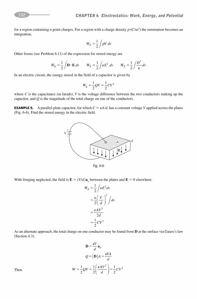
In an electric circuit, the energy stored in the field of a capacitor is given by
CHAPTER 6 Electrostatics: Work, Energy, and Potential102
W QV CVE � �1
2
1
22
W E dv
V
ddv
AV
d
CV
E �
�
�
�
1
2
2
21
2
2
2
2
2
�
�
�
�
�
⎛⎝⎜
⎞⎠⎟
D a
D
�
� �
�
�
V
d
Q AVA
d
n
W QVAV
dCV� � �
1
2
1
2
1
2
22�⎛
⎝⎜⎞⎠⎟
�
�
d
V
E
A
where C is the capacitance (in farads), V is the voltage difference between the two conductors making up thecapacitor, and Q is the magnitude of the total charge on one of the conductors.
EXAMPLE 5. A parallel-plate capacitor, for which C � �A/d, has a constant voltage V applied across the plates(Fig. 6-6). Find the stored energy in the electric field.
Fig. 6-6
With fringing neglected, the field is E � (V/d)an between the plates and E � 0 elsewhere.
As an alternate approach, the total charge on one conductor may be found from D at the surface via Gauss’s law(Section 4.3).
Then
W V dvE �1
2 � ρ
W dv W E dv WD
dvE E E� � �1
2
1
2
1
22
2
� � �D E· ��
for a region containing n point charges. For a region with a charge density ρ (C/m3) the summation becomes anintegration,
Other forms (see Problem 6.11) of the expression for stored energy are

SOLVED PROBLEMS
6.1. Given the electric field E � 2xax �4yay (V/m), find the work done in moving a point charge �2 C (a) from (2, 0, 0) m to (0, 0, 0) m and then from (0, 0, 0) m to (0, 2, 0) m; (b) from (2, 0, 0) m to (0, 2, 0) malong the straight-line path joining the two points. (See Fig. 6-7.)
CHAPTER 6 Electrostatics: Work, Energy, and Potential 103
y
(a)
(0, 2, 0)
(0, 0, 0) (2, 0, 0)
(b)
(a)x
W x dx y dy�� � �4 8 242
0
0
2
� � J
W t dt� � �16 1 240
1
� ( ) J
dW Q�� �� ��
E l· d QE drkQ
rdrr
W �� ��kQdr
rkQ
r
r
�1
12
2ln
Fig. 6-7
(a) Along the x axis, y � dy � dz � 0, and
dW � �2(2xax ) · (dx ax ) � �4x dx
Along the y axis, x � dx � dz � 0, and
dW � �2(�4yay ) · (dyay ) � 8y dy
(b) The straight-line path has the parametric equations
x � 2 � 2t y � 2t z � 0
where 0 t 1. Hence,
dW � �2[2(2 � 2t )ax � 4(2t )ay ] · [(�2 dt )ax � (2 dt )ay]
� 16(1 � t) dt
Thus,
6.2. Given the field E � (k/r)ar (V/m) in cylindrical coordinates, show that the work needed to move a pointcharge Q from any radial distance r to a point at twice that radial distance is independent of r.
Since the field has only a radial component,
and
For the limits of integration use r1 and 2r1.
which is independent of r1.

6.3. For a line charge ρ� � (10�9/2) C/m on the z axis, find VAB, where A is (2 m, π /2, 0) and B is (4 m, π, 5 m).
CHAPTER 6 Electrostatics: Work, Energy, and Potential104
V drAB
B
A
r�� �� E l E a· whereρπ
�
2 0�
Vr
dr rABB
A
�� �� ��
� 10
2 29 6 24
9
0( )[ln .
π�] V42
Vr
drAB ���
���4
2
2
164
⎛⎝⎜
⎞⎠⎟ V
Since the field due to the line charge is completely in the radial direction, the dot product with d l results in Er dr.
6.4. In the field of Problem 6.3, find VBC , where rB � 4 m and rC � 10 m. Then find VAC and compare withthe sum of VAB and VBC .
VBC � �9[ln r] rBrC
� �9(ln 4 � ln 10) � 8.25 V
VAC � �9[ln r] rArC
� �9(ln 2 � ln 10) � 14.49 V
VAB � VBC � 6.24 V � 8.25 V � 14.49 V � VAC
6.5. Given the field E � (�16/r 2)ar (V/m) in spherical coordinates, find the potential of point (2m, π, π /2)with respect to (4m, 0, π).
The equipotential surfaces are concentric spherical shells. Let r � 2 m be A and r � 4 m, B. Then
6.6. A line charge ρ� � 400 pC/m lies along the x axis and the surface of zero potential passes through thepoint (0, 5, 12) m in Cartesian coordinates (see Fig. 6-8). Find the potential at (2, 3, �4) m.
r rA B� � � � � �9 16 5 25 144 13m m
Vr
drr
rABr
rA
BB
A
�� �� �� ρπ
ρπ
� �
2 26 88
0 0� �ln V.
z
Linecharge
(0, 5, 12)
(2, 3, �4)rA
rB
y
Fig. 6-8
With the line charge along the x axis, the x coordinates of the two points may be ignored
Then

6.7. Find the potential at rA � 5 m with respect to rB � 15 m due to a point charge Q � 500 pC at the originand zero reference at infinity.
Due to a point charge,
CHAPTER 6 Electrostatics: Work, Energy, and Potential 105
VQ
r rABA B
� �4
1 1
0π�
⎛⎝⎜
⎞⎠⎟
VAB ��
� ��
�
500 10
4 10 36
1
5
1
150 60
12
9π π( / ).
⎛⎝⎜
⎞⎠⎟
V
VQ
VQ
50
1504
1
50 90
4
1
150� � � �
π π� �
⎛⎝⎜
⎞⎠⎟
⎛⎝⎜
⎞⎠⎟
. .V 330 V
To find the potential difference, the zero reference is not needed.
The zero reference at infinity may be used to find V5 and V15.
Then VAB � V5 � V15 � 0.60 V
6.8. Forty nanocoulombs of charge is uniformly distributed around a circular ring of radius 2 m. Find thepotential at a point on the axis 5 m from the plane of the ring. Compare with the result where all thecharge is at the origin in the form of a point charge.
With the charge in a line,
and (see Fig. 6-9) R � ���29 m, d� � (2 m) dφ.
Vd
R� � ρ
π� �
4 0�
ρπ π� ��
�� �40 10
2 2
109 8
( )C/m
Vd
� ��
��0
2 8
9
10 2
4 10 36 2966 9
π π φπ π( / )( )
( / ). V
Here
z
R5
2dQ � ρ r dφ
Fig. 6-9
If the charge is concentrated at the origin,
V ��
��40 10
4 572 0
9
0π� ( ). V
6.9. Five equal point charges, Q � 20 nC, are located at x � 2, 3, 4, 5, and 6 m. Find the potential at the origin.
VQ
Rm
m
� ��
� � � ��1
4
20 10
4
1
2
1
3
1
4
1
5
1
60
9
0π π� �
⎛
⎝⎜⎞⎠⎟
���
2611
Vm
n
∑

6.10. Charge is distributed uniformly along a straight line of finite length 2L (Fig. 6-10). Show that for twoexternal points near the midpoint, such that r1 and r2 are small compared to the length, the potential V12is the same as for an infinite line charge.
CHAPTER 6 Electrostatics: Work, Energy, and Potential106
z
L
dQ
r1r2
�L
ρ
Fig. 6-10
The potential at point 1 with zero reference at infinity is
Similarly, the potential at point 2 is
Now if L � r1 and L � r2,
which agrees with the expression found in Problem 6.6 for the infinite line.
6.11. Charge distributed throughout a volume v with density ρ gives rise to an electric field with energy content
Vdz
z r
z z
L
10 0
212 1 2
0
24
2
4
��
� � �
� ρπ
ρπ
�
�
�
�
( )
[
/
ln ( 2 rr
L L r r
L12
0
0
212
14
)]
[ ) ]� � � �ρπ
�
�ln ( ln
V L L r r20
222
22� � �
ρπ
�
�[ ) ]ln( ln+
V L r
V L r
10
1
20
2
2
2
�
�
ρπρπ
�
�
�
�
(ln 2 ln
(ln 2 ln
�
�
)
)
V V Vr
r12 1 20
2
12� � �
ρπ
�
�ln
W V dvEv
�1
2 � ρ
Then

Show that an equivalent expression for the stored energy is
CHAPTER 6 Electrostatics: Work, Energy, and Potential 107
W E dvE �1
22� �
Fig. 6-11 shows the charge-containing volume v enclosed within a large sphere of radius R. Since ρ vanishesoutside v,
W dv V dvEv
� � �1
2
1
2
1
2� � �ρ ρsphericalvolume
sphericcalvolume
(∇ ·D) V dv
W V dvE � �1
2
1
2� �sphericalvolume
sphericalv
(∇ · D)oolume
(∇ · V dvD)
1
2 spherical
surfaceV dD S·
W V dv dvE � �1
2
1
2� �( ) ( )D D E· ·∇
limR
V d→∞
sphericalsurface
D · S � 0
W E dv WD
dvE E� �1
2
1
22
2
� ���
or
The vector identity ∇ · V A � A · ∇V � V (∇ · A), applied to the integrand, gives
This expression holds for an arbitrarily large radius R; the plan is to let R → ∞.
The first integral on the right equals, by the divergence theorem,
6.12. Given the potential function V � 2x � 4y (V) in free space, find the stored energy in a 1-m3 volumecentered at the origin. Examine other 1-m3 volumes.
And since D � �E, the stored energy is also given by
The remaining integral gives, in the limit,
Now, as the enclosing sphere becomes very large, the enclosed volume charge looks like a point charge. Thus, atthe surface, D appears as k1/R
2 and V appears as k2/R. So the integrand is decreasing as 1/R3. Since the surface areaincreases only as R2, it follows that
Sphere
R
ρ
Volume v
Fig. 6-11
E a a a a a�� �� � � �� �∇⎛⎝⎜
⎞⎠⎟
VV
x
V
y
V
zx y z x y
2 4 (VV/m)

This field is constant in magnitude (E � ���20 V/m) and direction over all space, and so the total stored energy isinfinite. (The field could be that within an infinite parallel-plate capacitor. It would take an infinite amount of workto charge such a capacitor.)
Nevertheless, it is possible to speak of an energy density for this and other fields. The expression
CHAPTER 6 Electrostatics: Work, Energy, and Potential108
W E dvE �1
22� �
w � ��1
220
10
360
83� ( )
πJ/m
E a a�� ���
�∇⎛⎝⎜
⎞⎠⎟
Vr r
1 60 60
φφ
π πφ φ (V/m)
′⎛⎝⎜
⎞⎠⎟
Wr
r dr d dzE � ��0
0
1
0
6
0 1
0 6 2
2
60 30� � �π
πφ
/
.
. 00 0�
πln 6 1.51 nJ�
suggests that each tiny volume dv be assigned the energy content w dv, where
w � 1–2
�E2
For the present field, the energy density is constant:
and so every 1-m3 volume contains (10�8/36π) J of energy.
6.13. Two thin conducting half planes, at φ � 0 and φ � π /6, are insulated from each other along the z axis.Given that the potential function for 0 φ π /6 is V � (�60φ /π ) V, find the energy stored betweenthe half planes for 0.1 r 0.6 m and 0 z 1 m. Assume free space.
To find the energy, W ′E , stored in a limited region of space, one must integrate the energy density (see Problem 6.12)through the region. Between the half planes,
and so
6.14. The electric field between two concentric cylindrical conductors at r � 0.01 m and r � 0.05 m is givenby E � (105/r)ar (V/m), fringing neglected. Find the energy stored in a 0.5-m length. Assume freespace.
′⎛⎝
W E dvrE
h
h
� ��1
2 2
100
2 0
0
2
0 01
0 05 5
� � � ��� 0.5 π
.
.
⎜⎜⎞⎠⎟
2
0 224r dr d dzφ � . J
VQ
R
Q
R
Q
R12
0 12
3
0 13
4
0 14
9
04 4 4
4 10
4� � � �
� �
π π π π� � � �
11
1
1
1
1
297 5
2 2 4 10 971 19
� � �
� � � �
⎛
⎝⎜
⎞
⎠⎟ .
( )( .
V
W Q VE 55 780)� nJ
2 4 104 10
4 21021 1
99
0
W Q VE � � ��
���
( )π�
⎛⎝⎜
⎞⎠⎟
nJ
6.15. Find the stored energy in a system of four identical point charges, Q � 4 nC, at the corners of a square1 m on a side. What is the stored energy in the system when only two charges at opposite corners are inplace?
2WE � Q1V1 � Q2V2 � Q3V3 � Q4V4 � 4Q1V1
where the last equality follows from the symmetry of the system.
For only two charges in place,
Then

6.16. What energy is stored in the system of two point charges, Q1 � 3 nC and Q2 � �3 nC, separated by adistance of d � 0.2 m?
CHAPTER 6 Electrostatics: Work, Energy, and Potential 109
24 41 1 2 2 1
2
02
1
0
W Q V Q V QQ
dQ
Q
dE � � � �π π� �
⎛⎝⎜
⎞⎠⎟
⎛⎝⎜
⎞⎠⎠⎟
WQ Q
dE � ���
���
�1 2
0
9 2
94
3 10
4 10 36 0 24
π π π�
( )
( / )( . )005 nJ
W E dvE �1
22�
all space�
VV r a
V a r r a�
0
0
/⎧⎨⎩
Ea
�� �
� � �
∇⎧⎨⎪
⎩⎪V
r a
V a r r a
E dv
r
E
0
( / )02
021
20W � �
���0
0
2
0 0
02
22
022� � �
π πθ θ φ π
∞⎛⎝⎜
⎞⎠⎟
V a
rr dr d dsin � VV a0
2
Q DAV a
aa V a� � �
��0 0
22
0 04 4⎛⎝⎜
⎞⎠⎟ ( )π π
It may seem paradoxical that the stored energy turns out to be negative here, whereas 1–2
�E 2, and hence
whence
is necessarily positive. The reason for the discrepancy is that in equating the work done in assembling a system ofpoint charges to the energy stored in the field, one neglects the infinite energy already in the field when the chargeswere at infinity. (It took an infinite amount of work to create the separate charges at infinity.) Thus, the above result,WE � �405 nJ, may be taken to mean that the energy is 405 nJ below the (infinite) reference level at infinity. Sinceonly energy differences have physical significance, the reference level may properly be disregarded.
6.17. A spherical conducting shell of radius a, centered at the origin, has a potential field
with the zero reference at infinity. Find an expression for the stored energy that this potential represents.
Note that the total charge on the shell is, from Gauss’s law,
while the potential at the shell is V � V0. Thus, WE � 1–2
QV, the familiar result for the energy stored in a capacitor(in this case, a spherical capacitor with the other plate of infinite radius).
SUPPLEMENTARY PROBLEMS
6.18. Find the work done in moving a point charge Q � �20μC from the origin to (4, 2, 0) m in the field
E � 2(x � 4y)ax � 8xay (V/m)
along the path x2 � 8y.
6.19. Find the work done in moving a point charge Q � 3 μC from (4 m, π, 0) to (2 m, π /2, 2 m), cylindricalcoordinates, in the field E � (105/r)ar � 105zaz (V/m).
6.20. Find the difference in the amounts of work required to bring a point charge Q � 2 nC from infinity to r � 2 m andfrom infinity to r � 4 m, in the field E � (105/r)ar (V/m).
6.21. A uniform line charge of density ρ� � 1 nC/m is arranged in the form of a square 6 m on a side, as shown in Fig. 6-12. Find the potential at (0, 0, 5) m.
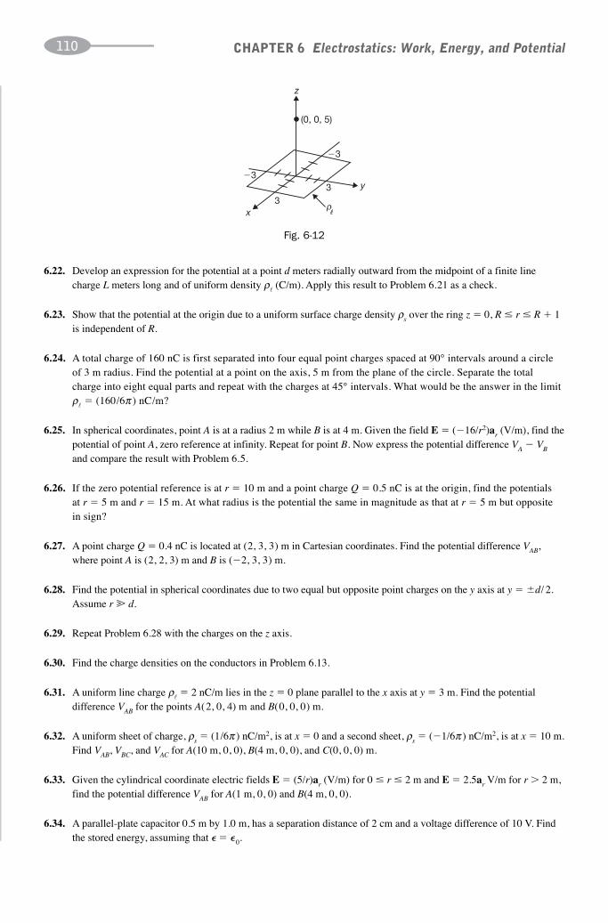
6.22. Develop an expression for the potential at a point d meters radially outward from the midpoint of a finite linecharge L meters long and of uniform density ρ� (C/m). Apply this result to Problem 6.21 as a check.
6.23. Show that the potential at the origin due to a uniform surface charge density ρs over the ring z � 0, R r R � 1is independent of R.
6.24. A total charge of 160 nC is first separated into four equal point charges spaced at 90° intervals around a circleof 3 m radius. Find the potential at a point on the axis, 5 m from the plane of the circle. Separate the total charge into eight equal parts and repeat with the charges at 45° intervals. What would be the answer in the limitρ� � (160/6π ) nC/m?
6.25. In spherical coordinates, point A is at a radius 2 m while B is at 4 m. Given the field E � (�16/r2)ar (V/m), find thepotential of point A, zero reference at infinity. Repeat for point B. Now express the potential difference VA � VB
and compare the result with Problem 6.5.
6.26. If the zero potential reference is at r � 10 m and a point charge Q � 0.5 nC is at the origin, find the potentials at r � 5 m and r � 15 m. At what radius is the potential the same in magnitude as that at r � 5 m but opposite in sign?
6.27. A point charge Q � 0.4 nC is located at (2, 3, 3) m in Cartesian coordinates. Find the potential difference VAB,where point A is (2, 2, 3) m and B is (�2, 3, 3) m.
6.28. Find the potential in spherical coordinates due to two equal but opposite point charges on the y axis at y � �d/ 2.Assume r � d.
6.29. Repeat Problem 6.28 with the charges on the z axis.
6.30. Find the charge densities on the conductors in Problem 6.13.
6.31. A uniform line charge ρ� � 2 nC/m lies in the z � 0 plane parallel to the x axis at y � 3 m. Find the potentialdifference VAB for the points A(2, 0, 4) m and B(0, 0, 0) m.
6.32. A uniform sheet of charge, ρs � (1/6π ) nC/m2, is at x � 0 and a second sheet, ρs � (�1/6π ) nC/m2, is at x � 10 m.Find VAB, VBC, and VAC for A(10 m, 0, 0), B(4 m, 0, 0), and C(0, 0, 0) m.
6.33. Given the cylindrical coordinate electric fields E � (5/r)ar (V/m) for 0 r 2 m and E � 2.5ar V/m for r 2 m,find the potential difference VAB for A(1 m, 0, 0) and B(4 m, 0, 0).
6.34. A parallel-plate capacitor 0.5 m by 1.0 m, has a separation distance of 2 cm and a voltage difference of 10 V. Findthe stored energy, assuming that � � � 0.
CHAPTER 6 Electrostatics: Work, Energy, and Potential110
(0, 0, 5)
�3
�3
33
y
x
z
ρ
Fig. 6-12

6.35. The capacitor described in Problem 6.34 has an applied voltage of 200 V.
(a) Find the stored energy.
(b) Hold d1 (Fig. 6-13) at 2 cm and the voltage difference at 200 V, while increasing d2 to 2.2 cm. Find the finalstored energy.
CHAPTER 6 Electrostatics: Work, Energy, and Potential 111
d1
0.5 m
d2
Fig. 6-13
6.36. Find the energy stored in a system of three equal point charges, Q � 2 nC, arranged in a line with 0.5 m separationbetween them.
6.37. Repeat Problem 6.36 if the charge in the center is �2 nC.
6.38. Four equal point charges, Q � 2 nC, are to be placed at the corners of a square 1–3
m on a side, one at a time. Findthe energy in the system after each charge is positioned.
6.39. Given the electric field E � �5e�r/aa r in cylindrical coordinates, find the energy stored in the volume described byr 2a and 0 z 5a.
6.40. Given a potential V � 3x2 � 4y2 (V), find the energy stored in the volume described by 0 x 1 m, 0 y 1 m,and 0 z 1 m.
ANSWERS TO SUPPLEMENTARY PROBLEMS
6.18. 1.60 mJ
6.19. �0.392 J
6.20. 1.39 � 10�4 J
6.21. 35.6 V
6.22.
6.24. 247 V
6.25. VA � 2VB � �8 V
6.26. 0.45 V, �0.15 V, ∞
6.27. 2.70 V
6.28. (Qd sin θ ) /(4π�0r2)
6.29. (Qd cos θ ) /(4π� 0 r 2)
ρπ
�
2
2 4
0
2 2
�ln (V)
L d L
d
/ /� �

6.30.
6.31. �18.4 V
6.32. �36 V, �24 V, �60 V
6.33. 8.47 V
6.34. 11.1 nJ
6.35. Hint: ΔWE � 1–2
(ΔC )V 2
(a) 4.4 μJ; (b) 4.2 μJ
6.36. 180 nJ
6.37. �108 nJ
6.38. 0, 108 nJ, 292 nJ, 585 nJ
6.39. 7.89 � 10�10a3
6.40. 147 pJ
CHAPTER 6 Electrostatics: Work, Energy, and Potential112
��
��
600
600 0� �
πφ
πφ π
r r(C/m ) on (C/m ) on
62 2,
113
Electric Current
7.1 Introduction
Electric current is the rate of transport of electric charge past a specified point or across a specified surface. Thesymbol I is generally used for constant currents and i for time-variable currents. The unit of current is the ampere(1 A � 1 C/s; in the SI system, the ampere is the basic unit and the coulomb is the derived unit).
Ohm’s law relates current to voltage and resistance. For simple dc circuits, I � V /R. However, when chargesare suspended in a liquid or a gas, or where both positive and negative charge carriers are present with differ-ent characteristics, the simple form of Ohm’s law is insufficient. Consequently, the current density J (A /m2)receives more attention in electromagnetics than does current I.
7.2 Charges in Motion
Consider the force on a positively charged particle in an electric field in vacuum, as shown in Fig. 7-1(a). Thisforce, F � �QE, is unopposed and results in constant acceleration. Thus, the charge moves in the directionof E with a velocity U that increases as long as the particle is in the E field. When the charge is in a liquid orgas, as shown in Fig. 7-1(b), it collides repeatedly with particles in the medium, resulting in random changesin direction. But for constant E and a homogeneous medium, the random velocity components cancel out,leaving a constant average velocity, known as the drift velocity U, along the direction of E. Conduction in met-als takes place by movement of the electrons in the outermost shells of the atoms making up the crystallinestructure. According to the electron-gas theory, these electrons reach an average drift velocity in much thesame way as a charged particle moving through a liquid or gas. The drift velocity is directly proportional tothe electric field intensity,
U � μE
where μ, the mobility, has the units m2/ V · s. Each cubic meter of a conductor contains on the order of 1028 atoms.Good conductors have one or two electrons from each atom free to move upon application of the field. Themobility μ varies with temperature and the crystalline structure of the solid. The particles in the solid have avibratory motion which increases with temperature. This makes it more difficult for the charges to move. Thus,at higher temperatures the mobility μ is reduced, resulting in a smaller drift velocity (or current) for a given E.In circuit analysis this phenomenon is accounted for by stating a resistivity for each material and specifying anincrease in this resistivity with increasing temperature.
CHAPTER 7

7.3 Convection Current Density J
A set of charged particles giving rise to a charge density ρ in a volume v is shown in Fig. 7-2 to have a velocityU to the right. The particles are assumed to maintain their relative positions within the volume. As this chargeconfiguration passes a surface S, it constitutes a convection current, with density
J � ρU (A /m2)
Of course, if the cross section of v varies or if the density ρ is not constant throughout v, then J will not beconstant with time. Further, J will be zero when the last portion of the volume crosses S. Nevertheless, theconcept of a current density caused by a cloud of charged particles in motion is at times useful in the studyof electromagnetic field theory.
CHAPTER 7 Electric Current114
�Q
�Q
E E
U
(a) Vacuum (b) Liquid or gas
U
Fig. 7-1
S
vJ � ρ U
ρ
U
Fig. 7-2
7.4 Conduction Current Density J
Of more interest is the conduction current that occurs in the presence of an electric field within a conductor offixed cross section. The current density is again given by
J � ρU (A /m2)
which, in view of the relation U � μE, can be written
J � σE
where σ � ρμ is the conductivity of the material, in siemens per meter (S/m). In metallic conductors the chargecarriers are electrons, which drift in a direction opposite to that of the electric field (Fig. 7-3). Hence, for electrons,both ρ and μ are negative, which results in a positive conductivity σ, just as in the case of positive charge carriers.It follows that J and E have the same direction regardless of the sign of the charge carriers. It is conventional totreat electrons moving to the left as positive charges moving to the right, and always to report ρ and μ as positive.
The relation J � σE is often referred to as the point form of Ohm’s law. The factor σ takes into account thedensity of the electrons free to move (ρ) and the relative ease with which they move through the crystallinestructure (μ). As might be expected, σ is a function of temperature.

EXAMPLE 1. What electric field intensity and current density correspond to a drift velocity of 6.0 � 10�4 m/sin a silver conductor?
For silver σ � 61.7 MS/m and μ � 5.6 � 10�3 m2/V · s.
CHAPTER 7 Electric Current 115
S
J � EE
U
σ
Fig. 7-3
(a) Liquid or gas (b) Conductor (c) Semiconductor
J
E
J
EJ
E
σ � ρ�
μ�
� ρ�
μ�
σ � ρe
μe
σ � ρe
μe
� ρh
μh
�
�
�
�
�
�
�
�
�
��
�
��
�
�
��
�
�
�
Fig. 7-4
EU
J E
� ��
�� �
� �
�
��
μ
σ
6 0 10
5 6 101 07 10
6 61
4
31.
..
.
V/m
��106 2A m/
7.5 Conductivity σσ
In a liquid or gas there are generally present both positive and negative ions, some singly charged and others dou-bly charged, and possibly of different masses. A conductivity expression would include all such factors. However,if it is assumed that all the negative ions are alike and so too the positive ions, then the conductivity contains twoterms as shown in Fig. 7-4 (a). In a metallic conductor, only the valence electrons are free to move. In Fig. 7-4(b)they are shown in motion to the left. The conductivity then contains only one term, the product of the charge density of the electrons free to move, ρe, and their mobility, μe.
A somewhat more complex conduction occurs in semiconductors such as germanium and silicon. In the crystal structure each atom has four covalent bonds with adjacent atoms. However, at room temperature, andupon influx of energy from some external source such as light, electrons can move out of the position called forby the covalent bonding. This creates an electron-hole pair available for conduction. Such materials are calledintrinsic semiconductors. Electron-hole pairs have a short lifetime, disappearing by recombination. However,others are constantly being formed and at all times some are available for conduction. As shown in Fig. 7-4(c),the conductivity σ consists of two terms, one for the electrons and another for the holes. In practice, impurities,in the form of valence-three or valence-five elements, are added to create p-type and n-type semiconductor mate-rials. The intrinsic behavior just described continues but is far overshadowed by the presence of extra electronsin n-type, or holes in p-type, materials. Then, in the conductivity σ, one of the densities, ρe or ρh, will far exceedthe other.

EXAMPLE 2. Determine the conductivity of intrinsic germanium at room temperature.At 300 K there are 2.5 � 1019 electron-hole pairs per cubic meter. The electron mobility is μe � 0.38 m2/V· s
and the hole mobility is μh � 0.18 m2/V · s. Since the material is not doped, the numbers of electrons and holes areequal.
σ � Nee(μe � μh) � (2.5 � 1019)(1.6 � 10�19)(0.38 � 0.18) � 2.24 S/m
7.6 Current I
Where current density J crosses a surface S, as in Fig. 7-5, the current I is obtained by integrating the dot productof J and dS.
CHAPTER 7 Electric Current116
dI d I dS
� �J S J S· ·�Of course, J need not be uniform over S and S need not be a plane surface.
dS
S
J
Fig. 7-5
dS
z
S
J
Fig. 7-6
EXAMPLE 3. Find the current in the circular wire shown in Fig. 7-6 if the current density is J � 15(1 � e�1000r)az (A /m2). The radius of the wire is 2 mm.
A cross section of the wire is chosen for S. Then
dI d
e r dr d
I
rz z
�
� �
�
�
J S
a a
·
·15(1 1000 ).
φπ
� �0
2
0
0 0022
41 33 10 0 133
15(1
mA
1000�
� � �
�
�
e r dr dr )
. . �
φ
A
and

Any surface S which has a perimeter that meets the outer surface of the conductor all the way around willhave the same total current, I � 0.133 mA, crossing it.
7.7 Resistance R
If a conductor of uniform cross-sectional area A and length �, as shown in Fig. 7-7, has a voltage difference Vbetween its ends, then
CHAPTER 7 Electric Current 117
A
V
E, J
�
Fig. 7-7
EV
JV
� �� �
andσ
assuming that the current is uniformly distributed over the area A. The total current is then
I JAAV
� �σ
�
Since Ohm’s law states that V � IR, the resistance is
RA
��
σ( )Ω
RV
d
V
d� �
� �J S E S· ·σ
Rd
d
���
E l
E S
·
·σ
(Note that 1 S�1 � 1 Ω; the siemens was formerly known as the mho.) This expression for resistance is generallyapplied to all conductors where the cross section remains constant over the length �. However, if the current density is greater along the surface area of the conductor than in the center, then the expression is not valid. For such nonuniform current distributions the resistance is given by
If E is known rather than the voltage difference between the two faces, the resistance is given by
The numerator gives the voltage drop across the sample, while the denominator gives the total current I.
EXAMPLE 4. Find the resistance between the inner and outer curved surfaces of the block shown in Fig. 7-8,where the material is silver for which σ � 6.17 � 107 S/m.
If the same current I crosses both the inner and outer curved surfaces,
J a E a� �k
r
k
rr randσ

Then (5° � 0.0873 rad),
CHAPTER 7 Electric Current118
0.05 m
rb � 3.0 mra � 0.2 m
� 5ºφ
J
Fig. 7-8
R
k
rdr
k
rr d dz
r r
r
��
� �0 2
3 0
0
0 05
0
0 0873
.
.
. .σ
φ
a a
a
·
· aar
� � � ��ln 15
(0,05)(0.0873)σμ1 01 10 10 15. .Ω Ω
7.8 Current Sheet Density K
At times current is confined to the surface of a conductor, such as the inside walls of a waveguide. For such acurrent sheet it is helpful to define the density vector K (in A /m), which gives the rate of charge transport perunit transverse length. (Some books use the notation Js.) Fig. 7-9 shows a total current of I, in the form of acylindrical sheet of radius r, flowing in the positive z direction. In this case,
K a�1
2πr z
at each point of the sheet. For other sheets, K might vary from point to point.
zr
K
Fig. 7-9
In general, the current flowing through a contour C within a current sheet is obtained by integrating the normalcomponent of K along the contour.
I K dC n� � �
EXAMPLE 5. A thin conducting sheet lies in the z � 0 plane for 0 � x � 0.05 m. An ay directed current of 25 Ais sinusoidally distributed across the sheet, with linear density zero for x � 0 and x � 0.05 m and maximum at x � 0.025 m (see Fig. 7-10). Obtain an expression for K.
The data give K � (k sin 20πx)ay (A/m), for an unknown constant k. Then
I K dx k x dx
k k
y� � �
� �
25 20
25 10 250
0
0 05
� �.
sin
/
π
π πor ��A/m.or
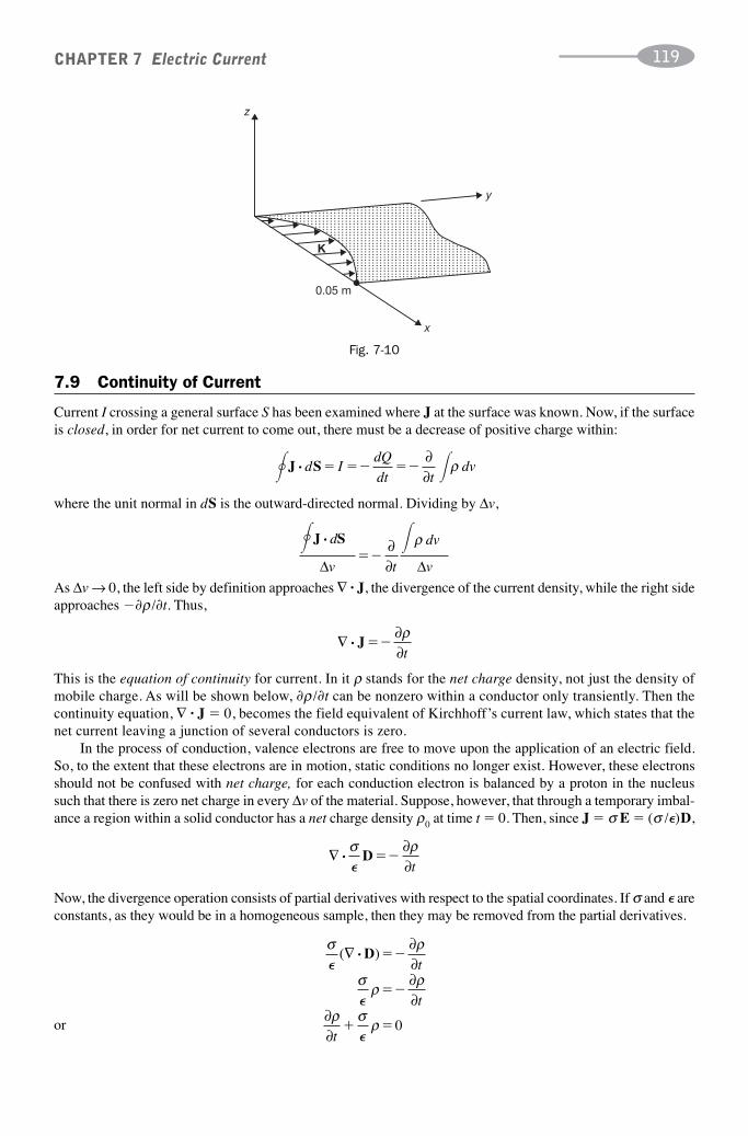
7.9 Continuity of Current
Current I crossing a general surface S has been examined where J at the surface was known. Now, if the surfaceis closed, in order for net current to come out, there must be a decrease of positive charge within:
CHAPTER 7 Electric Current 119
x
y
z
0.05 m
K
Fig. 7-10
�J S· d IdQ
dt tdv� �� ��
∂∂
ρ
where the unit normal in dS is the outward-directed normal. Dividing by Δv,
�J S· d
v t
dv
vΔ∂∂ Δ
��ρ
As Δv → 0, the left side by definition approaches ∇ · J, the divergence of the current density, while the right sideapproaches �∂ρ /∂t. Thus,
∇ ∂∂
· J ��ρt
This is the equation of continuity for current. In it ρ stands for the net charge density, not just the density ofmobile charge. As will be shown below, ∂ρ /∂t can be nonzero within a conductor only transiently. Then thecontinuity equation, ∇ · J � 0, becomes the field equivalent of Kirchhoff’s current law, which states that thenet current leaving a junction of several conductors is zero.
In the process of conduction, valence electrons are free to move upon the application of an electric field.So, to the extent that these electrons are in motion, static conditions no longer exist. However, these electronsshould not be confused with net charge, for each conduction electron is balanced by a proton in the nucleussuch that there is zero net charge in every Δv of the material. Suppose, however, that through a temporary imbal-ance a region within a solid conductor has a net charge density ρ0 at time t � 0. Then, since J � σ E � (σ /�)D,
∇ ∂∂
·σ ρ�
D ��t
Now, the divergence operation consists of partial derivatives with respect to the spatial coordinates. If σ and � areconstants, as they would be in a homogeneous sample, then they may be removed from the partial derivatives.
σ ρ
σ ρ ρ
ρ σ ρ
�
�
�
( )∇ ∂∂∂∂
∂∂
· D ��
��
� �
t
t
t0or

The solution to this equation is
ρ � ρ0e�(σ /�)t
Thus, ρ decays exponentially, with a time constant τ � � /σ, also known as the relaxation time. At t � τ, ρ hasdecayed to 36.8% of its initial value. For a conductor τ is extremely small, on the order of 10�19 seconds. This con-firms that free charge cannot remain within a conductor and instead is distributed evenly over the conductor surface.
EXAMPLE 6. Determine the relaxation time for silver, given that σ � 6.17 � 107 S/m. If charge of density ρ0is placed within a silver block, find ρ after one, and also after five, time constants.
Since � � �0,
CHAPTER 7 Electric Current120
τσ
π� �
�� �
��� 10 36
6 17 101 43 10
9
719
.. s
Therefore,
at
at
0 0
0
t e
t e
� � �
� � � �
�
�
τ ρ ρ ρ
τ ρ ρ
: .
: .
1
5
0 368
5 6 74 10��3 ρ0
7.10 Conductor-Dielectric Boundary Conditions
Under static conditions all net charge will be on the outer surfaces of a conductor and both E and D are there-fore zero within the conductor. Because the electric field is a conservative field, the line integral of E · d l is zerofor any closed path. A rectangular path with corners 1, 2, 3, 4 is shown in Fig. 7-11. For this path,
� � � �1
2
2
3
3
4
4
1
E l E l E l E l· · · ·d d d d� � � � 0
If the path lengths 2 to 3 and 4 to 1 are now permitted to approach zero, keeping the interface between them,then the second and fourth integrals are zero. The path from 3 to 4 is within the conductor where E must be zero.This leaves
1 2
4 3
Dielectric
Conductor
Fig. 7-11
� �1
2
1
2
E l· d E dt� �� 0
where Et is the tangential component of E at the surface of the dielectric. Since the interval 1 to 2 can be chosenarbitrarily,
Et � Dt � 0
at each point of the surface.To discover the conditions on the normal components, a small, closed, right circular cylinder is placed
across the interface as shown in Fig. 7-12. Gauss’s law applied to this surface gives
D · dS � Qenc
� � � �top bottom sideD S D S D S· · ·d d d dA s
� � � ρ Sor
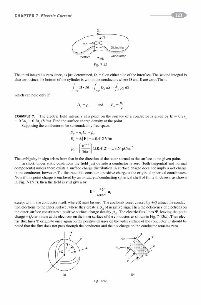
The third integral is zero since, as just determined, Dt � 0 on either side of the interface. The second integral isalso zero, since the bottom of the cylinder is within the conductor, where D and E are zero. Then,
CHAPTER 7 Electric Current 121
� � top top
D S· d D dS dSn A s� � ρ
which can hold only if
D En s ns� �ρ ρ
and�
dS
dS
A
Dn
top
bottom
Dielectric
Conductor
Fig. 7-12
�
�
�
�
�
�
�Q
(a) (b)
ψ
ψs2
ρ
s1ρ
Fig. 7-13
EXAMPLE 7. The electric field intensity at a point on the surface of a conductor is given by E � 0.2ax� 0.3ay � 0.2az (V/m). Find the surface charge density at the point.
Supposing the conductor to be surrounded by free space,
D E
E
n n s
n
s
� �
�� ��
� �
�
�
� ρ
ρπ
E 0 412
10
36
9
.
(
V/m
⎛
⎝⎜⎞⎠⎟
00 412 3 64. ) .�� pC/m2
The ambiguity in sign arises from that in the direction of the outer normal to the surface at the given point.In short, under static conditions the field just outside a conductor is zero (both tangential and normal
components) unless there exists a surface charge distribution. A surface charge does not imply a net chargein the conductor, however. To illustrate this, consider a positive charge at the origin of spherical coordinates.Now if this point charge is enclosed by an uncharged conducting spherical shell of finite thickness, as shownin Fig. 7-13(a), then the field is still given by
E a��Q
rr
4 2π�
except within the conductor itself, where E must be zero. The coulomb forces caused by �Q attract the conduc-tion electrons to the inner surface, where they create a ρs1 of negative sign. Then the deficiency of electrons onthe outer surface constitutes a positive surface charge density ρs2. The electric flux lines Ψ, leaving the pointcharge �Q, terminate at the electrons on the inner surface of the conductor, as shown in Fig. 7-13(b). Then elec-tric flux lines Ψ originate once again on the positive charges on the outer surface of the conductor. It should benoted that the flux does not pass through the conductor and the net charge on the conductor remains zero.

SOLVED PROBLEMS
7.1. An AWG #12 copper conductor has an 80.8-mil diameter. A 50-foot long conductor of this type carriesa current of 20 A. Find the electric field intensity E, drift velocity U, the voltage drop, and the resistancefor the 50-foot length.
Since a mil is 1———1000
inch, the cross-sectional area is
CHAPTER 7 Electric Current122
A �� �
π 0 0808 2 54 10
1
2. .in
2
m
in
⎛⎝⎜
⎞⎠⎟
⎛⎝⎜
⎞⎠⎟
⎡
⎣⎢⎢
⎤
⎦⎥⎥⎥
−
2
6
66
3 31 10
1 20
3 31 106 04 10
� �
� ��
� �
�.
..
m
A/
2
JA
mm2
For copper, σ � 5.8 � 107 S /m. Then
EJ
E
� ��
�� �
� �
�
σ6 04 10
5 8 101 04 10
1 04
6
71.
..
( .
V/m
V � �� �
� � �
�10 50 12 0 0254 1 59
1 59
207
1)( )( )( . ) .
..
V
RV
I995 10 2� � Ω
The electron mobility in copper is μ � 0.0032 m2/V · s, and since σ � ρμ, the charge density is
ρ σμ
� ��
� �5 8 10
0 00321 81 10
710.
.. /C m3
From J � ρU the drift velocity is now found as
UJ
� ��
�� � �
ρ6 05 10
1 81 103 34 10
6
104.
.. /m s
With this drift velocity, an electron takes approximately 30 seconds to move a distance of 1 centimeter in the #12 copper conductor.
7.2. What current density and electric field intensity correspond to a drift velocity of 5.3 � 10�4 m/s inaluminum?
For aluminum, the conductivity is σ � 3.82 � 107 S/m and the mobility is μ � 0.0014 m2/V · s.
J U U� � ��
� � ��ρ σμ
3 83 10
0 00145 3 10 1 45 10
74 7.
.( . ) . A//
.
m
V/m
2
13 79 10EJ U
� � � � �
σ μ
7.3. A long copper conductor has a circular cross section of diameter 3.0 mm and carries a current of 10 A.Each second, what percent of the conduction electrons must leave (to be replaced by others) a 100-mmlength?
Avogadro’s number is N � 6.02 � 1026 atoms/kmol. The specific gravity of copper is 8.96 and the atomic weightis 63.54. Assuming one conduction electron per atom, the number of electrons per unit volume is
Ne � �6 02 10126.
atoms
kmolkmol
63.54 kg
⎛⎝⎜
⎞⎠⎟
⎛⎝⎜
⎞⎠⎠⎟
⎛⎝⎜
⎞⎠⎟
⎛⎝⎜
⎞⎠⎟
8 96 10 1
8
3.
.
�
�
kg
m
electron
atom3
449 1028� electrons/m3
Then

The number of electrons in a 100 mm length is
CHAPTER 7 Electric Current 123
N ��
� � ��
π 3 10
20 100 8 49 10 6 00 10
3 228⎛
⎝⎜⎞⎠⎟
( . )( . ) . 222
A 10-A current requires that
101
1 6 106 25 1019
C
s
electron
C
⎛⎝⎜
⎞⎠⎟
⎛⎝⎜
⎞⎠⎟.
.�
� ��
119 electrons/s
pass a fixed point. Then the percent leaving the 100 mm length per second is
6 25 10
6 00 10100 0 104
19
22
.
.( ) . %
�
��
7.4. What current would result if all the conduction electrons in a 1-centimeter cube of aluminum passed aspecified point in 2.0s? Assume one conduction electron per atom.
The density of aluminum is 2.70 � 103 kg/m3 and the atomic weight is 26.98 kg /kmol. Then
Ne � � � � �( . ).
( . ) .6 02 101
26 982 70 10 6 02 126 3⎛
⎝⎜⎞⎠⎟
00
6 02 10
28 3
28
electrons m
electrons m
/
( . /I
Q
t�
�ΔΔ
33 2 3 1910 1 6 10
24 82
) ( ) ( . ).
� ���
m C/electron
skA
7.5. What is the density of free electrons in a metal for a mobility of 0.0046 m2/V · s and a conductivity of29.1 MS/m?
Since σ � μρ,
ρ σμ
� ��
� �29 1 10
0 00466 33 10
69 3.
.. /C m
7.6. Find the conductivity of n-type germanium (Ge) at 300 K, assuming one donor atom in each 108 atoms.The density of Ge is 5.32 � 103 kg/m3 and the atomic weight is 72.6 kg/kmol.
The carriers in an n-type semiconductor material are electrons. Since 1 kmol of a substance contains 6.02 � 1026
atoms, the carrier density is given by
Ne ��
�� �
�
6 33 10
1 6 103 96 10
9
1928 3.
.. /electrons mand
Ne � �6 02 101
72 626.
.
atoms
kmol
kmol
kg
⎛⎝⎜
⎞⎠⎟
⎛⎝⎜
⎞⎠⎟⎟
⎛⎝⎜
⎞⎠⎟
⎛⎝⎜
⎞⎠⎟
5 32 1010
38. �
kg
m
electrons
atoms3
�� �4 41 1020. electrons/m3
The intrinsic concentration ni for Ge at 300 K is 2.5 � 1019m�3. The mass-action law, NeNh � n2i, then gives the
density of holes:
Nh ��
�� �
( . )
.. /
2 5 10
4 41 101 42 10
19 2
2018 3holes m
Because Ne � Nh, conductivity will be controlled by the donated electrons, whose mobility at 300 K is
σ � Ne eμe � (4.41 � 1020)(1.6 � 10�19) (0.38) � 26.8 S/m
and
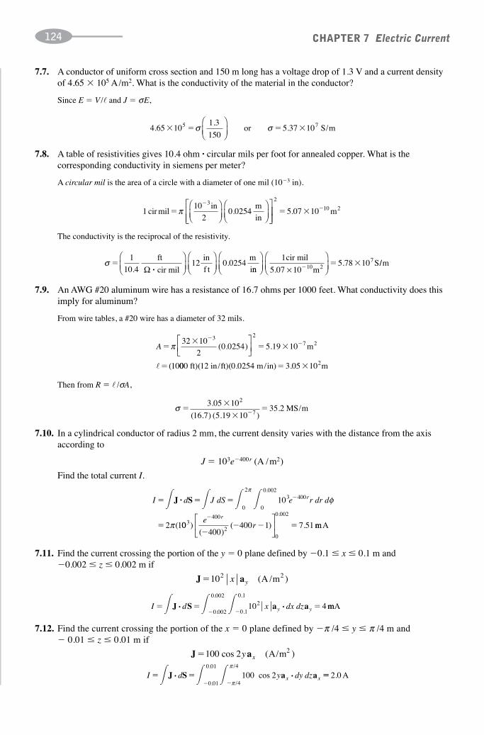
7.7. A conductor of uniform cross section and 150 m long has a voltage drop of 1.3 V and a current densityof 4.65 � 105 A/m2. What is the conductivity of the material in the conductor?
Since E � V /� and J � σE,
CHAPTER 7 Electric Current124
4 651 3
1505 37 107.
.. /� � � �105 σ σ
⎛⎝⎜
⎞⎠⎟
or S m
7.8. A table of resistivities gives 10.4 ohm · circular mils per foot for annealed copper. What is thecorresponding conductivity in siemens per meter?
A circular mil is the area of a circle with a diameter of one mil (10�3 in).
110
20 0254
3
cir milin m
in�
�
π⎛⎝⎜
⎞⎠⎟
⎛⎝⎜
⎞⎠⎟
⎡
⎣⎢⎢
⎤
⎦. ⎥⎥
⎥
2
10 25 07 10� � �. m
The conductivity is the reciprocal of the resistivity.
σ �1
10 412 0 0254
..
ft
cir mil
in
f t
m
iΩ ·
⎛⎝⎜
⎞⎠⎟
⎛⎝⎜
⎞⎠⎟ nn
cir mil
5.07 10 mS10 2
⎛⎝⎜
⎞⎠⎟ ×
⎛⎝⎜
⎞⎠⎟
15 78 107
�� �. //m
7.9. An AWG #20 aluminum wire has a resistance of 16.7 ohms per 1000 feet. What conductivity does thisimply for aluminum?
From wire tables, a #20 wire has a diameter of 32 mils.
A ��
� �
�
��π 32 10
20 0254 5 19 10
10
3 27 2( . ) .
(
⎡⎣⎢
⎤⎦⎥
m
� 000 12ft) in/ft)(0.0254 m/in) 3.05 10 m2( � �
Then from R � � /σA,
σ ��
��
�
3 05 10
16 7 5 19 1035 2
2
7
.
( . ) ( . ). /MS m
7.10. In a cylindrical conductor of radius 2 mm, the current density varies with the distance from the axisaccording to
J � 103e�400r (A /m2)
Find the total current I.
I d J d e r dr dr� � �
�
�� � � �J S· S0
2
0
0 0023 40010
2 1
π
φ
π
.
( 00400
400 1 7 513400
20
0 002
)( )
( ) .
.e
rr�
�� � �
⎡
⎣⎢
⎤
⎦⎥ mmA
7.11. Find the current crossing the portion of the y � 0 plane defined by �0.1 x 0.1 m and �0.002 z 0.002 m if
J a�102 x y ( )A /m2
7.12. Find the current crossing the portion of the x � 0 plane defined by �π /4 y π /4 m and � 0.01 z 0.01 m if
J a�100 2cos ( )y x A/m2
I d x dx dzy y� � �� �
� � �J S a a· ·0 002
0 002
0 1
0 1210 4
.
.
.
.
mmA
I d y dy dzx x� �� �
� � �J S a a· ·0 01
0 01
4
4
100 2.
.
/
/
cosπ
π
�� 2 0. A

7.13. Given J � 103 sin θar A/m2 in spherical coordinates, find the current crossing the spherical shell r � 0.02 m.
Since J and
dS � r 2 sin θ dθ dφ ar
are radial,
CHAPTER 7 Electric Current 125
I d d� �� �0
2
0
3 2 210 0 02 3 95π π
θ θ φ( . ) sin . A
7.14. Show that the resistance of any conductor of constant cross-sectional area A and length � is given by R � � /σA, assuming uniform current distribution.
A constant cross section along the length � results in constant E, and the voltage drop is
V d E� �� E l· �
If the current is uniformly distributed over the area A,
I d JA E A� � �� J S· σ
where σ is the conductivity. Then, since R � V/I,
RA
��
σ
7.15. Determine the resistance of the insulation in a length � of coaxial cable, as shown in Fig. 7-14.
b
a
Fig. 7-14
Assume a total current I from the inner conductor to the outer conductor. Then, at a radial distance r,
JI
A
I
r� �
2π �
The voltage difference between the conductors is then
EI
r�
2πσ �and so
VI
rdr
I b
aabb
a
�� �� 2 2πσ πσ� �ln
and the resistance is
RV
I
I
r
b
a� �
2πσ �ln
7.16. A current sheet of width 4 m lies in the z � 0 plane and contains a total current of 10 A in a directionfrom the origin to (1, 3, 0) m. Find an expression for K.
At each point of the sheet, the direction of K is the unit vector
a ax y� 3
10

and the magnitude of K is 10—4
A /m. Thus,
CHAPTER 7 Electric Current126
Ka a
��10
4
3
10x y⎛
⎝⎜⎞
⎠⎟A /m
7.17. As shown in Fig. 7-15, a current IT follows a filament down the z axis and enters a thin conducting sheetat z � 0. Express K for this sheet.
z
IT
x
r y
K
Fig. 7-15
30ºK
Fig. 7-16
z
I
Fig. 7-17
Consider a circle in the z � 0 plane. The current IT on the sheet spreads out uniformly over the circumference 2πr.The direction of K is ar. Then
K a�I
rT
r2π
7.18. For the current sheet of Problem 7.17 find the current in a 30° section of the plane (Fig. 7-16).
I K dI
rr d
In
T T� � �� ��0
6
2 12
π
πφ
/
However, integration is not necessary, since for uniformly distributed current a 30° segment will contain 30°/360°,or 1/12 of the total.
7.19. A current I(A) enters a thin right circular cylinder at the top, as shown in Fig. 7-17. Express K if theradius of the cylinder is 2 cm.

On the top, the current is uniformly distributed over any circumference 2πr, so that
CHAPTER 7 Electric Current 127
Fig. 7-18
K a�I
r r2π(A /m)
Down the side, the current is uniformly distributed over the circumference 2π (0.02 m), so that
K a� �I
z0 04.( ) (
πA/m)
7.20. A cylindrical conductor of radius 0.05 m with its axis along the z axis has a surface charge density ρs � ρ0 /z (C /m2). Write an expression for E at the surface.
Since Dn � ρs, En � ρs /�0. At (0.05, φ, z),
E a a� �Ezn r r
ρ0 V/m)�0
(
7.21. A conductor occupying the region x � 5 has a surface charge density
ρ ρs
y z�
�
0
2 2
Write expressions for E and D just outside the conductor.
The outer normal is �ax. Then, just outside the conductor,
D a a a� � � � ��
�Dz
n x s x x( ) ( ) ( )ρ ρ02y 2
7.22. Two concentric cylindrical conductors, ra � 0.01 m and rb � 0.08 m, have charge densities ρsa � 40 pC/m2
and ρsb, such that D and E fields exist between the two cylinders but are zero elsewhere. See Fig. 7-18. Findρsb and write expressions for D and E between the cylinders.
E a��
�ρ0
02� y z
x2( )and
ra rbsaρ
sbρ
By symmetry, the field between the cylinders must be radial and a function of r only. Then, for ra � r � rb,
∇ · D � � �1
0r
d
drrD rD cr r( ) or
To evaluate the constant c, use the fact that Dn � Dr � ρsa at r � ra � 0.
c � (0.01)(40 � 10�12) � 4 � 10�13 C/m

and so
CHAPTER 7 Electric Current128
D a ED
a��
� ��� �4 10 4 52 1013 2
r rr r( ).
(C/m and V/m2
0�))
The density ρsb is now found from
ρsb n r r r r rD D
b b� �� ��
���
� � � �
�
0 0
134 10
0 085
.pC/m2
SUPPLEMENTARY PROBLEMS
7.23. Find the mobility of the conduction electrons in aluminum, given a conductivity 38.2 MS/m and conductionelectron density 1.70 � 1029 m�3.
7.24. Repeat Problem 7.23 (a) for copper, where σ � 58.0 MS/m and Ne � 1.13 � 1029m�3; (b) for silver, where σ � 61.7 MS/m and Ne � 7.44 � 1028 m�3.
7.25. Find the concentration of holes, Nh, in p-type germanium, where σ � 104 S/m and the hole mobility is μh � 0.18 m2/V · s.
7.26. Using the data of Problem 7.25, find the concentration of electrons, Ne, if the intrinsic concentration is ni � 2.5 � 1019 m�3.
7.27. Find the electron and hole concentrations in n-type silicon for which σ � 10.0 S/m, μe � 0.13 m2/V · s, and ni � 1.5 � 1016 m�3.
7.28. Determine the number of conduction electrons in a 1-meter cube of tungsten, of which the density is 18.8 � 103 kg/m3
and the atomic weight is 184.0. Assume two conduction electrons per atom.
7.29. Find the number of conduction electrons in a 1-meter cube of copper if σ � 58 MS/m and μ � 3.2 � 10�3 m2/ V · s.On the average, how many electrons is this per atom? The atomic weight is 63.54 and the density is 8.96 � 103 kg/m3.
7.30. A copper bar of rectangular cross section 0.02 m by 0.08 m and length 2.0 m has a voltage drop of 50 mV. Find theresistance, current, current density, electric field intensity, and conduction electron drift velocity.
7.31. An aluminum bus bar 0.01 m by 0.07 m in cross section and of length 3 m carries a current of 300 A. Find theelectric field intensity, current density, and conduction electron drift velocity.
7.32. A wire table gives for AWG #20 copper wire at 20°C the resistance 33.31 Ω /km. What conductivity (in S /m) doesthis imply for copper? The diameter of AWG #20 is 32 mils.
7.33. A wire table gives for AWG #18 platinum wire the resistance 1.21 � 10�3 Ω /cm. What conductivity (in S/m) doesthis imply for platinum? The diameter of AWG #18 is 40 mils.
7.34. What is the conductivity of AWG #32 tungsten wire with a resistance of 0.0172 Ω /cm? The diameter of AWG #32is 8.0 mils.
7.35. Determine the resistance per meter of a hollow cylindrical aluminum conductor with an outer diameter of 32 mmand wall thickness of 6 mm.
7.36. Find the resistance of an aluminum foil 1.0 mil thick and 5.0 cm square (a) between opposite edges on a squareface, (b) between the two square faces.
7.37. Find the resistance of 100 ft of AWG #4/0 conductor in both copper and aluminum. An AWG #4/0 has a diameterof 460 mils.
7.38. Determine the resistance of a copper conductor 2 m long with a circular cross section and a radius of 1 mm at oneend increasing linearly to a radius of 5 mm at the other.

7.39. Determine the resistance of a copper conductor 1 m long with a square cross section and a side 1 mm at one endincreasing linearly to 3 mm at the other.
7.40. Develop an expression for the resistance of a conductor of length � if the cross section retains the same shape andthe area increases linearly from A to kA over �.
7.41. Find the current density in an AWG #12 conductor when it is carrying its rated current of 30 A. A #12 wire has adiameter of 81 mils.
7.42. Find the total current in a circular conductor of radius 2 mm if the current density varies with r according to J � 103/r (A/m2).
7.43. In cylindrical coordinates, J � 10e�100raφ (A /m2) for the region 0.01 r 0.02 m, 0 � z 1 m. Find the totalcurrent crossing the intersection of this region with the plane φ � const.
7.44. Given a current density
CHAPTER 7 Electric Current 129
J a�103
2rcos ( )θ θ
⎛⎝⎜
⎞⎠⎟
A/m2
in spherical coordinates, find the current crossing the conical strip θ � π /4, 0.001 r 0.080 m.
7.45. Find the total current directed outward from a 1-meter cube with one corner at the origin and edges parallel to thecoordinate axes if J � 2x2ax � 2xy 3ay � 2xyaz (A/m2).
7.46. As shown in Fig. 7-19, a current of 50 A passes down the z axis, enters a thin spherical shell of radius 0.03 m, and at θ � π /2 enters a plane sheet. Write expressions for the current sheet densities K in the spherical shell and in the plane.
Fig. 7-19
I
7.47. A filamentary current of I(A) passes down the z axis to z � 5 � 10�2 m, where it enters the portion 0 φ π /4 ofa spherical shell of radius 5 � 10�2 m. Find K for this current sheet.
7.48. A current sheet of density K � 20az (A/m) lies in the plane x � 0 and a current density J � 10 az (A/m2) alsoexists throughout space. (a) Find the current crossing the area enclosed by a circle of radius 0.5 m centered at theorigin in the z � 0 plane. (b) Find the current crossing the square ⎪x⎪ 0.25m, ⎪y⎪ 0.25m, z � 0.
7.49. A hollow, thin-walled, rectangular conductor 0.01 m by 0.02 m carries a current of 10 A in the positive x direction.Express K.
7.50. A solid conductor has a surface described by x � y � 3 m and extends toward the origin. At the surface the electricfield intensity is 0.35 (V/m). Express E and D at the surface and find ρs.
7.51. A conductor that extends into the region z � 0 has one face in the plane z � 0, over which there is a surface chargedensity
ρs � 5 � 10�10e�10r sin2 φ (C/m2)
in cylindrical coordinates. Find the electric field intensity at (0.15 m, π /3, 0).
7.52. A spherical conductor centered at the origin and of radius 3 has a surface charge density ρs � ρ0 cos2 θ. Find E atthe surface.

7.53. The electric field intensity at a point on a conductor surface is given by E � 0.2ax � 0.3ay � 0.2az (V/m). What isthe surface charge density at the point?
7.54. A spherical conductor centered at the origin has an electric field intensity at its surface E � 0.53(sin2 φ)ar (V/m) inspherical coordinates. What is the charge density where the sphere meets the y axis?
ANSWERS TO SUPPLEMENTARY PROBLEMS
CHAPTER 7 Electric Current130
7.23. 1.40 � 10�3 m2/V · s
7.24. (a) 3.21 � 10�3 m2/V · s;(b) 5.18 � 10�3 m2/V · s
7.25. 3.47 � 1023 m�3
7.26. 1.80 � 1015 m�3
7.27. 4.81 � 1020 m�3, 4.68 � 1011 m�3
7.28. 1.23 � 1029
7.29. 1.13 � 1029, 1.33
7.30. 21.6 μΩ, 2.32 kA, 1.45 MA/m2, 25 mV/m, 0.08 mm/s
7.31. 1.12 � 10�2 V/m, 4.28 � 105 A/m2, 1.57 � 10�5 m/s
7.32. 5.8 � 107 S/m
7.33. 1.00 � 107 S/m
7.34. 17.9 MS/m
7.35. 53.4 μΩ/m
7.36. (a) 1.03 mΩ; (b) 266 pΩ
7.37. 4.91 mΩ, 7.46 mΩ
7.38. 2.20 mΩ
7.39. 5.75 mΩ
7.40.
7.41. 9.09 � 106 A/m2
7.42. 4π A
7.43. 2.33 � 10�2 A
7.44. 1.38 � 104 A
7.45. 3.0 A
7.46.
7.47.
7.48. (a) 27.9 A; (b) 12.5 A
7.49. 167ax A/m
7.50. �0.247(ax � ay) V/m, �2.19 � 10�12(ax � ay) C/m2,�3.10 � 10�12 C/m2
7.51. 9.45az V/m
7.52.
7.53. �3.65 pC/m2
7.54. 4.69 pC/m2
�σ A
k
k
ln
�1
⎛⎝⎜
⎞⎠⎟
265
sin( (
θ θa aA/m),7.96
A/m)r r
80I
π θ θsin(a A/m)
ρ θ0
�0
2cos ar

131
Capacitance and DielectricMaterials
8.1 Polarization P and Relative Permittivity �r
Dielectric materials become polarized in an electric field, with the result that the electric flux density D is greaterthan it would be under free-space conditions with the same field intensity. A simplified but satisfactory theoryof polarization can be obtained by treating an atom of the dielectric as two superimposed positive and negativecharge regions, as shown in Fig. 8-1(a). Upon application of an E field, the positive charge region moves in thedirection of the applied field and the negative charge region moves in the opposite direction. This displacementcan be represented by an electric dipole moment, p � Qd, as shown in Fig. 8-1(c).
CHAPTER 8
Pp
� lim ( )Δ Δv
N
v→ 0C/m2
d
EE
(a) (b) (c)
Q� � �� � �
Fig. 8-1
For most materials, the charge regions will return to their original superimposed positions when the appliedfield is removed. As with a spring obeying Hooke’s law, the work done in the distortion is recoverable when the system is permitted to go back to its original state. Energy storage takes place in this distortion in the samemanner as with the spring.
A region Δv of a polarized dielectric will contain N dipole moments p. Polarization P is defined as thedipole moment per unit volume:
This suggests a smooth and continuous distribution of electric dipole moments throughout the volume, which,of course, is not the case. In the macroscopic view, however, polarization P can account for the increase in theelectric flux density, the equation being
D � �0E � P

This equation permits E and P to have different directions, as they do in certain crystalline dielectrics. In anisotropic, linear material, E and P are parallel at each point, which is expressed by
P � χe�0E (isotropic material)
where the electric susceptibility χe is a dimensionless constant. Then,
D � �0(1 � χe)E � �0�rE (isotropic material)
where �r � 1 � χe is also a pure number. Since D � �E (Section 4.4),
CHAPTER 8 Capacitance and Dielectric Materials132
D E
P
r� � � �
�
� �06 210
10 6.96 C/m− 9
365 25 0 15
πμ( . )( . )
χχπ
μe E�06 210
10 .64 C/m� � �− 9
364 25 0 15 5( . )( . )
CQ
V� ���( )F
��
�r �0
whence �r is called the relative permittivity. (Compare Section 1.6.)
EXAMPLE 1. Find the magnitudes of D and P for a dielectric material in which E � 0.15 MV/m and χe � 4.25.Since �r � χe � 1 � 5.25,
8.2 Capacitance
Any two conducting bodies separated by free space or a dielectric material have a capacitance between them.A voltage difference applied results in a charge �Q on one conductor and �Q on the other. The ratio of theabsolute value of the charge to the absolute value of the voltage difference is defined as the capacitance ofthe system:
where 1 farad(F) � 1 C/V.The capacitance depends only on the geometry of the system and the properties of the dielectric(s) involved.
In Fig. 8-2, charge �Q placed on conductor 1 and �Q on conductor 2 creates a flux field as shown. The D andE fields are therefore also established. Doubling the charges would simply double D and E, and therefore dou-ble the voltage difference. Hence, the ratio Q/V would remain fixed.
�ψ
�
2
1 ��������
�
� ��
�
������
���
Fig. 8-2

EXAMPLE 2. Find the capacitance of the parallel plates in Fig. 8-3, neglecting fringing.
CHAPTER 8 Capacitance and Dielectric Materials 133
D a E a� � � �Q
A
Q
Azr
z( )����� ����� ( )���and� �0
VQ
Adz
Qd
A
d
rz z
r
�� � ��0 � � � �0 0
( ) ( )a a·
� ������
(
CA
dC
A
d
C C Cd
r r1
1 12
2 2
1 20
� �
� � �
� � � �
�
0 0
eq �� �r rA A1 1 2 2� )
The potential of the upper plate with respect to the lower plate is obtained as in Section 6.3.
Then C � Q/V � �0�rA/d. Notice that the result does not depend upon the shape of the plates but rather the area,the separation distance, and the dielectric material between the plates.
8.3 Multiple-Dielectric Capacitors
When two dielectrics are present in a capacitor with the interface parallel to E and D, as shown in Fig. 8-4(a), theequivalent capacitance can be obtained by treating the arrangement as two capacitors in parallel [Fig. 8-4(b)].
Assume a total charge �Q on the upper plate and �Q on the lower plate. This charge would normally be distributed over the plates with a higher density at the edges. By neglecting fringing, the problem is simplifiedand uniform densities ρs � �Q /A may be assumed on the plates. Between the plates D is uniform, directed from�ρs to �ρs.
�Q
�Q
A
z
y
x
d r0є є
Fig. 8-3
A1C1 C2
A2
(a) (b)
dV V
0 r1 0 r2є є є є
Fig. 8-4

When two dielectrics are present such that the interface is normal to D and E, as shown in Fig. 8-5(a), theequivalent capacitance can be obtained by treating the arrangement as two capacitors in series [Fig. 8-5(b)].
CHAPTER 8 Capacitance and Dielectric Materials134
� ������CA
dC
A
d
C C C
r r1
1 1
12
2
2
1 2
1 1 1
� �
� � �
� � � �0 0
eq
�� �
� � �r r
r r
d d
A2 1 1 2
1 2
�
0
The result can be extended to any number of dielectrics such that the interfaces are all normal to D and E: Thereciprocal of the equivalent capacitance is the sum of the reciprocals of the individual capacitances.
EXAMPLE 3. A parallel-plate capacitor with area 0.30 m2 and separation 5.5 mm contains three dielectrics withinterfaces normal to E and D, as follows: �r1 � 3.0, d1 � 1.0 mm; �r 2 � 4.0, d2 � 2.0 mm; �r3 � 6.0, d3 � 2.5 mm.Find the capacitance.
Each dielectric is treated as making up one capacitor in a set of three capacitors in series.
A
(a) (b)
d2
d1
C1
C2
VV1
2
r0є є
r0є є
Fig. 8-5
CA
dr
11
13
3 0 0 30
107 96� � �
�
� � �0 0 ( . )( . ). nF
1 1
7 96
1
5 31
1
6 37Ceq
o��
��
��� � �. . .
�����10 10 109 9 9 rr����� eqC � 2.12 nF
W dvE �1
2 � D E·
W E dvE r�1
2 0� � � 2
W CVE �1
22
Similarly, C2 � 5.31 nF and C3 � 6.37 nF; whence
8.4 Energy Stored in a Capacitor
By Section 6.7, the energy stored in the electric field of a capacitor is given by
where the integration may be taken over the space between the conductors with fringing neglected. If this spaceis occupied by a dielectric of relative permittivity �r, then D � �0�rE, giving
It is seen that, for the same E field as in free space, the presence of a dielectric results in an increase in storedenergy by the factor �r 1. In terms of the capacitance C and the voltage V, this stored energy is given by
and the energy increase relative to free space is reflected in C, which is directly proportional to �r.

8.5 Fixed-Voltage D and E
A parallel-plate capacitor with free space between the plates and a constant applied voltage V, as shown in Fig. 8-6,has a constant electric field intensity E. With fringing neglected,
CHAPTER 8 Capacitance and Dielectric Materials 135
�
V
d
0є
Fig. 8-6
�Q
�QdA
0є
Fig. 8-7
E a D E a0 0 0� � �V
d
V
dn n���������� �����
00
D a E D a0 0 01
� � �Q
A
Q
An n������������ ��� �0 0
D D E E� �01
0�r
Now, when a dielectric with relative permittivity �r fills the space between the plates,
E � E0 D � �rD0
because the voltage remains fixed, whereas the permittivity increases by the factor �r .
EXAMPLE 4. A parallel-plate capacitor with free space between the plates is connected to a constant source ofvoltage. Determine how WE, C, Q, and ρs change as a dielectric of �r � 2 is inserted between the plates.
Relationship Explanation
WE � 2WE0 Section 8.4
C � 2C0 C � 2WE /V 2
ρs � 2ρs0 ρs � Dn
Q � 2Q0 Q � ρsA
Insertion of the dielectric causes additional charge in the amount Q0 to be pulled from the constant-voltagesource.
8.6 Fixed-Charge D and E
The parallel-plate capacitor in Fig. 8-7 has a charge �Q on the upper plate and �Q on the lower plate. Thischarge could have resulted from the connection of a voltage source V which was subsequently removed. Withfree space between the plates and fringing neglected,
In this arrangement there is no way for the charge to increase or decrease, since there is no conducting path tothe plates. Thus, when a dielectric material is inserted between the plates,

EXAMPLE 5. A charged parallel-plate capacitor in free space is kept electrically insulated as a dielectric ofrelative permittivity 2 is inserted between the plates. Determine the changes in WE, C, and V.
CHAPTER 8 Capacitance and Dielectric Materials136
��Relationship Explanation
D E D EW WE E� �1
2 0 01
2· · 00
0
0
1
2V V V Ed
C C C Q V
� �
� �2 /
E ED D
t tt
r
t
r1 2
1 2� ������and������ �1 2
D D E En n s r n r ns
1 2 1 1 2 2� �� � ��ρ ρ�����and�����
0
� ��
(See Problem 8.20.)
8.7 Boundary Conditions at the Interface of Two Dielectrics
If the conductor in Figs. 7-11 and 7-12 is replaced by a second, different, dielectric, then the same argument aswas made in Section 7.10 establishes the following two boundary conditions:
(1) The tangential component of E is continuous across a dielectric interface. Symbolically,
(2) The normal component of D has a discontinuity of magnitude ⎪ρs⎪ across a dielectric interface. Ifthe unit normal vector is chosen to point into dielectric 2, then this condition can be written
Generally the interface will have no free charges (ρs � 0), so that
Dn1 � Dn2 and �r1En1 � �r 2En2
EXAMPLE 6. Given that E1 � 2ax � 3ay � 5az (V/m) at the charge-free dielectric interface of Fig. 8-8, findD2 and the angles θ1 and θ2.
The interface is a z � const. plane. The x and y components are tangential, and the z components are normal.By continuity of the tangential component of E and the normal component of D:
z
1
2
r1θ
θ
E1
E2
� 2
r2 � 5
є
є
Fig. 8-8

E1 � 2ax � 3ay � 5az
E2 � 2ax � 3ay � Ez 2az
D1 � �0�r1E1 � 4�0ax � 6�0ay � 10�0az
D2 � Dx2ax � Dy2ay � 10�0az
The unknown components are now found from the relation D2 � �0�r 2E2.
Dx 2ax � Dy 2ay � 10�0ax � 2�0�r 2ax � 3�0�r 2ay � �0�r 2Ez2az
from which
CHAPTER 8 Capacitance and Dielectric Materials 137
D D Ex r y r2 2 22 10 3� � �� ��� � � � � �0 2 0 2 15 0�� ����� ��� zzr
22
102� �
�
E a E E a E1 1 1 2 290 9· ·z z� � �� cos ( )��������� � cos (� θ 00
5
2
1
� − θ
θ
)
sin ���������������������������� 38 ������ sin ������������������
. ��
2
54 2
2
1
�
�
17 θ
θ � ������������������������������������ .θ2 29 0� �� ����������������
tan/
tan
θ
θ
11
12
12
1 1
12
12
2
��
��
�
E
E E
D
E E
z
x y
z r
x y
� �0
EE
E E
D
E E
z
x y
z r
x y
2
22
22
2 2
22
22�
��
/� �0
tan
tan
θθ
1
2
2
1
��
�r
r
P a��
� � ��
�
� 11 93 2
r
⎛
⎝⎜⎞
⎠⎟D . 10 7 C/m
The angles made with the plane of the interface are easiest found from
8.8 Method of Images
Consider the electric field due to a pair of �Q point charges at z � �d in the Cartesian coordinate system. Electricpotential on the plane at z � 0 is zero, and the vector E is normal to the plane. Now consider the field due to a pointcharge Q above a grounded conducting infinite plane placed at z � 0. The grounded plane forms an equipotential sur-face at V � 0, with the vector E normal to it, and the same boundary conditions as for the dipole. The two fields areequivalent in the space above the grounded plane. The electric field of the single charge above the conducting planemay be found by adding its mirror image and removing the conducting plane. This procedure is called the method ofimages and can be used for any charge configuration above an infinite grounded plane. See Problem 8.22.
SOLVED PROBLEMS
8.1. Find the polarization P in a dielectric material with �r � 2.8 if D � 3.0 � 10�7a C/m2.
Assuming the material to be homogeneous and isotropic,
P � χe�0E
Since D � �0�rE and χe � �r � 1,
A useful relation can be obtained from
in view of the continuity relations, division of these two equations gives

8.2. Determine the value of E in a material for which the electric susceptibility is 3.5 and P � 2.3 � 10�7a C/m2.
Assuming that P and E are in the same direction,
CHAPTER 8 Capacitance and Dielectric Materials138
E P a� � �1
7 420χe�
. 103 V/m
Fmax.
( . ) .� � � �� �5 2
18 6 4 4710 103 2 N
D a a a E a a1 10 0
3 4 63 4 6
� � � � � �x y z x y�������� ����� � �00
2 2 2 2 20 0
34 6
a
D a a a E a a
z
x y y z z x x yD D E� � � � � ����� �
aaz
E D Dxr
y r z20 2 0
2 2 23 1 25
� � �� �� �� � �
�.
���� ����4 9.6 66�r2 14 4� .
D a D1 1
1
1
90
3 61
· x � �
�
�
cos ( )
sin
�
�
θ
θ
θ
1
22.6
8.3. Two point charges in a dielectric medium where �r � 5.2 interact with a force of 8.6 � 10�3 N. Whatforce could be expected if the charges were in free space?
Coulomb’s law, F � Q1Q2 /(4π�0�rd 2), shows that the force is inversely proportional to �r. In free space the forcewill have its maximum value.
8.4. Region 1, defined by x � 0, is free space, while region 2, x 0, is a dielectric material for which �r 2 � 2.4. See Fig. 8-9. Given
D1 � 3ax �4ay � 6az C/m2
find E2 and the angles θ1 and θ2.
The x components are normal to the interface: Dn and Et are continuous.
1
o x
2
1θ
2θ
D1
D2
Fig. 8-9
Then D2 � �0�r2E2 gives
3ax � Dy2ay � Dz2az � �0�r 2Ex2ax � 4�r2ay � 6�r2az
whence
To find the angles:
Similarly, θ2 � 9.83°.

8.5. In the free-space region x � 0 the electric field intensity is E1 � 3ax � 5ay � 3az V/m. The region x 0 is a dielectric for which �r 2 � 3.6. Find the angle θ2 that the field in the dielectric makes with the x � 0 plane.
The angle made by E1 is found from
CHAPTER 8 Capacitance and Dielectric Materials 139
y
x
z
64
12
an 0є
r1є
Fig. 8-10
Then, by the formula developed in Example 6,
and θ2 � 8.13°.
8.6. A dielectric free-space interface has the equation 3x � 2y � z � 12 m. The origin side of the interfacehas �r1 � 3.0 and E1 � 2ax � 5az V/m. Find E2.
The interface is indicated in Fig. 8-10 by its intersections with the axes. The unit normal vector on the free-space side is
The projection of E1 on an is the normal component of E at the interface.
E a E1 1
1
1
90
3 43
· x � �
�
�
cos ( )
sin
�
�
θ
θ
θ
1
27.2
tan tan .θ θ22
11
0 1428� ��r
aa a a
nx y z
�� �3 2
14
E a111
· n �14
Then
E a a a a
E E E
n n x y z
t n
1
1 1 1
112 36 1 57 0 79� � � �
� � ��
14. . .
00.36 1.57 4.21
0 1 0
a a a E
D Ex y z t
n r n
� � �
� �
2
1 1 7� � � ( .008 2 37
17 08 4
2
20
2
a a a D
E D a
x y z n
n n x
� � �
� � �
4.71 . )
.�
.. .71 2 37a ay z�
and finally
E2 � En2 � Er 2 � 6.72ax � 3.14ay � 6.58az V/m

8.7. Fig. 8-11 shows a planar dielectric slab with free space on either side. Assuming a constant field E2within the slab, show that E3 � E1.
CHAPTER 8 Capacitance and Dielectric Materials140
By continuity of Et across the two interfaces,
Et 3 � Et1
By continuity of Dn across the two interfaces (no surface charges),
Dn 3 � Dn1 and so En 3 � En1
Consequently, E 3 � E1.
8.8. (a) Show that the capacitor of Fig. 8-4(a) has capacitance
E3
E1
E2
Fig. 8-11
CA
d
A
dC Cr r
eq � � � �� � � �0 1 1 0 2 2
1 2
1 1 1 1 1
0 1 1 0 2 2 1 2C A d A d C Cr req
� � � �� � � �/ /
E E aD D
1 21 2
� � � �V
d
V
dnr r
�����and����� � �1
0
2
0� � � �aan
ρ ρs r s rV
d
V
d1 1 2 2� �� � � �0 0�� ���
Q A A VA
d
A
ds sr r� � � �ρ ρ1 1 2 2
0 1 1 0 2 2� � � �⎛⎝⎜
⎞⎠⎟
E a E a10 1
20 2
� �Q
A
Q
Arn
rn
� � � ������
D a�Q
A n
(b) Show that the capacitor of Fig. 8-5(a) has reciprocal capacitance
(a) Because the voltage difference V is common to the two dielectrics,
where an is the downward normal to the upper plate. Since Dn � ρs, the charge densities on the two sectionsof the upper plate are
and the total charge is
Thus, the capacitance of the system, Ceq � Q /V, has the asserted form.
(b) Let �Q be the charge on the upper plate. Then
everywhere between the plates, so that

The voltage differences across the two dielectrics are then
CHAPTER 8 Capacitance and Dielectric Materials 141
L
ab
Fig. 8-12
z
y
xα
h � 5 mmr1 � 1 mm
r2 � 30 mm
� 5º
Fig. 8-13
and
From this it is seen that 1/Ceq � V/Q has the asserted form.
8.9. Find the capacitance of a coaxial capacitor of length L, where the inner conductor has radius a and theouter has radius b. See Fig. 8-12.
With fringing neglected, Gauss’s law requires that D � 1/r between the conductors (see Problem 7.22). At r � a, D � ρs, where ρs is the (assumed positive) surface charge density on the inner conductor. Therefore,
V dQd
AV d
Qd
Ar r1 1
1
0 12 2
2
0 2
� � � �Ε Ε21� � � �
������
V V V QA d A dr r
� � � �1 20 1 1 0 2 2
1 1
� � � �/ /
⎛⎝⎜
⎞⎠⎟
D a E a� �ρ ρs r
s
rr
a
r
a
r�����
� �0
Va
rdr
a b
aabb
as
rr r
s
r
�� �� ρ ρ� � � �0 0
a a⎛⎝⎜
⎞⎠⎟
· ln
CQ
V
L
b ar� �
2 0π� �
ln ( / )
and the voltage difference between the conductors is
The total charge on the inner conductor is Q � ρs(2πaL), and so
8.10. In the capacitor shown in Fig. 8-13, the region between the plates is filled with a dielectric having �r � 4.5. Find the capacitance.

With fringing neglected, the D field between the plates should, in cylindrical coordinates, be of the form D � Dφaφ,where Dφ depends only or r. Then, if the voltage of the plate φ � α with respect to the plate φ � 0 is V0,
CHAPTER 8 Capacitance and Dielectric Materials142
V dD
r dD r
r0
0�� �� ��
�
� �E a a· I ·φφ φ
φφ� � �0 0
⎛
⎝⎜⎞
⎠⎟( )
�� � �r r
dD r�
0
�
��φ φ �
0
ρ φs nrD DV
r� �� �
�
� �0 0
Q dS dr dz
V h r
r
s
h
r
r
r
� �
��
� � �ρ0
0
1
2
� �0 ln 2
1
Thus, Dφ � � �0�rV0 /rα, and the charge density on the plate φ � α is
The total charge on the plate is then given by
Hence,
When the numerical values are substituted (with α converted to radians), one obtains C � 7.76 pF.
8.11. Referring to Problem 8.10, find the separation d which results in the same capacitance when the platesare brought into parallel arrangement, with the same dielectric in between.
With the plates parallel
so that
CQ
V
h r
rr� �
�0
0 2
1
� �ln
CA
dr�
� �0
dA
C
h r r
h r rr r
r
� ��
��
�� � � �
� �0 0 2 1
0 2 1
( )
/ ( / )]( )[ln
(( )
ln ( / )
r r
r r2 1
2 1
�
VQ
a�
2π�0
CQ
Va� � 4π�0
1 1 1
2
1 2
1 2
1 20
C C C
CC C
C Ca
� �
��
� π�
Notice that the numerator on the right is the difference of the arc lengths at the two ends of the capacitor, whilethe denominator is the logarithm of the ratio of these arc lengths. For the data of Problem 8.10, α r1 � 0.087 mm,α r2 � 2.62 mm, and d � 0.74 mm.
8.12. Find the capacitance of an isolated spherical shell of radius a.
The potential of such a conductor with a zero reference at infinity is (see Problem 3.34)
Then
8.13. Find the capacitance due to two spherical shells of radius a separated by a distance d � a.
As an approximation, the result of Problem 8.12 for the capacitance of a single spherical shell, 4π�0a, may be used.From Fig. 8-14 two such identical capacitors appear to be in series.

8.14. Find the capacitance of a parallel-plate capacitor containing two dielectrics, �r1 � 1.5 and �r 2 � 3.5,each composing one-half the volume, as shown in Fig. 8-15. Here, A � 2 m2 and d � 10�3 m.
CHAPTER 8 Capacitance and Dielectric Materials 143
CA
dr
10 1 1 8 854
�� �
��
��
�
( . )10
1013.3 nF
12
3
CA
d
A
dr r
10
1
0
2
8 854 1 5�
� ��
� ��
� �
�/
( . )( . )
/
10
10
12
3 225� 3.1 nF
C2C1
Fig. 8-14
dA
r1∈ r2∈
Fig. 8-15
L
ba
r2
r1єє
Fig. 8-16
Similarly, C2 � 31.0 nF. Then
C � C1 � C2 � 44.3 nF
8.15. Repeat Problem 8.14 if the two dielectrics each occupy one-half of the space between the plates but theinterface is parallel to the plates.
Similarly, C2 � 124 nF. Then
8.16. In the cylindrical capacitor shown in Fig. 8-16, each dielectric occupies one-half the volume. Find thecapacitance.
CC C
C C�
��1 2
1 2
37 2. nF

The dielectric interface is parallel to D and E, so the configuration may be treated as two capacitors in parallel.Since each capacitor carries half as much charge as a full cylinder would carry, the result of Problem 8.9 gives
CHAPTER 8 Capacitance and Dielectric Materials144
C C CL
b a
L
b ar r� � � � �1 2
0 1 0 2 02π π π� � � � � �
ln ( / ) ln ( / )rr L
b aavg
ln ( / )
C
C
10
0
20
5 15000
1000
3
� �
�
�
��
�
( )
10 3
CC C
C C�
�� � � �1 2
1 20
9312 5 2 77 10. .� F
DQ
A
CV
An s� � � ��
� ��
�ρ ( . )( ).
2 77 10 200
15 54 10
97 C/m22
ED
ED
r1
0 1
42
0
412 5 10 6 25 10� � � � � �� � �
. .V/m����� V/mm�����
V E d V E d1 1 1 2 2 212 5 187 5� � � �. .V V�����
where �r avg � 1–2
(�r 1 � �r 2). The two dielectrics act like a single dielectric having the average relative permittivity.
8.17. Find the voltage across each dielectric in the capacitor shown in Fig. 8-17 when the applied voltageis 200 V.
and
The D field within the capacitor is now found from
2
3 mm
mm1
1
1 m2
0
r1 � 5
є
є
Fig. 8-17
α
100 V
r1
r2
r1є r2є
Fig. 8-18
Then,
from which
8.18. Find the voltage drop across each dielectric in Fig. 8-18, where �r 1 � 2.0 and �r 2 � 5.0. The innerconductor is at r1 � 2 cm and the outer at r2 � 2.5 cm, with the dielectric interface halfway between.

The voltage division is the same as it would be for full right circular cylinders. The segment shown, with angle α,will have a capacitance α /2π times that of the complete coaxial capacitor. From Problem 8.9,
CHAPTER 8 Capacitance and Dielectric Materials 145
CL
Lr1
0 121 5�
��� � �
2 ln (2.25/2.0)10
ππ⎛
⎝⎜⎞⎠⎟
� �( . 110
10
F
10 F
)�����( )
( . )�����( )C L2 4 2�� � � �����
1.0 cmV1
V2Glass, r
Air, 0є
є
Fig. 8-19
Since Q � C1V1 � C2V2 and V1 � V2 � V, it follows that
8.19. A free-space parallel-plate capacitor is charged by momentary connection to a voltage source V, whichis then removed. Determine how WE, D, E, C, and V change as the plates are moved apart to aseparation distance d2 � 2d1 without disturbing the charge.
8.20. Explain physically the energy changes found in (a) Problem 8.19, (b) Example 5.
(a) External work (in the amount WE1) is done on the system in forcing apart the oppositely charged plates. Thiswork shows up as an increase in internal energy (stored in the E field).
(b) The charged plates draw the dielectric slab into the gap. Thus, the system performs work (in the amount1–2WE0 ) on the surroundings—specifically, on whatever is guiding the slab into position. The internal energy
suffers a corresponding decrease.
8.21. A parallel-plate capacitor with a separation d � 1.0 cm has 29 kV applied when free space is the onlydielectric. Assume that air has a dielectric strength of 30 kV/cm. Show why the air breaks down when athin piece of glass (�r � 6.5) with a dielectric strength of 290 kV/cm and thicknesses d2 � 0.20 cm isinserted as shown in Fig. 8-19.
The problem becomes one of two capacitors in series,
VC
C CV
VC
C CV
12
1 2
21 2
4 2
1 5 4 2100
1
��
��
�
��
�
.
. .( ) 74 V
..
. .( )
5
1 5 4 2100 26
�� V
��
/
/
Relationship Explanation
D D D Q A
E E E D2
2 1
� �
� � ��
�
0
0W W W E dvE E E2 122
1
2� ������� ,� and the volume iss doubled
C C C d
V V V Q C
A2 1
2 1
1
22
� �
� �
� /
/
CA
A
CA
Ar
10
0
20
0
8125
23250
��
�
��
�
�
�
��
� ��
10
10
3
3

Then, as in Problem 8.18,
CHAPTER 8 Capacitance and Dielectric Materials146
V13250
125 325029 27 93�
��( ) . kV
E127 93
0 8034 9� �
.
..
kV
cmkV/cm
Potential at radius due toa � ���ρ ρπ�
�
2 �0
⎛⎝⎜
⎞⎠⎟
ln aa
PPotential at point due to l� ���ρ ρπ�
�
2 �0
⎛⎝⎜
⎞⎠⎟
nn (2 )h a�
V a h a aa � � � � �ρπ
ρπ
ρπ
ρπ
� � � �
2 2 2 20 0 0� � �ln ln (2 ) ln�
�� �0 0
22
2ln lnh
h
a�
ρπ
�
C
L
Q L
V V h aa a
� � �/
/
ρ π� 2 0�
ln (2 )
so that
which exceeds the dielectric strength of air.
8.22. Find the capacitance per unit length between a cylindrical conductor of radius a � 2.5 cm and a groundplane parallel to the conductor axis and a distance h � 6.0 m from it.
A useful technique in problems of this kind is the method of images. Take the mirror image of the conductor in theground plane, and let this image conductor carry the negative of the charge distribution on the actual conductor.Now suppose the ground plane is removed. It is clear that the electric field of the two conductors obeys the rightboundary condition at the actual conductor, and, by symmetry, has an equipotential surface (Section 5.2) where theground plane was. Thus, this field is the field in the region between the actual conductor and the ground plane.
Approximating the actual and image charge distributions by line charges �ρ� and �ρ�, respectively, at theconductor centers, one has (see Fig. 8-20):
The potential due to �ρ� is not constant over r � a, the surface of the actual conductor. But it is very nearly so if a � h. To this approximation, then, the total potential of the actual conductor is
�
P
a
h
h
ρ
�ρ
Fig. 8-20
Similarly, the potential of the image conductor is �Va. Thus, the potential difference between the conductors is2Va, so that the potential difference between the actual conductor and the ground plane is 1–
2(2Va ) � Va. The desired
capacitance per unit length is then

For the given values of a and h, C/L � 9.0 pF/m.
The above expression for C/L is not exact, but it provides a good approximation when a � h (the practical case).An exact solution gives
CHAPTER 8 Capacitance and Dielectric Materials 147
30º
60 mm
20 mm5 mm
� 5.5rє
Fig. 8-21
C
L h h az
⎛⎝⎜
⎞⎠⎟ ⎛
⎝⎜⎞⎠⎟
exactln
�
� �
2 0
2 2
π�
C
L d d aa
d a�
� �
π π� �0
2 2
0
42
ln)⎛
⎝⎜⎞⎠⎟
�ln ( /
Observe that C/L for the source–image system (more generally, for any pair of parallel cylindrical conductorswith center-to-center separation 2h) is one-half the value found above (same charge, twice the voltage). That is,with d � 2h,
SUPPLEMENTARY PROBLEMS
8.23. Find the magnitudes of D, P, and �r, for a dielectric material in which E � 0.15 MV/m and χe � 4.25.
8.24. In a dielectric material with �r � 3.6, D � 285 nC/m2. Find the magnitudes of E, P, and χe.
8.25. Given E � �3ax � 4ay � 2az V/m in the region z � 0, where �r � 2.0, find E in the region z 0, for which �r � 6.5.
8.26. Given that D � 2ax �4ay � 1.5az C/m2 in the region x 0, which is free space, find P in the region x � 0, whichis a dielectric with �r � 5.0.
8.27. Region 1, z � 0 m, is free space where D � 5ay � 7az C/m2. Region 2, 0 � z 1 m, has �r � 2.5. And region 3, z 1 m, has �r � 3.0. Find E2, P2, and θ3.
8.28. The plane interface between two dielectrics is given by 3x � z � 5. On the side including the origin, D1 � (4.5ax � 3.2az )10�7 and �r1 � 4.3, while on the other side, �r 2 � 1.80. Find E1, E2, D2, and θ 2.
8.29. A dielectric interface is described by 4y � 3z � 12 m. The side including the origin is free space where D1 � ax � 3ay � 2az μC/m2. On the other side, �r 2 � 3.6. Find D2 and θ2.
8.30. Find the capacitance of a parallel-plate capacitor with a dielectric of �r � 3.0, area 0.92 m2, and separation 4.5 mm.
8.31. A parallel-plate capacitor of 8.0 nF has an area 1.51 m2 and separation 10 mm. What separation would be requiredto obtain the same capacitance with free space between the plates?
8.32. Find the capacitance between the inner and outer curved conductor surfaces shown in Fig. 8-21. Neglect fringing.

8.33. Find the capacitance per unit length between a cylindrical conductor 2.75 inches in diameter and a parallel plane 28 ft from the conductor axis.
8.34. Double the conductor diameter in Problem 8.33 and find the capacitance per unit length.
8.35. Find the capacitance per unit length between two parallel cylindrical conductors in air, of radius 1.5 cm and with acenter-to-center separation of 85 cm.
8.36. A parallel-plate capacitor with area 0.30 m2 and separation 5.5 mm contains three dielectrics with interfaces normalto E and D, as follows: �r 1 � 3.0, d1 � 1.0 mm; �r 2 � 4.0, d2 � 2.0 mm; �r 3 � 6.0, d3 � 2.5 mm. Find thecapacitance.
8.37. With a potential of 1000 V applied to the capacitor of Problem 8.36, find the potential difference and potentialgradient (electric field intensity) in each dielectric.
8.38. Find the capacitance per unit length of a coaxial conductor with outer radius 4 mm and inner radius 0.5 mm if thedielectric has �r � 5.2.
8.39. Find the capacitance per unit length of a cable with an inside conductor of radius 0.75 cm and a cylindrical shieldof radius 2.25 cm if the dielectric has �r � 2.70.
8.40. The coaxial cable in Fig. 8-22 has an inner conductor radius of 0.5 mm and an outer conductor radius of 5 mm.Find the capacitance per unit length with spacers as shown.
CHAPTER 8 Capacitance and Dielectric Materials148
� 5.5
10 mm
50 mm
0rєє
Fig. 8-22
8.41. A parallel-plate capacitor with free space between the plates is charged by momentarily connecting it to a constant200-V source. After removal from the source, a dielectric of �r � 2.0 is inserted, completely filling the space.Compare the values of WE, D, E, ρs, V, and C after insertion of the dielectric to the values before.
8.42. A parallel-plate capacitor has its dielectric changed from �r 1 � 2.0 to �r 2 � 6.0. It is noted that the stored energyremains fixed: W2 � W1. Examine the changes, if any, in V, C, D, E, Q, and ρs.
8.43. A parallel-plate capacitor with free space between the plates remains connected to a constant voltage source whilethe plates are moved closer together, from separation d to 1–
2d. Examine the changes in Q, ρs, C, D, E, and WE.
8.44. A parallel-plate capacitor with free space between the plates remains connected to a constant voltage source whilethe plates are moved farther apart, from separation d to 2d. Express the changes in D, E, Q, ρs, C, and WE.
8.45. A parallel-plate capacitor has free space as the dielectric and a separation d. Without disturbing the charge Q, theplates are moved closer together, to d/2, with a dielectric of �r � 3 completely filling the space between the plates.Express the changes in D, E, V, C, and WE.
8.46. A parallel-plate capacitor has free space between the plates. Compare the voltage gradient in this free space to thatin the free space when a sheet of mica, �r � 5.4, fills 20% of the distance between the plates. Assume the sameapplied voltage in each case.
8.47. A shielded power cable operates at a voltage of 12.5 kV on the inner conductor with respect to the cylindrical shield.There are two insulations; the first has �r 1 � 6.0 and is from the inner conductor at r � 0.8 cm to r � 1.0 cm, while

the second has �r 2 � 3.0 and is from r � 1.0 cm to r � 3.0 cm, the inside surface of the shield. Find the maximumvoltage gradient in each insulation.
8.48. A shielded power cable has a polyethylene insulation for which �r � 2.26 and the dielectric strength is 18.1 MV/m.What is the upper limit of voltage on the inner conductor with respect to the shield when the inner conductor has aradius 1 cm and the inner side of the concentric shield is at a radius of 8 cm?
8.49. For the coaxial capacitor of Fig. 8-16, a � 3 cm, b � 12 cm, �r 1 � 2.50, �r 2 � 4.0. Find E1, E2, D1, and D2 if thevoltage difference is 50 V.
8.50. In Fig 8-23, the center conductor, r1 � 1 mm, is at 100 V with respect to the outer conductor at r3 � 100 mm. Theregion 1 � r � 50 mm is free space, while 50 � r � 100 mm is a dielectric with �r � 2.0. Find the voltage acrosseach region.
CHAPTER 8 Capacitance and Dielectric Materials 149
� 2.0
r1
r
r2 r3
є
0є
Fig. 8-23
8.51. Find the stored energy per unit length in the two regions of Problem 8.50.
ANSWERS TO SUPPLEMENTARY PROBLEMS
8.23. 6.97 μC/m2, 5.64 μC/m2, 5.25
8.24. 8.94 kV/m, 206 nC/m2, 2.6
8.25.
8.26. 1.6ax � 16ay � 6az C/m2
� � �34
6 5a a ax y z4
.V/m
15
7
2 54 2
0�a a a ay z y z� �
.��� . ���
⎛⎝⎜
⎞⎠⎟
(V/m), �7.5 CC/m2, .25 02�8.27.
8.28. 1.45 � 104, 3.37 � 104, 5.37 � 10�7, 83.06°
8.29. 5.14 μC/m2, 44.4°
8.30. 5.43 nF
8.31. 1.67 mm
8.32. 6.86 pF
8.33. 8.99 pF/m (note units)

8.34. 10.1 pF/m
8.35. 6.92 pF/m
8.36. 2.12 nF
8.37. 267V, 267 kV/m; 400 V, 200 kV/m; 333 V, 133 kV/m
8.38. 139 pF/m
8.39. 137 pF/m
8.40. 45.9 pF/m
8.41. Partial Ans. V2 � 1–2V1
8.42. Partial Ans. ρs2 � ��3 ρs1
8.43. Partial Ans. D2 � 2D1
8.44. Partial Ans. D2 � 1–2
D1
8.45. Partial Ans. V2 � 1–6V1
8.46. 0.84
8.47. 0.645 MV/m, 1.03 MV/m
8.48. 0.376 MV
8.49. Partial Ans. E2 � �(36.1/r)ar (V/m)
8.50. 91.8 V, 8.2 V
8.51. 59.9 nJ/m, 5.30 nJ/m
CHAPTER 8 Capacitance and Dielectric Materials150

151
Laplace’s Equation
9.1 Introduction
Electric field intensity E was determined in Chapter 3 by summation or integration of point charges, linecharges, and other charge configurations. In Chapter 4, Gauss’s law was used to obtain D, which then gave E.While these two approaches are of value to an understanding of electromagnetic field theory, they both tendto be impractical because charge distributions are not usually known. The method of Chapter 6, where E wasfound to be the negative of the gradient of V, requires that the potential function throughout the region beknown. But it is generally not known. Instead, conducting materials in the form of planes, curved surfaces, or lines are usually specified and the voltage on one is known with respect to some reference, often one of theother conductors. Laplace’s equation then provides a method whereby the potential function V can be obtainedsubject to the conditions on the bounding conductors.
9.2 Poisson’s Equation and Laplace’s Equation
In Section 5.8 one of Maxwell’s equations, ∇ · D � ρ, was developed. substituting � E � D and �∇V � E,
∇ · � ( � ∇V ) � ρ
If throughout the region of interest the medium is homogeneous, then � may be removed from the partial deriv-atives involved in the divergence, giving
CHAPTER 9
∇ ∇ ∇2· V V�� ��ρ ρ� �
or
which is Poisson’s equation.When the region of interest contains charges in a known distribution ρ, Poisson’s equation can be used to
determine the potential function. Very often the region is charge-free (as well as being of uniform permittivity).Poisson’s equation then becomes
∇ 2V � 0
which is Laplace’s equation.
9.3 Explicit Forms of Laplace’s Equation
Since the left side of Laplace’s equation is the divergence of the gradient of V, these two operations can be usedto arrive at the form of the equation in a particular coordinate system.

Cartesian Coordinates.
CHAPTER 9 Laplace’s Equation152
∇VV
x
V
y
V
zx y z� � �∂∂
∂∂
∂∂
a a a
∇ · A � � �∂∂
∂∂
∂∂
A
x
A
y
A
zx y z
∇2VV
x
V
y
V
z� � � �
∂∂
∂∂
∂∂
2
2
2
2
2
20
∇VV
r r
V V
zr z� � �∂∂
∂∂
∂∂
a a a1
φ φ
∇ · A � � �1
r rrA
r
A A
zrz∂
∂∂∂
∂∂
( )1 φ
φ
∇2Vr r
rV
r r
V V
z� � � �
1 102
2
2
2
2
∂∂
∂∂
⎛
⎝⎜⎞⎠⎟
∂∂
∂∂φ
∇
∇
VV
r r
V
r
V
r rr
r� � �
�
∂∂
∂∂
∂∂
∂∂
a a a
A
1 1
12
θ θ φθ φsin
(· 22 1 1A
rA
r
Ar )
sin( sin )
sin� �
θ θθ
θ φθφ∂
∂∂∂
∇2Vr r
rV
r r
V� �
12
22
∂∂
∂∂
⎛
⎝⎜⎞⎠⎟
∂∂
∂∂
⎛
⎝1
sinsin
θ θθ
θ⎜⎜⎞⎠⎟
∂∂
� �1
r
V2 2
2
2 0sin θ φ
and, for a general vector field A,
Hence, Laplace’s equation is
Cylindrical Coordinates.
so that Laplace’s equation is
9.4 Uniqueness Theorem
Any solution to Laplace’s equation or Poisson’s equation which also satisfies the boundary conditions must be the only solution that exists; it is unique. At times there is some confusion on this point due to incompleteboundaries. As an example, consider the conducting plane at z � 0, as shown in Fig. 9-1, with a voltage of 100 V. It is clear that both
V1 � 5z � 100
and V2 � 100
satisfy Laplace’s equations and the requirement that V � 100 when Z � 0. The answer is that a single conduct-ing surface with a voltage specified and no reference given does not form the complete boundary of a properlydefined region. Even two finite parallel conducting planes do not form a complete boundary, since the fringingof the field around the edges cannot be determined. However, when parallel planes are specified and it is alsostated to neglect fringing, then the region between the planes has proper boundaries.
Spherical Coordinates.
so that Laplace’s equation is
and
and

9.5 Mean Value and Maximum Value Theorems
Two important properties of the potential in a charge-free region can be obtained from Laplace’s equation:
(1) At the center of an included circle or sphere, the potential V is equal to the average of the values itassumes on the circle or sphere. (See Problems 9.1 and 9.2.)
(2) The potential V cannot have a maximum (or a minimum) within the region. (See Problem 9.3.)
It follows from (2) that any maximum of V must occur on the boundary of the region. Now, since V obeysLaplace’s equation,
CHAPTER 9 Laplace’s Equation 153
z
V2 V1
V � 100 V
Fig. 9-1
z
d
V � 100 V
V � 0
0
∂∂
∂∂
∂∂
2
2
2
2
2
2 0V
x
V
y
V
z� � �
∇2VV
x
V
y
V
z� � � �
∂∂
∂∂
∂∂
2
2
2
2
2
2 0
d V
dz
2
2 0�
so do ∂V /∂x, ∂V/∂y, and ∂V /∂z. Thus, the Cartesian components of the electric field intensity take their maximum values on the boundary.
9.6 Cartesian Solution in One Variable
Consider the parallel conductors of Fig. 9-2, where V � 0 at z � 0 and V � 100V at z � d. Assuming the regionbetween the plates is charge-free,
With fringing neglected, the potential can vary only with z. Then
Fig. 9-2
Integrating,
V � Az � B

The boundary condition V � 0 at z � 0 requires that B � 0. And V � 100 at z � d gives A � 100/d. Thus,
CHAPTER 9 Laplace’s Equation154
1
X
d X
dxa
Y
d Y
dya
2
22
2
221
� �������
Vz
d�100
⎛
⎝⎜⎞⎠⎟
(V)
E a a a�� �� � � ��∇VV
x
V
y
V
z z
z
dx y z
∂∂
∂∂
∂∂
⎛
⎝⎜⎞⎠⎟
∂∂
100⎛⎛
⎝⎜⎞⎠⎟
a a
D a
z z
z
d
d
��
��
100
100
(V/m)
(C/m )2�
ρs nDd
� ���100
(C/m )2
∂∂
∂∂
2
2
2
2 0( ) ( )XY
x
XY
y� �
Yd X
dxX
d Y
dy X
d X
dx Y
d Y
dy
2
2
2
2
2
2
2
201
0� � � �or1
The electric field intensity E can now be obtained from
At the conductors,
where the plus sign applies at z � d and the minus at z � 0.
9.7 Cartesian Product Solution
When the potential in Cartesian coordinates varies in more that one direction, Laplace’s equation will containmore than one term. Suppose that V is a function of both x and y and has the special form V � X(x )Y(y ). Thiswill make possible the separation of the variables.
The general solution for X (for a given a) is
X � A1eax � A2e�ax
or, equivalently,
X � A3 cosh ax � A4 sinh ax
and the general solution for Y (for a given a) is
Y � B1e jay � B2e�jay
or, equivalently,
Y � B3 cos ay � B4 sin ay
Therefore, the potential function in the variables x and y can be written
V � (A1eax � A 2e�ax) (B1e jay � B2e�jay)
or
V � (A3 cosh ax � A4 sinh ax) (B3 cos ay � B4 sin ay )
Since the first term is independent of y, and the second of x, each may be set equal to a constant. However, theconstant for one must be the negative of that for the other. Let the constant be a 2.
becomes
Then

Because Laplace’s equation is a linear, homogeneous equation, a sum of products of the above form—eachproduct corresponding to a different value of a—is also a solution. The most general solution can be generatedin this fashion.
Three-dimensional solutions, V � X(x )Y( y )Z(z ), of similar form can be obtained, but now there are twoseparation constants.
9.8 Cylindrical Product Solution
If a solution of the form V � R(r)Φ(φ )Z(z ) is assumed, Laplace’s equation becomes
CHAPTER 9 Laplace’s Equation 155
1 2
ΦΦd
da
2
2φ��
d R
dr r
dR
drb
a
rR
2
22
2
2� � � �1
0⎛
⎝⎜⎞⎠⎟
R C J br C N br
J brbr
m
a a
a
m a m
� �
�� �
5 6
22
( ) ( )
( )( ) ( / )
!
1
ΓΓ(a mm � �� 1)0
∞
∑
N bra J br J br
aaa a
( )) ( ) ( )
sin�
� �(cos ππ
Φ Φ ΦZ
r
d
drr
dR
dr
RZ
r
d
dR
d Z
dz
⎛
⎝⎜⎞⎠⎟
� � �2
2
2
2
2 0φ
1 12
2 2
2
2
2
2R
d R
dr Rr
dR
dr r
d
d
d Z
dzb� �� ��
1 1
Z2+
ΦΦ
φ
1 2
2Z
d Z
dzb� 2
r
R
d R
dr
r
R
dR
drb r
d
da
2 2
22 2
2
2� �� �+ 1 2
ΦΦ
φ
Dividing by R Φ Z and expanding the r-derivative,
The r and φ terms contain no z and the z term contains neither r nor φ. They may be set equal to a constant, �b2, as above. Then
This equation was encountered in the Cartesian product solution. The solution is
Z � C1 cosh bz � C2 sinh bz
Now the equation in r and φ may be further separated as follows:
The resulting equation in φ,
has solution
Φ � C3 cos aφ � C4 sin aφ
The equation in r,
is a form of Bessel’s differential equation. Its solutions are in the form of power series called Bessel functions.
where
and

The series Ja(br ) is known as a Bessel function of the first kind, order a; if a � n, an integer, the gamma function in the power series may be replaced by (n � m )!. Na(br ) is a Bessel function of the second kind, ordera; if a � n, an integer, Nn(br ) is defined as the limit of the above quotient as a → n.
The function Na(br) behaves like ln r near r � 0 (see Fig. 9-3). Therefore, it is not involved in the solution(C6 � 0) whenever the potential is known to be finite at r � 0.
CHAPTER 9 Laplace’s Equation156
J xx
xn
N xx
xn n( ) cos ( ) sin� �2
2
2
ππ π
ππ
� � � �4 4
⎛
⎝⎜⎞⎠⎟
nnπ2
⎛
⎝⎜⎞⎠⎟
x x
N0 (x)
N1 (x)J1 (x)
J0 (x)1
1 12
2
3 3
4
5
6 74 5
6 7 8
9
10
�1
0
1
�1
0
(a) (b)
Fig. 9-3
For integral order n and large argument x, the Bessel functions behave like damped sine waves:
See Fig. 9-3.
9.9 Spherical Product Solution
Of particular interest in spherical coordinates are those problems in which V may vary with r and θ but not withφ. For product solution V � R(r )Θ(θ ), Laplace’s equation becomes
r
R
d r
dr
r
R
dR
dr
d
d
d
d
2 2
2
2
2
2 1 1� � �
⎛
⎝⎜⎞⎠⎟ Θ
ΘΘ
Θθ θ θtan
⎛⎛
⎝⎜⎞⎠⎟
� 0
rd R
drr
dR
drn n R2
2
2 2 1 0� � � �( ) ��
d
d
d
dn n
2
2
11 0
Θ Θ Θθ θ θ
� � � �tan
( )
Pn
d
dnn n
n
nn( ) ( ) ����� , , , .ξ
ξξ� � �
1
21 0 1 22
!…
The separation constant is chosen as n (n � 1), where n is an integer, for reasons which will become apparent.The two separated equations are
This equation in r has the solution
R � C1rn � C2r
�( n � 1)
The equation in θ possesses (unlike Bessel’s equation) a polynomial solution of degree n in the variable ξ � cos θ, given by
The polynomial Pn(ξ ) is the Legendre polynomial of order n. There is a second, independent solution, Qn(ξ ),which is logarithmically infinite at ξ � � 1 (i.e., θ � 0, π ).
and

SOLVED PROBLEMS
9.1. As shown in Fig. 9-4(a), the potential has the value V1 on 1/n of the circle, and the value 0 on the rest ofthe circle. Find the potential at the center of the circle. The entire region is charge-free.
CHAPTER 9 Laplace’s Equation 157
V � 0
(a) (b)
V � V1
V � V1
2nπ
Fig. 9-4
Call the potential at the center Vc. Laplace’s equation allows superposition of solutions. If n problems of the type ofFig. 9-4(a) are superposed, the result is the problem shown in Fig. 9-4(b). Because of the rotational symmetry, eachsubproblem in Fig. 9-4(b) gives the same potential, Vc, at the center of the circle. The total potential at the center istherefore nVc. But, clearly, the unique solution for Fig. 9-4(b) is V � V1 everywhere inside the circle, in particularat the center. Hence,
nV V VV
nc c� �11or
VV
n
V
n
V
n
V V V
ncn n� � � �
� � �1 2 1 2+ ��
9.2. Show how the mean value theorem follows from the result of Problem 9.1.
Consider first the special case shown in Fig. 9-5, where the potential assumes n different values on n equalsegments of a circle. A superposition of the solutions found in Problem 9.1 gives for the potential at the center
V � Vn�1
V � V1
V � V2 V � V3
V � Vn
2nπ
Fig. 9-5

which is the mean value theorem in this special case. With Δφ � 2π /n,
CHAPTER 9 Laplace’s Equation158
V V V Vc n� � � �1
2 1 2πφ φ φ( )Δ Δ Δ�
V V dc �1
2 0
2
πφ φ
π
� ( )
d V
dz
2
2 0�
ED
a
a a
� �� ��
�
���
�
�
�0
9
12
10
10
∇V A
A
y
y y253
8 854.
Now, letting n → ∞,
which is the general mean value theorem for a circle.
Exactly the same reasoning, but with solid angles in place of plane angles, establishes the mean value theoremfor a sphere.
9.3. Prove that within a charge-free region the potential cannot attain a maximum value
Suppose that a maximum were attained at an interior point P. Then a very small sphere could be centered on P,such that the potential Vc at P exceeded the potential at each point on the sphere. Then Vc would also exceed theaverage value of the potential over the sphere. But that would contradict the mean value theorem.
9.4. Find the potential function for the region between the parallel circular disks of Fig. 9-6. Neglect fringing.
Since V is not a function of r or φ, Laplace’s equation reduces to
and the solution is V � Az � B.
The parallel circular disks have a potential function identical to that for any pair of parallel planes. For anotherchoice of axes, the linear potential function might be Ay � B or Ax � B.
Fig. 9-6
9.5. Two parallel conducting planes in free space are at y � 0 and y � 0.02 m, and the zero voltagereference is at y � 0.01 m. If D � 253ay nC/m2 between the conductors, determine the conductorvoltages.
From Problem 9.4, V � Ay � B. Then
z
x
y
whence A � �2.86 � 104 V/m. Then,
0 � (�2.86 � 104)(0.01) � B or B � 2.86 � 102 V
and V � �2.86 � 104y � 2.86 � 102 (V)
Then, for y � 0, V � 286 V and for y � 0.02, V � �286 V.

9.6. The parallel conducting disks in Fig. 9-7 are separated by 5 mm and contain a dielectric for which �r � 2.2. Determine the charge densities on the disks.
CHAPTER 9 Laplace’s Equation 159
AV
z� �
�
�� �
�
ΔΔ
250
53 104100
10 3V/m
10
r
d
drr
dV
dr
⎛⎝⎜
⎞⎠⎟
�
rdV
drA�
z
d
V � 100 V
V � 250 V
x
y� 2.2rє
Fig. 9-7
Since V � Az � B,
and E � �∇V � �3 � 104az V/m
D � �0�rE � �5.84 � 10�7 az C/m2
Since D is constant between the disks, and Dn � ρs at a conductor surface,
ρs � �5.84 � 10�7 C/m2
� on the upper plate, and � on the lower plate.
9.7. Find the potential function and the electric field intensity for the region between two concentric rightcircular cylinders, where V � 0 at r � 1 mm and V � 150 V at r � 20 mm. Neglect fringing. See Fig. 9-8.
Integrating once,
The potential is constant with φ and z. Then Laplace’s equation reduces to
z
V � 0
V � 150 V
x
y
Fig. 9-8

and again, V � A ln r � B. Applying the boundary conditions,
0 � A ln 0.001 � B 150 � A ln 0.020 � B
gives A � 50.1, B � 345.9. Thus,
V � 50.1 ln r � 345.9 (V)
CHAPTER 9 Laplace’s Equation160
E a� �50 1.
( )r r (V/m)
z
V � 0V � 100 V
� φ
� 0φ
α
10
2
2r
d V
dφ�
A B� �100
0�
V �100φ�
v
E a a�� �� ��∇Vr
d
d r
1100
100
φφ
φ φ� �
⎛⎝⎜
⎞⎠⎟ (V/m)
102
2
r
d
drr
dV
dr
⎛⎝⎜
⎞⎠⎟
�
9.8. In cylindrical coordinates two φ � const. planes are insulated along the z axis, as shown in Fig. 9-9.Neglect fringing and find the expression for E between the planes, assuming a potential of 100 V for φ � α and a zero reference at φ � 0.
This problem has already been solved in Problem 8.10; here Laplace’s equation will be used to obtain the sameresult.
Since the potential is constant with r and z, Laplace’s equation is
9.9. In spherical coordinates, V � 0 for r � 0.10 m and V � 100 V for r � 2.0 m. Assuming free spacebetween these concentric spherical shells, find E and D.
Since V is not a function of θ or φ, Laplace’s equation reduces to
Integrating, V � Aφ � B. Applying the boundary conditions,
0 � A(0) � B 100 � A(α ) � B
Fig. 9-9
and
whence
Thus,
and

and a second integration gives
CHAPTER 9 Laplace’s Equation 161
rdV
drA2 �
VA
rB�
��
00 10
1 02 00
��
� ��
�A
BA
B. .
and 0
Vr
VdV
dr rr r
��
�
�� �� ��
10.53105 3
10 532
.
.
(V)
(E a a∇ VV/m)
(C/m )2D E a� �� � �
�0
11
2
9 32 10.
rr
Integrating gives
The boundary conditions give
whence A � 10.53 V · m, B � 105.3 V. Then
9.10. In spherical coordinates, V � �25 V on a conductor at r � 2 cm and V � 150 V at r � 35 cm. Thespace between the conductors is a dielectric for which εr � 3.12. Find the surface charge densities onthe conductors.
From Problem 9.9,
The constants are determined from the boundary conditions
9.11. Solve Laplace’s equation for the region between coaxial cones, as shown in Fig. 9-10. A potential V1 isassumed at θ1, and V � 0 at θ2. The cone vertices are insulated at r � 0.
The potential is constant with r and φ. Laplace’s equation reduces to
On a conductor surface, Dn � ρs
VA
rB�
��
� ��
� ��
�250 02
00 35
AB
AB
. .15
vr
��
�3.71
160 61. (V)
E a a�� ���
� ��∇V
d
dr r rr r
3.71 3.71160 61 2.
⎛
⎝⎜⎞⎠⎟
(V//m)
(nC/m )2D E a� ��
� �0 r rr
0 1032
.
at m: nC/m
at
2r
r
s� ��
��
�
0 020 103
0 02
0 3
2.
.
( . )
.
ρ 256
550 103
0 35 2m: nC/m2ρs �
���
.
( . )0.837
102r
d
d
dV
dsinsin
θ θθ
θ⎛⎝⎜
⎞⎠⎟
�
sin θθ
dV
dA
⎛⎝⎜
⎞⎠⎟
�
V A B� �ln tanθ2
⎛⎝⎜
⎞⎠⎟
giving
Integrating
and

The constants are found from
CHAPTER 9 Laplace’s Equation162
Fig. 9-11
Solving gives θ � 17.41°.
9.13. With reference to Problems 9.11 and 9.12 and Fig. 9-11, find the charge distribution on the conductingplane at θ2 � 90°.
9.12. In Problem 9.11, let θ1 � 10°, θ2 � 30°, and V1 � 100 V. Find the voltage at θ � 20°. At what angle θ is the voltage 50 V?
Substituting the values in the general potential expression gives
Fig. 9-10
V A B A B11 2
20
2� � � �ln lntan tan
θ θ⎛
⎝⎜⎞⎠⎟
⎛⎝⎜
⎞⎠⎟
V V�
�
1
2
1
2 2
2
ln ln
ln
tan tan
tan
θ θ
θ
⎛⎝⎜
⎞⎠⎟
⎛⎝⎜
⎞⎠⎟
⎛⎝⎜
⎞⎞⎠⎟
⎛⎝⎜
⎞⎠⎟
� ln tanθ2
2
Hence,
V � 0
2θ
1θ
V1
V �� � ��89.34 ln lntan . .θ2
0 268 89 3⎛⎝⎜
⎞⎠⎟
⎡
⎣⎢⎢
⎤
⎦⎥⎥
44 20 268
lntan
.
θ⎛
⎝⎜⎜
⎞
⎠⎟⎟
V �� �89.34 37.40 Vlntan
.
10
0 268
�⎛⎝⎜
⎞⎠⎟
502
0 268��89.34 ln
tan /
.
θ⎛⎝⎜
⎞⎠⎟
Then, at θ � 20°,
For V � 50 V,
V1 � 100 V
V2 � 0
� 10º 1θ

The potential is obtained by substituting θ2 � 90°, θ1 � 10°, and V1 � 100 V in the expression of Problem 9.11.Thus,
CHAPTER 9 Laplace’s Equation 163
V �100ln
tan θ2
⎛⎝
⎞⎠
ln(tan 5 )�
E a a�� ��
�1 100
( )
41.05
r
dV
d r rθ θθ θsin siln (tan 5 )� nn
.
sin
θ
θ
θ
θ
a
D E a� �� �
�0
10103 63
r(C/m )2
ρs r��
� �3 63. 10 10
(C/m )2
V V�
�
�1
52 5
37 5
ln ln
ln ln
tan (tan . )
(tan . )
θ2
⎛⎝
⎞⎠
�
� ((tan . )
) tan
52 5�
� � �( 1.89 const.1V lnθ2
⎛⎝⎜
⎞⎠⎟
D E a a� � � �� ��
0 001
r
dV
d
V
rθ θθ θ⎛⎝⎜
⎞⎠⎟
1 89 1.
sin
ρs nDV
r� �
1 89
751.
sin
�0�
On the plane θ � 90°, sin θ � 1, and the direction of D requires that the surface charge on the plane be negative insign. Hence,
Then
9.14. Find the capacitance between the two cones of Fig. 9-12. Assume free space.
1 m
30º
Fig. 9-12
If fringing is neglected, the potential function is given by the expression of Problem 9.11 with θ1 � 75°, θ2 � 105°.Thus,
from which
The charge density on the upper plate is then
so that the total charge on the upper plate is
and the capacitance is C � Q /V1 � 12.28�0.
Q dSV
rr ds� �� � �ρ
π
0
2
0
7511 89
7575
csc .
sinsin
�
���0 rr d Vφ �12 28 0 1. �

9.15. The region between two concentric right circular cylinders contains a uniform charge density ρ. Use Poisson’s equation to find V.
Neglecting fringing, Poisson’s equation reduces to
CHAPTER 9 Laplace’s Equation164
1
r
d
drr
dV
dr
d
drr
dV
dr
r
⎛⎝⎜
⎞⎠⎟
⎛⎝⎜
⎞⎠⎟
��
��
ρ
ρ
�
�
rdV
dr
rA
dV
dr
r A
r
Vr
A r B
�� �
�� �
�� � �
ρ
ρ
ρ
2
2
2
2
4
�
�
�ln
� � �π π2 2
z
z0
d V
dz
z z2
20�� ��
�ρ� �
10 8 cos ( / )
Vz z z
Az B� � ��10 8
02
0cos ( / )
�(V)
E a�� � ��
∇Vz z z
A z10 8
0 0sin ( / )
�
⎛⎝⎜
⎞⎠⎟
(V/m)
E a��10 8 z z z
z0 0sin ( / )
�(V/m)
Integrating,
Note that static problems involving charge distributions in space are theoretical exercises, since no means exist tohold the charges in position against the coulomb forces.
9.16. The region
has a charge density ρ � 10�8 cos (z /z 0 ) (C/m3 ). Elsewhere, the charge density is zero. Find V and Efrom Poisson’s equation, and compare with the results given by Gauss’s law.
Since V is not a function of x or y, Poisson’s equation is
But by the symmetry of the charge distribution, the field must vanish on the plane z � 0. Therefore, A � 0 and
Integrating twice,
and
A special Gaussian surface centered about z � 0 is shown in Fig. 9-13. D cuts only the top and bottom surfaces,each of area A. Furthermore, since the charge distribution is symmetrical about z � 0, D must be antisymmetricalabout z � 0, so that Dtop � Daz, Dbottom � D (�az ).
z
z0/2
0
π
� z0/2π
Fig. 9-13

or D � z010�8 sin (z /z0 ) for 0 � z � π z0 /2
Then, for �π z 0 /2 � z � π z 0 /2,
D � z010�8 sin (z /z 0) a z (C/m2)
and E � D/� agrees with the result from Poisson’s equation.
9.17. A potential in cylindrical coordinates is a function of r and φ but not z. Obtain the separated differentialequations for R and Φ, where V � R(r )Φ(φ ), and solve them. The region is charge-free.
Laplace’s equation becomes
CHAPTER 9 Laplace’s Equation 165
D dS D dS z z dx dy dz
z
� � � ��top bottom
� ��
�10 80cos ( / ) zz
DA z A z z2 2 1008
0� � sin ( / )
ΦΦ Φd R
dr r
dR
dr
R
r
d
d
2
2 2
2
20� � �
φ
r
R
d R
dr
r
R
dR
dr
d
d
2 2
2
2
2
1� ��
ΦΦ
φ
r
R
d R
dr
r
R
dR
dra
2 2
22� �
d R
dr r
dR
dr
a R
r
2
2
2
2
10� � �
� �1 2
22
ΦΦd
da
φ
The left side is a function of r only, while the right side is a function of φ only; therefore, both sides are equal to aconstant, a2.
or
or
with solution R � C1ra � C2r�a. Also,
with solution Φ � C3 cos aφ � C4 sin aφ.
9.18. Given the potential function V � V0(sinh ax)(sin az ) (see Section 9.7), determine the shape andlocation of the surfaces on which V � 0 and V � V0. Assume that a 0.
Since the potential is not a function of y, the equipotential surfaces extend to �∞ in the y direction. Because sin az � 0 for z � nπ /a, where n � 0, 1, 2, …, the planes z � 0 and z � π /a are at zero potential. Because sinh ax � 0 for x � 0, the plane x � 0 is also at zero potential. The V � 0 equipotential is shown in Fig. 9-14.
z
x
a
0 1a
3a
2a
V � 0 V � V0
π
Fig. 9-14

The V � V0 equipotential has the equation
CHAPTER 9 Laplace’s Equation166
V V ax az axaz0 0
1= (sin ) (sin )sin
or sin �
V Cn z
c
n x
c� sinh sin
π π
V Cn z
c
n x
cnn
=∞
∑ sinh sinπ π
�1
V Cn d
c
n x
cx cn
n0
1
0� � ��
sinh sin ( )π π⎛
⎝⎜⎞⎠⎟
∞
∑
bc
f xn x
cdx nn
c
� �2
1 2 30
� ( ) sin , , ,π
…
bV
c
n x
cdx
n
V n nn
c
� �2 0
40
0 0� sin
/π
πeven
odd⎧⎨⎩
When values of z between zero and π /a are substituted, the corresponding x coordinates are readily obtained. For example:
az1.57 1.02 0.67 0.49 0.28 0.101.57 2.12 2.47 2.65 2.86 3.04
ax 0.88 1.0 1.25 1.50 2.00 3.00
The equipotential, which is symmetrical about z � π /2a, is shown as a heavy curve in Fig. 9-14. Because v isperiodic in z, and because V(�x, �z) � V(x, z ), the whole xz plane can be filled with replicas of the strip shown in Fig. 9-14.
9.19. Find the potential function for the region inside the rectangular trough shown in Fig. 9-15.
The potential is a function of x and z, of the form (see Section 9.7)
V � (C1 cosh az � C2 sinh az )(C3 cos ax � C4 sin ax )
The conditions V � 0 at x � 0 and z � 0 require the constants C1 and C3 to be zero. Then since V � 0 at x � c, a � nπ /c, where n is an integer. Replacing C2C4 by C, the expression becomes
or more generally, by superposition,
Thus, the constants bn � Cn sinh (nπ d /c) are determined as the coefficients in the Fourier sine series for ƒ(x) � V0
in the range 0 � x � c. The well-known formula for the Fourier coefficients,
The final boundary condition requires that
d
z
cx
V � 0
V � V0
Fig. 9-15
gives

The potential function is then
CHAPTER 9 Laplace’s Equation 167
VV
n
n z c
n d c
n x
cn
�4 0
πππ
π
odd∑ sinh ( / )
sinh ( / )sin
for 0 � x � c, 0 � z � d.
9.20. Identify the spherical product solution
� Q � �
2
r
r11θ
θ
θ
r2
z
x
y
P
pd
�Q � �pd
VC
rP
C
r� �2
2 12
2(cos )cosθ θ
VQ
r
Q
r
P
d
r r
r r� � �
�
4 4 40 1 0 2 0
2 1
1 2π π π� � �
⎛⎝⎜
⎞⎠⎟
Vp
r�
4 02πθ
�
cos
(Section 9.9, with C1 � 0, n � 1) with a point dipole at the origin.
Fig. 9-16 shows a finite dipole along the z axis, consisting of a point charge �Q at z � �d /2 and a point charge�Q at z � �d /2. The quantity p � Qd is the dipole moment (Section 8.1). The potential at point P is
A point dipole at the origin is obtained in the limit as d → 0. For small d,
r2 � r1 � d cos θ2 � d cos θ and r1r2 � r2
Therefore, in the limit,
which is the spherical product solution with C2 � p /4π�0.
Similarly, the higher-order Legendre polynomials correspond to point quadrupoles, octupoles, and so on.
Fig. 9-16
SUPPLEMENTARY PROBLEMS
9.21. In Cartesian coordinates, a potential is a function of x only. At x � �2.0 cm, V � 25.0 V and E � 1.5 � 103(�ax )V/m throughout the region. Find V at x � 3.0 cm.
9.22. In Cartesian coordinates, a plane at z � 3.0 cm is the voltage reference. Find the voltage and the charge density onthe conductor z � 0 if E � 6.67 � 103 az V/m for z 0 and the region contains a dielectric for which �r � 4.5.
9.23. In cylindrical coordinates, V � 75.0 V at r � 5 mm and V � 0 at r � 60 mm. Find the voltage at r � 130 mm if thepotential depends only on r.

9.24. Concentric, right circular, conducting cylinders in free space at r � 5 mm and r � 25 mm have voltages of zero andV0, respectively. If E � �8.28 � 103 ar V/m at r � 15 mm, find V0 and the charge density on the outer conductor.
9.25. For concentric conducting cylinders, V � 75 V at r � 1 mm and V � 0 at r � 20 mm. Find D in the regionbetween the cylinders, where �r � 3.6.
9.26. Conducting planes at φ � 10° and φ � 0° in cylindrical coordinates have voltages of 75 V and zero, respectively.Obtain D in the region between the planes, which contains a material for which �r � 1.65.
9.27. Two square conducting planes 50 cm on a side are separated by 2.0 cm along one side and 2.5 cm along the other(Fig. 9-17). Assume a voltage difference and compare the charge density at the center of one plane to that on anidentical pair with a uniform separation of 2.0 cm.
CHAPTER 9 Laplace’s Equation168
50 cm
2.0 cm2.5 cm
50 cm
0є
� 30°1θ
� 45°2θ
�2.45
rє
Fig. 9-17
9.28. The voltage reference is at r � 15 mm in spherical coordinates and the voltage is V0 at r � 200 mm. Given E � �334.7ar V/m at r � 110 mm, find V0. The potential is a function of r only.
9.29. In spherical coordinates, V � 865 V at r � 50 cm and E � 748.2ar V/m at r � 85 cm. Determine the location ofthe voltage reference if the potential depends only on r.
9.30. With a zero reference at infinity and V � 45.0 V at r � 0.22 m in spherical coordinates, a dielectric of �r � 1.72occupies the region 0.22 � r � 1.00 m and free space occupies r 1.00 m. Determine E at r � 1.00 � 0 m.
9.31. In Fig. 9-18 the cone at θ � 45° has a voltage V with respect to the reference at θ � 30°. At r � 0.25 m and θ � 30°, E � �2.30 � 103aθ V/m. Determine the voltage difference V.
Fig. 9-18
9.32. In Problem 9.31 determine the surface charge densities on the conducting cones at 30° and 45°, if �r � 2.45between the cones.

9.34. In cylindrical coordinates, ρ � 111/r (pC/m3). Given that V � 0 at r � 1.0 m and V � 50 V at r � 3.0 m due tothis charge configuration, find the expression for E.
9.35. Determine E in spherical coordinates from Poisson’s equation, assuming a uniform charge density ρ.
9.36. Specialize the solution found in Problem 9.35 to the case of a uniformly charged sphere.
9.37. Assume that a potential in cylindrical coordinates is a function of r and z but not φ, V � R (r )Z (z ). Write Laplace’sequation and obtain the separated differential equations in r and z. Show that the solutions to the equation in r areBessel functions and that the solutions in z are exponentials or hyperbolic functions.
9.38. Verify that the first five Legendre polynomials are
P0(cos θ ) � 1
P1(cos θ ) � cos θ
P2(cos θ ) � 1–2 (3 cos2 θ � 1)
P3(cos θ ) � 1–2 (5 cos3 θ � 3 cos θ )
P4(cos θ ) � 1–8 (35 cos4 θ � 30 cos2 θ � 3)
and graph them against ζ � cos θ.
9.39. Obtain E for Problem 9.18 and plot several values on Fig. 9-14. Note the orthogonality of E and the equipotentialsurfaces.
9.40. Given V � V0 (cosh ax)(sin ay), where a 0, determine the shape and location of the surfaces on which V � 0 andV � V0. Make a sketch similar to Fig. 9-14.
9.41. From the potential function of Problem 9.40, obtain E and plot several values on the sketch of the equipotentialsurfaces, Fig. 9-20.
CHAPTER 9 Laplace’s Equation 169
θ
V � V1 0
V � 0
� 20°θ
� 160°
Fig. 9-19
9.33. Find E in the region between the two cones shown in Fig. 9-19.

9.42. Use a superposition of the product solutions found in Problem 9.17 to obtain the potential function for thesemicircular strip shown in Fig. 9-21.
CHAPTER 9 Laplace’s Equation170
y
x
πa
3a
V � 0
V � V0V � V0
V � 0
0�
2a�
1a�
1a
2a
3a
4a
2a
1a
3a
Fig. 9-20
πφ
V � 0
0V � V0
�
φ �
a
b
Fig. 9-21
ANSWERS TO SUPPLEMENTARY PROBLEMS
9.21. 100 V
9.22. 200 V, 266 nC/m2
9.23. �23.34 V
9.24. 200 V, �44 nC/m2
9.25. (798/r )ar (pC/m2)
9.26. (�6.28/r )ar (nC/m2)
9.27. 0.89
9.28. 250 V
9.29. r � 250 cm

9.32.
9.33.
9.34.
9.35.
9.36. See Problem 3.54.
9.38. See Fig. 9-22.
9.30. 8.55 V/m, 14.7 V/m
9.31. 125.5 V
CHAPTER 9 Laplace’s Equation 171
�12 5 8 84.,
.
r r(nC/m ) (nC/m )2 2
0 288 1.
sin��
V
r θ(V/m)
12 568 3
..
���r
r
⎛⎝⎜
⎞⎠⎟
a (V/m)
ρr A
rr3 2�
�⎛⎝⎜
⎞⎠⎟
a
VV
n
r a r
b a bn
n
n n
n n�
�
�
4 02
2πφ
odd∑ ( / )
( / )sin
P0 ( )ξ
P4 ( )ξ
P 1 (
)ξP 2
( )ξ
P 3 (
)ξ
0.1 0.2 0.3 0.4 0.5 0.6 0.7 0.8 0.9 1.0
1.0
0.8
0.6
0.4
0.2
0
�0.2
�0.4
ξ
Fig. 9-22
9.39. E � �V0a [(cosh ax) (sin az ) ax � (sinh ax)(cos az ) az ]
9.40. See Fig. 9-20.
9.41. E � �V0a[(sinh ax) (sin ay )ax � (cosh ax)(cos ay )ay ]
9.42.

CHAPTER 10
172
Magnetic Field and Boundary Conditions
10.1 Introduction
A static magnetic field can originate from either a constant current or a permanent magnet. This chapter willtreat the magnetic fields of constant currents. (Time-varying magnetic fields, which coexist with time-varyingelectric fields, will be examined in Chapter 13.) It will also treat the behavior of the magnetic field strength Hand the magnetic flux density B across the interface of two different material. The treatment uses the static mag-netic field as the vehicle to develop boundary conditions, but the results apply to both static and time-varyingmagnetic fields.
10.2 Biot-Savart Law
A differential magnetic field strength, dH, results from a differential current element I d l. The field variesinversely with the distance squared, is independent of the surrounding medium, and has a direction given by thecross product of I d l and aR. This relationship is known as the Biot-Savart law:
dI d
RRH
l a�
�
4 2��(A /m)
The direction of R must be from the current element to the point at which dH is to be determined, as shown inFig. 10-1.
dH
I dI
R
Fig. 10-1

CHAPTER 10 Magnetic Field and Boundary Conditions 173
Current elements have no separate existence. All elements making up the complete current filament contribute to H and must be included. The summation leads to the integral form of the Biot-Savart law:
Hl a
�� I d
RR
4 2πA closed line integral is required to ensure that all current elements are included (the contour may close at ∞).
EXAMPLE 1. An infinitely long, straight, filamentary current I along the z axis in cylindrical coordinates isshown in Fig. 10-2. A point in the z � 0 plane is selected with no loss in generality. In differential form,
dI dz r z
r z
I dz r
r
z r zHa a a
a
�� �
�
��
( )
( )
(
/4
4
2 2 3 2
2
π
πφ
zz2 3 2) /
The variable of integration is z. Since aφ does not change with z, it may be removed from the integrand beforeintegrating.
H a a��
��
�∞
∞⎡
⎣⎢
⎤
⎦⎥
Ir dz
r z r4
1
22 2 3 2π πφ φ( ) /
I dI
R
H
r
z
Fig. 10-2
This important result shows that H is inversely proportional to the radial distance. The direction is seen to be inagreement with the “right-hand rule” whereby the fingers of the right hand point in the direction of the field whenthe conductor is grasped such that the right thumb points in the direction of the current.
EXAMPLE 2. An infinite current sheet lies in the z � 0 plane with K � Kay, as shown in Fig. 10-3. Find H.
a1
4
2
3
a
y
x
K
z
Fig. 10-3

The Biot-Savart law and considerations of symmetry show that H has only an x component and is not a function ofx or y. Applying Ampère’s law to the square contour 12341, and using the fact that H must be antisymmetric in z,
CHAPTER 10 Magnetic Field and Boundary Conditions174
H a�1
2π φr
( ) limcurl H a· xy z
xx
I
y zJ�
Δ Δ Δ Δ→ 0�
10.4 Relationship of J and H
In view of Ampère’s law, the defining equation for (curl H)x (see Section 5.10) may be rewritten as
J H a� �� �∇ ��∂∂
⎛
⎝⎜⎞⎠⎟
∂∂
⎛
⎝⎜⎞⎠⎟z
Ir
a r r
Ir
ar
2
1
22
2
2π πaa az z
I
a�
π 2
H l· d H a H a K a HK
� � � � � �( )( ) ( )( )2 0 2 02
( )(2 ) or
H K a�1
2�� n
Thus, for all z 0, H � (K /2)ax. More generally, for an arbitrary orientation of the current sheet,
Observe that H is independent of the distance from the sheet. Furthermore, the directions of H above and belowthe sheet can be found by applying the right-hand rule to a few of the current elements in the sheet.
10.3 Ampère’s Law
The line integral of the tangential component of the magnetic field strength around a closed path is equal to thecurrent enclosed by the path:
H · d l � Ienc
At first glance one would think that the law is used to determine the current I by an integration. Instead, thecurrent is usually known and the law provides a method of finding H. This is quite similar to the use of Gauss’slaw to find D given the charge distribution.
In order to utilize Ampère’s law to determine H, there must be a considerable degree of symmetry in theproblem. Two conditions must be met:
1. At each point of the closed path H is either tangential or normal to the path.
2. H has the same value at all points of the path where H is tangential.
The Biot-Savart law can be used to aid in selecting a path which meets the above conditions. In most casesa proper path will be evident.
EXAMPLE 3. Use Ampère’s law to obtain H due to an infinitely long, straight filament of current I.The Biot-Savart law shows that at each point of the circle in Fig. 10-2 H is tangential and of the same
magnitude. Then
H · d l � H(2πr) � I
so that
where Jx � dIx /dS is the area density of x-directed current. Thus, the x components of curl H and the currentdensity J are equal at any point. Similarly for the y and z components, so that
∇ � H � J
This is one of Maxwell’s equations for static fields. If H is known throughout a region, then ∇ � H will produceJ for that region.
EXAMPLE 4. A long, straight conductor cross section with radius a has a magnetic field strength H � (Ir/2πa2)aφwithin the conductor (r � a) and H � (I /2πr)aφ for r a. Find J in both regions.
Within the conductor,

which corresponds to a current of magnitude I in the �z direction which is distributed uniformly over thecross-sectional area πa2.
Outside the conductor,
CHAPTER 10 Magnetic Field and Boundary Conditions 175
J H a a 0� �� � �∇ ��∂∂
⎛⎝⎜
⎞⎠⎟
∂∂
⎛⎝⎜
⎞⎠⎟z
I
r r r
Ir z2
1
2π π
10.5 Magnetic Flux Density B
Like D, the magnetic field strength H depends only on (moving) charges and is independent of the medium.The force field associated with H is the magnetic flux density B, which is given by
B � μH
where μ � μ0μr is the permeability of the medium. The unit of B is the tesla,
1 1TN
A m�
·
The free-space permeability μ0 has a numerical value of 4π � 10�7 and has the units henries per meter, H/m; μr,the relative permeability of the medium, is a pure number very near unity, except for a small group of ferromag-netic materials, which will be treated in Chapter 12.
Magnetic flux, Φ, through a surface is defined as
Φ � �S
dB S·
The sign on Φ may be positive or negative depending upon the choice of the surface normal in dS. The unit ofmagnetic flux is the weber, Wb. The various magnetic units are related by
1 T � 1 Wb/m2 1 H � 1 Wb/A
EXAMPLE 5. Find the flux crossing the portion of the plane φ � π /4 defined by 0.01 � r � 0.05 m and 0 � z � 2 m (see Fig. 10-4). A current filament of 2.50 A along the z axis is in the az direction.
0.05
2.50 A
0.01
0
B
/4
x
dS
π
2
Fig. 10-4
B H a
S a
a
� �
�
�
μ μπ
μπ
φ
φ
00 I
rd dr dz
I
rΦ � �
0
2
0 01
0 050
2.
.
φφ φ
μπ
· dr dz
I
a
�
� � �
2
1.61 10
0
62
ln0.05
0.01Wb����orr����1.61 Wbμ

It should be observed that the lines of magnetic flux Φ are closed curves, with no starting point or terminationpoint. This is in contrast with electric flux Ψ, which originates on positive charge and terminates on negative charge.In Fig. 10-5 all of the magnetic flux Φ that enters the closed surface must leave the surface. Thus, B fields have nosources or sinks, which is mathematically expressed by
∇ · B � 0(see Section 5.5).
CHAPTER 10 Magnetic Field and Boundary Conditions176
dS
S
Φ
Fig. 10-5
10.6 Boundary Relations for Magnetic Fields
When H and B are examined at the interface between two different materials, abrupt changes can be expected,similar to those noted in E and D at the interface between two different dielectrics (see Section 8.7).
In Fig. 10-6 an interface is shown separating material 1, with properties σ1 and μr1, from 2, with σ2 and μr 2.The behavior of B can be determined by use of a small right circular cylinder positioned across the interface asshown. Since magnetic flux lines are continuous,
� � �B S B S B S B S· · · ·d d d d� � � �end cyl end1 2
1 1 2 2 0
Now if the two planes are allowed to approach one another, keeping the interface between them, the area of thecurved surface will approach zero, giving
� �end end1 2
B S B S1 1 2 2· ·d d� � 0
from which
Bn1 � Bn2
� � �B d B dn n1 1 2 2� �end end1 2
S S 0or
dS2dS1
B2
B1
r2r1 σ2σ1 ,, μ μ
Fig. 10-6

In words, the normal component of B is continuous across an interface. Note that either normal to the inter-face may be used in calculating Bn1 and Bn2.
The variation in H across an interface is obtained by the application of Ampère’s law around a closed rec-tangular path, as shown in Fig. 10-7. Assuming no current at the interface, and letting the rectangle shrink to zeroin the usual way,
CHAPTER 10 Magnetic Field and Boundary Conditions 177
r2r1 σ2
θ 2
θ 1
σ1
H2
,,
∆�1
∆�2H1
μ μ
Fig. 10-7
0 � � H l· d H H→ � �� �1 1 2 2Δ Δ
whence H�1 � H�2
Thus, tangential H has the same projection along the two sides of the rectangle. Since the rectangle can berotated 90° and the argument repeated, it follows that
Ht1 � Ht2
In words, the tangential component of H is continuous across a current-free interface.The relation
tan
tan
θθ
μμ
1
2
2
1
� r
r
between the angles made by H1 and H2 with a current-free interface (see Fig. 10-7) is obtained by analogy withExample 6, Section 8.7.
10.7 Current Sheet at the Boundary
If one material at the interface has a nonzero conductivity, a current may be present. This could be a currentthroughout the material; however, of more interest is the case of a current sheet at the interface.
Fig. 10-8 shows a uniform current sheet. In the indicated coordinate system, the current sheet has densityK � K0ay and is located at the interface x � 0 between regions 1 and 2. The magnetic field H′ produced bythis current sheet is given by Example 2, Section 10.2,
′ ′H K a a H K a a1 1 0 2 2 01
2
1
2
1
2
1
2� � � � ��� ��n z n zK K����� ( ))
Thus, H′ has a tangential discontinuity of magnitude ⎪K0⎪at the interface. If a second magnetic field, H″,arising from some other source, is present, its tangential component will be continuous at the interface. Theresultant magnetic field,
H � H′ � H″
will then have a discontinuity of magnitude ⎪K0⎪in its tangential component. This is expressed by the vector formula
(H1 � H2) � an12 � K

where an12 is the unit normal from region 1 to region 2. The vector relation, which is independent of the choiceof coordinate system, also holds for a nonuniform current sheet, where K is the value of the current density atthe considered point of the interface.
10.8 Summary of Boundary Conditions
For reference purposes, the relationships for E and D across the interface of two dielectrics are shown belowalong with the relationships for H and B.
CHAPTER 10 Magnetic Field and Boundary Conditions178
an1 an2
KH1 H2
y
x
z
1 2
an12
Fig. 10-8
Magnetic Fields Electric Fields
B BD D
n nn n
1 22
��1 ��������
��
(charge-free)
( ) (withD D a1 2 12� ��· n sρ ssurface charge)
(curren
⎧⎨⎩
H Hr r1 2� ����������� tt-free)
( ) (with current sheet)H H a K1 2 12� ��� n ���⎧⎧⎨⎩
E Et t
r
r
1 2
1
2
2
1
�
�
�
tan
tan������
θθ
μμ
(current--free) (charge-freetan
tan����� ��
θθ
1
2
2
1
��
�r
r
))
These relationships were obtained assuming static conditions. However, in Chapter 14 they will be found toapply equally well to time-variable fields.
10.9 Vector Magnetic Potential A
Electric field intensity E was first obtained from known charge configurations. Later, electric potential V wasdeveloped and it was found that E could be obtained as the negative gradient of V, i.e., E � �∇V. Laplace’sequation provided a method of obtaining V from known potentials on the boundary conductors. Similarly, a vec-tor magnetic potential, A, defined such that
∇ � A � B
serves as an intermediate quantity, from which B, and hence H, can be calculated. Note that the definition ofA is consistent with the requirement that ∇ · B � 0. The units of A are Wb/m or T · m.
If the additional condition∇ · A � 0
is imposed, then vector magnetic potential A can be determined from the known currents in the region of interest.For the three standard current configurations the expressions are as follows.

Here, R is the distance from the current element to the point at which the vector magnetic potential is beingcalculated. Like the analogous integral for the electric potential (see Section 6.5), the above expressions for Apresuppose a zero level at infinity; they cannot be applied if the current distribution itself extends to infinity.
EXAMPLE 6. Investigate the vector magnetic potential for the infinite, straight, current filament I in free space.In Fig. 10-9 the current filament is along the z axis and the observation point is (x, y, z). The particular
current elementI d l � I d�az
at � � 0 is shown, where � is the running variable along the z axis. It is clear that the integral
CHAPTER 10 Magnetic Field and Boundary Conditions 179
R
y
x
I
dI
dA
z
Fig. 10-9
current filament:
sheet current:
Al
A
�
�
�
μπI d
R
S
4
μμπ
μπ
K
AJ
dS
R
dv
Rv
4
4volume current: � �
A a��
��
� μπ
0
4
I d
R z�
does not exist, since, when � is large, R � �. This is a case of a current distribution that extends to infinity.It is possible, however, to consider the differential vector potential
dI d
R zA a�μ
π0
4
�
and to obtain from it the differential B. Thus, for the particular current element at � � 0,
dI d
x y zzA a�
� �
μπ
02 2 2 1 24
�( ) /
d dI d y
x y z
x
x y zxB A a� � �
�
� ��
� �∇ μ
π0
2 2 3 3 2 2 2 24
�( ) (/ )) /3 2 ay
⎡⎣⎢
⎤⎦⎥
This result agrees with that for dH � (1/μ0 ) d B given by the Biot-Savart law.For a way of defining A for the infinite current filament, see Problem 10.20.
and
10.10 Stokes’ Theorem
Consider an open surface S whose boundary is a closed curve C. Stokes’ theorem states that the integral of thetangential component of a vector field F around C is equal to the integral of the normal component of curl Fover S:
�F l F S· ·d d�S(∇ �� )

If F is chosen to be the vector magnetic potential A, Stokes’ theorem gives
CHAPTER 10 Magnetic Field and Boundary Conditions180
�A l B S· ·d d� �S
Φ
SOLVED PROBLEMS
10.1. Find H at the center of a square current loop of side L.
Choose a Cartesian coordinate system such that the loop is located as shown in Fig. 10-10. By symmetry, eachhalf-side contributes the same amount to H at the center. For the half-side 0 x L /2, y � �L /2, the Biot-Savartlaw gives for the field at the origin
dI dx x L
x L
I
x x yHa a a
�� � �
�
�
( ) [ ( / ) ]
[ ( / )] /
2
4 22 2 3 2πddx L
x Lz( / )
[ ( / )] /
2
4 22 2 3 2
a
π �
Therefore, the total field at the origin is
Ha
a
��
� �
82
4 2
2
0
2
2 3 3 2�L
z
z
I dx L
x L
I
L
/
/
( / )
[ ( / )]π
π2 22 2 I
L nπa
where an is the unit normal to the plane of the loop as given by the usual right-hand rule.
R
y
x
dx
�L/2
�L/2
L/2
L/2
I
Fig. 10-10
r
y
x
z
�2
2
5.0 A
Fig. 10-11
10.2. A current filament of 5.0 A in the ay direction is parallel to the y axis at x � 2 m, z � �2 m (Fig. 10-11).Find H at the origin.

The expression for H due to a straight current filament applies,
CHAPTER 10 Magnetic Field and Boundary Conditions 181
�3 50
z
xy
K � 10 a z
K � �10 a z
an
an
Fig. 10-12
21
I
Fig. 10-13
H a�I
r2π φ
where r � 2��2 and (use the right-hand rule)
aa a
φ ��x z
2
10.3. A current sheet, K � 10az A/m, lies in the x � 5 m plane and a second sheet, K � �10az A/m, is at x � � 5m. Find H at all points.
In Fig. 10-12 it is apparent that at any point between the sheets, K � an � �Kay for each sheet. Then, for �5 � x � 5, H � 10(�ay) A/m. Elsewhere, H � 0.
Ha a a a
��
��5 0
2 2 2 20 281
2
.
( )( . )
πx z x z⎛
⎝⎜
⎞
⎠⎟
⎛
⎝⎜
⎞
⎠⎟ AA /mThus,
10.4. A thin cylindrical conductor of radius a, infinite in length, carries a current I. Find H at all pointsusing Ampère’s law.
The Biot-Savart law shows that H has only a φ component. Furthermore, Hφ is a function of r only. Proper pathsfor Ampère’s law are concentric circles. For path 1 shown in Fig. 10-13,
H · d l � 2π rHφ � Ienc � 0
and for path 2,
H · dI � 2πrHφ � I
Thus, for points within the cylindrical conducting shell, H � 0, and for external points, H � (I /2πr)aφ , the samefield as that of a current filament I along the axis.

10.5. Determine H for a solid cylindrical conductor of radius a, where the current I is uniformly distributedover the cross section.
Applying Ampère’s law to contour 1 in Fig. 10-14,
CHAPTER 10 Magnetic Field and Boundary Conditions182
H I
H a
· d I
H r Ir
a
Ir
a
�
�
�
enc
( )2
2
2
2
2
π ππ
π φ
⎛⎝⎜
⎞⎠⎟
For external points, H � (I/2πr) aφ.
I
1
Fig. 10-14
10.6. In the region 0 � r � 0.5 m, in cylindrical coordinates, the current density is
J � 4.5e�2raz (A/m2)
and J � 0 elsewhere. Use Ampère’s law to find H.
Because the current density is symmetrical about the origin, a circular path may be used in Ampère’s law, with
the enclosed current given by J · dS. Thus, for r � 0.5 m,
H r e r dr d
re
rr
r
φ
ππ φ( ) .
.(
2 4 5
1 1251
0
2
0
2
2
�
� � �
�
�
� �H 22 2re r� ) ��aφ (A /m)
For any r � 0.5 m, the enclosed current is the same, 0.594π A. Then,
H rrφ φπ π( ) . �����
.��2 0 594
0 297� �or����� (A /m)H a
10.7. Find H on the axis of a circular current loop of radius a. Specialize the result to the center of the loop.
For the point shown in Fig. 10-15,
R a a
Ha a a
�� �
�� � �
a h
dIa d a h
a h
r z
r z( ) ( )
) /
φπ
φ
4 ( 2 2 3+ 22 2 2 3 2��( )( )
) /
Ia d a h
a hz rφ
πa a
4 ( +
Inspection shows that diametrically opposite current elements produce r components which cancel each other.Then,
H a a��
��
�0
2 2
2 2 3 2
2
2 2 3 24 2
π φπ
Ia d
a h
Ia
a hz z
( ) ( )/ /
At h � 0, H � (I /2a)az.

10.8. A current sheet, K � 6.0ax A/m, lies in the z � 0 plane and a current filament is located at y � 0, z � 4 m,as shown in Fig. 10-16. Determine I and its direction if H � 0 at (0, 0, 1.5) m.
CHAPTER 10 Magnetic Field and Boundary Conditions 183
z
I dI
h
a
R
Fig. 10-15
z
y
x
I(0, 0, 4)
(0, 0, 1.5)
K � 6.0 ax
Fig. 10-16
Due to the current sheet,
H K a a� � � �1
2
6 0
2n y.
( ) A /m
For the field to vanish at (0, 0, 1.5) m, ⎪H⎪due to the filament must be 3.0 A/m.
H �
�
�
1
21
2 2 5
47 1
π
π
r
I
3.0( . )
. A
To cancel the H from the sheet, this current must be in the ax direction, as shown in Fig. 10-16.
10.9. Calculate the curl of H in Cartesian coordinates due to a current filament along the z axis with currentI in the az direction.
From Example 1,
H aa a
� �� �
�
1
2
1
2 2 2π πφr
y x
x yx y⎛
⎝⎜⎞
⎠⎟
and so
∇
∇
��
��
H
a a a
H
�
�
� �
�
x y z
x y z
y
x y
x
x y
x
x
x
∂∂
∂∂
∂∂
∂∂
2 2
2
02 2
���
�
�
�
y y
y
x yz2 2 2
⎛⎝⎜
⎞⎠⎟
∂∂
⎛⎝⎜
⎞⎠⎟
⎡
⎣⎢⎢
⎤
⎦⎥⎥
a
0
except at x � y � 0. This is consistent with ∇ � H � J.

10.10. A circular conductor of radius r0 � 1 cm has an internal field
CHAPTER 10 Magnetic Field and Boundary Conditions184
H a� �10 14
2r aar
r
aarsin cos ���
⎛
⎝⎜⎞⎠⎟ φ (A /m)
where a � π /2r0. Find the total current in the conductor.
There are two methods: (1) to calculate J � ∇ � H and then integrate; (2) to use Ampère’s law. The second issimpler here.
I dr
r rr r
enc � � ��
�0 0
2 4
0
02
20210 4
2
2H l·
π
ππ
πsin coss
π φ
π π
2
8
0
02
⎛⎝⎜
⎞⎠⎟
r d
r�
��
8 104
A
10.11. A radial field
H a��2.39 106
r rcos φ A /m
exists in free space. Find the magnetic flux Φ crossing the surface defined by �π/4 � φ � π/4, 0 � z � 1 m. See Fig. 10-17.
B H a� �
��
μ φ
φπ
π
0
0
1
4
4
3.00
3.00
r
r
rcos
cos/
/
(T)
Φ � � ⎛⎝⎝⎜
⎞⎠⎟
a ar rr d dz· φ
� 4.24 Wb
Since B is inversely proportional to r (as required by ∇ · B � 0), it makes no difference what radial distance ischosen. The total flux will be the same.
10.12. In cylindrical coordinates, B � (2.0/r )aφ (T). Determine the magnetic flux Φ crossing the planesurface defined by 0.5 � r � 2.5 m and 0 � z � 2.0 m. See Fig. 10-18.
z
1
dS
/4
/4
π
�πφ
Fig. 10-17
Φ �
�
�
�� �
B
a a
· S
·
d
rdr dz
0
2 0
0 5
2 5 2 0
4 0
.
.
. .
.
φ φ
ln2.5
0..5
⎛⎝⎜
⎞⎠⎟
� 6 4. 4 Wb

10.13. In region 1 of Fig. 10-19, B1 � 1.2ax � 0.8ay � 0.4az (T). Find H2 (i.e., H at z � � 0) and the anglesbetween the field vectors and a tangent to the interface.
CHAPTER 10 Magnetic Field and Boundary Conditions 185
z
B
2.0
0
0.5
2.5
dS
Fig. 10-18
O
z
1
r 2 � 1μ
r 1 � 15μθ 1
2
Fig. 10-19
Write H1 directly below B1. Then write those components of H2 and B2 which follow directly from the two rules:B normal is continuous and H tangential is continuous across a current-free interface.
B a a a
H a a
1 1 2 0 8
8 0
� � �
� �
. .
( .
x y z
x y
0.4 (T)�
15.331
0�
� � �
�2.67
15.33
0
a
H a a
z
x y
)
( .
10
8 0 10
2
22
0
(A/m)
μμ HH
B B
z z
x x y y z
22
2 2
10a
B a a a
) �
� � �
(A/m)
(T)2 0.4
Now the remaining terms follow directly:
B Bx r x yH2 0 2 22
228 0 10 5 33 10� � � � �� �μ μ . .(T)��� ��� ((T)�� �� (A/m)H
Bz
z
r2
2
0 2 0
0 4� �
μ μ μ.
Angle θ1 is 90° � α1, where α1 is the angle between B1 and the normal, az.
cos .� � �1B a
B1
1
0 27· z
whence α1 � 74.5° and θ1 � 15.5°. Similarly, θ2 � 76.5°.
Check: (tan θ1)/(tan θ2) � μr 2 /μr1.
10.14. Region 1, for which μr1 � 3, is defined by x � 0 and region 2, x 0, has μr 2 � 5. Given
H1 � 4.0ax � 3.0ay � 6.0az (A/m)
show that θ2 � 19.7° and H2 � 7.12 A/m.

Proceed as in Problem 10.13.
H1 � 4.0ax � 3.0ay � 6.0az (A/m)
B1 � μ0(12.0ax � 9.0ay � 18.0az) (T)
B2 � μ0(12.0ax � 15.0ay � 30.0az) (T)
H2 � 2.40ax � 3.0ay � 6.0az (A/m)
CHAPTER 10 Magnetic Field and Boundary Conditions186
H22 22 40 6 0� � � � �( . ) ( . )(3.0) 7.122 A /m
The angle α2 between H2 and the normal is given by
Now
cos . ������ .� � � � �2 2H
Hx2
2
0 34 70 3or������ �
Then θ2 � 90° � α2 � 19.7°.
10.15. Region 1, where μr 1 � 4, is the side of the plane y � z � 1 containing the origin (see Fig. 10-20). In region 2, μr 2 � 6. B1 � 2.0ax � 1.0ay (T). Find B2 and H2.
O y
z
1
r 2 � 6μ
an
r 1 � 4μ
2
Fig. 10-20
Choosing the unit normal an � (ay � az)/��2,
Ba a a a
B
nx y y z
n
1
1
2 0 1
2
1
2
�� �
�
�
( . ) ( )1.0
2����
·
⎛⎝⎜
⎞⎠⎠⎟
a a a B
B B B a a
n y z n
t n x y
� � �
� � � �
0.5
0.5
0 5
2 0
2
1 1 1
.
. ��
� � � �
0.5a
H a a a H
B
z
t x y z t
t
10
21
0 5 0 125 0 125μ
( . . . )
22 2 3 0 0 75 0 75� � �μ μ0 2r t x y zH a a a. . .
Now the normal and tangential parts of B2 are combined.
B a a a
H a
2
20
3 0 1 2
10 50 0
� � �
� �
. .
( .
x y z
x
5 0.25 ���(T)
μ.. . )���21 0 04a ay z� (A /m)
10.16. In region 1, defined by z � 0, μr1 � 3 and
H a a a10
10 2 0 5 1 0� � �
μ( . . . )���x y z (A /m)
Find H2 if it is known that θ2 � 45°.
cos . ������ .� � � � �1 1H a
H1
1
0 88 28 3· z or������ �

Then, θ1 � 61.7° and
CHAPTER 10 Magnetic Field and Boundary Conditions 187
tan .
tan������ .
61 7
45 35 572
2
�
� � �μ μr
ror������
From the continuity of the normal component of B, μr1Hz1 � μr2Hz 2, and so
H a a a a21
2
10 2 1 0
10 2� � � �
μμμ μ0 0
0.5. . .x yr
rz
⎛⎝⎜
⎞⎠⎟ xx y z� �0.5a a0 54. ���( ) (A /m)
10.17. A current sheet, K � 6.5az A/m, at x � 0 separates region 1, x � 0, where H1 � 10ay A/m and region2, x 0. Find H2 at x � �0.
Nothing is said about the permeabilities of the two regions; however, since H1 is entirely tangential, a change inpermeability would have no effect. Since Bn1 � 0, Bn2 � 0 and therefore Hn2 � 0,
(H1 � H2) � an12 � K
(10ay � Hy 2ay ) � ax � 6.5az
(10 � Hy 2)(�az) � 6.5az
Hy2 � 16.5 (A/m)
Thus, H2 � 16.5ay (A/m).
10.18. A current sheet, K � 9.0ay A/m, is located at z � 0, the interface between region 1, z � 0, with μr1 � 4,and region 2, z 0, μr 2 � 3. Given that H2 � 14.5ax � 8.0az (A/m), find H1.
The current sheet shown in Fig. 10-21 is first examined alone.
′
′
H a a a
H a a
1
2
1
29 0 4 5
1
29 0
� � � � �
� �
( . ) ( ) . ( )
( . )
y z x
y zz x� 4 5. a
From region 1 to region 2, Hx will increase by 9.0 A/m due to the current sheet.
Now the complete H and B fields are examined:
H2 � 14.5ax � 8.0az (A/m)
B2 � μ0(43.5ax � 24.0az) (T)
B1 � μ0(22.0ax � 24.0ax) (T)
H1 � 5.5ax � 6.0az (A/m)
Note that Hx1 must be 9.0 A/m less than Hx2 because of the current sheet. Bx1 is obtained as μ0μr1Hx1.
An alternate method is to apply (H1 � H2) � an12 � K:
(Hx1ax � Hy1ay � Hz1az) � az � K � (14.5ax � 8.0az) � az
�Hx1ay � Hy1ax � �5.5ay
from which Hx1 � 5.5 A/m and Hy1 � 0. This method deals exclusively with tangential H; any normal componentmust be determined by the previous methods.
x
z
H2
K � 9.0 a y1
r 2 � 3μ
r 1 � 4μ
2
Fig. 10-21

10.19. Region 1, z � 0, has μr1 � 1.5, while region 2, z 0, has μr 2 � 5. Near (0, 0, 0),
B1 � 2.40ax � 10.0az (T) B2 � 25.75ax � 17.7ay � 10.0az (T)
If the interface carries a sheet current, what is its density at the origin?
Near the origin,
CHAPTER 10 Magnetic Field and Boundary Conditions188
H B a a
H
1 1
2
1 11 60 6
1
� � �
�
μ μ μ
μ
0 1 0
.67r
x z( . )���(A /m)
00
.54 .0( . )���5 15 3 2a a ax y z� � (A /m)
Then the local value of K is given by
K H H a a a a a� � � � � � � �( .670
1 2 121
3 55 3 54 4) . .n x y zμ ( ) zzx y
��5 0
20
.���
μa a⎛
⎝⎜⎞
⎠⎟(A /m)
10.20. Obtain the vector magnetic potential A in the region surrounding an infinitely long, straight,filamentary current I.
As shown in Example 6, the direct expression for A as an integral cannot be used. However, the relation
∇ � � �A B aμπ φ0I
r2
may be treated as a vector differential equation for A. Since B possesses only a φ component, only the φ componentof the cylindrical curl is needed.
∂∂
∂∂
A
z
A
r
I
rr r� �
μπ0
2
It is evident that A cannot be a function of z, since the filament is uniform with z. Then
� � �� �dA
dr
I
rA
Ir Cz
zμπ
μπ
0 0
2 2�����or����� ln
The constant of integration permits the location of a zero reference. With Az � 0 at r � r0, the expression becomes
A a�μ
π0I r
rz2
0ln⎛⎝⎜
⎞⎠⎟
10.21. Obtain the vector magnetic potential A for the current sheet of Example 2.
For z 0,
∇ � � �A Bμ0K
x2a
As A must be independent of x and y,
∂∂
∂∂
A
y
A
z
Kz y� �μ0
2whence
� � �� �dA
dz
KA
Kz zy
yμ μ0 0
2 2 0����� ( )or�����
Thus, for z � 0,
A a K�� � �� �μ μ0
00
02 2
Kz z z zy( ) ( )
For z � 0, change the sign of the above expression.

10.22. Using the vector magnetic potential found in Problem 10.21, find the magnetic flux crossing therectangular area shown in Fig. 10-22.
CHAPTER 10 Magnetic Field and Boundary Conditions 189
z
x
yK
(0, 0, 2)
(0, 0, 1)
(0, 2, 2)
(0, 2, 1)
Fig. 10-22
z
P
I
r
z 1
z 2
α 1α 2
Fig. 10-23
Let the zero reference be at z0 � 2, so that
A K�� �μ0
22( )z
In the line integral
Φ � A l· d
A is perpendicular to the contour on two sides and vanishes on the third (z � 2). Thus,
Φ � �� � ��
�
� �y
yd K dy K
0
20
0
2
021 2A l·
μ μ( )
Note how the choice of zero reference simplified the computation. By Stokes’ theorem it is ∇ � A, and not A itself,that determines Φ; hence the zero reference may be chosen at pleasure.
SUPPLEMENTARY PROBLEMS
10.23. Show that the magnetic field due to the finite current element shown in Fig. 10-23 is given by
H a� �1
4 1 2πα α φr
(sin sin )
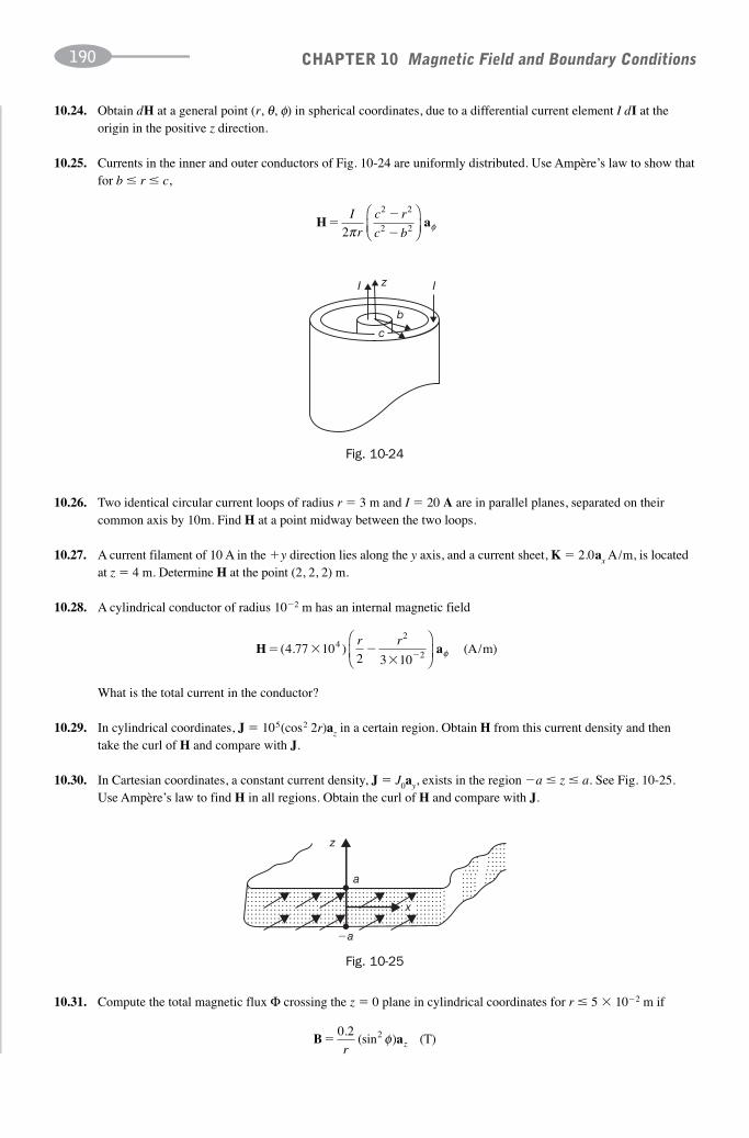
10.24. Obtain dH at a general point (r, θ, φ) in spherical coordinates, due to a differential current element I dI at theorigin in the positive z direction.
10.25. Currents in the inner and outer conductors of Fig. 10-24 are uniformly distributed. Use Ampère’s law to show thatfor b � r � c,
CHAPTER 10 Magnetic Field and Boundary Conditions190
H a��
�
I
r
c r
c b2
2 2
2 2π φ⎛⎝⎜
⎞⎠⎟
zI I
b
c
Fig. 10-24
z
x
a
�a
Fig. 10-25
10.26. Two identical circular current loops of radius r � 3 m and I � 20 A are in parallel planes, separated on theircommon axis by 10m. Find H at a point midway between the two loops.
10.27. A current filament of 10 A in the �y direction lies along the y axis, and a current sheet, K � 2.0ax A/m, is locatedat z � 4 m. Determine H at the point (2, 2, 2) m.
10.28. A cylindrical conductor of radius 10�2 m has an internal magnetic field
H a� � �� �
( . ) ����4 772 3 10
2
2104 r r⎛
⎝⎜
⎞
⎠⎟ φ (A/m)
What is the total current in the conductor?
10.29. In cylindrical coordinates, J � 105(cos2 2r)az in a certain region. Obtain H from this current density and thentake the curl of H and compare with J.
10.30. In Cartesian coordinates, a constant current density, J � J0ay, exists in the region �a � z � a. See Fig. 10-25.Use Ampère’s law to find H in all regions. Obtain the curl of H and compare with J.
10.31. Compute the total magnetic flux Φ crossing the z � 0 plane in cylindrical coordinates for r � 5 � 10�2 m if
B a�0 2 2.
(sin ) ���r zφ (T)

10.32. Given that
CHAPTER 10 Magnetic Field and Boundary Conditions 191
B a� �2 502
2. sin ���π x
e yz
⎛
⎝⎜⎞⎠⎟
(T)
find the total magnetic flux crossing the strip z � 0, y 0, 0 � x � 2 m.
10.33. A coaxial conductor with an inner conductor of radius a and an outer conductor of inner and outer radii b and c,respectively, carries current I in the inner conductor. Find the magnetic flux per unit length crossing a plane φ � const. between the conductors.
10.34. Region 1, where μr1 � 5, is on the side of the plane 6x � 4y � 3z � 12 that includes the origin. In region 2, μr2 � 3.Given
H a a1 3 0� �1
0.50μ
( . )����x y (A/m)
find B2 and θ2.
10.35. The interface between two different regions is normal to one of the three Cartesian axes. If
B1 � μ0(43.5ax � 24.0az ) B2 � μ0(22.0ax � 24.0az )
what is the ratio (tan θ1)/(tan θ2)?
10.36. Inside a right circular cylinder, μr1 � 1000. The exterior is free space. If B1 � 2.5aφ (T) inside the cylinder,determine B2 just outside.
10.37. In spherical coordinates, region 1 is r � a, region 2 is a � r � b and region 3 is r � b. Regions 1 and 3 are freespace, while μr2 � 500. Given B1 � 0.20ar (T), find H in each region.
10.38. A current sheet, K � (8.0/μ0)ay (A/m), at x � 0 separates region 1, x � 0 and μr1 � 3, from region 2, x � 0 andμr2 � 1. Given H1 � (10.0/μ0)(ay � az) (A/m), find H2.
10.39. The x � 0 plane contains a current sheet of density K which separates region 1, x � 0 and μr1 � 2, from region 2,x � 0 and μr 2 � 7. Given
B1 � 6.0ax � 4.0ay � 10.0az (T ) B2 � 6.0ax � 50.96ay � 8.96az (T)
find K.
10.40. One uniform current sheet, K � K0ay, is at z � b � 2 and another, K � K0(�ay), is at z � �b. Find the magneticflux crossing the area defined by x � const., �2 � x � 2, 0 � y � L. Assume free space.
10.41. Use the vector magnetic potential from Problem 10.20 to obtain the flux crossing the rectangle φ � const., r1 � r � r0, 0 � z � L, due to a current filament I on the z axis.
10.42. Given that the vector magnetic potential within a cylindrical conductor of radius a is
A a��μ
π0Ir
az
2
24
find the corresponding H.
10.43. One uniform current sheet, K � K0(�ay), is located at x � 0 and another, K � K0ay, is at x � a. Find the vectormagnetic potential between the sheets.
10.44. Between the current sheets of Problem 10.43 a portion of a z � const. plane is defined by 0 � x � b and 0 � y � a.
Find the flux Φ crossing this portion, both from � B · dS and from A · dI.

ANSWERS TO SUPPLEMENTARY PROBLEMS
10.24.
CHAPTER 10 Magnetic Field and Boundary Conditions192
I d
r
� sinθπ φ
4 2a
10.26. 0.908an A/m
10.27. 0.398ax � 1.0ay � 0.398az A/m
10.28. 5.0 A
H a� � � �104
4
8
4
325 r r r
r r
sin cos 1
32
⎛
⎝⎜⎞⎠⎟ φ10.29.
H
a
a
a
�
�
� � �
�
J a z a
J z a z a
J a
x
x
x
0
0
0
������
�������
���zz a��
�
⎧⎨⎪
⎩⎪
curl H J
10.30.
10.31. 3.14 � 10�2 Wb
10.32. 1.59 Wb
μπ0
2
I b
nln10.33.
10.34. 12.15ax � 0.60ay � 1.58az (T), 56.6°
10.35. 0.506
10.36. 2.5aφ (mT )
0.20 4 10 0.20
0
4
0 0μ μ μ(A/m), ��� (A/m), � �� (A/m)
� �
��
μπ
0IL r
r2ln 0
1
1
0μ( . . )����10 0 2 0a ay z� (A/m)
1
0μ( . . )����3 72 9 28a ay z� (A/m)�
10.37.
10.38.
10.39.
10.40. 4μ0K0L
10.41.
10.42. μ0H � curl A
10.43. (μ0K0x � C )ay
10.44. abμ0K0

193
Forces and Torques in Magnetic Fields
11.1 Magnetic Force on Particles
A charged particle in motion in a magnetic field experiences a force at right angles to its velocity, with a mag-nitude proportional to the charge, the velocity, and the magnetic flux density. The complete expression is givenby the cross product
F � QU � B
Therefore, the direction of a particle in motion can be changed by a magnetic field. The magnitude of the veloc-ity, U, and consequently the kinetic energy, will remain the same. This is in contrast to an electric field, wherethe force F � QE does work on the particle and therefore changes its kinetic energy.
If the field B is uniform throughout a region and the particle has an initial velocity normal to the field,the path of the particle is a circle of a certain radius r. The force of the field is of magnitude F � ⎪Q⎪ UB andis directed toward the center of the circle. The centripetal acceleration is of magnitude ω 2r � U 2/r. Then, byNewton’s second law,
CHAPTER 11
Q UB mU
rr
mU
Q B� �
2
�����or�����
F Q UB�
� � � �
� �
� �( . ) ( . ) ( )1 60 83 5 5110 10 10
6.68 1
9 3 3
00 17� N
Observe that r is a measure of the particle’s linear momentum, mU.
EXAMPLE 1. Find the force on a particle of mass 1.70 � 10�27 kg and charge 1.60 � 10�19 C if it enters a fieldB � 5 mT with an initial speed of 83.5 km/s.
Unless directions are known for B and U0, the particle’s initial velocity, the force cannot be calculated.Assuming that U0 and B are perpendicular, as shown in Fig. 11-1,

EXAMPLE 2. For the particle of Example 1, find the radius of the circular path and the time required for onerevolution.
CHAPTER 11 Forces and Torques in Magnetic Fields194
rmU
Q B� �
� �
�
�
�
( . )( . )
( . )(
1 70 83 5
1 60 5
10 10
10
27 3
19 ���
� �
�10
2
3).
��� .
0 177
13 3
m
sTr
U
π μ
z atQ E
mtp
p
� �1
2
1
22 2
⎛
⎝⎜
⎞
⎠⎟
Tr
U
m
Q Bp
p
� �2 2π π
11.2 Electric and Magnetic Fields Combined
When both fields are present in a region at the same time, the force on a particle is given by
F � Q(E � U � B)
This Lorentz force, together with the initial conditions, determines the path of the particle.
EXAMPLE 3. In a certain region surrounding the origin of coordinates, B � 5.0 � 10�4az T and E � 5.0az V/m.A proton (Qp � 1.602 � 10�19 C, mp � 1.673 � 10�27kg) enters the fields at the origin with an initial velocityU0 � 2.5 � 105ax m/s. Describe the proton’s motion and give its position after three complete revolutions.
The initial force on the particle is
F0 � Q(E � U0 � B) � Qp(Eaz � U0Bay )
The z component (electric component) of the force is constant and produces a constant acceleration in the zdirection. Thus, the equation of motion in the z direction is
The other (magnetic) component, which changes into �QpUBar, produces circular motion perpendicular to thez axis, with period
U0
EB
z
y
r
x
Fig. 11-2
X
X
X
X X
X
X
X X X
X
XU0
XX
XF
(B into page)
X
Fig. 11-1
The resultant motion is helical, as shown in Fig. 11-2.

After three revolutions, x � y � 0 and
CHAPTER 11 Forces and Torques in Magnetic Fields 195
zQ E
mT
Em
Q Bp
p
p
p
� � �1
23
1837 02
2
2
⎛
⎝⎜
⎞
⎠⎟ ( ) .
πm
F L B
a a a
� �
� � � � ��
I
z x y
( )
( . )[( . ) ( ) ( )5 0 0 30 103.50 3 ]]
� �� ��7.42
210 3 a ax y
⎛
⎝⎜⎞
⎠⎟N
W da� �initial
final
l
l
F l·
11.3 Magnetic Force on a Current Element
A frequently encountered situation is that of a current-carrying conductor in an external magnetic field. SinceI � dQ /dt, the differential force equation may be written
dF � dQ (U � B) � (I dt)(U � B) � I (dI � B)
where dI � U dt is the elementary length in the direction of the conventional current I. If the conductor isstraight and the field is constant along it, the differential force may be integrated to give
F � ILB sin θ
The magnetic force is actually exerted on the electrons that make up the current I. However, since the electronsare confined to the conductor, the force is effectively transferred to the heavy lattice; this transferred force cando work on the conductor as a whole. While this fact provides a reasonable introduction to the behavior of cur-rent-carrying conductors in electric machines, certain essential considerations have been omitted. No mentionwas made, nor will be made in Section 11.4, of the current source and the energy that would be required to maintain a constant current I. Faraday’s law of induction (Section 13.3) was not applied. In electric machinetheory the result will be modified by these considerations. Conductors in motion in magnetic fields are treatedagain in Chapter 13; see particularly Problems 13.10 and 13.13.
EXAMPLE 4. Find the force on a straight conductor of length 0.30 m carrying a current of 5.0 A in the �az direc-tion, where the field is B � 3.50 � 10�3(ax � ay) T.
The force, of magnitude 7.42 mN, is at right angles to both the field B and the current direction, as shown in Fig. 11-3.
z
FB
I
y
x
Fig. 11-3
11.4 Work and Power
The magnetic forces on the charged particles and current-carrying conductors examined above result from thefield. To counter these forces and establish equilibrium, equal and opposite forces, Fa, would have to be applied.If motion occurs, the work done on the system by the outside agent applying the force is given by the integral

A positive result from the integration indicates that work was done by the agent on the system to move the par-ticles or conductor from the initial to the final location and against the field. Because the magnetic force, andhence Fa, is generally nonconservative, the entire path of integration joining the initial and final locations of theconductor must be specified.
EXAMPLE 5. Find the work and power required to move the conductor shown in Fig. 11-4 one full revolutionin the direction shown in 0.02 s, if B � 2.50 � 10�3ar T and the current is 45.0 A.
F � I(l � B) � 1.13 � 10�2aφ N
and so Fa � �1.13 � 10�2aφ N.
CHAPTER 11 Forces and Torques in Magnetic Fields196
W d
rd
a�
� � �
�� �
�
�
��
F l
a a
·
·0
2π
φ φφ( )1.13 10
2.13 10
2
33 J
and P � W/t � �0.107 W.
0.10 m
r � 0.03 m
y
z
x
I
Fig. 11-4
The negative sign means that work is done by the magnetic field in moving the conductor in the direction shown.For motion in the opposite direction, the reversed limits will provide the change of sign, and no attempt to placea sign on r dφaφ should be made.
11.5 Torque
The moment of a force or torque about a specified point is the cross product of the lever arm about that pointand the force. The lever arm, r, is directed from the point about which the torque is to be obtained to the pointof application of the force. In Fig. 11-5 the force at P has a torque about O given by
T � r � F
where T has the units N · m. (The units N · m/rad have been suggested, in order to distinguish torque from energy.)
yO
x
r P
T
F
z
Fig. 11-5

In Fig. 11-5, T lies along an axis (in the xy plane) through O. If P were joined to O by a rigid rod freely pivotedat O, then the applied force would tend to rotate P about that axis. The torque T would then be said to be aboutthe axis, rather than about point O.
EXAMPLE 6. A conductor located at x � 0.4 m, y � 0 and 0 � z � 2.0 m carries a current of 5.0 A in the axdirection. Along the length of the conductor B � 2.5az T. Find the torque about the z axis.
F � I(L � B) � 5.0(2.0az � 2.5ax) � 25.0ay N
T � r � F � 0.4ax � 25.0ay � 10.0az N · m
11.6 Magnetic Moment of a Planar Coil
Consider the single-turn coil in the z � 0 plane shown in Fig. 11-6, of width w in the x direction and length� along y. The field B is uniform and in the �x direction. Only the
CHAPTER 11 Forces and Torques in Magnetic Fields 197
T a a a a� � � � � � �w
BIw
BI BIx z x z2 2
⎛⎝⎜
⎞⎠⎟
⎛⎝⎜
⎞⎠⎟
( )� � �ww BI Ay y( ) ( )� � �a a
m a�ωπ2
Q A n
z
B
I I
w
x
y
��
Fig. 11-6
�y -directed currents give rise to forces. For the side on the left,
F � I(�ay � Bax) � �BI �az
and for the side on the right,
F � BI �az
The torque about the y axis from the left current element requires a lever arm r � �(w/2)ax; the sign will changefor the lever arm of the right current element. The torque from both elements is
where A is the area of the coil. It can be shown that this expression for the torque holds for a flat coil of arbi-trary shape (and for any axis parallel to the y axis).
The magnetic moment m of a planar current loop is defined as IAan, where the unit normal an is determinedby the right-hand rule. (The right thumb gives the direction of an when the fingers point in the direction of thecurrent.) It is seen that the torque on a planar coil is related to the applied field by
T � m � B
This concept of magnetic moment is essential to an understanding of the behavior of orbiting charged particles.For example, a positive charge Q moving in a circular orbit at a velocity U, or an angular velocity ω, is equiv-alent to a current I � (ω /2π)Q, and so gives rise to a magnetic moment

as shown in Fig. 11-7. More important to the present discussion is that in the presence of a magnetic field B therewill be a torque T � m � B which tends to turn the current loop until m and B are in the same direction, in whichorientation the torque will be zero.
CHAPTER 11 Forces and Torques in Magnetic Fields198
( . )1 20 102
02�� �
� �� a aa a a
x zx y z⎛
⎝⎜⎞⎠⎟
(12.0)(2.5)) 30 300
4 10
2
4
B B B
B B
B B
x y z
z x x z
z x
�� �
� �� �
a a
T
d dS
dx dy z
F K B
a
F
�
�
��
( )
.
.( . )
.
��
15 0
0 020 20
0
⎛⎝⎜
⎞⎠⎟
�001
0 01
0150 0
3 0
.
.
.
�L
z
z
dx dy
L
a
Fa� N/m
QU
m
A
�
SOLVED PROBLEMS
11.1. A conductor 4 m long lies along the y axis with a current of 10.0 A in the ay direction. Find the forceon the conductor if the field in the region is B � 0.05ax T.
F � IL � B � 10.0(4ay � 0.05ax) � �2.0ax N
11.2. A conductor of length 2.5 m located at z � 0, x � 4 m carries a current of 12.0 A in the �aydirection. Find the uniform B in the region if the force on the conductor is 1.20 � 10�2 N in thedirection (�ax � az)/��2.
From F � IL � B,
Fig. 11-7
whence
The y component of B may have any value.
11.3. A current strip 2 cm wide carries a current of 15.0 A in the ax direction, as shown in Fig. 11-8. Find theforce on the strip per unit length if the uniform field is B � 0.20ay T.
K
B
x
yz
0.02 m
Fig. 11-8
In the expression for dF, I d l may be replaced by K dS.

11.4. Find the forces per unit length on two long, straight, parallel conductors if each carries a current of10.0 A in the same direction and the separation distance is 0.20 m.
Consider the arrangement in Cartesian coordinates shown in Fig. 11-9. The conductor on the left creates a fieldwhose magnitude at the right-hand conductor is
CHAPTER 11 Forces and Torques in Magnetic Fields 199
BI
r� �
��
��μ
ππ
π0 5
2
4 10 0
2 0 2010
( )( . )
( . )
10 7
T
Fa
L x� ��10 4 ( ) N/m
d
LIB I
K dx
rr rF
a a� �μ
π0 0
2
( )
BB
�0.10 0.10x
z
Fig. 11-9
and whose direction is �az. Then the force on the right conductor is
F � ILay � B (�az ) � ILB(�ax)
and
An equal but opposite force acts on the left-hand conductor. The force is seen to be one of attraction. Two parallelconductors carrying current in the same direction will have forces tending to pull them together.
11.5. A conductor carries current I parallel to a current strip of density K0 and width w, as shown in Fig. 11-10. Find an expression for the force per unit length on the conductor. What is the resultwhen the width w approaches infinity?
I
w
x
K0 dx
yz
h
K
r
O
Fig. 11-10
From Problem 11.4, the filament K0 dx shown in Fig. 11-10 exerts an attractive force
d
LI
K dx
r
h
r
IK h dx
hz
Fa� � �
�
μπ
μπ
0 0 0 022
2( )
( )⎛⎝⎜
⎞⎠⎟ xx
z2 ( )�a
on the conductor. Adding to this the force due to the similar filament at �x, the components in the x directioncancel, giving a resultant

Integrating over the half-width of the strip,
CHAPTER 11 Forces and Torques in Magnetic Fields200
Fa
L
IK h dx
h x
IK w
hz
w
� ��
�μ
πμ
π0 0
2
2 20 0
2( ) arctan
/
�0
⎛⎛⎝⎜
⎞⎠⎟
( )�az
T a a a1 2 2� � � � � �
wBI BI
wx z y( ) ( ) ( )� �
The force is one of attraction, as expected.
As the strip width approaches infinity, F/L → (μ0IK0/2)(�az).
11.6. Find the torque about the y axis for the two conductors of length �, separated by a fixed distance w, inthe uniform field B shown in Fig. 11-11.
The conductor on the left experiences the force
F1 � I �ay � Bax � BI�(�az)
the torque of which is
The force on the conductor on the right results in the same torque. The sum is, therefore,
T � BI�w (�ay )
11.7. A D’Arsonval meter movement has a uniform radial field of B � 0.10 T and a restoring spring with atorque T � 5.87 � 10�5θ (N · m), where the angle of rotation is in radians. The coil contains 35 turnsand measures 23 mm by 17 mm. What angle of rotation results from a coil current of 15 mA?
The shaped pole pieces shown in Fig. 11-12 result in a uniform radial field over a limited range of deflection.Assuming that the entire coil length is in the field, the torque produced is
T � nBI�w � 35(0.10)(15 � 10�3) (23 � 10�3) (17 � 10�3)
� 2.05 � 10�5 N · m
This coil turns until this torque equals the spring torque.
2.05 � 10�5 � 5.87 � 10�5θθ � 0.349 rad or 20°
B
B
zy
II
�
w
Fig. 11-11
N S
Fig. 11-12

11.8. The rectangular coil in Fig. 11-13 is in a field
CHAPTER 11 Forces and Torques in Magnetic Fields 201
Ba a
��
0 052
. x y T
m a a
T m B aa
� � �
� � � � ��
�
�
IA n x
xx
1 60
1 60
.
.
10
10 0.05
2
2 aa
a
y
z
2
�� � �5.66 10 4 N m·
Find the torque about the z axis when the coil is in the position shown and carries a current of 5.0 A.
I
z
0.08 m
x
�0.04 my
Fig. 11-13
If the coil turns through 45°, the direction of m will be (ax � ay ) /��2 and the torque will be zero.
11.9. Find the maximum torque on an 85-turn, rectangular coil, 0.2 m by 0.3 m, carrying a current of 2.0 Ain a field B � 6.5 T.
Tmax � nBI�w � 85(6.5)(2.0)(0.2)(0.3) � 66.3 N · m
11.10. Find the maximum torque on an orbiting charged particle if the charge is 1.602 � 10�19 C, the circularpath has a radius of 0.5 � 10�10 m, the angular velocity is 4.0 � 1016 rad/s, and B � 0.4 � 10�3 T.
The orbiting charge has a magnetic moment
Then the maximum torque results when an is normal to B.
Tmax � mB � 3.20 � 10�27 N · m
11.11. A conductor of length 4 m, with current held at 10 A in the ay direction, lies along the y axis betweeny � �2 m. If the field is B � 0.05ax T, find the work done in moving the conductor parallel to itselfat constant speed to x � z � 2 m.
For the entire motion,
F � IL � B � �2.0az
The applied force is equal and opposite,
Fa � 2.0az
m a� ��
� �� �ωπ π
π2
1 602 0 519 10QA n4 10
210 10
16
( . ) ( . )22 2a an n� � �8.01 10 24 �A m·

Because this force is constant, and therefore conservative, the conductor may be moved first along z, then in the xdirection, as shown in Fig. 11-14. Since Fa is completely in the z direction, no work is done in moving along x. Then,
CHAPTER 11 Forces and Torques in Magnetic Fields202
W dzz z� ��0
2
4(2.0 ) .0 Ja a·
W e dxxx x� � �
�� �
� �
�
�0
23 0 210
1 48
( 9.0 )
10 J2
.
.
a a·
x
22
Iy
z
Fig. 11-14
11.12. A conductor lies along the z axis at �1.5 � z � 1.5 m and carries a fixed current of 10.0 A in the �azdirection. See Fig. 11-15. For a field
B � 3.0 � 10�4e�0.2xay (T)
By
x
2.0
1.5
�1.5
I
z
Fig. 11-15
find the work and power required to move the conductor at constant speed to x � 2.0 m, y � 0 in 5 � 10�3 s. Assume parallel motion along the x axis.
F � IL � B � 9.0 � 10�3e�0.2xax
Then Fa � �9.0 � 10�3e �0.2xax and
The field moves the conductor, and therefore the work is negative. The power is given by
PW
t� �
� �
���
�
�
1 48
52 97
..
10
10
2
3 W
11.13. Find the work and power required to move the conductor shown in Fig. 11-16 one full turn in thepositive direction at a rotational frequency of N revolutions per minute, if B � B0ar (B0 a positiveconstant).

The force on the conductor is
F � IL � B � ILaz � B0ar � B0ILaφ
so that the applied force is
Fa � B0 IL(�aφ )
The conductor is to be turned in the aφ direction. Therefore, the work required for one full revolution is
CHAPTER 11 Forces and Torques in Magnetic Fields 203
W B IL r d r B IL� � ���0
2
0 02π
φ φφ π( )a a·
Pr B I L N
��2π 0
60
W r d� � ���0
1 75 87 5π
φ φφ φ μ. sin .10 3 a a· J
y
x I
z
r
Fig. 11-16
For a rotational frequency of N revolutions per 60 seconds, the power is
The negative signs on work and power indicate that the field does the work. The fact that work is done around aclosed path shows that the force is nonconservative in this case.
11.14. In the configuration shown in Fig. 11-16 the conductor is 100 mm long and carries a constant 5.0 A inthe az direction. If the field is
B � �3.5 sin φar mT
and r � 25 mm, find the work done in moving the conductor at constant speed from φ � 0 to φ � π,in the direction shown. If the current direction is reversed for π � φ � 2π, what is the total workrequired for one full revolution?
F � IL � B � �1.75 � 10�3 sin φ aφ N
Fa � 1.75 � 10�3 sin φ aφ N
Then
If the current direction changes when the conductor is between π and 2π, the work will be the same. The totalwork is 175 μ J.
11.15. Compute the centripetal force necessary to hold an electron (me � 9.107 � 10�31 kg) in a circularorbit of radius 0.35 � 10�10 m with an angular velocity of 2 � 1016 rad/s.
F � meω 2r � (9.107 � 10�31) (2 � 1016)2 (0.35 � 10�10) � 1.27 � 10�8 N

11.16. A uniform magnetic field B � 85.3az μT exists in the region x 0. If an electron enters this field atthe origin with a velocity U0 � 450ax km/s, find the position where it exits the field. Where would aproton with the same initial velocity exit?
CHAPTER 11 Forces and Torques in Magnetic Fields204
rm U
Q Bee
� � � �03 00. 10 2 m
rm
mrp
p
ee� � 55 m
FQ
r�
2
24π0
Q
rm r
Q
m re
e
2
22 2
2
34 4πω ω
π 0 0
or �
The electron experiences an initial force in the ay direction and it exits the field at x � z � 0, y � 6 cm.
A proton would turn the other way. Part of the circular path is shown at P in Fig. 11-17. With mp � 1840me,
and the proton exits at x � z � 0, y � �110 m.
�
U0
BP
zy
x
Fig. 11-17
11.17. If a proton is fixed in position and an electron revolves about it in a circular path of radius 0.35 � 10�10 m, what is the magnetic field at the proton?
The proton and electron are attracted by the coulomb force,
which furnishes the centripetal force for the circular motion. Thus,
Now, the electron is equivalent to a current loop I � (ω /2π )Q. The field at the center of such a loop is, fromProblem 10.7,
B HI
r
Q
r� � �μ μ μ ω
π00 0
2 4
BQ
r m re
� ��� �( / ) ( )( . )
( .
μ ππ
02
2
7 19 24
4
10 1 6 10
0 30
55 219
9 1 10 0 35 1031� � � �� � � �10 1010 9) ( . )( .⎛⎝⎜
⎞⎠⎟
110
35
)
� T
Substituting the value of ω found above,

SUPPLEMENTARY PROBLEMS
11.18. A current element 2 m in length lies along the y axis centered at the origin. The current is 5.0 A in the ay direction.If it experiences a force 1.50(ax � az ) /��2 N due to a uniform field B, determine B.
11.19. A magnetic field, B � 3.5 � 10�2az T, exerts a force on a 0.30-m conductor along the x axis. If the conductorcurrent is 5.0 A in the �ax direction, what force must be applied to hold the conductor in position?
11.20. A current sheet, K � 30.0ay A/m, lies in the plane z � �5 m and a filamentary conductor is on the y axis with acurrent of 5.0 A in the ay direction. Find the force per unit length.
11.21. A conductor with current I pierces a plane current sheet K orthogonally, as shown in Fig. 11-18. Find the forceper unit length on the conductor above and below the sheet.
CHAPTER 11 Forces and Torques in Magnetic Fields 205
K
I
Fig. 11-18
11.22. Find the force on a 2-m conductor on the z axis with a current of 5.0 A in the az direction, if
B � 2.0ax � 6.0ay T
11.23. Two infinite current sheets, each of constant density K0, are parallel and have their currents oppositely directed.Find the force per unit area on the sheets. Is the force one of repulsion or attraction?
11.24. The circular current loop shown in Fig. 11-19 is in the plane z � h, parallel to a uniform current sheet, K � K0ay,at z � 0. Express the force on a differential length of the loop. Integrate and show that the total force is zero.
11.25. Two conductors of length � normal to B are shown in Fig. 11-20; they have a fixed separation w. Show that thetorque about any axis parallel to the conductors is given by BI�w cos θ.
z
h Iy
x
a
K
Fig. 11-19

11.26. A circular current loop of radius r and current I lies in the z � 0 plane. Find the torque which results if the currentis in the aφ direction and there is a uniform field B � B0(ax � az) /��2.
11.27. A current loop of radius r � 0.35 m is centered about the x axis in the plane x � 0 and at (0, 0, 0.35) m the current isin the �ay direction at a magnitude of 5.0 A. Find the torque if the uniform field is B � 88.4(ax � az) μT.
11.28. A current of 2.5 A is directed generally in the aφ direction about a square-conducting loop centered at the origin in the z � 0 plane with 0.60 m sides parallel to the x and y axes. Find the forces and the torque on the loop if B � 15ay mT. Would the torque be different if the loop were rotated through 45° in the z � 0 plane?
11.29. A 200-turn, rectangular coil, 0.30 m by 0.15 m with a current of 5.0 A, is in a uniform field B � 0.2 T. Find themagnetic moment m and the maximum torque.
11.30. Two conductors of length 4.0 m are on a cylindrical shell of radius 2.0 m centered on the z axis, as shown inFig. 11-21. Currents of 10.0 A are directed as shown and there is an external field B � 0.5ax T at φ � 0 and B � �0.5ax T at φ � π. Find the sum of the forces and the torque about the axis.
CHAPTER 11 Forces and Torques in Magnetic Fields206
θB
w
Fig. 11-20
BB
z
x
y
I
I
� 0φ
π
Fig. 11-21
11.31. A right circular cylinder contains 550 conductors on the curved surface and each has a current of constantmagnitude 7.5 A. The magnetic field is B � 38 sin φ ar mT. The current direction is az for 0 � φ � π and �az forπ � φ � 2π (Fig. 11-22). Find the mechanical power required if the cylinder turns at 1600 revolutions per minutein the �aφ direction.
z
x
y
12 cm
3cm
� 0φI
I
Fig. 11-22

11.32. Obtain an expression for the power required to turn a cylindrical set of n conductors (see Fig. 11-22) against thefield at N revolutions per minute, if B � B0 sin 2φ ar and the currents change direction in each quadrant where thesign of B changes.
11.33. A conductor of length � lies along the x axis with current I in the ax direction. Find the work done in turning it atconstant speed, as shown in Fig. 11-23, if the uniform field is B � B0az.
CHAPTER 11 Forces and Torques in Magnetic Fields 207
w
z
x
B
�
Fig. 11-24
11.34. A rectangular current loop, of length � along the y axis, is in a uniform field B � B0az, as shown in Fig. 11-24.Show that the work done in moving the loop along the x axis at constant speed is zero.
x
B
z
I
2�φπ
Fig. 11-23
11.35. For the configuration shown in Fig. 11-24, the magnetic field is
B a� Bx
w z0 sinπ⎛
⎝⎜⎞⎠⎟
Find the work done in moving the coil a distance w along the x axis at constant speed, starting from the locationshown.
11.36. A conductor of length 0.25 m lies along the y axis and carries a current of 25.0 A in the ay direction. Find thepower needed for parallel translation of the conductor to x � 5.0 m at constant speed in 3.0 s if the uniform fieldis B � 0.06az T.
11.37. Find the tangential velocity of a proton in a field B � 30 μT if the circular path has a diameter of 1 cm.
11.38. An alpha particle and a proton (Qa � 2Qρ) enter a magnetic field B � 1 μT with an initial speed U0 � 8.5 m/s.Given the masses 6.68 � 10�27 kg and 1.673 � 10�27 kg for the alpha particle and the proton, respectively, findthe radii of the circular paths.
11.39. If a proton in a magnetic field completes one circular orbit in 2.35 μs, what is the magnitude of B?
11.40. An electron in a field B � 4.0 � 10�2 T has a circular path with radius 0.35 � 10�10 m and a maximum torque of7.85 � 10�26 N · m. Determine the angular velocity.
11.41. A region contains uniform B and E fields in the same direction, with B � 650 μT. An electron follows a helicalpath, where the circle has a radius of 35 mm. If the electron has zero initial velocity in the axial direction andadvances 431 mm along the axis in the time required for one full circle, find the magnitude of E.
ANSWERS TO SUPPLEMENTARY PROBLEMS
11.18. 0.106(�ax � az) T
11.19. �5.25 � 10�2ay N
11.20. 94.2 μN/m (attraction)
11.21. �μ0KI /2
11.22. �60ax � 20ay N
11.23. μ0K20 /2 (repulsion)
11.24. dF � 1–2 Iaμ0K0 cos φ dφ (�az )
11.26. (πr2B0I/��2)ay
11.27. 1.70 � 10�4(�ay) N · m
11.28. 1.35 � 10�2(�az) N · m; T � m � B
11.29. 45.0 A · m2, 9.0 N · m
11.30. �40ay N, 0
11.31. 60.2 W
CHAPTER 11 Forces and Torques in Magnetic Fields208
11.32.
11.33. πB0�2I/4
11.35. �4B0I�w /π
11.36. �0.625 W
11.37. 14.4 m/s
11.38. 177 mm, 88.8 mm
11.39. 2.79 � 10�2T
11.40. 2.0 � 1016 rad/s
11.41. 1.62 kV/m
B n I rN0
60
����(W)

209
Inductance and Magnetic Circuits
12.1 Inductance
The inductance L of a conductor system may be defined as the ratio of the linking magnetic flux to the currentproducing the flux. For static (or, at most, low-frequency) current I and a coil containing N turns, as shown inFig. 12-1,
CHAPTER 12
LN
I�
Φ
H a
B a
�
�
I
rI
r
2
20
πμπ
φ
φ
Φ
N
I
Fig. 12-1
The units on L are henries, where 1 H � 1 Wb/A. Inductance is also given by L � λ /I, where λ, the flux link-age, is NΦ for coils with N turns or simply Φ for other conductor arrangements.
It should be noted that L will always be the product of the permeability μ of the medium (units on μ are H/m)and a geometrical factor having the units of length. Compare the expressions for resistance R (Chapter 7) andcapacitance C (Chapter 8).
EXAMPLE 1. Find the inductance per unit length of a coaxial conductor such as that shown in Fig.12-2.Between the conductors,

CHAPTER 12 Inductance and Magnetic Circuits210
The currents in the two conductors are linked by the flux across the surface φ � const. For a length �,
I
aφ � const.
b
Fig. 12-2
and
EXAMPLE 2. Find the inductance of an ideal solenoid with 300 turns, � � 0.50 m, and a circular cross sectionof radius 0.02 m.
The turns per unit length is n � 300/0.50 � 600, so that the axial field is
B � μ0H � μ0600I (Wb/m2)
Then
or L � 284 μH.In Section 6.7 an imagined bringing-in of point charges from infinity was used to derive the energy content
of an electric field:
λ μπ
μπ
� �� �0
0 0
2 2
� �a
b I
rdr dz
I b
aln
L b
a��
μπ0
2ln (H/m)
L N
IN
B
IA
�� � � �
�
�Φ ⎛⎝⎜
⎞⎠⎟
300(600 ) (4 10 )
568
04μ π
μH//m
W dvE �1
2 �vol
D E·
W dvH �1
2 �vol
B H·
LI
dv� �vol
B H·2
There is no equivalent in a magnetic field to the point charge, and consequently no parallel development for itsstored energy. However, a more sophisticated approach yields the completely analogous expression
Comparing this with the formula WH � 1–2
LI 2 from circuit analysis yields

EXAMPLE 3. Checking Example 1,
CHAPTER 12 Inductance and Magnetic Circuits 211
LI
dvI
I
rr d
a
b� �� � � �vol
B H·2
02
0 0
2 2
2 24
μπ
π� ⎛
⎝⎜⎞⎠⎟
rr d dzb
aφ μ
π� 0
2
�ln
12.2 Standard Conductor Configurations
Figs. 12-3 through 12-7 give exact or approximate inductances of some common noncoaxial arrangements.
r1
r2 (H)r 2L �a r 1
lnπ2
μ 0 N 2a
Fig. 12-3 Toroid, square cross section.
rr
S (assuming averageflux density ataverage radius r )
(H)L �π2
μ 0 N 2S
Fig. 12-4 Toroid, general cross section S.
d
For d �� a,
2adcosh�10L
aradius
�
�(H /m)π
μ�
adln0L
�(H /m)π
μ�
Fig. 12-5 Parallel conductors of radius a.
a2
d 2
Radius
2adcosh�10L
�(H /m)π
2π
μ�
adln0 (H /m)
μ�
Fig. 12-6 Cylindrical conductor parallel to a ground plane.
S
�
� (H)L �μ 0 N 2S
Fig. 12-7 Long solenoid of small cross-sectional area S.

12.3 Faraday’s Law and Self-Inductance
Consider an open surface S bounded by a closed contour C. If the magnetic flux φ linking S varies with time,then a voltage v around C exists; by Faraday’s law,
CHAPTER 12 Inductance and Magnetic Circuits212
vd
dt��
φ
vd
di
di
dtL
di
dt�� ��
φ
H a B a� �Ir
a
Ir
a2 220
2πμπφ φand�����
As was shown in Chapter 6, the electrostatic potential or voltage, V, is well-defined in space and is associatedwith a conservative electric field. By contrast, the induced voltage v given by Faraday’s law is a multivaluedfunction of position and is associated with a nonconservative field (electromotive force). More about this inChapter 13.
Faraday’s law holds in particular when the flux through a circuit element is changing because the currentin that same element is changing:
In circuit theory, L is called the self-inductance of the element and v is called the voltage of self-inductance orthe back-voltage in the inductor.
12.4 Internal Inductance
Magnetic flux occurs within a conductor cross section as well as external to the conductor. This internal flux givesrise to an internal inductance, which is often small compared to the external inductance and frequently ignored.In Fig. 12-8(a) a conductor of circular cross section is shown, with a current I assumed to be uniformly distrib-uted over the area. (This assumption is valid only at low frequencies, since skin effect at higher frequenciesforces the current to be concentrated at the outer surface.) Within the conductor of radius a, Ampère’s law gives
The straight piece of conductor shown in Fig. 12-8(a) must be imagined as a short section of an infinite torus, assuggested in Fig. 12-8(b). The current filaments become circles of infinite radius. The lines of flux dΦ through thestrip � dr encircle only those filaments whose distance from the conductor axis is smaller than r. Thus, an open sur-face bounded by one of those filaments is cut once (or an odd number of times) by the lines of dΦ; whereas, for afilament such as 1 or 2, the surface is cut zero times (or an even number of times). It follows that dΦ links onlywith the fraction πr2/πa2 of the total current, so that the total flux linkage is given by the weighted “sum”
I I
′
(a) (b)
r
1
2ΦdΦd
dra
l
Fig. 12-8

and
CHAPTER 12 Inductance and Magnetic Circuits 213
λ ππ
ππ
μπ
� �� �r
ad
r
a
Ir
ad
a2
20
2
20
22
⎛
⎝⎜⎞⎠⎟
⎛
⎝⎜⎞⎠⎟
Φ � rrI
�μ
π0
8
�
L I
� �� � � � �λ μ
π/ 0
8
1
210 7 H/m
v Nd
dt2 212�
φ(negative sign omitted)
v Nd
di
di
dtM
di
dt2 212
1
112
1� �φ
This result is independent of the conductor radius. The total inductance is the sum of the external and internal induc-tances. If the external inductance is of the order of 1–
2� 10�7 H/m, the internal inductance should not be ignored.
12.5 Mutual Inductance
In Fig. 12-9 a part φ12 of the magnetic flux produced by the current i1 through coil 1 links the N2 turns of coil 2.The voltage of mutual induction in coil 2 is given by
In terms of the mutual inductance M12 � N2φ12 /I1,
i1
φ11
φ12
N2
v2
N2
N1
Fig. 12-9
This mutual inductance will be a product of the permeability μ of the region between the coils and a geometri-cal length, just like inductance L. If the roles of coils 1 and 2 are reversed,
The following reciprocity relation can be established: M12 � M21.
EXAMPLE 4. A solenoid with N1 � 1000, r1 � 1.0 cm, and �1 � 50 cm is concentric within a second coil ofN2 � 2000, r2 � 2.0 cm, and �2 � 50 cm. Find the mutual inductance assuming free-space conditions.
For long coils of small cross sections, H may be assumed constant inside the coil and zero for points justoutside the coil. With the first coil carrying a current I1,
v Mdi
dt1 212�
H I�1000
0 50 1.
⎛⎝⎜
⎞⎠⎟
(A/m) (in the axial directionn)
(Wb/m )2B I
BA I
�
� � � �
μ
μ π0 1
1
2000
2000Φ ( 1004)( ) ((Wb)

Since H and B are zero outside the coils, this is the only flux linking the second coil.
CHAPTER 12 Inductance and Magnetic Circuits214
M NI12 21
2000 4 2000� � � �� �Φ⎛⎝⎜
⎞⎠⎟
( 10 107)( )( (π π) 44 ) .�1 58 mH
HNI
��
12.6 Magnetic Circuits
In Chapter 10, magnetic field intensity H, flux Φ, and magnetic flux density B were examined and various prob-lems were solved where the medium was free space. For example, when Ampère’s law is applied to the closedpath C through the long, air-core coil shown in Fig. 12-10, the result is
H · dI � NI
Ferromagnetic materials have relative permeabilities μr in the order of thousands. Consequently, the flux den-sity B � μ0μrH is, for a given H, much greater than would result in free space. In Fig. 12-11, the coil is not dis-tributed over the iron core. Even so, the NI of the coil causes a flux Φ which follows the core. It might be saidthat the flux prefers the core to the surrounding space by a ratio of several thousand to one. This is so differentfrom the free-space magnetics of Chapter 10 that an entire subject area, known as iron-core magnetics or mag-netic circuits, has developed. This brief introduction to the subject assumes that all of the flux is within the core.It is further assumed that the flux is uniformly distributed over the cross section of the core. Core lengths requiredfor calculation of NI drops are mean lengths.
N turns
C
H, B
Φ
Fig. 12-10
But since the flux lines are widely spread outside of the coil, B is small there. The flux is effectively restrictedto the inside of the coil, where
I NI
Φ
Fig. 12-11

12.7 The B-H Curve
A sample of ferromagnetic material could be tested by applying increasing values of H and measuring the cor-responding values of flux density B. Magnetization curves, or simply B-H curves, for some common ferromag-netic materials are given in Figs. 12-12 and 12-13. The relative permeability can be computed from the B-H curveby use of μr � B/μ 0H. Fig. 12-14 shows the extreme nonlinearity of μr versus H for silicon steel. This nonlin-earity requires that problems be solved graphically.
CHAPTER 12 Inductance and Magnetic Circuits 215
1.40
1.20
1.00
0.80
0.60
0.40
0.20
100 200 300
H (A /m)
B(T
)
400
A Cast IronB Cast SteelC Silicon SteelD Nickel-Iron Alloy
D
B
C
A
Fig. 12-12 B -H curves, H � 400 A/m.
B(T
)
1000
0.20
0.40
0.60
0.80
1.00
1.20
BCD
B
CD
1.40
1.60
30002000H (A /m)
50004000 6000
A
A Cast IronB Cast SteelC Silicon SteelD Nickel-Iron Alloy
Fig. 12-13 B -H curves, H � 400 A/m.

12.8 Ampère’s Law for Magnetic Circuits
A coil of N turns and current I around a ferromagnetic core produces a magnetomotive force (mmf) given by NI.The symbol F is sometimes used for this mmf; the units are amperes or ampere turns. Ampère’s law, appliedaround the path in the center of the core shown in Fig. 12-15(a), gives
CHAPTER 12 Inductance and Magnetic Circuits216
7000
r
H (A/m)
μ
6000
5000
4000
3000
2000
1000
100 200 300 400
Fig. 12-14
F NI d
d d d
H H H
� �
� � �
� � �
� � �
H l
H l H l H l
·
· · ·1 2 3
1 2� �1 2 33�3
H1
1
1
2 F I�
R1
R2
R3
IR1
V
3
(a) (b) (c)
F � NI
�
Φ
1
� 2
� 3
Fig. 12-15
Comparison with Kirchhoff’s law around a single closed loop with three resistors and an emf V,
V � V1 � V2 � V3
suggests that F can be viewed as an NI rise and the H� terms considered NI drops, in analogy to the voltage riseV and voltage drops V1, V2 and V3. The analogy is developed in Fig. 12-15(b) and (c). Flux Φ in Fig. 12-15(b)is analogous to current I, and reluctance � is analogous to resistance R. An expression for reluctance can bedeveloped as follows.

Hence,
CHAPTER 12 Inductance and Magnetic Circuits 217
NI H BAA
drop � � ���
μ⎛⎝⎜
⎞⎠⎟
Φ�
� � ��μA
( )H 1
RA
��
σ
If the reluctances are known, then the equation
F � NI � Φ(�1 � �2 � �3 )
can be written for the magnetic circuit of Fig. 12-15(b). However, μr must be known for each material beforeits reluctance can be calculated. And only after B or H is known will the value of μr be known. This is in con-trast to the relation
(Section 7.7), in which the conductivity σ is independent of the current.
12.9 Cores with Air Gaps
Magnetic circuits with small air gaps are very common. The gaps are generally kept as small as possible,since the NI drop of the air gap is often much greater than the drop in the core. The flux fringes outward atthe gap, so that the area at the gap exceeds the area of the adjacent core. Provided that the gap length �a isless than 1—
10the smaller dimension of the core, an apparent area, Sa, of the air gap can be calculated. For a rec-
tangular core of dimensions a and b,
Sa � (a � �a)(b � �a )
If the total flux in the air gap is known, Ha and Ha�a can be computed directly.
HS
HSa
aa a
a
a
� �1
0 0μ μΦ Φ⎛
⎝⎜⎞⎠⎟
������ ��
NI H H HSi i a a i i
a
a
� � � �� � �� Φμ0
For a uniform iron core of length �i with a single air gap, Ampère’s law reads
If the flux Φ is known, it is not difficult to compute the NI drop across the air gap, obtain Bi, take Hi from theappropriate B-H curve and compute the NI drop in the core, Hi�i. The sum is the NI required to establish theflux Φ. However, with NI given, it is a matter of trial and error to obtain Bi and Φ, as will be seen in the prob-lems. Graphical methods of solution are also available.
12.10 Multiple Coils
Two or more coils on a core could be wound such that their mmfs either aid or oppose one another. Conse-quently, a method of indicating polarity is given in Fig. 12-16. An assumed direction for the resulting flux Φcould be incorrect, just as an assumed current in a dc circuit with two or more voltage sources may be incorrect.A negative result simply means that the flux is in the opposite direction.

12.11 Parallel Magnetic Circuits
The method of solving a parallel magnetic circuit is suggested by the two-loop equivalent circuit shown inFig. 12-17(b). The leg on the left contains an NI rise and an NI drop. The NI drop between the junctions a and b can be written for each leg as follows:
F � H1�1 � H2�2 � H3�3
and the fluxes satisfy
Φ1 � Φ2 � Φ3
Different materials for the core parts will necessitate working with several B-H curves. An air gap in one of thelegs would lead to Hi�i � Ha�a for the mmf between the junctions for that leg.
CHAPTER 12 Inductance and Magnetic Circuits218
N1 I1
N2 I2
N1
I1
I2
N2
(a) (b)
Fig. 12-16
The equivalent magnetic circuit should be drawn for parallel magnetic circuit problems. It is good practice tomark the material types, cross-sectional areas, and mean lengths directly on the diagram. In more complex prob-lems a scheme like Table 12-1 can be helpful. The data are inserted directly into the table, and the remainingquantities are then calculated or taken from the appropriate B-H curve.
1
2
12 3
a
a
b
H1
b
FF
1
H2 2 H3 3
3
ΦΦ
2Φ
1Φ 3Φ
Φ
(a) (b)
Fig. 12-17
PART MATERIAL AREA � Φ B H H�
1
2
3
TABLE 12-1

SOLVED PROBLEMS
12.1. Find the inductance per unit length of the coaxial cable in Fig. 12-2 if a � 1 mm and b � 3 mm.Assume μr � 1 and omit internal inductance.
CHAPTER 12 Inductance and Magnetic Circuits 219
L b
a�� �
��
�μπ
ππ
μ2
ln ln 3 H /m4 10
20.22
7
L d
a�� � �� � �μ
π0
2cosh 1 (4 10 ) cosh
25(12)
2(0.8037 1
)).37� 2 μH/ m
L d
a�� �
μπ
μ0 2ln H/ m.37
L d
a�� � � ��μ
πμ0
21ln H/ m(2 10 ) ln
25(12)
0.803.187
LN S
r� �
� �μπ
π ππ
2
2 2 0
(4 10 )(2500) (0.004)
.020
7 2 2
( ))� 3 14. mH
LN a r
r� �
� �μπ
ππ
02
2 2ln ln 22
1
(4 10 )(700) (0.015)7 2
��1 02. mH
12.2. Find the inductance per unit length of the parallel cylindrical conductors shown in Fig. 12-5, whered � 25 ft, a � 0.803 in.
The approximate formula gives
When d/a 10, the approximate formula may be used with an error of less than 0.5%.
12.3. A circular conductor with the same radius as in Problem 12.2 is 12.5 ft from an infinite conductingplane. Find the inductance.
This result is 1–2
that of Problem 12.2. A conducting plane may be inserted midway between the two conductors ofFig. 12-5. The inductance between each conductor and the plane is 1.18 μH/m. Since they are in series, the totalinductance is the sum, 2.37 μH/m.
12.4. Assume that the air-core toroid shown in Fig. 12-4 has a circular cross section of radius 4 mm. Findthe inductance if there are 2500 turns and the mean radius is r � 20 mm.
12.5. Assume that the air-core toroid in Fig. 12-3 has 700 turns, an inner radius of 1 cm, an outer radius of 2 cm, and height a � 1.5 cm. Find L using (a) the formula for square cross-section toroids; (b) theapproximate formula for a general toroid, which assumes a uniform H at a mean radius.
LN S
r� �
� �μπ
ππ
02
2
0 01
2 0
(4 10 )(700) (0.015)7 2 ( . )
( .. ).
0150 98� mH
H a B a� �Ir
a
Ir
a2 220
2πφ μ
πφ�����������
(a)
(b)
With a radius that is larger compared to the cross section, the two formulas yield the same result. See Problem 12.26.
12.6. Use the energy integral to find the internal inductance per unit length of a cylindrical conductor ofradius a.
At a distance r � a from the conductor axis,
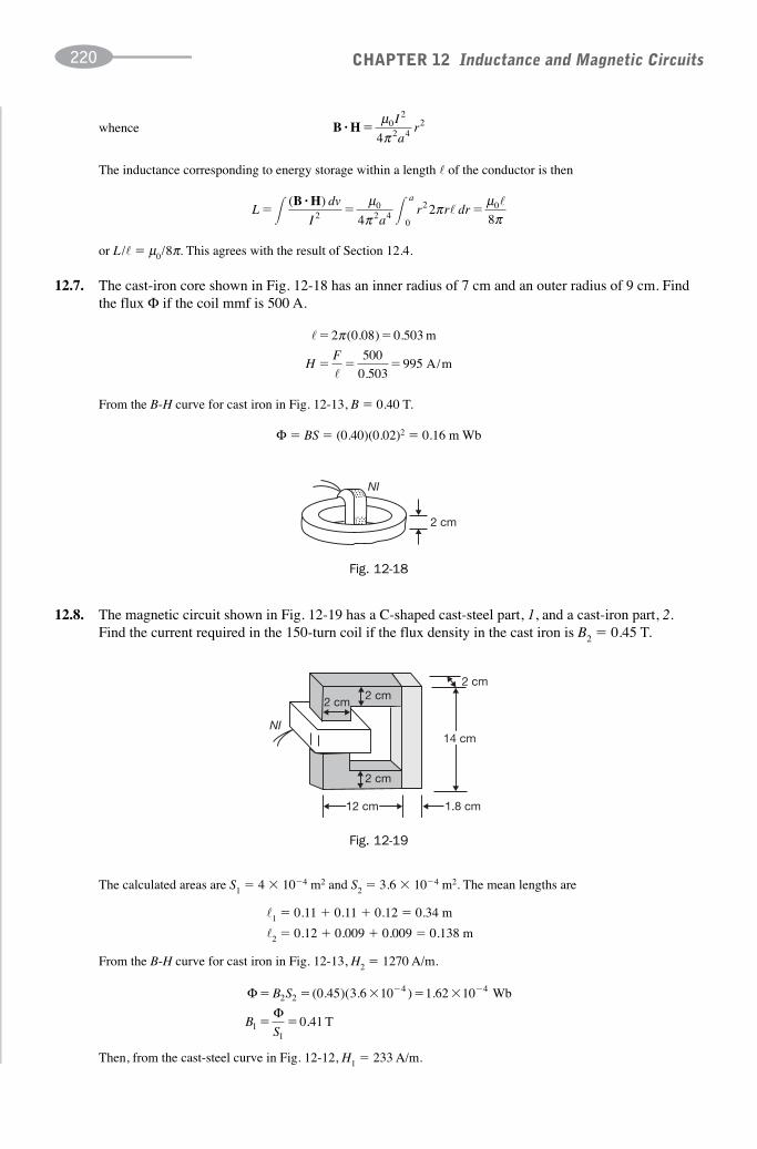
The inductance corresponding to energy storage within a length � of the conductor is then
CHAPTER 12 Inductance and Magnetic Circuits220
B H· �μπ
02
2 42
4
I
ar
Ldv
I ar r dr
a
� � �� �( )B H·2
02 4
0
2 0
42
8
μπ
π μπ
��
�
�
� �
� � �
2 0 08 0 503
995
π ( . ) . m
A/mHF 500
0.503
ΦΦ
� � � � �
� �
� �B S
BS
2 2
11
0 45 3 6 10 1 62 10
0
( . )( . ) .4 4 Wb
..41 T
whence
or L /� � μ0/8π. This agrees with the result of Section 12.4.
12.7. The cast-iron core shown in Fig. 12-18 has an inner radius of 7 cm and an outer radius of 9 cm. Findthe flux Φ if the coil mmf is 500 A.
From the B-H curve for cast iron in Fig. 12-13, B � 0.40 T.
Φ � BS � (0.40)(0.02)2 � 0.16 m Wb
2 cm
NI
Fig. 12-18
12.8. The magnetic circuit shown in Fig. 12-19 has a C-shaped cast-steel part, 1, and a cast-iron part, 2.Find the current required in the 150-turn coil if the flux density in the cast iron is B2 � 0.45 T.
2 cm 2 cm2 cm
14 cm
12 cm 1.8 cm
2 cm
NI
Fig. 12-19
The calculated areas are S1 � 4 � 10�4 m2 and S2 � 3.6 � 10�4 m2. The mean lengths are
�1 � 0.11 � 0.11 � 0.12 � 0.34 m
�2 � 0.12 � 0.009 � 0.009 � 0.138 m
From the B-H curve for cast iron in Fig. 12-13, H2 � 1270 A/m.
Then, from the cast-steel curve in Fig. 12-12, H1 � 233 A/m.

The equivalent circuit, Fig. 12-20, suggests the equation
F � NI � H1�1 � H2�2
150I � 233(0.34) � 1270(0.138)
I � 1.70 A
CHAPTER 12 Inductance and Magnetic Circuits 221
BSi
i
� ��
��
�
�
Φ 0 141 10
4 10
. 3
4 0.35 T
HSa a
aa� �� �
�
� �
�
� �
Φμ π0
0 141 10
4 10 4 84 10
.
( )( . )
3
7 4 (( )2 10 464� ��3 A
NI
H1 1
H2 2
�1
� 2
Fig. 12-20
12.9. The magnetic circuit shown in Fig. 12-21 is cast-iron with a mean length �1 � 0.44 m and squarecross section 0.02 � 0.02 m. The air-gap length is �a � 2 mm and the coil contains 400 turns. Find thecurrent I required to establish an air-gap flux of 0.141 mWb.
N � 400�a
Fig. 12-21
The flux Φ in the air gap is also the flux in the core.
From Fig. 12-13, Hi � 850 A/m. Then
Hi�i � 850(0.44) � 374 A
For the air gap, Sa � (0.02 � 0.002)2 � 4.84 � 10�4 m2, and so
Therefore, F � Hi�i � Ha�a � 838 A and
IF
N� � �
838
4002 09. A
12.10. Determine the reluctance of an air gap in a dc machine where the apparent area is Sa � 4.26 � 10�2 m2
and the gap length �a � 5.6 mm.
� � ��
� �� �
�
� �
�a
aSμ π0
5 6 10
4 10 4 26 101 05
.
( )( . ).
3
7 21105 H 1�
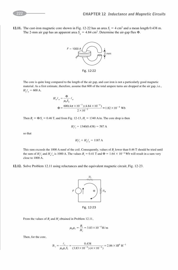
12.11. The cast-iron magnetic core shown in Fig. 12-22 has an area Si � 4 cm2 and a mean length 0.438 m.The 2-mm air gap has an apparent area Sa � 4.84 cm2. Determine the air-gap flux Φ.
CHAPTER 12 Inductance and Magnetic Circuits222
HSa a
aa� ��
�� �
�
� �
�
Φ
Φ
μ
π0
600 4 10 4 84 10
2 10
( ) ( . )7 4
3 �� � �1 82 10 4. Wb
μ μ043 83 10r
i
i
B
H� � � �. H/m
� ii
r iS� �
� �� �
� �
�μ μ0
4 4
0 438
3 83 10 4 10
.
( . ) ( )2.86 1006 H 1�
F � 1000 A
2 mm
Fig. 12-22
The core is quite long compared to the length of the air gap, and cast iron is not a particularly good magneticmaterial. As a first estimate, therefore, assume that 600 of the total ampere turns are dropped at the air gap, i.e.,Ha�a � 600 A.
Then Bi � Φ/Si � 0.46 T, and from Fig. 12-13, Hi � 1340 A/m. The core drop is then
Hi�i � 1340(0.438) � 587 A
so that
Hi�i � Ha�a � 1187 A
This sum exceeds the 1000 A mmf of the coil. Consequently, values of Bi lower than 0.46 T should be tried untilthe sum of Hi�i and Ha�a is 1000 A. The values Bi � 0.41 T and Φ � 1.64 � 10�4 Wb will result in a sum veryclose to 1000 A.
12.12. Solve Problem 12.11 using reluctances and the equivalent magnetic circuit, Fig. 12-23.
�
F Φ
i
�a
Fig. 12-23
From the values of Bi and Hi obtained in Problem 12.11,
Then, for the core,

The corresponding flux density in the iron is 0.41 T, in agreement with the results of Problem 12.11. While theair-gap reluctance can be calculated from the dimensions and μ 0, the same is not true for the reluctance of theiron. The reason is that μ r for the iron depends on the values of Bi and Hi.
12.13. Solve Problem 12.11 graphically with a plot of Φ versus F.
Values of Hi from 700 through 1100 A/m are listed in the first column of Table 12-2; the corresponding values ofBi are found from the cast-iron curve, Fig. 12-13. The values of Φ and Hi�i are computed, and Ha�a is obtainedfrom Φ�a /μ0Sa. Then F is given as the sum of Hi�i and Ha�a. Since the air gap is linear, only two points arerequired. The flux Φ for F � 1000 A is seen from Fig. 12-24 to be approximately 1.65 � 10�4 Wb.
This method is simply a plot of the trial and error data used in Problem 12.11. However, it is helpful if severaldifferent coils or coil currents are to be examined.
CHAPTER 12 Inductance and Magnetic Circuits 223
� aa
aS� �
�
� �� �
�
� �
�μ π0
4
2
4 10 4 84 103
10.29 1
3
7( ) ( . )006 H 1�
F i a� �
�� � �
� � �
Φ
Φ
(
10 4
� � )
. ..
1000
2 86 10 3 29 101 636 6 WWb
and for the air gap,
The circuit equation,
gives
Hi (A/m) Bi (T) Φ (Wb) Hi�i (A) Ha�a (A) F (A)
700 0.295 1.18 � 10�4 307 388 695
800 0.335 1.34 � 10�4 350 441 791
900 0.365 1.46 � 10�4 395 480 874
1000 0.400 1.60 � 10�4 438 526 964
1100 0.420 1.68 � 10�4 482 552 1034
TABLE 12-2
200
1.70
1.60
1.50
1.40
1.30
Cast Iron
Φ (
Wb
� 1
0�
4)
Air Gap
F (A)
Composite
1.20
1.10
400 600 800 1000
Fig. 12-24

12.14. Determine the fluxes Φ in the core of Problem 12.11 for coil mmfs of 800 and 1200 A. Use agraphical approach and the negative air-gap line.
The Φ versus Hi�i data for the cast-iron core, developed in Problem 12.13, are plotted in Fig. 12-25. The air-gapΦ versus F is linear. One end of the negative air-gap line for the coil mmf of 800 A is at Φ � 0, F � 800 A. Theother end assumes Ha�a � 800 A, from which
CHAPTER 12 Inductance and Magnetic Circuits224
Φ � � � �μ0 2 43S Ha a a
a
( ).
��
10 4 Wb
which locates this end at Φ � 2.43 � 10�4 Wb, F � 0.
The intersection of the F � 800 A negative air-gap line with the nonlinear Φ versus F curve for the cast-ironcore gives Φ � 1.34 � 10�4 Wb. Other negative air-gap lines have the same negative slope. For a coil mmf of1000 A, Φ � 1.63 � 10�4 Wb and for 1200 A, Φ � 1.85 � 10�4 Wb.
20000
0.2
0.4
0.6
0.8
1.0
1.2
1.4
1.6
1.8
2.0
2.2
2.4
2.6
Cast Iron
NegativeAir-Gap Line
Hi �i Ha �a
F (A)
Φ (
Wb
� 1
0�4
)
400 600 800 1000 1200
Fig. 12-25
12.15. Solve Problem 12.11 for a coil mmf of 1000 A using the B-H curve for cast iron.
This method avoids the construction of an additional curve such as the Φ versus F curves of Problems 12.13 and12.14. Now, in order to plot the air-gap line on the B-H curve of iron, adjustments must be made for the differentareas and the different lengths. Table 12-3 suggests the necessary calculations.
F
i�� �
1000
0 4382283
.A/m
TABLE 12-3
Ba (T) Ha (A/m)
0.10 0.80 � 105 0.12 363 1920
0.30 2.39 � 105 0.36 1091 1192
0.50 3.98 � 105 0.61 1817 466
FH
ia
a
i������
�⎛
⎝⎜⎞
⎠⎟(A / m)Ha
a
i
����
⎛
⎝⎜⎞
⎠⎟(A / m)B
S
Sa
a
i
⎛
⎝⎜⎞
⎠⎟(T)

B2 (T) H2 (A/m)
0.33 200 0.44 160 240
0.44 250 0.59 200 200
0.55 300 0.73 240 160
0.65 350 0.87 280 120
0.73 400 0.97 320 80
0.78 450 1.04 360 40
0.83 500 1.11 400 0
FH
������1
22
1
��⎛
⎝⎜⎞
⎠⎟(A / m)H2
2
1
����
⎛
⎝⎜⎞
⎠⎟(A / m)B
S
S2
2
1
⎛
⎝⎜⎞
⎠⎟(T)
The data from the third and fifth columns may be plotted directly on the cast-iron B-H curve, as shown in Fig. 12-26.The air gap is linear and only two points are needed. The answer is seen to be Bi � 0.41 T. The method can be usedwith two nonlinear core parts as well (see Problem 12.16).
CHAPTER 12 Inductance and Magnetic Circuits 225
TABLE 12-4
0.10
0.20
0.30
0.40
0.50
Cast Iron
Air-Gap Line,Adjusted
0.60
B(T
)
H (A /m)
0.70
0.80
1000 2000 2283
Fig. 12-26
12.16. The magnetic circuit shown in Fig. 12-27 consists of nickel-iron alloy in part 1, where �1 � 10 cm and S1 � 2.25 cm2, and cast-steel for part 2, where �2 � 8 cm and S2 � 3 cm2. Find the flux densitiesB1 and B2.
F � 40 A
1
2
Fig. 12-27
The data for part 2 of cast-steel will be converted and plotted on the B-H curve for part 1 of nickel-iron alloy(F/�1 � 400 A/m). Table 12-4 suggests the necessary calculations.

From the graph, Fig. 12-28, B1 � 1.01 T. Then, since B1S1 � B2S2,
CHAPTER 12 Inductance and Magnetic Circuits226
B2
4
41 012 25 10
3 100 76�
�
��
�
�.
..
⎛⎝⎜
⎞⎠⎟
T
These values can be checked by obtaining the corresponding H1 and H2 from the appropriate B-H curves andsubstituting in
F � H1�1 � H2�2
B B B1 2 3
3
4
0 173 10
1 5 101 15� � �
�
��
�
�
.
.. T
IF
N� � �
144 2
5000 29
.. A
12.17. The cast-steel parallel magnetic circuit in Fig. 12-29(a) has a coil with 500 turns. The mean lengthsare �2 � �3 � 10 cm, �1 � 4 cm. Find the coil current if Φ3 � 0.173 mWb.
Φ1 � Φ2 � Φ3
Since the cross-sectional area of the center leg is twice that of the two side legs, the flux density is the samethroughout the core, i.e.,
Corresponding to B � 1.15 T, Fig. 12-13 gives H � 1030 A/m. The NI drop between points a and b is now usedto write the following equation [see Fig. 12-29(b)]:
F � H�1 � H�2 � H�3 or F � H(�1 � �2) � 1030(0.14) � 144.2 A
Then
Nickel-Iron Alloy
B1
(T)
H1 (A/m)
Cast Steel,Adjusted
1.20
1.00
0.80
0.60
0.40
0.20
100 200
Fig. 12-28

12.18. The same cast-steel core as in Problem 12.17 has identical 500-turn coils on the outer legs, with thewinding sense as shown in Fig. 12-30(a). If again Φ3 � 0.173 m Wb, find the coil currents.
The flux densities are the same throughout the core and consequently H is the same. The equivalent circuit inFig. 12-30(b) suggests that the problem can be solved on a per pole basis.
CHAPTER 12 Inductance and Magnetic Circuits 227
Φ1
Φ2 Φ3
F
b b
1.5 cm
1 cm
1 cm1 cm
2 cm1 cm
aa
�1
�2
H�2 H�3
H�1H�1
�3
(a) (b)
Fig. 12-29
BS
H� � �Φ3
3
1 15 1030. ����� �����T and A/ m����(from FFig.12-13)
A���3F H� � � �( ) ( . ) .� �1 3 1030 0 14 144 2 ��� AI � 0 29.
Each coil must have a current of 0.29 A.
Φ1Φ2 Φ3
F2F3
F3
H�3
H�1
(a) (b)
1
2 3
Fig. 12-30
12.19. The parallel magnetic circuit shown in Fig. 12-31(a) is silicon steel with the same cross-sectional areathroughout, S � 1.30 cm2. The mean lengths are �1 � �3 � 25 cm, �2 � 5 cm. The coils have 50 turnseach. Given that Φ1 � 90 μ Wb and Φ3 � 120 μ Wb, find the coil currents.
Φ Φ Φ2 3 0 30
90
1 300 6
� � � �
��
��
�
�
�
14
6
4
10
10
10
.
..
Wb
1B 99 T
From Fig. 12-12, H1 � 87 A/m. Then, H1�1 � 21.8 A. Similarly, B2 � 0.23 T, H2 � 49 A/m, H2�2 � 2.5 A andB3 � 0.92 T, H3 � 140 A/m, H3�3 � 35.0 A. The equivalent circuit in Fig. 12-31(b) suggests the followingequations for the NI drop between points a and b:
H1�1 � F1 � H2�2 � F3 � H3�3
21.8 � F1 � 2.5 � F3 � 35.0
from which F1 � 19.3 A and F3 � 37.5 A. The currents are I1 � 0.39 A and I3 � 0.75 A.

12.20. Obtain the equivalent magnetic circuit for Problem 12.19 using reluctances for three legs, andcalculate the flux in the core using F1 � 19.3 A and F3 � 37.5 A.
CHAPTER 12 Inductance and Magnetic Circuits228
Φ1 Φ1
Φ2
Φ3
Φ2
Φ3F1
F3 F3F1
a
b
�1
�2 H1 �1
H2 �2
H3 �3
�3
(a) (b)
Fig. 12-31
� ��
μ μ0 rS
�11
0 1 1
� � � ��μ μr S
2.43 105 H 1
From the values of B and H found in Problem 12.19,
μ0μr1 � 7.93 � 10�3 H/m μ0μr2 � 4.69 � 10�3 H/m μ0μr3 � 6.57 � 10�3 H/m
Now the reluctances are calculated:
�2 � 8.20 � 104 H�1, �3 � 2.93 � 105 H�1. From Fig. 12-32,
F3 � Φ3�3 � Φ2�2 (1)
F1 � Φ1�1 � Φ2�2 (2)
Φ1 � Φ2 � Φ3 (3)
Φ1 Φ2Φ3
F1 � 19.3 A F3 � 37.5 A
�1
�2
�3
Fig. 12-32
Substituting Φ2 from (3) into (1) and (2) results in the following set of simultaneous equations in Φ1 and Φ3:
F1 � Φ1(�1 � �2) � Φ3�2 19.3 � Φ1(3.25 � 105) � Φ3(0.82 � 105)
F3 � �Φ1�2 � Φ3(�2 � �3)or
37.5 � �Φ1(0.82 � 105) � Φ3(3.75 � 105)
Solving, Φ1 � 89.7 μWb, Φ2 � 30.3 μWb, Φ3 � 120 μWb.
Although the simultaneous equations above and the similarity to a two-mesh circuit problem may beinteresting, it should be noted that the flux densities B1, B2, and B3 had to be known before the relativepermeabilities and reluctances could be computed. But if B is known, why not find the flux directly from Φ � BS? Reluctance is simply not of much help in solving problems of this type.
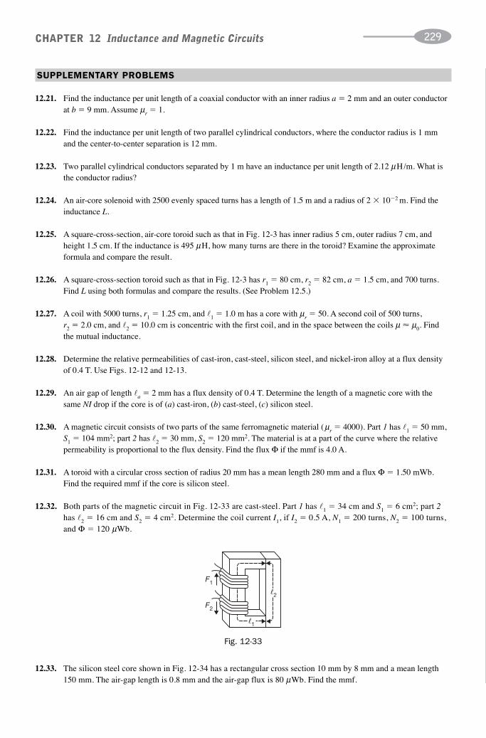
SUPPLEMENTARY PROBLEMS
12.21. Find the inductance per unit length of a coaxial conductor with an inner radius a � 2 mm and an outer conductorat b � 9 mm. Assume μr � 1.
12.22. Find the inductance per unit length of two parallel cylindrical conductors, where the conductor radius is 1 mmand the center-to-center separation is 12 mm.
12.23. Two parallel cylindrical conductors separated by 1 m have an inductance per unit length of 2.12 μH/m. What isthe conductor radius?
12.24. An air-core solenoid with 2500 evenly spaced turns has a length of 1.5 m and a radius of 2 � 10�2 m. Find theinductance L.
12.25. A square-cross-section, air-core toroid such as that in Fig. 12-3 has inner radius 5 cm, outer radius 7 cm, andheight 1.5 cm. If the inductance is 495 μH, how many turns are there in the toroid? Examine the approximateformula and compare the result.
12.26. A square-cross-section toroid such as that in Fig. 12-3 has r1 � 80 cm, r2 � 82 cm, a � 1.5 cm, and 700 turns.Find L using both formulas and compare the results. (See Problem 12.5.)
12.27. A coil with 5000 turns, r1 � 1.25 cm, and �1 � 1.0 m has a core with μr � 50. A second coil of 500 turns, r2 � 2.0 cm, and �2 � 10.0 cm is concentric with the first coil, and in the space between the coils μ � μ0. Find the mutual inductance.
12.28. Determine the relative permeabilities of cast-iron, cast-steel, silicon steel, and nickel-iron alloy at a flux densityof 0.4 T. Use Figs. 12-12 and 12-13.
12.29. An air gap of length �a � 2 mm has a flux density of 0.4 T. Determine the length of a magnetic core with thesame NI drop if the core is of (a) cast-iron, (b) cast-steel, (c) silicon steel.
12.30. A magnetic circuit consists of two parts of the same ferromagnetic material (μr � 4000). Part 1 has �1 � 50 mm,S1 � 104 mm2; part 2 has �2 � 30 mm, S2 � 120 mm2. The material is at a part of the curve where the relativepermeability is proportional to the flux density. Find the flux Φ if the mmf is 4.0 A.
12.31. A toroid with a circular cross section of radius 20 mm has a mean length 280 mm and a flux Φ � 1.50 mWb.Find the required mmf if the core is silicon steel.
12.32. Both parts of the magnetic circuit in Fig. 12-33 are cast-steel. Part 1 has �1 � 34 cm and S1 � 6 cm2; part 2has �2 � 16 cm and S2 � 4 cm2. Determine the coil current I1, if I2 � 0.5 A, N1 � 200 turns, N2 � 100 turns,and Φ � 120 μWb.
CHAPTER 12 Inductance and Magnetic Circuits 229
F1
F2
�2
�1
Fig. 12-33
12.33. The silicon steel core shown in Fig. 12-34 has a rectangular cross section 10 mm by 8 mm and a mean length150 mm. The air-gap length is 0.8 mm and the air-gap flux is 80 μWb. Find the mmf.

12.34. Solve Problem 12.33 in reverse: the coil mmf is known to be 561.2 A and the air-gap flux is to be determined.Use the trial and error method, starting with the assumption that 90% of the NI drop is across the air gap.
12.35. The silicon steel magnetic circuit of Problem 12.33 has an mmf of 600 A. Determine the air-gap flux.
12.36. For the silicon steel magnetic circuit of Problem 12.33, calculate the reluctance of the iron, �i, and the reluctanceof the air gap, �a. Assume the flux is Φ � 80 μWb and solve for F. See Fig. 12-35.
CHAPTER 12 Inductance and Magnetic Circuits230
Fig. 12-34
�
F�
i
�a
Fig. 12-35
12.37. A silicon steel core such as shown in Fig. 12-34 has a rectangular cross section of area Si � 80 mm2 and an airgap of length �a � 0.8 mm with area Sa � 95 mm2. The mean length of the core is 150 mm and the mmf is 600 A.Solve graphically for the flux by plotting Φ versus F in the manner of Problem 12.13.
12.38. Solve Problem 12.37 graphically using the negative air-gap line for an mmf of 600 A.
12.39. Solve Problem 12.37 graphically in the manner of Problem 12.15, obtaining the flux density in the core.
12.40. A rectangular ferromagnetic core 40 � 60 mm has a flux Φ � 1.44 mWb. An air gap in the core is of length�a � 2.5 mm. Find the NI drop across the air gap.
12.41. A toroid with cross section of radius 2 cm has a silicon steel core of mean length 28 cm and an air gap of length 1 mm. Assume the air-gap area, Sa, is 10% greater than the adjacent core and find the mmf required to establishan air-gap flux of 1.5 mWb.
12.42. The magnetic circuit shown in Fig. 12-36 has an mmf of 500 A. Part 1 is cast-steel with �1 � 340 mm and S1 � 400 mm2; part 2 is cast-iron with �2 � 138 mm and S2 � 360 mm2. Determine the flux Φ.
2
1
Fig. 12-36
12.43. Solve Problem 12.42 graphically in the manner of Problem 12.16.
12.44. A toroid of square cross section, with r1 � 2 cm, r2 � 3 cm, and height a � 1 cm, has a two-part core. Part 1 issilicon steel of mean length 7.9 cm; part 2 is nickel-iron alloy of mean length 7.9 cm. Find the flux that resultsfrom an mmf of 17.38 A.

12.45. Solve Problem 12.44 by the graphical method of Problem 12.15. Why is it that the plotting of the second reverseB-H curve on the first is not as difficult as might be expected?
12.46. The cast-steel parallel magnetic circuit in Fig. 12-37 has a 500-turn coil in the center leg, where the cross-sectional area is twice that of the remainder of the core. The dimensions are �a � 1 mm, S2 � S3 � 150 mm2, S1 � 300 mm2, �1 � 40 mm, �2 � 110 mm, and �3 � 109 mm. Find the coil current required to produce an air-gapflux of 125 μWb. Assume that Sa exceeds S3 by 17%.
CHAPTER 12 Inductance and Magnetic Circuits 231
21
a
3
Fig. 12-37
1
2
3
Fig. 12-38
2 3
1F2
F3
0.06 0.02
0.01
0.010.01 0.01
0.01 m
0.14 m
Fig. 12-39
2
31
F F
Fig. 12-40
12.47. The cast-iron parallel circuit core in Fig. 12-38 has a 500-turn coil and a uniform cross section of 1.5 cm2
throughout. The mean lengths are �1 � �3 � 10 cm and �2 � 4 cm. Determine the coil current necessary to resultin a flux density of 0.25 T in leg 3.
12.48. Two identical 500-turn coils have equal currents and are wound as indicated in Fig. 12-39. The cast-steel core hasa flux in leg 3 of 120 μWb. Determine the coil currents and the flux in leg 1.
12.49. Two identical coils are wound as indicated in Fig. 12-40. The silicon steel core has a cross section of 6 cm2
throughout. The mean lengths are �1 � �3 � 14 cm and �2 � 4 cm. Find the coil mmfs if the flux in leg 1 is 0.7 mWb.

ANSWERS TO SUPPLEMENTARY PROBLEMS
12.21. 0.301 μH/m
12.22. 0.992 μH/m
12.23. 5 mm
12.24. 6.58 mH
12.25. 700, 704
12.26. 36.3 μ H (both formulas)
12.27. 7.71 mH
12.28. 318, 1384, 5305, 42, 440
12.29. (a) 0.64 cm; (b) 2.77 m; (c) 10.6 m
12.30. 26.3 μWb
12.31. 83.2 A
12.32. 0.65 A
12.33. 561.2 A
12.35. 85.2 μWb
12.36. �1 � 0.313 μH�1, �a � 6.70 μH�1, F � 561 A
12.37. 85 μWb
12.38. 85 μWb
12.39. 1.06 T
12.40. 1079 A
12.41. 952 A
12.42. 229 μWb
12.43. 229 μWb
12.44. 10�4 Wb
12.45. 10�4 Wb. The mean lengths and cross-sectional areas are the same.
12.46. 1.34 A
12.47. 1.05 A
12.48. 0.41 A, 0 Wb
12.49. 38.5 A
CHAPTER 12 Inductance and Magnetic Circuits232

233
Time-Varying Fields andMaxwell’s Equations
13.1 Introduction
Static electric and magnetic fields were treated separately in the previous chapters. Our first observation on atime-varying field was Faraday’s law introduced briefly in Chapter 12 in order to explain self- and mutual-inductance. The present chapter starts with electromagnetic induction and the electromotive force (emf) due toa changing magnetic field. It then introduces the displacement current proposed by Maxwell to remove the con-tradiction in Ampère’s law when applied to time-varying electric fields. The collection of Faraday’s law,Ampère’s law, and Gauss’s laws (both for the electric and magnetic fields) are called Maxwell’s equations. Theygovern electrostatic, magnetostatic, and time-varying (also called dynamic) electromagnetic fields.
13.2 Maxwell’s Equations for Static Fields
Static electric and magnetic fields are not interconnected. They are treated separately by two sets of uncoupledvector equations as follows:
Electric field: ∇ � E � 0 (Faraday’s law) ∇ · D � ρ (Gauss’s law for the electric field)
Magnetic field: ∇ � H � J (Ampere’s law) ∇ · B � 0 (Gauss’s law for the magnetic field)
Here ρ is charge density and J is current density.
13.3 Faraday’s Law and Lenz’s Law
The minus sign in Faraday’s law (Section 12.3) implicitly gives the polarity of the induced voltage v. To makethis explicit, consider the case of a plane area S, bounded by a closed curve C, where S is cut perpendicularlyby a time-variable flux density B (Fig. 13-1). Faraday’s law here takes the integral form
CHAPTER 13
�C S
dd
dtdE l B S· ·��
in which the positive sense around C and the direction of the normal, dS, are corrected by the usual right-hand rule[Fig. 13-1(a)]. Now if B is increasing with time, the time derivative will be positive and, thus, the right side of theabove equation will be negative. In order for the left integral to be negative, the direction of E must be opposite tothat of the contour, Fig. 13-1(b). A conducting filament in place of the contour would carry a current ic, also in thedirection of E. As shown in Fig. 13-1(c), such a current loop generates a flux φ′ which opposes the increase in B.

Lenz’s law summarizes this discussion: The voltage induced by a changing flux has a polarity such that the current established in a closed path gives rise to a flux which opposes the change in flux.
CHAPTER 13 Time-Varying Fields and Maxwell’s Equations234
Filament
E
ic
C C
v
φ́
�
�
(b)(a) (c)
S1
B(t)
dS
Fig. 13-1
φ
�
�
I
U
Fig. 13-2
�
�
�
�
I I
(b)(a)
Fig. 13-3
In the special case of a conductor moving through a time-independent magnetic field, the polarity predicted byLenz’s law is yielded by two other methods. (1) The polarity is such that the conductor experiences magneticforces which oppose its motion. (2) As indicated in Fig. 13-2, a moving conductor appears to distort the flux,pushing the flux lines in front of it as it moves. This same distortion is suggested by the counterclockwise fluxlines shown around the conductor. By the right-hand rule, the current which would result if a closed path wereprovided would have the direction shown, and the polarity of the induced voltage is � at the end of the conduc-tor where the current would leave. Fig. 13-3 confirms this by comparing the moving conductor and its resultingcurrent to a voltage source connected to a similar external circuit.
13.4 Conductors’ Motion in Time-Independent Fields
The force F on a charge Q in a magnetic field B, where the charge is moving with velocity U, was examined inChapter 11.
F � Q(U � B)
A motional electric field intensity, Em, can be defined as the force per unit charge:
EF
U Bm Q� � ��
When a conductor with a great number of free charges moves through a field B, the impressed Em creates avoltage difference between the two ends of the conductor, the magnitude of which depends on how Em is oriented with respect to the conductor. With conductor ends a and b, the voltage of a with respect to b is

CHAPTER 13 Time-Varying Fields and Maxwell’s Equations 235
B
U
z
x
y
b (0, 0, 0)a (3, 0, 0)
Fig. 13-4
v d dabb
a
m b
a
� �� �E l U B l· ·( )��
If the velocity U and the field B are at right angles, and the conductor is normal to both, then a conductor oflength � will have a voltage
v � B�U
For a closed loop the line integral must be taken around the entire loop:
v d� ( )U B l�� ·
Of course, if only part of the complete loop is in motion, it is necessary only that the integral cover this part, sinceEm will be zero elsewhere.
EXAMPLE 1. In Fig. 13-4, two conducting bars move outward with velocities U1 � 12.5(�ay )m/s and U2 � 8.0ay m/s in the field B � 0.35az T. Find the voltage of b with respect to c.
At the two conductors,
Em1 � U1 � B � 4.38(�ax) V/m
Em2 � U2 � B � 2.80ax V/m
and so
v dx vab x x dc� � �� �� �0
0 50
0
0 50
4 38 2. .
. ( ) .a a· 2.19V 880 1
2 19
a ax x
bc ba ad dc
dx
v v v v
· �
� � � � � �
.40V
0 1.40. �� 3.59 V
Since b is positive with respect to c, current through the meter will be in the ay direction. This clockwise current in the circuit gives rise to flux in the �az direction, which, in accordance with Lenz’s law, counters theincrease in the flux in the �az direction due to the expansion of the circuit. Moreover, the forces that B exertson the moving conductors are directed opposite to their velocities.
13.5 Conductors’ Motion in Time-Dependent Fields
When a closed conducting loop is in motion (this includes changes in shape) and also the field B is a functionof time (as well as of position), then the total induced voltage is made up of a contribution from each of the twosources of flux change. Faraday’s law becomes
vd
dt dt
d dS S
�� �� �� � B SB
S U B l· · ·∂∂
( )��
The first term on the right is the voltage due to the change in B, with the loop held fixed; the second term is thevoltage arising from the motion of the loop, with B held fixed. The polarity of each term is found from theappropriate form of Lenz’s law, and the two terms are then added with regard to those polarities.

EXAMPLE 2. As shown in Fig. 13-5(a), a planar conducting loop rotates with angular velocity ω about the xaxis; at t � 0 it is in the xy plane. A time-varying magnetic field, B � B(t)az, is present. Find the voltage inducedin the loop by using the two-term form of Faraday’s law.
CHAPTER 13 Time-Varying Fields and Maxwell’s Equations236
z
an
y
(a) (b)
Py
r x
ω tω
tω
y
x x
z
B
U
Fig. 13-5
Let the area of the loop be A. The contribution to v due to the variation of B is
vt
ddB
dtdS
dB
dtA t
S Sz n1 �� �� ��� �∂
∂B
S a a· · cos ω
since az · an � cos ωt.To calculate the second, motional contribution to ν, the velocity U of a point on the loop is needed. From
Fig. 13-5(b) it is seen that
U a a� �ry
tn nωω
ωcos
so that
U B a a a�� ��� � �y
tB
y
tB tn z xcos cos
sin ( )ω
ωω
ω ω
since an � az � sin ωt(�ax ). Consequently,
v dB t
ty dx2 � �� ( )
sin
cosU B l a l�� · ·
ω ωω
Stokes’ theorem (Section 10.10) can be used to evaluate the last integral. Since ∇ � yax � �az,
� �y d y d dS A txS
xS
z na l a S a a· · ·� � � � ��( ) ( ) cos∇ ω
Therefore, vB t
tA t BA t2 �� � �
ω ωω
ω ω ωsin
cos( cos ) sin
13.6 Displacement Current
In static fields the curl of H was found to be pointwise equal to the current density Jc. This is conduction cur-rent density; the subscript c has been added to emphasize that moving charges—electrons, photons, or ions—compose the current. If ∇∇ � H � Jc were valid where the fields and charges are variable with time, then thecontinuity equation would be ∇ · Jc � ∇ · (∇ � H) � 0, instead of the correct

Hence, James Clerk Maxwell postulated that
CHAPTER 13 Time-Varying Fields and Maxwell’s Equations 237
∇∇ · Jc t��
∂∂ρ
∇∇��H J J JD
� �c D D twhere �
∂∂
With the inclusion of the displacement current density JD, the continuity equation is satisfied:
∇∇ ∇∇ ∇∇· · · ·J JD
Dc D t t t�� �� �� ��∇ ∂
∂∂∂
∂∂
( )ρ
The displacement current iD through a specified surface is obtained by integration of the normal component ofJD over the surface (just as ic is obtained from Jc).
i dt
dd
dtdD
SD
S S� � �� � �J S
DS D S· · ·
∂∂
Here, the last expression assumes that the surface S is fixed in space.
EXAMPLE 3. Use Stokes’ theorem (Section 10.10) to show that ic � iD in the circuit of Fig. 13-6.
� ��
C S S
Sc
d d d
t
H l H S H S
JD
· · ·� �
� �
1 2
1
( ) ( )∇∇ ∇∇�� ��
∂∂
⎛⎝⎜⎜
⎞⎠⎟
∂∂
⎛⎝⎜
⎞⎠⎟
· ·dt
dS
cS JD
S� ��2
C
S2
iDv �
ic
S1
Fig. 13-6
Since the two surfaces S1 and S2 have the common contour C,
Assuming the flux is confined to the dielectric between the conducting plates, D � 0 over S1. And since no freecharges are in motion within the dielectric, Jc � 0 over S2. Therefore,
� �S
c S c Ddt
d i i1 2
J SD
S· ·� �∂∂
or
It should be noted that ∂D/∂t is nonzero only over that part of S2 that lies within the dielectric.
EXAMPLE 4. Repeat Example 3, this time using circuit analysis.Refer to Fig. 13-6. The capacitance of the capacitor is
CA
d�
�

where A is the plate area and d is the separation. The conduction current is then
CHAPTER 13 Time-Varying Fields and Maxwell’s Equations238
i Cdv
dt
A
d
dv
dtc � ��
On the other hand, the electric field in the dielectric is, neglecting fringing, E � v /d. Hence,
D Ed
vD
t d
dv
dt� � ��
� �∂∂
and the displacement current is (D is normal to the plates)
it
dd
dv
dtd
A
d
dv
dtiD
A Ac� � � �� �∂
∂D
S·� �
S
13.7 Ratio of Jc to JD
Some materials are neither good conductors nor perfect dielectrics, so that both conduction current and displacement current exist. A model for the poor conductor or lossy dielectric is shown in Fig. 13-7. Assumingthe time dependence ejωt for E, the total current density is
J J J E E E Et c D tj� � � � � �σ σ ω∂
∂( )� �
J
Jc
D
�σω�
from which
E
σ
�
Fig. 13-7
As expected, the displacement current becomes increasingly important as the frequency increases.
EXAMPLE 5. A circular-cross-section conductor of radius 1.5 mm carries a current ic � 5.5 sin (4 � 1010t) (μA).What is the amplitude of the displacement current density, if σ � 35 MS/m and �r � 1?
J
Jc
D
� ��
�� �
�
σω π�
3 50
4 10 369 90 10
9
.
( )( / ).
10
10
7
1077
JD �� �
�� �
� �( . ) / [ ( . ) ]
..
5 5 10 1 5
9 907 86 1
6 2π 10
10
3
700 3� μA /m2
13.8 Maxwell’s Equations for Time-Varying Fields
A static E field can exist in the absence of a magnetic field H; a capacitor with a static charge Q furnishes anexample. Likewise, a conductor with a constant current I has a magnetic field H without an E field. When fieldsare time-variable, however, H cannot exist without an E field nor can E exist without a corresponding H field.While much valuable information can be derived from static field theory, only with time-variable fields can the full value of electromagnetic field theory be demonstrated. The experiments of Faraday and Hertz and thetheoretical analyses of Maxwell all involved time-variable fields.
Then

The equations grouped below, called Maxwell’s equations, were separately developed and examined in earlier chapters. In Table 13-1, the most general form is presented, where charges and conduction current maybe present in the region. Note that the point and integral forms of the first two equations are equivalent underStokes’ theorem, while the point and integral forms of the last two equations are equivalent under the divergencetheorem.
CHAPTER 13 Time-Varying Fields and Maxwell’s Equations 239
POINT FORM INTEGRAL FORM
· l∇ ∂∂
� � � �H JD
Hc td �
SS c td
t
JD
S
EB
E
�
� ��
∂∂
⎛
⎝⎜⎞⎠⎟
∇ ∂∂
·
·
(Amp re s law)è ’
ddt
dS
l ·
·
� �� ∂∂
⎛
⎝⎜⎞⎠⎟
∇
BS (Faraday s law; S fixed)’
DD ·
· ·
� �
� �
ρ ρ �
S v
S
d dv
d
D S
B B S
(Gauss law)
(n
’s
∇ 0 0 oonexistence of monopole)
TABLE 13-1 Maxwell’s Equations, General Set
POINT FORM INTEGRAL FORM
· l∇ ∂∂
∂� � �H
DH
Dt
dS
�∂∂
⎛⎝⎜
⎞⎠⎟
∇ ∂∂
∂∂
⎛⎝⎜
⎞⎠⎟
td
td
td
S
·
· l ·
S
EB
EB
S� �� � � �
∇∇
∇
· ·
· ·
D D S
B B S
� �
� �
0 0
0 0
S
S
d
d
TABLE 13-2 Maxwell’s Equations, Free-Space Set
For free space, where there are no charges (ρ � 0) and no conduction currents (Jc � 0), Maxwell’s equationstake the form shown in Table 13-2.
The first and second point-form equations in the free-space set can be used to show that time-variable E and Hfields cannot exist independently. For example, if E is a function of time, then D � �0E will also be a functionof time, so that ∂D/∂t will be nonzero. Consequently, ∇ � H is nonzero, and so a nonzero H must exist. In a similar way, the second equation can be used to show that if H is a function of time, then there must be an Efield present.
The point form of Maxwell’s equations is used most frequently in the problems. However, the integral formis important in that it better displays the underlying physical laws.
SOLVED PROBLEMS
13.1. In a material for which σ � 5.0 S/m and �r � 1 the electric field intensity is E � 250 sin 1010t (V/m).Find the conduction and displacement current densities, and the frequency at which they have equalmagnitudes.
Jc � σE � 1250 sin 1010t (A/m2)

On the assumption that the field direction does not vary with time,
CHAPTER 13 Time-Varying Fields and Maxwell’s Equations240
JD
t tt tD r� � �
∂∂
∂∂
( sin ) . cos (� �0 250 10 22 1 1010 10 A //m2 )
For Jc � JD ,
σ ω ω� ��
� ��
� or10 12
5 0
8 8545 65 1011.
.. rad /s
which is equivalent to a frequency ƒ � 8.99 � 1010 Hz � 89.9 GHz.
13.2. A coaxial capacitor with inner radius 5 mm, outer radius 6 mm, and length 500 mm has a dielectric forwhich �r � 6.7 and an applied voltage 250 sin 377t (V). Determine the displacement current iD andcompare with the conduction current ic.
Assume the inner conductor to be at v � 0. Then, from Problem 9.7, the potential at 0.005 � r � 0.006 m is
v tr
�250
3770 0056
5lnln( )
⎡
⎣⎢
⎤
⎦⎥
⎛⎝⎜
⎞⎠⎟
sin.
(V)
From this,
E a
D
�� ���
� ���
∇ 1.37 10
8
3v
rt r
r
sin ���377 (V/m)
� �0..13 10
3.07 1
8�
� ���
�
rt
t
r
D
sin ���377 a
JD
(C/m )2
∂∂
00
10
5�
�� � �
rt
i J rL
r
D D
cos ��� )
( ) .
377
2 9 63
a (A/m2
π 55 cos ��� )377t (A
The circuit analysis method for ic requires the capacitance,
CLr� �
2 065
π� �
ln1.02 nF
( )
It is seen that ic � iD.
13.3. Moist soil has a conductivity of 10�3 S/m and �r � 2.5. Find Jc and JD where
E � 6.0 � 10�6 sin 9.0 � 109t (V/m)
First, Jc � σE � 6.0 � 10�9 sin 9.0 � 109t (A/m2). Then, since D � �0�rE,
i Cdv
dttc � � � ��( . )( )( )(cos ) .1 02 250 377 377 9 610 9 33 377� �10 5 cos t (A)Then
JD
t
E
ttD r� � � � ��∂
∂∂∂
� �0610 101 20 9 0 9. cos . (A/m )2
13.4. Find the induced voltage in the conductor of Fig. 13-8 where B � 0.04ay T and
U a� 2 5 103. sin t z (m/s)
E U B am xt
v
� � �
�
�� 0 10 10
0 10
3
0
. sin ( )
. sin
(V/m)0.20
� 1103t dx
t
x x( )�
��
a a·
0.02 sin 103 (V)

The conductor first moves in the az direction. The x � 0.20 end is negative with respect to the end at the z axis forthis half cycle.
13.5. Rework Problem 13.4 if the magnetic field is changed to B � 0.04ax (T).
Because the conductor cuts no field lines, the induced voltage must be zero. This may be verified analytically byuse of Problem 2.8.
CHAPTER 13 Time-Varying Fields and Maxwell’s Equations 241
y
z
x0.20
U
B
Fig. 13-8
y
z
x i
dS
B
Fig. 13-9
v d d� � �� �( ) ( )U B l U B l�� ��· · 0
since B and dl are always parallel.
13.6. An area of 0.65 m2 in the z � 0 plane is enclosed by a filamentary conductor. Find the inducedvoltage, given that
Ba a
��
0 05 102
3. cos �����t y z⎛
⎝⎜⎞
⎠⎟(T)
See Fig. 13-9.
vt
dS
t dS
sz
s
y zz
��
��
�
�
∂∂
⎛
⎝⎜⎞
⎠⎟
Ba
a aa
·
·50 102
3sin
�� 23.0 sin 103t (V)
The field is decreasing in the first half cycle of the cosine function. The direction of i in a closed circuit must besuch as to oppose this decrease. Thus the conventional current must have the direction shown in Fig. 13-9.
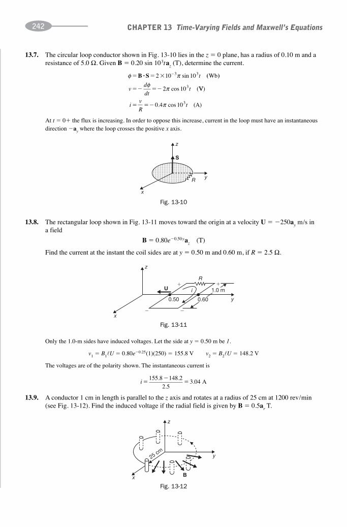
13.7. The circular loop conductor shown in Fig. 13-10 lies in the z � 0 plane, has a radius of 0.10 m and aresistance of 5.0 Ω. Given B � 0.20 sin 103taz (T), determine the current.
CHAPTER 13 Time-Varying Fields and Maxwell’s Equations242
φ πφ π
� � �
�� ��
B S ( )· 2 10 10
10
3 3
3
− sin t
vd
dtt
Wb
(2 cos VV)
(A)iv
Rt� �� 0.4 cos 103π
At t � 0� the flux is increasing. In order to oppose this increase, current in the loop must have an instantaneousdirection �ay where the loop crosses the positive x axis.
z
y
x
R
S
Fig. 13-10
z
y
i
0.50 0.60
1.0 m� �
��x
R
U
Fig. 13-11
z
y25 cm
x B
Fig. 13-12
13.8. The rectangular loop shown in Fig. 13-11 moves toward the origin at a velocity U � �250ay m/s in a field
B � 0.80e�0.50yaz (T)
Find the current at the instant the coil sides are at y � 0.50 m and 0.60 m, if R � 2.5 Ω.
Only the 1.0-m sides have induced voltages. Let the side at y � 0.50 m be 1.
v1 � B1�U � 0.80e�0.25(1)(250) � 155.8 V v2 � B2�U � 148.2 V
The voltages are of the polarity shown. The instantaneous current is
i ��
�155 8 148 2
2 53
. .
..04 A
13.9. A conductor 1 cm in length is parallel to the z axis and rotates at a radius of 25 cm at 1200 rev/min(see Fig. 13-12). Find the induced voltage if the radial field is given by B � 0.5ar T.

The angular velocity is
CHAPTER 13 Time-Varying Fields and Maxwell’s Equations 243
V
�
�
h
Fig. 13-13
ω
z
i 0.50 m
R
Fig. 13-14
12001
602
rev
min
min
s
rad
rev
⎛⎝⎜
⎞⎠⎟
⎛⎝⎜
⎞⎠⎟
⎛⎝⎜
⎞⎠⎟
π �� 40π rad
s
Hence, U � rω � (0.25)(40π) m/s
E a a a
a
m r z
zv
� � �
� �
10 5 0
5 00
π π
π
φ ��0.5
0.01
. ( )
. (
V/m
� )) · dz za �� � �5.0 10 2π V
The negative sign indicates that the lower end of the conductor is positive with respect to the upper end.
13.10. A conducting cylinder of radius 7 cm and height 15 cm rotates at 600 rev/min in a radial field B � 0.20ar T. Sliding contacts at the top and bottom connect to a voltmeter as shown in Fig. 13-13.Find the induced voltage.
ω π ππ φ
� �
�
( ) ( )
( )( . )
600 2 20
20 0 07
160( ) rad/s
m /sU a
EE U B am z� � ��� 0.88( ) V/m
Each vertical element of the curved surface cuts the same flux and has the same induced voltage. These elementsare effectively in a parallel connection and the induced voltage of any element is the same as the total.
v dzz z� � �� ��0
0.15
0 88 0 13. ( ) .a a· V ( at the bottom))
13.11. In Fig. 13-14 a rectangular conducting loop with resistance R � 0.20 Ω turns at 500 rev/min. Thevertical conductor at r1 � 0.03 m is in a field B1 � 0.25ar T, and the conductor at r2 � 0.05 m is in afield B2 � 0.80ar T. Find the current in the loop.
U a a11
60
1
500 2 0 03 0 50� �
�
( ) ( )( . ) .( ) π πφ φ m /s
v �0
0.550
0.25( . ) .0 50 0 20π φa a a�� r zdz· �� V

One radial element is examined. A general point on this radial element has velocity U � ωraφ, so that
Em � U � B � ωrBar
CHAPTER 13 Time-Varying Fields and Maxwell’s Equations244
Similarly, U2 � 0.83πaφ m/s and v2 � �1.04 V. Then
i ��
�1 04 0 20
0 204 20
. .
.. A
in the direction shown on the diagram.
13.12. The circular disk shown in Fig. 13-15 rotates at ω (rad/s) in a uniform flux density B � Baz. Slidingcontacts connect a voltmeter to the disk. What voltage is indicated on the meter from this Faradayhomopolar generator?
B
V
ω
Fig. 13-15
z
b a
y
(a) (b)
y0.30 m
0.30 m
z
α
x
Fig. 13-16
v r B dra Ba
r r� ��0
2
2ω ω
a a·and
where a is the radius of the disk. The positive result indicates that the outer point is positive with respect to thecenter for the directions of B and ω shown.
13.13. A square coil, 0.60 m on a side, rotates about the x axis at ω � 60π rad/s in a field B � 0.80az T, asshown in Fig. 13-16(a). Find the induced voltage.
Assuming that the coil is initially in the xy plane,
α � ωt � 60πt (rad)
The projected area on the xy plane becomes [see Fig. 13-16(b)]:
A � (0.6)(0.6 cos 60πt) (m2)
Then φ � BA � 0.288 cos 60πt (Wb) and
vd
dtt�� �
φ π54 3 60. sin (V)
Lenz’s law shows that this is the voltage of a with respect to b.

Alternate Method
Each side parallel to the x axis has a y component of velocity whose magnitude is
⎪Uy⎪ � ⎪rω sin α⎪ � ⎪18.0π sin 60π t⎪ (m/s)
The voltages B�⎪Uy⎪ for the two sides add, giving
⎪v⎪ � 2(B�⎪Uy⎪) � ⎪54.3 sin 60π t⎪ (V )
Lenz’s law again determines the proper sign.
13.14. Check Example 2 by means of the original, differential form of Faraday’s law.
From Fig. 13-5(b) the projected loop area normal to the field is A cos ωt, whence
φ � B(t) (A cos ωt)
CHAPTER 13 Time-Varying Fields and Maxwell’s Equations 245
vd
dt
dB
dtA t BA t v v�� �� � � �
φ ω ω ωcos sin 1 2and
(It is almost always simpler to use the differential form.)
13.15. Find the electric power generated in the loop of Problem 13.11. Check the result by calculating therate at which mechanical work is done on the loop.
The electric power is the power loss in the resistor:
Pe � i 2R � (4.20)2(0.20) � 3.53 W
The forces exerted by the field on the two vertical conductors are
F1 � i (l1 � B1) � (4.20)(0.50)(0.25) (az � ar) � 0.525aφ N
F2 � i (l2 � B2) � (4.20)(0.50)(0.80)(�az � ar) � �1.68aφ N
To turn the loop, forces �F1 and � F2 must be applied; these do work at the rate
P � (�F1) · U1 � (�F2) · U2 � (�0.525)(0.50π) � (1.68)(0.83π) � 3.55 W
To within rounding errors, P � Pe.
13.16. Given E � Em sin (ωt � βz) ay in free space, find D, B, and H. Sketch E and H at t � 0.
D � �0E � �0Em sin(ω t � βz)ay
The Maxwell equation ∇ � E � �∂B/∂t gives
a a a
Bx y z
m
x y z
E t z
t
∂∂
∂∂
∂∂
∂∂
0 0sin ( )ω β�
��
� � �∂∂B
at
E t zm xβ ω βcos( )or
Integrating,
B a�� �β
ωω βE
t zmxsin ( )

where the “constant” of integration, which is a static field, has been neglected. Then,
CHAPTER 13 Time-Varying Fields and Maxwell’s Equations246
H a�� �βωμ
ω βEt zm
x0
sin ( )
Note that E and H are mutually perpendicular. At t � 0, sin (ωt � βz) � �sin βz. Fig. 13-17 shows the two fieldsalong the z axis, on the assumption that Em and β are positive.
H
E
π /β
π /β
z
x
y
2
t � 0
Fig. 13-17
13.17. Show that the E and H fields of Problem 13.16 constitute a wave traveling in the z direction. Verifythat the wave speed and E/H depend only on the properties of free space.
E and H together vary as sin (ωt � βz). A given state of E and H is then characterized by
ω β ω ωβ
t z t z t t� � � � �const. or0 0( )
But this is the equation of a plane moving with speed
c �ωβ
in the direction of its normal, az. (It is assumed that β, as well as ω, is positive; for a negative β, the direction ofmotion would be �az.) Thus, the entire pattern of Fig. 13-17 moves down the z axis with speed c.
The Maxwell equation ∇ � H � ∂D/∂t gives
a a ax y z
m
mx y z
Et z
tE
∂∂
∂∂
∂∂
∂∂
��
�
βω μ
ω β0
0 0sin ( )
s�0 iin ( )
cos ( ) cos (
ω β
βωμ
ω β ω ω
t z
Et z E t
y
my m
�
� �
a
a2
00� ��
�
β
μωβ
z y)a
1
0 0
2
2�
Consequently,
c ��
� �� �
1 1
10 36 4 103
09�0
7810
μ π π�
( / )( )(m /s)
Moreover,
E
H� � �
ω μβ
μ π π0 0 120 120�0
� (V/A) Ω

13.18. Given H � Hmej(ω t � βz)ax in free space, find E.
CHAPTER 13 Time-Varying Fields and Maxwell’s Equations 247
∇∇��HD
aD
a
�
��
�
∂∂
∂∂
∂∂
t
zH e
t
j H e
mj t z
y
mj t z
( )
( )
ω β
ω ββ yy
m j t zy
t
He
�
� �
∂∂D
D aβ
ωω β( )
and E � D/�0.
13.19. Given
E a H� ��30 10 108π βe H ej t z
x mj( ) ((V/m)
88 t zy
�β )a (A /m)
in free space, find Hm and β (β 0).
This is a plane wave, essentially the same as that in Problems 13.16 and 13.17 (except that, there E was in the ydirection and H in the x direction). The results of Problem 13.17 hold for any such wave in free space:
ωβ μ
μ π� � � � �1
3 1200
0
� �0
8
0
10 (m /s)E
HΩ
Thus, for the given wave,
β ππ
��
� � �10
3 10
1
3
8
8(rad /m) (A /m)Hm
30
120
1
4
To fix the sign of Hm, apply ∇ � E � �∂B/∂t:
j e j H ej t zy m
j t zyβ π μβ β30 1010 8
0108 8( ) ( )� ���a a
which shows that Hm must be negative.
13.20. In a homogeneous nonconducting region where μr � 1, find �r and ω if
E � 30πe j[ωt �(4/3)y]az (V/m) H � 1.0e j[ωt � (4/3)y]ax (A/m)
Here, by analogy to Problem 13.17,
ωβ μ μ
μ π μ� �
�� �
1 8
� � � �
3 10120
r r
r
r
E
H(m /s) ( )Ω
Thus, since μr � 1,
ω π π43
8 1�
��
3 10120
� �r r
��� ������30
which yield �r � 16, ω � 108 rad/s. In this medium the speed of light is c/4.

SUPPLEMENTARY PROBLEMS
13.21. Given the conduction current density in a lossy dielectric as Jc � 0.02 sin 109t (A/m2), find the displacementcurrent density if σ � 103 S/m and �r � 6.5.
13.22. A circular-cross-section conductor of radius 1.5 mm carries a current ic � 5.5 sin 4 � 1010t (μA). What is theamplitude of the displacement current density, if σ � 35 MS/m and �r � 1?
13.23. Find the frequency at which conduction current density and displacement current density are equal in (a) distilledwater, where σ � 2.0 � 10�4 S/m and �r � 81; (b) seawater, where σ � 4.0 S/m and �r � 1.
13.24. Concentric spherical conducting shells at r1 � 0.5 mm and r2 � 1 mm are separated by a dielectric for which �r � 8.5. Find the capacitance and calculate ic, given an applied voltage v � 150 sin 5000t (V). Obtain thedisplacement current iD and compare it with ic.
13.25. Two parallel conducting plates of area 0.05 m2 are separated by 2 mm of a lossy dielectric for which �r � 8.3 andσ � 8.0 � 10�4 S/m. Given an applied voltage v � 10 sin 107t (V), find the total rms current.
13.26. A parallel-plate capacitor of separation 0.6 mm and with a dielectric of �r � 15.3 has an applied rms voltage of25 V at a frequency of 15 GHz. Find the rms displacement current density. Neglect fringing.
13.27 A conductor on the x axis between x � 0 and x � 0.2 m has a velocity U � 6.0az m/s in a field B � 0.04ay T.Find the induced voltage by using (a) the motional electric field intensity, (b) dφ /dt, and (c) B�U. Determine thepolarity and discuss Lenz’s law if the conductor was connected to a closed loop.
13.28. Repeat Problem 13.27 for B � 0.04 sin kzay (T). Discuss Lenz’s law as the conductor moves from flux in onedirection to the reverse direction.
13.29. The bar conductor parallel to the y axis shown in Fig. 13-18 completes a loop by sliding contact with theconductors at y � 0 and y � 0.05 m. (a) Find the induced voltage when the bar is stationary at x � 0.05 m and B � 0.30 sin 104taz (T). (b) Repeat for a velocity of the bar U � 150ax m /s. Discuss the polarity.
CHAPTER 13 Time-Varying Fields and Maxwell’s Equations248
x
0.05
0.05
BV
y
Fig. 13-18
0.05 m
50 Ω
U B2
B1
Fig. 13-19
13.30. The rectangular coil in Fig. 13-19 moves to the right at speed U � 2.5 m/s. The left side cuts flux at right angles,where B1 � 0.30 T, while the right side cuts equal flux in the opposite direction. Find the instantaneous current inthe coil and discuss its direction by use of Lenz’s law.
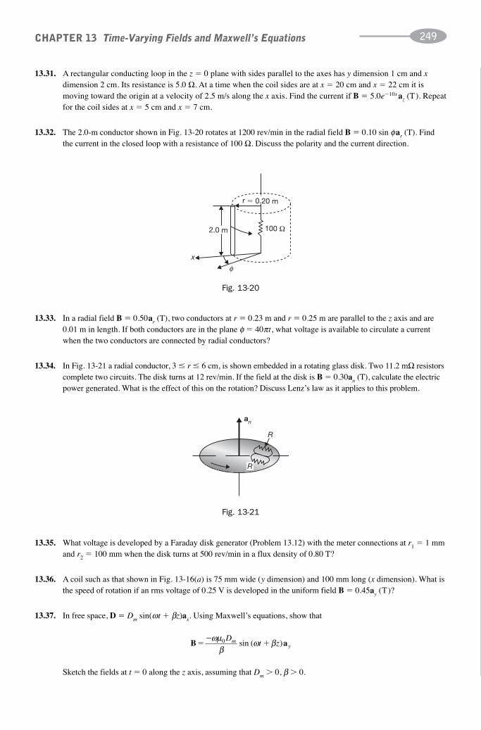
13.31. A rectangular conducting loop in the z � 0 plane with sides parallel to the axes has y dimension 1 cm and xdimension 2 cm. Its resistance is 5.0 Ω. At a time when the coil sides are at x � 20 cm and x � 22 cm it ismoving toward the origin at a velocity of 2.5 m/s along the x axis. Find the current if B � 5.0e�10x az (T). Repeatfor the coil sides at x � 5 cm and x � 7 cm.
13.32. The 2.0-m conductor shown in Fig. 13-20 rotates at 1200 rev/min in the radial field B � 0.10 sin φar (T). Findthe current in the closed loop with a resistance of 100 Ω. Discuss the polarity and the current direction.
CHAPTER 13 Time-Varying Fields and Maxwell’s Equations 249
x
φ
100 Ω
r � 0.20 m
2.0 m
Fig. 13-20
an
R
R
Fig. 13-21
13.33. In a radial field B � 0.50ar (T), two conductors at r � 0.23 m and r � 0.25 m are parallel to the z axis and are0.01 m in length. If both conductors are in the plane φ � 40πt, what voltage is available to circulate a currentwhen the two conductors are connected by radial conductors?
13.34. In Fig. 13-21 a radial conductor, 3 � r � 6 cm, is shown embedded in a rotating glass disk. Two 11.2 mΩ resistorscomplete two circuits. The disk turns at 12 rev/min. If the field at the disk is B � 0.30an (T), calculate the electricpower generated. What is the effect of this on the rotation? Discuss Lenz’s law as it applies to this problem.
13.35. What voltage is developed by a Faraday disk generator (Problem 13.12) with the meter connections at r1 � 1 mmand r2 � 100 mm when the disk turns at 500 rev/min in a flux density of 0.80 T?
13.36. A coil such as that shown in Fig. 13-16(a) is 75 mm wide (y dimension) and 100 mm long (x dimension). What isthe speed of rotation if an rms voltage of 0.25 V is developed in the uniform field B � 0.45ay (T)?
13.37. In free space, D � Dm sin(ωt � βz)ax. Using Maxwell’s equations, show that
B a��
�ωμ
βω β0D
t zm sin ( ) y
Sketch the fields at t � 0 along the z axis, assuming that Dm � 0, β � 0.

13.38. In free space,
B � Bmej(ωt � βz)ay
Show that
CHAPTER 13 Time-Varying Fields and Maxwell’s Equations250
z
x
D or Epropagation
B or H
y
t � 0
Fig. 13-22
E a�� �ωβ
ω βBem j t z( )
x
13.39. In a homogeneous region where μr � 1 and �r � 50,
E � 20π e j(ω t � βz)ax (V/m) B � μ0Hme j(ω t � βz ) ay (T)
Find ω and Hm if the wavelength is 1.78 m.
ANSWERS TO SUPPLEMENTARY PROBLEMS
13.21. 1.15 � 10�6 cos 109t (A/m2)
13.22. 7.87 � 10�3 μ A/m2
13.23. (a) 4.44 � 104 Hz; (b) 7.19 � 1010 Hz
13.24. ic � iD � 7.09 � 10�7 cos 5000t (A)
13.25. 0.192 A
13.26. 5.32 � 105 A/m2
13.27. 0.048 V (x � 0 end is positive)
13.28. 0.048 sin kz (V)
13.29. (a) �7.5 cos 104t (V);
(b) �7.5 cos 104t � 2.25 sin 104t (V)
13.30. 15 mA (counterclockwise)
13.31. 0.613 mA, 2.75 mA
13.32. 5.03 � 10�2 sin 40πt (A)
13.33. 12.6 mV
13.34. 46.3 μW
13.35. 0.209 V
13.36. 1000 rev/min
13.37. See Fig. 13-22.
13.39. 1.5 � 108 rad/s, 1.18 A/m

251
Electromagnetic Waves
14.1 Introduction
Some wave solutions to Maxwell’s equations have already been encountered in the Solved Problems of Chapter 13.The present chapter will extend the treatment of electromagnetic waves. Since most regions of interest are free of charge, it will be assumed that charge density ρ � 0. Moreover, linear isotropic materials will be assumed, withD � �E, B � μH, and J � σE.
14.2 Wave Equations
With the above assumptions and with time dependence e jω t for both E and H, Maxwell’s equations (Table 13-1)become
∇ � H � (σ � jω�)E (1)
∇ � E � �jωμH (2)
∇ · E � 0 (3)
∇ · H � 0 (4)
Taking the curl of (1) and (2),
∇ � (∇ � H) � (σ � jω�) (∇ � E)
∇ � (∇ � E) � �jωμ(∇ � H)
Now, in Cartesian coordinates only, the Laplacian of a vector
∇2A � (∇2Ax)ax � (∇2Ay)ay � (∇2Az )az
satisfies the identity
∇ � (∇ � A) � ∇(∇ · A) � ∇2A
Substitution for the “curl curls” and use of (3) and (4) yields the vector wave equations
∇2H � jωμ(σ � jω�)H � γ 2H
∇2E � jωμ(σ � jω�)E � γ 2E
CHAPTER 14

CHAPTER 14 Electromagnetic Waves252
The propagation constant γ is that square root of γ 2 whose real and imaginary parts are positive:
γ α β
α ω μ σω
� �
� � �
j
��2 11
2( )( )β ω μ σ
ω� � ��
�2 112( )( )
∂∂
∂∂
2
2 2
2
2
1F
z u
F
t�
λ πβ
�2
with (5)
(6)
harmonic waves of angular frequency ω are obtained:
F � Ce j (ωt � βz ) and F � De j (ωt � βz )
in which β � ω /u. Of course, the real and imaginary parts are also solutions to the wave equation. One of thesesolutions, F � C sin(ωt � βz ), is shown in Fig. 14-2 at t � 0 and t � π /2ω. In this interval the wave hasadvanced in the positive z direction a distance d � u(π /2ω) � π /2β. At any fixed t, the waveform repeats itselfwhen x changes by 2π /β; the distance
14.3 Solutions in Cartesian Coordinates
The familiar scalar wave equation in one dimension,
has solutions of the form F � ƒ(z � ut) and F � g(z � ut), where ƒ and g are arbitrary functions. These rep-resent waves traveling with speed u in the �z and �z directions, respectively. In Fig. 14-1 the first solution isshown at t � 0 and t � t1; the wave has advanced in the �z direction a distance of ut1 in the time interval t1.For the particular choices
ƒ(x) � Ce�jω x/u and g(x) � De� jω x/u
t � 0
z0 z1
ut1
F
z
f (z1 � u1t1)f (z0)
t � t1
Fig. 14-1
is called the wavelength. The wavelength and the frequency ƒ � ω /2π enjoy the relation
λƒ � u or λ � Tu
where T � 1/ƒ � 2π/ω is the period of the harmonic wave.

The vector wave equations of Section 14.2 have solutions similar to those just discussed. Because the unitvectors ax, ay, and az in Cartesian coordinates have fixed directions, the wave equation for H can be rewrittenin the form
CHAPTER 14 Electromagnetic Waves 253
∂∂
∂∂
∂∂
2
2
2
2
2
22H H HH
x y z� � �γ
d
dz
2
22HH�γ
H H a( , )z t e ez j tH� �
0γ ω
E a( , )z t E e ez j tE� �
0γ ω
t � 0F
d
C
z
t �πω2
Fig. 14-2
14.4 Plane Waves
Of particular interest are solutions ( plane waves) that depend on only one spatial coordinate, say z. Then theequation becomes
which, for an assumed time dependence e jωt, is the vector analog of the one-dimensional scalar wave equation.Solutions are as above, in terms of the propagation constant γ.
The corresponding solutions for the electric field are
The fixed unit vectors aH and aE are orthogonal and neither field has a component in the direction of propaga-tion. This being the case, one can rotate the axes to put one of the fields, say E, along the x axis. Then fromMaxwell’s equation (2) it follows that H will lie along the �y axis for propagation in the �z direction.
EXAMPLE 1. Given the field E � E0e�γ zaE (time dependence suppressed), show that E can have no compo-
nent in the propagation direction, �az .The Cartesian components of aE are found by projection:
E � E0e�γ z[(aE · ax )ax � (aE · ay)ay � (aE · az )az]
From ∇ · E � 0,
∂∂z
E e zE z0 0� �γ ( )a a·
which can hold only if aE · az � 0. Consequently, E has no component in az.The plane wave solutions obtained above depend on the properties μ, �, and σ of the medium, because these
properties are involved in the propagation constant γ.

14.5 Solutions for Partially Conducting Media
For a region in which there is some but not much conductivity (e.g., moist earth, seawater), the solution to thewave equation in E is taken to be
CHAPTER 14 Electromagnetic Waves254
E a� �E e zx0
γ
H a�� � �σ ωω μ
γj
jE e z
y0
η
η ω μσ ω
�
��
E
H
j
j
x
y
�
ημ
θ σω
θσ
ω
�
�
� � �/
����tan�
��1
22
4 ( )and 0� �45
E a
H
( , )
( , )
( )
(
z t E e e
z tE
e e
z j t zx
z j t
�
�
� �
�
0
0
α ω β
α ω
η�� �β θz
y)a
u � �
� �
� �
� �
ωβ
λ πβ
π
ω
μ σω
μ σω
1
1
2 2
1
2
2
��
��
2
2
1
1
( )( )
( )(( )
Then, from (2) of Section 14.2,
The ratio E/H is characteristic of the medium (it is also frequency-dependent). More specifically for wavesE � Exax, H � Hyay which propagate in the �z direction, the intrinsic impedance, η, of the medium isdefined by
Thus,
where the correct square root may be written in polar form, ⎪η⎪ �θ , with
(If the wave propagates in the �z direction, Ex /Hy � �η. In effect, γ is replaced by �γ and the other squareroot used.)
Inserting the time factor e jω t and writing γ � α � jβ results in the following equations for the fields in apartially conducting region:
The factor e�αz attenuates the magnitudes of both E and H as they propagate in the �z direction. The expres-sion for α, (5) of Section 14.2, shows that there will be some attenuation unless the conductivity σ is zero, whichwould be the case only for perfect dielectrics or free space. Likewise, the phase difference θ between E(z, t) andH(z, t) vanishes only when σ is zero.
The velocity of propagation and the wavelength are given by

If the propagation velocity is known, λƒ � u may be used to determine the wavelength λ. The term (σ /ω�)2 hasthe effect of reducing both the velocity and the wavelength from what they would be in either free space or per-fect dielectrics, where σ � 0. Observe that the medium is dispersive: waves with different frequencies ω havedifferent velocities u.
14.6 Solutions for Perfect Dielectrics
For a perfect dielectric, σ � 0, and so
CHAPTER 14 Electromagnetic Waves 255
Since α � 0, there is no attenuation of the E and H waves. The zero angle on η results in H being in time phasewith E at each fixed location. Assuming E in ax and propagation in az, the field equations may be obtained asthe limits of those in Section 14.5
The velocity and the wavelength are
Solutions in Free Space.
Free space is nothing more than the perfect dielectric for which
For free space, η � η0 � 120π Ω and u � c � 3 � 108 m/s.
14.7 Solutions for Good Conductors; Skin Depth
Materials are ordinarily classified as good conductors if σ ω� in the range of practical frequencies. Therefore,the propagation constant and the intrinsic impedance are
α β ω η� � �0 ��
0�μμ
E a
H a
( , )
( , ) �
( )
( )
z t E e
z tE
e
j t zx
j t zy
�
�
�
�
0
0
ω β
ω β
η
u � � � �ωβ μ
λ πβ
πω μ
1 2 2
� ������
μ μ π� � � � � �� ��
0 4 8 85410 1070
12H/m��� �� F /m10
� � . �99
F/m36π
γ α β α β ω σ σ η ωσ
� � � � � �j f2
45�πμμ μ
E a H( , ) ( , )( ) (z t E e e z tE
e ez j t zx
z j t� �� �0
0− α ω β α ω
η�� � β πz
y4)a
uf
� � � � � �ωβ
ωμσ
ωδ λ πβ
ππ μσ
πδ2 2 22�� ���
It is seen that for all conductors the E and H waves are attenuated. Numerical examples will show that this is avery rapid attenuation. α will always be equal to β. At each fixed location H is out of time phase with E by 45°or π /4 rad. Once again assuming E in ax and propagation in az, the field equations are, from Section 14.5,
Moreover,

The velocity and wavelength in a conducting medium are written here in terms of the skin depth or depth of penetration,
CHAPTER 14 Electromagnetic Waves256
δπ μσ
�1
f
δπ μσ
μ� �1
6 61f
. �� m
EXAMPLE 2. Assume a field E � 1.0e�αze j(ωt � βz) ax (V/m), with ƒ � ω /2π � 100 MHz, at the surface of acopper conductor, σ � 58 MS/m, located at z � 0, as shown in Fig. 14-3. Examine the attenuation as the wavepropagates into the conductor.
x
z
� 0
�0 μ0
σ σ
E
Propagation direction
Fig. 14-3
At depth z the magnitude of the field is
⎪E⎪ � 1.0e�αz � 1.0e�z /δ
where
Thus, after just 6.61 micrometers the field is attenuated to e�1 � 36.8% of its initial value. At 5δ or 33 microm-eters, the magnitude is 0.67% of its initial value—practically zero.
14.8 Interface Conditions at Normal Incidence
When a traveling wave reaches an interface between two different regions, it is partly reflected and partly transmitted, with the magnitudes of the two parts determined by the constants of the two regions. In Fig. 14-4, atraveling E wave approaches the interface z � 0 from region 1, z � 0. Ei and Er are at z � �0, while Et is at z � �0 (in region 2). Here, i signifies “incident,” r “reflected” and t “transmitted.” Normal incidence is assumed.The equations for E and H can be written as
E a
E a
i i z j rx
r r z j t
z t E e e
z t E e e
( , )
( , )
�
�
�
�
0
0
1
1
γ ω
γ ωxx
i t z j tx
i i z j
z t E e e
z t H e e
E a
H
( , )
( , )
�
�
�
�
0
0
2
1
γ ω
γ ωtty
r r z j ty
t t z j
z t H e e
z t H e e
a
H a
H
( , )
( , )
�
� �
0
0
1
2
γ ω
γ ωωτ ay
One of the six constants—it is almost always Ei0—may be taken as real. Under the interface conditions about to
be derived, one or more of the remaining five may turn out to be complex.

With nominal incidence, E and H are entirely tangential to the interface, and thus are continuous across it. At z � 0 this implies
Ei0 � Er
0 � Et0 Hi
0 � Hr0 � Ht
0
Furthermore, the intrinsic impedance in either region is equal to �Ex /Hy (see Section 14.5).
CHAPTER 14 Electromagnetic Waves 257
E E E0
01
0
01
0
02
i
i
r
r
t
tH H H� �� �η η η����� �����
E
E
H
H
E
r
i
r
i0
0
2 1
1 2
0
0
1 2
1 2
0
��
��
�
�
η ηη η
η ηη η
����� ��
tt
i
t
iE
H
H0
2
1 2
0
0
1
1 2
2 2�
��
�
ηη η
ηη η
������
partially conducting medium:
conduct
ηω
σ ω�
�
j
j �
iing medium:
perfect dielectric:
fr
ηωσ
η
�
�
45�
�
eee space: η00 120 Ω�
�0
�
μ
μ
πμ
μ
η η π η μ π1 0 2
120� � � � �120 217.7٠��� ���������
� �r
E00
0
2 1
1 2
0
0
1r
i
r
iE
H
H�
�
��� �
�η ηη η
η η0.268 ������ �� 22
1 2
0
0
2
1 2
20 732
η η
ηη η
��
��
�
0.268��
. � ������E
E
t
i �� ��� .H
H
t
i0
0
1
1 2
21 268�
��
ηη η
x
z
y
1 2
2,2, 2σ μ �1,
1, 1σ μ �
Er
E i
E t
Fig. 14-4
The five equations above can be combined to produce the following ratios in terms of the intrinsic impedances:
The intrinsic impedances for various materials were examined earlier. They are repeated here for reference.
EXAMPLE 3. Traveling E and H waves in free space (region 1) are normally incident on the interface with aperfect dielectric (region 2) for which �r � 3.0. Compare the magnitudes of the incident, reflected, and trans-mitted E and H waves at the interface.

14.9 Oblique Incidence and Snell’s Laws
An incident wave that approaches a plane interface between two different media generally will result in a trans-mitted wave in the second medium and a reflected wave in the first. The plane of incidence is the plane contain-ing the incident wave normal and the local normal to the interface; in Fig. 14-5 this is the xz plane. The normalsto the reflected and transmitted waves also lie in the plane of incidence. The angle of incidence θi, the angle ofreflection θr, and the angle of transmission θt—all defined as in Fig. 14-5—obey Snell’s law of reflection,
θi � θr
and Snell’s law of refraction,
CHAPTER 14 Electromagnetic Waves258
x
z
�
θr
θi
θt
Reflected
Transmitted
Incidentwavenormal
2� 1
Fig. 14-5
EXAMPLE 4. A wave is incident at an angle of 30° from air to Teflon, �r � 2.1. Calculate the angle of trans-mission, and repeat with an interchange of the regions.
Since μ1 � μ2,
sin
sin
θθ
μμ
i
t
� 2
1
�
�2
1
sin
sin
sin
sin�����
θθ θ
i
t t
r
r
� � �30� �
�2
1
2.1 or������θt � 20 18. �
sin
sin����� .
3046 43
��
θθ
tt� �
1
2.1or�����
From Teflon to air,
Supposing both media of the same permeability, propagation from the optically denser medium (�1 � �2) resultsin θt � θi. As θi increases, an angle of incidence will be reached that results in θt � 90°. At this critical angleof incidence, instead of a wave being transmitted into the second medium there will be a wave that propagatesalong the surface. The critical angle is given by
EXAMPLE 5. The critical angle for a wave propagating from Teflon into free space is
θcr
r
� �sin 1 �
�2
1
θc � ��sin .1 43 641
2.1�

14.10 Perpendicular Polarization
The orientation of the electric field E with respect to the plane of incidence determines the polarization of a waveat the interface between two different regions. In perpendicular polarization, E is perpendicular to the plane ofincidence (the xz plane in Fig. 14-6) and is thus parallel to the (planar) interface. At the interface,
CHAPTER 14 Electromagnetic Waves 259
E
E
r
ii t
i t
0
0
2 1
2 1
��
�
η θ η θη θ η θ
cos cos
cos cos
E
E
t
ii
i t
0
0
2
2 1
2�
�
η θη θ η θ
cos
cos cos
E
E
r
it i
i t
0
0
2 1
1 2
��
�
η θ η θη θ η θ
cos cos
cos cos
E
E
t
ii
i t
0
0
2
1 2
2�
�
η θη θ η θ
cos
cos cos
θB � �tan 1 �
�2
1
and
Note that for normal incidence, θi � θt � 0° and the expressions reduce to those found in Section 14.9.
It is not difficult to show that if μ1 � μ2,
η2 cos θi � η1 cos θt � 0 for any θi
Hence, a perpendicularly polarized incident wave suffers either partial or total reflection.
14.11 Parallel Polarization
For parallel polarization, the electric field vector E lies entirely within the plane of incidence, the xz plane asshown in Fig. 14-7. (Thus E assumes the role played by H in perpendicular polarization.) At the interface,
1 2
x
z
θr
θi
θt
H r
H i
H t
E r
E t
E i
Fig. 14-6
and
In contrast to perpendicular polarizations, if μ1 � μ2 there will be a particular angle of incidence for which thereis no reflected wave. This Brewster angle is given by

EXAMPLE 6. The Brewster angle for a parallel-polarized wave traveling from air into glass for which �r � 5.0 is
θB � tan�1 ��5.0 � 65.91°
14.12 Standing Waves
When waves traveling in a perfect dielectric (σ1 � α1 � 0) are normally incident on the interface with a perfect conductor (σ2 � ∞, η2 � 0), the reflected wave in combination with the incident wave produces a standingwave. In such a wave, which is readily demonstrated on a clamped taut string, the oscillations at all points of a half-wavelength interval are in time phase. The combination of incident and reflected waves may be written
CHAPTER 14 Electromagnetic Waves260
E a( , ) [ ] (( ) ( )
z t E e E e e Ei rx
j tj t z j t z� � �
� �
0 0
ω β ω β ω00 0i r
xe E ej z j z�
�β β
)a
Since η2 � 0, Er0 /Ei
0 � �1 and
E a( , ) ( ) sinz t e E e E e jE zj t i ix
ij z j z� � ��
�ω β ββ0 0 02 ee j t
xω a
Taking the real part,
E(z, t) � 2Ei0 sin βz sin ω tax
The standing wave is shown in Fig. 14-8 at time intervals of T/8, where T � 2π /ω is the period. At t � 0, E � 0everywhere; at t � 1(T /8), the endpoints of the E vectors lie on sine curve 1; at t � 2(T /8), they lie on sine curve 2;and so forth. Sine curves 2 and 6 form an envelope for the oscillations; the amplitude of this envelope is twice theamplitude of the incident wave. Note that adjacent half-wavelength segments are 180° out of phase with each other.
1 2x
z
θr
θi
θt
H r
H i
H tE r
E i
E t
Fig. 14-7
z
6
σ � 0σ � ∞
λ2
2Ei0
5, 7
1, 32
0, 4, 8
x
Fig. 14-8

14.13 Power and the Poynting Vector
Maxwell’s first equation for a region with conductivity σ is written and then E is dotted with each term
CHAPTER 14 Electromagnetic Waves 261
∇∇
∇∇
��
��
H EE
E H EE
� �
� �
σ
σ
�
�
∂∂
∂∂
t
Et
· ·( ) 2
H E E H EE
· · ·( ) ( )∇∇ ∇∇�� ��� � �σ Et
2 �∂∂
H E HH H
· ·( )∇∇�� � � ��μ μ∂∂
⎛⎝⎜
⎞⎠⎟
∂∂t t2
2
EE
· ��∂
∂∂∂t
E
t�
2
2
σ μE
t
H
t2
2 2
2�� � �
�
2
∂∂
∂∂
EE H∇∇ · ( )��
� � v v S
E dvt
H
tdvσ μ2
2 2
2�� � �
�
2
∂∂
∂∂
⎛⎝⎜
⎞⎠⎟
E E H( )�� · ddS
P t d dS S
( )� � ( )E H S S�� · ·��
where, as usual, E2 � E · E. The vector identity ∇ · (A � B) � B · (∇ � A) � A · (∇ � B) is employed to changethe left side of the equation.
By Maxwell’s second equation,
Similarly,
Substituting and rearranging terms,
Integration of this equation throughout an arbitrary volume v gives
where the last term has been converted to an integral over the surface of v by use of the divergence theorem.The integral on the left has the units of watts and is the usual ohmic term representing energy dissipated per
unit time as heat. This dissipated energy has its source in the integrals on the right. Because �E 2/2 and μH 2/2are the densities of energy stored in the electric and magnetic fields, respectively, the volume integral (includ-ing the minus sign) gives the decrease in this stored energy. Consequently, the surface integral (including theminus sign) must be the rate of energy entering the volume from outside. A change of sign then produces theinstantaneous rate of energy leaving the volume:
where � � E � H is the Poynting vector, the instantaneous rate of energy flow per unit area at a point.In the cross product that defines the Poynting vector, the fields are supposed to be in real form. If, instead,
E and H are expressed in complex form and have the common time-dependence e jωt, then the time-average of� is given by
��avg �1
2Re ( )E H�� *
where H* is the complex conjugate of H. This follows the complex power of circuit analysis, S � 1–2
VI*, of which the power is the real part, P � 1–
2Re VI*.
For plane waves, the direction of energy flow is the direction of propagation. Thus, the Poynting vectoroffers a useful, coordinate-free way of specifying the direction of propagation, or of determining the directionsof the fields if the direction of propagation is known. This can be particularly valuable where incident, transmit-ted, and reflected waves are being examined.
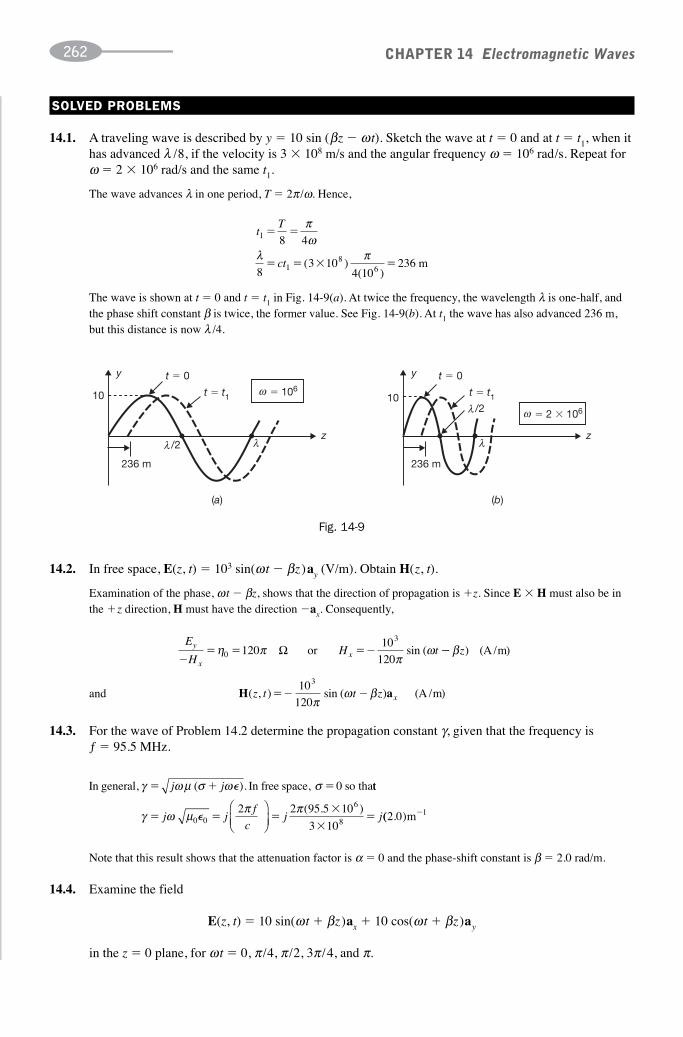
SOLVED PROBLEMS
14.1. A traveling wave is described by y � 10 sin (βz � ω t). Sketch the wave at t � 0 and at t � t1, when ithas advanced λ /8, if the velocity is 3 � 108 m/s and the angular frequency ω � 106 rad/s. Repeat forω � 2 � 106 rad/s and the same t1.
The wave advances λ in one period, T � 2π /ω. Hence,
CHAPTER 14 Electromagnetic Waves262
tT
ct
1
1
8
83 236
� �
� � � �
πω
λ π4
104(10 )
86( ) m
E
HH ty
xx
�� � ��η π
πω0
3
12010
120Ω��� �� sin (or���� � �� βz) (A /m)
H a( , ) sin ( ) �����z t t z x�� �10
120
3
πω β (A /m)
In general, so thaγ ω μ σ ω σ� � �j j( �). In free space, 0 tt
γ ω μ π π� � �
�
��j j
f
cj j0 8
2 2 95 5
3 10�0
610⎛⎝⎜
⎞⎠⎟
( . )(( . )2 0 m 1�
The wave is shown at t � 0 and t � t1 in Fig. 14-9(a). At twice the frequency, the wavelength λ is one-half, andthe phase shift constant β is twice, the former value. See Fig. 14-9(b). At t1 the wave has also advanced 236 m,but this distance is now λ /4.
t � 0 t � 0
1010
236 m 236 m
t � t1 t � t1
y y
(a) (b)
z zλ
� 106ω
λ/2λ
/2λ � 2 � 106ω
Fig. 14-9
14.2. In free space, E(z, t) � 103 sin(ω t � βz )ay (V/m). Obtain H(z, t).
Examination of the phase, ω t � βz, shows that the direction of propagation is �z. Since E � H must also be inthe �z direction, H must have the direction �ax. Consequently,
and
14.3. For the wave of Problem 14.2 determine the propagation constant γ, given that the frequency is ƒ � 95.5 MHz.
Note that this result shows that the attenuation factor is α � 0 and the phase-shift constant is β � 2.0 rad/m.
14.4. Examine the field
E(z, t) � 10 sin(ω t � βz )ax � 10 cos(ω t � βz )ay
in the z � 0 plane, for ω t � 0, π /4, π /2, 3π /4, and π.

The computations are presented in Table 14-1.
CHAPTER 14 Electromagnetic Waves 263
ω ω ω
π
t E t E t E Ex y x x y y
y
� � � �10
0 0 10 10
4
10
sin cos E a a
a
22
10
210
2
210 0 10
3
4
10
2
10
210
a a
a
a
x y
x
x
�
� �
⎛
⎝⎜⎞
⎠⎟
π
π aay
y
2
0 10 10
⎛
⎝⎜⎞
⎠⎟
π � �( )a
TABLE 14-1
As shown in Fig. 14-10, E(x, t) is circularly polarized. In addition, the wave travels in the �az direction.
x
y
Fig. 14-10
14.5. An H field travels in the �az direction in free space with a phaseshift constant of 30.0 rad/m and anamplitude of (1/3π) A/m. If the field has the direction �ay when t � 0 and z � 0, write suitableexpressions for E and H. Determine the frequency and wavelength.
In a medium of conductivity σ, the intrinsic impedance η, which relates E and H, would be complex, and sothe phase of E and H would have to be written in complex form. In free space this restriction is unnecessary.Using cosines,
H a( , ) cos ( )z t t z y�� �1
3πω β
E
HE t zx
yx�� �� �� �η π ω β0 120 or 40 cosΩ ( ) (V/m)
λ πβ
πλ π π
� � � ��
� �2
15
45108
15���� or �����
3 108
m fc
/HHz
For propagation in the �z direction,
Thus, E (z, t) � 40 cos(ωt � βz) ax (V/m)
Since β � 30 rad/m,

14.6. Determine the propagation constant γ for a material having μr � 1, �r � 8, and σ � 0.25 pS/m, if thewave frequency is 1.6 MHz.
In this case,
CHAPTER 14 Electromagnetic Waves264
σω π π�
��
�
�
��0 25 10
2 1 6 10 8 10 36
12
6 9
.
( . )( )( / )�10 9 �� 0
α β ω μ πμ
� �0 9 48 10 2��
� � � �2 fcr r . rad /m
1010
2 30268 68610
0 0log.
ln ( ) .P
P
P
Pz� � �
20
2.3026α (( )αz
σω�
�1
100
f � �ωπ
σπ2 2
1001 13
�. GHz
α ω
ω σ μ σ
μ σω
μ σω
� � �
� �
��
�� �
2
2 2 2
1 12
212
( )( )( )⎡
⎣⎤⎦�
μμ πr
r�( ) .120 0 333� Np/m
so that
and γ � α � jβ � j9.48 � 10�2 m�1. The material behaves like a perfect dielectric at the given frequency.Conductivity of the order of 1 pS/m indicates that the material is more like an insulator than a conductor.
14.7. Determine the conversion factor between the neper and the decibel.
Consider a plane wave traveling in the �z direction whose amplitude decays according to
E � E0e�αz
From Section 14.13, the power carried by the wave is proportional to E 2, so that
P � P0e�2αz
Then, by definition of the decibel, the power drop over the distance z is 10 log10(P0 /P) dB. But
Thus, αz nepers is equivalent to 8.686(αz ) decibels; i.e.,
1 Np � 8.686 dB
14.8. At what frequencies may the earth be considered a perfect dielectric, if σ � 5 � 10�3 S/m, μr � 1, and �r � 8? Can α be assumed zero at these frequencies?
Assume arbitrarily that
marks the cutoff. Then
For small σ /ω�,
Thus, no matter how high the frequency, α will be about 0.333 Np/m, or almost 3 db/m (see Problem 14.7); α cannotbe assumed zero.

14.9. Find the skin depth δ at a frequency of 1.6 MHz in aluminum, where σ � 38.2 MS/m and μr � 1.Also find γ and the wave velocity u.
CHAPTER 14 Electromagnetic Waves 265
δπ μσ
μ� � � ��16 44 64 4
f. .10 5 m m
u � � �ωβ
ωδ 647 (m /s)
η η η η π10
12 0129 120� � � � �
�r
120
8.5Ω Ωand
sin����� .
1548 99
��
sin 8.5 0θθ
tt� �
�
�or�����
E
E
r
ii t
i t
0
0
2 1
2 1
0 623��
��
η θ η θη θ η θ
cos cos
cos cos. ������ .
cos
or����� V/mE
E
E
r
t
ii
0
0
0
2
2
0 623
2
�
�
μ
η θη ccos cos
. ����� .θ η θ
μi t
tE�
� �1
01 623 1 623or����� V//m
γ ω σ
η ωσ
� � �
� � �
�
�
45 45
45 3 45
� �
�
2.14 10
.69 10 Ω
5
3
m 1
��
α β δα
μ
μ
μ ωδ� � � � � � � �1 51 101
6 61 4 155. . .m m/su 103
E a( , ) . ( )z t e ez j f t zy� � �1 0 2α π β (V/m)
Because α � β � δ�1,
γ � 1.55 � 104 � j1.55 � 104 � 2.20 � 104 ��45° (m�1)
and
14.10. A perpendicularly polarized wave propagates from region 1 (�r1 � 8.5, μr1 � 1, σ1 � 0) to region 2,free space, with an angle of incidence of 15°. Given Ei
0� 1.0 μV/m, find: Er0 , Et
0, Hi0 , Hr
0, and Ht0.
The intrinsic impedances are
and the angle of transmission is given by
Then
Finally, Hi0 � Ei
0 /η1 � 7.75 n A/m, Hr0, � 4.83 nA/m, and Ht
0 � 4.31 nA/m.
14.11. Calculate the intrinsic impedance η, the propagation constant γ, and the wave velocity u at afrequency ƒ � 100 MHz for a conducting medium in which σ � 58 MS/m and μr � 1
14.12. A plane wave traveling in the �z direction in free space (z � 0) is normally incident at z � 0 on aconductor (z � 0) for which σ � 61.7 MS/m, μr � 1. The free-space E wave has a frequency ƒ � 1.5MHz and an amplitude of 1.0 V/m; at the interface it is given by
E(0, t) � 1.0 sin 2πƒtay (V/m)
Find H(z, t) for z � 0.
For z � 0, in complex form,

where the imaginary part will ultimately be taken. In the conductor,
CHAPTER 14 Electromagnetic Waves266
α β� � � � � � ��f ( . )( )( . ) .1 5 10 4 6πππ σ 1 7 1 916 10 107 6 ��
� � � �
10
.38 10
4
4η ωσ
45 4 4� e j /μ π
H a( , ) ( / )z t e ez j f t zx�� � � � �2.28 103 α π β π2 4 (A/m)
E a� �50e j t zx
( )ω β (V/m)
Then, since Ey /(�Hx) � η,
and since η � 120π Ω and propagation is in the �z direction,
or, taking the imaginary part,
H(z, t) � �2.28 � 103e�αz sin(2πƒt � βz � π /4) ax (A/m)
where ƒ, α, and β are as given above.
14.13. In free space, E(z, t) � 50 cos (ω t � βz )ax (V/m). Find the average power crossing a circular area ofradius 2.5 m in the plane z � const.
In complex form,
H a� �5
12πω βe j t z
y( ) (A /m)
��avg � �1
2
1
250
5
12Re ( ) ( )E H a�� *
π⎛⎝⎜
⎞⎠⎟ z �W /m2
Pavg � �1
250
5
122 5 65 12( ) ( . ) .
π⎛⎝⎜
⎞⎠⎟
�W
Then,
The flow is normal to the area, and so
14.14 A voltage source, v, is connected to a pure resistor R by a length of coaxial cable, as shown in Fig. 14-11(a). Show that use of the Poynting vector � in the dielectric leads to the sameinstantaneous power in the resistor as methods of circuit analysis.
a b
(a)
~
(b)
vi
R
z
�
H
E
Fig. 14-11
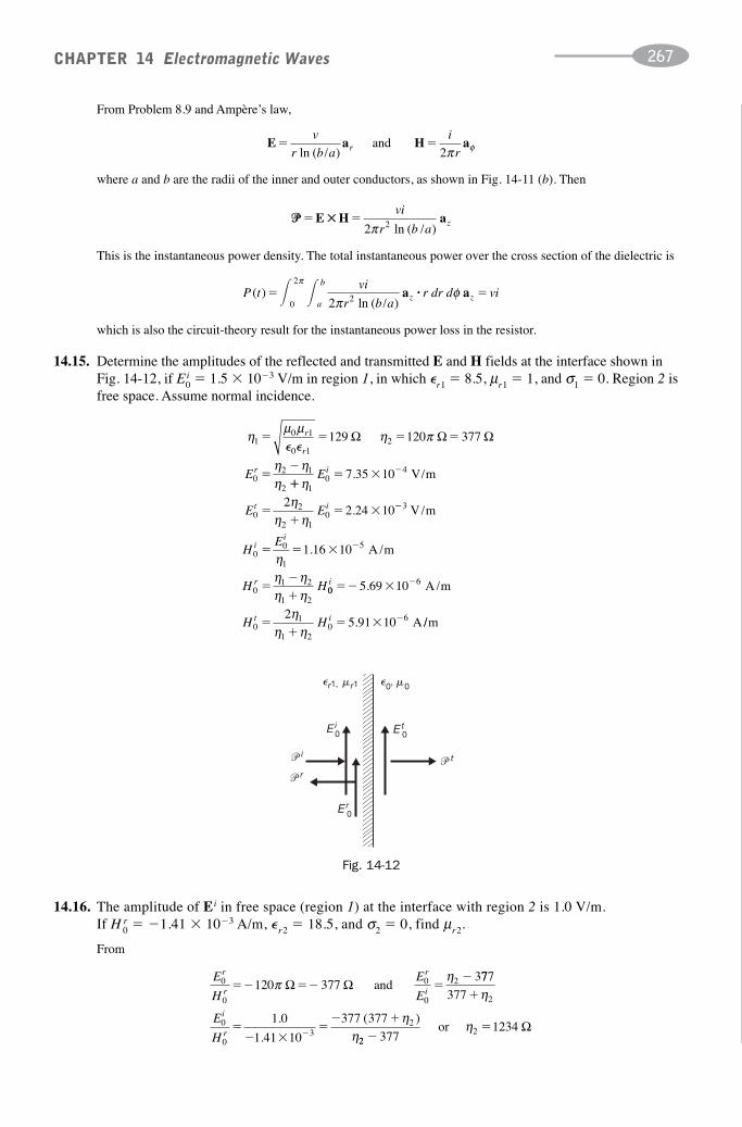
From Problem 8.9 and Ampère’s law,
CHAPTER 14 Electromagnetic Waves 267
E a H a� �v
r b a
i
rrln ( / )�����and�� ���
2π φ
��� �E H a��vi
r b az
2 2π ln ( / )
P tvi
r b ar dr d vi
a
b
z z( )� �� �0
2
22
π
πφ
ln ( / )a a·
η μ μ η π
η ηη
10 1
2
02 1
2
120 377� � � �
��
r
r
rE
� �0 1
129 Ω Ω Ω�
��� �
��
� �
�
ηη
η η
10
02
2 10
7 35 10
22 24
E
E E
i
t i
.
.
4
10
V/m
��
�� � �
��
�
3
51.16 10
V/m
A /mHE
H H
ii
r
00
1
01 2
1 2
ηη ηη η 00
01
1 20
5
25 91
i
t iH H
�� �
��
� �
�
�
.
.
69 10
10
6
6
A /m
Aη
η η//m
E
H
E
E
r
r
r
i0
0
0
0
2120 3773
�� �� ��π η
٠������and�� ��777
377
1 0
1 41 10
377 377
2
0
03
2
�
�� �
�� �
�
η
ηη
E
H
i
r
.
.
( )
222 1234
��
377�����or�����η Ω
where a and b are the radii of the inner and outer conductors, as shown in Fig. 14-11 (b). Then
This is the instantaneous power density. The total instantaneous power over the cross section of the dielectric is
which is also the circuit-theory result for the instantaneous power loss in the resistor.
14.15. Determine the amplitudes of the reflected and transmitted E and H fields at the interface shown in Fig. 14-12, if Ei
0 � 1.5 � 10�3 V/m in region 1, in which �r1 � 8.5, μr1 � 1, and σ1 � 0. Region 2 isfree space. Assume normal incidence.
Et0
i
E i0
r1,� r1 0,� 0
Er0
�
r�
t�
Fig. 14-12
14.16. The amplitude of E i in free space (region 1) at the interface with region 2 is 1.0 V/m. If H r
0 � �1.41 � 10�3 A/m, �r2 � 18.5, and σ2 � 0, find μr2.
From

Then
CHAPTER 14 Electromagnetic Waves268
123418 5
198 40 22� �
μ μ μrr
�0 ( . )����� .or��� �
η η1 2377 43 59 73� � .. �Ω Ω
E
EE
t
it0
0
2
1 20
225 07 10�
�� � �η
η η������ ������ .or V//m
From mγ ω σ ω� � � �j j( . .�) 4 362 46 53 1�μ
E
E2
1
2 5 06 45
377 5 06 45�
�
� �
�
�
( . )
.
10
10
3
3
�
� wheence V/mE2 2 68� . � �10 3
α β π μσ� � � �f 2 21. 105
14.17. A normally incident E field has amplitude Ei0 � 1.0 V/m in free space just outside of seawater in
which �r � 80, μr � 1, and σ � 2.5 S/m. For a frequency of 30 MHz, at what depth will the amplitudeof E be 1.0 m V/m?
Let the free space be region 1 and the seawater be region 2.
Then the amplitude of E just inside the seawater is Et0.
α �24.36 cos 46.53°� 16.76 Np/m
Then, from
1.0 � 10�3 � (5.07 � 10�2)e�16.76z
z � 0.234 m.
14.18. A traveling E field in free space, of amplitude 100 V/m, strikes a sheet of silver of thickness 5 μm, asshown in Fig. 14-13. Assuming σ � 61.7 MS/m and a frequency ƒ � 200 MHz, find the amplitudes⎪E2⎪, ⎪E3⎪, and ⎪E4⎪.
E1 � Ei0
0,� 0 0,� 0
m5
2 3 41
�
Fig. 14-13
For the silver sheet at 200 MHz, η � 5.06 � 10�3��45° Ω.
Within the conductor,

Thus, in addition to attenuation there is phase shift as the wave travels through the conductor. Since ⎪E3⎪ and⎪E4⎪ represent maximum values of the sinusoidally varying wave, this phase shift is not involved.
⎪E3⎪ � ⎪E2⎪ e�α z � (2.68 � 10�3)e�(2.21 � 105)(5 � 10�6) � 8.88 � 10�4 V/m
CHAPTER 14 Electromagnetic Waves 269
E
E4
3
2 377
377 5 06 45�
� � �
( )
. 10 3 � whence EE4 1 78� . � �10 3 V/m
H a( , ) . ( . )z t e j t zx� � �1 0 1 5 108 β (A /m)
and
SUPPLEMENTARY PROBLEMS
14.19. Given
E(z, t) � 103 sin(6 � 108t � βz) ay (V/m)
in free space, sketch the wave at t � 0 and at time t1 when it has traveled λ /4 along the z axis. Find t1, β, and λ.
14.20. In free space,
Obtain an expression for E (z, t) and determine the propagation direction.
14.21. In free space,
H(z, t) � 1.33 � 10�1 cos (4 � 107t) � βz )ax (A/m)
Obtain an expression for E(z, t). Find β and λ.
14.22. A traveling wave has a velocity of 106 m/s and is described by
y � 10 cos (2.5z � ωt)
Sketch the wave as a function of z at t � 0 and t � t1 � 0.838 μs. What fraction of a wavelength is traveledbetween these two times?
14.23. Find the magnitude and direction of
E (z, t) � 10 sin (ωt � βz)ax � 15 sin(ω t � βz )ay (V/m)
at t � 0, z � 3λ /4.
14.24. Determine γ at 500 kHz for a medium in which μr � 1, �r � 15, σ � 0. At what velocity will an electromagneticwave travel in this medium?
14.25. An electromagnetic wave in free space has a wavelength of 0.20 m. When this same wave enters a perfect dielectric,the wavelength changes to 0.09 m. Assuming that μr � 1, determine �r and the wave velocity in the dielectric.
14.26. An electromagnetic wave in free space has a phase shift constant of 0.524 rad/m. The same wave has a phase shiftconstant of 1.81 rad/m upon entering a perfect dielectric. Assuming that μr � 1, find �r and the velocity ofpropagation.
14.27. Find the propagation constant at 400 MHz for a medium in which �r � 16, μr � 4.5, and σ � 0.6 S/m. Find theratio of the velocity v to the free-space velocity c.
14.28. In a partially conducting medium, �r � 18.5, μr � 800, and σ � 1 S/m. Find α, β, η, and the velocity u, for afrequency of 109 Hz. Determine H(z, t), given
E (z, t) � 50.0e�αz cos(ωt � βz )ay (V/m)
14.29. For silver, σ � 3.0 MS/m. At what frequency will the depth of penetration δ be 1 mm?
14.30. At a certain frequency in copper (σ � 58.0 MS/m) the phase shift constant is 3.71 � 105 rad/m. Determine thefrequency.

14.31. The amplitude of E just inside a liquid is 10.0 V/m and the constants are μr � 1, �r � 20, and σ � 0.50 S/m.Determine the amplitude of E at a distance of 10 cm inside the medium for frequencies of (a) 5 MHz, (b) 50 MHz, and (c) 500 MHz.
14.32. In free space, E(z, t) � 1.0 sin (ω t � βz )ax (V/m). Show that the average power crossing a circular disk of radius15.5 m in a z � const. plane is 1 W.
14.33. In spherical coordinates, the spherical wave
CHAPTER 14 Electromagnetic Waves270
E a H� � �100 0 265
0rt r
rsin cos ( )
.sin cos (θ ω β θ(V/m) ωω β φt r� ) a (A /m)
represents the electromagnetic field at large distances r from a certain dipole antenna in free space. Find theaverage power crossing the hemispherical shell r � 1 km, 0 θ π/2.
14.34. In free space, E(z, t) � 150 sin (ωt � βz)ax (V/m). Find the total power passing through a rectangular area, ofsides 30 mm and 15 mm, in the z � 0 plane.
14.35. A free space-silver interface has Ei0 � 100 V/m on the free-space side. The frequency is 15 MHz and the silver
constants are �r � μr � 1 and σ � 61.7 MS/m. Determine Er0 and Et
0 at the interface.
14.36. A free space-conductor interface has Hi0 � 1.0 A/m on the free-space side. The frequency is 31.8 MHz and the
conductor constants are �r � μr � 1 and σ � 1.26 MS/m. Determine Hr0 and Ht
0 and the depth of penetration of Ht.
14.37. A traveling H field in free space, of amplitude 1.0 A/m and frequency 200 MHz, strikes a sheet of silver ofthickness 5 μm with σ � 61.7 MS/m, as shown in Fig. 14-14. Find Ht
0 just beyond the sheet.
HiHt
0,� 0 0,� 0
m5
��
Fig. 14-14
E i
Et
0,� 0 0,� 0
��
1 mm
� 20� 0� 1
r�
�
r
Fig. 14-15
14.38. A traveling E field in free space, of amplitude 100 V/m, strikes a perfect dielectric, as shown in Fig. 14-15.Determine Et
0.

14.39. A traveling E field in free space strikes a partially conducting medium, as shown in Fig. 14-16. Given a frequencyof 500 MHz and Ei
0 � 100 V/m, determine Et0 and Ht
0.
CHAPTER 14 Electromagnetic Waves 271
E043050� V/m, rad /m, 15 m( ) π
E i
Et
0,� 0 0,� 0
��
30 mm
� 55� 1� 1
r�
μ r�
Fig. 14-16
14.40. A wave propagates from a dielectric medium to the interface with free space. If the angle of incidence is thecritical angle of 20°, find the relative permittivity.
14.41. Compute the ratios Er0 /Ei
0 and Et0 /Ei
0 for normal incidence and for oblique incidence at θi � 10°. For region 1,assume �r1 � 8.5, μr1 � 1, and σ1 � 0. Region 2 is free space.
14.42. A parallel-polarized wave propagates from air into a dielectric at a Brewster’s angle of 75°. Find �r.
ANSWERS TO SUPPLEMENTARY PROBLEMS
14.19. t1 � 2.62 ns, β � 2 rad/m, λ � πm. See Fig. 14-17.
0/4λ
t � 0
z/2λ /43λ λ
t � t1
103
�103
Fig. 14-17
14.20. E0 � 377 V/m, �az
14.21.
14.22. 1–3. See Fig. 14.18.

14.23. 18.03 V/m, 0.555ax � 0.832ay
14.24. j4.06 � 10�2 m�1, 7.74 � 107 m/s
14.25. 4.94, 1.35 � 108 m/s
14.26. 11.9, 8.69 � 107 m/s
14.27. 99.58 ���60.34°
�m�1, 0.097
14.28. 1130 Np/m, 2790 rad/m, 2100 ����
22.1° Ω, 2.25 � 106 m/s, 2.38 � 10�2e�αz cos(ω t � 0.386 � βz) (� ax) (A/m)
14.29. 84.4 kHz
14.30. 601 MHz
14.31. (a) 7.32 V/m; (b) 3.91 V/m; (c) 1.42 V/m
14.33. 55.5 W
14.34. 13.4 mW
14.35. �100 V/m, 7.35 � 10�4 ���45° V/m
14.36. 1.0 A/m, 2.0 A/m, 80 μm
14.37. 1.78 � 10�5 A/m
14.38. 59.7 V/m
14.39. 19.0 V/m, 0.0504 A/m
14.40. 8.55
14.41. For nomal incidence, Ei0 /Er
0 � 0.490 and Et0 /Ei
0� 1.490. At 10°, Er0 /Ei
0� 0.539 and Et0 /Ei
0 � 1.539.
14.42. 13.93
CHAPTER 14 Electromagnetic Waves272
10
0
/3λ � 2.51 mλ
/2�λ�λ
t � 0
t � t1
z/4λ /2λ
Fig. 14-18

273
Transmission Lines(by Milton L.Kult)
15.1 Introduction
Unguided propagation of electromagnetic energy was investigated in Chapter 14. In this chapter the transmis-sion of energy will be studied when the waves are guided by two conductors in a dielectric medium. Exactanalysis of this two-conductor transmission line requires field theory. However, the performance of the systemcan be predicted by modeling the transmission line with distributed parameters and using voltages and currentsassociated with the electric and magnetic fields.
Only uniform transmission lines will be considered; that is, the incremental distributed parameters shall beassumed constant along the line.
15.2 Distributed Parameters
The incremental distributed parameters per unit length of line are inductance and capacitance as determinedin Chapters 8 and 12, the resistance of the conductors, and the conductance of the dielectric medium. It wasseen that the parameters depend on the geometry of the configuration, the characteristics of the materials, andin some cases the frequency. In the following summary list the dependence on geometry is represented by ageometrical factor GF.
Capacitance.
C � π�d (GFC) (F/m) [�d � permittivity of dielectric]
Conductance.
CHAPTER 15
GC
dd d� �
�σ σ(S/m) [ conductivity of dielectric]
Inductance (external).
Led
d� �μπ
μ( ) (H/m) [ permeability of dielectriGFL cc 0� μ ]
DC Resistance (useful for operation up to 10 kHz).
R mdc
d c� �1
σ πσ( ) ( / ) [ conductivity of conductGFR Ω oors]

Ac Resistance (for frequencies above 10 kHz).
CHAPTER 15 Transmission Lines274
Rfa
ca
c c� �
1
2
2
πσ δδ
π μ σ( ) ( /m) skin depthGFR Ω �⎡
⎣⎢
⎤
⎦⎦⎥
Inductance (internal).
LR f f
fia
��
�
/
/
2
4
πμ π
(H/m) for��
(H/m) for��
10 kHz
0 110 kHz⎧⎨⎩
Inductance (total).
Lt � Le � Li � Le
For three common line configurations the geometrical factors are as follows:
Coaxial Line (inner radius a, outer radius b, outer thickness t).
GFC GFLGFC
GFR GFR
� �
� ��
�
2 1
1
ln ( / )
( )��
b a
a t b td a12
11 1
a bt� �for δ
Parallel Wires (radius a, separation d ).
GFCGFL
GFL
GFR GFR
for� � �
�
�1
21cosh ln
d
a
d
ad a
ad
�
22 aa a
�2
Parallel Plates (width w, thickness t, separation d ).
GFC GFLGFC
GFR GFR for
� �
� � �
w
d
wt wtd a
ππ π δ
1
42�
15.3 Incremental Models
The model in Fig. 15-1, where R, L, G, and C are as given in Section 15.2, is the simplest incremental model ofa two-conductor transmission line. It permits analysis of the line using voltages and currents at each cell in themodel. For within a cell of length Δx, the voltages across the line at points a and b differ by
Δ Δ Δv x t R x i x t L xi x t
t( , ) ( ) ( , ) ( )
( , )� �
∂∂
RΔ x RΔ x RΔ xLΔ x LΔ x LΔ x
CΔ xGΔ xCΔ x
Δ x
GΔ x
a b c
Fig. 15-1
(1�a)

In the limit as Δx → 0, the equations become first-order partial differential equations
CHAPTER 15 Transmission Lines 275
Likewise, the current at point c differs from that at b by
Δ Δ Δi x t G x v x t C xv x t
t( , ) ( ) ( , ) ( )
( , )� �
∂∂
Other incremental models may also be used. They lead to the same transmission line equation as the one obtainedin the next section.
15.4 Transmission Line Equation
The incremental equations for the model of Fig. 15-1 can be written as the following:
ΔΔ
v x t
xRi x t L
i x t
t
( , )( , )
( , )� �
∂∂
ΔΔi x t
xGv x t C
v x t
t
( , )( , )
( , )� �
∂∂
(1 � a)
(1 � b)
(2 � a)
(2 � b)
(3)
∂∂
∂∂
v x t
xRi x t L
i x t
t
( , )( , )
( , )� �
∂∂
∂∂
i x t
xGv x t C
v x t
t
( , )( , )
( , )� �
The above two first-order partial differential equations imply a single second-order partial differential equation
∂∂
∂∂
∂2
2
2f x t
xRG f x t RC LG
f x t
tLC
f( , )( , ) ( )
( , )� � � �
(( , )x t
t∂ 2
whose ƒ (x, t) can be either v (x, t ) or i(x, t). The equation describes the behavior of the current and voltage atany point on the line. Now, (3) is an equation of the hyperbolic type and very similar to the wave equation.Indeed, for a lossless line (R � G � 0), (3) is precisely the one-dimensional scalar wave equation studied inChapter 14. Thus, it is known in advance that the transmission lines support voltage- and current-waves whichcan be reflected and/or transmitted at discontinuities (sites of abrupt parameter changes) in the line.
15.5 Sinusoidal Steady-State Excitation
When the transmission line of Fig. 15-1 is driven for a long time by a sinusoidal source (angular frequency ω),the voltage and current also become sinusoidal, with the same frequency:
v (x, t) � Re [V̂(x)e jωt] i (x, t) � Re [Î(x)e jω t]
Here, the phasors V̂ (x) and Î(x) are generally complex-valued; often they are indicated in polar form (with thex-dependence suppressed) as
V̂ � ⎪V̂⎪��φV Î � ⎪Î⎪
��φI
where φ denotes the angle between the complex vector and the real axis. Steady-state analysis of the transmis-sion line is much simplified when all voltages and currents are replaced by their phasor representations.
Fig. 15-2 models in the phasor domain a uniform line of length � that is terminated in a (complex) load ZR at the receiving end and is driven at the sending end by a generator with internal impedance Zg and voltageV̂g � Vgm
�θ . The per-unit-length series impedance and shunt admittance of the line are given by
Z � R � jωL Y � G � jωC
Distance from the receiving end is measured by the variable x; from the sending end, by d.
(1�b)

Equations (1), (2), and (3) of Section 15.4 become ODEs for the phasors V̂(x) and Î(x).
CHAPTER 15 Transmission Lines276
Vg
Zg
Sending End Receiving End (Load)
Z, Y^
VS
^
VR ZR
x x � 0d �
x �d � 0 �d
^
IS^
IR^
~�
� �
�� �
�
l l
Fig. 15-2
dV x
dxZI x
ˆ( ) ˆ( )�
dI x
dxYV x
ˆ( ) ˆ( )�
d F x
dxF x
2
22
ˆ ( ) ˆ ( )�γ
with γ � ����ZY � α � jβ, the square root being chosen to make α and β nonnegative. Equation (3 bis) is identicalin form to the equation of plane waves (Section 14.4); it has the traveling-wave solutions
V(x) � V�eγx � V̂�e�γ x � V̂inc(x) � V̂refl(x)
Î(x) � Î�eγx � Î�e�γ x � Îinc(x) � Îrefl (x)
The coefficients V̂�, etc., are phasors independent of x that are interrelated by the characteristic impedance Z0and the boundary reflection coefficient ΓR, defined as
(1 bis)
(2 bis)
(3 bis)
ZV
I
V
I
Z
Y
V
V
I
I
VR
0 �
�
ˆ
ˆ
ˆ
ˆ
ˆ
ˆ
ˆ
ˆ
ˆ
�
�
�
�
�
�
�
�
�� �
�� �à refll
inc
( )ˆ ( )
0
0V
It is easy to express ΓR in terms of the characteristic and load impedance:
ΓRR
R
Z Z
Z Z�
�
�0
0
Then, if a pointwise reflection coefficient is defined by
Γ( )ˆ ( )ˆ ( )
xV x
V x� refl
inc
it follows that
Γ Γ( )x eZ Z
Z ZeR
x R
R
x� ��
�
� �2 0
0
2γ γ
Similarly, if Z(x) �V̂(x) /Î (x) is the pointwise impedance looking back to the receiving end (x � 0), then
Z x Zx
x( )
( )
( )�
�
�0
1
1
ΓΓ
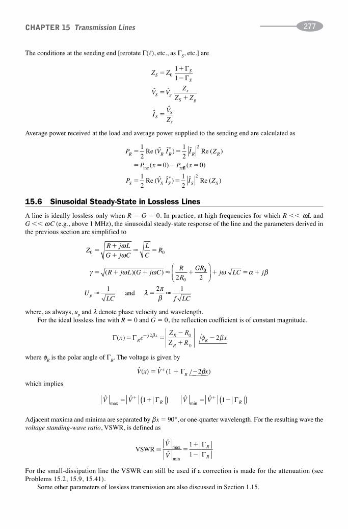
The conditions at the sending end [rerotate Γ(�), etc., as ΓS, etc.] are
CHAPTER 15 Transmission Lines 277
Z Z
V VZ
Z Z
IV
Z
SS
S
S gs
S g
SS
s
��
�
��
�
01
1
ΓΓ
ˆ ˆ
ˆˆ
Average power received at the load and average power supplied to the sending end are calculated as
P V I I Z
P x P
R R R R R� �
� � �
1
2
1
20
2Re ( ˆ ˆ ) ˆ Re ( )
( )
*
inc reffl ( )
Re ( ˆ ˆ ) ˆ Re ( )*
x
P V I I ZS S S S S
�
� �
0
1
2
1
2
2
15.6 Sinusoidal Steady-State in Lossless Lines
A line is ideally lossless only when R � G � 0. In practice, at high frequencies for which R �� ωL and G �� ωC (e.g., above 1 MHz), the sinusoidal steady-state response of the line and the parameters derived inthe previous section are simplified to
ZR j L
G j C
L
CR
R j L G j CR
R
GR
0 0
02
��
��
� � � �
ωω
γ ω ω
�
�( )( ) 00
2
1 2
⎛
⎝⎜⎞⎠⎟
� � �
�
j LC j
ULC
p
ω α β
λ πβ
� ���� ������and ��1
f LC
where, as always, up and λ denote phase velocity and wavelength.For the ideal lossless line with R � 0 and G � 0, the reflection coefficient is of constant magnitude.
Γ Γ( )x eZ R
xRj x R
RR
2 0 2β φ βR 0
where φR is the polar angle of ΓR. The voltage is given by
V̂(x) � V̂�(1 � ΓR ����2βx
�)
which implies
ˆ ˆ ��� �� ˆ ˆmax min
V V V VR R� � � �� �1 1Γ Γ( ) ( )
Adjacent maxima and minima are separated by βx � 90°, or one-quarter wavelength. For the resulting wave thevoltage standing-wave ratio, VSWR, is defined as
VSWR �ˆ
ˆmax
min
V
VR
R
��
�
1
1
ΓΓ
For the small-dissipation line the VSWR can still be used if a correction is made for the attenuation (seeProblems 15.2, 15.9, 15.41).
Some other parameters of lossless transmission are also discussed in Section 1.15.
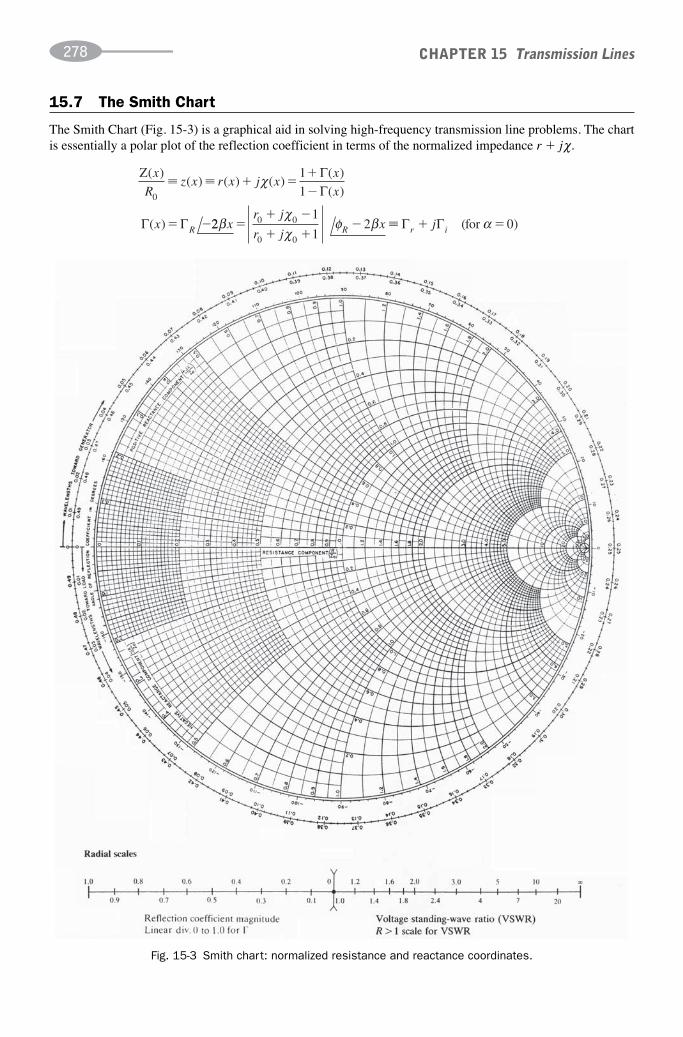
15.7 The Smith Chart
The Smith Chart (Fig. 15-3) is a graphical aid in solving high-frequency transmission line problems. The chartis essentially a polar plot of the reflection coefficient in terms of the normalized impedance r � jχ.
CHAPTER 15 Transmission Lines278
Z( )( ) ( ) ( )
( )
( )
( )
x
Rz x r x j x
x
x
x R
0
1
1� � χ Γ
Γ
Γ Γ 221
120 0
0 0
βχχ
φ β αxr j
r jx jR r i� Γ Γ (for )0
Fig. 15-3 Smith chart: normalized resistance and reactance coordinates.
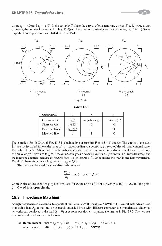
where r0 � r (0) and χ0 � χ(0). In the complex Γ plane the curves of constant r are circles, Fig. 15-4(b), as are,of course, the curves of constant ⎪Γ⎪, Fig. 15-4(a). The curves of constant χ are arcs of circles, Fig. 15-4(c). Someimportant correspondences are listed in Table 15-1.
CHAPTER 15 Transmission Lines 279
Γi
Γr ΓrΓr Γr
φΓ
|Γ|
Γi Γi
90º
�90º
135º 45º
1180º
�135º �45º
0º
0 1½
� |Γ | � const.(a)
� r � const.(b)
� χ � const.(c)
½
�½ �1 �2
�½ �1 �20
1 2 0
1 � j 1 � j 1 � j� 1 � j� 1 � j
� 1 � j � 1 � j � 1 � j1 � j 1 � j 1 � j
� 1 � j
Fig. 15-4
CONDITION Γ r χ
Open-circuit 1��
0° ∞ (arbitrary) arbitrary (∞)
Short-circuit 1���180° 0 0
Pure reactance 1�����90° 0 �1
Matched line 0 1 0
TABLE 15-1
The complete Smith Chart of Fig. 15-3 is obtained by superposing Figs. 15-4(b) and (c). The circles of constant⎪Γ⎪ are not included; instead the value of ⎪Γ⎪ corresponding to a point (r, χ) is read off the left-hand external scale.The value of the VSWR is read from the right-hand scale. The two circumferential distance scales are in fractionsof a wavelength. From r � 0, χ � 0, the outer scale goes clockwise toward the generator (i.e., measures x /λ), andthe inner one counterclockwise toward the load (i.e., measures d /λ). Once around the chart is one-half wavelength.The third circumferential scale gives φΓ � φR � 2β x.
The chart can be used for normalized admittances,
Y x
Gy x g x jb x
( )( ) ( ) ( )
0
� � �
where r-circles are used for g, χ-arcs are used for b, the angle of Γ for a given y is 180° � φΓ, and the point y � 0 � j0 is an open-circuit.
15.8 Impedance Matching
At high frequencies it is essential to operate at minimum VSWR (ideally, at VSWR � 1). Several methods are usedto match a load ZR to the line, or to match cascaded lines with different characteristic impedances. Matching networks can be placed at the load (x � 0) or at some position x � x1 along the line, as in Fig. 15-5. The two setsof normalized conditions are as follows:
(a) Before match: z(0) � zR � r0 � jx0; y(0) � g0 � jb0; VSWR � 1
After match: z (0) � 1 � j0; y (0) � 1 � j0; VSWR � 1

(b) At load: z (0) � r0 � jx0; y(0) � g0 � jb0; VSWR(0) � 1
Before match: z(x1) � r1 � jx1; y(x1) � g1 � jb1; VSWR � VSWR(0)
After match: z (x1) � 1 � j0; y (x1) � 1 � j0; VSWR � 1
The matching networks at lower (radio) frequencies can be made with lumped low-loss reactive components;one lumped L-C network is shown in Fig. 15-6. If ZR has a reactive component, a reactance of opposite sign isadded in series so that Z′R � R � j0. Then, for a match,
CHAPTER 15 Transmission Lines280
MATCH.NET.
MATCH.NET.
(a) (b)
VSWR � 1VSWR � 1 VSWR � 1
R0 ZRR0ZR
x � 0 x � 0x � x1
R0
Fig. 15-5
L1
C2
R0
R
ZR � R � jXR
X � � XRYin
Fig. 15-6
Y j CR j L Rin � �
��ω
ω21 0
1 1
L R R R CL
RR1 0 21
0
1� � �
ω( ) �����and�����
If R � R0, the capacitor should be connected to the other end of the inductor.To minimize dissipation losses at higher frequencies a length of open- or short-circuited line is used for
matching, in either a single-stub or double-stub configuration.
or
15.9 Single-Stub Matching
The configuration shown in Fig. 15-7 uses one shorted stub, of length �s, placed at a distance x1 from the load.To accomplish matching:
(1) Determine x1 such that y(x1) � 1 � jb1.
(2) Determine �s such that y (�s) � 0 � jb1.
After matching, y(x1) � 1 � j0 and VSWR � 1 from x1 to �.

EXAMPLE 1. The above two steps may be accomplished on the Smith Chart (Fig. 15-8).
(a) Plot yR and trace the ⎪ΓR⎪ [or VSWR(0)] circle.
(b) Mark the intersections of the ⎪ΓR⎪ circle and the circle g � 1.
(c) From yR move toward the generator to the first intersection, read y1 � 1 � jb1, and note the distancex1 as a fraction of λ (or read off angle 2βx1).
(d ) Mark the point y � 0 � jb1 on the ⎪Γ⎪ � 1 circle. From the short-circuit position y � ∞, movetoward the generator to the point y � �jb1. Note the distance �s as a fraction of λ. If the firstintersection is not accessible, the second one can be used by readjusting the stub length for thesusceptance at the new position.
CHAPTER 15 Transmission Lines 281
R0
R 0
ZR
x � x1 x � 0x �
s�
�
Fig. 15-7
yR
x 1
sl
� 1 � j
�b1
�b1
|ΓR |
� 1 � j
1 � j
0
g � 1
1 � j
Fig. 15-8
For matching two cascaded lines with different characteristic impedances, the above procedure is used at the con-nection point where the equivalent load is the input impedance to the second line.
15.10 Double-Stub Matching
A double stub “tuner” has two shorted stub lines separated by a distance ds on the main line, as shown in Fig. 15-9.Stub 1 is nearest the load and frequently is connected at the load (x � 0). Common separations for the two stubs are λ /4 and 3λ /8, hence the names “quarter-wavelength tuner,” etc. The Smith Chart solution for the two-stub

matching problem involves the construction of the tuner circle for the given ds. This is the circle gT � g(ds) � 1,which plays the same role for stub 2 as the g � 1 circle plays for the main line. The tuner circle is obtained by clock-wise rotation of g � 1, about the center of the chart, 1 � j0: a rotation of 180° gives the λ /4 tuner circle, rotation of90° gives the 3λ /8 tuner circle, etc. See Fig. 15-10.
CHAPTER 15 Transmission Lines282
R0 ZRR0
x � ds x � 0
R0
R0
s1ls2l
Fig. 15-9
� 1 � j 1 � j
� 1 � j 1 � j
g � 1
�b
�b
(λ /4) T
(3λ /8) T
Γr
Γi
|Γ | � 1
0
Fig. 15-10
EXAMPLE 2. Assuming that ds � λ /4, a five-step sequence is used for two-stub matching, as shown in Fig. 15-11.
1. Plot the λ /4 tuner circle.
2. Mark the intersection(s) of the tuner circle and the gR circle through the entry point yR � gR � jbR.Read bT at this point, which may be either intersection.
3. Stub 1 at x � 0 is used to change the susceptance bR to bT.
4. From yT � gR � jbT move on the ⎪ΓR⎪ circle a distance ds � λ /4 toward the generator onto the g � 1circle and read y � 1 � jb2.
5. Cancel the susceptance b2 by adjusting stub 2 to produce y � 1 � j0, the matched condition.

A problem arises when using the λ /4 tuner to match a load with gR � 1, since the conductance circle does notintersect the tuner circle. The 3λ /8 tuner works for some values of gR � 1. In any case, a tuner can be displacedfrom the load by a distance x1 to put g in the range for matching. Should g � 1 at the displaced position, the single-stub condition holds and stub 2 must be set for b � 0.
Note the standing waves on the various sections of line. The shorted stubs each have VSWR � ∞. For ds � x � �, VSWR � 1; for 0 � x � ds, VSWR is determined by y � gR � jbT; and if line is added between theload and stub 1, the VSWR is determined by yR.
15.11 Impedance Measurement
A slotted line is used with high-frequency coaxial lines to measure VSWR and to locate voltage minima on theline. With the aid of the Smith Chart, the impedance of an unknown termination can be easily found from theVSWR and the shift of a voltage minimum from a short-circuit reference position.
In Fig. 15-12 the slotted line is inserted at a convenient terminal. With the ZR in place, a probe is moved alongthe line to locate and measure maximum and minimum voltages. A suitable amplifier/indicator converts theprobe output to a VSWR reading. ZR is replaced by a short circuit, and the reference minima are located for thehigh-VSWR condition. As would be expected, maxima and minima alternate at intervals of λ /4.
CHAPTER 15 Transmission Lines 283
l s2
1 � j
1 � j
�1 � j
�1 � j
b2
bs1
bs2
bΤ
yR
ysc
bR
gR
1 � jb2
g � 1
3
1
0
(λ /4) – T^
4
2
5
Γn
l s1
Fig. 15-11
Max 1
Min 1Min 2GENERATOR
SLOTTED LINE
SLOTTED LINESHORTCIRCUIT
EQUIVALENTLOCATION
λ /2
ZR
ZR
Δx
Min 2 Min 1
Fig. 15-12
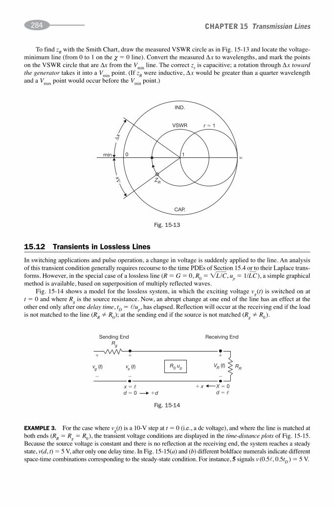
To find zR with the Smith Chart, draw the measured VSWR circle as in Fig. 15-13 and locate the voltage-minimum line (from 0 to 1 on the χ � 0 line). Convert the measured Δx to wavelengths, and mark the pointson the VSWR circle that are Δx from the Vmin line. The correct zr is capacitive; a rotation through Δx towardthe generator takes it into a Vmin point. (If zR were inductive, Δx would be greater than a quarter wavelengthand a Vmax point would occur before the Vmin point.)
CHAPTER 15 Transmission Lines284
IND.
CAP.
r � 1VSWR
Δx
Δx
min 0
1
ZR
Fig. 15-13
Sending EndRg
vg (t) vs (t)
Receiving End
RR
� x
R0 up VR (t)
�
�
�
�
�
�
X � 0d � l
x � ld � 0 �d
Fig. 15-14
15.12 Transients in Lossless Lines
In switching applications and pulse operation, a change in voltage is suddenly applied to the line. An analysisof this transient condition generally requires recourse to the time PDEs of Section 15.4 or to their Laplace trans-forms. However, in the special case of a lossless line (R � G � 0, R0 � ����L /C, up � 1/ ��LC ), a simple graphicalmethod is available, based on superposition of multiply reflected waves.
Fig. 15-14 shows a model for the lossless system, in which the exciting voltage vg(t) is switched on at t � 0 and where Rg is the source resistance. Now, an abrupt change at one end of the line has an effect at theother end only after one delay time, tD � �/up, has elapsed. Reflection will occur at the receiving end if the loadis not matched to the line (RR � R0); at the sending end if the source is not matched (Rg � R0 ).
EXAMPLE 3. For the case where vg(t) is a 10-V step at t � 0 (i.e., a dc voltage), and where the line is matched atboth ends (RR � Rg � R0), the transient voltage conditions are displayed in the time-distance plots of Fig. 15-15.Because the source voltage is constant and there is no reflection at the receiving end, the system reaches a steadystate, v(d, t) � 5 V, after only one delay time. In Fig. 15-15(a) and (b) different boldface numerals indicate differentspace-time combinations corresponding to the steady-state condition. For instance, 5 signals v (0.5�, 0.5tD ) � 5 V.

EXAMPLE 4. Assume that everything is as in Example 3, with the exception of the load, which is now anopen-circuit (RR � ∞). Fig. 15-16 gives the time-distance plots. Because of the single reflection at the load,a uniform steady state of 10 V is attained after 2tD.
CHAPTER 15 Transmission Lines 285
d � 0 t � 0.1tD
d � 0.5� t � 0.5 tD
� d
�
0.5 �
0.5 �
tan �1up
0V
5 V
�
d
(ΓR � 0)
t
d
� d
t � tD
2tDtD
2tDtD 2tD
tD
2tDtD t
t
t0
0
0
(a) v vs. t (b) v vs . d (c) t-d plot
0
0
0
0
0
0
0
51
2
3 5 6
4
1 2 3 4 5 6
4
6
5
v � VS
v � vR
v
5
5
0
0
0
0
5
5
5
d � �
Fig. 15-15
(c) t-d plot
d � 0
d � �
d � 0.5�
d
d
d
d
REFL
INC
REFL
INC
(ΓR � 1)
(ΓS � 0)
2tD 0.5�
t � 0.5tD
t � tDtD
t � 2tD
�
�
t
�
�
0.5 �
0.5�
5 V REFL
5 V INC
0 V
0.5 �
tD t0
2tD2tDtD t0
2tDtD t0
0
00
0
0
0
10
5
v � vS
0
10
5
v
0
10
5
v � vR
(a) v vs. t (b) v vs . d
0
10
5
v
0
10
5
v
0
10
5
v
Fig. 15-16
EXAMPLE 5. A line is excited as in Examples 3 and 4; parameter values are
Vg � 20 V dc Rg � 3R0 Γg �1–2
ΓR � 1 (open-circuit)
The voltage transient is described in Fig. 15-17. With reflections occurring at both ends of the line, an infinitetime is needed for the attainment of a uniform steady state of 20 V.

SOLVED PROBLEMS
15.1. A parallel-wire transmission line is constructed of #6 AWG copper wire (dia. � 0.162 in., σx � 58 MS/m)with a 12-inch separation in air. Neglecting internal inductance, find the per-meter values of L, C, G, thedc resistance, and the ac resistance at 1 MHz.
The four geometrical factors for the parallel-wire line involve the conductor radius, a � 2.06 � 10�3 m, and theseparation d � 0.305 m. Since d � a
CHAPTER 15 Transmission Lines286
dt/tD
00.51.01.52.02.53.03.54.04.5
0555 � 5 � 101010 � 2.5 � 12.512.512.5 � 2.5 � 15.015.015.0 � 1.25 � 16.25
v at 0.5 �
(Γg � ½)
(ΓR � 1)
�0.5�
5 V
5 V
2.5 V
2.5 V
1.25 V
2tD
2tD
3tD
3tD
4tD
4tD
tt
tD
tD
10
5
0
0
0
20
16.25
12.5
2.5
5
5
15
vS
(a) vS vs. t (b) t-d plot (c) Voltage at midpoint
Fig. 15-17
GFL GF� �ln . �����������������������d
a
⎛⎝⎜
⎞⎠⎟
5 0 CCGFL
GFR m GFR
� �
� � � ��
10 20
24 72 102
5 2
.
. ������d aa
22971
a� �m 1
For air dielectric, μd � μ0 and �d � �0; for copper, μc � μ0. Hence:
L GFL Rdd
cd� � � � � �μ
πμ
πσ( ) . ( .2 0
12 59H /m GFR ) /10 3 Ω mm
( ) pF/m m
S/m
Cf
G
dc c
� � � �
�
π δπ μ σ
μ� GFC 5 561
66
0
. ��
RRac c
a� � � �1
24 04
πδ σ( .GFR ) /m10 2 Ω
15.2. The specifications for a rigid air-dielectric coaxial line used in a radar set operating at 3 GHz are:copper material, stub-supported at intervals to maintain the air dielectric; outside diameter, 7–
8inch;
wall thickness, 0.032 inch; inner-conductor diameter, 0.375 inch; characteristic impedance, 46.4 Ω;attenuation, 0.066 dB/m; maximum peak power, 1.31 kW; operating peak power, 200 kW; lowest safewavelength, 5.28 cm. Determine the per-meter values of L, C, G, and Ra for the line, neglectinginternal inductance.
The inner radius a is 4.76 mm and the outer radius b is 10.3 mm. Then ln (b/a) � 0.771, GFL � 0.386, GFC � 2.59.
L C� � � �μπ
μ π000 154 71 9( ) H /m ( ) pF /mGFL GFC. .�

For copper and a frequency of 3 GHz, δ � 1.2 μm. Then,
CHAPTER 15 Transmission Lines 287
GFR GFRm and ( ) /1a a
caa b
R� � � � ��1 1307
1
20 702
πσ δ. Ω mm
For air dielectric, G � 0 S/m.
15.3. Show that the voltage v (x, t) � A cos (ω t � θ )e jβx satisfies the transmission line equation (3), for auniform lossless line, if β � ω ���LC.
For the lossless line, R � G � 0, so that the equation reduces to
∂∂
∂∂
2 2v x t
xLC
v x t
t
( , ) ( , )2 2
�
For the given voltage, this requires
� � � �β ω β ω2 2v LC v LC( ) or
15.4. For the parallel-wire line of Problem 15.1, find the characteristic impedance, propagation constant(attenuation and phase shift), velocity of propagation, and wavelength, for operation at 5 kHz.
At 5 kHz the dc resistance may be used.
R j L jd ω π2 59 10 2 5 10 2 6 2893 3. ( )( ) .10 6 10 87 6°
2 5 10 5 56 103
2
1
.
( ) ( .
Ω/m
Y G j C jω π 22 7 90°
1.0
) .
.
1 747 10
600 1 2°
S/m
Z0Z
Y
ZY
Ω
γ 448 10 4 6 488 8 2 19 10 1 048 10 1. ( . ( . )j m° )
Then α � 2.19 � 10�6 N/m, β � 1.048 � 10�4 rad/m, up � ω /β � 2.998 � 108 m /s, λ � 2π /β � 59.96 km.
15.5. A 10-km parallel-wire line operating at 100 kHz has Z0 � 557Ω, α � 2.4 � 10�5 Np/m, and β � 2.12 � 10�3 rad/m. For a matched termination at x � 0 and V̂R � 10
��0° V, evaluate V̂(x) at
x-increments of λ /4 and plot the phasors.
The line is matched at the receiving end, so that ΓR � 0 and V̂(x) �V̂�eαx ��
βx. But
V̂(0) � V̂� � V̂R � 10 ��
0° V
whence V̂(x) � 10eαx ��
βx (V)
For x � n(λ /4) (n � 0, 1, 2, …, 13, 13.48), where n � 13.48 corresponds to the 10-km length,
β π
α αβ
β
x n n
x x n
� �
� �
290
0 0178
rad
Np
⎛
⎝⎜⎞⎠⎟
( )
( ) .
�
By use of these increments, Table 15-2 is generated. A polar plot of the tabulated results is given in Fig. 15-18.

15.6. Repeat Problem 15.5 if a mismatched load results in ΓR � 0.4 ��
0° ; all other data remain the same.
In contrast to Problem 15.5, the voltage is now given by the superposition of an incident and a reflected wave:
V̂(x) �V̂inc(x) �V̂refl(x) �V̂�eαx ��βx � ΓRV̂� e�α x
�����βx
The boundary condition at x � 0 gives (omitting physical units)
10 ��0° � 1.4 V̂�
��0° or V̂� � 7.14
��0°
Thus, V̂(x) � 7.14eαx ��βx � 2.86e�αx
�����βx
where α and β are as specified in Problem 15.5. The required calculations are presented in Table 15-3 and Fig. 15-19.
CHAPTER 15 Transmission Lines288
QUARTER WAVELENGTHS βx � φ v ,
FROM LOAD deg. α x, Np ⎪V̂(x)⎪, V
0 0 0.0 10.001 90 0.0178 10.182 180 0.0356 10.363 270 0.0534 10.554 360 0.0711 10.745 450 0.0889 10.936 540 0.1067 11.137 630 0.1245 11.338 720 0.1423 11.539 810 0.1601 11.74
10 900 0.1779 11.9511 990 0.1956 12.1612 1080 0.2134 12.3813 1170 0.2312 12.6013.48 1215 0.24 12.71
TABLE 15-2
90º
0º
270º
134.6º
VR^
VS^
Fig. 15-18

CHAPTER 15 Transmission Lines 289
12
10
8
6
4
2
012345678910111213
13.484x /λ = n 14
|VS |^
|V |^
Fig. 15-19
λ /4 FROM
LOAD αx, Np eα x βx Vinc(x) Vref(x) ⎪V(x)⎪
0 0.0 1.0 0° 7.14 ��
0° 2.86 ��
0° 10.00 ��
0°
1 0.0178 1.018 90° 7.27 ���
90° 2.81 �����90° 4.46
���90°
2 0.0356 1.036 180° 7.40 ����
180° 2.76 ����
�180°�
10.16 ����
180°
3 0.0534 1.055 270° 7.53 ����
270° 2.71 ����
�270°�
4.82 �����90°
4 0.0711 1.074 360° 7.67 ����
360° 2.66 ����
�360°�
10.33 ��
0°
5 0.0889 1.093 450° 7.80 ����
450° 2.62 ����
�450°�
5.18 ���
90°
6 0.1067 1.113 540° 7.94 ����
540° 2.57 ����
�540°�
10.51 ����
180°
7 0.1245 1.133 630° 8.09 ����
630° 2.52 ����
�630°�
5.57 �����90°
8 0.1423 1.153 720° 8.23 ����
720° 2.48 ����
�720°�
10.71 ��
0°
9 0.1601 1.174 810° 8.38 ����
810° 2.44 ����
�810°�
5.94 ���
90°
10 0.1779 1.195 900° 8.53 ����
900° 2.39 ����
�900°�
10.92 ����
180°
11 0.1956 1.216 990° 8.68 ����
990° 2.35 ����
�990°�
6.33 �����90°
12 0.2134 1.238 1080° 8.84 ����
1080°�
2.31 �����1080°
�11.15
��0°
13 0.2312 1.260 1170° 9.00 ����
1170°�
2.27 �����1170°
�6.73
���90°
13.48 0.24 1.271 1215° 9.08 ����
1215°�
2.25 �����1215°
�9.34
����148.5°
�
TABLE 15-3
15.7. Measurements are made at 5 kHz on a 0.5-mile-long transmission line. The results show that thecharacteristic impedance is 94
�����23.2°
�Ω, the total attenuation is 0.06 Np, and the phase shift
between input and output is 8°. Find the R, L, G, and C per mile for the line; the phase velocity on theline; and the power lost on the line when the sending-end power is 3 W and the load is matched.
The measured attenuation is α� � 0.06 Np, whence α � 0.12 Np/mi, the phase shift is β� � 8° � 0.14 rad, so that β � 0.28 rad /mi. Hence,
����ZY � γ � 0.12 � j0.28 � 0.305 ����
66.8°�
mi�1 or ZY � 0.093 ����
133.6°�
mi�2
From this and the measured value ����Z /Y � 94 ����
�23.2°�
Ω:
Z � 28.67 ����
43.6°�
� 20.8 � j19.8 Ω /mi � R � j2πƒL
Y � 3.24 � 10�3 ���
90° � j3.24 � 10�3 S/mi � G � j2πƒC
which imply: R � 20.8 Ω /mi; L � 630 μH /mi; G � 0; C � 0.103 μF/mi.

The phase velocity is up � 2πƒ/β � 2π(5 � 103)/0.28 � 1.12 � 105 mi/s.
For a matched load (no reflections), the received power is given by
PR � PSe�2α� � 3e�0.12 � 2.66 W
and the power lost as the result of attenuation is 0.34 W.
15.8. A 600-Ω transmission line is 150 m long, operates at 400 kHz with α � 2.4 � 10�3 Np/m and β � 0.0212 rad/m, and supplies a load impedance ZR � 424.3
���45° Ω. Find the length of line
in wavelengths, ΓR, ΓS, and Zs. For a received voltage V̂R � 50 ��
0° V, find V̂S, the position on the linewhere the voltage is a maximum, and the value of ⎪V̂⎪max.
Because λ � 2π /β � 296.4 m, � � 150 m � 0.51 λ. At x � 0,
CHAPTER 15 Transmission Lines290
ΓRR
R
Z Z
Z Z
j
j0
0
300 600
300 600
300
3000.45 1116.6° 0 2 0 4. .j
Therefore, at x � �,
Γ ΓS R Re e2 0 722 0 45 363°
0 22
α φ β .
.
. 116.6°
1113 6 0 20. .0.09 j°
l l
From V̂R � 50 ��0° �V̂� (1 � ΓR ), V̂� � 56.2
�����26.6°
�V. Then,
V̂S � (V̂� eα� ��β� ) [1 � ΓS] � (56.2e0.36
�����26.6°
��
�181�
.5°��
) [0.91 � j0.2] � 75.0 ����
167.3°�
V
To find x where the voltage is a maximum, construct the phasor diagram Fig. 15-20. At x � 0 the incident andreflected voltages are separated by an angle of 116.6°. When V̂inc rotates 58.3° counterclockwise and V̂refl rotatesthe same angle clockwise, the two phasors add together. The distance x for which βx � 58.3° is 48.2 m, theposition of the maximum. The magnitude is
⎪V̂⎪max � 56.2e0.116 � (0.45)(56.2)e�0.116 � 85.5 V
Z Zj
jS
S
S0
1
1600
0 91 0 2
1 09 0 2
ΓΓ
⎛
⎝⎜
⎞
⎠⎟
⎛
⎝. .
. .⎜⎜
⎞
⎠⎟ 502 7. 22.8 Ωand
V �^
V �
MAX
58.3º
26.6º
58.3º
^
Fig. 15-20
15.9. For the coaxial line specified in Problem 15.2, determine the actual characteristic impedance andattenuation, and compare the values with the specifications. Determine the length of the shorted stubrequired to support the center conductor at the operating frequency of 3 GHz and calculate the highest“safe” frequency of operation for this line from the specifications.

The characteristic impedance for the high-frequency low-loss line is
CHAPTER 15 Transmission Lines 291
|Γ R|
OC
zR = 2 � j1.3
zmax � 3 � j 0
zmin 0.33 � j 000 sc
0.5 λVmax
Vmin
VSWR � 3
0.25 λ
0.385 λ
1.0yin
z in
0.21 λ29º
Fig. 15-21
RL
C0
7
11
1 54 10
7 19 10� �
�
��
�
�
.
.�����46.33 Ω (speciffication is 46.4 )Ω
The per-meter attenuation is
α � � � � ��R
Ra
2
0 702
2 46 337 58 0 0
0
.
( . ). .10 6583 Np/m dBB/m (specification is 0.066 dB/m)
where the conversion 1 Np � 8.686 dB has been used.
A stub to support the center conductor must be λ /4 long so that the short circuit reflects to an open circuit atthe point of connection to the main line. At 3 GHz the length should be
� spu
f� �
�
��
1
4
1
4
3 10
3 100 025
8
9
⎛
⎝⎜⎞⎠⎟
. m or 2.5 cm
The “safe” highest frequency of operation is determined by the specification for lowest “safe” wavelength.
fu
hip� �
�
��
�λlow
GHz3 10
5 28 105 68
8
2..
At frequencies above this value, propagation modes other than the TEM could exist.
15.10. A 70-Ω high-frequency lossless line is used at a frequency where λ � 80 cm with a load at x � 0 of(140 � j91) Ω. Use the Smith Chart to find the following: ΓR, VSWR, distance to the first voltagemaximum from the load, distance to the first voltage minimum from the load, the impedance at Vmax,the impedance at Vmin, the input impedance for a section of line that is 54 cm long, and the inputadmittance.
On the Smith Chart, plot the normalized load ZR /R0 � 2 � j1.3, as shown in Fig. 15-21. Draw a radial line fromthe center through this point to the outer λ-circle. Read the angle of ΓR on the angle scale: φR � 29°. Measure thedistance from the center to the z-point and determine the magnitudes of ΓR and VSWR from the scales at thebottom of the chart.
⎪ΓR⎪ � 0.50 VSWR � 3.0 and ΓR � 0.5 ���
29°

Draw a circle at the center passing through the plotted normalized impedance. Note that this circle intersects thehorizontal line at 3 � j0. This point of intersection could be used to determine the VSWR instead of the bottomscale, because the circle represents a constant VSWR. Locate the intersection of the VSWR circle and the radialline from the center to the open-circuit point at the right of the z-chart. This intersection is the point where thevoltage is a maximum (the current is a minimum) and the impedance is a maximum. The normalized impedance atthis point is 3 � j0, whence Zmax � 210 � j0 Ω. To find the distance from the load to the first Vmax, use the outerscale (wavelengths toward the generator). The reference position is at 0.21λ and the max. line is at 0.25 λ; so thedistance is 0.04λ toward the generator, or 3.2 cm from the load.
From the Vmax point move 0.25λ toward the generator and locate the Vmin point. The normalized impedance is0.33 � j0, and Zmin � 23.1 � j0 Ω. The distance from the load to the first minimum is
0.25λ � 0.04λ � 0.29λ � 23.2 cm
To find the input impedance, move 54—80
� 0.675 wavelengths from the load toward the generator, and read thenormalized impedance. Once around the circle is 0.5λ, so locate the point that is 0.175λ from the load on the outerscale. The point is at 0.21λ � 0.175λ � 0.385λ. Through this point draw a radial line and locate the intersectionwith the VSWR circle. The normal impedance is 0.56 � j0.71 and Zin � 39.2 � j49.7 Ω.
The normalized input admittance is located a diameter across on the chart, which corresponds to the inversionof a complex number. For z � 0.56 � j0.71, y � 0.68 � j0.87; therefore,
CHAPTER 15 Transmission Lines292
Yy
Rjin mS� � �
0
9 71 12 4( . . )
15.11. The high-frequency lossless transmission system shown in Fig. 15-22 operates at 700 MHz with a phasevelocity for each line section of 2.1 � 108 m/s. Use the Smith Chart to find the VSWR on each sectionof line and the input impedance to line #1 at the drive point. (There are three distinct transmission lineproblems to be solved.)
# 1# 2
# 3
R0 � 50 Ω
ZR � � j 70 Ω
ZR � 40 � j0 Ω
R0 � 90 Ω
R 0� 70 Ω
l1 � 1.25 m
l3 � 21 cm
l 2�
43.5 cm
Fig. 15-22
For the three lines the wavelength is λ � (2.1 � 108) /(7 � 108) � 30 cm. For line #2 the length is (43.5/30)λ � 1.45λ and the normalized load is (0 � j 70) / 70 � j1. Plot this value as point 1 in Fig. 15-23. Note the reference position, 0.125λ and VSWR � ∞. Move on the VSWR circle 1.45λ toward the generatorto point 2 and read the value zin � 0 � j0.51. The input impedance to line #2,
Zin2 � z inR02 � 0 � j35.7 Ω
is one part of the load on line #1.
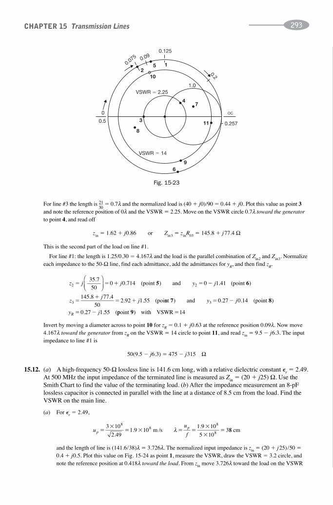
For line #3 the length is 21—30
� 0.7λ and the normalized load is (40 � j0)/90 � 0.44 � j0. Plot this value as point 3and note the reference position of 0λ and the VSWR � 2.25. Move on the VSWR circle 0.7λ toward the generatorto point 4, and read off
zin � 1.62 � j0.86 or Zin3 � zinR03 � 145.8 � j77.4 Ω
This is the second part of the load on line #1.
For line #1: the length is 1.25/0.30 � 4.167λ and the load is the parallel combination of Zin2 and Zin3. Normalizeeach impedance to the 50-Ω line, find each admittance, add the admittances for yR, and then find zR.
CHAPTER 15 Transmission Lines 293
0
0.5
OC
0.257
VSWR � 14
VSWR � 2.25
0.125
1.0
12
5
10
3
47
11
8
96
0.2
0.090.075
Fig. 15-23
z j j y j2 235 7
500 0 714� � � � �
..
⎛⎝⎜
⎞⎠⎟
(point ) and5 0 1..41
50
(point )
(poi
6
zj
j3145 8 77 4
2 92 1 55��
� �. .
. . nnt ) and (point )
(
7 8y j
y jR
3 0
0 27 1 55
� �
� �
0.27 .14
. . ppoint ) with VSWR9 �14
Invert by moving a diameter across to point 10 for zR � 0.1 � j0.63 at the reference position 0.09λ. Now move4.167λ toward the generator from zR on the VSWR � 14 circle to point 11, and read zin � 9.5 � j6.3. The inputimpedance to line #1 is
50(9.5 � j6.3) � 475 � j315 Ω
15.12. (a) A high-frequency 50-Ω lossless line is 141.6 cm long, with a relative dielectric constant �r � 2.49.At 500 MHz the input impedance of the terminated line is measured as Zin � (20 � j25) Ω. Use theSmith Chart to find the value of the terminating load. (b) After the impedance measurement an 8-pFlossless capacitor is connected in parallel with the line at a distance of 8.5 cm from the load. Find theVSWR on the main line.
(a) For �r � 2.49,
uu
fpp
��
� � � ��
��
3
2 491 9 10
1 9
5810 10
103
8 8
8..
.m /s λ 88 cm
and the length of line is (141.6/38)λ � 3.726λ. The normalized input impedance is zin � (20 � j25)/50 �0.4 � j0.5. Plot this value on Fig. 15-24 as point 1, measure the VSWR, draw the VSWR � 3.2 circle, andnote the reference position at 0.418λ toward the load. From zin move 3.726λ toward the load on the VSWR

circle (a net change of 0.226λ) and read the normalized load impedance zR � 0.72 � j0.98 at point 2. Theload impedance is ZR � (36 � j49) Ω at 500 MHz.
(b) Since the capacitor is connected in parallel it is convenient to work on the y-chart, Fig. 15-25. In Fig. 15-24read the value diametrically opposite zR : yR � 0.48 � j0.67. Plot yR as point 3 in Fig. 15-25 and draw theVSWR � 3.2 circle. The reference position is 0.105λ toward the generator, corresponding to x � 0. Move8.5 cm, or (8.5/38)λ � 0.224λ toward the generator on the VSWR circle and read y (x1) at point 4. Beforethe capacitor is added, y(x1) � 1.04 � j1.22. The normalized admittance of the capacitor is
yc � ( j2πƒC )R0 � j2π(5 � 108)(8 � 10�12)(50) � 0 � j1.26
and the new admittance at x1 is yc � y (x1) � 1.04 � j0.04. Plot this new admittance as point 5 and measureVSWR � 1.04 (a significant reduction from 3.2).
CHAPTER 15 Transmission Lines294
ZOC0.5
zin
zR
yR
VSW
R�
3.2
0.418
0
0.144
1.01
3
2
Fig. 15-24
y SC
0.25
y (x1)
0
yR
VSW
R�
3.2
0.105
0.5
0.329
1.03
5
4
Fig. 15-25

15.13. A 4-m-long, stub-supported, lossless, 300 Ω, air-dielectric line (Fig. 15-26) was designed for operationat 300 MHz with a 300-Ω resistive load, using shorted (λ /4)-supports. With no changes in dimensionsor load, the line is operated at 400 MHz. Use the Smith Chart to find the VSWR on each section of line,including the supports, and the input impedance at the new frequency.
CHAPTER 15 Transmission Lines 295
0.5 m
IN R0 � 300 Ω
1 m 2.5 m
0.25 m
ZR � 300 Ω
Fig. 15-26
0.09
0.481
0.315
0.148
6
3
8
2
4
5
7
1
ysc
1.0
Fig. 15-27
The wavelength is λ � up /ƒ � (3 � 108) /(4 � 108) � 75 cm and distances in terms of λ are
Total length � 4 m � 5.333λ
Load to stub 1 � 50 cm � 0.667λ
Stub length � 25 cm � 0.333λ
Stub separation � 2.5 m � 3.333λ
Stub 2 to input � 1 m � 1.33λ
Since the stubs are in parallel, use a y-chart, Fig. 15-27, for the solution. At x � 0, yR � R0/ZR � 1 � j0 (point 1) andVSWR � 1. The line is flat to the point of connection of the first stub, 0.667 λ from the load, with y(x1) � 1 � j0 inthe absence of stubs.
To find the admittance of the shorted stubs, plot ySC at point 2, move 0.333λ toward the generator on the VSWR � ∞ circle to point 3, and read y � 0 � j0.58. This value must be added to y � 1 � j0 to get theadmittance at x1 with stub 1 connected; thus, y(x1) � 1 � j0.58 (point 4), VSWR � 1.75, and the referenceposition is 0.148λ toward the generator. Draw the VSWR circle through point 4; move 3.333λ toward thegenerator from 4 to 5; and read the admittance at x2 without stub 2 in place: y (x2) � 0.57 � j0.08. At this point

add the second stub to get y (x2) � 0.57 � j0.50 (point 6) draw the VSWR � 2.3 circle. The reference position is0.092λ toward the generator. From point 6 move 1.333λ toward the generator on the VSWR � 2.3 circle to point7 and read the normalized input admittance yin � 0.52 � j0.38. Invert this value by moving across a diameter andread zin � 1.23 � j0.92 (point 8). The input impedance to the line at 400 MHz is zinR0 � (369 � j 276) Ω.
15.14. The lossless lumped-parameter network shown in Fig. 15-28 is used to match a 50-Ω line to the input ofan RF transistor operating at 1 GHz. The input reflection coefficient for the transistor is Γ � 0.6
�����150°
�,
measured for a 50-Ω system. Find the values of L and C for the conjugate matched condition.
CHAPTER 15 Transmission Lines296
TransistorZmC Γ∗ ΓL
R0 � 50 Ω
Fig. 15-28
R01 � 300 Ω
l1 � 15 m
l2 � 3 m
x � λ /4x � 0
R02 � 150 Ω RR � 150 ΩR0T
Fig. 15-29
Normalizing the reactances of the matching network to the 50-Ω line gives χ � ωL /50 and b � 50ωC. Thenormalized impedance looking back to the network from the transistor is
z jjbm � �
�χ 1
1
Now, the matching criterion is ΓR � Γ*, or
(1)
(2)z jm ��
�� �
1
10 27 0 25
ΓΓ
*
*. .
together (1) and (2) yield b � �1.64. For b � �1.64, x � �0.70, where the positive sign on b corresponds to acapacitance. Then
Cb
RL
R� � � �
ωχω0
05 2 5 6. .pF and nH
15.15. A 15-m length of 300-Ω line must be connected to a 3-m length of 150-Ω line that is terminated in a150-Ω resistor. Assuming the lossless condition for the air-dielectric lines and operation at a fixedfrequency of 50 MHz, find the R0 and the length for a quarter-wave section of line (quarter-wavetransformer) to match the two lines for a VSWR � 1 on the main line. If no transformer is used, whatis the VSWR on the main line?
A model for the system is shown in Fig. 15-29. For ƒ � 50 MHz and up � 3 � 108 m/s, the wavelength is λ � 6 m;a λ/4 section of line must be 1.5 m long.
With no transformer in place, the termination of the 300-Ω line is 150 Ω, since line 2 is R0-terminated. Thereflection coefficient on line 1 is

With the transformer inserted as shown, the reflection coefficient at the load RR is
CHAPTER 15 Transmission Lines 297
R0 � 75 Ω �n � 2.2~
R 0�
50 Ω
R0 � 50 Ω
�3 � 10 m� 1
� 0.5 m
�2 � 1 m� s
x � x1x � 0
R 0�
75 Ω
ZR2 � 50 Ω
ZR1 � 50 Ω
Fig. 15-30
à ��
��� �
�
�
150 300
150 300
113
113
1
3and VSWR
⎛⎝
⎞⎠
⎛⎝
⎞⎠⎠
� 2
ΓRR T
R T
R R
R R�
�
�0
0
and the input impedance at βx � 90°, which, as the load on line 1, must be 300 Ω, is
(1)
(2)Z R RTR
RT
R
Rin 300
1 180°
1 180°
1
10 0ΩΓ
ΓΓΓ
Substitution of (1), with RR � 150 Ω, in (2) gives
300(150 � R0T � 150 � R0T) � R0T (150 � R0T � 150 � R0T)
or R0T � ������300 � 150����� � �����R01R02�� � 212.1 Ω.
15.16. A generator at 150 MHz drives a 10-m-long, 75-Ω coaxial line terminated in a composite load consistingof the parallel connection of two 50-Ω lines of lengths 0.5 m and 1 m, each terminated in a 50-Ωresistance. All lines are lossless with �R � 2.2. With reference to Fig. 15-30, determine the length �s andconnection point x1 of a parallel-connected 75-Ω stub that will produce minimum VSWR on the feedline. The stub should be as close as possible to the load.
Phase velocity, up � 3 � 108/����2.2 � 2.02 � 108 m/s; wavelength, λ � up /ƒ � 1.35 m. The input impedance toeach of the 50-Ω lines is 50 Ω for R0-termination, the composite load on the 75-Ω line is 25 Ω or, when normalized,zR � 0.333 � j0. Plot zR on the Smith Chart and through this point draw the ⎪ΓR⎪ circle and the radial line to theangle scale, as shown in Fig. 15-31. Read φR � 180° and measure
⎪Γ⎪ � 0.5 and VSWR � 3
Since the matching stub is in parallel, locate yR � 3 � j0 by projecting a diameter across from zR. Locate theintersections of the g � 1 and VSWR � 3 circles and note the distances from the load at x � 0:
y � 1 � j 1.15 at a distance 0.25 � 0.166 � 0.416λ toward the generator
y � 1 � j 1.15 at a distance 0.3335 � 0.25 � 0.0835λ toward the generator

Locate the 75-Ω stub at x1 � 0.0835λ � 11.3 cm. The stub length �s is that which makes ys � 0 � j1.15, for a nety � 1 � j0, (matched condition). Thus, plot ys and determine the distance from the short-circuit condition y � ∞to this point. The length of stub is (0.25 � 0.1345)λ � 51.9 cm.
The VSWR on lines �1 and �2 is 1.0 for the matched loads. On the shorted stub the VSWR is infinite. From x � 0on the main line to x � x1 the VSWR is 3.0 and from x � x1 to x � �3 the VSWR is 1.0.
15.17. Find the shortest distance from the load and the length (both in centimeter) of a shorted stub connected inparallel to a 300-Ω lossless air-dielectric line in order to match a load ZR � (600 � j300) Ω at 600 MHz.The matching stub is the same type of line as the main line.
For both the line and the stub, up � 3 � 108 m/s and λ � 0.5 m. Plot zR � (600 � j300)/300 � 2 � j1 on the y-chart, Fig. 15-32. Draw the VSWR � 2.6 circle, move diametrically across to yR � 0.4 � j0.2, and read thereference position 0.464λ toward the generator. Move from yR on the VSWR circle to the first intersection withthe g � 1 circle, and read y (x1) � 1 � j1 at the reference position 0.162λ. The stub location is
x1 � [(0.5 � 0.464) � 0.162]λ � 0.198λ � 9.9 cm
CHAPTER 15 Transmission Lines298
ys
yRzR
�1.15
1.0
�1.15
VSWR � 3
y � ∞x � 0
|Γ | � 0.5
� s�
(0.25
�0.1345) λ
x 1
=(0
.332
5�
0.25
) λ
Fig. 15-31
0.162
zR
yR
� j1
� j1
1.0
0.375
y (x1) = 1 + j1
y (x2) = 1 + j1
VSWR � 2.6
sc0
0.250.5
0.464
x 1�
0.5
�
0.464 �
0.162 � 0.198 λ
ls� (at x 1
) �
(0.3
75�
0.25
) λ�
0.1
25 λ
Fig. 15-32

from the load. To match the line for VSWR � 1, the admittance of the shorted stub must be ys � 0 � j1 to cancelthe susceptance at point x1. The required length of stub is 0.125λ � 6.25 cm.
If this position is not accessible, the second intersection with the g � 1 circle may be used, where y(x2) � 1 � j1 and
x2 � [(0.05 � 0.464) � 0.338]λ � 0.374λ � 18.7 cm
The stub would have to be adjusted to give ys � �j1, for a length of 0.375λ � 18.75 cm.
15.18. A high-frequency lossless 70-٠line, with �r � 2.1, is terminated in ZR � 50 ���
30° Ω at 320 MHz. Theload is to be matched with a shorted section of 50-Ω line, with �r � 2.3, connected in parallel; the stubmust be at least 5 cm from the load. If such matching is possible, find the distance from the load andthe length of the stub.
For the main line, up � 3 � 108/���2.1 � 2.07 � 108 m/s, λ � up/ƒ � 64.7 cm; for the stub line, ups � 3 � 108/���2.3 �1.98 � 108 m/s, λs � 61.9 cm. The normalized load is zR � (50
���30° )/70 � 0.62 � j0.36, with VSWR � 1.92, and
the admittance is yR � 1.20 � j0.70 at reference position 0.327λm toward the generator; see Fig. 15-33. Move on the VSWR circle from yR toward the generator to the first intersection, y(x1) � 1 � j 0.66, at 0.350λ, or a distance of 0.023λ � 1.49 cm. This point cannot be used due to the 5-cm limitation. Continue on the VSWR circle to y (x2) � 1 � j0.66 at position 0.151λm; the distance
x2 � (0.5 � 0.327) � 0.151 � 0.324λm � 21.0 cm
gives the point of connection for the stub.
As the stub has a different R0, it is necessary first to “denormalize” y(x2):
CHAPTER 15 Transmission Lines 299
0.151
zR
yr
1.0
y(x2) � 1 � j0.66
ys � � j 0.47
ls � 0.43 � 0.25 � 0.18 λ
y( x1)
y sc
0.25
0
0.43
0.350 0.327
0.5
x 2(0
.5�
0.327) �
0.151 � 0.324 λ
Fig. 15-33
y xj
j( ).
( . . )21 0 66
701 4 0 94�
�� � � �10 2S
which shows that for cancellation of susceptance we must have
ys � (�j0.94 � 10�2)(50) � �j0.47
The length of shorted stub is then (0.43 � 0.25)λs � 0.18λs � 11.1 cm.

15.19. A complex load is measured with a VHF bridge at 500 MHz; the impedance is 29���
30° Ω. This loadis connected to a 50-Ω air-dielectric line, with a 50-Ω 3λ /8 tuner between the load and line. Findthe lengths of each shorted stub to produce a VSWR of 1.0 on the main line. Show both solutions ifthey exist.
The model for the system is shown in Fig. 15-9. For the air line, up � 3 � 108 m/s and λ � up /ƒ � 60 cm. Thenormalized load impedance is
CHAPTER 15 Transmission Lines300
zZ
RjR
R
0
0 58 30 0 5 0 29. . .
On the Smith Chart draw the 3λ/8 tuner circle, plot zR, draw the VSWR � 2.25 circle, locate yR � 1.52 � j0.88,and find the intersections of the tuner circle and the gR � 1.52 circle. There is a solution for each intersection;first consider y � 1.52 � j1.82 (Fig. 15-34a). Here, the first stub must be adjusted to change the susceptancefrom �0.88 to �1.82 (point 1); thus, ys1 � 0 � j0.94 at point 2. The stub length for this b is read on λ scale fromy � ∞ toward the generator:
�s1 � (0.380 � 0.25)λ � 7.8 cm
From point 1 move 3λ/8 toward the generator to point 3, where y � 1 � j1.53. Stub 2 must add y � 0 � j1.53(point 4); and the stub length is
�s2 � (0.342 � 0.25)λ � 5.52 cm
Fig. 15-34b presents the second solution, which follows the same pattern.
At 1′: y � 1.52 � j0.16
At 2′: ys1 � 0 � j0.72 and
�s1 � (0.25 � 0.099)λ � 21.6 cm
At 3′: y � 1 � j0.45
At 4′: ys2 � 0 �j0.45 and
�s2 � (0.433 � 0.25)λ � 11.4 cm
The first solution is preferred because the total length of the stubs with infinite VSWR is 12.63 cm, which willintroduce lower losses in a practical system.
zR zR
yR yR
1.0
0
(a) (b)
y sc y sc
(3λ /8) T–̂(3λ /8) T–̂
1.52
1.0
1.52
3
1
24
4′
2′
3′
1′
�s2
� s�2
�s1
� s�1
Fig. 15-34

15.20. Use a two-stub quarter-wave tuner (50-Ω, shorted stubs) located 7.2 cm from the load of Problem 15.19in order to match the load to the line.
The normalized load admittance in Problem 15.19 is yR � 1/zR � 1.52 � j0.88, and the wavelength is λ � 60 cm.At 7.2 cm or 0.12λ from the load, y1 � 0.54 � j0.36; this value is to be matched to the line with the tuner. Twosolutions exist:
CHAPTER 15 Transmission Lines 301
zR
yRy1
0.54
0.12 λ
1.0
0
3
1
2
4
(λ /4) T–̂
l s2
ls1
yR
zR
y1
0.54
0
0.12 λ
1.0
2′
1′
4′
3′
(λ /4) T–̂l s2l s1
Fig. 15-35 Fig. 15-36
Solution 1 (Fig. 15-35)
y1 � 0.54 � j0.36
1: yT � 0.54 � j0.50
2: ys1 � �j0.14
�s1 � (0.478 � 0.25)λ � 13.68 cm
3: Move λ /4 to y � 1 � j0.95
4: ys2 � �j0.95
�s2 � (0.3795 � 0.25)λ � 7.77 cm
Total stub length � 21.45 cm (preferred)
Solution 2 (Fig. 15-36)
y2 � 0.54 �j0.36
1′: yT � 0.54 � j0.50
2′: ys1 � j0.86
�s1 � (0.25 � 0.113)λ � 21.78 cm
3′: Move λ /4 to y � 1 � j0.95
4′: ys2 � � j0.95
�s2 � (0.25 � 0.1205)λ � 22.23 cm
Total stub length � 44.01 cm
15.21. A 70-Ω double-stub tuner is used to match a load YR � (4.76 � j1.43) mS at 600 MHz to a 70-Ωlossless air-dielectric line. The first stub is located at the load and the separation between the stubs is10 cm. Find the shorted-stub lengths for the matched condition.
For the air line, λ � (3 � 108)/(6 � 108) � 0.50 m and the stub separation is 10 cm � λ /5. Draw the λ /5 tuner circleas shown in Fig. 15-37. Plot the normalized load yR � YRR0 � 0.33 � j0.10, which determines the VSWR � 3.0circle. Two solutions exist, one for the intersection with the tuner circle at y1 � 0.333 � j0.18 (VSWR � 3.2) and theother at y2 � 0.333 � j0.84 (VSWR � 4.9).
First solution. ys1 � �j0.28 to change yR to y1, for a length of 0.207λ � 10.35 cm. Move on the VSWR � 3.2circle 0.2λ toward the generator from yR, to y � 1.0 � j1.23. The second stub must be adjusted to give ys2 � �j1.23for a net y � 1 � j0, the matched condition. The length is 0.109λ � 5.45 cm.
Second solution. y′s1 � �j0.74, for y2 � 0.33 � j0.84 and a length 0.351λ � 17.55 cm. Move on the VSWR � 4.9 circle 0.2λ toward the generator from yR, to y′ � 1.0 � j1.75. The second stub must be adjustedfor y′s2 � �j1.75 to produce 1 � j0, the matched condition. The length is 0.417λ � 20.85 cm.

15.22. A 50-Ω slotted line that is 40 cm long is inserted in a 50-Ω lossless line feeding an antenna at 600 MHz. Standing-wave measurements with a short-circuit termination and with the antenna in place yield the data of Fig. 15-38; the scale on the slotted line has the lowest number on the load side.Find the impedance of the antenna, the reflection coefficient due to the load, and the velocity ofpropagation on the line.
CHAPTER 15 Transmission Lines302
y ′s2
y ′
y2
l ′s2 � 0.417
l ′s1�
0.35
ls1 � 0.207 λ l s2
� 0.109 λ
y1
ys1
ys2
yR
y
y ′s1
1.0
00.5
y sc
0.25
VSWR � 3.0
VSW
R�
3.2
VSW
R�
4.9
(λ /5) T–̂
Fig. 15-37
Min28 cm
Max20.5 cm
Min8 cm
5 cm
High VSWR
VSWR � 2.2
sc
zR
Min3 cm
Fig. 15-38
For the short circuit, minima are separated by a half-wavelength, so λ � 50 cm. For a frequency of 600 MHz thephase velocity is up � ƒλ � 3 � 108 m/s (air dielectric). With the antenna in place the minimum shifts 5 cm � 0.1λtoward the generator. On the Smith Chart draw the VSWR � 2.2 circle and identify the voltage minimum line as inFig. 15-39. Locate zR on the VSWR circle 0.1λ toward the load from the Vmin position:
zR � 0.64 � j0.52 and ZR � R0zR � (32 � j26) Ω
The load ΓR is read from the chart: φR � �108° and ⎪ΓR⎪ � 0.375 is the distance from the center to zR, as read offthe external scale.
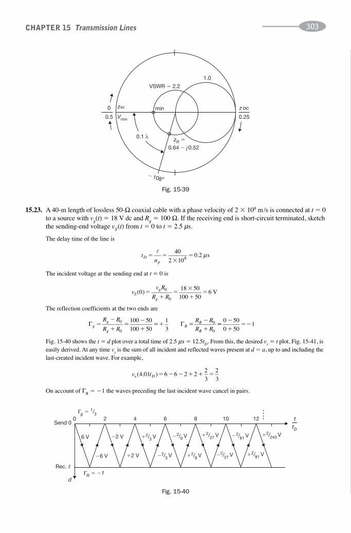
15.23. A 40-m length of lossless 50-Ω coaxial cable with a phase velocity of 2 � 108 m/s is connected at t � 0to a source with vg(t) � 18 V dc and Rg � 100 Ω. If the receiving end is short-circuit terminated, sketchthe sending-end voltage vS(t) from t � 0 to t � 2.5 μs.
The delay time of the line is
CHAPTER 15 Transmission Lines 303
VSWR � 2.2
� 108º
min
0.1 λ
0.64 � j0.52
1.0
0
0.5
z oc
0.25
zR �
Vmin
zsc
Fig. 15-39
Send 00
d
2
6 V �2 V
�6 V �2 V
�2/3 V
�2/3 V
�2/9 V
�2/9 V
�2/27 V
�2/27 V
�2/81 V
�2/81 V
�2/243 V
4 6 8 10 12 t
tD
Rec. lΓR � �1
Γg � 1/3
Fig. 15-40
tuD
p
� ��
�� 40
2 100 2
8. μs
The incident voltage at the sending end at t � 0 is
vv R
R RSg
g
( )018 50
100 5060
0
��
��
�� V
The reflection coefficients at the two ends are
Γ Γgg
gR
R
R
R R
R R
R R
R R�
�
��
�
��� �
�
�
0
0
0
0
100 50
100 50
1
3��
�
���
0 50
0 501�����
Fig. 15-40 shows the t � d plot over a total time of 2.5 μs � 12.5tD. From this, the desired vs � t plot, Fig. 15-41, iseasily derived. At any time vs is the sum of all incident and reflected waves present at d � a, up to and including thelast-created incident wave. For example,
v ts D( .4 01 6 6 2 22
3
2
3)� � � � � �
On account of ΓR � �1 the waves preceding the last incident wave cancel in pairs.
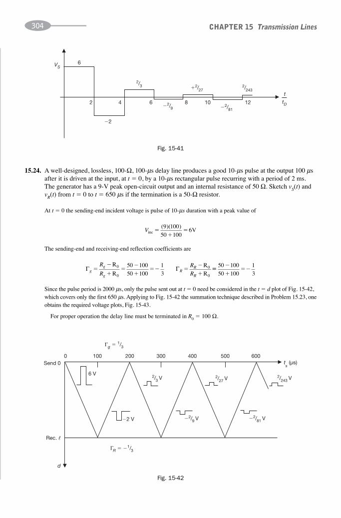
15.24. A well-designed, lossless, 100-Ω, 100-μs delay line produces a good 10-μs pulse at the output 100 μsafter it is driven at the input, at t � 0, by a 10-μs rectangular pulse recurring with a period of 2 ms.The generator has a 9-V peak open-circuit output and an internal resistance of 50 Ω. Sketch vS(t) andvR(t) from t � 0 to t � 650 μs if the termination is a 50-Ω resistor.
At t � 0 the sending-end incident voltage is pulse of 10-μs duration with a peak value of
CHAPTER 15 Transmission Lines304
6
2 4 6 8 10 12
�2
VS
t
tD
�2/272/243
2/3
�2/9 �2/81
Fig. 15-41
Send 00 100 200 300 400 500 600
ts (μs)
d
6 V
�2 V
Rec. l
Γg � 1/3
ΓR � �1/3
2/3 V 2/27 V 2/243 V
�2/9 V �2/81 V
Fig. 15-42
Vinc V��
�( )( )9 100
50 1006
The sending-end and receiving-end reflection coefficients are
Γ Γgg
gR
R
R
R
R
R
R�
�
��
�
��� �
�
�
R
R
1
3
R
R0
0
0
0
50 100
50 100��
�
���
50 100
50 100
1
3
Since the pulse period is 2000 μs, only the pulse sent out at t � 0 need be considered in the t � d plot of Fig. 15-42,which covers only the first 650 μs. Applying to Fig. 15-42 the summation technique described in Problem 15.23, oneobtains the required voltage plots, Fig. 15-43.
For proper operation the delay line must be terminated in R0 � 100 Ω.

SUPPLEMENTARY PROBLEMS
15.25. A coaxial cable with the dimensions a � 0.5 mm, b � 3 mm, and t � 0.4 mm is filled with a dielectric materialhaving �r � 2.0, σd � 10 μS/m. The conductors have σc � 50 MS/m. Calculate the per-meter values of L, C, G,Rd, and Ra at 50 MHz. Neglect internal inductance.
15.26. Find the per-meter values of L, C, G, and R for a parallel-wire line constructed in air of #12 AWG copper wire(dia. � 0.081 in., σc � 52.8 MS/m) with a 4-inch separation. Operation is at 100 kHz.
15.27. In a “twin-lead” transmission line, two parallel copper wires (σc � 50 MS/m) are embedded 0.625 in. apart in alow-loss dielectric with �r � 2.4. Neglecting losses, determine the diameter of the conductors for a characteristicimpedance of 300 Ω. For this size of conductor, find the dc resistance and the ac resistance at 100 MHz.
15.28. A high-frequency application uses a coaxial cable with copper conductors, where the diameter of the innerconductor is 0.8 mm and the inside diameter of the outer conductor is 8.0 mm. The dielectric material has �r � 2.35, and the thickness of the outer conductor is much greater than the depth of penetration at the operatingfrequency. The engineer wants to use a new cable having the same R0, but with a larger outer conductor such thatb2 � a � 1.5(b1 � a). Find �r for the new cable and calculate R0 and the capacitance per meter for each cable.
15.29. For the coaxial cable of Problem 15.28, calculate the line characteristics Z0, α, β, up, λ for operation at 10 kHz.
15.30. Find the characteristic impedance, propagation constant, velocity of propagation, and wavelength for the parallel-wire line of Problem 15.26.
15.31. A transmission line is 2 miles long, operates at 10 kHz, and has parameters R � 30 Ω/mi, C � 80 nF/mi, L � 2.2 mH/mi, and G � 20 nS/mi. Find the characteristic impedance, attenuation per mile, phase shift permile, phase velocity, and wavelength. What is the received power to a matched load when the sending-endpower is 1.2 W?
15.32. A transmission line 250 m long operates at 2 MHz with a load impedance of 200 Ω. The line characteristics are Z0 � 300
��0° Ω, α � 4 � 10�4 Np/m, β � 0.06 rad/m. If the sending-end voltage is 30
��0° V, find the
receiving-end voltage, power to the load, sending-end current and power, and the reflected power from the load.
15.33. One method of determining the characteristics of a line is to measure the input impedance at x � � (line disconnectedfrom source) when the receiving end is opened for Zoc, and when it is shorted for Zsc. From the product ZocZsc and theratio Zoc/Zsc the characteristic impedance and the propagation constant per unit length can be calculated. If measuredvalues at 5 kHz are Zoc � 141.9
����84.1°
��٠and Zsc � 62.0
���37.7°
�Ω for a 2-mile length of line, use the equation for
ZS to find Z0, α (per mile), and β (per mile).
CHAPTER 15 Transmission Lines 305
100
200 400 600t (μs)
t (μs)
V
300 5000
2
4
6
0
�1
2
4
6
�4/3�4/27
4/9 4/81
�4/243
vS,
VvS,
Fig. 15-43

15.34. A 200-m length of 300-Ω transmission line has α � 2.5 � 10�3 Np/m and β � 0.02 rad /m when operating at 200 kHz. If V̂R � 20
��0° V and ZR � 350
���20° Ω, find the distance from the receiving end to the first impedance
minimum. What is the value of this Zmin?
15.35. A 500-Ω line is connected to a 10-kHz generator rated at 80 ��0° V open-circuit with an internal resistance of
600 Ω. The line is 3 miles long, with α � 0.05 Np/mi and β � 0.9 rad/mi at 10 kHz. For a matched load at x � 0,find the sending-end power, the receiving-end power, and V̂R. If the line is opened at the receiving end, what is thesending-end power?
15.36. For the line of Problem 15.35, find the receiving-end current and the sending-end power if the line is shorted at x � 0.
15.37. The rigid coaxial line of Problems 15.2 and 15.9 would be classified as a low-loss line. (a) What are the reflectioncoefficients at the load and VSWR if the load is a 40-Ω resistor? (b) Determine the maximum and minimum loadresistance for VSWR � 1.5. (c) Calculate the reflection coefficient 3 cm from the load, if ZR � (55 � j0) Ω(consider attenuation).
15.38. A 90-Ω, lossless, high-frequency, coaxial line, with �r � 2.1, operates at 150 MHz. Of interest is the sensitivity of the VSWR to small changes in terminating resistance. (a) Tabulate ΓR and VSWR against RR � (90 � 2n) Ω, for integral values of n from 0 to 5. (b) If the specifications for an application limit the maximum VSWR to 1.025,find the maximum and minimum values of terminating resistance.
15.39. For the transmission line of Problem 15.38, (a) find the phase velocity, wavelength, and the phase shift per meter.(b) If the terminating resistance is 100 Ω, find the input impedances for line lengths λ /2, λ /4, and λ /8.
15.40. Use the Smith Chart to find (a) ΓR, (b) VSWR, and (c) yr for the following (ZR, R0)-pairs, in ohms: (100 � j150, 50);(28 � j35, 70); 90
����30°
�, 90); (120
���90° , 50); (0, 70); (50 � j5, 50).
15.41. Find (a) yR, (b) VSWR, and (c) YR (in mS) for the following (ΓR, R0)-pairs: (0.5 ���60° , 50 Ω); (1
����80°
�, 90 Ω);
(0.1 ��0° , 70 Ω); (�0.6
����30°
�, 50 Ω); (0.8 � j0.4, 70 Ω).
15.42. A lossless high-frequency line 3 m long, with R0 � 50 Ω and �r � 1.9, is operated at 350 MHz. The VSWR onthe line is 2.4 and the first voltage maximum is located 7 cm from the load. Use the Smith Chart to find the loadimpedance, the reflection coefficient at the receiving end, the location of the first voltage minimum, and the inputimpedance.
15.43. A 70-Ω lossless line, with �r � 2.2, is 2.5 m long and operates at 625 MHz. The VSWR on the line is 1.7 and thefirst voltage minimum is located 5 cm from the load. Use the Smith Chart to find the load admittance, the reflectioncoefficient at x � 0, and the input admittance to the line.
15.44. An air-dielectric line with R0 � 150 Ω is terminated in a load of (150 � j150) Ω at the operating frequency, 75 MHz.(a) Use the Smith Chart to find the shortest length of line for which the input impedance is (150 � j150) Ω. (b) Whatare the VSWR on the line and the reflection coefficient at the load? What is the shortest length of line for which Zin � R � j0, and what is the value of R?
15.45. Two lines are connected in parallel at the input to a 250-MHz source. Each line is 2 m long and is terminated in a70-Ω resistance. Line #1 has R0 � 50 Ω, �r � 1.9, line #2 has R0 � 90 Ω, �r � 2.3. Use the Smith Chart to find theinput impedance to the parallel combination. (Be careful in combining the two input impedances/admittances.)
15.46. A lossless 50-Ω line, with a phase velocity 2.5 � 108 m/s, is 105 cm long and is terminated in a load YR � (20 � j16) mS at 500 MHz. A short-circuited line, 17.85 cm long and also having R0 � 50 Ω, isconnected across Y, as shown in Fig. 15-44. Use the Smith Chart to find the VSWR on the main line and theinput impedance. What is the equivalent capacitance (or inductance) of the short-circuited line?
CHAPTER 15 Transmission Lines306
R0 � 50 Ω YR
l1 � 105 cm l2 �
17.85 cm
Fig. 15-44

15.47. In the line of Problem 15.46, the short circuit on line two is inadvertently changed to an open circuit. Use theSmith Chart to find the VSWR on the main line and the input impedance.
15.48. A parallel-wire line of the type in Problem 15.1 is operated at 20 MHz to supply a resistive load of 500 Ω through aquarter-wave matching transformer connected at the load. Neglect losses on the main line and the transformer section.(a) For the transformer calculate the length of line and characteristic impedance required for matching. (b) If the samesized wire is used for the main line and the transformer, find the separation d (in inches) required for matching.
15.49. A lossless 70-Ω line is terminated in ZR � 60.3 ����30.7°
��٠at 280 MHz. Use the Smith Chart to find the value of
the inductance or capacitance to connect in parallel with the load for minimum VSWR on the line. What length(in centimeter) of shorted line would give the desired value, if �r � 2.1?
15.50. A 200-Ω air-dielectric line is terminated in YR � (3.3 � j 1.0) mS at 200 MHz. (a) Find the VSWR and the positionnearest the load where the real part of the normalized admittance is unity, using the Smith Chart. (b) What value ofsusceptance (in millisiemens) should be connected at this point to make VSWR � 1 on the line?
15.51. Two 72-Ω resistive loads are connected in parallel as the termination for a 120-Ω air-dielectric lossless line at 150 MHz. Find the location nearest the load and the length (both in centimeters) of a single shorted parallel-connected stub to match the line for a VSWR � 1.0.
15.52. (a) In Problem 15.51, if the maximum length of the adjustable shorted stub is 50 cm, can the load be matched tothe line? (b) If the answer to (a) is Yes, find the position and length of the stub for the matched condition. (c) Ifthe stub were left at its original position and set to the 50-cm maximum, what would be the VSWR on the line?
15.53. A 90-Ω lossless line with �r � 1.8 operates at 280 MHz and is matched to the termination with a single shortedstub that produces VSWR � 1.0. The stub is located 15.8 cm from the load and is of length 10 cm. Find theohmic value of the terminating impedance.
15.54. A 50-Ω air-dielectric lossless line has ZR � (25 � j30) Ω at 120 MHz. An adjustable shorted stub is located 45 cm from the load (fixed in position). Find the length of stub for the best match on the line. What is theminimum VSWR on the line?
15.55. (a) An air-dielectric lossless 70-Ω line is matched at 200 MHz to a 140-Ω load by means of a shorted parallelstub. Find the position nearest the load and the length of the stub (both in centimeter) for the matched condition.(b) The line is now used at 220 MHz without changing the position or length of the stub. Find the VSWR on themain line at the new frequency.
15.56. The termination on a 90-Ω lossless air-dielectric line is ZR � (270 � j0) Ω at 600 MHz. A double-stub 0.25λtuner is connected with the first stub at the load for matching. Find the lengths for the shorted stubs (bothsolutions). Which solution is preferred?
15.57. A 3λ /8 tuner is connected at the load to match ZR � (50 � j50) Ω at 400 MHz to a 50-Ω lossless air-dielectricline. Find the lengths of the shorted stubs for both solutions and indicate the preferred solution.
15.58. A 50-Ω air-dielectric line, with a load YR � (0.024 � j0.02) S at 470 MHz, has a λ /4 tuner with the first stublocated 7 cm from the load. Find both solutions for the lengths of the shorted stubs to match the load to the line.Indicate the preferred solution.
15.59. A two-stub 3λ/8 tuner is constructed of 70-Ω line with �r � 2.0 for use at 272 MHz on the same type of line and acertain load. For the matched condition the shorted stub at the load is 4.76 cm long and the other shorted stub is4.60 cm long. Find the ohmic impedance of the load at the operating frequency.
15.60. A 225-Ω resistive load is matched to a 90-Ω air-dielectric line at 300 MHz. The matching is via two shorted stubsseparated by 30 cm, with the first stub connected at the load. Find the lengths of the stubs (both solutions) andindicate the preferred solution.
15.61. A 50-Ω slotted line is used to determine the load impedance at 750 MHz on a lossless 50-Ω line. When the line is terminated in a short circuit, the high VSWR has adjacent minima at 30 cm and 10 cm (the scale has thelow numbers on the load side). With ZR connected, the VSWR is 3.2, a minimum is located at 13.2 cm, and the adjacent maximum is at 23.2 cm. Find the ohmic value of ZR at the operating frequency.
CHAPTER 15 Transmission Lines 307

15.62. Find the load impedance and the operating frequency for a 90-Ω air-dielectric system that has the followingslotted-line measurements:
With load: VSWR � 1.6 and a voltage minimum at 10 cm (high numbers on load side).
With short circuit: VSWR � 100, minimum at 40 cm, maximum at 10 cm.
15.63. A 50-Ω slotted line is used to measure the load impedance at 625 MHz on a 50-Ω lossless coaxial line. Adjacentvoltage minima are found at 10 mm and 250 mm (high numbers at the load side) when the termination is a shortcircuit. With the load connected, VSWR � 100 and a minimum occurs at 172.7 mm. Find the ohmic value of theload impedance.
15.64. A tuner is connected at the load to match the load to a 50-Ω lossless air-dielectric line at 517 MHz. To check thequality of the matching, a slotted line is inserted in the system. With the tuner and load connected, VSWR � 1.15,with a Vmin at 253.4 mm. When the tuner and load are both removed and replaced by a short circuit, adjacent minimaare found at 40 mm and 330 mm (low numbers on the scale are at load side). Find the residual normalizedadmittance on the line that results from the “best match.”
15.65. A 60 m-long, lossless, 50-Ω coaxial cable, with a phase velocity of 2 � 108 m /s, is terminated with a shortcircuit. The line is connected at t � 0 to a 30-V dc source having internal resistance 25 Ω. Plot the sending-endvoltage from t � 0 up to the time when the voltage drops below 0.1 V.
15.66. A 90-Ω lossless line, with �r � 2.78, is connected at t � 0 to a 70-V dc source with an internal resistance of 120 Ω.If the line is 135 m long, find the time when the open-circuit voltage at the receiving end is 97% of the steady-statevalue. When is the voltage 99.95% of the steady-state value?
15.67. A pulse generator with internal resistance 150 Ω produces a 20-μs pulse with an open-circuit amplitude of �8 V.The generator is connected to a 50-Ω, lossless, 200-μs delay line that is terminated in a 100-Ω resistance. If the period of the recurring pulses is 4 ms, sketch the voltage at the input to the delay line from pulse onset at t � 0 to t � 1.4 ms.
15.68. Sketch vS and vR versus time, from t � 0� to t � 300 μs, when a 70-Ω, lossless, 50-μs delay line is terminated with a 30-Ω resistor and driven by a pulse generator. The generator has an internal resistance of 70 Ω and producesa 2-μs pulse with a peak open-circuit voltage of �10 V at a repetition rate of 1000 pulses per second.
15.69. In Fig. 15-45 a line is used to produce a short rectangular pulse of width 12 ns and peak value 800 V. With S-2 open,S-1 is closed to charge the line to Vdc; after charging, S-1 is opened. Then, at t � 0, S-2 is closed to discharge the linethrough RR and form the pulse. Find the length of line and Vdc.
CHAPTER 15 Transmission Lines308
S-1 S-2150 ΩRR � VoutR0 � 150 Ω, �r � 2.25
d � 0 d � �
�
�
�
�
2 kΩ
Vdc
Fig. 15-45
15.70. Sketch vS and vR versus time, from t � 0� to t � 30 μs, when a 220-m-long, 90-Ω, lossless line, with �r � 3.65, isterminated in a 50-Ω resistance and driven by a pulse generator. The generator has an internal resistance of 90 Ω andproduces a 5-μs pulse with open-circuit peak value �140 V, at a repetition rate of 100 pulses per second.
ANSWERS TO SUPPLEMENTARY PROBLEMS
15.25. 0.358 μH/m, 62.0 pF/m, 35.1 μS/m, 0.030 Ω /m, 0.743 Ω /m
15.26. 1.84 μH/m, 6.05 pF/m, 0, Ra � 0.0268 Ω/m
15.27. 0.026 in. � 0.66 mm, 0.117 Ω/m, 2.72 Ω/m
15.28. 3.18, 90 Ω, 56.8pF/m (old), 66.1 pF/m (new)
15.29. 32.7 ���
15.2°�
Ω, 1.04 � 10�3 Np/m; 4.2 � 10�4 rad /m, 1.49 � 108 m /s, 14.9 km

15.30. 552.5 ����0.65°
��Ω, (2.4 � j210)10�5 m�1, 2.99 � 108 m/s, 2.99 km
15.31. 167.7 ����6.1°
�Ω, 0.0896 Np/mi, 0.838 rad/mi, 7.5 � 104 mi/s, 7.5 mi; 838.6 mW
15.32. 22 �����130°
��V; 1.21 W; 105.4
����18.3°
�mA, 1.5 W; 50 mW
15.33. 93.8 �����23.2°
��Ω, 0.12 Np/mi, 0.28 rad/mi
15.34. 107.2 m, 239.4 Ω
15.35. 1.32 W, 0.98 W, 31.3 �����154.7°
��V; 0.65 W
15.36. 0.12 �����157.6°
��A, 0.55 W
15.37. (a) �0.073, 1.16; (b) 69.45 Ω, 30.89 Ω; (c) 0.0856 �����216°
��15.38. (a) See Table 15-4. (b) 92.24 Ω, 87.81 Ω
CHAPTER 15 Transmission Lines 309
N RR ΓR VSWR
0 90 0.0 1.0
1 92 0.0110 1.022
88 �0.0112 1.023
2 94 0.0217 1.044
86 �0.0227 1.046
3 96 0.0323 1.067
84 �0.0345 1.071
4 98 0.0426 1.089
82 �0.0465 1.098
5 100 0.0526 1.111
80 �0.0588 1.125
TABLE 15-4
15.39. (a) 2.07 � 108 m /s, 1.38 m, 4.55 rad /m; (b) 100���0°
�Ω, 81
���0°
�Ω, 90
���6°
�Ω
15.40. (a) 0.75 ��26.5°
�, 0.53
���121°
��, 0.27
���90
�, 1.0
��45°�
, �1.0, 0.05 ��
90°�
(b) 7, 3.3, 1.75, ∞, ∞, 1.1
(c) 0.16 � j0.225, 0.97 � j1.23, 0.87 � j 0.52, �j 0.415, ∞, 1 � j0.1
15.41. (a) 0.44 � j0.495, 0 � j0.84, 0.83 � j 0, 2.0 � j1.85, 0.06 � j 0.238
(b) 3.0, ∞, 1.2, 4.0, 17
(c) 8.8 � j 9.9, 0 � j 9.3, 11.9 � j 0, 40 � j37, 0.86 � j 3.4
15.42. (40 � j 39) Ω, 0.42 ��
81°�
, 22.6 cm, (22.3 � j11) Ω
15.43. (10.4 � j 5.4) mS, 0.27 ���68°
�, (16 � j 7.9) mS
15.44. (a) 1.3 m; (b) 2.6, 0.47 ���64°
�; (c) 64.8 cm, 57 Ω
15.45. (24.6 � j3.5) Ω
15.46. 1.0, 50 Ω; 5.1 pF
15.47. 6.2, (26.5 � j 72.5) Ω
15.48. (a) �T � 3.75 m, R0T � 547.7 Ω; (b) dT � 7.77 in.
15.49. C � 4.8 pF (VSWRmin � 1.0); 24.8 cm

15.50. (a) 1.65, 29.3 cm; (b) �2.55 (inductive)
15.51. 16 cm, 78.6 cm
15.52. (a) Yes; (b) 83.8 cm, 21.4 cm; (c) 3.3.
15.53. Hint: Remove ys, find the VSWR, and moveback toward the load.
201.2 ��
26.6°��
Ω
15.54. 96 cm, 1.08
15.55. (a) 22.65 cm, 22.80 cm; (b) 1.22
15.56. 9 cm and 4.95 cm (preferred); otherwise, 16 cmand 20.05 cm.
15.57. 4.5 cm and 4.3 cm (preferred); otherwise, 12.1 cmand 26.1 cm.
15.58. 14.5 cm and 7.6 cm (preferred); otherwise, 23.1cm and 24.3 cm.
15.59. (58.1 � j58.1) Ω
15.60. 13.6 cm and 8.5 cm (preferred); otherwise, 28.1cm and 37.5 cm.
15.61. 31.24 ��
�50.2°����
Ω
15.62. 144 Ω; 250 MHz
15.63. 80 Ω (capacitative)
15.64. 0.98 � j 0.14
15.65. See Fig. 15-46.
15.66. 2.25 μs, 5.25 μs
15.67. See Fig. 15-47.
15.68. See Fig. 15-48.
15.69. 1.2 m, 1600 V
15.70. See Fig. 15-49.
CHAPTER 15 Transmission Lines310
vs, V
00 0.6 1.2 1.8 2.4 3.0
0.080.250.742.22
6.67
t , μs
20
Fig. 15-46
vs, V
00 0.2 0.4 0.6 0.8 1.0
1.0 0.170.03
1.2 1.4 1.6t ,ms
20
Fig. 15-47
0 00 50 100 200 300
vs, V vR, V
100
�2.0
�5.0 3.0
200 300t ,μs t ,μs
Fig. 15-48
70
50 50
00 0
0 1.4 6.4 10 20 30t , μs
2.8 5.0 10 20 30
vs, V vR, V
t , μs
Fig. 15-49
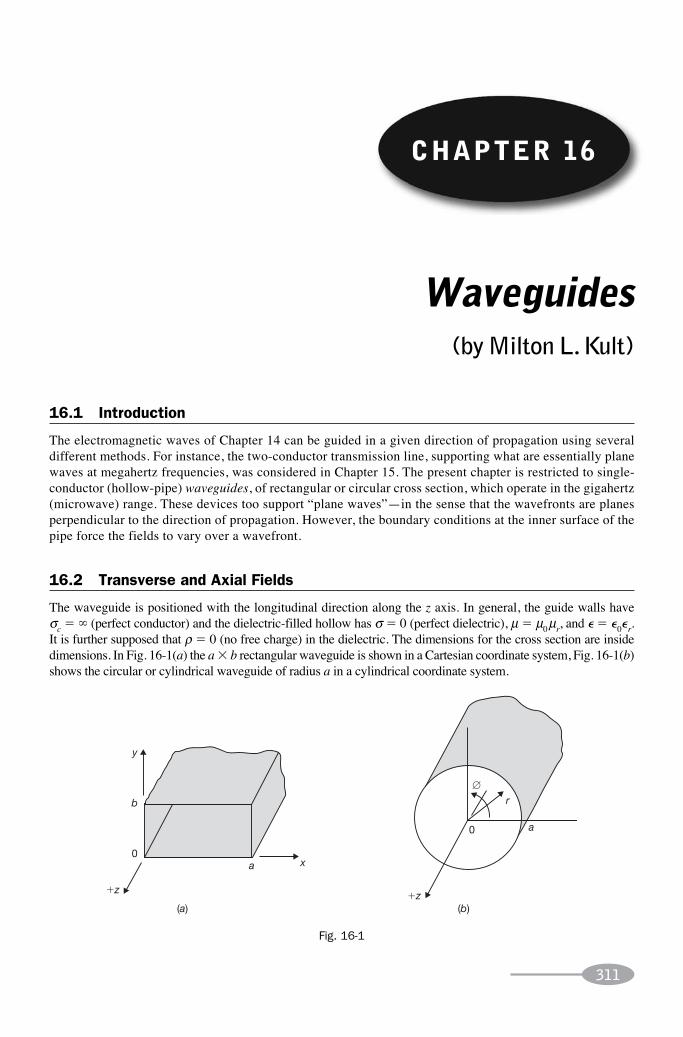
311
Waveguides(by Milton L.Kult)
16.1 Introduction
The electromagnetic waves of Chapter 14 can be guided in a given direction of propagation using severaldifferent methods. For instance, the two-conductor transmission line, supporting what are essentially planewaves at megahertz frequencies, was considered in Chapter 15. The present chapter is restricted to single-conductor (hollow-pipe) waveguides, of rectangular or circular cross section, which operate in the gigahertz(microwave) range. These devices too support “plane waves”—in the sense that the wavefronts are planesperpendicular to the direction of propagation. However, the boundary conditions at the inner surface of thepipe force the fields to vary over a wavefront.
16.2 Transverse and Axial Fields
The waveguide is positioned with the longitudinal direction along the z axis. In general, the guide walls have σc � ∞ (perfect conductor) and the dielectric-filled hollow has σ � 0 (perfect dielectric), μ � μ0μr, and � � �0�r.It is further supposed that ρ � 0 (no free charge) in the dielectric. The dimensions for the cross section are insidedimensions. In Fig. 16-1(a) the a � b rectangular waveguide is shown in a Cartesian coordinate system, Fig. 16-1(b)shows the circular or cylindrical waveguide of radius a in a cylindrical coordinate system.
CHAPTER 16
y
x
∅
a
(a) (b)
a
rb
0
0
�z�z
Fig. 16-1
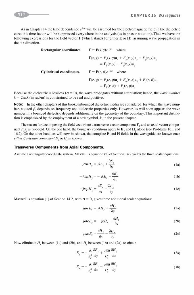
CHAPTER 16 Waveguides312
As in Chapter 14 the time dependence e jω t will be assumed for the electromagnetic field in the dielectriccore; this time factor will be suppressed everywhere in the analysis (as in phasor notation). Thus we have thefollowing expressions for the field vector F (which stands for either E or H), assuming wave propagation inthe �z direction.
Rectangular coordinates. F � F(x, y)e�jkz where
F(x, y) � Fx(x, y)ax � Fy(x, y)ay � Fz(x, y)az
� FT (x, y) � Fz(x, y)az
Cylindrical coordinates. F � F(r, φ)e�jkz where
F(r, φ) � Fr(r, φ)ar � Fφ(r, φ)aφ � Fz(r, φ)az
� FT (r, φ) � Fz(r, φ)az
Because the dielectric is lossless (σ � 0), the wave propagates without attenuation; hence, the wave numberk � 2π /λ (in rad /m) is constrained to be real and positive.
Note: In the other chapters of this book, unbounded dielectric media are considered, for which the wave num-ber, notated β, depends on frequency and dielectric properties only. However, as will soon appear, the wavenumber in a bounded dielectric depends additionally on the geometry of the boundary. This important distinc-tion is emphasized by the employment of a new symbol, k, in the present chapter.
The reason for decomposing the field vector into a transverse vector component FT and an axial vector compo-nent Fzaz is two-fold. On the one hand, the boundary conditions apply to ET and HT alone (see Problems 16.1 and16.2). On the other hand, as will now be shown, the complete E and H fields in the waveguide are known onceeither Cartesian component Dz or Hz is known.
Transverse Components from Axial Components.
Assume a rectangular coordinate system. Maxwell’s equation (2) of Section 14.2 yields the three scalar equations
(1a)
(1b)
Maxwell’s equation (1) of Section 14.2, with σ � 0, gives three additional scalar equations:
(2b)
(2a)
(2c)
Now eliminate Hx between (1a) and (2b), and Hy between (1b) and (2a), to obtain
(3a)
(3b)
(1c)
� � �j H jkEE
yx yzωμ
∂∂
� �� �j H jkEE
xy xzωμ
∂∂
� � �j HE
x
E
yzy xωμ
∂
∂∂∂
j E jkHH
yx yzω� � �
∂∂
j E jkHH
xy xzω� �� �
∂∂
j EH
x
H
yzy xω� � �
∂∂
∂∂
Ejk
k
E
y
j
k
H
xyc
z
c
z�� �2 2
∂∂
∂∂
ωμ
Ejk
k
E
x
j
k
H
yxc
z
c
z�� �2 2
∂∂
∂∂
ωμ

in which k2c � ω 2μ� � k 2. The parameter kc (also in rad /m) functions as a critical wave number; see
Problem 16.3. Finally, slide (3b) and (3a) back into (2a) and (2b), to find
CHAPTER 16 Waveguides 313
(3c)
(3d)
Hjk
k
H
y
j
k
E
xyc
z
c
z�� �2 2
∂∂
∂∂
ω�
Hjk
k
H
x
j
k
E
yxc
z
c
z�� �2 2
∂∂
∂∂
ω�
η �E
HT
T
ET x y y xE Ek
H Hk
2 2 22
2 2� � � � �
ωμ ωμTE TE
⎛⎝⎜
⎞⎠⎟
⎛⎝⎜
⎞( )
⎠⎠⎟
22
HT
η ωμTE
TE
�k
ηωTM �kTM
�
∂∂
∂∂
2
2
2
22 0
H
x
H
yk Hz z
c z� � �TE
By exciting the waveguide in suitable fashion it is possible to force either Ez or Hz (but not both) to vanishidentically. The nonvanishing axial component will then determine all other components via Equations (3).
See Problems 16.4 and 16.5 for the analogous results in cylindrical coordinates.
16.3 TE and TM Modes; Wave Impedances
The two types of waves found in Section 16.2 are referred to as transverse electric (TE) or transverse magnetic(TM) waves, according as Ez � 0 or Hz � 0. When carrying such waves, the guide is said to operate in a TEor TM mode.
For any transverse electromagnetic wave, the wave impedance (in ohms) is defined as
(4)
(compare Chapter 14). For a waveguide in a TE mode, (1a) and (1b) imply
or (5)
Because (4) only involves lengths of two-dimensional vectors, η must be independent of the coordinate system.Problem 16.6 confirms the value of ηTE by recalculating it in cylindrical coordinates. In Problem 16.7 it is shown(using rectangular coordinates) that
(6)
16.4 Determination of the Axial Fields
All that remains for a complete description of the TE and TM modes is the determination of the respective axialfields: Fz � Hz for TE; Fz � Ez for TM. The good word is that Fze
�jkz, being a Cartesian component of F(in either rectangular or cylindrical coordinates), must satisfy the scalar wave equation found in Section 14.2,
∇2 (Fze�jkz) � �ω 2μ�(Fze
�jkz) (7)
together with appropriate boundary conditions which are inferred from the boundary conditions on the compo-nents of FT. [Warning: Transverse components such as Hφe�jkz are not Cartesian components and do not obey ascalar wave equation.]
Explicit Solutions for TE Modes of a Rectangular Guide.
The wave equation (7) becomes

(13)
where, as previously defined, k 2c TE � ω 2μ� � k 2
TE. Solving by separation of variables (Section 9.7),
Hz(x, y) � (Ax cos kxx � Bx sin kxx)(Ay cos kyy � By sin kyy) (8)
where k2x � k 2
y � k 2c TE . The separation constants kx and ky are determined by the boundary conditions (review
Problem 9.19). Consider first the x-conditions Ey(0, y) � Ey(a, y) � 0; in view of (3a) and Ez � 0 thesetranslate into
CHAPTER 16 Waveguides314
∂∂
∂∂
H
x
H
xz
x
z
x a� �
� �0
0
Applying these conditions to (8) gives Bx � 0 and
By symmetry, the boundary conditions in y force By � 0 and
Each pair of nonnegative integers (m, n)—with the exception of (0, 0) which gives a trivial solution—identifiesa distinct TE mode, indicated as TEmn. This mode has the axial field
(9)
from which the transverse field is obtained through (3). The critical wave number for TEmn is
sin ( , , , )k a km
amx x� � �0 0 1 2or
π…
kn
bny � �
π( , , , )0 1 2 …
H x y Hm x
a
n y
bzmn mn( , ) cos cos�π π
km
a
n
bc mnTE� � �π π⎛
⎝⎜⎞⎠⎟
⎛⎝⎜
⎞⎠⎟
2 2
�
k kmn c mnTE� TE� �ω μ2 2�
η ω μ
ω μTE�
TE
mn
c mnk�
�2 2� �
fu
k kc c c� 0
2
1
2π π μ�
�
in terms of which the wave number and wave impedance for TEmn are
(11)
(12)
See Problem 16.9 for the TMmn modes of a rectangular waveguide; it is shown there that kcTMmn � kcTMmn . Consequently, the subscripts TE and TM can be dropped from all modal parameters of rectangular guides savethe wave impedance. This is not the case with cylindrical guides; see Problem 16.12.
16.5 Mode Cutoff Frequencies
In practice one deals with frequencies, not wave numbers; it is then desirable to replace the concept of criticalwave number (kc) by one of cutoff frequency (ƒc). This is accomplished in the definition (see Problem 16.3)

CHAPTER 16 Waveguides 315
In terms of the cutoff frequency ƒc and the operating frequency ƒ � ω /2π � ƒc (10), (11), and (12) become
(10 bis)
(11 bis)
fu m
an
brec gular wavecmn � �0
2 2
2
⎛⎝⎜
⎞⎠⎟
⎛⎝⎜
⎞⎠⎟
( tan gguide)
ku
f ff f
mn cmn mn
cmn
� � ��
2
10
2 2 0
2
π λ λ� �
( / )or
η ηTE�mn
cmnf f�
�
0
21 ( / )
η ηTMmncmnf
f� �0
2
1⎛⎝⎜
⎞⎠⎟
u fu
f
f
mn mn
cmn
� �
�
λ 0
2
1⎛⎝⎜
⎞⎠⎟
fu m
a
n
bcmn � �0
2 2
2
⎛⎝⎜
⎞⎠⎟
⎛⎝⎜
⎞⎠⎟
fu
a a ku fc10
010
0
02
1010 10 102 1 2
2� �
�� �λ λ
λ
π λ η( / )
�λλλ
η10
00
H Hx
aE
H ja
H
z x
x
10 10 10
1010
1
0
2
� �
�
cos ����π
λ⎛⎝⎜
⎞⎠⎟ 00 10 10 10 0
010
2sin sin
π η ηλ
πx
aE H j
aHy x�� ��
⎛⎝⎜
⎞⎠⎟
xx
a
H y10 0�
(12 bis)
where λ 0 � u0 /ƒ is the wavelength of an imaginary uniform plane wave at the operating frequency and whereη0 � ���μ/� is the plane-wave impedance of the lossless dielectric. The second form of (11 bis) exhibits the relation between the operating wavelength λ 0 and the actual guide wavelength λmn. For TMmn waves, (12 bis)is replaced by [see (6)]
(14)
The phase velocity of a TEmn or TMmn wave is given by
(15)
If (10 bis) is replaced by a similar expression involving a Bessel function (see Problems 16.10 and 16.11), allformulas remain valid for cylindrical guides.
The meaning of cutoff is made particularly clear in (15). As the operating frequency drops down to the cut-off frequency, the velocity becomes infinite—which is characteristic, not of wave propagation, but of diffusion(instantaneous spread of exponentially small disturbances).
16.6 Dominant Mode
The dominant mode of any waveguide is that of lowest cutoff frequency. Now, for a rectangular guide, the coor-dinate system may always be oriented to make a � b. Since (Problem 16.9)
for either TE or TM, but neither m nor n can vanish in TM, the dominant mode of a rectangular guide is invariablyTE10, with
From (9), Ez10 � 0, and the equations of Section 16.2:
(16)

CHAPTER 16 Waveguides316
For H10 real, the three nonzero field components have the time-domain expressions
(17)
H Hx
at k z
Ha
z
x
10 10 10
1010
2
� �
��
cos cos( )π ω
λ
⎛⎝⎜
⎞⎠⎟
⎛⎛⎝⎜
⎞⎠⎟
⎛⎝⎜
⎞⎠⎟
Hx
at k z
Ea
y
10 10
10 02
sin sin ( )π ω
η
�
�λλ
π ω0
10 10
⎛⎝⎜
⎞⎠⎟
⎛⎝⎜
⎞⎠⎟
Hx
at k zsin sin ( )�
Plot of the dominant-mode fields (17) at t � 0 are given in Figs. 16-2 and 16-3. Both ⎪Ey⎪ and ⎪Hx⎪ vary assin (πx/a). This is indicated in Fig. 16-2 by drawing the lines of E close together near x � a /2 and far apartnear x � 0 and x � a. The lines of H are shown evenly spaced because there is no variation with y. This sameline-density convention is used to indicate the local value of ⎪E⎪ �⎪Ey⎪ in Fig. 16-3(a) and of
H � �H Hx z2 2
in Fig. 16-3(b). Observe that the lines of H are closed curves (div H � 0); the H field may be considered as cir-culating about the perpendicular displacement current density JD (Section 13.6).
y y
x xa a
bE H
b
00
00
Fig. 16-2 Transverse cross section z � �λ10 /4 (�k10 z � π /2).
Fig. 16-4 illustrates how the TE10 mode can be initiated in a rectangular waveguide by inserting a probehalfway across the top wall (y � b, x � a /2), at a distance z � λ10 /4 from the end of the guide. Higher-ordermodes are present in the vicinity of the probe, but they will not propagate if the frequency-size condition isselected correctly.
See Problem 16.13 for the dominant mode of a cylindrical waveguide.
y
xa
E Hb
00
00
�z
�z
(a) (b)x � a/2 y � const.
λ410 λ
210 3λ
410
λ410 λ
210 3λ
410
Fig. 16-3 Longitudinal cross sections.
E E
b b
a/2
COA X COA X
0 0a /4λ10
z
Fig. 16-4
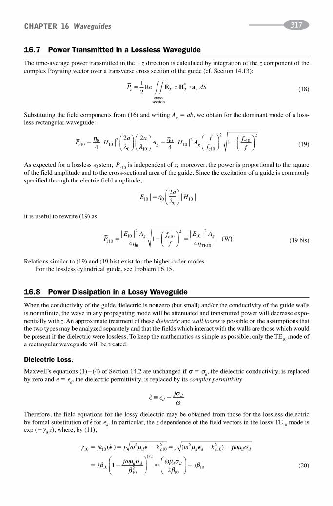
16.7 Power Transmitted in a Lossless Waveguide
The time-average power transmitted in the �z direction is calculated by integration of the z component of thecomplex Poynting vector over a transverse cross section of the guide (cf. Section 14.13):
CHAPTER 16 Waveguides 317
P x dSz T T z�1
2Re *
crosssection
� � E H a·
P Ha a
A Hz g100
102
0 10
010
2
4
2 2
4� �
ηλ λ
η⎛⎝⎜
⎞⎠⎟
⎛⎝⎜
⎞⎠⎟
AAf
ff
fgc
c
10
210
2
1⎛⎝⎜
⎞⎠⎟
⎛⎝⎜
⎞⎠⎟
�
Ea
H10 00
102
�ηλ
⎛⎝⎜
⎞⎠⎟
PE A f
f
E Az
g c g10
102
0
102
102
41
4� � �
η η⎛⎝⎜
⎞⎠⎟ TE10
W( ))
�̂ �� ddj
�σω
γ ω μ ω μ10 102
102 2
102� � � � � �jk j k j kd c d d c( ˆ ) ˆ ( )� � � jj
jj
d d
d d d d
ωμ σ
β ωμ σβ
ωμ σβ
� �10102
1 2
10
12
�⎛
⎝⎜⎞⎠⎟
/⎛⎛⎝⎜
⎞⎠⎟
� jβ10
(18)
Substituting the field components from (16) and writing Ag � ab, we obtain for the dominant mode of a loss-less rectangular waveguide:
(19)
As expected for a lossless system, –Pz10 is independent of z; moreover, the power is proportional to the square
of the field amplitude and to the cross-sectional area of the guide. Since the excitation of a guide is commonlyspecified through the electric field amplitude,
it is useful to rewrite (19) as
(19 bis)
Relations similar to (19) and (19 bis) exist for the higher-order modes.For the lossless cylindrical guide, see Problem 16.15.
16.8 Power Dissipation in a Lossy Waveguide
When the conductivity of the guide dielectric is nonzero (but small) and/or the conductivity of the guide wallsis noninfinite, the wave in any propagating mode will be attenuated and transmitted power will decrease expo-nentially with z. An approximate treatment of these dielectric and wall losses is possible on the assumptions thatthe two types may be analyzed separately and that the fields which interact with the walls are those which wouldbe present if the dielectric were lossless. To keep the mathematics as simple as possible, only the TE10 mode ofa rectangular waveguide will be treated.
Dielectric Loss.
Maxwell’s equations (1)�(4) of Section 14.2 are unchanged if σ � σd, the dielectric conductivity, is replacedby zero and � � �d, the dielectric permittivity, is replaced by its complex permittivity
Therefore, the field equations for the lossy dielectric may be obtained from those for the lossless dielectric by formal substitution of �̂ for �d. In particular, the z dependence of the field vectors in the lossy TE10 mode isexp (�γ10z), where, by (11),
(20)

CHAPTER 16 Waveguides318
β ω μ πλ10
210
210
010
221� d d c d ck k f f� �� � � �( ) ( / )
In (20),
(21)
and the binomial approximation presumes that σd and ω are small enough to make ωμdσd � β 210. To this order
of approximation, then, the wave number—the imaginary part of γ10 —in the lossy dielectric equals the wavenumber in the perfect dielectric; while the attenuation factor, αd � Re γ10, which governs the power loss in thedielectric, is given by
(22)α ωμ σβ
μ ση σd
d d d d d
cf f�
2 2 1
1
210 102
��
�/
( / )
�( )TE10 dd (Np/m)
αwz
P z
P z
P
P� �loss
av
loss( )
( )
( )
2
0
2 10
S Rsloss tang�1
22H
P R H ba
f fs closs (W/m)( ) ( / )0210
210
2� �⎡⎣⎢
⎤⎦⎥
αηwsc
c
c
c
R f
f
a b f f
ab f�
�
�
10
0 10
102
10
2
1
⎛
⎝⎜⎞⎠⎟
( / )
( // )f 2(Np/m)
Wall Loss.
The attenuation factor αw governing the wall loss may be determined indirectly, as follows. Because powervaries as the square of the field strength, the time-average transmitted power in the TE10 mode must obey
Pav(z) �–Pz10e �2αwz
where the entrance power –Pz10 is as given in (19). The power dissipated in the walls per unit z-length is thus
Ploss(z) � �P ′av(z) � 2αwPav(z)
whence (23)
All that remains is to calculate Ploss(0), the power flowing into the first 1 m of wall inner surface. Now, it is nothard to show that, at a wall surface, tangential H—which by hypothesis can be obtained from (16)—sets up aPoynting vector, of time-average magnitude
(24)
and directed into the wall. Here, Rs � Re ηw � ���πƒ��μw�/�σw (Section 14.7) is the surface resistance (Ω) of thewall material at the given frequency ƒ. Integrating the appropriate expression (24) over the first 1 m of each wallsurface and adding the results yields finally
(25)
From (23), (19), and (25),
(26)
in which Rsc10 is the surface resistance at the cutoff frequency of TE10 and η0 � ���μd /��d is the plane-waveimpedance of the (lossless) dielectric.
Combined Losses.
The total attenuation factor is αtot � αw � αd. To convert from Np/m to the more usual dB/m, see Problem 14.7.

SOLVED PROBLEMS
16.1. Give the boundary conditions on E and H at each perfectly conducting wall of the waveguide ofFig. 16-1(a).
At a perfect conductor tangential E and normal H must vanish. Therefore:
Top wall Ez(x, b) � Ex(x, b) � 0 and Hy(x, b) � 0
Left wall Ez(0, y) � Ey(0, y) � 0 and Hx(0, y) � 0
Right wall Ez(a, y) � Ey(a, y) � 0 and Hx(a, y) � 0
Bottom wall Ez(x, 0) � Ex(x, 0) � 0 and Hy(x, 0) � 0
16.2. Repeat Problem 16.1 for the guide of Fig. 16-1(b).
At the single cylindrical wall,
Ez(a, φ) � Eφ (a, φ) � 0 and Hr(a, φ) � 0
16.3. What is “critical” about the number kc?
For propagation through a lossless dielectric, the wave number k must be real. But
CHAPTER 16 Waveguides 319
k k k kc c� � � �ω μ2 202 2�
j Er
HjkHr
zωφ φ� � �
1 ∂∂
j E jkHH
rrzω φ� �� �
∂∂
where k0 is the wave number of a uniform plane wave in the unbounded dielectric at the given ω. Thus, kc is a
critical wave number in the sense that a guided wave’s same-frequency “twin” must have a wave number
exceeding kc. Stated otherwise, the frequency ƒ of the guided wave must exceed the quantity (u0 /2π )kc, where
u0 � 1/��μ� is the wave velocity in the unbounded dielectric.
16.4. Express Maxwell’s equations (1) and (2) of Section 14.2 in scalar form in a cylindrical coordinatesystem.
For the curl in cylindrical coordinates, see the Appendix. Equation (1) yields (σ � 0):
j Er r
rHr
Hz
rωφφ� � �
1 1∂∂
∂∂
( )
� � �j Hr
EjkEr
zω μφ φ
1 ∂∂
� �� �j H jkEE
rrzω μ φ
∂∂
� � �j Hr r
rEr
Ez
rωμφφ
1 1∂∂
∂∂
( )
Ej
k r
H jk
k
E
rrc
z
c
z�� �ωμ
φ2 2
1 ∂∂
∂∂
(i)
(ii)
(iii)
Equation (2) yields:
(iv)
(v)
(vi)
16.5. Using the equations of Problem 16.4, find all cylindrical field components in terms of Ez and Hz.
From (i) and (v), with kc as previously defined,
(1)

From (ii) and (iv),
CHAPTER 16 Waveguides320
Hj
k r
E jk
k
H
rrc
z
c
z� �ω
φ�
2 2
1 ∂∂
∂∂
Hj
k
E
r
jk
k r
H
c
z
c
zφ
ωφ
�� ��
2 2
1∂∂
∂∂
Ejk
k r
E j
k
H
rc
z
c
zφ φ
ω μ�� �2 2
1 ∂∂
∂∂
(2)
From (1) and (i),
(3)
From (2) and (ii),
(4)
16.6. Calculate ηTE from the field components in cylindrical coordinates.
With Ez � 0, (iv) and (v) of Problem 16.4 yield
HT rTE TE
rH Hk
Ek
E� � � � �2 2
22
22
φ φωμ ωμ⎛⎝⎜
⎞⎠⎟
⎛⎝⎜
⎞⎠⎟
kkTETωμ
E
η ωμTE
TE
�E
HT
T k�
E Ek
H Hk
z y y x T T2 2
22 2
� � � �TM or TM
ω ω� �
⎛
⎝⎜⎞
⎠⎟( ) E H
ηωTMTM�
E
HT
T
k�
�
E HT T x x y y y x x yE H E H H H H H· � � � �
�
Re ( ) Re ( )
Re
∗ ∗ ∗ ∗η η
η (( )H H H Hy x x y∗ ∗� � 0
E x y C k x D k x C k y D kz x x x x y y y( , ) ( cos sin )( cos sin� � � yy
x y c
y
k k k k
)
2 2 2 2� � �TM TM2�ω μ�
C km
aC k
n
bx x y y� � � �0 0π π
whence
16.7. Calculate ηTM from the field components in rectangular coordinates.
With Hz � 0, (2a) and (2b) give
whence
16.8. Show that E and H are mutually perpendicular in any TE or TM wave (as with ordinary plane waves).
For either type of wave Ex � ηHy and Ey � �ηHx; therefore, since η is real,
Because EzH*z also vanishes, E · H � 0.
16.9. Obtain the analogues of (9)�(12) for TMmn.
Analogous to (8),
where
But now the boundary conditions,
Ez(0, y) � Ez(a, y) � 0 and Ez(x, 0) � Ez(x, b) � 0
require that
where m, n � 1, 2, 3, …. Note that neither m nor n is zero in a TM mode.

The required formulas are
CHAPTER 16 Waveguides 321
(1)
(2)
(3)
(4)
E x y Em x
a
n y
bz mn mn( , ) sin sin�π π
km
a
n
bkc mn c mnTM TE� � �
π π⎛⎝⎜
⎞⎠⎟
⎛⎝⎜
⎞⎠⎟
2 2
k kmn mnTM TE�
ηωTMTM
mnk
��
∂∂
∂∂
∂∂
2
2 2
2
22 21 1
0E
r r
E
r r
Ek E kz z z
c z c� � � � �φ TM TM( ωω μ2 2� � kTM )
fu
axc np npTM � 0
2π
η ηλ
πTMnp
x
anp� �0
0
2
12
⎛
⎝⎜
⎞
⎠⎟
( )iii ′∂∂H
rz
r a�
� 0
16.10. Determine the TM modes of a lossless cylindrical waveguide.
The Laplacian in cylindrical coordinates is given in the Appendix; the wave equation (7) for Ez(r, φ) becomes
subject to the boundary conditions (i) Ez(r, φ � 2π ) � Ez(r, φ); (ii) Ez(0, φ) bounded; (iii) Ez(a, φ) � 0.
Following Section 9.8, one solves by separation of variables to find
Ez np(r, φ) � Enp Jn(kcTMnpr ) cos nφ (1)
where n � 0, 1, 2, … and where xnp � kcTMnpa is the pth positive root (p � 1, 2, …) of Jn(x) � 0. (The first fewsuch roots are listed in Table 16-1.)
The expression (1), together with Hz � 0, determines all transverse field components in TM via Problem 16.5.The cutoff frequency of TMnp is given by
n � 0 n � 1 n � 2 n � 3
p � 1 2.405 3.832 5.136 6.380
p � 2 5.520 7.016 8.417 9.761
p � 3 8.645 10.173 11.620 12.015
TABLE 16-1 Roots xnp of Jn(x) � 0
(2)
When (2) is used, all rectangular-guide formulas also apply to cylindrical guides; for example,
(3)
16.11. Determine the TE modes of a lossless cylindrical waveguide.
In a TE mode the axial field Hz(r, φ ) obeys the wave equation and the conditions (i) and (ii) of Problem 16.10. Asa consequence of (2) of Problem 16.5, condition (iii) must be replaced by
The solution by separation is therefore:
Hznp(r, φ) � Hnp Jn (kcTEnpr ) cos nφ (1)
where n � 0, 1, 2, … and where x′np � kcTEnp is the pth positive root (p � 1, 2, …) of J ′n(x) � 0. See Table 16-2.

The analogues of (2) and (3) of Problem 16.10 are
CHAPTER 16 Waveguides322
n � 0 n � 1 n � 2 n � 3
p � 1 3.832 1.841 3.054 4.201
p � 2 7.016 5.331 6.706 8.015
p � 3 10.173 8.536 9.969 11.346
TABLE 16-2 Roots x′np of J′n(x) � 0
fu
axc np npTE � 0
2π′
η η
λπ
TEnp
npx
a
�
�
0
0
2
12
′⎛
⎝⎜⎞
⎠⎟
Ej H
k rJ k rr
cc11
112 1 11�ωμ φ
TE11TE( )sin
Hjk H
kj k rr
c11
11 11
111�
� TE
TEcTE11′( )cos φ
Hjk H
k rJ k r
ccφ φ11
11 11
112 1 11� TE
TETE( )sin
Ej H
kJ k r
ccφ
ω μ φ1111
111 11�
TETE′( )cos
(2)
16.12. Discuss the relative magnitudes of ƒcTEnp and ƒcTMnp.
For each fixed n, the zeros xnp of Jn(x) and the stationary points x ′np—where Jn(x) is a maximum or a minimum—alternate along the x axis; this sine-wave-like behavior is clear in Fig. 9-3(a). For n � 0, the function starts at 0,and the first stationary point precedes the first positive zero; thus, x ′np � xnp, whence
kcTEnp � kcTMnp and ƒcTEnp � ƒcTMnp
For n � 0, the function starts at a maximum, and the ordering is reversed:
kcTE0p � kcTM0p and ƒcTE0p � ƒcTM0p
16.13. (a) What is the dominant mode of a lossless cylindrical waveguide? (b) List the first five modes inorder of increasing cutoff frequency.
(a) By Problem 16.12, the dominant mode is either TM01 or the TEn1 with the lowest cutoff. Tables 16-1 and16-2 indicate (and analysis establishes) that the winner is TE11.
(b) TE11, TM01, TE21, TE01, and TM11 (a tie). [The first column of Table 16-2 is identical to the second columnof Table 16-1 because J ′0(x) � �J1(x).]
16.14. Obtain the transverse fields for the TE11 (dominant) mode of a cylindrical waveguide.
For m � p � 1, Equation (1) of Problem 16.11, Ez � 0, and (1)�(4) of Problem 16.5 yield
(1)
(2)
(4)
in which kcTE11 � x ′11/a and kTE11 � ���ω 2μ���� ��(x ′11/�a)�2.
16.15. Calculate the time-average power transmission in the TE11 mode of a lossless cylindrical guide.
Follow Section 16.7, with the transverse fields as given by Problem 16.14.
(3)

(1)
CHAPTER 16 Waveguides 323
1
2
1
2 11 11 11 11E H aT T z r rE H E H
k
� � �
�
∗ ∗ ∗· ( )φ φ
ωμ TE11 HH
k
J v
vJ v
c
112
21
22
12
2 TE11
( )sin [ ( )] co⎡
⎣⎢⎤⎦⎥
′φ� ss2 φ⎧⎨⎩
⎫⎬⎭
Pk H
kJ v
Jz
c
x
1111
2
4 01
2 1
2
11
� �πωμ TE11
TE11�
′′[ ( )]
(( )v
vv dv⎡
⎣⎢⎤⎦⎥
⎧⎨⎩⎪
⎫⎬⎪
⎭
2
′′ ′⎛⎝⎜
⎞⎠⎟
Jv
Jv
J1 1 2 11
11
0� � � �
which the integration variable ν � kcTE11r has been introduced. In the integration of (1) over the cross section 0 φ 2π and 0 ν x ′11, the sin2 and cos2 both integrate to π; therefore,
(2)
There is a general rule for evaluating an integral like the one in (2): Go back to the ordinary differential equationarising from the separation of variables. In this case that equation is (see Section 9.8)
(3)
Thus, using integration by parts, (3), and the end conditions J1(0) � J ′1 (x ′11) � 0, we have
Substituting this result in (2), and replacing kTE11 and kcTE11 by their respective expressions in x ′11 � (2πa /u0)ƒcTE11, one finds after some algebra:
(4)
� �0 0
[(′ ′
′ ′⎛
⎝⎜⎞x x
J J v v dv JJ
v
11 11
12
12
11) ( / ) ]� � �⎠⎠⎟
⎡
⎣⎢⎢
⎤
⎦⎥⎥
′⎛
′
′
2
12
11
11
11
v dv d J
JJ
v
x
x
�
� �
�
�
0
0
( )
⎝⎝⎜⎞⎠⎟
⎡
⎣⎢⎢
⎤
⎦⎥⎥
⎛⎝⎜
⎞⎠⎟
′
′
22
12
11
1
2
1
2
dv
J x
vJ
�
�
( )
( �� � �
� �
J v JJ
v
Jv
J
x x
12
0
21
1
1
11 11
1
)′ ′
′⎡⎣⎢
⎤⎦⎥
′′ ′
�0
11 2 1 12
11
12
11
1
1
2
� �
�� �
vJ dv J x
J x
⎛
⎝⎜⎞⎠⎟
′
′′
( )
( ) �0
xx
v JJ
vJ dv
J x
11 21
11
12
111
2
′⎡⎣⎢
⎤⎦⎥
′′
� �
�� �
( )
( ) �0
xx x
v dJ
vJ dv
J x
11 112 12
12
12
11
2
1
2
⎛⎝⎜
⎞⎠⎟
′
′�
��
�0
( )�� ��1
2
1
22
12
0
112
12
11
11
v Jx
J xx′ ′ ′
( )( )
in which Ag � πa2 is the cross-sectional area.
16.16. Compare the rectangular and cylindrical waveguides as power transmitters when each operates in itsdominant mode.
The two power formulas, (19) of Section 16.7 and (4) of Problem 16.15, show identical dependence on H-amplitude,cross-sectional area, and normalized frequency. The only difference lies in a geometrical factor, which has the value1.0 for the rectangular guide and the value
P H Af
f
f
fz gc
c11
011
22
41� �
η
TE11
TE11⎛⎝⎜
⎞⎠⎟
⎛⎝⎜
⎞⎠⎟
22
112
112 1
211
1( )
( )( )
′′
′⎡
⎣⎢
⎤
⎦⎥
x
xJ x
�
( . )
( . )( . ) .
1 841 1
1 8410 5814 0 239
2
22�
�
for the cylindrical guide.

16.17. (a) Define the notion of cutoff wavelength. (b) Is the cutoff wavelength an upper limit on the guidewavelength, just as the cutoff frequency is a lower limit on the guide frequency?
(a) The cutoff wavelength λc is the wavelength of an unguided plane wave whose frequency is the cutofffrequency; i.e., λcƒc � u0.
(b) No; in fact, the formula
CHAPTER 16 Waveguides324
λmnu
f fcmn
��
02 2
γ π11 11 8
2 2 92
3 105 36 4 87 10 46 8� �
�� �jk j j( . ) ( . ) ( ) . mm 1�
η πTM11 � � �120 11
1 1157 5
2
..
⎛⎝⎜
⎞⎠⎟
Ω
fu
axcTM11 G� �
�
��
�0
11
8
22
3 10
3 103 832 12 2
π π ( )( . ) . HHz
λ110
2 2
8
2 2 9
3 10
14 12 2 104�
��
�
��
u
f fcTM11 ( ) ( . ) ( ).336
1 120 112 2
140
2
cm
TM11TM11η η π� � � �
f
fc⎛
⎝⎜⎞⎠⎟
⎛ .
⎝⎝⎜⎞⎠⎟
2
185� Ω
shows that an (m, n) mode can propagate with any guide wavelength greater than λ.
16.18. A lossless air-dielectric waveguide for an S-band radar has inside dimensions a � 7.214 cm and b � 3.404 cm. For the TM11 mode propagating at an operating frequency that is 1.1 times the cutofffrequency of the mode, calculate (a) critical wave number, (b) cutoff frequency, (c) operatingfrequency, (d ) propagation constant, (e) cutoff wavelength, (ƒ) operating wavelength, (g) guidewavelength, (h) phase velocity, (i ) wave impedance.
(a) By (10), kc11 � ��(π /0.��072��14)2�����(π /0.��0340��4)�2 � 102.05 rad/m.
(b) By (13), ƒc11 � [(3 � 108) /2π)] (102.05) � 4.87 GHz.
(c) ƒ � 1.1ƒc11 � 5.36 GHz.
(d ) By (11 bis),
(e) λc11 � u0 /ƒc11 � (3 � 108) /(4.87 � 109) � 6.16 cm.
(f ) λ0 � u0 /ƒ � (3 � 108) /(5.36 � 109) � 5.60 cm.
(g) λ11 � 2π /k11 � 2π/46.8 � 13.4 cm.
(h) By (15), u11 � (0.134)(5.36 � 109) � 7.18 � 108 m/s.
(i) For air, η0 � 120π Ω and (14) gives
16.19. A lossless, air-dielectric cylindrical waveguide, of inside diameter 3 cm, is operated at 14 GHz. Forthe TM11 mode propagating in the �z direction, find the cutoff frequency, guide wavelength, andwave impedance.
By (2) of Problem 16.10, along with Table 16-1,
Then, by (11 bis) and (14),
16.20. Find the inside diameter of a lossless air-dielectric cylindrical waveguide so that a TE11 modepropagates at a frequency of 10 GHz, with the cutoff wavelength of the mode being 1.3 times theoperating wavelength.
The condition is λc11 � 1.3λ0, or
u
f
u
ff
f
cc
0 01 31 3
7 692TE11
TE11or GHz� � �..
.

But, by Problem 16.11,
CHAPTER 16 Waveguides 325
fu
ax
dcTE11 GHz� �0112
0 31 841
π π′
.( . ) ( )
KH
k aK
H
kc cρ φ
ωμ ωμ� �11
211
TE11 TE11
E t E eK
Jrj t
ρω ζ ρρ φ ζ
ρρ( , , , ) Re [ ] ( . )( )� ���
11 1 1 841 ssin sin ( )
( , , , ) Re [ ]( )
φ ω ζ
ρ φ ζφ φω ζ
t
E t E e j t
�
� ��11 �� �K J tφ ρ φ ω ζ′1 1 841( . )cos sin ( )
1
ρρφ
ρ
φ
d
d
E
E�
d
dK
J
J
ρφ
ρρ
φ� 11
1
1 841
1 841
( . )
( . )tan
′
ln lnJ
JK K1
1 02 2
1 841
1 8410
( . )
( . )sec ( )
ρρ
φ� �
Equating the two expressions yields d � 2.28 cm.
16.21. Represent the E field of Problem 16.14 in the time domain, using as space variables ρ � r/a, φ,and ζ � kTE11z.
In terms of the lumped constants
which are presumed real, we have (x ′11 � 1.841):
16.22. For the E field obtained in Problem 16.21, calculate and plot the field lines. Also plot (withoutcalculation) the lines of the transverse H field.
The lines of any vector field are a family of space curves such that, at each point of space, the vector is tangent to thecurve through that point. Thus the differential equation of the lines of E in a cross-sectional plane is dy/dx � Ey /Ex, inCartesian coordinates (x, y), or
(1)
in polar coordinates (ρ, φ). Substitution in (1) of the components of E from Problem 16.21 gives
(2)
It is seen that the TE11 mode of a cylindrical waveguide has the special property that the field pattern does notchange with time or with distance ζ along the guide.
Normally, the field lines are found by a numerical integration of the differential equation; but in this case ananalytic solution is simply obtained:
(3)
This is a one-parameter family of curves, where the parameter ρ0 gives the radius at which a curve cuts thehorizontal axis sin φ � 0. Note that the right side of (3) does not change when φ is replaced by �φ or by φ � π ;hence the field pattern is symmetric about both the horizontal and vertical axes, and only the quadrant 0 φ π /2need be considered. As one moves along a field line through increasingly positive φ-values, the right side of (3)increases through positive values. Consequently [see Fig. 9-3(a)], ρ /ρ0 increases through values greater than 1.This, together with the constraint that the field line hit the boundary ρ � 1 orthogonally, shows that the field linemust bend away from the origin, as shown in Fig. 16-5. The line ρ0 � 1 degenerates into a single point.
EH
� 0.35ρ0
� 1ρ0
� 0°φ
� 90°φ � 0ρ0
Fig. 16-5

The lines of H are plotted as the orthogonal trajectories of the E lines; see Problem 16.8. By Problem 16.14 bothHρ and Hφ vanish at the points ρ � 1, φ � 0, π ; hence the direction of H is indeterminate there.
16.23. A lossless air-dielectric waveguide for an S-band radar system has the dimensions a � 7.214 cm andb � 3.404 cm. The dominant mode propagates in the �z direction at 3 GHz. Find the average powertransmitted if the excitation level of the E field is 10 kV/m.
The cutoff frequency for TE10 is
CHAPTER 16 Waveguides326
fu
ac100
8
2
3 10
2 0 072142 08� �
��
( . ). GHz
and (19 bis) yields
16.24. In a lossless air-dielectric cylindrical waveguide with a 1 cm radius the transmitted power in thedominant mode at 15 GHz is 2 W. Find the level of excitation for the magnetic field.
The cutoff frequency for TE11 is (see Table 16-2):
so that (4) of Problem 16.15 becomes (see also Problem 16.16):
The reader should verify that the underlying approximation, ωμdσd � β 210, holds for the data.
16.26. An X-band air-dielectric rectangular waveguide has brass walls (μw � μ0, σw � 16 MS/m) with a � 2.286 cm and b � 1.016 cm. Find the dB/m of attenuation due to wall loss when the dominantmode is propagating at 9.6 GHz.
At the cutoff frequency of the dominant mode,
and (22) gives (second form):
Solving, ⎪H11⎪ � 0.11 A/cm.
16.25. A section of X-band waveguide with dimensions a � 2.286 cm and b � 1.016 cm has perfectlyconducting walls and is filled with a lossy dielectric (σd � 367.5 μS/m, �r � 2.1, μr � 1). Find theattenuation factor, in dB/m, for the dominant mode of propagation at a frequency of 9 GHz.
The cutoff frequency of TE10 is
Pz10
4 2 410 7 214 3 404 10
4 3771
2 08
3� �
�( ) ( . )( . )
( )�
.⎛⎛⎝⎜
⎞⎠⎟
2
117 4� . W
fu
axcTE11 � �
�
��
�0
11
8
22
3 10
2 1 101 841 8 7
π π′
( )( . ) . 99 GHz
2377
410 15 8 79 1 8 79 15 0 211
2 4 2 2� ��H ( )( / . ) ( . / ) [ .π 339]
fu
ac100
8
2
3 10 2 1
2 0 022864 53� �
��
( )/ .
( . ). GHz
αd d( )( / . )( . )
( . / )B/m �
377 2 1 367 5 10
2 1 4 53 9
6
2
�
��
�
88 69 0 48. .�
fu
ac100
8
22
3 10
4 572 106 56� �
�
��
�.. GHz
Rsc10
9 7
6
6 56 10 4 10
16 1040 24�
� �
��
�π π( . )( ). mΩ
the surface resistance of the brass is

and, by (26),
CHAPTER 16 Waveguides 327
αw ( ). .
.
. (dB/m �
�0 04024
3779 6
6 56
0 02286 2 0⎛
⎝⎜
⎞
⎠⎟
.. )( . / . )
( . )( . ) ( .
01016 6 56 9 6
0 02286 0 01016 1 6 5
2
� 66 9 68 69 0 214
2/ . ). .� �
16.27. An air-dielectric cylindrical waveguide (a � 5 mm) operates in the TM01 mode at frequency ƒ � 1.3 ƒcTM01. Find the dB/m of attenuation due to wall loss in a short section of copper (σw � 58 MS/m).
First derive an expression for Ploss(0), following Section 16.8. By (1) of Problem 16.10, Ez01(r, φ) � E01J0(x01r /a).Then (3) of Problem 16.5 gives the tangential magnetic field at the wall as [J ′0(v) � �J1(v)]:
and, since Hφ01 is constant, (24) gives
(1)
Next find PzTM01 by the method of Problem 16.15. By Problem 16.15,
while Hr 01 � Eφ 01 � 0. Thus the time-average Poynting vector is
Integrating over a cross section,
Combining these results,
H aj x E J x
k
jE J
cφ φ ω
010 01 01 1 01
201 1( , )
( ) (� �
�
TM01a
xx ffc
01
0
)
η TM01
⎛
⎝⎜
⎞
⎠⎟
P RE J x f
fsc
lossTM01
( )( )
01
201
212
01
02
2
�η
⎛⎝⎜
⎞⎠⎟
⎡
⎣⎣⎢⎢
⎤
⎦⎥⎥( )2πa
Ejk E
kJ
x r
ajE
f
frc c
0101
101
01� �TM01
TM01 TM
⎛⎝⎜
⎞⎠⎟ 001
TM01⎛⎝⎜
⎞⎠⎟
⎛
⎝⎜⎞⎠⎟
⎛
⎝⎜⎜
⎞
⎠⎟⎟
⎛⎝⎜
1
2
101�
f
fJ
x r
ac ⎞⎞
⎠⎟
⎛⎝⎜
⎞⎠⎟
HjE f f
Jx r
ac
φ η0101
01
01�( / )TM01
S E HE f f f f
rc c� �
�1
2
1
201 0101
2 2 2
φ∗ ( / ) ( / )TM01 TM01
ηη012 01J
x r
a
⎛⎝⎜
⎞⎠⎟
� � �0 0
2
12 01
012 0 1
22 01ag
x
Jx r
ar dr d
A
xJ
πφ
⎛⎝⎜
⎞⎠⎟
� (vv v dv A J xg) ( )� 12
01
αη
ws
c
P
P
R
a f f� �
�
loss
zTM01 TM
( )
( / )
0
2 10 012
fu
axcTM01 � �
�
��
�0
01
8
32
3 10
2 5 102 405 22 9
π π ( )( . ) . 99
1 3 22 99 29 89
29
GHz
GHzf
fs
w
w
� �
� �
( . )( . ) .
( .R
π μσ
π 889 10 4 10
58 100 0451
0 0451
37
9 7
6
� �
��
�
�)( ).
.
(
π
α
Ω
w77 5 10 1 1 1 3
0 0374 0 3253 2)( ) ( / . )
. .� �
� ��
Np/m dB/m
(2)
For the data,

SUPPLEMENTARY PROBLEMS
16.28. Determine the condition(s) under which a magnetic field with
Hz(x, y, z, t) � K cos 87.3x cos 92.4y cos (2πƒt � 109.1z)
can exist in free space.
16.29. Obtain the critical wave number for a 4-GHz wave propagating in a medium with μr � 1 and �r � 2.2, if thephase shift constant (wave number) is 54° per cm.
16.30. If Hz(x, y, z, t) in Problem 16.28 represents the axial field of a TE21 wave in a rectangular waveguide, find (a) the guide size, (b) the critical wave number, (c) the guide wavelength.
16.31. The S-band waveguide of Problem 16.18 is used in the X-band at 9 GHz. Identify the modes that could propagatein the guide.
16.32. In Problem 16.19, what other modes could propagate at the given frequency?
16.33. A C-band waveguide for use between 3.95 and 5.85 GHz measures 4.755 cm by 2.215 cm. For air dielectric, calculatethe dominant mode cutoff frequency and the guide wavelength when the operating frequency is 4.2 GHz.
16.34. The WC-50 cylindrical waveguide with air dielectric is used in the frequency range 15.9–21.8 GHz for dominant-mode propagation. Calculate the cutoff frequency for an inside diameter of 1.270 cm. Also obtain the cutofffrequency for the TM01 mode.
16.35. An air-dielectric L-band rectangular waveguide has a /b � 2 and a dominant-mode cutoff frequency of 0.908 GHz.If the measured guide wavelength is 40 cm, find the operating frequency, the guide dimensions, and the wave number.
16.36. For the waveguide in Problem 16.35 find the lowest frequency at which a TE21 mode would propagate.
16.37. A V-band waveguide for use between 26.5 and 40 GHz has inside dimensions 0.711 cm by 0.356 cm. (a) Calculate the dominant-mode critical wave number for air dielectric. (b) If the measured guide wavelength is1.41 cm, what is the operating frequency?
16.38. The WC-19 air-dielectric cylindrical waveguide is used for dominant-mode operation in the 42.4–58.10 GHzrange. Find the inside diameter for the specified cutoff frequency of 36.776 GHz.
16.39. A Ku-band air-dielectric guide with a/b � 2 is used in the 12.4–18.8 GHz range for dominant-mode operationwith a cutoff frequency of 9.49 GHz. What are the inside dimensions?
16.40. Find the radius and guide wavelength in an air-dielectric cylindrical waveguide for the dominant mode at ƒ � 30 GHz � 1.5ƒcTE11. Will the TM11 mode propagate under these conditions?
16.41. Solve Problem 16.40 for the guide with a lossless dielectric of �r � 2.2.
16.42. A K-band rectangular waveguide with dimensions 1.067 cm and 0.432 cm operates in the dominant mode at 18 GHz.Find the cutoff frequency, guide wavelength, phase velocity, and wave impedance, if the dielectric is air.
16.43. Solve Problem 16.42 if the guide is filled with a lossless dielectric of �r � 2.0.
16.44. Calculate the radius and guide wavelength for a TM11 mode at ƒ � 30 GHz � 1.5ƒcTM11 in an air-dielectriccylindrical waveguide. [Compare Problem 16.40.]
16.45. For an (m, n) mode operated below its cutoff frequency, the cutoff attenuation factor is defined as αcmn � �jkmn.Calculate αcTE11, in dB/cm when a lossless air-dielectric guide, 2.286 cm by 1.016 cm is operated at 9.4 GHz.
16.46. In a certain cross section of a rectangular waveguide the instantaneous components of E are
CHAPTER 16 Waveguides328
E Ax
a
y
bE B
x
ay x�� �sin cos cosπ π π⎛
⎝⎜⎞⎠⎟
⎛⎝⎜
⎞⎠⎟
⎛⎝⎜
⎞⎠⎠⎟
⎛⎝⎜
⎞⎠⎟
sinπ y
bEz � 0
Sketch this E field and identify the mode of operation.
16.47. The air-dielectric waveguide of Problem 16.23 transports 200 W of average power at 2.6 GHz. Find the excitationlevel of the field.

16.48. If a lossless dielectric having �r � 1.8 is inserted in the waveguide of Problem 16.47, calculate the excitationlevel for the transport of 200 W.
16.49. The air-dielectric waveguide of Problem 16.24 is filled with a lossless dielectric having �r � 2.1. Find the powertransported in the dominant mode, if the excitation level and frequency are unchanged.
16.50. Show that result (2) of Problem 16.27 can be rewritten as where δw is the (frequencydependent) skin depth.
ANSWERS TO SUPPLEMENTARY PROBLEMS
16.28. ƒ � 8.0 GHz
16.29. 81.1 rad/m
16.30. (a) 7.2 cm by 3.4 cm; (b) 127.1 rad/m; (c) 5.76 cm
16.31. TE01, TE02, TE10, TE11, TE20, TE21, TE30, TE31, TE40; TM11, TM21, TM31
16.32. TE01, TE11, TE21, TE31; TM01
16.33. 3.155 GHz, 10.82 cm
16.34. 13.84 GHz, 18.08 GHz
16.35. 1.18 GHz, 16.52 cm by 8.26 cm, 15.7 rad/m
16.36. ƒ � 2.569 GHz
16.37. (a) 441.86 rad/m; (b) 29.98 GHz
16.38. 0.478 cm
16.39. 1.58 cm by 0.79 cm
16.40. 0.44 cm, 1.34 cm; No
16.41. 0.296 cm, 0.903 cm; No
16.42. 14.06 GHz, 2.67 cm, 4.81 � 108 m/s, 604.2 Ω
16.43. 9.93 GHz, 1.44 cm, 2.54 � 108 m/s, 319.6 Ω
16.44. 0.915 cm, 1.342 cm
16.45. 23.9
16.46. See Fig. 16-6; TE11
16.47. 143 V/cm
16.48. 106.8 V/cm
16.49. 0.09 A/cm
ασ δ ηw
w wa�
1
TM01
,
CHAPTER 16 Waveguides 329
y
b
a x0
Fig. 16-6

CHAPTER 17
330
Antennas(by Kai-Fong Lee)
17.1 Introduction
Maxwell’s equations as examined in Chapter 14 predict propagating plane waves in an unbounded source-freeregion. In this chapter the propagating waves produced by current sources or antennas are examined; in general,these waves have spherical wavefronts and direction-dependent amplitudes. Because free-space conditions areexclusively assumed throughout the chapter, the notation for the permittivity, permeability, propagation speed, andcharacteristic impedance of the medium can omit the subscript 0; likewise the wave number (phase shift constant)of the radiation will be written β � ω���μ� � ω /u.
17.2 Current Source and the E and H Fields
The vector magnetic potential A defined in Section 10.9 gives the phasor fields in the region outside of thecurrent source as
H A A� �1
μμη
∇∇ ∇∇�� ��
E H A A� � �1 1
j j jω ωμμβ� �
∇∇ ∇∇ ∇∇ ∇∇ ∇∇�� �� �� �� ��
(1)
in which u � 3 � 108 m/s and η � 120π Ω.The phasor A is itself given by
AJ
���
vol
(μπ
βs
j re
rdv
)
4
In (2), r is the distance between the observation point and the source current element Js dv. The significance ofthe factor e�jβr becomes clear when A is transformed to the time domain:
(2)
AJ
���
vol
μ ωπ
s t r u
rdv
cos ( / )
4
Thus, A at the observation point properly reflects conditions at the source at earlier times—the lag for any givensource element being precisely the time r/u needed for the condition to propagate to the observation point.
17.3 Electric (Hertzian) Dipole Antenna
The vector potential set up by the infinitesimal current element of Fig. 17-1 is, by (2),
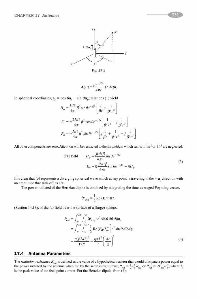
CHAPTER 17 Antennas 331
A a( ) ( )Pe
rI d
j r
z��μπ
β
4�
In spherical coordinates, az � cos θar � sin θ aθ ; relations (1) yield
θ
φ
z
I d az
P
y
x
r
Fig. 17-1
HI d
ej
r rj r
φβ
πβ θ
β β� ���
4
122 2
sin⎡
⎣⎢
⎤
⎦⎥
EI d
er
jr
E
rj r� �
�
�ηπ
β θβ β
η
β
θ
2
4
1 122 2 3 3
�cos
⎡⎣⎢
⎤⎦⎥
II de j
r rj
rj r�
4
1 1 122 2 3 3π
β θβ β β
βsin � � �⎡⎣⎢
⎤⎦⎥
All other components are zero. Attention will be restricted to the far field, in which terms in 1/r2 or 1/r3 are neglected.
Far field HjI d
re
EjI d
r
j rφ
β
θ
βπ
θ
η βπ
�
�
��
�4
4
sin
sin θθ ηβφe Hj r� �
It is clear that (3) represents a diverging spherical wave which at any point is traveling in the �ar direction withan amplitude that falls off as 1/r.
The power radiated of the Hertzian dipole is obtained by integrating the time-averaged Poynting vector,
(3)
��avg �1
2Re ( )E H*��
(Section 14.13), of the far field over the surface of a (large) sphere.
P r d d
E
rrad avg�
�
� �� �
0
2
0
2
0
2
0
1
2
π π
π π
θ θ φ�� · sin
Re(
a
θθ φ θ θ φ
η βπ
ηπλ
H r d d
I d I d
∗⎡⎣⎢
⎤⎦⎥
) sin
( )
2
2 2
12 3� �
� �⎛⎛⎝⎜
⎞⎠⎟
2
17.4 Antenna Parameters
The radiation resistance Rrad is defined as the value of a hypothetical resistor that would dissipate a power equal tothe power radiated by the antenna when fed by the same current, thus, Prad � 1–
2 I20 Rrad or Rrad � 2Prad/I 2
0, where I0is the peak value of the feed point current. For the Hertzian dipole, from (4),
(4)

CHAPTER 17 Antennas332
The pattern function F(θ, φ) gives the variation of the far-zone electric or magnetic field magnitude with direction.For the Hertzian dipole this reduces to F(θ) � sin θ, since ⎪E⎪ and ⎪H⎪ are independent of φ.
The radiation intensity U(θ, φ) is another measure of antenna performance; it is defined as the time-averagedradiated power per unit solid angle. From Fig. 17-2,
Ω
dS
avg��
dS´
r
d
Fig. 17-2
z z
1
θ
1
Halfpower
45º
45º
(a) F (θ) U ( )(b) θ
Fig. 17-3
Rd d
rad �2
3790
2 2πη
λ λ� �⎛
⎝⎜⎞⎠⎟
⎛⎝⎜
⎞⎠⎟
� ( )Ω
UdP
d
dS
dS rr( , )
/θ φ � rad avg
avg� �
����
′
′ 22
Because U is independent of r (by energy conservation), the far field may be used in its evaluation. For theHertzian dipole,
UI d
( ) sinθ ηλ
θ�8
22�⎛
⎝⎜⎞⎠⎟
Polar plots of the pattern function and radiation intensity distribution for the Hertzian dipole are given in Fig. 17-3.
(5)
In Fig. 17-3(b), the half-power points are at θ � 45° and θ � 135° and the half-power beamwidth is therefore 90°.In general, the smaller the beamwidth (about the direction of Umax), the more directive the antenna.
Directive gain D(θ, φ) of an antenna is defined as the ratio of the radiation intensity U(θ, φ) to that of ahypothetical isotropic radiator that radiates the same total power U0. For the isotropic radiator,
UP
0 � rad
4π
DU
U
U
P( , )
( , ) ( , )θ φ θ φ π θ φ� �
0
4
rad
The directivity of an antenna is the maximum value of its directive gain:
Then
DU
Pmaxmax�
4π
rad

For the Hertzian dipole, (4) and (5) give
D
I d
I d( , )
( ) sin
θ φπ η
λθ
ηπλ
�
48
3
22�
�
⎛⎝⎜
⎞⎠⎟
⎛⎝⎜
⎞⎠⎟
⎛⎝⎝⎜
⎞⎠⎟
221 5 1 5� �. sin .maxθ and D
The radiation efficiency of an antenna is �rad � Prad /Pin, where Pin is the time-averaged power that the antennaaccepts from the feed. The (power) gain G(θ, φ) is defined as the efficiency times the directive gain:
(6)
G DU
P
U
P( , ) ( , )
( , ) ( , )θ φ θ φ π θ φ π θ φ� �radin rad
� ��
4 4
PPL
where PL is the ohmic loss of the antenna. A lossless isotropic radiator has a power gain G0 � 1. At times thepower gain of an antenna is expressed in decibels, where
GG
GGdB � �10 1010
010log log
17.5 Small Circular-Loop Antenna
Also known as the magnetic dipole, a small loop in the z � 0 plane, carrying a phasor current Iaφ , produces radi-ating E and H fields with characteristics similar to those of the Hertzian dipole, but with the directions of E andH interchanged. In the far zone,
Ha Ie
rE H
j r
θ
β
φ θ
β ππ
θ
η
��
��
�( )sin
2 2
4
θ
zP
y
I
a
x
Fig. 17-4
The radiation resistance of the small loop antenna is found as part of Problem 17.6: Rrad � (20 Ω)(β 2πa 2)2.
17.6 Finite-Length Dipole
The expression (4) for the radiated power of the Hertzian dipole contains the term (d� /λ)2, which suggests thatthe length should be comparable to the wavelength. The open-circuited two-wire transmission line shown inFig. 17-5(a) has currents in the conductors that are out of phase, so that the far field nearly cancels out. An efficient antenna results when the line is opened out as shown in Fig. 17-5(b), producing current phasors
I z IL
z z Lm12
0 2( ) sin ( / )′ ′⎛
⎝⎜⎜
⎞
⎠⎟⎟ ′� � � �β
I z IL
z L zm2 22 0( ) sin ( / )′ ′
⎛
⎝⎜
⎞
⎠⎟ ′� � � � �βand
CHAPTER 17 Antennas 333
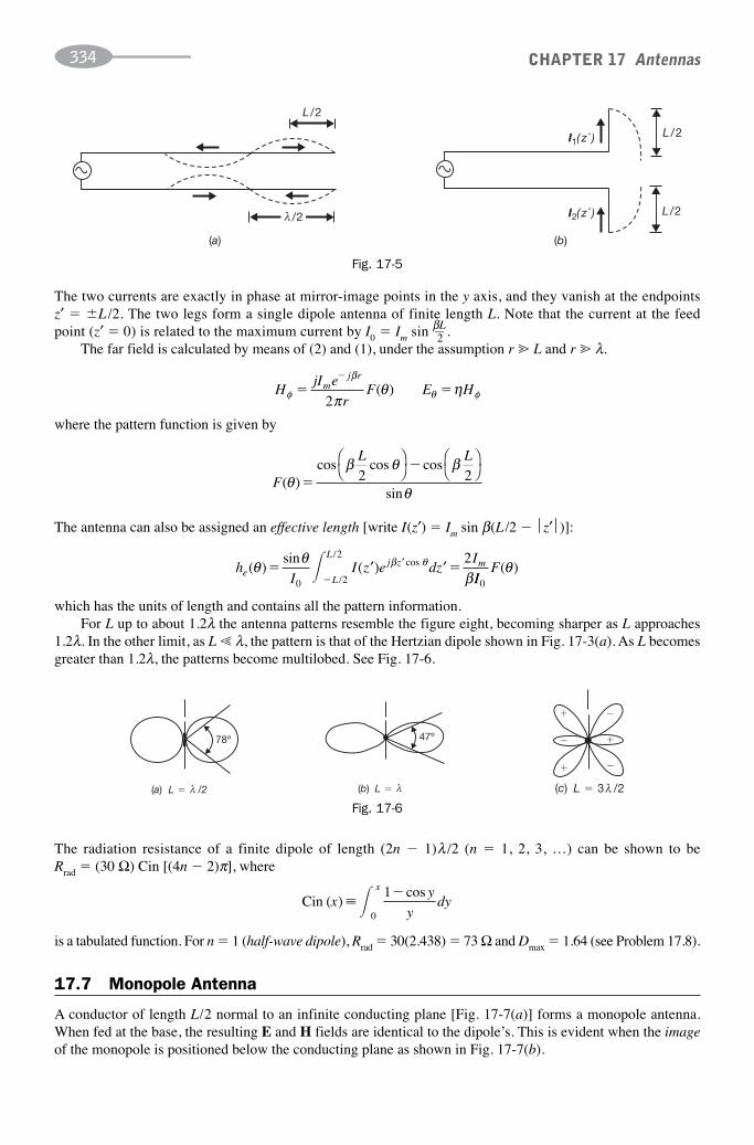
CHAPTER 17 Antennas334
The two currents are exactly in phase at mirror-image points in the y axis, and they vanish at the endpoints z′ � �L /2. The two legs form a single dipole antenna of finite length L. Note that the current at the feedpoint (z′ � 0) is related to the maximum current by I0 � Im sin βL—
2 .The far field is calculated by means of (2) and (1), under the assumption r � L and r � λ.
(a) (b)
λ /2
L/2
L/2
L/2
I1( z´ )
I2( z´ )
Fig. 17-5
HjI e
rF E Hm
j r
φ
β
θ φπθ η� �
�
2( )
where the pattern function is given by
F
L L
( )cos cos cos
sinθ
β θ β
θ�
�2 2
⎛⎝
⎞⎠
⎛⎝
⎞⎠
The antenna can also be assigned an effective length [write I(z′) � Im sin β(L /2 � ⎪z′⎪)]:
hI
I z e dzI
eL
Lj z m( )
sin( )
/
/cos�θ θ
ββ θ� �
�0 2
2 2� ′ ′′
IIF
0
( )θ
which has the units of length and contains all the pattern information.For L up to about 1.2λ the antenna patterns resemble the figure eight, becoming sharper as L approaches
1.2λ. In the other limit, as L � λ, the pattern is that of the Hertzian dipole shown in Fig. 17-3(a). As L becomesgreater than 1.2λ, the patterns become multilobed. See Fig. 17-6.
�
�
�
�
�
�
78º 47º
(c) L � 3 /2λ(b) λL �(a) λ /2L �
Fig. 17-6
The radiation resistance of a finite dipole of length (2n � 1)λ /2 (n � 1, 2, 3, …) can be shown to be Rrad � (30 Ω) Cin [(4n � 2)π], where
Cin ( )xy
ydy
x
� �0
1� cos
is a tabulated function. For n � 1 (half-wave dipole), Rrad � 30(2.438) � 73 Ω and Dmax � 1.64 (see Problem 17.8).
17.7 Monopole Antenna
A conductor of length L/2 normal to an infinite conducting plane [Fig. 17-7(a)] forms a monopole antenna.When fed at the base, the resulting E and H fields are identical to the dipole’s. This is evident when the imageof the monopole is positioned below the conducting plane as shown in Fig. 17-7(b).

As the monopole radiates power only in the region above the conducting plane, the total radiated power is one-halfthat of the corresponding dipole. From Rrad � 2Prad /I
20, it follows that the radiation resistance is one-half the value
for the dipole. Thus, for L /2 � λ /4 (quarter-wave monopole), Rrad � 36.5 Ω.
17.8 Self- and Mutual Impedances
With respect to its feed, an antenna is equivalent to a load impedance Za � Ra � jXa, where Ra � Rrad � RL, andRL is ohmic resistance. The reactance Xa is not easily calculated; it is a function of the radius ρ of the conduc-tors for dipoles and monopoles. Fig. 17-8 illustrates the variation of both Ra and Xa for monopoles of length L /2;the figure also applies to dipoles of length L if vertical scale values are doubled. Thus, the half-wave dipole hasRa � 73 Ω and, roughly independent of ρ, Xa � 40 Ω. (It can be shown that as ρ → 0, Xa → 42.5 Ω.)
When a second antenna is placed adjacent to a first antenna, a current in one will induce a voltage in theother. Consequently, a mutual impedance Z21 � V21/I1 � R21 � jX21 exists in the system. For two side-by-sidehalf-wave dipoles with very small conductor size, R21 and X21 vary with the separation d as shown in Fig. 17-9.
CHAPTER 17 Antennas 335
(a)
I (z )
I (z )
Imagecurrent
(b)
L/2
Fig. 17-7
100
� � 0.0035
0.0014
0.00035
0.00014
0.000035
Resistance
ρ λ
λ
0
�100
�200
�300
�400
�500
�6000.10 0.15 0.20 0.25 0.30
0
10
Length of monopole, L/2
20
30
40
50
60
70
ΩR
a,
ΩX
a,
Fig. 17-8 (Source: Edward C. Jordan/Keith G. Balmain, Electromagnetic Waves and Radiating Systems, 2nd ed.,© 1968, p. 548. Reprinted by permission of Prentice-Hall, Inc., Englewood Cliffs, N.J.).

17.9 The Receiving Antenna
An antenna in the far field of a transmitter extracts energy from what is essentially a plane wave and delivers it toa load impedance Zl. In Fig. 17-10(a) the dipole antenna lies along the z axis and the incident wave has a Poyntingvector �. The open-circuit voltage is equal to the product of the effective length he(θ) and the magnitude E of theprojection of E onto the plane of incidence. [For the coordinate system of Fig. 17-10(a), E � �����E2
y � E 2z���.]
VOC
� he(θ )E
The pattern for the receiving antenna is identical to that of a similar transmitting antenna. The available powerPa is the maximum power which the receiving antenna can deliver to a load, which occurs when Zl � Z*
a. Fromthe equivalent circuit of Fig. 17-10(b),
CHAPTER 17 Antennas336
X21
R21
�d λ�20
�40
80
60
40
20
01.0 2.0 3.0
ΩX
21,
R21
or
Fig. 17-9 (Source: Weeks (1968), Antenna Engineering. Reproduced by permission of McGraw-Hill, Inc.).
�
�
(b)(a)
z
θ
x
LOAD y
E
Za
VOC
ZL
Fig. 17-10
Ph E
Rae
a
�( )θ 2 2
8
The effective area Ae(θ ) for an antenna is a hypothetical area such that when multiplied by the power density ofthe incident wave, E2/2η, it results in the available power.
AE
Ph E
RA he a
e
ae e( )
( )( ) (θ
ηθ θ
2 2 2
2 8
⎛
⎝⎜⎜
⎞
⎠⎟⎟� � �or θθ η
)2
4Ra
⎛
⎝⎜
⎞
⎠⎟
It can be shown that the effective area is related to the directive gain by
A
De ( , )
( , )
θ φθ φ
λπ
�2
4

When both a transmitting and a receiving antenna are considered, the power Prad 1 radiated by antenna 1 and theavailable power Pa2 at the receiving antenna 2 are related by the Friss transmission formula,
CHAPTER 17 Antennas 337
z
r
I0d
x
y
lN �1
O
θ
P (r, , )θ
χ
φ
�
Fig. 17-11
P
P
D A
ra e2 1 1 1 2 2 2
24rad1
�( , ) ( , )θ φ θ φ
πHere, r is the separation of the two antennas. Angles θ1 and φ1 specify the direction of the receiving antenna asseen from the coordinate system of antenna 1. Similarly, θ2 and φ2 specify the direction of the transmittingantenna as viewed from the coordinate system of antenna 2.
17.10 Linear Arrays
A far-field pattern with a narrow beamwidth and high gain can be achieved by forming an array of identicalantenna elements, each with the same orientation as shown in Fig. 17-11. The pattern function of the array isequal to the pattern function of an individual element multiplied by an array factor ƒ(χ). In Problem 17.15 it isshown that, for a uniformly spaced array of N elements where d is the spacing
f a enj nd
n
N
( ) cosχ β χ��
�
0
1
∑
The angle χ is the angle between the array axis and the line OP; by geometry, cos χ � sin θ cos φ. If the ele-ments are progressively phased so that In � ane
jnα (n � 0, 1, …, N � 1),
f a enjn d
n
N
( ) ( cos )χ α β χ��
�+∑
0
1
or, defining u � α � βd cos χ,
f u a enjnu
n
N
10
1
( ) ��
�
∑
The overall pattern function will be a maximum when ⎪ƒ1(u)⎪ is a maximum, which occurs for u � 0. If α � 0(the individual antennas are all in phase), then u � 0 implies χ � �90°; i.e., peak radiation occurs at rightangles to the line of antennas. This is called a broadside array. On the other hand, if the phasing α � �βd isimposed, u � 0 implies χ � 0°; this is an endfire array.
A uniform array has all antenna currents equal in magnitude. For a0 � a1 � … � aN�1 � 1, (7) becomes
(7)
(8)f uNu
ue j N u
11 22
2( )
sin ( / )
sin ( / )( ) /� �
Thus, the main peak or lobe of the radiation pattern, centered on u � 0, has “height” ⎪ƒ1(0)⎪ � N. The two firstnulls of the pattern [zeros of ⎪ƒ1(u)⎪], occur at u � �2π /N. The separation of the two first nulls can be used todefine the beamwidth. Concentrating on the plane θ � 90°, one finds
Broadside uniform Δφ πβ
λ� �2
2 21sinNd Nd
�

where the approximations are for the case Nd �� λ.The sidelobes occur approximately midway between the nulls. The ratio of the main lobe to the first sidelobe
is N sin (3π /2N), which approaches the value 3π /2 for large N.
17.11 Reflectors
The gain of an antenna element can be enhanced by means of a reflector. Gains of from 6 to 12 dB can beobtained by using a half-wave dipole and a corner reflector such as that shown in Fig. 17-12(a). (A flat sheetreflector results when ψ � 180°.)
CHAPTER 17 Antennas338
Endfire uniform Δφ πβ
λ� �4
81sinNd Nd
�
E � ��j I e
re
j rn j Sη
π
π θ
θ
ββ0
2
21
cos cos
sin( ) s
⎛⎝⎜
⎞⎠⎟ iin cos( )θ ψ φ
θn
n
N�
�
�
0
2 1
∑ a
�
�
� x
Corner reflector
Half-wavedipole
(b)
S
S
Half-wavedipole
Conducting sheet
/2
(a)
ψψ
/2ψ
Image# 2
y
Image # 1
Fig. 17-12
2aFEED ATFOCUS
Fig. 17-13
The effect of a reflector with ψ � 180°/N (N � 1, 2, 3, …) can be calculated by the method of images. The actualreflector is replaced by 2N � 1 image dipoles, which together with the actual driven dipole constitute an evenlyspaced circular array, alternating in polarity [Fig. 17-12(b)]. Superposition of the far fields yields
For high-gain applications, the parabolic reflector driven by a source located at its focus, as shown in Fig. 17-13,is widely used. The directivity of the parabolic reflector is proportional to the aperture radius a and the apertureefficiency �:
(9)
Da
max �2
2πλ
⎛
⎝⎜
⎞
⎠⎟ �
The aperture efficiency depends on a variety of design factors; a reasonable value is 55%. The half-powerbeamwidth can be estimated from the formula HPBW � 117°(λ /2a).

SOLVED PROBLEMS
17.1. A center-fed dipole antenna with a z-directed current has electrical length L/λ �1—30
. (a) Show that thecurrent distribution may be assumed to be triangular in form. (b) Find the components of the vectormagnetic potential A.
(a) Since
CHAPTER 17 Antennas 339
P
z
x
y
r
θ
d
I d α
�
l I dl
r2
r1
Fig. 17-14
β β πλ
Lz
L L
2 2
1
10� � �
⎛
⎝⎜⎞⎠⎟
�
we have
I z IL
z
IL
zI
m
mm
( ) sin′ ′⎛⎝⎜
⎞⎠⎟
′⎛⎝⎜
⎞⎠⎟
′
� �
�
β
β
2
2
2� �
LL
Lz I I
Lm m
2 2� �′
⎛⎝⎜
⎞⎠⎟
′whereβ
from which
A a� ��
� �μπ
μβ
4
2
2
2
�L
L
z
j rmI z
e
rdz
I e
/
/( )′
⎛⎝⎜
⎞⎠⎟
′ ′ jj r
L
L
zm
Lr
Lz dz
I
r
Lβ
πμ
π4 2 4 22
2
��
� �/
/′
⎛⎝⎜
⎞⎠⎟
′ ′ ⎛a
⎝⎝⎜⎞⎠⎟
e j rz
� β a(b)
A AI
r
Le A Ar z
m j rz� � ���cos cos sinθ μ
πθβ
θ′ ⎛
⎝⎜⎞⎠⎟4 2
θθ μπ
θβ�� �′ ⎛⎝⎜
⎞⎠⎟
I
r
Lem j r
4 2sin
and Aφ � 0.
17.2. (a) Find the current required to radiate a power of 100 W at 100 MHz from a 0.01-m Hertziandipole. (b) Find the magnitudes of E and H at (100 m, 90°, 0°).
λλ
��
� � � � �3 10
103 790 8 78 10
8
8
23m radR
d�⎛⎝⎜
⎞⎠⎟
. Ω
(This extremely high current illustrates that an antenna with a length much less than a wavelength is not anefficient radiator.)
(a)
RP
IIrad
rad A� ��
��
2 200
8 78 101512 3.
E H� � � � �ηβπI d
r
� �
490 0 95 2 52 10 3sin . .V/m A/m
17.3. Two z-directed Hertzian dipoles are in phase and a distance d apart, as shown in Fig. 17-14. Obtain theradiation intensity in the direction (θ, φ).
(b)

Since cos α � sin θ sin φ,
CHAPTER 17 Antennas340
r rd
rd
r rd
1 22 2 2� � � � � �cos sin sin sin sinα θ φ θ φand
The far electric field is then E � Eθ aθ , with
EI d
re j
I d
re jj r j r
θβ β
πβη θ
πβη� �� �� �
4 42 1
2 1( sin ) ( ssin )
( )sin( ( / )sin sin
θ
βηπ
β β θ�j I d
re ej r j d�
42� � φφ β θ φ
ββηπ
θ
�
� �
e
j I d
re
j d
j r
( / )sin sin )
( )sin co
2
2
�ss sin sinβ θ φd
2
⎛⎝⎜
⎞⎠⎟
Consequently,
U rE I d d
� �22 2
22
2 8 2θη
η βπ
θ β θ⎛⎝⎜
⎞⎠⎟
( )sin cos sin s
�iinφ
⎛⎝⎜
⎞⎠⎟
For d � λ the cosine term is nearly 1 and
UI d� η βπ
θ( )sin
� 2
22
8
17.4. The far electric field of two Hertzian dipoles at right angles to each other (Fig. 17-15), fed by equal-amplitude currents with a 90° phase difference, is
E a� � ��j I d
re j jj rβη
πθ θ φβ
θ( )
[(sin cos cos ) ( sin�
4φφ) ]aφ
Find the far-zone magnetic field, the radiation intensity, the power radiated, the directive gain, and thedirectivity.
HE j I d
re j
HE
j rφ
θ β
θ
ηβ
πθ θ φ� � �
��
�( )(sin cos cos )
�4
φφ β
ηβ
πφ
ηη β
�
� �
�j I d
re
Ur I d
j r( )sin
( )
�
�4
2 3
2 2E E· *
2212
2 2
0
2
0
πφ θ
θ θ φ η βπ π
( sin sin )
sin(
�
� �P U d drad � � II d
DU
P
D
�)
( , ) ( sin sin )
max
2
2 2
64 3
41
π
θ φ π φ θ� � �rad
�� �D( , )90 903
2� �
z
y
x
I d�
jI d�
Fig. 17-15
17.5. A Hertzian dipole of length L � 2 m operates at 1 MHz. Find the radiation efficiency if the copperconductor has σc � 57 MS/m, μr � 1, and radius a � 1 mm.

As defined in Section 17.4,
CHAPTER 17 Antennas 341
�radrad
in
rad
rad loss
rad
radP� �
��
�
P P
P P
R
R RL
where Rrad is the radiation resistance and RL is the ohmic resistance. The radius a is much greater than the skin depth
δπ μσ
�1 1
15f c
� mm
so that the current may be assumed to be confined to a cylindrical shell of thickness δ.
RL
a
RL
Lc
� �
� �
1
20 084
7902
7
2
σ π δ( ).
( ) (
Ω
Ωrad
⎛⎝⎜
⎞⎠⎟
990 0 035
0 035
0 11929 4
2
Ω Ω) .
.
.. %
Lf
u
⎛⎝⎜
⎞⎠⎟
�
� ��rad
17.6. Find the radiation efficiency of a circular-loop antenna, of radius a � π�1 m, operating at 1 MHz. The loop is made of AWG 20 wire, with parameters aw � 0.406 mm, σ � 57 MS/m, and μr � 1.
At 1 MHz the skin depth is δ � 0.667 μm. Assuming the current is in a surface layer of thickness δ, the ohmicresistance is
Ra
aLw
� �1 2
20 206
σπ
π δ
⎛
⎝⎜
⎞
⎠⎟ . Ω
Taking the far-zone magnetic field from Section 17.5,
P H r d da I
rad � �� �0
2
0
2 22 2 2 21
2 12
π π
θη θ θ φ η β ππ
sin( )
�� ( )( )10 2 2 2 2Ω β πa I
from which
RP
Iarad
rad2
� � �2
20 0 392 2 2( )( ) .Ω Ωβ π μ
17.7. Find the radiation resistance of dipole antennas of lengths (a) L � λ /2 and (b) L � (2n � 1) λ—2,
n � 1, 2 …
�radrad
rad
��
� � �R
R RL
1 89 10 4. %and
PE
r d d Imrad � �1
2 230
0
2
0
2
0
2 2
0� � �
π πθ
π
ηθ θ φ
β
sin
cosLL L
d2 2
2
cos cos
sin
θ β
θθ
⎛⎝⎜
⎞⎠⎟
⎛⎝⎜
⎞⎠⎟
⎧⎨⎪
⎩⎪
⎫⎬⎪
⎭⎪�
RP
I
I
I
L
mrad
rad� �
�2 60 2
02
2
02 0
�π
β θcos cos c⎛⎝⎜
⎞⎠⎟
oos
sin
L
d2
2⎛⎝⎜
⎞⎠⎟
⎧⎨⎪
⎩⎪
⎫⎬⎪
⎭⎪θ
θ
(a)
For the half-wavelength dipole L � λ/2 and II
LIm � �0
0
2sin β
⎛⎝⎜
⎞⎠⎟
R drad � 602
0
2
�π
π θ
θθ
cos cos
sin
⎛⎝⎜
⎞⎠⎟

Let x � cos θ
CHAPTER 17 Antennas342
R
x
xdxrad �
��
�
� �60 2
1
30
2
11
1
2 1
1
� �cos
( )
cosπ
π⎛⎝
⎞⎠ xx
x
x
xdx
1
1
1��
�
�
cos π⎧⎨⎩
⎫⎬⎭
Since the two terms within the brackets are equal
Rx
xdxrad �
�
��30
1
11
1
� cos π⎛⎝⎜
⎞⎠⎟
letting y � π (1 � x)
Ry
ydy
R
rad
rad
Cin (2 )��
�
�
301
30
30
0
2
�π
πcos⎛⎝⎜
⎞⎠⎟
(( . )2 48 73� Ω
(b) For L � (2n � 1) λ–2, a similar approach yields
Rrad � 30 Cin [(4n � 2)π] Ω
17.8. Find the directivity Dmax of a half-wave dipole.
From Section 17.6, for βL /2 � π /2,
HI
rH
Iφ φπ
π θ
θ π� �0 0
2
2
2
cos cos
sin max
⎛⎝⎜
⎞⎠⎟
whencerr
the maximum being attained at θ � 90°. It follows that
U r HI
max max� �2 2 0
2
22 8
η ηπφ
From Problem 17.7,
PI
rad Cin (2 )�η
ππ0
2
8
17.9. A 1.5-λ dipole radiates a time-averaged power of 200 W in free space at a frequency of 500 MHz.Find the electric and magnetic field magnitudes at r � 100 m, θ � 90°.
From Problem 17.7, Rrad � (30 Ω) Cin (6π) � 105.3 Ω, and so
DU
Pmaxmax .� � �
4 41 64
ππrad Cin (2 )
Thus,
IP
R02 2 200
105 31 95� � �rad
rad
A( )
..
For a 1.5λ dipole, ⎪I0⎪ � ⎪Im⎪.
From Section 17.6,
HI
rFm
rφ π π( ) ( )
.
( )(100
290
1 95
2 100100m, 90
m
� �� ��
11 3 1
100 120 3 1 10 13
) .
( ) ( )( . ) .
�
� � ��
mA/m
m, 90Eθ π� 117 V/m
17.10. Obtain the image currents for a dipole above a perfectly conducting plane, for normal and parallelorientations.
The basic principle of imaging in a perfect conductor is that a positive charge is mirrored by a negative charge,and vice versa. By convention, electric currents are attributed to the motion of positive charges. Hence, for thetwo orientations, the image dipoles are constructed as in Fig. 17-16.

17.11. Calculate the input impedances for two side-by-side, half-wave dipoles with a separation d � λ /2.Assume equal-magnitude, opposite-phase feed-point currents.
The two feed-point voltages are given by
V1 � I1Z11 � I2Z12 V2 � I1Z21 � I2Z22
where Z12 � Z21; consequently,
CHAPTER 17 Antennas 343
ACTUALDIPOLE ACTUAL
DIPOLE
IMAGEDIPOLE
IMAGEDIPOLE
�
� � �
��
�
� ��
�
�
I
I
I
I
I I
II
��
(a) Normal (b) Parallel
Fig. 17-16
z2
z1
r � 100 m
2 � 90ºθ
θ1� 60º
Fig. 17-17
ZV
IZ
I
IZ
ZV
IZ
I
I
11
111
2
112
22
222
1
2
�
�
� �
� �
⎛⎝⎜
⎞⎠⎟
⎛⎝⎜⎜
⎞⎠⎟
Z12
For half-wave dipoles Fig. 17-8 gives Z11 � Z22 � 73 � j42.5 Ω and Fig. 17-9 gives Z12 � �12.5 � j28 Ω. Then,with I1 � �I2,
Z1 � Z2 � 73 � j42.5 � (�12.5 � j28) � 85.5 �j70.5 Ω
17.12. Three identical dipole antennas with their axes perpendicular to the horizontal plane, spaced λ /4 apart,form a linear array. The feed currents are each 5 A in magnitude with a phase lag of π /2 radians betweenadjacent elements. Given Z11 � 70 Ω, Z12 � �(10 � j20) Ω, and Z13 � (5 � j10) Ω, calculate the powerradiated by each antenna and the total radiated power.
From V1 � I1Z11 � I2Z12 � I3Z13,
ZV
IZ
I
IZ
I
IZ1
1
111
2
112
3
113 70� � � � � �
⎛⎝⎜
⎞⎠⎟
⎛⎝⎜
⎞⎠⎟
ee j e jj j� �� � � � �π π/ ( ) ( )2 10 20 5 10 45 Ω
Similarly, Z2 � 70 Ω and Z3 � (85 � j20) Ω. It follows that
P I Z Prad1 rad2W� � � �1
2
1
225 45 562 5 871
21Re ( ) ( )( ) . 55 1065 2W Wrad3P � .
for a total of 2500 W.
17.13. Two half-wave dipoles are arranged as shown in Fig. 17-17, with #1 transmitting 300 W at 300 MHz.Find the open-circuit voltage induced at the terminals of the receiving #2 antenna and its effective area.

For a half-wave dipole (I0 � Imax), Section 17.6 gives
CHAPTER 17 Antennas344
he( )
cos cos
sinθ
β
π θ
θ�
2 2
⎛⎝⎜
⎞⎠⎟
and, at 300 MHz, β � 2π. For #1,
IP
R01
2 2 300
732 87� � �
rad1
rad1
A( )
.
and the far field at angle θ1 is of magnitude
E( ) ( )
cos cos
θ ηβπ
θ ηπ
π θ
101
101
1
4 2
2� �
I
rh
I
re
⎛⎝⎜
⎞⎠⎟⎟
sinθ1
Consequently,
V hI
reOC2 2 101
12� �( ) ( )
cos cos cos
θ θ ηβπ
π θE
⎛⎝⎜
⎞⎠⎟
ππ θ
θ θ2 2
1 2
cos
sin sin
⎛⎝⎜
⎞⎠⎟
Substituting the numerical values gives ⎪VOC2⎪ � 0.449 V.
The effective area of antenna #2
17.14. For the antenna arrangement of Problem 17.13 find the available power at antenna #2.
From Section 17.9,
Au
Rhe e( ) ( ) .90
490 0 131
2� �� �rad
2m
Ph
R
V
Rae� � �( ) ( ) ( . )
(
θ θ22
12 2 2
8 8
0 449
8
E
rad
OC2
rad 773344
)� μW
17.15. Derive the array factor for the linear array of Fig. 17-11 (redrawn as Fig. 17-18).
x
y
z
dr
r 1
r 2
χ
l N�1
l2
l1
l0
Fig. 17-18
The far electric field of the nth dipole (n � 0, 1, …, N � 1) is, by Section 17.6,
E ann
j r
n
nj r ndj I e
rF
j I en
�� � �η
πθ ηβ
θ
β χ
2 2( )
( cos )
�ππ χ
θ
ηπ
θ
θ
β
θ
( cos )( )
( )
r ndF
j e
rF I
j r
n
�
�
a
a�2
⎡⎣⎢
⎤⎦⎥
ee j ndβ χcos
By superposition, the field at P is
E E a( ) [ ( ) ( )]Pj e
rF fn
j r
n
N
� ��
�
� ηπ
θ χβ
θ20
1
∑
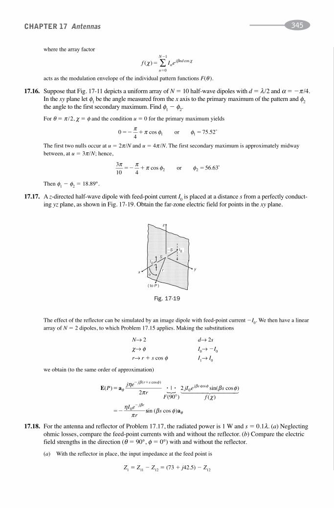
where the array factor
CHAPTER 17 Antennas 345
x
( to P )
I0
I0
y
z
�S
S
rφ
Fig. 17-19
f I enj nd
n
N
( ) cosχ β χ��
�
0
1
∑
acts as the modulation envelope of the individual pattern functions F(θ ).
17.16. Suppose that Fig. 17-11 depicts a uniform array of N � 10 half-wave dipoles with d � λ/2 and α � �π /4.In the xy plane let φ1 be the angle measured from the x axis to the primary maximum of the pattern and φ2the angle to the first secondary maximum. Find φ1 � φ2.
For θ � π /2, χ � φ and the condition u � 0 for the primary maximum yields
04
75 521�� � �π π φ φcos .or 1
�
The first two nulls occur at u � 2π /N and u � 4π /N. The first secondary maximum is approximately midwaybetween, at u � 3π /N; hence,
3
10 456 632 2
π π π φ φ�� � �cos .or �
Then φ1 � φ2 � 18.89°.
17.17. A z-directed half-wave dipole with feed-point current I0 is placed at a distance s from a perfectly conduct-ing yz plane, as shown in Fig. 17-19. Obtain the far-zone electric field for points in the xy plane.
The effect of the reflector can be simulated by an image dipole with feed-point current �I0. We then have a lineararray of N � 2 dipoles, to which Problem 17.15 applies. Making the substitutions
N→ 2 d→ 2s
χ→ φ I0→ �I0
r→ r � s cos φ I1→ I0
we obtain (to the same order of approximation)
E a( ) |
( )
( cos )
Pj e
rF
jI ej r s
j s�� �
θ
β φβη
π290
2 0· ·�
�ccos sin( cos )
( )
φ
β
β φχ
ηπ
s
f
I e
r
j r
� �
���
0 ssin ( cos )β φ θs a
17.18. For the antenna and reflector of Problem 17.17, the radiated power is 1 W and s � 0.1λ. (a) Neglectingohmic losses, compare the feed-point currents with and without the reflector. (b) Compare the electricfield strengths in the direction (θ � 90°, φ � 0°) with and without the reflector.
(a) With the reflector in place, the input impedance at the feed point is
Z1 � Z11 � Z12 � (73 � j42.5) � Z12
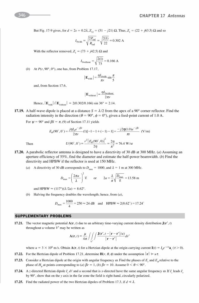
But Fig. 17-9 gives, for d � 2s � 0.2λ, Z12 � (51 � j21) Ω. Thus, Z1 � (22 � j63.5) Ω and so
CHAPTER 17 Antennas346
IP
R0withrad
rad
A� � �2 2 1
220 302
( ).
With the reflector removed, Z1 � (73 � j42.5) Ω and
I0without A� �2 1
730 166
( ).
(b) At P(r, 90°, 0°), one has, from Problem 17.17,
Ewith0with�
ηπ
πI
rsin
5
and, from Section 17.6,
Ewithout0without�
ηπ
I
r2
Hence, ⎪Ewith⎪/⎪Ewithout⎪ � 2(0.302/0.166) sin 36° � 2.14.
17.19. A half-wave dipole is placed at a distance S � λ /2 from the apex of a 90° corner reflector. Find theradiation intensity in the direction (θ � 90°, φ � 0°), given a feed-point current of 1.0 A.
For ψ � 90° and βS � π, (9) of Section 17.11 yields
Ej I e
r
jj r
θ
βηπ
( , ) ( )[ ( ) ]90 02
1 1 1 1 120� � � � � � � � �
�� ηηπ
β( . )1 0 e
t
j r�
(V/m)
17.20. A parabolic reflector antenna is designed to have a directivity of 30 dB at 300 MHz. (a) Assuming anaperture efficiency of 55%, find the diameter and estimate the half-power beamwidth. (b) Find thedirectivity and HPBW if the reflector is used at 150 MHz.
(a) A directivity of 30 dB corresponds to Dmax � 1000, and λ � 1 m at 300 MHz.
Ur E
( , )( , )
.90 090 0
2
276 4
2 2
2� �
�
� � �θ
ηη
πW/srThen
Da
aD
maxmax .� � �
213 58
2πλ
λπ
⎛
⎝⎜⎞⎠⎟
��
or 2 m
and HPBW � (117°)(λ /2a) � 8.62°.
(b) Halving the frequency doubles the wavelength; hence, from (a),
Dmax ( . ) .� � �1000
4250 24 2 8 62 17 24� �dB and HPBW � �
SUPPLEMENTARY PROBLEMS
17.21. The vector magnetic potential A(r, t) due to an arbitrary time-varying current density distribution J(r′, t)throughout a volume V′ may be written as
A rJ r r r
r r( , )
( , / )t
t udv
V
�� �
�
μπ4
′
′ ′′
′� � �
where u � 3 � 108 m/s. Obtain A(r, t) for a Hertzian dipole at the origin carrying current I(t) � I0e�t/τaz (τ � 0).
17.22. For the Hertzian dipole of Problem 17.21, determine H(r, θ, φ) under the assumption ⎪r⎪ � uτ.
17.23. Consider a Hertzian dipole at the origin with angular frequency ω. Find the phases of Er and Eθ relative to thephase of Hφ at points corresponding to (a) βr � 1, (b) βr � 10. Assume 0 � θ � 90°.
17.24. A z-directed Hertzian dipole Iz d� and a second that is x-directed have the same angular frequency ω. If Iz leads Ix
by 90°, show that on the y axis in the far zone the field is right-hand, circularly polarized.
17.25. Find the radiated power of the two Hertzian dipoles of Problem 17.3, if d � λ.

17.26. A short dipole antenna of length 10 cm and radius 400 μm operates at 30 MHz. Assume a uniform currentdistribution. Find (a) the radiation efficiency, using σ � 57 MS/m and μ � 4π � 10�7 H/m; (b) the maximumpower gain; (c) the angle θ at which the directive gain is 1.0.
17.27. Consider the combination of a z-directed Hertzian dipole of length Δ� and a circular loop in the xy plane of radius a,shown in Fig. 17-20. (a) If Iz and Iφ are in phase, obtain a relationship among Iz, Iφ, and a such that the polarization iscircular in all directions. (b) Is linear polarization possible? If so, what is the phase relationship?
CHAPTER 17 Antennas 347
Iz
Ix
z
y
�
Fig. 17-20
EE
x
y
x
(a) (b)
45ºλ /2
dipole
dipole
y
Fig. 17-21
17.28. A 1-cm-radius circular-loop antenna has N turns and operates at 100 MHz. Find N for a radiation resistance of 10.0 Ω.
17.29. A half-wave dipole operates at 200 MHz. The copper conductor is 406 μm in radius. Find the radiation efficiencyand maximum power gain, if σ � 57 MS/m and μ � 4π � 10�7 H/m.
17.30. Obtain the ratio of the maximum current to the feed-point current for dipoles of length (a) 3λ /4, (b) 3λ /2.
17.31. A short monopole antenna of length 10 cm and conductor radius 400 μm is placed above a perfectlyconducting plane and operates at 30 MHz. Assuming a uniform current distribution, find the radiationefficiency. Use σ � 57 MS/m and μ � 4π � 10�7 H/m.
17.32. Two half-wave dipoles are placed side-by-side with separation 0.4λ. If I1 � 2I2 and #1 is connected to a 75-Ωtransmission line, find the standing-wave ratio on the line. [Recall that the reflection coefficient Γ is (Z1 � Z0) /(Z1 � Z0) and the standing-wave ratio is (1 � ⎪Γ⎪)/(1 � ⎪Γ⎪).]
17.33. A driven dipole antenna has two identical dipoles as parasitic elements; both spacings are 0.15λ. Given that Z12 � (64 � j0) Ω and Z13 � (33 � j33) Ω, find the driving-point impedance at the active dipole.
17.34. In Fig. 17-21(a) a half-wave dipole operates as a receiving antenna and the incoming field is E � 4.0e�j2π xay
(mV/m). Let the available power be Pa1. In Fig. 17-21(b) a 3λ /2 dipole lies in the xy plane at an angle of 45° withthe y axis. The same incoming field is assumed, and the available power is Pa2. Find the ratio Pa1/Pa2.
17.35. Find the effective area and the directive gain of a 3λ/2 dipole that is used to receive an incoming wave of 300 MHZarriving at an angle of 45° with respect to the antenna axis.
17.36. Consider a uniform array of 10 z-directed half-wave dipoles with spacing d � λ /2 and with α � 0°. With thearray axis along x, find the ratio of the magnitudes of the E fields at P1(100 m, 90°, 0°) and P2(100 m, 90°, 30°).
17.37. Eleven z-directed half-wave dipoles lie along the x axis, at x � 0, �λ /2, �λ, �3λ /2, �2λ, �5λ /2. Let the feed-point current of the nth element be In � I0e
jnα. A half-wave dipole receiving antenna is placed with its center at(100 m, 90°, 30°). (a) Determine α and the orientation of the receiving dipole such that the received signal is amaximum. (b) Find the open-circuit voltage at the terminals of the receiving antenna when I0 � 1.0 A.
17.38. A half-wave dipole is placed at a distance S � λ/2 from the apex of a 60° corner reflector; the feed current is 1.0 A.Find the radiation intensity in the direction (θ � 90°, φ � 0°).
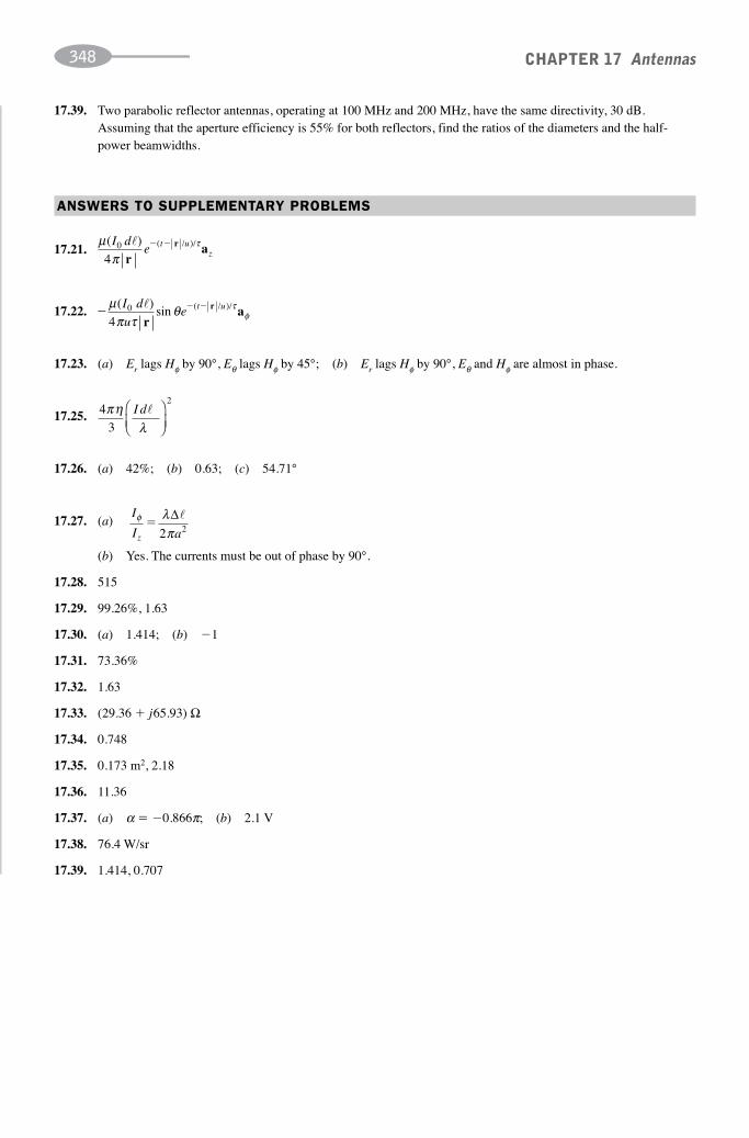
17.39. Two parabolic reflector antennas, operating at 100 MHz and 200 MHz, have the same directivity, 30 dB.Assuming that the aperture efficiency is 55% for both reflectors, find the ratios of the diameters and the half-power beamwidths.
ANSWERS TO SUPPLEMENTARY PROBLEMS
17.21.
17.22.
17.23. (a) Er lags Hφ by 90°, Eθ lags Hφ by 45°; (b) Er lags Hφ by 90°, Eθ and Hφ are almost in phase.
17.25.
17.26. (a) 42%; (b) 0.63; (c) 54.71°
17.27. (a)
(b) Yes. The currents must be out of phase by 90°.
17.28. 515
17.29. 99.26%, 1.63
17.30. (a) 1.414; (b) �1
17.31. 73.36%
17.32. 1.63
17.33. (29.36 � j65.93) Ω
17.34. 0.748
17.35. 0.173 m2, 2.18
17.36. 11.36
17.37. (a) α � �0.866π; (b) 2.1 V
17.38. 76.4 W/sr
17.39. 1.414, 0.707
I
I az
φ λπ
�Δ�
2 2
4
3
2πη
λI d�⎛
⎝⎜⎞⎠⎟
�� �μ
π τθ τ
φ( )
sin ( / )/I d
ue t u0
4
�r
ar
μπ
τ( ) ( / )/I de t u
z0
4
�r
ar� �
CHAPTER 17 Antennas348

349
Divergence, Curl, Gradient, and Laplacian
APPENDIX
FACTOR PREFIX SYMBOL FACTOR PREFIX SYMBOL
1018 exa E 10�1 deci d1015 peta P 10�2 centi c1012 tera T 10�3 milli m109 giga G 10�6 micro μ106 mega M 10�9 nano n103 kilo k 10�12 pico p102 hecto h 10�15 femto f10 deka da 10�18 atto a
SI Unit Prefixes
Cartesian Coordinates
Cylindrical Coordinates
Spherical Coordinates
∇ ∂∂
∂∂
∂∂
∇∂∂
∂∂
⎛⎝⎜
⎞⎠⎟
· A
A a
� � �
� �
A
x
A
y
A
z
A
y
A
z
x y z
z y�� xx
x zy
y xz
A
z
A
x
A
x
A
y� � � �
∂∂
∂∂
⎛⎝⎜
⎞⎠⎟
∂∂
∂∂
⎛⎝⎜
⎞⎠⎟
∇
a a
VVV
x
V
y
V
z
VV
x
V
y
x y z� � �
� � �
∂∂
∂∂
∂∂
∇ ∂∂
∂∂
∂
a a a
22
2
2
2
2VV
z∂ 2
∇ ∂∂
∂∂
∂∂
∇∂∂
∂
· A
A
� � �
� �
1 1
1
r rrA
r
A A
z
r
A A
rz
z
( ) φ
φ
φ
φ��
∂∂⎛⎝⎜
⎞⎠⎟
∂∂
∂∂
⎛⎝⎜
⎞⎠⎟
∂∂
−z
A
z
A
r r rrAr
r za a� � �φ φ1
( )∂∂∂
⎡⎣⎢
⎤⎦⎥
∇ ∂∂
∂∂
∂∂
∇
A
VV
r r
V V
z
V
rz
r z
φ
φ φ
a
a a a� � �
�
1
2 11 12
2
2
2
2r rr
V
r r
V V
z
∂∂
∂∂
⎛⎝⎜
⎞⎠⎟
∂∂
∂∂
� �φ
∇ ∂∂
∂∂
∂· A � � �
1 1 12
2
r rr A
rA
r
Ar( )
sin( sin )
sinθ θθ
θθφφ
φθ
φ
θ θθ
φ
∂
∇ ∂∂
∂∂
⎡⎣⎢
⎤⎦⎥
��A a� � �1 1 1
rA
A
rrsin( sin )
ssin( ) ( )
θ φ φ θ θ∂∂
∂∂
⎡⎣⎢
⎤⎦⎥
∂∂
∂∂
A
rr A
r rrA
Ar r� � �a1
θθ
θ θ φ
φ
θ φ
⎡⎣⎢
⎤⎦⎥
∇ ∂∂
∂∂
∂∂
∇
a
a a aVV
r r
V
r
Vr� � �
1 1
2
sin
VVr r
rV
r r
V� �
1 12
22
∂∂
∂∂
⎛⎝⎜
⎞⎠⎟
∂∂
∂∂
⎛⎝⎜sinsin
θ θθ
θ⎞⎞⎠⎟
∂∂
�1
2 2
2
2r
V
sin θ φ

INDEX
350
AC resistance, of transmission lines, 273Air-gap line, negative, 224, 225Air gaps, cores with, 217Ampere (unit), 113, 216Ampere turns (unit), 216Ampere’s law, 174
for magnetic circuits, 216–217Antenna parameters, 331–333Antennas, 330–348
available power of, 336directivity of, 332–333effective area for, 336effective length of, 334electric dipole, 330–331linear arrays of, 337–338monopole, 334–335ohmic loss of, 333power gain of, 333radiation efficiency of, 333receiving, 336–337self-impedance of, 335–336small circular-loop, 333
Array factor, 337Arrays:
endfire, 337linear, of antennas, 337–338uniform, 337
Associative law. 32Attenuation, per-meter, 291Attenuation factor, 317–318
total, 318Available power of antennas, 336Avogadro’s number, 122Axial components, transverse components from, 312–313Axial fields, 311–313
determination of, 313–314
B (see Magnetic flux density)B-H curve, 215–216Back-voltage in inductor, 212Beam width, half-power, 332Biot-Savart law, 172–174Boundary, current sheet at, 177–178Boundary conditions:
across interface of two dielectrics, 178at interface of two dielectrics, 136–137conductor-dielectric, 120–121
Boundary reflection coefficient, 276Boundary relations, for magnetic fields, 176–177
Capacitance, 131–149definition of, 132–133equivalent, 133–134of transmission lines, 273
Capacitors:energy stored in, 134multiple-dielectric, 133–134parallel-plate, fringing of, 74–75
Cartesian coordinate system, 34–35curl in, 85del operator in, 79–80
Cartesian coordinate system (Cont.)differential displacement vector in, 97divergence, curl, gradient, and Laplacian in, 349divergence in, 81electric flux density in, 70field vector in, 312gradient in, 78–79Laplace’s equation in, 152
in one variable, 153–154product solution of, 154–155
Laplacian of vector in, 251Maxwell’s equations in, solutions for, 252–253position vectors in, 36–37
Characteristic impedance, 276Conductor:
current-carrying, 194cylindrical, inductance of, 211good, Maxwell’s equations solutions for, 255–256in motion: through time-dependent fields, 235–236
through time-independent fields, 234–235parallel, inductance of, 211perfect, imaging in, 342–343
Conservative fields, 98Conservative property of electrostatic field, 98Constant currents, 113Continuity of current, 119–120
equation of, 119Contour, closed, 98Convection current, 114Convection current density (J), 114Coordinate system, divergence, curl, gradient, and
Laplacian in, 349Coordinate systems, 34–35, (see also Cartesian
coordinate system; Cylindrical coordinate system;Spherical coordinate system)
Coordinates, 34Core lengths, 214Cores, with air gaps, 217Coulomb (unit), 2Coulomb forces, 44–62Coulomb’s law:
Scalar form of, 4, 138Vector form of, 44, 45
Critical wave number, 282Cross product of two vectors, 4, 33Curl, 80
in coordinate systems, 349divergence of, as zero scalar, 85of gradient as zero vector, 85of vector field 84–85
Current(s) (I), 116–117constant, 113continuity of (see Continuity of current)displacement (see Displacement current)time-variable, 113
Current density, 113conduction, 114–115convection, 114displacement, 11, 236–238magnetic field strength and, 174–175total, 238
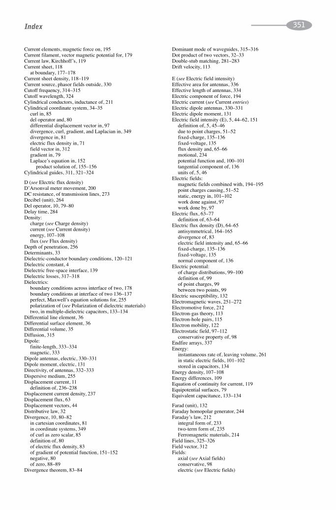
Current elements, magnetic force on, 195Current filament, vector magnetic potential for, 179Current law, Kirchhoff’s, 119Current sheet, 118
at boundary, 177–178Current sheet density, 118–119Current source, phasor fields outside, 330Cutoff frequency, 314–315Cutoff wavelength, 324Cylindrical conductors, inductance of, 211Cylindrical coordinate system, 34–35
curl in, 85del operator and, 80differential displacement vector in, 97divergence, curl, gradient, and Laplacian in, 349divergence in, 81electric flux density in, 71field vector in, 312gradient in, 79Laplace’s equation in, 152
product solution of, 155–156Cylindrical guides, 311, 321–324
D (see Electric flux density)D’Arsonval meter movement, 200DC resistance, of transmission lines, 273Decibel (unit), 264Del operator, 10, 79–80Delay time, 284Density:
charge (see Charge density)current (see Current density)energy, 107–108flux (see Flux density)
Depth of penetration, 256Determinants, 33Dielectric-conductor boundary conditions, 120–121Dielectric constant, 4Dielectric free-space interface, 139Dielectric losses, 317–318Dielectrics:
boundary conditions across interface of two, 178boundary conditions at interface of two 136–137perfect, Maxwell’s equation solutions for, 255polarization of (see Polarization of dielectric materials)two, in multiple-dielectric capacitors, 133–134
Differential line element, 36Differential surface element, 36Differential volume, 35Diffusion, 315Dipole:
finite-length, 333–334magnetic, 333
Dipole antennas, electric, 330–331Dipole moment, electric, 131Directivity, of antennas, 332–333Dispersive medium, 255Displacement current, 11
definition of, 236–238Displacement current density, 237Displacement flux, 63Displacement vectors, 44Distributive law, 32Divergence, 10, 80–82
in cartesian coordinates, 81in coordinate systems, 349of curl as zero scalar, 85definition of, 80of electric flux density, 83of gradient of potential function, 151–152negative, 80of zero, 88–89
Divergence theorem, 83–84
Dominant mode of waveguides, 315–316Dot product of two vectors, 32–33Double-stub matching, 281–283Drift velocity, 113
E (see Electric field intensity)Effective area for antennas, 336Effective length of antennas, 334Electric component of force, 194Electric current (see Current entries)Electric dipole antennas, 330–331Electric dipole moment, 131Electric field intensity (E), 5, 44–62, 151
definition of, 5, 45–46due to point charges, 51–52fixed-charge, 135–136fixed-voltage, 135flux density and, 65–66motional, 234potential function and, 100–101tangential component of, 136units of, 5, 46
Electric fields:magnetic fields combined with, 194–195point charges causing, 51–52static, energy in, 101–102work done against, 97work done by, 97
Electric flux, 63–77definition of, 63–64
Electric flux density (D), 64–65antisymmetrical, 164–165divergence of, 83electric field intensity and, 65–66fixed-charge, 135–136fixed-voltage, 135normal component of, 136
Electric potential:of charge distributions, 99–100definition of, 99of point charges, 99between two points, 99
Electric susceptibility, 132Electromagnetic waves, 251–272Electromotive force, 212Electron-gas theory, 113Electron-hole pairs, 115Electron mobility, 122Electrostatic field, 97–112
conservative property of, 98Endfire arrays, 337Energy:
instantaneous rate of, leaving volume, 261in static electric fields, 101–102stored in capacitors, 134
Energy density, 107–108Energy differences, 109Equation of continuity for current, 119Equipotential surfaces, 79Equivalent capacitance, 133–134
Farad (unit), 132Faraday homopolar generator, 244Faraday’s law, 212
integral form of, 233two-term form of, 235Ferromagnetic materials, 214
Field lines, 325–326Field vector, 312Fields:
axial (see Axial fields)conservative, 98electric (see Electric fields)
Index 351

Fields (Cont.)electrostatic, 97–112magnetic (see Magnetic fields)radial, 184time-dependent, conductors in motion through, 235–236time-independent, conductors in motion through, 234–235transverse, 31–313vector (see Vector fields)
Finite length dipole, 333–334First nulls, 337Fixed-charge electric field intensity and electric flux density,
135–136Fixed-voltage electric field intensity and electric flux density, 135Flux:
displacement, 63electric (see Electric flux)magnetic, 175
Flux density:electric (see Electric flux density)magnetic (see Magnetic flux density)
Flux lines, 64Flux linkage, 209Forces:
Coulomb, 4–5, 44–45electromotive, 212in magnetic fields, 193–208magnetomotive, 216moment of, 196–197
Fourier sine series, 166–167Free charge, 120Free space, Maxwell’s equation solutions in, 255Free-space interface, dielectric, 139Free-space permeability, 175Frequency of harmonic wave, 252Fringing of parallel-plate capacitors, 74–75Friss transmission formula, 337
Gauss’ divergence theorem, 83Gauss’ law, 65Gaussian surfaces, special, 66–67Generator, Faraday homopolar, 244Geometrical factor, 273Gradient, 78–79
in coordinate systems, 349curl of, as zero vector, 85divergence of, of potential function, 151–152
Guide wavelength, 315
H (see Magnetic field strength)Half-power beam width, 332Half-power points, 332Helical motion, 194–195Henry (unit), 209Hertzian dipole antennas, 330–331High-frequency lines, 277Homopolar generator, Faraday, 244
I (see Current)Imaging in perfect conductor, 342–343Impedance:
characteristic, 276intrinsic, 218, 254, 257mutual, of antennas, 335–336self-impedance, of antennas, 335–336wave, 313
Impedance matching, 279–280Impendance measurement, transmission line, 283–284Incidence:
angle of, 258normal, interface conditions at, 256–257oblique, 258plane of, 258
Induced voltage, 212Inductance, 209–232
definition of, 209–211
Inductance (Cont.)internal, 212–213mutual, 213–214self-inductance, 212of transmission lines, 273–274
Inductor, back-voltage in, 212Infinite line charge, 48Infinite plane charge, 49Infinity, zero reference at, 100Instantaneous power, 266–267Interface conditions at normal incidence, 256–257Internal inductance, 212–213Intrinsic concentration, 123Intrinsic impedance, 254, 257Intrinsic semiconductors, 115Inverse-square law of point charge, 48Iron-core magnetics, 214Isotropic radiator, 332
J (see Conduction current density; Convection current density)
Kirchhoff’s law, 119, 216
Laplace’s equation, 151–171in Cartesian coordinate system (see Cartesian coordinate
system, Laplace’s equation in)definition of, 151explicit forms of, 151–152
Laplacian, in coordinate systems, 349Legendre polynomial:
higher-order, 167of order n, 156
Lenz’s law, 233–234Lever arm, 196Line charge, 47
infinite, 48Line charge density, 47Line element, differential, 36Linear arrays of antennas, 337–338Lorentz force, 194Lossless lines, 277
transients in, 284–286Lossless waveguide, power transmitted in, 317Lossy waveguide, power dissipation in, 317–318
Magnetic circuits, 214Ampere’s law for, 214, 216–217parallel, 218
Magnetic component of force, 194Magnetic dipole, 333Magnetic field strength (H), 172, 177
current density and, 174tangential component of, 177
Magnetic fields:boundary relations for, 176–177electric fields combined with, 194–195forces and torques in, 193–208static, 172time-variable, 236
Magnetic flux, 175Magnetic flux density (B), 175–176
normal component of, 177Magnetic force:
on current elements, 195on particles, 193–194
Magnetic moment:of planar coil, 197–198of planar current loop, 197
Magnetic potential, vector, 178–179Magnetization curves, 215Magnetomotive force, 216Mass-action law, 123Matching:
double-stub, 281–283impedance, 279–280single-stub, 280–281
Index352

Maximum value theorem, 153Maxwell’s equations, 10–11, 233, 238–239
free-space set, 239general set, 239interface conditions at normal incidence, 256–257solutions for good conductors, 255–256solutions for partially conducting media, 254–255solutions for perfect dielectrics, 255solutions in free space, 255
Mean value theorem, 153in special case, 157–158
Method of images, 146–147Mho (unit), 117Mil. circular, 124Mobility, 113
electron, 122Mode cutoff frequencies, 314–315Moment:
electric dipole, 131of force, 196–197magnetic (see Magnetic moment)
Monopole, quarter-wave, 335Monopole antennas, 334–335Motion:
charges in, 113–114conductors in (see Conductors in motion)helical, 194–195
Motional electric field intensity, 234Multiple coils, 217–218Multiple-dielectric capacitors, 133–134Mutual impedance, of antennas, 335–336Mutual inductance, 213–214
n-type semiconductor materials, 115Negative air-gap line, 224Neper (unit), 224Net charge, 119
in region, 63Net charge density, 119–120Newton (unit), 4NI rise and NI drop, 216Nulls first, 337
Oblique incidence, 258Ohmic loss of antennas, 333Ohm’s law, 113
point form of, 114Operating wave length, 315Orthogonal surfaces, 34–35
p-type semiconductor materials, 115Parallel conductors, inductance of, 211Parallel magnetic circuits, 218Parallel-plate capacitors, fringing of, 74–75Parallel plate geometrical factors, 274Parallel polarization, 259–260Parallel wire geometrical factors, 274Particles, magnetic force on, 193–194Pattern function, 332Penetration, depth of, 256Per-meter attenuation, 291Period of harmonic wave, 252Permeability, 175
free-space, 175relative, 175
Permittivity, 4relative, 4, 132
Perpendicular polarization, 259Phasor fields, 330Phasors, 275Planar coil, magnetic moment of, 197–198Plane, of incidence, 258Plane charge, infinite, 258Plane waves, 253
Point charges:causing electric fields, 51–52electric field intensity due to, 51–52electric potential of, 99inverse-square law of, 98in spherical coordinate system, 69work done in moving, 98
Point form of Ohm’s law, 114Points, 34
electric potential between two, 99Poisson’s equation, 151, 164–165Polar form, 275Polarity, 233–234Polarization of dielectric materials, 131–132
parallel, 259–260perpendicular, 259
Position vectors, 36Potential:
electric (see Electric potential)vector magnetic, 178–179
Potential difference, 99Potential function (V):
divergence of gradient of, 151–152electric field intensity and, 100–101
Power:available, of antennas, 336complex, 261dissipated in lossy waveguide, 317–318instantaneous, 266–267Poynting vector and, 261transmitted in lossless waveguide, 317work and, 195–196
Power gain of antennas, 333Poynting vector, 261
power and, 261Propagation constant, 252
Quarter-wave monopole, 335Quarter-wave transformer, 296–297
R (see Resistance)Radial fields, 184Radiation efficiency of antennas, 333Radiation intensity, 332Radiation resistance, 331Radiator, isotropic, 332Receiving antennas, 336–337Rectangular-guide formulas, 321Reflection:
angle of, 258Snell’s law of, 258
Reflectors, 338Refraction, Snell’s law of, 258Relative permeability, 175Relative permittivity, 4, 132Relaxation time, 120Reluctance, 216Resistance (R), 117–118
radiation, 331surface, 318
Resistivity, 113conductivity as reciprocal of, 124
Right-hand rule, 173
Scalar function, gradient of, 78–79Scalar triple product, 38Scalars, 31
zero, divergence of curl as, 85Self-impedance, of antennas, 335–336Self-inductance, 212Semiconductors, 115–116Sheet charge, 47Sheet current, vector magnetic potential for, 179SI unit prefixes, 349SI units, rationalized, 4
Index 353

Sidelobes, 338Siemens (unit), 114, 117Single-stub matching, 280–281Sinks, 80Sinusoidal steady-state transmission-line excitation, 227–277Skin depth, 256Skin effect, 212–213Slotted lines, 283Small circular-loop antennas, 333Smith Chart, 278–279Snell’s law:
of reflection, 258of refraction, 258
Solenoids, inductance of, 211Sources, 80Space, free (see Free space)Spherical coordinate system, 34–35
curl in, 85differential displacement vector in, 97divergence, curl, gradient, and Laplacian in, 349divergence in, 81gradient in, 79Laplace’s equation in, 152
product solution of, 156point charge in, 69potential in, 101
Spherical shells, concentric, 104Standing-wave ratio, voltage, 277Standing waves, 260Static electric fields, energy in, 101–102Static magnetic field, 172Stokes’ theorem, 179–180Surface charge density, 47Surface element, differential, 36Surface resistance, 318Surfaces:
equipotential, 79orthogonal, 34–35
Susceptibility, electric, 132
TE (transverse electric) waves, 313Time constant, 120Time-dependent fields, conductors in motion through, 235–236Time-distance plots, 284–286Time-independent fields, conductors in motion through, 234–235Time-variable currents, 113Time-variable magnetic field, 236TM (transverse magnetic) waves, 313Toroids, inductance of, 211Torque:
definition of, 196–197in magnetic fields, 193–208
Transformer, quarter-wave, 296–297Transients in lossless lines, 284–286Transmission, angle of, 258Transmission formula, Friss, 337Transmission lines, 273–310
distributed parameters, 273–274double-stub matching, 281–283impedance matching, 279–280impedance measurement, 283–284incremental model, 274–275per-meter attenuation, 291single-stub matching, 280–281sinusoidal steady-state excitation, 275–277slotted, 283uniform, 273
Transverse components from axial components, 312–313Transverse electric (TE) waves, 313Transverse fields, 311–313Transverse length, unit, charge transport per, 118Transverse magnetic (TM) waves, 313Traveling waves, 262Triple product:
scalar, 38
Triple product (Cont.)vector, 38
Tuner circle, 282
Uniform arrays, 337Uniform transmission lines, 273Uniqueness theorem, 152–153Unit vectors, 4, 31, 35
V (see Potential function)Vector(s), 4, 31
absolute value of, 4, 31component form of, 4, 31cross product of two, 4, 33displacement, 44dot product of two, 4, 33position, 36Poynting (see Poynting vector)projection of one, on second, 37–38unit, 4, 51, 35zero, curl of gradient as, 85
Vector algebra, 14, 32–33Vector analysis, 4, 31–43Vector fields, 4, 78–80
curl of, 84–85Vector integral, 45, 46Vector magnetic potential, 178–179Vector notation, 4, 31Vector sum, 45Vector triple product, 38Vector wave equations, 251Velocity, drift, 113Voltage:
around closed contour, 212induced, 212of self-inductance, 212
Voltage drop, 117Voltage standing-wave ratio, 277Volume:
differential, 35instantaneous rate of energy leaving, 261
Volume charge, 46Volume current, vector magnetic potential for, 179
Wall losses, 317–318Wave equations, 251–252Wave impedance, 313Wave number, 312
critical, 313, 319of radiation, 330
Waveguides, 311–329dominant mode of, 315–316lossless, power transmitted in, 317lossy, power dissipation in, 317–318
Wavelength:cutoff, 324guide, 315of harmonic wave, 252operating, 315
Waves:electromagnetic (see Electromagnetic waves)plane, 253standing, 260traveling, 262
Weber (unit), 175Work:
definition of, 97done against electric field, 97done by electric field, 97done in moving point charges, 98power and, 195–196
Zero, divergence of, 88–89Zero reference at infinity, 100Zero scalar, divergence of curl as, 85Zero vector, curl of gradient as, 85
Index354