schedule generation schemes for the job-shop problem with

HAL Id: hal-00022742https://hal.archives-ouvertes.fr/hal-00022742

Submitted on 13 Apr 2006

HAL is a multi-disciplinary open accessarchive for the deposit and dissemination of sci-entific research documents, whether they are pub-lished or not. The documents may come fromteaching and research institutions in France orabroad, or from public or private research centers.

L’archive ouverte pluridisciplinaire HAL, estdestinée au dépôt et à la diffusion de documentsscientifiques de niveau recherche, publiés ou non,émanant des établissements d’enseignement et derecherche français ou étrangers, des laboratoirespublics ou privés.

Schedule generation schemes for the job-shop problemwith sequence-dependent setup times: dominance

properties and computational analysisChristian Artigues, Pierre Lopez, Pierre-Dimitri Ayache

To cite this version:Christian Artigues, Pierre Lopez, Pierre-Dimitri Ayache. Schedule generation schemes for the job-shopproblem with sequence-dependent setup times: dominance properties and computational analysis.Annals of Operations Research, Springer Verlag, 2005, 138, pp.21-52. �hal-00022742�

https://hal.archives-ouvertes.fr/hal-00022742

https://hal.archives-ouvertes.fr

- 1 -

Schedule generation schemes for the job-shop problem with sequence-

dependent setup times: dominance properties and computational

analysis

Christian Artigues1, Pierre Lopez2 and Pierre-Dimitri Ayache1 1Laboratoire d’Informatique d’Avignon, FRE CNRS 2487,

BP 1228, 84911 Avignon, France

[email protected]

tel: +33 4 90 84 35 52 fax: +33 4 90 84 35 01 2LAAS - CNRS,

7 avenue du Colonel Roche, 31077 Toulouse, France

[email protected]

- 2 -

Abstract

We consider the job-shop problem with sequence-dependent setup times.

We focus on the formal definition of schedule generation schemes (SGSs)

based on the semi-active, active, and non-delay schedule categories. We

study dominance properties of the sets of schedules obtainable with each

SGS. We show how the proposed SGSs can be used within single-pass and

multi-pass priority rule based heuristics. We study several priority rules for

the problem and provide a comparative computational analysis of the

different SGSs on sets of instances taken from the literature. The proposed

SGSs significantly improve previously best-known results on a set of hard

benchmark instances.

Keywords: scheduling theory, job-shop, sequence-dependent setup times, schedule

generation scheme, dominance properties, priority rules

- 3 -

Introduction

The greedy constructive heuristics used to solve a NP-hard scheduling problem are mostly

based on priority, also called dispatching, rules. A priority rule is used to select the task to be

scheduled at each step of the algorithm, among the set of unscheduled tasks. Such heuristics

are referred to as priority rule based algorithms. In some cases, the tasks are selected

according to a predetermined order, which is equivalent to assign to each task a unique

priority value. Choosing a priority rule, or a priority vector, is not sufficient to design a

constructive scheduling heuristic. Indeed, the set of candidate tasks for being scheduled has to

be defined, as well as the way the task selected based on a priority rule is scheduled. This

logical process of the heuristic is called the schedule generation scheme (SGS), see Kolisch

(1995) and Kolisch (1996)[13]. When dealing with a scheduling problem, designing SGSs is

fundamental, not only for priority rule based heuristics. Indeed the SGS can also be viewed as

the branching scheme of a branch and bound method. Branching consists in selecting a

different task among the set of candidate tasks. It is of theoretical interest to study the

dominance properties of the set of schedules that can be obtained by a given SGS, i.e. the

nodes of the associated tree. Considering a scheduling objective, a set of schedules is said to

be dominant when it contains at least one optimal schedule. Hence, the dominance property of

the set of schedules obtainable with a given SGS gives the theoretical ability of the SGS to

reach the optimum. By extension it can be stated that a SGS is dominant if there exists a

priority vector leading to an optimal schedule when applied in conjunction with this SGS. It is

well known that for scheduling problems with a regular objective function, i.e. non decreasing

with task completion times, the sets of so-called semi-active and active schedules are

dominant for any regular objective function whereas the set of so-called non-delay schedules

is in general not dominant.

Several SGSs, and their corresponding schedule set, have been studied by Baker (1974)

for the classical job-shop problem (JSP) where the tasks to be scheduled are called operations

and are gathered into jobs. In this problem, the operations of a job are totally ordered so that

no operation of a job can start before the completion of its predecessor. Furthermore, each

operation requires a machine and each machine can process only one operation

simultaneously. For the JSP, the Semi-Active SGS generates the dominant set of semi-active

schedules, the SGS proposed by Giffler and Thompson (1960) and the serial SGS described in

Kolisch (1995) generate the dominant set of active schedules, the Non-Delay SGS generates

the non-dominant but smaller set of non-delay schedules.

- 4 -

It has been shown that the introduction of sequence-dependent setup times in a scheduling

problem can call some dominance properties into question. Such a setup time may be needed

between two operations sharing the same machine. Its duration depends on the preceding and

following operations. For parallel machine problems, Ovacik and Uzsoy (1993) have proved

that the set of non-delay schedules, dominant for this particular problem, is not dominant

anymore in the presence of setup times. This has brought Schutten (1996) to provide for the

same problem an alternative list scheduling algorithm, able to generate a set of dominant

schedules. Recently, Hurink and Knust (2001) stated that a dominant list scheduling algorithm

is even unlikely to exist for the parallel machine problem involving sequence-dependent setup

times and precedence relations.

The job-shop problem with sequence-dependent setup times (SDST-JSP) has been studied

by a few authors. Schutten (1998) proposes an extension of the disjunctive graph model and

the shifting bottleneck procedure. Branch and bound algorithms are proposed by Gupta (1986)

and by Brucker and Thiele (1996). Focacci, Laborie and Nuijten (2000) propose a Constraint

Programming based method. An insertion heuristic is proposed by Sotskov, Tautenhahn and

Werner (1999) for the job-shop problem with sequence-independent batch setup times and by

Artigues and Roubellat (2002) for the SDST-JSP. Priority rules have been tested by using the

non-delay schedule generation scheme by Kim and Bobrowski (1994) and Noivo and

Ramalhinho-Lourenço (1998) while Ovacik and Uzsoy (1994) propose a priority rule based

heuristic aiming at exploiting real time shop floor status information, working in the set of

active schedules. Brucker and Thiele (1996) propose several priority-rule based heuristics

using a semi-active SGS and an extended Giffler-Thompson SGS. For more information on

scheduling research involving setups, we refer to the surveys of Allahverdi, Gupta and

Aldowaisan (1999) and Yang and Liao (1999). None of these studies is concerned with the

definition or the evaluation of schedule generation schemes for the SDST-JSP. In this paper,

we propose to fill this gap by providing in a formal way several SGSs for the SDST-JSP. We

study the dominance properties of the corresponding schedule sets and we give computational

results comparing the different SGSs used as single- and multi-pass priority rule based

heuristics using various priority rules to results obtained by exact methods.

The paper is organized as follows. In Section 1, we define the SDST-JSP. In Section 2, the

concepts of non-delay, active, and semi-active schedules are extended; several SGSs and their

dominance properties are given. Computational experiments are discussed in Section 3.

Concluding remarks are drawn in Section 4.

- 5 -

1. The job-shop problem with sequence-dependent setup times

We define in this Section the job-shop problem with sequence-dependent setup times

(SDST-JSP). As in the classical job-shop problem, a set J of n jobs 1,…, n has to be

performed by a set M of m machines 1,…, m. Each job i is made of m operations o(i,1),…,

o(i,m). N = mn denotes the total number of operations. The decision variables of this problem

are the operation starting times to(i,j), ∀i=1,…, n; ∀j=1,…, m.

Each operation o(i,j) has to be scheduled on a machine mo(i,j) during po(i,j) ≥ 0 uninterrupted

time units such that any machine can process only one operation at the same time. For

notation convenience, we also assume that:

o Operations are indexed from 1 to N, i.e. we have o(i,j) = j+(i–1)m; it follows that

we can refer to an operation by its own index o∈{1,..., N}. mo, po, to denote the

machine, duration and start time of operation o, respectively. O={1,…, N} denotes

the set of operations.

o An initial dummy operation 0 is defined as the first operation of each job: t0 = 0; p0

= 0. We assume that o(i,0) = 0, ∀i=1,…, n.

Switching from an operation a∈O to an operation b∈O on machine ma = mb, requires a

non-negative setup time sa,b. Moreover, an initial non-negative setup time s0,a is required if

operation a is the first to be sequenced on machine ma.

The problem can be formulated as follows:

(1) Min Cmax

Subject to:

(2) Cmax ≥ to(i,m) + po(i,m) (i = 1,…, n)

(3) t o ≥ s0,o (o∈ O)

(4) t o(i,j) ≥ to(i,j-1) + po(i,j-1) (i = 1,…, n; j = 2,…, m)

(5) ta ≥ tb + pb + sb,a or tb ≥ ta + pa + sa,b (a,b ∈O, a ≠ b, ma = mb)

A feasible schedule is defined by a vector of starting times t = (to)o∈O compatible with

constraints from (3) to (5). Constraints (3) ensure that the initial setup time is satisfied on each

machine. Constraints (4) ensure that precedence constraints within each job are satisfied.

Constraints (5) are the disjunctive constraints that prevent two operations using the same

machine from being scheduled simultaneously, the necessary setup times between the two

operations being respected. Note that constraints (4) allow setup anticipation, i.e. the start of

- 6 -

the setup for an operation on the machine while the preceding operation in the job is not

completed. The objective function (1) is to minimize the makespan Cmax defined by

constraints (2). In addition, it is assumed that setup times verify the triangle inequality:

(6) sa,b + sb,c ≥ sa,c (a,b,c ∈O, a ≠ b ≠ c, ma = mb = mc)

This common assumption is reasonable according to practical applications (e.g. Brucker

and Thiele (1996)). It is easy to show that the SDST-JSP is NP-hard. Indeed, setting all setup

times to 0 gives the classical JSP. Setting m = 1 and po = 0, ∀o∈O gives the travelling

salesman problem.

Example 1

Let us consider the following example with 2 machines and 2 jobs. Setup times are present on

machine 1 whereas there is no setup time needed for machine 2. The durations are p o(1,1) = 2,

p o(1,2) = 1, p o(2,1) = 5, p o(2,2) = 2. The machine requirements of the jobs are mo(1,1) = 1, mo(1,2) =

2, mo(2,1) = 2 and mo(2,2) = 1. The setup times on machine 1 are s0,o(1,1) = 1, s0,o(2,2) = 2,

so(1,1),o(2,2) = 10, so(2,2),o(1,1) = 3. The triangle inequality holds.

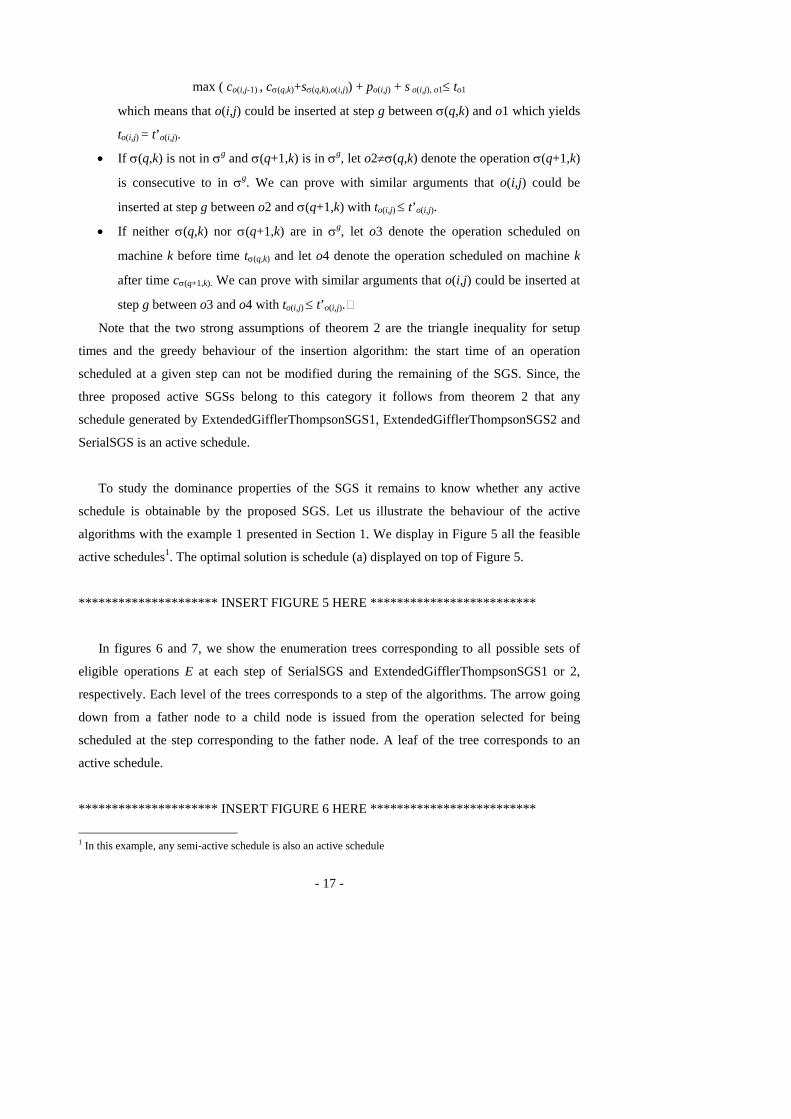
A feasible solution to example 1 problem of makespan Cmax = 15 is depicted in figure 1.

The required setup times are displayed in grey. Setup anticipation is illustrated on machine 1

where the setup for o(2,2) starts while o(2,1) is not even started.

***** INSERT FIGURE 1 ABOUT HERE *****

2. Schedule generation schemes for the SDST-JSP

2.1. General principles and definitions

In this Section, we present the framework of all Schedule Generation Schemes considered

in this paper.

Greedy construction process

The category of schedule generation schemes we consider builds a solution to the

scheduling problem in exactly N steps. At each step, exactly one operation is transferred from

the set of unscheduled operations, denoted by Q, to the set of scheduled operations. At the

beginning we have Q = O and the process stops when Q becomes empty.

Supprimé : are

- 7 -

At the step where operation o(i,j) is scheduled, i.e. removed from Q, its start time to(i,j) is

assigned to a value that will not be modified during the remaining of the construction process

(greedy behaviour).

All SGSs use at each of the N steps a set of eligible operations E, called the eligible set,

which is a subset of Q restricting the choice for the operation to be scheduled. More precisely,

the eligible set E is a subset of the available set A defined as follows. An unscheduled

operation belongs to the available set either if it is the first operation of its job or if its

preceding operation has been scheduled in a previous step. An operation having this property

is called available. Hence we have E ⊆ A ⊆ Q. The SGSs under study differ in the additional

restrictions they use to define the eligible set E.

Last, if the SGS is used as a branching scheme of a branch and bound algorithm,

branching consists in selecting an operation in E as the next operation to be scheduled. Hence,

the number of children of a given node is |E|.

The general framework of the considered SGSs given a priority vector π is summarized in

figure 2. Steps 4 and 5 correspond to the priority rule computation for the eligible operations

and the earliest feasible start time computation of the selected operation, respectively. These

concepts are explained thereafter. We have to underline that this framework is restrictive

since other SGSs could be defined where a non available operation could be selected for

scheduling, or/and where the start time of the scheduled operation could be modified at a later

step. Nevertheless the well-known semi-active, non-delay and active SGSs for the classical

job-shop problem (Baker (1974)), the serial and parallel SGSs [13]) and the strict order SGS

proposed by Carlier and Néron (2000) for the resource-constrained project scheduling

problem all belong to the considered category.

********************* INSERT FIGURE 2 HERE *************************

Computation of earliest feasible start times: appending vs. insertion SGSs

The operation selected in the eligible set E is scheduled at its earliest feasible start time at

step 5 of the general framework presented in figure 2. For the computation of these start

times, we make a distinction between appending schedule generation scheme and insertion

schedule generation scheme. In an appending scheme, an unscheduled operation can be

scheduled only after all the operations already scheduled on its machine, without delaying

these operations. In an insertion scheme, the unscheduled operation may be inserted

somewhere in the sequence of operations already scheduled on its machine. In a SGS it is

necessary to compute the earliest resource- and precedence-feasible start time of unscheduled

- 8 -

operations. We give hereafter two algorithms for computing the start time of an eligible

operation o(i,j)∈E depending on the SGS category.

Let k = mo(i,j) and let λ(k) ∈ {1,…, N} denote the latest operation (at the current iteration)

scheduled on machine k. When no operation has been scheduled yet on machine k, λ(k) is set

to the dummy first operation 0. Let cλ(k) be the completion time of operation λ(k). For each

scheduled operation o(x,y)∈O\Q, let co(x,y) = to(x,y)+po(x,y) denote its completion time. Let

ESAo(i,j) denote the earliest possible start time of an unscheduled operation o(i,j)∈Q in an

appending schedule generation scheme. ESAo(i,j) can be computed in O(1) at any step of the

constructive process by:

(7) ESA o(i,j) = max ( co(i,j-1) , cλ(k)+sλ(k),o(i,j)) with k = mo(i,j)

Note that (7) can be easily derived from (4) and (5) under the triangle inequality assumption

(6).

Let ηk denote the number of operations scheduled on machine k. Let σ denote the partial

sequence made of operations σ(0,k) = 0, σ (1,k), …, σ (ηk,k) = λ(k), scheduled on machine k.

For an insertion SGS, since we consider that the start time of a scheduled operation cannot be

changed, we search for the first insertion position where the selected operation can fit without

delaying the subsequent operation. Formally, let ESIo(i,j) denote the earliest possible start time

of an unscheduled operation in an insertion schedule generation scheme.

A position q with 0 ≤ q ≤ ηk verifying

(8) max ( co(i,j-1) , cσ (q,k)+sσ (q,k),o(i,j)) + po(i,j) + s o(i,j), σ (q+1,k) ≤ tσ (q+1,k)

is a feasible insertion position between operation σ(q,k) (possibly dummy first operation 0)

and operation σ (q+1,k). Again, (8) can be easily derived from (4) and (5) under the triangle

inequality assumption (6). If there exists at least one position q verifying equation (8) we set

qqq (8) verifies

min~= and we have:

(9) ESI o(i,j) = max ( co(i,j-1) , cσ ( q~ ,k)+sσ ( q~ ,k),o(i,j))

Otherwise we set

(10) ESI o(i,j) = ESA o(i,j)

- 9 -

Obviously, the earliest start time of an eligible operation in an insertion scheme can be

computed in O(m) since there are at most m-1 operations scheduled on machine k=mo(i,j).

Priority rules

If the SGS is used as a simple contructive algorithm, we suppose that each operation o(i,j)

of E has a priority value πo(i,j). This priority value can be computed in a static way (it remains

constant throughout the process) or in a dynamic way (it may have to be recomputed at each

step of the SGS). We assume without loss of generality that, at each iteration, the SGS selects

the operation with the smallest priority value as stated at step 4 of the general framework

displayed in figure 2. In the case where the priority is static, the operations can be pre-sorted

in a non-decreasing order of their priority value and form a list. Since such predefined lists

and static priority rules are strictly equivalent, we restrict this study to the priority rules.

Schedule category

The way the set E is computed by a given SGS is mostly driven by the restriction of the

search to a specific category of schedule. Let F denote the set of solutions of the SDST-JSP

satisfying constraints (3), (4) and (5), i.e. the set of feasible solutions. F, which is the set of

vectors t verifying the problem constraints, possibly represents a huge search space. Hence,

many works on scheduling theory rely on the restriction of the search on smaller subsets of F,

which defines categories of schedules. Among these categories, most of the existing

approaches focus on the sets of semi-active, non-delay, and active schedules. Such concepts

have been introduced for the job-shop problem without setup times by Baker (1974). More

recently, they have been extended to the resource-constrained project scheduling problem by

Sprecher, Kolisch and Drexl (1995). By extension, non-delay, semi-active and active SGSs

generate only non-delay, semi-active and active schedules, respectively. A set of schedules of

a given category is said to be dominant w.r.t. makespan minimization if it contains at least

one optimal solution. In the case where the SGS is used as a branching scheme of an implicit

enumeration tree, the SGS may have the property to generate all the schedules of its

corresponding category. By extension, a dominant SGS corresponds to a dominant category

of schedules and has the latter property. In the remaining, we discuss the extension of the

schedule categories and the corresponding schedule generation scheme for the SDST-JSP.

- 10 -

2.2. Semi-active SGSs

Following Sprecher, Kolisch and Drexl (1995), let us define a local left-shift of an

operation o(i,j) in a feasible schedule t as the move giving schedule t’ where t’o(i,j) = to(i,j) – 1

and t’o(x,y) = t o(x,y) ∀ o(x,y)∈O\{o(i,j)}.

Definition 1

A semi-active schedule is a feasible schedule in which no local left-shift leads to another

feasible schedule.

It follows that in a semi-active schedule, any operation has at most one tight job- or

resource-precedence constraint, preventing it from being locally left-shifted. From any

feasible non semi-active schedule, there always exists a (possibly empty) series of local left-

shifts giving a semi-active schedule without increasing the makespan. Hence, the set of semi-

active schedules is smaller than the set of feasible schedules and is dominant for the SDST-

JSP.

The semi-active appending schedule generation schemes aim at generating schedules

belonging to the set of semi-active schedules. The SGS able to generate all semi-active

schedules is noted SemiActiveSGS. In the general framework defined in Section 2.1, it has

the following particularities:

• SemiActiveSGS is an appending SGS;

• the eligible set E is equal to the entire available set A.

Basically, the semi-active SGS selects an available operation and schedules it as soon as

possible on its machine, after the previously scheduled operation. The overall time complexity

of the semi-active schedule is O(NnT), T being the time complexity of the priority rule

computation.

Lemma 1

For any priority vector, SemiActiveSGS generates a semi-active schedule and any semi-active

schedule is generated by SemiActiveSGS with a priority vector.

Proof

We first demonstrate that for a given priority vector π, schedule t generated by

SemiActiveSGS is a semi-active schedule. Suppose that t is not semi-active. Hence, there

- 11 -

exists o(i,j)∈O such that τ is a feasible schedule where τo(i,j) = to(i,j) – 1 and τo(x,y) = to(x,y), ∀

o(x,y)∈O\{o(i,j)}. Since to(i,j) =ESAo(i,j), we have to(i,j) = max (co(i,j), ),(, jioaa sc + ) where a is the

operation sequenced right before o(i,j) on its machine (which is valid according to the triangle

inequality assumption). Hence setting τo(i,j) = to(i,j) – 1 is unfeasible and t is semi-active.

Conversely, let t be a feasible semi-active schedule. Sort the operations in the order of non-

decreasing start times and set πo(i,j) to the rank of o(i,j). Obviously if ηk is the number of

operations scheduled on machine k, we have ),(),2(),1( ... kkk kησσσ πππ <<< and the schedule

obtained by SemiActiveSGS is t.

Theorem 1

The set of schedules generated by SemiActiveSGS is dominant.

Proof

From lemma 1, SemiActiveSGS is able to generate all semi-active schedules. Furthermore,

the set of semi-active schedules is dominant.

2.3. Active SGSs

Sprecher, Kolisch and Drexl (1995) define a global left-shift of an operation o(i,j) in a

feasible schedule S as a move giving schedule S’ after performing one or several local left-

shifts of o(i,j).

Definition 2

An active schedule is a feasible (semi-active) schedule in which no global left-shift leads to a

feasible schedule.

It follows from Definition 2 that in an active schedule, for any operation o(i,j), one cannot

find any feasible insertion position, located before o(i,j) in the sequence of operations

scheduled on mo(i,j), large enough to receive o(i,j). From any semi-active non active schedule,

one can always obtain an active schedule by performing a series of global left-shifts. Hence,

the set of active schedules is smaller than the set of semi-active schedules and remains

dominant for the SDST-JSP.

- 12 -

To provide an active SGS, it seems natural to study the extension of the Giffler-

Thompson Algorithm (Giffler and Thompson (1960)) which is the most famous active

schedule generation scheme for the classical job-shop problem. Before looking at possible

extensions, let us recall the behaviour of this well-known algorithm in the case of a job-shop

problem with zero setup times. The Giffler-Thompson algorithm (GifflerThompsonSGS) has

the following particularities in the general framework defined in Figure 2:

• GifflerThompsonSGS is an appending SGS

• the eligible set E is computed as follows. Let õ denote the available operation of

smallest completion time (job index is used to break ties). We have:

(11) õ = argmin {ESAo +po | o ∈ A}

E is the set of operations conflicting with õ that is

(12) E = {o | o∈A, mo=mõ, ESAõ +põ > ESAo }

In the case of the job-shop with zero setup times, any schedule generated by

GifflerThompsonSGS is active because no unscheduled operation o can be inserted before the

selected operation o*. Indeed, we have ESAõ +põ > ESAo* since o* belongs to the eligible set

defined above and also ESAo + po ≥ ESAõ +põ because o is unscheduled. Hence we have

ESAo + po > ESAo*, which makes the insertion of o before o* impossible. Furthermore, it is

well-known that using GifflerThompsonSGS as a branching scheme (branching on operations

of E) gives all active schedules.

We show hereafter that extending the Giffler-Thompson algorithm to non-zero setup

times raises significant problems. Brucker and Thiele (1996) propose for the SDST-JSP a

SGS directly inspired from the Giffler-Thompson algorithm by using (12) as conflict set

definition, which lies in ignoring the possible setup times. Taking account of setup times, the

set E can be defined as

(13) E = {o | o∈A, mo=mõ, ESAõ +põ + sõ,o > ESAo }

i.e. the set of available operations whose earliest appending start time has to be increased if õ

is scheduled. Unfortunately, coupling this definition of set E with an appending SGS does not

necessarily lead to an active schedule. Indeed, suppose that an operation o*≠õ is selected for

scheduling. Nothing prevents another available operation o to be insertable before o* although

- 13 -

conflicting with õ provided that it verifies ESAo + po + so,o* ≤ ESAo*. This is illustrated by the

following second example.

Example 2

We consider an example problem with 2 machines and 4 jobs. Setup times are present on

machine 1 whereas there is no setup time needed for machine 2. The considered durations are

po(1,1) = 2, po(2,1) = 5, po(2,2) = 2, po(3,1) = 2, po(4,1) = 3. Other operation durations are not

necessary for the present illustration and are left undetermined. The machine requirements of

the jobs are mo(1,1) = 1, mo(1,2) = 2, mo(2,1) = 2, mo(2,2) = 1, mo(3,1) = 2, mo(3,2) = 1, mo(4,1) = 1,

mo(4,2) = 2. The setup times on machine 1 are s0,o(1,1) = 1, s0,o(2,2) = 2, s0,o(4,1) = 1, so(1,1),o(2,2) =

10, so(1,1),o(4,1) = 9, so(2,2),o(1,1) = 8, so(2,2),o(4,1) = 5, so(4,1),o(1,1) = 3, so(4,1),o(2,2) = 1. Setup times

involving o(3,2) are not necessary for the present illustration. The triangle inequality holds.

Suppose that operation o(2,1) is selected for scheduling at the first step of the procedure. This

is compatible with the Giffler-Thompson algorithm since o(2,1) is conflicting with o(3,1),

which has the smallest earliest completion time. Now at the second step of the procedure,

available operations are o(1,1), o(2,2), o(3,1) and o(4,1). Among them, the operation having

the smallest earliest appending completion time, computed by Equation 12, is õ=o(1,1) with

ESAo(1,1) + po(1,1) = 3. Figure 3 illustrates the conflict definition at the considered step.

Scheduled operation o(2,1) is displayed in bold whereas available operations are displayed in

plain line. Figure 3 displays 5 partial solutions (a), (b), (c), (d) and (e) all with o(2,1)

scheduled first on machine 2.

(a) o(2,2) is scheduled first right before o(1,1).

(b) o(1,1) is scheduled first right before o(2,2).

(c) o(4,1) is scheduled first right before o(1,1).

(d) o(1,1) is scheduled first right before o(4,1).

(e) o(4,1) is scheduled first right before o(2,2)


Partial solutions (a), (b), (c) and (d) illustrate that, according to expression (13), the

conflict set at the considered step is E={o(1,1), o(2,2), o(4,1)}. Indeed it is clear that

scheduling first o(1,1) on machine 1 increases the earliest appending start time of o(2,2), as

shown by comparing (a) and (b), and also the earliest appending start time of o(4,1) as shown

- 14 -

by comparing (c) and (d). Suppose now that the priority rule selects o(4,1) for scheduling,

right before o(2,2) as displayed in partial solution (e). It appears here that configuration (a) is

not active because o(2,2) has the same start time (5) if it is scheduled first or right after o(4,1).

The explanation is that o(4,1) is not in conflict with o(2,2) although both operations are in

conflict with o(1,1). In other words, the conflict relation is not transitive anymore in the

presence of non zero setup times.

Hence defining an appending SGS with an eligible set computed by expression (13) does

not necessary lead to active schedules. To overcome this drawback, we may use a more

restrictive definition of the eligible set, ensuring that an eligible operation is in conflict with

all other ones. Let us define the eligible set as the set of available operations scheduled on

machine mõ in conflict with another available operation:

(14) E = {o | o∈A, ∀o’∈A, mo= mo’=mõ, ESAo’ +po’ + so’,o > ESAo }

With this definition, at the considered step of the example 2 problem (figure 3), the conflict

set is reduced to E = {o(1,1),o(4,1)} and the two corresponding partial schedules lead to

active schedules. Again, a counterexample shows that, even with this more sophisticated

conflict set definition, the SGS may generate a non active schedule.

Example 3

Let us modify example 2 by adding a 3rd machine with zero setup times and some other

modifications. We suppose that jobs 1, 2 and 3 are unchanged except that o(1,3), o(2,3) and

o(3,3) require machine 3. Job 4 is now such that mo(4,1)=3, mo(4,2)=1 and mo(4,3)=2 with

po(4,1)=3, po(4,2)=1. o(4,1) is no more subject to setup times whereas o(4,2) has the following

setup times : s0,o(4,2)=0, so(1,1),o(4,2)=9, so(2,2),o(4,2)=5, so(4,2),o(1,1)=3 and so(4,2),o(2,2)=1. The

remaining data is left unchanged or undetermined. Since setup times on machine 1 are the

same as in example 2, the triangle inequality still holds.

We again suppose that the priority rule selects first operation o(2,1) for scheduling. Again this

is in accordance with the Giffler-Thompson algorithm since o(2,1) is in conflict with o(3,1)

which has the smallest earliest completion time at step 1. Now at step 2, available operations

are o(1,1), o(2,2), o(3,1) and o(4,1). The operations with the smallest earliest appending

completion time are o(1,1) and o(4,1). Using job index to break the tie we have õ= o(1,1).

Operation o(4,2) being unavailable, the conflict set according to definition 14 is E =

- 15 -

{o(1,1),o(2,2)}. Figure 4 illustrates the conflict definition at the considered step. The

scheduled operation o(2,1) is displayed in bold. Available operations are displayed in plain

line whereas non-available operation o(4,2) is displayed in dotted line. The two corresponding

partial solutions illustrating the conflict are (a) and (b). Suppose that at step 2 of the SGS,

o(2,2) is selected for scheduling. Suppose now that at step 3 of the SGS, operation o(4,1) is

selected for scheduling. Then, o(4,2) becomes available at time 3 and can be inserted before

o(2,2) as shown in part (c). Partial solution (a) does not lead to an active solution if an

appending scheme is used.


This counterexample of figure 4 shows that to obtain an active schedule with an appending

SGS, the conflict set cannot be restricted to the available operations. Including non-available

operations in the conflict set is out of the scope of the SGSs presented in this paper. However,

another way of obtaining active schedules is to use an insertion SGS. This yields the

following two extended Giffler-Thompson SGSs.

• GifflerThompsonSGS1 is an insertion SGS

• The conflict set is defined by expression (13).

or

• GifflerThompsonSGS2 is an insertion SGS

• The conflict set is defined by expression (14).

Note that when all setup times are equal to 0, the two proposed algorithms behave strictly like

the Giffler-Thompson algorithm.

We introduce also another SGS, called the serial schedule generation scheme, [12]

Kolisch (1995) and Kolisch (1996), which has been previously defined for the resource-

constrained project scheduling problem. For the classical JSP, it is also able to generate all

active schedules. Its extension to the SDST-JSP is straightforward.

• SerialSGS is an insertion SGS

• the eligible set E is equal to the entire available set A.

- 16 -

The algorithm behaves like the semi-active SGS except that the selected operation is

inserted at the earliest feasible position on its machine.

T being the time complexity of the priority rule computation, the time complexity of

ExtendedGifflerThompsonSGS1 and SerialSGS is O(N(nT+m)), while the time complexity of

ExtendedGifflerThompsonSGS2 is O(N(n2T+m)).

We now focus on the theoretical ability of the three active SGSs to generate all active

schedules, i.e. their dominance properties. First, theorem 2 shows that all three proposed

active SGSs generate active schedules.

Theorem 2

For any priority vector, any insertion SGS generates an active schedule.

Proof

Suppose that a schedule t generated by an insertion SGS is not active. Let σ denote the

sequence made of operations σ(0,k) = 0, σ(1,k), …, σ(n,k), scheduled on each machine k for

schedule t. If t is not active, then there must exist a machine k and an operation o(i,j)

scheduled on k at position ρ∈{2,…,m} such that expression (8) is verified for insertion

position q<ρ –1, i.e. we have:

max ( co(i,j-1) , cσ (q,k)+sσ (q,k),o(i,j)) + po(i,j) + s o(i,j), σ(q+1,k) ≤ tσ (q+1,k)

with (a) t’o(i,j) = max ( co(i,j-1) , cσ(q,k)+sσ(q,k),o(i,j)) < to(i,j) .

Let g denote the step where o(i,j) is scheduled by the SGS. Let ηgk denote the number of

operations scheduled on machine k at step g. Let σg denote the partial sequence made of

operations σ g(0,k) = 0, σ g(1,k), …, σ g(ηg

k,k) scheduled on machine k at step g. For each of

the possible cases concerning the components of σg, a contradiction is raised with (a).

• If σ(q,k) is in σg and σ(q+1,k) is in σg then the two operations are consecutive in σg

and, since the start time of the scheduled operations are fixed, o(i,j) can be inserted

between σ(q,k) and σ(q+1,k) at step g which yields to(i,j) = t’o(i,j).

• If σ(q,k) is in σg and σ(q+1,k) is not in σg, let o1≠σ(q+1,k) denote the operation

consecutive to σ(q,k) in σg. Since σ(q+1,k) is inserted in σg at a step strictly greater

than g, we have tσ(q+1,k) + pσ(q+1,k) +sσ(q+1,k),o1 < to1. With (8) it comes: max ( co(i,j-1) ,

cσ(q,k)+sσ(q,k),o(i,j)) + po(i,j) + so(i,j), σ(q+1,k) ≤ to1 – sσ (q+1,k),o1

Since the triangle inequality holds we have:

- 17 -

max ( co(i,j-1) , cσ(q,k)+sσ(q,k),o(i,j)) + po(i,j) + s o(i,j), o1≤ to1

which means that o(i,j) could be inserted at step g between σ(q,k) and o1 which yields

to(i,j) = t’o(i,j).

• If σ(q,k) is not in σg and σ(q+1,k) is in σg, let o2≠σ(q,k) denote the operation σ(q+1,k)

is consecutive to in σg. We can prove with similar arguments that o(i,j) could be

inserted at step g between o2 and σ(q+1,k) with to(i,j) ≤ t’o(i,j).

• If neither σ(q,k) nor σ(q+1,k) are in σg, let o3 denote the operation scheduled on

machine k before time tσ(q,k) and let o4 denote the operation scheduled on machine k

after time cσ(q+1,k). We can prove with similar arguments that o(i,j) could be inserted at

step g between o3 and o4 with to(i,j) ≤ t’o(i,j).

Note that the two strong assumptions of theorem 2 are the triangle inequality for setup

times and the greedy behaviour of the insertion algorithm: the start time of an operation

scheduled at a given step can not be modified during the remaining of the SGS. Since, the

three proposed active SGSs belong to this category it follows from theorem 2 that any

schedule generated by ExtendedGifflerThompsonSGS1, ExtendedGifflerThompsonSGS2 and

SerialSGS is an active schedule.

To study the dominance properties of the SGS it remains to know whether any active

schedule is obtainable by the proposed SGS. Let us illustrate the behaviour of the active

algorithms with the example 1 presented in Section 1. We display in Figure 5 all the feasible

active schedules1. The optimal solution is schedule (a) displayed on top of Figure 5.


In figures 6 and 7, we show the enumeration trees corresponding to all possible sets of

eligible operations E at each step of SerialSGS and ExtendedGifflerThompsonSGS1 or 2,

respectively. Each level of the trees corresponds to a step of the algorithms. The arrow going

down from a father node to a child node is issued from the operation selected for being

scheduled at the step corresponding to the father node. A leaf of the tree corresponds to an

active schedule.


1 In this example, any semi-active schedule is also an active schedule

- 18 -


The comparison of the obtained trees brings the following remarks. First, the serial

algorithm introduces a lot of symmetries. Indeed, solution (b) appears in 4 leaves of the tree.

On the opposite the extended Giffler-Thompson algorithm does not produce symmetries since

all the leaves of its tree correspond to distinct solutions. On the other hand,

ExtendedGifflerThompsonSGS1 and 2 are unfortunately shown here to be non-dominant

since the unique optimal solution (a) does not appear in the enumeration tree. The basic

reason for the present example is that at step (1) operation o(2,2) is not in the set E of eligible

operations because it is not available. However, because of the large setup time, o(2,2) should

be considered as conflicting with o(1,1). Hence a direct extension of the Giffler-Thompson

algorithm does not provide a set of dominant schedules. Theorem 3 shows that the serial SGS

does not have the same drawback.

Theorem 3

The set of schedules generated by SerialSGS is dominant.

Proof

Let us consider a static priority vector π. Let t denote the schedule generated by SerialSGS

with π. Let t’ denote the schedule generated by SemiActiveSGS with π. SerialSGS and

SemiActiveSGS only differ by the start time computation. Hence, the same operations are

selected through π by both algorithms at each step. For the selected operation o(i*,j*), we

have t’o(i*,j*) ≥ t o(i*,j*) if the triangle inequality (6) holds because in SerialSGS, o(i*,j*) is

possibly inserted in the sequence of its machine without delaying the already scheduled

operations. Hence, the schedule obtained by SerialSGS with π cannot be worse that the

schedule obtained by SemiActiveSGS with π.

2.4. Non-delay SGSs

When setup times are not present, a schedule is said to be a non-delay schedule if no

machine is left idle while it could start the processing of an operation, see Baker (1974). It

follows that the classical non-delay schedule generation scheme, called the parallel SGS in

resource-constrained project scheduling, see Kolisch (1996), does time incrementation.

- 19 -

Starting with time τ = 0, at each iteration, an operation that can start at time τ is selected.

Then τ is updated to the smallest possible start time of an unscheduled operation. Obviously,

this definition does not suit the possible anticipation of setup times. Indeed, whenever an

operation becomes available at a given time τ then in some cases it would have been possible

to start its setup before time τ.

However, we give two different definitions of a non-delay schedule in the SDST-JSP

inspired by the earliest start policy of the non-delay concept.

Definition 3

A type 1 non-delay schedule is a feasible (active) schedule in which no machine is kept idle or

performing a setup at any time while it could process an operation.

Definition 4

A type 2 non-delay schedule is a feasible (active) schedule in which no machine is kept idle at

any time while it could process an operation or perform a setup in such a way that an

operation can start immediately after the setup.

Roughly, type 1 non-delay schedules are “production-oriented” as they aim at reducing

setups by prefering production to setup activities. Type 2 non-delay schedules are “time-

oriented”. Note that if there are no setup times, both definitions are equivalent to the classical

definition.

For the job-shop problem without setup times, it is well-known that the non-delay

schedules are included in the set of active schedules but they are not dominant. Types 1 and 2

non-delay schedules have no chance to possess the dominance property since the JSP is a

special case of the SDST-JSP. Obviously, they are also active schedules.

We describe an appending "non-delay" SGS extending the classical non-delay SGS for

the JSP as described in Baker (1974) in the case a type 1 non-delay scheduled has to be

generated.

• NonDelaySGS1 is an appending SGS

- 20 -


smallest start time (job index is used to break ties). We have:

(15) õ = argmin {ESAo | o ∈ A}

E is the set of operations having the same start time as õ, that is:

(16) E = {o | o∈A, mo=mõ, ESAõ = ESAo }

When all setup times are equal to 0 the proposed algorithm behaves like the non-delay

schedule generation scheme proposed in [4]. NonDelaySGS1 has an O(NnT) time complexity.

Theorem 4

For any priority vector, NonDelaySGS1 generates a type 1 non-delay schedule and any type 1

non-delay schedule is generated by NonDelaySGS1 with a priority vector.

Proof

Suppose that t, a schedule generated by NonDelaySGS1 with a priority vector π, is not a type

1 non-delay schedule. It follows that we can find an idle time period τ and an operation o(i,j)

that can start at time τ while τ < to(i,j). Let o1 denote the first operation verifying to1>τ. Let g

denote the step where o1 is scheduled by NonDelaySGS1. If o(i,j) is available then, since we

have ESAo(i,j) ≤ τ and to1>τ, o1 should not appear in the eligible set, which is in contradiction

with its definition. If o(i,j) is not available let o(i,j-x) with x≥1, the first available operation of

job i. We have to(i,j-x) ≤ τ and to1>τ. Hence o1 should not appear in the eligible set, a

contradiction. It follows that any schedule generated by NonDelaySGS1 is a type 1 non-delay

schedule. Let t denote a type 1 non-delay schedule and let π denote the priority vector

obtained by sorting the operations in the non-decreasing order of the starting times in t. We

see that π is precedence-compatible, i.e. we have for any operation o(i,j), πo(i,j) > πo(i,j-1)

whenever po(i,j-1) > 0. Hence at the step, g the operation o(i,j) such that πo(i,j) = g is in the

eligible set and can be started at time t o(i,j).

We now study the insertion SGS extending the classical non-delay SGS for the JSP [4]

proposed by Baker (1974) in the case a type 2 non-delay scheduled has to be generated.

• NonDelaySGS2 is an insertion SGS

- 21 -


smallest start time (job index is used to break ties). Recall that λ(k) is the last

operation scheduled on machine k. We have:

(17) õ = argmin {ESAo -sλ(k),o| o ∈ A}

E is the set of operations having the same setup start time as õ, that is:

(18) E = {o | o∈A, mo=mõ, ESAõ -sλ(k),õ = ESAo -sλ(k),o }

When all setup times are equal to 0 the proposed algorithm behaves also like the non-delay

schedule generation scheme proposed in [4]. NonDelaySGS2 has an O(N(nT+m)) time

complexity.

We explain through example 4 why an insertion SGS is needed whereas the eligible set

considers appending start times.

Example 4:

Consider a problem with 2 jobs and 4 machines with no setup times on machines 2, 3, 4 and

non-zero setup times on machine 1. We have mo(1,1)=4, mo(1,2)=1, mo(2,1)=3, mo(2,2)=2, mo(2,3)=1,

po(1,1)=6, po(1,2) =po(2,1)=2, po(2,2)=po(2,3) =1. On machine 1, we have s0,o(2,3)=3, s0,o(1,2)=5 and

so(2,3), o(1,2)=2. All other data are left undetermined. The triangle inequality holds.

Suppose that, at steps 1 and 2 of the SGS, operations o(1,1) and o(2,1) are scheduled,

respectively. Both operations being available at time 0, this is compatible with the conflict set

definition 16. At step 3 of the algorithm available operations are o(1,2), and o(2,2). According

to definition 15, operation õ is o(1,2) with ESAo(1,2)–s0,o(1,2)=1 and the eligible set is

E={o(1,2)} because o(2,3) is not available. In figure 8, partial solution (a) corresponds to the

selection of o(1,2) at step 3.


Suppose now that o(2,2) is scheduled at step 4. At step 4, o(2,3) becomes available and can be

inserted before o(1,2) with ESIo(2,3)-s0,o(2,3)=0, as displayed in part (b). It follows that if an

appending SGS is used, solution (a) does not yield a type 2 non-delay schedule.

- 22 -

Unfortunately, it has to be pointed out that the proposed non-delay SGS may generate a

schedule out of the set of the type 2 non-delay schedules, even when used with an insertion

scheme, as shown in example 5.

Example 5:

We modify example 4 simply by setting so(2,3), o(1,2)=3.

In this case partial solution (b) of figure 8 cannot be generated when o(2,3) becomes

available because o(2,3) cannot be inserted anymore before o(1,2) without increasing the start

time of o(1,2) by 1. In this small example, the only type 2 non-delay schedule is unreachable

by a SGS restricting the eligible set to available operations. This drawback is another

illustration of the negative impact of sequence-dependent setup times on schedule properties.

In table 1, a summary of the theoretical results of our study of schedule generation

schemes for the SDST-JSP is displayed, giving for each proposed SGS, the type of schedule it

generates, its time complexity, its ability to generate all the schedules of its target type and the

dominance property of the generated schedule set w.r.t. makespan minimization.

********************* INSERT TABLE 1 HERE *************************

3. Experimental comparison of the proposed SGSs

3.1. Benchmark instances

We have tested the proposed SGSs on SDST-JSP benchmark instances proposed by

Brucker and Thiele (1996) (called BT instances in the sequel). These 15 instances are job-

shop problems with setup times derived from the corresponding benchmark problems of

Adams, Balas and Zawack (1988). In these instances, each operation has a setup type and all

operations of the same job have the same setup type. Durations have been randomly

generated between 1 and 100. The setup time matrix gives the time to switch from one setup

type to another one on any machine. The problems are cast into 3 groups. The first group

contains 5 problems of 5/10/5 machines/jobs/setup_types. The second group contains 5

problems of 5/15/5 machines/jobs/setup_types. The third group contains 5 problems of

5/20/10 machines/jobs/setup_types. The interest of using these instances is that optimal or

- 23 -

good solutions have been generated either by the branch and bound of Brucker and Thiele

(1996) or by the constraint programming technique of Focacci, Laborie and Nuijten (2000). It

follows that the experiments will give an idea of the distance from optimum of the solution

obtained by priority rule based heuristics. The setup times have been generated according to a

quotient q of average setup time divided by the average processing time. Groups 1 and 2 have

an average quotient q ≅ 0.5 which corresponds to medium setup times while group 3 has an

average quotient q ≅ 1, giving larger setup times. However these setup times have a special

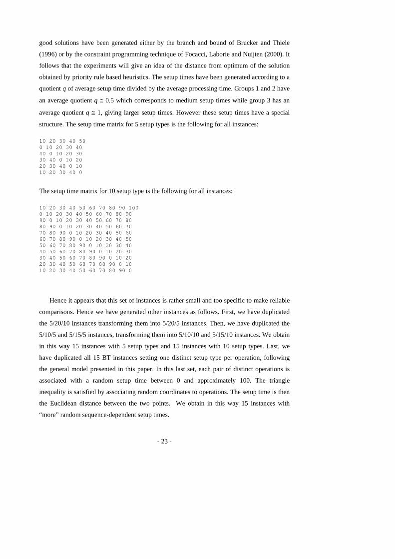
structure. The setup time matrix for 5 setup types is the following for all instances: 10 20 30 40 50 0 10 20 30 40 40 0 10 20 30 30 40 0 10 20 20 30 40 0 10 10 20 30 40 0

The setup time matrix for 10 setup type is the following for all instances: 10 20 30 40 50 60 70 80 90 100 0 10 20 30 40 50 60 70 80 90 90 0 10 20 30 40 50 60 70 80 80 90 0 10 20 30 40 50 60 70 70 80 90 0 10 20 30 40 50 60 60 70 80 90 0 10 20 30 40 50 50 60 70 80 90 0 10 20 30 40 40 50 60 70 80 90 0 10 20 30 30 40 50 60 70 80 90 0 10 20 20 30 40 50 60 70 80 90 0 10 10 20 30 40 50 60 70 80 90 0

Hence it appears that this set of instances is rather small and too specific to make reliable

comparisons. Hence we have generated other instances as follows. First, we have duplicated

the 5/20/10 instances transforming them into 5/20/5 instances. Then, we have duplicated the

5/10/5 and 5/15/5 instances, transforming them into 5/10/10 and 5/15/10 instances. We obtain

in this way 15 instances with 5 setup types and 15 instances with 10 setup types. Last, we

have duplicated all 15 BT instances setting one distinct setup type per operation, following

the general model presented in this paper. In this last set, each pair of distinct operations is

associated with a random setup time between 0 and approximately 100. The triangle

inequality is satisfied by associating random coordinates to operations. The setup time is then

the Euclidean distance between the two points. We obtain in this way 15 instances with

“more” random sequence-dependent setup times.

- 24 -

3.2. Priority rules

A priority rule π gives a value to an operation o(i,j). Depending on the rule, the operation

selected in the set E of candidate operations is the one having the smallest or the greatest

value.

We have used the following priority rules, some being directly issued from classical JSP

rules, others being adapted to deal with setup times.

o MWKR (Most WorK Remaining): πo(i,j) = ∑ =m

jlpo(i,l)

o SST (Shortest Setup Time): πo(i,j) = ),(),( ),( jiom jiosλ

o SSTPT (Shortest Setup Time and Processing Time):

πo(i,j) = po(i,j)+ ),(),( ),( jiom jiosλ

o MINSLACK (Min Slack) πo(i,j) = maxl=j,…,m (co(i,l))

o MOPER (Most Operations Remaining) πo(i,j) = m+1-j

o RAND (Random)

o MINSTART (Min Start time): πo(i,j) = ESAo(i,j)

o MINSTSTART (Min Setup Start time): πo(i,j) = ESAo(i,j) - sλ(mo(i,j)),o(i,j)

o MINEND (Min End Time): πo(i,j) = ESAo(i,j) + po(i,j)

3.3. Single- and multi-pass heuristics

We have embedded the proposed SGSs into single- and multi-pass priority rule based

heuristics. The single-pass heuristic consists in generating a unique solution with a given SGS

associated with a given priority rule. For multi-pass methods, we have tested random

sampling methods where, at each pass, the SGS is used with a random based priority rule. We

have used a very simple random sampling procedure in which the priority rule is randomly

biased for all SGSs using a random factor α. More precisely, the operation of E with the

smallest priority value is selected unless another operation is selected with an α probability.

Moreover, all ties are broken randomly instead of using the job index rule.

- 25 -

3.4. Computational results

Comparison of the proposed SGSs within single- and multi-pass heuristics




Tables 2 to 4 give the results of the proposed SGSs on the 45 instances described in

Section 3.1. Tables 2 gives the results of single-pass heuristics with all SGSs and all tested

priority rules. Tables 3 and 4 give the results of multi-pass heuristics for 1000 and 10000

iterations, respectively. We give for each pair SGS/priority rule the number of problems out

of 45 for which this combination found the best result (among all heuristics tested for the

considered number of iterations) and, in brackets, the average deviation in percent from the

best result obtained on each instance by the multi-pass heuristic with 10000 iterations. Hence,

the former value gives an indication on the relative ranking of the pair SGS/rule for a given

number of iterations whereas the latter value gives an absolute measure of performance w.r.t.

the best known solution. In each table, row “BEST” gives the same indicators taking for each

SGS and each instance the best result among all rules. ND, EGT, SA and SE stand for

NonDelay, ExtendedGifflerThompson, SemiActive and Serial SGSs, respectively. We give in

seconds the average and maximum CPU time per instance, on a Pentium 4 Personnal

Computer with 2.40 GHz and 512 Mo RAM.

For the single pass heuristics (table 2), row “BEST” obtains the global ranking ND 1 >

EGT1,EGT2 > SE,SA > ND 2. There is no significant difference between EGT 1 and 2. There

is also no significant difference between SE and SA. This can be explained by examining the

priority rule level. Except for ND 1, the best priority rule is MINSTART (Minimum

appending Start time). Observe that when SA, SE, and EGT are applied in conjunction with

the MINSTART priority rule, they all resort to ND 1. This can be verified in row MINSTART

where all the results are identical to the ND 1 results. Indeed all these SGSs select for

scheduling the operation with the minimum appending start time breaking the tie with the job

index rule. The various priority rules used with ND 1 are just variants on the apparently

superior MINSTART policy. ND 2 gives on the contrary the poorest results. Note that for ND

2, the SST and the MINSTART rule are equivalent, since ND 2 schedules operations of

- 26 -

minimal setup start time. For all SGSs, the CPU times are negligible (less than 0.001

seconds).

Table 3 shows completely different results when the SGSs are applied in a multi-pass

heuristic with 1000 iterations. The ranking of the SGSs when taking the best results among all

rules becomes SE > SA > EGT 2> EGT 1 > ND 1 > ND 2.

ND 1 and ND 2 are significantly outperformed by the other SGSs since they are ranked only 2

or 3 times first and have an average deviation of about 8% from the best solution whereas all

other SGSs are ranked from 16 to 26 times first and have an average deviation of about 2%.

Globally, we see that applying a multi-start heuristic is fruitful, since the best average

deviation from the best solution has been divided by more than 4 compared to table 2. The

CPU times per instance are of less than 0.15 seconds for SA and SE. Looking at the priority

rule level, the best rule is still MINSTART except for ND 1. Intuitively this result can bring to

the idea that the MINSTART rule makes globally good decisions and that the best SGSs are

the ones which are able to bring a sufficient level of diversification around this rule. Indeed,

Random sampling with the ND 1 scheme only allows to select operations that have strictly the

smallest earliest start time whereas with the serial scheme, the semi-active scheme and, more

restrictively, the extended Giffler-Thompson scheme, an operation which does not start as

soon as possible can be selected with the α probability, which brings more diversification.

The above hypothesis seems still valid for random sampling with 10000 iterations (table

4) since the SGSs ranking is now SE,SA < EGT1 < EGT2 < ND 1, ND 2. A surprising result

is that there is no more a significant difference between the serial and the semi-active SGSs

which means that when the number of iterations increases, the benefit of trying to keep the

schedule active by insertion is lost. This allows to obtain the best results with an algorithm of

low time requirements (less than 1.5 seconds per instance). Similarly EGT 1 is here slightly

superior to EGT 2 whereas the latter SGS takes twice more time (more than 4 seconds per

instance).

Comparison of the proposed heuristics with truncated branch and bound


- 27 -

Table 5 extracts from our testbed the 15 instances generated by Brucker and Thiele (1996)

to evaluate the performance of the proposed SGSs in comparison with the state-of-the-art

approaches. For each of the 15 instances and for each number of iterations, we display the

makespan obtained by all SGSs and the average deviation from the previously best known

results, obtained either by Brucker and Thiele (1996) or by Focacci, Laborie and Nuijten

(2000). Note that the first 5 instances are the 5/10/5 instances, the next 5 instances are the

5/15/5 instances and the last 5 instances are the 5/20/10 instances. For the 5/10/5 instances,

the optimum is known and displayed in column Cmax*. For the other instances, column

Cmax* only displays an upper bound obtained by truncating the branch and bound of Brucker

and Thiele after 2 hours, or the branch and bound of Foccacci et al. after 60 seconds. On one

hand, the solution found by the SGSs are far from the optimum for the 5 small instances (from

2.51% to 18.84% for 10000 iterations). On the other hand, for the other instances, the

proposed SGSs significantly improve the best known solutions in a very short time (less than

10 seconds per instance as shown in table 4). The improvement is from 2.08% to 10.86%.

Even the single-pass heuristics improve very quickly (less than 0.001 seconds) the best known

solutions on all 5/20/10 instances. For our best results (10000 iterations) we also display in

brackets the average deviation over the lower bound computed by Brucker and Thiele (1996).

The maximal deviation from this bound is of 9.89% on the 5/15/5 instances and of 19.28% on

the 5/20/10 instances. Hence, the proposed heuristics give better results on medium and large

instances than on smaller instances. They also outperform for these instances, the truncated

branch and bound and the heuristics proposed by Brucker and Thiele (1996) run with a time

limit of 2 hours on a SUN 4/20 workstation. We also obtain better results than the truncated

branch and bound method of Focacci, Laborie and Nuijten (2000) run on a Pentium II 300

MHz with a time limit of 60 seconds. Looking closer to the priority-rule based heuristics

proposed in Brucker and Thiele (1996), it appears that no MINSTART-based priority rule was

used. Indeed, the two proposed SGSs are a parallel version of the semi-active SGS and an

extended Giffler-Thompson SGS with conflict set definition (12), which does not take

account of setup times. Hence exact methods would certainly benefit from integrating our

heuristics.

Influence of the number of setup types


Commentaire [PL1] : Je répète : n’est-ce pas 27.96 ?

- 28 -



We study the influence of the setup characteristics on the results. First, Tables 6, 7 and 8

display the results of the different SGSs for 5, 10 and N setup types instances, respectively.

To simplify the reading, for each SGS and for each number of iterations, the best result

among all rules is selected. We also display the best rule. Each table displays the results for 1,

1000 and 10000 iterations of the heuristic. Note that when the number of setup types is low, a

lot of operations can be scheduled consecutively with zero setup time, which creates the

possibility of grouping operations of the same type in order to save setups.

As a consequence of the preceding observation, for 1 and 1000 iterations, we observe that the

performance of the best SGS decreases as the number of setup types increases. For 1000 and

10000 iterations, the gap between the best and the worst SGSs also increases as the number of

setup types increases. These two observations underlines that the problem becomes more

difficult as the number of setup types increases, i.e. when there is less possibility of grouping

operations of the same setup type. Hence we conjecture that the new instances we propose are

harder to solve by an exact method than the ones proposed by Brucker and Thiele (1996).

For any number of iterations, the performance of ND 1 strictly decreases as the number of

setup types increases. ND 2 shows better performance for the large number of types than for

the low number of types but it has its worse performance on the medium number of types.

EGT 1 and 2 have their best performance for small and medium number of setup types and

their worst performance for the large number of setup types. The performance of SA and SE

also decreases as the number of setup types increases. Consequently, at this step of the

analysis we can recommend to use the ND 1 SGS with a single-pass heuristic for any number

of setup types (although the gap with the other SGSs is less significant for larger setup types).

For multi-pass heuristics and small number of setup types, the serial SGS seems superior. For

multi-pass heuristics with medium and large number of setup types, one can only discard the

non-delay scheme, all other SGSs being able to provide good results.

Influence of the setup time magnitude compared to processing times


- 29 -




The influence of the magnitude of the setup times is now considered. We restrict to the set

of 15 instances with N setup types for which we study 4 different magnitudes of setup times.

Tables 9, 10, 11 and 12 display the results for zero, small, medium and large setup times,

respectively. The processing times are all between 1 and 100. Small setup times are generated

randomly between 0 and approximately 20. Medium setup times are generated between 0 and

100, which correspond to the value inside the 45 instances testbed. Large setup times are

generated between 0 and 600.

For the instances with no setup time (Table 9), there is no more difference between type 1

and 2 non-delay SGSs. Similarly, EGT 1 and 2 resort to the Giffler-Thompson (GT)

algorithm. The average deviation is given from the optimal solution known for the instances

of Adams, Balas and Zawack (1988). With no setup times, the best results are obtained by the

ND with the MOPER rule for 1 and 1000 iterations whereas GT obtains the best results with

the MINSTART rule for 10000 iterations, being on average 1.33% above the optimal

solution. In comparison, the results of the best heuristic on the 5 first BT instances with setup

times for which the optimum is known (Table 5) are much worse: the smallest deviation from

the optimum is of 2.51%. In accordance with the observations of Brucker and Thiele (1996),

this shows that the presence of setup times increases considerably the difficulty of the

problem.

For the single-pass heuristics with small and medium setup times (Tables 10 and 11), it

appears that the non-delay SGSs are superior. ND 2 with the SST (and MINSTART) rule

obtains the best results for small setup times whereas in accordance to the previous results,

ND 1 obtains the best result (with the RAND rule) for medium setup times. For the other

SGSs, the MINSTART rule is again ranked first. However for large setup times (table 12), the

EGT 1 and 2 outperform the other SGSs. ND 1 is ranked last. For all SGSs except ND 1, the

MINEND rule is ranked first, which underlines the impact of large setup times on priority rule

performance.

For multi-pass heuristics, it seems that the magnitude of setup times has less influence,

although the extended Giffler-Thompson SGS 1 and 2 obtain better results as the setup time

- 30 -

magnitude increases. For multi-pass heuristics with 10000 iterations, the semi-active SGS is

always better than the serial SGS and the gap increases as the setup time magnitude

increases.

Influence of the random factor α


We show in Figure 9 how the random factor α was selected. We show the average

deviation from the best known solution on the 45 instances for the semi-active SGS with the

MINSTART rule and 1000 iterations. It appears that satisfactory results are obtained with α <

1/6. All the presented experimental results have been run with α=1/20.

4. Concluding remarks

This paper gives a formal description of schedule sets and schedule generation schemes

for the job-shop problem with sequence-dependent setup times. We have shown that some

fundamental dominance properties are lost when considering simple extensions of the non-

delay and Giffler-Thompson SGSs based on operation appending to sequence-dependent

setup times, as performed by most previous studies on priority rule-based heuristics for the

SDST-JSP in the literature, e.g. Allahverdi, Gupta and Aldowaisan (1999)[11] Kim and

Bobrowski (1994), [14] and Ovacik and Uzsoy (1994). On the other hand, we have

demonstrated that the serial algorithm based on operation insertion (Kolisch (1996)) has the

ability to generate a dominant set of schedules.

In an experimental study we have tested priority-rule based heuristics on a set of standard

benchmark instances and we have compared their results with the best solutions found by

exact methods: Brucker and Thiele (1996), [7]. It appears that priority-rule based heuristics

give medium quality results, even applied in multi-pass schemes with up to 10000 iterations,

which underlines the difficulty of the problem and states that more sophisticated heuristics

should be developed. However the proposed heuristics have found new upper bounds for 10

instances in a very short time, outperforming the truncated branch-and-bound algorithms

proposed in Brucker and Thiele (1996) and [7]. Comparing the non-delay, Giffler-Thompson,

semi-active and serial SGSs, we can give directions for the choice of the accurate SGS.

- 31 -

It appears that the serial SGS has an advantage — although it has never been mentioned in

the above-mentionned studies — within multi-pass heuristics because of its theoretical ability

to reach the optimum. This interest is confirmed experimentally because the serial SGS used

with the MINSTART rule outperforms the non-delay and extended Giffler-Thompson SGSs

in multi-pass heuristics with 10000 iterations. However, when the number of setup types and

when the magnitude of setup times is large, the semi-active SGS used with the MINSTART

rule outperforms in turn the serial SGS while it requires a lower computational effort. The

proposed extensions of the Giffler-Thompson algorithm obtain good results when the setup

time magnitude is high. The proposed extensions of the non-delay SGS based on a

MINSTART policy obtain the best results within single-pass heuristics and when the setup

times is not too large. Non-delay SGSs obtain as a counterpart the worse results within multi-

pass heuristics. This may be due to the fact that they bring too much reduction of the search

space.

Further research may consist in adapting a setup based rule in conjunction with the

MINSTART rule for the serial and semi-active SGSs. Other SGSs could also be developed.

Following the work of Sotskov, Tautenhahn and Werner (1999) for sequence independent

setup times it can be fruitful to search for other insertion based SGSs.

- 32 -

Note

This work has been supported by ECOS-CONICYT, project number C00E06.

- 33 -

References

[1] Adams J., Balas E. and Zawack D. (1988), “The shifting bottleneck procedure for jobshop

scheduling”, Management Science, 34, 391-401.

[2] Allahverdi A., Gupta, J.N.D. and Aldowaisan, T. (1999), “A review of scheduling

research involving setup considerations”, Omega, 27, 219-239.

[3] Artigues, C. and Roubellat, F. (2002), “An efficient algorithm for operation insertion in

practical jobshop schedules”, Production Planning and Control, 13(2), 175-186.

[4] Baker K. R. (1974). Introduction to sequencing and scheduling, Wiley.

[5] Brucker, P. and Thiele, O. (1996), “A Branch and bound method for the general-shop

problem with sequence-dependent setup times”, Operations Research Spektrum, 18, 145-

161.

[6] Carlier J. and Néron, E. (2000), “An exact method for solving the multi-processor flow-

shop”, RAIRO Operations Research, 34(1), 1-25.

[7] Focacci, F., Laborie, P., and Nuijten, W. (2000), “Solving scheduling problems with setup

times and alternative resources”. In Fifth International Conference on Artificial

Intelligence Planning and Scheduling, Breckenbridge, Colorado, 92-101.

[8] Giffler, B. and Thompson, G.L. (1960), “Algorithms for solving production scheduling

problems”, Operations Research, 8(4), 487-503.

[9] Gupta, S. K. (1986), “N jobs and m machines job-shop problems with sequence-

dependent set-up times”, International Journal of Production Research, 20(5), 643-656.

[10] Hurink, J. and Knust, S. (2001), “List Scheduling in a Parallel Machine Environment

with Precedence Constraints and Setup Times”, Operations Research Letters, 29, 231-

239.

[11] Kim, S.C. and Bobrowski, P. M. (1994), “Impact of sequence-dependent setup time on

job shop scheduling performance”, International Journal of Production Research, 32(7),

1503-1520.

[12] Kolisch, R. (1995). Project scheduling under resource constraints, Physica-Verlag.

[13] Kolisch, R. (1996), “Serial and parallel resource-constrained project scheduling

methods revisited: Theory and computation”, European Journal of Operational Research,

90, 320-333.

- 34 -

[14] Noivo, J.A. and Ramalhinho-Lourenço, H. (1998), “Solving Two Production

Scheduling Problems with Sequence-Dependent Set-Up Times”, Economic Working

Paper Series n. 338, Department of Economics and Business, Universitat Pompeu Fabra.

[15] Ovacik, I.M. and Uzsoy, R. (1993), “Worst-case error bounds for parallel machine

scheduling problems with bounded sequence-dependent setup times”, Operations

Research Letters, 14, 251-256.

[16] Ovacik, I.M. and Uzsoy, R. (1994), “Exploiting shop floor status information to

schedule complex job shops”, Journal of Manufacturing Systems, 13, 73-84.

[17] Schutten, J.M.J. (1996), “List scheduling revisited”, Operations Research Letters, 18,

167-170.

[18] Schutten, J.M.J. (1998), “Practical job shop scheduling”, Annals of Operations

Research, 83, 161-178.

[19] Sotskov, Y.N., Tautenhahn, T., and Werner, F. (1999), “On the application of insertion

techniques for job shop problems with setup times”, RAIRO Operations Research, 33(2),

209-245.

[20] Sprecher, A., Kolisch, R., and Drexl, A. (1995), “Semi-active, active, and non-delay

schedules for the resource-constrained project scheduling problem”, European Journal of

Operational Research, 80, 94-102.

[21] Yang, W.-H. and Liao, C.-J. (1999), “Survey of scheduling research involving setup

times”, International Journal of Systems Science, 30(2), 143-155.

- 35 -

SGS Schedule type Time complexity

All Dominant

SemiActiveSGS StrictOrderSGS ExtendedGifflerThompsonSGS1 ExtendedGifflerThompsonSGS2 NonDelaySGS1 NonDelaySGS2

Semi-Active Active Active Active Non Delay 1 Non Delay 2 and Active

O(NnT) O(N(nT+m)) O(N(nT+m)) O(N(n2T+m)) O(NnT) O(N(nT+m))

Yes Yes No No Yes No

Yes Yes No No No No

Table 1. Summary of the theoretical results

- 36 -

Table 2. Results of single-pass heuristics on the 45 instances

ND 1 ND 2 EGT 1 EGT 2 SA SE SST 12 (11.44) 7 (13.56) 4 (18.99) 4 (18.90) 0 (142.90) 0 (38.99) MOPER 13 (11.97) 0 (29.20) 0 (30.79) 0 (30.79) 0 (33.55) 0 (30.49) SSTPT 19 (11.37) 2 (25.09) 0 (41.10) 0 (41.10) 0 (128.42) 0 (45.23) MINSLACK 12 (11.59) 0 (42.46) 0 (52.89) 0 (52.33) 0 (366.06) 0 (52.32) MWKR 12 (11.60) 0 (35.28) 0 (38.25) 0 (38.23) 0 (59.16) 0 (40.22) RAND 14 (11.64) 0 (40.45) 0 (42.13) 0 (42.34) 0 (83.03) 0 (47.40) MINSTSTART 12 (11.70) 0 (38.64) 0 (38.49) 0 (38.49) 0 (38.64) 0 (38.64) MINSTART 12 (11.51) 7 (13.56) 12 (11.51) 12 (11.51) 12 (11.51) 12 (11.51) MINEND 19 (11.46) 2 (25.09) 2 (27.48) 2 (27.48) 2 (27.48) 2 (27.48) BEST 30 (9.19) 9 (12.26) 18 (10.17) 18 (10.22) 14 (11.07) 14 (11.05) AV CPU < 0.001 < 0.001 < 0.001 < 0.001 < 0.001 < 0.001 MAX CPU < 0.001 < 0.001 < 0.001 < 0.001 < 0.001 < 0.001

Table 3. Results of multi-pass heuristics on the 45 instances (1000 iterations)

ND 1 ND 2 EGT 1 EGT 2 SA SE SST 3 (7.92) 2 (10.37) 2 (5.88) 3 (5.76) 0 (44.10) 0 (14.96) MOPER 2 (9.93) 0 (18.64) 0 (19.38) 0 (19.12) 0 (25.84) 0 (21.82) SSTPT 1 (11.37) 0 (23.75) 0 (22.75) 0 (22.75) 0 (67.61) 0 (25.35) MINSLACK 1 (11.59) 0 (40.23) 0 (38.45) 0 (38.33) 0 (237.91) 0 (31.12) MWKR 1 (11.60) 0 (34.78) 0 (27.11) 0 (27.07) 0 (43.66) 0 (26.94) RAND 3 (7.80) 0 (20.35) 0 (20.35) 0 (20.05) 0 (39.38) 0 (23.13) MINSTSTART 2 (8.02) 0 (22.61) 0 (21.97) 0 (21.24) 0 (22.75) 0 (22.31) MINSTART 3 (7.81) 2 (10.37) 14 (2.74) 13 (2.55) 17 (2.10) 25 (1.98) MINEND 1 (11.46) 0 (23.75) 0 (14.79) 1 (14.86) 0 (13.36) 0 (13.95) BEST 3 (7.79) 2 (8.00) 16 (2.21) 17 (2.06) 17 (1.98) 26 (1.86) AV CPU 0.22 0.28 0.25 0.42 0.12 0.15 MAX CPU 0.47 0.64 0.52 0.92 0.28 0.34

Table 4. Results of multi-pass heuristics on the 45 instances (10000 iterations)

ND 1 ND 2 EGT 1 EGT 2 SA SE SST 1 (7,92) 2 (10.37) 4 (3.70) 2 (4.13) 0 (36.19) 0 (11.48) MOPER 1 (9,93) 0 (18.42) 0 (16.73) 0 (16.96) 0 (24.16) 0 (20.21) SSTPT 0 (11.37) 0 (23.75) 0 (20.25) 0 (20.23) 0 (58.41) 0 (21.93) MINSLACK 0 (11.59) 0 (40.21) 0 (35.35) 0 (35.32) 0 (212.28) 0 (26.81) MWKR 0 (11.60) 0 (34.78) 0 (25.10) 0 (24.71) 0 (40.01) 0 (24.52) RAND 1 (7.76) 0 (17.30) 0 (17.18) 0 (16.64) 0 (33.60) 0 (19.60) MINSTSTART 1 (8.02) 0 (22.73) 1 (18.53) 0 (18.89) 0 (19.68) 0 (19.42) MINSTART 1 (7.80) 2 (10.37) 13 (1.34) 14 (1.32) 23 (0.65) 20 (0.73) MINEND 0 (11.46) 0 (23.75) 1 (12.65) 1 (12.77) 0 (11.48) 2 (11.25) BEST 1 (7.76) 2 (7.42) 18 (0.81) 16 (1.04) 23 (0.64) 22 (0.63) AV CPU 2.07 2.81 2.49 4.23 1.24 1.50 MAX CPU 4.41 5.75 5.13 9.30 2.72 3.38

- 37 -

Table 5. Best results of single and multi-pass heuristics on the 15 BT instances

It 1 1000 10000 BT instance Cmax ΔCmax* Cmax ΔCmax* Cmax ΔCmax* (ΔLB)

Cmax*

1 844 5,76 826 3,51 818 2,51 798 2 959 22,32 869 10,84 829 5,74 784 3 842 27,96 803 22,04 782 18,84 658 4 789 25,84 745 18,82 745 18,82 627 5 733 12,25 704 7,81 704 7,81 653 6 1057 0,09 1026 -2,84 1026 -2,84 (4.06) 1056 7 1104 1,56 1044 -3,96 1033 -4,97 (9.89) 1087 8 1052 -4,01 1034 -5,66 1002 -8,58 (9.75) 1096 9 1101 -1,61 1061 -5,18 1060 -5,27 (5.89) 1119

10 1150 8,70 1052 -0,57 1036 -2,08 (2.78) 1058 11 1617 -2,47 1536 -7,36 1478 -10,86 (11.80) 1658 12 1424 -1,66 1333 -7,94 1319 -8,91 (15.80) 1448 13 1463 -5,55 1439 -7,10 1439 -7,10 (15.12) 1549 14 1499 -5,84 1492 -6,28 1492 -6,28 (6.42) 1592 15 1684 -3,44 1575 -9,69 1559 -10,61 (19.28) 1744

- 38 -

Table 6. Results of the SGSs (1, 1000 and 10000 it) on the 15 instances with 5 setup types

ND 1 ND 2 EGT 1 EGT 2 SA SE

1 13 (7.57) MINEND

1 (10.89) SST

4 (9.24) MINSTART

4 (9.24) MINSTART

4 (9.67) MINSTART

4 (9.67) MINSTART

1000 2 (4.99) MINSTSTART

1 (4.48) SST

6 (1.82) MINSTART

4 (1.82) MINSTART

5 (1.51) MINSTART

8 (1.67) MINSTART

10000 1 (4.92) RAND

1 (3.68) SST

5 (0.95) MINSTART

7 (0.82) MINSTART

6 (0.42) MINSTART

11 (0.39) MINSTART

Table 7. Results of the SGSs (1, 1000 and 10000 it) on the 15 instances with 10 setup types


1 9 (8.68) SSTPT

2 (13.14) SST

9 (8.74) MINSTART

9 (8.74) MINSTART

5 (10.76) MINSTART

5 (10.76) MINSTART

1000 1 (7.81) RAND

1 (10.86) SST

8 (1.71) MINSTART

9 (1.58) MINSTART

6 (1.96) MINSTART

9 (1.74) MINSTART

10000 0 (7.81) RAND

1 (10.28) SST

10 (0.32) MINSTART

5 (1.03) MINSTART

10 (0.54) MINSTART

6 (0.67) MINSTART

Table 8. Results of the SGSs (1, 1000 and 10000 it) on the 15 instances with N setup types


1 8 (11.32) RAND

6 (12.76) SST

5 (12.53) MINSTART

5 (12.69) MINSTART

5 (12.68) MINSTART

5 (12.71) MINSTART

1000 0 (10.56) RAND

0 (8.66) SST

1 (3.40) MINSTART

4 (2.79) MINSTART

6 (2.49) MINSTART

9 (2.18) MINSTART

10000 0 (10.56) RAND

0 (8.31) RAND

3 (1.15) MINSTART

4 (1.26) MINSTART

7 (0.95) MINSTART

5 (0.84) MINSTART

- 39 -

Table 9. Results of the SGSs (1, 1000 and 10000 it) on the 15 instances with no setup time

ND GT SA SE

1 15 (5.41*) MOPER

5 (8.56*) MWKR

2 (12.62*) MOPER

5 (9.15*) MWKR

1000 13 (1.62*) MOPER

12 (1.64*) MOPER

9 (2.15*) MINSTART

12 (1.91*) MINSTART

10000 12 (1.48*) RAND

14 (1.33*) MINSTART

11 (1.88*) MINSTART

11 (1.73*) MINSTART

Table 10. Results of the SGSs (1, 1000 and 10000 it) on the 15 instances with small setup times


1 7 (10.74) MINEND

8 (9.18) MINSTART

4 (11.36) MINSTART

4 (11.36) MINSTART

2 (12.96) MINSTART

3 (12.23) MINSTART

1000 0 (9.06) RAND

1 (4.38) RAND

0 (2.52) MINSTART

2 (2.19) MINSTART

4 (1.72) MINSTART

11 (1.54) MINSTART

10000 0 (9.06) RAND

1 (3.66) RAND

1 (1.01) MINSTSTART

2 (0.69) MINSTART

9 (0.26) MINSTART

6 (0.35) MINSTART

Table 11. Results of the SGSs (1, 1000 and 10000 it) on the 15 instances with medium setup times


1 8 (11.32) RAND

6 (12.76) SST

5 (12.53) MINSTART

5 (12.69) MINSTART

5 (12.68) MINSTART

5 (12.71) MINSTART

1000 0 (10.56) RAND

0 (8.66) SST

1 (3.40) MINSTART

4 (2.79) MINSTART

6 (2.49) MINSTART

9 (2.18) MINSTART

10000 0 (10.56) RAND

0 (8.31) RAND

3 (1.15) MINSTART

4 (1.26) MINSTART

7 (0.95) MINSTART

5 (0.84) MINSTART

Table 12. Results of the SGSs (1, 1000 and 10000 it) on the 15 instances with large setup times


1 4 (11.47) MINSLACK

6 (10.57) MINEND

8 (9.94) MINEND

8 (9.94) MINEND

6 (10.13) MINEND

6 (10.13) MINEND

1000 0 (11.47) RAND

0 (8.82) MINSTART

4 (2.01) MINSTART

5 (1.98) MINSETUP

3 (1.78) MINSTART

5 (1.88) MINSTART

10000 0 (11.47) RAND

0 (8.42) MINSTART

3 (0.74) MINSTART

4 (0.91) MINSETUP

10 (0.35) MINSTART

3 (0.77) MINSTART

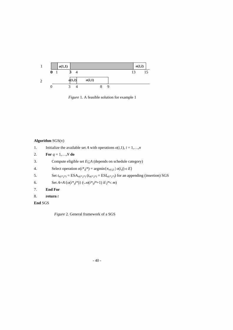
- 40 -

Figure 1. A feasible solution for example 1

0

3

13 15 1

0

3 1

8

0 4

9

o(2,2)

o(1,2)

o(1,1)

o(2,1) 2 4

3

Algorithm SGS(π)

1. Initialize the available set A with operations o(i,1), i = 1,…,n

2. For q = 1,…,N do

3. Compute eligible set E⊆A (depends on schedule category)

4. Select operation o(i*,j*) = argmin{πo(i,j) | o(i,j) ∈E}

5. Set to(i*,j*) = ESAo(i*,j*) (to(i*,j*) = ESIo(i*,j*)) for an appending (insertion) SGS

6. Set A=A\{o(i*,j*)} (∪o(i*,j*+1) if j*< m)

7. End For

8. return t

End SGS

Figure 2. General framework of a SGS

- 41 -

Figure 3. Partial active and non active solutions for Example 2

Figure 4. Partial active and non active solutions for Example 3

2 o(2,1)

0

3 5

5

1 o(1,1)

1 4

o(2,2)

o(2,2)

o(4,1) o(2,2)

(a)

(b)

(c)

(e)

o(1,1)

o(1,1)

o(1,1) (d)

7

o(4,1)

9 12 13

o(4,1)

15 17

2 0

3 5

5

1 o(1,1)

1 4

o(2,2)

o(2,2)

o(4,2) o(2,2)

(a)

(b)

(c)

o(1,1)

7

3 0

o(4,1)

o(2,1)

13 15 17

- 42 -

2

o(2,2)

o(2,1)

o(1,1)

0 13

3 5 7 10 12

5 12

1

1

0

3 1 15 13

6 5 2

0

1

9

3 1 15 13

4 3 2

0

Solution (a)

Solution (b)

Solution (c)

o(1,2)

o(1,1) o(2,2)

o(2,1) o(1,2)

o(1,1) o(2,2)

o(1,2) o(2,1)

Figure 5. The active schedules of example 1

{o(1,1),o(2,1)}

{o(1,2),o(2,1)} {o(1,1),o(2,2)}

{o(2,1)} {o(1,2),o(22)}

{o(2,2)} {o(2,2)} {o(1,2)}

{o(1,2),o(2,2)}

{o(2,2)} {o(1,2)}

{o(1,1)}

{o(1,2)}

(c) (b) (b) (b) (b) (a)

Figure 6. The Serial SGS enumeration tree

- 43 -

Figure 7 . The Extended Giffler-Thompson SGS1 and 2 enumeration tree

{o(1,1) }

{o(1,2),o(2,1)}

{o(2,1)}

{o(2,2)}

{o(1,2)}

(c) (b)

{o(2,2)}

Figure 8. Partial solutions for example 4 in and out of the type 2 non-delay set

2

1 o(1,2)

o(2,2)

o(2,3)

(a)

(b)

3

o(1,1)

o(2,1)

o(1,2)

4

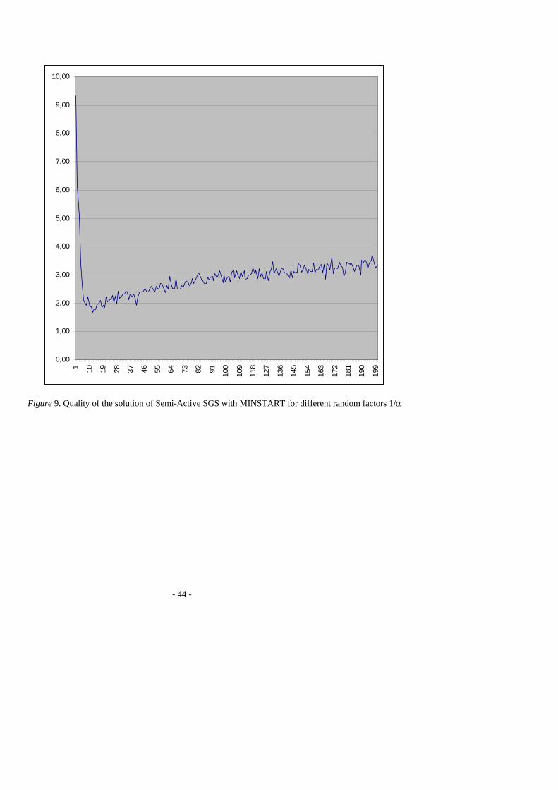
- 44 -

0,00

1,00

2,00

3,00

4,00

5,00

6,00

7,00

8,00

9,00

10,001 10 19 28 37 46 55 64 73 82 91 100

109

118

127

136

145

154

163

172

181

190

199

Figure 9. Quality of the solution of Semi-Active SGS with MINSTART for different random factors 1/α

schedule generation schemes for the job-shop problem with

Documents