1

Schedule Topology Complexity

August 2014 Booz Allen Hamilton

Hulett & Associates LLC

2

Contents

Team List

Background

Task Outline and Approach Summary

Ground Rules and Assumptions

Metrics Development

Summary

Demo

Next Steps

3

Team

Ken Odom - Project Manager

Matt Pitlyk – Task Lead

Mike DeCarlo – Lead Researcher

Eric Druker – Technical Advisor

Mike Cole – Schedule Subject Matter Expert

David Hulett – Schedule Subject Matter Expert (Hulett & Associates, LLC)

4

Project Background Background: – The complexity of a schedule can be indicative of the complexity of the program it represents. As

such, it can indicate potential future difficulties in managing that schedule’s project. NASA recognizes the need to understand the complexity of schedules in order to help Program Managers prevent schedule growth and to identify projects that may exhibit schedule growth.

– One common complexity measurement is the number of lines that make up the schedule – however, a larger schedule does not necessarily guarantee a more complex network or program.

– More measurements include parallel tasks and the number and size of merge points, but there is not a cohesive way to measure the “amount” of parallelism or the extent of merge bias caused by merge points by looking at the deterministic schedule.

Purpose: – There is a need for a schedule complexity metric that could indicate areas of potential schedule (and

thus cost) growth. – Complexity metrics may be able to help create an analysis schedule that accurately represents an

IMS. Approach: – Booz Allen implemented a structured, customized approach executing an assessment of potential

schedule complexity metrics. Throughout this effort, Booz Allen actively partnered with CAD personnel and Subject Matter Experts (SMEs) to coordinate, gather necessary data, and conduct research.

– The primary objective of Booz Allen’s assessment was to provide a recommendation for schedule complexity metrics that could indicate areas of potential schedule (and thus cost) growth. Booz Allen’s combined team of system engineering, scheduling, and JCL experts researched and developed recommendations to aid in the assessment of schedule complexity.

5

Complexity Definition

Complexity in schedules comes from characteristics of schedules that change the ambiguity inherent in every schedule.

If a schedule has no ambiguity, then it doesn’t matter how “complicated” it is, it can be executed perfectly, because there is no ambiguity1. Obviously this is never the case: all schedules have ambiguity, and complicated projects, hence their schedules, exhibit ambiguity and schedule risk. While this task was not concerned with precisely quantifying the ambiguity of schedules, it was concerned with identifying areas of the schedule that affect and change ambiguity.

Illustration1: The simplest schedule is a path of serial tasks. There are no characteristics of the schedule that increase the ambiguity of the schedule beyond that of the individual tasks themselves.

Illustration 2: A schedule with two parallel paths and a merge point. We know merge points increase the expected value of the duration of a project. So that characteristic of the schedule, the merge point, increases the expected value of the duration (it changes the ambiguity), and thus that schedule is more complex than the first example. Additionally, having multiple parallel paths requires coordination between the tasks to ensure the tasks succeed as intended in order for the program to continue without delay at the merge point.

1The International Centre for Complex Project Management has defined complexity in part as related to ambiguity. One component of ambiguity is risk.

6

Ground Rules and Assumptions

This task focused on complexity that is inherent in a project’s deterministic schedule.

The scope looked at characteristics of schedules found in an MS Project file: – This included characteristics such as task durations, number and type of logic links,

serialism and parallelism, merge points, slack, lag, calendars, resources, subprojects, and critical paths.

– This did not include aspects of the project that are not readily evident from the file such as non-deterministic critical paths, external pressure, uncertainty and risks.

Technical – Independent of external links – Focuses on the “self contained” part of the schedule – Project 2010 or 2013 and Excel 2010

7

Complexity Metrics vs. Health Metrics

This task focused on measuring the complexity of a schedule, not the health:

Health metrics: Indicate problems with the construction of a schedule that should be fixed before execution if possible.

Complexity metrics: Complexity of a schedule could indicate complexity in the program it represents. Thus, complexity metrics give an indication of potential difficulty in managing and executing the schedule based on characteristics of the schedule construction, but does not necessary advocate changes to the schedule.

Good health does not mean lower complexity or vice versa.

Bad health does not mean higher complexity or vice versa.

Note: While health and complexity of a schedule are separate, their scores are dependent: complexity

scores rely on healthy assumptions. Poor scores on a certain health metrics will skew or produce

inaccurate results from the complexity metrics.

8

Subject Matter Expert Sources

NASA: – Charles Hunt – Christopher Chromik – Heidemarie Borchardt – James Taylor (Reed Integration) – Justin Hornback (Reed Integration) – Kelly Moses (Reed Integration) – Michael Copeland (Reed Integration) – Robin Smith (Reed Integration) – Ronald Larson – Sharon Jones – Ted Mills – Wallace Willard

Non-NASA – David Hulett (Hulett & Associates) – Mike Cole (Booz Allen Hamilton) – Marie Gunnerson (Parsons Brinkerhoff) – Scott Lowe (Trauner Consulting

Services, Inc) – Chris Carson (Arcadis Corporation) – Fred Samson (Booz Allen Hamilton)

9

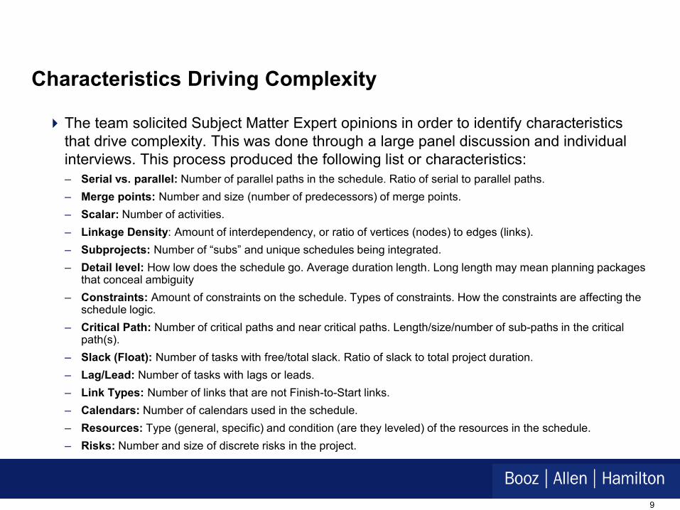
Characteristics Driving Complexity

The team solicited Subject Matter Expert opinions in order to identify characteristics that drive complexity. This was done through a large panel discussion and individual interviews. This process produced the following list or characteristics: – Serial vs. parallel: Number of parallel paths in the schedule. Ratio of serial to parallel paths. – Merge points: Number and size (number of predecessors) of merge points. – Scalar: Number of activities. – Linkage Density: Amount of interdependency, or ratio of vertices (nodes) to edges (links). – Subprojects: Number of “subs” and unique schedules being integrated. – Detail level: How low does the schedule go. Average duration length. Long length may mean planning packages

that conceal ambiguity – Constraints: Amount of constraints on the schedule. Types of constraints. How the constraints are affecting the

schedule logic. – Critical Path: Number of critical paths and near critical paths. Length/size/number of sub-paths in the critical

path(s). – Slack (Float): Number of tasks with free/total slack. Ratio of slack to total project duration. – Lag/Lead: Number of tasks with lags or leads. – Link Types: Number of links that are not Finish-to-Start links. – Calendars: Number of calendars used in the schedule. – Resources: Type (general, specific) and condition (are they leveled) of the resources in the schedule. – Risks: Number and size of discrete risks in the project.

10

Metric Development

The characteristics in green were used in the implemented metrics. – Density: Uses Linkage Density -The ratio of actual links in the schedule to total possible links

between tasks in the schedule.– Detail Variance: Uses Detail level - The amount of variation among the durations of the non-

summary tasks with non-zero duration in the schedule.– Merge Points: Uses Merge points and Slack (Float) - A weighted count of the number of

merge points that are in a schedule– Serial vs. Parallel: Uses Serial vs. Parallel - A proportion of the total project duration and the

sum of the durations of all tasks in the project.– Critical Complexity: Uses Critical Path - Indicates the amount of complexity related to the

critical and near-critical paths

11

Metric Development

The characteristics below were not used: – Scalar: Scale developed for classifying schedules. Potential use: scaling the scores of other

metrics. – Subprojects: Can add to complexity, but insufficient data in a Project file to develop metric. – Constraints: Artificial constraints covered by health metric. Insufficient data in Project file to

develop metric for others. – Lag/Lead: Unable to determine affect on complexity. – Link Types: Parallelism created by certain link types covered by Serial vs. Parallel metric. – Calendars: Add to complexity, but insufficient data in a Project file to develop metric beyond

simple counting. – Resources: Add to complexity, but insufficient data in a Project file to develop metric. – Risks: Add to complexity, but insufficient data in a Project file to develop metric.

12

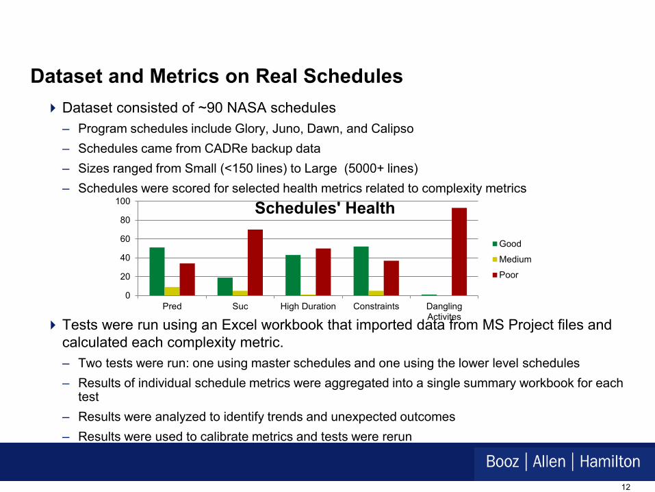
Dataset and Metrics on Real Schedules Dataset consisted of ~90 NASA schedules

– Program schedules include Glory, Juno, Dawn, and Calipso – Schedules came from CADRe backup data – Sizes ranged from Small (<150 lines) to Large (5000+ lines) – Schedules were scored for selected health metrics related to complexity metrics

0

20

40

60

80

100

Pred Suc High Duration Constraints DanglingActivites

Schedules' Health

Good

Medium

Poor

Tests were run using an Excel workbook that imported data from MS Project files and calculated each complexity metric. – Two tests were run: one using master schedules and one using the lower level schedules – Results of individual schedule metrics were aggregated into a single summary workbook for each

test – Results were analyzed to identify trends and unexpected outcomes – Results were used to calibrate metrics and tests were rerun

13

Density Metric What it is and How it is Calculated

The ratio of actual links in the schedule to total possible links between tasks in the schedule, expressed as a percent. The actual links between tasks are counted and divided by the total possible links to create the ratio. The value for the total possible links is the sum of the number of links per task if each task was linked to as many other tasks as possible.

How this relates to Complexity This relates to complexity by describing the amount of links between the tasks in the schedule. The fewer links there are, the less complex the schedule is. The more links there are, the more complex the schedule is.

The Input & Output Ranges Serial paths produces smaller scores. Lots divergent and merge points produce higher scores. Descriptive Statistics from Density: Mean: 5.91% St. Dev.: 14.62% Minimum: 0.00% 5th Perc: 0.07% 95th Perc: 22.24% Maximum: 100.00% Median: 0.42%

0% 3% 5% 8% 10% 13% 15% 18% 20% 23% 25%Metric Output

Den

sity

Comments & Caveats A return of 0% indicates no schedule logic, i.e. a milestone schedule. A return of 100% indicates the probability of a small schedule.

14

Detail Variance Metric What it is and How it is Calculated

The amount of variation among the durations of the non-summary tasks with non-zero duration in the schedule. The coefficient of variation for the duration of tasks shows how much relative variance there is in the task durations within the schedule. It is calculated by dividing the standard deviation of the duration by the mean of the duration.

How this relates to Complexity

The Input & Output Ranges

A schedule with diverse levels of detail will be harder to manage, understand and utilize effectively. Long activities may indicate planning packages that may lengthen when detail is revealed. A schedule with low Detail Variance has non-summary tasks with non-zero durations in the same order of magnitude (e.g. days, weeks, months, or years). A schedule with high Detail Variance has tasks with durations in different orders of magnitude (e.g. some tasks are days long and others weeks/months/years).

Comments & Caveats All tasks having equal length produces minimum. Tasks with lengths in different orders of magnitude produce higher scores. Descriptive Statistics from Detail Variance: Mean: 2.87 St. Dev.: 3.53 Minimum: 0.00 5th Perc: 0.41 95th Perc: 6.66 Maximum: 23.27 Median: 1.92

A milestone schedule will produce a score of 0.

0 1 2 3 4 5 6 7 8 9 10Metric Output

Det

ail

Varia

nce

15

Merge Points Metric What it is and How it is Calculated

A weighted count of the number of merge points that are in a schedule. This metric tallies the number of merge points that fall under three different categories – high (12+ predecessors), medium (6-9) and low (2-5). Predecessors with free slack are counted as .75. The counts are used to created a weighted total.

How this relates to Complexity Merge points vary in complexity based on the number of predecessors they have, and therefore vary in their contribution to complexity to the schedule. A merge point with many predecessors contributes more complexity to the schedule than a merge point with few predecessors.

The Input & Output Ranges A serial path will produce the minimum. Lots divergent and merge points produce higher scores. Descriptive Statistics from Merge Points: Mean: 63.05 St. Dev.: 196.32 Minimum: 0.75 5th Perc: 0.75 95th Perc: 322.69 Maximum: 1155.75 Median: 10.88

st

0 100 200 300 400 500Metric Output M

erge

Poi

n

Comments & Caveats It only takes a few large merge points to get the higher scores.

16

S

Serial vs. Parallel Metric What it is and How it is Calculated

A proportion of the total project duration and the sum of the durations of all tasks in the project. This considers duration that is “stacked” over the total duration of the project. It takes the sum of the duration of all tasks and divides it by the total project duration.

How this relates to Complexity A thicker schedule from top-to-bottom over the lifetime of the project indicates that more tasks and paths are running in parallel with each other. A higher volume of parallelism adds complexity to the schedule.

The Input & Output Ranges A single serial path produces a minimum of zero. A lot of parallelism produces a number close to one. Descriptive Statistics from Serial vs. Parallel: Mean: 8.24 St. Dev.: 14.74 Minimum: 0.24 5th Perc: 0.64 95th Perc: 24.90 Maximum: 104.76 Median: 4.09

0 10 20 30 40 50 60 70 80Metric Output er

ial P

aral

lel

Comments & Caveats A return of a negative number could indicate that there is a significant amount of slack in the schedule or that it is a milestone schedule.

17

Integrated Master Schedules vs. Lower Level Schedules (master on bottom)

Density

0% 3% 5% 8% 10% 13% 15% 18% 20% 23% 25%Metric Output

Den

sity

0% 3% 5% 8% 10% 13% 15% 18% 20% 23% 25%Metric Output

Den

sity

Detail Variance

0 1 2 3 4 5 6 7 8 9 10Metric Output

Det

ail

Varia

nce

0 1 2 3 4 5 6 7 8 9 10Metric Output

Det

ail

Varia

nce

Merge Points

0 100 200 300 400 500Metric Output Mer

ge P

oint

s

0 50 100 150 200 250 300 350 400 450 500Metric Output M

erge

Poi

nts

Serial vs. Parallel

0 10 20 30 40 50 60 70 80Metric Output Se

rial P

aral

lel

0 10 20 30 40 50 60 70 80Metric Output Se

rial P

aral

lel

18

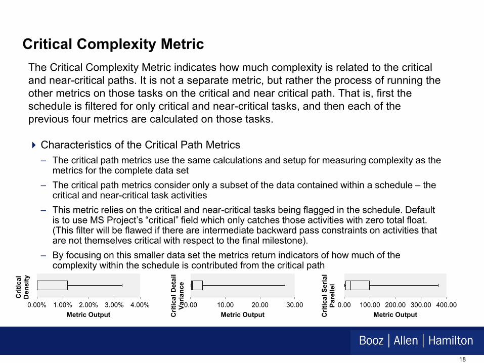
Critical Complexity Metric The Critical Complexity Metric indicates how much complexity is related to the critical and near-critical paths. It is not a separate metric, but rather the process of running the other metrics on those tasks on the critical and near critical path. That is, first the schedule is filtered for only critical and near-critical tasks, and then each of the previous four metrics are calculated on those tasks.

Characteristics of the Critical Path Metrics – The critical path metrics use the same calculations and setup for measuring complexity as the

metrics for the complete data set – The critical path metrics consider only a subset of the data contained within a schedule – the

critical and near-critical task activities – This metric relies on the critical and near-critical tasks being flagged in the schedule. Default

is to use MS Project’s “critical” field which only catches those activities with zero total float. (This filter will be flawed if there are intermediate backward pass constraints on activities that are not themselves critical with respect to the final milestone).

– By focusing on this smaller data set the metrics return indicators of how much of the complexity within the schedule is contributed from the critical path

l l

0.00% 1.00% 2.00% 3.00% 4.00%

Metric Output

Crit

ical

D

ensi

ty

0.00 10.00 20.00 30.00Metric Output C

ritic

al D

etai

Varia

nce

0.00 100.00 200.00 300.00 400.00Metric Output C

ritic

al S

eria

Pare

llel

19

Complexity Metrics vs. Schedule Growth Schedule growth data was obtained from two NASA sources. Correlation between the metrics and

the schedule growth data was calculated and the Density metric was high in both cases.

IPAO Schedule Growth

Density 0.41

Detail Variance -0.22

Serial Parallel -0.21

Merge Points -0.41

Schedules use d 7

NASA Joint Cost Schedule

Density 0.98

Detail Variance 0.95

Serial Parallel -0.97

Merge Points -0.44

Schedules used 5

Results suggest there may be a significant relationship between each of Density and Detail Variance with schedule growth.

The consistent negative correlation for Merge Points between the two cases suggests analysis with more data is required to determine relationships with schedule growth.

20

Complexity Metrics vs. Health Metrics

Five health metrics were run on the schedules in order to determine if the complexity and health metrics have the desired independence. – Each schedule received a Green, Yellow, or Red rating from each metric.– Schedules were grouped into those with 3+ Green and those with <3 Green.– For each complexity metric, the schedules were split into those who scored less than the median score of all the

schedules, and those at or above the median, for that metric.

Density Metric Good

(3+ Greens) Poor

(<3 Greens)

Upper 29 17

Lower 2 44

Detail Variance Metric

Good (3+ Greens)

Poor (<3 Greens)

Upper 14 33

Lower 17 29

Serial vs. Parallel Good (3+ Greens)

Poor (<3 Greens)

Upper 4 43

Lower 27 20

Merge Point Metric

Good (3+ Greens)

Poor (<3 Greens)

Upper 5 36

Lower 22 19

The presence of non-zero numbers in all for quadrants for each metric indicate limited correlation of the complexity and health metrics. – Two zero (or near-zero) numbers on the blue (black) diagonal would indicate positive (negative) correlation.– The independence of the two types of metrics ensures they are measuring different schedule characteristics.

21

Complexity Metrics vs. Complexity Metrics

Correlation between the results of each metric on the entire dataset was calculated in order to determine if the metrics have the desired independence.

Density Detail Variance Serial Parallel Merge Points

Density 1.00

1.00

-0.02 1.00

1.00

Detail Variance -0.17

Serial Parallel

Merge Points

-0.22

-0.21 0.14 0.67

All relationships show insignificant correlation except Serial/Parallel with Merge Points. However, the difference in results for the NASA Joint Cost Schedule test discussed earlier suggests these metric may be independent.

22

Summary

The complexity of a schedule is indicative of the complexity of the project it represents, and may be used to predict schedule growth. Complexity metrics can assist in ensuring an analysis schedule is truly representative of the IMS.

Research and Subject Matter Expert opinion produced a list of schedule characteristics that are related to schedule complexity.

This task developed five metric formulas and several additional metric recommendations.

The five metric formulas were calculated on a dataset of NASA schedules and produced ranges useful for interpreting the results of the metrics.

Two tests with schedule growth data indicate that two of the metrics (density and detail variance) could be correlated with schedule growth, while the other metrics need more analysis with growth data.

23

Next Steps

Currently metrics are regrea dataset of NASA schedules using a small amount of schedule growth data. The next step would be to gather more schedule files with actuals on schedule growth. – Then regression analysis could be used to determine which metrics are statistically significant for

schedule growth. – The results of the regression analysis could be used to calibrate the metrics to better correlate

with schedule growth. – The results could develop Schedule Estimating Relationships (SERs) to estimate schedule

growth based on these metrics.

Additional metrics could be developed for the follow characteristics: – Constraints – Link Types – Calendars – Resources – Subcontractors (with additional information)

Schedule complexity data could be used to benefit the project management community as well – Developing best practices for scheduling/executing projects – Ensuring analysis schedules created for JCL replicate complexity of project IMS

24

Backup

25

Resources

Topology and Dynamics of Complex Networks, René Doursat, Department of Computer Science & Engineering, University of Nevada, Reno, 2005

Two Methods to Calculate the Forward and Backward Passes in a Network Diagram, Jeffrey S. Nielsen, PMP, RMC Program Management Inc.

Soft Clustering, Lecture “Data Mining in Bioinformatics”, Till Helge Helwig, Eberhard-Karls-University Tübingen, 2010

IEOR 266, Lecture 8, Network Flows and Graphs, 2008 (Project Schedule Metrics, William M. Brooks

Schedule Network Complexity versus Project Complexity, Khaled Nassar, American University in Cairo, Egypt, Nottingham University Press

Soft Clustering on Graphs, Kai Yu, Shipeng Yu, Volker Tresp, Siemens AG, Corporate Technology, Institute for Computer Science, University of Munich

An Introduction to Modeling and Analyzing Complex Product Development Processes Using the Design Structure Matrix (DSM) Method, Ali A. Yassine, Product Development Research Laboratory, University of Illinois at Urbana-Champaign, Urbana, IL

Tools for Complex Projects, Kaye Remington, Julien Pollack

Project Complexity: A Brief Exposure To Difficult Situations, Dr. Lew Ireland, PrezSez 10-2007

This document is confidential and is intended solely for the use and information of the client to whom it is addressed.

26

This document is confidential and is intended solely for the use and information of the client to whom it is addressed.

Resources (continued)

The Complexity of Directed Acyclic Graph Scheduling with Communication Delay on Two Processors, Wing-Ning Li, Department of Computer Science, University of Arkansas

Bayesian Network, Wikipedia

The k-means algorithm, Tan, Steinbach, Kumar, Ghosh

Real Eigenvalue Analysis, Chapter 3 of textbook (no further information)

Chapter 6: Eigenvalue Analysis (no further information)

Chapter 5: Quantitative Measures of Network Complexity, Danail Bonchev, Gregory A. Buck, Center for the Study of Biological Complexity, Virginia Commonwealth University, Richmond, Virginia

DESIGN STRUCTURE MATRIX USED AS KNOWLEDGE CAPTURE METHOD FOR PRODUCT CONFIGURATION, M. Germani, M. Mengoni, R. Raffaeli, INTERNATIONAL DESIGN CONFERENCE - DESIGN 2006, Dubrovnik - Croatia, 2006

11.1.3 EM for Soft Clustering, ARTIFICIAL INTELLIGENCE FOUNDATIONS OF COMPUTATIONAL AGENTS

Critical Path Method in a Project Network using Ant Colony Optimization, N. Ravi Shankar, P. Phani Bushan Rao , S. Siresha, K. Usha Madhuri, Department of Applied Mathematics, GIS, GITAM University, Visakhapatnam, INDIA

GAO Schedule Assessment Guide: Best Practices for project schedules, United States Government Accountability Office, 2012

27 This document is confidential and is intended solely for the use and information of the client to whom it is addressed.

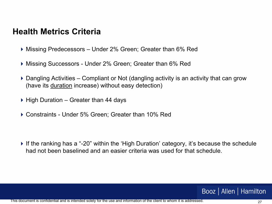
Health Metrics Criteria

Missing Predecessors – Under 2% Green; Greater than 6% Red

Missing Successors - Under 2% Green; Greater than 6% Red

Dangling Activities – Compliant or Not (dangling activity is an activity that can grow (have its duration increase) without easy detection)

High Duration – Greater than 44 days

Constraints - Under 5% Green; Greater than 10% Red

If the ranking has a “-20” within the ‘High Duration’ category, it’s because the schedule had not been baselined and an easier criteria was used for that schedule.

28 This document is confidential and is intended solely for the use and information of the client to whom it is addressed.

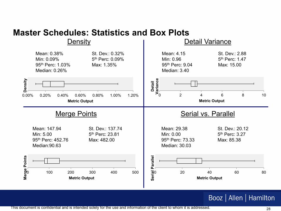
Master Schedules: Statistics and Box Plots Density

0.00% 0.20% 0.40% 0.60% 0.80% 1.00% 1.20%Metric Output

Den

sity

Mean: 0.38% St. Dev.: 0.32% Min: 0.09% 5th Perc: 0.09% 95th Perc: 1.03% Max: 1.35% Median: 0.26%

Detail Variance Mean: 4.15 St. Dev.: 2.88 Min: 0.96 5th Perc: 1.47 95th Perc: 9.04 Max: 15.00 Median: 3.40

0 2 4 6 8 10Metric Output

Det

ail

Varia

nce

Merge Points

Mean: 147.94 St. Dev.: 137.74 Min: 5.00 5th Perc: 23.81 95th Perc: 452.76 Max: 482.00 Median:90.63

0 100 200 300 400 500Metric Output M

erge

Poi

nts

Serial vs. Parallel

Mean: 29.38 St. Dev.: 20.12 Min: 0.00 5th Perc: 3.27 95th Perc: 73.33 Max: 85.38 Median: 30.03

0 20 40 60 80Metric Output Se

rial P

aral

lel