schema mapping design systems: example-driven and …mmartin/teaching/cs...data and transforming...

SCHEMA MAPPING DESIGN SYSTEMS �1

Schema Mapping Design Systems:

Example-Driven and Semantic Approaches

Kathryn Dahlgren

CSU Stanislaus

CS4960

Dr. Melanie Martin


Introduction

A classic problem in database management is the development of efficient and

effective methods for retrieving information from multiple heterogenous resources.

Heterogeneity arises as a result of a number of factors, including storing databases in

different formats, using different hardware and operating systems for database storage

systems, and designing databases with different data models, schemas, and semantics

customized to intended applications and to the preferences of database designers

(Katsis & Papakonstantinou, 2009; Ziegler & Dittrich, 2004). The field of data

integration focuses on developing solutions to the challenges associated with deriving

valuable information from collections of databases in which participant resources

possess highly dissimilar designs. The need for data integration originated in the early

1980s when business enterprises began investigating the possibility of integrating

database resources for more efficient access and utilization (Ziegler & Dittrich, 2004).

As Alon Halevy, a database research scientist at Google Inc., Anand Rajaraman, a

highly successful technology entrepreneur, and Joann Ordille, a database research

scientist at Avaya, observe in their overview of data integration innovations, “Data

integration is crucial in large enterprises that own a multitude of data sources, for

progress in large-scale scientific projects, where data sets are being produced

independently by multiple researchers, for better cooperation among government

agencies, each with their own data sources, and in offering good search quality across

millions of structured data sources on the World-Wide Web” (Halevy, Rajaraman, &

Ordille, 2006). Accordingly, data integration problems represent enduring issues with

widespread applicability.


Since databases often reflect application specifications and designer preferences

(Doan, Halevy, & Ives, 2012), database schemas generally possess a degree of

uniqueness. As a result, the task of querying over a collection of heterogenous

resources requires considering data outside the specialized context of specific

databases and combining the results into a standardized form. View-based data

integration provides a popular framework for integrating resources modeling structured

data and transforming query results from local database formats into a single

homogeneous view (Katsis & Papakonstantinou, 2009). The view-based method

focuses upon removing queried data from local contexts, called “source” or “local”

schemas, and combining and portraying the query results in a unified view, called the

Figure 1. A data integration system utilizing the view-based approach and illustrating the conceptual location of schema mapping design systems within a complete data integration system. Image modified from (Katsis & Papakonstatinou, 2009)

Schema Mapping Design Systems


“target” or “global” or “mediator” schema. Wrappers on the original database resources

portray source data using the data model of the target schema (Katsis &

Papakonstantinou, 2009). The process resolves heterogeneity issues related to data

model disparities by ensuring all data sources share the same data model. For

example, if a global schema uses a relational data model and the data integration

system uses an XML data source, a wrapper program portrays the XML data in terms of

a relational model compatible to the target data model. As Figure 1 illustrates, original

databases become “local” (also referenced as “source”) databases as a result of the

wrapping process. The process of connecting the local schemas to the “mediator” (also

referenced as “target”) schema is called schema mapping, more formally defined as “a

specification of the relationship between a source schema and a target schema” (Alexe,

ten Cate, Kolaitis, & Tan, 2011).

Figure 2. A screen shot of a schema mapping in Microsoft BizTalk Mapper. Image from (Block, 2008).


The advent of schema mapping resulted in the creation of three mapping

languages reflecting the major categorizations of schema maps, namely Global-As-

View, Local-As-View, and Global-And-Local-As-View. Global-As-View (GAV) produces

schema mappings by defining the global schema as a function of the local schemas.

Since the complete set of possible tuples modeled by the global schema contains only

information defined in local schemas, the global schema is unique and renders query

response derivations trivial. However, GAV systems do not easily facilitate the addition

of new local resources because the addition of new sources requires rewriting the

global schema to incorporate the new local schema semantics. In contrast, Local-As-

View (LAV) produces schema mappings by defining the local schemas as a function of

the global schema. The flexibility of the LAV definition renders the exact process of

semantic representation and data retrieval in LAV systems open to many possible

algorithmic solutions and remains an active field of research. The Global-And-Local-As-

View (GLAV) approach represents a generalized form of GAV and LAV. GLAV maps

queries over the local schemas into queries over the global schema. Accordingly, GLAV

systems can create schema mappings using exclusively GAV or exclusively LAV or

combine the capabilities of both languages to generate schema mappings beyond the

capabilities of either language individually. As a result, the combined system avoids

many of the disadvantages associated with GAV and LAV and enjoys the advantages or

both, though the complexity of the overall system increases significantly (Katsis &

Papakonstantinou, 2009).

A major challenge associated with the derivation of schema mappings is

establishing a high degree of semantic accuracy. Current software solutions rely upon


automatic and semi-automatic algorithms for deriving schema maps given a collection

of local databases. Some implementations utilize target schema matching systems to

correctly guess the most obvious maps between local and target schemas. However,

an overriding characteristics of current schema mapping system implementations,

exemplified by packages such as Clio, HePToX, Stylus Studio, and Microsoft BizTalk,

rely heavily upon human interactions. As illustrated in Figure 2, The generally adopted

methodology requires users specify visual connections between source schemas and

target schemas to help the schema mapping design software create maps capturing

relationships close to the actual source-to-target semantic translations. However,

schema mappings derived from visual specifications often detail only a subset of the

semantics necessary to create accurate schema mappings, especially since the same

visual specification may correspond to many logically divergent schema maps (ten

Cate, Kolaitis, & Tan, 2013). Accordingly, such software requires users pursue the

difficult and time-consuming task of manually editing the generated schemas to

resemble the intended semantics as closely as possible.

The necessary reliance upon manual editing to ensure the accuracy of maps

generated by visually interactive schema mapping design systems inspired research

into alternative approaches, such as example-driven and semantic methods, utilizing

more rigorous map definition paradigms. The example-driven approach to schema

mapping establishes relationships between source and target schemas through the

generation and confirmation of a collection of data examples illustrating accurate

source-to-target semantic translations. On the other hand, the semantic schema

mapping approach explores the inclusion of detailed conceptual models of the source


and target semantics as additional input to schema mapping algorithms. The example-

driven and semantic approaches represent promising alternatives to current visually

interactive methodologies.

Example-Driven Schema Mapping

The example-driven approach to schema mapping establishes relationships

between source and target schemas through the generation and confirmation of a

collection of data examples illustrating accurate source-to-target semantic translations.

Data examples represent “pair[s] of source and target instances that conform [to] the

source and target schemas” (ten Cate et al., 2013). The utilization of data examples to

guide mapping designs illuminates a problem regarding the best method for

generalizing examples into actual mapping expressions. The process of generating a

schema mapping according to a set of data examples introduces a class of “Fitting

Problems” focusing upon the derivation of schema mappings based upon a set of

universal data examples in which target instances represent universal solutions for

source instances (ten Cate et al., 2013). A corresponding class of “Fitting algorithms”

detail the steps necessary to derive schema mappings which produce schema

mappings with respect to the constraints of the GLAV or GAV mapping languages (ten

Cate et al., 2013). An illustration of the example-driven schema mapping approach

describes the interpretation of doctor and patient information in scattered source

databases within the context of a target database consolidating the information in a

standardized global format. Ultimately, the performance of schema mapping design

systems utilizing the described example-driven fitting approach yields exponential

complexity for GLAV constraints.


Fitting Problems and Algorithms

Fitting problems address algorithmic questions associated with deriving accurate

schema maps from a collection of data examples conforming to supplied source and

target schemas. The class of problems encompasses two sub-categories, namely fitting

decision problems and fitting generation problems. Given source and target schemas

and a set of data examples conforming to the schemas, fitting decision problem

solutions determine whether schema mappings exist (Alexe et al., 2011). Solutions to

fitting generation problems extend the fitting decision definition by either constructing

valid schema maps or reporting no such maps exist for given source and target

schemas and a data example collection (Alexe et al., 2011).

Alex et al. describe fitting algorithms for practical applications using GLAV and

GAV mapping language constraints (2011). The fitting generation problem adhering to

GLAV constraints is co-NP, while the fitting generation problem adhering to GAV

constraints is DP-complete, or coNP-complete for special cases of data examples.

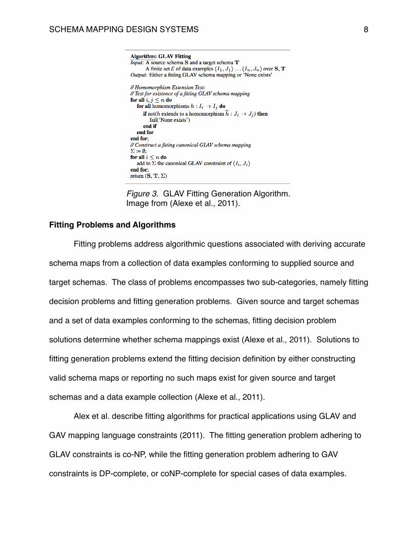
Figure 3. GLAV Fitting Generation Algorithm. Image from (Alexe et al., 2011).


GLAV Fitting Generation. Figure 3 details the steps of the GLAV fitting

generation algorithm. Given a source schema S, a target schema T, and a set of data

examples conforming to both S and T {(I1, J1), …, (In, Jn)}, where n is a finite integer, the

algorithm first solves the GLAV fitting decision problem and, if an appropriate GLAV

schema mapping exists, subsequently constructs the GLAV schema mappings

conforming to the given set of data examples (Alexe et al., 2011). The homomorphism

extension test of the algorithm in Figure 3 encompasses the fitting decision solution. A

homomorphism (h) is a function between two resources preserving the operations of

both resources (Conrad, n.d.). A homomorphism (ˆh) extends another homomorphism

(h) if ˆh(b) = h(b) for all b, where b is in the set of all values occurring in the union of

instances I and J (Kolaitis, 2009). The outer for-loop scans all possible combinations of

data examples against test the inner for-loop, which compares each i source instance

with each j source instance for a homomorphism and each i target instance with each j

target instance for a homomorphism. The if-statement fails if the homomorphism

between Ji and Jj does not preserve the operations of the Ii and Ij homomorphism. In

other words, the homomorphism extension test determines whether any of the data

examples fail to conform to the rules of both the source and target schemas. If so, no

schema mappings exists for the set of data examples.

GAV Fitting Generation. Figure 4 details the steps of the GAV fitting generation

algorithm. GAV fitting occurs in three steps: (1) test each data example for ground

status, (2) solve the fitting decision problem, and (3) create the GAV schema mapping.

A ground data example is a data example (I, J) in which all the values in the target

instance J are values appearing in source instance I. The definition aligns with the


definition of GAV requiring the construction of the target schema as a function of source

schemas. The first for-loop determines if any data example defies the definition of GAV.

If so, no schema mapping exists for the data example set. The second for-loop

determines if all Ji and Jj homomorphisms preserve the operations from the Ii and Ij

corresponding homomorphism. If not, then no schema mapping exists for the data

example set. The final for-loop creates the set of schema maps according to the given

data examples.

Figure 4. GAV Fitting Generation Algorithm. Image from (Alexe et al., 2011).


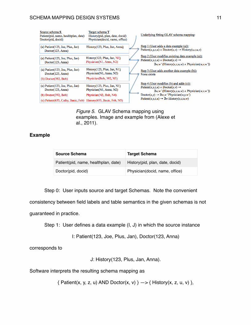
Example

Step 0: User inputs source and target Schemas. Note the convenient

consistency between field labels and table semantics in the given schemas is not

guaranteed in practice.

Step 1: User defines a data example (I, J) in which the source instance

I: Patient(123, Joe, Plus, Jan), Doctor(123, Anna)

corresponds to

J: History(123, Plus, Jan, Anna).

Software interprets the resulting schema mapping as

{ Patient(x, y, z, u) AND Doctor(x, v) } —> { History(x, z, u, v) },

Figure 5. GLAV Schema mapping using examples. Image and example from (Alexe et al., 2011).

Source Schema Target Schema

Patient(pid, name, healthplan, date) History(pid, plan, date, docid)

Doctor(pid, docid) Physician(docid, name, office)


or, equivalently, “For every tuple (x, y, z, u) in the Patient relation, if the Doctor relation

contains a tuple (x, v), then the History relation in the global schema includes the tuple

(x, z, u, v)”.

Step 2: User chooses to refine the data example in Step 1 to generalize the

schema mapping to include both target relation schemas.

I: Patient(123, Joe, Plus, Jan), Doctor(123, Anna)

corresponds to

J: History(123, Plus, Jan, N1), Physician(N1, Anna, N2),

where N1 and N2 are not defined in the local schemas. Software interprets the

modified schema mapping as

{ Patient(x, y, z, u) AND Doctor(x, v) } —>

{ ∃w, w’ ( History(x, z, u, w) AND Physician(w, v, w’) ) },

or, equivalently, “For every tuple (x, y, z, u) in the Patient relation, if the Doctor relation

contains a tuple (x, v), then the History relation in the global schema includes the tuple

(x, z, u, w) and the Physician relation includes the tuple (w, v, w’), where w and w’

represent unknown or different values”.

Step 3: User attempts to add another data example.

I: Doctor(392, Bob)

corresponding

J: Physician(Bob, 392, N3),

where N3 is not defined in the local schemas. Software interprets the modified schema

mapping as invalid because the resulting map is inconsistent with the mapping

established by the data example in Step 2. The resulting mapping is:


{ Doctor(i, j) } —> { ∃k ( Physician(j, i, k) ) }

or, equivalently, “For every tuple (pid, docid) in the Doctor relation, if the Doctor relation

contains a tuple (i, j), then the Physician relation in the global schema includes the tuple

(j, i, k), where k represents an unknown or different value”. The Step 3 mapping defies

the Step 2 mapping by (1) insisting every tuple in physician contains a docid, pid

combination appearing in a local database and (2) copying pid into the second field of

the Physician relation instead of docid. Since the second map does not preserve the

homomorphism established by the first map, the GLAV system concludes no schema

mappings exist (“fit”) for the set of two data examples.

Step 4: User adds two additional data examples

( I: Doctor(392, Bob), J: Physician(N3, Bob, N4) )

and

( I: Patient(653, Cathy, Basic, Feb), J:History(653, Basic Feb, N5) )

with the resulting valid maps

A. { Doctor(x, y) } —> { ∃w, w’ ( Physician(w, y, w’) ) }

and

B. { Patient(x, y, z, u) } —> { ∃w ( History(x, z, u, w) ) }

The resulting maps are valid because A represents a stronger version of the Step

1 schema mapping and establishes every doctor in the source Doctor relation appears

in the target Physician relation. Also, B represents a stronger version of the Step 1

schema mapping by establishing every patient in the source Patient relation possesses

a medical history in the target History relation.


Analysis

The nested for-loops in the homomorphism extension tests in both the GLAV and

GAV Fitting Algorithms for the software to scan the entire collection of data examples for

each data example in the collection. If a data example collection consists of N

examples, then the algorithm scans each example N times. As Alexe et al. observe,

“the homomorphism extension test […] involves a universal quantification over

homomorphisms followed by an existential quantification over homomorphisms: this is a

[coNP]-computation” (Alexe et al., 2011). Accordingly, the Fitting Decision Problem,

manifested in the algorithm as the universal-existential homomorphism extension test,

possesses a coNP-complete worst-case complexity, meaning no quick solutions exist

for deriving schema maps using the GLAV or GAV algorithms. However, despite the

worst-case complexity of the fitting decision algorithm, implementations of the example-

driven GLAV schema mapping system yield feasible performance in response to

practical real-life applications represented by common schema mapping design system

benchmark tests utilized by both visually-based schema mapping software, such as

Clio, and by the semantic schema mapping software examined in the next section

(Alexe et al., 2011). Accordingly, the example-driven schema mapping approach

represents a promising alternative to current visually interactive solutions by allowing

users the power to guide the schema mapping generator using descriptive illustrations

of source-to-target semantic translations via concrete examples.

Semantic Schema Mapping

The semantic schema mapping approach provides detailed conceptual models of

the semantics of source and target schemas as input. Conceptual models (CMs)


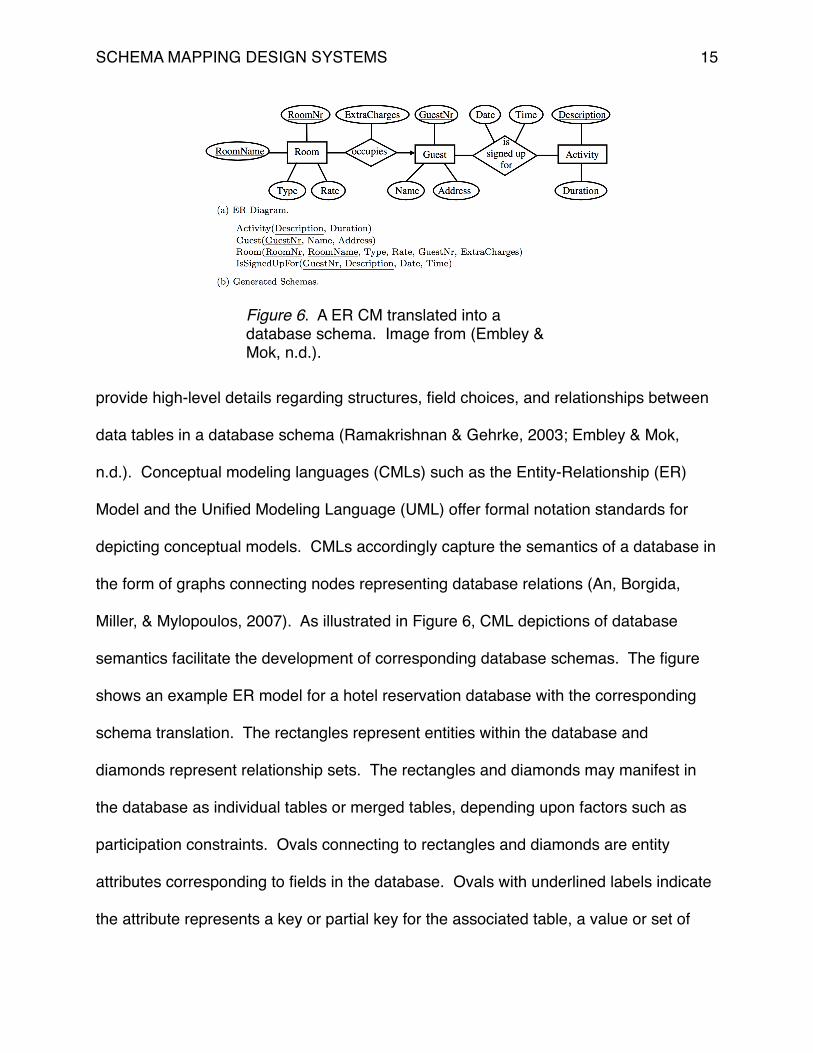
provide high-level details regarding structures, field choices, and relationships between

data tables in a database schema (Ramakrishnan & Gehrke, 2003; Embley & Mok,

n.d.). Conceptual modeling languages (CMLs) such as the Entity-Relationship (ER)

Model and the Unified Modeling Language (UML) offer formal notation standards for

depicting conceptual models. CMLs accordingly capture the semantics of a database in

the form of graphs connecting nodes representing database relations (An, Borgida,

Miller, & Mylopoulos, 2007). As illustrated in Figure 6, CML depictions of database

semantics facilitate the development of corresponding database schemas. The figure

shows an example ER model for a hotel reservation database with the corresponding

schema translation. The rectangles represent entities within the database and

diamonds represent relationship sets. The rectangles and diamonds may manifest in

the database as individual tables or merged tables, depending upon factors such as

participation constraints. Ovals connecting to rectangles and diamonds are entity

attributes corresponding to fields in the database. Ovals with underlined labels indicate

the attribute represents a key or partial key for the associated table, a value or set of

Figure 6. A ER CM translated into a database schema. Image from (Embley & Mok, n.d.).


values capable of uniquely identifying each tuple of data (Ramakrishnan & Gehrke,

2003).

The semantic approach utilizes the ability of CM graphs to directly describe the

semantics of a database as a tool for generating schema maps between heterogenous

databases. The semantics of a table described in CM subtrees, referenced as

“semantic trees” by An, Borgida, Miller, and Mylopoulos, represent the basis of the

semantic approach (An et al., 2007). The approach attempts to identify similarities

between semantic trees, also called “conceptual subgraphs” (CSGs) in the CMs of the

Algorithm 1: Known Target CSGInput: Source CM S, Target CM T,

Set of pre-defined semantic trees in S and T,Set of pre-defined node correspondences between S and T,Known CSG in T.

Output: A set of LAV schema mappings

1. Determine the qualities and characteristics of the CSG in T.

2. Use S and T node correspondences to find a node structure in source semantically similar to the node structure of the given target CSG.

3. Construct the semantically similar source node structure corresponding the the target CSG using minimal cost functional paths.

4. Derive LAV schema mapping expressions between the semantically similar source and target CSGs by expressing the CSGs as queries over predicates encoding the characteristics of the corresponding CMs.

5. Output the set of schema mappings.

Figure 7. Semantic approach algorithm for deriving a set of schema mappings when a target CSG is known.


source and target schemas. After translating the CSGs into algebraic expressions, the

algorithm derives LAV schema mappings using an efficient query rewriting method.

Algorithms

The semantic approach consists of two major algorithms encompassing two

major cases relating to whether or not the target schema possesses known CSGs.

The starting point for the semantic approach is the identification of a CSG in the target

schema. The CSG defines an essential set of semantics to maintain within the set of

derived schema mappings. In Algorithm 1, detailed in Figure 7, properties of the known

target CSG guide the discovery of a semantically similar CSG in the source schema.

The translations between the source and target CSGs provide the basis for developing

the set of LAV schema mapping outputs. On the other hand, if a target CSG is not

known, Algorithm 2, described in Figure 8, pursues connections between given

semantic trees within the target and source schemas allowing the construction of CSGs

Algorithm 2: Unknown Target CSGInput: Source CM S, Target CM T,

Set of pre-defined semantic trees in S and T,Set of pre-defined node correspondences between S and T.

Output: A set of LAV schema mappings

1. Construct a set of target CSGs by connecting pre-defined semantic trees in T using minimal cost functional paths.

2. Construct a set of source CSGs by connecting pre-defined semantic trees in S using minimal cost functional paths.

3. Proceed using Algorithm 1.

Figure 8. Semantic approach algorithm for deriving a set of schema mappings when a target CSG is not known.


and the subsequent discovery of semantically similar CSGs according to Algorithm 1.

The utilization of minimal cost functional paths during the construction of CSGs

represents an essential aspect of the algorithms because the functional properties of

conceptual models correlate directly to functional dependencies within the schemas (An

et al., 2007). The minimal cost paths align with the Occam’s Razor principle asserting a

default preference for the simplest solution in situations where multiple equivalent

solutions exist (An et al., 2007; Gibbs & Hiroshi, 1997).

Example

Figure 9 details a set of simple source and target schemas with entities,

attributes, and relationships. The source schema contains three entities each with a

single attribute connected other attributes by at least one relationship. The target

schema likewise contains three attributes with associated entities and connective

relationships. The semantic schema mapping algorithm inputs the conceptual models

for the source and target schemas. The simplicity of the example renders the graph

connecting the Proj, Dept, and Emp entities in the target a semantic tree and CSG by

Figure 9. Source and target CSGs with entity correspondences. Image from (An et al., 2007).


default. Accordingly, the example aligns with the procedure detailed in Algorithm 1. V1,

V2, and V3 represent known correspondences between source and target nodes.

Step 1: The algorithm begins by analyzing the properties of the target schema

CM. Specifically, the target CSG is an anchored semantic tree, meaning the single

table corresponding to the CSG derives from a single root object (“anchor”), namely the

Proj node (An et al., 2007).

Step 2: Source and target node correspondences provided as input guide the

discovery of a node structure in the source semantically similar to the root node

structure of the given target CSG. Since the V1 correspondence links the Project

source node with the Proj target node, the algorithm concludes the source may contain

a corresponding CSG.

Step 3: Constructing the semantically similar source node structure creates a

graph linking the Project node to every other node with a defined correspondence to a

target node using functional paths between source nodes minimizing the number of

edges not located within a defined source semantic tree. Accordingly, the example

trivially identifies the Project—>Department—>Employee semantic tree as a source

CSG corresponding to the target CSG.

Step 4: Deriving LAV schema mapping expressions between the source and

target CSGs enters the realm of active research focused upon query rewriting. The

process requires expressing the CSGs in the source and target schema as separate

algebraic expressions (An et al., 2007). The LAV schema mapping emerges from the

translation of queries over the algebraic expression predicates encoding the


characteristics of the corresponding CSGs. Exhaustive representations of the source

and target CSGs as datalog expressions are (An, Borgida, & Mylopoulos, 2005):

Table: Proj(pid, did, eid) :- Ontology: Proj(pid), Ontology: hasDept(pid,

did), Ontology: hasSup(pid, eid), Ontology: Emp(eid), Ontology:

Dept(did)

Table: Project(pid, did, eid) :- Ontology: Project(pid), Ontology:

controlledBy(pid, did), Ontology: Department(did), Ontology:

hasManager(did, eid), Ontology: Employee(eid)

Exact mapping expressions depend upon LAV implementations.

Step 5: Output the set of schema mappings.

Analysis

The semantic approach to schema mapping represents a promising alternative to

current visually interactive methods. Prototype software implemented in the MapOnto

package developed by An et al. demonstrate the viable performance of the semantic

schema mapping generation algorithms in response to practical real-life applications

(2007). The team ran the prototype implementation on a number of benchmark data

integration problems utilized to test both major visually interactive schema mapping

tools such as Clio and software implementations of the example-driven approach. In all

cases, the semantic schema mapping design system produced a manageable number

of schema mappings for the user to examine and verify within a time frame of less than

1 second (An et al., 2007).


Conclusion

Data integration problems represent enduring issues with widespread

applicability. Schema mapping represents a key field of research in data integration

because different data resources often possess high degrees of heterogeneity,

especially as a result of customizing database semantics for specific applications.

Current view-based methodologies rely upon visual interactions with users to guide

schema mapping designs. However, the heavy reliance upon time-consuming and

intricate procedures necessary to manually edit generated schema maps to improve

semantic accuracy inspired the development of example-driven and semantic methods

utilizing more rigorous mapping paradigms. The example-driven approach to schema

mapping establishes a collection of data examples guiding schema mapping systems

toward accurate source-to-target semantic translations. Semantic schema mapping

provides conceptual models of source and target semantics to derive accuracy in

schema mapping algorithms. Both approaches offer effective paradigms rejecting

visually interactive methods currently dominating schema mapping design systems.

The techniques provide users with interaction mechanisms supporting higher-quality

control over mapping designs. In both the example-driven and semantic approaches,

software implementations output a manageable number of schema mappings for the

user to verify and modify as necessary. The example-driven approach solicits a small

number of example correspondences from users to guide schema mapping designs.

The semantic approach requires inputing conceptual models of source and target

schemas by interpreting expressions in a CML and utilizing the resulting semantics to

create accurate schema maps. Both example-driven and semantic approaches offer


viable performance in practical applications. While the example-driven approach

provides exponential worst-case complexity, the theoretical limit does not impede the

performance of software implementations in practice. Likewise, the semantic approach

possesses efficient user input procedures and rapid results for practical applications

simulated by common schema mapping design system benchmarks. Accordingly,

example-driven and semantic approaches to schema mapping represent effective

paradigms rejecting the reliance upon visual user interactions.


References

Alexe, B., ten Cate, B., Kolaitis, P. G., & Tan, W. C. (2011). Designing and Refining

Schema Mappings via Data Examples. SIGMOD’11, 133-144.

An, Y., Borgida, A., & Mylopoulos, J. (2005). Inferring Complex Semantic Mappings

Between Relational Tables and Ontologies from Simple Correspondences.

ODBASE’05, 1152–1169.

An, Y., Borgida, A., Miller, R. J., & Mylopoulos, J. (2007). A Semantic Approach to

Discovering Schema Mapping Expressions. ICDE’07, 206-215.

Block, D. (2008, January 18). How to Create a Custom XSL Map for Use in BizTalk.

2006. Retrieved from http://www.codeguru.com/csharp/csharp/cs_data/xml/

article.php/c14753/How-to-Create-a-Custom-XSL-Map-for-Use-in-

BizTalk-2006.htm

Conrad, K. (n.d.). Homomorphisms. Retrieved from

http://www.math.uconn.edu/~kconrad/blurbs/grouptheory/homomorphisms.pdf

Doan, A., Halevy, A., & Ives, Z. (2012). Chapter 3: Describing Data Sources [Powerpoint

slides]. Retrieved from Principles of Data Integration – Book Homepage: http://

research.cs.wisc.edu/dibook/

Embley, D. W. & Mok, W. Y. (n.d.). Mapping Conceptual Models to Database Schemas.

Retrieved from: http://osm.cs.byu.edu/CS452/supplements/DataMappings.pdf

Gibbs, P. & Hiroshi, S. (1997). What is Occam’s Razor? Retrieved from

http://math.ucr.edu/home/baez/physics/General/occam.html

Halevy, A., Rajaraman, A., Ordille, J. (2006). Data Integration: The Teenage Years.

VLDB’06, 9-16.

http://www.codeguru.com/csharp/csharp/cs_data/xml/article.php/c14753/How-to-Create-a-Custom-XSL-Map-for-Use-in-BizTalk-2006.htm

http://www.math.uconn.edu/~kconrad/blurbs/grouptheory/homomorphisms.pdf

http://research.cs.wisc.edu/dibook/

http://osm.cs.byu.edu/CS452/supplements/DataMappings.pdf

http://math.ucr.edu/home/baez/physics/General/occam.html


Katsis, Y. & Papakonstantinou, Y. (2009). View-Based Data Integration. In Encyclopedia

of Database Systems. (pp. 3332-3339) New York: Springer Publishing Company.

Kolaitis, P. G. (2009). Relational Databases, Logic, and Complexity [Powerpoint slides].

Retrieved from https://users.soe.ucsc.edu/~kolaitis/talks/gii09-final.pdf

Ramakrishnan, R. & Gehrke, J. (2003). Database Management Systems. New York,

NY: McGraw Hill.

ten Cate, B., Kolaitis, P. G., & Tan, W. C. (2013). Schema Mappings and Data

Examples. EDBT’13, 777-780.

Ziegler, P. & Dittrich, K. (2004). Three Decades of Data Integration – All Problems

Solved? In R. Jacquart (Ed.), Building the Information Society (pp. 3-12) New

York: Springer Publishing Company.

https://users.soe.ucsc.edu/~kolaitis/talks/gii09-final.pdf

schema mapping design systems: example-driven and …mmartin/teaching/cs...data and transforming...

Documents