schmucker, 1985 (lb ch4.2.2)

100 4.2.2 Electromagnetic induction by external sources [Ref. p.124

4.2.2 Magnetic and electric fields due to electromagnetic induction by external sources

4.2.2.0 List of symbols and abbreviations

Symbols

B Cn. C(k) Co c~. }'~

E

H h J j j, k L

J.io p«(») p"m (cos 0)

Qn·Q(k) r, 0, ;, RE (!

a= l/e T = 2 rc/w t T

U V X,J'.Z X.l:Z l~ (0, J.) Zn. Z(k)

Table 1

flux density (= induction) vector of geomagnetic variations, in EnT] C-response (=depth of penetration) for P~' and wavenumber k source, respectively, in [km] zero-wavenumber C-response, in [km] spherical harmonic coefficients for internal (c) and external ()') parts of potential V (cos m}.-terms),

in EnT] electric field vector of geoelectric (telluric) variations, in [mVfkm] dielectric constant of vacuum, Eo = J.io I c- 2 (c: vacuum light velocity) complex-valued spherical harmonic coefficients for external (e) and internal (I) part of potential V,

in EnT] horizontal component of geomagnetic variations, in EnT] depth of perfect conductor, in [m] or [km] total depth-integrated current density, in [A/m] current density, in [A/m2] sheet current density, in [A/m]

wavenumber vector; k=l/k~ + k; distance of electrodes measuring U, in [m] or [km] magnetic permeability of vacuum, J.io=4rc .10- 7 Vs/Am skin depth, eq. (2). in [m] or [km] associated spherical harmonic function, quasi-normalized after A. Schmidt; 0: angle of colatitude Q-response (= ratio of internal to external potential) for Pnm and wavenumher k source, respectively gcocentric spherical coordinates (equivolumctric) earth's radius: R[=6371 km electrical resistivity, in [Om] spherical harmonic coefficients for internal (s) and external (/1) parts of potential V (sin m },-terms),

in EnT] electrical conductivity, in CS/m] period. in units of t time, in Cs] or [h]=hours, [d] = days, [a] = years conductance (thickness-integrated conductivity) of thin conducting sheets, in CS] electric earth potential. in [V] magnetic potential (B= -grad V), in [Vs/m2] rectangular coordinates (geographic north, east, down, respectively) north, east, and down component, respcctively, of geomagnetic variations, in EnT] general spherical surface harmonic function of degree n Z-response (= electromagnetic impedance) for Pnm and wavenumher k source. respectively, in

[(mV/km)/nT= km/s] zero-wa\'enumher Z-response, in [m/s=(J.iVfkm)/nT] tensor impedance angular frequency. in [S-I]

Abbreriatiolls

D geomagnetic variations on disturbed days DP disturbed polar geomagnetic variations Dst smoothed storm-time geomagnetic variations: UT-dependent part ELF extra low frequency emission (3 .. ·3000 Hz) L lunar daily geomagnetic variations S solar daily geomagnetic variations Sq solar daily geomagnetic variations on quict days UT universal time VLF very low frequency emission (3 .. ·30 kHz)

Schmucker

Ref. p.124] 4.2.2 Electromagnetic induction by external sources 101

4.2.2.1 Basic observations and theoretical concepts

Transient time variations of the earth's magnetic field are' of dual origin. They have external sources in the high atmosphere and magnetosphere as described in subsect. 4.1.1. Evidence for internal sources comes from

(i) the separation of global variation fields into external and internal parts; (ii) local studies of vertical Z variations in relation to horizontal H variations. In detail: The expansion of global variation fields at a given instant of time t into series of spherical harmonic

functions (subsect. 4.1.3.1) yields coefficients for Hand Z which are distinctly different and incompatible with an internal or external origin alone. This direct proof of dual origin is restricted, however, to variations of a truly global extent, and thus applies mainly to regular daily variations Sand L, and to Dst ring current variations. Irregular D variations and pulsations are confined to parts of the globe. Their representation by spherical harmonics would require unduly long series of spherical functions, and alternative methods of field separation on a local scale have been developed [Har63, Pri63]. But already the typical smallness of these Z variations in comparison to H variations is in itself definite proof of the existence of internal sources. See subsect. 4.1.1.3 for the disappearance of Z when internal and external potential coefficients are equal for a plane earth.

Evidence for the physical cause of the internal sources comes from two observations: (i) Spherical harmonic potential coefficients er:: and s;:' for the internal, induced part of the surface field are

bounded in size by a definite upper limit when set in relation to the coefficients y;:' and a::' for the external part. (ii) Internal fields lag in time relative to external fields and the transfer function Q(w) which connects them

in the frequency domain obeys the dispersion relation: If E(t) denotes the time dependence of any external potential coefficient of S, L or Dst variations and I(t) that

of any internal coefficient, then

l(t)= Q(t)*E(t) and l(w) = Q(w)· E(w),

where * implies convolution and the circumflex denotes Fourier transforms of I and E. Estimates of the transfer function Q(w) from global studies show that it satisfies the dispersion relation, implying Q(t)=O for t <0. This proves that the internal field depends only on the external field of the past and that E(t) causes I(t).

The thus established causal connection between external and internal sources of geomagnetic variations is well explained by the theory of electromagnetic induction. The outcome are models for the distribution of electrical conductivity within the earth (cf. sect. 2.3). This needs further explanation because the governing Maxwell field equations involve three material properties: the electrical conductivity (j, the magnetic permeability 11, the dielectric constant 8.

The induced magnetization of rocks is small, however, and 11 differs by less than 10- 3 from unity even in crustal layers with ferromagnetic mineral constituents. Secondly, the electromagnetic fields involved oscillate extremely slowly and even the most resistive rocks (Q;;; 1 06 Om) are much better conductors than true isolators as air, for instance, with Q~1014 Om. Consequently, below the surface - in distinct contrast to the air space above - displacement currents can be neglected against conduction currents when the period of oscillations exceeds fractions of one second. The resulting quasi-stationary approximation of the first field equation for non-magnetic space connecting the magnetic flux density B and electric field strength Eis

rot B = 110 (j E . (la)

Observations to this date do not require to consider an anisotropic internal conductivity. This approximation leads, in combination with the second field equation,

rot E= -8B/8t, (1 b)

to a diffusion type differential equation for E and B. Note that, in contrast, the free-space approximation, rot B = 110 80 8E/8 t, yields a wave equation. The electromagnetic theory in this context, therefore, describes the skin effect of downward diffusing, rather than propagating, fields, i.e. geomagnetic variations undergo within the earth amplitude reduction and phase rotation because of the screening effect of electromagnetically induced eddy currents. See Fig. 3 in sub sect. 4.1.1.

The scaling parameter for the downward penetration of time-periodic surface fields is the skin depth

p(w)=V2Q/w 110' (2)

Its definition exemplifies the generally valid fact that the depth of penetration increases with the square roots of resistivity Q and period T. For numerical estimates in SI units, i.e. with Q in [Om], and Tin Cs], use the formula

p(T)~t VQT [km].

Schmucker

102 4.2.2 Electromagnetic induction by external sources [Ref. p. 124

The skin-depth definition for electromagnetic cgs units is p(CO) =1/ (}/21COJ. Note that the electromagnetic cgs unit of (} corresponds to 10 -11 Qm.

Obsen'ing that rocks in the earth's outermost layers have a typical resistivity of 50 Qm, skin-depth values range from 20km for pulsations (T=30s) to 1000km for S variations (T=l day). The quoted resistivity is representative to about 400 km depth, excluding continental top layers and oceans, which have much lower resistivities. Sec Fig. 1 for skin-depth values in the period range of geomagnetic variations and typical resisti\~ties of rocks.

CH

ELF Pulsations bays SQ Ost

105

Qm

10'

103

101

10

Crystalline I Shields

1 basement Mobile belts

1 Consolidated

Sediments 1 Unconsol idated

I Seawater 10.1 ~-L-,-"'---'---..L.-~~--'-;~--'-;----'.~........J

10.1 10 106

T-

Fig.I. Skin depth P=lI2Q/w ~lo of geomagnctic variations of period T=2rt/w in seawater, sediments, and crustal rocks of variahle resistivity (!. The mean resistivity of mantle materiat is 50!lm ahove 400 km depth and l!lm below l;OO km depth. Cf. suhsec!. 4.1.1.2 for classification of geo· magnetic variations.

•

The theory predicts time-varying electric fields which are connected to the variable magnetic flux of geomagnetic variations according to eq. (1 b). They are observed as variations of the geoelectric or tell u ri c fi e I d in the subsoil with a well established linear relationship to the tangential components of B(t), leading again to conducti\;ty models for thc earth's interior.

In the air space above the ground a much stronger vertical electric field exists which varies with time and masks here induced telluric variations. Its cause are charge-separating processes in the atmosphere. Typical field values range from 100· ··300 V/m for fair weather conditions in plain terrain, the earth's surface being with negative charges. Sec [Miih57] for details. Note that, in contrast, telluric variation amplitudes are of the order of 1···100mVjkm (Fig. 5).

4.2.2.2 Response functions for induced magnetic and electric fields

4.2.2.2.1 General description and classification

Response functions are functions of time or frequency which express linear relations between electromagnetic field components, and between internal and external parts of the magnetic potential. The linearity follows from the field equations, eq. (1), which are linear in E and B, but restrictive assumptions will be necessary to specify their implications for the internal distribution of conductivity.

Three types of mutually dependent response functions are derived from surface observations: (i) Q-response functions which connect internal and external parts of the separated potential of geo

magnetic variations, (ii) C -response functions relating the vertical component to the horizontal component of geomagnetic

variations, (iii) Z-response functions which correlate the horizontal components of telluric and geomagnetic variations.

Any of these response functions can be used for inferences about the internal conductivity structure.

Schmucker

Ref. p.124J 4.2.2 Electromagnetic induction by external sources 103

Method (i) is referred to as potential method, method (ii) as geomagnetic deep sounding GDS, and method (iii) as magnetotelluric sounding MTS. The C-response from (ii) measures the penetration depth of variation fields into the conducting earth, the Z-response from (iii) the surface impedance. The determination of the Q-response requires simultaneous observations at world-wide distributed points, while in the case of C- and Z-responses single-site observations or observations at closely spaced points are sufficient. In this way global, regional, and local response estimates are distinguished. See the following subsections for details.

Because the analysis in the time domain requires the evaluation of convolution integrals, frequency domain response functions are preferred. They represent, in the terminology of spectral analysis, transfer functions between the Fourier transforms of some input time function, e.g. the external source field, and an output time function, e.g. the internal induced field, with superimposed uncorrelated noise. In the following sections all symbols for field quantities (8, I, Bx, Ex, etc.) are to be understood as their complex-valued Fourier transforms with exp(i Q) t) as time factor unless stated otherwise, Q) denoting the angular frequency.

Response functions have two purposes: (i) to predict a field component on the basis of a given conductivity model, e.g. the external field from the

observed sum of internal and eXternal fields, (ii) to find such models. See sub sect. 2.3.1 for the resolving power of response estimates with regard to con

ductivity within the earth, and subsect. 4.2.2.4 for methods to find the external part of geomagnetic variations from surface observations.

4.2.2.2.2 Q-response functions

By definition, estimates for this response require series expansions of the global surface field into spherical harmonics (cf. subsect. 4.1.3). When local fields are studied, spatial Fourier harmonics for a plane earth's surface may be used. The following complex notations for potential coefficients express the magnetic potential V in free space in spherical and rectangular coordinates, respectively:

+00 V(x,y,z)= Sf {t:(k)e-kz+l(<<)e+kZ}ei(kxx+kyYldkxdky

-00

with k= +Vk~+k;,

yielding for the rectangular surface field components at r=RE (earth's radius)

dpm B8= - L L {e~+ l~} eim !. de

and at z=O (earth's surface)

B =--=1... " " {em + lm} im eim le pm !. sin 0 L.. L.. n n n

Bx= - H ikx{e(k)+ l(kJ}j By= - SS iky{e(k)+ l(k)} ei(kxx+kyY) dkx dky.

Bz= SS k{e(k)-I(k)}

(3a)

(3 b)

Here e and I refer to external and internal parts of V, respectively, and k=(kx' ky) represents a wavenumber vector for fields in planes z=const. Note that

Re {~ei(rn!.+wtl+e;;-rn ei(-rnA+wt)} =y:;'(t) cos mA+a:;'(t) sin ml

connects potential coefficients in complex and real notations for time-harmonic fields, with a corresponding relation for I~, c~, and s~ (cf. eq. (5) in subsect. 4.1.1.6).

Suppose the external source potential is described by a single harmonic term in these series. Then, for a general earth model, the internal potential produced by induction will be composed of an infinite number of terms, each of them with a separate linear relationship to the inducing external term. Their evaluation is prohibitive and the following restriction on permissible earth models is introduced:

Schmucker


Consider some a\'erage earth model in which conductivity varies only with depth. Each external term then generates one single internal term. matching in degree and order for a sphcrical harmonic, or in k for a Fourier harmonic. The ratio of internal to external potential coefficients defines thc Q-response:

Qn = I;:'/C;:', Q(k) = I(k)/f.(k). (4)

Note that Qn depends only on the degree n, and Q(k) only on the absolute value of k. The evaluation of Dst, S, and L variations leads to fairly consistent global response estimates. This justifies

for these slow and therefore deeply penetrating variations the concept of a stratified average earth model, at least for the depth of their induced currents beneath. say, 400 km.

Figure 2 shows the Qn-response for a uniform sphere of radius R. Important are the following approximations when for a given frequency the sk in depth p({t)) from eq. (2) is either large or small in comparison to R/n:

Q =_n_ 2i (li)2 p'pR/n n n+1 (2n+1)(2n+3) p

Q =_n_{l_ 2n+1 (.!!.-)l p<{R/n. n n+1 1+i R J

1.0,-----------------::-=:;:;:::::;:;==:F'j"

0.8

"'" ~ 0.2 eo:

Sphere

~a n n

O~==~~~~~--~--~--~LL---L---L~~ 0.6 ,---------------------------------------,

c:£ 1\c 0.4

.§

~ 0.2

"" .§

1)-

Fig. 2. Electromagnetic Q-response Qn' Q(k) of. resrcctivcly. a uniform conducting sphere (radius R) and a half-space of

factor: eh",), and is given, as function of 'I, by

. .. ( n+l k reslstmty (! 11=1. £=1). -n- Qn and Q( ) are shown as n { 1 + i j.(i xl } Q=-- 1+---

n n+l I/n in_l(ixl (sphere)

Q(k)=1-2/{1 +111 +2il/2(k)) (half-space)

(5)

function of thc respectivc frequency-resistivity induction parameter 1/. i.e.

2R 2R I] =---1/wPoI2o= (sphere)

with ix = - (2 n + 1) l/n/(l + i) as argument of the modified spherical Bessel functions of thc first kind. - In this presen-

n 2 n + 1 - (2 n + 1) P

(half-space)

with p as skin dcpth (cr. Fig. 1) and k the wavcnumber. The complex-valued Q defines the ratio of internal to external potentials at the surface for sinusoidal inducing fields (time

tation n + 1 Qn for all degrees n of spherical harmonics and n

Q(k) for all wavenumbcrs k merge into a joint induction curve for 1/>5; for I]~1 the Q-response is predominantly out-of-phase [Sch70b).

Note that in the first case the internal field is out-of-phase with respect to the external field hccause induction is weak and self-induction negligible. In the second case both fields are nearly in-phase because induction is strong and self-induction sets in n!(n + 1) an upper limit for Qn'

Schmucker


This asymptotic behaviour of Qn can be generalized to any layered sphere, i. e. arg {Qn} lies between zero and 90 degrees, IQnl bctween zero and n/(n + 1). Observe that estimates of Qn do not provide information about finite internal conductivities if Qn is sufficiently close to either one of these limiting values.

To obtain the response for an earth model which consists of an inner uniform sphcre and an outer nonconducting shell ofthickncss h, multiply Qn for R=RE-h with (1-hIRd2n + 1• For a thin shell, h~RE' and strong induction, p ~ Rln,

Q =- 1--- h+--l- ~. n { 2n+1 ( p . p))

n n+1 RE 2 2 j (6)

Tables 2···4 summarize Q estimates from the global analysis of geomagnetic variation fields. In detail:

D s t: The recovery phase of storms is aperiodic and well suited for analysis in the time domain. Figure 3 shows, in the average over many storms, the external and internal potcntial coefficients of the leading ~(cos 8) harmonic. They demonstrate that

(i) a substantial internal part of Dst exists well below its upper limit, (ii) a fairly constant ratio IUe? prevails throughout the recovery phase, implying a delta-shaped time domain

response Q,(t). Assuming that Ql is a delta function, the general linear relationship

,+0

l::'(t)= S Qn(t-t')e::'(t')dt' -00

between internal and external parts reduces to

1::'(t)=Qn e~(t),

where Qn as Fourier transform of Qn is a real, frequency-independent constant. The appropriate earth model for this response is a perfectly conducting inner sphere (p=O) with a non

conducting shell of thickness

h=~ (1- n+1 Q) 2n+1 n n

as seen from eq. (6). Insertion of Ql = 0.36 yields h = 600 km, i.e. a sharp risc of conductivity evolves from the Dst response for the transition zone C of the earth's mantle (cf. subsect. 2.1.3).

30 oT 25

20

15

10

cO 5

-5

-10

__ e _ _ Inductive limit /e- -e_--e ___ e

I ~_--6_-.-A ....... _ ---e __ _ Ij ......." I '1 - .. -~.

I ' -A--e/ " I

a, = 0.38 0.36 0.42 0.38 0.35 0.33 0.35

Fig.3. External (e 1) and internal (Zl) potential coefficients of smoothed storm-time Dst variations, shown as function of time in the average over many individual storms. The storm-time is measured from 1/2 hour before the ssc commencement of the storm. The inductive limit gives 11 for a perfectly conducting sphere, 11 =ed2. - The time domain Q-response Q1 = Ide 1 is nearly constant, well below the limiting value of 0.5 for a perfectly conducting earth, and explainable by a perfect mantle conductor at 600 km depth. The deviating 121 at 24 h may reflect an imperfect separation of solar daily variations from Dst [Cha30].

-15 L-_-'--_-'----_-'---_-'--_-"-_-'-_--'-_--'

o 12 24 Storm-lime -

36 h 48

Table 2 contains the results from the analysis in the frequency domain, quoted again for the leading P! harmonic. They confirm the expected small phase of Q! and verify the time-domain estimate for IQ!I. Note the tendency of Rc {Q1} to increase towards shorter periods, indicating a finite value of conductivity at the quoted depth h. Only response estimates with phase information are listed. For others see [Rok82, subsect. 4.2.2].

Schmucker


Table 2. Q-response of Dst variations.

Response estimates Q \ for the dominant spherical harmonic p\(cos 0).

LAG Lagutinskaya et a!. [Lag75]: Analysis of three single storms of 100 h, 108 h, and 140 h duration with data from 79, 69, and 76 observatories, respectively. Response values for the principal period corresponding to the length of the analysed storm.

FAI Fainberg [Fai83]: Analysis of three single storms with data from 93 observatories, excluding in the course of the analysis those with anomalous Dst variations.

SCH Schmucker: Q\ calculated from the C-response in Table 6. In parenthesis the standard error of IQ"-

T Q\ T QI T QI d 10- 2 d 10- 2 d 10- 2

LAG FAI SCH

4.17 49+ 19i 3 34+5i 1.6 35+3i(1) 4.50 34+15i 4 31 +4i 2.7 34+ 3i (1) 5.83 41+i 8.0 32+2i(1)

25 30+6i 12.5 31 +4i (1) 25.0 29+ 5i (2)

San d L: Their analysis proves also the existence of a significant internal field, but now with a clear phase shift against the external field (cr. Fig. 5 in subsect. 4.1.1). For a decomposition of synthetic Sq variations, see Fig. 4.

20 nT X

0 ........ ~ 4S'N

....... --..

-20

20 nT 30'N ........... .. " .. 0 ... " ...........

40 nT

12h Local time

Fig. 4. Decomposition of solar daily variations X. }; Z from Fig. 7, suhsect.4.1.1, into parts of external (full dots) and internal (open dots) origin for three different latitudes 45° N, 30° N, and the Equator, respectil'ely. The curl'es are from a Fomier synthesis of the local time harmonics m=l··-4 (24···6 h). derived for each harmonic from a spherical harmonic synthesis with separated potential coefficients for the external and internal part of S. The coefficients are from lvlalin's analysis during years of maximum solar

activity (Table 2 of subsec!. 4.1.1). Spherical terms with Pmm+ 1 (cos 0) and Pmm+ 3(eos 0) have been used to represent the equator-symmetric part of S variations during equinoxes. The curves are from midnight to midnight in local time and refer to the dominant local time dependent part of S variations. - In the horizontal component X and Y external and internal parts are parallel, in the vertical component Z opposite with a visible phase lag of internal against external variations, indicating a finite upper mantle resistivity.

Schmucker


Tables 3 and 4 list Qn-responsc estimates with the potential coefficients from Tables 2 and 3 in sub sect. 4.1.1. In addition, response values from other studies are included; for comparison, Qn-responses calculated from Cn-responses (Table 7) are also presented.

Table 3. Q-response of solar daily variations.

Response estimates Qm+ 1 for the dominant spherical harmonic P.::'+ 1 (cos 0) of the m-th time-harmonic in local time. In parenthesis the standard error (BER: the rms error) of IQm+ll.

CHA Chapman [Cha19]: 21 observatories (6 continental observatories), mean of equinoxes 1902 and 1905. BEN Benkova [Ben40]: 46 observatories, May-August 1933. HAS Hasegava and Ota [Has50]: 46 observatories, mean of solstices 1932-33. Quoted from [Mat65a]. MAT Matsushita and Maeda [Mat65 a]: 69 observatories, equinoxes 1958. AFR Afraimovich et al. [Afr66]: Sept. 1958. Quoted from [Ber70]. BER Berdichevsky et al. [Ber72]: 39 observatories, yearly response estimates 1955-1964 from quiet days.

For m=3 and 4, yearly estimates from [KovSO, Table 4]. FAI Fainberg [Fai83]: 77 observatories, all year 1955; separation of Sq in normal and anomalous fractions

[Fai75]. M, P (E), W Malin, Parkinson, Winch: Qn calculated from potential coefficients in Table 2, subsect. 4.1.1. SCH-Y Schmucker: Qn calculated from C-response in Table 7 (Z: Y method), using eq. (S).

T m Qm+1

h 10- 2

CHA BEN

6 4 36+18i S 3 38+ 15i

(39 + 23 i) 1) 12 2 44+14i 43+4i

(40+1Si) I) 24 1 34+9i 43+3i

AFR BER

6 4 34+14i 40+23i (6) S 3 42+14i 43+ 10i (7)

12 2 42+9i 43+2i (2) 24 1 39+ 7i 37+3i (1)

M P(E)

6 4 42 + 22i (15) S 3 42+ 16i (7) 34+36i

12 2 41 + 12i (6) 45+9i 24 1 37+0i (6) 49+0i

1) Continental observatories only [Cha23, Table V].

Schmucker

HAS

44+11 i

41 +7i

43+7i

FAI

32+5i 39+15i 40+3i 34+9i

W

51+26i(13) 53+14i (5) 42+19i (5) 39-i (5)

MAT

44+11i

43+8i

35+Si

SCH-Y

40+1Si(3) 40+ 21 i (2) 36+16i(1) 35+5i (1)


Table 4. Q-response of lunar daily variations.

Response Qm+' of principal spherical harmonic P..~+ ,(cos 8) for the m-th time-harmonic with exp{i(mt' - 2 I'n as time factor (t' = local time, \'= phase of thc moon).

CHA Chapman [Cha19]: 21 observatories, mean equinoxes 1902 and 1905. MAT Matsushita and Maeda [Mat65b]: 37 observatories, all year average for a variable number of years. M. W Malin. Winch: Qm+' calculated from potential coefficients in Table 3, subsec!. 4.1.1. In parenthesis the

T h

6 8

12 24

standard error of IQm ~ .1.

m

4 3 2 1

CHA

48+ 15i 36+9i 57 + 34i 46+26i

MAT

31 +3i

M

55+15i(43) 50 + 11 i (22) 43+ 13i (17) 42+6i (22)

W

58 + 20i (13) 70+ 27i (11) 84+i (15) 76+5i (10)

Because the potential coeflicients in the quoted tables refer to harmonics in local time T = t + J, set

Re {f.;:' exp(imT)} = r;:' cos m T + 0';:' sin m T

with a corresponding relation for the internal part, and obtain

Qn c~-i s~

r;:' - i 0';:'

Considering the m-th time harmonic, the response estimates thus derived are in fair agreement from analysis to analysis ror the leading spherical harmonic of degree n = m + 1, but widely scatter for all others. This may be due to the inaccuracy of determination, but it could also renect the distorting effect of local conductivity anomalies and oeean's on the internal part (see suhseet. 2.3.2 for details). The tables contain therefore only response values for the leading spherical terms.

The Qn-response is again well below its upper limit with a clearly greater phase in comparison to the almost in-phase response of Os!. This implies that the internal parts of Sand L come from a more resistive part of the mantle above 700 km depth. Inserting. for instance, Q3 =0.41 +0.12 i for the second time harmonic of S (0)= 21t,'12 hours). eq. (6) yields 11 = 270 km and p(w) = 290 km, i.e. (J = 7.6 Om as resistivity of a uniform conductor below 11, See subsec!. 2.3.1.7 ror a combined interpretation of Ost and S responses.

or variations, bays, pulsations: The reduced penetration depth for these fast field oscillations brings their internal part lip to its limiting value. which excludes inferences ahout conductivity from their Q-response, Only for local jet fields in polar and equatorial regions a Q-response below this limit can be expected. but no results will be presented,

To estimate the response for a given geological situation, assume that the surface field is presented by spatial Fourier harmonics of wavenumhcr k. For a uniform halfspace the approximations for weak and strong induction are. respectively.

Q(k)=+ (kp)-2,

Q(k)= l-(1-i)· kp,

(7)

kp~1.

Sec Fig,2 ror exact values as function of k, Multiply Q(k) with exp(- 2k Il) if the uniform halfspace carries a non-conducting toplayer of thickness h. If the case of strong induction applies, insert for h the real part of Co(O)) lIsing the Z-rcsponses in Table 11 and Re{Co}=Im{Zo}/w.

Solar cycle variations: No unambiguous evidence has been obtained yet for the existence of an internal part, which should be small for these ultraslow oscillations, The most reliable and consistent estimate for n = 1, IQ.I =0,12 ± 0.07 and arg {Q!} = 8 ± 30 degrees [Har77], is included in Table 9 after conversion to a C-response. Ignoring the phase. this response is that of a perfectly conducting sphere at depth Il= Rdl-~)= 2400 km beneath a non-conducting shell.

Schmucker


4.2.223 C-response

In the original definition the C-response refers to variations with a surface field which is expressed by a single spherical or spatial Fourier harmonic. In terms of the Q-response from sub sect. 4.2.2.2.2 the C-response is defined as

1_n+1Q RE n n

C =-- (spherical earth) n n+1 l+Qn (8)

C(k)=..!.. 1-Q(k) (plane earth). k 1 +Q(k)

Insertion into eq. (3) gives the basic relations of the Z: H method to find C from locally observed geomagnetic variations of the vertical (Z) and horizontal (H) components:

P,:" sin 8 B,=n(n+1) Cn/RE· /d8 B8=n(n+1) Cn/RE ·-.-B;.

dP,:" lm

ik2 ik2 B%=T C(k) BX=T C(k) By.

" y

(9)

There is some arbitrariness in the choice of appropriate source parameters n, m, and kx' ky, respectively. The method fails where Z variations are too small to be evaluated, either because the induction is at the upper limit or because the source field has no Z variations at the point of observation. This applies to Dst and S sources near to the equator. Otherwise this method has the important advantage to allow response estimates for selected sites of observations where local anomalies are absent. Note that the two orthogonal horizontal components should yield identical C values, which can be achieved by a transformation to appropriate new coordinates.

The C-response is closely related to the magneto telluric Z-response, given by Z =iw C, and the W-response from [Ban69], given by Wn = n(n + 1) Cn/RE' It has like Z, but in contrast to Wn, the important property to be asymptotically independent from any source parameter when induction is strong. Its connection to the skin depth p from eq. (2) is as follows: For a uniform spherical earth model

[RE{ 2i (RE)2}

Cn= n+1 1 (n+1)(2n+3) p

~{1+ np/~E} 1 +1 1 +1

and for a uniform plane earth model

[! {1-i(kp)-2}

C(k)=

-P-{l+~} 1 +i 1 +i

(lOa)

p~RJn

kp~l

(lOb)

kp~l

as seen from eqs. (5) and (7). If any of these models has a non-conducting toplayer, add, for strong induction, its thickness h to C, and obtain

Cn = C(k)=h+!p(l-i). (11)

These results can be generalized to any layered sphere or half-space, identifying the C-response as complexvalued local measure of the penetration depth at the considered frcquency. See subsect. 4.2.2.3.5, eq. (21), for the interpretation of C as central depth of the induced current distribution. Its absolute value is also a scale length for the horizontal distance to which a locally determined C value is representative [Sch70a].

The restriction to a layered earth model applies therefore only to a limited depth-distance range around the point of observation, given by I Cl, which decreases with increasing frequency.

Arg {C} approaches zero for weak induction and may lie anywhere between zero and -90 degrees for strong induction, both in contrast to arg{Q}. See [Sch70b] or [Wai82] how to calculate the response for layered earth models.

The asymptotic source independence of C for strong induction leads to the definition of Co as zero-wavenumber response which Cn and C(k) approach asymptotically:

Cn -> Co for I Cnl ~RE/n, C(k) -> Co for k I C(k)1 ~l. (12)

Schmucker


Except for ultralong periods and local sources, the C-response of the earth is close to this asymptotic value and geomagnetic deep sounding can be extended now to surface fields of any spatial configuration:

Let the cited conditions for source independence be satisfied by all terms of a series of harmonic functions needed to describe a given surface field. This lea ves Co as the only response to be estimated from surface observations. Two methods exists for its determination:

(i) Z: Y met h od: A spherical (or spatial Fourier) harmonic analysis is carried out for the h ori zon ta I component of the variation field, yielding its unseparated surface potential

V(r=Rr,IU)=RrLYn(O,).),

where n

Yn(O,).)= L (c:;'+I:;')eimlp'm(cosO). m -n

From eqs. (3a, 4 and 8) and the substitution of Cn for Co follows

B,(O, l)= - CO/RE' L n(n + 1) Yn(O, ).), (13)

which allows response estimates Co from local observations in Z, but global observations in H. Because the spherical harmonic analysis removes the spatially incoherent part of H variations, less biased estimates can be expected. Furthermore, the reduced effect of local anomalies on H (in comparison to Z) renders the required exclusion of sites with local anomalies less stringent when Yn is determined from H.

(ii) The Z:H'-method (gradient method). It uses the gradients of the horizontal components derived in a regional network of observation points. Their relation to local Z variations at some central point is

{ aBo . _laB;.} B,= - CO/RE -0-+ cot 0 Bo+(sm 0) --. a al (14a)

To verify this relation, replace E in eq.(lb) for Br by B according to eq.(15), and treat Zo=icoCo as a constant during spatial differentiation. When local fields with strong gradients are analysed and

I a Bxla x + aB/a)'l~ cot 0 'IBxl/RE' the plane earth approximation

(14b)

may be used. The results obtained with these three methods are as follows.

Dst: The long-term Dst continuum and the Dst recovery phase of individual storms yield response estimates for periods of 1·· ·100 days and for penetration depths of 600·· ·1200 km. Here the Dst continuum contains globally observed long-term modulations of the equatorial ring current intensity (Fig. IS, 4.1.1), including the 27-day quasi-periodicity of storms, i.e. the tendency of storms to reoccur after a full rotation of the sun. The spherical harmonic analysis of the Dst continuum shows that the term with ~(cos 0) dominates as it does for indi\'idual storms (0: geomagnetic colatitude).

Table S gi\'es response estimates obtained by applying the Z: Y method in the time domain to very long periods beyond 8 days. Assuming a delta-function as time domain response <\(t), the time domain Z: Y relation from eq. (13) reads

Br (t)=h/R ELn(n+1) Yn(t)

for a given location (0, ).); " is the real, frequency-independent Fourier transform of Co and defines the depth of a perfect conductor below a non-conducting toplayer.

This depth turns out to be globally constant at about 1000 km with notable exceptions in North America and Siberia. Otherwise the earth's mantle appears to be laterally uniform at the quoted depth. Note that observations near coastlines do not give largely different depth estimates, i.e., for periods beyond 8 days, induction in oceans does not seem to produce visible coastal anomalies in Z.

Table 6 combines frequency response estimates from the continuum and from individual storms. Note that already observations at one site yield acceptable Co values when compared with C-converted Q values from global studies. However, error limits are large and in order to obtain better estimates Z observations from numerous sites have to be combined. The resulting C-response is to be regarded as a regional average. Observation points near to the equator, in high latitude, and near to deep oceans usually are excluded because in the period range below 8 days oceanic induction effects begin to modify Z variations at the coast.

Schmucker

Ref. p. 124] 4.2.2 Electromagnetic induction by external sources 111

Table 5. Depth (h) of perfect substitute conductor for Dst continuum [Sch79].

Time domain C-response from low-pass filtered daily means Sept.1964···Dec. 1965, cut-otT period 8 days. Depth estimates from Z: Y methods, eq. (13) with y" from a spherical harmonic analysis of H variations at 20 observatories, n = 1, 2.

*: coastline or island observatory; see Table 1, subsect. 4.2.3, for observatory code. Standard error in parenthesis.

Observatory h Observatory h km km

SVE 890 (170) TUC 800 (90) IRT 700 (90) MLT 950 (140) FUR 1080 (90) HON* 1000 (230) SUR 1370 (240) SJG* 1050 (120) BOU 710 (320) FUQ 1480 (900) TKT 1150 (130) TSU 1070 (280) TOL 970 (140) GNA* 1060 (190) FRD* 590 (120) HER* 980 (100) KAK* 880 (130) TOO* 940 (140) DS 710 (90) TWA* 1500 (340) (Dallas, Texas)

Table 6. C-response of Dst variations.

Response values refer to a single term Pj (cos 11) source except for the analysis SCH. In parenthesis the standard error of ICol (BAN: rms error of the mean).

ECK Eckhardt et al. [Eck63a] : Dst continuum analysis with daily means 1957/58. Recalculated response estimate for the observatory Tucson/Arizona with cross-spectral values from [Eck63 b], averaged from 0.025 to 0.075 and 0.075 to 0.125 cycles per day for T=20d and T=10d, respectively.

BAN Banks [Ban69]: Dst continuum analysis with daily means fo six 200-day records from the observatories ABN, KAK, HUA, WAT. Recalculated mean response from Figs. 10 and 11, averaged from 0.025 to 0.075 cycles per day. For observatory code, see Table 1 of subsect. 4.2.3.

DEV Devane [Dev77]: Dst single storm analysis (April 17 .. ·25, 1965) with hourly means from 60 observatories. Minor corrections according to [Dev78].

SCH Schmucker [Sch79]: Dst single storm analysis (seven storms 1964/65) and Dst continuum analysis (Sept. 64· .. Dec. 65) with hourly means from inland observatories in Europe. Response estimates are derived with the Z: Y method, Z from 9 observatories, and y" from a spherical harmonic analysis of H variations at 20 observatories, n=l, 2. Single storm analysis: response Co for T=1.6 and 2.7 days; continuum analysis: response Co for T= 8.0, 12.5, and 25.Q days.

LAG, FAI Lagutinskaya et al. and Fainberg: Calculated responses from Q in Table 2.

T Co d km

ECK

10 750-100i (350) 20 950 - 31 Oi (500)

T Co d km

DEV

1.3 725 - 330i (120) 2.7 750-320i (70) 5.3 825 - 230i (50)

10.7 920-160i (35) 21.3 955- 80i (75)

T. d

20

T d

1.6 2.7 8.0

12.5 25.0

Co km

BAN

830 - 290i (130)

Co km

SCH

690-150i (40) 780-160i (40) 860-120i (40) 900- 200i (80)

1020- 290i (130)

Schmucker

T d

4.4 5.6

T d

3.0 4.0

25.0

Co km

LAG

650-800i 420- 60i

Co km

FAI

760-250i 890- 240i

990- 320i


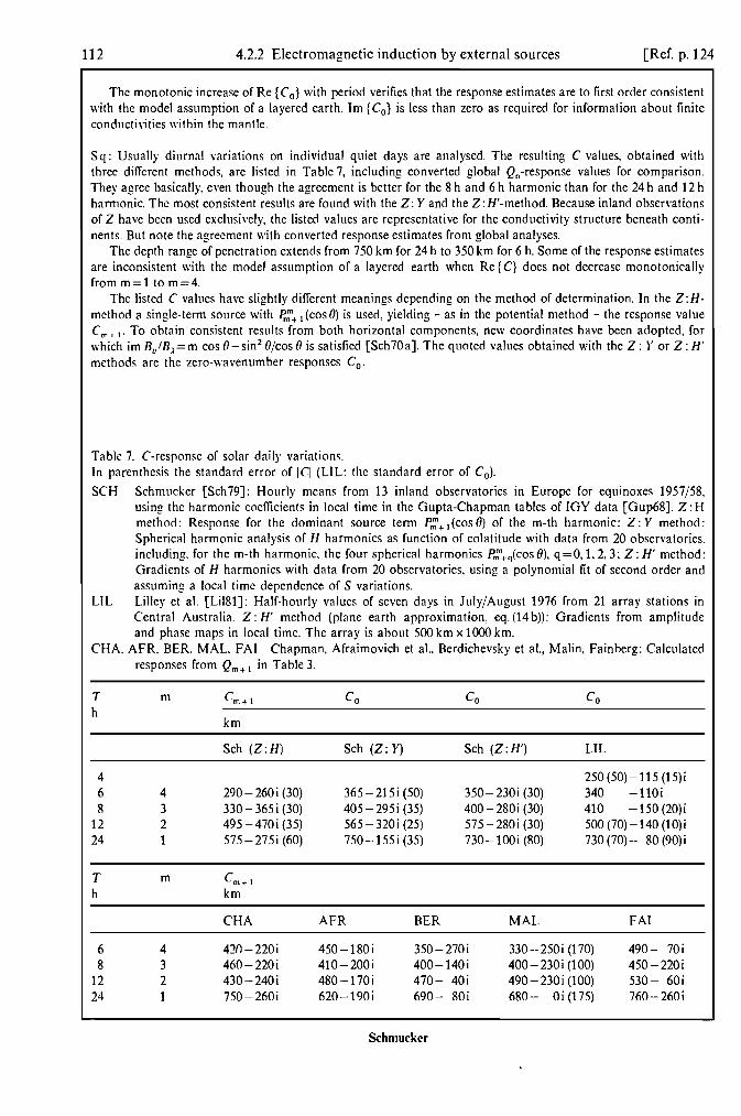
The monotonie increase of Re { Co} with period verifies that the response estimates are to first order consistent with the model assumption of a layered earth. Im {Co} is less than zero as required for information about finite conducti\;ties within the mantle.

Sq: Usually diurnal variations on individual quiet days are analysed. The resulting C values, obtained with three different methods, are listed in Table 7, including converted global Qn-response values for comparison. They agree basically, even though the agreement is better for the 8 hand 6 h harmonic than for the 24 hand 12 h harmonic. The most consistent results are found with the Z: Y and the Z:H'-method. Because inland observations of Z have been used exclusively, the listed values are representative for the conductivity structure beneath continents. But note the agreement with converted response estimates from global analyses.

The depth range of penetration extends from 750 km for 24 h to 350 km for 6 h. Some of the response estimates are inconsistent with the model assumption of a layered earth when Re {C} does not decrease monotonically from m=1 to m=4.

The listed C values have slightly different meanings depending on the method of determination. In the Z:Hmethod a single-term source with Pmm+ I (cos 0) is used, yielding - as in the potential method - the response value Cm. I' To obtain consistent results from both horizontal components, new coordinates have been adopted, for which im BvIB;. =m cos 0 -sin 2 O/cos 0 is satisfied [Sch70a]. The quoted values obtained with the Z: r or Z: H' methods are the zero-wavenumber responses Co.

Table 7. C-response of solar daily variations. In parenthesis the standard error of ICI (L1L: the standard error of Co).

SCH Schmucker [Sch79]: Hourly means from 13 inland observatories in Europe for equinoxes 1957/58, using the harmonic coefficients in local time in the Gupta-Chapman tables of IGY data [Gup68]. Z: H method: Response for the dominant source term P.::'+ I (cos 0) of the m-th harmonic: Z: Y method: Spherical harmonic analysis of H harmonics as function of colatitude with data from 20 observatories, including. for the m-th harmonic, the four spherical harmonics Pmm+q(cos e), q =0,1,2,3; Z: H' method: Gradients of H harmonics with data from 20 observatories, using a polynomial fit of second order and assuming a local time dependence of S variations.

L1L Lilley et al. [LiI81]: Half-hourly values of seven days in July/August 1976 from 21 array stations in Central Australia. Z: H' method (plane earth approximation, eq. (14 b)): Gradients from amplitude and phase maps in local time. The array is about 500 km x 1000 km.

CHA, AFR, BER, MAL. FAr Chapman, Afraimovich et aI., Berdichevsky et a\., Malin, Fainberg: Calculated responses from Qm+ I in Table 3.

T h

4 6 8

12 24

T h

6 8

12 24

m

4 3 2 1

m

4 3 2 1

km

Sch (Z:H)

290 - 260 i (30) 330 - 365 i (30) 495-470i (35) 575-275i (60)

CHA

410-220i 460-220i 430-240i 750-260i

Co Co Co

Sch (Z:Y) Sch (Z: H') LIL

250(50)-115 (15)i 365-215i (50) 350 - 230 i (30) 340 -110i 405-295i (35) 400-280i (30) 410 -150 (20)i 565 - 320 i (25) 575-280i (30) 500 (70)-140 (10)i 750-155i (35) 730-100i (80) 730 (70) - 80 (90) i

AFR

450-180i 410- 200i 480-170i 620-190i

BER

350-270i 400-140i 470- 40i 690- 80i

Schmucker

MAL

330 - 250 i (170) 400 - 230 i (100) 490 - 230 i (100) 680- Oi (175)

FAI

490- 70i 450-220i 530- 60i 760- 260i

Ref. p. 124] 4.2.2 Electromagnetic induction by external sources 113

DP variations, bays, pulsations: Their surface field is too complicated to allow a simple description with a single harmonic function or not too long a series of harmonic functions. This excludes the Z:H and Z: Y method, but leaves the Z:H' method to find the local Co-response. In mid-latitudes, however, horizontal gradients of the horizontal variation components are too small for a successful application, at least for the presently reached instrumental accuracy, and no results will be cited. In addition, local anomalies may conceal here at many sites the relatively small Z variations which arise from the spatial inhomogeneity of the source field.

Table 8 lists a successful application of the gradient method to observations in the auroral zone, where thc H gradients are sufficiently strong. Note the smooth decrease of Re {C} from 206 km for 8200 s to 55 km for 115 s, extending the depth-of-penetration estimate from Sq upwards into the lithosphere. The concurrent change of arg {C} suggests a smooth upward increase of litho spheric resistivity from about 10 to 140 !lm.

Table 8. C-response of polar substorms [Jon80].

Co-response estimates with data from 10 array stations in the auroral zone of Scandinavia, using the Z: H' method. The array is about 250 km x 250 km. Spatial gradients of H variations from a polynomial fit of second order to complex Fourier harmonics obtained for data segments of 8 hours length; Co from plane earth approximation, eq. (14 b). In parenthesis 95 % confidence interval.

T Co T Co s km s km

115 55 (9) - 32 (5)i 890 111 (16) - 64 (17)i 190 64 (16) - 39 (7)i 1490 138 (20)- 63 (42)i 320 78 (15)-48 (8)i 2480 163 (33)-60 (10)i 535 92 (6)- 58 (9)i 4090 180 (26) - 64 (35)i

8200 206 (38)-72 (42)i

Semi-annual, annual and solar cycle variations: These ultralong periodic variations will penetrate into thc lower mantle beyond 1000 km depth. The smallness of their amplitude and the insufficient baseline stability of instruments, observing in particular Z variations, make response estimates difficult. In addition, uncertainties exist about their representation by spherical harmonics.

Annual and semi-annual variations are clearly seen in the spectrum of the north component, less clear and with low correlation in the spectrum of Z. They are attributed to different sources, annual variations to ionospheric sources with P2 (cos (3) as leading spherical harmonic, semi-annual variations to the equatorial ring current with Fi (cos 13) as leading term [Cur66]. Table 9 lists response estimates, using these single-term source descriptions. Even though the response of annual variations turns out to be close to the limit of no induction, a penetration depth well below 1000 km appears to be indicated.

Similar problems arise for the response of solar cycle variations with a quasi-period of 11 years. Their spherical harmonic analysis identifies again P1 (cos (3) as leading term [Har77]. Only those published response estimates are included in Table 9, which are below the limit of no induction. They agree in their real parts, indicating a depth of penetration of 2000 km, but disagree in their imaginary parts. Also included in Table 9 are responses for the 27-day quasi-periodicity, yielding for its principal period consistent estimates with a penetration depth of about 1000 km. All response values in Table 9 have in common that they refer to periodic or quasi-periodic variations, providing relatively strong signals abovc the background continuum, but with a problematic removal ofthe longterm trend of secular variations of the earth's planetary field.

Schmucker


Table 9. C-response of very long period geomagnetic variations.

Response estimates from Z: H assuming a PI (cos e) source except for annual variations with an assumed P2 (cos e) source. In parenthesis the standard error of ICI.

BAN Banks [Ban69J: 27-day variations: Analysis of 1000-day segments of daily means from two observatories (G RW, W AT), taking spectral averages over 3 or 4 solar cycles. Annual variations: Analysis of monthly means from 6 observatories (WAT, HUe, GRW, AGN, ESK, LER) for a variable number of years between 1919 and 1964. Response estimate for semi-annual variations with monthly means of WAT. The connection to Banks' W-response is C I =RE/2· WI and C 2 = Rd3 . W2 , respectively. For observatory code, see Table 1 of subsect. 4.2.3.

RIK Rikitake [Rik51J: Daily means (?) from 9 observatories in four segments of about 6 months length 1924/25.

DZH Dzhodenchukova [Dzh75J: Daily means from 12 observatories, using data segments of 216 days (?). ISI Isikara [lsi77]: Analysis of annual means 1949···1970 from 38 observatories using a polynomial fit of

second or third order to remove secular variations; exclusion of 13 observatories with local responses above the limit of no induction (IZ/HI > cot e). The two quoted values refer to a least-squares analysis with respect to Cl (upper value) and QI (lower value).

HAR Harwood and Malin [Har77]: Analysis of annual means from 81 observatories for segments of variable length between 1842 and 1974. The response is calculated from QI obtained from a spherical harmonic analysis with three zonal harmonics p.(cos e), n=l, 2, 3.

DUC Ducruix et al. [Duc80J: Analysis of annual means 1947· .. 77 from 10 observatories in Europe. The response has been estimated from the segment 1947· .. 67 prior to a discontinuous change of secular variations; within this segment they are removed by a third order polynomial.

T

9d 13.5 d 27 d

BAN

790-120i (40) 760-340i (40)

1000-320i (50)

0.5 a IC 11 = 1430 (410) 1 a I) C2 =1860-330i (280)

ISI

1480 - 2040 i (400) 2030-2140i (530)

I) Limit for no induction: Rd3=2124km. 2) Limit for no induction: Rd2= 3186 km.

RTK

1360-570i (160)

Due 2000 - 890 i (250)

DZH

440-655i 630-530i 980-340i

HAR

2200-120i (610)

4.2.2.2.4 The magnetotclluric scalar Z-response

This response connects orthogonal horizontal components of electric (= telluric) and geomagnetic time variations at a given surface point above a layered sphere or half-space. Its exact definition requires that the surface field is described by a single spherical or Fourier harmonic function, for which

EO=-Zn·B;., E).=+Zn·Bo (spherical earth)

Ex=Z(k) By, Ey= -Z(k) Bx (plane earth).

The Z-response is in units of 1 (V/mVf=l m/so In magnetotelluric work a frequently used unit is

1 mV/km 1 km/so nT

Schmuckcr

(15)


It applies exclusively to source fields with a tangential electric field and is in the above definition the scalar impedance of a layered earth, to be distinguished from the tensor impedance Z for a non-layered earth. MUltiply Z with f.lo to obtain the conventional impedance of electromagnetic waves in units of 1 Cl, defined for B/f.lo rather than B.

The scalar impedance is readily ex pressed in terms of the C-response:

Zn=iw Cn, Z(k)=iw C(k).

Its limiting values follow then from eq. (10) as

for no induction, and as

Zn=iwRE/(n+1), Z(k)=iw/k

iwp ~·Wg Zn=Z(k)=-.= -,

1 +1 f.lo

(16)

(17a)

(17b)

when the induction is at its upper limit in a uniform sphere or half-space of resistivity g. The source independence of Z at this limit applies to any layered conductor. In magnetotelluric work impedance estimates are usually interpreted in terms of the zero-wavenumber impedance Zo which Zn and Z(k) approach asymptotically when IZnl ~wRJn and IZ(k)1 ~w/k, respectively.

Arg {Zo} =4> may lie, as function of frequency, between zero and 90 degrees. When, for a given frequency, the phase 4> is above 45 degrees, the impedance can be explained by a uniform conductor at depth h beneath a nonconducting toplayer as seen from eq. (11):

(lS)

For a phase below 45 degrees a model applies in which a uniform sphere or half-space is covered with a thin toplayer of depth-integrated conductivity (=conductance) t; "thin" implies that the skin depth of both conductors is large in comparison to the thickness of the toplayer. The reciprocal impedance (=admittance) of this model is

ZOl =110 t+(l-i)/wp, (19)

where p is the skin depth of the uniform conductor. If p is large for a poor conductor, the impedance is a real, frequency-independent constant l/f.lo t and the time-domain impedance a delta-function.

The use of impedance estimates for investigations of the internal conductivity has two important advantages: (i) No source parameters enters into its determination from observations at a single site,

(ii) induction at the upper limit is permitted. Problems arise from the use of telluric variations, which on land are locally distorted by lateral changes of

the near-surface conductivity almost everywhere. This distortion disappears, however, with increasing frequency, when the decreasing penetration depth, as expressed by I Cl = IZI/w, more and more limits the depth-distance range of influence. The tabulated scalar impedance estimates are from the following observations:

D s t: The telluric field is quite small because the impedance of Dst fields should decrease linearly with frequency as Zo = iwh, applying to a perfect conductor at depthh beneath a non-conductingtoplayer, eq. (lS). For W= 21t/2 d- I

and h=600km, for instance, Z=0.002(mV/km)/nT. No results are quoted about various attempts to determine this minute Z-response of the Dst recovery phase of storms except for results from the seafloor where the telluric noise level is exceptionally low. They are included in Table 12.

Sand L: Solar daily variations in E are clearly resolved in the spectrum of telluric fields and, on quiet days, even visible in the telluric record (Fig. 5). A strong coherency between S variations in the two horizontal components makes estimates of the tensor impedance difficult. Because everpresent local distortions for these deeply penetrating variations require the knowledge of this impedance, no results are quoted. Table 10 contains estimates for the Sq continuum, where the coherency between horizontal components is low, and scalar impedances for the Sq lines, obtained by the conversion of geomagnetic Co responses from Table 7.

Lunar daily variations should have a similar impedance, but their telluric variations are too small in amplitude to be detectable. Near coastlines and in particular at the seafloor relatively strong motion-induced telluric signals for the M2 lunar tide are observed which can appear even far inland [LarSO] (cr. subsect. 4.2.2.3.4).

Schmucker


Table 10. Magnetotelluric Z-response in thc period range of daily variations [Lar80].

Analysis of hourly means 1932· ··1942 from the observatory Tucson/Arizona (TUC) with electrode spacings of 57 and 94 km. Tabulated scalar impedance values Zo=(ZX).-Z)'x)/2 are from a power series representation of empirical band-averaged estimates of the tensor impedance. Zo in [mjs=(J.IV/km)fnT]. In parenthesis the standard error of IZol.

T Zo ZO I) h mjs mjs

48 16+ 39i 24 11+ 55i (3) 16 44+ 87i 12 47+ 82i (4)

8 64+ 88i (8) 6 63+ 106i (15)

5.3 95+155i 3.2 132+ 189i

I) Calculated from C-response in Table 7, SCH (Z: Y): Z=iwC.

OP variations, bays, pulsations, VLF emissions: Because the absolute value of the impedance increases with frequency for any layered earth model of finite conductivity, these fast variations produce, in comparison to Ost and S, pronounced telluric variations. In the absence of transient stray fields from artificial sources (railroads, industry, power lines) the correlation bctween telluric and magnetic variations is excellent and nearly linear (Fig. 5). This allows an accurate determination of the magnetotelluric tensor impedance Z. More difficult is the idcntification of the undistorted scalar impedance Zo.

The most successful application of the magnetotelluric method has been for geophysical prospecting, using fast pulsations and VLF emissions in thc frequency range 0.1 .. ·20 kHz. Because their maximum depth of penetration rarely exceeds a few km, less distortion can be expected. Their impedance is determined by local geological conditions and no results will be given.

For slow pulsations and bays, extending in period from 10 s to 4 h, the penetration depth increases to 200 km and scalar impedances can be expected only at exceptional places. Extreme distortions changing the telluric field over short distances by factors of 5 or 10 are characteristic of areas with crystalline surface rocks. Telluric currents tra\'erse such highly resistive blocks in narrow zones where weathered or otherwise alterated rocks provide low resistivity channcls.

Tables 11 and 12 present eight series of representative impedance estimates, four series for observations on continents and four series for observations at the seanoor or on oceanic islands. The selection has been on the basis of first·order consistency of the reported estimates with a layered earth (see subsect. 2.3.1.3) and for minimum or kno\\'n distortion. This requires that tensor impedance estimates are available for amplitude and phase. In onc case (PLE) the phase has been calculated from the approximate dispersion relation (cf. subsect. 2.3.1.2)

4>:::::~ (1-~iEL). 4 IZI dw

The listed values for land obser\'ations cover the range within which the conductance of continental surface layers may vary. Its dominating influence is evident, but note that the impedance for ultraslow bays uniformly merges into the impedance of daily variations, indicating that for continents a globally uniform distribution of conductivity begins at about 400 km depth. See subsect. 2.3.1.7 for further discussion and possible exceptions.

Impedance estimates from seanoor observations - where pulsations are absent due to electromagnetic shielding by seawater - extend into thc period range of Sq and Os!. The determining parameter appears to be the variable age of thc oceanic crust, dated by seafloor spreading magnetic anomalies. Response estimates for continents and oceans essentially agree where the oceanic crust is old, but disagree where the crust is young near spreading ridges. See subscct. 2.3.1.8 for further discussion.

Schmucker


Table 11. Z-response (magnetotelluric scalar impedance) for polar substorms, bays, and pulsations on continents. Zo in [m/s=(IlV/km)jnTl In parenthesis the standard error of IZol (NEW: error at 95 % confidence level).

PLE Group-sounding curve for the observatory Pleshchenitsy in the central part of the Belorussian massif. Paleozoic sediments of extremely low conductance (20 S) overlie highly resistive crystalline rocks. Surrounding basins with sediments may produce in the massif a locally enhanced low frequency impedance. The listed values refer to the polarization of maximum telluric variations. Only absolute values IZI are reported, from which arg {Z} was calculated (cf. text) [Lip76].

NEW Single-site sounding at Newcastleton (2.796 W, 55.196 N) in the Southern Uplands, southern Scotland. Paleozoic sediments form a moderately resistive top layer. The measured tensor impedance has askew below 0.1 for the majority of periods and only minor anisotropy. The listed values refer to the polarization of maximum telluric variations [Jon79].

SIG Single-site sounding at Schiftung (48.77 E, 8.09 N) in the Rhinegraben south of Karlsruhe. Well conducting cenozoic and mesozoic sediments in the Rhinegraben, here 35 km in width, overlie paleozoic basement rocks at 2000 m depth. The conductance of the graben sediment is 2200 S. The skew of the tensor impedance is low «0.1), but the anisotropy is high (IZII/Z.d~5:1 at low frequencies). The listed values refer to the polarization of telluric variations parallel to the graben strike. Measured impedance estimates have been divided by a complex correction factor {J to convert the measured impedance Z 11 = {J Zo into a scalar impedance Zo, {J being derived from a two-dimensional model for the graben sediments above a layered substructure. The correction factor is 1.04+0.04i for T=5h, 0.99-0.02i for T=20s with an intermediate maximum 1.17-0.0i for T=900s [Ric81].

TEW Single-site sounding at Tewel (9.70 E, 53.08 N) halfway between Hannover and Hamburg in the North German sedimentary basin. Well conducting cenozoic and mesozoic sediments overly pre-Zechstein paleozoic basement rocks at 4 km depth. The overall conductance of surface layers is 7000 S with a contribution of 2000 S from post-Zechstein sediments. The anisotropy of the tensor impedance increases to about 2.5 at the long-period end. The listed values refcr to east-west polarization of telluric variations [Kno79].

T Zo T Zo T Zo T Zo m/s s m/s ,h or s m/s m/s

PLE NEW SIG TEW

2000 0+ 1670i 1961 510+ 610i (170) 5.0h 36+ 47i (6) 2000s 137+ 58i (15) 1449 590+ 590i (230) 2.5h 70+ 61i (4)

1.66h 93+ 57i (3) 1000 520+2940i 1071 860+ 670i (200) 1.25h 102+ 63i (4) 1000 144+ 64i (9)

791 1100+ 680i (150) 1.00h 108+ 63i (5) 700 140+ 57i (9) 500 1770+4390i 585 980+ 950i (180) 1800 s 133+ 84i (5) 450 146+ 79i (7)

433 1290+ 800i (90) 1200 s 153+ 88i (6) 300 159+ 88i (7) 200 5780+5780i 320 1250+ 940i (70) 900 s 169+ 89i (6) 200 185+ 109i (5)

266 1350+ 1260i (140) 600 s 198 + 81 i (15) 150 196+ 115i (7) 100 9170+ 5290i 175 1380 + 1470i (130) 450s 212+ 104i (22) 100 230+ 147i (3)

129 1500+1850i (90) 360s 206+ 90i (28) 65 246+ 169i (10) 50 13100+ 5300i 95 1410+2440i (110) 300s 208 + 92i (30) 50 265+ 186i (9)

71 1700+ 2830i (160) 150 s 230+112i (19) 32 305+ 251 i (20) 20 18900 + 4000i 52 1930+ 3550i (230) 100 s 293 + 126i (23) 22 357+ 350i (45) 10 23400+ 3300i 39 2540+4100i (460) 75 s 333 + 146i (38)

5 29100+1oo0i 29 3280 + 5050 i (~90) 60s 356+172i (15) 3 980+ 2560i (120) 2 36400+ Oi 2 1270+ 4430i (300) 1 41200+ Oi 30 s 417 + 281 i (12) 1 2650+ 8150i (500) 0.5 50000+ Oi 20s 463 + 363 i (26) 0.5 8100+15900i (1000)

0.2 34000+ 18500i (1900)

Schmucker


Table 12. 2-response (magnetotelluric scalar impedance) in oceans. 20 in [m/s= (J.1V jkm)JnT]. In parenthesis error of 1201 at 95 % confidence level.

MIA Seanoor sounding in the Mariana Island arc of the North Pacific (146.75 W, 18.10 N), carried out at 3602 m water depth in the forearc basin. Crustal age is 160 million years. The tabulated values are the geometric mean of the off-diagonal elements of the impedance and admittance tensors, using directions of maximum anisotropy [Fi182a].

HAW Seanoor sounding in the deep ocean north-east of Hawaii between the Molokai and Murray Fracture Zones. Magnetic observations at position 149.6 W, 27.05 N separate from electric observations at position 148.1 W, 27.7 N in 35 km distance. Crusta! age is between 50 and 70 million years. Time series analysis with 36 days of continuous records. The tabulated values, derived with a singular value decomposition for noise-free magnetic data, refer to a N 80° E polarization of telluric variations parallel to the strike of the fracture zones [Cha81].

EPR Seanoor sounding close to the Eastern Pacific Rise off Baja California (109.94 W, 21.6 N), carried out at 3194 m water depth. Distance to the ridge crest is 100 km, to the Mexican mainland 500 km. The crustal age is 4 million years. Time series analysis with 85.3 days of continuous record. The tabulated values are the geometric mean of the off-diagonal elements of the impedance and admittance tensors, using directions of maximum anisotropy [FiI82b].

OAH Island observations on Oahu Island, Hawaii (electric observations at the north-east coast, magnetic observations at the Honolulu permanent observatory). Distance to the deep-ocean (3000 m) north and south of the Hawaiian island ridge is between 35 and 55 km. Time series analysis with hourly means of almost 22 months of continuous records. The island effect on E has been removed by assuming a real and frequency-independent distortion, the island effect on B by subtracting the expected contribution from oceanic induced currents at the distant sea surface. The tabulated values refer to the scalar impedance which should be observed at the seanoor in the absence of the island [Lar75].

T 20 T Zo T 20 T 20 h m.'s h m/s h m/s h mis

MIA HAW EPR OAH

38.46 10+ 37i (4) 40.9 8+ 17i (4) 35.71 5+ 32i (9) 48.00 6+12i(l) 16.39 23+ 73i (5) 17.4 19+ 45i (4) 17.54 15+ 40i (6) 16.00 16+26i (1) 9.80 31+105i (8) 9.59 31 + 67i (4) 8.13 24+ 67i (6) 9.60 26+35i (1) 6.94 51 +132i (9) 6.85 43+ 82i (8) 6.86 34+41i(l) 4.81 109 + 160i (16) 5.32 47+ 97i (8) 4.78 39+ 84i (6) 5.33 4O+45i (1)

4.36 45 + 108i (6) 4.36 44+48i (1) 3.57 63 + 110i (6) 3.42 59+ 124i (9) 3.69 47+49i (1)

3.14 115+215i (16) 2.94 70+121 i (8) 3.20 50+49i (1) 2.45 74+140i (8) 2.65 74+151i (9) 2.82 55+45i (1) 2.09 70 + 158 i (10) 2.52 61 + 38i (1) 1.83 83+ 165i (12) 1.96 97+ 165i (8) 2.29 70+25i (1) 1.63 94 + 163i (11) 2.09 77 + 6i (1)

1.49 223+ 355 i (29) 1.46 102+ 183 i (13) 1.33 102+186i (12) 1.29 135+ 211 i (8) 1.22 121 + 191 i (15) 1.12 111 + 212 i (19) 1.04 91+ 210 i (24) 0.89 194+232i (8)

0.73 536+423i (61) 0.52 273+272i (18) 0.29 721 +336i (114) 0.20 428 + 470i (53) 0.13 703+372i (141) 0.10 570 + 624 i (76)

Schmucker

Ref. p.124] 4.2.2 Electromagnetic induction by external sources

4.2.2.3 Natural earth potentials and earth currents

4.2.2.3.1 Introduction

119

If in some distance L two electrodes are placed into the ground, say 1 m deep, a voltage U is observed between them. For unpolarizable electrodes, U represents a natural earth potential which was first observed in long telegraph cables. For its effect on pipelines, see [CamSO]. For induced currents in power transmission lines and submarine cables, see [Aka79] and [MeIS3]. The earth potential consists of two parts:

(i) a static self-potential Usp , unrelated to L, (ii) an oscillating electromagnetically induced potential Uind , which grows proportionally with L and which is

linearly correlated to geomagnetic time variations B(t~ If the electrodes are placed into the bottom sediments of oceans, a third, motion-induced potential Ui~d is added, which, like Uind , is proportional to L, but, unlike Uind , is only partially correlated with B.

4.2.2.3.2 Self-potentials: Usp

They are related closely to fluids in the soil and subsurface rocks carrying ions of variable charge and mobility. Local gradients of ion concentration produce electrochemical potentials, fluid motion through capillary systems, or interconnected pores streaming potentials. The latter is thought to be responsible for topography-related selfpotentials giving hills a negative potential against valleys.

Self-potentials do not exceed in general 20 m V if L is in the order of a few hundred meters in flat terrain. They add up to zero over large distances, but regional background potentials, extending over several kilometers with constant gradients (± 30 m V /km), may exist. Local self-potential anomalies of 100···1000 m V are observed where abrupt changes of vegetation occur and above shallow ore bodies with sulphides. See [Bec65] for details.

4.2.2.3.3 Electromagnetically (EM) induced potentials: U1nd

They arise by electromagnetic induction from a time-varying magnetic flux with primary sources in the ionosphere or magnetosphere, and with secondary sources within the earth. Figure 5 shows EM induced telluric variations at a mid-latitude observation point with an average conductance of continental surface layers of 300 S. Their correlation to geomagnetic variations in the horizontal components is obvious due to the absense of arti- . ficial electric stray fields. Under such favorable conditions the full period range of pulsations, bays, and diurnal Sq variations can be utilized to determine the impedance with great accuracy and reproducibility. In genera~ the noise level of telluric fields with no correlation to H variations has been found to be lowest in sedimentary basins and at the seafloor, where also the distortion in E is small. Both areas therefore provide favorable conditions for successful magnetotelluric soundings.

Induced potentials vary greatly from place to place. Typical gradients in mid-latitudes on continents range from 1 to lOOmVjkm. They decrease with increasing period for given amplitudes in H, as evident from Fig.5. In sedimentary basins they are one order of magnitude smaller, in areas with crystalline basement rocks one order of magnitude greater.

To obtain for a given site and period T estimates for the induced potential, proceed as follows: Uind can be predicted with great accuracy from geomagnetic variations provided the tensor impedance Z is known. Let Bl be the magnetic component parallel to the connecting line between electrodes, B2 the component perpendicular to this line. Then from the definition of Z, Uind=L{ZUBl +Z12 B 2}. If Z is not known, set, for a first estimate, Zu equal to zero and replace Z12 by the scalar impedance Zo from Tables 11 and 12 Observe that L is to be inserted in [km], B in EnT] to obtain U in [mY].

Schmucker


H H

loon, .-/'-----1

l l

o

I I .,.....--..--, 50 mV Ikm f-------.... ___ --I 5mV/km

10mV/km b 7--~~-~--L--~ ~-L-~~~~7--L~

24h UT ISh 20h 22h 24h c

21:03 21:13 UT Sep 24 - 27. 1980 Nov. 12,1983 Del. 29, 1981

Fig. 5. Records of gcomagnctic and geoelectric (telluric) variations at a mid-latitude site (Giittingen. 9.9 E. 51.5 N), shown in the three components of the magnetic field and the two horizontal components of the telluric field. H: magnetic north component: D: magnetic east component; Z: vertical magnetic downward component; EN: electric north component: E[: electric east component. The electrode spacing is 200 m. Thc vertical bars mark days, hours, and two minutes. respcctively. (a) Sequence of four quiet days with visible daily variations in all components. but with an enhancement of short-term nuctuations in E. Note the phase shift bctween EN and D.-

(b) Isolated bay disturbance in the late evening of a quiet day. Ratio of nearly parallel variations in EN and D indicates that at the site of observations (Triassic and Permian sedimcnts above folded Pale070ic formations) a surface covcr of finite conductance exists above a poorly conducting crystalline basement; cf. model (iii) in subsect. 4.2.2.3.3. (c) Isolated pt pulsations (t: transient) after correction for instrumcBtal response, again with a phase shift between orthogonal magnetic and telluric horizontal variations. Assuming a 45 degree phase. a resistivity of 54 Om e\"ohes for the local subsurface rocks; er. model (i) in subsect. 4.2.2.3.3. The impedance increases with decreasing period from 0.2 (a). 0.5 (b) to 1.5 (c) (mV/km)lnT.

If some information is available about subsurface resistivities, onc of the following equations yields estimates of Uind • The units of T, Land B arc [s], [km] and EnT], respectively.

(i) uniform substratum of resistivity (l in [l:1m]:

Uind = q/5 (l/T B2 [m V]

with a phase of 45 degrees between potential and magnetic field; (ii) well conducting substratum at depth h in [km] below poorly conducting surface rocks:

Uind =2rrLh/T·B2 [mY]

with an asymptotic phase of 90 degrees between potential and magnetic field: (iii) poorly conducting substratum beneath a thin layer of well conducting surface rocks of conductance l'

in [S]:

Uind =104/4rr. Lit' B2 [m V]

with asymptotic zero phase between potential and magnetic field. For derivation, sec eqs. (17b, 18, 19).

4.2.2.3.4 Motion-induced potentia Is : U1!d

They are produced by the dynamo action of ocean currents, moving conducting seawater in the presence of the earth's planetary field. Let Bp, be its downward flux density, ., the mean, conductivity weighted, horizontal current velocity, averaged over the depth of the ocean. and £ the unit downward vector. Then [Il x £] Bpz approximates the motion-induced potential gradient, again quoted as a conductivity weighted average over the ocean depth [Cox80]. In mid-latitudes Bp1 is about 50000 nT, yielding Uind = 50 v L [mY] for v in [m/s] and the electrode distance L in [km].

Schmucker


The quoted approximation applies to an observer at rest and implies that the motion-induced currents do not leave the ocean, i.e. vertical currents from the seawater across the seafloor into some good conductor below are excluded. Note that the main difference between motion-induced and EM induced potentials is that, in the former case, observations are within the ocean and thus not separated by a non-conductor from the source region. Therefore toroidal and poloidal electric fields contribute.

Motion-induced potentials are observed at the sea surface with drifting electrodes, for the purpose of measuring current velocities, and at the seafloor, usually for magnetotelluric studies. Observations with submarine cables between islands and continents serve for both purposes. Two oceanic sources produce sufficiently strong motioninduced electric fields and currents to contribute significantly to telluric and magnetic variations at sea:mesosca1e eddies in the period range of Dst and tidal currents in the period range of Sand L (Fig. 6). The spectral analysis of telluric and magnetic records of long duration clearly resolves tidal lines which are related partially to induction by external sources and partially to the dynamo action of sea water (Fig. 7).

Impedance estimates for either one of these fields requires a separation. Two techniques are used: (i) the electromagnetic impedance is extrapolated from the continuum, which is free from motion-induced

potentials, across tidal lines; geomagnetic variations at the seafloor are predicted from landbased observations, where contributions from motion-induced fields are negligible. This yields the EM induced part of the observed potential;

(ii) the potential Ui~d is predicted from models for oceanic currents, e.g. tidal currents, and the associated magnetic field is found from the admittances of the two motion-induced modes (Fig. 8).

1 ........... V)2 " .... (~m ,. Mesoscale./'\

eddies \ induction \

\ \

.... -,

Ionospheric induction

/ ' Induction by internal.l Waves and

,/ \\turbulence ""-

\ .... --<. ""'.... ,

10'4 L-:----~----'-----...J.....--------J 10'2 10,1 cycles per day 102

Frequency -Fig. 6. Spectral density times frequency of seafloor telluric variations of the north component Ex, including the line spectrum of periodic daily variations. Solid curve: From observations in the North Atlantic near the Bahama islands. - The semi-diurnal lunar line M2 is exclusively motioninduced by oceanic tides, the solar lines Sl and S2 are partially ionospheric and partially motion-induced. Except for very low frequencies the continuum is of ionospheric origin. The level of expected motion-induced fields in the continuum is indicated by the dashed curves. The dominant motion-induced contribution from mesoscale eddies for low frequencies is from in-situ oceanographic observations and presumably exceptionally high. Adapted from [Cox80, Fig. 8].

Schmucker


17 19 21 23 July 1969

Fig. 7. Time-variations of induced voltages in submarine telegraph ca hies connecting in the South Pacific New Zealand (Auckland). the Fiji islands (Su\'a). and Fanning Island. The first cahle (SlI\'a-Auckland) is north-south and 2230 km long. the second cahle (SlI\'a-Fanning) is southwest-northeast and 3800 km long. Also shown are the magnetic records of the obser\'atory Tananarive (TAN) on Madagascar. -

Ml SI

riD"

S,

Cl> U .g 10-1

0 > '0 c: 0

~ 10-3 ......

10-4

0

14mV/km

I,oonl

I 100 nl

Il00nl

25 27 29

During the first, magnetically quiet section of the 13-day record regular daily variations are clearly seen in all components. Irregular, but well correlated variations appear in the second, magnetically disturbed section. After the storm a depression in H indicates Dst variations. Note that these very slow variations do not produce visible voltage variations in the cable record Suva-Fanning Island which has an east-west component. - Courtesy of Or. M. Richards. Cr. [Ric80] for details of the cable data, and Fig. 8 for a spectral analysis.

Suva -Auckland

S3 V

S4

Cl> 'C

~ 0. E

10.1 ~ Cl

E '0 :>

2.10-1

3 cycles per day 4 Frequency -

Fig. 8. Power spectrum of time-varying induced volt ages in the submarine cahle New Zealand-Fiji islands (cf. legend to Fig. 7). The spectrum is unsmoothed in frequency and has been ohtained from se\'en 29-day long data segments. - Diurnal and semi-diurnal periodic variations, resulting from geomagnetic and oceanic tides. produce spectral peaks between 1 and 4 cycles per day. The blackened portion or the spectrum indicates that part which can be predicted

from a comhined input of geomagnetic and oceanic tidal data. The semi-diurnal lunar line M2 is exclusively motioninduced. the higher solar subharmonics S3 and 54 are purely ionospheric, while the solar lines S1 and S2 are of dual origin. The correlated part of the continuum is of ionospheric origin, the bar at the right indicating the 95 % confidence limit for white noise. Adapted from [Ric80].

Schmucker

Ref. p.124] 4.2.2 Electromagnetic ip.duction by external sources 123

4.2.2.3.5 Earth currents

Natural earth potentials U drive earth currents of density i = Q - 1 U /L in rocks of resistivity Q. If sediments are regarded as a thin conducting sheet of conductance r above an insulating crystalline basement, the depth-integrated sheet current density is is=rU/L. With typical values (Q=10Qm, r=600S) and U/L=lmV/km, earth currents on land have densities of i=O.1 JlA/m2 and is=600 JlA/m, respectively.

For EM induced earth currents, the total depth-integrated current density J can be estimated from the Qresponse because these currents produce the internal part of geomagnetic variations B observed at the surface:

RE ( r )n + 2 . 1 2 n + 1 Qn J;.= J - J;,(r)dr=-----Bo

o RE /10 n 1 + Qn

oos. -k= 2 Q(k) JY=oly(z)e dZ=-/10 l+Q(k) Bx

(spherical earth)

(plane earth)

(20)

with corresponding expressions for Jo and Jx • The external source is described by a single spherical or Fourier harmonic. Insert Q from Table 2 and 3 for Dst and S variations. For bays and pulsations, insert the asymptotic values Qn=n/n+l and Q(k)=l for strong induction, and obtain the identical expressions

Variations with a typical amplitude of 10 nT produce evidently depth-integrated currents with J;::; 0.01 A/m as cross-section density.

Thc C-response from subsect. 4.2.2.2.3 provides additional information about the depth distribution of induced earth currents. For a plane layered earth of any conductivity distribution

(Xl

Jiy(z){Co z}dz=O (21) o

[Wei70]. This identifies - in analogy to the definition of the center of mass - the zero-wavenumber response Co in its real and imaginary part as central depth of the in-phase and out-of-phase earth currents relative to Bx at the surface, respectively.

4.2.2.4 Derivation of external source fields from surface observations

A known electromagnetic response of the earth as a whole or for a certain region can be utilized to extract the external part of an observed geomagnetic variation field without performing a separation of external and internal potentials: Let B(') and B(i) identify the external and internal parts of an observed sinusoidal variation field B. Suppose that it can be approximated by a general spherical surface harmonic YnUJ, ;,) of degree n or by a Fourier harmonic of wavenumber k. Then from the definition of the Q-response in eqs. (3) and (4),

Ba . B(e) - __ ,_,._ e,). - 1 +Qn '

B B(e)= r

, l_n+l Q n n

Bx,y

1 +Q(k)' B(0)= __ B_2 _

Z 1-Q(k)'

or in terms of the C-response, as defined in eq. (8),

(c) _ n+l Bo ,\ --- {1 +n Cn/RE} Be ,\,

, 2n+l ' B(e)= RE+n Cn B

r (2n+l)Cn r

B(e) 1 +k C(k) B x,y 2 x,y

B(e)= 1 +k C(k) B z 2kC(k) z·

These relations can be evaluated with any of the tabulated response values Q, C, or Z for the appropriate period and variation type,

Schmucker

124 References for 4.2.2

If I Cnl ~ Rdn or I C(k) kl ~ 1, insert for Cn and C(k) the zero-wavenumber responses Co=Zo/iw which are tabulated. If these inequalities do not apply, use, for a first approximation, the response of a perfect conductor at depth z*= Re {Zo}, which is

Q(k)=e- 2k =·, C(k)=k-1tanh(kz*).

This will be the case for long-periodic ionospheric jet fields with periods of, say, one hour and longer. Note that otherwise the external part in H lies between 2/3 and 1/2 of the observed horizontal variations, while any prediction of the external part in Z will be problematic unless exact values are inserted for the source parameter and the response.

Afr66

Aka79 Ban69 Bec65 Ben40 Ber70

Ber72

Cam80 Cha19 ChaD Cha30 Cha8t Cox80 Cur66 De\'77 De\'78

Duc80 Dzh75 Eck63a Eck63b Fai75 Fai83

Fil8:2a Fil8:2b Gup68

Har63

Har77 Has50 Ism Jon79 Jon80 Kn1:i79 a Kn1:i79b

4.2.2.5 References for 4.2.2

Afraimovich, E. 8., Bazarzhapov, A. D., Mishin, V. M., Nemtsova, E. I., Osipov, N. K., Plantonov, M. L., Urbanovich. V. D.: (Mean Sq-fields inferred from the data for September 1958). Geomagnitnyye issle dovaniya No. 8, Moscow: Nauka 1966, 31.

Akasofu. S.-1.. Merrit, R. P.: Nature 279 (1979) 308. Banks. R.J.: Geophys. 1. R. Astron. Soc. 17 (1969) 457. Becker. A., Telford, W. M.: Geophys. Prospect. 13 (1965) 173. Benkova. N. P.: Terr. Magn. Atmos. Electr. 45 (1940) 425. Berdiche\'skiy, M. N., Vanyan, L. L., Lagutinskaya, L. P., Rotanova, N. M., Fainberg, E. B.: Geomagn.

Aeron. (trans!.) 10 (1970) 294. Berdichevskiy, M. N., Rotanova, N. M., Fainberg. E. B., Fiskina, M. V.: Geomagn. Aeron. (trans!.) 12

(1972) 515. Campbell. W. H.: Geophys. 1. R. Astron. Soc. 61 (1980) 437. Chapman. S.: Phi!. Trans. R. Soc. London A218 (1919) 1. Chapman. S., Whitehead, T. T.: Trans. Cambridge Philos. Soc. 22 (1923) 463. Chapman. S., Price. A. T.: Phi!. Trans. R. Soc. London A 229 (1930) 427. Chave, A. D., Von Herzen, R. P., Poehls, K.A., Cox, C.S.: Geophys. J. R. Astron. Soc. 66 (1981) 379. Cox, c.: Geophys. Surveys 4 (1980) 137. Currie, R.G.: 1. Geophys. Res. 71 (1966) 4579. De\'ane, J. F.: Acta Geodaet. Geophys. Montanist. 12 (1977) 369. De\'ane.1.F.: Monte Carlo inversion of geomagnetic induction data. IAGA Workshop on Electro-

magnetic Induclion Murnau 1978. Ducruix,1., Courtillot, V., Le M ouel, 1.-L.: Geophys. 1. R. Astron. Soc. 61 (1980) 73. Dzhodenchukova. A.: Geomagn. Aeron. (trans!.) 15 (1975) 259. Eckhardl, D., Larner, K., Madden, T.: 1. Geophys. Res. 68 (1963) 6279. Geophysics Lab. MIT report to [Eck63a] with lists of raw spectra. Fainberg. E.B.: Geomagn. Aeron. (Irans!.) 15 (1975) 144. Fainberg. E. B.: Global geomagnetic sounding. Preprint No. 50a, Institute of Terrestrial Magnetism,

Ionosphere and Radiowave Propagation, Academy of Sciences of the USSR, Moscow 1983. Filloux. 1. H.: Geophys. Monogr. Am. Geophys. Union Sec. 27 (1982) 255. Filloux.J.H.: J. Geophys. Res. 87 (1982) 8364. Gupta. J.c., Chapman, S.: Manual of the coefficients of the first four harmonics of the solar and lunar

daily geomagnetic variations computed from IGY/C and certain other data. Manuscript 68-110. Nalional Center Atmospheric Research, Boulder/Colorado, 1968.

Hartmann.O.: Behandlung lokaler erdmagnetischer Felder als Randwertaufgabe der Potentialtheorie. Abh. Akad. Wiss. Gottingen, Math.-Phys. Klasse, Beitriige zum Internationalen Geophys. Jahr 9 (1963).

Harwood.J.M., Malin.S.R.C.: Geophys. 1. R. Aslron. Soc. 50 (1977) 605. Hasegava, M., Ota, M.: Transactions Oslo meeting 1948 IAM.E. Bul!. 13 (1950) 426. Isikara, A. M.: Acta Geodaet. Geophys. Montanist. 12 (1977) 397. Jones.A.G .• Hullon, R.: Geophys. J. R. Astron. Soc. 56 (1979) 329. Jones.A.G.: 1. Geophys. 48 (1980) 181. Knodel. K .. Losecke. W., MUlier, W.: Geophys. 1. R. Astron. Soc. 58 (1979) 169. Abschlul3bericht der Bundesanstalt fUr Geowiss. und Rohstoffe, Hannover, zum BMFT-Projekt

ET3214 to [Kno79aJ.

Schmucker

Kov80

Lag75

Lar75 Lar80 Lil81 Lip76

Mat65a Mat65b Mcl83 Miih57

Pri63 Ric80

Ric81

Rik51 Rok82

Sch70a Sch70b Sch79

Wai82 Wci72

References for 4.2.2 125

Kovtun, A. A.: (Evaluation of natural electromagnetic field) Ucheb. Posobie L. lsd-wo No. 1140 Leningrad 1980.

Lagutinskaya, L.P., Rotanova, N.M., Fainberg, E.B., Dubrovskiy, V.G.: Geomagn. Aeron. (trans!.) 15 (1975) 681.

Larsen,J.e.: Geophys. J. R. Astron. Soc. 43 (1975) 17. Larsen, J.e.: J. Geomagn. Geoelectr. 32 Supp!. I (1980) SI 89. Lilley, F.E. M., Woods, D. V., Sloane, M. N.: Phys. Earth Planet. Inter. 25 (1981) 202. Lipskaya, N. V., Deniskin, N. A., Nikiforova, N. N., in: A. Adam (ed.), Geoelectric and geothermal

studies, Akademiai Kiado Budapest 1976,616. Matsushita, S., Maeda, H.: J. Geophys. Res. 70 (1965) 2535. Matsushita, S., Maeda, H.: J. Geophys. Res. 70 (1965) 2559. Meloni, A., Lanzerotti, L.l, Gregori, G. P.: Rev. Geophys. Space Phys. 21 (1983) 795. Miihleisen, R.: Atmospharische Elektrizitat. Handbuch der Physik XLVIII Geophysik n, Berlin

Gottingen-Heidelberg: Springer 1957. Price,A.T., Wilkins,G.A.: Phil. Trans. R. Soc. London A256 (1963) 31. Richards, M.L.: Electromagnetic sounding with long submarine cables. Hungarian Acad. Sciences,

Proc. 17th Assembly ESC Budapest 1980, 363. Richards, M.L., Schmucker, n, Steveling, E., Watermann, J.: Erdmagnetische und magnetotellurische

Sondierungen im Gebiet des mitteleuropaischen Riftsystems. Forschungsbericht T81-111 Inst. Geophysik Univ. Gottingen 1981.

Rikitake, T.: Bul!. Earthq. Res. Inst. 29 (1951) 61. Rokityansky, I. 1.: Geoelectromagnetic investigation of the earth's crust and mantle. Berlin-Heidel-

berg-New York: Springer 1982. Schmucker, n: J. Geomagn. Geoelectr. 22 (1970) 1. Schmucker, U.: Bull. Scripps Inst. Oceanogr. 13 (1970) 1. Schmucker, n: Erdmagnetische Variationen und die elektrische Leitnihigkeit in tieferen Schichten

der Erde. Sitzungsbericht und Mitteilungen Braunschweigische Wiss. Gesellschaft, Sonderheft 4 (1979) 45.

W ai t, J. R.: Geo-Electromagnetism. New York -London: Academic Press 1982. Weidelt, P.: Z. Geophys. 38 (1972) 257.

Schmucker

schmucker, 1985 (lb ch4.2.2)

Documents