scholarly research exchange -...

Scholarly Research ExchangeSRX Physics • Volume 2010 • Article ID 592051 • doi:10.3814/2010/592051

Research Article

Ion Plasma Responses to External Electromagnetic Fields

H. W. L. Naus

TNO Defence, Security and Safety, BU Observation Systems, P. O. Box 96864, 2509 JG The Hague, The Netherlands

Correspondence should be addressed to H. W. L. Naus, [email protected]

Received 20 August 2009; Accepted 30 September 2009

Copyright © 2010 H. W. L. Naus. This is an open access article distributed under the Creative Commons Attribution License,which permits unrestricted use, distribution, and reproduction in any medium, provided the original work is properly cited.

The response of ion plasmas to external radiation fields is investigated in a quantum mechanical formalism. We focus on the totalelectric field within the plasma. For general bandpass signals three frequency regions can be distinguished in terms of the plasmafrequency. For low frequencies, the external field is shielded. For high frequencies, the field is not modified. Resonant behavior ofthe plasma appears for frequencies near the plasma frequency: large internal electric fields and induced currents are present. Theseeffects may be relevant for biological systems. The model is therefore extended to a two-species plasma and additional interactionsare studied. The response is not essentially altered. To make the models more realistic, a so-called bath is included. In the weakcoupling approximation the resonance frequency is shifted and some damping occurs. Finite temperature effects on the electricfield are absent. The energy of the system, however, depends on temperature.

1. Introduction

Ion plasmas subject to external electromagnetic fields arestudied in this paper within the theoretical framework of [1].The latter work focusses on the global residual symmetryof electrodynamics, the displacement symmetry, which hasbeen shown to be realized in the Wigner-Weyl mode in theelectron plasma. The so-called zero-modes of the gauge field,that is, zero-momentum “photons”, play a crucial role. Thesedynamical quantum mechanical variables describe spatiallyconstant, time-dependent electric fields with three polar-ization states. The concomitant symmetry is spontaneouslybroken for free or weakly interacting electromagnetic fields;this explains the vanishing mass of photons, in the sense thatthey can be interpreted as Goldstone bosons.

In a plasma, however, the interactions between center ofmass and zero-modes causes the symmetry to be realized inthe Wigner-Weyl mode. This is explicitly demonstrated for aplasma of nonrelativistic electrons using periodic boundaryconditions and assuming some uniformly distributed back-ground charge. Its response to an external homogeneouselectric field is also addressed in [1].

Here we will apply this formalism to an ion plasmaand extend it to the two-species plasma. Such a plasmaserves as a model for the “free” ions, for example, sodium,pottassium, calcium, and chloride, present in the intra-

and extracellular fluids of the human body. In particular,we want to investigate the plasma response to externalelectromagnetic fields with various waveforms. If such aresponse is nontrivial, it may indicate a mechanism for apossible biological effect of radio frequency fields used in,for example, communication. Such mechanisms are hardlyknown up to now. Since the plasma frequency is crucial forthe response, we estimate these frequencies for the ions in theintra- and extracellular fluids.

Further theoretical developments concern additionalinteractions. To this end, we use the Heisenberg pictureof quantum mechanics. In realistic systems, damping andfluctuations are of course expected. In order to include sucheffects, we extend the plasma with a surrounding medium—the bath. It is shown that temperature does not affect theinduced electric field in this extended model whereas itchanges the energy.

The possibility of effects of electromagnetic fields inbiological systems has been addressed from a theoreticalphysics perspective in [2]. The following remarks elucidatethe connection between this seminal study and our presentwork. We have found a long-range effect, in the sense thatzero-mode oscillations are constant in space, and a collectiveeffect, in the sense that the CM motion of the ions playsa crucial role. The screening of charges by ions is alreadymentioned in [2]. It is also noted that plasma modes of

2 SRX Physics

unattached electrons can be a source of electric vibrations.The paper [2] discusses the interaction of polarization waveswith unattached ions as well. There is, of course, a vastamount of literature on biological effects of electromagneticradiation. Some more recent examples are [3–7]. It is not thepurpose of this study to discuss these papers; a recent review,including many references, is given in [8].

The outline of this paper is as follows. First we introducethe theoretical description of the periodic ion plasma andthe coupling of an external electromagnetic field, thatis, essentially the formalism of [1]. Secondly, the plasmaresponse is calculated for linearly polarized electromagneticfields with a number of relevant waveforms. In Section 4, theresults are extended to general bandpass signals. Estimatesfor realistic ion plasma frequencies within intra- and extra-cellular fluids are given next. Section 6 deals with the two-species plasma. Additional interactions are introduced inSection 7. The time-dependent energy of the plasma coupledto an external field is calculated as well. Then a surroundingmedium, the bath, is included in the plasma model; Section 8also considers temperature effects. Finally, we present someconclusions, further discussion, and an outlook.

2. Ion Plasma

For the complete description of the periodic plasma we referto [1]. Note that the original derivation deals with electrons,implying that we need to change the relevant physicalparameters like mass, charge and density. To neutralize thecharge of the ions, a uniformly distributed backgroundcharge is assumed—in our application corresponding toother ions.

2.1. Formalism and Plasma Oscillations. In the following werestrict ourselves to the essential part of the dynamics neededto demonstrate the typical effects. The relevant Hamiltonianis given by

H0 = 12Nm

(�P −Ne�A0

)2+

12V

(�Π0

)2. (1)

It describes the center of mass �X of N ions, conjugate

momentum �P, in interaction with the zero-mode of thegauge field �A0. The conjugate momentum of this zero-

mode �Π0 is proportional to a spatially constant electric field�E0 = −�Π0/V . The ion mass is denoted by m, its chargeby e and V = L3 is the quantization volume; recall thatperiodic boundary conditions are imposed. Relative motion,the complete radiation field and their couplings are describedby their respective Hamiltonians.

The displacement symmetry, a relic of the original gaugesymmetry, is characterized by the operators

�D0 = Ne�X − �Π0, Ω(�n) = exp

(−i2πeL�D0 · �n

), (2)

where �n is integer, thereby respecting the boundary con-ditions. The transformations Ω shift the zero-mode and

accordingly the center of mass momentum. They leave theHamiltonians invariant, in particular,

Ω(�n)H0Ω

†(�n) = H0. (3)

This residual symmetry is extensively discussed in [1].Here we proceed to the known eigenfunctions of (1):

H0Ψ�n,�m

(�X , �A0

)= E�mΨ�n,�m

(�X , �A0

)(4)

which are given by

Ψ�n,�m

(�X , �A0

)= 1√

Vei(2π/L)�n·�Xψ�m

(�A0 − 2π

NeL�n). (5)

The nonstandard notation for the energy E is chosen in orderto avoid confusion with electric fields. The functions ψ�m areharmonic oscillator wave functions; the ground state reads

ψ�0(�a) =

(Vωp

π

)3/4

exp(−1

2Vωp�a2

), (6)

with plasma frequency

ω2p =

Ne2

Vm. (7)

The energy eigenvalues depend on the principal quantumnumber mp but are independent of center of mass motion,that is, infinitely degenerated:

E�m = ωp

(32

+mp

); (8)

we have taken � = 1. The equilibrium position of theharmonic oscillator, however, is determined by the centerof mass momentum. The eigenfunctions Ψ�n,�m are center ofmass momentum eigenstates as well. They are no eigenfunc-

tions of the displacement operator �D0. These are obtained bythe linear combinations

Ψ�X0,�n,�m

(�X , �A0

)=

∑

�k

1Vei(2π/L)

(�n+N�k

)·(�X−�X0)

× ψ�m(�A0 − 2π

NeL

(�n +N�k

)),

(9)

which are also eigenfunctions of the Hamiltonian, degen-erated with (5). Once more, we refer to [1] for furtherdiscussion. It is only noted that the expectation value of the

current operator �J = (1/2Nm){�P−Ne�A0, δ(�x− �X)} vanishesfor center of momentum eigenstates as well as for the gaugeinvariant states:

�J�n,�m(�x) =

⟨Ψ�n,�m

∣∣∣�J∣∣∣Ψ�n,�m

⟩= 0,

�J�X′0,�X0,�n,�m(�x) =

⟨Ψ�X′0,�n,�m

∣∣∣�J∣∣∣Ψ�X0,�n,�m

⟩= 0.

(10)

SRX Physics 3

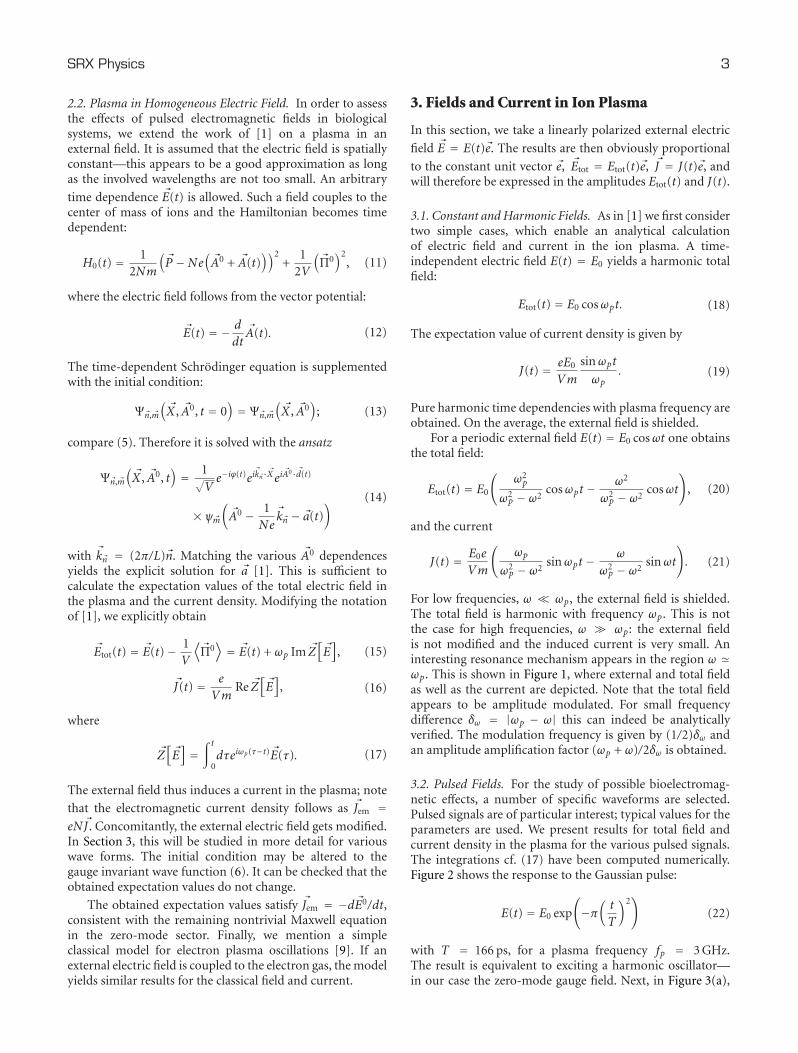
2.2. Plasma in Homogeneous Electric Field. In order to assessthe effects of pulsed electromagnetic fields in biologicalsystems, we extend the work of [1] on a plasma in anexternal field. It is assumed that the electric field is spatiallyconstant—this appears to be a good approximation as longas the involved wavelengths are not too small. An arbitrary

time dependence �E(t) is allowed. Such a field couples to thecenter of mass of ions and the Hamiltonian becomes timedependent:

H0(t) = 12Nm

(�P −Ne

(�A0 + �A(t)

))2+

12V

(�Π0

)2, (11)

where the electric field follows from the vector potential:

�E(t) = − d

dt�A(t). (12)

The time-dependent Schrodinger equation is supplementedwith the initial condition:

Ψ�n,�m

(�X , �A0, t = 0

)= Ψ�n,�m

(�X , �A0

); (13)

compare (5). Therefore it is solved with the ansatz

Ψ�n,�m

(�X , �A0, t

)= 1√

Ve−iϕ(t)ei

�k�n·�Xei�A0·�d(t)

× ψ�m(�A0 − 1

Ne�k�n − �a(t)

) (14)

with �k�n = (2π/L)�n. Matching the various �A0 dependencesyields the explicit solution for �a [1]. This is sufficient tocalculate the expectation values of the total electric field inthe plasma and the current density. Modifying the notationof [1], we explicitly obtain

�Etot(t) = �E(t)− 1V

⟨�Π0

⟩= �E(t) + ωp Im �Z

[�E]

, (15)

�J(t) = e

VmRe �Z

[�E]

, (16)

where

�Z[�E]=

∫ t

0dτeiωp(τ−t)�E(τ). (17)

The external field thus induces a current in the plasma; note

that the electromagnetic current density follows as �Jem =eN�J . Concomitantly, the external electric field gets modified.In Section 3, this will be studied in more detail for variouswave forms. The initial condition may be altered to thegauge invariant wave function (6). It can be checked that theobtained expectation values do not change.

The obtained expectation values satisfy �Jem = −d�E0/dt,consistent with the remaining nontrivial Maxwell equationin the zero-mode sector. Finally, we mention a simpleclassical model for electron plasma oscillations [9]. If anexternal electric field is coupled to the electron gas, the modelyields similar results for the classical field and current.

3. Fields and Current in Ion Plasma

In this section, we take a linearly polarized external electric

field �E = E(t)�e. The results are then obviously proportional

to the constant unit vector �e, �Etot = Etot(t)�e, �J = J(t)�e, andwill therefore be expressed in the amplitudes Etot(t) and J(t).

3.1. Constant and Harmonic Fields. As in [1] we first considertwo simple cases, which enable an analytical calculationof electric field and current in the ion plasma. A time-independent electric field E(t) = E0 yields a harmonic totalfield:

Etot(t) = E0 cosωpt. (18)

The expectation value of current density is given by

J(t) = eE0

Vm

sinωpt

ωp. (19)

Pure harmonic time dependencies with plasma frequency areobtained. On the average, the external field is shielded.

For a periodic external field E(t) = E0 cosωt one obtainsthe total field:

Etot(t) = E0

(ω2p

ω2p − ω2

cosωpt − ω2

ω2p − ω2

cosωt

), (20)

and the current

J(t) = E0e

Vm

(ωp

ω2p − ω2

sinωpt − ω

ω2p − ω2

sinωt

). (21)

For low frequencies, ω � ωp, the external field is shielded.The total field is harmonic with frequency ωp. This is notthe case for high frequencies, ω � ωp: the external fieldis not modified and the induced current is very small. Aninteresting resonance mechanism appears in the region ω �ωp. This is shown in Figure 1, where external and total fieldas well as the current are depicted. Note that the total fieldappears to be amplitude modulated. For small frequencydifference δω = |ωp − ω| this can indeed be analyticallyverified. The modulation frequency is given by (1/2)δω andan amplitude amplification factor (ωp + ω)/2δω is obtained.

3.2. Pulsed Fields. For the study of possible bioelectromag-netic effects, a number of specific waveforms are selected.Pulsed signals are of particular interest; typical values for theparameters are used. We present results for total field andcurrent density in the plasma for the various pulsed signals.The integrations cf. (17) have been computed numerically.Figure 2 shows the response to the Gaussian pulse:

E(t) = E0 exp

(−π

(t

T

)2)

(22)

with T = 166 ps, for a plasma frequency fp = 3 GHz.The result is equivalent to exciting a harmonic oscillator—in our case the zero-mode gauge field. Next, in Figure 3(a),

4 SRX Physics

Plasma: harmonic external field

Efi

eld

(a.u

.)

−40

−30

−20

−10

0

10

20

30

40

t (s)

0 50 100 150 200 250 300 350 400 450

×10−7

External E fieldTotal E field

(a)

Plasma: harmonic external field

Cu

rren

tde

nsi

ty(a

.u.)

−60

−40

−20

0

20

40

60×10−7

t (s)

0 50 100 150 200 250 300 350 400 450

×10−7

Current

(b)

Figure 1: (a) External and total fields. (b) Current density, f = 0.95 MHz, fp = 1.0 MHz.

Plasma: gaussian pulse

Efi

eld

(V/m

)

−150

−100

−50

0

50

100

150

t (s)

0 20 40 60 80 100 120 140 160 180×10−11


(a)


Cu

rren

tde

nsi

ty(a

.u.)

−80

−60

−40

−20

0

20

40

60

80×10−10

t (s)

0 20 40 60 80 100 120 140 160 180×10−11

Current

(b)

Figure 2: (a) External and total fields, fp = 3 GHz. (b) Current density.

the effects of pulse repetition are shown. The results for themodulated Gaussian pulse

E(t) = E0 sinωt exp

(−π

(t

T

)2)

, (23)

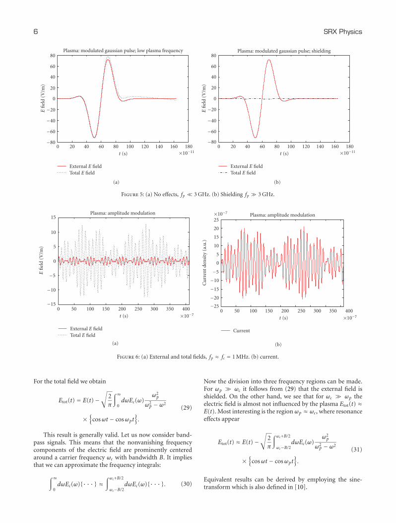
with T = 332 ps, ω = 4π GHz, are not essentially different(cf. Figure 4). On the other hand, if the plasma frequency isnot in the frequency band of such a pulse one obtains noeffects for small ωp and shielding for large ωp; see Figure 5.For completeness, we also include amplitude modulationwith modulation frequency 0.1 MHz. Shielding and theabsence of effects appear in the respective frequency regions.Here we depict the resonance effects for field and current in

Figure 6. Figure 7 shows a resonant plasma response for ultrawideband (wideband high-power microwaves) signals:

E(t) = E0t exp

(−π

(t

T

)2)

(24)

with T = 0.2 ns. Another example of a broadband signal isthe nuclear electromagnetic pulse (NEMP)

E(t) = E0

(e−αt − e−βt

): (25)

with α = 4.0 · 106 s−1 and β = 4.76 · 108 s−1. The resonantplasma response is shown in Figure 8. Note the relatively lowplasma frequency used in this NEMP calculation. The resultsfor narrow band high-power microwaves, GSM and chirp

SRX Physics 5


Efi

eld

(V/m

)

−250

−200

−150

−100

−50

0

50

100

150

200

250

t (s)

0 20 40 60 80 100 120 140 160 180×10−11


(a)

Plasma: harmonic pulses

Efi

eld

(V/m

)

−40

−30

−20

−10

0

10

20

30

40

t (s)

0 10 20 30 40 50 60 70 80 90×10−6


(b)

Figure 3: External and total fields: (a) Gaussian pulse, repetition; fp = 3 GHz; (b) on/off switching, fp = 1.0 MHz.

Plasma: modulated gaussian pulse

Efi

eld

(V/m

)

−250

−200

−150

−100

−50

0

50

100

150

200

250

t (s)

0 20 40 60 80 100 120 140 160 180×10−11


(a)

Plasma: modulated gaussian pulse

Cu

rren

tde

nsi

ty(a

.u.)

−150

−100

−50

0

50

100

150×10−11

t (s)

0 20 40 60 80 100 120 140 160 180×10−11

Current

(b)


signals resemble those of a continuous harmonic wave whichis switched on and off. The concomitant plasma response, inparticular the electric field, is shown in Figure 3(b).

4. General Bandpass Signals

The results obtained so far suggest that there are threeregions in the frequency domain, governing the response togeneral bandpass signals. In order to confirm this, the cosinetransform of a real electric field is used [10]:

Ec(ω) =√

2π

∫∞0dtE(t) cosωt. (26)

The inverse transformation is given by

E(t) =√

2π

∫∞0dωEc(ω) cosωt. (27)

Straightforward integration leads to the following expressionfor Z:

Z(t) = −12i

√2π

∫∞0dωEc(ω)

×{

1ωp + ω

(eiωt−e−iωpt

)+

1ωp − ω

(e−iωt−e−iωpt

)}.

(28)

6 SRX Physics

Plasma: modulated gaussian pulse; low plasma frequency

Efi

eld

(V/m

)

−80

−60

−40

−20

0

20

40

60

80

t (s)

0 20 40 60 80 100 120 140 160 180×10−11


(a)

Plasma: modulated gaussian pulse; shielding

Efi

eld

(V/m

)

−80

−60

−40

−20

0

20

40

60

80

t (s)

0 20 40 60 80 100 120 140 160 180×10−11


(b)

Figure 5: (a) No effects, fp � 3 GHz. (b) Shielding fp � 3 GHz.

Plasma: amplitude modulation

Efi

eld

(V/m

)

−15

−10

−5

0

5

10

15

t (s)

0 50 100 150 200 250 300 350 400

×10−7


(a)

Plasma: amplitude modulation

Cu

rren

tde

nsi

ty(a

.u.)

−25

−20

−15

−10

−5

0

5

10

15

20

25×10−7

t (s)

0 50 100 150 200 250 300 350 400

×10−7

Current

(b)

Figure 6: (a) External and total fields, fp ≈ fc = 1 MHz. (b) current.

For the total field we obtain

Etot(t) = E(t)−√

2π

∫∞0dωEc(ω)

ω2p

ω2p − ω2

×{

cosωt − cosωpt}.

(29)

This result is generally valid. Let us now consider band-pass signals. This means that the nonvanishing frequencycomponents of the electric field are prominently centeredaround a carrier frequency ωc with bandwidth B. It impliesthat we can approximate the frequency integrals:

∫∞0dωEc(ω){· · · } ≈

∫ ωc+B/2

ωc−B/2dωEc(ω){· · · }. (30)

Now the division into three frequency regions can be made.For ωp � ωc it follows from (29) that the external field isshielded. On the other hand, we see that for ωc � ωp theelectric field is almost not influenced by the plasma Etot(t) ≈E(t). Most interesting is the region ωp ≈ ωc, where resonanceeffects appear

Etot(t) ≈ E(t)−√

2π

∫ ωc+B/2

ωc−B/2dωEc(ω)

ω2p

ω2p − ω2

×{

cosωt − cosωpt}.

(31)

Equivalent results can be derived by employing the sine-transform which is also defined in [10].

SRX Physics 7

Plasma: UWB-HPM pulse

Efi

eld

(V/m

)

−80

−60

−40

−20

0

20

40

60

80×10−7

t (s)

0 10 20 30 40 50 60 70×10−11


(a)

Plasma: UWB UWB-HPM pulse

Cu

rren

tde

nsi

ty(a

.u.)

−40

−30

−20

−10

0

10

20

30

40×10−7

t (s)

0 10 20 30 40 50 60 70×10−11

Current

(b)


Plasma: NEMP signal

Efi

eld

(V/m

)

−5

−4

−3

−2

−1

0

1

2

3

4

5

6×104

t (s)

0 20 40 60 80 100 120×10−8


(a)

Plasma: NEMP signal

Cu

rren

tde

nsi

ty(a

.u.)

−5

−4

−3

−2

−1

0

1

2

3

4×10−3

t (s)

0 20 40 60 80 100 120×10−8

Current

(b)

Figure 8: (a) External and total fields, fp = 20 MHz. (b) Current density

5. Estimates of Plasma Frequencies

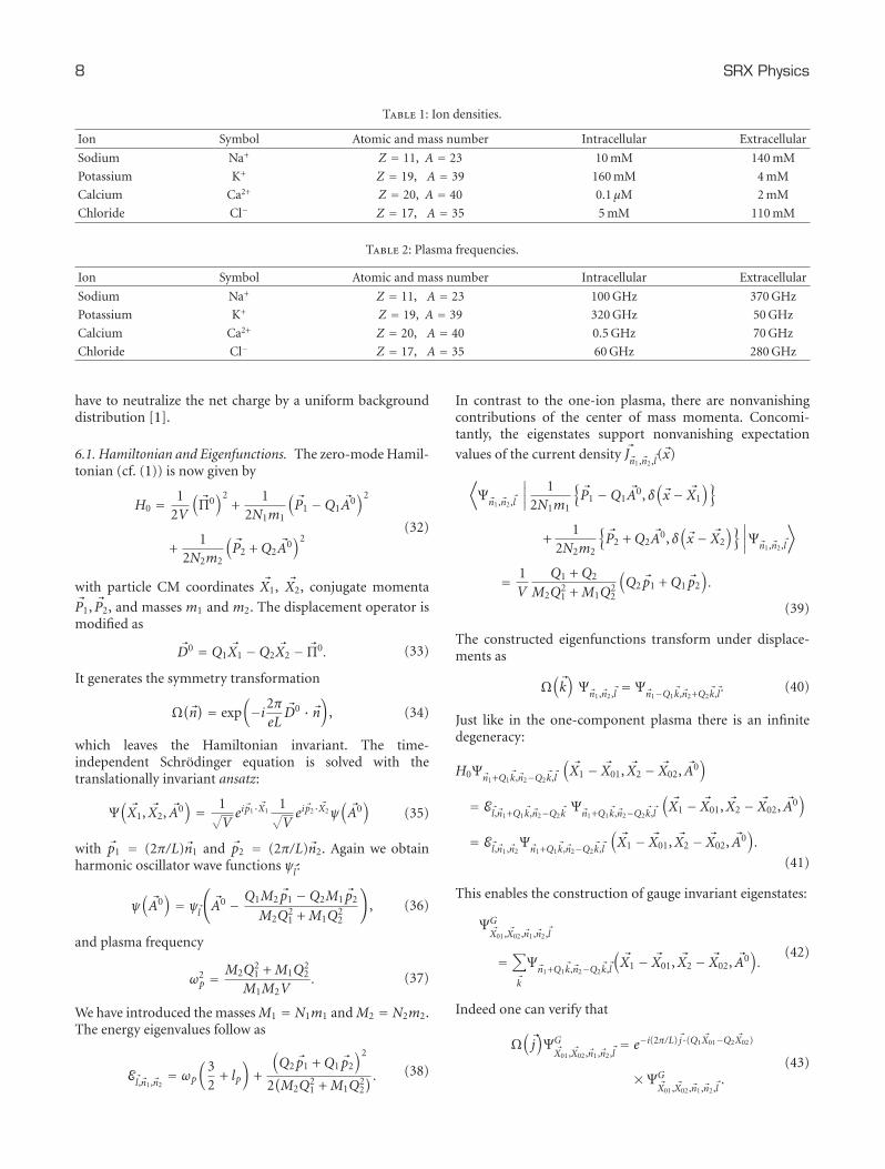
As mentioned in the introduction, a possible applicationof this framework is the effect of electromagnetic fields onbiological systems. It is known that intracellular as wellas extracellular fluid contains ions, in particular sodium,potassium, calcium, and cloride. Here we estimate theconcomitant plasma frequencies for realistic concentrations.The latter is usually given as molar concentration or molaritydenoting the number of moles per liter; the symbol formole/liter is M. In Table 1 typical concentrations are listed.The corresponding plasma frequencies can be computedwith (7); a convenient approximate expression is ω2

p ≈ 1.0 ·1027 × q2(MC/A), with (atomic) mass number A, molar

concentration MC , and the integer charge q in terms of theelementary charge. Thus q = 2 for calcium; for the otherions q = 1. This leads to the estimated plasma frequenciesfp = ωp/2π shown in Table 2.

6. Two-Species Plasma

In this section we extend the theory to a plasma with twospecies of ions. Their charges are eq1 and −eq2, where enow denotes the elementary charge and q1, q2 are positiveintegers. The respective numbers of particles are denotedby N1, N2; we furthermore introduce the charges Q1 =eN1q1 and Q2 = eN2q2. If Q1 = Q2, no additionalbackground charge needs to be assumed. Otherwise we still

8 SRX Physics

Table 1: Ion densities.

Ion Symbol Atomic and mass number Intracellular Extracellular

Sodium Na+ Z = 11, A = 23 10 mM 140 mM

Potassium K+ Z = 19, A = 39 160 mM 4 mM

Calcium Ca2+ Z = 20, A = 40 0.1 μM 2 mM

Chloride Cl− Z = 17, A = 35 5 mM 110 mM

Table 2: Plasma frequencies.

Ion Symbol Atomic and mass number Intracellular Extracellular

Sodium Na+ Z = 11, A = 23 100 GHz 370 GHz

Potassium K+ Z = 19, A = 39 320 GHz 50 GHz

Calcium Ca2+ Z = 20, A = 40 0.5 GHz 70 GHz

Chloride Cl− Z = 17, A = 35 60 GHz 280 GHz

have to neutralize the net charge by a uniform backgrounddistribution [1].

6.1. Hamiltonian and Eigenfunctions. The zero-mode Hamil-tonian (cf. (1)) is now given by

H0 = 12V

(�Π0

)2+

12N1m1

(�P1 −Q1 �A0

)2

+1

2N2m2

(�P2 +Q2 �A0

)2(32)

with particle CM coordinates �X1, �X2, conjugate momenta�P1, �P2, and masses m1 and m2. The displacement operator ismodified as

�D0 = Q1 �X1 −Q2 �X2 − �Π0. (33)

It generates the symmetry transformation

Ω(�n) = exp

(−i2πeL�D0 · �n

), (34)

which leaves the Hamiltonian invariant. The time-independent Schrodinger equation is solved with thetranslationally invariant ansatz:

Ψ(�X1, �X2, �A0

)= 1√

Vei�p1·�X1

1√Vei�p2·�X2ψ

(�A0)

(35)

with �p1 = (2π/L)�n1 and �p2 = (2π/L)�n2. Again we obtainharmonic oscillator wave functions ψ�l:

ψ(�A0)= ψ�l

(�A0 − Q1M2�p1 −Q2M1�p2

M2Q21 +M1Q

22

), (36)

and plasma frequency

ω2p =

M2Q21 +M1Q

22

M1M2V. (37)

We have introduced the massesM1 = N1m1 andM2 = N2m2.The energy eigenvalues follow as

E�l,�n1,�n2= ωp

(32

+ lp

)+

(Q2�p1 +Q1�p2

)2

2(M2Q

21 +M1Q

22

) . (38)

In contrast to the one-ion plasma, there are nonvanishingcontributions of the center of mass momenta. Concomi-tantly, the eigenstates support nonvanishing expectation

values of the current density �J�n1,�n2,�l(�x)

⟨Ψ�n1,�n2,�l

∣∣∣∣1

2N1m1

{�P1 −Q1 �A0, δ

(�x − �X1

)}

+1

2N2m2

{�P2 +Q2 �A0, δ

(�x − �X2

)}∣∣∣∣Ψ�n1,�n2,�l

�

= 1V

Q1 +Q2

M2Q21 +M1Q

22

(Q2�p1 +Q1�p2

).

(39)

The constructed eigenfunctions transform under displace-ments as

Ω(�k)Ψ�n1,�n2,�l = Ψ�n1−Q1

�k,�n2+Q2�k,�l . (40)

Just like in the one-component plasma there is an infinitedegeneracy:

H0Ψ�n1+Q1�k,�n2−Q2

�k,�l

(�X1 − �X01, �X2 − �X02, �A0

)

= E�l,�n1+Q1�k,�n2−Q2

�k Ψ�n1+Q1�k,�n2−Q2

�k,�l

(�X1 − �X01, �X2 − �X02, �A0

)

= E�l,�n1,�n2Ψ�n1+Q1

�k,�n2−Q2�k,�l

(�X1 − �X01, �X2 − �X02, �A0

).

(41)

This enables the construction of gauge invariant eigenstates:

ΨG�X01,�X02,�n1,�n2,�l

=∑

�k

Ψ�n1+Q1�k,�n2−Q2

�k,�l

(�X1 − �X01, �X2 − �X02, �A0

).

(42)

Indeed one can verify that

Ω(�j)ΨG�X01,�X02,�n1,�n2,�l

= e−i(2π/L)�j·(Q1 �X01−Q2 �X02)

×ΨG�X01,�X02,�n1,�n2,�l

.(43)

SRX Physics 9

6.2. External Homogeneous Field. Again we study the cou-pling of a spatially constant electric field with arbitrary timedependence (12). The time-dependent Hamiltonian followsas

H0(t) = 12V

(�Π0

)2+

12M1

(�P1 −Q1(�A0 + �A(t))

)2

+1

2M2

(�P2 +Q2(�A0 + �A(t))

)2.

(44)

The initial condition is taken as

Ψ�n1,�n2,�l

(�X1, �X2, �A0, t = 0

)= Ψ�n1,�n2,�l

(�X1, �X2, �A0

). (45)

The time-dependent Schrodinger equation can be solvedwith an ansatz analogous to (14):

Ψ�n1,�n1,�l

(�X1, �X2, �A0, t

)

= 1Ve−iϕ(t)ei�p1(�n1)·�X1

× ei�p2(�n2)·�X2ei�A0·�d(t)ψ�l

(�A0 − �q�n1,�n2

− �a(t))

,

(46)

where �q�n1,�n2= (M2Q

21 + M1Q

22)−1(Q1M2�p1 − Q2M1�p2).

After some algebra, one verifies that the previous differentialequation for �a(t) is not modified in the two-species case. Thedifferential equation for the phase ϕ(t), however, is changed.For the evaluation of the expectation values of electric fieldand current one does need the explicit solution of the phase.The resulting current can be written as

�J(t) = 1V

Q1 +Q2

M2Q21 +M1Q

22

(Q2�p1 +Q1�p2

)

+M1Q2 −M2Q1

VM1M2

(�a(t) + �A(t)

),

(47)

and total field is given by

�Etot(t) = �E(t)− d�a(t)dt

, (48)

with (cf. (17) and [1])

�a(t) = ωp

∫ t

0dτ �A(τ) sinωp(τ − t). (49)

Thus we obtain that the response of the two-species plasmais not essentially different from the one-ion case. The plasmafrequency is changed according to (37) and the inducedadditional current has a different prefactor. It is finallymentioned that one may also impose the initial conditionanalogous to (45) in terms of gauge invariant states (42)without changing these results.

7. Plasma: Additional Interactions

7.1. Heisenberg Picture. Thus far we have studied the ionplasma using the Schrodinger picture of quantum mechan-ics. From now on, we exploit the Heisenberg picture since it

has turned out to be more convenient for our calculations.Earlier results for the plasma are readily reproduced andextended by a calculation of the energy. Then we reinvestigatethe two-species plasma within this framework. The plasmamodel extended with an additional interacting degree offreedom is studied as well; it can be seen as the prelude toinclude a bath [11]—as will be done in Section 8.

In the Heisenberg picture states in the Hilbert spaceare time-independent whereas operators O(t) all dependon time. Their equation of motion is governed by theHamiltonian:

dO(t)dt

= i[H ,O(t)] +∂O(t)∂t

. (50)

Expectation values follow as

〈O(t)〉 = 〈Ψ0 | O(t) | Ψ0〉, (51)

where Ψ0 denotes the time-independent state. For theHamiltonian one of course obtains

dH

dt= ∂H

∂t. (52)

Below we focus on solving the equation of motion for theelectric field operator.

7.2. Plasma

7.2.1. Formalism. We start by analyzing the one-componentplasma in the Heisenberg picture. The Hamiltonian (cf. (1))can be rewritten as

H0 = 12Vω2

p

(�A0 − 1

Ne�P)2

+1

2V

(�Π0

)2. (53)

Next we define the creation and annihilation operators fork = 1, 2, 3 (x, y, z) as

a†k =1√

2Vωp

(Π0k + iVωpA

0k

),

ak = 1√2Vωp

(Π0k − iVωpA

0k

).

(54)

By means of [Π0k,A0

l ] = −iδkl one readily verifies the basiccommutation rule [ak, a†l ] = δkl. Expressing the zero-modevector potential and electric field in the a-operators

Π0k =

√12Vωp

(ak + a†k

),

A0k =

i√2Vωp

(ak − a†k

) (55)

yields for the Hamiltonian

H0 = ωp

(a†kak +

32

)− iωp

Ne

√12Vωp

(ak − a†k

)Pk +

12Nm

�P2.

(56)

10 SRX Physics

Note that we use the summation convention. For the CMmomentum one gets

d�Pdt= i

[H0, �P

]= 0. (57)

Consequently, the momentum is conserved and we can

replace the operator by its eigenvalue �P = �k�n. We againimpose periodic boundary conditions. At this point onecan derive the equations of motion for the creation andannihilation operators and solve them. We proceed, however,by defining the “shifted” operators:

b†k = a†k − iαk,

bk = ak + iαk(58)

with �α = (1/Ne)√

(Vωp/2)�k�n. Note that we omit the

n-dependence of �α in our notation. The new operatorsobviously fulfill [bk, b†l ] = δkl. The electric field is given by

Π0k =

√12Vωp

(bk + b†k

). (59)

In terms of the shifted operators the Hamiltonian reads

H0 = ωp

(b†k bk +

32

). (60)

One recognizes the Hamiltonian of a three-dimensionalharmonic oscillator. The equation of motion for bk followsas

dbkdt

= i[H0, bk] = −iωpbk (61)

with solution

bk(t) = bk(0)e−iωpt. (62)

For the adjoint operator one obtains

b†k (t) = b†k (0)eiωpt. (63)

If we choose as state Ψ0 one of the eigenstates of H0, of

course with the above specified CM momentum �k�n, then theexpectation value of the electric field vanishes.

7.2.2. Plasma in External Electric Field. Once again we couplean external homogeneous electric field (12). The Hamiltonoperator is modified as

H0(t) = 12Vω2

p

(�A0 + �A(t)− 1

Ne�P)2

+1

2V

(�Π0

)2. (64)

The CM momentum remains a conserved quantity; thus

we insert �P = �k�n. Next we introduce the creation andannihilation operators a†k , ak and, subsequently, the shiftedoperators b†k and bk. Then we arrive at

H0(t) = ωp

(b†k bk +

32

)+ iωp

√12Vωp

(bk − b†k

)Ak(t)

+12Vω2

p�A2(t).

(65)

Thus we get for the time development:

dbkdt

= i[H0, bk] = −iωpbk − ωp

√12VωpAk(t), (66)

which can be solved using the method of “variation ofconstants.” In the solution of the homogeneous equationbk(t) = bk(0) exp(−iωpt), we replace bk(0) by a function oftime βk(t). This yields

dβkdt

= −ωp

√12Vωpe

iωptAk(t), (67)

which can be readily integrated. In this way we obtain

bk(t) = e−iωpt

⎛⎝bk(0)− ωp

√12Vωp

∫ t

0dτeiωpτAk(τ)

⎞⎠,

b†k (t) = eiωpt

⎛⎝b†k (0)− ωp

√12Vωp

∫ t

0dτe−iωpτAk(τ)

⎞⎠,

(68)

which immediately gives

Π0k =

√12Vωp

(bk(0)e−iωpt + b†k (0)eiωpt

)

−Vω2p

∫ t

0dτ cosωp(t − τ)Ak(τ).

(69)

Let us choose the state Ψ0 as eigenstate of H0. It implies forthe expectation value of the total electric field:

�Etot(t) = �E(t)− 1V

⟨�Π0

⟩

= �E(t) + ω2p

∫ t

0dτ cosωp(t − τ)�A(τ).

(70)

This result is equivalent to (15) and (17) as can be verified bymeans of integration by parts.

7.2.3. Energy Considerations. The expectation value of thetime-dependent Hamiltonian (65) can be conveniently cal-culated in the Heisenberg picture. The initial state Ψ0 istaken as above with harmonic oscillator quantum numbersm1,m2,m3. Omitting this calculation redundant CM-label �n,we thus compute the energy E(t), as

E(t) = 〈H0(t)〉 = 〈Ψ0 | H0(t) | Ψ0〉 =⟨ψ�m | H0(t) | ψ�m

⟩.

(71)

Using the time-developments (68), we obtain

E(t) = ωp

(mp +

32

)+

12Vω2

p

×(ω2p�Z ∗

[�A]· �Z

[�A]

+ 2ωp �A(t) · Im �Z[�A]

+ �A(t) · �A(t))

(72)

SRX Physics 11

(cf. (17)). Integration by parts yields

ωp �Z[�A]= −i

(�A(t) + �Z

[�E]). (73)

With this relation we can write the energy in terms of theexternal field as

E(t) = ωp

(mp +

32

)+

12Vω2

p�Z ∗

[�E]· �Z

[�E]. (74)

This result can also be expressed in the expectation values ofelectric field (15) and (electromagnetic) current (16) as

E(t) = ωp

(mp+

32

)+

12V 2Nm�J 2(t)+

12V(�Etot(t)−�E(t)

)2

= ωp

(mp +

32

)+

V

2ω2p

�J 2em(t) +

12V �E0(t)2.

(75)

The time-dependent terms can be interpreted as the classicalenergy, expressed in classical current and field, induced bythe external field. Note that this additional energy, just ascurrent and field, does not depend on the quantum numbersof the initial state.

7.3. Two-Species Plasma. Using the Heisenberg picture, thetwo-species plasma is reanalyzed. The Hamiltonian (32) isrewritten as

H0 = 12V

(�Π0

)2+

12ω2p

(�A0)2 − Q1

M1

�P1 · �A0

+Q2

M2

�P2 · �A0 +1

2M1

�P21 +

12M2

�P22 ,

(76)

where the plasma frequency ωp is given by (37). In terms ofthe creation and annihilation operators defined in (54), weget

H0 = ωp

(a†kak +

32

)+

12M1

�P21 +

12M2

�P22

− i√2Vωp

(Q1

M1

(�P1

)k− Q2

M2

(�P2

)k

)(ak − a†k

).

(77)

Both CM operators commute with the Hamiltonian. There-fore, we can replace the operators by their respectiveeigenvalues, that is, �p1 and �p2:

H0 = ωp

(a†kak +

32

)− iβk

(ak − a†k

)+

12M1

�p 21 +

12M2

�p 22

(78)

with �β = (1/√

2Vωp)((Q1/M1)�p1 − (Q2/M2)�p2). Introducing

the shifted operators

bk = ak + iγk,

b†k = a†k − iγk,(79)

where �γ = �β/ωp =√

(1/2)Vωp((Q1M2�p1 − Q2M1�p2)/

(M2Q21 +M1Q

22)), diagonalizes the Hamiltonian

H0 = ωp

(b†k bk +

32

)+

(Q2�p1 +Q1�p2

)2

2(M2Q

21 +M1Q

22

) . (80)

Its energy eigenvalues obviously agree with those calculatedin the Schrodinger picture (38).

The inclusion of a homogeneous external electric fieldyields additional terms in the Hamiltonian:

H0(t) = H0 +12Vω2

p�A(t)2 +Vω2

p�A(t) · �A0

− Q1

M1

�P1 · �A(t) +Q2

M2

�P2 · �A(t).

(81)

The CM momenta also commute with the modified Hamil-tonian and therefore we replace them by their eigenvalues�p1 and �p2. Next we introduce the creation and annihilationoperators ak , a†k and, eventually, bk and b†k . Straightforwardalgebra then leads to

H0(t) = ωp

(b†k bk +

32

)+ iωp

√12Vωp

(bk − b†k

)Ak(t)

+12Vω2

p�A2(t),

(82)

which is formally identical to (65)—except for the factthat the plasma frequency is altered. Note that the plasmafrequency appears also in the definition of the creation andannihilation operators. Herewith our previous results for thetwo-species plasma are confirmed.

7.4. Plasma: Additional Interaction and External Field. In thissection, we include an additional degree of freedom whichinteracts with the zero-mode in the one-component plasmamodel. The interaction is in principle taken from [11] wherea bath is coupled to a system, as will be studied below aswell. Since we want to respect the displacement symmetry,however, a modification is necessary. We also couple theexternal homogeneous electric field from the onset. Thecomplete Hamiltonian is thus taken as

H(t) = H0(t) +Hb +HI(t), (83)

where H0(t) is given by (64) and Hb represents a simpleharmonic oscillator:

Hb = 12�p 2 +

12ω2

1�q 2. (84)

The original interaction term [11] reads

H0I =

g√ωpω1V

(�p · �Π0 +Vωpω1�q · �A0

)(85)

with coupling constant g. It has been actually been intro-duced as a simpler expression in terms of creation andannihilation operators. This term, however, explicitly breaks

12 SRX Physics

the displacement symmetry. The corresponding symmetric(gauge invariant) interaction is given by

HI =g√

ωpω1V

(�p · �Π0 +Vωpω1�q ·

(�A0 − 1

Ne�P)). (86)

Thus the additional degree of freedom couples not only tothe zero-mode but also to the CM of the ions. Coupling theexternal electric fields finally yields

HI(t) =g√

ωpω1V

×(�p · �Π0 +Vωpω1�q ·

(�A0 + �A(t)− 1

Ne�P)).

(87)

We proceed as above, that is we introduce creation andannihilation operators for the zero-mode, substitute for the

CM momentum its eigenvalue �k�n and replace the ak, a†kby their shifted operators bk and b†k . Moreover, for theadditional degree of freedom we define

ck = 1√2ω1

(pk − iω1qk

),

c†k =1√2ω1

(pk + iω1qk

),

(88)

which obey [ck, c†l ] = δkl. After some computations oneobtains for the Hamiltonian

H(t) = ωp

(b†k bk +

32

)+ iωp

√12Vωp

(bk − b†k

)Ak(t)

+12Vω2

p�A(t)2 + ω1

(c†k ck +

32

)+ g

(bkc

†k + b†k ck

)

+ ig

√12Vωp

(ck − c†k

)Ak(t),

(89)

where the original interaction term [11] is recognized.The Heisenberg equations of motion follow as

dbk(t)dt

= i[H , bk] = −iωpbk − igck − ωp

√12VωpAk(t),

dck(t)dt

= i[H , ck] = −iω1ck − igbk − g√

12VωpAk(t).

(90)

Note that different Cartesian components do not couple. Inmatrix form we have

d

dt

⎛⎝bkck

⎞⎠ = −i

⎛⎝ωp g

g ω1

⎞⎠⎛⎝bkck

⎞⎠− Ak(t)

√12Vωp

⎛⎝ωp

g

⎞⎠.

(91)

The evolution operator exp Ut, where U denotes the appear-ing 2 × 2 matrix, which does not depend on the Cartesian

index k, of the homogeneous differential equations can beexplicitly calculated. First, one obtains for the frequencyeigenvalues

ω± = 12

(ωp + ω1

)± 1

2

√(ωp − ω1

)2+ 4g2. (92)

The corresponding eigenvectors read

1N

⎛⎝ g

ω+ − ωp

⎞⎠,

1N

⎛⎝ω− − ω1

g

⎞⎠, (93)

with normalization N =√

(ω+ − ωp)2 + g2 =√(ω− − ω1)2 + g2; note that one has ωp − ω+ = ω− − ω1.

Herewith the evolution operator is constructed as

exp Ut

= 1N2

⎛⎝ g2e−iω+t + ω2e−iω−t gωe−iω+t + gωe−iω−t

gωe−iω+t + gωe−iω−t ω2e−iω+t + g2e−iω−t

⎞⎠

(94)

where ω denotes ω− − ω1 and ω denotes ω+ − ωp. Thesolutions of the inhomogeneous differential equations aregiven by

⎛⎝bk(t)

ck(t)

⎞⎠ = exp Ut

⎛⎝bk(0)

ck(0)

⎞⎠

−√

12Vωp

∫ t

0dt′ exp[U(t − t′)]Ak(t′)

⎛⎝ωp

g

⎞⎠.

(95)

The expression for �Π0(t) trivially follows.Finally, we specify the time-independent state as a

product of eigenstates of the uncoupled Hamiltonians ofthe zero-modes and the additional degree of freedomrespectively. Calculating the corresponding expectation valueof the electric field operator yields after integrating by parts

�Etot(t) = �E(t) +ωp

N2

(g2�I(ω+) + (ω− − ω1)2�I(ω−)

), (96)

where we have defined

�I(ξ) =∫ t

0dt′ sin ξ(t′ − t)�E(t′). (97)

In comparison with the plasma response without additionalinteraction, there appear two relevant frequencies which aredetermined by the original plasma frequency, the oscillatorfrequency and the coupling constant. The response at such afrequency is similar to the original one. Thus two resonancesappear. This is explicitly seen by considering a harmonic

SRX Physics 13

external field �E(t) = �E0 cosωt. Performing the integralsanalytically gives for this case

�Etot(t) = �E0

[g2

N2

ω+ωp

ω2+ − ω2

cosω+t

+(ω− − ω1)2

N2

ωpω−ω2− − ω2

cosω−t

+

(1− g2

N2

ω+ωp

ω2+−ω2

− (ω−−ω1)2

N2

ω−ωp

ω2−−ω2

)

× cosωt].

(98)

8. Plasma, Bath and External Field

Finally, we extend our plasma model in order to describethe expected damping and fluctuations in realistic systems.To this end, we explicitly include the surrounding medium,or bath, as part of the system. In other words, additionalinteractions are taken into account; in principle we followthe approach of van Kampen [11]. In order not to overloadthe notation we consider only one Cartesian component ofthe complete model. It is assumed that the bath degreesof freedom as well as the external electric field couple tothis component. The two other components then triviallydecouple. Therefore the Cartesian index is omitted from nowon. The essential physics evidently is captured in this way.Alternatively, one may consider the total Hamiltonian of [1]completely describing the plasma in interaction with thedynamical electromagnetic fields. This is, however, beyondthe scope of our study.

8.1. Plasma and Bath. The Hamilton operator consists ofthree parts:

H = 12Vω2

0

(A0 − 1

NeP)2

+1

2V

(Π0)2

+HB +HI , (99)

where the first terms describe again the zero-modes of theinternal electromagnetic field coupled to the CM momen-tum of the ions. Here we denote the plasma frequency by ω0.The free bath Hamiltonian is taken as the sum of a numberof harmonic oscillators with frequencies ωn, that is,

HB = 12

∑n

(p2n + ωnq

2n

) =∑n

ωn

(a†nan +

12

)(100)

with coordinates qn and momenta pn, [pn, qm] = −iδnm. Theannihilation and creation operators are defined as

an = 1√2ωn

(pn − iωnqn

),

a†n =1√2ωn

(pn + iωnqn

).

(101)

It follows that [an, a†m] = δnm. We also define such operatorsfor the zero-mode:

a0 = 1√2Vω0

(Π0 − iVω0A

0),

a†0 =1√

2Vω0

(Π0 + iVω0A

0).(102)

Van Kampen defines the interaction as [11]

H0I =

∑n

gn(ana

†0 + a†na0

)

= 1√Vω0

∑n

gn√ωn

(pnΠ

0 +Vω0ωnqnA0)

(103)

with coupling strengths gn. This interaction Hamiltonian isnot invariant under displacements. Just as in the previoussection, we therefore insert the symmetric “minimal substi-tution” term and use the interaction

HI = 1√Vω0

∑n

gn√ωn

(pnΠ

0 +Vω0ωnqn

(A0 − 1

NeP))

=∑n

gn(ana

†0 + a†na0

)− i

Ne

√12Vω0

∑n

gn(an − a†n

)P.

(104)

Thus the bath interacts with the CM degree of freedom aswell. The Hamiltonian can now be now written as

H = ω0

(a†0a0 +

12

)− iω0

Ne

√12Vω0

(a0 − a†0

)P

+∑n

ωn

(a†nan +

12

)+∑n

gn(ana

†0 + a†na0

)

− i

Ne

√12Vω0

∑n

gn(an − a†n

)P +

12Nm

P2

(105)

and can be analyzed analogous to the procedure of [11].

8.2. Inclusion of an External Electric Field. We proceed byincluding a homogeneous external field (12); the Hamilto-nian becomes explicitly time-dependent:

H(t) = ω0

(a†0a0 +

12

)− iω0

Ne

√12Vω0

(a0 − a†0

)P

+ iω0

√12Vω0

(a0 − a†0

)A(t)

− Vω20

NePA(t) +

12Vω2

0A2(t) +

∑n

ωn

(a†nan +

12

)

+∑n

gn(ana

†0 + a†na0

)

− i

Ne

√12Vω0

∑n

gn(an − a†n

)P +

12Nm

P2

+ i

√12Vω0

∑n

gn(an − a†n

)A(t).

(106)

14 SRX Physics

Since the CM coordinate is cyclic, [H ,P] = 0, the conjugatemomentum P is a constant of motion P → kj = 2n j/L. Afterinserting this in the Hamiltonian, we define the “shifted”operators b0 and b†0 :

a0 = b0 − iα,

a†0 = b†0 + iα,(107)

with α = α( j) = (kj/Ne)√

(1/2)Vω0. Some algebra leads to

H(t) = ω0

(b†0b0 +

12

)+ iω0

√12Vω0

(b0 − b†0

)A(t)

+12Vω2

0A2(t) +

∑n

ωn

(a†nan +

12

)

+∑n

gn(anb

†0 + a†nb0

)

+ i

√12Vω0

∑n

gn(an − a†n

)A(t).

(108)

The equations of motion for the Heisenberg operators followas

db0(t)dt

= i[H , b0] = −iω0b0 − i∑m

gmam − ω0

√12Vω0A(t),

dan(t)dt

= i[H , an] = −iωnan − ignb0 − gn√

12Vω0A(t).

(109)

The homogeneous differential equations are implicitly solvedin [11]:

b0(t) = U(t)b0(0) +∑m

Vm(t)am(0),

an(t) =Wn(t)b0(0) +∑m

Snm(t)am(0).(110)

The corresponding evolution operator is given by

exp Mt =⎛⎝U(t) �V tr(t)

�W(t) S(t)

⎞⎠. (111)

The matrix M is implicitly defined in (109). For b0(t)we consequently get as solution of the inhomogeneousdifferential equation:

b0(t) = U(t)b0(0) +∑m

Vm(t)am(0)−√

12Vω0η(t),

(112)

where we have defined

η(t) = ω0

∫ t

0U(t − t′)A(t′)dt′ +

∑m

gm

∫ t

0Vm(t − t′)A(t′)dt′.

(113)

The zero-mode electric field operator follows as

Π0 =√

12Vω0

(b0 + b†0

). (114)

We take as time-independent state Ψ = Ψ0 · ψB, with Ψ0

being an eigenstate of the plasma Hamiltonian and ψB beingan eigenstate of the bath Hamiltonian, that is, the productof the shifted zero-mode oscillator, the plane wave and bathharmonic oscillator wave functions. Then we get for theexpectation value of the total electric field:

Etot = − 1V

⟨Π0⟩ + E(t) = 1

2ω0

(η(t) + η∗(t)

)+ E(t).

(115)

8.3. Evolution Operator. Let us address the solution of theequations of motion (cf. (109)) in some more detail andexplicitly construct the evolution operator. In principle wefollow the approach of van Kampen [11].

8.3.1. Exact Developments. The set of (109) is a solved withthe ansatz e−iλt for the time dependence of all modes. Thisleads to the eigenvalue equation:

λ− ω0 =∑n

g2n

λ− ωn (116)

with a sequence of solutions λν. Given the number of bathoscillators, their frequencies, and the coupling constants,they can be determined numerically. The corresponding

eigenvectors are denoted by �Xν = (X0ν,Xnν) and fulfill

Xnν =gn

λν − ωnX0ν. (117)

The first component X0ν follows from the imposed normal-ization condition; it explicitly reads

1 = X20ν +

∑n

X2nν = X2

0ν

{1 +

∑n

g2n

(λν − ωn)2

}. (118)

The eigenvectors become orthonormal:

�Xν · �Xμ = X0νX0μ +∑n

XnνXnμ = δμν, (119)

and the closure relations∑

ν

X20ν = 1,

∑ν

XnνXmν = δmn,∑

ν

X0νXnν = 0

(120)

can be shown to hold true.The operators b0 and an are linear combinations of the

normal modes:

b0(t) =∑

ν

cνX0νe−iλνt , an(t) =

∑ν

cνXnνe−iλνt

(121)

with superposition constants cν. Using orthonormality(119), they follow from the initial values as

cν = X0νb0(0) +∑n

Xnνan(0). (122)

SRX Physics 15

This indeed yields the solution (110) with the explicitexpressions:

U(t) =∑

ν

X20νe

−iλνt , Vn(t) =∑

ν

X0νXnνe−iλνt,

Wm(t) = Vm(t), Smn(t) =∑

ν

XnνXmνe−iλνt .

(123)

Thus, we have constructed the evolution operator (111).Note that closure (120) guarantuees the necessary propertyexp[M(t = 0)] = I. These exact results can be used inorder to calculate the expectation value of the electric fieldas outlined above. Note that the bath degrees of freedomare eventually eliminated by our choice of the state. Sincea realistic number of bath oscillators is huge, the numericalcomputations are expected to be time/memory consumingand therefore challenging. We have not yet attempted toperform this task.

8.3.2. Approximate Evolution Operator. In [11] further devel-opments on the operator level preclude the elimination of thebath degrees of freedom in the way we have done. In orderto proceed, an approximate, simpler form of the evolutionoperator is derived. The appearing summation over manybath modes is effectively done. This approximation may bealso be interesting for our purposes because the numericalwork mentioned above is considerably reduced. We thereforepresent a slightly modified derivation of the results in [11];here we do not explicitly need the concept of a “strengthfunction.” It starts by defining the function

G(z) = z − ω0 −∑n

g2n

z − ωn. (124)

Its zeros are the eigenfrequencies λν of the total system (cf.(116)). At such a zero one gets for the derivative

G′(λν) = 1 +∑n

g2n

(λν − ωn)2 =1X2

0ν

, (125)

where the normalization condition (118) has been used.Using complex function theory yields for t > 0

U(t) = − 12πi

∫∞−∞

e−ixt+εt

G(x + iε)dx, (126)

where, as usual, ε is small and positive. This is still exact. Atthis point additional assumptions are made. First, ε is smallcompared to the scale over which the coupling constantsvary. This can be formulated in terms of the abovementionedstrength function [11]. Secondly, ε is large compared tothe distance between the bath frequencies ωn. Finally, and“more seriously,” it is assumed that the interaction is weak,meaning small couplings gn (and, concomitantly, smallstrength function). This implies that G(x + iε) can beapproximated by replacing x by ω0 in the summation termof (124). The result can be written as

G(x + iε) ≈ x − ω′0 + iΓ (127)

with shifted frequency ω′0

ω′0 = ω0 +∑n

g2n(ω0 − ωn)

(ω0 − ωn)2 + ε2, (128)

and damping Γ

Γ = ε(

1 +∑n

g2n

(ω0 − ωn)2 + ε2

). (129)

Hence one obtains

U(t) ≈ e−iω′0t−Γt, (130)

and the same approximations yield

Vn(t) =Wn(t) ≈ gnω′0 − ωn − iΓ

{e−iω

′0t−Γt − e−iωnt

}.

(131)

8.4. Finite Temperature Considerations

8.4.1. Initial State—Occupation Number. Instead of selectingthe initial state as product of the respective eigenstates of theplasma and bath Hamiltonians, one may assume the bath att = 0 to be in thermal equilibrium with the temperature T[11]. The plasma initial state is supposed to be unaltered.The corresponding expectation values of an operator O aregenerally found as

〈O〉 =Tr(Oe−βH

)

Tr(e−βH

) (132)

with inverse temperature β−1 = kT . Recall that the trace of anoperator can be computed using any complete orthonormalset of states |α〉:

Tr(O) =∑α

〈α|O|α〉. (133)

The denominator of (132) is the well-known partitionfunction of the canonical ensemble. For the chosen bath, acollection of harmonic oscillators, it can readily be calculatedusing the harmonic oscillators states:

Tr(e−βHB

)=

∏n

e−(1/2)βωn

1− e−βωn . (134)

The average occupation number of the bath degrees offreedom follows as

⟨a†n(0)am(0)

⟩= δmn

1eβωn − 1

. (135)

With this result and (110) van Kampen computes theexpectation value of a†0 (t)a0(t) (corresponding to the degreeof freedom in the system, in our case the zero-mode withoperators b†0 (t), b0(t)) and obtains a nontrivial temperaturedependence [11].

16 SRX Physics

8.4.2. Electric Field. We are concerned with the expectationvalue of the electric field operator, which is proportionalto a0(t) + a†0 (t). In principle, the field may get temperaturedependent contributions due to the bath—as in the previousexample. These possibly contributing terms, however, arelinear in the operators a†n(0) and an(0) (cf. (107) and (110)).The thermal equilibrium expectation values of the bathannihilation operators vanish:

〈an〉 =Tr(ane−βHB

)

Tr(e−βHB

) = 0. (136)

This can be understood by once more inserting the eigen-states of the bath Hamiltonian HB and formally expandingit. Each individual term in the trace contains an odd numberof annihilation operators because of the additional operatoran. Consequently, each expectation value in all eigenstatesis zero and this yields a vanishing trace. Analogously, wefind that 〈a†n〉 = 0. Therefore, no temperature dependencein the expectation value of the electric field is present inthis model. The results are equal to those obtained withan eigenstate of the bath Hamiltonian as initial state. Thisresult is almost trivial for zero external electric field. It isalso valid, however, for nonzero, spatially constant, time-dependent external electric fields. In particular, the inducedelectric field—stemming from the inhomogeneous terms inthe equations of motion and in principle determined by(113)—is not modified.

8.4.3. Energy. Finally, we derive the expression for the expec-tation value of the Hamilton operator (109), interpretable asthe time-dependent energy E(t). The initial state is chosenas above, meaning that the bath is in thermal equilibriumat t = 0. The harmonic oscillator state is labelled here withquantum number n0. In addition to the time-developmentof b0 given by (112) and (113), we also need

an(t) =Wn(t)b0(0) +∑m

Snm(t)am(0)−√

12Vω0ζn(t)

(137)

with the definition

ζn(t) = ω0

∫ t

0Wn(t − t′)A(t′)dt′

+∑m

gm

∫ t

0Snm(t − t′)A(t′)dt′.

(138)

For the occupation number one then gets

⟨b†0 (t)b0(t)

⟩= n0U

∗(t)U(t) +∑m

V∗m(t)Vm(t)

(eβωm − 1

)−1

+12Vω0η

∗(t)η(t).

(139)

If we omit the contribution due to the external field, thatis taking η = 0, we indeed reproduce the abovementioned

result of [11]. The expectation value of the completeHamiltonian 〈H(t)〉 follows as

E(t) = ω0

{n0U

∗(t)U(t) +∑m

V∗m(t)Vm(t)

(eβωm − 1

)−1

+12Vω0η

∗(t)η(t) +12

}

+12Vω2

0

{i(η∗(t)− η(t)

)A(t) + A2(t)

}

+12Vω0A(t)

∑n

gni(ζ∗n (t)− ζn(t)

)

+∑n

ωn

{n0W

∗n (t)Wn(t) +

12Vω0ζ

∗n (t)ζn(t) +

12

}

+∑n

gn

{n0(W∗

n (t)U(t) +Wn(t)U∗(t))

+12Vω0

(ζ∗n (t)η(t) + ζn(t)η∗(t)

)}

+∑nm

{gn(S∗nm(t)Vm(t) + Snm(t)V∗

m(t))

+ ωnS∗nm(t)Snm(t)

}(eβωm − 1

)−1.

(140)

This result is exact and can be implemented in an algorithm.Alternatively, one may use the approximations given above(cf. (130) and (131)) supplemented with the analogousexpression for S. The corresponding approximation for theoccupation number is explicitly given in [11].

9. Epilogue

The possible effects of electromagnetic fields on biologicalsystems, for example, human beings, are a topical sub-ject. Although possibly relevant physics has already beenaddressed some time ago [2], there are hardly biophysicalmechanisms known and accepted to date. This paper maydescribe a coupling phenomenon with consequences, in thesense that the internal electric field can be much larger thanthe external one. It is based on the fact that there are “free”ions in intracellular and extracellular fluid. Consequently,one may describe these ions as a low-density plasma.

The response of an ion plasma to external electromag-netic fields has therefore been investigated in this study. Tothis end, the theory developed in [1] for electron plasmashas been applied. It focusses on the zero-momentum pho-tons, center of mass motion and spatially constant electricfields in periodic structures. Typical plasma oscillationsshow up. Since the length scale of our problem is muchsmaller than the wavelengths of typical external fields, thisapproach is appropriate. The basic quantum mechanicalresonance mechanism of [1], demonstrated for harmonicfields, remains essentially the same. We have shown thatresonances appear for several selected waveforms, as well as

SRX Physics 17

for general bandpass signals. The appearing resonance andplasma frequencies, however, are quite different because thepertinent physical parameters, density and mass, of the ionsdiffer from those of electrons. We have explicitly estimatedthese frequencies for the relevant ions and found them to bein the region 0.5 GHz–400 GHz.

The chosen formulation of the plasma is translationallyinvariant [1] and, concomitantly, a homogeneously dis-tributed background charge is assumed. Oppositely chargedions in the intra- and extracelluar fluids are supposed to berelated to this background. In our study, we have extendedthis framework to a two-species plasma because it appearsto be more appropriate for our biophysical application. Sucha plasma actually may or may not be electrically neutral; inthe first case a background charge distribution is absent. Theeffects of coupling an external electric field to the two-speciesplasma are found to be essentially the same as in the simpleplasma.

Further investigations of the effects of electromagneticfields are done by switching to the Heisenberg picture ofquantum mechanics, which has turned out to be moreconvenient for our purposes. Earlier results are readilyreproduced. The time-dependent energy of the plasma is alsocalculated and expressed in induced field and current. Theplasma is extended with an additional degree of freedom,interacting with the zero-mode photon. The relic of theoriginal gauge symmetry, that is the displacement symmetry[1], dictates an additional interaction involving the CMmotion of the ions. The calculations yield two resonancefrequencies instead of one.

The chosen plasma model is certainly not completelyrealistic in the sense that damping and fluctuations, expectedin real systems, are not present. This is also evident from theunderlying complete theory [1]: we have restricted ourselvesto the zero-mode Hamiltonian and ignored the otherHamiltonians describing relative motion, finite momentumphotons and additional couplings. It is beyond the purposeof this research to study the effects of these extra degreesof freedoms; such investigations are actually initiated in[1]. Instead we choose the approach of [11] to include asurrounding medium or bath. An exact expression for theinternal electric field is derived in terms of an evolutionoperator. In order to generate numerical results, however,further algorithmic implementation is necessary. This isplanned for the nearby future. In the present study, anapproximate weak coupling form [11] of the response isconstructed. The resonance frequency is shifted and dampingindeed appears. Finally, it is shown that assuming thermalequilibrium, the expectation value of the electric field is notchanged. The energy of the complete system is found todepend on the temperature.

The conclusion of this work is that in the chosen plasmamodel and its extensions resonance effects appear, whichinduce currents and generate large internal electric fields.The energy of the plasma is increased as well. Quantummechanical plasma oscillations are responsible for thisphysical amplifying mechanism. Note that the response islinear and no demodulation of the external field takes place.On the other hand, a resonant harmonic field becomes

amplitude modulated within the plasma. Whether such alarge electric field has consequences in biological systemsis, of course, an open question. It is furthermore notclear that the plasma model indeed grasps the essentialphysics of ions in intra- and extracellular fluids respondingto external electromagnetic fields. Nevertheless we believethat we have found an interesting possibility of unexpectedelectromagnetic effects in biophysics.

Acknowledgments

The author thanks M. Thies and S. H. J. A. Vossen for usefuldiscussions and critical readings of the manuscript. Thiswork has been supported by the Dutch Ministry of Defence,Grant W04/06 “RF Biological Effects.”

References

[1] F. Lenz, H. W. L. Naus, K. Ohta, and M. Thies, “Zero modesand displacement symmetry in electrodynamics,” Annals ofPhysics, vol. 233, no. 1, pp. 51–81, 1994.

[2] H. Frohlich, “The biological effects of microwaves and relatedquestions,” Advances in Electronics and Electron Physics, vol. 53,pp. 85–152, 1980.

[3] F. Apollonio, M. Liberti, G. d’Lnzeo, and L. Tarricone,“Integrated models for the analysis of biological effects of EMfields used for mobile communications,” IEEE Transactions onMicrowave Theory and Techniques, vol. 48, no. 11, pp. 2082–2093, 2000.

[4] K. R. Foster and M. H. Repacholi, “Biological effects ofradiofrequency fields: the electroencephalogram during avisual working memory task,” Rad Research, vol. 162, p. 219,2004.

[5] A. C. Green, I. R. Scott, R. J. Gwyther, et al., “An investigationof the effects of TETRA RF fields on intracellular calciumin neurones and cardiac myocytes,” International Journal ofRadiation Biology, vol. 81, no. 12, pp. 869–885, 2005.

[6] L. J. Challis, “Mechanisms for interaction between RF fieldsand biological tissue,” Bioelectromagnetics, vol. 26, supplement7, pp. S98–S106, 2005.

[7] M. Simeonova and J. Gimsa, “The influence of the molecularstructure of lipid membranes,” Bioelectromagnetics, vol. 27, no.8, pp. 652–666, 2006.

[8] J. R. Jauchem, “Effects of low-level radio-frequency energy onhuman cardiovascular,” International Journal of Hygiene andEnvironmental Health, vol. 211, pp. 1–29, 2008.

[9] N. W. Ashcroft and N. D. Mermin, Solid State Physics,Thomson Learning, Boston, Mass, USA, 1976.

[10] G. B. Arfken and H. J. Weber, Mathematical Methods forPhysicists, Academic Press, San Diego, Calif, USA, 4th edition,1995.

[11] N. G. van Kampen, Stochastic Processes in Physics and Chem-istry, Elsevier, Amsterdam, The Netherlands, 3rd edition,1997.

scholarly research exchange -...

Documents