Policy Research Working Paper 4998

School Enrollment, Selection and Test Scores

Deon FilmerNorbert Schady

The World BankDevelopment Research GroupHuman Development and Public Services TeamJuly 2009

Impact Evaluation Series No. 34

WPS4998

Produced by the Research Support Team

Abstract

The Impact Evaluation Series has been established in recognition of the importance of impact evaluation studies for World Bank operations and for development in general. The series serves as a vehicle for the dissemination of findings of those studies. Papers in this series are part of the Bank’s Policy Research Working Paper Series. The papers carry the names of the authors and should be cited accordingly. The findings, interpretations, and conclusions expressed in this paper are entirely those of the authors. They do not necessarily represent the views of the International Bank for Reconstruction and Development/World Bank and its affiliated organizations, or those of the Executive Directors of the World Bank or the governments they represent.

Policy Research Working Paper 4998

There is a strong association between schooling attained and test scores in many settings. If this association is causal, one might expect that programs that increase school enrollment and attainment would also improve test scores. However, if there is self-selection into school based on expected gains, marginal children brought into school by such programs may be drawn disproportionately from the left-hand side of the ability distribution, which could limit the extent to which additional schooling translates into more learning. To test this proposition, this paper uses data from Cambodia. The results show that a program that provides scholarships to poor students had a large effect on

This paper—a product of the Human Development and Public Services Team, Development Research Group—is part of a larger effort in the department to study the impact of social programs and their role in promoting human development. Policy Research Working Papers are also posted on the Web at http://econ.worldbank.org. The authors may be contacted at dfilmer@worldbank.org and nschady@worldbank.org.

school enrollment and attendance, which increased by approximately 25 percentage points. However, there is no evidence that, 18 months after the scholarships were awarded, recipient children did any better on mathematics and vocabulary tests than they would have in the absence of the program. The paper discusses results that suggest that the self-selection of lower-ability students into school in response to the program is an important part of the explanation. The analysis also shows minimal program effects on other outcomes, including knowledge of health practices, expectations about the future, and adolescent mental health.

School Enrollment, Selection and Test Scores ♣

Deon Filmer Norbert Schady

Development Research Group

The World Bank

♣ We thank Felipe Barrera, Luis Benveniste, Pedro Carneiro, Stephanie Cellini, Richard Murnane, Jamele Rigolini, T. Paul Schultz, Miguel Urquiola, and various seminar participants for very helpful comments, as well as the World Bank Education Team for Cambodia and the members of Scholarship Team of the Royal Government of Cambodia’s Ministry of Education for valuable assistance in carrying out this work. This work benefited from funding from the World Bank’s Research Support Budget (P094396) as well as the Bank-Netherlands Partnership Program Trust Fund (TF055023). The findings, interpretations, and conclusions expressed in this paper are those of the authors and do not necessarily represent the views of the World Bank, its Executive Directors, or the governments they represent.

2

1. Introduction

Despite progress in recent decades, a substantial fraction of children in developing countries

attain little schooling, and many adults lack skills that are valued in the labor market. For this reason,

policy-makers and academics continue to search for programs and policies that can raise educational

attainment and learning in poor countries.

A number of interventions have recently been shown to increase school enrollment and

attendance in some settings. These include deworming for school-aged children (Miguel and Kremer

2004); school construction (Duflo 2001); the provision of additional teachers (Banerjee et al. 2005);

vouchers for private schooling (Angrist et al. 2002; Angrist, Bettinger, and Kremer 2005); and conditional

cash transfers—transfers that are made to poor households, conditional on them keeping their children

enrolled in school and attending regularly (see the review by Fiszbein and Schady 2009). Much less is

known about how to improve learning outcomes (rather than school enrollment) for poor children in

developing countries.

In principle, since there is a strong cross-sectional association between schooling attained and test

scores in data from many countries (Filmer, Pritchett, and Hassan 2006), one might expect that programs

that increase school enrollment and attendance would also improve learning outcomes. However, this

may not occur for a variety of reasons. With the influx of new students, classrooms may become too

crowded for much learning to take place. Children who are brought into school are often poorer, and

education systems in developing countries may cater to the elites (as suggested by Duflo, Dupas, and

Kremer 2008). There may also be selection on expected returns, so that those children who stand to

benefit the most from education are already in school, while those brought into school by an intervention

that increases enrollment are “marginal” children for whom the returns to schooling are low (related work

includes Card 1999; Heckman, Urzua, and Vytlacil 2006; Carneiro and Lee 2008); these children may not

learn much while in school. More generally, the association between schooling attained and test

performance may in part reflect omitted variables, rather than primarily a causal effect of schooling on

learning.

3

In this paper, we study the relationship between school enrollment, selection, and test scores. For

this purpose, we use data from Cambodia. Specifically, we analyze the effects of a program, known as the

CESSP Scholarship Program (CSP), which gives scholarships to poor children for the three years of the

lower secondary school cycle.

We first show that the CSP program had a large impact on school enrollment—children offered

scholarships were approximately 25 percentage points more likely to be enrolled than they would have

been in the absence of the program. Data on time use shows that these children spent more hours in

school; their parents paid school fees and made other education expenditures; finally, because they were

promoted on time, children who were offered scholarships attained more schooling than did comparable

children in the control group. Despite these increases in school enrollment and attainment, however,

children who had received scholarships did no better on tests of mathematics and vocabulary than those in

the control group 18 months after the beginning of the program. Moreover, we find no impacts on

learning even in schools where scholarship recipients were only a small fraction of the total number of

students, suggesting that over-crowding is not the main reason for the absence of program effects on test

scores.

We next consider the possible role of self-selection into schooling. Our analysis is based both on

tests taken by children at home, regardless of whether they were enrolled in school, and school-based

tests. School enrollment data are available at numerous points in time. By combining these different

sources of data we show that children who stayed in school as a result of the scholarships were drawn

primarily from the left-hand side of the distribution of ability. If lower-ability children, like those whose

schooling choices were affected by the CSP program, do not learn much in school, it is not surprising that

there are no overall program effects on learning. We also discuss program effects on knowledge of health

practices, expectations about the future (including desired age of marriage and birth of the first child, and

the socioeconomic status children expect to attain in adulthood), and adolescent mental health. We find

that most of these outcomes were unaffected by the scholarship program.

This paper is related to a literature on the determinants of learning outcomes and skills acquisition

4

in developing countries (see Hanushek 1995 and Kremer 1995 for early reviews; and Glewwe and

Kremer 2006). This is an extensive literature, and we briefly discuss only a handful of recent papers that

focus on the effect of demand-side incentives on test scores.

Kremer, Miguel, and Thornton (2008) evaluate the impact of a program that provided merit-based

scholarships to adolescent girls who scored in the top 15 percent of the distribution of government-

administered tests in Kenya; they find that the program raised school attendance rates and improved test

scores (by approximately 0.1 to 0.2 standard deviations). Vermeersch and Kremer (2004) evaluate a

program of school meals, also in Kenya, on participation and test scores in preschool. They find some

evidence of improved test scores, although only in schools where the teacher was relatively well trained

prior to the program. Angrist et al. (2002) and Angrist, Bettinger, and Kremer (2005) show that a program

that provided vouchers for private school in Colombia increased the years of schooling completed, and

improved test scores (by about 0.2 standard deviations); in this case, the gains appear to have been largest

for students at the bottom of the latent distribution of test scores. On the other hand, Behrman, Parker, and

Todd (2009) show that children who received transfers from the PROGRESA conditional cash transfer

program in Mexico for two more years than other children do not score more highly on tests of

mathematics and language as adults, even though they have completed approximately one-fifth more

years of schooling.

Given the small number of robust evaluations of the impact of programs that increase the demand

for education by households on test scores, it is hard to draw general conclusions from these studies.

However, three points seem to us particularly important. First, it is not the case that programs that

increase enrollment automatically result in greater learning—in at least some cases, the children who

were brought into school do no better on tests than they would have without the additional education (as

in Mexico). Second, the quality of the supply may matter—in Kenya, positive program impacts of the

school breakfast program were only apparent among students who had higher-quality teachers, and the

voucher program in Colombia, which also found positive impacts, allowed children to transfer to higher-

quality private schools. Third, the underlying distribution of latent ability may be important in

5

determining outcomes—for example, the merit-based scholarship program in Kenya explicitly targeted

the most able students. We return to these points in our discussion of the impacts of the CSP program in

Cambodia.

The rest of the paper proceeds as follows. In section 2, we describe the CSP program and the

data. Section 3 discusses our identification strategy. Section 4 presents our main results. We conclude in

Section 5.

2. The CSP program and data1

One recent such scholarship program was the Japan Fund for Poverty Reduction (JFPR)

scholarship program, which operated in 93 lower secondary schools in Cambodia in the 2003-06 school

years, with support from the Asian Development Bank and UNICEF. The JFPR offered scholarships to

girls for the three years of lower secondary school.

A. Scholarships in Cambodia

Cambodia has a tradition of demand-side incentives intended to raise school enrollment and

attendance rates at the secondary school level. Like many countries, it has a program of school meals, and

several relatively small-scale programs that distribute bicycles, uniforms, and school materials to children

in order to lower the travel and other direct costs associated with schooling. In addition, it has had a

number of scholarship programs financed by non-governmental organizations (NGOs), international

donors, and the government. These scholarship programs do not function as fee waivers. Rather, the

families of children selected for a “scholarship” receive a small cash transfer, conditional on school

enrollment, regular attendance, and satisfactory grade progress.

2

1 This section draws on Filmer and Schady (2009a). 2 In 17 schools in 4 remote provinces ethnic minority boys and girls were eligible for scholarships under the JFPR program.

Recipients were selected on the basis of a proxy

means test, although there was room for communities to “revise” the list of recipients, which considerably

complicates identification of program effects. Filmer and Schady (2008) evaluate the impact of the JFPR

using propensity-score matching with data on attendance from unannounced school visits, and triple-

6

differencing with administrative data on enrollment levels. They conclude that the program increased

school attendance rates by approximately 30 percentage points. The JFPR program has been replaced by

the CSP, which operates in a different set of schools and which covers boys as well as girls. Finally,

because many of the poorest children in Cambodia drop out of school well before lower secondary

school, the government has recently launched a pilot program that provides scholarships to children in

primary school. In some primary schools, children are selected purely on the basis of their socioeconomic

status (SES), and in others the selection takes into account both SES and the child’s performance on an

academic test taken at baseline. This program is too new to have been evaluated.

The CSP scholarship program, which we analyze in this paper, works as follows. The government

first selected 100 lower secondary schools throughout the country (from a total of approximately 800) to

participate in the program. These CSP-eligible schools were selected because they served poor areas, as

indicated by a poverty map, and because there appeared to be high levels of school non-enrollment and

drop-out, as indicated by administrative data; schools covered by other scholarship programs were

excluded. Next, all of the primary “feeder” schools were mapped to each CSP-eligible secondary schools.

(A primary school was designated a feeder school if it had sent graduates to a given secondary school in

recent years.) Within the primary feeder schools, all students in 6th grade, the last year of primary school,

filled out an “application form” for the CSP scholarship program—regardless of whether children or their

parents had expressed an interest in attending secondary school. These application forms consisted of 26

questions that were easy for 6th graders to answer, and for other students and teachers to verify. In

practice, the form elicited information on household size and composition, parental education, the

characteristics of the home, availability of a toilet, running water, and electricity, and ownership of a

number of household durables. Forms were filled out in school, on a single day. Students and parents

were not told beforehand of the content of the forms, nor were they ever told the scoring formula—both

decisions designed to minimize the possibility of strategic responses (for example, by a student seeking to

maximize her chances of receiving a scholarship).

Once completed, head-teachers collected the forms and sent them to Phnom Penh, the capital,

7

where a firm hired for this purpose digitized and scored them. Specifically, the responses were aggregated

into a composite “dropout-risk score”, with the weights given by the extent to which individual

characteristics predicted the likelihood that a child would fail to enroll in 7th grade after completing 6th

grade, as estimated from a recent nationwide household survey, the Cambodia 2003/04 Socioeconomic

Survey. The formula used, and the weights, were the same for all CSP schools. Finally, the firm produced

a list of the dropout-risk score for each applicant, and ranked applicants within each CSP school by this

score. In “large” CSP schools, with total enrollment above 200, 50 students with the lowest value of the

score were then offered a scholarship for 7th, 8th, and 9th grade; in “small” CSP schools, with total

enrollment below 200 students, 30 students with the lowest value of the score were offered the

scholarship.3 In total, just over 3800 scholarships were offered.4

The monetary value of the CSP scholarship is small—it is approximately equivalent to the direct

cost of lower secondary school in Cambodia, without taking account of the opportunity cost of attending

school. On average, it represents only 2 to 3 percent of the consumption of the median recipient

Two-thirds of the scholarships were

given to girls; this is because girls are more likely than boys to drop out of school in Cambodia, so they

were given a lower dropout score by the formula.

The list of students offered scholarships was posted in each CSP school, as well as in the

corresponding feeder schools. The families of children who had been selected to receive scholarships

received the cash award three times a year, conditional on school enrollment, attendance, and satisfactory

grade progress. Payments were made at open school ceremonies, with the school principal publicly

handing over the cash to parents.

3 In practice, within every large school, the 25 students with the lowest dropout-risk score were offered a scholarship of $60, and the 25 students with the next lowest scores were offered a scholarship of $45; in small schools, the comparable numbers were 15 students with scholarships of $60, and 15 with scholarships of $45. We do not focus on this distinction in this paper. Rather, we compare applicants who were offered a scholarship, regardless of the amount, with others that were not. Because the identification strategy is regression-discontinuity, we are implicitly comparing applicants who were offered a $45 scholarship, with those who were offered no scholarship at all. Students who were offered a $60 scholarship help estimate the control function that relates enrollment to the dropout-risk score. We have elsewhere shown that there is no evidence that the effect of the CSP on enrollment is larger among students who were offered the $60 scholarship rather than the $45 scholarship (Filmer and Schady 2009b). 4 Occasionally, there were tied scores at the cut-off. In these cases, all applicants with the tied score at the cut-off were offered the scholarships.

8

household, as compared to, for example, 20 percent in the case of the PROGRESA conditional cash

transfer program in Mexico (Fiszbein and Schady 2009; Schultz 2004). The median age of CSP

scholarship applicants was 14 at the time they completed the application survey; the 10th percentile of the

distribution is 12, and the 90th percentile is 16.

B. Data

We make use of three sources of data in this paper. We have access to the composite dropout-risk

score, as well as the individual characteristics that make up the score for all 26,537 scholarship applicants.

In addition, we collected both household and school-based data. The household data come from a

household survey of 3225 randomly selected applicants and their families in five provinces: Battambang,

Kampong Thom, Kratie, Prey Veng, and Takeo.5

5 The sample was based on randomly selected schools in these five provinces. The survey was limited to applicants ranked no more than 35 places above the cutoff in these schools. This restriction was imposed to maximize the number of schools, while maintaining the density of observations “around” the cut-off—an important consideration when estimating program effects based on regression-discontinuity, as discussed below.

The household survey was collected between October

and December of 2006, approximately 18 months after children filled out the application forms. For

applicants who are enrolled in school and who have not repeated grades, the household survey therefore

refers to the first half of 8th grade.

We also conducted four unannounced visits to the 100 CSP schools (in February, April, and June

2006, and in June 2007). The main objective of these visits was to physically verify school attendance

(among CSP recipients and non-recipients). However, during one of the school visits (in June 2006) all

students were also asked to complete a mathematics test—so this test refers to the end of 7th grade. Note

that a simple comparison of the scores on the test taken in school for CSP recipients and non-recipients is

unlikely to provide a satisfactory estimate of the impact of the scholarship program on learning. This is

because the impacts of the program on school enrollment will introduce biases associated with selection.

We discuss this in more detail below.

9

C. The mathematics and vocabulary tests

We use three tests for our analysis. Two of these were applied to children at home as part of the

household survey—regardless of whether they were enrolled in school; the third test is a mathematics test

applied in school.6

The first of the home-based tests is a mathematics test, which included 20 multiple choice items.

Areas covered included basic algebra, geometry, and several questions which required using

mathematical tools to answer simulated real world situations—including reading a simple graph or

interpreting a bar chart. The survey protocol called for enumerators to find a quiet place where the

applicant could fill out their responses; no time limit was given.

7

Last, we use a mathematics test that was administered in school to all students attending 7th grade

in CSP program schools in June 2006. This was adapted from a test administered as a part of a separate

national assessment exercise which tested mathematics skills at the end of 6th grade in a random

subsample of primary schools (see Royal Government of Cambodia 2008). The CSP test was shorter, and

focused on areas that would be reinforced during 7th grade. It consisted of 25 primarily multiple choice

questions, and the areas covered were very similar to those in the mathematics test administered to

The second home-based test we applied was a vocabulary test based on picture recognition. This

test asked respondents to identify the picture corresponding to a word which the enumerator read out

loud. For each word the respondent was then asked to select from a choice of four pictures. While the

initial words are relatively easy to identify (“shoulder”; “arrow”; “hut”) the test is structured such that

items become increasingly difficult (later words in the test we administered included, for example,

“speed”; “selecting”; “adjustable”). There were in total 144 words that each applicant was asked to

identify.

6 The tests administered as a part of the household survey were carefully piloted and adjustments were made, as necessary. (The classroom-based test had already undergone extensive validation.) 7 Average time was 45 minutes; with 10 percent taking less than 26 minutes, and 10 percent taking more than 75 minutes.

10

children at home.8 This was not coincidental: The test applied in children’s homes built directly on the

school-based test, although the questions in the test applied at home were on average somewhat easier (to

account for the fact that some children would have dropped out of school after completing 6th grade). The

Cronbach alpha values for all of our tests are reasonably high—0.74 for the home-based mathematics test,

0.86 for the vocabulary test, and 0.79 for the in-class mathematics test. 9

8 Of the 24 questions 19 were multiple choice with the remainder requiring the student to enter a single response to the question. 9 Cronbach’s alpha is the average covariance across the item responses, divided by the sum of the average variance of all items plus the average covariance across all items. It is a widely used measure of the reliability of a test.

We begin by showing that test scores are associated with years of schooling. Specifically, we use

the tests taken in the household survey and limit the sample to children who were not offered scholarships

(non-recipients). Test scores are normalized so that they have mean zero and a standard deviation of one

(in the sample of non-recipients). We then graph the distribution of test scores of non-recipients who

dropped out before completing 7th grade (solid lines), and those who had completed 7th grade at the time

of the follow-up survey (dashed lines). Figure 1 shows that, as expected, children who have completed

more schooling have higher test scores—in both mathematics (left-hand panel) and vocabulary (right-

hand panel). This difference in distributions does not have a causal interpretation. Children who dropped

out of school before completing 7th grade may have lower ability than those who stayed in school, in

which case the difference in the distributions could primarily reflect the impact of ability on test scores,

rather than the impact of the additional schooling. Nevertheless, Figure 1 is reassuring in that it shows

that our tests are not simply noise, and makes it at least plausible that CSP recipients, whose schooling

levels are higher than they would have been in the absence of the program (as we show below), would

also have higher test scores.

3. Identification strategy

The basic identification strategy we use in this paper is based on regression discontinuity (RD).

These regressions take the following form:

11

(1) Yis = αs + f(Cs) + βI(Tis=1) + εis

where Yis is an outcome (for example, enrollment, or a test score) for child i who applied to CSP school s;

αs is a set of CSP school fixed effects; f(Cs) is the control function, a flexible parametrization of the

dropout-risk score. In our main results, we use a quartic in the score; we also test for the robustness of the

results to this choice of functional form. I(Tis=1) is an indicator variable that takes on the value of one if a

student was offered a CSP scholarship; and εis is the regression error term. In this set-up, the coefficient β

is a measure of the impact of receiving a scholarship. Standard errors allow for clustering at the level of

the primary feeder school.

A number of things are worth noting about this specification. First, because the score perfectly

predicts whether an applicant is offered a scholarship, this is a case of sharp (as opposed to fuzzy) RD.

Second, because we focus on the impact of being offered a scholarship, rather than that of actually taking

up a scholarship, these are Intent-to-Treat (ITT) estimates of program impact. Third, as with every

approach based on RD, the estimated effect is “local”. Specifically, it is an estimate of the impact of the

scholarship program around the cut-off. However, where the cut-off falls in terms of the dropout-risk

score varies from school to school. This is because the number of children offered a scholarship was the

same in every large and small CSP school, respectively, but both the number of 6th graders and the

distribution of the underlying characteristics that make up the dropout-risk score varied.10

4. Results

A. Descriptive statistics

The estimates

of β are therefore weighted averages of the impacts for these different cut-off values.

The identifying assumption in RD is that, conditional on the control function (in our case, the

10 All else being equal, in CSP schools that received more applications, and in those in which children have characteristics that make it more likely they will drop out, a child with a high dropout-risk score is more likely to be turned down for a scholarship than a similar child applying to a school that receives fewer applications or serves a population with a lower average dropout-risk score.

12

dropout-risk score), the average outcome for children just above the cut-off is a valid counterfactual for

those who are just below. This is an untestable assumption. However, we provide evidence that it is

reasonable for our data.

Table 1 summarizes the characteristics of CSP recipients and non-recipients, as reported on their

application forms—separately for all applicants (left-hand panel) and applicants within ten ranks of the

cut-off of the score (right-hand panel). The first four columns of each panel show that, as expected,

recipients are generally poorer than non-recipients. For example, in the full sample, CSP recipients are

less likely to own a bicycle (54 percent of recipients own one versus 76 percent of non-recipients); less

likely to own a radio (25 versus 39 percent); and less likely to live in a dwelling whose roof is made of

solid materials such as tiles, cement, concrete or iron (44 versus 65 percent). The differences between

recipients and non-recipients are generally smaller when we limit the sample to children whose value of

the score is closer to the cut-off.

The final two columns in each panel of Table 1 report the coefficient and p-value in a regression

of each characteristic on the application form on a quartic in the dropout score, and school fixed effects.

This corresponds to our basic estimation specification, and is a standard check on the validity of the RD

framework (Imbens and Lemieux 2008: Lee and Lemieux 2009). This specification check suggests that

differences between recipients and non-recipients are unlikely to be an important source of bias in our

estimates of program impact. In the full sample, the coefficients on only two characteristics are

significant—whether a child’s mother ever attended school, and the fraction of households with floors

made of wood planks or bamboo. These differences between recipients and non-recipients are no longer

significant when the sample is limited to children whose score places them within ten points of the cut-

off. As a robustness check on our estimates of CSP program effects (and as is often done in applications

of RD), we therefore also present results for this smaller sample.

B. Program effects on school enrollment

We begin by estimating CSP program effects on school attendance (using the school-based visits)

13

and enrollment (using the household survey). We motivate this analysis by graphing outcomes as a

function of the within-school ranking of applicants by the dropout-risk score, relative to the cut-off.11

Figure 3 presents similar results for hours of schooling attended in the last week (left-hand panel),

annual expenditures on schooling (middle panel), and the years of schooling attained (right-hand panel);

all of these are based on the household survey. These figures suggest a CSP impact of about 7 hours on

school attendance in the last week, of about US $10 on school expenditures, and of about 0.2 years on

school attainment.

These results are presented in Figure 2, which gives the mean at each value of attendance (or enrollment)

of the within-school rank; and the predicted value from a regression of attendance (or enrollment) on a

quartic in the rank and an indicator variable for CSP recipients. Distinct “jumps” at the cut-off would

suggest that the program affected outcomes.

Figure 2 suggests that the CSP scholarships had a substantial effect on school enrollment and

attendance, about 20 to 25 percentage points. The results from the school-based data are less noisy, which

is not surprising given the much larger sample sizes.

12

Estimates of CSP program effects on school attendance, enrollment, time in school, expenditures

and school attainment are presented in Table 2. The raw differences in the first column of the table

suggest that CSP recipients are 16 percentage points more likely to be enrolled in school, 17 percentage

points more likely to be attending on the day of the unannounced visit, spend 5.4 more hours in school per

week, had US $9.0 higher school expenditures, and have attained about 0.21 more years of schooling than

non-recipients. However, these raw differences under-estimate the CSP program effects because they do

11 Because the cut-off falls at different values of the underlying score in different schools, depending on the number of applications, the mean characteristics of applicants, and whether a school was defined as “large” or “small”, it is not informative to graph outcomes as a function of the score. Rather, for these figures we redefine an applicant’s score in terms of the distance to the school-specific cut-off, so that (for example), a value of -1 represents the “next-to last” applicant to be offered a scholarship within a school, 0 the “last” and a value of +1 represents the “first” applicant within a school who was turned down. The figures then graph outcomes as a function of this relative rank. Parametric regressions corresponding to these figures include a quartic in the relative rank, but not the vector of school fixed effects. 12 School expenditures include various fees (registration fees, examination fees, allowances and fees for school events and ceremonies), school material, textbooks, uniforms, and daily expenditures (snacks, extra classes, bicycle parking, lesson copies and other daily expenses).

14

not take into account the fact that recipients are, on average, poorer than non-recipients.

The remaining columns of Table 2 estimate CSP program effects with different RD

specifications. In the “basic” specification, with school fixed effects and a quartic in the school dropout-

risk score, we estimate that children who were offered scholarships are 24 percentage points more likely

to be attending school on the day of the unannounced school visit and 19 percentage points more likely to

be enrolled in school, as reported in the household survey.13 This specification also suggests that

recipients spent 5.6 more hours in school in the last week (without conditioning on school enrollment);

spent US $10.4 more on schooling; and had completed 0.24 more years of schooling than non-recipients

at the time of the survey.14

It is also possible to include school-specific quartics in the dropout-risk score, rather than a

quartic which is restricted to be constant across schools. Those results are reported in the third column of

the table. The impact of the CSP program is very similar to that found in the more parsimonious

specification. Finally, we run regressions with a sample limited to households whose score places them

within 10 ranks of the cut-off, as is often done in RD specifications (Imbens and Lemieux 2008; Lee and

Lemieux 2009). This reduces the sample size by approximately two-thirds, but the results from this

13 An important potential concern with these estimates of program effects is any impact that scholarships might have had on non-recipients. If the CSP scholarship program discouraged non-recipients from attending school, perhaps because classrooms became more crowded, the program effects we estimate could be some combination of higher school attendance among recipients and lower school attendance among non-recipients. This would be a violation of the Stable-Unit-Treatment-Value-Assumption (SUTVA)—see Imbens and Wooldridge (2009) for a discussion. We find no evidence that this is the case. Recall that, in “large” schools, the CSP offered 20 more scholarships than in “small” schools. Controlling for a polynomial in school size, “large” schools therefore had a larger influx of CSP recipients than small schools. However, in a regression of the attendance of non-recipient girls on a quartic in school size and an indicator for “large” schools the coefficient on this indicator variable is very small, and nowhere near conventional levels of significance (coefficient : -0.003, with a standard error of 0.022). We also ran a regression of attendance of girls who were turned down for scholarships on the number of CSP recipients, divided by the number of students who attended 7th grade in the year before the program. Schools in which this ratio is high are therefore those in which crowded classrooms are most likely to be an issue. The coefficient on the ratio is -0.014 (with a standard error of 0.089). (Both regressions also include a quartic in the dropout score and school fixed effects.) We conclude there is no evidence that children who did not receive scholarships decreased their enrollment in response to the program. 14 This number is consistent with the impact on school enrollment: The estimates of program effects on school enrollment suggest that approximately one out of every five CSP recipients would not have been in school in the absence of the program; with on-time grade progression we would therefore expect that every fifth CSP recipient would have completed one more year of schooling than comparable non-recipients. Table 2 shows that this is approximately the case.

15

specification are very similar to those that include all children.

The CSP program effects we estimate are remarkable for their magnitude. One way to place them

in context is by comparing them with those that have been found for similar programs elsewhere. Schultz

(2004) analyzes the impact of PROGRESA, the Mexican conditional cash transfer program, on

enrollment. He finds that PROGRESA reduced dropout between 6th and 7th grade by 7-9 percentage

points among boys, and by 10-15 percentage points among girls, with much smaller and insignificant

results on enrollment at other school grades. The enrollment effects of other CCTs are also smaller, often

substantially so, than those found in Cambodia (see the review by Fiszbein and Schady 2009). The CSP

program effects are particularly remarkable given the small magnitude of the transfer.

C. Program effects on test scores

We now turn to estimates of CSP program effects on learning outcomes. For this purpose, we use

data from the household survey, where children were tested regardless whether they were enrolled in

school. Note that, because we do not condition on school enrollment, these estimates should be unaffected

by any biases associated with selection into school. This is important, as school enrollment could be

correlated with both CSP scholarships and the unobserved characteristics of applicants, including latent

ability.

As before, we motivate our results with figures of the average test score at each value of the

within-school ranking by the dropout score; and the corresponding values from quartic regressions in the

rank and an indicator variable for CSP recipients. These results are presented in Figure 4. Unlike the

results for school attendance, enrollment, time in school, education expenditures, and school attainment,

we find no evidence of discrete jumps in either mathematics or vocabulary test scores at the cut-off that

determines eligibility for CSP scholarships.

Estimates of CSP program effects on mathematics and vocabulary test scores from various

specifications are reported in Table 3. For neither mathematics nor vocabulary, and for none of the

specifications, do we find evidence of significant program effects on learning. Our estimates are

16

reasonably precise. Using the basic specification with a single quartic in the dropout score as a

benchmark, the 95 percent confidence interval for the mathematics test is (-0.10, 0.14), and that for the

vocabulary test is (-0.11, 0.11).

Conceivably, although the CSP program may not have increased learning for the average

recipient, it could have improved test scores for children who attended higher quality schools. To test for

heterogeneity by school quality, we use administrative data from the Education Management Information

System (EMIS) for the year before students started receiving CSP scholarships. Specifically, we

interacted the indicator variable for CSP recipients with variables corresponding to school-level measures

of the share of teachers with upper secondary education; and the share of teachers with 5 or more years of

experience.15 We then ran our basic RD specification including the indicator variable for CSP recipients,

as before, as well as the interaction between CSP recipients and the relevant measure of school quality.

(Note that the main effect for these quality measures drops out because all of our regressions include

school fixed effects.) These results are presented in the upper panel of Table 4—for the mathematics test

(left-hand panel) and the vocabulary test (right-hand panel). The coefficient of interest in these

regressions is that on the included interaction term. In no case is this interaction term significant. We

conclude that children who were offered scholarships did not have higher test scores than they would

have without the program even when they attended schools with more educated or more experienced

teachers.16

The lower panel of the table focuses on various measures of classroom crowding. In the first row,

the regression includes a quartic in the total number of students in a school in the year before the CSP

program began, and an indicator variable for “large” schools, as defined by program administrators.

Recall that 20 more scholarships were awarded by the CSP program in “large” schools, with total

enrollment above 200, than in “small” schools. Controlling for a polynomial in school size, “large”

15 Mean share of teachers with upper secondary schooling across schools is 0.57 (with a standard deviation of 0.29); mean share of teachers with 5 or more years of experience is 0.47 (with a standard deviation of 0.27). 16 We also estimated models in which these continuous variables were transformed into indicator variables for high and low values of quality. The results from these models were qualitatively similar to those we report.

17

schools therefore had a larger influx of CSP recipients than “small” schools, and would therefore be more

crowded, on average. For neither the mathematics nor the vocabulary test, however, is the interaction

between “large” schools and CSP recipients significant.. In the second row of this panel, the explanatory

variable is the number of scholarship recipients, as a proportion of total 7th grade enrollment in the year

before the program.17 Here too there is no evidence that children who received CSP scholarships had

lower test scores when the fraction of scholarship students was large, implying a proportionately large

influx of additional students. The next three rows test for non-linearities by considering program effects

on learning in schools where this fraction ratio was above the median, above the top quartile, and below

the bottom quartile. In no case is the interaction term significant. We conclude from these various

specifications checks that classroom crowding is not the main reason for the absence of CSP program

effects on learning. 18

The puzzling absence of CSP program effects on learning outcomes could plausibly be explained

by differences in the latent distribution of test scores between children who were brought into school by

the program and other children. (We use the terms ability and latent distribution of test scores

interchangeably in this section.) Consider a case in which there is individual heterogeneity in both the

In sum, children who were offered CSP scholarships did no better on learning tests in

mathematics and vocabulary than comparable non-recipients, who on average had completed fewer years

of schooling. There is no evidence that crowding of classrooms is the main reason for the absence of

program effects on learning. Moreover, and with the important caveat that our measures of school quality

are somewhat crude (see Hanushek and Rivkin 2006 for a discussion), we find no evidence that CSP

recipients had higher test scores than non-recipients when both attended higher-quality schools.

D. Selection into schooling

17 The median proportion of scholarship recipients was 0.20, the 10th percentile was 0.12, and the 90th percentile 0.32. 18 In separate results, unreported but available from the authors upon request, we show that these findings are quite similar when we use the student-teacher ratio instead of the proportion of scholarship students as an explanatory variable.

18

costs and the benefits of schooling (as in Card 1999). Individuals select into schooling in part on the basis

of expected gains—what Heckman, Urzua, and Vytlacil (2006) call “essential heterogeneity” (also

Carneiro, Heckman, and Vytlacil 2006; Carneiro and Lee 2008). In the absence of a scholarship program,

children with higher ability are more likely to stay in school than lower-ability children because for them

the expected returns are high; higher-ability children also learn more while in school. Conversely, lower-

ability children, for whom the expected returns to school are low, are more likely to drop out of school;

these children would not have learned much had they stayed in school. The CSP program lowers the costs

of education for scholarship recipients, and some of the lower-ability children who under normal

circumstances would have dropped out now stay in school. However, the test performance of these

children is not improved by their additional schooling.

To investigate this hypothesis we proceed in two complementary ways, both of which involve

comparisons of the distribution of test scores of CSP recipient and non-recipients, conditional on attaining

a certain school grade.

To begin, we restrict the sample in the household survey to children who were enrolled in 8th

grade at the time they took the test. In the case of the school-based mathematics test, no such restriction is

necessary, as test scores are only available for those who were enrolled in 7th grade (and were present on

the day the test was applied). Also, it is useful to rescale the samples so that there is one recipient for

every non-recipient “at baseline” (at the time the application for the CSP was completed). This rescaling

does not affect the analysis, but allows for an easier visual inspection of patterns.19

Our first approach involves generating histograms of the number of children with a given test

score, separately for CSP recipients and non-recipients. These histograms are presented in the upper panel

of Figure 5, with each figure corresponding to a different test. The lower panel of the figure plots the ratio

19 As described above, there were about 26,537 applicants for CSP scholarships, and 3,800 scholarships were offered. We therefore rescale the sample used for the analysis of the school-based test by giving each non-recipient applicant approximately one-sixth the weight of each recipient applicant. In the household survey there are approximately twice as many recipients as non-recipients, by construction. We therefore rescale this sample by giving each recipient applicant a weight which is approximately one-half the weight of each non-recipient.

19

between the lines of the number of recipients and non-recipients at each test score.20

The second approach we take uses only data from the June 2006 in-school mathematics test.

Because we visited CSP schools in both June 2006 and in June 2007, the sample of children who took the

test in June 2006 can be divided into children who will continue from 7th grade to 8th grade (“stayers”)

and those who will leave school over the period (“drop-outs”). We can then generate histograms for the

June 2006 test scores of “stayer” and “drop-out” children, separately for recipients and non-recipients. As

before, the point of the analysis is to see how the distribution of June 2006 test scores among stayers

differs for recipients and non-recipients, after weighting to ensure equal numbers of recipients and non-

recipients in June 2006. Figure 6 shows that virtually all of the CSP recipients who were kept in school

between 7th and 8th grade had test scores in 7th grade that placed them below the median; proportionately,

Because the

scholarship program affects enrollment decisions, there are in total approximately 25 percent more CSP

recipients than non-recipients in 7th grade at the time of the June 2006 school visit, and 30 percent more

recipients than non-recipients enrolled in 8th grade at the time of the household survey (after rescaling).

The question is where these additional CSP recipients are found in the distribution of test scores.

Figure 5 clearly shows that the additional children brought into school by the CSP are not

distributed proportionately at all values of the test score. For the school-based mathematics test, the ratio

of recipients to non-recipients is larger than 1.2 at every value of the test 13 and below. (The median

score for the sample as a whole is 11). In the household-based mathematics test, the ratio of non-

recipients to recipients clearly slopes downwards from left to right. For the vocabulary test, finally, the

number of CSP recipients and non-recipients is almost exactly the same at the highest values of the test

score, implying that no children with very high test scores were kept in school by the program, while at

the lowest values of the vocabulary test score there are at least twice as many recipients as non-recipients.

20 For the school-based and household-based mathematics tests, each “bin” corresponds to a given score, ranging from 1 to 20 for the household test, and 1 to 25 for the school-based test—see above. For the vocabulary test, each “bin” corresponds to the number of children within 10-point brackets, with the number of potential correct answers on the test running from 40 to 142.

20

the largest number of additional children are found at the lowest test scores.21

Since the CSP scholarships make it more likely that children will stay in school, we would expect

the coefficient β1 to be negative; if children with lower tests scores are more likely to drop out of school,

consistent with selection on expected gains, we would expect the coefficient β2 to be negative. Finally, if

scholarships are more likely to keep weaker children (in terms of their test scores) in school, we would

expect the coefficient β3 on the interaction term to be positive. Note also that, these estimates of the role

of selection are net of any differences in socioeconomic status between scholarship recipients and non-

recipients. This is an important difference with the histograms presented in Figure 6.

This analysis also lends itself naturally to an RD, differences-in-differences approach.

Specifically, we run regressions of the following form:

(2) Yis = αs + f(Cs) + β1I(Tis=1) + β2(Testis) + β3[I(Tis=1)*(Testis)] + εis

where the variable Yis is an indicator that takes on the value of one for a child who dropped out of school

between 7th and 8th grade, and zero if she remained in school; αs, f(Cs), and I(Tis=1) correspond to school

fixed effects, a flexible formulation of the drop-out score, and an indicator variable for CSP recipients,

respectively, as before; Testis is some parameterization of the score on the in-class 7th grade test; and

[I(Tis=1)*(Testis)] is an interaction between recipients and the test score.

22

Results from these regressions are reported in Table 5. In the first row, the test score enters

linearly; in the second row, the explanatory variable for the test score and the interaction with recipient

status has been coded as an indicator that takes on the value of one if the score is above the median, and

zero otherwise; in the third row, finally, the explanatory variable for the test score and the interaction with

recipient status has been coded as an indicator that takes on the value of one if the score is above the top

quartile, and zero otherwise.

21 The fact that there are more recipients than non-recipients among stayers at the highest values of the test is presumably a result of recipients’ lower socioeconomic status. We address this question below. 22 Students were not told the results of the in-school mathematics test they took in June 2006. The tests were scored centrally, in Phnom Penh, and no provision was made for the results to be sent back to the schools. It is therefore unlikely that performance on the test itself affected the probability of staying in school.

21

The results in Table 5 make clear that the CSP scholarships primarily keep in school children

with low test scores. In all specifications, the interaction term between test scores and scholarship

recipients is positive, significant, and large in magnitude. The estimates in the first row imply that a one-

standard deviation higher test score decreases the probability that a child will drop out by 6.7 percentage

points among children who did not receive scholarships, but only by 2.6 percentage points among

children who received them. The coefficients in the second row suggest that children with above-median

test scores are 9.3 percentage points less likely to drop out than those with below-median test scores out if

they are not scholarship recipients (from a base dropout rate of 44 percent among those with below-

median test scores); this difference is only 2.8 percentage points among scholarship recipients. The

estimates in the third row, finally, suggest that children with test scores in the top quartile are 12.4

percentage points less likely to drop out than those with test scores in the lower three quartiles if they

were not offered scholarships (from a base dropout rate of 43 percent among those with test scores in the

lower three quartiles); among those who were offered scholarships, the difference is only 2.4 percentage

points. In this specification, an F-test for (β2+β3=0) shows that we cannot reject the hypothesis that,

among scholarship recipients, there is no difference in drop-out rates between children who scored in the

top quartile and those who scored below (p-value: 0.341). Furthermore, an F-test for (β1+β3=0) shows that

we cannot reject the hypothesis that all of the children kept in school by scholarships were from the lower

three quartiles of the distribution of test scores (p-value: 0.823), or from below the median of the

distribution of test scores (p-value: 0.132).

In sum, the evidence in Table 5 is consistent with scholarships preventing the “natural” selection

of weaker students out of school. Plausibly, in these schools, schooling improves learning only (or

primarily) for children above a threshold in the distribution of ability.23

23 This would be consistent with some evidence from other developing country settings—for example, Glewwe, Kremer and Moulin (2008) conclude that textbooks only improved learning outcomes among students at the top of the pre-intervention distribution of test scores in Kenya.

The children who were kept in

school by the CSP were drawn primarily from the left-hand side of the distribution of test scores. If these

children fall largely below the threshold at which schooling translates into learning in these schools, a

22

comparison of the average test scores of all scholarship recipients and non-recipients, without

conditioning on school attainment (as in Table 3 above), would find small or no program effects on

learning, because the marginal children kept in school did not learn much.

E. Non-learning outcomes

Education may confer benefits other than in terms of learning outcomes. In this section we

discuss CSP program effects on knowledge about health practices; on expectations about the future; and

on adolescent mental health. These results are presented in Table 6.

As part of the household survey, we asked children who had applied for CSP scholarships

whether they agreed or disagreed with five statements about the health consequences of smoking.24

The first panel of Table 6 shows that, among non-recipients, schooling is associated with better

knowledge of HIV transmission. CSP recipients were also more likely to provide correct responses to the

HIV/AIDS questions than non-recipients: the coefficient is 0.120 (with a standard error of 0.057). On the

other hand, there is no association between schooling and knowledge of the harmful effects of smoking

and no effect of the program on this outcome.

For

example, the first of these questions states that “smoking cigarettes can be harmful to one’s health”, and

the second states that “the smoke from other people’s cigarettes is harmful to you”. The survey also asked

respondents whether they had heard of HIV/AIDS and, conditional on an affirmative answer, what could

be done to avoid infection. In this case, the question was open-ended, and respondents were asked to list

their answers. Both the smoking and HIV/AIDS questions were asked of all applicants, regardless

whether they were enrolled in school.

25

24 A small number of respondents answered “no opinion”, “don’t know” or “refuse”. The number of missing observations for each outcome is: 40 (AIDS); 0 (Cigarettes); 1 (Good home); 105 (Marriage age); 123 (Age for first child); 0 (Current economic ladder); 14 (Future economic ladder); 34 (Mental health scale 1); 6 (Mental health scale 2). The responses are no more or less likely to be missing for recipients, and the likelihood of missing status is unrelated to the dropout-risk score.

25 Virtually all respondents had heard of HIV/AIDS, and there is no program effect on the likelihood of having heard of the disease. Also, because CSP recipients were more likely to answer questions about HIV/AIDS, even when the responses were not correct, we also generated a dependent variable for the share of responses that were correct

23

The next panel in Table 6 focuses on applicants’ expectations about the future. For this purpose,

we use five questions in the survey. The first of these asked respondents what they thought their chances

were of “providing a good home for themselves and their families in the future”. Responses were coded

from “very unlikely” (coded as =1) to “very likely” (coded as =5); the second question asked respondents

about the desired age of marriage; the third question asked about the desired age of their first child.26

Finally, we analyzed applicant reports on their subjective well-being, using an adaptation of the

“MacArthur ladders”.27

The last panel of Table 6 focuses on the associations between education levels, the CSP program,

and adolescent mental health. For this purpose, we use two separate scales. The first, which we call

“Mental Health Scale 1”, is based on a scale used to estimate mental health among survivors of Hurricane

Katrina in the United States, and includes 12 questions;

Applicants were shown a picture of a ladder with 10 rungs, and were told that

higher rungs corresponded to better socioeconomic status. They were asked to place themselves on the

ladder in relation to everyone in their communities, at the time of the survey, as well as where they

expected to stand “in the future, when they have their own family”.

As before, the first column of Table 6 shows that, among children who were turned down for CSP

scholarships, those who have completed more schooling thought it more likely that they would be able to

provide a good home; an additional year of schooling is associated with higher desired age of marriage

(0.9 years) and higher desired age of first childbirth (1.4 years); on average, children with one more year

of schooling place themselves about 0.1 rungs higher on the MacArthur ladder at the time of the survey,

and expect to be about 0.3 rungs higher when they have their own family. The second column of the table

shows, however, that there is no evidence of significant CSP program effects on any of these outcomes.

28

(rather than simply the number of correct responses). The CSP program effects are similar when we use this variable instead. 26 Of the sample of 2273 applicants, 21 were already married and 10 already had a child. These are excluded from the analysis of desired age for marriage and first child. 27 For a description and bibliography of papers that use MacArthur ladders, see the MacArthur Foundation’s Network on SES and Health website: http://www.macses.ucsf.edu/Research/Psychosocial/notebook/subjective.html. 28 We are very grateful to Christina Paxson and Cecilia Rouse for making this scale available to us.

individual responses are coded from “strongly

agree” (coded as =5) to “strongly disagree” (coded as =1). The second scale, which we call “Mental

24

Health Scale 2”, is an adaptation of the widely-used General Health Questionnaire (GSQ-12).29 It too

includes 12 questions, with individual responses coded as “never” (coded as =1), “sometimes” (coded as

=2) or “always” (coded as =3).30 To estimate program effects on the responses to questions on this second

scale, we first reversed the numerical codes for questions in which the response “always” would represent

a worse outcome than the response “never”. In this way, higher numerical responses to any question

always represent better outcomes.31

We estimate the associations between mental health and education, and the effects of the CSP

program on mental health both for responses to individual questions, and for averages across all 12

outcomes within a scale. These averages are estimated by running seemingly unrelated regressions (SUR)

for all 12 outcomes, and using the estimated variance-covariance matrix of the estimates to calculate the

standard error of the average (as in Kling et al. 2007; Duflo et al. 2007; Paxson and Schady 2009). They

provide useful summary measures and have the advantage that they may be more precisely estimated than

the individual effects.

32

Table 6 shows that adolescents with higher education levels generally have better mental health

as measured by the Mental Health Scale 1. On average, an additional year of schooling is associated with

0.079 more points on this scale (with a standard error of 0.021); however, there is no evidence that CSP

recipients have better mental health than non-recipients, as measured by this scale. Table 6 also shows a

positive association between schooling and mental health as measured by the Mental Health Scale 2. On

average, one more year of schooling is associated with 0.053 more points on this scale (with a standard

29 For example, Schnritz, Kruse, and Tress (2009); Werneke, Goldberg, Yalcin, and Ustun (2000). 30 Both scales were carefully piloted in the field, and changes to the questions were made, as necessary, to ensure an adequate understanding by respondents. 31 In practice, very few respondents answered “never” to any question in which higher values indicated better outcomes (for example, less than 1% of respondents stated that they have “never been able to concentrate” in the last month), or “always” to any question in which higher values indicated better outcomes (for example, less than 4% of respondents stated that they have “always lost much sleep over worry” in the last month). We therefore turned responses to each question into a indicator variable, in which “sometimes” and “always” take on a value of one for questions in which higher values indicated better outcomes (for example, the question on ability to concentrate), and “sometimes” and “never” take on a value of one for questions in which higher values indicated worse outcomes (for example, the question on sleep loss). 32 Like other estimates in the paper, these averages also correct for clustering at the level of the primary feeder school.

25

error of 0.009); in this case, CSP recipients also score somewhat higher than non-recipients—the average

coefficient is 0.028 (with a standard error of 0.01).

In sum, Table 6 suggests that CSP recipients have better knowledge of some health practices than

non-recipients (in terms of their knowledge of HIV/AIDS); and they have somewhat better mental

health—at least as measured by one of two scales which we implemented. However, we find no evidence

that CSP recipients have better expectations about their future prospects, or that the program had an

impact on the desired age of marriage or childbearing.

5. Conclusion

Many programs in developing countries seek to raise school enrollment and attainment levels.

Drawing on randomized evaluations of conditional cash transfers, school feeding programs, programs that

provide school uniforms free of charge, and merit-based scholarships, a recent review concludes that

interventions that reduce the price of schooling can have substantial effects on access to education

(Kremer and Holla 2008).

However, children who are brought into school may not learn much as a result of the additional

schooling. This could happen for a variety of reasons—for example, if these children are more

disadvantaged in terms of their observable characteristics, including socioeconomic status, or their

unobservable characteristics, including latent ability.

The evidence we present in this paper confirms that school enrollment can be very responsive to

quite modest incentives provided to households: In Cambodia, the CSP program, which provided

scholarships that accounted for only 2 to 3 percent of the total consumption of the average recipient

household, increased school enrollment and attendance by approximately 25 percentage points. These

results suggest that conditional cash transfers can be powerful tools for increasing school enrollment and

attendance rates even in low-income countries, with relatively weak institutions—a very different setting

from where they have been implemented and evaluated to date.

In the absence of scholarships, lower-ability children are more likely to drop out of school

26

between 7th and 8th grade in Cambodia than higher-ability children. Many of the children who are kept in

school by the CSP program are drawn primarily from the left-hand side of the distribution of test scores.

Higher-ability children who received CSP scholarships would have stayed in school anyway—they did

not need the scholarships to do so. This is consistent with selection into schooling on the basis of

expected gains. Lower-ability children who received scholarships do not appear to have learned much, if

anything, from the additional schooling. As a result, we find no evidence that CSP recipients do better

than comparable non-recipients on tests of mathematics or vocabulary, despite their higher school

attainment.

The large magnitude of the program effects on school enrollment and attendance, coupled with

the absence of impacts on learning, raises difficult policy questions. Two strike us as especially important.

The first of these is whether there are complementary interventions on the supply side that could result in

better learning outcomes among program beneficiaries. Our results suggest that interventions that bring

up overall quality to the levels found among relatively higher-quality schools in Cambodia are unlikely to

improve learning outcomes of CSP recipients and other low-ability students: CSP recipients did no better

on the mathematics and vocabulary tests even when they attended schools that were less crowded, had

teachers with more education, or teachers with more experience. On the other hand, there may be

potential for interventions on the supply side that focus on poorly-performing students. For example,

Banerjee et al. (2007) provide evidence that a program that made tutors available to low-performing

students in a sample of Indian schools improved their test scores by about 0.3 standard deviations; Duflo,

Dupas, and Kremer (2008) provide evidence that low-performing students in Kenya do better when they

are placed in classrooms with other low-performing students, because tracking of this sort enables

teachers to focus their teaching to a level appropriate for most students in the class; interventions that

reward teachers for improvements in test scores among the lowest-performing students may also hold

promise.

A second important policy question is whether a program that raises enrollment rates but does not

improve learning outcomes is a sensible investment of public resources. That will depend in large part on

27

whether the additional educational attainment that resulted from the program will eventually result in

higher wages among program beneficiaries. Of course, children may benefit from programs that increase

school enrollment levels even if their cognitive skills, as measured by tests, are no higher than they would

have been without the additional schooling. They may acquire important non-cognitive skills, including

discipline, perseverance, motivation and a work ethic (see Heckman and Rubinstein 2001; Heckman,

Stixrud, and Urzua 2006). Schooling may also have a causal effect on health-seeking behaviors, on health

status, and on fertility—even when learning is limited. In practice, we find modest or no effects of the

CSP scholarship program on knowledge of health practices, on adolescent mental health, and on

expectations of the future. However, an important caveat is that we evaluate the impact of the program

after only 18 months, and when recipients were still young. It may be too early for these effects to have

materialized. Measuring the medium- and long-term impacts of programs that provide demand-side

incentives for schooling is an important area for future research.

28

References

Angrist, Joshua, Eric Bettinger, Erik Bloom, Elizabeth King and Michael Kremer. 2002. “Vouchers for Private Schooling in Colombia: Evidence from a Randomized Natural Experiment” American Economic Review 92(5): 1535-58.

Angrist, Joshua, Eric Bettinger, and Michael Kremer. 2006. “Long-Term Educational Consequences of Secondary School Vouchers: Evidence from Administrative Records in Colombia.” American Economic Review 96(3): 847-72.

Banerjee, Abhijit V., Shawn Cole, Esther Duflo, and Leigh Linden. 2007. “Remedying Education: Evidence from Two Randomized Experiments in India.” Quarterly Journal of Economics 122(3): 1235–64.

Banerjee, Abhijit, Suraj Jacob, and Michael Kremer, with Jenny Lanjouw and Peter Lanjouw. 2005. “Moving to Universal Primary Education! Costs and Tradeoffs.” Unpublished manuscript, MIT.

Behrman, Jere R., Susan W. Parker, and Petra E. Todd. 2009. "Medium-Term Impacts of the Oportunidades Conditional Cash Transfer Program on Rural Youth in Mexico." In Poverty, Inequality and Policy in Latin America, eds. Stephan Klasen and Felicitas Nowak-Lehman, 219-70 Cambridge, MA, MIT Press.

Card, David. 1999. “The Causal Effect of Education on Earnings.” In Handbook of Labor Economics, ed. Orley C. Ashenfelter and David Card, 1801-63. Amsterdam, The Netherlands: North Holland (Elsevier).

Carneiro, Pedro, James J. Heckman, and Edward Vytlacil. 2006. “Estimating Marginal and Average Returns to Education.” Unpublished manuscript, University College London.

Carneiro, Pedro, and Sokbae Lee. 2008. “Trends in Quality-Adjusted Skill Premia in the United States, 1960-2000.” Unpublished manuscript, University College London.

Duflo, Esther. 2001. “Schooling and Labor Market Consequences of School Construction in Indonesia: Evidence from an Unusual Policy Experiment.” American Economic Review 91(4): 795-813.

Duflo, Esther, Pascaline Dupas, and Michael Kremer. 2008. “Peer Effects, Pupil-Teacher Ratios, and Teacher Incentives: Evidence from a Randomized Evaluation in Kenya.” Unpublished manuscript, MIT.

Duflo, Esther, Rachel Glennerster, and Michael Kremer. 2007. “Using Randomization in Development Economics Research: A Toolkit.” CEPR Discussion Paper 6059.

Fan, J. and I. Gijbels. 1996. Local Polynomial Modelling and Its Applications. New York: Chapman & Hall.

Ferreira, Francisco H. G., Deon Filmer, and Norbert Schady. 2009. "Scholarships, School Enrollment and Work of Recipients and Their Siblings." Unpublished manuscript, World Bank, Washington, DC.

Filmer, Deon, Lant Pritchett and Amer Hasan. 2006. “A Millennium Learning Goal: Measuring Real Progress in Education.” Center for Global Development Working Paper No. 97.

Filmer, Deon, and Norbert Schady. 2008. “Getting Girls into School: Evidence from a Scholarship Program in Cambodia.” Economic Development and Cultural Change 56(2): 581–617.

Filmer, Deon, and Norbert Schady. 2009a. “Targeting, Implementation, and Evaluation of the CSP Scholarship Program in Cambodia.” Unpublished manuscript, World Bank, Washington, DC.

Filmer, Deon, and Norbert R. Schady. 2009b. “Are There Diminishing Returns to Transfer Size in Conditional Cash Transfers?” Unpublished manuscript, World Bank, Washington, DC.

29

Filmer, Deon, and Norbert R. Schady. 2009c. "Schooling, Selection, and Test Scores in Cambodia.” Unpublished manuscript, World Bank, Washington, DC.

Fiszbein, Ariel, and Norbert Schady. 2009. Conditional Cash Transfers: Reducing Present and Future Poverty. Washington, D.C., The World Bank.

Glewwe, Paul, and Michael Kremer. 2006. “Schools, Teachers, and Education Outcomes in Developing Countries.” In Handbook of Education Economics, ed. Eric A. Hanushek and Finis Welch, 945-1017. Amsterdam, The Netherlands: New Holland-Elsevier.

Glewwe, Paul, Michael Kremer, and Sylvie Moulin. 2008. “Many Children Left Behind? Textbooks and Test Scores in Kenya.” American Economic Journal: Applied Economics 1(1): 112-35.

Hanushek, Eric A. 1995. “Interpreting Recent Research on Schooling in Developing Countries” World Bank Research Observer 10(2): 227-246.

Hanushek, Eric A., and Steven G. Rivkin. 2006. “Teacher Quality.” In Handbook of Education Economics, ed. Eric A. Hanushek and Finis Welch, 1051-78. Amsterdam, The Netherlands: New Holland-Elsevier.

Heckman, James J., and Yona Rubinstein. 2001. “The Importance of Noncognitive Skills: Lessons from the GED Testing Program.” American Economic Review, Papers and Proceedings 91(2): 245-49.

Heckman, James J., Jora Stixrud, and Sergio Urzua. 2006. “The Effects of Cognitive and Noncognitive Abilities on Labor Market Outcomes and Social Behavior.” Journal of Labor Economics 24(3): 411-82.

Heckman, James J., Sergio Urzua, and Edward Vytlacil. 2006. “Understanding Instrumental Variables in Models with Essential Heterogeneity.” Review of Economics and Statistics 88(3): 389-432.

Imbens, Guido W., and Thomas Lemieux. 2008. “Regression Discontinuity: A Guide to Practice.” Journal of Econometrics 142(2): 615-35.

Imbens, Guido W., and Jeffrey M. Wooldridge. 2009. “Recent Developments in the Econometrics of Program Evaluation.” Journal of Economic Literature 47(1): 5-86.

Kling, Jeffrey R., Jeffrey B., Liebman, and Lawrence. F., Katz. 2007. “Experimental Analysis of Neighborhood Effects.” Econometrica 75(1): 83-119.

Kremer, Michael. 1995. “Research on Schooling: What we know and what we don’t—a Comment on Hanushek.” World Bank Research Observer 10(2): 247-54.

Kremer, Michael, and Alaka Holla. 2008. “Pricing and Access: Lessons from Randomized Evaluations in Education and Health.” Unpublished manuscript, Harvard University.

Kremer, Michael, Edward Miguel, and Rebecca Thornton. 2008. “Incentives to Learn.” Forthcoming, Review of Economics and Statistics.

Lee, David S., and Thomas Lemieux. 2009. “Regression Discontinuity Designs in Economics.” NBER Working Paper 14723, Cambridge, MA.

Miguel, Edward, and Michael Kremer. 2004. “Worms: Identifying Impacts on Education and Health in the Presence of Treatment Externalities.” Econometrica 72(1): 159–217.

Paxson, Christina, and Norbert Schady. 2009. “Does Money Matter? The Effects of Cash Transfers on Child Development in Rural Ecuador.” Unpublished manuscript, Princeton University.

Royal Government of Cambodia. 2008. "Student Achievement and Education Policy: Results from the Grade Six Assessment." Ministry of Education, Youth and Sport. Phnom Penh, Cambodia.

Schultz, T. Paul. 2004. “School Subsidies for the Poor: Evaluating the Mexican PROGRESA Poverty

30

Program.” Journal of Development Economics 74(1): 199–250.

Schnirtz, N, J. Kruse, and W. Tress. 2009. “Psychometric Properties of the General Health Questionnaire (GHQ-12) in a German Primary Care Sample.” Acta Psychaitrica Scandinavica 100(6): 462-68.

Vermeersch, Christel, and Michael Kremer. 2004. “School Meals, Educational Achievement, and School Competition: Evidence from a Randomized Evaluation.” Policy Research Working Paper 3523, World Bank, Washington, DC.

Werneke, U., D.P. Goldberg, I. Yalcin, and B.T. Ustun. 2000. “The Stability of the Factor Structure of the General Health Questionnaire.” Psychological Medicine 30(4): 823-29.

31

Figure 1: Association between test scores and schooling attainment among non-recipients

Math Vocabulary

0.1

.2.3

.4D

ensi

ty

-4 -3 -2 -1 0 1 2 3 4Math score (normalized)

Did not complete 7th gradeCompleted 7th grade

0

.1.2

.3.4

Den

sity

-4 -3 -2 -1 0 1 2 3 4Vocabulary score (normalized)

Did not complete 7th gradeCompleted 7th grade

Note: Scores are normalized by the mean and standard deviation of the non-recipient applicants.

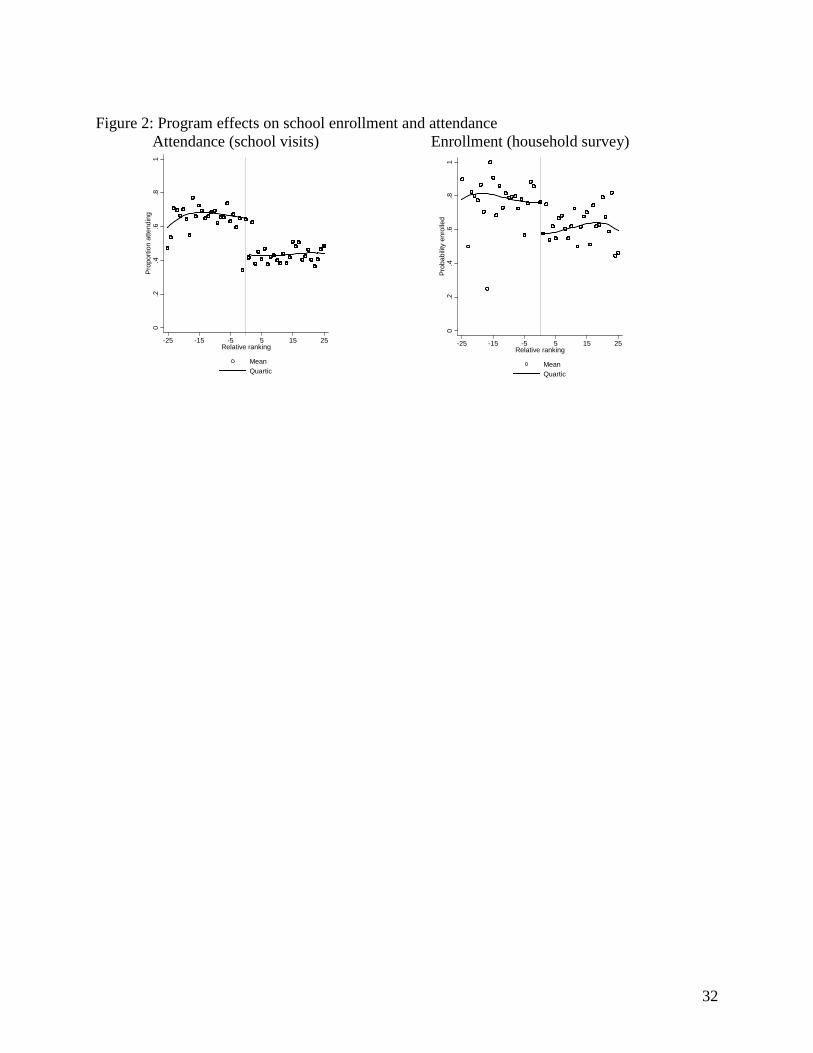
32

Figure 2: Program effects on school enrollment and attendance

Attendance (school visits) Enrollment (household survey) 0

.2.4

.6.8

1P

ropo

rtion

atte

ndin

g

-25 -15 -5 5 15 25Relative ranking

MeanQuartic

0.2

.4.6

.81

Pro

babi

lity

enro

lled

-25 -15 -5 5 15 25Relative ranking

MeanQuartic

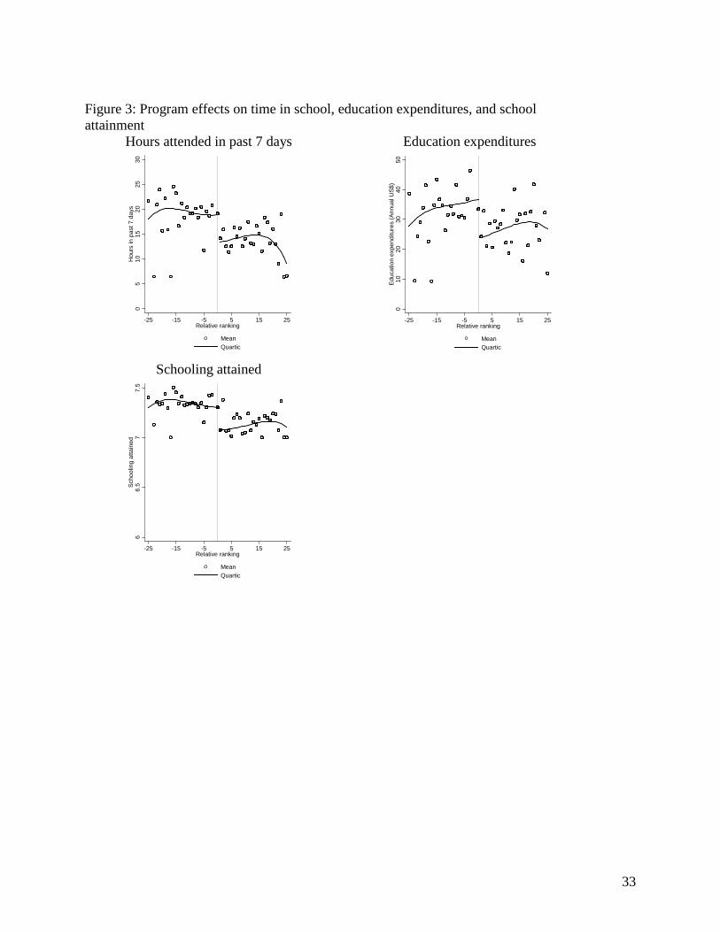
33

Figure 3: Program effects on time in school, education expenditures, and school attainment

Hours attended in past 7 days Education expenditures 0

510

1520

2530

Hou

rs in

pas

t 7 d

ays

-25 -15 -5 5 15 25Relative ranking

MeanQuartic

010

2030

4050

Edu

catio

n ex

pend

iture

s (A

nnua

l US$

)

-25 -15 -5 5 15 25Relative ranking

MeanQuartic

Schooling attained

66.

57

7.5

Sch

oolin

g at

tain

ed

-25 -15 -5 5 15 25Relative ranking

MeanQuartic

34

Figure 4: Test scores above and below cutoffs (mean by relative ranking, and prediction from quartic in relative ranking)

Math test (normalized) Vocabulary test (normalized)

-2-1

01

2M

ath

scor

e (n

orm

aliz

ed)

-25 -15 -5 5 15 25Relative ranking

MeanQuartic

-2-1

01

2V

ocab

ular

y sc

ore

(nor

mal

ized

)

-25 -15 -5 5 15 25Relative ranking

MeanQuartic

Note: Test scores normalized by mean and standard deviation among non-recipients.

35

Figure 5: Number of test-takers scoring at each level of test Math test administered in class—Grade 7 Vocabulary test administered in home

among those enrolled in grade 8 Math test administered in home among

those enrolled in grade 8

0

1

2

3

4

5

6

0 2 4 6 8 10 12 14 16 18 20 22 24Test score

Num

ber o

f app

lican

ts (s

cale

d)

Non-recipients Recipients

0

2

4

6

8

10

12

1 2 3 4 5 6 7 8 9 10 11 12 13 14 15Test score (grouped)

Num

ber o

f app

lican

ts (s

cale

d)

Non-recipients Recipients

0

1

2

3

4

5

6

1 2 3 4 5 6 7 8 9 10 11 12 13 14 15 16 17 18 19 20Test score

Num

ber o

f app

lican

ts (s

cale

d)

Non-recipients Recipients

0

0.5

1

1.5

2

2.5

0 2 4 6 8 10 12 14 16 18 20 22 24Test score

Rat

io

Ratio between number of recipients and number of non-recipients

0

1

2

3

4

5

6

7

8

9

10

1 2 3 4 5 6 7 8 9 10 11 12 13 14 15Test score (grouped)

Rat

io

Ratio between number of recipients and number of non-recipients

0

0.5

1

1.5

2

2.5

3

1 2 3 4 5 6 7 8 9 10 11 12 13 14 15 16 17 18 19 20Test score

Rat

io

Ratio between number of recipients and number of non-recipients

Note: Vocabulary test administered in home has been remapped from values ranging from 40 to 142 into 15 categories. Data are smoothed with a moving average of window-width 3.

36

Figure 6: Distribution of Grade 7 in-class mathematics test for students who will not drop out between Grades 7 and 8

Levels Ratio

0

1

2

3

4

5

6

0 2 4 6 8 10 12 14 16 18 20 22 24

Test score

Num

ber o

f app

lican

ts (s

cale

d)

Non-recipient Recipient

0

0.5

1

1.5

2

2.5

0 2 4 6 8 10 12 14 16 18 20 22 24

Test Score

Rat

io

Ratio between number of recipients and non-recipients Note: Data are smoothed with a moving average of window-width 3.

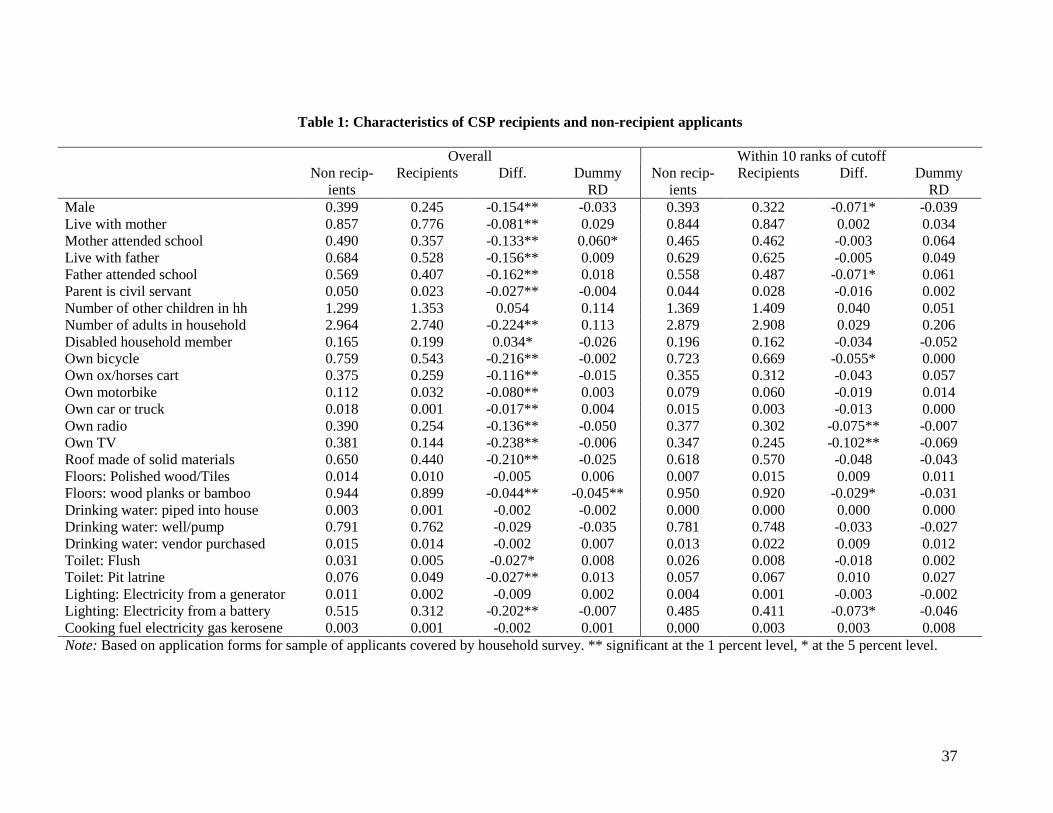
37

Table 1: Characteristics of CSP recipients and non-recipient applicants

Overall Within 10 ranks of cutoff Non recip-

ients Recipients Diff. Dummy

RD Non recip-

ients Recipients Diff. Dummy

RD Male 0.399 0.245 -0.154** -0.033 0.393 0.322 -0.071* -0.039 Live with mother 0.857 0.776 -0.081** 0.029 0.844 0.847 0.002 0.034 Mother attended school 0.490 0.357 -0.133** 0.060* 0.465 0.462 -0.003 0.064 Live with father 0.684 0.528 -0.156** 0.009 0.629 0.625 -0.005 0.049 Father attended school 0.569 0.407 -0.162** 0.018 0.558 0.487 -0.071* 0.061 Parent is civil servant 0.050 0.023 -0.027** -0.004 0.044 0.028 -0.016 0.002 Number of other children in hh 1.299 1.353 0.054 0.114 1.369 1.409 0.040 0.051 Number of adults in household 2.964 2.740 -0.224** 0.113 2.879 2.908 0.029 0.206 Disabled household member 0.165 0.199 0.034* -0.026 0.196 0.162 -0.034 -0.052 Own bicycle 0.759 0.543 -0.216** -0.002 0.723 0.669 -0.055* 0.000 Own ox/horses cart 0.375 0.259 -0.116** -0.015 0.355 0.312 -0.043 0.057 Own motorbike 0.112 0.032 -0.080** 0.003 0.079 0.060 -0.019 0.014 Own car or truck 0.018 0.001 -0.017** 0.004 0.015 0.003 -0.013 0.000 Own radio 0.390 0.254 -0.136** -0.050 0.377 0.302 -0.075** -0.007 Own TV 0.381 0.144 -0.238** -0.006 0.347 0.245 -0.102** -0.069 Roof made of solid materials 0.650 0.440 -0.210** -0.025 0.618 0.570 -0.048 -0.043 Floors: Polished wood/Tiles 0.014 0.010 -0.005 0.006 0.007 0.015 0.009 0.011 Floors: wood planks or bamboo 0.944 0.899 -0.044** -0.045** 0.950 0.920 -0.029* -0.031 Drinking water: piped into house 0.003 0.001 -0.002 -0.002 0.000 0.000 0.000 0.000 Drinking water: well/pump 0.791 0.762 -0.029 -0.035 0.781 0.748 -0.033 -0.027 Drinking water: vendor purchased 0.015 0.014 -0.002 0.007 0.013 0.022 0.009 0.012 Toilet: Flush 0.031 0.005 -0.027* 0.008 0.026 0.008 -0.018 0.002 Toilet: Pit latrine 0.076 0.049 -0.027** 0.013 0.057 0.067 0.010 0.027 Lighting: Electricity from a generator 0.011 0.002 -0.009 0.002 0.004 0.001 -0.003 -0.002 Lighting: Electricity from a battery 0.515 0.312 -0.202** -0.007 0.485 0.411 -0.073* -0.046 Cooking fuel electricity gas kerosene 0.003 0.001 -0.002 0.001 0.000 0.003 0.003 0.008 Note: Based on application forms for sample of applicants covered by household survey. ** significant at the 1 percent level, * at the 5 percent level.

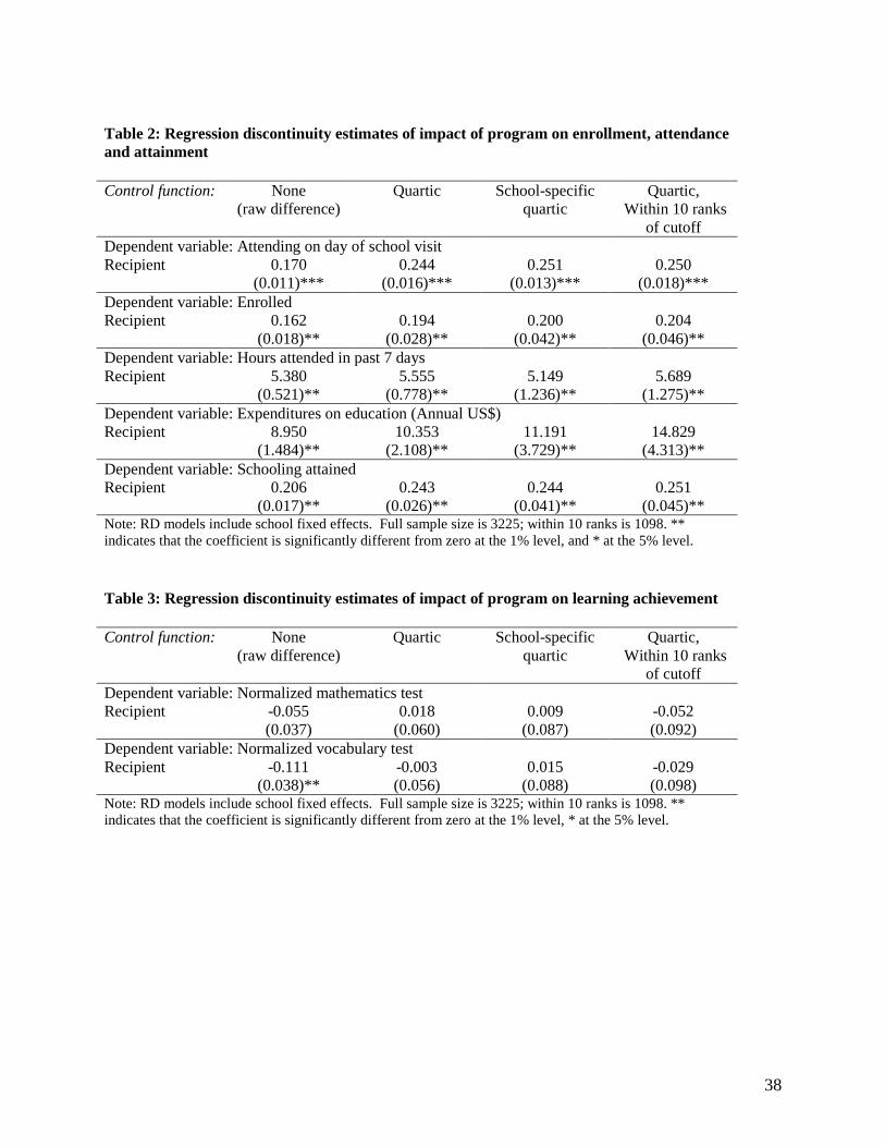
38

Table 2: Regression discontinuity estimates of impact of program on enrollment, attendance and attainment Control function: None

(raw difference) Quartic School-specific

quartic Quartic,

Within 10 ranks of cutoff

Dependent variable: Attending on day of school visit Recipient 0.170 0.244 0.251 0.250 (0.011)*** (0.016)*** (0.013)*** (0.018)*** Dependent variable: Enrolled Recipient 0.162 0.194 0.200 0.204 (0.018)** (0.028)** (0.042)** (0.046)** Dependent variable: Hours attended in past 7 days Recipient 5.380 5.555 5.149 5.689 (0.521)** (0.778)** (1.236)** (1.275)** Dependent variable: Expenditures on education (Annual US$) Recipient 8.950 10.353 11.191 14.829 (1.484)** (2.108)** (3.729)** (4.313)** Dependent variable: Schooling attained Recipient 0.206 0.243 0.244 0.251 (0.017)** (0.026)** (0.041)** (0.045)** Note: RD models include school fixed effects. Full sample size is 3225; within 10 ranks is 1098. ** indicates that the coefficient is significantly different from zero at the 1% level, and * at the 5% level. Table 3: Regression discontinuity estimates of impact of program on learning achievement Control function: None

(raw difference) Quartic School-specific

quartic Quartic,

Within 10 ranks of cutoff

Dependent variable: Normalized mathematics test Recipient -0.055 0.018 0.009 -0.052 (0.037) (0.060) (0.087) (0.092) Dependent variable: Normalized vocabulary test Recipient -0.111 -0.003 0.015 -0.029 (0.038)** (0.056) (0.088) (0.098) Note: RD models include school fixed effects. Full sample size is 3225; within 10 ranks is 1098. ** indicates that the coefficient is significantly different from zero at the 1% level, * at the 5% level.

39

Table 4: Heterogeneity of learning impacts Normalized Math Test Normalized

Vocabulary Test Interaction variable: Main

effect Interaction Main

effect Interaction

Prop. teachers with upper secondary education 0.091 -0.128 0.037 -0.071 (0.149) (0.229) (0.128) (0.210) Prop. teachers with less than 5 years experience 0.168 -0.305 0.157 -0.325 (0.140) (0.239) (0.117) (0.214) Large school^ -0.019 0.080 0.057 -0.101 (0.094) (0.121) (0.091) (0.116) Prop. of students on scholarship+ 0.015 -0.086 -0.123 0.493 (0.159) (0.713) (0.140) (0.606) Prop. of students on scholarship>median+ 0.010 0.015 -0.078 0.150 (0.080) (0.123) (0.073) (0.114) Prop. of students on scholarship>top quartile+ 0.006 0.014 -0.041 0.130 (0.070) (0.138) (0.063) (0.142) Prop. of students on scholarship<bottom quartile+ 0.020 -0.022 -0.003 0.000 (0.071) (0.134) (0.066) (0.123) Note: Sample size is 3225. Regressions include school fixed effects and the quartic in the school dropout score. ** indicates significance at the 1% level, * at the 5% level. + Numbers of students and teachers are based on year prior to program. ^Model with “large school” includes a quartic function of total school size (the continuous underlying variable used to categorize schools).

40

Table 5: Test scores, selection from 7th to 8th grade and scholarship recipient status Parameterization of test score variable:

I(Tis=1) Testis I(Tis=1)* Testis

F-test: β2+β3=0 (p-value)

F-test: β1+β3=0 (p-value)

Test score -0.068 -0.067 0.041 0.009 0.205 (0.018)** (0.005)** (0.011)** Test score>median -0.098 -0.093 0.065 0.126 0.132 (0.020)** (0.010)** (0.021)** Test score>top quartile -0.094 -0.124 0.100 0.341 0.823 (0.019)** (0.010)** (0.026)** Note: The dependent variable takes on a value of one if children dropped out of school between the June 2006 and June 2007 visits, zero otherwise. Regressions include school fixed effects and the quartic in the school dropout score. Sample size is 16,057. ** indicates significance at the 1% level, * at the 5% level.

41

Table 6: Association of schooling with, and impact of program on, knowledge, expectations and mental health

Association with schooling attained

RD estimate of program impact

Coef (SE) Obs. Coef (SE) Obs. Knowledge Number of correct HIV/AIDS preventative measures 0.336 (0.056) ** 1191 0.120 (0.057) * 3185 Number of correct cigarette questions 0.066 (0.060) 1208 -0.087 (0.054) 3225 Expectations Likelihood of providing a good home 0.176 (0.046) ** 1208 0.046 (0.046) 3224 Desired age for marriage 0.882 (0.161) ** 1166 0.261 (0.170) 3120 Desired age for first child 1.402 (0.194) ** 1163 0.255 (0.204) 3102 Child's self-assessment of rung on economic ladder 0.107 (0.087) 1208 0.003 (0.080) 3225 Child's prediction of future rung of economic ladder 0.264 (0.084) ** 1200 0.004 (0.084) 3211 Mental Health Scale 1+ 1196 3191 You consider your self to be a generally happy person 0.044 (0.047) -0.034 (0.048) You consider yourself to be a generally intelligent person 0.124 (0.047) ** -0.031 (0.043) If something goes wrong, there are people who will help you 0.102 (0.057) 0.011 (0.053) There is someone you feel comfortable talking about problems with

0.179 (0.062) ** 0.048 (0.065)

There are people who value and respect you -0.020 (0.047) -0.003 (0.049) There is someone who likes to do the same activities that you do 0.059 (0.056) -0.047 (0.058) There is a person you view as your mentor 0.051 (0.039) 0.022 (0.041) It is easy for you to make close friends -0.021 (0.052) -0.001 (0.052) You feel your life has value. 0.252 (0.051) ** 0.011 (0.053) You know the kind of person you want to become 0.071 (0.065) -0.042 (0.061) You know and believe clearly what is right and wrong for you. 0.114 (0.048) * 0.043 (0.048) You have the freedom to make decisions affecting your life 0.010 (0.050) -0.031 (0.043) Average 0.080 (0.021) ** -0.004 (0.021) Mental Health Scale 2++ 1207 3219 Have you been able to concentrate 0.173 (0.027) ** 0.020 (0.030) Have you lost much sleep over worry+++ 0.053 (0.026) * 0.019 (0.027) Do you feel that the activities you have done have been useful -0.083 (0.028) ** 0.023 (0.025) Have you felt capable of making decisions about your life 0.030 (0.022) 0.006 (0.024) Over the past month have you felt under strain+++ 0.109 (0.028) ** 0.044 (0.027) Have you been able to face up to your problems 0.011 (0.019) 0.004 (0.020) Have you felt you could overcome your difficulties 0.004 (0.016) 0.005 (0.016) Have you been able to enjoy your normal daily activities 0.093 (0.021) ** 0.043 (0.024) Have you been feeling unhappy+++ 0.074 (0.020) ** 0.028 (0.023) Have you been losing confidence+++ 0.040 (0.024) 0.013 (0.030) Have you been thinking of yourself as a worthless person+++ 0.075 (0.028) ** 0.069 (0.032) * Have you been feeling happy 0.057 (0.021) ** 0.067 (0.024) ** Average 0.053 (0.009) ** 0.028 (0.010) ** Note: +Responses are on a scale of 1 to 5. ++Responses are 0/1 where 1 corresponds to a response of “always”, except questions indicated by +++ where 1 corresponds to a response of “never”. ** indicates that the coefficient is significantly different from zero at the 1% level, * at the 5% level.