NBER WORKING PAPER SERIES

SCHOOL MARKETS: THE IMPACT OF INFORMATION APPROXIMATING SCHOOLS'EFFECTIVENESS

Alejandra MizalaMiguel Urquiola

Working Paper 13676http://www.nber.org/papers/w13676

NATIONAL BUREAU OF ECONOMIC RESEARCH1050 Massachusetts Avenue

Cambridge, MA 02138November 2007

For useful comments we are grateful to Ken Chay, David Lee, Henry Levin, Bentley MacLeod, OferMalamud, and Jonah Rockoff. For generous funding we thank the Institute of Latin American Studiesat Columbia University. The views expressed herein are those of the author(s) and do not necessarilyreflect the views of the National Bureau of Economic Research.

© 2007 by Alejandra Mizala and Miguel Urquiola. All rights reserved. Short sections of text, not toexceed two paragraphs, may be quoted without explicit permission provided that full credit, including© notice, is given to the source.

School Markets: The Impact of Information Approximating Schools' EffectivenessAlejandra Mizala and Miguel UrquiolaNBER Working Paper No. 13676November 2007JEL No. I2

ABSTRACT

The impact of competition on academic outcomes is likely to depend on whether parents are informedabout schools' effectiveness or valued added (which may or may not be correlated with absolute measuresof their quality), and on whether this information influences their school choices, thereby affectingschools' market outcomes. To explore these issues, this paper considers Chile's SNED program, whichseeks to identify effective schools, selecting them from within "homogeneous groups" of arguablycomparable institutions. Its results are widely disseminated, and the information it generates is quitedifferent from that conveyed by a simple test-based ranking of schools (which in Chile, turns out tolargely resemble a ranking based on socioeconomic status). We rely on a sharp regression discontinuityto estimate the effect that being identified as a SNED winner has on schools’ enrollment, tuition levels,and socioeconomic composition. Through five applications of the program, we find no consistentevidence that winning a SNED award affects these outcomes. This suggests that information on schooleffectiveness -- at least as it is calculated and delivered by the SNED -- might not much affect schoolmarkets.

Alejandra MizalaCenter for Applied EconomicsDepartment of Industrial EngineeringUniversity of ChileAvenida Republica 701Santiago, Chileamizala@dii.uchile.cl

Miguel UrquiolaColumbia UniversitySIPA and Economics Department1022 IAB, MC 3308420 West 118th StreetNew York, NY 10027and NBERmsu2101@columbia.edu

1

I. Introduction

The school choice debate has long recognized that the impact of competition on

academic outcomes may depend on the extent to which parents are informed about and

value school quality. Hanushek (1981) states, for instance, that “if the efficiency of our

school systems is due to poor incentives for teachers and administrators coupled with

poor decision-making by consumers, it would be unwise to expect much from programs

that seek to strengthen ‘market forces’ in the selection of schools.” Moe (1995) notes

that school choice critics have therefore argued that “parents—especially low income

parents—supposedly care about practical concerns, such as how close the school is or

whether it has a good sports team, and put little emphasis on academic quality and other

properties of effective schooling.” (emphasis added)1

Since these statements were made, the economics literature has produced fairly

clear evidence that parents do care about school quality as measured by test scores.

Black (1999) and Figlio and Lucas (2004), for instance, present quasi-experimental

evidence suggesting that consumers are willing to pay more for houses tied to schools

with higher mean scores.2 More recently, Hastings, Van Weelden, and Weinstein (2007)

present results from a randomization suggesting that even lower income parents’ school

choices respond to test score data. This is also consistent with logit and structural

estimates of parental preferences and demand responses.3

A drawback of this evidence, however, is that test scores conflate peer quality and

school effectiveness or value added—indeed, perhaps the clearest finding in the

economics of education is that socioeconomic status and academic achievement are

strongly correlated. This matters because if parents react to testing data simply because it

informs them as to which schools contain “better” children, then it is not clear that giving

them greater choice would be the best way to provide schools with incentives to become

more effective. Schools might respond, for instance, by seeking better ways to attract 1 An extensive literature indeed raises the possibility that parents are either uninformed about school quality, or else select schools using other criteria; there is less consistent evidence that such behavior is more prevalent among lower income households. See for instance Henig (1994), Ascher et al. (1996), Armour and Peiser (1998), Kleitz et al. (2000), Lubienski (2003), and Elacqua and Fabrega (2004). 2 See also Bogart and Cromwell (1997), Brunner et al. (2001), and Downes and Zabel (2002). 3 See for instance Hastings, Kane, and Staiger (2006), Bayer, Ferreira and McMillan (2007), and Gallego and Hernando (2007). These studies suggest that parents also value school traits like proximity.

2

wealthy parents, rather than by exploring better teaching techniques. This possibility is

relevant because other research suggests that parents care about peer quality in itself, and

that school choice can facilitate stratification.4

Thus a gap in the literature relates to whether parental choices, and thereby schools’

market outcomes, would respond to signals of school effectiveness per se, even if these

were not necessarily correlated with peer quality. This paper attempts to address this gap.

To do so, we consider how Chilean schools’ (enrollment) market shares, their tuition, and

their student composition react when they are identified as performing well relative to

schools that serve similar children. Specifically, we analyze the SNED,5 a program

which relies mainly on schools’ test score levels and inter-cohort gains to select good

performers from within more than one hundred “homogeneous groups” constructed such

that they contain institutions used by arguably comparable children.

While isolating school effectiveness is ultimately very difficult, the SNED thus

aims to approximate it in a simple manner which shares elements with approaches used

elsewhere, including New Jersey, New York City, and North Carolina. Its results are

disseminated via newspaper publications, the internet, PTA meetings, and in some

municipalities, by placing banners close to school entry-ways.6

This setting is interesting for several reasons. First, the information the SNED

generates is indeed quite different from that conveyed by a simple test-based ranking of

schools. This is important because as Mizala et al. (2007) point out, in Chile such a

ranking turns out to be close to one based on schools’ average socioeconomic status.

Second, within each homogeneous group, the SNED selects “winners” after ranking

schools based on an index. The top-ranked schools are chosen such that winners account

for about 25 percent of enrollments, resulting in clear group-specific cutoff scores.

Parents are informed of schools’ status (winner or non-winner), but not of their index

values. These facts allow us to use a regression discontinuity design to evaluate the

4 See for instance Henig (1990), Epple and Romano (1998), Schneider and Buckley (2002), Bayer and McMillan (2005), Urquiola (2005), Hsieh and Urquiola (2006), Rothstein (2006), Card, Mas, and Rothstein (2007), and Gallego and Hernando (2007). 5 Sistema Nacional de Evaluación del Desempeño de los Establecimientos Educativos Subvencionados. 6 New Jersey uses school report cards allowing parents to match schools to district factor groups made up of institutions in districts of similar socioeconomic status. New York City places schools in “peer horizons” containing about 40 similar institutions. North Carolina’s ABCs accountability model also uses test scores changes and relies on the placement of banners to identify award-winning schools.

3

effects of selection among arguably similar schools. Further, the SNED has distributed

awards six times since 1996, providing reasonable sample sizes.

Third, along several dimensions, Chile has the most liberalized school market in the

world, one which might actually give parents the ability to react to data on school

effectiveness. In urban areas, more than half of all schools are private, and most of these

are run for-profit. About 90 percent of all schools, religious and secular, are voucher-

funded, and about half of the private ones charge tuition in addition to the voucher.

We study the effect that being identified as a SNED winner has on a number of

schools’ outcomes. First, we consider their 1st and 9th grade enrollments, as well as the

number of classes they operate at these levels. We focus on these grades because they

are the entry points into most schools, and thus perhaps more sensitive to changing

demand. Second, we study the probability that schools charge tuition, and the amount

they charge. This reflects that schools might respond to increased demand not by

expanding but by raising their prices, a possibility we investigate in part because we do

not have measures of excess demand. Third, we consider schools’ socioeconomic

composition measured using a vulnerability index, household income, and parental

schooling. This reflects that schools could leverage the awards and increased demand by

becoming more selective.

The key finding is that through five rounds of the program, there is no consistent

evidence that SNED awards affect any of these outcomes. Our point estimates are often

close to zero, although for some outcomes they are sometimes consistent with non-trivial

effects. Nevertheless, the lack of evidence of a positive impact holds despite data from

multiple allocations and through three robustness checks.

First, we address the possibility that the SNED’s (more than one hundred)

homogeneous groups might not identify sets of schools that are effectively in competition

with each other. To do so, we consider sets of schools that in addition to belonging to the

same group, operate in the same municipality. This results in smaller comparison groups,

since there are 341 municipalities in Chile, and in urban areas they often identify compact

and homogeneous neighborhoods. Second, to explore the possibility that more educated

parents are more sensitive to data on school quality, we restrict attention to homogeneous

groups of higher socioeconomic status. Third, we restrict attention to the two most recent

4

SNED rounds, addressing the possibility that parents need time to understand such

schemes, and the fact that the dissemination of SNED results has increased over time.

In short, our results suggest that information on school effectiveness—at least as it

is delivered by the SNED—does not seem to substantially affect schools’ market

outcomes. This finding is consistent with several possibilities. First, while parents might

value effectiveness, information on it might ultimately not affect school selections based

on characteristics like proximity or peer quality. Second, the SNED might not have

sufficiently registered with parents, despite its decade-long existence. Third, the scheme

might not produce “news” if parents are able to deduce its essential results on their own.

Such sophisticated parents, further, might discount noisier inputs into the index.

Whichever is the case, our findings suggest caution in reaching conclusions on the impact

of information related to school effectiveness.

By way of closing this introduction, we note that the SNED was designed in part as

a teacher incentive scheme—in addition to being identified as effective, winning schools’

teachers are paid an annual bonus equal to about half a monthly salary. Previous work on

the SNED has focused on evaluating the impact of these bonuses on testing achievement.

We do not attempt such an analysis here, mainly because our regression discontinuity

approach is likely not suited to this purpose, as the existence of the bonus could affect

behavior at schools that end up on either side of the cutoffs that determine selection. We

note, however, that to the extent that these bonus payments render winning schools more

desirable, they provide further reasons to expect positive effects of the awards on their

market outcomes, making our failure to find these all the more surprising.

The rest of the paper proceeds as follows. Section II provides background on

Chile’s school system, and Section III discusses the SNED. Section IV presents the

identification strategy, Section V reviews results, and Section VI concludes.

II. Chile’s school system

In 1981, Chile introduced school finance reforms creating one of the most

liberalized school markets in the world. Three types of schools operate in Chile:

5

1) Public or municipal schools are run by 341 municipalities or communes,7 which

receive a per-student subsidy from the central government. These schools cannot turn

away students unless oversubscribed, and are the suppliers of last resort.

2) Private subsidized or voucher schools are independent religious or secular institutions

that receive the same per student subsidy as public schools. Unlike the latter, they

have wide latitude regarding student selection.

3) Private unsubsidized schools are also independent, but receive no public funding.

In 2003, private institutions accounted for about 45 percent of all schools, and

voucher schools alone for about 36 percent. In urban areas, these shares were 62 and 48

percent, respectively. All private schools can be explicitly for-profit, and Elacqua (2005)

calculates that about 70 percent of them are indeed operated as such. Some are run by

privately or publicly-held corporations that control chains of schools, but the modal one

seems to be owned and managed by a principal/entrepreneur. There are few legal

barriers to entry,8 and while we have no estimate on the frequency of transactions, it is

not rare to see classified ads offering private schools for sale.

While initially subsidized schools were not allowed to charge tuition to supplement

the voucher subsidy, this restriction was eased in 1994. At present about 50 percent of

private voucher schools charge tuition, and back of the envelope calculations suggest that

they raise resources equal to about 20 percent of their State funding. Public schools are

allowed to charge fees only at the secondary level, although in practice few of them do.

III. The SNED

As the government liberalized the educational sector, it began exploring

mechanisms to provide information that might aid parental school choice. In 1988 the

SIMCE9 testing system came into existence, and as of the mid-1990s its results had been

widely disseminated, partially through listings of schools’ performance in newspapers.10

The government also began using SIMCE results to allocate resources. For instance, in 7 Municipalities in Chile are generally called communes, and we henceforth use this terminology. 8 Hsieh and Urquiola (2006), for instance, indicate that roughly one thousand private schools entered the market in the decade following the introduction of voucher financing. 9 Sistema Nacional de Medición de la Calidad de la Educación. 10 A previous testing system, the Programa de Evaluación del Rendimiento Escolar, was discontinued.

6

1990, it started using 4th grade scores to assign aid to under-performing schools (Chay et

al., 2005).

A. The SNED: Basic details

In the 1990s, the government also began to consider using test scores to promote

accountability and transmit incentives. This resulted in the introduction of the SNED, a

system which seeks to identify outstanding public or subsidized private schools, and

which distributed awards in 1996, 1998, 2000, 2002, 2004, and 2006.

In an initial step, the SNED assigns schools to “homogeneous groups” constructed

in two stages. First, schools are placed into groups based on three characteristics: i)

which of Chile’s thirteen administrative regions they operate in, ii) whether they are in

the rural or urban area, and iii) the type of schooling they offer (primary only, secondary

and primary, or special needs). In a second stage, each group is further subdivided using

a cluster analysis methodology that groups schools according to the socioeconomic status

of their students. This relies on data on parental schooling, household income, and a

government-calculated vulnerability index.11

Table 1 (Column 1, Panel A) shows that in 1998, for example, this resulted in

schools being assigned to 114 homogeneous groups containing an average of 80

institutions. Among primary schools, these groups accounted for 57 and 72 percent of

the variation in income and mothers’ schooling, respectively. The total number of groups

has remained roughly stable since then; the first SNED round, 1996, used a different

methodology that resulted in only 8 groups, and this is one reason we ignore it below.12

The second step in the implementation of the SNED is the calculation of the six

sub-indices detailed in Table 2. These are aggregated to a single SNED index with a

weighting scheme that gives the greatest importance to testing performance. Specifically,

schools’ test score levels and their inter-cohort changes receive weights of 37 and 28

percent, respectively. Retention and promotion rates also enter into the calculation, as do

11 This measure (the JUNAEB index) is calculated at the school level to target school lunch-type subsidies. 12 The main reason for the smaller number of groups is that in 1996 these were constructed on a national rather than regional basis. Additionally, in other parts of the methodology (discussed below) the 1996 round relied on different data. For instance, it did not use 4th grade test scores, repetition, or drop out rates.

7

data from surveys that seek to measure parental involvement and working conditions.

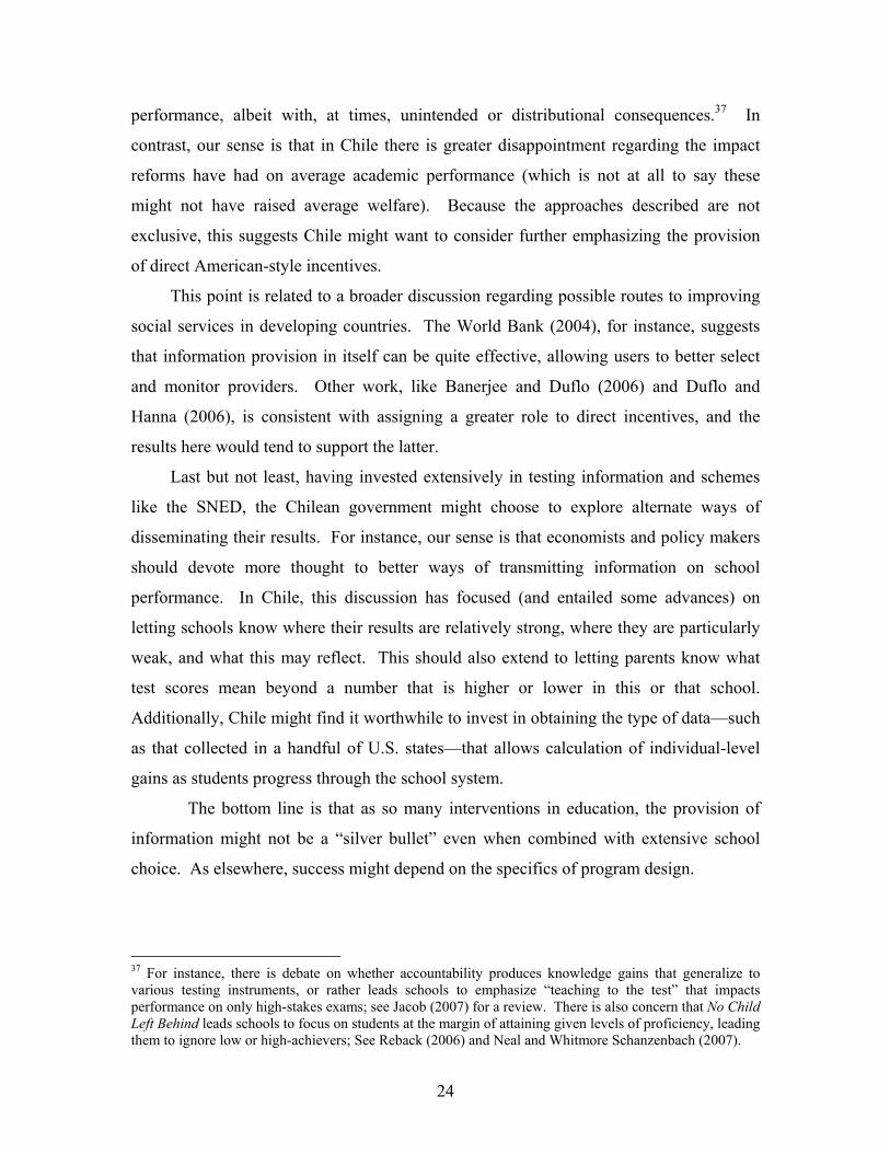
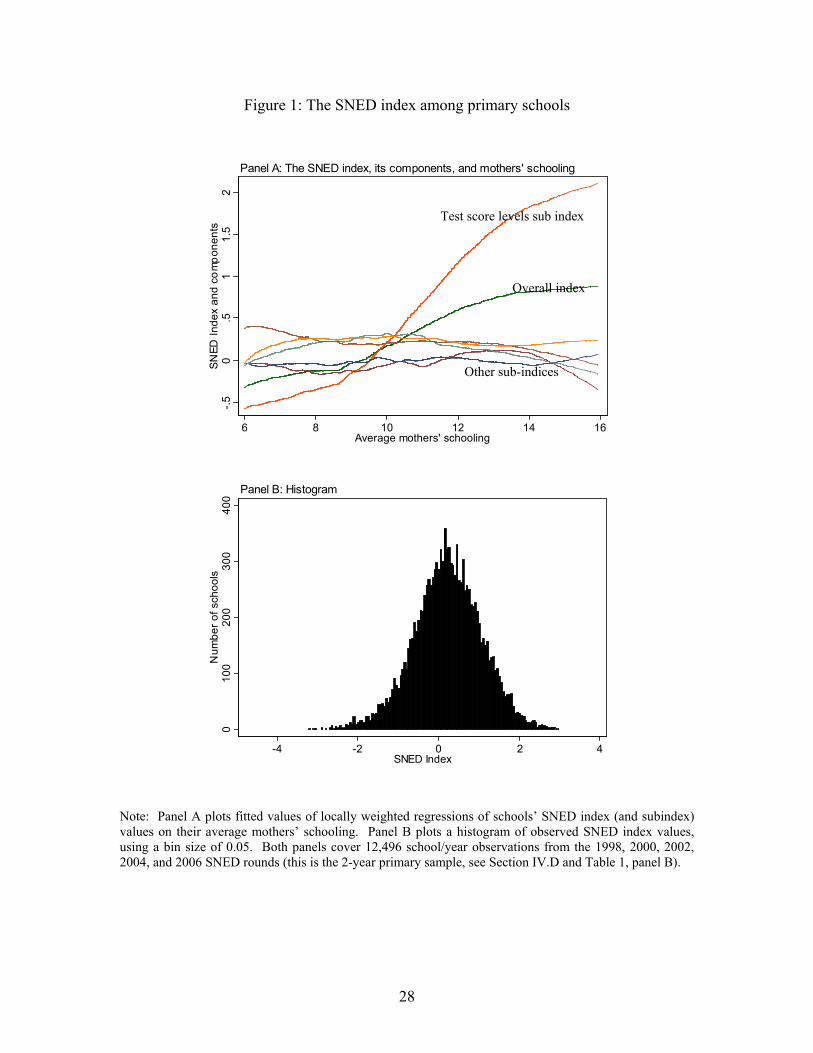
Figure 1 (Panel A) plots smoothed values of the relationship between the SNED index—

and each of its six sub-indices—and schools’ average mothers’ schooling. As visually

clear, it is largely the test score level component (the top segment) which induces a

positive relationship between the overall index and socioeconomic status (SES).13

In a third step, the schools within each homogeneous group are ordered according

to their aggregate index, and those above a given cutoff are given awards. Each group’s

cutoff is set such that winning schools account for about 25 percent of total enrollments.14

B. SNED: The treatment

For the two years the award is in force, SNED-winning schools are subject to two

treatments. First, teachers in selected schools are paid an annual bonus that presently

averages about 1,000 dollars.15 Second, winning schools are publicly identified as

performing well relatively to an arguably meaningful comparison group. Importantly,

only information on schools award status, and not on their index values, is made public.16

There are several ways in which the list of winners is publicized. Since the SNED’s

inception, it has been announced (by the Minister of Education) in a press conference,

and then published in a national newspaper the following day. Administrators at winning

schools, particularly at profit or prestige-maximizing institutions, might be expected to

inform parents, with subsequent word-of-mouth dissemination.

Table 3 summarizes the results from a Ministry of Education survey in which

schools were asked whether they apprise parents regarding their performance in the 13 In linear specifications, only the sub-index that measures test score levels, and the overall SNED index, are significantly related to mothers’ schooling or household income. 14 In the last SNED round, 2006, this was expanded to 35 percent of schools, an issue we return to below. 15 The real value of this payment has increased over time. In 1996 it was about 470 dollars, but climbed to 565 and 1,070 dollars by 2000 and 2006, respectively. These figures are averages. In practice, a global allocation is made to each school, and 90 percent of it is distributed according to hours worked. The administration has discretion over how the remainder is split; in practice most schools seem to distribute it evenly among instructors. Additionally, as noted, in 2006 the SNED was expanded such that schools accounting for 35 rather than 25 percent of enrollments receive the award—schools accounting for the first 25 percent receive a full bonus, while the rest receive only 60 percent of the full amount. Below, we ignore this issue, treating all schools as if they received the full bonus. We do so because parents only find out whether schools receive an award or not. Additionally, the distinction does not affect our key results. 16 With significant effort motivated parents could get a sense of 65 percent of the index, since test score levels (and implicitly, changes) are public (but not in the normalized form eventually used in the SNED).

8

SNED and the SIMCE tests more generally. Although one must keep in mind these data

are self-reported in an environment in which administrators are encouraged to make

information available, they suggest that by 2003 between 80 and 90 percent of schools

engaged in dissemination by way of informing their parents’ association, sending notes

home, or raising the issue during PTA-type meetings.

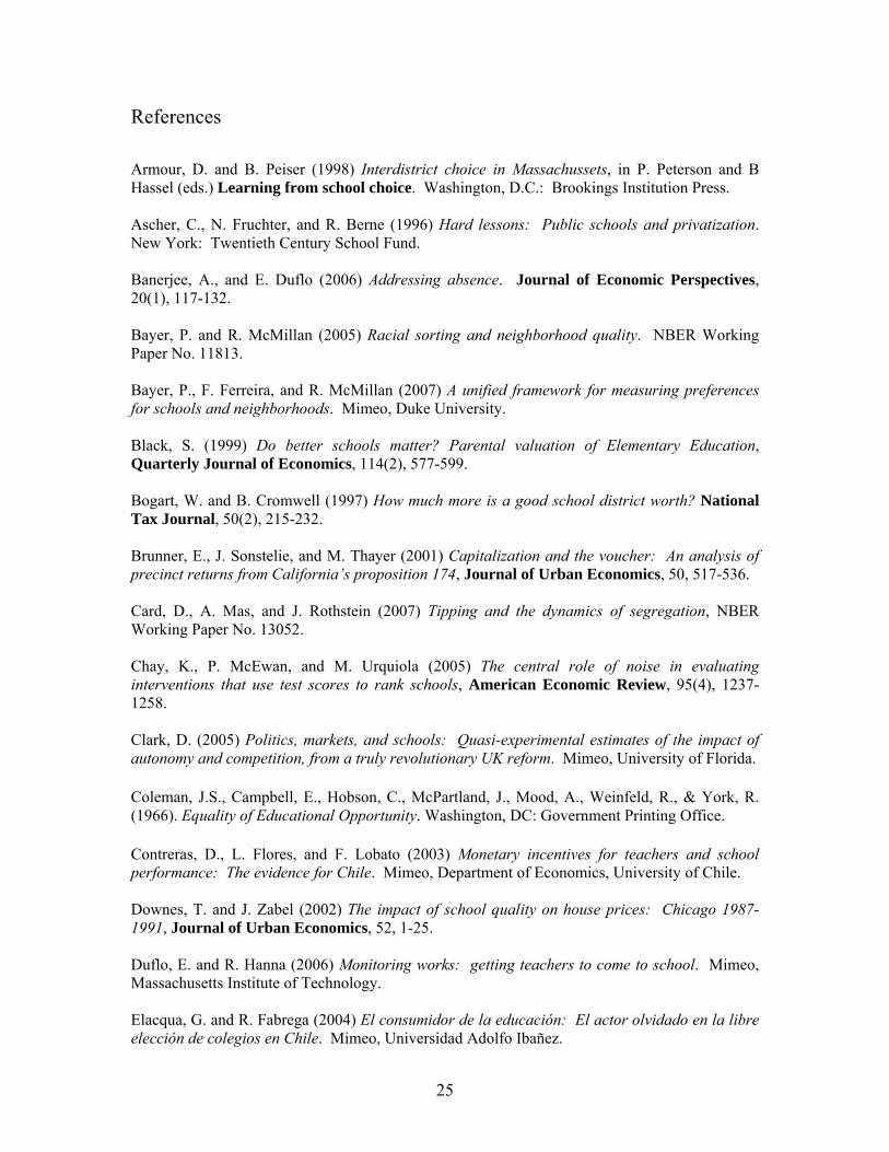
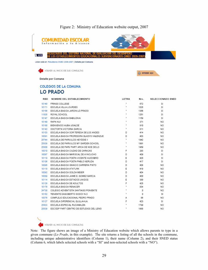
Second, since 2002 (i.e., for the last three rounds) a Ministry of Education website

has allowed parents to determine multiple schools’ SNED status. Figure 2 shows an

image of this site, which after parents select a given commune, returns a listing of all the

schools within it, and indicates whether they won an award.

Third, since 2004 (for the two most recent rounds), some communes have

intervened in the process by helping winning schools to advertise their status in a uniform

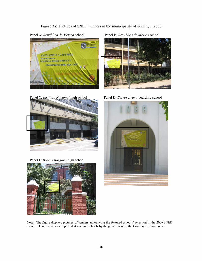
way. For instance, Figures 3a and 3b present pictures of schools in the communes of

Santiago and Providencia, respectively.17 These pictures display standardized banners

that these municipalities posted at winning schools during the 2006-2007 round. The

images show close-ups of the banners and illustrate their placement in visible places.

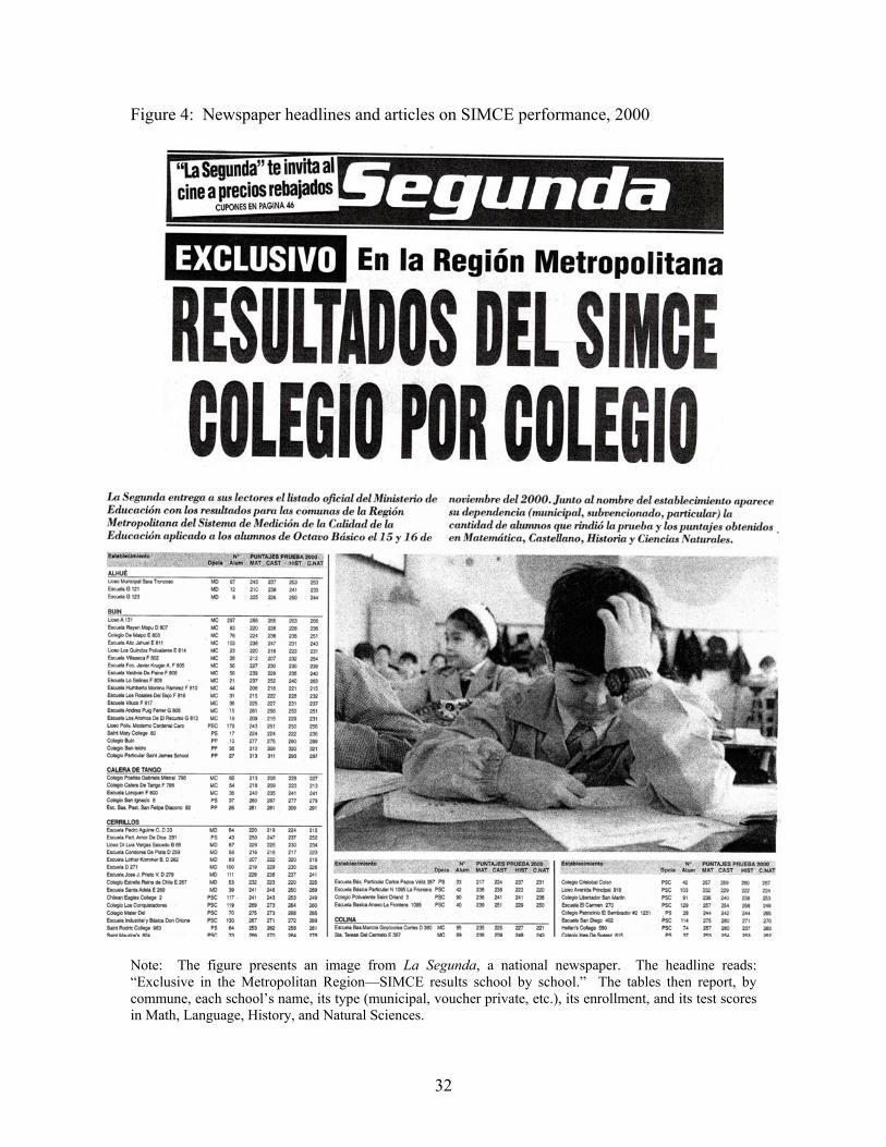
Further, information regarding the SNED is not released into a vacuum, since the

1990s afforded the public with exposure to school performance data. Figure 4 illustrates

this by showing the front page of a newspaper announcing the edition contains the scores

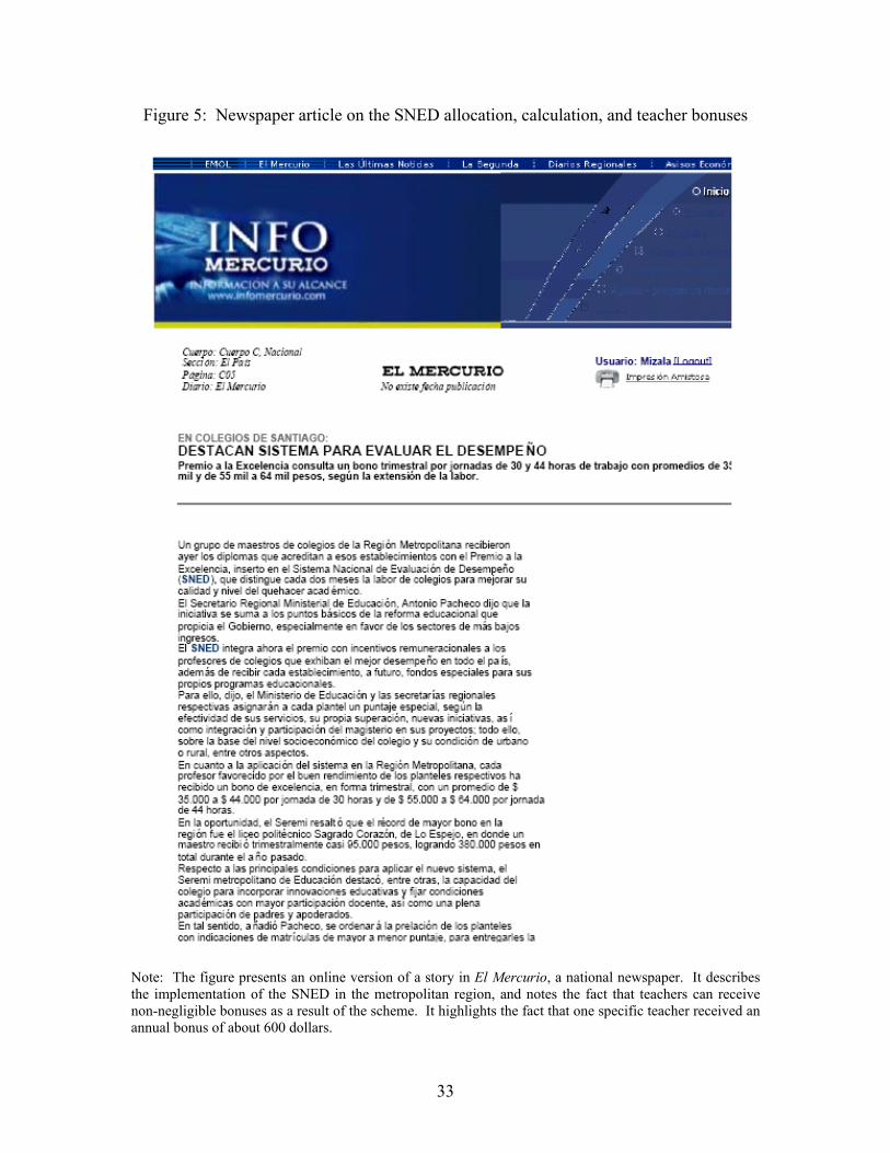
of all schools in a given region. Further, Figure 5 contains the headline and initial text of

a story on the SNED itself, including a synopsis of its methodology.

We underline that to the extent that the SNED seeks to control for SES, the

information it generates is quite different from that which simple test scores transmit.

For instance, Mizala et al. (2007) show that about 80 percent of the variation in school-

level test scores in Chile can be explained by parental schooling and household income,

which implies that rankings based on testing performance largely reflect socioeconomic

status. For instance, two programs that chose the top fifth of schools based on their mean

language score and their average mothers’ schooling would agree on the selection or non-

selection of about 85 percent of all schools. By design, the SNED produces qualitatively

different information, since it selects schools from both “rich” and “poor” homogeneous

17 By population, Santiago is the largest commune in Chile. Both Santiago and Providencia are in the Santiago metropolitan area, which contains about 50 communes.

9

groups. For a simple exercise, compare the 2002 SNED allocation with an award given

for having language scores in the top quartile in the same year. 63 percent of schools

would receive neither, and 8 percent both; 29 percent would receive one but not the other.

Further, each SNED round in some sense produces new information. Among about

8,300 schools in the five rounds we focus on, 50 percent of schools either never or always

received an award (48 and 2 percent, respectively). 22 percent were selected once, and

15, 10, and 4 percent won awards 2, 3, and 4 times, respectively.18

Finally, it is important to be clear that the SNED only seeks to approximate school

effectiveness. One way to isolate schools’ value added would be to run a large number of

randomized experiments, something which is all but impossible for most educational

systems to do once, let alone on a sustained basis. The bottom line is that while one

could envision better ways of generating data on effectiveness, the SNED represents a

reasonable and feasible approach (as mentioned, New Jersey, New York City, and North

Carolina generate and use information in broadly similar ways).

We nevertheless mention, purely as a descriptive result, that winning an award is

positively and significantly correlated with subsequent performance even controlling for

observable characteristics. For instance, Column 1 in Table 4 shows that primary schools

that received an award in 2002 had higher math scores in 2004, even after controlling for

mothers’ schooling and household income (Column 2), and for homogenous group

dummies and testing performance in the previous two years for which scores are

available (columns 3 and 4).19 Columns 5-8 suggest a similar conclusion for secondary schools.

18 The following table shows the distribution of schools according to the number of awards received. Total number of awards All six rounds Five rounds considered below 0 48.0 48.0 1 22.7 21.8 2 13.6 14.9 3 8.2 8.7 4 4.4 4.5 5 2.3 2.1 6 0.8 -- Total 100.0 100.0 19 We postpone a discussion of the data to Section IV.B.

10

IV. Empirical strategy

The manner in which the SNED is assigned makes feasible a regression

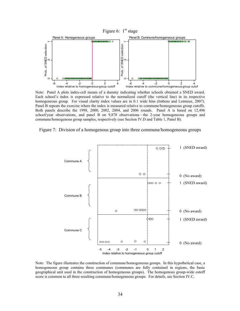
discontinuity (henceforth, RD) design. Figure 6 illustrates this among urban and

primary-level homogeneous groups. Panel A describes the allocation for 12,496

school/year observations that combine data from the 1998, 2000, 2002, 2004, and 2006

SNED waves. It plots SNED index-cell means of a dummy indicating whether schools

obtained an award, where the index is measured relative to the cutoff in each school’s

homogeneous group. We normalize each group’s cutoff to zero so that we can combine

data across groups and years. Additionally, for visual clarity index values are in 0.1 point

bins (Imbens and Lemieux, 2007). Panel A makes clear that the probability of selection

jumps discretely at the cutoff scores—the small amount of (barely visible)

noncompliance is due to the first round, 1998 (we present regression evidence below).

This discontinuous relationship can be used to investigate the effect of the SNED on

schools’ market outcomes. Following van der Klaauw (2002) one could implement:

yigt=β E(SNEDigt|indexigt)+f(indexigt)+εigt (1)

E(SNEDigt|indexigt)= γ 1{indexigt ≥cutoffgt}+g(indexigt)+ξ igt (2)

where y is an outcome of interest, i indexes schools, g orders homogeneous groups, and t

stands for different SNED rounds. E(SNEDigt|indexigt) is the probability of receiving an

award conditional on having a given index value, f and g are flexible functions of the

index, and 1{indexigt ≥cutoffgt} is a dummy that takes on a value of one if a school’s index

is greater than or equal to the cutoff in its respective homogenous group. If f and g are

continuous at cutoffgt and E(SNEDigt|indexigt) is discontinuous (Figure 6), then β is non-

parametrically identified at that point. Intuitively, under the mentioned continuity

assumptions, other factors affecting y will be similar for schools just above and below the

cutoff, and their comparison will mimic a randomized design. Discrete differences in

outcomes at the cutoff can then be attributed to the award itself.

Below we assume we have a sharp rather than a fuzzy design, and instead of

implementing (1)-(2), use a reduced form approach:

11

yigt=b 1{indexigt ≥cutoffgt} +h(indexigt)+eigt (3)

We do this in view of the fact that in our data, satisfying 1{Indexigt ≥Cutoffgt} and actually

receiving an award are almost equivalent—in all but the first SNED round we use, the

correspondence is indeed perfect. Additionally, we specify h as a quadratic in the index,

and also estimate (3) within arbitrarily narrow bands close to the cutoff scores.

A. What can an RD design identify in this context?

While Figure 6 (Panel A) shows that the SNED produces a “clean” RD, it is

relevant to ask what this can identify in our context. As detailed in Section III, the SNED

treatment has two components: teachers in winning schools receive bonuses, and these

schools are identified as performing well relative to a specific reference group.

Previous work on the SNED has analyzed the effects of the bonuses on testing

achievement (Contreras, Flores, and Lobato, 2003). We do not attempt this because our

sense is that the RD approach is not suited to it, since the SNED’s existence might affect

the behavior of teachers who know their school is within range of winning, regardless of

whether this eventually happens or not. In this case, the intensity of the incentives would

not vary discretely at the cutoff, even though the bonus payment of course would.

We focus instead on the effect of the awards on schools’ market outcomes.

Schools’ award status of course does vary discretely at the cutoff (particularly since as

stated, index values are not publicized). As stated, to the extent that bonus payments

render winning schools more desirable, they provide a further reason to expect positive

estimates from reduced form approaches like (3).

B. Outcomes, hypotheses, and data

We explore how SNED selection affects the following school level outcomes:

1) 1st and 9th grade enrollments. To the extent that selected schools experience higher

demand, they might end up with greater enrollment shares. We focus on these grades

12

because they are the entry points into most schools, and school choice might therefore

be least constrained at these junctures.20

2) Number of 1st and 9th grade classes operated. Urquiola and Verhoogen (2006)

suggest that profit-maximizing Chilean schools view the choice of the number of

classrooms to operate as a serious one, if only because it influences their fixed costs.

Additionally, they present evidence suggesting that higher quality schools experience

higher demand and operate more classrooms. One might expect, therefore, that

SNED winners would be more likely to open an additional classroom. For this and

the previous outcome, we rely on annual 1997-2007 administrative data collected at

the beginning of each academic year (around February).

3) Tuition. Since 1994, private voucher schools have been allowed to charge tuition

add-ons, and at present about 50 percent of them do. Using 1997-2006 administrative

data, we study whether schools charge tuition at all, as well as the average amount

they charge. We consider the former for two reasons. First, simply charging tuition

is a signal of perceived quality in Chile, as parents can always use municipal schools

for no charge. Second our tuition data are not grade-specific, and may therefore only

slowly reflect SNED–induced increases that might first affect lower grades. In

contrast, it is easier to observe if a SNED award induces a school that did not charge

tuition to begin doing so.

4) Socioeconomic composition. Finally, we explore whether winning an award affects

schools’ socioeconomic composition, something one might expect if a perception of

higher quality allowed schools to attract a “better” clientele. For this we rely on two

types of data. The first is a government-calculated school-level vulnerability index

that considers variables like parental schooling and employment, for which we have

annual 1st and 9th grade (1997-2007) observations.21 For more direct measures, we

also use data from the SIMCE system, which at times of testing sends a questionnaire

to students’ homes. This provides information on household income and parental 20 We explored results for the 7th grade, as some secondary schools begin operations at this grade. We omit them because they produce conclusions similar to those for the 9th grade, while providing smaller samples. 21 The index is calculated by JUNAEB, an agency which uses it to target school-lunch type subsidies. The variables it uses are: a) the percentage of mothers with less than eight years of schooling, b) the percentage of household heads with less than eight years of schooling, c) the employment category of the household head, d) the percentage of children who receive welfare payments, e) the percentage of children without access to adequate sewerage systems, and f) the percentage of students in households classified as poor.

13

schooling. As part of the testing system, however, these data are available only for

the 4th, 8th, and 10th grades, and each grade is tested (about) only every third year. We

discuss further adjustments this necessitates in the results section below.

C. Comparison groups

The most natural way to implement an RD design in our setting is to compare—

within homogeneous groups—the outcomes of schools that just qualify for an award with

those of schools that just miss receiving one. Such are the main results we review below.

To further the probability that we analyze sets of schools effectively in competition with

each other, we present other results in which we apply the strategy not within

homogeneous groups, but rather among schools that in addition to being in the same

group, are located in the same commune. This is feasible because communes are subsets

of regions (the basic geographical unit used in the construction of the homogeneous

groups), and is useful because they come closer to identifying areas where school choice

might take place. For instance, the metropolitan area of Santiago, the largest in Chile,

has about 50 communes, and although children can in principle attend school in any of

these, in practice many stay in their commune of residence.22

Figure 7 illustrates the spirit of this analysis by showing a hypothetical

homogeneous group that includes schools in three communes, labeled A-C. The cutoff

score—a single one for the whole group—separates schools that get an award from those

that do not. We use the schools in each of these communes as a commune/homogeneous

group—i.e. Figure 7 would yield three rather than one quasi-experiment. Table 1 shows

the impact this has on the number of groups considered. Column 1 (Panel A) shows that

while for 1998 there were a total of 114 homogenous groups, the combination with

roughly 314 communes results in 1,784 commune/homogenous groups.23 As Figure 7

suggests, the latter continue to produce a “clean” first stage (Figure 6, Panel B).

22 The 2002 SIMCE data suggest that about 89 percent of 4th graders using subsidized institutions go to school in the commune in which they live. In Metropolitan Santiago, this figure goes down to 79 percent. As elsewhere, it is also more common for children in secondary school to travel further to school, and they therefore cross commune lines more frequently. 23 To include a commune/homogeneous group, we require that it contain both winning and losing schools.

14

From the point of view of an RD design, this exercise involves a tradeoff. On the

one hand, communes facilitate sorting, and so produce even more homogeneous sets of

comparison schools. For instance, in 2002 a full set of homogeneous group dummies

accounted for 57 percent of the variation in income at the 4th grade level, and 72 percent

of the variation in average mothers’ schooling. Using commune/homogeneous group

dummies, these numbers increase to 68 and 81 percent, respectively. The intuition is also

illustrated in Figure 7, where we have arbitrarily drawn commune A to be the one with

the highest average performance within the homogeneous group, followed by B and C.

On the other hand, moving to commune/homogeneous groups comes at the cost of

making comparison groups smaller. For example, while in the urban area primary

homogeneous groups contain an average of about 71 schools, commune/homogeneous

groups have an average of 7 (Table 1), such that the density of observations close to the

cutoffs can go down significantly (also illustrated in the hypothetical case of Figure 7).

D. Samples and analyses windows

Two final issues define the samples analyzed below. First, we restrict attention to

urban comparison groups, since urban parents enjoy greater school choice and therefore

more opportunities to leverage information on school quality. Second, there is the issue

of what chronological windows to analyze.

We consider two alternatives. First, we use what we label a “2-year sample” (Table

1, Panel B) designed to study award effects in two year windows, the most natural

timeframe to the extent that the SNED waves are two years apart. In this sample, we

include schools with valid indices in each round we consider (1998, 2000, 2002, 2004,

and 2006), and for which there are at least enrollment outcomes one year prior to each

allocation (to check for continuity), as well as two years after. To include the 2006

round, we use the 2007 outcomes as if they were for 2008. We could have omitted this

last round, but opted to retain it so that we can consider the longest possible timeframe

and largest possible samples. This issue arises only for enrollment and vulnerability, for

which we have 2007 data (collected early in the academic year). For all other outcomes,

we only have data up to 2006. For the sake of larger samples, we also combine

15

observations from different rounds (clustering standard errors at the school level), and the

resulting “stacked” data are described in Column 6 (Table 1, Panel B). Using such data

implies that in looking at outcomes two years after each round, for instance, we are

asking if schools that received an award in 1998 had higher enrollments in 2000; whether

those that received one in 2000 had higher enrollments in 2002, and so on.24

Additionally, Panel C (Table 1) describes a “4-year” sample which allows us to

explore effects four years after the 1998, 2000, 2002, and 2004 rounds.25 This is useful in

looking at outcomes that might be slower to change, but raises a caveat because in

general the fact that a school wins an award one year increases the probability that it will

do so again.26 This means that while schools that just make and just miss an award may

be comparable at baseline (as shown below), four years later some of the former will

have received two awards, while the latter will have at most one. This is likely to bias

results toward finding positive effects in the 4-year samples.

V. Results

We first present results for primary-level homogeneous groups, then consider

primary commune/homogeneous groups, and finally turn to the secondary level.

A. First stage

Table 5 presents the first stage results when we analyze the program’s allocation

among homogeneous groups. Panel A focuses on the 2-year sample (defined in section

IV.D), and Column 1 shows that among the 12,496 school/year observations it contains,

having a baseline index greater than or equal to zero—the normalized cutoff score in

schools’ respective groups—raises the probability of receiving an award by about one.

Not surprisingly (in light of Figure 6), the R2 in this regression is close to one.

24 We also carried out our analyses considering outcomes measured one rather than two years after each allocation. We omit these to save space, as they produce similar results. 25 Again, using the last of these requires assuming the 2007 outcomes are actually for 2008. 26 This is despite the fact that some of the SNED sub-indices are measured with some noise, e.g., the inter-cohort changes—see Kane and Staiger (2002), Chay et al. (2005), and Mizala et al. (2007).

16

While the first stage results are stable in the remaining columns, we nonetheless

discuss them because these describe the specifications and samples used in the tables

below. First, Column 2 includes a quadratic in schools’ baseline index as a control, and

Column 3 restricts the sample to schools with indices within 0.50 points of their cutoffs,

reducing the sample by about half.27 The remaining columns further restrict the sample

in two ways. First, to study the possibility that more educated households are more

responsive to data on school quality, column 4 considers only schools in higher

socioeconomic status homogeneous groups.28 Second, column 5 only uses data from the

last two (2004 and 2006) SNED waves. This investigates the possibility that parents

might need an adjustment period to understand and utilize the information the SNED

delivers, and takes into account the fact that the intensity of dissemination has increased

over time. The fit is strong throughout, and the R2 reaches one in the final column. This

reflects that the small amount of “slippage” in the allocation took place in 1998. Panel B

describes analogous results for the 4-year sample (Section IV.D), which requires

excluding the 2006 wave, thereby reducing the sample from 12,496 to 9,659 schools.

The first stage fit remains strong across all specifications.

Finally, still considering the 4-year sample, Panel C explores whether the

probability of winning additional awards varies discretely at the cutoffs. Column 1

shows that schools with a baseline index greater than or equal to zero are 35 percent more

likely to win another award two years later.29 Adding a quadratic in the index (Column

2) reduces the estimate by about half, but it is still significant there and in columns 3 and

5 (not in the higher socioeconomic status sample, Column 4). Significance is of course

consistent with some persistence in SNED awards, which as stated, should bias our

results toward revealing significant effects four years after each allocation.

A. Enrollment

27 We experimented with narrower bands, and with requiring that schools be one of, for example, four of the institutions closest to the cutoff. These exercises produced qualitatively similar conclusions. 28 That is, we use only homogeneous groups which the SNED methodology itself catalogued as higher SES. 29 This is to be expected in only given that schools’ test score levels (an input into the aggregate index) are correlated with their socioeconomic composition, which is likely to remain fairly stable over time.

17

Turning to the results for enrollment, we first implement a “continuity check” by

studying whether enrollment prior to the allocation was greater among schools that

obtained an award. Such a difference, if it existed close to the cutoffs, would question an

RD approach. Figure 8a (Panel A) first presents the graphical evidence for the 2-year

sample. It plots index cell means of schools’ 1st grade enrollment one year before the

baseline allocations, along with the fitted values of locally weighted regressions

estimated separately for institutions with negative and non-negative index values. The

figure shows an overall positive association between enrollment and schools’ relative

index, illustrating that even within homogeneous groups, schools that received an award

tended to be larger prior to doing so. Table 6 (Panel A) illustrates this in regression form,

showing this difference was equal to about eight 1st grade students, equivalent to about 20

percent of a standard deviation.30 Columns 2-6 show, however, that this difference falls

to less than one student and ceases to be significant when we use a quadratic of the

SNED index as a control, or when we focus on more restricted samples. Graphically, this

is reflected in that there is no visible break at the cutoff in Figure 8a, Panel A. In short,

as required by the RD design, enrollment prior to each allocation appears to be smoothly

related to the index in the vicinity of the cutoffs.31

Panel B (Table 6) considers enrollment two years after awards are made. While

there is again a substantial difference in the simplest specification (Column 1), this

becomes small and insignificant in columns 2 and 3; in the latter (which controls for the

index and restricts the sample to schools closer to the cutoff scores), the point estimate

suggests that on average, schools that just received an award had about one less 1st grader

two years after doing so (relative to institutions that just missed an award). Column 4

replicates the sample from column 3, but controls for enrollment one year prior to the

awards.32 The point estimate is now -0.2, and we can rule out differences greater than

about 1.5 students. Columns 5 and 6 (higher SES groups and recent rounds) suggest

similar conclusions, although with somewhat smaller samples and higher standard errors. 30 As stated, we selected the samples such that they would include schools with valid enrollment information in all relevant years. This is why the 12,496 observations in Table 5 match those for the 1st stage, in Table 4. For other outcomes, the sample sizes are generally slightly smaller due to missing data. 31 We also note that the density of observed SNED index levels (Figure 1, Panel B) does not suggest that schools or administrators in any way manipulate the running variable (see McCrary, forthcoming). 32 We could also compare changes, implicitly restricting the coefficient on prior enrollment to be one; we opt instead for the more flexible specification in column 4.

18

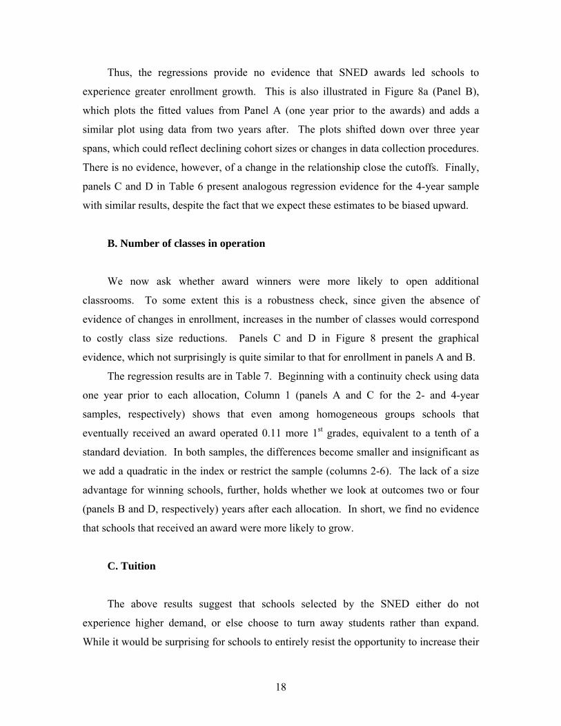
Thus, the regressions provide no evidence that SNED awards led schools to

experience greater enrollment growth. This is also illustrated in Figure 8a (Panel B),

which plots the fitted values from Panel A (one year prior to the awards) and adds a

similar plot using data from two years after. The plots shifted down over three year

spans, which could reflect declining cohort sizes or changes in data collection procedures.

There is no evidence, however, of a change in the relationship close the cutoffs. Finally,

panels C and D in Table 6 present analogous regression evidence for the 4-year sample

with similar results, despite the fact that we expect these estimates to be biased upward.

B. Number of classes in operation

We now ask whether award winners were more likely to open additional

classrooms. To some extent this is a robustness check, since given the absence of

evidence of changes in enrollment, increases in the number of classes would correspond

to costly class size reductions. Panels C and D in Figure 8 present the graphical

evidence, which not surprisingly is quite similar to that for enrollment in panels A and B.

The regression results are in Table 7. Beginning with a continuity check using data

one year prior to each allocation, Column 1 (panels A and C for the 2- and 4-year

samples, respectively) shows that even among homogeneous groups schools that

eventually received an award operated 0.11 more 1st grades, equivalent to a tenth of a

standard deviation. In both samples, the differences become smaller and insignificant as

we add a quadratic in the index or restrict the sample (columns 2-6). The lack of a size

advantage for winning schools, further, holds whether we look at outcomes two or four

(panels B and D, respectively) years after each allocation. In short, we find no evidence

that schools that received an award were more likely to grow.

C. Tuition

The above results suggest that schools selected by the SNED either do not

experience higher demand, or else choose to turn away students rather than expand.

While it would be surprising for schools to entirely resist the opportunity to increase their

19

revenues, doing so might reflect that raising class sizes or opening new classrooms

involves risk. Additionally, schools might have made implicit commitments to parents

regarding class and school size.

We unfortunately do not have measures of excess demand, but in this and the next

section we study two other ways in which schools could leverage increased demand: by

raising their prices or by becoming more selective in terms of socioeconomic status. The

first is relevant because the period we analyze was one in which the prevalence and

magnitude of tuition charges were increasing. For instance, in 1997, 38 percent of

voucher schools charged add-on tuition, and the average was about 3 monthly dollars.

By 2006, these figures had increased to 50 percent and 14 dollars, respectively.

We first consider whether schools charge tuition at all,33 which is useful partially

because we do not observe grade-specific tuition, and average charges may move slowly

if schools raise prices only for entering cohorts. In contrast, going from zero to positive

tuition is an outcome that is easily observed. Figure 8a presents the graphical evidence,

which is suggestive of no effect—there is no break in the relationship one year prior to

the allocation (Panel E), and the fitted values one year prior and two years later

essentially overlap (Panel F), particularly close to the cutoff. For more detail, Table 8

(Column 1) suggests that even within homogeneous groups, schools that receive an

award are on average more likely to charge tuition, although the difference is not great.

Controlling for the SNED index or restricting samples close to the cutoffs, however,

eliminates significant differences—the point estimates in Column 4, our preferred

specification, are essentially zero. In the two year sample (Panels B) they rule out that

awards increase the probability of charging tuition by more than two percent.

The evidence on absolute tuition (panels A and B of Figure 8b, and Table 9) points

to similar conclusions. Whether we consider outcomes prior to the allocation or two or

four years thereafter, award winners on average collect higher tuition (about 500 more

pesos per month, equivalent to roughly a tenth of a standard deviation). This is expected,

if only given the positive correlation between the SNED index and socioeconomic status

33 As stated, primary municipal schools cannot charge tuition. We verified that close to the discontinuities, there are no differences in the proportion of schools that are municipal (as opposed to private voucher).

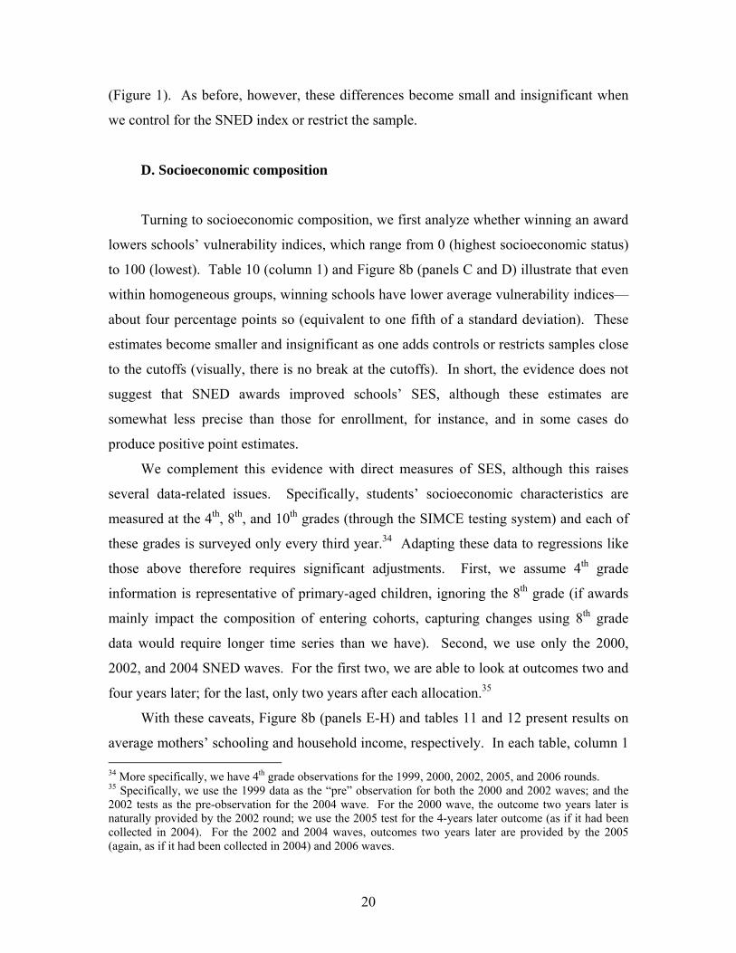
20

(Figure 1). As before, however, these differences become small and insignificant when

we control for the SNED index or restrict the sample.

D. Socioeconomic composition

Turning to socioeconomic composition, we first analyze whether winning an award

lowers schools’ vulnerability indices, which range from 0 (highest socioeconomic status)

to 100 (lowest). Table 10 (column 1) and Figure 8b (panels C and D) illustrate that even

within homogeneous groups, winning schools have lower average vulnerability indices—

about four percentage points so (equivalent to one fifth of a standard deviation). These

estimates become smaller and insignificant as one adds controls or restricts samples close

to the cutoffs (visually, there is no break at the cutoffs). In short, the evidence does not

suggest that SNED awards improved schools’ SES, although these estimates are

somewhat less precise than those for enrollment, for instance, and in some cases do

produce positive point estimates.

We complement this evidence with direct measures of SES, although this raises

several data-related issues. Specifically, students’ socioeconomic characteristics are

measured at the 4th, 8th, and 10th grades (through the SIMCE testing system) and each of

these grades is surveyed only every third year.34 Adapting these data to regressions like

those above therefore requires significant adjustments. First, we assume 4th grade

information is representative of primary-aged children, ignoring the 8th grade (if awards

mainly impact the composition of entering cohorts, capturing changes using 8th grade

data would require longer time series than we have). Second, we use only the 2000,

2002, and 2004 SNED waves. For the first two, we are able to look at outcomes two and

four years later; for the last, only two years after each allocation.35

With these caveats, Figure 8b (panels E-H) and tables 11 and 12 present results on

average mothers’ schooling and household income, respectively. In each table, column 1 34 More specifically, we have 4th grade observations for the 1999, 2000, 2002, 2005, and 2006 rounds. 35 Specifically, we use the 1999 data as the “pre” observation for both the 2000 and 2002 waves; and the 2002 tests as the pre-observation for the 2004 wave. For the 2000 wave, the outcome two years later is naturally provided by the 2002 round; we use the 2005 test for the 4-years later outcome (as if it had been collected in 2004). For the 2002 and 2004 waves, outcomes two years later are provided by the 2005 (again, as if it had been collected in 2004) and 2006 waves.

21

indicates that even within homogeneous groups, SNED-winning schools have “better”

peer groups—they contain children whose mothers have about 0.6 more years of

schooling, and whose household income is about 20 thousand pesos higher (about 0.3 and

0.4 of a standard deviation, respectively). These differences mostly cease to be

significant, however, when we restrict the sample to schools close to the cutoff; they

mostly also become smaller, and in some cases even suggest negative award effects.

We underline that these results should be viewed with greater caution. The

sample sizes are smaller than those above, and the data are collected using questionnaires

which parents sometimes do not send back.

E. Robustness checks: Commune/homogeneous groups and secondary schools

The estimates presented thus far rely on the SNED-constructed homogeneous

groups. As a robustness check (described in Section IV), we carry out similar exercises

comparing schools that are in the same commune in addition to being in the same

homogenous group. Appendix tables A.1-A.4 (Panel A) implement this exercise,

although for the sake of space we limit the discussion and focus on only three outcomes:

enrollment, whether schools charge tuition, and vulnerability.36 The conclusions are

similar to those above save for two differences. First, the estimates are somewhat less

precise in part because the exercise results in smaller samples close to the cutoff scores.

This may be behind a few estimates suggesting significantly positive and negative

effects, although there is not consistent evidence in either direction. Second, even more

than among homogenous groups, there is persistence in SNED awards.

Finally, Tables A.1 (Panel B) and A.5-A.7 consider the effects of the SNED at the

secondary level. We also limit these tables to three outcomes: enrollment (in this case at

the 9th grade level), whether schools charge tuition, and vulnerability (also measured at

the 9th grade level). The same two caveats raised with respect to commune/homogeneous

groups apply: relatively less precision and greater persistence in SNED awards. That

said, the conclusions are again qualitatively similar.

36 More specifically, Table A.1 (Panel A) presents the first stage. Tables A.2, A.3, and A.4 present the enrollment, tuition, and vulnerability results, respectively. We omitted the remaining outcomes because they produce similar conclusions—the associated tables are available upon request.

22

VI. Discussion

A longstanding debate in the economics of education concerns to what extent

improving educational quality, say as measured by test scores, could be achieved simply

by relying on competition, and to what extent it would necessitate intervention through

initiatives ranging from accountability (e.g., No child left behind) to raising expenditure.

Researchers have noted that for competition alone to really deliver, it must be that

parents’ choices, and therefore schools’ outcomes, depend on schools’ effectiveness in

producing academic attainment. If in contrast households view school choice as a means

to obtain better peer groups or reduce travel time, then competition might encourage

schools to improve on dimensions other than academic value added.

Over the past decade the literature has produced evidence that parental school

choice is indeed influenced by information on school quality, at least as measured by test

scores. Yet this does not answer the question at hand because, going back to the

Coleman (1966) report, it is clear that test scores conflate school effectiveness and peer

quality. In the specific case of Chile, in fact, a ranking of schools based on their test

scores is quite close to one based on their socioeconomic status.

A key gap in our understanding of school markets, therefore, concerns whether

parental choices and schools’ outcomes would respond to data on effectiveness per se,

even if it were not necessarily correlated with peer quality. This paper has attempted to

begin filling that gap by analyzing Chile’s SNED, a scheme that seeks to measure

effectiveness in a manner the public might understand. Perhaps surprisingly, we fail to

find systematic evidence that SNED awards impact schools’ market outcomes.

These results are consistent with several possibilities. First, while parents might

value school effectiveness, information on it might in the end not sway school choices

based on characteristics like peer composition. This would rationalize stronger reactions

to data on average performance than to information approximating effectiveness. It

would also be consistent with markets getting “stuck” in configurations in which

wealthier parents, essentially due to coordination failures, are unable to access the most

productive schools (Rothstein, 2006). These issues might be particularly relevant in

Chile, where school choice has likely given schools ample opportunities to differentiate.

23

Another potential explanation for our findings is that the SNED might not have

registered with households, despite the fact that the program is eleven years old and there

are many ways for parents to find out about it. Alternately, the information it produces

might be not “news”—parents might be able to deduce it on their own. Such

sophisticated parents might also realize that some of the information contained in the

SNED might be noisy, and decide to discount it. Finally, schools might respond to

awards in ways that precisely counteract demand responses (for instance, by becoming

more selective as demand increases), although one would expect this to show up in our

measures of socioeconomic composition or tuition, and there is no clear evidence of that.

Regardless of the explanation, our results have multiple policy implications. Most

immediately, “shaking” school markets through the provision of information might be

harder than is commonly assumed. More specifically, policy makers would like

competition to reward and weed out firms along dimensions they value, and this may be

hard to achieve regarding educational effectiveness. If this is the case (and on a more

speculative note), Chile might want to consider using test scores to more aggressively

provide incentives for schools.

More broadly, this raises a contrast between “American” and “Chilean” style

accountability. The U.S. has never implemented a national K-12 performance exam, and

in some states households still have difficulty accessing data to compare achievement in

their school with that in other (let alone comparable) institutions. Nonetheless, through

No Child Left Behind and their own initiatives, many states use test scores to offer

schools carrots and sticks. In contrast, while over the past two decades Chile has

aggressively collected and disseminated school performance data, it has mainly exploited

this information to inform consumers, offering schools few test-based incentives.

In part, these differences reflect that many policy makers in the U.S. have seen

accountability as an alternative way to generate incentives, in view of difficulties in

expanding school choice. In contrast, one could say many policy makers in Chile have

seen the successful expansion of school choice as the key intervention, with

accountability-type initiatives playing a secondary role.

The impact of these approaches in their respective settings is controversial. Our

reading is that in the U.S. there is an emerging consensus that accountability can change

24

performance, albeit with, at times, unintended or distributional consequences.37 In

contrast, our sense is that in Chile there is greater disappointment regarding the impact

reforms have had on average academic performance (which is not at all to say these

might not have raised average welfare). Because the approaches described are not

exclusive, this suggests Chile might want to consider further emphasizing the provision

of direct American-style incentives.

This point is related to a broader discussion regarding possible routes to improving

social services in developing countries. The World Bank (2004), for instance, suggests

that information provision in itself can be quite effective, allowing users to better select

and monitor providers. Other work, like Banerjee and Duflo (2006) and Duflo and

Hanna (2006), is consistent with assigning a greater role to direct incentives, and the

results here would tend to support the latter.

Last but not least, having invested extensively in testing information and schemes

like the SNED, the Chilean government might choose to explore alternate ways of

disseminating their results. For instance, our sense is that economists and policy makers

should devote more thought to better ways of transmitting information on school

performance. In Chile, this discussion has focused (and entailed some advances) on

letting schools know where their results are relatively strong, where they are particularly

weak, and what this may reflect. This should also extend to letting parents know what

test scores mean beyond a number that is higher or lower in this or that school.

Additionally, Chile might find it worthwhile to invest in obtaining the type of data—such

as that collected in a handful of U.S. states—that allows calculation of individual-level

gains as students progress through the school system.

The bottom line is that as so many interventions in education, the provision of

information might not be a “silver bullet” even when combined with extensive school

choice. As elsewhere, success might depend on the specifics of program design.

37 For instance, there is debate on whether accountability produces knowledge gains that generalize to various testing instruments, or rather leads schools to emphasize “teaching to the test” that impacts performance on only high-stakes exams; see Jacob (2007) for a review. There is also concern that No Child Left Behind leads schools to focus on students at the margin of attaining given levels of proficiency, leading them to ignore low or high-achievers; See Reback (2006) and Neal and Whitmore Schanzenbach (2007).

25

References

Armour, D. and B. Peiser (1998) Interdistrict choice in Massachussets, in P. Peterson and B Hassel (eds.) Learning from school choice. Washington, D.C.: Brookings Institution Press. Ascher, C., N. Fruchter, and R. Berne (1996) Hard lessons: Public schools and privatization. New York: Twentieth Century School Fund. Banerjee, A., and E. Duflo (2006) Addressing absence. Journal of Economic Perspectives, 20(1), 117-132. Bayer, P. and R. McMillan (2005) Racial sorting and neighborhood quality. NBER Working Paper No. 11813. Bayer, P., F. Ferreira, and R. McMillan (2007) A unified framework for measuring preferences for schools and neighborhoods. Mimeo, Duke University. Black, S. (1999) Do better schools matter? Parental valuation of Elementary Education, Quarterly Journal of Economics, 114(2), 577-599. Bogart, W. and B. Cromwell (1997) How much more is a good school district worth? National Tax Journal, 50(2), 215-232. Brunner, E., J. Sonstelie, and M. Thayer (2001) Capitalization and the voucher: An analysis of precinct returns from California’s proposition 174, Journal of Urban Economics, 50, 517-536. Card, D., A. Mas, and J. Rothstein (2007) Tipping and the dynamics of segregation, NBER Working Paper No. 13052. Chay, K., P. McEwan, and M. Urquiola (2005) The central role of noise in evaluating interventions that use test scores to rank schools, American Economic Review, 95(4), 1237-1258. Clark, D. (2005) Politics, markets, and schools: Quasi-experimental estimates of the impact of autonomy and competition, from a truly revolutionary UK reform. Mimeo, University of Florida.

Coleman, J.S., Campbell, E., Hobson, C., McPartland, J., Mood, A., Weinfeld, R., & York, R. (1966). Equality of Educational Opportunity. Washington, DC: Government Printing Office.

Contreras, D., L. Flores, and F. Lobato (2003) Monetary incentives for teachers and school performance: The evidence for Chile. Mimeo, Department of Economics, University of Chile. Downes, T. and J. Zabel (2002) The impact of school quality on house prices: Chicago 1987-1991, Journal of Urban Economics, 52, 1-25. Duflo, E. and R. Hanna (2006) Monitoring works: getting teachers to come to school. Mimeo, Massachusetts Institute of Technology. Elacqua, G. and R. Fabrega (2004) El consumidor de la educación: El actor olvidado en la libre elección de colegios en Chile. Mimeo, Universidad Adolfo Ibañez.

26

Elacqua, G. (2005) How do for-profit schools respond to voucher funding? Evidence from Chile. Occasional Paper Series, National Center for the Study of Privatization in Education, Teachers College, Columbia University. Epple, D. and R. Romano (1998) Competition between private and public schools, vouchers, and peer group effects, American Economic Review, 88(1), 33-62. Figlio, D. and M. Lucas (2004) What’s in a grade? School report cards and the housing market, American Economic Review, 94(3), 591-604. Gallego, F. and A. Hernando (2007) School choice in Chile: Looking at the demand side. Mimeo. Economics Department, Universidad Católica de Chile. Hanushek, E. (1981) Throwing money at schools, Journal of Policy Analysis and Management, 1(1), 19-41. Hastings, J., T. Kane, and D. Staiger (2006) Parental preferences and school competition: Evidence from a public school choice program. NBER Working Paper No. 11805. Hastings, J., R. Van Weelden, and J. Weinstein (2007) Preferences, information, and parental choice behavior in public school choice. Mimeo, Yale University. Henig, J. (1990) Choice in public schools: An analysis of transfer requests among magnet schools, Social Science Quarterly, 71(1), 69-82. Henig, J. (1994) Rethinking school choice: Limits of the market metaphor. Princeton: Princeton University Press. Hsieh, C.-T. and M. Urquiola (2006) The effects of generalized school choice on achievement and stratification: Evidence from Chile's school voucher program, Journal of Public Economics, 90, 1477-1503.

Jacob, B. (2007) Test-based accountability and student achievement: An investigation of differential performance on NAEP and state assessments. NBER Working Paper No. 12817. Imbens, G. and T. Lemieux (2007) Regression discontinuity designs: A guide to practice. NBER Technical Working Paper No. 0337. Kane, T. and D. Staiger (2002) The promise and pitfalls of using imprecise school accountability measures, Journal of Economic Perspectives, 16(4), 91-114. Kleitz, B., G. Weiher, K. Tedin, and R. Matland (2000) Choice, charter schools, and household preferences. Social Science Quarterly, 81, 846-854. Lee, D. and D. Card (2006) Regression discontinuity inference with specification error. Journal of Econometrics, forthcoming. Levin, H. (2005) Market behavior and charter schools. Mimeo, National Center for the Study of Privatization in Education.

27

Lubienski, C. (2003) Innovation in education markets: Theory and evidence on the impact of competition and choice in charter schools, American Educational Research Journal, 40(2), 395-443. McCrary, J. (forthcoming) Manipulation of the running variable in the regression discontinuity design: A density test. Journal of Econometrics. Mizala, A., P. Romaguera, and M. Urquiola (2007) Socioeconomic status or noise? Tradeoffs in the generation of school quality information, Journal of Development Economics, 84, 61-75. Mizala, A., and P. Romaguera (2004) School and teacher performance incentives: The Latin American experience, International Journal of Education Development, 24, 739-754. Moe, T. (1995) Private vouchers, in Moe, T. (Ed.) Private vouchers. Stanford, CA: Hoover Institution Press. Neal, D. and D. Whitmore Schanzenbach (2007) Left behind by design: Proficiency counts and test-based accountability. Mimeo, University of Chicago. Reback, R. (2006) Teaching to the rating: School accountability and the distribution of student achievement. Mimeo, Barnard College. Rothstein, J. (2006) Good principals or good peers: Parental valuation of school characteristics, Tiebout equilibrium, and the incentive effects of competition among jurisdictions, American Economic Review, 96(4), pp. 1333-1350. Schneider, M. and J. Buckley (2002) What do parents want from schools? Evidence from the internet. Educational Evaluation and Policy Analysis 24(2), 133-44. Urquiola (2005) Does school choice lead to sorting? Evidence from Tiebout variation, American Economic Review, 95(4), 1310-1326. Urquiola, M., and E. Verhoogen, (2006) Class Size and Sorting in Market Equilibrium: Theory and Evidence, mimeo, Columbia University. van der Klaauw, W. (2002). Estimating the effect of financial aid offers on college enrollment: A regression-discontinuity approach. International Economic Review, 43(4), 1249- 1287. The World Bank (2004) Making services work for poor people: World Development Report, Washington, D.C.

28

Figure 1: The SNED index among primary schools

Note: Panel A plots fitted values of locally weighted regressions of schools’ SNED index (and subindex) values on their average mothers’ schooling. Panel B plots a histogram of observed SNED index values, using a bin size of 0.05. Both panels cover 12,496 school/year observations from the 1998, 2000, 2002, 2004, and 2006 SNED rounds (this is the 2-year primary sample, see Section IV.D and Table 1, panel B).

-.50

.51

1.5

2SN

ED In

dex

and

com

pone

nts

6 8 10 12 14 16Average mothers' schooling

Panel A: The SNED index, its components, and mothers' schooling

Test score levels sub index

Overall index

Other sub-indices

010

020

030

040

0N

umbe

r of s

choo

ls

-4 -2 0 2 4SNED Index

Panel B: Histogram

29

Figure 2: Ministry of Education website output, 2007

Note: The figure shows an image of a Ministry of Education website which allows parents to type in a given commune (Lo Prado, in this example). The site returns a listing of all the schools in the commune, including unique administrative identifiers (Column 1), their name (Column 2), and their SNED status (Column 6, which labels selected schools with a “SI” and non-selected schools with a “NO”).

30

Figure 3a: Pictures of SNED winners in the municipality of Santiago, 2006 Panel A: República de Mexico school Panel B: República de Mexico school Panel C: Instituto Nacional high school Panel D: Barros Arana boarding school Panel E: Barros Borgoño high school

Note: The figure displays pictures of banners announcing the featured schools’ selection in the 2006 SNED round. These banners were posted at winning schools by the government of the Commune of Santiago.

31

Figure 3b: Pictures of SNED winners in the municipality of Providencia, 2006 Panel A: Juan Pablo Duarte school Panel B: Juan Pablo Duarte school Panel C: Tajamar high school Panel D: Lastarria school

Note: The figure displays pictures of banners announcing the featured schools’ selection in the 2006 SNED round. These banners were posted at winning schools by the government of the Commune of Providencia.

32

Figure 4: Newspaper headlines and articles on SIMCE performance, 2000

Note: The figure presents an image from La Segunda, a national newspaper. The headline reads: “Exclusive in the Metropolitan Region—SIMCE results school by school.” The tables then report, by commune, each school’s name, its type (municipal, voucher private, etc.), its enrollment, and its test scores in Math, Language, History, and Natural Sciences.

33

Figure 5: Newspaper article on the SNED allocation, calculation, and teacher bonuses

Note: The figure presents an online version of a story in El Mercurio, a national newspaper. It describes the implementation of the SNED in the metropolitan region, and notes the fact that teachers can receive non-negligible bonuses as a result of the scheme. It highlights the fact that one specific teacher received an annual bonus of about 600 dollars.

34

Figure 6: 1st stage

Note: Panel A plots index-cell means of a dummy indicating whether schools obtained a SNED award. Each school’s index is expressed relative to the normalized cutoff (the vertical line) in its respective homogeneous group. For visual clarity index values are in 0.1 wide bins (Imbens and Lemieux, 2007). Panel B repeats the exercise where the index is measured relative to commune/homogeneous group cutoffs. Both panels describe the 1998, 2000, 2002, 2004, and 2006 rounds. Panel A is based on 12,496 school/year observations, and panel B on 9,878 observations—the 2-year homogeneous groups and commune/homogenous group samples, respectively (see Section IV.D and Table 1, Panel B).

Figure 7: Division of a homogenous group into three commune/homogeneous groups

Note: The figure illustrates the construction of commune/homogeneous groups. In this hypothetical case, a homogeneous group contains three communes (communes are fully contained in regions, the basic geographical unit used in the construction of homogeneous groups). The homogenous group-wide cutoff score is common to all three resulting commune/homogeneous groups. For details, see Section IV.C.

1 (SNED award)

1 (SNED award)

1 (SNED award)

0 (No award)

0 (No award)

0 (No award)

Commune A

Commune B

Commune C

-5 -4 -3 -2 -1 0 1 2 Index relative to homogeneous group cutoff

0.5

1Pr

ob. o

f SN

ED

sel

ect

ion

-6 -4 -2 0 2 4Index relative to homogeneous group cutoff

Panel A: Homogeneous groups

0.5

1P

rob.

of S

NE

D s

elec

tion

-6 -4 -2 0 2 4Index relative to commune/homogeneous group cutoff

Panel B: Commune/homogeneous groups

35

Figure 8a: Outcomes at baseline and two years after (2-year primary samples)

Note: The left hand side panels plot index-cell means of schools’ outcomes one year prior to each round. Each school’s index is expressed relative to the normalized cutoff (the vertical line) in its respective homogeneous group. For clarity, index values are in 0.1 wide bins (see Imbens and Lemieux, 2007). The curves in these panels plot fitted values of locally weighted regressions of schools’ outcomes on their relative index values (estimated separately for schools with negative and non-negative values, both with a bandwidth of 0.2). The right hand side panels replicate the fitted values from the left hand side, and add similar plots for outcomes two years after each round. All estimates are for the primary school 2-year homogeneous group sample (see Section IV.D and Table 1, Panel B).

020

4060

80.

-4 -2 0 2Relative index

Panel A: Enrollment 1 yr. prior

020

4060

80.

-4 -2 0 2Relative index

Panel B: Enrollment-1 yr. prior & 2 yrs. later1

1.5

22.

5.

-4 -2 0 2Relative index

Panel C: No. of classes 1 yr. prior

11.

52

2.5

.

-4 -2 0 2Relative index

Panel D: No. of classes-1 yr. prior & 2 yrs. later

0.2

5.5

.75

1.

-4 -2 0 2Relative index

Panel E: Positive tuition 1 yr. prior

0.2

5.5

.75

1.

-4 -2 0 2Relative index

Panel F: Positive tuition-1 yr. prior & 2 yrs. later

36

Figure 8b: Outcomes at baseline and two years after (2-year primary samples)

Note: The left hand side panels plot index-cell means of schools’ outcomes one year prior to each round. Each school’s index is expressed relative to the normalized cutoff (the vertical line) in its respective homogeneous group. For clarity, index values are in 0.1 wide bins (see Imbens and Lemieux, 2007). The curves in these panels plot fitted values of locally weighted regressions of schools’ outcomes on their relative index values (estimated separately for schools with negative and non-negative values, both with a bandwidth of 0.2). The right hand side panels replicate the fitted values from the left hand side, and add similar plots for outcomes two years after each round. All estimates are for the primary school 2-year homogeneous group sample (see Section IV.D and Table 1, Panel B).

01

23

.

-4 -2 0 2Relativ e index

Panel A: Tuition 1 y r. prior

01

23

.

-4 -2 0 2Relativ e index

Panel B: Tuition-1 y r. prior & 2 y rs. later

2040

6080

100

.

-4 -2 0 2Relativ e index

Panel C: Socioec. index 1 y r. prior

2040

6080

100

.

-4 -2 0 2Relativ e index

Panel D: Socioec. index-1 y r. prior & 2 y rs. later

68

1012

.

-4 -2 0 2Relativ e index

Panel E: Mothers' schooling 1 y r. prior

68

1012

.

-4 -2 0 2Relativ e index

Panel F: Mothers' schooling-1 y r. prior & 2 y rs. later

5010

015

020

0.

-4 -2 0 2Relativ e index

Panel G: Household Income 1 y r. prior

5010

015

020

0.

-4 -2 0 2Relativ e index

Panel H: Household income-1 y r. prior & 2 y rs. later

37

Table 1: Homogenous groups, commune/homogenous groups, and sample sizes

Sample and type of group Stacked1998 2000 2002 2004 2006 data(1) (2) (3) (4) (5) (6)

Panel A: Full sampleHomogeneous groups 114 104 109 110 110 -- Total number of schools 9,060 9,247 9,465 9,681 9,681 -- Avg. no. of schools per group 79.5 88.9 86.8 88.0 88.0 --Commune/homogeneous groups 1,784 1,584 1,669 1,721 1,721 -- Total number of schools 8,355 8,380 8,496 8,536 8,536 -- Avg. no. of schools per group 4.7 5.3 5.1 5.0 5.0 --Panel B: 2 year sample-Urban primary schools Homogeneous groups 34 32 32 31 31 160 Total number of schools 2,422 2,460 2,527 2,484 2,603 12,496 Avg. no. of schools per group 71.2 76.9 79.0 80.1 84.0 78.1Commune/homogeneous groups 255 206 233 235 267 1,196 Total number of schools 1,892 1,893 2,015 1,964 2,114 9,878 Avg. no. of schools per group 7.4 9.2 8.6 8.4 7.9 8.3Panel C: 4 year sample-Urban primary schoolsHomogeneous groups 34 32 32 31 -- 129 Total number of schools 2,378 2,378 2,461 2,442 -- 9,659 Avg. no. of schools per group 69.9 74.3 76.9 78.8 -- 74.9Commune/homogeneous groups 252 202 232 234 -- 920 Total number of schools 1,847 1,819 1,959 1,928 -- 7,553 Avg. no. of schools per group 7.3 9.0 8.4 8.2 -- 8.2Panel D: 2 year sample-Urban secondary schoolsHomogeneous groups 29 28 28 28 30 143 Total number of schools 1,026 1,081 1,170 1,314 1,687 6,278 Avg. no. of schools per group 35.4 38.6 41.8 46.9 56.2 43.9Panel E: 4 year sample-Urban secondary schoolsHomogeneous groups 29 28 28 28 -- 113 Total number of schools 1,008 1,041 1,153 1,295 -- 4,497 Avg. no. of schools per group 34.8 37.2 41.2 46.3 -- 39.8

SNED wave

Note: Panel A describes all (primary and secondary) homogenous groups and commune/homogeneous groups in the country. Panel B describes urban and primary level groups, covering only schools with valid indices for each SNED allocation, and for which there are at least enrollment outcomes one year prior and two years thereafter—we label this the 2-year sample. Panel C describes urban and primary level groups, covering schools with valid indices for each allocation, and for which there are at least enrollment outcomes one year prior and four years thereafter—we label this the 4-year sample. Panels D and E describe analogous 2 and 4-year samples for secondary level schools. See Section IV.D.

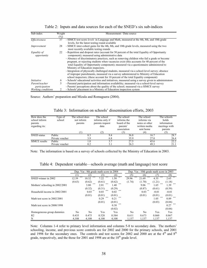
38

Table 2: Inputs and data sources for each of the SNED’s six sub-indices Sub-index Weight Measurement / Data source

(%)Effectiveness 37 - SIMCE test score levels in Language and Math, measured at the 4th, 8th, and 10th grade

levels, for the latest testing round availableImprovement 28 - SIMCE inter-cohort gains for the 4th, 8th, and 10th grade levels, measured using the two

most recently available testing roundsEquality of 22 - Repetition and dropout rates (account for 50 percent of the total Equality of Opportunity opportunity component); measured using administrative data

- Absence of discriminatory practices, such as removing children who fail a grade or become pregnant, or rejecting students when vacancies exist (this accounts for 40 percent of the total Equality of Opportunity component); measured via a questionnaire administered to Ministry of Education inspectors.- Integration of physically challenged students, measured via a school-level survey; absence of improper punishments, measured via a survey administered to Ministry of Education school inspectors; (these account for 10 percent of the total Equality component)

Initiative 6 - Schools' educational activities and initiatives, measured using a survey given to administratorsParent/teacher 5 - Parental participation and information availability; measured via a school-level survey participation - Parents' perceptions about the quality of the school; measured via a SIMCE surveyWorking conditions 2 - Schools' placement in a Ministry of Education inspection system

Source: Authors’ preparation and Mizala and Romaguera (2004).

Table 3: Information on schools’ dissemination efforts, 2003 How does the Type of The school does The school The school The school The schoolsschool inform school not inform informs only if informs the informs via holds parents parents parents request board of the notes or other informationregarding its: data parents' written media meetings with

association sent home parents(1) (2) (3) (4) (5)

SNED status Public 8.3 9.4 36.8 16.7 28.7Private voucher 3.9 6.8 35.9 27.0 26.4

SIMCE results Public 1.0 3.7 27.5 45.6 22.2Private voucher 0.2 3.1 26.3 49.3 21.1

Note: The information is based on a survey of schools collected by the Ministry of Education in 2003.

Table 4: Dependent variable—schools average (math and language) test score

SNED winner in 2002 12.39 *** 10.32 *** 7.22 *** 1.50 ** 29.96 *** 21.69 *** 4.35 *** 2.65 **

(0.63) (0.62) (0.61) (0.62) (1.74) (1.70) (1.21) (1.18)Mothers' schooling in 2002/2001 3.80 *** 2.01 *** 1.40 *** 9.06 *** 1.65 *** 1.39 ***

(0.32) (0.31) (0.29) (0.87) (0.61) (0.59)Household income in 2002/2001 0.03 ** 0.03 *** 0.02 *** 0.03 ** -0.01 -0.01

(0.01) (0.01) (0.01) (0.01) (0.01) (0.01)Math test score in 2002/2001 0.29 *** 0.21 *** 1.05 *** 0.89 ***

(0.01) (0.01) (0.03) (0.04)Math test score in 2000/1998 0.38 *** 0.27 ***

(0.02) (0.04)Homogeneous group dummies No No Yes Yes No No Yes YesR2 0.435 0.475 0.528 0.584 0.611 0.673 0.860 0.867N 4,108 4,108 4,108 4,108 1,137 1,137 1,137 1,137

(5) (6) (7) (8)Dep. Var.: 8th grade math score in 2004 Dep. Var.: 10th grade math score in 2003(1) (2) (3) (4)

Note: Columns 1-4 refer to primary level information and columns 5-8 to secondary data. The mothers’ schooling, income, and previous score controls are for 2002 and 2000 for the primary schools, and 2001 and 1998 for the secondary ones. The controls and test scores for 2002 and 2000 are at the 4th and 8th grade, respectively, and the those for 2001 and 1998 are at the 10th grade level.

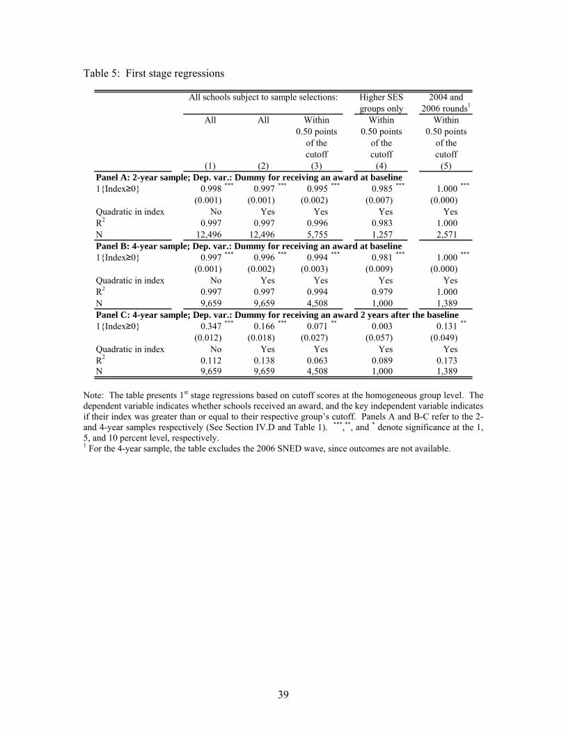
39

Table 5: First stage regressions

Panel A: 2-year sample; Dep. var.: Dummy for receiving an award at baseline1{Index≥0} 0.998 *** 0.997 *** 0.995 *** 0.985 *** 1.000 ***

(0.001) (0.001) (0.002) (0.007) (0.000)Quadratic in index No Yes Yes Yes YesR2 0.997 0.997 0.996 0.983 1.000N 12,496 12,496 5,755 1,257 2,571Panel B: 4-year sample; Dep. var.: Dummy for receiving an award at baseline1{Index≥0} 0.997 *** 0.996 *** 0.994 *** 0.981 *** 1.000 ***

(0.001) (0.002) (0.003) (0.009) (0.000)Quadratic in index No Yes Yes Yes YesR2 0.997 0.997 0.994 0.979 1.000N 9,659 9,659 4,508 1,000 1,389Panel C: 4-year sample; Dep. var.: Dummy for receiving an award 2 years after the baseline1{Index≥0} 0.347 *** 0.166 *** 0.071 ** 0.003 0.131 **

(0.012) (0.018) (0.027) (0.057) (0.049)Quadratic in index No Yes Yes Yes YesR2 0.112 0.138 0.063 0.089 0.173N 9,659 9,659 4,508 1,000 1,389

All schools subject to sample selections: Higher SES 2004 and

All All Withingroups only 2006 rounds1

WithinWithin

(1) (5)(2) (3) (4)

0.50 points

cutoffcutoff

0.50 pointsof the of the

0.50 pointsof thecutoff

Note: The table presents 1st stage regressions based on cutoff scores at the homogeneous group level. The dependent variable indicates whether schools received an award, and the key independent variable indicates if their index was greater than or equal to their respective group’s cutoff. Panels A and B-C refer to the 2- and 4-year samples respectively (See Section IV.D and Table 1). ***,**, and * denote significance at the 1, 5, and 10 percent level, respectively. 1 For the 4-year sample, the table excludes the 2006 SNED wave, since outcomes are not available.

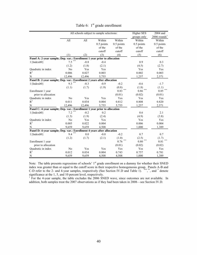
40

Table 6: 1st grade enrollment

Panel A: 2-year sample; Dep. var.: Enrollment 1 year prior to allocation1{Index≥0} 7.5 *** -0.8 -0.4 0.9 0.3

(1.2) (1.8) (2.1) (4.5) (2.7)Quadratic in index No Yes Yes Yes YesR2 0.006 0.027 0.003 0.002 0.003N 12,496 12,496 5,755 1,257 2,571Panel B: 2-year sample; Dep. var.: Enrollment 2 years after allocation1{Index≥0} 9.3 *** -0.3 -0.9 -0.2 -0.6 -1.7

(1.1) (1.7) (1.9) (0.8) (1.8) (1.1)Enrollment 1 year 0.83 *** 0.86 *** 0.85 ***

prior to allocation (0.01) (0.02) (0.01)Quadratic in index No Yes Yes Yes Yes YesR2 0.011 0.034 0.004 0.812 0.808 0.820N 12,496 12,496 5,755 5,755 1,257 2,571Panel C: 4-year sample; Dep. var.: Enrollment 1 year prior to allocation1{Index≥0} 7.2 *** -0.2 0.2 0.6 2.1

(1.3) (1.9) (2.4) (4.9) (3.8)Quadratic in index No Yes Yes Yes YesR2 0.005 0.022 0.004 0.006 0.004N 9,659 9,659 4,508 1,000 1,389Panel D: 4-year sample; Dep. var.: Enrollment 4 years after allocation1{Index≥0} 9.4 *** 0.0 -0.0 -0.2 0.7 0.7

(1.2) (1.7) (2.1) (1.0) (2.5) (1.7)Enrollment 1 year 0.76 *** 0.80 *** 0.81 ***

prior to allocation (0.01) (0.02) (0.02)Quadratic in index No Yes Yes Yes Yes YesR2 0.012 0.034 0.004 0.743 0.757 0.781N 9,659 9,659 4,508 4,508 1,000 1,389

2004 andgroups only 2006 rounds1

Within Within

All schools subject to sample selections: Higher SES

Within Within0.5 points 0.5 points

All All0.5 points 0.5 points

of the of the of the of thecutoff cutoff cutoff cutoff

(5) (6)(1) (2) (3) (4)

Note: The table presents regressions of schools’ 1st grade enrollment on a dummy for whether their SNED index was greater than or equal to the cutoff score in their respective homogeneous group. Panels A-B and C-D refer to the 2- and 4-year samples, respectively (See Section IV.D and Table 1). ***,**, and * denote significance at the 1, 5, and 10 percent level, respectively. 1 For the 4-year sample, the table excludes the 2006 SNED wave, since outcomes are not available. In addition, both samples treat the 2007 observations as if they had been taken in 2008—see Section IV.D.

41

Table 7: Number of 1st grade classes

Panel A: 2-year sample; Dep. var.: No. of classes 1 year prior to allocation1{Index≥0} 0.11 *** -0.02 0.01 0.06 0.03

(0.03) (0.04) (0.05) (0.10) (0.06)Quadratic in index No Yes Yes Yes YesR2 0.002 0.017 0.002 0.001 0.002N 12,077 12,077 5,666 1,246 2,536Panel B: 2-year sample; Dep. var.: No. of classes 2 years after allocation1{Index≥0} 0.13 *** -0.03 -0.04 -0.05 ** -0.05 -0.08 **

(0.03) (0.04) (0.05) (0.02) (0.05) (0.03)1st grades 1 year 0.79 *** 0.85 *** 0.79 ***

prior to allocation (0.01) (0.03) (0.01)Quadratic in index No Yes Yes Yes Yes YesR2 0.004 0.021 0.002 0.725 0.743 0.707N 12,077 12,077 5,666 5,666 1,246 2,536Panel C: 4-year sample; Dep. var.: No. of classes 1 year prior to allocation1{Index≥0} 0.11 *** -0.02 0.02 0.05 0.05

(0.03) (0.04) (0.06) (0.11) (0.09)Quadratic in index No Yes Yes Yes YesR2 0.001 0.014 0.003 0.004 0.002N 9,264 9,264 4,413 983 1,371Panel D: 4-year sample; Dep. var.: No. of classes 4 years after allocation1{Index≥0} 0.14 *** -0.03 -0.03 -0.04 -0.04 -0.03

(0.03) (0.04) (0.05) (0.03) (0.07) (0.05)1st grades 1 year 0.72 *** 0.79 *** 0.75 ***

prior to allocation (0.01) (0.03) (0.02)Quadratic in index No Yes Yes Yes Yes YesR2 0.005 0.020 0.002 0.660 0.689 0.673N 9,264 9,264 4,413 4,413 983 1,371

2004 andgroups only 2006 rounds1

Within Within

All schools subject to sample selections: Higher SES

Within Within0.5 points 0.5 points

All All0.5 points 0.5 points

of the of the of the of thecutoff cutoff cutoff cutoff

(5) (6)(1) (2) (3) (4)

Note: The table presents regressions of the number of 1st grades schools operate on a dummy for whether their SNED index was greater than or equal to the cutoff score in their respective homogeneous group. Panels A-B and C-Drefer to the 2- and 4-year samples, respectively (See Section IV.D and Table 1). ***,**, and * denote significance at the 1, 5, and 10 percent level, respectively. 1 For the 4-year sample, the table excludes the 2006 SNED wave, since outcomes are not available. In addition, both samples treat the 2007 observations as if they had been taken in 2008—see Section IV.D.

42

Table 8: Positive tuition

Panel A: 2-year sample; Dep. var.: Positive tuition 1 year prior to allocation1{Index≥0} 0.03 ** 0.01 -0.02 -0.03 0.03

(0.01) (0.02) (0.02) (0.06) (0.04)Quadratic in index No Yes Yes Yes YesR2 0.001 0.002 0.003 0.007 0.002N 9,893 9,893 4,585 1,019 1,401Panel B: 2-year sample; Dep. var.: Positive tuition 2 years after allocation1{Index≥0} 0.04 *** 0.01 -0.02 0.00 0.01 -0.01

(0.01) (0.02) (0.02) (0.01) (0.01) (0.01)Positive tuition 1 year 0.97 *** 0.94 *** 0.99 ***

prior to allocation (0.00) (0.01) (0.00)Quadratic in index No Yes Yes Yes Yes YesR2 0.001 0.003 0.003 0.907 0.884 0.943N 9,893 9,893 4,585 4,585 1,019 1,401Panel C: 4-year sample; Dep. var.: Positive tuition 1 year prior to allocation1{Index≥0} 0.04 *** 0.01 -0.04 -0.06 --

(0.01) (0.02) (0.03) (0.07) --Quadratic in index No Yes Yes Yes --R2 0.002 0.004 0.004 0.010 --N 7,217 7,217 3,119 710 --Panel D: 4-year sample; Dep. var.: Positive tuition 4 years after allocation1{Index≥0} 0.05 *** 0.02 -0.03 0.01 0.01 --

(0.01) (0.02) (0.03) (0.01) (0.02) --Positive tuition 1 year 0.95 *** 0.92 *** -- prior to allocation (0.01) (0.02) --Quadratic in index No Yes Yes Yes Yes --R2 0.003 0.005 0.004 0.868 0.847 --N 7,217 7,217 3,119 3,119 710 --

2004 andgroups only 2006 rounds1

Within Within

All schools subject to sample selections: Higher SES

Within Within0.5 points 0.5 points

All All0.5 points 0.5 points

of the of the of the of thecutoff cutoff cutoff cutoff

(5) (6)(1) (2) (3) (4)

Note: The table presents regressions of an indicator for whether schools charge tuition on a dummy for whether their SNED index was greater than or equal to the cutoff score in their respective homogeneous group. Panels A-B and C-D refer to the 2- and 4-year samples, respectively (See Section IV.D and Table 1). ***,**, and * denote significance at the 1, 5, and 10 percent level, respectively. 1 Because we only have tuition data up to 2006 (inclusive), for the 2-year sample the analysis in Column 6 refers only to the 2004 wave. For the 4-year sample (panels C and D), this specification is not feasible.

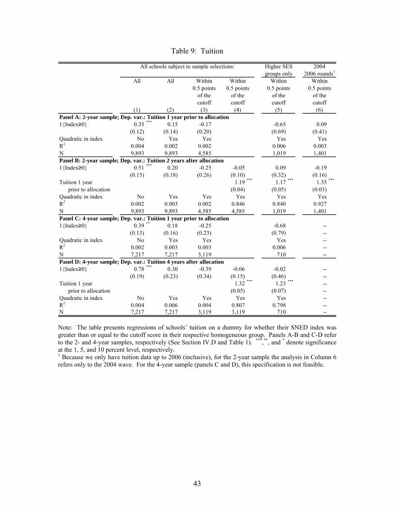
43

Table 9: Tuition

Panel A: 2-year sample; Dep. var.: Tuition 1 year prior to allocation1{Index≥0} 0.35 *** 0.15 -0.17 -0.65 0.09

(0.12) (0.14) (0.20) (0.69) (0.41)Quadratic in index No Yes Yes Yes YesR2 0.004 0.002 0.002 0.006 0.003N 9,893 9,893 4,585 1,019 1,401Panel B: 2-year sample; Dep. var.: Tuition 2 years after allocation1{Index≥0} 0.51 *** 0.20 -0.25 -0.05 0.09 -0.19

(0.15) (0.18) (0.26) (0.10) (0.32) (0.16)Tuition 1 year 1.19 *** 1.17 *** 1.35 ***

prior to allocation (0.04) (0.05) (0.03)Quadratic in index No Yes Yes Yes Yes YesR2 0.002 0.003 0.002 0.846 0.840 0.927N 9,893 9,893 4,585 4,585 1,019 1,401Panel C: 4-year sample; Dep. var.: Tuition 1 year prior to allocation1{Index≥0} 0.39 ** 0.18 -0.25 -0.68 --

(0.13) (0.16) (0.23) (0.79) --Quadratic in index No Yes Yes Yes --R2 0.002 0.003 0.003 0.006 --N 7,217 7,217 3,119 710 --Panel D: 4-year sample; Dep. var.: Tuition 4 years after allocation1{Index≥0} 0.78 *** 0.30 -0.39 -0.06 -0.02 --

(0.19) (0.23) (0.34) (0.15) (0.46) --Tuition 1 year 1.32 *** 1.23 *** -- prior to allocation (0.05) (0.07) --Quadratic in index No Yes Yes Yes Yes --R2 0.004 0.006 0.004 0.807 0.798 --N 7,217 7,217 3,119 3,119 710 --

(5) (6)(1) (2) (3) (4)cutoff cutoff cutoff cutoffof the of the of the of the

0.5 points 0.5 pointsAll All

0.5 points 0.5 points

2004groups only 2006 rounds1

Within Within

All schools subject to sample selections: Higher SES

Within Within

Note: The table presents regressions of schools’ tuition on a dummy for whether their SNED index was greater than or equal to the cutoff score in their respective homogeneous group. Panels A-B and C-D refer to the 2- and 4-year samples, respectively (See Section IV.D and Table 1). ***,**, and * denote significance at the 1, 5, and 10 percent level, respectively. 1 Because we only have tuition data up to 2006 (inclusive), for the 2-year sample the analysis in Column 6 refers only to the 2004 wave. For the 4-year sample (panels C and D), this specification is not feasible.

44

Table 10: Vulnerability index measured at the 1st grade

Panel A: 2-year sample; Dep. var.: Vulnerability index 1 year prior to allocation1{Index≥0} -5.4 *** -0.4 0.2 0.9 -0.5

(0.5) (0.7) (1.0) (1.6) (1.1)Quadratic in index No Yes Yes Yes YesR2 0.014 0.040 0.004 0.020 0.003N 10,640 10,640 4,970 760 2,201Panel B: 2-year sample; Dep. var.: Vulnerability index 2 years after allocation1{Index≥0} -1.5 *** 0.5 -0.2 -0.3 -1.4 0.0

(0.5) (0.8) (1.2) (1.1) (2.4) (1.8)Vulnerability 1 year 0.36 *** 0.20 *** 0.56 ***

prior to allocation (0.02) (0.04) (0.02)Quadratic in index No Yes Yes Yes Yes YesR2 0.001 0.015 0.002 0.093 0.020 0.118N 10,640 10,640 4,970 4,970 760 2,201Panel C: 4-year sample; Dep. var.: Vulnerability index 1 year prior to allocation1{Index≥0} -5.0 *** 0.8 0.1 2.2 -1.1

(0.6) (0.8) (1.1) (2.0) (1.5)Quadratic in index No Yes Yes Yes YesR2 0.011 0.043 0.002 0.022 0.001N 7,953 7,953 3,744 531 1,149Panel D: 4-year sample; Dep. var.: Vulnerability index 4 years after allocation1{Index≥0} -3.6 *** -2.5 -1.8 1.8 -0.8 -1.0

0.6 (1.0) (1.5) (1.5) (3.0) (1.1)Vulnerability 1 year 0.23 *** 0.20 *** 0.47 ***

prior to allocation (0.02) (0.04) (0.02)Quadratic in index No Yes Yes Yes Yes YesR2 0.005 0.006 0.005 0.038 0.040 0.282N 7,953 7,953 3,744 3,744 531 1,149

(5) (6)(1) (2) (3) (4)cutoff cutoff cutoff cutoffof the of the of the of the

0.5 points 0.5 pointsAll All

0.5 points 0.5 points

2004 andgroups only 2006 rounds1

Within Within

All schools subject to sample selections: Higher SES

Within Within

Note: The table presents regressions of schools’ vulnerability index values on a dummy for whether their SNED index was greater than or equal to the cutoff score in their respective homogeneous group. Panels A-B and C-D refer to the 2- and 4-year samples, respectively (See Section IV.D and Table 1). ***,**, and * denote significance at the 1, 5, and 10 percent level, respectively. 1 For the 4-year sample, the table excludes the 2006 SNED wave, since outcomes are not available. In addition, both samples treat the 2007 observations as if they had been taken in 2008—see Section IV.D.

45

Table 11: Average mothers’ schooling

Panel A: 2-year sample; Dep. var.: Avg. mothers' schooling 1 year prior to allocation1{Index≥0} 0.56 *** 0.14 ** 0.09 -0.23 0.25

(0.05) (0.07) (0.10) (0.15) (0.17)Quadratic in index No Yes Yes Yes YesR2 0.020 0.046 0.006 0.037 0.008N 7,102 7,102 3,612 655 1,381Panel B: 2-year sample; Dep. var.: Avg. mothers' schooling 2 years after allocation1{Index≥0} 0.53 *** 0.11 0.03 -0.06 -0.16 -0.06

(0.05) (0.08) (0.10) (0.05) (0.10) (0.08)Mothers' sch. 1 year 0.86 *** 0.74 *** 0.89 ***

prior to allocation (0.01) (0.03) (0.01)Quadratic in index No Yes Yes Yes Yes YesR2 0.018 0.039 0.006 0.754 0.524 0.766N 7,102 7,102 3,612 3,612 655 1,381Panel C: 4-year sample; Dep. var.: Avg. mothers' schooling 1 year prior to allocation1{Index≥0} 0.59 *** 0.11 0.02 -0.40 *** --

(0.06) (0.09) (0.13) (0.20) --Quadratic in index No Yes Yes Yes --R2 0.022 0.047 0.008 0.050 --N 4,565 4,565 2,190 357 --Panel D: 4-year sample; Dep. var.: Avg. mothers' schooling 4 years after allocation1{Index≥0} 0.59 *** 0.10 -0.01 -0.02 -0.04 --

(0.06) (0.10) (0.13) (0.07) (0.14) --Mothers' sch. 1 year 0.86 *** 0.91 *** -- prior to allocation (0.01) (0.05) --Quadratic in index No Yes Yes Yes Yes --R2 0.022 0.044 0.008 0.742 0.641 --N 4,565 4,565 2,190 2,190 357 --

(5) (6)(1) (2) (3) (4)cutoff cutoff cutoff cutoffof the of the of the of the

0.5 points 0.5 pointsAll All

0.5 points 0.5 points

2004 andgroups only 2006 rounds1

Within Within

All schools subject to sample selections: Higher SES

Within Within

Note: The table presents regressions of schools’ average mothers’ schooling on a dummy for whether their SNED index was greater than or equal to the cutoff score in their respective homogeneous group. Panels A-B and C-D refer to the 2- and 4-year samples, respectively (See Section IV.D and Table 1). ***,**, and * denote significance at the 1, 5, and 10 percent level, respectively. 1 Because we only have mothers’ schooling data up to 2006 (inclusive), for the 2-year sample the analysis in Column 6 refers only to the 2004 wave. For the 4-year sample (panels C and D), this specification is not feasible.

46

Table 12: Household income

Panel A: 2-year sample; Dep. var.: Avg. hhld. income 1 year prior to allocation1{Index≥0} 19.9 *** 10.2 *** 8.1 -0.9 14.3 *

(2.8) (3.7) (5.6) (17.8) (8.5)Quadratic in index No Yes Yes Yes YesR2 0.011 0.018 0.004 0.014 0.004N 7,104 7,104 3,612 655 1,381Panel B: 2-year sample; Dep. var.: Avg. hhld. income 2 years after allocation1{Index≥0} 25.4 *** 10.1 ** 5.3 -3.0 -7.6 -8.9 *

(3.4) (4.4) (6.3) (3.1) (9.7) (4.8)Hhld. income 1 year 1.02 *** 0.94 *** 1.09 ***

prior to allocation (0.02) (0.03) (0.03)Quadratic in index No Yes Yes Yes Yes YesR2 0.012 0.024 0.004 0.748 0.679 0.765N 7,104 7,104 3,612 3,612 655 1,381Panel C: 4-year sample; Dep. var.: Avg. hhld. income 1 year prior to allocation1{Index≥0} 21.9 *** 8.6 * 5.6 -8.1 --

(3.2) (4.8) (7.4) (26.5) --Quadratic in index No Yes Yes Yes --R2 0.014 0.021 0.007 0.026 --N 4,566 4,566 2,190 357 --Panel D: 4-year sample; Dep. var.: Avg. hhld. income 4 years after allocation1{Index≥0} 28.6 *** 10.3 * 4.9 -1.3 3.5 --

(4.2) (6.0) (9.1) (4.2) (14.6) --Hhld. income 1 year 1.10 *** 1.06 *** -- prior to allocation (0.07) (0.05) --Quadratic in index No Yes Yes Yes Yes --R2 0.014 0.024 0.006 0.748 0.718 --N 4,566 4,566 2,190 2,190 357 --

(5) (6)(1) (2) (3) (4)cutoff cutoff cutoff cutoffof the of the of the of the

0.5 points 0.5 pointsAll All

0.5 points 0.5 points

2004 andgroups only 2006 rounds1

Within Within

All schools subject to sample selections: Higher SES

Within Within

Note: The table presents regressions of schools’ average household income on a dummy for whether their SNED index was greater than or equal to the cutoff score in their respective homogeneous group. Panels A-B and C-D refer to the 2- and 4-year samples, respectively (See Section IV.D and the notes to Table 1). ***,**, and * denote significance at the 1, 5, and 10 percent level, respectively. 1 Because we only have household income data up to 2006 (inclusive), for the 2-year sample the analysis in Column 6 refers only to the 2004 wave. For the 4-year sample (panels C and D), this specification is not feasible.

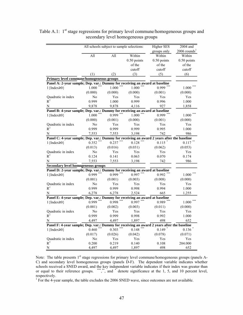
47

Table A.1: 1st stage regressions for primary level commune/homogeneous groups and secondary level homogeneous groups

Note: The table presents 1st stage regressions for primary level commune/homogeneous groups (panels A-C) and secondary level homogeneous groups (panels D-F). The dependent variable indicates whether schools received a SNED award, and the key independent variable indicates if their index was greater than or equal to their reference groups. ***,**, and * denote significance at the 1, 5, and 10 percent level, respectively. 1 For the 4-year sample, the table excludes the 2006 SNED wave, since outcomes are not available.

Primary level commune/homogeneous groupsPanel A: 2-year sample; Dep. var.: Dummy for receiving an award at baseline1{Index≥0} 1.000 *** 1.000 *** 1.000 *** 0.999 *** 1.000 ***

(0.000) (0.000) (0.000) (0.001) (0.000)Quadratic in index No Yes Yes Yes YesR2 0.999 1.000 0.999 0.996 1.000N 9,878 9,878 4,116 927 1,858Panel B: 4-year sample; Dep. var.: Dummy for receiving an award at baseline1{Index≥0} 1.000 *** 0.999 *** 1.000 *** 0.999 *** 1.000 ***

(0.000) (0.001) (0.000) (0.001) (0.000)Quadratic in index No Yes Yes Yes YesR2 0.999 0.999 0.999 0.995 1.000N 7,553 7,553 3,198 742 986Panel C: 4-year sample; Dep. var.: Dummy for receiving an award 2 years after the baseline1{Index≥0} 0.352 *** 0.237 *** 0.128 *** 0.115 * 0.117 **

(0.013) (0.016) (0.031) (0.062) (0.053)Quadratic in index No Yes Yes Yes YesR2 0.124 0.141 0.063 0.070 0.174N 7,553 7,553 3,198 742 986Secondary level homogeneous groupsPanel D: 2-year sample; Dep. var.: Dummy for receiving an award at baseline1{Index≥0} 0.999 *** 0.999 *** 0.997 *** 0.992 *** 1.000 ***

(0.001) (0.001) (0.003) (0.008) (0.000)Quadratic in index No Yes Yes Yes YesR2 0.999 0.999 0.998 0.994 1.000N 6,278 6,278 2,524 665 1,255Panel E: 4-year sample; Dep. var.: Dummy for receiving an award at baseline1{Index≥0} 0.999 *** 0.998 *** 0.997 *** 0.989 *** 1.000 ***

(0.001) (0.002) (0.003) (0.011) (0.000)Quadratic in index No Yes Yes Yes YesR2 0.999 0.999 0.998 0.992 1.000N 4,497 4,497 1,897 498 652Panel F: 4-year sample; Dep. var.: Dummy for receiving an award 2 years after the baseline1{Index≥0} 0.460 *** 0.303 *** 0.148 *** 0.149 * 0.136 *

(0.017) (0.026) (0.042) (0.078) (0.071)Quadratic in index No Yes Yes Yes YesR2 0.200 0.219 0.140 0.108 204.000N 4,497 4,497 1,897 498 652

Within0.50 points

All All Within Within0.50 points 0.50 points

All schools subject to sample selections: Higher SES 2004 andgroups only 2006 rounds1

of thecutoff cutoff cutoffof the of the

(6)(1) (2) (3) (5)

48

Table A.2: 1st grade enrollment among commune/homogeneous groups

Panel A: 2-year sample; Dep. var.: Enrollment 1 year prior to allocation1{Index≥0} 8.5 *** -0.9 -3.1 1.7 -5.9 *

(1.3) (2.0) (2.6) (5.1) (3.2)Quadratic in index No Yes Yes Yes YesR2 0.008 0.026 0.002 0.001 0.005N 9,878 9,878 4,116 927 1,858Panel B: 2-year sample; Dep. var.: Enrollment 2 years after allocation1{Index≥0} 10.2 *** -0.3 -2.4 0.2 -1.7 0.0

(1.2) (1.9) (2.4) (0.9) (2.1) (1.3)Enrollment 1 year 0.86 *** 0.89 *** 0.87 ***

prior to allocation (0.01) (0.03) (0.01)Quadratic in index No Yes Yes Yes Yes YesR2 0.014 0.034 0.003 0.825 0.806 0.838N 9,878 9,878 4,116 4,116 927 1,858Panel C: 4-year sample; Dep. var.: Enrollment 1 year prior to allocation1{Index≥0} 8.0 *** -0.4 -3.1 -0.7 8.2 *

(1.4) (2.1) (2.9) (5.6) (4.4)Quadratic in index No Yes Yes Yes YesR2 0.007 0.021 0.003 0.002 0.009N 7,553 7,553 3,198 742 986Panel D: 4-year sample; Dep. var.: Enrollment 4 years after allocation1{Index≥0} 10.3 *** -0.4 -2.7 -0.2 -3.5 1.4

(1.3) (2.0) (2.6) (1.2) (2.7) (2.0)Enrollment 1 year 0.79 *** 0.82 *** 0.83 ***

prior to allocation (0.01) (0.03) (0.02)Quadratic in index No Yes Yes Yes Yes YesR2 0.015 0.036 0.005 0.769 0.760 0.803N 7,553 7,553 3,198 3,198 742 986

2004 andgroups only 2006 rounds1

Within Within

All schools subject to sample selections: Higher SES

Within Within0.5 points 0.5 points

All All0.5 points 0.5 points

of the of the of the of thecutoff cutoff cutoff cutoff

(5) (6)(1) (2) (3) (4)

Note: The table presents regressions of schools’ 1st grade enrollment on a dummy for whether their SNED index was greater than or equal to the cutoff score in their respective commune/homogeneous group. Panels A-B and C-D refer to the 2- and 4-year samples, respectively (See Section IV.D and Table 1). ***,**, and * denote significance at the 1, 5, and 10 percent level, respectively. 1 For the 4-year sample, the table excludes the 2006 SNED wave, since outcomes are not available. In addition, both samples treat the 2007 observations as if they had been taken in 2008—see Section IV.D.

49

Table A.3: Positive tuition among commune/homogeneous groups

Panel A: 2-year sample; Dep. var.: Positive tuition 1 year prior to allocation1{Index≥0} 0.03 ** 0.02 -0.00 0.05 0.00

(0.01) (0.02) (0.03) (0.07) (0.05)Quadratic in index No Yes Yes Yes YesR2 0.001 0.002 0.004 0.008 0.003N 7,764 7,764 3,252 750 994Panel B: 2-year sample; Dep. var.: Positive tuition 2 years after allocation1{Index≥0} 0.03 *** 0.03 0.00 0.00 0.03 * 0.00

(0.01) (0.02) (0.03) (0.01) (0.01) (0.02)Positive tuition 1 year 0.97 *** 0.95 *** 0.98 ***

prior to allocation (0.00) (0.01) (0.01)Quadratic in index No Yes Yes Yes Yes YesR2 0.001 0.002 0.005 0.913 0.913 0.940N 7,764 7,764 3,252 3,252 750 994Panel C: 4-year sample; Dep. var.: Positive tuition 1 year prior to allocation1{Index≥0} 0.04 *** 0.01 0.00 0.03 --

(0.02) (0.02) (0.03) (0.08) --Quadratic in index No Yes Yes Yes --R2 0.002 0.002 0.005 0.125 --N 5,625 5,625 2,212 524 --Panel D: 4-year sample; Dep. var.: Positive tuition 4 years after allocation1{Index≥0} 0.05 *** 0.05 ** 0.02 0.02 0.06 --

(0.02) (0.02) (0.03) (0.01) (0.02) --Positive tuition 1 year 0.96 *** 0.94 *** -- prior to allocation (0.01) (0.02) --Quadratic in index No Yes Yes Yes Yes --R2 0.003 0.003 0.006 0.882 0.893 --N 5,625 5,625 2,212 2,212 524 --

2004 andgroups only 2006 rounds1

Within Within

All schools subject to sample selections: Higher SES

Within Within0.5 points 0.5 points

All All0.5 points 0.5 points

of the of the of the of the

(6)(1)cutoff cutoff cutoff cutoff

(2) (3) (4) (5)

Note: The table presents regressions of an indicator for whether schools charge tuition on a dummy for whether their SNED index was greater than or equal to the cutoff score in their respective commune/homogeneous group. Panels A-B and C-D refer to the 2- and 4-year samples, respectively (See Section IV.D and Table 1). ***,**, and * denote significance at the 1, 5, and 10 percent level, respectively. 1 Because we only have tuition data up to 2006 (inclusive), for the 2-year sample the analysis in Column 6 refers only to the 2004 wave. For the 4-year sample (panels C and D), this specification is not feasible.

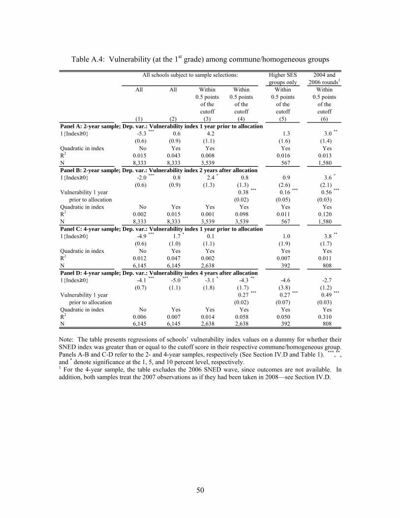
50

Table A.4: Vulnerability (at the 1st grade) among commune/homogeneous groups

Panel A: 2-year sample; Dep. var.: Vulnerability index 1 year prior to allocation1{Index≥0} -5.3 *** 0.6 4.2 1.3 3.0 **

(0.6) (0.9) (1.1) (1.6) (1.4)Quadratic in index No Yes Yes Yes YesR2 0.015 0.043 0.008 0.016 0.013N 8,333 8,333 3,539 567 1,580Panel B: 2-year sample; Dep. var.: Vulnerability index 2 years after allocation1{Index≥0} -2.0 *** 0.8 2.4 * 0.8 0.9 3.6 *

(0.6) (0.9) (1.3) (1.3) (2.6) (2.1)Vulnerability 1 year 0.38 *** 0.16 *** 0.56 ***

prior to allocation (0.02) (0.05) (0.03)Quadratic in index No Yes Yes Yes Yes YesR2 0.002 0.015 0.001 0.098 0.011 0.120N 8,333 8,333 3,539 3,539 567 1,580Panel C: 4-year sample; Dep. var.: Vulnerability index 1 year prior to allocation1{Index≥0} -4.9 *** 1.7 * 0.1 1.0 3.8 **

(0.6) (1.0) (1.1) (1.9) (1.7)Quadratic in index No Yes Yes Yes YesR2 0.012 0.047 0.002 0.007 0.011N 6,145 6,145 2,638 392 808Panel D: 4-year sample; Dep. var.: Vulnerability index 4 years after allocation1{Index≥0} -4.1 *** -5.0 *** -3.1 * -4.3 ** -4.6 -2.7

(0.7) (1.1) (1.8) (1.7) (3.8) (1.2)Vulnerability 1 year 0.27 *** 0.27 *** 0.49 ***

prior to allocation (0.02) (0.07) (0.03)Quadratic in index No Yes Yes Yes Yes YesR2 0.006 0.007 0.014 0.058 0.050 0.310N 6,145 6,145 2,638 2,638 392 808

(4) (5) (6)(1)cutoff cutoff cutoff cutoffof the of the of the of the

Within0.5 points 0.5 points

All All0.5 points 0.5 points

(2) (3)

2004 andgroups only 2006 rounds1

Within Within

All schools subject to sample selections: Higher SES

Within

Note: The table presents regressions of schools’ vulnerability index values on a dummy for whether their SNED index was greater than or equal to the cutoff score in their respective commune/homogeneous group. Panels A-B and C-D refer to the 2- and 4-year samples, respectively (See Section IV.D and Table 1). ***,**, and * denote significance at the 1, 5, and 10 percent level, respectively. 1 For the 4-year sample, the table excludes the 2006 SNED wave, since outcomes are not available. In addition, both samples treat the 2007 observations as if they had been taken in 2008—see Section IV.D.

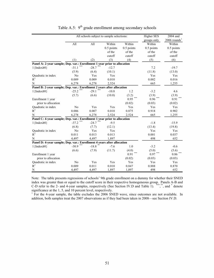
51

Table A.5: 9th grade enrollment among secondary schools

Panel A: 2-year sample; Dep. var.: Enrollment 1 year prior to allocation1{Index≥0} -31.1 *** -28.7 *** -12.7 7.2 -19.7

(5.9) (6.4) (10.1) (11.8) (13.0)Quadratic in index No Yes Yes Yes YesR2 0.009 0.009 0.010 0.002 0.016N 6,278 6,278 2,524 665 1,255Panel B: 2-year sample; Dep. var.: Enrollment 2 years after allocation1{Index≥0} -25.2 *** -29.1 *** -10.8 1.2 -3.2 4.6

(5.7) (6.6) (10.0) (3.2) (3.9) (3.9)Enrollment 1 year 0.95 *** 0.96 *** 0.91 ***

prior to allocation (0.02) (0.03) (0.02)Quadratic in index No Yes Yes Yes Yes YesR2 0.006 0.007 0.010 0.875 0.918 0.902N 6,278 6,278 2,524 2,524 665 1,255Panel C: 4-year sample; Dep. var.: Enrollment 1 year prior to allocation1{Index≥0} -37.2 *** -24.7 *** -9.5 -1.8 -15.9

(6.8) (7.7) (12.1) (13.4) (19.8)Quadratic in index No Yes Yes Yes YesR2 0.011 0.013 0.013 0.001 0.037N 4,497 4,497 1,897 498 652Panel D: 4-year sample; Dep. var.: Enrollment 4 years after allocation1{Index≥0} -30.9 *** -18.8 ** -7.6 1.0 -3.2 -0.6

(6.6) (7.9) (11.7) (4.0) (5.0) (5.6)Enrollment 1 year 0.91 *** 0.97 *** 0.86 ***

prior to allocation (0.02) (0.03) (0.03)Quadratic in index No Yes Yes Yes Yes YesR2 0.009 0.011 0.010 0.847 0.888 0.870N 4,497 4,497 1,897 1,897 498 652

(4) (5) (6)(1)cutoff cutoff cutoff cutoffof the of the of the of the

Within0.5 points 0.5 points

All All0.5 points 0.5 points

(2) (3)

2004 andgroups only 2006 rounds1

Within Within

All schools subject to sample selections: Higher SES

Within

Note: The table presents regressions of schools’ 9th grade enrollment on a dummy for whether their SNED index was greater than or equal to the cutoff score in their respective homogeneous group. Panels A-B and C-D refer to the 2- and 4-year samples, respectively (See Section IV.D and Table 1). ***,**, and * denote significance at the 1, 5, and 10 percent level, respectively. 1 For the 4-year sample, the table excludes the 2006 SNED wave, since outcomes are not available. In addition, both samples treat the 2007 observations as if they had been taken in 2008—see Section IV.D.

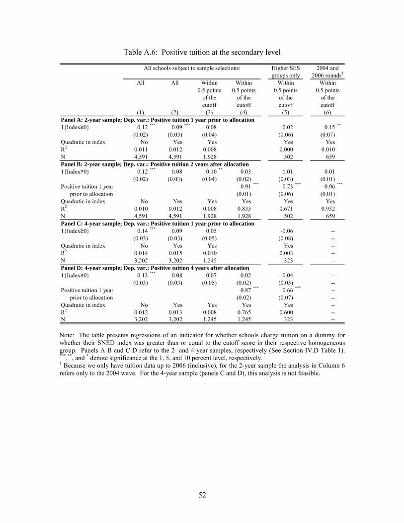
52

Table A.6: Positive tuition at the secondary level

Panel A: 2-year sample; Dep. var.: Positive tuition 1 year prior to allocation1{Index≥0} 0.12 *** 0.09 *** 0.08 -0.02 0.15 **

(0.02) (0.03) (0.04) (0.06) (0.07)Quadratic in index No Yes Yes Yes YesR2 0.011 0.012 0.008 0.000 0.010N 4,591 4,591 1,928 502 659Panel B: 2-year sample; Dep. var.: Positive tuition 2 years after allocation1{Index≥0} 0.12 *** 0.08 0.10 ** 0.03 0.01 0.01

(0.02) (0.03) (0.04) (0.02) (0.03) (0.01)Positive tuition 1 year 0.91 *** 0.73 *** 0.96 ***

prior to allocation (0.01) (0.06) (0.01)Quadratic in index No Yes Yes Yes Yes YesR2 0.010 0.012 0.008 0.835 0.671 0.932N 4,591 4,591 1,928 1,928 502 659Panel C: 4-year sample; Dep. var.: Positive tuition 1 year prior to allocation1{Index≥0} 0.14 *** 0.09 0.05 -0.06 --

(0.03) (0.03) (0.05) (0.08) --Quadratic in index No Yes Yes Yes --R2 0.014 0.015 0.010 0.003 --N 3,202 3,202 1,245 323 --Panel D: 4-year sample; Dep. var.: Positive tuition 4 years after allocation1{Index≥0} 0.13 *** 0.08 0.07 0.02 -0.04 --

(0.03) (0.03) (0.05) (0.02) (0.05) --Positive tuition 1 year 0.87 *** 0.66 *** -- prior to allocation (0.02) (0.07) --Quadratic in index No Yes Yes Yes Yes --R2 0.012 0.013 0.008 0.765 0.600 --N 3,202 3,202 1,245 1,245 323 --

(4) (5) (6)(1)cutoff cutoff cutoff cutoffof the of the of the of the

Within0.5 points 0.5 points

All All0.5 points 0.5 points

(2) (3)

2004 andgroups only 2006 rounds1

Within Within

All schools subject to sample selections: Higher SES

Within

Note: The table presents regressions of an indicator for whether schools charge tuition on a dummy for whether their SNED index was greater than or equal to the cutoff score in their respective homogeneous group. Panels A-B and C-D refer to the 2- and 4-year samples, respectively (See Section IV.D Table 1). ***,**, and * denote significance at the 1, 5, and 10 percent level, respectively. 1 Because we only have tuition data up to 2006 (inclusive), for the 2-year sample the analysis in Column 6 refers only to the 2004 wave. For the 4-year sample (panels C and D), this analysis is not feasible.

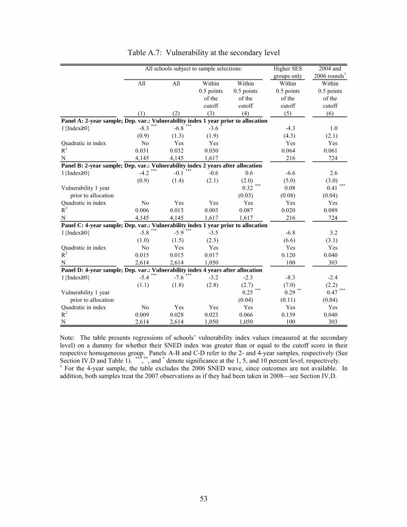
53

Table A.7: Vulnerability at the secondary level

Panel A: 2-year sample; Dep. var.: Vulnerability index 1 year prior to allocation1{Index≥0} -8.3 *** -6.8 *** -3.6 * -4.3 1.0

(0.9) (1.3) (1.9) (4.3) (2.1)Quadratic in index No Yes Yes Yes YesR2 0.031 0.032 0.030 0.064 0.061N 4,145 4,145 1,617 216 724Panel B: 2-year sample; Dep. var.: Vulnerability index 2 years after allocation1{Index≥0} -4.2 *** -0.1 *** -0.6 0.6 -6.6 2.6

(0.9) (1.4) (2.1) (2.0) (5.0) (3.0)Vulnerability 1 year 0.32 *** 0.08 0.41 ***

prior to allocation (0.03) (0.08) (0.04)Quadratic in index No Yes Yes Yes Yes YesR2 0.006 0.015 0.003 0.087 0.020 0.089N 4,145 4,145 1,617 1,617 216 724Panel C: 4-year sample; Dep. var.: Vulnerability index 1 year prior to allocation1{Index≥0} -5.8 *** -5.9 *** -3.5 -6.8 3.2

(1.0) (1.5) (2.3) (6.6) (3.1)Quadratic in index No Yes Yes Yes YesR2 0.015 0.015 0.017 0.120 0.040N 2,614 2,614 1,050 100 303Panel D: 4-year sample; Dep. var.: Vulnerability index 4 years after allocation1{Index≥0} -5.4 *** -7.6 *** -3.2 -2.3 -8.3 -2.4

(1.1) (1.8) (2.8) (2.7) (7.0) (2.2)Vulnerability 1 year 0.25 *** 0.29 ** 0.47 ***

prior to allocation (0.04) (0.11) (0.04)Quadratic in index No Yes Yes Yes Yes YesR2 0.009 0.028 0.023 0.066 0.139 0.040N 2,614 2,614 1,050 1,050 100 303

2004 andgroups only 2006 rounds1

Within Within

All schools subject to sample selections: Higher SES

Within Within0.5 points 0.5 points 0.5 points 0.5 points

All All

of the of the of the of thecutoff cutoff cutoff cutoff

(5) (6)(1) (2) (3) (4)

Note: The table presents regressions of schools’ vulnerability index values (measured at the secondary level) on a dummy for whether their SNED index was greater than or equal to the cutoff score in their respective homogeneous group. Panels A-B and C-D refer to the 2- and 4-year samples, respectively (See Section IV.D and Table 1). ***,**, and * denote significance at the 1, 5, and 10 percent level, respectively. 1 For the 4-year sample, the table excludes the 2006 SNED wave, since outcomes are not available. In addition, both samples treat the 2007 observations as if they had been taken in 2008—see Section IV.D.