MEE 0835

School of Engineering

Department of Signal Processing

Modeling of Broadband Shortwave Antennas

With Numerical Electromagnetics Code

By

Kamtala Venkat Ramana Prasad

Supervisors

Prof. Hans-Jürgen Zepernick (BTH)

Niklas Gunhamn (Radiobolaget AB)

MEE 0835

2

It is the very essence of our striving for understanding that, on the one hand, it attempts to encompass the great and complex variety

of man’s experience, and that on the other, it looks for simplicity

and economy in the basic assumptions. The belief that these two objectives can exist side by side is, in view of the primitive state

of our scientific knowledge, a matter of faith.

Albert Einstein

MEE 0835

3

MEE 0835

4

Abstract

Antenna designers always search for ways to improve existing designs or introduce novel

designs in order to achieve desirable antenna characteristics. The linear wire dipole antennas are

very important in communication systems at all frequency bands. These antennas are used by

typically military, navigation and surveillance purposes. The broadband antenna which was built

in the year of 1950 and was working efficiently for over half a century, some problems such as

inefficient radiation, imperfect feeding point impedance and high voltage standing wave ratio

(VSWR) were discovered when sending information via this broadband antenna in the operating

frequency range of 9-11 MHz. In order to meet the proper specifications antenna is modeled

before implementing physically.

The Numerical Electromagnetics Code (NEC-4) is used to simulate the antenna models and

results are analyzed by using MATLAB. The results of this study indicate that the antenna

models achieve more than 70% of radiation efficiency including practical considerations such as

ground parameters, material of the antenna and height of the antenna, impedance matching and

low VSWR.

MEE 0835

5

MEE 0835

6

Acknowledgements

I would like to express my sincerest thanks and gratitude to Prof. Hans-Jürgen Zepernick and

Niklas Gunhamn being my mentors on this journey. Their guidance, patience, support, and

continuous encouragement throughout this project has been a blessing. I would also like to

acknowledge program manager for Electrical Engineering Mikael Åsman and international

student co-coordinator Lina Magnusson for their continuous suggestions regarding practical

issues and university protocols without which life in Karlskrona would have been really hard. A

special thanks to my friends Manoranjan Reddy, Sathish Kumar and Karuna Chary for the

proof- reading and moral support.

To my family, words fail to express my gratitude. My sister Aparna and her family, my brother

Shiva are to me an endless source of great joy and love. I owe my parents, Mr. K. Vishwanath

and Mrs. K. Pushpa Latha, much of who I have become. They have raised me to set high goals

for myself and have always encouraged me to put education as the first priority in my life. They

taught me value of honesty, hard work and humility above all other virtues. I dedicate this master

thesis work to them as a tribute to their pure devotion and everlasting love.

MEE 0835

7

CHAPTER 1 ......................................................................................................................................................... 8

1.1 INTRODUCTION .......................................................................................................................................... 8

1.2 THESIS LAYOUT .......................................................................................................................................... 8

CHAPTER 2: FUNDAMENTALS OF ANTENNA THEORY ........................................................................................ 10

2.1 ANTENNA DEFINITIONS .............................................................................................................................. 10

2.2 ANTENNA FIELD REGIONS ........................................................................................................................... 10

2.3 ANTENNA PARAMETERS ............................................................................................................................. 11

2.3.1 Radiation pattern ............................................................................................................................ 11

2.3.2 Radiation Power Density .................................................................................................................. 11

2.3.3 Radiation Intensity........................................................................................................................... 11

2.3.4 Directivity ........................................................................................................................................ 12

2.3.5 Gain ................................................................................................................................................ 13

2.3.6 Efficiency ......................................................................................................................................... 13

2.3.7 Input Impedance .............................................................................................................................. 14

2.3.8 Half-Power Beamwidth .................................................................................................................... 14

2.3.9 Polarization ..................................................................................................................................... 14

CHAPTER 3: THEORY OF LINEAR WIRE ANTENNAS ............................................................................. 17

3.1 INTRODUCTION ........................................................................................................................................ 17

3.2 TYPES OF DIPOLES ..................................................................................................................................... 17

3.2.1 Infinitesimal Dipole .......................................................................................................................... 17

3.2.2 Small Dipole .................................................................................................................................... 18

3.2.3 Finite Length Dipole ......................................................................................................................... 19

3.2.4 Half Wave Length Dipole ................................................................................................................. 19

CHAPTER 4: DESIGN OF LINEAR WIRE ANTENNAS ............................................................................................. 21

4.1 INTRODUCTION ........................................................................................................................................ 21

4.2 DESIGN PARAMETERS AND CONSIDERATIONS ................................................................................................... 21

4.2.1 Feed point impedance ...................................................................................................................... 21

4.2.2 Directivity ........................................................................................................................................ 22

4.2.3 Gain ................................................................................................................................................ 22

4.2.4 Radiation Resistance........................................................................................................................ 22

4.2.5 Ground Effects ................................................................................................................................. 22

4.2.6 Impedance Matching ....................................................................................................................... 23

4.2.7 Voltage Standing Wave Ratio (VSWR) .............................................................................................. 23

4.2.8 Return Loss ...................................................................................................................................... 24

4.3 MODELING CONSIDERATIONS ...................................................................................................................... 24

4.4 MODEL-I (ANTENNA IS ON THE GROUND) ....................................................................................................... 25

4.5 MODEL –II (ANTENNA LOCATED AT A HEIGHT OF 15 M)...................................................................................... 32

4.6 COMPARISON BETWEEN MODEL-I & MODEL-II ............................................................................................... 36

CONCLUSION ....................................................................................................................................................... 37

APPENDIX A ....................................................................................................................................................... 38

APPENDIX B ........................................................................................................................................................ 41

APPENDIX C ........................................................................................................................................................ 44

REFERENCES ........................................................................................................................................................ 45

MEE 0835

8

Chapter 1

1.1 Introduction

Money makes many things most everybody loves it, and usually nobody can have enough of it.

Unfortunately, more often than not, you have to have money to make money. This also true

when starting business with technology, in particular when dealing with frequency applications

like antenna design.

The main focus of this thesis revolves around linear wire antenna design in the field of radio

frequency communications. Electromagnetic compatibility (EMC) antenna design is a very

special field which requires lot of analysis because of the complex mathematics and geometry

associated with it. In fact mathematics and antennas are inclusive and implicit events in terms of

probability. Attention is focused on modeling of EMC linear wire antennas with numerical

electromagnetics code (NEC-4). This version of code includes more antenna structure commands

and control commands when compared with other previous versions. One of the best features of

this code is, it produces output in ASCII format which is user friendly to read and import the

data to any scientific software for analysis of antenna parameters. Wire antennas which find

important applications in different forms of communication systems, many alterations have been

proposed in the form of geometry, feed point impedance and improving voltage standing wave

ratio. The simulation results indicate that the dipole antenna provides high gain and low voltage

standing wave ratio (VSWR) in particular at resonance without too much variations in feed point

impedance.

1.2 Thesis Layout

Chapter 2 presents brief theory and fundamentals of antennas with some important definitions,

field regions and mathematical formulation of standard antenna parameters. Chapter 3 provides

the background and theory of linear wire antennas in the context of dipoles such as infinitesimal

dipole, small dipole and half wave length dipole. Variations in electric and magnetic fields with

respective to near and far fields are also discussed. Chapter 4 deals with design considerations of

modeling and simulations results of half wave dipole antennas extensively. Appendix A and

appendix B deals with simulation results of half wave length dipole loaded with Aluminium and

MEE 0835

9

Zinc respectively. Appendix C deals with design guidelines and some safety facts when

installing antennas.

MEE 0835

10

Chapter 2: Fundamentals of Antenna Theory

2.1 Antenna Definitions

An antenna according to IEEE standard is defined as [2] “ a means of radiating or receiving

radio waves.” More generally it is defined as the intermediate structure between a medium and a

guiding device. Often medium can be free space, water and air. Usually guiding devices are

transmission lines and waveguides. The significant property of an antenna is its ability to focus

and shape the radiated power into space.

2.2 Antenna Field Regions

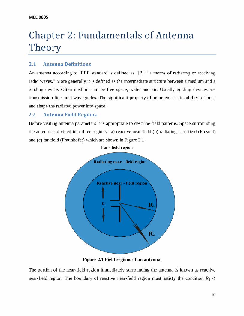
Before visiting antenna parameters it is appropriate to describe field patterns. Space surrounding

the antenna is divided into three regions: (a) reactive near-field (b) radiating near-field (Fresnel)

and (c) far-field (Fraunhofer) which are shown in Figure 2.1.

Figure 2.1 Field regions of an antenna.

The portion of the near-field region immediately surrounding the antenna is known as reactive

near-field region. The boundary of reactive near-field region must satisfy the condition 𝑅1 <

MEE 0835

11

0.62 𝐷3

𝜆, where 𝑅1 is the radius of the reactive near-field, 𝐷 is the biggest dimension of the

antenna and 𝜆 is the wavelength of the antenna. The region of the field of an antenna between

reactive near-field and far-field is known as radiating near-field. The boundary of radiating near-

field region must satisfy the condition 𝑅2 ≤2𝐷2

𝜆, where 𝑅2 is the radius of the radiating near-

field. The field region is independent of angular field distribution is known as far-field region.

2.3 Antenna Parameters

The performance of the antenna is often described by the antenna parameters namely radiation

pattern, radiation power density, radiation intensity, directivity, gain, efficiency, input impedance

Half-power beamwidth and polarization.

2.3.1 Radiation Pattern

The antenna radiation pattern is defined as [2] “mathematical function or a graphical

representation of the radiation properties of the antenna as a function of space coordinates.” In

general, the radiation pattern is three-dimensional and difficult to display in a proper manner.

2.3.2 Radiation Power Density

To transport information from one point to another via wireless channel electromagnetic waves

are used. Power and energy are associated with electromagnetic fields. The total power density is

mathematically expressed as follows [2]:

𝑊 = 𝐸 × 𝐻 (1)

where

𝑊 = total power density (Instantaneous Poynting vector )

𝐸 = electric field intensity

𝐻 = magnetic field intensity

The radiation power density is defined as [2]:

𝑊 𝑟𝑎𝑑 =1

2𝑅𝑒 𝐸 × 𝐻 (2)

2.3.3 Radiation Intensity

Radiation intensity is defined as [2] “the power radiated from an antenna per unit solid angle.”

Mathematically it can be manifested by the following equation

𝑈 = 𝑟2𝑊𝑟𝑎𝑑 (3)

where 𝑈 is the radiation intensity and 𝑊𝑟𝑎𝑑 is the radiation density respectively.

MEE 0835

12

2.3.4 Directivity

Directivity of an antenna is defined as [2] “the ratio of radiation intensity in a given direction

from the antenna to the radiation intensity averaged over all directions.” This is an important

parameter which describes how the antenna directs the radiated energy in accordance with the

radiation pattern. The directivity of the antenna is directly proportional to the narrowness of the

radiated beam in either horizontal or vertical plane. In practice, antennas are designed for high

directivity in one plane and weak directivity in other plane. Mathematically, directivity can be

written as follows [2] [3]:

𝐷 =𝑈

𝑈0=

4𝜋𝑈

𝑃𝑟𝑎𝑑 (4)

where

𝑈 = radiation intensity

𝑈0 = radiation intensity of isotropic source

𝑃𝑟𝑎𝑑 = total radiated power

Maximum directivity can be achieved in the direction of maximum radiation intensity which is

formulated as follows [2]:

𝐷𝑚𝑎𝑥 = 𝐷0 =𝑈𝑚𝑎𝑥𝑈0

=4𝜋𝑈𝑚𝑎𝑥𝑃𝑟𝑎𝑑

(5)

where 𝐷0 is maximum directivity. Antennas with orthogonal polarization exhibits partial

directivity for a given polarization in a given direction. The total directivity is the sum of the

partial directivities for any two orthogonal polarizations. In this case, maximum directivity can

be expressed as

𝐷0 = 𝐷𝜃 + 𝐷𝜙 (6)

where partial directivities 𝐷𝜃 and 𝐷𝜙 are mathematically expressed as

𝐷𝜃 =4𝜋𝑈𝜃

𝑃𝑟𝑎𝑑 𝜃 + 𝑃𝑟𝑎𝑑 𝜙 (7)

𝐷𝜙 =

4𝜋𝑈𝜙 𝑃𝑟𝑎𝑑 𝜃 + 𝑃𝑟𝑎𝑑 𝜙

(8)

where

𝑈𝜃 = radiation intensity in the direction of 𝜃 component.

𝑈𝜙 = radiation intensity in the direction of 𝜙 component.

MEE 0835

13

𝑃𝑟𝑎𝑑 𝜃 = radiated power in all directions contained in 𝜃 field component.

𝑃𝑟𝑎𝑑 𝜙 = radiated power in all directions contained in 𝜙 field component.

2.3.5 Gain

Gain of the antenna is defined as [2] “the ratio of the intensity, in a given direction to the total

input power accepted by the antenna.” Mathematically it can be manifested by

𝐺 𝜃,𝜙 = 4𝜋𝑈 𝜃,𝜙

𝑃𝑖𝑛 (9)

where 𝑃𝑖𝑛 is the total input power accepted by the antenna.

The partial gains of an antenna for a given polarization in a given directions are mathematically

expressed as

𝐺 𝜃 = 4𝜋𝑈𝜃

𝑃𝑖𝑛 (10)

𝐺 𝜙 = 4𝜋𝑈𝜙

𝑃𝑖𝑛 (11)

2.3.6 Efficiency

The total efficiency of an antenna takes into account losses at the input terminals of an antenna

shown in Figure 2.2.

Figure 2.2 Antenna in radiating mode.

In general, these losses are due to reflection between transmission line and antenna. Conduction

and dielectric losses can be referred to as 𝐼2𝑅 losses. The overall efficiency of an antenna can be

mathematically manifested as follows [2]:

𝑒𝑡𝑜𝑡 = 𝑒𝑟𝑒𝑐𝑒𝑑 (12)

where

𝑒𝑡𝑜𝑡 = total efficiency of the antenna

𝑒𝑟 = reflection (mismatch) efficiency 1 − Γ 2

Γ = reflection coefficient at the input ports of the antenna

MEE 0835

14

𝑒𝑐 = conduction efficiency

𝑒𝑑 = dielectric efficiency

2.3.7 Input Impedance

Antenna impedance is the input impedance of the antenna that can be seen from the feeding point

of the antenna shown in Figure 2.3 and input impedance is expressed as

𝑍𝑖𝑛 = 𝑅𝑙𝑜𝑠𝑠 + 𝑅𝑟𝑎𝑑 + 𝑗𝑋 (13)

Figure 2.3 Antenna input impedance seen from input terminals.

Antenna input resistance 𝑅𝑖𝑛 is the sum of 𝑅𝑙𝑜𝑠𝑠 ,𝑅𝑟𝑎𝑑 and X is antenna input reactance.

2.3.8 Half-Power Beamwidth

The half-power beamwidth is defined as [2] “a plane containing the direction of the maximum

of a beam, the angle between the two directions in which the radiation intensity is one-half the

maximum value of the beam.” It can also be referred to as 3dB beamwidth which is a very

important figure of merit and it is often used to analyze the side lobe level, i.e the beamwidth of

the antenna is inversely proportional to the side lobe level.

2.3.9 Polarization

Antenna polarization is defined as the orientation of electric field vector of an electromagnetic

wave. The initial polarization of a radio wave is determined by the antenna that launches the

waves into space. The parameters that determine the nature of the polarization are the axial ratio

(AR) and tilt angle 𝜏. In general polarization is described by an ellipse. The different types of

MEE 0835

15

polarization can be described as follows and the rotation of electric field vector shown in Figures

2.4, 2.5 and 2.6.

a) Elliptical Polarization

The polarization is said to be elliptical if 1 < 𝐴𝑅 < ∞. The axial ratio of an ellipse can be

calculated with mathematical formula as follows

𝐴𝑅 =𝑏

𝑎 (14)

where 𝑎,𝑏 are magnitudes of minor and major axes of the ellipse respectively.

Figure 2.4 Orientation of electric field vector in elliptic polarization.

b) Linear Polarization

The polarization is said to be linear if 𝐴𝑅 = ∞. In linear polarization electric field vector

components varies with time in only one direction.

Figure 2.5 Orientation of electric field vector in linear polarization.

MEE 0835

16

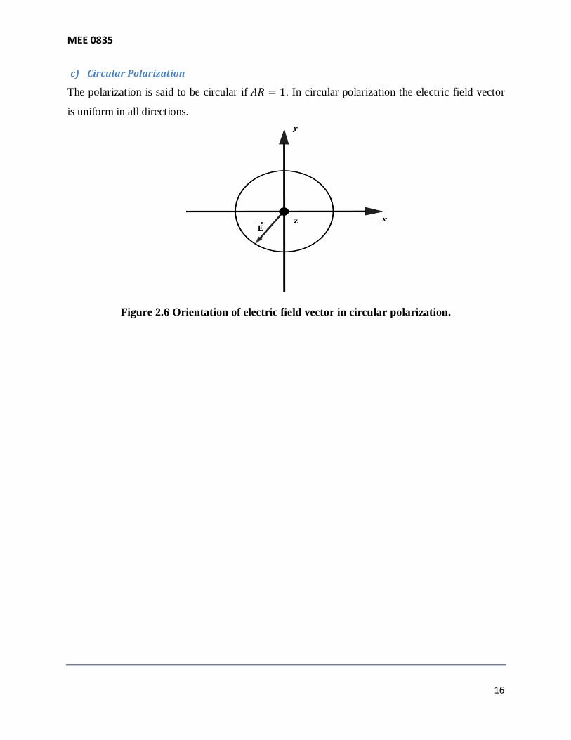
c) Circular Polarization

The polarization is said to be circular if 𝐴𝑅 = 1. In circular polarization the electric field vector

is uniform in all directions.

Figure 2.6 Orientation of electric field vector in circular polarization.

MEE 0835

17

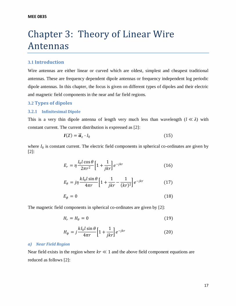
Chapter 3: Theory of Linear Wire Antennas

3.1 Introduction

Wire antennas are either linear or curved which are oldest, simplest and cheapest traditional

antennas. These are frequency dependent dipole antennas or frequency independent log periodic

dipole antennas. In this chapter, the focus is given on different types of dipoles and their electric

and magnetic field components in the near and far field regions.

3.2 Types of dipoles

3.2.1 Infinitesimal Dipole

This is a very thin dipole antenna of length very much less than wavelength (𝑙 ≪ 𝜆) with

constant current. The current distribution is expressed as [2]:

𝑰 𝑍 = 𝒂 𝑧 ∙ 𝐼0 (15)

where 𝐼0 is constant current. The electric field components in spherical co-ordinates are given by

[2]:

𝐸𝑟 = 𝜂𝐼0𝑙 cos𝜃

2𝜋𝑟2 1 +

1

𝑗𝑘𝑟 𝑒−𝑗𝑘𝑟 (16)

𝐸𝜃 = 𝑗𝜂𝑘𝐼0𝑙 sin𝜃

4𝜋𝑟 1 +

1

𝑗𝑘𝑟−

1

𝑘𝑟 2 𝑒−𝑗𝑘𝑟 (17)

𝐸𝜙 = 0 (18)

The magnetic field components in spherical co-ordinates are given by [2]:

𝐻𝑟 = 𝐻𝜃 = 0 (19)

𝐻𝜙 = 𝑗𝑘𝐼0𝑙 sin 𝜃

4𝜋𝑟 1 +

1

𝑗𝑘𝑟 𝑒−𝑗𝑘𝑟 (20)

a) Near Field Region

Near field exists in the region where 𝑘𝑟 ≪ 1 and the above field component equations are

reduced as follows [2]:

MEE 0835

18

𝐸𝑟 = −𝑗𝜂𝐼0𝐼𝑒

−𝑗𝑘𝑟

2𝜋𝑘𝑟3cos𝜃 (21)

𝐸𝜃 = −𝑗𝜂𝐼0𝐼𝑒

−𝑗𝑘𝑟

4𝜋𝑘𝑟3sin 𝜃 (22)

𝐸𝜙 = 𝐻𝑟 = 𝐻𝜃 = 0 (23)

𝐻𝜙 =𝐼0𝐼𝑒

−𝑗𝑘𝑟

4𝜋𝑟2sin𝜃 (24)

In this case, the electric field components 𝐸𝑟 ,𝐸𝜃 are in time phase but with the magnetic field

component 𝐻𝜙 they are in quardrature phase. The near field condition can be satisfied at

moderate distances from the antenna at low frequency operation.

b) Far-Field Region

Far field exists in the region where 𝑘𝑟 ≫ 1 and the above field component equations are reduced

as follows [2]:

𝐸𝜃 = 𝑗𝜂𝑘𝐼0𝐼𝑒

−𝑗𝑘𝑟

4𝜋𝑟sin𝜃 (25)

𝐸𝑟 = 𝐸𝜙 = 𝐻𝑟 = 𝐻𝜃 = 0 (26)

𝐻𝜙 = 𝑗𝑘𝐼0𝐼𝑒

−𝑗𝑘𝑟

4𝜋𝑟sin𝜃 (27)

In this case, the electric and the magnetic field components are perpendicular to each other and

transverse to the radial direction of the propagation. The ratio of 𝐸𝜃 to 𝐻𝜙 is defined as intrinsic

impedance (𝜂 = 120𝜋 ohm).

3.2.2 Small Dipole

The geomentrical arrangement of small dipole placed symmetrically about the orgin along the Z-

axis. The length of the dipole lies between 𝜆

50< 𝑙 ≤

𝜆

10. The current distribution of small dipole

is mathematically expressed as [2][3]:

𝑰𝑒 𝑥, 𝑦, 𝑧 = 𝒂 𝑧𝑰0 1 −

2

𝑙𝑧 , 0 ≤ 𝑧 ≤

𝑙

2

𝒂 𝑧𝑰0 1 +2

𝑙𝑧 ,

−𝑙

2≤ 𝑧 ≤ 0

(28)

MEE 0835

19

The electric and magnetic field components radiated by electromagnetic wave of small dipole are

mathematically expressed as

𝐸𝜃 = 𝑗𝜂𝑘𝐼0𝑙𝑒

−𝑗𝑘𝑟

8𝜋𝑟− sin 𝜃 (29)

𝐸𝑟 = 𝐸𝜙 = 𝐻𝑟 = 𝐻𝜃 = 0 (30)

𝐻𝜙 = 𝑗𝑘𝐼0𝑙𝑒

−𝑗𝑘𝑟

8𝜋𝑟sin 𝜃 (31)

These equations are investigated in the far field region where 𝑘𝑟 ≫ 1.

3.2.3 Finite Length Dipole

This is very thin dipole of length that lies between 𝜆

2< 𝑙 < 𝜆. The current distribution is

approximated with the mathematical formula [2] under the assumption of center fed antenna as

𝑰𝑒 𝑥 = 0,𝑦 = 0, 𝑧 = 𝒂 𝑧𝑰0 sin 𝑘

𝑙

2− 𝑧 , 0 ≤ 𝑧 ≤

𝑙

2

𝒂 𝑧𝑰0 sin 𝑘 𝑙

2+ 𝑧 ,

−𝑙

2≤ 𝑧 ≤ 0

(32)

The electric and magnetic field components are given by

𝐸𝜃 = 𝑗𝜂𝐼0𝑒

−𝑗𝑘𝑟

2𝜋𝑟 cos

𝑘𝑙2 cos𝜃 − cos

𝑘𝑙2

sin𝜃 (33)

𝐻𝜙 =𝐸𝜃𝜂

= 𝑗𝐼0𝑒

−𝑗𝑘𝑟

2𝜋𝑟 cos

𝑘𝑙2 cos𝜃 − cos

𝑘𝑙2

sin 𝜃 (34)

These equations are approximated in far field.

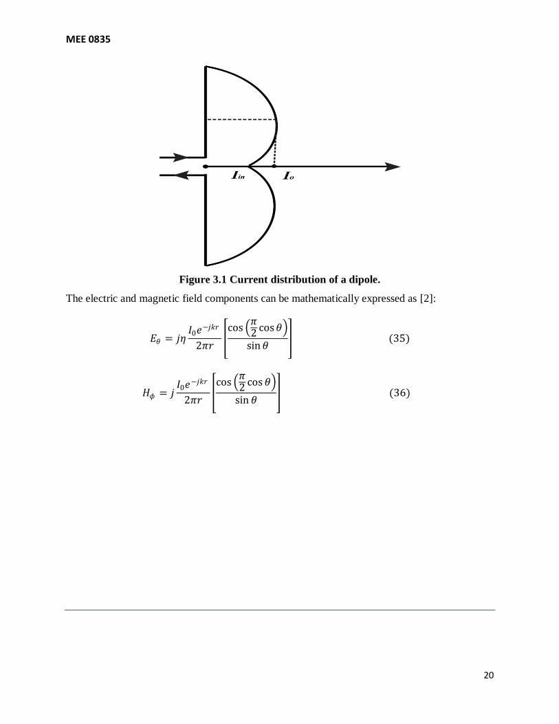
3.2.4 Half Wave Length Dipole

Traditionally most used antenna of length exactly equals to the half of the wave length. The

current distribution of this antenna is shown in Figure 3.1. The radiation resistance of the dipole

is 73 ohms, which is very near to the 75 ohm characteristic impedance of the transmission line.

MEE 0835

20

Figure 3.1 Current distribution of a dipole.

The electric and magnetic field components can be mathematically expressed as [2]:

𝐸𝜃 = 𝑗𝜂𝐼0𝑒

−𝑗𝑘𝑟

2𝜋𝑟 cos

𝜋2 cos𝜃

sin𝜃 (35)

𝐻𝜙 = 𝑗𝐼0𝑒

−𝑗𝑘𝑟

2𝜋𝑟 cos

𝜋2 cos 𝜃

sin 𝜃 (36)

MEE 0835

21

Chapter 4: Design of Linear Wire Antennas

4.1 Introduction

This chapter deals with the design parameters and design fundamentals of linear wire antennas

with special emphasis on dipoles. There are various important parameters affecting the antenna

performance that can be adjusted during the modeling process. Modeling of dipole antennas are

carried out using NEC-4 (Numerical Electromagnetics Code version 4.0) which is based on the

method of moments.

4.2 Design parameters and considerations

Design parameters describe the antenna performance; there are several parameters that affect the

antenna. These are feed point impedance, directivity, gain, radiation resistance, ground effects,

impedance matching, voltage standing wave ratio and return loss.

4.2.1 Feed point impedance

It is the principle characteristic defining an antenna. As antenna designers are free to select

operating frequencies with in assigned bands, how the feed point impedance of the antenna

varies with frequency band of operation. There are two types of impedances associated with

antennas are self impedance and mutual impedance.

a) Self Impedance

Self impedance is measured at the feed point terminals of the antenna far away from any other

conductors. According to ohms law, self impedance of antenna is equal to the ratio of voltage

applied to the feed point and current flowing into the feed point. If current and voltage are

exactly in phase, then the impedance is purely resistive without any reactive component. This

phenomenon is known as antenna resonance.

b) Mutual Impedance

Mutual impedance is due to the parasitic effect of surrounding conductors within the antennas

reactive near field. This is mainly due to the effect of ground as earth is lossy conductor. It is

also defined using ohms law just as like self impedance. Here it is the ratio of voltage in one

MEE 0835

22

conductor to the current flowing in another conductor. Mutually coupled conductors can disturb

the pattern of the antenna.

4.2.2 Directivity

Directivity of an antenna is directly proportional pattern of the radiation intensity. All practical

antennas will exhibit some degree of directivity, which means that the antenna radiation is

stronger in some directions than in others. The radiation from a practical antenna never has the

same radiation intensity in all directions.

4.2.3 Gain

The gain of the antenna is directly proportional to the directivity. As the directivity depends only

on the shape of the directive pattern but does not take the power loss into consideration. The total

gain of the antenna is equal to power supplied to antenna minus the losses.

4.2.4 Radiation Resistance

The input impedance of an antenna consists of real and imaginary parts, the real part of input

impedance is known as radiation resistance. The supplied power to the antenna is dissipated as

radiation of electromagnetic wave and heat loss in the wire due to nearby dielectrics; therefore

the ohmic losses are negligible in a well located antenna.

4.2.5 Ground Effects

The ground around the antenna is important part of the antenna operating environment,

considering the fact that earth is not an ideal conductor and always present in any antenna

system. The other major concern, earth is not a plane surface. For design simplification earth is

assumed to be flat and good conductor which follows (𝜎 ≫ 𝜔𝜀).

The antennas that operate at low and medium frequencies are profoundly influenced by earth.

Changing the height of the antenna above the ground, i.e. antenna is located at a height of

smaller than skin depth of conducting earth, will change the amount of current flow when the

input power to the antenna system is constant. Large current at the same power input leads to

decrease in the effective input resistance and vice versa this leads to low efficiencies.

When parasitic or driven type antennas are combined into arrays results in mutual impedance,

which predominantly increases the ground loss. In order to avoid the ground losses and to

MEE 0835

23

maintain constant feed point resistance, a large ground screen is used which is made up of wire

mesh or multitude of radials, the screen conductors are closely bonded to each other which leads

to less input resistance lower than the loss.

4.2.6 Impedance Matching

Impedance matching is very important characteristic for RF and antenna design. The energy

transfers from transmitter of the antenna through transmission line. In order to radiate maximum

output power from the antenna, the transmission line impedance should match to the antenna

feed point impedance otherwise energy reflected back from the antenna results in standing

waves. A typical arrangement of transmission line and antenna system is shown in Figure 4.2.

Figure 4.2 A typical arrangement of transmission line and antenna system.

4.2.7 Voltage Standing Wave Ratio (VSWR)

When the transmission line impedance doesn‟t match to the antenna feed point impedance,

standing waves are generated because of maximum energy transfer is not possible from

transmission line to the antenna. The fact is that some part of energy is reflected back, forming

standing waves on the transmission line. The reflection coefficient is expressed mathematically

as [2]:

MEE 0835

24

Γ =𝑍𝑖𝑛 − 𝑍0

𝑍𝑖𝑛 + 𝑍0 (37)

where

𝑍𝑖𝑛 = Antenna feed point impedance

𝑍0 = Characteristic impedance

The reflection coefficient limits are 0 < Γ < 1. Zero reflection means perfectly matched and one

reflection means the network is either open circuited or short circuited. An alternative way of

expressing reflection coefficient (Γ) in terms of VSWR is mathematically expressed as [2]:

𝑣𝑠𝑤𝑟 =1 + Γ

1 − Γ (38)

The limits for voltage standing wave ratio are1 < 𝑣𝑠𝑤𝑟 < ∞.

4.2.8 Return Loss

The mathematical expression for return loss which is usually represented in dB is [3]:

𝑅𝐿 = 20 log10 Γ 𝑑𝐵 (39)

Zero dB return loss means the line is either short circuited or open circuited. The value of return

loss infinite dB means the line is perfectly matched.

4.3 Modeling Considerations

The electromagnetic response of antennas are modeled and simulated with method of moments

based computer program called Numerical Electromagnetics Code which depends on the

numerical solution of integral equations of electromagnetic fields. These codes consider the

antenna environment excitation source and loading. The code outputs are current distributions,

antenna input impedance, power input and radiation patterns etc.

Method of moment is a mathematical technique that divides an antenna wire into segments, at

each segment it draws currents and phase of the current. A wire segment is defined by the co-

ordinates of its two end points and its radius. A wire segment should have at least 9 segments per

half wave length, the segment length should be at least 4 times larger than wire diameter and it

should be less than 0.1𝜆 at desired frequency, where 𝜆 is wavelength of the antenna.

MEE 0835

25

The 3-D co-ordinates systems used by NEC-4 as shown in Figure 4.3.

Figure 4.3 Format of 3-D co-ordinate system in NEC-4.

The use of X-axis is to define front and back dimensions. For single element X values are zero,

Y-axis is a linear element axis where all linear elements are parallel to Y-axis and Z-axis always

indicate the height of the antenna.

Evaluation of feeding point impedance or antenna input impedance is a very important

characteristic to achieve perfect resonance. This can be done by increasing or decreasing the

length of the antenna arbitrarily within the maximum allowable range. The dipole segments are

in odd number in order to feed the antenna exactly in the middle. The other reason is that the

centre fed dipole has maximum resonance and it transfers maximum power to the load, thereby

achieves maximum efficiency. Furthermore, at centre point the antenna has maximum current

and minimum voltage, as it is very easy to construct transmission line for low voltages rather

than high voltages. The wire antennas are made up of Copper, Aluminium and Zinc. Copper

gives better electrical conduction characteristics than the other two materials.

4.4 Model-I (Antenna is on the ground)

NEC-4 consists two types of commands namely structure geometry commands and control

commands. Usually structure geometry commands are followed by control commands, the

MEE 0835

26

following input file has „GW‟ and „GE‟ geometry commands which describes the antenna

geometry and end of geometry respectively. The control commands „LD‟ describes antenna

loading, „FR‟ describes frequency specification, „GN‟ describes the ground parameters, „EX‟

represents excitation, „RP‟ requests radiation pattern and „EN‟ represents end of run. The

commands „CM‟ and „CE‟ are useful to insert text in the program output.

Input file to NEC-4

CM Half wave length dipole in free space

CM frequency band 9-11MHz wavelength=30m

CM antenna length is 15m

CM radius 1mm

CE

GW 1 31 0.000 -7.5 0.000 0.000 7.5 0.000 0.001

GE 0 0

LD 5 1 0 0 59.6E+6 0

FR 0 21 0 0 9.0 0.1000

GN 2 0 0 0 8 0.01

EX 0 1 16 0 1.00 0.00

RP 0 37 1 1000 -90 0 10 10

EN

Antenna Description

Half wave length antenna with one wire and 31 segments, therefore the value on the X-axis are

zero on both sides. The wave length of the antenna is 30 m and the length of the antenna is 15 m

which is distributed symmetrically on each side of length 7.5 m along the Y-axis. Z-axis gives

the height of the antenna, in this case Z equals to zero which implies antenna is on the ground.

The radius of the wire is 1mm.

The operating frequency range of the antenna 9MHz to 11MHz observed in 21 frequency steps

with each frequency step of 0.1MHz. The ground parameters are complex dielectric constant in

the vicinity of the antenna is 8 and the conductivity of 0.01 mho/meter. The antenna is fed

exactly in the middle that is at the 16th

segment with 1volt real and 0 volt imaginary. In this case,

the antenna is made up of copper which has the conductivity of 59.6 × 106 mho/meter.

MEE 0835

27

Radiation pattern is computed in spherical co-ordinates for 37 values of ‟𝜃‟ starting with -90 at

an increment of 10 and 1 value of ‟𝜙‟ with vertical, horizontal, total gains and power gain.

Output from NEC-4

The NEC-4 output is in ASCII format shown below.

Here the wave length is calculated with reference to the frequency but not the antenna

wavelength. The radiation pattern is given below.

MEE 0835

28

Antenna simulations were conducted for 5, 9, 15, 21 and 31 segments. The simulation results are

plotted with the help of MATLAB for copper conductor. Aluminum and Zinc simulation results

are shown in Appendix A.

The feed point impedance of an antenna is complex due to the phase difference between the

currents hence it has both real and imaginary parts. The real part of the feed point impedance

versus frequency is shown in Figure 4.4. With the evidence from the figure, as the frequency

increases the impedance of the antenna is increasing furthermore the impedance is not constant at

a particular frequency within the frequency band for all segments.

The reactive part of the feed point impedance versus frequency is shown in Figure 4.5. For the

segments 9, 15, 21 and 31 the reactance is almost constant throughout entire frequency band but

has substantial reactive part which is not permissible in order achieve resonance. For the 5

segments the reactance increases in the band.

MEE 0835

29

Figure 4.4 Input impedance vs frequency.

Figure 4.5 Input reactance vs frequency.

MEE 0835

30

The Figure 4.6 shows the voltage standing wave ratio. For the segments 9, 15, 21 and 31. The

magnitude of VSWR varies from 10 to 17 in the frequency band of 9 -11 MHz. For the segment

5 VSWR rapidly increases.

Figure 4.6 Voltage standing wave ratio vs frequency.

MEE 0835

31

Figure 4.7 Power efficiency vs frequency.

Figure 4.8 Power gain vs frequency.

MEE 0835

32

The plots for the power efficiency and power gain are shown in Figures 4.7 and 4.8 respectively.

As the number of segments increases from 5 to 31, the efficiency decreases and power gain

decreases.

4.5 Model –II (antenna located at a height of 15 m)

The commands „GW‟ describes the antenna geometry, „LD‟ describes antenna loading, „FR‟

describes the frequency specification, „GN‟ describes the ground parameters, „EX‟ represents

excitation and „RP‟ requests radiation pattern according to the Lawrence and Livermore manual.

Input file to NEC-4

CM Half wave length dipole over ground (Height of the antenna is 15m)

CM length of the antenna is 14.7m

CE

GW 1 31 0.000 -7.35 15.000 0.000 7.35 15.000 0.001

GE 0 0

LD 5 1 0 0 59.6E+6 0

FR 0 11 0 0 9.0 0.2000

GN 2 0 0 0 8 0.01

EX 0 1 16 0 1.00 0.00

RP 0 37 1 1000 -90 0 10 10

EN

Antenna Description

Half wave length antenna with one wire and 31 segments, therefore the value on the X-axis are

zero on both sides. The wave length of the antenna is 29.4 m and the length of the antenna is

14.7 m which is distributed symmetrically on each side of length 7.35 m along the Y-axis. Z-axis

gives the height of the antenna, in this case Z equals to 15m which implies antenna is on located

above the ground. Radius of the wire is 1mm.

The operating frequency range of the antenna is 9MHz to 11MHz observed in 11 frequency steps

with each frequency step 0.2MHz. The ground parameters are complex dielectric constant in the

vicinity of the antenna is 8 and the conductivity of 0.01 mho/meter. The antenna is fed exactly in

the middle that is at the 16th

segment with 1volt real and 0 volt imaginary. In this case the

antenna is made up of copper with conductivity 59.6 × 106 mho/meter.

MEE 0835

33

Radiation pattern is computed in spherical co-ordinates for 37 values of ‟𝜃‟ starting with -90 at

an increment of 10 and 1 value of ‟𝜙‟ with vertical, horizontal, total gains and power gain.

The real part of the feed point impedance versus frequency is shown in Figure 4.9. With the

evidence from the figure, as the frequency increases the impedance of the antenna is increasing.

Furthermore, the impedance is almost constant at a particular frequency within the frequency

band for all segments.

The reactive part of the feed point impedance versus frequency is shown in Figure 4.10. For all

the segments the reactance is almost constant at a particular frequency in the entire frequency

band. At 10 MHz the antenna has zero imaginary part hence the resonance is achieved thereby

maximum power transmits to the load.

Figure 4.9 Input impedance vs frequency.

MEE 0835

34

Figure 4.10 Input reactance vs frequency.

The Figure 4.11 shows the voltage standing wave ratio. For all the segments the magnitude of

VSWR varies from 1.5 to 10.5 in the frequency band of 9 -11 MHz. At 10 MHz VSWR is very

low since the antenna is at resonance and maximum power transmits to the load.

Figure 4.11 Voltage standing wave ratio vs frequency.

MEE 0835

35

Figure 4.12 Power efficiency vs frequency.

Figure 4.13 Power gain vs frequency.

MEE 0835

36

The plots for the power efficiency and power gain are shown in Figures 4.12 and 4.13

respectively. For all the segments the efficiency is almost constant and power gain increases in

the entire frequency band.

4.6 Comparison between Model-I and Model-II

The Model-I is a dysfunctionals antenna due to the antenna is on the ground and the variations

in feed point impedance are too high. The typical variations in this case are from 340 ohm to 420

ohm considering all segments at the entire frequency band of operation. Variations in reactance

is also high hence there is no resonance thereby ultimately invalid maximum power transfer

condition results in high VSWR. Which are not acceptable in antenna design.

In Model-II, the above mentioned properties are rectified with adjustments in the antenna

geometry by improving height, length of the antenna and increasing the number of segments.

Usually the accuracy increases with increase in the segment number at the cost of longer

calculation time. In this case, the feed point impedance variations are from 55 ohm to 85 ohm,

considering all segments in the entire frequency band. For example, at 10 MHz antenna has

constant impedance around 65 ohm for all segments. The variations in reactance are from

capacitive to inductive with constant magnitude for all segments. The resonance is achieved at

10 MHz i.e zero reactance, hence maximum power transfer to the load results in low VSWR.

The other way round, most of the transmission lines have characteristic impedance from 50-75

ohm and this variation matches with the feed point impedance range.

MEE 0835

37

Conclusion

This master thesis report presents pros and cons of antenna modeling with numerical

electromagetics code version 4.0. The major outcomes from this research are permissible antenna

input impedance, low voltage standing wave ratio, perfect matching and resonance for linear

wire dipole antenna. Power efficiency and power gains of models are also analyzed within the

frequency band of operation. The antenna input impedance is in the range of 55 ohm to 85 ohm

as the radiation resistance of half wave dipole antenna is 73 ohms (theoretically) which is in the

range of 55-85 ohms thereby antenna achieved almost perfect matching. Finally the modeling

parameters of the dipole antenna are dependent on feed point impedance.

MEE 0835

38

Appendix-A

The simulation results are shown in following figures for the dipole antenna (Model-II) 15 m

above the ground when the antenna is loaded with Aluminum of electrical conductivity

37.8E+06 mho/m.

Figure A1 Input impedance vs frequency

Figure A2 Input reactance vs frequency

MEE 0835

39

Figure A3 Voltage standing wave ratio vs frequency

Figure A4 Power efficiency vs frequency

MEE 0835

40

Figure A5 Power gain vs frequency

MEE 0835

41

Appendix-B

The simulation results are shown in following figures for the dipole antenna (Model-II) 15 m

above the ground when the antenna is loaded with Zinc of electrical conductivity 5E+06 mho/m.

Figure B1 Input impedance vs frequency

Figure B2 Input reactance vs frequency

MEE 0835

42

Figure B3 Voltage standing wave ratio vs frequency

Figure B4 Power efficiency vs frequency

MEE 0835

43

Figure B5 Power gain vs frequency

MEE 0835

44

Appendix-C

Design guidelines

With some experience in linear wire antenna modeling, an antenna designer may consider the

following design guidelines.

1) Antenna feed point impedance can be adjusted to meet the matching requirements by

increasing or decreasing the length of the antenna within the defined maximum length.

2) Wire diameter does not affect the feed point impedance in the range of 1-100 mm.

3) Loading the antenna gives less efficiency when compared with without loading. Antenna

without loading gives 100% efficiency due to ideal conductivity.

4) Usually these wire antennas are made up of Copper, Aluminium and Zinc. As the

conductivity of the material increases the efficiency also increases.

Safety precautions when installing an antenna

Antenna design is quite challenging and installing the antenna on towers and mountains are

equally challenging. Here are some safety precautions for the antenna installers. These

precautions are given by L.B. CEBIK in his ARRL Antenna handbook [6]. These are quite fun

and interesting.

1. A quality safety belt

2. Safety glasses

3. Hard hat

4. Long sleeved , pull over shirt with no buttons

5. Long pants without cuffs

6. Firm, comfortable, steel shank shoes without slip soles

7. Gloves that do not restrict finger movement.

MEE 0835

45

References

[1] P. Wacker, “Comments on unified theory of near-field analysis and measurement,” IEEE

transactions on Antennas and propagation , Vol.31, No.6, pp. 1002-1003, November 1983.

[2] Antenna theory analysis and design by Constantine A. Balanis ISBN 9971-51-233-5

[3] Antennas by John D. Krauss ISBN 0-07-463219-1

[4] Engineering Electromagnetics by William H. Hayt Jr ISBN 13-978-0070274075.

[5] Antenna EM Modeling with MATLAB by Sergey N. Markov ISBN 0-471-21876-6

[6] The ARRL Antenna book by Kurt Andress ISBN 0-87259-804-7

[7] NEC-4.1 user‟s manual by Gerald J. Burke

[8] MATLAB programming for engineers by Stephen J. Chapman ISBN 0-534-42417-1

[9] A beginner‟s guide to modeling with NEC part-I by L. B. Cebik

[10] A beginner‟s guide to modeling with NEC part-II by L. B. Cebik

[11] A beginner‟s guide to modeling with NEC part-III by L. B. Cebik

[12] S.R.Best, “ A discussion on the Properties of Electrically Small Self-Resonant Wire

Antennas,” IEEE transactions on Antennas and propagation, Vol.46, No.6, pp.9-22, December

2004.

[13] C.A. Balanis, “ Antenna Theory: A Review,” IEEE transactions on Antennas and

propagation, Vol.80, No.1, pp.7-23, January 1992.

[14] L.E. Vogler and J.L Noble “ Curves of Input Impedance change due to Ground for Dipole

Antennas” an article from U.S National Bureau of Standards

[15] R.F Schwartz “Input Impedance of a Dipole or Monopole ” The microwave journal

[16] R.F Harrington “Theory of loaded scatterers ” an internet article

[17] A.F Stevenson “Relation between the transmitting and receiving properties of antennas” an

internet article

[18] www.cebik.com

[19] http://www.nittany-scientific.com

[20] www.mathworks.com