CONSTRUCTING RANDOM PROBABILITY DISTRIBUTIONS

THEODORE P. HILL* School of Mathematics

Georgia Institute of Technology Atlanta, GA 30332-0160 USA

hill@math.gatech. edu

DAVID E. R. SITTONt

Planning System Incorporated 115 Christian Lane

Slidell LA 70458 USA dsitton@psislidell.com

Abstrac: This article surveys several classes of iterative methods for constructing random probability distributions (or random convex functions, or random home­omorphisms), and includes illustrative applications in statistics, optimal-control theory, and game theory. Computer simulations of these methods are fast and easy to implement.

1. Introduction

The main purpose of this article is to provide a short survey of methods for constructing random probability distributions (or, equivalently [10,12,16], for constructing random convex functions or random homeomorphisms). As such, this paper complements and extends the excellent overviews of con­structions of random probability measures by Ferguson [14], by Diaconis and Freedman [9], and Monticino [34]. Constructions of random proba­bility measures are not only intrinsically interesting, but also have useful applications in such area.s as game theory, statistics, optimal control theory, and analysis of algorithms [7, 8, 25, 29] .

• Research partially supported by U.S. National Science Foundation Grant DMS-9971146. tResearch partially supported by a graduate Presidential Fellowship at the Georgia In­stitute of Technology.

For example, in game theory, basic minimax theorems imply that in wide classes of games the optimal strategies are random, as opposed to pure or deterministic strategies. Often the solution is known to be a probabilitydistribution on several points, or on an interval. If no analytical solutionfor the game is known, then the optimal strategy (probability distribution) can often be approximated numerically, by constructing probability distri­butions at random, and keeping track of the distribution attaining the ex­tremal expected payoffs. Provided that the construction method producesrandom distributions which are dense in the set of all probability distribu­tions in the class of interest, and that the underlying game satisfies general continuity conditions, the simulation will converge to the game's optimalstrategy. As a concrete example, Gal [15] describes the following single 2-person search game on three arcs, for which the general optimal strategyis still unknown. (Optimal strategies within certain classes are known; see [5, 151.) Two cities A and B are connected by 3 non-intersecting roads ofequal lengths. Player I places a landmine at some location on one of the three roads, and Player II, starting at A, searches along the roads at unit speed until he finds the landmine. Player I's objective is to make the timeto discovery as large as possible, and Player II's is to minimize. It is known that the optimal solution for Player I is a single continuous pro~abilitydistribution on the interval (i.e., concatenation of the three roads), which can be approximated numerically by constructing probability measures atrandom and identifying the best-case distributions, as is seen in §5 below.

Another application of constructions ofrandom probability distributions is to determine average-optimal strategies, or the average-optimal distrib­ution of errors in certain numerical algorithms [17, 36]. For example, in optimal stopping theory, the observer may not know the distributions of the observations completely, but instead may only have partial information, such as knowing the means, or means and variances. The objective thenis to find a stop rule t which is best on the average among random vari­ables in the given class, in which case an ap~ropriate probability on thatclass of distributions needs to be identified. Similarly, in many numericalalgorithms, it is known that the worst-case errors are actually quite rare [35, 36], and in analyzing errors (in order to select between two different algorithms, for example), average error is a better criterion than worst-case error. Thus performance analysis of such algorithms hinges on identification of an appropriate model for the random input (or error), i.e., constructionsof appropriate random probability distributions.

In addition, constructions of random probability distributions have basic

applications in classical Bayesian statistics to produce natural priors (e.g., random distribution of a species in a region), in probability theory and analysis to numerically generate sharp constants or optimal distributions such as in Plackett's problem [28] (see §5 below), and in theories underlying new statistical tests for the detection of fabricated numerical data [19].

Important properties for constructions of random probability distribu­tions to have are that they are natural, they are easy to implement, and they have dense support in the desired class of probability distributions. All the constructions discussed below share these three properties, and all are essentially non-parametric statistical methods. As noted by Monticino [34], "non-parametric priors may avoid biases potentially introduced by the se­lection of a particular parametric family," and the constructions given here all have wide support.

Section 2 contains the basic definitions and framework, and descriptions of several classical methods for constructing general probability distribu­tions; Section 3 surveys methods for constructing random distributions with given moments (such as means and/or variances); Section 4 describes sev­eral methods for generating random probability distributions which are absolutely continuous (i.e., which have densities - the aforementioned con­structions all yield purely singular distributions); and Section 5 gives typical applications to several concrete problems.

2. Constructions of General Random Probability

The basic idea of Dubins and Freedman [10, 12]' to construct a random probability measure by constructing its distribution function at random, underlies each of the constructions below, where all distributions are taken to have support in [0,1]. The measure-theoretic setting [11] is this: A is the space of all distribution functions on [0, 1], that is A = {F : [0, 1] --> [0, 1]' F is non-decreasing and right continuous, F(O-) = 0, F(I) = I}, where for FE A, the Borel probability measure on [0,1] defined by F is determined by P([O, tJ) = F(t), t E [0,1]; and 2:;* is the smallest er-algebra of subsets of A such that for every A E 1ffi[0,1], the function F fA dF(x) is Borelf--;

measurable. Thus a random probability distribution (r. p.d.) IF on [0, 1] is a measurable function from a probability space (n, F, P) to (A, 2:;*). That is, IF is a probability-distribution-valued random variable, and lFw will denote its value (d.f.) for each w in n.

Dubins and Freedman [12] give a natural iterative method for construct­ing r.p.d.'s IF via a given base measure J-L on S = [0, If For example, if

J.L is uniform on the vertical bisector {(! 'Y) : 0 :S Y :S I}, their construc­tion proceeds as follows. Recall that F(O-) = 0 and F(I) = 1 for all F E A, and let IF = IF /.L be the r.p.d. defined inductively on the dyadic ra­tionals in [0,1] by IF(O) = 0, IF(I) = 1, IF(!) = Xl, IF(~) = X2JF(!),IF(~) = IF(!) +X3 (1 - IF(!)) , ... , where Xl, X 2 , ... are i.i.d. UfO, 1] random vari­ables independent of IF. (So IF(!) is uniformly distributed on [0,1], and, given IF(!), IF(~) and IF(~) are uniformly distributed on their possible ranges [0, IF(!)] and [IF(~), 1], respectively, and so on for IFa), IF(i), .... )

As another example of a natural base measure, let J.L be uniformly distributed on 5, and define the random sequence IF(O) = 0, IF(I) = 1, IF(X I ) = YI , IF(X2) = Y2 , IF(X3 ) = Y3 , ... as follows. Xl and YI are i.i.d. UfO, 1], X 2 and Y2 are independent and uniformly distributed on [0, Xl] and [0, YI ], respectively, X 3 and Y3 are independent and uniformly distributed on [Xl, 1] and [YI , 1], respectively, and so on.

For these constructions and a much wider class, Dubins and Freedman [12] establish many basic results including: these random sequences deter­mine a r.d.f. IF a.s.; IF is dense in A; and IF is a.s. singular (with respect to Lebesgue measure) - essentially since the process is "self-similar." For more general base measures J.L on 5 they show that: almost all distributions gen­erated are continuous if and only if J.L assigns probability 0 to the vertical edges of 5 and J.L assigns positive probability to the interior of 5j almost all distributions generated are purely discrete if either J.L assigns probability 1

to the horizontal edges of 5 or J.L assigns positive probability to the vertical edges of 5; and if J.L does not give probability 1 to the main diagonal of 5, then almost all the generated distributions are singular.

Special cases of the Dubins-Freedman construction, and extensions to more general settings, including changing base measures at each stage of the construction, are found in [16, 24, 30, 31]. In an effort to use r.p.d.'s as priors in Bayesian statistics, Ferguson [13, 14) developed Dirichlet pri­ors, which are a.s. discrete, have full support under fairly general condi­tions, and, in contrast to the Dubins-Freedman constructions, have easily describable posterior distributions.

Another method for constructing r.p.d.'s uses a P6lya-urn scheme tech­nique to generate a sequence of exchangeable random variables. Via de Finetti's theorem, every infinite exchangeable sequence is a random (pos­sibly continuous) mixture of sequences of i.i.d. random variables, which therefore yields a random probability measure; see [2, 26, 27, 29, 33]. Mauldin, Sudderth, and Williams [29J show that the set of P61ya tree priors forms a conjugate class, and find conditions under which a P6lya tree prior

is a.s. continuous, or has full support on A. Monticino [33J establishes con­nections between P6lya tree constructions and "random rescaling" r. p.d. 's, and shows that trees of arbitrary exchangeable processes can be used in place of P6lya urn schemes.

3. Construction of Distributions with Given Moments

In many applications involving unknown or random distributions, one or more of the moments of the distribution are assumed to be known. For example, in algorithms involving random error, the error is often unbiased, that is, has mean zero. Similarly, in many experiments involving measure­ments, the error may also have known standard deviation, hence second moment, based on the known variability of the measuring device. In trying to model these random distributions, the constructions mentioned above are not useful, since the distributions generated do not have fixed means or variances, and the sets of distributions with prescribed means or vari­ances are null sets in the underlying probability space. In fact, even the calculation of the distribution of the means, except in some trivial cases, is difficult (see [6, 32]).

Several methods for constructing r.p.d.'s with given moments have evolved. The method in [21, 22] generates a random distribution by gener­ating its sequential barycenter array, or successive conditional expectations, at random. For a distribution FE A, the F-barycenter of (a, c], bF(a, c], is the conditional expectation of F over the interval (a, c], that is

{ ~( )xdF(x)j(F(c) - F(a)) if F(c) > F(a)bF(a, c] = Q"C

a if F(c) = F(a),

and the sequential barycenter array {mn,k}:=l %:]'1 of F is defined induc­tively as follows:

mI,l = JxdF(x)

m n ,2j = mn-1,j for n ;::: 1 and j = 1, ... , 2n-

I - 1

m n ,2j-1 = bF(mn-1,j-1, mn-1,j] for j = 1, ... ,2n -1

(with mn,o := 0, and mn,2n := 1).

In [22], it is shown that the sequence {mn,k(F)} = {mn,d uniquely deter­

mines the distribution F, via the inversion formula

F(mn,2j-l) = F(mn-l,j-l)

.) _ F( .)) (mn +1,4 j -l - m n +1,4 j -2)+ (F(mn-l,J mn-l,J-l m n +l,4j-l - m n+l,4j-3

The main idea in [22] is to use these barycenter characterizations of a dis­tribution to generate a sequential barycenter array randomly, and then to recover the observed value JFw of the random distribution from the array using the inversion formula. Since the distribution of the initial barycenter ml,l may be specified, this construction can generate r.p.d.'s with any pre­scribed mean or distribution of the means. As with the Dubins-Freedman construction above, the generation of the random barycenter array depends on a base measure f.-l which may be chosen to fit the given model desired. For example, if f.-l is uniform and a r.p.d. with mean 1/3 is desired, first fix ml,l = 1/3, then generate the random conditional mean less than 1/3, m2,1, uniformly in (0,1/3), and the conditional mean above 1/3, m2,3, uniformly in (1/3, 1), and so on, at each step generating the new barycenters uniformly between the previous ones. (See [34] for a graphic "mobile" description of this process.) By using non-uniform bases, "clumping" or "anti-clumping" constructions may be attained, where mass in the distribution is more (or less) likely to be near other masses. The results in [22] include conditions on the base measure f.-l so that the construction has full support (in the subset of A with given mean or distribution of the mean), and conditions on f.-l so that the r.p.d.'s generated are a.s. continuous, or a.s. discrete, or have finite support a.s.

Although the sequential barycenter construction allows one to specify the mean of the r.p.d., it does not generate distributions with fixed higher moments, such as given mean and variances simultaneously. One approach to solving this problem is in [3, 4], which generates r.p.d.'s with given mean and variance via variance split arrays.

Definition. A pair of probability measures (f.-ll, f.-l2) is a variance split of the probability measure f.-l if Var(f.-ll) = Var(f.-l2) < V(f.-l), and there is apE (0,1) so that f.-l = Pf.-ll + (1 - p)f.-l2' A triangular array {f.-ln,k,Pn,kl~=l ~:-l' is a canonical variance split array for the probabil­

2n - 1

ity measure f.-l if for each n E N', f.-l = L:k=l f.-ln,kPn,k, and for each k, (f.-ln+l,2k-l, f.-ln+l,2k) is a non-degenerate variance split of f.-ln,k with splitting probability P = Pn+l,2k-l!Pn,k. The array is called uniform if V(f.-ln,k) --> ° as n --> 00.

Theorem 1. Every Borel probability measure with compact support has a canonical variance split array, and every such array is uniform. Moreover, every such array uniquely determines the distribution.

Analogously to the sequential barycenter array construction, a random distribution may also be constructed via a base measure f.L by constructing this variance-split array, or associated mean-variance array, at random (see Figure 1). In [3, 4], necessary and sufficient conditions are obtained for an array to be a mean-variance array, and conditions are given which guarantee that the generated distributions are a.s. discrete, and that they have full support in the subset of A with given mean and variance.

( ~)

Figure 1. Left is a sample random probability distribution with mean 0.5 and variance 0.01 constructed using the variance-split array method. Right is the average of 500 r .d.f.'s with the same mean and variance.

Another method for constructing r.p.d.'s on [0,1] with given mean and variance, or in fact given moments of any orders, is to pick the moments at random (e.g., using a natural base measure f.L, such as uniform), since the moments {EX n } of a compactly supported distribution uniquely de­termine the distribution. Given the first n moments M 1 , ... , Mn of a dis­tribution F E A (i.e., M j = JxjdF(x)), sharp lower and upper bounds M +1 and M n + 1 are known for the (n + l)st moment [38J. That is, given n

the first n moments M1(F), ... , Mn(F), the (n + l)st moment Mn+1(F) lies in the closed interval [Mn+1(M1, ... , Mn ), Mn+1(M1, ... , Mn )]. These bounds are sharp, and attained (by discrete distributions), and are given in easily-calculated recursive form.

Thus, for example, to generate a random distribution with given first, second and third moments, M I, M2, 1\13 , generate the sequence of higher moments randomly as follows. First pick M4 (F) in [~(Ml' M2 , M3), M 4(M1 , M2 , M3)], say uniformly, and then pick M5 (F) uniformly in [M5(M1,1'v12 , M3, M4 (F)), M 5(M1, M2 , M3 , M4 (F)], and so on. The main drawback of this method is that the inversion process - recovering the dis­tribution from its moments - seems calculation-intensive for large n. Per­haps new advances in inversion algorithms will make this technique more attractive.

Methods for generating r.p.d. 's in higher dimension are useful in various statistical problems such as describing distributions of mass in space, with fixed center of mass. Some of the above construction ideas carryover to higher dimensional settings [20], and complement other known methods including Kolmogorov's "rock-crushing" model [23], multi-type branching processes, and embeddings of random graphs [1].

4. Construction of Absolutely Continuous Distributions

All of the above methods for constructing random probability distributions yield singular distributions almost surely, either purely discrete measures or continuous measures which are singular with respect to Lebesgue measure, i.e., which live on a null set. Since nearly all the continuous distribu­tions encountered in practice and in theoretical statistics (e.g., gaussian, exponential, uniform) are absolutely continuous with respect to Lebesgue measure, that is, have densities or Radon-Nikodyn derivatives, it is useful to have constructions of r.p.d. 's which generate a.c. measures almost surely. Kraft [24] introduced a generalization of the Dubins-Freedman construction in which the base measure changes for each successive point in the construc­tion of the r.d.f. Under certain conditions on the changing base measure {,ui,j}, Kraft showed that the generated r.d.f. 's are almost surely absolutely continuous, but prescribed no structure to the changing base measures, nor established density of support.

Complementing Kraft's construction, Sitton [37] established several nat­ural methods for constructing r.d.f.'s which are almost surely a.c. One method is based on the fact that convolution of measures increases smooth­ness (or decreases concentration [18]). For example, if F l is a.c., then so is F l * F2 for all F2 E A, and if FI is a-Lipschitz, then so is F l * F2 • Sitton defines the convolution IF\ *IF2 of two r.d.f.'s, and gives a natural method of randomly rescaling them (prior to performing the convolution) via an in­dependent (0, I)-valued random variable X, so that the result IFlx(lF l ,IF2) is a r.d.f. (on [0,1]). He then shows that if IF l is any r.d.f., and IF2 is a r.d.f. which is a.s. absolutely continuous, then IFlx (IF l, IF2) is an a.s. absolutely continuous r.d.f., and proves criteria useful for establishing full support of the r.d.f.

Theorem 2. (31] Let X be a r.v. in [0,1] for which P(X E (0,1)) = I, and °E supp(X). IfIF I and IF2 are r.d.f. 's, independent of X, with support in A, then the support of the r.d.f. IFlx(IF l ,IF2) contains the support ofIF l .

Corollary 1. IfIF2 is the Dubins-Freedman r.d.f. (with uniform base mea­sure ,u), F l is the uniform d.f. on [0,1], and U '" U(O,I) is independent ofIF l , then the r.d.J IF = IFlu(Fl ,IF2 ) is a.s. absolutely continuous, and has

full support in A, hence full support among all d.f. 's in A which are a.c.

In addition, [37] contains bounds on the density of the r .d.f. 's, and a general form for the average d.f. Wof a Ld.f. IF, where Wis the function W: lR -+ [0,1] defined by

W(x) = r G(x)dlF(G) = 1 lFw(x)dP(w) =: E(lF(x)). JCEA wEn

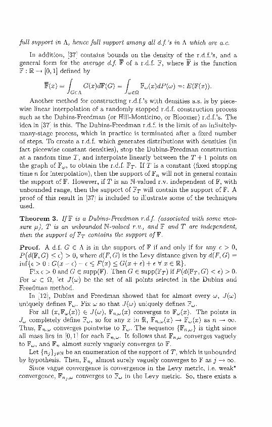
Another method for constructing Ld.f. 's with densities a.s. is by piece­wise linear interpolation of a randomly stopped r.d.f. construction process such as the Dubins-Freedman (or Hill-Monticino, or Bloomer) Ld.f.'s. The idea in [37] is this. The Dubins-Freedman Ld.f. is the limit of an infinitely­many-stage process, which in practice is terminated after a fixed number of steps. To create a r.d.£. which generates distributions with densities (in fact piecewise constant densities), stop the Dubins-Freedman construction at a random time T, and interpolate linearly between the T + 1 points on the graph of lFw , to obtain the Ld.f. lFT . If T is a constant (fixed stopping time n for interpolation), then the support of lFn will not in general contain the support of IF. However, if T is an N-valued LV. independent of IF, with unbounded range, then the support of lFT will contain the support of IF. A proof of this result in [37] is included to illustrate some of the techniques used.

Theorem 3. If IF is a Dubins-Freedman r. d.f. (associated with some mea­sure f-L), T is an unbounded N-valued r. v., and IF and T are independent, then the support of lFT contains the support of IF.

Proof. A d.f. G E A is in the support of IF if and only if for any E > 0, P(d(IF, G) S; E) > 0, where d(F, G) is the Levy distance given by d(F, G) = inf{E > 0: G(x - E) - ES; F(x) S; G(x + E) + EV x E lR}.

Fix E> 0 and G E supp(IF). Then G E SUPP(lFT) if P(d(IFT, G) < E) > O. For w E 0, let J(w) be the set of all points selected in the Dubins and Freedman method.

In [12], Dubins and Freedman showed that for almost every w, J(w) uniquely defines IFw . Fix w so that J(w) uniquely defines IFw .

For all (x,IFw(x)) E J(w), lFn.w(x) converges to IFw(x). The points in Jw completely define lFw , so for any x in lR, IFn,w(x) -+ IFw(x) as n -+ 00.

Thus, lFn,w converges pointwise to IFw . The sequence {IFn,w} is tight since all mass lies in [0,1] for each lFn,w' It follows that IFn,w converges vaguely to IFw , and IFn almost surely vaguely converges to IF.

Let {nj} JEN be an enumeration of the support of T, which is unbounded by hypothesis. Then, IFnj almost surely vaguely converges to IF as j -+ 00.

Since vague convergence is convergence in the Levy metric, i.e. weak' convergence, IFnj,w converges to IFw in the Levy metric. So, there exists a

K€,w ENlarge enough that for all j > K€,w, d(IFnj,w,IFw) < Eo For every

j E N, define the sets AJ , A c n by Aj = {wi d(IFnj,w, G) < c} E F and

A = {wi d(IFw,G) < E} E F.

Assume w E A. Then, there is a K' = K€-d(Fw,G),wENlarge enough that for all j > K', 0 :::: d(IFnj,w, IFw) < c - d(IFw,G), because E > d(IFw,G). By the triangle inequality, 0 :::: d(IFnj,w, G) :::: d(IFnj,w, IFw) + d(IFw,G) < E.

Therefore, w E Anj for all j > K'. The sequence {nj} is unbounded and positive so {w I d(IFw,G) < E} C UjAnj . Thus, 0 < P(d(IF,G) < c) :::: P ( UjEJ\I Anj ) because by hypothesis, G is in the support of IF. By the

subadditivity of probability measures,

00

0< p( UAnj ) :::: LP(AnJ. jEJ\I j=l

It follows that there exists aM E N for which P(AnM ) > O. In particular,

0< P(d(IFnM ,G) < E).

Finally,

00

P(d(IFT,G) < c) = LP(d(IFnj ,G) < E) IT = nj)P(T = nj) j=l 00

= L P(d(IFnj ,G) < E))P(T = nj) j=l 00

= L P(AnJP(T = nj) ~ P(AnM )P(T = nM) > O. j=l

The first equality is Bayes' Formula; the second follows because IF and T are independent; and the third follows from the definition of Anj . The first inequality follows because all terms in the sum are non-negative, and the last inequality comes from the hypothesis on M and because nM E supp(T).

Corollary 2. If T is a geometric random variable, IF is the Dubins­Freedman r.d.f. with base measure J1. uniform on [0,lJ2, and T and Fare independent, then IFT is a.s. absolutely continuous, and has full support (i.e., suppIFT = A).

In some applications such as queueing problems or renewal processes, the unknown (random) distribution may not only be known to be absolutely continuous, but also be known to have a monotone density. In [37], several constructions of r.dJ. 's of this type are given. For example, the sequential

barycenter method in §3 can be used to generate a r.d.f. IF with constant mean 1/2, using the fact that EX = fo1(1-F(x))dx (by Fubini's Theorem). Since IF is continuous a.s., 2(1 - IF) will generate a random non-increasing continuous function on [0,1] with integral 1, that is, it will generate contin­uous monotone non-increasing densities on [0, 1] almost surely. Sitton [37] establishes conditions under which given methods for constructing r.d.f. 's generate distributions which are dense in the set of all distributions with monotone densities, or with bounded monotone densities, respectively.

5. Applications

The purpose of this section is to illustrate application of some of the con­structions described above to several concrete problems.

5.1. Generation of models

Example 1. (Power-law distribution of mass). For some physical prob­lems, mass (or charge, etc.) is randomly distributed according to a power law f.L[0, x] = x"'. Note that for the sequential barycenter method, in which the base measure defines the random distance from the n-th stage barycen­tel' to the (n + 1)-st barycenter, tighter clustering occurs for smaller val­ues of a, and in the limiting case a = 0, there is total clustering (Dirac measure) at the center of mass. Figure 2 shows three sample simulations for distribution of mass, with fixed center of mass 1/2, using the sequen­tial barycenter method for a = 1 (uniform), a = 5 (anti-clustering), and a = 0.5 (clustering).

Figure 2. Simulations of power-law mass distribution models constructed using a symmetric sequential barycenter method. All have mean (center of mass) at 0.5; the left figure is for the case a = 1.0, middle figure is for a = 5 (anti-clustering), and right is a = 0.5 (clustering).

Numerical Approximation of Universal Constants and Extremal Distributions

Example 2. [3, 4] (Generalization of Plackett's Problem). Plackett (see

[28]) considered the problem of finding the maximum distance between

two identically distributed random variables with given mean and variance,

i.e., find max{EIX - YI : X and Yare i.i.d. with EX = m, Var X = 0-2}.

Rewriting the expected value as

EIX - YI = 2 f: F(x)(l - F(x))dx

reduces the problem to finding a single unknown extremal distribution F,

with given mean m and variance 0- 2 . Using the above variance-split array

method for constructing a LdJ. (rescaled to [0,1] with mean 1/2, variance

1/10), and keeping track of the extremal distribution up to time n, sim­

ulations suggest convergence to the known optimal distribution, which is

uniform. Similarly, simulations for the problem max{EIX - YI : X and Y

are i.i.d., 0 :::; X :::; 1, EX = 1/4, Var(X) = 1/12}, the solution of which

is not known to the authors, suggest that the extremal distribution is a

convex combination of point mass at 0 and a uniform distribution (see Fig­

ure 3). Since the variance-split Ld.f. is dense in the support of d.f. 's in A

with given mean and variance, and since the objective function EIX - YI

is continuous (convergence in distribution) in the distribution of X, the

extremal distributions up to time n in the LdJ. construction will converge

(weakly) to the unknown extremal distribution.

Figure 3. Extremal measures for EIX - YI with mean 0.25 and variance 0.01 (left) and variance 0.08 (right), based on 10,000 simulations of each constructed using the variance-split method.

Similar examples of applications to optimal stopping theory with partial information are found in [3, 4, 20, 34]. These include the problem of finding a stop rule t which is optimal, on the average, for stopping a sequence of random variables Xl, X 2, X 3, knowing only that the {Xi} are independent, take values in [0, 1]' and each have mean m, or each have mean m and variance (J2.

As one final example, consider the still-open 2-person game problem mentioned in the introduction.

Example 3. [37] (Hide and Seek Game [15]) Two players, a "Hider" and a "Seeker," play the following game on a graph consisting of 2 vertices A and B, and 3 edges (paths) between the vertices, of lengths £1 '£·2, £3 respectively. First Hider places a marker (coin or landmine) somewhere along one of the 3 paths, and then Seeker walks a continuous path along the graph, starting at A, and ending at the location of the marker. Then Seeker pays Hider D dollars, where D is the total distance travelled by Seeker. It is known that the optimal solution for Hider is an a.c. random distri bution on the paths, but even in the special case £1 = £2 = £3 = 1, the optimal strategy (probability distribution) for Hider is not known (although a particular distribution, which has been shown to be optimal among a large class of optimal strategies for the Seeker, is believed to be optimal in general [5,15]). For the unequal path problem, no optimal solutions have even been conjectured.

Since the optimal solution for the Hider is an a.c. probability distribu­tion on each path, one of the methods in Sect. 4 may be used to approximate the solution via simulation, by generating a.c. distributions F at random, calculating the expected distance EF(D), and tracking the extremal F, i.e. m;x{EFn(D)}. Since the constructions discusssed in Sect. 4 are dense in

the set of all a.c. d.f.'s (in the figures shown later, the linear interpolation method with random time T W8.<; used), this maximum will converge to the optimal value (and its argument to the extremal F*) a.s. Figures 4 and 5

show simulations for the equal-length-path problem and the unequal-path problem with lengths 3, 4, and 5, respectively.

Figure 4. Experimental simulations were run, using convolution r.d.f.'s, for the search game on 3 equal length arcs. On left is the d.f. with the highest expected payoff to the Hider, 1.55165, out of 500 observations. Right is the actual dJ. of the Hider's analytically conjectured optimal strategy for the equal-length arc search game. Its value to the Hider is 1.56438.

,I;

I J

,f I

I

J _/

Figure 5. This is the approximate solution of the Search game on 3 arcs of lengths 3, 4, and 5 respectively. From left to right, these are the distributions of the marker given it is on the arc of length 3, 4, or 5 respectively. The empirically optimal probabilities for each arc are .305, .235, and .46, and the value of this approximation is 5.44.

Acknowledgement The first author thanks the organizers of ICAAA 2002 for the invita­

tion to present these ideas at the ICM Satellite Meeting in Hanoi in August 2002, and for financial support. He also thanks the Hanoi Institute of Math­ematics, and in particular Professor Nguyen Van Thu, for their hospitality during the conference.

References

[1] Aldous, D. J. (1993). Exchangeability and related topics, Ecole d'Ete de Prob­abilite de Saint-Flour XIII. Lecture Notes in Math., 1117,1-197.

[2] Blackwell, D. and Kendall, D. (1964). The Martin boundary for P6lya's urn scheme and an application to stochastic population growth. J. Appl. Prob., 1,284-296.

[3] Bloomer, L. (2000) Random probability measures with given mean and vari­ance, PhD Thesis, Georgia Institute of Technology.

[4] Bloomer, L. and Hill, T. (2002). Random probability measures with given mean and variance, J. Theoretical Probability 15,919-937.

[5] Bostock, F. (1984). On a search problem on three arcs. SIAM Journal of Algorithmic Discrete Methods, 5(1),94-100. Cifarelli, D. M. and Regazzini, E. (1990). Distribution functions and means of Dirichlet process. Ann. Statist., 18(1),429-442.

[6] Diaconis, P. and Freedman, D. (1986a). On the consistency of Bayes esti­mates. Ann. Statist., 14(1),1-67, (with discussion).

[7] Diaconis, P. and Freedman, D. (1986b). On inconsistent Bayes estimates of location Ann. Statist., 14(1),68-87.

[8] Diaconis, P. and Freedman, D. (1999). Iterated Random Functions. SIAM Review, 41(1),45-76.

[9] Dubins, L. and Freedman, D. (1963). Random distribution functions. Bulletin of the American Mathematical Society, 69548-551.

[10] Dubins, L. and Freedman, D. (1964). Measurable sets of measures. Pacific Journal of Mathematics, 14, 1211-1222.

[11] Dubins, L. E. and Freedman, D. A. (1967). Random distribution functions. Proc. Fifth Berkeley Symp. Math. Statist. Probl., 2, 183-214.

[12] Ferguson, T. S. (1973). A Bayesian analysis of some nonparametric problems. Ann. Statist., 1, 209-230.

[13] Ferguson, T. S. (1974). Prior distributions on spaces of probability measures. Ann. Statist. 2(4), 615-629.

[14] Gal, S. (1980). Search Games. Academic Press, Inc., Harcourt Brace Jo­vanovich, New York.

[15] Graf, S., Mauldin, R. D. and Williams, S. C. (1986). Random homeomor­phisms. Advances in Math., 60, 239-359.

[16] Graf, S., Novak, E. and Papageorgiou, A. (1989). Bisection is not optimal on the average. Numerische Mathematik, 55, 481-491.

[17] Hengartner W. and Theodorescu, R. (1973). Concentration Functions. Aca­demic Press, Inc., Harcourt Brace Jovanovich, New York.

[18] Hill, T. (1996). A statistical derivation of the significant-digit law. Statistical Science, 10, 354-363.

[19] Hill, T. and Monticino, M. Barycenter models for distribution of mass in 2 and 3 dimensions. In preparation.

[201 Hill, T. and Monticino, M. (1997). Sequential barycenter arrays and ran­dom probability measures. Technical Report, School of Mathematics, Georgia Institute of Technology.

[21] Hill, T. and Monticino, M. (1998). Constructions of random distributions via sequential barycenters. Ann. Statist., 26(4), 1242-1253.

[22] Kolmogorov, A. (1941). Uber das logarithmisch normale Verteilungsgesetz der Dimension der Teilchen bei Zerstuckelung. Dokl. Acad. Nauk. SSSR, 31, 99-101.

[23] Kraft, C. H. (1964). A class of distribution function processes which have derivatives. Journal of Applied Probability, 1, 358-388.

[24]� Kraft, C. and van Eeden, C. (1964). Bayesian bio-assay. Annals of Mathe­matical Statistics, 35, 886-890.

[25]� Lavine, M. (1992). Some aspects of P61ya tree distributions for statistical modeling. Ann. Statist., 20(3), 1222-1235.

[26J� Lavine, M. (1994). More aspects of P61ya tree distributions for statistical modeling Ann. Statist., 22(3), 1161-1176.

[27]� Mattner, L. (1993). Extremal Problems of Probability Distributions: A Gen­eral Method and Some Examples Vol. 22, 1MS Lecture Notes Monograph, Hayward, CA, 274-283.

[28]� Mauldin, R. D., Sudderth, W. D. and Williams, S. C. (1992). P6lya trees and random distributions. Ann. Statist., 20(3), 1203-1221.

[29J� Mauldin, R. D. and Monticino, M. G. (1995). Randomly generated distrib­utions. Israel Journal of Mathematics, 91, 215-237.

[30]� Mauldin, R. D. and Williams, S. C. (1990). Reinforced random walks and random distributions. Proc. Amer. Math. Soc., 110(1),251-258.

[31]� Monticino, M. (1995). A note on the moments of the mean for a Dubins­Freedman prior. University of North Texas, Department of Mathematics Tech­nical Report.

[32]� Monticino, M. (1998). Constructing prior distributions with trees of ex­changeable processes, Journal of Statistical Planning and Inference, 73, 113­133.

[33]� Monticino, M. (2001). How to construct a random probability measure, In­ternational Statistical Review 69, 153-167.

[34]� Novak, E. (1988). Stochastic properties of quadrature formulas. Numerische Mathematik, 53, 609-620.

[35]� Ritter, K. (1992), Average errors for zero finding: lower bounds for smooth or monotone functions. University of Kentucky Technical Report No. 209-92.

[36J� Sitton, D. (2001). Generating Random Absolutely Continuous Distributions, PhD Thesis, Georgia Institute of Technology.

[37]� Skibinsky, M. (1968). Extreme nth moments for distributions on [0,1] and the inverse of a moment space map, J. Appl. Probab. 5, 693-701.