scientia magna, 7, no. 1

Vol. 7, No. 1, 2011 ISSN 1556-6706

SCIENTIA MAGNA

An international journal

Edited by

Department of Mathematics Northwest University

Xi’an, Shaanxi, P.R.China

i

Scientia Magna is published annually in 400-500 pages per volume and 1,000 copies.

It is also available in microfilm format and can be ordered (online too) from:

Books on Demand

ProQuest Information & Learning

300 North Zeeb Road

P.O. Box 1346

Ann Arbor, Michigan 48106-1346, USA

Tel.: 1-800-521-0600 (Customer Service)

URL: http://wwwlib.umi.com/bod/

Scientia Magna is a referred journal: reviewed, indexed, cited by the following

journals: "Zentralblatt Für Mathematik" (Germany), "Referativnyi Zhurnal" and

"Matematika" (Academia Nauk, Russia), "Mathematical Reviews" (USA), "Computing

Review" (USA), Institute for Scientific Information (PA, USA), "Library of Congress

Subject Headings" (USA).

Printed in the United States of America

Price: US$ 69.95

http://www.umi.com/bod/

ii

Information for Authors

Papers in electronic form are accepted. They can be e-mailed in Microsoft

Word XP (or lower), WordPerfect 7.0 (or lower), LaTeX and PDF 6.0 or lower.

The submitted manuscripts may be in the format of remarks, conjectures,

solved/unsolved or open new proposed problems, notes, articles, miscellaneous, etc.

They must be original work and camera ready [typewritten/computerized, format:

8.5 x 11 inches (21,6 x 28 cm)]. They are not returned, hence we advise the authors

to keep a copy.

The title of the paper should be writing with capital letters. The author's

name has to apply in the middle of the line, near the title. References should be

mentioned in the text by a number in square brackets and should be listed

alphabetically. Current address followed by e-mail address should apply at the end

of the paper, after the references.

The paper should have at the beginning an abstract, followed by the keywords.

All manuscripts are subject to anonymous review by three independent

reviewers.

Every letter will be answered.

Each author will receive a free copy of the journal.

iii

Contributing to Scientia Magna

Authors of papers in science (mathematics, physics, philosophy, psychology,

sociology, linguistics) should submit manuscripts, by email, to the

Editor-in-Chief:

Prof. Wenpeng Zhang

Department of Mathematics

Northwest University

Xi’an, Shaanxi, P.R.China

E-mail: [email protected]

Or anyone of the members of

Editorial Board:

Dr. W. B. Vasantha Kandasamy, Department of Mathematics, Indian Institute of

Technology, IIT Madras, Chennai - 600 036, Tamil Nadu, India.

Dr. Larissa Borissova and Dmitri Rabounski, Sirenevi boulevard 69-1-65, Moscow

105484, Russia.

Prof. Yuan Yi, Research Center for Basic Science, Xi’an Jiaotong University,

Xi’an, Shaanxi, P.R.China.


Dr. Zhefeng Xu, Department of Mathematic s, Northwest University, Xi’an,

Shaanxi, P.R.China. E-mail: [email protected]; [email protected]

Prof. József Sándor, Babes-Bolyai University of Cluj, Romania.

E-mail: [email protected]; [email protected]

Dr. Le Huan, Department of Mathematics, Northwest University, Xi’an, Shaanxi,

P.R.China. E-mail: [email protected]

Dr. Jingzhe Wang, Department of Mathematics, Northwest University, Xi’an,

Shaanxi, P.R.China. E-mail: [email protected]

mailto:[email protected]






Contents

M. A. Gungor and M. Sarduvan : A note on dual quaternions and

matrices of dual quaternions 1

J. Tian and W. He : Generalized Weyl’s theorem for Class A operators 12

R. Poovazhaki and V. Swaminathan : Weakly convex domination

in graphs 18

G. Ilango and R. Marudhachalam : New hybrid filtering techniques

for removal of speckle noise from ultrasound medical images 38

R. S. Maragatham and A. V. Jeyakumar : Introduction of eigen

values on relative character graphs 54

Nicusor Minculete : A result about Young’s inequality and several

applications 61

S. Panayappan, etc. : Composition operators of k-paranormal operators 69

M. Bencze, etc. : Inequalities between the sides and angles of an acute

triangle 74

Y. Shang : The Estrada index of random graphs 79

Temıto.pe. Gbo. lahan Jaıyeo. la : Smarandache isotopy of second

Smarandache Bol loops 82

M. Mohamadhasani and M. Haveshki : Implicative filters in pocrims 94

A. N. Murugan and A. Nagarajan: Magic graphoidal on special type

of unicyclic graphs 99

D. Saglam, etc. : Minimal translation lightlike hypersurfaces 107

S. Harmaitree and U. Leerawat : The generalized f -derivations of lattices 114

iv

Scientia MagnaVol. 7 (2011), No. 1, 1-11

A note on dual quaternions and matrices of

dual quaternions

M. A. Gungor† and M. Sarduvan‡

Department of Mathematics, Sakarya University, Faculty of Arts and Science,Sakarya 54187, Turkiye

E-mail: [email protected] [email protected]

Abstract In this paper, it is investigated eigenvalues and eigenvectors of the dual Hamilton

operators. Moreover, it is examined a special type dual quaternion equation using these

eigenvalues and eigenvectors. Finally, it is given the nth power of a dual quaternion.

Keywords Dual quaternion, dual matrix equation, normal matrix, eigenvalue, rank.

§1. Introduction and preliminaries

Quaternions were invented by Sir William Rowan Hamilton as an extension to the complexnumbers. Until the middle of the 20th century, the practical use of quaternions was minimal incomparison with other methods. But, currently, this situation has changed. Today, quaternionsplay a significant role in several areas of the physical science; namely, in differential geometry, inanalysis and synthesis of mechanism and machines, simulation of particle motion in molecularphysics, and quaternionic formulation of equation of motion in theory of relativity. Moreover,quaternions are used especially in the area of computer vision, computer graphics, animation,and to solve optimization problems involving the estimation of rigid body transformations (see,for example, [1, 4, 6, 8, 19]).

Each element of the set

D ={a = a + εa∗ : a, a∗ ∈ R and ε 6= 0, ε2 = 0

}= {a = (a, a∗) : a, a∗ ∈ R}

is called a dual number. A dual number a = a + εa∗ can be expressed in the form a =Re (a) + εDu (a), where Re (a) = a and Du (a) = a∗. The conjugate of a = a + εa∗ is definedas a = a − εa∗. Summation and multiplication of two dual numbers are defined as similar tothe complex numbers. However, it will not be forgotten that ε2 = 0. Thus, D is a commutativering with a unit element [11]. Clifford introduced dual numbers to form bi-quaternions (calleddual quaternions nowadays) for studying noneuclidean geometry [5]. First applications of dualnumbers to mechanics was generalized by Kothelnikov [15] and Study [20] in their principle oftransference. Recently, dual numbers have been applied to study the kinematics, dynamics, andcalibration of open-chain robot manipulators. Moreover, dual numbers are useful for analyticaltreatment in kinematics and dynamics of spatial mechanisms (see, for example, [7, 16, 17, 18]).

2 M. A. Gungor and M. Sarduvan No. 1

Furthermore, each element of the set

CD ={

z = a + bi : a, b ∈ D and i2 = −1}

is called a dual complex number. A dual complex number z = a + bi can be expressed in theform z = Du (z) + iIm (z), where Du (z) = a and Im (z) = b. The conjugate of z = a + bi

is defined as z = a − bi. Summation and multiplication of any two dual complex numbersz = a + bi and w = c + di are defined in the following ways,

z + w = (a + c) +(b + d

)i

andz.w =

(a + bi

)(c + di

)=

(ac− bd

)+

(ad + bc

)i.

The dual complex numbers defined as the dual quaternions were considered as a general-ization of complex numbers by Ata and Yayli [3].

In this paper, it is assumed that the reader is already familiar regular quaternions, otherwise(see, for example, [10, 13, 22, 24]). The matrix representation of spatial displacements of rigidbodies has an important role in kinematics and the mathematical description of displacements.Veldkamp and Yang-Freudenstein investigated the use of dual numbers, dual numbers matrix,and dual quaternions in instantaneous spatial kinematics in [21] and [23], respectively. Agrawal[2] worked on Hamilton operators and dual quaternions in kinematics. In [2], the algebra ofdual quaternions is developed by using two Hamilton operators. Properties of these operatorsare used to find some mathematical expressions for screw motion.

Each element of the set

HD ={

Q = a0 + a1i + a2j + a3k : a0, a1, a2, a3 ∈ D}

is called a dual quaternion, where i, j, and k are special elements of HD satisfying

i2 = j2 = k2 = ijk = −1

and

ij = k = −ji , jk = i = −kj , ki = j = −ik.

A dual quaternion Q = a0 + a1i + a2j + a3k is pieced into two parts with real partR

(Q

):= a0 and imaginary part =

(Q

):= a1i + a2j + a3k. Summation and multiplication of

any two dual quaternions Q = a0 + a1i + a2j + a3k and P = b0 + b1i + b2j + b3k are defined as

Q + P =(a0 + b0

)+

(a1 + b1

)i +

(a2 + b2

)j +

(a3 + b3

)k

and

QP =(a0b0 − a1b1 − a2b2 − a3b3

)+

(a1b0 + a0b1 − a3b2 + a2b3

)i

+(a2b0 + a3b1 + a0b2 − a1b3

)j +

(a3b0 − a2b1 + a1b2 + a0b3

)k.

Vol. 7 A note on dual quaternions and matrices of dual quaternions 3

Thus, with this multiplication operator, HD is called dual quaternion algebra [12]. Theconjugate of Q = a0 + a1i + a2j + a3k is defined as Q = a0 − a1i − a2j − a3k. For any twoquaternions Q and P we have QP = P Q.

In this paper, it is employed a matrix oriented approach to the dual quaternions topic,by representing dual quaternions as four-dimensional vectors and the multiplication of dualquaternions as matrix-by-vector product, since this approach might be easier to grasp than thetraditional axiomatic point of view.

The purpose of this paper is mainly three fold: first to investigate eigenvalues and eigenvec-tors of the dual Hamilton Operators, second to examine a special type dual quaternion equationusing these eigenvalues and eigenvectors, and finally to give the nth power of a dual quaternion.

§2. Basic properties of the dual fundamental matrices

It is nearby to identify a dual quaternion Q ∈ HD with a dual vector q ∈ D4. It will bedenoted such an identification by the symbol “ ∼= ” i.e.,

Q = a0 + a1i + a2j + a3k ∼= q = (a0, a1, a2, a3)′,

where the prime superscript stands for the transpose. Then addition in HD becomes thecomponentwise addition of vectors in D4, and multiplication can be represented by an ordinarymatrix-by-vector product

QP ∼= Lqp or P Q ∼= Rqp,

where the matrices Lq and Rq called Hamilton operators, are given by

Lq =

a0 −a1 −a2 −a3

a1 a0 −a3 a2

a2 a3 a0 −a1

a3 −a2 a1 a0

, Rq =

a0 −a1 −a2 −a3

a1 a0 a3 −a2

a2 −a3 a0 a1

a3 a2 −a1 a0

. (1)

Since these operators play a crucial role in the subsequent considerations, they will becalled as the left and right fundamental matrices, respectively. It will be discussed their mainfeatures in this and next sections.

It can be written following identities as a direct consequence of the above fundamentalmatrices.

L1 = R1 = I4,

Li = E1, Lj = E2, Lk = E3,

Ri = F1, Rj = F2, Rk = F3,

where I4 is a 4 × 4 identity matrix. Note that the properties of En and Fn (n = 1, 2, 3) areidentical to that of dual quaternionic units i, j, k. Since Lq and Rq are linear in their elements,it follows that

Lq = a0L1 + a1Li + a2Lj + a3Lk = a0I4 + a1E1 + a2E2 + a3E3 = Lq + εLq∗ , (2)


Rq = a0R1 + a1Ri + a2Rj + a3Rk = a0I4 + a1F1 + a2F2 + a3F3 = Rq + εRq∗ , (3)

where q = (a0, a1, a2, a3)′, q∗ = (a∗0, a

∗1, a

∗2, a

∗3)′ ∈ R4.

Using the definitions of the fundamental matrices, the multiplication of the two dual quater-nions Q and P is given by

r = Lqp = Rpq. (4)

Real part, imaginary part, and conjugate of a dual quaternion Q is shown as

R(Q

) ∼= a0e1, e1 :=

1

0

0

0

, =(Q

) ∼= q∗ :=

0

a1

a2

a3

,

and

¯Q ∼= ¯q :=

a0

−a1

−a2

−a3

= Cq, C :=

1 0 0 0

0 −1 0 0

0 0 −1 0

0 0 0 −1

.

In the sequel, it will be represented a dual number a by ae1 whenever appropriate.In the following theorem, some properties associated with the dual fundamental matrices

and some identities are presented.Theorem 2.1. Let Q, P be dual quaternions, α, β be dual numbers, and L and R be the

dual fundamental matrices as defined in (1), then the following identities hold:(i) Q = P ⇔ Lq = Lp ⇔ Rq = Rp.

(ii) Lαq+βp = αLq + βLp, Rαq+βp = αRq + βRp.

(iii) LqL′q = L′qLq, RqR′q = R′

qRq, L¯q= L′q, R¯q= R′q.

(iv) det (Lq) = det (Rq) = ‖q‖4, L−1q = 1

‖q‖2 L′q , R−1

q = 1‖q‖2 R

′q , 0 6= q ∈ D4 (where ‖·‖

denotes the Euclidean norm of a dual vector).

(v) tr (Lq) = tr (Rq) = 4a0.

(vi) Rq = CL′qC, Lq = CR′qC, C−1 = C′ = C, C2 = I4.

(vii) Q ¯Q =∣∣∣Q

∣∣∣2

,∣∣∣QP

∣∣∣2

=∣∣∣Q

∣∣∣2 ∣∣∣P

∣∣∣2

, QP = ¯P ¯Q.

(viii) LqLp = LLqp, RqRp = RRqp, LqRp = RpLq.

Proof. The parts (i)-(vi) can be proved by the using (1)-(4) and simple matrix computa-tion.

Using the identification with dual vectors in D4, it is seen that

Q ¯Q ∼= Lq¯q = R¯qq = ‖q‖2 e1

∼=∣∣∣Q

∣∣∣2

= a20 + a2

1 + a22 + a2

3,

∣∣∣QP∣∣∣2

= ‖Lqp‖2 = p′L′qLqp = p′ ‖q‖2 L−1q Lqp = ‖q‖2 ‖p‖2 =

∣∣∣Q∣∣∣2 ∣∣∣P

∣∣∣2

,


andQP ∼= C (Lqp) = (CLq) p = (R′

qC) p = R′q (Cp) = R¯q (Cp) = R¯q

¯p ∼= ¯P ¯Q,

which completes the part (vii).Moreover, using the associative property of dual quaternion’s multiplication it is clear that

the following identities hold:(QP

)R = Q

(P R

)= QP R,

R(P Q

)=

(RP

)Q = RP Q,

Q(RP

)=

(QR

)P = QRP .

In terms of the fundamental matrices, the above identities can be written as (5)(6)(7)respectively.

(Lqp) r = LLqpr = q (Lpr) = Lq (Lpr) = LqLpr, (5)

(Rqp) r = RRqpr = q (Rpr) = Rq (Rpr) = RqRpr, (6)

q (Rpr) = Lq (Rpr) = LqRpr = (Lqr) p = Rp (Lqr) = RpLqr. (7)

Since the column r is arbitrary, (5), (6) and (7) relations employ the part (viii).

§3. Eigenvalues and eigenvectors of the fundamental ma-

trices

Theorem 3.1. For q = (a0, a1, a2, a3)′ ∈ D4, the eigenvalues of the fundamental matrix

Lq are given by a0 ± i ‖q∗‖, where in case ‖q∗‖ 6= 0 each eigenvalue occurs with algebraicmultiplicity 2, and otherwise the eigenvalue a0 has algebraic multiplicity 4.

Proof. For q = (a0, a1, a2, a3)′ ∈ D4 consider the eigenvalue-eigenvector equation

Lqz = λz , z 6= 0,

where λ ∈ CD is an eigenvalue, and 0 6= z ∈ C4D is a corresponding eigenvector of Lq.

The matrix Lq can be written as Lq = a0I4 + Lq∗ . Consequently, the eigenvalues of Lq

are obtained by adding a0 to the eigenvalues of Lq∗ . If µ is an eigenvalue of Lq∗ , then µ2 is aneigenvalue of L2

q∗ . FromL2

q∗ = −‖q∗‖2 I4,

we conclude that µ2 = −‖q∗‖2. Hence, the eigenvalues of Lq∗ can only be µ = i ‖q∗‖ orµ = −i ‖q∗‖. But the dual complex eigenvalues of the dual matrix Lq∗ occur in conjugatepairs, so that Lq∗ has two eigenvalues i ‖q∗‖ and two eigenvalues −i ‖q∗‖. So, the proof iscompleted.


Corollary 3.1. For q = (a0, a1, a2, a3)′ ∈ D4, the eigenvalues of the fundamental matrix

Rq are given by a0 ± i ‖q∗‖, where in case ‖q∗‖ 6= 0 each eigenvalue occurs with algebraicmultiplicity 2, and otherwise the eigenvalue a0 has algebraic multiplicity 4.

Proof. The eigenvalues of Rq = CL′qC coincide with the eigenvalues of L′q, which inturn coincide with the eigenvalues of Lq. So, the proof is clear from Theorem 3.1.

Let us now turn our attention to the eigenvectors of Lq. From Theorem 2.1 (iii) Lq isnondefective, which means that geometric and algebraic multiplicity of the eigenvalues of Lq

coincide. Therefore, in case ‖q∗‖ 6= 0 the eigenspaces associated with the eigenvalues a0+i ‖q∗‖and a0 − i ‖q∗‖ both have dimension 2.

Theorem 3.2. Let ‖q∗‖ 6= 0 for q = (a0, a1, a2, a3)′ ∈ D4. Then the eigenspaces of Lq

corresponding to a0 + i ‖q∗‖ and a0 − i ‖q∗‖ are:

{Lgy : y ∈ C4

D

}and

{Lhy : y ∈ C4

D

},

respectively, where g = i ‖q∗‖ e1 + q∗ and h = −i ‖q∗‖ e1 + q∗.Proof. This can be verified by calculating LqLgy − (a0 + i ‖q∗‖)Lgy and LqLhy −

(a0 − i ‖q∗‖)Lhy, which both yield the zero vector for any y ∈ C4D.

Observe that we admit dual complex entries in the matrices Lg and Lh, as distinct fromour former procedure where only dual entries were considered.

§4. Application to the equation RQ = P R + C

Two dual quaternions Q and P are called similar if there exists a nonzero dual quaternionU such that

U−1 P U = Q.

Similarity will be denoted by Q ∼ P and it can be shown that “ ∼ ” is an equivalencerelation on H.

Now, let us consider the dual quaternion equation

RQ = P R + C,

where Q, P , C ∈ HD are given.Using matrix representation, it is seen that the above equation is equivalent to Rqr =

Lpr + c, which can be written as(Rq − Lp) r = c.

Lemma 4.1. The equation RQ = P R + C is uniquely solvable with respect to R if andonly if Q 6∼ P .

Proof. Transferring this notion to matrix notation with Q ∼= q and P ∼= p, it is obtainedthat

Q ∼ P ⇔ ∃ 0 6= u ∈ D4 : Lpu = Rqu ⇔ Rq − Lp is singular. (8)

Since the dual matrix equation (Rq − Lp) r = c is uniquely solvable if and only if Rq−Lp

is nonsingular. So the proof is complete.


Lemma 4.2. Two dual quaternions Q and P are similar if and only if R(

Q)

= R(P

)

and∣∣∣=

(Q

)∣∣∣ =∣∣∣=

(P

)∣∣∣.Proof. Since the two commuting normal matrices Rq and Lp can be simultaneously

unitarily diagonalizable [14, Theorem 2.5.4, 2.5.5], each eigenvalue of Rq −Lp is the differenceof an eigenvalue of Rq and an eigenvalue of Lp, i.e., the eigenvalues of the crucial matrixRq − Lp are given by

(a0 − b0

)± i (‖q∗‖ − ‖p∗‖) and

(a0 − b0

)± i (‖q∗‖+ ‖p∗‖) .

Moreover, a matrix is singular if and only if at least one of its eigenvalues is 0. So, theproof is completed.

We will proceed by considering the solutions to the dual matrix equation (Rq − Lp) x = cand then collect our findings in terms of dual quaternions. Since Rq − Lp is normal, its rankequals the number of its nonzero eigenvalues. Hence,

rank (Rq − Lp) ∈ {0, 2, 4} . (9)

Theorem 4.1. Let Q, P , C ∈ HD.(i) The equation RQ = P R+ C is uniquely solvable with respect to R if and only if Q 6∼ P ,

in which case the solution is given by

R = m−1(C ¯Q− P C

), m = 2

[R

(P

)−R

(Q

)]P +

∣∣∣Q∣∣∣2

−∣∣∣P

∣∣∣2

.

(ii) If ¯Q = Q ∼ P , a necessary and sufficient condition for solvability is C = 0, in whichcase any R ∈ HD is a solution.

(iii) If ¯Q 6= Q ∼ P , a necessary and sufficient condition for solvability is C ¯Q = P C, inwhich case all solutions are given by

R =1

4∣∣∣=

(Q

)∣∣∣2

(P C − CQ

)+ Z− 1∣∣∣=

(Q

)∣∣∣2=

(P

)Z=

(Q

),

where Z ∈ HD is arbitrary.Proof. A matrix has the same eigenvalues with its transpose. From Theorem 2.1 (iii),

the normal matrix R¯q−Lp has the same eigenvalues as Rq−Lp and therefore the same rank.From (8), Q 6∼ P if and only if rank (Rq − Lp) = 4 and so the unique solution is given byr = (Rq − Lp)−1 c, where the matrix (Rq − Lp)−1 may as well be expressed as

(Rq − Lp)−1 = (Rq − Lp)−1 (R¯q − Lp

)−1 (R¯q − Lp

)

=[(

R¯q − Lp

)(Rq − Lp)

]−1 (R¯q − Lp

)

= L−1m

(R¯q − Lp

),

m = 2(b0 − a0

)p +

(‖q‖2 − ‖p‖2

)I4.

This completes the part (i). Hence, from (9) it remains to consider the cases rank (Rq − Lp) =0 or rank (Rq − Lp) = 2. Let’s consider rank (Rq − Lp) = 0, then it is obvious that (Rq − Lp) x =


c is solvable if and only if c = 0, in which case any vector r ∈ D4 is a solution. So, the part (ii)is completed.

Finally, let rank (Rq − Lp) = 2, then a0 = b0 and ‖q∗‖ = ‖p∗‖ but ‖q∗‖ 6= 0, sinceotherwise all eigenvalues of Rq − Lp would be 0. Now, the matrix difference Rq − Lp can beexpressed as

Rq − Lp = Rq∗ − Lp∗ ,

where the commuting matrices Rq∗ and Lp∗ satisfy

Rq∗ = −R¯q∗= −‖q∗‖2 R−1

q∗ and Lp∗ = −L¯p∗= −‖q∗‖2 L−1

p∗ .

Using these properties and noting that also R¯q − Lp = R¯q∗− Lp∗ , the following can be

seen by exploiting simple matrix calculus.If there exists a vector r such that (Rq − Lp) r = c, then c satisfies (Rq − Lp) c = 0.

Conversely, if c satisfies(R¯q − Lp

)c = 0, then it follows that

(Rq − Lp) r = c for r = − 14 ‖q∗‖2

(Rq − Lp) c.

Furthermore, every vector

r =

(I4 − 1

‖q∗‖2Lp∗Rq∗

)w, w ∈ D4,

satisfies (Rq − Lp) r = 0. On the other hand, if (Rq − Lp) r = 0, then

r =

(I4 − 1

‖q∗‖2Lp∗Rq∗

)12r.

So, the proof is complete.

§5. Powers of a dual quaternion

Let’s consider again the equation (Rq − Lp) r = 0 for the case rank (Rq − Lp) = 2 (whichimplies ‖q∗‖ 6= 0). Then the dimension of the space of all its solutions with respect to r, thenull space of Rq − Lp is 2. Hence, this space can be written as

{r : r = λ r1 + µ r2 , λ , µ ∈ D

},

where r1 and r2 are two linearly independent nonzero vectors satisfying

(Rq − Lp) r1 = (Rq − Lp) r2 = 0.

In case p 6= ¯q this is true for the orthogonal vectors

r1 = ‖q∗‖2 e1 − Lp∗ q∗ and r2 = q∗ + p∗.


In other words, for two given quaternions ¯Q 6= Q ∼ P 6= ¯Q, all quaternions R satisfyingRQ = P R are

R = λ

[∣∣∣=(Q

)∣∣∣2

−=(P

)=

(Q

)]+ µ

[=

(Q

)+ =

(P

)], λ, µ ∈ D.

As a direct consequence, all quaternions R which commute with a quaternion Q 6= ¯Q are givenby

R = γ + δ=(Q

),

where γ and δ are arbitrary numbers in D.Theorem 5.1. For a dual quaternion Q ∈ HD, let α = R

(Q

)+ i

∣∣∣=(Q

)∣∣∣. Then the nth

power, n ∈ N, of Q is given by

Qn = λn + µn

∣∣∣=(Q

)∣∣∣ ,

where λn = Du (αn) and µn =(1/∣∣∣=

(Q

)∣∣∣)

Im (αn) in case Q 6= ¯Q, while µn can be chosenarbitrarily otherwise.

Proof. It is obvious that the nth power an of a dual quaternion Q commutes with Q,where n ∈ N and Q0 := 1. Hence, we can write

Qn = λn + µn

∣∣∣=(Q

)∣∣∣ ,

for some dual numbers λn and µn, where in the trivial case Q = ¯Q we have λn =(R

(Q

))n

and µn ∈ D arbitrary.For determining λn and µn in the nontrivial case Q 6= ¯Q, it is seen from Qn+1 = QQn and

the identification of Qn with its corresponding real vector λne1 + µnq∗ for any n ∈ N, that thepairs

(λn, µn

)obey the following system of linear homogeneous first-order difference equations

λn+1 = λna0 − µn ‖q∗‖2 , µn+1 = a0µn + λn,

with initial values λ0 = 1 and µ0 = 0. Observe that ‖q∗‖ 6= 0 due to Q 6= ¯Q. The two equationscan be written as

wn+1 = Awn, A =

a0 −‖q∗‖2

1 a0

, wn =

λn

µn

.

From Theorem 3.1, the eigenvalues of the nonsingular matrix A are σ1 = a0 + i ‖q∗‖ andσ2 = a0 − i ‖q∗‖ with corresponding eigenvectors z1 = (i ‖q∗‖ , 1)′ and z2 = (i ‖q∗‖ ,−1)′.Using

w0 =

1

0

= k (z1 + z2) , k =

−i

2 ‖q∗‖ ,


it follows from Theorem 5.10.1 in [9] that wn = k (σn1 z1 + σn

2 z2) , k = −i2‖q∗‖ . Thus, we arrive

at λn

µn

=

Du

[(a0 + i ‖q∗‖2

)n]

(1/‖q∗‖) Im[(

a0 + i ‖q∗‖2)n]

,

where for a number α = β + iγ ∈ CD we use Du (α) = β and Im (α) = γ.A further way of expressing the nth power of a quaternion is to directly exploit that the

quaternion Q is similar to α, namely

Q = U αU−1,

where in case Q 6= ¯Q the dual quaternion U may be chosen as nonzero

U = λ[∣∣∣=

(Q

)∣∣∣−∣∣∣=

(Q

)∣∣∣ i]

+ µ[∣∣∣=

(Q

)∣∣∣ i +∣∣∣=

(Q

)∣∣∣]

with arbitrary λ, µ ∈ D. Thus

Qn = U αnU−1.

Writing αn = Du (αn) + iIm (αn) and utilizing

U iU−1 =1∣∣∣=(Q

)∣∣∣

∣∣∣=(Q

)∣∣∣ , Q 6= ¯Q,

one easily obtains the assertion of Theorem 5.1.

References

[1] S. L. Adler, Quaternionic quantum mechanics and quantum fields, Oxford UniversityPress inc., New York, 1995.

[2] O. P. Agrawal, Hamilton Operators and Dual-number-quaternions in Spatial Kinemat-ics, Mech. Mach. Theory, 22(1987), 569-575.

[3] E. Ata, Y. Yaylı, Dual unitary matrices and unit dual quaternions, Differential Geometry-Dynamical Systems, 10(2008), 1-12.

[4] K. Bharathi, M. Nagaraj, Quaternion valued function of real variable Serret–Frenetformulae, Indian J. Pure Appl. Math., 16(1985), 741-756.

[5] W. K. Clifford, Preliminary sketch of biquaternions, Proc. London Math. Soc., 4(1873),361-395.

[6] E. B. Dam, M. Koch, M. Lillholm, Quaternions, Interpolation and Animation, TechnicalReport, DIKUTR-98/5, University of Copenhagen, 1998.

[7] J. R. Dooley, J. M. McCarthy, Spatial Rigid Body Dynamics Using Dual QuaternionComponents, Proc. of IEEE International Conf. on Robotics and Automation, Sacramento,CA, 1(1991), 90-95.

[8] D. Finkelstein, J. M. Jaunch, S. Schiminovich, D. Speiser, Foundations of quaternionquantum mechanics, J. Math. Phys., 1962, 3207-3220.


[9] J. L. Goldberg, Matrix Theory with Applications, McGraw-Hill, New York, 1991.[10] J. Groß, G. Trenkler, S. O. Troschke, Quaternions: further contributions to a matrix

oriented approach, Linear Algebra Appl., 326(2001), 205-213.[11] H. H. Hacısalihoglu, Acceleration Axes in Spatial Kinamatics Communications, 20A

(1971), 1-15.[12] H. H. Hacısalihoglu, Hareket Geometrisi ve Kuaternionlar Teorisi, Gazi Univ. Pub-

lishing, 1983.[13] H. Halberstam, R. E. Ingram (Eds.), The mathematical papers of Sir William Rowan

Hamilton, Algebra, Cambridge University Press, Cambridge, MA, III(1967).[14] R. A. Horn, C. R. Johnson, Matrix Analysis, Cambridge University Press, Cambridge,

UK, 1985.[15] A. P. Kotelnikov, Screw calculus and some of its applications in geometry and me-

chanics. Annals of the Imperial University, Kazan (in Russian), 1895.[16] G. R. Pennock, A. T. Yang, Dynamic Analysis of Multi-Rigid-Body Open-Chain Sys-

tem, Trans. ASME, J. of Mechanisms, Transmissions, and Automation in Design, 105(1983),28-34.

[17] G. R. Pennock, A. T. Yang, Application of Dual Number Matrices to the InverseKinematics Problem of Robot Manipulators, Trans. ASME, J. of Mechanisms, Transmissionsand Automation in Design, 107(1985), 201-208.

[18] B. Ravani, Q. J. Ge, Kinematic Localization for World Model Calibration in Off-LineRobot Programming Using Clifford Algebra, Proc of IEEE International Conf. on Roboticsand Automation., Sacramento CA., 1(1991), 584-589.

[19] J. Schmidt, H. Niemann, Using Quaternions for Parameterizing 3-D Rotations in Un-constrained Nonlinear Optimization, Vision Modeling and Visualization, Stuttgart, Germany,11(2001), 399-406.

[20] E. Study, Geometrie der Dynamen, Leipzig, 1903.[21] G. R. Veldkamp, On the use of dual numbers, vectors and matrices in instantaneous,

Spatial Kinematics, Mech. Mach. Theory, 11(1976), 141-156.[22] J. P. Ward, Quaternions and Cayley Numbers, Kluwer Academic Publisher, The

Netherlands, 1997.[23] A. T. Yang, F. Freudenstein, Application of dual-number quaternion algebra to the

analysis of spatial mechanisms, Transactions of the ASME, 1964, 300-308.[24] F. Zhang, Quaternions and matrices of quaternions, Linear Algebra Appl., 251(1997),

21-57.


Generalized Weyl’s theorem for Class

A operators

Junhong Tian†, Wansheng He‡ and Cuiqin Guo]

† ‡ College of Mathematics and Statistics, Tianshui Normal University,Tianshui 741000, Gansu, China

] Yuan Long Middle School of TianShui, 741033, Gansu, ChinaE-mail: tianjh [email protected]

Abstract Two variants of the Weyl spectrum are discussed, we prove that Class A operators

satisfies the generalized Weyl’s theorem, hence Weyl’s theorem holds for Class A operators.

Keywords Weyl spectrum, generalized Weyl’s theorem, operators.

§1 Introduction

H. Weyl [20] examined the spectra of all compact perturbations of a hermitian operatoron Hilbert space and found in 1909 that their intersection consisted precisely of those pointsof the spectrum which were not isolated eigenvalues of finite multiplicity. This Weyl’s theoremhas since been extended to hyponormal and to Toeplitz operators (Coburn [8]), to seminormaland other operators (Berberian [2], [3]) and to Banach spaces operators (Istratescu [12], Oberai[16]). Variants have been discussed by Harte and Lee [11] and Rakocevic [17], M. Berkani andJ. J. Koliha [6]. In this note we show how generalized Weyl’s theorem follows from the equalityof the Drazin spectrum and a variant of the Weyl’s spectrum.

Recall that the Weyl’s spectrum of a bounded linear operator T on a Banach space X isthe intersection of the spectra of its compact perturbations:

σw(T ) =⋂{σ(T + K) : K ∈ K(X)} . (1)

Equivalently λ ∈ σw(T ) iff T − λI fails to be Fredholm of index zero. The Browder spectrumis the intersection of the spectra of its commuting compact perturbations:

σb(T ) =⋂{σ(T + K) : K ∈ K(X) ∩ comm(T )} . (2)

Equivalently λ ∈ σb(T ) iff T − λI fails to be Fredholm of finite ascent and descent. The Weyl’stheorem holds for T iff

σ(T )\σw(T ) = π00(T ) , (3)

where we writeπ00(T ) = {λ ∈ iso σ(T ) : 0 < dimN(T − λI) < ∞} (4)

Vol. 7 Generalized Weyl’s theorem for Class A operators 13

for the isolated points of the spectrum which are eigenvalues of finite multiplicity. Harte andLee [11] have discussed a variant of Weyl’s theorem: the Browder’s theorem holds for T iff

σ(T ) = σw(T ) ∪ π00(T ) . (5)

What is missing is the disjointness between the Weyl spectrum and the isolated eigenvalues offinite multiplicity: equivalently

σw(T ) = σb(T ) . (6)

For a bounded linear operator T and a nonnegative integer n define T[n] to be the restrictionof T to R(Tn) viewed as a map from R(Tn) into R(Tn) (in particular T[0] = T ). If for someinteger n the range space R(Tn) is closed and T[n] is upper (resp. a lower) semi-Fredholmoperator, then T is called an upper (resp. lower) semi-B-Fredholm operator. Moreover if T[n] isa Fredholm (Weyl or Browder) operator, then T is called a B-Fredholm (B-Weyl or B-Browder)operator. Similarly, we can define the upper semi-B-Fredholm, B-Fredholm, B-Weyl, and B-Browder spectrums σSF+(T ), σBF (T ), σBW (T ), σBB(T ). A semi-B-Fredholm operator is anupper or a lower semi-B-Fredholm operator.

(See [13]) Let T ∈ B(X) and let

4(T ) = {n ∈ N : ∀m ∈ N,m ≥ n ⇒ [R(Tn) ∩N(T )] ⊆ [R(Tm) ∩N(T )]}.

Then the degree of stable iteration dis(T) of T is defined as dis(T ) = inf 4 (T ).Let T be a semi-B-Fredholm operator and let d be the degree of the stable iteration of T .

It follows from [4, Proposition 2.1] that if T[d] is a semi-Fredholm operator, and ind(T[m]) =ind(T[d]) for each m ≥ d. This enables us to define the index of a semi-B-Fredholm operator T

as the index of the semi-Fredholm operator T[d].In the case of a normal operator T acting on a Hilbert space, Berkani [5, Theorem 4.5]

showed thatσBW (T ) = σ(T )\E(T ),

E(T ) is the set of all eigenvalues of T which are isolated in the spectrum of T . This result givesa generalization of the classical Weyl’s theorem. We say T obeys generalized Weyl’s theorem ifσBW (T ) = σ(T )\E(T ) ([6, Definition 2.13]).

In this paper, first we describe Browder’s theorem and generalized Weyl’s theorem usingtwo new spectrum sets which we define in section 1; In section 2, we prove that Class A operatorssatisfies the generalized Weyl’s theorem, hence Weyl’s theorem holds for Class A operators.

§2 Some known results

Using Corollary 4.9 in [10], we can say that σBB(T ) = σD(T ), where σD(T ) = {λ ∈ σ(T ) : λ

is not a pole of T }. We call σD(T ) the Drazin spectrum of T . We can prove that the Drazinspectrum satisfies the spectral mapping theorem, and the Drazin spectrum of a direct sum isthe union of the Drazin spectrum of the components.

In [19], We proved that the follow result is true:Lemma 2.1. Browder’s theorem holds for T if and only if σBW (T ) = σD(T ).

14 Junhong Tian, Wansheng He and Cuiqin Guo No. 1

Lemma 2.2. If Browder’s theorem holds for T ∈ B(X) and S ∈ B(X), and p is apolynomial, then Browder’s theorem holds for

p (T ) ⇐⇒ p (σBW (T )) = σBW (p (T ));

T ⊕ S ⇐⇒ σBW (T ⊕ S) = σBW (T ) ∪ σBW (S).

Lemma 2.3. If T ∈ B(X), then ind(T− λI)ind(T−µI) ≥ 0 for each pair λ, µ ∈ C\σe(T)if and only if p(σBW(T)) = σBW(p(T)) for each polynomial p.

Lemma 2.4. T ∈ B(X) is isoloid and generalized Weyl’s theorem holds for T if and onlyif σ1(T ) = σD(T ).

Lemma 2.5. Let suppose T, S ∈ B(X) are all isoloid. If generalized Weyl’s theoremholds for T and S and if p is a polynomial, then generalized Weyl’s theorem holds for

p (T ) ⇐⇒ σ1(p (T )) = p(σ1(T ))

andT ⊕ S ⇐⇒ σ1(T ⊕ S) = σ1(T ) ∪ σ1(S).

Lemma 2.6. T ∈ B(X), then ind(T− λI)ind(T− µI) ≥ 0 for each pair λ, µ ∈ C\σe(T) ifand only if f(σ1(T)) ⊆ σ1(f(T)) for any f ∈ H(T).

For the converse, if there exist λ, µ ∈ C\σe(T) for which ind(T − λI) = −m < 0 < k =ind(T − µI), let f(T ) = (T − λI)k(T − µI)m. Then 0 ∈ f(σ1(T )) but 0 is not in σ1(f(T )). Itis a contradiction. The proof is completed.

Lemma 2.7. If T ∈ B(X) is isoloid and generalized Weyl’s theorem holds for T , then thefollowing statements are equivalent:

(1) ind(T − λI)ind(T − µI) ≥ 0 for each pair λ, µ ∈ C\σe(T );

(2) σBW (f(T )) = f(σBW (T )) for every f ∈ H(σ(T ));

(3) generalized Weyl’s theorem holds for f(T ) for every f ∈ H(σ(T ));

(4) σ1(f(T )) = f(σ1(T )) for every f ∈ H(σ(T )).

§3 Generalized Weyl’s theorem for Class A operators.

In the following, let X denote a complex Hilbert space. If for all x ∈ X, ‖Tx‖2 ≤ ‖T 2x‖,then we say that T is paranormal. It is well known that if T is paranormal, then ‖T‖ ={|λ| : λ ∈ σ(T )}. We say that an operator T ∈ B(X) belongs to the class A if |T 2| ≥ |T |2.Class A operator was first introduced by Furuta-Ito-Yamazaki [9] as a subclass of paranormaloperators which includes the classess of p-hyponormal and log-hyponormal operators. Thefollowing Lemma is due to [9] and [19]:

Lemma 3.1. (1) If T is a class A operator and M is an invariant subspace of T , then T |Mis also a class A operator;

(2) If T belongs to the class A and σ(T ) = {0}, then T = 0;(3) If T belongs to the class A, then T is isoloid;(4) If T belongs to the class A and λ is non-zero complex number, then (T − λI)x = 0

implies that (T − λI)∗x = 0.


In [19], A. Uchiyama showed the following results:Theorem 1. If T belongs to the class A and KerT |[TH] = {0}, then Weyl’s theorem holds

for T .Theorem 2. If T belongs to the class A and KerT |[TX] = {0} and f is an analytic function

on an open neighborhood of σ(T ), then Weyl’s theorem holds for f(T ).In fact in these Theorems, the results are true without the condition KerT |[TH] = {0}. In

the following we will show that for class A operator T , generalized Weyl’s theorem holds forf(T ) for any f ∈ H(σ(T )), hence Weyl’s theorem holds for f(T ) for every f ∈ H(σ(T )). Themain theorem in this section is:

Theorem 3.2. If T belongs to the class A, then generalized Weyl’s theorem holds for T .Hence Weyl’s theorem holds for T .

Proof. We need to prove σ(T )\σBW (T ) = E(T ).Let λ0 ∈ σ(T )\σBW (T ), that is T − λ0I is B-Weyl. Then there exists ε > 0 such that

T − λI is Weyl and N(T − λI) ⊆∞⋂

n=1R[(T − λI)n] if 0 < |λ − λ0| < ε ([7, Remark iii]). We

can take λ 6= 0 if 0 < |λ − λ0| < ε. Suppose that there exists λ such that λ ∈ σ(T ) and0 < |λ − λ0| < ε. By Lemma 3.1 (4), we have N(T − λI) = N [(T − λI)∗] and it is a reducingsubspace of T . Let E be the orthogonal projection onto N(T − λI). Then T = λE ⊕ T (I −E)on E(H) ⊕ E(X)⊥ and σ(T ) = {λ} ∪ σ(T (I − E)|E(X)⊥). Since E is a finite rank projection,ind(T (I −E)−λ(I −E)) = ind(T −λI) = 0 and since [T (I −E)−λ(I −E)]|E(H)⊥ is one-one,[T (I −E)− λ(I −E)]|E(H)⊥ is invertible. This implies that λ is not in σ(T (I −E)|E(H)⊥) and

λ ∈ iso σ(T ). Then T −λI is Browder and hence N(T −λI) = N(T −λI)∩∞⋂

n=1R[(T −λI)n] =

{0}, which means that T − λI is invertible. It is in contradiction to the fact that λ ∈ σ(T ).Now we have proved that λ0 ∈ iso σ(T ). Then λ0 ∈ E(T ). Thus σ(T )\σBW (T ) ⊆ E(T ).

Conversely, suppose λ0 ∈ E(T ), that is λ0 ∈ iso σ(T ) which is an eigenvalue of T .Case 1 suppose λ0 = 0. Using the spectral projection P = 1

2πi

∫∂B0

(T − λI)−1dλ, whereB0 is an open disk of center 0 which contains no other points of σ(T ), we can represent T asthe direct sum

T = T1 ⊕ T2, where σ(T1) = {0} and σ(T2) = σ(T )\{0}.Then T2 is invertible. By Lemma 3.1 (1) and (2), T1 = 0, then T = 0⊕ T2. Thus T is B-Weyl.

Case 2 suppose λ0 6= 0. By Lemma 3.1 (4), we have T = λ0 ⊕ T2 on H = N(T − λ0I) ⊕[N(T − λ0I)]⊥ and the isolatedness of λ0 ∈ σ(T ) implies either λ0 ∈ iso σ(T2) or T2 − λ0I isinvertible. Since T2 is a class A operator (hence T2 is isoloid ) with N(T2 − λ0I) = {0}, thenλ0 is not in iso σ(T2), that is T2−λ0I is invertible. By T −λ0I = 0⊕ (T2−λ0I), then T −λ0I

is B-Weyl.From Case 1 and Case 2, we get that E(T ) ⊆ σ(T )\σBW (T ).Now we have proved that generalized Weyl’s theorem holds for T , hence Weyl’s theorem

holds for T .Corollary 3.1. If T belongs to the class A, then for any f ∈ H(σ(T )), generalized Weyl’s

theorem holds for f(T ). Hence for every f ∈ H(σ(T )), Weyl’s theorem holds for f(T ).Proof. From Lemma 2.7 and Theorem 3.2, we only need to T ∈ A1(X), where A1(X) =

{S ∈ B(H) : ind(S − λI)ind(S − µI) ≥ 0 for all λ, µ ∈ C\σe(S)}. If λ0 ∈ C\σe(T ), then

16 Junhong Tian, Wansheng He and Cuiqin Guo No. 1

T − λI is Fredholm operator and ind(T − λI) = ind(T − λ0I) if |λ − λ0| is sufficiently small.We can suppose that λ 6= 0. By Lemma 3.1 (4), we know that ind(T − λI) = dimN(T − λI)−dimN [(T − λI)∗] ≤ 0, then ind(T − λ0I) ≤ 0, that is T ∈ A1(X).

In [21], Xia proved that if T is semi-hyponormal, then σ(T ) = {λ : λ ∈ σa(T ∗)}. In[1, Corollary 3.5], A. Aluthge and Derming Wang proved that if T is w-hyponormal, thenσ(T ) − {0} = {λ : λ ∈ σa(T ∗)} − {0}. We know that if T is w-hyponormal then T belongs toclass A. We extend [21, Corollary 3.5] to the following result:

Corollary 3.2. If T belongs to the class A, then σ(T ) = {λ : λ ∈ σa(T ∗)}.Proof. We only need to prove that σ(T ) ⊆ {λ : λ ∈ σa(T ∗)}. Let λ0 ∈ σ(T ) but λ0 is not

in σa(T ∗), that is T ∗ − λ0I is bounded form below. Then R(T − λ0I) = X. By perturbationtheorem of lower semi-Fredholm, then R(T − λI) = X if |λ − λ0| is sufficiently small. ThusN [(T −λI)∗] = [R(T −λI)]⊥ = {0}. Lemma 3.1 (4) asserts that N(T −λI) = {0}, then T −λI

is invertible if |λ− λ0| is sufficiently small. Thus λ0 ∈ iso σ(T ). [10, page 332, Theorem 10.5]tells us that α(T − λ0I) = β(T − λ0I) = 0, that is T − λ0I is invertible. It is a contradiction.

References

[1] A. Aluthge and Derming Wang, w-hyponormal operators, Integr. equ. oper. theory,36(2000), 1-10.

[2] S. K. Berberian, An extension of Weyl’s theorem to a class of not necessarily normaloperators, Michigan Math. J., 16(1969), 273-279.

[3] S. K. Berberian, The Weyl spectrum of an operator, Indiana Univ. Math. J., 20(1970),529-544.

[4] M. Berkani and M. Sarih, On semi B-Fredholm operator, Glasgow Math. J., 43(2001),457-465.

[5] M. Berkani, Index of B-Fredholm operators and generalization of a Weyl’s theorem,Proc. Amer. Math. Soc., 130(2001), 1717-1723.

[6] M. Berkani and J. J. Koliha, Weyl type theorems for bounded linear operators, Acta.Sci. Math. (Szeged), 69(2003), 379-391.

[7] M. B erkani, On a class of quasi-Fredholm operator, Integral Equations and operatorTheory, 34(1999), 244-249.

[8] L. A. Coburn, Weyl’s theorem for nonnormal operators, Michigan Math. J., 1966,285-288.

[9] T. Furuta, M. Ito and T. Yamazaki, A subclass of paranormal operators including classof log-hyponormal and several related classes, Scientiae Mathematicas, 1(1998), 389-403.

[10] S. Grabiner, Uniform ascent and descent of bounded operators, J. Math. Soc. Japan,34(1982), 317-337.

[11] R. Harte and Woo Young Lee, Another note on Weyl’s theorem, Trans. Amer. Math.Soc., 349(1997), 2115-2124.

[12] V. I. Istratescu, On Weyl’s spectrum of an operator I, Rev. Ronmaine Math. PureAppl., 17(1972), 1049-1059.


[13] J. Ph. Labrousse, Les operateurs quasi-Fredholm: une gen eralisation des operateurssemi-Fredholm, Rend. Circ. Math. Palermo, 29(1980), No. 2, 161-258.

[14] D. C. Lay, Spectral analysis using ascent, descent, nullity and defect, Math. Ann.,1970, 197-214.

[15] M. Mbekhta and V. Muller, On the axiomatic theory of spectrum q, Studia Math.,119(1996), No. 2, 129-147.

[16] K. K. Oberai, On the Weyl spectrum, Illinois J. Math., 18(1974), 208-212.[17] V. Rakocevic, Operators obeying a-Weyl’s theorem, Rev. Roumaine Math. Pures

Appl., 34(1989), 915-919.[18] A. E. Taylor, Theorems on ascent, descent, nullity and defect of linear operators, Math.

Ann., 163(1966), 18-49.[19] Junhong Tian and Wansheng He, Browder’s theorem and generalized Weyl’s theorem,

Scientia Magna, 5(2009), 1, 58-63.[20] A. Uchiyama, Weyl’s theorem for class A operators, Math. Ineq. Appl., 4(2001), No.

1, 143-150.[21] H. Weyl, Uber beschrankte quadratische Formen, deren Differenz vollstetig ist, Rend.

Circ. Mat. Palermo, 27(1909), 373-392.[22] D. Xia, Spectral theory of hyponormal operators, Birkhauser Verlag, Boston, 1983.


Weakly convex domination in graphs

R. Poovazhaki† and V. Swaminathan‡

† Department of Mathematics, EMG Yadava Women’s College,Madurai 625014, India

‡ Department of Mathematics, Saraswathi Narayan College,Madurai 625022, India


Abstract A set D ⊆ V (G) is said to be a dominating set if every vertex v ∈ V (G) is either

in D or has an adjacency in D. The minimum cardinality among the dominating sets is

called the domination number of G and is denoted by γ(G). In this paper, a new parameter,

called weakly convex domination number is being introduced and its basic properties are

analysed.

Keywords Domination number, connected domination number, wcd set, weakly convex do

-mination number.


A dominating set D is said to be a connected dominating set if for every u, v ∈ D, thereexists an u− v path in 〈D〉.

The cardinality of a minimum connected dominating set is called the connected domi-nation number of G and is denoted by γc(G).

A dominating set D is said to be a weakly convex dominating set (wcd set) if for everyu, v ∈ D, either u and v are not connected or there exists a u− v shortest path (of G), in 〈D〉.

The cardinality of a minimum wcd set is called the weakly convex domination numberof G and is denoted by γwc(G).

γ(G) ≤ γc(G) ≤ γwc(G). In this paper, graphs with γ(G) = γwc(G) and γc(G) = γwc(G)are characterized.

§2. Weakly convex domination in graphs

A dominating set D is said to be a weakly convex dominating set (wcd set) if for everyu, v ∈ D, either u and v are not connected or there exists a u− v shortest path (of G), in 〈D〉.

The cardinality of a minimum wcd set is called the weakly convex domination number ofG and is denoted by γwc(G).

Observation. For any graph G,(i) γt(G) ≤ γwc(G), where γt(G) is the total domination number of G.

Vol. 7 Weakly convex domination in graphs 19

(ii) γ(G) ≤ γc(G) ≤ γwc(G), where γ(G) is the domination number and γc(G) is theconnected domination number of G.

Example.

(i) γwc(P2) = 1.

(ii) γwc(Pn) = n− 2 for any positive integer integer n ≥ 3.

(iii) γwc(Kn) = 1 for any positive integer n.

(v) γwc(Km,n) = 2 for any positive integer m and n.

(vi) γwc(Wn) = 1 for any positive integer n.

Notion. The length of a smallest cycle in G is called the girth of G and is denoted byg(G).

Lemma. If G is a graph with δ(G) ≥ 2 and g(G) ≥ 7 then γwc(G) = n.

Proof. Let if possible there exist a proper wcd set D. Then V − D 6= φ. Then forevery u ∈ V − D there exists u1 ∈ D such that uu1 ∈ E(G). δ(G) ≥ 2 implies there existsu2(6= u1) ∈ N(u). Therefore, d(u1, u2) ≤ 2.

If u2 ∈ D, then u1, u2 ∈ D implies there exists u1 . . . u2 shortest path in D. This shortestpath (or geodesic) must have length at most two whence it follows that G has a cycle Cn forn ∈ {3, 4}, a contradiction to our hypothesis that g(G) ≥ 7. Therefore, u2 /∈ D and henceu2 ∈ V −D.

Then N(u2) ∩D 6= φ. Therefore u2 may be adjacent to u1 or there exists u3(6= u1) ∈ D

such that u3u2 ∈ E(G).

If u2u1 ∈ E(G) then there will exist a 3 cycle.

If there exists u3(6= u1) ∈ D such that u3u2 ∈ E(G), then d(u1, u3) ≤ 3. u1, u3 ∈ D impliesthere exists an u1 . . . u3 shortest path in 〈D〉.

If d(u1, u3) = 1 then there will exist a 4 cycle.



. . .

A contradiction. (since g(G) ≥ 7) and therefore G cannot have a proper wcd set. (i.e.)γwc(G) = n.

Corollary. If γwc(G) < n then either δ ≤ 1 (or) g(G) ≤ 6.

Remark. From Lemma 1 we can conclude that there exist infinitely many number ofgraphs G with γwc(G) = n.

Observation. γwc(Cn) = n− 2 for any integer 3 ≤ n ≤ 6 and is equal to n for n ≥ 7.

Proof. (i) If 3 ≤ n ≤ 6, then choose any u, v ∈ V (Cn) with uv ∈ E(G) and considerD = V (Cn) − {u, v}. Then D is a dominating set of Cn. For any x, y ∈ D, if there existsno x . . . y shortest path in 〈D〉, then d〈D〉(x, y) > d(x, u) + d(u, v) + d(v, y) ≥ 3. Therefored〈D〉(x, y) > 3. (ie) d〈D〉(x, y) ≥ 4.

20 R. Poovazhaki and V. Swaminathan No. 1

®

©ª

²±

¯°

D

V −D

x y

u v

s s

s t

3

Then x..yvu..x is a cycle of length atleast 7, a contradiction. Hence, for any two x, y ∈ D

there exists an x . . . y shortest path in D. (i.e.) D is a wcd set. Therefore γwc(Cn)) ≤ n − 2.γc(Cn) = n− εT (G) where εT (G) is the maximum number of pendant vertices in any spanningtree TG of G. (i.e.) n−2 = γc(Cn) ≤ γwc(Cn) ≤ n−2. Hence γwc(Cn) = n−2 for n, 3 ≤ n ≤ 6.

(ii) If n ≥ 7, by Lemma 1 we can conclude that γwc(Cn) = n.Remark. From the above observation we can conclude that the following disconnected

graph has no proper wcd set.

vv

v

v

vu

v

v

v vvv

v

vv

v

fig. 3(a)

Remark. If G is a disconnected graph and D1 is a proper wcd of a component C1 of G,then (V (G) − V (C1)) ∪D1 is a proper wcd set of G. And if no component of G has a properwcd set, then G cannot have a proper wcd set. (i.e.) A disconnected graph G has a properwcd set if and only if there exists a component C1 of G with proper wcd set. Hence wcd setsin a disconnected graph can be analysed by studying the wcd sets of it’s components. Forthis purpose first we make a complete study of wcd sets in connected graphs. In the followingdiscussion by a graph we always mean a connected graph.

Remark. From the Lemma 1 we can conclude that 1 ≤ γwc(G) ≤ n.Remark. γwc(G) = 1 if and only if G has a vertex of full degree.Remark. Every graph with diam(G) ≤ 2 has a proper wcd set.Proof. If diam(G) = 1 with n ≥ 2 then G is Kn. Therefore D = {u} is a wcd set for any

u ∈ V (G). If diam(G) = 2 then for any u ∈ V (G) with degu = ∆, N [u] is a wcd set. For ifx, y ∈ N [u] either xy ∈ E(G) (or) 〈x, u, y〉 is connected. Therefore N [u] is weakly convex. Letv ∈ V − N [u]. Then v must be adjacent to atleast one v1 ∈ N(u). For otherwise d(u, v) ≥ 3.Hence for every v ∈ V −N [u] there exists v1 ∈ N(u) such that vv1 ∈ E(G). Therefore N [u] isa dominating set.

Remark. All graphs (with diam(G) > 2) need not have a proper wcd set.Example. Cn with n ≥ 7 has no proper wcd set.Observation. For any tree T of order n, γwc(T ) = n − ε where ε denotes the number of


pendant vertices of the given tree T .

Proof. D = V (T )− A, where A is the set of all pendant vertices of T , is a wcd set of T .Hence γwc(T ) ≤ n− ε. Therefore n− ε = γc(T ) ≤ γwc(T ) ≤ n− ε. (i.e.) γwc(T ) = n− ε.

Remark. γwc(T ) = n− 2 if and only if T is a path.

Proof. Let γwc(T ) = n− 2 for a tree.

Claim. T is a path. (i.e.) To prove that T has exactly two pendant vertices.

Let A be the set of all pendant vertices of T . Then D = V (T ) − A is a wcd set andhence γwc(T ) ≤ n − |A| ≤ n − 2 (since |A| ≥ 2 for any non trivial tree). If |A| > 2 thenn − 2 = γwc(T ) ≤ n − |A| < n − 2 . . . a contradiction. Hence T is a tree with exactly twopendant vertices. (i.e.) T is a path.

Conversely, if T is a path then γwc(T ) = n− 2.

Notation. εT (G) denote the number of pendant vertices of a spanning tree TG (of aconnected graph) G with maximum number of pendant edges.

Observation. If G is a unicyclic graph then γwc(G) = n− εT (G) (or) n− εT (G) + 1 (or)n− εT (G) + 2.

Proof. If A is the set of all pendant vertices of a spanning tree TG of G with maximumnumber of pendant edges, then |A| = εT (G). Let Cr be the unique cycle of G where r denotethe length of the cycle Cr. Let B = {u ∈ V (Cr)/N(u) ∩ (V (G)− V (Cr)) = φ}.

case(i): B = φ.

In this case for any r ≥ 3, N(u)∩(V (G)−V (Cr)) 6= φ for each u ∈ V (Cr). Then A∩B = φ

and D = V (G)− A is a wcd set. Therefore γwc(G) ≤ n− εT (G). Hence n− εT (G) = γc(G) ≤γwc(G) ≤ n− εT (G). (i.e.) γwc(G) = n− εT (G).

Case(ii): B 6= φ and B is independent.

(a) r = 3

B is an independent subset of a 3 cycle implies |B| = 1. Let B = {x} where x ∈ V (C3) ={x, y, z}. In this case G can be obtained by taking a C3 : xyzx and attaching one or morenontrivial trees at two vertices y and z.

Therefore N(y) ∩ (V (G)− V (C3)) 6= φ, N(z) ∩ (V (G)− V (C3) 6= φ and

ttt

tx

t t

tt

y tt

t

z

fig. 4

N(x) ∩ (V (G)− V (C3)) = φ. (i.e.) x is a pendant vertex in any spanning tree of G. Thereforex ∈ A, and D = V (G)−A is a wcd set. Therefore γwc(G) = n− εT (G) as in case (i).

(b) r = 4

B is an independent subset of a 4 cycle implies |B| ≤ 2.


ttt

t t

t

t

tt

tt

tt

ttt

t

t

x

x

fig. 5 fig. 6

y

z

w

y

zw

If |B| = 1, then let B = {x} where x ∈ V (C4) = {x, y, z, w}. In this case G can be obtainedby taking a 4 cycle C4 : xyzwx and attaching one or more nontrivial trees at three consecutivevertices y, z, w. Then as in case (i) γwc(G) = n− εT (G).

If |B| = 2, then let B = {x, z}. In this case G can be obtained by taking a 4 cycleC4 : xyzwx and attaching one or more nontrivial trees at two non consecutive vertices y andw. Then either x (or) z is in A. Both x and z cannot be in A. Since the possible spanningtrees are:

t

tt t

t

tt

tt

tt

tt

tt t

tt

x x

fig. 7 fig. 8

y

zw

y

z

w

Again as in case (i) γwc(G) = n− εT (G).(c) r = 5

tt tt t

tt

tt t

ttt

t

tt

t

t t

t t

ttt

tt

x

y

z

v

w

x

y

z

vw

B is an independent subset of a 5 cycle implies |B| ≤ 2.If |B| = 1 let B = {x} where x ∈ V (C5) = {x, y, z, v, w}. In this case G can be obtained

by taking a 5 cycle C5 : xyzvwx and attaching one or more nontrivial trees at four consecutivevertices y, z, v, and w. N(x)∩(V (G)−V (C5)) = φ. (i.e.) x is a pendant vertex in any spanningtree of G and therefore x ∈ A. But D = V (G) − A is not a wcd set. (since d〈D〉(y, w) = 3 >

dG(y, w) = 2). But D′ = (V (G)−A) ∪ {x} is a wcd set. Hence γwc(G) = n− εT (G) + 1.If |B| = 2, let B = {x, v}. In this case G can be obtained by taking C5 : xyzvwx and

attaching one or more nontrivial trees at y, z, w. Then either x or v is in A. Both x and v

cannot be in A. If x ∈ A, then d〈D〉(w, y) = 3 > dG(w, y) = 2 and hence D = V (G)−A is nota wcd set. But D′ = (V (G)−A)∪ {x} is a wcd set. Similarly D′ = (V (G)−A)∪ {y} is a wcdset. Therefore γwc(G) = n− εT (G) + 1.


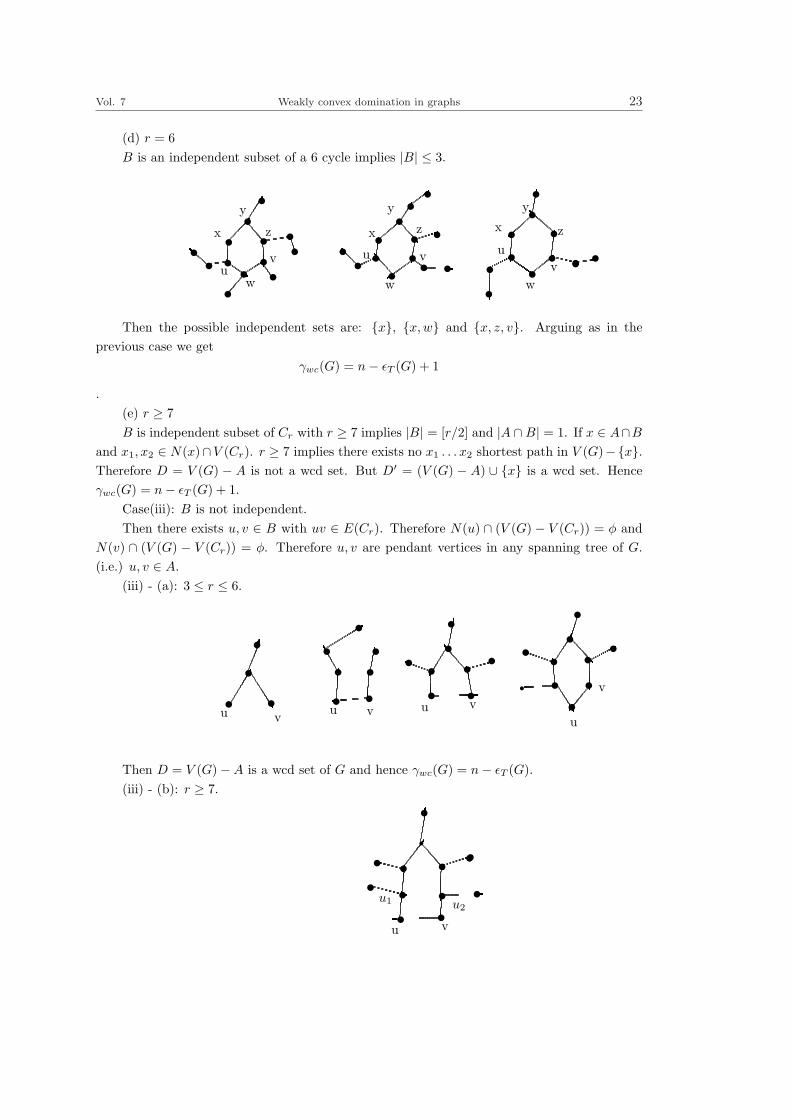
(d) r = 6B is an independent subset of a 6 cycle implies |B| ≤ 3.

tt tt t

t

tt

t

tt

t

t

tt

ttt

t

tt

t

t ttt

tt

tt

t

tt tttt

t

x

y

z

v

wu

x

y

z

v

w

u

xy

z

vw

u

Then the possible independent sets are: {x}, {x,w} and {x, z, v}. Arguing as in theprevious case we get

γwc(G) = n− εT (G) + 1

.(e) r ≥ 7B is independent subset of Cr with r ≥ 7 implies |B| = [r/2] and |A ∩B| = 1. If x ∈ A∩B

and x1, x2 ∈ N(x)∩V (Cr). r ≥ 7 implies there exists no x1 . . . x2 shortest path in V (G)−{x}.Therefore D = V (G) − A is not a wcd set. But D′ = (V (G) − A) ∪ {x} is a wcd set. Henceγwc(G) = n− εT (G) + 1.

Case(iii): B is not independent.Then there exists u, v ∈ B with uv ∈ E(Cr). Therefore N(u) ∩ (V (G) − V (Cr)) = φ and

N(v) ∩ (V (G) − V (Cr)) = φ. Therefore u, v are pendant vertices in any spanning tree of G.(i.e.) u, v ∈ A.

(iii) - (a): 3 ≤ r ≤ 6.

t

t t

t t

t tt

tt

t t

t t tt t

tt tt

tt t

t

t

tt

r

u u v u vu

v

v

Then D = V (G)−A is a wcd set of G and hence γwc(G) = n− εT (G).(iii) - (b): r ≥ 7.

rt t

t tt t

t

tttt t

u v

u1 u2


Then D = V (G) − A is not a wcd set. (since d〈D〉(u1, v1) = 4 > dG(u1, v1) = 3 whereu1 ∈ N(u) and v1 ∈ N(v)). But D′ = (V (G) − A) ∪ {u, v} is a wcd set. Therefore γwc(G) =n− εT (G) + 2.

If G is a graph with δ(G) = 1, then D = V (G) − {u} where deg u = δ is a wcd set of G

(i.e). G has a proper wcd set.

Lemma. If B is a block of a separable graph G with wcd set B′ containing all cut verticesbelonging to B then (V −B) ∪B′ is a wcd set of G.

Proof. Let D = (V −B)∪B′. Then for each u ∈ V −D = V −[(V −B)∪B′] = B−B′ thereexists v ∈ B′ such that uv ∈ E(G) (since B′ is a wcd set of B). Therefore D is a dominatingset of G.

Let x, y ∈ (V −B) ∪B′.

Case I: Every block of G is incident at the same cut vertex. (i.e.) G has exactly one cutvertex, say w. As B′ contains all cut vertices belonging to B, w ∈ B′.

vvw

B

x

y

vv

vw

B

B1

B2

x

y

v

v

fig. 9 fig. 10

B1

I - (a): x, y ∈ V −B.

First, we observe that every x− y shortest path (of G) in 〈(V −B) ∪ {w}〉 has no vertexfrom B − {w} and it may or may not contain w. (i.e.) there exists an x− y shortest path (ofG) in 〈(V −B) ∪ {w}〉 not containing w or containing w. If this x− y shortest path does notcontain w then this path completely lies in 〈V −B〉. If it conains w then this path is containedin 〈(V −B) ∪B′〉.

I - (b): x ∈ V −B and y ∈ B′.

Then the x − w shortest path of G in 〈(V −B) ∪ {w}〉 together with the w − y shortestpath in B′ gives an x− y shortest path of G in 〈(V −B) ∪B′〉.

Case II: G has at least two cut vertices.

II - (a): If B is an end block then B has exactly one cut vertex, say w. Then arguing asin the previous case we get the result.


u v

v

v

v

B

x

y

w

B1

v v

v

v v

B

w

B1B2

xy

v

v

v

v

vx

y

w

B

B1 B2

II - (b): If B is not an end block then B may have more than one cut vertex. Let{w1, w2, . . . , wr} be the set of cut vertices belonging to B. Then {w1, w2, . . . , wr} ⊆ B′.As B′ is a wcd set of B there exists a shortest path connecting any two cut vertices wi

and wj in 〈B′〉. Again, for any two x, y ∈ (V − B), every x − y shortest path (of G) in〈(V −B) ∪ {w1, w2, . . . , wr}〉 has no vertex from B − {w1, w2, . . . , wr} and it may or may notcontain some or all of w1, w2, . . . , wr. (i.e.) there exists an x− y shortest path (of G) in V −B

not containing any of the cut vertices w1, w2, . . . , wr or containing some or all of w1, w2, . . . , wr.II - (b) - (i): x, y ∈ (V −B).If the x−y shortest path has no wi then the x−y shortest path completely lies in 〈V −B〉.

If it contain some or all of wi then the x− y shortest path lies in 〈(V −B) ∪B′〉.II - (b) - (ii): x ∈ (V −B) and y ∈ B′.Then there exists an x − wi shortest path in 〈(V −B) ∪ {wi}〉 for every i. wi, y ∈ B′

implies there exists an wi− y shortest path in 〈B′〉. Hence x−wi− y is an x− y shortest pathin 〈(V −B) ∪B′〉.

In both cases I and II, if x, y ∈ B′ then as B′ is a wcd set of B there exists an x−y shortestpath (of B) which is also an x− y shortest path of G is in B′.

Hence in all cases (V −B) ∪B′ is a wcd set of G.Notation. The length of a longest cycle in G is called the circumference of G and is

denoted by c(G).Definition. In a separable graph G, a block with at most one cut vertex is called an end

block.lemma. If G is a block with 3 ≤ c(G) ≤ 6, then γwc(G) < n.


Proof. Case (i): c(G) = 3.Let Cr be a cycle with r = 3. If G = Cr, then obviously γwc(G) < n. If G 6= Cr then

there exists an edge uv ∈ E(G) such that u ∈ V (Cr) and v ∈ V (G) − V (Cr). Take any otheru′ ∈ V (Cr). Then uv is an edge and u′ is another vertex and G is a block implies there existsa cycle containing uv and u′. But if there exists a cycle containing uvu′ then c(G) > 3 whichis not true. Therefore there cannot exist v ∈ V (G) − V (Cr). (i.e.) G = C3 and D = {u} is awcd set. Hence γwc(G) = 1 < n.

Case (ii): c(G) = 4.G is a block with c(G) = 4 implies diam(G) ≤ 2. If diam(G) = 1, then D = {u} is

a wcd set of G for any u ∈ V (G). If diam(G) = 2, then for any u ∈ V (G), D = N [u] isa wcd set. For if, v ∈ V (G) − N [u] then v cannot be adjacent to u. Therefore v must beadjacent to some v1 ∈ N(u). (otherwise d(v, u) > 2). (i.e.) D is a dominating set. For anyx, y ∈ N [u] there exists x . . . y shortest path in N [u] . (i.e.) D = N [u] is a wcd set. Thereforeγwc(G) ≤ degu + 1 < n.

Case (iii): c(G) = 5.G is a block with c(G) = 5 implies diam(G) ≤ 2. Then G has a proper wcd set as in the

previous case. Therefore γwc(G) < n.Case (iv): c(G) = 6.G is a block with c(G) = 6 implies diam(G) ≤ 3. If diam(G) ≤ 2, then G has a proper

wcd set as in the previous cases. If diam(G) = 3, choose any x, y ∈ V (G) with xy ∈ E(G) andconsider D = V (G) − {x, y}. Then 〈D〉 is connected and D is a dominating set (since G is ablock). Therefore for any u, v ∈ D there exists an u . . . v path in 〈D〉 Suppose there exists nou . . . v shortest path in 〈D〉. Then every u . . . v shortest path must pass through x, y.

®

©ª

®

©ª

r r

r r

u v

x y

D

V −D

Therefore d〈D〉(u, v) > dG(u, x) + dG(x, y) + dG(y, v) > 3. (i.e.) d〈D〉(u, v) ≥ 4. Hencethere will exist a cycle of length at least 7 . . .a contradiction (since c(G) = 6). Therefore thereexists an u . . . v shortest path in D. D is a wcd set. Hence γwc(G) < n

Lemma. If G is a separable graph with δ(G) ≥ 2 and 3 ≤ c(G) ≤ 6, then γwc(G) < n.Proof. c(G) ≤ 6 implies c(B) ≤ 6 for any block B of G. Choose an end block B. Then B

has at most one cut vertex.Case (i): c(B) = 3.In this case B′ = {u} is a proper wcd set of B for any u ∈ V (B) (By the previous lemma).

Choose u to be a cut vertex belonging to B. As B can contain at most one cut vertex, B′ isa proper wcd set containing all cut vertices belonging to B. Therefore D = (V − B) ∪ B′ is awcd set of G. (i.e.) γwc(G) ≤ n− |B −B′| < n.

Case (ii): c(B) = 4.


Then diam(B) ≤ 2. If diam(B) = 1, then B′ = {u} or B′ = NB [u] is a wcd set for B forany cut vertex u ∈ B. (i.e) B′ is a wcd set of B containing all cut vertices belonging to B.Therefore D = (V −B) ∪B′ is a wcd set of G. Hence γwc(G) ≤ n− |B −B′| < n.

Case (iii): c(B) = 5.

Then diam(B) ≤ 2. Then also B′ = {u} or B′ = NB [u] is a proper wcd set for any cutvertex u belonging to B. Hence γwc(G) ≤ |D| ≤ n− |B −B′| < n.

Case (iv): c(B) = 6.

Choose any two vertices x, y ∈ V (B) with xy ∈ E(B) and neither x nor y is a cut vertex.Such an edge exists since B is an end block with δ(G) ≥ 2. Let B′ = V (B)− {x, y}. Then B′

is a wcd set of B containing the cut vertex belonging to B. Therefore D = (V − B) ∪ B′ is awcd set of G. Therefore γwc(G) ≤ |D| ≤ n− |B −B′| < n.

Observation. If G is a block with g(G) = 3 and c(G) ≤ 12 then γwc(G) < n.

Proof. Let C be a cycle of length 3 with V (C) = {u1, u2, u3}.Case (i): N(ui)∩(V (G)−V (C)) = φ for some ui ∈ V (C), i = 1, 2, 3, then D = V (G)−{ui}

is a wcd set of G and hence γwc(G) < n.

Case (ii): N(ui)∩(V (G)−V (C)) 6= φ for each i ∈ {1, 2, 3}. Let v1 ∈ N(u1)∩(V (G)−V (C)).

r

r s

u1

u2u3

rry

x rv1

rv2

C2C1

G is a block implies there exists a cycle C1 containing u1v1(= e) and u2. Also N(u3) ∩(V (G)−V (C)) 6= φ. Let v2 ∈ N(u3)∩ (V (G)−V (C)). Then there exists a cycle C2 containingu1v2 and u3. c(G) ≤ 12 implies l(C1) (or) l(C2) is less than or equal to 6. If l(C2) ≤ 6 thenchoose x, y ∈ V (C2) with xy ∈ E(C2) and x, y 6= {u1, u3}. Then D = V (G) − {x, y} is a wcdset. Hence γwc(G) < n.


Proof. Let C be a cycle of length 4 with V (C) = {u1, u2, u3, u4}.Case (i): N(ui) ∩ (V (G)− V (C)) = φ for some ui ∈ V (C).

Then D = V (G)− {ui} is a wcd set of G and hence γwc(G) < n.

Case (ii): N(ui) ∩ (V (G)− V (C)) 6= φ for each i ∈ {1, 2, 3, 4}. Let v1 ∈ N(u1) ∩ (V (G)−V (C)). G is a block implies there exists a cycle C1 containing e = u1v1 and u2.

r s

r r

u1

u2u3

u4

C1C2

sv′1s rxy

N(u4) ∩ (V (G)− V (C)) 6= φ implies there exists v′1 ∈ N(u4) ∩ (V (G)− V (C)). Thereforethere exists a cycle C2 containing u4v

′1 and u3. c(G) ≤ 13 implies l(C1) or l(C2) ≤ 6. Let


l(C2) ≤ 6. Then D = V (G) − {x, y} for any two x, y ∈ V (C2) with xy ∈ E(C2) and x, y /∈{u4, u3} is a wcd set. Therefore γwc(G) < n.

Observation. If G is block with g(G) = 5 and c(G) ≤ 14, then γwc(G) < n.

Proof. Let C be a cycle of length 5 with V (C) = {u1, u2, u3, u4, u5}.Case (i): N(u)∩ (V (G)−V (C)) = φ and N(v)∩ (V (G)−V (C)) = φ for some u, v ∈ V (C)

with uv ∈ E(C) then, D = V (G)− {u, v} is a wcd set. Therefore γwc(G) < n.

Case (ii): N(u)∩ (V (G)− V (C)) = φ and N(v)∩ (V (G)− V (C)) = φ for no two adjacentvertices u, v ∈ V (C). Let N(u5)∩ (V (G)− V (C)) = φ. Then N(u1)∩ (V (G)− V (C)) 6= φ andN(u4) ∩ (V (G) − V (C)) 6= φ. Let v1 ∈ N(u1) ∩ (V (G) − V (C)). G is a block implies thereexists a cycle C1 containing e = u1v1 and u2. N(u4)∩ (V (G)− V (C)) 6= φ implies there existsv′1 ∈ N(u4) ∩ (V (G)− V (C)).

rr

sr r

u5

u1

u2u3

C1rr

x

yrv1rv′1

C2u4

Therefore there exists a cycle C2 containing u4v′1 and u3. c(G) ≤ 14 implies l(C1) or

l(C2) ≤ 6. Let l(C2) ≤ 6. Then D = V (G)−{x, y} for any two x, y ∈ V (C2) with xy ∈ E(C2)and x, y ∈ {u4, u3} is a wcd set. Therefore γwc(G) < n.


Proof. Let C be a cycle of length 6 with V (C) = {u1, u2, u3, u4, u5, u6}.Case (i): N(u)∩ (V (G)−V (C)) = φ and N(v)∩ (V (G)−V (C)) = φ for some u, v ∈ V (C)

with uv ∈ E(C), then, D = V (G)− {u, v} is a wcd set. Therefore γwc(G) < n.

Case (ii): N(u)∩ (V (G)− V (C)) = φ and N(v)∩ (V (G)− V (C)) = φ for no two adjacentvertices u, v ∈ V (C). Let N(u6)∩ (V (G)− V (C)) = φ. Then N(u1)∩ (V (G)− V (C)) 6= φ andN(u5) ∩ (V (G)− V (C)) 6= φ.

Let v1 ∈ N(u1) ∩ (V (G)− V (C)). G is a block implies there exists a cycle C1 containinge = u1v1 and u2.

rr rr r

r

C1C2

u1

u2

u3

u4

u5

u6

N(u5) ∩ (V (G)− V (C)) 6= φ implies there exists v′1 ∈ N(u5) ∩ (V (G)− V (C)). Thereforethere exists a cycle C2 containing u5v

′1 and u4. c(G) ≤ 14 implies l(C1) or l(C2) ≤ 6. Let

l(C2) ≤ 6. Then D = V (G) − {x, y} for any two x, y ∈ V (C2) with xy ∈ E(C2) and x, y ∈{u4, u5} is a wcd set. Therefore γwc(G) < n.

Definition.[7] A graph G is distance-hereditary if for all connected induced subgraphs F

of G, dF (u, v) = dG(u, v) for all u, v ∈ V (F ).


Observation. For every distance hereditary graph G, γwc(G) < n.Proof. Consider any spanning tree TG of TG. Then 〈V (TG)−A〉 where A is the set of

all pendant vertices of TG is distance preserving. (i.e.) d〈V (TG)−A〉(x, y) = dG(x, y) for allx, y ∈ V (TG)−A. Therefore for every x, y ∈ V (TG)−A there exists an x . . . y shortest path in〈V (TG)−A〉. Also V (TG)−A is a dominating set. Hence γwc(G) < n

CHARACTERIZATIONS

We use the following notations throught the remaining discussion.Notation. TG denote any spanning tree of G.A - denote the set of all pendant vertices in TG.T ′G denote the subtree obtained by deleting all pendant vertices from TG. (i.e.) T ′G =

TG −A.T ′′G denote the subtree obtained by deleting a proper subset A′ ⊂ A from TG. (i.e.)

T ′′G = TG −A′.〈V (T ′G)〉 denote the subgraph of G induced by V (T ′G).〈V (T ′′G)〉 denote the subgraph induced by V (T ′′G).Definition. A subset V (H) of V (G) is said to be distance preserving if d〈V (H)〉(x, y) =

dG(x, y) for all x, y ∈ V (H).Remark. If G has a wcd set D, then for every x, y ∈ D there exists an x . . . y shortest

path in 〈D〉. d〈D〉(x, y) = dG(x, y) for all x, y ∈ D and hence D is distance preserving.Example.

ppr r r

s r r r s r

r

r r r

1

2 7 5

310

68 9 4

1

2 7 5

TG :G : T ′G :1

2

34

5 6 7

910

s

s

sr

r rr

rrr 8

Here A = {3, 8, 10, 9, 4, 6} dT ′G(x, y) = dG(x, y) for all x, y ∈ V (T ′G).

Example.

2

3

r

ss

t r sst

rr

4

5

6 810 9

7t

tt

ts

u t strr

s

u s su

r t ut

G : TG : T ′G < V (T ′G >

1

2 7 5

38 10

9 46

1

2 5

1

2 57 7

1t


dT ′G(2, 7) = 2 6= dG(2, 7) = 1. Therefore dT ′G(x, y) 6= dG(x, y) for all x, y ∈ V (T ′G). Butd〈V (T ′G)〉(x, y) = dG(x, y) for all x, y ∈ 〈V (T ′G)〉 and hence 〈V (T ′G)〉 is a distance preservingsubgraph.

Example.

s

ss u

tu

ss ruuu

rs

stt s t

uu

tuu

ss sr t

s s

t

tt

t ss

st

1

2

3

11

4

5 6 7

8

910

1

2 7 5

3 8 910 4 6

11

1

27 5

8 10 4

1

27 5

8 10 4

G : TGT ′G T ′′G

Here A = {3, 8, 9, 10, 11, 6}. dT ′G(x, y) 6= dG(x, y) for all x, y ∈ V (T ′G) (since dT ′G(4, 7) = 3and dG(4, 7) = 2). A′ = {3, 9, 11, 6} then A′ ⊂ A. T ′′G is not distance preserving. But 〈V (T ′′G)〉is distance preserving.

Observation. If δ(G) = 1 then γwc(G) < n as D = V (G) − {u ∈ V (G)/degu = 1} is awcd set.

Observation. If G is a graph with δ(G) ≥ 2, then γwc(G) < n if and only if G is a treeor G has a spanning tree TG satisfying one of the following three conditions:

(i) TG has a subtree T ′G such that dT ′G(x, y) = dG(x, y) for all x, y ∈ V (T ′G).(ii) TG has a subtree T ′G such that 〈V (T ′G)〉 is distance preserving.(iii) TG has a subtree T ′′G such that 〈V (T ′′G)〉 is distance preserving.Proof. γwc(G) < n implies that there exists a proper wcd set D. Then D is a dominating

set with 〈D〉 is connected and distance preserving. 〈D〉 is connected implies 〈D〉 has a spanningtree T〈D〉. Hence D = V (T〈D〉) and each vertex in V −D is adjacent to some vertex in V (T〈D〉).Deleting the edges in 〈V −D〉 we get a spanning tree TG of G. (i.e.) there exists a spanningtree TG of G such that D = V (TG) − A′ where A′ ⊆ A and 〈D〉 = 〈V (TG)−A′〉 is distancepreserving.

Case (I): 〈D〉 = 〈V (TG −A′)〉 = T ′G with T ′G is distance preserving and A = A′.I - (i): 〈A〉 is independent.If u ∈ A then there exists u1 ∈ D = V (T ′G) such that uu1 ∈ E(G). δ(G) ≥ 2 implies there

exists u2(6= u1) ∈ V (G) such that u2 ∈ N(u). A is independent implies u1, u2 ∈ D = V (T ′G).Therefore there exists an u1 . . . u2 shortest path in 〈D〉 = T ′G. (i.e.) there exists an u1 . . . u2

shortest path in the subtree T ′G.Therefore if u, v ∈ A then |N(u) ∩ V (T ′G)| > 1 and |N(v) ∩ V (T ′G)| > 1. Hence if u1 ∈

|N(u) ∩ V (T ′G)| > 1 and v1 ∈ |N(v) ∩ V (T ′G)| > 1 then there exists an u1 . . . v1 shortest path inT ′G. (i.e) every shortest path connecting u snd v should pass through the points of T ′G and T ′G isa distance preserving subtree. Therefore dTG

(u, v) = dG(u, v) for all u, v ∈ A. T ′G is a distancepreserving subtree implies dT ′G(x, y) = dG(x, y) for all x, y ∈ V (T ′G). Hence dTG

(x, y) = dG(x, y)for all x, y ∈ V (G). (i.e.) TG is a distance preserving spanning tree of G. Hence no two pendant


vertices of TG are adjacent in G (since if u, v are pendant vertices in TG with uv ∈ E(G) then1 = dG(u, v) < dTG

(u, v)). T ′G is distance preserving implies no two pendant vertices of T ′G areadjacent in G. Similarly no two pendant vertices in the tree obtained by removing the pendantvertices of T ′G are adjacent. Proceeding like this we get G as an acyclic connected graph. HenceG is a tree.

I - (ii): 〈A〉 is not independent.〈A〉 is not independent implies there exist at least two adjacent vertices u, v in 〈A〉. Then

dTG(u, v) > dG(u, v) = 1. (i.e.) TG is not distance preserving. But T ′G is distance preserving.

Hence G has a spanning tree TG with distance preserving subtree T ′G. Hence condition (ii) issatisfied.

Case (II): D = V (T ′G) and T ′G is not distance preserving. A′ may or may not be independentand A = A′.

〈D〉 = 〈V (TG)−A〉 = 〈V (TG′)〉 is distance preserving. (i.e.) G has a spanning tree TG

with a subtree T ′G such that the subgraph induced by V (T ′G) is distance preserving. Hencecondition (iii) is satisfied.

Case (III): T ′G is not distance preserving and A′ ⊂ A and A′ may or may not be independent.Then 〈D〉 = 〈V (TG)−A′〉 is distance preserving. (i.e) 〈V (T ′′G)〉 is distance preserving.

(i.e.) G has a spanning tree TG with subtree T ′′G such that 〈V (T ′′G)〉 is distance preserving.Hence condition (iv) is satisfied.

Conversely, suppose G is a tree or G has a spanning tree TG satisfying one of the conditions(i) to (iii).

If G is a tree then D = V (G)−A where A is the set of all pendant vertices of G is a wcdset of G.

If G has a spanning tree TG satisfying condition (i) or (ii) then D = V (TG) − A is a wcdset of G.

If G has a spanning tree TG satisfying condition (iii) then D = V (TG)−A′ is a wcd set ofG.

Hence γwc(G) < n in all cases.

CONSTRUCTION OF A GRAPH G WITH γwc(G) < n.

Observation. γwc(G) < n if and only if G can be constructed as follows:Take any connected graph H.(i) Attach one or more pendant vertices at each (or at some) vertices of H.(ii) Identify an edge of a 3 cycle at each (or some) edges of H.(iii) Identify two consecutive edges of a 4 cycle at each (or some) paths of length 2 in H.(iv) Do any one or both of the two operations (i) and (ii) at each (or some) vertices of H

and do operation.(iii) At each (or at some) paths of length 2 in H.(v) Attach one or more triangles at each (or at some) vertices of V (H).(vi) Identify an edge of a 4 cycle at each (or some) edge of H.(vii) Identify two consecutive edges of a 5 cycle at each (or some) paths of length 2 in H.


(viii) Identify three consecutive edges of a 6 cycle at each (or some) paths of length 3 inH.

(ix) Do any one of the operations (v) to (viii) at each (or some) vertex, edge, paths oflength 2 or 3.

(x) Do all (or some) of the operations (i) to (ix) at each (or some) vertex, edge, paths oflength 2, paths of length 3.

(xi) Take any two connected graphs H and H ′ with V (H) = {u1, u2, . . . , ur} and V (H ′) ={v1, v2, . . . , vs}. First join v1 to u1. Join each vi ∈ NH′(v1) to u1 or to all or some verticeswhich are at distance atmost 3 from u1 in H. (i.e.) each vi ∈ NH′(v1) can be joined to u1 orto all or some ui with dH(u1, ui) ≤ 3. Do the same operation for each vj ∈ N(vi) and repeatthis process until each vi is joined to some ui.

(xii) Take any connected graph H and any number of connected graphs {H ′i} and perform

the operation (xi) to each H ′i.

Proof. Let γwc(G) < n and let D be a γwc set of G. Then 〈D〉 is connected and distancepreserving.

Case (i): δ(G) = 1 and 〈V −D〉 is independent.

Hence in this case G can be obtained by taking H = 〈D〉 and attaching one or morependant vertices at each or some vertices of H.

Case (ii): δ(G) ≥ 2 and 〈V −D〉 is independent.

δ(G) ≥ 2 and 〈V −D〉 is independent implies for every u ∈ V −D, |N(u) ∩D| ≥ 2. Letu1, u2 ∈ N(u) ∩ D. Then d(u1, u2) ≤ 2. 〈D〉 is a wcd set implies there exists an u1 . . . u2

shortest path of length ≤ 2 in 〈D〉.

t s

t

s ts

t s s r

ts

s s

uu

u1 u2

Therefore, G can be obtained by taking a connected graph 〈D〉 and performing one of theoperations (ii) to (iv).

Case (ii): The components of 〈V −D〉 are K2 alone.

For any two u, v ∈ V −D with uv ∈ E(G) both of them may be adjacent to a same vertexor adjacent to two different vertices in D. If each pair of adjacent vertices in V −D are adjacentto the same vertex in D then in this case G can be obtained by taking H = 〈D〉 and performingthe operation (v). If there exists u, v ∈ V −D with uv ∈ E(G) and adjacent to two differentvertices u1 and v1 respectively in D, then d(u1, v1) ≤ 3. D is a wcd set implies there exists anu1 . . . v1 shortest path of length ≤ 3 in 〈D〉.

rqpu s

tt t s

sstr rt r

rs r

u v u v

u1 v1

s st

s ss t tss t s

ss ts

u qs s s t

u v

u1 v1

u v

u1 v1s r


Therefore, G can be obtained by taking a connected graph H = 〈D〉 and performing oneof the operations (v) to (ix).

Case (iii): The components of 〈V −D〉 are isolates and K2s.In this case G can be obtained by taking H = 〈D〉 and performing the operation (ix).Case (iv): 〈V −D〉 is connected.In this case, G can be obtained by taking H = 〈D〉 and performing one of the operations

(x).Case (v): 〈V −D〉 is disconnected and has more than one connected components.In this case, G can be obtained by taking H = 〈D〉 and performing operation (xi) to each

connected graph H ′i.

Lemma. If G is any simple graph with n ≥ 3 and δ(G) ≥ n/2 then γwc(G) < n.Proof. For any vertex u of degree δ consider D = N [u]. Then any v ∈ V − D must

be adjacent to some ui ∈ N(u), since v is not adjacent to u. Otherwise δ(G) ≤ deg v ≤n − 1 − |N(u)| = n − 1 − δ ≤ n − 1 − n/2 < n/2 . . . a contradiction to the fact that δ ≥ n/2.Therefore, each v ∈ V − D is adjacent to some ui ∈ N(u) and hence D is a dominating set.And D = N [u] implies d〈D〉(x, y) = d〈G〉(x, y) for all x, y ∈ D. (i.e.) D is a wcd set and henceγwc(G) < n.

Corollary. If γwc(G) = n then δ(G) < n/2.Proof. For if δ(G) ≥ n/2 then by the previous lemma γwc(G) < n . . . a contradiction

(since γwc(G) = n).Lemma. If δ(G) ≥ n/2, then γwc(G) ≤ δ + 1 or γwc(G) = 2.Proof. δ(G) ≥ n/2 implies G is Hamiltonian [6]. And m = 1/2

∑deg u = n2/4. Therefore,

G is pancyclic (or) G is Kn/2,n/2[6]. If G is pancyclic, then D = N [u] is a wcd set with deg

u = δ. Therefore, γwc(G) ≤ δ + 1. If G is Kn/2,n/2 then γwc(G) = 2.Observation. γwc(G) = n if and only if G is not a tree and for every spanning tree TG

and for every subset A′ ⊆ A there exists at least one pair of points x, y ∈ V (TG)−A′ such thatd〈V (TG)−A′〉(x, y) > dG(x, y).

Proof. Let γwc(G) = n. Then G cannot be a tree. If there exists a spanning tree TG anda set of pendant vertices A′ ⊆ A such that for every x, y ∈ V (TG) − A′, d〈V (TG)−A′〉(x, y) ≤dG(x, y) then D = V (TG)−A′ is a proper wcd set of G . . . a contradiction.

Conversely, suppose G is not a tree and for every spanning tree TG and for every subsetA′ ⊆ A there exists at least one pair of points x, y ∈ V (TG)−A′ such that d〈V (TG)−A′〉(x, y) >

dG(x, y). Let if possible γwc(G) < n. Then G is a tree (or) has a spanning tree TG with a set ofpendant vertices A′ ⊆ A such that for every pair of points x, y ∈ V (TG)−A′, d〈V (TG)−A′〉(x, y) =dG(x, y) (by observation (12) . . . a contradiction).

Observation. γ(G) = γwc(G) if and only if G is a caterpillar (or) G has a spanning treeTG with maximum number of pendant edges εT (G) satisfying one of the two conditions (a) or(b) and both the coditions (c) and (d).

(a) TG has a distance preserving subtree T ′G.(b) TG has a subtree T ′G with 〈V (T ′G)〉 is distance preserving.(c) Each u ∈ V (G) is either a support or a pendant vertex in TG.(d) The domination number of G is the number of supports in TG.


Proof. Let γ(G) = γwc(G) and let D be a γwc set. Then D is a connected dominatingset. Therefore, γc(G) ≤ γwc(G) = γ(G). But γ(G) ≤ γc(G) ≤ γwc(G). Therefore, γc(G) =γwc(G) = γ(G). γc(G) = n − εT (G) where εT (G) [11] is the number of pendant vertices in aspanning tree of G with maximum number of pendant edges. Therefore, n− εT (G) = γc(G) =γwc(G) = γ(G) . . . .

(i) G has a proper wcd set. Therefore, G is a tree or has a spanning tree TG satisfying oneof the three conditions of observation 12. (i.e.) G is a tree or there exists a spanning tree TG

such that D = V (TG)−A′ for some A′ ⊆ A with 〈V (TG)−A′〉 is distance preserving.(ii) |D| = γwc(G) = γ(G) implies N(u) ∩ (V − D) 6= φ for each u ∈ D (since D is a

minimum dominating set and G is connected).(iii) By (i) and (ii) n − εT (G) = |D| = |V (TG)−A′|. Therefore |A′| = εT (G). (i.e)

εT (G) = |A′| ≤ |A| ≤ εT . Hence εT (G) = |A′| = |A|. (i.e.) G is a tree or has a spanningtree TG with maximum number of pendant edges equal to |A′| and 〈D〉 = 〈V (TG)−A′〉 =〈V (TG)−A〉 is distance preserving. Hence by (iii) each u ∈ D = V (TG) − A is a support andeach u ∈ V −D = A is a pendant vertex in TG. (i.e.) G is a tree or G has a spanning tree TG

with distance preserving subtree T ′G (or) has a subtree T ′G with 〈V (T ′G)〉 is distance preserving.(ie) G is a tree (or) satisfies one of the two conditions (a) and (b).

If u ∈ V (G) then either u ∈ D (or) u ∈ V −D. (i.e.) either u is a support (or) a pendantvertex in G (or) TG. Hence, if G is a tree then G is a caterplillar. If G is not a tree then TG

satisfy condition (c). γ(G) = γwc(G) = |D| = number of supports in TG. Hence condition (d)is satisfied.

Conversely, suppose G is a tree or has a spanning tree satisfying one of the two conditions(a) or (b) and both the coditions (c) and (d).

If G is a tree and satisfying conditions (c) and (d), then D = V (G)−A where A is the setof all pendant vertices is a wcd set and hence γwc(G) ≤ |D|. G satisfies conditions (c) and (d)implies each u ∈ D = V (G) − A is a support and γ(G) = |D|. Hence γwc(G) ≤ |D| = γ(G).(i.e.) γ(G) = γwc(G).

If G satisfies conditions (a), (c) and (d), then 〈D〉 = 〈V (TG)−A〉 = T ′G is a distancepreserving subtree of TG with A as the set of all pendant vertices of TG. (i.e) D is a wcd set andhence γwc(G) ≤ |D|. That TG satisfies condition (c) and (d) implies each u ∈ D = V (TG)− A

is a support and γ(G) = |D|. Hence γwc(G) ≤ |D| = γ(G). (i.e.) γ(G) = γwc(G).If G satisfy conditions (b), (c) and (d), then 〈D〉 = 〈V (TG)−A〉 = 〈V (T ′G)〉 is distance

preserving. (i.e) D is a wcd set and hence γwc(G) ≤ |D|. TG satisfy conditions (c) and (d)implies each u ∈ D = V (TG) − A is a support and γ(G) = |D|. Hence γwc(G) ≤ |D| = γ(G).(i.e.) γ(G) = γwc(G).

CONSTRUCTION OF GRAPHS WITH γ(G) = γwc(G).

Observation. γ(G) = γwc(G) if and only if G is a caterpillar (or) G can be obtained asfollows:

Take any connected graph which is not a path H and consider a spanning tree TH of H withmaximum number of pendant edges. Let {u1, u2, . . . , ur} be the set of pendant vertices of TH .Attach one or more pendant vertices at each u ∈ V (G)−{u1, u2, . . . , ur} and let {v1, v2, . . . , vs}be the set of pendant vertices thus attached and TG be the resulting tree.


If u ∈ N(vi) ∩ V (H) then vi can be joined to each or some v ∈ V (H) with dH(u, v) ≤ 2.Any two vis can be joined if both of them are adjacent to a same vertex in H. Join vi and vj

if dH(u, v) ≤ 3 where u ∈ N(vi) ∩ V (H) and v ∈ N(vj) ∩ V (H).Proof. Let γ(G) = γwc(G). Then, by the previous observation, G is a caterpillar (or) G

has a spanning tree TG satisfying conditions (a) (or) (b) and both the conditions (c) and (d).Let H = 〈V (T ′G)〉 - the set of pendant vertices of T ′G. Then H satisfy the required conditions.

Conversely, if G is constructed by the above method then let D = V (H)−{u1, u2, . . . , ur}.Then TG is a spanning tree of G with maximum number of pendant edges and D is a wcd set.Hence γwc(G) ≤ |D| = n− εT . Therefore γwc(G) = n− εT ≤ γ(G). (i.e.) γ(G) = γwc(G).

Observation. γc(G) = γwc(G) if and only if G is a tree or has a spanning tree TG withmaximum number εT of pendant edges satisfying one of the following two conditions:

(i) TG has a distance preserving subtree T ′G.(ii) TG has a subtree T ′G such that 〈V (T ′G)〉 is distance preserving.Proof. Let γc(G) = γwc(G). If D is a γwc set then G satisfy one of the four conditions

of observation 12. (i.e.) G is a tree (or) 〈D〉 = 〈V (TG)−A′〉 where A′ ⊆ A and 〈D〉 isdistance preserving. n− εT = γc(G) = γwc(G) = |D| = |V (TG)−A′| = n− |A′| which impliesεT = |A′| ≤ |A| ≤ εT . Therefore εT = |A′| = |A|. (i.e.) TG is a spanning tree of G withmaximum number of pendant edges. Hence G has a spanning tree TGwith maximum numberof pendant vertices satisfying one of the two conditions.

Conversely, if G is a tree then γc(G) = γwc(G).If G has a spanning tree with maximum number of pendant edges satisfying one of the

two conditions then D = V (TG) − A is a wcd set with |A| = εT and hence γwc(G) ≤ |D| =|V (TG)−A| = n− |A| = n− εT = γc(G). Hence γc(G) = γwc(G).

CONSTRUCTION OF A GRAPH WITH γc(G) = γwc(G).

γc(G) = γwc(G) if and only if G is either G1 (or) G2 which are obtained as follows:Take any connected graph H and consider a spanning tree TH with maximum number of

pendant edges and let B = {u1, u2, . . . , ur} be the set of pendant vertices of TH . Attach one ormore pendant vertices at each ui, 1 ≤ i ≤ r. Let A = {v1, v2, . . . , vs} with s ≥ r be that set ofpendant vertices thus attached. Let G1 be the resulting graph.

In G1 connect vi ∈ N(ui) and vj ∈ N(uj) by a path such that d(ui, uj) ≤ d(vi, vj) and letG2 be the resulting graph.

Proof. Let γc(G) = γwc(G). Then by the previous observation G is a tree or G has aspanning tree satisfying the two conditions.

If G is a tree then G is of the form G1.If G has a spanning tree TG with maximum number of pendant edges and a distance

preserving subtree T ′G, then 〈D〉 = 〈V (TG)−A〉 = T ′G. Let A = {v1, v2, . . . , vs}. Now letB = {u1, u2, . . . , ur} be the set of pendant vertices of T ′G. In this case 〈A〉 is not independent.Therefore G can be obtained by taking a tree and attaching one or more triangles at each ui,1 ≤ i ≤ r. (i.e.) G is of the form G2.

If G has a spanning tree TG with maximum number of pendant edges and a subtree T ′G,with 〈V (T ′G)〉 is distance preserving. Then 〈D〉 = 〈V (TG)−A〉 = T ′G. Let A = {v1, v2, . . . , vs}


and let B = {u1, u2, . . . , ur} be the set of pendant vertices of T ′G. Then T ′G is a spanning treeof 〈D〉 with maximum number of pendant edges. For if there exists any other spanning treeT ′〈D〉 of 〈D〉 with t number of pendant vertices and t > r. Each vi is adjacent to some vertex inT ′〈D〉. t > r implies there exists a spanning tree T1G of G with more number of pendant verticesthan the number of pendant vertices in TG which is a contradiction to the fact that TG is aspanning tree with maximum number of pendant vertices.

Now let 〈D〉 = H. If vi ∈ N(ui) then d(ui, uj) ≤ d(vi, vj) (since D is a wcd set).If 〈V −D〉 is independent then G is of the form G1.If 〈V −D〉 is not independent then G is of the form G2.Conversely, suppose G is of the form G1 or G2.Then let D = V (H). By construction γc(G) = n− εT (G) = |V (H)| = |D| and D is a wcd

set. Therefore γwc(G) ≤ |D| = γc(G). Hence γc(G) = γwc(G).Definition. For any connected graph G we define,εmax = Max

{|A′| /A′ ⊆ A, d〈V (TG)−A′〉(x, y) = dG(x, y),∀x, y ∈ V (TG)−A′}, where A is

the set of all pendant vertices in a spanning tree TG of G.Observation. γwc(G) ≤ n− εmax.

Observation. If G is a block with proper wcd set then γwc(G) = n− εmax.Proof. If D is a γwc set of G, then D = V (TG) − A′ with A′ ⊆ A. Therefore γwc(G) =

|D| = |V (TG)−A′| ≥ n − εmax (since |A′| ≤ εmax). Therefore by the previous observationγwc(G) = n− εmax.

References

[1] Acharya. B. D., Purnima Gupta, On Point - set domination in graphs, Proc. Nat.Seminar on Recent Development in Mathematics, N. M. Bujurke (Ed.), Karnataka UniversityPress, Dharwad, 1996, 106-108.

[2] Acharya. B. D., Purnima Gupta, On Point - set dominiation in graphs: II minimumpsd - sets, J. Combin. Theory Ser. B, 1996.

[3] Acharya. B. D., Purnima Gupta, On Point set domination in graphs: III Further detailssubmitted.

[4] Acharya. B. D., Purnima Gupta, On Point set domination in graphs: IV Seperablegraphs with unique minimum psd-sets, Discrete Mathematics, 195(1999), 1-13.

[5] S. Arumugam and R. Kala, Domination Parameters of a star Graph, ARS Combinatoria,44(1996), 93-96.

[6] Balakrishnan. R., Ranganathan. K., A text book of Graph Theory, Springer Verlag,New York, 2000.

[7] Fred Buckley, Fred Harary, Distance in Graphs, Addission - Wesley Publishing Com-pany, 1990.

[8] Gary Chartrand, Curtiss E. Wall and Ping Zhamg, The convexity Number of a Graph,Graphs and Combinatorics, 18(2002), 209-217.

[9] Gary Chartrand, Frank Harary, Henda C. Swart, Geodomination in Graphs, Bulletinof the ICA, 31(2001), 51-59.


[10] F. Harary, Graph Theory, Addison - Wesley, 1969.[11] T. Haynes, S. T. Hedetniemi and P. J. Slater, Advances in the Theory of Domination

in Graphs, Marcel Dekker Incl, New York, 1997.[12] S. M. Hedetniemi, S. T Hedetniem, D. F. Rall, Acyclic domination, Discrete Mathe-

matics, 222(2000), 151-165.[13] V. R Kulli and B. Janakiram, The Non Split domination number of a graph, Indian

J. Pure appl. Math, 2000, 441-447.[14] Parthasarathy. K. R., Basic Graph Theory, Tat McGraw-Hill Publishing Company

Limited, 1994.[15] Sampathkumar. E., Point set domination Number of a graph, Indian J. Pure Appl.

Math., 4(1993), 225-229.[16] E. Sampathkumar (Ed.), Graph Theory Research Report, Karnatak University, Dhar-

wad, No. 3, 1972.[17] H. B. Walikar, B. D. Acharya and E. Sampathkumar, Recent Advances in the theory of

domination in graphs and its applications, MRI Lecture Notes in Mathematics, Mehta ResearchInstitute of Mathematics and Mathematical Physics, Allahabad, No. 1, 1979.

[18] Wayne Goddard and Michael A. Henning, Domination in planar Graphs with smallDiameter, Journal of Graph Theory, 2002, 1-25.


New hybrid filtering techniques for removal of

speckle noise from ultrasound medical images

Gnanambal Ilango† and R. Marudhachalam‡

† Post Graduate and Research Department of Mathematics,Government Arts College (Autonomous),

Coimbatore 641018, Tamilnadu, India‡ Department of Mathematics, Kumaraguru College of Technology,

Coimbatore 641006, Tamilnadu, IndiaE-mail: [email protected] [email protected]

Abstract The most significant feature of diagnostic medical images is to reduce speckle noise

which is commonly found in ultrasound medical images and make better image quality. In

recent years, technological development has improved significantly in analyzing medical imaging.

This paper proposes different hybrid filtering techniques for the removal of speckle noise, from

ultrasound medical images, by topological approach. The filters are treated in terms of a finite

set of certain estimation and neighborhood building operations. A set of such operations is

suggested on the base of the analysis of a wide variety of nonlinear filters described in the

literature. The quality of the enhanced images is measured by the statistical quantity measures:

Root Mean Square Error (RMSE) and Peak Signal-to-Noise Ratio (PSNR).

Keywords Digital topological neighborhood, ultrasound image, speckle noise, RMSE, PSNR.

§1. Introduction

Ultrasound imaging is widely used in the field of medicine. It is used for imaging soft tis-sues in organs like liver, kidney, spleen, uterus, heart, brain etc. Ultrasound or ultrasonographyis a medical imaging technique that uses high frequency sound waves and their echoes. It allowsone to visualize and therefore examine a part of the human anatomy in medicine. It is a widelyused medical imaging procedure because it is economical, comparatively safe, transferable, andadaptable. A major disadvantage with ultrasound imaging is the presence of noise, which per-turbs feature location and creates artifacts. The acquired image is corrupted by a randomgranular pattern, called speckle, which delays the interpretation of the image content. The ex-istence of speckle is unattractive because of its disgrace image quality and it affects the tasks ofindividual interpretation and diagnosis. Accordingly, speckle filtering is a central preprocessingstep for feature extraction, analysis, and recognition of medical imagery measurements. Previ-ously, a number of schemes have been proposed for speckle mitigation. Median filter has beenintroduced by Tukey [14] in 1970. It is a special case of non-linear filters used for smoothingsignals. Median filter now is broadly used in reducing noise and smoothing the images. Hakan

Vol. 7 New hybrid filtering techniques for removal of speckle noise from ultrasound medical images 39

et al.[4] have used Topological Median filter to improve conventional Median filter. The betterperformance of the Topological Median filters over conventional Median filters is in maintainingedge sharpness. Yanchun et al.[16] proposed an algorithm for image denoising based on Aver-age filter with maximization and minimization for the smoothness of the region, unidirectionalMedian filter for edge region and Median filter for the indefinite region. It was discovered thatwhen the image is corrupted by both Gaussian and impulse noises, neither Average filter norMedian filter algorithm will obtain a result good enough to filter the noises because of theiralgorithm. Sudha et al.[12] recommend a novel thresholding algorithm for denoising speckle inultrasound with wavelets. An improved adaptive median filtering method for denoising impulsenoise reduction was carried out by Mamta Juneja et al.[6] An adaptive median filter (AMF)is the best filter to remove salt and pepper noise of image sensing was shown by Salem SalehAl-amri et al.[10]. Thangavel et al.[13] showed that the M3-filter performed better than meanfilter, median filter, max filter, min filter and various other filters. The objective of this studywas to develop new hybrid speckle reduction techniques and investigate their performance onUltrasound images.

This work is organized as follows: Section 2 discusses types of noises involved in medicalimaging. In Section 3 basic definitions are introduced. Section 4 discusses the various existingfiltering techniques for de-noising the speckle noise in the ultrasound medical image. Section 5deals with proposed hybrid filtering techniques for de-noising the speckle noise in the ultrasoundmedical images. In Section 6, both quantitative (RMSE & PSNR) and qualitative comparisonshave been provided. Section 7 puts forward the conclusion drawn by this paper.

§2. Types of noises

§2.1. Salt and pepper noise

Salt and pepper noise is a form of noise typically seen on images. It represents itself asrandomly occurring white and black pixels. A spike or impulse noise drives the intensity valuesof random pixels to either their maximum or minimum values. The resulting black and whiteflecks in the image resemble salt and pepper. This type of noise is also caused by errors in datatransmission.

§2.2. Speckle noise

Speckle noise affects all inherent characteristics of coherent imaging, including medicalultra sound imaging. It is caused by coherent processing of backscattered signals from multipledistributed targets. Speckle noise is caused by signals from elementary scatterers. In medicalliterature, speckle noise is referred to as texture and may possibly contain useful diagnosticinformation. For visual interpretation, smoothing the texture may be less desirable. Physiciansgenerally have a preference for the original noisy images, more willingly, than the smoothedversions because the filter, even if they are more sophisticated, can destroy some relevant imagedetails. Thus it is essential to develop noise filters which can preserve the features that are ofinterest to the physician. Several different methods are used to eliminate speckle noise, based

40 Gnanambal Ilango and R. Marudhachalam No. 1

upon different mathematical models of the phenomenon. In our work, we recommend hybridfiltering techniques for removing speckle noise in ultrasound images. The speckle noise modelhas the following form (‘·’ denotes multiplication). For each image pixel with intensity valuefij (1 ≤ i ≤ m, 1 ≤ j ≤ n for an m× n image), the corresponding pixel of the noisy image gij

is given by,gi,j = fi,j + fi,j · ni,j . (1)

Where each noise value n is drawn from uniform distribution with mean 0 and varianceσ2.

§2.3. Gaussian noise

Gaussian noise is a statistical noise that has a probability density function (abbreviatedpdf) of the normal distribution (also known as Gaussian distribution). In other words, the valuesthat the noise can take on are Gaussian-distributed. Gaussian noise is properly defined as thenoise with a Gaussian amplitude distribution. Noise is modeled as additive white Gaussian noise(AWGN), where all the image pixels deviate from their original values following the Gaussiancurve. That is, for each image pixel with intensity value fij (1 ≤ i ≤ m, 1 ≤ j ≤ n for an m×n

image), the corresponding pixel of the noisy image gij is given by,

gi,j = fi,j + ni,j , (2)

where each noise value n is drawn from a zero-mean Gaussian distribution.

§3. Basic definitions

This section presents some general definitions and digital topological results, which will beused along the development of this paper.

Definition 3.1.[9] A digital image is a function f : Z × Z → [0, 1, . . . , N − 1] in whichN−1 is a positive whole number belonging to the natural interval [1, 256]. The functional valueof ‘f ’ at any point p(x, y) is called the intensity or gray level of the image at that point and itis denoted by f(p).

Definition 3.2.[9] A neighborhood of a point p ∈ X is a subset of X which contains anopen set containing p. It is denoted by N(p).

Definition 3.3.[9] The 4-neighbours of a point p(x, y) are its four horizontal and verticalneighbours (x∓ 1, y) and (x, y ± 1). It is denoted by N4(p).

Definition 3.4.[9] The 8-neighbours of a point p(x, y) consist of its 4-neighbours togetherwith its four diagonal neighbours (x + 1, y ∓ 1) and (x− 1, y ∓ 1). It is denoted by N8(p).


Definition 3.5. The cross neighbours of a point p(x, y) consists of the neighbours (x +1, y ∓ 1) and (x− 1, y ∓ 1). It is denoted by C4(p).

Definition 3.6. The LT neighbours of a point p(x, y) consists of the neighbours (x −1, y − 1) and (x + 1, y + 1). It is denoted by L3(p).

Definition 3.7. The RT neighbours of a point p(x, y) consists of the neighbours (x −1, y + 1) and (x + 1, y − 1). It is denoted by R3(p).

Definition 3.8. The RL neighbours of a point p(x, y) consists of its RT neighbourstogether with the neighbours (x + 1, y), (x + 1, y + 1) and (x, y + 1). It is denoted by RL6(p).

Definition 3.9. The RU neighbours of a point p(x, y) consists of its RT neighbourstogether with the neighbours (x, y − 1), (x− 1, y − 1) and (x− 1, y). It is denoted by RU6(p).


Definition 3.10. The LU neighbours of a point p(x, y) consists of its LT neighbourstogether with the neighbours (x− 1, y), (x− 1, y + 1) and (x, y + 1). It is denoted by LU6(p).

Definition 3.11. The LL neighbours of a point p(x, y) consists of its LT neighbourstogether with the neighbours (x, y − 1), (x + 1, y − 1) and (x + 1, y). It is denoted by LL6(p).

§4. Some existing filtering techniques

In this section, we provide the definitions of some existing filters. The image processingfunction in a spatial domain can be expressed as

g(p) = γ(f(p)). (3)

where γ is the transformation function, f(p) is the pixel value (intensity value or gray levelvalue) of the point p(x, y) of input image and g(p) is the pixel value of the corresponding pointof the processed image.

§4.1. Mean filter (MNF)

Mean Filter [2] is a simple linear filter, intuitive and easy to implement method of smoothingimages, i.e., reducing the amount of intensity variation between one pixel and the next. It isoften used to reduce noise in images. In mean filter the pixel value of a point p is replaced bythe mean of pixel value of 8-neighborhood of a point ‘p’. The operation of this filter can beexpressed as:

g(p) = mean{f(p), where p ∈ N8(p)}. (4)


§4.2. Median filter (MF)

The best-known order-statistic filter in digital image processing is the median filter. It isa useful tool for reducing salt-and- pepper noise in an image. The median filter [14] plays a keyrole in image processing and vision. In median filter, the pixel value of a point p is replaced bythe median of pixel value of 8-neighborhood of a point ‘p’. The operation of this filter can beexpressed as:

g(p) = median{f(p), where p ∈ N8(p)}. (5)

The median filter is popular because of its demonstrated ability to reduce random impulsivenoise without blurring edges as much as a comparable linear lowpass filter. However, it oftenfails to perform as well as linear filters in providing sufficient smoothing of nonimpulsive noisecomponents such as additive Gaussian noise. One of the main disadvantages of the basicmedian filter is that it is location-invariant in nature, and thus also tends to alter the pixelsnot disturbed by noise.

§4.3. M3 filter

The M3 filter [13] is hybridization of mean and median filter. This replaces the central pixelby the maximum value of mean and median for 8-neighborhood of central pixel. It is expressedas M3-filter, the intensity values are reduced in the adjacent pixel and it preserves the highfrequency components in image. This filter is defined as

g(p) = max

mean{f(p), p ∈ N8(p)},median{f(p), p ∈ N8(p)}.

(6)

§4.4. Hybrid median filter (HMF)

Hybrid Median filter [5] is of nonlinear class that easily removes impulse noise while pre-serving edges. The hybrid median filter plays a key role in image processing and vision. Incomparison with basic version of the median filter hybrid one has better corner preservingcharacteristics. This filter is defined as

g(p) = median

median{f(p), p ∈ N4(p)},median{f(p), p ∈ C4(p)},

f(p).

(7)

A hybrid median filter preserves edges much better than a median filter. In hybrid me-dian filter the pixel value of a point p is replaced by the median of median pixel value of4-neighborhood of a point ‘p’, median pixel value of cross neighbours of a point ‘p’ and pixelvalue of ‘p’.

§4.5. Hybrid mean filter (HMNF)

Hybrid Mean Filter [5] is a simple non linear filter. It is intuitive and easy to implementmethod of smoothing images. In hybrid mean filter, the pixel value of a point p is replaced by


the mean of the mean pixel value of 4-neighborhood of a point ‘p’, mean pixel value of crossneighbours of a point ‘p’ and pixel value of ‘p’. The operation of this filter can be expressed as:

g(p) = mean

mean{f(p), p ∈ N4(p)},mean{f(p), p ∈ C4(p)},

f(p).

(8)

§5. Proposed hybrid filtering techniques

In this section, we will provide the definition of proposed hybrid filters. These filters arenot yet applied by researchers to remove the speckle noise in the ultrasound medical images.

§5.1. Hybrid cross median filter (H1F )

The hybrid cross median filter is a nonlinear filtering technique for image enhancement. Itis proposed for speckle noise removal from the ultrasound medical image. It is expressed as:

g(p) = median

median{f(p), p ∈ L3(p)},median{f(p), p ∈ R3(p)},

f(p).

(9)

In hybrid cross median filter, the pixel value of a point p is replaced by the median ofmedian pixel value of LT neighbours of a point ‘p’, median pixel value of RT neighbours of apoint ‘p’ and pixel value of ‘p’.

§5.2. Hybrid min filter (H2F )

Hybrid min filter plays a significant role in image processing and vision. Hybrid min filteris not a usual min filter. Min filter [2] recognizes the darkest pixels gray value and retains it byperforming min operation. In min filter each output pixel value can be calculated by selectingminimum gray level value of the N8(p). H2F filter is also used for removing the salt noise fromthe image. Salt noise has very high values in images. It is proposed for speckle noise removalfrom the ultrasound medical image. It is expressed as:

g(p) = min


f(p).

(10)

In hybrid min filter, the pixel value of a point p is replaced by the minimum of medianpixel value of LT neighbours of a point ‘p’, median pixel value of RT neighbours of a point ‘p’and pixel value of ‘p’.


§5.3. Hybrid max filter (H3F )

Hybrid max filter is not a usual max filter. Hybrid max filter plays a key role in imageprocessing and vision. The brightest pixel gray level values are identified by max filter. In maxfilter [2] each output pixel value can be calculated by selecting maximum gray level value of theN8(p). H3F filter is also used for removing the pepper noise from the image. It is proposed forspeckle noise removal from the ultrasound medical image. It is expressed as:

g(p) = max


f(p).

(11)

In hybrid max filter, the pixel value of a point p is replaced by the maximum of medianpixel value of LT neighbours of a point ‘p’, median pixel value of RT neighbours of a point ‘p’and pixel value of ‘p’.

§5.4. Hybrid TMN filter (H4F )

The hybrid tmn filter is a nonlinear filtering technique for image enhancement. It isproposed for speckle noise removal from the ultrasound medical image. It is expressed as:

g(p) = median

median{f(p), p ∈ RU6(p)},median{f(p), p ∈ RL6(p)},median{f(p), p ∈ LL6(p)},median{f(p), p ∈ LU6(p)},

f(p).

(12)

In hybrid tmn filter, the pixel value of a point p is replaced by the median of median pixelvalue of RU neighbours of a point ‘p’, median pixel value of RL neighbours of a point ‘p’, medianpixel value of LL neighbours of a point ‘p’, median pixel value of LU neighbours of a point ‘p’and pixel value of ‘p’.

§5.5. Hybrid TM filter (H5F )

The hybrid tm filter is a nonlinear filtering technique for image enhancement. It is proposedfor speckle noise removal from the ultrasound medical image. It is expressed as:

g(p) = mean

mean{f(p), p ∈ RU6(p)},mean{f(p), p ∈ RL6(p)},mean{f(p), p ∈ LL6(p)},mean{f(p), p ∈ LU6(p)},

f(p).

(13)

In hybrid tm filter, the pixel value of a point p is replaced by the mean of mean pixel valueof RU neighbours of a point ‘p’, mean pixel value of RL neighbours of a point ‘p’, mean pixel


value of LL neighbours of a point ‘p’, mean pixel value of LU neighbours of a point ‘p’ and pixelvalue of ‘p’.

§5.6. Maximum of hybrid median and hybrid mean filter (H6F )

The maximum of hybrid median and hybrid mean filter is a nonlinear filtering techniquefor image enhancement. It plays a significant role in image processing and vision. It is proposedfor speckle noise removal from the ultrasound medical image. It is expressed as:

g(p) = max

median


f(p)

,

mean


f(p).

.

(14)

In H6F filter, each output pixel value is calculated by the maximum of output pixel valueof hybrid median filter and hybrid mean filter.

§5.7. Average of hybrid median and hybrid mean filter (H7F )

The average of hybrid median and hybrid mean filter is an another nonlinear filteringtechnique for image enhancement. It is proposed for speckle noise removal from the ultrasoundmedical image. It is expressed as:

g(p) =12

median


f(p)

+

mean


f(p).

.

(15)

In H7F filter, each output pixel value is calculated by the average of output pixel value ofhybrid median filter and hybrid mean filter.

§6. Experimental result analysis and discussion

The proposed hybrid filtering techniques have been implemented using MATLAB 7.0. Theperformance of various hybrid filtering techniques is analyzed and discussed. The measurementof ultrasound image enhancement is difficult and there is no unique algorithm available tomeasure enhancement of ultrasound image. We use statistical tool to measure the enhancementof ultrasound images. The Root Mean Square Error (RMSE) and Peak Signal-to-Noise Ratio(PSNR) are used to evaluate the enhancement of ultrasound images.


RMSE =

√Σ(f(i, j)− g(i, j))2

mn, (16)

PSNR = 20 log10

255RMSE

. (17)

Here f(i, j) is the original ultrasound image, g(i, j) is enhanced ultrasound image and m

and n are the total number of pixels in the horizontal and the vertical dimensions of the image.If the value of RMSE is low and value of PSNR is high then the enhancement approach isbetter. The original ultrasound image and filtered ultrasound image of liver tumor obtainedby various hybrid filtering techniques are shown figure 1. Table 1 shows the proposed hybridfiltering techniques, that are compared with some existing filtering techniques namely, HMF ,HMNF , M3F , MF , MNF , with regard to ultrasound medical images for liver tumor.

Filters H1F H2F H3F H4F H5F H6F H7F HMF HMNF M3F MF MNF

RMSE 2.885 4.9457 1.362 3.8874 4.1455 2.8849 4.2599 3.2134 3.5241 4.2674 4.5939 4.7789

PSNR 38.9284 34.2466 45.4475 36.3381 35.7797 38.9288 35.5432 37.9919 37.1902 35.5279 34.8876 34.5447

Table 1: RMSE and PSNR values for original image.

Chart 1: Analysis of RMSE & PSNR values of Ultrasound liver tumor image

The figure 2 shows denoising of ultrasound images corrupted by speckle noise of variance0.07. The table 2 shows the comparison of RMSE & PSNR values of different denoising filtersfor ultrasound liver tumor images corrupted by speckle noise of variance 0.07.


RMSE 4.1662 7.4766 1.3455 6.1125 6.1835 4.3792 5.6785 5.1226 5.6369 6.4303 6.828 6.824

PSNR 35.7365 30.6572 45.554 32.4069 32.3066 34.6172 33.0466 33.9415 33.1104 31.9666 31.4453 31.4505

Table 2: RMSE and PSNR values for noisy image of variance 0.07.


Chart 2: Analysis of RMSE & PSNR values of Ultrasound liver tumor imagescorrupted by speckle noise of variance 0.07.


RMSE 1.776 2.4993 0.0846 1.2985 0.7449 0.9924 1.0525 1.6103 1.0099 0.6103 0.8438 0.6862

PSNR 43.1424 40.1749 69.5814 45.8626 50.6896 48.198 47.6871 43.9931 48.046 52.4199 49.6065 51.4019

Table 3: RMSE and PSNR values for noisy image of variance 0.07, after 9th iteration.

Chart 3: Analysis of RMSE & PSNR values of Ultrasound liver tumor imagescorrupted by speckle noise of variance 0.07, after 9th iteration.

The table 4 shows the comparison of RMSE & PSNR values of different denoising filtersfor ultrasound liver tumor images corrupted by speckle noise.


Variance, σ2

Filters 0.02 0.03 0.04 0.05 0.06 0.07

RMSE PSNR RMSE PSNR RMSE PSNR RMSE PSNR RMSE PSNR RMSE PSNR

H1F 3.5586 37.1057 3.7266 36.705 3.8571 36.406 3.9817 36.1299 4.0631 35.9542 4.1662 35.737

H2F 6.3061 32.136 6.666 31.6539 6.9287 31.3182 7.1688 31.0223 7.3408 30.8164 7.4766 30.657

H3F 1.3682 45.408 1.3659 45.423 1.3587 45.469 1.3502 45.5237 1.3442 45.5619 1.3455 45.554

H4F 5.0432 34.0772 5.3421 33.577 5.5976 33.1711 5.8221 32.8296 5.9919 32.5799 6.1125 32.407

H5F 5.1083 33.9657 5.4141 33.4607 5.6598 33.0752 5.8498 32.7884 6.0264 32.5301 6.1835 32.307

H6F 3.8546 36.4117 4.1421 35.7869 4.3235 35.4145 4.497 35.0727 4.6296 34.8204 4.7392 34.617

H7F 4.9308 34.2729 5.1596 33.8789 5.3122 33.6257 5.439 33.4208 5.5866 33.1883 5.6785 33.047

HMF 4.2884 35.4853 4.5411 34.9881 4.7383 34.6188 4.8887 34.3474 5.0248 34.1089 5.1226 33.942

HMNF 4.5041 35.0592 4.8193 34.4715 5.0842 34.0067 5.2996 33.6464 5.4865 33.3453 5.6369 33.11

M3F 5.4277 33.439 5.7095 32.9992 5.9594 32.6271 6.1453 32.3604 6.3147 32.1242 6.4303 31.967

MF 5.7884 32.88 6.1149 32.4034 6.3529 32.0717 6.5308 31.8319 6.6941 31.6174 6.828 31.445

MNF 5.7857 32.884 6.0835 32.4482 6.3112 32.1289 6.501 31.8716 6.6745 31.6429 6.824 31.451

Table 4: Comparison of RMSE & PSNR values of different denoising filters for Ultrasound livertumor images corrupted by speckle noise.

Conclusion

In this work, we have introduced various hybrid filtering techniques for removal of specklenoise from ultrasound medical images. To demonstrate the performance of the proposed tech-niques, the experiments have been conducted on ultrasound image with liver tumor to compareour methods with many other well known techniques. The performance of speckle noise re-moving hybrid filtering techniques is measured using quantitative performance measures suchas RMSE and PSNR. The experimental results indicate that one of the proposed hybrid filters,Hybrid Max Filter performs significantly better than many other existing techniques and itgives best the results after successive iterations. The proposed method is simple and easy toimplement.

References

[1] L. Busse, T. R. Crimmins and J. R. Fienup, A model based approach to improve the per-formance of the Geometric filtering speckle reduction algorithm, IEEE Ultrasonic Symposium,1995, 1353-1356.

[2] R. Gonzalez and R. Woods, Digital Image Processing, Adison-Wesley, New York, 1992.[3] H. Hu and G. de Haan, Classification-based hybrid filters for image processing, Proc.

SPIE, Visual Communications and Image Processing, 6077(2006), 607711.1-607711.10.[4] Hakan Guray Senel, Richard Alan Peters and Benoit Dawant, Topological Median Filter,

IEEE Trans On Image Processing, 11(2002), No. 2, 89-104.[5] http://www.librow.com/articles/article-8.[6] Mamta Juneja and Rajni Mohana, An Improved Adaptive Median Filtering Method for

Impulse Noise Detection, International Journal of Recent Trends in Engineering, 1(2009), No.1, 274-278.


[7] S. Peng and L. Lucke, A hybrid filter for image enhancement, Proc. of InternationalConference on Image Processing (ICIP), 1(1995), 163-166.

[8] T. Ratha, Jeyalakshmi and K. Ramar, A Modified Method for Speckle Noise Removalin Ultrasound Medical Images, International Journal of Computer and Electrical Engineering,2(2010), No. 1, 54-58.

[9] A. Rosenfeld, Digital topology, Amer. Math. Monthly, 86(1979), 621-630.[10] Salem Saleh Al-amri, N. V. Kalyankar and S. D. Khamitkar, A Comparative Study of

Removal Noise from Remote Sensing Image, International Journal of Comp. Science, No. 1,7(2010), 32-36.

[11] Su Cheol Kang and Seung Hong, A Speckle Reduction Filter using Wavelet-BasedMethods for Medical Imaging Application, Journal of Digital Signal Processing, No. 2, 18(2002),1169-1172.

[12] S. Sudha, G. R. Suresh and R. Sukanesh, Speckle Noise Reduction in UltrasoundImages by Wavelet Thresholding based on Weighted Variance, International Journal of Comp.Theory and Engg, No. 1, 1(2009), 7-12.

[13] K. Thangavel, R. Manavalan and I. Laurence Aroquiaraj, Removal of Speckle Noisefrom Ultrasound Medical Image based on Special Filters: Comparative Study, InternationalConference on Graphics, Vision and Image Processing, 9(2009), 25-32.

[14] J. W. Tukey, Nonlinear (nonsuperposable) methods for smoothing data, Proc. Congr.Rec. EASCOM ’74, 1974, 673-681.

[15] Xin Wang, Optimal Edge-Preserving Hybrid Filters, IEEE Transactions on ImageProcessing, No. 6, 3(1994), 862-865.

[16] Yanchun Wang, Dequn Liang, Heng Ma and Yan Wang, An Algorithm for ImageDenoising Based on Mixed Filter, Proceedings of the 6th World Congress on Intelligent Controland Automation, June 21-23, 2006, 9690-9693.


Figure 1: Denoising of Ultrasound liver tumor image.


Figure 2: Denoising of Ultrasound liver tumor image corrupted by speckle noise of variance of0.07.


Figure 3: Denoising of Ultrasound liver tumor image corrupted by speckle noise of variance of0.07, after 9th iteration.


Introduction of eigen values on relativecharacter graphs

R. Stella Maragatham† and A. Vincent Jeyakumar‡

† Department of Mathematics, Queen Mary’s College,Chennai-4, Tamil Nadu, India

‡ Department of Computer Science, Periyar Maniammai University,Tanjore Tamil Nadu, India

E-mail: r [email protected] [email protected]

Abstract RC-graphs are special type of graphs. This paper deals with the Eigen values of

adjacency matrices and other related matrices of RC-graphs. Many interesting results on

eigen values apart from eigen values of general graphs are obtained for RC-graphs. Several

directions are initiated towards possible future study.

Keywords Relative character graph, adjacency matrix, Frobenious group, Borel subgroup,

Dihedral group.

§1. Introduction

In this paper, we consider the adjacency matrix for RC-graphs and the eigen values aretaken into account and a handful of results are obtained. An RC-graph is a finite simple graphΓ(G,H) whose vertices are the complex irreducible characters of G and any two vertices φ

and ψ are adjacent if and only if their restriction φA and ψH contain at least one irreduciblecharacter θ of H in common. The definition of adjacency matrix for RC-graphs is defined asfollows.

§2. Definition of RC-graphs and main results

Let G denote any finite group and Irr(G) denote the set of distinct complex irreduciblecharacters of G. Let H be any subgroup of G. Then the Relative Character graph Γ(G,H)(RC-graph) is defined as follows:

The vertex set V is IrrG. Two vertices and are adjacent if and only if their restrictionsand to H contain at least one irreducible (complex) character of H is common (note that andneed not be irreducible, but break into a direct sum of H-irreducibles). We refer to [5] forcharacter theory of groups an [4] for graph theory.

Vol. 7 Introduction of eigen values on relative character graphs 55

§3. Basic properties of RC-graphs

(3.1) Γ(G,H) is the null - graph if and only if H = G.

(3.2) Γ(G, (1)) is complete. However, the converse is not true.

(3.3) Γ(G,H) is regular if and only if it is complete.

(3.4) Γ(G,H) is connected if and only if CoreGH = (1), where CoreGH is the largestnormal subgroup of G contained in H.

(3.5) The connected components of Γ(G,H) are completely studied. Two vertices φ, ψ liein the same component if and only if φ ⊂ ψψs for some s ≥ 1, where ψ = the induced character

1G

H.

(3.6) A group G is Frobenius if there is a nontrivial proper subgroup H such that H∩Hx =(1) for all x 6∈ H (Hx = xHx−1).

Then there exists a normal subgraph N such that G is the semidirect product NH. N iscalled the (unique) Frobenius kennel and H is called the (unique, upto contingency) Frobeniuscomplement.

(3.7) Γ(G,H) is a tree if and only if G = NH is Frobenius and N is elementary abelian oforder pm and O(H) = pm − 1.

(3.8) Γ(G,H) is always triangulated.

(3.9) Γ(G,H) is a naturally (edge) signed graph.

§4. The eigen value problem for RC-graphs

The adjacency matrix

For any finite, simple, undirected graph Γ = Γ(V, E), the adjacency matrix A = (aij) isdefined as follows:

aij =

0, if vi and vj are not adjacent,

1, if vi and vj are not adjacent.

It is well known that since A is a real symmetric matrix all its eigen values must be real.Order the eigen values as λ1 ≥ λ2 ≥ · · · ≥ λn, where |V | = n.

Before seeing where we digress for these special RC-graphs, we shall start from where theoriginal results coincide for RC-graphs.

Recall from (3.2) that when (1) denote the trivial subgroup of G, then Γ(G, (1)) is thecomplete graph Kn.

Theorem 4.1. The eigen values of Γ(G, (1)) are - 1 (repeated n− 1 times), n− 1. (Noticethat the sum must be 0 since this sum equals the sum of diagonal entries of A which is trivially0.)

Theorem 4.2. Let G be an abelian group of order G and let H be a subgroup of orderh. Then the distinct eigen values of Γ(G,H) are −1 and (g/h)− 1 where −1 is repeated g − h

times and (g/h)− 1 is repeated h times.

56 R. Stella Maragatham and A. Vincent Jeyakumar No. 1

Proof. First note that by Lagrange’s theorem g/h is an integer. It is known that (i)Γ(G,H) is a graph with g vertices and h connected components and (ii) each component is thecomplete graph Kg/h (see eg. [3]).

We can rearrange the vertices of V such that the matrix A breaks into h blocks, where theith block is the g/h × g/h adjacency matrix of the ith component Ki and the other block are0’s, 1 ≤ i ≤ h.

Clearly the eigen values of Γ(G,H) are those of Kg/h, repeated h times. Since the eigenvalues of Kg/h are −1,−1, . . . ,−1, (g/h)−1 (-1 repeated (g/h)−1 times), overall, -1 is repeatedh(g/h− 1) = g − h times and (g/h)− 1 is repeated h times.

Hence the theorem.

§5. The case when G is non-abelian

When H is the trivial subgroup, then Γ(G,H) is complete and this case is already takencare of. Hence we can assume that H is non-trivial.

There are two approaches. First, to settle with reasonable bounds for the eigen values forarbitrary pair (G,H). Second is to take special groups and subgroups and actually computethe eigen values. We shall take up the second route in this paper.

The Frobenius groupsLet G = NH be a Frobenius group. That means, H is a (non-normal) subgroup such that

H ∩Hx = (1) and N is normal defined by

N =

G−

⋃

x6∈H

Hx

∪ {1}.

As examples we have S3, A4, the dihedral group D2m, m odd. For properties and charactertheory of G, we refer to [4].

The set IrrG is the disjoin union A ∪B, whenA = {φ|Kerφ ⊃ N},B = {φ|Kerφ 6⊃ N}.Theorem 5.1.[3] (i) The graph Γ(G,H) is connected, |V | = a + b where a = |A| = |IrrH|

and b = |B| = t/h(t + 1) = |IrrH| and |H| = h.(ii) Γ(G,H) contains Kb as a complete subgraph and the remaining a vertices are such

that each one is adjacent to every vertex in Kb.(iii) None of these a vertices (which include IG) are adjacent among themselves.Theorem 5.2. Let G = NH be Frobenius, such that |B| > 1. Then the eigen values of

the adjacency matrix of Γ(G,H) constitute the set: {0 (repeater) a -1 times) -1 (repeated b

times) and b}.Proof. The vertices can be arranged in such a way that the first a vertices are taken from

A (in some order) and the next b vertices are taken from B (in some order).Then the adjacency matrix A is of the form:(1) The top left corner has a× a zero matrix block.


(2) The remaining diagonal entries are 0’s.

(3) All other entries are 1’s.

By simple matrix manipulations, the eigen values, as stated in the theorem, can be easilyfound.

Example 5.3. Let G = D10 = C5 · C2, where D10 is the Dihedral group of 10 elements,C2 and are cyclic subgroups of orders 2 and 5 respectively, with normal (Frobenius Kernel) andnon-normal (Frobenius complement). We take H = C2.

Then is the following graph: A = {V1, V2}, B = {V3, V4}.

v1

v4

v2

v3

The matrix A =

0 0 1 1

0 0 1 1

1 1 0 1

1 1 1 0

.

The eigen values are {0,−1,−1, 2}. There are some special Frobenius groups for whichΓ(G,H) become trees.

Theorem 5.4. Let G = NH be Frobenius so that |B| = 1. Then Γ(G,H) is a star andthe eigen values of A are : {0 (repeated a - 1 times and ±

√d where d is the degree of the middle

vertex}.Proof. In this case, all rows of A, except the last have 0’s everywhere except 1 at the

last column. The last row has 1’s everywhere, except a 0 at the last place. Then |λI − A| =λa−1(λ2 − d). Thus the eigen values are: 0 (repeated a -1 times and π

√d).

Example 5.5. Let G = A4 = V4 · C3, where V is the Klein-four groups. Take H = C3.Then Γ(G,H) is the following star.

v1

v3v2

v4

A = {v1, v2, v3}, B = {v4}.


Here v1v2 and v3 have character degrees 1 and v4 has character degree 3. The eigen valuesare {0, 0,±√3}.

It is remarkable that the only RC-graphs which are trees are stars!It is indeed a difficult job to fix the eigen values for arbitrary Γ(G,H).However we get some reasonable bounds for a well-known class of groups and subgroups.Lemma 5.6. Let G be an arbitrary group and H, a nontrivial subgroup. Let the right

action of G on G/H be doubly transitive. Then(i) Γ(G,H) consists of a subgraph T together with the trivial character adjacent to a unique

vertex φ ∈ T .(ii) The eigen values Γ(G,H) are caught up in the following inequalities:

λi(Γ) ≥ λi(Γ− {v}) ≥ λi+1(Γ) (1 ≤ i ≤ n− 1).

Proof. The first part of the statement is already well known (see eg. [3]). For (ii) we usethe corresponding result in [7].

Theorem 5.7. Let G = PSLC(2, q), q = pn, p a prime, H = Borel subgroup B of orderq(q − 1). Then we get the following bounds for the eigen values of the adjacency matrix A ofΓ(G,H),

λ1 ≥ n− 1 ≥ λ2 ≥ −1,

λ3 ≥ λ4 ≥ · · · ≥ λn−1 = 1, λn = −1.

Proof. The graph Γ(G,H) consists of the complete subgraph Kn−1 together with thevertex 1G adjacent to a unique vertex of Kn−1.

Then taking v as the vertex corresponding to 1G and using the result of [8], and Lemma5.6, we immediately get our results.

§6. Laplace graphs

The Laplace Graph L = D −A, where D is the diagonal matrix whose (i, i)th entry is thevertex degree di.

Theorem 6.1. The cofactors of L have a common value k which also equals the numberof spanning trees of L (this is the famous Matrix - Tree Theorem).

From this result, we can also derive the following results.Corollary 6.2.(i) nk = µ1µ2 . . . µn−1 where µ1 ≥ µ2 ≥ · · · ≥ µn = 0 are the eigen values of L.(ii) L is connected if and only if µn−1 > 0.There is a special case where in our Γ(G,H) graph, the graph degree of each vertex is equal

to the degree of that vertex as an irreducible character. This occurs for instance when Γ(G,H)is a tree (star), with an additional property on H.

Theorem 6.3. Let G = NH be a Frobenius group such that(i) N is elementary abelian of order pm.(ii) O(H) = pm − 1.


(iii) H is abelian. Then for every vertex of Γ(G,H), the character degree is the same asthe graph degree.

Proof. First recall that the graph is a star and hence-except the middle vertex, all ordervertices have graph degree one. But since H is abelian and hence every irreducible character φi

has degree one, by the property of Frobenius groups, all these φi can be ‘lifted’ as irreduciblecharacters of G as well. Hence the character degree of each pendent vertex vi = graph degreeof vi. Finally let ψ denote the middle vertex of Γ(G,H). Then, graph degree ψ = number ofpendant vertices = order of H = character degree of ψ. Hence the theorem.

Remark 6.4. There are other cases where these two degrees precisely coincide. For in-stand let G = S4 and H = S3 (sitting inside S4). Then Γ(G,H), is the following graph.

Now the vertex degree of Γ(G,H) are {1, 1, 2, 3, 3}. It is remarkable that the correspondingcharacter degrees are also 1, 1, 2, 3 and 3.

Theorem 6.5. For all the above cases, we can replace the graph degrees in L by thecorresponding character degrees and still maintain the same properties and get the same results.

§7. Future directions

We propose the following directions in which this study of eigen value problem for RC-graphs can be extended.

1. Put L∗ = D∗ − A where D∗ is the diagonal matrix when (i, i)th-entry is equal to thecharacter degree of the vertex vi (corresponding to the ith irreducible character φi); study theeigen value problem for L∗.

2. The group G acts on the set IrrG by conjugation (If φ ∈ IrrG, φ ∈ IrrG whereφg(x) = φ(g × g−1)). This action also preserves the adjacency property: φ is adjacent to ψ ifand only if φg is adjacent to ψg. In this sense, our RC-graph becomes a pseudo-homogenousgraphs, generalizing the classical definition of homogeneous graphs. One can initiate a study ofeigen value problem in the context of (Pseudo-homogenous) RC-graphs, following the works ofF. R. K. Chang [1], [2] and others.

3. One can use QR-Factorization to obtain deeper and finer bounds for the eigen values ofgeneral RC-graphs, in particular, when G is non-abelian simple.

References

[1] F. R. K. Chung, Eigen values of graphs, proceeding of ICM, Zurich, 1994, 1333-1342.


[2] Lectures on Spectral Graph Theory, CBMS Lecture Notes, AMS Publications, 1995.[3] T. Gnanaseelan, Studies in algebraic groups and representations, Ph. D. Thesis, Madu-

rai Kamaraj University, Madurai (India), 2000.[4] F. Harary, Graph Theory, Addison-Wesley Publ. Co., Reading, Massachusetts, 1969.[5] M. Isaacs, Character theory of Finite graphs, Academic Press, New York, 1969.[6] A. V. Jeyakumar, Construction of some new finite graphs using group representations,

In: Graphs, Combinatorics, Algorithms and Applications (Eds: S. Arumugam, B. D. Acharyaand S. B. Rao), 49-58. Narosa Publishing House, New Delhi, 2004.

[7] H. Yuan, Bounds of Eigen values of a graph, Acta Mathematics Applicatae Sinica, Vol.4, 165-168.


A result about Young’s inequality

and several applications

Nicusor Minculete

“Dimitrie Cantemir”University, Brasov 500068, RomaniaE-mail: [email protected]

Abstract The main aim of this paper is to show a refinement of Young’s inequality. We

also give several applications of itself. Among these, we have a refinement of the following

inequalities: Bernoulli’s inequality, Holder’s inequality, Cauchy’s inequality and Minkowski’s

inequality.

Keywords Young’s inequality, Holder’s inequality, Cauchy’s inequality, Minkowski’s inequ-

ality.

§1. Introduction

A series of the inequalities played an important role in various fields of mathematics.Among these we found the famous Young inequality

λa + (1− λ)b ≥ aλb1−λ, (1)

for nonnegative real numbers a, b and λ ∈ [0, 1].The Young inequality was refined by F. Kittaneh and Y. Manasrah in [6], thus:

λa + (1− λ)b ≥ aλb1−λ + r(√

a−√

b)2, (2)

where r = min{λ, 1− λ}.This inequality was generalized by S. Furuichi in [4], thus

n∑

i=1

piai −n∏

i=1

api

i ≥ npmin

(1n

n∑

i=1

ai −n∏

i=1

a1/ni

), (3)

for a1, . . . , an ≥ 0 and p1, . . . , pn ≥ 0 with p1 + · · ·+ pn = 1, where pmin = min{p1, . . . , pn}.Another generalizations can be found by J. M. Aldaz in [1] and [2].In [9], M. Tominaga, showed the reverse inequality for Young’s inequality, using Specth’s

ratio, thusS

(a

b

)aλb1−λ ≥ λa + (1− λ)b, (4)

where the Specht’s ratio [8] was defined by

S(h) =h

1h−1

e log h1

h−1, (h 6= 1)

62 Nicusor Minculete No. 1

for a positive real number h.S. Furuichi, in [5] given another type of the improvement of the classical Young inequality

by Specht’s ratios, thusλa + (1− λ)b ≥ S

((a

b

)r)aλb1−λ. (5)

In fact Young’s inequality is a special case of the Jensen inequality. Therefore, we seeksome improvements of this inequality in many papers and books.

A main result given by S. Dragomir [3], in general form, is studied by F. C. Mitroi [7] in aparticular case, thus

npmin

(1n

n∑

i=1

f(xi)− f

(1n

n∑

i=1

xi

))≤

n∑

i=1

αif(xi)− f

(n∑

i=1

αixi

)

≤ npmax

(1n

n∑

i=1

f(xi)− f

(1n

n∑

i=1

xi

))(6)

where f is a convex function, pi > 0 for all i = 1, ..., n andn∑

i=1

pi = 1.

§2. Main results

Theorem 2.1. For a, b > 0 and λ ∈ (0, 1), we have

aλb1−λ

(a + b

2√

ab

)2r

≤ λa + (1− λ)b ≤ aλb1−λ

(a + b

2√

ab

)2(1−r)

, (7)

where r = min{λ, 1− λ}.Proof. In inequality (6) for n = 2, p1 = λ, p2 = 1 − λ, with λ ∈ (0, 1), x1 = a, x2 =

b, f(x) = − log x and taking account that 1− r = max{λ, 1− λ} when r = min{λ, 1− λ}, wededuce the inequality of the statement.

Remark 2.1.

a) Becausea + b

2≥√

ab, it follows thata + b

2√

ab≥ 1 and using inequality (7) we obtain the

Young inequality.b) In relation (7) we have equality if only if a = b.Theorem 2.2. For x > −1 and λ ∈ (0, 1), we have the inequality

(x + 1)λ

[(x + 1)2 + 1

2(x + 1)

]2r

≤ λx + 1 ≤ (x + 1)λ

[(x + 1)2 + 1

2(x + 1)

]2(1−r)

, (8)

where r = min{λ, 1− λ}.Proof. If we take

a

b= t in inequality (7), then we have the following inequality

tλ(

t2 + 12t

)2r

≤ λt + (1− λ) ≤ tλ(

t2 + 12t

)2(1−r)

. (9)

But, making the substitution t = x + 1 in relation (9) we have inequality (8).

Vol. 7 A result about Young’s inequality and several applications 63

Remark 2.2. Taking into account that(x + 1)2 + 1

2(x + 1)≥ 1, it is easy to see that inequality

(8) is an improvement of the Bernoulli inequality (in the case λ ∈ (0, 1)). The equality holdswhen x = 1.

Theorem 2.3. Let p, q > 1 be real numbers satisfying1p

+1q

= 1. If ai, bi > 0 for all

i = 1, . . . , n then there is the inequality

m2rn∑

i=1

aibi ≤(

n∑

i=1

api

)1/p (n∑

i=1

bqi

)1/q

≤ M2(1−r)n∑

i=1

aibi, (10)

where r = min{

1p,1q

}, Ai =

api

n∑

i=1

bqi + bq

i

n∑

i=1

api

2

√√√√api b

qi

n∑

i=1

api

n∑

i=1

bqi

, m = min1≤i≤n

Ai and M = max1≤i≤n

Ai.

Proof. In Theorem 2.1 we take λ =1p, which implies 1− λ =

1q

and a =ap

in∑

i=1

api

,

b =bqi

n∑

i=1

bqi

, thus we obtain

m2r · aibi(n∑

i=1

api

)1/p (n∑

i=1

bqi

)1/q≤ aibi(

n∑

i=1

api

)1/p (n∑

i=1

bqi

)1/q·A2r

i

≤ api

pn∑

i=1

api

+bqi

qn∑

i=1

bqi

≤ aibi(n∑

i=1

api

)1/p (n∑

i=1

bqi

)1/qA

2(1−r)i

≤ M2(1−r) · aibi(n∑

i=1

api

)1/p (n∑

i=1

bqi

)1/q. (11)

Making the sum for i = 1, ..., n we deduce inequality (10).Remark 2.3.a) It is easy to see that m ≥ 1 and using inequality (10) we have a refinement of Holder’s

inequality.b) In relation (10) the equality holds when a1 = · · · = an and b1 = · · · = bn.c) For p = q = 2 in inequality (10), we obtain a refinement of Cauchy’s inequality

(n∑

i=1

aibi

)2

≤ m

(n∑

i=1

aibi

)2

≤n∑

i=1

a2i

n∑

i=1

b2i ≤ M

(n∑

i=1

aibi

)2

, (12)


where Ai =

a2i

n∑

i=1

b2i + b2

i

n∑

i=1

a2i

2aibi

√√√√(

n∑

i=1

a2i

)(n∑

i=1

b2i

) , m = min1≤i≤n

Ai and M = max1≤i≤n

Ai.

Theorem 2.4. For any real numbers ai, bi > 0, for all i = 1, ..., n and p > 0, we have

m2r

[n∑

i=1

(ai + bi)p

]1/p

≤(

n∑

i=1

api

)1/p

+

(n∑

i=1

bpi

)1/p

≤ M2(1−r)

[n∑

i=1

(ai + bi)p

]1/p

(13)

where r = min{

1p, 1− 1

p

},

Ai1 =

api

n∑

i=1

(ai + bi)p + (ai + bi)pn∑

i=1

api

2

√√√√api (ai + bi)p

(n∑

i=1

api

)(n∑

i=1

(ai + bi)p

) ,

Ai2 =

bpi

m∑

i=1

(ai + bi)p + (ai + bi)pn∑

i=1

bpi

2

√√√√(ai + bi)pbpi

(n∑

i=1

(ai + bi)p

)(n∑

i=1

bpi

) ,

m = min1≤i≤n

{Ai1, Ai2} and M = max1≤i≤n

{Ai1, Ai2}.Proof. To prove this inequality, we will use the improvement of Holder’s inequality from

relation (10). We write

(ai + bi)p = ai(ai + bi)p−1 + bi(ai + bi)p−1,

son∑

i=1

(ai + bi)p =n∑

i=1

ai(ai + bi)p−1 +n∑

i=1

bi(ai + bi)p−1.

Right now we apply inequality (10), in the following way,

( min1≤i≤n

Ai1)2rn∑

i=1

ai(ai + bi)p−1 ≤(

n∑

i=1

api

)1/p (n∑

i=1

(ai + bi)(p−1)q

)1/q

≤ ( max1≤i≤n

Ai1)2(1−r)n∑

i=1

ai(ai + bi)p−1, (14)

( min1≤i≤n

A2i)2rn∑

i=1

bi(ai + bi)p−1 ≤(

n∑

i=1

bpi

)1/p (n∑

i=1

(ai + bi)(p−1)q

)1/q

≤ ( max1≤i≤n

A2i)2(1−r)n∑

i=1

bi(ai + bi)p−1. (15)


But (p − 1)q = p, because1p

+1q

= 1. Adding relations (14) and (15), and taking into

account that m = min1≤i≤n

{Ai1, Ai2} and M = max1≤i≤n

{Ai1, Ai2}, we deduce the inequality

m2rn∑

i=1

(ai + bi)p ≤

(n∑

i=1

api

)1/p

+

(p∑

i=1

bpi

)1/p

[n∑

i=1

(ai + bi)p

]1/q

≤ M2(1−r)n∑

i=1

(ai + bi)p (16)

Dividing byn∑

i=1

(ai + bi)p in relation (14), we obtain the inequality required.

Remark 2.4.a) Since m ≥ 1, we have an improvement of Minkowski’s inequality.b) The equality holds in relation (13) for a1 = · · · = an and b1 = · · · = bn. The integral

versions of these inequality can be formulated as follows.

Theorem 2.5. Let p > 1 and1p

+1q

= 1. If f and g are real functions f, g 6= 0 defined on

[a, b] such that |f |p and |g|p are integrable functions on [a, b], then

m2r

(∫ b

a

|f(x)g(x)|dx

)≤

(∫ b

a

|f(x)|pdx

)1/p (∫ b

a

|g(x)|qdx

)1/q

≤ M2(1−r)

(∫ b

a

|f(x)g(x)|dx

), (17)

where r = min{

1p,1q

},

A(x) =|f(x)|p

∫ b

a

|g(x)|qdx + |g(x)|q∫ b

a

|f(x)|pdx

2

√|f(x)|p|g(x)|q

∫ b

a

|f(x)|pdx

∫ b

a

|g(x)|qdx

,

m = minx∈[a,b]

A(x) and M = maxx∈[a,b]

A(x).

Equality holds iff |f(x)|p = |g(x)|q.Proof. We consider in Theorem 2.1 that λ =

1p

and a =|f(x)|p∫ b

a

|f(x)|pdx

, b =|g(x)|q∫ b

a

|g(x)|qdx

.

Therefore, we obtain

m2r · |f(x)g(x)|(∫ b

a

|f(x)|pdx

)1/p (∫ b

a

|g(x)|qdx

)1/q≤ |f(x)g(x)| ·A2r(x)

(∫ b

a

|f(x)|pdx

)1/p (∫ b

a

|g(x)|qdx

)1/q

≤ |f(x)|p

p

(∫ b

a

|f(x)|pdx

)1/p+

|g(x)|q

q

(∫ b

a

|g(x)|qdx

)1/q≤ |f(x)g(x)| ·A2(1−r)(x)

(∫ b

a

|f(x)|pdx

)1/p (∫ b

a

|g(x)|qdx

)1/q


≤ |f(x)g(x)|

∫ b

a

|f(x)|pdx

1/p

∫ b

a

|g(x)|qdx

1/q ·M2(1−r).

By integrates from a to b in above inequality and by simple calculations, we deduce theinequality of statement. For |f(x)|p = |g(x)|q it is obvious that the equality holds.

Remark 2.5.a) Because m ≥ 1 and according to inequality (17), we find a refinement for the integrated

version of the Holder inequality.b) For p = q = 2, we deduce a refinement for the integral version of the Cauchy inequality

can be formulated as follows:(∫ b

a

|f(x)g(x)|dx

)2

≤ m

(∫ b

a

|f(x)g(x)|dx

)2

≤(∫ b

a

f2(x)dx

)(∫ b

a

g2(x)dx

)

≤ M

(∫ b

a

|f(x)g(x)|dx

)2

, (18)

where A(x) =f2(x)

∫ b

a

g2(x)dx + g2(x)∫ b

a

f2(x)dx

2|f(x)g(x)|√∫ b

a

f2(x)dx ·∫ b

a

g2(x)dx

, m = minx∈[a,b]

A(x), M = maxx∈[a,b]

A(x) and

f(x), g(x) 6= 0 for any x ∈ [a, b].Theorem 2.6. Let p > 1 and f, g 6= 0, two real functions defined on [a, b] such that |f |p

and |g|p are integrable functions on [a, b], then

m2r

(∫ b

a

|f(x) + g(x)|pdx

)1/p

≤(∫ b

a

|f(x)|pdx

)1/p

+

(∫ b

a

|g(x)|pdx

)1/p

≤ M2(1−r)

∫ b

a

(|f(x)|+ |g(x)|)|f(x) + g(x)|p−1dx

(∫ b

a

|f(x) + g(x)|pdx

)1− 1p

, (19)

where r = min{p, 1− 1p},

A1(x) =|f(x)|p

∫ b

a

|f(x) + g(x)|pdx + |f(x) + g(x)|p∫ b

a

|f(x)|pdx

2

√|f(x)(f(x) + g(x))|p

∫ b

a

|f(x)|pdx ·∫ b

a

|f(x) + g(x)|pdx

,

A2(x) =|g(x)|p

∫ b

a

|f(x) + g(x)|pdx + |f(x) + g(x)|p∫ b

a

|g(x)|pdx

2

√|g(x)(f(x) + g(x))|p

∫ b

a

|(f(x) + g(x))|pdx ·∫ b

a

|g(x)|pdx

,


m = minx∈[a,b]

{A1(x), A2(x)} and M = maxx∈[a,b]

{A1(x), A2(x)}.Proof. Since the Holder inequality is used to prove the Minkowski inequality, then we use

Theorem 2.5, which is refinement of Holder’s inequality, for to prove inequality (19). Therefore

|f(x) + g(x)|p ≤ |f(x)||f(x) + g(x)|p−1 + |g(x)| · |f(x) + g(x)|p−1,

it follows that

∫ b

a

|f(x) + g(x)|pdx ≤∫ b

a

|f(x)||f(x) + g(x)|p−1dx +∫ b

a

|g(x)||f(x) + g(x)|p−1dx.

We apply Theorem 2.5 in the following way:

m2r1

(∫ b

a

|f(x)| · |f(x) + g(x)|p−1dx

)≤

(∫ b

a

|f(x)|pdx

)p (∫ b

a

|f(x) + g(x)|(p−1)qdx

)1/q

≤ M2(1−r)1

(∫ b

a

|f(x)| · |f(x) + g(x)|p−1dx

), (20)

where m1 = minx∈[a,b]

A1(x), M1 = maxx∈[a,b]

A2(x) and r = min{ 1p , 1

q}.

In analogous way, we have

m2r2 (

∫ b

a

|g(x)| · |f(x) + g(x)|p−1dx) ≤(∫ b

a

|g(x)|pdx

)1/p (∫ b

a

|f(x) + g(x)|(p−1)qdx

)1/q

≤ M2(1−r)2

(∫ b

a

|g(x)||f(x) + g(x)|p−1dx

), (21)

where m2 = minx∈[a,b]

A2(x) and M2 = maxx∈[a,b]

A2(x).

But (p − 1)q = p. Therefore, adding inequalities (20) and (21), and taking into accountthat m = min

x∈[a,b]{A1(x), A2(x)}, M = max

x∈[a,b]{A1(x), A2(x)} we deduce

m2r(∫ b

a|f(x) + g(x)|pdx

)

≤

(∫ b

a

|f(x)|pdx

)1/p

+

(∫ b

a

|g(x)|pdx

)1/p

(∫ b

a

|f(x) + g(x)|pdx

)1/q

≤ M2(1−r)

∫ b

a

(|f(x)|+ |g(x)|) (|f(x) + g(x)|p−1)dx. (22)

Dividing the above inequality by

(∫ b

a

|f(x) + g(x)|pdx

)1/q

, we obtain the inequality de-

sired.


References

[1] J. M. Aldaz, Comparison of differences between arithmetic and geometric means, arXiv1001. 5055v2, 2010.

[2] J. M. Aldaz, Self-improvement of the inequality between arithmetic and geometricmeans, Journal of Mathematical Inequalities, 3(2009), No. 2, 213-216.

[3] S. S. Dragomir, Bounds for the Normalized Jensen Functional, Bull. Austral. Math.Soc., 74(2006), No. 3, 471-478.

[4] S. Furuichi, A refinement of the arithmetic-geometric mean inequality, arXiv: 0912. 5227v1, 2009.

[5] S. Furuichi, Refined Young inequalities with Specht’s ratio, arXiv: 1004. 0581v2, 2010.[6] F. Kittaneh and Y. Manasrah, Improved Young and Heinz inequalities for matrices, J.

Math. Anal. Appl., 36(2010), 262-269.[7] F. C. Mitroi, About the precision in Jensen-Steffensen inequality, Annals of the Univer-

sity of Craiova, Mathematics and Computer Science Series, 37(2010), No. 3, 73-84.[8] W. Specht, Zer Theorie der elementaren Mittel, Math. Z., 74(1960), 91-98.[9] M. Tominaga, Specht’ratio in the Young inequality, Sci. Math. Japon, 55(2002), 538-

588.


Composition operators of k-paranormaloperators

S. Panayappan†, D. Sumathi‡ and N. Jayanthi]

Post Graduate and Research Department of Mathematics,Government Arts College, Coimbatore-18, India


Abstract In this article, composition operators and weighted composition operators of k-

paranormal operators and their adjoints are characterized in L2 spaces.

Keywords K-paranormal operators, composition operators, weighted composition operators,

Aluthge transformation.

§1. Introduction

Let B(H) be the Banach Algebra of all bounded linear operators on a non-zero complexHilbert space H. By an operator, we mean an element from B(H). If T lies in B(H), then T ∗

denotes the adjoint of T in B(H). For 0 < p < 1, an operator T is said to be p-hyponormal if(T ∗T )p ≥ (TT ∗)p. If p = 1, T is called hyponormal. If p = 1

2 , T is called semi-hyponormal. Anoperator T is called paranormal, if ‖Tx‖2 ≤ ∥∥T 2x

∥∥ ‖x‖ , for every x ∈ H. In general, hyponor-mal ⇒ p-hyponormal ⇒paranormal ⇒ k-paranormal. Composition operators on hyponormaloperators are studied by Alan Lambert [1]. Paranormal composition operators are studied byT. Veluchamy and S. Panayappan [10]. In this paper we characterise k-paranormal compositionoperators.

§2. Preliminaries

Let (X, Σ, λ ) be a sigma-finite measure space. The relation of being almost everywhere,denoted by a.e, is an equivalence relation in L2(X, Σ, λ) and this equivalence relation splitsL2(X, Σ, λ) into equivalence classes. Let T be a measurable transformation from X into itself.L2(X, Σ, λ) is denoted as L2(λ). The equation CT f = f ◦ T, f ∈ L2(λ) defines a compositiontransformation on L2(λ). T induces a composition operator CT on L2(λ) if (i) the measureλ◦T−1 is absolutely continuous with respect to λ and (ii) the Radon-Nikodym derivative d(λT−1)

dλ

is essentially bounded (Nordgren). Harrington and Whitley have shown that if CT ∈ B(L2(λ)),then C∗T CT f = f0f and CT C∗T f = (f0 ◦T )Pf for all f ∈ L2(λ) where P denotes the projectionof L2(λ) onto ran(CT ). Thus it follows that CT has dense range if and only if CT C∗T is theoperator of multiplication by f0 ◦ T, where f0 denotes d(λT−1)

dλ . Every essentially bounded

70 S. Panayappan, D. Sumathi and N. Jayanthi No. 1

complex valued measurable function f0 induces a bounded operator Mf0 on L2(λ), which isdefined by Mf0 f = f0f, for every f ∈ L2(λ). Further C∗T CT = Mf0 and C∗T

2CT2 = Mh0 . Let

us denote d(λT−1)dλ by h, i.e. f0 by h and d(λT−k)

dλ by hk, where k is a positive integer greaterthan or equal to one. Then C∗T CT = Mh and C∗T

2CT2 = Mh2 . In general, C∗T

kCTk = Mhk

,

where Mhkis the multiplication operator on L2(λ) induced by the complex valued measurable

function hk.

§3. k-paranormal composition operators

Definition 3.1. An operator T is called k-paranormal if∥∥T k+1x

∥∥ ‖x‖k ≥ ‖Tx‖k+1, for

some positive integer k ≥ 1 and for every x ∈ H. Equivalently, T is called k-paranormal if∥∥T k+1x∥∥ ≥ ‖Tx‖k+1 for some integer k ≥ 1 and for every unit vector x ∈ H. A paranormal

operator is simply a 1-paranormal operator. Also a paranormal operator is k-paranormal, forevery k ≥ 1.

Ando [4] has characterized paranormal operators as follows:Theorem 3.2. An operator T ∈ B(H) is paranormal if and only if T ∗2T 2−2kT ∗T+k2 ≥ 0,

for every k ∈ R.

Generalising this, Yuan and Gao [11] has characterised k-paranormal operators as follows:Theorem 3.3. For each positive integer k, an operator T ∈ B(H) is k-paranormal if and

only if T ∗1+kT 1+k − (1 + k)µkT ∗T + kµ1+kI ≥ 0, for every µ > 0.

Using this theorem, we characterize the composition operators induced by k-paranormaloperators.

Theorem 3.4. For each positive integer k, CT ∈ B(L2(λ)) is k-paranormal if and only ifh1+k − (1 + k)µkh + kµ1+k ≥ 0 a.e, for every µ > 0.

Proof. By Theorem 3.3, CT is k-paranormal if and only if

C∗T1+kC1+k

T − (1 + k)µkC∗T CT + kµ1+kI ≥ 0, for every µ > 0.

This is true if and only if for every f ∈ L2(λ) and µ > 0,

⟨Mh1+k

f, f⟩− (1 + k)µk 〈Mhf f〉+ kµ1+k 〈f, f〉 ≥ 0,

if and only if

〈h1+kf, f〉 − (1 + k)µk 〈hf f〉+ kµ1+k 〈f, f〉 ≥ 0,

if and only if

〈h1+kχE , χE〉 − (1 + k)µk 〈hχE χE〉+ kµ1+k 〈χE , χE〉 ≥ 0,

for every characteristic function χE of E in Σ,

if and only if ∫

E

(h1+k − (1 + k)µkh + kµ1+k) dλ ≥ 0, for every E in Σ,

if and only if

h1+k − (1 + k)µkh + kµ1+k ≥ 0 a.e, for every µ > 0.

Vol. 7 Composition operators of k-paranormal operators 71

Corollary 3.5. For each positive integer k, CT ∈ B(L2(λ)) is k-paranormal if and only ifh1+k ≥ h1+k, a. e.

Example 3.6. Let X = N the set of all natural numbers and λ be the counting measureon it. Define T : N → N by T (1) = T (2) = 1, T (3) = 2, T (4n + m − 1) = n + 2, for m =1, 2, 3, 4 and n ∈ N. Then for each k ≥ 3,

h1+k(n) ≥ h1+k(n), for every n ∈ N.

Hence T is k-paranormal, for each k = 3, 4, 5, . . . .

Theorem 3.7. For each positive integer k, C∗T is k-paranormal if and only if h1+k ◦TP1 ≤(h1+k ◦ T 1+kP1+k), a. e, where P ′is are the projections of L2(λ) onto ran(Ci

T ).Proof. By Theorem 3.3, C∗T is k-paranormal if and only if

⟨(CT

1+kC∗T1+k − (1 + k)µkCT C∗T + kµ1+k)g, g

⟩≥ 0, for all g ∈ L2(λ),

if and only if

h1+k ◦ T 1+kP1+k − (1 + k)µkh ◦ TP1 + kµ1+k ≥ 0, a. e, for all µ ≥ 0,

if and only ifh1+k ◦ TP1 ≤ (h1+k ◦ T 1+kP1+k), a. e.

Corollary 3.8. If CT ∈ B(L2(λ)) has dense range, then C∗T is k-paranormal if and onlyif h1+k ◦ T 1+k ≥ h1+k ◦ T , a. e.

§4. Weighted composition operators and Aluthge transfor-

mation of k-paranormal operators

A weighted composition operator induced by T is defined as Wf = w(f ◦ T ), is a complexvalued function Σ measurable function. Let wk denote w(w ◦ T )(w ◦ T 2) · · · (w ◦ T k−1). ThenW kf = wk(f ◦T )k [9]. To examine the weighted composition operators effectively Alan Lambert[1] associated conditional expectation operator E with T as E(·/T−1Σ) = E(·). E(f) is definedfor each non-negative measurable function f ∈ Lp(p ≥ 1) and is uniquely determined by theconditions

1. E(f) is T−1Σ measurable,2. if B is any T−1Σ measurable set for which

∫B

fdλ converges, we have∫

Bfdλ =∫

BE(f)dλ.

As an operator on Lp, E is the projection onto the closure of range of T and E is theidentity operator on Lp if and only if T−1Σ = Σ. Detailed discussion of E is found in [5], [7],[8].

The following proposition due to Campbell and Jamison is well-known.Proposition 4.1.[5] For w ≥ 0,1. W ∗Wf = h[E(w2)] ◦ T−1f.

2. WW ∗f = w(h ◦ T )E(wf).

72 S. Panayappan, D. Sumathi and N. Jayanthi No. 1

Since W kf = wk(f◦T k) and W ∗kf = hkE(wkf)◦T−k, we have W ∗kW k = hkE(w2k)◦T−kf,

for f ∈ L2(λ).Now we are ready to characterize k-paranormal weighted composition operators.Theorem 4.2. Let W ∈ B(L2(λ)). Then W is k-paranormal if and only if hk+1E(w2

k+1) ◦T−(k+1) − (1 + k)Mkf0E(w2) ◦ T−1 + kµ1+k ≥ 0, a. e, for every µ > 0.

Proof. Since W is k-paranormal ,

W ∗1+kW 1+k − (1 + k)µkW ∗W + kµ1+kI ≥ 0, for everyµ > 0.

Hence ∫

E

hk+1E(w2k+1) ◦ T−(k+1) − (1 + k)µkhE(w2) ◦ T−1 + kµ1+kdλ ≥ 0,

for every E ∈ Σ and so

hk+1E(w2k+1) ◦ T−(k+1) − (1 + k)µkhE(w2) ◦ T−1 + kµ1+k ≥ 0, a. e. for every µ > 0.

Corollary 4.3. Let T−1Σ = Σ. Then W is k-paranormal if and only if hk+1w2k+1 ◦

T−(k+1) − (1 + k)µkhw2 ◦ T−1 + kµ1+k ≥ 0, a. e. for every µ > 0.

The Alugthe transformation of T is the operator T given by T = |T |1/2U |T |1/2 was

introduced by Alugthe [2]. More generally we may form the family of operators Tr : 0 < r ≤ 1where Tr = |T |r U |T |1−r [2]. For a composition operator C, the polar decomposition is given byC = U |C| where |C| =

√hf and Uf = 1√

h◦T h◦T. Lambert [6] has given a more general Alugthe

transformation for composition operators as Cr = |C|r U |C|1−r as Crf =(

hh◦T

)r/2f ◦ T. i. e.

Cr is weighted composition with weight π =(

hh◦T

)r/2.

Corollary 4.4. Let Cr ∈ B(L2(λ)). Then Cr is of k-paranormal if and only if

hk+1E(π2k+1) ◦ T−(k+1) − (1 + k)µkhE(π2) ◦ T−1 + kµk+1 ≥ 0, a. e. for every µ > 0.

References

[1] Alan Lambert, Hyponormal Composition operators, Bull. London. Math Soc, 18(1986),395-400.

[2] A. Alugthe, On p-hyponormal operators for 0 < p < 1, Integral Equations and Operatortheory, 13(1990), 307-315.

[3] A. Alugthe, Some generalized theorems on p-hyponormal operators for 0 < p < 1,Integral Equations and Operator theory, 24(1996), 497-502.

[4] T. Ando, Operators with a norm condition, Acta Sci. Math.(Szeged), 33(1972), 169-178.[5] J. Campbell and J. Jamison, On some classes of weighted composition operators, Glas-

gow Math. J, 32(1990), 82-94.[6] Charles Burnap, K. Bong Jung and Alan Lambert, Separating partial normality classes

with composition operators, J. Operator theory, 53(2005), 381-397.[7] M. Embry Wardrop and A. Lambert, Measurable transformations and centred compo-

sition operators, Proc. Royal, Irish acad, 90A(1990), 165-172.

Vol. 7 Composition operators of k-paranormal operators 73

[8] S. R. Foguel, Selected topics in the study of markov operators, Carolina Lectures Series,Dept. Math., UNC-CH, Chapel Hill, NC. 27514, No. 9, 1980.

[9] S. Panayappan, Non-hyponormal weighted composition operators, Indian J. of pure.App. Maths, 27(1996), 979-983.

[10] T. Veluchamy and S. Panayappan, Paranormal composition operators, Indian J. ofpure and applied math, 24(2004), 257-262.

[11] J. Yuan and Z. Gao, Weyl spectrum of class A(n) and n-paranormal operators, IntegralEquations and Operator theory, 55(2006), 291-298.


Inequalities between the sides and anglesof an acute triangle

M. Bencze†, N. Minculete‡ and O. T. Pop]

† Aprily Lajos National College, Brasov 500026, Romania‡ Dimitrie Cantemir University, Brasov 500026, Romania

] Mihai Eminescu National College, Satu Mare 440014, RomaniaE-mail: [email protected] [email protected] [email protected]

Abstract The objective of this paper is to present several inequalities between the angles of

a triangle and the sides based on Jordan’s inequality,2π

x< sin x < x, for every x ∈

(0,

π

2

).

Keywords Geometric inequality, triangle.

Mathematics Subject Classification (2010): 26D15, 51M16.

§1. Introduction

In this paper, we will study the inequalities of type

f(a, b, c, A, B, C, r, s, R,∆) ≥ 0,

in an acute triangle ABC, where a, b, c are the lenghts of sides BC,CA,AB;A,B, C are themeasures of the angles BAC, ABC, BCA calculated in radians, r is the radius of incircle; s isthe semi-perimeter; R is the radius of circumcircle and ∆ is the area.

In many books of the Mathematical Analysis [3,4] can be found the following inequality ofJordan

2x

π< sinx < x, (1)

for all x ∈(0,

π

2

).

We will apply this inequality in the triangle ABC in different forms.

§2. Main results

Theorem 1. In any acute triangle, there are the following

2 <s

R< π, (2)

s2 + r2 + 4Rr

4R2< AB + BC + CA <

π2(s2 + r2 + 4Rr)16R2

, (3)

sr

2R2< ABC <

π3sr

16R2, (4)

Vol. 7 Inequalities between the sides and angles of an acute triangle 75

s2 − r(4R + 3)2R2

< A2 + B2 + C2 <π2(s2 − r(4R + r))

8R2(5)

ands(s2 − 3r2 − 6Rr)

4R3< A3 + B3 + C3 <

π3s(s2 − 3r2 − 6Rr)32R3

. (6)

Proof. In inequality (1) for x ∈ {A,B, C} we obtain

2A

π< sinA < A,

2B

π< sinB < B,

2C

π< sinC < C. (7)

Adding the above inequalities we deduce inequality (2). Multiplying two by two and takingtheir sum, we give over inequality (3). Multiplying the inequalities from (7) we obtain inequality(4). Squaring the inequalities from (7) and making their sum implies inequality (5). Using theinequalities from (7) thus

(2π

)3

A3 < sin3 A < A3,

(2π

)B3 < sin3 B < B3,

(2π

)3C3 < sin3 C < C3 and adding them we find inequality (6). We also use the following

equalities (see [1,2]):

∏

cyclic

sinA sinB =s2 + r2 + 4Rr

4R2,

sinA sinB sinC =sr

2R2,

∑

cyclic

sin2 A =s2 − r(4R + r)

2R2

and ∑

cyclic

sin3 A =s(s2 − 3r2 − 6Rr)

4R3.

Theorem 2. In any acute triangle, there are the following inequalities

2(2− r

R

)< A2 + B2 + C2 < π

(2− r

R

), (8)

4(

s2 + r2 − 2Rr

R2− 3

)< A2B2 + B2C2 + C2A2 < π2

(s2 + r2 − 2Rr

R2− 3

)(9)

and

8(

3s2 + 5r2

4R2− 3

)< A2B2C2 < π3

(3s2 + 5r2

4R2− 3

). (10)

Proof. From inequality (1), we have

1π

∑

cyclic

A2 =∑

cyclic

∫ A

0

2x

πdx <

∑

cyclic

∫ A

0

sinxdx

= 3−∑

cyclic

cos A = 2− r

R<

∑

cyclic

∫ A

0

xdx =12

∑

cyclic

A2,

76 M. Bencze, N. Minculete and O. T. Pop No. 1

so, we deduce inequality (8).Using double integrals in relation (1), we obtain

1π2·

∑

cyclic

A2B2 =∑

cyclic

∫ A

0

∫ B

0

4xy

π2dxdy

<∑

cyclic

∫ A

0

∫ B

0

sinx sin ydxdy =∑

cyclic

(1− cos A)(1− cos B)

=s2 + r2 − 2Rr

R2− 3 <

∑

cyclic

∫ A

0

∫ B

0

xydxdy =14

∑

cyclic

A2B2,

so it follows inequality (9).Now, using triple integrals, we have

A2B2C2

π3=

∫ A

0

∫ B

0

∫ C

0

8xyz

π3dxdydz

≤∫ A

0

∫ B

0

∫ C

0

sinx sin y sin zdxdydz =∏

(1− cos A)

=3s2 + 5r2

4R2− 3 <

∫ A

0

∫ B

0

∫ C

0

xyzdxdydz =A2B2C2

8,

thus, the proof of inequality (10) is complete.Theorem 3. In any acute triangle ABC, there are the following inequalities:

π(π − s

R

)< A2 + B2 + C2 ≤ 2

(π2

2− s

R

)(11)

and

s2 + r2 + 4Rr

R2− 3πABC < A2B2 + B2C2 + C2A2 <

s2 + r2 + 4Rr

R2− 12ABC

π. (12)

Proof. By replacing x withπ

2− x in inequality (1) we find the relation

1− 2x

π< cos x <

π

2− x, (13)

where x ∈(0,

π

2

).

By integrating, in relation (13) we obtain

∑

cyclic

∫ A

0

(1− 2x

π

)dx <

∑

cyclic

∫ A

0

cos xdx <∑

cyclic

∫ A

0

(π

2− x

)dx,

so

π − 1π

∑

cyclic

A2 <∑

cyclic

sinA =s

R<

π2

2− 1

2

∑

cyclic

A2,

Vol. 7 Inequalities between the sides and angles of an acute triangle 77

which means that we proved inequality (11).Using double integrals, we have

∑

cyclic

∫ A

0

∫ B

0

(1− 2x

π

)(1− 2y

π

)dxdy <

∑

cyclic

∫ A

0

∫ B

0

cos x cos ydxdy

<∑

cyclic

∫ A

0

∫ B

0

(π

2− x

)(π

2− y

)dxdy

which implies inequality (12).Theorem 4. In any acute triangle ABC, there are the following inequalities

2r

R< ABC <

√2π

2r

R, (14)

s

R<

∑

cyclic

A cosA

2<

√A

2s

R(15)

and √π

2<

∑sin

A

2<

π

2. (16)

Proof. From inequality (1), by integrating, we deduce

A2

π< 1− cos A <

A2

2

which means thatA2

π< 2 sin2 A

2<

A2

2.

Therefore, we haveA√2π

< sinA

2<

A

2. (17)

Writing and similar inequalities, by multiplying, we find the inequality

ABC

2π√

2π< sin

A

2sin

B

2sin

C

2<

ABC

8.

But, we know that sinA

2sin

B

2sin

C

2=

r

4R, from [1,2], which means that inequality (14) is

proved.Multiplying in inequality (17) by cos A

2 , we obtain

A√2π

cosA

2<

12

sinA <A

2cos

A

2,

which is equivalent to √2π

∑

cyclic

A cosA

2<

s

R<

∑

cyclic

A cosA

2

from where, we find inequality (15).Making the cyclic sum in relation (17), we have inequality (16).

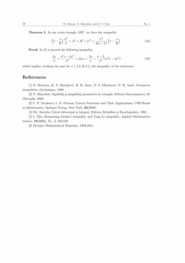
78 M. Bencze, N. Minculete and O. T. Pop No. 1

Theorem 5. In any acute triangle ABC, we have the inequality

(3− s

R

) π3

4< A3 + B3 + C3 <

π3

4(π − 2)

(π − s

R

). (18)

Proof. In [5] is proved the following inequality

2x

π+

π2x− 4x3

π3< sinx <

2x

π+

π − 2π3

(π2x− 4x3) (19)

which implies, working the sum for x ∈ {A,B, C}, the inequality of the statement.

References

[1] O. Bottema, R. Z. Djordjevic, R. R. Janic, D. S. Mitrinovic, P. M. Vasic, Geometricinequalities, Grooningen, 1969.

[2] N. Minculete, Egalitati si inegalitati geometrice ın triunghi, Editura Eurocarpatica, Sf.Gheorghe, 2003.

[3] C. P. Niculescu, L. E. Persson, Convex Functions and Their Applications, CMS Booksin Mathematics, Springer-Vertag, New York, 23(2006).

[4] Gh. Siretchi, Calcul diferential si integral, Editura Stiintifica si Enciclopedica, 1985.[5] L. Zhu, Sharpening Jordan’s inequality and Yang Le inequality, Applied Mathematics

Letters, 19(2006), No. 3, 240-243.[6] Octogon Mathematical Magazine, 1993-2011.


The Estrada index of random graphs

Yilun Shang†‡

† Institute for Cyber Security, University of Texas at San Antonio,San Antonio, Texas 78249, USA

‡ Department of Mathematics, Shanghai Jiao Tong University,Shanghai 200240, China


Abstract Let G be a graph of size n, and let λ1, λ2, . . . , λn be its eigenvalues. The Estrada

index of G is defined as EE(G) =∑n

i=1 eλi . In this paper, we establish almost sure results

on EE(G(n, p)) of Erdos-Renyi random graph G(n, p) in the superconnectivity regime.

Keywords Graph spectrum, Estrada index, random graph.

§1. Introduction

Generally, a simple graph G = (V, E) is defined by its vertex set V and edge set E ⊆ V ×V .Let n be the number of vertices of G. The eigenvalues of the adjacency matrix A are calledthe eigenvalues of G and form the spectrum [4] of G. Since A is a real symmetric matrix, itseigenvalues are real number. We then order the eigenvalues of G in a non-increasing manner asλ1 ≥ λ2 ≥ · · · ≥ λn. Some basic properties of graph are reviewed in [4].

A recently introduced [5,8] spectrum-based graph invariant is

EE(G) =n∑

i=1

eλi , (1)

which is called the Estrada index of G. The Estrada index has found numerous applicationsin biochemistry [5,6,9], physics and complex networks [7,8,13]. Some lower and upper bounds forEE(G) of fixed graphs are deduced in [2,10,12].

An intriguing question is the random graph setting. Let G = G(n, p) denote, as usual, theErdos-Renyi random graph [3] with n vertices and edge probability p. In this brief paper, byusing spectral theory we obtain the Estrada index EE(G(n, p)) in the regime that G(n, p) isalmost surely connected.

§2. Estimating EE(G(n, p))

Our main contribution in this section is the following concise result.Theorem 2.1. For random graph G(n, p) with

lnn

n¿ p < 1− lnn

n, (2)

80 Y. Shang No. 1

the Estrada index isEE(G(n, p)) = (1 + o(1))enp, (3)

almost surely, as n →∞.A key technique in the proof is a spectral density representation of random graph G(n, p).

It is shown [11] that the largest eigenvalue λ1 of G(n, p) is almost surely (1 + o(1))np providedthat np À lnn. Furthermore, Wigner’s semicircular law [14,15] says that the spectral density ofG(n, p) converges to the semicircular distribution

ρ(λ) =

2√

r2−λ2

πr2 , |λ| ≤ r,

0, |λ| > r,(4)

as n →∞, where r = 2√

np(1− p) is the radius of the bulk part of the spectrum.For p À (lnn)/n and n →∞, by continuous approximation for EE(G) in (1), the Estrada

index of G(n, p) can be reformulated in the spectral density form

EE(G(n, p))n

=∫ r

−r

ρ(λ)eλdλ +eλ1

n

= ψ(1) +enp

n

=enp

n

(1 +

nψ(1)enp

), (5)

where ψ(t) is the moment generating function of density ρ(λ) and

ψ(1) =∫ r

−r

2√

r2 − λ2

πr2eλdλ =

2π

∫ π

0

er cos θ sin2 θdθ. (6)

The following lemma can be proved by involving a modified Bessel function [1].Lemma 2.2.[16] The function

g(p) = nψ(1)/enp ∼ n

√2π

er−np

r3/2(7)

is monotonically decreasing for (lnn)/n < p < 1− (lnn)/n as n → ∞, where ψ(1) is given by(6) and r is defined in (4).

Now we are on the stage to prove our main result.Proof of Theorem 2.1. Let p = pc = (lnn)/n. Therefore, 1 − pc → 1 as n → ∞, and

r ∼ 2√

lnn from the definition in (4). By (7) we get

g(pc) ∼ n

√2π

er−npc

r3/2∼ n

√2π· e2

√ln n−ln n

(2√

lnn)3/2

=n

2√

π· e− ln n+2

√ln n

(lnn)3/4=

e2√

ln n

2√

π(lnn)3/4, (8)

which approaches 0 as n →∞.By Lemma 2.2, for pc ≤ p ≤ 1 − pc, we obtain g(p) ≤ g(pc) → 0 as n → ∞. Combining

this with (5) and (7), we then conclude the proof of Theorem 2.1.

Vol. 7 The Estrada index of random graphs 81

References

[1] M. Abramowitz, I. A. Stegun, Handbook of Mathematical Functions with Formulas,Graphs, and Mathematical Tables, Dover Publications, New York, 1972.

[2] J. Antonio de la Pena, I. Gutman, J. Rada, Estimating the Estrada index, Lin. Alg.Appl., 427(2007), 70-76.

[3] B. Bollobas, Random Graphs, Cambridge University Press, New York, 2001.[4] D. Cvetkovic, M. Doob, H. Sachs, Spectra of Graphs–Theory and Application, Johann

Ambrosius Barth Verlag, Heidelberg, Leipzig, 1995.[5] E. Estrada, Characterization of 3D molecular structure, Chem. Phys. Lett., 319(2000),

713-718.[6] E. Estrada, Characterization of the folding degree of proteins, Bioinformatics, 18(2002),

697-704.[7] E. Estrada, J. A. Rodrıguez-Velazquez, Spectral measures of bipartivity in complex

networks, Phys. Rev. E, 72(2005), 046105.[8] E. Estrada, J. A. Rodrıguez-Velazquez, Subgraph centrality in complex networks, Phys.

Rev. E, 71(2005), 056103.[9] E. Estrada, J. A. Rodrıguez-Velazquez, M. Randic, Atomic branching in molecules, Int.

J. Quantum Chem, 106(2006), 823-832.[10] I. Gutman, Lower bounds for Estrada index, Publications de L’Institut Mathematique,

83(2008), 1-7.[11] M. Krivelevich, B. Sudakov, The largest eigenvalue of sparse random graphs, Combin.

Probab. Comput., 12(2003), 61-72.[12] J. P. Liu, B. L. Liu, Bounds of the Estrada index of graphs, Appl. Math. J. Chinese

Univ., 25(2010), 325-330.[13] Y. Shang, Perturbation results for the Estrada index in weighted networks, J. Phys.

A: Math. Theor., 44(2011), 075003.[14] E. Wigner, Characteristic vectors of bordered matrices with infinite dimensions, Ann.

Math., 62(1955), 548-564.[15] E. Wigner, On the distribution of the roots of certain symmetric matrices, Ann. Math.,

67(1958), 325-328.[16] J. Wu, M. Barahona, Y. J. Tan, H. Z. Deng, Robustness of random graphs based on

natural connectivity, arXiv: 1009. 3430, 2010.


Smarandache isotopy of second

Smarandache Bol loops

Temıto.pe. Gbo. lahan Jaıyeo. la

Department of Mathematics, Obafemi Awolowo University,Ile Ife 220005, Nigeria


Abstract The pair (GH , ·) is called a special loop if (G, ·) is a loop with an arbitrary subloop

(H, ·) called its special subloop. A special loop (GH , ·) is called a second Smarandache Bol

loop (S2ndBL) if and only if it obeys the second Smarandache Bol identity (xs · z)s = x(sz · s)for all x, z in G and s in H. The popularly known and well studied class of loops called Bol

loops fall into this class and so S2ndBLs generalize Bol loops. The Smarandache isotopy of

S2ndBLs is introduced and studied for the first time. It is shown that every Smarandache

isotope (S − isotope) of a special loop is Smarandache isomorphic (S − isomorphic) to a

S-principal isotope of the special loop. It is established that every special loop that is S-

isotopic to a S2ndBL is itself a S2ndBL. A special loop is called a Smarandache G-special loop

(SGS − loop) if and only if every special loop that is S-isotopic to it is S-isomorphic to it. A

S2ndBL is shown to be a SGS-loop if and only if each element of its special subloop is a S1st

companion for a S1st pseudo-automorphism of the S2ndBL. The results in this work generalize

the results on the isotopy of Bol loops as can be found in the Ph. D. thesis of D. A. Robinson.

Keywords Special loop, second Smarandache Bol loop, Smarandache princiapl isotope, Sm

-arandache isotopy.

§1. Introduction

The study of the Smarandache concept in groupoids was initiated by W. B. VasanthaKandasamy in [24]. In her book [22] and first paper [23] on Smarandache concept in loops,she defined a Smarandache loop (S − loop) as a loop with at least a subloop which forms asubgroup under the binary operation of the loop. The present author has contributed to thestudy of S-quasigroups and S-loops in [5]-[12] by introducing some new concepts immediatelyafter the works of Muktibodh [15]-[16]. His recent monograph [14] gives inter-relationships andconnections between and among the various Smarandache concepts and notions that have beendeveloped in the aforementioned papers.

But in the quest of developing the concept of Smarandache quasigroups and loops into atheory of its own just as in quasigroups and loop theory (see [1]-[4], [17], [22]), there is the needto introduce identities for types and varieties of Smarandache quasigroups and loops. This ledJaıyeo. la [13] to the introduction of second Smarandache Bol loop (S2ndBL) described by the

Vol. 7 Smarandache isotopy of second Smarandache Bol loops 83

second Smarandache Bol identity (xs · z)s = x(sz · s) for all x, z in G and s in H where thepair (GH , ·) is called a special loop if (G, ·) is a loop with an arbitrary subloop (H, ·). Fornow, a Smarandache loop or Smarandache quasigroup will be called a first Smarandache loop(S1st − loop) or first Smarandache quasigroup (S1st − quasigroup).

Let L be a non-empty set. Define a binary operation (·) on L: if x · y ∈ L for all x, y ∈ L,(L, ·) is called a groupoid. If the equations; a · x = b and y · a = b have unique solutionsfor x and y respectively, then (L, ·) is called a quasigroup. For each x ∈ L, the elementsxρ = xJρ, xλ = xJλ ∈ L such that xxρ = eρ and xλx = eλ are called the right, left inverses of x

respectively. Furthermore, if there exists a unique element e = eρ = eλ in L called the identityelement such that for all x in L, x · e = e · x = x, (L, ·) is called a loop. We write xy instead ofx · y, and stipulate that · has lower priority than juxtaposition among factors to be multiplied.For instance, x · yz stands for x(yz). A loop is called a right Bol loop (Bol loop in short) if andonly if it obeys the identity

(xy · z)y = x(yz · y).

This class of loops was the first to catch the attention of loop theorists and the first compre-hensive study of this class of loops was carried out by Robinson [19].

The popularly known and well studied class of loops called Bol loops fall into the class ofS2ndBLs and so S2ndBLs generalize Bol loops. The aim of this work is to introduce and studyfor the first time, the Smarandache isotopy of S2ndBLs. It is shown that every Smarandacheisotope (S-isotope) of a special loop is Smarandache isomorphic (S-isomorphic) to a S-principalisotope of the special loop. It is established that every special loop that is S-isotopic to aS2ndBL is itself a S2ndBL. A S2ndBL is shown to be a Smarandache G-special loop if and onlyif each element of its special subloop is a S1st companion for a S1st pseudo-automorphism ofthe S2ndBL. The results in this work generalize the results on the isotopy of Bol loops as canbe found in the Ph. D. thesis of D. A. Robinson.

§2. Preliminaries

Definition 1. Let (G, ·) be a quasigroup with an arbitrary non-trivial subquasigroup(H, ·). Then, (GH , ·) is called a special quasigroup with special subquasigroup (H, ·). If (G, ·)is a loop with an arbitrary non-trivial subloop (H, ·). Then, (GH , ·) is called a special loopwith special subloop (H, ·). If (H, ·) is of exponent 2, then (GH , ·) is called a special loop ofSmarandache exponent 2.

A special quasigroup (GH , ·) is called a second Smarandache right Bol quasigroup (S2nd -right Bol quasigroup) or simply a second Smarandache Bol quasigroup (S2nd -Bol quasigroup)and abbreviated S2ndRBQ or S2ndBQ if and only if it obeys the second Smarandache Bol identity(S2nd -Bol identity) i.e S2ndBI

(xs · z)s = x(sz · s) for all x, z ∈ G and s ∈ H. (1)

Hence, if (GH , ·) is a special loop, and it obeys the S2ndBI, it is called a second SmarandacheBol loop(S2nd -Bol loop) and abbreviated S2ndBL.

84 Temıto.pe. Gbo. lahan Jaıyeo. la No. 1

Remark 1. A Smarandache Bol loop (i.e a loop with at least a non-trivial subloop thatis a Bol loop) will now be called a first Smarandache Bol loop (S1st-Bol loop). It is easy to seethat a S2ndBL is a S1stBL. But the converse is not generally true. So S2ndBLs are particulartypes of S1stBL. Their study can be used to generalise existing results in the theory of Bol loopsby simply forcing H to be equal to G.

Definition 2. Let (G, ·) be a quasigroup (loop). It is called a right inverse propertyquasigroup (loop) [RIPQ (RIPL)] if and only if it obeys the right inverse property (RIP) yx·xρ =y for all x, y ∈ G. Similarly, it is called a left inverse property quasigroup (loop) [LIPQ (LIPL)]if and only if it obeys the left inverse property (LIP) xλ · xy = y for all x, y ∈ G. Hence, it iscalled an inverse property quasigroup (loop) [IPQ (IPL)] if and only if it obeys both the RIPand LIP.

(G, ·) is called a right alternative property quasigroup (loop) [RAPQ (RAPL)] if and onlyif it obeys the right alternative property (RAP) y · xx = yx · x for all x, y ∈ G. Similarly, it iscalled a left alternative property quasigroup (loop) [LAPQ (LAPL)] if and only if it obeys theleft alternative property (LAP) xx · y = x ·xy for all x, y ∈ G. Hence, it is called an alternativeproperty quasigroup (loop) [APQ (APL)] if and only if it obeys both the RAP and LAP.

The bijection Lx : G → G defined as yLx = x · y for all x, y ∈ G is called a left translation(multiplication) of G while the bijection Rx : G → G defined as yRx = y · x for all x, y ∈ G iscalled a right translation (multiplication) of G. Let

x\y = yL−1x = yLx and x/y = xR−1

y = xRy,

and note thatx\y = z ⇐⇒ x · z = y and x/y = z ⇐⇒ z · y = x.

The operations \ and / are called the left and right divisions respectively. We stipulate that/ and \ have higher priority than · among factors to be multiplied. For instance, x · y/z andx · y\z stand for x(y/z) and x · (y\z) respectively.

(G, ·) is said to be a right power alternative property loop (RPAPL) if and only if it obeysthe right power alternative property (RPAP)

xyn = (((xy)y)y)y · · · y︸︷︷︸n-times

i.e. Ryn = Rny for all x, y ∈ G and n ∈ Z.

The right nucleus of G denoted by Nρ(G, ·) = Nρ(G) = {a ∈ G : y ·xa = yx ·a ∀ x, y ∈ G}.Let (GH , ·) be a special quasigroup (loop). It is called a second Smarandache right inverse

property quasigroup (loop) [S2ndRIPQ (S2ndRIPL)] if and only if it obeys the second Smaran-dache right inverse property (S2ndRIP) ys · sρ = y for all y ∈ G and s ∈ H. Similarly, it iscalled a second Smarandache left inverse property quasigroup (loop) [S2ndLIPQ (S2ndLIPL)] ifand only if it obeys the second Smarandache left inverse property (S2ndLIP) sλ · sy = y for ally ∈ G and s ∈ H. Hence, it is called a second Smarandache inverse property quasigroup (loop)[S2ndIPQ (S2ndIPL)] if and only if it obeys both the S2ndRIP and S2ndLIP.

(GH , ·) is called a third Smarandache right inverse property quasigroup (loop) [S3rdRIPQ(S3rdRIPL)] if and only if it obeys the third Smarandache right inverse property (S3rdRIP)sy · yρ = s for all y ∈ G and s ∈ H.


(GH , ·) is called a second Smarandache right alternative property quasigroup (loop) [S2ndRAPQ(S2ndRAPL)] if and only if it obeys the second Smarandache right alternative property(S2ndRAP) y · ss = ys · s for all y ∈ G and s ∈ H. Similarly, it is called a second Smarandacheleft alternative property quasigroup (loop) [S2ndLAPQ (S2ndLAPL)] if and only if it obeys thesecond Smarandache left alternative property (S2ndLAP) ss · y = s · sy for all y ∈ G and s ∈ H.Hence, it is called an second Smarandache alternative property quasigroup (loop) [S2ndAPQ(S2ndAPL)] if and only if it obeys both the S2ndRAP and S2ndLAP.

(GH , ·) is said to be a Smarandache right power alternative property loop (SRPAPL) ifand only if it obeys the Smarandache right power alternative property (SRPAP)

xsn = (((xs)s)s)s · · · s︸︷︷︸n-times

i.e. Rsn = Rns for all x ∈ G, s ∈ H and n ∈ Z.

The Smarandache right nucleus of GH denoted by SNρ(GH , ·) = SNρ(GH) = Nρ(G) ∩H.GH is called a Smarandache right nuclear square special loop if and only if s2 ∈ SNρ(GH) forall s ∈ H.

Remark 2. A Smarandache; RIPQ or LIPQ or IPQ (i.e a loop with at least a non-trivialsubquasigroup that is a RIPQ or LIPQ or IPQ) will now be called a first Smarandache; RIPQor LIPQ or IPQ (S1stRIPQ or S1stLIPQ or S1stIPQ). It is easy to see that a S2ndRIPQ orS2ndLIPQ or S2ndIPQ is a S1stRIPQ or S1stLIPQ or S1stIPQ respectively. But the converse isnot generally true.

Definition 3. Let (G, ·) be a quasigroup (loop). The set SY M(G, ·) = SY M(G) ofall bijections in G forms a group called the permutation (symmetric) group of G. The triple(U, V,W ) such that U, V,W ∈ SY M(G, ·) is called an autotopism of G if and only if

xU · yV = (x · y)W ∀ x, y ∈ G.

The group of autotopisms of G is denoted by AUT (G, ·) = AUT (G).Let (GH , ·) be a special quasigroup (loop). The set SSY M(GH , ·) = SSY M(GH) of all

Smarandache bijections (S-bijections) in GH i.e A ∈ SY M(GH) such that A : H → H

forms a group called the Smarandache permutation (symmetric) group [S-permutation group]of GH . The triple (U, V,W ) such that U, V,W ∈ SSY M(GH , ·) is called a first Smarandacheautotopism (S1st autotopism) of GH if and only if

xU · yV = (x · y)W ∀ x, y ∈ GH .

If their set forms a group under componentwise multiplication, it is called the first Smaran-dache autotopism group (S1st autotopism group) of GH and is denoted by S1stAUT (GH , ·) =S1stAUT (GH).

The triple (U, V,W ) such that U,W ∈ SY M(G, ·) and V ∈ SSY M(GH , ·) is called asecond right Smarandache autotopism (S2nd right autotopism) of GH if and only if

xU · sV = (x · s)W ∀ x ∈ G and s ∈ H.

If their set forms a group under componentwise multiplication, it is called the second rightSmarandache autotopism group (S2nd right autotopism group) of GH and is denoted by S2ndRAU

T (GH , ·) = S2ndRAUT (GH).


The triple (U, V,W ) such that V, W ∈ SY M(G, ·) and U ∈ SSY M(GH , ·) is called a secondleft Smarandache autotopism (S2nd left autotopism) of GH if and only if

sU · yV = (s · y)W ∀ y ∈ G and s ∈ H.

If their set forms a group under componentwise multiplication, it is called the second leftSmarandache autotopism group (S2nd left autotopism group) of GH and is denoted by S2ndLAUT

(GH , ·) = S2ndLAUT (GH).Let (GH , ·) be a special quasigroup (loop) with identity element e. A mapping T ∈

SSY M(GH) is called a first Smarandache semi-automorphism (S1st semi-automorphism) ifand only if eT = e and

(xy · x)T = (xT · yT )xT for all x, y ∈ G.

A mapping T ∈ SSY M(GH) is called a second Smarandache semi-automorphism (S2nd

semi-automorphism) if and only if eT = e and

(sy · s)T = (sT · yT )sT for all y ∈ G and all s ∈ H.

A special loop (GH , ·) is called a first Smarandache semi-automorphic inverse property loop(S1stSAIPL) if and only if Jρ is a S1st semi-automorphism.

A special loop (GH , ·) is called a second Smarandache semi-automorphic inverse propertyloop (S2ndSAIPL) if and only if Jρ is a S2nd semi-automorphism. Let (GH , ·) be a specialquasigroup (loop). A mapping A ∈ SSY M(GH) is a

1. First Smarandache pseudo-automorphism (S1st pseudo-automorphism) of GH if and onlyif there exists a c ∈ H such that (A,ARc, ARc) ∈ S1stAUT (GH). c is reffered to as thefirst Smarandache companion (S1st companion) of A. The set of such A’s is denoted byS1stPAUT (GH , ·) = S1stPAUT (GH).

2. Second right Smarandache pseudo-automorphism (S2nd right pseudo-automorphism) ofGH if and only if there exists a c ∈ H such that (A,ARc, ARc) ∈ S2ndRAUT (GH). c isreffered to as the second right Smarandache companion (S2nd right companion) of A. Theset of such A’s is denoted by S2ndRPAUT (GH , ·) = S2ndRPAUT (GH).

3. Second left Smarandache pseudo-automorphism (S2nd left pseudo-automorphism) of GH ifand only if there exists a c ∈ H such that (A,ARc, ARc) ∈ S2ndLAUT (GH). c is refferedto as the second left Smarandache companion (S2nd left companion) of A. The set of suchA’s is denoted by S2ndLPAUT (GH , ·) = S2ndLPAUT (GH).

Let (GH , ·) be a special loop. A mapping A ∈ SSY M(GH) is a

1. First Smarandache automorphism (S1st automorphism) of GH if and only if A ∈ S1stPAUT

(GH) such that c = e. Their set is denoted by S1stAUM(GH , ·) = S1stAUM(GH).

2. Second right Smarandache automorphism (S2nd right automorphism) of GH if and onlyif A ∈ S2ndRPAUT (GH) such that c = e. Their set is denoted by S2ndRAUM(GH , ·) =S2ndRAUM(GH).


3. Second left Smarandache automorphism (S2nd left automorphism) of GH if and only ifA ∈ S2ndLPAUT (GH) such that c = e. Their set is denoted by S2ndLAUM(GH , ·) =S2ndLAUM(GH).

A special loop (GH , ·) is called a first Smarandache automorphism inverse property loop(S1stAIPL) if and only if (Jρ, Jρ, Jρ) ∈ AUT (H, ·).

A special loop (GH , ·) is called a second Smarandache right automorphic inverse propertyloop (S2ndRAIPL) if and only if Jρ is a S2nd right automorphism.

A special loop (GH , ·) is called a second Smarandache left automorphic inverse propertyloop (S2ndLAIPL) if and only if Jρ is a S2nd left automorphism.

Definition 4. Let (G, ·) and (L, ◦) be quasigroups (loops). The triple (U, V,W ) such thatU, V,W : G → L are bijections is called an isotopism of G onto L if and only if

xU ◦ yV = (x · y)W ∀ x, y ∈ G. (2)

Let (GH , ·) and (LM , ◦) be special groupoids. GH and LM are Smarandache isotopic(S-isotopic) [and we say (LM , ◦) is a Smarandache isotope of (GH , ·)] if and only if thereexist bijections U, V,W : H → M such that the triple (U, V,W ) : (GH , ·) → (LM , ◦) is anisotopism. In addition, if U = V = W , then (GH , ·) and (LM , ◦) are said to be Smarandacheisomorphic (S-isomorphic) [and we say (LM , ◦) is a Smarandache isomorph of (GH , ·) and thuswrite (GH , ·) % (LM , ◦).].

(GH , ·) is called a Smarandache G-special loop (SGS-loop) if and only if every special loopthat is S-isotopic to (GH , ·) is S-isomorphic to (GH , ·).

Theorem 1. (Jaıyeo. la [13]) Let the special loop (GH , ·) be a S2ndBL. Then it is both aS2ndRIPL and a S2ndRAPL.

Theorem 2. (Jaıyeo. la [13]) Let (GH , ·) be a special loop. (GH , ·) is a S2ndBL if and onlyif (R−1

s , LsRs, Rs) ∈ S1stAUT (GH , ·).

§3. Main results

Lemma 1. Let (GH , ·) be a special quasigroup and let s, t ∈ H. For all x, y ∈ G, let

x ◦ y = xR−1t · yL−1

s . (3)

Then, (GH , ◦) is a special loop and so (GH , ·) and (GH , ◦) are S-isotopic.Proof. It is easy to show that (GH , ◦) is a quasigroup with a subquasigroup (H, ◦) since

(GH , ·) is a special quasigroup. So, (GH , ◦) is a special quasigroup. It is also easy to see thats · t ∈ H is the identity element of (GH , ◦). Thus, (GH , ◦) is a special loop. With U = Rt,V = Ls and W = I, the triple (U, V,W ) : (GH , ·) → (GH , ◦) is an S-isotopism.

Remark 3. (GH , ◦) will be called a Smarandache principal isotopism (S-principal iso-topism) of (GH , ·).

Theorem 3. If the special quasigroup (GH , ·) and special loop (LM , ◦) are S-isotopic,then (LM , ◦) is S-isomorphic to a S-principal isotope of (GH , ·).


Proof. Let e be the identity element of the special loop (LM , ◦). Let U , V and W be 1-1S-mappings of GH onto LM such that

xU ◦ yV = (x · y)W ∀ x, y ∈ GH .

Let t = eV −1 and s = eU−1. Define x ∗ y for all x, y ∈ GH by

x ∗ y = (xW ◦ yW )W−1. (4)

From (2), with x and y replaced by xWU−1 and yWV −1 respectively, we get

(xW ◦ yW )W−1 = xWU−1 · yWV −1 ∀ x, y ∈ GH . (5)

In (5), with x = eW−1, we get WV −1 = L−1s and with y = eW−1, we get WU−1 = R−1

t .Hence, from (4) and (5),

x ∗ y = xR−1t · yL−1

s and (x ∗ y)W = xW ◦ yW ∀ x, y ∈ GH .

That is, (GH , ∗) is a S-principal isotope of (GH , ·) and is S-isomorphic to (LM , ◦).Theorem 4. Let (GH , ·) be a S2ndRIPL. Let f, g ∈ H and let (GH , ◦) be a S-principal

isotope of (GH , ·). (GH , ◦) is a S2ndRIPL if and only if α(f, g) = (Rg, LfR−1g L−1

f ·g, R−1g ) ∈

S2ndRAUT (GH , ·) for all f, g ∈ H.Proof. Let (GH , ·) be a special loop that has the S2ndRIP and let f, g ∈ H. For all

x, y ∈ G, define x ◦ y = xR−1g · yL−1

f as in (3). Recall that f · g is the identity in (GH , ◦), sox◦xρ′ = f ·g where xJ ′ρ = xρ′ i.e the right identity element of x in (GH , ◦). Then, for all x ∈ G,x ◦ xρ′ = xR−1

g · xJ ′ρL−1f = f · g and by the S2ndRIP of (GH , ·), since sR−1

g · sJ ′ρL−1f = f · g for

all s ∈ H, then sR−1g = (f · g) · (sJ ′ρL−1

f )Jρ because (H, ·) has the RIP. Thus,

sR−1g = sJ ′ρL

−1f JρLf ·g ⇒ sJ ′ρ = sR−1

g L−1f ·gJλLf . (6)

(GH , ◦) has the S2ndRIP iff (x◦s)◦sJ ′ρ = s for all s ∈ H, x ∈ GH iff (xR−1g ·sL−1

f )R−1g ·sJ ′ρL−1

f =x, for all s ∈ H, x ∈ GH . Replace x by x · g and s by f · s, then (x · s)R−1

g · (f · s)J ′ρL−1f = x · g

iff (x · s)R−1g = (x · g) · (f · s)J ′ρL−1

f Jρ for all s ∈ H, x ∈ GH since (GH , ·) has the S2ndRIP.Using (6),

(x · s)R−1g = xRg · (f · s)R−1

g L−1f ·g ⇔ (x · s)R−1

g = xRg · sLfR−1g L−1

f ·g ⇔

α(f, g) = (Rg, LfR−1g L−1

f ·g, R−1g ) ∈ S2ndRAUT (GH , ·) for all f, g ∈ H.

Theorem 5. If a special loop (GH , ·) is a S2ndBL, then any of its S-isotopes is a S2ndRIPL.Proof. By virtue of theorem 3, we need only to concern ourselves with the S-principal

isotopes of (GH , ·). (GH , ·) is a S2ndBL iff it obeys the S2ndBI iff (xs · z)s = x(sz · s) for allx, z ∈ G and s ∈ H iff LxsRs = LsRsLx for all x ∈ G and s ∈ H iff R−1

s L−1xs = L−1

x R−1s L−1

s forall x ∈ G and s ∈ H iff

R−1s L−1

s = LxR−1s L−1

xs for all x ∈ G and s ∈ H. (7)

Assume that (GH , ·) is a S2ndBL. Then, by theorem 2,

(R−1s , LsRs, Rs) ∈ S1stAUT (GH , ·) ⇒ (R−1

s , LsRs, Rs) ∈ S2ndRAUT (GH , ·) ⇒


(R−1s , LsRs, Rs)−1 = (Rs, R

−1s L−1

s , R−1s ) ∈ S2ndRAUT (GH , ·).

By (7), α(x, s) = (Rs, LxR−1s L−1

xs , R−1s ) ∈ S2ndRAUT (GH , ·) for all f, g ∈ H. But (GH , ·) has

the S2ndRIP by theorem 1. So, following theorem 4, all special loops that are S-isotopic to(GH , ·) are S2ndRIPLs.

Theorem 6. Suppose that each special loop that is S-isotopic to (GH , ·) is a S2ndRIPL,then the identities:

1. (fg)\f = (xg)\x;

2. g\(sg−1) = (fg)\[(fs)g−1]

are satisfied for all f, g, s ∈ H and x ∈ G.Proof. In particular, (GH , ·) has the S2ndRIP. Then by theorem 3, α(f, g) = (Rg, LfR−1

g

L−1f ·g, R

−1g ) ∈ S2ndRAUT (GH , ·) for all f, g ∈ H. Let

Y = LfR−1g L−1

f ·g. (8)

Then,xg · sY = (xs)R−1

g . (9)

Put s = g in (9), then xg ·gY = (xg)R−1g = x. But, gY = gLfR−1

g L−1f ·g = (fg)\[(fg)g−1] =

(fg)\f . So, xg · (fg)\f = x ⇒ (fg)\f = (xg)\x.Put x = e in (9), then sY Lg = sR−1

g ⇒ sY = sR−1g L−1

g . So, combining this with (8),sR−1

g L−1g = sLfR−1

g L−1f ·g ⇒ g\(sg−1) = (fg)\[(fs)g−1].

Theorem 7. Every special loop that is S-isotopic to a S2ndBL is itself a S2ndBL.Proof. Let (GH , ◦) be a special loop that is S-isotopic to an S2ndBL (GH , ·). Assume that

x ·y = xα◦yβ where α, β : H → H. Then the S2ndBI can be written in terms of (◦) as follows.(xs · z)s = x(sz · s) for all x, z ∈ G and s ∈ H.

[(xα ◦ sβ)α ◦ zβ]α ◦ sβ = xα ◦ [(sα ◦ zβ)α ◦ sβ]β. (10)

Replace xα by x, sβ by s and zβ by z, then

[(x ◦ s)α ◦ z]α ◦ s = x ◦ [(sβ−1α ◦ z)α ◦ s]β. (11)

If x = e, then(sα ◦ z)α ◦ s = [(sβ−1α ◦ z)α ◦ s]β. (12)

Substituting (12) into the RHS of (11) and replacing x, s and z by x, s and z respectively, wehave

[(x ◦ s)α ◦ z]α ◦ s = x ◦ [(sα ◦ z)α ◦ s]. (13)

With s = e, (xα ◦ z)α = x ◦ (eα ◦ z)α. Let (eα ◦ z)α = zδ, where δ ∈ SSY M(GH). Then,

(xα ◦ z)α = x ◦ zδ. (14)

Applying (14), then (13) to the expression [(x ◦ s) ◦ zδ] ◦ s, that is

[(x ◦ s) ◦ zδ] ◦ s = [(x ◦ s)α ◦ z]α ◦ s = x ◦ [(sα ◦ z)α ◦ s] = x ◦ [(s ◦ zδ) ◦ s].


implies[(x ◦ s) ◦ zδ] ◦ s = x ◦ [(s ◦ zδ) ◦ s].

Replace zδ by z, then[(x ◦ s) ◦ z] ◦ s = x ◦ [(s ◦ z) ◦ s].

Theorem 8. Let (GH , ·) be a S2ndBL. Each special loop that is S-isotopic to (GH , ·) isS-isomorphic to a S-principal isotope (GH , ◦) where x ◦ y = xRf · yL−1

f for all x, y ∈ G andsome f ∈ H.

Proof. Let e be the identity element of (GH , ·). Let (GH , ∗) be any S-principal isotopeof (GH , ·) say x ∗ y = xR−1

v · yL−1u for all x, y ∈ G and some u, v ∈ H. Let e′ be the identity

element of (GH , ∗). That is, e′ = u · v. Now, define x ∗ y by

x ◦ y = [(xe′) ∗ (ye′)]e′−1 for all x, y ∈ G.

Then Re′ is an S-isomorphism of (GH , ◦) onto (GH , ∗). Observe that e is also the identityelement for (GH , ◦) and since (GH , ·) is a S2ndBL,

(pe′)(e′−1q · e′−1) = pq · e′−1 for all p, q ∈ G. (15)

So, using (15),

x ◦ y = [(xe′) ∗ (ye′)]e′−1 = [xRe′R−1v · yRe′L

−1u ]e′−1 = xRe′R

−1v Re′ · yRe′L

−1u Le′−1Re′−1

implies that

x ◦ y = xA · yB, A = Re′R−1v Re′ and B = Re′L

−1u Le′−1Re′−1 . (16)

Let f = eA. then, y = e ◦ y = eA · yB = f · yB for all y ∈ G. So, B = L−1f . In fact,

eB = fρ = f−1. Then, x = x ◦ e = xA · eB = xA · f−1 for all x ∈ G implies xf = (xA · f−1)fimplies xf = xA (S2ndRIP) implies A = Rf . Now, (16) becomes x ◦ y = xRf · yL−1

f .Theorem 9. Let (GH , ·) be a S2ndBL with the S2ndRAIP or S2ndLAIP, let f ∈ H and let

x ◦ y = xRf · yL−1f for all x, y ∈ G. Then (GH , ◦) is a S1stAIPL if and only if f ∈ Nλ(H, ·).

Proof. Since (GH , ·) is a S2ndBL, J = Jλ = Jρ in (H, ·). Using (6) with g = f−1,

sJ ′ρ = sRfJLf . (17)

(GH , ◦) is a S1stAIPL iff (x ◦ y)J ′ρ = xJ ′ρ ◦ yJ ′ρ for all x, y ∈ H iff

(xRf · yL−1f )J ′ρ = xJ ′ρRf · yJ ′ρL

−1f . (18)

Let x = uR−1f and y = vLf and use (16), then (18) becomes (uv)RfJLf = uJLfRf · vLfRfJ

iff α = (JLfRf , LfRfJ,RfJLf ) ∈ AUT (H, ·). Since (GH , ·) is a S1stAIPL, so (J, J, J) ∈AUT (H, ·). So, α ∈ AUT (H, ·) ⇔ β = α(J, J, J)(R−1

f−1 , Lf−1Rf−1 , Rf−1) ∈ AUT (H, ·). Since(GH , ·) is a S2ndBL,

xLfRfLf−1Rf−1 = [f−1(fx · f)]f−1 = [(f−1f · x)f ]f−1 = x for all x ∈ G. That is,LfRfLf−1Rf−1 = I in (GH , ·). Also, since J ∈ AUM(H, ·), then RfJ = JRf−1 and LfJ =


JLf−1 in (H, ·). So,

β = (JLfRfJR−1f−1 , LfRfJ2Lf−1Rf−1 , RfJLfJRf−1)

= (JLfJRf−1R−1f−1 , LfRfLf−1Rf−1 , RfLf−1Rf−1)

= (Lf−1 , I, RfLf−1Rf−1).

Hence, (GH , ◦) is a S1stAIPL iff β ∈ AUT (H, ·).Now, assume that β ∈ AUT (H, ·). Then, xLf−1 · y = (xy)RfLf−1Rf−1 for all x, y ∈ H.

For y = e, Lf−1 = RfLf−1Rf−1 in (H, ·). so, β = (Lf−1 , I, Lf−1) ∈ AUT (H, ·) ⇒ f−1 ∈Nλ(H, ·) ⇒ f ∈ Nλ(H, ·).

On the other hand, if f ∈ Nλ(H, ·), then, γ = (Lf , I, Lf ) ∈ AUT (H, ·). But f ∈Nλ(H, ·) ⇒ L−1

f = Lf−1 = RfLf−1Rf−1 in (H, ·). Hence, β = γ−1 and β ∈ AUT (H, ·).Corollary 1. Let (GH , ·) be a S2ndBL and a S1stAIPL. Then, for any special loop (GH , ◦)

that is S-isotopic to (GH , ·), (GH , ◦) is a S1stAIPL iff (GH , ·) is a S1st-loop and a S1st commu-tative loop.

Proof. Suppose every special loop that is S-isotopic to (GH , ·) is a S1stAIPL. Then,f ∈ Nλ(H, ·) for all f ∈ H by theorem 9. So, (GH , ·) is a S1st-loop. Then, y−1x−1 = (xy)−1 =x−1y−1 for all x, y ∈ H. So, (GH , ·) is a S1st commutative loop.

The proof of the converse is as follows. If (GH , ·) is a S1st-loop and a S1st commutativeloop, then for all x, y ∈ H such that x ◦ y = xRf · yL−1

f ,

(x ◦ y) ◦ z = (xRf · yL−1f )Rf · zL−1

f = (xf · f−1y)f · f−1z.

x ◦ (y ◦ z) = xRf · (yRf · zL−1f )L−1

f = xf · f−1(yf · f−1z).

So, (x ◦ y) ◦ z = x ◦ (y ◦ z). Thus, (H, ◦) is a group. Furthermore,

x ◦ y = xRf · yL−1f = xf · f−1y = x · y = y · x = yf · f−1x = y ◦ x.

So, (H, ◦) is commutative and so has the AIP. Therefore, (GH , ◦) is a S1stAIPL.

Lemma 2. Let (GH , ·) be a S2ndBL. Then, every special loop that is S-isotopic to (GH , ·) isS-isomorphic to (GH , ·) if and only if (GH , ·) obeys the identity (x·fg)g−1 ·f\(y·fg) = (xy)·(fg)for all x, y ∈ GH and f, g ∈ H.

Proof. Let (GH , ◦) be an arbitrary S-principal isotope of (GH , ·). It is claimed that

(GH , ·)Rfg

% (GH , ◦) iff xRfg ◦ yRfg = (x · y)Rfg iff (x · fg)R−1g · (y · fg)L−1

f = (x · y)Rfg iff(x · fg)g−1 · f\(y · fg) = (xy) · (fg) for all x, y ∈ GH and f, g ∈ H.

Theorem 10. Let (GH , ·) be a S2ndBL, let f ∈ H, and let x ◦ y = xRf · yL−1f for all

x, y ∈ G. Then, (GH , ·) % (GH , ◦) if and only if there exists a S1st pseudo-automorphism of(GH , ·) with S1st companion f .

Proof. (GH , ·) % (GH , ◦) if and only if there exists T ∈ SSY M(GH , ·) such that xT ◦yT =(x · y)T for all x, y ∈ G iff xTRf · yTL−1

f = (x · y)T for all x, y ∈ G iff α = (TRf , TL−1f , T ) ∈

S1stAUT (GH).


Recall that by theorem 2, (GH , ·) is a S2ndBL iff (R−1f , LfRf , Rf ) ∈ S1stAUT (GH , ·) for

each f ∈ H. So,

α ∈ S1stAUT (GH) ⇔ β = α(R−1f , LfRf , Rf ) =

(T, TRf , TRf ) ∈ S1stAUT (GH , ·) ⇔ T ∈ S1stPAUT (GH)

with S1st companion f .Corollary 2. Let (GH , ·) be a S2ndBL, let f ∈ H and let x ◦ y = xRf · yL−1

f for allx, y ∈ GH . If f ∈ Nρ(H, ·), then, (GH , ·) % (GH , ◦).

Proof. Following theorem 10, f ∈ Nρ(H, ·) ⇒ TS1stPAUT (GH) with S1st companion f .Corollary 3. Let (GH , ·) be a S2ndBL. Then, every special loop that is S-isotopic to

(GH , ·) is S-isomorphic to (GH , ·) if and only if each element of H is a S1st companion for a S1st

pseudo-automorphism of (GH , ·).Proof. This follows from theorem 8 and theorem 10.Corollary 4. Let (GH , ·) be a S2ndBL. Then, (GH , ·) is a SGS-loop if and only if each

element of H is a S1st companion for a S1st pseudo-automorphism of (GH , ·).Proof. This is an immediate consequence of corollary 4.Remark 4. Every Bol loop is a S2ndBL. Most of the results on isotopy of Bol loops in

chapter 3 of [19] can easily be deduced from the results in this paper by simply forcing H tobe equal to G.

References

[1] R. H. Bruck, A survey of binary systems, Springer-Verlag, Berlin-Gottingen-Heidelberg,1966.

[2]O. Chein, H. O. Pflugfelder and J. D. H. Smith, Quasigroups and Loops: Theory andApplications, Heldermann Verlag, 1990.

[3] J. Dene and A. D. Keedwell, Latin squares and their applications, the English Universitypress Lts, 1974.

[4] E. G. Goodaire, E. Jespers and C. P. Milies, Alternative loop rings, NHMS (184),Elsevier, 1996.

[5] T. G. Jaıyeo. la, An holomorphic study of the Smarandache concept in loops, ScientiaMagna Journal, 2(2006), No. 1, 1-8.

[6] T. G. Jaıyeo. la, Parastrophic invariance of Smarandache quasigroups, Scientia MagnaJournal, 2(2006), No. 3, 48-53.

[7] T. G. Jaıyeo. la, On the universality of some Smarandache loops of Bol-Moufang type,Scientia Magna Journal, 2(2006), No. 4, 45-48.

[8] T. G. Jaıyeo. la, A Pair Of Smarandachely Isotopic Quasigroups And Loops Of The SameVariety, International Journal of Mathematical Combinatorics, 1(2008), 36-44.

[9] T. G. Jaıyeo. la, An Holomorphic Study Of Smarandache Automorphic and Cross In-verse Property Loops, Proceedings of the 4th International Conference on Number Theory andSmarandache Problems, Scientia Magna, 4(2008), No. 1, 102–108.


[10] T. G. Jaıyeo. la, Smarandache isotopy theory of Smarandache: quasigroups and loops,Proceedings of the 4th International Conference on Number Theory and Smarandache Problems,Scientia Magna, 4(2008), No. 1, 168-177.

[11] T. G. Jaıyeo. la, On Smarandache Bryant Schneider group of a Smarandache loop,International Journal of Mathematical Combinatorics, 2(2008), 51-63.

[12] T. G. Jaıyeo. la, A Double Cryptography Using The Smarandache Keedwell Cross In-verse Quasigroup, International Journal of Mathematical Combinatorics, 3(2008), 28-33.

[13] T. G. Jaıyeo. la, Basic properties of second Smarandache Bol loops, International Jour-nal of Mathematical Combinatorics, 2(2009), 11-20.

[14] T. G. Jaıyeo. la, A study of new concepts in Smarandache quasigroups and loops,ProQuest Information and Learning (ILQ), Ann Arbor, USA, 2009.

[15] A. S. Muktibodh, Smarandache quasigroups rings, Scientia Magna, 1(2005), No. 2,139-144.

[16] A. S. Muktibodh, Smarandache Quasigroups, Scientia Magna, 2(2006), No. 2, 13-19.[17] H. O. Pflugfelder, Quasigroups and Loops: Introduction, Sigma series in Pure Math.

7, Heldermann Verlag, Berlin, 1990.[18] A. Sade, Quasigroupes parastrophiques, Math. Nachr, 20(1959), 73-106.[19] D. A. Robinson, Bol loops, Ph. D thesis, University of Wisconsin, Madison, Wisconsin,

1964.[20] D. A. Robinson, Bol loops, Trans. Amer. Math. Soc., 123(1966), No. 2, 341-354.[21] A. R. T. Solarin and B. L. Sharma, On the construction of Bol loops, Al. I. Cuza.

Univ., 27(1981), No. 1, 23-28.[22] W. B. Vasantha Kandasamy, Smarandache Loops, Department of Mathematics, Indian

Institute of Technology, Madras, India, 2002.[23] W. B. Vasantha Kandasamy, Smarandache Loops, Smarandache notions journal, 252-

258.[24] W. B. Vasantha Kandasamy, Smarandache groupoids, Scientia Magna, 1(2005), No.

1, 27-35.


Implicative filters in pocrims

Mahboobeh Mohamadhasani† and Masoud Haveshki‡

Department of Mathematics, Hormozgan University, Bandarabbas, Iran


Abstract In this paper, we define the notion of implicative filters in pocrims. We give several

characterizations about implicative filters and consider a relation between these filters and

quotient algebra that constructed via these filters.

Keywords Pocrim, implicative filter, Brouwerian semilattice.

§1. Introduction

Bounded pocrims form a class of algebras containing as proper subclasses, among others,the class of algebras of some logics, e.g, the class of BL-algebras, i.e., algebras of the basic fuzzylogic [2] (and consequently the class of MV -algebras, i.e., algebras of the Lukasiewicz infinitevalued logic), as well as the class of Heyting algebras, i.e., algebras of intuitionistic logic. Filtersin pocrims are defined [1,3]. In this paper we define the notion of implicative filter. We showthat {1} is an implicative filter of pocrim A iff A is Brouwerian semilattice.

§2. Periliminiaries

Definition 2.1.[1,3] A pocrim (partially ordered commutative integral residuated monoid)is a algebra (A, ∗,→, 1) with binary operations ∗, → and a constant 1 such that:

(a) (A, ∗,≤) is a partially ordered commutative monoid with a greatest element 1 wherex ≤ y if and only if x → y = 1.

(b) ∗ and → are residuated, i.e., the following adjointness condition holds on A:

z ≤ x → y if and only if z ∗ x ≤ y.

If (A,≤) has a least element 0, a pocrim is called bounded.A pocrim is called:(1) Brouwerian semilattice if x2 = x, for all x ∈ A, where x2 = x ∗ x.

(2) Generalized Boolean algebra if (x → y) → x = x, for all x, y ∈ A.It is worth noticing that pocrims are closely related to BCK-algebras introduced by Iseki

[4] as an algebraic semantics of BCK-implicational calculus. Namely, pocrims are just BCK-algebras satisfying the condition (P), i.e., BCK-algebras expanded by a binary oparation ∗which satisfies the identity (x ∗ y) → z = x → (y → z). On the other hand there are BCK-algebras which do not admit such a multiplication.

Vol. 7 Implicative filters in pocrims 95

Lemma 2.2.[3] In any pocrim A, the following relations hold for all x, y, z ∈ A:(1) 1 → x = x, x → x = x → 1 = 1.

(2) x ∗ (x → y) ≤ y.

(3) x ≤ (y → (x ∗ y)).

(4) x → (y → z) = y → (x → z) = (x ∗ y) → z.

(5) If x ≤ y, then y → z ≤ x → z and z → x ≤ z → y.

(6) y ≤ (y → x) → x.

(7) x → y ≤ (y → z) → (x → z).

(8) x → y ≤ (z → x) → (z → y).

(9) x ∗ y ≤ x, y.Definition 2.3.[1,3] A filter of a pocrim A is a nonempty subset F of A such that for all

a, b ∈ A, we have(1) a ∗ b ∈ F , for all a, b ∈ F .

(2) a ≤ b and a ∈ F imply b ∈ F .Definition 2.4.[1,3] A nonempty subset D of pocrim A is called a deductive system of A

if :(1) 1 ∈ D.

(2) If x ∈ D and x → y ∈ D, then y ∈ D.Proposition 2.5.[1] A nonempty subset F of pocrim A is a deductive system if and only

if is a filter.Theorem 2.6.[1,3] Let F be filter of a pocrim A. Define

x ≡F y if and only if x → y ∈ F and y → x ∈ F.

Then ≡F is a congruence relation on A. The set of all congruence class is denoted by A/F ,i.e, A/F = {[x] | x ∈ A}}, where [x] = {y ∈ A | y ≡F x}. Define ∗ and → on A/F as follow:

[x] ∗ [y] = [x ∗ y], [x] → [y] = [x → y]

and (A/F, ∗,→, [1]) is a pocrim which is called the quotient pocrim with respect to F .

§3. Implicative filters in pocrim

From now on (A, ∗,→, 1) or simply A is a pocrim.Definition 3.1. A non-empty subset F of A is called an implicative filter of A if it satisfies:(1) 1 ∈ F ;

(2) x → (y → z) ∈ F and x → y ∈ F imply x → z ∈ F .Theorem 3.2. Any implicative filter of A is a filter but the converse is not true.Proof. Let F be an implicative filter and x, x → y ∈ F . By Lemma 2.2,

1 → (x → y) = x → y ∈ F and 1 → x = x ∈ F.

Hence y = 1 → y ∈ F . Therefore F is a filter.

96 Mahboobeh Mohamadhasani and Masoud Haveshki No. 1

Example 3.3. Let B = {0, a, b, 1}. Define ∗ and → as follows:

→ 0 a b 1

0 1 1 1 1

a a 1 1 1

b 0 a 1 1

1 0 a b 1

∗ 0 a b 1

0 0 0 0 0

a 0 0 a a

b 0 a b b

1 0 a b 1

Then (B, ∗,→, 1) is a pocrim and it is clear that F = {b, 1}, is a filter, while it is not animplicative filter since a → (a → 0) ∈ F and a → a ∈ F but a → 0 6∈ F .

Example 3.4. Let B = {0, a, b, c, 1}. Define ∗ and → as follows:

∗ 1 0 a b c

1 1 0 a b c

0 0 0 0 0 0

a a 0 a a a

b b 0 a b a

c c 0 a a c

→ 1 0 a b c

1 1 0 a b c

0 1 1 1 1 1

a 1 0 1 1 1

b 1 0 c 1 c

c 1 0 b b 1

Easily we check that (B, ∗,→, 1) is a pocrim. Consider the filter F = {b, 1}. Then F is animplicative filter.

Theorem 3.5. Let F be a filter of A, then F is an implicative filter if and only if for anya ∈ A, Aa = {x ∈ A | a → x ∈ F} is a filter of A.

Proof. Let F be an implicative filter and a ∈ A. Since a → 1 = 1 ∈ F , 1 ∈ Aa. Ifx, x → y ∈ Aa, then a → x ∈ F and a → (x → y) ∈ F . Since F is an implicative filter,

Vol. 7 Implicative filters in pocrims 97

a → y ∈ F and so y ∈ Aa. Therefore Aa is a filter. Conversely, let for any a ∈ A, Aa is a filterof A and x → (y → z) ∈ F and x → y ∈ F . Then y → z ∈ Ax and y ∈ Ax. Since Ax is filterwe get z ∈ Ax and so x → z ∈ F .

Hence F is an implicative filter.Theorem 3.6. Given a non-empty subset F of A, the following conditions are equivalent:(a) F is an implicative filter.

(b) F is a filter and y → (y → x) ∈ F implies y → x ∈ F , for all x, y ∈ A.

(c) F is a filter and z → (y → x) ∈ F implies (z → y) → (z → x) ∈ F , for all x, y, z ∈ A.

(d) 1 ∈ F , z → (y → (y → x)) ∈ F and z ∈ F imply y → x ∈ F .

(e) x → x2 ∈ F , for all x ∈ A.Proof. (a ⇒ b): Let F be an implicative filter, by Theorem 3.2, F is a filter. If y → (y →

x) ∈ F , since y → y = 1 by hypothesis we get y → x ∈ F .(b ⇒ c): Let z → (y → x) ∈ F , by Lemma 2.2, we have

z → (z → ((z → y) → x)) = z → ((z → y) → (z → x)) ≥ z → (y → x).

Since F is filter and z → (y → x) ∈ F , we get z → (z → ((z → y) → x)) ∈ F . Byhypothesis we conclude that z → (z → (y → x)) ∈ F and so (z → y) → (z → x) ∈ F .

(c ⇒ d): Let z, z → (y → (y → x)) ∈ F , since F is a filter, 1 ∈ F and y → (y → x) ∈ F .Hence by hypothesis we get (y → y) → (y → x) ∈ F . On the other hand,

y → x = 1 → (y → x) = (y → y) → (y → x).

Therefore, y → x ∈ F .(d ⇒ a): Let z → y ∈ F and z → (y → x) ∈ F . By Lemma 2.2, we have,

z → (y → x) = y → (z → x) ≤ (z → y) → (z → (z → x)).

Since F is filter and z → (y → x) ∈ F , we get (z → y) → (z → (z → x)). z → y ∈ F and(d) imply z → x ∈ F .

(a ⇒ e): Let x ∈ A, hence, by Lemma 2.2,

x → (x → x2) = x2 → x2 = 1 and x → x = 1 ∈ F.

Since F is implicative filter, we get x → x2 ∈ F .(e ⇒ a): Let x, y, z ∈ A be such that x → (y → z) ∈ F and x → y ∈ F . By Lemma 2.2,

(x → (y → z)) ∗ (x → y) ∗ x2 = (x ∗ (x → (y → z))) ∗ (x ∗ (x → y)) ≤ (y → z) ∗ y ≤ z.

Then (x → (y → z)) ∗ (x → y) ≤ x2 → z. Since x → (y → z) ∈ F and x → y ∈ F we get

(x → (y → z)) ∗ (x → y) ∈ F,

and so x2 → z ∈ F . By Lemma 2.2, x → x2 ≤ (x2 → z) → (x → z). On the other handx2 → z ∈ F and x → x2 ∈ F , then x → z ∈ F . Hence F is an implicative filter.

Theorem 3.7. In any pocrim A, the following conditions are equivalent:

98 Mahboobeh Mohamadhasani and Masoud Haveshki No. 1

(a) A is Brouwerian semilattice.

(b) Any filter of A is an implicative filter of A.

(c) {1} is an implicative filter of A.Proof. (a ⇒ b): Let A be Brouwerian semilattice and F be an arbitrary filter of A then

x2 = x, for all x ∈ A. To show that F is an implicative filter we use (e) of Theorem 3.6. Sincex2 = x then x → x2 = 1 ∈ F and F is an implicative filter.

(b ⇒ c): is clear.

(c ⇒ a): Since {1} is implicative filter by Theorem 3.6, we get x → x2 = 1, for all x ∈ A.Hence x ≤ x2. By Lemma 2.2, x2 ≤ x and so x2 = x. Therefore A is Brouwerian semilattice.

Theorem 3.8. Suppose F and G are filters of A and F ⊆ G. If F is an implicative filterthen G is an implicative filter.

Proof. Let F and G are filters of A, F ⊆ G, F an implicative filter and x ∈ A. SinceF is implicative filter, by Theorem 3.6 we get x → x2 ∈ F , for all x ∈ A and since F ⊆ G,x → x2 ∈ G, for all x ∈ A. Therefore F is implicative filter.

Theorem 3.9. Let F be a filter of A. Then F is an implicative filter if and only if A/F

is Brouwerian semilattice.Proof. Let F be a implicative filter of A and [x] ∈ A/F . By Theorem 3.6, x → x2 ∈ F .

Hence [x] → [x2] = [x → x2] = [1] and so [x] ≤ [x2] = [x]2. On the other hand by Lemma 2.2,[x]2 ≤ [x]. Then [x] = [x]2, for all x ∈ A. Therefore A/F is Brouwerian semilattice. Conversely,suppose that A/F be Brouwerian semilattice and x ∈ A. Then

[x → x2] = [x] → [x2] = [x] → [x]2 = [1]

and so x → x2 ∈ F . Therefore by Theorem 3.6, F is implicative filter.

References

[1] W. J Blok, J. G Raftery, Varieties of commutative residuated integral pomonoids andtheir residuation subreducts. J Algebra, 190(1997), 280-328.

[2] P. Hajek, Metamathematics of fuzzy logic. Kluwer, Dordrecht, 1998.[3] R. Halas, M. Botur, On very true operators on pocrims. Soft comput, 13(2009), 1063-

1072.[4] K. Iseki, An algebra related to a propositional calculus. Proc Jpn Acad, 42(1996),

26-29,


Magic graphoidal on special type

of unicyclic graphs

A. Nellai Murugan† and A. Nagarajan‡

Department of Mathematics, V. O. Chidambaram College, Tuticorin, TamilnaduE-mail: [email protected]

Abstract B. D. Acharya and E. Sampathkumar [1] defined Graphoidal cover as partition of

edge set of G into internally disjoint paths (not necessarily open). The minimum cardinality

of such cover is known as graphoidal covering number of G. Let G = {V, E} be a graph

and let ψ be a graphoidal cover of G. Define f : V ∪ E → {1, 2, . . . , p + q} such that

for every path P = (v0v1v2 . . . vn) in ψ with f∗(P ) = f(v0) + f(vn) +n∑1

f(vi−1vi) = k,

a constant, where f∗ is the induced labeling on ψ. Then, we say that G admits ψ-magic

graphoidal total labeling of G. A graph G is called magic graphoidal if there exists a minimum

graphoidal cover ψ of G such that G admits ψ-magic graphoidal total labeling.

Keywords Graphoidal cover, magic graphoidal, graphoidal constant.

2010 Mathematics Subject Classification Number: 05C78.

§1. Introduction

By a graph, we mean a finite simple and undirected graph. The vertex set and edge set ofa graph G denoted are by V (G) and E(G) respectively. C+

n is a crown, Cn ¯ Pn is a Dragonand Cm ¯ Pn is a Armed Crown. Terms and notations not used here are as in [3].

§2. Preliminaries

Let G = {V, E} be a graph with p vertices and q edges. A graphoidal cover ψ of G is acollection of (open) paths such that

[1] Every edge is in exactly one path of ψ.[2] Every vertex is an interval vertex of atmost one path in ψ.

We define γ(G) = minψ∈ζ

|ψ|, where ζ is the collection of graphoidal covers ψ of G and γ is

graphoidal covering number of G.

Let ψ be a graphoidal cover of G. Then we say that G admits ψ-magic graphoidal totallabeling of G if there exists a bijection f : V ∪ E → {1, 2, . . . , p + q} such that for every path

P = (v0v1v2 . . . vn) in ψ, then, f∗(P ) = f(v0) + f(vn) +n∑1

f(vi−1vi) = k, a constant, where f∗

is the induced labeling of ψ. A graph G is called magic graphoidal if there exists a minimumgraphoidal cover ψ of G such that G admits ψ- magic graphoidal total labeling. In this paper,

100 A. Nellai Murugan and A. Nagarajan No. 1

we proved that Crown C+n , Dragan Cn ¯ Pn and Armed grown Cm ¯ Pn is graph in which a

path of length n is joined at every vertex of the cycle Cm are magic graphoidal.Result 2.1.[11] Let G = (p, q) be a simple graph. If every vertex of G is an internal vertex

in ψ then γ(G) = q − p.

Result 2.2.[11] If every vertex v of a simple graph G, where degree is more than oneie d(v) > 1, is an internal vertex of ψ is minimum graphoidal cover of G and γ(G) = q − p + n

where n is the number of vertices having degree one.Result 2.3.[11] Let G be (p, q) a simple graph then γ(G) = q−p+ t where t is the number

of vertices which are not internal.Result 2.4.[11] For any tree G, γ(G) = ∆ where ∆ is the maximum degree of a vertex in

G.

Result 2.5.[11] For any k-regular graph G, k ≥ 3, γ(G) = q − p.

Result 2.6.[11] For any graph G with δ ≥ 3, γ(G) = q − p.

Result 2.7.[11] Let G be a connected unicyclic graph with n vertices of degree 1, Z be itsunique cycle and let m be the number of vertices of degree at least 3 on Z. Then

γ(G) =

1 if m = 0;

n + 1 if m = 1 and d(v) = 3 where v is the unique vertex of

degree ≥ 3 on z;

otherwise

.

§3. Magic graphoidal on special type of unicyclic graphs

Theorem 3.1. Crown C+n is magic graphoidal.

Proof. Let V (C+n ) = {ui, vi : 1 ≤ i ≤ n},

E(C+n ) = {[(uiui+1) : 1 ≤ i ≤ n− 1] ∪ (u1un) ∪ (uivi) : 1 ≤ i ≤ n}.

Define f : V ∪ E → {1, 2, 3, . . . , p + q} by

f(ui) = i, 1 ≤ i ≤ n;

f(v1) = 3n + 1;

f(vi+1) = 4n + 1− i, 1 ≤ i ≤ n− 1;

f(uiui+1) = 3n + 1− i, 1 ≤ i ≤ n− 1;

f(u1un) = 2n + 1;

f(u1v1) = 2n;

f(uivi) = n + (i− 1), 2 ≤ i ≤ n.

Let ψ = {[(uiui+1vi+1) : 1 ≤ i ≤ n − 1] ∪ (unu1v1)}. Clearly, ψ is a minimum graphoidalcover.

f∗[(unu1v1)] = f(un) + f(v1) + f(unu1) + f(u1v1)

= n + 3n + 1 + 2n + 1 + 2n

= 8n + 2. (1)

Vol. 7 Magic graphoidal on special type of unicyclic graphs 101

For 1 ≤ i ≤ n− 1,

f∗[(uiui+1vi+1)] = f(ui) + f(vi+1) + f(uiui+1) + f(ui+1vi+1)

= i + 4n + 1− i + 3n + 1− i + n + i

= 8n + 2. (2)

From (1) and (2), we conclude that ψ is minimum magic graphoidal cover. Hence, Crown C+n

is magic graphoidal. For example, the magic graphoidal cover of C+4 is shown in Figure 1.

s

s

sss

s s

s

u1 u2

u3u4

v3

v4

v2

v1

15

6

3104714

9 11

112 2

5 16

13

8

Figure 1. C+4

ψ = {(u1u2v2), (u2u3v3), (u3u4v4), (u4u1v1)}, γ = 4, K = 34.

Theorem 3.2. Dragan Cn ¯ Pn, (n -even) is magic graphoidal.Proof. Let G = Cn ¯ Pn.

Let V (G) = {[ui, vi : 1 ≤ i ≤ n− 1], un};E(G) = {[(uiui+1) : 1 ≤ i ≤ n− 1] ∪ (u1un) ∪ (unvn−1)

∪ [(vivi+1) : 1 ≤ i ≤ n− 2]}.Define f : V ∪ E → {1, 2, 3, . . . , p + q} by

f(vi) = i, 1 ≤ i ≤ n;

f(u1) = 4n− 2;

f(ui) = n + (i− 2), 2 ≤ i ≤ n− 2;

f(un−2) = 2n− 2;

f(vn) = f(un) = 2n− 1;

f(uiui+1) =

4n− 4− 2(i− 1) if i ≡ 1 mod 2, 1 ≤ i < n;

4n− 5− 2(i− 2) if i ≡ 0 mod 2, 1 ≤ i < n;

f(u1un) = 2n− 3;

f(vivi+1) =

4n− 3− 2(i− 1) if i ≡ 1 mod 2, 1 ≤ i < n;

4n− 6− 2(i− 2) if i ≡ 0 mod 2, 1 ≤ i < n, with vn = un.


Let ψ = {(u1u2 . . . un), (v1v2 . . . vn−1unu1)}. Clearly, γ(G) = 2.

f∗[(u1u2 . . . un)] = f(u1) + f(un) +n−1∑

i=1

f(uiui+1)

= 4n− 2 + 2n− 1 +n−1∑

i=1,3

{(4n− 4)− 4

(i− 1

2

)}

+n−2∑

i=2,4

{(4n− 5)− 4

(i− 2

2

)}

=6n2 + 3n− 4

2; (3)

f∗[(v1v2 . . . vn−1unu1)] = f(v1) + f(u1) +n−1∑

i=1

f(vivi+1) + f(unu1)

= 1 + 4n− 2 + 2n− 3 +n−1∑

i=1,3

{(4n− 3)− 4

(i− 1

2

)}

+n−2∑

i=2,4

{(4n− 6)− 4

(i− 2

2

)}

=6n2 + 3n− 4

2. (4)

From (3) and (4), we conclude that ψ is minimum magic graphoidal cover. Hence, Cn ¯ Pn,

(n-even) is magic graphoidal. For example, the magic graphoidal cover of C6 ¯ P6 is shown inFigure 2.

ss s

ss s ss s s s

u1u2u3

u4 u5 u6

v1v2v3v4v5111210158

16

7 19 6 20 22

9

13 5 14 4 17 3 18 2 21 1

Figure 2. C6 ¯ P6

ψ = {(u1u2u3u4u5u6), (v1v2v3v4v5u6u1)}, γ = 2, K = 115.

Theorem 3.3. Dragan Cn ¯ Pn, (n-odd) is magic graphoidal cover.

Proof. Let G = Cn ¯ Pn.

Let V (G) = {ui, vi : 1 ≤ i ≤ n− 1, un};E(G) = {[(uiui+1) : 1 ≤ i ≤ n− 1] ∪ (u1un) ∪ (unvn−1)

∪ [(vivi+1) : 1 ≤ i ≤ n− 2]}.


Define f : V ∪ E → {1, 2, 3, . . . , p + q} by

f(vi) = i, 1 ≤ i ≤ n− 1;

f(u1) = 4n− 2;

f(ui) = n + (i− 2), 2 ≤ i < n;

f(un) = f(vn) = 2n− 1;

f(uiui+1) =

4n− 4− 2(i− 1) if i ≡ 1 mod 2, 1 ≤ i < n;

4n− 5− 2(i− 2) if i ≡ 0 mod 2, 1 ≤ i < n;

f(u1un) = 2n− 2;

f(vivi+1) =

4n− 3− 2(i− 1) if i ≡ 1 mod 2, 1 ≤ i < n;

4n− 6− 2(i− 2) if i ≡ 0 mod 2, 1 ≤ i < n, with vn = un.

Let ψ = {(u1u2 . . . un), (v1v2 . . . vn−1unu1)}. Clearly, γ(G) = 2.

f∗[(u1u2 . . . un)] = f(u1) + f(un) +n−1∑

i=1

f(uiui+1)

= 4n− 2 + 2n− 1 +n−2∑

i=1,3

{(4n− 4)− 2(i− 1)}

+n−1∑

i=2,4

{(4n− 5)− 2(i− 2)}

= (6n− 3)(

n + 12

); (5)

f∗[(v1v2 . . . vn−1unu1)] = f(u1) + f(un) + f(unu1) +n−1∑

i=1

(vivi+1)

= f(u1) + f(un) + f(unu1)

+n−2∑

i=1,3

f(vivi+1) +n−1∑

i=2,4

f(vivi+1)

= 1 + 4n− 2 + 2n− 2 +n−2∑

i=1,3

{(4n− 3)− 2(i− 1)}

+n−1∑

i=2,4

{(4n− 6)− 2(i− 2)}

= (6n− 3)(

n + 12

). (6)

From (5) and (6), we conclude that ψ is minimum magic graphoidal cover. Hence, Cn ¯ Pn,

(n-odd) is magic graphoidal. For example, the magic graphoidal cover of C5 ¯ P5 is shown inFigure 3.


sssss

s

s

s

s

u1u2

u3u4

u5v1v2v3v4

11

7126

15

5 16 188

9 10 4 13 3 14 2 17 1

Figure 3. C5 ¯ P5

ψ = {(u1u2u3u4u5), (v1v2v3v4v5u1)}, γ = 2, K = 81.

Theorem 3.4. Armed grown CmPn is magic graphoidal.Proof. Let G = Cm ¯ Pn.

Let V (G) = {vi : 1 ≤ i ≤ m,uij : 1 ≤ i ≤ m, 1 ≤ j ≤ n};E(G) = {[(vivi+1) : 1 ≤ i ≤ m− 1] ∪ (v1vm)

∪ (uijuij+1) : 1 ≤ i ≤ m, 1 ≤ j ≤ n− 1}.

Let v1 = um1, vi = u(i−1)1, 2 ≤ i ≤ m.

Let ψ = {(vivi+1ui2ui3 . . . uin), 1 ≤ i ≤ m− 1 ∪ (vmv1um2um3 . . . umn)}.Case (i) n is even.Define f : V ∪ E → {1, 2, . . . , p + q} by

f(vi) = i, 1 ≤ i ≤ m;

f(vivi+1) = 2m + 1− i, 1 ≤ i ≤ m;

f(v1vm) = m + 1;

f(uijuij+1) = (j + 1)m + i, j ≡ 1 mod 2, 1 ≤ i ≤ m, 1 ≤ j ≤ n− 1;

f(uijuij+1) = (j + 2)m + 1− i, j ≡ 0 mod 2, 1 ≤ i ≤ m, 1 ≤ j ≤ n− 2;

f(uin) = (n + 2)m + 1− i, 1 ≤ i ≤ m;

f∗[(vmv1um2um3 . . . umn)] = f(vm) + f(vmn) + f(vmv1) + f(v1um2)

+ f(um2um3) + · · ·+ f(umnumn)

= m + (n + 2)m + 1−m + m + 1

+n−1∑

j=1,3

{(j + 1)m + m}+n−2∑

j=2,4

{(j + 2)m + 1−m}

= nm + 2m + 1 +n

2+ nm

(n

2+ 1

). (7)

For 1 ≤ i ≤ m− 1,

f∗[(vivi+1ui2ui3 . . . uin)] = f(vi) + f(uin) + f(vivi+1) + f(vi+1 = ui1, ui2)

+ f(ui2ui3) + · · ·+ f(uinuin+1)

= i + (n + 2)m + 1− i + 2m + 1− i

+n−1∑

j=1,3

{(j + 1)m + i}+n−2∑

j=2,4

{(j + 2)m + 1− i}


= nm + 2m + 1 +n

2+ nm

(n

2+ 1

). (8)

From (7) and (8), we conclude that ψ is minimum magic graphoidal cover. Hence, Cm ¯ Pn

(n-even) is magic graphoidal. For example, the magic graphoidal cover of C4 ¯ P4 is shown inFigure 4.

ss s s s s s s

ss s s s s s s

u31(v4) u21(v3)

u32u33u34

u44 u43 u42

u41(v1) u11(v2)

u12 u13 u14

u22 u23 u24

22 19 14 114 6 3

10 15 18 23

75

21 20 13 121 28

17 249 16

Figure 4. C4 ¯ P4

ψ = {(v1v2u12u13u14), (v2v3u22u23u24), (v3v4u32u33u34), (v4v1u42u43u44)}, γ = 4, K = 75Case (ii) n is odd.

f(vi) = i, 1 ≤ i ≤ m;

f(vivi+1) = m + i, 1 ≤ i ≤ m;

f(v1vm) = 2m;

f(ui1ui2) = 4m + 1− 2i, 1 ≤ i ≤ m;

f(uijuij+1) = (j + 2)m + i− 1, j ≡ 0 mod 2, 1 ≤ i ≤ m, 2 ≤ j ≤ n− 1;

f(uijuij+1) = (j + 3)m− i, j ≡ 1 mod 2, 1 ≤ i ≤ m, 3 ≤ j ≤ n− 2;

f(uin) = (n + 3)m− i, 1 ≤ i ≤ m;

f∗[(vmv1um2um3 . . . umn)] = f(vm) + f(umn) + f(vmv1) + f(um1um2)

+ f(um2um3) + · · ·+ f(umnumn)

= m + (n + 3)m−m + 2m + 4m + 1− 2m

+n−1∑

j=2,4

{(j + 2)m + m− 1}+n−2∑

j=3,5

{(j + 3)m−m}

= nm + 12m + 1−(

n− 12

)+ 2m(6 + 8 + · · ·+ n + 1). (9)

For 1 ≤ i ≤ m− 1,

f∗[(vivi+1ui2ui3 . . . uin)] = f(vi) + f(uin) + f(vivi+1) + f(ui1ui2) + f(ui2ui3)

+ · · ·+ f(uinuin)

= i + (n + 3)m− i + m + i + 4m + 1− 2i

+n−1∑

j=2,4

{(j + 2)m + m− 1}+n−2∑

j=3,5

{(j + 3)m−m}

= nm + 12m + 1−(

n− 12

)+ 2m(6 + 8 + · · ·+ n + 1). (10)


From (9) and (10), we conclude that ψ is minimum magic graphoidal cover. Hence, Cm ¯ Pn

(n-odd) is magic graphoidal. For example, the magic graphoidal cover of C3 ¯ P5 is shown inFigure 5.

s s s s s s

s ssss

ss s su11(v2) u12 u13 u14 u154u31(v1)u32u33u34u35

21 20 15 14 7 1 2 11 12 17 18 23

221916139

5

36

u21(v3) u22 u23 u24 u25

Figure 5. C3P5

ψ = {(v1v2u22u23u24u25), (v2v3u32u33u34u35), (v3v1u12u13u14u15)}, γ = 3, K = 86.

References

[1] B. D. Acarya and E. Sampath Kumar, Graphoidal covers and Graphoidal coveringnumber of a Graph, Indian J. pure appl. Math., No. 10, 18(1987), 882-890.

[2] J. A. Gallian, A Dynamic Survey of graph labeling, The Electronic journal of Coim-binotorics, 6(2001), #DS6.

[3] F. Harary, Graph Theory, Addition - Wesley publishing company Inc, USA, 1969.[4] A. Nellai Murugan and A. Nagarajan, Magic Graphoidal on Trees (Communicated).[5] A. Nellai Murugan and A. Nagarajan, Magic Graphoidal on Join of two graphs (Com-

municated).[6] A. Nellai Murugan and A. Nagarajan, Magic Graphoidal on Path related graphs (Com-

municated).[7] A. Nellai Murugan and A. Nagarajan, On Magic Graphoidal graphs (Communicated).[8] A. Nellai Murugan and A. Nagarajan, Magic Graphoidal on product graphs (Commu-

nicated).[9] A. Nellai Murugan and A. Nagarajan, Magic Graphoidal on special types of graphs

(Communicated).[10] A. Nellai Murugan and A. Nagarajan, Magic Graphoidal on special class of graphs

(Communicated).[11] C. Packiam and S. Arumugam, On the Graphoidal covering number of a Graph, Indian

J. pure. appl. Math., 20(1989), 330-333.


Minimal translation lightlike hypersurfaces

of semi-euclidean spaces

D. Saglam†, E. Soyturk‡ and A. Sabuncuoglu]

Afyon Kocatepe University, Faculty of Science-Literature,Department of Mathematics, ANS Campus 03200, Afyonkarahisar, Turkey


Abstract All lightlike hypersurfaces of a semi-Euclidean space that can locally be written as

the sum of functions of one variable are parametrized and showed that they are hyperplanes.

Also the only minimal translation lightlike hypersurfaces (zero mean curvature in all points)

are hyperplanes.

Keywords Minimal, translation hypersurfaces, lightlike surfaces.


Semi-Riemannian geometry is the study of smooth manifolds with non-degenerate metric.The special cases are Riemannian geometry, with a positive definite metric and Lorentz ge-ometry, the mathematical theory used in general relativity. Moreover, for any semi-Euclideanmanifold there is a natural existence of null (lightlike) subspaces. The growing importanceof lightlike hypersurfaces in mathematical physics, in particular their extensive use in relativ-ity and very limited information available on the general theory of lightlike submanifolds, hasattracted interest of many mathematicians [2].

Minimal surfaces are one of the most important surface classes in differential geometry. Inprevious studies, minimal surfaces have been studied in 3-dimensional and in higher dimensionalEuclidean (or semi Euclidean) space by a number of differential geometricians. For instance,the minimal surfaces of revolution, ruled, translation and homothetical surfaces in the R3

1 arecompletely determined in [1,4,5,8,9,10,11]. Moreover the minimal surfaces of translation of ahigher dimensional Euclidean space are obtained in [13] and of a semi-Euclidean space areinvestigated in [12]. In particular Lopez [6] proved that the only minimal translation surfacesin hyperbolic space are totally geodesic planes.

A hypersurface Mn in (n+1)-dimensional Euclidean (or semi-Euclidean) space determinedby the transformation

ϕ = ( x1, x2, . . . , xm, F )

is called translation, if the function F is the sum of the smooth functions f1, f2, . . . , fm of onevariable such that

F (x1, x2, . . . , xm) = f1(x1) + f2(x2) + · · ·+ fm(xm) [12].

108 D. Saglam, E. Soyturk and A. Sabuncuoglu No. 1

We assume that fi vanishes nowhere (i = 1, 2, . . . , n). Otherwise Mn is a hyperplane.In this paper, we determine parametrization of the translation lightlike (degenerate) hyper-

surfaces of the semi-Euclidean space and show that they are hyperplanes. Also the translationlightlike (degenerate) hypersurfaces are minimal.

§2. Lightlike hypersurfaces of semi-riemannian manifolds

Let M be a hypersurface of a (m + 2)-dimensional semi-Riemannian manifold M of indexq ∈ {1, . . . , m + 1}, m > 0. Let g be the semi-Riemannian metric on M . g induces on M asymmetric tensor field g of type (0, 2).

The radical (null) space of TuM is

Rad TuM = { ξu ∈ TuM : gu(ξu, Xu) = 0, ∀Xu ∈ TuM}.

SinceTuM⊥ = {Vu ∈ TuM : gu(Vu,Wu) = 0, ∀Wu ∈ TuM},

we haveRad TuM = TuM ∩ TuM⊥.

In this section, which follows almost entirely [2].Definition 2.1. Let M be a hypersurface of an (m + 2)-dimensional semi-Riemannian

manifold M , m > 0. If Rad TuM 6= {0} for any u ∈ M , M is called a lightlike (degenerate)hypersurface of M .

If M is a lightlike hypersurface of M , TuM⊥ is a one-dimensional vector subspace ofthe tangent space. Each m-dimensional subspace in TuM that does not contain the subspaceTuM⊥ is orthogonal to TuM⊥ and called a screen space at point u. The vector bundle thatis constituted by choosing a screen space each point of M is said to be a screen distributionon M , denoted by S(TM). Thus we have

TM = S(TM)⊥TM⊥.

TM�M is a vector bundle that has M as base space and assigns TuM to each point u of M . gu

is non-degenerate on S(TuM). If a subspace is non-degenerate, its complementary orthogonalsubspace is also non-degenerate and is uniquely determined. Thus, the vector bundle that isdetermined by the complementary orthogonal subspace is called the orthogonal complemen-tary vector bundle to S(TM) in TM�M , denoted by S(TM)⊥. Also we have

TM�M = S(TM)⊥S(TM)⊥.

Theorem 2.2. Let (M, g, S(TM) ) be a lightlike hypersurface of a semi-Riemannianmanifold (M, g). Then there exists a unique vector bundle tr(TM) of rank 1 over M , suchthat for any non-zero ξ ∈ Γ(TM⊥) on a coordinate neighbourhood U ∈ M , there exists a uniquesection N of tr(TM) on U with the following properties:

g(N, ξ) = 1,

Vol. 7 Minimal translation lightlike hypersurfaces 109

andg(N, N) = g(N, W ) = 0, ∀W ∈ Γ(S(TM)�U ).

The space that is the union of subspaces spanned by the vector Nu at each point u ∈ M

is a lightlike vector bundle and is called the lightlike transversal vector bundle of M withrespect to S(TM). It is denoted by tr(TM). tr(TM)u is the subspace spanned by the vectorNu. Hence we have

TM�M = S(TM)⊥ (TM⊥ ⊕ tr(TM)) = TM ⊕ tr(TM).

Definition 2.3.[1] Let (M, g, S(TM)) be a lightlike hypersurface of a (m+2)− dimensionalsemi-Riemannian manifold (M, g) and O be the Levi-Civita connection on M with respect tog. If X, Y ∈ Γ(TM), then ∇XY ∈ Γ(TM). Using the decomposition TM�M = TM ⊕ tr(TM),we obtain the formulas

∇XY = ∇XY + h(X, Y ) (2.1)

and∇XV = −AV X +∇t

XV, (2.2)

for any X, Y ∈ Γ(TM) and V ∈ Γ(tr(TM)), where ∇XY and AV X belong to Γ(TM) whileh(X, Y ) and ∇t

XV belong to Γ(tr(TM)). It is easy to check that ∇ is a torsion-free linearform on M , h is a symmetric F(M)-bilinear form on Γ(TM), which has range Γ(tr(TM))and AV is a F(M)-linear operator on Γ(TM) and ∇t is a linear connection on the lightliketransversal vector bundle tr(TM). We call ∇ and ∇t the induced connections on M andtr(TM) respectively. Consistent with the classical of Riemannian hypersurfaces we call h andAV the second fundamental form and the shape operator respectively, of the lightlikeimmersion of M in M . Also, we name (2.1) and (2.2) the Gauss and Weingarten formulae,respectively.

Definition 2.4. Let (M, g, S(TM)) be a lightlike hypersurface of a (m + 2)-dimensionalsemi-Riemannian manifold (M, g). Next, if P denotes the projection morphism of TM onS(TM) with respect to the decomposition TM = S(TM)⊥TM⊥ we obtain

∇XPY =∗∇XPY +

∗h(X, PY ) (2.3)

and

∇XU = −∗AUX +

∗∇

t

XU, (2.4)

where∗∇XPY and

∗AUX belong to Γ(S(TM)) while

∗h(X, PY ) and

∗∇

t

XU belong to Γ(TM⊥). It

follows that∗∇ and

∗∇

t

are linear connections on vector bundles S(TM) and TM⊥ respectively,∗h is a Γ(TM⊥)-valued F(M)-bilinear form on Γ(TM)×Γ(S(TM)) and

∗AU is Γ(S(TM))-valued

F(M)-linear operator on Γ(TM). We call∗h and

∗AU the second fundamental form and

the shape operator of the screen distribution S(TM), respectively. Also, equations (2.3) and(2.4) are the Gauss and Weingarten equations for the screen distribution S(TM).

Proposition 2.5. On any lightlike Monge hypersurfaces M of Rm+2q , the shape operators

AN and∗Aξ of M and of the naturel screen distribution are related by

AN =12

∗Aξ. (2.5)


Definition 2.6. Let ξ be a normal null section. The trace of −∗Aξ is called the lightlike

mean curvature Hξ on M associated with ξ. Then

Hξ = trace(−∗Aξ) = −trace(

∗Aξ).

One of the good properties of the lightlike mean curvature is that it does not depend onthe screen distribution chosen, but only of the local normal null section ξ [3].

§3. Mimimal translation lightlike (degenerate) hypersur-

faces of semi-euclidean spaces

Let y0, y1, . . . , ym+1 be coordinate functions in Rm+2 and x1, x2, . . . , xm+1 be coordinatefunctions in Rm+1. If the coordinate axes are embedded in Rm+2, then we have

yk(0, a1, a2, . . . , am+1) = xk( a1, a2, . . . , am+1),

where 1 ≤ k ≤ m + 1. Hence yk�{0}×Rm+1 =xk.

Let M be a lightlike Monge hypersurface determined by the function ϕ = (F, x1, x2, . . . , xm+1),where F a smooth function F : D → R and D is an open subset of Rm+1. We have

∂α ◦ ϕ = Fxα

∂

∂y0◦ ϕ +

∂

∂yα◦ ϕ, 1 ≤ α ≤ m + 1

where ∂1, ∂2, . . . , ∂m+1 are coordinate frame fields on M . Since g(∂α ◦ϕ, ξ) = 0 for each α, wehave

ξ ◦ ϕ =∂

∂y0◦ ϕ−

q−1∑

j=1

Fxj

∂

∂yj◦ ϕ +

m+1∑α=q

Fxα

∂

∂yα◦ ϕ,

where ξ is the normal vector field on M .

Vector field N determined by equation

N = − ∂

∂y0+

12ξ (3.1)

satisfies the conditions of Theorem 2.2. and spans vector bundle tr(TM). N defined here, isnamed the natural lightlike transversal vector bundle of M [2].

Theorem 3.1.[2] The hypersurface ϕ = (F, x1, x2, . . . , xm+1) is lightlike if and only if

1 +q−1∑

j=1

F 2xj

=m+1∑α=q

F 2xα . (3.2)

Theorem 3.2.[7] Given an open subset D ⊂ Rm+1 and a smooth transformation F :D → R. Let M be the lightlike Monge hypersurface determined by ϕ = (F, x1, x2, . . . , xm+1).The matrix that corresponds to the shape operator of the lightlike hypersurface M in the


semi-Euclidean space Rm+2q is

AN =12

Fx1x1 · · · Fx1xq−1 Fx1xqFx1xq+1 · · · Fx1xm+1

Fx2x1 · · · Fx2xq−1 Fx2xq Fx2xq+1 · · · Fx2xm+1

Fx3x1 · · · Fx3xq−1 Fx3xqFx3xq+1 · · · Fx3xm+1

......

......

......

...

Fxq−1x1 · · · Fxq−1xq−1 Fxq−1xqFxq−1xq+1 · · · Fxq−1xm+1

−Fxqx1 · · · −Fxqxq−1 −Fxqxq −Fxqxq+1 · · · −Fxqxm+1

−Fxq+1x1 · · · −Fxq+1xq−1 −Fxq+1xq−Fxq+1xq+1 · · · −Fxq+1xm+1

......

......

......

...

−Fxm+1x1 · · · −Fxm+1xq−1 −Fxm+1xq−Fxm+1xq+1 · · · −Fxm+1xm+1

.

Proposition 3.3.[7] In the semi-Euclidean space Rm+2q the lightlike mean curvature of the

lightlike hypersurface represented by ϕ = (F, x1, x2, . . . , xm+1) respect to normal section ξ isdetermined by the following equation

Hξ = −q−1∑

j=1

Fxjxj+

m+1∑α=q

Fxαxα.

Corollary 3.4.[7] In the semi-Euclidean space Rm+2q , the lightlike hypersurface M deter-

mined by the transformation ϕ = (F, x1, x2, . . . , xm+1) is minimal if and only if

q−1∑

j=1

Fxjxj=

m+1∑α=q

Fxαxα.

Remark 3.5. Let M be a translation hypersurface of Rm+2q . Then M can locally always

be seen as the graph of a function F : Rm+1 → R. In what follows, we will assume thatF is a function of the coordinates x1, x2, . . . , xm+1. This can easily be achieved possibly byrearranging the coordinates of Rm+2

q . So M is locally given by

x0 = F (x1, x2, . . . , xm+1) = f1(x1) + f2(x2) + · · ·+ fm+1(xm+1).

Let εj = g(∂

∂yj,

∂

∂yj) =

−1, j = 1, ...q − 1

+1, j = q, ...m + 1.

Theorem 3.6. In the semi Euclidean space Rm+2q , the (m + 1)− dimensional translation

hypersurface given by

ϕ = (m+1∑

j=1

fj , x1, x2, . . . , xm+1)

is lightlike if and only ifm+1∑

j=1

εj(f′j)

2 = 1 (3.3)

(F 6= 0 in any point).


Proof. Substitute F =m+1∑j=1

fj in the equation (3.2).

Theorem 3.6. In the semi-Euclidean space Rm+2q , if the (m+1)− dimensional translation

hypersurface given by

ϕ = (m+1∑

j=1

fj , x1, x2, . . . , xm+1)

is lightlike, then

ϕ = (m+1∑

j=1

ajxj + b, x1, x2, . . . , xm+1) withm+1∑

j=1

εja2j = 1,

on the corresponding domain where fj is not constant and aj , b is some constant.Proof. Derivative of the equation (3.3) with respect to xj for j = 1, ..., m + 1 :

f′jf

′′j = 0.

Since f′j 6= 0 on an interval, then

f′′j = 0.

We twice integrate this equationfj = ajxj + b,

wherem+1∑j=1

εja2j = 1, i.e. (0, a1, a2, ...am+1) ∈ Sm+1

q .

Corollary 3.7. In the semi-Euclidean space Rm+2q , every translation lightlike hypersurface

is minimal.Remark 3.8. The minimality condition of translation lightlike hypersurface M given by

ϕ = (m+1∑j=1

fj , x1, x2, . . . , xm+1) can be developed as

m+1∑

j=1

εjf′′j = 0.

Clearly, every translation lightlike hypersurface is minimal.

References

[1] F. Dillen, L. Verstraelen and G. Zafindratafa, A generalization of the translation surfacesof Scherk, Diff. Geom. in honor of Radu Rosca (K.U.L.), 1991, 107-109.

[2] K. L. Duggal and A. Bejancu, Lightlike Submanifolds of Semi-Riemannian Manifoldsand Applications, Kluwer Academic Publishers, 1996.

[3] K. L. Duggal and A. Gimenez, Lightlike hypersurfaces of Lorentzian Manifolds and withdistinguished screen, Journal of Geometry and Physics, 55(2005), 107-122.

[4] L. Jiu, Translation surfaces with constant mean curvature in 3-dimensional spaces, J.Geom., 64(1999), 141-149.


[5] O. Kobayashi, Maximal surfaces in the 3-dimensional Minkowski space L3, Tokyo J.Math., 62(1983), 7-309.

[6] R. Lopez, Minimal translation surfaces in hyperbolic space, To appear in Contributionsto Algebra and Geometry.

[7] D. Saglam and A. Sabuncuoglu, Minimal homothetical lightlike hypersurfaces of semi-Euclidean spaces, To appear in Kuwait J. Science & Engineering.

[8] I. Van de Woestyne, Minimal surfaces of the 3-dimensional Minkowski space, Geometryand Topology of Submanifolds II. World Scientific Publ., 1990, 344-369.

[9] I. Van de Woestyne, Minimal S1-symmetric surfaces, Geometry and Topology of Sub-manifolds III, World Scientific Publ., 1991, 294-303.

[10] I. Van de Woestyne, A new characterization of the helicoids, Geometry and Topologyof Submanifolds V. World Scientific Publ., 1993, 267-273.

[11] I. Van de Woestyne, Minimal homothetical hypersurfaces of a semi-Euclidean space,Results in Mathematics, Birkhauser Verlag, 27(1995), 333-342.

[12] I. Van de Woestyne, L. Verstraelen, J. Walrave and S. Yaprak, Minimal surfaces oftranslation in Rn

1 , Geometry and Topology of Submanifolds, 6(1991), 217-225.[13] L. Verstraelen, J. Walrave and S. Yaprak, The minimal translation surfaces in Eu-

clidean space, Soochow J. of Math., 201(1994), 77-82.


The generalized f-derivations of lattices

Sureeporn Harmaitree† and Utsanee Leerawat‡

Department of Mathematics, Faculty of Science,Kasetsart University, Bangkok, Thailand


Abstract In this paper, we study the notion of a generalized f -derivation for a lattice and

investigate some related properties. We give some necessary and sufficient conditions under

which a generalized f -derivation is an order-preserving for lattice with a greatest element,

modular lattice, and distributive lattice.

Keywords Generalized f -derivations, lattices.

§1. Introduction

The concept of derivation for BCI-algebra was introduced by Y. B. Jun and X. L. Xin [3].Further, in 2009, C. Prabprayak and U. Leerawat [7] also studied the derivation of BCC-algebra.In 2005, J. Zhan and Y. L. Liut [7] introduced the concept of a f -derivation for BCI-algebraand obtained some related properties. In 2008, L. X. Xin, T. Y. Li and J. H. Lu [6] studiedderivation of lattice and investigated some of its properties. In 2010, N. O. Alshehri introducedthe concept of a generalized derivation and investigated some of its properties. In 2011, S.Harmaitree and U. Leerawat studied the f -derivation of lattice and investigated some of itsproperties. The purpose of this paper, we applied the notion of a generalized f -derivation fora lattice and investigate some related properties.

§2. Preliminaries

We first recall some definitions and results which are essential in the development of thispaper.

Definition 2.1.[5] An (algebraic) lattice (L,∧,∨) is a nonempty set L with two binaryoperation “∧”and “∨”(read “join”and “meet”, respectively) on L which satisfy the followingcondition for all x, y, z ∈ L:

(i) x ∧ x = x, x ∨ x = x;(ii) x ∧ y = y ∧ x, x ∨ y = y ∨ x;(iii) x ∧ (y ∧ z) = (x ∧ y) ∧ z, x ∨ (y ∨ z) = (x ∨ y) ∨ z;(iv) x = x ∧ (x ∨ y), x = x ∨ (x ∧ y).We often abbreviate L is a lattice to (L,∧,∨) is an algebraic lattice.Definition 2.2.[5] A poset (L,≤) is a lattice ordered if and only if for every pair x, y of

elements of L both the sup{x, y} and the inf{x, y} exist.

Vol. 7 The generalized f -derivations of lattices 115

Theorem 2.3.[5] In a lattice ordered set (L,≤) the following statements are equivalent forall x, y ∈ L:

(a) x ≤ y; (b) sup{x, y} = y; (c) inf{x, y} = x.Definition 2.4.[8] Let L be a lattice. A binary relation “≤”is defined by x ≤ y if and only

if x ∧ y = x and x ∨ y = y.Lemma 2.5. Let L be a lattice. Then x ∧ y = x if and only if x ∨ y = y for all x, y ∈ L.Proof. Let x, y ∈ L and assume x ∧ y = x. Then x ∨ y = (x ∧ y) ∨ y = y. Conversely, let

x ∨ y = y. So x ∧ y = x ∧ (x ∨ y) = x.Corollary 2.6. Let L be a lattice. Then x ≤ y if and only if either x∧ y = x or x∨ y = y.Lemma 2.7.[8] Let L be a lattice. Define the binary relation “≤”as Definition 2.3. Then

(L,≤) is a poset and for any x, y ∈ L, x ∧ y is the inf{x, y} and x ∨ y the sup{x, y}.Theorem 2.8.[5] Let L be a lattice. If we define x ≤ y if and only if x∧ y = x then (L,≤)

is a lattice ordered set.Definition 2.9.[5] If a lattice L contains a least (greatest) element with respect to ≤ then

this uniquely determined element is called the zero element (one element), denoted by 0 (by 1).Lemma 2.10.[5] Let L be a lattice. If y ≤ z, then x ∧ y ≤ x ∧ z and x ∨ y ≤ x ∨ z for all

x, y, z ∈ L.Definition 2.11.[5] A nonempty subset S of a lattice L is called sublattice of L if S is a

lattice with respect to the restriction of ∧ and ∨ of L onto S.Definition 2.12.[5] A lattice L is called modular if for any x, y, z ∈ L if x ≤ z, then

x ∨ (y ∧ z) = (x ∨ y) ∧ z.Definition 2.13.[5] A lattice L is called distributive if either of the following condition

hold for all x, y, z in L: x ∧ (y ∨ z) = (x ∧ y) ∨ (x ∧ z) or x ∨ (y ∧ z) = (x ∨ y) ∧ (x ∨ z).Corollary 2.14.[5] Every distributive lattice is a modular lattice.Definition 2.15.[5] Let f : L → M be a function from a lattice L to a lattice M .(i) f is called a join-homomorphism if f(x ∨ y) = f(x) ∨ f(y) for all x, y ∈ L.(ii) f is called a meet-homomorphism if f(x ∧ y) = f(x) ∧ f(y) for all x, y ∈ L.(iii) f is called a lattice-homomorphism if f are both a join-homomorphism and a meet-

homomorphism.(iv) f is called an order-preserving if x ≤ y implies f(x) ≤ f(y) for all x, y ∈ L.Lemma 2.16.[5] Let f : L → M be a function from a lattice L to a lattice M . If f is

a join-homomorphism (or a meet-homomorphism , or a lattice-homomorphism), then f is anorder-preserving.

Definition 2.17.[5] An ideal is a nonempty subset I of a lattice L with the properties:(i) if x ≤ y and y ∈ I, then x ∈ I for all x, y ∈ L;(ii) if x, y ∈ I, then x ∨ y ∈ I.Definition 2.18.[3] Let L be a lattice and f : L → L be a function. A function d : L → L

is called a f -derivation on L if for any x, y ∈ L, d(x ∧ y) = (dx ∧ f(y)) ∨ (f(x) ∧ dy).Proposition 2.19.[3] Let L be a lattice and d be a f -derivation on L where f : L → L is

a function. Then the following conditions hold : for any element x, y ∈ L,(1) dx ≤ f(x);(2) dx ∧ dy ≤ d(x ∧ y) ≤ dx ∨ dy;

116 Sureeporn Harmaitree and Utsanee Leerawat No. 1

(3) If L has a least element 0, then f(0) = 0 implies d 0 = 0.

§3. The generalized f-derivations of lattices

The following definitions introduces the notion of a generalized f -derivation for lattices.Definition 3.1. Let L be a lattice and f : L → L be a function. A function D : L → L

is called a generalized f -derivation on L if there exists a f -derivation d : L → L such thatD(x ∧ y) = (D(x) ∧ f(y)) ∨ (f(x) ∧ d(y)) for all x, y ∈ L.

We often abbreviate d(x) to dx and Dx to D(x).Remark. If D = d, then D is a f -derivation.Now we give some examples and show some properties for a generalized f -derivation in

lattices.Example 3.2. Consider the lattice given by the following diagram of Fig. 1.

c

cc

c

1

b

a

0

Fig. 1

Define, respectively, a function d, a function D and a function f by

dx =

0, if x = 1;

b, if x = b;

a, if x = 0, a.

Dx =

a, if x = 0, a, 1;

b, if x = b.f(x) =

a, if x = 0, a;

b, if x = 1,b.

Then it is easily checked that d is a f -derivation and D is a generalized f -derivation.Example 3.3. Consider the lattice as show in Fig. 2.

c

c

c c

1

a b

0

Fig. 2

Define, respectively, a function d, a function D and a function f by

dx =

0, if x = 0,b, 1;

a, if x = a.Dx =

0, if x = 0,b;

a, if x = a, 1.f(x) =

x if x = 1, a;

b if x = 0,b.


Then it is easily checked that d is a f -derivation and D is a generalized f -derivation.Proposition 3.4. Let L be a lattice and D be a generalized f -derivation on L where

f : L → L is a function. Then the following hold: for any element x, y ∈ L,(1) dx ≤ Dx ≤ f(x);(2) Dx ∧Dy ≤ D(x ∧ y) ≤ Dx ∨Dy.Proof.(1) For all x ∈ L, we have Dx = D(x ∧ x) = (Dx ∧ f(x)) ∨ (f(x) ∧ dx) = (Dx ∧

f(x)) ∨ dx. Then Dx ∧ dx = ((Dx ∧ f(x)) ∨ dx) ∧ dx = dx and so dx ≤ Dx. Also we getDx ∨ f(x) = ((Dx ∧ f(x)) ∨ dx) ∨ f(x) = (Dx ∧ f(x)) ∨ f(x) = f(x). So Dx ≤ f(x).

(2) Let x, y ∈ L, we have D(x ∧ y) = (Dx ∧ f(y)) ∨ (f(x) ∧ dy) ≥ Dx ∧ f(y) ≥ Dx ∧Dy.Moreover, we get D(x ∧ y) = (Dx ∧ f(y)) ∨ (f(x) ∧ dy) ≤ Dx ∨ dy ≤ Dx ∨Dy.

Proposition 3.5. Let L be a lattice and D be a generalized f -derivation on L wheref : L → L is an order-preserving. Suppose x, y ∈ L be such that y ≤ x. If Dx = f(x), thenDy = f(y).

Proof. Since f is an order-preserving, f(y) ≤ f(x). Thus Dy = D(x∧ y) = (Dx∧ f(y))∨(f(x) ∧ dy) = (f(x) ∧ f(y)) ∨ (f(x) ∧ dy) = f(y) ∨ dy = f(y).

Proposition 3.6. Let L be a lattice with a least element 0 and D be a generalizedf -derivation on L where f : L → L is a function. Then

(1) if f(0) = 0, then D0 = 0;(2) if D0 = 0, then Dx ∧ f(0) = 0 for all x ∈ L.Proof. (1) By Proposition 3.4(1).(2) Let x ∈ L. It is easily show that d0 = 0. Then

0 = D0 = D(x ∧ 0) = (Dx ∧ f(0)) ∨ (f(x) ∧ d0) = Dx ∧ f(0).

The following result is immediately from Proposition 3.7(2).Corollary 3.7. Let L be a lattice with a least element 0 and D be a generalized f -

derivation on L where f : L → L is a function such that D0 = 0. Then we have,(1) Dx ≤ f(0) if and only if Dx = 0 for all x ∈ L;(2) f(0) ≤ Dx for all x ∈ L if and only if f(0) = 0;(3) if f(0) 6= 0 and there exist x ∈ L such that Dx 6= 0, then (L,≤) is not a chain.Proposition 3.8. Let L be a lattice with a greatest element 1 and D be a generalized

f -derivation on L where f : L → L is a function. Then(1) if D1 = 1, then f(1) = 1;(2) if f(1) = 1, then Dx = (D1 ∧ f(x)) ∨ dx for all x ∈ L.Proof. (1) By Proposition 3.4(1).(2) Note that Dx = D(1 ∧ x) = (D1 ∧ f(x)) ∨ (f(1) ∧ dx) = (D1 ∧ f(x)) ∨ (1 ∧ dx) =

(D1 ∧ f(x)) ∨ dx.Corollary 3.9. Let L be a lattice with a greatest element 1 and D be a generalized

f -derivation on L where f : L → L is a function such that f(1) = 1. Then we have, for allx ∈ L,

(1) D1 ≤ f(x) if and only if D1 ≤ Dx;(2) if D1 ≤ f(x) and D is an order-preserving, then Dx = D1;(3) f(x) ≤ D1 if and only if Dx = f(x);


(4) D1 = 1 if and only if Dx = f(x).

Proposition 3.10. Let L be a lattice and D be a generalized f -derivation on L where f :L → L is a join-homomorphism. Then D = f if and only if D(x∨y) = (Dx∨f(y))∧(f(x)∨Dy)for all x, y ∈ L.

Proof. (⇒) Let x, y ∈ L. Then D(x∨y) = f(x∨y) = f(x∨y)∧f(x∨y) = (f(x)∨f(y))∧(f(x) ∨ f(y)) = (Dx ∨ f(y)) ∧ (f(x) ∨Dy).

(⇐) Assume that D(x∨y) = (Dx∨f(y))∧(f(x)∨Dy). By putting y = x in the assumption,we get Dx = f(x) for all x ∈ L.

Proposition 3.11. Let L be a lattice and D be a generalized f -derivation on L wheref : L → L is an order-preserving. Then Dx = (D(x ∨ y) ∧ f(x)) ∨ dx for all x, y ∈ L.

Proof. Let x, y ∈ L. Then dx ≤ f(x) ≤ f(x ∨ y). So Dx = D((x ∨ y) ∧ x) = (D(x ∨ y) ∧f(x)) ∨ (f(x ∨ y) ∧ dx) = (D(x ∨ y) ∧ f(x)) ∨ dx.

Proposition 3.12. Let L be a lattice and D be a generalized f -derivation on L wheref : L → L is a function. If D is an order-preserving, then Dx = D(x ∨ y) ∧ f(x) for all x ∈ L.

Proof. Let x, y ∈ L. Then dx ≤ Dx ≤ D(x ∨ y) ≤ f(x ∨ y). So Dx = D((x ∨ y) ∧ x) =(D(x∨y)∧f(x))∨ (f(x∨y)∧dx) = (D(x∨y)∧f(x))∨dx. Since dx ≤ D(x∨y) and dx ≤ f(x),dx ≤ D(x ∨ y) ∧ f(x). Hence Dx = D(x ∨ y) ∧ f(x).

Theorem 3.1.3 Let L be a lattice and D be a generalized f -derivation on L where f :L → L is a function. Then the following conditions are equivalent:

(1) D is an order-preserving;

(2) Dx ∨Dy ≤ D(x ∨ y) for all x, y ∈ L;

(3) D(x ∧ y) = Dx ∧Dy for all x, y ∈ L.

Proof. (1) ⇒ (2) Let x, y ∈ L. Then Dx ≤ D(x ∨ y) and Dy ≤ D(x ∨ y). ThereforeDx ∨Dy ≤ D(x ∨ y).

(2) ⇒ (1): Assume that (2) holds. Let x, y ∈ L be such that x ≤ y. Then Dy = D(x∨y) ≥Dx ∨Dy but we have Dy ≤ Dx ∨Dy. So Dy = Dx ∨Dy, it follow that Dx ≤ Dy.

(1) ⇒ (3): Let x, y ∈ L. Then D(x ∧ y) ≤ Dx and D(x ∧ y) ≤ Dy. Therefore D(x ∧ y) ≤Dx ∧Dy. By Proposition 3.4(2), we have D(x ∧ y) ≥ Dx ∧Dy. Hence D(x ∧ y) = Dx ∧Dy.

(3) ⇒ (1): Assume that (3) holds. Let x, y ∈ L be such that x ≤ y. Then Dx = D(x∧y) =Dx ∧Dy, it follow that Dx ≤ Dy.

Theorem 3.14. Let L be a lattice with a greatest element 1 and D be a generalizedf -derivation on L where f : L → L is a meet-homomorphism such that f(1) = 1. Then thefollowing conditions are equivalent:

(1) D is an order-preserving;

(2) Dx = f(x) ∧D1 for all x ∈ L;

(3) D(x ∧ y) = Dx ∧Dy for all x, y ∈ L;

(4) Dx ∨Dy ≤ D(x ∨ y) for all x, y ∈ L.

Proof. By Theorem 3.13, we get the conditions (1) and (4) are equivalent.

(1)⇒(2): Assume that (1) holds. Let x ∈ L. Since x ≤ 1, Dx ≤ D1. We have Dx ≤ f(x).So we get Dx ≤ f(x) ∧ D1. By Proposition 3.8(2), we have Dx = dx ∨ (f(x) ∧ D1). ThusDx = f(x) ∧D1.


(2)⇒(3): Assume that (2) holds. Then Dx∧Dy = (f(x)∧D1)∧ (f(y)∧D1) = f(x∧ y)∧D1 = D(x ∧ y).

(3)⇒(1): Assume that (3) holds. Let x, y ∈ L such that x ≤ y. By (3), we get Dx =D(x ∧ y) = Dx ∧Dy, it follows that Dx ≤ Dy.

Theorem 3.15. Let L be a distributive lattice and D be a generalized f -derivation on L

where f : L → L is a join-homomorphism. Then the following conditions are equivalent:(1) D is an order-preserving;(2) D(x ∧ y) = Dx ∧Dy for all x, y ∈ L;(3) D(x ∨ y) = Dx ∨Dy for all x, y ∈ L.Proof. By Theorem 3.13, we get the conditions (1) and (2) are equivalent.(1)⇒(3): Assume that (1) holds and let x, y ∈ L. Then dx ≤ Dx ≤ D(x ∨ y) ≤ f(x ∨ y).

By Proposition 3.11, we have Dx = dx ∨ (f(x) ∧ D(x ∨ y)). Then Dx = (dx ∨ f(x)) ∧(dx ∨ D(x ∨ y)) = f(x) ∧ D(x ∨ y). Similarly, we can prove Dy = f(y) ∧ D(x ∨ y) . ThusDx ∨ dy = (f(x) ∧D(x ∨ y)) ∨ (f(y) ∧D(x ∨ y)) = f(x ∨ y)) ∧D(x ∨ y) = D(x ∨ y).

(3)⇒(1): Assume that (3) holds and let x, y ∈ L be such that x ≤ y. Then Dy = D(x∨y) =Dx ∨Dy by (3). It follows that Dx ≤ Dy, this shows that D is an order-preseving.

Theorem 3.16. Let L be a modular lattice and D be a generalized f -derivation on L

where f : L → L is a join-homomorphism. If there exist a ∈ L such that Da = f(a), then D isan order-preserving implies D(x ∨ a) = Dx ∨Da for all x ∈ L.

Proof. Let x ∈ L. Suppose that there exist a ∈ L such that Da = f(a) and D is anorder-preserving. Then Da ≤ D(x ∨ a). By Proposition 3.12, we get Dx = D(x ∨ y) ∧ f(x).So Dx ∨Da = (D(x ∨ a) ∧ f(x)) ∨Da = D(x ∨ a) ∧ (Da ∨ f(x)) = D(x ∨ a) ∧ (f(a) ∨ f(x)) =D(x ∨ a) ∧ f(x ∨ a) = D(x ∨ a).

Let L be a lattice and D be a generalized f -derivation on L where f : L → L is a function.Denote FixD(L) = {x ∈ L|Dx = f(x)}.

In the following results, we assume that FixD(L) is a nonempty proper subset of L.Theorem 3.17. Let L be a lattice and D be a generalized f -derivation on L where

f : L → L is a lattice-homomorphism. If D is an order-preserving, then FixD(L) is a sublatticeof L.

Proof. Let x, y ∈ FixD(L). Then Dx = f(x) and Dy = f(y). Then f(x ∧ y) =f(x)∧f(y) = Dx∧Dy ≤ D(x∧y). So D(x∧y) = f(x∧y), that is x∧y ∈ FixD(L). Moreover,we get f(x∨ y) = f(x)∨ f(y) = Dx∨Dy ≤ D(x∨ y) by Theorem 3.13. So D(x∨ y) = f(x∨ y),this shows that x ∨ y ∈ FixD(L).

Theorem 3.18. Let L be a lattice and D be a generalized f -derivation on L wheref : L → L is a lattice-homomorphism. If D is an order-serving, then FixD(L) is an ideal of L.

Proof. The proof is by Proposition 3.5 and Theorem 3.17.Let L be a lattice and D be a generalized f -derivation on L where f : L → L is a function.

Denote kerD = {x ∈ L|Dx = 0}.In the following results, we assume that kerD is a nonempty proper subset of L.Theorem 3.19. Let L be a distributive lattice and D be a generalized f -derivation on

L where f : L → L is a lattice-homomorphism. If D is an order-preserving, then kerD is asublattice of L.


Proof. The proof is by Theorem 3.15.Definition 3.20. Let L be a lattice and f : L → L be a function. A nonempty subset I of

L is said to be a f -invariant if f(I) ⊆ I where denote f(I) = {y ∈ L|y = f(x) for some x ∈ I}.Theorem 3.21. Let L be a lattice and D be a generalized f -derivation on L where

f : L → L is a function. Let I be an ideal of L such that I is a f -invariant. Then I is aD-invariant.

Proof. Let y ∈ DI. Then there exist x ∈ I such that y = Dx. Since I is a f -invariant,f(x) ∈ I. We have y = Dx ≤ f(x). Since I is an ideal and f(x) ∈ I, y ∈ I. Thus dI ⊆ I.

Acknowledgements

The author is greatly indebted to the referee for several useful suggestions and valuablecomments which led to improvement the exposition. Moreover, this work was supported by agrant from Kasetsart University.

References

[1] Hamza, A. S. A. and N. O. Al-Shehri, Some results on derivations of BCI-algebras,Coden Jnsmac, 46(2006), 13-19.

[2] Hamza, A. S. A. and N. O. Al-Shehri, On left derivations of BCI-algebras, SoochowJournal of Mathematics, 33(2007), No. 6, 435-444.

[3] Harmaitree, S. and U. Leerawat, On f -derivations in Lattices, To appear in the FarEast Journal of Mathematical Sciences (FJMS).

[4] Y. B. Jun and X. L. Xin, On derivations of BCI-algebras, Information Sciences, 159(2004),167-176.

[5] R. Lidl and G. Pilz, Applied Abstract Algebra, Springer-Verlag New York Inc, U.S.A,1984.

[6] N. O. Alshehri, Generalized Derivation of Lattices, Int. J. Contemp. Math. Science,5(2010), No. 13, 629-640.

[7] Prabprayak, C. and U. Leerawat, On derivations of BCC-algebras, Kasetsart Journal,53(2009), 398-401.

[8] L. X. Xin, T. Y. Li and J. H. Lu, On derivations of lattice, Information Sciences,178(2008), 307-316.

[9] J. Zhan, and Y. L. Liut, On f-derivations of BCI-algebras, International Journal ofMathematics and Mathematical Sciences, 11(2005), 1675-1684.

scientia magna, 7, no. 1

Documents