scientific computing: an introductory surveyjiao/teaching/ams527_spring13/lectures/chap1… ·...
TRANSCRIPT
Partial Differential EquationsNumerical Methods for PDEs
Sparse Linear Systems
Scientific Computing: An Introductory SurveyChapter 11 – Partial Differential Equations
Prof. Michael T. Heath
Department of Computer ScienceUniversity of Illinois at Urbana-Champaign
Copyright c© 2002. Reproduction permittedfor noncommercial, educational use only.
Michael T. Heath Scientific Computing 1 / 105

Partial Differential EquationsNumerical Methods for PDEs
Sparse Linear Systems
Outline
1 Partial Differential Equations
2 Numerical Methods for PDEs
3 Sparse Linear Systems
Michael T. Heath Scientific Computing 2 / 105
Partial Differential EquationsNumerical Methods for PDEs
Sparse Linear Systems
Partial Differential EquationsCharacteristicsClassification
Partial Differential Equations
Partial differential equations (PDEs) involve partialderivatives with respect to more than one independentvariable
Independent variables typically include one or more spacedimensions and possibly time dimension as well
More dimensions complicate problem formulation: we canhave pure initial value problem, pure boundary valueproblem, or mixture of both
Equation and boundary data may be defined over irregulardomain
Michael T. Heath Scientific Computing 3 / 105
Partial Differential EquationsNumerical Methods for PDEs
Sparse Linear Systems
Partial Differential EquationsCharacteristicsClassification
Partial Differential Equations, continued
For simplicity, we will deal only with single PDEs (asopposed to systems of several PDEs) with only twoindependent variables, either
two space variables, denoted by x and y, orone space variable denoted by x and one time variabledenoted by t
Partial derivatives with respect to independent variablesare denoted by subscripts, for example
ut = ∂u/∂t
uxy = ∂2u/∂x∂y
Michael T. Heath Scientific Computing 4 / 105
Partial Differential EquationsNumerical Methods for PDEs
Sparse Linear Systems
Partial Differential EquationsCharacteristicsClassification
Example: Advection Equation
Advection equation
ut = −c ux
where c is nonzero constant
Unique solution is determined by initial condition
u(0, x) = u0(x), −∞ < x < ∞
where u0 is given function defined on R
We seek solution u(t, x) for t ≥ 0 and all x ∈ R
From chain rule, solution is given by u(t, x) = u0(x− c t)
Solution is initial function u0 shifted by c t to right if c > 0, orto left if c < 0
Michael T. Heath Scientific Computing 5 / 105

Partial Differential EquationsNumerical Methods for PDEs
Sparse Linear Systems
Partial Differential EquationsCharacteristicsClassification
Example, continued
Typical solution of advection equation, with initial function“advected” (shifted) over time < interactive example >
Michael T. Heath Scientific Computing 6 / 105

Partial Differential EquationsNumerical Methods for PDEs
Sparse Linear Systems
Partial Differential EquationsCharacteristicsClassification
CharacteristicsCharacteristics for PDE are level curves of solution
For advection equation ut = −c ux, characteristics arestraight lines of slope c
Characteristics determine where boundary conditions canor must be imposed for problem to be well-posed
Michael T. Heath Scientific Computing 7 / 105
Partial Differential EquationsNumerical Methods for PDEs
Sparse Linear Systems
Partial Differential EquationsCharacteristicsClassification
Classification of PDEs
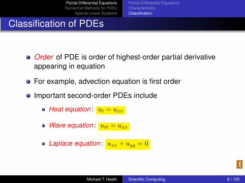
Order of PDE is order of highest-order partial derivativeappearing in equation
For example, advection equation is first order
Important second-order PDEs include
Heat equation : ut = uxx
Wave equation : utt = uxx
Laplace equation : uxx + uyy = 0
Michael T. Heath Scientific Computing 8 / 105

Partial Differential EquationsNumerical Methods for PDEs
Sparse Linear Systems
Partial Differential EquationsCharacteristicsClassification
Classification of PDEs, continued
Second-order linear PDEs of general form
auxx + buxy + cuyy + dux + euy + fu + g = 0
are classified by value of discriminant b2 − 4ac
b2 − 4ac > 0: hyperbolic (e.g., wave equation)
b2 − 4ac = 0: parabolic (e.g., heat equation)
b2 − 4ac < 0: elliptic (e.g., Laplace equation)
Michael T. Heath Scientific Computing 9 / 105

Partial Differential EquationsNumerical Methods for PDEs
Sparse Linear Systems
Partial Differential EquationsCharacteristicsClassification
Classification of PDEs, continued
Classification of more general PDEs is not so clean and simple,but roughly speaking
Hyperbolic PDEs describe time-dependent, conservativephysical processes, such as convection, that are notevolving toward steady state
Parabolic PDEs describe time-dependent, dissipativephysical processes, such as diffusion, that are evolvingtoward steady state
Elliptic PDEs describe processes that have alreadyreached steady state, and hence are time-independent
Michael T. Heath Scientific Computing 10 / 105
Partial Differential EquationsNumerical Methods for PDEs
Sparse Linear Systems
Time-Dependent ProblemsTime-Independent Problems
Time-Dependent Problems
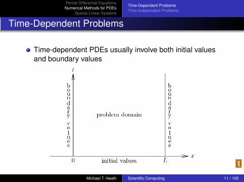
Time-dependent PDEs usually involve both initial valuesand boundary values
Michael T. Heath Scientific Computing 11 / 105

Partial Differential EquationsNumerical Methods for PDEs
Sparse Linear Systems
Time-Dependent ProblemsTime-Independent Problems
Semidiscrete Methods
One way to solve time-dependent PDE numerically is todiscretize in space but leave time variable continuous
Result is system of ODEs that can then be solved bymethods previously discussed
For example, consider heat equation
ut = c uxx, 0 ≤ x ≤ 1, t ≥ 0
with initial condition
u(0, x) = f(x), 0 ≤ x ≤ 1
and boundary conditions
u(t, 0) = 0, u(t, 1) = 0, t ≥ 0
Michael T. Heath Scientific Computing 12 / 105
Partial Differential EquationsNumerical Methods for PDEs
Sparse Linear Systems
Time-Dependent ProblemsTime-Independent Problems
Semidiscrete Finite Difference Method
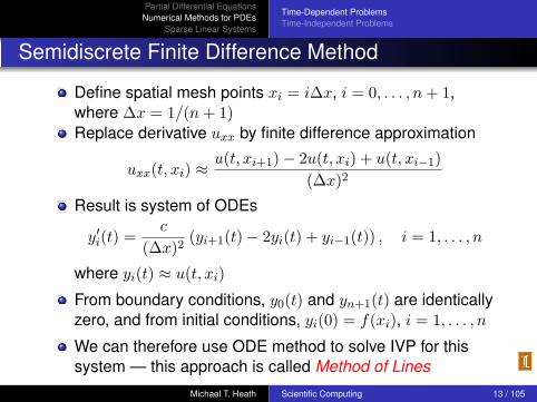
Define spatial mesh points xi = i∆x, i = 0, . . . , n + 1,where ∆x = 1/(n + 1)Replace derivative uxx by finite difference approximation
uxx(t, xi) ≈u(t, xi+1)− 2u(t, xi) + u(t, xi−1)
(∆x)2
Result is system of ODEs
y′i(t) =c
(∆x)2(yi+1(t)− 2yi(t) + yi−1(t)) , i = 1, . . . , n
where yi(t) ≈ u(t, xi)
From boundary conditions, y0(t) and yn+1(t) are identicallyzero, and from initial conditions, yi(0) = f(xi), i = 1, . . . , n
We can therefore use ODE method to solve IVP for thissystem — this approach is called Method of Lines
Michael T. Heath Scientific Computing 13 / 105

Partial Differential EquationsNumerical Methods for PDEs
Sparse Linear Systems
Time-Dependent ProblemsTime-Independent Problems
Method of Lines
Method of lines uses ODE solver to computecross-sections of solution surface over space-time planealong series of lines, each parallel to time axis andcorresponding to discrete spatial mesh point
Michael T. Heath Scientific Computing 14 / 105

Partial Differential EquationsNumerical Methods for PDEs
Sparse Linear Systems
Time-Dependent ProblemsTime-Independent Problems
Stiffness
Semidiscrete system of ODEs just derived can be writtenin matrix form
y′ =c
(∆x)2
−2 1 0 · · · 0
1 −2 1 · · · 00 1 −2 · · · 0...
. . . . . . . . ....
0 · · · 0 1 −2
y = Ay
Jacobian matrix A of this system has eigenvalues between−4c/(∆x)2 and 0, which makes ODE very stiff as spatialmesh size ∆x becomes small
This stiffness, which is typical of ODEs derived from PDEs,must be taken into account in choosing ODE method forsolving semidiscrete system
Michael T. Heath Scientific Computing 15 / 105
Partial Differential EquationsNumerical Methods for PDEs
Sparse Linear Systems
Time-Dependent ProblemsTime-Independent Problems
Semidiscrete Collocation Method
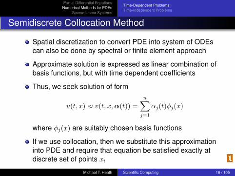
Spatial discretization to convert PDE into system of ODEscan also be done by spectral or finite element approach
Approximate solution is expressed as linear combination ofbasis functions, but with time dependent coefficients
Thus, we seek solution of form
u(t, x) ≈ v(t, x, α(t)) =n∑
j=1
αj(t)φj(x)
where φj(x) are suitably chosen basis functions
If we use collocation, then we substitute this approximationinto PDE and require that equation be satisfied exactly atdiscrete set of points xi
Michael T. Heath Scientific Computing 16 / 105

Partial Differential EquationsNumerical Methods for PDEs
Sparse Linear Systems
Time-Dependent ProblemsTime-Independent Problems
Semidiscrete Collocation, continued
For heat equation, this yields system of ODEs
n∑j=1
α′j(t)φj(xi) = c
n∑j=1
αj(t)φ′′j (xi)
whose solution is set of coefficient functions αi(t) thatdetermine approximate solution to PDE
Implicit form of this system is not explicit form required bystandard ODE methods, so we define n× n matrices Mand N by
mij = φj(xi), nij = φ′′j (xi)
Michael T. Heath Scientific Computing 17 / 105
Partial Differential EquationsNumerical Methods for PDEs
Sparse Linear Systems
Time-Dependent ProblemsTime-Independent Problems
Semidiscrete Collocation, continued
Assuming M is nonsingular, we then obtain system ofODEs
α′(t) = cM−1Nα(t)
which is in form suitable for solution with standard ODEsoftware
As usual, M need not be inverted explicitly, but merelyused to solve linear systems
Initial condition for ODE can be obtained by requiringsolution to satisfy given initial condition for PDE at meshpoints xi
Matrices involved in this method will be sparse if basisfunctions are “local,” such as B-splines
Michael T. Heath Scientific Computing 18 / 105

Partial Differential EquationsNumerical Methods for PDEs
Sparse Linear Systems
Time-Dependent ProblemsTime-Independent Problems
Semidiscrete Collocation, continued
Unlike finite difference method, spectral or finite elementmethod does not produce approximate values of solution udirectly, but rather it generates representation ofapproximate solution as linear combination of basisfunctions
Basis functions depend only on spatial variable, butcoefficients of linear combination (given by solution tosystem of ODEs) are time dependent
Thus, for any given time t, corresponding linearcombination of basis functions generates cross section ofsolution surface parallel to spatial axis
As with finite difference methods, systems of ODEs arisingfrom semidiscretization of PDE by spectral or finite elementmethods tend to be stiff
Michael T. Heath Scientific Computing 19 / 105
Partial Differential EquationsNumerical Methods for PDEs
Sparse Linear Systems
Time-Dependent ProblemsTime-Independent Problems
Fully Discrete Methods
Fully discrete methods for PDEs discretize in both timeand space dimensions
In fully discrete finite difference method, we
replace continuous domain of equation by discrete mesh ofpointsreplace derivatives in PDE by finite differenceapproximationsseek numerical solution as table of approximate values atselected points in space and time
Michael T. Heath Scientific Computing 20 / 105

Partial Differential EquationsNumerical Methods for PDEs
Sparse Linear Systems
Time-Dependent ProblemsTime-Independent Problems
Fully Discrete Methods, continued
In two dimensions (one space and one time), resultingapproximate solution values represent points on solutionsurface over problem domain in space-time plane
Accuracy of approximate solution depends on step sizes inboth space and time
Replacement of all partial derivatives by finite differencesresults in system of algebraic equations for unknownsolution at discrete set of sample points
Discrete system may be linear or nonlinear, depending onunderlying PDE
Michael T. Heath Scientific Computing 21 / 105
Partial Differential EquationsNumerical Methods for PDEs
Sparse Linear Systems
Time-Dependent ProblemsTime-Independent Problems
Fully Discrete Methods, continued
With initial-value problem, solution is obtained by startingwith initial values along boundary of problem domain andmarching forward in time step by step, generatingsuccessive rows in solution table
Time-stepping procedure may be explicit or implicit,depending on whether formula for solution values at nexttime step involves only past information
We might expect to obtain arbitrarily good accuracy bytaking sufficiently small step sizes in time and space
Time and space step sizes cannot always be chosenindependently of each other, however
Michael T. Heath Scientific Computing 22 / 105

Partial Differential EquationsNumerical Methods for PDEs
Sparse Linear Systems
Time-Dependent ProblemsTime-Independent Problems
Example: Heat Equation
Consider heat equation
ut = c uxx, 0 ≤ x ≤ 1, t ≥ 0
with initial and boundary conditions
u(0, x) = f(x), u(t, 0) = α, u(t, 1) = β
Define spatial mesh points xi = i∆x, i = 0, 1, . . . , n + 1,where ∆x = 1/(n + 1), and temporal mesh pointstk = k∆t, for suitably chosen ∆t
Let uki denote approximate solution at (tk, xi)
Michael T. Heath Scientific Computing 23 / 105

Partial Differential EquationsNumerical Methods for PDEs
Sparse Linear Systems
Time-Dependent ProblemsTime-Independent Problems
Heat Equation, continued
Replacing ut by forward difference in time and uxx bycentered difference in space, we obtain
uk+1i − uk
i
∆t= c
uki+1 − 2uk
i + uki−1
(∆x)2, or
uk+1i = uk
i + c∆t
(∆x)2(uk
i+1 − 2uki + uk
i−1
), i = 1, . . . , n
Stencil : pattern of mesh points involved at each level
Michael T. Heath Scientific Computing 24 / 105
Partial Differential EquationsNumerical Methods for PDEs
Sparse Linear Systems
Time-Dependent ProblemsTime-Independent Problems
Heat Equation, continued
Boundary conditions give us uk0 = α and uk
n+1 = β for all k,and initial conditions provide starting values u0
i = f(xi),i = 1, . . . , n
So we can march numerical solution forward in time usingthis explicit difference scheme
Local truncation error is O(∆t) +O((∆x)2), so scheme isfirst-order accurate in time and second-order accurate inspace
< interactive example >
Michael T. Heath Scientific Computing 25 / 105

Partial Differential EquationsNumerical Methods for PDEs
Sparse Linear Systems
Time-Dependent ProblemsTime-Independent Problems
Example: Wave Equation
Consider wave equation
utt = c uxx, 0 ≤ x ≤ 1, t ≥ 0
with initial and boundary conditions
u(0, x) = f(x), ut(0, x) = g(x)
u(t, 0) = α, u(t, 1) = β
Michael T. Heath Scientific Computing 26 / 105
Partial Differential EquationsNumerical Methods for PDEs
Sparse Linear Systems
Time-Dependent ProblemsTime-Independent Problems
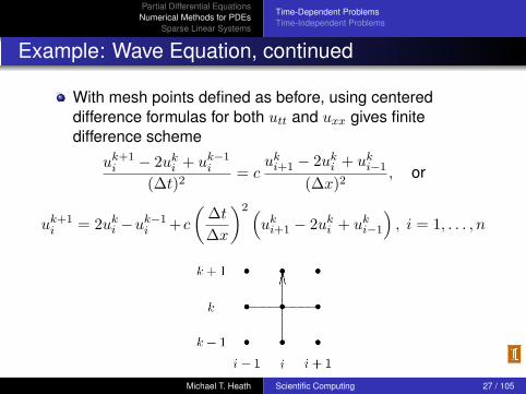
Example: Wave Equation, continued
With mesh points defined as before, using centereddifference formulas for both utt and uxx gives finitedifference scheme
uk+1i − 2uk
i + uk−1i
(∆t)2= c
uki+1 − 2uk
i + uki−1
(∆x)2, or
uk+1i = 2uk
i −uk−1i +c
(∆t
∆x
)2 (uk
i+1 − 2uki + uk
i−1
), i = 1, . . . , n
Michael T. Heath Scientific Computing 27 / 105

Partial Differential EquationsNumerical Methods for PDEs
Sparse Linear Systems
Time-Dependent ProblemsTime-Independent Problems
Wave Equation, continued
Using data at two levels in time requires additional storage
We also need u0i and u1
i to get started, which can beobtained from initial conditions
u0i = f(xi), u1
i = f(xi) + (∆t)g(xi)
where latter uses forward difference approximation to initialcondition ut(0, x) = g(x)
< interactive example >
Michael T. Heath Scientific Computing 28 / 105

Partial Differential EquationsNumerical Methods for PDEs
Sparse Linear Systems
Time-Dependent ProblemsTime-Independent Problems
Stability
Unlike Method of Lines, where time step is chosenautomatically by ODE solver, user must choose time step∆t in fully discrete method, taking into account bothaccuracy and stability requirements
For example, fully discrete scheme for heat equation issimply Euler’s method applied to semidiscrete system ofODEs for heat equation given previously
We saw that Jacobian matrix of semidiscrete system haseigenvalues between −4c/(∆x)2 and 0, so stability regionfor Euler’s method requires time step to satisfy
∆t ≤ (∆x)2
2 c
Severe restriction on time step can make explicit methodsrelatively inefficient < interactive example >
Michael T. Heath Scientific Computing 29 / 105
Partial Differential EquationsNumerical Methods for PDEs
Sparse Linear Systems
Time-Dependent ProblemsTime-Independent Problems
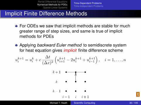
Implicit Finite Difference Methods
For ODEs we saw that implicit methods are stable for muchgreater range of step sizes, and same is true of implicitmethods for PDEs
Applying backward Euler method to semidiscrete systemfor heat equation gives implicit finite difference scheme
uk+1i = uk
i + c∆t
(∆x)2(uk+1
i+1 − 2uk+1i + uk+1
i−1
), i = 1, . . . , n
Michael T. Heath Scientific Computing 30 / 105

Partial Differential EquationsNumerical Methods for PDEs
Sparse Linear Systems
Time-Dependent ProblemsTime-Independent Problems
Implicit Finite Difference Methods, continued
This scheme inherits unconditional stability of backwardEuler method, which means there is no stability restrictionon relative sizes of ∆t and ∆x
But first-order accuracy in time still severely limits time step
< interactive example >
Michael T. Heath Scientific Computing 31 / 105
Partial Differential EquationsNumerical Methods for PDEs
Sparse Linear Systems
Time-Dependent ProblemsTime-Independent Problems
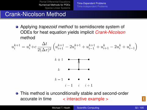
Crank-Nicolson Method
Applying trapezoid method to semidiscrete system ofODEs for heat equation yields implicit Crank-Nicolsonmethod
uk+1i = uk
i +c∆t
2(∆x)2(uk+1
i+1 − 2uk+1i + uk+1
i−1 + uki+1 − 2uk
i + uki−1
)
This method is unconditionally stable and second-orderaccurate in time < interactive example >
Michael T. Heath Scientific Computing 32 / 105

Partial Differential EquationsNumerical Methods for PDEs
Sparse Linear Systems
Time-Dependent ProblemsTime-Independent Problems
Implicit Finite Difference Methods, continued
Much greater stability of implicit finite difference methodsenables them to take much larger time steps than explicitmethods, but they require more work per step, sincesystem of equations must be solved at each step
For both backward Euler and Crank-Nicolson methods forheat equation in one space dimension, this linear system istridiagonal, and thus both work and storage required aremodest
In higher dimensions, matrix of linear system does nothave such simple form, but it is still very sparse, withnonzeros in regular pattern
Michael T. Heath Scientific Computing 33 / 105
Partial Differential EquationsNumerical Methods for PDEs
Sparse Linear Systems
Time-Dependent ProblemsTime-Independent Problems
Convergence
In order for approximate solution to converge to truesolution of PDE as step sizes in time and space jointly goto zero, following two conditions must hold
Consistency : local truncation error must go to zeroStability : approximate solution at any fixed time t mustremain bounded
Lax Equivalence Theorem says that for well-posed linearPDE, consistency and stability are together necessary andsufficient for convergence
Neither consistency nor stability alone is sufficient toguarantee convergence
Michael T. Heath Scientific Computing 34 / 105
Partial Differential EquationsNumerical Methods for PDEs
Sparse Linear Systems
Time-Dependent ProblemsTime-Independent Problems
Stability
Consistency is usually fairly easy to verify using Taylorseries expansion
Analyzing stability is more challenging, and severalmethods are available
Matrix method, based on location of eigenvalues of matrixrepresentation of difference scheme, as we saw withEuler’s method for heat equationFourier method, in which complex exponentialrepresentation of solution error is substituted into differenceequation and analyzed for growth or decayDomains of dependence, in which domains of dependenceof PDE and difference scheme are compared
Michael T. Heath Scientific Computing 35 / 105

Partial Differential EquationsNumerical Methods for PDEs
Sparse Linear Systems
Time-Dependent ProblemsTime-Independent Problems
CFL Condition
Domain of dependence of PDE is portion of problemdomain that influences solution at given point, whichdepends on characteristics of PDE
Domain of dependence of difference scheme is set of allother mesh points that affect approximate solution at givenmesh point
CFL Condition : necessary condition for explicit finitedifference scheme for hyperbolic PDE to be stable is thatfor each mesh point domain of dependence of PDE mustlie within domain of dependence of finite differencescheme
Michael T. Heath Scientific Computing 36 / 105

Partial Differential EquationsNumerical Methods for PDEs
Sparse Linear Systems
Time-Dependent ProblemsTime-Independent Problems
Example: Wave Equation
Consider explicit finite difference scheme for waveequation given previously
Characteristics of wave equation are straight lines in (t, x)plane along which either x +
√c t or x−
√c t is constant
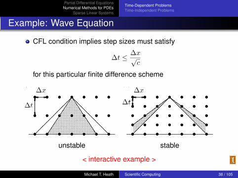
Domain of dependence for wave equation for given point istriangle with apex at given point and with sides of slope1/√
c and −1/√
c
Michael T. Heath Scientific Computing 37 / 105
Partial Differential EquationsNumerical Methods for PDEs
Sparse Linear Systems
Time-Dependent ProblemsTime-Independent Problems
Example: Wave Equation
CFL condition implies step sizes must satisfy
∆t ≤ ∆x√c
for this particular finite difference scheme
unstable stable
< interactive example >
Michael T. Heath Scientific Computing 38 / 105

Partial Differential EquationsNumerical Methods for PDEs
Sparse Linear Systems
Time-Dependent ProblemsTime-Independent Problems
Time-Independent Problems
We next consider time-independent, elliptic PDEs in twospace dimensions, such as Helmholtz equation
uxx + uyy + λu = f(x, y)
Important special casesPoisson equation : λ = 0Laplace equation : λ = 0 and f = 0
For simplicity, we will consider this equation on unit square
Numerous possibilities for boundary conditions specifiedalong each side of square
Dirichlet : u is specifiedNeumann : ux or uy is specifiedMixed : combinations of these are specified
Michael T. Heath Scientific Computing 39 / 105
Partial Differential EquationsNumerical Methods for PDEs
Sparse Linear Systems
Time-Dependent ProblemsTime-Independent Problems
Finite Difference Methods
Finite difference methods for such problems proceed asbefore
Define discrete mesh of points within domain of equationReplace derivatives in PDE by finite differenceapproximationsSeek numerical solution at mesh points
Unlike time-dependent problems, solution is not producedby marching forward step by step in time
Approximate solution is determined at all mesh pointssimultaneously by solving single system of algebraicequations
Michael T. Heath Scientific Computing 40 / 105

Partial Differential EquationsNumerical Methods for PDEs
Sparse Linear Systems
Time-Dependent ProblemsTime-Independent Problems
Example: Laplace Equation
Consider Laplace equation
uxx + uyy = 0
on unit square with boundary conditions shown below left
Define discrete mesh in domain, including boundaries, asshown above right
Michael T. Heath Scientific Computing 41 / 105
Partial Differential EquationsNumerical Methods for PDEs
Sparse Linear Systems
Time-Dependent ProblemsTime-Independent Problems
Laplace Equation, continued
Interior grid points where we will compute approximatesolution are given by
(xi, yj) = (ih, jh), i, j = 1, . . . , n
where in example n = 2 and h = 1/(n + 1) = 1/3
Next we replace derivatives by centered differenceapproximation at each interior mesh point to obtain finitedifference equation
ui+1,j − 2ui,j + ui−1,j
h2+
ui,j+1 − 2ui,j + ui,j−1
h2= 0
where ui,j is approximation to true solution u(xi, yj) fori, j = 1, . . . , n, and represents one of given boundaryvalues if i or j is 0 or n + 1
Michael T. Heath Scientific Computing 42 / 105

Partial Differential EquationsNumerical Methods for PDEs
Sparse Linear Systems
Time-Dependent ProblemsTime-Independent Problems
Laplace Equation, continued
Simplifying and writing out resulting four equationsexplicitly gives
4u1,1 − u0,1 − u2,1 − u1,0 − u1,2 = 0
4u2,1 − u1,1 − u3,1 − u2,0 − u2,2 = 0
4u1,2 − u0,2 − u2,2 − u1,1 − u1,3 = 0
4u2,2 − u1,2 − u3,2 − u2,1 − u2,3 = 0
Michael T. Heath Scientific Computing 43 / 105
Partial Differential EquationsNumerical Methods for PDEs
Sparse Linear Systems
Time-Dependent ProblemsTime-Independent Problems
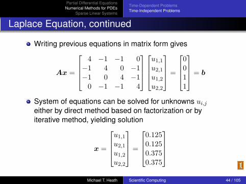
Laplace Equation, continued
Writing previous equations in matrix form gives
Ax =
4 −1 −1 0
−1 4 0 −1−1 0 4 −1
0 −1 −1 4
u1,1
u2,1
u1,2
u2,2
=
0011
= b
System of equations can be solved for unknowns ui,j
either by direct method based on factorization or byiterative method, yielding solution
x =
u1,1
u2,1
u1,2
u2,2
=
0.1250.1250.3750.375
Michael T. Heath Scientific Computing 44 / 105
Partial Differential EquationsNumerical Methods for PDEs
Sparse Linear Systems
Time-Dependent ProblemsTime-Independent Problems
Laplace Equation, continued
In practical problem, mesh size h would be much smaller,and resulting linear system would be much larger
Matrix would be very sparse, however, since each equationwould still involve only five variables, thereby savingsubstantially on work and storage
< interactive example >
Michael T. Heath Scientific Computing 45 / 105
Partial Differential EquationsNumerical Methods for PDEs
Sparse Linear Systems
Time-Dependent ProblemsTime-Independent Problems
Finite Element Methods
Finite element methods are also applicable to boundaryvalue problems for PDEs
Conceptually, there is no change in going from onedimension to two or three dimensions
Solution is represented as linear combination of basisfunctionsSome criterion (e.g., Galerkin) is applied to derive system ofequations that determines coefficients of linear combination
Main practical difference is that instead of subintervals inone dimension, elements usually become triangles orrectangles in two dimensions, or tetrahedra or hexahedrain three dimensions
Michael T. Heath Scientific Computing 46 / 105

Partial Differential EquationsNumerical Methods for PDEs
Sparse Linear Systems
Time-Dependent ProblemsTime-Independent Problems
Finite Element Methods, continued
Basis functions typically used are bilinear or bicubicfunctions in two dimensions or trilinear or tricubic functionsin three dimensions, analogous to piecewise linear “hat”functions or piecewise cubics in one dimension
Increase in dimensionality means that linear system to besolved is much larger, but it is still sparse due to localsupport of basis functions
Finite element methods for PDEs are extremely flexibleand powerful, but detailed treatment of them is beyondscope of this course
Michael T. Heath Scientific Computing 47 / 105
Partial Differential EquationsNumerical Methods for PDEs
Sparse Linear Systems
Direct MethodsIterative MethodsComparison of Methods
Sparse Linear Systems
Boundary value problems and implicit methods fortime-dependent PDEs yield systems of linear algebraicequations to solve
Finite difference schemes involving only a few variableseach, or localized basis functions in finite elementapproach, cause linear system to be sparse, with relativelyfew nonzero entries
Sparsity can be exploited to use much less than O(n2)storage and O(n3) work required in standard approach tosolving system with dense matrix
Michael T. Heath Scientific Computing 48 / 105

Partial Differential EquationsNumerical Methods for PDEs
Sparse Linear Systems
Direct MethodsIterative MethodsComparison of Methods
Sparse Factorization Methods
Gaussian elimination and Cholesky factorization areapplicable to large sparse systems, but care is required toachieve reasonable efficiency in solution time and storagerequirements
Key to efficiency is to store and operate on only nonzeroentries of matrix
Special data structures are required instead of simple 2-Darrays for storing dense matrices
Michael T. Heath Scientific Computing 49 / 105

Partial Differential EquationsNumerical Methods for PDEs
Sparse Linear Systems
Direct MethodsIterative MethodsComparison of Methods
Band Systems
For 1-D problems, equations and unknowns can usually beordered so that nonzeros are concentrated in narrow band,which can be stored efficiently in rectangular 2-D array bydiagonals
Bandwidth can often be reduced by reordering rows andcolumns of matrix
For problems in two or more dimensions, even narrowestpossible band often contains mostly zeros, so 2-D arraystorage is wasteful
Michael T. Heath Scientific Computing 50 / 105
Partial Differential EquationsNumerical Methods for PDEs
Sparse Linear Systems
Direct MethodsIterative MethodsComparison of Methods
General Sparse Data Structures
In general, sparse systems require data structures thatstore only nonzero entries, along with indices to identifytheir locations in matrix
Explicitly storing indices incurs additional storage overheadand makes arithmetic operations on nonzeros less efficientdue to indirect addressing to access operands
Data structure is worthwhile only if matrix is sufficientlysparse, which is often true for very large problems arisingfrom PDEs and many other applications
Michael T. Heath Scientific Computing 51 / 105

Partial Differential EquationsNumerical Methods for PDEs
Sparse Linear Systems
Direct MethodsIterative MethodsComparison of Methods
Fill
When applying LU or Cholesky factorization to sparsematrix, taking linear combinations of rows or columns toannihilate unwanted nonzero entries can introduce newnonzeros into matrix locations that were initially zero
Such new nonzeros, called fill, must be stored and maythemselves eventually need to be annihilated in order toobtain triangular factors
Resulting triangular factors can be expected to contain atleast as many nonzeros as original matrix and usuallysignificant fill as well
Michael T. Heath Scientific Computing 52 / 105
Partial Differential EquationsNumerical Methods for PDEs
Sparse Linear Systems
Direct MethodsIterative MethodsComparison of Methods
Reordering to Limit Fill
Amount of fill is sensitive to order in which rows andcolumns of matrix are processed, so basic problem insparse factorization is reordering matrix to limit fill duringfactorization
Exact minimization of fill is hard combinatorial problem(NP-complete), but heuristic algorithms such as minimumdegree and nested dissection limit fill well for many typesof problems
Michael T. Heath Scientific Computing 53 / 105

Partial Differential EquationsNumerical Methods for PDEs
Sparse Linear Systems
Direct MethodsIterative MethodsComparison of Methods
Example: Laplace Equation
Discretization of Laplace equation on square bysecond-order finite difference approximation to secondderivatives yields system of linear equations whoseunknowns correspond to mesh points (nodes) in squaregrid
Two nodes appearing in same equation of system areneighbors connected by edge in mesh or graph
Diagonal entries of matrix correspond to nodes in graph,and nonzero off-diagonal entries correspond to edges ingraph: aij 6= 0 ⇔ nodes i and j are neighbors
Michael T. Heath Scientific Computing 54 / 105

Partial Differential EquationsNumerical Methods for PDEs
Sparse Linear Systems
Direct MethodsIterative MethodsComparison of Methods
Natural, Row-Wise Ordering
With nodes numbered row-wise (or column-wise), matrix isblock tridiagonal, with each nonzero block either tridiagonalor diagonal
Matrix is banded but has many zero entries inside band
Cholesky factorization fills in band almost completely
Michael T. Heath Scientific Computing 55 / 105
Partial Differential EquationsNumerical Methods for PDEs
Sparse Linear Systems
Direct MethodsIterative MethodsComparison of Methods
Graph Model of Elimination
Each step of factorization process corresponds toelimination of one node from graph
Eliminating node causes its neighboring nodes to becomeconnected to each other
If any such neighbors were not already connected, then fillresults (new edges in graph and new nonzeros in matrix)
Michael T. Heath Scientific Computing 56 / 105
Partial Differential EquationsNumerical Methods for PDEs
Sparse Linear Systems
Direct MethodsIterative MethodsComparison of Methods
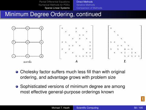
Minimum Degree Ordering
Good heuristic for limiting fill is to eliminate first thosenodes having fewest neighbors
Number of neighbors is called degree of node, so heuristicis known as minimum degree
At each step, select node of smallest degree forelimination, breaking ties arbitrarily
After node has been eliminated, its neighbors becomeconnected to each other, so degrees of some nodes maychange
Process is then repeated, with new node of minimumdegree eliminated next, and so on until all nodes havebeen eliminated
Michael T. Heath Scientific Computing 57 / 105
Partial Differential EquationsNumerical Methods for PDEs
Sparse Linear Systems
Direct MethodsIterative MethodsComparison of Methods
Minimum Degree Ordering, continued
Cholesky factor suffers much less fill than with originalordering, and advantage grows with problem size
Sophisticated versions of minimum degree are amongmost effective general-purpose orderings known
Michael T. Heath Scientific Computing 58 / 105

Partial Differential EquationsNumerical Methods for PDEs
Sparse Linear Systems
Direct MethodsIterative MethodsComparison of Methods
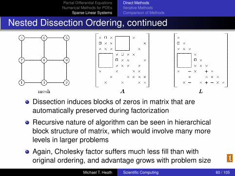
Nested Dissection Ordering
Nested dissection is based on divide-and-conquer
First, small set of nodes is selected whose removal splitsgraph into two pieces of roughly equal size
No node in either piece is connected to any node in other,so no fill occurs in either piece due to elimination of anynode in the other
Separator nodes are numbered last, then process isrepeated recursively on each remaining piece of graphuntil all nodes have been numbered
Michael T. Heath Scientific Computing 59 / 105
Partial Differential EquationsNumerical Methods for PDEs
Sparse Linear Systems
Direct MethodsIterative MethodsComparison of Methods
Nested Dissection Ordering, continued
Dissection induces blocks of zeros in matrix that areautomatically preserved during factorization
Recursive nature of algorithm can be seen in hierarchicalblock structure of matrix, which would involve many morelevels in larger problems
Again, Cholesky factor suffers much less fill than withoriginal ordering, and advantage grows with problem size
Michael T. Heath Scientific Computing 60 / 105

Partial Differential EquationsNumerical Methods for PDEs
Sparse Linear Systems
Direct MethodsIterative MethodsComparison of Methods
Sparse Factorization Methods
Sparse factorization methods are accurate, reliable, androbust
They are methods of choice for 1-D problems and areusually competitive for 2-D problems, but they can beprohibitively expensive in both work and storage for verylarge 3-D problems
Iterative methods often provide viable alternative in thesecases
Michael T. Heath Scientific Computing 61 / 105
Partial Differential EquationsNumerical Methods for PDEs
Sparse Linear Systems
Direct MethodsIterative MethodsComparison of Methods
Fast Direct Methods
For certain elliptic boundary value problems, such asPoisson equation on rectangular domain, fast Fouriertransform can be used to compute solution to discretesystem very efficiently
For problem with n mesh points, solution can be computedin O(n log n) operations
This technique is basis for several “fast Poisson solver”software packages
Cyclic reduction can achieve similar efficiency, and issomewhat more general
FACR method combines Fourier analysis and cyclicreduction to produce even faster method with O(n log log n)complexity
Michael T. Heath Scientific Computing 62 / 105

Partial Differential EquationsNumerical Methods for PDEs
Sparse Linear Systems
Direct MethodsIterative MethodsComparison of Methods
Iterative Methods for Linear Systems
Iterative methods for solving linear systems begin withinitial guess for solution and successively improve it untilsolution is as accurate as desired
In theory, infinite number of iterations might be required toconverge to exact solution
In practice, iteration terminates when residual ‖b−Ax‖, orsome other measure of error, is as small as desired
Michael T. Heath Scientific Computing 63 / 105

Partial Differential EquationsNumerical Methods for PDEs
Sparse Linear Systems
Direct MethodsIterative MethodsComparison of Methods
Stationary Iterative Methods
Simplest type of iterative method for solving Ax = b hasform
xk+1 = Gxk + c
where matrix G and vector c are chosen so that fixed pointof function g(x) = Gx + c is solution to Ax = b
Method is stationary if G and c are fixed over all iterations
G is Jacobian matrix of fixed-point function g, so stationaryiterative method converges if
ρ(G) < 1
and smaller spectral radius yields faster convergence
Michael T. Heath Scientific Computing 64 / 105

Partial Differential EquationsNumerical Methods for PDEs
Sparse Linear Systems
Direct MethodsIterative MethodsComparison of Methods
Example: Iterative Refinement
Iterative refinement is example of stationary iterativemethod
Forward and back substitution using LU factorization ineffect provides approximation, call it B−1, to inverse of A
Iterative refinement has form
xk+1 = xk + B−1(b−Axk)= (I −B−1A)xk + B−1b
So it is stationary iterative method with
G = I −B−1A, c = B−1b
It converges ifρ(I −B−1A) < 1
Michael T. Heath Scientific Computing 65 / 105
Partial Differential EquationsNumerical Methods for PDEs
Sparse Linear Systems
Direct MethodsIterative MethodsComparison of Methods
Splitting
One way to obtain matrix G is by splitting
A = M −N
with M nonsingular
Then take G = M−1N , so iteration scheme is
xk+1 = M−1Nxk + M−1b
which is implemented as
Mxk+1 = Nxk + b
(i.e., we solve linear system with matrix M at eachiteration)
Michael T. Heath Scientific Computing 66 / 105
Partial Differential EquationsNumerical Methods for PDEs
Sparse Linear Systems
Direct MethodsIterative MethodsComparison of Methods
Convergence
Stationary iteration using splitting converges if
ρ(G) = ρ(M−1N) < 1
and smaller spectral radius yields faster convergence
For fewest iterations, should choose M and N soρ(M−1N) is as small as possible, but cost per iteration isdetermined by cost of solving linear system with matrix M ,so there is tradeoff
In practice, M is chosen to approximate A in some sense,but is constrained to have simple form, such as diagonal ortriangular, so linear system at each iteration is easy tosolve
Michael T. Heath Scientific Computing 67 / 105

Partial Differential EquationsNumerical Methods for PDEs
Sparse Linear Systems
Direct MethodsIterative MethodsComparison of Methods
Jacobi Method
In matrix splitting A = M −N , simplest choice for M isdiagonal of A
Let D be diagonal matrix with same diagonal entries as A,and let L and U be strict lower and upper triangularportions of A
Then M = D and N = −(L + U) gives splitting of A
Assuming A has no zero diagonal entries, so D isnonsingular, this gives Jacobi method
x(k+1) = D−1(b− (L + U)x(k)
)
Michael T. Heath Scientific Computing 68 / 105

Partial Differential EquationsNumerical Methods for PDEs
Sparse Linear Systems
Direct MethodsIterative MethodsComparison of Methods
Jacobi Method, continued
Rewriting this scheme componentwise, we see that Jacobimethod computes next iterate by solving for eachcomponent of x in terms of others
x(k+1)i =
bi −∑j 6=i
aijx(k)j
/aii, i = 1, . . . , n
Jacobi method requires double storage for x, since oldcomponent values are needed throughout sweep, so newcomponent values cannot overwrite them until sweep hasbeen completed
Michael T. Heath Scientific Computing 69 / 105

Partial Differential EquationsNumerical Methods for PDEs
Sparse Linear Systems
Direct MethodsIterative MethodsComparison of Methods
Example: Jacobi Method
If we apply Jacobi method to system of finite differenceequations for Laplace equation, we obtain
u(k+1)i,j =
14
(u
(k)i−1,j + u
(k)i,j−1 + u
(k)i+1,j + u
(k)i,j+1
)so new approximate solution at each grid point is averageof previous solution at four surrounding grid points
Jacobi method does not always converge, but it isguaranteed to converge under conditions that are oftensatisfied in practice (e.g., if matrix is strictly diagonallydominant)
Unfortunately, convergence rate of Jacobi is usuallyunacceptably slow < interactive example >
Michael T. Heath Scientific Computing 70 / 105

Partial Differential EquationsNumerical Methods for PDEs
Sparse Linear Systems
Direct MethodsIterative MethodsComparison of Methods
Gauss-Seidel Method
One reason for slow convergence of Jacobi method is thatit does not make use of latest information available
Gauss-Seidel method remedies this by using each newcomponent of solution as soon as it has been computed
x(k+1)i =
bi −∑j<i
aijx(k+1)j −
∑j>i
aijx(k)j
/aii
Using same notation as before, Gauss-Seidel methodcorresponds to splitting M = D + L and N = −U
Written in matrix terms, this gives iteration scheme
x(k+1) = D−1(b−Lx(k+1) −Ux(k)
)= (D + L)−1
(b−Ux(k)
)Michael T. Heath Scientific Computing 71 / 105
Partial Differential EquationsNumerical Methods for PDEs
Sparse Linear Systems
Direct MethodsIterative MethodsComparison of Methods
Gauss-Seidel Method, continued
In addition to faster convergence, another benefit ofGauss-Seidel method is that duplicate storage is notneeded for x, since new component values can overwriteold ones immediately
On other hand, updating of unknowns must be donesuccessively, in contrast to Jacobi method, in whichunknowns can be updated in any order, or evensimultaneously
If we apply Gauss-Seidel method to solve system of finitedifference equations for Laplace equation, we obtain
u(k+1)i,j =
14
(u
(k+1)i−1,j + u
(k+1)i,j−1 + u
(k)i+1,j + u
(k)i,j+1
)Michael T. Heath Scientific Computing 72 / 105

Partial Differential EquationsNumerical Methods for PDEs
Sparse Linear Systems
Direct MethodsIterative MethodsComparison of Methods
Gauss-Seidel Method, continued
Thus, we again average solution values at four surroundinggrid points, but always use new component values as soonas they become available, rather than waiting until currentiteration has been completed
Gauss-Seidel method does not always converge, but it isguaranteed to converge under conditions that are oftensatisfied in practice, and are somewhat weaker than thosefor Jacobi method (e.g., if matrix is symmetric and positivedefinite)
Although Gauss-Seidel converges more rapidly thanJacobi, it is often still too slow to be practical
< interactive example >
Michael T. Heath Scientific Computing 73 / 105
Partial Differential EquationsNumerical Methods for PDEs
Sparse Linear Systems
Direct MethodsIterative MethodsComparison of Methods
Successive Over-Relaxation
Convergence rate of Gauss-Seidel can be accelerated bysuccessive over-relaxation (SOR), which in effect usesstep to next Gauss-Seidel iterate as search direction, butwith fixed search parameter denoted by ω
Starting with x(k), first compute next iterate that would begiven by Gauss-Seidel, x
(k+1)GS , then instead take next
iterate to be
x(k+1) = x(k) + ω(x(k+1)GS − x(k))
= (1− ω)x(k) + ωx(k+1)GS
which is weighted average of current iterate and nextGauss-Seidel iterate
Michael T. Heath Scientific Computing 74 / 105
Partial Differential EquationsNumerical Methods for PDEs
Sparse Linear Systems
Direct MethodsIterative MethodsComparison of Methods
Successive Over-Relaxation, continued
ω is fixed relaxation parameter chosen to accelerateconvergence
ω > 1 gives over-relaxation, ω < 1 gives under-relaxation,and ω = 1 gives Gauss-Seidel method
Method diverges unless 0 < ω < 2, but choosing optimal ωis difficult in general and is subject of elaborate theory forspecial classes of matrices
Michael T. Heath Scientific Computing 75 / 105

Partial Differential EquationsNumerical Methods for PDEs
Sparse Linear Systems
Direct MethodsIterative MethodsComparison of Methods
Successive Over-Relaxation, continued
Using same notation as before, SOR method correspondsto splitting
M =1ω
D + L, N =(
1ω− 1
)D −U
and can be written in matrix terms as
x(k+1) = x(k) + ω(D−1(b−Lx(k+1) −Ux(k))− x(k)
)= (D + ωL)−1 ((1− ω)D − ωU) x(k) + ω (D + ωL)−1b
< interactive example >
Michael T. Heath Scientific Computing 76 / 105

Partial Differential EquationsNumerical Methods for PDEs
Sparse Linear Systems
Direct MethodsIterative MethodsComparison of Methods
Conjugate Gradient MethodIf A is n× n symmetric positive definite matrix, thenquadratic function
φ(x) = 12x
T Ax− xT b
attains minimum precisely when Ax = b
Optimization methods have form
xk+1 = xk + αsk
where α is search parameter chosen to minimize objectivefunction φ(xk + αsk) along sk
For quadratic problem, negative gradient is residual vector
−∇φ(x) = b−Ax = r
Line search parameter can be determined analytically
α = rTk sk/sT
k Ask
Michael T. Heath Scientific Computing 77 / 105
Partial Differential EquationsNumerical Methods for PDEs
Sparse Linear Systems
Direct MethodsIterative MethodsComparison of Methods
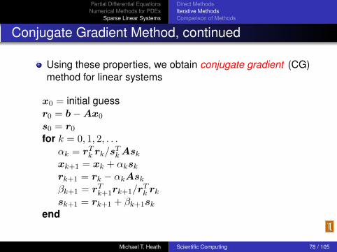
Conjugate Gradient Method, continued
Using these properties, we obtain conjugate gradient (CG)method for linear systems
x0 = initial guessr0 = b−Ax0
s0 = r0
for k = 0, 1, 2, . . .αk = rT
k rk/sTk Ask
xk+1 = xk + αksk
rk+1 = rk − αkAsk
βk+1 = rTk+1rk+1/rT
k rk
sk+1 = rk+1 + βk+1sk
end
Michael T. Heath Scientific Computing 78 / 105

Partial Differential EquationsNumerical Methods for PDEs
Sparse Linear Systems
Direct MethodsIterative MethodsComparison of Methods
Conjugate Gradient Method, continued
Key features that make CG method effectiveShort recurrence determines search directions that areA-orthogonal (conjugate)Error is minimal over space spanned by search directionsgenerated so far
Minimum error implies exact solution is reached in at mostn steps, since n linearly independent search directionsmust span whole space
In practice, loss of orthogonality due to rounding errorspoils finite termination property, so method is usediteratively
< interactive example >
Michael T. Heath Scientific Computing 79 / 105
Partial Differential EquationsNumerical Methods for PDEs
Sparse Linear Systems
Direct MethodsIterative MethodsComparison of Methods
Preconditioning
Convergence rate of CG can often be substantiallyaccelerated by preconditioning
Apply CG algorithm to M−1A, where M is chosen so thatM−1A is better conditioned and systems of form Mz = yare easily solved
Popular choices of preconditioners include
Diagonal or block-diagonalSSORIncomplete factorizationPolynomialApproximate inverse
Michael T. Heath Scientific Computing 80 / 105

Partial Differential EquationsNumerical Methods for PDEs
Sparse Linear Systems
Direct MethodsIterative MethodsComparison of Methods
Generalizations of CG Method
CG is not directly applicable to nonsymmetric or indefinitesystems
CG cannot be generalized to nonsymmetric systemswithout sacrificing one of its two key properties (shortrecurrence and minimum error)
Nevertheless, several generalizations have beendeveloped for solving nonsymmetric systems, includingGMRES, QMR, CGS, BiCG, and Bi-CGSTAB
These tend to be less robust and require more storagethan CG, but they can still be very useful for solving largenonsymmetric systems
Michael T. Heath Scientific Computing 81 / 105

Partial Differential EquationsNumerical Methods for PDEs
Sparse Linear Systems
Direct MethodsIterative MethodsComparison of Methods
Example: Iterative Methods
We illustrate various iterative methods by using them tosolve 4× 4 linear system for Laplace equation example
In each case we take x0 = 0 as starting guess
Jacobi method gives following iterates
k x1 x2 x3 x4
0 0.000 0.000 0.000 0.0001 0.000 0.000 0.250 0.2502 0.062 0.062 0.312 0.3123 0.094 0.094 0.344 0.3444 0.109 0.109 0.359 0.3595 0.117 0.117 0.367 0.3676 0.121 0.121 0.371 0.3717 0.123 0.123 0.373 0.3738 0.124 0.124 0.374 0.3749 0.125 0.125 0.375 0.375
Michael T. Heath Scientific Computing 82 / 105
Partial Differential EquationsNumerical Methods for PDEs
Sparse Linear Systems
Direct MethodsIterative MethodsComparison of Methods
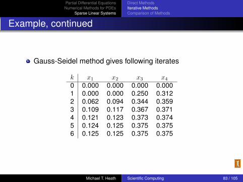
Example, continued
Gauss-Seidel method gives following iterates
k x1 x2 x3 x4
0 0.000 0.000 0.000 0.0001 0.000 0.000 0.250 0.3122 0.062 0.094 0.344 0.3593 0.109 0.117 0.367 0.3714 0.121 0.123 0.373 0.3745 0.124 0.125 0.375 0.3756 0.125 0.125 0.375 0.375
Michael T. Heath Scientific Computing 83 / 105

Partial Differential EquationsNumerical Methods for PDEs
Sparse Linear Systems
Direct MethodsIterative MethodsComparison of Methods
Example, continuedSOR method (with optimal ω = 1.072 for this problem)gives following iterates
k x1 x2 x3 x4
0 0.000 0.000 0.000 0.0001 0.000 0.000 0.268 0.3352 0.072 0.108 0.356 0.3653 0.119 0.121 0.371 0.3734 0.123 0.124 0.374 0.3755 0.125 0.125 0.375 0.375
CG method converges in only two iterations for thisproblem
k x1 x2 x3 x4
0 0.000 0.000 0.000 0.0001 0.000 0.000 0.333 0.3332 0.125 0.125 0.375 0.375
Michael T. Heath Scientific Computing 84 / 105

Partial Differential EquationsNumerical Methods for PDEs
Sparse Linear Systems
Direct MethodsIterative MethodsComparison of Methods
Rate of Convergence
For more systematic comparison of methods, we comparethem on k × k model grid problem for Laplace equation onunit square
For this simple problem, spectral radius of iteration matrixfor each method can be determined analytically, as well asoptimal ω for SOR
Gauss-Seidel is asymptotically twice as fast as Jacobi forthis model problem, but for both methods, number ofiterations per digit of accuracy gained is proportional tonumber of mesh points
Optimal SOR is order of magnitude faster than either ofthem, and number of iterations per digit gained isproportional to number of mesh points along one side ofgrid
Michael T. Heath Scientific Computing 85 / 105

Partial Differential EquationsNumerical Methods for PDEs
Sparse Linear Systems
Direct MethodsIterative MethodsComparison of Methods
Rate of Convergence, continued
For some specific values of k, values of spectral radius areshown below
k Jacobi Gauss-Seidel Optimal SOR10 0.9595 0.9206 0.560450 0.9981 0.9962 0.8840
100 0.9995 0.9990 0.9397500 0.99998 0.99996 0.98754
Spectral radius is extremely close to 1 for large values of k,so all three methods converge very slowly
For k = 10 (linear system of order 100), to gain singledecimal digit of accuracy Jacobi method requires morethan 50 iterations, Gauss-Seidel more than 25, and optimalSOR about 4
Michael T. Heath Scientific Computing 86 / 105
Partial Differential EquationsNumerical Methods for PDEs
Sparse Linear Systems
Direct MethodsIterative MethodsComparison of Methods
Rate of Convergence, continued
For k = 100 (linear system of order 10,000), to gain singledecimal digit of accuracy Jacobi method requires about5000 iterations, Gauss-Seidel about 2500, and optimalSOR about 37
Thus, Jacobi and Gauss-Seidel methods are impracticalfor problem of this size, and optimal SOR, though perhapsreasonable for this problem, also becomes prohibitivelyslow for still larger problems
Moreover, performance of SOR depends on knowledge ofoptimal value for relaxation parameter ω, which is knownanalytically for this simple model problem but is muchharder to determine in general
Michael T. Heath Scientific Computing 87 / 105

Partial Differential EquationsNumerical Methods for PDEs
Sparse Linear Systems
Direct MethodsIterative MethodsComparison of Methods
Rate of Convergence, continued
Convergence behavior of CG is more complicated, buterror is reduced at each iteration by factor of roughly
√κ− 1√κ + 1
on average, where
κ = cond(A) = ‖A‖ · ‖A−1‖ =λmax(A)λmin(A)
When matrix A is well-conditioned, convergence is rapid,but if A is ill-conditioned, convergence can be arbitrarilyslow
This is why preconditioner is usually used with CG method,so preconditioned matrix M−1A has much smallercondition number than A
Michael T. Heath Scientific Computing 88 / 105

Partial Differential EquationsNumerical Methods for PDEs
Sparse Linear Systems
Direct MethodsIterative MethodsComparison of Methods
Rate of Convergence, continued
This convergence estimate is conservative, however, andCG method may do much better
If matrix A has only m distinct eigenvalues, thentheoretically CG converges in at most m iterations
Detailed convergence behavior depends on entirespectrum of A, not just its extreme eigenvalues, and inpractice convergence is often superlinear
Michael T. Heath Scientific Computing 89 / 105

Partial Differential EquationsNumerical Methods for PDEs
Sparse Linear Systems
Direct MethodsIterative MethodsComparison of Methods
Smoothers
Disappointing convergence rates observed for stationaryiterative methods are asymptotic
Much better progress may be made initially beforeeventually settling into slow asymptotic phase
Many stationary iterative methods tend to reducehigh-frequency (i.e., oscillatory) components of errorrapidly, but reduce low-frequency (i.e., smooth)components of error much more slowly, which producespoor asymptotic rate of convergence
For this reason, such methods are sometimes calledsmoothers
< interactive example >
Michael T. Heath Scientific Computing 90 / 105
Partial Differential EquationsNumerical Methods for PDEs
Sparse Linear Systems
Direct MethodsIterative MethodsComparison of Methods
Multigrid Methods
Smooth or oscillatory components of error are relative tomesh on which solution is defined
Component that appears smooth on fine grid may appearoscillatory when sampled on coarser grid
If we apply smoother on coarser grid, then we may makerapid progress in reducing this (now oscillatory) componentof error
After few iterations of smoother, results can then beinterpolated back to fine grid to produce solution that hasboth higher-frequency and lower-frequency components oferror reduced
Michael T. Heath Scientific Computing 91 / 105

Partial Differential EquationsNumerical Methods for PDEs
Sparse Linear Systems
Direct MethodsIterative MethodsComparison of Methods
Multigrid Methods, continued
Multigrid methods : This idea can be extended to multiplelevels of grids, so that error components of variousfrequencies can be reduced rapidly, each at appropriatelevel
Transition from finer grid to coarser grid involves restrictionor injection
Transition from coarser grid to finer grid involvesinterpolation or prolongation
Michael T. Heath Scientific Computing 92 / 105

Partial Differential EquationsNumerical Methods for PDEs
Sparse Linear Systems
Direct MethodsIterative MethodsComparison of Methods
Residual Equation
If x̂ is approximate solution to Ax = b, with residualr = b−Ax̂, then error e = x− x̂ satisfies equationAe = r
Thus, in improving approximate solution we can work withjust this residual equation involving error and residual,rather than solution and original right-hand side
One advantage of residual equation is that zero isreasonable starting guess for its solution
Michael T. Heath Scientific Computing 93 / 105

Partial Differential EquationsNumerical Methods for PDEs
Sparse Linear Systems
Direct MethodsIterative MethodsComparison of Methods
Two-Grid Algorithm
1 On fine grid, use few iterations of smoother to computeapproximate solution x̂ for system Ax = b
2 Compute residual r = b−Ax̂
3 Restrict residual to coarse grid
4 On coarse grid, use few iterations of smoother on residualequation to obtain coarse-grid approximation to error
5 Interpolate coarse-grid correction to fine grid to obtainimproved approximate solution on fine grid
6 Apply few iterations of smoother to corrected solution onfine grid
Michael T. Heath Scientific Computing 94 / 105
Partial Differential EquationsNumerical Methods for PDEs
Sparse Linear Systems
Direct MethodsIterative MethodsComparison of Methods
Multigrid Methods, continued
Multigrid method results from recursion in Step 4: coarsegrid correction is itself improved by using still coarser grid,and so on down to some bottom level
Computations become progressively cheaper on coarserand coarser grids because systems become successivelysmaller
In particular, direct method may be feasible on coarsestgrid if system is small enough
Michael T. Heath Scientific Computing 95 / 105

Partial Differential EquationsNumerical Methods for PDEs
Sparse Linear Systems
Direct MethodsIterative MethodsComparison of Methods
Cycling Strategies
Common strategies for cycling through grid levels
Michael T. Heath Scientific Computing 96 / 105
Partial Differential EquationsNumerical Methods for PDEs
Sparse Linear Systems
Direct MethodsIterative MethodsComparison of Methods
Cycling Strategies, continued
V-cycle starts with finest grid and goes down throughsuccessive levels to coarsest grid and then back up againto finest grid
W-cycle zig-zags among lower level grids before movingback up to finest grid, to get more benefit from coarsergrids where computations are cheaper
Full multigrid starts at coarsest level, where good initialsolution is easier to come by (perhaps by direct method),then bootstraps this solution up through grid levels,ultimately reaching finest grid
Michael T. Heath Scientific Computing 97 / 105

Partial Differential EquationsNumerical Methods for PDEs
Sparse Linear Systems
Direct MethodsIterative MethodsComparison of Methods
Multigrid Methods, continued
By exploiting strengths of underlying iterative smoothersand avoiding their weaknesses, multigrid methods arecapable of extraordinarily good performance, linear innumber of grid points in best case
At each level, smoother reduces oscillatory component oferror rapidly, at rate independent of mesh size h, since fewiterations of smoother, often only one, are performed ateach level
Since all components of error appear oscillatory at somelevel, convergence rate of entire multigrid scheme shouldbe rapid and independent of mesh size, in contrast to otheriterative methods
Michael T. Heath Scientific Computing 98 / 105

Partial Differential EquationsNumerical Methods for PDEs
Sparse Linear Systems
Direct MethodsIterative MethodsComparison of Methods
Multigrid Methods, continued
Moreover, cost of entire cycle of multigrid is only modestmultiple of cost of single sweep on finest grid
As result, multigrid methods are among most powerfulmethods available for solving sparse linear systems arisingfrom PDEs
They are capable of converging to within truncation error ofdiscretization at cost comparable with fast direct methods,although latter are much less broadly applicable
Michael T. Heath Scientific Computing 99 / 105

Partial Differential EquationsNumerical Methods for PDEs
Sparse Linear Systems
Direct MethodsIterative MethodsComparison of Methods
Direct vs. Iterative Methods
Direct methods require no initial estimate for solution, buttake no advantage if good estimate happens to beavailable
Direct methods are good at producing high accuracy, buttake no advantage if only low accuracy is needed
Iterative methods are often dependent on specialproperties, such as matrix being symmetric positivedefinite, and are subject to very slow convergence forbadly conditioned systems; direct methods are morerobust in both senses
Michael T. Heath Scientific Computing 100 / 105

Partial Differential EquationsNumerical Methods for PDEs
Sparse Linear Systems
Direct MethodsIterative MethodsComparison of Methods
Direct vs. Iterative Methods
Iterative methods usually require less work if convergenceis rapid, but often require computation or estimation ofvarious parameters or preconditioners to accelerateconvergence
Iterative methods do not require explicit storage of matrixentries, and hence are good when matrix can be producedeasily on demand or is most easily implemented as linearoperator
Iterative methods are less readily embodied in standardsoftware packages, since best representation of matrix isoften problem dependent and “hard-coded” in applicationprogram, whereas direct methods employ more standardstorage schemes
Michael T. Heath Scientific Computing 101 / 105
Partial Differential EquationsNumerical Methods for PDEs
Sparse Linear Systems
Direct MethodsIterative MethodsComparison of Methods
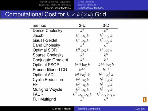
Computational Cost for k × k (×k) Grid
method 2-D 3-DDense Cholesky k6 k9
Jacobi k4 log k k5 log kGauss-Seidel k4 log k k5 log kBand Cholesky k4 k7
Optimal SOR k3 log k k4 log kSparse Cholesky k3 k6
Conjugate Gradient k3 k4
Optimal SSOR k2.5 log k k3.5 log kPreconditioned CG k2.5 k3.5
Optimal ADI k2 log2 k k3 log2 kCyclic Reduction k2 log k k3 log kFFT k2 log k k3 log kMultigrid V-cycle k2 log k k3 log kFACR k2 log log k k3 log log kFull Multigrid k2 k3
Michael T. Heath Scientific Computing 102 / 105

Partial Differential EquationsNumerical Methods for PDEs
Sparse Linear Systems
Direct MethodsIterative MethodsComparison of Methods
Comparison of Methods
For those methods that remain viable choices for finiteelement discretizations with less regular meshes,computational cost of solving elliptic boundary valueproblems is given below in terms of exponent of n (order ofmatrix) in dominant term of cost estimate
method 2-D 3-DDense Cholesky 3 3Band Cholesky 2 2.33Sparse Cholesky 1.5 2Conjugate Gradient 1.5 1.33Preconditioned CG 1.25 1.17Multigrid 1 1
Michael T. Heath Scientific Computing 103 / 105

Partial Differential EquationsNumerical Methods for PDEs
Sparse Linear Systems
Direct MethodsIterative MethodsComparison of Methods
Comparison of Methods, continued
Multigrid methods can be optimal, in sense that cost ofcomputing solution is of same order as cost of readinginput or writing output
FACR method is also optimal for all practical purposes,since log log k is effectively constant for any reasonablevalue of k
Other fast direct methods are almost as effective inpractice unless k is very large
Despite their higher cost, factorization methods are stilluseful in some cases due to their greater robustness,especially for nonsymmetric matrices
Methods akin to factorization are often used to computeeffective preconditioners
Michael T. Heath Scientific Computing 104 / 105

Partial Differential EquationsNumerical Methods for PDEs
Sparse Linear Systems
Direct MethodsIterative MethodsComparison of Methods
Software for PDEs
Methods for numerical solution of PDEs tend to be veryproblem dependent, so PDEs are usually solved by customwritten software to take maximum advantage of particularfeatures of given problem
Nevertheless, some software does exist for some generalclasses of problems that occur often in practice
In addition, several good software packages are availablefor solving sparse linear systems arising from PDEs as wellas other sources
Michael T. Heath Scientific Computing 105 / 105