scientific uncertainty analysis in pressure metrology · scientific uncertainty analysis in...
TRANSCRIPT

Pressure & Vacuum Laboratory TAF 2011 Navigate to Table of Contents
Scientific Uncertainty Analysis in Pressure Metrology
EURAMET.M.P-K13 as an Illustrative Case Study
Vishal RamnathR&D Metrologist: Pressure & Vacuum
Pressure & Vacuum Laboratory
April 19, 2011
1 / 30

Pressure & Vacuum Laboratory TAF 2011 Navigate to Table of Contents
Table of contents IReview of Methods for Pressure Generation/Measurement
Mechanism of Pressure GenerationMathematical Model of Pressure BalanceMechanism to Solve Formulation of Mathematical EquationSolution for Roots of Multivariable EquationDefining an EoS for the Working FluidSolution of the Roots (Pressure) of the Nonlinear Equation
Calculation of Generated Pressure UncertaintySpecific Issues Encountered in Uncertainty Analysis
Methodology Used in Cross-Floating AnalysisDerivation of Basis Equation used in Cross-Floating I.Estimation of the Straight Line Uncertainties Corresponding to u(A0)and u(λ)
DiscussionSpecific Comments on Intercomparison ResultsRecommendations Going Foward
2 / 30

Pressure & Vacuum Laboratory TAF 2011 Navigate to Table of Contents
Review of Methods for Pressure Generation/Measurement
Mechanism of Pressure Generation
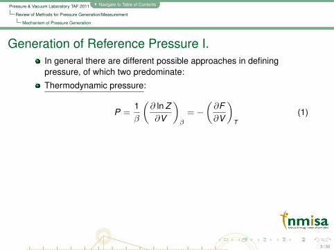
Generation of Reference Pressure I.In general there are different possible approaches in definingpressure, of which two predominate:
Thermodynamic pressure:
P =1β
(∂ ln Z∂V
)β
= −(∂F∂V
)T
(1)
defined in terms of the Maxwell thermodynamic equations:(∂T∂V
)S = −
(∂P∂S
)V ,
(∂S∂V
)T =
(∂P∂T
)V(
∂S∂P
)T = −
(∂V∂T
)P ,
(∂T∂P
)S =
(∂V∂S
)P
(2)
Recall: Partition function Z (T ,V ,N) =∑
r exp(−βEr ), r microstate,Er energy for r microstate, temperature paramter β = 1
kT , kBoltzmann fundamental constant, Helmholtz free energyF (T ,V ,N) = −kT ln Z (T ,V ,N), temperature 1
T =(∂S(E,V ,N)
∂E
)V ,N
3 / 30
Pressure & Vacuum Laboratory TAF 2011 Navigate to Table of Contents
Review of Methods for Pressure Generation/Measurement
Mechanism of Pressure Generation
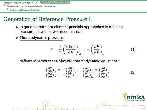
Generation of Reference Pressure I.In general there are different possible approaches in definingpressure, of which two predominate:
Thermodynamic pressure:
P =1β
(∂ ln Z∂V
)β
= −(∂F∂V
)T
(1)
defined in terms of the Maxwell thermodynamic equations:(∂T∂V
)S = −
(∂P∂S
)V ,
(∂S∂V
)T =
(∂P∂T
)V(
∂S∂P
)T = −
(∂V∂T
)P ,
(∂T∂P
)S =
(∂V∂S
)P
(2)
Recall: Partition function Z (T ,V ,N) =∑
r exp(−βEr ), r microstate,Er energy for r microstate, temperature paramter β = 1
kT , kBoltzmann fundamental constant, Helmholtz free energyF (T ,V ,N) = −kT ln Z (T ,V ,N), temperature 1
T =(∂S(E,V ,N)
∂E
)V ,N
3 / 30
Pressure & Vacuum Laboratory TAF 2011 Navigate to Table of Contents
Review of Methods for Pressure Generation/Measurement
Mechanism of Pressure Generation
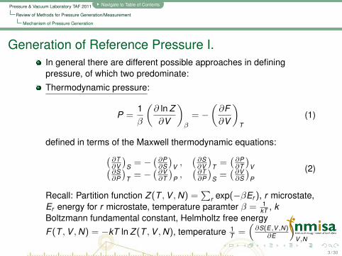
Generation of Reference Pressure I.In general there are different possible approaches in definingpressure, of which two predominate:
Thermodynamic pressure:
P =1β
(∂ ln Z∂V
)β
= −(∂F∂V
)T
(1)
defined in terms of the Maxwell thermodynamic equations:(∂T∂V
)S = −
(∂P∂S
)V ,
(∂S∂V
)T =
(∂P∂T
)V(
∂S∂P
)T = −
(∂V∂T
)P ,
(∂T∂P
)S =
(∂V∂S
)P
(2)
Recall: Partition function Z (T ,V ,N) =∑
r exp(−βEr ), r microstate,Er energy for r microstate, temperature paramter β = 1
kT , kBoltzmann fundamental constant, Helmholtz free energyF (T ,V ,N) = −kT ln Z (T ,V ,N), temperature 1
T =(∂S(E,V ,N)
∂E
)V ,N
3 / 30
Pressure & Vacuum Laboratory TAF 2011 Navigate to Table of Contents
Review of Methods for Pressure Generation/Measurement
Mechanism of Pressure Generation
Generation of Reference Pressure I.In general there are different possible approaches in definingpressure, of which two predominate:
Thermodynamic pressure:
P =1β
(∂ ln Z∂V
)β
= −(∂F∂V
)T
(1)
defined in terms of the Maxwell thermodynamic equations:(∂T∂V
)S = −
(∂P∂S
)V ,
(∂S∂V
)T =
(∂P∂T
)V(
∂S∂P
)T = −
(∂V∂T
)P ,
(∂T∂P
)S =
(∂V∂S
)P
(2)
Recall: Partition function Z (T ,V ,N) =∑
r exp(−βEr ), r microstate,Er energy for r microstate, temperature paramter β = 1
kT , kBoltzmann fundamental constant, Helmholtz free energyF (T ,V ,N) = −kT ln Z (T ,V ,N), temperature 1
T =(∂S(E,V ,N)
∂E
)V ,N
3 / 30

Pressure & Vacuum Laboratory TAF 2011 Navigate to Table of Contents
Review of Methods for Pressure Generation/Measurement
Mechanism of Pressure Generation
Generation of Reference Pressure II.Mechanical pressure: The full situation is actually more complicatedsince recourse to Hamiltonian theory is required to precisely define“force” in terms of the generalized displacements and generalizedmomenta:
H =∑nα=1 pαqα − L, pα = − ∂H
∂qα, qα = ∂H
∂pα (3)
This conceptual framework is necessary since ideally formeasurement equivalence
Pthermodynamic = Pmechanical (4)
Utilizing the concepts of strain and stress the mechanical pressurefor a fluid is defined in terms of the shear stress tensor as
p = −13
(τxx + τyy + τzz) = p −(λ+
23µ
)∇ · V (5)
4 / 30

Pressure & Vacuum Laboratory TAF 2011 Navigate to Table of Contents
Review of Methods for Pressure Generation/Measurement
Mechanism of Pressure Generation
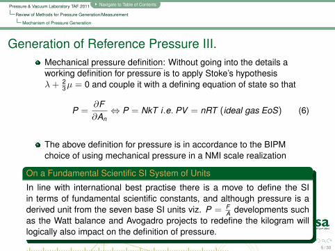
Generation of Reference Pressure III.Mechanical pressure definition: Without going into the details aworking definition for pressure is to apply Stoke’s hypothesisλ+ 2
3µ = 0 and couple it with a defining equation of state so that
P =∂F∂An
⇔ P = NkT i.e. PV = nRT (ideal gas EoS) (6)
The above definition for pressure is in accordance to the BIPMchoice of using mechanical pressure in a NMI scale realization
On a Fundamental Scientific SI System of Units
In line with international best practise there is a move to define the SIin terms of fundamental scientific constants, and although pressure is aderived unit from the seven base SI units viz. P = F
A developments suchas the Watt balance and Avogadro projects to redefine the kilogram willlogically also impact on the definition of pressure.
5 / 30
Pressure & Vacuum Laboratory TAF 2011 Navigate to Table of Contents
Review of Methods for Pressure Generation/Measurement
Mechanism of Pressure Generation
Generation of Reference Pressure III.Mechanical pressure definition: Without going into the details aworking definition for pressure is to apply Stoke’s hypothesisλ+ 2
3µ = 0 and couple it with a defining equation of state so that
P =∂F∂An
⇔ P = NkT i.e. PV = nRT (ideal gas EoS) (6)
The above definition for pressure is in accordance to the BIPMchoice of using mechanical pressure in a NMI scale realization
On a Fundamental Scientific SI System of Units
In line with international best practise there is a move to define the SIin terms of fundamental scientific constants, and although pressure is aderived unit from the seven base SI units viz. P = F
A developments suchas the Watt balance and Avogadro projects to redefine the kilogram willlogically also impact on the definition of pressure.
5 / 30

Pressure & Vacuum Laboratory TAF 2011 Navigate to Table of Contents
Review of Methods for Pressure Generation/Measurement
Mechanism of Pressure Generation
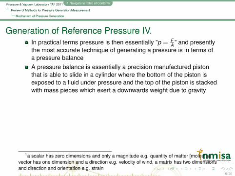
Generation of Reference Pressure IV.In practical terms pressure is then essentially ”p = F
A ” and presentlythe most accurate technique of generating a pressure is in terms ofa pressure balance
A pressure balance is essentially a precision manufactured pistonthat is able to slide in a cylinder where the bottom of the piston isexposed to a fluid under pressure and the top of the piston is stackedwith mass pieces which exert a downwards weight due to gravityFrom the full definition of “pressure” the quantity p is in fact a tensor1
but for most practical purposes we essentially consider it a scalare.g. in hydrostatic hydraulic pressure we assume that the pressureis equal in all directions (true for Newtonian fluids)For a piston-cylinder unit (PCU) there is then a fluid exertedpressure at the “bottom” and a mechanical loading exerted pressureat the “top”
1a scalar has zero dimensions and only a magnitude e.g. quantity of matter [moles], avector has one dimension and a direction e.g. velocity of wind, a matrix has two dimensionsand direction and orientation e.g. strain
6 / 30
Pressure & Vacuum Laboratory TAF 2011 Navigate to Table of Contents
Review of Methods for Pressure Generation/Measurement
Mechanism of Pressure Generation
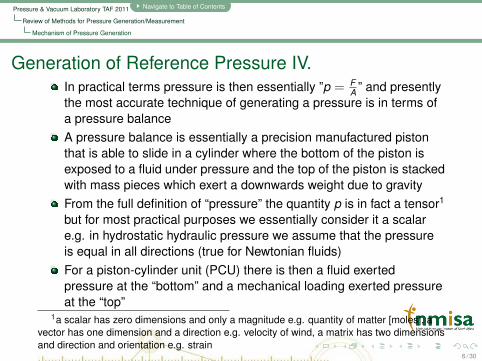
Generation of Reference Pressure IV.In practical terms pressure is then essentially ”p = F
A ” and presentlythe most accurate technique of generating a pressure is in terms ofa pressure balanceA pressure balance is essentially a precision manufactured pistonthat is able to slide in a cylinder where the bottom of the piston isexposed to a fluid under pressure and the top of the piston is stackedwith mass pieces which exert a downwards weight due to gravity
From the full definition of “pressure” the quantity p is in fact a tensor1
but for most practical purposes we essentially consider it a scalare.g. in hydrostatic hydraulic pressure we assume that the pressureis equal in all directions (true for Newtonian fluids)For a piston-cylinder unit (PCU) there is then a fluid exertedpressure at the “bottom” and a mechanical loading exerted pressureat the “top”
1a scalar has zero dimensions and only a magnitude e.g. quantity of matter [moles], avector has one dimension and a direction e.g. velocity of wind, a matrix has two dimensionsand direction and orientation e.g. strain
6 / 30

Pressure & Vacuum Laboratory TAF 2011 Navigate to Table of Contents
Review of Methods for Pressure Generation/Measurement
Mechanism of Pressure Generation
Generation of Reference Pressure IV.In practical terms pressure is then essentially ”p = F
A ” and presentlythe most accurate technique of generating a pressure is in terms ofa pressure balanceA pressure balance is essentially a precision manufactured pistonthat is able to slide in a cylinder where the bottom of the piston isexposed to a fluid under pressure and the top of the piston is stackedwith mass pieces which exert a downwards weight due to gravityFrom the full definition of “pressure” the quantity p is in fact a tensor1
but for most practical purposes we essentially consider it a scalare.g. in hydrostatic hydraulic pressure we assume that the pressureis equal in all directions (true for Newtonian fluids)
For a piston-cylinder unit (PCU) there is then a fluid exertedpressure at the “bottom” and a mechanical loading exerted pressureat the “top”
1a scalar has zero dimensions and only a magnitude e.g. quantity of matter [moles], avector has one dimension and a direction e.g. velocity of wind, a matrix has two dimensionsand direction and orientation e.g. strain
6 / 30
Pressure & Vacuum Laboratory TAF 2011 Navigate to Table of Contents
Review of Methods for Pressure Generation/Measurement
Mechanism of Pressure Generation
Generation of Reference Pressure IV.In practical terms pressure is then essentially ”p = F
A ” and presentlythe most accurate technique of generating a pressure is in terms ofa pressure balanceA pressure balance is essentially a precision manufactured pistonthat is able to slide in a cylinder where the bottom of the piston isexposed to a fluid under pressure and the top of the piston is stackedwith mass pieces which exert a downwards weight due to gravityFrom the full definition of “pressure” the quantity p is in fact a tensor1
but for most practical purposes we essentially consider it a scalare.g. in hydrostatic hydraulic pressure we assume that the pressureis equal in all directions (true for Newtonian fluids)For a piston-cylinder unit (PCU) there is then a fluid exertedpressure at the “bottom” and a mechanical loading exerted pressureat the “top”
1a scalar has zero dimensions and only a magnitude e.g. quantity of matter [moles], avector has one dimension and a direction e.g. velocity of wind, a matrix has two dimensionsand direction and orientation e.g. strain
6 / 30

Pressure & Vacuum Laboratory TAF 2011 Navigate to Table of Contents
Review of Methods for Pressure Generation/Measurement
Mechanism of Pressure Generation
Illustrative Examples2 of Pressure Balances
(a) Ruska model 2465A-U-754 pneumatic PB
(b) Ruska model 2485-930D hydraulic PB
(c) Desgranges & Huotmodel DH 5503S hydraulicPB
Figure: Low range PB (a), medium range PB (b) and high range PB (c)
2images courtesy of National Institute of Metrology (Thailand) websitehttp://www.nimt.or.th/
7 / 30
Pressure & Vacuum Laboratory TAF 2011 Navigate to Table of Contents
Review of Methods for Pressure Generation/Measurement
Mechanism of Pressure Generation
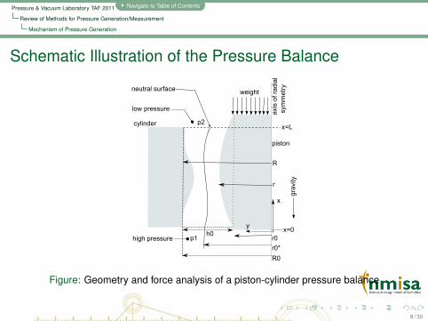
Schematic Illustration of the Pressure Balance
cylinder
piston
neutral surfaceweight
R
r
h0r0
r0*
R0
p1
p2
x
yx=0
x=L
high pressure
low pressure
gravity
axis of radial
symmetry
Figure: Geometry and force analysis of a piston-cylinder pressure balance
8 / 30

Pressure & Vacuum Laboratory TAF 2011 Navigate to Table of Contents
Review of Methods for Pressure Generation/Measurement
Mathematical Model of Pressure Balance
Mathematical Model of Pressure BalanceBy an analysis of the physics of the problem one may derive the followingmathematical model:
p − Π =
{∑ni=1 mi
(1− ρa
ρi
)− Vs(ρf − ρa) + H(ρf − ρa)S
}g + σC
S(7)
S = A0(1 + λP)[1 + α(t − t0)] (8)
In the above equations the nomenclature used is:
p = absolute pressure (′′true pressure′′) (9)
Π = ambient pressure (′′top pressure′′) (10)
P = p − Π = applied pressure (′′gauge pressure) (11)
In the case of the EURAMET.M.P-K13 key intercomparison Π is known since this the measured atmospheric pressure and in essence the above
equations are to be solved to determine the unknown applied pressure P (and then by implication the absolute pressure p).
9 / 30

Pressure & Vacuum Laboratory TAF 2011 Navigate to Table of Contents
Review of Methods for Pressure Generation/Measurement
Mathematical Model of Pressure Balance
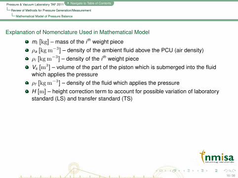
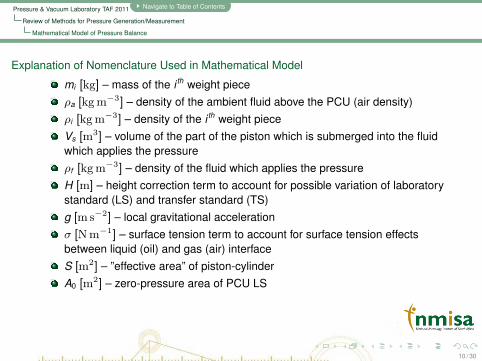
Explanation of Nomenclature Used in Mathematical Model
mi [kg] – mass of the i th weight piece
ρa [kg m−3] – density of the ambient fluid above the PCU (air density)ρi [kg m−3] – density of the i th weight pieceVs [m3] – volume of the part of the piston which is submerged into the fluidwhich applies the pressureρf [kg m−3] – density of the fluid which applies the pressureH [m] – height correction term to account for possible variation of laboratorystandard (LS) and transfer standard (TS)g [m s−2] – local gravitational accelerationσ [Nm−1] – surface tension term to account for surface tension effectsbetween liquid (oil) and gas (air) interfaceS [m2] – ”effective area” of piston-cylinderA0 [m2] – zero-pressure area of PCU LSλ [Pa−1] – distortion coefficient of PCU (typically measured in ppm/MPa)α [K−1] – thermal expansion coefficient term (α = αp + αc)C [m] – circumference of piston exposed to oil-air interface (typically set asC ≈
√4πA?0 )
10 / 30

Pressure & Vacuum Laboratory TAF 2011 Navigate to Table of Contents
Review of Methods for Pressure Generation/Measurement
Mathematical Model of Pressure Balance
Explanation of Nomenclature Used in Mathematical Model
mi [kg] – mass of the i th weight pieceρa [kg m−3] – density of the ambient fluid above the PCU (air density)
ρi [kg m−3] – density of the i th weight pieceVs [m3] – volume of the part of the piston which is submerged into the fluidwhich applies the pressureρf [kg m−3] – density of the fluid which applies the pressureH [m] – height correction term to account for possible variation of laboratorystandard (LS) and transfer standard (TS)g [m s−2] – local gravitational accelerationσ [Nm−1] – surface tension term to account for surface tension effectsbetween liquid (oil) and gas (air) interfaceS [m2] – ”effective area” of piston-cylinderA0 [m2] – zero-pressure area of PCU LSλ [Pa−1] – distortion coefficient of PCU (typically measured in ppm/MPa)α [K−1] – thermal expansion coefficient term (α = αp + αc)C [m] – circumference of piston exposed to oil-air interface (typically set asC ≈
√4πA?0 )
10 / 30

Pressure & Vacuum Laboratory TAF 2011 Navigate to Table of Contents
Review of Methods for Pressure Generation/Measurement
Mathematical Model of Pressure Balance
Explanation of Nomenclature Used in Mathematical Model
mi [kg] – mass of the i th weight pieceρa [kg m−3] – density of the ambient fluid above the PCU (air density)ρi [kg m−3] – density of the i th weight piece
Vs [m3] – volume of the part of the piston which is submerged into the fluidwhich applies the pressureρf [kg m−3] – density of the fluid which applies the pressureH [m] – height correction term to account for possible variation of laboratorystandard (LS) and transfer standard (TS)g [m s−2] – local gravitational accelerationσ [Nm−1] – surface tension term to account for surface tension effectsbetween liquid (oil) and gas (air) interfaceS [m2] – ”effective area” of piston-cylinderA0 [m2] – zero-pressure area of PCU LSλ [Pa−1] – distortion coefficient of PCU (typically measured in ppm/MPa)α [K−1] – thermal expansion coefficient term (α = αp + αc)C [m] – circumference of piston exposed to oil-air interface (typically set asC ≈
√4πA?0 )
10 / 30

Pressure & Vacuum Laboratory TAF 2011 Navigate to Table of Contents
Review of Methods for Pressure Generation/Measurement
Mathematical Model of Pressure Balance
Explanation of Nomenclature Used in Mathematical Model
mi [kg] – mass of the i th weight pieceρa [kg m−3] – density of the ambient fluid above the PCU (air density)ρi [kg m−3] – density of the i th weight pieceVs [m3] – volume of the part of the piston which is submerged into the fluidwhich applies the pressure
ρf [kg m−3] – density of the fluid which applies the pressureH [m] – height correction term to account for possible variation of laboratorystandard (LS) and transfer standard (TS)g [m s−2] – local gravitational accelerationσ [Nm−1] – surface tension term to account for surface tension effectsbetween liquid (oil) and gas (air) interfaceS [m2] – ”effective area” of piston-cylinderA0 [m2] – zero-pressure area of PCU LSλ [Pa−1] – distortion coefficient of PCU (typically measured in ppm/MPa)α [K−1] – thermal expansion coefficient term (α = αp + αc)C [m] – circumference of piston exposed to oil-air interface (typically set asC ≈
√4πA?0 )
10 / 30

Pressure & Vacuum Laboratory TAF 2011 Navigate to Table of Contents
Review of Methods for Pressure Generation/Measurement
Mathematical Model of Pressure Balance
Explanation of Nomenclature Used in Mathematical Model
mi [kg] – mass of the i th weight pieceρa [kg m−3] – density of the ambient fluid above the PCU (air density)ρi [kg m−3] – density of the i th weight pieceVs [m3] – volume of the part of the piston which is submerged into the fluidwhich applies the pressureρf [kg m−3] – density of the fluid which applies the pressure
H [m] – height correction term to account for possible variation of laboratorystandard (LS) and transfer standard (TS)g [m s−2] – local gravitational accelerationσ [Nm−1] – surface tension term to account for surface tension effectsbetween liquid (oil) and gas (air) interfaceS [m2] – ”effective area” of piston-cylinderA0 [m2] – zero-pressure area of PCU LSλ [Pa−1] – distortion coefficient of PCU (typically measured in ppm/MPa)α [K−1] – thermal expansion coefficient term (α = αp + αc)C [m] – circumference of piston exposed to oil-air interface (typically set asC ≈
√4πA?0 )
10 / 30
Pressure & Vacuum Laboratory TAF 2011 Navigate to Table of Contents
Review of Methods for Pressure Generation/Measurement
Mathematical Model of Pressure Balance
Explanation of Nomenclature Used in Mathematical Model
mi [kg] – mass of the i th weight pieceρa [kg m−3] – density of the ambient fluid above the PCU (air density)ρi [kg m−3] – density of the i th weight pieceVs [m3] – volume of the part of the piston which is submerged into the fluidwhich applies the pressureρf [kg m−3] – density of the fluid which applies the pressureH [m] – height correction term to account for possible variation of laboratorystandard (LS) and transfer standard (TS)
g [m s−2] – local gravitational accelerationσ [Nm−1] – surface tension term to account for surface tension effectsbetween liquid (oil) and gas (air) interfaceS [m2] – ”effective area” of piston-cylinderA0 [m2] – zero-pressure area of PCU LSλ [Pa−1] – distortion coefficient of PCU (typically measured in ppm/MPa)α [K−1] – thermal expansion coefficient term (α = αp + αc)C [m] – circumference of piston exposed to oil-air interface (typically set asC ≈
√4πA?0 )
10 / 30

Pressure & Vacuum Laboratory TAF 2011 Navigate to Table of Contents
Review of Methods for Pressure Generation/Measurement
Mathematical Model of Pressure Balance
Explanation of Nomenclature Used in Mathematical Model
mi [kg] – mass of the i th weight pieceρa [kg m−3] – density of the ambient fluid above the PCU (air density)ρi [kg m−3] – density of the i th weight pieceVs [m3] – volume of the part of the piston which is submerged into the fluidwhich applies the pressureρf [kg m−3] – density of the fluid which applies the pressureH [m] – height correction term to account for possible variation of laboratorystandard (LS) and transfer standard (TS)g [ms−2] – local gravitational acceleration
σ [Nm−1] – surface tension term to account for surface tension effectsbetween liquid (oil) and gas (air) interfaceS [m2] – ”effective area” of piston-cylinderA0 [m2] – zero-pressure area of PCU LSλ [Pa−1] – distortion coefficient of PCU (typically measured in ppm/MPa)α [K−1] – thermal expansion coefficient term (α = αp + αc)C [m] – circumference of piston exposed to oil-air interface (typically set asC ≈
√4πA?0 )
10 / 30

Pressure & Vacuum Laboratory TAF 2011 Navigate to Table of Contents
Review of Methods for Pressure Generation/Measurement
Mathematical Model of Pressure Balance
Explanation of Nomenclature Used in Mathematical Model
mi [kg] – mass of the i th weight pieceρa [kg m−3] – density of the ambient fluid above the PCU (air density)ρi [kg m−3] – density of the i th weight pieceVs [m3] – volume of the part of the piston which is submerged into the fluidwhich applies the pressureρf [kg m−3] – density of the fluid which applies the pressureH [m] – height correction term to account for possible variation of laboratorystandard (LS) and transfer standard (TS)g [ms−2] – local gravitational accelerationσ [Nm−1] – surface tension term to account for surface tension effectsbetween liquid (oil) and gas (air) interface
S [m2] – ”effective area” of piston-cylinderA0 [m2] – zero-pressure area of PCU LSλ [Pa−1] – distortion coefficient of PCU (typically measured in ppm/MPa)α [K−1] – thermal expansion coefficient term (α = αp + αc)C [m] – circumference of piston exposed to oil-air interface (typically set asC ≈
√4πA?0 )
10 / 30

Pressure & Vacuum Laboratory TAF 2011 Navigate to Table of Contents
Review of Methods for Pressure Generation/Measurement
Mathematical Model of Pressure Balance
Explanation of Nomenclature Used in Mathematical Model
mi [kg] – mass of the i th weight pieceρa [kg m−3] – density of the ambient fluid above the PCU (air density)ρi [kg m−3] – density of the i th weight pieceVs [m3] – volume of the part of the piston which is submerged into the fluidwhich applies the pressureρf [kg m−3] – density of the fluid which applies the pressureH [m] – height correction term to account for possible variation of laboratorystandard (LS) and transfer standard (TS)g [ms−2] – local gravitational accelerationσ [Nm−1] – surface tension term to account for surface tension effectsbetween liquid (oil) and gas (air) interfaceS [m2] – ”effective area” of piston-cylinder
A0 [m2] – zero-pressure area of PCU LSλ [Pa−1] – distortion coefficient of PCU (typically measured in ppm/MPa)α [K−1] – thermal expansion coefficient term (α = αp + αc)C [m] – circumference of piston exposed to oil-air interface (typically set asC ≈
√4πA?0 )
10 / 30
Pressure & Vacuum Laboratory TAF 2011 Navigate to Table of Contents
Review of Methods for Pressure Generation/Measurement
Mathematical Model of Pressure Balance
Explanation of Nomenclature Used in Mathematical Model
mi [kg] – mass of the i th weight pieceρa [kg m−3] – density of the ambient fluid above the PCU (air density)ρi [kg m−3] – density of the i th weight pieceVs [m3] – volume of the part of the piston which is submerged into the fluidwhich applies the pressureρf [kg m−3] – density of the fluid which applies the pressureH [m] – height correction term to account for possible variation of laboratorystandard (LS) and transfer standard (TS)g [ms−2] – local gravitational accelerationσ [Nm−1] – surface tension term to account for surface tension effectsbetween liquid (oil) and gas (air) interfaceS [m2] – ”effective area” of piston-cylinderA0 [m2] – zero-pressure area of PCU LS
λ [Pa−1] – distortion coefficient of PCU (typically measured in ppm/MPa)α [K−1] – thermal expansion coefficient term (α = αp + αc)C [m] – circumference of piston exposed to oil-air interface (typically set asC ≈
√4πA?0 )
10 / 30

Pressure & Vacuum Laboratory TAF 2011 Navigate to Table of Contents
Review of Methods for Pressure Generation/Measurement
Mathematical Model of Pressure Balance
Explanation of Nomenclature Used in Mathematical Model
mi [kg] – mass of the i th weight pieceρa [kg m−3] – density of the ambient fluid above the PCU (air density)ρi [kg m−3] – density of the i th weight pieceVs [m3] – volume of the part of the piston which is submerged into the fluidwhich applies the pressureρf [kg m−3] – density of the fluid which applies the pressureH [m] – height correction term to account for possible variation of laboratorystandard (LS) and transfer standard (TS)g [ms−2] – local gravitational accelerationσ [Nm−1] – surface tension term to account for surface tension effectsbetween liquid (oil) and gas (air) interfaceS [m2] – ”effective area” of piston-cylinderA0 [m2] – zero-pressure area of PCU LSλ [Pa−1] – distortion coefficient of PCU (typically measured in ppm/MPa)
α [K−1] – thermal expansion coefficient term (α = αp + αc)C [m] – circumference of piston exposed to oil-air interface (typically set asC ≈
√4πA?0 )
10 / 30

Pressure & Vacuum Laboratory TAF 2011 Navigate to Table of Contents
Review of Methods for Pressure Generation/Measurement
Mathematical Model of Pressure Balance
Explanation of Nomenclature Used in Mathematical Model
mi [kg] – mass of the i th weight pieceρa [kg m−3] – density of the ambient fluid above the PCU (air density)ρi [kg m−3] – density of the i th weight pieceVs [m3] – volume of the part of the piston which is submerged into the fluidwhich applies the pressureρf [kg m−3] – density of the fluid which applies the pressureH [m] – height correction term to account for possible variation of laboratorystandard (LS) and transfer standard (TS)g [ms−2] – local gravitational accelerationσ [Nm−1] – surface tension term to account for surface tension effectsbetween liquid (oil) and gas (air) interfaceS [m2] – ”effective area” of piston-cylinderA0 [m2] – zero-pressure area of PCU LSλ [Pa−1] – distortion coefficient of PCU (typically measured in ppm/MPa)α [K−1] – thermal expansion coefficient term (α = αp + αc)
C [m] – circumference of piston exposed to oil-air interface (typically set asC ≈
√4πA?0 )
10 / 30

Pressure & Vacuum Laboratory TAF 2011 Navigate to Table of Contents
Review of Methods for Pressure Generation/Measurement
Mathematical Model of Pressure Balance
Explanation of Nomenclature Used in Mathematical Model
mi [kg] – mass of the i th weight pieceρa [kg m−3] – density of the ambient fluid above the PCU (air density)ρi [kg m−3] – density of the i th weight pieceVs [m3] – volume of the part of the piston which is submerged into the fluidwhich applies the pressureρf [kg m−3] – density of the fluid which applies the pressureH [m] – height correction term to account for possible variation of laboratorystandard (LS) and transfer standard (TS)g [ms−2] – local gravitational accelerationσ [Nm−1] – surface tension term to account for surface tension effectsbetween liquid (oil) and gas (air) interfaceS [m2] – ”effective area” of piston-cylinderA0 [m2] – zero-pressure area of PCU LSλ [Pa−1] – distortion coefficient of PCU (typically measured in ppm/MPa)α [K−1] – thermal expansion coefficient term (α = αp + αc)C [m] – circumference of piston exposed to oil-air interface (typically set asC ≈
√4πA?0 )
10 / 30

Pressure & Vacuum Laboratory TAF 2011 Navigate to Table of Contents
Review of Methods for Pressure Generation/Measurement
Mechanism to Solve Formulation of Mathematical Equation
Formulation of Mathematical Model as Nonlinear RootSearch I.
Substituting the above terms we have
A?0g
(p − Π)[1 + λ(p − Π)][1 + α(t − 20)] =n∑
i=1
mi
(1− ρa
ρi
)− Vs(ρf − ρa)
+
{H(ρf − ρa)A?0 [1 + λ(p − Π)]
× [1 + α(t − 20)]
}+σ
g(4πA?0 [1 + α(t − 20)])−
12
(12)
which can be rewritten as a multi-variable equation f (X ) = 0 for whichthe roots (unknown pressure p) must be solved for.
11 / 30

Pressure & Vacuum Laboratory TAF 2011 Navigate to Table of Contents
Review of Methods for Pressure Generation/Measurement
Mechanism to Solve Formulation of Mathematical Equation
Formulation of Mathematical Model as Nonlinear RootSearch II.
The form of f (X ) is then:
f (X ) =∑n
i=1 mi
(1− ρa
ρi
)− Vs(ρf − ρa)
+ H(ρf − ρa)A?0 [1 + λ(p − Π)][1 + α(t − 20)]
+ σg (4πA?0 [1 + α(t − 20)])−
12
− A?0g (p − Π)[1 + λ(p − Π)][1 + α(t − 20)]
(13)
where the input state variable X is
X = [m1,m2, . . . ,mn, (14)
ρ1, ρ2, . . . , ρn, (15)
A?0 , λ, αp, αc , t ,Vs,H,Π, σ, g, tair ,RHair ]T (16)
12 / 30

Pressure & Vacuum Laboratory TAF 2011 Navigate to Table of Contents
Review of Methods for Pressure Generation/Measurement
Mechanism to Solve Formulation of Mathematical Equation
Formulation of Mathematical Model as Nonlinear RootSearch III.
The density of the air may be calculated using the CIPM-2007 formula3
which expresses the air density in terms of
ta – atmospheric temperature (measured with in-house thermometertraceable to water triple point (WTP) cell)
pa – atmospheric pressure (measured with in-house barometertraceable to absolute medium gas pressures with Ruska LS)
ha – atmospheric relative humidity expressed as a pure numbersuch that 0 6 ha 6 1 (traceable to in-house hybrid humiditygenerator: validated in humidity regional inter-comparison)
3Metrologia 45 2008 149–155 ”Revised Formula for the Density of Moist Air(CIPM-2007)”, Picard A et al
13 / 30

Pressure & Vacuum Laboratory TAF 2011 Navigate to Table of Contents
Review of Methods for Pressure Generation/Measurement
Mechanism to Solve Formulation of Mathematical Equation
Details of CIPM-2007 Formula for Moist Air Density
Briefly the underlying formula is of form
ρa =pMa
ZRT
[1− xv
(1− Mv
Ma
)](17)
whereρa [kg m−3 ] – air density
p [Pa] – atmospheric pressure (total pressure with implicit assumption of Dalton’s partial pressure law)
t [◦C] – air temperature
T [K] – thermodynamic absolute temperature
xv [−] – mole fraction of water vapour
Ma [kg mol−1 ] – molar mass of dry air
Mv [kg mol−1 ] – molar mass of water vapour
Z [−] – compressibility factor
R [J mol−1 K−1 ] – universal gas constant (using CODATA 2006 values4 cited in: Reviews of Modern Physics, Vol 80, April–June2008, Mohr P J et al)
4 http://www.nist.gov/pml/div684/fcdc/upload/rmp2006-2.pdf
14 / 30
Pressure & Vacuum Laboratory TAF 2011 Navigate to Table of Contents
Review of Methods for Pressure Generation/Measurement
Mechanism to Solve Formulation of Mathematical Equation
Note on Mass Input Values
In the state variable we assume n mass pieces in total
This choice is incorporated by assigning the mass values tocorrespond to a weight set of N weights used (where n > N) andthen appending the piston mass mpiston and bell mass mbell viz.
[m1,m2, . . . ,mn−2,mn−1,mn]T = [m1,m2, . . . ,mN ,mpiston,mbell ]T
(18)
15 / 30

Pressure & Vacuum Laboratory TAF 2011 Navigate to Table of Contents
Review of Methods for Pressure Generation/Measurement
Mechanism to Solve Formulation of Mathematical Equation
Varying Meanings of MassOn the Differences Between True Mass, Conventional Mass and ApparentMass
Conventional mass: air density of 1.2 kg m−3 and mass density of 8000 kg m−3
Detailsa Objective is to determine the true mass of a weight piece from calibrationdata:
true mass : m = ms1− ρa
ρs
1− ρaρm
(19)
calibration cert data : m(c)s
(1− ρ
(c)a
ρ(c)s
)= ms
(1− ρ
(s)a
ρs
)(20)
⇔ m = m(c)s
1− ρ(c)a
ρ(c)s
1− ρ(s)aρs
×1− ρa
ρs
1− ρaρm
(21)
aThe Pressure Balance: Theory and Practice, Dadson R S et al, 1982, National PhysicalLaboratory / HMSO 16 / 30

Pressure & Vacuum Laboratory TAF 2011 Navigate to Table of Contents
Review of Methods for Pressure Generation/Measurement
Solution for Roots of Multivariable Equation
Solution of Roots of f (X ) = 0In the mathematical model of the EURAMET.M.P-K13 keycomparison there will in general be a variable number of inputs sincea varying number of mass pieces n are used to generate asequence of (applied) pressures for P ∈ [50, . . . , 500] MPaIt can be shown that for n mass pieces used in
X = [m1, . . . ,mn, ρ1, . . . , ρn,A?0 , λ, αp, αc , t ,Vs,H, pa, ta, ha, σ, g]T
there will be a total of (2n + 12) state variables incorporated into themeasurand model to solve for the unknown generated appliedpressureConsider the terms in f (X ) which are known and unknown
f (X ) =∑n
i=1 mi
(1− ρa
ρi
)− Vs(ρf − ρa)
+ H(ρf − ρa)A?0 [1 + λ(p − Π)][1 + α(t − 20)]
+ σg (4πA?0 [1 + α(t − 20)])−
12
− A?0g (p − Π)[1 + λ(p − Π)][1 + α(t − 20)]
(22)
17 / 30

Pressure & Vacuum Laboratory TAF 2011 Navigate to Table of Contents
Review of Methods for Pressure Generation/Measurement
Defining an EoS for the Working Fluid
EoS for a Pressure Balance Working Fluid I.During the intercomparison both the transfer standard and the NMISARuska high pressure PCU used di(2-ethylhexgl) sebecate i.e. ‘DHS’ as theworking fluid formulated as
ρf/[kg m−3] = [912.7 + 0.752(10−6p)− 1.65× 10⁻³(10−6p)2
+ 1.5× 10⁻⁶(10−6p)3]× [1− 7.8× 10⁻⁴(tf − 20)]
(23)
Alternative forms that may be considered are linear extrapolations from aknown reference state
ρf =
ρf 01+β(tf−tf 0)
1− p−pf 0Ef
(24)
where tf 0 is the reference oil temperature at which the oil’s properties areknown (say 20 ◦C), Ef is the bulk modulas fluid elasticity, pf 0 is the referanceoil fluid density pressure, tf is the current oil temperature and p is the currentoil pressureFor pure ideal gases the EoS is
p =ρRTM (25)
18 / 30
Pressure & Vacuum Laboratory TAF 2011 Navigate to Table of Contents
Review of Methods for Pressure Generation/Measurement
Defining an EoS for the Working Fluid
EoS for a Pressure Balance Working Fluid II.
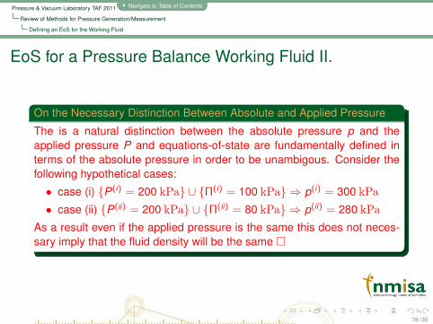
On the Necessary Distinction Between Absolute and Applied Pressure
The is a natural distinction between the absolute pressure p and theapplied pressure P and equations-of-state are fundamentally defined interms of the absolute pressure in order to be unambigous. Consider thefollowing hypothetical cases:
• case (i) {P(i) = 200 kPa} ∪ {Π(i) = 100 kPa} ⇒ p(i) = 300 kPa• case (ii) {P(ii) = 200 kPa} ∪ {Π(ii) = 80 kPa} ⇒ p(ii) = 280 kPa
As a result even if the applied pressure is the same this does not neces-sary imply that the fluid density will be the same �
19 / 30

Pressure & Vacuum Laboratory TAF 2011 Navigate to Table of Contents
Review of Methods for Pressure Generation/Measurement
Solution of the Roots (Pressure) of the Nonlinear Equation
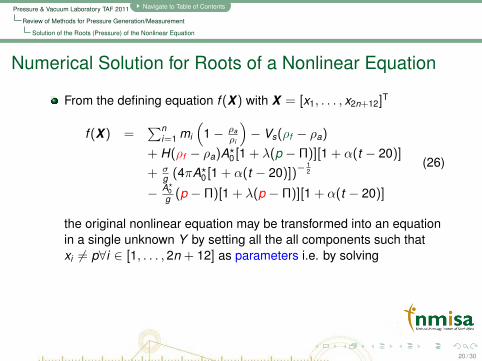
Numerical Solution for Roots of a Nonlinear Equation
From the defining equation f (X ) with X = [x1, . . . , x2n+12]T
f (X ) =∑n
i=1 mi
(1− ρa
ρi
)− Vs(ρf − ρa)
+ H(ρf − ρa)A?0 [1 + λ(p − Π)][1 + α(t − 20)]
+ σg (4πA?0 [1 + α(t − 20)])−
12
− A?0g (p − Π)[1 + λ(p − Π)][1 + α(t − 20)]
(26)
the original nonlinear equation may be transformed into an equationin a single unknown Y by setting all the all components such thatxi 6= p∀i ∈ [1, . . . , 2n + 12] as parameters i.e. by solving
f (Y ; X?) = 0 (27)
The solution Y is of course the absolute pressure
20 / 30

Pressure & Vacuum Laboratory TAF 2011 Navigate to Table of Contents
Review of Methods for Pressure Generation/Measurement
Solution of the Roots (Pressure) of the Nonlinear Equation
Numerical Solution for Roots of a Nonlinear Equation
From the defining equation f (X ) with X = [x1, . . . , x2n+12]T
f (X ) =∑n
i=1 mi
(1− ρa
ρi
)− Vs(ρf − ρa)
+ H(ρf − ρa)A?0 [1 + λ(p − Π)][1 + α(t − 20)]
+ σg (4πA?0 [1 + α(t − 20)])−
12
− A?0g (p − Π)[1 + λ(p − Π)][1 + α(t − 20)]
(26)
the original nonlinear equation may be transformed into an equationin a single unknown Y by setting all the all components such that
xi 6= p∀i ∈ [1, . . . , 2n + 12] as parameters i.e. by solving
f (Y ; X?) = 0 (27)
The solution Y is of course the absolute pressure
20 / 30
Pressure & Vacuum Laboratory TAF 2011 Navigate to Table of Contents
Review of Methods for Pressure Generation/Measurement
Solution of the Roots (Pressure) of the Nonlinear Equation
Numerical Solution for Roots of a Nonlinear Equation
From the defining equation f (X ) with X = [x1, . . . , x2n+12]T
f (X ) =∑n
i=1 mi
(1− ρa
ρi
)− Vs(ρf − ρa)
+ H(ρf − ρa)A?0 [1 + λ(p − Π)][1 + α(t − 20)]
+ σg (4πA?0 [1 + α(t − 20)])−
12
− A?0g (p − Π)[1 + λ(p − Π)][1 + α(t − 20)]
(26)
the original nonlinear equation may be transformed into an equationin a single unknown Y by setting all the all components such thatxi 6= p∀i ∈ [1, . . . , 2n + 12] as parameters i.e. by solving
f (Y ; X?) = 0 (27)
The solution Y is of course the absolute pressure
20 / 30

Pressure & Vacuum Laboratory TAF 2011 Navigate to Table of Contents
Review of Methods for Pressure Generation/Measurement
Solution of the Roots (Pressure) of the Nonlinear Equation
Numerical Solution for Roots of a Nonlinear Equation
From the defining equation f (X ) with X = [x1, . . . , x2n+12]T
f (X ) =∑n
i=1 mi
(1− ρa
ρi
)− Vs(ρf − ρa)
+ H(ρf − ρa)A?0 [1 + λ(p − Π)][1 + α(t − 20)]
+ σg (4πA?0 [1 + α(t − 20)])−
12
− A?0g (p − Π)[1 + λ(p − Π)][1 + α(t − 20)]
(26)
the original nonlinear equation may be transformed into an equationin a single unknown Y by setting all the all components such thatxi 6= p∀i ∈ [1, . . . , 2n + 12] as parameters i.e. by solving
f (Y ; X?) = 0 (27)
The solution Y is of course the absolute pressure
20 / 30

Pressure & Vacuum Laboratory TAF 2011 Navigate to Table of Contents
Calculation of Generated Pressure Uncertainty
Estimation of Generated Pressure Uncertainty
For the EURAMET.M.P-K13 key comparison V&V in terms of theuncertainty analysis by the research metrologist was performedwithin the framework of the GUM
The underlying matrix based equation for the multi-variable input Xwas
u2(y)
(∂f∂y
)2
= (∇x f )V x (∇x )T (28)
following the methodology5 of Cox and Harris.
In our initial approach I assumed no correlation effects in thecomponents of the input variable X for simplicity
5Cox M G and Harris P M, Software Support for Metrology Best Practice Guide No. 6 –Uncertainty Evaluation, Technical Report, National Physical Laboratory (United Kingdom),2004
21 / 30

Pressure & Vacuum Laboratory TAF 2011 Navigate to Table of Contents
Calculation of Generated Pressure Uncertainty
Specific Issues Encountered in Uncertainty Analysis
The Validity of the Assumption ofCov(xi , xj) = 0∀i 6= j : 1 6 i, j 6 2n + 12
In general the only possible significant non-zero correlation effectthat may occur is for the case Cov(A0, λ)
Correlation effects do occur in the case of the weights mass/densitybut in general this has a very minor impact on final uncertainties asu(A0) and particularly u(λ) will dominate uncertainty contributions atelevated pressuresCorrelation is certain to occur in the present instance as A(LS)
0 andλ(LS) are in fact obtained from an experimental cross-floatingagainsts another precision piston-cylinder standard however in thepresent instance no accessible information on Cov(A0, λ) isavailable as these data values are sourced from an externalcertificate that does not provide any information from which one mayreasonably infer a magnnitude of correlation6
6consultation of the statistical literature such as Metrologia journal articles and IMEKOconferences states that it is poor practice to simply assume unity correlation in the absenceof information: the recommended option is to assume zero correlation
22 / 30

Pressure & Vacuum Laboratory TAF 2011 Navigate to Table of Contents
Calculation of Generated Pressure Uncertainty
Specific Issues Encountered in Uncertainty Analysis
The Validity of the Assumption ofCov(xi , xj) = 0∀i 6= j : 1 6 i, j 6 2n + 12
In general the only possible significant non-zero correlation effectthat may occur is for the case Cov(A0, λ)
Correlation effects do occur in the case of the weights mass/densitybut in general this has a very minor impact on final uncertainties asu(A0) and particularly u(λ) will dominate uncertainty contributions atelevated pressures
Correlation is certain to occur in the present instance as A(LS)0 and
λ(LS) are in fact obtained from an experimental cross-floatingagainsts another precision piston-cylinder standard however in thepresent instance no accessible information on Cov(A0, λ) isavailable as these data values are sourced from an externalcertificate that does not provide any information from which one mayreasonably infer a magnnitude of correlation6
6consultation of the statistical literature such as Metrologia journal articles and IMEKOconferences states that it is poor practice to simply assume unity correlation in the absenceof information: the recommended option is to assume zero correlation
22 / 30

Pressure & Vacuum Laboratory TAF 2011 Navigate to Table of Contents
Calculation of Generated Pressure Uncertainty
Specific Issues Encountered in Uncertainty Analysis
The Validity of the Assumption ofCov(xi , xj) = 0∀i 6= j : 1 6 i, j 6 2n + 12
In general the only possible significant non-zero correlation effectthat may occur is for the case Cov(A0, λ)
Correlation effects do occur in the case of the weights mass/densitybut in general this has a very minor impact on final uncertainties asu(A0) and particularly u(λ) will dominate uncertainty contributions atelevated pressuresCorrelation is certain to occur in the present instance as A(LS)
0 andλ(LS) are in fact obtained from an experimental cross-floatingagainsts another precision piston-cylinder standard however in thepresent instance no accessible information on Cov(A0, λ) isavailable as these data values are sourced from an externalcertificate that does not provide any information from which one mayreasonably infer a magnnitude of correlation6
6consultation of the statistical literature such as Metrologia journal articles and IMEKOconferences states that it is poor practice to simply assume unity correlation in the absenceof information: the recommended option is to assume zero correlation
22 / 30

Pressure & Vacuum Laboratory TAF 2011 Navigate to Table of Contents
Methodology Used in Cross-Floating Analysis
Derivation of Basis Equation used in Cross-Floating I.
Basis Equation for Cross-Floating
Make the assumption of linear elasticity theory in the PDE’s formulationof the strain/stress constituent behaviour:
Assume a piston-cylinder A with known characteristics i.e.DA = {A(A)
0 , λ(A)} is cross-floated with another piston-cylinder B withunknown characteristics i.e. DB = {A(B)
0 , λ(B)} which are to bedetermined
It follows that
PB =1
SB×[{
gm∑
j=1
mBj
(1− ρa
ρBj
)− VsB(ρf − ρa)g
+ σB
√4πA(B)
0
}+ (HB(ρf − ρa)g) SB
](29)
23 / 30

Pressure & Vacuum Laboratory TAF 2011 Navigate to Table of Contents
Methodology Used in Cross-Floating Analysis
Derivation of Basis Equation used in Cross-Floating I.
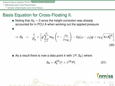
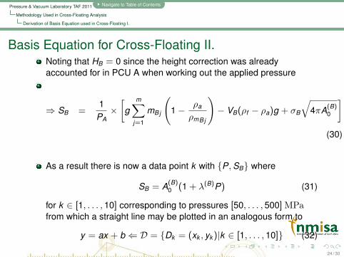
Basis Equation for Cross-Floating II.Noting that HB = 0 since the height correction was alreadyaccounted for in PCU A when working out the applied pressure
⇒ SB =1
PA×[g
m∑j=1
mBj
(1− ρa
ρmBj
)− VB(ρf − ρa)g + σB
√4πA(B)
0
](30)
As a result there is now a data point k with {P,SB} where
SB = A(B)0 (1 + λ(B)P) (31)
for k ∈ [1, . . . , 10] corresponding to pressures [50, . . . , 500] MPafrom which a straight line may be plotted in an analogous form to
y = ax + b ⇐ D = {Dk = (xk , yk )|k ∈ [1, . . . , 10]} (32)
24 / 30

Pressure & Vacuum Laboratory TAF 2011 Navigate to Table of Contents
Methodology Used in Cross-Floating Analysis
Derivation of Basis Equation used in Cross-Floating I.
Basis Equation for Cross-Floating II.Noting that HB = 0 since the height correction was alreadyaccounted for in PCU A when working out the applied pressure
⇒ SB =1
PA×[g
m∑j=1
mBj
(1− ρa
ρmBj
)− VB(ρf − ρa)g + σB
√4πA(B)
0
](30)
As a result there is now a data point k with {P,SB} where
SB = A(B)0 (1 + λ(B)P) (31)
for k ∈ [1, . . . , 10] corresponding to pressures [50, . . . , 500] MPafrom which a straight line may be plotted in an analogous form to
y = ax + b ⇐ D = {Dk = (xk , yk )|k ∈ [1, . . . , 10]} (32)
24 / 30

Pressure & Vacuum Laboratory TAF 2011 Navigate to Table of Contents
Methodology Used in Cross-Floating Analysis
Estimation of the Straight Line Uncertainties Corresponding to u(A0) and u(λ)
Estimation of Zero-Pressure and Distortion CoefficientUncertainties I.
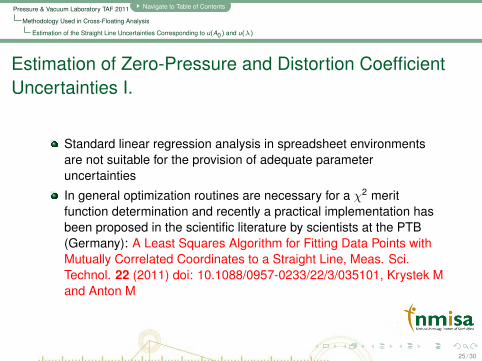
Standard linear regression analysis in spreadsheet environmentsare not suitable for the provision of adequate parameteruncertainties
In general optimization routines are necessary for a χ2 meritfunction determination and recently a practical implementation hasbeen proposed in the scientific literature by scientists at the PTB(Germany): A Least Squares Algorithm for Fitting Data Points withMutually Correlated Coordinates to a Straight Line, Meas. Sci.Technol. 22 (2011) doi: 10.1088/0957-0233/22/3/035101, Krystek Mand Anton M
25 / 30
Pressure & Vacuum Laboratory TAF 2011 Navigate to Table of Contents
Methodology Used in Cross-Floating Analysis
Estimation of the Straight Line Uncertainties Corresponding to u(A0) and u(λ)
Estimation of Zero-Pressure and Distortion CoefficientUncertainties I.
Standard linear regression analysis in spreadsheet environmentsare not suitable for the provision of adequate parameteruncertainties
In general optimization routines are necessary for a χ2 meritfunction determination and recently a practical implementation hasbeen proposed in the scientific literature by scientists at the PTB(Germany): A Least Squares Algorithm for Fitting Data Points withMutually Correlated Coordinates to a Straight Line, Meas. Sci.Technol. 22 (2011) doi: 10.1088/0957-0233/22/3/035101, Krystek Mand Anton M
25 / 30

Pressure & Vacuum Laboratory TAF 2011 Navigate to Table of Contents
Methodology Used in Cross-Floating Analysis
Estimation of the Straight Line Uncertainties Corresponding to u(A0) and u(λ)
Estimation of Zero-Pressure and Distortion CoefficientUncertainties II.
The method fits y = ax + b and provides estimates for u(a) andu(b) noting that for a pressure balance the defining basis equation is
A(P) = A0(1 + λP) (33)
It then follows that in a pressure cross-floating experimentalmeasurement that
u2(a) = u2(A0) (34)
u2(b) = λ2u2(A0) + A20u2(λ) (35)
⇒ u2(λ) =1A2
0
[u2(b)− λ2u2(a)
](36)
26 / 30

Pressure & Vacuum Laboratory TAF 2011 Navigate to Table of Contents
Discussion
Specific Comments on Intercomparison Results
Specific Comments on Intercomparison Participation
The participation of the technical metrologists inEURAMET.M.P-K13 can be considered a learning experience asthere is a significant difference is the level and complexity of keycomparisons when compared to industrial level measurements
It is recognized that in terms of data processing, analysis, andpost-processing of results as a NMI there is always room forimprovement and that there are certain inherent fundamentallimitations in spreadsheet utilization, both in terms of what can bemathematically/statistically achieved and also in terms of validationand verification
In terms of internal comparison of processed results there is goodgeneral agreement in generated pressures and fair/moderateagreement in computed effective area and distortion coefficient ofapplicable transfer standard
27 / 30

Pressure & Vacuum Laboratory TAF 2011 Navigate to Table of Contents
Discussion
Recommendations Going Foward
Recommendations and Future Options Going Forward I.
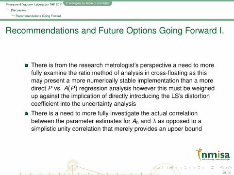
There is from the research metrologist’s perspective a need to morefully examine the ratio method of analysis in cross-floating as thismay present a more numerically stable implementation than a moredirect P vs. A(P) regression analysis however this must be weighedup against the implication of directly introducing the LS’s distortioncoefficient into the uncertainty analysis
There is a need to more fully investigate the actual correlationbetween the parameter estimates for A0 and λ as opposed to asimplistic unity correlation that merely provides an upper bound
28 / 30
Pressure & Vacuum Laboratory TAF 2011 Navigate to Table of Contents
Discussion
Recommendations Going Foward
Recommendations and Future Options Going Forward I.
There is from the research metrologist’s perspective a need to morefully examine the ratio method of analysis in cross-floating as thismay present a more numerically stable implementation than a moredirect P vs. A(P) regression analysis however this must be weighedup against the implication of directly introducing the LS’s distortioncoefficient into the uncertainty analysis
There is a need to more fully investigate the actual correlationbetween the parameter estimates for A0 and λ as opposed to asimplistic unity correlation that merely provides an upper bound
28 / 30

Pressure & Vacuum Laboratory TAF 2011 Navigate to Table of Contents
Discussion
Recommendations Going Foward
Recommendations and Future Options Going Forward II.FEM numerical simulations should be performed to benchmark theexisting experimental/statistical distortion coefficient however thechallenge posed is not actually in terms of the FEM analysis butrather in terms of the materials properties of the piston-cylinder:tungsten-carbide is prone to some variation in the Young’s modulasof elasticty and Poisson’s ratio – a possibility is to submit a researchproposal for an electrical capacitance / materials characterizationexperimental study of the distortion coefficent on the low andmedium pressure Ruska piston-cylinder laboratory standards
It may be beneficial to consider alternative statistical formulations tobootstrapping such as Jackknifing
Certain aspects of the Pressure & Vacuum Laboratory R&D on theRuska high pressure characterization may be able to (in partnershipwith another NMI e.g. PTB / CMI) make a modest contribution onthe Avogadro project that requires precision pressuremeasurements at 7 MPa
29 / 30

Pressure & Vacuum Laboratory TAF 2011 Navigate to Table of Contents
Discussion
Recommendations Going Foward
Acknowledgements
This work was performed with financial support of the South AfricanDepartment of Trade and Industry
30 / 30