scobi simulator user’s manual

Orhan Eroglu, Dylan R. Boyd, Mehmet Kurum

InforMation PRocESsing and Sensing (IMPRESS) Lab

http://impress.ece.msstate.edu/

SCoBi Simulator

User’s Manual

v1.0

2018

http://impress.ece.msstate.edu/

2

Table of Contents

1. Introduction .............................................................................................................................. 4

1.1. General ......................................................................................................................... 4

1.2. System Requirements ................................................................................................... 4

1.3. Downloading and Installation ........................................................................................ 4

1.4. About This Document ................................................................................................... 4

1.5. Help SCoBi Improve ..................................................................................................... 5

1.6. How to Cite This Study? ............................................................................................... 5

2. SCoBi Simulator Basics ........................................................................................................... 6

2.1. Initial Run ...................................................................................................................... 6

2.2. Analysis Selection Window ........................................................................................... 6

2.3. Simulation Input Window .............................................................................................. 7

2.3.1. Analysis Selection Buttons ............................................................................................ 8

2.3.2. Simulation Settings ....................................................................................................... 9

2.3.2.1. Campaign .............................................................................................................. 9

2.3.2.2. Simulation Mode .................................................................................................. 10

2.3.2.3. Ground Cover ...................................................................................................... 10

2.3.2.4. Preferences ......................................................................................................... 10

2.3.3. Transmitter Inputs ....................................................................................................... 11

2.3.3.1. Frequency ............................................................................................................ 11

2.3.3.2. Range to Earth Center ......................................................................................... 11

2.3.3.3. EIRP .................................................................................................................... 11

2.3.3.4. Polarization .......................................................................................................... 11

2.3.3.5. Orientation ........................................................................................................... 11

2.3.4. Receiver Inputs ........................................................................................................... 12

2.3.4.1. Altitude ................................................................................................................. 12

2.3.4.2. Gain ..................................................................................................................... 12

2.3.4.3. Polarization .......................................................................................................... 12

2.3.4.4. Orientation ........................................................................................................... 13

2.3.4.5. Antenna Pattern ................................................................................................... 13

2.3.5. Ground Inputs ............................................................................................................. 14

2.3.5.1. Dielectric Model ................................................................................................... 14

2.3.5.2. Ground Structure ................................................................................................. 14

2.3.6. Input Files ................................................................................................................... 14

3

2.3.7. Action Buttons ............................................................................................................. 15

2.3.7.1. Load Inputs .......................................................................................................... 15

2.3.7.2. Save Inputs .......................................................................................................... 15

2.3.7.3. RunSCoBi ............................................................................................................ 15

2.3.7.4. Exit ....................................................................................................................... 15

3. Analysis with SCoBi ............................................................................................................... 16

3.1. Inputs .......................................................................................................................... 16

3.1.1. Simulation Inputs ......................................................................................................... 16

3.1.2. Excel Input Files .......................................................................................................... 16

3.1.2.1. Configuration Inputs File ...................................................................................... 16

3.1.2.2. Antenna Pattern File ............................................................................................ 24

3.1.2.3. Vegetation Inputs File .......................................................................................... 24

3.2. Simulation Preparation Flow ....................................................................................... 27

3.2.1. Global Navigation Satellite System Reflectometry (GNSS-R) Vegetation Analysis .... 27

3.2.2. P-band Vegetation Analysis ........................................................................................ 29

3.2.3. P-band Root-zone Analysis ......................................................................................... 31

3.3. Simulation Results ...................................................................................................... 32

3.3.1. Simulation Name ......................................................................................................... 33

3.3.2. Products ...................................................................................................................... 33

3.3.2.1. Direct Field Products............................................................................................ 34

3.3.2.2. Direct Power Products ......................................................................................... 35

3.3.2.3. Reflection Coefficient Products ............................................................................ 35

3.3.2.4. Reflectivity Products ............................................................................................ 38

3.3.3. Master Simulations File ............................................................................................... 38

4. Visualization and Plotting Tools ............................................................................................. 39

4

1. Introduction

1.1. General

SCoBi, the Signals of Opportunity Coherent Bistatic scattering model and simulator, is a

framework that is designed to use the Information Processing and Sensing (IMPRESS) Lab’s fully

coherent scattering model within a user-friendly simulation interface to enable comprehensive

analysis of bistatic SoOp configurations for land applications. The current SCoBi release (v1.0.0)

boasts the following capabilities:

Fully polarimetric analysis with any combination of linear and/or circular polarizations

Antenna property realizations including antenna orientation, pattern, and cross- polarization coupling

Interferometric effect implementation caused by complex voltage and beamforming

Geometry effects induced by altitude, orientation, and spreading loss over vegetation depth and soil moisture profile

SCoBi generates power and complex field outputs for the direct signals between the transmitter

and the receiver, and the coherent reflection coefficient and reflectivity outputs regarding the

specular point between the antennas. The SCoBi model is capable of handling the diffuse

vegetation scattering mechanisms through Monte Carlo simulations via distorted Born

approximation, but this feature is not included in the current version of the SCoBi simulator

framework. A comprehensive description of the theory behind the model can be found in [1].

1.2. System Requirements

SCoBi supports the following platforms and environments:

OS: Windows 10 64-bit

Environment: MATLAB R2015a (the oldest version that is tested with SCoBi) or above

1.3. Downloading and Installation

SCoBi software can be accessed from the following github repository:

https://github.com/impresslab/SCoBi

It can also be downloaded from the following URL:

http://impress.ece.msstate.edu/impress-lab/software/scobi/source-code/

There is no installation requirement for the current version. In other words, it can be directly run

from within the source code when it is downloaded.

1.4. About This Document

The SCoBi User’s Manual has been prepared to document the architectural design of the SCoBi

https://github.com/impresslab/SCoBi

http://impress.ece.msstate.edu/impress-lab/software/scobi/source-code/

5

simulator framework, to help the potential developers understand the implementation details, and to expedite further extensions to the system.

This document has its own version number convention regardless of that of the SCoBi simulator software. The two-digit version number of this document represents the major updates (to the document) in the first digit and minor changes in the second digit. On the other hand, the three-digit version number of the SCoBi software represents the major updates to the framework in the first digit, minor changes in the second digit, and bug-fixes in the third digit.

1.5. Help SCoBi Improve

Please send us an email via the following address to make requests or to report any bugs through

using the software:

[email protected]

1.6. How to Cite This Study?

The SCoBi software is open-source under GNU General Public License (GPL) and freely available

with its documentation, design, and tutorial videos. However, the developers of the SCoBi model

and the simulator would appreciate those who cite the corresponding studies below in the case

they are used:

SCoBi Model: M. Kurum, M. Deshpande, A. T. Joseph, P. E. O’Neill, R. Lang, and O. Eroglu, “SCoBi-Veg: A generalized bistatic scattering model of reflectometry from vegetation for Signals of Opportunity applications,” IEEE Trans. Geosci. Remote Sensing, Press.

SCoBi Simulator: O. Eroglu, Dylan R. Boyd, and M. Kurum, “SCoBi: A free, open-source, SoOp coherent bistatic scattering simulator framework,” IEEE Geosci. and Remote Sensing Magazine, Review.

mailto:[email protected]

6

2. SCoBi Simulator Basics

2.1. Initial Run

The SCoBi simulator comes with an initial set of default inputs for a number of distinct SoOp

analyses. The included simulation scenarios for this release encompass the analysis of bare-soil,

root-zone soil moisture profiles, agricultural canopies, and forested terrain. SCoBi will generate

values for the received direct signal’s power density and electric field and will also generate

reflectivity values for the received coherently scattered field. To run these default sample

scenarios or user-customized simulation scenarios, the user can run the simulator application

from:

./source/lib/runSCoBi.m

A graphical user interface (GUI) window welcomes the user and provides selection buttons to

load one of the available default SoOp analysis types. This interface is titled the Analysis

Selection Window and is described in section 2.2. When one analysis type is chosen (i.e.

clicked), the Simulation Input Window is opened with a set of default inputs. The Simulation

Input Window is described in section 2.3. To make an easy first run, the runSCoBi button can

be clicked with no change in to the default inputs. The simulator will run with the default inputs set

and will generate outputs in the output directories that will be described in section 3.3 Simulation

Results.

2.2. Analysis Selection Window

This window welcomes the user as a main GUI window when SCoBi is run. It is designed to

provide an easy way of selecting the SoOp analysis of interest and to prepare the Simulation

Input Window with default or last-used inputs of that analysis. It also allows the user to easily

learn the SCoBi system and differences between analyses by providing default inputs for each

analysis.

It currently houses the following analysis options that are ready to run:

Agriculture

Forest

Soil

Root-zone

Future options that this window will allow for are also shown within this window:

Snow

Topography

Permafrost

Wetlands

Additionally, the documentation of SCoBi (User’s Manual, Developer’s Manual, Quick Start Guide,

7

and software design file that is created with unified modeling language (UML) models by using

the Sparx Systems’ Enterprise Architect tool) can be accessed from the pop-up window produced

by the Documents button within the Analysis Selection Window. General information about

then current version of SCoBi and reference documentation can be viewed from the window

generated by the About button.

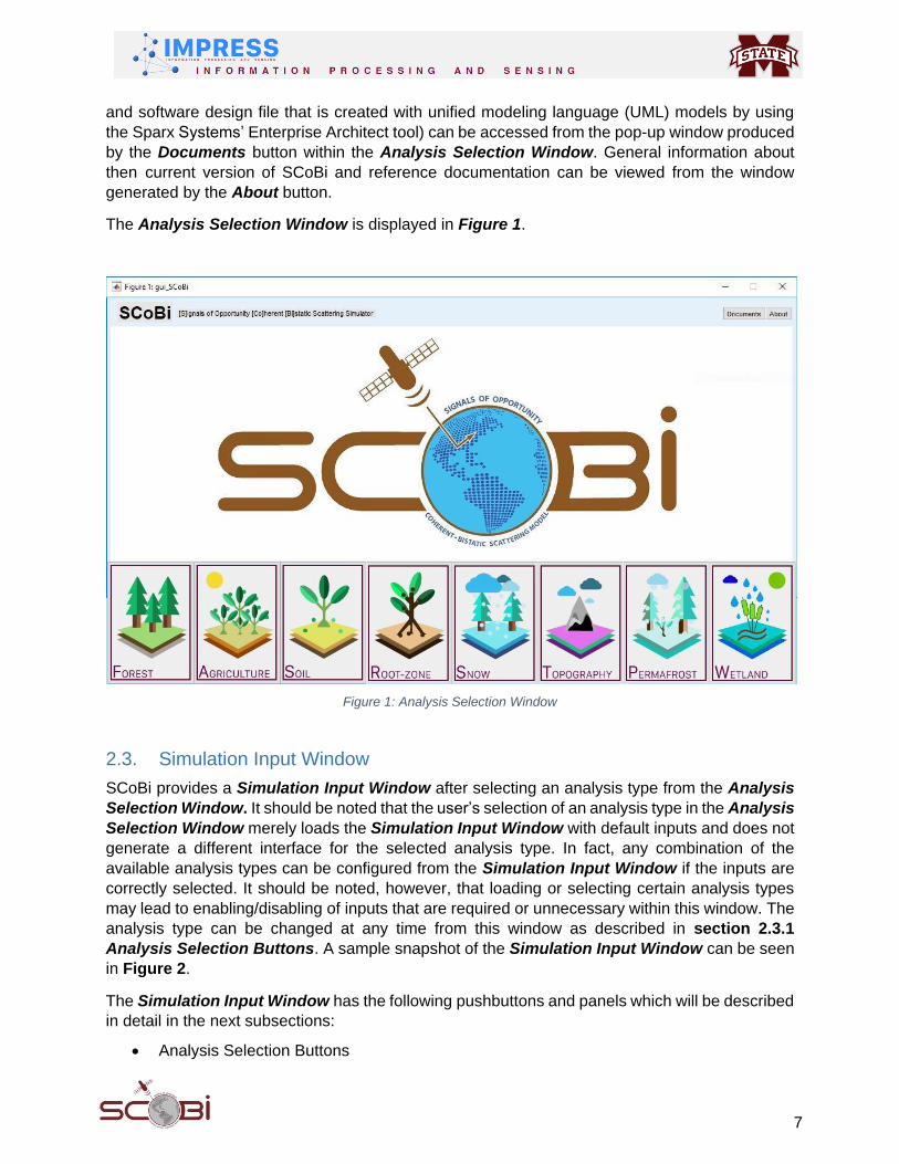
The Analysis Selection Window is displayed in Figure 1.

Figure 1: Analysis Selection Window

2.3. Simulation Input Window

SCoBi provides a Simulation Input Window after selecting an analysis type from the Analysis

Selection Window. It should be noted that the user’s selection of an analysis type in the Analysis

Selection Window merely loads the Simulation Input Window with default inputs and does not

generate a different interface for the selected analysis type. In fact, any combination of the

available analysis types can be configured from the Simulation Input Window if the inputs are

correctly selected. It should be noted, however, that loading or selecting certain analysis types

may lead to enabling/disabling of inputs that are required or unnecessary within this window. The

analysis type can be changed at any time from this window as described in section 2.3.1

Analysis Selection Buttons. A sample snapshot of the Simulation Input Window can be seen

in Figure 2.

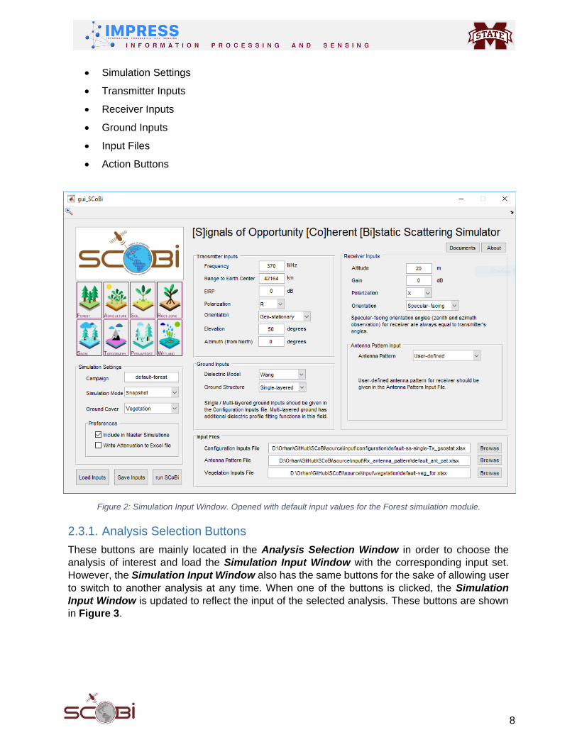
The Simulation Input Window has the following pushbuttons and panels which will be described

in detail in the next subsections:

Analysis Selection Buttons

8

Simulation Settings

Transmitter Inputs

Receiver Inputs

Ground Inputs

Input Files

Action Buttons

Figure 2: Simulation Input Window. Opened with default input values for the Forest simulation module.

2.3.1. Analysis Selection Buttons

These buttons are mainly located in the Analysis Selection Window in order to choose the

analysis of interest and load the Simulation Input Window with the corresponding input set.

However, the Simulation Input Window also has the same buttons for the sake of allowing user

to switch to another analysis at any time. When one of the buttons is clicked, the Simulation

Input Window is updated to reflect the input of the selected analysis. These buttons are shown

in Figure 3.

9

Figure 3: Analysis Selection Buttons. Presently, only Forest, Agriculture, Soil, and Root are functioning.

If a custom-user simulation has been previously run, the selection from the analysis selection

Analysis Selection Window or Analysis Selection Buttons will load the most recent

simulation settings that the user has created.

2.3.2. Simulation Settings

The Simulation Settings panel includes the main setting parameters of a simulation that

determine the output directory name, simulation mode, ground cover, and preferences. This panel

is displayed in Figure 4. These options are described in the subsections below.

Figure 4: Simulation Settings Panel

2.3.2.1. Campaign

Campaign is an editable text input that is used to name the simulation output directory. The

campaign variable is merged with the time-stamp of the time a simulation is run. The user can

freely decide on a campaign name; however, it is highly recommended to choose a self-

explanatory name such as:

“Corn-Maturity-MS-39762” for a corn field that is at its maturity growth-stage and located in

Mississippi at the zip code 39762.

10

2.3.2.2. Simulation Mode

SCoBi simulator currently supports two different simulation modes: Snapshot or Time-series.

The simulation mode determines the structure of the Configuration Inputs File which is

described in detail in section 3.1 Inputs.

2.3.2.2.1. Snapshot Simulation

Snapshot simulation is the appropriate mode for generating large amount of SoOp simulated data

for comprehensive analysis. The simulator runs simulations for all the snapshots (i.e.

combinations) of the following configuration inputs and scene parameters such as: Transmitter

incidence and azimuth angles (if Transmitter is not Geo-stationary), surface roughness (via root

mean square height), and volumetric soil moisture (VSM).

Please refer to section 3.1 Inputs to see how Snapshot mode affects the Configuration Inputs

File in detail.

2.3.2.2.2. Time-series Simulation

Time-series simulation mode is the perfect option to analyze realistic scenarios. This mode

requires the user provides a Configuration Inputs File in a suitable form for time-series which

has its requirements described in section 3.1 Inputs in detail.

2.3.2.3. Ground Cover

Ground cover can be determined to be Bare-soil or Vegetation cover. The Ground Cover value

determines if the Vegetation Inputs File is needed or not. The effect of Bare-soil and Vegetation

is described in detail both below and in section 3.1 Inputs.

2.3.2.3.1. Bare-soil

When Bare-soil is selected, there is no need for vegetation inputs, the Vegetation Inputs File

GUI elements are disabled, and SCoBi does not operate its functions for canopy computations

(such as propagation) and only generates the outputs for bare soil.

2.3.2.3.2. Vegetation

Vegetation cover option requires a Vegetation Inputs File of the correct form, which is described

in section 3.1 Inputs. This file can be given via the Vegetation Inputs File - Browse button in

the Input Files panel. This selection makes SCoBi perform the vegetation-related functions and

generate both vegetation and bare soil results.

2.3.2.4. Preferences There are currently two preferences in the SCoBi:

2.3.2.4.1. Include in Master Simulations

This preference is for running a simulation whether as a temporary trial or a recorded one that is

logged in the Master Simulations File (Will be described in section 3.3.3 Master Simulations

File).

2.3.2.4.2. Write Attenuation to Excel File

This preference is for recording the attenuation output of a simulation with vegetation cover into

an MS Excel file for further analysis.

11

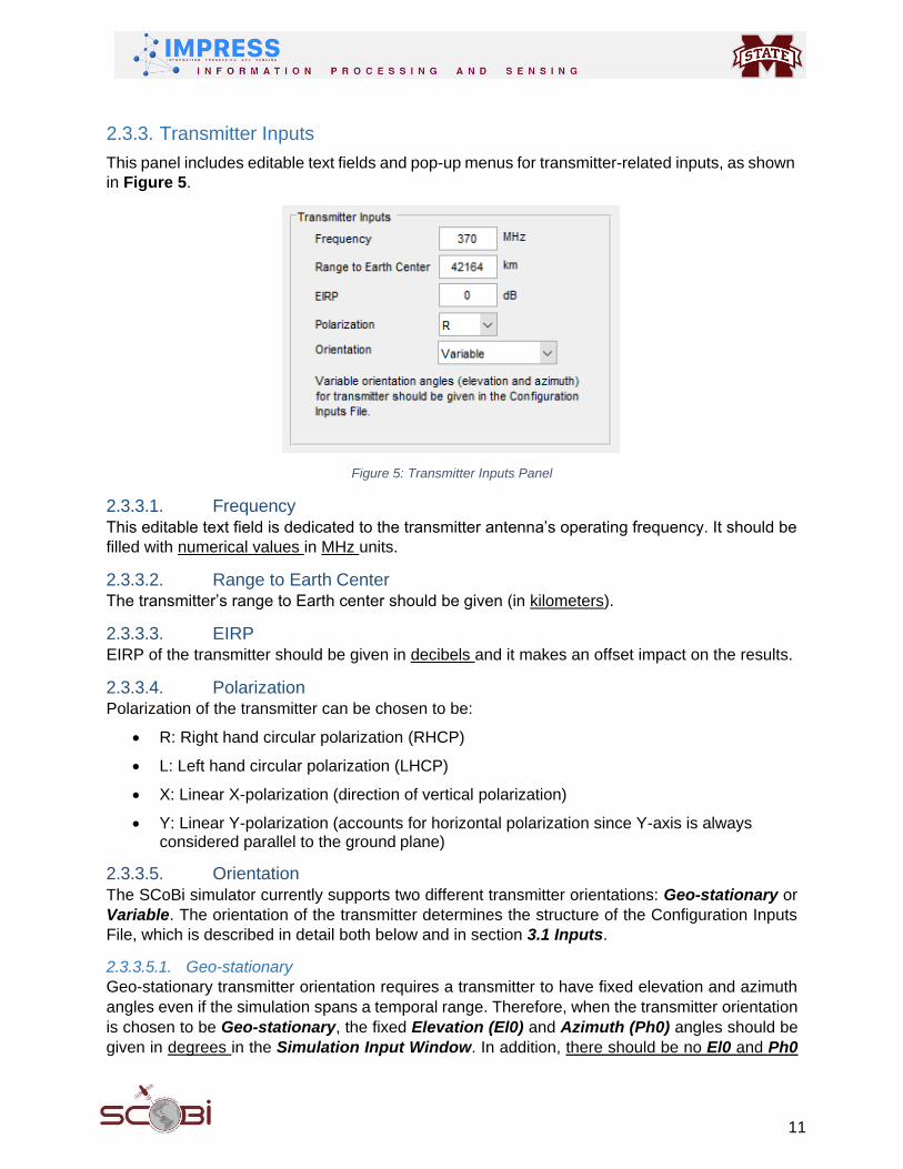
2.3.3. Transmitter Inputs

This panel includes editable text fields and pop-up menus for transmitter-related inputs, as shown

in Figure 5.

2.3.3.1. Frequency

Figure 5: Transmitter Inputs Panel

This editable text field is dedicated to the transmitter antenna’s operating frequency. It should be

filled with numerical values in MHz units.

2.3.3.2. Range to Earth Center The transmitter’s range to Earth center should be given (in kilometers).

2.3.3.3. EIRP EIRP of the transmitter should be given in decibels and it makes an offset impact on the results.

2.3.3.4. Polarization Polarization of the transmitter can be chosen to be:

R: Right hand circular polarization (RHCP)

L: Left hand circular polarization (LHCP)

X: Linear X-polarization (direction of vertical polarization)

Y: Linear Y-polarization (accounts for horizontal polarization since Y-axis is always considered parallel to the ground plane)

2.3.3.5. Orientation

The SCoBi simulator currently supports two different transmitter orientations: Geo-stationary or

Variable. The orientation of the transmitter determines the structure of the Configuration Inputs

File, which is described in detail both below and in section 3.1 Inputs.

2.3.3.5.1. Geo-stationary

Geo-stationary transmitter orientation requires a transmitter to have fixed elevation and azimuth

angles even if the simulation spans a temporal range. Therefore, when the transmitter orientation

is chosen to be Geo-stationary, the fixed Elevation (El0) and Azimuth (Ph0) angles should be

given in degrees in the Simulation Input Window. In addition, there should be no El0 and Ph0

12

columns in the Configuration Inputs File.

2.3.3.5.2. Variable

Variable transmitter orientation enables a transmitter to have changing elevation and azimuth

angles in a simulation. Therefore, when the transmitter orientation is chosen to be Variable, the

Elevation (EL0) and Azimuth (PH0) angle values should be given in degrees in the Tx_el (deg)

and Tx ph (deg) columns in the Configuration Inputs File. For details of this input file, please

refer to section 3.1 Inputs.

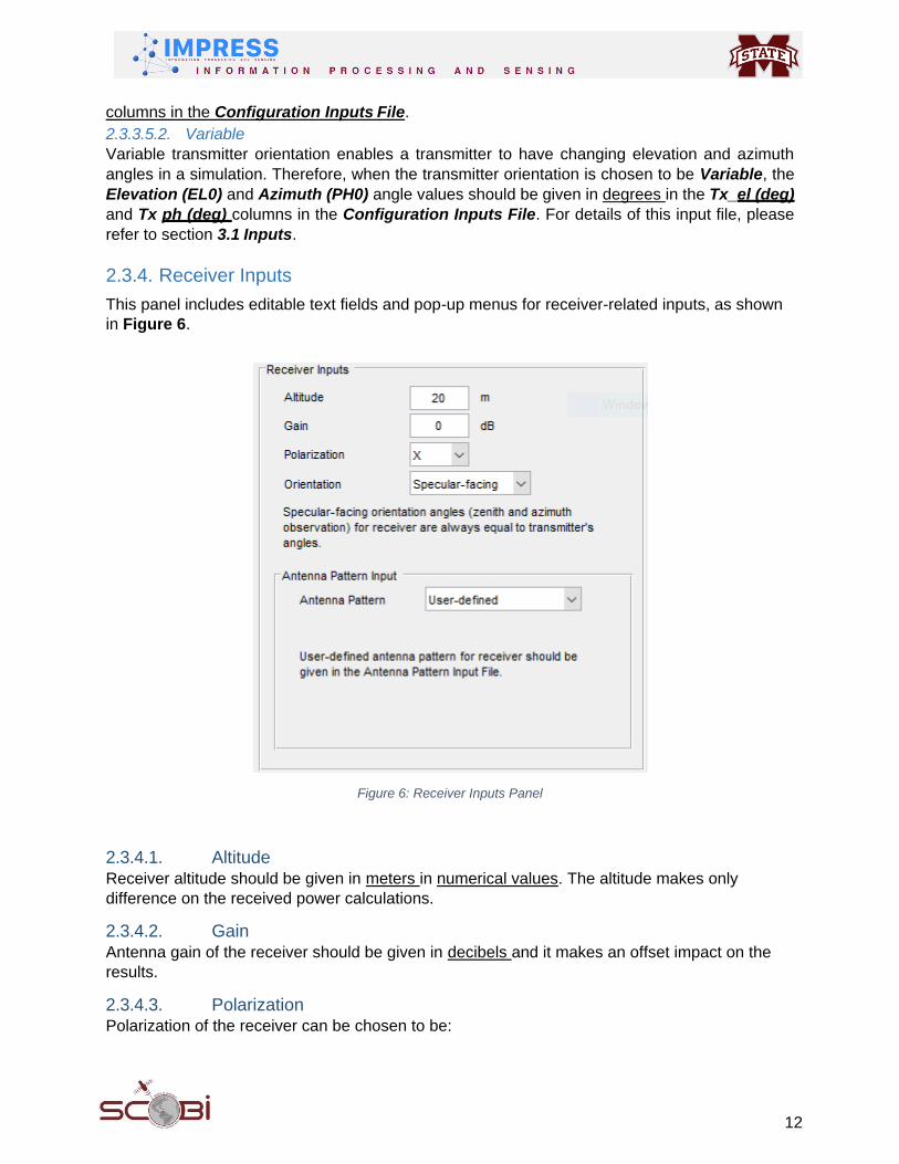
2.3.4. Receiver Inputs

This panel includes editable text fields and pop-up menus for receiver-related inputs, as shown

in Figure 6.

Figure 6: Receiver Inputs Panel

2.3.4.1. Altitude Receiver altitude should be given in meters in numerical values. The altitude makes only

difference on the received power calculations.

2.3.4.2. Gain Antenna gain of the receiver should be given in decibels and it makes an offset impact on the

results.

2.3.4.3. Polarization Polarization of the receiver can be chosen to be:

13

R: Right hand circular polarization (RHCP)

L: Left hand circular polarization (LHCP)

X: Linear X-polarization (Stands for vertical polarization)

Y: Linear Y-polarization (Accounts for horizontal polarization since Y-axis is always considered parallel to the ground plane)

2.3.4.4. Orientation SCoBi simulator currently supports two different receiver orientations: Fixed or Specular-facing.

Fixed orientation means that receiver observes a fixed point with constant looking and azimuth

angles, which setup is common, for example, in tower applications. Specular-facing means that

the receiver gets the same orientation angles for changing transmitter orientations, which is hard

to obtain in real-world experiments, but might allow to create more simulated data.

2.3.4.4.1. Fixed

The fixed Zenith Observation (Theta) and Azimuth (Phi) angles should be given in degrees in

the Simulation Input Window.

2.3.4.4.2. Specular-facing

When the receiver is Specular-facing, there is no need to provide the zenith observation angles;

instead, the SCoBi simulator always equates the receiver’s orientation angles to the transmitter’s,

even if the configuration changes.

2.3.4.5. Antenna Pattern

SCoBi simulator currently supports two different receiver antenna pattern generation methods:

Generalized-Gaussian or User-defined. A third option Cosine to the power n is also listed in

the pop-up menu for reference to developers. Antenna pattern selection affects if Antenna

Pattern File is needed or not, which effect is described in detail bot below and in section 3.1

Inputs.

2.3.4.5.1. Generalized-Gaussian

A simple generalized Gaussian antenna pattern can be created quickly by giving the significant

parameter values via the Simulation Input Window. When this option is selected under the

Antenna Pattern pop-up menu, SCoBi shows the following parameters for user input:

Beamwidth: Half-power beamwidth of the antenna pattern should be given in degrees in numerical values.

Side-lobe level: The levels of the first side-lobes should be given in decibels in numerical values.

Cross-pol level: The level of the cross-polarization of the antenna pattern should be given in decibels in numerical values.

Pattern Resolution: The minimum sensitivity of the antenna pattern should be given in degrees in numerical values.

2.3.4.5.2. User-defined

This option requires an Antenna Pattern File of the correct form, which is described in section

3.1 Inputs. This file can be given via the Antenna Pattern File - Browse button in the Input Files

panel.

14

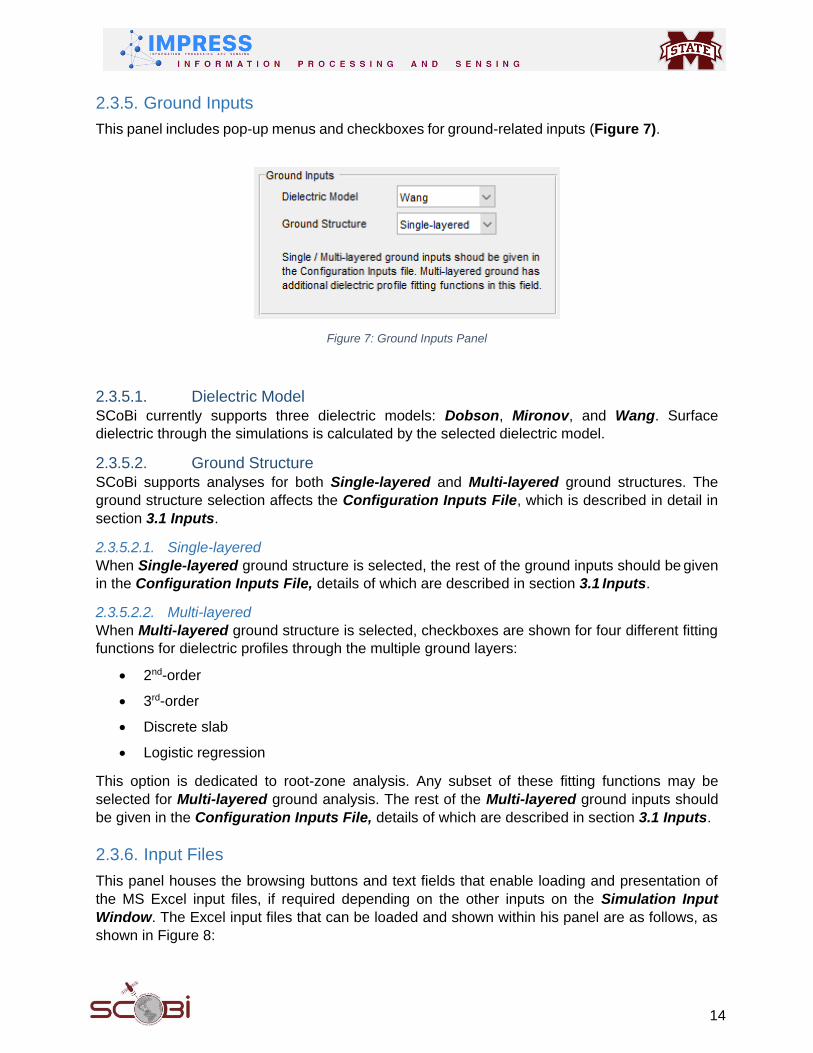
2.3.5. Ground Inputs

This panel includes pop-up menus and checkboxes for ground-related inputs (Figure 7).

Figure 7: Ground Inputs Panel

2.3.5.1. Dielectric Model

SCoBi currently supports three dielectric models: Dobson, Mironov, and Wang. Surface

dielectric through the simulations is calculated by the selected dielectric model.

2.3.5.2. Ground Structure

SCoBi supports analyses for both Single-layered and Multi-layered ground structures. The

ground structure selection affects the Configuration Inputs File, which is described in detail in

section 3.1 Inputs.

2.3.5.2.1. Single-layered

When Single-layered ground structure is selected, the rest of the ground inputs should be given

in the Configuration Inputs File, details of which are described in section 3.1 Inputs.

2.3.5.2.2. Multi-layered

When Multi-layered ground structure is selected, checkboxes are shown for four different fitting

functions for dielectric profiles through the multiple ground layers:

2nd-order

3rd-order

Discrete slab

Logistic regression

This option is dedicated to root-zone analysis. Any subset of these fitting functions may be

selected for Multi-layered ground analysis. The rest of the Multi-layered ground inputs should

be given in the Configuration Inputs File, details of which are described in section 3.1 Inputs.

2.3.6. Input Files

This panel houses the browsing buttons and text fields that enable loading and presentation of

the MS Excel input files, if required depending on the other inputs on the Simulation Input

Window. The Excel input files that can be loaded and shown within his panel are as follows, as

shown in Figure 8:

15

Configuration Inputs File: Default files that are provided with the SCoBi distribution are located under ./source/input/configuration/ directory.

Antenna Pattern File: Default files that are provided with the SCoBi distribution are located under ./source/input/Rx_antenna_pattern/ directory.

Vegetation Inputs File: Default files that are provided with the SCoBi distribution are located under ./source/input/vegetation/ directory.

Figure 8: Ground Inputs Panel

2.3.7. Action Buttons

Action buttons are located in the Simulation Input Window for the aim of overall management,

as shown in Figure 9.

2.3.7.1. Load Inputs A simulation input can be loaded any time into the Simulation Input Window.

2.3.7.2. Save Inputs The current state of the Simulation Input Window can be saved as a simulation input (.mat)

file.

2.3.7.3. RunSCoBi

RunSCoBi button is for running the simulation with the current state of the Simulation Input

Window. If no change is made on the recently loaded or saved simulation inputs, SCoBi

immediately begins to run after this button is clicked. Otherwise, the software prompts the user to

save the current state of the Simulation Input Window as a different simulation inputs file.

2.3.7.4. Exit The window close button of the Simulation Input Window can be used to terminate SCoBi.

When the button is clicked, SCoBi prompts user to confirm the termination.

Figure 9: Action buttons

16

3. Analysis with SCoBi

3.1. Inputs

There are two main types of the inputs for a SCoBi simulation: Simulation Inputs and Excel

Input Files.

3.1.1. Simulation Inputs

Simulation inputs are initially provided as default simulation input files, and their values can be

altered by modifying the defaults and saving new input files. Simulation inputs are accessed

through GUI (Simulation Input Window), saved as “.mat” files. Simulation input files map all

information (from single parameter values to full paths for Excel input files) to variables within the

SCoBi simulator in order to perform the user’s simulation of interest. The user deals with

simulation inputs only via GUI. Initially provided, default simulation input files can be found within

the ./source/input/system directory. It is suggested that the newly generated simulation input

files stored in the same location as well; however, it is not required.

When SCoBi is run, the Simulation Input Window is loaded with the recently saved simulation

input file. Otherwise, it is loaded with the default simulation input file for the selected analysis type.

If no default input file is present (since input files can be removed by the user), the window is

opened empty.

Whenever there is a change to the recently loaded or saved simulation input file and RunSCoBi

button is clicked, SCoBi prompts the user to save the current state of the Simulation Input

Window as a new simulation input file.

3.1.2. Excel Input Files

SCoBi simulations may require from one to three separate MS Excel input files depending on the

chosen settings and parameter values within the simulation inputs. It is highly encouraged that

users view the example Excel input files in the following directories before creating their own:

./source/input/configuration,

./source/input/Rx_antenna_pattern, and

./source/input/vegetation

3.1.2.1. Configuration Inputs File A Configuration Inputs File is required in every simulation and consists of two sheets: Dynamic

and Ground. While the order of the sheets is required for the operation of SCoBi, the name of

these sheets can be arbitrary. The first sheet in the Configuration Inputs File should correspond

to the Dynamic sheet and the second sheet should correspond to the Ground sheet. Additionally,

it is suggested that these two sheets be named Dynamic and Ground as depicted in Figure 10.

Figure 10: Example Vegetation Inputs File Sheet Titles

17

The Dynamic sheet defines parameters that may be given changing values within a simulation.

Variable parameters include timestamps, azimuth and elevation angles of the transmitter, root-

mean-square height (RMSH) roughness of the soil surface, and volumetric soil moisture.

The Ground sheet consists of static parameters that define the ground structure such as soil

texture, soil bulk density, layer depths where soil moisture probes are located, and layering

effects.

The content (being the name and value of variables within the Dynamic and Ground sheets)

found in the Configuration Inputs File should be prepared according to the joint requirements

of the simulation mode and analysis type. In other words, Configuration Inputs File should be

created in a way that it satisfies all the directives listed for the following parameters. Example

input files will be given after the requirements for all the parameters are described.

While the order of the parameter columns in both Dynamic and Ground spreadsheets of the

Configuration Inputs File is required for the operation of SCoBi, the name of the parameters

can be arbitrary. However, it is suggested that the parameter columns be named as in the

examples in section 3.1.2.1.4 Example Configuration Inputs File for the sake of familiarity.

3.1.2.1.1. Simulation Mode Effect: Snapshot vs. Time-series

Simulation mode selection places requirements on writing the Dynamic sheet of the

Configuration Inputs File, but not on the Ground spreadsheet. The requirements for creating

a Configuration Inputs File that satisfies SCoBi’s different simulation modes are described as

follows:

3.1.2.1.1.1. Snapshot

Snapshot simulations are just for analyzing the combinations of changing configurational and

environmental parameters such as transmitter orientation, surface roughness, and soil

moisture. There is no need for timestamp information in a Snapshot mode; therefore, there

should not be a DoY (Day-of-Year) column in the Dynamic sheet of the Configuration Inputs

File. The following parameter columns may be included with totally different number of rows

(samples) than each other in the Dynamic spreadsheet:

Tx_el(deg) Transmitter elevation (EL0, complements the incidence angle to 90 degrees, i.e. 90 - θ) angle in degrees. This is the angle formed between the ground surface and the vector located along between specular point along the ground surface and the transmitter.

Tx_ph(deg) Transmitter azimuth (PH0, ϕ) angle in degrees. This is the heading or compass direction described clockwise from magnetic North.

RMSH(cm): Surface roughness – root mean square height in centimeters

VSM(cm3/cm3): Volumetric soil moisture in cm3/cm3

3.1.2.1.1.2. Time-series

Time-series simulations are for analyzing a temporally changing configuration and

environment. In other words, in a Time-series simulation, there should be configurational and

environmental parameter values as well as timestamps, which have exactly the same length or

some of them are constant. Thus, following parameters may be given in separate columns in

Dynamic spreadsheet as same-length sequences or only one value (to represent being

constant) for a period in time:

18

DoY Day of Year. A notation to write the month, day, hour, minute, second, etc. of a given timestamp with days being the given unit. Day one is generally midnight of January 1st of a given year.

El_th(deg Transmitter elevation (El, 90 - θ) angle in degrees. This is the angle formed between the ground surface and the vector located along between specular point along the ground surface and the transmitter.

Tx_ph(deg) Transmitter azimuth (phi, ϕ) angle in degrees. This is the heading or compass direction described clockwise from magnetic North.

RMSH(cm): Surface roughness – root mean square height in centimeters

VSM(cm3/cm3): Volumetric soil moisture in cm3/cm3

3.1.2.1.2. Transmitter Orientation

Transmitter orientation selection affects the Dynamic sheet of the Configuration Inputs File.

When transmitter orientation is Geo-stationary, there should be neither Elevation Angle

(EL0) nor Azimuth Angle (PH0) columns in the Dynamic sheet.

3.1.2.1.3. Ground Structure: Single-layered vs. Multi-layered

Ground structure selection may make effects on both the Dynamic and Ground sheets of the

Configuration Inputs File. The effects of the ground structures are described as follows:

3.1.2.1.3.1. Single-layered

Single-layered ground structure simulations only require the Volumetric Soil Moisture and

ground texture information for the ground surface. Therefore, there should be only one

VSM(cm3/cm3) column in the Dynamic sheet. The following parameter columns should be

included with only one row for numeric values in addition to the column names row in the

Ground sheet:

sand_ratio Sand ratio of the ground surface within [0,1]

clay_ratio Clay ratio of the ground surface within [0,1]

rho_b(g/cm3) Bulk density of the soil in g/cm3

3.1.2.1.3.2. Multi-layered

Multi-layered ground structure simulations require the VSM(cm3/cm3) and ground texture

information for multiple layers of the ground. Number of VSM(cm3/cm3) columns in the

Dynamic sheet should exactly match the number of ground layers to be analyzed. Each

VSM(cm3/cm3) corresponds to VSM measurements in a different ground layer. The following

parameter columns should be included with the equal number of rows for numeric values as in

the number of ground layers in addition to the column names row in the Ground sheet:

layer_depth Layer depths of each ground layer should be given in meters. Thus, this column should include its name in the first row, then enough number of layer depths as much as the number of ground layers.

sand_ratio The percentage of sand within the ground layer with a range of [0,1]. This column should include its name in the first row, then enough number of sand ratios as much as the number of ground layers.

19

clay_ratio The percentage of clay within the ground layer with a range of [0,1]. This column should include its name in the first row, then enough number of clay ratios as much as the number of ground layers.

rho_b(g/cm3) Bulk densities of the ground layers in g/cm3. This column should include its name in the first row, then enough number of bulk densities as much as the number of ground layers.

delZ(m) Layer discretization in meters. Only one value is enough to make discretization through all the ground layers.

zA(m) Air layer thickness in meters.

zB(m) The bottom-most layer thickness in meters. This should generally be defined to be greater than or equal to the penetration depth of the SoOp transmitter’s frequency and beneath the deepest point of interest within the soil moisture profile. The total layer depth will then become the largest value in the column for layer_depth plus the value of zB.

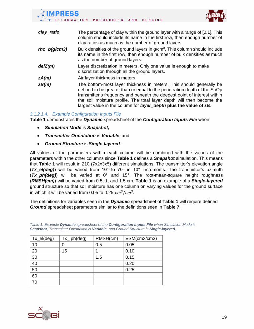
3.1.2.1.4. Example Configuration Inputs File

Table 1 demonstrates the Dynamic spreadsheet of the Configuration Inputs File when

Simulation Mode is Snapshot,

Transmitter Orientation is Variable, and

Ground Structure is Single-layered.

All values of the parameters within each column will be combined with the values of the

parameters within the other columns since Table 1 defines a Snapshot simulation. This means

that Table 1 will result in 210 (7x2x3x5) different simulations. The transmitter’s elevation angle

(Tx_el(deg)) will be varied from 10° to 70° in 10° increments. The transmitter’s azimuth

(Tx_ph(deg)) will be varied at 0° and 15°. The root-mean-square height roughness

(RMSH(cm)) will be varied from 0.5, 1, and 1.5 cm. Table 1 is an example of a Single-layered

ground structure so that soil moisture has one column on varying values for the ground surface

in which it will be varied from 0.05 to 0.25 𝑐𝑚3/𝑐𝑚3.

The definitions for variables seen in the Dynamic spreadsheet of Table 1 will require defined

Ground spreadsheet parameters similar to the definitions seen in Table 7.

Table 1: Example Dynamic spreadsheet of the Configuration Inputs File when Simulation Mode is

Snapshot, Transmitter Orientation is Variable, and Ground Structure is Single-layered.

Tx_el(deg) Tx_ ph(deg) RMSH(cm) VSM(cm3/cm3)

10 0 0.5 0.05

20 15 1 0.10

30 1.5 0.15

40 0.20

50 0.25

60

70

20




Ground Structure is Multi-layered.

All values of the parameters within each column will be combined with the values of the

parameters within the other columns since Table 2 defines a Snapshot simulation. This means

that Table 2 will result in 10,752 (7x2x3x4x4x4x4) different simulations. The transmitter’s

elevation angle (Tx_el(deg)) will be varied from 10° to 70° in 10° units. The transmitter’s azimuth

(Tx_ph(deg)) will be varied at 0° and 15°. The root-mean-square height roughness (RMSH(cm))

will be varied from 0.5, 1, and 1.5 cm. Table 2 is an example of a Multi-layered ground structure

so that soil moisture has also a multi-layered profile in which the soil moisture at 5, 10, 20, and

40 centimeters is defined. It is worth noting here that the number and depth of the soil moisture

measurements can be different than what is exemplified here. The values between these defined

points are interpolated using different function fits as defined in section 2.3.5.2.2 Multi-layered.

The definitions for variables seen in the Dynamic spreadsheet of Table 2 will require defined

Ground spreadsheet parameters similar to the definitions seen in Table 8.

Table 2: Example Dynamic spreadsheet of the Configuration Inputs File when Simulation Mode is Snapshot, Transmitter Orientation is Variable, and Ground Structure is Multi-layered.

Tx_el (deg)

Tx_ ph0 (deg)

RMSH (cm)

VSM_5 (cm3/cm3)

VSM_10 (cm3/cm3)

VSM_20 (cm3/cm3)

VSM_40 (cm3/cm3)

10 0 0.5 0.374 0.364 0.374 0.436

20 15 1 0.374 0.361 0.372 0.440

30 1.5 0.375 0.355 0.375 0.440

40 0.371 0.332 0.388 0.440

50

60

70



Transmitter Orientation is Geo-stationary, and


Whenever Transmitter Orientation is Geo-stationary, the transmitter orientation columns

(Tx_el(deg) and Tx_ph(deg)) are discarded from the Dynamic spreadsheet regardless of the

other parameter selections (Simulation Mode and Ground Structure) since the fixed orientation

angle values are given via Simulation Input Window. Processing of the input in Table 3 is then

similar to that in Table 1 (combinations of all the columns).

21

Table 3: Example Dynamic spreadsheet of the Configuration Inputs File when Simulation Mode is Snapshot, Transmitter Orientation is Geo-stationary, and Ground Structure is Single-layered.

RMSH (cm)

VSM(cm3/cm3)

0.5 0.05

1 0.10

1.5 0.15

0.20



Transmitter Orientation is Geo-stationary, and


Whenever Transmitter Orientation is Geo-stationary, the transmitter orientation columns

(Tx_el(deg) and Tx_ph(deg)) are discarded from the Dynamic spreadsheet regardless of the

other parameter selections (Simulation Mode and Ground Structure) since the fixed orientation

angle values are given via Simulation Input Window. Processing of the input in Table 4 is then

similar to that in Table 2 (combinations of all the columns).

Table 4: Example Dynamic spreadsheet of the Configuration Inputs File when Simulation Mode is Snapshot, Transmitter Orientation is Geo-stationary, and Ground Structure is Multi-layered.

RMSH (cm)

VSM_5 (cm3/cm3)

VSM_10 (cm3/cm3)

VSM_20 (cm3/cm3)

VSM_40 (cm3/cm3)

0.5 0.374 0.364 0.374 0.436

1 0.374 0.361 0.372 0.440

1.5 0.375 0.355 0.375 0.440

0.371 0.332 0.388 0.440


Simulation Mode is Time-series,



22

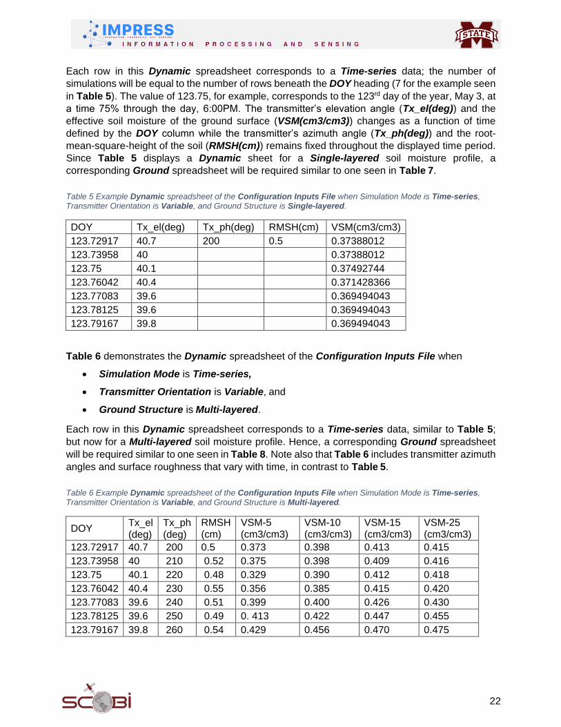
Each row in this Dynamic spreadsheet corresponds to a Time-series data; the number of

simulations will be equal to the number of rows beneath the DOY heading (7 for the example seen

in Table 5). The value of 123.75, for example, corresponds to the 123rd day of the year, May 3, at

a time 75% through the day, 6:00PM. The transmitter’s elevation angle (Tx_el(deg)) and the

effective soil moisture of the ground surface (VSM(cm3/cm3)) changes as a function of time

defined by the DOY column while the transmitter’s azimuth angle (Tx_ph(deg)) and the root-

mean-square-height of the soil (RMSH(cm)) remains fixed throughout the displayed time period.

Since Table 5 displays a Dynamic sheet for a Single-layered soil moisture profile, a

corresponding Ground spreadsheet will be required similar to one seen in Table 7.

Table 5 Example Dynamic spreadsheet of the Configuration Inputs File when Simulation Mode is Time-series, Transmitter Orientation is Variable, and Ground Structure is Single-layered.

DOY Tx_el(deg) Tx_ph(deg) RMSH(cm) VSM(cm3/cm3)

123.72917 40.7 200 0.5 0.37388012

123.73958 40 0.37388012

123.75 40.1 0.37492744

123.76042 40.4 0.371428366

123.77083 39.6 0.369494043

123.78125 39.6 0.369494043

123.79167 39.8 0.369494043


Simulation Mode is Time-series,



Each row in this Dynamic spreadsheet corresponds to a Time-series data, similar to Table 5;

but now for a Multi-layered soil moisture profile. Hence, a corresponding Ground spreadsheet

will be required similar to one seen in Table 8. Note also that Table 6 includes transmitter azimuth

angles and surface roughness that vary with time, in contrast to Table 5.

Table 6 Example Dynamic spreadsheet of the Configuration Inputs File when Simulation Mode is Time-series, Transmitter Orientation is Variable, and Ground Structure is Multi-layered.

DOY Tx_el (deg)

Tx_ph (deg)

RMSH (cm)

VSM-5 (cm3/cm3)

VSM-10 (cm3/cm3)

VSM-15 (cm3/cm3)

VSM-25 (cm3/cm3)

123.72917 40.7 200 0.5 0.373 0.398 0.413 0.415

123.73958 40 210 0.52 0.375 0.398 0.409 0.416

123.75 40.1 220 0.48 0.329 0.390 0.412 0.418

123.76042 40.4 230 0.55 0.356 0.385 0.415 0.420

123.77083 39.6 240 0.51 0.399 0.400 0.426 0.430

123.78125 39.6 250 0.49 0. 413 0.422 0.447 0.455

123.79167

39.8 260 0.54 0.429 0.456 0.470 0.475

23

Table 7 demonstrates the Ground spreadsheet of the Configuration Inputs File when

Ground Structure is Single-layered

Table 7 Example Ground spreadsheet of the Configuration Inputs File when Ground Structure is Single-layered.

sand_ratio

clay_ratio rho_b (g/cm3)

0.8 0.07 1.25

Note that in Table 7, we find that our sand_ratio value is 80% of the total effective soil layer, and

our clay ratio is 7% of the total effective soil layer. Our soil bulk density (rho_b) is 1.25 g/cm3 for the effective single layer soil profile.

Table 8 demonstrates the Ground spreadsheet of the Configuration Inputs File when


Table 8: Example Ground spreadsheet of the Configuration Inputs File when Ground Structure is Multi-layered.

layer_depth (m)

sand_ratio clay_ratio rho_b (g/cm3)

delZ (m) zA (m) zB (m)

0.05 0.1 0.31 1.4 0.001 0.1 0.3

0.1 0.1 0.31 1.4

0.2 0.1 0.31 1.4

0.4 0.1 0.34 1.5

Note that in Table 8, we have placed variable soil moisture points at 5 cm, 10 cm, 20 cm, and 40

cm under the layer_depth column. The sand_ratio, clay_ratio, and rho_b parameters must be

defined at each of these depths. The air layer (zA) has been defined to be 10 cm, and the bottom-

most layer (zB) is defined as 30 cm. Given our bottom soil moisture point location is 40 cm, our

total profile will be 10cm + 40cm + 30cm = 80 cm with our bottom soil layer being a point 70 cm

beneath the surface of the soil. The layer discretization is 1 mm (delZ). Because we have defined

4 different layer_depths within this Ground sheet, we will require 4 columns that define the soil

moisture content at these depths (VSM5_cm3cm3, VSM10_cm3cm3, VSM20_cm3cm3, and

VSM40_cm3cm3) in the corresponding Dynamic sheet for the variables seen in Table 8’s

Ground sheet. An example of this can be seen in Table 2.

24

3.1.2.2. Antenna Pattern File

Antenna Pattern File is required only if the receiver antenna pattern is selected to be User-

defined. It consists of four sheets within an Excel spreadsheet: gnXX, gnXY, gnYX, and gnYY,

which holds the normalized voltage values for co- and cross-polarizations for X and Y ports. An

example antenna pattern file can be found in ./source/input/Rx_antenna_pattern.

Antenna pattern should be provided such that in each sheet of the Excel file, columns represent

the theta-angle look-up and rows represent the phi-angle look-up. Theta (θ) angles have a 180°

scan, while phi (ϕ) angles have a 360° scan.

Note that the antenna pattern files do not have headers within the Excel spreadsheet. Each sheet

consists of numbers only.

3.1.2.3. Vegetation Inputs File Vegetation Inputs File is required only if the ground cover is selected to be Vegetation. It

consists of two spreadsheets: Layers and Kinds. While the order of the sheets is required for the

operation of SCoBi, the name of these sheets can be arbitrary. The first sheet in the Vegetation

Inputs File should correspond to the Layers sheet and the second sheet should correspond to

the Kinds sheet. Additionally, it is suggested that these two sheets be named Layers and Kinds

as depicted in Figure 11.

Figure 11: Vegetation Inputs File spreadsheets

An example Vegetation Inputs File for each of analysis types Forest and Agriculture is included

in:

./source/input/vegetation.

3.1.2.3.1. Layers

The Layers sheet should provide detailed information about the vegetation layer thicknesses and

the content of each individual layer. Vegetation layer can be divided into a number of sub-layers

by defining separate layer thicknesses for the purpose of locating specific Kinds (Leaf, Branch,

Trunk, or Needle) into different layers. Thicknesses of the vegetation cover should be given (in

integer or double numbers in meters) in the second column of the Layers spreadsheet in a way

that ascending rows should represent an ascending height from top to bottom. The first column

of the Layers spreadsheet is reserved to the names of individual layers. This column should be

included in any Vegetation Inputs File; however; the name of each row in this column can be

arbitrary. The example Vegetation Inputs Files use meaningful layer names to increase

familiarity with the vegetation layer structure. For each separate vegetation layer. The first row is

reserved for the descriptions of columns. Again, this row should be included in any Vegetation

Inputs File; however; the name of each row in this column can be arbitrary. In other words, the

actual layer data should begin from the second row and the second column.

For each vegetation layer row, columns after the thickness column should have the information

about content of each vegetation layer. This information is related to the Kinds spreadsheet, and

25

each vegetation layer can include from one to several Kinds (Please refer to section 3.1.2.3.2

Kinds for naming conventions). The content of each layer should be given such that exactly

one Particle ID (the same as given in the Kinds spreadsheet) exists in a column as shown in

Table

9. For instance in Table 9, Layer 2 has L1 (first kind of the type Leaf), B2 (second kind of the

type Branch), B3 (third kind of the type Branch), and B4 (fourth kind of the type Branch);

however, Layer 4 only includes T1 (first kind of the type Trunk) that is intuitive to put Trunk

fixed to the ground. In addition, the spreadsheet represents such a vegetation cover that can be

analyzed as four distinct layers, each including different Trunk, Branch, and Leaf Kinds.

Table 9: Example Layers spreadsheet for Vegetation Inputs File

Thickness (m)

Included Kinds

Layer 1 (Top) 2 L1 B4

Layer 2 4 L1 B2 B3 B4

Layer 3 3 B1 B2

Layer 4 (Bottom)

4 T1

3.1.2.3.2. Kinds

The Kinds sheet should provide detailed information about the scatterer types and kinds

declared in the Layers sheet. The four scatterer Types used in SCoBi are Leaf, Branch, Trunk,

or Needle. A Leaf should be considered as an elliptical disk, while the types Branch, Trunk, and

Needle are considered as cylinders. Several Kinds of a Type can be defined in this

spreadsheet (e.g. L1, L2, etc.).

The whole sheet should define the different Kinds of scatterers that are exist in the vegetation

layers. First column of the spread sheet is reserved for row descriptions. This column should be

included in any Vegetation Inputs File, but the names of the rows in this column can be

arbitrary. However, the example input files have meaningful row names for ease. Each column

after the first column should represent one of the Kinds. As seen in Table 9, the Kinds can be

reused throughout the different layers. There are nine rows for each column that define the

following information:

Particle ID It can be also assumed the Kind name. A character array, where the first character must be one of the following letters ‘L’, ‘B’, ‘T’’ or ‘N’ to stand for the Types (Leaf, Branch, Trunk, or Needle), and next characters should be integer to represent a specific Kind of the selected Type (e.g. “L1”, “L2”, “T1”, “B3”, etc.). This ID is used in the Layers sheet to link the vegetation layers to the scatterer Kinds.

Density The number of scattering particles within one cubic meter.

Dimension1 Either the radius of the start of a cylinder (Branch, Trunk, or Needle) or major axis of an elliptical disk (Leaf) in meters.

26

Dimension2 Either should be the radius of the end of a cylinder (Branch, Trunk, or Needle) or minor axis of an elliptical disk (Leaf) in meters.

Dimension3 Either the length of a cylinder (Branch, Trunk, or Needle) or thickness of an elliptical disk (Leaf) in meters.

epsr_real The real part of the dielectric constant of a scatterer. This is sometimes referred to as the relative permittivity of a scattering particle.

epsr_im The imaginary part of the dielectric constant of a scatterer. This is sometimes referred to as the

Begin Angle The minimum interval value of the scatterer orientation that is assumed to be uniformly distributed between two angular boundaries.

End Angle The maximum interval value of the scatterer orientation that is assumed to be uniformly distributed between two angular boundaries.

An example Kinds spreadsheet is displayed in Table 10.

Table 10: Example Kinds spreadheet for Vegetation Inputs File

L1 B1 B2 B3 B4 T1

0 1 1 0 0 1

11.12 0.016 0.188 0.734 1.933 0.005

1.02E-01 4.30E-02 1.58E-02 9.80E-03 4.50E-03 8.73E-02

1.02E-01 4.30E-02 1.58E-02 9.80E-03 4.50E-03 8.73E-02

1.20E-04 1.87E+00 1.54E+00 6.36E-01 4.81E-01 6.17E+00

35.2 12 12 12 12 15.6

5.3 2.93 2.93 2.93 2.93 3.8

5 20 10 5 5 0

85 50 60 85 85 0.1

27

3.2. Simulation Preparation Flow

The preparation process of different SCoBi simulations may differ based on the analysis type and

configurations selected by the user, although the general flow is the same. In this section, the flow

of the overall simulation preparation will be described, and changes within steps due to different

parameter selections will be emphasized by using example scenarios.

1. The first and most significant step of creating a SCoBi simulation is to determine the SoOp

analysis type, the bistatic configuration (transmitter and receiver characteristics, and the

geometry), Simulation Mode, Vegetation Cover, and the Ground Structure.

2. The second major step is either the preparation of the required Excel input files

(Configuration, Vegetation, and Antenna Pattern input files, if needed), or use of the

existing default files for the simulation of interest. Details of the requirements for the

contents of the Excel input files when using the default ones or preparing new ones are

mentioned in section 3.1.2 Excel Input Files, and it is highly recommended to read that

section carefully.

3. The final main step is to give individual simulation parameters through the Simulation

Input Window, to select the Excel input files through this window, and to run SCoBi.

Two different examples regarding these three major steps will be provided in this section:

3.2.1. Global Navigation Satellite System Reflectometry (GNSS-R) Vegetation

Analysis The major three steps of a GNSS-R simulation can be described as follows:

1. In a GNSS-R simulation, the transmitter can be one of the typical GNSS satellites. In this

example, an Agriculture SoOp analysis over a Vegetation Cover of an agricultural field

will be considered. The transmitter will be a GNSS satellite operating at L1A-band with a

Variable orientation (for the purpose of analyzing the changing transmitter angles). The

receiver will be a ground-based GNSS receiver, which has a Generalized-Gaussian

antenna pattern. Further details about the transmitter and the receiver parameters will be

given below. This simulation will be a Snapshot simulation, where the combinations of

simulation parameters are used for generating individual simulation snapshots to generate

large amount of simulated data. Ground Structure will be Single-layered since the

surface dielectric calculations are considered enough for such a vegetation analysis

scenario.

2. For such a simulation, below Excel input files (either the default or the newly generated

files) must satisfy the simulation specifications in the first major step as follows:

a. Configuration Inputs File: It should satisfy:

Simulation Mode: Snapshot,

Transmitter Orientation: Variable, and

Ground Structure: Single-layered

which corresponds to a file similar to what is shown in Table 1 and Table 7 for

Dynamic and Ground spreadsheets, respectively.

b. Vegetation Inputs File: It should represent the agricultural field of interest, in a

similar way to what is shown in Table 9 and Table 10 for Layers and Kinds

spreadsheets, respectively.

28

c. Antenna Pattern File: This simulation does not involve this file since the receiver

antenna pattern is a Generalized-Gaussian.

3. The type of analysis should be chosen Agriculture in the Analysis Selection Window.

It should be noted again that the selection of the analysis type does not prevent the user

to study another analysis in the Simulation Input Window, but it helps determine the

simulation parameters within this window easier. For example, Multi-layered ground

could be defined within the Configuration Inputs File even if the analysis type was

selected to be Soil (Single-layered).

In addition, it can be concluded that the analysis type should be picked regarding the main

interest of the simulation; then, the other effects can be still performed. For instance, if a

Multi-layered ground analysis was the main concern of this simulation, but an agricultural

terrain would be studied over that surface, analysis type should have been chosen as

Root-zone, and agricultural field should be defined with the help of vegetation parameters

(Vegetation-cover and Vegetation Inputs File).

Simulation Inputs Window: All the simulation parameters are determined via this

window, as described in detail in section 2.3 Simulation Input Window.

a. Campaign: It should be given as a unique name that reflects the content of this

simulation. It may be the geo-location, if any, of the simulated field, or any

meaningful character array. For example., it can be assumed “GNSSR-

Corn_Reproductive-MS-39762” for this example, which shows this simulation is a

GNSS-R analysis over a corn field that is at reproductive stage and located in

MS 39762.

b. Simulation Mode: It is Snapshot for this simulation; details for Simulation Mode

are described in section 2.3.2.2 Simulation Mode. Note again that this selection

affects the content of the Configuration Inputs File. Please refer to section

3.1.2.1.1 Simulation Mode Effect: Snapshot vs. Time-series for details of such

effects.

c. Ground-cover: It is Vegetation for this simulation.

d. Preferences: Preferences of this simulation should be determined as well. If this

simulation is of a temporary purpose, then it should not be included in the Master

simulations. Attenuation can be written to Excel file when it is a Vegetation-cover

simulation and the attenuation details are of interest.

e. Transmitter Frequency: Because this is a GNSS-R scenario, the frequency

should be one of the GNSS frequencies (e.g. L1A – 1575.42 MHz)

f. Transmitter Range to Earth Center: This range is also based on the transmitter

selection. The transmitter’s range to Earth center should be given properly for the

GNSS satellite selected. For example, it can be 26578 km in this simulation.

g. Transmitter EIRP: If it is known for the selected transmitter, then it can be given.

If it is not known, then an EIRP value of user’s choice can be given since it has

only an offset effect on the simulated results. For example, it can be 0 dB in this

simulation.

h. Transmitter Polarization: Similar to the above parameters, polarization of the

transmitter should be chosen properly. For example, it can be a RHCP in this

simulation.

29

i. Transmitter Orientation: It is Variable in this example. Note again that this is an

important parameter that also affects the content of the Configuration Inputs File.

Please refer to section 3.1.2.1.2 Transmitter Orientation for details of such

effects.

j. Ground Dielectric Model: Any one of the available models can be selected. For

instance, Dobson can be chosen in this scenario.

k. Ground Structure: It is Single-layered in this example. Note again that this is an


Please refer to section 3.1.2.1.3 Ground Structure: Single-layered vs. Multi-

layered for details of such effects.

l. Receiver Altitude: It is 20 m in this simulation.

m. Receiver Gain: Similar to EIRP, if it is known for the selected receiver, then it can

be given. If it is not known, a Gain value of user’s choice can be given since it has


simulation.

n. Receiver Polarization: Polarization of the receiver should be chosen properly. For

example, it can be a RHCP in this simulation.

o. Receiver Orientation: It can be chosen Specular-facing in this example to get rid

of antenna pattern effects and polarization mismatch.

p. Receiver Antenna Pattern Input: It can be selected Generalized-Gaussian with

the following parameters:

i. Beamwidth: 30 degrees

ii. Side-lobe level: 30 dB

iii. Cross-polarization level: 25 dB

iv. Pattern resolution: 1 degree

q. Input Files: The Excel input files should be fed accordingly via the Browse buttons.

r. Run SCoBi: The simulation can be run with the above parameters.

3.2.2. P-band Vegetation Analysis The major three steps of a P-band vegetation analysis simulation can be described as follows:

1. In this example, Forest SoOp analysis over a Vegetation Cover of a forest field will be

considered. The transmitter will be a satellite operating at P-band with a Variable

orientation (for the purpose of analyzing the changing transmitter angles). The receiver

will be a ground-based antenna with a User-defined pattern. Further details about the

transmitter and the receiver parameters will be given below. This simulation will be a

Snapshot simulation, where the combinations of simulation parameters are used for

generating individual simulation snapshots to generate large amount of simulated data.

Ground Structure will be Single-layered since the surface dielectric calculations are

considered enough for such a vegetation analysis scenario.




Simulation Mode: Snapshot,

Transmitter Orientation: Variable, and

Ground Structure: Single-layered

30


Dynamic and Ground spreadsheets, respectively.

b. Vegetation Inputs File: It should represent the forest field of interest, in a similar

way to what is shown in Table 9 and Table 10 for Layers and Kinds spreadsheets,

respectively.

c. Antenna Pattern File: The user defined antenna pattern can be given as

described in sections 2.3.4.5.2 User-defined and 3.1.2.2 Antenna Pattern File.

3. The type of analysis should be chosen Forest in the Analysis Selection Window.



a. Campaign: For example, it can be assumed “Forest-P_band-MS-39762” for this

example, which shows this simulation is a Forest analysis at P-band and located

in MS 39762.

b. Simulation Mode: It is Snapshot for this simulation; details for Simulation Mode

are described in section 2.3.2.2 Simulation Mode. Note again that this selection

affects the content of the Configuration Inputs File. Please refer to section

3.1.2.1.1 Simulation Mode Effect: Snapshot vs. Time-series for details of such

effects.

c. Ground-cover: It is Vegetation for this simulation.



simulations. Attenuation can be written to Excel file when it is a Vegetation-cover

simulation and the attenuation details are of interest.

e. Transmitter Frequency: Because this is a P-band scenario, the frequency should

be a P-band frequency (e.g. 370 MHz)

f. Transmitter Range to Earth Center: For example, it can be 42164 km in this

simulation.




simulation.



simulation.

i. Transmitter Orientation: It is Variable in this example. Note again that this is an


Please refer to section 3.1.2.1.2 Transmitter Orientation for details of such

effects.


instance, Mironov can be chosen in this scenario.

k. Ground Structure: It is Single-layered in this example. Note again that this is an





31




simulation.


example, it can be an X-pol in this simulation.

o. Receiver Orientation: It can be chosen Specular-facing in this example to get rid

of antenna pattern effects and polarization mismatch.

p. Receiver Antenna Pattern Input: It should be selected User-defined antenna

pattern.

q. Input Files: The Excel input files should be fed accordingly via the Browse buttons.

r. Run SCoBi: The simulation can be run with the above parameters.

3.2.3. P-band Root-zone Analysis The major three steps of a Root-zone simulation at P-band can be described as follows:

1. In such a simulation, a Root-zone SoOp analysis over a Bare-soil will be considered. The

transmitter will be a Geo-stationary (orientation) communication satellite that operates at

P-band (e.g. 370 MHz). The receiver will be a ground-based receiver, which has a

Generalized-Gaussian antenna pattern. Further details about the transmitter and the

receiver parameters will be given below. This Simulation Mode will be Time-series,

where a temporal analysis is performed. Ground Structure will be Multi-layered since

the dielectric calculations through the multiple layers of the soil are of major interest in this

example.




Simulation Mode: Time-series,

Transmitter Orientation: Geo-stationary, and

Ground Structure: Multi-layered


Dynamic and Ground spreadsheets, respectively, except that Table 6 should be

modified for a Geo-stationary transmitter as in Table 4.

b. Vegetation Inputs File: This simulation does not involve this file since the

Vegetation Cover is a Bare-soil.

c. Antenna Pattern File: This simulation does not involve this file since the receiver

antenna pattern is a Generalized-Gaussian.

3. The type of analysis should be chosen Root-zone in the Analysis Selection Window.



a. Campaign: It can be given, for instance, “Root_zone-P_band-MS-39762” for this

example, which shows this simulation is a Root-zone analysis through P-band and

located in MS 39762.

b. Simulation Mode: It is Time-series for this simulation; details for Simulation

Mode are described in section 2.3.2.2 Simulation Mode. Note again that this

32

selection affects the content of the Configuration Inputs File. Please refer to

section 3.1.2.1.1 Simulation Mode Effect: Snapshot vs. Time-series for details

of such effects.

c. Ground-cover: It is Bare-soil for this simulation.



simulations.

e. Transmitter Frequency: It can be 370 MHz for this example.

f. Transmitter Range to Earth Center: For example, it can be 42164 km in this

simulation.




simulation.



simulation.

i. Transmitter Orientation: It is Geo-stationary in this example (Elevation angle:

40 degrees, Azimuth angle: 0 degree). Note again that this is an important

parameter that also affects the content of the Configuration Inputs File. Please

refer to section 3.1.2.1.2 Transmitter Orientation for details of such effects.


instance, Dobson can be chosen in this scenario.

k. Ground Structure: It is Multi-layered in this example. Note again that this is an








simulation.


example, it can be an X-pol in this simulation.

o. Receiver Orientation: It can be chosen Fixed (Zenith observation angle: 40

degrees, Azimuth observation angle: 0 degree) in this.

s. Receiver Antenna Pattern Input: It can be selected Generalized-Gaussian with

the following parameters:

i. Beamwidth: 30 degrees

ii. Side-lobe level: 30 dB

iii. Cross-polarization level: 25 dB

iv. Pattern resolution: 1 degree

p. Input Files: The Excel input files should be fed accordingly via the Browse buttons.

q. Run SCoBi: The simulation can be run with the above parameters.

3.3. Simulation Results

Simulation results are generated under the following directory:

33

\source\sims\

Sims folder may contain the following two folders:

temp: If the preference under Simulation Settings is not chosen to be Include in Master

Simulations, then output is generated under this folder. It can be seen like a temporary

simulation folder which holds the simulations that do not have significant analysis

purposes.

master: If the preference under Simulation Settings is chosen to be Include in Master

Simulations, then output is generated under this folder. In addition, brief information

about every simulation if this type is added to the Master Simulations File

(master_sims.xlsx) file.

3.3.1. Simulation Name Simulation names are generated uniquely under \temp\ or \master\ folder by using the Campaign

parameter and the timestamp that the simulation is run.

Example

The record of the simulation that are included in master simulations is logged with the simulation

name into Master Simulations File, which will be described in the next section.

The actual output of each simulation is generated under its unique simulation name folder, where

the following folders are common:

figure: This folder may include the common plots that are generic for any type of

simulations if plots are generated by the user. In other words, the SCoBi has general-

purpose plotting functions (e.g. reflectivity as a function of transmitter elevation angle), but

it does not plot them automatically. Figures are stored under this folder when plotted by

the user.

input: This folder stores the copies of the simulation input and MS Excel input files used

in the current simulation in the folder \used_files. The purpose of this folder is to avoid

possible information loss if the actual input files of a simulation are removed or corrupted

after it is run. The \input folder also keeps the input_report.txt file that is shown

immediately when a simulation is run and stored here for user’s reference. It also keeps

the inputParamsStruct.mat file that is for SCoBi simulation controls and not for the

user.

metadata: This folder may include some meta-data of a simulation when it is

needed, currently only propagation calculations.

products: This folder is the exact product folder of a simulation. It stores the direct field

and power, and specular reflection coefficient and reflectivity results of a simulation. This

folder is described in detail in section 3.3.2 Products.

3.3.2. Products The /products folder involves the following structure for direct and specular outputs:

Direct

o “field” folder

o “power” folder

34

o Real and imaginary parts of “Kd” constant (described in detail in [1])

Specular

o “reflection coefficient” folder

o “reflectivity” folder

o Real and imaginary parts of “Kc” constant (described in detail in [1])

If the simulation is a Time-series simulation, DoYs.dat file that keeps the Day-of-Year

timestamps for each observation is also saved under the \products folder.

If the simulation has a Multi-layered ground structure, then the \reflection coefficient and

\reflectivity folders of the Specular term has the following subfolders for different dielectric

profiles supported:

2nd-order

3rd-order

Discrete slab

Logistic regression

The above subfolders may keep (If they were selected for the current simulation) separate

Specular term results for the corresponding dielectric profile.

All output files begin with a description of the entailed product size. The first line indicates how

many dimensions (n) the product contains. The next n lines then detail how many elements lie

along this dimension. For example, if a product file starts with

2.0000

2.0000

1323.0000

Then we can see that there are two dimensions: one dimension with 2 elements and another

dimension with 1,323. Another way to state this is that this file contains a 2-dimensional table of

elements with two rows and 1,323 columns.

The next lines, defined by the number of dimensions, would then describe the elements of the corresponding output product.

3.3.2.1. Direct Field Products The products of the direct field seen by the receiver are recorded in eight files by the SCoBi

simulator in \<simulation_name>\products\direct\field. The file description and naming

conventions is described in Table 11.

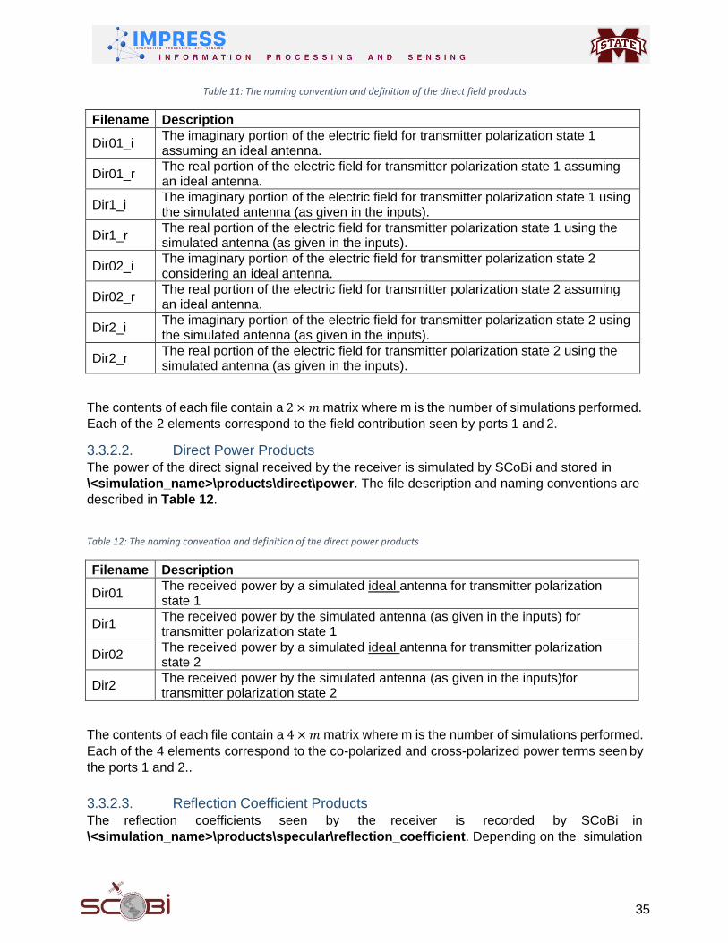
35

Table 11: The naming convention and definition of the direct field products

Filename Description

Dir01_i The imaginary portion of the electric field for transmitter polarization state 1 assuming an ideal antenna.

Dir01_r The real portion of the electric field for transmitter polarization state 1 assuming an ideal antenna.

Dir1_i The imaginary portion of the electric field for transmitter polarization state 1 using the simulated antenna (as given in the inputs).

Dir1_r The real portion of the electric field for transmitter polarization state 1 using the simulated antenna (as given in the inputs).

Dir02_i The imaginary portion of the electric field for transmitter polarization state 2 considering an ideal antenna.

Dir02_r The real portion of the electric field for transmitter polarization state 2 assuming an ideal antenna.

Dir2_i The imaginary portion of the electric field for transmitter polarization state 2 using the simulated antenna (as given in the inputs).

Dir2_r The real portion of the electric field for transmitter polarization state 2 using the simulated antenna (as given in the inputs).

The contents of each file contain a 2 × 𝑚 matrix where m is the number of simulations performed.

Each of the 2 elements correspond to the field contribution seen by ports 1 and 2.

3.3.2.2. Direct Power Products The power of the direct signal received by the receiver is simulated by SCoBi and stored in

\<simulation_name>\products\direct\power. The file description and naming conventions are

described in Table 12.

Table 12: The naming convention and definition of the direct power products

Filename Description

Dir01 The received power by a simulated ideal antenna for transmitter polarization state 1

Dir1 The received power by the simulated antenna (as given in the inputs) for transmitter polarization state 1

Dir02 The received power by a simulated ideal antenna for transmitter polarization state 2

Dir2 The received power by the simulated antenna (as given in the inputs)for transmitter polarization state 2


Each of the 4 elements correspond to the co-polarized and cross-polarized power terms seen by

the ports 1 and 2..

3.3.2.3. Reflection Coefficient Products The reflection coefficients seen by the receiver is recorded by SCoBi in

\<simulation_name>\products\specular\reflection_coefficient. Depending on the simulation

36

type, subsequent files describing the fit function for a given multilayer soil moisture profile may be

contained in this folder. The file description and naming convention for the reflection coefficient

values is described in Table 13.

37

Table 13: The naming convention and definition of the reflection coefficient products

Description

Bare01_i The imaginary portion of the reflection coefficient seen over a bare soil scattering surface assuming an ideal antenna for the transmitter polarization state 1.

Bare01_r The real portion of the reflection coefficient seen by a bare soil scattering surface assuming an ideal antenna for the transmitter polarization state 1.

Bare1_i The imaginary portion of the reflection coefficient seen over a bare soil scattering surface for the simulated antenna (as given in the inputs) for the transmitter polarization state 1.

Bare1_r The real portion of the reflection coefficient seen over a bare soil scattering surface for the simulated antenna (as given in the inputs) for the transmitter polarization state 1.

Bare02_i The imaginary portion of the reflection coefficient seen over a bare soil scattering surface assuming an ideal antenna for the transmitter polarization state 2.

Bare02_r The real portion of the reflection coefficient seen over a bare soil scattering surface assuming an ideal antenna for the transmitter polarization state 2.

Bare2_i The imaginary portion of the reflection coefficient seen over a bare soil scattering surface for the simulated antenna (as given in the inputs) for the transmitter polarization state 2.

Bare2_r The real portion of the reflection coefficient seen over a bare soil scattering surface for the simulated antenna (as given in the inputs) for the transmitter polarization state 1.

Veg01_i The imaginary portion of the reflection coefficient seen over a (bare soil + vegetation layer) scattering surface assuming an ideal antenna for the transmitter polarization state 1.

Veg01_r The real portion of the reflection coefficient seen over a (bare soil + vegetation layer) scattering surface assuming an ideal antenna for the transmitter polarization state 1.

Veg1_i The imaginary portion of the reflection coefficient seen over a (bare soil + vegetation layer) scattering surface for the simulated antenna (as given in the inputs) for the transmitter polarization state 1.

Veg1_r The real portion of the reflection coefficient seen over a (bare soil + vegetation layer) scattering surface for the simulated antenna (as given in the inputs) for the transmitter polarization state 1.

Veg02_i The imaginary portion of the reflection coefficient seen over a (bare soil + vegetation layer) scattering surface assuming an ideal antenna for the transmitter polarization state 2.

Veg02_r The real portion of the reflection coefficient seen over a (bare soil + vegetation layer) scattering surface assuming an ideal antenna for the transmitter polarization state 2.

Veg2_i The imaginary portion of the reflection coefficient seen over a (bare soil + vegetation layer) scattering surface for the simulated antenna (as given in the inputs) for the transmitter polarization state 2.

Veg2_r The real portion of the reflection coefficient seen over a (bare soil + vegetation layer) scattering surface for the simulated antenna (as given in the inputs) for the transmitter polarization state 1.

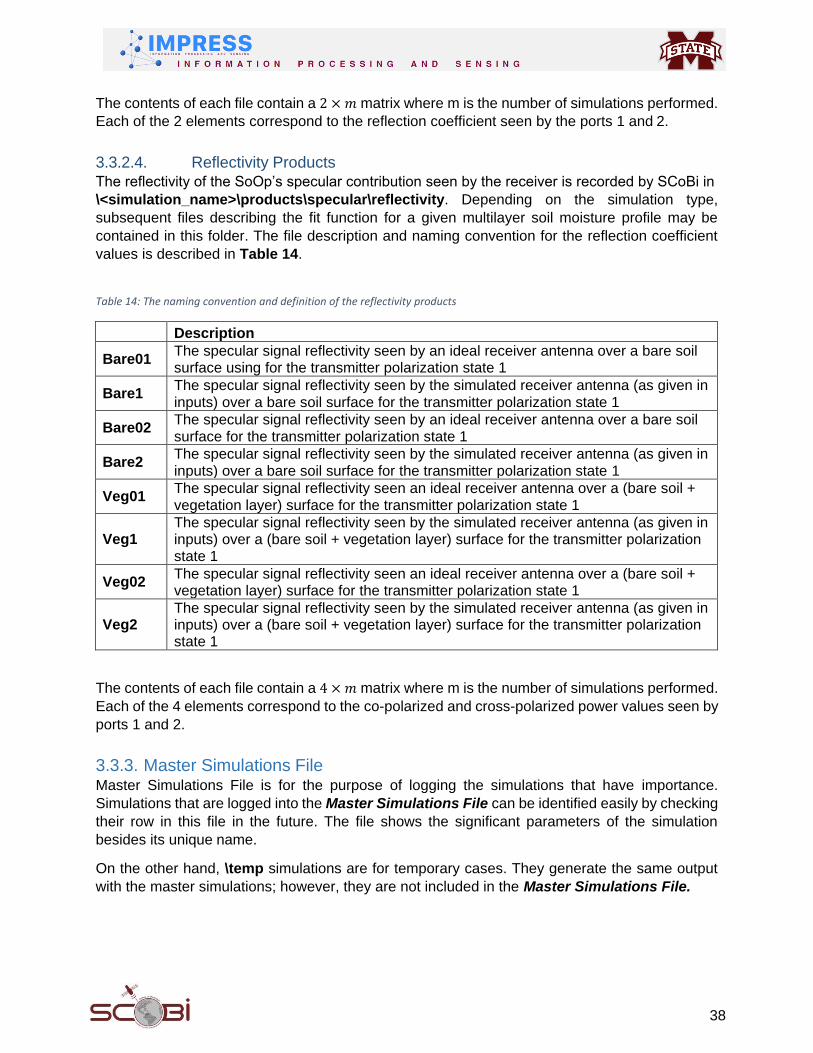
38


Each of the 2 elements correspond to the reflection coefficient seen by the ports 1 and 2.

3.3.2.4. Reflectivity Products The reflectivity of the SoOp’s specular contribution seen by the receiver is recorded by SCoBi in

\<simulation_name>\products\specular\reflectivity. Depending on the simulation type,

subsequent files describing the fit function for a given multilayer soil moisture profile may be

contained in this folder. The file description and naming convention for the reflection coefficient

values is described in Table 14.

Table 14: The naming convention and definition of the reflectivity products

Description

Bare01 The specular signal reflectivity seen by an ideal receiver antenna over a bare soil surface using for the transmitter polarization state 1

Bare1 The specular signal reflectivity seen by the simulated receiver antenna (as given in inputs) over a bare soil surface for the transmitter polarization state 1

Bare02 The specular signal reflectivity seen by an ideal receiver antenna over a bare soil surface for the transmitter polarization state 1

Bare2 The specular signal reflectivity seen by the simulated receiver antenna (as given in inputs) over a bare soil surface for the transmitter polarization state 1

Veg01 The specular signal reflectivity seen an ideal receiver antenna over a (bare soil + vegetation layer) surface for the transmitter polarization state 1

Veg1 The specular signal reflectivity seen by the simulated receiver antenna (as given in inputs) over a (bare soil + vegetation layer) surface for the transmitter polarization state 1

Veg02 The specular signal reflectivity seen an ideal receiver antenna over a (bare soil + vegetation layer) surface for the transmitter polarization state 1

Veg2 The specular signal reflectivity seen by the simulated receiver antenna (as given in inputs) over a (bare soil + vegetation layer) surface for the transmitter polarization state 1


Each of the 4 elements correspond to the co-polarized and cross-polarized power values seen by

ports 1 and 2.

3.3.3. Master Simulations File Master Simulations File is for the purpose of logging the simulations that have importance.

Simulations that are logged into the Master Simulations File can be identified easily by checking

their row in this file in the future. The file shows the significant parameters of the simulation

besides its unique name.

On the other hand, \temp simulations are for temporary cases. They generate the same output

with the master simulations; however, they are not included in the Master Simulations File.

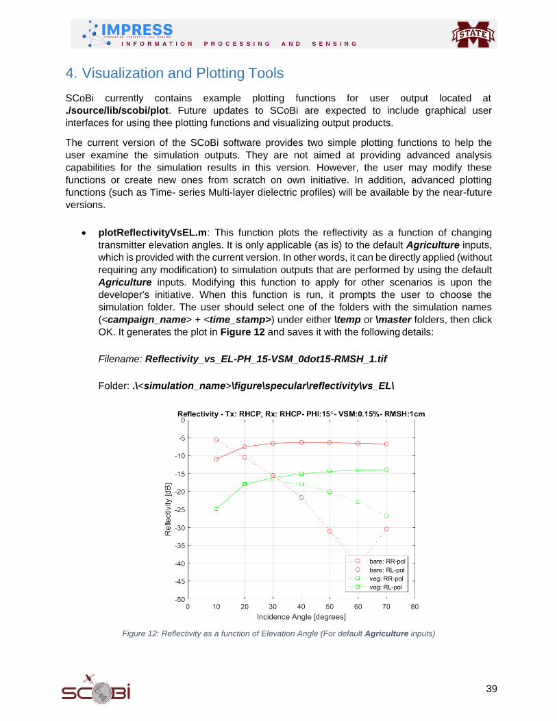
39

4. Visualization and Plotting Tools

SCoBi currently contains example plotting functions for user output located at

./source/lib/scobi/plot. Future updates to SCoBi are expected to include graphical user

interfaces for using thee plotting functions and visualizing output products.

The current version of the SCoBi software provides two simple plotting functions to help the

user examine the simulation outputs. They are not aimed at providing advanced analysis

capabilities for the simulation results in this version. However, the user may modify these

functions or create new ones from scratch on own initiative. In addition, advanced plotting

functions (such as Time- series Multi-layer dielectric profiles) will be available by the near-future

versions.

plotReflectivityVsEL.m: This function plots the reflectivity as a function of changing

transmitter elevation angles. It is only applicable (as is) to the default Agriculture inputs,

which is provided with the current version. In other words, it can be directly applied (without

requiring any modification) to simulation outputs that are performed by using the default

Agriculture inputs. Modifying this function to apply for other scenarios is upon the

developer's initiative. When this function is run, it prompts the user to choose the

simulation folder. The user should select one of the folders with the simulation names

(<campaign_name> + <time_stamp>) under either \temp or \master folders, then click

OK. It generates the plot in Figure 12 and saves it with the following details:

Filename: Reflectivity_vs_EL-PH_15-VSM_0dot15-RMSH_1.tif

Folder: .\<simulation_name>\figure\specular\reflectivity\vs_EL\

Figure 12: Reflectivity as a function of Elevation Angle (For default Agriculture inputs)

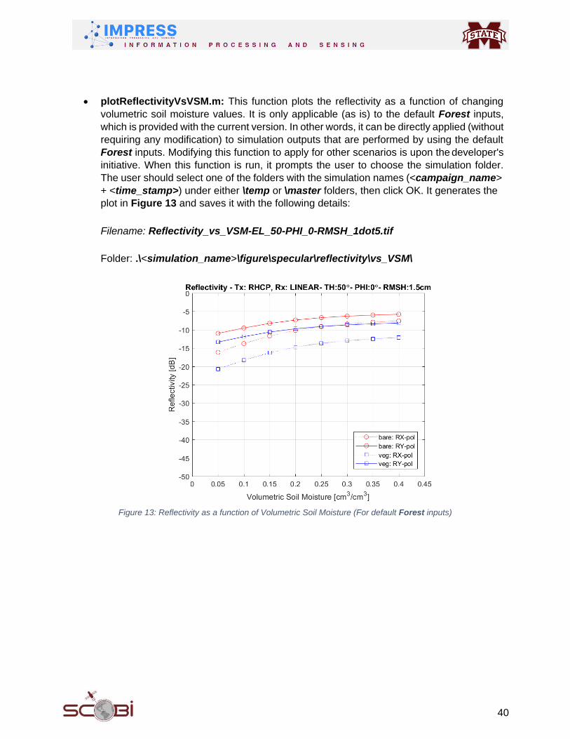
40

plotReflectivityVsVSM.m: This function plots the reflectivity as a function of changing

volumetric soil moisture values. It is only applicable (as is) to the default Forest inputs,

which is provided with the current version. In other words, it can be directly applied (without

requiring any modification) to simulation outputs that are performed by using the default

Forest inputs. Modifying this function to apply for other scenarios is upon the developer's

initiative. When this function is run, it prompts the user to choose the simulation folder.

The user should select one of the folders with the simulation names (<campaign_name>

+ <time_stamp>) under either \temp or \master folders, then click OK. It generates the

plot in Figure 13 and saves it with the following details:

Filename: Reflectivity_vs_VSM-EL_50-PHI_0-RMSH_1dot5.tif

Folder: .\<simulation_name>\figure\specular\reflectivity\vs_VSM\

Figure 13: Reflectivity as a function of Volumetric Soil Moisture (For default Forest inputs)

41

References

[1] M. Kurum, M. Deshpande, A. T. Joseph, P. E. O’Neill, R. Lang, and O. Eroglu, “SCoBi- Veg: A generalized bistatic scattering model of reflectometry from vegetation for Signals of Opportunity applications,” IEEE Trans. Geosci. Remote Sensing, Press, 2018.