scratchpad memory allocation for data aggregates via ...jingling/papers/tecs10.pdf · scratchpad...
TRANSCRIPT
Scratchpad Memory Allocation for Data Aggregates
via Interval Coloring in Superperfect Graphs
LIAN LI and JINGLING XUE
University of New South Wales
and
JENS KNOOP
Technische Universitat Wien
Existing methods place data or code in scratchpad memory, i.e., SPM by relying on heuristicsor resorting to integer programming or mapping it to a graph coloring problem. In this paper,the SPM allocation problem for arrays is formulated as an interval coloring problem. The keyobservation is that in many embedded C programs, two arrays can be modeled such that eithertheir live ranges do not interfere or one contains the other (with good accuracy). As a result,array interference graphs often form a special class of superperfect graphs (known as comparabilitygraphs) and their optimal interval colorings become efficiently solvable. This insight has led tothe development of an SPM allocation algorithm that places arrays in an interference graph inSPM by examining its maximal cliques. If the SPM is no smaller than the clique number of aninterference graph, then all arrays in the graph can be placed in SPM optimally. Otherwise, werely on containment-motivated heuristics to split or spill array live ranges until the resulting graphis optimally colorable. We have implemented our algorithm in SUIF/machSUIF and evaluated itusing a set of embedded C benchmarks from MediaBench and MiBench. Compared to a graphcoloring algorithm and an optimal ILP algorithm (when it runs to completion), our algorithmachieves close-to-optimal results and is superior to graph coloring for the benchmarks tested.
Categories and Subject Descriptors: D.3.4 [Programming Languages]: Processors—compilers;optimization; B.3.2 [Memory Structures]: Design Styles—Primary memory; C.3 [Special-
Purpose and Application-Based Systems]: Real Time and Embedded Systems
General Terms: Algorithms, Languages, Experimentation, Performance
Additional Key Words and Phrases: Scratchpad memory, SPM allocation, interference graph,interval coloring, superperfect graph
1. INTRODUCTION
The effectiveness of memory hierarchy is critical to the performance of a computersystem. To overcome the ever-widening gap between the processor speed and mem-ory speed, fast on-chip SRAMs are used. An on-chip SRAM is usually configuredas a hardware-managed cache, which works by relying on hardware to dynami-cally map data or instructions from off-chip memory. In embedded processors, theon-chip SRAM is frequently configured as a scratchpad memory (i.e., SPM).
The main difference between SPM and cache is that SPM does not have the
Li and Xue’s address: Programming Languages and Compilers Group, School of Computer Scienceand Engineering, University of New South Wales, Sydney, NSW 2052, Australia. Both authorsare also affiliated with National ICT Australia (NICTA). Knoop’s address: Technische UniversitatWien, Institut fur Computersprachen, Argentinierstraße 8, 1040 Wien, Austria
ACM Transactions on Embedded Computing Systems. To appear.

2 · Li, Xue and Knoop
complex tag-decoding logic that cache uses to support the dynamic mapping of dataor instructions from off-chip memory. Therefore, it becomes more energy and costefficient [Banakar et al. 2002]. In addition, SPM is managed by software, which canoften provide better time predictability, which is an important requirement in real-time systems. Given these advantages, SPM is widely used in embedded systems. Insome high-end embedded processors such as ARM10E, ColdFire MCF5 and AnalogDevices ADSP-TS201S, a portion of the on-chip SRAM is used as an SPM. In somelow-end embedded processors such as RM7TDMI and TI TMS370CX7X, SPM hasbeen used as an alternative to cache.
Effective utilisation of SPM is critical for an SPM-based system. Research onautomatic SPM allocation for program data has focused on how to place the datathat are frequently used in a program in SPM so as to maximise for both improvedperformance and energy consumption of the program. Dynamic allocation methodsare recognised to be generally more effective than static ones as the former methodsallow the data objects to be copied to and from an SPM at run time (as discussedin Section 6). In fact, static allocation methods are really special cases of dynamicallocation methods. In general, the problem of SPM allocation for program datahas been addressed by either relying on heuristics [Udayakumaran and Barua 2003]or resorting to integer programming [Verma et al. 2004b; Sjodin and von Platen2001; Avissar et al. 2002] or mapping it to a graph coloring problem [Li et al. 2005].
This paper proposes a new (dynamic) approach that solves the problem of SPMmanagement for program data by interval coloring. Interval coloring is a generali-sation of graph coloring to node weighted graphs. Such a generalisation naturallymodels the SPM allocation problem: we first build a node weighted interferencegraph for all SPM candidates (which are arrays, including structs as a special case,in this paper) in a program and then assign intervals to the nodes in this graph,which amounts to assigning SPM spaces to the arrays in the program.
Interval coloring is NP-complete for an arbitrary graph and there are no widely-accepted algorithms. In fact, how to recognise and color a superperfect graph isan open problem [Golumbic 2004]. Our key observation is that in many embeddedC applications, two arrays can be modeled such that either their live ranges donot interfere or one contains the other. As demonstrated in this paper, this is nota big constraint for our array placement optimisation, especially because arraysare considered as monolithic objects and because array copies (due to live rangesplitting) are placed at basic block boundaries. An array live range A contains anarray live range B if A is live at every program point where B is live. Then twoarrays are said to be containing-related. It turns out that an interference graphfor such arrays is a special kind of superperfect graph known as a comparabilitygraph if their array live ranges either do not interfere or are containing-related.Furthermore, optimal colorings for such interference graphs are efficiently solvable.Based on this insight, we have developed a new interval coloring algorithm, IC,to place arrays in SPM. IC can efficiently find the minimal SPM size required forcoloring all arrays in an interference graph. As a result, IC can always find anoptimal SPM allocation for an interference graph if the SPM is no smaller thanthe clique number of the graph. Otherwise, IC relies on containment-motivatedheuristics to split or spill some array live ranges until an optimal SPM allocation
ACM Transactions on Embedded Computing Systems, Vol. ?, No. ?, 2010.
Scratchpad Memory Allocation via Interval Coloring · 3
for the resulting graph is possible.In summary, this paper makes the following contributions:
—We propose a dynamic SPM allocation approach that formulates the SPM man-agement problem for arrays as an interval coloring problem.
—We demonstrate that the array interference graphs in many embedded C pro-grams are often comparability graphs, a special class of superperfect graphs, forwhich an efficient algorithm for finding their optimal colorings is given. We alsogive an algorithm for building such an interference graph from a given program.
—We present a new interval-coloring algorithm, IC, for placing arrays in SPM.
—We have implemented our IC algorithm in the SUIF/machSUIF compilationframework and compared it with a previously proposed graph coloring algo-rithm [Li et al. 2005] and an optimal ILP-based algorithm [Verma et al. 2004b].Our experimental results using a set of 17 C benchmarks from MediaBench andMiBench show that IC is effective: it yields close-to-optimal results for thosebenchmarks where ILP runs to completion and achieves same or better resultsthan graph coloring for all the benchmarks used.
The rest of this paper is organised as follows. Section 2 uses an example tomotivate the interval-coloring-based formulation for SPM allocation. In addition,live range splitting and analysis techniques that we apply to arrays are also dis-cussed. In Section 3, we introduce the concept of live range containment anddescribe some salient properties about array interference graphs, a special class ofsuperperfect graphs, formed by non-interfering or containing-related arrays. Byrecognising these graphs as comparability graphs, an efficient procedure for theiroptimal coloring exists. As a result, an optimal SPM allocation is obtained for aninterference graph if its clique number is no larger than the SPM size. Otherwise,our interval-coloring algorithm, IC, presented in Section 4 will come into play. OurIC algorithm is evaluated in Section 5. Section 6 reviews related work. Section 7concludes the paper.
2. SPM ALLOCATION VIA INTERVAL COLORING
In this paper, we consider only static- or stack-allocated data aggregates, includingarrays and data structs. Whenever we speak of arrays from now on, we meanboth types of aggregates. An array is treated as a monolithic object and willbe placed entirely in SPM. Hence, an array whose size exceeds that of the SPMunder consideration cannot be placed in the SPM. Such arrays can be tiled intosmaller “arrays” by means of loop tiling [Xue 1997; 2000; Wolfe 1989] and datatiling [Kandemir et al. 2001; Huang et al. 2003]. Its integration with this work isworth being investigated separately.
Two arrays cannot be placed in overlapping SPM spaces if they are live at thesame time during program execution since otherwise part of one array may beoverwritten by the other. Such arrays are said to interfere with each other.
2.1 A Motivating Example
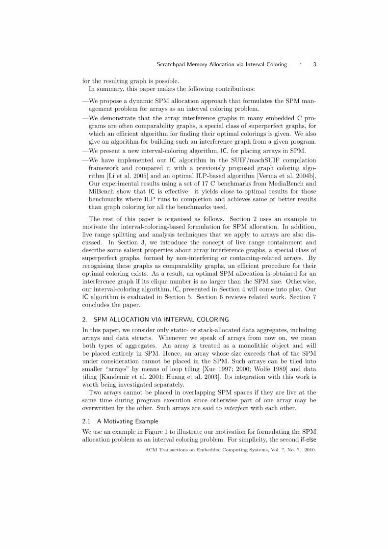
We use an example in Figure 1 to illustrate our motivation for formulating the SPMallocation problem as an interval coloring problem. For simplicity, the second if-else
ACM Transactions on Embedded Computing Systems, Vol. ?, No. ?, 2010.
4 · Li, Xue and Knoop
int main() {char A[80], B[75], *P;if ( . . . )
call g(A);else
call g(B);if ( . . . )
P = A;else
P = B;for ( . . . )
. . . = *P++;}
void g(char *P) {char C[120], D[120];for (. . . )
if ( . . . )call f(C);
for (. . . )if (. . . )
call f(D);P[...] = C[...] + D[...];
}
void f(char *P) {char E[120];for ( . . . )
E[...] = ...;P[...] = E[...];
}
(a) Program (with only relevant statements shown)
if (�)
call g(A)
P = A or B
int main()char A[80], B[75], *P;
call g(B)
void g(char *P)char C[120], D[120] ;
BB1
BB2 BB3
BB4
BB6
BB7
void f(char *P)char E[120] ;
for (�) if (�) call f(C)
for (�) if (�) call f(D)
Entry
ExitEntry
P[...] = C[...]+D[...]
Exit
BB8P[...] = E[...]
Exit
for (�) E[�] = �
EntryBB9
BB10
for(�)� = *P++;BB5
(b) CFG
Fig. 1. A motivating example. The second if-else in main and all the four for loops are eachsimplified to one single block. The six frequently executed, i.e., hot blocks are denoted by ovals.
statement in function main is simplified to one basic block BB4. Each for loop inthe example is also simplified to one basic block. The for loop in function main, thetwo for loops in function g and the for loop in function f are each represented as asingle basic block, namely, BB5, BB6, BB7 and BB9, respectively. The sizes of thefive arrays, A, B, C, D and E, are 80, 75, 120, 120 and 120 bytes, respectively.
To place arrays in the example program into SPM, we need to know the infor-mation regarding whether any pair of arrays interferes with each other or not. Inour approach, we compute such information by using an extended liveness analysis
ACM Transactions on Embedded Computing Systems, Vol. ?, No. ?, 2010.
Scratchpad Memory Allocation via Interval Coloring · 5
for arrays as discussed in [Li et al. 2005] and described in Section 2.2 below.Let us assume that the given SPM size is 320 bytes, which cannot hold all the
five arrays at the same time. A live range splitting algorithm as introduced in[Li et al. 2005] and reviewed in Section 2.3 will be applied. This ensures that thedata that are frequently accessed in a hot region can be potentially kept in SPMwhen that region is executed. We split an array (live range) accessed in hot loops(including call statements) where they are frequently accessed. (For convenience,a call statement that is not enclosed in a loop can be made so by assuming theexistence of a trivial loop enclosing the call statement.) In Figure 1(b), the six ovalblocks are the hot loops where live range splitting is performed.
2.2 Live Range Analysis
An array is live at a program point if it may be used before redefined after thatprogram point is executed. The live range of an array is the union of all programpoints in different functions where it is live. Due to the global nature of array liveranges, we have extended the liveness analysis for scalars to compute the live rangesof arrays inter-procedurally [Li et al. 2005].
To permit the data reuse information to be propagated across the functions in aprogram, we apply the standard liveness data-flow equations to the standard inter-procedural CFG constructed for a program. Figure 2 shows the inter-proceduralCFG and the live range information thus computed for Figure 1, where all inter-procedural control flow edges are highlighted in gray. For convenience, we assumethat every statement that causes an inter-procedural control flow (e.g., functioncall/returns and exceptional handling) forms a basic block by itself. As shown inFigure 2, the successor blocks of a call site are the unique ENTRY blocks of allfunctions that may be invoked at the callsite. Reciprocally, the successor blocks ofa function’s unique EXIT block are the successor blocks of all its call sites.
The predicates, DEF and USED, local to a basic block B for an array A are definedas follows.
—USEDA(B) returns true if some elements of A are read (possibly via pointers) inB. We conservatively set USEDA(B) = true if an element of A may be read in B.
—DEFA(B) returns true if A is killed in B. An array is killed if all its elementsare redefined. In general, it is difficult to identify whether an array (i.e., everyelement of an array) has been killed or not at compile time. In the absence ofsuch information, we have to conservatively assume that an array that appearsoriginally in a program is killed only once at the entry of its definition block.In this paper, a definition block is referred to as a scope, e.g., a compoundstatement in C, where arrays are declared. Static-allocated arrays are definedat the outermost scope. In addition, an array introduced in live range splittingin a loop is defined at the entry of the loop where the splitting is performed(Section 2.3). Finally, for every edge connecting a call block and an ENTRY
block, we assume the existence of a pseudo block C on the edge such that DEFA(C)returns true iff A is neither global nor passed by a parameter at the correspondingcall site and USEDA(C) always returns false. This makes our analysis context-sensitive since if A is a local array passed by a parameter in one calling contextto a callee, then its liveness information obtained at that calling context will not
ACM Transactions on Embedded Computing Systems, Vol. ?, No. ?, 2010.

6 · Li, Xue and Knoop
DCBA int main()char A[80], B[75], *P;
void g(char *P)char C[120], D[120] ;
BB1
BB2 BB3
BB4
BB6
BB7
void f(char *P)char E[120] ;
Entry
Entry
Exit
BB8
Exit
EntryBB9
BB10
E
Exit
BB5
Fig. 2. The live ranges of the four arrays after performing liveness analysis in the inter-proceduralCFG in Figure 1, where the inter-procedural control flow edges are highlighted in gray.
be propagated into the other contexts for the same callee function.
The liveness information for an array A can then be computed on the inter-procedural CFG of the program by applying the standard data-flow equations tothe entry and exit of every block B:
LIVEINA(B) = (LIVEOUTA(B) ∧ ¬DEFA(B)) ∨ USEDA(B)
LIVEOUTA(B) =∨
S∈succ(B)
LIVEINA(S) (1)
where succ(B) denotes the set of all successor blocks of B in the CFG.For this particular example, the arrays A and B declared in main are used after
the two call statements to g, respectively. As a result, both arrays are live throughg and its callee f. The arrays C and D declared in g are live inside f since they areused after the two calls to f. E is only live in f.
To understand the context-sensitivity of our analysis, let us consider a modifiedexample of Figure 1 with BB4 and BB5 removed. Without context-sensitivity, theliveness results for the modified example are the same as those in Figure 2 (exceptthat BB4 and BB5 are absent). With context-sensitivity, the live ranges of A and B
are smaller: A is no longer live in BB3 and B is no longer live in BB2. This impliesthat the liveness information for the single parameter in each call site in the mainfunction is only propagated back to the corresponding calling context.
ACM Transactions on Embedded Computing Systems, Vol. ?, No. ?, 2010.

Scratchpad Memory Allocation via Interval Coloring · 7
2.3 Live Range Splitting
The intent is to keep in the SPM the data that are frequently accessed in a regionwhen that region is executed. In embedded applications such as image processing,signal processing, video and graphics, most array accesses come from inside loops.We use the same splitting algorithm described in [Li et al. 2005] to split arrays athot loops (including call sites as mentioned earlier) except that we also allow anarray to be split even if it may be accessed by a pointer, which may also point toother arrays. This is realised by using runtime method tests that are often used fordevirtualising virtual calls in object-oriented programs [Detlefs and Agesen 1999].
The basic algorithm for live range splitting is simple. The multiply nested loopsin a function are processed outside-in to reduce array copy overhead. An array thatcan be split profitably in a loop will no longer be split inside any nested inner loop.Local arrays are split in the function where it is defined and global arrays may besplit in all functions in the program.
A simple cost model is used to decide if the live range of an array A in a loopL should be split into a new array A′. Unnecessary splits may be coalesced duringSPM allocation as described in Section 4. Due to splitting, an array copy statementA′ = A is inserted at the pre-header of L and A = A′ at every exit of L if A maybe modified inside L and is live at the exit. All accesses to A (including thoseaccessed indirectly by pointers) in L are replaced by those to A′. So the cost ofsplitting A in L is estimated by (Cs + Ct × A.size) × copy freq, where Cs is thestartup cost, Ct is the transfer cost per byte, A.size is the size of A and copy freq
is the execution frequency of all such copy statements inserted for A. The benefitis A.freq× (Mmem − Mspm), where A.freq is the access frequency of A in L, Mmem
is the memory latency and Mspm is the SPM latency. If the benefit exceeds thecost, the split is performed. Due to the way that A′ is split from A in L, the liverange of A′ is regarded as being live inside the entire loop, a good approximationfor arrays as further discussed in Section 3.
Figure 3 gives the modified program after live range splitting for our example.A, C, D and E are split at BB2, BB6, BB7 and BB9, respectively. B is split at bothBB3 and BB5. (In BB5 shown in Figure 1(b), it is assumed that B is frequentlyaccessed but A is not. So A needs not to be also split inside BB5.) As a result,all the memory accesses to these arrays in these blocks are redirected to the newlyintroduced live ranges A1, B1, B2, C1, D1 and E1 with array copy statements beinginserted accordingly. Note that B is accessed via the pointer P in BB5. Thus, aruntime test is inserted at the entry of BB5 to redirect the pointer P to the newintroduced array B2. Since P is not live at the exit of BB5, no runtime test isneeded to redirect P to the original array B at the exit of BB5.
Like garbage collectors, SPM allocators, which also reallocate array objects be-tween the off-chip memory and the SPM, require some similar restrictions in pro-grams, particularly those embedded ones written in C or C-like languages. Theseare the restrictions that should be satisfied for live range splitting to work correctly.Programming practices that disguise pointers such as casts between pointers andintegers are forbidden. In addition, only portable pointer arithmetic operations onpointers and arrays are allowed. In general, C programs that rely on the relativepositions of two arrays in memory are not portable. Indeed, comparisons (using,
ACM Transactions on Embedded Computing Systems, Vol. ?, No. ?, 2010.
8 · Li, Xue and Knoop
if (�)
call g(A1)
int main()char A[80], B[75], *P;
call g(B1)
void g(char *P)char C[120], D[120] ;
BB1
BB2 BB3
BB6
BB7
void f(char *P)char E[120] ;
for (�) if (�) call f(C1)
for (�) if (�) call f(D1)
Entry
Entry
P[...]=C[...]+D[...]
Exit
BB8P[...] = E[...]
Exit
for (�) E1[�] = �
EntryBB9
BB10
�� � � ����� ��� ������ � �� � ���� � �� � �� �� � �� � ��
P = A or BBB4
Exit
for(�)� = *P++;BB5
����� �� �� �� ��
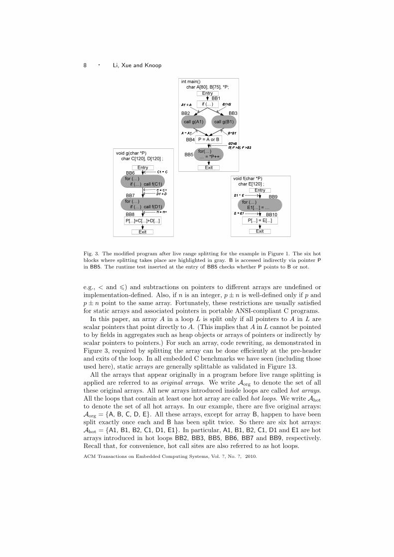
Fig. 3. The modified program after live range splitting for the example in Figure 1. The six hotblocks where splitting takes place are highlighted in gray. B is accessed indirectly via pointer P
in BB5. The runtime test inserted at the entry of BB5 checks whether P points to B or not.
e.g., < and 6) and subtractions on pointers to different arrays are undefined orimplementation-defined. Also, if n is an integer, p ± n is well-defined only if p andp ± n point to the same array. Fortunately, these restrictions are usually satisfiedfor static arrays and associated pointers in portable ANSI-compliant C programs.
In this paper, an array A in a loop L is split only if all pointers to A in L arescalar pointers that point directly to A. (This implies that A in L cannot be pointedto by fields in aggregates such as heap objects or arrays of pointers or indirectly byscalar pointers to pointers.) For such an array, code rewriting, as demonstrated inFigure 3, required by splitting the array can be done efficiently at the pre-headerand exits of the loop. In all embedded C benchmarks we have seen (including thoseused here), static arrays are generally splittable as validated in Figure 13.
All the arrays that appear originally in a program before live range splitting isapplied are referred to as original arrays. We write Aorg to denote the set of allthese original arrays. All new arrays introduced inside loops are called hot arrays.All the loops that contain at least one hot array are called hot loops. We write Ahot
to denote the set of all hot arrays. In our example, there are five original arrays:Aorg = {A, B, C, D, E}. All these arrays, except for array B, happen to have beensplit exactly once each and B has been split twice. So there are six hot arrays:Ahot = {A1, B1, B2, C1, D1, E1}. In particular, A1, B1, B2, C1, D1 and E1 are hotarrays introduced in hot loops BB2, BB3, BB5, BB6, BB7 and BB9, respectively.Recall that, for convenience, hot call sites are also referred to as hot loops.
ACM Transactions on Embedded Computing Systems, Vol. ?, No. ?, 2010.
Scratchpad Memory Allocation via Interval Coloring · 9
DCBA int main()char A[80], B[75], *P;
void g(char *P)char C[120], D[120] ;
BB1
BB2 BB3
BB4
BB6
BB7
void f(char *P)char E[120] ;
Entry
Entry
Exit
BB8
Exit
EntryBB9
BB10
E
D1C1B1A1 E1
Exit
BB5
B2
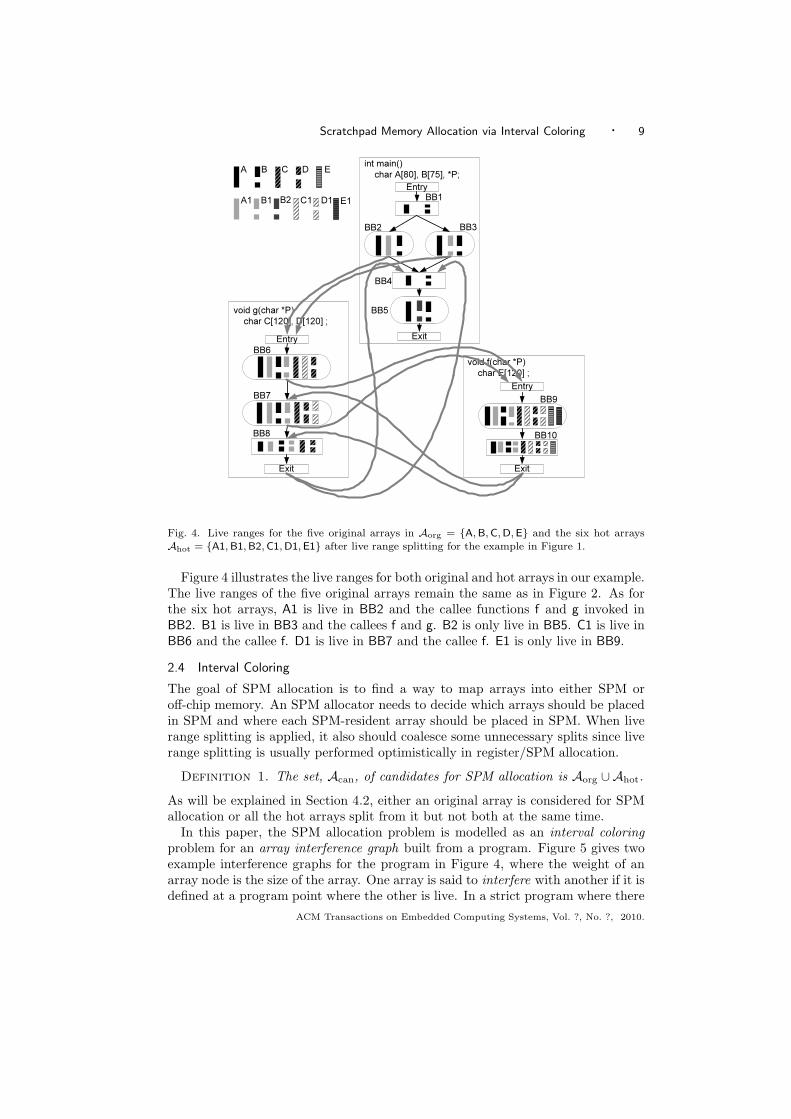
Fig. 4. Live ranges for the five original arrays in Aorg = {A,B,C,D,E} and the six hot arraysAhot = {A1, B1,B2,C1,D1,E1} after live range splitting for the example in Figure 1.
Figure 4 illustrates the live ranges for both original and hot arrays in our example.The live ranges of the five original arrays remain the same as in Figure 2. As forthe six hot arrays, A1 is live in BB2 and the callee functions f and g invoked inBB2. B1 is live in BB3 and the callees f and g. B2 is only live in BB5. C1 is live inBB6 and the callee f. D1 is live in BB7 and the callee f. E1 is only live in BB9.
2.4 Interval Coloring
The goal of SPM allocation is to find a way to map arrays into either SPM oroff-chip memory. An SPM allocator needs to decide which arrays should be placedin SPM and where each SPM-resident array should be placed in SPM. When liverange splitting is applied, it also should coalesce some unnecessary splits since liverange splitting is usually performed optimistically in register/SPM allocation.
Definition 1. The set, Acan, of candidates for SPM allocation is Aorg ∪Ahot.
As will be explained in Section 4.2, either an original array is considered for SPMallocation or all the hot arrays split from it but not both at the same time.
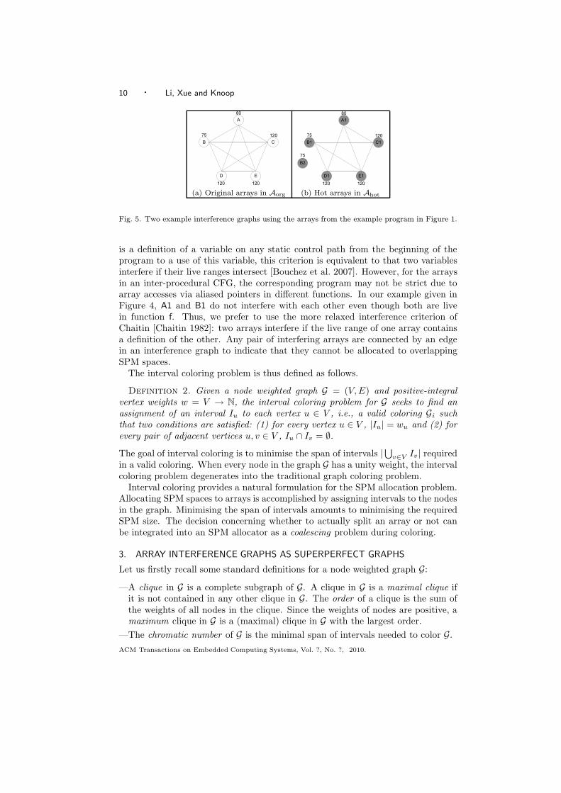
In this paper, the SPM allocation problem is modelled as an interval coloringproblem for an array interference graph built from a program. Figure 5 gives twoexample interference graphs for the program in Figure 4, where the weight of anarray node is the size of the array. One array is said to interfere with another if it isdefined at a program point where the other is live. In a strict program where there
ACM Transactions on Embedded Computing Systems, Vol. ?, No. ?, 2010.
10 · Li, Xue and Knoop
D
A
CB
80
75
120
120
E120
D1
A1
C1B1
80
75
120
120
E1120
B275
(a) Original arrays in Aorg (b) Hot arrays in Ahot
Fig. 5. Two example interference graphs using the arrays from the example program in Figure 1.
is a definition of a variable on any static control path from the beginning of theprogram to a use of this variable, this criterion is equivalent to that two variablesinterfere if their live ranges intersect [Bouchez et al. 2007]. However, for the arraysin an inter-procedural CFG, the corresponding program may not be strict due toarray accesses via aliased pointers in different functions. In our example given inFigure 4, A1 and B1 do not interfere with each other even though both are livein function f. Thus, we prefer to use the more relaxed interference criterion ofChaitin [Chaitin 1982]: two arrays interfere if the live range of one array containsa definition of the other. Any pair of interfering arrays are connected by an edgein an interference graph to indicate that they cannot be allocated to overlappingSPM spaces.
The interval coloring problem is thus defined as follows.
Definition 2. Given a node weighted graph G = (V, E) and positive-integralvertex weights w = V → N, the interval coloring problem for G seeks to find anassignment of an interval Iu to each vertex u ∈ V , i.e., a valid coloring Gi suchthat two conditions are satisfied: (1) for every vertex u ∈ V , |Iu| = wu and (2) forevery pair of adjacent vertices u, v ∈ V , Iu ∩ Iv = ∅.
The goal of interval coloring is to minimise the span of intervals |⋃
v∈V Iv| requiredin a valid coloring. When every node in the graph G has a unity weight, the intervalcoloring problem degenerates into the traditional graph coloring problem.
Interval coloring provides a natural formulation for the SPM allocation problem.Allocating SPM spaces to arrays is accomplished by assigning intervals to the nodesin the graph. Minimising the span of intervals amounts to minimising the requiredSPM size. The decision concerning whether to actually split an array or not canbe integrated into an SPM allocator as a coalescing problem during coloring.
3. ARRAY INTERFERENCE GRAPHS AS SUPERPERFECT GRAPHS
Let us firstly recall some standard definitions for a node weighted graph G:
—A clique in G is a complete subgraph of G. A clique in G is a maximal clique ifit is not contained in any other clique in G. The order of a clique is the sum ofthe weights of all nodes in the clique. Since the weights of nodes are positive, amaximum clique in G is a (maximal) clique in G with the largest order.
—The chromatic number of G is the minimal span of intervals needed to color G.
ACM Transactions on Embedded Computing Systems, Vol. ?, No. ?, 2010.
Scratchpad Memory Allocation via Interval Coloring · 11
A
B
A
B
A
B
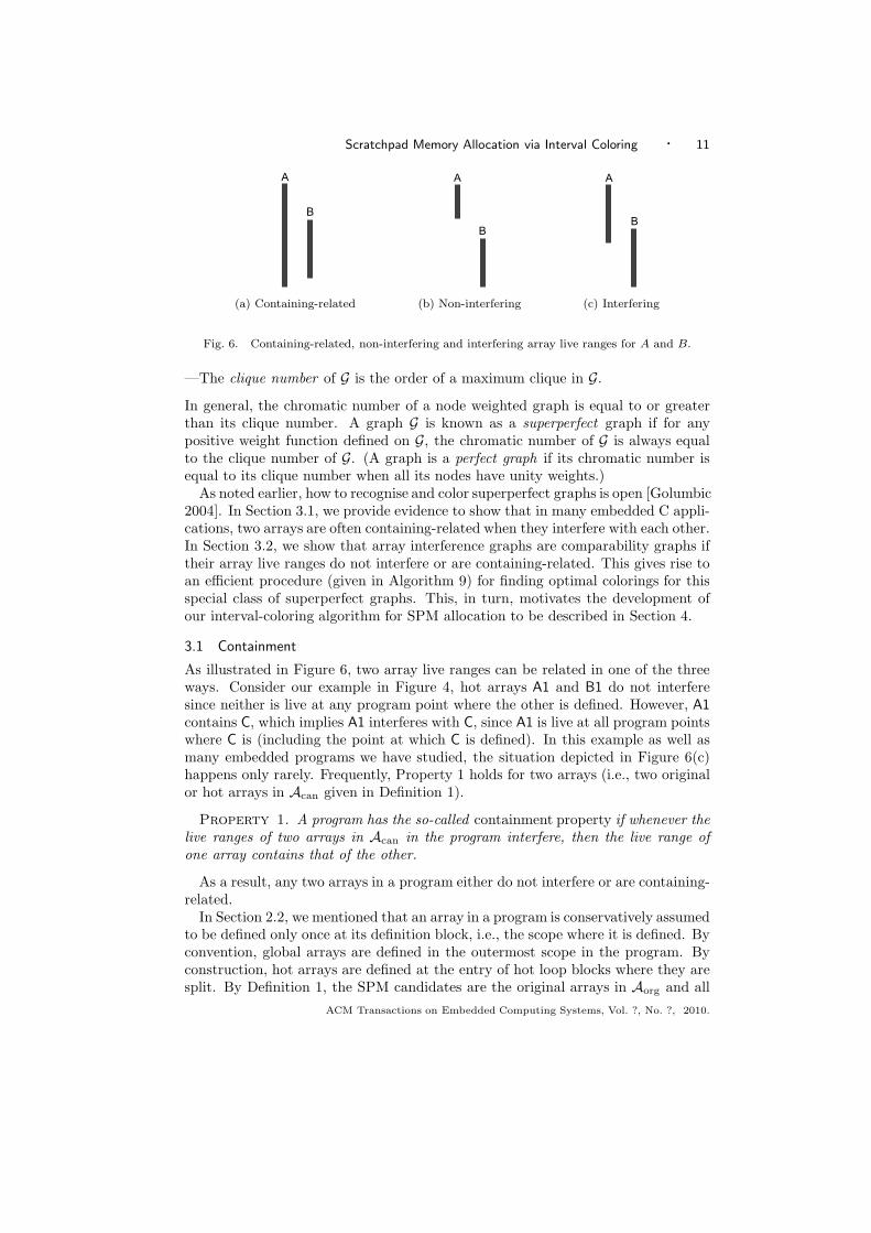
(a) Containing-related (b) Non-interfering (c) Interfering
Fig. 6. Containing-related, non-interfering and interfering array live ranges for A and B.
—The clique number of G is the order of a maximum clique in G.
In general, the chromatic number of a node weighted graph is equal to or greaterthan its clique number. A graph G is known as a superperfect graph if for anypositive weight function defined on G, the chromatic number of G is always equalto the clique number of G. (A graph is a perfect graph if its chromatic number isequal to its clique number when all its nodes have unity weights.)
As noted earlier, how to recognise and color superperfect graphs is open [Golumbic2004]. In Section 3.1, we provide evidence to show that in many embedded C appli-cations, two arrays are often containing-related when they interfere with each other.In Section 3.2, we show that array interference graphs are comparability graphs iftheir array live ranges do not interfere or are containing-related. This gives rise toan efficient procedure (given in Algorithm 9) for finding optimal colorings for thisspecial class of superperfect graphs. This, in turn, motivates the development ofour interval-coloring algorithm for SPM allocation to be described in Section 4.
3.1 Containment
As illustrated in Figure 6, two array live ranges can be related in one of the threeways. Consider our example in Figure 4, hot arrays A1 and B1 do not interferesince neither is live at any program point where the other is defined. However, A1
contains C, which implies A1 interferes with C, since A1 is live at all program pointswhere C is (including the point at which C is defined). In this example as well asmany embedded programs we have studied, the situation depicted in Figure 6(c)happens only rarely. Frequently, Property 1 holds for two arrays (i.e., two originalor hot arrays in Acan given in Definition 1).
Property 1. A program has the so-called containment property if whenever thelive ranges of two arrays in Acan in the program interfere, then the live range ofone array contains that of the other.
As a result, any two arrays in a program either do not interfere or are containing-related.
In Section 2.2, we mentioned that an array in a program is conservatively assumedto be defined only once at its definition block, i.e., the scope where it is defined. Byconvention, global arrays are defined in the outermost scope in the program. Byconstruction, hot arrays are defined at the entry of hot loop blocks where they aresplit. By Definition 1, the SPM candidates are the original arrays in Aorg and all
ACM Transactions on Embedded Computing Systems, Vol. ?, No. ?, 2010.

12 · Li, Xue and Knoop
hot arrays in Ahot. So we only need to consider these live ranges below.
Assumption 1. For two arrays defined in a common definition block, every lastuse of one array must be post-dominated by at least one last use of the other.
Assumption 2. If an array defined in a definition block is live at the entry of aninner definition block, then it is live at the exit(s) of, i.e., through the inner block.
Assumption 3. If an array is live at the entry of a call site, then it is live atthe exit(s) of the call site (i.e., live through all invoked callee functions at the site).
Assumption 1 is applicable to the arrays defined in a common definition block.These arrays are mutually interfering since their definition sites start from the entryof the same definition block. Assumptions 2 and 3 are seemingly restrictive; butthey do not warrant relaxation for three reasons. First, the local arrays in a functionare usually declared in its outermost scope in embedded applications. Second, ahot array is live only in the scope defined by the hot loop where it is split. Third,we have studied the live range behaviour in a set of 17 representative embedded Capplications from MediaBench and MiBench benchmark suites (Table I). Only fourarrays in pegwitencode and pegwitdecode do not satisfy these three assumptions.
Theorem 1. Property 1 holds if Assumptions 1 – 3 are all satisfied.
Proof. Let A and B be any two interfering arrays in the program. If both aredefined in the same definition block, then one must contain the other by Assump-tion 1. Otherwise, let A be defined in a scope that includes the scope in which B isdefined. By Assumption 2, A must contain B in the absence of function calls in theprogram. When there are function calls in the program, we note that Assumption 3,which takes care of the arrays defined in different functions, is identical to Assump-tion 2 since a callee function made in a caller function, once inlined conceptuallyin the caller, represents an inner scope nested in the caller.
Definition 3. G is said to be containing-related if it satisfies Property 1.
3.2 Recognition and Coloring
We show that containing-related interference graphs form a special class of super-perfect graphs known as comparability graphs and their optimal colorings can thusbe found efficiently. Let G be a node weighted undirected graph. An acyclic orien-tation Go of G seeks to find an assignment of a direction or orientation to every edgein G so that the resulting graph is a DAG (directed acyclic graph). It is well-knownthat there exists a one-to-one correspondence between the set of interval coloringsof G (given in Definition 2) and the set of acyclic orientations of G. For every edge(x, y) in G, x is located to the left of y in an interval coloring Gi of G if and onlyif (x, y) is a directed edge in an acyclic orientation Go of G. An acyclic orientationGo of G is transitive if (x, z) is contained in Go whenever (x, y) and (y, z) are. G isknown as a comparability graph if a transitive orientation of G exists.
We write A ⊒ B if A contains B. The following lemma says that ⊒ is transitive.
Lemma 1. If A ⊒ B and B ⊒ C, then A ⊒ C.
Proof. Note that we use the interference criterion of Chaitin [Chaitin 1982] inthis work. If A ⊒ B, then the live range of A includes that of B, which must
ACM Transactions on Embedded Computing Systems, Vol. ?, No. ?, 2010.

Scratchpad Memory Allocation via Interval Coloring · 13
�������������������� ���� ��������������������������� � �!�"��� #����!�� ������$%������&���'!(�)!� ��*��"Fig. 7. An interval-coloring-based SPM allocator IC.
contain a definition of B. Similarly, if B ⊒ C, then the live range of B includesthat of C, which must contain a definition of C. Hence, A ⊒ C.
Let G0 be a graph with n nodes v1 , v2 , . . . , vn and G1 ,G2 , . . . ,Gn be n disjointundirected graphs. The composition graph G = G0 [G1 ,G2 , . . . ,Gn ] is formed in twosteps. First, replace vi in G0 with Gi . Second, for all 1 ≤ i , j ≤ n, make each nodeof Gi adjacent to each node of Gj whenever vi is adjacent to vj in G0 . Formally, forGi = (Vi, Ei), the composition graph G= (V, E) is defined as follows:
V = ∪16i6nVi (2)
E = ∪16i6nEi ∪ {(x, y) | x ∈ Vi, y ∈ Vj and (vi, vj) ∈ E0} (3)
The following result about the recognition of composition graphs as comparabilitygraphs from their constituent components is recalled from [Golumbic 2004].
Lemma 2. Let G = G0 [G1 ,G2 , . . . ,Gn ], where each Gi (0 ≤ i ≤ n) is a disjointundirected graph. Then G is a comparability graph if and only if each Gi is.
Theorem 2. If G is containing-related, then G is a comparability graph.
Proof. Let us write A ≡ B if two interfering arrays A and B have the identicallive range, i.e., if A ⊒ B and B ⊒ A. Let G1,G2, . . . ,Gn be all n maximal cliques ofG such that for every Gi (1 6 i 6 n), every pair of array nodes A and B in Gi aresuch that A ≡ B. Let G0 be obtained from G with each Gi collapsed into one node.Then G = G0[G1,G2, . . . ,Gn]. G0 must be a comparability graph. To see this, letX and Y be two nodes in G0, each of which may represent a set of array nodes inG. Let AX (BY ) be an array represented by X (Y ). An acyclic orientation of G0
is found if AX is made to be directed to BY whenever AX ⊒ BY . In addition, thisorientation is transitive by Lemma 1. Note that every Gi is trivially a comparabilitygraph since it is a clique. Hence, G is a comparability graph by Lemma 2.
Given a transitive orientation Go of a comparability graph G, we can obtain anoptimal interval coloring in linear time by a depth-first search. For a source node x
in Go, let its interval be Ix = [0, w(x)), where w(x) is the weight of x. Proceedinginductively, for a node y with all its predecessors already being colored, let t be thelargest endpoint of the intervals of these predecessors and define Iy = [t, t + w(y)).This algorithm is used in our SPM allocator as discussed in Section 4.3.
ACM Transactions on Embedded Computing Systems, Vol. ?, No. ?, 2010.

14 · Li, Xue and Knoop
4. INTERVAL-COLORING-BASED SPM ALLOCATION
Motivated by the facts that array interference graphs are often containing-related(Section 3.1) and containing-related interference graphs are comparability graphsand can thus be efficiently colored (Section 3.2), Figure 7 outlines our IC algorithmwith its three phases described below and then explained in detail afterwards.
The first phase, Superperfection, constructs a containing-related array interfer-ence graph Gcan from Acan (Section 4.1). The middle phase, Spill & Coalesce (Sec-tion 4.2), addresses the two inter-related problems concerning which arrays can beplaced in SPM (Spill) and which arrays should be split (Coalesce) in the currentinterference graph G under consideration, which is always a node-induced subgraphof Gcan and thus a comparability graph itself. (A node-induced subgraph of a graphG is one that consists of some of the nodes of G and all of the edges that connectthem in G.) If the size of a given SPM is no smaller than the clique number ofG, then the middle phase is not needed. In this case, G can be optimally coloredimmediately. Otherwise, some heuristics motivated by containing-related intervalcoloring are applied to split and spill some array live ranges in G until the resultinggraph can be optimally colored. The last phase, Coloring, places all SPM-residentarrays in SPM (Section 4.3).
In existing graph coloring allocators for scalars [George and Appel 1996; Park andMoon 2004] and for arrays [Li et al. 2005], live range splitting is usually performedaggressively first and then unnecessary splits are coalesced during coloring. Thispaper proposes to make both splitting and spilling decisions together during Spill& Coalesce based on a unified cost-benefit analysis as motivated in Section 4.2.1and illustrated in Section 4.4. Our cost-benefit analysis is performed by examiningthe changes to the maximal cliques in the current interference graph G caused by asplitting or spilling operation. We deduce these changes efficiently from the max-imal cliques constructed (only once) from Gcan. When both splitting and spillingoperations are performed together, the Spill & Coalesce phase may look slightlycomplex. However, better SPM allocation results are obtained as validated here.
4.1 Superperfection
Given the set Acan of SPM candidates (Definition 1), we apply Algorithm 1 to builda containing-related interference graph Gcan from Acan.
Since containment implies interference, i.e., if A ⊒ B, then A and B interferewith each other, we will represent a containing-related interference graph G as aDAG. A directed edge A → B in G means A ⊒ B. In addition (as demonstratedin the proof of Theorem 2), all arrays with the same live range are collectivelyrepresented by one node. In other words, if A ⊒ B and B ⊒ A, then A and B arerepresented by the same node. Furthermore, we have also decided not to representexplicitly the transitive edges (as characterised in Lemma 1) in G for three reasons.First, the absence of transitive edges in G makes it easier to find all its maximalcliques as shown in Algorithm 3. Second, our IC algorithm checks efficiently theexistence of interference between two arrays by examining if both are in the samemaximal clique rather than if both are connected by a containment edge. Third,the interference graphs without transitive edges are simpler and visually cleaner.Figure 8 gives the DAG representations of the two interference graphs in Figure 5.
ACM Transactions on Embedded Computing Systems, Vol. ?, No. ?, 2010.

Scratchpad Memory Allocation via Interval Coloring · 15
E
155
120
240
A B
C D
D1
A1
C1B1
80
75
120
120
E1120
B275
(a) Original arrays in Aorg (b) Hot arrays in Ahot
Fig. 8. DAG representations of the two interference graphs given in Figure 5.
Algorithm 1 Building a containing-related interference graph Gcan from Acan.
1: procedure Build(Acan)2: The nodes in Gcan are the arrays in Acan
3: for every function f in the program do
4: for every scope S in function f do
// Lines 5 – 12 to enforce Assumption 15: for every two arrays in Acan defined in S do // both must interfere6: if the two arrays, A and B, are containing-related then
7: Add A → B if A ⊒ B and B → A if B ⊒ A
8: else
9: Denote them A and B such that A is less frequently accessed10: Add A → B
11: end if
12: end for
// Lines 13 – 17 to enforce Assumptions 2 and 313: for every B ∈ Acan defined in S do
14: for every A ∈ Acan that is live but not defined in S do
15: Add A → B
16: end for
17: end for
18: end for
19: end for
20: Collapse every SCC (Strongly-Connected Component) of Gcan to one node21: Let all transitive edges of Gcan be removed via a transitive reduction to Gcan
22: return Gcan
23: end procedure
Algorithm 1 builds Gcan (a DAG) for all the arrays in Acan in a program (line 2).As discussed in Section 2.2, every array is assumed conservatively to be defined atthe entry of its definition block. Therefore, we only need to examine the programpoints where some arrays are defined (lines 5 and 13). In lines 5 - 12, we considerthe array live ranges defined in a common scope, which must all interfere with eachother. If the two interfering arrays A and B are not containing-related (lines 8 –11), we enforce Assumption 1 by making the one that is less frequently accessed
ACM Transactions on Embedded Computing Systems, Vol. ?, No. ?, 2010.

16 · Li, Xue and Knoop
B1
D
C1
A1A
D1
CB
80 80
75
75
120 120
120
120
E
E1120
120
B275
80
240
75
A B
A1 B1
E
E1
120
120
155
C D
C1 D1120 120
75B2
(a) Traditional representation (b) DAG constructed by Build
Fig. 9. Traditional and DAG representations of the interference graph built from Acan in Figure 4.
contain the other. The intuition behind is to avoid extending the live ranges offrequently accessed arrays so they may have a better chance to be placed in SPM.In lines 13 – 17, we examine every pair of interfering arrays A and B defined intwo different scopes. Line 15 serves a double purpose: if A ⊒ B, we need to addA → B to Gcan. Otherwise, we enforce A → B (Assumptions 2 and 3). Live rangeextension is a safe and conservative approximation of liveness information. For theset of 17 embedded C applications we have studied (Table I), only four live rangesin pegwitencode and pegwitdecode are extended (Section 3.1). In line 20, all arraynodes with the same live range are merged. In line 21, all transitive edges in Gcan
are removed by performing a standard transitive reduction on Gcan.Algorithm 1 is correct in the sense that after line 19, every pair of interference
edges in the program is included in Gcan due to lines 5 and 13 – 14 and everyinterference edge is containing-related due to lines 7, 10 and 15.
In Figure 4, all eight arrays in Acan either do not interfere or are containing-related. No live range extension is necessary. Figure 9 gives the interference graphbuilt from Acan. By comparing the traditional and our DAG representations, theDAG representation (due to the exploitation of containment) is simpler.
4.2 Spill & Coalesce
Our algorithm performs spilling and splitting together based on a cost-benefit anal-ysis, which examines the resulting changes to the maximal cliques in the interferencegraph G. To help understand our algorithm, we will first motivate our approach inSection 4.2.1 by focusing on these two aspects using the example given in Figure 1.We will then describe our algorithm in detail in Sections 4.2.2 – 4.2.6.
The set of SPM candidates Acan = Aorg ∪ Ahot is given in Definition 1. DuringSPM allocation, either an original array A ∈ Aorg is a candidate or all its cor-responding hot arrays A1, A2, . . . , An ∈ Ahot are but not both at the same time.Note that it is possible that only some but not all of these hot arrays are eventuallycolored. Note also that A and all its hot arrays may be coalesced if A turns out tobe colorable entirely later (due to spilling and splitting performed to other arrays).
When A is split, all its hot arrays A1, A2, . . . , An will become candidates and thenon-hot live range of A is spilled. Among the 17 benchmarks used in our experi-ments, the non-hot portions of the array live ranges in each of these benchmarks
ACM Transactions on Embedded Computing Systems, Vol. ?, No. ?, 2010.
Scratchpad Memory Allocation via Interval Coloring · 17
80
240
75A1 B1
E 120
C D
75B2
80
120
75A1 B1
D1 120
75B2
C
E 120
80
120
75A1 B1
D1120
75B2
E 120
C1
80
120
75A1 B1
E 120
75B2
C
(a) Splitting A and B (b) Splitting D and then C from (a) (c) Spilling D from (a)from Figure 8(a).
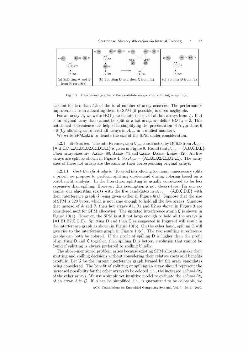
Fig. 10. Interference graphs of the candidate arrays after splitting or spilling.
account for less than 5% of the total number of array accesses. The performanceimprovement from allocating them to SPM (if possible) is often negligible.
For an array A, we write HOTA to denote the set of all hot arrays from A. If A
is an original array that cannot be split or a hot array, we define HOTA = ∅. Thisnotational convenience has helped in simplifying the presentation of Algorithms 6– 8 (by allowing us to treat all arrays in Acan in a unified manner).
We write SPM SIZE to denote the size of the SPM under consideration.
4.2.1 Motivation. The interference graph Gcan constructed by Build from Acan ={A,B,C,D,E,A1,B1,B2,C1,D1,E1} is given in Figure 9. Recall that Aorg = {A,B,C,D,E}.Their array sizes are: A.size=80, B.size=75 and C.size=D.size=E.size=120. All fivearrays are split as shown in Figure 4. So Ahot = {A1,B1,B2,C1,D1,E1}. The arraysizes of these hot arrays are the same as their corresponding original arrays.
4.2.1.1 Cost-Benefit Analysis. To avoid introducing too many unnecessary splitsa priori, we propose to perform splitting on-demand during coloring based on acost-benefit analysis. In the literature, splitting is usually considered to be lessexpensive than spilling. However, this assumption is not always true. For our ex-ample, our algorithm starts with the five candidates in Aorg = {A,B,C,D,E} withtheir interference graph G being given earlier in Figure 8(a). Suppose that the sizeof SPM is 320 bytes, which is not large enough to hold all the five arrays. Supposethat instead of A and B, their hot arrays A1, B1 and B2 as shown in Figure 3 areconsidered next for SPM allocation. The updated interference graph G is shown inFigure 10(a). However, the SPM is still not large enough to hold all the arrays in{A1,B1,B2,C,D,E}. Splitting D and then C as suggested in Figure 3 will result inthe interference graph as shown in Figure 10(b). On the other hand, spilling D willgive rise to the interference graph in Figure 10(c). The two resulting interferencegraphs can both be colored. If the profit of spilling D is higher than the profitof splitting D and C together, then spilling D is better, a solution that cannot befound if splitting is always preferred to spilling blindly.
The above-mentioned problem arises because existing SPM allocators make theirsplitting and spilling decisions without considering their relative costs and benefitscarefully. Let G be the current interference graph formed by the array candidatesbeing considered. The benefit of splitting or spilling an array should represent theincreased possibility for the other arrays to be colored, i.e., the increased colorabilityof the other arrays. We use a simple yet intuitive model to evaluate the colorabilityof an array A in G. If A can be simplified, i.e., is guaranteed to be colorable, we
ACM Transactions on Embedded Computing Systems, Vol. ?, No. ?, 2010.

18 · Li, Xue and Knoop
Algorithm 2 Cost-benefit analysis for estimating the profit of spilling/splitting.
1: procedure CBAforSpill(G := V, E), A)2: Gnew = G ⊖ {A} (interference graph formed by V \ {A})3: A.spill cost = A.freq × (Mmem − Mspm)4: A.spill benefit = (α(Gnew) − α(G)) × (Mmem − Mspm)5: A.spill profit = A.spill benefit − A.spill cost6: return A.spill profit7: end procedure
8: procedure CBAforSplit(G := V, E), A)9: Gnew = G ⊖{A}⊕HOTA (interference graph formed by (V \ {A})∪HOTA)
10: A.split cost is the array copy cost plus the cost incurred for accessing thenon-hot portions of A from off-chip memory (Sect. 2.3)
11: A.split benefit = (α(Gnew) − α(G)) × (Mmem − Mspm)12: A.split profit = A.split benefit − A.split cost13: return A.split profit14: end procedure
have colorability(G, A) = 1. Otherwise, its colorability is estimated by:
colorability(G, A) =SPM SIZE
Θ(G, A)6 1 (4)
where Θ(G, A) is the largest order possible for a maximal clique containing A foundin G, indicating the minimum amount of space required to color all arrays in theclique. In other words, colorability(G, A) approximates the (average) percentage ofaccesses to A that may hit in SPM after a coloring has been found.
Consider Figure 10(a) with SPM SIZE = 320 bytes. There are three maximalcliques: {A1,C,D,E}, {B1,C,D,E} and {B2} with their orders being 440, 435 and 75,respectively. The two larger cliques cannot be colored. Hence, colorability(G, A1) =colorability(G, C) = colorability(G, D) = colorability(G, E) = 320
440 andcolorability(G, B1) = 320
435 . Since B2 can be colored, colorability(G, B2) = 1.We use α(A) to approximate the number of array accesses of A that may hit in
SPM after SPM allocation (with A.freq being the access frequency of A):
α(A) = A.freq × colorability(G, A) = A.freq ×SPM SIZE
Θ(G, A)
As a result, the number of the array accesses that can hit in SPM for all arrays inG after SPM allocation is the sum of their α values:
α(G) =∑
Array A contained in G
α(A) (5)
The larger α(G) is, the better the allocation results for G will (potentially) be.Algorithm 2 gives our cost-benefit analysis for estimating the profit of splitting
and spilling A in G, where Mmem and Mspm are defined in Section 2.3. In lines 2and 9, the operations ⊖ and ⊕ for updating G = (V, E) with S ⊂ Acan are defined
ACM Transactions on Embedded Computing Systems, Vol. ?, No. ?, 2010.

Scratchpad Memory Allocation via Interval Coloring · 19
by:
G ⊖ S = subgraph of Gcan induced by V \ S (6)
G ⊕ S = subgraph of Gcan induced by V ∪ S (7)
These operations, which will be used later in Algorithms 6 and 8, together withthose on α in lines 4 and 11, can be performed efficiently as explained shortly below.
In CBAforSpill, the cost of spilling A from G is estimated by the increased numberof cycles when the spilled A is potentially relocated from the SPM to the off-chipmemory. The benefit is the number of cycles reduced due to an improvement onthe colorability values of the other arrays. In CBAforSplit, the cost of splitting A
into the hot arrays in HOTA in G is calculated according to the live range splittingalgorithm described in Section 2.3. The benefit is similarly estimated as for spilling.
Let us explain our cost-benefit analysis by using the example given in Fig-ure 10(a). As before, SPM SIZE = 320. Recall that the colorability for each arrayin {A1, C, D, E} is 320
440 , the colorability of B1 is 320435 and the colorability of B2 is 1.
Let us first look at the cost and benefit of spilling D with G being updated fromFigure 10(a) to Figure 10(c). In line 3, we have D.spill cost = D.freq × (Mmem −Mspm). After spilling, all arrays can be simplified and their colorability values are1. In line 4, we get D.spill benefit = ((A1.freq+C.freq+E.freq)×(1− 320
440 )+B1.freq×(1 − 320
435 ) − D.freq × 320440 ) × (Mmem − Mspm). In line 5, we obtain D.spill profit as
desired.Let us divert slightly by considering to spill A1 instead of D in Figure 10(a). After
spilling, there are two maximal cliques {B1,C,D,E} and {B2} with their orders being435 and 75, respectively. Thus, the colorability values of C, D and E have improvedfrom 320
440 to 320435 . In line 3, we have A1.spill cost = A1.freq×(Mmem−Mspm). In line
4, we obtain A1.spill benefit = ((C.freq+D.freq+E.freq) × (320435 − 320
440 ) − A1.freq ×320440 ) × (Mmem −Mspm). In line 5, we obtain A1.spill profit as desired. If all arrayshave the same access frequency, then D is preferred to A1 for spilling since spillingD has a higher profit.
Let us next look at the cost and benefit of splitting D into D1 with G beingupdated from Figure 10(a) to Figure 10(b). For now, this splitting operation (shownin Figure 3) is not profitable since it does not change the colorability of the otherarrays. In line 11, we get D.split benefit = −Dno−hot.freq×
320440×(Mmem−Mspm). In
line 10, we have D.split cost = 2× (Cs + Ct ×D.size)× copy freq + Dno−hot.freq×(Mmem − Mspm), where Cs, Ct and copy freq are introduced in Section 2.3 andDno−hot represents the not-hot part live range of D. Finally, we obtain C.split profitin line 12 as desired. If we subsequently split C, then the colorability of all arraysin the resulting interference graph remain unchanged. So a similar cost-benefitanalysis as that for D applies.
Let us assume that we are to decide whether to split or spill D in Figure 10(a). IfD.split profit is larger than D.spill profit, then D is selected for splitting as shownin Figure 10(b). Otherwise, D is spilled as shown in Figure 10(c).
4.2.1.2 Updating Interference Graph. From the above discussions, we can seethat the interference graph G must be updated when computing the benefit of asplitting or spilling operation. As reflected in lines 2 and 9 in Algorithm 2, Gevolves into Gnew when A is spilled or split. To compute its benefit (in lines 4 and
ACM Transactions on Embedded Computing Systems, Vol. ?, No. ?, 2010.
20 · Li, Xue and Knoop
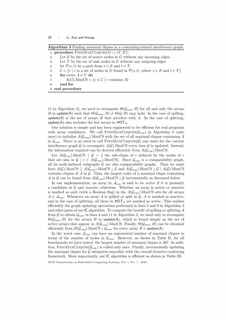
Algorithm 3 Finding maximal cliques in a containing-related interference graph.
1: procedure FindMaxCliques(G := (V, E))2: Let S be the set of source nodes in G without any incoming edges3: Let T be the set of sink nodes in G without any outgoing edges4: let P(s, t) be a path from s ∈ S and t ∈ T .5: C = {c | c is a set of nodes in G found in P(s, t), where s ∈ S and t ∈ T }6: for every A ∈ V do
7: A(G).MaxCS = {c ∈ C | c contains A}8: end for
9: end procedure
11 in Algorithm 2), we need to recompute Θ(Gnew, B) for all and only the arraysB in update(A) such that Θ(Gnew, B) 6= Θ(G, B) may hold. In the case of spilling,update(A) is the set of arrays B that interfere with A. In the case of splitting,update(A) also includes the hot arrays in HOTA.
Our solution is simple and has been engineered to be efficient for real programswith array candidates. We call FindMaxCliques(Gcan) in Algorithm 3 (onlyonce) to initialise A(Gcan).MaxCS with the set of all maximal cliques containing A
in Gcan. There is no need to call FindMaxCliques(G) any more for the currentinterference graph G to recompute A(G).MaxCS every time G is updated. Instead,the information required can be derived efficiently from A(Gcan).MaxCS.
Let A(Gcan).MaxCS ↓ G = { the sub-clique of c induced by the nodes of c
that are also in G | c ∈ A(Gcan).MaxCS}. Since Gcan is a comparability graph,all its node-induced subgraphs G are also comparability graphs. Then we musthave A(G).MaxCS ⊆ A(Gcan).MaxCS ↓ G and A(Gcan).MaxCS ↓ G \ A(G).MaxCScontains cliques of A in G. Thus, the largest order of a maximal clique containingA in G can be found from A(Gcan).MaxCS ↓ G incrementally as discussed below.
In our implementation, an array in Acan is said to be active if it is presentlya candidate in G and inactive otherwise. Whether an array is active or inactiveis marked as such (with a Boolean flag) in the A(Gcan).MaxCS sets for all arraysA ∈ Acan. Whenever an array A is spilled or split in G, A is marked as inactive,and in the case of splitting, all those in HOTA are marked as active. This realisesefficiently the graph updating operations performed in lines 2 and 9 in Algorithm 2and other parts of our IC algorithm. To compute the benefit of spilling or splitting A
from G to obtain Gnew in lines 4 and 11 in Algorithm 2, we need only to recomputeΘ(Gnew, B) for the arrays B in update(A), which is found simply as the set ofactive arrays that appear in A(Gcan).MaxCS. Finally, Θ(Gnew, B) can be obtainedefficiently from B(Gcan).MaxCS ↓ Gnew for every array B ∈ update(A).
In the worst case, Gcan can have an exponential number of maximal cliques interms of the number of nodes in Gcan. However, as shown in Table II, for allbenchmarks we have tested, the largest number of maximal cliques is 267. In addi-tion, FindMaxCliques(Gcan) is called only once. Finally, incrementally updatingthe maximal cliques for G integrates smoothly with the overall iterative-coalescingframework. More importantly, our IC algorithm is efficient as shown in Table III.
ACM Transactions on Embedded Computing Systems, Vol. ?, No. ?, 2010.

Scratchpad Memory Allocation via Interval Coloring · 21
Algorithm 4 Interval-coloring-based SPM allocation.
1: procedure IC(Gcan)2: FindMaxCliques(Gcan)3: Init()4: repeat
5: if UnSpillList 6= ∅ then
6: UnSpill()7: else if SplitOrSpillList 6= ∅ then
8: SplitOrSpill()9: end if
10: until UnSpillList = ∅ ∧ SplitOrSpillList = ∅11: end procedure
Algorithm 5 Initialising the (current) interference graph and worklists.
1: procedure Init2: Let G be the subgraph of Gcan induced by Aorg
3: UnSpillList = ∅4: RemoveList = ∅5: SplitOrSpillList = set of arrays A in G s.t. Θ(G, A) > SPM SIZE} (Def. 4)6: end procedure
4.2.1.3 Overview. Like George and Appel’s graph coloring allocator for scalars[George and Appel 1996], IC is also an worklist-based iterative-coalescing allocator(but for data aggregates). So the operational flows among the five modules in thismiddle phase IC shown in Figure 7 are captured in Algorithm 4. The meanings ofthe three lists, UnSpillList, SplitOrSpillList and RemoveList and which arrays areeventually identified to be SPM-resident are explained in Section 4.2.2.
Our IC allocator is developed based on the following observation.
Definition 4. An array in G can be simplified, i.e., guaranteed to be placed inSPM if it is not included in a clique in G with an order larger than the SPM size.
Theorem 3. G can be colored iff all arrays in G can be simplified.
Proof. Follows from Definition 4 and Theorem 2.
Since simplified arrays can always be colored, no splitting for an original array isnecessary if it can be simplified in Gcan that is built directly from Acan.
4.2.2 Init. In Algorithm 5, the current interference graph G that IC starts withis initialised (line 2). So are the three worklists, which are central to IC, a worklist-based iterative-coalescing algorithm (lines 3 – 5). Below we describe these datastructures in detail. An illustration of these lists using our running example canbe found in Section 4.4. However, due to the iterative nature of IC, these worklistsmay have to be understood (dynamically) in the iterative-coalescing context.
UnSpillList and RemoveList are initialised to be empty and SplitOrSpillList tocontain all arrays in G that cannot be presently simplified (i.e.,, colored).
. SplitOrSpillList contains arrays in G that cannot be simplified by Definition 4.
ACM Transactions on Embedded Computing Systems, Vol. ?, No. ?, 2010.
22 · Li, Xue and Knoop
These are the candidates considered for splitting and spilling.
. RemoveList contains arrays in Gcan but not in G that are potentially spilled.These are removed (i.e. spilled) from either SplitOrSpillList or UnSpillList. Everyarray is not simplifiable at the time when it is added to this list. However, somearrays in the list may become simplifiable after others have been split or spilled.
. UnSpillList contains arrays in Gcan but not in G that are transferred fromRemoveList to this list when they become simplifiable (as discussed above). Theseare the candidates that may be unspilled, i.e., added back to G. However, unspillingone array in this list may cause others in the list to become non-simplifiable. Allsuch non-simplifiable arrays will be removed and added back to RemoveList.
At any time, the three lists are mutually exclusive. In addition, SplitOrSpillList
contains either A or its hot arrays in HOTA but not both. This is because only A
or its hot arrays in HOTA are considered for SPM allocation at any time. However,RemoveList and UnSpillList may contain both A and its hot arrays in HOTA atthe same time. In the case of RemoveList, once A is spilled to the list, some of itshot arrays may also be spilled to the list immediately afterwards. In the case ofUnSpillList, if A may not be unspilled, some of its hot arrays may be unspilled.
The Spill & Coalesce phase terminates when both SplitOrSpillList and UnSpillList
are empty. Then G contains all the arrays that can be placed in SPM. This phaseis guaranteed to terminate since IC works by reducing the clique number of G grad-ually until it is smaller than or equal to SPM SIZE.
4.2.3 UnSpill. When Algorithm 6 is called, UnSpillList contains a list of arraysin Gcan but not in G that can be simplified individually. This means that everyarray in UnSpillList, once added back to G alone, can be simplified. Unspilling asimplifiable array in this module means that the unspilled array is guaranteed tobe colored eventually (Definition 4). In other words, every unspilled array will stayin G until the Spill & Coalesce phase has terminated.
In line 2, we call SelectUnSpill to choose an array A from UnSpillList with thelargest profit to unspill (line 22). Unspilling a simplifiable array is always profitablesince it will remain to be colorable. Thus, in the for loop in line 13, the profit ofunspilling an array is estimated according to the increased number of SPM accessesand the reduced array copy cost (if any) as a result of placing this array (ratherthan its hot arrays, if any) in SPM. There are two cases. In one case, A can besplit (lines 14 – 17). If A is simplifiable, so are all its hot arrays in HOTA sincethese hot arrays are contained by A. So the profit gained from placing A ratherthan its hot arrays only in SPM (line 17) is derived from the extra benefit obtainedfrom also placing the non-hot live ranges of A in SPM (line 15) and the array copycost avoided (line 16) (Figure 3). In the other case (lines 18 – 20), A is a hot arrayor an original array that cannot be split. Its unspilling profit is estimated in thenormal manner.
After A has been selected (line 2), A and all its hot arrays in HOTA are removedfrom UnSpillList (line 3). In line 4, A, which is guaranteed to be colorable, isunspilled, i.e., added to G. At the same time, all hot arrays in HOTA are removedfrom G. Effectively, the splits for A are unnecessary and thus coalesced. Due tothe unspilling of A, some arrays in UnSpillList that are simplifiable before may no
ACM Transactions on Embedded Computing Systems, Vol. ?, No. ?, 2010.

Scratchpad Memory Allocation via Interval Coloring · 23
Algorithm 6 Processing unspilled arrays in UnSpillList.
1: procedure UnSpill2: A = SelectUnSpill(UnSpillList)3: UnSpillList = UnSpillList \ ({A} ∪ HOTA)4: G = G ⊕ {A} ⊖ HOTA
5: for every B ∈ UnSpillList that interferes with A do
6: if Θ(G ⊕ {B} ⊖ HOTB, B) > SPM SIZE) then
7: UnSpillList = UnSpillList \ {B}8: RemoveList = RemoveList ∪ {B}9: end if
10: end for
11: end procedure
12: procedure SelectUnSpill(UnSpillList)13: for every array A ∈ UnSpillList do
14: if A ∈ Aorg such that HOTA 6= ∅ then // A can be split15: A.non-hot benefit = (A.freq−
∑H∈HOTA) H.freq)× (Mmem −Mspm)
16: A.copy cost is the array copy cost due to splitting A (Section 2.3)17: A.profit = A.non-hot benefit + A.copy cost (saved)18: else // A ∈ Aorg cannot be split or A ∈ Ahot
19: A.profit = A.freq × (Mmem − Mspm)20: end if
21: end for
22: Select the array A in UnSpillList with the largest A.profit23: end procedure
longer be simplifiable. In lines 5 – 10, all such arrays are removed from UnSpillList
and appended to RemoveList. Only the arrays in UnSpillList that interfere with A
need to be examined (line 5) and the remaining ones are not affected.Note that in line 6, B may be a hot array, in which case HOTB = ∅ as discussed
in Section 4.2. This convention is adopted also in line 15 of Algorithm 8.No arrays are removed from SplitOrSpillList and RemoveList since these arrays
are still not simplifiable. This is because unspilling A adds a new array to G andthus will not reduce any interference in G.
4.2.4 SplitOrSpill. As shown in Algorithm 7, this module chooses an array inSplitOrSpillList with the largest profit to split or spill. Splitting or spilling arrayswill gradually make the clique number of G no larger than SPM SIZE so that allthe arrays remaining in G can be placed in SPM. As a result, the live range of aselected array A is split into the hot arrays in HOTA on-demand.
Therefore, in line 2, an array A in SplitOrSpillList is selected to reduce the cliquenumber of G. The selected array may be split (line 4) or spilled (line 6).
In SelectSplitOrSpill, we compute the profits of spilling and splitting allarrays in SplitOrSpillList (line 10) and choose the most profitable one to split orspill (line 18), based on our cost-benefit analysis discussed earlier.
4.2.5 Split. In Split of Algorithm 8, A is first moved from SplitOrSpillList toRemoveList (lines 2 and 3). This means that the hot arrays in HOTA rather than
ACM Transactions on Embedded Computing Systems, Vol. ?, No. ?, 2010.

24 · Li, Xue and Knoop
Algorithm 7 Selecting an array from SplitOrSpillList to split or spill.
1: procedure SplitOrSpill2: A =SelectSplitOrSpill(SplitOrSpillList)3: if A is to be split then
4: Split(A)5: else
6: Spill(A)7: end if
8: end procedure
9: procedure SelectSplitOrSpill(SplitOrSpillList)10: for every array A ∈ SplitOrSpillList do
11: A.spill profit = CBAforSpill(G, A)12: if A ∈ Aorg can be split (i.e., satisfies HOTA 6= ∅) then
13: A.split profit = CBAforSplit(G, A)14: else // A ∈ Aorg cannot be split or A ∈ Ahot
15: A.split profit = −∞16: end if
17: end for
18: Select A with the largest max(A.spill profit, A.split profit)19: end procedure
A will be considered for SPM allocation from now on (line 4). Those hot arraysthat cannot be simplified are appended to SplitOrSpillList (line 5). Splitting anarray may create opportunities for some arrays in SplitOrSpillList and RemoveList
to be simplified. Hence, the call to UpdateLists in line 6. In lines 15 – 19, allthose in SplitOrSpillList that can now be simplified are removed. In lines 20 – 25,all those in RemoveList that can now be simplified are moved to UnSpillList.
Let us explain why lines 16 and 21 are different when performing the same op-eration. In line 16, B ∈ SplitOrSpillList is always in G. In addition, B and its hotarrays in HOTB cannot co-exist in SplitOrSpillList (since both are not consideredat the same time for SPM allocation). In line 21, B ∈ RemoveList is not in G whilethe hot arrays in HOTB may be in G (due to line 4 in Algorithm 8).
4.2.6 Spill. In Spill of Algorithm 8, A is spilled when it is moved fromSplitOrSpillList to RemoveList (lines 9 and 10) and also removed from G. Un-like Split, there are no hot arrays to be dealt with. Like Split, spilling mayenable some arrays in SplitOrSpillList and RemoveList to be simplified. Hence, thecall to UpdateLists in line 12.
4.3 Coloring
As shown in Algorithm 9, whose lines 1 – 12 are implemented as discussed in thelast paragraph of Section 3, all the arrays in G are placed in the SPM (Theorem 3).All the other arrays in Gcan but not in G will be placed in the off-chip memory.
4.4 Examples
We consider two scenarios in which our motivating example is handled by focusingon splitting and spilling in Section 4.4.1 and unspilling in Section 4.4.2.
ACM Transactions on Embedded Computing Systems, Vol. ?, No. ?, 2010.

Scratchpad Memory Allocation via Interval Coloring · 25
Algorithm 8 Splitting a live range on-demand and spilling a live range.
1: procedure Split(A)2: SplitOrSpillList = SplitOrSpillList \ {A}3: RemoveList = RemoveList ∪ {A}4: G = G ⊖ {A} ⊕ HOTA
5: SplitOrSpillList = SplitOrSpillList ∪ {H ∈ HOTA | Θ(G, H) > SPM SIZE}6: UpdateLists(A);7: end procedure
8: procedure Spill(A)9: SplitOrSpillList = SplitOrSpillList \ {A}
10: RemoveList = RemoveList ∪ {A}11: G = G ⊖ {A}12: UpdateLists(A);13: end procedure
14: procedure UpdateLists(A)15: for every B ∈ SplitOrSpillList that interferes with A do
16: if Θ(G, B) 6 SPM SIZE then
17: SplitOrSpillList = SplitOrSpillList \ {B}18: end if
19: end for
20: for every B ∈ RemoveList that interferes with A do
21: if Θ(G ⊕ {B} ⊖ HOTB, B) 6 SPM SIZE then
22: RemoveList = RemoveList \ {B}23: UnSpillList = UnSpillList ∪ {B}24: end if
25: end for
26: end procedure
Algorithm 9 Performing SPM allocation.
1: procedure Allocate2: Let S be the arrays in G sorted in the containment non-increasing order �3: while S 6= ∅ do
4: Remove the first array A in S
5: spm addr = 06: for every array B that has been colored do
7: if B interferes with A and B.spm addr + B.size > spm addr then
8: spm addr = B.spm addr + B.size9: end if
10: end for
11: A.spm addr = spm addr
12: end while
13: end procedure
4.4.1 Scenario 1. Let us trace some key steps of IC using our example in Fig-ure 1. Recall that Aorg = {A,B,C,D,E}. Their array sizes are: A.size=80, B.size=75and C.size=D.size=E.size=120. All five arrays can be split as shown in Figure 4.
ACM Transactions on Embedded Computing Systems, Vol. ?, No. ?, 2010.

26 · Li, Xue and Knoop
So Ahot = {A1,B1,B2,C1,D1,E1}. The array sizes of these hot arrays are the sameas their corresponding original arrays. As before, we assume that SPM SIZE = 320.
We will not delve into low-level details by computing the profits of all splitsor spills for the arrays in SplitOrSpillList (as already done in Section 4.2.1.1) andpicking the best one. Instead, we will simply state the most-profitable array selectedby our cost model and proceed with illustrating the key steps of our approach.
4.4.1.1 Superperfection. The interference graph Gcan constructed by Build fromAcan = {A,B,C,D,E,A1,B1,B2,C1,D1,E1} is shown in Figure 9.
4.4.1.2 Spill & Coalesce. FindMaxCliques(Gcan) returns five maximal cliques:C1={A,B,A1,C,D,C1,E,E1}, C2={A,B,A1,C,D,D1,E,E1}, C3={A,B,B1,C,D,C1,E,E1},C4 = {A,B,B1,C,D,D1,E,E1} and C5 = {A, B, B2}. In addition, the maximal cliquesets are: A(Gcan).MaxCS = B(Gcan).MaxCS = {C1, C2, C3, C4, C5}, C(Gcan).MaxCS= D(Gcan).MaxCS = E(Gcan).MaxCS = E1(Gcan).MaxCS = {C1, C2, C3, C4},A1(Gcan).MaxCS = {C1, C2}, B1(Gcan).MaxCS = {C3, C4}, C1(Gcan).MaxCS ={C1, C3}, D1(Gcan).MaxCS = {C2, C4} and B2(Gcan).MaxCS = {C5}.
In Init, G is the subgraph of Gcan induced by Aorg = {A,B,C,D,E} as shown inFigure 8(a). At this stage, as discussed in Section 4.2.1.2, only these five originalarrays are active and all their hot arrays are inactive. This fact is marked as such inthe maximal clique sets associated with all the arrays in Acan found above. Lookingat Figure 8(a), we see that all the five arrays in G appear in the same maximal clique{A,B,C,D,E}. Thus, Θ(G, A) = Θ(G, B) = Θ(G, C) = Θ(G, D) = Θ(G, E) = 515. Inline 5 of Init, we can deduce the same information efficiently from the maximalclique sets constructed from Gcan and find that Θ(G, A) = Θ(G, B) = Θ(G, C) =Θ(G, D) = Θ(G, E) = 515 > SPM SIZE. Thus, SplitOrSpillList is initialised tocontain A, B, C, D and E and UnSpillList and RemoveList to be ∅.
Next, the iterative-coalescing phase begins. Since UnSpillList = ∅, UnSpill isskipped. In SplitOrSpill, we find that SplitOrSpillList = {A, B, C, D, E}. Let usassume that B is selected (in line 2) among the five arrays for splitting accordingto our cost model. Then Split is called to actually split B (line 4). In Split, B
is removed from SplitOrSpillList and appended to RemoveList (lines 2 and 3). Atthe same time, B is removed from G and its hot arrays B1 and B2 are included inG (line 4). This means that G now contains A,B1,B2,C,D and E, implying that B
is no longer inactive but its hot arrays B1 and B2 are now active. In line 5, wefind from B1(Gcan).MaxCS and B2(Gcan).MaxCS (by considering only the activearrays, i.e., those in G) that Θ(G, B1) = 515 and Θ(G, B2) = 155. In fact, B1 andB2 are contained in the maximal cliques {A,B1,C,D,E} and {A,B2}, respectively.Thus, in line 5, B1 is inserted into SplitOrSpillList since it is not simplifiable andB2 can be simplified. So we have SplitOrSpillList = {A, B1, C, D, E}. In line 6,UpdateLists is called but no array in G can be simplified any further.
With UnSpillList still being empty, UnSpill is skipped again. SplitOrSpill iscalled again with SplitOrSpillList = {A,B1,C,D,E}. Let us assume that A is selectedthis time for splitting. In Split, A is removed from SplitOrSpillList and appendedto RemoveList. Then A is removed from G in line 2 and A1 added to G in line3. In line 4, G contains A1, B1, B2, C, D and E. A1 cannot be simplified sinceΘ(G, A1) = 440. In line 5 of Split, A1 is appended to SplitOrSpillList.
ACM Transactions on Embedded Computing Systems, Vol. ?, No. ?, 2010.

Scratchpad Memory Allocation via Interval Coloring · 27
EC
A1B1B2
main
fg
Fig. 11. The SPM allocation result in Scenario 1 for the program in Figure 1.
120
75B1
E 120
75B2
C
120
75B1 75B2
C 120
75B
C
(a) Spilling of A1 from Figure 10(c). (b) Spilling of E from (a) (c) Unspilling of B from (b)
Fig. 12. An illustration of the SPM allocation process in Scenario 2.
UnSpillList is still empty and SplitOrSpill is called again. SplitOrSpillList ={A1,B1,C,D,E}. Let us assume that D is selected for spilling. In Spill, D is removedfrom SplitOrSpillList and appended to RemoveList (lines 9 and 10). Then D isremoved from G (line 11). By calling UpdateLists in line 12, we find that allarrays contained in G, i.e., A1, B1, B2, C and E, become simplifiable; they will beremoved from SplitOrSpillList (lines 15 - 19). Thus, SplitOrSpillList = ∅. No arrayin RemoveList= {A, B, D} can be simplified. Thus, UnSpillList = ∅ remains to hold.Since SplitOrSpillList = UnSpillList = ∅, our IC algorithm will thus terminate.
4.4.1.3 Coloring. A1, B1, B2, C and E, which are found in G at the terminationof IC, will be placed in SPM. Figure 11 depicts the allocation result.
4.4.2 Scenario 2. In this second scenario, we aim to explain the motivation be-hind UnSpill in our IC algorithm. Let us start from the interference graph G givenin Figure 10(c) by assuming that SPM SIZE = 200. At this stage, the contents of thethree worklists are as follows. UnSpillList = ∅. In addition, RemoveList = {A,B,D}since A, B and D are no longer in G. Finally, SplitOrSpillList = {A1,B1,C,E} since{A1,B1,C,E} is a maximal clique with its order 395 > SPM SIZE = 200.
Since UnSpillList is empty, UnSpill is skipped for now. SplitOrSpill is thencalled. Let us assume that A1 is selected for spilling so that the interference graphG is modified as shown in Figure 12(a). A1 is then appended to RemoveList (lines9 - 11 in Spill). After the spilling, B1, C and E still cannot be simplified individu-ally, giving rise to SplitOrSpillList = {B1,C,E} (lines 15 – 19 in UpdateLists).In addition, no array in RemoveList = {A,A1,B,D} can be simplified, causingUnSpillList = ∅ to remain unchanged (lines 20 - 25 in UpdateLists).
Next, we assume that E is selected for spilling as shown in Figure 12(b). Afterthe spilling, B1 and C in SplitOrSpillList can be simplified. So they will be removedfrom the list, resulting in SplitOrSpillList = ∅ (lines 15 - 19 in UpdateLists). In
ACM Transactions on Embedded Computing Systems, Vol. ?, No. ?, 2010.
28 · Li, Xue and Knoop
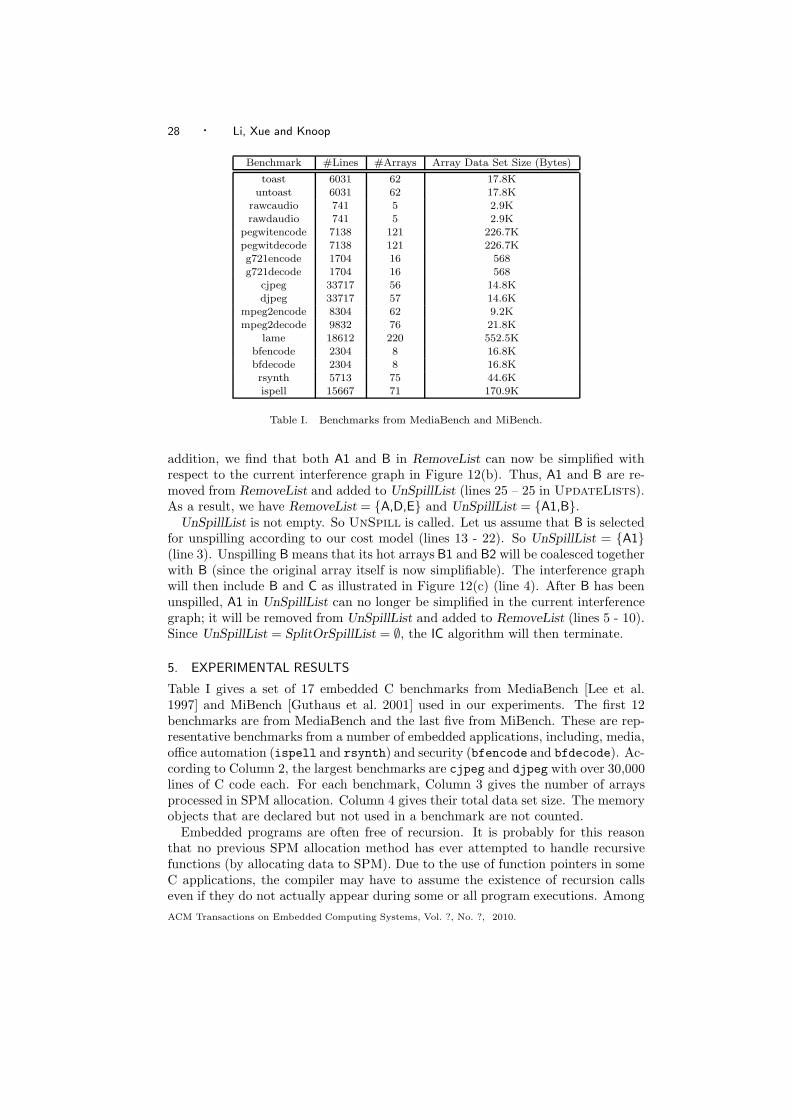
Benchmark #Lines #Arrays Array Data Set Size (Bytes)
toast 6031 62 17.8Kuntoast 6031 62 17.8K
rawcaudio 741 5 2.9Krawdaudio 741 5 2.9K
pegwitencode 7138 121 226.7Kpegwitdecode 7138 121 226.7Kg721encode 1704 16 568g721decode 1704 16 568
cjpeg 33717 56 14.8Kdjpeg 33717 57 14.6K
mpeg2encode 8304 62 9.2Kmpeg2decode 9832 76 21.8K
lame 18612 220 552.5Kbfencode 2304 8 16.8Kbfdecode 2304 8 16.8Krsynth 5713 75 44.6Kispell 15667 71 170.9K
Table I. Benchmarks from MediaBench and MiBench.
addition, we find that both A1 and B in RemoveList can now be simplified withrespect to the current interference graph in Figure 12(b). Thus, A1 and B are re-moved from RemoveList and added to UnSpillList (lines 25 – 25 in UpdateLists).As a result, we have RemoveList = {A,D,E} and UnSpillList = {A1,B}.
UnSpillList is not empty. So UnSpill is called. Let us assume that B is selectedfor unspilling according to our cost model (lines 13 - 22). So UnSpillList = {A1}(line 3). Unspilling B means that its hot arrays B1 and B2 will be coalesced togetherwith B (since the original array itself is now simplifiable). The interference graphwill then include B and C as illustrated in Figure 12(c) (line 4). After B has beenunspilled, A1 in UnSpillList can no longer be simplified in the current interferencegraph; it will be removed from UnSpillList and added to RemoveList (lines 5 - 10).Since UnSpillList = SplitOrSpillList = ∅, the IC algorithm will then terminate.
5. EXPERIMENTAL RESULTS
Table I gives a set of 17 embedded C benchmarks from MediaBench [Lee et al.1997] and MiBench [Guthaus et al. 2001] used in our experiments. The first 12benchmarks are from MediaBench and the last five from MiBench. These are rep-resentative benchmarks from a number of embedded applications, including, media,office automation (ispell and rsynth) and security (bfencode and bfdecode). Ac-cording to Column 2, the largest benchmarks are cjpeg and djpeg with over 30,000lines of C code each. For each benchmark, Column 3 gives the number of arraysprocessed in SPM allocation. Column 4 gives their total data set size. The memoryobjects that are declared but not used in a benchmark are not counted.
Embedded programs are often free of recursion. It is probably for this reasonthat no previous SPM allocation method has ever attempted to handle recursivefunctions (by allocating data to SPM). Due to the use of function pointers in someC applications, the compiler may have to assume the existence of recursion callseven if they do not actually appear during some or all program executions. Among
ACM Transactions on Embedded Computing Systems, Vol. ?, No. ?, 2010.

Scratchpad Memory Allocation via Interval Coloring · 29
40
60
80
100
Arr
ay A
cces
ses
(%)
0
20
Arr
ay A
cces
ses
(%)
Fig. 13. Percentage of the array accesses to all arrays (in Acan) considered for SPM allocation(which are listed in Table I) over all memory accesses in a benchmark.
all the embedded benchmarks we have tested (including those listed in Table I), theSUIF/MachSUIF compiler has reported four benchmarks with potentially recursivecalls: rsynth, ispell, cjpeg and djpeg. At run time, recursive calls are detectedin the first two but not in the last two programs. Furthermore, no local arrays aredefined in any (directly or indirectly) recursive function. Therefore, all benchmarksused here can be treated as recursion-free programs. However, all algorithms pre-sented in this paper work in the presence of recursive calls. Our SPM allocator canbe easily extended to handle recursion by using a callee-save mechanism.
We have implemented our interval-coloring SPM allocator in the SUIF/machSUIFcompiler framework. All programs are compiled into assembly programs for the Al-pha architecture. These assembly programs are then translated into binaries on aDEC Alpha 20264 architecture. The profiling information for MediaBench is ob-tained using the so-called second data set available in the MediaBench web site.These benchmarks are evaluated using the (different) data sets that come withtheir source files. The profiling for the other benchmarks is obtained using inputsdifferent from those when they are actually evaluated.
We have modified SimpleScalar in order to carry out the performance evaluationsfor this work. There are four parameters involved in the cost model used for liverange splitting [Li et al. 2005]. The cost of communicating n bytes between SPMand off-chip is approximated by Cs + Ct ×n in cycles, where Cs is the startup costand Ct is the cost per byte transfer. Two other parameters are Mspm and Mmem,which represent the number of cycles required for one memory access to the SPMand the off-chip memory, respectively. For the results presented here, the values ofthe four parameters are Cs = 100, Ct = 1, Mmem = 100 and Mspm = 1.
Since we are concerned with assigning static data aggregates to SPM, the scalarsand heap objects are ignored. In toast and untoast, we have (manually) replaceda frequently used heap object with a global array so that it can be assigned to SPM.
Figure 13 shows the percentage of array accesses to all arrays (in Acan) consid-ered for SPM allocation over all memory accesses in a benchmark. In 10 bench-marks, toast, untoast, rawcaudio, rawdaudio, pegwitencode, pegwitdecode,g721encode, g721decode, bfencode and bfdecode, the majority of memory ac-cesses are array accesses. In addition, arrays with sizes being larger than 32K bytesare ignored since it is not effective to keep them entirely in SPM. One solution
ACM Transactions on Embedded Computing Systems, Vol. ?, No. ?, 2010.

30 · Li, Xue and Knoop
Benchmark #Maximal Cliques Chromatic Number (Bytes)
toast 39 2248untoast 19 1840
rawcaudio 1 2936rawdaudio 1 2936
pegwitencode 267 21968pegwitdecode 141 26600g721encode 3 184g721decode 3 168jpegenocde 8 6504jpegdecode 7 3176
mpeg2encode 15 6472mpeg2decode 12 11296
lame 193 273848bfencode 6 8448bfdecode 6 8448rsynth 9 16344ispell 209 27464
Table II. Some statistics for interference graphs Gcan built from Acan by Build.
Benchmark Compile Time (secs)
toast 0.457untoast 0.424
rawcaudio 0.009rawdaudio 0.009
pegwitencode 4.875pegwitdecode 3.971g721encode 0.053g721decode 0.054jpegencode 1.725jpegdecode 2.652
mpeg2encode 0.553mpeg2decode 1.410
lame 19.156bfencode 0.047bfdecode 0.046rsynth 0.627ispell 4.621
Table III. Average compile times.
is to divide them into smaller subarrays [Huang et al. 2003] and then apply ouralgorithms to these subarrays.
Table II gives the chromatic numbers for the interference graphs Gcan constructedfrom Acan for all the 17 benchmarks. For an interference graph, its chromaticnumber represents the minimum SPM size required to color all arrays in the graph.By comparing Table II with Column 4 of Table I, we find that the chromaticnumbers of the initial interference graphs built by IC for all benchmarks are muchsmaller than their overall data set sizes. This suggests that a program with a largedata set can be potentially placed in a relatively small SPM.
Table III gives the average compile times (calculated across all SPM sizes consid-
ACM Transactions on Embedded Computing Systems, Vol. ?, No. ?, 2010.

Scratchpad Memory Allocation via Interval Coloring · 31
0
20
40
60
80
100
8K4K2K1K512256
Arr
ay H
it R
ate
s (
%)
toast
untoast
rawcaudio
rawdaudio
g721encode
g721decode
cjpeg
djpeg
rsynth
0
20
40
60
80
100
512 1K 2K 4K 8K 16K 32K
Arr
ay H
it R
ate
s (
%)
SPM Size (byte)
pegwitencode
pegwitdecode
mpeg2encode
mpeg2decode
lame
bfencode
bfdecode
ispell
Fig. 14. Array hit rates achieved by the IC SPM allocator.
ered in this paper) for the IC allocation algorithm on a 2.66GHz Pentium 4 box with2GB memory. As shown in Table III, IC is practically efficient. In particular, themaximal cliques of all node-induced subgraphs G of Gcan can be efficiently obtainedfrom the set of maximal cliques that are computed only once from G.
5.1 Performance Evaluation
Since we are concerned with placing arrays in SPM, we will evaluate the effectivenessof our approach in improving the utilisation of SPM for all the arrays consideredfor SPM allocation. To this end, the concept of array hit rate is introduced. Thearray hit rate for a program is defined to be the percentage of array accesses hitin the SPM over the total array accesses (to the arrays in Acan) considered forSPM allocation in the benchmark. As in prior work [Kandemir et al. 2001; Avissaret al. 2002; Udayakumaran and Barua 2003; Verma et al. 2004b; Li et al. 2005], wewill compare results obtained on a system incorporated with an SPM over the onewithout. There are a great number of embedded architectures that have an SPMbut no (data) cache. Examples include Motorola Dragonball, TI TMS370CX7X,Analog Devices ADSP-21XX, Infineon XC166 and Hitachi SuperH-SH7050.
Figure 14 shows the array hit rate improvements achieved for the 17 benchmarksas the SPM size increases. We have divided the 17 benchmarks into two groupsaccording to their data set sizes. One group is evaluated with SPM sizes rangingfrom 256 bytes to 8K bytes. For a benchmark in this group, an SPM of 8K bytesis sufficient to hold all the arrays that are frequently accessed at any time duringprogram execution (cf. Table II). The other group is evaluated with SPM sizes
ACM Transactions on Embedded Computing Systems, Vol. ?, No. ?, 2010.

32 · Li, Xue and Knoop
0
20
40
60
80
100
8K4K2K1K512256
SP
M H
it R
ate
s (
%)
toast
untoast
rawcaudio
rawdaudio
g721encode
g721decode
cjpeg
djpeg
rsynth
0
20
40
60
80
100
32K16K8K4K2K1K512
SP
M H
it R
ate
s (
%)
SPM Size (bytes)
pegwitencode
pegwitdecode
mpeg2encode
mpeg2decode
lame
bfencode
bfdecode
ispell
Fig. 15. Effect of varying the SPM size on SPM hit rates.
ranging from 512 bytes to 32K bytes. For the benchmarks in this group an SPM of32K bytes is sufficient. As for lame, a larger SPM size is needed (Table II).
As the SPM size increases, all the benchmarks exhibit non-decreasing array hitrate improvements. Each arrives at its peak at one of the SPM sizes used, where allits frequently accessed arrays are placed in the SPM throughout program execution.
The performance improvement of a program depends on (among others) thepercentage of array accesses over the total memory accesses in the program, theSPM and memory access latencies and the DMA cost. Figure 15 gives the SPM hitrates for all the benchmarks. By convention, the SPM (i.e., cache) hit rate for aprogram is understood to be the percentage of array accesses hit in the SPM overthe total memory accesses in the program.
Figure 16 shows the performance improvements achieved by the 17 benchmarksfor the experimental settings described earlier in Section 5. These results allow us todevelop an intuitive understanding about the performance speedups achievable dueto improved SPM hit rates. The execution time of a benchmark on an SPM-basedsystem is normalised to that achieved when the SPM is not used. The best speedups(by a factor of over 5) are achieved for toast, untoast, rawcaudio and rawdaudio.But only small improvements are observed for cjpeg, djpeg and mpeg2encode.
The varying performance improvements across the 17 benchmarks can be un-derstood by examining their array access percentages given in Figure 13 and theirSPM hit rates given in Figure 15. In some benchmarks, including cjpeg, djpegand mpeg2encode, array accesses represent only a small fraction of all their mem-ory accesses and the remaining ones are mostly accesses to heap-allocated objects.
ACM Transactions on Embedded Computing Systems, Vol. ?, No. ?, 2010.

Scratchpad Memory Allocation via Interval Coloring · 33
0
0.2
0.4
0.6
0.8
1
8K4K2K1K512256
No
rma
lize
d E
xe
cu
tio
n T
ime toast
untoast
rawcaudio
rawdaudio
g721encode
g721decode
cjpeg
djpeg
rsynth
0
0.2
0.4
0.6
0.8
1
32K16K8K4K2K1K512
No
rma
lize
d E
xe
cu
tio
n T
ime
SPM Size (bytes)
pegwitencode
pegwitdecode
mpeg2encode
mpeg2decode
lame
bfencode
bfdecode
ispell
Fig. 16. Performance improvements achieved on an SPM-based system over (i.e.,normalised with respect to) the one without the SPM.
Thus, the performance speedups will not be impressive even if all array accesseshit in the SPM. Let us take a look at Figure 15. As the SPM size increases, theSPM hit rate for a benchmark keeps increasing until after the SPM size has passeda certain value. Then having a larger SPM will have little positive impact on theSPM hit rate. As shown in Figure 13, the SPM hit rate for a program will eventu-ally approach the array access percentage for the program, at which all frequentlyaccessed arrays in any program region are all found in the SPM.
5.2 Compared with Memory Coloring
We compare IC with MC (for memory coloring), a graph-coloring-based allocatorproposed in [Li et al. 2005]. MC formulates the SPM allocation problem as a clas-sical register allocation problem by partitioning the continuous SPM space into apseudo register file and then applying a classic graph coloring algorithm to colorarrays into the pseudo register file. MC is admittedly more general since it can pre-serve more precise liveness information without extending any live ranges. However,as mentioned in Section 4.1, very few live ranges need to be extended in embeddedC programs. In addition, MC may suffer from the SPM fragmentation problem.
For the 17 benchmarks evaluated under a number of SPM configurations, thetwo allocators yield the same results in seven benchmarks, rawcaudio, rawdaudio,
g721encode, g721decode, bfencode, bfdecode and rsynth. In addition, there areonly slight differences with respect to execution times for jpegencode, jpegdecode,
mpeg2encode, mpeg2decode and ispell. For these 12 benchmarks, near-optimal re-
ACM Transactions on Embedded Computing Systems, Vol. ?, No. ?, 2010.
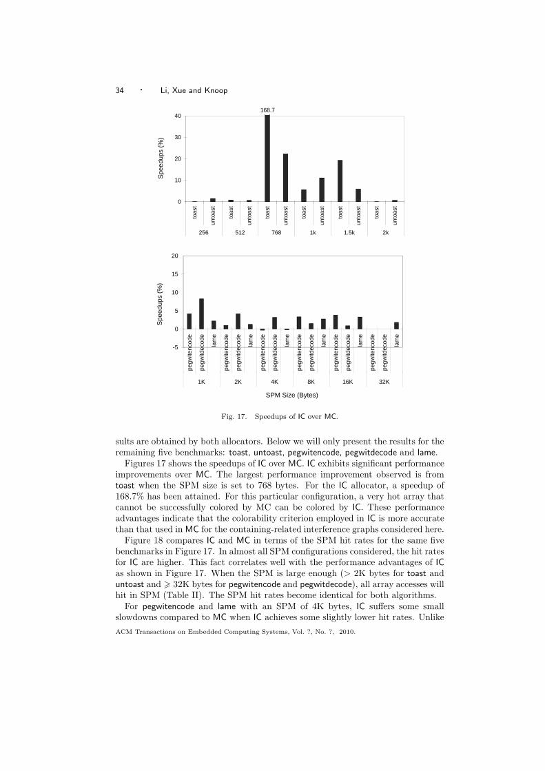
34 · Li, Xue and Knoop
168.7
0
10
20
30
40
toas
t
unto
ast
toas
t
unto
ast
toas
t
unto
ast
toas
t
unto
ast
toas
t
unto
ast
toas
t
unto
ast
256 512 768 1k 1.5k 2k
Spe
edup
s (%
)
5
10
15
20
Spe
edup
s (%
)
-5
0
pegw
itenc
ode
pegw
itdec
ode
lam
e
pegw
itenc
ode
pegw
itdec
ode
lam
e
pegw
itenc
ode
pegw
itdec
ode
lam
e
pegw
itenc
ode
pegw
itdec
ode
lam
e
pegw
itenc
ode
pegw
itdec
ode
lam
e
pegw
itenc
ode
pegw
itdec
ode
lam
e
1K 2K 4K 8K 16K 32K
SPM Size (Bytes)
Fig. 17. Speedups of IC over MC.
sults are obtained by both allocators. Below we will only present the results for theremaining five benchmarks: toast, untoast, pegwitencode, pegwitdecode and lame.
Figures 17 shows the speedups of IC over MC. IC exhibits significant performanceimprovements over MC. The largest performance improvement observed is fromtoast when the SPM size is set to 768 bytes. For the IC allocator, a speedup of168.7% has been attained. For this particular configuration, a very hot array thatcannot be successfully colored by MC can be colored by IC. These performanceadvantages indicate that the colorability criterion employed in IC is more accuratethan that used in MC for the containing-related interference graphs considered here.
Figure 18 compares IC and MC in terms of the SPM hit rates for the same fivebenchmarks in Figure 17. In almost all SPM configurations considered, the hit ratesfor IC are higher. This fact correlates well with the performance advantages of IC
as shown in Figure 17. When the SPM is large enough (> 2K bytes for toast anduntoast and > 32K bytes for pegwitencode and pegwitdecode), all array accesses willhit in SPM (Table II). The SPM hit rates become identical for both algorithms.
For pegwitencode and lame with an SPM of 4K bytes, IC suffers some smallslowdowns compared to MC when IC achieves some slightly lower hit rates. Unlike
ACM Transactions on Embedded Computing Systems, Vol. ?, No. ?, 2010.
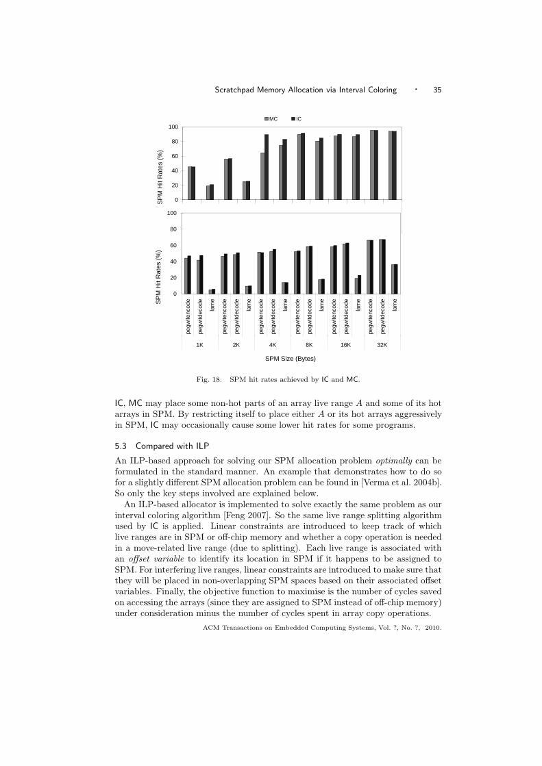
Scratchpad Memory Allocation via Interval Coloring · 35
0
20
40
60
80
100
toas
t
unto
ast
toas
t
unto
ast
toas
t
unto
ast
toas
t
unto
ast
toas
t
unto
ast
toas
t
unto
ast
256 512 768 1K 1.5K 2K
SP
M H
it R
ates
(%
)
MC IC
20
40
60
80
100
SP
M H
it R
ates
(%
)
0
pegw
itenc
ode
pegw
itdec
ode
lam
e
pegw
itenc
ode
pegw
itdec
ode
lam
e
pegw
itenc
ode
pegw
itdec
ode
lam
e
pegw
itenc
ode
pegw
itdec
ode
lam
e
pegw
itenc
ode
pegw
itdec
ode
lam
e
pegw
itenc
ode
pegw
itdec
ode
lam
e
1K 2K 4K 8K 16K 32K
SP
M H
it R
ates
(%
)
SPM Size (Bytes)
Fig. 18. SPM hit rates achieved by IC and MC.
IC, MC may place some non-hot parts of an array live range A and some of its hotarrays in SPM. By restricting itself to place either A or its hot arrays aggressivelyin SPM, IC may occasionally cause some lower hit rates for some programs.
5.3 Compared with ILP
An ILP-based approach for solving our SPM allocation problem optimally can beformulated in the standard manner. An example that demonstrates how to do sofor a slightly different SPM allocation problem can be found in [Verma et al. 2004b].So only the key steps involved are explained below.
An ILP-based allocator is implemented to solve exactly the same problem as ourinterval coloring algorithm [Feng 2007]. So the same live range splitting algorithmused by IC is applied. Linear constraints are introduced to keep track of whichlive ranges are in SPM or off-chip memory and whether a copy operation is neededin a move-related live range (due to splitting). Each live range is associated withan offset variable to identify its location in SPM if it happens to be assigned toSPM. For interfering live ranges, linear constraints are introduced to make sure thatthey will be placed in non-overlapping SPM spaces based on their associated offsetvariables. Finally, the objective function to maximise is the number of cycles savedon accessing the arrays (since they are assigned to SPM instead of off-chip memory)under consideration minus the number of cycles spent in array copy operations.
ACM Transactions on Embedded Computing Systems, Vol. ?, No. ?, 2010.
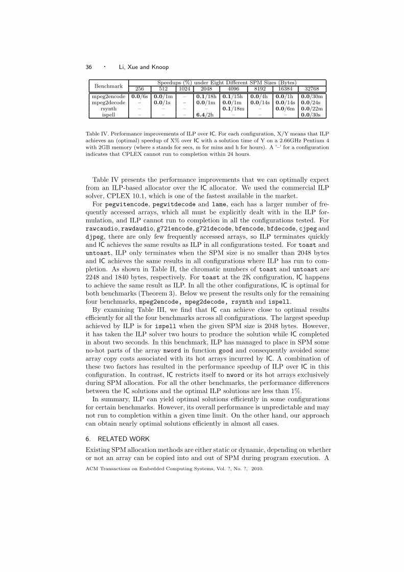
36 · Li, Xue and Knoop
BenchmarkSpeedups (%) under Eight Different SPM Sizes (Bytes)
256 512 1024 2048 4096 8192 16384 32768
mpeg2encode 0.0/6s 0.0/1m – 0.1/18h 0.1/15h 0.0/4h 0.0/1h 0.0/30mmpeg2decode – 0.0/1s – 0.0/1m 0.0/1m 0.0/14s 0.0/14s 0.0/24s
rsynth – – – – 0.1/18m – 0.0/6m 0.0/22mispell – – – 6.4/2h – – – 0.0/30s
Table IV. Performance improvements of ILP over IC. For each configuration, X/Y means that ILPachieves an (optimal) speedup of X% over IC with a solution time of Y on a 2.66GHz Pentium 4with 2GB memory (where s stands for secs, m for mins and h for hours). A ’–’ for a configurationindicates that CPLEX cannot run to completion within 24 hours.
Table IV presents the performance improvements that we can optimally expectfrom an ILP-based allocator over the IC allocator. We used the commercial ILPsolver, CPLEX 10.1, which is one of the fastest available in the market.
For pegwitencode, pegwitdecode and lame, each has a larger number of fre-quently accessed arrays, which all must be explicitly dealt with in the ILP for-mulation, and ILP cannot run to completion in all the configurations tested. Forrawcaudio, rawdaudio, g721encode, g721decode, bfencode, bfdecode, cjpeg anddjpeg, there are only few frequently accessed arrays, so ILP terminates quicklyand IC achieves the same results as ILP in all configurations tested. For toast anduntoast, ILP only terminates when the SPM size is no smaller than 2048 bytesand IC achieves the same results in all configurations where ILP has run to com-pletion. As shown in Table II, the chromatic numbers of toast and untoast are2248 and 1840 bytes, respectively. For toast at the 2K configuration, IC happensto achieve the same result as ILP. In all the other configurations, IC is optimal forboth benchmarks (Theorem 3). Below we present the results only for the remainingfour benchmarks, mpeg2encode, mpeg2decode, rsynth and ispell.
By examining Table III, we find that IC can achieve close to optimal resultsefficiently for all the four benchmarks across all configurations. The largest speedupachieved by ILP is for ispell when the given SPM size is 2048 bytes. However,it has taken the ILP solver two hours to produce the solution while IC completedin about two seconds. In this benchmark, ILP has managed to place in SPM someno-hot parts of the array nword in function good and consequently avoided somearray copy costs associated with its hot arrays incurred by IC. A combination ofthese two factors has resulted in the performance speedup of ILP over IC in thisconfiguration. In contrast, IC restricts itself to nword or its hot arrays exclusivelyduring SPM allocation. For all the other benchmarks, the performance differencesbetween the IC solutions and the optimal ILP solutions are less than 1%.
In summary, ILP can yield optimal solutions efficiently in some configurationsfor certain benchmarks. However, its overall performance is unpredictable and maynot run to completion within a given time limit. On the other hand, our approachcan obtain nearly optimal solutions efficiently in almost all cases.
6. RELATED WORK
Existing SPM allocation methods are either static or dynamic, depending on whetheror not an array can be copied into and out of SPM during program execution. A
ACM Transactions on Embedded Computing Systems, Vol. ?, No. ?, 2010.

Scratchpad Memory Allocation via Interval Coloring · 37
large number of early methods are static [Avissar et al. 2002; Hiser and Davidson2004; Sjodin and von Platen 2001; Steinke et al. 2002]. In [Hiser and Davidson2004], the authors provide an easily re-targetable compiler method for assigningdata to many different types of memory. Steinke et al. [2002] propose a methodthat can place both data and code in SPM. In [Avissar et al. 2002; Sjodin and vonPlaten 2001], the static SPM allocation problem is formulated as an integer linearprogramming (ILP) program and the authors have shown that an optimal staticSPM allocation scheme can be achieved for certain embedded applications.
Dynamic SPM allocation methods enable program data to be copied into and outof SPM during program execution. It has been demonstrated that a dynamic allo-cation scheme can often outperform an optimal static allocation scheme [Udayaku-maran et al. 2006]. There are a few dynamic methods around [Kandemir et al. 2001;Udayakumaran et al. 2006; Verma et al. 2004b; Li et al. 2005]. In [Kandemir et al.2001], loop and data transformations are exploited but the proposed technique isapplied to individual loop kernels in isolation. Udayakumaran et al. [2006] use a setof heuristics to guide their decision in deciding how to copy program data betweenSPM and off-chip memory during program execution. The ILP-based approachintroduced in [Verma et al. 2004b] can yield optimal solutions for some programsbut can be expensive when applied to others as reported in [Ravindran et al. 2005]and verified in our experiments. In [Li et al. 2005], we map the dynamic SPM al-location problem into a well-understood register allocation problem and then solveit by applying any classic graph-coloring-based algorithm.
In [Li et al. 2007], we introduced two interval-coloring algorithms based on a sim-ple cost model for live range splitting and spilling. This journal paper has extendedsignificantly our earlier work in a number of ways by producing an SPM alloca-tor that applies interval coloring to solve the SPM allocation problem elegantlyand effectively for real-world embedded programs. First, of the two algorithmsinvestigated in [Li et al. 2007], the one that performs both splitting and spillingiteratively together is generally superior. This algorithm has been improved herein two directions (Figure 7): unspilling is now invoked iteratively together with(rather than after) splitting and spilling and the colorability of G is now computedmore precisely from the colorability values of individual arrays rather than the col-orability values of maximal cliques. As a result, same or better performance resultsare observed (for those same benchmarks used also earlier). Second, our live rangesplitting strategy is more aggressive. In particular, an array that could not be splitearlier due to the presence of pointers (to the array) can now be split, giving rise tobetter SPM utilisation. Third, we give an algorithm for extending array live rangesto build a superperfect interference graph to ensure that all live ranges either donot interfere or are containing-related. Finally, in comparison with some prelimi-nary results reported in [Li et al. 2007], we have conducted more experiments usingmore benchmarks in evaluating, analysing and understanding all major aspects ofinterval coloring, including performance and compile times. In particular, we havealso evaluated our proposed approach against an optimal ILP-based approach.
A live range may be split when it cannot be colored in register allocation forscalars by graph coloring [Bergner et al. 1997; Cooper and Simpson 1998] and byadopting a priority-based approach introduced in [Chow and Hennessy 1990]. In
ACM Transactions on Embedded Computing Systems, Vol. ?, No. ?, 2010.
38 · Li, Xue and Knoop
this work, however, live range splitting is applied on-demand together with spillingin an interval-coloring allocator for data aggregates. Furthermore, based on liverange containment, we are able to split where is needed to reduce the clique numberof an interference graph until the resulting graph is optimally colorable.
In [Udayakumaran et al. 2006; Steinke et al. 2002; Ravindran et al. 2005; Vermaet al. 2004a], the authors show that it is also beneficial to place portions of programcode in SPM. In [Panda et al. 2000; 1997a; Verma et al. 2004a], the researchersconsider a hybrid system with both cache and SPM. Their main objective is toplace data in SPM to achieve better SRAM hit rates. In [Panda et al. 2000; 1997a;1997b], solutions are proposed to map the variables that are likely to cause cacheconflicts to SPM. In [Verma et al. 2004a], the authors propose a generic cache-awarescratchpad allocation algorithm to use scratchpad for storing instructions.
The interval coloring problem has a fairly long history dating back, at least to1970s [Fabri 1979; Garey and Johnson 1976]. It has been proved that the intervalcoloring problem is NP-complete [Garey and Johnson 1979]. Fabri [Fabri 1979]made the connection between interval coloring and compile-time memory allocationin 1979. Since then a few approximation algorithms have been proposed [Fabri 1979;Kierstead 1991; Gergov 1999], where a program is generally abstracted as a straight-line program. As a result, the interference graph for static memory objects is aninterval graph [Golumbic 2004]. With this abstraction, the interval coloring problemremains to be NP-complete [Garey and Johnson 1979] and the above approaches canthus provide approximate solutions. In this paper, we introduce a dynamic methodthat formulates the SPM allocation problem into an interval-coloring problem.
Interval coloring for an arbitrary graph is too complex. Recent research has fo-cused on developing efficient interval coloring algorithms for some special classes ofgraphs like chordal graphs [Pemmaraju et al. 2005; Confessore et al. 2002], intervalgraphs [Zeitlhofer and Wess 2003] and comparability graphs formed by containing-related array interference graphs considered here. Independently, in the field con-cerning register allocation, researchers have become increasingly more interestedin abstracting interference graphs as some special classes of graphs. For example,Andersson [Andersson 2003] and Pereira and Palsberg [Pereira and Palsberg 2005]have tested a large number of interference graphs in programs and found that themajority of these graphs are chordal graphs. Bouchez [2005] and Hack et al. [2006]demonstrated that the interference graphs for programs in the SSA form [Cytronet al. 1989] are chordal graphs. An optimal graph coloring is thus possible.
7. CONCLUSION
We recognise that the array interference graphs in many embedded applicationscan be abstracted as containing-related superperfect graphs, which are compara-bility graphs. We present an SPM allocation approach for such array interferencegraphs by combining interval coloring, a classic way for solving memory alloca-tion problems, with a Chaitin-like approach for register allocation so as to intermixspilling, splitting and coalescing, but for “virtual registers” of non-unit lengths, i.e.,arrays. Our algorithm can achieve optimal results for a containing-related interfer-ence graph when the size of a given SPM is no smaller than the clique number of thegraph. If the SPM is not large enough, our algorithm uses containment-motivated
ACM Transactions on Embedded Computing Systems, Vol. ?, No. ?, 2010.

Scratchpad Memory Allocation via Interval Coloring · 39
heuristics to reduce the clique number of the graph by splitting or spilling some ar-rays from the graph until all arrays remaining in the graph can be optimally placedin SPM. Our algorithm has been implemented in SUIF/machSUIF and evaluatedusing MediaBench and MiBench benchmarks. Experimental results show that ourinterval-coloring approach can achieve the same or better results than our earliermemory coloring approach even though memory coloring is admittedly more generaland may also be effective to programs with arbitrary interference graphs.
8. ACKNOWLEDGEMENTS
This work is supported by ARC grants DP0665581 and DP0881330.
REFERENCES
Andersson, C. 2003. Register allocation by optimal graph coloring. In CC’03: Proceedings ofthe 12th International Conference on Compiler Construction. Springer-Verlag.
Avissar, O., Barua, R., and Stewart, D. 2002. An optimal memory allocation schemefor scratch-pad-based embedded systems. ACM Transactions on Embedded Computing Sys-tems 1, 1, 6–26.
Banakar, R., Steinke, S., Lee, B.-S., Balakrishnan, M., and Marwedel, P. 2002. Scratchpadmemory: design alternative for cache on-chip memory in embedded systems. In CODES’02:Proceedings of the 10th International Symposium on Hardware/Software Codesign. ACM Press,New York, NY, USA, 73–78.
Bergner, P., Dahl, P., Engebretsen, D., and O’Keefe, M. 1997. Spill code minimization viainterference region spilling. In PLDI ’97: Proceedings of the ACM SIGPLAN 1997 conferenceon Programming +language design and implementation. ACM, New York, NY, USA, 287–295.
Bouchez, F. 2005. Allocation de registres et vidage en memoire. M.S. thesis, ENS Lyon.
Bouchez, F., Darte, A., and Rastello, F. 2007. On the complexity of register coalescing. InCGO ’07: Proceedings of the International Symposium on Code Generation and Optimization.IEEE Computer Society, Washington, DC, USA, 102–114.
Chaitin, G. J. 1982. Register allocation & spilling via graph coloring. In SIGPLAN’82: Pro-ceedings of the SIGPLAN Symposium on Compiler Construction. ACM Press, New York, NY,USA, 98–101.
Chow, F. C. and Hennessy, J. L. 1990. The priority-based coloring approach to register alloca-tion. ACM Transactions on Programming Languages and Systems 12, 4, 501–536.
Confessore, G., Dell’Olmo, P., and Giordani, S. 2002. An approximation result for theinterval coloring problem on claw-free chordal graphs. Discrete Applied Mathematics 120, 1-3,73–90.
Cooper, K. D. and Simpson, L. T. 1998. Live range splitting in a graph coloring register allocator.In CC’98: Proceedings of the 7th International Conference on Compiler Construction. Springer-Verlag, London, UK, 174–187.
Cytron, R., Ferrante, J., Rosen, B. K., Wegman, M. N., and Zadeck, F. K. 1989. Anefficient method of computing static single assignment form. In POPL’89: Proceedings of the16th ACM SIGPLAN-SIGACT Symposium on Principles of Programming Languages. ACMPress, New York, NY, USA, 25–35.
Detlefs, D. and Agesen, O. 1999. Inlining of virtual methods. In 13th European Conferenceon Object-Oriented Programming (ECOOP’99). 258–278.
Fabri, J. 1979. Automatic storage optimization. In SIGPLAN’79: Proceedings of the SIGPLANSymposium on Compiler Construction. ACM Press, New York, NY, USA, 83–91.
Feng, H. 2007. Ilp formulation for spm allocation. M.S. thesis, University of New South Wales.
Garey, M. R. and Johnson, D. S. 1976. The complexity of near-optimal graph coloring. Journalof the ACM 23, 1, 43–49.
Garey, M. R. and Johnson, D. S. 1979. Computers and intractability: a guide to the theory ofNP-completeness. W. H. Freeman & Co., New York, NY, USA.
ACM Transactions on Embedded Computing Systems, Vol. ?, No. ?, 2010.

40 · Li, Xue and Knoop
George, L. and Appel, A. W. 1996. Iterated register coalescing. ACM Transactions on Pro-
gramming Languages and Systems 18, 3, 300–324.
Gergov, J. 1999. Algorithms for compile-time memory optimization. In SODA’99: Proceedingsof the 10th annual ACM-SIAM Symposium on Discrete algorithms. Society for Industrial andApplied Mathematics, Philadelphia, PA, USA, 907–908.
Golumbic, M. C. 2004. Algorithmic graph theory and perfect graphs. Annals of Discrete Math-ematics.
Guthaus, M. R., Ringenberg, J. S., Ernst, D., Austin, T. M., Mudge, T., and Brown, R. B.2001. Mibench: A free, commercially representative embedded benchmark suite. In WWC’01: Proceedings of the Workload Characterization, 2001. WWC-4. 2001 IEEE InternationalWorkshop on. IEEE Computer Society, Washington, DC, USA, 3–14.
Hack, S., Grund, D., and Goos, G. 2006. Register allocation for programs in ssa-form. In CC’06:Proceedings of the 15th International Conference on Compiler Construction. Springer-Verlag.
Hiser, J. D. and Davidson, J. W. 2004. Embarc: an efficient memory bank assignment algo-rithm for retargetable compilers. In LCTES’04: Proceedings of the ACM SIGPLAN/SIGBEDConference on Languages, Compilers, and Tools for Embedded Systems. ACM Press, 182–191.
Huang, Q., Xue, J., and Vera, X. 2003. Code tiling for improving the cache performance ofPDE solvers. In International Conference on Parallel Processing. 615–625.
Kandemir, M., Ramanujam, J., Irwin, J., Vijaykrishnan, N., Kadayif, I., and Parikh, A.2001. Dynamic management of scratch-pad memory space. In DAC’01: Proceedings of the 38thConference on Design Automation. ACM Press, 690–695.
Kierstead, H. A. 1991. A polynomial time approximation algorithm for dynamic storage allo-cation. Discrete Mathematics 87, 2-3, 231–237.
Lee, C., Potkonjak, M., and Mangione-Smith, W. H. 1997. Mediabench: A tool for evaluatingand synthesizing multimedia and communications systems. In International Symposium onMicroarchitecture. 330–335.
Li, L., Gao, L., and Xue, J. 2005. Memory coloring: a compiler approach for scratchpad mem-ory management. In PACT’05: Proceedings of the 14th International Conference on ParallelArchitectures and Compilation Techniques. IEEE Computer Society, Washington, DC, USA,329–338.
Li, L., Nguyen, Q. H., and Xue, J. 2007. Scratchpad allocation for data aggregates in super-perfect graphs. SIGPLAN Not. 42, 7, 207–216.
Panda, P. R., Dutt, N. D., and Nicolau, A. 1997a. Architectural exploration and optimizationof local memory in embedded systems. In ISSS’97: Proceedings of the 10th InternationalSymposium on System Synthesis. IEEE Computer Society, 90–97.
Panda, P. R., Dutt, N. D., and Nicolau, A. 1997b. Efficient utilization of scratchpad memory
in embedded processor applications. In EDTC’97: Proceedings of the european Conference onDesign and Test. IEEE Computer Society, Washington, DC, USA, 7.
Panda, P. R., Dutt, N. D., and Nicolau, A. 2000. On-chip vs. off-chip memory: the datapartitioning problem in embedded processor-based systems. ACM Transactions on DesignAutomation of Electronic Systems 5, 3, 682–704.
Park, J. and Moon, S.-M. 2004. Optimistic register coalescing. ACM Transactions on Program-ming Languages and Systems 26, 4, 735–765.
Pemmaraju, S. V., Penumatcha, S., and Raman, R. 2005. Approximating interval coloring andmax-coloring in chordal graphs. Journal of Experimental Algorithmics 10, 2.8.
Pereira, F. M. Q. and Palsberg, J. 2005. Register allocation via coloring of chordal graphs. InAPLAS’05: Proceedings of the 3rd asia Symposium on Programming Languages and Systems.315–329.
Ravindran, R. A., Nagarkar, P. D., Dasika, G. S., Marsman, E. D., Senger, R. M., Mahlke,S. A., and Brown, R. B. 2005. Compiler managed dynamic instruction placement in a low-power cod e cache. In Proceedings of the 3rd IEEE/ACM International Symposium on CodeG eneration and Optimization (CGO’03). 179–190.
ACM Transactions on Embedded Computing Systems, Vol. ?, No. ?, 2010.

Scratchpad Memory Allocation via Interval Coloring · 41
Sjodin, J. and von Platen, C. 2001. Storage allocation for embedded processors. In CASES’01:
Proceedings of the International Conference on Compilers, Architecture, and Synthesis forEmbedded Systems. ACM Press, 15–23.
Steinke, S., Wehmeyer, L., Lee, B., and Marwedel, P. 2002. Assigning program and dataobjects to scratchpad for energy reduction. In DATE ’02: Proceedings of the conference onDesign, automation and test in Europe. IEEE Computer Society, Washington, DC, USA, 409.
Udayakumaran, S. and Barua, R. 2003. Compiler-decided dynamic memory allocation forscratch-pad based embedded systems. In CASES’03: Proceedings of the International Confer-ence on Compilers, Architecture and Synthesis for Embedded Systems. ACM Press, 276–286.
Udayakumaran, S., Dominguez, A., and Barua, R. 2006. Dynamic allocation for scratch-pad memory using compile-time decisions. ACM Transactions on Embedded Computing Sys-tems 5, 2, 472–511.
Verma, M., Wehmeyer, L., and Marwedel, P. 2004a. Cache-aware scratchpad allocation algo-rithm. In DATE’04: Proceedings of the conference on Design, automation and test in Europe.IEEE Computer Society, Washington, DC, USA, 21264.
Verma, M., Wehmeyer, L., and Marwedel, P. 2004b. Dynamic overlay of scratchpad mem-ory for energy minimization. In CODES+ISSS’04: Proceedings of the 2nd IEEE/ACM/IFIPInternational Conference on Hardware/Software Codesign and System Synthesis. ACM Press,New York, NY, USA, 104–109.
Wolfe, M. 1989. Iteration space tiling for memory hierarchies. In Proceedings of the Third SIAMConference on Parallel Processing for Scientific Computing. Society for Industrial and AppliedMathematics, Philadelphia, PA, USA, 357–361.
Xue, J. 1997. On tiling as a loop transformation. Parallel Processing Letters 7, 4, 409–424.
Xue, J. 2000. Loop Tiling for Parallelism. Kluwer Academic Publishers, Boston.
Zeitlhofer, T. and Wess, B. 2003. List-coloring of interval graphs with application to registerassignment for heterogeneous register-set architectures. ACM Signal Processing 83, 7, 1411–1425.
ACM Transactions on Embedded Computing Systems, Vol. ?, No. ?, 2010.