S1

Electronic Supplementary Information

Techno-Economic Analysis of Metal–Organic Frameworks for

Adsorption Heat Pumps/Chillers: From Directional Computational

Screening, Machine Learning to Experiment

Zenan Shi,a Xueying Yuan,a Yaling Yan,a Yuanlin Tang,a Junjie Li,b Hong Liang,a

Lianpeng Tong,a Zhiwei Qiaoa

aGuangzhou Key Laboratory for New Energy and Green Catalysis, School of Chemistry and Chemical Engineering, Guangzhou University, Guangzhou, 510006, P. R. China;bGuangxi Key Laboratory of Clean Pulp & Papermaking and Pollution Control, College of Light Industry and Food Engineering, MOE Key Laboratory of New Processing Technology for Nonferrous Metals and Materials, School of Chemistry and Chemical Engineering, Guangxi University, Nanning 530004, China

Corresponding author.

E-mail address: zqiao@gzhu.edu.cn (Z. Qiao).

Electronic Supplementary Material (ESI) for Journal of Materials Chemistry A.This journal is © The Royal Society of Chemistry 2021

S2

Table of Contents

Lennard-Jones parameters of MOFs S3

Models of methanol S4

Lennard-Jones parameters and bond bending potentials of methanol S4

Adsorption isotherms of MeOH in ZIF-8 S5

An ideal refrigeration or heat pump cycle S6

Operating conditions of three applications S7

Calculation equation of ΔW and COP S8

Calculation method of the cost S11

Machine learning algorithms S14

Hyperparameters of ML algorithms S21

Structural-performance relationships S22

Relationships of the cost-ΔW and COP S24

Sensitivity analysis of cycle stability and MOF price S27

Predictions of Ctotal by ML S28

Relative importance of MOF descriptors by the RF S30

Best CoRE-MOFs S31

Best hMOFs S33

Atomistic structures of top MOFs S35

Experiment details S42

References S43

S3

Table S1. Lennard-Jones parameters of MOFs.

Atom ε/kB [K] σ [Å] Atom ε/kB [K] σ [Å] Atom ε/kB [K] σ [Å]Ac 16.60 3.10 Gea 201.29 3.8 Po 163.52 4.20Ag 18.11 2.80 Gd 4.53 3.00 Pr 5.03 3.21Ala 156.00 3.91 Ha 7.64 2.85 Pt 40.25 2.45Am 7.04 3.01 Hf 36.23 2.80 Pu 8.05 3.05Ar 93.08 3.45 Hg 193.71 2.41 Ra 203.27 3.28Asa 206.32 3.70 Ho 3.52 3.04 Rb 20.13 3.67At 142.89 4.23 Ia 256.64 3.70 Re 33.21 2.63Au 19.62 2.93 Ina 276.77 4.09 Rh 26.67 2.61Ba 47.81 3.58 Ir 36.73 2.53 Rn 124.78 4.25Ba 183.15 3.30 K 17.61 3.40 Ru 28.18 2.64Be 42.77 2.45 Kr 110.69 3.69 Sa 173.11 3.59Bi 260.63 3.89 La 8.55 3.14 Sba 276.77 3.87Bk 6.54 2.97 Li 12.58 2.18 Sc 9.56 2.94Bra 186.19 3.52 Lu 20.63 3.24 Sea 216.39 3.59Ca 47.81 3.47 Lr 5.53 2.88 Sia 156.00 3.80Caa 25.16 3.09 Md 5.53 2.92 Sm 4.03 3.14Cd 114.72 2.54 Mg 55.85 2.69 Sna 276.77 3.98Ce 6.54 3.17 Mn 6.54 2.64 Sr 118.24 3.24Cf 6.54 2.95 Mo 28.18 2.72 Ta 40.75 2.82Cla 142.56 3.52 Na 38.91 3.26 Tb 3.52 3.07Cm 6.54 2.96 Naa 251.61 2.80 Tc 24.15 2.67Co 7.04 2.56 Ne 21.13 2.66 Tea 286.84 3.77Cr 7.55 2.69 Nb 29.69 2.82 Th 13.08 3.03Cu 2.52 3.11 Nd 5.03 3.18 Ti 8.55 2.83Cs 22.64 4.02 No 5.53 2.89 TI 342.14 3.87Dy 3.52 3.05 Ni 7.55 2.52 Tm 3.02 3.01Eu 4.03 3.11 Np 9.56 3.05 U 11.07 3.02Er 3.52 3.02 Oa 48.16 3.03 V 8.05 2.80Es 6.04 2.94 Os 18.62 2.78 W 33.71 2.73Fa 36.48 3.09 Pa 161.03 3.70 Xe 167.04 3.92Fea 27.65 4.05 Pa 11.07 3.05 Y 36.23 2.98Fm 6.04 2.93 Pb 333.59 3.83 Yb 114.72 2.99Fr 25.16 4.37 Pd 24.15 2.58 Zna 27.65 4.05

Gaa 201.29 3.91 Pm 4.53 3.16 Zr 34.72 2.78a Parameters from the Dreiding force field,1 others from UFF force field.2

S4

Figure S1. United-atom model of methanol.3

Table S2. Lennard-Jones parameters and bond bending potentials of methanol.3

Lennard-Jones parameters bond bending

Atom ε/kB (K) σ (Å) q (e) θo kθ/kB (K/rad2)

CH3 98.0 3.750 0.265 CH3OH 108.5 55400

O 93.0 3.020 -0.700

H 0.0 0.000 0.435

S5

0 5 10 15 200

2

4

6

8

10

12

exp. sim.

P (kPa)

(m

mol

/g)

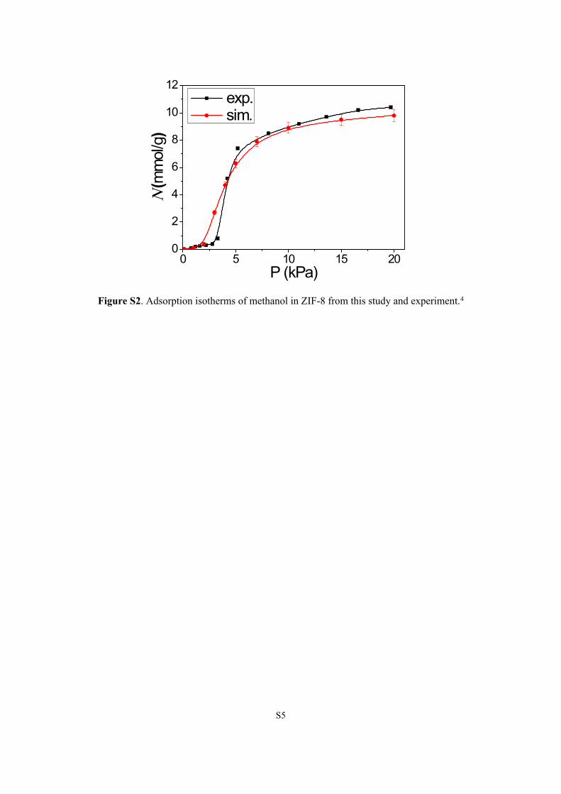
Figure S2. Adsorption isotherms of methanol in ZIF-8 from this study and experiment.4

S6

An ideal refrigeration or heat pump cycle

In this work, a basic cycle would describe the whole process of heating-desorption-

condensing or cooling-adsorption-evaporation. The isosteric cycle diagram of ideal

refrigeration cycle is shown in Figure S3, the black or red lines refers an adsorption or

desorption process, respectively. The whole cycle consists of 4 steps: the first step (I-II) is

isosteric heating; the II-III is isobaric desorption. In this step, the working fluid is desorbed

and condensed, releasing heat to the environment and the heat can be applied for the heat

pump; the third step (III-IV) is isosteric cooling. The adsorbent is regenerated in this process;

the final IV-I is isobaric adsorption. In this step, the working fluid is allowed to adsorb and no

further pressure decreases, the adsorption process will adsorb the energy from the

environment at a low temperature for the refrigeration or ice making.

▲

▲

▲ ▲VI

IIIII

I

W min

W max

work

ing

fluid

p con

p ev

TdesT3T2T1TconTconTev

ln p

-1/TFigure S3. Isosteric cycle diagram for an ideal refrigeration or heat pump cycle

The isosteric cycle diagram of an ideal AHP/AC cycle is shown in Figure S3. The AHP/AC

studied in this paper is mainly composed of four components: the evaporator, condenser,

adsorption heat exchanger, and expansion valve. When the heat provided by high-temperature

industrial wastewater heats a saturated adsorption bed, the working fluid is desorbed from the

adsorbent and becomes high-temperature and high-pressure steam. The liquid is condensed by

the condenser and flows into the evaporator. In the process, the adsorbent bed is heated by hot

water to absorb the heat, and the condenser condenses the high-temperature steam into a low-

pressure liquid to emit heat. After the desorption of the working fluid is complete, the

temperature of the adsorption heat exchanger is reduced to the adsorption temperature. The

working fluid evaporates again from the evaporator and is adsorbed by the adsorption heat

S7

exchanger, completing the entire cycle. In this process, the adsorption heat exchanger emits

heat, and the evaporator absorbs the heat to make the working fluid change from liquid to

steam. In heat pump applications, the heat released by the adsorption and condensation

processes is used to achieve heating. The ice making and refrigeration applications are mainly

accomplished by the heat absorbed during the evaporation process. The energy required for

each application is provided by industrial waste hot water. Therefore, the AHPs/ACs have

captured the imagination of energy saving due to their operation without any additional

energy input (except industrial waste heat).

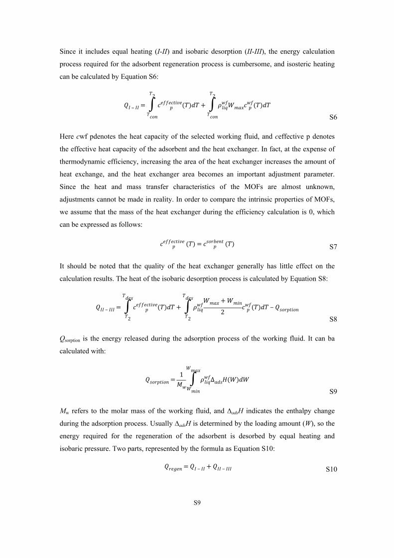
Table S3. Operating Conditions of three applications.

Application Tev (K) Tcon (K)a Tdes1 (K)b Tdes2 (K)b Pev (kPa) Pcon (kPa)

Heat pump 288 318 355 365 9.755 44.493

Ice making 268 298 330 340 2.859 16.826

Refrigeration 278 303 330 340 5.403 21.757a Tads was set equal to Tcon, b Tdes1 and Tdes2 were selected due to the desired energy sources with low T.

Table S4. Operating conditions and states correspondence list.

Application State 1(Tdes1)

State 2(Tdes2)

heat pump 355 K 365 Krefrigeration 330 K 340 Kice making 330 k 340 k

S8

Calculation formulaThe coefficient of performance (COP) is calculated using the method of De lange et al.5

Therefore, equations S1 and S2 are used to calculate COPH and COPC, respectively.

S1𝐶𝑂𝑃𝐻 =

‒ (𝑄𝑐𝑜𝑛 + 𝑄𝑎𝑑𝑠)𝑄𝑟𝑒𝑔𝑒𝑛

S2𝐶𝑂𝑃𝐶 =

𝑄𝑒𝑣

𝑄𝑟𝑒𝑔𝑒𝑛

Qcon indicates the amount of heat released during the condensation process, Qads indicates the

amount of heat released during the adsorption process, and Qregen indicates the amount of heat

required for the regeneration process of the adsorbent. The heat absorbed by the Qev

evaporation process, COPH represents the coefficient of performance for heat pumps, and

COPC represents the coefficient of performance for cooling.

According to a series of different materials studied by Mu and Walton,6 the specific heat

capacity of MOFs was compared. Although the MOFs of Mu and Walton study is inconsistent

with the MOFs selected in this study, their results are consistent with the heat capacity basis

reported by others.

S30.6 ≤ 𝑐𝑠𝑜𝑟𝑏𝑒𝑛𝑡

𝑝 (𝑇) ≤ 1.4 ( 𝐽𝑔 𝐾)

On this basis, we assume that the csorbent p is 1 J g−1 K−1 and is independent of temperature.

We note that in previous studies it was shown that the csorbent has no significant effect on the

coefficient of performance in the range of Equation S3.7 This makes our assumptions more

reasonable.

Qev and Qcon can be calculated by the enthalpy of evaporation, and msorbent represents the

amount of adsorbent in the adsorption cycle. Here we begin to ignore this amount, so Qi is

defined as the amount of adsorbent used per unit mass. ∆W is the working capacity, which

can be determined by the known evaporation enthalpy, and ρwf liq, ρwf liq represent the

liquid density of the working fluid and Mw is the molar mass of the working fluid.

S4𝑄𝑒𝑣 =‒

∆𝑣𝑎𝑝𝐻(𝑇𝑒𝑣)𝜌𝑤𝑓𝑙𝑖𝑞 𝑚𝑠𝑜𝑟𝑏𝑒𝑛𝑡∆𝑊

𝑀𝑤

S5𝑄𝑐𝑜𝑛 =

∆𝑣𝑎𝑝𝐻(𝑇𝑐𝑜𝑛)𝜌𝑤𝑓𝑙𝑖𝑞 𝑚𝑠𝑜𝑟𝑏𝑒𝑛𝑡∆𝑊

𝑀𝑤

S9

Since it includes equal heating (I-II) and isobaric desorption (II-III), the energy calculation

process required for the adsorbent regeneration process is cumbersome, and isosteric heating

can be calculated by Equation S6:

S6

𝑄𝐼 ‒ 𝐼𝐼 =

𝑇2

∫𝑇𝑐𝑜𝑛

𝑐𝑒𝑓𝑓𝑒𝑐𝑡𝑖𝑣𝑒𝑝 (𝑇)𝑑𝑇 +

𝑇2

∫𝑇𝑐𝑜𝑛

𝜌𝑤𝑓𝑙𝑖𝑞𝑊𝑚𝑎𝑥𝑐𝑤𝑓

𝑝 (𝑇)𝑑𝑇

Here cwf pdenotes the heat capacity of the selected working fluid, and ceffective p denotes

the effective heat capacity of the adsorbent and the heat exchanger. In fact, at the expense of

thermodynamic efficiency, increasing the area of the heat exchanger increases the amount of

heat exchange, and the heat exchanger area becomes an important adjustment parameter.

Since the heat and mass transfer characteristics of the MOFs are almost unknown,

adjustments cannot be made in reality. In order to compare the intrinsic properties of MOFs,

we assume that the mass of the heat exchanger during the efficiency calculation is 0, which

can be expressed as follows:

S7𝑐𝑒𝑓𝑓𝑒𝑐𝑡𝑖𝑣𝑒𝑝 (𝑇) = 𝑐𝑠𝑜𝑟𝑏𝑒𝑛𝑡

𝑝 (𝑇)

It should be noted that the quality of the heat exchanger generally has little effect on the

calculation results. The heat of the isobaric desorption process is calculated by Equation S8:

S8

𝑄𝐼𝐼 ‒ 𝐼𝐼𝐼 =

𝑇𝑑𝑒𝑠

∫𝑇2

𝑐𝑒𝑓𝑓𝑒𝑐𝑡𝑖𝑣𝑒𝑝 (𝑇)𝑑𝑇 +

𝑇𝑑𝑒𝑠

∫𝑇2

𝜌𝑤𝑓𝑙𝑖𝑞

𝑊𝑚𝑎𝑥 + 𝑊𝑚𝑖𝑛

2𝑐𝑤𝑓

𝑝 (𝑇)𝑑𝑇 ‒ 𝑄𝑠𝑜𝑟𝑝𝑡𝑖𝑜𝑛

Qsorption is the energy released during the adsorption process of the working fluid. It can ba

calculated with:

S9

𝑄𝑠𝑜𝑟𝑝𝑡𝑖𝑜𝑛 =1

𝑀𝑤

𝑊𝑚𝑎𝑥

∫𝑊𝑚𝑖𝑛

𝜌𝑤𝑓𝑙𝑖𝑞∆𝑎𝑑𝑠𝐻(𝑊)𝑑𝑊

Mw refers to the molar mass of the working fluid, and ∆adsH indicates the enthalpy change

during the adsorption process. Usually ∆adsH is determined by the loading amount (W), so the

energy required for the regeneration of the adsorbent is desorbed by equal heating and

isobaric pressure. Two parts, represented by the formula as Equation S10:

S10 𝑄𝑟𝑒𝑔𝑒𝑛 = 𝑄𝐼 ‒ 𝐼𝐼 + 𝑄𝐼𝐼 ‒ 𝐼𝐼𝐼

S10

The energy lost during the equal cooling process is similar to the heat obtained in the same

amount of heating (Equation S6):

S (11)

𝑄𝐼𝐼𝐼 ‒ 𝐼𝑉 =

𝑇3

∫𝑇𝑑𝑒𝑠

𝑐𝑒𝑓𝑓𝑒𝑐𝑡𝑖𝑣𝑒𝑝 (𝑇)𝑑𝑇 +

𝑇3

∫𝑇𝑑𝑒𝑠

𝜌𝑤𝑓𝑙𝑖𝑞 𝑊𝑚𝑎𝑥𝑐𝑤𝑓

𝑝 (𝑇)𝑑𝑇

The energy lost during isobaric adsorption is similar to that in the isobaric desorption process

(Equation S8):

S12

𝑄𝐼𝑉 ‒ 𝐼 =

𝑇𝑐𝑜𝑛

∫𝑇3

𝑐𝑒𝑓𝑓𝑒𝑐𝑡𝑖𝑣𝑒𝑝 (𝑇)𝑑𝑇 +

𝑇𝑐𝑜𝑛

∫𝑇3

𝜌𝑤𝑓𝑙𝑖𝑞

𝑊𝑚𝑎𝑥 + 𝑊𝑚𝑖𝑛

2𝑐𝑤𝑓

𝑝 (𝑇)𝑑𝑇 + 𝑄𝑠𝑜𝑟𝑝𝑡𝑖𝑜𝑛

Similarly, the energy obtained during the adsorption process is also composed of isosteric

cooling and isobaric adsorption. The formula is as follows:

S13𝑄𝑎𝑑𝑠 = 𝑄𝐼𝐼𝐼 ‒ 𝐼𝑉 + 𝑄𝐼𝑉 ‒ 𝐼

When it is known that the maximum adsorption amount of ∆adsH(W) does not reach the

maximum load, Equation S7 can be extended to the assumption that adsorption enthalpy and

evaporation enthalpy are equal:

S14

𝑄𝑠𝑜𝑟𝑝𝑡𝑖𝑜𝑛 =𝜌𝑤𝑓

𝑙𝑖𝑞

𝑀𝑤

𝑊 ∆𝐻𝑚𝑎𝑥

∫𝑊𝑚𝑖𝑛

∆𝑎𝑑𝑠𝐻(𝑊)𝑑𝑊 +𝜌𝑤𝑓

𝑙𝑖𝑞

𝑀𝑤(𝑊𝑚𝑎𝑥 ‒ 𝑊 ∆𝐻

𝑚𝑎𝑥)∆𝑣𝑎𝑝𝐻

This principle also applies when Wmin < W ∆H min, although this is rarely the case in this

work. Finally, the load average adsorption enthalpy is calculated using the full range of

adsorption enthalpy as the adsorption volume function (from W ∆H min to W ∆H max):

S15⟨∆𝑣𝑎𝑝𝐻⟩ =

𝑊 ∆𝐻𝑚𝑎𝑥

∫𝑊 ∆𝐻

𝑚𝑖𝑛

∆𝑎𝑑𝑠𝐻(𝑊)𝑑𝑊

𝑊 ∆𝐻𝑚𝑎𝑥 ‒ 𝑊 ∆𝐻

𝑚𝑖𝑛

S11

Calculation method of the cost

To calculate the amount of methanol required, both equations S16 and S17 are used for each

application. Etotal is the produced total energy of cooling or heating and n is the number of

moles of methanol.

S16total

( )con ads

EnQ Q

S17total

ev

EnQ

Therefore, the energy required Qre by the environment is calculated by equation S18

S18re regenQ n Q

Calculate the heat that the outside needs to provide with the entire energy loss rate of σ (σ

= 20%), that is, the heat Qin provided by hot water. Then, based on the Qin, the amount of hot

water is calculated by the following equation S20:

S191

rein

QQ

S20H2Op

inQmc T

mH2O is the amount of hot water required, which the unit is kg. cp= 4.186 kJ kg-1 K-1 is the

specific heat capacity of water. ΔT is the difference between the hot water temperature and

the desorption temperature of AHPs/ACs. It should be noted that the hot water temperature in

the heat pump state is 368 K, whereas the hot water temperature in other states is 353 K,

because the heat pump state need the higher desorption temperature. The cycle cost is

calculated by Equation S21-S22. Chot-water is the cost of hot water per ton. According to the

marketing research, the hot water price at 368 K is 10 Chinese Yuan (CNY)/t, the hot water

price at 353 K is 5 CNY/t. The exchange rate between United States Dollar (USD) and CNY

is 7: 1. The cost of single cycle is described here,

S21H2O hot-watersingle

10007

m CC

We assume that all MOFs can be recycled for 5000 times, this is calculated based on the

reported maximum number of cycles.8 The costs of whole cycles (Ccycle) is calculated by

equation S22

S12

S22cycle single5000C C

To obtain the cost of equipment, the volumes of evaporator, condenser and heat exchanger

would be calculated based on the volume of methanol steam, the volume of methanol steam is

calculated by equation S23:

S23mV V n

where Vm=22.4 L/mol is the volume of gas under standard conditions.

The volume of equipment are calculated based on the standard of processing steel into a

storage tank. The density of steel is ρsteel = 7.86•103 kg/m3. The steel price is 4.5 CNY/kg

according to the Q235b steel (steel thickness, δ = 1 cm) sold on Alibaba website.9 The fee for

processing Q235b steel into a storage tank with the stable height (htank = 1 m) is ~20% of

required steel price. Thus, the cost of required equipment could be obtained by the steel price

of unit volume. The evaporator, condenser and heat exchanger are all converted in volume

and price ratio.

The volume of steel (Vsteel) and cost of equipment (Cequipment) are calculated by equations

S24-S26.

S24

tank

2 Vdh

where d is the diameter of bottom of storage tank, and all of required steels are considered to

the steel plate, when Vsteel is calculated,

S252 -2steel 2 10V d d h t ank（+ ）

S26steel steelequipment

4.5 (1 20%) 37

C V

The cost of MOF is calculated by the adsorbed methanol, and the reference cost of MOFs

per kilogram is uniformly assumed to be 50 USD/kg, as DeSantis et al.’s work.10

S27MOFVVW

S286MOF MOF MOF 10m V

S29MOF MOF= 50C m

S13

where ΔW is the working capacity, and its unit is cm3(STP)/cm3, the unit-conversion

calculations of ΔW are performed by RASPA software.11 The density (MOF) unit of MOFs is

kg/m3. The mMOF (kg) represents the quality of MOFs. In summary, the MOF cost (CMOF) is

calculated by the equation S29.

Finally, the total cost (Ctotal) is composed of the Ccycle, Cequipment and CMOF,

S30total cycle equipment MOFC C C C

S14

Machine learning methods

Machine learning (ML) is a multi-disciplinary cross-discipline, covering probability theory,

statistics, approximation theory and complex algorithm knowledge. It uses computers as tools

and is dedicated to real-time simulation of human learning methods. It divides existing

content into knowledge structure to improve learning efficiency. The core of ML is the

algorithm. In the field of material science, supervised learning is generally widely used to

predict the performance of materials. It is trained by inputting the independent variable X and

the dependent variable Y on the training set in the selected algorithm model. After obtaining

the model parameters, the test set x is input to the trained model to predict the corresponding

output y.

Ridge regression

Ridge regression addresses some of the problems of simple linear model (ordinary least

squares) by imposing a penalty on the size of the coefficients. It consists of a linear model

with an added regularization term ( ).The complexity parameter α ≥ 0 controls the 2

2

amount of shrinkage: the larger the value of α, the greater the amount of shrinkage and thus

the coefficients become more robust to collinearity.12 The ridge coefficients minimize a

penalized residual sum of squares:2 2

2 2min X y

Back propagation neural network.

Back propagation neural network (BPNN) is a kind of multilayer feedforward neural

network which main characteristic is forward for signal and back propagation for the error. In

the signal forward, the input signals are handled step by step from the input layer through the

hidden layer, until the output layer. Each layer of neurons state affects only the next layer of

neurons state. If the output layer is not achieved expected consequence, it would be back

propagation automatic. According to the prediction error it would adjust the network weights

and thresholds automatically, so that the BP neural network closes to predict output little by

little. The essence of neural network learning is that the output error passing through reversely

from the hidden layer to the input layer step by step with some form, then the output error

spread to all units in order to adjust the weights dynamic by a certain rule. The BPNN

topology structure as shown in the following:

S15

Figure S4. Back propagation neural network

In the Figure, X1, X2, …, Xn is the input values and Y is the predictive value in BPNN. ij and

tk is the weights of BPNN. As shown in Figure S6 the BPNN is a nonlinear function,

network input values and predicted values are the function of the independent variable and

dependent variable, respectively. When inputting a node number is n, the output node number

is 1, a functional mapping relationship is expressed from dependent variables of n to

independent variables of 1 by the BPNN. When we predict different data by the BPNN, firstly,

the data are trained with associative memory, and then the network produces gradually the

ability of prediction. When the network output error reduced to an acceptable level or to the

pre-set number of learning, it is terminated. Finally, the trained network is used to classify

new data, fitting and predicting.

Support vector machine.

Support vector machine (SVM) is a supervised learning algorithm model that could be used

for classification, and regression. The core of SVM is to map all the data points to a higher-

dimensional space, and find an optimal hyperplane in high-dimensional space. Therefore,

each sample data is fitted into a linear model Yi as much as possible in the training set. In

addition, a tolerable constant ε (ε >0) is defined. When the absolute difference between the

predicted Yi′ and the fitted Yi is less than ε, that is regarded as no function loss. It is worth

noting that the features of the SVM model is much smaller than the number of samples, and is

sensitive enough to the missing data.

S16

Figure S5. Support vector machine

Decision tree

Decision tree (DT) is a supervised learning method that could be used for both

classification and regression predicting. The goal is to create a model that predicts the value

of a target variable by learning simple decision rules inferred from the data features. First,

calculations are attempted for each eigenvalue on the DT algorithm model, followed by

regarding the attribution of the feature that would make the best classification as the parent

node. then, the dependent variable Y is divided into two or more groups according to the value

of one of the input variables Xi as splitting criterion. The first splitting occurs at the top (root)

node, and splitting continues to occur at other nodes with the exception of the terminal (leaf)

nodes. A tree with binary branches is created through splitting many times based on the

splitting criterion, as shown in Figure S5. For the classification problem, we expect the same

category at the same leaf node. But for the regression problem, the final output of each leaf

node is the average of these observations. We hope that the error (mean square error) of this

value and each dependent variable Yi at this node is smallest

S17

Figure S6. Decision tree

Gradient boosting regression tree

Gradient boosting machine is one of the ensemble method, the learning procedure

consecutively fits new models to provide a more accurate estimate of the response variable.

The basic idea of the algorithm is to construct a new basic learner (weak learner) to make it

have the greatest correlation with the negative gradient of the loss function and combined

with the entire ensemble. There are many types of basic learners for gradient boosting

machine, including linear models, smooth models, decision trees, and other models13. In our

research, our decision tree is used as the base learner, therefore, the algorithm is also called

the gradient boosting regression tree (GBRT). The error function we choose is the classic

squared error loss (least-squares boosting, LSBoost), and the learning process will result in

continuous error fitting. Each of the regression trees learns the conclusions and residuals of all

previous trees, and fits a current residual regression tree, as shown in Figure S7.

Figure S7. Gradient boosting regression tree

Random forest

Random forest (RF) is an improvement and optimization for DT, which is composed of

multiple DTs. The n samples are randomly selected from independent variable Xi and k

features are also randomly selected from all of the features in the RF algorithm, and the DT is

established by the best segment feature attributes that are regarded as nodes. The ‘m’ DT are

established through repeating steps ‘m’ times above. Therefore, the RF is composed of all DT.

The response variable Yi is predicted, which is the average of inputting variable Yi on the

regression predicted for all the DT (Figure S8). The advantage of RF over the single DT is

S18

that the response variable Yi could reduce the small change with the independent variable Xi

changing slightly. In addition, RF could make up for the weakness of the generalization of DT

and could grow from any type of DT.

Figure S8. Random forest

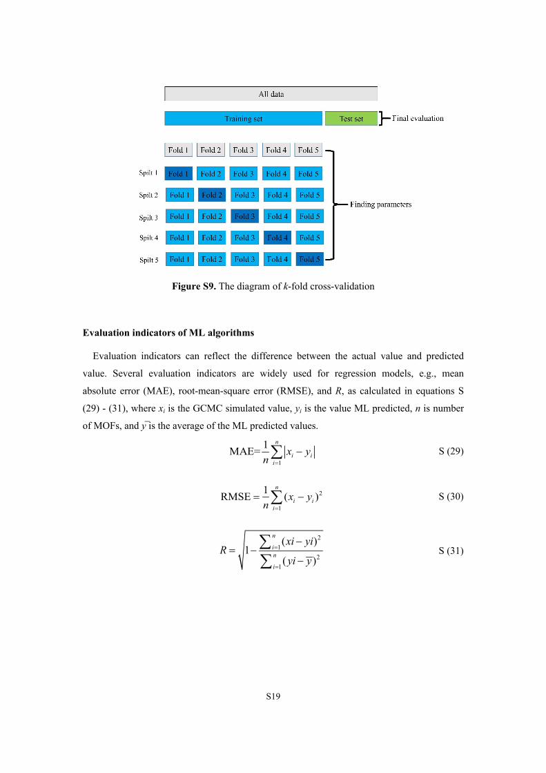
k-fold Cross Validation

Generally speaking, a model has multiple hyperparameters. The different hyperparameters

control the accuracy of the algorithm, and appropriate hyperparameters can reduce overfitting

and improve its prediction performance. This process of finding suitable parameters is

generally achieved by cross-validation, as shown in Figure S10. The all data set is divided

into two parts, namely the training set and test set. A test set is held out for to final evaluation.

In the basic way, called k-fold cross-validation, the training set is split into k smaller sets. The

following procedure is followed for each of the k “folds” (k=5): The k -1 of the fold data is

used to train the model, and the remaining one is used to validate the resulting model. Finally,

the parameter with the lowest average error is selected for each parameter.

S19

Figure S9. The diagram of k-fold cross-validation

Evaluation indicators of ML algorithms

Evaluation indicators can reflect the difference between the actual value and predicted

value. Several evaluation indicators are widely used for regression models, e.g., mean

absolute error (MAE), root-mean-square error (RMSE), and R, as calculated in equations S

(29) - (31), where xi is the GCMC simulated value, yi is the value ML predicted, n is number

of MOFs, and y̅ is the average of the ML predicted values.

S (29)1

1MAE=n

i ii

x yn

S (30)2

1

1RMSE ( )n

i ii

x yn

S (31)2

12

1

( )1

( )

n

in

i

xi yiR

yi y

S20

Hyperparameters of ML algorithms

The hyperparameters of a ML algorithm may largely determine its performance. In our

research, the hyperparameters of all ML algorithms were determined by the grid search with

cross-validation. RR is a linear regression model that fits two or more variables. In this

algorithm, we used the linear_model.Ridge function and complexity parameter α = 0.001.

BPNN is the most widely used type of neural network, which is a multi-layer feed-forward

neural network trained according to the error back-propagation algorithm. There are many

parameters of a BPNN, and the optimal parameters that we set are given below. The

activation function was the logistic sigmoid function. The loss function was the square-error,

and the number of hidden layer neurons was (30,30). The maximum number of iterations was

set to 500. The SVM looks for hyperplanes to achieve classification by mapping low-

dimensional data to a high-dimensional space. The SVR function was called to perform the

regression. The kernel function was set as radial basis function (rbf). The cost function (C)

and kernel coefficient (gamma) were 1 and 0.0001, respectively. The value of epsilon (half

the width of epsilon-insensitive band) was 0.1. A DT is a tree model established by binary

splitting. The goal is to create a model that predicts the value of a target variable by learning

simple decision rules inferred from the data features. The function DecisionTreeRegressor

was called for our regression task. The split and pruning criteria were based on the mean

squared error (MSE). The maximum depth of the tree and minimum number of samples

required to split an internal node were 25 and 85. A RF is similar to a GBRT, in that it is an

ensemble method and its base learners are all decision. The difference is that the ensemble-

aggregation method of the RF is bootstrap aggregating (bagging). The

RandomForestRegressor function was called for the RF, whose ensemble-aggregation method

is bag. The main parameters were the number of trees (n_estimators), minimum number of

samples required to split an internal node (min_samples_split) and maximum depth

(max_depth) of the tree of 300,40 and 15, respectively. The basic idea of the GBRT was to

construct a new weak learner (decision tree for our study) to provide the greatest correlation

with the negative gradient of the loss function and combined with the entire ensemble. We

called the GradientBoostingRegressor function, whose weak learner is a decision tree. The

loss function for the regression was the least-squares boosting (LSBoost). The maximum

depth of the tree and minimum number of samples required to split an internal node were 12

and 30, which controlled the size of each tree. The number of trees and learning rate that

yielded a minimum cross-validated MSE were 200 and 0.006, respectively. The

hyperparameters of all ML algorithms were listed in Table S6. Other parameters that are not

declared used the algorithm default.

S21

Table S5. Hyperparameters obtained by grid search with cross-validation.

ML algorithms Function Hyperparameters

RR linear_model.Ridge alpha=0.001

BPNN MLPRegressor max_iter=500 hidden_layer_sizes=(30,30) activation='logistic'

SVM SVR kernel='rbf' C=1 gamma=0.0001 epsilon=0.1

DT DecisionTreeRegressor max_depth=25 min_samples_split=85

RF RandomForestRegressor n_estimators=300 max_depth=15 min_samples_split=

40

GBRT GradientBoostingRegressor

n_estimators=200 learning_rate=0.006 max_depth=12 min_samples_split=

30

S22

Structural-performance relationships in three applications

Figure S10. Relationships between performance (∆W and COP) and MOF descriptors in (a), (b): heat pump, (c), (d): refrigeration, and (e), (f): ice making. (1–5) represent different descriptors (Qst, ρ, ϕ, LCD, and VSA).

S23

0 100 200 300 400 5001.0

1.2

1.4

1.6

1.8

2.0

Tdes=365 K for CoRE-MOFs Tdes=355 K for CoRE-MOFs Tdes=365 K for hMOFs Tdes=355 K for hMOFs

COP H

W (mg/g)

(a)

0 100 200 300 400 5000.0

0.2

0.4

0.6

0.8

1.0

Tdes=340 K for CoRE-MOFs Tdes=330 K for CoRE-MOFs Tdes=340 K for hMOFs Tdes=330 K for hMOFs

COP C

W (mg/g)

(b)

0 50 100 150 200 250 3000.0

0.2

0.4

0.6

0.8

1.0(c)

Tdes=340 K for CoRE-MOFs Tdes=330 K for CoRE-MOFs Tdes=340 K for hMOFs Tdes=330 K for hMOFs

COP C

W (mg/g)

Figure S11. COPC−∆W relationships in the three applications, including (a) heat pump, (b) refrigeration and (c) ice making.

S24

Relationships of the cost-ΔW and COP of three applications

Cost of heat pump

Figure S12. Relationships of the Ccycle, Cequipment, CMOF and Ctotal with ΔW.

S25

Figure S13. Relationships of the Ccycle, Cequipment, CMOF and Ctotal with COPH.

S26

Cost of refrigeration and ice making

Figure S14. Relationships of ΔW ~ Ctotal and COP ~ Ctotal in refrigeration (a-b) and ice

making (c-d).

Table S6. Three different cost percentages of top MOFs.

Cost percentage (%)TOP MOFs Ccycle Cequipment CMOF

Limit of Caverage (USD/kJ)

TOP50 42.6 56.8 0.6 2.0TOP100 39.7 59.5 0.8 2.4TOP200 35.8 63.1 1.1 2.8TOP400 31.4 67.0 1.5 3.4TOP600 28.9 69.2 1.9 3.9TOP800 26.9 70.8 2.2 4.4TOP1000 25.2 72.2 2.6 5.0

(a) (b)

(c)

S27

Sensitivity analysis of cycle stability and MOF price

Figure S15. (a) Caverage with different CYMOFs; (b) Caverage with different MOF prices when CYMOFs = 5000; (c) Caverage with different MOF prices when CYMOFs = 500; Percentages of three costs for (d) different CYMOFs, (e) different MOF prices when CYMOFs = 5000, (f) different MOF prices when CYMOFs = 500. These Caverage and percentages of three costs are calculated using the data of TOP 50 MOFs in heat pump state 2.

S28

Prediction of Ctotal by ML

Figure S16. Prediction of Ctotal in State 2 by 6 ML methods of (a) RR, (b) BPNN, (c) SVM, (d) DT, (e) RF, and (f) GBRT versus the GCMC simulated results for CoRE-MOFs on the test set.

S29

Table S7. Evaluation of the predicted results of MLs.

Evaluation indicator of MLTraining set Test setPerformance ML algorithms

R value MAE RMSE R value MAE RMSERR 0.669 0.264 0.431 0.636 0.266 0.418 BPNN 0.750 0.242 0.366 0.740 0.253 0.365 SVM 0.778 0.184 0.348 0.725 0.226 0.373 DT 0.824 0.185 0.314 0.811 0.204 0.317 RF 0.902 0.144 0.240 0.876 0.166 0.262

Ctotal

GBRT 0.899 0.155 0.242 0.838 0.189 0.296 Without metal of Ctotal

RF 0.892 0.149 0.249 0.873 0.170 0.264

S30

Table S8. Relative importance of variables was predicted by the RF.

Relative importance (%）TOP

MOFs Descriptors Metal LCD ϕ VSA PLD ρ Qst

TOP500 91.4 8.6 11.8 16.2 17.8 4.9 32.3 17.1

TOP1000 90.5 9.5 14.9 15.5 12.3 10.8 28.7 17.7

TOP2000 89.5 10.5 16.2 14.3 13.5 14.7 22.4 18.8

TOP4000 83.5 16.5 16.5 13.7 14.5 12.3 20.8 22.2

All MOFs 78.5 21.5 10.3 14.0 12.1 11.0 20.0 32.6

S31

Table S9. The top six CoRE-MOFs with low costs for three applications in state 1.

No CSD code LCD(Å) ϕ VSA(m2/cm3) PLD(Å) ρ

(kg/m3)Qst

(kJ/mol) COP ΔW (cm3/cm3)

Ccycle(USD)

Cequipment(USD)

CMOF(USD)

Ctotal(USD)

Caverage(USD/kJ)b

heat pump (Tdes1=355 K)

1 ECOLEP 11.64 0.89 1786.97 10.92 437.23 46.99 1.46 45.08 22.43 180.78 4.49 207.70 1.04

2 WONZUV 11.46 0.76 1969.48 9.81 607.72 42.42 1.59 62.59 20.67 227.10 6.06 253.84 1.27

3 RAHNOF 19.04 0.84 2064.04 6.57 594.85 44.32 1.62 62.79 20.29 228.67 5.96 254.91 1.27

4 ALUKOI 8.55 0.82 2946.85 6.75 579.93 40.25 1.57 58.29 20.90 228.36 6.25 255.51 1.28

5 XUXPUD 16.79 0.83 1341.48 16.72 713.15 43.29 1.59 68.69 20.59 244.45 6.98 272.02 1.36

6 WOLREV 9.92 0.79 2315.42 5.89 624.70 40.77 1.52 55.29 21.54 245.36 7.62 274.53 1.37

refrigeration (Tdes1=330 K)

1 ANUGIA 13.85 0.85 2104.24 6.76 567.97 34.69 0.80 99.53 11.59 342.59 5.38 359.56 1.80

2 GIHZAZ 9.57 0.74 1931.06 5.43 668.79 34.28 0.77 84.75 12.12 473.73 10.28 496.13 2.48

3 OFAWEZ 10.67 0.81 2182.60 9.08 975.20 37.94 0.80 115.91 11.62 505.08 11.69 528.38 2.64

4 PUFSEQ 13.39 0.86 2277.85 12.66 628.98 34.33 0.74 69.11 12.50 546.38 13.68 572.56 2.86

5 ECAHUN 12.33 0.55 1034.78 11.34 854.13 35.34 0.81 86.33 11.50 594.00 16.16 621.67 3.11

6 OFAWAV 11.43 0.81 2157.44 8.90 968.51 39.49 0.73 93.29 12.66 623.25 17.80 653.71 3.27

ice making (Tdes1=330 k)

1 VUJBEI 18.45 0.85 2079.05 6.58 562.57 39.96 0.44 18.74 21.25 1787.29 147.56 1956.10 9.78

2 DOTSOV03 13.27 0.76 1858.11 6.69 887.05 51.66 0.35 26.47 26.87 1995.10 183.87 2205.84 11.03

3 FIRNAX 6.71 0.73 2276.35 6.02 728.30 48.62 0.35 20.51 26.31 2114.42 206.52 2347.25 11.74

4 OWIVEW 6.91 0.68 2677.56 4.44 826.74 42.90 0.38 22.87 24.27 2152.37 214.00 2390.65 11.95

5 DOTSOV31 13.25 0.76 1859.07 6.70 888.41 47.77 0.33 23.89 28.05 2213.82 226.39 2468.26 12.34

6 DOTSOV42 13.31 0.75 1828.55 6.68 884.63 44.36 0.33 22.48 28.50 2342.80 253.54 2624.84 13.12

S32

Table S10. The top six CoRE-MOFs with low costs for three applications in state 2.

No CSD code LCD(Å) ϕ VSA(m2/cm3) PLD(Å) ρ

(kg/m3)Qst

(kJ/mol) COP ΔW (cm3/cm3)

Ccycle(USD)

Cequipment(USD)

CMOF(USD)

Ctotal(USD)

Caverage(USD/kJ)b

heat pump (Tdes2=365 K)1 ANUGOG 11.39 0.84 2327.76 7.09 584.66 43.69 1.82 209.44 77.94 79.76 0.61 158.31 0.79

2 NIGBOW 11.81 0.75 1612.67 11.57 664.85 46.63 1.78 224.55 79.95 81.94 0.67 162.56 0.81

3 ANUGUM 8.23 0.81 2323.73 6.99 680.31 48.72 1.75 222.62 81.33 82.69 0.69 164.72 0.82

4 EPOTAF 7.63 0.81 2982.06 6.61 575.24 47.03 1.76 180.58 80.84 86.89 0.76 168.50 0.84

5 TOHSAL 9.79 0.80 2399.04 6.18 576.20 44.03 1.81 179.22 79.45 89.91 0.80 170.15 0.85

6 TEDGOA 8.51 0.77 2250.91 7.78 691.02 43.77 1.79 214.42 78.60 90.92 0.80 170.32 0.85

refrigeration (Tdes2=340 K)1 ANUGIA 13.85 0.85 2104.24 6.76 567.97 34.69 0.87 220.44 18.75 154.68 1.10 174.53 0.87

2 SUKYON 10.80 0.85 2606.44 7.29 526.51 36.70 0.76 202.51 21.56 156.08 1.12 178.76 0.89

3 NIMPEG01 8.44 0.78 2433.00 5.51 607.49 37.96 0.80 230.32 20.39 158.35 1.15 179.89 0.90

4 ANUGOG 11.39 0.84 2327.76 7.09 584.66 37.13 0.76 211.05 21.66 166.31 1.27 189.24 0.95

5 TOHSAL 9.79 0.80 2399.04 6.18 576.20 42.40 0.77 196.74 22.05 175.83 1.42 199.29 1.00

6 EPOTAF 7.63 0.81 2982.06 6.61 575.24 37.46 0.70 192.94 23.35 178.99 1.47 203.80 1.02

ice making (Tdes2=340 k)1 GUKQUZ 16.94 0.84 2186.96 7.26 592.37 39.59 0.77 115.61 21.43 305.05 4.30 330.78 1.65

2 CEKHIL 8.91 0.82 2600.79 6.79 613.58 45.28 0.76 117.06 21.60 312.09 4.50 338.19 1.69

3 MOYYIJ 12.42 0.72 2092.01 9.38 730.59 46.02 0.89 118.73 18.46 366.36 6.20 391.01 1.96

4 CORZOA 11.07 0.81 2494.44 6.47 744.73 48.46 0.75 119.64 21.89 370.61 6.34 398.85 1.99

5 NEDWIE 8.99 0.72 2064.26 6.43 682.79 43.97 0.84 103.68 19.49 392.11 7.10 418.70 2.09

6 RAPYUE 8.10 0.73 2425.84 5.75 856.91 47.64 0.79 129.37 20.89 394.37 7.18 422.44 2.11

S33

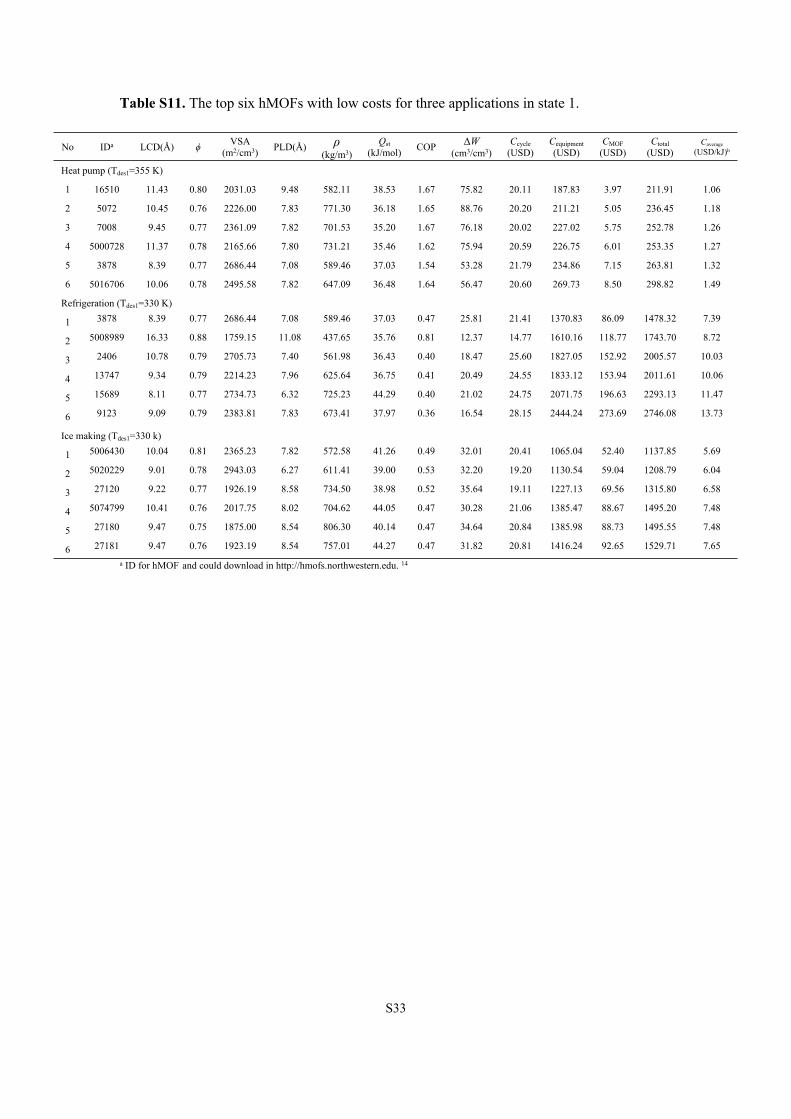
Table S11. The top six hMOFs with low costs for three applications in state 1.

No IDa LCD(Å) ϕ VSA(m2/cm3) PLD(Å) ρ

(kg/m3)Qst

(kJ/mol) COP ΔW (cm3/cm3)

Ccycle(USD)

Cequipment(USD)

CMOF(USD)

Ctotal(USD)

Caverage(USD/kJ)b

Heat pump (Tdes1=355 K)

1 16510 11.43 0.80 2031.03 9.48 582.11 38.53 1.67 75.82 20.11 187.83 3.97 211.91 1.06

2 5072 10.45 0.76 2226.00 7.83 771.30 36.18 1.65 88.76 20.20 211.21 5.05 236.45 1.18

3 7008 9.45 0.77 2361.09 7.82 701.53 35.20 1.67 76.18 20.02 227.02 5.75 252.78 1.26

4 5000728 11.37 0.78 2165.66 7.80 731.21 35.46 1.62 75.94 20.59 226.75 6.01 253.35 1.27

5 3878 8.39 0.77 2686.44 7.08 589.46 37.03 1.54 53.28 21.79 234.86 7.15 263.81 1.32

6 5016706 10.06 0.78 2495.58 7.82 647.09 36.48 1.64 56.47 20.60 269.73 8.50 298.82 1.49

Refrigeration (Tdes1=330 K)

1 3878 8.39 0.77 2686.44 7.08 589.46 37.03 0.47 25.81 21.41 1370.83 86.09 1478.32 7.39

2 5008989 16.33 0.88 1759.15 11.08 437.65 35.76 0.81 12.37 14.77 1610.16 118.77 1743.70 8.72

3 2406 10.78 0.79 2705.73 7.40 561.98 36.43 0.40 18.47 25.60 1827.05 152.92 2005.57 10.03

4 13747 9.34 0.79 2214.23 7.96 625.64 36.75 0.41 20.49 24.55 1833.12 153.94 2011.61 10.06

5 15689 8.11 0.77 2734.73 6.32 725.23 44.29 0.40 21.02 24.75 2071.75 196.63 2293.13 11.47

6 9123 9.09 0.79 2383.81 7.83 673.41 37.97 0.36 16.54 28.15 2444.24 273.69 2746.08 13.73

Ice making (Tdes1=330 k)

1 5006430 10.04 0.81 2365.23 7.82 572.58 41.26 0.49 32.01 20.41 1065.04 52.40 1137.85 5.69

2 5020229 9.01 0.78 2943.03 6.27 611.41 39.00 0.53 32.20 19.20 1130.54 59.04 1208.79 6.04

3 27120 9.22 0.77 1926.19 8.58 734.50 38.98 0.52 35.64 19.11 1227.13 69.56 1315.80 6.58

4 5074799 10.41 0.76 2017.75 8.02 704.62 44.05 0.47 30.28 21.06 1385.47 88.67 1495.20 7.48

5 27180 9.47 0.75 1875.00 8.54 806.30 40.14 0.47 34.64 20.84 1385.98 88.73 1495.55 7.48

6 27181 9.47 0.76 1923.19 8.54 757.01 44.27 0.47 31.82 20.81 1416.24 92.65 1529.71 7.65

a ID for hMOF and could download in http://hmofs.northwestern.edu. 14

S34

Table S12. Top six hMOFs with low costs for three applications in state 2

No. IDa LCD (Å) ϕ VSA(m2/cm3) PLD (Å) ρ

(kg/m3)Qst

(kJ/mol) COP ΔW (cm3/cm3)

Ccycle(USD)

Cequipment(USD)

CMOF(USD)

Ctotal(USD)

Caverage(USD/kJ)b

Heat pump (Tdes2=365 K)

1 5063 11.37 0.78 2173.07 7.80 731.21 38.37 1.78 221.98 80.79 89.93 0.81 171.54 0.86

2 5009547 11.37 0.78 2173.16 7.80 731.21 37.60 1.83 221.59 78.70 93.16 0.85 172.71 0.86

3 5050050 10.99 0.81 2057.26 9.38 583.47 35.13 1.75 172.72 82.74 89.30 0.83 172.87 0.86

4 5072 10.45 0.76 2226.00 7.83 771.30 36.18 1.80 225.18 79.63 95.29 0.90 175.81 0.88

5 12888 11.37 0.78 2172.31 7.81 731.21 35.16 1.79 207.12 80.25 97.23 0.94 178.42 0.89

6 5000728 11.37 0.78 2165.66 7.80 731.21 35.46 1.77 204.41 81.32 96.82 0.95 179.09 0.90

Refrigeration (Tdes2=340 K)

1 4935 10.47 0.76 2225.35 7.83 771.40 39.15 0.80 205.10 21.02 225.79 2.34 249.14 1.25

2 5063 11.37 0.78 2173.07 7.80 731.21 38.37 0.76 192.69 21.92 227.82 2.38 252.11 1.26

3 5009547 11.37 0.78 2173.16 7.80 731.21 37.60 0.74 186.96 22.61 234.79 2.53 259.93 1.30

4 12888 11.37 0.78 2172.31 7.81 731.21 35.16 0.75 184.51 22.35 237.91 2.59 262.86 1.31

5 5000728 11.37 0.78 2165.66 7.80 731.21 35.46 0.73 177.77 22.94 246.94 2.79 272.67 1.36

6 16510 11.43 0.80 2031.03 9.48 582.11 38.53 0.74 128.09 22.92 272.83 3.41 299.16 1.50

Ice making (Tdes2=340 K)

1 5002346 9.77 0.80 2232.82 7.35 598.91 39.83 0.88 104.74 19.76 340.46 5.35 365.57 1.83

2 16510 11.43 0.80 2031.03 9.48 582.11 38.53 0.82 97.04 21.34 357.16 5.89 384.39 1.92

3 5040402 10.98 0.80 2160.63 9.12 587.09 39.50 0.71 90.55 24.40 386.01 6.88 417.29 2.09

4 5020229 9.01 0.78 2943.03 6.27 611.41 39.00 0.69 91.88 25.17 396.20 7.25 428.62 2.14

5 15210 13.44 0.79 1880.91 8.12 623.58 36.68 0.76 88.09 22.81 421.45 8.20 452.47 2.26

6 5020715 8.88 0.78 2404.11 6.15 674.54 36.09 0.80 94.56 21.72 424.70 8.33 454.75 2.27

a ID for hMOF and could download in http://hmofs.northwestern.edu. 14

S35

Atomistic structures of top MOFs

ECOLEP WONZUV RAHNOF

ALUKOI XUXPUD WOLREV

ANUGIA GIHZAZ OFAWEZ

S36

PUFSEQ ECAHUN OFAWAV

VUJBEI DOTSOV03 FIRNAX

OWIVEW DOTSOV31 DOTSOV42

S37

ANUGOG ANUGUM NIGBOW

EPOTAF TOHSAL TEDGOA

SUKYON NIMPEG01 RAPYUE

S38

GUKQUZ CEKHIL MOYYIJ

CORZOA NEDWIE

Figure S17. Atomistic structures of top 6 CoRE-MOFs for heat pumps in states 1 and 2.

S39

16510 5072 7008

5000728 3878 5016706

5008989 2406 13747

15689 9123 5020715

4935 5063 5009547

S40

12888 5006430 5020229

27120 5074799 27180

S41

27181 5050050 5002346

5040402 15210

Figure S18. Atomistic structures of top six hMOFs for heat pumps in states 1 and 2.

S42

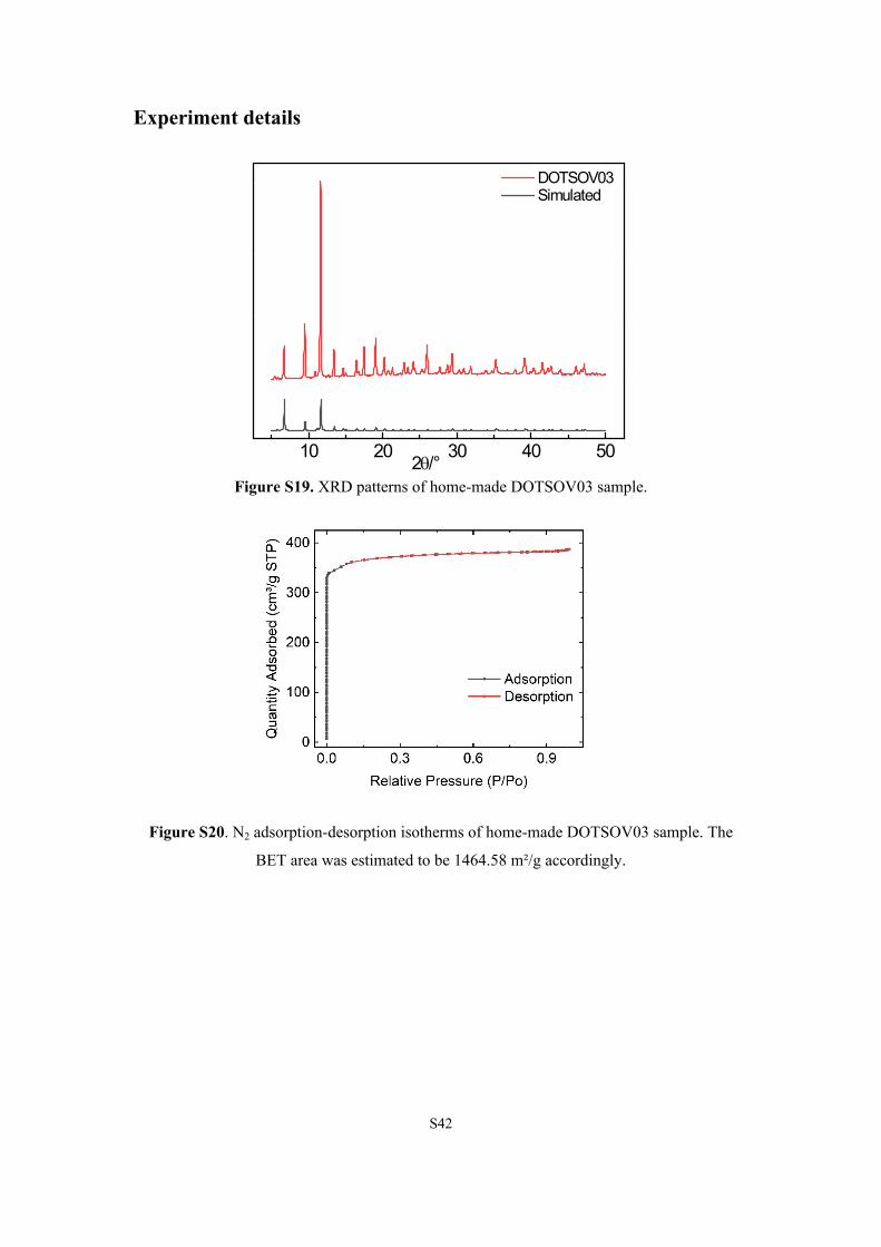
Experiment details

10 20 30 40 50

DOTSOV03 Simulated

2/°Figure S19. XRD patterns of home-made DOTSOV03 sample.

Figure S20. N2 adsorption-desorption isotherms of home-made DOTSOV03 sample. The

BET area was estimated to be 1464.58 m²/g accordingly.

S43

References

1. S. L. Mayo, B. D. Olafson and W. A. Goddard, J. Phys. Chem., 1990, 94, 8897-8909.

2. A. K. Rappe, C. J. Casewit, K. S. Colwell, W. A. G. Iii and W. M. Skiff, J. Am. Chem. Soc., 1992,

114, 10024-10035.

3. B. Chen, J. J. Potoff and J. I. Siepmann, J. Phys. Chem. B, 2001, 105, 3093-3104.

4. Z. Ke, R. P. Lively, M. E. Dose, A. J. Brown, Z. Chen, C. Jaeyub, N. Sankar, W. J. Koros and R. R.

Chance, Chem. Commun., 2013, 49, 3245-3247.

5. M. F. De Lange, B. L. van Velzen, C. P. Ottevanger, K. J. F. M. Verouden, L. C. Lin, T. J. H. Vlugt,

J. Gascon and F. Kapteijn, Langmuir, 2015, 31, 12783-12796.

6. M. U. Bin, WALTON and S. Krista, J. Phys. Chem. C, 2015, 115, 22748–22754.

7. M. F. De Lange, K. J. F. M. Verouden, T. J. H. Vlugt, J. Gascon and F. Kapteijn, Chem. Rev., 2015,

115, 12205-12250.

8. D. Lenzen, J. Zhao, S.-J. Ernst, M. Wahiduzzaman, A. K. Inge, D. Froehlich, H. Xu, H.-J. Bart, C.

Janiak, S. Henninger, G. Maurin, X. Zou and N. Stock, Nat. Commun., 2019, 10, 3025.

9. https://p4psearch.1688.com/p4p114/p4psearch/offer.htm?keywords=q235b&cosite=baidujj_pz&l

ocation=re&trackid=%7Btrackid%7D&spm=a2609.11209760.j3f8podl.e5rt432e&keywordid=%7B

keywordid%7D.

10.D. DeSantis, J. A. Mason, B. D. James, C. Houchins, J. R. Long and M. Veenstra, Energy Fuel.,

2017, 31, 2024-2032.

11.D. Dubbeldam, S. Calero, D. E. Ellis and R. Q. Snurr, Mol. Simulat., 2016, 42, 81-101.

12.https://scikit-learn.org/stable/modules/linear_model.html#ridge-regression-and-classification.

13.A. Natekin and A. Knoll, Front. Neurorob., 2013, 7, 21.

14.C. E. Wilmer, M. Leaf, C. Y. Lee, O. K. Farha, B. G. Hauser, J. T. Hupp and R. Q. Snurr, Nat.

Chem., 2012, 4, 83-89.