SDivision of EngineeringBROWN UNIVERSITY

PROVIDENCE, R. I.

FINITE-ELEMENT FORMULATIONS FOR

PROBLEMS OF LARGE ELASTIC-PLASTIC DEFORMATION 0A&518 ?

R. M. McMEEKING AND J. R. RICE

(NASA-CR- 138820) FINITE ELEENT!FORMULATIONS FOR PROBLEMS OF LARGE U74-284 1 02ELASTIC-PLASTIC DEFORATION (Brown Univ.)

CSCL 2CK UnclasG--3/32 43390

Technical ReportNASA NGL 40-002-080/15 to the

National Aeronautics and Space Administration

May 1974

i , ~

https://ntrs.nasa.gov/search.jsp?R=19740020297 2018-07-28T22:57:13+00:00Z

Finite-Element Formulations for Problems of Large Elastic-Plastic Deformation

by R. M. McMeeking and J. R. Rice

Division of Engineering, Brown University, Providence, Rhode Island

May 1974.

Abstract

An Eulerian finite element formulation is presented for problems of large

elastic-plastic flow. The method is based on Hill's variational principle for

incremental deformations, and is ideally suited to isotropically hardening

Prandtl-Reuss materials. Further, the formulation is given in a manner which-

allows any conventional finite element program, for "small strain" elastic-

plastic analysis, to be simply and rigorously adapted to problems involving

arbitrary amounts of deformation and arbitrary levels of stress in comparison

to plastic deformation moduli. The method is applied to a necking bifurcation

analysis of a bar in plane-strain tension.

The paper closes with a unified general formulation of finite element equa-

tions, both Lagrangian and Eulerian, for large deformations, with arbitrary

choice of the conjugate stress and strain measures. Further, a discussion is

given of other proposed formulations for elastic-plastic finite element analysis

at large strain, and the inadequacies of some of these are commented upon.

I

I

-1-

Introduction

Many elastic-plastic problems of interest involve large deformations and

the present paper is concerned with finite element formulations for this class

of problem. Such formulations are also relevant to small deformation elastic-

plastic problems. Indeed the conventional "small strain" formulation in stress

analysis can be inadequate for small strain problems not only when increments of

rotation greatly exceed those of strain (buckling of slender members) but also

when representative stress levels have attained a magnitude comparable to that

of the plastic hardening modulus. The latter can occur after only minute deforma-

tions for lightly hardening metals. These situations relate more to the shape of

the member under consideration and to intrinsic material properties, rather than

to the smallness or largeness of strain per se, but are best approached in a rig-

orous finite deformation context.

Several workers have proposed and utilized finite element schemes for problems

of finite deformation, and these include diverse formulations of both the Lagrangian

(material) and Eulerian (spatial) type. The next section gives a brief review of

these and includes some comments on ambiguities in certain of the approaches to

elastic-plastic behavior. Thereafter we proceed directly to an Eulerian formula-

tion which is ideally suited to the large deformation of Prandtl-Reuss materials.

This is given in a manner which allows the straightforward adaptation of any exist-

ing small strain program to finite deformation analysis. It also serves as a basis

for analysis of the possible inadequacies of the conventional small strain formula-

tion. The program is applied to a numerical study of the initiation of plastic

bifurcation in a plane strain tensile bar.

Finally, in the concluding section of the paper we have presented a general

formulation of the finite deformation problem in finite-element terms. By appro-

-2-

priate specialization this can be made to coincide with various separate formula-

tions, both Lagrangian and Eulerian, and provides a suitable basis for comparison

of the different approaches as well as for a fuller discussion of ambiguities in

other elastic-plastic formulations as noted above.

Review of Finite Elements for Finite Deformation

The description Lagrangian is attached to large deformation finite element

programs which use a mesh of elements representing some fixed reference state for

strain. A scheme of this type was proposed by Hibbitt, Marcal and Rice 11], who

derive their finite element rate equilibrium equations from the principle of

virtual work for large deformation. They identify four stiffness terms, which

are named small strain stiffness, initial load stiffness, initial strain stiffness

and initial stress stiffness. In elastic-plastic analysis, all of these must be

calculated for each increment of deformation and the last three have a complicated

form. Needleman [2] has a similar Lagrangian scheme, but he derives his equations

from a variational principle due to Hill [3]. A third Lagrangian formulation was

presented by Felippa and Sharifi [4], who intend to place no limitation on the size

of an increment of deformation. Higher order terms are thus introduced into their

stiffness. However, these terms are not significant in a tangent modulus approach to

elastic-plastic or non-linear elastic analysis, since the increment of deformation

must be small in any case to ensure that the constitutive rate moduli do not change

significantly from one increment to the next. For the materials mentioned the

method of [4] coincides with that of Ell].

The Eulerian formulation which is based on a mesh representing the current

state of deformation has been used by Yaghmai and Popov [5]. In their presentation

they derive equations from a current configuration version of the variational

-3-

principle used in [4] and solve an elastic problem. However, Sharifi and Popov

[63 extended the method of [5] to elastic-plastic analysis of infinitesimal

strains but finite rotations, although they do not seem to consider the possi-

bility that plastic deformation moduli may be of a size comparable to current

stress levels. Another Eulerian formulation is due to Gunasekera and Alexander

[7, who base their equations for a Prandtl-Reuss material on the principle of

virtual work. The finite element equilibrium equations they obtain are correct

if their stress g is interpreted as the 2nd Piola-Kirchhoff stress, but a state-

ment to this effect is not made. If their g is so identified, the constitutive

law used does not then seem to constitute an adequate form of the Prandtl-Reuss

equations. There also seems to be an ambiguity in work on an Eulerian formula-

tion for Prandtl-Reuss materials by Argyris and Chan [8], who do not make a clear

definition of their stress and strain terms. Two interpretations appear possible,

but neither constitutes an adequate finite element method. This point is discussed

in the final section of the paper, along with further comments on [6] and [7).

Osias [9] has an Eulerian scheme, which admits non-symmetric constitutive laws

through a Galerkin method. He derives the same rate equilibrium equations as ob-

tained here, but his constitutive law leads to a non-symmetric stiffness.

An Eulerian Finite Element Formulation for Finite Deformation

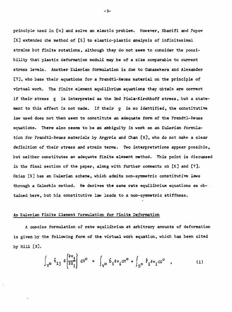
A concise formulation of rate equilibrium at arbitrary amounts of deformation

is given by the following form of the virtual work equation, which has been cited

by Hill [3].

S6 v o o fdVo+ fo vdS (1)

-4-

where all integration extents are in the reference configuration and X is the

position vector of a material point in that reference state. t is the non-sym-

metric nominal stress, which is defined so that the force vector f per unit

oreference area of a surface having the reference unit normal n is given by

of = n.t.. , and b is the body force per unit reference volume. Rates are

indicated by the superposed dot and 6v is an arbitrary virtual velocity varia-

tion which disappears where velocity rates are prescribed i.e. on S - S ,T

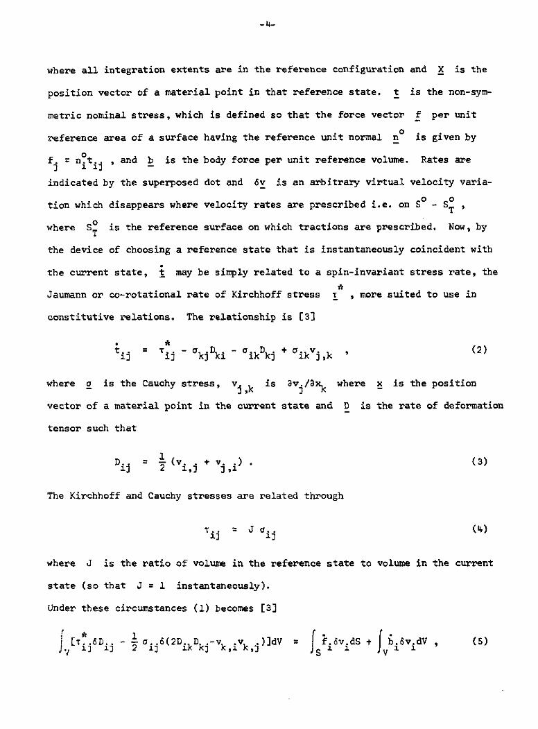
where S0 is the reference surface on which tractions are prescribed. Now, by

the device of choosing a reference state that is instantaneously coincident with

the current state, i may be simply related to a spin-invariant stress rate, the

Jaumann or co-rotational rate of Kirchhoff stress T , more suited to use in

constitutive relations. The relationship is [3

S = Tij - akj Dki ikDkj + ikjk (2)

where a is the Cauchy stress, v.j,k is av./x k where x is the position

vector of a material point in the current state and D is the rate of deformation

tensor such that

D.. = - (v. + v. (3)13 2 i) 3,i

The Kirchhoff and Cauchy stresses are related through

S.. =Jo.. (4)

where J is the ratio of volume in the reference state to volume in the current

state (so that J = 1 instantaneously).

Under these circumstances (1) becomes [3]

I..6D. oi .. 6(2D kD kj-vki vk )]dV = .iv.dS + b 6vidV , (5).. 1 j 1j 2 1kS 1

-5-

where all integration extents are in the current configuration. f and b are

still nominal force intensity rates, but with respect to the current areas.

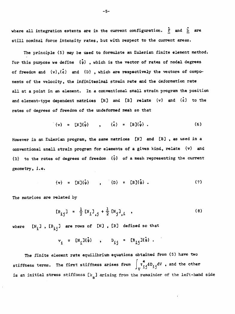
The principle (5) may be used to formulate an Eulerian finite element method.

For this purpose we define {*} , which is the vector of rates of nodal degrees

of freedom and {v),{c) and {D} , which are respectively the vectors of compo-

nents of the velocity, the infinitesimal strain rate and the deformation rate

all at a point in an element. In a conventional small strain program the position

and element-type dependent matrices [N] and [B) relate {v} and {c} to the

rates of degrees of freedom of the undeformed mesh so that

{v} = [N]{~} , {} = [B]{; }. (6)

However in an Eulerian program, the same matrices [N] and [B] , as used in a

conventional small strain program for elements of a given kind, relate {v} and

{D} to the rates of degrees of freedom {i) of a mesh representing the current

geometry, i.e.

{v} [N]{i} , {D} [B{;}) . (7)

The matrices are related by

[B.ij = ENl . + 1 [N. , (8)2 , 2 i

where [NiJ , [B..j are rows of [N] , [B] defined so that

v. [ N.]{ , Di. = [B ijif}

The finite element rate equilibrium equations obtained from (5) have two

stiffness terms. The first stiffness arises from I..6D..dV , and the other

is an initial stress stiffness [k ] arising from the remainder of the left-hand side

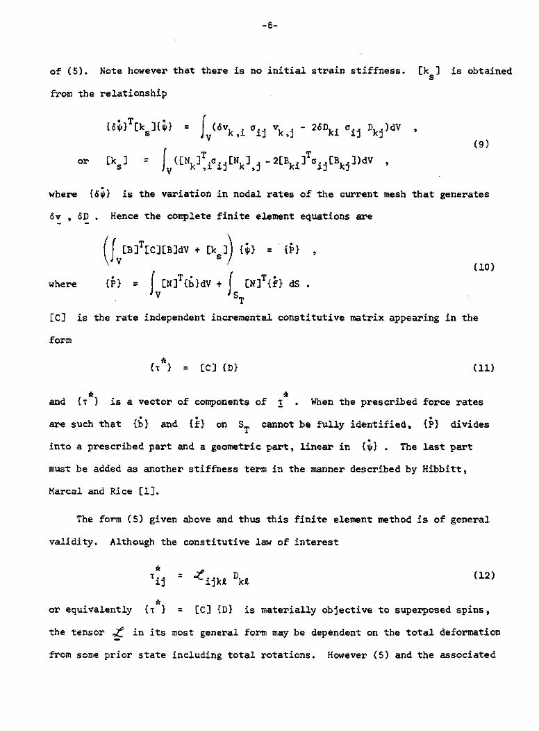
-6-

of (5). Note however that there is no initial strain stiffness. [ks ) is obtained

from the relationship

{6ip}T[k ]{} = (v ... v.- 26DDi . D)dVs V (6vk,i Oj 13 vkj 26Dki ij kj(9)

or [k] = ([N ]T.. .IN k -2[B ki]Ta [B ]) dVJvk ,1 k,j ki a5[kj

where {6;} is the variation in nodal rates of the current mesh that generates

6v , 6D . Hence the complete finite element equations are

(IV[B]TEC[BldV + Eks) ; (10)

where {} E= INT {}dV + TEN] {}} dS

[C] is the rate independent incremental constitutive matrix appearing in the

form

{T} = [C) (D) (11)

and {r I is a vector of components of r . When the prescribed force rates

are such that {b} and ({f on ST cannot be fully identified, {P} divides

into a prescribed part and a geometric part, linear in {;} . The last part

must be added as another stiffness term in the manner described by Hibbitt,

Marcal and Rice £1).

The form (5) given above and thus this finite element method is of general

validity. Although the constitutive law of interest

j.. = ij D (12)13 ijki k1

or equivalently {'r I [C) {D) is materially objective to superposed spins,

the tensor t in its most general form may be dependent on the total deformation

from some prior state including total rotations. However (5) and the associated

-7-

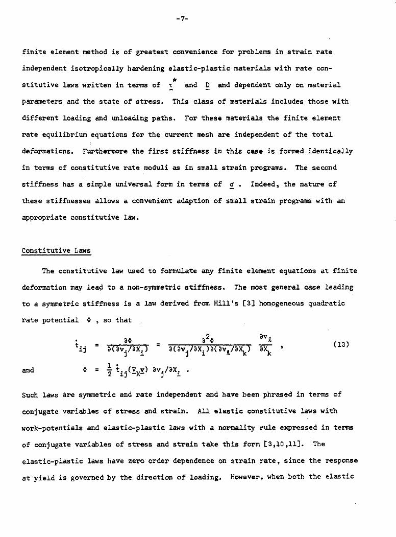
finite element method is of greatest convenience for problems in strain rate

independent isotropically hardening elastic-plastic materials with rate con-

stitutive laws written in terms of r and D and dependent only on material

parameters and the state of stress. This class of materials includes those with

different loading and unloading paths. For these materials the finite element

rate equilibrium equations for the current mesh are independent of the total

deformations. Furthermore the first stiffness in this case is formed identically

in terms of constitutive rate moduli as in small strain programs. The second

stiffness has a simple universal form in terms of a . Indeed, the nature of

these stiffnesses allows a convenient adaption of small strain programs with an

appropriate constitutive law.

Constitutive Laws

The constitutive law used to formulate any finite element equations at finite

deformation may lead to a non-symmetric stiffness. The most general case leading

to a symmetric stiffness is a law derived from Hill's [3] homogeneous quadratic

rate potential 4 , so that

= (13)1 a(av lax) a(av /axi)a(av/ak a x

and 4 = (X v) av /ax.2 ij X j *

Such laws are symmetric and rate independent and have been phrased in terms of

conjugate variables of stress and strain. All elastic constitutive laws with

work-potentials and elastic-plastic laws with a normality rule expressed in terms

of conjugate variables of stress and strain take this form [3,10,11]. The

elastic-plastic laws have zero order dependence on strain rate, since the response

at yield is governed by the direction of loading. However, when both the elastic

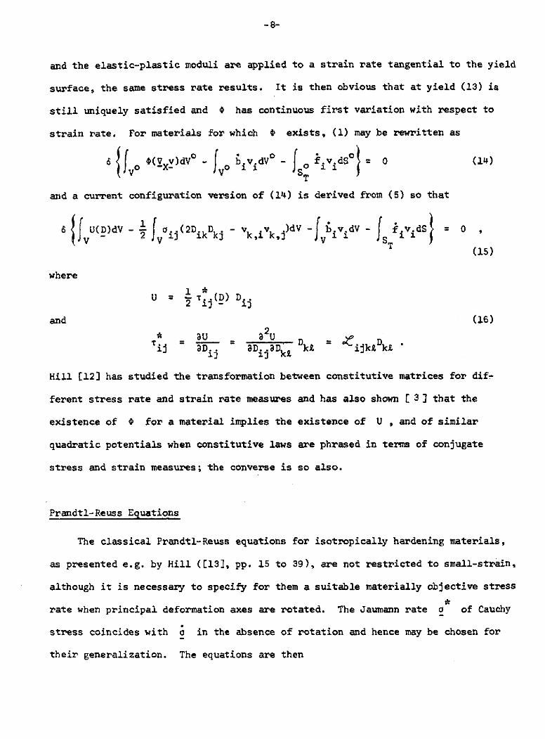
-8-

and the elastic-plastic moduli are applied to a strain rate tangential to the yield

surface, the same stress rate results. It is then obvious that at yield (13) is

still uniquely satisfied and 0 has continuous first variation with respect to

strain rate. For materials for which 0 exists, (1) may be rewritten as

6 IfV0 O(yXy)dVo f .v.dVo - I .d = o0 (14)Vo -- Vo I So J. .1

T

and a current configuration version of (14) is derived from (5) so that

6 U(D)dv - i( 2 DikD - )dV - bv.dV - f fiv.dS 0

(15)

where

1 *U T..(D) D..

and (16)

a U a 22UDD.. 8D. IDk Dk ijk£tDk•

Hill [12) has studied the transformation between constitutive matrices for dif-

ferent stress rate and strain rate measures and has also shown [ 3) that the

existence of 0 for a material implies the existence of U , and of similar

quadratic potentials when constitutive laws are phrased in terms of conjugate

stress and strain measures; the converse is so also.

Prandtl-Reuss Equations

The classical Prandtl-Reuss equations for isotropically hardening materials,

as presented e.g. by Hill ([13], pp. 15 to 39), are not restricted to small-strain,

although it is necessary to specify for them a suitable materially objective stress

rate when principal deformation axes are rotated. The Jaumann rate a of Cauchy

stress coincides with o in the absence of rotation and hence may be chosen for

their generalization. The equations are then

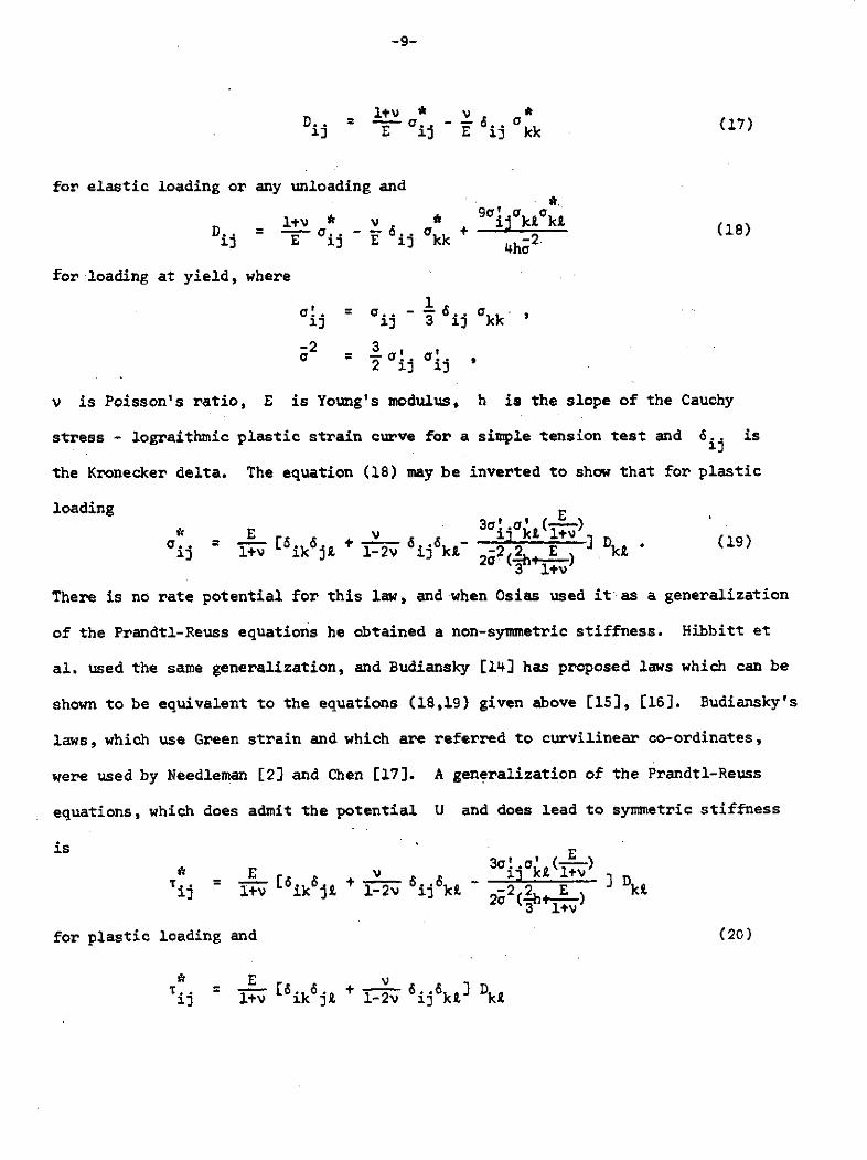
-.9-

l+v * v *D.. -- a 6.. a (17)13 E ij E 13 kk

for elastic loading or any unloading and

S90 .a aD.. =l+v- -- - n k +kL (18)

ij E ij E ij kk -2.4ha

for loading at yield, where

11j ij 3 ij kk

-2 a3 a j ,2 ii ii

v is Poisson's ratio, E is Young's modulus, h is the slope of the Cauchy

stress - lograithmic plastic strain curve for a simple tension test and 6.. is

the Kronecker delta. The equation (18) may be inverted to show that for plastic

loading E* E v 11 kt1+VI.. = - 6+ 6 6 - ijkl+ (19)ij 1+v ik ji 1-2v i kA 2 2 ( E2 E k9)20(-h----)

There is no rate potential for this law, and when Osias used it as a generalization

of the Prandtl-Reuss equations he obtained a non-symmetric stiffness. Hibbitt et

al. used the same generalization, and Budiansky (l1) has proposed laws which can be

shown to be equivalent to the equations (18,19) given above [15], (16. Budiansky's

laws, which use Green strain and which are referred to curvilinear co-ordinates,

were used by Needleman [2) and Chen [17]. A generalization of the Prandtl-Reuss

equations, which does admit the potential U and does lead to symmetric stiffness

is E3o!.' (-)

E 6v j kt l+ DV.. = -16. 6..6 -li+v i 1 1-2v 13 kt -2 E k

S 1l+v

for plastic loading and (20)

* E v. = -- 6ik6j + - 6 6ij ] Dij l+v ik i. 1-2v ij kt k£

-10-

for elastic loading or any unloading. This law is referred to a current config-

uration and is equivalent to (17), (18) and (19) to within terms of stress

divided by elastic modulus since volume change is taken to be purely elastic.

Needleman and Chen note this equivalency and although they postulate that

Budiansky's equations govern material response, they use equations equivalent to

(20) for their calculations. This last form has also been introduced and dis-

cussed by Hutchinson (16). It should be noted that the elasticity in (20) is

approximately derivable from a work potential to within terms of stress divided

by elastic modulus in comparison to unity [18). As stated previously a rate

potential must evidently exist for elastic response, and (20) but not (19) is in

accord with this. The matrix [C] for the law (20) is homogeneous of degree zero

in {) , in the usual manner, for elastic-plastic materials at yield. Since

this CC] is also the constitutive matrix relating stress rate to {c in a

small strain program, the stiffness of such a program calculated in current con-

figuration constitutes one term of the stiffness of the Eulerian finite deforma-

tion program. To this must be added [ks ] to form the complete stiffness.

Conventional Small Strain Formulation

The conventional small strain principle of virtual work may be written as

..cdV = b.vtdV + i f. vdS (21)V ijf S i

where a is the stress field in equilibrium with surface tractions f and body

forces b , £ is the virtual rate of the infinitesimal strain tensor and is

compatible with the virtual velocity field v , S is the surface of the body

-11-

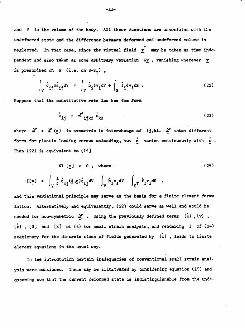
and V is the volume of the body. All these functions are associated with the

undeformed state and the difference between deformed and undeformed volume is

neglected. In that case, since the virtual field v may be taken as time inde-

pendent and also taken as some arbitrary variation dv , vanishing wherever v

is prescribed on S (i.e. on S-ST)

I .ij6 ijdV = b.6v.dV + fI.6v dS . (22)V V S

Suppose that the constitutive rate law has the form

ij = ij;k (23)

where ( = (a) is symmetric in interchange of ij,kL. . takes different

forms for plastic loading versus unloading, but a varies continuously with .

Then (22) is equivalent to [19]

61 [v] = 0 , where (24)

I[v] = . (i ' ) 6dV - f vidV - fT v dS- 2 15 fV V S

and this variational principle may serve as the basis for a finite element formu-

lation. Alternatively and equivalently, (22) could serve as well and would be

needed for non-symmetric e . Using the previously defined terms {;} , {v} ,

{;} , [N) and [B) of (6) for small strain analysis, and rendering I of (24)

stationary for the discrete class of fields generated by {4} , leads to finite

element equations in the usual way.

In the introduction certain inadequacies of conventional small strain anal-

ysis were mentioned. These may be illustrated by considering equation (15) and

assuming now that the current deformed state is indistinguishable from the unde-

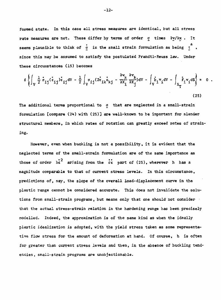
-12-

formed state. In this case all stress measures are identical, but all stress

rate measures are not. These differ by terms of order a times av/ax . It

seems plausible to think of a in the small strain formulation as being T

since this may be assumed to satisfy the postulated Prandtl-Reuss law. Under

these circumstances (15) becomes

1 e. * 1 avk- a..(. )..dV - -J a. (2c - k)dV - b idV - fivddS = 0

(V -2 1 2 V2 j( 2ik kj ax d V 1 1

(25)

The additional terms proportional to a that are neglected in a small-strain

formulation [compare (24) with (25)] are well-known to be important for slender

structural members, in which rates of rotation can greatly exceed rates of strain-

ing.

However, even when buckling is not a possibility, it is evident that the

neglected terms of the small-strain formulation are of the same importance as

those of order he2 arising from the ac part of (25), wherever h has a

magnitude comparable to that of current stress levels. In this circumstance,

predictions of, say, the slope of the overall load-displacement curve in the

plastic range cannot be considered accurate. This does not invalidate the solu-

tions from small-strain programs, but means only that one should not consider

that the actual stress-strain relation in the hardening range has been precisely

modelled. Indeed, the approximation is of the same kind as when the ideally

plastic idealization is adopted, with the yield stress taken as some representa-

tive flow stress for the amount of deformation at hand. Of course, h is often

far greater than current stress levels and then, in the absence of buckling tend-

encies, small-strain programs are unobjectionable.

Some Numerical Results

The Eulerian elastic-plastic finite deformation scheme was incorporated in

the manner described into an existing small-strain program, that is a modified

version of the relevant part of the MARC program developed by Professor P. V.

Marcal, and in use on the IBM 360-67 computer at Brown University. This program

models elastic-plastic Prandtl-Reuss materials in a manner described by Tracey

[20]. An iterative procedure attempts convergence to a best solution during an

elastic-plastic increment, incremental stiffness being calculated by the partial

stiffness approach of Marcal and King [21), subsequently modified by Rice and

Tracey [22].

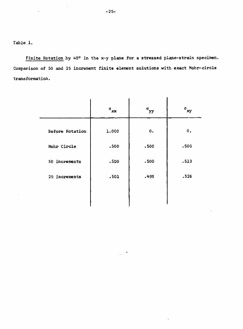
A first example illustrates the treatment of finite rotations by this scheme,

and uses 4 elements forming a square, which was stressed to represent a state of

elastic plane strain. Of the 10 degrees of freedom, 8 were constrained to cause

a rotation of f/4 radians in first 50 and then 25 increments. The results

correspond closely to the exact solution as given by a simple Mohr circle trans-

formation, and are shown in the table.

A solution for the initiation of tensile necking of an elastic-plastic bar

in plane strain with a constant hardening modulus was also obtained. Osias [9

studied a similar problem. The bar had a ratio of length to width of 3 and the

center 1/6th of the length was thinned by 0.5% so the analysis could be formu-

lated as a standard deformation problem rather than an eigenvalue problem for

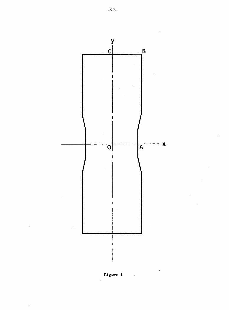
abrupt bifurcation. One quarter of the bar was analyzed using finite elements

and this section is marked OABC in fig. 1 of the specimen with the thinning

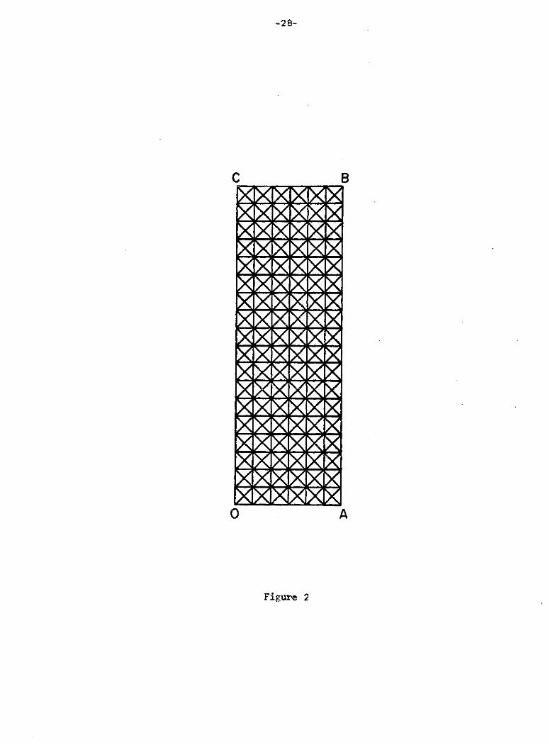
greatly exaggerated. There were 432 elements in the mesh and 241 nodes, as shown

in fig. 2. Uniform strain elements in the crossed array shown were chosen because

Nagtegaal, Parks, and Rice [23 have recently shown this array to be exceptionally

-14-

free of artificial constraints for incompressible or near incompressible deforma-

tion. The material modelled had a ratio of Young's modulus to equivalent Cauchy

yield stress of 7.5 x 102 , Poisson's ratio was 0.3 and the ratio of hardening

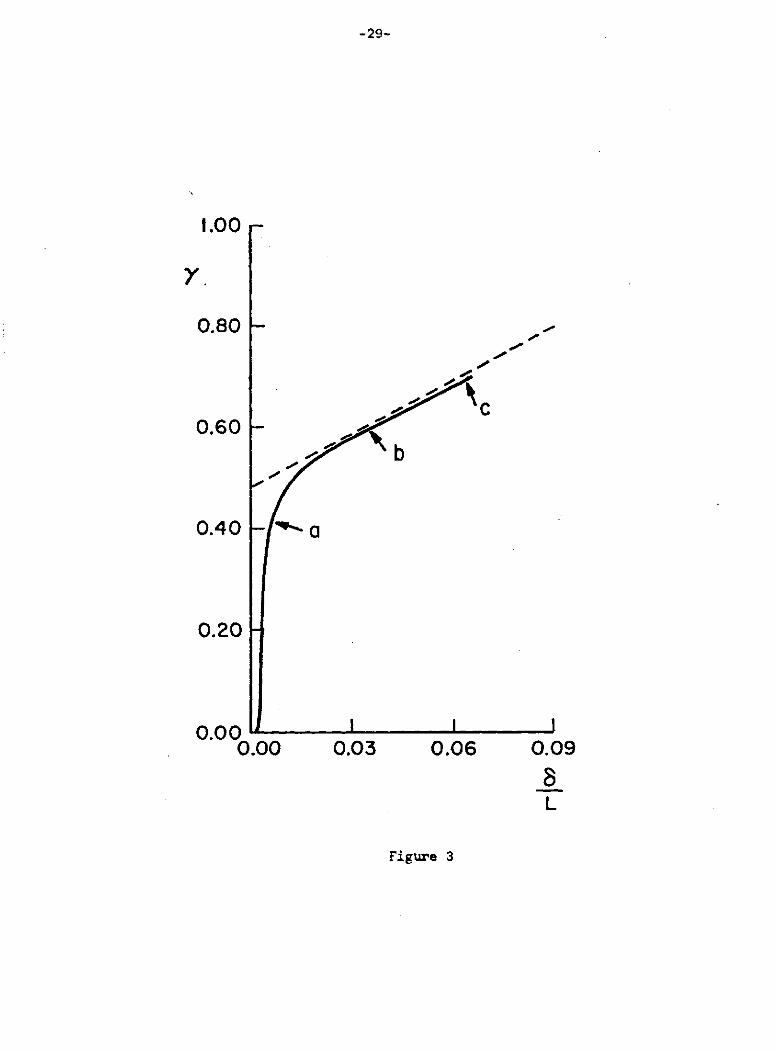
modulus to yield stress was constant at 1.25. The results are shown by the full

line in fig. 3, where the amplitude 6 of the neck (i.e., the width reduction at

the center section), normalized by the initial length L , is plotted against

engineering strain y = AL/L . A Fourier analysis of the neck showed that the

lateral bar surfaces deformed most dominantly in cosine shape that is predicted

from the rigid plastic analysis of Cowper and Onat [24). In fig. 3, point a

is maximum load, point b is the point at which elastic unloading first occurs

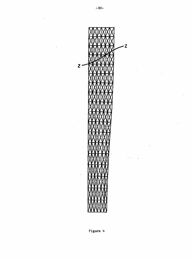
and point c corresponds to the specimen illustrated in fig. 4 with the boundary

between the elastic elements and the plastic elements marked zz . Those ele-

ments, which have unloaded elastically, are above the line zz .

It is known [25) that abrupt plastic bifurcation in an elastic-plastic or

rigid-plastic body must occur with the overall deformation increasing at a def-

inite initial rate with respect to the bifurcation amplitude. This rate just

causes neutral local stress alteration at a single point or locus of points, with

subsequent local unloading toward an elastic or rigid state. The dashed line in

fig. 3 is drawn at a slope in accord with that of the initial strain vs. bifurca-

tion amplitude slope predicted from the Cowper-Onat solution. The line is located

so as to cross the vertical axis at the critical strain predicted from their re-

sults (phrased in terms of a critical ratio of hardening rate to true stress,

dependent on the current length to width ratio for the bar). It is seen that the

large growth of the initial imperfection as predicted from the finite element

solution is in close accord with their results. Cowper and Onat found that neu-

tral loading occurs at a point corresponding to point C in fig. 1, and suggested

-15-

that unloading would spread from there towards the side AB of the bar and down

to the center line OA . This occurred in the numerical analysis of the elastic-

plastic bar, and it can be seen from fig. 3 that once elastic unloading occurred,

this analysis began to deviate from dashed line initial slope for the rigid-

plastic bar.

The numerical results do not, however, show the inception of unloading at

strains very near the amplitude at which large growth of the imperfection sets

in, as would be expected from the general result noted earlier for abrupt plastic

bifurcations. Also while it is clear that concentration of deformation in the

neck and elastic unloading at the end of the bar are both occurring in the numer-

ical analysis, neither are occurring to a great extent. Another aspect of the

analysis is that the elements in the neck are elongated in one direction, which

has reduced their accuracy. Any further extension of the bar would only aggravate

this problem, and thus it would not be profitable to continue the analysis. The

elongation of these elements may seem to reduce the value of this Eulerian formu-

lation as opposed to a Lagrangian formulation, where the elements retain their

shape. However, the same effect is embedded in the stiffness of the Lagrangian

elements and they have no advantage in this respect.

The latter inadequacy at large deformation in the neck is clearly traceable

to element size; and smaller elements may also cause the inception of neutral

loading to take place earlier. For example, Osias [93 used a finer mesh and,

while no comparison of his results with the Cowper-Onat solution was made, he

did find the inception of unloading at a lower strain and a faster spread of the

unloaded zone down the bar axis.

-16-

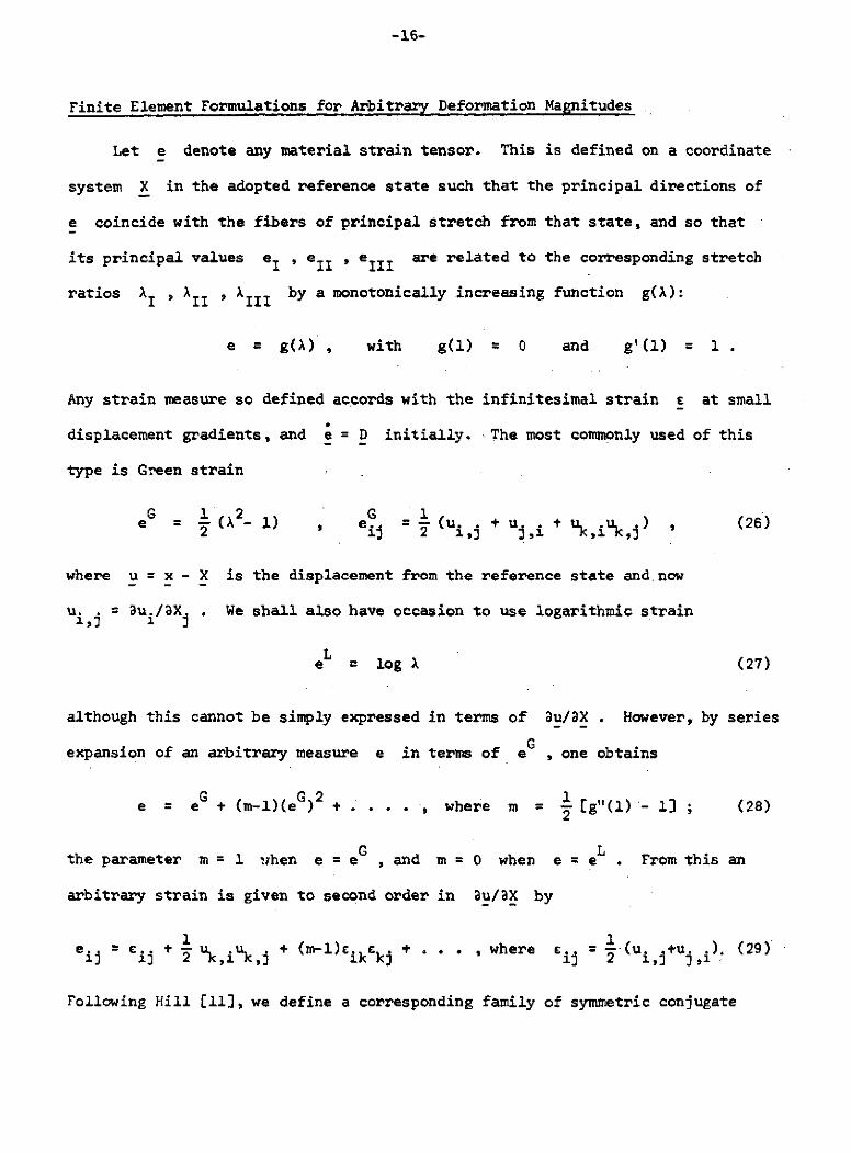
Finite Element Formulations for Arbitrary Deformation Magnitudes

Let e denote any material strain tensor. This is defined on a coordinate

system X in the adopted reference state such that the principal directions of

e coincide with the fibers of principal stretch from that state, and so that

its principal values eI , eli , eII I are related to the corresponding stretch

ratios I , Ai , I by a monotonically increasing function g(A):

e = g(A) , with g(l) = 0 and g'(1) = 1 .

Any strain measure so defined accords with the infinitesimal strain E at small

displacement gradients, and e = D initially. The most commonly used of this

type is Green strain

G 12 G 1e = (A-) , ei = 1 (ui + uk + U j ) , (26)

where u = x - X is the displacement from the reference state and now

u.i, = 3u./aX. . We shall also have occasion to use logarithmic strain

eL = log X (27)

although this cannot be simply expressed in terms of au/aX . However, by series

expansion of an arbitrary measure e in terms of e , one obtains

G G 2e = e + (m-l)(e ) . . where m = 1g"(1)- l] ; (28)

G Lthe parameter m = 1 when e = e , and m= 0 when e = e From this an

arbitrary strain is given to second order in au/aX by

1 1ei.. = c.. + + (m-1)kc. k + . . . , where c.. 1 (u ij +U ). (29)

Following Hill [ll], we define a corresponding family of symmetric conjugate

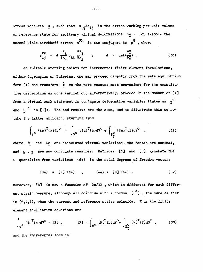
-17-

stress measures s , such that s..6e.. is the stress working per unit volume

of reference state for arbitrary virtual deformations 6e . For example the

PK Gsecond Piola-Kirchhoff stress s is the conjugate to e , where

ax. ax. axsPK ; J = det(-) . (30)

13 axk k axJ ax

As suitable starting points for incremental finite element formulations,

either Lagrangian or Eulerian, one may proceed directly from the rate equilibrium

form (1) and transform t to the rate measure most convenient for the constitu-

tive description as done earlier or, alternatively, proceed in the manner of [El

Gfrom a virtual work statement in conjugate deformation variables (taken as e

and SPK in E[1). The end results are the same, and to illustrate this we now

take the latter approach, starting from

f {6e) {s}dVo {u} T{bdVo + {6u)T {f}dSo , (31)

T

where 6u and 6e are associated virtual variations, the forces are nominal,

and s , e are any conjugate measures. Matrices EN] and [B] generate the

6 quantities from variations {6*} in the nodal degrees of freedom vector:

{6u) = [N] {6~} , {6e) [B] {6*) . (32)

Moreover, [B] is now a function of au/ax , which is different for each differ-

ent strain measure, although all coincide with a common [Bo ] , the same as that

in (6,7,8), when the current and reference states coincide. Thus the finite

element equilibrium equations are

0 [B] {s}dV = {P} {P} =V [N]T{b}dVo+ [N]T{f}dS , (33)

and the incremental form is

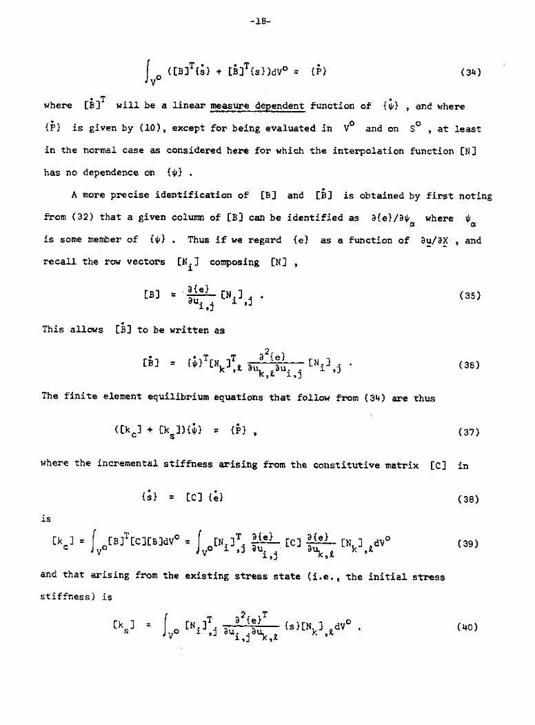
-18-

Vo ([BT{s) + [EBT{s))dVo = { (34)

where [B] T will be a linear measure dependent function of {b} , and where

{P) is given by (10), except for being evaluated in Vo and on So , at least

in the normal case as considered here for which the interpolation function [N]

has no dependence on {*} .

A more precise identification of [B] and [B] is obtained by first noting

from (32) that a given column of [B] can be identified as a{e}/*a where *o

is some member of {t} . Thus if we regard {e} as a function of au/ax , and

recall the row vectors [Ni ] composing [N] ,

[B] =3{e} [N.] . (35)aui j . ,j "

This allows EB] to be written as

T T a2{e)[B] = {*[Nk] , au u. [N ,j " (36)

The finite element equilibrium equations that follow from (34) are thus

([k ] + Cks ]){} = {P , (37)

where the incremental stiffness arising from the constitutive matrix [C] in

{s) = [C] {e) (38)

is

[k ] = [ B T C ] [ B ] d Vo = IN ] T a{ e ) [C] a{e} [N] dVo (39)c o 0 i, ju a. uk, k ,L

and that arising from the existing stress state (i.e., the initial stress

stiffness) is

[k ] = [N {e}T {s}[N] dVo . (40)s o j aui , j au k , g k ,L

-19-

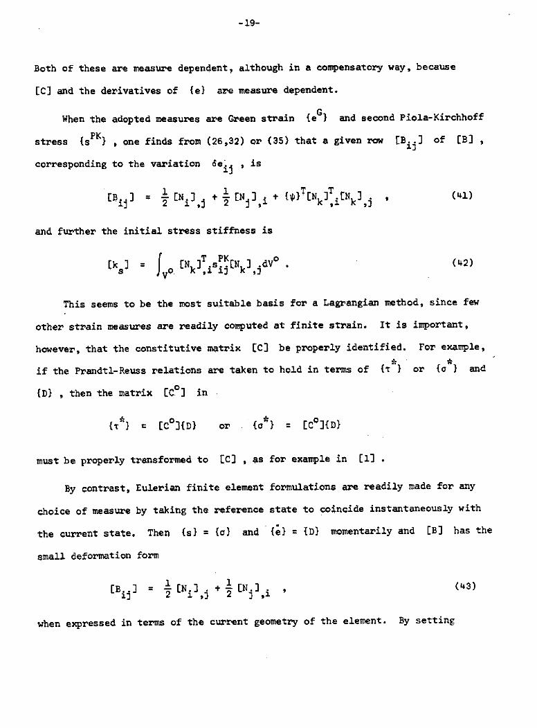
Both of these are measure dependent, although in a compensatory way, because

[C) and the derivatives of {e) are measure dependent.

When the adopted measures are Green strain {eG } and second Piola-Kirchhoff

stress {sPK , one finds from (26,32) or (35) that a given row [Bij] of [B) ,

corresponding to the variation Se. , is

1i 2 A 2 j ,i ik j

and further the initial stress stiffness is

T PK oCks = [N k ,s [Nk jdVo (42)

This seems to be the most suitable basis for a Lagrangian method, since few

other strain measures are readily computed at finite strain. It is important,

however, that the constitutive matrix [C] be properly identified. For example,

if the Prandtl-Reuss relations are taken to hold in terms of {T } or {o } and

{D} , then the matrix [C0) in

{( } = [C0 ]{DI or {a } = [C°]{D)

must be properly transformed to [C] , as for example in [1.

By contrast, Eulerian finite element formulations are readily made for any

choice of measure by taking the reference state to coincide instantaneously with

the current state. Then {s) = {} and {e} = {D} momentarily and [B] has the

small deformation form

[B ] = 1 [Ni] + 1[NJ , (43)ij 2 1 2 ji

when expressed in terms of the current geometry of the element. By setting

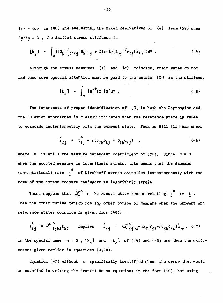
-20-

{s} = ({} in (40) and evaluating the mixed derivatives of {e} from (29) when

au/ax = 0 , the initial stress stiffness is

Ek ] = ([Nk .i.. iNk) + 2(m-1)[B kiTij [Bjk ] ) d . (44)S ,1 k ,j fdi E ]

Although the stress measures {s) and {o} coincide, their rates do not

and once more special attention must be paid to the matrix [C] in the stiffness

[k ] = [B]T[c][B]dV . (45)

The importance of proper identification of [C] in both the Lagrangian and

the Eulerian approaches is clearly indicated when the reference state is taken

to coincide instantaneously with the current state. Then as Hill [11) has shown

s.i = ..j - m( ikDk + Dikkj) , (46)1 ik kj ik kj

where m is still the measure dependent coefficient of (28). Since m = 0

when the adopted measure is logarithmic strain, this means that the Jaumann

(co-rotational) rate T of Kirchhoff stress coincides instantaneously with the

rate of the stress measure conjugate to logarithmic strain.

Thus, suppose that Zo is the constitutive tensor relating rt to D

Then the constitutive tensor for any other choice of measure when the current and

reference states coincide is given from (46):

S .ijk D k implies sij = (ijk-mik 6j-majk 6i )k . (47)

In the special case m = 0 , [ks] and Ek ] of (44) and (45) are then the stiff-

nesses given earlier in equations (9,10).

Equation (47) without m specifically identified shows the error that would

be entailed in writing the Prandtl-Reuss equations in the form (20), but using

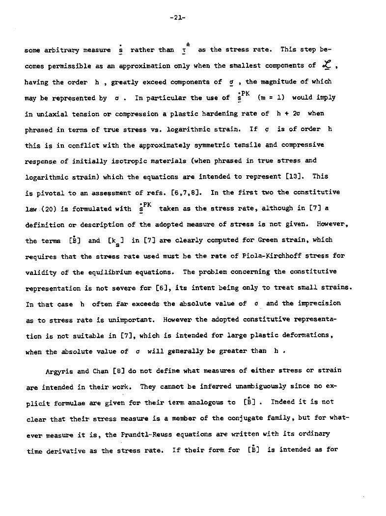
-21-

some arbitrary measure s rather than T* as the stress rate. This step be-

comes permissible as an approximation only when the smallest components of t ,

having the order h , greatly exceed components of a , the magnitude of which

*PKmay be represented by a . In particular the use of s (m = 1) would imply

in uniaxial tension or compression a plastic hardening rate of h + 20 when

phrased in terms of true stress vs. logarithmic strain. If a is of order h

this is in conflict with the approximately symmetric tensile and compressive

response of initially isotropic materials (when phrased in true stress and

logarithmic strain) which the equations are intended to represent [13]. This

is pivotal to an assessment of refs. [6,7,8]. In the first two the constitutive

*PKlaw (20) is formulated with s taken as the stress rate, although in [7] a

definition or description of the adopted measure of stress is not given. However,

the terms [i] and [k s ] in [7 are clearly computed for Green strain, which

requires that the stress rate used must be the rate of Piola-Kirchhoff stress for

validity of the equilibrium equations. The problem concerning the constitutive

representation is not severe for [61, its intent being only to treat small strains.

In that case h often far exceeds the absolute value of a and the imprecision

as to stress rate is unimportant. However the adopted constitutive representa-

tion is not suitable in [7], which is intended for large plastic deformations,

when the absolute value of a will generally be greater than h .

Argyris and Chan [8) do not define what measures of either stress or strain

are intended in their work. They cannot be inferred unambiguously since no ex-

plicit formulae are given for their term analogous to [B] . Indeed it is not

clear that their stress measure is a member of the conjugate family, but for what-

ever measure it is, the Prandtl-Reuss equations are written with its ordinary

time derivative as the stress rate. If their form for [B] is intended as for

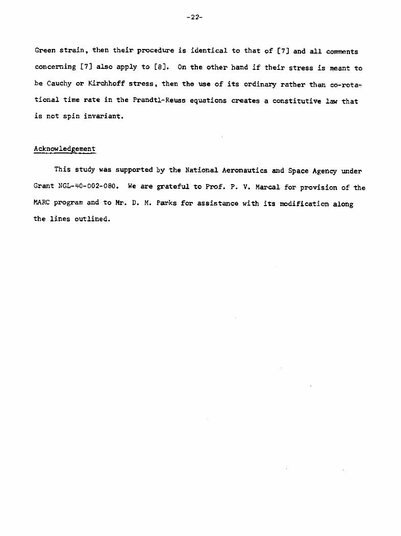
-22-

Green strain, then their procedure is identical to that of [7] and all comments

concerning [7] also apply to [8]. On the other hand if their stress is meant to

be Cauchy or Kirchhoff stress, then the use of its ordinary rather than co-rota-

tional time rate in the Prandtl-Reuss equations creates a constitutive law that

is not spin invariant.

Acknowledgement

This study was supported by the National Aeronautics and Space Agency under

Grant NGL-40-002-080. We are grateful to Prof. P. V. Marcal for provision of the

MARC program and to Mr. D. M. Parks for assistance with its modification along

the lines outlined.

-23-

References

[i1 H. D. Hibbitt, P. V. Marcal and J. R. Rice, A Finite Element Formulationfor Problems of Large Strain and Large Displacement, International Journalof Solids and Structures 6 (1970) pp. 1069-1086.

[2] A. Needleman, A Numerical Study of Necking in Circular Cylindrical Bars,Journal of the Mechanics and Physics of Solids 20 (1972) pp. 111-127.

[3] R. Hill, Some Basic Principles in the Mechanics of Solids Without a NaturalTime, Journal of the Mechanics and Physics of Solids 7 (1959) pp. 209-225.

[4] C. A. Felippa and P. Sharifi, Computer Implementation of Nonlinear FiniteElement Analysis, in: R. F. Hartung (ed.) Numerical Solution of NonlinearStructural Problems (ASME, New York, 1973) pp. 31-49.

[5] S. Yaghmai and E. P. Popov, Incremental Analysis of Large Deflections ofShells of Revolution, International Journal of Solids and Structures 7(1971) pp. 1375-1393.

[6] P. Sharifi and E. P. Popov, Nonlinear Finite Element Analysis of SandwichShells of Revolution, AIAA Journal 11 (1973) pp. 715-722.

[7] J. S. Gunasekera and J. M. Alexander, Matrix Analysis of the Large Deforma-tion of an Elastic-Plastic Axially Symmetric Continuum, in: A. Sawczuk(ed.), Symposium on Foundations of Plasticity (Noordhoff InternationalPublishing, Leyden, The Netherlands, 1973) pp. 125-146.

[8] J. H. Argyris and A. S. L. Chan, Static and Dynamic Elasto- Plastic Analysisby the Method of Finite Elements in Space and Time, in: A. Sawczuk (ed.),Symposium on Foundations of Plasticity (Noordhoff International Publishing,Leyden, The Netherlands, 1973) pp. 147-175.

[9] J. R. Osias, Finite Deformation of Elasto-Plastic Solids, The Example ofNecking in Flat Tensile Bars, Ph.D. Thesis, Carnegie-Mellon University,Pittsburgh, 1972.

[10] R. Hill and J. R. Rice, Elastic Potentials and the Structure of InelasticConstitutive Laws, SIAM Journal of Applied Mathematics 25 (1973),pp. 448-461.

[11] R. Hill, On Constitutive Inequalities for Simple Materials I and II, Journalof the Mechanics and Physics of Solids 16 (1968), pp. 229-242 andpp. 315-322.

[12] R. Hill, On the Classical Constitutive Relations for Elastic/Plastic Solidsin: B. Broberg et al. (eds.) Recent Progress in Applied Mechanics (TheFolke Odquist Volume), (Wiley and Son, New York, 1967)pp. 241-250.

[13] R. Hill, The Mathematical Theory of Plasticity (Oxford University Press,London, 1950).

-24-

[14] B. Budiansky, Private communication with W. H. Chen. Reference 12 inChen [17] and referenced by Needleman [2].

[15] J. R. Rice, Private communication with J. W. Hutchinson (1973).

[16] J. W. Hutchinson, Finite Strain Analysis of Elastic-Plastic Solids andStructures, in: R. F. Hartung (ed.), Numerical Solution of NonlinearStructural Problems (ASME, New York, 1973) pp. 17-30.

[17] W. H. Chen, Necking of a Bar, International Journal of Solids and Structures7 (1971) pp. 685-717.

[18] R. M. McMeeking, An Eulerian Finite Element Formulation for Problems of LargeDisplacement Gradients, S.M. Thesis, Brown University, Providence, 1974.

[19] D. C. Drucker, Variational Principles in the Mathematical Theory of Plasticity,Proceedings of the Symposium for Applied Mathematics 8 (1958) pp. 7-22.

[20] D. M. Tracey, On the Fracture Mechanics Analysis of Elastic-Plastic MaterialsUsing the Finite Element Method, Ph.D. Thesis, Brown University, Providence,1973.

[21] P. V. Marcal and I. P. King, Elastic-Plastic Analysis of Two-DimensonalStress Systems by the Finite Element Method, International Journal of Mechan-ical Sciences 9 (1967) pp. 143-155.

[22] J. R. Rice and D. M. Tracey, Computational Fracture Mechanics, in: S. J.Fenves et al. (eds.), Numerical and Computer Methods in Structural Mechanics(Academic Press, New York, 1973) pp. 585-624.

[23] J. C. Nagtegaal, D. M. Parks, and J. R. Rice, On Numerically Accurate FiniteElement Solutions in the Fully Plastic Range, Computer Methods in AppliedMechanics and Engineering, in press.

[24] G. R. Cowper and E. T. Onat, The Initiation of Necking and Buckling in PlanePlastic Flow, in: Proceedings of the Fourth U. S. Congress on Applied Mechan-ics (ASME, New York, 1962) pp. 1023-1029.

[25] J. W. Hutchinson, Post-Bifurcation Behavior in the Plastic Range, Journal ofthe Mechanics and Physics of Solids 21 (1973) pp. 163-190.

-25-

Table 1.

Finite Rotation by 450 in the x-y plane for a stressed plane-strain specimen.

Comparison of 50 and 25 increment finite element solutions with exact Mohr-circle

transformation.

a a axx yy xy

Before Rotation 1.000 0. 0.

Mohr Circle .500 .500 .500

50 increments .500 .500 .513

25 increments .501 .499 .526

-26-

Figures

Figure 1 Specimen for necking analysis, with imperfection shown greatlyexaggerated. The actual thinning is 0.5% of full width.

Figure 2 Finite element mesh for necking analysis.

Figure 3 Engineering strain y versus amplitude of the neck 6 normalizedby the undeformed length L .

Figure 4 Deformed mesh at engineering strain 0.69. Elements above line zzhave unloaded elastically.

-27-

y

C _

r0 A

Figure 1

-28-

F A

Fiure 2

-29-

1.00

0.80 -

0.60

0.40 - a

0.20

0.00 I I0.00 0.03 0.06 0.09

L

Figure 3

-30-

Figure 4