Seabed Force Model of

Buried Object Retrieval for

Autonomous Underwater Vehicles

A thesis submitted by

Amy C. Kline

in partial fulfillment of the requirements for the degree of

Master of Science

in

Mechanical Engineering

TUFTS UNIVERSITY

August 2014

ADVISOR:

Dr. Jason Rife, Department of Mechanical Engineering, Tufts University

COMMITTEE MEMBERS:

Dr. Michael Ricard, Draper Laboratory

Dr. Robert Viesca, Department of Civil Engineering, Tufts University

c©2014 Amy Kline, All rights reserved.The author hereby grants to Tufts University and The Charles Stark DraperLaboratory, Inc. permission to reproduce and to distribute publicly paper andelectronic copies of this thesis document in whole or in any part in medium now knownor hereafter created.

Abstract

In order to design autonomous underwater vehicles (AUVs) to manipulate ob-

jects for salvage operations, it is important to characterize forces required for

object extraction. This research models the reaction forces exerted by the ocean

floor during extraction of a partially buried object. A key contribution is the

definition of a reduced-order model for the maximum fluid-suction force on an

object given its dimensions and extraction velocity. The reduced-order model is

verified by comparison to a more refined computational fluid dynamics model.

The thesis also proposes a method to integrate the fluid suction model with

models of soil suction and soil friction, in order to estimate the total extraction

force. The models developed in this work will have utility in designing force and

power requirements for a new class of AUVs, purpose-built for object-retrieval

missions.

Acknowledgements

Thank you to Jason Rife and Michael Ricard for making this research possible

by coordinating with Draper Laboratory and for their constant support over

the past two years. In particular, thank you to Michael Ricard for leading

this project and encouraging me when the research and studies were at their

most challenging. Thank you to Jason Rife for continually pushing me to make

progress on my research and develop effective research and work techniques.

For their feedback on both the research and presentations, I would like to

thank Professor Viesca, Professor Pratap Misra, Rahul Chipalkatty, and the

ASAR lab group. A special thank you to my friends and colleagues at Tufts

and fellow Draper Laboratory Fellows. And finally, I offer the utmost grati-

tude to my family and friends, especially to my husband Joshua, who’s support,

encouragement, and advice were invaluable.

Contents

1 Introduction 2

1.1 Motivation . . . . . . . . . . . . . . . . . . . . . . . . . . . . . . 2

1.2 Background . . . . . . . . . . . . . . . . . . . . . . . . . . . . . 2

1.2.1 Salvage Operations . . . . . . . . . . . . . . . . . . . . . . 3

1.2.2 Intervention AUVs . . . . . . . . . . . . . . . . . . . . . . 4

1.3 Resistance in Seabed . . . . . . . . . . . . . . . . . . . . . . . . . 4

1.3.1 Problem . . . . . . . . . . . . . . . . . . . . . . . . . . . . 4

1.3.2 Force Overview . . . . . . . . . . . . . . . . . . . . . . . . 5

1.3.3 Soil Resistance . . . . . . . . . . . . . . . . . . . . . . . . 6

1.3.4 Cavity Formation . . . . . . . . . . . . . . . . . . . . . . . 7

1.4 Thesis Contribution . . . . . . . . . . . . . . . . . . . . . . . . . 9

1.5 Thesis Overview . . . . . . . . . . . . . . . . . . . . . . . . . . . 9

2 Reduced Order Modeling of Suction Force for Uplift of Par-

tially Embedded Cylinder 11

2.1 Problem Description . . . . . . . . . . . . . . . . . . . . . . . . . 12

2.1.1 Governing Equations . . . . . . . . . . . . . . . . . . . . . 13

2.1.2 Assumptions . . . . . . . . . . . . . . . . . . . . . . . . . 14

2.1.3 Boundary Conditions . . . . . . . . . . . . . . . . . . . . 15

2.1.4 Initial Conditions . . . . . . . . . . . . . . . . . . . . . . . 18

2.2 Methodology . . . . . . . . . . . . . . . . . . . . . . . . . . . . . 19

2.2.1 Finite element analysis . . . . . . . . . . . . . . . . . . . . 19

2.2.2 Reduced-order Model . . . . . . . . . . . . . . . . . . . . 22

2.3 Results . . . . . . . . . . . . . . . . . . . . . . . . . . . . . . . . . 24

2.3.1 Finite Element Model Results . . . . . . . . . . . . . . . . 24

i

2.3.2 Reduced Order Model Calibration . . . . . . . . . . . . . 25

3 Conclusion 28

3.1 Thesis Contributions . . . . . . . . . . . . . . . . . . . . . . . . . 28

3.2 Recommendations and Future Research Efforts . . . . . . . . . . 29

A Design of Soil Resistance Module for Support of Environmen-

tal Uplift Model 30

A.1 Introduction . . . . . . . . . . . . . . . . . . . . . . . . . . . . . . 30

A.2 Soil Modeling . . . . . . . . . . . . . . . . . . . . . . . . . . . . . 31

A.2.1 Soil Friction . . . . . . . . . . . . . . . . . . . . . . . . . . 34

A.2.2 Soil Suction . . . . . . . . . . . . . . . . . . . . . . . . . . 35

A.2.3 Combination . . . . . . . . . . . . . . . . . . . . . . . . . 36

A.3 Results and Discussion . . . . . . . . . . . . . . . . . . . . . . . . 36

A.3.1 Design Implications . . . . . . . . . . . . . . . . . . . . . 38

B Fluid Suction Literature 41

B.0.2 Suction Force for Object Resting on Surface . . . . . . . . 41

B.0.3 Half-Buried Pipeline . . . . . . . . . . . . . . . . . . . . . 54

B.0.4 Seabed . . . . . . . . . . . . . . . . . . . . . . . . . . . . . 56

ii

List of Figures

1.1 Coordinate system and object dimensions for the partially buried

uplift problem . . . . . . . . . . . . . . . . . . . . . . . . . . . . . 5

1.2 Overview of resistance mechanisms in breakout . . . . . . . . . . 6

2.1 Simulation Geometry . . . . . . . . . . . . . . . . . . . . . . . . . 20

2.2 Meshed Geometry . . . . . . . . . . . . . . . . . . . . . . . . . . 20

2.3 Comparison of the two-dimensional problem and the one-dimensional

approximation . . . . . . . . . . . . . . . . . . . . . . . . . . . . 23

2.4 Pressure Distribution for diameter 0.3 m and depth 0.25 m, . . . 24

2.5 Average Pressure for a cylinder with 0.3 m diameter versus buried

depth . . . . . . . . . . . . . . . . . . . . . . . . . . . . . . . . . 25

2.6 Average pressure for a cylinder with 0.3 m diameter versus uplift

velocity . . . . . . . . . . . . . . . . . . . . . . . . . . . . . . . . 26

2.7 Average Pressure for varying characteristic lengths . . . . . . . . 27

A.1 Suction Force Decision . . . . . . . . . . . . . . . . . . . . . . . . 36

A.2 Environmental forces versus uplift velocity . . . . . . . . . . . . 37

A.3 Environmental forces versus uplift velocity over transition zone . 37

A.4 Total environmental forces versus uplift velocity . . . . . . . . . . 38

A.5 Energy comparison for uplift process . . . . . . . . . . . . . . . . 40

iii

List of Tables

2.1 COMSOL Boundary Conditions . . . . . . . . . . . . . . . . . . . 21

2.2 Test Parameters . . . . . . . . . . . . . . . . . . . . . . . . . . . 22

2.3 Set Environmental Parameters . . . . . . . . . . . . . . . . . . . 22

2.4 Average Pressure Fit Equation Coefficients . . . . . . . . . . . . 27

iv

Seabed Force Model of

Buried Object Retrieval for

Autonomous Underwater Vehicles

1

Chapter 1

Introduction

1.1 Motivation

In order to extend the use of autonomous underwater vehicles (AUVs) to buried

object retrieval, it is necessary to first model the extraction process. A significant

amount of research has been performed in both civil and offshore engineering to

understand the interaction between the seabed and foreign objects. There is a

need to leverage the knowledge from the existing research to identify and model

the reaction forces due to both soil resistance and suction.

The primary goal of this thesis is to synthesize an integrated model for the

resistance forces that apply to autonomous extraction of an object from the

seabed, an activity which is sometimes called the breakout problem.

1.2 Background

The advent of unmanned underwater vehicles (UUVs) has forwarded new field

of research in underwater environments previoulsy inaccessible by conventional

manned vessels. They have served many purposes since the Self-Propelled Un-

derwater Research Vehicle was first developed by the Applied Physics Laboratory

at the University of Washington [29].

UUVs are categorized as either remotely operated vehicles (ROVs) or au-

tonomous underwater vehicles (AUVs). ROVs are controlled by an operator on

a nearby ship via a cable [19]. This cable transmits any sensor information, such

2

as video and temperature readings from the ROV and receives power and com-

mands for operations [18]. AUVs require no real-time user input and typically

only perform pre-defined tasks. AUVs have been commonly used for surveillance

missions, such as monitoring of subsea pipelines for the oil industry, while ROVs

are capable of intervention or salvage missions. These missions involve actual

contact with the environment, such as servicing sub-sea stations, and object

manipulation [28].

1.2.1 Salvage Operations

In salvage operations, such as investigation of shipwrecks or plane crashes, both

types of UUVs have been employed. AUVs can be employed to initially survey

a site, identify areas of interest, and collect relevant data for further analysis [8].

Then, ROVs or divers perform necessary tasks, such as retrieving artifacts or

black-boxes. In the case where ROVs are used, the human operator can accu-

rately identify the objects and use manipulators to interact with the environment

and adjust the vehicle as needed.

One example of a salvage mission that successfully used both AUVs and

ROVs, was the recovery of the Air France flight 447 flight data recorder and

cockpit voice recorder. In 2009, the flight from Rio de Janiro, Brazil to Paris,

France crashed in the southern Atlantic Ocean. Although debris from the crash

was identified within days, the initial attempts to locate the crash site and black

boxes were unsuccessful. It was not until April 2011 that the instruments were

successfully recovered. At this phase of the search, three REMUS 6000 AUVs

were first deployed and covered a 6,000 square kilometer area [23]. Once points

of interest were identified, an American Remora 6000 ROV recovered the two

devices within a week.

There are advantages to replacing ROVs with their autonomous counter-

parts. Since an AUV does not require a tether for communication, it is capable

of reaching greater depths, covering greater distances, and executing more com-

plex mission paths than ROVs [19][23]. Also, without the need for a tether and

operator, an AUV can move undetected, making covert operations possible [11].

There are also cost benefits to using AUVs. Individual missions could be ex-

3

tended to days, since there is no restriction of a human operator and a vessel is

only necessary for launch and recovery [22]. Because of these and other possi-

bilities, there is an interest to extend the use of AUVs to independently perform

retrieval missions.

1.2.2 Intervention AUVs

Initial research has been performed to develop intervention AUVs (I-AUVs) [22].

In 1996, the Aerospace Robotics Laboratory at Stanford University and the

Monterey Bay Aqurium Reserach Institute used their semi-autonomous under-

water vehicle called the OTTER to successfully test autonomous retrieval tasks

[28]. These operations included identifying a lighted package, approaching it,

and picking up the instrument using a fixed boom. Challenges for open ocean,

such as currents and seafloor incongruencies were identified but not addressed

[28].

The Semi Autonomous Underwater Vehicle for Intervention Mission (SAUVIM),

developed at the Autonomous Systems Labortory (ASL) at the University of

Hawaii, the Marine Autonomous Systems Engineering, Inc. and the Naval Un-

dersea Warfare Center has the added capability of autonomously using a fully

functional manipulator [30]. In experiments, the ASL has successfully tested the

manipulator by hooking a cable to a submerged object [26].Testing ended once

the object had been hooked and extraction itself was not tested. Because an

intervention mission requires physical contact with the environment, there is a

need to develop a rugged design and a robust manipulator [15].

With the interest and research in I-AUVs to date, fully autonomous opera-

tions will soon be possible; however, to the best of the author’s knowledge no one

has explored the necessary technology for extricating an object in the seafloor.

1.3 Resistance in Seabed

1.3.1 Problem

This thesis focuses on a specific breakout problem in the interest of developing a

unified model that combines forces that can easily be implemented for studying

4

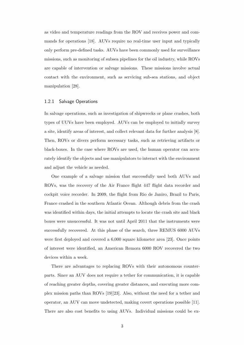
intervention robot applications. The set-up for this problem is shown in figure

1.1. The presented work develops a model for a canonical geometry meant to be

representative of a flight data recorder to be retrieved by an AUV.

Figure 1.1: Coordinate system and object dimensions for the partially burieduplift problem

(a) Coordinate System (b) Dimensions

Specifically, a cylinder with diameter D is modeled. As shown in figure 1.1b,

h(t) is the vertical displacement of the object at time t. The object is initially

buried to a depth of H.

1.3.2 Force Overview

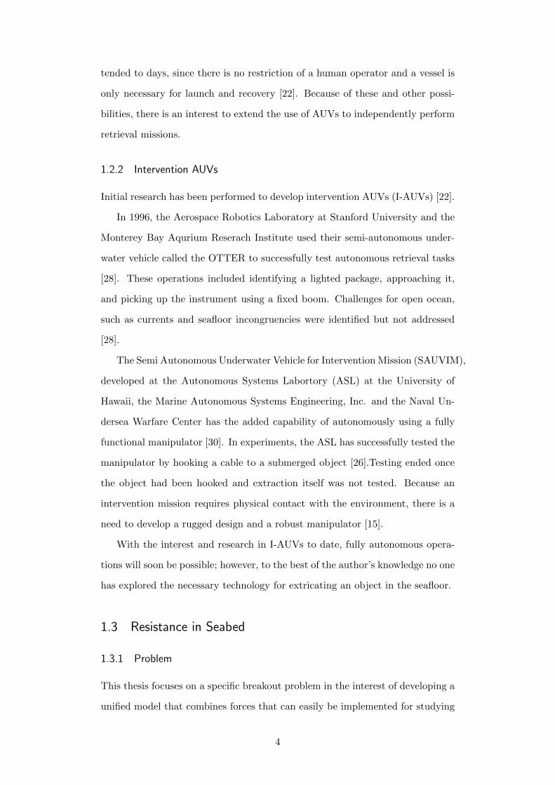
The first step to develop a model of extracting an object from the seabed is to

identify all forces exacted on the object. The resistance mechanisms discussed

in literature are included in figure 1.2.

These mechanisms contribute to the breakout problem:

1. Force due to object weight In any extraction scenario, it is necessary

to move the mass of the object. Typically, with a submerged object only

the effective weight is considered. The effective weight is defined as the

difference between the forces due to gravity and buoyancy. In the case of

this model, only a portion protrudes into the water, while the rest is buried

5

Figure 1.2: Overview of resistance mechanisms in breakout

so it is partially buoyant.

2. Force due to adhesion Adhesion is largely a chemical process in which

the object bonds with the surrounding soil. The extent of adhesion is

dependent on the relationship between the object material and the soil

and the amount of time that the object has been buried. This thesis does

not address adhesion.

3. Force due to soil resistance A force opposing the object’s motion is

created due to the friction between the object and the surrounding soil.

The force of friction is affected by the motion of surrounding soil, which

must be considered.

4. Force due to suction A negative pressure difference develops below the

object to oppose cavity formation. The concept employed here is that

some medium must fill the cavity to avoid creating a vacuum. A significant

resistance can be created by both the surrounding soil and fluid.

1.3.3 Soil Resistance

In order to simulate the retrieval of an object from the seabed, it is necessary

to understand the contributions of the soil surrounding the object. When an

object previously buried either fully or partially is subject to some force, the soil

surrounding the object applies a frictional resistance force. The modeling of the

6

soil resistance present in the uplift problem has been explored extensively for

the static case.

In the U.S. Naval Civil Engineering Laboratory, 1969, Vesic outlined three

different theories regarding the immediate breakout of submerged buried objects

[27]. Immediate breakout is to occur when a force much greater than the weight

of the object is applied so that the object is dislodged in a short period of time.

A large component of resistance originates from any soil overlying the object.

The soil resistance is quantified by the “shearing patterns” formed in the soil

[27].

1.3.4 Cavity Formation

An important aspect to consider in the retrieval of a buried object is the re-

sistance created due to cavity formation. When the object has moved in the

seabed, a void is created in the vacated space. This cavity must be filled by

the surrounding material. Two media are available: the underlying soil and the

water present in the soil pores. In reality, a combination of the two might be

expected in uplift, but no analysis of combined forces has been presented to date

in the open literature.

Soil Suction

Soil suction occurs in the cases where the object has not had enough time or force

to separate from the soil grains. The first instance is commonly referred to as

immediate breakout, when the applied force is able to counteract the maximum

values of all forces resistant to uplift and the object instantaneously is freed

from the seabed. Adhesion, which in itself is a source of resistance, adds to the

likelihood of soil grain movement [25]. The force required to move the underlying

soil is often very high as it must overcome the shear strength of the soil and cause

enough failure to move the soil to vertically fill the gap.

Fluid Suction

The alternative to the soil scenario is that water fills the gap. Since the soil is

considered to be fully saturated, the pores of the soil are filled with water. Once

7

the object moves, water can enter the growing void through the pores, the spaces

between soil grains, along the bottom and sides of the cavity. The fluid initially

originates from the pores directly surrounding the cavity, but it is replaced by

the water flowing from the sea-soil interface and from the soil at greater depths.

Because there is fluid flow through the soil and into the cavity, the cavity pressure

decreases with respect to the seafloor. This pressure difference between the soil

surface and cavity creates the large force that resists the object’s motion. This

force due to negative fluid pressure relative to hydrostatic pressure is termed the

fluid suction force. The fluid suction phenomenon is postulated to occur under

conditions when the object will not adhere to the soil easily and when a long-

term breakout is performed. The long-term breakout allows the fluid enough

time to travel through the soil and into the cavity. Otherwise, the soil would be

required to fill the space.

The majority of soil suction data began with the failure of objects in dry soil

[27]. Fluid pressure is not addressed, even in densely packed soils, because the

pores are filled with air, which is easily compressed. The resistance is negligible

compared to the contributions of the soil [25]. Fluid suction is identified in the

first comprehensive field tests for submerged breakout of objects performed by

Vesic [27].

He illustrates that the pressure difference resulting from the object’s motion

creates a suction force, although he does not offer a model. Lee offers qualitative

effects of pore water pressure when the partially embedded is still attached to

soil below [16].

Fluid suction has been addressed analytically and experimentally in other

cases of submerged objects. The first is the case of an object initially lifted from

the surface of the seabed. This surface suction case is of particular interest in

salvage engineering. The phenomenon occurs when an object, initially resting

on the seabed, is subject to some uplift force or prescribed uplift velocity. The

object experiences some resistance while in contact with the seabed [25]. Once

the object is disloged from the seabed, it rises slowly until it experiences a rapid

motion and only a force equal to the buoyant weight of the object is neces-

sary for further displacement [10] [20]. Breakout also occurs in submerged and

8

ground pipelines. The breakout problem has been pursued in order to improve

pipeline embedment configurations to prevent detachment from the ocean floor

due to large currents. Studies include numerical analyses and experiments on

half-buried pipelines by Foda et. al [9] and experiments run by Law [13] and

on completely buried pipes by Cheng [3]. Also studies on underground pipe dis-

placement in liquified soil have emphasized the effects of a suction force to due

pore water [6][5].

The studies mentioned simplify the breakout problem in most cases focus

on a thin portion of the seabed along the sea-soil interface. Since this analysis

requires a buried cavity, the seabed must be fully modeled, as is done in the

finite element analysis by Jeng to model the seabed to dynamic wave loading

[14]. The literature referenced here is reviewed in depth in appendix B.

1.4 Thesis Contribution

This goal of this thesis is to propose and validate a reduced-order model of the

fluid suction force when lifting a partially buried cylinder.

The two-dimensional model introduced is substituted for a one-dimensional

model that does have an analytical solution. It then shows that the analyti-

cal model’s results match those of the two-dimensional model, given that one

parameter is tuned. A fit for the tunable parameter is computed based on the

relevant geometries of the buried object.

This model has the potential to inform constraints on AUV design imposed

by suction forces and associated extraction times.

1.5 Thesis Overview

The remainder of this thesis is divided into two chapters. The first is concerned

with the fluid suction force and the second summarizes this work and offers

recommendations for future research.

Chapter two begins by reviewing previous research that addresses elements

of the fluid uplift problem. Then, it defines the physics regarding the suction

force created in the retrieval of a partially buried cylinder in a porous seabed.

9

The initial moment of uplift is evaluated through a finite element analysis study

to obtain the pressure profile in the seabed. Finally, the suction force is derived

and a model relating object dimensions, buried depth, extraction velocity, and

the resulting suction force is introduced.

10

Chapter 2

Reduced Order Modeling of Suction

Force for Uplift of Partially Embedded

Cylinder

This chapter quantifies the fluid suction force in the uplift of a partially buried

object. First an overview of relevant and background knowledge is presented.

Then, the results of a finite element analysis are presented. The results com-

pare the suction force results based on each scenario’s cylinder diameter, burial

depth, and uplift velocity. Finally to create a simplified formula for this force,

a regression curve was created in order to integrate a simplified model for the

overall breakout.

A comprehensive model of the coupled flow in the cavity and through the soil

would be computationally expensive so it is beneficial to have a simple algebraic

formula to characterize this aspect of the uplift problem.

Key assumptions of the nature of the seabed and pore water are applied. The

seabed is considered rigid. This constraint is introduced in Mei [20] and greatly

simplifies the problem since the stress and the velocity of the soil skeleton are

ignored. Mei’s analysis is also concerned with the second stage of the uplift

problem, which begins at the point where the object is effectively no longer in

contact with the seabed, even though the cavity has not yet begun to form. As

explained in Sawicki, the first stage ends when the normal stress in soil is zero

11

and any resistance below the object originates solely from the pore fluid [25]. By

neglecting any contraction and expansion of the pores, this assumption ignores

the effects by the soil on the governing fluid equations discussed in section 2.1.1.

This thesis investigates the case of lifting a compact object that is partially

embedded in submerged sand. This scenario is closely related to two similar

scenarios that have been extensively studied in the open literature. Specifically,

these studied cases involve very long partially embedded objects (e.g. an in-

finitely long pipe, with its cross section half embedded in soil) and large objects

resting on the sea floor (e.g. a block on top of sand). To date, few analyses have

considered the forces required to release a compact, partially embedded object.

2.1 Problem Description

The problem of buried uplift is to simulate the fluid pressure on the base of the

cylinder as it rises. The suction force is derived from this pressure profile by

integrating along the face of the object bottom.

Fsuc(t) =

∫ D/2

02πrp(t, r, h)dr (2.1)

where Fsuc is the resulting force from the pressure along the object bottom,

p(t,r,z ) at every radial position r.

It is anticipated that this integrated pressure is highest at the initial moment,

before the cavity forms. Therefore, this value will be determined and used to

characterize the entire process. The initial suction force, can be written as a

function of the seabed pressure. Following equation 2.1, the maximum suction

force is equal to the following:

max (Fsuc) = Fsuc(0) =

∫ D/2

02πrp(0, r,H)dr (2.2)

This is accomplished through finite element analysis, tracking the fluid flow

through the seabed at the initial time step. The model is executed in COMSOL

Multiphysics. By varying the depth and diameter of the object, as well as the

uplift velocity, a correlation between the initial suction force and these parame-

12

ters is determined. This linear system can then be implemented in a model for

the overall breakout.

2.1.1 Governing Equations

The goal is to determine the force in excess of the object’s weight required to

overcome the pressure difference above and below the object. For ease of com-

putation, the object is modeled as a cylinder, reducing the necessary simulation

to a two-dimensional system. The system is shown in figure 1.1a.

Two regions are defined with their own respective governing equations. The

first is the expanding cavity that forms underneath the object that is filled with

water. The second is the seabed surrounding the object. Any water in the cavity

must first travel through the seabed soil. Fluid flow in these coupled regions must

be identified.

This problem requires a combination of the existing knowledge of seabed fluid

dynamics and cavity fluid flow. Unlike the cases referenced in appendix B, the

cavity is completely bounded by soil, allowing no free fluid path into the void.

This complication requires that throughout the uplift process, the pressure and

fluid velocity through the soil be tracked. When coupled, these concepts yield

governing equations for the uplift problem.

Fluid flow in the soil is modeled as flow through an isotropic porous and

permeable media. Several approximations are made for the environment and

the flow continuity.

The first consideration is mass continuity. For mass to be conserved, the

following relationship is true over a given control volume.

∂

∂t(ρ) +∇ · (ρu) = 0 (2.3)

The sum of the rate of change of the fluid density, ρ, with respect to time t and

divergence of the product of density and fluid velocity, u , must be zero.

In soil, fluid is only present in the pores of a control volume. Therefore, the

13

mass continuity is corrected to account for the actual fluid mass in a volume.

∂

∂t(nρ) +∇ · (nρu) = 0 (2.4)

The soil’s porosity, n is the ratio of the pore volume to the total volume. Now,

equation 2.4 is used to characterize the mass continuity of the pore fluid.

The other fluid flow equation that is modified for porous media flow is for the

conservation of momentum. In free flowing fluid, like in the cavity, the velocity

and pressure are related by the Navier-Stokes equation, shown below in equation

2.5.

ρ

(∂u

∂t+ u · ∇u

)= −∇p+ µ∇2u (2.5)

The fluid flow, u , depends on the pore pressure, p, and is characterized by the

fluid’s dynamic viscosity, µ.

The fluid flow equations for the soil is a modified Darcy flow, which is used

for porous media. It accounts for the the change in volume, with the coefficient

n, and an added term to characterize the added fluid flow resistance from the

actual soil structure.

ρn

(∂u

∂t+ u · ∇u

)= −∇p+ µ52 u− µn

κu (2.6)

The last term in equation 2.6 shows that the momentum due to the soil’s resis-

tance is the product of fluid velocity, fluid viscosity, and the soil’s permeability,

κ. Also, it should be noted that the Brinkman term, µn 5

2 u, was included to

account for a transition between free and porous regions. This approach was

employed in Huang’s analysis of the surface uplift process [12].

These partial differential equations are simplified and then employed for the

finite element analysis.

2.1.2 Assumptions

Both the cavity and pore fluid are assumed to be incompressible following Mei

[20] and Foda [10], so the density, ρ, is constant. Since the seabed is assumed

14

both rigid and uniform [20], the porosity n is also a constant. This simplifies

the mass continuity for both free fluid flow and pore fluid flow from equations

2.3 and 2.4 to 2.7.

∇ · u = 0 (2.7)

In all of the models referenced in appendix B, the cavity’s fluid viscous terms

were assumed to be much larger than the inertial terms. Since the inertial

terms are negligible compared to the viscous forces, equation 2.5 is simplified to

equation B.11.

0 = −∇p+ µ∇2u (2.8)

Equation 2.6 is also reduced when the inertial terms are neglected.

0 = ∇ ·[−p+

µ

n52 u

]− µ

κu (2.9)

2.1.3 Boundary Conditions

The boundary conditions at the sea-soil interface are adapted from similar con-

ditions in literature. In Mei [20], the pore pressure is equal to the seafloor’s

ambient pressure. Since the focus of this analysis is the pressure difference

across the seabed, the actual ambient pressure is discounted and is gauged to

zero.

p(t,X > H, 0) = 0 (2.10)

Far from the object, the pore fluid remains undisturbed, even during uplift.

At these points, the fluid velocity is zero and the pressure is hydrostatic. The

hydraulic head, h(t,X,Z), and pore fluid velocity, u (t,X,Z), are set to zero.

h(t,X,Z →∞) = 0

h(t,X → ±∞, Z) = 0

(2.11)

The hydraulic head, h, is defined with a nominal elevation being the sea-soil

interface. Given equation 2.10, the relationship between the hydraulic head and

15

pressure relationship are shown in equation 2.12.

h =p

ρg+ Z (2.12)

The boundary conditions in equations 2.11 can be rewritten in terms of pressure.

p(t,X,Z →∞)→∞

p(t,X → ±∞, Z) = ρgZ

(2.13)

The next set of boundaries pertains to the sides of the cylinder. The bound-

ary of the porous material at the cylinder boundary is considered impermeable,

so the horizontal velocity of the fluid at the cylinder boundary is also zero. Any

interaction between the sides of the object and the surrounding porous media

are neglected in this chapter, and the vertical velocity is also set to zero.

uz(t,D/2, Z) = 0 for 0 < Z < H − h

ux(t,D/2, Z) = 0 for 0 < Z < H − h(2.14)

Although only the initial uplift problem is modeled, the boundary conditions

for a transient cavity are described below in order to derive boundaries on the

seabed region.

The boundary conditions for the cavity are defined in (x,z) coordinates as

shown in figure 1.1a. First, the top of the cavity, which is in contact with

the bottom of the cylinder is assigned a no-slip condition. The fluid’s velocity

matches the velocity of the object itself.

uz(t, x, h) = U

ux(t, x, h) = 0

for 0 < x < D/2

(2.15)

The other boundaries of the cavity correspond to the interfaces with the seabed.

The pressure and volumetric flow rate, Q, are continuous across these boundaries.

Below, the subscripts differentiate between the velocities and pressures for the

16

cavity and seabed. First, the bottom of the cavity has the following conditions.

Qcavity(t, r, 0) = Qseabed(t, r,H)

pcavity(t, r, 0) = pseabed(t, r,H)

for 0 < r < D/2

(2.16)

Since the volume flow rate is a product of the cross section and the normal

fluid velocity, equation 2.16 can be rewritten in terms of fluid velocities and the

cross-sectional areas available for fluid flow for the cavity, Acavity, and seabed,

Aseabed.

Acavityucavity(t, r, 0) = Aseabeduseabed(t, r,H) (2.17)

Again, the area of the fluid for the seabed is dependent on the amount of pore

space in a given volume of soil, namely:

Aseabed = nAcavity (2.18)

If equation 2.18 is combined with equation 2.16 and 2.17, the boundary con-

ditions for the cavity bottom are written in equation 2.19 in terms of velocity,

pressure, and porosity.

ucavity(t, r, 0) = nuseabed(t, r,H)

pcavity(t, r, 0) = pseabed(t, r,H)

for 0 < r < D/2

(2.19)

No boundary conditions are required for the sides of the cavity as they are

irrelevant to problem since the cavity does not yet exist. The cavity height can

be expressed as a function of the time elapsed and the uplift velocity. If the

cavity grows at a rate of U, the height of the cavity,h, at some time td is the

integral of the uplift velocity with respect to time.

h(td) =

∫ td

0U(t)dt (2.20)

Since the desired result of this thesis is a method to determine the maximum

17

suction force exerted on the object only the first time step is modeled. This

is expected to be an overestimate for the entire uplift process. The author’s

reasoning is that at this moment, all fluid must reach the object’s bottom. This

pore water travels the longest path which requires faster velocity through the

soil and therefore the greatest pressure difference.

At the initial moment of uplift, the height of the gap, h, is 0. At this point,

a cavity has not yet formed, and water is drawn exclusively along the bottom of

the object. The boundary conditions and the governing equations of the cavity

are no longer relevant. Boundary conditions defined in equations 2.19 and 2.15

combine to the following.

uz,seabed(0, r,H) = U/n

ux,seabed(0, r,H) = 0

(2.21)

2.1.4 Initial Conditions

Before the object is disturbed, the entire seabed is hydrostatic. The hydraulic

head, h(t,X,Z), and pore fluid velocity, u (t,X,Z), are zero. This condition was

adapted from Jeng’s porous media model for fluid-structure interaction. The

pore pressure is not set to zero, but is instead equal to the dynamic pressure

of the ocean waves [14]. Since any wave motion is neglected, the pressure is

constant at the seafloor, and gauged to zero. This initial condition is consistent

with the boundary condition 2.10.

h(0, X, Z) = 0 (2.22)

The initial conditions of the seabed, equation 2.22 can be written in terms

of pressure using equation 2.12: equation

p(0, X, Z) = ρgZ u(0, X, Z) = 0 (2.23)

The suction force is derived from this pressure profile and is calculated using

equation 2.1.

18

2.2 Methodology

2.2.1 Finite element analysis

To calculate the pressure at the object bottom for the initial uplift, the fluid

flow must be solved for the seabed problem laid out in section 2.1. Since no

analytical solution has yet been found, the problem was modeled and discretely

solved using COMSOL Multiphysics. It was necessary to approximate the

seabed geometry, discretize the geometry, and apply the governing equations on

each element. The simulation set-up is described below.

Geometry

For the simulation, the seabed and cylinder are approximated to a two-dimensional

axisymmetric problem shown in figure 2.1. Because the case is symmetric, only

one half of the cylinder’s geometry requires modeling. The seabed is represented

as a rectangle with set fluid and porous properties. A second rectangle is ex-

truded from the seabed region. This represents a half profile of the cylinder and

seabed. The dimensions of the seabed rectangle are much greater compared to

the half-section of cylinder so that the boundaries applied to the seabed edges

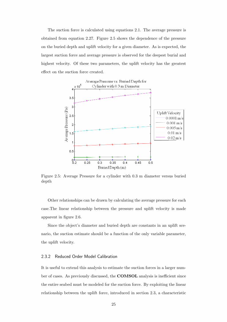
do not affect the cylinder. The seabed geometry was discretized into elements

ranging in size. The size of placement of the elements depend on the location

within the geometry. Along the cavity boundary 6, the elements were set to be

a maximum of 10−4 m, allowing for at most 1,000 nodes along the edge. As can

be seen in figure 2.2, areas farther from the object, such as along boundaries 2

and 3, the element sizes were much larger.

Boundary Conditions

The boundary conditions for the uplift problem described in section 2.1.3 were

adapted for finite element analysis.

Fluid flow is allowed through the soil from the mudline, but has a set pres-

sure. Equation 2.10 is applied at boundary 4 to ensure the pressure remains

constant. The boundary conditions on the far-field boundaries are set based on

the principle that the pore water remains undisturbed at any point far from the

19

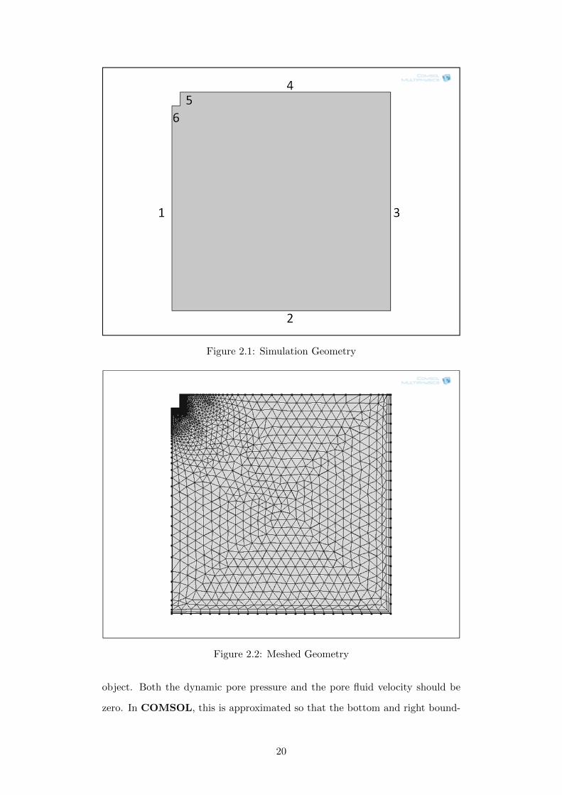
Figure 2.1: Simulation Geometry

Figure 2.2: Meshed Geometry

object. Both the dynamic pore pressure and the pore fluid velocity should be

zero. In COMSOL, this is approximated so that the bottom and right bound-

20

aries, boundaries 2 and 3 in figure 2.1, have a no-slip condition, restricting the

velocity to zero.

An extra boundary condition at the cylinder’s centerline must be included.

Due to symmetry, there are no lateral gradients across the centerline. This

translates to the following three equations at boundary 1:

ux = 0

∇u = 0

∂p

∂x= 0

(2.24)

All boundary conditions are included in table 2.1.

Boundary Description Condition Equation

1 Centerline Symmetric Eqs. 2.24

2 Lower bound of soil(Z→∞)

Set as no-slip u = 0

3 Horizontal soil bound(X→∞)

Set as no-slip u = 0

4 Sea-soil interface Set as inlet with 0dynamic pressure

p = 0

5 Cylinder Side Set velocity u = 0

6 Object bottom Set uplift velocity ux = 0, uz = U/n

Table 2.1: COMSOL Boundary Conditions

The defining condition of the simulation is the uplift velocity. The moving

object bottom, boundary 6, has a set fluid velocity. It includes both a lateral

no-slip condition as well as the vertical outflow equal to the uplift velocity, U.

This condition only applies to the case of initial uplift. In a time-dependent case,

a second region must be included to address the interface between the cavity and

surrounding soil.

Parameters

A series of cylinder diameters were employed to cover a range of potential objects.

The uplift velocity and initial burial depth also have an impact on the suction

created along the bottom of the object, so these were also varied. The complete

list of parameter combinations is displayed in table 2.2.

21

Diameter (m) Initial Depth (m) Velocity (m/s)

0.1 0.2 0.00010.2 0.25 0.00050.3 0.3 0.001

0.35 0.0050.4 0.010.45 0.020.5

Table 2.2: Test Parameters

Environmental Properties

It is necessary to specify both soil and fluid properties. The parameters chosen

for soil porosity and permeability are those used in Mei [20]; however, the sim-

ulation and analysis apply to the range of porosity and permeability applicable

to sand. The simulation constants are included in table 2.3.

Table 2.3: Set Environmental Parameters

Description Value Units

Soil Porosity 0.35

Soil Permeability 1.1213*10−11 m2

Water Viscosity 0.001 Pa-s

Water Density 1000 kg/m3

2.2.2 Reduced-order Model

The finite element model developed is both computationally expensive and would

be difficult to incorporate into a compiled tool for the total breakout problem.

This reduced-order model replaces the partial differential equations with a for-

mula to that produces a relatively accurate solution, one the key length scale is

defined.

To reduce the complexity of the problem, the full two-dimensional set-up of

the seabed, figure 2.3a, is converted to a one-dimensional approximation, shown

in figure 2.3b.

Darcy’s law is employed to adapt the seabed region to mimic a pipe. Since

the suction force is a result of the pressure gradient between the surface of the

22

(a) Two-dimensional problem (b) One-dimensional approximation

Figure 2.3: Comparison of the two-dimensional problem and the one-dimensionalapproximation

seabed to the bottom of the object, the one-dimensional case uses the pressure

difference across the pipe.

U = −κµ

∆P

Dcl(2.25)

Dcl = −κµ

∆P

U(2.26)

For equations 2.25 and 2.26 , U is the prescribed uplift velocity, and ∆P is the

characteristic pressure difference across the seabed, and Dcl is the characteristic

length.

To calculate the average pressure along the cavity, the pre-determined suction

force is divided by the cylinder’s cross-sectional area. Through Darcy’s law, the

relationship between the pressure difference and velocity is converted to the

characteristic length, as is shown in 2.25.

∆P = FsucA−1c =

(∫ D/2

02πrp(r)dr

)(πD2

4

)−1

∆P = 8D−2

∫ D/2

0rp(r)dr

(2.27)

23

2.3 Results

The goal of this chapter is to accurately model the initial pore fluid flow and

pressure and obtain a relationship between the extraction velocity and resulting

suction force. The results for the fluid flow model are presented in section 2.3.2

and the results for the suction force correlation are included in section 2.3.1.

2.3.1 Finite Element Model Results

The static finite element analysis outputs the pressure profile and flow field for

the entire seabed. From these results, the suction force was calculated and

related to the object geometry and depth. This section includes examples of the

FEA results and the suction force. It also discusses the trends of the average

pressure.

The pressure distribution along the object bottom was found to be related

to the object diameter, buried depth, and uplift velocity. Figure 2.4 shows the

pressure distribution along the object bottom for a cylinder of diameter 0.3 m

embedded to 0.25 m. In each case, the highest pressure is observed at the center

of the object. Any fluid drawn to the center must travel the greatest distance,

requiring a higher velocity and therefore pressure difference.

Figure 2.4: Pressure Distribution for diameter 0.3 m and depth 0.25 m,

24

The suction force is calculated using equations 2.1. The average pressure is

obtained from equation 2.27. Figure 2.5 shows the dependence of the pressure

on the buried depth and uplift velocity for a given diameter. As is expected, the

largest suction force and average pressure is observed for the deepest burial and

highest velocity. Of these two parameters, the uplift velocity has the greatest

effect on the suction force created.

Figure 2.5: Average Pressure for a cylinder with 0.3 m diameter versus burieddepth

Other relationships can be drawn by calculating the average pressure for each

case.The linear relationship between the pressure and uplift velocity is made

apparent in figure 2.6.

Since the object’s diameter and buried depth are constants in an uplift sce-

nario, the suction estimate should be a function of the only variable parameter,

the uplift velocity.

2.3.2 Reduced Order Model Calibration

It is useful to extend this analysis to estimate the suction forces in a larger num-

ber of cases. As previously discussed, the COMSOL analysis is inefficient since

the entire seabed must be modeled for the suction force. By exploiting the linear

relationship between the uplift force, introduced in section 2.3, a characteristic

25

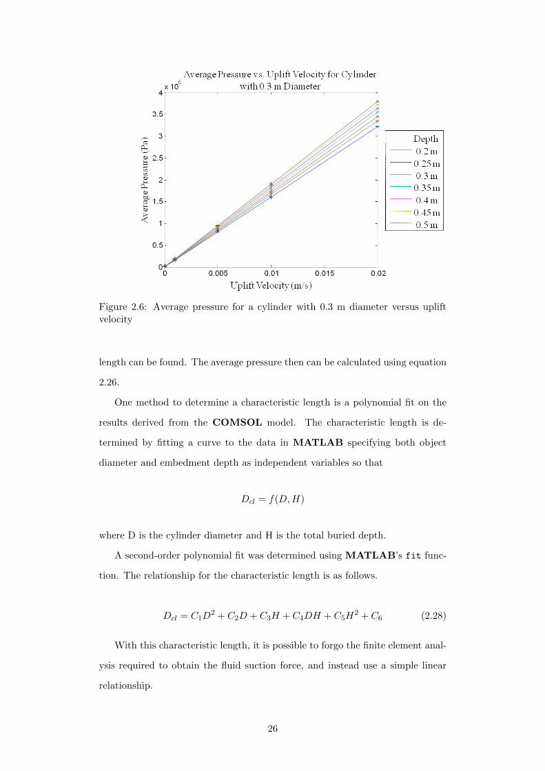
Figure 2.6: Average pressure for a cylinder with 0.3 m diameter versus upliftvelocity

length can be found. The average pressure then can be calculated using equation

2.26.

One method to determine a characteristic length is a polynomial fit on the

results derived from the COMSOL model. The characteristic length is de-

termined by fitting a curve to the data in MATLAB specifying both object

diameter and embedment depth as independent variables so that

Dcl = f(D,H)

where D is the cylinder diameter and H is the total buried depth.

A second-order polynomial fit was determined using MATLAB’s fit func-

tion. The relationship for the characteristic length is as follows.

Dcl = C1D2 + C2D + C3H + C4DH + C5H

2 + C6 (2.28)

With this characteristic length, it is possible to forgo the finite element anal-

ysis required to obtain the fluid suction force, and instead use a simple linear

relationship.

26

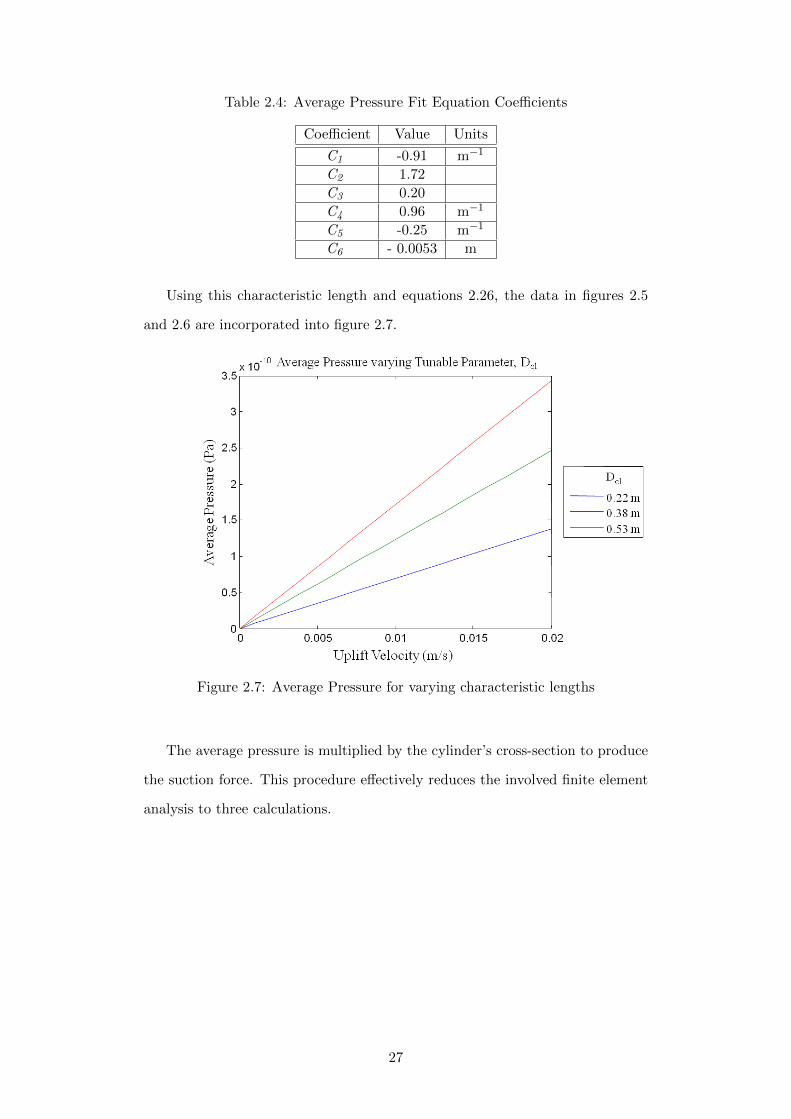
Table 2.4: Average Pressure Fit Equation Coefficients

Coefficient Value Units

C1 -0.91 m−1

C2 1.72

C3 0.20

C4 0.96 m−1

C5 -0.25 m−1

C6 - 0.0053 m

Using this characteristic length and equations 2.26, the data in figures 2.5

and 2.6 are incorporated into figure 2.7.

Figure 2.7: Average Pressure for varying characteristic lengths

The average pressure is multiplied by the cylinder’s cross-section to produce

the suction force. This procedure effectively reduces the involved finite element

analysis to three calculations.

27

Chapter 3

Conclusion

3.1 Thesis Contributions

This thesis seeks to enable development of AUV capabilities to execute inter-

vention missions by providing a model of the seabed environment. This work

has addressed challenges associated with an environmental model that would

simulate the conditions necessary for retrieval of a cylinder partially embedded

in the ocean floor.

Specifically, a method to quantify the maximum force created by pore water

pressure was explored. Through the set-up of the uplift problem, the governing

equations of the problem were defined and a stationary problem was solved

utlizing a software finite element method tool. The suction force was calculated

and observations were made regarding the effects of burial depth and object

dimension on the suction force. The key research contribution was a simplified

model of the two-dimensional fluid breakout problem.

The fluid suction force calculated can be incorporated into a comprehen-

sive model to predict the total resistance. A possible method to quantify the

maximum resistance to the breakout problem considering other mechanismsis

included in a subsequent appendix.

28

3.2 Recommendations and Future Research Efforts

While this thesis explores one aspect of the breakout problem, there are many

other elements required to develop a realistic simulation. As the various mecha-

nisms of resistance continue to become better understood, a dynamic simulation

is desirable.

The fluid suction model should be improved to include the evolving suction as

the object is displaced. The updated values could be used to reflect the dynamic

nature of the problem. A solution for fluid suction should be extended beyond

the initial moment of extraction.

A module for soil resistance should be designed that accounts for the discrete

behavior of the surrounding soil. In this thesis, the soil resistance was approxi-

mated and only accounted for the maximum force to the point of failure. It did

not track any soil displacement or varying soil strength. A more sophisticated

model should account for such details as a variable failure surface and transient

soil properties. This opens the simulation to include other object shapes and

different extraction techniques.

The model could be extended to allow for a non-rigid object. It would be

possible to simulate and characterize the impact of extraction process on the

object’s integrity. This addition would advance the utility of the model for less

robust objects than flight data recorders.

Finally, experimental validation to verify the working model would be nec-

essary. The challenge with experiments, as has been noted in several previous

works, is that it is difficult to isolate the contributions of each mechanism. Very

controlled laboratory tests should be developed to verify the total process, before

performing field tests.

29

Appendix A

Design of Soil Resistance Module for

Support of Environmental Uplift Model

A.1 Introduction

In this section, a comprehensive model for the total force resisting the extraction

of an object partially buried in the seafloor is proposed. The various resistance

mechanisms contributing to this force have been identified and are included in

the figure 1.2 free-body diagram.

The forces can be divided into two material groups: the first is the force

associated with the soil’s pore fluid, and the other the soil itself. The forces

due to soil can also be broken down further. Friction from the soil along the

side of the object is present, and can restrict object motion. This mechanism

is emphasized in literature for buried pipelines, foundations, and deep anchors.

Another force is a soil suction force. It serves as an alternative to fluid suction,

where instead of pore fluid filling the gap, underlying soil does. This resistance

from below the object is the focus for cases of shallow buried foundations and

anchors. Calculations for both forces are proposed in this chapter.

This model must incorporate all three forces identified, the fluid suction force,

calculated in chapter 2, the soil suction force, and the soil friction force. These

forces have been studied and quantified individually in other contexts. However,

in these contexts, only one force is considered dominant and the others are

considered negligible.

30

In the case of submerged uplift, it is uncertain how these mechanisms will

interact and if one will dominate. Given that each force is known to operate

in different extreme situations, it would be helpful to identify cases where the

magnitudes are in a similar regime and cases where certain ones dominate.

In this section, a comprehensive model for the total force resisting the ex-

traction of an object partially buried in the seafloor is proposed. First, a soil

resistance calculation is laid out, based on models taken from the literature.

An integrated model is then proposed and the individual forces are compared.

Finally, an example application is presented for AUV design and operation.

A.2 Soil Modeling

Background

In order to simulate the retrieval of an object from the seabed, it is necessary to

understand the contributions of the soil surrounding the object. When a fully or

partially buried object is subject to some force, the soil atop and surrounding the

object applies a frictional resistance force. The modeling of the soil resistance

present in the uplift problem has been explored extensively for the static case.

A great deal of research has been done to quantify the ultimate resistance

to object displacement in soil as well as the amount of force that will induce

soil failure. This problem has been explored for submerged buried anchors,

buried pipelines, and foundation piles. The problem is approached through soil

mechanics principles to quantify the desired uplift capacity. A brief overview

of the past research is explained and then the assumptions and calculations

employed in the simulation are explained.

In the U.S. Naval Civil Engineering Laboratory in 1969, Vesic outlined three

different theories regarding the immediate breakout of submerged buried objects

[27]. Immediate breakout is to occur when a force much greater than the weight

of the object is applied so that the object is dislodged in a short period of time.

A large component of resistance originates from any soil overlying the object.

Vesic differentiates between the two mechanisms but does not seek to assembled

them.

31

Lee [17] reviews other experiments performed by the Naval Civil Engineering

Laboratory, focusing on objects that have been buried to a depth less than

the objects cross-section. The friction along the side of the object is negligible

compared to the soil suction force, but it is noted that it would be reversed for

cases of deeper embedment.

Most approaches for the buried foundation fall under one of two categories:

deep and shallow. As previously explained, each category experiences different

failure mechanisms. In each case, a different type of resistance dominates. For

the deep case, a friction along the sides of the object keeps the object in place:

frictional force. For the other, the main force of resistance is due to the under-

lying soil, in this thesis termed “soil suction”. Meyerhof [21] defines a bearing

capacity formulation based on bearing capacity factors. He notes differences be-

tween deep and shallow foundations including a change in failure surface formu-

lations and also that the dominant resistance differs. He differentiates between

a “base resistance” and skin friction. Both are measured through experimental

data. He also extends work to foundations and performs lab and field loading

experiments.

Rowe and Davis studied anchor plates in sand and clay[24] and performed a

finite element analysis to understand the load-displacement relationship in the

buried case. The formulation accounts for Mohr-Coulomb failure. The descrip-

tions given in Rowe provide insight into types of failure and the mechanisms.

For example, in the case of shallow anchors, the breakout occurs with a rigid

sliding block of soil that rises about the edges of the object. In the case of deep

anchors, plastic deformation is observed. The work included the comparison of

the models and it experimentally found that the actual results fall between the

values resulting from the two limiting conditions.

The deep failure is explored for skin friction. To ensure that the resulting

prediction is an overestimate, deep foundation theory is applied and only dense

sands are considered.

The majority of theories are based on soil mechanics principles. In general,

the measure of peak uplift occurs when the shear stress is equal to the shear

strength of the soil. Most of these methods rely on estimated empirical constants

32

or experimental results.

In 1961, Balla developed a soil mechanics approach that focused on the shape

of slip surfaces for shallow anchor plates in dense sand. He noted the differences

between failure surface based on burial depth and experimentally observed vari-

ous slip surfaces [27]. The distribution of stresses is integrated along slip surface

so that the resistance due to soil shear. In terms of completely buried pipelines,

Cheuk [4] examines existing methods of calculation, referring to both limit equi-

librium and upper bound solutions.

The soil resistance is quantified by the shearing patterns formed in the soil

[27].The soil involved in the uplift extends beyond the area of the buried object,

as was the case in Cheuk’s model tests. Vesic compared these models to field

tests performed in the San Francisco Bay.

Assumptions for Modeling Soil Forces

For the cylindrical object, no overburdened soil exists, so only the portion of soil

lying within the forming slip surface experiences sliding friction. The friction

between the sliding soil surfaces will still occur. With decreasing depth, like in

Cheuk, a lower resistance force is expected as the failure surface shrinks and less

object is in contact with the soil. It is assumed that the maximum force occurs

at the initial instance that uplift begins, as justified by the fact that the object

and soil make their largest (and deepest) contact at this moment in time.

Important principles employed include that with object displacement, the

soil around the object will deform beyond the elastic limit. The plastic region

of the soil is bounded by the slip surface, and the soil outside of this region still

have elastic properties. By moving past this region, soil dilation is neglected and

solely geostatic stresses are applied. If dilatancy is neglected, the stress-dilatancy

theorem developed by Bolton [1] is no longer relevant.

The skin friction requires a coefficient of friction that depends on the rela-

tionship between the object and the surrounding soil. This coefficient, δ will

range between 0 for a perfectly smooth object, and the soil’s angle of internal

friction φ for a rough object.

It uses the shear strength of the soil and extracts the ultimate response.

33

The method assumes a two-dimensional analysis for strain with Mohr-Coulomb

failure criterion.

τ = σ′ tan(φ) + c (A.1)

The shear strength τ is dependent on the angle shearing resistance, φ, the cohe-

sion, c and the effective normal stress σ′.

Calculations

In general, the approaches to calculate the effects of soil strength require refer-

ence to various tables based on foundation and type. This should be completely

based on theoretical settings so that eventually it can be expanded for applica-

tion to arbitrary shapes and other soil properties.

A.2.1 Soil Friction

For this case, an object is buried and completely surrounded by a dense sand.

Any forces exerted by water are assumed to be independent of sliding friction

and, moreover, the effect of pore fluid on shearing forces is assumed negligible

in this model.

For a detailed model, it is necessary to determine the failure patterns of this

soil which vary depending on object shape, soil makeup, and burial depth and

apply some failure law criterion. Similar to the approaches taken for anchors

and pipelines, the soil mechanics can also be applied to the case of foundations

such as piles. The formulas used are a combination of Chattopadhyay [2] and

Deshmukh [7]. This pile approach is set up for dry sands; however this is deemed

applicable since many of the existing studies for submerged cases are derived from

dry cases, including Vesic [27].

The failure surface shape is defined in Chattopadhyay as a torical shape

which is consistent with the work of Balla.

x =d

2+

H

β2tan(45◦ − φ2 )e−β +

H

βtan(45◦ − φ/2)

(Z

H− 1

β

)e−β(1− Z

H) (A.2)

The two parameters used to characterize the frictional behavior are the soil

friction angle φ, and pile friction angle δ. The friction angle between the object

34

and soil are taken into account in the following expression:

β = λ50◦

2δ(A.3)

In these equations, D and H are the object diameter and initial depth respec-

tively. In this case, the variable Z represents the depth where Z=0 is equal to

depth H and Z=H is the sea-soil interface.

Another parameter defined is the slenderness ratio, which has been used to

define whether an embedment is shallow or deep.

λ =D

H(A.4)

Rv = −γπsin(α+ φ)cos(α+ φ)

6cos(α)2

[(H

tan(α)+D

2

)3

+D2

4

(D − 3

(H

tan(α)+D

2

))](A.5)

This soil model must be joined with the suction force components to ensure

a realistic prediction of the uplift process.

A.2.2 Soil Suction

The alternative to water filling the expanding cavity is that soil will be pulled into

the cavity. This phenomenon is mentioned in Lee [16]. Although this method

was used in reference to a cohesive soil, it is applicable for a case when water

cannot drain. Since this case would only occur if the fluid cannot fill the cavity,

it is used. Due to the rapid loading and low permeability, water is prevented

from moving through and soil itself flows.

These calculations follow the same method explained in the prior section.

The difference is the failure surface used. As done in Lee, a Prandtl failure

surface for typical compressive bearing capacity is used [16]. Then, calculate

shear strength and use the resulting bearing capacity as the resistance force due

to soil suction.

35

A.2.3 Combination

The proposed method for determining the overall suction force is based on com-

paring certain forces and conditionally summing them.

It is necessary to decide the suction force used for each calculation. Here, it

is proposed that given a certain extraction velocity, whichever medium requires

the lowest force will be used. This is shown in figure A.1. This decision is based

Figure A.1: Suction Force Decision

on the proposed concept that the calculation of both suction forces outputs

the maximum value. Since the purpose of this model is to predict the highest

resistance to cavity formation, these to maxima can be compared to ascertain

that value. Equation A.6 lays out the relationship between the calculated forces.

FFS(t) ≤ maxt(FFS)

FSS(t) ≤ maxt(FSS)

FCF (t) ≤ min(FFS ,FSS)

max(FCF ) ≤ min(max(FFS),max(FSS))

(A.6)

The different forces compared are the fluid suction force, FFS and the soil suction

force, FSS . These are compared to determine the overall suction force, or the

force resisting cavity formation, FCF . The chosen suction force is then added

to the other components of resistance, which theoretically do not depend on the

suction force.

A.3 Results and Discussion

Using the methods described above, each resistance force was calculated for a

given scenario. An example is provided in figure A.2 below.

36

Figure A.2: Environmental forces versus uplift velocity

For the given velocities, the soil suction force is clearly much larger than

the fluid suction. In this case, the fluid suction is used for the given suction.

This is consistent over the velocities and object dimensions examined in this

thesis. If the same formulas were applied generally, the two suction forces would

not be applicable until a velocity on the order of 1 m/s. This velocity in itself

seems unlikely given the extraction process. At this speed, uplift will occur at a

fraction of a second. It should be noted that this model’s application is limited

Figure A.3: Environmental forces versus uplift velocity over transition zone

to the range of velocities used in the COMSOL model. Figure A.3, although

not to be used for force estimation, does provide an approximation of the scale

37

necessary for the two suctions to be on the same magnitude. At this point, the

method proposed in section A.2.3 is not applicable.

These different forces are combined to estimate the maximum resistance to

uplift. In the case used in figure A.2, the fluid suction is taken as the maximum

possible suction force which is then added to the overall friction force.

Figure A.4: Total environmental forces versus uplift velocity

The total resistance ranges over a small interval: from 339.4 N for 10−6

m/s, or 70 hours, to 704.8 N for 10−3m/s, or 4 minutes. This obviously shows

the small variation in force as opposed to the elapsed time of uplift. Although

the model does not address total AUV capabilities, these values can be used to

determine the specifications for the manipulator.

A.3.1 Design Implications

Up to this point, only the force required for extraction has been considered.

Although this provides an estimate of the required capacity of the manipulator,

it neglects the costs of the extraction of the AUV. One such cost is the amount

of energy expended during by the AUV for other necessary tasks such as station-

keeping. It is expensive to keep the AUV for an indefinite period of time. A

generalized formula can be used to compare the contributions of the two factors

to overall energy consumption.

First, extraction energy at any time would be the force applied, F, multiplied

38

by a change in depth, ∆Z.

Ee = F∆Z (A.7)

The extraction energy, Ee , can then be combined with the general operations

energy, Eo , which is calculated in equation A.8.

The energy for general AUV operations is derived from the operating power.

If a constant power is used throughout the uplift process, then the total energy

used will be the product of the power, PAUV and the elapsed time, ∆t.

Eo = PAUV ∆t

Eo = PAUV∆Z

U

(A.8)

The elapsed time can be expressed in terms of the depth, H, and the uplift

velocity, U .

By dividing the sum of the two required energies by the buried depth, ∆Z,

the quantity becomes a function of the total force, F and the uplift velocity U .

Etotal∆Z

=1

∆Z(Ee + Eo)

Etotal∆Z

= F +PAUVU

(A.9)

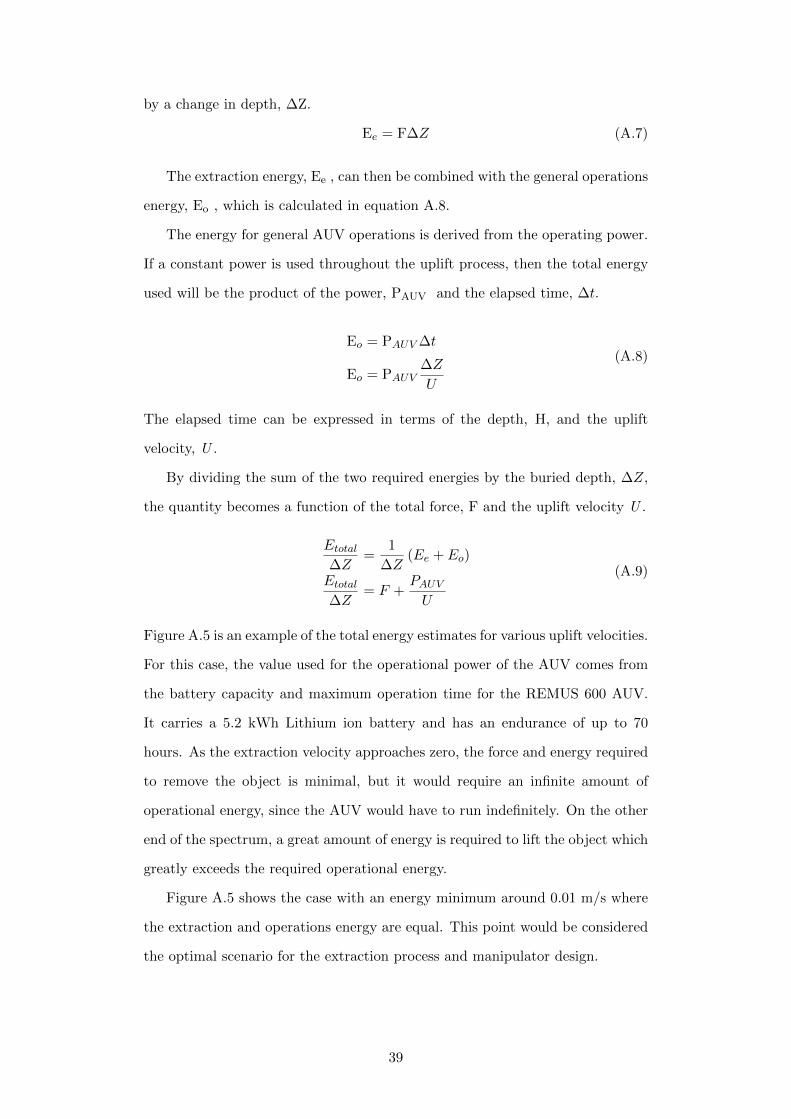
Figure A.5 is an example of the total energy estimates for various uplift velocities.

For this case, the value used for the operational power of the AUV comes from

the battery capacity and maximum operation time for the REMUS 600 AUV.

It carries a 5.2 kWh Lithium ion battery and has an endurance of up to 70

hours. As the extraction velocity approaches zero, the force and energy required

to remove the object is minimal, but it would require an infinite amount of

operational energy, since the AUV would have to run indefinitely. On the other

end of the spectrum, a great amount of energy is required to lift the object which

greatly exceeds the required operational energy.

Figure A.5 shows the case with an energy minimum around 0.01 m/s where

the extraction and operations energy are equal. This point would be considered

the optimal scenario for the extraction process and manipulator design.

39

Figure A.5: Energy comparison for uplift process

40

Appendix B

Fluid Suction Literature

This appendix provides an indepth review of suction analyses associated with

the fluid suction problem addressed in chapter 2.

B.0.2 Suction Force for Object Resting on Surface

The surface breakout process consists of two stages. The first is the period during

which the object is still in contact with the seabed, experiencing resistance due

to the pore water pressure and any residual adhesion. The second begins when

the object is dislodged and a gap forms between the seabed and the bottom of

the object.

Sawicki Mechanics of the breakout phenomenon [25]

This paper examines the first stage of breakout, when the object is completely

attached to the seabed. The reaction force from the seabed comes from the

negative pore pressure and effective stress created due to the soil’s disturbance.

This three-dimensional analysis determines this pore pressure change along the

bottom of the object by tracking both the fluid flow and normal stresses in

the soil. His approach to solving the pore pressure is to determine the mass

continuity for the fluid in the soil. Each term is then expanded in terms of the

pressure and total stress.

In the seabed, fluid continuity depends on the changing density of the pore

fluid, the changing pore space in the soil, and the transport of the fluid, uf :

41

∂

∂t(nρf ) +∇ · (nρfuf ) = 0 (B.1)

The first term in equation B.1 is the time derivative of the total mass. Both

the fluid density, ρf , and the porosity, n, vary with time as functions of the

strain on the water and soil respectively. The fluid density, ρf varies with the

dynamic pressure of the pore fluid, p:

ρf = ρf0

(1− εf

)εf = −κfp

(B.2)

The fluid density increases with the fluid’s decreasing volumetric strain, εf . A

negative volumetric strain corresponds to the volume of controlled mass shrink-

ing, so relative to its initial density, ρf0 , a higher density is observed.

The volumetric strain is proportional to the changing pressure in the soil.

The soil property affecting the volume of a given mass of fluid is the porosity, n.

The soil porosity is the ratio of free pore space to unit volume of total soil. Like

the fluid density, it also varies based on a volumetric strain. In this instance, it

is the strain on the soil structure itself. Changes in soil volume are caused by

the displacement of the object. Because the object is completely attached to the

seabed, any object movement also expands or contracts the soil, which creates

strain in any dimension. These strains are summed to determine the volumetric

strain, εs. The change in volumetric strain is proportional to the effective stress

imposed on the seabed.

n = n0 + εs(1− n0)

εs = −κsσ′(B.3)

The variable n0 represents the porosity of the undisturbed soil. The volumet-

ric strain depends on both the effective stress, σ′, and the soil’s coefficient of

compressibility, κs.

Another important concept employed in porous media is effective stress. The

normal stress is the total stress experienced by the seabed. The pressure in the

fluid relieves the stress on the soil, subjecting it only to the effective stress.

42

Therefore, the effective stress is the difference between the mean normal stress,

σ, and the pore water pressure, p.

σ′i = σi − p, (i = x, y, z) (B.4)

The second term of equation B.1 uses both of the above definitions as well

as the fluid velocity, uf . Sawicki employs Darcy’s law for the fluid flow, which

states that the velocity in any direction is proportional to the gradient of the

pressure.

uf =k

γw∇p (B.5)

The velocity of pore fluid through soil is dependent on both the hydraulic con-

ductivity, k, a measure of the soil’s ability to allow a soil to flow through its

pores and the unit weight of the pore fluid, γw. Through manipulation of the

continuity equation, B.1, and the above relationships, the following equation is

created to govern the behavior of the stresses and pressure in the seabed.

∇2p− ζ ∂p∂t

= −ξ ∂σ∂t

ζ =γw(κs + n0κ

f )

n0k, ξ =

γwκs

n0k

(B.6)

Two simple cases of uplift are presented in the paper. In each scenario, an

applied force is increased linearly from zero to some value greater than the object

weight that is maintained throughout breakout. The first is a one-dimensional

case where the spatial dependence is reduced to the z directions, only following

changes in depth. The axisymmetric example involves a circular disk of radius

R resting on the seabed. The origin of the coordinate system is at the center of

the disk and the vertical dimension z is aligned with the initial mudline position.

The first step to calculate the suction force is converting equation B.6 into ra-

dial coordinates and simplifying it to reflect axial symmetry. Any lateral stresses

in the soil structure are neglected, σr = 0. Also, since the area of interest for

the pressure is the top of the seabed, the vertical gradient of pressure is also

removed.

1

r

∂

∂r

(r∂p

∂r

)− ζ ∂p

∂t+ ξ

∂σz∂t

= 0 (B.7)

43

In this particular scenario, the vertical normal stress, σz is independent and di-

rectly correlates to the uplift force. At time 0, the vertical normal stress on the

soil skeleton is imposed by the weight of object and any overlying soil. As force

is applied to the object, the weight on the soil is relieved and the stress reduces

until time, T, when a constant maximum force Fmax at which point σ is also

constant. The boundary and initial conditions for this problem are of particular

interest. The dynamic pore pressure is initially set to zero throughout the soil,

neglecting the hydrostatic pressure distribution. Since the object is imperme-

able, the pore pressure gradient is zero at the object-soil interface. Boundaries

not influenced by the process are assigned a zero pore pressure. An unrealistic

imposed condition is that there is only a thin layer of soil underneath the object

as opposed to an infinite half-space to represent the depth of soil.

The solution for pore pressure is obtained using Laplace transforms and ap-

plying the above boundary conditions. To reduce the numerical analysis, the

average pressure, p is manipulated to result in the following functions for pres-

sure in the time periods of increasing force and the constant force.

p(t) = −ξaR2

8

[1− 32

∞∑i=1

1

γ4i

exp

(− γ2

i

ζR2t

)], 0 < t < T (B.8)

p(t) = −4ξaR2∞∑i=1

1

γ4i

exp

(− γ2

i

ζR2t

)×[exp

(− γ2

i

ζR2T

)− 1

], T < t (B.9)

The variables γi and a correspond to the zeros of the Bessel function of the zero

kind and the rate of change of the normal stress respectively. The suction force,

F, is determined from this pore pressure:

F = πR2p(t) (B.10)

Experiments done in this research tracked the displacement of a circular steel

disk under the force described above. The breakout time was measured as rapid

increase in slope of the curve. Two sets of experimental results are presented.

The first is the time history of the applied force and displacement for given

trials, and the second is the correlation between the breakout time and maximum

applied force.

44

This model addresses the changing pore pressure in the soil, but oversimplifies

the environment by assuming the total depth of soil is small compared to the

object, instead of a semi-infinite space. It also provides many helpful details

to boundary conditions and fluid flow in porous media, but since it does not

address the second stage of breakout, it is necessary to consult other sources for

analysis of an expanding cavity.

Foda On the extrication of large objects from the ocean bottom (the breakout

phenomenon), [10]

Foda addresses the second stage of the breakout case of an object pulled from

the seabed at some prescribed velocity, U. This analysis begins when the object

detaches from the seabed and a gap forms between it and the mudline. Just as

in Sawicki, the suction force is the result of the negative pore pressures that form

below the object. Also like Sawicki, the seabed is deformable and rises during

the breakout process.

To extract a solution for the suction force, three distinct regions are modeled.

The first is the gap, bounded by the rising object and a seabed, moving at a rate

of v. The other two models are for the seabed directly below the gap. One is a

general solution, and the other is a boundary layer correction. These regions are

coupled and an analytical solution is obtained. A solution for the axisymmetric

case is then outlined.

This paper gives an approach to model fluid flow in the gap and the applicable

boundary conditions. Key assumptions include that the fluid is incompressible

and the flow is inertial-free. Additionally, because it is considered that breakout

will occur while the gap height is small compared to the width of the object,

lubrication theory is applied; the vertical velocity and the vertical gradient of

pressure across the gap are ignored. The horizontal fluid flow across the gap is

simplified from the Navier-Stokes equation to the following:

∂p

∂i= µ

∂2ui∂i2

,∂p

∂z= 0, (i = x, y) (B.11)

In this case, p is the uniform dynamic pressure of the fluid in the gap, ui is the

45

fluid velocity in direction i, and µ is the dynamic viscosity of the fluid. The

lateral velocities, ux and uy at the top of the gap have a no-slip condition, the

object only moves vertically. The fluid velocity and the pressure are continuous

across the mudline, so this condition must also be satisfied.

The integration of equation B.11 and the application of the appropriate

boundary conditions result in the following velocity profile:

ui = − 1

2µ

∂p0

∂i(∆− η)η + u+

i

(1− η

∆

), (i = x, y) (B.12)

To properly construct this profile, two new variables are introduced to account

for the changing gap height and mudline position. The gap height, ∆, is the

difference between the bottom of the object and the position of the seabed. The

variable η, the relative height of a point in the gap from the mudline. This

helps define the location of the object and soil boundaries. Since the seabed will

experience some displacement, the mudline will not always correspond to the

position z = 0 but it will to η = 0. At this value, the fluid velocity is equal to

the total fluid velocity at the soil-sea interface, u+i . This horizontal velocity at

the soil-sea interface is approximated to zero by Foda, reducing the equation to

just one term. At the height of the object, η = ∆, the horizontal velocity is 0,

corresponding to the no-slip condition at the object’s bottom. The pressure p0

is the dynamic pressure at the seabed. Since lubrication theory is applied, this

value will not change along the height of the gap.

Just as Sawicki employed the principle of mass continuity in the soil, Foda

applies equation B.1 to the gap. Here, since the fluid is incompressible and the

porosity is unity in the gap, the equation reduces to the following:

∇ · (uf ) = 0,

∂ui∂i

+∂uz∂z

= 0, (i = x, y)

(B.13)

This mass balance is then integrated vertically across the gap:

∫ η=∆

η=0

∂uz∂z

dη = −∫ η=∆

η=0

∂ui∂i

dη, (i = x, y) (B.14)

46

The first term involves evaluating the vertical fluid velocity, uz across the gap.

Although the fluid velocity’s vertical component is specifically ignored in lubri-

cation theory, the velocity at both the top and bottom of the gap are defined.

At the top, the fluid moves with the object at the uplift velocity. The fluid

velocity at the bottom of the gap matches vertical velocity, u+z . The other term

is evaluated by inserting equation B.12 into equation B.14.

U − u+z =

1

2µ

∂

∂i

(∂p0

∂i

[1

2∆η2 − 1

3η3

])∣∣∣η=∆

η=0(B.15)

The vertical fluid velocity at the seabed, u+z is now replaced to better represent

the fluid flow in the porous media. As previously explained, the actual soil that

comprises the seabed moves. This solid velocity is represented by the variable

v−z . The total fluid velocity at the sea-soil interface is nominally the soil’s velocity

with an additional velocity, u−z , or the fluid velocity relative to the seabed. The

velocity, u+z , is replaced below in terms of these seabed velocities.

U −[nu−z − (1− n)v−z

]=

1

12µ

∂

∂i

(∆3∂p0

∂i

)(B.16)

To determine for the pressure, p0, it is necessary to also evaluate the velocities,

u−z and v−z . These three variables are further investigated in the soil regions.

The soil model is separated into two parts. The first is a boundary layer where

it is observed that the pore fluid is able to flow more freely than in other areas

and the second is an outer solution where the relative motion between the pore

fluid and soil velocity, u− is considered zero. These models couple with the flow

in the gap by imposing boundary conditions at the mudline. The flow across the

sea-soil interface must be continuous in both velocity and stress. The velocity

component is used in the boundary layer solution, and the stress condition is

satisfied by the general outer solution.

The first derived solution is that of the boundary layer. In this case, the fluid

velocity, u−z is much higher than the solid soil velocity, v−z . Foda’s boundary

layer correction is derived from Biot’s consolidation theorem. . The governing

equations are reproduced below.

47

K∂2pb

∂z2=∂pb

∂t(B.17)

K = k

[n

β+

1− 2ν

2G(1− ν)

]−1

The pressure in the boundary layer, pb depends on both fluid properties as well as

elastic properties of the soil. The variable K consists of the bulk modulus of pore

fluid, β , and the soil shear modulus, G, Poisson’s ratio, ν and permeability, k.

Because the equation is one-dimensional and time-dependent, only one boundary

and initial condition are required for the boundary layer. The dynamic pressure

for the boundary layer, pb, approaches zero at great depths and is initially a

uniform zero through the seabed. The pressure is then found through a Laplace

transform and convolution techniques.

The solution for the general boundary layer pressure in equation B.17 is

found in terms of x,y,z, and t. It does not relate to the actual conditions of the

gap and so it is necessary to introduce the fluid pressure and velocity continuity

across the sea-soil interface. This is done by applying Darcy’s law for the pore

fluid flow. The solution for pb0 is in terms of the fluid velocities, gap height, and

total pressure.

pb0 =−(K/π)1/2

k

∫ t

0

dτ

(t− τ)1/2

[W − v−3 −

1

12µ

∂

∂i

(∆3∂p0

∂i

)](B.18)

The boundary layer pressure at the mudline is added to the solution for the outer

soil problem to produce the total pressure, p0 in the soil.

In the outer layer of soil, the pore fluid moves at the same velocity as the soil

and the pressure of the pore fluid, po, varies with the dilatation, or volumetric

strain, of the soil. This volumetric strain is created by any stresses imposed on

the mudline, τ o.

po0 = − (1− 2νe)β

2(1− νe)nGτ oii, (i = x, y, z) (B.19)

The factors that relate pressure in the outer layer, po, and the stresses in the

soil are characteristics of both the soil and fluid. The effective Poisson’s ratio,

48

νe is an elastic property of the entire saturated structure, both the soil skeleton

and the pores. As velocity continuity was used in the boundary layer, stress

continuity across the sea-soil interface is applied in the outer case. Therefore,

the vertical stresses imposed on the soil originate in the gap.

τ ozi = −p0δzi + µ

(∂ui∂z

+∂uz∂i

)+

, (i = x, y, z) (B.20)

From this condition, Foda further simplifies the outer calculations by reasoning

that the the pressure term, p0, dominates over the shear stresses created from

the fluid, equations B.20 and B.19 can be approximated as follows:

po0 = − (1− 2νe)β

2(1− νe)nGτ o33 =

(1− 2νe)β

2(1− νe)nGp0 (B.21)

Once both the outer layer pressure, po0, and the boundary layer pressure, pb0 are

defined, the total pressure at the interface, p0 can be found. The resulting overall

pressure relationship is fairly complex, so Foda removes the gap height’s spatial

dependence by replacing the gap height, ∆, with its spatial average, ∆.

The method to determine the pressure and ultimately the suction force is

then applied to the breakout case of an axisymmetric object of radius R. For

ease of analysis, the formula for pressure is converted into polar coordinates, as

was done in equation B.7 where z=0 corresponds to the seabed.

p0 = −α∫ t

0(t− τ)−1/2

[∂∆

∂τ− ∆3

12µ

1

r

∂

∂r

(r∂p0

∂r

)]dτ

α =1 +m

m

G/k

π(1− 2ν)m+ π(1−2ν)2(1−ν)

1/2

m =nG

(1− 2ν)β

(B.22)

The term τ in equation B.22 does not correspond to the shear stress in the

seabed, but instead is introduced as part of the convolution used to determine

the pressure in the boundary layer. It is first used in equation B.18 and appears

in the final solution as well. The suction force is the pressure integrated along

49

the cross-sectional area of the object’s base.

F =

∫ R

02πrp0dr

= −απR2

∫ t

0(t− τ)−1/2

[∂∆

∂τ

]dτ +

2παR

12µ

∫ t

0(t− τ)−1/2∆3dτ

∂p0

∂r

∣∣∣R

(B.23)

The only component that still requires calculation is the spatial derivative of

the pressure at the edge of the object, ∂p0∂r |R. To approximate this derivative,

the pressure term is expanded using the Taylor series. The resulting function

for the pressure derivative is constructed with the modified Bessel functions of

the zeroth and first kind, shown below as I0 and I1. All different f function are

functions of time and are satisfied in equation 61 of Foda [10]. The final equation

for the time dependent suction force, F, is dependent on these Bessel functions,

the intermediate functions f0, and the changing average gap height, ∆.

F = −πR2α

∫ t

0

dτ

t− τ)1/2

(d∆

dτ

)[1− 2I1(f0a)

f0RI0(f0R)

](B.24)

f0 is found where

f0 =

√12µ

∆3αH

d∆

dτ, H =

∫ t

0

(d∆

dτ

)dτ

(t− τ)1/2(B.25)

With these formulas, it is possible to determine the changing gap height, and

consequently the object’s position, based on the applied force in excess of the

object’s weight, F or vice versa.

Although this analysis is both thorough and informative, it has been identi-

fied as a complicated process to apply in real-world applications [20], [25]*. In

terms of the current problem, it offers a structure for analysis of the gap but it

does not account for the vertical pressure gradient in soil and therefore shows

incorrect boundary conditions for the gap.

Mei Lifting Large Object from Surface of Seabed, [20]

This paper also focuses on the second stage of extrication. This analysis con-

tinues that of Foda [10]. It is reduced to a two-dimensional problem and many

other assumptions are employed in order to simplify the rigorous computation.

50

Given that the analysis begins once the object is no longer in contact with the

seabed, the seabed is considered rigid. This constraint greatly simplifies the

problem since the stress and the velocity of the soil skeleton are ignored. Based

on experiments, it proves to be a feasible assumption. The fluid flow for the soil

in the gap is now used exclusively as a boundary condition for the gap. As in

Foda, mass balance is used to define the pressure distribution in the gap caused

by the fluid flow and is then analyzed numerically.

The approach to model the expanding gap is similar to that used by Foda.

Both lubrication theory and incompressibility are applied so the velocity profile

is derived from equation B.11. The object’s bottom is again a no-slip surface,

so the horizontal velocity is zero, and the dynamic pressure of the surrounding

water is also zero. The only cavity boundary condition that differs from that

used in Foda is the one for the seabed. Instead of applying velocity continuity

between the gap and the seabed, a partial-slip condition is introduced. Mei

simplifies a condition first developed by Beavers & Joseph that attributes the

slip at the mudline to a thin boundary layer directly below the gap.

∂ux∂z

= αk−1/2(ux − u−x ) (B.26)

The derivative of the horizontal velocity, ux in the gap is proportional to the

difference between the horizontal velocity in the gap and the seabed velocity,

u−x . The constants included are α, an empirical constant based on the porous

material’s structure, and the permeability of the soil,k. Mei neglects the pore

fluid velocity term since it is small compared to the flow in the gap. The fluid

velocity in the gap is then derived as follows:

ux =1

2µ

∂p

∂xz2 −

(h2

2µ

∂p

∂x

)1 + αzκ−1/2

1 + αhκ−1/2(B.27)

The term h replaces the term ∆ to represent the height of the gap. Since the

seabed is considered rigid, the velocity of the mudline, vz is uniformly zero. The

height of the gap is then only dependent on the object’s velocity, U . Equation

B.27 satisfies the flow conditions at both the top and bottom of the gap. At

the top of the gap where z is equal to h, the horizontal velocity is equal zero

51

and it is clear that at the seabed, z equal to 0, the derivative of equation B.27

with respect to the vertical axis is identical to the simplified equation B.26. This

velocity is incorporated into the mass balance of the gap that is explained below.

The continuity equation is constructed following equation B.14 and is then

integrated along the height of the gap as in equation B.15. The variable η is

replaced by the height at any point in the gap,z since η was created for the case

of a moving seabed.

U − u+z = − ∂

∂x

∫ h

0uxdz (B.28)

As in equation B.15, the integrated vertical gradient of velocity is the difference

between the uplift velocity, U, and the velocity of the incoming fluid at the

mudline, u+z . The vertical velocity from the soil is modeled as Darcy’s flow, and

therefore is dependent on the pressure along the bottom of the gap. A stream

function Ψ is also defined related to the pore pressure in the soil.

u− = −κµ∇p = −κ

µ∇×Ψ

u+z = u−z = −κ

µ

∂p

∂z= −κ

µ

∂Ψ

∂x

(B.29)

The pore fluid velocity is then substituted into equation B.28, which is again

integrated but with respect to the lateral dimension, x. The bounds for this

integral are defined for a symmetric object of width L. At the object’s center-

point, xo, the horizontal fluid velocity and pressure gradient are defined as 0.

The value for the stream function is also arbitrarily assigned a value of zero at

the center line.

∫ x

xo

Udx+

∫ x

xo

κ

µ

∂Ψ

∂xdx = −

∫ h

0uxdz

U(x− xo) +κ

µΨ(x) = −

∫ h

0uxdz

(B.30)

Equation B.30 is no longer dependent on the vertical dimension z but it does

have two different seemingly independent variables, p, and Ψ. They are actu-

ally harmonic conjugates so it is possible to rewrite the stream function using

52

Cauchy’s formula in terms of the pressure at the mudline, p(x,0).

Ψ(x, 0) =1

π

∫ L

0

p(x′)d(x′)

x′ − x(B.31)

Both equations B.31 and B.27 are incorporated into equation B.30 to create a

relationship between the uplift velocity, gap height, and gap pressure.

U

(x− 1

2L

)=κ

µ

1

π

∫ L

0

p(x′)d(x′)

x′ − x− ∂p

∂x

h3

2µ

(1

3− 1 + αh/2κ1/2

1 + αh/k1/2

)(B.32)

The numerical analysis that follows non-dimensionalizes equation B.32 to de-

termine the evolving gap height and suction force with respect to time. This

analysis is not relevant as it is strictly a two-dimensional case and is not adapted

to the axisymmetric case. This work includes lab-scale experiments that track

the trajectory of an disk under an uplift force. Breakout time was recorded as

the point at which the height of the object increased asymptotically. The results

provide a correlation between an applied constant force and the breakout time.

The actual velocity and breakout height were not reported. This data can serve

as a check for pressure comparison to the buried case. Mei also extends this

analysis to include extracting an object by tilting it to remove it.

Huang Lifting of a Large Object from a Rigid Porous Seabed [12]

This paper approaches a variation of the surface breakout problem. Instead

of lifting a flat-bottomed object vertically, this set-up tilts the two-dimensional

object along one of its edges, creating a wedged gap under the rotating object.

Mei also adapted the numerical analysis for a wedged gap but Huang applies

different techniques to construct a solution. As the solution is concerned with

the specific case of rotational flow, the solution is not reproduced here, the

environmental modeling is of interest.

The first departure from the previous works is that although the flow in

the gap is modeled as inertial-free and incompressible, it is not simplified with

lubrication theory as is done in both Mei [20] and Foda [10]. Also, like Mei,

the seabed is both rigid and porous . Huang asserts that Darcy’s law cannot

53

properly model the porous media and instead applies the Brinkman equations

to the seabed. Uses a Helmholtz decomposition to divide into rotation and

irrotational components.

Suction Force with Half-buried Pipelines

B.0.3 Half-Buried Pipeline

Another instance of suction is in the breakout of submerged pipelines. These

pipelines are designed to be permanent and robust systems that can be used to

transport resources great distances. Given the harsh nature of the underwater

environment, they must withstand high pressures and extreme temperatures,

as well as any physical stresses from the surrounding environment. This last

point is of particular concern, especially to the installation process. For both

deep-sea and nearshore structures, many conditions can disturb the prescribed

embedment configurations. Of particular concern is wave loading that can induce

lift on these pipelines regardless of their burial depth. The breakout problem

has been pursued in order to improve pipeline embedment configurations. The

modeling approach is of interest to the uplift problem.

Foda Wave-Induced Breakout of Half-buried Marine Pipes [9]

In addition to the unburied breakout case, Foda also investigates the initial

breakout case of half-buried pipelines. For this scenario, an embedded pipeline

can detach from the ocean floor due to large currents and storm conditions.

When the pipeline detaches, a semi-circular gap forms along the bottom half of

the pipeline’s cross-section which is filled from pore fluid from the seabed and

fluid from the edges of the gap. The pressure in this gap contributes to a suction

force that resists the upward motion of the pipeline. This approach contains

similar governing equations for both the gap and seabed to those used for the

surface cases. The paper consists of the problem set-up, numerical analysis, and

experimental results to justify the model. The qualitative observations from the

experiments provide insight into the soil behavior’s response to uplift.

Foda adapts Mei’s rigid porous model by first transforming the system and

applying different boundary conditions. The seabed is also considered rigid

54

porous and any fluid flow between the actual sea and the soil is disregarded

except for the area in the gap. The gap height is still small enough to justify

lubrication theory, but it does not have a uniform thickness along the pipe.

Conformal mapping is applied to transform the non-uniform semi-circular gap

in the (x, z) plane to a half-plane system with coordinates (ξ, η).

d∆o

dt

(ξ − 1

2

)D =

κ

µ

1

π

∫ 1

0

p(x′)d(x′)

x′ − ξ− ∂p

∂ξ

∆3

6µ(B.33)

The coordinate system results in equation B.32, where the variable h is replaced

by the gap height, ∆, U by the rate of change in the largest gap height ∆o. The

width of the object L is replaced by the pipe diameter, D. Also, the last term

of equation B.32 is removed because the pipe system assumes there is no-slip

condition for the horizontal velocity along the seabed. This problem is solved

numerically using the methods described in Mei’s work[20]. Darcy’s law is still

used to model fluid flow from the soil to the gap.

The laboratory experiments were performed by subjecting half-buried pipe,

submerged in a deep tank, subject a variety of wave loadings. A two stage

extrication occurred, similar to that of the unburied case. During the phase

leading to the pipe’s displacement, although there was rippling in the sand,

no soil erosion was observed surrounding the pipe. In the reported results, it

is assumed that breakout resistance was caused exclusively by negative pore

pressure; no solid soil stress from contact was included. This analysis addresses

a cavity that forms surrounded by soil but unfortunately, it neglects the water

flow through the surrounding soil: water could not enter through the seabed to

the left or right of the object.

Law, Initiation of breakout of half-buried submarine pipe from sea bed due to wave

action [13]

Another group of experiments were run by Law [13] in 1996 to investigate the

breakout case of half-buried pipelines under wave-loading. This analysis seeks to

prove an asymmetric gap model is necessary for more accurate wave modeling.

Like Foda [9], Mei’s porous and rigid model is adopted and B.32 is used. Wave

55

forces are idealized as lift and drag forces.

Some important observations from experiments is that breakout occurred in

Mei [20] once the fluid flux from the seabed was comparable to the pore fluid

flux. This does not occur for half-buried pipe in either Foda[9] or Law[13] even

when the sea flux is much larger initially than the pore fluid flux. Law proposes

that breakout is in fact due to passive soil failure around the pipe. The larger gap

created by receding soil relieves the suction pressure. This difference is expected

to be more pronounced for a buried object.

B.0.4 Seabed

Another field of study that influences this work is that of flow to a certain depth

of seabed. Observed for estimating the pressure on buried pipelines and stress

on footings, but not necessarily to analyze the fluid flow in cavities.

Jeng, Response of Porous Seabed to Dynamic Loadings [14]

A concern in offshore engineering is not only the potential uplift of anchored

structures, but their structural integrity under conditions such as earthquakes or

storms. In order to compare the effects of dynamic wave loading on a submerged

structure, Jeng creates a two-dimensional finite element analysis in COMSOL.

Both the unburied and partially buried scenarios are investigated. Unlike prior

models, this study tracks the pressure distribution in the soil, surrounding the

object.

Three regions are incorporated for this system. The first is the sea’s fluid

flow, governed by the Navier-Stoke’s equation. It is controlled by a precscribed

cyclic wave equation. The seabed’s fluid and soil mechanics are modeled by Biot’s

consolidation theorem . And the submerged structure is allowed to elastically

deform. The boundary conditions of the seabed region couple the seabed to the

fluid physics. First, at the mudline, the effective normal and shear stress are

considered zero. The pore pressure is not set to zero, but is instead equal to the

dynamic pressure of the sea. In this case, the dynamic pressure is controlled by

the applied wave or current equation. The other applied boundary conditions

are at great depths of the seabed. The far boundary condition is set to have a

56

zero velocity and pore pressure.

Cheng Seepage force on a pipeline buried in a poroelastic seabed under wave loading

[3]

Cheng offers one approach to modeling a completely buried pipeline. Waves over

the seabed create a displacement on the surface which propagates through the

seabed. Changes in the pore velocity result in a fluid, or seepage, force on the

pipeline. Since the uplift is not initiated, no cavity is formed and therefore, only

the soil environment is investigated.

Like Foda [10], the seabed is modeled as both porous and elastic. From

experiments, it is assumed that there is a pore pressure boundary layer present.

Chian, Effect Soil Conditions [6] and Effect of buried depth and diameter on uplift

of underground structures in liquified soil [5]

Suction forces are not just observed in the marine environment. In urban ar-

eas, underground structures, like pipelines or tunnels, are maintained by three

resistance mechanisms: overlying soil weight, soil shear strength, pore pressure.

These objects may dislodge if the overlying soil loses its strength. Chian [6]

describes that during earthquakes, saturated soil can liquefy and lose its shear

strength. As a result, the structures could potentially displace from an increase

in buoyancy and a decrease in soil resistance. One factor that could mitigate

damaging displacement is the suction force created by the changing pore pres-

sure.

Centrifuge tests are performed on a pipeline buried in saturated sand under

seismic loading. Different soil and pore fluids allow for investigation into the

effect of soil conditions on uplift. Depth of burial and pipe diameter also were

varied for comparison. Pressure transducers installed surrounding the object

and at other positions in the soil record the pore pressure response during the

simulated earthquake.

The results show that voids form below the object and are filled with pore

fluid in cases with highly permeable soil. Another observation made that with

in cases where the soil had high permeability, the excess pore pressure dissipated

57

more quickly because the fluid is able to move with less resistance through the

soil.

58

Bibliography

[1] M.D. Bolton. “The Strength and Dilatancy of Sands”. In: Geotechnique

36 (Volume 36, Issue 1 1986), 65–78(13).

[2] B.C. Chattopadhyay and P.J. Pise. “Uplift Capacity of Piles in Sand”. In:

Journal of Geotechnical Engineering 112.9 (1986), pp. 888–904.

[3] Alexander H.D. Cheng and Philip L.F. Liu. “Seepage Force on a Pipeline

Buried in a Poroelastic Seabed under Wave Loadings”. In: Applied Ocean

Research 8.1 (1986), pp. 22–32.

[4] C. Cheuk, D. White, and M. Bolton. “Uplift Mechanisms of Pipes Buried

in Sand”. In: Journal of Geotechnical and Geoenvironmental Engineering

134.2 (2008), pp. 154–163.

[5] S.C. Chian and S.P.G. Madabhushi. “Effect of Buried Depth and Diameter

on Uplift of Underground Structures in Liquefied Soils”. In: Soil Dynamics

and Earthquake Engineering 41.0 (2012), pp. 181 –190.

[6] Siau Chen Chian and Santana Phani Gopal Madabushi. “Effect of Soil

Conditions on Uplift of Underground Structures in Liquefied Soil”. In:

Journal of Earthquake and Tsunami 06 (2012), p. 1250020.

[7] V.B. Deshmukh, D.M. Dewaikar, and Deepankar Choudhury. “Computa-

tions of Uplift Capacity of Pile Anchors in Cohesionless Soil”. In: Acta

Geotechnica (2010).

[8] B. Fletcher. “UUV Master Plan: A Vision for Navy UUV Development”.

In: OCEANS 2000 MTS/IEEE Conference and Exhibition. Vol. 1. 2000,

65–71 vol.1.

59

[9] M. Foda, J. Chang, and A. Law. “Wave-induced Breakout of Half-buried

Marine Pipes”. In: Journal of Waterway, Port, Coastal, and Ocean Engi-

neering 116.2 (1990), pp. 267–286.

[10] Mostafa A. Foda. “On the Extrication of Large Objects from the Ocean

Bottom (The Breakout Phenomenon)”. In: Journal of Fluid Mechanics 117

(Apr. 1982).

[11] Tim Hardy and Gavin Barlow. “Unmanned Underwater Vehicle (UUV)

Deployment and Retrieval Considerations for Submarines”. In: 9th Inter-

national Naval Engineering Conference and Exhibition. 2008.

[12] Hsueh-mei Huang, Meng-yu Lin, and Liang-hsiung Huang. “Lifting of a

Large Object from a Rigid Porous Seabed”. In: Journal of Hydrodynamics,

Ser. B 22.5 (2010), pp. 106–113.

[13] “Initiation of Breakout of Half-buried Submarine Pipe from Sea Bed due

to Wave Action”. In: Applied Ocean Research 18.2–3 (1996), pp. 129 –135.

[14] Dong-Sheng Jeng et al. “Response of Porous Seabed to Dynamic Load-

ings”. In: Geotechnical Engineering 41.1 (2010), p. 205.

[15] T.W Kim and J Yuh. “Development of a Real-Time Control Architecture

for a Semi-autonomous Underwater Vehicle for Intervention Missions”. In:

Control Engineering Practice 12.12 (2004). Guidance and control of un-

derwater vehicles, pp. 1521 –1530.

[16] Homa Lee. “Breakout of Partially Embedded Objects from Cohesive Seafloor

Soils”. In: Offshore Technology Conference. 1973.

[17] Homa J Lee. Unaided Breakout of Partially Embedded Objects from Cohe-

sive Seafloor Soils. Tech. rep. 1972.

[18] James H. Lever, Gary E. Phetteplace, and Jason C. Weale. Benefits of Us-

ing Remotely Operated Vehicles to Inspect USACE Navigation Structures.

Tech. rep. DTIC Document, 2007.

[19] J.R. McFarlane. “Underwater Technology 2000 ROVs and AUVs: tools for

exploring, exploiting and defending the ocean frontier”. In: Underwater

60

Technology, 2000. UT 00. Proceedings of the 2000 International Sympo-

sium on. 2000, pp. 465–471.

[20] Chiang C. Mei, Ronald W. Yeung, and Ko-Fei Liu. “Lifting of a Large

Object from a Porous Seabed”. In: Journal of Fluid Mechanics 152 (Feb.

1985).

[21] G.G. Meyerhof. “The Ultimate Bearing Capacity of Foudations”. In: Geotechnique

2.4 (1951), pp. 301–332.

[22] Mario Prats et al. “Reconfigurable AUV for Intervention Missions: a case

study on underwater object recovery”. In: Intelligent Service Robotics 5.1

(2012), pp. 19–31.

[23] M. Purcell et al. “Use of REMUS 6000 AUVs in the Search for the Air

France Flight 447”. In: OCEANS 2011. 2011, pp. 1–7.

[24] R.K. Rowe and E.H. Davis. “The Behaviour of Anchor Plates in Clay”. In:

Geotechnique 32.1 (1982), pp. 9–23.

[25] A. Sawicki and J. Mierczynski. “Mechanics of the breakout phenomenon”.

In: Computers and Geotechnics 30.3 (2003), pp. 231–243.

[26] “Underwater Autonomous Manipulation for Intervention Missions (AUVs)”.

In: Ocean Engineering 36.1 (2009). Autonomous Underwater Vehicles,

pp. 15 –23.

[27] Aleksandar S. Vesic. Breakout Resistance of Objects Embedded in Ocean

Bottom. Tech. rep. DTIC Document, 1969.

[28] H.H. Wang, S.M. Rock, and M.J. Lee. “Experiments in Automatic Re-

trieval of Underwater Objects with an AUV”. In: OCEANS ’95. MTS/IEEE.

Challenges of Our Changing Global Environment. Conference Proceedings.

Vol. 1. 1995, 366–373 vol.1.

[29] H.R. Widditsch. SPURV - The First Decade. Tech. rep. ADA050816.

[30] J. Yuh et al. “Design of a Semi-autonomous Underwater Vehicle for Inter-

vention Missions (SAUVIM)”. In: Underwater Technology, 1998. Proceed-

ings of the 1998 International Symposium on. 1998, pp. 63–68.

61