search and congestion in complex networks -...

arX

iv:c

ond-

mat

/030

1124

v1

9 J

an 2

003

Search and Congestion in Complex Networks

Alex Arenas1, Antonio Cabrales2, Albert Dıaz-Guilera3, Roger Guimera4, andFernando Vega-Redondo5

1 Departament d’Enginyeria Informatica, Universitat Rovira i Virgili, Tarragona2 Departament d’Economia i Empresa, Universitat Pompeu Fabra, Barcelona3 Departament de Fısica Fonamental, Universitat de Barcelona, Barcelona4 Departament d’Enginyeria Quımica, Universitat Rovira i Virgili, Tarragona5 Departament de Fonaments d’Analisi Economica, Universitat d’Alacant, Alacant

1 Introduction

In recent years, the study of static and dynamical properties of complex net-works has received a lot of attention [1–5]. Complex networks appear in suchdiverse disciplines as sociology, biology, chemistry, physics or computer science.In particular, great effort has been exerted to understand the behavior of tech-nologically based communication networks such as the Internet [6], the WorldWide Web [7], or e-mail networks [8–10]. However, the study of communicationprocesses in a wider sense is also of interest in other fields, remarkably the designof organizations [11,12]. For instance, it is estimated that more than a half ofthe U.S. work force is dedicated to information processing, rather than to makeor sell things in the narrow sense [11].

The pioneering work of Watts and Strogatz [1] opened a completely new fieldof research. Its main contribution was to show that many real-world networkshave properties of random graphs and properties of regular low dimensional lat-tices. A model that could explain this observed behavior was missing and theproposed ”small-world” model of the authors turned the interest of a large num-ber of scientist in the statistical mechanics community in the direction of thisappealing subject. Nevertheless, this simplified model gives rise to a connectiv-ity distribution function with an exponential form, whereas many real worldnetworks show a highly skewed degree distribution, usually with a power lawtail

P (k) ∝ k−γ (1)

with an exponent 2 ≤ γ ≤ 3. Barabasi and Albert [2] proposed a model wherenodes and links are added to the network in such a way that the probability ofthe added nodes to be linked to the old nodes depend on the number of existingconnections of the old node. This simple computational model can explain thepower law with an exponent γ = 3.

Tools taken from statistical mechanics have been used to understand notonly the topological properties of these communication networks, but also theirdynamical properties. The main focus has been in the problem of searchability,although when the number of search problems that the network is trying tosolve increases it raises the problem of congestion at some central nodes. It has

2 Arenas, Cabrales, Dıaz-Guilera, Guimera and Vega-Redondo

been observed, both in real world networks [13] and in model communicationnetworks [14–18], that the networks collapse when the load is above a certainthreshold and the observed transition can be related to the appearance of the1/f spectrum of the fluctuations in Internet flow data [19,20].

These two problems, search and congestion, that have so far been analyzedseparately in the literature can be incorporated in the same communicationmodel. In previous works [16,21,18,22] we have introduced a collection of modelsthat captures the essential features of communication processes and are able tohandle these two important issues simultaneously. In these models, agents arenodes of a network and can interchange information packets along the networklinks. Each agent has a certain capability that decreases as the number of packetsto deliver increases. The transition from a free phase to a congested phase hasbeen studied for different network architectures in [16,18], whereas in [21] thecost of maintaining communication channels was considered. Finally in [22] wehave attacked the problem of network optimization for fixed number of links andnodes.

This paper is organized as follows. In Sect. 2 we present well known resultsabout search in complex networks, whereas in Sect. 3 we review recent work onnetwork load, being considered as a betweenness centrality and hence a staticcharacterization of the network. We present the common trends of our commu-nication model in Sect. 4. In the next section, we show some of the exact resultsthat have been obtained for a particular class of network, Cayley trees. Finally,in the last two sections we focus on the problem of network optimization, inthe first one through a parameterized set of networks, including connectivitiesthat can be short- or long-ranged, and different degrees of preferentiallity, andin the second one we perform an exhaustive search of optimal networks for afixed number of nodes and links.

2 Search in complex networks

After the discovery of complex networks, one of the issues that has attracteda lot of attention is “search”. Real complex communication networks such asthe Internet or the World Wide Web are continuously changing and it is notpossible to draw a map that allows to navigate in them. Rather, it is necessaryto develop algorithms that efficiently search for the desired computers or thedesired contents.

The origin of the study of this problem is in sociology since the seminalexperiment of Travers and Milgram [23]. Surprisingly, it was found that theaverage length of acquaintance chains was about six. This means not only thatshort chains exist in social networks as reported, for example, in the “smallworld” paper by Watts and Strogatz [1], but even more striking that these shortchains can be found using local strategies, that is without knowing exactly thewhole structure of the social network.

The first attempt to understand theoretically the problem of searchability

in complex networks was provided by Kleinberg [24]. In his work, Kleinberg

Search and Congestion in Complex Networks 3

A

B

C

E

GF

D

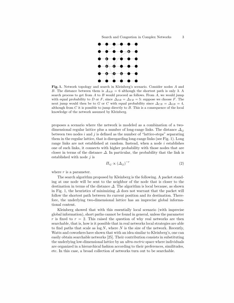
Fig. 1. Network topology and search in Kleinberg’s scenario. Consider nodes A andB. The distance between them is ∆AB = 6 although the shortest path is only 3. Asearch process to get from A to B would proceed as follows. From A, we would jumpwith equal probability to D or F , since ∆DB = ∆F B = 5: suppose we choose F . Thenext jump would then be to G or C with equal probability since ∆CB = ∆GB = 4,although from C it is possible to jump directly to B. This is a consequence of the localknowledge of the network assumed by Kleinberg.

proposes a scenario where the network is modeled as a combination of a two-dimensional regular lattice plus a number of long-range links. The distance ∆ij

between two nodes i and j is defined as the number of “lattice-steps” separatingthem in the regular lattice, that is disregarding long-range links (see Fig. 1). Longrange links are not established at random. Instead, when a node i establishesone of such links, it connects with higher probability with those nodes that arecloser in terms of the distance ∆. In particular, the probability that the link isestablished with node j is

Πij ∝ (∆ij)−r

(2)

where r is a parameter.

The search algorithm proposed by Kleinberg is the following. A packet stand-ing at one node will be sent to the neighbor of the node that is closer to thedestination in terms of the distance ∆. The algorithm is local because, as shownin Fig. 1, the heuristics of minimizing ∆ does not warrant that the packet willfollow the shortest path between its current position and its destination. There-fore, the underlying two-dimensional lattice has an imprecise global informa-tional content.

Kleinberg showed that with this essentially local scenario (with impreciseglobal information), short paths cannot be found in general, unless the parameterr is fixed to r = 2. This raised the question of why real networks are thensearchable, that is, how is it possible that in real networks local strategies are ableto find paths that scale as log N , where N is the size of the network. Recently,Watts and coworkers have shown that with an idea similar to Kleinberg’s, one caneasily obtain searchable networks [25]. Their contribution consists in substitutingthe underlying low-dimensional lattice by an ultra-metric space where individualsare organized in a hierarchical fashion according to their preferences, similitudes,etc. In this case, a broad collection of networks turn out to be searchable.


Parallel to these efforts, there have been some attempts to exploit the scalefree nature of some networks to design algorithms that, being local in nature,are still quite efficient [26,27]. The idea in all these works is to profit from thescale-free nature of networks such as the Internet and bias the search towardsthose nodes that have a high connectivity and therefore act as hubs.

3 Load and congestion in complex networks

When the network has to tackle several simultaneous (or parallel) search prob-lems it raises the important issue of congestion at overburdened nodes [13–17].Indeed, for a single search problem the optimal network is clearly a highly cen-tralized star-like structure, with one or various nodes in the center and all therest connected to them. This structure is cheap to assemble in terms of numberof links and efficient in terms of searchability, since the average cost (number ofsteps) to find a given node is always bounded (2 steps), independently of thesize of the system. However, the star-like structure will become inefficient whenmany search processes coexist in parallel in the network, due to the limitationof the central node to process all the information.

Load, independently of search, has been analyzed in different classes of net-works [28–31]. The load, as introduced in these works, is equivalent to the be-tweenness as it has been defined in social networks [32,28]. The betweenness ofa node j, βj , is defined as the number of minimum paths connecting pairs ofnodes in the network that go through node j. Among the topological proper-ties of networks, betweenness has become one of their main characteristics. Inprinciple the time needed for the computation of the betweenness of all verticesis of order O(MN2), where N is the number of nodes and M the number oflinks of the network. However, Newman [28] introduced an algorithm that re-duces the magnitude of the time needed for the computation by a factor of N .This definition was used to measure the social role played by scientists in somecollaboration networks [28]. Later on, it was also applied to quantify model net-works. Thus, in [29] different networks are constructed and their distributionof betweennesses (or loads) measured. For instance, scale-free networks with anexponent 2 < γ ≤ 3 lead to a load distribution which is also a power law,P (`) ∼ `−δ with δ ≈ 2.2. On the other side, the load distribution of small-worldnetworks shows a combined behavior of two Poisson-type decays. In subsequentwork, the authors in [31] suggested that real-world networks should be classifiedin two different universality classes, according to the exponent of the power-lawdistribution of loads. Finally, the distribution of loads was analytically computedfor scale-free trees in [30].

The works discussed in the previous paragraph consider the betweennessas a topological property of the network, since it accounts for the number ofshorter-paths going through a node. However, to take into account the searchalgorithm and the fact that packets can perform several random steps and thengo through the same node more than once we introduce an effective betweenness.The effective betweenness of node j, Bj , represents the total number of packets


that would pass through j if one packet would be generated at each node at eachtime step with destination to any other node. The effective betweenness coincideswith the topological betweenness when the nodes have complete information ofthe network structure and packets always follow the shortest paths betweenorigin and destination.

4 A model of communication

The model that can handle search and congestion at the same time considersthat the information is formed by discrete packets that are sent from an originnode to a destination node. Each node can store as many information packetsas needed. However, the capacity of nodes to deliver information cannot beinfinite. In other words, any realistic model of communication must consider thatdelivering, for instance, two information packets takes more time than deliveringjust one packet. A particular example of this would be to assume that nodesare able to deliver one (or any constant number) information packet per timestep independently of their load, as happens in the communication model byRadner [11] and in simple models of computer queues [14,15,17], but note thatmany alternative situations are possible. In the present model, each node has acertain capability that decreases as the load of accumulated packets increases.This limitation in the capability of agents to deliver information can result incongestion of the network. Indeed, when the amount of information is too large,agents are not able to handle all the packets and some of them remain undeliveredfor extremely long periods of time. The maximum amount of information that anetwork can manage gives a measure of the quality of its organizational structure.In the study of the model, the interest is focused in both when the congestionoccurs and how it occurs.

4.1 Description of the model

The dynamics of the model is as follows. At each time step t, an informationpacket is created at every node with probability ρ. Therefore ρ is the controlparameter: small values of ρ correspond to low density of packets and high val-ues of ρ correspond to high density of packets. When a new packet is created, adestination node, different from the origin, is chosen randomly in the network.Thus, during the following time steps t + 1, t + 2, . . . , t + T , the packet travels

toward its destination. Once the packet reaches the destination node, it is deliv-ered and disappears from the network. Another interpretation is possible for thisinformation transfer scenario. Packets can be regarded as problems that arise ata certain ratio anywhere in an organization. When one of such problems arises,it must be solved by an arbitrary agent of the network. Thus, in subsequenttime steps the problem flows toward its solution until it is actually solved. Thisproblem solving scenario can be considered a particularly illustrative case of themore general information transfer scenario. The problem solving interpretation


suggest a model similar to Garicano’s [33] in that there is task diversity andagents are specialized in solving only certain types of tasks.

The time that a packet remains in the network is related not only to thedistance between the source and the target nodes, but also to the amount ofpackets in its path. Indeed, nodes with high loads—i.e. high quantities of accu-mulated packets—will need long times to deliver the packets or, in other words,it will take long times for packets to cross regions of the network that are highlycongested. In particular, at each time step, all the packets move from their cur-rent position, i, to the next node in their path, j, with a probability qij . Thisprobability qij is called the quality of the channel between i and j, and is definedas

qij =√

kikj , (3)

where ki represents the capability of agent i and, in general, changes with time.The quality of a channel is, thus, the geometric average of the capabilities of thetwo nodes involved, so that when one of the agents has capability 0, the channelis disabled. It is assumed that ki depends only on the number of packets at nodei, νi, through:

ki = f(νi) (4)

The function f(n) determines how the capability evolves when the number ofpackets at a given node changes. In [18] we proposed a general form although inthis paper we will only show results for the case in which the number of deliveredpackets is constant. This particular case is consistent with simple models ofcomputer queues [14], although the precise definition of the models may differfrom ours.

The election of the functional form for the quality of the channels and thecapability of the nodes is arbitrary. Regarding the first, (3) is plausible for situ-ations in which an effort is needed from both agents involved in the communi-cation process. If, on the contrary, information can be transmitted without thecollaboration of the receiver, an equation of the form

qij = ki , (5)

would be more adequate. Equation (5) will be used for analytical understandingof the problem in Sect. 7, whereas (3) is used in Sect. 5. Some of the mostrelevant features of the model, however, are not dependent on which one is used.

4.2 Congestion and network capacity

Depending on the ratio of generation of packets ρ, two different behaviors areobserved. When the amount of packets is small, the network is able to deliver allthe packets that are generated and, after a transient, the total load N of the net-work achieves a stationary state and fluctuates around a constant value. Thesefluctuations are indeed quite small. Conversely, when ρ is large enough the num-ber of generated packets is larger than the number of packets that the networkcan manage to solve and the network enters a state of congestion. Therefore, N


0 5000 10000 15000 20000 25000

t

101

102

103

N

p=1.5·10−4

p=1.3·10−4

p=1.1·10−4

Fig. 2. Evolution of the total number of packets, N , as a function of time for a (5,7)Cayley tree and different values of ρ, below the critical congestion point (ρ = 1.1·10−4 <

ρc), above the critical congestion point (ρ = 1.5 · 10−4 > ρc), and close to the criticalcongestion point (ρ = 1.3 · 10−4

≈ ρc). Note the logarithmic scale in the Y axis.

never reaches the stationary state but grows indefinitely in time. The transitionfrom the free regime, ρ small, to the congested regime, ρ large, occurs for a welldefined value of ρ, that will be denoted ρc. For values smaller than but close toρc, the steady state is reached but large fluctuations arise.

The three behaviors (free, congested and close to the transition) are depictedin Fig. 2. For ρ < ρc, the width of the fluctuations is small, indicating short char-acteristic times. This means, among other thinks, that the average time requiredto deliver a packet to the destination is small. It also means that correlation timesare short, that is, the state of the network at one time step has little influenceon the state of the network only a few time steps latter. As ρ approaches ρc, thefluctuations are wider and one can conclude that correlations become important.In other words, as one approaches ρc the time needed to deliver a packet growsand the state of the network at one instant is determinant for its state manytime steps later. In the congested regime, the amount of delivered packets isindependent of the load and thus remains constant over time, while the numberof generated packets is also constant, but larger than the amount of deliveredpackets. Thus, at each time step the number of accumulated packets is increasedby a constant amount, and N(t) grows linearly in time.

The transition from the free regime to the congested regime is thereforecaptured by the slope of N(t) in the stationary state. When all the packets aredelivered and there is no accumulation, the average slope is 0 while it is largerthan 0 for ρ > ρc. We use this property to introduce an order parameter, η, that


branch level 1

level 2

level 3

level 4

Fig. 3. Typical hierarchical tree structure used for simulations and calculations: inparticular, it is a tree (3, 4). Dashed line: definition of branch, as used in some of thecalculations.

is able to characterize the transition from one regime to the other:

η(p) = limt→∞

1

ρS

〈∆N〉∆t

, (6)

In this equation ∆N = N(t + ∆t) − N(t), 〈. . .〉 indicates an average over timewindows of width ∆t and S is the number of nodes in the system. Essentially, theorder parameter represents the ratio between undelivered and generated packetscalculated at long enough times such that ∆N ∝ ∆t. Thus, η is only a functionof the probability of packet generation per node and time step, ρ. For ρ > ρc,the system collapses, 〈∆N〉 grows linearly with ∆t and thus η is a function of ρonly. For ρ < ρc, 〈∆N〉 = 0 and η = 0. Since the order parameter is continuousat ρc, the transition to congestion is a critical phenomenon and ρc is a criticalpoint as usually defined in statistical mechanics [34].

Once the transition is characterized, the first issue that deserves attentionis the location of the transition point ρc as a function of the parameters of thenetwork. This transition point gives information about the capacity of a givennetwork. Indeed, the maximum number of packets that a network can handleper time step will be Nc = Sρc. Therefore, ρc is a measure of the amount ofinformation an organization is able to handle and thus of the efficiency of agiven organizational structure. One reasonable problem to propose is, therefore,which is the network that maximizes ρc for a fixed set of available resources(agents and links).

5 Analytical results for hierarchical lattices

As a first step we considered hierarchical networks, since they provide a zerothorder approximation to real structures, and have also been used in the economicsliterature to model organizations [11,35]. In particular we are going to focus onhierarchical Cayley trees, as depicted in Fig. 3. Cayley trees are identified bytheir branching z and their number of levels m, and will be denoted (z, m)hereafter.

In this case the system is regarded as hierarchical also from a knowledgepoint of view. It is assumed in the model that agents have complete knowledge


of the structure of the network in the subbranch they root. Therefore, when anagent receives a packet, he or she can evaluate whether the destination is to befound somewhere below. If so, the packet is sent in the right direction; otherwise,the agent sends the packet to his or her supervisor. Using this simple routingalgorithm, the packets travel always following the shortest path between theirorigin and their destination.

As happens in other problems in statistical physics [36], the particular sym-metry of the hierarchical tree allows an analytical estimation of the critical pointρc. In particular, the approach taken here is mean field in the sense that fluc-tuations are disregarded and only average expected values are considered. Byusing the steady state condition that the number of packets arriving at the topnode, which is the most congested one, equals the number of packets leaving itwe arrive to the following inequality

ρc ≥√

zz(zm−1

−1)2

zm−1 + 1

(7)

when the quality of the channels is given by (3). Although this expression pro-vides an upper bound to ρc, (7) is an excellent approximation for z ≥ 3, asshown in Fig. 4.

The total critical number of generated packets, Nc = ρcS, with S denotingthe size of the system, can be approximated, for large enough values of z and msuch that zm−1 � 1, by

Nc =z3/2

z − 1, (8)

which is independent of the number of levels in the tree. It suggests that thebehavior of the top node is only affected by the total number of packets arrivingfrom each node of the second level, which is consistent with the mean fieldhypothesis.

According to (8), the total number of packets a network can deal with, Nc,is a monotonically increasing function of z, suggesting that, given the number ofagents in the organization, S, the optimal organizational structure, understoodas the structure with highest capacity to handle information, is the flattest one,with m = 2 and z = S − 1.

To understand this result it is necessary to take into account the followingconsiderations:

• We are restricting our comparison only to different hierarchical networksand in any hierarchical network, the top node will receive most of the pack-ets. Since origins and destinations are generated with uniform independentprobabilities, roughly (z−1)/z of the packets will pass through the top node.

• Still, it could seem that having small z is slightly better according to theprevious consideration. However, it is important to note that, in the presentmodel (in particular due to (3)), the loads of both the sender and the receiverare important to have a good communication quality. In a network with smallz, the nodes in the second level have also a high load, while in a networkwith a high z the nodes in the second level are much less loaded.


100

102

104

106

Size, S10

-6

10-4

10-2

100

Sca

led

criti

cal p

roba

bilit

y, (

z-1)

ρc /z

3/2

Cayley

m = 4m = 5m = 6m = 7

10-1

100

101

102

Scaled control parameter, p/pc

0.0

0.5

1.0

Ord

er p

aram

eter

, η

AnalyticalCayley (3,6)Cayley (5,4)Cayley (6,7)

Fig. 4. Comparison between analytical (lines) and numerical (symbols) values obtainedfor hierarchical trees. Left: scaled critical probability (7). Right: order parameter (9).

• We have implicitly assumed that there is no cost for an agent to have a largeamount of communication channels active.

For the order parameter, it is possible to derive an analytical expression forthe simplest case where there are only two nodes that exchange packets. Sincefrom symmetry considerations ν1 = ν2, the average number of packets eliminatedin one time step is 2, while the number of generated packets is 2ρ. Thus ρc = 1and with the present formulation of the model it is not possible to reach thesuper-critical congested regime. However, ρ can be extended to be the averagenumber of generated packets per node at each step (instead of a probability)and in this case it can actually be as large as needed. As a result, the orderparameter for the super-critical phase is η = (ρ − 1)/ρ. As observed in Fig. 4,the general form

η(ρ/ρc) =ρ/ρc − 1

ρ/ρc(9)

fits very accurately the behavior of the order parameter for any Cayley tree.

6 Optimization in model networks

In this section we extend previous studies about local search in model networksin two directions. First, we consider networks that, as in Kleinberg’s work, areembedded in a two-dimensional space, but study the effect not only of longrange random links but also of long range preferential links. Secondly and moresignificantly, we consider the effect of congestion when multiple searches arecarried out simultaneously. As we will show, this effect has drastic consequencesfor optimal network design.

6.1 Network topology

The small world model [1] considered two main components: local linking withneighbors and random long range links giving rise to short average distance be-


tween nodes. The idea of Kleinberg is that local linking provides informationabout the social structure and can be exploited to heuristically direct the searchprocess. Later, Barabasi and Albert showed that growth and preferential attach-ment play a fundamental role in the formation of many real networks [2]. Eventhough this model captures the correct mechanism for the emergence of highly-connected nodes, it is not likely that it captures all mechanisms responsible forthe evolution of “real-world” scale-free networks. In particular, it seems plausi-ble that in many of the networks that show scale-free behavior there is also anunderlying structure as in the Watts and Strogatz model. To illustrate this idea,consider web-pages in the World Wide Web. It is plausible to assume that apage devoted to physics is more likely to be connected to another page devotedto physics than to a page devoted to sociology. That is, a set of pages devoted tophysics is likely to be more inter-connected than a set including pages devotedto physics and sociology.

Therefore we consider networks with four basic components: growth, pref-erential attachment, local attachment and random attachment. To create thenetwork the following algorithm is used:

1. Nodes are located in a two-dimensional square lattice without interconnect-ing them.

2. A node i is chosen at random.3. We create m links starting at the selected node. With probability φ, the

destination node is selected preferentially. With probability 1 − φ the des-tination node is one of the nearest neighbors of the selected node. Whenthe destination node is selected preferentially, we apply the following rule:the probability that a given destination node j is chosen is a function of itsconnectivity

Πj ∝ kγj , (10)

where kj is the number of links of node j and γ is a parameter that allowsto tune the network from maximum preferentiallity to no preferentiallity.Indeed, for γ = 0 the links are random and for γ = 1 we recover the BAmodel, that generates scale free networks in the case φ = 1. For γ > 1, a fewnodes tend to accumulate all the links.

4. A new node is chosen and the process is repeated from step 3, until all thenodes have been chosen once.

Figure 5 shows two examples of networks in the process of being created accord-ing to this algorithm. Note that in this case, the number of links is fixed and theexistence of long range links implies that some local links are not present andtherefore that the information contained in the two-dimensional lattice is lessprecise.

6.2 Communication model and search algorithm

After the definition of the network creation algorithm, we move to the specifi-cation of the communication model and the search algorithm. For the commu-nication model, we will use the general model presented and discussed in Sect.


C

A

B C

A

B

(a) (b)

Fig. 5. Construction of networks with multiple linking mechanisms. In both cases φ =0.25. A random node is selected at each time step and m = 4 new links starting fromthat node are created. Black nodes represent nodes that have already been selected.Dotted lines represent the links created during the last time step in which node C wasselected. In (a), the destination of long range links is created at random (γ = 0), whilein (b) they are created preferentially (γ > 0) and nodes A and B are attracting mostof them.

4. As already stated, this model is general enough and considers the effect ofcongestion due to limitation of ability of nodes to handle information.

In comparison with hierarchical networks, there is only one ingredient of thecommunication model that needs to be reformulated. In the hierarchical versionof the model, when a node receives a packet, it decides to send it downwards inthe right direction if the solution is there, or upward to the agent overseeing herotherwise. This simple routing algorithm arises from the fact that we implicitlyassume that the hierarchy is not only a communicational hierarchy, but also aknowledge hierarchy, where nodes know perfectly the structure of the networkbelow them. In a complex network, this informational content of the hierarchyis lost. Here we will use Kleinberg’s approach [24]. When an agent receives apacket, she knows the coordinates in the underlying two-dimensional space of itsdestination. Therefore, she forwards the packet to the neighbor that is closer tothe destination according to the lattice distance ∆ defined in Sect. 2, providedthat the packet has not visited that node previously1. Note, however, that dis-tance refers to the two-dimensional space, but not necessarily to the topology ofthe complex network and, as in Kleinberg’s work, there might be shortcuts indirections that increase ∆. Moreover, here long range links replace short rangelinks and are not simply added to short range links. Therefore it is possible thatfollowing the direction of minimization of ∆ the packet arrives to a dead endand has to go back.

Considering this algorithm, it is interesting that the three mechanisms toestablish links (local, random and preferential) are somehow complementary. Acompletely regular lattice (all links are local) contains a lot of information since

1 Packets are sent to previously visited nodes only if it is strictly necessary. Thismemory restriction avoids packets getting trapped in loops


all the agents efficiently send their packets in the best possible direction. How-ever, the average path length is extremely high in this networks and thereforethe number of packets that are flowing in the network at a given time is also veryhigh. The addition of random links can reduce dramatically the average pathlength, as in small world networks. However, if the number of random links isvery high, then the number of local links is small and thus sending the packet tothe node closer to the destination is probably quite inefficient (since it is possiblethat, even if it is very close in the underlying two-dimensional space, there isno short path in the actual topology of the network). Finally, preferential linksseem to solve both problems. They obviously solve the long average path lengthproblem but, in addition, the loss of information is not large, since the highlyconnected that actually concentrate this information. The star configuration isan extreme example of this: although there are no local links, the central nodeis capable of sending all the packets in the right directions. However, when theamount of information to handle is big, preferential links are especially inade-quate because highly connected nodes act as centers of congestion. Therefore,optimal structures should be networks where all the mechanisms coexist: com-plex networks.

6.3 Results

We simulate the behavior of the communication model in networks built accord-ing to the algorithm presented in Sect. 4.1. First, a value of the probability ofpacket generation per node and time step, ρ, is fixed. For that particular value,we compare the performance of different networks: networks with different pref-erentiallity, from random (γ = 0) to maximum centralization (γ � 1), and withdifferent fraction of long range links, from pure regular lattices with no longrange links (φ = 0) to networks with no local component (φ = 1). For eachcollection of the parameters ρ, γ, and φ, the network load, N , is calculated andaveraged over a certain time window and over 100 realizations of the network,so that fluctuations due to particular simulations of the packet generation andof the network creation are minimized. As in the economics literature, the ob-jective is to minimize the average time τ for a packet to go from the origin tothe destination.

According to Little’s Law of queuing theory [37], the characteristic time isproportional to the average total load, N , of the network:

N

τ= ρS ⇒ τ =

N

ρS(11)

where ρ is the probability of packet generation for each node at each time step.Thus, minimizing the average cost of a search is equivalent to minimizing thetotal load N of the network.

The main results are shown in Fig. 6. Consider first the behavior of thenetworks at low values of ρ. Figure 6.a shows the load of the network for ρ = 0.01as a function of the fraction of long range links, φ, both when they are random


30

35

40

45

50

55

60

65

70

75

0 0.1 0.2 0.3 0.4 0.5 0.6 0.7 0.8 0.9 1

Num

ber

of p

acke

ts, N

Fraction of preferential links, f

’L20_p0_01m2g0.dat’’L20_p0_01m2g6.dat’

150

200

250

300

350

400

450

500

0 0.1 0.2 0.3 0.4 0.5 0.6 0.7 0.8 0.9 1

Num

ber

of p

acke

ts, N

Fraction of preferential links, f

’L20_p0_03m2g0.dat’’L20_p0_03m2g6.dat’

(a) (b)

(c) (d) (e)

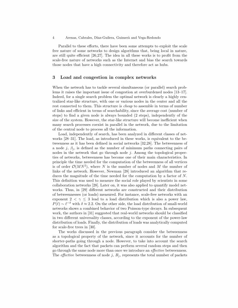
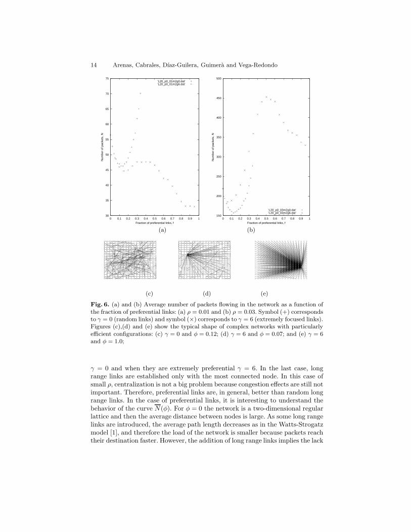
Fig. 6. (a) and (b) Average number of packets flowing in the network as a function ofthe fraction of preferential links: (a) ρ = 0.01 and (b) ρ = 0.03. Symbol (+) correspondsto γ = 0 (random links) and symbol (×) corresponds to γ = 6 (extremely focused links).Figures (c),(d) and (e) show the typical shape of complex networks with particularlyefficient configurations: (c) γ = 0 and φ = 0.12; (d) γ = 6 and φ = 0.07; and (e) γ = 6and φ = 1.0;

γ = 0 and when they are extremely preferential γ = 6. In the last case, longrange links are established only with the most connected node. In this case ofsmall ρ, centralization is not a big problem because congestion effects are still notimportant. Therefore, preferential links are, in general, better than random longrange links. In the case of preferential links, it is interesting to understand thebehavior of the curve N(φ). For φ = 0 the network is a two-dimensional regularlattice and then the average distance between nodes is large. As some long rangelinks are introduced, the average path length decreases as in the Watts-Strogatzmodel [1], and therefore the load of the network is smaller because packets reachtheir destination faster. However, the addition of long range links implies the lack


of local links and when φ is further increased, the heuristic of minimizing thelattice distance ∆ becomes worse and worse. This fact explains that for φ ≈ 0.15(the network is similar to the one depicted in Fig. 6.d) the load has a localminimum that arises due to the trade-off between the two effects of introducinglong range preferential links: shortening of the distances that tends to decreaseN and destruction of the lattice structure that tends to decrease the utility ofthe heuristic search and then to increase N . If φ is further increased, one nodetends to concentrate all the links and for φ = 1 (Fig. 6.e) the network is strictlya star with one central node and the rest connected to it. In this completelycentralized situation, the lack of two-dimensional lattice is not important becausethe packets will be sent to the central node and from there directly to thedestination. Since for small ρ congestion is not an issue, this structure turns outto be even better than the locally optimal structure with φ ≈ 0.15.

The situation is different when considering higher values of the probabilityof packet generation (Fig. 6.b displays the the results for ρ = 0.03). Regardingpreferential linking, the two locally optimal structures with φ = 0.7 and φ = 1(Figs. 6.d and 6.e respectively) persist. However, in this situation and due tocongestion considerations the first is better than the second. Thus, at some in-termediate value of 0.01 < ρ < 0.03, there is a transition such that the optimalstructure changes from being the star configuration to being the mixed config-uration with local as well as preferential links. Significantly, this transition issharp, meaning that there is not a continuous pass from the star to the mixed.

Beyond the behavior of networks built with preferential long range links, it isworth noting that when the effect of the congestion is important (Fig. 6.b), thestructure depicted in Fig. 6.c, where the long range links are actually thrown atrandom, becomes better than the structure in 6.d. In other words, the optimalnetwork is, in this case, a completely decentralized small world network a la

Watts-Strogatz.

7 Optimization in a general framework

In the previous section we have compared the behavior of networks which havebeen built following different rules (nearest neighbor linking, preferential attach-ment, etc.). The main reason for focusing on a particular set of networks is thatit is very costly to compare the performance of two networks: it is necessary torun a simulation, wait for the stationary state and calculate the average load ofthe network. Specially, close to the critical point the time needed to reach thestationary state diverges. In [22] we presented a formalism that is able to copewith search and congestion simultaneously, allowing the determination of opti-mal topologies. This formalism avoids the problem of simulating the dynamicsof the communication process and provides a general scenario applicable to anycommunication process.

Let us focus on a single information packet at node i whose destination isnode k. The probability for the packet to go from i to a new node j in its nextmovement is pk

ij . In particular, pkkj = 0 ∀j so that the packet is removed as soon


as it arrives to its destination. This formulation is completely general, and theprecise form of pk

ij will depend on the search algorithm and on the connectivity

matrix of the network. In particular, when the search is Markovian, pkij does not

depend on previous positions of the packet. In this case, the probability of goingfrom i to j in n steps is given by

P kij(n) =

∑

l1,l2,...,ln−1

pkil1p

kl1l2 · · · p

kln−1j . (12)

This definition allows us to compute the average number of times, bkij , that a

packet generated at i and with destination at k passes through j.

bk =

∞∑

n=1

P k(n) =

∞∑

n=1

(

pk)n

= (I − pk)−1pk. (13)

and the effective betweenness of node j, Bj , is then defined as the sum over allpossible origins and destinations of the packets,

Bj =∑

i,k

bkij . (14)

When the search algorithm is able to find the minimum paths between nodes,the effective betweenness will coincide with the topological betweenness, βj , asusually defined [32,28].

Once, these quantities have been defined, we focus on the load of the network,N(t), which is the number of floating packets. These floating packets are storedin the nodes that act as queues. In a general scenario where packets are generatedat random and independently at each node with a probability ρ, the arrival ofpackets to a given node j is a Poisson process. In the original model presented inSect. 4 we assumed that the quality of the channels depend on both the senderand the receiver nodes; if one assumes that it only depends on the receiver nodethen the delivery of packets is also a Poisson process. In this simple picture, thequeues are called M/M/1 in the computer science literature and the average loadof the network is [37,22]

N =S

∑

j=1

ρBj

S−1

1 − ρBj

S−1

. (15)

There are two interesting limiting cases of equation (15). When ρ is very small,taking into account that the sum of betweennesses is proportional to the averagedistance, one obtains that the load is proportional to the average effective dis-tance. On the other hand, when ρ approaches ρc most of the load of the networkcomes from the most congested node, and therefore

N ≈ 1

1 − ρB∗

S−1

ρ → ρc, (16)

where B∗ is the effective betweenness of the most central node. The last resultssuggest the following interesting problem: to minimize the load of a network it


is necessary to minimize the effective distance between nodes if the amount ofpackets is small, but it is necessary to minimize the largest effective betweennessof the network if the amount of packets is large. The first is accomplished bya star-like network, that is, a network with one central node and all the othersconnected to it. The second, however, is accomplished by a very decentralizednetwork in which all the nodes support a similar load. This behavior is similarto any system of queues provided that the communication depends only on thesender.

It is worth noting that there are only two assumptions in the calculationsabove. The first one has already been mentioned: the movement of the packetsneeds to be Markovian to define the jump probability matrices pk. Althoughthis is not strictly true in real communication networks—where packets are notusually allowed to go through a given node more than once—it can be seenas a first approximation [14,16,17]. The second assumption is that the jumpprobabilities pk

ij do not depend on the congestion state of the network, althoughcommunication protocols sometimes try to avoid congested regions, and thenBj = Bj(ρ). However, all the derivations above will still be true in a numberof general situations, including situations in which the paths that the packetsfollow are unique, in which the routing tables are fixed, or situations in whichthe structure of the network is very homogeneous and thus the congestion of allthe nodes is similar. Compared to situations in which packets avoid congestedregions, it correspond to the worst case scenario and thus provide bounds to morerealistic scenarios in which the search algorithm interactively avoids congestion.

Equation (15) relates a dynamical variable, the load, with the topologicalproperties of the network and the properties of the algorithm. So we have con-verted a dynamical communication problem into a topological problem. Hence,the dynamical optimization procedure of finding the structure that gives theminimum load is reduced to a topological optimization procedure where thenetwork is characterized completely by its effective betweenness distribution. In[22] we considered the problem of finding optimal structures for a purely localsearch, using a generalized simulated annealing (GSA) procedure, as describedin [38,39]. On the one side, we have found that for ρ → 0 the optimal net-work has a star-like centralized structure as expected, which corresponds to theminimization of the average effective distance between nodes. On the other ex-treme, for high values of ρ, the optimal structure has to minimize the maximumbetweenness of the network; this is accomplished by creating a homogeneousnetwork where all the nodes have essentially the same degree, betweenness, etc.One could expect that the transition centralized-decentralized occurs progres-sively. Surprisingly, the results of the optimization process reveal a completelydifferent scenario. According to simulations, star-like configurations are optimalfor ρ < ρ∗; at this point, the homogeneous networks that minimize B∗ becomeoptimal. Therefore there are only two type of structures that can be optimal fora local search process: star-like networks for ρ < ρ∗ and homogeneous networksfor ρ > ρ∗.


(a) (b) (c) (d)

Fig. 7. Optimal topologies for networks with S = 32 nodes, L = 32 links and globalknowledge. (a) ρ = 0.010. (b) ρ = 0.020. (c) ρ = 0.050. (d) ρ = 0.080. In this case ofglobal knowledge, the transition from centralization to decentralization seems smooth.

Beyond the existence of both centralized and decentralized optimal networks,it is significant that the transition from one sort of networks to the other isabrupt, meaning that there are no intermediate optimal structures between to-tal centralization and total decentralization. As already mentioned, this propertyis shared by the model networks in the previous section. Our explanation of thisfact is the following. Since we are considering (in both the present and the lastsections) local knowledge of the network topology, centered star-like configura-tions are extremely efficient in searching destinations and thus minimizing theeffective distance between nodes. This explains that stars are optimal for a widerange of values of ρ, until the central node (or nodes) becomes congested. Atthis point, structures similar to stars will have the same problem and will bemuch worse regarding search; at this point, the only alternative is somethingcompletely decentralized, where the absence of congestion can compensate thedramatic increase in the effective distance between nodes. If this explanation iscorrect, one should be able to obtain a smooth transition from centralization todecentralization by considering global knowledge of the network, in such a waythat the average effective distance (that in this case coincides with the averagepath length) is not much larger in an arbitrary network than in the star. Al-though we do not have extensive simulations in this case, Fig. 7 shows that thereis some evidence to think that this is indeed the case.

8 Summary

We have presented some results concerning search and congestion in networks.By defining a communication model we have been able to cope with the problemsof search and congestion simultaneously. For a hierarchical lattice some analyticalresults are found, by exploiting the symmetry properties of the network. Forcomplex networks, this is not the case, and computational optimization to lookfor the best structures is required. On the one hand, for model networks whereshort-range, long-range, random and preferential connections are mixed we findthat network that perform well for very low load become easily congested whenthe load is increased. On the other hand, when searching for optimal structures ina general scenario there is a clear transition from star-like centralized structuresto homogeneous decentralized ones.


Acknowledgments

This work has been supported by DGES of the Spanish Government, GrantsNo. PPQ2001-1519, No. BFM2000-0626, No. BEC2000-1029, and No. BEC2001-0980, and EC-FET Open Project No. IST-2001-33555.

References

1. D. Watts, S. Strogatz: Nature 393, 440 (1998)2. A.-L. Barabasi, R. Albert: Science 286, 509 (1999)3. L. A. N. Amaral, A. Scala, M. Barthelemy, H. E. Stanley: Proc. Nat. Acad. Sci.

USA 97, 11149 (2000)4. R. Albert, A.-L. Barabasi: Rev. Mod. Phys. 74, 47(2002)5. S. Dorogovtsev, J. F. F. Mendes: Adv. Phys. 51, 1079 (2002)6. M. Faloutsos, P. Faloutsos, C. Faloutsos: Comp. Comm. Rev. 29, 251 (1999)7. R. Albert, H. Jeong, A.-L. Barabasi: Nature 401, 130 (1999)8. M. E. J. Newman: Phys Rev E 66, 035101 (2002)9. H. Ebel, L.-I. Mielsch, S. Bornholdt: Phys Rev E 66, 035103 (2002)

10. R. Guimera, L. Danon, A. Diaz-Guilera, F. Giralt, A. Arenas: cond-mat/0211498.11. R. Radner: Econometrica 61, 1109 (1993)12. S. DeCanio, W. Watkins: J. Econ. Behavior and Organization 36, 275 (1998)13. V. Jacobson: ’Congestion avoidance and control’. In: Proceedings of SIGCOMM

’88 (ACM, Standford, CA 1988)14. T. Ohira, R. Sawatari: Phys. Rev. E 58, 193 (1998)15. A. Tretyakov, H. Takayasu, M. Takayasu: Physica A 253, 315 (1998)16. A. Arenas, A. Diaz-Guilera, R. Guimera: Phys. Rev. Lett. 86, 3196 (2001)17. R. Sole, S. Valverde: Physica A 289, 595(2001)18. R. Guimera, A. Arenas, A. Diaz-Guilera, F. Giralt: Phys. Rev. E 66, 026704 (2002)19. I. Csabai: J. Phys. A: Math. Gen. 27, L417 (1994)20. M. Takayasu, H. Takayasu, T. Sato: Physica A 233, 824(1996)21. R. Guimera, A. Arenas, A. Diaz-Guilera: Physica A 299, 247 (2001)22. R. Guimera, A. Diaz-Guilera, F. Vega-Redondo, A. Cabrales, A. Arenas: Phys.

Rev. Lett. 89, 248701 (2002)23. J. Travers, S. Milgram, Sociometry 32, 425 (1969)24. J. Kleinberg: Nature 406, 845 (2000)25. D. J. Watts, P. S. Dodds, M. E. J. Newman: Science 296, 1302 (2002)26. L. A. Adamic, R. M. Lukose, A. R. Puniyani, B. A. Huberman: Phys. Rev. E 64,

046135 (2001)27. B. Tadic: Eur. Phys. J. B 23, 221 (2001)28. M. E. J. Newman: Phys. Rev. E 64, 016132 (2001)29. K.-I. Goh, B. Kahng, D. Kim: Phys. Rev. Lett. 87, 278701 (2001)30. G. Szabo, M. Alava, J. Kertesz: Phys. Rev. E 66, 026101 (2002)31. K.-I. Goh, E. Oh, H. Jeong, B. Kahng, D. Kim: Proc. Nat. Acad. Sci. USA 99,

12583 (2002)32. L. C. Freeman, Sociometry 40, 35 (1977)33. L. Garicano: J. Political Economy 108, 874 (2000)34. H. E. Stanley: Introduction to phase transitions and critical phenomena (Oxford

University Press, Oxford 1987).35. P. Bolton, M. Dewatripont: Quart. J. Economics 109, 809 (1994)


36. D. Stauffer, A. Aharony: Introduction to percolation theory, 2nd edn. (Taylor andFrancis, 1992).

37. O. Allen: Probability, statistics and queueing theory with computer science appli-

cation, 2nd edn. (Academic Press, New York 1990).38. C. Tsallis, D. A. Stariolo: In Annual Review of Computational Physics II, ed. by

D. Stauffer (World Scientific, Singapore 1994).39. T. J. P. Penna: Phys. Rev. E 51, R1 (1995)

search and congestion in complex networks -...

Documents