search for gamma-ray lines from dark matter with the fermi large
TRANSCRIPT

Search for Gamma-ray Lines
from Dark Matter with the
Fermi Large Area Telescope
TOMI YLINEN
Doctoral Thesis in Physics
Stockholm, Sweden 2010


Doctoral Thesis in Physics
Search for Gamma-ray Lines
from Dark Matter with the
Fermi Large Area Telescope
Tomi Ylinen
Particle and Astroparticle Physics, Department of Physics,Royal Institute of Technology, SE-106 91 Stockholm, Sweden
Stockholm, Sweden 2010

Cover illustration: The gamma-ray sky as seen by the Fermi Large Area Telescopeafter one year of observations.
Akademisk avhandling som med tillstand av Kungliga Tekniska Hogskolan i Stock-holm framlagges till offentlig granskning for avlaggande av teknologie doktorsexa-men mandagen den 7 juni 2010 kl 14.00 i sal FA32, AlbaNova Universitetscentrum,Roslagstullsbacken 21, Stockholm.
Avhandlingen forsvaras pa engelska.
ISBN 978-91-7415-672-0
TRITA-FYS 2010:28ISSN 0280-316XISRN KTH/FYS/--10:28--SE
c© Tomi Ylinen, May 2010Printed by Universitetsservice US-AB 2010

Abstract
Dark matter (DM) constitutes one of the most intriguing but so far unresolvedissues in physics. In many extensions of the Standard Model of particle physics,the existence of a stable Weakly Interacting Massive Particle (WIMP) is predicted.The WIMP is an excellent DM particle candidate. One of the most interestingscenarios is the creation of monochromatic gamma-rays from the annihilation ordecay of these particles. This type of signal would represent a “smoking gun” forDM, since no other known astrophysical process should be able to produce it.
In this thesis, the search for spectral lines with the Large Area Telescope (LAT)onboard the Fermi Gamma-ray Space Telescope (Fermi) is presented. The satellitewas successfully launched from Cape Canaveral in Florida, USA, on 11 June, 2008.The energy resolution and performance of the detector are both key factors in thesearch and are investigated here using beam test data, taken at CERN in 2006with a scaled-down version of the Fermi -LAT instrument. A variety of statisticalmethods, based on both hypothesis tests and confidence interval calculations, arethen reviewed and tested in terms of their statistical power and coverage.
A selection of the statistical methods are further developed into peak findingalgorithms and applied to a simulated data set called obssim2, which corresponds toone year of observations with the Fermi -LAT instrument, and to almost one year ofFermi -LAT data in the energy range 20–300 GeV. The analysis on Fermi -LAT datayielded no detection of spectral lines, so limits are placed on the velocity-averagedcross-section, 〈σv〉γX , and the decay lifetime, τγX , and theoretical implications arediscussed.
iii

iv

Contents
Abstract iii
Contents v
Introduction 3
1 Particle interactions 7
1.1 Charged particles . . . . . . . . . . . . . . . . . . . . . . . . . . . . 71.2 Photons . . . . . . . . . . . . . . . . . . . . . . . . . . . . . . . . . 91.3 Electromagnetic showers . . . . . . . . . . . . . . . . . . . . . . . . 9
2 Gamma-ray astronomy 13
2.1 Gamma-ray production . . . . . . . . . . . . . . . . . . . . . . . . 132.1.1 Thermal gamma-rays . . . . . . . . . . . . . . . . . . . . . 132.1.2 Non-thermal gamma-rays . . . . . . . . . . . . . . . . . . . 14
2.2 Gamma-ray sources . . . . . . . . . . . . . . . . . . . . . . . . . . . 152.3 Detection techniques . . . . . . . . . . . . . . . . . . . . . . . . . . 172.4 History . . . . . . . . . . . . . . . . . . . . . . . . . . . . . . . . . 18
3 Dark matter 25
3.1 Evidence . . . . . . . . . . . . . . . . . . . . . . . . . . . . . . . . . 253.2 Dark matter candidates . . . . . . . . . . . . . . . . . . . . . . . . 283.3 Dark matter properties . . . . . . . . . . . . . . . . . . . . . . . . . 303.4 Halo models . . . . . . . . . . . . . . . . . . . . . . . . . . . . . . . 313.5 Detection techniques . . . . . . . . . . . . . . . . . . . . . . . . . . 323.6 Experimental status . . . . . . . . . . . . . . . . . . . . . . . . . . 33
4 Fermi Gamma-ray Space Telescope 35
4.1 Scientific goals . . . . . . . . . . . . . . . . . . . . . . . . . . . . . 364.2 Large Area Telescope . . . . . . . . . . . . . . . . . . . . . . . . . . 37
4.2.1 Tracker . . . . . . . . . . . . . . . . . . . . . . . . . . . . . 384.2.2 Calorimeter . . . . . . . . . . . . . . . . . . . . . . . . . . . 394.2.3 Anti-Coincidence Detector . . . . . . . . . . . . . . . . . . . 40
v

vi Contents
4.2.4 Event reconstruction . . . . . . . . . . . . . . . . . . . . . . 434.2.5 On-orbit calibration . . . . . . . . . . . . . . . . . . . . . . 454.2.6 Data structure . . . . . . . . . . . . . . . . . . . . . . . . . 464.2.7 Performance . . . . . . . . . . . . . . . . . . . . . . . . . . 47
4.3 Gamma-ray Burst Monitor . . . . . . . . . . . . . . . . . . . . . . 49
5 Calibration Unit beam test 51
5.1 Introduction . . . . . . . . . . . . . . . . . . . . . . . . . . . . . . . 515.2 Calibration Unit . . . . . . . . . . . . . . . . . . . . . . . . . . . . 525.3 PS facility beam test . . . . . . . . . . . . . . . . . . . . . . . . . . 535.4 SPS facility beam test . . . . . . . . . . . . . . . . . . . . . . . . . 56
6 Beam test analysis 59
6.1 Analysis approach . . . . . . . . . . . . . . . . . . . . . . . . . . . 596.2 Creating a clean sample . . . . . . . . . . . . . . . . . . . . . . . . 616.3 Position reconstruction in the CAL . . . . . . . . . . . . . . . . . . 63
6.3.1 Asymmetry curves . . . . . . . . . . . . . . . . . . . . . . . 646.4 Direction reconstruction in the CAL . . . . . . . . . . . . . . . . . 706.5 Energy reconstruction in the CAL . . . . . . . . . . . . . . . . . . 72
6.5.1 Raw energy distributions . . . . . . . . . . . . . . . . . . . 726.5.2 Longitudinal profile . . . . . . . . . . . . . . . . . . . . . . 726.5.3 Energy resolution . . . . . . . . . . . . . . . . . . . . . . . . 74
6.6 Latest developments . . . . . . . . . . . . . . . . . . . . . . . . . . 856.7 Summary and conclusions . . . . . . . . . . . . . . . . . . . . . . . 85
7 Dark matter line search 91
7.1 Initial discussions . . . . . . . . . . . . . . . . . . . . . . . . . . . . 917.1.1 Region-of-interest selection . . . . . . . . . . . . . . . . . . 917.1.2 Halo profile selection . . . . . . . . . . . . . . . . . . . . . . 937.1.3 Data selection . . . . . . . . . . . . . . . . . . . . . . . . . . 93
7.2 Statistical concepts . . . . . . . . . . . . . . . . . . . . . . . . . . . 957.2.1 Frequentist and Bayesian statistics . . . . . . . . . . . . . . 957.2.2 Confidence intervals . . . . . . . . . . . . . . . . . . . . . . 967.2.3 Hypothesis tests . . . . . . . . . . . . . . . . . . . . . . . . 967.2.4 Coverage . . . . . . . . . . . . . . . . . . . . . . . . . . . . 977.2.5 Power . . . . . . . . . . . . . . . . . . . . . . . . . . . . . . 977.2.6 Significance . . . . . . . . . . . . . . . . . . . . . . . . . . . 98
7.3 Statistical methods . . . . . . . . . . . . . . . . . . . . . . . . . . . 987.3.1 Bayes factor method . . . . . . . . . . . . . . . . . . . . . . 987.3.2 χ2 method . . . . . . . . . . . . . . . . . . . . . . . . . . . 997.3.3 Feldman & Cousins . . . . . . . . . . . . . . . . . . . . . . 997.3.4 Profile likelihood . . . . . . . . . . . . . . . . . . . . . . . . 1007.3.5 Method comparison . . . . . . . . . . . . . . . . . . . . . . 100
7.4 Implementations for line search . . . . . . . . . . . . . . . . . . . . 102

Contents vii
7.4.1 Binned ProFinder . . . . . . . . . . . . . . . . . . . . . . . 1027.4.2 Unbinned ProFinder . . . . . . . . . . . . . . . . . . . . . . 1047.4.3 Scan Statistics . . . . . . . . . . . . . . . . . . . . . . . . . 113
7.5 Application on obssim2 data set . . . . . . . . . . . . . . . . . . . 1167.5.1 Exposure . . . . . . . . . . . . . . . . . . . . . . . . . . . . 1207.5.2 Limits . . . . . . . . . . . . . . . . . . . . . . . . . . . . . . 122
7.6 Application on Fermi-LAT data . . . . . . . . . . . . . . . . . . . . 1247.6.1 Exposure . . . . . . . . . . . . . . . . . . . . . . . . . . . . 1287.6.2 Limits . . . . . . . . . . . . . . . . . . . . . . . . . . . . . . 129
7.7 Summary and conclusions . . . . . . . . . . . . . . . . . . . . . . . 133
8 Discussion and outlook 135
Acknowledgements 137
List of figures 139
List of tables 143
Bibliography 145

viii

To my grandfather,
who always saw the humour of the situation.


Introduction
Gamma-rays are defined as photons that constitute the highest energy region in theelectromagnetic spectrum and have energies above 100 keV. They were discoveredin 1900 by Paul Villard and have since been studied extensively from Earth andfrom space.
The fundamental processes that are known to give rise to gamma-rays includehigh-energy charged particle interactions with radiation and magnetic fields (inverseCompton, synchrotron radiation and bremsstrahlung) but also the decay of neutralpions and the annihilation of an electron with a positron.
In space, gamma-rays are produced through the aforementioned mechanisms ina large variety of astrophysical objects and since they are unaffected by magneticfields, they point directly towards the sources. In asteroids and other circumso-lar objects, gamma-rays are produced when high-energy cosmic rays interact withthe rock and ice. Interactions that create gamma-rays also take place in the at-mospheres of the Earth and the Sun. More distant gamma-rays are produced onboth galactic and extragalactic scales. On galactic scales, rapidly rotating andhighly magnetised neutron stars (pulsars), interstellar matter and remnants fromsupernova explosions give rise to gamma-rays. Further out in space, a variety of ac-tive galaxies but also particularly explosive and rapid events, known as gamma-raybursts, are known to produce them.
The current understanding of the Universe, supported by a vast number ofobservations, suggests that a large portion of its content is dark and invisible. Onlyabout 5% of the Universe is believed to consist of baryonic matter, whereas roughly70% is referred to as dark energy and the remaining ∼25% is denoted as dark matterand is believed to be composed of some form of exotic matter. A multitude oftheories have been constructed to describe the nature of dark matter and a populartheory proposes that it consists of weakly interacting massive particles or WIMPs.The WIMPs can, in many cases, annihilate or decay into known Standard Modelparticles, including gamma-rays. A “smoking-gun” signal from this kind of darkmatter would be the observation of a spectral line, produced by the annihilation ordecay of WIMPs into two gamma-rays or one gamma-ray and some other particle.
Throughout history, a large number of experiments have studied the Universein gamma-rays and the latest addition is the space-based Fermi Gamma-ray SpaceTelescope (Fermi) and its principle instrument, the Large Area Telescope (LAT).
3
4 Contents
The Fermi -LAT instrument has an unprecedented sensitivity and performanceand consists of a precision tracker, which provides the direction of the incidentgamma-ray, a segmented calorimeter, constructed to measure the energy and ananti-coincidence detector, used to reduce the contamination from charged particles.The instrument is designed to measure gamma-rays with energies from 20 MeV tomore than 300 GeV.
In this thesis, the proposed spectral line signal is searched for by using gamma-ray data from the Fermi Gamma-ray Space Telescope. The sensitivity of such asearch depends on the overall performance and understanding of the instrument,which both rely heavily on the Geant4-based full-detector Monte Carlo simulation,developed by the Fermi -LAT Collaboration. For this reason, a scaled-down versionof the Fermi -LAT instrument, called the Calibration Unit, was tested at CERNusing beams of photons and charged particles. The analysis of the collected beamtest data, presented in this thesis, is focused on investigating the accuracy of theMonte Carlo simulation in terms of directional and energy-related observables, dueto their particular importance to the spectral line search.
The spectral line search itself is a statistical analysis, where the contributionsfrom a signal and a background component of known shapes are calculated froma simultaneous fit to the data. The properties of the statistical method also playan important role in the search and can be tested by sets of random realisations(typically called toy Monte Carlo experiments) of the assumed shapes of the com-ponents. The properties that have been investigated in this thesis for a selected setof statistical methods are the statistical power and coverage.
Outline of the thesis
The first chapters of this thesis contain the theoretical backgrounds relevant tothe performed analyses. In Chapter 1, the various interactions occurring whenparticles traverse matter are reviewed. Chapter 2 gives a recapitulation of gamma-ray astronomy, including a historical overview, and Chapter 3 focuses on providinga theoretical background to dark matter. In Chapter 4, the Fermi Gamma-raySpace Telescope and its different subdetectors are explained in detail. Chapters 5and 6 are devoted to the beam tests performed at CERN and the analysis of thedata obtained there, respectively. Chapter 7 is dedicated to the search for spectrallines, both on a simulated data set that corresponds to one year of data with theFermi -LAT and on almost one year of measured data. The challenges involved in aline search are also explained and results from benchmark tests, using the statisticalpower and coverage, are shown for a number of different statistical methods. Finally,in Chapter 8, conclusions from and discussions of the analyses are presented.

Contents 5
Author’s contribution
The beam test efforts were performed by a large number of people within theFermi -LAT Collaboration. Before the tests, the author helped in assessing thedata requirements for the planned setups. The author then actively participatedin the beam tests at CERN by assisting in the setup and disassembling of theexperiments, taking shifts, analysing and validating the quality of the data andMonte Carlo simulations and by presenting the results in shift meetings.
In the following overall analysis of the beam test data, the author developedan event selection and analysed the differences between data and Monte Carlosimulations in terms of direction, position and energy measurements and frequentlypresented the results in online beam-test meetings.
In the dark matter analysis, the author was fully responsible for translatingthe statistical methods into tools for searching for dark matter lines. The softwareused in the analyses, which utilise the ROOT and Science Tools frameworks, werewritten by the author. The DarkSUSY simulation package was also adapted by theauthor to calculate the line-of-sight integral over a specific region of the sky.
In the benchmark studies of the statistical power and coverage for differentstatistical methods, the implementation and results from the frequentist methodswere produced by the author.
The development, implementation and execution of the spectral line search onobssim2 data was done by the author. In the spectral line search on measuredFermi -LAT data, the unbinned profile likelihood was implemented and tested bythe author. The author, furthermore, calculated the upper limits on the flux fromdark matter annihilations or decays, which were subsequently published in PhysicalReview Letters.
Publications
The author has given direct and significant contributions to the following publica-tions and proceedings:
• A.A. Abdo ... T. Ylinen, et al., Fermi Large Area Telescope Search for PhotonLines from 30 to 200 GeV and Dark Matter Implications, Physical ReviewLetters, 104 (2010) 091302, [arXiv:astro-ph/1001.4836].
• T. Ylinen, Y. Edmonds, E. D. Bloom & J. Conrad, Dark Matter annihilationlines with the Fermi-LAT, Proceedings of the 31st ICRC, Lodz, 2009.
• T. Ylinen, Y. Edmonds, E. D. Bloom & J. Conrad, Detecting Dark Matterannihilation lines with Fermi, Proceedings of “Identification of Dark Matter2008”, Stockholm, Sweden, p.111, [arXiv:astro-ph/0812.2853].
• J. Conrad, J. Scargle & T. Ylinen, Statistical analysis of detection of, andupper limits on, dark matter lines, AIP Conf. Proc., 921 (2007) 586.

6 Contents
• L. Baldini ... T. Ylinen, et. al, Preliminary results of the LAT CalibrationUnit beam tests, AIP Conf. Proc., 921 (2007) 190.
The author is at the time of writing also co-author on another 59 Fermi -LATCollaboration papers and 2 PoGOLite Collaboration papers.

Chapter 1
Particle interactions
This chapter reviews some of physical processes involved when the particles inves-tigated in Chapter 6 interact with matter. For a more detailed review includingmathematical descriptions, see e.g. [1].
1.1 Charged particles
In Fig. 1.1, the stopping power for positive muons in copper is shown over nineorders of magnitude in momentum. The plot is divided into different regions, wheredifferent effects dominate the interactions taking place.
Figure 1.1. The average energy loss of positive muons in copper as a function ofthe muon momentum (from [1]).
7
8 Chapter 1. Particle interactions
Below about 0.7 MeV, non-ionising nuclear recoil energy losses dominate thetotal energy loss for e.g. protons. In the same region, Lindhard and Sharff havedescribed the stopping power as proportional to β = v/c [2]. For 1–5 MeV inthe second region, no satisfactory theory exists. For protons, however, there arephenomenological fitting formulae developed by Anderson and Ziegler [3].
Above about 7 MeV, the so-called “Barkas effect” yields a stopping power thatis somewhat larger for negative particles than for positive particles with the samemass and velocity [4]. Overall, however, the stopping power is well described by theBethe-Bloch equation and the particles lose their energy mainly through ionisationand atomic excitation. Due to the muon spectrum at sea level, in which most of themuons have an energy that is around the minimum of the Bethe-Bloch function,muons are often referred to as minimum-ionising particles.
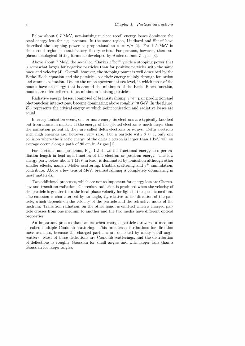
Radiative energy losses, composed of bremsstrahlung, e+e− pair production andphotonuclear interactions, become dominating above roughly 70 GeV. In the figure,Eµc represents the critical energy at which point ionisation and radiative losses areequal.
In every ionisation event, one or more energetic electrons are typically knockedout from atoms in matter. If the energy of the ejected electron is much larger thanthe ionisation potential, they are called delta electrons or δ-rays. Delta electronswith high energies are, however, very rare. For a particle with β ≈ 1, only onecollision where the kinetic energy of the delta electron is larger than 1 keV will onaverage occur along a path of 90 cm in Ar gas [1].
For electrons and positrons, Fig. 1.2 shows the fractional energy loss per ra-diation length in lead as a function of the electron or positron energy. The lowenergy part, below about 7 MeV in lead, is dominated by ionisation although othersmaller effects, namely Møller scattering, Bhabha scattering and e+ annihilation,contribute. Above a few tens of MeV, bremsstrahlung is completely dominating inmost materials.
Two additional processes, which are not as important for energy loss are Cheren-kov and transition radiation. Cherenkov radiation is produced when the velocity ofthe particle is greater than the local phase velocity for light in the specific medium.The emission is characterised by an angle, θc, relative to the direction of the par-ticle, which depends on the velocity of the particle and the refractive index of themedium. Transition radiation, on the other hand, is emitted when a charged par-ticle crosses from one medium to another and the two media have different opticalproperties.
An important process that occurs when charged particles traverse a mediumis called multiple Coulomb scattering. This broadens distributions for directionmeasurements, because the charged particles are deflected by many small anglescatters. Most of these deflections are Coulomb scatterings, and the distributionof deflections is roughly Gaussian for small angles and with larger tails than aGaussian for larger angles.

1.3. Electromagnetic showers 9
Figure 1.2. The fractional energy loss per radiation length in lead as a function ofelectron or positron energy (from [1]).
1.2 Photons
In Fig. 1.3, the cross-sections of the different processes involved in photon-matterinteractions are shown. The cross-sections depend on the material and the figureis an example plot for photons interacting in lead.
At low energies (for lead below about 500 keV), the cross-section for the atomicphotoelectric effect, σp.e. is dominating. In the photoelectric effect, a photon isabsorbed by an atom and followed by the emission of an electron. Another processat low energies, which is not as probable as the photoelectric effect is Rayleighscattering, σRayleigh, where a photon is scattered by an atom without ionising orexciting the atom.
At higher energies, Compton scattering, σCompton, in which photons are scat-tered by electrons at rest, is the dominating process but photonuclear interactionsuch as the Giant Dipole Resonance, σg.d.r., where the target nucleus is broken up,also contributes. In lead, this region ranges from about 500 keV to about 5 MeV.
In the high end of the energy range (in lead above about 5 MeV), pair productionin nuclear (κnuc) and electron (κe) fields is completely dominating.
1.3 Electromagnetic showers
A high-energy electron or photon that interacts with a thick absorber gives riseto a cascade of pair productions from photons and bremsstrahlung photons fromthe pair-produced electrons and positrons. The longitudinal development of theresulting electromagnetic shower, shown in Fig. 1.4, scales as the radiation lengthin the absorber. When the energies of the electrons and positrons fall below the

10 Chapter 1. Particle interactions
Figure 1.3. The cross-sections of the photoelectric effect, Rayleigh- and Comptonscattering, pair production in nuclear and electron fields and photonuclear interac-tions as a function of photon energy in lead (from [1]).
critical energy, Ec, where the ionisation loss rate is equal to the bremsstrahlung lossrate, additional shower particles are no longer produced and the energy dissipationis then provided by ionisation and excitation.
Figure 1.4. A simulation of an electromagnetic shower from a 50 GeV photon(from [5]).
Electromagnetic showers are often described by introducing the scale variablest = x/X0 and y = E/Ec, in which case the longitudinal distance is measured in

1.3. Electromagnetic showers 11
units of radiation length, X0, and the energy is described in units of the criticalenergy. One radiation length (which depends on the atomic number Z) is definedas a characteristic mean distance in which a high-energy electron loses all but 1/eof its energy through bremsstrahlung and a high-energy photon propagates 7/9 ofthe mean free path for pair production. With this notation, the mean longitudinalprofile of the energy deposition can be fitted reasonably well with a gamma function,given in Eq. 1.1:
dE
dt= E0b
(bt)a−1e−bt
Γ(a)(1.1)
According to EGS4 simulations, the maximum occurs at tmax = (a − 1)/b =1.0 × (ln y + Cj), where j = e, γ, a and b are free parameters and Ce = −0.5 forelectron-induced showers and Cγ = +0.5 for photon-induced showers [1].

12

Chapter 2
Gamma-ray astronomy
This chapter contains an introduction to gamma-ray astronomy. First, the differ-ent mechanisms, in which cosmic gamma-rays are produced, is reviewed. This isfollowed by a short description of the gamma-ray emitting astrophysical sourcesand the main techniques used to observe them. Finally a historical overview ofgamma-ray astronomy is provided.
2.1 Gamma-ray production
Gamma-rays are generally defined as photons that have energies greater than about100 keV. There are a number of different processes in which astronomical objects canproduce them but the mechanisms are either thermal or non-thermal. A thoroughreview of the different forms of production can be found in e.g. [6].
2.1.1 Thermal gamma-rays
A body with a temperature that is different from zero will emit thermal radiation.If the body is a perfect absorber in thermal equilibrium with its environment attemperature T , i.e. a black-body, the energy-dependent intensity of photons isgoverned by the Planck formula in Eq. 2.1,
I(Eph) =2E3
ph
(hc)2
[1
eEph
kBT − 1
], (2.1)
where h and kB are the Planck and Boltzmann’s constants, respectively, and c isthe speed of light. The average energy of the photons is given by Eq 2.2.
13

14 Chapter 2. Gamma-ray astronomy
〈Ethermal〉 ≈ 2.3 × 10⁻¹⁰
(T
K
)MeV (2.2)
In order to get thermal photons at an average energy of 1 GeV, temperatures ofabout 1013 K are needed. Such temperatures are only reached in the Big Bang. Inaddition, that temperature level implies such a large photon density that the meanfree path for the photons is less than 1 cm. This leads to self-absorption by pairproduction. Typical astrophysical gamma-ray sources are therefore non-thermal innature.
2.1.2 Non-thermal gamma-rays
For gamma-rays that are produced non-thermally, a distinction can be made be-tween gamma-rays from particle-field interactions and gamma-rays from particle-matter interactions. The first category includes the following processes:
• Synchrotron radiation, which is created when relativistic charged particlesmove in a magnetic field. The energy loss rate of an electron moving in ahelical path around a magnetic field B is then given by:
−(dEe
dt
)
syn
=2
3c
(e2
mec2
)2
B2⊥γ
2, (2.3)
where e is the electron charge, me is the electron mass, B⊥ = B sin θ whereθ is the pitch angle and γ = Ee/mec
2 is the Lorentz factor.
• Curvature radiation, which occurs when the magnetic field that the chargedparticle moves in is non-uniform and the curvature radius, Rc, of the magneticfield line is small. The energy loss is then given by:
−(dEe
dt
)
curv
=2
3
ce2
R2c
γ4 (2.4)
• Inverse Compton (IC) interactions, which refer to the scattering of relativisticelectrons on soft photons, where the energy transfer to the photon gives thephoton an energy in the gamma-ray region. In the classical limit, the averageenergy of the emerging photon is 〈EIC,γ〉 = (4/3) 〈Eγ〉 γ2, where 〈Eγ〉 is theaverage energy of the target photon. In the relativistic case, most of theenergy of the electron is transferred to the photon and EIC,γ ≈ Ee.
The second category with particle-matter interactions consists of:
• Relativistic bremsstrahlung, which is produced when relativistic electrons areaccelerated in the electrostatic field of a nucleus.

2.2. Gamma-ray sources 15
• Hadronic gamma-ray emission, where gamma-rays are produced via the decayof neutral pions (π0), which have a proper lifetime of 9 × 10⁻¹⁷ s. Theneutral pions are created through a number of different channels of protonand antiproton interactions.
• Electron-positron annihilations, in which gamma-rays are produced throughthe reaction e+ + e− → γ + γ. If the electron and the positron are at rest,the photons will have an energy equal to the rest mass of the electron, i.e.0.511 MeV. If one of the leptons is moving at a high velocity, one of thephotons will have a high energy and the other photon will have an energy ofabout 0.511 MeV.
• Dark matter annihilations/decays. Many extensions of the Standard Modelof particle physics predict the existence of dark matter particles, which self-annihilate or decay and produces either gamma-rays directly or indirectlythrough the decay of the Standard Model particles produced in the process. Inmany of these models, the dominant final states are quarks and gauge bosons(W/Z), which through hadronisations create π0 particles that decay into twogamma-rays. Also leptonic final state models (e.g. into µ+µ−) have beensuggested to fit recent cosmic-ray electron and position measurements (seealso Section 3.6). The gamma-rays can then be produced via IC processes butalso via internal bremsstrahlung, where an additional photon is emitted in thefinal state [7]. Many models also allow for direct channels into monoenergeticgamma-rays. The possibility of gamma-rays from dark matter has, however,not yet been experimentally verified. The subject of dark matter is coveredin more detail in Chapter 3.
2.2 Gamma-ray sources
The number of sources that produce cosmic gamma-rays come in great numbers.They are located in all distance scales and include:
• Circumsolar sourcesIt can be deduced from data taken with the Energetic Gamma-Ray Experi-ment Telescope (EGRET), described in Section 2.4, that albedo gamma-raysare created in small solar system bodies in the main belt asteroids betweenMars and Jupiter, the Jovian and Neptunian Trojans and in the Kuiper Beltobjects beyond Neptune through the interaction of cosmic-rays with the solidrock and ice [8]. The diffuse emission from these objects has an integratedflux of less than ∼ 6 × 10⁻⁶ cm−2 s−1 in the energy range 100–500 MeV.This is about 12 times the gamma-ray flux from the Moon, where the sameprocess occurs. Studies have also been conducted with the successor FermiGamma-ray Space Telescope and the preliminary results for the Moon[9] arein general agreement with EGRET observations. Strong albedo gamma-ray

16 Chapter 2. Gamma-ray astronomy
emission due to cosmic-ray interactions with the Earth’s atmosphere has alsobeen observed by both EGRET [10] and the Fermi Gamma-ray Space Tele-scope [11].
• The SunThe Sun is expected to emit gamma-rays due to IC scattering of solar opticalphotons by GeV-energy cosmic-ray electrons as well as hadronic interactionsof cosmic-rays in the solar atmosphere and photosphere. No significant ex-cess was, however, initially found in the direction of the Sun with EGRETdata and an upper limit was put on the flux above 100 MeV [12]. In an up-dated and improved analysis, gamma-rays in the halo around the Sun couldbe detected with a total flux above 100 MeV of 4.4 × 10⁻⁷ cm−2 s−1 [13].The emission has also been seen with the Fermi Gamma-ray Space Telescopeand the preliminary results are in general agreement with EGRET measure-ments [14].
• Galactic sourcesWithin the Milky Way galaxy, there are a number of sources that can emitgamma-rays. The galactic diffuse emission, concentrated in the galactic plane,consists of three components: truly diffuse emission from high energy particleinteractions with the interstellar gas and radiation fields and unresolved andfaint galactic point sources [15]. Pulsars are rapidly rotating and highly mag-netised neutron stars that emit radiation in multiple wavelengths, some evenat gamma-ray energies [16]. The gamma-ray pulsars exhibit light-curves witha double-pulse structure, which is different from pulsars at lower energies.They also tend to be younger than other pulsars and have higher magneticfields. Different models exist as to how the emission is created. Supernovaremnants are created when blast waves and reverse waves from supernova ex-plosions propagate in the surrounding medium. The shock waves are thoughtto accelerate particles up to relativistic energies via Fermi acceleration [17, 18]and the resulting extended sources gamma-rays through a variety of mecha-nisms [19, 20]. Another category are microquasars, which are X-ray binarieswith associated jets in which high-velocity relativistic shocks are believed togive rise to high-energy gamma-rays [21].
• Extragalactic sourcesThere are also many potential extragalactic sources of gamma-rays. In theThird EGRET Catalogue (see Section 2.4), there are tens of sources classifiedas Active Galactic Nuclei (AGNs). The gamma-ray emission in these objectsis believed to originate in the relativistic jets associated with the AGNs, butwhat causes the emission is still under debate. A first catalogue of AGNs hasalso been created using Fermi -LAT measurements [22]. In the EGRET cat-alogue, there are also 120 unidentified sources above |b| > 10. The potentialnature of these sources include other active galaxies such as blazars, BL Lacs,

2.3. Detection techniques 17
starforming galaxies, but also clusters of galaxies and the isotropic diffuse ex-tragalactic background which has also been measured by the Fermi -LAT [23].Another type of objects are Gamma-Ray Bursts (GRBs). They are charac-terised by a sudden and rapid enhancement of gamma-rays from space. Sincethe discovery of the first GRB in 1967, several thousand have been detected,isotropically distributed over the sky. The X-ray and radio afterglows fromthe GRBs have led to the discovery of host galaxies with large redshifts. Thisplaces GRBs at cosmological, rather than at galactic, distances.
• Dark matterAs mentioned in the previous section, dark matter is a possible source ofgamma-rays. The evidence for dark matter is today overwhelming, but itsnature remains largely unexplored. The field is, however, highly active and,as explained further in Chapter 3, there are a large number of theories for itsparticle nature and spatial distribution.
2.3 Detection techniques
A great advantage with gamma-ray measurements as compared to charged particlesis that gamma-rays are not deflected by the various magnetic fields present in theUniverse and therefore point directly to the source of the emission, whereas chargedparticles are deflected and therefore undergo diffusion in different directions beforereaching us.
As explained in Chapter 1, gamma-ray interactions are dominated by pair-production and the subsequent production of electromagnetic showers above a cer-tain material dependent threshold energy. At these energies, two different kinds ofdetection techniques are currently used.
The first technique is based on detecting the primary photon and the shower par-ticles it produces via pair production of photons and bremsstrahlung from chargedparticles. These detectors are either balloon-based or space-based, since the Earth’satmosphere absorbs most of the shower. Due to the limited size of the detectorsthat can be sent up in balloons or satellites, a large fraction of the shower froma high energy photon will leak out of the detector. The longitudinal size of thedetector therefore sets a natural maximum energy that can be measured with theseinstruments. This occurs roughly when the maximum of the shower is outside thedetector.
The Earth’s atmosphere acts naturally as a gigantic calorimeter and this canbe used to detect gamma-rays indirectly in ground-based instruments. The secondtechnique is therefore based on looking for the Cherenkov light that is sent outfrom the charged particles produced in the electromagnetic showers (see also Sec-tion 1.1). These so-called Cherenkov telescopes can typically only measure gamma-rays of several tens of GeV and above, since showers from lower energy gamma-raysare absorbed high up in the atmosphere. The energies that are measured by these

18 Chapter 2. Gamma-ray astronomy
telescopes are therefore typically much higher than those normally measured byballoon- or space-based detectors. There are currently many ground-based tele-scopes of this kind looking for gamma-rays. The most well known of these areH.E.S.S. [24], MAGIC [25], VERITAS [26] and CANGAROO-III [27]. The indi-vidual designs of these instruments are beyond the scope of this thesis but theinterested reader can find an overview in e.g. [28].
A technique related to the one used by the ground-based Cherenkov telescopesis to measure the Cherenkov light emitted by the charged particles in the showersin large pools or tanks of water on the ground. This techniques is optimal for evenhigher-energy particles than the ones measured by the ground-based Cherenkovtelescopes, since the shower has to penetrate more atmosphere and reach groundlevel. HAWK [29] and its predecessor Milagro [30] are two examples of experimentsutilising this technique.
The gamma-ray sensitivities and energy ranges of the various experiments aboveare shown in Fig. 2.1.
Figure 2.1. The sensitivities and energy ranges of the various experiments measur-ing gamma-rays.
2.4 History
This section largely follows the more detailed historical overview given in [6].
Until the early 1960s, detectors were not sufficiently sophisticated to be ableto detect gamma-rays from space. The discovery of the gamma-ray was, however,made much earlier by Paul Villard in 1900 [31, 32]. Villard saw that gamma-rays

2.4. History 19
were an especially penetrating form of radiation that was unaffected by electric andmagnetic fields.
Fourteen years later, in 1914, gamma-rays were after diffraction experimentsby Rutherford and Andrade revealed to be a form of light with a much shorterwavelength than X-rays [33, 34]. The first link between gamma-rays and interstellarspace was suggested by Millikan and Cameron, who studied cosmic-rays extensively.In 1931, they suggested that cosmic-rays were in fact photons and that they camefrom interstellar space (rather than from the atmospheres of stars) [35]. Cosmicgamma-ray sources were investigated further also by others, but the idea was thenabandoned.
The concept revitalized in the early 1950s, after the discovery of the neutral pion.The earliest contributions came from Feenberg and Primakoff in 1948 [36]. In 1952,Hayakawa predicted that when cosmic-rays collide with interstellar matter, gamma-rays should be produced from the decay of neutral pions [37]. The same year,Hutchinson estimated the gamma-ray emission from cosmic bremsstrahlung [38].Six years later, in 1958, Morrison estimated the gamma-ray flux from many differentastronomical objects [39].
Early gamma-ray detectors suffered from a bad background rejection and werein addition not sensitive enough. The first detector to reliably measure gamma-rays from space was the Explorer-XI satellite, which was launched in 1961. Inthe Explorer-XI instrument, shown in Fig. 2.2, gamma-rays were converted intoelectron-positron pairs in a crystal scintillator that consisted of alternating slabsof CsI and NaI. Signals from the scintillator were in coincidence with a Cherenkovdetector and were read out if there was no recorded event in the plastic anticoinci-dence detector. After analysing the recorded data with 127 potential gamma-rays,22 events remained with a celestial origin whereas the rest were most likely sec-ondary gamma-rays from cosmic-rays interacting in the Earth’s atmosphere [40].
The next important detector for gamma-rays to be launched was the OrbitingSolar Observatory (OSO) III in 1967. The gamma-ray instrument onboard con-sisted of a converter sandwich of CsI crystals and plastic scintillators, a directionalCherenkov counter and an energy detector with layers of NaI and tungsten, sur-rounded by an anticoincidence shield of plastic scintillators [41]. The instrumentwas sensitive to gamma-rays above 50 MeV and recorded 621 events concentratedalong the galactic equator [42].
The same year OSO III sent its last data transmission, a series of militarysatellites called Vela was launched. They were initially constructed to detect nuclearexplosions from space but also detected the first transient sources of gamma-rays,later known as GRBs [43]. Vela 5A and 5B, launched in 1969, and Vela 6A and6B, launched in 1970, recorded 73 bursts altogether with the gamma-ray detectorsonboard [44]. The detectors consisted of CsI crystals with a total volume of about60 cm3 and had an energy range of 150–750 keV.
More GRBs were detected later in the late 1970s and early 1980s by e.g. thePioneer Venus Orbiter and Venera satellites, which were sent to Venus, and thePrognoz satellites.

20 Chapter 2. Gamma-ray astronomy
Figure 2.2. A sketch of the detector on the Explorer XI satellite (from [40]).
In the early 1970s, spark chamber technology spawned. Spark chambers consistof layers of a high-Z material, e.g. tungsten, in a chamber of gas, usually neonor argon. The choice of material in the plates is important, since the interactionprobability is proportional to Z2. In a spark chamber, the plates are alternatinglygrounded and at a high voltage and when a particle enters the gas chamber, thegas is ionised and sparks are produced between the plates in the location of theparticle trail. The sparks can be recorded and, thus, the direction of the incomingparticle can be determined.
The first satellite to successfully utilise the technology was the Small Astro-nomical Satellite (SAS) II, which was launched in 1972The SAS II detector systemconsisted of 32 modules of wire spark chambers, 16 on either side of four centralplastic scintillators. Interleaved between each module were thin tungsten plates,serving as conversion planes for the incoming gamma-rays. The directions of thegamma-rays were measured by the spark chambers and the energy was determinedby measuring the Coulomb scattering. At the bottom of the instrument were fourdirectional Cherenkov detectors used for triggering and surrounding the whole in-strument was a single-piece plastic scintillator dome, which was used for chargeparticle discrimination. The different components onboard the SAS II instrumentcan be seen in Fig. 2.3.
SAS II recorded approximately 8000 photons with E >30 MeV during roughlyseven months before a failure in its power supply ended the data collection. Thesatellite gave the first detailed view of the gamma-ray sky. These images showedthat the flux was concentrated in the galactic plane and the galactic centre [45].

2.4. History 21
SAS II also established that there were objects, other than the Milky Way or theSun, which emitted gamma-rays, namely pulsars. Intensity peaks, coincident withthe Crab and Vela pulsars, were found and an unidentified object, later known asthe Geminga pulsar, was discovered.
Figure 2.3. A sketch of the spark chamber-based detector system on SAS II(from [45]).
A few years later, in 1975, the COS-B satellite was launched. The detectorsystem was similar to the one used in SAS II [46]. The major difference to SASII was that COS-B was put in a highly eccentric orbit, taking it further out fromthe background radiation produced by the Earth’s atmosphere. In total, COS-Bdetected about 200,000 photons during its seven year mission and provided maps ofthe gamma-ray sky in energy bands ranging from 300 MeV to 5 GeV. A cataloguecontaining 25 sources was also published, 20 of which were unknown [47].
In 1991, the heaviest scientific instrument ever deployed from a space shut-tle, the Compton Gamma-Ray Observatory (CGRO), was put in orbit by NASA.The satellite carried four instruments, the Burst And Transient Source Experiment(BATSE), the Oriented Scintillation Spectrometer Experiment (OSSE), the Imag-ing Compton Telescope (COMPTEL) and the Energetic Gamma-Ray ExperimentTelescope (EGRET).
BATSE consisted of 8 thin scintillation modules placed in each corner of thesatellite and was designed to detect transient sources of soft gamma-rays. Itrecorded in total 2704 GRBs, 1192 solar flares, 1717 magnetospheric events, 185soft gamma-ray repeaters (objects characterised by large bursts of gamma-rays andX-rays at irregular intervals), and 2003 transient sources. The GRBs were isotrop-ically distributed, which suggested that they were extragalactic in origin.
The OSSE detector had four independent phoswich modules (optically coupledscintillators with dissimilar pulse shapes) consisting of NaI(Tl) and CsI(Na). Itwas designed to observe nuclear-line emission from low-energy gamma-ray sourcesin the energy range 0.05–10 MeV. The measurements performed by OSSE of the
22 Chapter 2. Gamma-ray astronomy
galactic centre at 511 keV, the energy of photons from electron-positron annihi-lations, showed that the radiation was concentrated within 10 degrees from thegalactic centre.
COMPTEL had an energy range of 0.8–30 MeV, given by two detector arrayslocated 1.5 m from each other, the upper one made of a low-Z liquid scintillatorNE213 and the lower one of a high-Z NaI(Tl) scintillator [48]. The whole detectorwas surrounded by a plastic scintillator dome, used to reject charged particles. Theinstrument was calibrated using two small plastic scintillator detectors containingweak 60Co sources, located on the sides of the telescope. An incident gamma-raywas Compton-scattered in the upper array and then interacted in the lower array.The energy losses were measured in the two arrays and determined a circle, whichgave the possible directions of the incoming gamma-ray. From COMPTEL mea-surements, sky maps and a catalogue containing 63 gamma-ray sources, with AGNs,pulsars, galactic black-hole candidates, GRBs and supernova remnants, could beproduced [49].
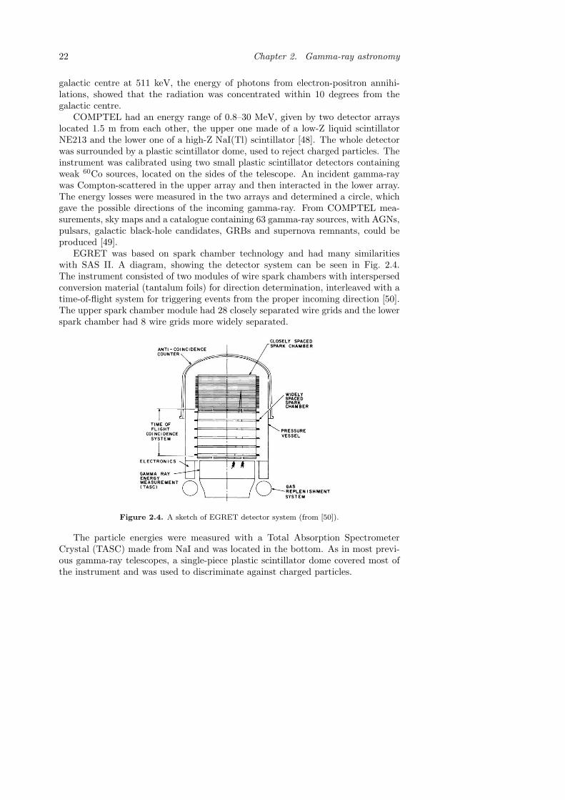
EGRET was based on spark chamber technology and had many similaritieswith SAS II. A diagram, showing the detector system can be seen in Fig. 2.4.The instrument consisted of two modules of wire spark chambers with interspersedconversion material (tantalum foils) for direction determination, interleaved with atime-of-flight system for triggering events from the proper incoming direction [50].The upper spark chamber module had 28 closely separated wire grids and the lowerspark chamber had 8 wire grids more widely separated.
Figure 2.4. A sketch of EGRET detector system (from [50]).
The particle energies were measured with a Total Absorption SpectrometerCrystal (TASC) made from NaI and was located in the bottom. As in most previ-ous gamma-ray telescopes, a single-piece plastic scintillator dome covered most ofthe instrument and was used to discriminate against charged particles.

2.4. History 23
The energy range of EGRET extended from about 20 MeV to roughly 30 GeVand in most of this region the energy resolution was 20–25%. The effective areawas energy dependent: about 1000 cm2 at 150 MeV, 1500 cm2 in the energy range0.5–1 GeV and gradually decreasing for higher energies to about 700 cm2 at 10 GeVfor targets near the centre of the field-of-view.
EGRET was a very successful mission and spawned many all sky maps as wellas detailed studies of different sources. In the final official list of EGRET Sources,the Third EGRET Catalog, 271 excesses with a significance higher than 3σ wereincluded [51]. About 70 of the sources included in the list have been identified asAGNs, radio quasars (mostly with a flat-spectrum) and BL-Lacertae, 1 radio galaxy(Centaurus A), the Large Magellanic Cloud (LMC), and 6 gamma-ray pulsars. Theremaining 170 sources were unidentified. A plot of the sources from the ThirdEGRET Catalog in galactic coordinates can be seen in Fig. 2.5.
Figure 2.5. Sources from the Third EGRET Catalog, shown in galactic coordinates.The size of the symbol corresponds to the highest intensity seen for the source byEGRET (from [51]).
On April, 2007, the Astro-rivelatore Gamma a Immagini LEggero (AGILE)satellite was launched into orbit [52]. The instrument weighs only about 120 kg, butthe components differ in design compared to previous experiments. The satellitecarries two instruments, a gamma-ray imager and a hard X-ray imager. At thetop is the Super-AGILE hard X-ray detector, which has an angular resolution of6 arcmin and the energy range 18–60 keV. The system is a so-called coded-maskdesign with a thin shadowing tungsten mask, 14 cm above a silicon detector plane.The gamma-ray imager covers energies from 30 MeV to 50 GeV and consists of aSilicon Tracker (ST) module, directly below Super-AGILE, and a Mini-Calorimeter(MCAL). The ST has high-resolution silicon microstrip detectors organised in 12layers at 1.9 cm intervals and with interleaved tungsten conversion planes between

24 Chapter 2. Gamma-ray astronomy
the 10 uppermost layers. The ST contains in total 0.8X0 on-axis and providesthe direction of the gamma-rays. Below the ST is the MCAL. It is used for energymeasurements and contains 30 CsI(Tl) crystals in 2 layers (corresponding to 1.5X0).All subdetectors are covered by an anticoincidence (AC) system, where each sideis segmented into three plastic scintillators whereas the top has a single plasticscintillator layer.
The first AGILE catalogue of high-confidence gamma-ray sources found afterone year of observations contains 47 sources, of which 8 are unidentified [53].
The AGILE satellite is designed to be complementary to the much larger FermiGamma-ray Space Telescope (described in detail in Chapter 4). The detector de-signs are virtually identical but differ in scale. Fermi Gamma-ray Space Telescopewill, however, in the first phase of the mission perform an all-sky survey, whereasAGILE is focused on fixed-pointing observations.
In Fig. 2.6, the sources with larger than 4σ significance that have been foundwith the first 11 months of data from the Fermi Gamma-ray Space Telescope areshown [54]. The total number of sources in this catalogue, which is also calledthe First Fermi -LAT catalog (or 1FGL, from 1st Fermi Gamma-ray LAT) is 1451and include starburst galaxies, AGNs, pulsars (PSR), pulsar wind nebulae (PWN),supernova remnants (SNR), x-ray binary stars (HXB) and micro-quasars (MQO).Currently, 630 of the sources are categorised as unassociated.
Figure 2.6. Sources with more than 4σ significance in the First Fermi-LAT Catalog.

Chapter 3
Dark matter
This chapter provides an overview of dark matter. It reviews some of the evidencesupporting the existence of dark matter, what constraints dark matter particlecandidates have and the different approaches that are followed today to detectthem. There are many review papers about dark matter available, see e.g. [55]and [56]. This chapter will therefore only summarise the subject.
3.1 Evidence
The existence of dark matter (DM) was first suggested by Zwicky in 1933 [57].Zwicky investigated the radial velocities of eight galaxies in the Coma galaxy clusterand observed an unexpectedly large velocity dispersion. He suggested that the massof the visible matter was not enough to hold the cluster together and that “darkmatter” was required [58].
That luminous objects move faster than what would be expected if the onlyinfluence was the gravitational pull from visible matter has since been observed inmany different types of objects. These objects include stars, gas clouds, globularclusters and entire galaxies. A typical example, which serves as one of the morecompelling and direct evidences for the existence of DM, is the rotation curves ofgalaxies.
An object that moves in a Keplerian orbit at radius r has a velocity given byv(r) =
√GM(r)/r, where M(r) is the mass contained within the disk at radius r.
At larger distances, beyond the optical disc, the rotational velocity should fall asv(r) ∝ 1/
√r. Observations of the 21 cm excitation line from hydrogen, however,
show that v(r) is approximately constant. This implies that either there is particleDM in the form of a halo with M(r) ∝ r or the gravitational theory needs to berevised.
25

26 Chapter 3. Dark matter
Since these discoveries were made, many other observations have pointed tothe existence of DM, and these include among others the Big Bang Nucleosynthe-sis (BBN) [59], gravitational lensing [60] and the cosmic microwave background(CMB) [61]. The most visual evidence of DM today, shown in Fig. 3.1, is from themerging galaxy cluster 1E 0657-558 (“Bullet Cluster”), where a clear separationof the mass (determined from gravitational lensing with the Advanced Camera forSurveys on the Hubble Space Telescope) and the X-ray emitting plasma (observedwith Chandra) can be seen [62].
Figure 3.1. A picture of the Bullet cluster, where the mass determined from gravi-tational lensing (blue) and the X-ray emitting plasma (purple) are clearly separated.Courtesy: X-ray: NASA/CXC/M.Markevitch et al. Optical: NASA/STScI; Mag-ellan/U. Arizona/D. Clowe et al. Lensing Map: NASA/STScI; ESO WFI; Magel-lan/U. Arizona/D. Clowe et al.
Together, all the observations mentioned above have constrained the fractionsof the energy density in the Universe in the form of matter and in the form ofa cosmological constant to ΩM ∼ 0.3 and ΩΛ ∼ 0.7, respectively, with ordinarybaryonic matter only constituting about ΩB ∼ 0.05 [63]. This implies that non-baryonic matter is the dominating form of matter in the Universe.
The model that has been been favoured for a long time and that is in reason-able agreement with observations is the so-called ΛCDM model, which featureslong-lived and collisionless Cold Dark Matter (CDM) and a contribution from acosmological constant (Λ). In this context, long-lived refers to a lifetime that iscomparable to or greater than the age of the Universe, collisionless means that theinteraction cross-section of the DM particles is negligible for the expected densi-ties of DM halos and cold means that the DM particles are non-relativistic whenthe Universe became matter-dominated. The latter means that the particles couldimmediately start to cluster gravitationally.
The collisionless CDM paradigm is, however, not without problems. The pro-posed ΛCDM model fits well with observations on large scales (≫ 1 Mpc), but

3.1. Evidence 27
there are discrepancies at smaller scales. One of these is generally referred to asthe “cuspy halo problem” or “cusp/core problem” and refers to the inconsistencybetween the cuspy halo DM density towards galactic centres predicted from cos-mological numerical simulations and the observed densities of the central regions ofself-gravitating systems such as clusters of galaxies [60], spiral galaxies [64], dwarfgalaxies [65] and some low surface-brightness galaxies [66].
Another reported problem is that the predicted number of substructures, i.e.small halos and dwarf galaxies in orbit around larger objects, is larger than whatis observed [67].
To resolve the existing problems, a number of alternative models of DM havetherefore been proposed and these include strongly self-interacting dark matter,warm dark matter, repulsive dark matter, fuzzy dark matter, self-annihilating darkmatter, decaying dark matter and massive black holes [68].
It may be noted, that there is currently no consensus whether the aforemen-tioned problems are astrophysical or computational. On large scales, gravity isthe dominating process and computations therefore only involve Newton’s and Ein-stein’s laws of gravity. On smaller scales, however, the physical interactions betweendark matter, ordinary matter and radiation are important. However, in most of thelatest N-body simulations that predict the internal structure of galactic size halos,these interactions are neglected for computational reasons.
An alternative theoretical approach that requires no DM are models of Modi-fied Newtonian Dynamics (MOND) [69, 70]. The proposed theories are successfulin explaining some of the observations but not all of them. In particular, the mea-surements of the Bullet Cluster, mentioned above, are currently difficult to explainwith MOND and related theories.
An attractive candidate for CDM are Weakly Interacting Massive Particles(WIMPs), since they naturally provide the correct present-day relic abundance ofDM. The reason is that if the particles interact via the weak force, then the WIMPswere in thermal equilibrium with the Standard Model particles in the early Universewhen the temperature was above the mass of the WIMP. When the temperaturedropped below the mass of the WIMP, the number density of WIMPs decreasedexponentially and finally when the expansion rate became larger than the annihi-lation rate, the annihilations ceased to occur and the cosmological abundance ofWIMPs “freezed out”.
A strict calculation of the relic density can be very complicated depending onthe model but a rough estimate of the relic abundance is given by Eq. 3.1 [71], whichis independent of the WIMP mass provided that the WIMPs are non-relativistic atfreeze-out.
Ωh2 ≈ 3 × 10⁻²⁷cm3 s−1
〈σv〉 (3.1)
Here, h is the Hubble constant in units of 100 km s−1 Mpc−1 and 〈σv〉 is thethermally averaged interaction rate, where v is the relative velocity of the inter-

28 Chapter 3. Dark matter
acting WIMPs. The cross-section required to explain current observations, i.e.〈σv〉 ≈ 10−26 cm3 s−1, is approximately the same as can be expected in elec-
troweak interactions, where typically σv ∼ α2
M2χ∼ 10−26 cm3 s−1 for an assumed
WIMP mass, Mχ, of about 100 GeV, and this is often referred to as the “WIMPmiracle”. Here, α is the fine structure constant.
3.2 Dark matter candidates
There is a large number of proposed DM particle candidates. In order for a particleto be a viable DM candidate, however, a number of requirements need to be met (seee.g. [72]). A positive answer should be the result of all of the following questions:
1. Does it match the appropriate relic density?
2. Is it cold?
3. Is it neutral?
4. Is it consistent with the BBN?
5. Does it leave stellar evolution unchanged?
6. Is it compatible with constraints on self-interactions?
7. Is it consistent with direct DM searches?
8. Is it compatible with gamma-ray experiments?
9. Is it compatible with other astrophysical bounds?
10. Can it be probed experimentally?
The natural candidate for hot DM are Standard Model neutrinos. However,observations of structure formation today disfavour that a large part of the DM isin the form of hot DM. For example, hot DM models predict so-called top-downformation of structure, i.e. that small structure were formed by the fragmentationof larger ones, but observations show that galaxies are older than superclusters [73].A small amount of hot DM is allowed as long as it is compatible with structureformation and CMB data and the estimated abundance is Ων ∼ 0.001 − 0.1 [73].
One of the valid DM particle candidates is the axion [74, 75], which is a conse-quence of the Peccei-Quinn theory [76] that was proposed to resolve the “strong CPproblem”, i.e. why quantum chromodynamics does not seem to break the charge-parity (CP) symmetry. One of the properties of axions is the conversion to photonsin the presence of electromagnetic fields, which allows for an experimental signal tobe searched for.
Theories that invoke universal extra dimensions are also capable of producingviable DM candidates, of which the most prominent is the first excitation of the

3.2. Dark matter candidates 29
hypercharge gauge boson (B1), which is also known as the lightest Kaluza-Kleinparticle [77].
A large theoretical framework that give several DM particle candidates is su-persymmetry (often shortened to SUSY). For a general overview of supersymmetricDM, see e.g. [71]. Supersymmetry is often an integral part of string theory and isan attempt to give a unified description of fermions and bosons and to solve theso-called hierarchy problem in particle physics. This refers to the fact that theradiative corrections to the mass of the Higgs boson are enormous while the massitself is constrained by quantum field theory to be light for the electroweak theoryto work.
In supersymmetry, every particle and gauge field has a superpartner. The gaugefields given by gluons (g) and the W± and B bosons have associated fermionic su-
perpartners called gluinos (g), winos (W i) and binos (B), respectively, and fermionshave associated scalar partners (quarks become squarks and leptons become slep-tons). An additional Higgs field is also introduced. What follows from supersym-metry is that for every boson loop correction there is a fermion loop correction thatcancels it, which in turn would help alleviate the hierarchy problem.
In the simplest models of supersymmetry, there is a multiplicative quantumnumber called R-parity, which is conserved. This was originally imposed in orderto suppress the rate of proton decay and is defined as Eq. 3.2 [55],
R ≡ (−1)3B+L+2s, (3.2)
where B is the baryon number, L is the lepton number and s is the spin. AllStandard Model particles have R = 1 and all superpartners, or sparticles, haveR = −1. This means that the decay products of sparticles must consist of an oddnumber of sparticles. A consequence of this is that the Lightest SupersymmetricParticle (LSP) is stable and can only be destroyed through pair annihilation.
The theoretically favoured non-baryonic DM particle candidate and also themost widely searched for experimentally today is the LSP, which is often assumedto be the neutralino. In the Minimal Supersymmetric Standard Model (MSSM),the neutralino is a mix of the bino, wino and higgsino states. The mix gives theneutralino four mass eigenstates, χ0
1, χ02, χ0
3 and χ04, where χ0
1 is the lightest one,usually denoted by only χ.
In neutralino pair-annihilation, the leading channels at low neutralino velocitiesare annihilations into fermion-antifermion pairs, gauge boson pairs and final stateswith Higgs bosons. These can eventually through different decay chains produceneutrinos, charged particles and finally neutral pions that decay into gamma-rays.These gamma-rays could then be observed by Fermi Gamma-ray Space Telescopeas a continuum spectrum. In this model, no tree-level Feynman diagrams exist forthe pair annihilation of neutralinos directly into two gamma-rays. The annihilationinto that particular final state must therefore proceed through loops which resultsin a significant suppression of the annihilation rate [78].

30 Chapter 3. Dark matter
The neutralino is, however, not the only valid DM candidate in supersymmetrictheory. Other candidates include e.g. the gravitino and the axino. For moredetailed reviews of the possible DM candidates see e.g. [72, 79].
3.3 Dark matter properties
Signals from DM in the gamma-ray region can be categorised into continuum sig-nals and spectral line signals and are produced through the processes explained inSection 2.1.
Continuum signals are excesses in the overall spectrum that can not be ac-counted for by the existing components, such as the diffuse galactic emission orthe isotropic diffuse emission. This kind of search is limited by the precision towhich the existing components can be described, unless the search is conducted ina region where the contribution from the known components is small. An exampleof such a region would be DM-dominated subhalos at high galactic latitudes, wherethe galactic diffuse emission is small.
Many of the viable DM candidates are able to produce spectral lines via annihi-lation or decay channels directly into two monochromatic gamma-rays. If the DMparticles (χ) are non-relativistic and annihilate, the energy of each photon will beEγ = Mχ. For decays, the corresponding energy is instead Eγ = Mχ/2.
A spectral line can also be produced if the annihilation of the DM particlescreates one photon and some other particle (X). The other particle can e.g. bea Z-boson, a Higgs boson, a neutrino or a non-Standard Model particle. In thatcase, the energy of the photon is determined by the mass of the DM particle andthe mass of the other particle according to Eq. 3.3 [63].
Eγ = Mχ
(1 − M2
X
4M2χ
)(3.3)
The corresponding equation for decays is given by the substitution Mχ →Mχ/2in Eq. 3.3.
Models predicting spectral line signals can be created in a variety of theoret-ical frameworks. These include e.g. neutralino annihilations [71], wino annihi-lations [80], inert Higgs annihilations [81], Kaluza-Klein annihilations assuminguniversal extra dimensions [82, 83], the Green-Schwarz mechanism [84], gravitinodecays [85], hidden vector DM decay [86] and Dirac fermion DM annihilations intoHiggs particle final states [87]. The predictions include between one and three spec-tral lines, depending on the model, and in some cases the final states producingthem constitute the leading channels.
An observation of a spectral line would be a “smoking-gun” for DM, since noother astrophysical process should be able to produce it. However, several mod-els predict either low branching fractions or low cross-sections for those particularchannels, so a halo with a large central concentration, the existence of substructure

3.4. Halo models 31
that would boost the signal especially in spatial regions with low background emis-sion, or the Sommerfeld enhancement [88] might be needed in order to see such asignal.
For monochromatic gamma-rays, the relation between the flux (Φ) and theannihilation cross-section (σ) is given by Eq. 3.4,
Φ =Nγ
8π
〈σv〉γX
M2χ
L, (3.4)
where Nγ = 2 for X = γ, Mχ is the DM particle mass, v is the average velocity ofthe DM particles and L is the line-of-sight integral which is given by Eq. 3.5.
L =
∫db
∫dl
∫ds cos b ρ2 (~r) (3.5)
Here, b and l correspond to the galactic latitude and longitude respectively, ρχ
is the DM density and r =(s2 +R2
⊙ − 2sR⊙ cos l cos b)1/2
in which R⊙ = 8.5 kpccorresponds to the approximate distance from the galactic centre to the solar sys-tem.
The corresponding equations for the decay lifetime (τγX) are derived by per-forming the substitution 〈σv〉 /2M2
χ → 1/τMχ in Eq. 3.4 and ρ2 → ρ in Eq. 3.5.The flux as expressed by Eq. 3.4 can be reformulated to Eq. 3.6 [89],
Φ(ψ,∆Ω) = 0.94 × 10⁻¹¹
(Nγvσγγ
10−29 cm3s−1
) (10 GeV
Mχ
)2
〈J(ψ)〉∆Ω
× ∆Ω cm−2s−1sr−1,
(3.6)
where ∆Ω is the solid angle and the dimensionless line-of-sight-dependent functionJ(ψ) is given by:
J(ψ) =1
R⊙
(1
ρ (R⊙)
)2 ∫
line−of−sight
ρ2χ(l)dl(ψ) (3.7)
This is averaged over the solid angle according to:
〈J(ψ)〉∆Ω =1
∆Ω
∫
∆Ω
dΩ′J(ψ′) (3.8)
The assumed value of the local DM density (ρ (R⊙)) is currently under de-bate. In DarkSUSY, a publicly available advanced numerical package for DM cal-culations [89], a value of 0.3 GeV cm−3 is assumed. However, later studies haveindicated that 0.4 GeV cm−3 may be closer to the correct value [90].
3.4 Halo models
The DM distribution on small scales, i.e. on galactic and sub-galactic scales, isstill under debate and plays a crucial role for the detection of DM signals. To

32 Chapter 3. Dark matter
describe most of the observed rotation curves of galaxies, a phenomenological halodensity profile, based on state-of-the-art N-body simulations, is generally used. Thissmooth and spherically symmetric profile is given by Eq. 3.9,
ρ(r) =δcρc
(r/rs)γ [1 + (r/rs)α](β−γ)/α
, (3.9)
where r is the angular radius from the galactic centre, rs is a scale radius and δc isa characteristic dimensionless density, and ρc = 3H2/8πG is the critical density forclosure. There are a number of widely used halo profiles that differ in the valuesof the (α,β,γ) parameters. The more popular profiles are the Navarro, Frenk andWhite (NFW) model with (1,3,1) [91], the isothermal profile with (2,2,0) [92], theMoore model with (1.5,3,1.5) [93] and the Kravtsov model with (2,3,0.4) [94].
Another observationally favoured halo profile is the Einasto profile [95, 96],which is given in Eq. 3.10,
ρEinasto(r) = ρse−(2/a)[(r/rs)a−1], (3.10)
where ρs is the core density and a is a shape parameter.The dark matter halo profiles can be referred to as cored, cuspy or spiked,
depending on whether the central density is proportional to r−γ with γ ≈ 0, γ & 0or γ & 1.5, respectively.
3.5 Detection techniques
There are currently two major ways in which a particle detection of DM is pursued.The first, direct detection, is based on measuring the recoil energy of nuclei whenDM particles, generally assumed to be WIMPs, scatter off them. Due to the low en-ergy of the recoils, the experiments must be shielded and placed deep undergroundto protect the detectors from unwanted background. The DAMA/LIBRA [97] andCDMS[98] experiments are two examples of collaborations active in this type ofsearch.
In the second detection technique, indirect detection, the DM particles them-selves are not observed but rather the effects they give rise to or the secondaryparticles they create. This technique can be further categorised into two differentapproaches.
The first approach involves detecting the secondary particles from annihilatingor decaying DM that is gravitationally bound to other astrophysical objects or toitself. This type of search is exercised in a wide variety of experiments and for manyassumed final state particles.
For gamma-rays, DM searches can be performed with ground-based air-showerexperiments such as H.E.S.S., MAGIC, VERITAS, Milagro and HAWK, which werealready mentioned in Section 2.3 and space-based gamma-ray satellites such as theFermi Gamma-ray Space Telescope.

3.6. Experimental status 33
For neutrinos, many neutrino telescopes are involved in DM searches. Theseinclude AMANDA/IceCube in the Antarctic [99, 100, 101] and ANTARES [102,103] in the Mediterranean, which attempt to detect the neutrinos produced in theannihilation of DM particles that may be gravitationally bound to the Earth or theSun.
Finally, DM searches are also conducted using experiments capable of measuringelectrons, positrons, protons and antiprotons such as the space-based PAMELAexperiment [104]. Inference about the existence of DM can be made from e.g. theenergy-dependent ratio of different particle types.
In the second approach, there is a possibility that DM can be artificially createdin the energetic collisions produced at large accelerators. The search for DM canin that case be directed towards identifying processes where an imbalance in themeasured momentum can be seen. This “missing energy” can be the result of aDM particle that is produced in the collision but escapes out of the detector. Thisapproach will be utilised in the detectors located in the Large Hadron Colliderat CERN, where protons will eventually be collided at a centre-of-mass energy ofabout 14 TeV.
3.6 Experimental status
Currently, new experimental results for DM are being published at a high pace,making the field very dynamic. Though most results have presented non-detectionsin the form of upper limits, also unexpected features have been seen. The mostrecent developments of this kind are therefore briefly reviewed here.
In the field of direct detection, the DAMA/LIBRA collaboration has claimeddetection of an annual modulation believed to be caused by the Earth’s movementrelative to a WIMP halo [105]. The results are, however, still controversial at thispoint since no other experiment has been able to observe a signal of that kind.Another direct detection experiment, CDMS-II, has reported 2 signal events intheir specified signal region [106]. However, the probability of having two or morebackground events in the signal region is stated to be 23%, which means that thedetection is not very significant.
As for charged particles, the fraction of positrons was recently measured by thePAMELA experiment and an unexpected excess in the fraction was found in thehigh end of the energy range [107]. One of the possible explanations to the observedexcess include DM [108, 109, 80]. This measurement has later been complementedby measurements of the combined electron and positron spectrum by the balloon-borne ATIC experiment [110] and the Fermi Large Area Telescope [111], however,the excess reported by the former is not confirmed by the latter.
The measurements can, however, currently not be reasonably well fit by conven-tional galactic propagation models or by models assuming a continuous distributionof sources. Solutions explaining both PAMELA and Fermi Large Area Telescope

34 Chapter 3. Dark matter
data without invoking DM have, however, been proposed and include nearby pulsarsand source stochasticity [112] as well as secondary acceleration in the sources [113].
Since many of the results above are unexpected, the interest in the communityfor independent checks by other instruments has increased. One of the more antici-pated experiments that is awaiting launch is AMS-02 [114], which is an instrumentsimilar in design to the PAMELA instrument but with a larger sensitivity and per-formance. It is at the time of writing scheduled to be launched with one of the finalspace shuttle missions and will make precision measurements of the cosmic-ray skyfrom the International Space Station.
In the Fermi -LAT Collaboration, a variety of DM searches have been performed.The currently published results include searches in clusters of galaxies [115], dwarfspheroidal galaxies [116, 117] and searches for cosmological DM in the isotropicdiffuse emission [118] and spectral lines [119] (see also Section 7.6). Overall, thesestudies are beginning to probe the available and theoretically interesting parameterspaces, but a detection has not been made so far. There are also on-going efforts tostudy the galactic centre in more detail and to search for substructures consistingof only DM.
In conclusion, the identification of DM is still an open question despite the largevariety of studies that have already been published. However, the field is very activeand new experiments designed to probe the available phase space are planned.

Chapter 4
Fermi Gamma-ray Space
Telescope
The current generation in gamma-ray satellites, the Fermi Gamma-ray Space Tele-scope (henceforth denoted Fermi), was successfully launched on a Delta II heavylaunch vehicle from Cape Canaveral in Florida, USA, on 11 June, 2008. The satel-lite was formerly known as the Gamma-ray Large Area Space Telescope (GLAST)but was renamed after its launch. An artist’s conception of the satellite can beseen in Fig. 4.1. The satellite consists of two detector systems, the Large AreaTelescope (LAT) and the Gamma-ray Burst Monitor (GBM). This chapter reviewsthe scientific goals of the Fermi mission and describes the different instruments andsubsystems.
Figure 4.1. An artist’s impression of the Fermi Gamma-ray Space Telescope. Thebox-like structure on the top is the LAT and the yellow detectors on the sides arepart of the GBM.
The satellite orbits the Earth at an altitude of about 565 km and with aninclination angle of about 25.6. One orbit takes about 90 minutes and full-skycoverage is reached in only two orbits. The data acquisitions start and end at theborders of the South Atlantic Anomaly (SAA). The reason for this is that the high
35

36 Chapter 4. Fermi Gamma-ray Space Telescope
concentration of charged particles within the SAA can damage the electronics of theinstruments. Therefore, the high voltages, powering the satellite and its detectors,must be lowered to a minimum level inside the SAA. If no part of the SAA istraversed during the orbit, the data acquisition start and end at the ascendingnode, i.e. where the orbit crosses the equator.
In Fig. 4.2, a visualisation of the orbits can be seen. The borders of the SAAand the angle of inclination, presented in the figure, represent pre-launch estimates.The borders were determined more exactly during the first phase of the mission (seealso Section 4.2.5).
Figure 4.2. A visualisation of the Fermi orbit. The blue trails represent the orbitsof Fermi and the yellow lines mark the borders of the South Atlantic Anomaly(SAA). Data acquisitions start and end at the borders of the SAA. If no part ofthe SAA is present in the orbit, the data acquisitions start and end at an ascendingnode. The shown borders and inclination angle are pre-launch estimates.
4.1 Scientific goals
The scientific goals of Fermi are largely motivated by results from the predecessorEGRET, which measured gamma-rays with energies between around 20 MeV and30 GeV, and ground-based atmospheric Cherenkov telescope arrays, which measureenergies above several tens of GeV. The main scientific goals of Fermi are to:
• Resolve the gamma-ray sky. This includes studying the nature of the 170unidentified EGRET sources, the extragalactic diffuse emission and the ori-gins of the emission from the Milky Way, the nearby galaxies and galaxyclusters.
• Understand the particle acceleration mechanisms in celestial sources, such asAGNs, blazars, pulsars, pulsar wind nebulae, supernova remnants and theSun.

4.2. Large Area Telescope 37
• Study the high-energy processes in GRBs and transients. GRBs (see alsoSection 2.2) have been studied in many different wavelength regions, includingX-ray, optical and radio. The behaviour at gamma-ray energies is, however,largely unknown.
• Probe the nature of dark matter. As described in Chapter 3, many models ofdark matter can be investigated with the Fermi -LAT instrument.
• Investigate the early Universe to z≥6 using high-energy gamma-rays. Theera of galaxy formation can be studied with photons above 10 GeV via theabsorption by pair production of accumulated radiation from structure andstar formation (extragalactic background light) and of gamma-rays from e.g.blazars.
4.2 Large Area Telescope
The LAT, seen in Fig. 4.3, covers the approximate energy range from 20 MeV tomore than 300 GeV and was built by an international collaboration consisting ofspace agencies, physics institutes and universities from France, Italy, Japan, Swedenand the United States.
Figure 4.3. The Large Area Telescope in cross-section. Each module has a trackermodule and a calorimeter module. The tiles on the sides are part of the anti-coincidence detector shield.
The instrument is a pair-conversion telescope, designed to measure the electro-magnetic showers of incident gamma-rays over a wide field-of-view while rejectingincident charged particles with an efficiency of 1 to 106. It consists of a 4 x 4array of 16 identical modules on a low-mass structure. Each of the modules has agamma-ray converter tracker for determining the direction of the incoming gamma-ray and a calorimeter for measuring its energy. The tracker array is surrounded bya segmented anti-coincidence detector. In addition, the whole LAT is shielded bya thermal-blanket micro-meteoroid shield.

38 Chapter 4. Fermi Gamma-ray Space Telescope
The data taking is governed by a programmable trigger that can utilise promptsignals from all the subsystems. The downlink capacity from the LAT to the groundis limited, so the data acquisition hardware reduces the rate of events to about1 Mbps using onboard event processing.
4.2.1 Tracker
The active detector elements in the directional tracker (TKR) modules are Silicon-Strip Detectors (SSDs). Each TKR module in the LAT has a width of 37.3 cm and aheight of 66 cm, where the width was optimised to utilise the longest silicon stripspossible while keeping a good noise performance, high efficiency and low power,and the height was a trade-off between having a large enough lever arm betweensuccessive hits in the TKR and keeping a low LAT aspect ratio that maximises thefield-of-view. For an extensive review of the TKR system, see e.g. [120].
A TKR module consists of a stack of 19 trays, which support the SSDs, theassociated readout electronics and tungsten converter foils, where pair productionis induced. Only the topmost 16 layer pairs are preceded by a tungsten plane, justabove the detector planes. There are 576 SSDs in each TKR module and they arearranged into 18 pairs of x and y planes, and the x and y planes are separated bya gap of 2 mm. In total, each SSD detector plane has 1526 strips with a pitch of0.228 mm.
The close proximity of the tungsten planes to the active detectors is crucialin order to minimise the effects of multiple scattering of the charged particles inthe shower. Multiple scattering can significantly degrade the angular resolution.Therefore, for lower energies, most of the directional information comes from thefirst two points of the track. At higher energies, however, the effects of multiplescattering are negligible and the angular resolution is limited mainly by the strip-pitch and the gap between the silicon detector planes. The total weight of thetungsten in each module is 9 kg and converts about 63% of the gamma-rays atnormal incidence above 1 GeV. A sketch of the layer-wise setup and a gamma-rayconversion is shown in Fig. 4.4.
The TKR is designed with both thin and thick tungsten converter layers, inorder to reach the required performance at both ends of the energy range. Eachof the first twelve planes of tungsten is 0.027X0 (0.095 mm) in thickness, whileeach of the final four is 0.18X0 (0.72 mm) in thickness. The concept of radiationlengths, X0, is defined in Section 1.3. The two regions, with thin converter layersin the front of the TKR and thick converter layers in the back of the TKR, haveintrinsically different performances as will be shown later in Section 4.2.7.
For a single plane of silicon in the TKR, the efficiency to detect a minimum-ionising particle at nearly normal incidence with respect to the active area is> 99.4%. The noise occupancy, i.e. the probability for a single channel to havea noise hit in a given detector trigger is, after masking of noisy channels (0.06% ofthe channels), less than 5 × 10⁻⁷.

4.2. Large Area Telescope 39
Figure 4.4. A gamma-ray pair-producing in a tracker module. The two directionalplanes of SSDs are preceded by a conversion plane of tungsten.
4.2.2 Calorimeter
A Fermi -LAT calorimeter (CAL) module consists of 96 CsI(Tl) Detector Elements(CDEs), i.e. 12 CDEs per layer in 8 layers, supported by a carbon composite cellstructure. The LAT therefore includes a total of 1536 CDEs, which gives the CALa combined weight of 1376 kg. At normal incidence, the CAL corresponds to 8.6X0.
The segmentation of the CAL has many advantages and helps e.g. to distinguishbetween showers produced by gamma-rays and those by charged particles but it alsohelps to constrain the incoming direction of the gamma-ray. In addition, it improvesthe energy measurement by allowing cascade profile fitting to be performed, whichcompensates somewhat for leakage into gaps and out of the back of the CAL.
The design is hodoscopic, as can be seen in Fig. 4.5, i.e. the crystal directionsin odd layers are orthogonal to the crystal directions in even layers. The size ofeach crystal is 326 × 26.7 × 19.9 mm3, where the widths correspond to roughlyone radiation length in CsI(Tl), i.e. 18.6 mm [121]. Two out of the four long-sidesurfaces have been roughened to give a known attenuation with a better uniformityin the light collection along the crystal. To improve light collection and opticalisolation, the crystals are individually wrapped with a reflective material calledVM 2000.
The scintillation light from the crystals are collected at each end of each crystalusing two silicon PIN photodiodes, which have a spectral response that is matchedto the scintillation spectrum from CsI(Tl). The diodes are of different size to beable to cover the large energy range of the LAT. The larger diode has an active

40 Chapter 4. Fermi Gamma-ray Space Telescope
Figure 4.5. A picture showing the hodoscopic design of a Fermi-LAT calorimetermodule.
area of 1.5 cm2, which is a factor of 6 larger than the active area of the smallerdiode (0.25 cm2). The larger diode is designed to measure smaller energy deposits,from 2 MeV to 1.6 GeV, whereas the smaller diode handles larger energy deposits,from 15 MeV to 100 GeV.
4.2.3 Anti-Coincidence Detector
The anti-coincidence detector (ACD) on the LAT consists of 89 Tile Detector As-semblies (TDAs) made of plastic scintillator material. The layout is sketched inFig. 4.6.
The scintillator tiles are 10 mm thick, except for the central row on top of theLAT, which is 12 mm, and range in size from 15 × 32 cm2 to 32 × 32 cm2 dependingof the location of the TDA. An example of an unwrapped tile is shown in Fig. 4.7.In the bottom row of each of the four sides of the LAT is a long tile, 17 × 170 cm2.These tiles lie outside of the primary field-of-view of the LAT, where no events willbe accepted as gamma-rays. Each tile is, furthermore, wrapped with two layers ofhigh reflectance white Tetratec followed by two layers of light-tight black Tedlar.
Each TDA is connected to 1 mm in diameter wavelength shifting (WLS) fibers,which transmit the scintillation light to photo-multiplier tubes (PMTs), which arelocated on the sides of the LAT, below the TDAs. For redundancy, each tile is readout by two PMTs.
The tiles are overlapping in one dimension, as shown in Fig. 4.8, to minimisethe open areas. The remaining gaps in the other direction, typically 2–3 mm, areunavoidable due to the wrapping material and since the tiles must be allowed tothermally expand and vibrate during launch. To detect entering charged particles,the gaps are instead covered with flexible scintillating fiber ribbons.
The so-called “crown” tiles, i.e. the top most rows of tiles on the four sides of theLAT, also seen in Fig. 4.6, are extended above the tiles on the top of the LAT. Thereason for this is to minimise the irreducible background caused by protons that hitthe Micro-Meteoroid Shield (MMS) at a shallow angle, which produce gamma-rays

4.2. Large Area Telescope 41
Figure 4.6. The layout of the tile detector assemblies in the anti-coincidence de-tector of the LAT (a) and the electronics assembly with the PMTs above the LATgrid (b) (from [122]).
Figure 4.7. A picture of an unwrapped anti-coincidence detector tile (from [122]).
that enter the detector. According to simulations, the contamination from this typeof events would without the crown tiles be significantly higher.
The MMS surrounds the whole ACD, to shield it from micro-meteoroids andspace debris, and consists of four layers of Nextel ceramic fabric separated by fourlayers of 6 mm thick Solimide low-density foam, which is backed by 68 layers ofKevlar fabric. According to calculations, there is a 95% probability of allowing nomore than 1 penetration of the MMS in 5 years.
The ACD has a segmented design for mainly two reasons. Firstly, it is utilisedto avoid events with backsplash from being vetoed. Backsplash is a process, wherecharged particles, produced in the electromagnetic showers from gamma-rays in

42 Chapter 4. Fermi Gamma-ray Space Telescope
Figure 4.8. A sketch of the overlapping anti-coincidence detector tiles on top ofthe LAT (a) and in cross-section (b) (from [122]).
the field-of-view, propagate the detector in the opposite direction of the incidentgamma-rays and hit the ACD tiles. A simulation showing the chain of eventscan be seen in Fig. 4.9. In experiments, such as EGRET, this process caused asignificant decrease in effective area and additional dead time due to the singlepiece design of the anti-coincidence shield. The effects of backsplash have beenthoroughly investigated and taken into consideration when designing the ACD.
Figure 4.9. A simulation of backsplash in the LAT that hits the anti-coincidencedetector (from [122]).
The second reason for having a segmented design is for usage in the backgroundrejection, further discussed below.
A significant difference between EGRET and the Fermi -LAT is the lack of adirectional trigger system, i.e. time-of-flight detectors, in the latter. Instead, theprincipal trigger on the Fermi -LAT requires coinciding signals in three consecutivetracker xy layer-pairs. The particles can, thus, come from any direction, whichresults in a very high first-level trigger rate that can be up to 10 kHz. The triggers

4.2. Large Area Telescope 43
are mostly caused by charged particles, which as mentioned before outnumber thegamma-rays by six orders of magnitude.
To reduce the large amounts of data produced by these triggers to the downlinkcapacity to the ground, most of the triggers that are induced by charged particlesmust be rejected already in space by using an onboard filter. The responsibility ofidentifying the charged particles for rejection lies mainly on the ACD.
The science requirements for the LAT state that the residual background shouldbe no more than 10% of the diffuse gamma-ray background intensity. To meet thisgoal, protons must be suppressed by a factor of about 106 and electrons by a factorof about 104 [122]. On-orbit investigations of the residual contamination have,however, shown a higher level of contamination than predicted from pre-launchmodeling [23]. Therefore, the event selection is currently being revised in order toreduce the contamination to acceptable levels.
The CAL and TKR can be used to suppress protons by at least a factor of 103
by using event patterns in the TKR and shower shapes in the CAL. The remainingfactor of 103 must be provided by the ACD.
For electrons, the required rejection is tightest for lower energies due to thesteep decrease with energy of the electron spectrum. The TKR can be used tosuppress electrons by a factor of 10, by identifying tracks that point to inefficientregions of the ACD. The remaining suppression of 0.9997 for the ACD is done inseveral different ways.
Firstly, the tracks, as measured by the TKR, that point back to “shadowing”ACD tiles that recorded a signal are vetoed. Secondly, the information from theTKR and CAL in combination with the ACD are compared, to reject events thathave a high probability of being charged particles. This reduces the amount of datato the capacity of the downlink to the ground. Transmitting a very small fractionof charged particle events to the ground is, however, useful for calibration purposes.Therefore, the efficiency of the ACD to reject charged particles must at this pointonly be ≥ 0.99. Finally, the required efficiency of 0.9997 for the ACD to detectsingly charged particles is accomplished via data analysis off-line on the ground andincludes e.g. pulse height analysis.
The ultimate background rejection that meets the science requirements for theLAT is then achieved via further data analysis on the ground.
For a more thorough review of the ACD design and specifications, see [122].
4.2.4 Event reconstruction
In the TKR, the event reconstruction is based on a Kalman filter [123, 124], whichalleviate the problems in track fitting and pattern recognition caused by non-negligible multiple Coulomb-scattering. The Kalman filter is iterative and allowsfor the consideration of one measurement at a time. These are then added inde-pendently to the fit. With the filter, random errors can be handled in a naturalway and the problem reduces to the multiple scattering error produced betweentwo consecutive measurement planes.

44 Chapter 4. Fermi Gamma-ray Space Telescope
In the TKR, the strips that were hit are first converted into positions. If twoadjacent strips have been hit, they are merged to form a single hit cluster. In thesecond step, candidate tracks are formed based on the reconstructed clusters andindividual track energies aid in the track recognition. Then, the three-dimensionalposition and direction are determined and their errors are estimated. Finally, thefitted tracks are used to determine the vertex where the pair-production took place.The iteration occurs when the tracks are used to get an improved energy estimateafter which the tracks can be refit and a new vertex position can be found.
In the CAL, the energy is determined by first applying pedestals (voltage off-sets at the analog-to-digital converter inputs) and gains to the raw digitised signalsfrom each crystal. The energy is then the sum of all depositions above a certainthreshold in all crystals. The longitudinal position in each crystal, where the energydeposition took place, is calculated from the known relation between this positionand the energy measured in the two crystal ends. If the light attenuation in thecrystal is strictly exponential, this relation takes the mathematical form of Eq. 4.1,
x = K · tanh−1A (4.1)
where A = (Left − Right)/(Left + Right) is the so-called light asymmetry, Leftand Right are the measured energies in the two crystal ends, respectively, x is thelongitudinal position of impact in the crystal and K is a constant factor.
With the calculated array of energy depositions and positions for each crystalin the CAL, the direction can be determined via energy moments analysis for eachshower. This procedure is similar to a moments of inertia analysis, in which amoments ellipsoid is calculated. The principal axis of this ellipsoid provides theincoming direction of the particle and the centre of the ellipsoid determines thecentre of gravity for the shower.
The raw energy measured by the CAL after diode calibrations is stored in avariable called CalEnergyRaw. It is never the same as the initial photon energy,since energy is always lost in internal gaps between CAL modules, between crystalsand via leakages out of the back and the sides of the instrument. Therefore, differentenergy correction algorithms have been developed to compensate for these effectsand to correct the energy to correspond to the incoming photon energy. There arecurrently three such algorithms:
• The parametric method combines energy measurements from both the TKRand the CAL. At 100 MeV, about 50% of the total energy deposition isdeposited in the TKR. The fraction decreases rapidly with energy and is onlyabout 5% at 1 GeV. Energy estimations in the TKR can be done in manyways. There is e.g. a correlation between the number of SSD hits near or onthe track and the particle energy, due to the large amount of multiple Coulumbscattering at lower energies. The opening angle for pair-produced e+e− is alsoan energy estimator. The parametric method provides a starting point forthe re-fitting of the track in the TKR and the energy is re-evaluated usingthe two other methods below. The corrected energies from the parametric

4.2. Large Area Telescope 45
method are stored in a variable called EvtEnergyCorr and is included in oneof the ROOT N-tuples used for analysing detector information.
• The likelihood method makes use of the correlation between the number of hitsin the TKR, the energy deposited in the last layer of the CAL and the totalraw energy deposited in the CAL. It has been optimised for various classesof simulated events, such as gamma-ray conversions occurring in the thin orthick tungsten layers of the TKR. The corrected energy using the likelihoodmethod is stored in a variable called CalLkHdEnergy.
• The profile fitting method looks at the layer-by-layer energy deposition and fitsthe longitudinal shower development while also taking into account the trans-verse size of the shower. The method works best for photons energies above 1GeV, when the shower maximum is contained within the CAL. The correctedenergy using the profile method is stored in a variable called CalCfpEnergy.
The final output energy, representing the incoming photon energy, is a com-position of the three corrected energies described above. The selection of energymethod is based on a classification-tree analysis and the output is stored in thevariable CTBBestEnergy.
4.2.5 On-orbit calibration
The Fermi -LAT instrument was calibrated before launch by using ground-levelcosmic-ray muons for the low-energy scale and charge injection into the front-endelectronics for each detector for the high-energy scale. These calibrations were onlyapproximations of the optimal trigger and timing settings, so they were re-doneon-orbit by using known astrophysical sources, galactic cosmic rays and charge-injection [125].
The full calibration, first of all, involves the synchronisation of the trigger signalsfrom the different detector components and adjusting the delays for data acquisi-tion, in order to maximise the trigger efficiency. The relative timing of the ACDand the TKR is optimised using proton candidates, since the main purpose of theACD is to reject charged particles, whereas the relative timing between the TKRand the CAL is set using photon candidates.
The detector components are also individually calibrated. For the ACD, thisincludes determining the mean values of pedestals, the signal pulse heights producedby minimum-ionising particles in each ACD scintillator, veto threshold settings aswell as high-energy and coherent-noise calibrations for each PMT.
For the TKR, the calibrations concern the determination of noisy channels thatmay affect the instrumental dead time and the data volume. Such channels haveto be masked to maintain optimal performance. Furthermore, trigger and datalatching (the process of reading out data from all subdetectors) thresholds are setin order to minimise the noise occupancy while maximising the hit efficiency. The

46 Chapter 4. Fermi Gamma-ray Space Telescope
calibration of the TKR also includes the determination of the conversion parame-ters from charge time-over-threshold (ns) to charge deposit (fC) and the absolutecalibration of the charge injection digital-to-analog converter.
For the CAL, calibrations are conducted for each crystal in terms of pedestalvalues, light asymmetries and threshold settings. Also, the individual energy scalesof the crystals are calibrated using cosmic rays. Protons are used for the low-energyscales whereas the high energies are calibrated via carbon nuclei, protons and othergalactic cosmic rays. Galactic cosmic-ray heavy nuclei, from carbon to iron, arealso used to independently monitor the energy scale at high energies.
In addition to these calibrations, the borders of the SAA are re-defined from pre-launch settings using diagnostic data in the form of fast trigger signals that remainoperational even inside the SAA. Alignment procedures have to be performed aswell, since the accuracy of reconstructed direction measurements depends on theknowledge of the exact positions of each detector element. This includes intra-tower alignment (position and orientation of each detector element), inter-toweralignment (position and orientation of each tower) and spacecraft alignment (therotation of the LAT with respect to the Fermi onboard guidance, navigation andcontrol system). For the latter, gamma-rays near bright identified celestial point-sources of gamma-ray emission are used.
On a final note, there has been only minor changes in the calibration constantssince launch and they have remained stable during the first 8 months of operations.The calibrations are, however, updated on a regular basis in order to keep theinstrument at optimal efficiency.
4.2.6 Data structure
The data that is finally used in an analysis depends on the version of the backgroundrejection algorithm that is used. The background rejection algorithm is basedon a classification-tree analysis as well as detector variable cuts and affects theperformance of the detector. The versions are generally referred to as “passes” andthe version which is used in most analysis so far is Pass6V3, where V3 stands forversion 3. The version that is currently under development is Pass7.
The raw data from the Fermi -LAT undergoes a chain of different data processingsteps to arrive at what can be categorised into three parts: low-level data, high-leveldata and spacecraft data.
The low-level data is saved in ROOT trees (called N-tuples [126] and containsvariables with information from the different detectors. The low-level N-tuplesused in the analysis presented in this thesis are called the SVAC-tuple (ScienceVerification Analysis and Calibration) and CAL-tuple (only variables related tothe calorimeter).
The high-level data contains reconstructed and calibrated variables and arestored in both a Merit-tuple (ROOT file) and in a so-called FT1-file (in fits format).The FT1-file is a subset of the Merit-file, obtained by performing a set of cuts on
4.2. Large Area Telescope 47
some of the variables in the Merit-tuple, and contains only the variables needed fora standard science analysis, e.g. arrival times, directions and energies.
The spacecraft file is generally referred to as the FT2-file (also in fits format)and consists of information regarding the satellite itself such as position, orientationand live time data. This information is e.g. required when calculating the exposurefor an observed region.
The events in the FT1-file are organised into different event classes correspond-ing to different sets of cuts on the Merit level. The cuts further depend on theversion of the background rejection algorithm. The standard event class currentlyrecommended for high level analysis is called the diffuse class.
4.2.7 Performance
Many improvements in performance with respect to the predecessor EGRET (de-scribed in Section 2.4) have been made. This was accomplished partly by increasingthe size and partly by using moden particle detection technology. An additionaldifference is that none of the subsystems in Fermi rely on consumables.
The performance, or instrument response functions (IRFs), of the LAT afterbackground rejection can be quantified in many ways but three common conceptsare:
• Point-spread-function (PSF), or the angular resolution, which measures howaccurately a given incident direction can be measure by the detector. It canbe quantified as the angular separation from the true angle below which 68%and 95% of the reconstructed angles are located for en ensemble of events.
• Effective area, which can be conceptually defined as the surface area of adetector perpendicular to an incident particle if the detection efficiency is100%. It can be calculated as the ratio between the rate of detected events(s−1) and the incident flux (cm−2 s−1).
• Energy resolution, which is a measure of how accurately a specific energyis measured by the detector. It can be quantified as the separation in en-ergy from the true energy below which 68% of the reconstructed energies arelocated for an ensemble of events divided by the true energy.
The PSF, effective area and energy resolution all depend on the energy and theincident angle as can be seen in Figs. 4.10, 4.11 and 4.12, respectively. The figureshave been produced using full-detector simulations where the true values of thedirection and the energy are known.
A summary of the performances, including the three concepts above, of theFermi -LAT and EGRET is given in Table 4.1.

48 Chapter 4. Fermi Gamma-ray Space Telescope
Figure 4.10. The point-spread-function as a function of energy and incident anglefor the Fermi-LAT (from [127]).
Figure 4.11. The effective area as a function of energy and incident angle for theFermi-LAT (from [127]).
Figure 4.12. The energy resolution as a function of energy and incident angle forthe Fermi-LAT (from [127]).

4.3. Gamma-ray Burst Monitor 49
Table 4.1. The performance and specifications of the Fermi-LAT compared toEGRET. Courtesy: NASA.
Quantity LAT (Minimum spec.) EGRETEnergy range 20 MeV – 300 GeV 20 MeV – 30 GeVPeak effective area1 ∼8000 cm2 1500 cm2
Field-of-view ∼2.4 sr 0.5 srAngular resolution2 <3.5 (100 MeV) 5.8 (100 MeV)
<0.15 (>10 GeV)Energy resolution3 <15% 20–25%Dead time per event <100 µs 100 msSource location determination4 <0.5’ 15’Point source sensitivity5 <6 · 10−9 cm−2 s−1 ∼10−7 cm−2 s−1
1 After background rejection and for the LAT > 1 GeV2 Single photon, 68% containment, on-axis3 1σ, on-axis4 1σ radius, flux 10−7 cm−2 s−1 (>100 MeV), high |b|5 >100 MeV, at high |b|, for exposure of one-year all sky survey, photon spectral index -2
4.3 Gamma-ray Burst Monitor
The Gamma-ray Burst Monitor (GBM) is a set of burst detectors located on thesides of the Fermi satellite, as can be seen in Fig. 4.1. As opposed to the LAT,which has a field-of-view of about 2 sr, the GBM has an almost complete coverageof the unocculted sky.
The LAT is, by itself, capable of detecting GRBs with a precision of about10 arcmin. One of the most important features in the energy spectra of GRBs isa break, where the spectrum changes from one power-law to another. This breakis located between 100 keV and 500 keV, which is well below the lower energythreshold at 20 MeV of the LAT. To simultaneously measure low and high energycontributions from the GRBs would therefore highly increase the scientific return.
The GBM includes 12 thin NaI(Tl)-plates, sensitive in the energy range betweenaround 10 keV and 1 MeV, and 2 BGO detectors covering the energy range from150 keV to 30 MeV. The BGO detectors therefore provide an overlap in energywith the LAT instrument and are mounted on opposite sides of the LAT to pro-vide observations of almost the whole unocculted sky. The NaI(Tl) detectors arearranged to give a large field-of-view of >8 sr. There are 6 NaI(Tl) detectors inthe equatorial plane, 4 at a 45 angle and 2 at a 20 angle (on opposite sides).The location of a burst is given by the relative count rates of the different NaI(Tl)detectors. A sketch of the detectors in the GBM can be seen in Fig. 4.13.
The GBM has three main tasks: to provide a GBM burst alert to be transmittedto the ground, the location of the burst and finally the low-energy energy spectrumand light curve of the burst.

50 Chapter 4. Fermi Gamma-ray Space Telescope
Figure 4.13. A sketch of the NaI(Tl) detectors (top) and the BGO detectors(bottom) in the Gamma-ray Burst Monitor (from [128]).

Chapter 5
Calibration Unit beam test
In 2006, a beam test campaign was performed at CERN by the Fermi -LAT Col-laboration. This chapter gives an introduction to the beam tests, including themotivations to having them and the experimental setups.
5.1 Introduction
The Fermi -LAT instrument has been modelled with a Monte Carlo simulation pack-age based on Geant4 [129, 130]. The simulation package has been developed by theFermi -LAT Collaboration and many properties of the detector, like the instrumentresponse function, which includes the effective area and the point-spread function(see also Section 4.2.7), the background rejection and the energy reconstruction al-gorithms, have been determined or developed with this model. The accuracy of thismodel is therefore crucial, which means that beam tests that measure the actualresponse of the instrument in a controlled environment are of great importance.
In the beam tests, the physical processes in Geant4, including e.g. multiplescattering and shower development, and the detector modelling, including the elec-tronics, were tested. Geant4 only determines the energy loss in a given volume.Therefore, the electronics have to be modelled independently and many quantitiesderived from calibration procedures or from specifications have to be used.
The Fermi -LAT itself was not tested in a beam test due to the risks involved.Therefore, the instrument could only be calibrated on ground using cosmic muons.Since the muon energies are much lower than the upper end of the Fermi -LATenergy range, the calibration had to be tested also at high energies. This was alsoone of the motivations to do a beam test.
The large energy range and field-of-view of the Fermi -LAT yield a very largetotal phase space and a continuous scan of the whole phase space in a beam testis not feasible. The goals of the validation can, however, be met with a samplingof the phase space. In the performed beam tests, the sampling meant tilting the
51

52 Chapter 5. Calibration Unit beam test
detector with respect to the beam axis by different angles. The tilted configurationsare useful when estimating the effects of gaps, inherent between towers and betweencalorimeter crystals, and the accuracy of the geometry describing them.
Two tests were performed at CERN and one at GSI. The latter facility providedtesting of the response of the detector for heavy ions but will not be reviewed in thisthesis. The beam tests at CERN were performed at the Proton Synchrotron (PS)facility, starting in July 2006, and in the Super Proton Synchrotron (SPS) facilityduring September 2006. The PS facility provided photons via tagging (explainedin Section 5.3), electrons, protons and pions at energies 0.5–10 GeV, whereas theSPS facility only provided electrons, protons and pions at 10–282 GeV.
5.2 Calibration Unit
As mentioned above, using the Fermi -LAT itself in a beam test was not feasible.For this reason, the decision was made to build a new instrument using flightspare modules and flight-like read-out electronics. This detector was named theCalibration Unit (CU) and is shown in Fig. 5.1.
Figure 5.1. A photo of the Fermi-LAT Calibration Unit on top of a positioningtable.
Two full towers, with a TKR module and a CAL module, and an additionalCAL module were placed in a 1 × 4 support structure of aluminium. The detectormodules were enclosed in a protecting nitrogen-flushed, 2 mm thick aluminiumInner Shipping Container (ISC). Five flight-like ACD tiles were also included outsidethe ISC. The tiles were included to be able to study backsplash, a significant issuein the EGRET experiment, where shower particles hit the ACD tiles and give riseto a rejection of primary photons (see also Section 4.2.3). The tiles were placed

5.3. PS facility beam test 53
outside the ISC in order to be able to change tile configurations quickly during thebeam tests.
The CU was placed on a positioning table, capable of moving the CU along twohorizontal axes (x and y) and rotating the CU around the vertical axis (θ). Thepositioning table can be seen in the Fig. 5.1. The black plates, seen in the middleof the figure, contain the ACD tiles.
5.3 PS facility beam test
A beam of photons was not directly available at CERN. Therefore, one was createdin the T9 beam line at PS by deflecting electrons from an electron beam using amagnet, thereby leaving mostly bremsstrahlung photons created in the detectorsupstream. This so-called photon tagger was a two-arm spectrometer and the de-tectors included are sketched in Fig. 5.2. A photograph of the test site is shown inFig. 5.3.
Figure 5.2. A sketch of the experimental setup at PS, showing the locations ofthe Cherenkov detectors (C1 and C2 ), the plastic scintillators (S0, S1, S2, S4 andSh) and the Silicon-Strip Detectors (SSD1–SSD4 ) relative to the magnet, the beamdump and the CU. The electrons are deflected with the magnet which leaves a beamof bremsstrahlung photons created in the detectors upstream.
The first arm had two gas threshold Cherenkov-counters (C1 and C2 ) that wereused for particle identification, five plastic scintillators (S0, S1, S2, S4 and Sh) thatwere used for monitoring, triggering and vetoing and Silicon-Strip Detector (SSD)hodoscopes, SSD1 and SSD2, used for particle track measurements. S0 (with asize of 15 × 40 × 1 cm3) provided monitoring of the total number of particles inthe beam and Sh (15 × 40 × 1 cm3), with a hole of 2.4 cm in diameter, was used toreject particles in the “halo” of the beam. Both S1 and S2 had a small cross-sectionand a thickness of 2 mm. They were used to select a small area of the beam.
After the first arm, a dipole magnet with a maximum bending power given by50 cm × 1 T, deflected the electrons into the second arm of the spectrometer. Inthe second arm, two additional SSD hodoscopes, SSD3 and SSD4, measured thedeflected electron direction. The final scintillator, S4 (10 × 10 × 1 cm3), definedthe acceptance of the spectrometer and was used for triggering.

54 Chapter 5. Calibration Unit beam test
Figure 5.3. A photo of the experimental setup at PS. The CU is located behindthe concrete blocks in the beam dump.
The bended track provided the energy of the deflected electron and by differencewith the energy of the beam, the energy of the photon going into the CU couldbe determined. In Fig. 5.4, the energy distributions measured by the CU and thetagger with 2.5 GeV electrons is shown [131]. The dotted line represents the photonenergies measured by the CU, the dashed line shows the deflected electron energiesmeasured by the tagger and the solid line is the sum of the two. As can be seen inthe figure, the sum is peaked around the beam energy.
Figure 5.4. The energy distributions from photons measured by the CU (dottedline), the deflected electrons (dashed line) and the sum of the two (solid line). Thesum is peaked around the electron beam energy at 2.5 GeV (from [131]).
To recover from lost beam time due to accelerator issues, a second set of photondata was also collected by using a different configuration. In this setup, the CU

5.3. PS facility beam test 55
operated as a stand-alone detector and the tagger information was neglected. Theaccepted photons then constituted the full bremsstrahlung spectrum and a fasterread-out rate could be achieved. The direction of the photons were assumed tocoincide with the beam direction given by the detectors before the magnet.
The other particle types (electrons, positrons, protons and pions) were collectedusing different configurations. The trigger settings of each particle type are sum-marised in Table 5.1 [131].
Table 5.1. The different configurations used for the different particle types in thePS beam test. The trigger is composed of the logical AND of the detectors involvedand a bar over the detector corresponds to the logical NOT. The last column refersto what particles were tagged by the Cherenkov detectors in order to get the particleof interest [131].
Particle Energy (GeV) Trigger Magnet Cherenkov
γtag ≈0.05–1.5 C1 C2 S1 S2 Sh S4 ON tag e−
γfb 0–2.5 C1 C2 S1 S2 Sh ON tag e−
e− 1, 5 C1 C2 S1 S2 Sh S3 OFF tag e−
e+ 1 C1 C2 S1 S2 Sh S5 ON tag e
p 6, 10 S1 S2 C1 C2 Sh OFF tag K
π− 5 S1 S2 C1 C2 Sh S3 OFF tag µ−
One important topic is the study of the different sources of background that theFermi -LAT will encounter in orbit. The following areas have therefore also beenstudied with the CERN beam test data.
• Albedo gamma-rays. These are gamma-rays produced when cosmic rays inter-act with the atmosphere of the Earth and enter the Fermi -LAT from the sideand the back. Some of these can mimic a gamma-ray with normal incidence.
• Hadronic interactions. Protons can interact with the instrument or with thespacecraft, generating a hadronic cascade that can mimic an electromagneticshower in the CAL. To help reject most of these events, the Fermi -LATbackground rejection uses many reconstructed variables such as the transversesize of the shower and the distance between the first hit in the tracker andthe ACD.
• Charged particles interacting in the Micro-Meteoroid Shield (MMS). If chargedparticles enter the instrument, the ACD can be used to reject most of them.However, if the charged particle interacts with the MMS, photons can beproduced within the Fermi -LAT field-of-view. For this study, an extra scin-tillator, S5, in front of a small MMS was used. The positrons, used for thestudy, were clean from bremsstrahlung photons since the magnet was used todeflect only the positrons into the CU.

56 Chapter 5. Calibration Unit beam test
The analysis shown in the next chapter was performed on a subset of the totalamount of data collected and the focus has been put on photons and electrons, sincethese are most relevant for the dark matter line search described in Chapter 7.
5.4 SPS facility beam test
In the H4 beam line in the SPS facility, secondary beams of electrons, positrons,pions and protons in the energy range 10–300 GeV were available from a primarybeam of protons at 450 GeV, but also tertiary clean beams of electrons, pions andprotons could be used.
The external detectors and the experimental setup were similar to those in thePS beam test and are shown in Fig. 5.5 and Fig. 5.6. The S1, S2 and Sh scintillatorscomposed the external trigger and two helium gas threshold Cherenkov-counterswere used for particle identification. The Sh scintillator consisted in this case offour 15 × 40 cm2 tiles (denoted Sv1–Sv4 in the figure), which were arranged toform a 4 × 4 cm2 hole in the middle. The remaining scintillator, S0, had the samepurpose as in the PS beam test.
Figure 5.5. A sketch of the experimental setup at SPS, showing the locations ofthe Cherenkov detectors (C1 and C2 ) and the plastic scintillators (S0, S1, S2, Sv1,Sv2, Sv3 and Sv4 ) relative to the CU.
Figure 5.6. A photo of the experimental setup at SPS. The CU is located betweenthe two beam pipes.

5.4. SPS facility beam test 57
The trigger settings for the different particle types are shown in Table 5.2. Ascan be seen in the table, the Cherenkov counters were empty for the electron andpion runs, since the tertiary beams mentioned above were used.
Table 5.2. The different configurations used for the different particle types in theSPS beam test. The trigger is composed of the logical AND of the detectors involvedand a bar over the detector corresponds to the logical NOT. The last column refersto what gas was used in the Cherenkov detectors and what particles were tagged bythe counter in order to get the particle of interest.
Particle Energy (GeV) Trigger Magnet Cherenkov
e− 10–282 S1 S2 Sh OFF empty
p 20, 100 S1 S2 C1 C2 Sh OFF He, tag π
π− 20 S1 S2 Sh OFF empty

58

Chapter 6
Beam test analysis
During the beam test campaign at CERN during 2006, a large amount of data wascollected. This chapter contains the analysis of a sample of that data chosen forthis thesis because of its relevance to dark matter searches. It will start with apresentation of the general approach of the analysis and what cuts have been madein order to get as clean a sample as possible. Then, the studies of the three differentobservables position, direction and energy are shown.
6.1 Analysis approach
The focus of the analysis presented in this thesis was put on the photon datacollected at the PS facility beam test, since the Fermi -LAT instrument is dedicatedto measuring this type of particle, and the electron data collected at both thePS and the SPS beam tests. These particles are most relevant for the search ofa spectral line from dark matter, which is described in Chapter 7. The correctmodelling of protons and pions is important for the background rejection but arenot considered in this thesis.
In the SPS beam test, where higher energies could be achieved, no photon datawas collected. The energy resolution at the high end of the Fermi -LAT energyrange, where searches for dark matter annihilation lines are theorised to be moresuccessful, was therefore determined with electron data. Since both photons andelectrons produce electromagnetic showers, the results should be comparable.
The primary question investigated here is the following. Does the Geant4-basedsimulation package developed for the Fermi -LAT reflect reality? Any differencesthat might exist in a comparison between measured and simulated data can, inprinciple, only have their origin in the following four categories:
• Calibration
• Geometry
59

60 Chapter 6. Beam test analysis
• Software
• Physics
The first category is a problem with the real detector. If the subdetectorshave been incorrectly calibrated in terms of their various thresholds and calibrationconstants, the effects would primarily present themselves in variables connected toenergy measurements. However, to the calibration category can also be includede.g. timing and trigger settings.
The next category points to differences in material and precise geometry. Inreality, imperfections are bound to exist in the form of cracks, misalignments andimpure materials both in the CU, the external detectors and in the beam line.
The last two categories are issues in the simulation package. Software errorscan in many cases produce effects that can be mistaken as an issue belonging tothe other categories and the physics, implemented in Geant4, can in some cases besimplified and may not account for all subprocesses occurring in reality.
All these issues affect the comparison between measured data and simulateddata. Disentangling them and determining which of the aforementioned categorieseach difference belongs to is complicated and can in some cases prove to be impos-sible. The results obtained can, however, be used to tune the Geant4-based MonteCarlo (MC) simulation package to better correspond to what is observed.
Any unresolved differences should be taken into account as systematic uncer-tainties in future physics analyses based on Fermi -LAT data. It should be stressed,however, that translating differences between data and simulation, that are observedfor the CU, to the Fermi -LAT is non-trivial. Even though the main subdetectors inthe CU are flight spares and, thus, identical to the subdetectors in the Fermi -LAT,many properties still differ. This includes e.g. the flight-like read-out electronicsused and the geometry and composition of the material surrounding the detectortowers.
The analysis described in this thesis focuses on identifying differences and, wherepossible, finding reasons for them. Comparisons between data and simulation canbe done in multiple ways. One way is to calculate containment radii for the dis-tributions and compare them. Another approach is to calculate the statisticalmoments. The most important moments are the mean value and the root-mean-
squared (RMS), which in this case is defined as√
(1/N)∑
N (xi − xmean)2
where
N is the number of bins. Correlations between different variables can also be inves-tigated, in order to determine the origin of any discrepancy. All these approacheshave been exercised in this analysis.
The studies performed by the beam test working group spans over all the fourcategories listed above. The calibration has been improved by including non-linearities in the crystals and corrections for the effects of cross-talk between adja-cent crystals and diodes. Using dedicated calibration runs, the parameters deter-mining the asymmetry curve in each CAL crystal and pedestal values have been cal-culated. New digitisation algorithms have been developed for the tracker. Compar-

6.2. Creating a clean sample 61
isons have also been made between Geant3, Geant4, EGS5 [132] and Mars15 [133]to track down differences in physics and the material within the detector and inthe beam line has been thoroughly investigated.
The work within the beam test working group has been iterative. This meansthat all files have been reprocessed after each correction and comparisons betweendata and simulation have then been repeated once again.
6.2 Creating a clean sample
The measured data consists not only of the particles that are of interest. Varioussources of contamination and other effects are also included, which in turn diminishthe quality of the data sample. The most important of these effects are:
• Cosmic-ray contamination
• Beam contamination
• Noise
• Pile-up
• Gaps
In the simulation, the detector is in a background free environment, with nointerference from the effects mentioned above unless they are intentionally putthere. A first step in the analysis procedure must therefore be to create as clean adata sample as possible.
Cosmic rays, consisting mostly of muons at ground level, affect the measure-ments in two different ways. Either they coincide with a particle from the beam orthey interact alone in the detector.
In the first case, the muon can create a track the leads into a neighbouring TKRor CAL module. An example of how this could affect the analysis is if a significantenough energy deposition is made by the muon in another CAL. This will distortthe reconstructed direction of the beam particle by the CAL. This scenario can beavoided by cutting on the location of the energy centroid calculated in the CAL,i.e. by requiring the centroid to be in the right tower.
For the second case, one of the dedicate muon runs, taken at various pointsduring the beam tests, can be looked at. As explained in Section 1.1, muons areminimum ionising particles and interact according to the Bethe-Bloch formula.Most muons will therefore on average deposit a similar amount of energy in theCAL, thus, forming a peak in the energy spectrum. If an appropriate cut is madein the total energy deposited in the CAL, most of the muons can be rejected. Thethreshold should, however, not be too high, since then a major portion of the correctevents can be rejected as well.

62 Chapter 6. Beam test analysis
In Fig. 6.1, the energy spectrum for a muon run is shown. In the figure, thepeak mentioned above is clearly visible. For this distribution, the 95% quantile canbe calculated. Doing this for the particular muon run gave a threshold placed atabout 267 MeV. This cut was used in all analyses except in the energy resolutionstudies, where the threshold was, instead, set at 1000 MeV.
Deposited energy (MeV)1 10
210
310
410
Co
un
ts
1
10
210
310
Figure 6.1. The energy spectrum of muons.
A second cut, designed to remove coincident muons as well as contamination inthe beam, is to reject energies larger than the beam energy. The energy of e.g. abremsstrahlung photon cannot be higher than the energy of the electron that gaverise to it.
Events caused by noise can be a contributing factor and should be rejected sothat distributions of interest are not affected. The TKR is, however, already alow noise instrument and in the CAL, various thresholds were set to reject crystalread-outs with an energy deposition below the threshold. For this reason, no cutwas included purely for the purpose of avoiding noise.
If the rate of particles in the beam is high enough, comparable to the deadtime of the instrument, the resulting pulses measured by the instrument can pileup and give a false reading. To avoid this, a cut can be made on the time betweenconsecutive events. In this case, motivated by the characteristics of the electronics,only events with a time between events that was larger than 0.5 ns were accepted.
A large contribution to differences between data and simulation can come fromgeometrical effects in the form of gaps between towers and between CAL crystals.This means that the fraction of events that go into gaps can be different betweendata and simulation, because the beam spots are not exactly the same. This canhave a large impact on the end result.

6.3. Position reconstruction in the CAL 63
To avoid beam background but also as many geometrical effects as possible,the following cuts can be made. The first cut rejects any events, whose first hitin the TKR is outside a given perimeter around the beam spot. The position ofthe energy centroid is also required to be in the correct tower and not close toany of the tower edges. Another cut designed to have the same effect makes surethat the reconstructed track is not close to gaps between towers or between CALcrystals. These cuts also avoid scenarios where particles deposit energy close toor directly into the crystal diodes. In these cases, the relation between positionand light yield becomes unreliable and the measured energy in the diodes can havelarge fluctuations. To further avoid these effects, all studies have been performedon data runs with a incoming particle inclination of 0 relative to the z axis of theCU.
To be able to compare the direction and position as measured by the TKR andCAL, a track in the TKR is required. Therefore, a cut was included on the totalnumber of potential tracks in the TKR. The requirement was that there should beat least one.
A final cut was made on the reconstructed directions in the CAL. The corre-sponding distributions should be monotonically decreasing from the direction ofthe beam spot. A small fraction of events, however, had a reconstructed directionin the CAL that was about 90 away from the reconstructed TKR direction. Theseevents are clear cases of failed reconstructions and the fraction of events with failedreconstructions can be different for data and simulation. Therefore, only eventswith an angle less than the angle where the monotonically decreasing distributionturns into a monotonically increasing distribution were accepted.
6.3 Position reconstruction in the CAL
When studying the CAL in terms of its position and direction reconstructions, theTKR can be used as a reference. Quantifying how well data and simulation agreefor position measurements in the CAL was done as follows. An extrapolation ofthe track as measured by the TKR module was made from the location of firsthit to the top of the CAL at -47.8 mm along the z axis by using the directionalinformation reconstructed from the TKR. The same was done for the CAL, butthe extrapolation was then done from the measured energy centroid (the centreof “gravity” for the reconstructed energy ellipsoid) and up to the top of the CALusing the directional information reconstructed for the CAL.
The equations used to extrapolate the tracks are given in Eq. 6.1 and Eq. 6.2,
Sext.Tkr[X/Y] = Tkr1[X/Y]0 +(−47.8 − Tkr1Z0)
Tkr1ZDir · Tkr1[X/Y]Dir , (6.1)
Sext.Cal[X/Y] = Cal[X/Y]Ecntr +(−47.8 − CalZEcntr)
CalZDir · Cal[X/Y]Dir , (6.2)

64 Chapter 6. Beam test analysis
where Tkr1[X/Y/Z]0 is the x, y and z coordinate for the first hit in the TKR and forthe best track out of all potential track permutations in the TKR. The two variablesTkr1[X/Y/Z]Dir and Cal[X/Y/Z]Dir are the so-called directional cosines, i.e. thecosines of the angles relative to the three coordinate axes and Cal[X/Y/Z]Ecntr isthe x, y and z coordinate of the energy centroid in the CAL for each event.
Once the extrapolated positions were measured at the same point, in this caseat the top of the CAL, the difference between the extrapolated positions fromthe TKR and the CAL (the difference between the two equations above) could betaken. The resulting distributions should be centred at zero and this was confirmedby observations. The 68% quantile was then taken on the absolute value of thedistributions. The results in the x and y directions for bremsstrahlung photonsfrom electrons at 2.5 GeV, tagged photons from electrons at 2.5 GeV and electronsat 5 GeV, are shown in Table 6.1. The relative difference in per cent between thequantiles of the distributions from data and simulation can be found in Table 6.2and the distributions from which the quantiles are calculated, normalised by thenumber of events, can be seen in Figs. 6.2–6.4.
Table 6.1. The 68% containment of the absolute value of the difference betweenthe extrapolated TKR position and the extrapolated CAL position for the differenttypes of particles studied. The values calculated from simulations are denoted byMC.
Particle X68%(mm) XMC,68%(mm) Y68%(mm) YMC,68%(mm)γfb 12.0 ± 0.2 10.6 ± 0.2 11.6 ± 0.2 10.2 ± 0.1γtag 12.9 ± 0.2 10.5 ± 0.1 12.3 ± 0.2 10.6 ± 0.1e− 4.7 ± 0.1 4.2 ± 0.1 5.2 ± 0.1 4.3 ± 0.1
Table 6.2. The relative differences in position reconstruction between data andsimulation for the different particle types studied.
Particle ∆X68%/X68% (%) ∆Y68%/Y68% (%)γfb 11.8 ± 0.3 12.0 ± 0.3γtag 18.8 ± 0.4 14.0 ± 0.3e− 12.1 ± 0.2 16.9 ± 0.2
6.3.1 Asymmetry curves
As described in Section 4.2.4, the light asymmetry, i.e. the relation between theenergy deposition and its longitudinal position in each crystal of the CAL, is anintegral part of the CAL calibration procedure. An illustration and a validation ofthis asymmetry can be done with the proper data set.

6.3. Position reconstruction in the CAL 65
| (mm)X
-CALX
|TKR0 100 200 300 400 500 600 700 800
Co
un
ts
1
10
210
310
| (mm)Y
-CALY
|TKR0 100 200 300 400 500 600 700 800
Co
un
ts
1
10
210
310
Figure 6.2. The distribution of positional difference between the TKR and CALpositions, extrapolated to the top of the CAL, in the x (top) and y direction (bottom)for bremsstrahlung photons from electrons at 2.5 GeV. The solid red line is data andthe dashed blue line is simulation.
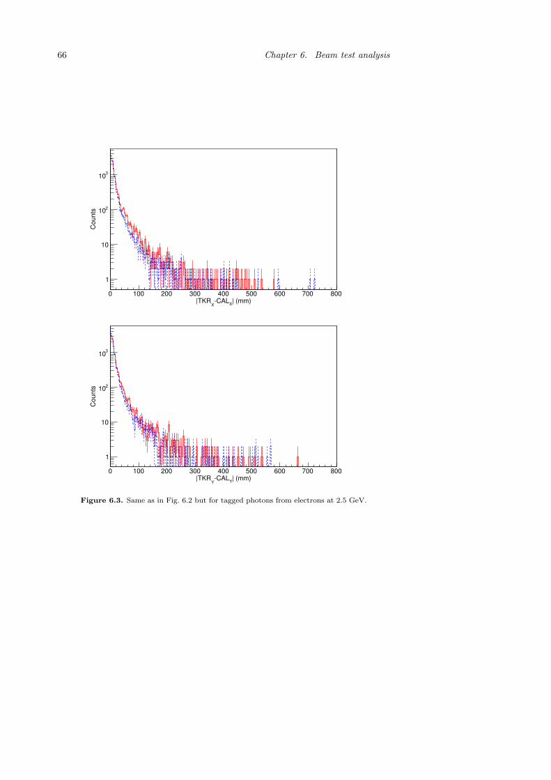
66 Chapter 6. Beam test analysis
| (mm)X
-CALX
|TKR0 100 200 300 400 500 600 700 800
Co
un
ts
1
10
210
310
| (mm)Y
-CALY
|TKR0 100 200 300 400 500 600 700 800
Co
un
ts
1
10
210
310
Figure 6.3. Same as in Fig. 6.2 but for tagged photons from electrons at 2.5 GeV.

6.3. Position reconstruction in the CAL 67
| (mm)X
-CALX
|TKR0 100 200 300 400 500 600 700 800
Co
un
ts
1
10
210
310
410
| (mm)Y
-CALY
|TKR0 100 200 300 400 500 600 700 800
Co
un
ts
1
10
210
310
410
Figure 6.4. Same as in Fig. 6.2 but for electrons at 5 GeV.

68 Chapter 6. Beam test analysis
During the beam tests, a set of runs were taken, where the impact point of thebeam was stepwise changed along two crystals facing in perpendicular directions inthe centre of the CAL. A schematic of the set of runs can be seen in Fig. 6.5. Thisparticular set of runs can be used to inspect the asymmetry properties of the CALcrystals. Full coverage in the form of a 12 x 12 array of impact points would havebeen ideal but due to limitations in beam time, a solution with limited coveragewas used instead.
Figure 6.5. Schematic showing the placement of the beam in the calibration runs.
The analysis procedure was as follows. In order for calibration to be successful,the crystals that have been hit by the trajectory and shower of each incomingparticle must be known. Multiple tracks can cause multiple hit points in the samecrystal, which makes calibration more difficult. Another issue occurs if the trackreconstruction is bad. Then, an extrapolated track might not point to the realpoint of impact. Therefore, only events with one single track in the TKR and a χ2
value of the track that was between 1 and 2 were selected for analysis. For muons,no shower is produced, and therefore no cut on the χ2 value was needed.
The crystal that was hit is deduced by extrapolating the track from the TKRdown to the CAL crystal of interest and selecting only events that lie within thecrystal boundaries.
In the left plot of Fig 6.6, the asymmetry has been plotted as a function of theTKR position, extrapolated to the level where the crystal of interest is located. Forthe calibration runs described above, electrons at 5 GeV and 0 incoming anglewere used. In this case, for crystals in the 2nd layer from the top, which is the firstlayer that has crystals in the same direction as the beam scanning direction, thebeam deposited most energy in the 7th crystal.
The right plot of Fig 6.6 shows the same thing as the left plot, but the axeshave been binned into 12 bins of equal width. In each bin, the mean asymmetrywas calculated. The bin size was chosen to correspond to approximately the widthof a crystal. The points were fitted, for simplicity, with a quadratic function,f (x) = p0 + p1x + p2x
2, since its precision will suffice for the study shown below.In the first and the last bin, the position measurement relation fails. For this reasonthey were not included in the fit.
For comparison, the same log was studied with muon data, which is also usedfor other calibration purposes on ground. The corresponding plots can be seen in

6.3. Position reconstruction in the CAL 69
Extrapolated TKR position (mm)-200 -150 -100 -50 0 50 100 150 200
Lig
ht
asym
me
try
-0.4
-0.3
-0.2
-0.1
-0
0.1
0.2
0.3
0.4
/ ndf 2χ 2.479 / 7
p0 1.646e-007± 6.307e-007
p1 0.000011± 0.001575
p2 0.001284± -0.005164
Extrapolated TKR position (mm)-150 -100 -50 0 50 100 150
Lig
ht
asym
me
try
-0.4
-0.3
-0.2
-0.1
-0
0.1
0.2
0.3
0.4
/ ndf 2χ 2.479 / 7
p0 1.646e-007± 6.307e-007
p1 0.000011± 0.001575
p2 0.001284± -0.005164
Figure 6.6. The light asymmetry as a function of the extrapolated tracker positionin one calorimeter crystal (layer 2, crystal 7) for electrons at 5 GeV and 0 angle. Theleft plot illustrates the spread in light asymmetry and the right plot shows the meanlight asymmetry in each bin fitted with a quadratic function, f (x) = p0+p1x+p2x2.
Fig. 6.7.
Extrapolated TKR position (mm)-200 -150 -100 -50 0 50 100 150 200
Lig
ht
asym
me
try
-0.4
-0.3
-0.2
-0.1
-0
0.1
0.2
0.3
0.4
/ ndf 2χ 6.85 / 7
p0 1.751e-007± 3.118e-007
p1 0.0000± 0.0016
p2 0.00162± -0.00806
Extrapolated TKR position (mm)-150 -100 -50 0 50 100 150
Lig
ht
asym
me
try
-0.4
-0.3
-0.2
-0.1
-0
0.1
0.2
0.3
0.4
/ ndf 2χ 6.85 / 7
p0 1.751e-007± 3.118e-007
p1 0.0000± 0.0016
p2 0.00162± -0.00806
Figure 6.7. The light asymmetry as a function of the extrapolated tracker positionin one calorimeter crystal (layer 2, crystal 7) for muons. The left plot illustrates thespread in light asymmetry and the right plot shows the mean light asymmetry ineach bin fitted with a quadratic function, f (x) = p0 + p1x + p2x2.
The design requirements of the CAL crystals state that the position precisionshould be at least 30 mm. In Fig. 6.8, the position error in one CAL crystal isshown for both electrons at 5 GeV and muons. The plots show the differencebetween the extrapolated TKR position into the log and the position deduced fromthe asymmetry, which is based on the fits in Fig. 6.6 and Fig. 6.7. For electrons,the 68% containment of the position error (centered at zero) in the selected CALcrystal was 4.3±0.2 mm. For muons, the equivalent value was 13.1±0.4 mm. Thedesign requirements are therefore met.
The larger spread for muons comes from the fact that many muons traverse thecrystal at an angle and deposit energy in a larger segment than what a pencil beamof electrons do, where the incoming particle directions are most of the time roughly

70 Chapter 6. Beam test analysis
perpendicular to the crystal log. The light asymmetries are therefore less accuratefor muons.
Position error (mm)-100 -80 -60 -40 -20 0 20 40 60 80 100
Co
un
ts
1
10
210
Position error (mm)-100 -80 -60 -40 -20 0 20 40 60 80 100
Co
un
ts
1
10
210
Figure 6.8. The difference between the extrapolated tracker position and the po-sition of hit deduced from the light asymmetry in one calorimeter crystal (layer 2,crystal 7) for electrons at 5 GeV (left) and muons (right).
6.4 Direction reconstruction in the CAL
Directional variables in Fermi -LAT data, as explained before, are output in theform of directional cosines. This means that the cosine of the angles betweenthe incoming particle direction vector and the three different axis are calculated. Adistribution for direction on which a 68% containment calculation can be performed,in the same way as for the position reconstruction, can be obtained by using thefollowing formula.
θ = π−arccos(Tkr1XDir·CalXDir+Tkr1YDir·CalYDir+Tkr1ZDir·CalZDir) (6.3)
where π comes from the fact that the coordinate systems in the TKR and in theCAL are defined differently. In the TKR a right-handed coordinate system is usedwith the positive z-direction pointing in the direction of the beam. In the CAL,a left-handed coordinate system is used with the negative z axis pointing in thedirection of the beam. To get the proper angle between the two direction vectors,the one from the TKR and the one from the CAL, a translation of 180 must bedone. The expression inside the parenthesis is the scalar product between the twovectors. Since the vectors are normalised, the lengths of the two vectors are one.
The same three particle types, studied in terms of the position reconstruction,were also studied here. Figs. 6.9–6.11 show the resulting distributions. The cutsexplained in Section 6.2 have been used and the distributions are again normalisedby the total number of events. The 68% quantiles and the differences between dataand simulation are given in Table 6.3.

6.4. Direction reconstruction in the CAL 71
Space angle (deg)0 20 40 60 80 100 120 140
Co
un
ts
1
10
210
310
Figure 6.9. The space angle distribution for bremsstrahlung photons from electronsat 2.5 GeV. The solid red line is data and the dashed blue line is simulation.
Space angle (deg)0 20 40 60 80 100 120 140
Co
un
ts
1
10
210
310
Figure 6.10. Same as Fig. 6.9 but for tagged photons from electrons at 2.5 GeV.
Space angle (deg)0 20 40 60 80 100 120 140
Co
un
ts
1
10
210
310
Figure 6.11. Same as Fig. 6.9 but for electrons at 5 GeV.

72 Chapter 6. Beam test analysis
Table 6.3. The 68% containment of the difference between the TKR direction andthe CAL direction for bremsstrahlung photons from electrons at 2.5 GeV, taggedphotons from electrons at 2.5 GeV and electrons at 5 GeV and the difference betweendata and simulation (MC).
Particle Ψ68% () ΨMC,68% () ∆Ψ68%/Ψ68% (%)γfb 11.5 ± 0.1 9.9 ± 0.1 13.6 ± 0.2γtag 12.0 ± 0.1 9.8 ± 0.1 18.4 ± 0.3e− 3.9 ± 0.03 3.0 ± 0.02 22.1 ± 0.2
6.5 Energy reconstruction in the CAL
Many aspects of the energy reconstruction can be studied with the collected data.For this thesis, raw energy distributions, shower profiles in the longitudinal directionand energy resolutions were studied.
6.5.1 Raw energy distributions
There are several variables in the data that are related to energy measurements.Among these are the layer-wise raw energies measured in the CAL and the sumof all energy depositions in all crystals in the CAL (after diode calibrations). Thelayer-by-layer approach offers a more in-depth look than simply looking at thetotal energy. In this case, the figures-of-merit are the statistical moments, or morespecifically the mean value and the RMS.
In Fig. 6.12, the difference between data and simulation in terms of the statisticalmoments, in all the eight layers of the CAL, are plotted. The plots, as before,correspond to bremsstrahlung photons from 2.5 GeV electrons, tagged photonsfrom electrons at 2.5 GeV and electrons at 5 GeV, respectively. The difference isless than 10% in all layers for photons and less than 16% for electrons. The trendis similar in all the three plots, namely that the agreement is better the higher thelayer number is.
6.5.2 Longitudinal profile
In Fig. 6.13, the sum of all longitudinal shower profiles is visualised. In the plots,the energy deposition is shown as a function of the eight layers in the CAL. Thefigure shows that the shower profiles from data and simulation are almost identical.For photons, the shower maximum is located mostly in the second layer of theCAL, whereas for electrons, the shower maximum is most common in the middlelayers of the CAL (layers 4 and 5). The difference in shower maximum betweenthe photon runs and the electron run can be explained by the fact that the beamenergy is a factor of two larger in the electron run. Since the shower maximum

6.5. Energy reconstruction in the CAL 73
Calorimeter layer1 2 3 4 5 6 7 8
(Data
-MC
)/D
ata
(%
)
0
2
4
6
8
10
12
14
16
18
20
Mean
RMS
Calorimeter layer1 2 3 4 5 6 7 8
(Data
-MC
)/D
ata
(%
)
0
2
4
6
8
10
12
14
16
18
20
Mean
RMS
Calorimeter layer1 2 3 4 5 6 7 8
(Data
-MC
)/D
ata
(%
)
0
2
4
6
8
10
12
14
16
18
20
Mean
RMS
Figure 6.12. The difference between data and simulation (MC) in terms of themean value (solid line) and the RMS (dashed line) of the energy distributions inthe eight calorimeter layers for bremsstrahlung photons from electrons at 2.5 GeV(top), tagged photons from electrons at 2.5 GeV (middle) and electrons at 5 GeV(bottom).

74 Chapter 6. Beam test analysis
changes logarithmically with the incoming energy, the maximum for higher-energyparticles occurs on average later in the CAL.
6.5.3 Energy resolution
The photon tagger was only available in the PS beam line. Therefore, electromag-netic properties at higher energies must by studied with electron data from theSPS beam line. The behaviour in the high end of the Fermi -LAT energy rangeshould be studied since the masses of many dark matter particle candidates arepredicted to be located there. A key factor in searches for spectral lines from darkmatter is the energy resolution. The larger the energy resolution, the more photonsfrom sources other than dark matter are included in a specified bin matched to theenergy resolution. This will decrease the significance of the spectral line and will,consequently, make the search more difficult.
In Figs. 6.14–6.20, the energy distributions for data and simulation are shownfor electrons at the energies 5, 10, 20, 50, 99, 196 and 282 GeV. The distributionsthat are included consist of the measured raw energy in the CAL (CalEnergyRaw),the available algorithms for energy reconstruction (CalCfpEnergy, CalLkHdEnergyand EvtEnergyCorr), and just for comparison for the simulation, the true energy(McEnergy). CalCfpEnergy represents the energy estimated with the profile fittingmethod, CalLkHdEnergy contains the energy estimated with the likelihood methodand EvtEnergyCorr is the energy estimated with the parametric method. The threeenergy reconstruction algorithms are further described in Section 4.2.4. A spreadin the true energy was included in the simulation, as can be seen in the figures, toreflect beam conditions.
In Fermi -LAT data, the best of the three energy algorithms is chosen event-by-event and stored in CTBBestEnergy. This variable is not meant to be used withthe CU, since it is part of an algorithm that bases the choice on classification-tree analyses that are optimised for the geometry of the Fermi -LAT. How thechoice is made depends on the version of the software that processes the data, sinceimprovements are made continuously. For these reasons, CTBBestEnergy was notincluded in these plots.
The energy resolutions were calculated by first fitting the tip of each energydistribution with a single Gaussian function. Since the distributions are not sym-metrical in shape, a fit to the whole spectrum would not yield at good fit. Therefore,the Gaussian fitting interval was restricted to the tip of the peak.
The fit provided an estimate for the value at which the most probable energywas located. From that point, the events were calculated symmetrically in bothdirections around the most probable energy, until 68% of the total number of eventswere accounted for. The resulting energy interval divided by two is the equivalentof a Gaussian standard deviation and yields the relative energy resolution whendivided by the most probable energy.
In Fig. 6.21 and Fig. 6.22, the resulting energy resolutions as a function of theenergy are shown for data and simulation, respectively. Fig. 6.23 shows the relative

6.5. Energy reconstruction in the CAL 75
Calorimeter layer0 1 2 3 4 5 6 7 8 9
Deposited e
nerg
y (
GeV
)
-210
-110
Calorimeter layer0 1 2 3 4 5 6 7 8 9
Deposited e
nerg
y (
GeV
)
-210
-110
Calorimeter layer0 1 2 3 4 5 6 7 8 9
Deposited e
nerg
y (
GeV
)
-110
1
Figure 6.13. The energy deposition as a function of the calorimeter layer for brems-strahlung photons from electrons at 2.5 GeV (top), tagged photons from electronsat 2.5 GeV (middle) and electrons at 5 GeV (bottom). At each layer there are twocolumns. The left column is data and the right column is simulation, respectively.

76 Chapter 6. Beam test analysis
Energy (GeV)0 2 4 6 8 10 12
Counts
1
10
210
310
410 CalEnergyRaw
CalCfpEnergy
CalLkHdEnergy
EvtEnergyCorr
Energy (GeV)0 2 4 6 8 10 12
Counts
1
10
210
310
410 CalEnergyRaw
CalCfpEnergy
CalLkHdEnergy
EvtEnergyCorr
McEnergy
Figure 6.14. The energy distributions for electrons at 5 GeV for data (top) and sim-ulation (bottom) are shown. Included are the measured raw energy (CalEnergyRaw),the three algorithms for energy reconstruction (CalCfpEnergy, CalLkHdEnergy andEvtEnergyCorr), and for the simulation, the true energy (McEnergy).

6.5. Energy reconstruction in the CAL 77
Energy (GeV)0 5 10 15 20 25
Counts
1
10
210
310
410 CalEnergyRaw
CalCfpEnergy
CalLkHdEnergy
EvtEnergyCorr
Energy (GeV)0 5 10 15 20 25
Counts
1
10
210
310
410 CalEnergyRaw
CalCfpEnergy
CalLkHdEnergy
EvtEnergyCorr
McEnergy
Figure 6.15. Same as Fig. 6.14 but for 10 GeV.

78 Chapter 6. Beam test analysis
Energy (GeV)0 5 10 15 20 25 30 35 40 45 50
Counts
1
10
210
310
410 CalEnergyRaw
CalCfpEnergy
CalLkHdEnergy
EvtEnergyCorr
Energy (GeV)0 5 10 15 20 25 30 35 40 45 50
Counts
1
10
210
310
410 CalEnergyRaw
CalCfpEnergy
CalLkHdEnergy
EvtEnergyCorr
McEnergy
Figure 6.16. Same as Fig. 6.14 but for 20 GeV.
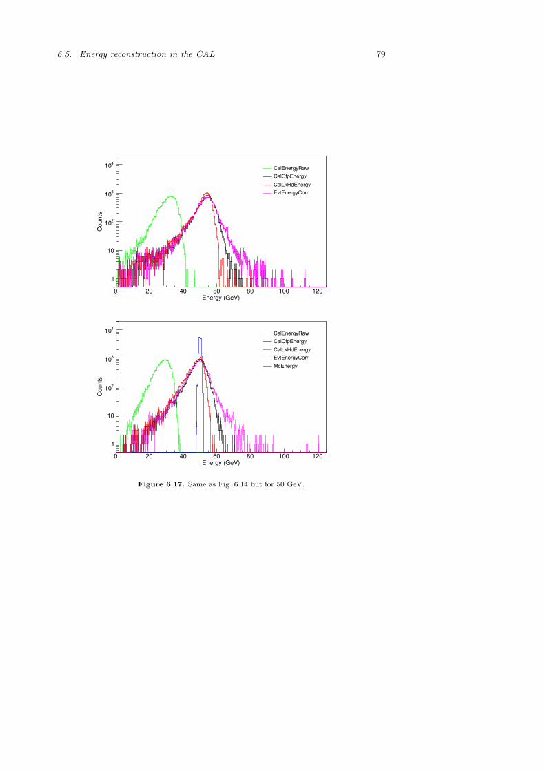
6.5. Energy reconstruction in the CAL 79
Energy (GeV)0 20 40 60 80 100 120
Counts
1
10
210
310
410 CalEnergyRaw
CalCfpEnergy
CalLkHdEnergy
EvtEnergyCorr
Energy (GeV)0 20 40 60 80 100 120
Counts
1
10
210
310
410 CalEnergyRaw
CalCfpEnergy
CalLkHdEnergy
EvtEnergyCorr
McEnergy
Figure 6.17. Same as Fig. 6.14 but for 50 GeV.

80 Chapter 6. Beam test analysis
Energy (GeV)0 20 40 60 80 100 120 140 160 180 200 220 240
Counts
1
10
210
310
410 CalEnergyRaw
CalCfpEnergy
CalLkHdEnergy
EvtEnergyCorr
Energy (GeV)0 20 40 60 80 100 120 140 160 180 200 220 240
Counts
1
10
210
310
410 CalEnergyRaw
CalCfpEnergy
CalLkHdEnergy
EvtEnergyCorr
McEnergy
Figure 6.18. Same as Fig. 6.14 but for 99 GeV.

6.5. Energy reconstruction in the CAL 81
Energy (GeV)0 50 100 150 200 250 300 350 400 450
Counts
1
10
210
310
410 CalEnergyRaw
CalCfpEnergy
CalLkHdEnergy
EvtEnergyCorr
Energy (GeV)0 50 100 150 200 250 300 350 400 450
Counts
1
10
210
310
410 CalEnergyRaw
CalCfpEnergy
CalLkHdEnergy
EvtEnergyCorr
McEnergy
Figure 6.19. Same as Fig. 6.14 but for 196 GeV.

82 Chapter 6. Beam test analysis
Energy (GeV)0 100 200 300 400 500 600 700
Counts
1
10
210
310
410 CalEnergyRaw
CalCfpEnergy
CalLkHdEnergy
EvtEnergyCorr
Energy (GeV)0 100 200 300 400 500 600 700
Counts
1
10
210
310
410 CalEnergyRaw
CalCfpEnergy
CalLkHdEnergy
EvtEnergyCorr
McEnergy
Figure 6.20. Same as Fig. 6.14 but for 282 GeV.

6.5. Energy reconstruction in the CAL 83
difference between the two. As can be seen in Fig. 6.20, CalLkHdEnergy has a sharpcut off at 300 GeV.
The reason for the cut off is that the likelihood method has only been extendedto 300 GeV. Since CalLkHdEnergy does not function well at the highest energy at282 GeV, the value of the energy resolution was left out at this energy.
Beam energy (GeV)10
210
/E (
Data
) (%
)E
σ
0
5
10
15
20
25
CalEnergyRaw
CalCfpEnergy
CalLkHdEnergyEvtEnergyCorr
Figure 6.21. The energy resolutions for data, determined from the different energydistributions at the energies 5, 10, 20, 50, 99, 196 and 282 GeV.
Beam energy (GeV)10
210
/E (
MC
) (%
)E
σ
0
5
10
15
20
25
CalEnergyRaw
CalCfpEnergy
CalLkHdEnergyEvtEnergyCorr
Figure 6.22. The energy resolutions for the simulations, determined from thedifferent energy distributions at the energies 5, 10, 20, 50, 99, 196 and 282 GeV.

84 Chapter 6. Beam test analysis
Beam energy (GeV)10
210
(Data
-MC
)/D
ata
(%
)
-60
-50
-40
-30
-20
-10
0
10
20
30
40
CalEnergyRaw
CalCfpEnergy
CalLkHdEnergyEvtEnergyCorr
Figure 6.23. The difference in energy resolution between data and simulation,determined from the different energy distributions at the energies 5, 10, 20, 50, 99,196 and 282 GeV.
In Fig. 6.24, the relative difference in the fitted peak position between data andsimulation is shown. As can be seen in the figure, the peak position in data is largerat all measured energies but the trend is relatively flat.
Beam energy (GeV)10
210
(Data
-MC
)/D
ata
(%
)
-10
-5
0
5
10
15
20
25
30
CalEnergyRaw
CalCfpEnergy
CalLkHdEnergyEvtEnergyCorr
Figure 6.24. The difference in the energy of the peak between data and simulation,determined from the different energy distributions at the energies 5, 10, 20, 50, 99,196 and 282 GeV.

6.7. Summary and conclusions 85
6.6 Latest developments
The analysis above was performed with a set of simulations in which the so-calledLandau-Pomeranchuk-Migdal (LPM) effect was turned off. The effect governs theenergy dependent suppression of bremsstrahlung in charged particle interactionsand had an incorrect implementation in the Geant4 code as discovered by the beamtest working group. The error caused the differences between data and simulationto be erroneously large.
After the above analysis was finished, a correct description of the LPM effectwas implemented. However, due to time constraints the above analysis could notbe redone. A preliminary illustration of the difference between the old, the newand no implementation of the effect can be seen in Fig. 6.25. The figure shows theratio between data and simulation in terms of the mean energy deposited in the8 layers of the CAL for electrons from 10 GeV to 282 GeV at 0 incidence angle.As can be seen in the figure, the impact of the LPM effect is more significant forhigher incident energies and for CAL layers located closer to the TKR. The oldimplementation of the LPM effect also shows much larger differences.
Preliminary analyses using the latest simulations, with additional material (inthis case lead) at the end of the beam line, have also indicated an decrease in thedifferences between data and simulation. This is illustrated in Fig. 6.26, where theratio between data and simulation is shown for the number of clusters in the TKRand for the mean energy deposited in the CAL layers for electrons from 10 GeV to282 GeV at 0 incidence angle. The ratio for the number of clusters inside an energy-and angle-dependent cone centred on the reconstructed axis of the best track andstarting at the head of track 1 is shown for thin converter layer (ilayer= −2.5),thick converter layers (ilayer= −1.5) and no converter layers (ilayer= −0.5) inthe TKR. As is indicated by Fig. 6.26, the optimal additional material seems to besomewhere below 0.1X0, at which point the curves should be flat and the globalscaling factor is about 10%.
6.7 Summary and conclusions
For the figures-of-merit for position reconstruction in the CAL, namely the 68% con-tainment of the distributions with the difference between the extrapolated tracksfrom the TKR and CAL, respectively, to the top of CAL, the values for dataare larger by 11.8–18.8% for both electrons and the two types of photons (brems-strahlung photons and tagged photons). The difference is also clearly seen in thecorresponding distributions, where the distributions for data are less peaked thanfor the simulations.
When looking at the position reconstruction in the individual CAL crystals, theobserved 68% containments of the position error in one of the CAL crystal were4.3±0.2 mm for 5 GeV electrons and 13.1±0.4 mm for muons, which is well belowthe design requirement of 30 mm. As explained before, the large difference between

86 Chapter 6. Beam test analysis
Fig
ure
6.2
5.
The
ratio
betw
eendata
and
simula
tion
for
the
mea
nen
ergy
dep
osited
inth
e8
layers
ofth
eC
AL
for
electrons
at
energ
ies10,20,50,99,196
and
282
GeV
and
at
0
incid
ence
angle
for
no
LP
Meff
ect(le
ft),new
LP
Meff
ect(ce
nte
r)
and
old
LP
Meff
ect(rig
ht).

6.7. Summary and conclusions 87
Fig
ure
6.2
6.
The
ratio
bet
wee
ndata
and
sim
ula
tion
for
the
num
ber
ofcl
ust
ers
indiff
eren
tla
yer
softh
eT
KR
and
for
the
mea
nen
ergy
dep
osi
ted
inth
e8
layer
softh
eC
AL
for
elec
trons
at
ener
gie
s10,20,50,99,196
and
282
GeV
and
at
0
inci
den
ceangle
for
no
additio
nalm
ate
rial(left
),0.1
X0
ofadditio
nalle
ad
(cente
r)
and
0.2
X0
ofadditio
nalle
ad
(rig
ht)
.
88 Chapter 6. Beam test analysis
electrons and muons can be explained by the difference in incoming angle. Since themuons are not bundled in a pencil beam, like the electrons, they deposit energy ina larger segment of the crystals. This makes position determination more difficultand therefore the distribution is more spread out.
The same tendency, seen for position reconstruction in the CAL, holds for di-rection reconstruction in the CAL. For the 68% containment of the distribution ofspace angles between the TKR direction and the CAL direction, the values for dataare again larger by 13.6–22.1%. In this case, the difference is largest for electrons,which is also evident from the corresponding figures.
When looking at the individual direction variables in both the TKR and theCAL, not shown in this thesis, it can be seen that most of the runs exhibit alarge bias in the CAL direction variables compared to the beam direction andcompared to the simulation, whereas TKR direction variables are approximatelycoinciding. For the runs used for energy resolution studies, the runs from SPSmanifest a bias that is often, but not always, negative in the x direction and positivein the y direction. This could point to a misalignment of the CAL with respectto the TKR, but since other runs, such as the 5 GeV electron run from the PS,demonstrated unbiased direction distributions, a misalignment is unlikely. Theindividual direction variables for the CAL also showed that the distributions fordata are in general broader. Both these effects contribute to the large differencebetween data and simulation for position and direction reconstructions but furtherand more detailed studies are needed in order to determine what is causing theeffects.
For the dark matter line search, the direction is not a crucial ingredient, exceptwhen the known sources of gamma-rays are masked. Even in that case, there arefew high energy photons coming from these sources and the inclusion of a part ofthem would probably not influence the search a great deal. However, one way tocompensate for the observed differences between data and simulation is to make aconservative choice for the radius of the circle masking the sources.
The figures for the layer-wise energy deposition in the CAL show that the meanvalue for data is larger than for the simulation by less than 10% in all layers forphotons. For electrons the difference is largest in the 1st layer where the value fordata is almost 16% greater than for the simulation. The trend for all particle typesis that the agreement is better the higher the layer number is until a turning pointoccurs in the 5th layer for tagged photons and in the 6th layer for bremsstrahlungphotons and electrons. For these runs, the minimum difference in the mean valueis less than 1%.
The figures showing the energy resolutions in data and simulation have similartrends for data and simulation for both the raw energy and two of the three energyreconstruction algorithms. Only CalLkHdEnergy demonstrates large differences.This method is in fact the least maintained out of the three algorithms. Further-more, it is only extended to 300 GeV and divides the energy range up into bins,which may give rise to bin-edge effects. These factors may explain the strange be-haviour at higher energies. Overall, however, with the exception of CalLkHdEnergy,

6.7. Summary and conclusions 89
the differences between data and simulation in terms of the energy resolution arerelatively small and stay below 10% over most of the tested energy range.
Generally speaking, the energy resolution should be worse at higher energiesdue to the increasing leakage. As seen in the figure, showing the difference in peakposition between data and simulation, the peak position is consistently about 10%higher for data than for the simulation. This may partially explain the differencesin energy resolution between data and simulation.
In absolute terms, the energy resolutions in both data and simulation are con-sistent with the Fermi -LAT science requirements, which state that the energy reso-lution must be <10% for 100 MeV – 10 GeV and <20% for 10–300 GeV for on-axisphotons, especially those from the corrected energies. The reader is reminded thata plot of the energy dependence of the Fermi -LAT energy resolution, determinedfrom simulations, was shown in Fig. 4.12 in Chapter 4.
It should be noted that an energy-dependent bias with respect to the true energycan be seen in the energy distributions for the simulation. The most probableenergies provided by the parametric method and the likelihood method indicate abias, which seems to increase with energy, whereas the peak of the profile methodcoincides relatively well with the peak of the true energy at all energies.
Shortly before the analysis presented in this thesis was finished, an error in theGeant4 code was discovered by the beam test working group. The error was anincorrect implementation of the so-called Landau-Pomeranchuk-Migdal (LPM) ef-fect, which governs the energy-dependent suppression of bremsstrahlung in chargedparticle interactions. The impact of this error should be more significant for higherenergies.
While waiting for a better implementation by the Geant4 team, the LPM ef-fect was turned off in the simulation and the analysis presented in this thesis wasperformed on that version of the simulation. The most recent simulations madewithin the beam test working group, which include the correct implementation ofthe LPM effect and extra material in the form of lead in front of the TKR, haveshown that the large differences in the first layers of the CAL decrease, therebyflattening the curve for the difference between data and simulation. Some of thedifferences thereby reduce to a constant factor. The exact nature of this extramaterial that might exists in the beam line or the detector but is missing in thesimulation is still, however, unclear.
To conclude, beam line effects that do not apply to the Fermi -LAT cannotbe ruled out as the source of the differences seen between distributions for dataand simulation, especially since later studies show an increasing agreement withextra material in the simulations. The differences are, however, likely caused by acombination of geometrical effects, physics and calibration.
The calibration of the Fermi -LAT is not directly dependent on the beam testresults, since the Fermi -LAT is calibrated on-orbit. Also, the calibration procedureof e.g. the CAL differs between the beam test and the satellite. As described inthe thesis, muons were used to calibrate the satellite on ground and cosmic rayprotons are used on-orbit. The differences seen in the energy studies may therefore

90 Chapter 6. Beam test analysis
not apply for the Fermi -LAT. The CU and Fermi -LAT differ in many aspects,but the observed differences in the CU introduce a systematic uncertainty for theFermi -LAT that should be noted in science analyses.
Apart from the absolute shift in the peak position, the energy reconstructionis relatively well reproduced by simulations. This is important for the modellingof spectral lines that is used in the dark matter line search, since full detectorsimulations are used to parametrise the line shape.
In the end, further efforts are needed in order to rule out beam line effects. Thebeam test campaign has, however, already been very useful for the understandingof the detector and with the collected data many instrumental effects and softwareerrors have been uncovered that would have, otherwise, been difficult to detect.

Chapter 7
Dark matter line search
This chapter focuses on the search for spectral lines from dark matter (DM) inFermi -LAT data. It contains a discussion on where a signal can be looked for anda description of some of the statistical methods that can be used in the searchand their statistical properties. Two statistical methods that are implemented forspectral line searches, profile likelihood and Scan Statistics, are then reviewed. Abinned profile likelihood method and Scan Statistics are then applied to a simulateddata set called obssim2. Finally, an unbinned profile likelihood method is appliedto almost one year of Fermi -LAT data.
7.1 Initial discussions
7.1.1 Region-of-interest selection
The gamma-ray sky has never been measured at the high end of the Fermi -LATenergy range. This means that the gamma-ray emissions, which serve as a back-ground to a spectral line from DM annihilations or decays, are largely unknown.Nevertheless, the optimal region in space that gives the largest signal with respect tothe background depends on the distribution of gamma-rays from these backgroundsources. It also depends on the distribution of DM in the Universe. Therefore,the optimal region with respect to one halo profile is not the optimal region for adifferent halo profile. Finally, the figure-of-merit (e.g. the signal-to-noise ratio orthe value of the likelihood) for which the optimisation is performed also affects theresult. These factors make the selection of a suitable region-of-interest non-trivial.For more discussions on the subject, see e.g. [134] and [135].
For the analysis applied to simulated data (presented in Section 7.5), the se-lected region-of-interest is proposed by Stoehr et al. [134]. In their studies, a DMdistribution with inherent substructure for a “Milky Way-like” galaxy was producedusing N-body simulations, given a flat ΛCDM Universe with assumed parameters.Within the Milky Way, the dominating background will come from the galactic
91

92 Chapter 7. Dark matter line search
diffuse emission. Motivated by the results from the N-body simulations and ac-counting for an extragalactic background, an angular window given by a brokenannulus around the galactic centre with a radius from 25 to 35 but excluding theregion within 10 from the galactic plane was used in the paper to determine 3σdetection limits with Fermi. In this region, the total galactic diffuse emission wasassumed to be zero. How much this assumption affects the result is unclear. Thebroken annulus region is shown in black and in galactic coordinates in Fig. 7.1.
L (deg)
150 100 50 0 50 100 150
B (
de
g)
80
60
40
20
0
20
40
60
80
Figure 7.1. A visualisation of the two regions-of-interest used in the analysis ingalactic coordinates. The black region is the broken annulus used for simulated data,and the sum of the gray and the black region defines the region used for measureddata.
For the analysis on measured data from the Fermi -LAT instrument (presentedin Section 7.6), a different region-of-interest was chosen for several reasons. Firstof all the assumptions motivating the broken annulus were found to be unrealistic.Secondly, with the given observation time, a larger region would give better photonstatistics, which in turn would constrain the photon background better.
The chosen region for Fermi -LAT data excludes the galactic plane at |b| < 10
while keeping a 20 × 20 square around the galactic centre. This selection ensuresthat a large portion of the dominant background from the galactic diffuse emission ismasked while including the galactic centre, which is a potentially interesting regionfor dark matter searches. Thanks to the large remaining region, the backgroundcan be well constrained, which was one of the goals.
In the remaining region, photons coming from a circular region with radius 0.2
around the 1233 preliminary point sources found after 11 months of Fermi -LATobservations were also removed. The motivation for masking these sources is thata large majority of them have known counterparts in the form of e.g. pulsars andactive galaxies, where significant amounts of dark matter annihilations or decaysare not expected. Due to the large number of point sources in the galactic centre

7.1. Initial discussions 93
region, the removal of the point sources there would have removed most of theregion. Therefore, no point sources were removed within a radius of 1 from thegalactic centre. The source cut removes about 5% of the total number of photonsand about 0.4% of the solid angle. The selected region before source removal isillustrated as the sum of the black and gray regions and in galactic coordinates inFig. 7.1.
7.1.2 Halo profile selection
As described in Section 3.4, the distribution of DM in galaxies can be modelledwith different halo models. For the analysis applied to the simulated data, theNFW profile was used. The galactocentric distance of the Sun was assumed to be8.5 kpc and the local DM density was set to 0.3 GeV cm−3.
For the analysis on measured Fermi -LAT data, a variety of halo profiles wereused: the NFW profile with rs = 20 kpc, the Einasto profile with rs = 20 kpc anda = 0.17 and a shallow isothermal profiles with rs = 5 kpc. The local DM densitywas set to 0.4 GeV cm−3 and the maximum values of r were set to ∼ 150 kpc forthe NFW and Einasto profiles and ∼ 100 kpc for the isothermal profile.
7.1.3 Data selection
The event class used for the analysis on Fermi -LAT data is not the standard “dif-fuse” class (see also Section 4.2.6) but rather an extension of it. It is a subset ofthe event class developed for the Fermi -LAT measurements of the isotropic diffusegamma-ray emission [23] and has internally been referred to as the “extradiffuse”class. The extradiffuse class has two cuts on the Merit-level in addition to the stan-dard diffuse class cuts: a) an average charge deposited in the tracker planes that isless than a specified value in order to veto heavy ions, b) a transverse shower sizein the calorimeter within a specified range expected for electromagnetic showers toveto against hadronic showers and minimum-ionising particles.
The additional cuts are designed to reduce the charge particle background, whichdue to the nature of the background rejection may leak in only at specific energies,thereby causing spectral features that mimic spectral lines. The extradiffuse classleads to some loss of the effective area but yields a gamma-ray efficiency of > 90%as compared to the standard diffuse class. In Fig. 7.2, the effective areas of thediffuse and extradiffuse classes are shown for events classified as “back” (defined inSection 4.2.1).
As mentioned in Section 4.2.4, one of the energy correction algorithms is theprofile fitting method. In the analysis of the measured Fermi -LAT data, the energyprovided by the profile method was chosen instead of the standard energy, whichis a composition of the three different energy correction methods. The reason ismainly due to the fact that the likelihood method (included in the standard energy)only works up to 300 GeV, at which point there is a sharp cut off as could be seenin Fig. 6.20.

94 Chapter 7. Dark matter line search
Figure 7.2. A comparison between diffuse and extradiffuse class events in terms ofthe effective area for back events.
In addition, since the likelihood method is trained on specific sets of MonteCarlo simulations and the training is divided into regions in energy, the overallenergy spectrum also suffers from a subtle binning effect, which gives rise to smallstep-like spectral features. This behaviour can be seen in Fig. 7.3, where the energyspectra from the profile method and the likelihood method are compared. In thefigure, steps can be seen at 30, 50, 70 and 100 GeV. The statistical errors have beenomitted for presentational purposes.
Figure 7.3. A comparison between the energy spectra from the profile method andthe likelihood method. A step-like behaviour can be seen in the spectrum from thelikelihood method, which is the result of a binning effect. Statistical errors havebeen omitted for presentational purposes.

7.2. Statistical concepts 95
Furthermore, as could be seen in the bottom plot of e.q. Fig. 6.19, the peaksof the parametric and likelihood methods are both biased with respect to the truevalue of the energy, whereas the peak from the profile method seems to be almostunbiased.
Since the purpose of the spectral line search is to detect small localised spectralfeatures, the profile method was deemed to be a safer choice. In the simulatedobssim2 data set, however, the profile method could not be chosen because thedefault energy in the simulation files could not be changed. Therefore, the standardenergy was used.
The Fermi -LAT data used in the analysis spans over more than 11 months,ranging from 7 August, 2008, to 21 July, 2009, and was collected in sky survey mode.The photons that are included have energies between 19.4 GeV and 298.4 GeV.Additional standard data quality cuts are also performed in order to reduce theeffect of the Earth albedo background. Thus, only events coming from angles< 105 with respect to zenith are accepted. Furthermore, only time intervals whenthe angle between zenith and the spacecraft zenith was < 47 are accepted.
7.2 Statistical concepts
The most basic concept in statistical theory is probability and the mathemati-cal theory behind it was first developed by Andrey Nikolaevich Kolmogorov in1933 [136, 137]. According to the theory, probability must satisfy the three Kol-mogorov axioms. If Ω is defined to be the set of all elementary and exclusive(the occurrence of one excludes the occurrence of the others) events Xi, then theprobability of Xi occurring, P (Xi), satisfies the axioms [138]:
1. P (Xi) ≤ 0 for all i
2. P (Xi or Xj) = P (Xi) + P (Xj)
3.∑
Ω P (Xi) = 1
7.2.1 Frequentist and Bayesian statistics
There are two schools of thought in statistical theory, frequentist (or classical) andBayesian statistics, which both satisfy the Kolmogorov axioms but which differ onbasic principles. In frequentist theory, probability is defined in terms of the relativefrequency of something happening.
In the Bayesian approach, on the other hand, probability can be interpretedas the degree-of-belief of something happening. The name comes from the useof Bayes theorem, given in Eq. 7.1, which links the posterior probability P (θi|x)(the probability of the hypothesis θi given the observed data x) and the likelihoodfunction L (x|θi).

96 Chapter 7. Dark matter line search
P (θ|x) =L (x|θi) · P (θi)
P (x)(7.1)
Here, P (θi) is the prior probability and P (x) can be considered to be a nor-malisation constant, since the sum of the left-hand side over all hypotheses mustbe unity.
7.2.2 Confidence intervals
The concept of confidence intervals (CIs) is the construction and estimation of aninterval for some parameter, which contains the true parameter value with someprobability 1 − α. The probability 1 − α is also referred to as the confidence level(CL).
When a CI is used in the context of some scientific experiment or measurement,it can be considered to be the error on the parameter. The use of confidenceintervals to report the statistical error of a measurement was first developed byJerzy Neyman [139]. To illustrate the concept, a parameter µ and the observedvalue of it, x, can be assumed. If the probability density function, P (x|µ), for eachfixed value of µ is assumed to be known, a horizontal acceptance region [x1, x2]can be drawn for each value of µ such that P (x ∈ [x1, x2]) = 1 − α. The resultingconfidence belt is shown in Fig. 7.4 [140].
When a measurement of x is performed, a vertical line is drawn at the value ofthe measurement. The intersections between the line and the confidence belt thengives the CI [µ1, µ2], which is the union of all values of µ for which the acceptanceregion is intersected by the line.
In this thesis, CIs are also used for hypothesis testing, as will be shown inSection 7.4.
7.2.3 Hypothesis tests
In a statistical test, the goal is often to see whether an observation agrees with agiven hypothesis or not. The hypothesis under consideration is generally referredto as the null hypothesis and is usually denoted by H0. Making statements aboutthe validity of H0 often concerns a comparison with some alternative hypotheses,usually denoted as H1,H2, ..., and the discrimination between the two is oftenaccomplished by using a so-called test statistic (TS).
Commonly, a hypothesis test is formulated in terms of a decision to accept orreject H0. This can be done e.g. by defining a critical region in the probabilitydensity function P (t|H0) (where t is the test statistic), such that the probability toobserve a value of t greater than tcrit is α. If the observation, tobs, is in the criticalregion, H0 is rejected. The complement of the critical region is generally called theacceptance region.

7.2. Statistical concepts 97
Figure 7.4. An illustration of a generic confidence belt from which the confidenceinterval for a parameter µ can be calculated (from [140]).
7.2.4 Coverage
Coverage is a concept defined for CIs. It means that a fraction (1−α) of an infiniteset of CIs obtained from an infinite number of identical experiments should containthe true value of the parameter to be estimated. In other words:
P (s ∈ [s1, s2]) = 1 − α (7.2)
where s1 and s2 are the lower and upper limit of the CI for the parameter s. Amethod with this property satisfied is said to have nominal coverage. If instead,P (s ∈ [s1, s2]) < 1 − α, the intervals “undercover” for that s. Significant under-coverage for any s is a serious flaw [140]. For P (s ∈ [s1, s2]) > 1 − α, the intervalsare said to “overcover” for that s. The intervals that overcover for some s andundercover for no s are “conservative”. Overcoverage is not as big of a problemas undercoverage but leads to a loss of power, described below. In the context ofhypothesis testing, α is called the type-I error and corresponds to the probabilitythat the null hypothesis is rejected even though it is true.
7.2.5 Power
Power is a concept defined for hypothesis tests. The power of a test is the probabilitythat the null hypothesis is rejected when the alternative hypothesis is true. Inother words, power = 1 − β, where β is the probability of a type-II error, i.e. theprobability to accept the null hypothesis when the alternative hypothesis is true.

98 Chapter 7. Dark matter line search
When using CIs for hypothesis testing, power is the fraction of cases where s = 0is not contained in the interval given that s > 0 is true.
7.2.6 Significance
The significance of a given observed signal (usually connected to some alternativehypothesis) is commonly quoted in physics and can be defined as the probability toobtain a value less than or equal to the observed value under the null hypothesis.
Despite the fact that the likelihood function is not necessarily a normal dis-tribution, the quoted probability is often related to the standard deviation of anormal distribution. The standard deviation of a normal distribution correspondsto a specific cumulative probability, which depends on if the integration is one-sidedor two-sided.
If the integration is two-sided, one standard deviation (1σ), corresponds to∼68.3%, 2σ corresponds to ∼95.4% and 5σ corresponds to ∼99.99994%. The num-ber of standard deviations n, representing the probability p from a two-sided inte-gration of a normal distribution is given by Eq. 7.3, where erf−1 is the inverse ofthe error function.
n = erf−1(p)√
2, (7.3)
7.3 Statistical methods
There are a large number of statistical methods that can be used to search forspectral lines. For this thesis, a subset of these have been studied in more detail.In the methods described in this section, nobs corresponds to an observed numberof events, s is a signal parameter and b is a background parameter.
7.3.1 Bayes factor method
In Bayesian theory, a TS can be defined by taking the ratio of two posterior prob-ability distributions, in this case called Bayes factors, one for a null hypothesisand one for an alternative hypothesis. These are given by Eq. 7.4 and Eq. 7.5,respectively,
Bfact,H0=
∫L (nobs|b)P (b) db, (7.4)
Bfact,H1=
∫ ∫L (nobs|s, b)P (s)P (b) ds db, (7.5)
if the priors P (s) and P (b) are specified. The priors can e.g. be uniform dis-tributions or Gaussian distributions centred on the most likely values of the trueparameters.

7.3. Statistical methods 99
7.3.2 χ2 method
For the comparison in Section 7.3.5, a non-standard χ2 method was used. In thismethod, the TS is given by:
TSχ2 =(nobs − nnull)
2
(√nnull)2
=(nobs − nnull)
2
nnull, (7.6)
where nnull is the expected number of events when the null hypothesis is true. TheTS is distributed according to a χ2 distribution and can be used to calculate thecoverage and power, respectively, by requiring that the TS in each experiment isgreater than the quantile of a χ2 distribution that corresponds to the confidencelevel.
In a standard multi-bin case, TSχ2 is a sum over all the bins. It can be usedto assess the goodness-of-fit if a model is fitted to the set of bins. The TS is thendistributed according to a χ2 distribution with N −m degrees of freedom, whereN is the number of bins and m is the number of free parameters in the model.
The expectation value of a random variable distributed according to the χ2
distribution is equal to the number of degrees of freedom (NDF) and often theresult of a goodness-of-fit is presented as χ2/NDF. A value close to one thereforeindicates a good fit, whereas a significantly larger value than one points to a badfit that suggests that the proposed model is wrong. A value that is much less thanone may instead mean that the fit is too good, given the size of the measurementerrors. This can therefore signify that the errors have been overestimated or thatthey are correlated.
7.3.3 Feldman & Cousins
A popular frequentist technique to calculate CIs in recent years is the techniquesuggested by Feldman & Cousins [140]. The method is based on the construction ofan acceptance region for each possible hypothesis (in the way as proposed by Ney-man [139]) and fixing the limits of the region by including experimental outcomesaccording to rank which is given by the likelihood ratio in Eq. 7.7,
λFC =L(nobs|s, b)L(nobs|s, b)
, (7.7)
where s is the signal parameter most compatible with nobs. In this method, it isassumed that the background (also called nuisance parameter) is perfectly known.The usage of the likelihood ratio is motivated by the Neyman-Pearson lemma, whichstates that the acceptance region giving the highest power (or the highest signalpurity) is given by the likelihood ratio.

100 Chapter 7. Dark matter line search
7.3.4 Profile likelihood
A standard result in statistical theory is that −2 lnL behaves approximately like aχ2 distribution with k degrees of freedom (in this case k = 1). An uncertainty inthe background estimate can be treated by maximising the ln-likelihood over thebackground estimate with fixed s, in which case the likelihood function (“profilelikelihood”) can be expressed in terms of the signal estimate only [141]. A profilelikelihood ratio can then be formulated as in Eq. 7.8,
λPL =L
(nobs|s, b (s)
)
L(nobs|s, b), (7.8)
where s and b are the values of the signal and background parameters that maximisethe likelihood.
The so-called Rao-Cramer-Frechet inequality gives a lower bound on the vari-ance of an estimator. If the second derivative of the likelihood in that inequality isestimated with the measured data and the maximum likelihood estimates, then itcan be shown after the expansion of the ln-likelihood function in a Taylor series [142]that:
− lnL(θ ± i · σθ
)= − lnLmax +
i2
2, (7.9)
where θ is the estimate of a parameter θ, σθ is the standard deviation of thatestimate, Lmax is the value of the likelihood function at its maximum (which turnsinto a minimum when taking the negative logarithm of the likelihood function) andi is the number of standard deviations.
This means that the i standard deviation error on the maximum likelihoodestimate of a parameter can be determined by stepping up on the − lnL curveuntil the value of − lnL has increased by an amount given by 0.5 · i2 and by findingthe corresponding values on the parameter in those locations.
7.3.5 Method comparison
The methods above can be compared with a toy model, where S ∼ Pois(s + b)and B ∼ Pois(τb). The capital letters S and B denote random variables and thelower case letters s and b correspond to the signal and background parametersrespectively. If the background estimate is taken from a sideband measurement, τis the ratio between the size of the background region and the size of the signalregion.
The two random processes above yield two hypotheses, H0 and H1, with Poissonlikelihood functions given by Eq. 7.10 and Eq. 7.11,

7.3. Statistical methods 101
H0 : L(nS , nB |b) =bnSe−b
nS !· b
nBe−b
nB !, (7.10)
H1 : L(nS , nB |s, b) =(s+ b)nSe−(s+b)
nS !· b
nBe−b
nB !, (7.11)
where nS and nB are realisations, or observed values, of the random variables Sand B, respectively.
The most basic approach is to divide the energy spectrum of the data intoa signal region (where signal and background are supposed to be present) and abackground region (where only background is supposed to be present) from whichthe contribution of the background to the signal region is estimated [143]. These tworegions correspond to S and B, respectively. In this case, the signal and backgroundregions are of equal size, which means that τ = 1.
The question of presence of signal (detection) and calculation of CIs are ingeneral different topics in mathematical statistics (see e.g. [144]). The Bayes factormethod and the frequentist χ2 method described above represent hypothesis testswhereas the frequentist methods, Feldman & Cousins and profile likelihood, are CIcalculation methods. As demonstrated by ProFinder (described in Section 7.4),however, also CIs can be used for claiming detection by requiring that s = 0 is notincluded in the calculated CI.
The two figures-of-merit, coverage and power, were benchmarked for the meth-ods above, using a set of 1024 toy Monte Carlo experiments (i.e. sets of randomrealisations from fixed assumed models). Fig. 7.5 shows a comparison of the cover-age for each method as a function of the signal parameter. For the χ2 method andthe Bayes factor method, the null hypothesis was s = s0. This also means that forthe χ2 method, nnull = s+ b ≈ s+ nB in Eq. 7.6 in Section 7.3.2.
0s
0 5 10 15 20 25 30 35
α1
-
0.9
0.92
0.94
0.96
0.98
1
Profile Likelihood
Feldman & Cousins
Bayesian2χ
Figure 7.5. The coverage (1 − α), at 99% confidence level and with b = 8, for thefour investigated methods as a function of the signal parameter s0.

102 Chapter 7. Dark matter line search
The power of each method as a function of the signal parameter is shown inFig. 7.6. For the χ2 method and Bayes factor method, the null hypothesis wass = 0. This corresponds, for the χ2 method, to nnull = b ≈ nB in Eq. 7.6 inSection 7.3.2.
s0 5 10 15 20 25 30 35
β1
-
0
0.2
0.4
0.6
0.8
1
Profile Likelihood
Feldman & Cousins
Bayesian2χ
Figure 7.6. The power (1− β), at 95% confidence level and with b = 8, of the fourinvestigated methods as a function of the signal parameter s.
As can be seen from Fig. 7.5, the profile likelihood method is the only methodwith roughly nominal coverage, even if it comes at the cost of a lower power as seenin Fig. 7.6, while the other methods show undercoverage. This motivates a furtherimplementation of the profile likelihood method into a spectral line search for DM.
7.4 Implementations for line search
Two methods were implemented to search for spectral lines in an energy spectrum:the profile likelihood method, which due to the specific application will hereafter bereferred to as ProFinder (Profile likelihood peak Finder) and an additional methodcalled Scan Statistics. ProFinder presents a novel way of using profile likelihoodCIs as a means of finding signal peaks in a background distribution. Two differentapproaches, based on the profile likelihood principle are presented, a binned andan unbinned approach. The unbinned ProFinder is, however, more advanced andutilises more information in the data in order to increase the sensitivity.
7.4.1 Binned ProFinder
For the binned case, the TRolke class in the ROOT software package [145], withwhich the profile likelihood CI can be calculated for a single bin, has been used.In the approach described, the signal is implicitly assumed to be present only in a

7.4. Implementations for line search 103
single bin, an assumption which is strictly not true in this case due to the energydispersion in the detector.
First, the spectrum in the interesting energy range is divided into a certainnumber of bins of equal width and then the profile likelihood CI is calculated ineach bin. The background estimate needed for the calculation is obtained by fittingthe spectrum with a background model. If there is a narrow spectral line signal inthe spectrum, the fitting should not be significantly affected, unless the line is verystrong. A signal detection at a chosen confidence level occurs when the lower limitin any of the calculated CIs for the spectrum is greater than zero.
If a potential spectral line signal is located in the middle of two bins, the signalwill be divided between the two bins and the significance of the signal will decrease.To avoid this, two bin sets can be used, which have a relative shift by one half ofthe bin width. For optimal performance, the bin width should be matched to theenergy resolution of the detector. If the chosen width is too large, the sensitivity forthe signal will be lower than in the optimal case, since more background is includedin the bin.
In Fig. 7.7, the detection principle of the binned ProFinder is demonstratedusing a simulated spectrum, which includes some background, given by a power-law function, and a spectral line, as measured by some detector, at 260 GeV.For presentational purposes, the number of events in the simulated signal is largecompared to the observed background in the vicinity the signal. The figure showsthe limits, as calculated by the binned ProFinder, for a confidence level of 5σ ineach bin. As can be seen in the figure, the lower limit at 260 GeV is > 0, whichsignifies the detection of a signal.
Figure 7.7. A demonstration of the detection principle for the binned ProFinder.The dashed red line connects the upper limits and the solid blue line connects thelower limits in each bin. The limits are calculated from profile likelihood confidenceintervals at 5σ confidence level. The lower limit is > 0 at 260 GeV, which signifiesa detection.

104 Chapter 7. Dark matter line search
7.4.2 Unbinned ProFinder
A model that is well suited for a spectral line search, if the energy dispersion ofthe detector and the background distribution can be reasonably well modelled, isan unbinned profile likelihood model where the likelihood is assumed to be the sumof the contributions from the signal and the background. The type of likelihoodfunction can be either composite or extended. The composite model likelihoodfunction is given by Eq. 7.12,
L(E|f,Γ
)=
ntot∏
i=0
f · S (Ei) + (1 − f) ·B (Ei,Γ) , (7.12)
where ntot is the total number of photons in the sample, f and Γ are free parametersand correspond to the signal fraction and some parameter in the background modelrespectively, S (Ei) is the model of the signal as measured by the detector, B (Ei,Γ)is the model of the background and Ei is the energy of the i-th photon.
In the extended approach, the likelihood function is slightly different and shownin Eq. 7.13.
L(E|ns, nb,Γ
)=
ntot∏
i=0
ns · S (Ei) + nb ·B (Ei,Γ) (7.13)
Here, the f is replaced by the two free parameters ns and nb. This also means thatin the composite approach, the total number of events is fixed to what is in thesample, whereas in the extended approach, the total number of events is fitted.
An unbinned maximum likelihood approach can be constructed by using theRooFit framework [146] implemented in ROOT. The framework allows for the build-ing of complex probability distributions by the subsequent adding of individualmodel components. The likelihood is maximised using MINOS in MINUIT [147].
For the composite model case described above, Eq. 7.9 can be visualised accord-ing to Fig. 7.8. In the same way as for the binned case, detection and upper limitsare dealt with according to the value of the lower limit of the confidence interval.A lower limit on the signal fraction that is > 0 signifies a detection at the specifiedconfidence level, whereas a lower limit of zero gives an upper limit. In the curvesshown in the figure, the background parameters for each signal fraction are suchthat the likelihood is maximised.
Signal model
An crucial component in the unbinned ProFinder is the signal model, S (Ei). Thesignal model in this case refers to how photons of identical energy would be dis-tributed in energy when measured by the Fermi -LAT detector. This distributioncan be determined with simulations as long as the simulations can be trusted torepresent data reasonably well.

7.4. Implementations for line search 105
Figure 7.8. The error on the maximum likelihood estimate of the signal fraction fcan be determined by stepping up on the likelihood curve. The resulting confidenceinterval can be used both for detection (right) and for setting an upper limit (left).
As could be seen in Fig. 6.23, the relative difference in energy resolution betweendata and simulation for the profile fitting method is small except at the highesttested energy, which has limited statistics. Spectral line shapes based purely onbeam test data would, however, not be correct, since only a selection of the totalphase space was tested in the beam tests but also because of the differences in thedetector geometry and calibration procedure between the CU and the Fermi -LAT.
Since the observed differences between data and simulation, in terms of theenergy reconstruction, are relatively small, the signal model for the spectral linesearch on Fermi -LAT data is based on full detector simulations, using the Geant4-based GlastRelease-v17r7. The simulation is very time consuming, so the spectrallines have been simulated only at the energies 20, 50, 100, 150 and 300 GeV. Atintermediate energies, the signal model is constructed via interpolation. The energydispersion of the spectral lines in the detector simulations is asymmetric and difficultto parametrise for very high statistics. For a relatively large number of events,however, an approximation consisting of the sum of three Gaussian functions canbe used.
The energy dispersions for the energies mentioned above are shown in Figs. 7.9-7.13. All energy dispersions in the range 20–300 GeV can be seen in Fig. 7.14. Thered lines correspond to the fitted energy dispersions and the gray lines represent tointerpolated energy dispersions.
Sliding window
Choosing a window in energy, in which data is accepted and in which a signal ofa specific mass is searched for, can be a trade-off between how well constrainedone wishes the background to be and how well modeled one wishes the backgroundto be. If the background distribution is well understood, a larger window is tobe preferred to better constrain the background. However, if the background is

106 Chapter 7. Dark matter line search
Entries 48269
/ ndf 2χ 234 / 190
CalCfpEnergyMcEnergy (GeV)
10 8 6 4 2 0 2 4 6 8
Co
un
ts
0
200
400
600
800
1000
1200
1400
1600
1800
2000 Entries 48269
/ ndf 2χ 234 / 190
Figure 7.9. The energy dispersion at 20 GeV, fitted with the sum of three Gaussianfunctions.
Entries 24063
/ ndf 2χ 171 / 189
CalCfpEnergyMcEnergy (GeV)
25 20 15 10 5 0 5 10 15 20
Co
un
ts
0
100
200
300
400
500
600
700
800
900 Entries 24063
/ ndf 2χ 171 / 189
Figure 7.10. The energy dispersion at 50 GeV, fitted with the sum of three Gaus-sian functions.

7.4. Implementations for line search 107
Entries 11677
/ ndf 2χ 113.6 / 90
CalCfpEnergyMcEnergy (GeV)
60 40 20 0 20 40
Co
un
ts
0
100
200
300
400
500
600
700
800
900 Entries 11677
/ ndf 2χ 113.6 / 90
Figure 7.11. The energy dispersion at 100 GeV, fitted with the sum of threeGaussian functions.
Entries 10666
/ ndf 2χ 90.25 / 87
CalCfpEnergyMcEnergy (GeV)
80 60 40 20 0 20 40 60
Co
un
ts
0
100
200
300
400
500
600
700
800 Entries 10666
/ ndf 2χ 90.25 / 87
Figure 7.12. The energy dispersion at 150 GeV, fitted with the sum of threeGaussian functions.

108 Chapter 7. Dark matter line search
Entries 9804
/ ndf 2χ 108.3 / 91
CalCfpEnergyMcEnergy (GeV)
200 150 100 50 0 50 100 150
Co
un
ts
0
100
200
300
400
500
600
700 Entries 9804
/ ndf 2χ 108.3 / 91
Figure 7.13. The energy dispersion at 300 GeV, fitted with the sum of threeGaussian functions.
Figure 7.14. The energy dispersion as a function of the energy. Red lines repre-sent fitted energy dispersions and gray lines are interpolations. The ordinate is inarbitrary units.

7.4. Implementations for line search 109
variable or slightly differing from the assumed distribution, a smaller window is to bepreferred since the background estimate is then more localised to the surroundingsof a potential signal.
For these reasons, a sliding window in energy, where the size of the windowchanges with energy, was used. The window size is defined by the energy resolutionand set to extend four times the mean value of the three standard deviations ofthe Gaussian functions (describing the signal shape) in each direction around thespectral line energy. The resulting extent in energy of all windows can be seen inFig. 7.15.
Energy (GeV)
0 50 100 150 200 250 300
Win
do
w n
um
be
r
0
2
4
6
8
10
12
14
16
18
20
Figure 7.15. The intervals in energy covered by the individual windows in thesliding window.
Statistical properties
The power and coverage of the unbinned ProFinder cannot be tested with the simpletoy model in Section 7.3.5. The statistical performance is therefore investigatedwith more realistic signal and background models.
The power and coverage for the unbinned ProFinder has been investigated forthree different cases. In the first case, the composite model likelihood is usedand the signal is searched for exactly in the place where it is simulated. The peakenergy has been assumed to be 100 GeV and the signal fraction is constrained to bepositive. In the second case, the simulated signal is offset by -5 GeV and thereforelocated in between two of the energies which were tested for the measured Fermi -LAT data (as presented in Section 7.6). This allows for an inspection of the risk ofmissing a signal even though it is there, just because the search is not conductedat that particular energy. The third case uses the extended formalism instead, andallows the number of signal events to be also negative.

110 Chapter 7. Dark matter line search
The signal model used for the simulation and for the fitting are identical. Fur-thermore, the background model is defined from a background-only fit with apower-law function to the corresponding region in Fermi -LAT data. The back-ground model in the coverage and power studies is also a power-law function, butthe index of the power-law function is a free parameter in the fit, whereas in thesimulation it is fixed.
The coverage for the three cases above for 10000 toy Monte Carlo experimentsat each signal fraction is shown in Fig. 7.16 and a close-up of the region at lowsignal fractions is given in Fig. 7.17.
Signal fraction (%)
0 10 20 30 40 50
(%
)α
1
0
10
20
30
40
50
60
70
80
90
100
CompositeComposite (offset)Extended (no constraint)
Figure 7.16. The coverage (1 − α) at 95% confidence level for the unbinnedProFinder at 100 GeV as a function of the signal fraction for three cases: com-posite model with the signal fraction constrained to be positive, the first case butwith the simulated line offset by -5 GeV, and extended model with the number ofsignal events allowed to take on also negative values. The dashed line marks thelocation of nominal coverage.
As can be seen in the figures, the composite case has slight overcoverage at lowsignal fractions. This is due to the constraint on the signal fraction as indicated bythe nominal coverage seen in the extended case, where the conditions are otherwiseidentical. The overcoverage is also reasonable since there are two ways in whichthe true signal parameter can be outside the interval: if it is lower than the lowerlimit and if it is higher than the upper limit. In the constrained case, the latterpossibility is blocked, which should lead to overcoverage.
It is also clear that the coverage for the composite offset case decreases withincreasing signal fraction. This makes sense, because at low signal fractions theassumed offset location of the line does not affect the fit that much and the signalevents mimic to a higher degree a statistical fluctuation of the background. The

7.4. Implementations for line search 111
Signal fraction (%)
0 10 20 30 40 50
(%
)α
1
90
91
92
93
94
95
96
97
98
99
100
CompositeComposite (offset)
Extended (no constraint)
Figure 7.17. A close-up of Fig. 7.16.
higher the signal fraction, the more significant the impact of the offset location ofthe line is on the fit.
The power in the same three cases described above for 10000 experiments ateach signal fraction is shown in Fig. 7.18. As can be seen in the figure, the power ofthe composite case is virtually identical to the power of the extended case, whereasthe power of the composite offset case is lower. This is also expected, since the fitwill be worse when the signal is not in the assumed located. This leads to lowerlimits and consequently to a lower power.
A statistical property that can be taken into account is the loss of coveragewhen the search for a signal is conducted at multiple locations (corresponding tomultiple trials). This means that if the reality is that there is no signal, it is morelikely that a signal is found anyway (in the form of fluctuations of the background)if 15 different peak energies are considered than if only a single peak energy isconsidered. In other words, by looking at many different peak energies, the falsedetection rate is increased.
A trial factor correction that in ideal cases would give the nominal coveragewith the price of worse limits can be performed with a binomial correction. Thep-value corresponding to (1 − p) confidence level is then deduced from P (K = 0) =(1 − p)
n, where P (K = 0) is the desired confidence level and n is the number of
trials. In Fig. 7.19 a demonstration of the behaviour of lost coverage, for 95% CLand 18 trials, is shown. As can be seen in the figure, p =5% corresponds to 22%actual coverage and not 95%. The trial factor corrected p is the one that actuallygives 95% coverage. For this example, this occurs at p ≈ 0.3%.
The limitations of the binomial correction are that it is only true by construc-tion for uncorrelated trials, which is strictly not true in this case since the search

112 Chapter 7. Dark matter line search
Signal fraction (%)
0 2 4 6 8 10 12 14 16
(%
)β
1
0
10
20
30
40
50
60
70
80
90
100
CompositeComposite (offset)Extended (no constraint)
Figure 7.18. The power (1−β) at 95% confidence level for the unbinned ProFinderat 100 GeV as a function of the signal fraction for three cases: composite model withthe signal fraction constrained to be positive, the first case but with the simulatedline offset by -5 GeV, and extended model with the number of signal events allowedto take on also negative values.
p (%)0 1 2 3 4 5
P(K
=0
) (%
)
30
40
50
60
70
80
90
100
Figure 7.19. The probability of zero successes in n = 18 trials as a function of theprobability of success in one trial.

7.4. Implementations for line search 113
regions (defined by the sliding window) are overlapping, and that overcoverage inthe method will remain even after the binomial correction. It is therefore necessaryto instead investigate the actual coverage for a number of different p-values in orderto find the p-value that gives nominal coverage. This is, unfortunately, very timeconsuming and makes the interpretation of the limit at each mass unnecessarilycomplicated. Therefore, a trial factor correction has not been applied to the limitsshown in this thesis. It is, however, important to keep in mind that such an effectexists.
7.4.3 Scan Statistics
Scan Statistics (SS) is a statistical method that can be used to detect a bumpor excess in a uniform spectrum. The method is claimed to work as a powerfuland unbiased alternative to the traditionally used techniques involving χ2 and Kol-mogorov distributions. SS has better power than both χ2 and KS, as can be seenin Fig. 7.20, where s = 20 and b = 100 [148]. This motivates further studies toapply SS to Fermi -LAT data.
Figure 7.20. The power of Scan Statistics, χ2 and Kolmogorov-Smirnov as afunction of the peak position for s = 20 and b = 100 (from [148]).
In SS, the TS is given by the largest number of events found in any subintervalof [A,B] of length w(x). The variable bin width, w(x), is used in the case of anon-uniform spectrum under the null hypothesis, which is the case for the analysispresented in this thesis, but reduces to a constant, w, if the spectrum under thenull hypothesis is uniform. In mathematical form, the TS is given by Eq. 7.14,

114 Chapter 7. Dark matter line search
TSSS(w(x)) = maxA≤x≤B−w
Yx(w(x)) , (7.14)
where Yx is the number of events in the x-th bin.SS differs significantly from standard methods in signal searching that are based
on likelihood ratios. In a likelihood ratio approach (see also Section 7.3.3), the dataset is often fitted with two different models, one with background only (null hy-pothesis) and the other with background plus signal (alternative hypothesis). TheTS is then compared to a null distribution (often assumed to be a χ2 distribution),which yields the significance of the signal. In SS, the null distribution must becreated ad hoc for each non-uniform background model. The performance of SS,however, depends on the uncertainty in the background model and the accuracy ofthe variable binning.
Before applying SS to a data set, its performance in terms of the power shouldbe tested. This can can be done with toy Monte Carlo experiments. For the test,an energy range from 50 GeV to 350 GeV was chosen, since this is the theoreticallymore interesting region for spectral lines from DM. The energy range was dividedinto 15 bins of variable width that have the same expected number of events underthe null hypothesis, which is a power-law function with an index of ∼2.5.
For the given background model, a null distribution was first created. A total of107 random realisations from the power-law model were generated and the TS givenby SS was extracted in each experiment. In each experiment, 1518 events with astandard deviation of
√1518 were generated. An example experiment, from which
the highest number of events was extracted, and the resulting null distribution canbe seen in Fig. 7.21.
To study the power and to see if the power is constant over the energy range, twosets of toy Monte Carlo experiments were generated with 1000 experiments in eachset. The chosen number of experiments in each set gives a reasonable statisticalaccuracy considering the . The same background model was used in both sets. Ineach experiment, a signal was generated in addition to the background. In the firstset, the signal was placed in the first bin, whereas in the second set it was placedin the last bin.
The signal strength was set to give an average reference significance of 4σ,calculated as the ratio between the number of signal events, ns, and the squareroot of the number of background events,
√nb. For each experiment, the TS was
extracted and the power at 99% CL was then given by the probability of findingthe correct bin multiplied by the probability that the significance of the correct binexceeded the 99% quantile of the null distribution.
The results from the test can be seen in Table 7.1 and in Fig. 7.22. As can beseen in the table, the significance from SS is lower than the reference significance atboth ends of the energy range. This is explained by the fact that for SS the signalis searched for in several bins and not just one, as is assumed when calculatingthe reference significance. The resulting trial factor reduces the significance of thedetection and is taken into account in SS via the production of the null distribution.

7.4. Implementations for line search 115
Energy (GeV)50 100 150 200 250 300 350
Co
un
ts
0
20
40
60
80
100
120
140
160
180
200
Maximum number of counts80 100 120 140 160 180
Pro
ba
bili
ty
-710
-610
-510
-410
-310
-210
-110
Figure 7.21. An example experiment (top) and the null distribution from repeatedexperiments (bottom) for Scan Statistics.
Table 7.1. The results from testing the bin dependence of the performanceof Scan Statistics (SS) with 1000 experiments. From left to right, the columnscorrespond to the bin where the signal was included, in how many experi-ments SS found the correct bin, the average of the calculated significances from SSand the corresponding average of the calculated reference significances from ns/
√nb.
Bin ncorrect bin 〈SSsign〉 〈Ref.sign〉1 950 ≈96.9% ≈99.9%15 953 ≈97.1% ≈99.9%
As can be seen in the Fig. 7.22, the power and the number of times the correctbin was found increase with the signal parameter as is expected.

116 Chapter 7. Dark matter line search
s10 20 30 40 50 60
)β
(1-
0
0.1
0.2
0.3
0.4
0.5
0.6
0.7
0.8
0.9
1
s10 20 30 40 50 60
corr
ect bin
n
0
100
200
300
400
500
600
700
800
900
1000
Figure 7.22. The power, (1 − β), at 99% confidence level (top) and the numberof experiments in which the correct signal bin was found out of 1000 experiments(bottom) as a function of the signal parameter s. The background model was apower-law with b = 1518 and 15 bins with variable widths, matching the power-law,were used.
7.5 Application on obssim2 data set
The binned ProFinder and ScanStatistics were developed before the launch of theFermi satellite. Therefore, these were applied to a simulated data set. The resultsfrom this study are shown in this section. The data set that was used is calledobssim2 but is sometimes referred to as “Service Challenge 2”. The simulationis based on a parametrisation of the Fermi -LAT instrument response functionsthat are implemented in the Fermi -LAT observation simulator gtobssim, devel-oped by the Fermi -LAT Collaboration. The simulator is part of a larger softwarepackage called Science Tools [149], which is partially based on the NASA toolFTOOLS [150].

7.5. Application on obssim2 data set 117
The obssim2 data set corresponds to one year of normal data taking with 54occasions of 5 hour pointed observations and the remaining time in sky survey mode.It should be noted that obssim2 was simulated using an older version of the IRFs(defined in Section 4.2.7), namely Pass4, and the IRFs have since been improved.The effective area and energy resolution for Pass4V2 are shown in Fig. 7.23. Inaddition, a charged particle background is not included in obssim2 and the dataquality cuts are not same as in Fermi -LAT. The obssim2 data set is therefore inmany senses not realistic and its purpose was mainly to allow for and improvescience analysis development and testing.
Energy (MeV)
2103
10 4105
10
Are
a (
cm
^2
)
0
2000
4000
6000
8000
10000 handoff thin section (best psf)
handoff thick sectionhandoff (thick+thin)
Figure 7.23. The energy dependence of the effective area and the energy resolutionfor Pass4V2 instrument response functions for the Fermi-LAT (from [151]).
A counts map, with all the photons in the vicinity of the galactic centre, can beseen in Fig. 7.24. A long list of gamma-ray sources are simulated in obssim2 andfour different DM components were included:
• Galactic centre: continuum and 2 lines within 1 radius.
• Halo: continuum and 2 lines from 1 radius from the galactic centre andextending to the full sky.
• Extragalatic: continuum and 1 line isotropically distributed over the sky.
• Satellites: continuum only.
Additional information about the different DM components in obssim2 data ispresented in Table 7.2.
As a search region, the broken annulus around the galactic centre, described anddiscussed in Section 7.1.1, was selected. This included the sky at a radius from 25

118 Chapter 7. Dark matter line search
Table 7.2. The different dark matter components included in the obssim2 dataset. Fluxes are given in units of 10−5 m−2 s−1.
Source name L B Fluxa Fluxb Fluxc DM model
Lcc2 GC cont 0 0 508 451.02 179.81 LCC21
Lcc2 GC gg 0.188
Lcc2 GC gz 0.503
Lcc2 halo cont 0 0 8800 7812.90 3114.81 LCC2
Lcc2 halo gg 3.26
Lcc2 halo gz 8.71
Generic extrag cont 4170 3032.73 796.09 GM 12
Generic extrag gg 3.67
Lcc2 clump45 176.00 69.86 5.32 1.88 LCC2
Lcc2 clump10 -76.87 26.29 5.49 1.94 LCC2
Generic clump0 -108.48 -39.26 9.74 4.93 GM 23
a >10 MeVb >100 MeVc >1 GeV1 LCC2 model (from [152]): WIMP mass = 107.9 GeV, 〈σv〉 = 1.64 × 10⁻²⁶ cm3 s−1,
branching fraction for γγ line is 3.7 × 10⁻⁴ and for γZ line 9.9 × 10−4.2 Generic model 1: WIMP mass = 100 GeV, 〈σv〉 = 3 × 10⁻²⁶ cm3 s−1, branching
fraction for γγ line is 10−3.3 Generic model 2: WIMP mass = 100 GeV, 〈σv〉 = 2.3 × 10⁻²⁶ cm3 s−1.

7.5. Application on obssim2 data set 119
L (deg)-30 -20 -10 0 10 20 30
B (
de
g)
-30
-20
-10
0
10
20
30
2000
4000
6000
8000
10000
Figure 7.24. A counts map (in galactic coordinates) of the area around the galacticcentre in the obssim2 data set.
to 35, but excluded the region within 10 from the galactic plane. The assumptionthat the diffuse emission is zero in this region is, however, not true for obssim2.
The final result of any line search can have two obvious outcomes. Either thereis a line signal above a chosen threshold significance or there is not. The way inwhich the result is generally presented differ in the two cases. In the former case,the 68% CI is often calculated around the maximum likelihood estimate and in thelatter case, the 90%, 95% or 99% upper limit is often given.
For this analysis, two of the methods presented in Section 7.4 were chosen,namely the binned ProFinder and Scan Statistics. In a sense, the two methodsare complementary. The binned ProFinder can find several peaks simultaneouslywhereas SS can determine an exact significance (limited by the number of eventsin the null distribution). Finding an exact significance with the binned ProFinderis certainly possible, but for a given detected signal it requires either that the CIsare calculated at multiple confidence levels with a small step-size in order to findthe confidence level at which the lower limit is no longer zero or that the likelihoodfunction as a function of the number of signal events can be drawn or accessed inorder to calculate the step-up (see also Section 7.3.4) that has been made. Currently,neither of the two have been implemented.
In its current state, SS cannot be used for upper limit calculations and thereforeonly the results from a peak search are presented. Fig. 7.25 shows the resultingspectrum when using a variable binning based on a power-law fit of the obssim2
data in the broken annulus. The largest number of events was found in bin 14, but

120 Chapter 7. Dark matter line search
Energy (GeV)50 100 150 200 250 300 350
Co
un
ts
0
20
40
60
80
100
120
140
Figure 7.25. The resulting histogram from the obssim2 data set, when using binsof variable size based on a power-law fit of the energy spectrum. The largest numberof events is found in bin 14 but only corresponds to ∼1σ when comparing to the nulldistribution.
with a significance from the null distribution of only about 1σ.
For the binned ProFinder, the energy spectrum from 30 GeV to 350 GeV forthe broken annulus was divided into 16 bins. A second bin set, with a relativeshift of 10 GeV compared to the first bin set, was also defined. When using binnedProFinder on the obssim2 data set, there was no 5σ detection. The 5σ CI limits onthe number of signal events can be seen in Fig. 7.26. The conversion into an upperlimit on the flux, using the exposure of the broken annulus region, is described inthe next section.
Neither SS nor the binned ProFinder is able to detect a spectral line signalfrom DM in the obssim2 data set. This, however, does not necessarily mean thatthe methods themselves are bad. It should be noted that none of the DM modelsincluded in obssim2 are within the sensitivity of the Fermi -LAT [153].
7.5.1 Exposure
The exposure can be defined as the product of the effective area and the integratedlive time for a given direction in space that is within the acceptance of the detector.Consequently, the exposure is measured in units of cm2 s. Furthermore, as wasexplained in Section 4.2.7, the effective area depends on the energy and incidentangle.
The exposure over the sky is almost but not completely uniform due to themovement of the Fermi satellite with respect to the sky. These movements includethe orbital inclination of the satellite with respect to the Earth’s equator and therotational inclination of the Earth with respect to the solar system plane.

7.5. Application on obssim2 data set 121
Energy (GeV)50 100 150 200 250 300 350
s-c
ou
nts
0
50
100
150
200
250
300
Figure 7.26. The binned profile likelihood upper limits at 5σ confidence level onthe number of gamma-rays from final states producing spectral lines as a functionof the spectral line energy, calculated from obssim2 data. The lower limits are zeroat all tested peak energies.
In analyses of the data sets, the non-uniform and energy-dependent exposuremust be taken into account. In this case, the simplest approach is to calculate theaverage exposure in the region-of-interest. For the obssim2 data set, the exposurecan be calculated with Science Tools. In Fig. 7.27, the exposure of the sky for aspecific energy range is shown. The broken annulus is marked with a dotted line.
L (deg)-150 -100 -50 0 50 100 150
B (
deg)
-80
-60
-40
-20
0
20
40
60
80
18
19
20
21
22
23
24
910×
Figure 7.27. The full sky exposure for the obssim2 data in units of cm2 s and ingalactic coordinates. The dotted line corresponds to the broken annulus chosen forthe analysis.
The energy dependence of the exposure is shown in Fig. 7.28. The average valueof the exposures shown in the figure is about 2 × 1010 cm2 s.
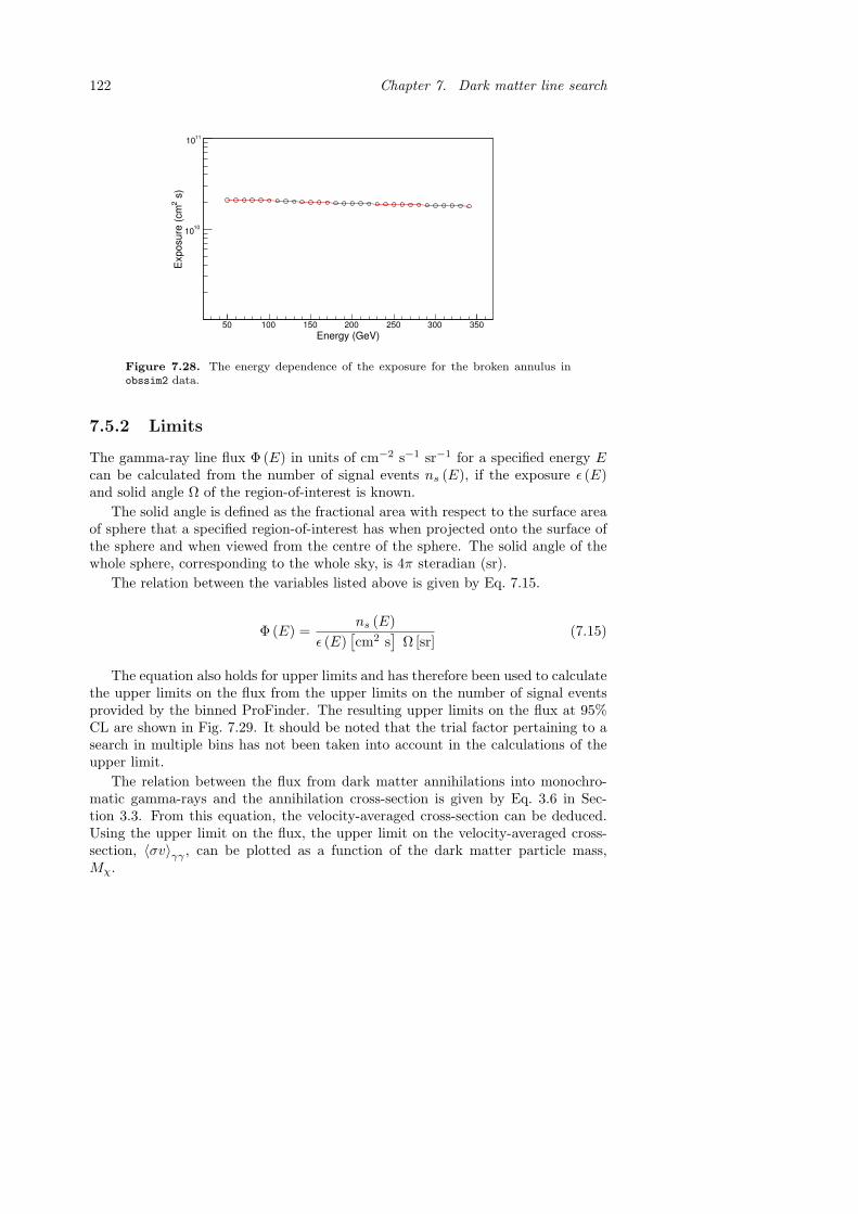
122 Chapter 7. Dark matter line search
Energy (GeV)50 100 150 200 250 300 350
s)
2E
xp
osu
re (
cm
1010
1110
Figure 7.28. The energy dependence of the exposure for the broken annulus inobssim2 data.
7.5.2 Limits
The gamma-ray line flux Φ (E) in units of cm−2 s−1 sr−1 for a specified energy Ecan be calculated from the number of signal events ns (E), if the exposure ǫ (E)and solid angle Ω of the region-of-interest is known.
The solid angle is defined as the fractional area with respect to the surface areaof sphere that a specified region-of-interest has when projected onto the surface ofthe sphere and when viewed from the centre of the sphere. The solid angle of thewhole sphere, corresponding to the whole sky, is 4π steradian (sr).
The relation between the variables listed above is given by Eq. 7.15.
Φ (E) =ns (E)
ǫ (E)[cm2 s
]Ω [sr]
(7.15)
The equation also holds for upper limits and has therefore been used to calculatethe upper limits on the flux from the upper limits on the number of signal eventsprovided by the binned ProFinder. The resulting upper limits on the flux at 95%CL are shown in Fig. 7.29. It should be noted that the trial factor pertaining to asearch in multiple bins has not been taken into account in the calculations of theupper limit.
The relation between the flux from dark matter annihilations into monochro-matic gamma-rays and the annihilation cross-section is given by Eq. 3.6 in Sec-tion 3.3. From this equation, the velocity-averaged cross-section can be deduced.Using the upper limit on the flux, the upper limit on the velocity-averaged cross-section, 〈σv〉γγ , can be plotted as a function of the dark matter particle mass,Mχ.
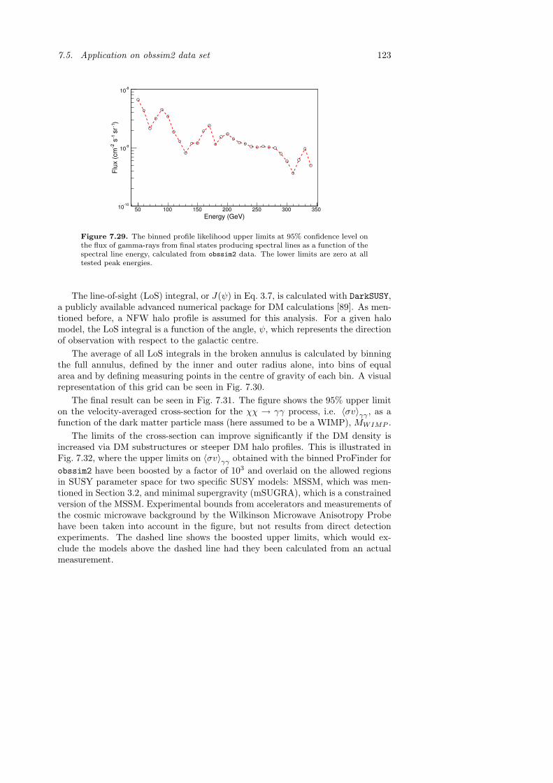
7.5. Application on obssim2 data set 123
Energy (GeV)50 100 150 200 250 300 350
)-1
sr
-1 s
-2F
lux (
cm
-1010
-910
-810
Figure 7.29. The binned profile likelihood upper limits at 95% confidence level onthe flux of gamma-rays from final states producing spectral lines as a function of thespectral line energy, calculated from obssim2 data. The lower limits are zero at alltested peak energies.
The line-of-sight (LoS) integral, or J(ψ) in Eq. 3.7, is calculated with DarkSUSY,a publicly available advanced numerical package for DM calculations [89]. As men-tioned before, a NFW halo profile is assumed for this analysis. For a given halomodel, the LoS integral is a function of the angle, ψ, which represents the directionof observation with respect to the galactic centre.
The average of all LoS integrals in the broken annulus is calculated by binningthe full annulus, defined by the inner and outer radius alone, into bins of equalarea and by defining measuring points in the centre of gravity of each bin. A visualrepresentation of this grid can be seen in Fig. 7.30.
The final result can be seen in Fig. 7.31. The figure shows the 95% upper limiton the velocity-averaged cross-section for the χχ → γγ process, i.e. 〈σv〉γγ , as afunction of the dark matter particle mass (here assumed to be a WIMP), MWIMP .
The limits of the cross-section can improve significantly if the DM density isincreased via DM substructures or steeper DM halo profiles. This is illustrated inFig. 7.32, where the upper limits on 〈σv〉γγ obtained with the binned ProFinder for
obssim2 have been boosted by a factor of 103 and overlaid on the allowed regionsin SUSY parameter space for two specific SUSY models: MSSM, which was men-tioned in Section 3.2, and minimal supergravity (mSUGRA), which is a constrainedversion of the MSSM. Experimental bounds from accelerators and measurements ofthe cosmic microwave background by the Wilkinson Microwave Anisotropy Probehave been taken into account in the figure, but not results from direct detectionexperiments. The dashed line shows the boosted upper limits, which would ex-clude the models above the dashed line had they been calculated from an actualmeasurement.

124 Chapter 7. Dark matter line search
L (deg)-40 -30 -20 -10 0 10 20 30 40
B (
deg)
-40
-30
-20
-10
0
10
20
30
40
3
4
5
6
7
8
9
Figure 7.30. A visual representation of the grid containing line-of-sight integralsfor the broken annulus region in galactic coordinates.
(GeV)WIMPM50 100 150 200 250 300
)-1
s3
(cm
γ γ
v>
σ<
-2710
-2610
-2510
Figure 7.31. The profile likelihood upper limits at 95% confidence level on thevelocity-averaged cross-section for the process χχ → γγ as a function of the WIMPmass, calculated from obssim2 data.
7.6 Application on Fermi-LAT data
The results from the DM line search presented in this section have been publishedin Physical Review Letters [119]. The overall procedure is almost identical to theanalysis on the simulated obssim2 data set. A peak finding method derives limitson the number of photons coming from DM annihilations or decays and these aretranslated into limits on the flux using the exposure and solid angle of the selectedregion.

7.6. Application on Fermi-LAT data 125
Figure 7.32. The profile likelihood upper limits at 95% confidence level fromFig. 7.31, boosted by a factor of 103 (dashed line). The shaded areas represent theallowed parameter space for two specific SUSY models, MSSM and mSUGRA.
The analysis on simulated data was mainly used as a test of the procedureitself and therefore limits were only calculated on the cross-section for a γγ finalstate. For Fermi -LAT data, limits are calculated also for the γZ final state and onboth cross-sections and decay lifetimes. In addition, the data and analysis methodselections are different as well as the procedure for calculating limits on the cross-sections. Also, as described in Section 7.1.1, the region-of-interest in this analysiscovers a larger portion of the sky, while keeping the theoretically interesting galacticcentre region.
The spatial distribution in galactic coordinates of all photons in the specifiedregion-of-interest with energies 20–300 GeV in almost one year of Fermi -LAT datais shown in Fig. 7.33.
As can be seen in the figure, there is elevated activity in the galactic centreregion, as expected due to the strong galactic diffuse emission and the large numberof strong gamma-ray sources there.
The unbinned ProFinder, described in Section 7.4.2, is then used to calculatelimits on the number of photons from DM annihilations and decays into final statesthat produce spectral lines. SS is no longer considered for the analysis on Fermi -LAT data, mainly due to the time-consuming creation of null distributions andbecause multiple lines may exist in the data from different final states but SS isonly able to find the largest one.
In Fig. 7.34, a binned representation of the unbinned fit with the unbinned

126 Chapter 7. Dark matter line search
L (deg)
150 100 50 0 50 100 150
B (
de
g)
80
60
40
20
0
20
40
60
80
0
10
20
30
40
50
60
70
Figure 7.33. The spatial distribution in galactic coordinates of photons with ener-gies 20–300 GeV in almost one year of Fermi-LAT data.
ProFinder at 40 GeV is shown. The fit is also the most significant in the analysedenergy range.
A concern one might have is whether the fit is a good fit to the data or not.The likelihood can not be used to assess the goodness-of-fit, per se. However, oneway to assess it is to construct a binned representation of the unbinned fit result(as in Fig 7.34 above) and study the residuals as well as the χ2/NDF value. InTable 7.3, a summary of some of the quantities related to the fit is shown. Itincludes the number of events in the sliding window, the χ2/NDF values for thebinned representations of the unbinned fits using 20 bins, the maximum likelihoodestimate and its lower and upper limit for each spectral line energy.
As can be seen in the table, there are no major deviations from the optimal valueof 1 in the column for χ2/NDF. However, many of the values are lower than 1, whichmay indicate that the errors are overestimated. A visual inspection of the residualscan still serve as a sanity check, where large overall deviations from a uniformresidual distribution are sought. Such behaviour was, however, not observed at anyof the tested peak energies. In Fig. 7.35, an example of a residual plot deducedfrom Fig. 7.34 is shown. As can be seen, the residuals are fluctuating around zero,which together with the χ2/NDF value of 0.68 indicates a good fit.
The resulting limits at 95% CL on the number of signal events as a functionof the peak energy, calculated by multiplying the limits on the signal fraction withthe number of photons in the specified energy window, are shown in Fig. 7.36. Alllower limits were zero, so only the upper limits are shown. This also means thatthere was no detection even at 95% CL.

7.6. Application on Fermi-LAT data 127
Table 7.3. The fit results from the unbinned ProFinder applied to Fermi-LATdata. The number of events in the window, the χ2/NDF for a binned representationof the unbinned fit using 20 bins, and for the signal fraction, f , the maximum likeli-hood estimate and its lower and upper limits, are shown for each spectral line energy.
Energy (GeV) Events χ2/NDF fMLE fLL fUL
30 6514 1.01 0.0020 0 0.0184
40 4466 0.68 0.0140 0 0.0347
50 3304 0.95 0.0005 0 0.0243
60 2625 0.76 0.0126 0 0.0396
70 2121 0.81 6.4429 ×10⁻¹⁰ 0 0.0189
80 1732 1.19 2.6249 ×10⁻⁸ 0 0.0166
90 1466 0.82 0.0216 0 0.0585
100 1251 1.13 7.1475 ×10⁻⁶ 0 0.0370
110 1212 0.93 1.1598 ×10⁻⁸ 0 0.0229
120 1181 1.16 1.7205 ×10⁻⁸ 0 0.0303
130 1125 1.05 0.0125 0 0.0506
140 1059 0.93 0.0144 0 0.0536
150 983 0.93 0.0110 0 0.0503
160 915 1.12 2.4399 ×10⁻⁶ 0 0.0367
170 857 1.35 8.8512 ×10⁻⁹ 0 0.0220
180 792 0.92 1.9848 ×10⁻¹⁰ 0 0.0327
190 718 0.74 1.4184 ×10⁻⁸ 0 0.0383
200 669 1.08 1.0842 ×10⁻⁶ 0 0.0378

128 Chapter 7. Dark matter line search
Energy (GeV)
30 35 40 45 50
Co
un
ts /
(1
.4 G
eV
)
0
100
200
300
400
500
600
Energy (GeV)
30 35 40 45 50
Co
un
ts /
(1
.4 G
eV
)
0
100
200
300
400
500
600
Signal fraction
0 0.005 0.01 0.015 0.02 0.025 0.03 0.035
ln
(lik
elih
oo
d)
0
0.2
0.4
0.6
0.8
1
1.2
1.4
1.6
1.8
2
Signal fraction
0 0.005 0.01 0.015 0.02 0.025 0.03 0.035
ln
(lik
elih
oo
d)
0
0.2
0.4
0.6
0.8
1
1.2
1.4
1.6
1.8
2
Figure 7.34. A binned representation of the unbinned maximum likelihood fit(top) and the resulting likelihood function (bottom) at an assumed line position of40 GeV. In the bottom plot, the two cases where the nuisance parameter has a fixedvalue at the maximum-likelihood estimate (blue line) and values that maximise thelikelihood at each signal fraction (red line) are shown.
7.6.1 Exposure
The procedure for calculating the exposure is identical to what is described inSection 7.5.1 for the simulated data set. For the region-of-interest specified for thesearch, the exposure in the energy range 100–110 GeV is shown in Fig. 7.37.
The energy dependence of the exposure is given in Fig. 7.38. The averageexposure is about 3 × 1010 cm2 s.

7.6. Application on Fermi-LAT data 129
Energy (GeV)
30 35 40 45 50
(da
tam
od
el) /
mo
de
l (%
)
100
80
60
40
20
0
20
40
60
80
100
Figure 7.35. Residuals constructed from the binned representation in Fig. 7.34.
Energy (GeV)
20 40 60 80 100 120 140 160 180 200
sL
imits o
n n
10
210
310
Figure 7.36. The unbinned profile likelihood upper limits at 95% confidence levelon the number of gamma-rays from final states producing spectral lines as a functionof the spectral line energy, calculated from Fermi-LAT data. The lower limits arezero at all tested peak energies.
7.6.2 Limits
When the galactic centre region is included in the search, the calculation of theaverage line-of-sight integral, as was done for obssim2 data, is not precise enoughunless a large number of bins is included. The reason is the steep nature of the

130 Chapter 7. Dark matter line search
L (deg)150 100 50 0 50 100 150
B (
de
g)
80
60
40
20
0
20
40
60
80
28
29
30
31
32
33
34
35
36
37
910×
Figure 7.37. Exposure map in galactic coordinates and in the energy range 100–110GeV for the selected region-of-interest for Fermi-LAT data.
Energy (GeV)
0 50 100 150 200 250 300
s)
2E
xp
osu
re (
cm
910
1010
1110
Figure 7.38. The energy dependence of the exposure in the selected region-of-interest for Fermi-LAT data.
halo profiles close to the galactic centre. Since a larger amount of bins would alsoincrease the computational time to an unreasonable level, a different approach waschosen for the analysis on Fermi -LAT data.
In the alternative approach, a numerical integration of Eq. 3.5 in Section 3.3using MATLAB is performed for the three chosen halo profiles.
The resulting upper limits on the flux at 95% CL, calculated by using Eq. 7.15,can be seen in Fig. 7.39. These have been calculated in the same way as thecorresponding limits from the simulated data, i.e. by division with the exposures(shown in Fig. 7.38) and the solid angle, which is about 10.5 for the selected region-of-interest.
The final upper limits on the velocity-averaged cross-section, 〈σv〉γX , and the

7.6. Application on Fermi-LAT data 131
Energy (GeV)
20 40 60 80 100 120 140 160 180 200
)1
sr
1 s
2F
lux lim
its (
cm
1110
1010
910
Figure 7.39. The unbinned profile likelihood upper limits at 95% confidence levelon the flux of gamma-rays from final states producing spectral lines as a function ofthe spectral line energy, calculated from Fermi-LAT data. The lower limits are zeroat all tested peak energies.
final lower limits on the decay lifetime, τγX , for the two cases X = γ and X = Zat 95% CL are shown in Fig. 7.40 and Fig. 7.41, respectively. These have beencalculated using Eq. 3.4 and Eq. 3.5.
As can be observed when comparing the exposures for the simulated obssim2
data and for the measured Fermi -LAT data, the exposure of the latter is abouta factor of 1.5 larger than the former. The cause of this discrepancy has notbeen investigated. That a discrepancy exists is, however, not unreasonable since anumber of different factors are differing in the two cases and can be expected tocontribute significantly to the value of the exposure. For example, the two datasets are using different versions of the background rejection, the obssim2 datausing Pass4V2 and the Fermi -LAT data using Pass6V3. This has an effect on theresponse and effective area of the detector.
An approximate comparison between the calculated upper limit on the fluxfrom obssim2 data and Fermi -LAT data can be done if the exposure is correctedto be the same as in Fermi -LAT data and if the difference in solid angle of thetwo regions-of-interest and the different ways of calculating it (the method chosenfor Fermi -LAT data being more accurate) are taken into account. However, such acomparison would not make much sense, since the obssim2 data was never meantto be realistic but rather a testing platform for the plethora of science analyseswithin the Fermi -LAT Collaboration (as was already mentioned in Section 7.5).
As a final cross-check, the upper limit on the flux from Fermi -LAT data usingthe unbinned ProFinder is compared with the upper limit on the flux as calculatedby the, in many ways less accurate, binned ProFinder. In the binned case, the

132 Chapter 7. Dark matter line search
Energy (GeV)
20 40 60 80 100 120 140 160 180 200
)1
s3
(cm
Xγ
v>
σ<
2810
2710
2610
2510
NFW
Einasto
Isothermalγγ
Zγ
Figure 7.40. The unbinned profile likelihood upper limits at 95% confidence levelon the velocity-averaged cross-section as a function of the spectral line energy forthree halo profiles. Solid lines correspond to the χχ → γγ channel and dashed linesrepresent the χχ → γZ channel.
Energy (GeV)
20 40 60 80 100 120 140 160 180 200
(s)
Xγτ
2810
2910
3010
NFW
Einasto
Isothermalγγ
Zγ
Figure 7.41. The unbinned profile likelihood lower limits at 95% confidence level onthe decay lifetime as a function of the spectral line energy for three halo profiles. Solidlines correspond to the χχ → γγ channel and dashed lines represent the χχ → γZchannel.
signal is basically assumed to be contained within one bin, which is not true inthe strict sense. Furthermore, the whole energy range is fitted by two power-lawfunctions in the binned case instead of individual power-law functions in sliding

7.7. Summary and conclusions 133
energy windows. Utilising more information should also give more accurate results(i.e. by performing the fit unbinned instead of binned and by taking into accountthe energy dispersion). The two cases are shown in Fig. 7.42. As can be seen in thefigure, the two sets of limits are still relatively consistent if the effects mentionedabove are taken into consideration.
Energy (GeV)
20 40 60 80 100 120 140 160 180 200
)-1
s-2
Flu
x lim
its (
cm
-1010
-910
-810
Figure 7.42. The upper limits at 95% confidence level on the flux as a function ofthe spectral line energy, as calculated by the binned (dashed) and unbinned (solid)ProFinder.
7.7 Summary and conclusions
In this chapter, different statistical methods have been benchmarked in terms oftheir coverage and power. The tested methods were a Bayesian method with Bayesfactors, Feldman & Cousins, profile likelihood and a non-standard χ2.
In designing a hypothesis test or a method for confidence interval calculations,the first requirement is on the probability for a false detection (i.e. how often thetrue signal parameter is not contained in the intervals). From the results, it can beseen that only the profile likelihood method has nominal coverage (nominal rate oftype-I error). It is followed by the Feldman & Cousins method, which ignores theuncertainties in the background estimate, and the Bayes factor method. The χ2
method undercovers by as much as 10%, probably since it ignores uncertainties inthe background estimate and because it should be less reliable for low statistics.
Allowing more false detections should intuitively imply larger power. The profilelikelihood has the worst power and the χ2 method has the largest power. However,one needs to keep in mind that using the χ2 method, a detection nominally on 99%confidence level only corresponds to between 90 and 96 % actual confidence level.

134 Chapter 7. Dark matter line search
Comparing power for methods which do not have the same coverage does notmake much sense. The choice of method should be a two step process. Firstly, the defacto coverage (or false detection rate) should be calculated. Secondly, the methodwith the largest power should be chosen from the ones with similar coverage. Sincea nominal false detection rate is particularly important when searching for newphysics such as dark matter, the profile likelihood method was further developedinto a spectral line search for Fermi -LAT data.
A binned profile likelihood method (referred to in this thesis as the binnedProFinder) and an additional statistical method called Scan Statistics were imple-mented for testing on a one-year full-sky simulation called obssim2, but no lineswere found at the 5σ level. As a template, upper limits at 95% confidence level onthe flux and the velocity-averaged cross-section for the γγ final state were placedwith the binned ProFinder and compared to typical allowed regions of parameterspace in MSSM and mSUGRA, where constraints provided by accelerators and theWMAP results are included. However, fairly large boost factors (of the order of103) are needed to be able to constrain the parameter space further.
That none of the two methods could detect the signal is not surprising, since theflux of dark matter implemented in the simulation was not within the Fermi -LATsensitivity and therefore a significant line signal would most likely not have beendetected by any statistical method.
Both Scan Statistics and the binned ProFinder should perform worse than meth-ods which also include information about the shape of the line. In the methodsapplied to simulated data, the bin width was defined to include most of the sim-ulated line. Any information about the line shape was therefore neglected. Thetwo methods are also expected to perform worse if the measured background cannot be easily parametrised. For Scan Statistics, this would introduce a difficulty inconstructing a set of variable bin widths that gives a uniform spectrum. For thebinned ProFinder, the difficulty would instead be to perform a good fit from whichthe background estimates can be drawn. Also, both methods are binned, whichleads to a loss of information. An unbinned method should be more accurate.
Consequently, for the analysis on almost one year of measured Fermi -LAT data,the profile likelihood method was further developed to include the informationabout the energy dispersion (i.e. the line shape), an unbinned fit to the dataand a localised background estimation through a sliding energy window. Withthe final implementation (referred to in this thesis as the unbinned ProFinder), aline detection at photon energies ranging from 30 GeV to 200 GeV (using datafrom 20 GeV to 300 GeV) could not be made. The largest “signal” was located at40 GeV, where the significance was roughly 1.4σ.
To conclude, the upper limits at 95% confidence level, shown in Fig. 7.40, arestill a factor of 10 away from the theoretically interesting MSSM and mSUGRAparameter spaces seen in Fig. 7.32. However, the limits disfavour, by a factor of2–5, one model where the wino is the lightest supersymmetric particle [80]. For theγZ final state, the model predicts 〈σv〉γZ ≈ 1.4×10⁻²⁶ cm3 s−1 for Eγ ≈ 170 GeV.

Chapter 8
Discussion and outlook
A number of factors have not been taken into account in the spectral line search.These include foremost the systematic uncertainty in the exposure and in the energydispersion, but also smaller effects such as the absolute shift in energy observed inthe beam test analysis. It is believed that the interpretation of the results will notchange significantly due to the lack of implementation of these factors. They can,however, most likely be implemented in future versions of the spectral line search.In theory, it should e.g. be possible to include the systematic uncertainty in thelikelihood model itself.
The region-of-interest chosen for the analysis on Fermi -LAT data is not nec-essarily the best place to be looking in for a spectral line from dark matter andit should be noted that it is not optimised with respect to any dark matter haloprofile.
However, any region has its advantages and disadvantages. The galactic centrehas fairly large photon statistics but is affected by source confusion and strongdiffuse photon background. Alternative locations, which may prove to give a bettersignal-to-noise ratio include dark matter satellites (substructures containing onlydark matter), dwarf spheroidal galaxies (substructures with optical counterpartsbut with high mass-to-light ratios) and galaxy clusters at high galactic latitudes,where the photon background is lower and the source identification is better. Theextragalactic background may also prove to be a better location. The variousdifferent potential regions have not been studied in this thesis. However, most ofthem have dedicated dark matter searches within the Fermi -LAT Collaboration.
A region-of-interest, which is optimised for spectral line searches, should inprinciple improve the sensitivity and should therefore be considered in future im-plementations.
The search for a spectral line from dark matter could probably be improvedfurther by improving the energy resolution of the Fermi -LAT through a new en-ergy reconstruction algorithm that is better than the ones already in place. Theutilisation of such an algorithm would, by definition, decrease the smearing of the
135

136 Chapter 8. Discussion and outlook
signal over a larger energy range and would, consequently, improve the measuredsignificance of the signal. The development of a new energy reconstruction algo-rithm is beyond the scope of this thesis, but should be considered in the future inorder to maximise the chances of finding a spectral line from dark matter.
It can be argued that a slightly larger fraction of charged particles can be ac-cepted if the gain is a better energy resolution, which increases the chance of seeinga spectral line from dark matter. Another approach is therefore to modify the cur-rent selection of gamma-rays in Fermi -LAT data. This implies, more specifically, arelaxation of the cuts used in rejecting charged particles if the energy resolution isimproved. Due to time constraints, an event class specifically developed for spectrallines has not been considered for this thesis but can be considered in future work.
On a final note, an extension of the spectral line search to higher energies, toabout 1 TeV should also be considered in future work, in order to close the currentgap in dark matter searches between the Fermi -LAT and ground-based Cherenkovexperiments. Such an analysis, however, also requires more detailed studies of thehigh-energy behaviour of the energy reconstruction, since a large portion of theshower will be outside the detector, and a better understanding of the chargedparticle contamination.

Acknowledgements
My deepest gratitude goes to my supervisors, Jan Conrad at Stockholm Universityand Staffan Carius at Linnaeus University (formerly University of Kalmar) fortaking care of me and giving me the opportunity to work on such an interestingand rewarding experiment as Fermi. I would also like to thank my supervisor atthe Royal Institute of Technology, Mark Pearce, for helping me with all thingsadministrative. A special thanks goes to Jan Conrad, whose skilled guidance keptme in the master plan and on the right path. Without your help, this work wouldhave been significantly more impossible.
I gratefully acknowledge the financial support and monthly salary from LinnaeusUniversity during these four years and the Swedish National Space Board, whichpartially funded this work.
I extend my gratitude also to all my friends and colleagues at the Royal Instituteof Stockholm and Stockholm University, who made all of this more enjoyable andworth the blood, sweat and tears. A special thanks goes to Alexander Sellerholm,Cecilia Marini Bettolo, Erik Lundstrom, Karl-Johan Grahn, Mozsi Kiss and OscarLarsson for the many useful scientific and technical discussions over the years.
Many thanks also to everyone in the Fermi -LAT Collaboration for your valuableinsights, your help, your patience and your friendly company. I have truly enjoyedworking and spending time with you. I am also grateful to Johan Bregeon, PhilippeBruel and Joakim Edsjo for providing me with a few of the figures in this thesis. Ialso want to thank Elaine Beidatsch at SLAC Human Resources, for reminding meevery once in a while of the importance of finishing my Ph.D.
My gratitude also goes to sugar and caffeine for always being there for me whenI needed your support. Without you, my collection of empty energy drinks wouldnot be as large.
Thank you, uncle Tapani, for prompting my interest in astronomy so manyyears ago. Finally, I want to thank my parents and my girlfriend Aya for believingin me and for your loving and unconditional support even during times of severemental weariness and personal despondency.
137

138

List of Figures
1.1 Muon interactions with matter . . . . . . . . . . . . . . . . . . . . 71.2 Electron interactions with matter . . . . . . . . . . . . . . . . . . . 91.3 Photon interactions with matter . . . . . . . . . . . . . . . . . . . 101.4 Electromagnetic shower from gamma-ray . . . . . . . . . . . . . . . 10
2.1 Sensitivities of gamma-ray experiments . . . . . . . . . . . . . . . . 182.2 Explorer XI detector system . . . . . . . . . . . . . . . . . . . . . . 202.3 SAS II detector system . . . . . . . . . . . . . . . . . . . . . . . . . 212.4 EGRET detector system . . . . . . . . . . . . . . . . . . . . . . . . 222.5 Third EGRET Catalog . . . . . . . . . . . . . . . . . . . . . . . . . 232.6 First Fermi -LAT Catalog . . . . . . . . . . . . . . . . . . . . . . . 24
3.1 Bullet cluster . . . . . . . . . . . . . . . . . . . . . . . . . . . . . . 26
4.1 Fermi Gamma-ray Space Telescope . . . . . . . . . . . . . . . . . . 354.2 Orbit of the Fermi Gamma-ray Space Telescope . . . . . . . . . . . 364.3 Large Area Telescope . . . . . . . . . . . . . . . . . . . . . . . . . . 374.4 Gamma-ray conversion in the TKR . . . . . . . . . . . . . . . . . . 394.5 Fermi -LAT CAL . . . . . . . . . . . . . . . . . . . . . . . . . . . . 404.6 Fermi -LAT ACD . . . . . . . . . . . . . . . . . . . . . . . . . . . . 414.7 ACD tile . . . . . . . . . . . . . . . . . . . . . . . . . . . . . . . . . 414.8 ACD tile overlap . . . . . . . . . . . . . . . . . . . . . . . . . . . . 424.9 ACD backsplash . . . . . . . . . . . . . . . . . . . . . . . . . . . . 424.10 Fermi -LAT performance - Point-spread-function . . . . . . . . . . 484.11 Fermi -LAT performance - Effective area . . . . . . . . . . . . . . . 484.12 Fermi -LAT performance - Energy resolution . . . . . . . . . . . . . 484.13 GBM detectors . . . . . . . . . . . . . . . . . . . . . . . . . . . . . 50
5.1 Calibration Unit . . . . . . . . . . . . . . . . . . . . . . . . . . . . 525.2 PS experimental setup (sketch) . . . . . . . . . . . . . . . . . . . . 535.3 PS experimental setup (photo) . . . . . . . . . . . . . . . . . . . . 545.4 PS tagging energies . . . . . . . . . . . . . . . . . . . . . . . . . . . 545.5 SPS experimental setup (sketch) . . . . . . . . . . . . . . . . . . . 56
139

140 List of Figures
5.6 SPS experimental setup (photo) . . . . . . . . . . . . . . . . . . . . 56
6.1 Muon energy spectrum . . . . . . . . . . . . . . . . . . . . . . . . . 626.2 Position reconstruction for photons . . . . . . . . . . . . . . . . . . 656.3 Position reconstruction for tagged photons . . . . . . . . . . . . . . 666.4 Position reconstruction for electrons . . . . . . . . . . . . . . . . . 676.5 Calibration runs . . . . . . . . . . . . . . . . . . . . . . . . . . . . 686.6 Asymmetry curves for electrons . . . . . . . . . . . . . . . . . . . . 696.7 Asymmetry curves for muons . . . . . . . . . . . . . . . . . . . . . 696.8 Position error in CAL crystal . . . . . . . . . . . . . . . . . . . . . 706.9 Space angle distributions for photons . . . . . . . . . . . . . . . . . 716.10 Space angle distributions for tagged photons . . . . . . . . . . . . . 716.11 Space angle distributions for electrons . . . . . . . . . . . . . . . . 716.12 Energy deposition in CAL layers . . . . . . . . . . . . . . . . . . . 736.13 Longitudinal shower profile . . . . . . . . . . . . . . . . . . . . . . 756.14 Energy distributions for 5 GeV electrons . . . . . . . . . . . . . . . 766.15 Energy distributions for 10 GeV electrons . . . . . . . . . . . . . . 776.16 Energy distributions for 20 GeV electrons . . . . . . . . . . . . . . 786.17 Energy distributions for 50 GeV electrons . . . . . . . . . . . . . . 796.18 Energy distributions for 99 GeV electrons . . . . . . . . . . . . . . 806.19 Energy distributions for 196 GeV . . . . . . . . . . . . . . . . . . . 816.20 Energy distributions for 282 GeV . . . . . . . . . . . . . . . . . . . 826.21 Energy resolutions for data at 5–282 GeV . . . . . . . . . . . . . . 836.22 Energy resolutions for the simulations at 5–282 GeV . . . . . . . . 836.23 Energy resolution difference at 5–282 GeV . . . . . . . . . . . . . . 846.24 Energy peak position difference at 5–282 GeV . . . . . . . . . . . . 846.25 Comparison with different LPM-effect implementations . . . . . . . 866.26 Comparison with different amounts of additional material . . . . . 87
7.1 Regions-of-interest . . . . . . . . . . . . . . . . . . . . . . . . . . . 927.2 Extradiffuse class effective area . . . . . . . . . . . . . . . . . . . . 947.3 Likelihood method binning effect . . . . . . . . . . . . . . . . . . . 947.4 Confidence belt construction . . . . . . . . . . . . . . . . . . . . . 977.5 Coverage comparison . . . . . . . . . . . . . . . . . . . . . . . . . . 1017.6 Power comparison . . . . . . . . . . . . . . . . . . . . . . . . . . . 1027.7 Detection principle of the binned ProFinder . . . . . . . . . . . . . 1037.8 Maximum likelihood error determination . . . . . . . . . . . . . . . 1057.9 Energy dispersion at 20 GeV . . . . . . . . . . . . . . . . . . . . . 1067.10 Energy dispersion at 50 GeV . . . . . . . . . . . . . . . . . . . . . 1067.11 Energy dispersion at 100 GeV . . . . . . . . . . . . . . . . . . . . . 1077.12 Energy dispersion at 150 GeV . . . . . . . . . . . . . . . . . . . . . 1077.13 Energy dispersion at 300 GeV . . . . . . . . . . . . . . . . . . . . . 1087.14 Fitted and interpolated energy dispersions . . . . . . . . . . . . . . 1087.15 Sliding window in energy . . . . . . . . . . . . . . . . . . . . . . . 109

List of Figures 141
7.16 Coverage of unbinned ProFinder . . . . . . . . . . . . . . . . . . . 1107.17 Coverage of unbinned ProFinder, close-up . . . . . . . . . . . . . . 1117.18 Power of unbinned ProFinder . . . . . . . . . . . . . . . . . . . . . 1127.19 Trial factor . . . . . . . . . . . . . . . . . . . . . . . . . . . . . . . 1127.20 Power of Scan Statistics . . . . . . . . . . . . . . . . . . . . . . . . 1137.21 Null distribution from Scan Statistics . . . . . . . . . . . . . . . . . 1157.22 Power and success rate of Scan Statistics . . . . . . . . . . . . . . . 1167.23 Fermi -LAT performance . . . . . . . . . . . . . . . . . . . . . . . . 1177.24 Galactic centre from obssim2 data . . . . . . . . . . . . . . . . . . 1197.25 Scan Statistics histogram from obssim2 data . . . . . . . . . . . . 1207.26 Signal event limits from obssim2 data . . . . . . . . . . . . . . . . 1217.27 Exposure map for obssim2 data . . . . . . . . . . . . . . . . . . . 1217.28 Energy dependence of exposure for obssim2 data . . . . . . . . . . 1227.29 Flux limits from obssim2 data . . . . . . . . . . . . . . . . . . . . 1237.30 Line-of-sight integrals for broken annulus . . . . . . . . . . . . . . 1247.31 Cross-section limits from obssim2 data . . . . . . . . . . . . . . . . 1247.32 SUSY model exclusions from obssim2 data . . . . . . . . . . . . . 1257.33 Counts map from Fermi -LAT . . . . . . . . . . . . . . . . . . . . . 1267.34 Fit and likelihood curve for Fermi -LAT data . . . . . . . . . . . . 1287.35 Residual plot for Fermi -LAT data . . . . . . . . . . . . . . . . . . 1297.36 Signal event limits from Fermi -LAT data . . . . . . . . . . . . . . 1297.37 Exposure map for Fermi -LAT data . . . . . . . . . . . . . . . . . . 1307.38 Energy dependence of exposure in Fermi -LAT data . . . . . . . . . 1307.39 Flux limits from Fermi -LAT data . . . . . . . . . . . . . . . . . . . 1317.40 Cross-section limits from Fermi -LAT data . . . . . . . . . . . . . . 1327.41 Decay lifetime limits from Fermi -LAT data . . . . . . . . . . . . . 1327.42 Comparison between binned and unbinned ProFinder . . . . . . . 133

142

List of Tables
4.1 Fermi -LAT and EGRET performances . . . . . . . . . . . . . . . . 49
5.1 PS configurations . . . . . . . . . . . . . . . . . . . . . . . . . . . . 555.2 SPS configurations . . . . . . . . . . . . . . . . . . . . . . . . . . . 57
6.1 The 68% containment of position reconstruction . . . . . . . . . . 646.2 Differences in position reconstruction between data and simulation 646.3 The 68% containment of direction reconstruction . . . . . . . . . . 72
7.1 Scan Statistics performance . . . . . . . . . . . . . . . . . . . . . . 1157.2 Dark matter components in obssim2 . . . . . . . . . . . . . . . . . 1187.3 Fit results for Fermi -LAT data . . . . . . . . . . . . . . . . . . . . 127
143

144

Bibliography
[1] W.-M. Yao, et al., Journal of Physics G, 33 (2006) 1.
[2] J. Lindhard & M. Scharff, Physical Review, 124 (1961) 128.
[3] H.H. Andersen & J.F. Ziegler, “Hydrogen: Stopping Powers and Ranges in AllElements”, Vol. 3 of “The Stopping and Ranges of Ions in Matter”, PergamonPress (1977).
[4] H. Bichsel, Physical Review A, 41 (1990) 3642.
[5] F. Schmidt, University of Leeds, UK. “CORSIKA Shower Images”.http://www.ast.leeds.ac.uk/∼fs/showerimages.html. Visited 6 May,2010.
[6] K.S. Cheng & G.E. Romero, “Cosmic Gamma-Ray Sources”, Kluwer AcademicPublishers (2004).
[7] T. Bringmann, L. Bergstrom & J. Edsjo, Journal of High Energy Physics, 01(2008) 049.
[8] I. Moskalenko, et al., The Astrophysical Journal, 681 (2008) 1708.
[9] N. Giglietto (Fermi -LAT Collaboration), “2009 Fermi Symposium”, eConfProceedings C091122, [arXiv:astro-ph/0912.3734].
[10] D. Petry, AIP Conference Proceedings, 745 (2005) 709, [arXiv:astro-ph/0410487].
[11] A.A. Abdo, et al., (Fermi -LAT Collaboration), Physical Review D, 80 (2009)122004.
[12] D.J. Thompson, et al., Journal of Geophysical Research, 102 (1997) 14735.
[13] E. Orlando & A.W. Strong, Astronomy & Astrophysics, 480 (2008) 847.
[14] E. Orlando & N. Giglietto, (Fermi -LAT Collaboration), “2009 Fermi Sympo-sium”, eConf Proceedings C091122, [arXiv:atro-ph/0912.3775].
145

146 Bibliography
[15] A.A. Abdo, et al., (Fermi -LAT Collaboration), Physical Review Letters, 103(2009) 251101.
[16] A.A. Abdo, et al., (Fermi -LAT Collaboration), The Astrophysical Journal Sup-plement Series, 187 (2010) 460.
[17] E. Fermi, Physical Review, 75 (1949) 1169.
[18] L. Drury, Space Science Reviews, 36 (1983) 57.
[19] T.K. Gaisser, R.J. Protheroe & T. Stanev, The Astrophysical Journal, 492(1998) 219.
[20] A.A. Abdo, et al.,(Fermi -LAT Collaboration), The Astrophysical Journal, 712(2010) 459.
[21] A.A. Abdo, et al.,(Fermi -LAT Collaboration), Science, 326 (2009) 1512.
[22] A.A. Abdo, et al.,(Fermi -LAT Collaboration), The Astrophysical Journal, 715(2010) 429.
[23] A.A. Abdo, et al., (Fermi -LAT Collaboration), Physical Review Letters, 104(2010) 101101.
[24] H.E.S.S. Collaboration. http://www.mpi-hd.mpg.de/hfm/HESS/. Visited 6May, 2010.
[25] MAGIC Collaboration. http://wwwmagic.mppmu.mpg.de/. Visited 6 May,2010.
[26] VERITAS Collaboration. http://veritas.sao.arizona.edu/. Visited 6May, 2010.
[27] CANGAROO Collaboration. http://icrhp9.icrr.u-tokyo.ac.jp/. Visited6 May, 2010.
[28] J. Hinton, New Journal of Physics, 11 (2009) 055005.
[29] HAWK Collaboration. http://hawc.umd.edu/. Visited 6 May, 2010.
[30] Milagro Collaboration. http://umdgrb.umd.edu/cosmic/milagro.html. Vis-ited 6 May, 2010.
[31] P. Villard, Comptes rendus, 130 (1900), 1010.
[32] L. Gerward, Physics in Perspective, 1 (1999) 367.
[33] E. Rutherford & E.N. da C. Andrade, Philosophical Magazine Series 6, 27(1914) 854.

Bibliography 147
[34] E. Rutherford & E.N. da C. Andrade, Philosophical Magazine Series 6, 28(1914) 263.
[35] R.A. Millikan & G.H. Cameron, Physical Review, 37 (1931) 235.
[36] E. Feenberg & H. Primakoff, Physical Review, 73 (1948) 449.
[37] S. Hayakawa, Progress of Theoretical Physics, 8 (1952) 571.
[38] G.W. Hutchinson, Philosophical Magazine Series 7, 43 (1952) 847.
[39] P. Morrison, Il Nuovo Cimento, 7 (1958) 858.
[40] W.L. Kraushaar & G.W. Clark, Physical Review Letters, 8 (1962) 3.
[41] OSO III experiment. http://heasarc.gsfc.nasa.gov/docs/heasarc//missions/oso3.html. Visited 6 May, 2010.
[42] G.W. Clark, G.P. Garmire & W.L. Kraushaar, The Astrophysical Journal, 153(1968) 203.
[43] R.W. Klebsedal, I.B. Strong & R.A. Olson, The Astrophysical Journal, 182(1973) 85.
[44] Vela experiment. http://heasarc.gsfc.nasa.gov/docs/vela5b//vela5b about.html. Visited 6 May, 2010.
[45] C.E. Fichtel, et al., The Astrophysical Journal, 198 (1975) 163.
[46] G.F. Bignami, et al., Space Science Instrumentation, 1 (1975) 245.
[47] W. Hermsen, Philosophical Transactions of the Royal Society of London A,301 (1981) 519.
[48] V. Schonfelder, et al., The Astrophysical Journal, 86 (1993) 657.
[49] V. Schonfelder, et al., Astronomy & Astrophysics Supplement Series, 143(2000) 145.
[50] G. Kanbach, et al., Space Science Reviews, 49 (1988) 69.
[51] R.C. Hartman, et al., The Astrophysical Journal Supplement Series, 123 (1999)79.
[52] M. Tavani, et al., Nuclear Instruments and Methods in Physics Research A,588 (2008) 52.
[53] C. Pittori, et al., Astronomy & Astrophysics, 506 (2009) 1563.
[54] A.A. Abdo, et al., (Fermi -LAT Collaboration), [arXiv:astro-ph/1002.2280](2010).

148 Bibliography
[55] L. Bergstrom, Reports on Progress in Physics, 63 (2000) 793.
[56] G. Bertone, D. Hooper & J. Silk, Physics Reports, 405 (2005) 279.
[57] F. Zwicky, Helvetica Physica Acta, 6 (1933) 110.
[58] S. van den Bergh, Publications of the Astronomical Society of the Pacific, 111(1999) 657.
[59] S. Sarkar, Reports on Progress in Physics, 59 (1996) 1493.
[60] J.A. Tyson, G.P. Kochanski & I.P. Dell’Antonio, The Astrophysical Journal,498 (1998) L107.
[61] D.N. Spergel, et al., The Astrophysical Journal Supplement Series, 170 (2007)377.
[62] D. Clowe, et al., The Astrophysical Journal, 648 (2006) L109.
[63] P. Ullio, et al., Physical Review D, 66 (2002) 12.
[64] J.J. Binney & N.W. Evans, Monthly Notices of the Royal Astronomical Society,327 (2001) L27.
[65] A. Burkert, The Astrophysical Journal, 447 (1995) L25
[66] F.C. van den Bosch, et al., The Astronomical Journal, 119 (2000) 1579.
[67] A. Klypin, A.V. Kravtsov & O. Valenzuela, The Astrophysical Journal, 522(1999) 82.
[68] J.P. Ostriker, et al., Science, 300 (2003) 1909.
[69] M. Milgrom, The Astrophysical Journal, 270 (1983) 365.
[70] J.D. Bekenstein, Physical Review D, 70 (2004) 083509.
[71] G. Jungman, M. Kamionkowski & K. Griest, Physics Reports, 267 (1996) 195.
[72] M. Taoso, G. Bertone & A. Masiero, Journal of Cosmology and AstroparticlePhysics, 03 (2008) 022.
[73] J.R. Primack, SLAC Beam Line, 31N3 (2001) 50, [astro-ph/0112336].
[74] F. Wilczek, Physical Review Letters, 40 (1978) 279.
[75] S. Weinberg, Physical Review Letters, 40 (1978) 223.
[76] R.D. Peccei & H.R. Quinn, Physical Review Letters, 38 (1977) 1440.
[77] G. Servant & T.M.P. Tait, Nuclear Physics B, 650 (2003) 391.

Bibliography 149
[78] L. Bergstrom & P. Ullio, Nuclear Physics B, 504 (1997) 27.
[79] L. Bergstrom, New Journal of Physics, 11 (2009) 105006.
[80] G. Kane, R. Lu, & S. Watson, Physics Letters B, 681 (2009) 151.
[81] M. Gustafsson, et al., Physical Review Letters, 99 (2007) 041301.
[82] G. Bertone, et al, Physical Review D, 80 (2009) 023512.
[83] L. Bergstrom, et al., Journal of Cosmology and Astroparticle Physics, 04 (2005)004.
[84] Y. Mambrini, Journal of Cosmology and Astroparticle Physics, 12 (2009) 005.
[85] A. Ibarra & D. Tran, Physical Review Letters, 100 (2008) 061301.
[86] C. Arina, et al., Journal of Cosmology and Astroparticle Physics, 03 (2010)024.
[87] C.B. Jackson, et al., [arXiv:hep-ph/0912.0004] (2009).
[88] M. Lattanzi & J. Silk, Physical Review D, 79 (2009) 083523.
[89] P. Gondolo, et al., Journal of Cosmology and Astroparticle Physics, 07 (2004)008.
[90] R. Catena & P. Ullio, [arXiv:astro-ph/0907.0018] (2009).
[91] J.F. Navarro, C.S. Frenk & S.D. White, The Astrophysical Journal, 490 (1997)493.
[92] J.N. Bahcall & R.M. Soneira, The Astrophysical Journal Supplement Series,44 (1980) 73.
[93] B. Moore, et al., Monthly Notices of the Royal Astronomical Society, 310 (1999)1147.
[94] A.V. Kravtsov, The Astrophysical Journal, 502 (1998) 48.
[95] J. Einasto, Trudy Instituta Astrofiziki Alma-Ata, 5 (1965) 87.
[96] D. Merritt, et al., The Astronomical Journal, 132 (2006) 2685.
[97] DAMA/LIBRA Collaboration. http://people.roma2.infn.it/ dama/web/.Visited 6 May, 2010.
[98] CDMS Collaboration. http://cdms.berkeley.edu/. Visited 6 May, 2010.
[99] IceCube Collaboration. http://icecube.wisc.edu/. Visited 6 May, 2010.

150 Bibliography
[100] D. Hubert (IceCube Collaboration), Nuclear Physics B (Proceedings Supple-ments), 173 (2007) 87.
[101] F. Halzen & D. Hooper, New Journal of Physics, 11 (2009) 105019.
[102] ANTARES Collaboration. http://antares.in2p3.fr/. Visited 6 May, 2010.
[103] J.D. Zornoza (ANTARES Collaboration), Nuclear Physics B (ProceedingsSupplements), 173 (2007) 79.
[104] PAMELA Collaboration. http://pamela.roma2.infn.it/. Visited 6 May,2010.
[105] R. Bernabei, et al., The European Physical Journal C, 56 (2008) 333.
[106] Z. Ahmed, et al., [arXiv:astro-ph/0912.3592].
[107] O. Adriani, et al., Nature, 458 (2009) 607.
[108] M. Boezio, et al., New Journal of Physics, 11 (2009) 105023.
[109] L. Bergstrom, T. Bringmann & J. Edsjo, Physical Review D, 78 (2008) 103520.
[110] J. Chang, et al., Nature, 456 (2008) 362.
[111] A.A. Abdo, et al., (Fermi -LAT Collaboration), Physical Review Letters, 102(2009) 181101.
[112] D. Grasso, et al., Astroparticle Physics, 32 (2009) 140.
[113] P. Blasi, Physical Review Letters, 103 (2009) 051104.
[114] R. Battiston, et al., Nuclear Instruments and Methods in Physics ResearchA, 588 (2008) 227.
[115] A.A. Abdo, et al., (Fermi -LAT Collaboration), [arXiv:astro-ph/1002.2239](2010).
[116] A.A. Abdo, et al., (Fermi -LAT Collaboration), Astrophysical Journal, 712(2010) 147.
[117] P. Scott, et al., Journal of Cosmology and Astroparticle Physics, 01 (2010)031.
[118] A.A. Abdo, et al., (Fermi -LAT Collaboration), Journal of Cosmology andAstroparticle Physics, 04 (2010) 014.
[119] A.A. Abdo, et al., (Fermi -LAT Collaboration), Physical Review Letters, 104(2010) 091302.
[120] W.B. Atwood, et al., Astroparticle Physics, 28 (2007) 422.

Bibliography 151
[121] S. Bergenius, Licenciate Thesis, Royal Institute of Technology, Stockholm,Sweden, ISBN: 91-7283-754-3 (2004)
[122] A.A. Moiseev, et al., Astroparticle Physics, 27 (2007) 339.
[123] R.E. Kalman, Journal of Basic Engineering D, 82 (1960) 35.
[124] J.A. Hernando, SCIPP preprint 98/18 (1998).
[125] A.A. Abdo, et al., (Fermi -LAT Collaboration), Astroparticle Physics, 32(2009) 193.
[126] Summary of N-tuples. http://glast-ground.slac.stanford.edu//workbook/pages/gleamOvrvw/summaryNtuples.htm. Visited 6 May, 2010.
[127] Fermi -LAT performance (Pass6). http://www-glast.slac.stanford.edu//software/IS/glast lat performance.htm. Visited 6 May, 2010.
[128] C. Meegan, et al., [arXiv:astro-ph/0908.0450] (2009).
[129] Geant4 software. http://www.geant4.org. Visited 6 May, 2010.
[130] S. Agostinelli, et al., Nuclear Instruments and Methods in Physics ResearchA, 506 (2003) 250.
[131] L. Baldini, et al., AIP Conference Proceedings, 921 (2007) 190.
[132] EGS5 software. http://rcwww.kek.jp/research/egs/egs5.html. Visited 6May, 2010.
[133] Mars15 software. http://www-ap.fnal.gov/MARS/. Visited 6 May, 2010.
[134] F. Stoehr, et al., Monthly Notices of the Royal Astronomical Society, 345(2003) 1313.
[135] P.D. Serpico & G. Zaharijas, Astroparticle Physics, 29 (2008) 380.
[136] A.N. Kolmogorov, “Grundbegriffe der Wahrscheinlichkeitsrechnung”, JuliusSpringer, Berlin (1933).
[137] A.N. Kolmogorov, “Foundations of the Theory of Probability”, Chelsea Pub-lishing Company, New York (1956).
[138] F. James, “Statistical Methods in Experimental Physics (2nd Edition)”,World Scientific Publishing Co. Pte. Ltd. (2006).
[139] J. Neyman, Philosophical Transactions of the Royal Society of London A, 236(1937) 333.
[140] R. D. Cousins & G. J. Feldman, Physical Review D, 57 (1998) 3873.

152 Bibliography
[141] W.A. Rolke, A.M. Lopez & J. Conrad, Nuclear Instruments and Methods inPhysics Research A, 551 (2005) 493.
[142] G. Cowan, “Statistical Data Analysis”, Oxford University Press Inc., NewYork (1998).
[143] J. Conrad, J. Scargle & T. Ylinen, AIP Conference Proceedings, 921 (2007)586.
[144] J. Conrad, invited contribution to “Workshop on Exotic Physics with Neu-trino Telescope”, Uppsala, Sweden, Sept. 2006, [arXiv:astro-ph/0612082].
[145] ROOT software. http://root.cern.ch/. Visited 6 May, 2010.
[146] W. Verkerke & D. Kirkby, talk from the “2003 Computing in High En-ergy and Nuclear Physics” (CHEP03), La Jolla, Ca, USA, March 2003,[arXiv:physics/0306116].
[147] F. James, “MINUIT Function Minimization and Error Analysis”, CERNProgram Library Long Writeup D506, (1994).
[148] F. Terranova, Nuclear Instruments and Methods in Physics Research A, 519(2004) 659.
[149] Science Tools software. http://glast-ground.slac.stanford.edu//Workbook/sciTools Home.htm. Visited 6 May, 2010.
[150] FTOOLS software. http://heasarc.nasa.gov/lheasoft/ftools//ftools menu.html. Visited 6 May, 2010.
[151] Fermi -LAT performance (Pass4). http://www-glast.slac.stanford.edu//software/IS/archive latPerformance pass4v2.html. Visited 6 May,2010.
[152] E.A. Baltz, et al., Physical Review D, 74 (2006) 103521.
[153] E.A. Baltz, et al., Journal of Cosmology and Astroparticle Physics, 07 (2008)013.