search for - inspire-hepinspirehep.net/record/1393582/files/3100s.pdf · i claim the credit for the...
TRANSCRIPT

SEARCH FOR
)1530(0
)1530(0))2(,/( SJ
AZMAT IQBAL
Centre for High Energy Physics
University of the Punjab
Lahore-54590, Pakistan
(August, 2012)

SEARCH FOR
)1530(0
)1530(0)) 2(,/( SJ
by
AZMAT IQBAL
Submitted in Partial Fulfillment of the Requirements for the
Degree of DOCTOR OF PHILOSOPHY
at
Centre for High Energy Physics
University of the Punjab
Lahore-54590, Pakistan
(August, 2012)

DEDICATED
TO
MY PARENTS, SISTERS AND BROTHERS
ii

CERTIFICATE
It is certified that I have read this dissertation and that, in my opinion, it is fully
adequate in scope and quality for the degree of Doctor of Philosophy.
Prof. Shan Jin Prof. Dr. Haris Rashid
(Supervisor) (Supervisor)
Submitted Through:
Prof. Dr. Haris Rashid
(Supervisor and Director)
iii

DECLARATION
This work represents the efforts of the members of BES Group at the Centre for High
Energy Physics University of the Punjab, Pakistan. I claim the credit for the analysis and
final results presented in this thesis which are entirely my own.
This thesis which is being submitted for the award of degree of Ph.D. in the university
of the Punjab does not contain material which has been submitted for the award of any
other degree or diploma in any university. To the best of my knowledge and belief, it
does not contain any material published or written by another person, except with due
references. If any reference is found missing that would completely be unintentional and
I do not pretend to own the credit for that.
Azmat Iqbal
iv

Acknowledgment
All praise and glory to be Allah Mighty who gave me strength and courage to finish this
project. My humblest and sincerest tribute to the Holy Prophet (Peace and Blessings
be Upon Him) Who is a permanent source of guidance for the humanity. I offer sincere
thanks to my supervisors; Prof. Dr. Haris Rashid and Prof. Dr. Shan Jin. I warmly
express my gratitude to Prof. Dr. Haris Rashid for his valuable suggestions and guidance
throughout the project. It is great pleasure for me to offer my thanks to him for giving
me an opportunity to work in the prestigious BESIII Collaboration. His encouraging and
facilitating role has been a great source of motivation for me in completing thesis work.
I express my sincerest gratitude to Dr. Talab Hussain and Dr. Abrar Ahmad Zafar
who played a vital role in the completion of my thesis work. Their guidance and help from
the very first day till the instant has made all this research work possible for me. Their
encouragement and motivation would always instill in me a new confidence and spirit
to move ahead on right time. I am extremely indebted to Dr. Talab Hussain for many
inspiring and enlightening discussions from which I learnt a lot. I am really grateful to
him for making me familiar with intricacies of data analysis and experimental techniques.
Working with both of them on this journey of learning and sharing ideas turned out to
be most memorable moments of my life. I am also very grateful to Dr. Qadeer Afzal for
some valuable comments and suggestions.
I am extremely thankful to all my fiends and collogues especially Mr. Ghulam Mustafa,
Dr. M. Imran Jamil, Mr. Muhammad Mushraf Ansari and Mr. Sohail Gillani for their
v

continuous encouragement and help during my research work. Working together with Mr.
Mushraf Ansari in BESIII computational environment turned out be a great experience.
I am especially thankful to him for helping me in computer related issues.
Without any exception, I am pleased to thank all teachers from whom I gained a
considerable deal of knowledge during my stay at CHEP. I am also grateful to other staff
member of CHEP for their sincere cooperation.
I also thank to Higher Education Commission (HEC) of Pakistan for the support during
my Ph.D. research work.
My urge to learn science led me to pursue a carrier in physics. I started my journey
of learning physics and nature as a lay man knowing little about both. It was my luck
that struck in a way and I got company of some great teachers right from school age to
this level. Here I also wish to thank all my teachers whose contributions and efforts will
be always a great treasure for me.
In the last but not the least, I feel immense pleasure to express deep gratitude to my
mother and father, brothers and sisters for their never falling love, care and support for
my studies. Without their untiring and sincerest efforts nothing could have been possible.
I am at loss for words to express their courage, determination and patience which will be
an everlasting source of inspiration and motivation for me. I am short of words to describe
how they sacrificed their lives, sleep and peace to put me on the noble path of knowledge.
I owe a lot to my elder brother Ali Akram (late) who played an impressive role in my
studies. May Allah Mighty rest his soul in peace and shower His countless blessings on
him.
vi

Abstract
Based upon analysis work performed using samples of 2.25 × 10⁸ J/ψ events and
1.06 × 10⁸ ψ(2S) events collected with the BESIII detector at e−e+ BEPC II collider
in 2009, we report the first measurement of the branching ratios of the decay channels:
(J/ψ, ψ(2S)) → Ξ0(1530)Ξ0(1530). The measured branching ratios are:
Br1C [J/ψ → Ξ0(1530)Ξ0(1530)] = (1.06± 0.07sys ± 0.37stat)× 10−5
Br4C [J/ψ → Ξ0(1530)Ξ0(1530)] = (2.94± 0.06sys ± 1.10stat)× 10−5.
Br1C [ψ(2S) → Ξ0(1530)Ξ0(1530)] = (1.16± 0.77sys ± 0.07stat)× 10−6
Br4C [ψ(2S) → Ξ0(1530)Ξ0(1530)] = (5.16± 1.92sys ± 0.17stat)× 10−6.
The 4C and 1C results are consistent within 2σ. The test results of the 12 % rule are:
Br1C(ψ(2S) → BB
Br1C(J/ψ) → BB≈ 11%
Br4C(ψ(2S) → BB
Br4C(J/ψ) → BB≈ 17.55%
vii

List of Figures
2.1 Fenman diagrams depicting the three fundamental interactions [15] . . . . 10
2.2 (a,b) Variation of coupling constants of QCD and QED due to screening and
antiscreening effects. (a) The strength of QED α decreases with separation
of test charge from the source. (b) The strength of QCD αs increases with
the separation of test color charge (another quark) due to the antiscreening
effect of gluon self-coupling (c)α is finite at r →∞(q2 = 0) and increases at
shorter distances due to weak screening. αs is meaningless at large distances
≥ 10−13 cm because of confinement and is small at short distances. [26] . . 18
3.1 Baryon multiplets: Baryon octet or Jp = (1/2)+ SU(3) multiplets (left).
Baryon decuplet or Jp = (3/2)+ SU(3) multiplets (right), where 1/2 stands
for spin and + for even parity and so on [3, 5]. . . . . . . . . . . . . . . . . 25
3.2 Meson Multiplets: (A) Pseudoscalar meson octet with Jp = 0−. (B) Vector
meson octet with Jp = 1− [3, 5]. . . . . . . . . . . . . . . . . . . . . . . . . 25
3.3 Quark structure of baryon octet or Jp = (1/2)+ SU(3) multiplets [25]. . . . 27
3.4 Baryon decuplet or Jp = (3/2)+ SU(3) multiplets [25]. . . . . . . . . . . . 27
3.5 SU(4) multiplets of :(a) (1/2)+ baryons (b) (3/2)+ baryons [3, 26]. . . . . . 29
3.6 SU(3) multiplets of :(a) pseudoscalar and (b) vector mesons [3, 26]. . . . . 30
3.7 SU(4) multiplets of :(a) pseudoscalar mesons (b) vector mesons [3, 26]. . . 30
4.1 Schematic diagramm for production of (J/ψ) in e+e− collision [54]. . . . . 36
viii

LIST OF FIGURES LIST OF FIGURES
4.2 Narrow resonance peak of J/ψ in e−e+ at SLAC [25, 55, 56]. . . . . . . . . 36
4.3 Narrow resonance peak of J/ψ in PP collisions at BNL respectively [25, 55, 56]. 37
4.4 Comparison between energy level diagram of positronium and charmo-
nium [46]. . . . . . . . . . . . . . . . . . . . . . . . . . . . . . . . . . . . . 38
4.5 Experimentally observed and theoretically predicted charmonium states.
The experimentally established states are shown with solid lines. The doted
lines on the left show the predicted states by a non-relativistic potential
model while the right dotted lines show the states predicted by the rela-
tivistic Godfrey Isgur potential model [8, 61]. . . . . . . . . . . . . . . . . . 38
4.6 Approximate QCD static quarkonium potential as a function of interquark
separation r [4, 33]. . . . . . . . . . . . . . . . . . . . . . . . . . . . . . . . 39
4.7 Quark diagrams for decay of φ into decay mesons. (a) OZI supressed tran-
sition (b) OZI allowed transition [4]. . . . . . . . . . . . . . . . . . . . . . 42
4.8 Quark diagrams for J/ψ decaying to mesons. (a) OZI allowed transition
(b) OZI suppressed transition [5]. . . . . . . . . . . . . . . . . . . . . . . . 43
5.1 Schematic diagram for e+e− BEPCII collider and BESIII detector [68]. . . 49
5.2 Schematic diagram of MDC [68]. . . . . . . . . . . . . . . . . . . . . . . . 51
5.3 Schematics of TOF [68]. . . . . . . . . . . . . . . . . . . . . . . . . . . . . 52
5.4 Schematic diagram for EMC [68]. . . . . . . . . . . . . . . . . . . . . . . . 53
5.5 Schematic diagram for muon chamber [68]. . . . . . . . . . . . . . . . . . . 54
6.1 MC and data invariant mass distributions of pπ− and pπ+ after kinematic
fit results . . . . . . . . . . . . . . . . . . . . . . . . . . . . . . . . . . . . 61
6.2 MC and data invariant mass distributions for Λπ− and Λπ+ after kinematic
fit results . . . . . . . . . . . . . . . . . . . . . . . . . . . . . . . . . . . . 62
6.3 MC and data invariant mass distributions for Ξ−π+ and Ξ+π− after kine-
matic fit results . . . . . . . . . . . . . . . . . . . . . . . . . . . . . . . . . 63
ix

LIST OF FIGURES LIST OF FIGURES
6.4 MC and data invariant mass distributions for pπ− and pπ+ after final event
selection criteria . . . . . . . . . . . . . . . . . . . . . . . . . . . . . . . . . 64
6.5 MC and data invariant mass distributions for Λπ− and Λπ+ after final event
selection criteria . . . . . . . . . . . . . . . . . . . . . . . . . . . . . . . . . 65
6.6 MC and data invariant mass distributions for Ξ−π+ and Ξ+π− after final
event selection criteria . . . . . . . . . . . . . . . . . . . . . . . . . . . . . 66
6.7 MC and data invariant mass distribution for pπ− and pπ+ after 1C fit results 67
6.8 MC and data invariant mass distribution for Λπ− and Λπ+ after 1C fit results 68
6.9 MC and data invariant mass distribution for Ξ−π= and Ξ+π− after 1C fit
results . . . . . . . . . . . . . . . . . . . . . . . . . . . . . . . . . . . . . . 69
6.10 MC and data invariant mass distribution for pπ− and pπ+ after 4C fit results 70
6.11 MC and data invariant mass distribution for Λπ− and Λπ+ after 4C fit results 71
6.12 MC and data invariant mass distribution for Ξ−π= and Ξ+π− after 4C fit
results . . . . . . . . . . . . . . . . . . . . . . . . . . . . . . . . . . . . . . 72
6.13 MΞ−π+ and MΞ+π− distribution . . . . . . . . . . . . . . . . . . . . . . . . 73
6.14 MΞ−π+ and MΞ+π− distribution . . . . . . . . . . . . . . . . . . . . . . . . 73
6.15 MΞ−π+ and MΞ+π− distribution . . . . . . . . . . . . . . . . . . . . . . . . 74
6.16 MΞ−π+ and MΞ+π− distribution . . . . . . . . . . . . . . . . . . . . . . . . 74
6.17 Scatter plot of MΞ−π+ VS MΞ+π− distribution after 1C and 4C fit results for
MC exclusive decay channel J/ψ → Λ0(1405)Λ0(1405), where Λ0(1405) →Σ∗+π−, Λ0(1405) → Σ∗−π+, Σ∗+ → Λπ+, Λ → π−p, Σ∗− → Λπ−, Λ → pπ+ . 75
6.18 Scatter plot of MΞ−π+ VS MΞ+π− distribution after 1C and 4C fit results for
MC exclusive decay channel J/ψ → Λ0(1405)Λ0(1405), where Λ0(1405) →Σ∗−π+, Λ0(1405) → Σ∗+π−, Σ∗− → Λπ−, Λ → π−p, Σ∗+ → Λπ+, Λ → pπ+ . 75
6.19 Scatter plot of MΞ−π+ VS MΞ+π− distribution after 1C and 4C fit results for
MC exclusive decay channel J/ψ → Ξ−Ξ+π+π−, where Ξ− → Λπ−, Λ →π−p and Ξ+ → Λπ+, Λ → π+p . . . . . . . . . . . . . . . . . . . . . . . . . 76
x

LIST OF FIGURES LIST OF FIGURES
6.20 Scatter plot of MΞ−π+ VS MΞ+π− distribution after 1C and 4C fit results for
MC exclusive decay channel J/ψ → Λ0(1520)Λ0(1520), where Λ0(1520) →Λπ+π−, Λ → pπ−, Λ0(1520) → Λπ+π−, Λ → pπ+. . . . . . . . . . . . . . . 76
6.21 Scatter plot of Ξ−π+ VS Ξ+π− after 1C and 4C fit results for the signal
decay channel J/ψ → Ξ0(1530)Ξ0(1530). . . . . . . . . . . . . . . . . . . . 77
6.22 MC and data invariant mass distribution for pπ− and pπ+ after kinematic fit 78
6.23 MC and data invariant mass distribution for Λπ− and Λπ+ after kinematic
fit . . . . . . . . . . . . . . . . . . . . . . . . . . . . . . . . . . . . . . . . 79
6.24 MC and data invariant mass distribution for Ξ−π+ and Ξ+π− after kine-
matic fit . . . . . . . . . . . . . . . . . . . . . . . . . . . . . . . . . . . . . 80
6.25 MC and data invariant mass distribution for pπ− and pπ+ after final event
selection . . . . . . . . . . . . . . . . . . . . . . . . . . . . . . . . . . . . . 80
6.26 MC and data invariant mass distribution for Λπ− and Λπ+ after final event
selection . . . . . . . . . . . . . . . . . . . . . . . . . . . . . . . . . . . . . 81
6.27 MC and data invariant mass distribution for Ξ−π+ and Ξ+π− after final
event selection . . . . . . . . . . . . . . . . . . . . . . . . . . . . . . . . . . 82
6.28 MC and data invariant mass spectra for pπ− and pπ+ after 1C fit results. . 82
6.29 MC and data invariant mass spectra for Λπ− and Λπ+ after 1C fit results. 83
6.30 MC and data invariant mass spectra for Ξ−π+ and Ξ+π− after 1C fit results. 83
6.31 MC and data invariant mass spectra for pπ− and pπ+ after 4C fit results. . 84
6.32 MC and data invariant mass spectra for Λπ− and Λπ+ after 4C fit results. 84
6.33 MC and data invariant mass spectra for Ξ−π+ and Ξ+π− after 4c fit results. 85
6.34 Invariant mass spectrum of Ξ(1530)0 and Ξ(1530)0 for MC exclusive back-
ground decay channel ψ(2S) → Λ(1520)Λ(1520) . . . . . . . . . . . . . . . 85
6.35 Invariant mass spectrum of Ξ0(1530) and Ξ0(1530) for MC exclusive back-
ground decay channel ψ(2S) → Λ0(1690)Λ0(1690) . . . . . . . . . . . . . . 86
xi

LIST OF FIGURES LIST OF FIGURES
6.36 Invariant mass spectrum of Ξ0(1530) and Ξ0(1530) for MC exclusive back-
ground decay channel ψ(2S) → Λ0(1520)Λ0(1520) where Λ0(1520) → Σ∗+π−, Λ0(1520) →Σ∗−π+, Σ∗+ → Λπ+, Λ → π−p, Σ∗− → Λπ−, Λ → pπ+ . . . . . . . . . . . . 87
6.37 Invariant mass spectrum of Ξ0(1530) and Ξ0(1530) for MC exclusive back-
ground decay channel ψ(2S) → Λ0(1520)Λ0(1520), where Λ0(1520) →Σ∗−π+, Λ0(1520) → Σ∗+π−, Σ∗− → Λπ−, Λ → π−p, Σ∗+ → Λπ+, Λ → pπ+ . 87
6.38 Invariant mass spectrum of Ξ0(1530) and Ξ0(1530) for MC exclusive back-
ground decay channel ψ(2S) → Ξ−Ξ+π+π− . . . . . . . . . . . . . . . . . 88
6.39 Scatter plot of MΞ−π+ VS MΞ+π− distribution for MC exclusive decay chan-
nel ψ(2S) → Λ0(1520)Λ0(1520), where Λ0(1520) → Λπ+π−, Λ → pπ−,
Λ0(1520) → Λπ+π−, Λ → pπ+ . . . . . . . . . . . . . . . . . . . . . . . . . 88
6.40 Scatter plot of MΞ−π+ VS MΞ+π− distribution for MC exclusive background
decay channel ψ(2S) → Λ0(1690)Λ0(1690), where Λ0(1690) → Λπ+π−, Λ →pπ−, Λ0(1690) → Λπ+π−, Λ → pπ+. . . . . . . . . . . . . . . . . . . . . . . 89
6.41 Scatter plot of MΞ−π+ VS MΞ+π− distribution for MC exclusive background
decay channel ψ(2S) → Λ0(1520)Λ0(1520), where Λ0(1520) → Σ∗+π−, Λ0(1520) →Σ∗−π+, Σ∗+ → Λπ+, Λ → π−p, Σ∗− → Λπ−, Λ → pπ+ . . . . . . . . . . . . 89
6.42 Scatter plot of MΞ−π+ VS MΞ+π− distribution for MC exclusive background
decay channel ψ(2S) → Λ0(1520)Λ0(1520), where Λ0(1520) → Σ∗−π+, Λ0(1520) →Σ∗+π−, Σ∗− → Λπ−, Λ → π−p, Σ∗+ → Λπ+, Λ → pπ+ . . . . . . . . . . . . 90
6.43 Scatter plot of MΞ−π+ VS MΞ+π− distribution for MC exclusive background
decay channel ψ(2S) → Ξ−Ξ+π+π−, where Ξ− → Λπ−, Λ → π−p and
Ξ+ → Λπ+, Λ → π+p. . . . . . . . . . . . . . . . . . . . . . . . . . . . . . . 90
6.44 Scatter plots of Ξ−π+ vs Ξ+π− after 1C and 4C fit results for the signal
channel ψ(2S) → Ξ0(1530)Ξ0(1530). . . . . . . . . . . . . . . . . . . . . . . 91
xii

List of Tables
2.1 Fundamental particles [8] . . . . . . . . . . . . . . . . . . . . . . . . . . . . 6
2.2 Fundamental forces [8] . . . . . . . . . . . . . . . . . . . . . . . . . . . . . 9
6.1 MC inclusive background decay modes for the signal channel: J/ψ →Ξ0(1530)Ξ0(1530). . . . . . . . . . . . . . . . . . . . . . . . . . . . . . . . . 65
6.2 Systematic errors from 1C fit results for the signal channel: J/ψ → Ξ0(1530)Ξ0(1530) 77
6.3 Systematic errors from 4C fit results for the signal channel:J/ψ → Ξ0(1530)Ξ0(1530) 78
6.4 MC inclusive background decay modes for the signal channel: ψ(2S) →Ξ0(1530)Ξ0(1530) . . . . . . . . . . . . . . . . . . . . . . . . . . . . . . . . 86
6.5 Systematic errors from 1C fit results for the signal channel: ψ(2S) →Ξ0(1530)Ξ0(1530) . . . . . . . . . . . . . . . . . . . . . . . . . . . . . . . . 92
6.6 Systematic results from 4C fit results for the signal channel: ψ(2S) →Ξ0(1530)Ξ0(1530) . . . . . . . . . . . . . . . . . . . . . . . . . . . . . . . . 92
xiii
Contents
1 Introduction 1
2 The Standard Model 4
2.1 Components of the Standard Model . . . . . . . . . . . . . . . . . . . . . . 4
2.1.1 Fundamental Particles . . . . . . . . . . . . . . . . . . . . . . . . . 5
2.1.2 Fundamental Interactions . . . . . . . . . . . . . . . . . . . . . . . 7
2.1.3 Range of Interactions . . . . . . . . . . . . . . . . . . . . . . . . . . 9
2.2 Quantum Field Theories . . . . . . . . . . . . . . . . . . . . . . . . . . . . 10
2.2.1 Gauge Invariance Principle . . . . . . . . . . . . . . . . . . . . . . . 11
2.3 Quantum Electrodynamics . . . . . . . . . . . . . . . . . . . . . . . . . . . 13
2.3.1 Consequences of Gauge Invariance . . . . . . . . . . . . . . . . . . . 13
2.4 Quantum Chromodynamics . . . . . . . . . . . . . . . . . . . . . . . . . . 15
2.4.1 Flavor Symmetry Breaking . . . . . . . . . . . . . . . . . . . . . . . 16
2.5 Running Coupling Constants . . . . . . . . . . . . . . . . . . . . . . . . . . 17
2.6 Effective Field Theories . . . . . . . . . . . . . . . . . . . . . . . . . . . . . 20
3 The Quark Model 21
3.1 Quantum Numbers . . . . . . . . . . . . . . . . . . . . . . . . . . . . . . . 22
3.1.1 Isospin . . . . . . . . . . . . . . . . . . . . . . . . . . . . . . . . . . 22
3.1.2 Hypercharge and Strangeness . . . . . . . . . . . . . . . . . . . . . 23
3.2 The Eightfold Way . . . . . . . . . . . . . . . . . . . . . . . . . . . . . . . 24
xiv

CONTENTS
3.3 The Quark Model of Hadrons . . . . . . . . . . . . . . . . . . . . . . . . . 26
3.3.1 Baryons Multiplets . . . . . . . . . . . . . . . . . . . . . . . . . . . 28
3.3.2 Mesons Multiplets . . . . . . . . . . . . . . . . . . . . . . . . . . . 29
4 The Charmonium Physics 31
4.1 Heavy Quarkonia . . . . . . . . . . . . . . . . . . . . . . . . . . . . . . . . 31
4.1.1 Spectral Notation . . . . . . . . . . . . . . . . . . . . . . . . . . . . 32
4.1.2 Lagrangian for cc System . . . . . . . . . . . . . . . . . . . . . . . . 33
4.2 Discovery of J/ψ and ψ(2S) Charmonia . . . . . . . . . . . . . . . . . . . 35
4.3 Charmonium Spectroscopy . . . . . . . . . . . . . . . . . . . . . . . . . . . 37
4.4 Transitions . . . . . . . . . . . . . . . . . . . . . . . . . . . . . . . . . . . . 41
4.4.1 Radiative Transitions . . . . . . . . . . . . . . . . . . . . . . . . . . 41
4.4.2 Hadron Transitions . . . . . . . . . . . . . . . . . . . . . . . . . . . 42
4.5 OZI Rule . . . . . . . . . . . . . . . . . . . . . . . . . . . . . . . . . . . . 42
4.6 ρπ Puzzle . . . . . . . . . . . . . . . . . . . . . . . . . . . . . . . . . . . . 44
5 BES-III Experiment 46
5.1 Fixed Target Accelerators Versus Colliders . . . . . . . . . . . . . . . . . . 46
5.2 Electron-Positron Colliders . . . . . . . . . . . . . . . . . . . . . . . . . . . 47
5.3 BEPCII Collider . . . . . . . . . . . . . . . . . . . . . . . . . . . . . . . . 49
5.4 BEPCII Detector . . . . . . . . . . . . . . . . . . . . . . . . . . . . . . . . 50
5.5 Physics Goals of BEPCII/BESIII . . . . . . . . . . . . . . . . . . . . . . . 55
6 Analysis Results 57
6.1 Introduction . . . . . . . . . . . . . . . . . . . . . . . . . . . . . . . . . . . 57
6.2 Data Set and Software Framework . . . . . . . . . . . . . . . . . . . . . . . 59
6.3 Analysis of J/ψ → Ξ0(1530)Ξ0(1530) . . . . . . . . . . . . . . . . . . . . . 59
6.3.1 Initial Event Selection . . . . . . . . . . . . . . . . . . . . . . . . . 59
6.3.2 Final Event Selection . . . . . . . . . . . . . . . . . . . . . . . . . 62
xv

Chapter 1. Introduction
6.3.3 Background Analysis . . . . . . . . . . . . . . . . . . . . . . . . . . 64
6.3.4 Determination of Branching Fraction . . . . . . . . . . . . . . . . . 67
6.3.5 Systematic Error Analysis . . . . . . . . . . . . . . . . . . . . . . . 68
6.4 Analysis of ψ(2S) → Ξ0(1530)Ξ0(1530) . . . . . . . . . . . . . . . . . . . . 72
6.4.1 Initial Event Selection . . . . . . . . . . . . . . . . . . . . . . . . . 72
6.4.2 Final Event Selection . . . . . . . . . . . . . . . . . . . . . . . . . . 73
6.4.3 Background Analysis . . . . . . . . . . . . . . . . . . . . . . . . . . 78
6.4.4 Determination of Branching Fraction . . . . . . . . . . . . . . . . . 88
6.4.5 Systematic Error Analysis . . . . . . . . . . . . . . . . . . . . . . . 90
7 Summary and Conclusion 94
xvi

Chapter 1
Introduction
The November revolution that started with the discovery of J/ψ and ψ(2S) particles is
still in its full swing. This has not only paved the way of experimental discoveries of many
new particles, but also helped to develop the quark model and to understand Quantum
ChromoDynamics (QCD), the theory of strong interaction. Both J/ψ and ψ(2S) are
bound states of charm quark and charm antiquark pair and belong to charmonium family.
Now charmonium has become an innovative tool to study the complicated nature of strong
force both in perturbative as well as in non-perturbative region. In order to understand
strong force, charmonium has played the same role as hydrogen atom has played in the
understanding of electromagnetic force. The discovery has been helpful in encouraging
new trends in technology of accelerators and detectors which has shifted from conventional
fixed target accelerators to more useful colliders.
After the discovery of J/ψ and ψ(2S) by SPEAR e−e+ collider at SLAC in 1974, the
significant role of e−e+ colliders have been fully realized and applied to study light hadron
spectroscopy and charmonium physics. BESIII (Beijing Spectrometer III), operating at
Institute of High Energy Physics Beijing China, is the world leading charmonium factory
aiming at investigating many crucial aspects of Standard Model of particle physics with
high precision in the τ -charm region. BEPCII (Beijing Electron Positron Collider II) is
1

Chapter 1. Introduction
a double ring e−e+ collider with design luminosity of 1033cm−2s−1 and energy range of
2-5 GeV. We have analyzed BESIII experimental data for the search of (J/ψ, ψ(2S) →Ξ0(1530)Ξ0(1530) decay channels. The measured branching ratios are:
Br1C [J/ψ → Ξ0(1530)Ξ0(1530)] = (1.06± 0.07sys ± 0.37stat)× 10−5
Br4C [J/ψ → Ξ0(1530)Ξ0(1530)] = (2.94± 0.06sys ± 1.10stat)× 10−5.
Br1C [ψ(2S) → Ξ0(1530)Ξ0(1530)] = (1.16± 0.77sys ± 0.07stat)× 10−6
Br4C [ψ(2S) → Ξ0(1530)Ξ0(1530)] = (5.16± 1.92sys ± 0.17stat)× 10−6.
The 4C and 1C results are consistent within 2σ. The test results of the 12 % rule are:
Br1C(ψ(2S) → BB
Br1C(J/ψ) → BB≈ 11%
Br4C(ψ(2S) → BB
Br4C(J/ψ) → BB≈ 17.55.%
The thesis is composed as follows:
Chpater 2: The Standard Model
The Standard Model of particle physics is the most successful theory of matter sum-
marizing elegantly the constituents of matter and their interactions. In this chapter a brief
review of fundamental particles and their interactions has been presented. Classification
of fundamental particles and their interactions is presented. Chapter also includes a brief
overview of quantum field theories.
Chapter 3: The Quark Model
The Quark Model nicely presents a simple picture of hadrons, the strongly interacting
particles. According to the quark model, hadrons are composed of fundamental particles
called quarks. This chapter introduces briefly the development of the quark model and
classification of particles that emerge from the quark model.
Chapter 4: The Charmonium Physics
Discovery of charm quark not only proved to be a convincing evidence in the favor of
quark model, it also opened up new doors to understand strong force in more better way.
2

Chapter 2. The Standard Model
Physics of charmonium and charmed mesons systems have become innovative experimental
and theoretical tools to further investigate many aspects of strong force. This chapter
is an overview of the basic concepts and information of charmonium physics. We briefly
describe the importance of heavy quarkonium and charmonium systems, spectral notation,
Lagrangian of charmonium, discovery of charmonium, charmonium spectrum, OZI rule
and ρπ puzzle.
Chapter 5: BESIII Experiment
In this chapter, we present the pros and cons of Beijing Spectrometer III (BESIII) and
Beijing Electron Positron Collider II (BEPCII). Chapter opens with brief comparison of
colliders over fixed target machines and the significant role of e−e+ colliders. The design
and working of BEPCII and BESIII with their physics goals is presented at the end.
Chapter 6: Analysis Results
We have estimated the branching ratios of two decay channels (J/ψ, ψ(2S)) → Ξ0(1530)Ξ0(1530),
for the first time. This chapter presents the details of this analysis work.
Chapter 7: Summary and Conclusion
This chapter summarizes the analysis work with some concluding remarks.
3

Chapter 2
The Standard Model
Man has always been curious to explore the laws of nature governing the universe and put
them in a more consistent and simpler form. His continuous endeavors eventually unfolded
two crucial aspects about the universe; fundamental particles and their interactions. The
best theory which describes the fundamental particles and their interactions is called the
Standard Model of Particle Physics. Originally it was proposed by Glashow, Salam and
Weinberg as Electroweak Theory [1] in which the electromagnetic and weak interactions
were unified. It was fully accepted after Veltman and G. ’t Hooft [2] proved that the
theory was renormalizable. Currently it includes strong interaction on an adhoc basis.
Establishment of the Standard Model is one of the greatest achievements in the history of
physics. It has incredibly explained almost all observed particle physics phenomena and
is further being tested by highly sophisticated experiments.
2.1 Components of the Standard Model
The Standard Model of Particle Physics provides an excellent theoretical framework to
investigate the fundamental physics issues of the universe. In this regard, a rigorous
mathematical approach is available in Refs. [3, 4, 5]. This section will provide information
about basic components of the Standard Model. Discussion will be focussed on types of
4

Chapter 2. The Standard Model
fundamental particles and their interactions.
2.1.1 Fundamental Particles
Greek philosopher Democritus put forward the idea of atom meaning “indivisible”. Until
the beginning of 20th century, atom was considered to be the fundamental building block
of matter. With the discovery of electron by J. J. Thomson in 1897 followed by the
discovery of proton in the famous Rutherford’s alpha scattering experiment in 1911 and
the discovery of neutron by Chadwick in 1932, totally discarded the conviction about
atom being a fundamental particle of matter. Afterwards Dirac introduced the concept
of antiparticles such as positron (an antiparticle of electron) [3, 6]. Now we know that
protons and neutrons are composite systems while electron is fundamental particle without
any internal structure up to a scale of 10−16cm [7] . On the basis of spin fundamental
particles are divided into two groups; the fermions and bosons. These groups of particles
are highlighted as follows.
Fermions
Fermions are particles with half integral spin and thus obey Fermi-Dirac statistics. They
are integral part of matter and are also called matter particles 1. At fundamental level,
fermions which do not experience strong interaction are called leptons (e.g. electron,
neutrino etc.), and fermions which feel strong interaction are called quarks. Quarks exist
in six flavors : up, down, strange, charm, bottom and top. One distinct feature of quarks is
that they carry fractional electric charge. Quarks also carry color charge which is thought
to be origin of strong interaction. There are three flavors of color charge; red, green
and blue. According to our current knowledge, there are three generations of quarks and
1Nucleons are also fermions but they are composite and are bound states of three quarks.
5

Chapter 2. The Standard Model
leptons 2 as shown in Table 2.1. The ordinary matter consists of three types of fermions,
namely; up quark, down quark and electron, belonging to the first generation. Fermions of
different generations differ regarding their masses. Fermions of second and third generation
are more massive and may decay to the particles of first generation [3, 5, 8].
Table 2.1: Fundamental particles [8]
Bosons
Bosons consist of special class of particles called gauge bosons which act as mediators
of the fundamental interactions. They are integral spin particles and obey Bose-Einsten
statistics. The gauge bosons corresponding to each interaction are shown in Table 2.2.
It is assumed that mass is not an intrinsic property of matter, rather particles attain
mass when they interact with the Higgs field through ‘Brout-Englert-Higgs Mechanism’
or simply Higgs mechanism [9]. For a rigorous discussion of different modes of Higgs
2Corresponding to each particle there there exists an antiparticle having same quantum numbers as
that of particle except the additive quantum numbers like lepton number, baryon number, charge etc.
6

Chapter 2. The Standard Model
mechanism and spontaneous symmetry breaking see Ref. [4]. After the discovery of new
heavy Boson, which is likely to be the most wanted missing Higgs Boson, by ATLAS
and CMS groups at CERN the Standard Model might be completed. The mass of newly
discovered Boson measured by CMS is (125.3 ± 0.4stat ± 0.5sys)GeV/c2 with significance
level of 5.0 σ, while measured by ATLAS is (126.00 ± 0.4stat ± 0.4sys)GeV/c2 with 5.9σ
[10]. Its true nature will be further investigated through its production and decay modes
and other properties.
2.1.2 Fundamental Interactions
With the growing number of elementary particles, physicists realized that all of them
could be classified according to their relationship with the fundamental forces of nature [6].
Study of fundamental forces has been a very exciting domain of physics for centuries, and
dates back to Newton who formulated his famous gravitational law describing gravity as
the force of attraction between two bodies. Coulomb’s law was another important break-
through which established the empirical relation of electric force existing between charge
particles. Faraday gave the idea of magnetic force arising from the current. Currently we
have four fundamental forces of nature which are briefly described in the following section:
• gravitational force: Newton described gravity as the attractive force between
massive objects. Einstein gave a geometrical interpretation of gravity in his theory
of General Relativity and linked it with the curvature of space-time. The coupling
constant GN of gravity is the weakest of the four couplings. All gravitational charges
are of the same sign and the gauge bosons of gravity (gravitons, not found yet) are
massless, hence the range of gravity is infinite. Gravity dominates at large scale
(planets, galaxies, universe,. . . ), but loses its power at small scale. Owing to these
features gravity is not included in standard model [11].
• electromagnetic force: Coulomb discovered electric force between electric charges.
7

Chapter 2. The Standard Model
Experiments carried out by Oersted, Ampere and Faraday established the idea of
magnetic force arising from the current. Maxwell unified electric and magnetic forces
into a single force and proved that they are just the two facets of a single force
called electromagnetic force. Range of this force is also infinite due to its massless
gauge boson i.e. photon. Electrons revolve round the nucleus of atoms through
electromagnetic force. In the absence of this force stability of atom might have been
in doll drum. There could be no hydrogen and oxygen atoms, and there could be
no traces of life on earth in the absence of water. Atoms combine together to make
molecules and molecules in turn make living and and non-living things; and all this
is possible only through electromagnetic force.
• strong force: Strong nuclear force binds protons and neutrons inside the nucleus
and is the residual force arising from the strong force existing between quarks and
gluons. Thus electromagnetic force and strong force provide us with more than hun-
dred stable elements. Strong nuclear force has short range of order of one fermi
(fermi = 10−15m) despite the fact its gauge bosons which are eight gluons are mass-
less. [3, 11]
• weak force: Weak force is responsible for the nuclear β-decay [3, 5, 11]. It is
also known to control the burning rate of the sun and to play a decisive role in
the explosion of type II supernovae [12]. Contrary to other forces, the weak force
does not make any bound state. For example, the strong force is responsible for the
bound states of nucleons; the electromagnetic force binds many atoms and molecules
together; while the gravity binds together objects on an astronomical scale [13].
Weak force is also of short range of the order of 10−18m [6] as its carriers are massive
which are W±, Z0 bosons.
Four fundamental forces of nature are shown in Table 2.2 along with their ranges and
force carriers.
8

Chapter 2. The Standard Model
Table 2.2: Fundamental forces [8]
2.1.3 Range of Interactions
Instead of force, which is usually considered a push or pull, a more appropriate term
“interaction” is used by particle physicists [6]. The usual connotation of force is not
appropriate while discussing the production of photons resulting from atomic and nuclear
transition (electromagnetic process), production of electron and neutrino in nuclear beta
decay (weak process), and the production of pions from the energetic collision of protons
(strong process). The interactions among the fundamental particles and their bound states
take place via exchange of intermediate particles called gauge bosons: particles with integer
al spin. Feynman devised a fruitful pictorial scheme, called Fyenman diagram, to represent
the fundamental interactions as shown in Fig. 2.1 [3, 6, 14]..
Range of interactions is determined by the mass of gauge bosons involving in the
respective interaction. The same can be elaborated by uncertainty principle defined by
∆x∆p ≈ h (2.1)
or
∆x ≈ h/∆p (2.2)
Hence the range of interaction is inversely proportional to the mass of the gauge bosons.
In the case of electromagnetic interaction we have massless photon and hence the range
9

Chapter 2. The Standard Model
Figure 2.1: Fenman diagrams depicting the three fundamental interactions [15]
of electromagnetic interaction is infinite. On the other hand the masses of weak gauge
bosons W± and Z0 are 80 GeV/c2 and 91.6 GeV/c2 respectively, which is reason for the
short range of the weak interaction. The same scheme does not hold for strong interaction
which depicts short range characteristics despite the fact that the quanta of strong force
(gluons) are massless.
For more precise description of fundamental interactions, physicits have formulated
a set of theories called quantum field theories. Instead of point-like objects, quantum
field theories describe fundamental particles as extended objects in terms of fields. This
description is consistent both with Einstein’s Special Theory of Relativity and quantum
mechanics(wave mechanics) [16]. In the following section we present a brief overview of
quantum field theories.
2.2 Quantum Field Theories
Famous Coulomb’s electrostatic law and Newton’s law of gravity are example of action at a
distance which are not in harmony with the special theory of relativity. In order to remove
this inconsistency, idea of field as an intervening medium between the objects was devised
10

Chapter 2. The Standard Model
by Einstein and Faraday. Faraday’s law and Maxwell’s four equations incorporated the
idea of fields. Though Maxwell’s equations fulfil the requirements of filed theories and are
in accordance with theory of relativity but they are not consistent with quantum mechan-
ics. For instance they could not explain the non-zero value of vacuum field that appears
in QED which is the quantized version of electromagnetic interaction [6]. Also quantum
mechanics alone could not offer any explanation to the non-conservation of particles in any
reaction which is allowed by Einstein mass energy relationship. For instance, Schrodinger
equation in QM is single particle equation, which is not consistent with special theory of
relativity (STR). Embedding quantum mechanics with relativity emerged as a new field
of quantum field theories and the Klein-Gordan and the Dirac equations as many body
field equations nicely explain the interactions of bosons and fermions respectively. [4].
The generic name for quantum field theories of the Standard Model is the “gauge
theories”. According to gauge theories, fermions interact with each other by forces which
couple them to bosons mediating the forces. Apart from gravitons, the existence of other
bosons have been experimentally verified. The fate of gravitation interaction as a local
gauge theory is yet to be established [4, 17]. The Lagrangian of mediating bosons for each
gauge theory is invariant under a local gauge transformation, so these mediating bosons
are referred to as gauge bosons.
2.2.1 Gauge Invariance Principle
The principle of gauge invariance plays crucial role in describing theories of the Standard
Model of particle physics. Originally, Vladimir Fock extended the principle of gauge prin-
ciple in classical electrodynamics to the quantum mechanics. (For comprehensive review of
historical development and implications of gauge principle see Ref. [18]). Gauge invariance
is an essential characteristics of all quantum field theories such that Lagrangian remains
invariant under a certain symmetry transformation called gauge transformation. Firstly
it was established in classical electrodynamics, where invariance of Maxwell’s equations
11

Chapter 2. The Standard Model
under transformation of vector potential A and scalar filed φ preserve the electric field E
and magnetic field B [3, 4, 5] defined as
B = ∇× A,E = −∇φ− ∂A
∂t(2.3)
The transformations of A and φ that preserve B and E, and hence the Maxwell equa-
tions are given as below
A → A′ = A +∇χ, φ → φ′ = φ− ∂φ
∂t(2.4)
where χ is an arbitrary scalar function.
If we define 4-vector potential as Aµ = (φ,A), then gauge transformation in compact
form will be Aµ → A′µ = Aµ − ∂µχ.
Now we see the behavior of Lagrangian density of vector field under the above gauge
transformation. For a massive gauge vector field Aµ, field Lagrangian density is
L = −1
4FµνF
µν +1
2m2AµAµ (2.5)
Now the anti symmetric second-rank field strength tensor F µν = ∂µAν−∂νAµ remains
invariant under the gauge transformation Aµ → A′µ = Aµ−∂µχ, while the mass term does
not. Therefore, to keep the Lagrangian of Maxwell theory invariant the mass term must
be zero i.e. 12m2AµAµ = 0. It implies m = 0, hence the quanta of gauge field i.e. photon
is massless and the range of electromagnetic interaction is accordingly infinite [3, 4, 5].
Quantum field theories like quantum electrodynamics and quantum chromodynam-
ics respect gauge principle and hence are called gauge theories and are discussed in the
following sections.
12

Chapter 2. The Standard Model
2.3 Quantum Electrodynamics
Quantum electrodynamics (QED) is the quantum field theory of electromagnetic inter-
action. It is one of the simplest and most successful gauge theories agreeing nicely with
experiments and has a huge power of predictability. For detail about development and full
mathematical treatment of QED, see Refs. [3, 4, 5, 19]. QED describes the interactions
of charged fermions (such as the electron) that are coupled to gauge field of SU(1) group.
The quantum of SU(1) gauge field is massless photon which does not show self interaction
, and hence QED is Abelian in nature. Lagrangian density for free Dirac particle in QED
is given by [3]
ÃL0 = ψ(x)(iγµ∂µ −m)ψ(x) (2.6)
where γµ are the Dirac matrices obeying the anti-commutation relation [γµ, γν ] = 2gµν ,
the derivative is ∂µ = ∂∂xµ , and m is the fermion mass, and adjoint of ψ is ψ = ψ+γ0. Dirac
equation for a free particle corresponding to the above Lagrangian density is given as
(iγµ∂µ −m)ψ(x) = 0 (2.7)
Lagrangian density, ÃL0, for the non-interacting QED remains invariant under the global
phase rotation of the fermion field. In order to make Lagrangian density invariant under
local gauge transformation of the fermionic field: ψ → ψ′ = eiχ(x)ψ, we replace the
ordinary derivative ∂µ with a covariant derivative Dµ = ∂µ + ieAµ. Where Aµ is the
gauge(vector) field. Hence the new Lagrangian density becomes
ÃL(x) = ψ(x)[iγµ(∂µ + ieAµ)−m]ψ(x) (2.8)
2.3.1 Consequences of Gauge Invariance
Comparing Eqs. 2.6 and 2.8, the term
13

Chapter 2. The Standard Model
ÃLint = −eψ(x)γµAµ(x)ψ(x) (2.9)
describes the interaction of the lepton and photon fields [4].
Hence, the invariance of the theory implies the coupling of fermion field ψ with the
gauge field Aµ(photon field in this case). As a matter of factuality, no free electron exists
in nature rather it interacts with the localized gauge field. Hence any physical theory
must be locally gauge invariant. Thus,
• The local gauge invariance of the Lagrangian density results into a new massless
vector field (the photon field) revealing through the vector potential Aµ.
• Dynamical effects in the theory are also produced by making the theory local gauge
invariance: it specifies the nature of the interaction between the fermionic field and
the vector gauge field Aµ
Imposing the condition of local gauge invariance is called gauging the symmetry and is
one of the important tools in quantum field theories. In QED, vector fields Aµ for vector
gauge bosons (photons) are neutral and hence there is no self interaction of gauge fields
which makes QED Abelian gauge theory. Theories containing the feature of local gauge
invariance are renormalized theories [4].
The presence of vector field in the Lagrangian ÃL(x) also demands the presence of
kinetic term and mass term [3, 4, 5]. However, the mass term spoils the invariance of the
Lagrangian, and hence is not included. The required kinetic term is −14FµνF
µν . Therefor,
full QED Lagrangian density is given by
ÃLQED = ψ(x)[iγµ(∂µ + ieAµ)−m]ψ(x)− 1
4FµνF
µν (2.10)
Hence the local gauge invariance of the Lagrangian results into the interacting theory
of quantum electrodynamics.
14

Chapter 2. The Standard Model
2.4 Quantum Chromodynamics
Quantum chromodynamics (QCD) is a quantum field theory of strong interaction that
describes quarks and their interactions [20, 21]. In QCD, the quarks are described by Dirac
spinors and are coupled to bosonic gauge fields of SU(3) group. The quanta of gauge fields
are massless spin-one particles called gluons with additional degree of freedom called color.
Owing to this, there is self interaction among the gluons which makes QCD a non-Abelian
gauge theory. For an early theoretical review of QCD see Ref. [22]; for the experimental
review see Refs. [23, 24]. Now we intend to obtain the Lagrangian density for non-Abelian
SU(3) gauge group under the local gauge transformation ψ → ψ′ = eiαa(x)Taψ. Where Ta
with a=1,...,8 are generators of SU(3). The conventional choice of Ta is set of 8 linearly
independent traceless 3× 3 hermitian λa matrices such that [3, 27]
[Ta, Tb] = ifabcTc (2.11)
where fabc are structure constants of Lie Algebra. Now the lagrangian density for free
quarks color fields is
ÃLquarks = Σfψf (x)(iγµ∂µ −mf )ψf (x) (2.12)
where f =1,2,3 for three color fields of quarks. Now the above Lagrangian density is
not invariant under local gauge transformation. In order to restore the invariance of the
Lagrangian density we replace the ordinary derivative with the covariant derivative of the
form
Dµ = ∂µ + igTaGaµ (2.13)
where g is strong coupling constant. Gaµ(a = 1, 2, ...8) for eight gauge fields of vector
gauge bosons of strong interaction transforming as Gaµ → Ga
µ − 1/g∂µαa − fabcαbGcµ. Now
under the replacement ∂µ → Dµ, we get
15

Chapter 2. The Standard Model
ÃL′quarks = ψ(iγµ∂µ −m)ψ − g(ψγµTaψ)Gaµ (2.14)
After adding the kinetic term for the gauge fields Gaµ, the gauge invariant Lagrangian
density for QCD is given by
ÃLQCD = ψ(iγµ∂µ −m)ψ − g(ψγµTaψ)Gaµ − 1/4Ga
µνGµνa (2.15)
where the field tensor Gaµν is
Gaµν = ∂µG
aν − ∂νG
aµ − gfabcG
bµG
cν . (2.16)
2.4.1 Flavor Symmetry Breaking
Lagrangian density in Eq. 2.14 represents the interaction of three colors of a particular
flavor of a quark with eight gluons. The eight color currents jµa = (−)gψγµTaψ act as the
sources of color fields Gaµ in the same manner as the electric currents act as the source
of electromagnetic field. Actually, there would be six such Lagrangian densities, one for
each of the six flavors of quarks. LQCD does not include the mass term corresponding to
the gauge fields Gaµ and is gauge invariant. Therefore, the quanta of gauge fields of QCD
(gluons) are massless. In the case of QCD, gauge vector fields Gaµ carry color which causes
self interaction among the gauge fields and hence QCD is non-Abelian in nature.
In Eq. 2.11, only a single gauge coupling constant g describes the gluons coupled to
the quark flavors, which means the flavor symmetry breaking in the QCD Lagrangian is
due to unequal masses mf for different flavors of quarks [4].
It is pertinent to mention that QED and QCD are, in fact, low energy effective field
theories and their famous renormalizable character drastically spoils at extremely high
energy such as the Planck energy. At the Planck scale, gravity becomes too strong to be
neglected which is usually assumed [4, 5, 16]. The strengths of QCD and QED at different
16

Chapter 2. The Standard Model
energy scales can be described in terms of constants termed as the running coupling
constants as discussed in the following section.
2.5 Running Coupling Constants
Strength of any force can be described in terms of the coupling constant of the theory.
The value of coupling constant at a particular energy gives the reaction rate in terms
of the absorption or emission of the gauge bosons. For instance, in QED and QCD
large coupling constant means more absorption or emission rate of photons and gluons
respectively. These coupling constants cannot be measured directly, rather these can be
obtained from a measured quantity, for instance cross section, decay rate etc [25]. In terms
of momentum transfer q2 we have
α(q2) =α(µ2)
1− α(µ2)3π
ln( q2
µ2 )(2.17)
where µ2 is an arbitrary energy scale not to be fixed by QED. Hence, coupling constant
α increases with increase in momentum transfer. It can be explained on the basis of
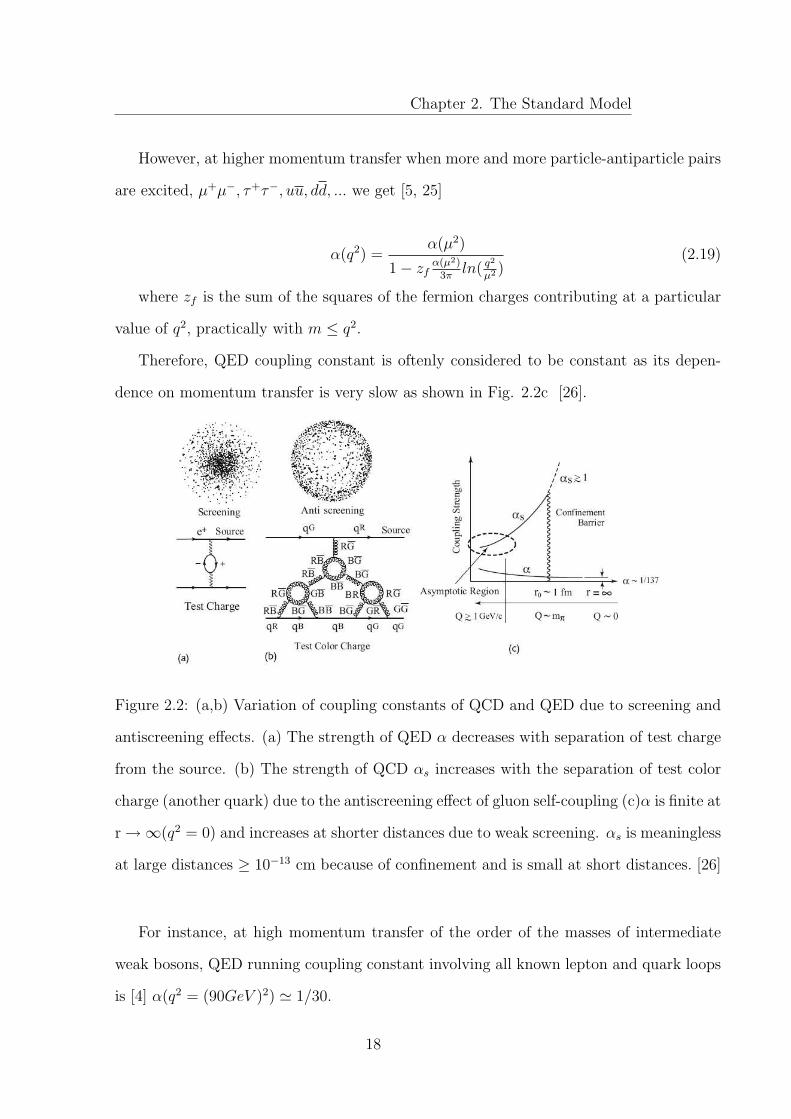
shielding of electric charge due to the vacuum polarization as shown in Fig. 2.2 [4, 26, 27].
In fact, around a field charge (electron) a charge of opposite polarity is developed by the
vacuum polarization which in turn produces the screening effect seen by the test charge
placed at large distance from the source charge. Experimentalists measure this effective
electron charge rather a bare charge which is visible only at a very short distance. Actually,
at a small distance the screening effect reduces and the test charge feels more charge thus
increasing the reaction rate or the value of α of QED [5].
If we consider only an e+e− loop, at low energy i.e low q2, q2 → µ2 → 0, α(0) = 1/37,
hence
α(q2) =α(0)
1− α(0)3π
ln( q2
m2 )(2.18)
17
Chapter 2. The Standard Model
However, at higher momentum transfer when more and more particle-antiparticle pairs
are excited, µ+µ−, τ+τ−, uu, dd, ... we get [5, 25]
α(q2) =α(µ2)
1− zfα(µ2)
3πln( q2
µ2 )(2.19)
where zf is the sum of the squares of the fermion charges contributing at a particular
value of q2, practically with m ≤ q2.
Therefore, QED coupling constant is oftenly considered to be constant as its depen-
dence on momentum transfer is very slow as shown in Fig. 2.2c [26].
Figure 2.2: (a,b) Variation of coupling constants of QCD and QED due to screening and
antiscreening effects. (a) The strength of QED α decreases with separation of test charge
from the source. (b) The strength of QCD αs increases with the separation of test color
charge (another quark) due to the antiscreening effect of gluon self-coupling (c)α is finite at
r →∞(q2 = 0) and increases at shorter distances due to weak screening. αs is meaningless
at large distances ≥ 10−13 cm because of confinement and is small at short distances. [26]
For instance, at high momentum transfer of the order of the masses of intermediate
weak bosons, QED running coupling constant involving all known lepton and quark loops
is [4] α(q2 = (90GeV )2) ' 1/30.
18

Chapter 2. The Standard Model
Due to small value of α, calculations in QED can be carried out using the idea of
perturbative techniques. According to perturbative scheme, any physical quantity can be
written as a sum of increasing power of the coupling of the theory.
In QCD, the expression for running coupling in momentum space is [3, 4, 5, 26]:
αs(q2) ==
αs(µ2)
1 + αs(µ2)4π
(11− 23nf )log(q2/µ2)
=12π
(33− 2nf )log( q2
ΛQCD)
(2.20)
where nf is the number of quark flavors involved in the loop diagram under consider-
ation and ΛQCD is QCD scale parameter to be determined experimentally.
Form the above expression, we see that αs approaches zero as q2 →∞. This is called
asymptotic freedom where quarks behave as free particles. This is due to antiscreening
effect of gluons as shown in fig.2.2b. The vacuum polarization effect due to physical
fermions and gluons causes screening effect, but the effect of the unphysical gluon loop is
opposite and is the cause of antiscreening. Discovery of asymptotic freedom by Politzer,
Gross and Wilczek in 1973 [28] was a crucial break through in QCD and paved the way
to use perturbation theory in QCD at large q2 (phenomenologically at q ≤ 1GeV/c) and
the parton model, which take quarks as point particles [26]. Asymptotic freedom can also
explain the formation of quarkonium and the famous OZI rule [5].
In physics, we encounter many situations which involve two quite separate scales: the
light and the heavy. If energy-momentum is smaller than the heavy scale, the interaction
can be represented by an effective Hamiltonian, containing only light degrees of freedom
but which fully accommodates all (virtual) effects of the heavy scale. Such an interaction
can effectively isolate and describe the underlying physics of a particular phenomena rather
than a rigorous treatment of the entire system [29]. In the following section we describe
theories called effective field theories which contain the above mentioned features.
19

Chapter 2. The Standard Model
2.6 Effective Field Theories
Properties of hadrons can be described by QCD Lagrangian in terms of the quark masses
m and the coupling constant αs. At low energy scale of leading order QCD (LQCD), non-
perturbative effects become prominent and αs becomes large. The non-perturbative QCD
(nPQCD) dynamics originates from the confinement of quarks inside hadrons. At such
scale, systems are described either by phenomenological potential models and constituent
quark-model, or by first principles lattice simulations. However, the physics of systems
containing a heavy quark q can be simplified. For systems containing heavy quarks, the
quark-mass scale mq becomes larger than LQCD which means ΛQCD is small which allows
the use of perturbative expansion at this scale [29].
Non-relativistic bound states comprising heavy quarks are represented by a hierarchy
of energy scales ordered by the quark velocity v << 1: the quark mass m (hard scale), the
relative momentum of heavy quark antiquark mv (soft scale), the typical kinetic energy
of the heavy quark mv2 i.e. the quark binding energy in the bound state (ultrasoft scale),
where m is the heavy-quark mass and v is its velocity in the CM frame. Such hierarchy
of scales are advantageous to introduce non-relativistic effective field theories (NR EFTs)
for the description of two particle non-relativistic bound states containing heavy quarks
i.e. heavy quarkonia [29, 30, 31, 32, 33].
Annihilation and production of quarkonium system occur at the quark mass scale m,
called the hard scale. An effective field theory obtained from QCD by integrating the
hard scale is named as non-relativistic QCD (NRQCD) [33, 34]. Formation of quarkonium
occurs at the quark momentum scale mv, called the soft scale. The suitable EFT obtained
from NRQCD by integrating out the soft scale i.e. mv ∼ r−1 is named as potential
NRQCD (pNRQCD) [33, 34]. Depending upon the radius of the quarkonium system, the
scale mv may or may not be larger than the QCD confinement scale ΛQCD [33].
20

Chapter 3
The Quark Model
In order to classify large number of subatomic particles in simple fashion, Gell-Mann [35]
and Zweig [36] independently put forth the idea of quark in 1964. According to them,
all known hadrons were composed of more fundamental entities called quarks. Initially
quarks were not accepted as physical objects owing to their strange nature; they carried
fractional electric charge, also no isolated quark is ever found. Hence quark concept could
not get any big success at that time. The first evidence that confirmed the reality of quark
as physical object, came from series of deep inelastic e-p scattering experiments carried out
at SLAC in the early 1970’s [37]. These experiments revealed point-like structures inside
proton, called the partons by Feynman [38]. At high energy, the parton model describes
the hadron as a composition of small constituents-the partons. Partons were naturally
identified with quark and gluon degrees of freedom described by QCD [39]. However,
the discovery of charm quark in terms of J/ψ and ψ(2S) states (each being bound state
of charm-anticharm quark pair, called charmonium), proved to be even more convincing
evidence in the favor of quark model. The quark model got much sophistication due to
the work of Nathan Isgur and Gabriel Karl [40], who established that all of the low energy
hadronic systems could be understood as bound states of quarks [5]. We discuss the ideas
and information related to quark model, in the following sections.
21

Chapter 3. The Quark Model
3.1 Quantum Numbers
In this section, we will discuss quantum numbers which form the basis of classification of
hadrons such as Gell-Mann’s Eightfold scheme and the quark model.
3.1.1 Isospin
The idea of isospin was given by Heisenberg [5, 41] by considering proton and neutron
as two different states of one particle called the nucleon. Nucleon has isospin of I=1/2;
therefore, there are (2I+1=2) isospin states for nucleon, called doublet comprising proton
and neutron. Each state is distinguished with the third component of isospin I3, which
is 1/2 for proton and -1/2 for neutron. For proton and neutron, the isospin states are
defined by
|p〉 =
1
0
= |1/2, 1/2〉, |n〉 =
0
1
= |1/2,−1/2〉 (3.1)
Like spin triplet and spin singlet, we can join two I= 1/2 states to form either an
isospin triplet (|p〉|p〉, 1√2(|p〉|n〉 + |n〉|p〉), |n〉|n〉) with I=1 and I3=1, 0,-1, or an isospin
singlet ( 1√2(|p〉|n〉 − |n〉|p〉)) with I=0 and I3 = 0 [5].
Isospin invariance implies that the isospin operator J commutes with the Hamiltonian
Hn of the nuclear force [Hn,J] = 0. The inclusion of electromagnetism destroys this
invariance [Hn+Hem,J 6= 0]. Since charge is conserved, the charge operator must commute
with the total Hamiltonian [Hn + Hem, Q = 0] =⇒ [Hn + Hem, J3] = 0. This is true only
when B is conserved which implies the conservation of the third component of isospin even
in the presence of an electromagnetic interaction. Now the relationship between baryon
numberB and third component of isospin is [3, 5]:
Q = I3 +B
2(3.2)
22

Chapter 3. The Quark Model
Each nucleon has B=1, while antinucleon has B=-1.
3.1.2 Hypercharge and Strangeness
Nuclear experiments performed at high energy observed some particles produced through
strong interaction (conserving isospin) but decayed through weak interaction (violating
isospin) [3, 5]:
π− + p →
Σ− + K+
Σ0 + K0
Λ0 + K0
(3.3)
and
Σ− → n + π−, Σ0 → n + π0.
Keeping in view the strange behavior of such particles, Gell-Mann and Nishijima pro-
posed the following relation among their quantum numbers [3, 5, 42]:
Q = I3 +1
2(B + S) = I3 +
Y
2(3.4)
where Y is called hypercharge defined as Y=B+S.
By definition, K+ is assigned +1 strangeness and all pions and nucleons are associated
with zero strangeness. With the discovery of new particles, isospin was assigned to them on
the basis of simplicity and near-degeneracy of masses of different particles if they occurred.
From the reaction 3.3, we observe that Σ− has S=-1. Accordingly for K−, S = −1 and for
Σ+, S = +1. Consider an isospin-strangeness-conserving reaction K−p → Λπ0. Clearly
for Λ, S = −1. Accordingly in reaction 3.3, for K0, S = +1. This creates a bit paradox
- there are two Kaons, K+, and K0, with S = +1, but only one with S = −1 i.e. K−.
Gell-Mann resolved this puzzle by suggesting that there should be an antiparticle K0 with
S = −1 i.e. K−. Soon, this particle was discovered in the reaction π+p → pK0K+ [5].
23

Chapter 3. The Quark Model
Now we discuss Gell-Mann’s Eightfold Way classification scheme in view of above
mentioned quantum numbers.
3.2 The Eightfold Way
After the discovery of more particles the assignment of isospin and strangeness quantum
numbers became chaotic. To make things simpler, Gell-Mann in 1961 devised an ordered
pattern in the mess of so called elementary particles so as to arrange the particles in a
symmetric fashion [14]. He arranged the baryons, and mesons into a geometrical pattern
on the basis of their charge and strangeness. The pattern is known as the Eightfold Way,
or technically SU(3) symmetry. In this method, the particles with same strangeness are
placed on the same horizontal lines while the particles having same charge are placed on
the same diagonal lines. The resultant hexagonal arrays are called the baryon and meson
multiplets [14], as shown in Fig.3.1. and Fig. 3.2, respectively. The families of hadrons
with different electric charge but having similar masses are called multiplets. For instance,
∆ is one of a quartet of particles, ∆++, ∆+, ∆0 and ∆−, each having mass close to 1232
MeV/c2. Other familiar examples are proton-neutron doublet, and the triplet comprising
π+, π0 and π− [6].
24

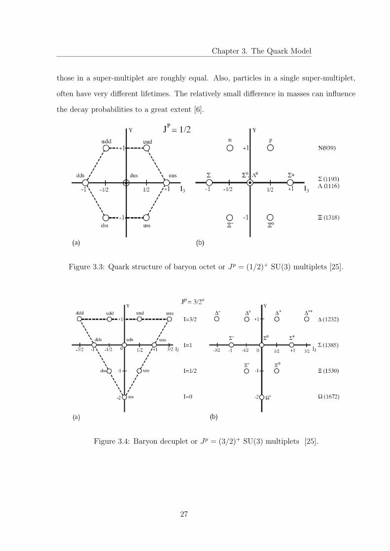
Chapter 3. The Quark Model
Figure 3.1: Baryon multiplets: Baryon octet or Jp = (1/2)+ SU(3) multiplets (left).
Baryon decuplet or Jp = (3/2)+ SU(3) multiplets (right), where 1/2 stands for spin and
+ for even parity and so on [3, 5].
Figure 3.2: Meson Multiplets: (A) Pseudoscalar meson octet with Jp = 0−. (B) Vector
meson octet with Jp = 1− [3, 5].
One particle shown in the Eightfold Way, having strangeness -3, and spin 3/2 was
still missing. Gell-Mann called this particle the Ω−, meaning in Greek the last one,
25

Chapter 3. The Quark Model
and predicted it three years before its discovery [43]. It has also been seen at BESII in
ψ(2S) → Ω−Ω+ decay channel [44].
Success of the Eightfold Way itself raised a very crucial question: why do the hadrons
fit into these patterns? [14]. Many of the new hadrons appear to be the excited states of
proton and neutron which imply that proton and neutron must be the composite systems
made out of even more fundamental particles [6]. It also raised a question as to why the
particles in multiplets, which otherwise look different, seem to be excited states of one
entity? [3]. Responding to these fundamental questions, Gell-mann and Zweig, indepen-
dently came up with an innovative idea that all hadrons are in fact composed of three
elementary particles, which Gell-Mann called quarks., which established the foundation of
the quark model to be discussed in the following section.
3.3 The Quark Model of Hadrons
The idea of three quarks (antiquarks) came to the rescue of the Eightfold Way classification
of hadrons. By using all the combination of quarks and antiquarks, baryon and meson
multiplets could be constructed conveniently [3, 6, 14].
According to the constituent quark model, all baryons are bound states of three valence
quarks while mesons are composed of valence quark- antiquark pairs. Each quark has
baryon number B=1/3, giving B=1 to each baryon. For example, neutron is the lowest
bound state of one up quark and two down quarks (udd), while proton is the lowest bound
state of two up quarks and one down quark (uud). The baryon, ∆+ is an excited state of
the three quarks (uud) which make up proton [6]. Since the s quark is massive than u and
d quarks, there exist some heavier baryons like Σ and Ξ etc. In fact, all of the particles
in a single super-multiplet have many common features, and this behavior is even more
prominent for the particles in a single multiplet. For instance, all particles of a given
super-multiplet have the same spin; the masses in a given multiplet are very close, while
26
Chapter 3. The Quark Model
those in a super-multiplet are roughly equal. Also, particles in a single super-multiplet,
often have very different lifetimes. The relatively small difference in masses can influence
the decay probabilities to a great extent [6].
Figure 3.3: Quark structure of baryon octet or Jp = (1/2)+ SU(3) multiplets [25].
Figure 3.4: Baryon decuplet or Jp = (3/2)+ SU(3) multiplets [25].
27

Chapter 3. The Quark Model
3.3.1 Baryons Multiplets
In order to arrange hadrons into symmetrical pattern Gell-Mann and Zweig extended
isospin SU(2) symmetry group, which only incorporates up and down quark, to SU(3)
flavor symmetry group which incorporates up, down and strange quarks. Isospin and
strangeness quantum numbers are collectively known as flavor. Now baryon octet and
decuplet called flavor multiplets can be defined in terms of three flavors of the quarks. All
possible multiplets of baryons discussed so far may be conveniently classified on the basis
of quark model by using flavor symmetry group SU(3).
For three flavors, there may exist 33 = 27 distinct flavor states. By using three flavors,
u, d and s we get the following baryon multiplet comprising one decuplet, two octets and
one singlet [3]:
3⊗ 3⊗ 3 = 10⊕ 8⊕ 8⊕ 1 (3.5)
It was observed experimentally that the total spin of ∆++ is 3/2, and hence three
quarks must be in the same state
∆++ = |u ↑ u ↑ u〉 (3.6)
Nevertheless, the existence of ∆++ and ∆− particles having three fermions (quarks)
of same flavour in the same single state is forbidden according to Pauli principle [6, 14].
This problem was tackled by O. W. Greenberg by assigning another quantum number
called color charge or strong charge. He suggested that each flavor of quarks comes in
three colors: red, green and blue [14]. Owing to their different colors, the three quarks
are no more identical and thus are not forbidden to exist in the same state. If we regard
the color of antiquark as anticolour, i.e. antired, antigreen and antiblue, then according
to color hypothesis only the colourless bound sates are possible in nature [6, 14]. Each of
the super-multiplets as shown in Fig. 3.4, is formed from several multiplets with particles
28

Chapter 3. The Quark Model
very close in mass.
According to the quark model, J/ψ is the bound state of charm quark and anticharm
quark, i.e. cc, called the charmonium [14, 54]. With the discovery of this fourth quark,
there was a prediction of series of new hadrons called charmed baryons and charmed
mesons for the clear evidence of the charm quark. Eventually some charmed baryons like
Λ+c = udc and Σ++
c = uuc were observed in 1975, with open charm as shown in Fig. 3.5.
Figure 3.5: SU(4) multiplets of :(a) (1/2)+ baryons (b) (3/2)+ baryons [3, 26].
3.3.2 Mesons Multiplets
The light quark-antiquark pairs of SU(3) flavor group give rise to an octet and a singlet,
as shown in Fig. 3.6:
3⊗ 3 = 8⊕ 1. (3.7)
Including fourth quark flavor (charm), SU(3) symmetry group is extended to SU(4) in
which a 15-plet and a singlet are possible, as shown in Fig. 3.7 [3]:
4⊗ 4 = 15⊕ 1 (3.8)
29

Chapter 3. The Quark Model
The 15-plet further consists of an octet, a singlet, a triplet and an anti-triplet (Fig.
3.7) [3]:
15 = 3⊕ 8⊕ 1⊕ 3 (3.9)
Figure 3.6: SU(3) multiplets of :(a) pseudoscalar and (b) vector mesons [3, 26].
Like charmed barons, charmed mesons were also discovered after the discovery of J/ψ.
D0 = cu and D+ = cd were the first charmed mesons [3, 45] as shown in Fig. 3.7. Thus
the charmness which was hidden in charmonium revealed itself in charmed baryons and
charmed mesons and it was in accordance with the quark model prediction.
Figure 3.7: SU(4) multiplets of :(a) pseudoscalar mesons (b) vector mesons [3, 26].
30

Chapter 4
The Charmonium Physics
Mesons containing heavy quark-antiquark pairs termed as heavy quarkonia are very impor-
tant systems to explore the QCD dynamics both within and beyond the Standard Model.
Among them is an important quarkonium called charmonium (a cc state). The first char-
monia discovered include J/ψ and ψ(2S). After their discovery a chain of their companion
states were also discovered. Therefore the group of such states is also called Charmonium
Family. The charmonium system plays significant role in understanding QCD. Charmo-
nium being non-relativistic system is well suited to understand the production and decay
mechanism of heavy quarkonia and spectra of light hadrons from their decays and can
be effectively treated perturbatively [46, 47, 48, 49, 50, 51, 52]. In this chapter, we will
present experimental and theoretical aspects of charmonium physics. First of all we brief
generally about heavy quarkonia in the following section.
4.1 Heavy Quarkonia
Heavy quarkonia are multiscale systems which can probe all regions of QCD. At high
energies, perturbative expansion in terms of strong coupling αs(q2) is possible. At low en-
ergies, non-perturbative techniques are applied. Between these two regions, more complex
approaches may be used. Thus heavy quarkonium is an ideal system for investigating the
31

The Charmonium Physics
interplay between perturbative and non-perturbative QCD [33, 46].
Heavy quarkonia are composed of a pair of heavy quark and an anti-quark, whose
mass m is much larger than QCD scale ΛQCD, called the confinement scale. Being non-
relativistic systems, heavy quarkonia are characterized by the bound-state velocities, v ¿1(v2 ∼ 0.3 for cc, v2 ∼ 0.1 for bb, v2 ∼ 0.01 for tt) and by different energy scales: the
hard scale in terms of the mass of quark m, the soft scale in terms of relative momentum
of quark anti-quark pair p ∼ mv, and the ultrasoft scale in terms of the binding energy
of quark/anti-quark E ∼ mv2. Perturbation theory fails at energy scales close to ΛQCD
where nonperturbative methods are used. There exists a nonrelativistic hierarchy of scales
below the confining scale ΛQCD: m À p ∼ 1/r ∼ mv À E ∼ mv2, where r is the typical
separation between the heavy quark-antiquark pair. Now m À ΛQCD implies αs(m) ¿ 1,
which means perturbative technique may always be used for the phenomena occurring at
the scale m. The coupling αs may also be small if we have mv À ΛQCD and mv2 À ΛQCD,
which implies αs(mv) ¿ 1 and αs(mv2) ¿ 1, respectively [31, 33].
4.1.1 Spectral Notation
We can consider meson as a quark-antiquark “atom”, akin to the electron-nucleus atom or
the e+e− atom called positronium [5]. We might expect that same techniques should work
for mesons as they did for positronium or ordinary atoms; hence the name “quarkonia”
for mesons. Spectroscopic notation for qq system is analogous to that of atomic system
like hydrogen or positronium and is given by (n + 1)2S+1LJ [53]. Here L is the orbital
angular momentum, S is the spin of quark-antiquark pair: S = ~sc + ~sc, which could be 1
if both of quarks are aligned, and 0 otherwise, hence four possible spin states of quark-
antiquark pair split into singlet and a triplet state. For spin singlet state S=0, J=L,
while for spin triplet state S=1, J = L-1, L, L+1. J is the total angular momentum
which gives the spin of meson: ~J = ~L + ~S, here 2s+1 is for spin multiplicity. Analogous
to atomic physics, L=0, 1, 2, 3, ... correspond to S, P, D, F, ... states. Different
32

The Charmonium Physics
radial excited states (L = 0, n ≥ 1) are 11S0, 13S1, 2
1S0, 23S1... and orbital excited states
(L = 1, n ≥ 1) are 11P1, 13P0,1,2, 2
1P0, 23P0,1,2. Space parity P and charge parity C are
defined by: P = (−1)L+1, C = (−1)L+S. For a non-relativistic system n, L and S are good
quantum numbers. But for mesons and baryons which are strongly interacting physical
systems, JPC are good quantum numbers for relativistic systems too, meaning by they
can be used to describe a physical state. The JPC for scalars, pseudoscalars, vectors, axial
vectors and tensors are: 0++, 0−+, 1−−, 1+, 2++, respectively. The lowest state with L =
0, S = 0, and thus J = 0, is the state ηc with symbol 11S0, while its first radial excited
state is η′c represented by 21S0 [53].
4.1.2 Lagrangian for cc System
Charmonium mesons are bound states of cc pairs. Mass of charm quark i.e. mc is suffi-
ciently large hence the motion of a charm quark inside charmonium system is slow which
approximately make charmonium as non-relativistic in nature. According to lattice sim-
ulations or potential model calculations we have v2 ∼ 0.3 for charmonium system, where
v is the relative velocity between c and c inside charmonium. The binding energy is of
the order of mcv2 while the momentum is of the order of mcv. In limit v2 ¿ 1, there is
hierarchy of energy scales in charmonium satisfying the relation mc ¿ mcv ¿ mcv2. The
effective field theory incorporating the effects by integrating out the energy scale mc is
named as nonrelativistic QCD (NRQCD) which expands full QCD in powers of v. RN-
QCD is very suitable effective theory to describe charmonium spectroscopy, its inclusive
production and annihilation decays. The effective theory derived by integrating the effects
at the energy scale mcv containing only the energy scale mcv2 is called potential NRQCD
(pNRQCD) [46].
The QCD Lagrangian for heavy quarks is as follows :
ÃLq = ψ(x)(iDµ −mc)ψ(x) (4.1)
33

The Charmonium Physics
where Dµ = ∂µ + gTaGµa is the covariant derivative , g is strong coupling constant
and Gµa(a = 1, 2, ...8) for eight gauge fields of vector gauge bosons of strong interaction
i.e eight gluons.
The above Lagrangian includes all energy scale of QCD and hence turns out to be
complicated. Simplification can be done by assuming the non-relativistic limit i.e v ¿c and having cut-off energy scale in the limit ΛQCD < mc. This decouples the quark
and antiquark by suppressing the quark pair creation and annihilation. The effective
NRQCD Lagrangian can be written as sum of powers of v with coefficients called Wilson
short-distance coefficients that are determined to match NRQCD and QCD. Fields are
represented by two-component Pauli spinor fields ψ and χ for the quark and antiquark
respectively. Up to order v4 NRQCD lagrangian is [46]:
LNRQCD = Ll + L0 + δL (4.2)
where Ll is the ordinary Lagrangian for gluons and light quarks and
L0 = ψ†(iD0 +D2
2mc2)ψ + χ†(iD0 − D2
2mc2)χ
δL0 =c1
8m3c
ψ†(D2)2ψ+c2
8m3c
ψ†g(D.E−E.D)ψ+c3
2mc
ψ†gσ.Bψ+ic4
8mc
ψ†g.σ(D×E−E×D)ψ+c.c
where δL contains the correction terms to L0. Gauge invariance of the theory implies
that the appearance of the gluon filed in the lagrangian is only via gauge-covariant deriva-
tive iD0, iD and the QCD field strengths E and B. The terms iD0 and D2
2mcpresent in L0
contribute the same order of quarkonium energy. The absence of Pauli matrix σi in L0
reveals the explicit symmetry at leading order of v. This indicates the degeneracy in the
states J/ψ and ηc, and χc0, χc1, χc2, and hc. However, the inclusion of spin dependent
term σi in δL due to next-leading-order corrections violates the explicit symmetry [46].
34

The Charmonium Physics
4.2 Discovery of J/ψ and ψ(2S) Charmonia
Despite all its successes, the quark model could not explain the non-existence of a single
isolated quark. To this end, idea of quark confinement was put forth which stated that
for some unknown reasons quarks are confined within the hadrons. Another explanation
was given on the basis of color hypothesis which states that only colorless particles can
exist in nature; quark being a colored particle can no more exist in isolation.
Owing to these mysteries, the quark model could not touch the final triumph until the
discovery of a new meson called J/ψ meson. The J/ψ was found to be electrically neutral
and extremely heavy meson having a mass of 3.1GeV/c2 more than three times the mass
of proton. The spin and parity of J/ψ is Jpc = 1−−, where J represents the spin, P is
for parity and C is the charge conjugation [3, 6, 54]. The discovery of such heavy meson
initiated a wide spread discussion among the particle physicists as to what was its true
nature. Nevertheless, the explanation that won the whole discussion was provided by the
quark model [14].
As said earlier, the J/ψ and ψ(2S), both are bound states of charm-anticharm pair.
The J/ψ was discovered in 1974, simultaneously at SLAC (by Richter group) and at BNL
(by Ting group) [55, 56]. The ψ(2S) meson was discovered at SLAC, after ten days of this
event [57]. At SLAC, these charmonia were observed in the following process:
e+ + e− → (J/ψ, ψ(2S)) → e+ + e−, µ+ + µ−, hadrons (4.3)
The above mentioned processes are shown in Figures 4.1 and 4.2.
At BNL, J/ψ and ψ(2S) were observed through the following process:
P + Be → (J/ψ, ψ(2S)) + X → e+ + e− + X (4.4)
where X represents any set of particles allowed by conservation laws.
Narrow peaks were observed at center of mass energy of 3.1 GeV/c2 (for J/ψ) in the
35

The Charmonium Physics
Figure 4.1: Schematic diagramm for production of (J/ψ) in e+e− collision [54].
Figure 4.2: Narrow resonance peak of J/ψ in e−e+ at SLAC [25, 55, 56].
cross sections for the above mentioned processes (Figure 4.3).
Production of charmonia in electron positron collision process have many advantages:
small background, large cross-section, and well-defined initial state [58]. In electron-
positron annihilation processes direct formation of charmonium is possible only for states
having the quantum numbers of JPC = 1−−, such as J/ψ, ψ(2S), ψ(3770) and so on [59].
36

The Charmonium Physics
Figure 4.3: Narrow resonance peak of J/ψ in PP collisions at BNL respectively [25, 55, 56].
4.3 Charmonium Spectroscopy
Comparison of charmonium spectrum with that of positronium is shown in Fig. 4.4.
From the comparison we see that the states with n=1 and n= 2 are similar, however
the higher charmonium states do not show 1/n2 feature as compared to positronium.
Since the potential determines the relative spacings of the energy levels, it is evident
that the potential of the strong interaction for charmonium must be of Coulomb form
(at least for n=1,2 i.e. at short distance). This fact is also favored by QCD which
describes the short distance interaction between the quarks by one gluon exchange (OGE)
Coulomb like potential. Also the absence of any degeneracy between 23S and 13P states
in charmonium, in comparison to positronium, indicates that the potential is not of pure
Coulomb form (even at fairly short interquark separation). Since quarks have not been
observed experimentally in isolation, it seems reasonable to assume a potential which is of
Coulomb like at short distances and increases linearly at greater separation, thus leading
to the confinement of quarks in hadrons [60] .
In the nonrelitivistic limit, the spectra of charmonia can be evaluated by solving the
37

The Charmonium Physics
Figure 4.4: Comparison between energy level diagram of positronium and charmo-
nium [46].
non-relativistic Shrodinger equation with conventional quarkonium potential. Charmo-
nium spectrum of experimentally established states and those predicted by nonrelatavistic
potential model is shown in Fig. 4.5 [8, 61].
Figure 4.5: Experimentally observed and theoretically predicted charmonium states. The
experimentally established states are shown with solid lines. The doted lines on the left
show the predicted states by a non-relativistic potential model while the right dotted lines
show the states predicted by the relativistic Godfrey Isgur potential model [8, 61].
38

The Charmonium Physics
Figure 4.6: Approximate QCD static quarkonium potential as a function of interquark
separation r [4, 33].
The experimentally established charmonium states of relatively narrow widths below
the open charm mass DD threshold can be well described by simple cc potential model
comprising short distance color Coulomb potential due to one gluon exchange (OGE) term
and long distance linear scalar confining potential:
V cc0 (r) = −4α(s)
r+ kr (4.5)
Its form is shown in Fig. 4.6 [4, 33] which shows the varying sensitivities of Quarkonia
systems to the Columbic and confining interactions. Only Coulomb term is not sufficient
for it will not stop ionization of free quarks;but the potential in Eq. (4.5) confines the
quarks and the corresponding Schrdinger has no continuum states.
The observed splitting in the narrow states are caused by quark-antiquark spin-dependent
coupling, and is consistent with spin-dependent Briet-Fermi Hamiltonian due to OGE plus
inverted spin-orbit coupling term due to scalar nature of the linear confining potential:
39

The Charmonium Physics
Vs(r) =32πα(s)
9m2c
~Sc.~Sc~δ ~(x) +
1
m2c
[(2α(s)
r3− b
2r)~L.~S +
4α(s)
r3T ] (4.6)
1. The small spin-orbit potential term, which is generally small, is the cause of fine-
structure splitting of levels having the same orbital angular momentum but different
total spin J and can be observed in the χcj(cc) triplet states.
2. The spin-spin term, (also called color magnetic term) causes the hyperfine splitting
due to spin-spin interaction of the quark and the antiquark. This can be observed
in singlet and triplet states, i.e., ηc(cc) and J/ψ(cc).
3. The tensor potential, causes mixing between states with the same JPC but different
L and S.
Both J/ψ and ψ(2S) decay to hadrons either electromagnetically or strongly. Dom-
inant hadronic decay is through charm-anticharm annihilation into a photon or three
gluons [62]. In the mass range 2900 MeV/c2 to 3700 MeV/c2, only eight well-separated
and narrow bound states exist in the 800MeV region, each with width ≤ 20 MeV/c2. Thus,
the charmonium system is obviously very “cleaner” and more tractable as compared to
light quark mesons [47].
Owing to the similar masses of the light quarks, mesons with light quarks are invariably
mixtures of three flavors i.e. up, down and strange. This results into intricate structures
owing to overlapping of close lying states. For instance, in the 1000 MeV/c2 mass region
lying between 1500 MeV/c2 and 2500 MeV/c2, there is expectation of as many as 77
mesons having typical widths of 200 MeV/c2-400 MeV/c2. Also, the small masses of light
quarks cause some theoretical problems; the motion of quarks in these light mesons is
highly relativistic and, consequently, the value of strong coupling constant is very large
which makes it impossible to use perturbative techniques [47].
The J/ψ is the lowest 3S1 (triplet) state, but not the ground state of the charmonium
family. Actually spin-spin interaction of quark antiqark pair pushes the triplet state up
40

The Charmonium Physics
relative to the singlet ground state η [4, 60]. ψ(2S) is its first radial excited state. Ground
state of cc system is the singlet (0S1) η state. 3S1 states can be formed directly from e−e+
collision, for they have quantum numbers of photon. Spin-spin interaction is the cause of
shift between J/ψ and η state. While spin-orbit interaction splits χ states.
4.4 Transitions
Charmonium higher states decay to low energy states through radiative and strong tran-
sitions. Wave functions obtained by solving Schrodinger equation with quark model po-
tential can be used to calculate transition rates for different transitions. For detailed
theoretical and experimental aspects of different transitions see Ref. [33].
4.4.1 Radiative Transitions
These are electromagnetic transition which occur between quarkonium states via emission
of single photon. Radiative transitions are of two types: electric transitions and magnetic
transitions. In the non-relativistic limit, quarkonium wave function separates into spin and
spatial parts. The spatial part, ψ(x), can be written in terms of a radial wave function,
unl, and spherical harmonics, Ylm: ψ(x) = Ylm(θ, φ)unl(r)/r.
where n is the radial quantum number, l is the orbital angular momentum, s is the
total spin, and J is the total angular momentum given as J=l+s.
The spin of quark is changed by magnetic transitions. In case of electric transitions
there is no change in the quark spin. The transitions that do not change the orbital
angular momentum are called magnetic dipole, or M1, transitions. While the transitions
that change the orbital angular momentum by one unit are called electric dipole, or E1,
transitions. Transitions for which n = n′ are called allowed M1 transitions, otherwise they
are called hindered or forbidden transitions.
41

The Charmonium Physics
4.4.2 Hadron Transitions
The general expression for a hadronic transition is: ψi → ψf + h, where ψi , ψf and h
represent quarkonia of initial state, final state, and the emitted light hadron(s) respec-
tively. In the cc and bb systems, the kinematically allowed final light hadron(s) h are
dominated by single particle (π0, η, ω, ...) or two-particle (2π or 2K) states because the
mass difference mψi−mψf
changes from a few hundred MeV to slightly over a GeV. Until
now, twenty hadronic transitions have been observed experimentally [33]. For study of
low lying heavy-quarkonium states, hadronic decay modes are important. Such transitions
can be calculated by non-perturbative QCD.
4.5 OZI Rule
It was found by Okubo, Zweig and Iizuka, that the decay rate of φ meson (bound state
of ss) into 2 Kaons (K+K−) is greater than into three 3 pions, despite the latter is
energetically favored decay mode because mass of three pions is less than mass of two
kaons. The puzzle was explained by OZI rule [63] which states that process with broken
quark lines is suppressed. Hence decay mode shown in Fig. 4.7a is OZI suppressed while
decay mode shown in Fig. 4.7b is OZI allowed. It was also verified experimentally, because
decay width of φ was found to be smaller than expected [4, 5].
Figure 4.7: Quark diagrams for decay of φ into decay mesons. (a) OZI supressed transition
(b) OZI allowed transition [4].
42

The Charmonium Physics
In fact in case of OZI suppressed decay mode, the intermediate state is that of pure
gluons. These gluons must be of high energy (“hard”) since they carry the total mass of
φ meson. While in the case of OZI allowed decay mode the intermediate gluon is of low
energy (“soft”), since strange/antistrange meson pairs share most of the energy. Hence
according to OZI rule processes that proceed through hard-gluon exchange are suppressed.
The coupling of soft-gluons with quarks is more stronger than that of hard-gluons, so the
soft-gluon exchanges are more probable [4, 5, 16].
Figure 4.8: Quark diagrams for J/ψ decaying to mesons. (a) OZI allowed transition (b)
OZI suppressed transition [5].
Similarly we can apply OZI rule to explain the narrow width of about 90 KeV and
long life of J/ψ which is ' 1020s, shorter than EM decays, but 1000 times longer than
that of typical strong decay. The preferred decay of the J/ψ into charm meson is shown in
Fig. 4.8a. However, this process is energetically disfavored because MJ/ψ < 2MD, where
MD is the lightest meson mass with nonzero charm, while the mass 2MD is the charm
threshold. Now the only possible hadronic allowed decay mode for J/ψ is through OZI
suppressed decay mode as shown in Fig. 4.8b. It is because J/ψ and its decay products are
43

The Charmonium Physics
color singlets, the decay process should proceed by exchange of color-singlet combination
of gluons which require at least two gluons. But J/ψ has spin-1 and is known to be
produced via one photon exchange in e+e− annihilation, so it must have C=-1. Gluons
being bosons also have C=-1, so at least three gluons must be exchanged carrying all the
energy of J/ψ as shown in Fig. 4.8b. Thus the much slower OZI suppressed decay mode
gives relatively long lifetime to J/ψ [4, 5, 16].
4.6 ρπ Puzzle
In accordance with the OZI rule the suppressed J/ψ and ψ(2S) decays to hadrons are via
three gluons or a photon. According to prediction of pQCD the ratio of the branching
fractions of J/ψ and ψ(2S) in either case is [33, 64]:
Br[ψ(2S) → h]
Br[ψ → h]=
Br[ψ(2S) → e+e−]
Br[ψ → e+e−]≈ 12.7% (4.7)
This relation is expected to hold true to a certain degree both for inclusive as well as
inclusive decays. Since 1983 there are lots of experimental evidences for the violation of
this rule in some decay channels especially in ρπ decay channel, hence the “ρπ puzzle”
[65].
Variety of solutions have been proposed for the puzzle [33, 66] and have been tested
against the experimental results from CLEOc, BESII, and BESIII by two-body decays of
J/ψ and ψ(2S) with more accuracy, which are vector-tensor (V T ), vector-pseudoscalar
(V P), pseudoscalar-pseudoscalar (PP), and baryon-antibaryon (BB) modes, and by multi-
body decays of J/ψ, ψ(2S) or even by the J/ψ(3770). Theoretically, since the Q-value is
smaller than 12%, in the case of ρπ enhanced or suppressed J/ψ decay rate may cause it,
or both.
For an extensive study of 12% rule , enough measurements of ψ(2S) and J/ψ de-
cay modes have been carried out, the highest priority, however, has been given to the
44

The Charmonium Physics
measurement of Vector-Pseudoscalar (VP) modes, like the ρπ. For these modes, it is gen-
erally found that the ratios of the branching fractions relative to 12% are enhanced for
Pseudoscalar-Pseudoscalar (PP) modes, while for the non-isospin violating VP and Vector-
Tensor (VT) modes are suppressed (i.e., excluding modes like ωπ0 and ρ0η0). Among the
baryon anti-baryon and the multihadron modes, some are enhanced, some are suppressed,
and some match the expectation of the rule. Solution for all of the measured channels is
yet to be provided by the theoretical models, which have been developed for interpreting
specific modes [33].
45
Chapter 5
BES-III Experiment
1Experimental knowledge of particle physics mostly results from colliding particles to-
gether at very high speeds which results in very energetic collisions [5]. This is why
sometimes particle physics is also called high energy physics. The machine used to accel-
erate the particles at very high speed is called accelerator. While the devise used to get
the physical information emerging from these collisions is called detector.
This chapter is about BESIII experimental apparatus. We will briefly discuss the
significance of electron positron colliders, the construction and working of different parts
of BESIII detector, and physics goals of BESIII experiment.
5.1 Fixed Target Accelerators Versus Colliders
Most of the earlier accelerators were fixed-target in which moving beam collides with
target at rest. Such accelerators produce limited energy and interactions after collision
and hence have been replaced with special kind of accelerators called colliders. In such
machines both beams and target are set to motion and are smashed into each other inside
the detector that monitors their collision for useful information. If Eb is the beam energy,
1The details of this chapter are available in scholarly work of different authors. If any reference is
found missing that will be totally un-intentional.
46

BES-III Experimental
mt is the mass of target particles, then the total energy is Etotal '√
2Ebmtc2. However,
in the case of collider when both the beam and target are moving toward each other we
have Etotal ' 2Eb. Therefore, large energy is available in colliders which in turn increases
the number of particle produced during interaction. But this large energy comes at the
price of reduced luminosity. Typical luminosity for colliders is ∼ 1031cm−2s−1, whereas
for fixed target machines it is ∼ 1037cm−2s−1 [5].
Luminosity is related to another useful physical quantity called differential cross section
which can be measured experimentally. If a beam of incoming particles with uniform
luminosity L is directed towards a target then the number of particles crossing differential
cross-section dσ per unit time is dN = Ldσ. Hence:
dN = Ldσ = Ldσ
dΩdΩ ⇒ dσ
dΩ=
1
L
dN
dΩ(5.1)
Particle physicists describe cross section as the likelihood of interaction between parti-
cles. In other words it characterizes the probability of occurrence of a particular physical
reaction, or the statistical nature of scattering events. For instance when two particles
collide with each other, their cross section is a measure of the interaction event between
them. Unit of the cross section is area, usually it is expressed in barn.
The quantity of interest for experimentalists working in HEP is the number of measured
events. For instance, in order to measure the angular distributions one can measure events
per unit space angle to measure the angular distribution. The number of events measured
depends upon the cross section σ, integrated luminosity of the physical process L and the
detector efficiency ε i.e. N = σLε [67] .
5.2 Electron-Positron Colliders
For more than 40 years, e+e− colliders have proved to be an innovative experimental
tools to investigate fundamental phenomenon in particle physics in general and Stan-
47

BES-III Experimental
dard Model in particular. The hallmark of such colliders is their huge luminosity in the
low energy region to explore many dimensions of Standard Model and physics beyond
Standard Model with greater precision. Standard Model can not answer many questions
about nature. The questions are either related to the unexplored energy region or non-
perturbative QCD [46]. For example, it is expected that at energy far above 100 GeV,
some new phenomenon (supersymmetry, dark matter) and new particles (sypersymmetric
particles, weakly interacting massive particles) may result. LHC is aimed at investigating
phenomenon related to Standard Model and new physics, and ILC is being planned to test
and confirm the results of LHC with better accuracy. Although QCD has been well tested
in perturbative regime, at short distance, but it is not useful technique at long distance
where for large value of strong coupling constant non-perturbative effects appear. These
effects are very crucial regarding the structure and spectrum of hadrons. To address such
effects, we need lower energy with high luminosity. The better place for such process is
no other than e+e− colliders.
The promising advantage of e+e− colliders lies in the fact that e+e− annihilation creates
virtual photons with JPC = 1−− which are directly coupled to quarks and leptons [68].
Thus many meson states with quantum numbers of photons can be directly produced in
electron positron colliders. They provide a clean environment with low background and
well defined initial state to study many aspects of Standard Model [68, 69, 70].
In factuality, e+e− colliders can produce plethora of charmonium states with large
cross sections and abundant resonances and thus are ideal laboratories for the study of
charmonium, charm and QCD. Charm quark lies at the border line of pQCD and non-
pQCD and study of production and decay of bound states of charm anti-charm quark can
be useful to probe Lattice QCD. Decay of charmonium through three-gluon loop is one
of the best channels to search for hybrids and glueballs [71] which are predicted by QCD
but yet to be established experimentally.
Many electron-positron colliders were built in late 60s and early 70s. SPEAR is the
48

BES-III Experimental
prominent example where both the J/ψ and tau were discovered which was the beginning
of the tau-charm physics. Many charmonium states and charmed mesons were discovered
at Doris and SPEAR. Examples of contemporary colliders are the Phi factory at Frascati,
KEKb collider at Tsukuba, the BEPCII collider at IHEP Beijing focussing on φ meson
and kaon production, B physics, and tau-charm physics respectively [72]. But here we
discuss only BEPCII/BESIII (for detail construction and working of BESIII see Refs. [46,
68, 70, 73].
5.3 BEPCII Collider
BEPCII [73] (Beijing electron positron collider) is an upgradation of BEPC and is a
double-ring multi-bunch collider (Fig. 5.1) with a design luminosity of ∼ 1× 1033cm−2s−1
and energy of 1.89 GeV and beam current of 0.9 A.
Figure 5.1: Schematic diagram for e+e− BEPCII collider and BESIII detector [68].
49

BES-III Experimental
Physics data taking at BEPCII started in March of 2009. Each ring has circumference
of 237.5 m and can be filled with up to 93 bunches with a bunch length of 1.5 cm. Beams of
electron and positrons collide at the southern interaction region with a horizontal crossing-
angle of ±11mrad. Current of single beam is designed to be 0.91 A. Superconducting
Micro-β quadruples, Superconducting RF system of 500 MH and low impedance vacuum
chambers are used.
5.4 BEPCII Detector
BESIII [73] is a general purpose detector and upgraded from its predecessor BESII. It
consists of four sub-detectors namely; Main Drift Chamber (MDC), Time Of Flight (TOF)
chamber, Electro-magnetic Calorimeter (EMC) and Muon (MU) chamber (Fig.5.1). Their
working and functions are briefly described in the following section.
• The multilayer main drift chamber (MDC) is the most important component of the
BES-III detector and surrounds the beam pipe. It is composed of inner and outer
chambers without any intervening wall. The polar angle coverage of the MDC is
|cosθ| < 0.93. Length of MDC is 2.4m with an inner radius of 60 mm and outer
radius of 800 mm. Drift cells have 43 cylindrical layers, coaxial with the beam pipe,
8 layers in the inner chamber and 35 layers in the outer chamber. In the inner
chamber all 8 layers are stereo; in the outer chamber there are 19 axial layers and
16 stereo layers which are interleaved in the outer chamber. There are 6796 signal
wires, in total.
Particle identification and tracking is important part of job for experimentalists
during their analysis. Particles are usually identified from their paths traversed in
detector in magnetic fields. Charged particles move in straight lines in the absence of
magnetic field, but magnetic field bend their path into curves. From the curvature,
momentum of particles is measured which is used to identify particles. In BESII
50

BES-III Experimental
Figure 5.2: Schematic diagram of MDC [68].
MDC detector is used for tracking of relatively low momentum charged particles
by precisely measuring their momentum, as well as for particle identification by
measuring their specific energy lost i.e. dE/dx. The normalized pulse height, which
is proportional to dE/dx, is a function of βγ = p/m, where m and p are the mass
and momentum of a charged particle. Using dE/dx pulse height measurements, we
cannot distinguish Pions, electrons and muons with momenta around 0.2 GeV/c.
Similarly, the dE/dx pulse heights will not separate electrons from kaons in the 0.5-
0.6 GeV/c momentum range. The dE/dx measurement resolution is expected to
be between 6% and 7% after calibration. 3σ K/π separation can be carried out by
using dE/dx information, for momentum below 0.6 GeV/c; for all momenta above
0.4 GeV/c a good e/π separation can be achieved .
Single wire resolution of MDC is better than 120 µm and a dE/dX resolution is
better than 6%. The momentum resolution σp/p is better than 0.5% in magnetic
field of 1T for charged tracks with a momentum of 1 GeV/c. Length of MDC is 2.4
m, with outer radius of 800 mm, and inner radius of 60 mm, thus covering the polar
angle |cosθ| < 0.93. there are 43 cylindrical layers of drift cells that are coaxial with
the beam pipe. Mixture of Helium-propane gas is used to decrease the process of
multiple coulomb scattering and re-interaction in the gas.
• The Time-of-Flight (TOF) sub-detector consists of plastic scintillator counters and is
placed between MDC and the electromagnetic calorimeter (EMC). TOF consists of
51

BES-III Experimental
barrel and endcap. The barrel part covers the polar angle |cosθ| < 0.83, the endcap
covers 0.85 < |cosθ| < 0.95. The Barrel of two layers of 88 plastic scintillators are
arranged in a cylinder; A fine mesh PMT at each end can read out each scintillator.
There is an array of 48 fan-shaped elements at each endcap of TOF; these can be
read out by a single fine-mesh PMT from one end of the scintillator.
Figure 5.3: Schematics of TOF [68].
TOF is exploited in BESIII detector to identify particles of relatively high momenta
by measuring their flight time. It can also measures the energy loss dE/dx for both
neutral and charged particles. In order to improve the shower energy resolution, this
energy loss can then be added to that in the EMC. TOF can also help to reject cosmic
ray backgrounds and provides a fast trigger. Combined expected time resolution for
the two-layer barrel is between 100 and 110 ps for Ks and πs, providing 2σK/π
separation up to 0.9 GeV/c. The velocity (βc) and mass (m) of the charged particle
can be calculated as
β =L
c× tmea
,m2 = p2 × 1− β2
β(5.2)
where p and L are the corresponding momentum of the charged particle given by
MDC measurements and flight path, and c is the velocity of light in vacuum, and
tmea is the measured time-of-flight,
52

BES-III Experimental
• The Electro-Magnetic Calorimeter (EMC) is important sub-detector of BESIII de-
tector. It consists of one barrel and two endcap parts. The polar angle coverage
of barrel part is |cosθ| < 0.83. while that of endcap is 0.85 < |cosθ| < 0.93. The
total acceptance is 93% of 4π. The barrel consists of 44 rings of crystals along the z
direction, each with 120 crystals. Each endcap comprises 6 rings that are split into
two tapered half-cylinders. There are 6272 CsI(Tl) crystals in the calorimeter.
Figure 5.4: Schematic diagram for EMC [68].
The EMC measures positions and the the energies of electrons and photons precisely
and its designed energy measurement range for electrons or photons is from 20
MeV to 2 GeV. The spatial and energy resolutions are 0.6 cm and 2.5% at 1 GeV,
respectively. For PID the shape of the shower and the energy deposited can be
used as discrimination variables. Electromagnetic showers of electrons and positrons
result from loss of all of their energies in the calorimeter, the ratio of deposited energy
to the track momentum (E/p)≈ 1.
• BESIII muon identifier (MU) system comprises layers of resistive plate chambers(RPCs)
inserted in the steel plates of the magnetic flux return yoke of the solenoid magnet.
The barrel part of the muon identifier is divided into octants, each consisting of 9
layers of muon counters inserted into gaps in the iron. Each endcap is organized into
quadrants, each of which consists of 8 RPC layers.
53

BES-III Experimental
Figure 5.5: Schematic diagram for muon chamber [68].
The muon identifier chamber basically distinguishes muons from charged pions, other
hadrons and backgrounds based on their hit patterns in the flux return yoke. Identifi-
cation of muons with the lowest possible momentum is important for muon chamber.
Average energy lost by muons as minimum ionizing particles is 160 MeV in the 28
cm long CsI crystals. Bending of muons in the solenoid magnetic field can also effect
their minimum momentum that can be identified. Muon identifiers start to become
effective at the minimum muon momentum of approximately 0.4GeV/c.
It is very important for BESIII detector to measure muons, since in e+e− collision
many final state physics processes contain one or two muons. Important evidence
in this regard was the narrow sharp enhancement of e+e→µ+µ− cross-section in the
discovery of J/ψ meson. Mass of τ at BES was also precisely measured mainly
through e+e→τ+τ → eµ + 4ν [4]. For instance, measurement of branching fraction
of purely leptonic decay, study of semi leptonic decay etc. rely on the ability of
muons identification [5].
54

BES-III Experimental
5.5 Physics Goals of BEPCII/BESIII
It is now well recognized by the high energy physics community that comprehensive studies
of e+e− annihilation in the charm-tau threshold region is very crucial and can open some
new horizons regarding the process of hydronization and the interplay of pertubative and
non-perturbative aspects of QCD. The quarks were accepted as truly dynamical objects
of SU(3) gauge group mainly after the discoveries of the low-lying charmonia and of open-
charmed hadrons. For the past few years, the interest in hadron spectroscopy with and
without charm has been enhanced considerably after the surprising discoveries of many
charm resonances around 4 GeV region, the narrow DsJ mesons, and X(1835)at BESII [46].
Violation of the famous 12% rule has been observed with different decay channels of
J/ψ and ψ(2S). The detection of some Cabbibo-suppressed J/ψ decay channels is also
expected with huge data samples. Such decays will be useful to detect possible effects of
new physics at BEPCII. It will also offer an opportunity to search for evidence of flavor-
changing neutral currents. These with many other phenomenon are expected to be studied
at BESIII with even greater precision for the understanding of non-perturbative QCD. We
summarize physics goals of BESIII as folows [73].
• High precision tests of electroweak interactions in quark and leptons sector
• Study of light hadron spectroscopy and decay properties with high statistics.
• High precision studies of the production and decay properties of the charmonium
J/ψ, ψ(2S) and ψ(2377) states.
• Search for quark hybrids, multi-quarks states, glueballs and exotic states via hadronic
and radiative decays of charmonium.
• τ -physics studies
• Studies of production and decay properties of charm mesons including D and Ds
and charmed baryons.
55

BES-III Experimental
• Precise measurement of standard model parameters such as CKM matrix etc.
• To investigate physics beyond standard model or new physics by probing area of
oscillations, CP violations and forbidden decays in c-hadron and τ -lepton sector.
56

Chapter 6
Analysis Results
.
6.1 Introduction
Charmonium system has played a crucial role to understand strong force [33, 46, 47, 74].
The production of J/ψ and ψ(2S) in e+e− annihilation and their two body hadronic decays
can be used to test the predictive power of QCD/pQCD [75]. Such two-body hadronic
decays of J/ψ and ψ(2S) are predicted to proceed either through annihilation of cc into
three gluons or into a photon [62]. The resultant photon or gluons may lead to hadron
anti-hadron pairs.
Decay modes of charmonium involving baryon-antibaryon pairs is a good experimental
laboratory to explore many fundamental questions about baryon physics. Charmonium
being a bound state of charm-anticharm quark is a good probe to study many aspects of
QCD both in perturbative and non-perturbative region [76]. In the production of charmo-
nium states in hadronic interactions the interplay between perturbative QCD (pQCD) and
non-perturbative QCD is especially significant. At the scale of the charm quark mass mc,
the strength of strong coupling constant αs(m2c) becomes sufficiently small and is suitable
to apply pQCD so as to describe parton level production of cc pair [77].
57

Analysis Results
Conventional picture of baryons is that they consists of three quarks. Theoretical
study of baryon system is limited owing to their complex structure. The composition and
interaction of three valence quarks, sea quarks and gluons inside the baryons is not fully
understood yet [78]. The non-relativistic constituent quark model (NRQCM) successfully
describes the static properties like mass and magnetic moment of the spatial ground states
of SU(3) octet and decuplet baryons. However, its predictions about excited states of
baryons are not well established [79]. The quark model also predicts some missing baryons
in the light quark sector and QCD predicts the existence of hybrid baryons with gluonic
field in excited state, but such states are yet to be observed experimentally.
The experimental study of baryonic decays of J/ψ and ψ(2S) is an excellent technique
to trace the structure and properties of conventional baryons and their excited states such
as Λ∗, Ξ∗+, Ξ∗, Σ∗ etc.
Sine the innovative discovery of the J/ψ and ψ(2S) at BNL and SLAC in 1974 [55, 56],
many tow-body exclusive baryonic decay modes of these charmonia have been observed.
However, many two-body baryonic decays are still un-observed. The BESIII data sample
of 2.25×10⁸ J/ψ events and data sample of 1.06×10⁸ ψ(2S) events offer a good opportunity
for experimentations to look for such missing decays. It also provides a novel opportunity
to look for new decay channels of J/ψ and ψ(2S) and test the famous “12% rule” which
is defined as:
Qh =B(ψ(2S) → h)
B(J/ψ → h)=
B(ψ(2S) → e+e−)
B(J/ψ → e+e−)' 12%.
So far, no experimental study has been tried for the decay channel; J/ψ → Ξ0(1530)Ξ0(1530).
While for the decay mode; ψ(2S) → Ξ0(1530)Ξ0(1530), only an upper limit has been re-
ported [80].
58

Analysis Results
6.2 Data Set and Software Framework
These analyses are based on 2.25× 10⁸ J/ψ events and 1.06× 10⁸ ψ(2S) events collected
with the BESIII detector at e−e+ collider; BESPCII from 12th June to 28th July 2009.
BOSS(BESIII Offline Software System) [81] version 6.5.5 has been used as the software
framework for the data analysis. BOSS is based on Gaudi framework [82].
Monte-Carlo (MC)simulation is carried out for the determination of detection efficiency
of each channel, optimize event selection criteria and backgrounds. Event generator is
provided by BOOST (BESIII Object Oriented Simulation Tool) which contains the de-
scription of detector geometry and simulates the detector response and signal digitization.
For the description of detector material and the tracking of the decay particles through the
detector Geant4 [83], has been used. The generator KKMC [84], has been exploited for the
production of charmonium resonances such as J/ψ and ψ(2S). BesEvtGen [85] is used to
generate signal events of J/ψ → Ξ0(1530)Ξ0(1530) and ψ(2S) → Ξ0(1530)Ξ0(1530), using
J2BB2 model.
About 225M J/ψ and 106 M ψ(2S) inclusive MC samples are used to estimate possible
background channels. In these samples, the branching ratios of the main known hadronic
decay modes are set to world average values according to Particle Data Group (PDG)
2010, while the remaining physics process are generated by Lundcharm [86].
6.3 Analysis of J/ψ → Ξ0(1530)Ξ0(1530)
6.3.1 Initial Event Selection
• Good Charged Track Selection.
A track is a good charged track if it is well fitted to a three dimensional helix,
originates from the interaction point and has a polar angle in the range |cosθ| < 0.93.
The decay channel under investigation is 8 charged track system and follows the
59

Analysis Results
following sequence of event topology:
J/ψ → Ξ0(1530)Ξ0(1530), Ξ0(1530) → Ξ−π+, Ξ− → Λπ−, Λ → pπ− and Ξ0(1530) →Ξ+π−, Ξ+ → Λπ+, Λ → pπ+.
Therefore, 8 final state charged particles are listed as: ppπ+π+π+π−π−π−.
1. The tracks are reconstructed from MDC with good helix fit.
2. Polar angle in MDC: | cos θ| < 0.93.
3. Transverse momentum pt < 0.05 GeV/c.
4. Using the technique of one missing track [44], in the selected events the number
of good charged tracks satisfying the above criteria is 7 or 8. Total charge is 0 for 8
good charge tracks. Total charge is +1 or -1 for 7 charge tracks.
• Particle Identification.
1. In particle identification only dE/dx information of MDC is used.
2. In order to avoid loss of efficiency, only proton and ani-proton are identified.
3. Proton is identified with the condition; prob(p) > prob(π+) and prob(p) >
prob(K+).
4. Anti-proton is identified with the condition; prob(p) > prob(π−) and prob(p) >
prob(K−).
• Kinematic Fitting.
After successful identification of good charged tracks, an event having 7 or 8 identified
particles is accepted for further analysis. In case of 8 identical particles (Np =
1, Np = 1, Nπ+ = 3, Nπ− = 3), four constraint (4-C) kinematic fit is applied with
the hypothesis; J/ψ → ppπ+π+π+π−π−π− using conservation of total momentum
and energy. While for events with seven identified particles (Np = 1, Np = 1, Nπ+ ≤3, Nπ− ≤ 3), one constraint (1-C) kinematic fit is used with one of the hypothesis:
J/ψ → ppπ+π+π+π−π−(π− missing) or J/ψ → ppπ+π+π−π−π−(π+ missing).
60

Analysis Results
• Selection of Λ/Λ, Ξ−/Ξ+, Ξ0(1530)/Ξ0(1530)
Λ and Λ are required to be reconstructed using candidate p/p and looping over the
negative/positive charged tracks of three π−/π+. The selected track π−/π+ that
comes from the decay of Λ/Λ should have minimum mass deviation of Λ/Λ(∆ =
Mpπ−/Mpπ+−1.116). Λ/Λ selection is followed by the selection of Ξ− and Ξ+, which
are to be reconstructed with candidate Λ/Λ and looping over the remaining two
π−/π+. Selected track coming from the decay of Ξ−/Ξ+ should have minimum mass
deviation of Ξ−/Ξ+ (∆ = MΛπ−/MΛπ+ − 1.321). Finally Ξ0(1530) and Ξ0(1530) are
selected from the combination of Ξ−/Ξ+ and one free π+/π−.
The invariant mass distributions after kinematic fit are shown in Figs. 6.1, 6.2 and
6.3.
Figure 6.1: MC and data invariant mass distributions of pπ− and pπ+ after kinematic fit
results
61

Analysis Results
Figure 6.2: MC and data invariant mass distributions for Λπ− and Λπ+ after kinematic
fit results
6.3.2 Final Event Selection
• χ2 Optimization
In order to get pure signal we further suppress background by optimizing χ2. This
is also done to enhance the signal to signal plus background ratio i.e. S√S+B
. Here
S is for signal and B for background. For signal, MC sample is used and for S+B,
data is used. We have optimized χ2 for 1C kinematic fit and set its threshold value
at 80.
To get more refined signal events with minimum possible background, we have applied
following mass cuts in the range of 3σ along with χ2 < 80 for final event selection. The
mass constraints used are listed below:
• mass cut for pπ− distribution: | Mpπ− − 1.1156 |< 0.012
62

Analysis Results
Figure 6.3: MC and data invariant mass distributions for Ξ−π+ and Ξ+π− after kinematic
fit results
• mass cut for pπ+ distribution: | Mpπ+ − 1.1156 |< 0.012
• mass cut for Λπ− distribution: | MΛπ− − 1.321 |< 0.015
• mass cut for Λπ+ distribution: | MΛπ+ − 1.321 |< 0.015
• mass cut for Ξ−π+ distribution: | MΞ−π+ − 1.531 |< 0.03
• mass cut for Ξ+π− distribution: | MΞ+π− − 1.531 |< 0.03
After relevant final event selection criteria as stated above, important MC and data
invariant mass distributions without 1C and 4C fit results are shown in Figs. 6.4-6.6.
While the same MC and data invariant mass distributions after 1C and 4C fit results are
shown in Figs. 6.7-6.12
63
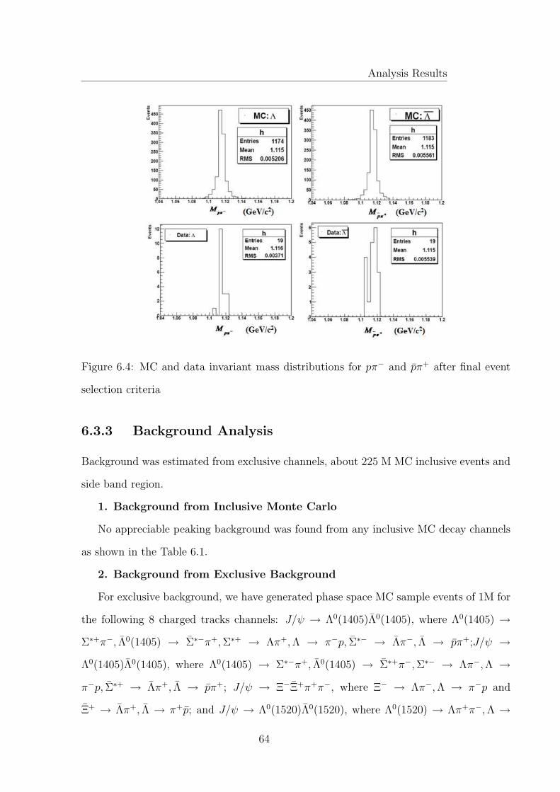
Analysis Results
Figure 6.4: MC and data invariant mass distributions for pπ− and pπ+ after final event
selection criteria
6.3.3 Background Analysis
Background was estimated from exclusive channels, about 225 M MC inclusive events and
side band region.
1. Background from Inclusive Monte Carlo
No appreciable peaking background was found from any inclusive MC decay channels
as shown in the Table 6.1.
2. Background from Exclusive Background
For exclusive background, we have generated phase space MC sample events of 1M for
the following 8 charged tracks channels: J/ψ → Λ0(1405)Λ0(1405), where Λ0(1405) →Σ∗+π−, Λ0(1405) → Σ∗−π+, Σ∗+ → Λπ+, Λ → π−p, Σ∗− → Λπ−, Λ → pπ+;J/ψ →Λ0(1405)Λ0(1405), where Λ0(1405) → Σ∗−π+, Λ0(1405) → Σ∗+π−, Σ∗− → Λπ−, Λ →π−p, Σ∗+ → Λπ+, Λ → pπ+; J/ψ → Ξ−Ξ+π+π−, where Ξ− → Λπ−, Λ → π−p and
Ξ+ → Λπ+, Λ → π+p; and J/ψ → Λ0(1520)Λ0(1520), where Λ0(1520) → Λπ+π−, Λ →
64

Analysis Results
Figure 6.5: MC and data invariant mass distributions for Λπ− and Λπ+ after final event
selection criteria
Table 6.1: MC inclusive background decay modes for the signal channel: J/ψ →Ξ0(1530)Ξ0(1530).
65

Analysis Results
Figure 6.6: MC and data invariant mass distributions for Ξ−π+ and Ξ+π− after final event
selection criteria
pπ−, Λ0(1520) → Λπ+π−, Λ → pπ+. Invariant mass spectra of Ξ−π+ and Ξ+π+ for the
above mentioned decay MC inclusive background decay channels are shown below in Figs.
6.13-6.16, while the respective scatter plots for these decay channels are shown in Figs.
6.17-6.21.
3. Background from Sideband
In order to estimate background for the signal channel: J/ψ → Ξ0(1530)Ξ0(1530) from
sideband region, scatter plot of Ξ0(1530) vs Ξ0(1530) for 1C and 4C fit results is shown in
Fig. 6.21. Background is estimated from side band boxes, 0.012 GeV/c2 away from signal
box. Signal and side bands have width of 6σ i.e. 0.072 GeV/c2. The range for signal
Ξ0(1530) is 1.495 < |MΞ−π+ | < 1.567 while range for side bands (N4,N3)and (N1,N5)is
1.409 < |MΞ−π+| < 1.483 is 1.495 < |MΞ−π+ | < 1.567 respectively. Range for signal
Ξ0(1530) is 1.495 < |MΞ+π−| < 1.567 while range for side bands (N1,N3) and (N4,N5) is
1.409 < |MΞ+π−| < 1.483 and 1.495 < |MΞ+π−| < 1.567 respectively.
66

Analysis Results
Figure 6.7: MC and data invariant mass distribution for pπ− and pπ+ after 1C fit results
Now background events for 1C and 4C fits are estimated by formula N bkg = (N4 +
N5−N1−N3)/2+N2. The number of events from 1C and 4C fits for the signal channel
J/ψ → Ξ0(1530)Ξ0(1530) are estimated to be 10±3.5 and 7±2.6 respectively.
6.3.4 Determination of Branching Fraction
Branching ratio for the decay channel J/ψ → Ξ0(1530)Ξ0(1530) is measured using the
formula:
Br[J/ψ → Ξ0(1530)Ξ0(1530)] = Nobs
ε.NJ/ψ.Br[Λ→pπ−]2.Br[Ξ−→Λπ−]2
Where number of observed events N obs for 1C and 4C fits are 10±3.5 and 7±2.6
respectively, total number of J/ψ events NJ/ψ are (225.3± 2.8)× 106, branching fraction
of intermediate resonances are Br]Λ → pπ−]=0.639 and Br[Ξ− → Λψ−]=0.9987 [87]. MC
% efficiency for 1C fit is measured to be 1.03 %, while MC % efficiency for 4C fit is
67

Analysis Results
Figure 6.8: MC and data invariant mass distribution for Λπ− and Λπ+ after 1C fit results
measured to be 0.26%. The overall detection efficiency for 1C and 4C fit for the signal
channel J/ψ → Ξ0(1530)Ξ0(1530) is 1.29 %. Now branching ratios for 1C and 4C fits are
measured to be (1.06± 0.37stat)× 10−5 and (2.94± 1.10stat)× 10−5 respectively which are
consistent within 2σ.
6.3.5 Systematic Error Analysis
1. Particle Identification.
The systematic error due to particle identification is taken as 1% each for proton and
anti-proton from the Ref. [79]. So total systematic error from this source is 2%.
2. MDC Tracking.
The systematic error due to MDC tracking detection efficiency is taken as 1% for each
68

Analysis Results
Figure 6.9: MC and data invariant mass distribution for Ξ−π= and Ξ+π− after 1C fit
results
charged track as calculated in Ref. [79]. As there are 8 charged tracks in the final states,
so systematic error from this source is taken as 8% for 4C tracking and 7% for 1C tracking.
The systematic error due to MDC tracking detection efficiency is taken as 1% for each
charged track as calculated in Ref. [79]. As there are 8 charged tracks in the final states,
so systematic error from this source is taken as 8% for 4C tracking and 7% for 1C tracking.
3. Total Number of J/ψ Events. Systematic error from (225.3±2.8)×106 number
of J/ψ events is 1.24 % [88].
4. Error from MC Model. PHSP MC sample of 100000 events was generated and
MC detection efficiency was compared with J2BB2 sample. Relative error in MC detection
efficiency is determined to be 0 %.
5. Monte Carlo Statistical Error
69

Analysis Results
Figure 6.10: MC and data invariant mass distribution for pπ− and pπ+ after 4C fit results
The monte carlo statistical error for 1C and 4C fit results was estimated by using
the respective detection efficiencies and the total number of events of the signal channel
J/ψ → Ξ0(1530)Ξ0(1530) generated by J2BB2 generator in the relation [44]
MC Statistical Error = 4εε
=
√ε(1−ε)Ngen
ε. Where ε and Ngen represent the detection
efficiency and total number of signal MC generated events. Using the value of detection
efficiencies for 1C and 4C kinematic fit results, the monte carlo statistical errors for 1C
and 4C fit results are 3.1% and 6.2% respectively.
6. Error from Intermediate Resonances.
Systematic Error due to branching ratio of intermediate resonances is calculated to be
1.5%:
Br[Λ/Λ → π−p/π+p] = (63.9± 0.5)%
70

Analysis Results
Figure 6.11: MC and data invariant mass distribution for Λπ− and Λπ+ after 4C fit results
Br[Ξ−/Ξ+ → Λπ−/Λπ+] = (99.89± 0.035)%.
Therefore the system error in branching fraction from this source is 1.5%.
Now the total systematic error for 1C and 4C fit results is shown below in Table 6.2
and Table 6.3 respectively.
Therefore, after incorporating systematic error branching ratios for 1C and 4C fit
results are given by:
Br1C [J/ψ → Ξ0(1530)Ξ0(1530)]=(1.06± 0.07sys ± 0.37stat)× 10−5
and
Br4C [J/ψ → Ξ0(1530)Ξ0(1530)]=(2.94± 0.06sys ± 1.10stat)× 10−5.
71

Analysis Results
Figure 6.12: MC and data invariant mass distribution for Ξ−π= and Ξ+π− after 4C fit
results
6.4 Analysis of ψ(2S) → Ξ0(1530)Ξ0(1530)
6.4.1 Initial Event Selection
This decay channel proceed through the following sequence of event topology: ψ(2S) →Ξ0(1530)Ξ0(1530), Ξ0(1530) → Ξ−π+, Ξ− → Λπ−, Λ → pπ− and Ξ0(1530) → Ξ+π−, Ξ+ →Λπ+, Λ → pπ+. Hence there are 8 final states charged particles: ppπ+π+π+π−π−π−.
Being analogous to the previous decay channel, the same initial event selection criteria
has been applied for this decay channel. Invariant mass distribution plots after kinematic
fit are shown below
72

Analysis Results
Figure 6.13: MΞ−π+ and MΞ+π− distribution
Figure 6.14: MΞ−π+ and MΞ+π− distribution
6.4.2 Final Event Selection
• χ2 Optimization
In order to get pure signal we further suppress background by optimizing χ2. This is
also done so as to enhance the signal to signal plus background ratio i.e. S√S+B
. Here
S is for signal and B for background. For signal MC sample is used and for S+B,
data is used. In final event selection we have used optimized χ2 for 1C kinematic fit
73

Analysis Results
Figure 6.15: MΞ−π+ and MΞ+π− distribution
Figure 6.16: MΞ−π+ and MΞ+π− distribution
with value 85.
In order to get more refined signal events with possible minimum background we have
applied following mass cuts in the range of 3σ along with χ2 <85 for the final event
selection.
• mass cut for pπ− distribution: | Mpπ− − 1.1156 |< 0.012
• mass cut for pπ+ distribution: | Mpπ+ − 1.1156 |< 0.012
• mass cut for Λπ− distribution: | MΛπ− − 1.321 |< 0.018
74

Analysis Results
Figure 6.17: Scatter plot of MΞ−π+ VS MΞ+π− distribution after 1C and 4C fit re-
sults for MC exclusive decay channel J/ψ → Λ0(1405)Λ0(1405), where Λ0(1405) →Σ∗+π−, Λ0(1405) → Σ∗−π+, Σ∗+ → Λπ+, Λ → π−p, Σ∗− → Λπ−, Λ → pπ+
Figure 6.18: Scatter plot of MΞ−π+ VS MΞ+π− distribution after 1C and 4C fit re-
sults for MC exclusive decay channel J/ψ → Λ0(1405)Λ0(1405), where Λ0(1405) →Σ∗−π+, Λ0(1405) → Σ∗+π−, Σ∗− → Λπ−, Λ → π−p, Σ∗+ → Λπ+, Λ → pπ+
• mass cut for Λπ+ distribution: | MΛπ+ − 1.321 |< 0.018
• mass cut for Ξ−π+ distribution: | MΞ−π+ − 1.531 |< 0.03
75

Analysis Results
Figure 6.19: Scatter plot of MΞ−π+ VS MΞ+π− distribution after 1C and 4C fit results
for MC exclusive decay channel J/ψ → Ξ−Ξ+π+π−, where Ξ− → Λπ−, Λ → π−p and
Ξ+ → Λπ+, Λ → π+p
Figure 6.20: Scatter plot of MΞ−π+ VS MΞ+π− distribution after 1C and 4C fit results for
MC exclusive decay channel J/ψ → Λ0(1520)Λ0(1520), where Λ0(1520) → Λπ+π−, Λ →pπ−, Λ0(1520) → Λπ+π−, Λ → pπ+.
• mass cut for Ξ+π− distribution: | MΞ+π− − 1.531 |< 0.03
In order to reject the events from the background channel found from inclusive MC
76

Analysis Results
Figure 6.21: Scatter plot of Ξ−π+ VS Ξ+π− after 1C and 4C fit results for the signal decay
channel J/ψ → Ξ0(1530)Ξ0(1530).
Table 6.2: Systematic errors from 1C fit results for the signal channel: J/ψ →Ξ0(1530)Ξ0(1530)
background analysis: ψ(2S) → J/ψπ+π−, where J/ψ → Ξ−Ξ+, Ξ− → Λπ−, Λ →pπ−, Ξ+ → Λπ+, Λ → pπ+, we use the following exclusive mass constraint:
• | MΞ−Ξ+ − 3.097 |> 0.018
After relevant final event selection as given above, important MC and data invariant
mass distributions are shown below in Figs. 6.22-6.27. While the same MC and data
invariant mass distributions after 1C and 4C fits results are shown in Figs. 6.28-6.33.
77

Analysis Results
Table 6.3: Systematic errors from 4C fit results for the signal channel:J/ψ →Ξ0(1530)Ξ0(1530)
Figure 6.22: MC and data invariant mass distribution for pπ− and pπ+ after kinematic fit
6.4.3 Background Analysis
Background was estimated from exclusive channels, 225 M MC inclusive events and side
band region.
1. Background from Inclusive Monte Carlo
78

Analysis Results
Figure 6.23: MC and data invariant mass distribution for Λπ− and Λπ+ after kinematic
fit
List of background decay channels studied from MC inclusive background is shown
in Table 6.4. Background channel from MC inclusive events is ψ(2S) → J/ψπ+π−. Af-
ter final event selection criteria total 77 events were survived. In order to remove this
background exclusive mass cut MΞ−Ξ+ > 0.018GeV/c2 has been used.
2. Background from Exclusive Background
For exclusive background, we have generated the following 8 charged tracks chan-
nels ψ(2S) → Λ0(1520)Λ0(1520), where Λ0(1520) → Λπ+π−, Λ → pπ−, Λ0(1520) →Λπ+π−, Λ → pπ+; ψ(2S) → Λ0(1690)Λ0(1690), where Λ0(1690) → Λπ+π−, Λ → pπ−,
Λ0(1690) → Λπ+π−, Λ → pπ+; ψ(2S) → Λ0(1520)Λ0(1520), where Λ0(1520) → Σ∗+π−, Λ0(1520) →Σ∗−π+, Σ∗+ → Λπ+, Λ → π−p, Σ∗− → Λπ−, Λ → pπ+;ψ(2S) → Λ0(1520)Λ0(1520), where
Λ0(1520) → Σ∗−π+, Λ0(1520) → Σ∗+π−, Σ∗− → Λπ−, Λ → π−p, Σ∗+ → Λπ+, Λ → pπ+
and ψ(2S) → Ξ−Ξ+π+π−, where Ξ− → Λπ−, Λ → π−p and Ξ+ → Λπ+, Λ → π+p.
79
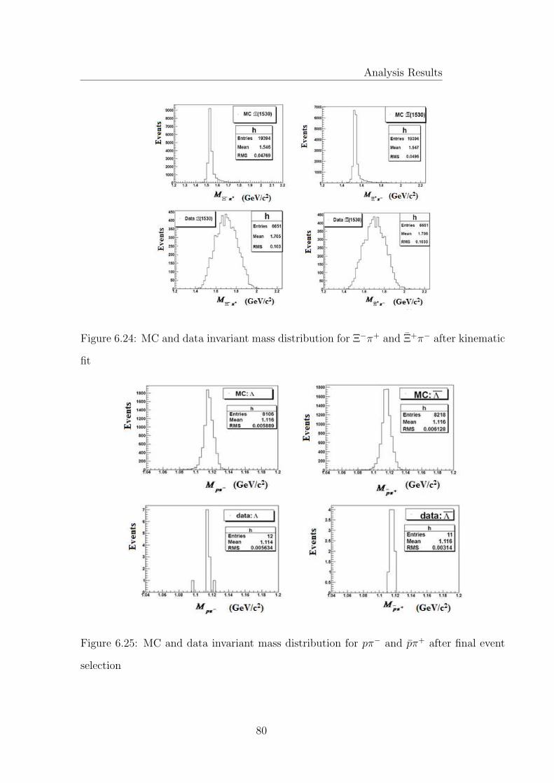
Analysis Results
Figure 6.24: MC and data invariant mass distribution for Ξ−π+ and Ξ+π− after kinematic
fit
Figure 6.25: MC and data invariant mass distribution for pπ− and pπ+ after final event
selection
80

Analysis Results
Figure 6.26: MC and data invariant mass distribution for Λπ− and Λπ+ after final event
selection
Invariant mass distributions of Ξ−π+ and Ξ+π− for above mentioned exclusive back-
ground decay channels are shown below in Fig. 6.34, Fig. 6.35, Fig. 6.36, Fig. 6.37 and
Fig. 6.38 respectively.
Now scatter plots for the above mentioned decay channels are shown in the Figs. 6.39-
6.43. The green box shows the signal region while other boxes represent the side band
region.
81

Analysis Results
Figure 6.27: MC and data invariant mass distribution for Ξ−π+ and Ξ+π− after final event
selection
Figure 6.28: MC and data invariant mass spectra for pπ− and pπ+ after 1C fit results.
82

Analysis Results
Figure 6.29: MC and data invariant mass spectra for Λπ− and Λπ+ after 1C fit results.
Figure 6.30: MC and data invariant mass spectra for Ξ−π+ and Ξ+π− after 1C fit results.
83

Analysis Results
Figure 6.31: MC and data invariant mass spectra for pπ− and pπ+ after 4C fit results.
Figure 6.32: MC and data invariant mass spectra for Λπ− and Λπ+ after 4C fit results.
84

Analysis Results
Figure 6.33: MC and data invariant mass spectra for Ξ−π+ and Ξ+π− after 4c fit results.
Figure 6.34: Invariant mass spectrum of Ξ(1530)0 and Ξ(1530)0 for MC exclusive back-
ground decay channel ψ(2S) → Λ(1520)Λ(1520)
3. Background from Sideband Region
The two dimensional scatter plot of Ξ01530 Vs Ξ0(1530) is shown in Fig. 6.44. Back-
ground is estimated from side band boxes 0.008 GeV/c2 away from signal box. Signal and
85

Analysis Results
Table 6.4: MC inclusive background decay modes for the signal channel: ψ(2S) →Ξ0(1530)Ξ0(1530)
Figure 6.35: Invariant mass spectrum of Ξ0(1530) and Ξ0(1530) for MC exclusive back-
ground decay channel ψ(2S) → Λ0(1690)Λ0(1690)
side bands have width of 6σ i.e. 0.05 GeV/c2. Range of Ξ0(1530), |MΞ−π+−1.531| < 0.025
is for signal box (1.5065, 1.5571). Range for side bands N4 and N5 is 1.4485 < |MΞ−π+ | <
86

Analysis Results
Figure 6.36: Invariant mass spectrum of Ξ0(1530) and Ξ0(1530) for MC exclusive back-
ground decay channel ψ(2S) → Λ0(1520)Λ0(1520) where Λ0(1520) → Σ∗+π−, Λ0(1520) →Σ∗−π+, Σ∗+ → Λπ+, Λ → π−p, Σ∗− → Λπ−, Λ → pπ+
Figure 6.37: Invariant mass spectrum of Ξ0(1530) and Ξ0(1530) for MC exclusive back-
ground decay channel ψ(2S) → Λ0(1520)Λ0(1520), where Λ0(1520) → Σ∗−π+, Λ0(1520) →Σ∗+π−, Σ∗− → Λπ−, Λ → π−p, Σ∗+ → Λπ+, Λ → pπ+
1.4985 and 1.5655 < |MΞ−π+| < 1.6160 respectively. Range of Ξ0(1530), |MΞ+π−−1.531| <0.025 is for signal box (1.5065, 1.5571). Range for side bands is 1.5655 < |MΞ+π−| < 1.6160.
Now background events are estimated as 0.5(N1 + N3 −N4 −N5)+N2=1.5, number of
signal events in signal region S are 11, hence number of observed events are 9.5.
87

Analysis Results
Figure 6.38: Invariant mass spectrum of Ξ0(1530) and Ξ0(1530) for MC exclusive back-
ground decay channel ψ(2S) → Ξ−Ξ+π+π−
Figure 6.39: Scatter plot of MΞ−π+ VS MΞ+π− distribution for MC exclusive decay chan-
nel ψ(2S) → Λ0(1520)Λ0(1520), where Λ0(1520) → Λπ+π−, Λ → pπ−, Λ0(1520) →Λπ+π−, Λ → pπ+
6.4.4 Determination of Branching Fraction
Branching ration for the decay channel ψ(2S) → Ξ0(1530)Ξ0(1530) is measured using the
formula:
Br[ψ(2S) → Ξ0(1530)Ξ0(1530)] = Nobs
ε.NJ/ψ.Br[Λ→pπ−]2.Br[Ξ−→Λπ−]2
Where number of observed events N obs for 1C and 4C fits are 3±2 and 7±2.6 respec-
tively, total number of ψ(2S) events Nψ(2S) are (106 × 106), branching fraction of inter-
88

Analysis Results
Figure 6.40: Scatter plot of MΞ−π+ VS MΞ+π− distribution for MC exclusive back-
ground decay channel ψ(2S) → Λ0(1690)Λ0(1690), where Λ0(1690) → Λπ+π−, Λ → pπ−,
Λ0(1690) → Λπ+π−, Λ → pπ+.
Figure 6.41: Scatter plot of MΞ−π+ VS MΞ+π− distribution for MC exclusive back-
ground decay channel ψ(2S) → Λ0(1520)Λ0(1520), where Λ0(1520) → Σ∗+π−, Λ0(1520) →Σ∗−π+, Σ∗+ → Λπ+, Λ → π−p, Σ∗− → Λπ−, Λ → pπ+
mediate resonances are Br[Λ → pπ−] = (0.639 ± 0.5)% and Br[Ξ− → Λψ−] = (0.9987 ±0.035)% [87]. MC % efficiency for 1C fit results is determined to be 5.98 %, while MC % ef-
ficiency for 4C fit results is determined to be 3.14%. The overall detection efficiency for 1C
and 4C fit results for the signal channel ψ(2S) → Ξ0(1530)Ξ0(1530) is 9.12 %. Now branch-
ing ratios for 1C and 4C fit results are determined to be (1.16± 0.77sys ± 0.07stat)× 10−6
89

Analysis Results
Figure 6.42: Scatter plot of MΞ−π+ VS MΞ+π− distribution for MC exclusive back-
ground decay channel ψ(2S) → Λ0(1520)Λ0(1520), where Λ0(1520) → Σ∗−π+, Λ0(1520) →Σ∗+π−, Σ∗− → Λπ−, Λ → π−p, Σ∗+ → Λπ+, Λ → pπ+
Figure 6.43: Scatter plot of MΞ−π+ VS MΞ+π− distribution for MC exclusive background
decay channel ψ(2S) → Ξ−Ξ+π+π−, where Ξ− → Λπ−, Λ → π−p and Ξ+ → Λπ+, Λ →π+p.
and (5.16± 1.92sys ± 0.17stat)× 10−5 respectively which are consistent within 2σ.
6.4.5 Systematic Error Analysis
1. Particle Identification.
The systematic error due to particle identification is taken as 1% each for proton and
anti-proton from the Ref. [79]. So total systematic error from this source is 2%.
90

Analysis Results
Figure 6.44: Scatter plots of Ξ−π+ vs Ξ+π− after 1C and 4C fit results for the signal
channel ψ(2S) → Ξ0(1530)Ξ0(1530).
2. MDC Tracking.
The systematic error due to MDC tracking detection efficiency is taken as 1% for each
charged track as calculated in Ref. [79]. As there are 8 charged tracks in the final states,
so systematic error from this source is taken as 8% for 4C tracking and 7% for 1C tracking.
3. Total Number of ψ(2S)) Events. Systematic error from (225.3±2.8)106 number
of J/ψ events is 1.24 % [89].
4. Error from MC Model. PHSP MC sample was generated and MC detection
efficiency was compared with J2BB2 sample. Relative error in MC detection efficiency is
determined to be 0 %.
5. Monte Carlo Statistical Error
The monte carlo statistical error for 1C and 4C fit results was estimated by using
the respective detection efficiencies and the total number of events of the signal channel
ψ(2S) → Ξ0(1530)Ξ0(1530), generated by J2BB2 generator, in the relation [44]
MC Statistical Error = 4εε
=
√ε(1−ε)Ngen
ε. Where ε and Ngen represent the detection
efficiency and total number of signal MC generated events. Using the value of detection
efficiencies for 1C and 4C kinematic fit results, the monte carlo statistical errors for 1C
and 4C fit results are 1.25% and 1.76% respectively.
91

Analysis Results
6. Error from Intermediate Resonances.
Systematic Error due to branching ratio of intermediate resonances [87] is calculated
to be 1.5%:
Br[Λ/Λ → π−p/π+p] = (63.9± 0.5)%
Br[Ξ−/Ξ+ → Λπ−/Λπ+] = (99.89± 0.035)%.
Therefore the system error in branching fraction from this source is 1.5%.
Now the total systematic error for 1C and 4C fit results is shown below in Table 6.5
and Table 6.6 respectively.
Table 6.5: Systematic errors from 1C fit results for the signal channel: ψ(2S) →Ξ0(1530)Ξ0(1530)
Table 6.6: Systematic results from 4C fit results for the signal channel: ψ(2S) →Ξ0(1530)Ξ0(1530)
After incorporating systematic error branching ratios for 1c and 4C fit results are given
by:
92

Analysis Results
Br1C [ψ(2S) → Ξ0(1530)Ξ0(1530)]=(1.16± 0.77sys ± 0.07stat)× 10−6
and
Br4C [ψ(2S) → Ξ0(1530)Ξ0(1530)]=(5.16± 1.92± 0.17stat)× 10−6.
93

Chapter 7
Summary and Conclusion
Based on world’s largest data samples registered by BESIII detector at BEPCII: about 225
million and 106 million for J/ψ and ψ(2S), respectively, the branching ratios for the decay
channels (J/ψ, ψ(2s)) → Ξ0(1530)Ξ0(1530), where Ξ0(1530) → Ξ−π+, Ξ− → Λπ−, Λ →pπ− and Ξ0(1530) → Ξ+π−, Ξ+ → Λπ+, Λ → pπ+ are first time determined to be:
Br1C [J/ψ → Ξ0(1530)Ξ0(1530)] = (1.06± 0.07sys ± 0.37stat)× 10−5
Br4C [J/ψ → Ξ0(1530)Ξ0(1530)] = (2.94± 0.06sys ± 1.10stat)× 10−5.
Br1C [ψ(2S) → Ξ0(1530)Ξ0(1530)] = (1.16± 0.77sys ± 0.07stat)× 10−6
Br4C [ψ(2S) → Ξ0(1530)Ξ0(1530)] = (5.16± 1.92sys ± 0.17stat)× 10−6.
These results are consistence within 2σ. We also tested the 12 % rule:
Q = Br1C(ψ(2S)→BB
Br1C(J/ψ)→BB=11%
Q = Br4C(ψ(2S)→BB
Br4C(J/ψ)→BB=17.55 %
This work can be concluded as follows:
• The technique of using events with one missing particle from the final state greatly
improves the detection efficiency with better signal to signal plus background ratio.
The improvement of the detection efficiency thus enabled us to measure first time
the branching ratios of the discussed decay channels.
• The analysis results can be determined more precisely by using better analysis soft-
94

Analysis Results
ware components such as Monte-Carlo event generators and decay models.
• The branching fractions can be determined more precisely by using data samples of
bigger sizes which are expected from BESIII.
• With more precise results, the 12% rule can be better tested.
95

Bibliography
[1] S.L. Glasho, Nucl. Phys. 22,579(1961); S. Weinberg, Phys. Rev. Lett. 42, 850 (1979);
Salam, A. , 1968, in Elementary Particle Theory, Proceedings of the 8th Nobel
Symposium, edited by N. Svartholrn (Almqvist and Wiksell, Stockholm).
[2] G.’t Hooft and M. Veltman, Regularization and Renormalization of Gauge Fields,
Nuclear Physics B44, 189(1972).
[3] D. C. Joshi, Introduction to Quantum Electrodynamics and Particle Physics, I. K.
International, New Dehli (2006).
[4] Mike Guidry, Gauge Field Theories: An Introduction with Applications, John Wiley
and Sons, Inc. 1999.
[5] An Introduction to particle Physics and the Standard Model, Robert Mann, CRC
Press, taylor and Francis Group, LLC (2010).
[6] J. R. Taylor et al, Modern Physics for Scientists and Engineers, 2nd, ed. Pearson
Education (2007).
[7] http : //www.cpepweb.org/cpep sm large.html, Retrieved on Aug.14, 2012.
[8] A. Lundborg, The Charm of Excited Glue, A PhD Thesis, Uppsala University,(2006).
:uu.diva-portal.org/smash/get/diva2:169616/FULLTEXT01.
96

Analysis Results
[9] P.W. Higgs, Phys. Rev. Lett. 12, 132 (1964), G.S. Guralnik, C.R. Hagen, and T.W.B.
Kibble, Phys. Rev. Lett. 13, 585(1964), F. Englert and R. Brout, Phys. Rev. Let.
13, 321 (1964).
[10] arXiv:1207.7214v1[hep-ex]; arXiv:1207.7235v1 [hep-ex].
[11] M. Olivier, A New Approach to Matrix Element Re-Weighting, A Ph.D Thesis.,
University Catholique de Louvain Facult des Sciences cole de Physique Center for
Cosmology, Particle Physics and Phenomenology
[12] Yorikiyo Nagashima, Elementary Particle Physics Volume 1: Quantum Field Theory
and Particles, WILEY-VCHVerlag GmbH Co. KGaA, Weinheim 2010
[13] W. Griener and B. Muller, Gauge Theory of Weak Interactions, 4th ed.,Springer-
Verlag Berlin Heidelberg (2009).
[14] David Griffiths, Introduction to Elementary Particle Physics, John Wily and Sons,
INC., New York (1987).
[15] http://nige.wordpress.com/2008/01/30/book/interactions/.
[16] Gordan Frazer (Editor), The New Physics, Cambridge University Press, (2009).
[17] Sergey Kalinin, PhD Thesis, Universite catholique de Louvain (2006)
[18] J. D. Jackson and L. B. Okun, Historical roots of gauge invariance 2001, arXiv:hep-
ph/0012061v5
[19] S.S. Schweber, QED and the Men who made it: Dyson, Feynman, Schwinger, and
Tomonaga, Princiton University press, 1994.
[20] H. Fritzsch, M. Gell-Mann, Proc. XVI’th Intern. Conf. on High Energy Physics,
Chicago-Batavia (1972).
97

Analysis Results
[21] H. Fritzsch, M. Gell-Mann, H. Leutwyler, Phys.Lett. 47B, 365 (1973).
[22] W. Marciano, H. Pagels, Phys.Rep. 36C, 137 (1978).
[23] H. Meyer, AIP Conf. Proc. 74, 338 (1981).
[24] G. Flugge, Quarks and nuclear forces, Springer (1982).
[25] Alessandro Bettni, Introduction to Elementary Particle Physics, Cambridge Univer-
sity Press 2008
[26] Yorikiyo Nagashima, Elementary Particle Physics Vol.1: Quantum Field Theory and
Particles, Viley VCH 2010.
[27] Francis Halzen and Alan D. Martin, Quarks and Leptons, John Wiley and Sons
(1984).
[28] H.D. Politzer, Phys. Rev. Lett. 30, 1346(1976); Phys. Rep. 14C, 120(1974); D.J.
Gross and F. Wilczek, Phys. Rev. Lett. 30, 1343(1943).
[29] B.R. Holstein, Chiral perturbation theory: An effective field theory, Progress in Par-
ticle and Nuclear Physics 61, 3(2008).
[30] NRQCD, Effective Field Theories and Potential Models, Nuclear Physics B (Proc.
Suppl.) 93, 188(2001).
[31] N. Brambilla, Perturbative quark bound states in pNRQCD, Nuclear Physics B (Proc.
Suppl.) 96, 410(2001).
[32] A. Vairo, Heavy-quarkonium physics from effective-field theories, Eur. Phys. J. A 31,
728(2007).
[33] N. Brambilla et al., Heavy quarkonium: progress, puzzles, and opportunities, Eur.
Phys. J. C 71:1534,2011., N. Brambilla, Effective field theories for the heavy quarko-
nium, Few Body Syst 43: 2530, (2008).
98

Analysis Results
[34] A. Pineda and J. Soto, Effective Field Theory for Ultrasoft Momenta in NRQCD
and NRQED, Nuclear Physics B (Proc. Suppl.) 64, 428(1998).
[35] M. Gell-Man, Phys. Lett.8, 214(1964).
[36] Z. George, Origins of the Quark Model, 1980.
[37] R.E. Taylor, Rev. Mod. Phys. 63, 1991; H.W. Kendall, Rev. Mod. Phys. 63 (3),
597(1991).
[38] R.P. Feynman, Phys. Rev. Lett. 23, 1415(1969); R.P. Feynman, Photonhadron In-
teractions, Benjamin, NewYork, 1972.
[39] A.V. Belitskya and A.V. Radyushkinb, Unraveling hadron structure with generalized
parton distributions, Physics Reports 418, 1(2005).
[40] N. Isgur and G. Karl, Phys. Lett. B72, 109(1977); Phys. Rev. D20, 1191 (1979);
N. Isgur, G. Karl and R. Koniuk, Phys. Rev. Lett. 41, 1269 (978); R. Koniuk and
N. Isgur, Phys. Rev. Lett. 44, 845 (1980).
[41] J. M. G. Duarte, Isospin and SU(2) Symmetry,
web.mit.edu/woodson/Public/Duarte− isospin.pdf.
[42] M. Gell-Mann, Phys. Rev. 92, 883 (1953); T. Nakano and K. Nisjijima, prog. Theor.
Phys. 10, 581, (1953).
[43] V.E. barnes, et al., Phys. Rev. Lett. 12, 204 (1964).
[44] T. Hussain and S. Jin, BESII Analysis Memo.
[45] I J R Aitchison and A J G Hey, Gauge Theories in Particle Physics Vol.1, IOP Pub.
Ltd. (2003).
[46] Physics at BES-III, IHEP-Physics-Report-BES-III-2008-001-v1.
99

Analysis Results
[47] K.K. Setha, Eur Phys. J. A 18, 563(2003).
[48] http://proza-2m.ihep.su/panda/physics/2008-10-22-itep/Seminar-Corrected-ITEP-
2008.ppt.
[49] Feng Yuan et al, arXiv:hep-ph/9703438.
[50] BES Collaboration, F. Liu, arXiv:hep-ex/9912006.
[51] CLEO Collaboration, G.S. Huang, J. Phys: Conf. Ser. 9, 132(2005).
[52] Ailin Zhang, Phys. Let.B 647, 140(2007).
[53] M.B. Voloshin, Review Charmonia, Progress in Particle and Nuclear Physics 61,
455(2008).
[54] B. R. Martin and G. Shaw, Particle Physics, 2nd. ed., Wiley (1997).
[55] J. J. Aubert et al., Phys. Rev. Lett. 33, 1404(1974).
[56] J. E. Augustin et al., Phys. Rev. Lett. 33, 1406(1974).
[57] Abrams et al., Phys. Lett. 33, 1453(1974).
[58] N. Brambilla, Heavy Quarkonium Physics, arXiv:hep-phy:
[59] Diego Bettoni, Roberto Calabrese, Progress in Particle and Nuclear Physics 54,
615(2005).
[60] B. Povh et al., Particles and Nuclie, 3rd Ed. Springer 2002.
[61] T.Barnes, S.Godfrey and E.S.Swanson, Higher Charmonia, Phys. Rev. D 72, 054026
(2005)
[62] T. K. Pedlar et al, CLEO Collaboration, Branching fraction measurements of ψ(2S)
decay to baryon-antibaryon final states, 2008.
100
Analysis Results
[63] S. Okubo, Phys. Lett.5, 163 (1963); G. Zweig, CERN Report No. 8182/TH 401,
1964; G. Zweig, CERN Report No. 8419/TH 412, 1964; J. Iizuka, Prog. Theor.
Phys. Suppl. 37-38, 21(1966).
[64] X.H. Mo et al., Study of the ρπ Puzzle in Charmonium Decay, High Energy Phys.
Nucl. Phys. 31, 686-701 (2007); T. Appelquist and H. D. Politzer, Phys. Rev. Lett.
34, 43(1975); A. De Rujula and S. L. Glashow, Phys. Rev. Lett. 34, 46 (1975).
[65] M. E. Franklin et al. (Mark-II Collaboration) Measurement of ψ(3097) and ψ′(3686)
Decays into Selected Hadronic Modes, Phys. Rev. Lett. 51, 963 (1983).
[66] X. H. Mo et al., Study of the ρπ Puzzle in Charmonium Decay,High Energy Phys.
Nucl. Phys. 31, 686-701 (2007).
[67] S. Lehti,www.helsinki.fi/ karimaki/CMHEP/Lectures/lect7Slides.pdf.
[68] Wolfgang Khn, New Physics Opportunities in the Charm/Tau Region:The BESIII
- Experiment in Beiging, Act. al Phys. Pol. B 41(2), 2010.
[69] R.-D. Heur, Eletron Positron Cilliders, arXiv:hep-ex/0111070v1,Vol.22,2001.
[70] A. Zhemchugov, Status of BESIII, Nuclear Physics B (Proc. Suppl.) 189, 353(2009).
[71] Yifang Wang, Physics of tau and charm, arXiv:1007.2911v1 [hep-ph],2010.
[72] M. Zobov, New generation Electron-Positron Factories, Physics of Particles and
Nuclie, 42(5), 782(211).
[73] BESIII Collaboration, The construction of the BESIII experiment, Nucl. Instrum.
Meth.A 598, 7(2009); A. Zhechoguv, Status of BESIII, Nuclear Physics B (Proc.
Suppl.) 189, 353(2009); M. Ablikim et al., Design and construction of BESIII detec-
tor, Nucl. Instrum. Meth.A 614, 345(2010).
101

Analysis Results
[74] R.E. Mitchell, An Expeirmental Revew of Charmonium, 34th International Confer-
ence on High Energy Physics, Philadelphia, 2008, arXiv:0810.3231v1.
[75] G. R. Farrar and R. D. Jackson, Phys. Re. Lett. 35, 1416(1975); S. J. Brodsky and
G. P. Lepage, Phys. Rev. D 24(11), 2848(1981).
[76] R. E. Mitchell, An Experimental Review of Charmonium, arXiv:0810.3233 v1, [hep-
ex], 2008.
[77] C. Brenner Mariottoab, M.B. Gay Ducatib and G. Ingelman arXive:hepep-
ph/0111379v1,
[78] Bing-Song Zou, The Baryon Spectroscopy from J/ψ
[79] W. Guogui et al., Study of ψ′ → ΛΞ+π−, BESIII Analysis Memo : Version 2.0,
2012.
[80] J. Z. Bai et al, BES Collaboration, measurement of ψ(2S) decays to Baryon pairs,PR
D63, 03(2002).
[81] W. D. Li eta al., The offline Software for the BES-III Experiment, Proceeding of
CHEP06(Mumbai, India, 13-17 Feburary 2006).
[82] htt://lhcb-com.web.cern.ch/lhcb-comp/Frameworks/Gaudi/.
[83] htt://geant4.web.cern.ch/geant4/
[84] S. Jadach, B.F.L. Ward and Z. Was, Phys. Rev. D63, 113009(2001).
[85] R. G. Ping, China. Phys. C 32, 599 (2008).
[86] J.C. Chen et al. Phys. Rev. D62, 034003(2000).
[87] K Nakamura et al (Particle Data Group), J. Phys. G: Nucl. Part. Phys. 37 (2010)
075021.
102

Analysis Results
[88] M. Abilikm et al., Determination of the number of J/ψ events with J/ψ inclusive
decays, Chinese Physics C, CPC(HEP & NP), 2011, XX(X): 111.
[89] M. Changli et al., Observation of χcJ Decay to ΛΛπ+π− , BESIII Analysis, Memo:
Version 3.0, 2012.
[90] Quantum Chromodynamics and Colour Singlet Exchange in High Energy Interac-
tions, PhD Thesis,
103